handbook of
statistics 14
Statistical Methods
in Finance
Edited by
i ;.s
C.R.kau
l

ELSEVIER SCIENCE B.V.
Sara Burgerhartstraal 25
P.O. Box 211, 1000 AE Amsterdam, The Netherlands
ISBN: 0-444-81964-9
© 1996 Elsevier Science B.V. All rights reserved.
No part of this publication may be reproduced, stored in a retrieval system or transmitted in any form
or by any means, electronic, mechanical, photocopying, recording or otherwise, without the prior
written permission of the publisher, Elsevier Science B.V . Copyright & Permissions Department. P.O.
Box 521, 1000 AM Amsterdam. The Netherlands.
Special regulations for readers in the U.S.A.-This publication has been registered wilh the Copyright
Clearance Center Inc. (CCC). 222 Rosewood Drive. Danvers, MA 0192.1. Information can be obtained
from the CCC about conditions under which photocopies of parts oi' this publication may be made in
the U.S.A. All other copyright questions, including photocopying outside the U.S.A., should be
referred to the Publishers unless otherwise specified.
No responsibility is assumed by the publisher for any injury and or damage to persons or property as a
matter of products liability, negligence or otherwise, or from any use of operation of any methods,
products, instructions or ideas contained in the material herein.
This book is printed on acid-free paper.
Printed in The Netherlands.

Table of contents
Preface v
Contributors xv
PART I. ASSET PRICING
Ch. I. Econometric Evaluation of Asset Pricing Models 1
W. E. Person and R. Jagannathan
1. Introduction 1
2. Cross-sectionaI regression methods for testing beta pricing models 3
3. Asset pricing models and stochastic discount factors 10
4. The generalized method of moments 15
5. Model diagnostics 23
6. Conclusions 28
Appendix 29
References 30
Ch. 2. Instrumental Variables Estimation of Conditional Beta
Pricing Models 35
C. R. Harvey and C. M. Kirby
1. Introduction 35
2. Single beta models 37
3. Models with multiple betas 44
4. Latent variables models 46
5. Generalized method of moments estimation 47
6. Closing remarks 58
References 58

VIII
Table of contents
Ch. 3. Semiparametric Mclhods for Asset Pricing Models 61
B. N. Lehmann
1. Introduction 61
2. Some relevant aspects of the generalized method of moments (GMM) 62
3. Asset pricing relations and their econometric implications 68
4. Efficiency gains within alternative beta pricing formulations 74
5. Concluding remarks 87
References 88
PART II. TERM STRUCTURES OF INTEREST RATES
Ch. 4. Modeling the Term Structure 91
A. R. Pagan, A. D. Hall, and V. Martin
1. Introduction 91
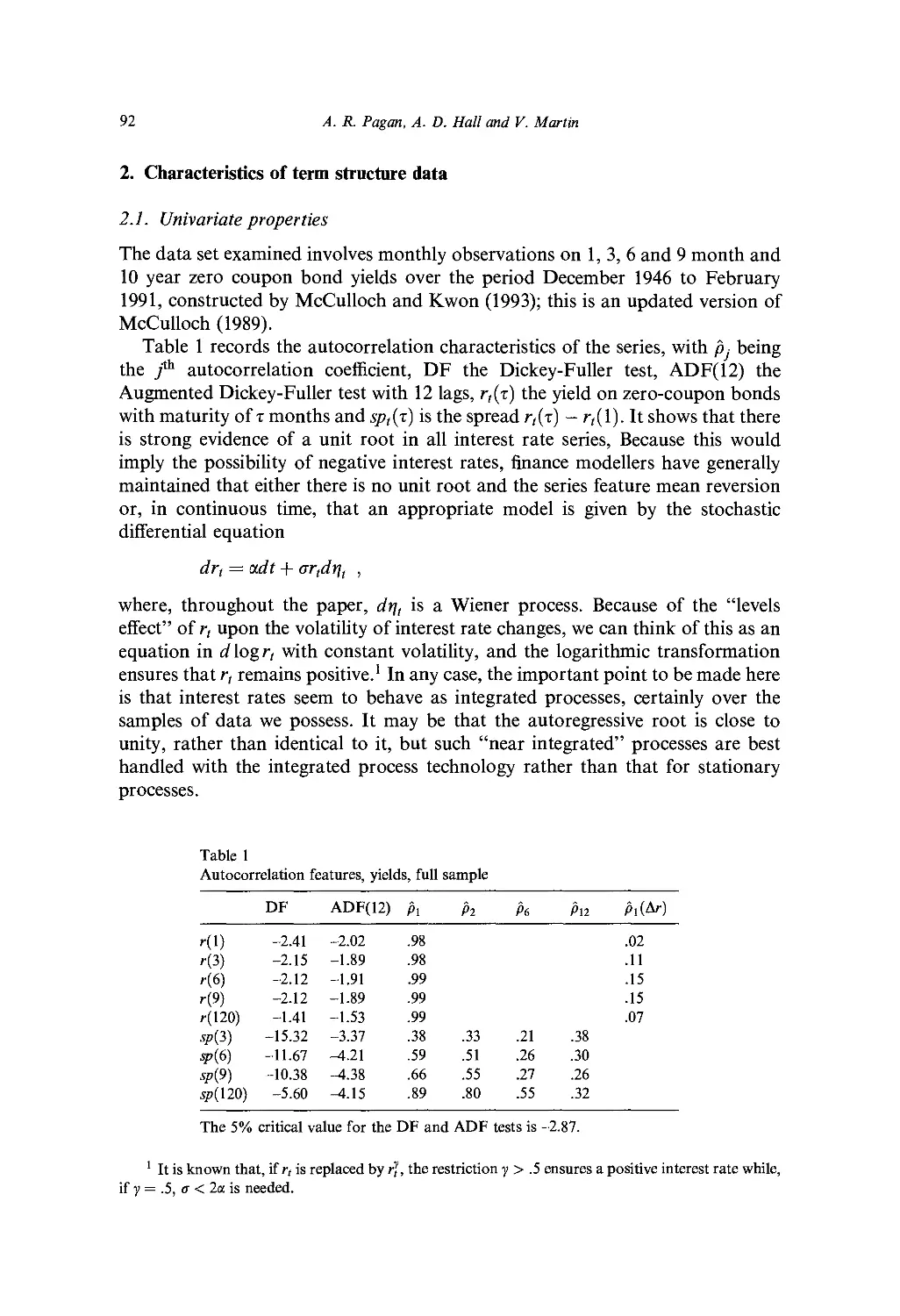
2. Characteristics of term structure data 92
3. Models of the term structure 104
4. Conclusion 116
References 116
PART III. VOLATILITY
Ch. 5. Stochastic Volatility 119
E. Ghysels, A. C. Harvey and E. Renault
1. Introduction 119
2. Volatility in financial markets 120
3. Discrete lime models 139
4. Continuous time models 153
5. Statistical inference 167
6. Conclusions 182
References 183
Ch. 6. Slock Price Volatility 193
£ E. LeRoy
1. Introduction 193
2. Statistical issues 195
3. Dividend-smoothing and non stationarity 198
4. Bubbles 201
5. Time-varying discount rates 203

Table of contents
ix
6. Interpretation 204
7. Conclusion 206
References 207
Ch. 7. GARCH Models of Volatility 209
1. Introduction 209
2. GARCH models 210
3. Statistical inference 224
4. Statistical properties 229
5. Conclusions 234
References 235
PART IV. PREDICTION
Ch. 8. Forecast Evaluation and Combination 241
F. X. Diebold and J. A. Lopez
1. Evaluating a single forecast 242
2. Comparing the accuracy of multiple forecasts 247
3. Combining forecasts 252
4. Special topics in evaluating economic and financial forecasts 256
5. Concluding remarks 264
References 265
Ch. 9. Predictable Components in Stock Returns 269
G. Kaul
I Introduction 269
2. Why predictability 270
3. Predictability of stock returns: The methodology 273
4. Power comparisons 287
5. Conclusion 291
References 292
Ch. 10. Interest Rate Spreads as Predictors of Business Cycles 297
K. Lahiri and 7. G. Wang
1. Introduction 297
2. Hamilton's non-linear filter 299
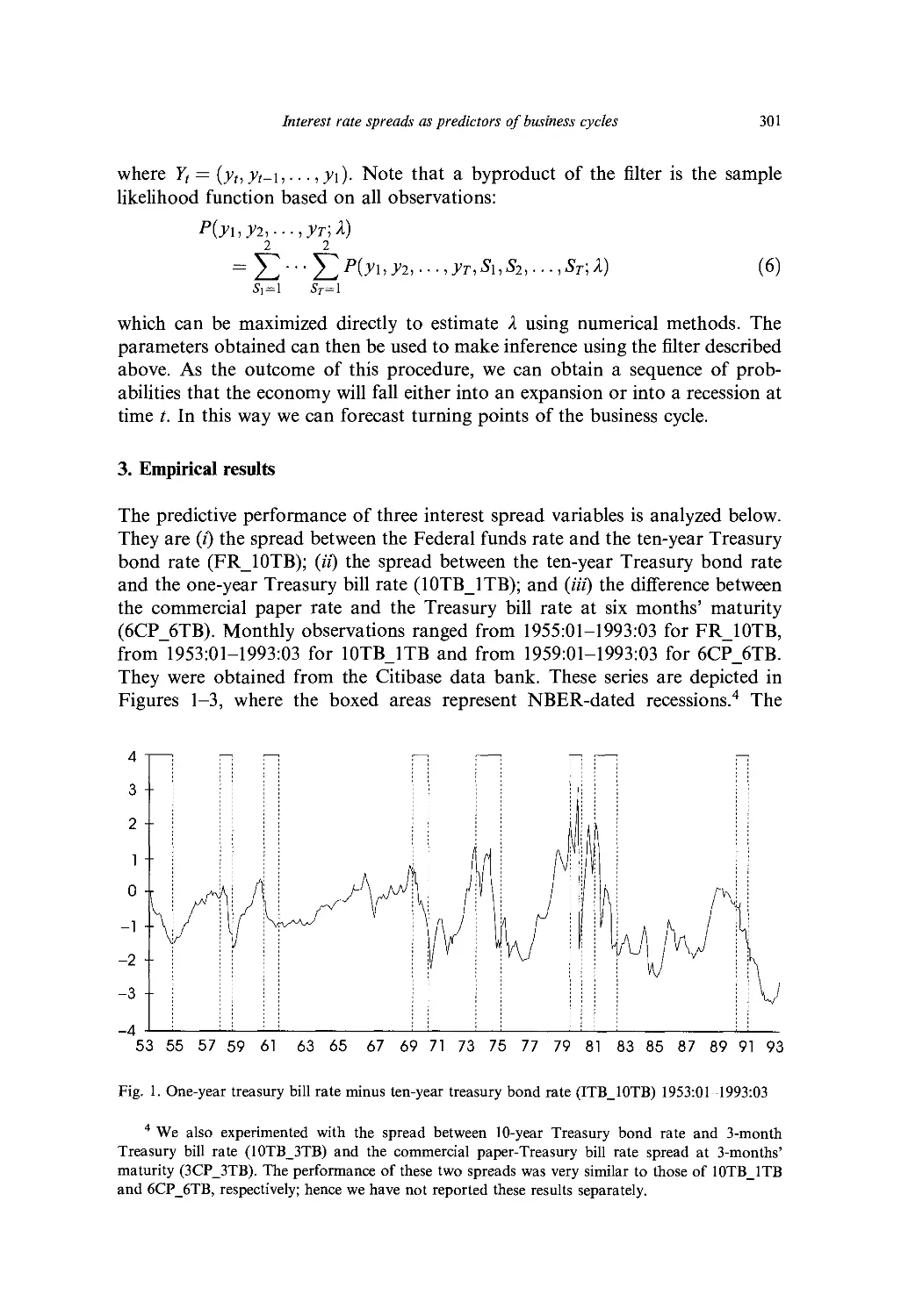
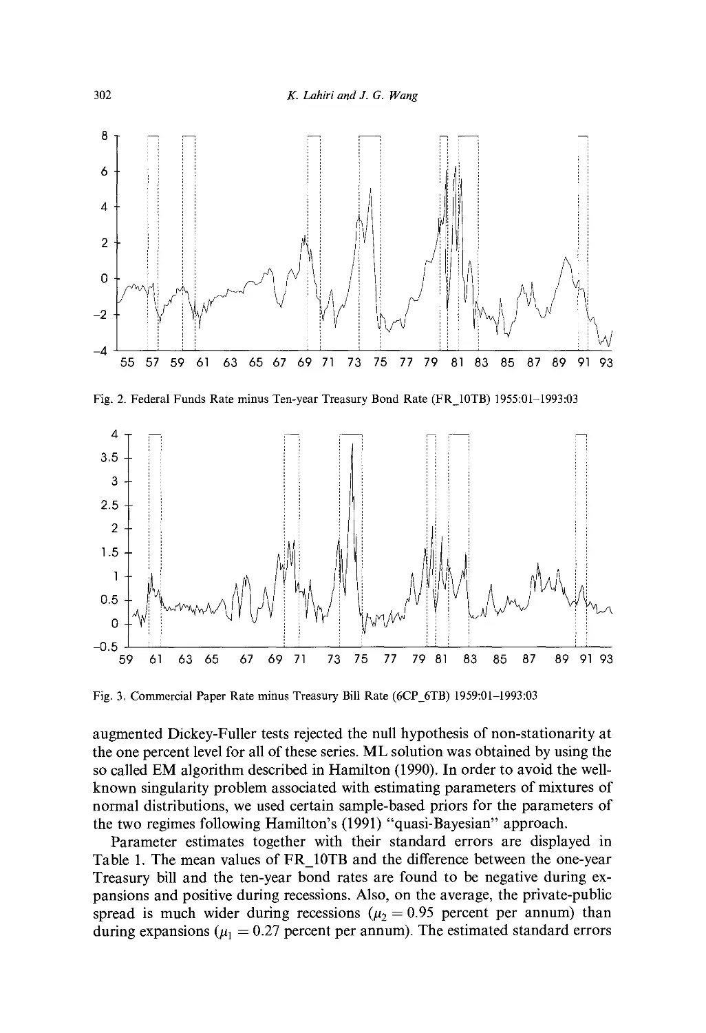
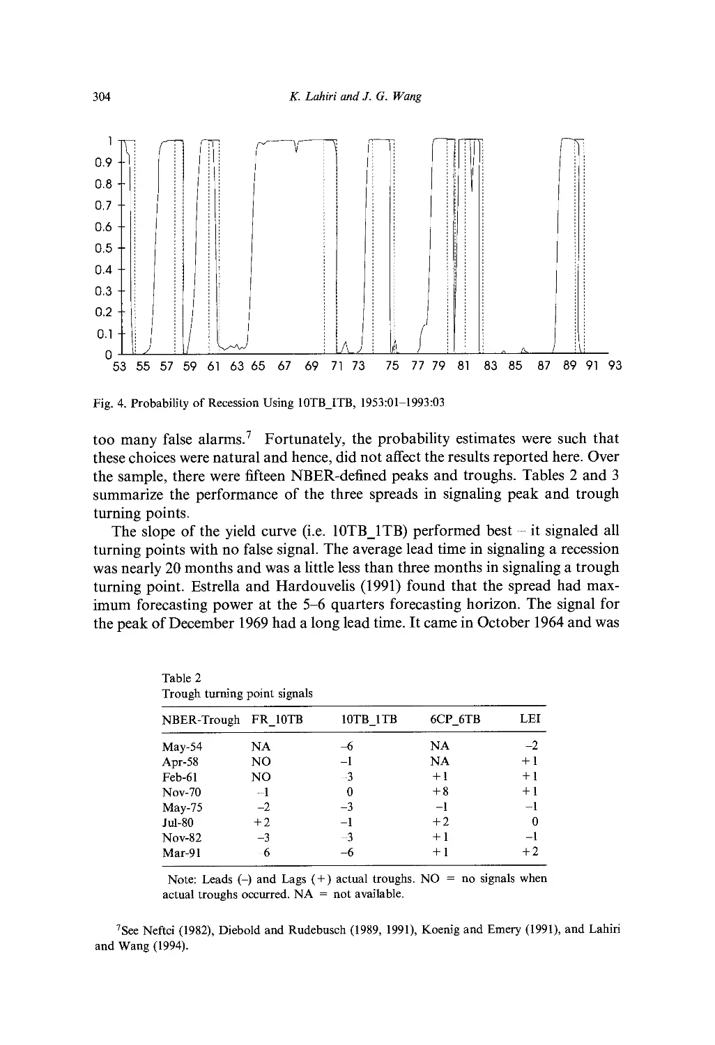
3. Empirical results 301
4. Implications for the monetary transmission mechanism 308

X
Table of contents
5. Conclusion 311
Acknowledgement 313
References 313
PART V. ALTERNATIVE PROBABILISTIC MODELS
Ch. 11. Nonlinear Time Series, Complexity Theory, and Finance 317
W. A. Brock and P. J. F. de Lima
1. Introduction 317
2. Nonlinearity in stock returns 326
3. Long memory in stock returns 337
4. Asymmetric information structural models and stylized features of stock returns 349
5. Concluding remarks 353
References 353
Ch. 12. Count Data Models for Financial Data 363
A. C. Cameron and P. K. Trivedi
1. Introduction 363
2. Stochastic process models for count and duration data 366
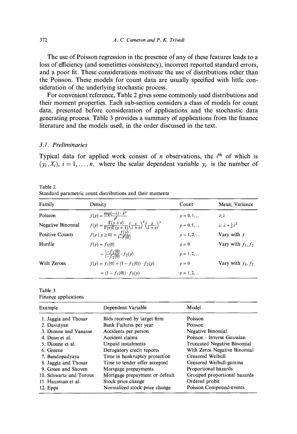
3. Econometric models of counts 371
4. Concluding remarks 388
Acknowledgement 389
References 390
Ch. 13. Financial Applications of Stable Distributions 393
/. //. McCulloch
1. Introduction 393
2. Basic properties of stable distributions 394
3. Stable portfolio theory 401
4. Log-stable option pricing 404
5. Parameter estimation and empirical issues 415
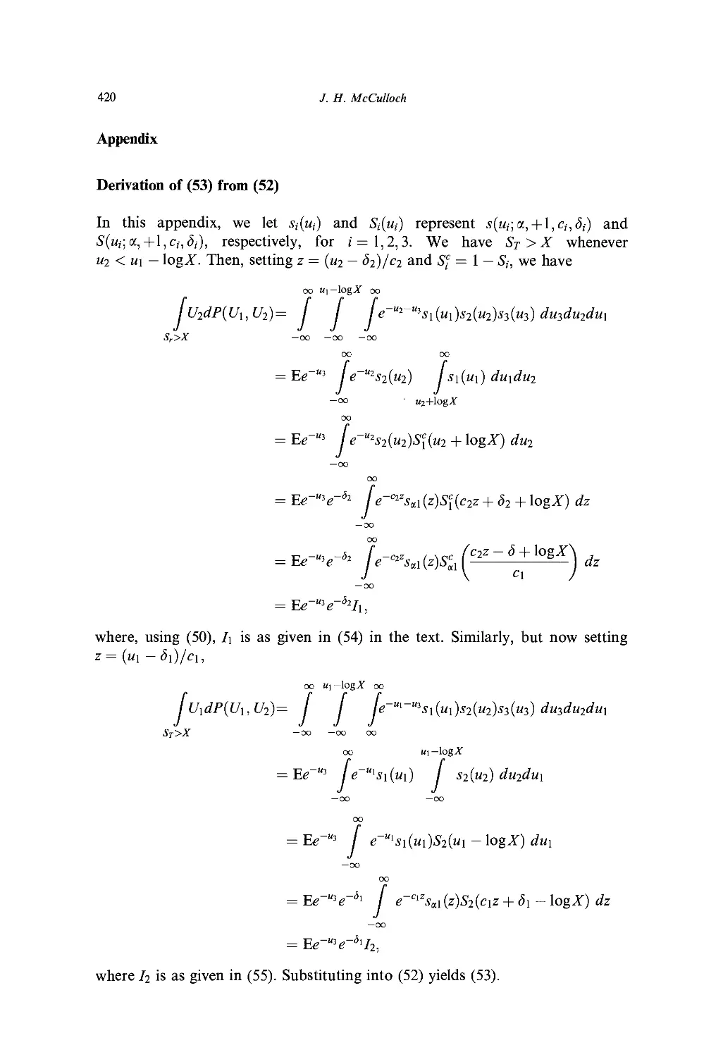
Appendix 420
Acknowledgements 421
References 421
Ch. 14. Probability Distributions for Financial Models 427
./. B. McDonald
1. Introduction 427
2. Alternative models 428

Table of contents
xi
Applicalions in finance 437
Appendix A: Special functions 454
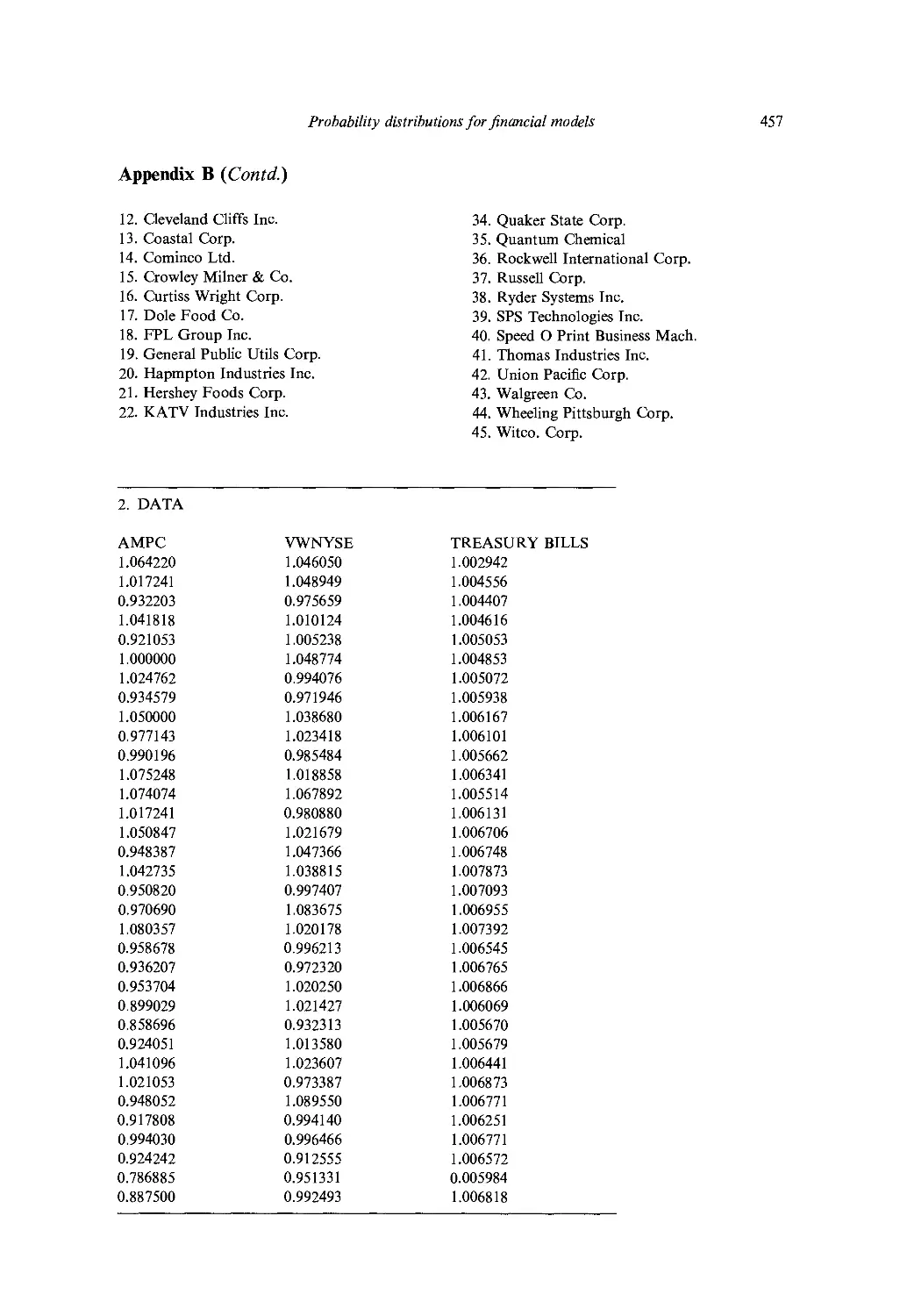
Appendix B: Data 456
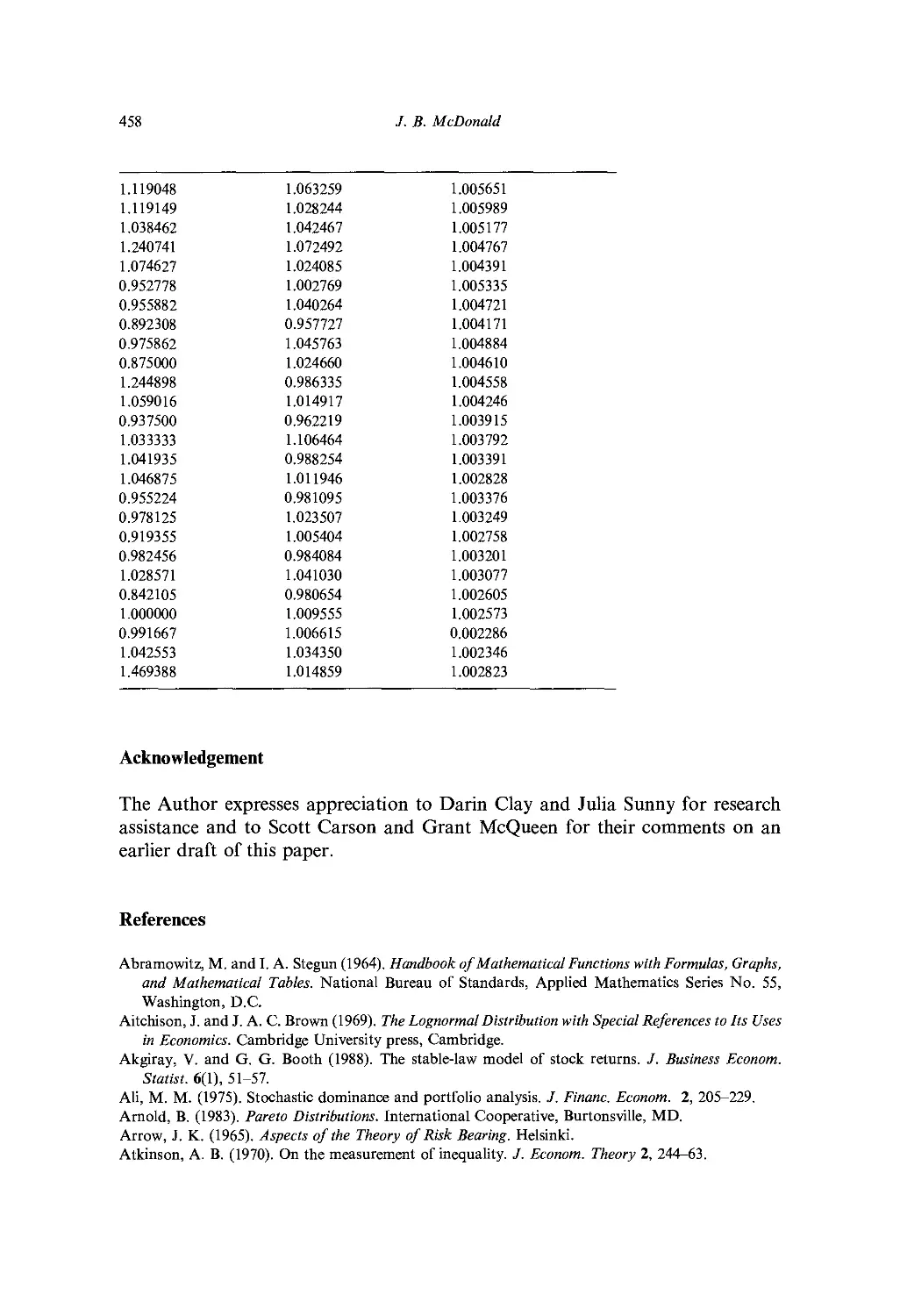
Acknowledgement 458
References 45H
PART VI. APPLICATIONS OF SPECIALIZED STATISTICAL METHODS
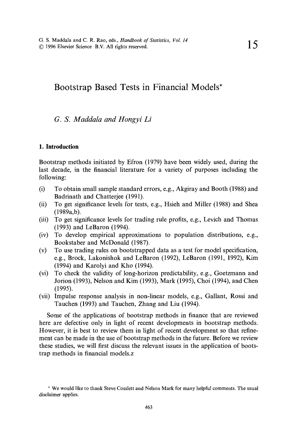
Ch. 15. Bootstrap Based Tests in Financial Models 463
(7. S, Maddala and H. Li
I. Introduction 463
2
3
4
5
6
7
8
A review of different bootstrap methods 464
Issues in the generation of bootstrap samples and the test statistics 466
A critique of the application of bootstrap methods in financial models 469
Bootstrap methods for model selection using trading rules 476
Bootstrap methods in long-horizon regressions 478
Impulse response analysis in nonlinear models 483
Conclusions 484
References 485
Ch 16. Principal Components and Factor Analyses 489
C, R. Rao
1. Introduction 489
2. Principal components 490
3. Model based principal components 496
4. Factor analysis 498
5. Conclusions 503
References 5(M
Ch. 17. Errors-in-Variables Problems in Financial Models 507
G. S. Maddala and M'. Nimalendran
1. Introduction 507
2. Grouping methods 508
3. Alternatives to the two-pass estimation method 513
4. Direct and reverse regression methods 514
5. Latent variables / structural equation models with measurement 515
6. Artificial neural networks (ANN) as alternatives to MIMIC models 522
7. Signal extraction methods and tests for rationality 523
8. Qualitative and limited dependent variable models 523
9. Factor analysis with measurement errors 524
10. Conclusion 525
References 525

Ml
Table of contents
Ch. 18. Financial Applications of Artificial Neural Networks 529
M. Qi
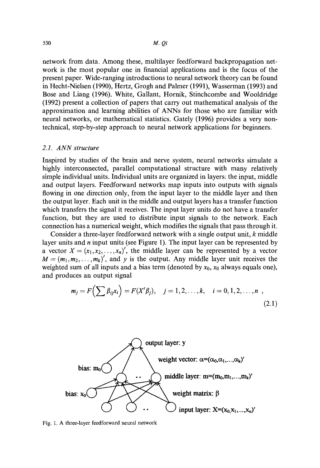
\. Introduction 529
2. Artificial Neural Networks 529
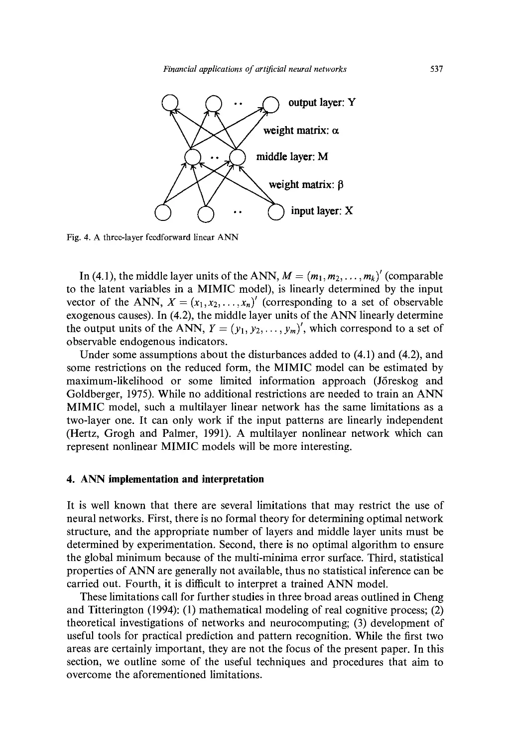
3. Relationship between ANN and interpretational statistical models 533
4. ANN implementation and interpretation 537
5. Financial applications 544
6. Conclusions 547
Acknowledgement 548
References 548
Ch. 19. Applications of Limited Dependent Variable Models in Finance 553
G. S. Maddala
1. Introduction 553
2. Studies on loan discrimination and default 553
3. Studies on bond ratings and bond yields 555
4. Event studies 557
5. Savings and loan and bank failures 559
6. Miscellaneous other applications 562
7. Suggestions for future research 564
References 565
PART VII. MISCELLANEOUS OTHER PROBLEMS
Ch. 20. Testing Option Pricing Models 567
D. S. Bates
1. Introduction 367
2. Option pricing fundamentals 568
3. Time series-based tests of option pricing models 574
4. Implicit parameter estimation 587
5. Implicit parameter tests of alternate distributional hypotheses 600
6. Summary and conclusions 604
References 605
Ch. 21. Peso Problems: Their Theoretical and Empirical Implications 613
M. D. D. Evans
1. Introduction 613
2. Peso problems and forecast errors 615
3. Peso problems, asset prices and fundamentals 626
4. Risk aversion and peso problems 634

Table of contents
5. Econometric issues 641
6. Conclusion 644
References 645
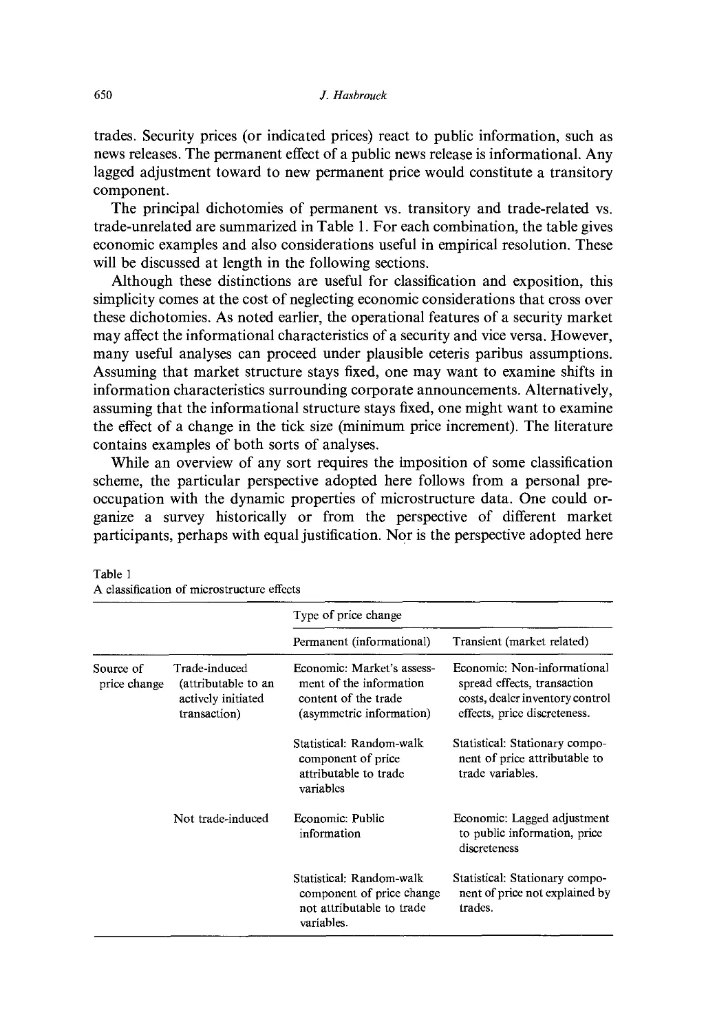
Ch. 22. Modeling Market Microstructure Time Series 647
J. Ilasbrouck
1. Introduction 647
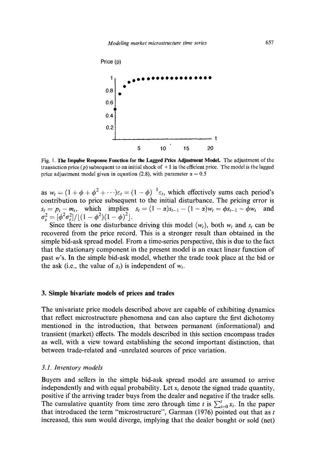
2. Simple univariate models of prices 651
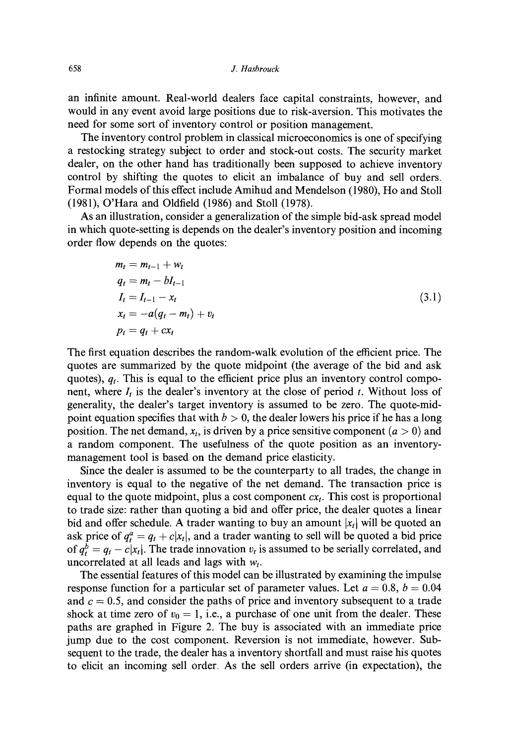
3. Simple bivariate models of prices and trades 657
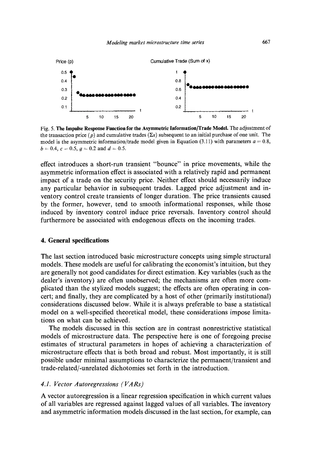
4. General specifications 667
5. Time 673
6. Discreteness 677
7. Nonlinearity 679
8. Multiple mechanisms and markets 680
9. Summary and directions for further work 685
References 687
Ch. 23. Statistical Methods in Tests of Portfolio Efficiency: A Synthesis
J. Shanken
1. Introduction 693
2. Testing efficiency with a riskless asset 695
3. Testing efficiency without a riskless asset 701
4. Related work 708
References 709
Subject Index 713
Contents of Previous Volumes 719

Preface
As with the earlier volumes in this series, the main purpose of this volume of
the Handbook of Statistics is to serve as a source reference and teaching
supplement to courses in empirical finance. Many graduate students and researchers in
the finance area today use sophisticated statistical methods but there is as yet no
comprehensive reference volume on this subject. The present volume is intended
to fill this gap.
The first part of the volume covers the area of asset pricing. In the first paper,
Ferson and Jagannathan present a comprehensive survey of the literature on
econometric evaluation of asset pricing models. The next paper by Harvey and
Kirby discusses the problems of instrumental variable estimation in latent
variable models of asset pricing. The next paper by Lehman reviews semi-parametric
methods in asset pricing models. Chapter 23 by Shanken also falls in the category
of asset pricing.
Part II of the volume on term structure of interest rates consists of only one
paper by Pagan, Hall and Martin. The paper surveys both the econometric and
finance literature in this area, and shows some similarities and divergences
between the two approaches. The paper also documents several stylized facts in the
data that prove useful in assessing the adequacy of the different models.
Part III of the volume deals with different aspects of volatility. The first paper
by Ghysels, Harvey and Renault present a comprehensive survey on the
important topic of stochastic volatility models. These models have their roots both
in mathematical finance and financial econometrics and are an attractive
alternative to the popular ARCH models. The next paper by LeRoy presents a critical
review of the literature on variance-bounds tests for market efficiency. The third
paper by Palm on GARCH models of stock price volatility, surveys some more
recent developments in this area. Several surveys on the ARCH models have
appeared in the literature and these are cited in the paper. The paper surveys
developments since the appearance of these surveys.
Part IV of the volume deals with prediction problems. The first paper by Diebold
and Lopez deals with the statistical methods of evaluation of forecasts. The second
paper by Kaul, reviews the literature on the predictability of stock returns. This area
has always fascinated those involved in making money in financial markets as well
as academics who presumably are interested in studying whether one can, in fact,
make money in the financial markets. The third paper by Lahiri reviews statistical

VI
Preface
evidence on interest rate spreads as predictors of business cycles. Since there is not
much of a literature to survey in this area, Lahiri presents some new results.
Part V of the volume deals with alternative probabilistic models in finance. The
first paper by Brock and deLima surveys several areas subsumed under the rubic
"complexity theory." This includes chaos theory, nonlinear time series models,
long memory models and models with asymmetric information. The next paper
by Cameron and Trivedi surveys the area of count data models in finance. In
some financial studies, the dependent variable is a count, taking non-negative
integer values. The next paper by McCulloch surveys the literature on stable
distributions. This area was very active in finance in the early 60's due to the work
by Mandelbrot but since then has not received much attention until recently when
interest in stable distributions has revived. The last paper by McDonald reviews
the variety of probability distributions which have been and can be used in the
statistical analysis of financial data.
Part VI deals with application of specialized statistical methods in finance. This
part covers important statistical methods that are of general applicability (to all
the models considered in the previous sections) and not covered adequately in the
other chapters. The first paper by Maddala and Li covers the area of bootstrap
methods. The second paper by Rao covers the area of principal component and
factor analyses which has, during recent years, been widely used in financial
research particularly in arbitrage pricing theory (APT). The third paper by
Maddala and Nimalendran reviews the area of errors in variables models as
applied to finance. Almost all variables in finance suffer from the errors in
variables problems. The fourth paper by Qi surveys the applications of artificial
neutral networks in financial research. These are general nonparametric nonlinear
models. The final paper by Maddala reviews the applications of limited dependent
variable models in financial research.
Part VII of the volume contains surveys of miscellaneous other problems. The
first paper by Bates surveys the literature on testing option pricing models. The
next paper by Evans discusses what are known in the financial literature as "peso
problems." The next paper by Hasbrouck covers market microstructure, which is
an active area of research in finance. The paper discusses the fime series work in
this area. The final paper by Shanken gives a comprehensive survey of tests of
portfolio efficiency.
One important area left out has been the use of Bayesian methods in finance.
In principle, all the problems discussed in the several chapters of the volume can
be analyzed from the Bayesian point of view. Much of this work remains to be
done.
Finally, we would like to thank Ms. Jo Ducey for her invaluable help at several
stages in the preparation of this volume and patient assistance in seeing the
manuscript through to publication.
G. S. Maddala
C. R. Rao

Contributors
D. S. Bates, Department of Finance, Wharton School, University of Pennsylvania,
Philadelphia, PA 19104, USA (Ch. 20)
W. A. Brock, Department of Economics, University of Wisconsin, Madison, WI
53706, USA (Ch. 11)
A. C. Cameron, Department of Economics, University of California at Davis,
Davis, CA 95616-8578, USA (Ch. 12)
P. J. F. de Lima, Department of Economics, The Johns Hopkins University,
Baltimore, MD 21218, USA (Ch. 11)
F. X. Diebold, Department of Economics, University of Pennsylvania,
Philadelphia, PA 19104, USA (Ch. 8)
M. D. D. Evans, Department of Economics, Georgetown University, Washington
DC 20057-1045, USA (Ch. 21)
W. E. Ferson, Department of Finance, University of Washington, Seattle, WA
98195, USA (Ch. 1)
E. Ghysels, Department of Economics, The Pennsylvania State University,
University Park, PA 16802 and CIRANO (Centre interuniversitaire de
recherche en analyse des organisations), Universite de Montreal, Montreal,
Quebec, Canada H3A2A5 (Ch. 5)
A. D. Hall, School of Business, Bond University, Gold Coast, QLD 4229, Australia
(Ch. 4)
A. C. Harvey, Department of Statistics, London School of Economics, Houghton
Street, London WC2A 2AE, UK (Ch. 5)
C. R. Harvey, Department of Finance, Fuqua School of Business, Box 90120, Duke
University, Durham, NC 27708-0120, USA (Ch. 2)
J. Hasbrouck, Department of Finance, Stern School of Business, 44 West 4th
Street, New York, NY 10012-1126, USA (Ch. 22)
R. Jagannathan, Finance Department, School of Business and Management, The
Hong Kong University of Science and Technology, Clear Water Bay, Kowloon,
Hong Kong (Ch. 1)
G. Kaul, University of Michigan Business School, Ann Harbor, MZ 48109-
1234 (Ch. 9)
C. M. Kirby, Department of Finance, College of Business & Mgm., University of
Maryland, College Park, MD 20742, USA (Ch. 2)
K. Lahiri, Department of Economics, State University of New York at Albany,
Albany, NY 12222 USA (Ch. 10)
XV

XVI
Contributors
B. N. Lehmann, Graduate School of International Relations, University of
California at San Diego, 9500 Gilman Drive, LaJolla, CA 92093-0519, USA
(Ch. 3)
S. F. LeRoy, Department of Economics, University of California at Santa
Barbara, Santa Barbara, CA 93106-9210 (Ch. 6)
H. Li, Department of Management Science, The Chinese University of Hongkong,
302 Leung Kau Kui Building, Shatin, NT, Hong Kong (Ch. 15)
J. A. Lopez, Department of Economics, University of Pennsylvania, Philadelphia,
PA 19104, USA (Ch. 8)
G. S. Maddala, Department of Economics, Ohio State University, 1945 N. High
Street, Columbus, OH 43210-1172, USA (Chs. 15, 17, 19)
V. Martin, Department of Economics, University of Melbourne, Parkville, VIC
3052, Australia (Ch. 4)
J. H. McCulloch, Department of Economics and Finance, 410 Arps Hall, 1945 N.
High Street, Columbus, OH 43210-1172, USA (Ch. 13)
J. B. McDonald, Department of Economics, Brigham Young University, Provo, UT
84602, USA (Ch. 14)
M. Nimalendran, Department of Finance, College of Business, University of
Florida, Gainesville, FL 32611, USA (Ch. 17)
A. R. Pagan, Economics Program, RSSS, Australian National University,
Canberra, ACT 0200, Australia (Ch. 4)
F. C. Palm, Department of Quantitative Economics, University of Limburg, P.O.
Box 616, 6200 MD Maastricht, The Netherlands (Ch. 7)
M. Qi, Department of Economics, College of Business Administration, Kent State
University, P.O. Box 5190, Kent, OH 44242 (Ch. 18)
C. R. Rao, The Pennsylvania State University, Center for Multivariate Analysis,
Department of Statistics, 325 Classroom Bldg., University park, PA 16802-
6105, USA (Ch. 16)
E. Renault, Institut D'Economie Industrielle, Universite des Sciences Sociales,
Place Anatole France, F-31042 Toulouse Cedex, France (Ch. 5)
J. Shanken, Department of Finance, Simon School of Business, University of
Rochester, Rochester, NY 14627, USA (Ch. 23)
P. K. Trivedi, Department of Economics, Indiana University, Bloomington, IN
47405-6620, USA (Ch. 12)
J. G. Wang, AT&T, Rm. N460-WOS, 412 Mt. Kemble Avenue, Morristown, NJ
07960, USA (Ch. 10)

G. S. Maddala and C. R. Rao, eds., Handbook of Statistics, Vol. 14
© 1996 Elsevier Science B.V. All rights reserved.
Econometric Evaluation of Asset Pricing Models
Wayne E. Ferson and Ravi Jagannathan
We provide a brief review of the techniques that are based on the generalized
method of moments (GMM) and used for evaluating capital asset pricing models.
We first develop the CAPM and multi-beta models and discuss the classical two-
stage regression method originally used to evaluate them. We then describe the
pricing kernel representation of a generic asset pricing model; this representation
facilitates use of the GMM in a natural way for evaluating the conditional and
unconditional versions of most asset pricing models. We also discuss diagnostic
methods that provide additional insights.
1. Introduction
A major part of the research effort in finance is directed toward understanding
why we observe a variety of financial assets with different expected rates of return.
For example, the U.S. stock market as a whole earned an average annual return
of 11.94% during the period from January of 1926 to the end of 1991. U.S.
Treasury bills, in contrast, earned only 3.64%. The inflation rate during the same
period was 3.11% (see Ibbotson Associates 1992).
To appreciate the magnitude of these differences, note that in 1926 a nice
dinner for two in New York would have cost about $10. If the same $10 had been
invested in Treasury bills, by the end of 1991 it would have grown to $110, still
enough for a nice dinner for two. Yet $10 invested in stocks would have grown to
$6,756. The point is that the average return differentials among financial assets
are both substantial and economically important.
A variety of asset pricing models have been proposed to explain this
phenomenon. Asset pricing models describe how the price of a claim to a future
payoff is determined in securities markets. Alternatively, we may view asset pri-
* Ferson acknowledges financial support from the Pigott-PACCAR Professorship at the
University of Washington. Jagannathan acknowledges financial support from the National Science
Foundation, grant SBR-9409824. The views expressed herein are those of the authors and not
necessarily those of the Federal Reserve Bank of Minneapolis or the Federal Reserve System.
1

2
W. E. Ferson and R. Jagannathan
cing models as describing the expected rates of return on financial assets, such as
stocks, bonds, futures, options, and other securities. Differences among the
various asset pricing models arise from differences in their assumptions that restrict
investors' preferences, endowments, production, and information sets; the
stochastic process governing the arrival of news in the financial markets; and the
type of frictions allowed in the markets for real and financial assets.
While there are differences among asset pricing models, there are also
important commonalities. All asset pricing models are based on one or more of three
central concepts. The first is the law of one price, according to which the prices of
any two claims which promise the same future payoff must be the same. The law
of one price arises as an implication of the second concept, the no-arbitrage
principle. The no-arbitrage principle states that market forces tend to align the
prices of financial assets to eliminate arbitrage opportunities. Arbitrage
opportunities arise when assets can be combined, by buying and selling, to form
portfolios that have zero net cost, no chance of producing a loss, and a positive
probability of gain. Arbitrage opportunities tend to be eliminated by trading in
financial markets, because prices adjust as investors attempt to exploit them. For
example, if there is an arbitrage opportunity because the price of security A is too
low, then traders' efforts to purchase security A will tend to drive up its price. The
law of one price follows from the no-arbitrage principle, when it is possible to buy
or sell two claims to the same future payoff. If the two claims do not have the
same price, and if transaction costs are smaller than the difference between their
prices, then an arbitrage opportunity is created. The arbitrage pricing theory
(APT, Ross 1976) is one of the most well-known asset pricing model based on
arbitrage principles.
The third central concept behind asset pricing models is financial market
equilibrium. Investors' desired holdings of financial assets are derived from an
optimization problem. A necessary condition for financial market equilibrium in
a market with no frictions is that the first-order conditions of the investors'
optimization problem be satisfied. This requires that investors be indifferent at the
margin to small changes in their asset holdings. Equilibrium asset pricing models
follow from the first-order conditions for the investors' portfolio choice problem
and from a market-clearing condition. The market-clearing condition states that
the aggregate of investors' desired asset holdings must equal the aggregate
"market portfolio" of securities in supply.
The earliest of the equilibrium asset pricing models is the Sharpe-Lintner-
Mossin-Black capital asset pricing model (CAPM), developed in the early
1960s. The CAPM states that expected asset returns are given by a linear function
of the assets' betas, which are their regression coefficients against the market
portfolio. Merton (1973) extended the CAPM, which is a single-period model, to
an economic environment where investors make consumption, savings, and
investment decisions repetitively over time. Econometrically, Merton's model
generalizes the CAPM from a model with a single beta to one with multiple betas.
A multiple-beta model states that assets' expected returns are linear functions of a
number of betas. The APT of Ross (1976) is another example of a multiple-beta

Econometric evaluation of asset pricing models
3
asset pricing model, although in the APT the expected returns are only
approximately a linear function of the relevant betas.
In this paper we emphasize (but not exclusively) the econometric evaluation of
asset pricing models using the generalized method of moments (GMM, Hansen
1982). We focus on the GMM because, in our opinion, it is the most important
innovation in empirical methods in finance within the past fifteen years. The
approach is simple, flexible, valid under general statistical assumptions, and often
powerful in financial applications. One reason the GMM is "general" is that
many empirical methods used in finance and other areas can be viewed as special
cases of the GMM.
The rest of this paper is organized as follows. In Section 2 we develop the
CAPM and multiple-beta models and discuss the classical two-stage regression
procedure that was originally used to evaluate these models. This material
provides an introduction to the various statistical issues involved in the empirical
study of the models; it also motivates the need for multivariate estimation
methods. In Section 3 we describe an alternative representation of the asset
pricing models which facilitates the use of the GMM. We show that most asset
pricing models can be represented in this stochastic discount factor form. In
Section 4 we describe the GMM procedure and illustrate how to use it to estimate
and test conditional and unconditional versions of asset pricing models. In
Section 5 we discuss model diagnostics that provide additional insight into the causes
for statistical rejections and that help assess specification errors in the models. In
order to avoid a proliferation of symbols, we sometimes use the same symbols to
mean different things in different subsections. The definitions should be clear from
the context. We conclude with a summary in Section 6.
2. Cross-sectional regression methods for testing beta pricing models
In this section we first derive the CAPM and generalize its empirical specification
to include multiple-beta models. We then describe the intuitively appealing cross-
sectional regression method that was first employed by Black, Jensen, and Scholes
(1972, abbreviated here as BJS) and discuss its shortcomings.
2.1. The capital asset pricing model
The CAPM was the first equilibrium asset pricing model, and it remains one of
the foundations of financial economics. The model was developed by Sharpe
(1964), Lintner (1965), Mossin (1966), and Black (1972). There are a huge number
of theoretical gapers which refine the necessary assumptions and provide
derivations of the CAPM. HeTewe provide-a-brief-review of the theory.
Let Rit denote one plus the return on asset i during period t, i = 1,2,..., N. Let
Rmt denote the corresponding gross return for the market portfolio of all assets in
the economy. The return on the market portfolio envisioned by the theory is not
observable. In view of this, empirical studies of the CAPM commonly assume

4
W. E. Ferson and R. Jagannathan
that the market return is an exact linear function of the return on an observable
portfolio of common stocks.1 Then, according to the CAPM,
E(Ru) = So + SiPt (2.1)
where
ft = Cov(tf;„tfm,)/Var(tfm,).
According to the CAPM, the market portfolio with return Rmt is on the
minimum-variance frontier of returns. A return is said to be on the minimum-
variance frontier if there is no other portfolio with the same expected return but
lower variance. If investors are risk averse, the CAPM implies that Rmt is on the
positively sloped portion of the minimum-variance frontier, which implies that
the coefficient b\ > 0. In equation (2.1), d0 = E(Ro,), where the return i?0i is
referred to as a zero-beta asset to Rmt because of the condition Cov(Rot,Rmt) = 0.
To derive the CAPM, assume that investors choose asset holdings at each date
t — 1 so as to maximize the following one-period objective function:
V[E(Rpt\I),Var(Rpl\I)} (2.2)
where Rpt denotes the date t return on the optimally chosen portfolio and E(-\I)
and Var(-|7) denote the expectation and variance of return, conditional on the
information set / of the investor as of time t-\. We assume that the function V[- > •]
is increasing and concave in its first argument, decreasing in its second argument,
and time-invariant. For the moment we assume that the information set /includes
only the unconditional moments of asset returns, and we drop the symbol / to
simplify the notation. The first-order conditions for the optimization problem
given above can be manipulated to show that the following must hold:
E(RU) = E(R0t) + pipE(Rpt - R0I) (2.3)
for every asset / = 1, 2, ..., N, where Rpt is the return on the optimally chosen
portfolio, Rot is the return on the asset that has zero covariance with Rpt, and pip
= Cov(Rit,Rpt)IVar(Rpt).
To get from the first-order condition for an investor's optimization problem, as
stated in equation (2.3), to the CAPM, it is useful to understand some of the
properties of the minimum-variance frontier, that is, the set of portfolio returns
with the minimum variance, given their expected returns. It can be readily verified
that the optimally chosen portfolio of the investor is on the minimum-variance
frontier.
One property of the minimum-variance frontier is that it is closed to portfolio
formation. That is, portfolios of frontier portfolios are also on the frontier.
1 When this assumption fails, it introduces market proxy error. This source of error is studied by
Roll (1977), Stambaugh (1982), Kandel (1984), Kandel and Stambaugh (1987), Shanken (1987),
Hansen and Jagannathan (1994), and Jagannathan and Wang (1996), among others. We will ignore
proxy error in our discussion.

Econometric evaluation of asset pricing models
5
Suppose that all investors have the same beliefs. Then every investor's optimally
chosen portfolio will be on the same frontier, and hence the market portfolio of
all assets in the economy - which is a portfolio of every investor's optimally
chosen portfolio - will also be on the frontier. It can be shown (Roll 1977) that
equation (2.3) will hold if Rpt is replaced by the return of any portfolio on the
frontier and RQt is replaced by its corresponding zero-beta return. Hence we can
replace an investor's optimal portfolio in equation (2.3) with the return on the
market portfolio to get the CAPM, as given by equation (2.1).
2.2. Testable implications of the CAPM
Given an interesting collection of assets, and if their expected returns and market-
portfolio betas Pi are known, a natural way to examine the CAPM would be
to estimate the empirical relation between the expected returns and the betas and
see if that relation is linear. However, neither betas nor expected returns are
observed by the econometrician. Both must be estimated. The finance literature
first attacked this problem by using a two-step, time-series, cross-sectional
approach.
Consider the following sample analogue of the population relation given in
(2.1):
Rt = 50 + Sibi + <?,-, i = 1,... ,JV (2.4)
which is a cross-sectional regression of i?; on bt, with regression coefficients equal
to S0 and ^i- IQ equation (2.4), i?, denotes the sample average return of the asset, i,
and bt is the (OLS) slope coefficient estimate from a regression of the return, Rit,
over time on the market index return, Rmt; bt is a constant. Let ut = Ri—E(Rit)
and vt = Pf-bi. Substituting these relations for E(RU) and /?, in (2.1) leads to (2.4)
and specifies the composite error as et = Ut + d^t- This gives rise to a classic
errors-in-variables problem, as the regressor bt in the cross-sectional regression
model (2.4) is measured with error. Using finite time-series samples for the
estimate of bh the regression (2.4) will deliver inconsistent estimates of d0 and di, even
with an infinite cross-sectional sample. However, the cross-sectional regression
will provide consistent estimates of the coefficients as the time-series sample size T
(which is used in the first step to estimate the beta coefficient /},) becomes very
large. This is because the first-step estimate of pt is consistent, so as T becomes
large, the errors-in-variables problem of the second-stage regression vanishes.
The measurement error in beta may be large for individual securities, but it is
smaller for portfolios. In view of this fact, early research focused on creating
portfolios of securities in such a way that the betas of the portfolios could be
estimated precisely. Hence one solution to the errors-in-variables problem is to
work with portfolios instead of individual securities. This creates another
problem. Arbitrarily chosen portfolios tend to exhibit little dispersion in their betas. If
all the portfolios available to the econometrician have the same betas, then
equation (2.1) has no empirical content as a cross-sectional relation. Black,
Jensen, and Scholes (BJS, 1972) came up with an innovative solution to overcome

6
W. E. Ferson and R. Jagannathan
this difficulty. At every point in time for which a cross-sectional regression is run,
they estimate betas on individual securities based on past history, sort the
securities based on the estimated values of beta, and assign individual securities to
beta groups. This results in portfolios with a substantial dispersion in their betas.
Similar portfolio formation techniques have become standard practice in the
empirical finance literature.
Suppose that we can create portfolios in such a way that we can view the
errors-in-variables problem as being of second-order importance. We still have to
determine how to assess whether there is empirical support for the CAPM. A
standard approach in the literature is to consider specific alternative hypotheses
about the variables which determine expected asset returns. According to the
CAPM, the expected return for any asset is a linear function of its beta only.
Therefore, one natural test would be to examine if any other cross-sectional
variable has the ability to explain the deviations from equation (2.1). This is the
strategy that Fama and MacBeth (1973) followed by incorporating the square of
beta and measures of nonmarket (or residual time-series) variance as additional
variables in the cross-sectional regressions. More recent empirical studies have
used the relative size of firms, measured by the market value of their equity, the
ratio of book-to-market-equity, and related variables.2 For example, the
following model may be specified:
E(Ru) = d0 + SiP, + <5size LMEt (2.5)
where LMEt is the natural logarithm of the total market value of the equity
capital of firm i. In what follows we will first show that these ideas extend easily to
the general multiple-beta model. We will then develop a sampling theory for the
cross-sectional regression estimators.
2.3. Multiple-beta pricing models and cross-sectional regression methods
According to the CAPM, the expected return on an asset is a linear function of its
market beta. A multiple-beta model asserts that the expected return is a linear
function of several betas, i.e.,
E(Rit)=50+ J2 W* (2-6)
k=\,...JC
where fiik, k — 1,... ,K, are the multiple regression coefficients of the return of
asset i on K economy-wide pervasive risk factors, fk,k — \,...,K. The coefficient
(5o is the expected return on an asset that has p0k = 0, for k = 1,..., K; i.e., it is the
expected return on a zero- (multiple-) beta asset. The coefficient bk, corresponding
to the £th factor, has the following interpretation: it is the expected return
differential, or premium, for a portfolio that has Pik = 1 and ptJ = 0 for all j =£ k,
2 Fama and French (1992) is a prominent recent example of this approach. Berk (1995) provides a
justification for using relative market value and book-to-price ratios as measures of expected returns.

Econometric evaluation of asset pricing models
7
measured in excess of the zero-beta asset's expected return. In other words, it is
the expected return premium per unit of beta risk for the risk factor, k. Ross
(1976) showed that an approximate version of (2.6) will hold in an arbitrage-free
economy. Connor (1984) provided sufficient conditions for (2.6) to hold exactly in
an economy with an infinite number of assets in general equilibrium. This version
of the multiple-beta model, the exact APT, has received wide attention in the
finance literature. When the factors, /&, are observed by the econometrician, the
cross-sectional regression method can be used to empirically evaluate the
multiple-beta model.3 For example, the alternative hypothesis that the size of the firm
is related to expected returns, given the factor betas, may be examined by using
cross-sectional regressions of returns on the K factor betas and the LMEh similar
to equation (2.5), and by examining whether the coefficient Ssize is different from
zero.
2.4. Sampling distributions for coefficient estimators: The two-stage,
cross-sectional regression method
In this section we follow Shanken (1992) and Jagannathan and Wang (1993, 1996)
in deriving the asymptotic distribution of the coefficients that are estimated using
the cross-sectional regression method. For the purposes of developing the
sampling theory, we will work with the following generalization of equation (2.6):
E(**)=f>,^* + f>2*fl* (2.7)
fc=0 k=\
where {Aik} are observable characteristics of firm /, which are assumed to be
measured without error (the first "characteristic," when k = 0, is the constant
1.0). One of the attributes may be the size variable LMEt. The ft are regression
betas on a set of A^ economic risk factors, which may include the market index
return. Equation (2.7) can be written more compactly using matrix notation as
li=Xy (2.8)
where Rt = [Rlt,... ,Rm], A* = E(Rt),X = [A : ft1, and the definition of the matrices
A and ji and the vector y follow from (2.7).
The cross-sectional method proceeds in two stages. First, ft is estimated by
time-series regressions of Ru on the risk factors and a constant. The estimates are
denoted by b. Let x = [A : b], and let R denote the time-series average of the return
vector Rt. Let g denote the estimator of the coefficient vector obtained from the
following cross-sectional regression:
g = (x'x)~xx!R (2.9)
3 See Chen (1983), Connor and Korajczyk (1986), Lehmann and Modest (1987), and McElroy and
Burmeister (1988) for discussions on estimating and testing the model when the factor realizations are
not observable under some additional auxiliary assumptions.

8
W. E. Ferson and R. Jagannathan
where we assume that x is of rank I + K\ + K2. If b and R converge respectively
to fi and E(Rt) in probability, then g will converge in probability to y.
Black, Jensen, and Scholes (1972) suggest estimating the sampling errors
associated with the estimator, g, as follows. Regress Rt on x at each date / to obtain
gt, where
g, = {x'x)~lx'Rt . (2.10)
The BJS estimate of the covariance matrix of Tl! (g — y) is given by
v = T-1'£(gt-g)(gt-g)' (2.11)
t
which uses the fact that g is the sample mean of the gt's. Substituting the
expression for gt given in (2.10) into the expression for v given in (2.11) gives
v = (x'x)-lx'[T-l^2(Rt - R)(Rt - R)'}x{x'XyX . (2.12)
t
To analyze the BJS covariance matrix estimator, we write the average return
vector, R, as
R=xy + (R-n) -{x-X)y . (2.13)
Substitute this expression for R into the expression for g in (2.9) to obtain
g-y = (x'xylx'[(R - ») - (b - fi)y2] . (2.14)
Assume that b is a consistent estimate of ft and that TXI2{R — fi) —>d u and
Txl2{b — fi) —>,/ h, where u and h are random variables with well-defined
distributions and —></ indicates convergence in distribution. We then have
Tl/2(g - y) -^d (x'x)~lx'u - (x'x)~lx'hy2 . (2.15)
In (2.15) the first term on the right side is that component of the sampling error
that arises from replacing u by the sample average R. The second term is the
component of the sampling error that arises due to replacing fi by its estimate b.
The usual consistent estimate of the asymptotic variance of u is given by
T-lJ2(Rt-R)(Rt-R)' . (2.16)
t
Therefore, a consistent estimate of variance of the first term in (2.15) is given by
(x'x)-lx'[T-1 J2(Rt -R)(Rt -R)']x{x'xYx
t
which is the same as the expression for the BJS estimate for the covariance matrix
of the estimated coefficients v, given in (2.12). Hence if we ignore the sampling
error that arises from using estimated betas, then the BJS covariance estimator

Econometric evaluation of asset pricing models
9
provides a consistent estimate of the variance of the estimator g. However, if the
sampling error associated with the betas is not small, then the BJS covariance
estimator will have a bias. While it is not possible to determine the magnitude of
the bias in general, Shanken (1992) provides a method to assess the bias under
additional assumptions.4
Consider the following univariate time-series regression for the return of asset i
on a constant and the kth economic factor:
Ru = ocik + Pikfkt + eat . (2.17)
We make the following additional assumptions about the error terms in (2.17): (1)
the error £,& is mean zero, conditional on the time series of the economic factors
fk; (2) the conditional covariance of eikt and £/&, given the factors, is a fixed
constant <7y«. We denote the matrix of the {ffywjy by Z«. Finally, we assume that
(3) the sample covariance matrix of the factors exists and converges in probability
to a constant positive definite matrix Q, with the typical element Q«.
Theorem 2.1. (Shanken, 1992/Jagannathan and Wang, 1996)
Txl2(g — y) converges in distribution to a normally distributed random variable
with zero mean and covariance matrix V + W, where V is the probability limit of
the matrix v given in (2.12) and
W= Y. {^x)-xX'{y2ky2l{Qr^Ilkl^)}x{xlx)-x (2.18)
l,k=\,...fa
where JJW is defined in the appendix.
Proof. See the appendix.
Theorem 2.1 shows that in order to obtain a consistent estimate of the co-
variance matrix of the BJS two-step estimator g, we first estimate v (a consistent
estimate of V) by using the BJS method. We then estimate W by its sample
analogue.
Although the cross-sectional regression method is intuitively very appealing,
the above discussion shows that in order to assess the sampling errors associated
with the parameter estimators, we need to make rather strong assumptions. In
addition, the econometrician must take a stand on a particular alternative
hypothesis against which to reject the model. The general approach developed in
Section 4 below has, among its advantages, weaker statistical assumptions and
the ability to handle both unspecified as well as specific alternative hypotheses.
4 Shanken (1992) uses betas computed from multiple regressions. The derivation which follows
uses betas computed from univariate regressions, for simplicity of exposition. The two sets of betas are
related by an invertible linear transformation. Alternatively, the factors may be orthogonalized
without loss of generality.

10
W. E. Ferson and R. Jagannathan
3. Asset pricing models and stochastic discount factors
Virtually all financial asset pricing models imply that any gross asset return
Ri,t+i, multiplied by some market-wide random variable mt+1, has a constant
conditional expectation:
E, {mt+iRitt+i} = l,all i. (3.1)
The notation Et{} will be used to denote the conditional expectation, given a
market-wide information set. Sometimes it will be convenient to refer to
expectations conditional on a subset Z, of the market information, which are
denoted as E(-1 Zt). For example, Zt can represent a vector of instrumental variables
for the public information set which are available to the econometrician. When Zt
is the null information set, the unconditional expectation is denoted as E(-). If we
take the expected values of equation (3.1), it follows that versions of the same
equation must hold for the expectations E(-1Zt) and E().
The random variable mt+\ has various names in the literature. It is known as a
stochastic discount factor, an equivalent martingale measure, a Radon-Nicodym
derivative, or an intertemporal marginal rate of substitution. We will refer to an
mt + i which satisfies (3.1) as a valid stochastic discount factor. The motivation for
use of this term arises from the following observation. Write equation (3.1) as
Pit = E,{m,+iXij+i}
where Xiyt+1 is the payoff of asset i at time t + 1 (the market value plus any cash
payments) and R^t+i = Xif+\jPit. Equation (3.1) says that if we multiply a future
payoff Xtj+i by the stochastic discount factor mt+\ and take the expected value,
we obtain the present value of the future payoff.
The existence of an mt+\ that satisfies (3.1) says that all assets with the same
payoffs have the same price (i.e., the law of one price). With the restriction that
mt+1 is a strictly positive random variable, equation (3.1) becomes equivalent to a
no-arbitrage condition. The condition is that all portfolios of assets with payoffs
that can never be negative, but are positive with positive probability, must have
positive prices.
The no-arbitrage condition does not uniquely identify mt+\ unless markets are
complete, which means that there are as many linearly independent payoffs
available in the securities markets as there are states of nature at date t + 1. To
obtain additional insights about the stochastic discount factor and the
no-arbitrage condition, assume for the moment that the markets are complete. Given
complete markets, positive state prices are required to rule out arbitrage
opportunities.5 Let qts denote the time t price of a security that pays one unit at date
t + 1 if, and only if, the state of nature at t + 1 is s. Then the time t price of a
5 See Debreu (1959) and Arrow (1970) for models of complete markets. See Beja (1971),
Rubinstein (1976), Ross (1977), Harrison and Kreps (1979), and Hansen and Richard (1987) for further
theoretical discussions.

Econometric evaluation of asset pricing models
11
security that promises to pay {XiiS>l+l} units at date t + 1, as a function of the
state of nature s, is given by
2_^1ts^i,s,t+\ = / Kts{<ltslftts)Xi,s,t+\
s s
where nts is the probability, as assessed at time t, that state s occurs at time t + 1.
Comparing this expression with equation (3.1) shows that mStt+\ = qts/nts is the
value of the stochastic discount factor in state s, under the assumption that the
markets are complete. Since the probabilities are positive, the condition that the
random variable defined by {mst+\} is strictly positive is equivalent to the
condition that all state prices are positive.
Equation (3.1) is convenient for developing econometric tests of asset pricing
models. Let Rt+\ denote the vector of gross returns on the N assets on which the
econometrican has observations. Then (3.1) can be written as
E{Rt+lmt+l} - I =0 (3.2)
where 1_ denotes the N vector of ones and 0 denotes the N vector of zeros. The set
of N equations given in (3.2) will form the basis for tests using the generalized
method of moments. It is the specific form of mt+ \ implied by a model that gives
the equation empirical content.
3.1. Stochastic discount factor representations of the CAPM
and multiple-beta asset pricing models
Consider the CAPM, as given by equation (2.1):
E(Rit+l) = d0 + dlpi
where
ft = Cov(Ri!+uRmt+i)/Yar(Rmt+i) .
The CAPM can also be expressed in the form of equation (3.1), with a particular
specification of the stochastic discount factor. To see this, expand the expected
product in (3.1) into the product of the expectations plus the covariance, and then
rearrange to obtain
E(Ri[+l) = l/E(i»r+i) + Cov(Rit+i;-mt+i/E(mt+l)) . (3.3)
Equating terms in equations (2.1) and (3.3) shows that the CAPM of equation
(2.1) is equivalent to a version of equation (3.1), where
E(Rit+iml+i) = 1
where
mt+\ = cq - c\Rmt+\
c0 = [1 +E(Rmt+l)dl/Yar(Rml+l)}/So
(3.4)

12
W. E. Ferson and R. Jagannathan
and
ci = <5i/[<50Var(tfm(+i)].
Equation (3.4) was originally derived by Dybvig and Ingersoll (1982).
Now consider the following multiple-beta model which was given in equation
(2.6):
E(Rlt+i) = S0 + ]T dkpik .
k=\,...,K
It can be readily verified by substitution that this model implies the following
stochastic discount factor representation:
E(Rit+lmit+l) = 1
where
mu+i = Co + ci/h+i + ■ • • + cKfKt+i
with
co = [1 + £{4E(/*)/Var(/t)}]/«5o (3.5)
k
and
cj = - {8j/50Var(fj)}, j=l,...,K .
The preceding results apply to the CAPM and multiple-beta models, interpreted
as statements about the unconditional expected returns of the assets. These
models are also interpreted as statements about conditional expected returns in
some tests where the expectations are conditioned on predetermined, publicly
available information. All of the analysis of this section can be interpreted as
applying to conditional expectations, with the appropriate changes in notation. In
this case, the parameters c0, cu S0, Su etc., will be functions of the time /
information set.
3.2. Other examples of stochastic discount factors
In equilibrium asset pricing models, equation (3.1) arises as a first-order condition
for a consumer-investor's optimization problem. The agent maximizes a lifetime
utility function of consumption (including possibly a bequest to heirs). Denote
this function by V(-). If the allocation of resources to consumption and to
investment assets is optimal, it is not possible to obtain higher utility by changing
the allocation. Suppose that an investor considers reducing consumption at time /
to purchase more of (any) asset. The utility cost at time / of the forgone
consumption is the marginal utility of consumption expenditures Ct, denoted
by (dV jdCt) > 0, multiplied by the price Pu of the asset, measured in the same
units as the consumption expenditures. The expected utility gain of selling the
share and consuming the proceeds at time / + 1 is

Econometric evaluation of asset pricing models
13
Et{{Pif+l+Dtt+l){dVldCt+l)}
where A,*+i is the cash flow or dividend paid at time t+l. If the allocation
maximizes expected utility, the following must hold:
p^Midv/dc,)} = e,{(/Vh +Dit!+l)(dv/dct+l)}.
This intertemporal Euler equation is equivalent to equation (3.1), with
mt+l = (dv/dct+l)/Et{(dv/dct)} . (3.6)
The mt+i in equation (3.6) is the intertemporal marginal rate of substitution
(IMRS) of the representative consumer. The rest of this section shows how many
models in the asset pricing literature are special cases of (3.1), where mt+\ is
defined by equation (3.6).6
If a representative consumer's lifetime utility function V(-) is time-separable,
the marginal utility of consumption at time t, (dV/dCt), depends only on variables
dated at time t. Lucas (1978) and Breeden (1979) derived consumption-based
asset pricing models of the following type, assuming that the preferences are time-
separable and additive:
V = ^P'u(Ct)
t
where ft is a time discount parameter and «(■) is increasing and concave in current
consumption Ct. A convenient specification for w() is
u(C) = [Cl-« - 1]/(1 - a) . (3.7)
In equation (3.7), a > 0 is the concavity parameter of the period utility function.
This function displays constant relative risk aversion equal to a.7 Based on these
assumptions and using aggregate consumption data, a number of empirical
studies test the consumption-based asset pricing model.8
Dunn and Singleton (1986) and Eichenbaum, Hansen, and Singleton (1988),
among others, model consumption expenditures that may be durable in nature.
Durability introduces nonseparability over time, since the flow of consumption
services depends on the consumer's previous expenditures, and the utility is de-
6 Asset pricing models typically focus on the relation of security returns to aggregate quantities. It
is therefore necessary to aggregate the Euler equations of individuals to obtain equilibrium expressions
in terms of aggregate quantities. Theoretical conditions which justify the use of aggregate quantities
are discussed by Gorman (1953), Wilson (1968), Rubinstein (1974), Constantinides (1982), Lewbel
(1989), Luttmer (1993), and Constantinides and Duffle (1994).
7 Relative risk aversion in consumption is defined as -Cw"(C)/w'(C). Absolute risk aversion is
—u"(C)/u'(C), where a prime denotes a derivative. Ferson (1983) studies a consumption-based asset
pricing model with constant absolute risk aversion.
8 Substituting (3.7) into (3.6) shows that m,+1 = /3(C,+i/'C,)~a:. Empirical studies of this model
include Hansen and Singleton (1982, 1983), Ferson (1983), Brown and Gibbons (1985), Jagannathan
(1985), Ferson and Merrick (1987), and Wheatley (1988).

14
W. E. Ferson and R. Jagannathan
fined over the services. Current expenditures increase the consumer's future
utility of services if the expenditures are durable. The consumer optimizes over the
expenditures Ct; thus, durability implies that the marginal utility, (dV/dCt),
depends on variables dated other than date t.
Another form of time-nonseparability arises if the utility function exhibits
habit persistence. Habit persistence means that consumption at two points in time
are complements. For example, the utility of current consumption is evaluated
relative to what was consumed in the past. Such models are derived by Ryder and
Heal (1973), Becker and Murphy (1988), Sundaresan (1989), Constantinides
(1990), Detemple and Zapatero (1991), and Novales (1992), among others.
Ferson and Constantinides (1991) model both the durability of consumption
expenditures and habit persistence in consumption services. They show that the
two combine as opposing effects. In an example where the effect is truncated at a
single lag, the derived utility of expenditures is
V=(l~arlJ2P'(Ct + bCt^0i . (3.8)
t
The marginal utility at time t is
(dv/dct) = p{c, + bc-x)-" + pt+lbEt {(ct+y + bctya} . (3.9)
The coefficient b is positive and measures the rate of depreciation if the good is
durable and there is no habit persistence. If habit persistence is present and the
good is nondurable, this implies that the lagged expenditures enter with a negative
effect (b < 0).
Ferson and Harvey (1992) and Heaton (1995) consider a form of
time-nonseparability which emphasizes seasonality. The utility function is
(l-ay^PiQ + bQ-rf-"
t
where the consumption expenditure decisions are assumed to be quarterly. The
subsistence level (in the case of habit persistence) or the flow of services (in the
case of durability) is assumed to depend only on the consumption expenditure in
the same quarter of the previous year.
Abel (1990) studies a form of habit persistence in which the consumer evaluates
current consumption relative to the aggregate consumption in the previous
period, consumption that he or she takes as exogenous. The utility function is like
equation (3.8), except that the "habit stock," bCt-\, refers to the aggregate
consumption. The idea is that people care about "keeping up with the Joneses."
Campbell and Cochrane (1995) also develop a model in which the habit stock is
taken as exogenous by the consumer. This approach results in a simpler and more
tractable model, since the consumer's optimization does not have to take account
of the effects of current decisions on the future habit stock.
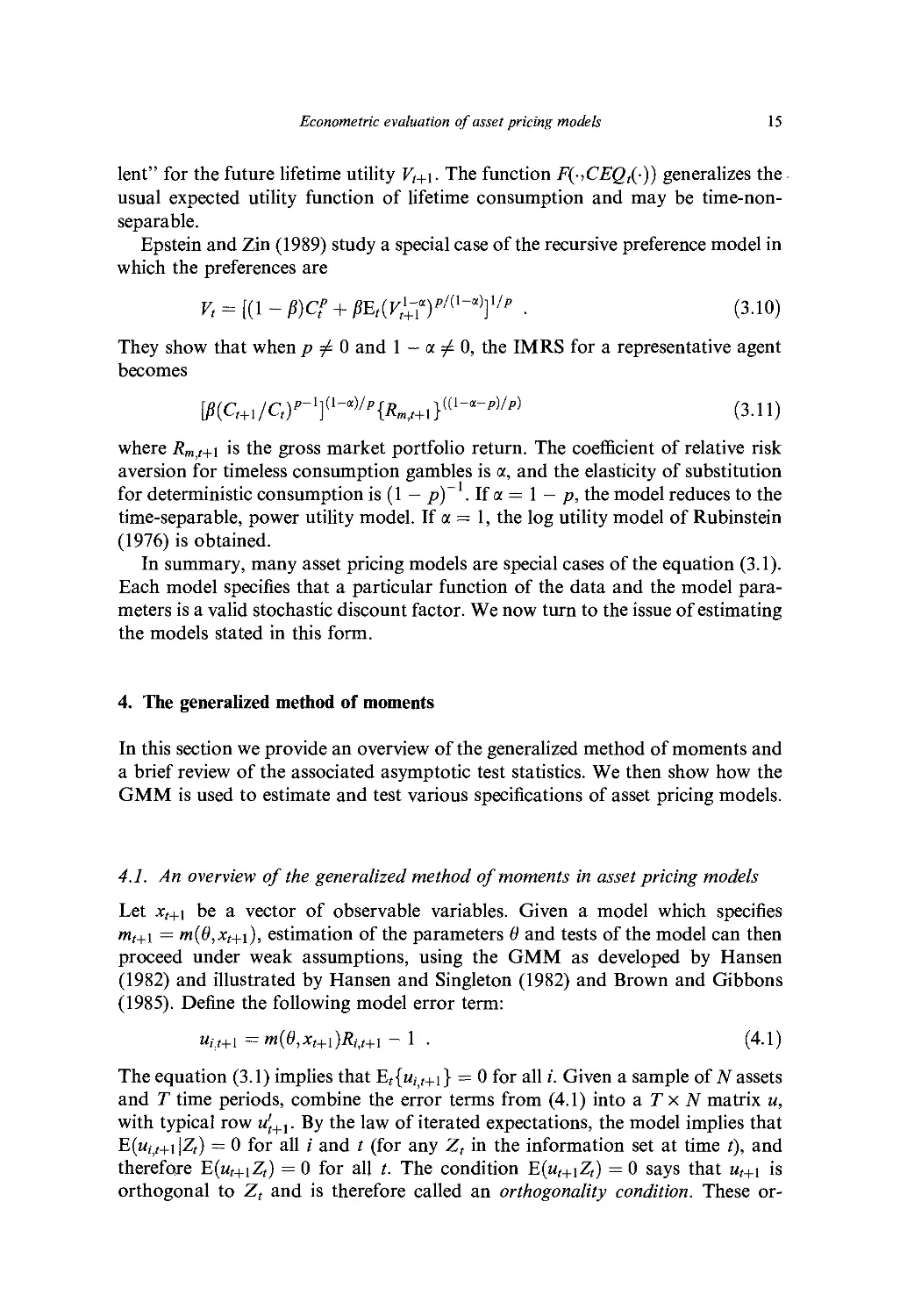
Epstein and Zin (1989, 1991) consider a class of recursive preferences which
can be written as Vt =F(Ct,CEQt{Vt+i)). CEQt{-) is a time t "certainty equiva-

Econometric evaluation of asset pricing models
15
lent" for the future lifetime utility Vt+\. The function F(-,CEQt(-)) generalizes the
usual expected utility function of lifetime consumption and may be time-non-
separable.
Epstein and Zin (1989) study a special case of the recursive preference model in
which the preferences are
V, = [(1 - P)C? + pEt(V?-nP/(l~x)]l/p ■ (3-10)
They show that when p =£ 0 and 1 - a =£ 0, the IMRS for a representative agent
becomes
[P(Ct+ilCt)p-l}(l-*)lp{Rm,t+x}({l-a-p)lp) (3.11)
where Rm>t+\ is the gross market portfolio return. The coefficient of relative risk
aversion for timeless consumption gambles is a, and the elasticity of substitution
for deterministic consumption is (1 — p)~ . If a = 1 — p, the model reduces to the
time-separable, power utility model. If a = 1, the log utility model of Rubinstein
(1976) is obtained.
In summary, many asset pricing models are special cases of the equation (3.1).
Each model specifies that a particular function of the data and the model
parameters is a valid stochastic discount factor. We now turn to the issue of estimating
the models stated in this form.
4. The generalized method of moments
In this section we provide an overview of the generalized method of moments and
a brief review of the associated asymptotic test statistics. We then show how the
GMM is used to estimate and test various specifications of asset pricing models.
4.1. An overview of the generalized method of moments in asset pricing models
Let xt+\ be a vector of observable variables. Given a model which specifies
mt+\ = m(8,xt+\), estimation of the parameters 8 and tests of the model can then
proceed under weak assumptions, using the GMM as developed by Hansen
(1982) and illustrated by Hansen and Singleton (1982) and Brown and Gibbons
(1985). Define the following model error term:
Uij+i =m{e,xt+])Rut+i - 1 . (4.1)
The equation (3.1) implies that Et{uiit+i} = 0 for all i. Given a sample of TV assets
and T time periods, combine the error terms from (4.1) into a T x N matrix u,
with typical row u't+1. By the law of iterated expectations, the model implies that
E(iijj+i \Zt) = 0 for all / and t (for any Zt in the information set at time t), and
therefore E(ut+\Zt) = 0 for all t. The condition E(ut+\Zt) = 0 says that ut+\ is
orthogonal to Zt and is therefore called an orthogonality condition. These or-

16
W. E. Ferson and R. Jagannathan
thogonality conditions are the basis of tests of asset pricing models using the
GMM.
A few points deserve emphasis. First, GMM estimates and tests of asset pricing
models are motivated by the implication that E(«,-]t+i \Zt) = 0, for any Zt in the
information set at time t. However, the weaker condition H(ut+\Zt) = 0, for a
given set of instruments Zt, is actually used in the estimation. Therefore, GMM
tests of asset pricing models have not exploited all of the predictions of the
theories. We believe that further refinements to exploit the implications of the
theories more fully will be useful.
Empirical work on asset pricing models relies on rational expectations,
interpreted as the assumption that the expectation terms in the model are
mathematical conditional expectations. For example, the rational expectations assumption
is used when the expected value in equation (3.1) is treated as a mathematical
conditional expectation to obtain expressions for E(|Z) and E(). Rational
expectations implies that the difference between observed realizations and the
expectations in the model should be unrelated to the information that the
expectations are conditioned on.
Equation (3.1) says that the conditional expectation of the product of mt+\ and
Ritt+i is the constant 1.0. Therefore, the error term 1 — mt+\Riit+\ in equation (4.1)
should not be predictably different from zero when we use any information
available at time t. If there is variation over time in a return Ri^+\ that is
predictable using instruments Z„ the model implies that the predictability is removed
when Ri,t+\ is multiplied by a valid stochastic discount factor, mt+\. This is the
sense in which conditional asset pricing models are asked to "explain" predictable
variation in asset returns. This idea generalizes the "random walk" model of
stock values, which implies that stock returns should be completely unpredictable.
That model is a special case which can be motivated by risk neutrality. Under risk
neutrality the IMRS is a constant. In this case, equation (3.1) implies that the
return Riit+\ should not differ predictably from a constant.
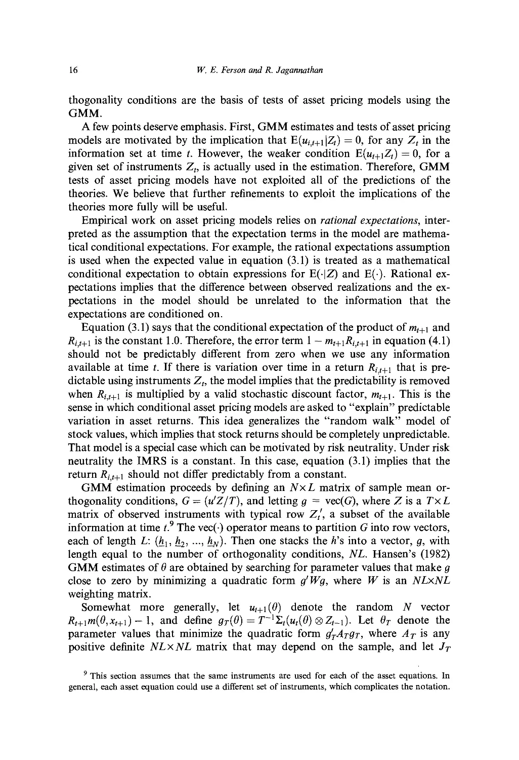
GMM estimation proceeds by defining an NxL matrix of sample mean
orthogonality conditions, G — (u'Z/T), and letting g = vec(G), where Z is a TxL
matrix of observed instruments with typical row Z/, a subset of the available
information at time t? The vec(-) operator means to partition G into row vectors,
each of length L: (hu h2, ..., hN). Then one stacks the h's into a vector, g, with
length equal to the number of orthogonality conditions, NL. Hansen's (1982)
GMM estimates of 8 are obtained by searching for parameter values that make g
close to zero by minimizing a quadratic form g'Wg, where W is an NLxNL
weighting matrix.
Somewhat more generally, let ut+\{&) denote the random TV vector
Rt+xm(0,x,+\)-\, and define gT(0) = T~%(u,(8) <8>Zt_i). Let 8T denote the
parameter values that minimize the quadratic form c/tAt9t, where AT is any
positive definite NLxNL matrix that may depend on the sample, and let JT
9 This section assumes that the same instruments are used for each of the asset equations. In
general, each asset equation could use a different set of instruments, which complicates the notation.

Econometric evaluation of asset pricing models
17
denote the minimized value of the quadratic form g'TArgT- Jagannathan and
Wang (1993) show that JT will have a weighted chi-square distribution which can
be used for testing the hypothesis that (3.1) holds.
Theorem 4.1. (Jagannathan and Wang, 1993). Suppose that the matrix AT
converges in probability to a constant positive definite matrix A. Assume also that
VTgriOo) -+d N(0,S), where iV(-> •) denotes the multivariate normal distribution,
do are the true parameter values, and S is a positive definite matrix. Let
D = E[dgT/de}\g=9o
and let
Q= (Sl'2)(Al?2)[I - {All2)'D{D'AD)-lD'{All2)\(All2){Sll2)
where A1'2 and S1'2 are the upper triangular matrices from the Cholesky
decompositions of A and S. Then the matrix Q has NL-d\m(Q) nonzero, positive
eigenvalues. Denote these eigenvalues by 1;, i = 1,2,..., NL-dim(6). Then JT
converges to
^lZl + • • • + ^NL-dim(9)XNL-dim(e)
where Xi, i = 1,2,..., NL-dim(6) independent random variables, each with a Chi-
Square distribution with one degree of freedom.
Proof. See Jagannathan and Wang (1993).
Notice that when the matrix A is W = S~l, the matrix Q is idempotent of rank
NL-dim(6). Hence the nonzero eigenvalues of Q are unity. In this case, the
asymptotic distribution reduces to a simple chi-square distribution with NL-
dim(0) degrees of freedom. This is the special case considered by Hansen (1982),
who originally derived the asymptotic distribution of the /r-statistic. The JT-
statistic and its extension, as provided in Theorem 4.1, provide a goodness-of-fit
test for models estimated by the GMM.
Hansen (1982) shows that the estimators of 6 that minimize g'Wg are consistent
and asymptotically normal, for any fixed W. If the weighting matrix Wis chosen
to be the inverse of a consistent estimate of the covariance matrix of the
orthogonality conditions S, the estimators are asymptotically efficient in the class of
estimators that minimize g'Wg for fixed Ws. The asymptotic variance matrix of
this optimal GMM estimator of the parameter vector is given as
Cov(0) = [E(dg/de)'WE(dg/de)]-1 (4.2)
where dg/86 is an NLxdim(6) matrix of derivatives. A consistent estimator for
the asymptotic covariance of the sample mean of the orthogonality conditions is
used in practice. That is, we replace W in (4.2) with Cov(#)-1 and replace
E(dg/d6) with its sample analogue. An example of a consistent estimator for the
optimal weighting matrix is given by Hansen (1982) as

18
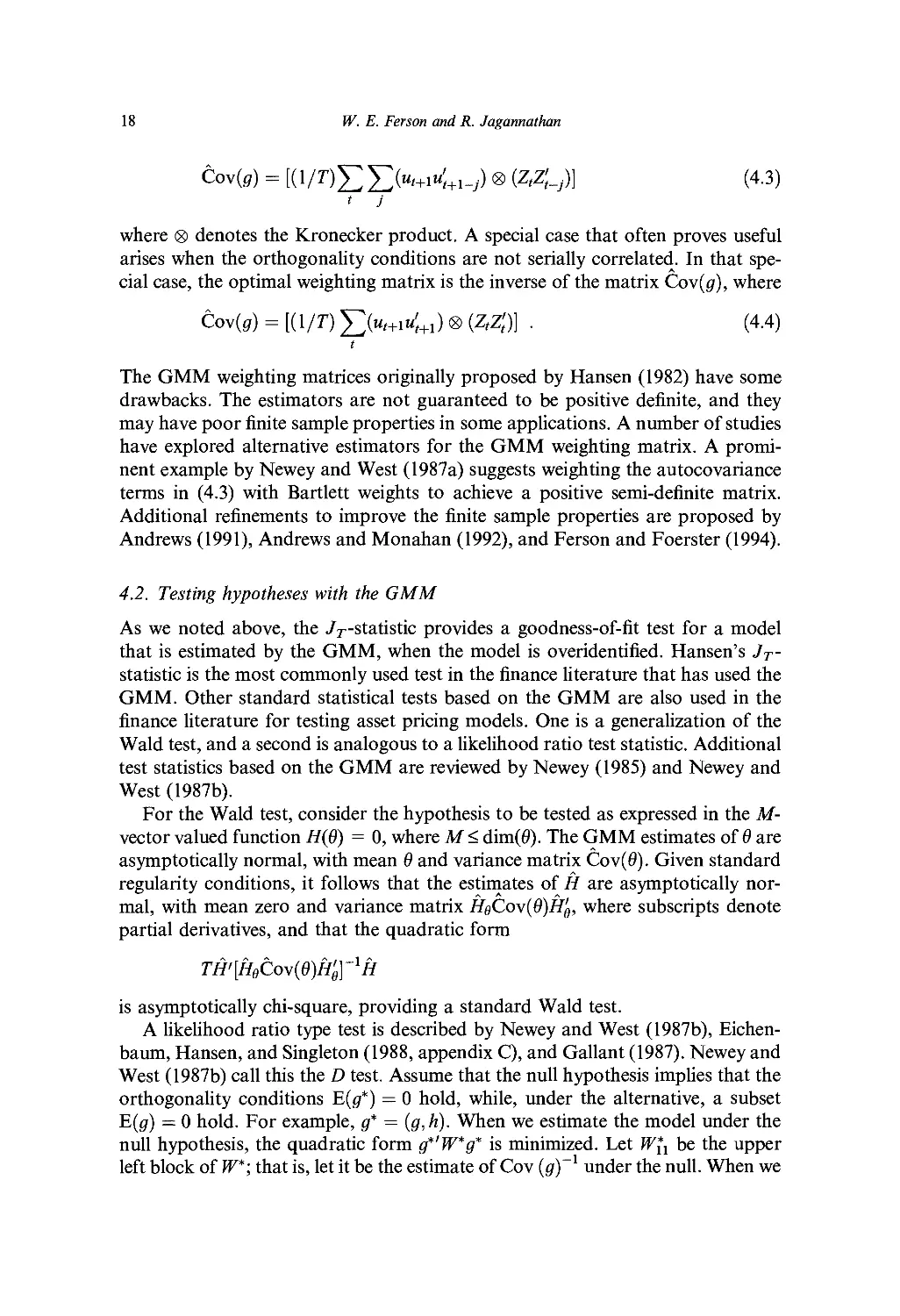
W. E. Ferson and R. Jagannathan
Cov(gr) = [(l/r)£ 5>n-i«;+w) ® (Z^)] (4.3)
where <g> denotes the Kronecker product. A special case that often proves useful
arises when the orthogonality conditions are not serially correlated. In that
special case, the optimal weighting matrix is the inverse of the matrix Cov(gr), where
Cov(gr) = [(1/T) 5>,+i«;+1) ® (ZtZ't)} . (4.4)
t
The GMM weighting matrices originally proposed by Hansen (1982) have some
drawbacks. The estimators are not guaranteed to be positive definite, and they
may have poor finite sample properties in some applications. A number of studies
have explored alternative estimators for the GMM weighting matrix. A
prominent example by Newey and West (1987a) suggests weighting the autocovariance
terms in (4.3) with Bartlett weights to achieve a positive semi-definite matrix.
Additional refinements to improve the finite sample properties are proposed by
Andrews (1991), Andrews and Monahan (1992), and Ferson and Foerster (1994).
4.2. Testing hypotheses with the GMM
As we noted above, the /^-statistic provides a goodness-of-fit test for a model
that is estimated by the GMM, when the model is overidentified. Hansen's JT-
statistic is the most commonly used test in the finance literature that has used the
GMM. Other standard statistical tests based on the GMM are also used in the
finance literature for testing asset pricing models. One is a generalization of the
Wald test, and a second is analogous to a likelihood ratio test statistic. Additional
test statistics based on the GMM are reviewed by Newey (1985) and Newey and
West (1987b).
For the Wald test, consider the hypothesis to be tested as expressed in the M-
vector valued function H{9) = 0, where M < dim(0). The GMM estimates of 9 are
asymptotically normal, with mean 9 and variance matrix Cov(0). Given standard
regularity conditions, it follows that the estimates of H are asymptotically
normal, with mean zero and variance matrix HeCov(9)H'e, where subscripts denote
partial derivatives, and that the quadratic form
TH>[HeCov(9)H'e]~lH
is asymptotically chi-square, providing a standard Wald test.
A likelihood ratio type test is described by Newey and West (1987b), Eichen-
baum, Hansen, and Singleton (1988, appendix C), and Gallant (1987). Newey and
West (1987b) call this the D test. Assume that the null hypothesis implies that the
orthogonality conditions E(gr*) — 0 hold, while, under the alternative, a subset
E(gr) — 0 hold. For example, g* = (g, h). When we estimate the model under the
null hypothesis, the quadratic form g*'W*g* is minimized. Let W\x be the upper
left block of W; that is, let it be the estimate of Cov (g)'1 under the null. When we

Econometric evaluation of asset pricing models
19
hold this matrix fixed the model can be estimated under the alternative by
minimizing (/W^ g. The difference of the two quadratic forms
T[g*'Wg* - g'W*ng]
is asymptotically chi-square, with degrees of freedom equal to M if the null
hypothesis is true. Newey and West (1987b) describe additional variations on
these tests.
4.3. Illustrations: Using the GMM to test the conditional CAPM
The CAPM imposes nonlinear overidentifying restrictions on the first and second
moments of asset returns. These restrictions can form a basis for econometric
tests. To see these restrictions more clearly, notice that if an econometrician
knows or can estimate Cov(Rit,Rmt), E(Rmt), Var(i?mr), and E(R0t), it is possible to
compute E(Rit) from the CAPM, using equation (2.1). Given a direct sample
estimate of E(Rit), the expected return is overidentified. It is possible to use the
overidentification to construct a test of the CAPM by asking if the expected
return on the asset is different from the expected return assigned by the model. In
this section we illustrate such tests by using both the traditional, return-beta
formulation and the stochastic discount factor representation of the CAPM.
These examples extend easily to the multiple-beta models.
4.3.1. Static or unconditional CAPMs
If we make the assumption that all the expectation terms in the CAPM refer to
the unconditional expectations, we have an unconditional version of the CAPM. It
is straightforward to estimate and then test an unconditional version of the
CAPM, using equation (3.1) and the stochastic discount factor representation
given in equation (3.4). The stochastic discount factor is
mt+\ = co + c\Rmt+\
where c0 and c\ are fixed parameters. Using only the unconditional expectations,
the model implies that
E{(c0+ci^mr+i)^+i-l} = 0
where Rt+i is the vector of gross asset returns. The vector of sample
orthogonality conditions is
gr = gT(co,ci) = (l/T)^2{(c0 + ciRmt+l)Rt+l - 1} .
t
With assets N > 2, the number of orthogonality conditions is N and the number
of parameters is 2, so the /^-statistic has N - 2 degrees of freedom. Tests of the
unconditional CAPM using the stochastic discount factor representation are
conducted by Carhart et al. (1995) and Jagannathan and Wang (1996), who reject
the model using monthly data for the postwar United States.

20
W. E. Ferson and R. Jagannathan
Tests of the unconditional CAPM may also be conducted using the linear,
return-beta formulation of equation (2.1) and the GMM. Let rt = Rt-.%! be the
vector of excess returns, where i?or is the gross return on some reference asset and
1 is an N vector of ones; also let ut = rt- f5rmt, where /? is the N vector of the betas
of the excess returns, relative to the market, and rmt = Rmt - Rot is the excess
return on the market portfolio. The model implies that
E(ut) = E(utrmt) = 0 .
Let the instruments be Zt = (l,rmt)'. The sample orthogonality condition is then
gT(P) = T-lJ2(rt-Prmt)®Zt .
t
The number of orthogonality conditions is 2N and the number of parameters is
N, so the model is overidentified and may be tested using the /r-statistic.
An alternative approach to testing the model using the return-beta formulation
is to estimate the model under the hypothesis that expected returns depart from
the predictions of the CAPM by a vector of parameters a, which are called
Jensen's alphas. Redefining ut = rt — a — firmt, the model has 2N parameters and
2N orthogonality conditions, so it is exactly identified. It is easy to show that the
GMM estimators of a and /? are the same as the OLS estimators, and equation
(4.4) delivers White's (1980) heteroskedasticity-consistent standard errors. The
CAPM may be tested using a Wald test or the D-statistic, as described above.
Tests of the unconditional CAPM using the linear return-beta formulation are
conducted with the GMM by MacKinlay and Richardson (1991), who reject the
model for monthly U.S. data.
4.3.2. Conditional CAPMs
Empirical studies that rejected the unconditional CAPM, as well as mounting
evidence of predictable variation in the distribution of security rates of return, led
to empirical work on conditional versions of the CAPM starting in the early
1980s. In a conditional asset pricing model it is assumed that the expectation terms
in the model are conditional expectations, given a public information set that is
represented by a vector of predetermined instrumental variables Zt. The multiple-
beta models of Merton (1973) and Cox, Ingersoll, and Ross (1985) are intended to
accommodate conditional expectations. Merton (1973, 1980) and Cox-Ingersoll-
Ross also showed how a conditional version of the CAPM may be derived as a
special case of their intertemporal models. Hansen and Richard (1987) describe
theoretical relations between conditional and unconditional versions of mean-
variance efficiency.
The earliest empirical formulations of conditional asset pricing models were
the latent variable models developed by Hansen and Hodrick (1983) and Gibbons
and Ferson (1985) and later refined by Campbell (1987) and Ferson, Foerster,
and Keim (1993). These models allow time-varying expected returns, but
maintain the assumption that the conditional betas are fixed parameters. Consider the

Econometric evaluation of asset pricing models
21
linear, return-beta representation of the CAPM under these assumptions, writing
E(r(|Z(_i) = /}E(r„,f|Zf_i). The returns are measured in excess of a risk-free asset.
Let r1( be some reference asset with nonzero /?i, so that
E(r1(|Z(_1)=jS1E(rm(|Z(_1) .
Solving this expression for E(rmt\Zt-i) and substituting, we have
E(r,|Zi_i) = CE(n,|£_i)
where C= (j3.//?i) and ./ denotes element-by-element division. With this
substitution, the expected market risk premium is the latent variable in the model,
and C is the N vector of the model parameters. When we form the error term
ut = rt — Cr\t, the model implies E(«f|Zf_i) = 0 and we can estimate and test the
model by using the GMM. Gibbons and Ferson (1985) argued that the latent
variable model is attractive in view of the difficulties in measuring the true market
portfolio, but Wheatley (1989) emphasized that it remains necessary to assume
that ratios of the betas, measured with respect to the unobserved market
portfolio, are constant parameters.
Campbell (1987) and Ferson and Foerster (1995) show that a single-beta latent
variable model is rejected in U.S. data. This finding rejects the hypothesis that
there is a (conditional) minimum-variance portfolio such that the ratios of
conditional betas on this portfolio are fixed parameters. Therefore, the empirical
evidence suggests that conditional asset pricing models should be consistent with
either (1) a time-varying beta or (2) more than one beta for each asset.10
Conditional, multiple-beta models with constant betas are examined
empirically by Ferson and Harvey (1991), Evans (1994), and Ferson and Korajczyk
(1995). They reject such models with the usual statistical tests but find that they
still capture a large fraction of the predictability of stock and bond returns over
time. When allowing for time-varying betas, these studies find that the time-
variation in betas contributes a relatively small amount to the time-variation in
expected asset returns. Intuition for this finding can be obtained by considering
the following approximation. Suppose that time-variation in expected excess
returns is E(r|Z) = A/?, where X is a vector of time-varying expected risk premiums
for the factors and /? is a matrix of time-varying betas. Using a Taylor series, we
can approximate
Var[E(r|Z)] « E(jS)'Var[l]E(jS) + E(l)'Var[jS]E(l) .
The first term in the decomposition reflects the contribution of the time-varying
risk premiums; the second reflects the contribution of time-varying betas. Since
the average beta E(fi) is on the order of 1.0 in monthly data, while the average risk
1 A model with more than one fixed beta, and with time-varying risk premiums, is generally
consistent with a single, time-varying beta for each asset. For example, assume that there are two
factors with constant betas and time-varying risk premiums, where a time-varying combination of the
two factors is a minimum-variance portfolio.

22
W. E. Ferson and R. Jagannathan
premium E(l) is typically less than 0.01, the first term dominates the second term.
This means that time-variation in conditional betas is less important than time-
variation in expected risk premiums, from the perspective of modeling predictable
variation in expected asset returns.
While from the perspective of modeling predictable time-variation in asset
returns, time-variation in conditional betas is not as important as time-variation
in expected risk premiums, this does not imply that beta variation is empirically
unimportant. From the perspective of modeling the cross-sectional variation in
expected asset returns, beta variation over time may be very important. To see
this, consider the unconditional expected excess return vector, obtained from the
model as
E{E(r|Z)} = E{ljS} = E(A)EQS) + Cov(l, J?) .
Viewed as a cross-sectional relation, the term Cov(l, /?) may vary significantly in a
cross section of assets. Therefore, the implications of a conditional version of the
CAPM for the cross section of unconditional expected returns may depend
importantly on common time-variation in betas and expected market risk
premiums. The empirical tests of Jagannathan and Wang (1996) suggest that this is
the case.
Harvey (1989) replaced the constant beta assumption with the assumption that
the ratio of the expected market premium to the conditional market variance is a
fixed parameter, as in
E(rw,|Z,_i)/Var(r,„,|Z,_i) = y .
The conditional expected returns may then be written according to the
conditional CAPM as
E(r,\Z,-i) = yCo\(r„rmt\Z,-i) .
Harvey's version of the conditional CAPM is motivated by Merton's (1980)
model in which the ratio y, called the market price of risk, is equal to the relative
risk aversion of a representative investor in equilibrium. Harvey also assumes that
the conditional expected risk premium on the market (and the conditional market
variance, given fixed y) is a linear function of the instruments, as in
E(rwt|Zt_i) = &'mZ,-\
where bm is a coefficient vector. Define the error terms vt = rmt — 5'mZt-i and
wt = rt(\ - vty). The model implies that the stacked error term ut = (vt,wt)
satisfies E(wt|Zf_i) = 0, so it is straightforward to estimate and then test the model
using the GMM. Harvey (1989) rejects this version of the conditional CAPM for
monthly data in the U.S. In Harvey (1991) the same formulation is rejected when
applied using a world market portfolio and monthly data on the stock markets of
21 developed countries.
The conditional CAPM may be tested using the stochastic discount factor
representation given by equation (3.4): mt+\ — cq( - cuRmt+\. In this case the

Econometric evaluation of asset pricing models
23
coefficients c0, and cu are measurable functions of the information set Zt. To
implement the model empirically it is necessary to specify functional forms for the
c0t and c\t. From the expression (3.4) it can be seen that these coefficients are
nonlinear functions of the conditional expected market return and its conditional
variance. As yet there is no theoretical guidance for specifying the functional
forms. Cochrane (1996) suggests approximating the coefficients using linear
functions, and this approach is followed by Carhart et al. (1995), who reject the
conditional CAPM for monthly U.S. data.
Jagannathan and Wang (1993) show that the conditional CAPM implies an
unconditional two-factor model. They show that
mt+i =a0+ fliE(rm,+i \It) + Rmt+\
(where /, denotes the information set of investors and ao and a.\ are fixed
parameters) is a valid stochastic discount factor in the sense that E(i?^+im,+1) = 1 for
this choice of mt+\. Using a set of observable instruments Z„ and assuming that
E(rmH-i \Zt) is a linear function of Zt, they find that their version of the model
explains the cross section of unconditional expected returns better than does an
unconditional version of the CAPM. Bansal and Viswanathan (1993) develop
conditional versions of the CAPM and multiple-factor models in which the
stochastic discount factor m,+ 1 is a nonlinear function of the market or factor
returns. Using nonparametric methods, they find evidence to support the
nonlinear versions of the models. Bansal, Hsieh, and Viswanathan (1993) compare
the performance of nonlinear models with linear models, using data on
international stocks, bonds, and currency returns, and they find that the nonlinear
models perform better. Additional empirical tests of the conditional CAPM and
multiple-beta models, using stochastic discount factor representations, are
beginning to appear in the literature. We expect that future studies will further refine
the relations among the various empirical specifications.
5. Model diagnostics
We have discussed several examples of stochastic discount factors corresponding
to particular theoretical asset pricing models, and we have shown how to test
whether these models assign the right expected returns to financial assets. The
stochastic discount factors corresponding to these models are particular
parametric functions of the data observed by the econometrician. While empirical
studies based on these parametric approaches have led to interesting insights, the
parametric approach makes strong assumptions about the economic
environment. In this section we discuss some alternative econometric approaches to the
problem of asset pricing models.

24
W. E. Ferson and R. Jagannathan
5.1. Moment inequality restrictions
Hansen and Jagannathan (1991) derive restrictions from asset pricing models
while assuming as little structure as possible. In particular, they assume that the
financial markets obey the law of one price and that there are no arbitrage
opportunities. These assumptions are sufficient to imply that there exists a
stochastic discount factor mt+i (which is almost surely positive, if there is no
arbitrage) such that equation (3.1) is satisfied.
Note that if the stochastic discount factor is a degenerate random variable (i.e.,
a constant), then equation (3.1) implies that all assets must earn the same
expected return. If assets earn different expected returns, then the stochastic
discount factor cannot be a constant. In other words, cross-sectional differences in
expected asset returns carry implications for the variance of any valid stochastic
discount factor, which satisfies equation (3.1). Hansen and Jagannathan make use
of this observation to derive a lower bound on the volatility of stochastic discount
factors. Shiller (1979, 1981), Singleton (1980), and Leroy and Porter (1981) derive
a related volatility bound in specific models, and their empirical work suggests
that the stochastic discount factors implied by these simple models are not volatile
enough to explain expected returns across assets. Hansen and Jagannathan (1991)
show how to use the volatility bound as a general diagnostic device.
In what follows we derive the Hansen and Jagannathan (1991) bound and
discuss their empirical application. To simplify the exposition, we focus on an
unconditional version of the bound using only the unconditional expectations.
We posit a hypothetical, unconditional, risk-free asset with return Rf =
E(mr+i)_1. We take the value of Rf, or equivalently E(wr+ 0, as a parameter to be
varied as we trace out the bound.
The law of one price guarantees the existence of some stochastic discount
factor which satisfies equation (3.1). Consider the following projection of any
such mt+\ on the vector of gross asset returns, Rt+\.
mt+i = R't+lP + et+i (5.1)
where
E(er+1^r+1) = 0
and where /? is the projection coefficient vector. Multiply both sides of equation
(5.1) by Rt+i and take the expected value of both sides of the equation, using
E[Rt+iet+i] = 0, to arrive at an expression which may be solved for /?. Substituting
this expression back into (5.1) gives the "fitted values" of the projection as
<i = K+iP = K+MRt+iK+i)~ll ■ (5-2)
By inspection, the m*+l given by equation (5.2) is a valid stochastic discount
factor, in the sense that equation (3.1) is satisfied when m*+l is used in place of
mt+\. We have therefore constructed a stochastic discount factor m*+l that is also
a payoff on an investment position in the N given assets, where the vector

Econometric evaluation of asset pricing models
25
E(Rt+\R't+l)~l I provides the weights. This payoff is the unique linear least
squares approximation of every admissible stochastic discount factor in the space
of available asset payoffs.
Substituting m*+l for R't+l(3 in equation (5.1) shows that we may write any
stochastic discount factor, mt+\, as
m,+l = m*+l + e,+l
where E{et+\m*t+x) = 0. It follows that Var(w?+i) > Var(/»*+1). This expression is
the basis of the Hansen-Jagannathan bound11 on the variance of mt+1. Since m*+l
depends only on the second moment matrix of the N returns, the lower bound
depends only on the assets available to the econometrician and not on the
particular asset pricing model that is being studied. To obtain an explicit expression
for the variance bound in terms of the underlying asset-return moments,
substitute from the previous expressions to obtain
Var(m,+i) > Var(m,*+1)
= pVai(Rt+l)P (5.3)
= [Cov(m,R')VsLr(Ryl] xVar(R)[Var(R)~lCoy(m,R')}
= [l~ E(m)E(R')]Var(R)~l\l - E(m)E(R)]
where the time subscripts are suppressed to conserve notation and the last line
follows from E(mR) = I = E(m)E(R) + Cov(m,R). As we vary the hypothetical
values of E(m) = Rjl, the equation (5.3) traces out a parabola in E(m), o.(m) space,
where o.(m) is the standard deviation of mt+\. If we place o.(m) on the y axis and
E(m) on the x axis, the Hansen-Jagannathan bounds resemble a cup, and the
implication is that any valid stochastic discount factor mt+\ must have a mean and
standard deviation that place it within the cup.
The lower bound on the volatility of a stochastic discount factor, as given by
equation (5.3), is closely related to the standard mean-variance analysis that has
long been used in the financial economics literature. To see this, recall that if
r = R — Rf is the vector of excess returns, then (3.1) implies that
0 = E(mr) = E(m)E(r) + po(m)o(r) .
Since —1 < p < 1, we have that
ff(m)/E(m) > E(rt)/ff(rt)
for all /. The right side of this expression is the Sharpe ratio for asset /. The Sharpe
ratio is defined as the expected excess return on an asset, divided by the standard
deviation of the excess return (see Sharpe 1994 for a recent discussion of this
ratio). Consider plotting every portfolio that can be formed from the N assets in
the Standard Deviation (x axis) - Mean (y axis) plane. The set of such portfolios
"Related bounds were derived by Kandel and Stambaugh (1987), Mackinlay (1987, 1995), and
Shanken (1987).

26
W. E. Ferson and R. Jagannathan
with the smallest possible standard deviation for a given mean return is the
minimum-variance boundary. Consider the tangent to the minimum-variance
boundary from the point 1/E(m) on the y axis. The tangent point is a portfolio of
the asset returns, and the slope of this tangent line is the maximum Sharpe ratio
that can be attained with a given set of N assets and a given risk-free
rate, Rf = 1/E(m). The slope of this line is also equal to Rf multiplied by the
Hansen-Jagannathan lower bound on a(m) for a given E(m) =R7X- That is, we
have that
ff(m) > E(m)|Max{E(r,-)/ff(r,-)}|
for the given Rf.
The preceding analysis is based on equation (3.1), which is equivalent to the
law of one price. If there are no arbitrage opportunities, it implies that mt+\ is a
strictly positive random variable. Hansen and Jagannathan (1991) show how to
obtain a tighter bound on the standard deviation of mt+\ by making use of the
restriction that there are no arbitrage opportunities. They also show how to
incorporate conditioning variables into the analysis. Snow (1991) extends the
Hansen-Jagannathan analysis to include higher moments of the asset returns. His
extension is based on the Holder inequality, which implies that for given values of
5 and p such that
(l/5) + (l//») = l
it is true that
E(mR) < E(ms)l/dE(Rp)l/p.
Cochrane and Hansen (1992) refine the Hansen-Jagannathan bound to consider
information about the correlation between a given stochastic discount factor and
the vector of asset returns. This provides a tighter set of restrictions than the
original bounds, which only make use of the fact that the correlation must be
between -1 and + 1.
5.2. Statistical inference for moment inequality restrictions
Cochrane and Hansen (1992), Burnside (1994), and Cecchetti, Lam, and Mark
(1994) show how to take sampling errors into account when examining whether a
particular candidate stochastic discount factor satisfies the Hansen-Jagannathan
bound. In what follows we will outline a computation which allows for sampling
errors, following the discussion in Cochrane and Hansen (1992).
Assume that the econometrician has a time series of T observations on a
candidate for the stochastic discount factor, denoted by yt, and the N asset
returns Rt. We also assume that the risk-free asset is not one of the N assets. Hence
v = E(m) = \/RF is an unknown parameter to be estimated. Consider a linear
regression of mt+\ onto the unit vector and the vector of asset returns as
m,+1 = a + R't P + ut+\. We use the regression function in the following system of
population moment conditions:

Econometric evaluation of asset pricing models
27
E(a + R'tp) = v (5.4)
E(*,a + RtR'tp) = \N
E(yt) = v
E[(a + R'tP)2}-E[yt}<0 .
The first equation says that the expected value of mt = a + R'tP = v. The second
equation says that the regression function for mt is a valid stochastic discount
factor. The third equation says that v is the expected value of the particular
candidate discount factor that we wish to test. The fourth equation states that the
Hansen-Jagannathan bound is satisfied by the particular candidate stochastic
discount factor.
We can estimate the parameters v, a, and the N vector /?, using the N + 3
equations in (5.4), by treating the last inequality as an equality and using the
GMM. Treating the last equation as an equality corresponds to the null
hypothesis that the mean and variance of yt place it on the Hansen-Jagannathan
boundary. Under the null hypothesis that the last equation of (5.4) holds as an
equality, the minimized value of the GMM criterion function JT, multiplied by T,
has a chi-square distribution with one degree of freedom. Cochrane and Hansen
(1992) suggest testing the inequality relation using the one-sided test.
5.3. Specification error bounds
The methods we have examined so far are developed, for the most part, under the
null hypothesis that the asset pricing model under consideration by the econo-
metrician assigns the right prices (or expected returns) to all assets. An alternative
is to assume that the model is wrong and examine how wrong the model is. In this
section we will follow Hansen and Jagannathan (1994) and discuss one possible
way to examine what is missing in a model and assign a scalar measure of the
model's misspecification.12
Let yt denote the candidate stochastic discount factor corresponding to a given
asset pricing model, and let m* denote the unique stochastic discount factor that
we constructed earlier, as a combination of asset payoffs. We assume that E[j(if(]
does not equal lN, the N vector of ones; i.e., the model does not correctly price all
of the gross returns. We can project yt on the N asset returns to get yt = R'ta + ut,
and project m* on the vector of asset returns to get m* = R'tP + et. Since the
candidate yt does not correctly price all of the assets, then a. and /? will not be the
same. Define pt = {fi — a)'Rt as the modifying payoff'to the candidate stochastic
12 GMM-based model specification tests are examined in a general setting by Newey (1985). Other
related work includes that by Boudoukh, Richardson, and Smith (1993), who compute approximate
bounds on the probabilities of the test statistics in the presence of inequality restrictions; Chen and
Knez (1992) develop nonparametric measures of market integration by using related methods; and
Hansen, Heaton, and Luttmer (1995) show how to compute specification error and volatility bounds
when there are market frictions such as short-sale constraints and proportional transaction costs.

28
W. E. Ferson and R. Jagannathan
discount factor yt. Clearly, (jt+pt) is a valid stochastic discount factor, satisfying
equation (3.1). Hansen and Jagannathan (1994) derive specification tests based on
the size of the modifying payoff, which measures how far the model's candidate
for a stochastic discount factor yt is from a valid stochastic discount factor.
Hansen and Jagannathan (1994) show that a natural measure of this distance is
5 = E(/?/2), which provides an economic interpretation for the model's mis-
specification. Payoffs that are orthogonal to pt are correctly priced by the
candidate yt, and E(p2) is the maximum amount of mispricing by using yt for any
payoff normalized to have a unit second moment. The modifying payoff pt is also
the minimal modification that is sufficient to make yt a valid stochastic discount
factor.
Hansen and Jagannathan (1994) consider an estimator of the distance measure
5 given as the solution to the following maximization problem:
ST = Maxo.r-1 JTtf - (yt + a%)2 + 2oc'IJV]1/2. (5.5)
t
If a.T is the solution to (5.5), then the estimate of the modifying payoff is tx'TRt. It
can be readily verified that the first-order condition to (5.5) implies that a!TRt
satisfies the sample counterpart to the asset pricing equation (3.1).
To obtain an estimate of the sampling error associated with the estimated value
6t, consider
ut = y2t - (yt + a'TRt)2 + 2a'rlJV •
The sample mean of ut is b\. We can obtain a consistent estimator of the variance
of b\ by the frequency zero spectral density estimators described in Newey and
West (1987a) or Andrews (1991) and applied to the time series {u, - b\}t=lT. Let
sT denote the estimated standard deviation of b\ obtained this way. Then, under
standard assumptions, we have that TXI2(5T — 5)/sT converges to a normal (0,1)
random variable. Hence, using the delta method, we obtain
Tx?2dT/2sT(dT - S) — N(0,1) . (5.6)
6. Conclusions
In this article we have reviewed econometric tests of a wide range of asset pricing
models, where the models are based on the law of one price, the no-arbitrage
principle, and models of market equilibrium with investor optimization. Our
review included the earliest of the equilibrium asset pricing models, the CAPM,
and also considered dynamic multiple-beta and arbitrage pricing models. We
provided some results for the asymptotic distribution of traditional two-pass
estimators for asset pricing models stated in the linear, return-beta formulation.
We emphasized the econometric evaluation of asset pricing models by using

Econometric evaluation of asset pricing models
29
Hansen's (1982) generalized method of moments. Our examples illustrate the
simplicity and flexibility of the GMM approach. We showed that most asset
pricing models can be represented in a stochastic discount factor form, which
makes the application of the GMM straightforward. Finally, we discussed model
diagnostics that provide additional insight into the causes of the statistical
rejections in GMM tests and which help assess the specification errors in these
models.
Appendix
Proof of Theorem 2.1 The proof comes from Jagannathan and Wang (1996).
We first introduce some additional notation. Let IN be the TV-dimensional identity
matrix and lrbe a T-dimensional vector of ones. It follows from equation (2.17)
that
R-V=T-1 (IN ® \'T)'ek, k=l,...,K2
where
e* = (eijti, • • •, eitr, • • •, emi, ■ ■ ■, emr) ■
By the definition of bk, we have that
bk-Pk = [In ® ((fk'fk)-lfk%k
where fk is the vector-demeaned factor realizations, conformable to the vector ek.
In view of the assumption that the conditional covariance of e^ and tjit, given the
time series of the factors (denoted by fk), is a fixed constant aijki, we have that
E[(i4-/J4)(*i-A«i)|/t]
= T~l[IN ® (U'ir'jOlEh^liK/iv ® lr)
= T-%®((g£)-lg)]Xkl(Ilf®lT)
= r-%®[(//i)-1//ir)] = o
where we denote the matrix of the {ffy/u},-,- by S&. The last line follows from the
fact fhat^'lr = 0. Hence we have shown that (bk - /}t) is uncorrelated with
(R - n). Therefore, the terms u and hyi should be uncorrelated, and the
asymptotic variance of Tll2{g — y) in equation (2.15) is given by
(x'xylx'[VsLr(u) + VeLT{hy2)]x{x'x)~l .
Let nt]ti denote the limiting value of Con(\ff fleikl y/Tfltji), as T —> oo. Let the
matrix with nt]ki being its ifh element be denoted by n&. We assume that the
sample covariance matrix of the factors exists and converges in probability to a
constant positive definite matrix Q, with typical element Qw. Since \ff (bik - fiik)
converges in distribution to the random variable Si^y/f' f'k^ik, we have

30
W. E. Person and R. Jagannathan
and
W = {x'x)~xx'y&x(hy2)x(x'x)~x
= J2 (x'x)-lx'{y2ky2l(n^Uk!ai!l)}x(x'xrl
l,k=l,...,k2
where Tl'kl is a matrix whose 1,7th element is the limiting value of Cov(Vffk €,*,
Vffl&ji) as T-^oo.
Q.E.D.
References
Abel, A. (1990). Asset prices under habit formation and catching up with the Jones. Amer. Econom.
Rev. Papers Proc. 80, 38-42.
Andrews, D. W. K. (1991). Heteroskedasticity and autocorrelation consistent covariance matrix
estimation. Econometrica 59, 817-858.
Andrews, D. W. K. and J. C. Monahan (1992). An improved heteroskedasticity and autocorrelation
consistent covariance matrix estimator. Econometrica 60, 953-966.
Arrow, K. J. (1970). Essays in the Theory of Risk-Bearing. Amsterdam: North-Holland.
Bansal, R. and S. Viswanathan (1993). No- arbitrage and arbitrage pricing: A new approach. /. Finance
8, 1231-1262.
Bansal, R., D. A. Hsieh and S. Viswanathan (1993). A new approach to international arbitrage
pricing. /. Finance 48, 1719-1747.
Becker, G. S. and K. M. Murphy (1988). A theory of rational addiction. /. Politic. Econom. 96, 675-
700.
Beja, A. (1971). The structure of the cost of capital under uncertainty. Rev. Econom. Stud. 38(8), 359-
368.
Berk, J. B. (1995). A critique of size-related anomalies. Rev. Financ. Stud. 8, 275-286.
Black, F. (1972). Capital market equilibrium with restricted borrowing. /. Business 45, 444-455.
Black, F., M. C. Jensen and M. Scholes (1972). The capital asset pricing model: Some empirical tests.
In: Studies in the Theory of Capital Markets, M. C. Jensen, ed., New York: Praeger, 79-121.
Boudoukh, J., M. Richardson and T. Smith (1993). Is the ex ante risk premium always positive? A new
approach to testing conditional asset pricing models. /. Financ. Econom. 34, 387-408.
Breeden, D. T. (1979). An intertemporal asset pricing model with stochastic consumption and
investment opportunities. J. Financ. Econom. 7, 265-296.
Brown, D. P. and M. R. Gibbons (1985). A simple econometric approach for utility-based asset pricing
models. /. Financed, 359-381.
Burnside, C. (1994). Hansen-Jagannathan bounds as classical tests of asset-pricing models. /. Business
Econom. Statist. 12, 57-79.
Campbell, J. Y. (1987). Stock returns and the term structure. /. Financ. Econom. 18, 373-399.
Campbell, J. Y. and J. Cochrane (1995). By force of habit. Manuscript, Harvard Institute of Economic
Research, Harvard University.
Carhart, M., K. Welch, R. Stevens and R. Krail (1995). Testing the conditional CAPM. Working
Paper, University of Chicago.
Cecchetti, S. G., P. Lam and N. C. Mark (1994). Testing volatility restrictions on intertemporal
marginal rates of substitution implied by Euler equations and asset returns. /. Finance 49, 123-152.

Econometric evaluation of asset pricing models
31
Chen, N. (1983). Some empirical tests of the theory of arbitrage pricing. J. Finance 38, 1393-1414.
Chen, Z. and P. Knez (1992). A measurement framework of arbitrage and market integration.
Working Paper, University of Wisconsin.
Cochrane, J. H. (1996). A cross-sectional test of a production based asset pricing model. Working
Paper, University of Chicago.
Cochrane, J. H. and L. P. Hansen (1992). Asset pricing explorations for macroeconomics. In: NBER
Macroeconomics Annual 1992, O. J. Blanchard and S. Fischer, eds., Cambridge, Mass.: MIT Press.
Connor, G. (1984). A unified beta pricing theory. /. Econom. Theory 34, 13-31.
Connor, G. and R. A. Korajczyk (1986). Performance measurement with the arbitrage pricing theory:
A new framework for analysis. /. Financ. Econom. 15, 373-394.
Constantinides, G. M. (1982). Intertemporal asset pricing with heterogeneous consumers and without
demand aggregation. J. Business 55, 253-267.
Constantinides, G. M. (1990). Habit formation: A resolution of the equity premium puzzle. /. Politic.
Econom. 98, 519-543.
Constantinides, G. M. and D. Duffle (1994). Asset pricing with heterogeneous consumers. Working
Paper, University of Chicago and Stanford University.
Cox, J. C, J. E. Ingersoll, Jr. and S. A. Ross (1985). A theory of the term structure of interest rates.
Econometrica 53, 385-407.
Debreu, G. (1959). Theory of Value: An Axiomatic Analysis of Economic Equilibrium. New York:
Wiley.
Detemple, J. B. and F. Zapatero (1991). Asset prices in an exchange economy with habit formation.
Econometrica 59, 1633-1657.
Dunn, K. B. and K. J. Singleton (1986). Modeling the term structure of interest rates under non-
separable utility and durability of goods. /. Financ. Econom. 17, 27-55.
Dybvig, P. H. and J. E. Ingersoll, Jr., (1982). Mean-variance theory in complete markets. /. Business
55, 233-251.
Eichenbaum, M. S., L. P. Hansen and K. J. Singleton (1988). A time series analysis of representative
agent models of consumption and leisure choice under uncertainty. Quart. J. Econom. 103, 51-78.
Epstein, L. G. and S. E. Zin (1989). Substitution, risk aversion and the temporal behavior of
consumption and asset returns: A theoretical framework. Econometrica 57, 937-969.
Epstein, L. G. and S. E. Zin (1991). Substitution, risk aversion and the temporal behavior of
consumption and asset returns. /. Politic. Econom. 99, 263-286.
Evans, M. D. D. (1994). Expected returns, time-varying risk, and risk premia. /. Finance 49, 655-679.
Fama, E. F. and K. R. French. (1992). The cross-section of expected stock returns. /. Finance 47, 427-
465.
Fama, E. F. and J. D. MacBeth (1973). Risk, return, and equilibrium: Empirical tests. /. Politic.
Econom. 81, 607-636.
Ferson, W. E. (1983). Expectations of real interest rates and aggregate consumption: Empirical tests.
/. Financ. Quant. Anal. 18, 477-497.
Ferson, W. E. and G. M. Constantinides (1991). Habit persistence and durability in aggregate
consumption: Empirical tests. /. Financ. Econom. 29, 199-240.
Ferson, W. E. and S. R. Foerster (1994). Finite sample properties of the generalized method of
moments tests of conditional asset pricing models. /. Financ. Econom. 36, 29-55.
Ferson, W. E. and S. R. Foerster (1995). Further results on the small-sample properties of the
generalized method of moments: Tests of latent variable models. In: Res. Financ, Vol. 13.
Greenwich, Conn.: JAI Press, pp. 91-114.
Ferson, W. E., S. R. Foerster and D. B. Keim (1993). General tests of latent variable models and
mean-variance spanning. /. Finance 48, 131-156.
Ferson, W. E. and C. R. Harvey (1991). The variation of economic risk premiums. /. Politic. Econom.
99, 385-415.
Ferson, W. E. and C. R. Harvey (1992). Seasonality and consumption-based asset pricing. /. Finance
47,511-552.

32
W. E. Ferson and R. Jagannathan
Ferson, W. E. and R. A. Korajczyk (1995). Do arbitrage pricing models explain the predictability of
stock returns? J. Business 68, 309-349.
Ferson, W. E. and J. J. Merrick, Jr. (1987). Non-stationarity and stage-of-the-business-cycle effects in
consumption-based asset pricing relations. J. Financ. Econom. 18, 127-146.
Gallant, R. (1987). Nonlinear Statistical Models. New York: Wiley.
Gibbons, M. R. and W. Ferson (1985). Testing asset pricing models with changing expectations and an
unobservable market portfolio. J. Financ. Econom. 14, 217-236.
Gorman, W. M. (1953). Community preference fields. Econometrica 21, 63-80.
Hansen, L. P. (1982). Large sample properties of generalized method of moments estimators.
Econometrica 50, 1029-1054.
Hansen, L. P., J. Heaton and E. G. J. Luttmer (1995). Econometric evaluation of asset pricing models.
Rev. Financ. Stud. 8, 237-274.
Hansen, L. P. and R. Hodrick (1983). Risk averse speculation in the forward foreign exchange market:
An econometric analysis of linear models. In: Exchange Rates and International Macroeconomics,
J. A. Frenkel, ed., Chicago: University of Chicago Press.
Hansen, L. P. and R. Jagannathan (1991). Implications of security market data for models of dynamic
economies. J. Politic. Econom. 99, 225-262.
Hansen, L. P. and R. Jagannathan (1994). Assessing specification errors in stochastic discount factor
models. NBER Technical Working Paper No. 153.
Hansen, L. P. and S. F. Richard (1987). The role of conditioning information in deducing testable
restrictions implied by dynamic asset pricing models. Econometrica 55, 587-613.
Hansen, L. P. and K. J. Singleton (1982). Generalized instrumental variables estimation of nonlinear
rational expectations models. Econometrica 50, 1269-1286.
Hansen, L. P. and K. J. Singleton (1983). Stochastic consumption, risk aversion, and the temporal
behavior of asset returns. J. Politic. Econom. 91, 249-265.
Harrison, M. and D. Kreps (1979). Martingales and arbitrage in multi-period securities markets.
/. Econom. Theory 20, 381-408.
Harvey, C. R. (1989). Time-varying conditional covariances in tests of asset pricing models. J. Financ.
Econom. 24, 289-317.
Harvey, C. R. (1991). The world price of covariance risk. J. Finance 46, 111-157.
Heaton, J. (1995). An empirical investigation of asset pricing with temporally dependent preference
specifications. Econometrica 63, 681-717.
Ibbotson Associates. (1992). Stocks, bonds, bills, and inflation. 1992 Yearbook. Chicago: Ibbotson
Associates.
Jagannathan, R. (1985). An investigation of commodity futures prices using the consumption-based
intertemporal capital asset pricing model. /. Finance 40, 175-191.
Jagannathan R. and Z. Wang (1993). The CAPM is alive and well. Federal Reserve Bank of
Minneapolis Research Department Staff Report 165.
Jagannathan, R. and Z. Wang (1996). The conditional-CAPM and the cross-section of expected
returns. J. Finance 51, 3-53.
Kandel, S. (1984). On the exclusion of assets from tests of the mean-variance efficiency of the market
portfolio. J. Finance 39, 63-75.
Kandel, S. and R. F. Stambaugh (1987). On correlations and inferences about mean-variance
efficiency. /. Financ. Econom. 18, 61-90.
Lehmann, B. N. and D. M. Modest (1987). Mutual fund performance evaluation: A comparison of
benchmarks and benchmark comparisons. J. Finance 42, 233-265.
Leroy, S. F. and R. D. Porter (1981). The present value relation: Tests based on implied variance
bounds. Econometrica 49, 555-574.
Lewbel, A. (1989). Exact aggregation and a representative consumer. Quart. J. Econom. 104, 621-633.
Lintner, J. (1965). The valuation of risk assets and the selection of risky investments in stock portfolios
and capital budgets. Rev. Econom. Statist. 47, 13-37.
Lucas, R. E. Jr. (1978). Asset prices in an exchange economy. Econometrica 46, 1429-1445.
Luttmer, E. (1993). Asset pricing in economies with frictions. Working Paper, Northwestern University.

Econometric evaluation of asset pricing models
33
McElroy, M. B. and E. Burmeister (1988). Arbitrage pricing theory as a restricted nonlinear
multivariate regression model. /. Business Econom. Statist. 6, 29-42.
MacKinlay, A. C. (1987). On multivariate tests of the CAPM. /. Financ. Econom. 18, 341-371.
MacKinlay, A. C. and M. P. Richardson (1991). Using generalized method of moments to test mean-
variance efficiency. /. Finance 46, 511-527.
MacKinlay, A. C. (1995). Mulifactor models do not explain deviations from the CAPM. /. Financ.
Econom. 38, 3-28.
Merton, R. C. (1973). An intertemporal capital asset pricing model. Econometrica 41, 867-887.
Merton, R. C. (1980). On estimating the expected return on the market: An exploratory investigation.
/. Financ. Econom. 8, 323-361.
Mossin, J. (1966). Equilibrium in a capital asset market. Econometrica 34, 768-783.
Newey, W. (1985). Generalized method of moments specification testing. /. Econometrics 29, 229-256.
Newey, W. K. and K. D. West (1987a). A simple, positive semi-definite, heteroskedasticity and
autocorrelation consistent covariance matrix. Econometrica 55, 703-708.
Newey, W. K. and K. D. West. (1987b). Hypothesis testing with efficient method of moments
estimation. Internat. Econom. Rev. 28, 777-787.
Novales, A. (1992). Equilibrium interest-rate determination under adjustment costs. /. Econom.
Dynamic Control 16, 1-25.
Roll, R. (1977). A critique of the asset pricing theory's tests: Part 1: On past and potential testability of
the theory. J. Financ. Econom. 4, 129-176.
Ross, S. A. (1976). The arbitrage pricing theory of capital asset pricing. J. Econom. Theory 13, 341-
360.
Ross, S. (1977). Risk, return and arbitrage. In: Risk and Return in Finance, I. Friend and J. L. Bicksler,
eds. Cambridge, Mass.: Ballinger.
Rubinstein, M. (1974). An aggregation theorem for securities markets. /. Financ. Econom. 1, 225-244.
Rubinstein, M. (1976). The valuation of uncertain income streams and the pricing of options. Bell J.
Econom. Mgmt. Sci. 7, 407-425.
Ryder H. E., Jr. and G. M. Heal (1973). Optimum growth with intertemporally dependent preferences.
Rev. Econom. Stud. 40, 1-33.
Shanken, J. (1987). Multivariate proxies and asset pricing relations: Living with the roll critique.
/. Financ. Econom. 18, 91-110.
Shanken, J. (1992). On the estimation of beta-pricing models. Rev. Financ. Stud. 5, 1-33.
Sharpe, W. F. (1964). Capital asset prices: A theory of market equilibrium under conditions of risk.
/. Finance 19, 425-442.
Sharpe, W. F. (1994). The Sharpe ratio. /. Port. Mgmt. 21, 49-58.
Shiller, R. J. (1979). The volatility of long-term interest rates and expectations models of the term
structure. /. Politic. Econom. 87, 1190-1219.
Shiller, R. J. (1981). Do stock prices move too much to be justified by subsequent changes in
dividends? Amer. Econom. Rev. 71, 421-436.
Singleton, K. J. (1980). Expectations models of the term structure and implied variance bounds.
J. Politic. Econom. 88, 1159-1176.
Snow, K. N. (1991). Diagnosing asset pricing models using the distribution of asset returns. /. Finance
46, 955-983.
Stambaugh, R. F. (1982). On the exclusion of assets from tests of the two-parameter model: A
sensitivity analysis. /. Financ. Econom. 10, 237-268.
Sundaresan, S. M. (1989). Intertemporally dependent preferences and the volatility of consumption
and wealth. Rev. Financ. Stud. 2, 73-89.
Wheatley, S. (1988). Some tests of international equity integration. /. Financ. Econom. 21, 177-212.
Wheatley, S. M. (1989). A critique of latent variable tests of asset pricing models. /. Financ. Econom.
23, 325-338.
White, H. (1980). A heteroskedasticity-consistent covariance matrix estimator and a direct test for
heteroskedasticity. Econometrica 48, 817-838.
Wilson, R. (1968). The theory of syndicates. Econometrica 36, 119-132.

G. S. Maddala and C. R. Rao, eds., Handbook of Statistics, Vol. 14
© 1996 Elsevier Science B.V. All rights reserved.
2
Instrumental Variables Estimation of Conditional
Beta Pricing Models
Campbell R. Harvey and Chris Kirby
A number of well-known asset pricing models imply that the expected return on
an asset can be written as a linear function of one or more beta coefficients that
measure the asset's sensitivity to sources of undiversifiable risk. This paper
provides an overview of the econometric evaluation of such models using the method
of instrumental variables. We present numerous examples that cover both single-
beta and multi-beta models. These examples are designed to illustrate the various
options available to researchers for estimating and testing beta pricing models.
We also examine the implications of a variety of different assumptions concerning
the time-series behavior of conditional betas, covariances, and reward-to-risk
ratios. The techniques discussed in this paper have applications in other areas of
asset pricing as well.
1. Introduction
Asset pricing models often imply that the expected return on an asset can be
written as a linear combination of market-wide risk premia, where each risk
premium is multiplied by a beta coefficient that measures the sensitivity of the
return on the asset to a source of undiverifiable risk in the economy. Indeed, this
type of tradeoff between risk and expected return is implied by some of the most
famous models in financial economics. The Sharpe (1964) - Lintner (1965) capital
asset pricing model (CAPM), the Black (1972) CAPM, the Merton (1973)
intertemporal CAPM, the arbitrage pricing theory (APT) of Ross (1976), and the
Breeden (1979) consumption CAPM can all be classified under the general
heading of beta pricing models. Although these models differ in terms of
underlying structural assumptions, each implies a pricing relation that is linear in
one or more betas.
The fundamental difference between conditional and unconditional beta pricing
models is the specification of the information environment that investors use to
form expectations. Unconditional models imply that investors set prices based on
an unconditional assessment of the joint probability distribution of future
returns. Under such a scenario we can construct an estimate of an investor's
35

36
C. R. Harvey and C. Kirby
expected return on an asset by taking an average of past returns. Conditional
models, on the other hand, imply that investors have time-varying expectations
concerning the joint probability distribution of future returns. In order to
construct an estimate of an investor's conditional expected return on an asset we
have to use the information available to the investor at time t — 1 to forecast the
return for time t.
Both conditional and unconditional models attempt to explain the cross-
sectional variation in expected returns. Unconditional models imply that
differences in average risk across assets determine differences in average returns.
There are no time-series predictions other than expected returns are constant.
Conditional models have similar cross-sectional implications: differences in
conditional risk determine differences in conditional expected returns. But
conditional models have implications concerning the time-series properties of
expected returns as well. Conditional expected returns vary with changes in
conditional risk and fluctuations in market-wide risk premiums. In theory, we can
test a conditional beta pricing model using a single asset.
Empirical tests of beta pricing models can be interpreted within the familiar
framework of mean-variance analysis. Unconditional tests seek to determine
whether a certain portfolio is on the efficient portion of the unconditional mean-
variance frontier. The unconditional frontier is determined by the unconditional
means, variances and covariances of the asset returns. Conditional tests of beta
pricing models are designed to answer a similar question: does a certain portfolio
lie on the efficient portion of the mean-variance frontier at each point in time? In
conditional tests, however, the mean-variance frontier is determined by the
conditional means, conditional variances, and conditional covariances of asset
returns.
As a general rule, the rejection of unconditional efficiency does not imply a
rejection of conditional mean-variance efficiency. This is easily demonstrated
using an example given by Dybvig and Ross (1985) and Hansen and Richard
(1987). Suppose we are testing whether the 30-day Treasury bill is unconditionally
efficient using monthly data. Unconditionally, the 30-day bill does not lie on the
efficient frontier. It is a single risky asset (albeit low risk) whose return has
non-zero variance. Thus it is surely dominated by an appropriately chosen
portfolio. At the conditional level, however, the conclusion is much different.
Conditionally, the 30-day bill is nominally risk free. At the end of each month we
know precisely what the return will be over the next month. Because the
conditional variance of the return on the T-bill is zero, it must be conditionally
efficient.
A number of different methods have been proposed for testing beta pricing
models. This paper focuses on one in particular: the method of instrumental
variables. Instrumental variables are a set of data, specified by the econome-
trician, that proxy for the information that investors use to form expectations.
The primary advantage of the instrumental variables approach is that it provides
a highly tractable way of characterizing tinie-varying risk and expected returns.
Our discussion of the instrumental variables methodology is organized along the

Instrumental variables estimation of conditional beta pricing models 37
following lines. Section 2 uses the conditional version of the Sharpe (1964) -
Lintner (1965) CAPM to illustrate how the instrumental variables approach can
be employed to estimate and test single beta models. Section 3 extends the
analysis to multi-beta models. Section 4 introduces the technique of latent
variables. Section 5 provides an overview of the estimation methodology. The
final section offers some brief closing remarks.
2. Single beta models
A. The conditional CAPM
The conditional version of the Sharpe (1964) - Lintner (1965) CAPM is
undoubtedly one of the most widely studied conditional beta pricing models. We can
express the pricing relation associated with this model as:
cr lrt , Cov [rjt,rmt | *Vi]m ,n i m
E[r*|0-l] = Var[r„|fl^] E[r-|fl'-l] ' (1)
where rjt is the return on portfolio j from time t — 1 to time t measured in excess of
the risk free rate, rmt is the excess return on the market portfolio, and ilt~\
represents the information set that investors use to form expectations. The ratio
of the conditional covariance between the return on portfolio j and the return on
the market, Co\[rjt,rmt\Qt-\\, to the variance of the return on the market,
Var[r„rt|ftf_i], is the conditional beta of portfolio j with respect to the market.
Any cross-sectional variation in expected returns can be attributed solely to
differences in conditional beta coefficients.
As it stands the pricing relation shown in (1) is untestable. To make it testable
we have to impose additional structure on the model. In particular, we have to
specify a model for conditional expectations. Thus any test of (1) will be a joint
test of the conditional CAPM and the assumed specification for conditional
expectations. In theory any functional form could be used. Let f(Zt-\) denote the
statistical model that generates conditional expectations where Z is a set of
instrumental variables. The function /(•) could be a linear regression model, a
Fourier flexible form [Gallant (1982)], a nonparametric kernel estimator
[Silverman (1986), Harvey (1991), and Beneish and Harvey (1995)], a seminon-
parametric density [Gallant and Tauchen (1989)], a neural net [Gallant and White
(1990)], an entropy encoder [Glodjo and Harvey (1995)], or a polynomial series
expansion [Harvey and Kirby (1995)].
Once we take a stand on the functional form of the conditional expectations
operator it is straightforward to construct a test of the conditional CAPM. First
we use /(•) to obtain fitted values for the conditional mean of rp. This nails down
the left-hand side of the pricing relation in (1). Then we apply /(•) again to get
fitted values for the three components on the right-hand side of (1). Combining
the fitted values for the conditional mean of rmt, those for the conditional
covariance between rjt and rmt, and those for the conditional variance of rmt yields

38
C. R. Harvey and C. Kirby
fitted values for the right-hand side of (1). If the conditional CAPM is valid then
the pricing errors - the difference between the fitted values for the left-hand and
right-hand sides of (1) - should be small and unpredictable. This is the basic
intuition behind all tests of conditional beta pricing models.
In the presentation that follows we focus on one particular specification for
conditional expectations: the linear model. This model, though very simple, has
distinct advantages over the many nonlinear alternatives. The linear model is
exceedingly easy to implement, and Harvey (1991) shows that it performs well
against nonlinear alternatives in out-of-sample forecasting of the market return.
In addition, the linear specification is actually more general than it may seem.
Recent work has shown that many nonlinear models can be consistently
approximated via an expanding sequencing of finite-dimensional linear models.
Harvey and Kirby (1995) exploit this fact to develop a simple procedure for
constructing analytic tests of both single beta and multi-beta pricing models.
B. Linear conditional expectations
The easiest way to motivate the linear specification for conditional expectations is
to assume that the joint distribution of the asset returns and instrumental
variables is spherically invariant. This class of distributions is analyzed in Vershik
(1964), who shows that it is sufficient for linear conditional expectations, and
applied to tests of the conditional CAPM in Harvey (1991). Vershik (1964)
provides the following characterization. Consider a set of random variables,
{xi,... ,xn}, that have finite second moments. Let H denote a linear manifold
spanned by this set. If all random variables in the linear manifold H that have the
same variance have the same distribution then: (i) H is a spherically invariant
space; (ii) {xi,... ,x„} is spherically invariant; and (iii) every distribution function
of any variable in H is a spherically invariant distribution. The above requirements
are satisfied, for example, by both the multivariate normal and multivariate t
distributions.
A potential disadvantage of Vershik's (1964) definition is that it does not
encompass processes like Cauchy for which the variance is undefined. Blake and
Thomas (1968) and Chu (1973) propose a definition for an elliptical class of
distributions that addresses this shortcoming. A random vector x is said to have
an elliptical distribution if and only if its probability density function p(x) can be
expressed as a function of a quadratic form, p(x) = f(^x'C~:x), where C is
positive definite. When the variance-covariance matrix of x exists it is
proportional to C and the Vershik (1964), Blake and Thomas (1968) and Chu
(1973) definitions are equivalent.2 But the quadratic form of the density also
covers processes like Cauchy that imply linear conditional expectations where the
projection constants depend on the characteristic matrix.
2 Implicit in Chu's (1973) definition is the existence of the density function. Kelker (1970) provides
an alternative approach in terms of the characteristic function. See also Devlin, Gnanadesikan and
Kettenring (1976).

Instrumental variables estimation of conditional beta pricing models
39
C. A general framework for testing the CAPM
A linear specification for conditional expectations implies that the return on
portfolio j can be written as:
rjt = Z,^Sj + Uj, , (2)
where uJt is the error in forecasting the return on portfolio j at time t, Zt_\ is a row
vector of I instrumental variables, and dj is a I x 1 set of time-invariant weights.
Substituting the expression shown in (2) into equation (1) yields the restriction:
Zt-\$j = pr -, | J" , E[M/fKmf|Zf_i] , (3)
h[Umt\Zt-\\
where umt is the error in forecasting the return on the market portfolio. Note that
both the variance term, E[m^|Z,_i], and the covariance term, E[ujtumt\Zt^i], are
conditioned on Zt-\. Therefore, the pricing relation in (3) should be regarded as
an approximation. This is the case because the expectation of the true conditional
covariance is not the covariance conditioned on Zt_\. The two are connected via
the relation: E[Cov(ry/,rIB/|ft/_i)|Z/_i] = Cov(r//,rm/|Z/_i)-Cov(E[r//|fl/_i],E[rIB/
|fl,_i]|Z/_i). An analogous relation holds for the true conditional variance of rmt
and the variance conditioned on Zt-\. There is no way to construct a test of the
original version of pricing restriction given that the true information set Q is
unobservable.
If we multiply both sides of (3) by the conditional variance of the return on the
market portfolio we obtain the restriction:
E[m^i/Z/_i5/|Z/_i] = E[m//mib/Z/_i5ib|Z/_i] . (4)
Notice that the conditional expected return on both the market portfolio and
portfolio j have been moved inside the expectations operator. This can be done
because both of these quantities are known conditional on Z,_i. As a result, we
do not need to specify an explicit model for the conditional variance and co-
variance terms. We simply note that, under the null hypothesis, the disturbance:
eP = umtzt-i8j - UjtUmtZt-\5m , (5)
should have mean zero and be uncorrelated with the instrumental variables. If we
divide ejt by the conditional variance of the market return, then the resulting
quantity can be interpreted as the deviation of the observed return from the
return predicted by the model. Thus ep is essentially just a pricing error. A
negative pricing error implies the model is overpricing while a positive pricing
error indicates that the model is underpricing.
The generalized method of moments (GMM), which is discussed in detail in
Section 5, provides a direct way to test the above restriction. Suppose we have a
total of n assets. We can stack the disturbances in (2) and the pricing errors in (5)
into the (2n + 1) x 1 vector:

40
C. R. Harvey and C. Kirby
£,= («( umt et)'=\ [rmt - Zt-i5m]' J , (6)
where u is the innovation in the lxn vector of conditional means and e is the
1 x n vector of pricing errors. The conditional CAPM implies that s, should be
uncorrected with Z,_i. So if we form the Kronecker product of st with the vector
of instrumental variables:
*k®Z't-\ , (7)
and take unconditional expectations, we obtain the vector of orthogonality
conditions:
E[et ® Z't_x] = 0 . (8)
With n assets there are n + 1 columns of innovations for the conditional means
and n columns of pricing errors. Thus, with I instrumental variables we have
l(2n + 1) orthogonality conditions. Note, however, that there are £(n + 1)
parameters to estimate. This leaves n(. overidentifying restrictions.3
We can obtain consistent estimates of the n£ matrix of coefficients d and the
I x 1 vector of coefficients 5m by minimizing the quadratic objective function:
JT = g'TS^gT , (9)
where:
1 T
t=\
and Sj denotes a consistent estimate of:
oo
So ee J2 e[(*®zufa-j®z;^)'] . (ii)
j=—oo
If the conditional CAPM is true then T times the minimized value of the objective
function converges to a central chi-square random variable with nl degrees of
freedom. Thus we can use this criterion as a measure of the overall goodness-of-fit
of the model.
3 An econometric specification of this form is explored for New York Stock Exchange returns in
Harvey (1989) and Huang (1989), for 17 international equity returns in Harvey (1991), for
international bond returns in Harvey, Solnik and Zhou (1995), and for emerging equity market returns in
Harvey (1995).

Instrumental variables estimation of conditional beta pricing models
41
D. Constant conditional betas
The econometric specification shown in (6) assumes that all of the conditional
moments - the means, variances and covariances - change through time. If some
of these moments are constant then we can construct more powerful tests of the
conditional CAPM by imposing this additional structure. Traditionally, tests of
the CAPM have focused on whether expected returns are proportional to the
expected return on a benchmark portfolio. We can construct the same type of test
within our conditional pricing framework with a specification of the form:
% = (r, -/wfl' , (12)
where /? is a row vector of n beta coefficients. The coefficient /?y represents the ratio
of conditional covariance between the return on portfolio j and the return on the
benchmark to the conditional variance of the benchmark return.
Typically, we think of rmt as a proxy for the market portfolio. It is important to
note, however, that the beta coefficients in (12) are left unrestricted. Thus (12) can
also be interpreted as a test of a single factor latent variables model.4 In the latent
variables framework, /?y represents the ratio of conditional covariance between
the return on portfolio j and an unobserved factor to the conditional covariance
between the return on the benchmark portfolio and this factor. The testable
implication is that E[et|.Zr_i] = 0 where st is the vector of pricing errors associated
with the constant conditional beta model. There are nl orthogonality
conditions and n parameters to estimate so we have l{n — 1) overidentifying
restrictions.
Of course we can easily incorporate the restrictions on the conditional beta
coefficients by changing the specification to:
£; = («; umt b, e, )'=
( [rt - Z^Q' f\
[rmt ~ Zt-\$m]'
l"ltP ~ "*<»<]'
(13)
where b is the disturbance vector associated with the constant conditional beta
assumption. Tests based on this specification may shed additional light on the
plausibility of the assumption of constant conditional betas. With n assets there
are n+\ columns of innovations in the conditional means, n columns in b and n
columns in e. Thus there are £(3n+l) orthogonality conditions, l(n+\)+n
parameters to estimate, and n{2l~ 1) overidentifying restrictions.
E. Constant conditional reward-to-risk ratio
Another formulation of the conditional CAPM assumes that the conditional
reward-to-risk ratio is constant. The conditional reward-to-risk ratio,
4 See, for example, Hansen and Hodrick (1983), Gibbons and Ferson (1985) and Ferson (1990).

42
C. R. Harvey and C. Kirby
E[rm,|f2,_i]/Var[rm,|f2,_i], is simply the price of covariance risk. This version of
the conditional CAPM is examined in Campbell (1987) and Harvey (1989). The
vector of pricing errors for the model becomes:
e, = rt - Xutumt , (14)
where X is the conditional expected return on the market divided by its
conditional variance. To complete the econometric specification we have to include
models for the conditional means. The overall system is:
/ [rt-Zt^g\' \
£, = {ut um e,)'= \ [r„, - Z,_i3m]' \ . (15)
\ [r, - X{umtut)}' j
With n assets there are n + 1 columns of innovations in the conditional means and
n columns in e. Thus with £ instrumental variables there are £(2n + 1)
orthogonality conditions and l + (£(n + l)) parameters. This leaves n£ — 1 over-
identifying restrictions.
One way to simplify the estimation in (15) is to note that E[umtUjt\Zt_i]
= E[umtrjt\Zt-i]. This follows from the fact that:
E[umtuJt\Zt-i] = E[umt{rjt - Zt-idj)\Z,-i]
= ^[umtrjt\Zt-i] - E[umtZt-i5j\Zt_i]
= E[umtrjt\Z,^} - E[umt\Zt_i]Zt_idj
= ^[umtrJt\Zt^} .
As a result, we can drop n of the conditional mean equations. The more
parsimonious system is:
Now we have n + 1 equations and £(n + 1) orthogonality conditions. With £ + 1
parameters there are (n£) — 1 overidentifying restrictions. The specifications
shown in (15) and (16) are asymptotically equivalent. But (16) is more
computationally manageable.
The specifications in (15) and (16) do not restrict X to be the conditional
covariance to variance ratio. We can easily add this restriction:
[rt-Zt-XS( \
[i-, - X(umtr,)]' J
(17)
where m is the disturbance associated with the constant reward-to-risk
assumption. Tests of this specification should shed additional light on the plausibility of
the assumption of a constant price of covariance risk. With n assets there are n
columns in u, one column in um, one column in m and n columns in e. Thus there

Instrumental variables estimation of conditional beta pricing models
43
are l{2n + 2) orthogonality conditions, l(n + 1) + 1 parameters, and n - 1 over-
identifying restrictions.
F. Linear conditional betas
Ferson and Harvey (1994, 1995) explore specifications where the conditional
betas are modelled as a linear functions of the instrumental variables. We could,
for example, specify an econometric system of the form:
Zi.w s?
tll<>i
u2t = rmt — Z t-\ m
uat = [ul^Z'^Ki)' - rmtuUt]' (18)
Zi.w s
t-\°i
uat = (-«/ + Hi) - Z't^lKi(Z^_lSm)'
where the elements of Z''wKt are the fitted conditional betas for portfolio /, nt is
the mean return on portfolio /, and <x,- is the difference between the unrestricted
mean return and the mean return that incorporates the pricing restriction of the
conditional CAPM. Note that (18) uses two sets of instruments. The set used to
estimate the conditional mean return on portfolio i and the conditional beta for
the portfolio, Z''w, includes both asset specific (/) and market-wide (w)
instruments. The conditional mean return on the market is estimated using only the
market-wide instruments. This yields an exactly identified system of equations.5
The intuition behind the system shown in (18) is straightforward. The first two
equations follow from our assumption of linear conditional expectations. They
represent statistical models for expected returns. The third equation follows from
the definition of the conditional beta:
h = {^\u\\Z^_x\)-^\rmmu\Z)\\ . (19)
In (18) the conditional beta is modelled as a linear function of both the asset-
specific and market-wide information. The last two equations deliver the average
pricing error for the conditional CAPM. Note that m is the average fitted return
from the statistical model. Thus a, is the difference between the average fitted
return from our statistical model and the fitted return implied by the pricing
relation of conditional CAPM. It is analogous to the Jensen a. In the current
analysis, however, both the betas and the risk premiums are changing through
time.
Because of the complexity and size of the above system it is difficult to estimate
from more one asset at a time. Thus, in general, not all the cross-sectional
restrictions of conditional CAPM can be imposed, and it is not possible to report
a multivariate test of whether the a, are equal to zero. Note, however, that (18)
5 For analysis of related systems see Ferson (1990), Shanken (1990), Ferson and Harvey (1991),
Ferson and Harvey (1993), Ferson and Korajzcyk (1995), Ferson (1995), Harvey (1995) and Ja-
gannathan and Wang (1996).

44
C. R. Harvey and C. Kirby
does impose one important cross-sectional restriction. Because the system is
exactly identified, the market risk premium, Z^_x8m, will be identical for every
asset examined. There are no overidentifying restrictions, so tests of the model are
based on whether the coefficient a, is significantly different from zero. Additional
insights might be gained by analyzing the time-series properties of the
disturbance:
u6it = rit - Z^MZT-iO)' • (20)
Under the null hypothesis, E[Mfe|Z^j] is equal to zero. Thus diagnostics can be
conducted by regressing u^it on various information variables. We could also
construct tests for time-varying of betas based on the coefficient estimates
associated with Z''wKj.
3. Models with multiple betas
A. The multi-beta conditional CAPM
The conditional CAPM can easily be generalized to a model that has multiple
sources of risk. Consider, for example, a Ar-factor pricing relation of the form:
E[r,|Z,_i] = EK|Z,_i] (E[u'ftuft\Zt-{\yXV[u'ftut\Zt^} (21)
where r is a row vector of n asset returns,/is \ x K vector of factor realizations,
Uf is a vector of innovations in the conditional means of the factors, and u is a
vector of innovations in the conditional means of the returns. The first term on
the right-hand side of (21) represents the conditional expectation of the factor
realizations. It has dimension 1 x k. The second term is the inverse of the k x k
conditional variance-covariance matrix of the factors. The final term measures the
conditional covariance of the asset returns with the factors. Its dimension is k x n.
The multi-beta pricing relation shown in (21) cannot be tested in the same
manner as its single-beta counterpart. Recall that in our analysis of single-beta
models it was possible to take the conditional variance of the market return to the
left-hand side of the pricing relation. As a result, we could move the conditional
means inside the expectations operator. This is not possible with a multi-beta
specification. We can, however, get around this problem by focusing on
specializations of the multi-beta model that parallel those discussed in the
previous section. We begin by considering specifications that restrict the
conditional betas to be linear functions of the instruments.
B. Linear conditional betas
The multi-beta analogue of the linear conditional beta specification shown in (18)
takes the form:

Instrumental variables estimation of conditional beta pricing models
45
Zl.W ff
t-\0i
tHt=f,-Zy_l5f
u3it = W2tu2i(z't-iKi)' -f'i«m]' (22)
Zl.W s
t-\di
M5, = (-a,. + ^-z;i>!.(zr^/)/
where the elements of Z'<wKi are the fitted conditional betas associated with the k
sources of risk and/is a row vector of factor realizations. Note that as before the
system is exactly identified, and the vector of conditional betas:
/?, = (EK«2(|Z«> ]r'E[/>h.(|Z;> ] . (23)
is modelled as a linear function, ZhwKt, of the instruments. This specification can
be tested by assessing the statistical significance of the pricing errors and checking
to see whether the disturbance:
u6u = ru-Zi£Mz?-isf)' - (M)
is orthogonal to instruments. The primary advantage of the above formulation is
that fitted values are obtained for the risk premiums, the expected returns, and the
conditional betas. Thus it is simple to conduct diagnostics that focus on the
performance of the model. Its main disadvantage is that it requires a heavy
parameterization.
C. Constant conditional reward-to-risk ratios
Harvey (1989) suggests an alternative approach for testing multi-beta pricing
relations. His strategy is to assume that the conditional reward-to-risk ratio is
constant for each factor. This results is a multi-beta analogue of the specification
shown in (15):
/ [r,-Z,_,*r\
£, = («( Uft e,)'= I \ft-Z,-i5f]' , (25)
where A is a row vector of k time-invariant reward-to-risk measures. The above
system can be simplified to:
-<■/>*>'=(#:&;$)• w
using the same approach that allowed us to simplify the single-beta specification
discussed earlier.6
6 Kan and Zhang (1995) generalize this formulation by modelling the conditional reward-to-risk
ratios as linear functions of the instrumental variables. Their approach eliminates the need for asset-
specific instruments and permits joint estimation of the pricing relation using multiple portfolios. But
the type of diagnostics that fall out of the linear conditional beta model - fitted expected returns,
betas, etc. - are no longer available.

46
C. R. Harvey and C. Kirby
4. Latent variables models
The latent variables technique introduced by Hansen and Hodrick (1983) and
Gibbons and Ferson (1985) provides a rank restriction on the coefficients of the
linear specifications that are assumed to describe expected returns. Suppose we
assume that ratio formed by taking the conditional beta for one asset and dividing
it by the corresponding conditional beta another asset is constant. Under these
circumstances, the ^-factor conditional beta pricing model implies that all of the
variation in the expected returns is driven by changes in the k conditional risk
premiums. We can still form our estimates of the conditional means by projecting
returns on the ^-dimensional vector of instrumental variables. But if all the
variation in expected returns is being driven changes in the k risk premiums then we
should not need all n£ projection coefficients to characterize the time variation in
the n returns. Thus the basic idea of the latent variables technique is to test
restrictions on the rank of the projection coefficient matrix.
A. Constant conditional beta ratios
First we take the vector of excess returns on our set of portfolios and partition it
as:
»"r=(rir i r2t), (34)
where r\t is a 1 x k vector of returns on the reference assets and j-2r is a 1 x (n — k)
vector of returns on the test assets. Then we partition the matrix of conditional
beta coefficients associated with our multi-factor pricing model accordingly:
P={Pi '■ hi (35)
where fLx is k x k and /J2 is k x (n - k). The pricing relation for the multi-beta
model tells us that:
E[rlr|Zr_!] = yA (36)
and
E[i*|Zr_i] = ytp2 , (37)
where y, is a 1 x k vector of time-varying market-wide risk premiums. We can
manipulate (36) to obtain the relation yt = E[rit\Zt_i}P^1. Substituting this
expression for yt into (37) yields the pricing restriction:
E[i*|Zr_i] = ElmlZ,-!]^ . (38)
This says that the conditional expected returns on the test assets are proportional
to the conditional expected returns on the reference assets. The constants of
proportionality are determined by ratios of conditional betas.

Instrumental variables estimation of conditional beta pricing models
47
The pricing relation in (38) can be tested in much the same manner as the
models discussed earlier.7 The only real difference is that we no longer have to
identify the factors. One possible specification is:
/ [n,-z,_i*,]' \
*, = (*!, "2, et)'= [rx-Z^dj]' , (39)
\[Z,_i*2-Z,_i*itf]7
where «& = /fj"1/^- There are k columns in u\t, n — K columns in u2t and n — k
columns in et. Thus we have l(2n - k) orthogonality conditions and In + k(n — k)
parameters. This leaves {(. — k){n — k) overidentifying restrictions. Note that both
the number of instrumental variables and the total number of assets must be
greater than the number of factors.
B. Linear conditional covariance ratios
An important disadvantage of (39) is that the ratio of conditional betas,
<5 = PllP2, is assumed to be constant. One way to generalize the latent variables
model is to assume the elements of <5 are linear in the instrumental variables.8 This
assumption follows naturally from the previous specifications that imposed the
assumption of linear conditional betas. The resulting latent variables system is:
/ [rlt - Z,_!*i]' \
t,t = (ult u2t £t)'=\ [r* - Z,_i*2]' , (40)
V[z_1^2-z_1^(I®z;_1)4>t/
where i is a k x 1 vector of ones. With the original set of instruments the
dimension of <5* in the final set of moment conditions is l(n — k) and the system is
not identified. Thus the researcher must specify some subset of the original
instruments, Z*, with dimension I * < I to be used in the estimation.
Finally, the parameterization in both (39) and (40) can be reduced by
substituting the third equation block into the second block. For example,
* = («„ et)>=(.^<-Z<-fl) , (41)
\[r2t - Zt^di0] J
In this system, it is not necessary to estimate d2.
5. Generalized method of moments estimation
Contemporary empirical research in financial economics makes frequent use of a
wide variety of econometric techniques. The generalized method of moments has
proven to be particularly valuable, however, especially in the area of estimating
and testing asset pricing models. This section provides an overview of the gen-
7 Harvey, Solnik and Zhou (1995) and Zhou (1995) show to construct analytic tests of latent
variables models.
8 See Ferson and Foerster (1994).

48
C. R. Harvey and C. Kirby
eralized method of moments (GMM) procedure. We begin by illustrating the
intuition behind GMM using a simple example of classical method of moments
estimation. This is followed by brief discussion of the assumptions underlying the
GMM approach to estimation and testing along with a review of some of the key
distributional results. For detailed proofs of the consistency and asymptotic
normality of GMM estimators see Hansen (1982), Gallant and White (1988), and
Potscher and Pracha (1991a,b).
A. The Classical method of moments
The easiest way to illustrate the intuition behind the GMM procedure is to
consider a simple example of classical method of moments (CMM) estimation.
Suppose we observe a random sample %\,X2, ■ ■. ,xj of T observations drawn from
a distribution with probability density function f(x; 0), where 0= [61,62, •■-,0k]
denotes a k x 1 vector of unknown parameters. The CMM approach to
estimation exploits the fact that in general the /h population moment of x about zero:
mj = W] , (42)
can be written as known function of 0. To implement the CMM procedure we first
compute they* sample moment of x about zero:
1 i=\
Then we set the /h sample moment equal to the corresponding population
moment for j = 1,2,..., k:
rh\ = m\{0)
m2 = m2{0)
: : : <44)
mk = mk(0)
This yields a set of k equations in k unknowns that can be solved to obtain an
estimator for the unknown vector 0. Thus the basic idea behind the CMM
procedure is to estimate 0 by replacing population moments with their sample
analogues.
Now let's take a more concrete version of the above example. Suppose that
x\,X2, ■ ■ ■ ,xj is a random sample of size T drawn from a normal distribution with
mean (j. and variance a2. To obtain the classical method of moments estimators of
ix and a2 we note that a2 = rti2 - {m\)2. This implies that the system of moments
equations takes the form:
1 T
TU
±±x2=a2+,2
(45)
T^

Instrumental variables estimation of conditional beta pricing models
49
Consequently, the CMM estimators for the mean and variance are:
1 N
1 i=i
i=i \ i=i
Notice that these are also the maximum likelihood estimators of fj. and a1.
B. The Generalized method of moments
The classical method of moments is just a special case of the generalized method
of moments developed by Hansen (1982). This latter procedure provides a general
framework for estimation and hypothesis testing that can be used to analyze a
wide variety of dynamic economic models. Consider, for example, the class of
models that generate conditional moment restrictions of the form:
ErfBr+x] = 0 , (47)
where E,[ • ] is the expectations operator conditional on the information set at time
t, ut+t = h{Xt+x, #o) is an n x 1 vector of vector of disturbance terms, Xt+t is an
5x1 vector of observable random variables, and 0o is an m x 1 vector of
unknown parameters. The basic idea behind the GMM procedure is to exploit the
moment restrictions in (47) to construct a sample objective function whose
minimizer is a consistent and asymptotically normal estimate of the unknown
vector #o-
In order to construct such an objective function, however, we need to make
some assumptions about the nature of the data generating process. Let Zt denote
the date t realization of an I x 1 vector of observable instrumental variables. We
assume, following Hansen (1982), that the vector process {Xt,Zt]^_oo is strictly
stationary and ergodic. Note that this assumption rules out a number of features
sometimes encountered in economic data such as deterministic trends, unit roots,
and unconditional heteroskedasticity. It accommodates many common forms of
conditional heterogeneity, however, and it does not appear to be overly restrictive
in most applications.9
With suitable restrictions on the data generating process in place we can
proceed to construct the GMM objective function. First we form the Kronecker
product:
jXXt+t,ZuOo) = ut+z®Zt . (48)
Then we note that because Zt is in the information set at time t, the model in (47)
implies that:
9 Although is possible to establish consistency and asymptotic normality of GMM estimators
under weaker assumptions, the associated arguments are too complex for an introductory discussion.
The interested reader can consult Potscher and Prucha (1991a,b) for an overview of recent advances in
the asymptotic theory of dynamic nonlinear econometric models.

50
C. R. Harvey and C. Kirby
Et[f(Xt+t,Zt,00)}=0 . (49)
Applying the law of iterated expectations to equation (49) yields the
unconditional restriction:
E\f(Xt+I,Zt,00)]=0 . (50)
Equation (50) represents a set of n£ population orthogonality conditions. The
sample analogue ofE[f(Xt+r,Zt,8)]:
9A9)=]=Y/{Xt+t,Zue) , (51)
(=1
forms the basis for the GMM objective function. Note that for any given value of
8 the vector gT(0) is just the sample mean of T realizations of the random vector
f[Xt+1,Zt,8). Given that/(-) is continuous and {Xt,Zty^=_ao is strictly stationary
and ergodic we have:
gT(8)^E[f(Xt+1,Zt,8)] (52)
by the law of large numbers. Thus if the economic model is valid the vector gT(6o)
should be close to zero when evaluated for a large number of observations. The
GMM estimator of 8q is obtained by choosing the value of 8 that minimizes the
overall deviation of gT(0) from zero. As long as E\f(Xt+r, Zt, 8)] is continuous in 8
it follows that this estimator is consistent under fairly general regularity conditions.
If the model is exactly identified (m — rd), the GMM estimator is the value of 8
that sets the sample moments equal to zero. For the more common situation
where the model is overidentified (m < rd), finding a vector of parameters that
sets all of the sample moments equal to zero is not feasible. It is possible, however,
to find a value of 8 that sets m linear combinations of the rd sample moment
conditions equal to zero. We simply let AT be an m x n£ matrix such that
ATgT{8) = 0 has a well-defined solution. The value of 8 that solves this system of
equations is the GMM estimator. Although we have considerable leeway in
choosing the weighting matrix At, Hansen (1982) shows that the variance-
covariance matrix of the estimator is minimized by letting At equal D'TS^1 where
DT and St are consistent estimates of:
oo
and So = Y, r«C/') , (53)
J=—oo
with r0(j) = E\f(Xt+r,Zt>Oo)f(Xt+T-j,Zt-j,Oo)']. Before considering how to
derive this result we first have to establish the asymptotic normality of GMM
estimators.
C. Asymptotic normality of GMM estimators
We begin by expressing equation (51) as:
Do
dh(Xt+r,8)
88'

Instrumental variables estimation of conditional beta pricing models
51
y/TgT{6)=±=Y,f{Xt+l,Zt,0)
(54)
The assumption that {Xt, Zty^_ao is stationary and ergodic, along with standard
regularity conditions, implies that a version of the central limit theorem holds. In
particular we have that:
VfgT(e0)^N(0,S0) , (55)
with So given by (53). This result allows us to establish the limiting distribution of
the GMM estimator 6T. First we make the following assumptions:
1. The estimator 8T converges in probability to do-
2. The weighting matrix AT converges in probability to A0 where A0 has
rank m.
3. Define:
1 T
^4e
'dh{Xt+T,0)
T
§ flWt\ A . , HI 1
TfiK d6' ~-i- (56)
t=\ \ Or /
For any 0T such that #7—>#o the matrix DT converges in probability to Z)0 where
Do has rank m.
Then we apply the mean value theorem to obtain:
gT{0T) = gT(00) + D*T(0T - 00) , (57)
where D*T is given by (56) with QT replaced by a vector 8*T that lies somewhere
within the interval whose endpoints are given by 8T and do- Recall that 8T is the
solution to the system of equations ATgT(0) = 0. So if we premultiply equation
(57) by At we have:
ATgr(.Oo) + ATDT{0T - 6>0) = 0 . (58)
Solving (58) for (8T - 00) and multiplying by y/f gives:
Vf(6T - e0) = -[ATDrrlATVfgT(6o) , (59)
and by Slutsky's theorem we have:
Vf(0T-Oo)^-[AoDo}-1Ao
x {the limiting distribution of VfgT(6o)} .
Thus the limiting distribution of the GMM estimator is:
Vf(eT-eo)^N(0,(A0DoylA0SoA'0(AoDo)-1') . (61)
Now that we know the limiting distribution of the generic GMM estimator we
can determine the best choice for the weighting matrix AT- The natural metric by

52
C. R. Harvey and C. Kirby
which to measure our choice is the variance-covariance matrix of the distribution
shown in (61). We want, in other words, to choose the AT that minimizes the
variance-covariance matrix of the limiting distribution of the GMM estimator.
D. The asymptotically efficient weighting matrix
The first step in determining the efficient weighting matrix is to note that S0 is
symmetric and positive definite. Thus S0 can be written as S0 = PP' where P is
nonsingular, and we can express the variance-covariance matrix in (61) as:
V=(A0D0ylA0S0A'0(A0D0yv
= (A0D0r[A0P((A0D0)-[A0P)' (62)
= (h+ (Di0^D0yiD'0(pr1)(H+ MtfDor'wr1)'
where:
H= (A0D0r1A0P-(D'0^D0r1D'0(P)-1 .
At first it may appear a bit odd to define H in this manner, but it simplifies the
problem of finding the efficient choice for At- To see why this is true note that:
HP1 Do = (AoDoy'AoPP-'Do - (D,0S^1Do)-iD'0(Pyip-lDo
= 1-1 (63)
= 0
As a consequence equation (62) reduces to:
V=HH' + (D'0SQ-1Do)-i (64)
Because His an m x n£ matrix with rank m it follows that Hit is positive definite.
Thus (Dr0S0~1 D0)~[ is the lower bound on the asymptotic variance-covariance
matrix of the GMM estimator. It is easily verified by direct substitution that
choosing A0 = D'0So~l achieves this lower bound.
This completes our review of the distribution theory for GMM estimators.
Next we want to consider some of the practical aspects of GMM estimation and
see how we might go about testing the restrictions implied economic models. We
begin with a strategy for implementing the GMM procedure.
E. The estimation procedure
To obtain an estimate for the vector of unknown parameters 60 we have to solve
the system of equations:
ArgT(0) = 0 .
Substituting the optimal choice for the weighting matrix into this expression
yields:

Instrumental variables estimation of conditional beta pricing models
53
D'TSjXgT{e) = 0 , (65)
where St is a consistent estimate of the matrix So- But it is apparent that (65) is
just the first-order condition for the problem:
min JT(B) = gABySr'gAO) . (66)
8
So given a consistent estimate of So we can obtain the GMM estimator for #o by
minimizing the quadratic form shown in equation (66).
In order to estimate #o we need a consistent estimate of So. But, in general, So
is a function of do- The solution to this dilemma is to perform a two-step
estimation procedure. Initially we set St equal to the identify matrix and perform
the minimization to get a first-stage estimate for do- Although this estimate is not
asymptotically efficient it is still consistent. Thus we can use it to construct a
consistent estimate of So. Once we have a consistent estimate of So we obtain the
second-stage estimate for 60 by minimizing the quadratic form shown above.
Let's assume that we have performed the two-step estimation procedure and
obtained the efficient GMM estimate of the vector of parameters do- Typically we
would like to have some way of evaluating how well the model fits the observed
data. One way of obtaining such a goodness-of-fit measure is to construct a test of
the overidentifying restrictions.
F. The test for overidentifying restrictions
Suppose the model under consideration is overidentified (m < nl). Under such
circumstances we can develop a test for the overall goodness-of-fit of the model.
Recall that by the mean value theorem we can express gT(0T) as:
9t(0t) = gT(0o) + D*r(6T - fl0) • (67)
If we multiply equation (67) by \ff and substitute for Vf(6T - Oo) from equation
(59) we obtain:
VfgT(eT) = (I~DT(ATDr)-1AT)VfgT(eo) . (68)
Substituting in the optimal choice for AT yields:
VfgT(eT) = (I~DT(D'rST:1D*rylDlrST-l)VTgT(0o) , (69)
so that by Slutsky's theorem:
VfgT(eT)M'- iMJWA))-1^1) x N(0,So) . (70)
Because So is symmetric and positive definite it can be factored as S0 = W, where
P is nonsingular. Thus (70) can be written as:

54
C. R. Harvey and C. Kirby
Vfp-'gAer^il-p-'Doiiy^Doy'D^Py^xN^r) . (71)
The matrix premultiplying the normal distribution in (71) is idempotent with rank
nl — m. It follows, therefore, that the overidentifying test statistic:
MT = Tgr(0T)'S^lgr(0T) (72)
converges to a central chi-square random variable with nl — m degrees of
freedom. The limiting distribution of Mj remains the same if we use a consistent
estimate ST in place of S0-
Note that in many respects the test for overidentifying restrictions is analogous
to the Lagrange multiplier test in maximum likelihood estimation. The GMM
estimator of Oq is obtained by setting m linear combinations of the nl
orthogonality conditions equal to zero. Thus there are nl — m linearly independent
combinations which have not been set equal to zero. Suppose we took these
nl — m linear combinations of the moment conditions and set them equal to a
(nl — m) x 1 vector of unknown parameters a. The system would then be exactly
identified and Mj would be identically equal to zero. Imposing the restriction that
a = 0 yields the efficient GMM estimator along with a quantity
TgT(6T)'S^.1 gT(6T) that can be viewed as the GMM analogue of the score form
of the Lagrange multiplier test statistic.
The test for overidentifying restrictions is appealing because it provides a
simple way to gauge how well the model fits the data. It would also be convenient,
however, to be able to test restrictions on the vector of parameters for the model.
As we shall see, such tests can be constructed in a straightforward manner.
G. Hypothesis testing in GMM
Suppose that we are interested in testing restrictions on the vector of parameters
of the form:
q(00) = 0 , (73)
where q is a known p x 1 vector of functions. Let the p x m matrix Q0 = dq/dO'
denote the Jacobian of q(6) evaluated at Oq. By assumption Q0 has rank p. We
know that for the efficient choice of the weighting matrix the limiting distribution
of the GMM estimator is:
Vf(eT-e0)^N(o,(iy0sslDo)-1) . (74)
Thus under fairly general regularity conditions the standard large-sample test
criteria are distributed asymptotically as central chi-square random variables with
p degrees of freedom when the restrictions hold.
Let 6ur and ffT denote the unrestricted estimator and the estimator obtained by
minimizing Jt{0) subject to q(0) = 0. The Wald test statistic is based on the
unrestricted estimator. It takes the form:

Instrumental variables estimation of conditional beta pricing models
55
WT = Tq{0T)'{QT{D'TS-TlDT)-lQ'T)-lq{eT) , (75)
where QT, DT and St are consistent estimates of Q0, D0 and So computed using
ffj. The Lagrange multiplier test statistic is constructed using the gradient of Jt(0)
evaluated at restricted estimator. It is given by:
LMT = TgT{erT)%lDT{BfTS^lDT)~lDfTS^gT[»T) » (76)
where DT and St are consistent estimates of Do and So computed from ffj. The
likelihood ratio type test statistic is equal to the difference between the over-
identifying test statistic for the restricted and unrestricted estimations:
LRT = T(gT(tfT)'SjlgT((rT) ~ 9tW)%19t{^t)) ■ (77)
The same estimate St must be used for both estimations.
It should be clear from the foregoing discussion that a consistent estimate of So
is one of the key elements of the GMM approach to estimation and testing. In
practice there are a number of different methods for estimating So, and the
appropriate method often depends on the specific characteristics of the model
under consideration. The discussion below provides an introduction to
heteroskedasticity and autocorrelation consistent estimation of the variance-
covariance matrix. A more detailed treatment can be found in Andrews (1991).
H. Robust estimation of the variance-covariance matrix
The variance-covariance matrix of Vfgr(Oo) is given by:
oo
So = £ r0(j) , (78)
J=-oo
where r0(/) = E[f(Xt+z,Zt,Oo)f(Xt+z-j,Zt-j,Oo)']. Because we have assumed
stationarity, this matrix can also be written as:
oo
So = ro(o) + ^(ro(/) + ro(/)') , (79)
using the relation r0(-y') = r0(/')'. Now we want to consider how we might go
about estimating So consistently. First take the scenario where the vector
J[Xt+z,Zt,Oo) is serially uncorrelated. Under such circumstances the second term
on the right-hand side of equation (79) drops out and
rr(0) = i/r^+tlz(,flr)/(^t,zr,()r)'
t=\
provides a consistent estimate for So-
The case where f[-) exhibits serial correlation is more complicated. Note that
the sum in equation (79) contains an infinite number of terms. It is obviously

56
C. R. Harvey and C. Kirby
impossible to estimate each of these terms. One way to proceed would be to treat
/(•) as if it were serially correlated for a finite number of lags L. Under such
circumstances a natural estimator for S0 would be:
sr = rr(o)+ ]£(/>(/)+ />(/)')
(80)
7=1
where />(/) = \/TY:li+jJ{Xt+x,Zt,er)J{Xt+^j,Zt_j,er)'. As long as the
individual rT(j) in equation (80) are consistent the estimator ST will be consistent
providing that L is allowed to increase at suitable rate as the sample size T
increases. But the estimator of 50 in (80) is not guaranteed to be positive semi-
definite. This can lead to problems in empirical work.
The solution to this difficulty is to calculate St as a weighted sum of the rT{j)
where the weights gradually decline to zero as j increases. If these weights are
chosen appropriately then ST will be both consistent and positive semidefinite.
Suppose we begin by defining the nl(L + 1) x rd(L + 1) partitioned matrix:
CT(L) =
/>(0)
/>(1)
/>(0)
rT{L) rT{L-\)
rT{L)'
rT(L-\)'
/>(o)
(81)
The matrix Ct(L) can always be written in the form Ct(L) = FT where Y is an
(T + L) x n£(L + 1) partitioned matrix. Take L = 2 as an example. The matrix Y
is given by:
Y =
Vf
o o f[xl+1,zx,eT)'
o j[xl+t,zueT)' ■
J[Xi+x,Zi,6T) : J{Xt+%,Zt,Qt)
'■ J[Xt+i,Zt,0t) 0
\j[xT+x,zT,eT)' o o
(82)
From this result it follows that Ct(L) is a positive semidefinite matrix. Next
consider the matrix:
ST(L) = [a07 oliI...ollI]
/>(0) ... rT(L)'
/>(1) ... rT{L-\)'
jT(L) ... rr(0)
a0/'
a]/
(83)
where the a, are scalars. Because St(L) is the partitioned-matrix equivalent of a
quadratic form in a positive semidefinite matrix it must also be positive semi-
definite. Equation (83) can be rearranged to show that:

Instrumental variables estimation of conditional beta pricing models
57
ST(L) = (a20 + --- + a2L)rT(0)
+ E (|! a<a^) (rrW + *>(/)') • (84)
The weighted sum on right-hand side of equation (84) has the general form of an
estimator for the variance-covariance matrix So. Thus if we select the a, so that
the weights in (84) are a decreasing function of L and we allow L to increase with
the sample size at an appropriately slow rate we obtain a consistent positive
semidefinite estimator for S0.
The modified Bartlett weights proposed by Newey and West (1987) have been
used extensively in empirical research. Let wj be the weight placed on rT(j) in the
calculation of the variance-covariance matrix. The weighting function for
modified Bartlett weights takes the form:
Wj={l~l^\ 7 = 0,1,2,...,! ,85j
1 \0 ]>L, X '
where L is the lag truncation parameter. Note that these weights are obtained by
setting at = l/y/T+T for i = 0,1,... ,L. Newey and West (1987) show that if L is
allowed to increase at a rate proportional to T1^ then St based on these weights
will be a consistent estimator of So. Although the weighting scheme proposed by
Newey and West (1987) is popular, recent research has shown that other schemes
may be preferable. Andrews (1991) explores both the theoretical and empirical
performance of a variety of different weighting functions. Based on his results
Parzen weights seem to offer an good combination of analytic tractability and
overall performance. The weighting function for Parzen weights is:
i-£ + ¥ 0<£<i
20 -if i<f<l • (86)
0 i>\
The final question we need to address is how choose the lag truncation
parameter L in (86). The simplest strategy is to follow the suggestions of Gallant
(1987) and set L equal to the integer closest to T1^5. The main advantage of this
plug-in approach is that it is yields an estimator that depends only on the sample
size for the data set in question. An alternative strategy developed by Andrews
(1991), however, may lead to better performance in small samples. He suggests
the following data-dependent approach: use the first-stage estimate of 0O to
construct the sample analogue of J[Xt+t,Zt,6o). Then estimate a first-order
autoregressive model for each element of this vector. The autocorrelation
coefficients along with the residual variances can be used to estimate the value of
L that minimizes the asymptotic truncated mean-squared-error of the estimator.
Andrews (1991) presents Monte Carlo results that suggest that estimators of So
constructed in this manner perform well under most circumstances.

58
C. R. Harvey and C. Kirby
6. Closing remarks
Asset pricing models often imply that the expected return on an asset can be
written as a linear function of one or more beta coefficients that measure the
asset's sensitivity to sources of undiversifiable risk in the economy. This linear
tradeoff between risk and expected return makes such models both intuitively
appealing and analytically tractable. A number of different methods have been
proposed for estimating and testing beta pricing models, but the method of
instrumental variables is the approach of choice in most situations. The primary
advantage of the instrumental variables approach is that it provides a highly
tractable way of characterizing time-varying risk and expected returns.
This paper provides an introduction the econometric evaluation of both
conditional and unconditional beta pricing models. We present numerous
examples of how the instrumental variable methodology can be applied to
various models. We began with a discussion of the conditional version of the
Sharpe (1964) - Lintner (1965) CAPM and used it to illustrate how the
instrumental variables approach could be used to estimate and test single beta
models. Then we extended the analysis to models with multiple betas and
introduced the concept of latent variables. We also provided an overview of the
generalized method of moments approach (GMM) to estimation and testing. All
of the techniques developed in this paper have applications in other areas of asset
pricing as well.
References
Andrews, D. W. K. (1991). Heteroskedasticity and autocorrelation consistent covariance matrix
estimation. Econometrica 59, 817-858.
Bansal, R. and C. R. Harvey (1995). Performance evaluation in the presence of dynamic trading
strategies. Working Paper, Duke University, Durham, NC.
Beneish, M. D. and C. R. Harvey (1995). Measurement error and nonlinearity in the earnings-returns
relation. Working Paper, Duke University, Durham, NC.
Black, F. (1972). Capital market equilibrium with restricted borrowing. J. Business 45, 444-454.
Blake, I. F. and J. B. Thomas (1968). On a class of processes arising in linear estimation theory. IEEE
Transactions on Information Theory IT-14, 12-16.
Bollerslev, T., R. F. Engle and J. M. Wooldridge (1988). A capital asset pricing model with time
varying covariances. J. Politic. Econom. 96, 116-31.
Breeden, D. (1979). An intertemporal asset pricing model with stochastic consumption and investment
opportunities. J. Financ. Econom. 7, 265-296.
Campbell, J. Y. (1987). Stock returns and the term structure. J. Financ. Econom. 18, 373^00.
Carhart, M. and R. J. Krail (1994). Testing the conditional CAPM. Working Paper, University of
Chicago.
Chu, K. C. (1973). Estimation and decision for linear systems with elliptically random processes. IEEE
Transactions on Automatic Control AC-18, 499-505.
Cochrane, J. (1994). Discrete time empirical finance. Working Paper, University of Chicago.
Devlin, S. J. R. Gnanadesikan and J. R. Kettenring, Some multivariate applications of elliptical
distributions. In: S. Ideka et al., eds., Essays in probability and statistics, Shinko Tsusho, Tokyo,
365-393.

Instrumental variables estimation of conditional beta pricing models
59
Dybvig, P. H. and S. A. Ross (1985). Differential information and performance measurement using a
security market line. J. Finance 40, 383-400.
Dumas, B. and B. Solnik (1995). The world price of exchange rate risk. J. Finance 445^80.
Fama, E. F. and J. D. MacBeth (1973). Risk, return, and equilibrium: Empirical tests. J. Politic.
Econom. 81, 607-636.
Ferson, W. E. (1990). Are the latent variables in time-varying expected returns compensation for
consumption risk. J. Finance 45, 397-430.
Ferson, W. E. (1995). Theory and empirical testing of asset pricing models. In: Robert A. J. W. T.
Ziemba and V. Maksimovic, eds. North Holland 145-200
Ferson, W. E., S. R. Foerster and D. B. Keim (1993). General tests of latent variables models and
mean-variance spanning. J. Finance 48, 131-156.
Ferson, W. E. and C. R. Harvey (1991). The variation of economic risk premiums. J. Politic. Econom.
99, 285-315.
Ferson, W. E. and C. R. Harvey (1993). The risk and predictability of international equity returns.
Rev. Financ. Stud. 6, 527-566.
Ferson, W. E. and C. R. Harvey (1994a). An exploratory investigation of the fundamental
determinants of national equity market returns. In: Jeffrey Frankel, ed., The internationalization of
equity markets, Chicago: University of Chicago Press, 59-138.
Ferson, W. E. and R. A. Korajczyk (1995) Do arbitrage pricing models explain the predictability of
stock returns. J. Business, 309-350.
Ferson, W. E. and Stephen R. Foerster (1994). Finite sample properties of the Generalized Method of
Moments in tests of conditional asset pricing models. J. Financ. Econom. 36, 29-56.
Gallant, A. R. (1981). On the bias in flexible functional forms and an essentially unbiased form: The
Fourier flexible form. J. Econometrics 15, 211-224.
Gallant, A. R. (1987). Nonlinear statistical models. John Wiley and Sons, NY.
Gallant, A. R. and G. E. Tauchen (1989). Seminonparametric estimation of conditionally constrained
heterogeneous processes. Econometrica 57, 1091-1120.
Gallant, A. R. and H. White (1988). A unified theory of estimation and inference for nonlinear
dynamic models. Basil Blackwell, NY.
Gallant, A. R. and H. White (1990). On learning the derivatives of an unknown mapping with
multilayer feedforward networks. University of California at San Diego.
Gibbons, M. R. and W. E. Ferson (1985). Tests of asset pricing models with changing expectations
and an unobservable market portfolio. J. Financ. Econom. 14, 217-236.
Glodjo, A. and C. R. Harvey (1995). Forecasting foreign exchange market returns via entropy coding.
Working Paper, Duke University, Durham NC.
Hansen, L. P. (1982). Large sample properties of generalized method of moments estimators.
Econometrica 50, 1029-1054.
Hansen, L. P. and R. J. Hodrick (1983). Risk averse speculation in the forward foreign exchange
market: An econometric analysis of linear models. In: Jacob A. Frenkel, ed., Exchange rates and
international macroeconomics, University of Chicago Press, Chicago, IL.
Hansen, L. P. and R. Jagannathan (1991). Implications of security market data for models of dynamic
economies. J. Politic. Econom. 99, 225-262.
Hansen, L. P. and R. Jagannathan (1994). Assessing specification errors in stochastic discount factor
models. Unpublished working paper, University of Chicago, Chicago, IL.
Hansen, L. P. and S. F. Richard (1987). The role of conditioning information in deducing testable
restrictions implied by dynamic asset pricing models. Econometrica 55, 587-613.
Hansen, L. P. and K. J. Singleton (1982). Generalized instrumental variables estimation of nonlinear
rational expectations models. Econometrica, 50, 1269-1285.
Harvey, C. R. (1989). Time-varying conditional covariances in tests of asset pricing models. J. Financ.
Econom. 24, 289-317.
Harvey, C. R. (1991a). The world price of covariance risk. J. Finance 46, 111-157.
Harvey, C. R. (1991b). The specification of conditional expectations. Working Paper, Duke
University.

60
C. R. Harvey and C. Kirby
Harvey, C. R. (1995), Predictable Risk and returns in emerging markets, Rev. Financ. Stud. 773-816.
Harvey, C. R. and C. Kirby (1995). Analytic tests of factor pricing models. Working Paper, Duke
University, Durham, NC.
Harvey, C. R., B. H. Solnik and G. Zhou (1995). What determines expected international asset
returns? Working Paper, Duke University, Durham, NC.
Huang, R. D. (1989). Tests of the conditional asset pricing model with changing expectations.
Unpublished working Paper, Vanderbilt University, Nashville, TN.
Jagannathan, R. and Z. Wang (1996). The CAPM is alive and well. J. Finance 51, 3-53.
Kan, R. and C. Zhang (1995). A test of conditional asset pricing models. Working Paper, University of
Alberta, Edmonton, Canada.
Keim, D. B. and R. F. Stambaugh (1986). Predicting returns in the bond and stock market. J. Financ.
Econom. 17, 357-390.
Kelker, D. (1970). Distribution theory of spherical distributions and a location-scale parameter
generalization. Sankhya, series A, 419-430.
Kirby, C (1995). Measuring the predictable variation in stock and bond returns. Working Paper, Rice
University, Houston, Tx.
Lintner, J. (1965). The valuation of risk assets and the selection of risky investments in stock portfolios
and capital budgets. Rev. Econom. Statist. 47, 13-37.
Merton, R. C. (1973). An intertemporal capital asset pricing model. Econometrica 41, 867-887.
Newey, W. K. and K. D. West (1987). A simple, positive semi-definite, heteroskedasticity-consistent
covariance matrix. Econometrica 55, 703-708.
Potscher, B. M. and I. R. Prucha (1991a). Basic structure of the asymptotic theory in dynamic
nonlinear econometric models, part I: Consistency and approximation concepts. Econometric Rev.
10, 125-216.
Potscher, B. M. and I. R. Prucha (1991b). Basic structure of the asymptotic theory in dynamic
nonlinear econometric models, part II: Asymptotic normality. Econometric Rev. 10, 253-325.
Ross, S. A. (1976). The arbitrage theory of capital asset pricing. J. Econom. Theory 13, 341-360.
Shanken, J. (1990). Intertemporal asset pricing: An empirical investigation. J. Econometrics 45, 99-
120.
Sharpe, W. (1964). Capital asset prices: A theory of market equilibrium under conditions of risk. J.
Finance 19, 425^42.
Silverman, B. W. (1986). Density estimation for statistics and data analysis. London: Chapman and
Hall.
Solnik, B. (1991). The economic significance of the predictability of international asset returns.
Working Paper, HEC-School of Management.
Vershik, A. M. (1964). Some characteristics properties of Gaussian stochastic processes. Theory
Probab. Appl. 9, 353-356.
White, H. (1980). A heteroskedasticity consistent covariance matrix estimator and a direct test of
heteroskedasticity. Econometrica 48, 817-838.
Zhou, G. (1995). Small sample rank tests with applications to asset pricing. J. Empirical Finance 2, 71-
94.

G.S. Maddala and C.R. Rao, eds., Handbook of Statistics, Vol. 14
© 1996 Elsevier Science B.V. All rights reserved.
3
Semiparametric Methods for Asset Pricing Models
Bruce N. Lehmann
This paper discusses semiparametric estimation procedures for asset pricing
models within the generalized method of moments (GMM) framework. GMM is
widely applied in the asset pricing context in its unconditional form but the
conditional mean restrictions implied by asset pricing theory are seldom fully
exploited. The purpose of this paper is to take some modest steps toward
removing these impediments. The nature of efficient GMM estimation is cast in a
language familiar to financial economists: the language of maximum correlation
or optimal hedge portfolios. Similarly, a family of beta pricing models provides a
natural setting for identifying the sources of efficiency gains in asset pricing
applications. My hope is that this modest contribution will facilitate more routine
exploitation of attainable efficiency gains.
1. Introduction
Asset pricing relations in frictionless markets are inherently semiparametric. That
is, it is commonplace for valuation models to be cast in terms of conditional
moment restrictions without additional distributional assumptions. Accordingly,
a natural estimation strategy replaces population conditional moments with their
sample analogues. Put differently, the generalized method of moments (GMM)
framework of Hansen (1982) tightly links the economics and econometrics of
asset pricing relations.
While applications of GMM abound in the asset pricing literature, empirical
workers seldom make full use of the GMM apparatus. In particular, researchers
generally employ the unconditional forms of the procedures which do not exploit
all of the efficiency gains inherent in the moment conditions implied by asset
pricing models. There are two plausible reasons for this: (1) the information
requirements are often sufficiently daunting to make full exploitation seem
infeasible and (2) the literature on efficient semiparametric estimation is
somewhat dense.
The purpose of this paper is to take some modest steps toward removing these
impediments. The nature of efficient GMM estimation is cast in terms familiar to
financial economists: the language of maximum correlation or optimal hedge
61

62
B. N. Lehmann
portfolios. Similarly, a family of beta pricing models provides a natural setting for
identifying the sources of efficiency gains in asset pricing applications. My hope is
that this modest contribution will facilitate more routine exploitation of
attainable efficiency gains.
The layout of the paper is as follows. The next section provides an outline of
GMM basics with a view toward the subsequent application to asset pricing
models. The third section lays out the links between the economics of asset prices
when markets do not permit arbitrage opportunities and the econometrics of asset
pricing model estimation given the conditional moment restrictions implied by the
absence of arbitrage. The general efficiency gains discussed in these two sections
are worked out in detain in the fourth section, which documents the sources of
efficiency gains in beta pricing models. The final section provides some concluding
remarks.
2. Some relevant aspects of the generalized method of moments (GMM)
Before elucidating the links between GMM and asset pricing theory, it is
worthwhile to lay out some GMM basics with an eye toward the applications that
follow. The coverage is by no means complete. For example, the relevant large
sample theory is only sketched (and not laid out rigorously) and that which is
relevant is only a subset of the estimation and inference problems that can be
addressed with GMM. The interested reader is referred to the three surveys in
Volume 11 of this series Hall (1993), Newey (1993), and Ogaki (1993) for more
thorough coverage and references.
The starting point for GMM is a moment restriction of the form:
E[gt(60)\It-l]=E\gt(80)} = 0 (2.1)
where g (00) is the conditional mean zero random qxl vector in the model, 0o is
the associated pxl vector of parameters in the model, and It-\ is some
unspecified information set that at least includes lagged values of g (0O). The
restriction to zero conditional mean random variables means that g (0q) follows a
martingale difference sequence and, thus, is serially uncorrected.1
A variety of familiar econometric models take this form. Consider, for
example, the linear regression model:
Yt=xt% + et (2.2)
where yt is the tth observation on the dependent variable, xt is a pxl vector of
explanatory variables, and et is a random disturbance term. In this model,
suppose that the econometrician observes a vector zt for which it is known that
E[£f|if_i] = 0. Then this model is characterized by the conditional moment
condition:
1 The behavior of GMM estimators can be readily established when gjjf) is serially dependent so
long as a law of large numbers and central limit theorem apply to its time series average.

Semiparametric methods for asset pricing models
63
£»(&) = *&-*'> E[£^-ila-il = E[£^-i] = E[£fe-i = o ■ (2.3)
When z,_j = x, this is the linear regression model with possibly stochastic re-
gressors; otherwise, it is an instrumental variables estimator.
GMM involves setting sample analogues of these moment conditions as close
to zero as possible. Of course, they cannot all be set to zero if the number of
linearly independent moment conditions exceeds the number of unknown
parameters. Instead, GMM takes p linear combinations of these moment
conditions and seeks values of 6 for which these linear combinations are zero.
First, consider the unconditional version of the moment condition - that is,
E[g (Gq)] = 0. In order for the model to be identified, assume that a (Oq) possesses
a nonsingular population covariance matrix and that E[dgt(60)'/d6] has full row
rank. The GMM estimator can be derived in two ways. Following Hansen (1982),
the GMM estimator 6T minimizes the sample quadratic form based on a sample
of T observations on g (0O):
mragr(0)'0VC0o)£r(0) ; lr(0) =^^(0) (2.4)
- t=\
given a positive definite weighting matrix ^V(^o) converging in probability to a
positive definite limit W(60). In this variant, the econometrician chooses WT(60)
to give the GMM estimator desirable asymptotic properties.
Alternatively, we can simply define the estimator dT as the solution to the
equation system:
AT^ri^T) = ^MOo^iir) = 0 (2.5)
t=\
where^7-(0o) is a sequence of p x ^0^(1) matrices converging to a limit A(6) with
row rank p. In this formulation, AT(60) is chosen to give the resulting estimator
desirable asymptotic properties. The estimating equations for the two variants
are, of course, identical in form since:
At(0o)It(Ot) = GT8TWT(80)gT(§r) = 0 ;
_%(0)' 1^%(0O)' (2-6)
G
T(2)
T 2-~i
96 Tj^ 86
For my purpose, equation (2.5) is a more suggestive formulation.
The large sample behavior of 6T is straightforward, particularly in this case
where g^Q^) a martingale difference sequence.2 An appropriate weak law of large
numbers insures that gT(60)—>0, which, coupled with the identification conditions,
implies that 6T^>6a. So long as the necessary time series averages converge:
2 The standard reference on estimation and inference in this framework is Hansen (1982).

64
B. N. Lehmarm
M0o) = ^i>[£,(0o)0r(0o)lAs(0o)
TtJ "^ "~ (2.7)
\S(00)\>0 Gr(0o)-G(0o)
the standard first order Taylor expansion coupled with Slutsky's theorem yields:
and an appropriate central limit theorem for martingales ensures that
Vf(6T - 0o) ^N[0, D(eo)S(0o)D(eo)'] . (2.9)
Consistent standard error estimates that are robust to conditional hetero-
skedasticity can be calculated from this expression by replacing 0$ with 6T?
What choice of AT(Oo) or, equivalently, of WriOg) is optimal? All fixed weight
estimators - that is, those that apply the same matrix At{Qsj) to each g (60) for
fixed T - are consistent under the weak regularity conditions sketched above.
Accordingly, it is natural to compare the asymptotic variances of estimators, a
criterion that can, of course, be justified more formally by confining attention to
the class of regular estimators that rules out superefficient estimators. The
asymptotically optimal A^(60) is obtained by equating WT(0O) with SV(0o)~\
yielding an asymptotic covariance matrix of [G(0o)S(0o)_ G(0O)']_1. Once again,
St (So) can be estimated consistently by replacing 0 with 6T.4
The optimal unconditional GMM estimator has a clear connection with the
maximum likelihood estimator (MLE), even though we do not know the
probability law generating the data. Let ifr(0o,jj) denote the logarithm of the
population conditional distribution of the data underlying g (0q) where r\ is a
possibly infinite dimensional set of nuisance parameters. Similarly, let i?J(0o,»?)
denote the true score function, the vector of derivatives of i?f(0o>^)> with respect
to 6. Consider the unconditional population projection of Z£\{Q$,r\) on the
moment conditions g (0$):
3 Autocorrelation is not present under the hypothesis that (l(Q) has conditional mean zero and is
sampled only once per period (that is, the data are not overlapping). If the data are overlapping, the
moment conditions will have a moving average error structure. See Hansen and Hodrick (1980) for a
discussion of covariance matrix estimation in this case and Hansen and Singleton (1982) and Newey
and West (1987) for methods appropriate for more general autocorrelation.
4 The possible singularity of ST(6) is discussed indirectly in Section 4.3 as part of the justification
for factor structure assumptions. While my focus is not on hypothesis testing, the quadratic form in the
fitted value of the moment conditions and the optimal weighting matrix yields the test statistic
T 3j.(67-)'St(02-)~137.(02-)—>Z2(? ~ p) since p degrees of freedom are used in estimating Q. This test of
overidentifying conditions is known as Hansen's J test.

Semiparametric methods for asset pricing models
65
JS?;(0o)2) = Cov[if;(0Ol2),^(0o)']Var[0r(0o)]-10r(0o) + v^ut ;
= -4>xP-1gf(e0) + vj?ut ;
<?
Mo)''
(2.10)
do
v = E\Sx(e0)gt(e0)']
since E[i?J(0Q, jj)'0 (0o)'] = ~^ 1S zero given sufficient regularity to allow
differentiation of the moment condition E[g (0$)] = 0 under the integral sign. In this
notation, the asymptotic variance of the unconditional GMM estimator is
Hence, the optimal fixed linear combination of moment conditions A^,(6o) has
the largest unconditional correlation with the true, but unknown, conditional
score in finite samples. This fact does not lead to finite sample efficiency
statements for at least two reasons. First, the MLE itself has no obvious efficiency
properties in finite samples outside the case where the score takes the linear form
I{Qa){S- — So) where /(0O) is the Fisher information matrix. Second, the feasible
optimal estimator replaces 8$ with 0T in ^(0O), yielding a consistent estimator
with no obvious finite sample efficiency properties. Nevertheless, the optimal fixed
weight GMM estimator retains this optimality property in large samples.
Now consider the conditional version of the moment condition; that is,
E[g (0o)|/r_i] = 0. The prior information available to the econometrician is that
g (0O) is a martingale difference sequence. Hence, the econometrician knows only
that linear combinations of the g (6$) with weights based on information available
at time t—\ have zero means - nonlinear functions of g (0$) have unknown
moments given only the martingale difference assumption. Since the
econometrician is free to use time varying weights, consider estimators of the form:5
1 T
-Y,At-xgt{0T) = Q- 4_ie/,_i (2.11)
1 r=i
where At-\ is a sequence of p x q op{\) matrices chosen by the econometrician. In
order to identify the model, assume gf((0o) has a nonsingular population
conditional covariance matrix E[gr (0o)^ (0o)/[7r_1] and that E[dg (Qo)'/d6\It-i] has full
row rank.
The basic principles of asymptotically optimal estimation and inference in the
conditional and unconditional cases are surprisingly similar ignoring the
difficulties associated with the calculation of conditional expectations E[«|/r].6
Once again, under suitable conditional versions of the regularity conditions
sketched above:
5 The estimators could, in principle, involve nonlinear functions of these time series averages but
their asymptotic linearity means that their effect is absorbed in At-\.
6 Hansen (1985), Tauchen (1986), Chamberlain (2987), Hansen, Heaton, and Ogaki (1988), Newey
(1990), Robinson (1991), Chamberlain (1992), and Newey (1993) discuss efficient GMM estimation in
related circumstances.

66
B. N. Lehmann
1 T
-i
*<-i = E
as
dgt(80)'
1 T
t=i
>Dc(e)0 ;
80
\h
(2.12)
*Sc(So)
the sample moment condition (2.11) is asymptotically linear so that:
V^(gr_&)4-Z>c(&)-^£>_lgr
(So)
and
Vf(6T - Oa) ZN%Dc(eo)Sc{0o)Dc(0o)']
(2.12)
(2.13)
The econometrician can choose the weighting matrices At_\ to minimize the
asymptotic variance of this estimator. The weighting matrices A°t_\ which are
optimal in this sense are given by:
1t-i
*,_i«7-!i ; «Vi = e^)^)'!/,-!]
and the resulting minimal asymptotic variance is:
Var[VT(0r-0o)]^
7fP'-^'-v
(2.14)
(2.15)
4[E(*,_197-i*<-
i-i
The evaluation of A\'_{ need not be straightforward and doing so in asset pricing
applications is the main preoccupation of Section 4.7
The relations between the optimal conditional GMM estimator and the MLE
are similar to the relations arising in the unconditional case. The conditional
population projection of .S?J(0o, r\) on the moment conditions g (Qq) reveals that:
7 The implementation of this efficient estimator is straightforward given the ability to calculate the
relevant conditional expectations. Under weak regularity conditions, the estimator can be
implemented in two steps by first obtaining an initial consistent estimate (perhaps using the unconditional
GMM estimator (2.5)), estimating the optimal weighting matrix At_\ using this preliminary estimate,
and then solving (2.14) for the efficient conditional GMM estimator. Of course, equations (2.11) and
(2.14) can be iterated until convergence, although the iterative and two step estimators are
asymptotically equivalent to first order.

Semiparametric methods for asset pricing models
67
^(So.i?) = Cov[if;(0o,»Z),^(0o)'|/,-i]Var[^(0o)|/,_1]-1 gj^) +v#ct
since E[i?',(i90, jj)g (Qo)'+ dg {0^)'IdQ\It-\] is zero given sufficient regularity to
interchange the order of differentiation and integration of the conditional
moment condition E[g (0o)|7,_i] = 0. Hence, the optimal linear combination of
moment conditions A°t_x has the largest conditional correlation with the true, but
unknown, conditional score in finite samples. While this observation does not
translate into clear finite sample efficiency statements, the GMM estimator based
on A°t_x is that which is most highly correlated with the MLE asymptotically.
It is easy to characterize the relative efficiency of the optimal conditional and
unconditional GMM estimators. As is usual, the variance of the difference
between the optimal unconditional and conditional GMM estimators is the
difference in their variances since the latter is efficient relative to the former. The
difference in the optimal weights given to the martingale increments g (<90) is:
4-i -4(0<>) = [**-i - gt(6)}v;_\ + gt{6)[v;\ - srm1]
4[*/_1-*]«^i1 + *[«pr_11-y-1].
Note that the law of iterated expectations applies to both <P,_i and *f,_i
separately but not to the composite A°t_x so that E[A°t_x —A^Oq)] does not generally
converge to zero. In any event, the relative efficiency of the conditional estimator
is higher when there is considerable time variation in both $,_i and f^i.
Finally, the conventional application of the GMM procedure lies somewhere
between the conditional and unconditional cases. It involves the observation that
zero conditional mean random variables are also uncorrelated with the elements
of the information set. Let Z,_i e I,^\ denote an r x q(r > p) matrix of
predetermined variables and consider the revised moment conditions
E[Zt.lg4{60)\It-l] = EiZ^Oo)] = 0 V 3_! e /,_! . (2.18)
In the unconditional GMM procedure discussed above, Zt_\ is lq, the q x q
identity matrix. In many applications, the same predetermined variables z,_!
multiply each element of g (6$) so that Zt_\ takes the form lq®zt-\- Finally,
different subsets of the information available to the econometrician zit_{ g lt_\
can be applied to each element of g (0q) so that Zt_\ is given by
Zt-
(Zxt-i Q ■•• 0 \
V Q o ••• z^_J
(2.19)
While optimal conditional GMM can be applied in this case, the main point of
this procedure is to modify unconditional GMM. As before, the unconditional
population projection of i^(#o) on the moment conditions Z,_\g (6$) yields

68
B. N. Lehmarm
i?;(0o,2) = Cov[if;(0o,?I),0r(0o)'z;_i]Var[Zr_1gr(0o)]-1Zr_1£r(0o) + v^uZt
(2.20)
VguZt
$7.
VZ = E{Zr_l£r(0o)^(0o)Xi}
since E{i?'r(0o, r^g^)' Z^} = -4>z given sufficient regularity to allow
differentiation under the integral sign. The weights ^y^t-i can also be viewed as
a linear approximation to the optimal conditional weights A^{ = (P^if^.
Put differently, ^4°_1 would generally be a nonlinear function of Zr_i if Zr_i
were the relevant conditioning information from the perspective of the econ-
ometrician.
3. Asset pricing relations and their econometric implications
Modern asset pricing theory follows from the restrictions on security prices that
arise when markets do not permit arbitrage opportunities. That the absence of
arbitrage implies substantive restrictions is somewhat surprising. Outside of
international economics, it is not commonplace for the notion that two eggs should
sell for the same price in the absence of transactions costs to yield meaningful
economic restrictions on egg prices - after all, two eggs of equal grade and
freshness are obviously perfect substitutes.8 By contrast, the no-arbitrage
assumption yields economically meaningful restrictions on asset prices because of
the nature of close substitutes in financial markets. Different assets or, more
generally, portfolios of assets may be perfect substitutes in terms of their random
payoffs but this might not be obvious by inspection since the assets may represent
claims on seemingly very different cash flows.
The asset pricing implications of the absence of arbitrage have been elucidated
in a number of papers including Rubinstein (1976), Ross (1978b), Harrison and
Kreps (1979), and Chamberlain and Rothschild (1983), Hansen and Richard
(1987). Consider trade in a securities market on two dates: date t — 1 (i.e., today)
and date t (i.e., tomorrow). There are N risky assets, indexed by i = 1, • • •, N,
which need not exhaust the asset menu available to investors. The nominal price
of asset i today is Pu~\. Its value tomorrow - that is, its price tomorrow plus any
cash flow distribution between today and tomorrow - is uncertain from the
perspective of today and takes on the random value Pit + Dit tomorrow. Hence,
its gross return (that is, one plus its percentage return) is given by
Rit = (Pu + Dit)/Pit_i. Finally, the one period riskless asset, if one exists, has
the sure gross return Rft = \)Pft-\ and i always denotes a suitably conformable
vector of ones.
This observation was translated into a lively diatribe by Summers (1985, 1986).

Semiparametric methods for asset pricing models
69
The market has two crucial elements: one environmental and one behavioral.
First, the market is frictionless: trade takes place with no taxes, transactions costs,
or other restrictions such as short sales constraints.9 Second, investors vigorously
exploit any arbitrage opportunities, behavior that is facilitated by the no frictions
assumption, that is, investors are delighted to make something for nothing and
they can costlessly attempt to do so.
In order to illustrate the asset pricing implications of the absence of arbitrage,
suppose that a finite number of possible states of nature s = 1, ...,5 can occur
tomorrow and that the possible security values in these states are Pht + Dut.10
Clearly, there can be at most min [N,S] portfolios with linearly independent
payoffs. Hence, the prices of pure contingent claims - securities that pay one unit
of account if state s occurs and zero otherwise - are uniquely determined if N > S
and if there are at least S assets with linearly independent payoffs. If N < S, the
prices of such claims are not uniquely determined by arbitrage considerations
alone, although they are restricted to lie in an N-dimensional subspace if the asset
payoffs are linearly independent.
Let ^ist_\ denote the price of a pure contingent claim that pays one unit of
account if state s occurs tomorrow and zero otherwise. These state prices are all
positive so long as each state occurs with positive probability according to the
beliefs of all investors. The price of any asset is the sum of the values of its payoffs
state by state.11 In particular:
s s
or, equivalently:
s s
^st-xRis, = i ; R/t-i $>*-! = i • (3.2)
s=\ s=\
Since they are non-negative, scaling state prices so that they sum to one gives
them all of the attributes of probabilities. Hence, these risk neutral probabilities:
9 Some frictions can be easily accommodated in the no-arbitrage framework but general frictions
present nontrivial complications. For recent work that accommodates proportional transactions costs
and short sales constraints, see Hansen, Heaton, and Luttmer (1993), He and Modest (1993), and
Luttmer (1993).
10 The restriction to two dates involves little loss of generality as the abstract states of nature could
just as easily index both different dates and states of nature. In addition, most of the results for finite S
carry over to the infinite dimensional case, although some technical issues arise in the limit of
continuous trading. See Harrison and Kreps (1979) for a discussion.
11 The frictionless market assumption is implicit in this statement. In markets with frictions, the
return of a portfolio of contingent claims would not be the weighted average of the returns on the
component securities across states but would also depend on the trading costs or taxes incurred in this
portfolio.

70
B. N. Lehmarm
"st-l
■■Rfrt.
st-l
Pft-i
(3.3)
comprise the risk neutral martingale measure, so called because the price of any
asset under these probability beliefs is given by:
P„-i = Pft-i ^2 Kt-i (P*t + Dist)
(3.4)
s=l
that is, its expected present value. Risk neutral probabilities are one summary of
the implications of the absence of arbitrage; they exist if and only if there is no
arbitrage.
This formulation of the state pricing problem is extremely convenient for
pricing derivative claims. Under the risk neutral martingale measure, the riskless
rate is the expected return of any asset or portfolio that does not change the span of
the market and for which there is a deterministic mapping between its cash flows
and states of nature. However, it is not a convenient formulation for empirical
purposes. Actual return data is provided according to the true (objective)
probability measure. That is, actual returns are generated under rational expectations.
Accordingly, let nst-\ be the objective probability that state s occurs at time t
given some arbitrary set of information available at time t—\ denoted by lt-\. The
reformulation of the pricing relations (3.1) and (3.2) in terms of state prices per
unit probability qst-\ = \l/st_l/itst-i reveals:
*Vi=E
V»-i
^ qst-\ {Pist + Djst) \It-i
s=l
S
= E[Qt(Pit+Dit)\It
f-i
X^-'l7'-
.5=1
(3.5)
E[&|/«-
or, equivalently, in their expected return form:
s
UstUt-l
y~]qst-\RiSt\I,
s=l
S
/ ,qst-\Rft-\\it
s=l
E[&W-i] = 1
= RftE[Qt\It_l] = l
(3.6)
At this level of generality, these conditional moment restrictions are the only
implications of the hypothesis that markets are frictionless and that market prices
are marked by the absence of arbitrage.
Asset pricing theory endows these conditional moment conditions with
expirical content through models for the pricing kernel Qt couched in terms of

Semiparametric methods for asset pricing models
71
potential observables.12 Such models equate the state price per unit probability
qst-\, the cost per unit probability of receiving one unit of account in state s, with
some corresponding measure of the marginal benefit of receiving one unit of
account in state s.13 Most equilibrium models equate Qt, adjusted for inflation,
with the intertemporal marginal rate of substitution of a hypothetical,
representative optimizing investor.14 The most common formulation is additively
separable, constant relative risk aversion preferences for which Qt = p(c,/c,_i)~a
where p is the rate of time preference, c,/c,_i is the rate of consumption growth,
and a is the coefficient of relative risk aversion, all for the representative
agent.15
Accordingly, let xt denote the relevant observables that characterize these
marginal benefits in some asset pricing model. Hence, pricing kernel models take
the general form:
Qt = Q(xl,iQ) ; a>0 ; *,€/, (3.7)
where Oq is a vector of unknown parameters. To be sure, the parametric
component can be further weakened in settings where it is possible to estimate the
function g(«) nonparametrically given only observations on R^ and xt. However,
the bulk of the literature involves models in the form (3.7).16
Equations (3.5) through (3.7) are what make asset pricing theory inherently
semiparametric.17 The parametric component of these asset pricing relations is a
12 It is also possible to identify the pricing kernel nonparametrically with the returns of particular
portfolios. For example, the return of growth optimal portfolio which solves max
E{lnvi'(_15(|//_i;H'g/_i 6/(_i} is equal to Q~x. Of course, it is hard to solve this maximum problem
without parametric distributional assumptions. See Bansal and Lehmann (1955) for an application to
the term structure of interest rates. The addition of observables can serve to identify payoff relevant
states, giving nonparametric estimation a somewhat semiparametric flavor. Put differently, the econo-
metrician typically observes a sequence of returns without information on which states have been
realized; the vector x, provides is an indicator of the payoff relevant state of nature realized at time t
that helps identify similar outcomes (i.e., states with similar state prices per unit probability). Bansal
and Viswanathan (1993) estimate a model along these lines.
13 The marginal benefit side of this equation rationalizes the peculiar dating convention for Q,
when it is equal to the time t-\ state price per unit probability.
14 Embedding inflation in Q, eliminates the need for separate notation for real and nominal pricing
kernels. That is, Q, is equal to Q^PalPa~\ where Pa is an appropriate index for translating real cash
flows and the real pricing kernel 2fai into nominal cash flows and kernels.
15 More general models allow for multiple goods and nonseparability of preferences in
consumption over time and states as would arise from durability in consumption goods and from
preferences marked by habit formation and non-expected utility maximization. Constantinides and
Ferson (1991) summarize much of the durability and habit formation literatures, both theoretically
and empirically. See Epstein and Zin (1991a) and Epstein and Zin (1991b) for similar models for Q,
which do not impose state separability. Cochrane (1991) exploits the corresponding marginal
conditions for producers.
16 Exceptions include Bansal and Viswanathan (1993) and the linear model Q, = a>J_1x, with («,_,
unobserved, a model discussed in the next section.
17 To be sure, the econometrician could specify a complete parametric probability model for asset
returns and such models figure prominently in asset pricing theory. Examples include the Capital Asset
Pricing Model (CAPM) when it is based on normally distributed returns and the family of continuous
time intertemporal asset pricing models when prices are assumed to follow ltd processes.

72
B. N. Lehmann
model for the pricing kernel Q(x„0q). The conditional moment conditions (3.6)
can then be used to identify any unknown parameters in the model for Q, and to
test its overidentifying restrictions without additional distributional assumptions.
Note also that the structure of asset pricing theory confers an obvious
econometric simplification. The constructed variables QtRit — 1 constitute a
martingale difference sequence and, hence, are serially uncorrelated. This fact
greatly simplifies the calculation of the second moments of sample analogues of
(3.6), which in turn simplifies estimation and inference.18
Moreover, the economics of these relations constrains how these conditional
moment restrictions can be used for estimation and interference. Ross (1978b)
observed that portfolios are the only derivative assets that can be priced solely as
a function of observables, time, and primary asset values given only the absence
of arbitrage opportunities in frictionless markets. The same is true for
econometricians - for a given asset menu, the econometrician knows only the
prices and payoffs of portfolios with weights w/_1 Glt~i.
Hence, only linear combinations of the conditional moment conditions based
on information available at time t—\ can be used to estimate the model.
Accordingly, in the absence of distributional restrictions, the econometrician must
base estimation and inference on estimators of the form:
1 T
-Y,A,-x%Q{Xi,lQ) -i] = 0 ; A^ e /,_! (3.8)
1 (=i
where At-\ is a sequence of p x N op{\) matrices chosen by the econometrician
and p is the number of elements in Oq. The matrices At^\ can be interpreted as the
weights of p portfolios with random payoffs At-iE* that cost At-\i units of
account.
How would a financial econometrician choose A°t_{> An econometrician who
favors likelihood methods for their desirable asymptotic properties might prefer
the p portfolios with maximal conditional correlation with the true, but
unknown, conditional score. In this application, the conditional projection of
^",(Sjo,U) on %Q(x,,0Q) -i] is given by:
Coy[^(90,r,),S4Q(xt,eQ)'\It^]ySiT[RtQ(xt,eQ)\It^r1
x &efe,ee)-i] + t^ce(,
-*,_i ¥7-1 [&tQ(xt,eQ) - j] + v#cQt ; (3.9)
aE[8fe,ge)g,|/(.i]/
do
E{fee(xr, ee) - mtQ(xT,eQ) - i]'|/(~i}
18 This observation fails if returns and Q, are sampled more than once per period. For example,
consider the two period total return (i.e., with full reinvestment of intermediate cash flows)
Riv+\ =RitRit+\ which satisfies the two period moment condition E[Q,Ql+\Riltt+\ |/<_i] = 1. In this
case, the constructed random variable g,g!+iiJ„,(+i-l follows a first order moving average process.
See Hansen and Hodrick (1980) and Hansen, Heaton, and Ogaki (1988) for more complete
discussions.

Semiparametric methods for asset pricing models
73
since E{i^(0o,rf)[R,Q(xt,6Q) - i\'\It-i} = -$t-\ given sufficient regularity to
permit differentiation under the integral sign. The p portfolios with payoffs
^t-i^-i&t that cost 4>t-\f^il units of account have no obvious optimality
properties from the perspective of prospective investors. However, they are
definitely optimal from the perspective of financial econometricians - they are the
optimal hedge portfolios for the conditional score of the true, but unknown, log
likelihood function.
Put differently, the economics and the econometrics coincide here. The
econometrician can only observe conditional linear combinations of the
conditional moment conditions and seeks portfolios whose payoffs provide
information about the parameters of the pricing kernel Q(Xj,@q)- The optimal
portfolio weights are $/_iy,".1, and the payoffs $(_i f^1^ maximize the
information content of each observation, resulting in an incremental contribution
of ^-ilPjl1! <£,_!< to the information about 6Q. In other words, the Fisher
information matrix of the true score is Qt-xW'}^',^ — C and the positive
semidefinite matrix C is the smallest such matrix produced by linear combinations
of the conditional moment conditions.
This development conceals a host of implementation problems associated with
the evaluation of conditional expectations.19 To be sure, $r_i and fr-i can be
estimated with nonparametric methods when they are time invariant functions
#(Zr-i) and ^{zf-i) for zt_{ &It-\. The extension of the methods of Robinson
(1987), Newey (1990), Robinson (1991), and Newey (1993) to the present setting,
in which RTQ(JC,, 0q) — i is serially uncorrelated but not independently
distributed over time or homoskedastic, appears to be straightforward. However,
the circumstances in which A^ is a time invariant function of zt_x would appear
to be the exception rather than the rule. Accordingly, the econometrician
generally must place further restrictions on the no-arbitrage pricing model in
order to proceed with efficient estimation based on conditional moment
restrictions, a subject that occupies the next section.
Alternatively, the econometrician can work with weaker moment conditions
like the unconditional moment restrictions. The analysis of this case parallels that
of optimal conditional GMM. Once again, the fixed weight matrices At{@o) from
(2.10) are the weights of p portfolios with random payoffs AT(0o)Rt that cost
At(§jo)i units of account. As noted in the previous section, the price of these
random payoffs is 4>W~li which generally differs from E(A^_l)i. These portfolios
produce the fixed weight moment condition that has maximum unconditional
correlation with the derivatives of the true, but unknown, log likelihood function.
19 The nature of the information set itself is less of an issue. While investors might possess more
information than econometricians, this is not a problem because the law of iterated expectations
implies that E[iJ„g,|/^,j = lV/j^c/l-i. Of course, the conditional probabilities 7tj£_, implicit in this
moment condition generally differ from those implicit in E[Rt,Q,\It^\] = 1 as will the associated values
of the pricing kernel Qf (i.e., qft_x = "Psr-i/itf!,). The dependence of Qf on nft_x is broken in models
for Q, that equate the state price per unit probability qsl_\ with the marginal benefit of receiving one
unit of account in state s.

74
B. N. Lehmarm
Of course, conventional GMM implementations use conditioning information
within the optimal unconditional GMM procedure as discussed in the previous
section. Let Z,_i e It_\ denote anrxJV matrix of predetermined variables and
consider the revised moment conditions:
Eft_i(&e&,0e)--)|Ji-i]
= E[Z,_{ (RtQfa, Oq)-,)] =0 V Z,_! e /,_!.
In the preceding paragraph, Z,_i is /#, the N x N identity matrix; otherwise, it
could reflect identical or different elements of the information set available to
investors (i.e., z,_! in IN <£>?,_! and za_1 in (2.19), respectively) being applied to
each element of RtQ(xt,0o)—i as given in the previous section.
The introduction of z!t_l and zt_{ into the unconditional moment condition
(3.10) is often described as invoking trading strategies in estimation and inference
following Hansen and Jagannathan (1991) and Hansen and Jagannathan (1994).
This characterization arises because security returns are given different weights
temporally and, when zrY_j ^ zt_l; cross-sectionally after the fashion of an active
investor. In unconditional GMM, the returns weighted in this fashion are then
aggregated into p portfolios with weights that are refined as information is added
to (3.10) in the form of additional components of Zt-\.
Once again, there is an optimal fixed weight portfolio strategy for the revised
moment conditions based on Z,_i (RjQfa, 0q)— l)- From (2.20), the active portfolio
strategy with portfolio weights ^z^^A-i has random payoffs ^z^'Z,-]^ and
costs ^z^z^t-il units of account. The resulting moment conditions have the
largest unconditional correlation with the true, but unknown, unconditional score
in finite samples within the class of time varying portfolios with weights that are
fixed linear combinations of predetermined variables Zt-\. Of course, optimal
conditional weights can be obtained from the appropriate reformulation of (3.9)
above but the whole point of this approach is that the implementation of this
linear approximation to the optimal procedure is straightforward.
4. Efficiency gains within alternative beta pricing formulations
The moment condition E[Q(x„ 6Q)Rit\It-\] = 1 is often translated into the form of
a beta pricing model, so named for its resemblance to the expected return relation
that arises in the Capital Asset Pricing Model (CAPM). Beta pricing models serve
another purpose in the present setting; they highlight specific dimensions in which
fruitful constraints on the pricing kernel model can be added to facilitate more
efficient estimation and inference. Put differently, beta pricing models point to
assumptions that permit consistent estimation of the components of A°t_v
Accordingly, consider the population projection of the vector of risky asset
returns R^ on <3(x,,0g):

Semiparametric methods for asset pricing models
75
£ = «, + £fi&, 0g) + & ; E|c,|/,_i] = 0
^Covfe,efe,ge)|/(-i] (4.1)
& Var[(gfe)0G)|//_i]
and Var[«] and Cov[«] denote the variance and covariance of their arguments,
respectively. Asset pricing theory restricts the intercept vector a, in this projection
which are determined by substituting (4.1) into the moment condition (3.6):
I = E&e&.flg)!/,-!] = atE[Q(xt, flg) |/,_!] +PtE\Q(xt,eQf\It-l] (4.2)
which, after rearranging terms and insertion into (4.1), yields:
Rt = a0t + j^lQix,,§q) -^]+e,; Efel/^i] = 0 ;
ht = Efegfe, 0g)|/*-i]-1 ; AG/ = Ao,E02(xr»fiG)2|A-i] -
The riskless asset, if one exists, earns Ao<; otherwise, Ao* is the expected return of all
assets with returns uncorrelated with Qt. As noted earlier, the lack of serial
correlation in the residual vector et is econometrically convenient.
The bilinear form of (4.3) is a distinguishing characteristic of these beta pricing
models. Put differently, the moment conditions (3.6) constrain expected returns to
be linear in the covariances of returns with the pricing kernel. This linear structure
is a central feature of all models based on the absence of arbitrage in frictionless
markets; that is, the portfolio with returns that are maximally correlated with Qt
is conditionally mean-variance efficient.20 Hence, these asset pricing relations
differ from semiparametric multivariate regression models in their restrictions on
risk premiums like Xq( and lo<-21
The multivariate representation of these no-arbitrage models produces a
somewhat different, though arithmetically equivalent, description of efficient
GMM estimation. The estimator is based on the moment conditions:
1 T
- Y,Ai»-& = 0; k = Rt- dot - Pt[Q(xt, flg) - *&] (4.4)
t=i
and, after solving in terms of the expressions for Xot and Xq( (in particular, that
E[2(x„ Qq) - XQt\It-\\ = -XotVa.r[Q(xt, 6Q)\It-i]) and given sufficient regularity to
allow differentiation under the integral sign, the optimal choice of A\t_l is:
20 A portfolio is (conditionally) mean-variance efficient if it minimizes (conditional) variance for
given level of (conditional) mean return. A portfolio is (conditionally) mean-variance efficient for a
given set of assets if only if the (conditional) expected returns of all assets in the set are linear in their
(conditional) convariances with the portfolio. See Merton (1972), Roll (1977), and Hansen and
Richard (1987).
21 They differ in at least one other respect - most regression specifications with serially
uncorrelated errors have E[£,|g,] = 0, which need not satisfied by (4.3).

76
B. N. Lehmarm
*V-i -^/Var|fi(S()0G)|/,_1] = E[£,e/l^-i]
^(var[g(„ge)|^]| + 9Var^^)M,;) (4.5)
-^(l-Variefe.fle)!/,-!]^)'
°' 00 gg-d-cov[euc,,0e),&l^-i]) •
The last line in the expression for ##_! illustrates the relations with (3.9) in the
previous section. Note that the observation of the riskless rate eliminates the term
involving dAot/dOg.22
There is no generic advantage to casting no-arbitrage models in this beta
pricing form unless the econometrician is willing to make additional assumptions
about the stochastic processes followed by returns.23 As is readily apparent, there
are only three places where useful restrictions can be placed on beta pricing
models: (1) constraints on the behavior of the conditional betas, (2) additional
restrictions on the model QQc^Qq), and (3) on the regression residuals. We discuss
each of these in turn in the Sections 4.1-4.3 and these ingredients are combined in
Section 4.4.
4.1. Conditional beta models
The benefits of a model for conditional betas are obvious. Conditional beta
models facilitate the estimation of the pricing kernel model Q(xt,6o) by
sharpening the general moment restrictions (3.6) with a model for the covariances
embedded in them (i.e.,E|g(x„0G)*tf|/,_i] = CowlQ^^Ru^+^BiRu^-i]).
They also mitigate some of the problems associated with efficient of asset pricing
relations. Put differently, the econometrician is explicitly modeling some of the
components of $pt-\ in this case.
21 In the case of risk neutral pricing, $^_i collapses to -(dXo,/d9)i since Var[g(x„ 6g)|/,„jj is zero
and to zero if, in addition, the econometrician measures the riskless rate.
23 The law of iterated expectations does not apply to the second moments in these multivariate
regression models so that this representation alone does nothing to sharpen unconditional GMM
estimation. Additional covariances are introduced in the passage from conditional to unconditional
moments because of the bilinear form of beta pricing models. The unconditional moment condition for
security i is E[EaZjf-i|i<-i] = is[£j,z,(_[] = 0 Vz,(_j E /r_i and the sum of the two offending covariances
Cov{ft((E[e(x,,e)-Ae,)|/,_i], z,,_i} + Cov{ft„ (E[Q(x„6) - Aq^EIz,,^) cannot be separated without
further restrictions.
*Vi
Qpt-i =

Semiparametric methods for asset pricing models
11
Accordingly, suppose the econometrician observes a set of variables zt_x e It-\,
perhaps also contained in x, (i.e., zt_l e x,), and specifies a model of the form:
£ = /»&_, ,0p) ; &_, e/,_i (4.6)
where 0» is the vector of unknown parameters in the model for /?. In these
circumstances, the beta pricing model becomes:
R, = iht + £(&_!, ip) [Q(xt, Oq) - XQt] + spt . (4.7)
In the most common form of this model, the conditional betas are constant, the
Zf_! is simply the scalar 1, and 6p is the corresponding vector of constant
conditional betas p. All serial correlation in returns is mediated through the risk
premiums given constant conditional betas.24
Models for conditional betas make efficient GMM estimation more feasible by
refining the optimal weighting matrices since:
*^_, = e(^|/,_,} = ^(Var[g(x(,fle)|/t-i]^(g^'^)
~d~w y-~ Varts(&.%)i^-i]£fe-i.^)J (4-8)
where, as before, an observed riskless rate eliminates the last line of (4.8). Since
the parameter vector 6 is (OqO/)', $pzt-\ and $pt-\ in (4.5) differ in two respects:
=h,{ de m—£&-i.^)j
4^ ^ } = ^Varlefe,^)!/,-.] d-^M . (4.9)
24 Linear models of the form pit = 0;/S,-0z,-i are also common where Stp is a selection matrix that
picks the elements of z,_j relevant for fiu. Linear models for conditional betas naturally arise when the
APT holds both conditionally and unconditionally (cf., Lehmann (1992)). Some commercial risk
management models allow Oy to vary both across securities and over time; see Rosenberg (1974) and
Rosenberg and Marathe (1979) for early examples. Error terms can be added to these conditional beta
models when their residuals are orthogonal to the instruments z,_, e I»_j. Nonlinear models can be
thought of as specifications of the relevant components of $p,-\ by the econometrician.

78
B. N. Lehmann
A tedious calculation using partitioned matrix inversion verifies that the variance
of the efficient GMM estimator of 6Q falls after the imposition of the conditional
beta model, both because of the reduction in dimensionality in the transition from
the derivatives of Cov[g(x,,0g),i?,|/,_i] to the derivatives of Va.rlQfa,^)]!^] in
the first line of (4.9) and because of the additional moment conditions arising
from the conditional beta model in the second line of (4.9).
Hence, the problem of constructing estimates of the covariances between
returns and the derivatives of the pricing kernel in (3.9) is replaced by the
somewhat simpler problem of estimating the conditional variance of the pricing
kernel along with its derivatives in these models. Both formulations require
estimation of the conditional mean of Q(xj, 9q) and its derivatives through k0t, a
requirement eliminated by observation of a riskless asset. While stochastic
process assumptions are required to compute E[£>(x„ 0g)|/,_i], Var[£>(x„ 0g)|/,_i], and
their derivatives, a conditional beta model and, when possible, measurement of
the riskless rate simplifies efficient GMM estimation considerably.25
Note also that the optimal conditional weighting matrix ^^\W^_X has a
portfolio interpretation similar to that in the last section. The portfolio
interpretation in this case has a long standing tradition in financial econometrics.
Ignoring scale factors, the portfolio weights associated with the estimation of the
premium kgt are proportional to j6(S-ii^)- Similarly, the portfolio weights
associated with the estimation of the Xq( are proportional to i — fi{zt_x,d_^) after
scaling Var[g(xn0g)|/?_i] to equal one, as is appropriate when the econometrician
observes the return of portfolio perfectly correlated with Qt but not a model for
Qt itself (a case discussed briefly below). Such procedures have been used
assuming returns are independently and identically distributed with constant
betas beginning with Douglas (1968) and Lintner (1965) and maturing into a
widespread tool in Black, Jensen, and Scholes (1972), Miller and Scholes (1972),
and Fama and MacBeth (1973). Shanken (1992) provides a comprehensive and
rigorous description of the current state of the art for the independently and
identically distributed case.
Models for the determinants of conditional betas have another use-they make
it possible to identify aspects of the no-arbitrage model without an explicit model
for the pricing kernel Qt. Given only /^(z^j,^), expected returns are given by:
U]RMt-i] = Iht + Nzt-uOpWp, - h,} ■ (4.10)
The potentially estimable conditional risk premiums lot and Xpt are the expected
returns of conditionally mean-variance efficient portfolios since the expected
returns on the assets in this menu are linear in their conditional betas.26 However,
25 The presence of Var[g(x,,gg)|/,_i] and its derivatives in (4.8) arises because (4.6) is a model for
conditional betas, not for conditional covariances. In most applications, conditional beta models are
more appropriate.
26 The CAPM is the best known model which takes this form, in which portfolio p is the market
portfolio of all risky assets. The market portfolio return is maximally correlated with aggregate wealth
(which is proportional to Qt in this model) in the CAPM in general; it is perfectly correlated if markets
are complete.

Semiparametric methods for asset pricing models
79
these parameters are also the expected returns of any assets of portfolios that cost
one unit of account and have conditional betas of one and zero, respectively.
Portfolios constructed to have given betas are often called mimicking or basis
portfolios in the literature.27
Mimicking portfolios arise in the portfolio interpretation of efficient
conditional GMM estimation in this case and delimit what can be learned from
conditional beta models alone. Given only the beta model (4.6):
R, =iXo, + /?(£_!, dp)[Xp! - Xq,] + eppt ;
V/lpt-l = V[tpptgppt'\It-x]
(4.11)
$Ppt-i = (Xp! - ht) t^—^ + -00-[L-Hz-uOfi)]
+ -
dX
pt
M)t
dB
08
Note that if we treat the risk premiums as unknown parameters in each period,
the limiting parameter space is infinite dimensional. Ignoring this obvious
problem, the optimal conditional moment restrictions are given by:
E
(Xpt ~ Xq,)
d8R
Tppt-\
x Et- iht - jKzt-i, dp) {Xpt - X0t)
and the solution for each Xq, and Xp, — X0t is:
Xot
Xpt — Xq,
X (igfe-l,^))'^-!*,
(4.12)
(4.13)
27 See Grinblatt and Titman (1987), Huberman, Kandel, and Stambaugh (1987), Lehmann (1987),
Lehmann and Modest (1988), Lehmann (1990), and Shanken (1992) for related discussions. In
econometric terms, the portfolio weights that implicitly arise in cross-sectional regression models with
arbitrary matrices r solve the programming problems:
minw'rpt-l^rpt-l subject to w!rpt_{i = \ and w^,/?^!,^) = 1
min yJm_xrwm_, subject to }^r0t_il = 1 and w^or-l^fe-l^fl) = 0
Ordinary least squares corresponds to r = I,T = Diag{Var[jR,|/,-i]} to weighted least squares, and
r = Var^l/,-!] to generalized least squares.

80
B. N. Lehmann
which are, in fact, the actual, not the expected, returns of portfolios that cost one
and zero units of account and that have conditional betas of zero and one,
respectively.
Hence, there are three related limitations on what can be measured from risky
asset returns given only a conditional beta model. First, the conditional beta model
is identified only up to scale: P{zt_l,9p)(kpt — Ao») is observationally equivalent to
<p/?(z(_j, 0^) (Ap, - h)t)/(p for any <p ^ 0. Second, the portfolio returns Xo< and
hpt — hot have expected returns /lo< and kpt — Ao(, respectively, but the expected
returns can only be recovered with an explicit time series model for E[Rt\It^\].2&
Third, the pricing kernel Qt cannot be recovered from this model - only Rpt, the
return of the portfolio of these N risk assets that is maximally correlated with Qt,
can be identified from Xpt in the limit (i.e., as j8(z(_1( dp)—>j6(z(_1;^)).
4.2. Multifactor models
Another parametric assumption that facilitates estimation and inference is a
linear model for Qt. The typical linear models found in the literature
simultaneously strengthen and weaken the assumptions concerning the pricing kernel.
Clearly, linearity is more restrictive than possible nonlinear functional forms.
However, linear models generally involve weakening the assumption that Qt is
known up to an unknown parameter vector since the weights are usually treated
as unobservable variables.
Some equilibrium models restrict Qt to be a linear combination (that is, a
portfolio) of the returns of portfolios. In intertemporal asset pricing theory, these
portfolios let investors hedge against fluctuations in investment opportunities (cf.,
Merton (1973) and Breeden (1979)). Related results are available from portfolio
separation theory, in which such portfolios are optimal for particular preferences
(cf., Cass (1970)) or for particular distributions of returns (cf., Ross (1978a)).
Similarly, the Arbitrage Pricing Theory (APT) of Ross (1976) and Ross (1977)
combines the no-arbitrage assumption with distributional assumptions describing
diversification prospects to produce an approximate linear model for Qt.29
In these circumstances, the pricing kernel Qt (typically without any adjustment
for inflation) follows the linear model:
Qt = dxt-\h + e4(_i£m( ; Qt > 0 ; mxt_x, mmt^ e 7(_i (4.14)
where xt is a vector of variables that are not asset returns while R^, is a vector of
portfolio returns. These models typically place no restrictions on the (unobserved)
weights coxt_l and comt_l save for the requirement that they are based on
information available at time t— 1 and that they result in strictly positive values of
28 Moments of X0t and Xpt — A0( can be estimated. For example, the projection of Xq, and Xp, — Xq,
on z,_[ £ It-\ recovers the unconditional projection of Xq, and Xpt — X& on zJ_l £ 7,_i in large samples.
29 The APT as developed by Ross (1976) and Ross (1977) places insufficient restrictions on asset
prices to identify Q,. In order to obtain the formulation (4.14), sufficient restrictions must be placed on
preferences and investment opportunities so that diversifiable risk commands no risk premium.

Semiparametric methods for asset pricing models
81
£>,.30 Put differently, a model takes the more general form Q{xt,&) when (oxt—\ and
(Bint-i are parameterized as (ox(z4_l, 0) and co^fe-i, 0).
Accordingly, consider the linear conditional multifactor model:
R, = at+Bx (zt_,, 6Bx)xt + Bm (z,_,, 0Bm )£„, + &, ■ (4-15)
The imposition of the moment conditions (2.6) yields the associated restriction on
the intercept vector:
a, = [l -#m(?(_[, dBm)i]Xot -Bx(zt_{,Os^ka
r '1 (4-16)
4( = /W [Efjyc, |/(-i]«)*(_i + E[x(£m(J/,_i]fl)m(_1J
so that, in principle, coxt_{ and fl^^! can be inverted from the expression for Xxt.
Finally, insertion of this expected return relation into the multifactor model
yields:
R, = d0( +Bx(zt^,iBx)[xt - lxt]+Bm{zt_u6Bm)[Rmt ~ ik>t\
+ sBl;E[eBt\It-i}=0 . (4.17)
Once again, the residual vector has conditional mean zero because expected
returns are spanned by the factor loading matrix B(zi_l,6B) and a vector of ones.31
As is readily apparent, this model requires estimates of the conditional mean
vector and covariance matrix of (x/2?^,)'.
Note that, no restrictions are placed on E[/?m(|4_i] in (4.17). If the
econometrician observes the returns ^ and the variables x, with no additional
information on Qt, the absence of a model linking R^ with Qt eliminates the
restrictions on Efif^l/,-!] that arise from the moment condition E^^d^i-i] = I-
The same observation would hold if the returns of portfolio p were observed in
(4.10)—(4.13). Put differently, a linear combination of the returns R,„t or of the
return Rpt provides a scale-free proxy for Qt. In the absence of data on or of a
model for Qt, asset pricing relations explain relative asset prices and expected
returns, not the levels of asset prices and risk premiums.
As with the imposition of conditional beta models, linear factor models
simplify estimation and inference by weakening the information requirements.
Linearity of the pricing kernel confers three modest advantages compared with
the conditional beta models of the previous section: (1) the derivatives of the
conditional mean and variance of Q{xt,9_g) are no longer required; (2) the
conditional covariance matrices involving xt and R,„t contains no unknown model
parameters (in contrast to Var[£>(x(,0g)|/(_i]); and (3) the linear model permits
flirt^! and gymt_x to remain unobservable. The third point comes at a cost - the
30 Imposing the positivity constraint in linear models is sometimes quite difficult.
31 Since the multifactor models described above are cast in terms of Q,, [i — 5m(z,_1,6Sm)ji] will not
be identically zero. In multifactor models with no explicit link between Q, and the underlying common
factors, this remains a possibility. See Huberman, Kandel, and Stambaugh (1987), Huberman and
Kandel (1987), and Lehmann and Modest (1988) for a discussion of this issue.

82
B. N. Lehmann
model places no restrictions on the levels of asset prices and risk premiums. Once
again, additional simplifications arise if there is an observed riskless rate.
Multifactor models also take the form of prespecified beta models. The analysis
of these models parallels that of the single beta case in (4.10)—(4.13). A conditional
factor loading model B(zt_l, 6B) can only be identified up to scale and, at best, the
econometrician can estimate the returns of the minimum variance basis portfolios,
each with a loading of one on one factor and loadings of zero on the others. In
terms of the single beta representation, a portfolio of these optimal basis
portfolios with time-varying weights has returns that are maximally correlated
with Qt or, equivalently, a linear combination of Bf&^jdg) is proportional to the
conditional betas B in this multifactor prespecified beta model.
4.3. Diversifiable residual models and estimation in large cross-sections
One other simplifying assumption is often made in these models: that the residual
vectors are only weakly correlated cross-sectionally. This restriction is the
principal assumption of the APT and it implies that residual risk can be eliminated in
large, well-diversified portfolios. It is convenient econometrically for the same
reason; the impact of residuals on estimation can be eliminated through
diversification in large cross-sections.
In terms of efficient estimation of beta pricing models, this assumption
facilitates estimation of "P^_i, the remaining component of the efficient GMM
weighting matrix. To be sure, efficient estimation could proceed by postulating a
model for Wpt-i in (4.7) of the form ^z^). However, it is unlikely that an
econometrician, particularly one using semiparametric methods, would possess
reliable prior information of this form save for the factor models of Section 4.2.
Accordingly, consider the addition of a linear factor model to the conditional
beta models. Once again, consider the projection:32
Et = «, +^i,0/i)fife,0e) +Bx(zt-i,SBx)xt
+ Bm(zt_ueBm)Rml + £liBl (4.19)
and the application of the pricing relation to the intercept vector:
«u = \l-Bm(zt_u6Bm)L]ht - /%,_i,9p)XQt -Bxiz,^,0^)4, (4.20)
which, after rearranging terms and insertion into (4.19), yields:
Rt = do, + £&_i, 0p) [fife, fig) - ht\ + **&-i»&*) fe - 4J
+ Bm(z,_i, 6_Bm) [R^i - iXot] + £pBt
l& = h,E\Q{xt,6Q)2\It-i]; (4.21)
VpBt-i = E[e^£^/|/f_i]
X^ = k>tB[xiQ{xt,BjQ)\It-.\\ .
32 Of course, one element of (x/R^/) must be dropped if (x/Rm,') and g(x,,0o) are linearly
dependent.

Semiparametric methods for asset pricing models
83
When all of these components are present in the model, assume that a vector of
ones does not lie in the column span of either Bx(z4_l,6Bx) or 5m(zr_1, 0gm).
This formulation nests all of the models in the preceding subsections. When
Bx(zt-i,@.Bx) and Bm(zt_u6Bm) are identically zero, equations (4.21) yield the
conditional beta model (4.7) or, in the absence of the pricing kernel model
2(*f)0g)> tne prespecified beta model (4.11). Similarly, when ^(zt_l,6p) is
identically zero, equations (4.21) yield the observable linear factor model (4.17)
or, without observations on xt and B^,, the multifactor analogue of the
prespecified beta model. When all components are included simultaneously, the
conditional factor model places structure on the conditional covariance matrix of
the residuals f^_tin the conditional beta model (4.7).
This factor model represents more than mere elegant variation - it makes it
plausible to place a a priori restrictions on the conditional variance matrix "Ppst-i ■
In terms of the conditional beta model (4.7), the residual covariance matrix "Ppt-i
has an observable factor structure in this model given by:33
V/fc-i = (5,fe-i AJ^mfe-i Aj)var (!' )l4-i
x /**&-!. &*)' '
\Bm(zt_i,6Bm)'
= BpBt-\ VpBt-\BpBt-\ + *FpBt-l
and its inverse is given by:
V„
(4.22)
f;
-1 - r m-\ ~ vpBi-iBm-i{vPBt-i +BpBt-\xppBt-\Bt-\)
H/-1
TfiBl-
xBR
(4.23)
Hence, the factor model provides the final input necessary for the efficient
estimation of beta pricing models.
Chamberlain and Rothschild (1983) provide a convenient characterization of
diversifiability restrictions for residuals like £pBl. They assume that the largest
eigenvalue of the conditional residual covariance matrix *PpBt-i remains bounded
as the number of assets grows without bound. This condition is sufficient for a
weak law of large numbers to apply because the residual variance of a
portfolio with weights of order 1/iV (i.e., one for which vt/_,w,_| —> 0 as
N —> 00 V wt_
^maxC?'fiBt-i)
argument.
i^-i^
-1.2^-1
e It-\) converges to zero since <t^(.
-> 0 as N —> 00 where £max(») is the largest eigenvalue of its
-iwt_i < w,
t-i^t-i
33 Unobservable factor models can be imposed as well as long as the associated conditional betas
are constant. The methods developed for the iid case in Chamberlain and Rothschild (1983), Connor
and Korajczyk (1988) and Lehmann and Modest (1988) apply since the residuals in this application are
serially uncorrelated. Lehmann (1992) discusses the serially correlated case.

84
B. N. Lehmann
Unfortunately, there is no obvious way to estimate YpBt_i subject to this
boundedness condition.34 Hence, the imposition of diversification constraints in
practice generally involves the stronger assumption of a strict factor structure:
that is, that YpBt~i is diagonal. Of course, there is no guarantee that a diagonal
specification leads to an estimator of higher efficiency than an identity matrix
(that is, ordinary least squares) when generalized least squares is appropriate, as
would be the case if fpst-i is unrestricted save for the diversifiability condition
lim ^maxCPfiBt-i) < oo. While weighted least squares may in fact be superior in
most applications, conservative inference can be conducted assuming that this
specification is false. In any event, the econometrician can allow for a generous
amount of dependence in the idiosyncratic variances in the diagonal specification.
What is the large cross-section behavior of GMM estimators assuming that a
weak law applies to the residuals? To facilitate large N analysis, append the
subscript N to the residuals e^BNt and to the associated parameter vectors and
matrices PN{zt_l,dpN),BxN(zt_ueBxN),BmN(zt_ue£mN), and *PpBN,-\ and take all
limits as N grows without bound by adding elements to vectors and rows to
matrices as securities are added to the asset menu. An arbitrary conditional
GMM estimator can be calculated from:
1 T
-5«iv(a-i,lft»iv)[&tf-I^] • (4-24)
where Apsm-i is a sequence of p x Nop{l) matrices chosen by the econometrician
having full row rank for which {minG^M-i^BM-i) -> oo as N -> oo where ^min(»)
is the smallest eigenvalue of its argument. This latter condition ensures that the
weights are diversified across securities and not concentrated on only a few assets.
Examination of the estimating equations (4.24) reveals the benefits of large
cross-sections when residuals are diversifiable. The sample and population
residuals are related by:
IfiBNt =ZpBNt+l{^Ot ~ kit) + {P{Zt-\,ip)[Q{x„6e) ~ ^Qt]
+ [BxN(Zt-\, Q.Bxn) - 5xivfe-l > fiflxivfe
+ [BxN(Zt-\) Q.BxN)kct ~ BxN{Zt-\ i Q-Bxn)^]
+ [BmN (?(-1, iBmN) ~ BmN(z,_u 0BmN)]Rmt
+ {BmN{^\iS_BmN)ikjt -BmN(zt^u9BmN)i^it} (4-25)
the first component of which is the population residual vector e^BNt and the
remaining components of which represent the difference between the population and
34 Recently, Ledoit (1994) has proposed estimating covariance matrices using shrinkage estimators
of the eigenvalues, an approach that might work here.

Semiparametric methods for asset pricing models
85
fitted part of the model. Clearly, e^BN1 can be eliminated through diversification
and, hence, the application of ApBm-\ to e^BNt will do so since it places implicit
weights of order l/Non each asset as the number of assets grows without bound.
However, the benefits of diversification have a limit because of the difference
between the population and fitted part of the model. For example, the sampling
errors in Q(x„ 6Q), XQt, Xxl,BxN(zt_u 6BxN) and B^k,^,IW) generally cannot be
diversified away in a single cross-section. To be sure, some components of EpBNl
are amenable to diversification in some models. For example, if P{zt_l, Op) is
identically zero (i.e., if the pricing kernel Qt is given by coxt_{xt + comt_lRmt) and, if
the models for both BxN{zt_x,&BxN) and iJ^z,..!, 0gmJV)^ are linear, the
sampling errorsB^^^d^) ~ BxN(zt_uiBxN) and^fe.!,^,^) —JffmAr(^_i,0smAf)
can, in principle, be eliminated through diversification. In this case, the only risk
premium that can be consistently estimated from a single cross-section is X0t since
the difference Xxt — Xxt can only be eliminated in large time series samples.35
4.4. Feasible (nearly efficient) conditional GMM estimation
of beta pricing models
With these preliminaries in mind, we now consider efficient conditional GMM
estimation of the composite conditional beta model (4.21). In this model, the
optimal choice of A\Bt_x is $~jBt_\ where these matrices are given by:
*/i»-i = -~{i--^r[Q(xt,eQ)\it-l]^l,eli)~-Bx(zi_ueBx)
xCovfe, £>(*,, 0e)|/(_!]
-fl,fe-i,fl»,)i}'+mml - .w-ii'^k^'
+ Xot{Var[Q(xJAQ)\It-i}mitdleip)
dN3j[Q{xt,dQ)\It-X\ 0Covk,e(xtI0fi)|/,_1]'
+ m K^uk) + m
**fe-i, 0*)' + Covfe, gk,fle)!/,-i]'d*'(^,gfa)'} (4.26)
35 This point has resulted in much confusion in the beta pricing literature. The literature abounds
with inferences drawn from cross-sectional regressions of returns on the betas of individual assets
computed with respect to particular portfolios. If the betas in these prespecified beta models are
computed with respect to an efficient portfolio, the best one can do in a single cross-section (with a
priori knowledge of the population betas and return covariance matrix) is to recover the returns of the
efficient portfolio. Information on the risk premium of portfolios like p in Section 4.1 can only be
recovered over time while the return of portfolio 0 converges to the riskless rate in a single cross-
section if the residuals of the prespecified beta model are diversifiable given the population value of
<bppt-\. Shanken (1992) shows that this is the case using the sample analogue of <f^(_i in a model with
constant conditional betas and independently and identically distributed idiosyncratic disturbances
given appropriate corrections for biases induced by sampling error. See also Lehmann (1988) and
Lehmann (1990).

86
B. N. Lehmann
xBpBt-i'yjjBt-i ■
In the original formulation (3.6)-(3.9), efficient estimation required $t-\, the
derivatives of the conditional expectation of Q(xt, BqJR,, and "P,.;, the conditional
covariance matrix of RtQ(xt,(L^) — i. Equations (4.21) reflect the kinds of
assumptions that the econometrician can make to facilitate efficient estimation. The
conditional beta model eases the evaluation of the beta pricing version of $t^\
and the factor model assumption places structure on the associated analogue of
Vt-i.
Consistent estimation of ^am_\ requires the evaluation of a number of
conditional moments - Aot,E[Rmt\lt-\],Va.r[Q(xt,9o)\It-\], and Co v[x,, £>(*,, 0g)|
It-\] and their derivatives, when necessary, along with BpBt-i, Vpst-i, and Vpst-i-
The most common strategy by far is simply to assume that the relevant
conditional moments are time invariant functions of available informations. This
strategy was taken throughout this section in the models for conditional betas and
conditional factor loadings. For the evaluation of j$uBt_\, this approach requires
the econometrician to posit relations of the form:
^o(lt-i,i)
Amfe-1,£)
VfiB&-uS)
which permit the consistent estimation of A°.Bt_{ using initial consistent estimates
of 0.
It is far from obvious that a financial econometrician can be expected to have
reliable to prior information in this form. In most asset pricing applications, the
possession of such information about the conditional second moments Ogfe-i; S)
and ffgxfe-ijfi) is somewhat more plausible than the existence of the
corresponding conditional first moment specifications ^o(z(_i,0) and Am(^t-uS)
in its conditional mean from. However, observation of the riskless rate eliminates
the need to model Ao(z,_i,£) and models for Cov^,, £>(*,, 0g)|z,_i] seem no more
demanding than those for other conditional second moments. The conditional
covariance matrix Vpsfe-i, 9) is somewhat less problematic as well, although the
specification of multivariate conditional covariance models is in its infancy. The
discussion in Section 4.3 left some ambiguity concerning the availability of
plausible models of this sort for WpBt-\ due to the inability to impose the general
bounded eigenvalue condition. As noted there, the specification of idiosyncratic
= E[Q(xt,eQ)\zi_l]~l
= E&^-i] = -4>fe-i>£)(l- Cov&a.efe,^.,])
= Var[efe,0fi)|2/_1]
= Cov|xr)e(x,)0G) !*,_,] (4.27)
Var
Emt
lif-1
Var[£„B(|5
^-u

Semiparametric methods for asset pricing models
87
variances is comparatively straightforward if VpBt-i is diagonal. Finally,
conservative inference is always available through the use of the asymptotic
covariance matrix in (2.13).
Equations (4.27) can either represent parametric models for these conditional
moments or functions that are estimable by semiparametric or nonparametric
methods. Robinson (1987), Newwy (1990), Robinson (1991), and Newey (1993)
discuss bootstrap, nearest neighbor, and series estimation of functions such as
those appearing in (4.27). All of these methods suffer from the curse of
dimensionality so their invocation must be justified on a case by case basis.
Neural network approximations promising somewhat less impairment from this
source might be employed as well.36
5. Concluding remarks
This paper shows that efficient semiparametric estimation of asset pricing
relations is straightforward in principle if not in practice. Efficiency follows from the
maximum correlation property of the optimal GMM estimators described in the
second section, a property that has analogues in the optimal hedge portfolios that
arise in asset pricing theory. The semiparametric nature of asset pricing relations
naturally leads to a search for efficiency gains in the context of beta pricing
models.
The structure of these models suggests that efficient estimation is made feasible
by the imposition of conditional beta models and/or multifactor models with
residuals that satisfy a law of large numbers in the cross-section, models that exist
in various incarnations in the beta pricing literature. Hence, strategies that have
proved useful in the iid environment have natural, albeit nonlinear and perhaps
nonparametric, analogues in this more general setting, the details of which are
worked out in the paper. While it has offered no evidence on the magnitude of
possible efficiency gains, the paper has surely pointed to more straightforward
interpretation and implementation than has been heretofore attainable.
What remains is to extend there results in two dimensions. The analysis
sidestepped the development of the most general approximations of the
conditional moments that comprise the optimal conditional weighting matrices,
the subtleties of which arise from the martingale difference nature of the residuals
in no-arbitrage asset pricing models as opposed to the independence assumption
frequently made in other applications. The second dimension involves
examination of less parametric semiparametric estimators. In the asset pricing arena, this
amounts to semiparametric estimation of pricing kernels and state price densities,
a more ambitious and perhaps more interesting task.
36 Barron (1993) and Hornik et al. (1993) discuss the superior approximation properties of neural
networks in the multidimensional case.

88
B. N. Lehmann
References
Bansal, R. and B. N. Lehmann (1995). Bond returns and the prices of state contingent claims.
Graduate School of International Relations and Pacific Studies, University of California at San
Diego.
Bansal, R. and S. Viswanathan (1993). No arbitrage and arbitrage pricing: A new approach. J. Finance
48, pp. 1231-1262.
Barron, A. R. (1993). Universal approximation bounds for superpositions of a sigmoidal function.
IEEE Transactions on Information Theory 39, pp. 930-945.
Black, F., M. C. Jensen and M. Scholes (1972). The capital assest pricing model: Some empirical tests.
In: M. C. Jensen, ed., Studies in the Theory of Capital Markets, New York: Praeger.
Breeden, D. T. (1979). An intertemporal asset pricing model with stochastic consumption and
investment opportunities. J. Financ. Econom. 7, pp. 265-299.
Cass, D. and J. E. Stiglitz (1970). The structure of investor preferences and asset returns and
separability in portfolio allocation: A contribution to the pure theory of mutual funds. J. Econom.
Theory 2, pp. 122-160.
Chamberlain, G. (1987). Asymptotic efficiency in estimation with conditional moment conditions. J.
Econometrics 34, pp. 305-334.
Chamberlain, G. (1992). Efficiency bounds for semiparametric regression. Econometrica 60, pp. 567-
596.
Chamberlain, G. and M. Rothschild (1983). Arbitrage and mean-variance analysis on large asset
markets. Econometrica 51, pp. 1281-1304.
Cochrane, J. (1991). Production-based asset pricing and the link between stock returns and economic
fluctuations. J. Finance 146, pp. 207-234.
Connor, G. and R. A. Korajczyk (1988). Risk and return in an equilibrium APT: Application of a new
test methodology. J. Financ. Econom. 21, pp. 255-289.
Constantinides, G. and W. Ferson (1991). Habit persistence and durability in aggregate consumption:
Empirical tests. J. Financ. Econom. 29, pp. 199-240.
Douglas, G. W. (1968). Risk in the Equity Markets: An Empirical Appraisal of Market Efficiency. Ann
Arbor, Michigan: University Microfilms, Inc.
Epstein, L. G. and S. E. Zin (1991a). Substitution, risk aversion, and the temporal behavior of
consumption and asset returns: A theoretical framework. Econometrica 57, pp. 937-969.
Epstein, L. G. and S. E. Zin (1991b). Substitution, risk averison, and the temporal behavior of
consumption and asset returns: An empirical analysis. J. Politic. Econom. 96, pp. 263-286.
Fama, E. F. and J. D. MacBeth (1973). Risk, return, and equilibrium: Empirical tests. J. Politic.
Econom. 81, pp. 607-636.
Grinblatt, M. and S. Titman (1987). The relation between mean-variance efficiency and arbitrage
pricing. J. Business 60, pp. 97-112.
Hall, A. (1993). Some aspects of generalized method of moments estimation. In: G. S. Maddala, C. R.
Rao and H. D. Vinod, ed., Handbook of Statistics: Econometrics. Amsterdam, The Netherlands:
Elsevier Science Publishers, pp. 393-418.
Hansen, L. P. (1982). Large sample properties of generalized method of moments estimators.
Econometrica 50, pp. 1029-1054.
Hansen, L. P. (1985). A method for calculating bounds on the asymptotic covariance matrices of
generalized method of moments estimators. J. Econometrics 30, pp. 203-238.
Hansen, L. P., J. Heaton and E. Luttmer (1995). Econometric evaluation of assest pricing models. Rev.
Financ. Stud. 8 pp. 237-274.
Hansen, L. P., J. Heaton and M. Ogaki (1988). Efficiency bounds implied by multi-period conditional
moment conditions. J. Amer. Stat. Assoc. 83, pp. 863-871.
Hansen, L. P. and R. J. Hodrick (1980). Forward exchange rates as optimal predictors of future spot
rates: An econometric analysis. J. Politic. Econom. 88, pp. 829-853.
Hansen, L. P. and R. Jagannathan (1991). Implications of security market data for models of dynamic
Economies. J. Politic. Econom. 99, pp. 225-262.

Semiparametric methods for asset pricing models
89
Hansen, L. P. and R. Jagannathan (1994). Assessing specification errors in stochastic discount factor
models. Research Department, Federal Reserve Bank of Minneapolis, Staff" Report 167.
Hansen, L. P. and S. F. Richard (1987). The role of conditioning information in deducing testable
restrictions implied by dynamic asset pricing models. Econometrica 55, pp. 587-613.
Hansen, L. P. and K. J. Singleton (1982). Generalized instrumental variables estimation of nonlinear
rational expectations models. Econometrica 50, pp. 1269-1286.
Harrison, M. J. and D. Kreps (1979). Martingales and arbitrage in multiperiod securities markets. J.
Econom. Theory 20, pp. 381-^08.
He, H. and D. Modest (1995). Market frictions and consumption-based asset pricing. J. Politic.
Econom. 103, pp. 94-117.
Hornik, K., M. Stinchcombe, H. White and P. Auer (1993). Degree of approximation results for
feedforward networks approximating unknown mappings and their derivatives. Neural
Computation 6, pp. 1262-1275.
Huberman, G. and S. Kandel (1987). Mean-variance spanning. J. Finance 42, pp. 873-888.
Huberman, G., S. Kandel and R. F. Stambaugh (1987). Mimicking portfolios and exact asset pricing.
J. Finance 42, pp. 1-9.
Ledoit, O. (1994). Portfolio selection: Improved covariance matrix estimation. Sloan School of
Management, Massachusetts Institute of Technology,
Lehmann, B. N. (1987). Orthogonal portfolios and alternative mean-variance efficiency tests.
J. Finance 42, pp. 601-619.
Lehmann, B. N. (1988). Mean-variance efficiency tests in large cross-sections. Graduate School of
International Relations and Pacific Studies, University of California at San Diego.
Lehmann, B. N. (1990). Residual risk revisited. J. Econometrics 45, pp. 71-97.
Lehmann, B. N. (1992) Notes of dynamic factor pricing models. Rev. Quant. Finance Account. 2, pp.
69-87.
Lehmann, B. N. and David M. Modest (1988), The empirical foundations of the arbitrage pricing
theory. J. Financ. Econom. 21, pp. 213-254.
Lintner, J. (1965). Security prices and risk: The theory and a comparative analysis of A.T &T. and
leading industrials. Graduate School of Business, Harvard University.
Luttmer, E. (1993). Asset pricing in economies with frictions. Department of Finance, Northwestern
University.
Merton, R. C. (1972). An analytical derivation of the efficient portfolio frontier. J. Financ. Quant.
Anal. 7, pp. 1851-1872.
Merton, R. C. (1973). An intertemporal capital asset pricing model. Econometrica 41, pp. 867-887.
Miller, M. H. and M. Scholes (1972). Rates of return in relation to risk: A reexamination of some
recent findings. In: M.C. Jensen, ed., Studies in the Theory of Capital Markets, New York: Praeger,
pp. 79-121.
Newey, W. K. (1990). Efficient instrumental variables estimation of nonlinear models. Econometrica
58, pp. 809-837.
Newey, W. K. (1993). Efficient estimation of models with conditional moment restrictions. In: G. S.
Maddala, C. R. Rao and H. D. Vinod, eds., Handbook of Statistics: Econometrics. Amsterdam,
The Netherlands: Elsevier Science Publishers.
Newey, W. K. and K. D. West (1987). A simple, positive semi-definite, heteroskedasticity and
autocorrelation consistent covariance matrix. Econometrica 55, pp. 703-708.
Ogaki, M. (1993). Generalized method of moments: Econometric applications. In: G. S. Maddala, C.
R. Rao and H. D. Vinod, eds., Handbook of Statistics: Econometrics, Amsterdam, The Netherlands:
Elsevier Science Publishers, pp. 455-488.
Robinson, P. M. (1987). Asymptotically efficient estimation in the presence of heteroskedasticity of
unknown form. Econometrica 59, pp. 875-891.
Robinson, P. M. (1991). Best nonlinear three-stage least squares estimation of certain econometric
models. Econometrica 59, pp. 755-786.
Roll, R. W. (1977). A critique of the asset Pricing Theory's Tests - Part I: On past and potential
testability of the theory. J. Financ. Econom. 4, pp. 129-176.

90
B. N. Lehmann
Rosenberg, B. (1974). Extra-market components of covariance in security returns. /. Financ. Quant.
Anal. 9, pp. 262-274.
Rosenberg, B. and V. Marathe (1979). Tests of capital asset pricing hypotheses. Research in Finance:
A Research Annual 1, pp. 115-223.
Ross, S. A. (1976). The arbitrage theory of capital assest pricing. /. Economic Theory 13, pp. 341-360.
Ross, S. A. (1977). Risk, return, and arbitrage. In: I. Friend and J.L. Bicksler, eds., Risk and Return in
Finance. Cambridge, Mass.: Ballinger.
Ross, S. A. (1978a). Mutual fund separation and financial theory - the separating distributions. /.
Econom. Theory 17, pp. 254-286.
Ross, S. A. (1978b). A simple approach to the valuation of risky streams. /. Business 51, pp. 1^0
Rubinstein, M. (1976). The valuation of uncertain income streams and the pricing of options. Bell J.
Econom. Mgmt. Sci. 7, pp. 407-^125.
Shanken, J. (1992). On the estimation of beta pricing models. Rev. Financ. Stud. 5, pp. 1-33.
Summers, L. H. (1985). On economics and finance. /. Finance 40, pp. 633-636.
Summers, L. H. (1986). Does the stock market rationally reflect fundamental values? J. Finance 41, pp.
591-600.
Tauchen, G. (1986). Statistical properties of generalized method of moments estimators of structural
parameters obtained from financial market data. /. Business Econom. Statist. 4, pp. 397-^4-25.

G.S. Maddala and C.R. Rao, eds., Handbook of Statistics, Vol. 14
© 1996 Elsevier Science B.V. All rights reserved.
4
Modeling the term structure*
A. R. Pagan, A. D. Hall and V. Martin
1. Introduction
Models of the term structure of interest rates have assumed increasing importance
in recent years in line with the need to value interest rate derivative assets.
Economists and econometricians have long held an interest in the subject, as an
understanding of the determinants of the the term structure has always been
viewed as crucial to an understanding of the impact of monetary policy and its
transmission mechanism. Most of the approaches taken to the question in the
finance literature have revolved around the search for common factors that are
thought to underlie the term structure and little has been borrowed from the
economic or econometrics literature on the subject. The converse can also be said
about the small amount of attention paid in econometric research to the finance
literature models. The aim of the present chapter is to look at the connections
between the two literatures with the aim of showing that a synthesis of the two
may well provide some useful information for both camps.
The paper begins with a description of a standard set of data on the term
structure. This results in a set of stylized facts pertaining to the nature of the
stochastic processes generating yields as well as their spreads. Such a set of facts is
useful in forming an opinion of the likelihood of various approaches to term
structure modelling being capable of replicating the data. Section 3 outlines the
various models used in both the economics and finance literature, and assesses
how well these models perform in matching the stylized facts. Section 4 presents a
conclusion.
* We are grateful for comments on previous versions of this paper by John Robertson, Peter
Phillips and Ken Singleton. All computations were performed with a beta version of MICROFIT 4
and GAUSS 3.2
91

92
A. R. Pagan, A. D. Hall and V. Martin
2. Characteristics of term structure data
2.1. Univariate properties
The data set examined involves monthly observations on 1, 3, 6 and 9 month and
10 year zero coupon bond yields over the period December 1946 to February
1991, constructed by McCulloch and Kwon (1993); this is an updated version of
McCulloch (1989).
Table 1 records the autocorrelation characteristics of the series, with pj being
the /h autocorrelation coefficient, DF the Dickey-Fuller test, ADF(12) the
Augmented Dickey-Fuller test with 12 lags, rt(x) the yield on zero-coupon bonds
with maturity oft months and sp,(t) is the spread t,(t) — r,(l). It shows that there
is strong evidence of a unit root in all interest rate series, Because this would
imply the possibility of negative interest rates, finance modellers have generally
maintained that either there is no unit root and the series feature mean reversion
or, in continuous time, that an appropriate model is given by the stochastic
differential equation
dr, = adt + artdr\t ,
where, throughout the paper, dv\t is a Wiener process. Because of the "levels
effect" of r, upon the volatility of interest rate changes, we can think of this as an
equation in dlogr, with constant volatility, and the logarithmic transformation
ensures that r, remains positive.1 In any case, the important point to be made here
is that interest rates seem to behave as integrated processes, certainly over the
samples of data we possess. It may be that the autoregressive root is close to
unity, rather than identical to it, but such "near integrated" processes are best
handled with the integrated process technology rather than that for stationary
processes.
Table 1
Autocorrelation features, yields, full sample
r(l)
r(3)
r(6)
r(9)
#•(120)
*>(3)
sp{S)
sp{9)
sp{\20)
DF
-2.41
-2.15
-2.12
-2.12
-1.41
-15.32
-11.67
-10.38
-5.60
ADF(12)
-2.02
-1.89
-1.91
-1.89
-1.53
-3.37
-^.21
-^.38
-^.15
h
.98
.98
.99
.99
.99
.38
.59
.66
.89
h
.33
.51
.55
.80
h
.21
.26
.27
.55
Pl2
.38
.30
.26
.32
Pi(Ar)
.02
.11
.15
.15
.07
The 5% critical value for the DF and ADF tests is -2.87.
1 It is known that, if r, is replaced by r], the restriction y > .5 ensures a positive interest rate while,
if y = .5, a < 2a is needed.

Modeling the term structure
93
Instead of the yields one might examine the time series characteristics of the
forward rates. The forward rate F*(x) contracted at time t for a x period bond to
be bought at t + k is F*(x) = [\] [(x + k)r,(x + k) - krt{k)\. For a forward contract
one period ahead this becomes F}(x) = Ft(x) = ±[(t + l)n(x + 1) -rt{\)}. For
reasons that become apparent later it is also of interest to examine the properties
of the forward "spreads" Fp,(x,x- 1) = Ft(x - 1) -Ft_i(x). These results are to
be found in Table 2. Generally, the conclusions would be the same as for yields,
except that the persistence in forward rate spreads is not as marked, particularly
as the maturity gets longer.
As Table 1 also shows, there is a lot of persistence in spreads between short-
dated maturities; after fitting an AR(2) to spt(3) the LM test for serial correlation
over 12 lags is 80.71. This persistence shows up in other transformations of the
yield series, e.g. the realized excess holding yield ht+](x) = xrt(x) — (x — l)r,+i
(t — 1) — r,(l), when x = 3, has serial correlation coefficients of .188 (lag 1), .144
(lag 8), and .111 (lag 10). Such processes are persistent, but not integrated, as the
ADF(12) for ht+i(3) clearly shows with its value of -5.27. Papers have appeared
concluding that the excess holding yield is a non-stationary process-Evans and
Lewis (1994) and Hejazi (1994). That conclusion was reached by the authors
performing a Phillips-Hansen (1990) regression of ht+\(x) on Ft-\(x). Applying
the same test to our data, with McCulloch's forward rate series, produces an
estimated coefficient on Ft-\(x) of .11 with a t ratio of 10, quite consistent with
both Evans and Lewis' and Hejazi's results. However, it does not seem reasonable
to interpret this as evidence of non-stationarity. Certainly the series is persistent,
and an 1(1) series like the forward rate exhibits extreme persistence, so that
regressing one upon the other can be expected to lead to some "correlation", but
to conclude, therefore, that the excess holding yield is non-stationary is quite
incorrect. A fractionally integrated process that is stationary would also show
such a relationship with an 1(1) process. Indeed, the autocorrelation functions of
the spreads and excess yields are reminiscent of those for the squares of yield
changes, which have been modelled by fractionally integrated processes - see
Table 2
Autocorrelation features, forward rates, full sample
F(l)
F(3)
F{6)
F{9)
Fp(0,1)
Fp(2,3)
Fp(5,6)
Fp(i,9)
DF
-2.28
-2.18
-2.39
-2.14
-17.08
-19.52
-20.61
-19.73
ADF(12)
-1.92
-1.97
-1.91
-1.77
-4.07
-5.17
-5.77
-^.69
Pi
.98
.98
.98
.98
.29
.16
.11
.15
h
.18
.06
-.12
-.00
P6
.11
.01
-.05
.08
Pl2
.18
-.02
-.03
.02
Pi(Ar)
.07
.04
.09
.07
The 5% critical value for the DF and ADF tests is -2.87.

94
A. R. Pagan, A. D. Hall and V. Martin
Baillie et al. (1993). Nevertheless, the strong persistence in spreads is a
characteristic which is a substantial challenge to term structure models.2
As is well known, there was a switch in monetary policy in the US in October
1979 away from targeting interest rates, and this fact generally means that any
analyses have to be re-done to ensure that the results do not simply reflect
outcomes from 1979 to 1982. Table 3 therefore presents the same statistics as in
Table 1 but using only pre October 1979 data. It is apparent that the conclusions
drawn above are quite robust.
It is also well known that there is a substantial dependence of the conditional
volatility of Ar((t)upon the past, but the exact nature of this dependence has been
subject to much less analysis. As will become clear, the most important issue is
whether the conditional variance, a\v exhibits a levels effect and, if so, exactly
what relationship is likely to hold. Here we examine the evidence for a "levels
effect" in volatility, i.e. a\t depends on rt(i), concentrating upon the five yields
mentioned earlier. Evidence of the effect can be marshalled in a number of ways.
By far the simplest approach is to plot (Ar((t) - (i) against r(_i(T), (and this is
done in Fig. 1 for r((l)).3 The evidence of a levels effect looks very strong. A more
structured approach is to estimate the parameters of a diffusion process for yields
of the form
dr, = (o<i - $xrt)dt + rytldrjt
;i)
and to examine the estimate of yl. To estimate this requires some approximation
scheme. Chan et al. (1992) consider a discretization based on the Euler scheme
with h = 1 (ht being the discretized steps) producing
Table 3
Autocorrelation features, pre October 1979
r(l)
r(3)
r(6)
r(9)
r(120)
*>(3)
4P(6)
*>&)
sp(120)
DF
-.76
-.64
-.52
-.55
-.14
-11.99
-8.80
-8.20
-4.05
ADF(12)
-.79
-1.03
-1.00
-.89
.33
-2.64
-2.89
-3.10
-4.30
Pi
.97
.97
.98
.98
.99
.46
.70
.71
.90
Pi
.34
.56
.60
.84
k
.22
.39
.38
.59
Pl2
.34
.38
.36
.23
P.(Ar)
-.14
-.07
.08
.11
-.04
2 Throughout the paper we will take the term structure data as corresponding to actual
observations. In practice this may not be so, as a complete term structure is interpolated from
observations on parts of the curve. This may introduce some biases of unknown magnitude into
relationships between yields. McCulloch and Kwon (1993) interpolate with spline functions. Others
e.g. Gourieroux and Scaillet (1994), actually utilize some of the factor models discussed later to suggest
forms for the yield curve that may be used for interpolation.
3 Marsh and Rosenfeld (1983) also did this and commented on the relation.

Modeling the term structure
95
24.1132
15.3448 -
6.5763
-2.1921
.24900 5.5693 10.8897
Fig. 1. Plot of squared changes in one month yield against lagged yield
16.2100
Art = oci - fan-i + ar]]_
(2)
where here and in the remainder of the paper e, is n.i.d.{Q, 1).
Equation (2) can be estimated by OLS simply by defining the dependent
variable as krtr~]_\, while the regressors become xt= [r~]_\ rtZ{1], as the error
term is then <ret, which is n.i.d(0, a2). Because the conditional mean for rt depends
only on oci, jSj, while the conditional variance of ut = rt — Er_i(rr) is <r2rtl\, which
does not involve these parameters, we could estimate the parameters in the
following way.
1. Regress Art on 1 and rr_
2. Since
to get ai and fix
Er_, [u]] = ctr]l\
then
2 2 2i>,
+ vr ,
(3)
(4)
where Er_i(vr) = E[u2 — Et-i(u2)] = 0. Hence we can estimate yx by using a
nonlinear regression program.
3. We can re-estimate ai,/?! by then doing a weighted regression of Artr~]l
against r~2\ and rt~Jl.
The above steps would produce a maximum likelihood estimator if et was
taken to be Jf{0,1) and the estimation of yx was done by a weighted non-linear

96
A. R. Pagan, A. D. Hall and V. Martin
regression on (3) using the conditional standard deviation of vt as weights.4 Chan
et al. (1992) use a GMM estimator, which jointly estimates ai, f$x, yl and a from
the set of moments
E(£r) = 0, E(r,_i%) = 0, E(vt) = 0, E(r,_,v,) = 0 .
Their estimator would coincide with the one described above if the last moment
condition was replaced by ~E(r]_xvt) = 0. A potential problem with all the
estimators is that, if jSj is likely to be close to zero, the regressors in (2) and (4) will be
close to 1(1), and so non-standard distribution theory almost certainly applies to
the GMM estimator.
Table 4 presents estimates of the parameters <x\, p1 and yl found by using three
estimation methods. The first one is based on estimating the diffusion with an
Euler approximation,
Arth = ai/!-/?1/!r(r_1)A + ff/!1/2r[;_1)A£r , (5)
with h = 1. It is the estimator described above as GMM. The others stem from
the modern approach of indirect estimation proposed by Gourieroux et al. (1993)
Table 4
Estimates of diffusion process parameters
r,(l) r,(3) r,(6) r,(9) r,(120)
GMM
«i
ft
Ti
MLE
«i
ft
Tl
EGARCH
«i
ft
7i
.106
(2.19)
.020
(1.52)
1.351
(6.73)
.071
(2.17)
.012
(.74)
.583
(2.39)
.107
(1.63)
-.004
(2.15)
.838
(2.67)
.090
(1.82)
.015
(1.24)
1.424
(5.61)
.047
(2.48)
.007
(7.89)
.648
(1.92)
.044
(1.89)
-.010
(1.57)
.974
(5.73)
Asymptotic t-ratios in parentheses
4 Frydman (1994) argues that the distribution of the MLE of fly is non-standard when yx =1/2
and there is no drift.
.089
(1.80)
.015
(1.25)
1.532
(4.99)
.041
(3.00)
.005
(2.08)
.694
(2.31)
.045
(4.34)
-.008
(2.24)
.947
(7.21)
.091
(1.87)
.015
(1.31)
1.516
(5.12)
.037
(3.82)
.004
(1.08)
.753
(3.34)
.043
(1-67)
-.008
(2.04)
.941
(3.09)
.046
(1.77)
.006
(.98)
1.178
(9.80)
.015
(3.74)
-.001
(2.35)
1.136
(19.30)
.009
(3.30)
-.009
(2.36)
1.104
(4.88)

Modeling the term structure
97
and Gallant and Tauchen (1992). In these methods one simulates K multiple sets
of observations J*h (k = 1, ...,K) from (5), with given values of h (we use 1/100)
and 6' = («i f$x yx a2), and then finds the estimates of 6 that set Y%=i {K~l
!C*=i d(/>(r%;4>)} to zero> where (j> is an estimator of the parameters of some
auxiliary model found by solving ^J=l d^,(rt; $) = 0.5 The logic of the estimator is
that, if the model (5) is true, then </> —> </>*, where E[d,p(rt; 4>*)] = 0, and the term in
curly brackets estimates this expectation by simulation. Consistency and
asymptotic normality of the indirect estimator follows from the properties of </>
under mis-specification. It is important to note that the auxiliary model need not
be correct, but it should be a good representation of the data, otherwise the
indirect estimator will be very inefficient. We use two auxiliary models and, in
each instance, d$ are the scores for <j> from those models. The first is (5) with h = 1
and e, being assumed n.i.d.(0, \){MLE), while the second has r, being an AR(l)
with EGARCH(1,1) errors. The visual evidence of Figure 1 is strongly supported
by the estimated parametric models, although there is considerable diversity in
the estimates obtained. Perhaps the most interesting aspect of the table is the fact
that y! tends to increase with maturity. Based on the evidence from the indirect
estimators, yl = 1/2 seems a reasonable choice for the shortest maturity, which
would correspond to the diffusion process used by Cox et.al. (1985).
A problem in simply fitting a model with a "levels" effect is that the observed
conditional heteroskedasticity in the data might be better accounted for by a
GARCH process, and so the appropriate questions should either be whether there
is evidence of a levels effect after removing a GARCH process, or, whether a
levels representation fits the data better than a GARCH model does. To shed
some light on these questions, our strategy was to fit augmented EGARCH(1,1)
models to At,(t) = [i + oxtEtt, £%t ~./T(0,1), of the form
log ffj, = a0t + flit log o2t_x
+ alxEtt-\ + a3i I |ert-i | - \J- ) + Srt-i (t) . (6)
This specification is used to generate a diagnostic test for the presence of a levels
effect, and is not intended to be a good representation of the actual volatility.
Hence the /-statistic for testing if S is zero can be regarded as a valid test for more
general specifications, e.g. 8g{rt^\{z)), where g(-) is some function, provided
?7-i(t) is correlated with g(r,^\(x)). Table 5 gives the estimates of S and the
Table 5
S and t Ratios for Levels Effect
-5
t
*(1)
.050
3.73
0(3)
.025
3.51
0(6)
.023
3.42
0(9)
.021
3.04
o(120)
.019
2.42
5 A Mihlstein (1974) rather than Euler approximation of (5) was also tried, but there were very
minor differences in the results.

98
A. R. Pagan, A. D. Hall and V. Martin
associated t ratios. Every yield displays a levels effect, although with the 10 year
maturity it seems weaker.6 The same conclusion applies to the spreads between
forward rates, Fpt(x,x— 1). Fitting EGARCH(1,1) models to these series for
t = 1,3,6 and 9 months maturity, and allowing the levels effect to be a function of
F(_i(t), the f-ratios that this coefficient was zero were 3.85, 3.72, 17.25 and 12.07
respectively.
A number of studies have appeared that look at this phenomenon. Apart from
our own work, Chan et al. (1992), Broze et al. (1993), Koedijk et al. (1994), and
Brenner et al. (1994) have all considered the question, while Vetzal (1992) and
Kearns (1993) have tried to allow for stochastic volatility, i.e. of is not only a
function of the past history of yields. To date no formal comparison of the
different models is available, unlike the situation for stock returns e.g. Gallant
et al. (1994). All studies find strong evidence for a levels effect on volatility.
Brenner et al. provide ML estimates of the parameters of a discretized joint
GARCH/levels model in which the volatility function, of, is the product of a
GARCH(1,1) process and a levels effect i.e. of — (ao -\- a\<j^_^_^ +Q20f_i)'"J_i-
The estimated value of y falls to around .5, but remains highly significant. Koedijk
et al. (1993) have a similar formulation except that of is driven by £t_x rather than
of_i^_i- Again y is reduced but remains highly significant.
One might question the use of conventional significance levels for the "raw" t
ratios, owing to the fact that one of the regressors is a near-integrated process. To
examine the effects of this we simulated data from an estimated model, equation
(6) for r((l), treating the estimates obtained by MLE estimation as the true
parameter values, and then found the distribution of the t ratio for the hypothesis
that d = 0 using the MLE, constructed by taking one step from the true values of
the coefficients (this would be a simulation of the asymptotic distribution). The
results indicate that the distribution of the ?-ratio has fatter tails than the normal
with critical values for two tailed tests of 2.90 (5%) and 2.41 (10%), but use of
these would not change the decisions.
2.2. Multivariate properties
2.2.1. The level of the yield curve
As was mentioned in the introduction a great deal of work on the term structure
views yields as being driven by a set of M factors
M
6 It is interesting to observe that the distribution of the Dickey-Fuller test is very sensitive to
whether there is a levels effect or not. To see this we simulated a model in which Ar; = .001 + ti\r]_xet,
where e, ~ nid(0,1) and y either took the value of zero or unity. A small drift was added, although its
influence upon the distribution is likely to be small. The simulated critical values for 1 %, 2.5% and 5%
significance levels when 7 = 0,1 are (-3.14, -6.41), (-2.71, -4.97) and (-2.39, -4.03) respectively.
Clearly, the presence of a levels effect in volatility means that the critical values are much larger (in
absolute terms), strengthening the claim that Table 1 suggests a unit root in yields.

Modeling the term structure
99
and it is important to investigate whether this is a reasonable characterization of
the data. It is useful here to recognise that the modern econometrics literature on
multivariate relations admits just such a parameterization. Suppose the yields are
collected into an (n x 1) vector yt and that it is assumed that yt can be represented
as a VAR. Then, if yt are 1(1) and, in the n yields there are k co-integrating
vectors, Stock and Watson (1988) showed this to mean that the yields can be
described in the format
y_t=Jl + ut (g)
it = £t-i + vt ,
where 1t are the n — k common trends to the system, and ~Et-\vt = 0. The format
(8) is commonly referred to as the Beveridge-Nelson-Stock-Watson (BNSW)
representation. If there are (n — 1) co-integrating vectors, there will be a single
common factor, £y, that determines the level of the yields. How the yields relate to
one another is governed by yt — J£,\t = ut i.e. the yield curve is a function of ut.
Johansen's (1988) tests for the number of co-integrating vectors may be applied
to the data described earlier. Table 6 provides the two most commonly used - the
maximum eigenvalue (Max) and trace (Tr) tests - for the five yields under
investigation, and assuming a VAR of order one.7 From this table there appears to
be four co-integrating vectors, i.e. a single common trend. Johnson (1994),
Engsted and Tanggaard (1994) and Hall et al. (1992) reach the same conclusion.
Zhang (1993) argues that there are three common trends but Johnson shows that
this is due to Zhang's use of a mixture of yields from zero and non-zero coupon
bonds.
What is the common trend? There is no unique answer to this. One solution is
to find a yield that is determined outside of the system, as that will be the driving
force. For a small country, that rate is likely to be the "world interest rate", which
in practice either means a Euro-Dollar rate or some combination of the US,
German and Japanese interest rates. Another candidate for the common trend is
Table 6
Tests for cointegration amongst yields
5 vs 4 trends
4 vs 3 trends
3 vs 2 trends
2 vs 1 trends
1 vs 0 trends
Max
273.4
184.7
95.6
30.9
2.4
Crit.
33.5
27.1
21.0
14.1
3.8
Value (.05)
Tr.
586.9
313.5
128.8
33.3
2.4
Crit. Value (.05)
68.5
47.2
29.6
15.4
3.8
1 Changing this order to four does not affect any conclusions, but restricting it to unity fits in
better with the theoretical discussion.

100
A. R. Pagan, A. D. Hall and V. Martin
the simple average of the rates.8 In any case we will take this to be the first factor
Zu in (7).
2.2.2. The shape of the yield curve
The existence of k co-integrating vectors a (a is an (n x k) matrix), such that
Ct = v!yt is 7(0), means that any VAR in yt has the ECM format
Aj, = yCt-i + £>(i)Aj,_! + et , (9)
where E,_i (et) = 0 and D(L) is a polynomial in the lag operator. It is also possible
to show that ut in (8) can be written as a function of the k EC (error correction)
terms (t and this suggests that we might take these to be the remaining factors £Jt
(J = 2,..., K) in (7). To make the following discussion more concrete assume that
the expectations theory of the term structure holds i.e. a t period yield is the
weighted average of the expected one period yields into the future. In the case of
discount bonds the weights are equal to \ so that the theory states
l.-1
r,(T)=-£E,(r„*(l)) .
Tt=o
Of course this is an hypothesis, albeit one that seems quite sensible. It implies that
r,(t) - r,(l) = J ^E^+t(l) - E,r,(l) I
= {;EEE«^(1)}-
Now, if the yields are 7(1) processes, the yield spread rt{x) — rt{\) should be 7(0),
i.e. rt{x) and r,(l) should be co-integrated with co-integrating vector [1 — 1], and
these spreads are the EC terms. Therefore, to test the expectations hypothesis for
the five yields we need to test if the matrix of co-integrating vectors has the form
(10)
Johansen's (1988) test for this gives a #2(4) of 36.8, leading to a very strong
rejection of the hypothesis. Such an outcome has also been observed by Hall et al.
(1992), Johnson (1994) and Engsted and Tanggaard (1994).
A number of possible explanations for the rejection were canvassed in those
papers, involving the size of the test statistic being incorrect etc. One's inclination
is to examine the estimated matrix of co-integrating vectors given by Johansen's
a' =
"-1 1
-1 0
-1 0
-1 0
0
1
0
0
0
0
0
1
See Gonzalo and Granger (1991) for other alternatives.

Modeling the term structure
101
procedure, a, and to see how closely these correspond to the hypothesized values
but, unfortunately, the vectors are not unique and the estimated quantities will
always be linear combinations of the true values. Some structural information is
needed to recover the latter, and to this end we write a' = Aa, where
" -03 10 0"
-ft 0 1 0
a -09 0 0 0 '
.-^120 0 0 1
and then proceed to solve the equations a = Aa, where A is some non-singular
matrix. This produces 03 = 1.038, 06 = 1.063, 09 = 1.075 and 012O = 1.076, which
indicates that the point estimates are quite close to those predicted by the
expectations theory. It is also possible to estimate the 0T by "limited information"
rather than "full-information" methods. To that end the Phillips-Hansen (1990)
estimator was adopted with a Parzen kernel and eight lags being used to form the
long-run covariance matrices, producing 03 = 1.021, 06 = 1.034, 09 = 1.034 and
0120 = -91 • With the exception of the 10 year rate, neither set of estimates seems to
be greatly divergent from that predicted.
Some insight into why the rejection occurs may be had from (9). Given that co-
integration has been established, and working with a VAR(l), i.e. D(L) = 0 in (9),
the change in each yield should be governed by
5
t*tw = J2y^r<-iw - 0/vi(i))+««. (ii)
7=2
where j = 2,..., 5 maps one to one into the elements x = 3,6,9,120. If the
expectations theory is valid 0y = 1 and the system becomes
5
tot{v) = X^OviO') ~ 'ViO)) + *« ,
j=a
and the hypothesis Ho : fy = 1 can be tested by computing the likelihood ratio
statistic. It is well known that such a test will be distributed as a x2(4) under the
null hypothesis.
If the yields were taken to be 1(0), the simplest way to test if 0, = 1 would be to
re-write (11) as
tot{T)=J2yjArt-xU) -n-i(i)) + (E^(1 -A/)Vi(i) +e«> (i2)
7=2 \j=2 )
and to test if the coefficient of r?_i(l) in each of the equations for Art(x) was zero.
For a number of reasons this does not reproduce the x2(4) test cited above - there
are five coefficients being tested and rt-i(l) will be 1(1), making the distribution
non-standard. Nevertheless, the separate single equation tests might still be
informative. In this case the ^-values that rt-i(l) has a zero coefficient in each

102
A. R. Pagan, A. D. Hall and V. Martin
equation were -4.05, -1.77, -.72, -.24 and .55 respectively, suggesting that the
rejection of (10) lies in the behaviour of the one month rate i.e. the spreads are not
capable of fully accounting for its movement. Engsted and Tanggaard (1994) also
reach this conclusion. It may be that r(_i(l) is proxying for some omitted
variable, and the literature has in fact canvassed the possibility of non-linear effects
upon the short-term rate. Anderson (1994) makes the influence of spreads upon
Ar((l) non-linear, while Pfann et al. (1994) take the process driving rt(\) to be a
non-linear autoregression - in particular, the latter allow for a number of regimes
according to the magnitude of rt{\), with some of these regimes featuring 1(1)
behaviour of the rate while others do not. Another possibility, used in Conley
et.al. (1994) is that the "drift term" in a continuous time model has the form
Y0j=-m a-iA and this would induce a non-linearity into the relation between Art
and r(_i.
Instead of a mis-specification in the mean, rejection of (10) may be due to levels
effects in ezt. As noted earlier, the Dickey-Fuller test critical values are very
sensitive to this effect, and the test that ru^\ has a zero coefficient in the Ar((l)
equation in (12) is actually an ADF test, if the augmenting variables are taken to
be the spreads. This led us to produce a small Monte Carlo simulation of Jo-
hansen's test for (10) under different assumptions about levels effects in the errors
of the VAR. The example is a simplified version of the system above featuring
only two variables y\t and yu with co-integrating vector [1 — 1], and being
generated from the vector ECM,
Ayn = -.8(j>i,_i - y2t-\) + ^y\t^u
kyit = -•lO'if-i - yit-\) + -\y\t-\Zit ■
The 95% critical value for Johansen's test that the co-integrating vector is the true
one varies according to the value of y : 3.95(y = 0), 4.86(y = .5), 5.87(y = .6),
11.20(7 = .8), and 23.63(y = 1). Clearly, there is a major impact of the levels
effect upon the sampling distribution of Johansen's test, and the phenomenon
needs much closer investigation, but it is conceivable that rejection of (10) may
just be due to the use of critical values that are too small.
Even if one rejects the co-integrating vectors predicted by the expectations
theory, the evidence is still that there are k = n — 1 error correction terms. It is
natural to equate the remaining M — 1 factors in (7) (after elimination of the
common trend) with these EC terms, but this is not very helpful, as it would mean
thatM = n, i.e. the number of factors would equal the number of yields. Hall et al.
(1992) provide an example of forecasting the term structure using the ECM
relation (9), imposing the expectations theory co-integrating vectors to form £„ and
then regressing Ayt on Ct~\ and anY lags needed in Ayt. Hence their model is
equivalent to using a single factor, the common trend, to forecast the level, and
(n — 1) factors to forecast the slope (the EC or spread terms). In practice however
they impose the feature that some of the coefficients in y were zero, i.e. the number
of factors determining the yield varies with the maturity being examined. It is
interesting to note that their representation for Ar((4) has no EC terms i.e. it is

Modeling the term structure
103
effectively determined outside the system and plays the role of the "world interest
rate" mentioned earlier.
In an attempt to reduce the number of non-trend factors below » — 1, it is
tempting to assume that (say) only m — M - 1 of the (n - 1) terms in (, appear as
determinants of Art(x) and that these constitute the requisite common factors, but
such a restriction would necessitate m of the columns of y being zero, thereby
violating the rank condition, p(y) = n—\. Consequently the factors will need to
be combinations of the EC terms. Now, pre-multiplying (7) by a' gives
M
7=1
where M = [/? -j... fSjn] is a 1 x « vector. If we designate the first factor as the
common trend then it must be that a!b\ = 0 as the LHS is 1(0) by construction,
meaning that
t;t = a'f2bjZjt = x'BSt , (14)
7=2
where H, is the (K — 1) x 1 vector containing £2( • • ■ £&, and B is an n x (K — 1)
matrix with p(B) =K—\, where p(-) designates rank.
Equation (14) enables us to draw a number of interesting conclusions. Firstly,
p[co\(gt)] = min[p(a), p(B)], provided cov(E,) has rank K—\. Since K <n
implies K — 1 < « — 1, it must be that p(B) < p(a.), and therefore p[cov((,)] =K—\
i.e. the number of factors in the term structure (other than the common trend)
may be found by examining the rank of the covariance matrix of the
co-integrating errors. Secondly, since C = a'B has p{C) =K-l, Ft = {C'C)~XC%„
and hence the factors will be linear combinations of the EC terms. Applying
principal components to the data set composed of spreads spt(3), spt(6), spt(9)
and 5p((120), the eigenvalues of the covariance matrix are 4.1, .37, .02 and .002,
pointing to the fact that these four spreads can be summarized very well by three
components (at most).9 The three components are:
9 The principal components approach, or variants of it, has been used in a number of papers -
Litterman and Scheinkman (1991), Dybvig (1989) and Egginton and Hall (1993). This technique finds
linear combinations of the yields such that the variance of each combination is as small as possible.
Thus the i'th principal component of y, will be b^y,, where bt is a set of weights. Because one could
always multiply through by a scale factor the bt are normalized, i.e. 6Ji, = 1. With this restriction b
becomes the eigenvectors of var(y,). Since bt is an eigenvector it is clear that b'v&r{y,)b = A, where A is
a diagonal matrix with the eigenvalues (h ■■■ K) on it, and that tr[b'vaT(y,)b] = J^JLi h- It is
conventional to order the components according to the magnitude of A,-; the first principal component
having the largest Xt. There is a connection between principal components and common trends. Both
seek linear combinations of y, and, in many cases, one of the components can be interpreted as the
common trend, e.g. in Egginton and Hall (1993) the first component is effectively the average of the
interest rates, which we have mentioned as a possible common trend earlier.

104
A. R. Pagan, A. D. Hall and V. Martin
4>u = 32sPt(3) - .86.sp,(6) - 37sPt(9) + .17spt{l20)
4>2t = ~.78sPt(3) + .00sPt(6) - .55spt(9) + .29spt{l20)
4>* = .54spt{3) + .52spt(6) - .Sispt(9) + 37spt(120).
3. Models of the term structure
In this section we describe some popular ways of modelling the term structure. In
order to assess whether these models are capable of replicating observed term
structures, it is necessary to decide on some way to compare them to the data.
There is a small literature wherein formal statistical tests have been performed on
how well the models replicate the data in some designated dimension. Generally,
however, the reasons for any rejection of the models remain unclear, as many
characteristics are being tested at the one time. In contrast, this chapter uses the
method of "stylized facts", i.e. it seeks to match up the predictions of the model
with the nature of the data as summarized in Section 2. Thus, we look at whether
the models predict that yields are near-integrated, have levels effects in volatility,
exhibit specific co-integrating vectors, produce persistence in spreads, and would
be compatible with two or (at most) three factors in the term structure.10
3.1. Solutions from the consumer's Euler equations
Consider a consumer maximising expected utility over a period subject to a
budget constraint, i.e.
maxE,
X>(C,)/F
where P is a discount factor, and Cs is consumption at time s. It is well known that
a first order condition for this is
U'(Ct)vt = Et{ps-'U'(Cs)vs} ,
where vt is the value of an asset (or portfolio) in terms of consumption goods.
This can be re-arranged to give
E,
Vs ]r'U'(Cs)/U'(Q)
= 1 ■ (15)
Assuming that the asset is a discount bond, and the general price level is fixed,
consider setting s = t + z giving vt = fti?)- The solution of this equation will then
10 There are many other characteristics of these yields that we ignore in this paper but which are
challenging to explain e.g. the extreme leptokurtosis in the density of the change in yields and in the
spreads.

Modeling the term structure
105
provide a complete set of discount bond prices for any maturity. It is useful to re-
express (15) as
/,(t) = E([/r[/'(Q+T)/C/'(G)] ,
(16)
imposing the restriction that f,(t + t) = 1, so as to find the price of a zero coupon
bond paying SI at maturity. Hence the term structure would then be determined.
If the price level is not fixed (16) needs to be modified to
/,(t) = Et[FP,U'(Ct+z)/(U'(Ct)Ps+<)} ,
(17)
where Pt is the price level at time t.
There have been a few attempts to price bonds from (16) or (17). Canova
and Marrinan (1993) and Boudoukh (1993) do this by assuming that ct
= log (Q+i/Q) - 1 and pt = log (Pt+\/Pt) — 1, follow a VAR process with some
volatility in the errors, and that the utility function has the CRAA form,
U(Q) = C]~y/(l - y), where y is the coefficient of risk aversion.11
10g/,(T) •
It is necessary to evaluate (17) for the yield rt(x)
r,(r) = - - log E,\p*(Ct+z/Ct)-y(Pt/Pt+z)}
T
= --log Vt\p\\ + cH)-\\ + Pn)-x
where
cn = Ct+Z/Ct - 1 ~ log Cr+T - log C,
Pn = Pt+z/Pt ~ 1 ^ log A+t " log Pt .
Expanding around Et(cn) and E,(/>„), and ignoring all cross terms and terms of
higher order than a quadratic,12
where
~ _ logjS - 1 log { [(1 + E,(crt)P(l + MPn))'
+ aiT,var((c,T)+a2TfVar,(^rt)} ,
aut = 1/2(1 + 7)7(1 + Et(crT))-''-2(l + E,(At))"
^^(l+E,^))"^^^^))^
(18)
11 Canova and Marrinan actually use the Cambridge equation for the price level, Pt = M,/Yt, and
so their VAR involves the growth in money, output and consumption.
12 The conditional covariance terms between c,t and ptx are ignored as one is a real and the other a
nominal quantity and most general equilibrium models would make this zero. Boudoukh (1993)
however argues that the conditional covariance is important for explaining the term structure.

106
A. R. Pagan, A. D. Hall and V. Martin
~ - log j3 +1 log (1 + Et(cn)) + - log (1 + Et(PtT))
\ T (19)
- - log {Z>irtvar,(cft) + b2rt\ah{Ptr)} ,
z
where
but = \(l+ 7)7(1 +E((ctt)r2
b2Tt = (l+Et(Ptt))~2 .
Equation (19) points to a four factor model of the term structure with the level
being driven by the first two conditional moments of the inflation rate and
consumption growth. However, the relation is not easily interpreted as a linear
one, since the weights attached to volatilities are functions of the conditional
means.
The problem remains to evaluate the conditional moments. To complete the
model it is necessary to assume something about the evolution of zlt = ct\ and
zit = Pt\ -These are generally taken to be AR processes of the form
zJt = $oj + ®\jZjt-\ + ejt .
Canova and Marrinan (1993) take o^+1 = \aTt(eJt+i) to be GARCH processes of
the form
4+i = a0j + cijtft + aiie)t -
whereby the formulae in Baillie and Bollerslev (1992) can be used to evaluate
Et{zjH) and var,(z,tt), while Boudoukh (1993) has ajt as a stochastic volatility
process. For GARCH models var,(z,tt) is a linear function of o)t+\-
How well does this model perform in replicating the stylized facts of the term
structure? To produce a near unit root in yields it is necessary that
log(l +Et(pH)) ~ Et{pn) be near integrated i.e. inflation must be a near
integrated process, as it is the only one of the two series that has such persistence in
either mean or variance - see Boudoukh (1993) for a description of the time series
properties of the two series. Then the inflation rate becomes the common trend in
the term structure, and the spreads will depend upon consumption growth and
the two volatilities. As there is rather weak evidence for much dependence in
either inflation or consumption volatility - see the test statistics in Boudoukh- it is
difficult to see the persistence in spreads being explained by these models.13
Whether a levels effect in Art(z) can be produced is unclear; the GARCH
structures used by Canova and Marrinan will not produce it, but Boudoukh's
stochastic volatility formulation does allow for a levels effect in var, (p,). Moreover,
even if volatilities were constant, the conditional means enter the weights attached
13 Although Boudoukh finds much more in his estimated stochastic volatility specification than
GARCH specifications.

Modeling the term structure
107
to them, and this dependence might be used to induce a levels effect into Arf(r).
Whilst Et(cn) is likely to be close to a constant due to the weak autocorrelation in
consumption growth, there is strong serial correlation in inflation rates, and, with
inflation as the common trend, it is conceivable that the requisite effect could be
found in that way, although the question was not addressed by the authors.14
Another attempt at working within this framework is Constantinides (1992)
who writes (17) as
/,(t) = Et[Kt+x/Kt] ,
where Kt = P'U'(Ct)/Pt is referred to as a "pricing kernel". He then makes
assumptions about the evolution of Kt, in particular that
Kt = exp< - [g +-y-y + zQt+ ^2{zit - at)2 \ .
He works in continuous time and makes z0t a Weiner process while the other zit
are Ornstein-Uhlenbeck diffusion processes with parameters Xt and variances of.
Each of the zit are taken to be independent. Under these assumptions it turns out
that
f,(x) = {n^-Wr^cxpH-ff + E^T
+ fx'w^ - a<e"iT)2 - x> - a<-)2)»
i=\ i=l J
where Ht(x) = of/A, + (1 — of /'Xi)e2i-'t'. Consequently, rt(x) has the format
N N
r,(x) = <5o, + E di"(z'' ~ ^"f + E T_1 (z« " a<)2 ■
i=\ i=l
Terms such as (zit - a,)2 reflect the fact that the "variance" of the change in zit of
an Orstein-Uhlenbeck process depends upon the level of the variable zit.
Constantinides' model will have trouble producing the right outcomes. After
converting to yields his model has no factor that would be 1(1). The difficulty
arises from his specification of the "pricing kernel". The pricing kernel used to
evaluate (17) has an 1(2) variable Pt as it is the inflation rate which is 1(1).
Consequently it is the assumption implictly made by Constantinides that the
kernel is only 1(1) through the presence of the term z§t which is the root of the
problem with his model.
14 Essentially, these are "calibrated" models that emphasise the use of a highly specified theory to
explain an observed phenomenon. Hence, one should really distinguish between the model prediction
of yields, t*(x), and the observed outcomes, rt{%). The gap between the two variables is due to factors
not captured within the model, or perhaps to specification errors. Examination of the characteristics of
the gap may be very informative.

108
A. R. Pagan, A. D. Hall and V. Martin
3.2. One factor models from finance
Finance theory has developed by working with factor models to determine the
term structure. Common to the material just discussed is the use of models of an
economy in which there is inter-temporal optimization, but a notable difference is
the introduction of a production sector and a concern with ensuring that the
pricing formulae prohibit the possibility of arbitrage i.e the solution tends to be
closer to a general rather than partial equilibrium solution. The basic work horse
of the literature is the model due to Cox, Ingersoll and Ross (1985) (CIR).
Essentially they propose an economy driven by a number of processes that affect the
rate of return to assets e.g. technological change and (possibly) an inflation factor.
Dealing with the simplest case where there is just a single state vector, /j,t, perhaps
total factor productivity (TFP), it is assumed that this variable follows a diffusion
process of the form
dfit = (b — Kfit)dt + cpfj./ dr\t .
General equilibrium in asset markets for such an economy results in an expression
for the instantaneous rate of interest of the form
drt = (a — firt)dt + art' dr\t . (20)
Once one has the expression for the instantaneous rate the whole term
structure ft(x) is priced according to a partial differential equation
1/2 a2r /„ + {*- M fr + ft- MT ~ rf = 0 , (21)
where f„ = cff/drdr, fr = df/dr, ft = df/dt and the term Xrfr , which
depends upon the covariance of the change in the price of the factor with the
percentage change in the optimal portfolio, is the "market price of risk"
associated with that factor. This partial differential equation comes from the fact that
a zero coupon riskless bond maturing at t + x must be valued at
/rW = E,
'(-/
exp - / r(\j/)d\j/
(22)
Since the expected rate of change of the price of the bond is given by
r + krfr/f, it also can be interpreted as a liquidity premium. It is clear that we
could group together the terms (a - fir)fr and -Xrfr and treat the problem as
one of pricing an asset using a "hypothetical " instantaneous rate that is
generated by
dr, = (a - fir, - krt)dt + ar),2dr\t,
1/2 *■ '
= (a - yrt)dt + art' dy\t .
The distinction is between the true probability measure in (20) and the
"equivalent martingale measure " in (23).

Modeling the term structure
109
The analytic solution for the term structure in the CIR model is then (see Cox
et al. (p. 393))
f,{z) = Al(x)exp(-Bl(x)rt) ,
where
r 2dcW((d + y)z/2) l2^
|_(<5 + 7)(exp(<5T)-l) + 2<5j '
= 2(exp(<k) - 1)
l{ ' [(<5+y)(exp(<5T)-l) + 2<5
Converting to a yield
r,(T) = {-\og{Ax{z))+Bx{z)rt}/x . (24)
This is a single factor model with the instantaneous rate or, more fundamentally,
the "returns" factor, driving the whole term structure, i.e. the level of the term
structure depends on the value of rt at any point in time. The slope of the yield
curve depends upon the parameters of the diffusion equation as well as the market
price of risk.
Perhaps the biggest problem with this methodology is that it will never exactly
reproduce an observed yield curve. This bothers practitioners a lot. One response
has been to allow a to change according to t and t. What this does is to add on
"fudge factors" to the model based yield curve so that the modified curve equals
the observed yield structure. Then, after forecasting rt+\ and finding the predicted
term structure, the "fudge factors" from the previous period are added on. The
need for "fudge factors" suggests that there is substantial mis-specification in the
CIR model as a description of the term structure, just as "intercept corrections"
in macro econometric models were given such an interpretation.
Brown and Dybvig (1986) estimated the parameters of the CIR model by
maximum likelihood and then computed the residuals denned by the gap between
the observed bond prices (/,) and the predictions of the model (/*). Examination
of the residuals pointed to specification errors in the model.15 Looking at the CIR
model in the light of stylized facts, the data should posess the characteristic that
interest rates are near-integrated processes and possibly co-integrated with co-
integrating vectors between any pair of rates of [1 -1] i.e. the spreads should be
1(0). The question that arises is whether the CIR model would deliver such a
prediction. One problem to be overcome is quantifying the market price of risk, X,
in the CIR bond formulae. As CIR point out, X — 0 if the factor had no effect on
the real economy e.g. if it was some nominal quantity such as the inflation rate.
Accordingly, we will adopt this interpretation, allowing us to set X — 0. To induce
a unit root we set ft = 0, and we also put the drift term a = 0. This makes
15 Since there are n yields but only one factor they needed to add on a vector of errors to the model
to produce a non-singular covariance matrix for /*, in order to be able to form a likelihood. It may be
that the mis-specification reflects the assumptions made in this step.
,and<5 = (y + 2ff2)1/2.

110
A. R. Pagan, A. D. Hall and V. Martin
' w ' w <5[exp(<5T)-l)]+2<5
Now the spread spt(z) will be
rt(z)-rt(l) = [z-lBl(z)-Bl(l)}rt ,
so that we will not get spreads to be 1(0) unless the term in square brackets is zero.
Generally it will not be. Realistic values for a, /? and a might be the GMM
estimates for rt(\) of .049, .02 and .106. These produce values of z~xB\(z)
= .990, .967, .930, .890 and .181 for the five maturities. In the limit (z -► oo)Bi(z)
= 2/3, and so the spreads between adjoining yields tend to zero as the maturity
lengthens.
The source of the failure of the spreads to be 1(0) is the fact that 3 ^ 0. If 3 = 0
then, using L'Hopital's rule, B\ (z) = z, and so the spreads should be identically
zero. By making a very small we can always produce results in which the spreads
will be very close to being 1(0) i.e. even if a is not exactly zero it can be regarded
as sufficiently close to zero that the spreads are nearly non-integrated, although
the longer the maturity which the spread is based on the less likely we are to see
such an outcome.
Another way of understanding the problem is to look at a discrete form of the
fundamental pricing equation (22), ft(z) = E,[exp(— J2%]~1 r])\- Suppose that rt
is 1(1) with martingale difference innovations that are normally distributed. Then
ft(z)=exp(-zrt){H<z\[l/2(z-j)\art(Yl%]-{Art+j)]}. If the conditional
variance is a constant the spreads will therefore be 1(0). However, if it depends upon
the level of the instantaneous rate, the spreads at any maturity would be equal to
a non-linear function of rt. For example, substituting the "square-root"
formulation of CIR gives var((Ar(+y) = a2rt, and spt(z) = cnst — (1 — 1) log rt.
Thus, it is important to determine the nature of the conditional variances in the
data. Most econometric models of the term structure make these conditional
variances GARCH processes, which effectively means that they are functions of
Art_j. But, as seen in the section examining the term structure data, there is prima
facie evidence of a levels effect after allowing for a GARCH specification of the
conditional variance.
Given the conflicting evidence in Section 2, one might look at other
co-integrating vectors when performing the comparison with CIR. In general, the CIR
model points towards co-integrating vectors that are of the form
rt(z) = d(z)rt(\) ,
where d(z) < 1 and decreasing with z. As seen in Section 2, with one exception
both the Johansen and Phillips-Hansen estimates of d(z) have d(z) > 1 and

Modeling the term structure
111
increasing in z. The predictions from CIR type models are therefore diametrically
opposed to the data.16
3.3. Two factor models from finance
Another response to the discrepancy between the model based prediction of a
yield curve and the observed one, is to seek to make the model more complex. It is
not uncommon in this literature to see people "bypassing" the step between the
instantaneous rate and the fundamental driving forces and simply postulating a
process for the instantaneous rate, after which this is used to price all the bonds.
An example of this is the paper by Chen and Scott (1992) who assume that the
instantaneous rate is the sum of two factors
r, = ft, + & , (25)
where
dlu = (ai - h l\t)dt + a\£\lt2dr\u
d&t = (<*2 - ht,it)dt + (r2£l2t2dti2t ,
where dr\jt are independent, thereby making each factor independent. Then the
solution for the bond price is
ft(z) =Al(z)A2(z)Sxp{-Bl(z)^t-B2(z)i2t} ,
where A2 and B2 are defined analogously to A\ and B\. Obviously this framework
could be extended to encompass any number of factors, provided they are
assumed to be independent.
Another method is that of Longstaff and Schwartz (1992) who also have two
factors but these are related to the underlying rate of return process fj.t rather than
directly to the instantaneous rate. In particular they wish to have the two factors
being linear combinations of the instantaneous rate and its conditional variance.
The model is interesting because the second factor they use, £2?, affects only the
conditional variance of the fj.t process, whereas both factors affect the conditional
mean. This is unlike Chen and Scott's model which has £lt and £2t affecting both
the mean and variance. Empirically, the two factors are regarded as the short
term rate and its conditional volatility, where the latter is estimated by a GARCH
16 Brown and Schaefer (1994) find that the CIR model closely fits the term structure of real yields,
where these are computed from British government index-linked bonds. Note in constructing the
Johansen and Phillips-Hansen estimators that an intercept was allowed into the relations in order to
correspond to A(z).

112
A. R. Pagan, A. D. Hall and V. Martin
process when assessing the quality of the model.17 Tests of the model are limited
to how well it replicates the unconditional standard deviations of yield changes.
There are a number of other two factor models. Brennan and Schwartz (1979)
and Edmister and Madan (1993) begin with the long and short rates following a
joint diffusion process. After imposing the "no arbitrage condition" and assuming
that the long rate is a traded instrument, Brennan and Schwatz find that the price
of the instantaneous risk associated with the long rate can be eliminated, and the
two factors then effectively become the instantaneous rate and the yield spread
between that rate and the long rate. Eliminating the price of risk for the long rate
makes the model non-linear and they need to linearize to find a solution. Even
then there is no analytical solution for the yield curve as with CIR. Another
possibility for a two factor model might be to allow for stochastic volatility as a
factor. Edmister and Madan find closed form solutions for the term structure in
their formulation.
Suppose that the first factor in Chen and Scott's model is a "near 7(1)" process
whereas the second factor is 7(0) .Then the instantaneous rate has the common
trend format (compare (25) and (8) recognising that J can be regarded as the unit
column vector). Using the same parameter values for the first factor as the polar
case discussed in the preceding sub-section i.e. fix = 0, k\ = 0, g\ = 0, the first
factor disappears from the spreads, which now equal
rt{z) - r,(l) = log(^2(l)/^2(T)) + [t-1^) -52(l)]fc, ■
Hence, they are now stochastic and inherit the properties of the second factor.
For them to be persistent, it is necessary that the second factor have that
characteristic. Notice also that rt(z) — rt(z - 1) will tend to zero as z —> oo, and this
may make it implausible to use this model with a large range of maturities.
Consequently, this two factor model can be made to reproduce the standard
results of the co-integration approach in the sense that the EC terms are
decomposed into a smaller number of factors. Of course the model would predict
that the coefficients on the factors would be negative as z~lB2(z) < 52(1). The
conclusion of negative weights extends to any number of factors, provided they
are independent, so it is interesting to look at the evidence upon the signs of the
coefficients of the factors in our data set, where the non-trend factors are equated
with the principal components. Although one cannot uniquely move from the
principal components/spreads relation to a spreads/principal components
relation, a simple way to get some information on the relationship between spreads
and factors is to regress each of the spreads against the principal components.
Doing so the R2 are .999, .999, .98 and .99 respectively, showing that the spreads
are well explained by the three components. The results from the regressions are
17 Volatility affects the term structure here by its impact upon r, in (25). Shen and Starr (1992)
raise the interesting question of why volatility should be priced; if one thinks of bonds as part of a
larger portfolio only their covariances with the market portfolio would be relevant. To justify the
observed importance of volatility they note that the bid/ask spread will be a function of volatility and
that has an immediate effect upon yields.

Modeling the term structure
113
spt(3) = .36iAu - .83^ + .48^,
spt(6) = -J6il/u-. 09il/2t + .42^,
spt(9) = -1.28^,, + .33^ + .44^
5^(120) = -1.44^ + 1.84^ + 2.12^3, ,
where \j/jt are the first three principal components. It is clear that independent
factor models would not generate the requisite signs. Formal testing of two factor
pricing models is in its infancy. Pearson and Sun (1994) and Chen and Scott
(1993) estimate the parameters of the model by maximum likelihood and provide
some evidence that at least two factors are needed to capture the term structure
adequately.
The two factor model is also useful for examining some of the literature on the
validity of the expectations hypothesis. Campbell and Shiller (1991) pointed out
that the hypothesis implies that
r»+i(T - 1) - rt(z) = a0 +—-\rt{z) - rt{\)\ , (26)
if the liquidity premium was a constant. They found that this restriction was
strongly rejected by the data. With McCulloch and Kwon's data and z = 3, the
regression of rt+\{2) — r,(3) against rt(3) — rt{\) yields an estimated coefficient of
-.09, well away from the predicted value of .5. Of course, the assumption of a
constant premium is incorrect. Bond prices are determined by (22) which, when
discretized, would be,
tt-T-l
j=t
"■+*-! w (27)
exp (- iz rj)
L \ j=t /
Vt
where ff (t) is the bond price predicted by the expectations theory. Thus rt(z)
differs from that of the expectations theory by the term - z~l log v,, and this in
turn will be a function of the conditional moments of Art. In the case where Art is
conditionally normal it depends upon the conditional variance, and the equation
corresponding to (26) will now feature a time varying ao that depends on this
moment. If the conditional variance relates to the spreads with a negative
coefficient, then that could cause there to be a negative bias in the coefficient of
rt(z) — rt{\) in the Campbell and Shiller regressions. One scenario in which this
happens is if the conditional variance depended upon Art, as happens with an
EGARCH model. Then, due to cointegration amongst yields, Art could also be
replaced by the lagged spreads, and these will have negative coefficients. More
generally, since we observed in Section 2 that the factors influencing the term
structure, such as volatility, could be written as linear combinations of the

114
A. R. Pagan, A. D. Hall and V. Martin
spreads, there is a possibility that term structure anomalies might be explained in
this way.
3.4. Multiple non-independent factor models in finance
Duffle and Kan (1993) present a multi-factor model of the term structure where
the factors may not be independent. As for the two factor models it is assumed
that the instantaneous rate is a linear function of M factors, collected in an M x 1
vector £„ which evolves according to the diffusion process
where dr\t is a vector of standard Brownian motions and n(£t),a{£t) are vectors
and matrices corresponding to drift and volatility functions. They then ask what
type of functions /z(-) and a{-) are capable of producing a solution for the n bond
prices ft{z), z = 1, •. •, n, of the exponential affine form
ft(z)=exp[(A(z)+B(z)i;t)}
= exp
u
i=i
It turns out that n(£t) and a{£t) should be linear (affine) functions of £,.
Thereupon the solution for B[z) can be found by solving an ordinary differential
equation of the form
B{z) = B(B(z)), 5(0) =0.
In most cases only numerical solutions for B(z) are available. Duffle and Kan
consider some special cases, differing according to the evolution of £,. When the
£it are joint diffusions driven by Brownian motion with covariance matrix Q that
is not diagonal, there is the possibility that the weights attached to the factors can
have different signs, and so the principal defect with the two factor models of the
preceding sub-section might be overcome. To date little empirical work seems to
be available on these models, with the exception of El Karoui and Lacoste (1992)
who make £, Gaussian with constant volatility.
3.5. Forward rate models
In recent years it has become popular to model the forward rate structure directly
rather than the yields, e.g. in Ho and Lee (1986) and Heath, Jarrow and Morton
(1992) (HJM). Since the forward rates are linear combinations of the yields,
specifications based on the nature of the forward rate structure imply some
restriction upon the nature of the yield curve, and conversely. In the light of what is
known about the behavior of yields, this sub-section considers the likelihood that
popular models of forward rates can replicate the term structure. In what follows,
one step ahead forward rates are used along with the HJM framework. In the

Modeling the term structure
115
interest of space only a simple Euler discretization of the HJM stochastic
differential equations describing the evolution of the forward rate curve is used.
Many variants of these equations have emerged, but they have the common
format,
F,{z - 1) -F,-\(x) = c/]t_i + oviT_i£,,.T_i ,
where e,jT_i is n.i.d.(0,1). Differences among the models reflect differences in the
assumptions made about volatilities. Examples would be a constant volatility
model in which c/]T_i = a0 + a2z and ff/]t_i = a, or a proportional volatility model
that has ct<t-\ = -aF,(z)X + oFt(z)(^2"k=xF,(k)) and ov]T_i = oF,(z). The nature
of c/jT_i reflects the no-arbitrage assumption. After some manipulation it can be
shown that
Ft{z - \) -F,.x{z) =
1
Z + 1
sPt(z) (r<(T + 0 ~ ^(T))
fI±iAr/(T + l)--Ar/(l) ,
Z Z
so that the equation used by HJM for the evolution of the forward rate
incorporates spreads and changes in yields. In turn, using co-integration ideas,
Art(z + 1) depends upon spreads, and this shows quite clearly that the
characteristics of F,(z — 1) — F/_i(t) will be those of the spreads - see Table 2.
Consequently, at least for small z, constant volatility models with martingale
difference errors could not adequately describe the data. It is possible that
proportional volatility models might do so due to the dependence of their c/>T_i upon
Ft(z), as the latter is near integrated. To check this out we regressed
F,(2) — F,_i(3) against c/j2 and spt-\(3) for n = 9 and a variety of values for
the market price of risk X. For X = 0 the t ratio of the coefficient of spt-\ (3) was
-4.37, while for very large X it was -4.70. Adopting other values for X resulted in t
ratios between these extremes. Hence, the conditional mean for the forward rates
is far more complex than that found in HJM models. Moreover, the rank of the
covariance matrix of the errors e,T_i must reflect the number of factors in the
term structure, which appears to be two or three, so that the common assumption
of a single error to drive all forward spreads seems inaccurate.
A number of formal investigations have been made into the compatibility of
the HJM model with the data - Abken(1993) and Thurston(1994) fitted HJM
models to forward rate data by GMM whilst Amin and Morton(1994) used
options prices to recover implied volatilities whose evolution was compared to
those of the most popular variants of the HJM model. Abken and Thurston reach
conflicting conclusions - the latter favours a constant volatility formulation and
the former a proportional one, although his general conclusion was that all
models were rejected by the data. Consequently, it seems interesting to look at the
stylized facts regarding volatility and to compare them with model specifications.
Equation (28) is useful for this task. As it has been shown that there is a levels
effect in Art(k), in order to have constant volatility it would be necessary that

116
A. R. Pagan, A. D. Hall and V. Martin
there be some "co-levels" effect, analogous to the co-persistence phenomenon of
the GARCH literature - Bollerslev and Engle (1993) - i.e. even though Ar,(k)
displays a levels effect the linear combination ^Art(x + 1) — \Art(l) does not.
This contention is easily rejected - a plot of that variable squared against r(_i(3)
looks almost identical to Figure 1, and such an observation points to the
proportional volatility model as being the appropriate one.
4. Conclusion
This chapter has described methods of modeling the term structure that are to be
found in the econometrics and finance literatures. By utilizing a factor
representation we have been able to show that there are many similarities in the two
approaches. However, there were also some differences. Within the econometrics
literature it is common to assume that yields are integrated processes and that
spreads constitute the co-integrating relations. Although the finance literature
takes the stance that yields are near integrated but stationary, it emerges that the
models used in that literature would not predict that the spreads are
co-integrating errors if we actually replaced the stationarity assumption by one of a
unit root. The reason for this outcome is found to lie in the assumption that the
conditional volatility of yields is a function of the level of the yields. Empirical
work tends to support such an hypothesis and we suggest that the consequences
of such a relationship can be profound for testing propositions about the term
structure. We also document a number of stylized facts about a set of data on
yields that prove useful in assessing the likely adequacy of many of the models
that are used in finance for capturing the term structure
References
Abken, P. A. (1993). Generalized method of moments tests of forward rate processes. Working Paper,
93-7. Federal Reserve Bank of Atlanta.
Amin, K. I. and A. J. Morton (1994). Implied volatility functions in arbitrage-free term structure
models. /. Financ. Econom. 35, 141-180.
Anderson, H. M. (1994). Transaction costs and nonlinear adjustment towards equilibrium in the US
treasury bill market. Mimeo, University of Texas at Austin.
Baillie, R. T. and T. Bollerslev (1992). Prediction in dynamic models with time-dependent conditional
variances, /. Econometrics 52, 91-113.
Baillie, R. T., T. Bollerslev and H. O. Mikkelson (1993). Fractionally integrated autoregressive
conditional heteroskedasticity. Mimeo, Michigan State University.
Bollerslev T. and R. F. Engle (1993). Common persistence in conditional variances: Definition and
representation. Econometrica 61, 167-186.
Boudoukh, J. (1993). An equilibrium model of nominal bond prices with inflation-output correlation
and stochastic volatility. /. Money, Credit and Banking 25, 636-665.
Brennan M. J. and E. S. Schwartz (1979). A continuous time approach to the pricing of bonds.
J. Banking Finance 3, 133-155.
Brenner R. J., R. H. Harjes and K. F. Kroner (1994). Another look at alternative models of the short-
term interest rate. Mimeo, University of Arizona.

Modeling the term structure
117
Brown, S. J. and P. H. Dybvig (1986). The empirical implications of the Cox-Ingersoll-Ross theory of
the term structure of intestest rates. J. Finance XLI, 617-632.
Brown, R. H. and S. M. Schaefer (1994). The term structure of real interest rates and the Cox,
Ingersoll and Ross model. J. Financ. Econom. 35, 3-42.
Broze, L. O. Scaillet and J. M. Zakoian (1993). Testing for continuous-time models of the short-term
interest rates. CORE Discussion Paper 9331.
Campbell, J. Y. and R. J. Shiller (1991). Yield spreads and interest rate movements: A bird's eye view.
Rev. Econom. Stud. 58, 495-514.
Canova F. and J. Marrinan (1993). Reconciling the term structure of interest rates with the
consumption based ICAP model. Mimeo, Brown University.
Chan K. C, G. A. Karolyi, F. A. Longstaff and A. B. Sanders (1992). An empirical comparison of
alternative models of the short-term interest rate. J. Finance XLVII. 1209-1227.
Chen R. R. and L. Scott (1992). Pricing interest rate options in a two factor Cox-Ingersoll-Ross model
of the term structure. Rev. Financ. Stud. 5, 613-636.
Chen R. R. and L. Scott (1993). Maximum likelihood estimation for a multifactor equilibrium model
of the term structure of interest rates. J. Fixed Income 3, 14-31.
Conley T., L. P. Hansen, E. Luttmer and J. Scheinkman (1994). Estimating subordinated diffusions
from discrete time data. Mimeo, University of Chicago.
Constantinides, G. (1992). A theory of the nominal structure of interest rates. Rev. Financ. Stud. 5,
531-552.
Cox, J. C, J. E. Ingersoll and S. A. Ross. (1985). A theory of the term structure of interest rates.
Econometrica 53, 385-408.
DufBe, D. and R. Kan (1993). A yield-factor model of interest rates. Mimeo, Graduate School of
Business, Stanford University.
Dybvig, P. H. (1989). Bonds and bond option pricing based on the current term structure. Working
Paper, Washington University in St. Louis.
Edmister, R. O. and D. B. Madan (1993). Informational content in interest rate term structures. Rev.
Econom. Statist. 75, 695-699.
Egginton, D. M. and S. G. Hall (1993). An investigation of the effect of funding on the slope of the
yield curve. Working Paper No. 6, Bank of England.
El Karoui, N. and V. Lacoste, (1992). Multifactor models of the term structure of interest rates.
Working Paper. University of Paris VI.
Engsted, T. and C. Tanggaard (1994). Cointegration and the US term structure. J. Banking Finance 18,
167-181.
Evans, M. D. D. and K. L. Lewis (1994). Do stationary risk premia explain it all? Evidence from the
term structure. J. Monetary Econom. 33, 285-318.
Frydman, H. (1994). Asymptotic inference for the parameters of a discrete-time square-root process.
Math. Finance 4, 169-181.
Gallant, A. R. and G. Tauchen (1992). Which moments to match? Mimeo, Duke University.
Gallant, A. R., D. Hsieh and G. Tauchen (1994). Estimation of stochastic volatility models with
diagnostics. Mimeo, Duke University.
Gonzalo, J. and C. W. J. Granger, (1991). Estimation of common long-memory components in
cointegrated systems. UCSD, Discussion Paper 91-33.
Gourieroux, C, A. Monfort and E. Renault (1993). Indirect inference. J. Appl. Econometrics 8, S85-
Sl 18.
Gourieroux, C. and O. Scaillet (1994). Estimation of the term structure from bond data. Working
Paper No. 9415 CEPREMAP.
Hall, A. D., H. M. Anderson and C. W. J. Granger. (1992). A cointegration analysis of treasury bill
yields. Rev. Econom. Statist. 74, 116-126.
Heath, D., R. Jarrow and A. Morton (1992). Bond pricing and the term structure of interest rates: A
new methodology for contingent claims valuation. Econometrica 60, 77-105.
Hejazi, W. 1994. Are term premia stationary? Mimeo, University of Toronto.

118
A. R. Pagan, A. D. Hall and V. Martin
Ho, T. S. and S-B Lee (1986). Term structure movements and pricing interest rate contingent claims. J.
Finance 41, 1011-1029.
Johansen, S. (1988). Statistical analysis of cointegrating vectors. J. Econom. Dynamic Control 12, 231—
254.
Johnson, P. A. (1994). On the number of common unit roots in the term structure of interest rates.
Appl. Econom. 26, 815-820.
Kearns, P. (1993). Volatility and the pricing of interest rate derivative claims. Unpublished doctoral
dissertation, University of Rochester.
Koedijk, K. G., F. G. J. A. Nissen, P. C. Schotman and C. C. P. Wolff (1993). The dynamics of short-
term interest rate volatility reconsidered. Mimeo, Limburg Institute of Financial Economics.
Litterman, R and J. Scheinkman (1991). Common factors affecting bond returns. J. Fixed Income 1,
54-61.
Longstaff, F. and E. S. Schwartz (1992). Interest rate volatility and the term structure: A two factor
general equilibrium model. J. Finance XLVII 1259-1282.
Marsh, T. A. and E. R. Rosenfeld (1983). Stochastic processes for interest rates and equilibrium bond
prices. J. Finance XXXVIII, 635-650.
Mihlstein, G. N. (1974). Approximate integration of stochastic differential equations. Theory Probab.
Appl. 19, 557-562.
McCuUoch, J. H. (1989). US term structure data. 1946-1987, Handbook of Monetary Economics 1,
672-715.
McCuUoch, J. H. and H. C. Kwon (1993). US term structure data. 1947-1991. Ohio State University
Working Paper 93-6.
Pearson, N. D. and T-S Sun (1994). Exploiting the conditional density in estimating the term structure:
An application to the Cox, Ingersoll and Ross model. J. Fixed Income XLIX, 1279-1304.
Pfann, G. A., P. C. Schotman and R. Tschernig (1994). Nonlinear interest rate dynamics and
implications for the term structure. Mimeo, University of Limburg.
Phillips, P. C. B. and B. E. Hansen (1990). Statistical inference in instrumental variables regression
with 1(1) processes. Rev. Econom. Stud. 57, 99-125.
Shen, P. and R. M. Starr (1992). Liquidity of the treasury bill market and the term structure of interest
rates. Discussion paper 92-32. University of California at San Diego.
Stock, J. H. and M. W. Watson (1988). Testing for common trends. J. Amer. Statist. Assoc. 83, 1097-
1107.
Thurston, D. C. (1994). A generalized method of moments comparison of discrete Heath-Jarrow-
Morton interest rate models. Asia Pac. J. Mgmt. 11, 1-19.
Vetzal, K. R. (1992). The impact of stochastic volatility on bond option prices. Working Paper 92-08.
University of Waterloo. Institute of Insurance and Pension Research, Waterloo, Ontario.
Zhang, Z. (1993). Treasury yield curves and cointegration. Appl. Econom. 25, 361-367.

G. S. Maddala, and C. R. Rao, eds., Handbook of Statistics, Vol. 14
© 1996 Elsevier Science B.V. All rights reserved.
5
Stochastic Volatility*
Eric Ghysels, Andrew C. Harvey and Eric Renault
1. Introduction
The class of stochastic volatility (SV) models has its roots both in mathematical
finance and financial econometrics. In fact, several variations of SV models
originated from research looking at very different issues. Clark (1973), for instance,
suggested to model asset returns as a function of a random process of information
arrival. This so-called time deformation approach yielded a time-varying
volatility model of asset returns. Later Tauchen and Pitts (1983) refined this work
proposing a mixture of distributions model of asset returns with temporal
dependence in information arrivals. Hull and White (1987) were not directly
concerned with linking asset returns to information arrival but rather were interested
in pricing European options assuming continuous time SV models for the
underlying asset. They suggested a diffusion for asset prices with volatility following
a positive diffusion process. Yet another approach emerged from the work of
Taylor (1986) who formulated a discrete time SV model as an alternative to
Autoregressive Conditional Heteroskedasticity (ARCH) models. Until recently
estimating Taylor's model, or any other SV model, remained almost infeasible.
Recent advances in econometric theory have made estimation of SV models much
easier. As a result, they have become an attractive class of models and an
alternative to other classes such as ARCH.
Contributions to the literature on SV models can be found both in
mathematical finance and econometrics. Hence, we face quite a diverse set of topics. We
say very little about ARCH models because several excellent surveys on the
subject have appeared recently, including those by Bera and Higgins (1995),
Bollerslev, Chou and Kroner (1992), Bollerslev, Engle and Nelson (1994) and
* We benefited from helpful comments from Torben Andersen, David Bates, Frank Diebold, Rene
Garcia, Eric Jacquier and Neil Shephard on preliminary drafts of the paper. The first author would
like to acknowledge the financial support of FCAR (Quebec), SSHRC (Canada) as well as the
hospitality and support of CORE (Louvain-la-Neuve, Belgium). The second author wishes to thank the
ESRC for financial support. The third author would like to thank the Institut Universitaire de France,
the Federation Francaise des Societes d'Assurance as well as CIRANO and C.R.D.E. for financial
support.
119

120
E. Ghysels, A. C. Harvey and E. Renault
Diebold and Lopez (1995). Furthermore, since this chapter is written for the
Handbook of Statistics, we keep the coverage of the mathematical finance
literature to a minimum. Nevertheless, the subject of option pricing figures
prominently out of necessity. Indeed, Section 2, which deals with definitions of
volatility has extensive coverage of Black-Scholes implied volatilities. It also
summarizes empirical stylized facts and concludes with statistical modeling of
volatility. The reader with a greater interest in statistical concepts may want to
skip the first three subsections of Section 2 which are more finance oriented and
start with Section 2.4. Section 3 discusses discrete time models, while Section 4
reviews continuous time models. Statistical inference of SV models is the subject
of Section 5. Section 6 concludes.
2. Volatility in financial markets
Volatility plays a central role in the pricing of derivative securities. The Black-
Scholes model for the pricing of an European option is by far the most widely used
formula even when the underlying assumptions are known to be violated. Section
2.1 will therefore take the Black-Scholes model as a reference point from which to
discuss several notions of volatility. A discussion of stylized facts regarding
volatility and option prices will appear next in Section 2.2. Both sections set the scene
for a formal framework defining stochastic volatility which is treated in Section
2.3. Finally, Section 2.4 introduces the statistical models of stochastic volatility.
2.1. The Black-Scholes model and implied volatilities
More than half a century after the seminal work of Louis Bachelier (1900),
continuous time stochastic processes have become a standard tool to describe the
behavior of asset prices. The work of Black and Scholes (1973) and Merton (1990)
has been extremely influential in that regard. In Section 2.1.1 we review some of
the assumptions that are made when modeling asset prices by diffusions, in
particular to present the concept of instantaneous volatility. In Section 2.1.2 we
turn to option pricing models and the various concepts of implied volatility.
2.1.1. An instantaneous volatility concept
We consider a financial asset, say a stock, with today's (time t) market price
denoted by St.2 Let the information available at time t be described by I, and
consider the conditional distribution of the return St+h/St of holding the asset
over the period [t, t + h] given lt? A maintained assumption throughout this
chapter will be that asset returns have finite conditional expectation given I, or:
2 Here and in the remainder of the paper we will focus on options written on stocks or exchange
rates. The large literature on the term structure of interest rates and related derivative securities will
not be covered.
3 Section 2.3 will provide a more rigorous discussion of information sets. It should also be noted
that we will indifferently be using conditional distributions of asset prices St+h and of returns St+h/St
since S, belongs to /,.

Stochastic volatility
121
Et(St+h/St) = S^EtSt+h < +00 (2.1.1)
and likewise finite conditional variance given It, namely
vt{st+h/st) = s;2vtst+h < +00 . (2.1.2)
The continuously compounded expected rate of return will be characterized by
h~x \ogEt(St+f,/St). Then a first assumption can be stated as follows:
Assumption 2.1.1.A. The continuously compounded expected rate of return
converges almost surely towards a finite value fis(It) when h > 0 goes to zero.
From this assumption one has EtSt+h - S, ~ hfis{It)St or in terms of its differential
representation:
sE<<«
fis(It)St almost surely (2.1.3)
z=t
where the derivatives are taken from the right. Equation (2.1.3) is sometimes
loosely defined as: E,(dSt) = fis(I,)Stdt. The next assumption pertains to the
conditional variance and can be stated as:
Assumption 2.1.l.B. The conditional variance of the return h~xVt(St+h/St)
converges almost surely towards a finite value o2s(It) when h > 0 goes to zero.
Again, in terms of its differential representation this amounts to:
—Var,(ST) = a](I,)Sf almost surely (2.1.4)
®x t.=t
and one loosely associates with the expression Vt(dSt) = a^(It)S2dt.
Both assumptions 2.1.1.A and B lead to a representation of the asset price
dynamics by an equation of the following form:
dSt = ns(I,)Stdt + as(I,)StdW, (2.1.5)
where Wt is a standard Brownian Motion. Hence, every time a diffusion equation
is written for an asset price process we have automatically defined the so-called
instantaneous volatility process as (It) which from the above representation can
also be written as:
°si!t)
\imh-lVt(St+h/St)
h[o
1/2
(2.1.6)
Before turning to the next section we would like to provide a brief discussion of
some of the foundations for the Assumptions 2.1.1.A and B. It was noted that
Bachelier (1900) proposed Brownian Motion process as a model of stock price
movements. In modern terminology this amounts to the random walk theory of
asset pricing which claims that asset returns ought not to be predictable because
of the informational efficiency of financial markets. Hence, it assumes that returns

122
E. Ghysels, A. C. Harvey and E. Renault
on consecutive regularly sampled periods [t + k, t + k + 1], k = 0,2,..., h - 1 are
independently (identically) distributed. With such a benchmark in mind, it is
natural to view the expectation and the variance of the continuously
compounded rate of return log (St+h/St) as proportional to the maturity h of the
investment.
Obviously we no longer use Brownian Motions as a process for asset prices
but it is nevertheless worth noting that Assumptions 2.1.1. A and B also imply that
the expected rate of return and the associated squared risk (in terms of variance of
the rate of return) of an investment over an infinitely-short interval [t, t + h] is
proportional to h. Sims (1984) provided some rationale for both assumptions
through the concept of "local unpredictability".
To conclude, let us briefly discuss a particular special case of (2.1.5)
predominantly used in theoretical developments and also highlight an implicit
restriction we made. When ps(It) = ns and os(It) = as are constants for all t the
asset price is a Geometric Brownian Motion. This process was used by Black and
Scholes (1973) to derive their well-known pricing formula for European options.
Obviously, since os(It) is a constant we no longer have an instantaneous volatility
process but rather a single parameter as - a situation which undoubtedly greatly
simplifies many things including the pricing of options. A second point which
needs to be stressed is that Assumptions 2.1.1.A and B allow for the possibility of
discrete jumps in the asset price process. Such jumps are typically represented by a
Poisson process and have been prominent in the option pricing literature since the
work of Merton (1976). Yet, while the assumptions allow in principle for jumps,
they do not appear in (2.1.5). Indeed, throughout this chapter we will maintain
the assumption of sample path continuity and exclude the possibility of jumps as
we focus exclusively on SV models.
2.1.2. Option prices and implied volatilities
It was noted in the introduction that SV models originated in part from the
literature on the pricing of options. We have witnessed over the past two
decades a spectacular growth in options and other derivative security markets.
Such markets are sometimes characterized as places where "volatilities are
traded". In this section we will provide the rationale for such statements and
study the relationship between so-called options implied volatilities and the
concepts of instantaneous and averaged volatilities of the underlying asset
return process.
The Black-Scholes option pricing model is based on a Log-Normal or
Geometric Brownian Motion model for the underlying asset price:
dSt = UsStdt + asStdWt (2.1.7)
where ns and as are fixed parameters. A European call option with strike price K
and maturity t + h has a payoff:

Stochastic volatility
123
Since the seminal Black and Scholes (1973) paper, there is now a well
established literature proposing various ways to derive the pricing formula of such a
contract. Obviously, it is beyond the scope of this paper to cover this literature in
detail.4 Instead, the bare minimum will be presented here allowing us to discuss
the concepts of interest regarding volatility.
With continuous costless trading assumed to be feasible, it is possible to form
in the Black-Scholes economy a portfolio using one call and a short-sale strategy
for the underlying stock to eliminate all risk. This is why the option price can be
characterized without ambiguity, using only arbitrage arguments, by equating the
market rate of return of the riskless portfolio containing the call option with the
risk-free rate. Moreover, such arbitrage-based option pricing does not depend on
individual preferences.5
This is the reason why the easiest way to derive the Black-Scholes option
pricing formula is via a "risk-neutral world", where asset price processes are
specified through a modified probability measure, referred to as the risk neutral
probability measure denoted Q (as discussed more explicitly in Section 4.2). This
fictitious world where probabilities in general do not coincide with the Data
Generating Process (DGP), is only used to derive the option price which remains
valid in the objective probability setup. In the risk neutral world we have:
dSt/St = rtdt + asdWt (2.1.9)
Ct = C(St,K,h,t)=B(t,t + h)E?(St+h-K)+ (2.1.10)
where Ep is the expectation under Q, B(t, t + h) is the price at time t of a pure
discount bond with payoff one unit at time t + h and
rt = -limTLogB(t,t + h) (2.1.11)
is the riskless instantaneous interest rate.6 We have implicitly assumed that in this
market interest rates are nonstochastic (Wt is the only source of risk) so that:
ft+h
B(t, t + h)— exp
/t+h
rTd%
(2.1.12)
By definition, there are no risk premia in a risk neutral context. Therefore rt
coincides with the instantaneous expected rate of return of the stock and hence
4 See however Jarrow and Rudd (1983), Cox and Rubinstein (1985), Duffle (1989), Duffle (1992),
Hull (1993) or Hull (1995) among others for more elaborate coverage of options and other derivative
securities.
5 This is sometimes refered to as preference free option pricing. This terminology may somewhat be
misleading since individual preferences are implicitly taken into account in the market price of the
stock and of the riskless bond. However, the option price only depends on individual preferences
through the stock and bond market prices.
6 For notational convenience we denote by the same symbol W, a Brownian Motion under P (in
2.1.7) and under Q (in 2.1.9). Indeed, Girsanov's theorem establishes the link between these two
processes (see e.g. Duffle (1992) and section 4.2.1).

124
E. Ghysels, A. C. Harvey and E. Renault
the call option price Ct is the discounted value of its terminal payoff (St+h - K)+
as stated in (2.1.10).
The log-normality of St+h given St allows one to compute the expectation in
(2.1.10) yielding the call price formula at time t:
C, = St<t>{dt) - KB{t, t + h)4>(dt - osVh) (2.1.13)
where <f> is the cumulative standard normal distribution function while dt will be
defined shortly. Formula (2.1.13) is the so-called Black-Scholes option pricing
formula. Thus, the option price Ct depends on the stock price St, the strike price K
and the discount factor B(t, t + h). Let us now define:
x, = Log St/KB(t,t + h) . (2.1.14)
Then we have:
Q/St = <t>{dt) - e-x><t>{dt - as\fh) (2.1.15)
with dt = (xt/os\fJi) + 0SVh/2. It is easy to see the critical role played by the
quantity xt, called the moneyness of the option.
- If xt — 0, the current stock price St coincides with the present value of the strike
price K. In other words, the contract may appear to be fair to somebody who
would not take into account the stochastic changes of the stock price between t
and t + h. We shall say that we have in this case an at the money option.
- If xt > 0 (respectively xt < 0) we shall say that the option is in the money
(respectively out the money).7
It was noted before that the Black-Scholes formula is widely used among
practitioners, even when its assumptions are known to be violated. In particular
the assumption of a constant volatility as is unrealistic (see Section 2.2 for
empirical evidence). This motivated Hull and White (1987) to introduce an option
pricing model with stochastic volatility assuming that the volatility itself is a state
variable independent of Wt:&
dS,/St = rtdt + aStdWt (2 116}
{°st)t<$>,T\i{wt)t<z$,T\ independent Markovian . \- ■ )
It should be noted that (2.1.16) is still written in a risk neutral context since rt
coincides with the instantaneous expected return of the stock. On the other hand
the exogenous volatility risk is not directly traded, which prevents us from de-
7 We use here a slightly modified terminology with respect to the usual one. Indeed, it is more
common to call at the money /in the money/ out of the money options, when St = KjSt > K/St < K
respectively. From an economic point of view, it is more appealing to compare St with the present
value of the strike price K.
8 Other stochastic volatility models similar to Hull and White (1987) appear in Johnson and
Shanno (1987), Scott (1987), Wiggins (1987), Chesney and Scott (1989), Stein and Stein (1991) and
Heston (1993) among others.

Stochastic volatility
125
fining unambiguously a risk neutral probability measure, as discussed in more
detail in Section 4.2. Nevertheless, the option pricing formula (2.1.10) remains
valid provided the expectation is computed with respect to the joint probability
distribution of the Markovian process (S, as), given (St, ast)-9 We can then rewrite
(2.1.10) as follows:
Ct = B(t,t + h)Et(St+h-K)+
= B(t,t + h)Et{E[(St+h -K) + \KU<,+J}
where the expectation inside the brackets is taken with respect to the conditional
probability distribution of St+h given It and a volatility path oSt, t <% <t + h.
However, since the volatility process osz is independent of Wt, we obtain using
(2.1.15)
B(t,t + h)Et[{St+h -K)+\{aST)t^t+h] i
= StEt[4>(dlt) - e-*>4>(d2t)}
Here d\t and d2t are defined as follows:
d\t = (xt/y(t, t + h)Vh) + y(t, t + h)Vh/2
dn = di -y(t,t + h)Vh
where y(t,t + h) > 0 and:
1 ft+h
y2(t,t + h)=-Jt a2Sxdx . (2.1.19)
This yields the so-called Hull and White option pricing formula:
Ct = StEt[4>(dlt)-e-x>4>(d2t)} , (2.1.20)
where the expectation is taken with respect to the conditional probability
distribution (for the risk neutral probability measure) of y(t, t + h) given oSt-w
In the remainder of this section we will assume that observed option prices
obey Hull and White's formula (2.1.20). Then option prices would yield two types
of implied volatility concepts: (1) an instantaneous implied volatility, and (2) an
averaged implied volatility. To make this more precise, let us assume that the risk
neutral probability distribution belongs to a parametric family, Pg, 6 e ©. Then,
the Hull and White option pricing formula yields an expression for the option
price as a function:
Ct = StF[aSt,xt,eo] (2.1.21)
9 We implicitly assume here that the available information /, contains the past values (S,z,<rz)t<r
This assumption will be discussed in Section 4.2.
10 The conditioning is with respect to a, since it summarizes the relevant information taken from /,
(the process <r is assumed to be Markovian and independent of W).

126
E. Ghysels, A. C. Harvey and E. Renault
where 0o is the true unknown value of the parameters. Formula (2.1.21) reveals
why it is often claimed that "option markets can be thought of as markets trading
volatility" (see e.g. Stein (1989)). As a matter of fact, if for any given (xh6),
F(-,xt, 6) is one-to-one, then equation (2.1.21) can be inverted to yield an implied
instantaneous volatility:11
oi™v(6) = G[St,Ct,xt,6} . (2.1.22)
Bajeux and Rochet (1992), by showing that this one-to-one relationship
between option prices and instantaneous volatility holds, in fact formalize the use of
option markets as an appropriate instrument to hedge volatility risk. Obviously
implied instantaneous volatilities (2.1.22) could only be useful in practice for
pricing or hedging derivative instruments when we know the true unknown value
0o or, at least, are able to compute a sufficiently accurate estimate of it.
However, the difficulties involved in estimating SV models has for long
prevented their widespread use in empirical applications. This is the reason why
practitioners often prefer another concept of implied volatility, namely the so-
called Black-Scholes implied volatility introduced by Latane and Rendleman
(1976). It is a process w[mp(t,t + h) defined by:
' Ct = St[4>(dlt) - e-x'4>(d2t)}
< dit=(xt/(Qimv{t,t + h)y/h)+a)imv(t,t + h)^/2 (2.1.23)
Jit = dit- aF*(t,t + h)Vh
where Ct is the observed option price.12
The Hull and White option pricing model can indeed be seen as a theoretical
foundation for this practice; the comparison between (2.1.23) and (2.1.20) allows
us to interpret the Black-Scholes implied volatility a>imp(f, t + h) as an implied
averaged volatility since a>imp(f, t + h) is something like a conditional expectation
of y(t, t + h) (assuming observed option prices coincide with the Hull and White
pricing formula). To be more precise, let us consider the simplest case of at the
money options (the general case will be studied in Section 4.2). Since xt — 0 it
follows that du = —d\t and therefore: <j){d\t) — e~x'(f>(d2t) = 2(j>(d\t) — 1. Hence,
a>™p(f, t + h) (the index o is added to make explict that we consider at the money
options) is defined by:
0{&l+3^\ = ^fe'+»)^ . (2,.24)
Since the cumulative standard normal distribution function is roughly linear in
the neighborhood of zero, if follows that (for small maturities h):
11 The fact that F(-,x,,d) is one-to-one is shown to be the case for any diffusion model on trst under
certain regularity conditions, see Bajeux and Rochet (1992).
12 We do not explicitly study here the dependence between colmp(f, (+ h) and the various related
processes: C,, St, xt. This is the reason why, for sake of simplicity, this dependence is not apparent in
the notation <uimp(f, t + h).

Stochastic volatility
127
(J™V(t,t + h)*Ety(t,t + h) .
This yields an interpretation of the Black-Scholes implied volatility
co™p(f, t + h) as an implied average volatility:
rt+h _ -] 1/2
rdx
1 /"+
a^r(t,t + h)^Et- a2Szdx . (2.1.25)
2.2. Some stylized facts
The search for model specification and selection is always guided by empirical
stylized facts. A model's ability to reproduce such stylized facts is a desirable
feature and failure to do so is most often a criterion to dismiss a specification,
although one typically does not try to fit or explain all possible empirical
regularities at once with a single model. Stylized facts about volatility have been well
documented in the ARCH literature, see for instance Bollerslev, Engle and
Nelson (1994). Empirical regularities regarding derivative securities and implied
volatilities are also well covered, for instance, by Bates (1995a). In this section we
will summarize empirical stylized facts, complementing and updating some of the
material covered in the aforementioned references.
(a) Thick tails
Since the early sixties it was observed, notably by Mandelbrot (1963), Fama
(1963, 1965), among others that asset returns have leptokurtic distributions. As a
result, numerous papers have proposed to model asset returns as i.i.d. draws from
fat-tailed distributions such as Paretian or Levy.
(b) Volatility clustering
Any casual observations of financial time series reveal bunching of high and low
volatility episodes. In fact, volatility clustering and thick tails of asset returns are
intimately related. Indeed, the latter is a static explanation whereas a key insight
provided by ARCH models is a formal link between dynamic (conditional)
volatility behavior and (unconditional) heavy tails. ARCH models, introduced by
Engle (1982) and the numerous extensions thereafter, as well as SV models are
essentially built to mimic volatility clustering. It is also widely documented that
ARCH effects disappear with temporal aggregation, see e.g. Diebold (1988) and
Drost and Nijman (1993).
(c) Leverage effects
A phenomenon coined by Black (1976) as the leverage effect suggests that stock
price movements are negatively correlated with volatility. Because falling stock
prices imply an increased leverage of firms it is believed that this entails more
uncertainty and hence volatility. Empirical evidence reported by Black (1976),
Christie (1982) and Schwert (1989) suggests, however, that leverage alone is too

128
E. Ghysels, A. C. Harvey and E. Renault
small to explain the empirical asymmetries one observes in stock prices. Others
reporting empirical evidence regarding leverage effects include Nelson (1991),
Gallant, Rossi and Tauchen (1992, 1993), Campbell and Kyle (1993) and Engle
and Ng (1993).
(d) Information arrivals
Asset returns are typically measured and modeled with observations sampled at
fixed frequencies such as daily, weekly or monthly observations. Several authors,
including Mandelbrot and Taylor (1967) and Clark (1973) suggested linking asset
returns explicitly to the flow of information arrival. In fact it was already noted
that Clark proposed one of the early examples of SV models. Information arrival
is non-uniform through time and quite often not directly observable.
Conceptually, one can think of asset price movements as the realization of a process
Yt = Yz, where Zt is a so-called directing process. This positive nondecreasing
stochastic process Zt can be thought of as being related to the arrival of
information. This idea of time deformation or subordinated stochastic processes
was used by Mandelbrot and Taylor (1967) to explain fat tailed returns, by Clark
(1973) to explain volatility and was recently refined and further explored by
Ghysels, Gourieroux and Jasiak (1995a). Moreover, Easley and O'Hara (1992)
provide a microstructure model involving time deformation. In practice, it
suggests a direct link between market volatility and (1) trading volume, (2) quote
arrivals, (3) forecastable events such as dividend announcements or macro-
economic data releases, (4) market closures, among many other phenomena
linked to information arrival.
Regarding trading volume and volatility there are several papers documenting
stylized facts notably linking high trading volume with market volatility, see for
example Karpoff (1987) or Gallant, Rossi and Tauchen (1992).13 The intraday
patterns of volatility and market activity measured for instance by quote arrivals
are also well-known and documented. Wood, Mclnish and Ord (1985) and Harris
(1986) studied this phenomenon for securities markets and found a U-shaped
pattern with volatility typically high at the open and close of the market. The
around the clock trading in foreign exchange markets also yields a distinct
volatility pattern which is tied with the intensity of market activity and produces
strong seasonal patterns. The intraday patterns for FX markets are analyzed for
instance by Muller et al. (1990), Baillie and Bollerslev (1991), Harvey and Huang
(1991), Dacorogna et al. (1993), Bollerslev and Ghysels (1994), Andersen and
Bollerslev (1995), Ghysels, Gourieroux and Jasiak (1995b) among others.
Another related empirical stylized fact is that of overnight and weekend market
closures and their effect on volatility. Fama (1965) and French and Roll (1986)
have found that information accumulates more slowly when the NYSE and
AMEX are closed resulting in higher volatility on those markets after weekends
13 There are numerous models, theoretical and empirical, linking trading volume and asset returns
which we cannot discuss in detail. A partial list includes Foster and Viswanathan (1993a,b), Ghysels
and Jasiak (1994a,b), Hausman and Lo (1991), Huffman (1987), Lamoureux and Lastrapes (1990,
1993), Wang (1993) and Andersen (1995).

Stochastic volatility
129
and holidays. Similar evidence for FX markets has been reported by Baillie and
Bollerslev (1989). Finally, numerous papers documented increased volatility of
financial markets around dividend announcements (Cornell (1978), Patell and
Wolfson (1979,1981)) and macroeconomic data releases (Harvey and Huang
(1991, 1992), Ederington and Lee (1993)).
(e) Long memory and persistence
Generally speaking volatility is highly persistent. Particularly for high frequency
data one finds evidence of near unit root behavior of the conditional variance
process. In the ARCH literature numerous estimates of GARCH models for
stock market, commodities, foreign exchange and other asset price series are
consistent with an IGARCH specification. Likewise, estimation of stochastic
volatility models show similar patterns of persistence (see for instance Jacquier,
Poison and Rossi (1994)). These findings have led to a debate regarding modeling
persistence in the conditional variance process either via a unit root or a long
memory process. The latter approach has been suggested both for ARCH and SV
models, see Baillie, Bollerslev and Mikkelsen (1993), Breidt et al. (1993), Harvey
(1993) and Comte and Renault (1995). Ding, Granger and Engle (1993) studied
the serial correlations of \r(t, t + l)|c for positive values of c where r(t, t + 1) is a
one-period return on a speculative asset. They found \r(t,t+ \)\c to have quite
high autocorrelations for long lags while the strongest temporal dependence was
for c close to one. This result initially found for daily S&P500 return series was
also shown to hold for other stock market indices, commodity markets and
foreign exchange series (see Granger and Ding (1994)).
(/) Volatility comovements
There is an extensive literature on international comovements of speculative
markets. Concerns on whether globalization of equity markets increases price
volatility and correlations of stock returns has been the subject of many recent
studies including, von Fustenberg and Jean (1989), Hamao, Masulis and Ng
(1990), King, Sentana and Wadhwani (1994), Harvey, Ruiz and Sentana (1992),
and Lin, Engle and Ito (1994). Typically one uses factor models to model the
commonality of international volatility, as in Diebold and Nerlove (1989),
Harvey, Ruiz and Sentana (1992), Harvey, Ruiz and Shephard (1994) or explores so-
called common features, see e.g. Engle and Kozicki (1993) and common trends as
studied by Bollerslev and Engle (1993).
(g) Implied volatility correlations
Stylized facts are typically reported as model-free empirical observations.14
Implied volatilities are obviously model-based as they are calculated from a pricing
14 This is in some part fictitious even for macroeconomic data for instance when they are de-
trended or seasonally adjusted. Both detrending and seasonal adjustment are model-based. For the
potentially severe impact of detrending on stylized facts see Canova (1992) and Harvey and Jaeger
(1993) and for the effect of seasonal adjustment on empirical regularities see Ghysels et al. (1993).

130
E. Ghysels, A. C. Harvey and E. Renault
equation of a specific model, namely the Black and Scholes model as noted in
Section 2.1.3. Since they are computed on a daily basis there is obviously an
internal inconsistency since the model presumes constant volatility. Yet, since
many option prices are in fact quoted through their implied volatilities it is
natural to study the time series behavior of the latter. Often one computes a
composite measure since synchronous option prices with different strike prices
and maturities for the same underlying asset yield different implied volatilities.
The composite measure is usually obtained from a weighting scheme putting more
weight on the near-the-money options which are the most heavily traded in
organized markets.15
The time series properties of implied volatilities obtained from stock, stock
index and currency options are quite similar. They appear stationary and are well
described by a first order autoregressive model (see Merville and Pieptea (1989)
and Sheikh (1993) for stock options, Poterba and Summers (1986), Stein (1989),
Harvey and Whaley (1992) and Diz and Finucane (1993) for the S&P100 contract
and Taylor and Xu (1994), Campa and Chang (1995) and Jorion (1995) for
currency options). It was noted from equation (2.1.25) that implied (average)
volatilities are expected to contain information regarding future volatility and
therefore should predict the latter. One typically tests such hypotheses by
regressing realized volatilities on past implied ones.
The empirical evidence regarding the predictable content of implied volatilities
is mixed. The time series study of Lamoureux and Lastrapes (1993) considered
options on non-dividend paying stocks and compared the forecasting
performance of GARCH, implied volatility and historical volatility estimates and found
that implied volatility forecasts, although biased as one would expect from
(2.1.25), outperform the others. In sharp contrast, Canina and Figlewski (1993)
studied S&P100 index call options for which there is an extremely active market.
They found that implied volatilities were virtually useless in forecasting future
realized volatilities of the S&P100 index. In a different setting using weekly
sampling intervals for S&P100 option contracts and a different sample Day and
Lewis (1992) not only found that implied volatilities had a predictive content but
also were unbiased. Studies examining options on foreign currencies, such as
Jorion (1995), also found that implied volatilities were predicting future
realizations and that GARCH as well as historical volatilities were not outperforming
the implied measures of volatility.
(h) The term structure of implied volatilities
The Black-Scholes model predicts a flat term structure of volatilities. In reality,
the term structure of at-the-money implied volatilities is typically upward sloping
when short term volatilities are low and the reverse when they are high (see
Stein(1989)). Taylor and Xu (1994) found that the term structure of implied
15 Different weighting schemes have been suggested, see for instance Latane and Rendleman
(1976), Chiras and Manaster (1978), Beckers (1981), Whaley (1982), Day and Lewis (1988), Engle and
Mustafa (1992) and Bates (1995b).

Stochastic volatility
131
volatilities from foreign currency options reverses slope every few months. Stein
(1989) also found that the actual sensitivity of medium to short term implied
volatilities was greater than the estimated sensitivity from the forecast term
structure and concluded that medium term implied volatilities overreacted to
information. Diz and Finucane (1993) used different estimation techniques and
rejected the overreaction hypothesis, and instead reported evidence suggesting
underreaction.
(i) Smiles
If option prices in the market were conformable with the Black-Scholes formula,
all the Black-Scholes implied volatilities corresponding to various options written
on the same asset would coincide with the volatility parameter a of the underlying
asset. In reality this is not the case, and the Black-Scholes implied volatility
w™p(f, t + h) denned by (2.1.23) heavily depends on the calendar time t, the time
to maturity h and the moneyness xt = Log St/KB(t, t + h) of the option. This may
produce various biases in option pricing or hedging when BS implied volatilities
are used to evaluate new options with different strike prices K and maturities h.
These price distortions, well-known to practitioners, are usually documented in
the empirical literature under the terminology of the smile effect, where the so-
called "smile" refers to the U-shaped pattern of implied volatilities across
different strike prices. More precisely, the following stylized facts are extensively
documented (see for instance Rubinstein (1985), Clewlow and Xu (1993), Taylor
and Xu (1993)):
- The U-shaped pattern of wimp (t,t + h) as a function of K (or \ogK) has its
minimum centered at near-the-money options (discounted K close to St, i.e. xt
close to zero).
- The volatility smile is often but not always symmetric as a function of log K (or
of x,). When the smile is asymmetric, the skewness effect can often be described
as the addition of a monotonic curve to the standard symmetric smile: if a
decreasing curve is added, implied volatilities tend to rise more for decreasing
than for increasing strike prices and the implied volatility curve has its
minimum out of the money. In the reverse case (addition of an increasing curve),
implied volatilities tend to rise more with increasing strike prices and their
minimum is in the money.
- The amplitude of the smile increases quickly when time to maturity decreases.
Indeed, for short maturities the smile effect is very pronounced (BS implied
volatilities for synchronous option prices may vary between 15% and 25%)
while it almost completely disappears for longer maturities.
It is widely believed that volatility smiles have to be explained by a model of
stochastic volatility. This is natural for several reasons: First, it is tempting to
propose a model of stochastically time varying volatility to account for
stochastically time varying BS implied volatilities. Moreover, the decreasing
amplitude of the smile being a function of time to maturity is conformable with a
formula like (2.1.25). Indeed, it shows that, when time to maturity is increased,

132
E. Ghysels, A. C. Harvey and E. Renault
temporal aggregation of volatilities erases conditional heteroskedasticity, which
decreases the smile phenomenon. Finally, the skewness itself may also be
attributed to the stochastic feature of the volatility process and overall to the
correlation of this process with the price process (the so-called leverage effect).
Indeed, this effect, while sensible for stock prices data, is small for interest rate
and exchange rate series which is why the skewness of the smile is more often
observed for options written on stocks.
Nevertheless, it is important to be cautious about tempting associations:
stochastic implied volatility and stochastic volatility; asymmetry in stocks and
skewness in the smile. As will be discussed in Section 4, such analogies are not
always rigorously proven. Moreover, other arguments to explain the smile and its
skewness (jumps, transaction costs, bid-ask spreads, non-synchronous trading,
liquidity problems, ...) have also to be taken into account both for theoretical
reasons and empirical ones. For instance, there exists empirical evidence
suggesting that the most expensive options (the upper parts of the smile curve) are
also the least liquid; skewness may therefore be attributed to specific
configurations of liquidity in option markets.
2.3. Information sets
So far we left the specification of information sets vague. This was done on
purpose to focus on one issue at the time. In this section we need to be more
formal regarding the definition of information since it will allow us to clarify
several missing links between the various SV models introduced in the literature
and also between SV and ARCH models. We know that SV models emerged from
research looking at a very diverse set of issues. In this section we will try to define
a common thread and a general unifying framework. We will accomplish this
through a careful analysis of information sets and associate with it notions of
non-causality in the Granger sense. These causality conditions will allow us to
characterize in Section 2.4 the distinct features of ARCH and SV models.16
2.3.1. State variables and information sets
The Hull and White (1987) model is a simple example of a derivative asset pricing
model where the stock price dynamics are governed by some unobservable state
variables, such as random volatility. More generally, it is convenient to assume
that a multivariate diffusion process Ut summarizes the relevant state variables in
the sense that:
' dSt/St = fitdt + atdWt
. dUt = ytdt + 5,dW}J (2.3.1)
Cov(dWt,dWY) =ptdt
16 The analysis in this section has some features in common with Andersen (1992) regarding the
use of information sets to clarify the difference between SV and ARCH type models.

Stochastic volatility
133
where the stochastic processes fit,at,yt,St and pt are if = [UT,z<t] adapted
(Assumption 2.3.1). This means that the process U summarizes the whole
dynamics of the stock price process S (which justifies the terminology "state"
variable) since, for a given sample path (Ut)0<T<T of state variables, consecutive
returns Stk+1/Stk,0 < t\ < t2 < ■■■ < h < T are stochastically independent and log-
normal (as in the benchmark BS model).
The arguments of Section 2.1.2 can be extended to the state variables
framework (see Garcia and Renault (1995)) discussed here. Indeed, such an extension
provides a theoretical justification for the common use of the Black and Scholes
model as a standard method of quoting option prices via their implied
volatilities.17 In fact, it is a way of introducing neglected heterogeneity in the BS
option pricing model (see Renault (1995) who draws attention to the similarities
with introducing heterogeneity in microeconometric models of labor markets,
etc.).
In continuous time models, available information at time t for traders (whose
information determines option prices) is characterized by continuous time
observations of both the state variable sample path and stock price process sample
path; namely:
I, = <t[Ut,Sx; z<t] . (2.3.2)
2.3.2. Discrete sampling and Granger noncausality
In the next section we will treat explicitly discrete time models. It will necessitate
formulating discrete time analogues of equation (2.3.1). The discrete sampling
and Granger noncausality conditions discussed here will bring us a step closer to
building a formal framework for statistical modeling using discrete time data.
Clearly, a discrete time analogue of equation (2.3.1) is:
log St+l/St = fi(Ut) + a{Ut)et+l (2.3.3)
provided we impose some restrictions on the process et. The restrictions we want
to impose must be flexible enough to accommodate phenomena such as leverage
effects for instance. A setup that does this is the following:
Assumption 2.3.2.A. The process et in (2.3.3) is i.i.d. and not Granger-caused by
the state variable process Ut.
Assumption 2.3.2.B. The process et in (2.3.3) does not Granger-cause Ut.
Assumption 2.3.2.B is useful for the practical use of BS implied volatilities as it
is the discrete time analogue of Assumption 2.3.1 where it is stated that the
coefficients of the process U are 1^ adapted (for further details see Garcia and
17 Garcia and Renault (1995) argued that Assumption 2.3.1 is essential to ensure the homogeneity
of option prices with respect to the pair (stock price, strike price) which in turn ensures that BS implied
volatilities do not depend on the stock price level but only on the moneyness S/K. This homogeneity
property was first emphasized by Merton (1973).

134
E. Ghysels, A. C. Harvey and E. Renault
Renault (1995)). Assumption 2.3.2.A is important for the statistical interpretation
of the functions n(Ut) and o(Ut) respectively as trend and volatility coefficients,
namely,
E[log St+l/St\{Sx/Sx^t<t)]
= E[E[log St+l/St\(UT,eT;x < t)]\{Sx/Si-i;x < t)] (2.3.4)
= E\M(Ut)\(St/St-i;x<t)]
since E[£,+i | (£/t,£t;t < t)] = E[£,+i | et;z < t] = 0 due to the Granger non-
causality from Ut to et of Assumption 2.3.2.A. Likewise, one can easily show that
Var[log St+l/St - n(Ut)\(S,/^l;x < t)] ^
= E[a?(Ul)\(S,/S,-l;x<t)] •
Implicitly we have introduced a new information set in (2.3.4) and (2.3.5)
which, besides It denned in (2.3.2), will be useful as well for further analysis.
Indeed, one often confines (statistical) analysis to information conveyed by a
discrete time sampling of stock return series which will be denoted by the
information set
If = afo/Si-i : t = 0,1,..., / - 1, /] (2.3.6)
where the superscript R stands for returns. By extending Andersen (1994), we
shall adopt as the most general framework for univariate volatility modelling, the
setup given by the Assumptions 2.3.2.A, 2.3.2.B and:
Assumption 2.3.2.C. n{Ut) is if- measurable.
Therefore in (2.3.4) and (2.3.5) we have essentially shown that:
E[log St+l/St\I*] = n(Ut) (2.3.7)
Var[(log St+l/St)\l*] = E[o\Ut)\lf] . (2.3.8)
2.4. Statistical modelling of stochastic volatility
Financial time series are observed at discrete time intervals while a majority of
theoretical models are formulated in continuous time. Generally speaking there
are two statistical methodologies to resolve this tension. Either one considers for
the purpose of estimation statistical discrete time models of the continuous time
processes, or alternatively, the statistical model may be specified in continuous
time and inference done via a discrete time approximation. In this section we will
discuss in detail the former approach while the latter will be introduced in
Section 4. The class of discrete time statistical models discussed here is general. In
Section 2.4.1 we introduce some notation and terminology. The next section
discusses the so-called stochastic autoregressive volatility model introduced by

Stochastic volatility
135
Andersen (1994) as a rather general and flexible semi-parametric framework to
encompass various representations of stochastic volatility already available in the
literature. Identification of parameters and the restrictions required for it are
discussed in Section 2.4.3.
2.4.1. Notation and terminology
In Section 2.3, we left unspecified the functional forms which the trend /*(■) and
volatility <x(-) take. Indeed, in some sense we built a nonparametric framework
recently proposed by Lezan, Renault and de Vitry (1995) which they introduced
to discuss a notion of stochastic volatility of unknown form.18 This nonparametric
framework encompasses standard parametric models (see Section 2.4.2 for more
formal discussion). For the purpose of illustration let us consider two extreme
cases, assuming for simplicity that fi(Ut) = 0 : (i) the discrete time analogue of the
Hull and White model (2.1.16) is obtained when a{Ut) = at is a stochastic process
independent from the stock return standardized innovation process e and (ii) at
may be a deterministic function h(et, x < t) of past innovations. The latter is the
complete opposite of (z) and leads to a large variety of choices of parameterized
functions for h yielding X-ARCH models (GARCH, EGARCH, QTARCH,
Periodic GARCH, etc.).
Besides these two polar cases where Assumption 2.3.2.A is fulfilled in a trivial
degenerate way, one can also accommodate leverage effects.19 In particular the
contemporaneous correlation structure between innovations in U and the return
process can be nonzero, since the Granger non-causality assumptions deal with
temporal causal links rather than contemporaneous ones. For instance, we may
have a(Ut) = at with:
log St+i/S, = atet+i (2.4.1)
Cov(<x,+i,e(+i|lf)^0 . (2.4.2)
A negative covariance in (2.4.2) is a standard case of leverage effect, without
violating the non-causality Assumptions 2.3.2.A and B.
A few concluding observations are worth making to deal with the burgeoning
variety of terminology in the literature. First, we have not considered the
distinction due to Taylor (1994) between "lagged autoregressive random variance
models" given by (2.4.1) and "contemporaneous autoregressive random variance
models" defined by:
log St+i/S, = a,+iet+i . (2.4.3)
18 Lezan, Renault and de Vitry (1995) discuss in detail how to recover phenomena such as
volatility clustering in this framework. As a nonparametric framework it also has certain advantages
regarding (robust) estimation. They develop for instance methods that can be useful as a first
estimation step for efficient algorithms assuming a specific parametric model (see Section 5).
19 Assumption 2.3.2.B is fulfilled in case (i) but may fail in the GARCH case (ii). When it fails to
hold in the latter case it makes the GARCH framework not very well-suited for option pricing.

136
E. Ghysels, A. C. Harvey and E. Renault
Indeed, since the volatility process at is unobservable, the settings (2.4.1) and
(2.4.3) are observationally equivalent as long as they are not completed by precise
(non)-causality assumptions. For instance: (i) (2.4.1) and assumption 2.3.2.A
together appear to be a correct and very general definition of a SV model possibly
completed by Assumption 2.3.2.B for option pricing and (2.4.2) to introduce
leverage effects, (ii) (2.4.3) associated with (2.4.2) would not be a correct definition
of a SV model since in this case in general: E[log St+\/St | lf\ ^ 0, and the model
would introduce via the process a a forecast which is related not only to volatility
but also to the expected return.
For notational simplicity, the framework (2.4.3) will be used in Section 3 with
the leverage effect captured by Cov(<t(+i , et) ^ 0 instead of Cov(<r(+i, et+\) ^ 0.
Another terminology was introduced by Amin and Ng (1993) for option pricing.
Their distinction between "predictable" and "unpredictable" volatility is very
close to the leverage effect concept and can also be analyzed through causality
concepts as discussed in Garcia and Renault (1995). Finally, it will not be
necessary to make a distinction between weak, semi-strong and strong definitions of
SV models in analogy with their ARCH counterparts (see Drost and Nijman
(1993)). Indeed, the class of SV models as defined here can accommodate para-
meterizations which are closed under temporal aggregation (see also Section 4.1
on the subject of temporal aggregation).
2.4.2. Stochastic autoregressive volatility
For simplicity, let us consider the following univariate volatility process:
yt+\ = rt + °t£t+\ (2-4.4)
where \it is a measurable function of observables yt elf, x < t. While our
discussion will revolve around (2.4.4), we will discuss several issues which are general
and not confined to that specific model; extensions will be covered more explicitly
in Section 3.5. Following the result in (2.3.8) we know that:
Var[J(+1|/f]=E[^|/f] (2.4.5)
suggesting (1) that volatility clustering can be captured via autoregressive
dynamics in the conditional expectation (2.4.5) and (2) that thick tails can be
obtained in either one of three ways, namely (a) via heavy tails of the white noise et
distribution, (b) via the stochastic features of E \o2t \lf] and (c) via specific
randomness of the volatility process at which makes it latent i.e. o0f?® The
volatility dynamics that follow from (1) and (2) are usually an AR(1) model for some
nonlinear function of ot. Hence, the volatility process is assumed to be stationary
and Markovian of order one but not necessarily linear AR(1) in at itself. This is
20 Kim and Shephard (1994), using data on weekly returns on the S&P500 Index , found that a t-
GARCH model has an almost identical likelihood as the normal based SV model. This example shows
that a specific randomness in at may produce the same level of marginal kurtosis as a heavy tailed
student distribution of the white noise e.

Stochastic volatility
137
precisely what motivated Andersen (1994) to introduce the Stochastic Auto-
regressive Variance or SARV class of models where at (or of) is a polynomial
function g(Kt) of a Markov process Kt with the following dynamic specification:
K, = w + pK,-i + [y + aK,.i]u, (2.4.6)
where ut = ut — 1 is zero-mean white noise with unit variance. Andersen (1994)
discusses sufficient regularity conditions which ensure stationarity and ergodicity
for Kt. Without entering into the details, let us note that the fundamental non-
causality Assumption 2.3.2A implies that the ut process in (2.4.6) does not
Granger-cause et in (2.4.4). In fact, the non-causality condition suggests a slight
modification of Andersen's (1994) definition. Namely, it suggests assuming et+\
independent of ut-j, j > 0 for the conditional probability distribution, given et-j,
j > 0 rather than for the unconditional distribution. This modification does not
invalidate Andersen's SARV class of models as the most general parametric
statistical model studied so far in the volatility literature. The GARCH(1,1)
model is straightforwardly obtained from (2.4.6) by letting Kt = aj,y = 0 and
ut = ej. Note that the deterministic relationship ut — ej between the stochastic
components of (2.4.4) and (2.4.6) emphasizes that, in GARCH models, there is no
randomness specific to the volatility process. The Autoregressive Random
Variance model popularized by Taylor (1986) also belongs to the SARV class. Here:
log ov+i = £, + (j) log a, + r\t+x (2-4.7)
where r\t+l is a white noise disturbance such that Cov(^+1,£(+i) ^ 0 to
accommodate leverage effects. This is a SARV model with Kt = log at, a = 0 and
tlt+i =yut+i.21
2.4.3. Identification of parameters
Introducing a general class of processes for volatility, like the SARV class
discussed in the previous section prompts questions regarding identification.
Suppose again that
yt+i = <Jt£t+\
o? = g(Kt), g£{\,2} (2.4.8)
Kt = w + 0K,-i + [y + <jKt-i}u, .
Andersen (1994), noted that the model is better interpreted by considering the
zero-mean white noise process ut = ut — 1:
K, = (w + y) + (« + 0)K,-i + {y + aKt_x)ut . (2.4.9)
It is clear from the latter that it may be difficult to distinguish empirically the
constant w from the "stochastic" constant yut. Similarly, the identification of the
a and fi parameters separately is also problematic as (a + /?) governs the persis-
21 Andersen (1994) also shows that the SARV framework encompasses another type of random
variance model that we have considered as ill-specified since it combines (2.4.2) and (2.4.3).

138
E. Ghysels, A. C. Harvey and E. Renault
tence of shocks to volatility. These identification problems are usually resolved by
imposing (arbitrary) restrictions on the pairs of parameters (w,y) and (a, /?).
The GARCH(1,1) and Autoregressive Random Variance specifications assume
that 7 = 0 and a = 0 respectively. Identification of all parameters without such
restrictions generally requires additional constraints, for instance via some
distributional assumptions on £t+\ and ut, which restrict the semi-parametric
framework of (2.4.6) into a parametric statistical model.
To address more rigorously the issue of identification, it is useful to consider,
according to Andersen (1994), the following reparameterization (assuming for
notational convenience that a ^ 0):
(2.4.10)
Hence equation (2.4.9) can be rewritten as:
Kt=K + p{Kt.x -K) + (d + Kt-i)Ut
where Ut — aut.
It is clear from (2.4.10) that only three functions of the original parameters
a, /?, y, w may be identified and that the three parameters K, p, 8 are identified from
the first three unconditional moments of the process Kt for instance.
To give to these identification results an empirical content, it is essential to
know: (1) how to go from the moments of the observable process Yt to the
moments of the volatility process at, and (2) how to go from the moments of the
volatility process a, to the moments of the latent process Kt. The first point is
easily solved by specifying the corresponding moments of the standardized
innovation process e. If we assume for instance a Gaussian probability distribution,
we obtain:
= 2/n E(otot-j) (2.4.11)
= a/^ E(of<T(_y) .
The solution of the second point requires in general the specification of the
mapping g and of the probability distribution of ut in (2.4.6). For the so-called
Log-normal SARV model, it is assumed that a = 0 and Kt — log at (Taylor's
autoregressive random variance model) and that ut is normally distributed (Log-
normality of the volatility process). In this case, it is easy to show that:
Ecr? = exp[«E^ + n2Var^/2]
E(afa"t_j) = Eo?Eo?_Jexp[mnCov(Kt,Kt-J)] (2.4.12)
Co\(Kt,K,-j) = pJVarKt .
Without the normality assumption (i.e. QML, mixture of normal, Student
distribution ...) this model will be studied in much more detail in sections 3 and 5

Stochastic volatility
139
from both probabilistic and statistical points of view. Moreover, this is a template
for studying other specifications of the SARV class of models. In addition,
various specifications will be considered in Section 4 as proxies of continuous time
models.
3. Discrete time models
The purpose of this section will be to discuss the statistical handling of discrete
time SV models, using simple univariate cases. We start by defining the most basic
SV model corresponding to the autoregressive random variance model discussed
earlier in (2.4.7). We study its statistical properties in Section 3.2 and provide a
comparison with ARCH models in Section 3.3. Section 3.4 is devoted to filtering,
prediction and smoothing. Various extensions, including multivariate models, are
covered in the last section. Estimation of the parameters governing the volatility
process is discussed later in section 5.
3.1. The discrete time SV model
The discrete time SV model may be written as
yt = atet , t=l,...,T , (3.1.1)
where yt denotes the demeaned return process yt = log (St/St-i) — n and log of
follows an AR(1) process. It will be assumed that e, is a series of independent,
identically distributed random disturbances. Usually et is specified to have a
standard distribution so its variance of is known. Thus for a normal distribution
of is unity while for a ^-distribution with v degrees of freedom it will be v/(v - 2).
Following a convention often adopted in the literature we write ht = log of:
yt = aete0-5h- (3.1.2)
where o is a scale parameter, which removes the need for a constant term in the
stationary first-order autoregressive process
ht+l = j,ht + r,nr,t~IID(0,tf) , \4>\<l. (3.1.3)
It was noted before that if et and r\t are allowed to be correlated with each
other, the model can pick up the kind of asymmetric behavior which is often
found in stock prices. Indeed a negative correlation between et and r\t induces a
leverage effect. As in Section 2.4.1, the timing of the disturbance in (3.1.3) ensures
that the observations are still a martingale difference, the equation being written
in this way so as to tie in with the state space literature.
It should be stressed that the above model is only an approximation to the
continuous time models of Section 2 observed at discrete intervals. The accuracy
of the approximation is examined in Dassios (1995) using Edgeworth expansions
(see also Sections 4.1 and 4.3 for further discussion).

140
E. Ghysels, A. C. Harvey and E. Renault
3.2. Statistical properties
The following properties of the SV model hold even if e, and r\t are
contemporaneously correlated. Firstly, as noted, y, is a martingale difference.
Secondly, stationarity of ht implies stationarity of yt. Thirdly, if rjt is normally
distributed, it follows from the properties of the lognormal distribution that
E[exp(aA/)] = exp(a2cr2/2), where a is a constant and a\ is the variance of ht.
Hence, if e, has a finite variance, the variance of y, is given by
Var(Jr) = cr2^exp(cr2/2) . (3.2.1)
Similarly if the fourth moment of e, exists, the kurtosis of y, is Kexp(cr2), where k
is the kurtosis of et, so y, exhibits more kurtosis than et. Finally all the odd
moments are zero.
For many purposes we need to consider the moments of powers of absolute
values. Again, r\t is assumed to be normally distributed. Then for e, having a
standard normal distribution, the following expressions are derived in Harvey
(1993):
E|ylr = ^y/2r(c^/2)exp(y«i) , c >-I , c^O (3.2.2)
and
r(i/2)
Varl^r^^^exp^cr2'
T(c/2 + 1/2)12>
r(i/2)
c > -0.5, c ^ 0
Note that T(l/2) =y/n and T(l) = 1. Corresponding expressions may be
computed for other distributions of e, including Student's t and the General Error
Distribution (see Nelson (1991)).
Finally, the square of the coefficient of variation of of is often used as a
measure of the relative strength of the SV process. This is
Var(<72)/[E(c-2)]2 = exp(cr^) - 1. Jacquier, Poison and Rossi (1994) argue that this
is more easily interpretable than cr2. In the empirical studies they quote it is rarely
less than 0.1 or greater than 2.
3.2.1. Autocorrelation functions
If we assume that the disturbances e, and r\t are mutually independent, and r\t is
normal, the ACF of the absolute values of the observations raised to the power c
is given by
(e) _E(|yinyl-tn-{E(|yir)}2„, «p($«fa, j ~ 1
E(\yt)-{m<\C)}2 Kcexp(£cr2)-1 ' (3-2.3)
t> 1 , c> -0.5 , c^O

Stochastic volatility
141
where kc is
Kc = v{\yt)l{H\yt\c)}2 , (3-2.4)
and ph , t = 0,1,2,... denotes the ACF of ht. Taylor (1986) gives this expression
for c equal to one and two and et normally distributed. When c = 2, kc is the
kurtosis and this is three for a normal distribution. More generally,
Kc = r(c + i/2)r(i/2)/{r(c/2 +1/2)}2 , c ± 0 .
For Student's /-distribution with v degrees of freedom:
^ r{c + i/2)r(-c + v/2)r(i/2)r(v/2)
Kc ~~ {r(c/2 + l/2)r(-C/2 + v/2)}2 ' (3.2.5)
\c\ < v/2 , c^O
Note that v must be at least five if c is two.
The ACF, p\, has the following features. First, if a\ is small and/or pA is
close to one,
(»ccexp(^-o^)-l)
compare Taylor (1986, p. 74-5). Thus the shape of the ACF of ht is approximately
carried over to p\c' except that it is multiplied by a factor of proportionality,
which must be less than one for c positive as kc is greater than one. Secondly, for
the /-distribution, kc declines as v goes to infinity. Thus p^ is a maximum for a
normal distribution. On the other hand, a distribution with less kurtosis than the
normal will give rise to higher values of pi°'.
Although (3.2.6) gives an explicit relationship between pic' and c, it does not
appear possible to make any general statements regarding p\c' being maximized
for certain values of c. Indeed different values of a\ lead to different values of c
maximizing pf . If a\ is chosen so as to give values of p[ of a similar size to those
reported in Ding, Granger and Engle (1993) then the maximum appears to be
attained for c slightly less than one. The shape of the curve relating p\c' to c is
similar to the empirical relationships reported in Ding, Granger and Engle, as
noted by Harvey (1993).
3.2.2. Logarithmic transformation
Squaring the observations in (3.1.2) and taking logarithms gives
log y] = log a2 + ht + log e2 . (3.2.7)
Alternatively
log yj = m + h, + Zt , (3.2.8)

142
E. Ghysels, A. C. Harvey and E. Renault
where a> = log a2 + Elog e^,so that the disturbance £t has zero mean by
construction.
The mean and variance of log e1 are known to be -1.27 and 7t2/2 = 4.93 when
et has a standard normal distribution; see Abramovitz and Stegun (1970).
However, the distribution of log e1 is far from being normal, being heavily
skewed with a long tail.
More generally, if et has a ^-distribution with v degrees of freedom, it can be
expressed as:
where £t is a standard normal variate and Kt is independently distributed such that
vk{ is chi-square with v degrees of freedom. Thus
log e2 = log £ - log k,
and again using results in Abramovitz and Stegun (1970), it follows that the mean
and variance of log E2t are -1.27 -ij/(v/2) - log (v/2) and 4.93 + t^'(v/2)
respectively, where »/^(-) is the digamma function. Note that the moments of £r exist even
if the model is formulated in such a way that the distribution of et is Cauchy, that
is v — 1. In fact in this case t,t is symmetric with excess kurtosis two, compared
with excess kurtosis four when et is Gaussian.
Since log e^ is serially independent, it is straightforward to work out the ACF
of log yj for ht following any stationary process:
P<0)=Pv/{l + ^} , t>1 . (3.2.9)
The notation pi' reflects the fact that the ACF of a power of an absolute value
of the observation is the same as that of the Box-Cox transform, that is
{|jr|c-l}/c, and hence the logarithmic transform of an absolute value, raised to
any (non-zero) power, corresponds to c = 0. (But note that one cannot simply set
c = 0 in (3.2.3)).
Note that even if r\t and et are not mutually independent, the r\t and t,t
disturbances are uncorrected if the joint distribution of et and rjt is symmetric, that
is f{£t,qt) — fi~£ti —fit)'' see Harvey, Ruiz and Shephard (1994). Hence the
expression for the ACF in (3.2.9) remains valid.
3.3. Comparison with ARCH models
The GARCH(1,1) model has been applied extensively to financial time series. The
variance in (3.1.1) is assumed to depend on the variance and squared observation
in the previous time period. Thus
(x? = y-l-ay*.!+/»*?_, , t=l,...,T. (3.3.1)
The GARCH model was proposed by Bollerslev (1986) and Taylor (1986), and
is a generalization of the ARCH model formulated by Engle (1982). The

Stochastic volatility
143
ARCH(l) model is a special case of GARCH(1,1) with /? = 0. The motivation
comes from forecasting; in an AR(1) model with independent disturbances, the
optimal prediction of the next observation is a fraction of the current observation,
and in ARCH(l) it is a fraction of the current squared observation (plus a
constant). The reason is that the optimal forecast is constructed conditional on the
current information and in an ARCH model the variance in the next period is
assumed to be known. This construction leads directly to a likelihood function for
the model once a distribution is assumed for et. Thus estimation of the parameters
upon which of depends is straightforward in principle. The GARCH formulation
introduces terms analogous to moving average terms in an ARMA model, thereby
making forecasts a function of a distributed lag of past squared observations.
It is straightforward to show that yt is a martingale difference with
(unconditional) variance y/(l - a - /?). Thus a + /? < 1 is the condition for
covariance stationarity. As shown in Bollerslev (1986), the condition under which the
fourth moment exists in a Gaussian model is 2a2 + (a + fi)2 < 1. The model then
exhibits excess kurtosis. However, the fourth moment condition may not always
be satisfied in practice. Somewhat paradoxically, the conditions for strict
stationarity are much weaker and, as shown by Nelson (1990), even include the case
a + /J=l.
The specification of GARCH(1,1) means that we can write
y2 = y + ay2_x + jScr2,! + vt = y + (a + $)y)_x + vt - /to,_!
where vt = y2 - of is a martingale difference. Thus y2 has the form of an
ARMA(1,1) process and so its ACF can be evaluated in the same way. The ACF
of the corresponding ARMA model seems to be indicative of the type of patterns
likely to be observed in practice in correlograms of yj.
The GARCH model extends by adding more lags of of and y2. However,
GARCH(1,1) seems to be the most widely used. It displays similar properties to
the SV model, particularly if cf> is close to one. This should be clear from (3.2.6)
which has the pattern of an ARM A( 1,1) process. Clearly (f> plays a role similar to
that of a + p. The main difference in the ACFs seems to show up most at lag one.
Jacquier et al. (1994, p. 373) present a graph of the correlogram of the squared
weekly returns of a portfolio on the New York Stock Exchange together with the
ACFs implied by fitting SV and GARCH(1,1) models. In this case the ACF
implied by the SV model is closer to the sample values.
The SV model displays excess kurtosis even if <j> is zero since yt is a mixture of
distributions. The a2 parameter governs the degree of mixing independently of the
degree of smoothness of the variance evolution. This is not the case with a
GARCH model where the degree of kurtosis is tied to the roots of the variance
equation, a and /? in the case of GARCH(1,1). Hence, it is very often necessary to
use a non-Gaussian GARCH model to capture the high kurtosis typically found
in a financial time series.
The basic GARCH model does not allow for the kind of asymmetry captured
by a SV model with contemporaneously correlated disturbances, although it can

144
E. Ghysels, A. C. Harvey and E. Renault
be modified as suggested in Engle and Ng (1993). The EGARCH model,
proposed by Nelson (1991), handles asymmetry by taking log of to be a function of
past squares and absolute values of the observations.
3.4. Filtering, smoothing and prediction
For the purposes of pricing options, we need to be able to estimate and predict the
variance, of, which of course, is proportional to the exponent of ht. An estimate
based on all the observations up to, and possibly including, the one at time t is
called a filtered estimate. On the other hand an estimate based on all the
observations in the sample, including those which came after time t is called a
smoothed estimate. Predictions are estimates of future values. As a matter of
historical interest we may wish to examine the evolution of the variance over time
by looking at the smoothed estimates. These might be compared with the
volatilities implied by the corresponding options prices as discussed in Section 2.1.2.
For pricing "at the money" options we may be able to simply use the filtered
estimate at the end of the sample and the predictions of future values of the
variance, as in the method suggested for ARCH models by Noh, Engle and Kane
(1994). More generally, it may be necessary to base prices on the full distribution
of future values of the variance, perhaps obtained by simulation techniques; for
further discussion see Section 4.2.
One can think of constructing filtered and smoothed estimates in a very simple,
but arbitrary way, by taking functions (involving estimated parameters) of
moving averages of transformed observations. Thus:
£2 = A E wtjf(yt-j) 1 , t= l,.., t , (3.4.1)
where r = 0 or 1 for a filtered estimate and r = t - T for a smoothed estimate.
Since we have formulated a stochastic volatility model, the natural course of
action is to use this as the basis for filtering, smoothing and prediction. For a
linear and Gaussian time series model, the state space form can be used as the
basis for optimal filtering and smoothing algorithms. Unfortunately, the SV
model is nonlinear. This leaves us with three possibilities:
a. compute inefficient estimates based on a linear state space model;
b. use computer intensive techniques to estimate the optimal filter to a desired
level of accuracy;
c. use an (unspecified) ARCH model to approximate the optimal filter.
We now turn to examine each of these in some detail.
3.4.1. Linear state space form
The transformed observations, the log yfs, can be used to construct a linear state
space model as suggested by Nelson (1988) and Harvey, Ruiz and Shephard
(1994). The measurement equation is (3.2.8) while (3.1.3) is the transition equa-

Stochastic volatility
145
tion. The initial conditions for the state, ht, are given by its unconditional mean
and variance, that is zero and <72/(l - 4>2) respectively.
While it may be reasonable to assume that r\t is normal, £r would only be
normal if the absolute value of et were lognormal. This is unlikely. Thus
application of the Kalman filter and the associated smoothers yields estimators of the
state, h,, which are only optimal within the class of estimators based on linear
combinations of the log yfs. Furthermore, it is not the h'ts which are required, but
rather their exponents. Suppose h,\T denotes the smoothed estimator obtained
from the linear state space form. Then exp^y) is of the form (3.4.1), multiplied
by an estimate of the scaling constant, a2. It can be written as a weighted
geometric mean. This makes the estimates vulnerable to very small observations and
is an indication of the limitations of this approach.
Working with the logarithmic transformation raises an important practical
issue, namely how to handle observations which are zero. This is a reflection of
the point raised in the previous paragraph, since obviously any weighted
geometric mean involving a zero observation will be zero. More generally we wish to
avoid very small observations. One possible solution is to remove the sample
mean. A somewhat more satisfactory alternative, suggested by Fuller, and studied
by Breidt and Carriquiry (1995), is to make the following transformation based
on a Taylor series expansion:
log y] ~ log (y2 + cs2y) - cs2y/\y2 + cs2y) , t = 1, ■ ■ ■, T , (3.4.2)
where s2 is the sample variance of the /ts and c is a small number, the suggested
value being 0.02. The effect of this transformation is to reduce the kurtosis in the
transformed observations by cutting down the long tail made up of the negative
values obtained by taking the logarithms of the "inliers". In other words it is a
form of trimming. It might be more satisfactory, to carry out this procedure after
correcting the observations for heteroskedasticity by dividing by preliminary
estimates, a2's. The log afs are then added to the transformed observations. The
dt^s could be constructed from a first round or by using a totally different
procedure, perhaps a nonparametric one.
The linear state space form can be modified so as to deal with asymmetric
models. It was noted earlier that even if r\t and e, are not mutually independent,
the disturbances in the state space form are uncorrelated if the joint distribution
of e, and Tj, is symmetric. Thus the above filtering and smoothing operations are
still valid, but there is a loss of information stemming from the squaring of the
observations. Harvey and Shephard (1993) show that this information may be
recovered by conditioning on the signs of the observations denoted by st, a
variable which takes the value + 1 (-1) when y, is positive (negative). These signs
are, of course, the same as the signs of the er's. Let E+(E_) denote the expectation
conditional on et being positive (negative), and assign a similar interpretation to
variance and covariance operators. The distribution of £, is not affected by
conditioning on the signs of the e/s, but, remembering that E(f/,|e,) is an odd
function of e,,

146
E. Ghysels, A. C. Harvey and E. Renault
V* = E+fe) = E+[Et]t\£t} = -E_(jj() ,
and
f =Cov+(i/„&) = E+(i,,&) - E+(i/,)E(&) = E+(i/r&)
= -Cov_(jj(,^) ,
because the expectation of £, is zero and
E+(i/,&) = E+tE(i/,|eO log e,] - /i*E(log e,) = -E_(i/r&) .
Finally
Var+J?, - E+(i£) - (E+(i/r)]2 = ^ - ^*2 .
The linear state space form is now
log y* = w + ht + £t
h,+\ = 4>h, + s,/i* + n* ,
($MG)-(;uv))-
The Kalman filter may still be initialized by taking ho to have mean zero and
variance o^/(l — <t>2)-
The parameterization in (3.4.3) does not directly involve a parameter
representing the correlation between zt and r\t. The relationship between ff and y*
and the original parameters in the model can only be obtained by making a
distributional assumption about et as well as r\t. When e, and r\t are bivariate
normal with Corr(e(, jj() = p, E(jj(|er) = ponet, and so
/i* = E+fe) = pff,E+(er) - PSv^ = 0.7979^, . (3.4.4)
Furthermore,
y* = p«T,E(|e(| log e?) - 0.7979pcr^E(log e?) = 1.1061p<r, . (3.4.5)
When e, has a ^-distribution, it can be written as Ct^7°'5, and £( and r\t can be
regarded as having a bivariate normal distribution with correlation p, while Kt is
independent of both. To evaluate /i* and y* one proceeds as before, except that
the initial conditioning is on £, rather than on et, and the required expressions are
found to be exactly as in the Gaussian case.
The filtered estimate of the log volatility ht, written as ht+\\t, takes the form:
ht+\\t = 4>ht\t-\ + -ir-*—TT (lo8 >7 ~ « ~ ht\t-\) + W >
Pt\t-\ + iy st-\- a^
where pt\t~\ is the corresponding mean square error of the ht\t-\. If p < 0, then
y* < 0, and the filtered estimator will behave in a similar way to the EGARCH

Stochastic volatility
147
model estimated by Nelson (1991), with negative observations causing bigger
increases in the estimated log volatility than corresponding positive values.
3.4.2. Nonlinear filters
In principle, an exact filter may be written down for the original (3.1.2) and
(3.1.3), with the former taken as the measurement equation. Evaluating such a
filter requires approximating a series of integrals by numerical methods. Kita-
gawa (1987) has proposed a general method for implementing such a filter and
Watanabe (1993) has applied it to the SV model. Unfortunately, it appears to be
so time consuming as to render it impractical with current computer technology.
As part of their Bayesian treatment of the model as a whole, Jacquier, Poison
and Rossi (1994) show how it is possible to obtain smoothed estimates of the
volatilities by simulation. What is required is the mean vector of the joint
distribution of the volatilities conditional on the observations. However, because
simulating this joint distribution is not a practical proposition, they decompose it
into a set of univariate distributions in which each volatility is conditional on all
the others. These distributions may be denoted p(et\o-t, y), where &-t denotes all
the volatilities apart from at. What one would like to do is to sample from each of
these distributions in turn, with the elements of <r_f set equal to their latest
estimates, and repeat several thousand times. As such this is a Gibbs sampler.
Unfortunately, there are difficulties. The Markov structure of the SV model may
be exploited to write
p(ot\<r-t,y) = p{°t\°t-\,°t+\,yt) « p{yt\ht)p{h,\ht-\)p{h,+i\h,)
but although the right hand side of the above expression can be written down
explicitly, the density is not of a standard form and there is no analytic expression
for the normalizing constant. The solution adopted by Jacquier, Poison and Rossi
is to employ a series of Metropolis accept/reject independence chains.
Kim and Shephard (1994) argue that the single mover algorithm employed by
Jacquier, Poison and Rossi will be slow if (f> is close to one and/or a1 is small. This
is because at changes slowly; in fact when it is constant, the algorithm will not
converge at all. Another approach based on the linear state space form, is to
capture the non-normal disturbance term in the measurement equation, t,t, by a
mixture of normals. Watanabe (1993) suggested an approximate method based on
a mixture of two moments. Kim and Shephard (1994) propose a multimove
sampler based on the linear state space form. Blocks of the h'ts are sampled, rather
than taking them one at a time. The technique they use is based on mixing an
appropriate number of normal distributions to get the required level of accuracy in
approximating the disturbance in (3.2.7). Mahieu and Schotman (1994a) extend
this approach by introducing more degrees of freedom in the mixture of normals
where the parameters are estimated rather than fixed a priori. Note that the
distribution of the o'ts can be obtained from the simulated distribution of the h'ts.
Jacquier, Poison and Rossi (1994, p.416) argue that no matter how many
mixture components are used in the Kim and Shephard method, the tail behavior
of log z] can never be satisfactorily approximated. Indeed, they note that given

148
E. Ghysels, A. C. Harvey and E. Renault
the discreteness of the Kim and Shephard state space, not all states can be visited
in the small number of draws mentioned, i.e. the so called inlier problem (see also
Section 3.4.1 and Nelson (1994)) is still present.
As a final point it should be noted that when the hyperparameters are
unknown, the simulated distribution of the state produced by the Bayesian
approach allows for their sampling variability.
3.4.3. ARCH models as approximate filters
The purpose here is to draw attention to a subject that will be discussed in greater
detail in Section 4.3. In an ARCH model the conditional variance is assumed to
be an exact function of past observations. As pointed out by Nelson and Foster
(1994, p.32) this assumption is ad hoc on both economic and statistical grounds.
However, because ARCH models are relatively easy to estimate, Nelson (1992)
and Nelson and Foster (1994) have argued that a useful strategy is to regard them
as niters which produce estimates of the conditional variance. Thus even if we
believe we have a continuous time or discrete time SV model, we may decide to
estimate a GARCH(1,1) model and treat the afs as an approximate filter, as in
(3.4.1). Thus the estimate is a weighted average of past squared observations. It
delivers an estimate of the mean of the distribution of <rj, conditional on the
observations at time t—\. As an alternative, the model suggested by Taylor (1986)
and Schwert (1989), in which the conditional standard deviation is set up as a
linear combination of the previous conditional standard deviation and the
previous absolute value, could be used. This may be more robust to outliers as it is a
linear combination of past absolute values.
Nelson and Foster derive an ARCH model which will give the closest
approximation to the continuous time SV formulation (see Section 4.3 for more
details). This does not correspond to one of the standard models, although it is
fairly close to EGARCH. For discrete time SV models the filtering theory is not as
extensively developed. Indeed, Nelson and Foster point out that a change from
stochastic differential equations to difference equations makes a considerable
difference in the limit theorems and optimality theory. They study the case of near
diffusions as an example to illustrate these differences.
3.5. Extensions of the model
3.5.1. Persistence and seasonality
The simplest nonstationary SV model has ht following a random walk. The
dynamic properties of this model are easily obtained if we work in terms of the
logarithmically transformed observations, log yj. All we have to do is first
difference to give a stationary process. The untransformed observations are non-
stationary but the dynamic structure of the model will appear in the ACF of
\y,/y,-i\c, provided that c < 0.5.
The model is an alternative to IGARCH, that is (3.3.1) with a. + ft = 1. The
IGARCH model is such that the squared observations have some of the features
of an integrated ARM A process and it is said to exhibit persistence; see Bollerslev

Stochastic volatility
149
and Engle (1993). However, its properties are not straightforward. For example it
must contain a constant, y, otherwise, as Nelson (1990) has shown, of converges
almost surely to zero and the model has the peculiar feature of being strictly
stationary but not weakly stationary. The nonstationary SV model, on the other
hand, can be analyzed on the basis that h, is a standard integrated process of
order one .
Filtering and smoothing can be carried out within the linear state space
framework, since log y2 is just a random walk plus noise. The initial conditions are
handled in the same way as is normally done with nonstationary structural time
series models, with a proper prior for the state being effectively formed from the
first observation; see Harvey (1989). The optimal filtered estimate of h, within the
class of estimates which are linear in past log yj's, that is ht\t_\, is a constant plus
an equally weighted moving average (EWMA) of past log yf's. In IGARCH a2 is
given exactly by a constant plus an EWMA of past squared observations.
The random walk volatility can be replaced by other nonstationary
specifications. One possibility is the doubly integrated random walk in which A2h, is white
noise. When formulated in continuous time, this model is equivalent to a cubic
spline and is known to give a relatively smooth trend when applied in levels
models. It is attractive in the SV context if the aim is to find a weighting function
which fits a smoothly evolving variance. However, it may be less stable for
prediction.
Other nonstationary components can easily be brought into ht. For example, a
seasonal or intra-daily component can be included; the specification is exactly as
in the corresponding levels models discussed in Harvey (1989) and Harvey and
Koopman (1993). Again the dynamic properties are given straightforwardly by
the usual transformation applied to log y2, and it is not difficult to transform the
absolute values suitably. Thus if the volatility consists of a random walk plus a
slowly changing, nonstationary seasonal as in Harvey (1989, p. 40-3), the
appropriate transformations are A, log y2 and | yt/yt-s \c where s is the number of
seasons. The state space formulation follows along the lines of the corresponding
structural time series models for levels. Handling such effects is not so easy within
the GARCH framework.
Different approaches to seasonality can also be incorporated in SV models
using ideas of time deformation as discussed in a later sub-section. Such
approaches may be particularly relevant when dealing with the kind of abrupt
changes in seasonality which seem to occur in high frequency, like five minute or
tick-by-tick, foreign exchange data.
3.5.2. Interventions and other deterministic effects
Intervention variables are easily incorporated into SV models. For example, a
sudden structural change in the volatility process can be captured by assuming
that
log a2 = log cr2 + h, + Aw,

150
E. Ghysels, A. C. Harvey and E. Renault
where w, is zero before the break and one after, and A is an unknown parameter.
The logarithmic transformation gives (3.2.8) but with kw, added to the right hand
side. Care needs to be taken when incorporating such effects into ARCH models.
For example, in the GARCH(1,1) a sudden break has to be modelled as
(P-t = y + Aw, - (a + j?)M-i + aj'Li + P^-i
with k constrained so that of is always positive.
More generally observable explanatory variables, as opposed to intervention
dummies, may enter into the model for the variance.
3.5.3. Multivariate models
The multivariate model corresponding to (3.1.2) assumes that each series is
generated by a model of the form
yu = aieife0-5h' , t=l,...,T, (3.5.1)
with the covariance (correlation) matrix of the vector et = (e\t,..., eNt)' being
denoted by 2e. The vector of volatilities, ht, follows a VAR(l) process, that is
ht+i — ®h, + t]t ,
where r\t ~ /ZD(0,E,,). This specification allows the movements in volatility to be
correlated across different series via 2,. Interactions can be picked up by the off-
diagonal elements of <P.
The logarithmic transformation of squared observations leads to a
multivariate linear state space model from which estimates of the volatilities can be
computed as in Section 3.4.1.
A simple nonstationary model is obtained by assuming that the volatilities
follow a multivariate random walk, that is <P = /. If E, is singular, of rank K < N,
there are only K components in volatility, that is each hit in (3.5.1) is a linear
combination of K < N common trends, that is
h, = 0h} + h (3.5.2)
where h\ is the ^xl vector of common random walk volatilities, h is a vector of
constants and 0 is an N x K matrix of factor loadings. Certain restrictions are
needed on 0 and It to ensure identifiability; see Harvey, Ruiz and Shephard
(1994). The logarithms of the squared observations are "co-integrated" in the
sense of Engle and Granger (1987) since there are N — K linear combinations of
them which are white noise and hence stationary. This implies, for example, that
if two series of returns exhibit stochastic volatility, but this volatility is the same
with ©' = (1,1), then the ratio of the series will have no stochastic volatility. The
application of the related concept of "co-persistence" can be found in Bollerslev
and Engle (1993). However, as in the univariate case there is some ambiguity
about what actually constitutes persistence.

Stochastic volatility
151
There is no reason why the idea of common components in volatility should
not extend to stationary models. The formulation of (3.5.2) would apply, without
the need for \ and with h] modelled, for example, by a VAR(l).
Bollerslev, Engle and Wooldridge (1988) show that a multivariate GARCH
model can, in principle, be estimated by maximum likelihood, but because of the
large number of parameters involved computational problems are often
encountered unless restrictions are made. The multivariate SV model is much
simpler than the general formulation of a multivariate GARCH. However, it is
limited in that it does not model changing covariances. In this sense it is
analogous to the restricted multivariate GARCH model of Bollerslev (1986) in which
the conditional correlations are assumed to be constant.
Harvey, Ruiz and Shephard (1994) apply the nonstationary model to four
exchange rates and find just two common factors driving volatility. Another
application is in Mahieu and Schotman (1994b). A completely different way of
modelling exchange rate volatility is to be found in the latent factor ARCH model
of Diebold and Nerlove (1989).
3.5.4. Observation intervals, aggregation and time deformation
Suppose that a SV model is observed every 8 time periods. In this case, hz, where x
denotes the new observation (sampling) interval, is still AR(1) but with parameter
(f>d. The variance of the disturbance, qt, increases, but a\ remains the same. This
property of the SV model makes it easy to make comparisons across different
sampling intervals; for example it makes it clear why if (f> is around 0.98 for daily
observations, a value of around 0.9 can be expected if an observation is made
every week (assuming a week has 5 days).
If averages of observations are observed over the longer period, the
comparison is more complicated, as h% will now follow an ARMA(1,1) process. However,
the AR parameter is still 4>d. Note that it is difficult to change the observation
interval of ARCH processes unless the structure is weakened as in Drost and
Nijman (1993); see also Section 4.4.1.
Since, as noted in Section 2.4, one typically uses a discrete time approximation
to the continuous time model, it is quite straightforward to handle irregularly
spaced observations by using the linear state space form as described, for
example, in Harvey (1989). Indeed the approach originally proposed by Clark
(1973) based on subordinated processes to describe asset prices and their volatility
fits quite well into this framework. The techniques for handling irregularly spaced
observations can be used as the basis for dealing with time deformed
observations, as noted by Stock (1988). Ghysels and Jasiak (1994a,b) suggest a SV model
in which the operational time for the continuous time volatility equation is
determined by the flow of information. Such time deformed processes may be
particularly suited to dealing with high frequency data. If x = g{t) is the mapping
between calendar time x and operational time t, then
dS, = fJ,S,dt + o{g{t))StdWXt
and

152
E. Ghysels, A. C. Harvey and E. Renault
d\og <t(t) = a((b — log a(x))dx + cdW2x
where W\t and W2x are standard, independent Wiener processes. The discrete time
approximation generalizing (3.1.3), but including a term which in (3.1.2) is
incorporated in the constant scale factor a, is then
ht+1 = [1 - e-"^}b + e-"^ht + r,t
where \g(t) is the change in operational time between two consecutive calendar
time observations and nt is normally distributed with mean zero and variance
c2(l - e-2aAgW)/2a. Clearly if Ag(t) = 1, 0 = e~a in (3.1.3). Since the flow of
information, and hence Ag(t), is not directly observable, a mapping to calendar
time must be specified to make the model operational. Ghysels and Jasiak (1994a)
discuss several specifications revolving around a scaled exponential function
relating g(t) to observables such as past volume of trade and past price changes with
asymmetric leverage effects. This approach was also used by Ghysels and Jasiak
(1994b) to model return-volume co-movements and by Ghysels, Gourieroux and
Jasiak (1995b) for modeling intra-daily high frequency data which exhibit strong
seasonal patterns (cf. Section 3.5.1).
3.5.5. Long memory
Baillie, Bollerslev and Mikkelsen (1993) propose a way of extending the GARCH
class to account for long memory. They call their models Fractionally Integrated
GARCH (FIGARCH), and the key feature is the inclusion of the fractional
difference operator, (1 - L) , where L is the lag operator, in the lag structure of
past squared observations in the conditional variance equation. However, this
model can only be stationary when d = 0 and it reduces to GARCH. In a later
paper, Bollerslev and Mikkelsen (1995) consider a generalization of the
EGARCH model of Nelson (1991) in which log of is modelled as a distributed lag
of past e, 's involving the fractional difference operator. This FIEGARCH model
is stationary and invertible if | d |< 0.5.
Breidt, Crato and de Lima (1993) and Harvey (1993) propose a SV model with
ht generated by fractional noise
h, = ti,/(l-L)d , nt~NID(0,<fy , 0<d<l. (3.5.1)
Like the AR(1) model in (3.1.3), this process reduces to white noise and a
random walk at the boundary of the parameter space, that is d = 0 and 1
respectively. However, it is only stationary if d < 0.5. Thus the transition from
stationarity to nonstationarity proceeds in a different way to the AR(1) model. As
in the AR(1) case it is reasonable to constrain the autocorrelations in (3.5.1) to be
positive. However, a negative value of d is quite legitimate and indeed differencing
ht when it is nonstationary gives a stationary "intermediate memory" process in
which -0.5 < d < 0.
The properties of the long memory SV model can be obtained from the
formulae in sub-Section 3.2. A comparison of the ACF for ht following a long

Stochastic volatility
153
memory process with d = 0.45 and a\ = 2 with the corresponding ACF when ht is
AR(1) with (j> = 0.99 can be found in Harvey (1993). Recall that a characteristic
property of long memory is a hyperbolic rate of decay for the autocorrelations
instead of an exponential rate, a feature observed in the data (see Section 2.2e).
The slower decline in the long memory model is very clear and, in fact, for
t = 1000, the long memory autocorrelation is still 0.14, whereas in the AR case it
is only 0.000013. The long memory shape closely matches that in Ding, Granger
and Engle (1993, p. 86-8).
The model may be extended by letting r\t be an ARMA process and/or by
adding more components to the volatility equation.
As regards smoothing and filtering, it has already been noted that the state
space approach is approximate because of the truncation involved and is
relatively cumbersome because of the length of the state vector. Exact smoothing and
filtering, which is optimal within the class of estimators linear in the log y\ 's , can
be carried out by a direct approach if one is prepared to construct and invert the
T x T covariance matrix of the log y\ 's .
4. Continuous time models
At the end of Section 2 we presented a framework for statistical modelling of SV
in discrete time and devoted the entire Section 3 to specific discrete time SV
models. To motivate the continuous time models we study first of all the exact
relationship (i.e. without approximation error) between differential equations and
SV models in discrete time. We examine this relationship in Section 4.1 via a class
of statistical models which are closed under temporal aggregation and proceed
(1) from high frequency discrete time to lower frequencies and (2) from
continuous time to discrete time. Next, in Section 4.2, we study option pricing and
hedging with continuous time models and elaborate on features such as the smile
effect. The practical implementation of option pricing formulae with SV often
requires discrete time SV and/or ARCH models as filters and forecasters of the
continuous time volatility processes. Such filters, covered in Section 4.3, are in
general discrete time approximations (and not exact discretizations as in Section
4.1) of continuous time SV models. Section 4.4 concludes with extensions of the
basic model.
4.1. From discrete to continuous time
The purpose of this section is to provide a rigorous discussion of the relationship
between discrete and continuous time SV models. The presentation will proceed
first with a discussion of temporal aggregation in the context of the SARV class of
models and focus on specific cases including GARCH models. This material is
covered in Section 4.1.1. Next we turn our attention to the aggregation of
continuous time SV models to yield discrete time representations. This is the subject
matter of Section 4.1.2.

154
E. Ghysels, A. C. Harvey and E. Renault
4.1.1. Temporal aggregation of discrete time models
Andersen's SARV class of models was presented in Section 2.4 as a general
discrete time parametric SV statistical model. Let us consider the zero-mean case,
namely:
y,+\ = a,£t+i (4.1.1)
and of for q = 1 or 2 is a polynomial function g(Kt) of the Markov process Kt
with stationary autoregressive representation:
Kt = co + pKt^ + vt (4.1.2)
where |/?| < 1 and
E[e(+i|eT,uTT<f]=0 (4.1.3a)
E[e^+l\eT,v,x<t} =1 (4.1.3b)
E[u(+i|eT,uTT<f] = 0 . (4.1.3c)
The restrictions (4.1.3a-c) imply that v is a martingale difference sequence with
respect to the filtration Jf= <r[eT,uT,T < t].22 Moreover, the conditional moment
conditions in (4.3.1a-c) also imply that e in (4.1.1) is a wliite noise process in a
semi-strong sense, i.e. E[e(+i|eT,T < t] = 0 and E[e2+1|eT,T < t\ = 1, and is not
Granger-caused by u.23 From the very beginning of Section 2 we choose the
continuously compounded rate of return over a particular time horizon as the
starting point for continuous time processes. Therefore, let yt+\ in (4.1.1) be the
continuously compounded rate of return for [t, t + 1] of the asset price process Sh
consequently:
j(+i=log St+l/St . (4.1.4)
Since the unit of time of the sampling interval is to a large extent arbitrary, we
would surely want the SV model defined by equations (4.1.1) through (4.1.3), (for
given q and function g) to be closed under temporal aggregation. As rates of
return are flow variables, closure under temporal aggregation means that for any
integer m:
-l
ytn = log StmlStm-m = ^ ytm~k
k=0
is again conformable to a model of the type (4.1.1) through (4.1.3) for the same
choice of q and g involving suitably adapted parameter values. The analysis in this
section follows Meddahi and Renault (1995) who study temporal aggregation of
SV models in detail, particularly the case of = Kt, i.e. q = 2 and g is the identity
22 Note that we do not use here the decomposition appearing in (2.4.9) namely, u, = [y + aK,-i]ut.
23 The Granger noncausality considered here for e, is weaker than Assumption 2.3.2.A as it
applies only to the first two conditional moments.

Stochastic volatility
155
function. It is related to the so called continuous time GARCH approach of Drost
and Werker (1994). Hence, we have (4.1.1) with:
o? = © + /&»?_!+o, (4.1.5)
With conditional moment restrictions (4.1.3a-c) this model is closed under
aggregation. For instance, for m = 2:
with:
where:
v(2) _ v , , v _ J2) .(2)
yt+\ - yt+i +yt — <rt-\£t+\
(^)W> + ^>(^2+,£>
= 2©(1+/?)
= (/?+l)D?0,_2 + V,-i] .
Moreover, it also worth noting that whenever a leverage effect is present at the
aggregate level, i.e.:
Cov
,(2) J2)
^o
with ef\ = (j^-i + yt-2)/of\, it necessarily appears at the disaggregate level, i.e.
Cov(o,, et) ± 0.
For the general case Meddahi and Renault (1995) show that model (4.1.5)
together with conditional moment restrictions (4.1.3a-c) is a class of processes
closed under aggregation. Given this result, it is of interest to draw a comparison
with the work of Drost and Nijman (1993) on temporal aggregation of GARCH.
While establishing this link between Meddahi and Renault (1995) and Drost and
Nijman (1993) we also uncover issues of leverage properties in GARCH models.
Indeed, contrary to what is often believed, we find leverage effect restrictions
in GARCH processes. Moreover, we also find from the results of Meddahi
and Renault that the class of weak GARCH processes includes certain SV
models.
To find a class of GARCH processes which is closed under aggregation Drost
and Nijman (1993) weakened the definition of GARCH, namely for a positive
stationary process a,:
a] = w + ay]_x + ba]_x (4.1.6)
where a + b < 1, they defined:
- strong GARCH if yt+\/at is i.i.d. with mean zero and variance 1

156
E. Ghysels, A. C. Harvey and E. Renault
- semi-strong GARCH if E {yt+i\y%,x < t] = 0 and E[y2+1\yz,x < t] = a2
- weak GARCH if EL[yt+l \y%, y2,x < t] = 0; EL [y2+l \y%, y2, x < t] = a2.24
Drost and Nijman show that weak GARCH processes temporally aggregate
and provide explicit formulae for their coefficients. In Section 2.4 it was noted
that the framework of SARV includes GARCH processes whenever there is no
randomness specific to the volatility process. This property will allow us to show
that the class of weak GARCH processes - as defined above - in fact includes
more general SV processes which are strictly speaking not GARCH. The
arguments, following Meddahi and Renault (1995), require a classification of the
models defined by (4.1.3) and (4.1.5) according to the value of the correlation
between ut and yj, namely:
(a) Models with perfect correlation: This first class, henceforth denoted C\, is
characterized by a linear correlation between ut and yj conditional on
(eT, \>%,x < t) which is either 1 or -1 for the model in (4.1.5).
(b) Models without perfect correlation: This second class, henceforth denoted C2,
has the above conditional correlation less than one in absolute value.
The class C\ contains all semi-strong GARCH processes, indeed whenever
Var[y^|£f,\>%,x < t] is proportional to Var[uf|£T, vz,x < t] in C\ we have a semi-
strong GARCH. Consequently, a semi-strong GARCH processes is a model
(4.1.5) with (1) restrictions (4.1.3), (2) a perfect conditional correlation as in C\,
and (3) restrictions on the conditional kurtosis dynamics.25
Let us consider now the following assumption:
Assumption 4.1.1. The following two conditional expectations are zero:
E[etvt\e%,vz,x<t] = 0 (4.1.7a)
E[e3t\e%,v%,x<t] = 0 . (4.1.7ft)
This assumption amounts to an absence of leverage effects, where the latter is
defined in a conditional covariance sense to capture the notion of instantaneous
causality discussed in Section 2.4.1 and applied here in the context of weak white
noise.26 It should also be noted that (4.1.7a) and (4.1.7b) are in general not
equivalent except for the processes of class C\.
The class C2 allows for randomness proper to the volatility process due to the
imperfect correlation. Yet, despite this volatility-specific randomness one can
24 For any Hilbert space H of L2, EL[x,|z, z e H] is the best linear predictor of x, in terms of 1 and
z e H. It should be noted that a strong GARCH process is a fortiori semi-strong which itself is also a
weak GARCH process.
25 In fact, Nelson and Foster (1994) observed that the most commonly used ARCH models
effectively assume that the variance of the variance rises linearly in of, which is the main drawback of
ARCH models in approximating SV models in continuous time (see also Section 4.3).
26 The conditional expectation (4.1.7b) can be viewed as a conditional covariance between e, and
e2. It is this conditional covariance which, if nonzero, produces leverage effects in GARCH.

Stochastic volatility
157
show that under Assumption 4.1.1 processes of C2 satisfy the weak GARCH
definition. A fortiori, any SV model conformable to (4.1.3a-c), (4.1.5), (4.7.1a-b)
and Assumption 4.1.1 is a weak GARCH process. It is indeed the symmetry
assumptions (4.1.7a-b), or restrictions on leverage in GARCH, that make
EL[j^+1|}'.c,}^,t < f] = of (together with the conditional moment restrictions
(4.1.3a-c)) and yield the internal consistency for temporal aggregation found by
Drost and Nijman (1993, example 2, p. 915) for the class of so called symmetric
weak GARCH(1,1). Hence, this class of weak GARCH( 1,1) processes can be
viewed as a subclass of processes satisfying (4.1.3) and (4.1.5).27
4.1.2. Temporal aggregation of continuous time models
To facilitate our discussion we will specialize the general continuous time model
(2.3.1) to processes with zero drift, i.e.:
d\ogSt = atdWt (4.1.8a)
da, = ytdt + btdWat (4.1.8b)
Cov (dWh dWt) = Ptdt (4.1.8c)
where the stochastic processes at,yt,8t and pt are If = [az;x < t] adapted. To
ensure that at is a nonnegative process one typically follows either one of two
strategies: (1) considering a diffusion for log of or (2) describing of as a CEV
process (or Constant Elasticity of Variance process following Cox (1975) and Cox
and Ross (1976)).28 The former is frequently encountered in the option pricing
literature (see e.g. Wiggins (1987)) and is also clearly related to Nelson (1991),
who introduced EGARCH, and to the log-Normal SV model of Taylor (1986).
The second class of CEV processes can be written as
da) = k(6 - a))dt + y(a2t)&dW? (4.1.9)
where 8 < 1/2 ensures that of is a stationary process with nonnegative values.
Equation (4.1.9) can be viewed as the continuous time analogue of the discrete
time SARV class of models presented in Section 2.4. This observation establishes
links with the discussion of the previous Section 4.1.1 and yields exact
discretization results of continuous time SV models. Here, as in the previous section,
it will be tempting to draw comparisons with the GARCH class of models, in
particular the diffusions proposed by Drost and Werker (1994) in line with the
temporal aggregation of weak GARCH processes.
27 As noted before, the class of processes satisfying (4.1.3) and (4.1.5) is closed under temporal
aggregation, including processes with leverage effects not satisfying Assumption 4.1.1.
28 Occasionally one encounters specifications which do not ensure nonnegativity of the ot process.
For the sake of computational simplicity some authors for instance have considered Ornstein-Uh-
lenbeck processes for a, or of (see e.g. Stein and Stein (1991)).

158
E. Ghysels, A. C. Harvey and E. Renault
Firstly, one should note that the CEV process in (4.1.9) implies an auto-
regressive model in discrete time for a\ , namely:
aj+At = 0(1 - e~kA<) + e-^a] + e~kAl J ek^y{<j2rfdW°u .
(4.1.10)
Meddahi and Renault (1995) show that whenever (4.1.9) and its discretization
(4.1.10) govern volatility, the discrete time process log St+(k+i)At/St+kAt,k G Z is a
SV process satisfying the model restrictions (4.1.3a-c) and (4.1.5). Hence, from the
diffusion (4.1.9) we obtain the class of discrete time SV models which is closed
under temporal aggregation, as discussed in the previous section. To be more
specific, consider for instance At = 1 , then from (4.1.10) it follows that:
yt+\ = log St+i/S, = <7,(1)£(+i
(^)2=-+K'<(1))2+* (4'U1)
where from (4.1.10):
p = e-k,w = e(l-e-k),
/ x * (4.1.12)
It is important to note from (4.1.12) that absence of leverage effect in
continuous time, i.e. p, = 0 in (4.1.8c), means no such effect at low frequencies and
the two symmetry conditions of Assumption 4.1.1 are fulfilled. This line of
reasoning also explains the temporal aggregation result of Drost and Werker (1994),
but one more generally can interpret discrete time SV models with leverage effects
as exact discretizations of continuous time SV models with leverage.
4.2. Option pricing and hedging
Section 4.2.1 is devoted to the basic option pricing model with SV, namely the
Hull and White model of Section 2. We are better equipped now to elaborate on
its theoretical foundations. The practical implications appear in Section 4.2.2
while 4.2.3 concludes with some extensions of the basic model.
4.2.1. The basic option pricing formula
Consider again formula (2.1.10) for a European option contract maturing at time
t + h = T. As noted in Section 2.1.2, we assume continuous and frictionless
trading. Moreover no arbitrage profits can be made from trading in the
underlying asset and riskless bonds ; interest rates are nonstochastic so that B(t, T)
defined by (2.1.12) denotes the time t price of a unit discount bond maturing at
time T. Consider now the probability space (Q ,J*,P), which is the fundamental
space of the underlying asset price process S:

Stochastic volatility
159
dS,jSt = n(t,S„ U,)dt + <jtdWf
a2 = f(Ut) (4-2-1)
dUt = a(t, U,)dt + b(t, Ut)dWta
where Wt = (Wf, Wf) is a standard two dimensional Brownian Motion (Wf and
Wf are independent, zero-mean and unit variance) defined on (Q ,#,.P). The
function /, called the volatility function, is assumed to be one-to-one. In this
framework (under suitable regularity conditions) the no free lunch assumption is
equivalent to the existence of a probability distribution Q on (Q,#"), equivalent to
P, under which discounted price processes are martingales (see Harrison and
Kreps (1979)). Such a probability is called an equivalent martingale measure and
is unique if and only if the markets are complete (see Harrison and Pliska
(1981)).29 From the integral form of martingale representations (see Karatzas and
Shreve (1988), p. 184), the (positive) density process of any probability measure Q
equivalent to P can be written as:
[^dWsu-\j\xsu)2du
[Kdw:-\j\x:fdu
ft 1 rt
Mt = exp
)o LJo
(4.2.2)
where the processes Xs and X" are adapted to the natural filtration
ot = a[Wz,x <t],t> 0, and satisfy the integrability conditions (almost surely):
I (Xsufdu < + oo and / (X°)2du < +oo .
Jo Jo
~ ~ ~ '
By Girsanov's theorem the process W = (Ws, W") defined by:
Wf =Wf + I Xsudu and Wta = Wt" + f Xaudu (4.2.3)
Jo Jo
is a two dimensional Brownian Motion under Q. The dynamic of the underlying
asset price under Q is obtained directly from (4.2.1) and (4.2.3). Moreover, the
discounted asset price process StB(0, t), 0 < t < T, is a g-martingale if and only if
for rt defined in (2.1.11):
xs^{t,St,Ut)-rt
Since S is the only traded asset, the process X" is not fixed. The process Xs
defined by (4.2.4) is called the asset risk premium. By analogy, any process X"
satisfying the required integrability condition can be viewed as a volatility risk
29 Here, the market is seen as incomplete (before taking into account the market pricing of the
option) so that we have to characterize a set of equivalent martingale measures.

160
E. Ghysels, A. C. Harvey and E. Renault
premium and for any choice of X" , the probability Q(X") defined by the density
process M in (4.2.2) is an equivalent martingale measure. Therefore, given the
volatility risk premium process Xa:
Cf = B(t, 7,)Ep(r) [Max[0, ST - K]] , 0<t<T (4.2.5)
is an admissible price process of the European call option.30
The Hull and White option pricing model relies on the following assumption,
which restricts the set of equivalent martingale measures:
Assumption 4.2.1. The volatility risk premium Xat only depends on the current
value of the volatility process: X"t = Xa(t, Ut),Vt e [0, T}.
This assumption is consistent with an intertemporal equilibrium model where
the agent preferences are described by time separable isoelastic utility functions
(see He (1993) and Pham and Touzi (1993)). It ensures that Ws and W" are
independent, so that the Q(X") distribution of log ST/St, conditionally on if and
the volatility path (ah0 <t<T) is normal with mean Jt rudu — \y2(t,T) and
variance y2(t, T) = Jt o\du. Under Assumption 4.2.1 one can compute the
expectation in (4.2.5) conditionally on the volatility path, and obtain finally:
Cf = StT$(n[<$>{du) - e-X'Md*)} (4.2.6)
with the same notation as in (2.1.20). To conclude it is worth noting that many
option pricing formulae available in the literature have a feature common with
(4.2.6) as they can be expressed as an expectation of the Black-Scholes price over a
heterogeneous distribution of the volatility parameter (see Renault (1995) for an
elaborate discussion on this subject).
4.2.2. Pricing and hedging with the Hull and White model
The Markov feature of the process (S, a) implies that the option price (4.2.6) only
depends on the contemporaneous values of the underlying asset prices and its
volatility. Moreover, under mild regularity conditions, this function is differ-
entiable. Therefore, a natural way to solve the hedging problem in this stochastic
volatility context is to hedge a given option of price C\ by A* units of the
underlying asset and £)* units of any other option of price Cj where the hedging
ratios solve:
r dc}/ast - a; - e; dcj/ast = 0
\dCl/dat-J2*tdCf/dat = 0 .
Such a procedure, known as the delta-sigma hedging strategy, has been studied
by Scott (1991). By showing that any European option completes the market, i.e.
dCf/dot + 0, 0 < t < T, Bajeux and Rochet (1992) justify the existence of an
30 Here elsewhere Ep(-) = Ee(-|#",) stands for the conditional expectation operator given J5",
when the price dynamics are governed by Q.

Stochastic volatility
161
unique solution to the delta-sigma hedging problem (4.2.7) and the implicit
assumption in the previous sections that the available information It contains the
past values (St, at), x < t. In practice, option traders often focus on the risk due to
the underlying asset price variations and consider the imperfect hedging strategy
Y,t = 0 and A, = dC}/dSt. Then, the Hull and White option pricing formula
(4.2.6) provides directly the theoretical value of A,:
At = dC?/dSt = E?{n4>(du) ■ (4.2.8)
This theoretical value is hard to use in practice since: (1) even if we knew the
Q(X") conditional probability distribution of d\t given It (summarized by at), the
derivation of the expectation (4.2.8) might be computationally demanding and (2)
the conditional probability is directly related to the conditional probability
distribution of y2(t, T) = J a\du given at, which in turn may involve nontrivially the
parameters of the latent process at. Moreover, these parameters are those of the
conditional probability distribution of y2(t, T) given at under the risk-neutral
probability Q{X") which is generally different from the Data Generating Process
P. The statistical inference issues are therefore quite complicated. We will argue in
Section 5 that only tools like simulation-based inference methods involving both
asset and option prices (via an option pricing model) may provide some
satisfactory solutions.
Nevertheless, a practical way to avoid these complications is to use the Black-
Scholes option pricing model, even though it is known to be misspecified. Indeed,
option traders know that they cannot generally obtain sufficiently accurate option
prices and hedge ratios by using the BS formula with historical estimates of the
volatility parameters based on time series of the underlying asset price. However,
the concept of Black-Scholes implied volatility (2.1.23) is known to improve the
pricing and hedging properties of the BS model. This raises two issues: (1) what is
the internal consistency of the simultaneous use of the BS model (which assumes
constant volatility) and of BS implied volatility which is clearly time-varying and
stochastic and (2) how to exploit the panel structure of option pricing errors?31
Concerning the first issue, we noted in Section 2 that the Hull and White
option pricing model can indeed be seen as a theoretical foundation for this
practice of pricing. Hedging issues and the panel structure of option pricing errors
are studied in detail in Renault and Touzi (1992) and Renault (1995).
4.2.3. Smile or smirk?
As noted in Section 2.2, the smile effect is now a well documented empirical
stylized fact. Moreover the smile becomes sometimes a smirk since it appears
more or less lopsided (the so called skewness effect). We cautioned in Section 2
that some explanations of the smile/smirk effect are often founded on tempting
analogies rather than rigorous proofs.
31 The value of a which equates the BS formula to the observed market price of the option heavily
depends on the actual date t, the strike price K, the time to maturity (T - i) and therefore creates a
panel data structure.

162
E. Ghysels, A. C. Harvey and E. Renault
To the best of our knowledge, the state of the art is the following: (i) the first
formal proof that a Hull and White option pricing formula implies a symmetric
smile was provided by Renault and Touzi (1992), (ii) the first complete proof that
the smile/smirk effects can alternatively be explained by liquidity problems (the
upper parts of the smile curve, i.e. the most expensive options are the least liquid)
was provided by Platten and Schweizer (1994) using a micro structure model,
(iii) there is no formal proof that asymmetries of the probability distribution of
the underlying asset price process (leverage effect, non-normality,...) are able to
capture the observed skewness of the smile. A different attempt to explain the
observed skewness is provided by Renault (1995). He showed that a slight
discrepancy between the underlying asset price St used to infer BS implied volatilities
and the stock price St considered by option traders may generate an empirically
plausible skewness in the smile. Such nonsynchronous St and St may be related to
various issues: bid-ask spreads, non-synchronous trading between the two
markets, forecasting strategies based on the leverage effect, etc.
Finally, to conclude it is also worth noting that a new approach initiated by
Gourieroux, Monfort, Tenreiro (1994) and followed also by Ait-Sahalia, Bickel,
Stoker (1994) is to explain the BS implied volatility using a nonparametric
function of some observed state variables. Gourieroux, Monfort, Tenreiro (1995)
obtain for example a good nonparametric fit of the following form:
at(St,K) = a(K)+b(K)(log St/St.xf .
A classical smile effect is directly observed on the intercept a(K) but an inverse
smile effect appears for the path-dependent effect parameter b(K). For American
options a different nonparametric approach is pursued by Broadie, Detemple,
Ghysels and Torres (1995) where, besides volatility, exercise boundaries for the
option contracts are also obtained.32
4.3. Filtering and discrete time approximations
In Section 3.4.3 it was noted that the ARCH class of models could be viewed as
filters to extract the (continuous time) conditional variance process from discrete
time data. Several papers were devoted to the subject, namely Nelson (1990,
1992, 1995a,b) and Nelson and Foster (1994, 1995). It was one of Nelson's
seminal contributions to bring together ARCH and continuous time SV.
Nelson's first contribution in his 1990 paper was to show that ARCH models, which
model volatility as functions of past (squared) returns, converge weakly to a
diffusion process, either a diffusion for log aj or a CEV process as described in
Section 4.1.2. In particular, it was shown that a GARCH(1,1) model observed at
finer and finer time intervals At = h with conditional variance parameters
a>h = hco, ah = a(h/2)1'2 and Ph = 1 - a.(h/2)x'2-Qh and conditional mean
32 See also Bossaerts and Hillion (1995) for the use of a nonparametric hedging procedure and the
smile effect.

Stochastic volatility
163
Hh = hcaj converges to a diffusion limit quite similar to equations (4.1.8a)
combined with (4.1.9) with <5 = 1, namely
d logS; = cajdt + OtdWt
d a2 = (co - 9a2) dt + a\dW°t .
Similarly, it was also shown that a sequence of AR(1)-EGARCH(1,1) models
converges weakly to an Ornstein-Uhlenbeck diffusion for In a2:
d In a) = u(P- In a2)dt + dW? .
Hence, these basic insights showed that the continuous time stochastic
difference equations emerging as diffusion limits of ARCH models were no longer
ARCH but instead SV models. Moreover, following Nelson (1992), even when
misspecified, ARCH models still kept desirable properties regarding extracting
the continuous time volatility. The argument was that for a wide variety of
misspecified ARCH models the difference between the ARCH filter volatility
estimates and the true underlying diffusion volatilities converges to zero in
probability as the length of the sampling time interval goes to zero at an
appropriate rate. For instance the GARCH(1,1) model with cot,, ctf, and fih described
before estimates a2 as follows:
oo
i=o
where yt = log St/St_h- This filter can be viewed as a particular case of equation
(3.4.1). The GARCH(1,1) and many other models, effectively achieve consistent
estimation of at via a lag polynomial function of past squared returns close to
time t.
The fact that a wide variety of misspecified ARCH models consistently extract
at from high frequency data raises questions regarding efficiency of niters. The
answers to such questions are provided in Nelson (1995a,b) and Nelson and
Foster (1994, 1995). In Section 3.4 it was noted that the linear state space Kalman
filter can also be viewed as a (suboptimal) extraction filter for at. Nelson and
Foster (1994) show that the asymptotically optimal linear Kalman filter has
asymptotic variance for the normalized estimation error /i_1/4[ln(6f) -ln<r2]
equal to lY(l/2)^2 where Y(x) = d[\nr(x)]/dx and X is a scaling factor. A
model, closely related to EGARCH of the following form:
H°2t+h) = H^) + pKSt+h - st)a;x
+i(i - p^'^ni/if^rwif^-s^ - 2-v*]
yields the asymptotically optimal ARCH filter with asymptotic variance for the
normalized estimation error equal to l[2(l — p2)] where the parameter p
measures the leverage effect. These results also show that the differences between

164
E. Ghysels, A. C. Harvey and E. Renault
the most efficient suboptimal Kalman filter and the optimal ARCH filter can be
quite substantial. Besides filtering one must also deal with smoothing and
forecasting. Both of these issues were discussed in Section 3.4 for discrete time SV
models. The prediction properties of (misspecified) ARCH models were studied
extensively by Nelson and Foster (1995). Nelson (1995) takes ARCH models a
step further by studying smoothing filters, i.e. ARCH models involving not only
lagged squared returns but also future realizations, i.e. r = t—T in equation
(3.4.1).
4.4. Long memory
We conclude this section with a brief discussion of long memory in continuous
time SV models. The purpose is to build continuous time long memory stochastic
volatility models which are relevant for high frequency financial data and for
(long term) option pricing. The reasons motivating the use of long memory
models were discussed in sections 2.2 and 3.5.5. The advantage of considering
continuous time long memory is their relative ability to provide a more structural
interpretation of the parameters governing short term and long term dynamics.
The first subsection defines fractional Brownian Motion. Next we will turn our
attention to the fractional SV model followed by a section on filtering and discrete
time approximations.
4.4.1. Stochastic integration with respect to fractional Brownian Motion
We recall in this subsection a few definitions and properties of fractional and long
memory processes in continuous time, extensively studied for instance in Comte
and Renault (1993). Consider the scalar process:
x,= f a(t-s)dWs . (4.4.1)
Jo
Such a process is asymptotically equivalent in quadratic mean to the stationary
process:
yt= [ a{t-s)dWs (4.4.2)
J — oo
whenever j^00 a2(x)dx < +oo. Such processes are called fractional processes if
a(x) =xaa(x)/r(l + a)for |a| < 1/2, a continuously differentiable on [0,7] and
where r(l + a) is a scaling factor useful for normalizing fractional derivative
operators on [0,T\. Such processes admit several representations, and in
particular they can also be written:
xt= [ c{t-s)dWas, Wat= [ rf~*\dWs (4.4.3)
Jo Jo / (1 + «)
where Wa is the so-called fractional Brownian Motion of order a (see Mandelbrot
and Van Ness (1968)).

Stochastic volatility
165
The relation between the functions a and c is one-to-one. One can show that
Wa is not a semi-martingale (see e.g. Rogers (1995)) but stochastic integration with
respect to Wa can be defined properly. The processes xt are long memory if:
lim xa(x) = a^, 0 < a < 1/2 and 0 < ax < +oo , (4.4.4)
x—>+oo v '
for instance,
dxt = -kxtdt + adWat xt = 0, k > 0 , 0 < a < 1/2 (4.4.5)
with its solution given by:
xt = [ (t - s)a(r(l + a))"1^ (4.4.6a)
Jo
x\a) = f e-W-tadW, . (4.4.6b)
Jo
Note that, xy the derivative of order a of xr, is a solution of the usual SDE:
dzt = —kztdt + adWt-
4.4.2. The fractional SV model
To facilitate comparison with both the FIEGARCH model and the fractional
extensions of the log-Normal SV model discussed in Section 3.5.5 let us consider
the following fractional SV model (henceforth FSV):
dSt/St = otdWt (4.4.7a)
d log at = -klog atdt + ydWat (4.4.7b)
where k > 0 and 0 < a. < 1/2. If nonzero, the fractional exponent a will provide
some degree of freedom in the order of regularity of the volatility process, namely
the greater a the smoother the path of the volatility process. If we denote the
autocovariance function of a by ra{-) then:
a > 0 =>• (ra(h) - ra(0))/h -> 0 as A -> 0 .
This would be incorrectly interpreted as near-integrated behavior, widely
found in high frequency data for instance, when:
re{h) - ra(0)/h = (ph - \)/h -f log p as h -► 0 ,
and at is a continuous time AR(1) with correlation p near 1.
The long memory continuous time approach allows us to model persistence
with the following features:(l) the volatility process itself (and not just its
logarithm) has hyperbolic decay of the correlogram ; (2) the persistence of volatility
shocks yields leptokurtic features for returns which vanishes with temporal

166
E. Ghysels, A. C. Harvey and E. Renault
aggregation at a slow hyperbolic rate of decay.33 Indeed for rate of return on
[0,h]:
Epog St+h/ S, - E(log St+h/St)}4
(Epog St+h/St - E(log St+h/St)}2)
as h —» oo at a rate /j2*-1 if a e [0,1/2] and a rate exp(-M/2) if a = 0.
4.4.J. Filtering and discrete time approximations
The volatility process dynamics are described by the solution to the SDE (4.4.5),
namely:
log <jt = f (t - s)x/r( 1 + a)d log <jW (4.4.6)
Jo
where log a^ follows the O-U process:
d log <j{ta) = -kloga^dt + ydW, . (4.4.7)
To compute a discrete time approximation one must evaluate numerically the
integral (4.4.6) using only values of the process log a^ on a discrete partition of
[o,t] at points j/nj = 0,1..., [nt].34 A natural way to proceed is to use step
functions, generating the following proxy process:
M
logo? = £(* - (/ - l)/»)7r(l + «)Alog<T$ (4.4.8)
where Alog^ = log^"),-logff(^_1)/n. Comte and Renault (1995) show that
log <Tnt converges to the log at process for n —> oo uniformly on compact sets.
Moreover, by rearranging (4.4.8) one obtains:
log o% (4.4.9)
los fyn = E([(« + iT-n/n«r(i + «))4
L >'=o
where Ln is the lag operator corresponding to the sampling scheme j/n, i.e.
L„Zj/„ =Zq_i)/„. With this sampling scheme loga^ is a discrete time AR(1)
deduced from the continuous time process with the following representation:
(l-pnLn)\oga^n = uJ/n (4.4.10)
where pn = exp(-£/n) and uj/„ is the associated innovations process. Since the
process
J < 0):
process is stationary we are allowed to write (assuming logOj) = iij/„ = 0 for
33 With usual GARCH or SV models, it vanishes at an exponential rate (see Drost and Nijman
(1993) and Drost and Werker (1994) for these issues in the short memory case).
34 [z] is the integer k such that k < z < k + 1.

Stochastic volatility
167
.(»)
kg*£
(1-/>„!„)«;/„ (4.4.11)
which gives a parameterization of the volatility dynamics in two parts: (1) a long
memory part which corresponds to the filter Y^oSi>L'„/na with
a, = [(i + \)a~ia]/r(\ + a) and (2) a short memory part which is characterized by
the AR(1) process: (1 - pnLn)~lUj/n. Indeed, one can show that the long memory
filter is "long-term equivalent" to the usual discrete time long memory filters
(1 - L)~a in the sense that there is a long term relationship (a cointegration
relation) between the two types of processes. However, this long-term equivalence
between the long-memory filter and the usual discrete time one (1 - L)~a does not
imply that the standard parametrization FARIMA(l,a,0) is well-suited in our
framework. Indeed, one can show that the usual discrete time filter (1 — L)"a
introduces some mixing between long and short term characteristics whereas the
parsimonious continuous time model doesn't.35 This feature clearly puts the
continuous time FSV at an advantage with regard to the discrete time SV and
GARCH long-memory models.
5. Statistical inference
Evaluating the likelihood function of ARCH models is a relatively
straightforward task. In sharp contrast for SV models it is impossible to obtain explicit
expressions for the likelihood function. This is a generic feature common to
almost all nonlinear latent variable models. The lack of estimation procedures for
SV models made them for a long time an unattractive class of models in
comparison to ARCH. In recent years, however, remarkable progress has been made
regarding the estimation of nonlinear latent variable models in general and SV
models in particular. A flurry of methods are now available and are up and
running on computers with ever increasing CPU performance. The early attempts
to estimate SV models used a GMM procedure. A prominent example is Melino
and Turnbull (1990). Section 5.1 is devoted to GMM estimation in the context of
SV models. Obviously, GMM is not designed to handle continuous time
diffusions as it requires discrete time processes satisfying certain regularity conditions.
A continuous time GMM approach, developed by Hansen and Scheinkman
(1994), involves moment conditions directly drawn from the continuous time
representation of the process. This approach is discussed in Section 5.3. In
between, namely in Section 5.2, we discuss the QML approach suggested by Harvey,
Ruiz and Shephard (1994) and Nelson (1988). It relies on the fact that the
nonlinear (Gaussian) SV model can be transformed into a linear non-Gaussian state
space model as in Section 3, and from this a Gaussian quasi-likelihood can be
computed. None of the methods covered in Sections 5.1 through 5.3 involve
simulation. However, increased computer power has made simulation-based es-
Namely, (1 -Z„)"logo^, is not an AR(1) process.

168
E. Ghysels, A. C. Harvey and E. Renault
timation techniques increasingly popular. The simulated method of moments, or
simulation-based GMM approach proposed by Duffie and Singleton (1993), is a
first example which is covered in Section 5.4. Next we discuss the indirect
inference approach of Gourieroux, Monfort and Renault (1993) and the moment
matching methods of Gallant and Tauchen (1994) in Section 5.5. Finally, Section
5.6 covers a very large class of estimators using computer intensive Markov Chain
Monte Carlo methods applied in the context of SV models by Jacquier, Poison
and Rossi (1994) and Kim and Shephard (1994), and simulation based ML
estimation proposed in Danielsson (1994) and Danielsson and Richard (1993).
In each section we will only try to limit our focus to the use of estimation
procedures in the context of SV models and avoid details regarding econometric
theory. Some useful references to complement the material which will be covered
are (1) Hansen (1992), Gallant and White (1988), Hall (1993) and Ogaki (1993)
for GMM estimation, (2) Gourieroux and Monfort (1993b) and Wooldridge
(1994) for QMLE, (3) Gourieroux and Monfort (1995) and Tauchen (1995) for
simulation based econometric methods including indirect inference and moment
matching, and finally (4) Geweke (1995) and Shephard (1995) for Markov Chain
Monte Carlo methods.
5.7. Generalized method of moments
Let us consider the simple version of the discrete time SV as presented in
equations (3.1.2) and (3.1.3) with the additional assumption of normality for the
probability distribution of the innovation process (et,nt). This log-normal SV
model has been the subject of at least two extensive Monte Carlo studies on
GMM estimation of SV models. They were conducted by Andersen and Serensen
(1993) and Jacquier, Poison and Rossi (1994). The main idea is to exploit the
stationary and ergodic properties of the SV model which yield the convergence of
sample moments to their unconditional expectations. For instance, the second
and fourth moments are simple expressions of a2 and a\, namely <72exp(<7|/2) and
3(74exp(2<7|) respectively. If these moments are computed in the sample, o\ can be
estimated directly from the sample kurtosis, k, which is the ratio of the fourth
moment to the second moment squared. The expression is just a\ = log(ic/3). The
parameter a2 can then be estimated from the second moment by substituting in
this estimate of o\. We might also compute the first-order autocovariance of y\,
or simply the sample mean of y\y\^\ which has expectation <r4exp({l + 4>}<r\) and
from which, given the estimate of a2 and o\ , it is straightforward to get an
estimate of 4>.
The above procedure is an example of the application of the method of
moments. In general terms, m moments are computed. For a sample of size T, let
gr(P) denote the m x 1 vector of differences between each sample moment and its
theoretical expression in terms of the model parameters fi. The generalized method
of moments (GMM) estimator is constructed by minimizing the criterion function
fiT = Arg min gT(PJWTgT(P)
P

Stochastic volatility
169
where WT is an m x m weighting matrix reflecting the importance given to
matching each of the moments. When et and t\t are mutually independent, Jac-
quier, Poison and Rossi (1994) suggest using 24 moments. The first four are given
by (3.2.2) for c = 1,2,3,4, while the analytic expression for the others is:
E[|y^T|] = |^2e[r0 + i)] /Aexp(j<Tl[l + <P]) ,
c= 1,2 , x-- ...
In the more general case when et and r\t are correlated, Melino and Turnbull
(1990) included estimates of: E[| yt \ yt^],x = 0, ±1, ±2,..., 10. They presented
an explicit expression in the case of x = 1 and showed that its sign is entirely
determined by p.
The GMM method may also be extended to handle a non-normal distribution
for et. The required analytic expressions can be obtained as in Section 3.2. On the
other hand, the analytic expression of unconditional moments presented in
Section 2.4 for the general SARV model may provide the basis of GMM estimation
in more general settings (see Andersen (1994)).
From the very start we expect the GMM estimator not to be efficient. The
question is how much inefficiency should be tolerated in exchange for its relative
simplicity. The generic setup of GMM leaves unspecified the number of moment
conditions, except for the minimal number required for identification, as well as
the explicit choice of moments. Moreover, the computation of the weighting
matrix is also an issue since many options exist in practice. The extensive Monte
Carlo studies of Andersen and Sorensen (1993) and Jacquier, Poison and Rossi
(1994) attempted to answer these outstanding questions. In general they find that
GMM is a fairly inefficient procedure primarily stemming from the stylized fact,
noted in Section 2.2, that <f> in equation (3.1.3) is quite close to unity in most
empirical findings because volatility is highly persistent. For parameter values of 0
close to unity convergence to unconditional moments is extremely slow suggesting
that only large samples can rescue the situation. The Monte Carlo study of
Andersen and S0rensen (1993) provides some guidance on how to control the extent
of the inefficiency, notably by keeping the number of moment conditions small.
They also provide specific recommendations for the choice of weighting matrix
estimators with data-dependent bandwidth using the Bartlett kernel.
5.2. Quasi maximum likelihood estimation
5.2.1. The basic model
Consider the linear state space model described in sub-Section 3.4.1, in which
(3.2.8) is the measurement equation and (3.1.3) is the transition equation. The
36 A simple way to derive these moment conditions is via a two-step approach similar in spirit to
(2.4.8) and (2.4.9) or (3.2.3).

170
E. Ghysels, A. C. Harvey and E. Renault
QML estimators of the parameters <f>, a2 and the variance of £„ a2, are obtained
by treating ^ and r\t as though they were normal and maximizing the prediction
error decomposition form of the likelihood obtained via the Kalman filter. As
noted in Harvey, Ruiz and Shephard (1994), the quasi maximum likelihood
(QML) estimators are asymptotically normal with covariance matrix given by
applying the theory in Dunsmuir (1979, p. 502). This assumes that t]t and & have
finite fourth moments and that the parameters are not on the boundary of the
parameter space.
The parameter co can be estimated at the same time as the other parameters.
Alternatively, it can be estimated as the mean of the log yf's, since this is
asymptotically equivalent when 0 is less than one in absolute value.
Application of the QML method does not require the assumption of a specific
distribution for et. We will refer to this as unrestricted QML. However, if a
distribution is assumed, it is no longer necessary to estimate a2, as it is known,
and an estimate of the scale factor, a2, can be obtained from the estimate of m.
Alternatively, it can be obtained as suggested in sub-Section 3.4.1.
If unrestricted QML estimation is carried out, a value of the parameter
determining a particular distribution within a class may be inferred from the
estimated variance of £,. For example in the case of the Student's t,v may be
determined from the knowledge that the theoretical value of the variance of £, is
4.93 + ij/'(v/2) (where *P(-) is the digamma function introduced in Section 3.2.2).
5.2.2. Asymmetric model
In an asymmetric model, QML may be based on the modified state space form in
(3.4.3). The parameters a2, o2v 0, ju*, and y* can be estimated via the Kalman filter
without any distributional assumptions, apart from the existence of fourth
moments of r\t and £t and the joint symmetry of ^ and r\t. However, if an estimate of
p is wanted it is necessary to make distributional assumptions about the
disturbances, leading to formulae like (3.4.4) and (3.4.5). These formulae can be used
to set up an optimization with respect to the original parameters a2,a2^> and p.
This has the advantage that the constraint \p\ < 1 can be imposed. Note that any
^-distribution gives the same relationship between the parameters, so within this
class it is not necessary to specify the degrees of freedom.
Using the QML method with both the original disturbances assumed to be
Gaussian, Harvey and Shephard (1993) estimate a model for the CRSP daily
returns on a value weighted US market index for 3rd July 1962 to 31st December
1987. These data were used in the paper by Nelson (1991) to illustrate his
EGARCH model. The empirical results indicate a very high negative correlation.
5.2.3. QML in the frequency domain
For a long memory SV model, QML estimation in the time domain becomes
relatively less attractive because the state space form (SSF) can only be used by
expressing h, as an autoregressive or moving average process and truncating at a
suitably high lag. Thus the approach is cumbersome, though the initial state
covariance matrix is easily constructed, and the truncation does not affect the

Stochastic volatility
171
asymptotic properties of the estimators. If the autoregressive approximation, and
therefore the SSF, is not used, time domain QML requires the repeated
construction and inversion of the T x T covariance matrix of the log yj's; see Sowell
(1992). On the other hand, QML estimation in the frequency domain is no more
difficult than it is in the AR(1) case. Cheung and Diebold (1994) present
simulation evidence which suggests that although time domain estimation is more
efficient in small samples, the difference is less marked when a mean has to be
estimated.
The frequency domain (quasi) log-likelihood function is, neglecting constants,
logL = -^loggj - nY,I{Xj)lgj (5.2.1)
where I(2.j) is the sample spectrum of the log yfs and gj is the spectral generating
function (SGF), which for (3.5.1) is
gj = (T>[2(l-cos).j)]-d + ff1( .
Note that the summation in (5.2.1) is from j = 1 rather than j = 0. This is because
go cannot be evaluated for positive d . However, the omission of the zero
frequency does remove the mean. The unknown parameters are <tjj, <7^ and d, but <P^
may be concentrated out of the likelihood function by a reparameterisation in
which a* is replaced by the signal-noise ratio q = a^/a^. On the other hand if a
distribution is assumed for st, then a^ is known. Breidt, Crato and de Lima (1993)
show the consistency of the QML estimator.
When d lies between 0.5 and one, ht is nonstationary, but differencing the
log yj 's yields a zero mean stationary process, the SGF of which is
gj = o*[2(l - cos^-)]1^ + 2(1 - cos kj) a\ .
One of the attractions of long memory models is that inference is not affected by
the kind of unit root issues which arise with autoregressions. Thus a likelihood
based test of the hypothesis that d = 1 against the alternative that it is less than
one can be constructed using standard theory; see Robinson (1993).
5.2.4. Comparison of GMM and QML
Simulation evidence on the finite sample performance of GMM and QML can be
found in Andersen and Sorensen (1993), Ruiz (1994), Jacquier, Poison and Rossi
(1994), Breidt and Carriquiry (1995), Andersen and Sorensen (1996) and Harvey
and Shephard (1996). The general conclusion seems to be that QML gives
estimates with a smaller MSE when the volatility is relatively strong as reflected in a
high coefficient of variation. This is because the normally distributed volatility
component in the measurement equation, (3.2.8), is large relative to the non-
normal error term. With a lower coefficient of variation, GMM dominates.
However, in this case Jacquier, Poison and Rossi (1994, p. 383) observe that "...
the performance of both the QML and GMM estimators deteriorates rapidly." In

172
E. Ghysels, A. C. Harvey and E. Renault
other words the case for one of the more computer intensive methods outlined in
Section 5.6 becomes stronger.
Other things being equal, an AR coefficient, 4>, close to one tends to favor
QML because the autocorrelations are slow to die out and are hence captured less
well by the moments used in GMM. For the same reason, GMM is likely to be
rather poor in estimating a long memory model.
The attraction of QML is that it is very easy to implement and it extends easily
to more general models, for example nonstationary and multivariate ones. At the
same time, it provides filtered and smoothed estimates of the state, and
predictions. The one-step ahead prediction errors can also be used to construct
diagnostics, such as the Box-Ljung statistic, though in evaluating such tests it must be
remembered that the observations are non-normal. Thus even if the hyperpara-
meters are eventually estimated by another method, QML may have a valuable
role to play in finding a suitable model specification.
5.3. Continuous time GMM
Hansen and Scheinkman (1995) propose to estimate continuous time diffusions
using a GMM procedure specifically tailored for such processes. In Section 5.1 we
discussed estimation of SV models which are either explicitly formulated as
discrete time processes or else are discretizations of the continuous time diffusions.
In both cases inference is based on minimizing the difference between
unconditional moments and their sample equivalent. For continuous time processes
Hansen and Scheinkman (1995) draw directly upon the diffusion rather than its
discretization to formulate moment conditions. To describe the generic setup of
the method they proposed let us consider the following (multivariate) system of n
diffusion equations:
dyt = n{yt]6)dt + o{yt;6)dWt . (5.3.1)
A comparison with the notation in Section 2 immediately draws attention to
certain limitations of the setup. First, the functions ne{-) = n(-;9) and
ag{-) = a{-\0) are parameterized by yt only which restricts the state variable
process Ut in Section 2 to contemporaneous values of yt. The diffusion in (5.3.1)
involves a general vector process yt, hence yt could include a volatility process to
accommodate SV models. Yet, the yt vector is assumed observable. For the
moment we will leave these issues aside, but return to them at the end of the
section. Hansen and Scheinkman (1995) consider the infinitesimal operator A
defined for a class of square integrable functions q>: W —> U as follows:
AeHy) = "pM ATi^^^W) ■ (53"2)
Because the operator is defined as a limit, namely:
Aecp{y) = \imCl[fc.{q>{yt)\y0 = y) - y] ,

Stochastic volatility
173
it does not necessarily exist for all square integrable functions (p but only for a
restricted domain D. A set of moment conditions can now be obtained for this
class of functions (p E D. Indeed, as shown for instance by Revuz and Yor (1991),
the following equalities hold:
EAe<p(yt) = 0 , (5.3.3)
E[Ag(p(yt+l)(p(yt) - (p(yt+i)A*g(p{yt)] = 0 , (5.3.4)
where A*e is the adjoint infinitesimal operator of Ag for the scalar product
associated with the invariant measure of the process y?1 By choosing an appropriate
set of functions, Hansen and Scheinkman exploit moment conditions (5.3.3) and
(5.3.4) to construct a GMM estimator of 6.
The choice of the function cp e D and q> € D* determines what moments of the
data are used to estimate the parameters. This obviously raises questions
regarding the choice of functions to enhance efficiency of the estimator but first and
foremost also the identification of 9 via the conditions (5.3.3) and (5.3.4). It was
noted in the beginning of the section that the multivariate process yt, in order to
cover SV models, must somehow include the latent conditional variance process.
Gourieroux and Monfort (1994, 1995) point out that since the moment conditions
based on cp and q> cannot include any latent process it will often (but not always)
be impossible to attain identification of all the parameters, particularly those
governing the latent volatility process. A possible remedy is to augment the model
with observations indirectly related to the latent volatility process, in a sense
making it observable. One possible candidate would be to include in yt both the
security price and the Black-Scholes implied volatilities obtained through option
market quotations for the underlying asset. This approach is in fact suggested by
Pastorello, Renault and Touzi (1993) although not in the context of continuous
time GMM but instead using indirect inference methods which will be discussed
in Section 5.5.38 Another possibility is to rely on the time deformation
representation of SV models as discussed in the context of continuous time GMM
by Conley et al. (1995).
5.4. Simulated method of moments
The estimation procedures discussed so far do not involve any simulation
techniques. From now on we cover methods combining simulation and estimation
beginning with the simulated method of moments (SMM) estimator, which is
covered by Duffie and Singleton (1993) for time series processes.39 In Section 5.1
37 Please note that A% is again associated with a domain D* so that q> 6 D and <j> 6 D* in (5.3.4).
38 It was noted in section 2.1.3 that implied volatilities are biased. The indirect inference
procedures used by Pastorello, Renault and Touzi (1993) can cope with such biases, as will be explained in
section 5.5. The use of option price data is further discussed in section 5.7.
39 SMM was originally proposed for cross-section applications, see Pakes and Pollard (1989) and
McFadden (1989). See also Gourieroux and Monfort (1993a).

174
E. Ghysels, A. C. Harvey and E. Renault
we noted that GMM estimation of SV models is based on minimizing the distance
between a set of chosen sample moments and unconditional population moments
expressed as analytical functions of the model parameters. Suppose now that such
analytical expressions are hard to obtain. This is particularly the case when such
expressions involve marginalizations with respect to a latent process such a
stochastic volatility process. Could we then simulate data from the model for a
particular value of the parameters and match moments from the simulated data
with sample moments as a substitute? This strategy is precisely what SMM is all
about. Indeed, quite often it is fairly straightforward to simulate processes and
therefore take advantage of the SMM procedure. Let us consider again as point
of reference and illustration the (multivariate) diffusion of the previous section
(equation (5.3.1)) and conduct H simulations i = l,...,H using a discretization:
A#(0) = ji(#(0); 0) + o(yt(6); B)et and i = 1,... ,H and t = 1,..., T
where yt(6) are simulated given a parameter 9 and et is i.i.d. Gaussian.40 Subject
to identification and other regularity conditions one then considers
9HT=ATgr^n\\f(yl,...yT)-j-J2f{y\(e),...,yiT(e))\\
with a suitable choice of norm, i.e. weighting matrix for the quadratic form as in
GMM, and function / of the data, i.e. moment conditions. The asymptotic
distribution theory is quite similar to that of GMM, except that simulation
introduces an extra source of random error affecting the efficiency of the SMM
estimator in comparison to its GMM counterpart. The efficiency loss can be
controlled by the choice of H.41
5.5. Indirect inference and moment matching
The key insight of the indirect inference approach of Gourieroux, Monfort and
Renault (1993) and the moment matching approach of Gallant and Tauchen
(1994) is the introduction of an auxiliary model parameterized by a vector, say /?,
in order to estimate the model of interest. In our case the latter is the SV model.42
In the first subsection we will describe the general principle while the second will
focus exclusively on estimating diffusions.
5.5.7. The principle
We noted at the beginning of Section 5 that ARCH type models are relatively easy
to estimate in comparison to SV models. For this reason an ARCH type model
40 We discuss in detail the simulation techniques in the next section. Indeed, to control for the
discretization bias, one has to simulate with a finer sampling interval.
41 The asymptotic variance of the SMM estimator depends on H through a factor(l +H~l), see
e.g. Gourieroux and Monfort (1995).
42 It is worth noting that the simulation based inference methods we will describe here are
applicable to many other types of models for cross-sectional, time series and panel data.

Stochastic volatility
175
may be a possible candidate as an auxiliary model. An alternative strategy would
be to try to summarize the features of the data via a SNP density as developed by
Gallant and Tauchen (1989). This empirical SNP density, or more specifically its
score, could also fulfill the role of auxiliary model. Other possibilities could be
considered as well. The idea is then to use the auxiliary model to estimate /?, so that:
T
PT = Arg max V log/*(* I y,-ij) (5-5.1)
where we restrict our attention here to a simple dynamic model with one lag for
the purpose of illustration. The objective function f* in (5.5.1) can be a pseudo-
likelihood function when the auxiliary model is deliberately misspecified to
facilitate estimation. As an alternative /* can be taken from the class of SNP
densities.43 Gourieroux, Monfort and Renault then propose to estimate the same
parameter vector fi not using the actual sample data but instead using samples
{y't(®)},-i smlulated i = 1, ...H times drawn from the model of interest given 6.
This yields a new estimator of /?, namely:
Pm{e) = Arg max(l//O25>gr$(0) I tf-iW./O • (5-5-2)
fi 1=1 «=i
The next step is to minimize a quadratic distance using a weighting matrix WT to
choose an indirect estimator of 6 based on H simulation replications and a sample
of T observations, namely:
0HT = Arg min(j8r - jM0)) Vr(j8r - jM0)) (5.5.3)
The approach of Gallant and Tauchen (1994) avoids the step of estimating
Pht(@) by computing the score function of f* and minimizing a quadratic
distance similar to (5.5.3) but involving the score function evaluated at fiT and
replacing the sample data by simulated series generated by the model of interest.
Under suitable regularity conditions the estimator GHT is root T consistent and
asymptotically normal. As with GMM and SMM there is again an optimal
weighting matrix. The resulting asymptotic covariance matrix depends on the
number of simulations in the same way the SMM estimator depends on H.
Gourieroux, Monfort and Renault (1993) illustrated the use of indirect
inference estimator with a simple example that we would like to briefly discuss here.
Typically AR models are easy to estimate while MA models require more
elaborate procedures. Suppose the model of interest is a moving average model of
order one with parameter 9. Instead of estimating the MA parameter directly
from the data they propose to estimate an AR(p) model involving the parameter
43 The discussion should not leave the impression that the auxiliary model can only be estimated
via ML-type estimators. Any root T consistent asymptotically normal estimation procedure may be
used.

176
E. Ghysels, A. C. Harvey and E. Renault
vector /?. The next step then consists of simulating data using the MA model and
proceeding further as described above.44 They found that the indirect inference
estimator for 9HT appeared to have better finite sample properties than the more
traditional maximum likelihood estimators for the MA parameter. In fact the
indirect inference estimator exhibited features similar to the median unbiased
estimator proposed by Andrews (1993). These properties were confirmed and
clarified by Gourieroux, Renault and Touzi (1994) who studied the second order
asymptotic expansion of indirect inference estimators and their ability to reduce
finite sample bias.
5.5.2. Estimating diffusions
Let us consider the same diffusion equation as in Section 5.3 which dealt with
continuous time GMM, namely:
dy, = n(yt; &)dt + o{yt; 6)dWt . (5.5.4)
In Section 5.3 we noted that the above equation holds under certain
restrictions such as the functions \i and a being restricted to yt as arguments. While
these restrictions were binding for the setup of Section 5.3 this will not be the case
for the estimation procedures discussed here. Indeed, equation (5.5.4) is only used
as an illustrative example. The diffusion is then simulated either via exact
discretizations or some type of approximate discretization (e.g. Euler or Mil'shtein,
see Pardoux and Talay (1985) or Kloeden and Platten (1992) for further details).
More precisely we define the process y) ' such that:
j&o, - $ + *{&<>)* + °{yfhey,24U ■ (5-5-5)
Under suitable regularity conditions (see for instance Strook and Varadhan
(1979)) we know that the diffusion admits a unique solution (in distribution) and
the process y) ' converges to yt as 5 goes to zero. Therefore one can expect to
simulate yt quite accurately for S sufficiently small. The auxiliary model may be a
discretization of (5.5.4) choosing 5 = 1. Hence, one formulates a ML estimator
based on the nonlinear AR model appearing in (5.5.5) setting d = 1. To control
for the discretization bias one can simulate the underlying diffusion with 8 = 1/10
or 1/20, for instance, and aggregate the simulated data to correspond with the
sampling frequency of the DGP. Broze, Scaillet and Zako'ian (1994) discuss the
effect of the simulation step size on the asymptotic distribution.
The use of simulation-based inference methods becomes particularly
appropriate and attractive when diffusions involve latent processes, such as is the case
44 Again one could use a score principle here, following Gallant and Tauchen (1994). In fact in a
linear Gaussian setting the SNP approach to fit data generated by a MA (1) model would be to
estimate an AR(p) model. Ghysels, Khalaf and Vodounou (1994) provide a more detailed discussion of
score-based and indirect inference estimators of MA models as well as their relation with more
standard estimators.

Stochastic volatility
177
with SV models. Gourieroux and Monfort (1994, 1995) discuss several examples
and study their performance via Monte Carlo simulation. It should be noted that
estimating the diffusion at a coarser discretization is not the only possible choice
of auxiliary model. Indeed, Pastorello, Renault and Touzi (1993), Engle and Lee
(1994) and Gallant and Tauchen (1994) suggest the use of ARCH-type models.
There have been several successful applications of these methods to financial
time series. They include Broze et al. (1995), Engle and Lee (1994), Gallant, Hsieh
and Tauchen (1994), Gallant and Tauchen (1994, 1995), Ghysels, Gourieroux and
Jasiak (1995b), Ghysels and Jasiak (1994a,b), Pastorello et al. (1993), among
others.
5.6. Likelihood-based and Bayesian methods
In a Gaussian linear state space model the likelihood function is constructed from
the one step ahead prediction errors. This prediction error decomposition form of
the likelihood is used as the criterion function in QML, but of course it is not the
exact likelihood in this case. The exact filter proposed by Watanabe (1993) will, in
principle, yield the exact likelihood. However, as was noted in Section 3.4.2,
because this filter uses numerical integration, it takes a long time to compute and
if numerical optimization is to be carried out with respect to the hyperparameters
it becomes impractical.
Kim and Shephard (1994) work with the linear state space form used in QML
but approximate the log(x2) distribution of the measurement error by a mixture
of normals. For each of these normals, a prediction error decomposition
likelihood function can be computed. A simulated EM algorithm is used to find the
best mixture and hence calculate approximate ML estimates of the hyperpar-
amaters.
The exact likelihood function can also be constructed as a mixture of
distributions for the observations conditional on the volatilities, that is
L{y-4>,c1vG1) = J p{y\h)p{h)dh
where y and h contain the T elements of yt and ht respectively. This expression
can be written in terms of the a2 's, rather than their logarithms, the ht 's, but it
makes little difference to what follows. Of course the problem is that the above
likelihood has no closed form, so it must be calculated by some kind of simulation
method. Excellent discussions can be found in Shephard (1995) and in Jacquier,
Poison and Rossi (1994), including the comments. Conceptually, the simplest
approach is to use Monte Carlo integration by drawing from the unconditional
distribution of h for given values of the parameters,(0, a2, a2), and estimating the
likelihood as the average of the p(y\h) 's. This is then repeated, searching over
0, a2 until the maximum of the simulated likelihood is found. As it stands this
procedure is not very satisfactory, but it may be improved by using ideas of
importance sampling. This has been implemented for ML estimation of SV

178
E. Ghysels, A. C. Harvey and E. Renault
models by Danielsson and Richard (1993) and Danielsson (1994). However, the
method becomes more difficult as the sample size increases.
A more promising way of attacking likelihood estimation by simulation
techniques is to use Markov Chain Monte Carlo (MCMC) to draw from the
distribution of volatilities conditional on the observations. Ways in which this can
be done were outlined in sub-Section 3.4.2 on nonlinear filters and smoothers.
Kim and Shephard (1994) suggest a method of computing ML estimators by
putting their multimove algorithm within a simulated EM algorithm. Jacquier,
Poison and Rossi (1994) adopt a Bayesian approach in which the specification of
the model has a hierarchical structure in which a prior distribution for the hy-
perparameters, q> = (<x,,,<^,<x)', joins the conditional distributions, y\h and h\q>.
(Actually the at 's are used rather than the ht 's). The joint posterior of h and q> is
proportional to the product of these three distributions, that is
p(h, q>\y) oc p(y\h)p{h\(p)p{q>). The introduction of h makes the statistical
treatment tractable and is an example of what is called data augmentation; see
Tanner and Wong (1987). From the joint posterior, p(h,q>\y), the marginal
p{h\y) solves the smoothing problem for the unobserved volatilities, taking
account of the sampling variability in the hyperparameters. Conditional on h, the
posterior of q>, p(q>\h, y) is simple to compute from standard Bayesian treatment
of linear models. If it were also possible to sample directly from p(h\q>, y) at low
cost, it would be straightforward to construct a Markov chain by alternating back
and forth drawing from p(q>\h,y) and p(h\q>,y). This would produce a cyclic
chain, a special case of which is the Gibbs sampler. However, as was noted in sub-
Section 3.4.2, Jacquier, Poison and Rossi (1994) show that it is much better to
decompose p{h\<p,y) into a set of univariate distributions in which each ht, or
rather ct, is conditioned on all the others.
The prior distribution for co, the parameters of the volatility process in JPR
(1994), is the standard conjugate prior for the linear model, a (truncated) Normal-
Gamma. The priors can be made extremely diffuse while remaining proper. JPR
conduct an extensive sampling experiment to document the performance of this
and more traditional approaches. Simulating stochastic volatility series, they
compare the sampling performances of the posterior mean with that of the QML
and GMM point estimates. The MCMC posterior mean exhibit root mean
squared errors anywhere between half and a quarter of the size of the GMM and
QML point estimates. Even more striking are the volatility smoothing
performance results. The root mean squared error of the posterior mean of h, produced
by the Bayesian filter is 10% smaller than the point estimate produced by an
approximate Kalman filter supplied with.the true parameters.
Shephard and Kim in their comment of JPR (1994) point out that for very high
(j> and small an, the rate of convergence of the JPR algorithm will slow down.
More draws will then be required to obtain the same amount of information.
They propose to approximate the volatility disturbance with a discrete mixture of
normals. The benefit of the method is that a draw of the vector h is then possible,
faster than T draws from each h,. However this is at the cost that the draws
navigate in a much higher dimensional space due to the discretisation effected.

Stochastic volatility
179
Also, the convergence of chains based upon discrete mixtures is sensitive to the
number of components and their assigned probability weights. Mahieu and
Schotman (1994) add some generality to the Shephard and Kim idea by letting the
data produce estimates of the characteristics of the discretized state space
(probabilities, mean and variance).
The original implementation of the JPR algorithm was limited to a very basic
model of stochastic volatility, AR(1) with uncorrected mean and volatility
disturbances. In a univariate setup, correlated disturbances are likely to be
important for stock returns, i.e., the so called leverage effect. The evidence in
Gallant, Rossi, and Tauchen (1994) also points at non normal conditional errors
with both skewness and kurtosis. Jacquier, Poison, and Rossi (1995a) show how
the hierarchical framework allows the convenient extension of the MCMC
algorithm to more general models. Namely, they estimate univariate stochastic
volatility models with correlated disturbances, and skewed and fat-tailed variance
disturbance, as well as multivariate models. Alternatively, the MCMC algorithm
can be extended to a factor structure. The factors exhibit stochastic volatility and
can be observable or non-observable.
5.7. Inference and option price data
Some of the continuous time SV models currently found in the literature were
developed to answer questions regarding derivative security pricing. Given this
rather explicit link between derivates and SV diffusions it is perhaps somewhat
surprising that relatively little attention has been paid to the use of option price
data to estimate continuous time diffusions. Melino (1994) in his survey in fact
notes: "Clearly, information about the stochastic properties of an asset's price is
contained both in the history of the asset's price and the price of any options written
on it. Current strategies for combining these two sources of information, including
implicit estimation, are uncomfortably ad hoc. Statistically speaking, we need to
model the source of the prediction errors in option pricing and to relate the
distribution of these errors to the stock price process". For example implicit
estimation, like computation of BS implied volatilities, is certainly uncomfortably ad
hoc from a statistical point of view. In general, each observed option price
introduces one source of prediction error when compared to a pricing model. The
challenge is to model the joint nondegenerate probability distribution of options
and asset prices via a number of unobserved state variables. This approach has
been pursued in a number of recent papers, including Christensen (1992), Renault
and Touzi (1992), Pastorello et al. (1993), Duan (1994) and Renault (1995).
Christensen (1992) considers a pricing model for n assets as a function of a
state vector xt which is (/ + n) dimensional and divided into a /-dimensional
observed (zt) and «-dimensional unobserved (cot) components. Let pt be the price
vector of the n assets, then:
Pt = m(z„ co„ 6) .
(5.7.1)

180
E. Ghysels, A. C. Harvey and E. Renault
Equation (5.7.1) provides a one-to-one relationship between the n latent state
variables cot and the n observed prices pt, for given zt and 0. From a financial
viewpoint, it implies that the n assets are appropriate instruments to complete the
markets if we assume that the observed state variables zt are already mimicked by
the price dynamics of other (primitive) assets. Moreover, from a statistical
viewpoint it allows full structural maximum likelihood estimation provided the
log-likelihood function for observed prices can be deduced easily from a statistical
model for xt. For instance, in a Markovian setting where, conditionally on xq , the
joint distribution of x\ = [xt)x<t<T is given by the density:
T
/x(*f|*O,0) =n/(z,,o>,|zr_,,«»,_,, 0) (5.7.2)
t=\
the conditional distribution of data D\ = (pt,zt)i<t<T given D0 = (po,zo) is
obtained by the usual Jacobian formula:
T
fD{DTx\D0,e) =Y[f[zt,mgi{zt, pt)\zt-i,mg\zt-u pt-\),0]x
t=\
x \Vam(zt,nqx{zt,pt),e)\~X (5.7.3)
where nigl(z,.) is the co-inverse of m(z,.,6) denned formally by
mg\z,m(z,co,6)) = co while Vram (■) represents the columns corresponding to co
of the Jacobian matrix. This MLE using price data of derivatives was proposed
independently by Christensen (1992) and Duan (1994). Renault and Touzi (1992)
were instead more specifically interested in the Hull and White option pricing
formula with: zt = St observed underlying asset price, and cot — at unobserved
stochastic volatility process. Then with the joint process xt = (St, at) being
Markovian we have a call price of the form:
Ct = m{x„e,K)
where 0 = (a',y') involves two types of parameters: (1) the vector a of parameters
describing the dynamics of the joint process xt — (St, at) which under the
equivalent martingale measure allows to compute the expectation with respect to
the (risk-neutral) conditional probability distribution of y2(t,t + h) given o>; and
(2) the vector y of parameters which characterize the risk premia determining the
relation between the risk neutral probability distribution of the x process and the
Data Generating Process.
Structural MLE is often difficult to implement. This motivated Renault and
Touzi (1992) and Pastorello, Renault and Touzi (1993) to consider less efficient
but simpler and more robust procedures involving some proxies of the structural
likelihood (5.7.3).
To illustrate these procedures let us consider the standard log-normal SV
model in continuous time:

Stochastic volatility
181
d logff, = k(a - logat)dt + cdWat . (5.7.4)
Standard option pricing arguments allow us to ignore misspecifications of the
drift of the underlying asset price process. Hence, a first step towards simplicity
and robustness is to isolate from the likelihood function the volatility dynamics,
namely:
IK2
7rc2)-1/2exp
-(2c2)-1 (log ex, - e-^logcx,,, - 0(1 - e~m))
(5.7.5)
associated with a sample atj,i = 1,..., n and u — f,-_, = At. To approximate this
expression one can consider a direct method, as in Renault and Touzi (1992) or an
indirect method, as in Pastorello et al. (1993). The former involves calculating
implied volatilities from the Hull and White model to create pseudo samples ctl
parameterized by k, a and c and computing the maximum of (5.7.5) with respect
to those three parameters.45 Pastorello et al. (1993) proposed several indirect
inference methods, described in Section 5.5, in the context of (5.7.5). For instance,
they propose to use an indirect inference strategy involving GARCH(1,1)
volatility estimates obtained from the underlying asset (also independently suggested
by Engle and Lee (1994)). This produces asymptotically unbiased but rather
inefficient estimates. Pastorello et al. indeed find that an indirect inference
simplification of the Renault and Touzi direct procedure involving option prices is far
more efficient. It is a clear illustration of the intuition that the use of option price
data paired with suitable statistical methods should largely improve the accuracy
of estimating volatility diffusion parameters.
5.8. Regression models with stochastic volatility
A single equation regression model with stochastic volatility in the disturbance
term may be written
y, = x'tp + ut , t=l,...,T , (5.8.1)
where yt denotes the tth observation, xt is a k x 1 vector of explanatory variables,
P is a k x 1 vector of coefficients and ut = aet exp(0.5/z,) as discussed in Section 3.
As a special case, the observations may simply have a non-zero mean so that
x\p =]i yt.
Since ut is stationary, an OLS regression of yt on xt yields a consistent
estimator of p. However it is not efficient.
45 The direct maximization of (5.7.5) using BS implied volatilities has also been proposed, see e.g.
Heynen, Kemna and Vorst (1994). Obviously the use of BS implied volatility induces a misspecification
bias due to the BS model assumptions.

182
E. Ghysels, A. C. Harvey and E. Renault
For given values of the SV parameters, $ and a1, a smoothed estimator of ht,
ht\T, can be computed using one of the methods outlined in Section 3.4.
Multiplying (5.8.1) through by exp(-.5Afir) gives
yt
1 + u,, t = l,
(5.8.2)
where the u/s can be thought of as heteroskedasticity corrected disturbances.
Harvey and Shephard (1993) show that these disturbances have zero mean,
constant variance and are serially uncorrelated and hence suggest the
construction of a feasible GLS estimator
(=i
t\T
XtXt
(=1
~A||7
xtyt
(5.8.3)
In the classical heteroskedastic regression model ht is deterministic and
depends on a fixed number of unknown parameters. Because these parameters can
be estimated consistently, the feasible GLS estimator has the same asymptotic
distribution as the GLS estimator. Here ht is stochastic and the MSE of its
estimator is of 0(1). The situation is therefore somewhat different. Harvey and
Shephard (1993) show that, under standard regularity conditions on the sequence
of xt, P is asymptotically normal with mean P and a covariance matrix which can
be consistently estimated by
avar(jS) =
-i -i
,-h,
■l\T
xtxt
J2(yt-x'tp)2e-
2h*Txtx't
t=\
^ e^Tx,x't
(=1
(5.8.4)
When ht\T is the smoothed estimate given by the linear state space form, the
analysis in Harvey and Shephard (1993) suggests that, asymptotically, the feasible
GLS estimator is almost as efficient as the GLS estimator and considerably more
efficient than the OLS estimator. It would be possible to replace exp(A!|r) by a
better estimate computed from one of the methods described in Section 3.4 but
this may not have much effect on the efficiency of the resulting feasible GLS
estimator of p.
When ht is nonstationary, or nearly nonstationary, Hansen (1995) shows that it
is possible to construct a feasible adaptive least squares estimator which is
asymptotically equivalent to GLS.
Conclusions
No survey is ever complete. There are two particular areas we expect will flourish
in the years to come but which we were not able to cover. The first is the area of
market microstructures which is well surveyed in a recent review paper by
Goodhart and O'Hara (1995). With the ever increasing availability of high fre-

Stochastic volatility
183
quency data series, we anticipate more work involving game theoretic models.
These can now be estimated because of recent advances in econometric methods,
similar to those enabling us to estimate diffusions. Another area where we expect
interesting research to emerge is that involving nonparametric procedures to
estimate SV continuous time and derivative securities models. Recent papers
include Ait-Sahalia (1994), Ait-Sahalia et al. (1994), Bossaerts, Hafner and Hardle
(1995), Broadie et al. (1995), Conley et al. (1995), Elsheimer et al. (1995), Gourie-
roux, Monfort and Tenreiro (1994), Gourieroux and Scaillet (1995), Hutchinson,
Lo and Poggio (1994), Lezan et al. (1995), Lo (1995), Pagan and Schwert (1992).
Research into the econometrics of Stochastic Volatility models is relatively
new. As our survey has shown, there has been a burst of activity in recent years
drawing on the latest statistical technology. As regards the relationship with
ARCH, our view is that SV and ARCH are not necessarily direct competitors, but
rather complement each other in certain respects. Recent advances such as the use
of ARCH models as filters, the weakening of GARCH and temporal aggregation
and the introduction of nonparametric methods to fit conditional variances,
illustrate that a unified strategy for modelling volatility needs to draw on both
ARCH and SV.
References
Abramowitz, M. and N. C. Stegun (1970). Handbook of Mathematical Functions. Dover Publications
Inc., New York.
Ait-Sahalia, Y. (1994). Nonparametric pricing of interest rate derivative securities. Discussion Paper,
Graduate School of Business, University of Chicago.
Ait-Sahalia, Y. S. J. Bickel and T. M. Stoker (1994). Goodness-of-Fit tests for regression using kernel
methods. Discussion Paper, University of Chicago.
Amin, K. L. and V. Ng (1993). Equilibrium option valuation with systematic stochastic volatility. J.
Financed, 881-910.
Andersen, T. G. (1992). Volatility. Discussion paper, Northwestern University.
Andersen, T. G. (1994). Stochastic autoregressive volatility: A framework for volatility modeling.
Math. Finance 4, 75-102.
Andersen, T. G. (1996). Return volatility and trading volume: An information flow interpretation of
stochastic volatility. J. Finance, to appear.
Andersen, T. G. and T. Bollerslev (1995). Intraday seasonality and volatility persistence in financial
Markets. J. Emp. Finance, to appear.
Andersen, T. G. and B. Sarensen (1993). GMM estimation of a stochastic volatility model: A Monte
Carlo study. J. Business Econom. Statist, to appear.
Andersen, T. G. and B. Sarensen (1996). GMM and QML asymptotic standard deviations in
stochastic volatility models: A response to Ruiz (1994). J. Econometrics, to appear.
Andrews, D. W. K. (1993). Exactly median-unbiased estimation of first order autoregressive unit root
models. Econometrica 61, 139-165.
Bachelier, L. (1900). Theorie de la speculation. Ann. Sci. Ecole Norm. Sup. 17, 21-86, [On the Random
Character of Stock Market Prices (Paul H. Cootner, ed.) The MIT Press, Cambridge, Mass. 1964].
Baillie, R. T. and T. Bollerslev (1989). The message in daily exchange rates: A conditional variance
tale. J. Business Econom. Statist. 7, 297-305.
Baillie, R. T. and T. Bollerslev (1991). Intraday and Interday volatility in foreign exchange rates. Rev.
Econom. Stud. 58, 565-585.

184
E. Ghysels, A. C. Harvey and E. Renault
Baillie, R. T., T. Bollerslev and H. O. Mikkelsen (1993). Fractionally integrated generalized auto-
regressive conditional heteroskedasticity. J. Econometrics, to appear.
Bajeux, I. and J. C. Rochet (1992). Dynamic spanning: Are options an appropriate instrument? Math.
Finance, to appear.
Bates, D. S. (1995a). Testing option pricing models. In: G. S. Maddala ed., Handbook of Statistics,
Vol. 14, Statistical Methods in Finance. North Holland, Amsterdam, in this volume.
Bates, D. S. (1995b). Jumps and stochastic volatility: Exchange rate processes implicit in PHLX
Deutschemark options. Rev. Financ. Stud., to appear.
Beckers, S. (1981). Standard deviations implied in option prices as predictors of future stock price
variability. J. Banking Finance 5, 363-381.
Bera, A. K. and M. L. Higgins (1995). On ARCH models: Properties, estimation and testing. In: L.
Exley, D. A. R. George, C. J. Roberts and S. Sawyer eds., Surveys in Econometrics. Basil Blackwell:
Oxford, Reprinted from J. Econom. Surveys.
Black, F. (1976). Studies in stock price volatility changes. Proceedings of the 1976 Business Meeting of
the Business and Economic Statistics Section, Amer. Statist. Assoc. 177-181.
Black, F. and M. Scholes (1973). The pricing of options and corporate liabilities. J. Politic. Econom.
81, 637-654.
Bollerslev, T. (1986). Generalized autoregressive conditional heteroskedasticity. J. Econometrics 31,
307-327.
Bollerslev, T., Y. C. Chou and K. Kroner (1992). ARCH modelling in finance: A selective review of the
theory and empirical evidence. J. Econometrics 52, 201-224.
Bollerslev, T. and R. Engle (1993). Common persistence in conditional variances. Econometrica
61, 166-187.
Bollerslev, T., R. Engle and D. Nelson (1994). ARCH models. In: R. F. Engle and D. McFadden eds.,
Handbook of Econometrics, Volume IV. North-Holland, Amsterdam.
Bollerslev, T., R. Engle and J. Wooldridge (1988). A capital asset pricing model with time varying
covariances. J. Politic. Econom. 96, 116-131.
Bollerslev, T. and E. Ghysels (1994). On periodic autoregression conditional heteroskedasticity. J.
Business Econom. Statist., to appear.
Bollerslev, T. and H. O. Mikkelsen (1995). Modeling and pricing long-memory in stock market
volatility. J. Econometrics, to appear.
Bossaerts, P., C. Hafner and W. Hardle (1995). Foreign exchange rates have surprising volatility.
Discussion Paper, CentER, University of Tilburg.
Bossaerts, P. and P. Hillion (1995). Local parametric analysis of hedging in discrete time. J.
Econometrics, to appear.
Breidt, F. J., N. Crato and P. de Lima (1993). Modeling long-memory stochastic volatility. Discussion
paper, Iowa State University.
Breidt, F. J. and A. L. Carriquiry (1995). Improved quasi-maximum likelihood estimation for
stochastic volatility models. Mimeo, Department of Statistics, University of Iowa.
Broadie, M., J. Detemple, E. Ghysels and O. Torres (1995). American options with stochastic
volatility: A nonparametric approach. Discussion Paper, CIRANO.
Broze, L., O. Scaillet and J. M. Zakoian (1994). Quasi indirect inference for diffusion processes.
Discussion Paper CORE.
Broze, L., O. Scaillet and J. M. Zakoian (1995). Testing for continuous time models of the short term
interest rate. J. Emp. Finance, 199-223.
Campa, J. M. and P. H. K. Chang (1995). Testing the expectations hypothesis on the term structure of
implied volatilities in foreign exchange options. J. Finance 50, to appear.
Campbell, J. Y. and A. S. Kyle (1993). Smart money, noise trading and stock price behaviour. Rev.
Econom. Stud. 60, 1-34.
Canina, L. and S. Figlewski (1993). The informational content of implied volatility. Rev. Financ. Stud.
6, 659-682.
Canova, F. (1992). Detrending and Business Cycle Facts. Discussion Paper, European University
Institute, Florence.

Stochastic volatility
185
Chesney, M. and L. Scott (1989). Pricing European currency options: A comparison of the modified
Black-Scholes model and a random variance model. J. Financ. Quant. Anal. 24, 267-284.
Cheung, Y.-W. and F. X. Diebold (1994). On maximum likelihood estimation of the differencing
parameter of fractionally-integrated noise with unknown mean. J. Econometrics 62, 301-316.
Chiras, D. P. and S. Manaster (1978). The information content of option prices and a test of market
efficiency. J. Financ. Econom. 6, 213-234.
Christensen, B. J. (1992). Asset prices and the empirical martingale model. Discussion Paper, New
York University.
Christie, A. A. (1982). The stochastic behavior of common stock variances: Value, leverage, and
interest rate effects. J. Financ. Econom. 10, 407-432.
Clark, P. K. (1973). A subordinated stochastic process model with finite variance for speculative
prices. Econometrica 41, 135-156.
Clewlow, L and X. Xu (1993). The dynamics of stochastic volatility. Discussion Paper, University of
Warwick.
Comte, F. and E. Renault (1993). Long memory continuous time models. J. Econometrics, to appear.
Comte, F. and E. Renault (1995). Long memory continuous time stochastic volatility models. Paper
presented at the HFDF-I Conference, Zurich.
Conley, T., L. P. Hansen, E. Luttmer and J. Scheinkman (1995). Estimating subordinated diffusions
from discrete time data. Discussion paper, University of Chicago.
Cornell, B. (1978). Using the options pricing model to measure the uncertainty producing effect of
major announcements. Financ. Mgmt. 7, 54-59.
Cox, J. C. (1975). Notes on option pricing I: Constant elasticity of variance diffusions. Discussion
Paper, Stanford University.
Cox, J. C. and S. Ross (1976). The valuation of options for alternative stochastic processes. J. Financ.
Econom. 3, 145-166.
Cox, J. C. and M. Rubinstein (1985). Options Markets. Englewood Cliffs, Prentice-Hall, New Jersey.
Dacorogna, M. M, U. A. Miiller, R. J. Nagler, R. B. Olsen and O. V. Pictet (1993). A geographical
model for the daily and weekly seasonal volatility in the foreign exchange market. J. Internal.
Money Finance 12, 413-438.
Danielsson, J. (1994). Stochastic volatility in asset prices: Estimation with simulated maximum
likelihood. J. Econometrics 61, 375-400.
Danielsson, J. and J. F. Richard (1993). Accelerated Gaussian importance sampler with application to
dynamic latent variable models. J. Appl. Econometrics 3, S153-S174.
Dassios, A. (1995). Asymptotic expressions for approximations to stochastic variance models. Mimeo,
London School of Economics.
Day, T. E. and C. M. Lewis (1988). The behavior of the volatility implicit in the prices of stock index
options. J. Financ. Econom. 22, 103-122.
Day, T. E. and C. M. Lewis (1992). Stock market volatility and the information content of stock index
options. J. Econometrics 52, 267-287.
Diebold, F. X. (1988). Empirical Modeling of Exchange Rate Dynamics. Springer Verlag, New York.
Diebold, F. X. and J. A. Lopez (1995). Modeling Volatility Dynamics. In: K. Hoover ed.,
Macroeconomics: Developments, Tensions and Prospects.
Diebold, F. X. and M. Nerlove (1989). The dynamics of exchange rate volatility: A multivariate latent
factor ARCH Model. J. Appl. Econometrics 4, 1-22.
Ding, Z., C. W. J. Granger and R. F. Engle (1993). A long memory property of stock market returns
and a new model. J. Emp. Finance 1, 83-108.
Diz, F. and T. J. Finucane (1993). Do the options markets really overreact? J. Futures Markets 13,
298-312.
Drost, F. C. and T. E. Nijman (1993). Temporal aggregation of GARCH processes. Econometrica
61, 909-927.
Drost, F. C. and B. J. M. Werker (1994). Closing the GARCH gap: Continuous time GARCH
modelling. Discussion Paper CentER, University of Tilburg.
Duan, J. C. (1994). Maximum likelihood estimation using price data of the derivative contract. Math.
Financed 155-167.

186
E. Ghysels, A. C. Harvey and E. Renault
Duan, J. C. (1995). The GARCH option pricing model. Math. Finance 5, 13-32.
Duffle, D. (1989). Futures Markets. Prentice-Hall International Editions.
Duffle, D. (1992). Dynamic Asset Pricing Theory. Princeton University Press.
Duffie, D. and K. J. Singleton (1993). Simulated moments estimation of Markov models of asset
prices. Econometrica 61, 929-952.
Dunsmuir, W. (1979). A central limit theorem for parameter estimation in stationary vector time series
and its applications to models for a signal observed with noise. Ann. Statist. 7, 490-506.
Easley, D. and M. O'Hara (1992). Time and the process of security price adjustment. J. Finance, 47,
577-605.
Ederington, L. H. and J. H. Lee (1993). How markets process information: News releases and
volatility. J. Finance 48, 1161-1192.
Elsheimer, B., M. Fisher, D. Nychka and D. Zirvos (1995). Smoothing splines estimates of the discount
function based on US bond Prices. Discussion Paper Federal Reserve, Washington, D.C.
Engle, R. F. (1982). Autoregressive conditional heteroskedasticity with estimates of the variance of
United Kingdom inflation. Econometrica 50, 987-1007.
Engle, R. F. and C. W. J. Granger (1987). Co-integration and error correction: Representation,
estimation and testing. Econometrica 55, 251-576.
Engle, R. F. and S. Kozicki (1993). Testing for common features. J. Business Econom. Statist. 11, 369-
379.
Engle, R. F. and G. G. J. Lee (1994). Estimating diffusion models of stochastic volatility. Discussion
Paper, Univeristy of California at San Diego.
Engle, R. F. and C. Mustafa (1992). Implied ARCH models from option prices. J. Econometrics 52,
289-311.
Engle, R. F. and V. K. Ng (1993). Measuring and testing the impact of news on volatility. J. Finance
48, 1749-1801.
Fama, E. F. (1963). Mandelbrot and the stable Paretian distribution. J. Business 36, 420-429.
Fama, E. F. (1965). The behavior of stock market prices. J. Business 38, 34-105.
Foster, D. and S. Viswanathan (1993a). The effect of public information and competition on trading
volume and price volatility. Rev. Financ. Stud. 6, 23-56.
Foster, D. and S. Viswanathan (1993b). Can speculative trading explain the volume volatility relation.
Discussion Paper, Fuqua School of Business, Duke University.
French, K. and R. Roll (1986). Stock return variances: The arrival of information and the reaction of
traders. J. Financ. Econom. 17, 5-26.
Gallant, A. R., D. A. Hsieh and G. Tauchen (1994). Estimation of stochastic volatility models with
suggestive diagnostics. Discussion Paper, Duke University.
Gallant, A. R., P. E. Rossi and G. Tauchen (1992). Stock prices and volume. Rev. Financ. Stud. 5,199-
242.
Gallant, A. R., P. E. Rossi and G. Tauchen (1993). Nonlinear dynamic structures. Econometrica
61, 871-907.
Gallant, A. R. and G. Tauchen (1989). Semiparametric estimation of conditionally constrained
heterogeneous processes: Asset pricing applications. Econometrica 57, 1091-1120.
Gallant, A. R. and G. Tauchen (1992). A nonparametric approach to nonlinear time series analysis:
Estimation and simulation. In: E. Parzen, D. Brillinger, M. Rosenblatt, M. Taqqu, J. Geweke and
P. Caines eds., New Dimensions in Time Series Analysis. Springer-Verlag, New York.
Gallant, A. R. and G. Tauchen (1994). Which moments to match. Econometric Theory, to appear.
Gallant, A. R. and G. Tauchen (1995). Estimation of continuous time models for stock returns and
interest rates. Discussion Paper, Duke University.
Gallant, A. R. and H. White (1988). A Unified Theory of Estimation and Inference for Nonlinear
Dynamic Models. Basil Blackwell, Oxford.
Garcia, R. and E. Renault (1995). Risk aversion, intertemporal substitution and option pricing.
Discussion Paper CIRANO.
Geweke, J. (1994). Comment on Jacquier, Poison and Rossi. J. Business Econom. Statist. 12, 397-399.

Stochastic volatility
187
Geweke, J. (1995). Monte Carlo simulation and numerical integration. In: H. Amman, D. Kendrick
and J. Rust eds., Handbook of Computational Economics. North Holland.
Ghysels, E., C. Gourieroux and J. Jasiak (1995a). Market time and asset price movements: Theory and
estimation. Discussion paper CIRANO and C.R.D.E., Univeriste de Montreal.
Ghysels, E., C. Gourieroux and J. Jasiak (1995b). Trading patterns, time deformation and stochastic
volatility in foreign exchange markets. Paper presented at the HFDF Conference, Zurich.
Ghysels, E. and J. Jasiak (1994a). Comments on Bayesian analysis of stochastic volatility models. J.
Business Econom. Statist. 12, 399-401.
Ghysels, E. and J. Jasiak (1994b). Stochastic volatility and time deformation an application of trading
volume and leverage effects. Paper presented at the Western Finance Association Meetings, Santa
Fe.
Ghysels, E., L. Khalaf and C. Vodounou (1994). Simulation based inference in moving average
models. Discussion Paper, CIRANO and C.R.D.E.
Ghysels, E., H. S. Lee and P. Siklos (1993). On the (mis)specification of seasonality and its
consequences: An empirical investigation with U.S. Data. Empirical Econom. 18, 747-760.
Goodhart, C. A. E. and M. O'Hara (1995). High frequency data in financial markets: Issues and
applications. Paper presented at HFDF Conference, Zurich.
Gourieroux, C. and A. Monfort (1993a). Simulation based Inference: A survey with special reference
to panel data models. J. Econometrics 59, 5-33.
Gourieroux, C. and A. Monfort (1993b). Pseudo-likelihood methods in Maddalaet al. ed., Handbook
of Statistics Vol. 11, North Holland, Amsterdam.
Gourieroux, C. and A. Monfort (1994). Indirect inference for stochastic differential equations.
Discussion Paper CREST, Paris.
Gourieroux, C. and A. Monfort (1995). Simulation-Based Econometric Methods. CORE Lecture
Series, Louvain-la-Neuve.
Gourieroux, C, A. Monfort and E. Renault (1993). Indirect inference. J. Appl. Econometrics 8, S85-
S118.
Gourieroux, C, A. Monfort and C. Tenreiro (1994). Kernel M-estimators: Nonparametric diagnostics
for structural models. Discussion Paper, CEPREMAP.
Gourieroux, C, A. Monfort and C. Tenreiro (1995). Kernel M-estimators and functional residual
plots. Discussion Paper CREST - ENSAE, Paris.
Gourieroux, C, E. Renault and N. Touzi (1994). Calibration by simulation for small sample bias
correction. Discussion Paper CREST.
Gourieroux, C. and O. Scaillet (1994). Estimation of the term structure from bond data. J. Emp.
Finance, to appear.
Granger, C. W. J. and Z. Ding (1994). Stylized facts on the temporal and distributional properties of
daily data for speculative markets. Discussion Paper, University of California, San Diego.
Hall, A. R. (1993). Some aspects of generalized method of moments estimation in Maddala et al. ed.,
Handbook of Statistics Vol. 11, North Holland, Amsterdam.
Hamao, Y., R. W. Masulis and V. K. Ng (1990). Correlations in price changes and volatility across
international stock markets. Rev. Financ. Stud. 3, 281-307.
Hansen, B. E. (1995). Regression with nonstationary volatility. Econometrica 63, 1113-1132.
Hansen, L. P. (1982). Large sample properties of generalized method of moments estimators.
Econometrica 50, 1029-1054.
Hansen, L. P. and J. A. Scheinkman (1995). Back to the future: Generating moment implications for
continuous-time Markov processes. Econometrica 63, 767-804.
Harris, L. (1986). A transaction data study of weekly and intradaily patterns in stock returns. J.
Financ. Econom. 16, 99-117.
Harrison, M. and D. Kreps (1979). Martingale and arbitrage in multiperiod securities markets. J.
Econom. Theory 20, 381-408.
Harrison, J. M. and S. Pliska (1981). Martingales and stochastic integrals in the theory of continuous
trading. Stochastic Processes and Their Applications 11, 215-260.

188
E. Ghysels, A. C. Harvey and E. Renault
Harrison, P. J. and C. F. Stevens (1976). Bayesian forecasting (with discussion). J. Roy. Statis. Soc,
Ser. B, 38, 205-247.
Harvey, A. C. (1989). Forecasting, Structural Time Series Models and the Kalman Filter. Cambridge
University Press.
Harvey, A. C. and A. Jaeger (1993). Detrending, stylized facts and the business cycle. J. Appl.
Econometrics 8, 231-247.
Harvey, A. C. (1993). Long memory in stochastic volatility. Discussion Paper, London School of
Economics.
Harvey, A. C. and S. J. Koopman (1993). Forecasting hourly electricity demand using time-varying
splines. J. Amer. Statist. Assoc. 88, 1228-1236.
Harvey, A. C, E. Ruiz and E. Sentana (1992). Unobserved component time series models with ARCH
Disturbances, J. Econometrics 52, 129-158.
Harvey, A. C, E. Ruiz and N. Shephard (1994). Multivariate stochastic variance models. Rev.
Econom. Stud. 61, 247-264.
Harvey, A. C. and N. Shephard (1993). Estimation and testing of stochastic variance models, STI-
CERD Econometrics. Discussion paper, EM93/268, London School of Economics.
Harvey, A. C. and N. Shephard (1996). Estimation of an asymmetric stochastic volatility model for
asset returns. J. Business Econom. Statist, to appear.
Harvey, C. R. and R. D. Huang (1991). Volatility in the foreign currency futures market. Rev. Financ.
Stud. 4, 543-569.
Harvey, C. R. and R. D. Huang (1992). Information trading and fixed income volatility. Discussion
Paper, Duke University.
Harvey, C. R. and R. E. Whaley (1992). Market volatility prediction and the efficiency of the S&P 100
index option market. J. Financ. Econom. 31, 43-74.
Hausman, J. A. and A. W. Lo (1991). An ordered probit analysis of transaction stock prices.
Discussion paper, Wharton School, University of Pennsylvania.
He, H. (1993). Option prices with stochastic volatilities: An equilibrium analysis. Discussion Paper,
University of California, Berkeley.
Heston, S. L. (1993). A closed-form solution for options with stochastic volatility with applications to
bond and currency options. Rev. Financ. Stud. 6, 327-343.
Heynen, R., A. Kemna and T. Vorst (1994). Analysis of the term structure of implied volatility. J.
Financ. Quant. Anal.
Hull, J. (1993). Options, futures and other derivative securities. 2nd ed. Prentice-Hall International
Editions, New Jersey.
Hull, J. (1995). Introduction to Futures and Options Markets. 2nd ed. Prentice-Hall, Englewood Cliffs,
New Jersey.
Hull, J. and A. White (1987). The pricing of options on assets with stochastic volatilities. J. Finance 42,
281-300.
Huffman, G. W. (1987). A dynamic equilibrium model of asset prices and transactions volume. J.
Politic. Econom. 95, 138-159.
Hutchinson, J. M., A. W. Lo and T. Poggio (1994). A nonparametric approach to pricing and hedging
derivative securities via learning networks. J. Finance 49, 851-890.
Jacquier, E., N. G. Poison and P. E. Rossi (1994). Bayesian analysis of stochastic volatility models
(with discussion). J. Business Econom. Statist. 12, 371-417.
Jacquier, E., N. G. Poison and P. E. Rossi (1995a). Multivariate and prior distributions for stochastic
volatility models. Discussion paper CIRANO.
Jacquier, E., N. G. Poison and P. E. Rossi (1995b). Stochastic volatility: Univariate and multivariate
extensions. Rodney White center for financial research. Working Paper 19-95, The Wharton
School, University of Pennsylvania.
Jacquier, E., N. G. Poison and P. E. Rossi (1995c). Efficient option pricing under stochastic volatility.
Manuscript, The Wharton School, University of Pennsylvania.
Jarrow, R. and Rudd (1983). Option Pricing. Irwin, Homewood III.
Johnson, H. and D. Shanno (1987). Option pricing when the variance is changing. J. Financ. Quant.
Anal. 22, 143-152.

Stochastic volatility
189
Jorion, P. (1995). Predicting volatility in the foreign exchange market. J. Finance 50, to appear.
Karatzas, I. and S. E. Shreve (1988). Brownian Motion and Stochastic Calculus. Springer-Verlag: New
York, NY.
Karpoff, J. (1987). The relation between price changes and trading volume: A survey. J. Financ. Quant.
Anal. 22, 109-126.
Kim, S. and N. Shephard (1994). Stochastic volatility: Optimal likelihood inference and comparison
with ARCH Model. Discussion Paper, Nuffield College, Oxford.
King, M., E. Sentana and S. Wadhwani (1994). Volatility and links between national stock markets.
Econometrica 62, 901-934.
Kitagawa, G. (1987). Non-Gaussian state space modeling of nonstationary time series (with
discussion). J. Amer. Statist. Assoc. 79, 378-389.
Kloeden, P. E. and E. Platten (1992). Numerical Solutions of Stochastic Differential Equations.
Springer-Verlag, Heidelberg.
Lamoureux, C. and W. Lastrapes (1990). Heteroskedasticity in stock return data: Volume versus
GARCH effect. J. Finance 45, 221-229.
Lamoureux, C. and W. Lastrapes (1993). Forecasting stock-return variance: Towards an
understanding of stochastic implied volatilities. Rev. Financ. Stud. 6, 293-326.
Latane, H. and R. Jr. Rendleman (1976). Standard deviations of stock price ratios implied in option
prices. J. Finance 31, 369-381.
Lezan, G., E. Renault and T. deVitry (1995) Forecasting foreign exchange risk. Paper presented at 7th
World Congres of the Econometric Society, Tokyo.
Lin, W. L., R. F. Engle and T. Ito (1994). Do bulls and bears move across borders? International
transmission of stock returns and volatility as the world turns. Rev. Financ. Stud., to appear.
Lo, A. W. (1995). Statistical inference for technical analysis via nonparametric estimation. Discussion
Paper, MIT.
Mahieu, R. and P. Schotman (1994a). Stochastic volatility and the distribution of exchange rate news.
Discussion Paper, University of Limburg.
Mahieu, R. and P. Schotman (1994b). Neglected common factors in exchange rate volatility. J. Emp.
Finance 1,279-311.
Mandelbrot, B. B. (1963). The variation of certain speculative prices. J. Business 36, 394--416.
Mandelbrot, B. and H. Taylor (1967). On the distribution of stock prices differences. Oper. Res. 15,
1057-1062.
Mandelbrot, B. B. and J.W. Van Ness (1968). Fractal Brownian motions, fractional noises and
applications. SI AM Rev. 10, 422-437.
McFadden, D. (1989). A method of simulated moments for estimation of discrete response models
without numerical integration. Econometrica 57, 1027-1057.
Meddahi, N. and E. Renault (1995). Aggregations and marginalisations of GARCH and stochastic
volatility models. Discussion Paper, GREMAQ.
Melino, A. and M. Turnbull (1990). Pricing foreign currency options with stochastic volatility. J.
Econometrics 45, 239-265.
Melino, A. (1994). Estimation of continuous time models in finance. In: C.A. Sims ed., Advances in
Econometrics (Cambridge University Press).
Merton, R. C. (1973). Rational theory of option pricing. Bell J. Econom. Mgmt. Sci. 4, 141-183.
Merton, R. C. (1976). Option pricing when underlying stock returns are discontinuous. J. Financ.
Econom. 3, 125-144.
Merton, R. C. (1990). Continuous Time Finance. Basil Blackwell, Oxford.
Merville, L. J. and D. R. Pieptea (1989). Stock-price volatility, mean-reverting diffusion, and noise. J.
Financ. Econom. 242, 193-214.
Metropolis, N., A. W. Rosenbluth, M. N. Rosenbluth, A. H. Teller and E. Teller (1954). Equation of
state calculations by fast computing machines. J. Chem. Physics 21, 1087-1092.
Miiller, U. A., M. M. Dacorogna, R. B. Olsen, W. V. Pictet, M. Schwarz and C. Morgenegg (1990).
Statistical study of foreign exchange rates. Empirical evidence of a price change scaling law and
intraday analysis. J. Banking Finance 14, 1189-1208.

190
E. Ghysels, A. C. Harvey and E. Renault
Nelson, D. B. (1988). Time series behavior of stock market volatility and returns. Ph.D. dissertation,
MIT.
Nelson, D. B. (1990). ARCH models as diffusion approximations. J. Econometrics 45, 7-39.
Nelson, D. B. (1991). Conditional heteroskedasticity in asset returns: A new approach. Econometrica
59, 347-370.
Nelson, D. B. (1992). Filtering and forecasting with misspecified ARCH Models I: Getting the right
variance with the wrong model. J. Econometrics 25, 61-90.
Nelson, D. B. (1994). Comment on Jacquier, Poison and Rossi. J. Business Econom. Statist. 12, 403-
406.
Nelson, D. B. (1995a). Asymptotic smoothing theory for ARCH Models. Econometrica, to appear.
Nelson, D. B. (1995b). Asymptotic filtering theory for multivariate ARCH models. J. Econometrics, to
appear.
Nelson, D. B. and D. P. Foster (1994). Asymptotic filtering theory for univariate ARCH models.
Econometrica 62, 1-41.
Nelson, D. B. and D. P. Foster (1995). Filtering and forecasting with misspecified ARCH models II:
Making the right forecast with the wrong model. J. Econometrics, to appear.
Noh, J., R. F. Engle and A. Kane (1994). Forecasting volatility and option pricing of the S&P 500
index. J. Derivatives, 17-30.
Ogaki, M. (1993). Generalized method of moments: Econometric applications. In: Maddalaet al. ed.,
Handbook of Statistics Vol. 11, North Holland, Amsterdam.
Pagan, A. R. and G. W. Schwert (1990). Alternative models for conditional stock volatility. J.
Econometrics 45, 267-290.
Pakes, A. and D. Pollard (1989). Simulation and the asymptotics of optimization estimators.
Econometrica 57, 995-1026.
Pardoux, E. and D. Talay (1985). Discretization and simulation of stochastic differential equations.
Acta Appl. Math. 3, 23-47.
Pastorello, S., E. Renault and N. Touzi (1993). Statistical inference for random variance option
pricing. Discussion Paper, CREST.
Patell, J. M. and M. A. Wolfson (1981). The ex-ante and ex-post price effects of quarterly earnings
announcement reflected in option and stock price. J. Account. Res. 19, 434-458.
Patell, J. M. and M. A. Wolfson (1979). Anticipated information releases reflected in call option prices.
J. Account. Econom. 1, 117-140.
Pham, H. and N. Touzi (1993). Intertemporal equilibrium risk premia in a stochastic volatility model.
Math. Finance, to appear.
Platten, E. and Schweizer (1995). On smile and skewness. Discussion Paper, Australian National
University, Canberra.
Poterba, J. and L. Summers (1986). The persistence of volatility and stock market fluctuations. Amer.
Econom. Rev. 76, 1142-1151.
Renault, E. (1995). Econometric models of option pricing errors. Invited Lecture presented at 7th
W.C.E.S., Tokyo, August.
Renault, E. and N. Touzi (1992). Option hedging and implicit volatility. Math. Finance, to appear.
Revuz, A. and M. Yor (1991). Continuous Martingales andBrownian Motion. Springer-Verlag, Berlin.
Robinson, P. (1993). Efficient tests of nonstationary hypotheses. Mimeo, London School of
Economics.
Rogers, L. C. G. (1995). Arbitrage with fractional Brownian motion. University of Bath, Discussion
paper.
Rubinstein, M. (1985). Nonparametric tests of alternative option pricing models using all reported
trades and quotes on the 30 most active CBOE option classes from August 23, 1976 through
August 31, 1978. J. Finance 40, 455-480.
Ruiz, E. (1994). Quasi-maximum likelihood estimation of stochastic volatility models. J. Econometrics
63, 289-306.
Schwert, G. W. (1989). Business cycles, financial crises, and stock volatility. Camegie-Rochester
Conference Series on Public Policy 39, 83-126.

Stochastic volatility
191
Scott, L. O. (1987). Option pricing when the variance changes randomly: Theory, estimation and an
application. J. Financ. Quant. Anal. 22, 419-438.
Scott, L. (1991). Random variance option pricing. Advances in Futures and Options Research, Vol. 5,
113-135.
Sheikh, A. M. (1993). The behavior of volatility expectations and their effects on expected returns. J.
Business 66, 93-116.
Shephard, N. (1995). Statistical aspect of ARCH and stochastic volatility. Discussion Paper 1994,
Nuffield College, Oxford University.
Sims, A. (1984). Martingale-like behavior of prices. University of Minnesota.
Sowell, F. (1992). Maximum likelihood estimation of stationary univariate fractionally integrated time
series models. J. Econometrics 53, 165-188.
Stein, J. (1989): Overreactions in the options market. J. Finance 44, 1011-1023.
Stein, E. M. and J. Stein (1991). Stock price distributions with stochastic volatility: An analytic
approach. Rev. Financ. Stud. 4, 727-752.
Stock, J. H. (1988). Estimating continuous time processes subject to time deformation. J. Amer.
Statist. Assoc. 83, 77-84.
Strook, D. W. and S. R. S. Varadhan (1979). Multi-dimensional Diffusion Processes. Springer-Verlag,
Heidelberg.
Tanner, T. and W. Wong (1987). The calculation of posterior distributions by data augmentation. J.
Amer. Statist. Assoc. 82, 528-549.
Tauchen, G. (1995). New minimum chi-square methods in empirical finance. Invited Paper presented
at the 7th World Congress of the Econometric Society, Tokyo.
Tauchen, G and M. Pitts (1983). The price variability-volume relationship on speculative markets.
Econometrica 51, 485-505.
Taylor, S. J. (1986). Modeling Financial Time Series. John Wiley: Chichester.
Taylor, S. J. (1994). Modeling stochastic volatility: A review and comparative study. Math. Finance 4,
183-204.
Taylor, S. J. and X. Xu (1994). The term structure of volatility implied by foreign exchange options. J.
Financ. Quant Anal. 29, 57-74.
Taylor, S. J. and X. Xu (1993). The magnitude of implied volatility smiles: Theory and empirical
evidence for exchange rates. Discussion Paper, University of Warwick.
Von Furstenberg, G. M. and B. Nam Jeon (1989). International stock price movements: Links and
messages. Brookings Papers on Economic Activity 1,125-180.
Wang, J. (1993). A model of competitive stock trading volume. Discussion Paper, MIT.
Watanabe, T. (1993). The time series properties of returns, volatility and trading volume in financial
markets. Ph.D. Thesis, Department of Economics, Yale University.
West, M. and J. Harrison (1990). Bayesian Forecasting and Dynamic Models. Springer-Verlag, Berlin.
Whaley, R. E. (1982). Valuation of American call options on dividend-paying stocks. J. Financ.
Econom. 10, 29-58.
Wiggins, J. B. (1987). Option values under stochastic volatility: Theory and empirical estimates. J.
Financ. Econom. 19, 351-372.
Wood, R. T. Mclnish and J. K. Ord (1985). An investigation of transaction data for NYSE Stocks. J.
Finance 40, 723-739.
Wooldridge, J. M. (1994). Estimation and inference for dependent processes. In: R.F. Engle and D.
McFadden eds., Handbook of Econometrics Vol. 4. North Holland, Amsterdam.

G. S. Maddala and C. R. Rao, eds., Handbook of Statistics, Vol. 14
© 1996 Elsevier Science B.V. All rights reserved
6
Stock Price Volatility
Stephen F. LeRoy
1. Introduction
In the early days of the efficient capital markets literature, discourse between
finance academics and practitioners was characterized by mutual
incomprehension. Academics held that security prices were governed exclusively by their
prospective payoffs - in fact, the former equaled the discounted expected value of
the latter. Practitioners, on the other hand, made no secret of their opinion that
only naive academics could take the present value relation seriously as a theory of
asset pricing: everyone knows that traders routinely ignore cash flows, and that
large price changes often occur in the complete absence of news about future cash
flows. Academics, at least since Samuelson's (1965) paper, responded that
rejection of the present value relation implies the existence of profitable trading rules.
Given that no one appeared to be identifying a trading rule that significantly
outperforms buy-and-hold, academics saw no grounds for rejecting the present-
value relation.
Prior to the 1980's, empirical tests of market efficiency were conducted on the
home court of the academics: one searched for evidence of return predictability;
failing to find it, one concluded in favor of market efficiency. The variance-
bounds tests introduced by Shiller (1981) and LeRoy and Porter (1981), however,
can be interpreted as shifting the locus of the debate from the home court of the
academics to that of the practitioners - instead of looking for patterns in returns
that are ruled out by market efficiency, one looked for the price patterns that are
implied by market efficiency. Specifically, one asked whether security price
changes are of about the magnitude one would expect if they were generated
exclusively by fundamentals.
The implications of this shift from returns tests to price-level tests were at first
difficult to sort out since finding a predictable pattern has opposite interpretations
in the two cases: finding that fundamentals predict future security returns argues
against market efficiency, whereas finding that fundamentals predict current
prices supports market efficiency. In both cases the early evidence suggested that
the correlation being sought was not in the data; hence the returns tests accepted
market efficiency, whereas the variance-bounds tests rejected efficiency.
193

194
S. F. LeRoy
To understand the relation between returns and variance-bounds tests of
market efficiency, note that the simplest specification of the efficient markets
model (applied to stock prices) says that
E,(r,+i) = p, (1.1)
where rt is the (gross) rate of return on stock, p is a constant greater than one, and
E, denotes mathematical expectation conditional on some information set /,.
Equation 1.1 says that no matter what agents' information is, the conditional
expected rate of return on stock is p; past information, such as past realized stock
returns, should not be correlated with future returns. Conventional efficiency tests
directly investigated this implication.
Variance-bounds tests, on the other hand, used the definition of the rate of
return,
_ dt+\ +pt+\ . ..
r,+i= , (1.2)
Pt
to derive from 1.1 the relation
p, = PE,(d,+i + p,+i) , (1.3)
where /? = 1/(1 + p). After successive substitution and application of the law of
iterated expectations, (1.3) may be written as
pt = E,(M+i + fdt+2 + ... + Pn+ldl+n+l + Pn+lpt+n+i) ■ (1.4)
Assuming the convergence condition
lim/f+1E,(^+„+1)=0 (1.5)
n—»oo
is satisfied, sending n to infinity in (1.4) results in
Pt = W) , (1-6)
where p* is the ex-post rational stock price; i.e., the value stock would have if
future dividends were perfectly forecastable:
oo
p*(=Y,Pndt+n ■ (1-7)
n=\
Because the conditional expectation of any random variable is less volatile
than that random variable itself, (1.6) implies the variance bounds inequality
V(pt) < V(p*) . (1.8)
Both Shiller and LeRoy-Porter reported reversal of the empirical counterpart to
inequality (1.8): prices appear to be more volatile than the upper bound implied
by the volatility of dividends under market efficiency.

Stock price volatility
195
2. Statistical issues
Several statistical issues must be considered in interpreting the fact that the
empirical counterpart of inequality 1.8 is apparently reversed. These are (1) bias in
parameter estimation, (2) nuisance parameter problems, and (3) sample variation
of parameter estimates. Of these, discussion in the variance-bounds literature has
concentrated almost exclusively on bias. However, bias is not a serious problem in
the absence of nuisance parameter or sample variability problems since the
rejection region can always be modified to allow for bias. In contrast, nuisance
parameter problems - which occur whenever the sample distribution of the test
statistic is materially affected by a parameter which is unrestricted under the null
hypothesis - make it difficult or impossible to set rejection regions so that
rejection will occur with prespecified probability if the null hypothesis is true.
Therefore they are much more serious. High sample variability in the test statistic
is also a serious problem since it diminishes the ability of the test to distinguish
between the null and the alternative, therefore reducing the power of the test for
given size.
In testing (1.8) one immediately encounters the fact that/7* cannot be directly
constructed from any finite sample since dividends after the end of the sample
are unobservable. The problems of bias, nuisance parameters and sample
variability in testing (1.8) take different forms depending on how this problem is
addressed. Two methods for estimating V(p*) are available, the model-free
estimator used by Shiller and the model-based estimator used by LeRoy-Porter.
The model-free estimator simply replaces the unobservable p* with the expected
value of p* conditional on the sample, which is observable. This is given by
setting the terminal value p*j,T of the observable proxy series p*,T equal to actual
pT:
P*t\t=Pt (2.1)
and computing earlier values p*, T from the backward recursion
P:\T = P(P*,+x\T + dt+i) , (2-2)
which has the required property:
E(p*\T\pi,du...,pT,dT)=p* (2.3)
(under the assumption that the population value of ft is used in the discounting).
The estimated series is model-free in the sense that its construction requires no
assumptions about how dividends are generated, an attractive property.
Using the model-free /jjjr series to construct V(p*) has several less attractive
consequences. Most important, if the model-builder is unwilling to commit to a
model for dividends, there is no prospect of evaluating the sample variability of
V(p*t), rendering construction of confidence intervals impossible. Thus it was no
accident that Shiller reported point estimates of V{pt) and V{p*t), but no ?-sta-
tistics.

196
S. F. LeRoy
One can, however, investigate the statistical properties of V(p*t) under
particular models of dividends, and this has been done. As Flavin (1983) and Kleidon
(1986) showed, because of the very high serial correlation of p*,T, V(p*t) is severely
biased downward as an estimator of V(p*t); see Gilles and LeRoy (1991) for
intuitive interpretation. As noted above, this by itself is not a problem since the
rejection region can always be modified to offset the effect of bias. However, such
modification cannot be implemented without committing to a dividends model, so
if one takes this route the advantage of the model-free estimator is foregone. Also,
it is known that the model-free estimator V(p*t) has higher sample variability than
its model-based counterpart, discussed below.
A model-based estimator of V(p*t) can be constructed if one is willing to specify
a statistical model assumed to generate dividends. For example, suppose
dividends are generated by a first-order autoregression:
dt+i = kdt + er+i . (2.4)
Then an expression for the population value of V(p*) is readily computed as a
function of 1, c\ and /?, and a model-based estimator V(p*) can be constructed by
substituting parameter estimates for their population counterparts. Assuming the
dividends model is correctly specified, the model-based estimator has little bias (at
least in some settings) and, more important, very low sample variability (LeRoy-
Parke (1992)). In the setting of LeRoy-Parke the model-based point estimate of
V(p*) is about three times greater than the estimate of V(pt), suggesting
acceptance of (1.8). However, due to the nuisance-parameter problem to be discussed
now, this result is not of much importance.
Besides the ambiguities resulting from the various methods of constructing
V(p*t), an even more basic problem arises from the fact that 1.8 is an inequality
rather than an equality. Assuming that the null hypothesis is true, the population
value of V(pt) depends on the magnitude of the error in investors' estimates of
future dividends. Therefore the same is true of the volatility parameter
V(p*t) - V{pt), the sample counterpart of which constitutes the test statistic. This
error variance is not restricted by the assumption of market efficiency, leading to
its characterization as a nuisance parameter. In LeRoy-Parke it is argued that this
problem is very serious quantitatively: there is no way to set a rejection region for
the volatility statistic V(p*t) — V(pt)- It is argued there that because of this
nuisance parameter problem, directly testing Eq. (1.8) is essentially impossible. Since
(1.8) is the best-known of the variance-bounds relations, this is not a minor
conclusion.
There exist other variance-bounds tests that are better-behaved econometri-
cally than inequality (1-8). To develop these, define e,+i as the innovation in stock
payoffs:
e,+i =dt+i +p,+i -Et(dt+i +p,+\) , (2.5)
so that the present-value relation (1.3) can be written as
pt = j?Er(dr+i +Pt+\) = P{d,+i +pt+\ - £r+i) • (2-6)

Stock price volatility
197
Substituting recursively, using the definition 1.7 of p* and assuming convergence,
(2.6) becomes
oo
tf =/>« + £ A+/ , (2-7)
(=1
so that the difference between p* and pt is expressible as a weighted sum of payoff
innovations. Equation (2.7) implies
V(p*t) = V(j>t)+J^j1V{Et) . (2.8)
Put this result aside for the moment.
The upper bound for price volatility is derived by considering the volatility of a
hypothetical price series that would obtain if investors had perfect information
about future dividends. LeRoy-Porter also showed that a lower bound on price
volatility could be derived if one was willing to specify that investors have at least
some minimal information about future dividends. Suppose that one assumes that
investors know at least current and past dividends; they may or may not have
access to other variables that predict future dividends. Let p, denotes the stock
price that would prevail under this minimal information specification:
pt = E(p*t\dt,dt-Udt-2,...) . (2.9)
Then because It is a refinement of the information partition induced by
dt,dt-\,dt-i,..., we have
pt=E({E(p*t\It)]\dt,dt-Udt-2,...) , (2.10)
by the law of iterated expectations, or
pt = E(pt\d„dt-Udt-2,---) , (2.11)
using (1.6). Therefore, by exactly the same reasoning used to derive (1.8), we
obtain
V(p,) < V(p,) , (2.12)
so the variance of pt is a lower bound for the variance of pt.
This lower bound is without direct empirical interest since no one has seriously
suggested that stock prices are less volatile than is implied by the present-value
model under the assumption that investors know current and past dividends.
However, the lower bound may be put to a more interesting use. By defining lt+\
as the payoff innovation under the information set generated by du dt~\, dt-i,...,
e(+i =dt+i +pt+i -E(dt+i +p,+l\dt,dt-udt-2,---) , (2.13)
we derive
oo
pl=~Pt + J2F~£<+i ■ (2-14)

198
S. F. LeRoy
by following exactly the derivation of (2.7). Equation (2.14) implies
V(p*t) = V(pt)+j£-pV(lt) . (2.15)
Equations (2.8) and (2.15) plus the lower bound inequality (2.12) imply
V(l,) > V(et) . (2.16)
Thus the present-value relation implies not just that prices are less volatile than
they would be if investors had perfect information, but also that net one-period
payoffs are less volatile than they would be if investors had less information than
they (by assumption) do.
To test (2.16), one simply fits a univariate time-series model to dividends and
uses it to compute V(st), while V(et) is just the estimated residual variance in the
regression
d,+p, = prlPt-i+et ■ (2.17)
This adaptation of LeRoy-Porter's lower bound on price volatility to the formally
equivalent - but much more interesting econometrically - upper bound on payoff
volatility is due to West (1988). The West test, like Shiller and LeRoy-Porter's
upper bound tests on price volatility, resulted in rejection. West reported
statistically significant rejection (as noted, Shiller did not compute confidence intervals,
while LeRoy-Porter's rejections were only of borderline statistical significance).
Generally, the West test is free of the most serious econometric problems that
beset the price bounds tests. Most important, under the null hypothesis payoff
innovations are serially uncorrelated, so sample means yield good estimates of
population means (recall that model-free tests of price volatility are subject to the
problem that pt and p* are highly serially correlated). Further, the associated
^-statistics can be used to compute rejection regions. Finally, there is no need to
specify investors' information since a model-free estimate of V(et) is used,
implying that the nuisance parameter problem that occurs under model-based price
bounds tests does not appear here.
3. Dividend-smoothing and nonstationarity
One objection sometimes raised against the variance-bounds tests is that
corporate managers smooth dividends. That being the case, and because the ex-post
rational stock price is in turn a highly smoothed average of dividends, it is argued
that we should not be surprised that actual stock prices are choppier than ex-post
rational prices. This point was raised most forcefully by Marsh and Merton
(1983), (1986).l Marsh-Merton asserted that the variance-bounds theorems re-
1 This discussion is drawn from the 1988 version of Gilles-LeRoy (1991), available from the
author. Discussion of Marsh-Merton was deleted from the published version of that paper in response
to an editor's request.

Stock price volatility
199
quire for their derivation the assumption that dividends are exogenous, and also
that the resulting series is stationary.
If these assumptions are not satisfied the variance-bounds theorems are
reversed. To prove this, Marsh-Merton (1986) assumed that managers set dividends
as a distributed lag on past stock prices:
iV
dt = Y^hPt-t . (3.1)
/=i
Further, from (1.7) the ex-post rational stock price can be written as
p^^dM + f-%. (3.2)
i=i
Finally, Marsh-Merton took the terminal ex-post rational stock price to be given
by the sample average stock price:
p*T = l2=±2L . (3.3)
Substituting (3.1) and (3.3) into (3.2), it is seen that p* is expressible as a weighted
average of the in-sample p/s. Using this result, Marsh-Merton proved that in
every sample p* has lower variance than pt, just the opposite of the variance-
bounds theorem.
Questions emerge about Marsh-Merton's assertion that the variance-bounds
inequality is reversed if managers smooth dividends. The most important
question arises from the fact that none of the rigorous derivations of the variance-
bounds theorems available in the literature make use, explicitly or implicitly, of
any assumption of exogeneity or stationarity: instead, the theorems depend only
on the fact that the conditional expectation of a random variable is less volatile
than the random variable itself. How, then, does dividend smoothing reverse the
variance-bounds theorem? It turns out that Marsh-Merton are not in fact
asserting that the variance-bounds theorems are incorrect, but only that in the
setting they specify the sample counterparts of the variance of;?* and pt reverse
the population inequality; Marsh-Merton's failure to use notation that
distinguishes population from sample moments renders careful reading of their paper
needlessly difficult.
Marsh-Merton's dividend specification implies that dividends and prices are
necessarily nonstationary (this is proved explicitly in Shiller's (1986) comment on
Marsh-Merton). Sample moments cannot be expected to satisfy the same
inequalities as population moments if the latter are infinite (or time-varying,
depending on the interpretation). In nonstationary populations, in fact, there is
essentially no relation between population moments and the corresponding
sample moments2 - indeed, the very idea that there is a correspondence between
2 Gilles-LeRoy (1991) set out an example, adapted from Kleidon (1986), in which the martingale
convergence theorem implies that the sample counterpart of the variance-bounds inequality is reversed
with arbitrarily high probability in arbitrarily long samples despite being troe at each date in the
population. As with Marsh-Merton, nonstationarity is the culprit.

200
S. F. LeRoy
sample and population moments in time-series analysis derives its meaning from
the analysis of stationary series. Thus there is no inconsistency whatever between
the assertion that the population variance-bounds inequality is satisfied at every
date, as it is in Marsh-Merton's model, and Marsh-Merton's demonstration that
under their specification its sample counterpart is reversed for every possible
sample.
What Marsh-Merton's example demonstrates is that if one uses analytical
methods appropriate under stationarity when the data under investigation are
nonstationary, one can be misled. Thus formulated, Marsh-Merton's conclusion
is surely correct. The logical implication is that one wishes to make progress with
the analysis of stock price volatility, one should go on to formulate statistical
procedures that are appropriate in the nonstationary setting they assume. Marsh-
Merton did not do so, and no easy extension of their model would have allowed
them to take this next step. The reason is that Marsh-Merton's model does not
contain any specification of what exogenous variables drive their model; the only
behavior they model is managers' response to stock prices, treated as exogenous,
in setting dividends.
Marsh-Merton made two criticisms of the variance-bounds tests: (1) that they
depend on the assumption that dividends are stationary, and (2) that they depend
on the assumption that dividends are exogenous, as opposed to being smoothed
by managers (this second criticism is especially prominent in Marsh-Merton's
unpublished paper (1983) dealing with LeRoy-Porter (1981)). Marsh-Merton
treated the two points as interchangeable, so that exogeneity was taken to imply
stationarity, and dividend-smoothing nonstationarity. In fact dividend exogeneity
neither implies nor is implied by stationarity, and the variance-bounds theorems
require neither one, as we saw above.
It is true that the specific empirical implementation adopted by Shiller has
attractive econometric properties only when dividends are stationary in levels.3
However, whether or not the analyst chooses to model the dividend-payout
decision, as Marsh-Merton did, or directly assigns dividends a probabilistic model,
as LeRoy-Porter did, is immaterial: if the assumed dividends model under the
latter coincides with the behavior implied for dividends in the former case, the
two are equivalent. It follows that any implementation of the variance-bounds
tests that accurately characterizes dividend behavior is acceptable, regardless of
whether corporate managers are smoothing dividends and regardless of whether
such behavior, if occurring, is modeled.
Whether or not Shiller's assumption of trend-stationarity is acceptable has
been controversial: many analysts believe that major macroeconomic time series,
such as GNP, have a unit root. The debate about trend-stationarity vs. unit roots
in macroeconomic time-series is not reviewed here, except to note that (1) of all
3 LeRoy-Porter used a trend correction based on reversing the effect of earnings retention that
should have resulted in stationary data, but in fact produced series with a downward trend (which
explained why their rejections of the variance-bounds theorems were of only marginal statistical
significance). The reasons for the failure of LeRoy-Porter's trend correction are unclear.

Stock price volatility
201
the major macroeconomic time series, aggregate dividends appears closest to
trend-stationarity, and (2) many econometricians believe that it is difficult to
distinguish empirically between the trend-stationary and unit-root cases.
Kleidon (1986) showed that if dividends have a unit root, so that dividend
shocks have a permanent component, then stock prices should be more volatile
than they would be if dividends were stationary. Kleidon expressed the opinion
that the evidence of excess volatility reflects nothing more than the
nonstationarity of dividends. However, this opinion cannot be sustained. First, the
West test is valid if dividends are generated by a linear time-series process with a
unit root, so that, if the expected present-value model is correct, dividends and
stock prices are cointegrated. West, it is recalled, found significant excess
volatility. Other tests, of which Campbell and Shiller (1988) was the first to be
published, dealt with dividend nonstationarity by working with the price-dividend
ratio instead of price levels. Again the conclusion was that stock prices are
excessively volatile. LeRoy-Parke (1992) showed that the variance equality that
LeRoy-Porter had used,
VW) = V(P,)+J^ , (3-4)
could be adapted to apply to the intensive price-dividend variables, yielding
V(p*t/dt)=V(p,/dt) + dV{rt) , (3.5)
where 5 is a function of various parameters, under the assumption that all
variances of the intensive variables pt/d,, p*/d, and r, remain constant over time
(this is the counterpart of the assumption, required to derive (3.4), that variances
of extensive variables like p,, p* and e, remain constant over time). LeRoy-Parke
also found excess volatility (see also LeRoy and Steigerwald, 1993).
Thus the debate about whether dividends are trend-stationary or have a unit
root is, from the point of view of the variance-bounds tests, irrelevant: either way,
volatility exceeds that predicted by the present-value model.
4. Bubbles
These results show that excess volatility occurs under at least some forms of
dividend nonstationarity. However, they do not necessarily completely dispose of
Marsh-Merton's criticisms; any model-based variance-bounds test requires some
specification of the probability law, stationary or nonstationary, assumed to
generate dividends, and critics can always question this specification. For
example, LeRoy-Parke assumed that dividends follow a geometric random walk, a
characterization that appears not to do great violence to the data. However, it
may be that the dividend-smoothing behavior of managers results in a less
parsimonious model for dividends, in which case LeRoy-Parke's results may reflect
nothing more than misspecification of the dividends model.

202
S. F. LeRoy
Two sets of circumstances might invalidate variance-bounds tests based on
particular dividend specification such as the geometric random walk. First, it may
be that even data sets as long as a century (the length of Shiller's 1981 data set,
which was also used in several of the subsequent variance-bounds papers) are too
short to allow accurate estimation of dividend volatility. Regime shift models, for
example, require very long data sets for accurate estimation. Alternatively, the
stock market may be subject to a "peso problem" - investors might attach time-
varying probabilities to an event which did not occur in the finite sample.
The second circumstance that might invalidate variance-bounds tests is
rational speculative bubbles. Thus consider an extreme case of Marsh-Merton's
dividend-smoothing behavior: suppose that firms pay some positive (but low)
level of dividends that is deterministic.4 Thus all fluctuations in earnings show up
as additions to (or subtractions from) capital. In this setting the market value of
the firm will reflect the value of its capital, which by assumption does not depend
on past dividends. Price volatility will obviously exceed the volatility implied by
dividends, since the latter is zero, so the variance-bounds theorem is violated.
Theoretically, what is happening in this case is that the limiting condition (1.5) is
not satisfied, so that stock prices do not equal the limit of the present value of
dividends. Models in which (1.5) fails are defined as rational speculative bubbles:
prices are higher than the present value of future dividends but, because they are
expected to rise still higher, (1.3) is satisfied. Thus insofar as they are suggesting
that dividend smoothing invalidates empirical tests of the variance-bounds
relations even in infinite samples, Marsh-Merton are asserting the existence of
rational speculative bubbles.
Bubbles have received much study in the recent economics literature, partly
because of their potential role in resolving the excess volatility puzzle (for
theoretical studies of rational bubbles, see Gilles and LeRoy (1992) and the sources
cited there; for a summary of the empirical results as they apply to variance-
bounds, see Flood and Hodrick (1990)). This is not the place for a complete
discussion of bubbles; we remark only that the widely-held impression that
bubbles cannot occur in models incorporating rationality is incorrect. This
impression is fostered by the practice of referring incorrectly to (1.5) as a trans-
versality condition (a transversality condition is associated with an optimization
problem; no such problem has been specified here), suggesting that its satisfaction
is somehow virtually automatic. In fact, (1) there exist well-posed optimization
problems that do not have necessary transversality conditions, and (2)
transversality conditions, even when necessary for optimization, do not always imply
(1.5.) Examples are found in Gilles-LeRoy (1992). These examples, it is true,
appear recondite. However, recall that the goal here is to explain behavior -
4 This specification conflicts with limited liability, which in conjunction with random earnings
implies that firm managers may not be able to commit to paying positive dividends with certainty into
the infinite future. This objection, while valid, is extraneous to the present concern, and hence is set
aside.

Stock price volatility
203
excess volatility - that is itself counterintuitive; given this, we should not readily
dismiss out of hand counterintuitive specifications of preferences.
If (1.3) is satisfied but (1.5) fails, then the price of stock differs from the
expected present value of dividends by a bubble term that satisfies
bt+i =^+p)bt + n,+x , (4-1)
so that a bubble is a martingale with drift p. Since the bubble increases in value at
average rate p, which exceeds the growth rate of dividends (otherwise stock prices
would be infinite), stock prices rise more rapidly than dividends. Therefore the
dividend-price ratio will decrease over time. Informal examination of a plot of the
dividend-price ratio shows no clear downward trend, and the majority of the
empirical studies surveyed by Flood-Hodrick (1990) do not find evidence of
bubbles. This literature is under rapid development, however, from both the
theoretical and empirical sides, and this conclusion may shortly be reversed. For
now, however, it is difficult to find support for the contention that firms are
smoothing dividends in such a way as to invalidate the stationarity presumed in
the variance-bounds tests.
5. Time-varying discount rates
One possible explanation for the apparent excess volatility of securities prices is
that conditionally expected rates of return depend on the values taken on by the
conditioning variables, contradicting (1.1). There is no reason, other than a desire
for simplification, to adopt the restriction that the conditional expected return on
stock is constant over time, as implied by (1.1). If agents are risk averse, one
would expect the conditions of equilibrium in asset markets to reflect a risk-return
tradeoff, so that (1.1) would be replaced by a term involving the higher moments
of return distributions as well as the conditional mean (consider CAPM, for
example). Thus equilibrium conditions like (1.1) are best interpreted as obtaining
in efficient markets under the additional assumption of risk-neutrality (LeRoy
(1973), Lucas (1978)).
Further, in simple models in which agents are risk averse, price volatility is
likely to exceed that predicted by risk-neutrality. The intuition is simple: under
risk aversion agents try to transfer consumption from dates when income and
consumption are high to dates when they are low. Decreasing returns in
production mean that this transfer is increasingly costly, so security prices must
behave in such a way as to penalize agents who make this transfer. If stock prices
are high (low) when income is high (low), then agents are motivated to adapt their
saving or dissaving to the production technology, as they must in equilibrium.
Thus the more risk averse agents are, the more choppy equilibrium stock prices
will be (LaCivita and LeRoy (1981), Grossman and Shiller (1981)). This raises the
possibility that the apparent volatility is nothing more than an artifact of the
misspecification of risk neutrality implicit in (1.1).

204
S. F. LeRoy
A very simple modification of the efficient markets model is seen to be, in
principle, sufficient to explain existing price volatility. Providing other
explanations subsequently became a minor cottage industry, perhaps because it is so easy
to modify the characterization of market efficiency so as to alter its volatility
prediction (1.8) (see Eden and Jovanovic 1994, Romer 1993 or Allen and Gale
1994, for example, for recent contributions).
For example, consider an overlapping generations model in which the
aggregate endowment is deterministic, but some stochastic factor like a random
wealth transfer or monetary shock affects individual agents. In general this
random shock will affect equilibrium stock prices. This juxtaposition of deterministic
aggregate dividends and stochastic prices contradicts the simplest formulation of
market efficiency, since deterministic dividends means that the right-hand side of
(1.8) is zero, while the left-hand side is strictly positive. Evidently, however, such
models are efficient in any reasonable sense of the word: transactions costs are
excluded and agents are assumed to be rational and to have rational expectations.
Models with asymmetric information can be shown to predict price volatility that
exceeds that associated with the conventional market efficiency definition.
These efforts have been instructive, but should not be viewed as disposing of
the volatility puzzle. The variance-bounds literature was never properly
interpreted as pointing to a puzzle for which potential theoretical explanations were in
short supply. Rather, it consisted in showing that a simple model which had
served well in some contexts did not appear to serve so well in another context.
Resolving the puzzle would consist not in pointing out that other more general
models do not generate the volatility implication that the data contradict - this
was never in doubt - but in showing that these models actually explain the
observed variations in security prices. Such explanations have not been
forthcoming. For example, attempts to incorporate the effects of risk aversion in
security pricing have not succeeded (Hansen and Singleton (1983), Mehra and
Prescott (1985)), nor have any of the other proposed explanations of excess
volatility been successfully implemented empirically.
The enduring interest of the variance-bounds controversy lies in the fact that it
was here that it was first pointed out that we do not have good explanations, even
ex post, for why security prices behave as they do. It is hard to imagine a more
important conclusion, and nothing in the recent development of empirical finance
has altered it.
6. Interpretation
Variance-bounds tests as currently formulated appear to be essentially free of
major econometric problems - for example, LeRoy-Parke (1992) relied on Monte
Carlo simulations to assess the behavior of test statistics, thus ensuring that any
econometric biases in the real-world statistics appears equally in the simulated
statistics. Therefore econometric problems are automatically accommodated in

Stock price volatility
205
setting the rejection region. These reformulated variance-bounds tests have
continued to find excess price volatility.
The debate about statistical problems with the variance-bounds tests has died
out in recent years: it is no longer seriously argued that there does not exist excess
price volatility relative to that implied by the simplest expected present-value
relation. As important as the above-mentioned refinements of the variance-
bounds tests were in leading to this outcome, another development was still more
important: conventional market efficiency tests were themselves evolving at the
same time as the variance-bounds tests were being developed. The most important
modification of the conventional return market efficiency tests was that they
investigated return autocorrelations over much longer time horizons than had the
earlier tests. Fama and French (1988) found significant predictability in returns.
These return autocorrelations are most significant when returns are averaged over
five to ten years; earlier studies, such as those reported in Fama (1970), had
investigated return autocorrelations over weeks or months rather than years.
There are several general methodological lessons to be learned from
comparison of conventional market efficiency tests and variance bounds tests about
econometric testing of economic theories. Since the same null hypothesis is tested,
one would presume that there exist no grounds for a different interpretation of
rejection in one case relative to the other. Yet it is extraordinarily difficult to keep
this in mind: the existence of excess volatility suggests the conclusion that "we
cannot explain security prices", whereas the return autocorrelation results suggest
the more workaday conclusion that "average security returns are subject to
gradual shifts over time".
To bring home the point that this difference in interpretation is unjustified,
assume that security prices equal those predicted by the present-value model plus
a random term independent of dividends which has low innovation variance, but
is highly autocorrelated. One can interpret that random term either as
representing an irrational fad or as capturing smooth shifts in security returns due to
changes in investment opportunities, shifts in social conditions, or whatever. This
modification will generate excess volatility, and will also generate return
autocorrelations of the type observed. With the same alternative hypothesis generating
both the excess volatility and the return autocorrelations by assumption, there
can be no justification for attaching different verbal interpretations to the two
rejections. The lesson to be learned is that rejection of a model is just that:
rejection of a model. One must be careful about basing interpretations of the
rejection on the particular test leading to the rejection, rather than on the model
being rejected.
Despite being generally aware of the possibility that excess price volatility is
the same thing statistically as long-horizon return autocorrelation, many financial
economists nonetheless dismiss the possibility that excess price volatility has
anything to do with capital market efficiency. Fama (1991) is a good example.
Fama began his 1991 update of his survey (1970) by reemphasizing the point
(made also in his 1970 survey) that any test of market efficiency is necessarily a
joint test with a particular returns model. He then surveyed the evidence (to which

206
S. F. LeRoy
he has been a major contributor) that there exists high negative autocorrelation in
returns at long horizons, remarking that this is statistically equivalent to "long
swings away from fundamental value" (p. 1581). However, in discussing the
variance-bounds tests, Fama expressed the opinion that, despite the fact that they
are "another useful way to show that expected returns vary through time",
variance-bounds tests "are not informative about market efficiency". Contrary to
this, it would seem that the joint-hypothesis problem applies no less or more to
variance-bounds tests than to return autocorrelation tests: if one type of evidence
is relevant to market efficiency, so is the other.
Another lesson is that one must be careful about applying implicit
psychological metrics that seem appropriate, but in fact are not. For example, it is easy to
regard the apparently spectacular rejections of the variance bounds tests as
justifying a strong verbal characterization, whereas the extraneous random term that
accounts for return autocorrelations appears too small to justify a similar
interpretation. This too is incorrect: a random term that adds and subtracts two or
three percentage points, on average, to real stock returns (which average some six
or eight per cent) will, if it is highly autocorrelated, routinely translate into a large
increase in price variance. The small change in real stock returns is the same thing
arithmetically as the large increase in price volatility, so the two should be
accorded a similar verbal characterization.
7. Conclusion
In the introduction it was noted that the early interchanges between academics
and finance practitioners about capital market efficiency generated more heat
than light. Models derived from market efficiency, such as CAPM-based portfolio
management models, made some inroads among practitioners, but for the most
part the debate between proponents and opponents of rationality in financial
markets died down. Parties on both sides agreed to disagree. The evidence of
excess price volatility reopened the debate, since it seemed at first to give
unambiguous testimony to the existence of irrational elements in security price
determination. Now it is clear that there exist other more conservative ways to
interpret the evidence of excess volatility: for example, that we simply do not
know what causes changes in the rates at which future expected dividends are
discounted.
The variance-bounds controversy, together with parallel developments in
financial economics, permit a considerable narrowing of the gap separating
proponents and opponents of market efficiency. The existence of excess volatility
implies that there are profitable trading rules, but it is known that these generate
only small utility gains to those employing them. In fact, this juxtaposition
between large departures from present-value pricing and small gains to those who
try to exploit these departures provides the key to finding some middle ground in
the efficiency debate. Proponents of market efficiency are vindicated because no
one has identified trading rules that are more than marginally profitable. De-

Stock price volatility
207
tractors of market efficiency are vindicated because a large proportion of the
variation in security prices remains unexplained by market fundamentals. Both
are correct; both are discussing the same sets of stylized facts.
Some proponents of market efficiency go to great lengths to argue that it is
unscientific to interpret excess volatility as evidence in favor of the importance of
psychological elements in security price determination; see, for example, Co-
chrane's otherwise excellent review (1991) of Shiller's (1989) book. On this view,
evidence is scientific only when it is incontrovertible and, presumably, not
susceptible to interpretations other than that proposed. At best this is an
unconventional use of the term "scientific". Indeed, if the term "unscientific" is to be
applied at all, should it not be to those who feel no embarrassment about the
continuing presence in their models of an uninterpreted residual that accounts for
most of the variation in the data? Given the continuing failure of financial models
based exclusively on received neoclassical economics to provide ex-post
explanations of security price behavior, why does being scientific rule out
broadening the field of inquiry to include psychological considerations?
References
Allen, F. and D. Gale (1994). Limited market participation and volatility of asset prices. Amer.
Econom. Rev. 84, 933-955.
Campbell, J. Y. and R. J. Shiller (1988). The dividend-price ratio and expectations of future dividends
and discount factors. Rev. Financ. Stud. 1, 195-228.
Cochrane, J. (1991). Volatility tests and efficient markets: A review essay. /. Monetary Econom. 27,
463-485.
Eden, B. and B. Jovanovic (1994). Asymmetric information and the excess volatility of stock prices.
Economic Inquiry 32, 228-235.
Fama, E. F. (1970). Efficient capital markets: A review of theory and empirical work. /. Finance 25,
283-417.
Fama, E. F. (1991). Efficient capital markets: II. /. Finance 46, 1575-1617.
Fama, E. F. and K. R. French (1988). Permanent and transitory components of stock prices. /. Politic.
Econom. 96, 246-273.
Flavin, M. (1983). Excess volatility in the financial markets: A reassessment of the empirical evidence.
/. Politic. Econom. 91, 929-956.
Flood, R. P. and R. J. Hodrick (1990). On testing for speculative bubbles. /. Econom. Perspectives 4,
85-101.
Gilles, C. and S. F. LeRoy (1992). Bubbles and charges. Internat. Econom. Rev. 33, 323-339.
Gilles, C. and S. F. LeRoy (1991). Economic aspects of the variance-bounds tests: A survey. Rev.
Financ. Stud. 4, 753-791.
Grossman, S. J. and R. J. Shiller (1981). The determinants of the variability of stock prices. Amer.
Econom. Rev. Papers Proc. 71, 222-227.
Hansen, L. and K. J. Singleton (1983). Stochastic consumption, risk aversion, and the temporal
behavior of asset returns. Econometrica 91, 249-265.
Kleidon, A. W. (1986). Variance bounds tests and stock price valuation models. /. Politic. Econom. 94,
953-1001.
LaCivita, C. J. and S. F. LeRoy (1981). Risk aversion and the dispersion of asset prices. /. Business 54,
535-547.

208
S. F. LeRoy
LeRoy, S. F. (1973). Risk aversion and the martingale model of stock prices. Internal. Econom. Rev.
14, 436-446.
LeRoy, S. F. and W. R. Parke (1992). Stock price volatility: Tests based on the geometric random
walk. Amer. Econom. Rev. 82, 981-992.
LeRoy, S. F. and A. D. Porter (1981). Stock price volatility: Tests based on implied variance bounds.
Econometrica 49, 555-574.
LeRoy, S. F. and D. G. Steigerwald (1993). Volatility. University of Minnesota.
Lucas, R. E. (1978). Asset prices in an exchange economy. Econometrica 46, 1429-1445.
Marsh, T. A. and R. C. Merton (1986). Dividend variability and variance bounds tests for the
rationality of stock market prices. Amer. Econom. Rev. 76, 483^498.
Marsh, T. A. and R. E. Merton (1983). Earnings variability and variance bounds tests for stockmarket
prices: A comment. Reproduced, MIT
Mehra, R. and E. C. Prescott (1985). The equity premium: A puzzle. /. Monetary Econom. 15, 145—
161.
Romer, D. (1993). Rational asset price movements without news. Amer. Econom. Rev. 83, 1112-1130.
Samuelson, P. A. (1965). Proof that properly anticipated prices flutuate randomly. Indust. Mgmt. Rev.
6, 41^19.
Shiller, R. J. (1981). Do stock prices move too much to be justified by subsequent changes in
dividends? Amer. Econom. Rev. 71, 421^436.
Shiller, R. J. (1989). Market Volatility. MIT Press, Cambridge, MA.
Shiller, R. J. (1986). The Marsh-Merton model of managers' smoothing of dividends. Amer. Econom.
Rev. 76, 499-503.
West, K. (1988), Bubbles, fads and stock price volatility: A partial evaluation. /. Finance 43, 636-656.

G. S. Maddala and C. R. Rao, eds., Handbook of Statistics, Vol. 14
© 1996 Elsevier Science B. V. All rights reserved.
7
GARCH Models of Volatility*
F. C. Palm
1. Introduction
Until some fifteen years ago, the focus of statistical analysis of time series centered
on the conditional first moment. The increased role played by risk and
uncertainty in models of economic decision making and the finding that common
measures of risk and volatility exhibit strong variation over time lead to the
development of new time series techniques for modeling time-variation in second
moments.
In line with Box-Jenkins type models for conditional first moments, Engle
(1982) put forward the Autoregressive Conditional Heteroskedastic (ARCH)
class of models for conditional variances which proved to be extremely useful for
analyzing economic time series. Since then an extensive literature has been
developed for modeling higher order conditional moments. Many applications can
be found in the field of financial time series. This vast literature on the theory and
empirical evidence from ARCH modeling has been surveyed in Bollerslev et al.
(1992), Nijman and Palm (1993), Bollerslev et al. (1994), Diebold and Lopez
(1994), Pagan (1995) and Bera and Higgings (1995). A detailed treatment of
ARCH models at a textbook level is also given by Gourieroux (1992).
The purpose of this chapter is to provide a selective account of certain aspects
of conditional volatility modeling in finance using ARCH and GARCH
(generalized ARCH) models and to compare the ARCH approach to alternatives lines
of research. The emphasis will be on recent developments for instance in
multivariate modeling using factor-ARCH models. Finally, an evaluation of the state
of the art will be given.
In Section 2, we introduce the univariate and multivariate GARCH models
(including ARCH models), discuss their properties and the choice of the
functional form and compare them with alternative volatility models. Section 3 will be
devoted to problems of inference in these models. In Section 4, the statistical
properties of GARCH models, their relationships with continuous time diffusion
* The author acknowledges many helpful comments by G. S. Maddala on an earlier version of the
paper.
209

210
F. C. Palm
models and the forecasting volatility will be discussed. Finally in Section 5 we
conclude and comment on potentially fruitful directions of future research.
2. GARCH models
2.1. Motivation
GARCH models have been developed to account for empirical regularities in
financial data. As emphasized by Pagan (1995) and Bollerslev et al. (1994), many
financial time series have a number of characteristics in common. First, asset
prices are generally nonstationary, often have a unit root whereas returns are
usually stationary. There is increasing evidence that some financial series are
fractionally integrated. Second, return series usually show no or little
autocorrelation. Serial independence between the squared values of the series however
is often rejected pointing towards the existence of nonlinear relationships between
subsequent observations. Volatility of the return series appears to be clustered.
Heavy fluctuations occur for longer periods. Small values for returns tend to be
followed by small values. These phenomena point towards time-varying
conditional variances. Third, normality has to be rejected frequently in favor of some
thick-tailed distribution. The presence of unconditional excess kurtosis in the
series could be related to the time-variation in the conditional variance. Fourth,
some series exhibit so-called leverage effects [see Black (1976)], that is changes in
stock prices tend to be negatively correlated with changes in volatility. Some
series have skewed unconditional empirical distributions pointing towards the
inappropriateness of the normal distribution. Fifth, volatilities of different
securities very often move together, indicating that there are linkages between markets
and that some common factors may explain the temporal variation in conditional
second moments. In the next subsection, we shall present several models which
account for temporal dependence in conditional variances, for skewness and
excess kurtosis.
2.2. Univariate GARCH models
Consider stochastic models of the form
yt = Bth]/2 , (2.1)
p i
/*r = a0 + ]T PA-i + J2 arf-i (2-2)
e=i i=i
with Eer = 0, Var(et) = 1, a0 > 0, ft > 0, «, > 0, and £f=1 ft + £?=i «* < L This
is the (p,q)th order GARCH model introduced by Bollerslev (1986). When
ft = 0, i = 1,2, ...p, it specializes to the ARCH(^) model put forward in a seminal
paper by Engle (1982). The nonnegativity conditions imply a nonnegative
variance, while the condition on the sum of the a,'s and ft's is required for wide sense

GARCH models of volatility
211
stationarity. These sufficient conditions for a nonnegative conditional variance
can be substantially weakened as shown by Nelson and Cao (1992). The
conditional variance of yt can become larger than the unconditional variance given by
a2 = ao/(l— J2jLi $i ~ 121=1 ad if past realizations of y2 have been larger than a2.
As shown by Anderson (1992), the GARCH model belongs to the class of
deterministic conditional heteroskedasticity models in which the conditional
variance is a function of variables that are in the information set available at time
t. Adding the assumption of normality, the model can be written as
j,,|*,_, ~JV(0,A,) , (2.3)
with ht being given by (2.2) and <P,^\ being the set of information available at time
t-\. Anderson (1994) distinguishes between deterministic, conditionally hetero-
skedastic, conditionally stochastic and contemporaneously stochastic volatility
processes. Loosely speaking, the volatility process is deterministic if the
information set (ff-field) <P is identical to the c-field of all random vectors in the
system up to and including time t = 0, the process is conditionally heteroskedastic
if 0 contains information available and observable at time t—\, the process is
conditionally stochastic if <P contains all random vectors up to period t—\
whereas the volatility process is contemporaneously stochastic if the information
set 0 contains the random vectors up to period t. Notice the order imposed on the
information structure of the various volatility representations.
When 5X, Pt + 5X, a, = 1, the integrated GARCH (IGARCH) model arises
[see Engle and Bollerslev (1986)]. From the GARCH(p,q) model in (2.2), we
obtain that [1 - a(L) - fi(L)]y2 = «0 + [1 - fi(L)]vt, where v, =y2 - h, are the
innovations in the conditional variance process and a{L) = £^? cctL' and
P(L) =JXi faL'. The fractionally integrated GARCH model [FIGARCH(/>, <*,?)]
proposed by Baillie, Bollerslev and Mikkelsen (1993) arises when the polynomial
in the lag operator L, 1 - a(L) — fi(L), can be factorized as 4>(L)(l — L)d where the
roots of (f>(z) = 0 lie outside the unit circle and 0 < d < 1. The FIGARCH model
nests the GARCH(p, q) model for d = 0, and the IGARCH(^,^) model for
d = 1. Allowing d to take a value in the interval between zero and one gives
additional flexibility that may be important when modeling long-run dependence
in the conditional variance.
In the empirical analysis of financial data, GARCH(1,1) or GARCH(1,2)
models have often been found to appropriately account for conditional
heteroskedasticity. This finding is similar to that low order ARMA models usually
describe the dynamics of the conditional mean of many economic time series quite
well.
It is important to notice that for the above models positive and negative past
values have a symmetric effect on the conditional variance. Many financial series
however are strongly asymmetric. Negative equity returns are followed by larger
increases in volatility than equally large positive returns. Black (1976) interpreted
this phenomenon as the leverage effect according to which large declines in equity
values would not be matched by a decrease in the value of debt and would raise
the debt to equity ratio. Models such as the exponential GARCH (EGARCH)

212
F. C. Palm
put forward by Nelson (1991), the quadratic GARCH (QGARCH) model of
Sentana (1991) and Engle (1990) and the threshold GARCH (TGARCH) of
Zakoian (1994) allow for asymmetry.
Nelson's EGARCH model reads as follows
p i
In h, = a0 + *T, &ln h'-1 + XI a«(<?<*-■■ + <t> I e'-i I _<£E I e'-i I) > (2-4)
i=i i=i
where the parameters ao,at,f}t are not restricted to be nonnegative. A negative
shock to the returns which would increase the debt to equity ratio and therefore
increase uncertainty of future returns could be accounted for when a,- >- 0 and
<p -< 0. Similarly, when fractional integration is allowed for in an exponential
GARCH model, the FIEGARCH model is obtained.
The QGARCH model is written by Sentana (1991) as
p
h, = (T2 + (//*,_„ + Jf^t-q + J2 Pi*1'-'' ' (2-5)
i=l
where xt-q = {yt-i, y,-2, •••, yt-q)'■ The linear term allows for asymmetry. The off-
diagonal elements of A account for interaction effects of lagged values of x, on the
conditional variance. The various quadratic variance functions proposed in the
literature are nested in (2.5). The augmented GARCH (GAARCH) model of Bera
and Lee (1990) assumes ij/ = 0. Engle's (1982) ARCH model restricts
\ji = 0, f}t, = 0 and A to be diagonal. The asymmetric GARCH model of Engle
(1990) and Engle and Ng (1993) assumes A to be diagonal. The linear standard
deviation model studied by Robinson (1991) restricts j5, = 0, a1 — p2,ij/ = 2pq>
and A = q>q>', a matrix of rank 1. The conditional variance then becomes
h, = (p + (p'xt^q)2.
The TGARCH model put forward by Zakoian (1994) is given by
p i
ht = «o + J2&h>~i + 12&yti + a7y7-,) . (2-6)
!=1 !=1
where yf = max{j,,0} and y~ — min{j,, 0}. It accounts for asymmetries by
allowing the coefficients af and aj to differ.
As shown by Hentschel (1994) many members of the family of GARCH
models (taking p = q = 1) can be embedded in a Box-Cox transformation of the
absolute GARCH (AGARCH) model
[a] - 1)/A = «o + «i^_i 7v(er-i) + j?(<! - 1)/A , (2.7)
where a, = h,'2, f(et) =\ et — b \ ~c(e, - b) is the news impact curve introduced
by Pagan and Schwert (1990). For X >- 1, the Box-Cox transformation is convex,
for X -< 1, it is concave. For X — v — 1 and | c |< 1 expression (2.7) specializes to
become the AGARCH model. The model for the conditional standard deviation
suggested by Taylor (1986) and Schwert (1989) arises when X = v = 1 and
b = c = 0. The exponential GARCH model (2.4) for p = q = 1 arises from (2.7)

GARCH models of volatility
213
when X = 0, v = 1 and b = 0. The TGARCH model for the standard deviation is
obtained from (2.7) when X = v = 1, b = 0 and | c |< 1. The GARCH model (2.2)
arises if X — v = 2 and £ = c = 0. Engle and Ng's (1993) nonlinear asymmetric
GARCH corresponds to the values of X = v = 2 and c = 0 whereas the GARCH
model proposed by Glosten-Jagannathan-Runkle (1993) is obtained when
X — v = 2, b = 0. The nonlinear ARCH model of Higgings and Bera (1992) leaves
X free and v equal to X with b = c — 0. The asymmetric power ARCH (APARCH)
of Ding, Granger and Engle (1993) leaves X free and v equal to X,b — 0 and
| c |< 1. Sentana's (1991) QGARCH is not nested in the specification (2.7). As
shown by Hentschel (1994), nesting existing GARCH models in a general
specification like (2.7) highlights the relations between these models and offers
opportunities for testing sequences of nested hypotheses regarding the functional
form for conditional second order moments. Crouhy and Rockinger (1994) put
forward the general so-called hysteresis GARCH (HGARCH) model, in which, in
addition to a threshold GARCH part, they include a short term, up to a few days,
and a long term, up to a few weeks, impact of returns on volatility.
Engle, Lilien and Robins (1987) introduce the ARCH in mean (ARCH-M)
model in which the conditional mean is a function of the conditional variance of
the process
yt = g{z,~x,ht) + h]l2z, , (2.8)
where zt-\ is a vector of predetermined variables, g is some function of zt-\ and ht
is generated by an ARCH(^) process. Of course, when ht follows a GARCH
process, expression (2.8) will be a GARCH in mean equation. The most simple
ARCH-M model has g(zt-\, ht) — Sht. GARCH in mean models arise in a natural
way in theories of finance where for instance g{zt-\,ht) could denote expected
return on some asset with ht being a measure of risk. The mean equation (2.8)
would then reflect the trade-off between risk and expected return. Pagan and
Ullah (1988) refer to these models as models with risk terms.
2.3. Alternative models for conditional volatility
Measures of volatility which are not based on ARCH type specifications have
also been put forward in the literature. For instance, French et al. (1987)
construct monthly stock return variance estimates by taking the average of the
squared daily returns and fit ARMA models to these monthly variance estimates.
A procedure which uses high frequency data to estimate the conditional variance
of low frequency observations does not make efficient use of all the data. Also, the
conventional standard errors from the second stage estimation may not be
appropriate. Nevertheless, the computational simplicity of this procedure and a
related one put forward by Schwert (1989), in which the conditional standard
deviation is measured by the absolute value of the residuals from a first step
estimate of the conditional mean, makes them appealing alternatives to more
complicated ARCH type models for preliminary data analysis.

214
F. C. Palm
A related estimator for the volatility may be obtained from the inter-period
highs and lows. As shown by Parkinson (1980), a high-low estimator for the
variance in a random walk with constant variance and continuous time parameter
is more efficient than the conventional sample variance based on the same number
of end-of-interval observations. Along these lines, the relationship between
volatility and the bid-ask spread for prices could be used to construct variance
estimates for returns [see e.g. Bollerslev and Domowitz (1993)]. Similarly, the
recent efforts into developing option pricing formulae in the presence of
stochastic volatility [see e.g. Melino and Turnbull (1990)] have established a positive
relationship between the value of an option and the variance of the underlying
security, that could be used to assess the volatility of the security price. Finally,
information on the price returns distribution across assets at given points in time
could also be used to quantify market volatility.
When deciding on the form of the specification for the conditional variance
one has to define the conditioning set of information and to select a functional
form for the mapping between the conditioning set and the conditional variance.
Usually, the conditioning set is restricted to include past values of the series
itself. A simple two-step estimator of the conditional residual variance can be
obtained from a regression of the square residuals against their own lagged
values [see Davidian and Caroll (1987)]. Pagan and Schwert (1990) show that the
OLS estimator is consistent although not efficient. This two-step estimator's role
is that of a benchmark which can be computed in a straightforward way. Jump
or mixture models possibly combined with a GARCH specification for the
conditional variance have been used to describe time-variation in volatility
measures, fat-tails and skewness of financial series. In the Poisson jump model it
is assumed that upon the arrival of abnormal information a jump occurs in the
returns. The number of jumps occuring at time t, nt, is generated by a Poisson
distribution with parameter X. Conditionally on the number of jumps nt, returns
are normally distributed with mean nt6 and variance of = c^ + nta^. The
parameter 9 denotes the expected jump size. The conditional mean and variance of
the returns depend on the number of jumps at period t. Additional time
dependency could be introduced by assuming that o^ is generated by a GARCH-
type process.
In the finance literature, stochastic jumps have been usually modeled by means
of a Poisson process [see e.g. Ball and Torous (1985), Jorion (1988), Hsieh (1989),
Nieuwland et al. (1991) and Ball and Roma (1993)]. Vlaar and Palm (1993)
compare the Poisson jump process with the Bernoulli jump model for weekly
exchange rate data from the European Monetary System (EMS). The
performance of both models is very similar in most instances. Using the Bernoulli
process has the advantage that one avoids making a truncation error when cutting
off the infinite sum in a Poisson process.
The mixing parameter k could be allowed to vary over time. For instance Vlaar
and Palm (1994) assume that the mixing parameter X of a Bernoulli jump model
for risk premia on European currencies depends on the inflation differential with
respect to Germany.

GARCH models of volatility
215
Another way of allowing for time dependence is to assume that the probabilities
of being in state 1 during period t differ, depending on whether the economy was in
say state 1 or state 2 in period t—\. Such a model has been put forward by
Hamilton (1989) and applied to exchange rates [Engel and Hamilton (1990)],
interest rates [Hamilton (1988)] and stock returns [Pagan and Schwert (1990)].
In Hamilton's basic model, an unobserved state variable zt can take the values
0 or 1. The transition probabilities from state j in period t— 1 to state i in period t,
Pij are constant and given by P\\ = p, P\o = 1 — p, Poo = q and Po\ — 1 — q. As
shown by Pagan (1995), zt evolves as an AR(1) process. Observed returns yt in
Hamilton's model are assumed to be generated by
y, = jj0 + fiz, + (<r2 + <t>zt)1/2st , (2.9)
with st ~ MD(0, a2). The expected values of y, in the two states are f50 and f50 + j?i
respectively. The variances are a1 and a1 + <t>. The model therefore generates
states with high volatility and states with low volatility. Expected returns can also
vary across these types of states. The variance of returns conditional on the state
in the period t—l can be expressed as
Var(j, | z,_i) = [a1 + (1 - q)4>]{\ - zt_x) + [P(f> + a2]zt^ . (2.10)
Quite obviously the conditional variance (2.10) exhibits time dependence.
Hamilton and Susmel (1994) generalize the Markov switching regime model by
allowing the disturbances to be ARCH. Their model is called switching regime
ARCH model (SWARCH). As in equation (2.9), the conditional mean of the
SWARCH model depends linearly on the state variable zt.
The disturbance term of yt is assumed to follow an autoregressive process of
order p with an error ut = yfch&t where ut follows an ARCH(^) process with
leverage effects as in the model of Glosten et al. (1993) and gst is constant factor
which differs across regimes. The innovation ut is assumed to have a conditional
student ^-distribution with mean zero. Transitions between regimes are governed
by an unobserved Markov chain. The authors use weekly returns on the value-
weighted portfolio of stocks traded on the New York Stock Exchange for the
period July 3, 1962 to December 29, 1987. Various ARCH models are compared
to SWARCH models allowing for up to four regimes. The SWARCH
specification with leverage terms, a conditional student ^-distribution with a low number
of degrees of freedom and allowing for four regimes is found to perform best.
Along similar lines using a two-state SWARCH model, Cai (1994) examines the
issue of volatility persistence in monthly returns of three-month treasury bills in
the period 1964,8 to 1991,11. The persistence in ARCH processes found in
previous studies can be accounted for by discrete shifts in the intercept in the
conditional variance of the process. Two periods during which a regime shift
occurred are the period of the oil crisis 1974,2 - 1974,8 and the period 1979,
9 - 1982,8 associated with a policy change of the Federal Reserve Bank.
Estimates of the conditional variance which do not depend on specific
assumptions about the functional form can be obtained using nonparametric

216
F. C. Palm
methods. Pagan and Schwert (1990) and Pagan and Hong (1991) use a non-
parametric kernel estimator and a nonparametric flexible Fourier form estimator.
The kernel estimator of a conditional moment of yt, denoted by g(yt) with a
finite number of conditioning variables xt reads as
T T
%U) I *t] = ^g(ys)K(xt - xs)l Y,K{xt - xs) , (2.11)
where AT is a kernel function which smoothes the data. Various types of kernels
might be employed. A popular one is the normal kernel which has also been used
by Pagan and Schwert (1990)
K(xt - xs) = (2n)~l/2 | H |"1/2 exp[- ]- (xt - xs)'H(xt - xs)] . (2.12)
H is a diagonal matrix with kth diagonal element set equal to the bandwidth
akT~xl^+q\ with o> being the standard deviation of x^, k = 1, ...q, with q being the
dimension of the conditioning set.
An alternative nonparametric estimator involves a global approximation of the
conditional variance using a series expansion. Among the many existing series
expansions, the Flexible Fourier Form (FFF) proposed by Gallant (1981) has
been used extensively in finance. The conditional variance is represented as the
sum of a low-order polynomial and trigonometric terms constructed from past
e/s (the residuals from a regression for yt). Then, the specification for of becomes
L 2
of = <P + Y^A-] + P$-j + Sty/* COs(*g,-y)
J=\ k=\
+8Jksin(ket-j)]} . (2.13)
In theory, the number of trigonometric terms should tend to infinity, but in
practice in terms of significance, it is often not worthwhile to go beyond an order
of two. A drawback of (2.13) is the possibility that estimates of of can be negative.
The estimator in (2.13) has been applied to stock returns by Pagan and Schwert
(1990) for L = 1. The estimate of a\ is roughly constant and similar for the kernel,
GARCH(1,2) and FFF estimation methods across most of the range of et-\. Only
for large positive and negative values of e?_i the estimators exhibit a different
behavior. For negative values of et_\, the volatility estimates increase
dramatically. Also, the trigonometric terms in (2.13) appear to be highly significant when
tested jointly using an F-test.
The nonparametric estimates of conditional volatility using kernels or Fourier
series differ from the parametric estimates for the GARCH, EGARCH and
Hamilton model in periods when stock prices fall. In particular, large negative
unexpected returns lead to a large increase in volatility. Parametric estimates
appear to slowly adjust to large shocks and the effects of these shocks exhibit
persistence. The parametric methods use the persistent aspects while the
nonparametric methods use the highly nonlinear response to large negative shocks.
While the nonparametric estimators of conditional volatility have a much higher

GARCH models of volatility
217
explanatory power than the parametric GARCH, EGARCH and Hamilton
models, in particular in explaining asymmetries, they are inefficient compared
with parametric methods. This suggests that improvements could be obtained by
merging the two approaches to capture a richer set of specifications than are
currently employed.
Other nonparametric approaches have been put forward in the literature.
Gourieroux and Monfort (1992) propose to approximate the unknown relation
between yt and er by a step function of the form
j j
yt = ^o^fo-i) + £jJ/l^fo-iK , (2-14)
7=1 7=1
where Aj,j = 1,2, ...J is a partition of the set of values of yt-\, lAj(yt-\) is an
indicator variable taking the value 1 when yt_\ is in Aj and zero otherwise and et is
white noise. This model is called Qualitative Threshold Autoregressive
Conditionally Heteroskedastic (QTARCH) model.
If regime j applies to the variable yt-\, the conditional mean and variance of yt
are given by a,- and /J • respectively. The process of yt is determined by qualitative
state variables zt = (1^,(^), —\Aj(yt)) which are generated by a Markov chain.
For instance, the partition A\,...Aj may correspond to the different stages of
expansion and contraction of the financial market. By refining the partition
A\,..Aj sufficiently, one can use (2.14) to approximate more complex
specifications for the conditional mean and variance of yt. Alternatively the conditional
variance specification could be refined by adding a GARCH term. The pseudo-
maximum likelihood estimators of a, and /J ■ are the sample mean and variance
computed for regime j. The QTARCH model approximates the conditional mean
and variance by step functions whereas the TARCH model of Zakoian (1994)
relies on a piecewise linear approximation of the conditional variance function.
The nonparametric kernel estimators smooth the conditional moments and the
FFF estimators approximate the conditional moments using functions which are
smoother than piecewise linear or step functions. Along similar lines, Engle and
Ng (1993) use linear splines to estimate the shape of the response to news. Their
procedure is called partially nonparametric (PNP) as the long memory
component is modeled as parametric and the relationship between news and volatility is
treated nonparametrically.
Among semiparametric methods extensively used in analyzing dependencies in
financial data, we should mention the seminonparametric (SNP) models based on
a series expansion with a Gaussian VAR leading term proposed by Gallant and
Tauchen (1989).
Assume that the conditional distribution of an N x 1 vector yt given the entire
past depends only on a finite number L of lagged values of yt, denoted by xr_i =
(^,-1,^,-1+1, —y't-i)' which is a vector of length L.N. The procedure consists of
approximating the conditional density of yt given xt-\ by a truncated Hermite
expansion which has the form of a polynomial in zt times the standard normal
density, where zt is the centered and scaled value of y,, zt = R~l{yt — bo - Bxt_\).

218
F. C. Palm
The truncated expansion is the semiparametric model. The conditional SNP
density for zt given xt-\ is approximated by
f% I **-0 = rL |Z'"° ^ , (2.15)
/[Hh-o^'-i)"" <?(«)«*«
where <p denotes the standard Gaussian density, a = {a\,a2...a.N)', z* = rc^z,)0"
which is of degree | a |= £f=1 I m I, ««W = £^=0^, P = (PnPi, -Pnl)', I P I
= J^i I Pi I ^ = ^i (*«/' and ^z and i^ are positive integers. The conditional
density of y, given x,_i is h(y, \ xt-\) = f[R~l(yt - b0 - Bxt-{) \ xt_x}/&et{R).
As pointed out by Gallant and Tauchen (1989), by increasing Kz and Kx
simultaneously, an SNP model will yield arbitrarily accurate approximations to a
class of models which includes fat-tail distributions (Mike distributions) and
skewed distributions. As the stationary distribution of the ARCH models is not
known in closed form, one cannot say that the ARCH model belongs to the above
class. However, the stationary distribution of the ARCH model has fat tails and
only a finite number of moments as the ^-distribution. Conditionally, the
variances of ARCH and SNP models are polynomials in a finite number of lags. One
might therefore expect that the conditional density of an ARCH model could be
approximated arbitrarily closely by SNP for large Kz and Kx. For large L, this may
also be true for GARCH models, of which the conditional variance is a
polynomial in an infinite number of lags.
An alternative to using the ARCH framework is to assume the changing
variance to follow some latent process. This leads to a stochastic variance or
volatility (SV) model [see e.g. Ghijsels et al. (1995)]. Assuming for the sake of
simplicity of exposition that the drift parameter is zero, a simple SV model for
returns y, has been proposed by Taylor (1986)
^ = e(exp(o%/2),e(~MD(0,l) , (2.16)
at+i = a0 + <M + *l„ m ~ MD(0, ofy ,
where the random variables et and rjt are independent.
This model has been used by Hull and White (1987) for instance in pricing
foreign currency options. Its time series properties are discussed by Taylor
(1986,1994). The statistical properties of SV models are documented in Taylor
(1994) who denotes these models as autoregressive variance (ARV) models. A
major difficulty arises with the estimation of SV models which are nonlinear and
not conditionally Gaussian. Many estimation methods such as the generalized
method of moments (GMM) or quasi maximum likelihood method (QML) used
to estimate SV models are inefficient. But methods relying on simulation-based
techniques make it possible to perform Bayesian estimation or classical likelihood
analysis [see e.g. Kim and Shephard (1994)]. Currently, only few studies compare
the performance of the GARCH and SV approaches to modeling volatility. Ruiz

GARCH models of volatility
219
(1993) compares the GARCH(1,1), EGARCH(1,0) and ARV(l) models when
applied to daily exchange rates from 1/10/1981 to 28/6/1985 for the Pound
sterling, Deutsche mark, Yen and Swiss franc vis-a-vis the U.S. dollar. Within
sample performance of the three models is very similar. When the models are used
to forecast out-of-sample volatility, the ARCH models exhibit severe biases which
do not occur for the SV volatilities.
For daily and weekly returns on the S&P 500 index over the periods 7/3/1962
to 12/31/1987 and 7/11/1962 to 12/30/1992 respectively, Kim and Shephard
(1994) conclude that a simple first order SV model fits the data as well as the
popular ARCH models. For daily data on the S&P 500 index for the years 1980
to 1987, Danielsson (1994) finds that the EGARCH(2,1) model performs better
than ARCH(5), GARCH(1,2), IGARCH(1,1,0) models. It also outperforms a
simple SV model estimated by simulated maximum likelihood. The difference
between a dynamic SV model and the EGARCH log-likelihood values is 25.5 in
favor of the SV model with four parameters whereas the EGARCH model has
five parameters.
2.4. Multivariate GARCH models
With the exception of the SNP model, the models presented in the Sections 2.2
and 2.3 are univariate. The analysis of many issues in asset pricing and portfolio
allocation requires a multivariate framework.
Consider an N x 1 vector stochastic process {yt} which we write as
y, = Q\'\ , (2.17)
with et being an N x 1 i.i.d. vector with Ee, = 0 and Var(et) = In and Qt being the
N x N covariance matrix of y, conditional on information available at time t.
In a multivariate linear GARCH(j9, q) model, Bollerslev, Engle and Wool-
dridge (1988) assume that Qt is given by a linear function of the lagged cross
squared errors and lagged values of Qt
i p
vech(Qt) = ocp + zyAjVech^t-jd^ + ^y^BiVech{Qt-i) , (2.18)
t=\ ;=i
where vech(.) denotes the operator that stacks the lower portion of an N x N
matrix as an N{N + l)/2 by 1 vector. In (2.18), oto is an N(N + l)/2 vector and the
At and 5,'s are N(N + l)/2 matrices. The number of unknown parameters in
(2.18) equals N(N + 1)[1 +N(N + \){p + q)/2]/2 and in practice some
simplifying assumptions have to be imposed to achieve parsimony. For instance,
Bollerslev et al. (1988) use the diagonal GARCH(p,q) model assuming that the
matrices At and Bt are diagonal. Other representations include the constant
conditional correlation model used by Baillie and Bollerslev (1990) and Vlaar and
Palm (1993) who assume the conditional variances to be GARCH processes.
Conditions for the parametrization (2.18) to ensure that Qt is positive definite
for all values of e, are difficult to check in practice. Engle and Kroner (1995)

220
F. C. Palm
propose a parametrization of the multivariate GARCH process to which they
refer as the BEKK (Baba, Engle, Kraft and Kroner) representation
Qt = c*0>c*0 + j£i2A*£<-'£'<-iA* + EE<W-*<%> (2-19)
k=\ i=l k=\ i=l
where Cl,A*k and G*ik are N x N parameter matrices with Cq being triangular and
the summation limit K determines the generality of the process. The covariance
matrix in (2.19) will be positive definite under weak conditions. Also this
representation is sufficiently general that it includes all positive definite diagonal
representations and most positive definite vec representations of the form (2.18).
The representation (2.19) is usually more parsimonious in terms of numbers of
parameters than (2.18). Given that the two parametrizations are found to be
equivalent under quite general circumstances, the BEKK parametrization might
be preferred because then positive definiteness is ensured quite easily.
Engle, Ng and Rothschild (1990) have proposed the factor-ARCH model as a
parsimonious structure for the conditional covariance matrix of asset excess
returns. These models incorporate the notion that risk on financial assets can be
decomposed in a limited number of common factors ft and an asset specific
(idiosyncratic) disturbance term. A factor structure arises from the Arbitrage
Pricing Theory (APT) although APT does not imply that the number of factors is
finite. The factor-ARCH model is used by Engle, Ng and Rothschild (1990) to
model interest rate risk while in a companion paper, Ng et al. (1992) consider risk
premia and anomalies to the capital asset pricing model (CAPM) on the U.S.
stock market. Diebold and Nerlove (1989) apply a one factor model to exchange
rates whereas King, Sen tana and Wadhwani (1994) analyze the links between
national stock markets using a factor model.
The factor model reads as follows
y, = H, + Bf, + e, , (2.20)
with yt being an N x 1 vector of returns, fit is an N x 1 vector of expected returns,
B is a N x k matrix of factor loadings, ft is a k x 1 vector of factors with
conditional covariance matrix At and st denotes an N x 1 vector of idiosyncratic
shocks with conditional covariance matrix *Ft. The factors and the idiosyncratic
shocks are uncorrelated. The conditional covariance matrix of yt is then given by
Qt=BAtB' + Wt . (2.21)
When Wt is constant and At has constant (possibly zero) off-diagonal elements,
the covariance matrix Qt can be expressed as
k
Qt = J2bib'^t + ^ , (2.22)
where bt denotes the i — th column of B and f groups the off-diagonal elements of
At with the constant elements of the covariance matrix of st. As pointed out by

GARCH models of volatility
221
Engle et al. (1990) the model in (2.22) is observationally equivalent to a similar
model with constant X 's but time-varying b 's. An implication of the factor model
(2.22) is that if k -< N, we can construct N — k portfolio's of assets, i.e. linear
combinations of y,, which have constant variance. There are k portfolios which
have lit plus a constant as conditional variance.
The factor model (2.20) has to be completed by specifying processes for the
factor variances. One could for instance assume that Xit is generated by a
univariate GARCH process. Applying a one factor model to weekly data on the log
differences for seven exchange rates vis a vis the US dollar for the period July
1973 to August 1985, Diebold and Nerlove (1989) assume that the single common
factor has a variance Xt = oto + ^S!=i(13 — ')/?-/■ Notice that their covariance
matrix is of dimension seven by seven but contains only nine unknown
parameters, cf. those of W, oto and @- By imposing a linearly decreasing pattern on the
ARCH-coefficients, they achieve a substantial reduction of the number of
parameters to estimate. A GARCH(1,1) specification would instead yield
geometrically decreasing ARCH coefficients.
An alternative proposed by Engle et al. (1990) consists in assuming that the
returns of each of the k factor-representing portfolios follow a GARCH process.
For i = l,...k, the conditional variance of the i — th portfolio is then given by
tffith = m, + <x,(<#£f-i)2 + M'tOi-iti , (2-23)
where for simplicity reason a GARCH(1,1) model is assumed and <£, is an N x 1
vector of weights of the portfolio. The conditional variances of the portfolios
differ from Xit by a constant term only, i.e. §\Qt§i — K + <t>'i*P<t>i, which together
with (2.23) can be substituted into (2.22) so as to express the conditional covar-
iance matrix Q, in (2.22) in terms of the conditional portfolio variances. Notice
that <$>'& = 1 and <j>'tbj = 0,j ^ i. While the factor-GARCH model has
theoretically appealing features, its estimation requires highly nonlinear methods.
Maximum likelihood estimation has been considered among others by Lin (1992).
Also, an identification issue has to be resolved when the factor portfolios are not
directly observed before the model can be estimated [see Sentanta (1992)]. In
particular the factor representing portfolios have to be identified. In some
instances, it is appropriate to assume that the factor representing portfolios are
known and observed. For example, Engle et al. (1990) explain the monthly
returns on Treasury bills with maturities ranging from one to twelve months and
the value-weighted index of NYSE-AMSE stocks, for the period from August
1964 to November 1985. They select two factor-representing portfolios one of
which having equal weights on each of the bills and zero weight on the stock index
and the other having zero weights on the bills and all weight on the stock index.
Models with observed factor-representing portfolios can be consistently estimated
in two-steps. One can first estimate the univariate models for the portfolios. Using
the estimates obtained in the first step, the factor loadings can be estimated
consistently up to a sign as individual assets have a variance which is linear in the
factor variances with coefficients that are equal to the squared factor loadings.

222
F. C. Palm
King et al. (1994) estimate a multivariate factor model as in (2.20) from
monthly data on US dollar excess returns for 16 national stock markets for the
period 1970,1 to 1988,10 using the maximum likelihood method. They assume
that the risk premium nt can be expressed as fit = BA,i, with A, being a diagonal
matrix and t being aixl vector of constant parameters representing the price of
risk for each factor. King et al. (1994) consider the model for k = 6 with 4
observed and 2 unobserved factors. The observable factors represent the
unanticipated shocks to asset returns. These shocks are estimated as the common
factors extracted from a four-factor model applied to the residuals from a vector
auto regression for x,, a set of 10 observed macroeconomic variables. The
variances of the common and idiosyncratic terms are assumed to follow univariate
GARCH(1,1) processes in which the past squared values of the factors are
replaced by their linear projection given some available information set. Notice that
when the covariance matrix of the factor-GARCH model depends on prior un-
observables, the return components have a conditionally stochastic volatility
representation [see Anderson (1992), Harvey et al. (1992)].
A major finding is that only a small proportion of the covariances between
national stock markets and their time-variation can be explained by observed
factors. Conditional second moments are explained to a large extent by
unobserved factors. This finding underlines the usefulness of models allowing for
unobservable factors in explaining volatility within markets and volatility
spillovers between markets. The application in King et al. (1994) also illustrates the
appropriateness and feasibility of the use of factor models to explain the time-
dependence in second order moments of a multivariate time series of dimension
16. While it was possible to jointly estimate the factor model with some 200
parameters, the authors had to estimate the vector autoregression for xt separately
in a first step. Given that the dimension of the parameter space of multivariate
factor-GARCH models will usually be high, two-step estimation procedures will
be a feasible alternative to fully joint estimation procedures based on the
likelihood principle.
2.5. Persistence in the conditional variance
For high-frequency time series data, the conditional variance estimated using a
GARCH(j9, q) process (2.2) often exhibits persistence, that is J2?=i Pi + ELi x' *s
close to one. When this sum is equal to one, the IGARCH model arises. This
means that current information remains of importance when forecasting the
conditional variance for all horizons. The unconditional variance does not exist in
that case. Bollerslev (1986) has shown that under normality, the GARCH process
(2.2) is wide sense stationary with unconditional variance var(yt) = oto(l —
Ef=i Pi - EL «i)~l and cov(yt, ys) = 0 for t? s if and only if £f=1 Pi + E?=i <*'
-< 1. Nelson (1990a) and Bougerol and Picard (1992) prove that the IGARCH
model is strictly stationary and ergodic but not covariance stationary.
Similarly, as shown in Bollerslev and Engle (1993), the multivariate GARCH
(p,q) process (2.18) is covariance stationary if and only if the roots of the

GARCH models of volatility
223
characteristic polynomial det[7 — A(X ) — B(X )} = 0 lie inside the unit circle. In
that case, there will be no persistence in the variance. On the other hand, if some
eigenvalues lie on the unit circle, shocks to the conditional covariance matrix
remain important for forecasts of all horizons. If the eigenvalues are outside the
unit circle, the effect of a shock to the covariance matrix will explode over time.
Notice that the above conditions on the roots of the characteristic polynomial
also apply to the BEKK model (2.19), as shown by Engle and Kroner (1995).In
many empirical studies of financial data using univariate GARCH(/?, q) models,
the estimated parameters are found to have a sum close to one. A detailed survey
of the literature can be found in Bollerslev, Chou and Kroner (1992). The
multivariate k factor model (2.20) with a GARCH(j9, q) process of the form (2.23) for
the factors will be covariance stationary if the portfolios and et are covariance
stationary.
In line with the concept of cointegration between a set of variables, Bollerslev
and Engle (1993) put forward a definition of co-persistence in variance. The basic
idea is that several time series may show persistence in the variance while at the
same time some linear combinations of the variables may exhibit no persistence in
the variance. Bollerslev and Engle (1993) derive necessary and sufficient
conditions for co-persistence in the variances of a multivariate GARCH(/?, q) process.
In practice, co-persistence in the variances allows one to construct portfolios with
stationary volatilities from the assets which have nonstationary return volatilities.
The finding of unit roots in multivariate GARCH models has led to new
developments in factor-ARCH models. Engle and Lee (1993) formulate a factor
model of the form of the King et al. (1994) within which they allow for permanent
IGARCH(1,0,1) and transitory GARCH(1,1) components in the volatilities.
Engle and Lee (1993) apply several variants of the component model to daily
returns on the CRSP value-weighted index and fourteen individual stocks of large
U.S. companies for a sample period from July 1, 1962 to December 31, 1991.
Their major empirical finding is that the persistence of individual return
volatilities is due to the persistence of both market volatility (assumed to be a common
factor) and idiosyncratic volatilities of individual stocks. These results imply that
the hypothesis that stock return volatility is co-persistent with market volatility is
rejected when market shocks are assumed not to affect idiosyncratic volatility.
Using a factor-component-GARCH model with observed factors, Palm and
Urbain (1995) also find significant persistence in the common and idiosyncratic
factors volatilities using daily observations on returns of stock price indices for
Europe, the Far-East and North-America for the period February 1982-August
1995.
While the use of factor-component-GARCH models is still in its infancy, the
empirical finding of persistence in return volatilities [see e.g. French, Schwert and
Stambaugh (1987), Chou (1988), Pagan and Schwert (1990), Ding et al. (1993)
and Engle and Gonzalez-Rivera (1991)], common factor and/or idiosyncratic
factor volatilities raises a number of important questions. For instance is the
finding of persistence in volatilities in agreement with the stationarity assumption
for asset returns which has often been made in the literature? Would finance

224
F. C. Palm
theory not predict that a nonstationarity in the volatility leads to a non-
stationarity in asset returns? What is the precise form of the persistence in
volatilities and in the return series? Should it be modeled as a unit root in the
permanent component of the conditional variances or should one allow for
fractional integration or should it be modeled as regimes switches as e.g. in Cai
(1994) or in Hamilton and Susmel (1994)? There is increasing evidence that return
series exhibit fractional integration [see e.g. Baillie (1994)]. The difficulty of
empirically distinguishing between persistence arising from unit roots or from
fractional differencing is due to the low power of many existing testing
procedures.
3. Statistical inference
3.1. Estimation and testing
GARCH models are usually estimated by the method of maximum likelihood
(ML) or quasi-maximum likelihood (QML). In some applications, the generalized
method of moments (GMM) has been used [see e.g. Glosten et al. (1993)].
Stochastic volatility models were usually estimated by GMM. More recently indirect
inference methods [see e.g. Gourieroux and Monfort (1993) and Gallant et al.
(1994)] have been advocated and used to estimate stochastic volatility models.
Bayesian methods have been developed for volatility models [see e.g. Jacquier et al.
(1994) for the estimation of stochastic volatility models and Geweke (1994) for the
estimation of stochastic volatility and GARCH models]. For simplicity reason, we
discuss ML estimation of the GARCH(1,1) model (2.1) and (2.2) under the
assumption that st is distributed as IN(0,1). The log-likelihood function L for T
observations on yt, denoted by y = (y\, yi-.-yr)', can be written as
L{y\Q)=Y^Lt, (3.1)
(=i
where Lt = c -jln ht — \y1t/ht with 6 = (oiQ,a.\,fix)',h\ = a1 = ao/(l — ai — A)
and ht given by (2.2) for t > 1.
Given initial values for the parameter vector 6, the log-likelihood function (3.1)
can be evaluated by computing ht,t= 1,2, ...T recursively and substituting the
values in (3.1). Standard numerical algorithms can be used to compute the
maximum of (3.1). As is well-known, under regularity conditions given for
instance in Crowder (1976), the value of 6 which maximizes L, 6ml, is consistent,
asymptotically normally distributed and efficient
Vf(6ML - 0) ~ JV(0,Var(0MI)) , (3.2)
where Var(0Mi) = -[77-1 £f=1 Ei?2Z,r/i?0i?0']-1 . The asymptotic covariance
matrix of 6ml can be consistently estimated by the inverse of the Hessian matrix
associated with (3.1), evaluated at 9ml- A proof of the consistency and asymptotic

GARCH models of volatility
225
normality of the ML-estimator in GARCH(1,1) and IGARCHQ, 1) models is
given by Lumsdaine (1992) under the condition that E[ln(ai£,2 + Pi)] < 0. The
existence of finite fourth moments of e, is not required. Unlike models with a unit
root in the conditional mean, the ML estimator in models with and without a unit
root in the conditional variance have the same limiting distribution.
As shown by Weiss (1986) for time series models with ARCH errors, by
Bollerslev and Wooldridge (1992) and Gourieroux (1992) for GARCH processes,
the quasi-ML estimator or the pseudo-ML estimator of 6 is obtained by
maximizing the normal log-likelihood function (3.1) although the true probability
density function is non-normal. Under regularity conditions the QML-estimator
has the following asymptotic distribution
VtCOqml - 9) ~ N(0,B-lAB~l) , (3.3)
where A = Eo[#L,/i?0 • §Lt/'&&] is the covariance matrix of the score vector of L
and B = -Eo[$2Lt/tfOfiO1] where Eo denotes the expectation conditional on the
true probability density function for the data. Of course, if the latter is the normal
distribution, the asymptotic distributions in (3.2) and (3.3) will be identical. Lee
and Hansen (1994) prove consistency and asymptotic normality of the QML
estimator of the Gaussian GARCH(1,1) model. The disturbance scaled by its
conditional standard deviation need not be normally distributed nor independent
over time. The GARCH process may be integrated ai + pl = \ and even
explosive ai + px > 1 provided the conditional fourth moment of the scaled
disturbance is bounded. In finite samples, for symmetric departures from conditional
normality the QML has been found close to the exact ML-estimator in a
simulation study by Bollerslev and Wooldridge (1992). For non-symmetric conditional
true distributions, both in small and large samples the loss of efficiency of QML
compared to exact ML can be quite substantial. Semi-parametric density
estimation as proposed by Engle and Gonzalez-Rivera (1991) using a linear spline
with smoothness priors will then be an attractive alternative to QML.
With respect to ML and QML methods to estimate GARCH models, some
comments can be made. First, although GARCH generates fat-tails in the
unconditional distribution, when combined with conditional normality, it does not
fully account for excess-kurtosis present in many financial data. The student
/-distribution with the number of degrees of freedom to be estimated has been
used by several authors. Other densities which have been used in the estimation of
GARCH models are the normal-Poisson mixture [see e.g. Jorion (1988),
Nieuwland et al. (1991)], the normal-lognormal mixture distribution [e.g. Hsieh
(1989)] and the generalized error distribution [see e.g. Nelson (1991)] and the
Bernoulli-normal mixture [Vlaar and Palm (1993)]. De Vries (1991) proposes to
use a GARCH-like process with conditional stable distribution which models the
clustering of volatility, has fat tails and an unconditional stable distribution.
Second, for some models such as the regression model under conditional
normal ARCH-disturbances, the information matrix is block-diagonal [see e.g.
Engle (1982)]. The implications are important in that the regression coefficients

226
F. C. Palm
and the ARCH parameters can be estimated separately without loss of asymptotic
efficiency. Also, their variances can be obtained separately. These results have
been generalized by Linton (1993) who shows that the parameters of the
conditional mean are adaptive in the sense of Bickel when the errors follow a stationary
ARCH(<7) process with an unknown conditional density which is symmetric about
zero. In other words, estimating the unknown score function using the kernel
method based on the normal density function yields parameter estimates of the
conditional mean which have the same asymptotic distribution as the ML
estimator based on the true distribution. This block-diagonality does not hold for the
ARCH-M model as there the conditional mean of a series depends on parameters
of the conditional variance process. Also for an EGARCH disturbance process,
the block-diagonality of the information matrix fails to hold.
Indirect inference put forward by Gourieroux and Monfort (1993) and the
efficient method of moments by Gallant et al. (1994) will be attractive when it is
difficult to apply QML or ML but it is possible to estimate some function of the
parameters of interest from the data.
The indirect estimator has been used by Engle and Lee (1994) to estimate
diffusion models of stochastic volatility. As a starting point, they estimate
GARCH(1,1) models from daily returns on the S&P 500 Index for the period
1991,1-1990,9. The resulting QML estimates for 9 are used to estimate the
parameters of the underlying diffusion model for the asset price pt and its
conditional variance of
(a) yt = \l dt + Gtdwyt
(b) do\ = <f>{m - of)dt + &btdwm (3.4)
(c) cowd{dwy, dw„) = p
with yt = dpt/pt, dwy and dw„ being Wiener processes, using the relationships
which match the first and second order conditional moments of the GARCH
model and the diffusion model (see Nelson (1990b): m — oto, 4> = (1 ~~ ai ~~ P\)dt,
£ = otj ^J(k — l)dt, 5 = 1 with k being the conditional kurtosis of the shocks of the
GARCH model. Indirect estimation based on estimates of a discrete time
GARCH model appears to be an appropriate way to estimate the parameters of
the underlying diffusion process.
To estimate stochastic volatility models, Gallant et al. (1994) use an indirect
method based on the score of two auxiliary models. Both auxiliary models assume
an SNP density as given in (2.15). When the SNP density is in the form of an
ARCH model with conditionally homogeneous non-Gaussian innovations, it is
termed nonparametric ARCH model because it is similar to the nonparametric
ARCH process considered by Engle and Gonzalez-Rivera (1991). In the second
model, the homogeneity constraint is dropped and the model is called the fully
nonparametric specification. The SNP models are estimated by QML.
Gallant et al. (1994) use daily observations on the S&P Composite Index for
the period 1928-1987 to estimate a univariate model and daily observations for
the period 1977-1992 to estimate a trivariate model for the S&P NYSE Index, the

GARCH models of volatility
227
DM/$ exchange rate and the tree month Eurodollar interest rate. The stochastic
volatility model is found to be able to match the ARCH part of the nonpara-
metric ARCH score for stock prices and interest rates. However it does not match
the moments of the distribution of the innovations. For the exchange rate series,
the stochastic volatility model fails to fit the ARCH part.
Testing for the presence of ARCH(^) has also been extensively considered
in the literature. A simple and frequently used test of the hypothesis
Ho : oti = «2 — ■■■ — aq = 0 against the alternative Ho : a.\ > 0, ...a.q > 0 with at
least one strict inequality is the Lagrange multiplier (LM) test proposed by Engle
LM=1-f0z(z>z)-lz>f0 , (3.5)
where zt = (1, y2_x, ...y2)', z=(z\,...zr)' and fo is the column vector of
b7«o - 1).
An asymptotically equivalent statistic is LM = TR2, where R2 is the squared
multiple correlation between fo and z and T is the sample size. This is also the R2
of a regression of yj on an intercept and q lagged values of yj. As shown by Engle
(1982), a two-sided LM test has an asymptotic x2-distribution with q degrees of
freedom. Demos and Sentana (1991) report critical values for the one-sided LM
test which are robust to non-normality. A difficulty in constructing LM tests for
GARCH disturbances is that the block of the information matrix whose inverse is
required, is singular, as pointed out by Bollerslev (1986). This is due to the fact
that under the null hypothesis, fix in the GARCH(1,1) model is not identified. Lee
(1991) has shown how this difficulty can be avoided and that the LM tests for
ARCH and GARCH errors are identical.
Lee and King (1993) derive a locally most mean powerful (LMMP)-based
score (LBS) test for the presence of ARCH and GARCH disturbances. The test is
based on the sum of the scores evaluated at the null hypothesis and nuisance
parameters replaced by their ML estimates. In the absence of nuisance
parameters, the test is LMMP. The sum of the scores is then standardized by dividing
it by its large sample standard error. The resulting test statistic has an asymptotic
Af(0,l) distribution. The test statistics used to test against an ARCH(^) process
can also be used to test against a GARCH(j9, q) process. In small samples, the
LBS test appears to have better power than the LM-test and its asymptotic critical
values were found to be at least as accurate.
Wald and likelihood ratio (LR) criteria could be used to test the hypothesis of
conditional homoskedasticity e.g. against a GARCH(1,1) alternative. The
statistics associated with Ho : ai = 0 and f}x = 0 against H\ : a.\ > 0 or ^ > 0 with at
least one strict inequality do not have a x2-distribution with two degrees of
freedom as the standard assumption that the true parameter value under Ho does
not lie on the border of the parameter space does not hold. A LR test which uses a
X2-distribution with two degrees of freedom can be shown to be conservative [see
e.g. Kodde and Palm (1986)]. Also, the problem of lack of identification of some
parameters mentioned above can lead to a break down of standard Wald and LR
testing procedures. These ARCH statistics test for specific forms of conditional

228
F C. Palm
heteroskedasticity. Many tests however have been designed to test for general
departures from independently, identically distributed random variables. For
instance, the BDS test put forward by Brock, Dechert and Scheinkman (1987)
tests for general nonlinear dependence. Its power against ARCH alternatives is
similar to that of the LM-ARCH test [see e.g. Brock, Hsieh and LeBaron (1991)].
For other alternatives, the power of the BDS test may be higher. The application
by Bera and Lee (1993) of the White Information Matrix (IM) criterion to the
linear regression model with autoregressive disturbances lead to a generalization
of Engle's LM test for ARCH where ARCH processes are specified as random
coefficient autoregressive models. Several authors have noted that ARCH can be
given a random coefficient interpretation [see e.g. Tsay (1987)]. Bera, Lee and
Higgings (1992) point out the dangers of tackling specification problems one at a
time rather than considering them jointly and provide a framework for analyzing
autocorrelation and ARCH simultaneously. That such a framewok is needed has
been illustrated by e.g. Diebold (1987) in a convincing way by showing that in the
presence of ARCH, standard tests for serial correlation will lead to over-rejection
of the null hypothesis. Notice that the presence of ARCH could be interpreted in
several ways such as nonnormality (excess kurtosis, skewness for asymmetric
ARCH) [see e.g. Engle (1982)] and nonlinearity [see e.g. Higgings and Bera (1992)].
Recently Bollerslev and Wooldridge (1992) have developed robust LM tests for
the adequacy of the jointly parametrized mean and variance. Their test is based
on the gradient of the log-likelihood function evaluated at the constrained QML-
estimator and can be computed from simple auxiliary regressions. Only first
derivatives of the conditional mean and variance functions are required. The
authors present simulation results revealing that in most cases, the robust test
statistics compare favorably to nonrobust (standard) Wald and LM tests.
This conclusion is in line with findings by Lumsdaine (1995) who compares
GARCH(1,1) and IGARCH(1,1) models in a simulation study of the finite-
sample properties of the ML estimator and related test statistics. While the
asymptotic distribution is found to be well approximated by the estimated
^-statistics, parameter estimators are skewed for finite sample size, Wald tests have
the best size, the standard LM test is highly oversized but versions that are robust
to possible nonnormality perform better.
Various model diagnostics have been proposed in the literature. For instance,
Li and Mak (1994) examine the asymptotic distribution of the squared
standardized residual autocorrelations from a Gaussian process with time-dependent
conditional mean and variance estimated by ML. The residuals are then
standardized by dividing them by their conditional standard deviation and sub-
stracting their sample mean. The conditional mean and variance of the process
can be nonlinear functions of the information available at time t. These functions
are assumed to have continuous second order derivatives. When the data
generating process is ARCH(g), a Box-Pierce type portmanteau test based on
autocorrelations of squared standardized residuals of order r up to M will have an
asymptotic ^-distribution with M — r degrees of freedom when r > q. These
types of diagnostics are very useful for checking the adequacy of the model.

GARCH models of volatility
229
Specific kinds of hypotheses can arise in multivariate GARCH models. For
instance, GARCH can be a common feature to several time series. Engle and
Kozicki (1993) define a feature that is present in a group of time series as common
to those series if there exists a nonzero linear combination of the series that does
not have the feature. As an example, consider the bivariate version of the factor-
ARCH model in (2.20) with one factor and constant idiosyncratic factor covar-
iance matrix. If the variance of ft follows a GARCH process, the series yit will
also be GARCH, but the linear combination y\t — b\/b2y2t will have a constant
conditional variance. In this example, the series y\t and y2t share a common
feature of the form of a common factor with a time-varying conditional variance.
Engle and Kozicki (1993) put forward tests for common features. Engle and
Susmel (1993) apply the procedure to test for ARCH as common feature in
international equity markets. The approach is as follows. First, test for the
presence of ARCH in the individual time series. Second, if the ARCH effects are
significant in both series, consider the linear combination yu — 8y2t and regress its
squared value on lagged squared values and lagged cross products of the series yit
up to lag q and minimize TR2(8) over the coefficient 8. If instead of two series, a
set of k series is considered, 8 becomes a(t-l)xl vector. As shown by Engle
and Kozicki (1993) the test statistic which minimizes TR2{8) with respect to 8 has
a ^-distribution with degrees of freedom given by the number of lagged squared
values included in the regressions minus (k — 1). Engle and Susmel (1993) applied
the test to weekly returns on stock market indexes for 18 major stock markets in
the world over the period January 1980 to January 1990. They found two groups
of countries, one of European countries and one of Far East countries which
show similar time-varying volatility. The common feature tests therefore confirm
the existence of a common factor-ARCH structure for each group.
4. Statistical properties
In this section, we shall summarize the main results about the statistical properties
of GARCH models and give appropriate references to the literature.
4.1. Moments
Bollerslev (1986) has shown that under conditional normality, the GARCH
process (2.2) is wide sense stationary with Eyt = 0 and va.r(yt)= ao[l - a(l) - ftl)]-1
and cov(yt, ys) = 0 for t^ s if and only if a(l) + ftl) < 1. For the GARCH(1,1)
model given in (2.2), a necessary and sufficient condition for the existence of the
2 r-th moment is Yfj=oCj)aja{Pi~J' < 1 when ao = I and a, = rii=x
(2i — l),j= 1,2,... Bollerslev (1986) also provides a recursive formula for even
moments of yt when p = q= 1. The fourth moment of a conditionally normal
GARCH(1,1) variable will be Eyf = 3(E^2)2[1 - (ft + <*i)2]/[l - (ft + <*i)2
-2<x\\ if it exists. As a result of the symmetry of the normal distribution, odd
moments are zero if they exist. These results extend results for the ARCH(#)
process given in Engle (1982). The condition given above is sufficient for strict
stationarity but not necessary.

230
F. C. Palm
As shown in Krengel (1985), strict stationarity of a vector ARCH process y, is
equivalent to the conditions that Qt = Q(yt-\, yt-2, ■■•) being measurable and trace
QtQ't < oo a.s. [see also Bollerslev et al. (1994)]. Moment boundedness i.e. E[ trace
(Qtflft)r] being finite for some r > 0 implies trace (QtQ't) < oo a.s. Nelson (1990a)
has shown that for the GARCH(1,1) model (2.2), y, is strictly stationary if and
only if E[ln(jS1 + a.\sf)] < 0 with s, being i.i.d. (not necessarily conditional normal)
and y2t nondegenerate. This requirement is much weaker than ai + fix < 1. He
also has shown that the IGARCH(1,1) model without drift converges almost
surely to zero, while in the presence of a positive drift it is strictly stationary and
ergodic. Extensions to general univariate GARCH(/j, q) processes have been
obtained by Bougerol and Picard (1992).
4.2. GARCH and continuous time models
GARCH models are nonlinear stochastic difference equations which can be
estimated more easily than the stochastic differential equations used in the
theoretical finance literature to model time-varying volatility. In practice, observations
are usually recorded at discrete points in time so that a discrete time model or a
discrete time approximation to a continuous model will have to be used in
statistical inference. Nelson (1990b) derives conditions for the convergence of
stochastic difference equations, among which ARCH processes, to stochastic
differential equations as the length of the interval between observations h goes to
zero. He applies these results to the GARCH(1,1) and the EGARCH model.
Nelson (1992) investigates the properties of estimates of the conditional
covariance matrix generated by a misspecified ARCH model. When a diffusion process
is observed at discrete time intervals of length h, the difference between an
estimate of its conditional instantaneous covariance matrix based on a GARCH(1,1)
model or on an EGARCH model and the true value converges to zero in
probability as h I 0. The required regularity conditions are that the distribution does
not have fat tails and that the conditional covariance matrix moves smoothly over
time. Using high-frequency data, misspecified ARCH models can yield accurate
estimates of volatility. In a way, the GARCH model which averages squared
values of variables can be interpreted as a nonparametric estimate of the
conditional variance at time t. Discrete time models can also be approximated by
continuous time diffusion models. Different ARCH models will in general have
different diffusion limits. As shown by Nelson (1990b), the continuous limit may
yield convenient approximations for forecast and other moments when a discrete
time model leads to intractable distributions.
Nelson and Foster (1994) examine the issue of selecting an ARCH process to
consistently and efficiently estimate the conditional variance of the diffusion
process generating the data. They obtain the approximate distribution of the
measurement error resulting from the use of an approximate ARCH filter. Their
result allows to compare the efficiency of various ARCH filters and to
characterize asymptotically optimal ARCH conditional variance estimates. They
derive optimal ARCH filters for three diffusion models and examine the filtering

GARCH models of volatility
231
properties of several GARCH models. For instance, if the data generating process
is given by the diffusion equations (3.4) with independent Brownian motions
(p = 0) and 8 = 1, the asymptotically optimal filter for a2 sets the drift for yt p,
= n and the conditional variance
ci\+h = w.h +(\-4>h- ah1'2)^ + h1/2as2ytt+h (4.1)
with eyit+h = h'1/2[y,+h ~ yt~ Et(yt+h - y,)], w = mcj) and a = £/\/2 .
The asymptotically optimal filter for (3.4) with independent Brownian motions
therefore is the GARCH(1,1) model. When wy and wa are correlated, the
GARCH(1,1) model (4.1) is no longer optimal. Nelson and Foster (1994) show
that the nonlinear asymmetric GARCH model proposed by Engle and Ng (1993)
fulfills the optimality conditions in this case. Nelson and Foster (1994) also study
the properties of various ARCH filters when the data are generated by a discrete
time near-diffusion process. Their findings have important implications for the
choice of a functional form for the ARCH filter in empirical research.
The use of continuous record asymptotics has greatly enhanced our
understanding of the relationship between continuous time stochastic differential
equations and discrete time ARCH models as the sampling frequency increases.
Similarly, issues of temporal aggregation play an important role in modeling
time-varying volatilities, in particular when an investigator has the choice
between using data observed with a high frequency or using observations sampled
less frequently.
More efficient parameter estimates may be obtained from the high frequency
data. On other occasions, an investigator may be interested in the parameters
of the high frequency model while only low frequency observations are
available.
The temporal aggregation problem has been addressed by Diebold (1988) who
has shown that the conditional heteroskedasticity disappears in the limit as the
sampling frequency decreases and that in the case of flow variables the marginal
distribution of the low frequency observations converges to the normal
distribution.
Drost and Nijman (1993) study the question whether the class of GARCH
processes is closed under temporal aggregation when either stock or flow
variables are modeled.
The question can be answered if some qualifications are made. Three
definitions of GARCH are adopted. The sequence of variables yt in (2.2) is defined to
be generated by a strong GARCH process if ao,a,-, i = \,2,...q and /?,-,/ = 1,2, ...p
can be chosen such that et = yfc is i.i.d. with mean zero and variance l.The
sequence yt is said to be semi-strong GARCH if E[yt | yt-i,yt-2,—] =0 and
Ely2 | yt-i,yt-2, ■•■] = ht whereas it is weakly GARCH(j9,#) is P[yt\yt-\i
yt-i,..] = 0 and P[yf | yt^i,yt^2,--] = ht where P denotes the best linear
predictor in terms of a constant, yt-\,yt-2, •••, y2-\,y2t-2-> ■■■ ■
The main finding of Drost and Nijman (1993) is that the class of symmetric
weak GARCH processes for either stock or flow variables is closed under tem-

232
F. C. Palm
poral aggregation. This means that if the high frequency process is symmetric
(weak) GARCH, the low frequency process will also be symmetric weak
GARCH. The parameters of the conditional variance of the low frequency
process depend upon the mean, variance and kurtosis of the corresponding high
frequency process. The conditional heteroskedasticity disappears as the sampling
frequency increases for GARCH processes with Y%=i ai + J2t=i ft < 1- The class
of strong or semi-strong GARCH processes is generally not closed under
temporal aggregation suggesting that strong or semi-strong GARCH processes will
often be approximations only to the data generating process if the observation
frequency does not exactly correspond with the frequency of the data generating
process.
In a companion paper, Drost and Werker (1995) study the properties of a
continuous time GARCH process, i.e. a process of which the increments
Xt+h -Xt,t e hN are weak GARCH for each fixed time interval h > 0. Obviously
in the light of the results by Drost and Nijman (1993) a continuous time GARCH
process cannot be strong or semi-strong GARCH as the classes of these processes
are not closed under temporal aggregation.
The assumption of an underlying continuous time GARCH process leads to a
kurtosis in excess of three for the associated discrete GARCH models, implying
thick tails. Drost and Werker (1995) show how the parameters of the continuous
time diffusion process can be identified from the discrete time GARCH
parameters. The relations between the parameters of the continuous and discrete time
models can be used to estimate the diffusion model from discrete time
observations in a fairly straightforward way.
Nijman and Sen tana (1993) complement the results of Drost and Nijman
(1993) by showing that contemporaneous aggregation of independent univariate
GARCH processes yields a weak GARCH process. Then they generalize this
finding by showing that a linear combination of variables generated by a
multivariate GARCH process will also be weak GARCH. The marginal processes of
multivariate GARCH models will be weak GARCH as well. Finally, from
simulation experiments the authors conclude that in many instances, estimators
which are ML under the assumption that the process is strong GARCH with
conditional normal distribution converge to values close to the weak GARCH
parameters as the sample size increases.
The findings on temporal and contemporaneous aggregation of GARCH
processes indicate that linear transformations of GARCH processes are generally
only weak GARCH.
4.3. Forecasting volatility
Time series models are often built to generate out-of-sample forecasts. The issue
of forecasting in models with time-dependent conditional heteroskedasticity has
been investigated by several authors. Engle and Kraft (1983) and Engle and
Bollerslev (1986) obtain expressions for the multi-step forecast error variance for
time series models with ARCH and GARCH errors respectively. Bollerslev

GARCH models of volatility
233
(1986), Granger, White and Kamstra (1989) are concerned with the construction
of one-step-ahead forecast intervals with time-varying variances. Baillie and
Bollerslev (1992) consider a single equation regression model with ARMA-
GARCH disturbances, for which they derive the minimum MSE forecast. They
also derive the moments of the forecast error distribution for the dynamic model
with GARCH(1,1) disturbances. These moments are used in the construction of
forecast intervals using the Cornish-Fisher asymptotic expansion. Geweke (1989)
obtains the multi-step ahead forecast error density for linear models with ARCH
disturbances by numerical integration within a Bayesian context.
Nelson and Foster (1995) derive conditions under which for data observed at
high frequency a misspecified ARCH model performs well in forecasting of a time
series process and its volatility. In line with the conditions for successful filtering
obtained by Nelson and Foster (1994), the basic requirement is that the ARCH
model correctly specifies the functional form of the first two conditional moments
of all state variables.
To illustrate the construction of estimates of the forecast error variance,
consider a stationary AR(1) process
y, = 4>y,-i + ut , (4.2)
1/2
where u, = s,ht is a GARCH(1,1) process as in (2.2). The minimum MSE
forecast of yt+s at period t is E,(yt+S) = <j)syt- The forecast error we = yt+s — <j)syt
can be expressed as wts = ut+s + cj>u,+s^i + ... + (j>s~lut+\. Its conditional variance
at time t
s-l
Var(wfa) = J2 <t>2%(uls-i)> s > « , (4.3)
!=0
can be computed recursively. The GARCH(1,1) process for ut leads to an ARMA
representation for itf [see Bollerslev (1986)]
u] = ao + (ai + $x)u]-\ - hvt~\ + vt , (4.4)
with vt = u] — h,. The expectations on the r.h.s. of (4.3) can be readily obtained
from expression (4.4)
E,(hl+s) = Z,{uhs) = «o + («i + P^Etiuf^^)^ > 1 , (4.5)
as shown by Engle and Bollerslev (1986). As the forecast horizon increases, the
optimal forecast converges monotonically to the unconditional variance
oco/(l — ai — Pi). For the IGARCH(1,1) model, shocks to the conditional
variance are persistent and Et{ht+S) = cto(s - 1) + ht. The expression (4.5) can be used
as a forecast of future volatility. Baillie and Bollerslev (1992) derive an expression
for the conditional MSE of Et{ht+S) as a forecast of the conditional variance at
period t + s.

234
F. C. Palm
5. Conclusions
In this paper, we have surveyed the literature on modeling time-varying volatility
using GARCH processes. In reviewing the vast number of contributions we have
put most emphasis on recent developments.
In less than fifteen years since the path-breaking publication of Engle (1982)
much progress has been made in understanding GARCH models and in applying
them to economic time series. This progress has drastically changed the way in
which empirical time series research is carried out. At the same time, the statistical
properties of time series, in particular financial time series which were not
accounted for by existing models have led to new developments in the field of
volatility modeling. The finding of skewness and skewed correlations defined as
[(I2t yliyt+k)l{T(Tiy/k)\ fostered the development of asymmetric GARCH models.
The presence of excess kurtosis in GARCH models with conditional normally
distributed innovations has led to the use of student-GARCH models and
GARCH-jump models. Persistence in conditional variances was modeled using
variance component models with a stochastic trend component.
The finding of time-variation in conditional covariances and correlations
resulted in the development of multivariate GARCH and factor-GARCH models.
Factor-GARCH models have several attractive features. First, they can be easily
interpreted in terms of economic theory (factor models like the arbitrage pricing
theory have been used extensively in finance). Second, they allow for a
parsimonious representation of time-varying variances and covariances for a high
dimensional vector of variables. Third, they can account for both observed and
unobserved factors. Fourth, they have interesting implications for common
features of the variables. These common features can be tested in a straightforward
way. Fifth, they have appeared to fit well in several instances.
As has become apparent in Section 2, the functional forms of time-varying
volatility has attracted a lot of attention by researchers to an extent where one
wonders whether the returns from designing new GARCH specification are still
positive. While some specifications are close if not perfect substitutes for others,
the results by Nelson and Foster on the use of GARCH as filters to estimate the
conditional variance of an underlying diffusion model put the issue of choosing a
functional form for the GARCH model in a new perspective. For a given
diffusion process some GARCH model will be an optimal (efficient) filter whereas
others with similar properties might not be optimal. The research by Nelson and
Foster (1994) suggests that prior knowledge about the form of the underlying
diffusion process will be useful when choosing the functional form for the
GARCH model.
As shown by Anderson (1992,1994) GARCH processes belong to the class of
deterministic, conditionally heteroskedastic volatility processes. The ease of
evaluating the GARCH likelihood function and the ability of the GARCH
specification to accommodate the time-varying volatility, in particular to yield a
flexible, parsimonious representation of the correlation found for the squared
values of many series (comparable to the parsimonious representation of condi-

GARCH models of volatility
235
tional means using ARMA schemes) has led to the widespread use of GARCH
models. The history of the stochastic volatility model is brief. This model has been
put forward as a parsimoniously parameterized alternative to GARCH models.
While one of its attractive features is the low number of parameters needed to fit
the time-variation of volatility of many time series, likelihood-based inference of
stochastic volatility models requires numerical integration or the use of the
Kalman filter. As mentioned in Section 3, many of these problems have by now
been resolved. The statistical properties of GARCH models and stochastic
volatility models differ. Comparisons of these models [see for instance Danielson
(1994), Hsieh (1991), Jacquier et al. (1995) and Ruiz (1993)] on the basis of
financial time series led to the conclusion that these models put different weights
on various moments functions. The choice among these models will very often be
an empirical question.
In other instances, a GARCH model will be preferred because it yields an
optimal filter of the variance of the underlying diffusion model. Factor-GARCH
models with unobserved factors will lead to stochastic volatility components
when one has to condition on the latent factors. The borders between the two
classes of volatility models are expected to lose sharpness.
Results on temporal aggregation of GARCH processes indicate that weak
GARCH is the most common case. For reasons of aggregation, models relying on
strong GARCH are at best approximations to the data generating process, a
situation in which a pragmatic view of using data information to select the model
might be the most appropriate.
Topics for future research are improving our understanding and the modeling
of relationships between volatilities of different series and markets. Multivariate
GARCH, factor-GARCH and stochastic volatility models will be used and
extended. Questions regarding the nature and the transmission of persistence in
volatility from one series to another, the transmission of persistence in volatility
into the conditional expected return will have to receive more attention in the
future. Finally, statistical methods for testing and estimating volatility models
and for forecasting volatility will be on the research agenda for a while. In
particular, nonparametric and semiparametric methods appear to open up new
perspectives to modeling time-variation in conditional distributions of economic
time series.
References
Anderson, T. G. (1992). Volatility. Department of Finance, Working Paper No. 144, Northwestern
University.
Anderson, T. (1994). Stochastic autoregressive volatility: A framework for volatility modeling. Math.
Finance 4, 75-102.
Baillie, R. T. and T. Bollerslev (1990). A multivariate generalized ARCH approach to modeling risk
premia in forward foreign exchange rate markets. J. Internal. Money Finance 9, 309-324.
Baillie, R. T. and T. Bollerslev (1992). Prediction in dynamic models with time-dependent conditional
variances. J. Econometrics 52, 91-113.

236
F. C. Palm
Baillie, R. T., T. Bollerslev, and H. 0. Mikkelsen (1993). Fractionally integrated generalized auto-
regressive conditional heteroskedasticity. Michigan State University, Working Paper.
Baillie, R. T. (1994) Long memory processes and fractional integration in econometrics. Michigan
State University, Working Paper.
Ball, C. A. and A. Roma (1993). A jump diffusion model for the European Monetary System. J.
Internal. Money Finance 12, 475-492.
Ball, C. A. and W. N. Torous (1985). On jumps in common stock prices and their impact on call
option pricing. J. Finance 40, 155-173.
Bera, A. K. and S. Lee (1990). On the formulation of a general structure for conditional
heteroskedasticity. University of Illinois at Urbana-Champaign, Working Paper.
Bera, A. K., S. Lee, and M. L. Higgins (1992). Interaction between autocorrelation and conditional
heteroskedasticity : A random coefficient approach. J. Business Econom. Statist. 10, 133-142.
Bera, A. K. and S. Lee (1993). Information matrix test, parameter heterogeneity and ARCH. Rev.
Econom. Stud. 60, 229-240.
Bera, A. K. and M. L. Higgins (1995). On ARCH models : Properties, estimation and testing. In:
Oxley L., D. A. R. George, Roberts, C. J., and S. Sayer eds., Surveys in Econometrics, Oxford, Basil
Blackwell, 215-272.
Black, F. (1976). Studies in stock price volatility changes. Proc. Amer. Statist. Assoc, Business and
Economic Statistics Section 177-181.
Bollerslev, T. (1986). Generalized autoregressive conditional heteroskedasticity. J. Econometrics 31,
307-327.
Bollerslev, T., R. F. Engle, and J. M. Wooldridge (1988). A capital asset pricing model with time
varying covariances. J. Politic. Econom. 96, 116-131.
Bollerslev, T., R. Y. Chou, and K. F. Kroner (1992). ARCH modeling in finance: A review of the
theory and empirical evidence. J. Econometrics 52, 5-59.
Bollerslev, T. and J. M. Wooldridge (1992). Quasi maximum likelihood estimation and inference in
dynamic models with time varying covariances. Econometric Rev. 11, 143-172.
Bollerslev, T. and I. Domowitz (1993). Trading patterns and the behavior of prices in the interbank
foreign exchange market. J. Finance, to appear.
Bollerslev, T. and R. F. Engle (1993). Common persistence in conditional variances. Econometrica 61,
166-187.
Bollerslev, T. and H. O. Mikkelsen (1993). Modeling and pricing long-memory in stock market
volatility. Kellogg School of Management, Northwestern University, Working Paper No. 134.
Bollerslev, T., R. F. Engle and D. B. Nelson (1994). ARCH models. Northwestern University,
Working Paper, prepared for The Handbook of Econometrics Vol. 4.
Bougerol, Ph. and N. Picard (1992). Stationarity of GARCH processes and of some nonnegative time
series. J. Econometrics 52, 115-128.
Brock, A. W., W. D. Dechert and J. A. Scheinkman (1987). A test for independence based on
correlation dimension. Manuscript, Department of Economics, University of Wisconsin, Madison.
Brock, A.W., D. A. Hsieh and B. LeBaron (1991). Nonlinear Dynamics, Chaos and Instability:
Statistical Theory and Economic Evidence. MIT Press, Cambridge, MA.
Cai, J. (1994). A Markov model of switching-regime ARCH. J. Business Econom. Statist. 12, 309-316.
Chou, R. Y. (1988). Volatility persistence and stock valuations: Some empirical evidence using
GARCH. /. Appl. Econometrics 3, 279-294.
Crouhy, M. and C. M. Rockinger (1994). Volatility clustering, asymmetry and hysteresis in stock
returns : International evidence. Paris, HEC-School of Management, Working Paper.
Crowder, M. J. (1976). Maximum likelihood estimation with dependent observations. J. Roy. Statist.
Soc. Ser. B 38, 45-53.
Danielson, J. (1994). Stochastic volatility in asset prices : Estimation with simulated maximum
likelihood. J. Econometrics 64, 375-400.
Davidian, M. and R. J. Carroll (1987). Variance function estimation. J. Amer. Statist. Assoc. 82, 1079-
1091.

GARCH models of volatility
237
Demos, A. and E. Sentana (1991). Testing for GARCH effects: A one-sided approach. London School
of Economics, Working Paper.
De Vries, C. G. (1991). On the relation between GARCH and stable processes. J. Econometrics 48,
313-324.
Diebold, F. X. (1987) Testing for correlation in the presence of ARCH. Proceedings from the ASA
Business and Economic Statistics Section, 323-328.
Diebold, F. X. (1988). Empirical Modeling of Exchange Rates. Berlin, Springer-Verlag.
Diebold, F. X. and M. Nerlove (1989). The dynamics of exchange rate volatility: A multivariate latent
factor ARCH model. J. Appl. Econometrics 4, 1-21.
Diebold, F. X. and J. A. Lopez (1994). ARCH models. Paper prepared for Hoover K. ed., Macro-
econometrics: Developments, Tensions and Prospects.
Ding, Z., R. F. Engle, and C. W. J. Granger (1993). A long memory property of stock markets returns
and a new model. J. Empirical Finance 1, 83-106.
Drost, F. C. and T. E. Nijman (1993). Temporal aggregation of GARCH processes. Econometrica 61,
909-927.
Drost, F. C. and B. J. M. Werker (1995). Closing the GARCH gap: Continuous time GARCH
modeling. Tilburg University, paper to appear in J. Econometrics.
Engel, C. and J . D. Hamilton (1990). Long swings in the exchange rate : Are they in the data and do
markets know it ? Amer. Econom. Rev. 80, 689-713.
Engle, R. F. (1982). Autoregressive conditional heteroskedasticity with estimates of the variance of
U.K. inflation. Econometrica 50, 987-1008.
Engle, R. F. and D . F. Kraft (1983). Multiperiod forecast error variances of inflation estimated from
ARCH models. In: Zellner, A. ed., Applied Time Series Analysis of Economic Data, Bureau of the
Census, Washington D.C., 293-302.
Engle, R. F. and T. Bollerslev (1986). Modeling the persistence of conditional variances. Econometric
Rev. 5, 1-50.
Engle, R. F., D . M. Lilien, and R. P. Robins (1987). Estimating time varying risk premia in the term
structure : The ARCH-M model, Econometrica 55, 391-407.
Engle, R. F. (1990). Discussion: Stock market volatility and the crash of 87. Rev. Financ. Stud. 3, 103—
106.
Engle, R. F., V . K. Ng, and M. Rothschild (1990). Asset pricing with a factor ARCH covariance
structure: Empirical estimates for treasury bills. J. Econometrics 45, 213-238.
Engle, R. F. and G. Gonzalez-Rivera (1991). Semiparametric ARCH models. J. Business Econom.
Statist. 9, 345-359.
Engle, R. F. and V . K. Ng (1993). Measuring and testing the impact of news on volatility. J. Finance
48, 1749-1778.
Engle, R. F. and G. G. J. Lee (1993). Long run volatility forecasting for individual stocks in a one
factor model. Unpublished manuscript, Department of Economics, UCSD.
Engle, R. F. and S. Kozicki (1993). Testing for common features (with discussion). J. Business
Econom. Statist. 11, 369-380.
Engle, R. F. and R. Susmel (1993). Common volatility and international equity markets. J. Business
Econom. Statist. 11, 167-176.
Engle, R. F. and G. G. J. Lee (1994). Estimating diffusion models of stochastic volatility. Mimeo,
University of California at San Diego.
Engle, R. F. and K . F. Kroner (1995). Multivariate simultaneous generalized ARCH. Econometric
Theory 11, 122-150.
French, K. R., G . W. Schwert and R . F. Stambaugh (1987). Expected stock returns and volatility. J.
Financ. Econom. 19, 3-30.
Gallant, A. R. (1981). On the bias in flexible functional forms and an essentially unbiased form : The
Fourier flexible form. J. Econometrics 15, 211-244.
Gallant, A. R. and G. Tauchen (1989). Seminonparametric estimation of conditionally constrained
heterogeneous processes : Asset pricing applications. Econometrica 57, 1091-1120.

238
F. C Palm
Gallant, A. R., D. Hsieh and G. Tauchen (1994). Estimation of stochastic volatility models with
suggestive diagnostics. Duke University, Working Paper.
Geweke, J. (1989). Exact predictive densities for linear models with ARCH disturbances. J.
Econometrics 40, 63-86.
Geweke, J. (1994). Bayesian comparison of econometric models. Federal Reserve Bank of
Minneapolis, Working Paper.
Ghysels, E., A. C. Harvey and E. Renault (1995). Stochastic volatility. Prepared for Handbook of
Statistics, Vol.14.
Glosten, L. R., R. Jagannathan, and D. Runkle (1993). Relationship between the expected value and
the volatility of the nominal excess return on stocks. J. Finance 48, 1779-1801.
Gourieroux, C. and A. Monfort (1992). Qualitative threshold ARCH models. J. Econometrics 52, 159-
199.
Gourieroux, C. (1992). Modeles ARCH et Application Financieres. Paris, Economica.
Gourieroux, C, A. Monfort and E. Renault (1993). Indirect inference. J. Appl. Econometrics 8, S85-
S118.
Granger, C. W. J., H. White and M. Kamstra (1989). Interval forecasting: An analysis based upon
ARCH-quantile estimators. J. Econometrics 40, 87-96.
Hamilton, J. D. (1988). Rational-expectations econometric analysis of changes in regime: An
investigation of the term structure of interest rates. J. Econom. Dynamic Control 12, 385-423.
Hamilton, J. D. (1989). Analysis of time series subject to changes in regime. J. Econometrics 64, 307-
333.
Hamilton, J. D. and R. Susmel (1994). Autoregressive conditional heteroskedasticity and changes in
regime. J. Econometrics 64, 307-333.
Harvey, A. C, E. Ruiz and E. Sentana (1992). Unobserved component time series models with
ARCH disturbances. J. Econometrics 52, 129-158.
Hentschel, L. (1994). All in the family : Nesting symmetric and asymmetric GARCH models. Paper
presented at the Econometric Society Winter Meeting, Washington D.C., to appear in J. Financ.
Econom. 39, nr. 1.
Higgins, M. L. and A . K. Bera (1992). A class of nonlinear ARCH models. Internal. Econom. Rev. 33,
137-158.
Hsieh, D. A. (1989). Modeling heteroskedasticity in daily foreign exchange rates. J. Business Econom.
Statist.!, 307-317.
Hsieh, D. (1991). Chaos and nonlinear dynamics: Applications to financial markets. J. Finance 46,
1839-1877.
Hull, J. and A. White (1987). The pricing of options on assets with stochastic volatilities. J. Finance
42, 281-300.
Jacquier, E., N. G. Poison and P. E. Rossi (1994). Bayesian analysis of stochastic volatility models.
J. Business. Econom. Statist. 12, 371-389.
Jorion, P. (1988). On jump processes in foreign exchange and stock markets. Rev. Finan. Stud. 1, 427-
445.
Kim, S. and N. Sheppard (1994). Stochastic volatility: Likelihood inference and comparison with
ARCH models. Mimeo, Nuffield College, Oxford.
King, M., E. Sentana and S. Wadhwani (1994). Volatility links between national stock markets.
Econometrica 62, 901-933.
Kodde, D. A. and F. C. Palm (1986). Wald criteria for jointly testing equality and inequality
restrictions. Econometrica 54, 1243-1248.
Krengel, U. (1985). Ergodic Theorems. Walter de Gruyter, Berlin.
Lee, J. H. H. (1991). A Lagrange multiplier test for GARCH models. Econom. Lett. 37, 265-271.
Lee, J. H. H. and M . L. King (1993). A locally most mean powerful based score test for ARCH and
GARCH regression disturbances. J. Business Econom. Statist. 11, 17-27.
Lee, S. W. and B. E. Hansen (1994). Asymptotic theory for the GARCH(1,1) quasi-maximum
likelihood estimator. Econometric Theory 10, 29-52.
Li, W. K. and T. K. Mak (1994). On the squared residual autocorrelations in non-linear time series
with conditional heteroskedasticity. J. Time Series Analysis 15, 627-636.

GARCH models of volatility
239
Lin, W.-L. (1992). Alternative estimators for factor GARCH models - A Monte Carlo comparison. J.
Appl. Econometrics 7, 259-279.
Linton, O. (1993). Adaptive estimation in ARCH models. Econometric Theory 9, 539-569.
Lumsdaine, R. L. (1992). Asymptotic properties of the quasi-maximum likelihood estimator in
GARCH(1,1) and IGARCH(1,1) models. Unpublished manuscript, Department of Economics,
Princeton University.
Lumsdaine, R. L. (1995). Finite-sample properties of the maximum likelihood estimator in
GARCH(1,1) and IGARCH(1,1) models: A Monte Carlo investigation. J. Business Econom.
Statist. 13, 1-10.
Melino, A. and S. Turnbull (1990). Pricing foreign currency options with stochastic volatility. J.
Econometrics 45, 239-266.
Nelson, D. B. (1990a). Stationarity and persistence in the GARCH(1,1) model. Econometric Theory 6,
318-334.
Nelson, D. B. (1990b). ARCH models as diffusion approximations. J. Econometrics 45, 7-38.
Nelson, D. B. (1991). Conditional heteroskedasticity in asset returns : A new approach. Econometrica
59, 347-370.
Nelson, D. B. (1992). Filtering and forecasting with misspecified ARCH models I. J. Econometrics 52,
61-90.
Nelson, D. B. and C . Q. Cao (1992). Inequality constraints in univariate GARCH models. J. Business
Econom. Statist. 10, 229-235.
Nelson, D. B. and D . P. Foster (1994). Asymptotic filtering theory for univariate ARCH models.
Econometrica 62, 1-41.
Nelson, D. B. and D. P. Foster (1995). Filtering and forecasting with misspecified ARCH models II -
Making the right forecast with the wrong model. J. Econometrics 67, 303-335.
Ng, V., R. F. Engle, and M. Rothschild (1992). A multi-dynamic-factor model for stock returns. J.
Econometrics 52, 245-266.
Nieuwland, F. G. M. C, W. F. C. Verschoor, and C. C. P. Wolff (1991). EMS exchange rates.
J. Internat. Financial Markets, Institutions and Money 2, 21-42.
Nijman, T. E. and F. C. Palm (1993). GARCH modelling of volatility : An introduction to theory and
applications. In: De Zeeuw, A . J. ed., Advanced Lectures in Quantitative Economics II, London,
Academic Press, 153-183.
Nijman, T. E. and E. Sentana (1993). Marginalization and contemporaneous aggregation in
multivariate GARCH processes. Tilburg University, CentER, Discussion Paper No. 9312, to appear in
J. Econometrics.
Pagan, A. R. and A. Ullah (1988). The econometric analysis of models with risk terms. J. Appl.
Econometrics 3, 87-105.
Pagan, A. R. and G. W. Schwert (1990). Alternative models for conditional stock volatility. J.
Econometrics 45, 267-290.
Pagan, A. R. and Y. S. Hong (1991). Nonparametric estimation and the risk premium. In: Barnet,
W. A., J. Powell and G. Tauchen, eds., Nonparametric and Semiparametric Methods in
Econometrics and Statistics, Cambridge University Press, Cambridge.
Pagan, A. R. (1995). The econometrics of financial markets. ANU and the University of Rochester,
Working Paper, to appear in the J. Empirical Finance.
Palm, F. C. and J. P. Urbain (1995). Common trends and transitory components of stock price
volatility. University of Limburg, Working Paper.
Parkinson, M. (1980). The extreme value method for estimating the variance of the rate of return. J.
Business 53, 61-65.
Ruiz, E. (1993). Stochastic volatility versus autoregressive conditional heteroskedasticity. Universidad
Carlos III de Madrid, Working Paper.
Robinson, P. M. (1991). Testing for strong serial correlation and dynamic conditional
heteroskedasticity in multiple regression. J. Econometrics 47, 67-84.
Schwert, G. W. (1989). Why does stock market volatility change over time? J. Finance 44, 111 5—
1153.

240
F. C. Palm
Sentana, E. (1991). Quadratic ARCH models: A potential re-interpretation of ARCH models.
Unpublished manuscript, London School of Economics.
Sentana, E. (1992). Identification of multivariate conditionally heteroskedastic factor models. London
School of Economics, Working Paper.
Taylor, S. (1986). Modeling Financial Time Series. J. Wiley & Sons, New York, NY.
Taylor, S. J. (1994). Modeling stochastic volatility: A review and comparative study. Math. Finance 4,
183-204.
Tsay, R. S. (1987). Conditional heteroskedastic time series models. J. Amer. Statist. Assoc. 82, 590-
604.
Vlaar, P. J. G. and F. C. Palm (1993). The message in weekly exchange rates in the European
Monetary System : Mean reversion, conditional heteroskedasticity and jumps. J. Business. Econom.
Statist. 11, 351-360.
Vlaar, P. J. G. and F. C. Palm (1994). Inflation differentials and excess returns in the European
Monetary System. CEPR Working Paper Series of the Network in Financial Markets, London.
Weiss, A. A. (1986), Asymptotic theory for ARCH models: Estimation and testing. Econometric
Theory 2, 107-131.
Zakoian, J. M. (1994). Threshold heteroskedastic models. J. Econom. Dynamic Control 18, 931-955.

G. S. Maddala and C. R. Rao, eds., Handbook of Statistics, Vol. 14
© 1996 Elsevier Science B.V. All rights reserved.
8
Forecast Evaluation and Combination*
Francis X. Diebold and Jose A. Lopez
It is obvious that forecasts are of great importance and widely used in economics
and finance. Quite simply, good forecasts lead to good decisions. The importance
of forecast evaluation and combination techniques follows immediately - forecast
users naturally have a keen interest in monitoring and improving forecast
performance. More generally, forecast evaluation figures prominently in many
questions in empirical economics and finance, such as:
- Are expectations rational? (e.g., Keane and Runkle, 1990; Bonham and Cohen,
1995)
- Are financial markets efficient? (e.g., Fama, 1970, 1991)
- Do macroeconomic shocks cause agents to revise their forecasts at all horizons,
or just at short- and medium-term horizons? (e.g., Campbell and Mankiw,
1987; Cochrane, 1988)
- Are observed asset returns "too volatile"? (e.g., Shiller, 1979; LeRoy and
Porter, 1981)
- Are asset returns forecastable over long horizons? (e.g., Fama and French,
1988; Mark, 1995)
- Are forward exchange rates unbiased and/or accurate forecasts of future spot
prices at various horizons? (e.g., Hansen and Hodrick, 1980)
- Are government budget projections systematically too optimistic, perhaps for
strategic reasons? (e.g., Auerbach, 1994; Campbell and Ghysels, 1995)
- Are nominal interest rates good forecasts of future inflation? (e.g., Fama, 1975;
Nelson and Schwert, 1977)
Here we provide a five-part selective account of forecast evaluation and
combination methods. In the first, we discuss evaluation of a single forecast, and
in particular, evaluation of whether and how it may be improved. In the second,
we discuss the evaluation and comparison of the accuracy of competing forecasts.
In the third, we discuss whether and how a set of forecasts may be combined to
produce a superior composite forecast. In the fourth, we describe a number of
* We thank Clive Granger for useful comments, and we thank the National Science Foundation,
the Sloan Foundation and the University of Pennsylvania Research Foundation for financial support.
241

242
F. X. Diebold and J. A. Lopez
forecast evaluation topics of particular relevance in economics and finance,
including methods for evaluating direction-of-change forecasts, probability
forecasts and volatility forecasts. In the fifth, we conclude.
In treating the subject of forecast evaluation, a tradeoff emerges between
generality and tedium. Thus, we focus for the most part on linear least-squares
forecasts of univariate covariance stationary processes, or we assume normality
so that linear projections and conditional expectations coincide. We leave it to the
reader to flesh out the remainder. However, in certain cases of particular interest,
we do focus explicitly on nonhnearities that produce divergence between the
linear projection and the conditional mean, as well as on nonstationarities that
require special attention.
1. Evaluating a single forecast
The properties of optimal forecasts are well known; forecast evaluation essentially
amounts to checking those properties. First, we establish some notation and recall
some familiar results. Denote the covariance stationary time series of interest by
yt. Assuming that the only deterministic component is a possibly nonzero mean,
H, the Wold representation is yt = n + et + &i £t-\ + bj et-2 + • • ■, where
et ~ WN(0, a2), and WN denotes serially uncorrelated (but not necessarily
Gaussian, and hence not necessarily independent) white noise. We assume in-
vertibility throughout, so that an equivalent one-sided autoregressive
representation exists.
The A>step-ahead linear least-squares forecast is yt+k,t = H + bk£t + bk+\ £t-\
+ ..., and the corresponding A>step-ahead forecast error is
et+k,t = yt+k — yt+k,t = £t+k + b\ et+k-\ + • • • + bk-\ et+\ ■ (1)
Finally, the A>step-ahead forecast error variance is
al = vaT(et+k,t)=a2(y2b2) . (2)
Four key properties of errors from optimal forecasts, which we discuss in greater
detail below, follow immediately:
(1) Optimal forecast errors have a zero mean (follows from (1));
(2) 1-step-ahead optimal forecast errors are white noise (special case of (1)
corresponding to k= 1);
(3) A>step-ahead optimal forecast errors are at most MA(£-1) (general case of (1));
(4) The A>step-ahead optimal forecast error variance is non-decreasing in k
(follows from (2)).
Before proceeding, we now describe some exact distribution-free nonpara-
metric tests for whether an independently (but not necessarily identically)
distributed series has a zero median. The tests are useful in evaluating the properties

Forecast evaluation and combination
243
of optimal forecast errors listed above, as well as other hypotheses that will
concern us later. Many such tests exist; two of the most popular, which we use
repeatedly, are the sign test and the Wilcoxon signed-rank test.
Denote the series being examined by xt, and assume that T observations are
available. The sign test proceeds under the null hypothesis that the observed series
is independent with a zero median.1 The intuition and construction of the test
statistic are straightforward - under the null, the number of positive observations
in a sample of size T has the binomial distribution with parameters T and 1/2. The
test statistic is therefore simply
T
1=1
where
+v ; 10 otherwise.
In large samples, the studentized version of the statistic is standard normal,
S-^LB an(o,i) .
Thus, significance may be assessed using standard tables of the binomial or
normal distributions.
Note that the sign test does not require distributional symmetry. The Wilcoxon
signed-rank test, a related distribution-free procedure, does require distributional
symmetry, but it can be more powerful than the sign test in that case. Apart from
the additional assumption of symmetry, the null hypothesis is the same, and the
test statistic is the sum of the ranks of the absolute values of the positive
observations,
^=£/+(xr)Rank(|xr|)
t=\
where the ranking is in increasing order (e.g., the largest absolute observation is
assigned a rank of T, and so on). The intuition of the test is simple - if the
underlying distribution is symmetric about zero, a "very large" (or "very small")
sum of the ranks of the absolute values of the positive observations is "very
unlikely." The exact finite-sample null distribution of the signed-rank statistic is
free from nuisance parameters and invariant to the true underlying distribution,
and it has been tabulated. Moreover, in large samples, the studentized version of
the statistic is standard normal,
1 If the series is symmetrically distributed, then a zero median of course corresponds to a zero
mean.

244
F. X. Diehold and J. A. Lopez
W-[T{T+l)\H
y/[T(T+l)(2T+l)}/24
Testing properties of optimal forecasts
Given a track record of forecasts, yt+k,t, and corresponding realizations, yt+k,
forecast users will naturally want to assess forecast performance. The properties
of optimal forecasts, cataloged above, can readily be checked.
a. Optimal forecast errors have a zero mean
A variety of standard tests of this hypothesis can be performed, depending on the
assumptions one is willing to maintain. For example, if et+k,t is Gaussian white
noise (as might be the case for 1-step-ahead errors), then the standard ?-test is the
obvious choice because it is exact and uniformly most powerful. If the errors are
non-Gaussian but remain independent and identically distributed (iid), then the t-
test is still useful asymptotically. However, if more complicated dependence or
heterogeneity structures are (or may be) operative, then alternative tests are
required, such as those based on the generalized method of moments.
It would be unfortunate if non-normality or richer dependence/heterogeneity
structures mandated the use of asymptotic tests, because sometimes only short
track records are available. Such is not the case, however, because exact
distribution-free nonparametric tests are often applicable, as pointed out by
Campbell and Ghysels (1995). Although the distribution-free tests do require
independence (sign test) and independence and symmetry (signed-rank test), they
do not require normality or identical distributions over time. Thus, the tests are
automatically robust to a variety of forecast error distributions, and to hetero-
skedasticity of the independent but not identically distributed type.
For k > 1, however, even optimal forecast errors are likely to display serial
correlation, so the nonparametric tests must be modified. Under the assumption
that the forecast errors are (k — Independent, each of the following k series of
forecast errors will be free of serial correlation: {e\+k,\, e\+2k,\+k, e\+T,k,\+2k, ■ ■ ■},
{e2+k,2, e2+2k,2+k, e2+3k,2+2k, ■ ■ •}, {e3+£,3, ^3+2i,3+i, ^3+3i,3+2i, •■•},•••, {^2i,i, ^3i,2i,
e4k,3k, ■ ■ •}■ Thus, a Bonferroni bounds test (with size bounded above by a) is
obtained by performing k tests, each of size a/k, on each of the k error series, and
rejecting the null hypothesis if the null is rejected for any of the series. This
procedure is conservative, even asymptotically. Alternatively, one could use just
one of the k error series and perform an exact test at level a, at the cost of reduced
power due to the discarded observations.
In concluding this section, let us stress that the nonparametric distribution-free
tests are neither unambiguously "better" nor "worse" than the more common
tests; rather, they are useful in different situations and are therefore
complementary. To their credit, they are often exact finite-sample tests with good
finite-sample power, and they are insensitive to deviations from the standard

Forecast evaluation and combination
245
assumptions of normality and homoskedasticity required to justify more standard
tests in small samples. Against them, however, is the fact that they require
independence of the forecast errors, an assumption even stronger than conditional-
mean independence, let alone linear-projection independence. Furthermore,
although the nonparametric tests can be modified to allow for £>dependence, a
possibly substantial price must be paid either in terms of inexact size or reduced
power.
b. 1-Step-ahead optimal forecast errors are white noise
More precisely, the errors from linear least squares forecasts are linear-projection
independent, and the errors from least squares forecasts are conditional-mean
independent. The errors never need be fully serially independent, because
dependence can always enter through higher moments, as for example with the
conditional-variance dependence of GARCH processes.
Under various sets of maintained assumptions, standard asymptotic tests may
be used to test the white noise hypothesis. For example, the sample
autocorrelation and partial autocorrelation functions, together with Bartlett
asymptotic standard errors, may be useful graphical diagnostics in that regard. Standard
tests based on the serial correlation coefficient, as well as the Box-Pierce and
related statistics, may be useful as well.
Dufour (1981) presents adaptations of the sign and Wilcoxon signed-rank tests
that yield exact tests for serial dependence in 1-step-ahead forecast errors, without
requiring normality or identical forecast error distributions. Consider, for
example, the null hypothesis that the forecast errors are independent and
symmetrically distributed with zero median. Then median (et+ittet+2j+i) = 0; that is, the
product of two symmetric independent random variables with zero median is
itself symmetric with zero median. Under the alternative of positive serial
dependence, median (et+ijet+2j+i) > 0, and under the alternative of negative serial
dependence, median {et+\^t+2,t+\) < 0. This suggests examining the
cross-product series zt = et+i^t+2,t+i f°r symmetry about zero, the obvious test for which is
the signed-rank test, WD = J^jT+^Rankdz/l). Note that the zt sequence will be
serially dependent even if the et+itt sequence is not, in apparent violation of the
conditions required for validity of the signed-rank test (applied to zt). Hence the
importance of Dufour's contribution - Dufour shows that the serial correlation is
of no consequence and that the distribution of WD is the same as that of W.
c. k-Step-ahead optimal forecast errors are at most MA(k-l)
Cumby and Huizinga (1992) develop a useful asymptotic test for serial
dependence of order greater than k — 1. The null hypothesis is that the et+t-t series is
MA(#) (0 < q < k - 1) against the alternative hypothesis that at least one
autocorrelation is nonzero at a lag greater than k - 1. Under the null, the sample
autocorrelations of et+kj,p = [pq+l,... ,pq+s], are asymptotically distributed
Vfp ~ N{0, V).2 Thus, '
2 s is a cutoff lag selected by the user.

246
F. X. Diebold and J. A. Lopez
C=Tp'V~xp
is asymptotically distributed as %% under the null, where V is a consistent
estimator of V.
Dufour's (1981) distribution-free nonparametric tests may also be adapted to
provide a finite-sample bounds test for serial dependence of order greater than
k — 1. As before, separate the forecast errors into k series, each of which is serially
independent under the null of (k— Independence. Then, for each series, take
Zkj = et+kjet+2kj+k and reject at significance level bounded above by a if one or
more of the subset test statistics rejects at the u/k level.
d. The k-step-ahead optimal forecast error variance is non-decreasing in k
The A>step-ahead forecast error variance, a\ = var(et+ic,t) — a2(Y2ki=itf)' *s non~
decreasing in k. Thus, it is often useful simply to examine the sample A>step-ahead
forecast error variances as a function of k, both to be sure the condition appears
satisfied and to see the pattern with which the forecast error variance grows with
k, which often conveys useful information.3 Formal inference may also be done,
so long as one takes care to allow for dependence of the sample variances across
horizons.
Assessing optimality with respect to an information set
The key property of optimal forecast errors, from which all others follow
(including those cataloged above), is unforecastability on the basis of information
available at the time the forecast was made. This is true regardless of whether
linear-projection optimality or conditional-mean optimality is of interest,
regardless of whether the relevant loss function is quadratic, and regardless of
whether the series being forecast is stationary.
Following Brown and Maital (1981), it is useful to distinguish between partial
and full optimality. Partial optimality refers to unforecastability of forecast errors
with respect to some subset, as opposed to all subsets, of available information,
Qt. Partial optimality, for example, characterizes a situation in which a forecast is
optimal with respect to the information used to construct it, but the information
used was not all that could have been used. Thus, each of a set of competing
forecasts may have the partial optimality property if each is optimal with respect
to its own information set.
One may test partial optimality via regressions of the form et+k,t = °^xt +ut,
where xt c Qt. The particular case of testing partial optimality with respect to
yt+k,t has received a good deal of attention, as in Mincer and Zarnowitz (1969).
The relevant regression is et+k,t = «o + «\yt+k,t + ut or yt+k = p0 + fixyt+k,t +ut,
where partial optimality corresponds to (oo, «i) = (0,0) or (P0,p\) = (0, l).4 One
3 Extensions of this idea to nonstationary long-memory environments are developed in Diebold
and Lindner (1995).
4 In such regressions, the disturbance should be white noise for 1-step-ahead forecasts but may be
serially correlated for multi-step-ahead forecasts.

Forecast evaluation and combination
247
may also expand the regression to allow for various sorts of nonlinearity. For
example, following Ramsey (1969), one may test whether all coefficients in the
regression et+t,t = Y^=oajyi+k,t + ut are zero-
Full optimality, in contrast, requires the forecast error to be unforecastable on
the basis of all information available when the forecast was made (that is, the
entirety of Qt). Conceptually, one could test full rationality via regressions of the
form et+k,t = dxt + ut. If a = 0 for all xt C Qt, then the forecast is fully optimal. In
practice, one can never test for full optimality, but rather only partial optimality
with respect to increasing information sets.
Distribution-free nonparametric methods may also be used to test optimality
with respect to various information sets. The sign and signed-rank tests, for
example, are readily adapted to test orthogonality between forecast errors and
available information, as proposed by Campbell and Dufour (1991, 1995). If, for
example, et+\tt is linear-projection independent of xt G Qt, then cov(e(+ij(,X() = 0.
Thus, in the symmetric case, one may use the signed-rank test for whether
E[zt] = E[et+\ttXt] = 0, and more generally, one may use the sign test for whether
median(z() = median^+i,^) = 0.5 The relevant sign and signed-rank statistics
are S± = X)Li^+(z<) an(* ^± = 5D/Li-'+ (-zr)Rank(l^|). Moreover, one may allow
for nonlinear transformations of the elements of the information set, which is
useful for assessing conditional-mean as opposed to simply linear-projection
independence, by taking zt = et+iitg(xt), where g(.) is a nonlinear function of
interest. Finally, the tests can be generalized to allow for &-step-ahead forecast
errors as before. Simply take zt — et+k,tg(xt), divide the zt series into the usual k
subsets, and reject the orthogonality null at significance level bounded by a if any
of the subset test statistics are significant at the a/k level.6
2. Comparing the accuracy of multiple forecasts
Measures of forecast accuracy
In practice, it is unlikely that one will ever stumble upon a fully-optimal forecast;
instead, situations often arise in which a number of forecasts (all of them sub-
optimal) are compared and possibly combined. The crucial object in measuring
forecast accuracy is the loss function, L(yt+k,yt+k,t), often restricted to L(et+kj),
which charts the "loss," "cost" or "disutility" associated with various pairs of
forecasts and realizations. In addition to the shape of the loss function, the
forecast horizon (k) is also of crucial importance. Rankings of forecast accuracy
5 Again, it is not obvious that the conditions required for application of the sign or signed-rank
test to z< are satisfied, but they are; see Campbell and Dufour (1995) for details.
6 Our discussion has implicitly assumed that both e(+]|/ and g(xt) are centered at zero. This will
hold for et+\f if the forecast is unbiased, but there is no reason why it should hold for g(xt). Thus, in
general, the test is based on g(xt) - n,, where fi, is a centering parameter such as the mean, median or
trend of g{xt). See Campbell and Dufour (1995) for details.

248
F. X. Diebold and J. A. Lopez
may be very different across different loss functions and/or different horizons.
This result has led some to argue the virtues of various "universally applicable"
accuracy measures. Clements and Hendry (1993), for example, argue for an
accuracy measure under which forecast rankings are invariant to certain
transformations.
Ultimately, however, the appropriate loss function depends on the situation at
hand. As stressed by Diebold (1993) among many others, forecasts are usually
constructed for use in particular decision environments; for example, policy
decisions by government officials or trading decisions by market participants. Thus,
the appropriate accuracy measure arises from the loss function faced by the
forecast user. Economists, for example, may be interested in the profit streams
(e.g., Leitch and Tanner, 1991, 1995; Engle et al., 1993) or utility streams (e.g.,
McCulloch and Rossi, 1990; West, Edison and Cho, 1993) flowing from various
forecasts.
Nevertheless, let us discuss a few stylized statistical loss functions, because they
are used widely and serve as popular benchmarks. Accuracy measures are usually
denned on the forecast errors, et+k,t = yt+k — h+k,t, or percent errors, pt+k,t
= {yt+k~ yt+k,t)/yt+k- For example, the mean error, ME = jJ2Liet+k,t, and
mean percent error, MPE = \Y?t=\Pt+kf, provide measures of bias, which is one
component of accuracy.
The most common overall accuracy measure, by far, is mean squared error,
MSE = jY^^ef+kt' or mean squared percent error, MSPE = fYlJ=\P^+kf Often
the square roots of these measures are used to preserve units, yielding the root
mean squared error, RMSE = \J\Y?t=\elt+kv an(^tne root mean squared percent
error, RMSPE = \j\Y^t=\P1t+kr Somewhat less popular, but nevertheless
common, accuracy measures are mean absolute error, MAE = fJ2t=i\et+k,t\i and
mean absolute percent error, MAPE = jYll=\\Pt+k,t\-
MSE admits an informative decomposition into the sum of the variance of the
forecast error and its squared bias,
MSE =
or equivalently
MSE =
= E
(yt+k - h+k,t)
= var (yt+k ~ yt+k,t)
+ (E[yt+k] - E[yt+k,t})2 ,
= var{yt+k) + var(>'(+^() - 2cov(yt+k, yt+k,t)
+
(E[yt+k\ - E[yt
*J)2 ■
This result makes clear that MSE depends only on the second moment structure
of the joint distribution of the actual and forecasted series. Thus, as noted in
Murphy and Winkler (1987, 1992), although MSE is a useful summary statistic
for the joint distribution of yt+k and yt+k,t, in general it contains substantially less
information than the actual joint distribution itself. Other statistics highlighting
different aspects of the joint distribution may therefore be useful as well.
Ultimately, of course, one may want to focus directly on estimates of the joint dis-

Forecast evaluation and combination
249
tribution, which may be available if the sample size is large enough to permit
relatively precise estimation.
Measuring forecastability
It is natural and informative to evaluate the accuracy of a forecast. We hasten to
add, however, that actual and forecasted values may be dissimilar, even for very
good forecasts. To take an extreme example, note that the linear least squares
forecast for a zero-mean white noise process is simply zero - the paths of forecasts
and realizations will look very different, yet there does not exist a better linear
forecast under quadratic loss. This example highlights the inherent limits to
forecastability, which depends on the process being forecast; some processes are
inherently easy to forecast, while others are hard to forecast. In other words,
sometimes the information on which the forecaster optimally conditions is very
valuable, and sometimes it isn't.
The issue of how to quantify forecastability arises at once. Granger and
Newbold (1976) propose a natural definition of forecastability for covariance
stationary series under squared-error loss, patterned after the familiar R1 of linear
regression
= var(yt+u) = var(ef+M)
var(yr+i) var(yr+1)
where both the forecast and forecast error refer to the optimal (that is, linear least
squares or conditional mean) forecast.
In closing this section, we note that although measures of forecastability are
useful constructs, they are driven by the population properties of processes and
their optimal forecasts, so they don't help one to evaluate the "goodness" of an
actual reported forecast, which may be far from optimal. For example, if the
variance ofyt+\j is not much lower than the variance of the covariance stationary
series yt+\, it could be that either the forecast is poor, the series is inherently
almost unforecastable, or both.
Statistical comparison of forecast accuracy1
Once a loss function has been decided upon, it is often of interest to know which
of the competing forecasts has smallest expected loss. Forecasts may of course be
ranked according to average loss over the sample period, but one would like to
have a measure of the sampling variability in such average losses. Alternatively,
one would like to be able to test the hypothesis that the difference of expected
losses between forecasts / and/ is zero (i.e., E[L(yt+k, $+*,)] = E[L(yt+k, y^t+kt)}),
against the alternative that one forecast is better.
7 This section draws heavily upon Diebold and Mariano (1995).

250
F. X. Diebold and J. A. Lopez
Stekler (1987) proposes a rank-based test of the hypothesis that each of a set of
forecasts has equal expected loss.8 Given N competing forecasts, assign to each
forecast at each time a rank according to its accuracy (the best forecast receives a
rank of N, the second-best receives a rank of N — 1, and so forth). Then aggregate
the period-by-period ranks for each forecast,
Hl ^^nk{L{yt+k,y\+k,)) ,
(=i
/ = 1,..., N, and form the chi-squared goodness-of-fit test statistic,
N{Hi„NT/2)2
if NT/2
Under the null, H ~ xjt-i- As described here, the test requires the rankings to be
independent over space and time, but simple modifications along the lines of the
Bonferroni bounds test may be made if the rankings are temporally (k —
Independent. Moreover, exact versions of the test may be obtained by exploiting
Fisher's randomization principle.9
One limitation of Stekler's rank-based approach is that information on the
magnitude of differences in expected loss across forecasters is discarded. In many
applications, one wants to know not only whether the difference of expected losses
differs from zero (or the ratio differs from 1), but also by how much it differs.
Effectively, one wants to know the sampling distribution of the sample mean loss
differential (or of the individual sample mean losses), which in addition to being
directly informative would enable Wald tests of the hypothesis that the expected
loss differential is zero. Diebold and Mariano (1995), building on earlier work by
Granger and Newbold (1986) and Meese and Rogoff (1988), develop a test for a
zero expected loss differential that allows for forecast errors that are nonzero
mean, non-Gaussian, serially correlated and contemporaneously correlated.
In general, the loss function is L(yt+k, y't+kt)- Because in many applications the
loss function will be a direct function of the forecast error, L{yt+k,yt+kt) =
L(e't+kt), we write L{e't+kt) from this point on to economize on notation, while
recognizing that certain loss functions (such as direction-of-change) don't
collapse to the L(e't+kt) form.10 The null hypothesis of equal forecast accuracy for
two forecasts is E[L(e\+kt)] = E[L{elt+k t)}, or E[dt] = 0, where dt = L(e't+kt)—
Z(eJ+i() is the loss differential.
If dt is a covariance stationary, short-memory series, then standard results may
be used to deduce the asymptotic distribution of the sample mean loss differential,
8 Stekler uses RMSE, but other loss functions may be used.
9 See, for example, Bradley (1968), Chapter 4.
10 In such cases, the L(Y1+k, >fy+*,<) form should be used.

Forecast evaluation and combination
251
where 3 = \/TJ2f=l[L(e't+kt) -L(e*t+kt)] is the sample mean loss differential,
fd(0) = l/2nJ2'?L-00yd('c) i's tne spectral density of the loss differential at
frequency zero, yd(x) = E[(d, - n)(d,^z - n)] is the autocovariance of the loss
differential at displacement x, and \i is the population mean loss differential. The
formula for /</(0) shows that the correction for serial correlation can be
substantial, even if the loss differential is only weakly serially correlated, due to the
cumulation of the autocovariance terms. In large samples, the obvious statistic for
testing the null hypothesis of equal forecast accuracy is the standardized sample
mean loss differential,
\j2nfMIT '
where /</(0) is a consistent estimate of /</(0).
It is useful to have available exact finite-sample tests of forecast accuracy to
complement the asymptotic tests. As usual, variants of the sign and signed-rank
tests are applicable. When using the sign test, the null hypothesis is that the
median of the loss differential is zero, median{L(e't+kt) -L(eJt+kt)) = 0. Note that
the null of a zero median loss differential is not the same as the null of zero
difference between median losses; that is, median(Z(ej+i/) -L(eJt+kt)) ^
median(Z(eJ+i/)) - median(L(eit+kt)). For this reason, the null differs slightly in
spirit from that associated with the asymptotic Diebold-Mariano test, but
nevertheless, it has the intuitive and meaningful interpretation that
P{L{e\+ktt) > Z(e^,)) = P(L(e't+kt) < Z(e^,)).
When using the Wilcoxon signed-rank test, the null hypothesis is that the loss
differential series is symmetric about a zero median (and hence mean), which
corresponds precisely to the null of the asymptotic Diebold-Mariano test.
Symmetry of the loss differential will obtain, for example, if the distributions of
L(e't+kt) and L(eJt+kt) are the same up to a location shift. Symmetry is ultimately
an empirical matter and may be assessed using standard procedures.
The construction and intuition of the distribution-free nonparametric test
statistics are straightforward. The sign test statistic is Sb = Ymm^+(^')^ and tne
signed-rank test statistic is Wb = Y^l=iI+(dt)R&nk(\dt\). Serial correlation may be
handled as before via Bonferroni bounds. It is interesting to note that, in multi-
step forecast comparisons, forecast error serial correlation may be a "common
feature" in the terminology of Engle and Kozicki (1993), because it is induced
largely by the fact that the forecast horizon is longer than the interval at which the
data are sampled and may therefore not be present in loss differentials even if
present in the forecast errors themselves. This possibility can of course be checked
empirically.
West (1994) takes an approach very much related to, but nevertheless different
from, that of Diebold and Mariano. The main difference is that West assumes
that forecasts are computed from an estimated regression model and explicitly
accounts for the effects of parameter uncertainty within that framework. When
the estimation sample is small, the tests can lead to different results. However, as

252
F. X. Diebold and J. A. Lopez
the estimation period grows in length relative to the forecast period, the effects of
parameter uncertainty vanish, and the Diebold-Mariano and West statistics are
identical.
West's approach is both more general and less general than the Diebold-
Mariano approach. It is more general in that it corrects for nonstationarities
induced by the updating of parameter estimates. It is less general in that those
corrections are made within the confines of a more rigid framework than that of
Diebold and Mariano, in whose framework no assumptions need be made about
the often unknown or incompletely known models that underlie forecasts.
In closing this section, we note that it is sometimes informative to compare the
accuracy of a forecast to that of a "naive" competitor. A simple and popular such
comparison is achieved by Theil's (1961) U statistic, which is the ratio of the 1-
step-ahead MSE for a given forecast relative to that of a random walk forecast
h+u = yr, that is,
T
^(yt+i - h+u)
u = ^- .
T
Generalization to other loss functions and other horizons is immediate. The
statistical significance of the MSE comparison underlying the U statistic may be
ascertained using the methods just described. One must remember, of course, that
the random walk is not necessarily a naive competitor, particularly for many
economic and financial variables, so that values of the U statistic near one are not
necessarily "bad." Several authors, including Armstrong and Fildes (1995), have
advocated using the U statistic and close relatives for comparing the accuracy of
various forecasting methods across series.
3. Combining forecasts
In forecast accuracy comparison, one asks which forecast is best with respect to a
particular loss function. Regardless of whether one forecast is "best," however,
the question arises as to whether competing forecasts may be fruitfully combined
- in similar fashion to the construction of an asset portfolio - to produce a
composite forecast superior to all the original forecasts. Thus, forecast
combination, although obviously related to forecast accuracy comparison, is logically
distinct and of independent interest.
Forecast encompassing tests
Forecast encompassing tests enable one to determine whether a certain forecast
incorporates (or enczompasses) all the relevant information in competing fore-

Forecast evaluation and combination
253
casts. The idea dates at least to Nelson (1972) and Cooper and Nelson (1975), and
was formalized and extended by Chong and Hendry (1986). For simplicity, let us
focus on the case of two forecasts, y\+kt and yj+kr Consider the regression
yt+k = P0 + hy\+k,t + hft+k,t + £>+k,t ■
If {Po,Pi,p2) — (0) 1,0), one says that model 1 forecast-encompasses model 2, and
if ()S0,ySl5jS2) = (0)0)1). then model 2 forecast-encompasses model 1. For any
other (p0, j81; p2) values, neither model encompasses the other, and both forecasts
contain useful information about yt+k. Under certain conditions, the
encompassing hypotheses can be tested using standard methods.11 Moreover, although
it does not yet seem to have appeared in the forecasting literature, it would be
straightforward to develop exact finite-sample tests (or bounds tests when k > 1)
of the hypothesis using simple generalizations of the distribution-free tests
discussed earlier.
Fair and Shiller (1989, 1990) take a different but related approach based on the
regression
(yt+k - yt) = P0 + Pi(y]+k,t- yt) + Pi\y2t+k,t- yt) + £<+*,« •
As before, forecast-encompassing corresponds to coefficient values of (0,1,0) or
(0,0,1). Under the null of forecast encompassing, the Chong-Hendry and Fair-
Shiller regressions are identical. When the variable being forecast is integrated,
however, the Fair-Shiller framework may prove more convenient, because the
specification in terms of changes facilitates the use of Gaussian asymptotic
distribution theory.
Forecast combination
Failure of one model's forecasts to encompass other models' forecasts indicates
that all the models examined are misspecified. It should come as no surprise that
such situations are typical in practice, because all forecasting models are surely
misspecified - they are intentional abstractions of a much more complex reality.
What, then, is the role of forecast combination techniques? In a world in which
information sets can be instantaneously and costlessly combined, there is no role;
it is always optimal to combine information sets rather than forecasts. In the long
run, the combination of information sets may sometimes be achieved by improved
model specification. But in the short run - particularly when deadlines
must be met and timely forecasts produced - pooling of information sets is
typically either impossible or prohibitively costly. This simple insight motivates the
pragmatic idea of forecast combination, in which forecasts rather than models are
the basic object of analysis, due to an assumed inability to combine information
sets. Thus, forecast combination can be viewed as a key link between the short-
11 Note that MA(k - 1) serial correlation will typically be present in er+t, if k > 1.

254
F. X. Diebold and J. A. Lopez
run, real-time forecast production process, and the longer-run, ongoing process of
model development.
Many combining methods have been proposed, and they fall roughly into two
groups, "variance-covariance" methods and "regression-based" methods. Let us
consider first the variance-covariance method due to Bates and Granger (1969).
Suppose one has two unbiased forecasts from which a composite is formed as12
yCt+k,t = a>ylt+kf + 0 " a>)tf+k, ■
Because the weights sum to unity, the composite forecast will necessarily be
unbiased. Moreover, the combined forecast error will satisfy the same relation as
the combined forecast; that is,
«?+*,» = (Be?+*,» + (1-a,)e?4*,» '
with a variance a2c = co2(jIi + (1 — co) o\2 + 2cu(l — co)a 12, where a2n and a\2 are
unconditional forecast error variances and ayi is their covariance. The combining
weight that minimizes the combined forecast error variance (and hence the
combined forecast error MSE, by unbiasedness) is
CO — -J 2 ^ '
<T22 + <?!! — 2(712
Note that the optimal weight is determined by both the underlying variances and
co variances. Moreover, it is straightforward to show that, except in the case
where one forecast encompasses the other, the forecast error variance from the
optimal composite is less than min((721, o\2). Thus, in population, one has nothing
to lose by combining forecasts and potentially much to gain.
In practice, one replaces the unknown variances and covariances that underlie
the optimal combining weights with consistent estimates; that is, one estimates of
by replacing atj with &,-,- = l/TY,Liei+kA+k,v vielding
03 =^2 ^2 ^ '
°22 + a\\ ~ 2ff12
In finite samples of the size typically available, sampling error contaminates the
combining weight estimates, and the problem of sampling error is exacerbated by
the collinearity that typically exists among primary forecasts. Thus, while one
hopes to reduce out-of-sample forecast MSE by combining, there is no guarantee.
In practice, however, it turns out that forecast combination techniques often
perform very well, as documented Clemen's (1989) review of the vast literature on
forecast combination.
Now consider the "regression method" of forecast combination. The form of
the Chong-Hendry and Fair-Shiller encompassing regressions immediately sug-
12 The generalization to the case of M > 2 competing unbiased forecasts is straightforward, as
shown in Newbold and Granger (1974).

Forecast evaluation and combination
255
gests combining forecasts by simply regressing realizations on forecasts. Granger
and Ramanathan (1984) showed that the optimal variance-covariance combining
weight vector has a regression interpretation as the coefficient vector of a linear
projection of yt+k onto the forecasts, subject to two constraints: the weights sum
to unity, and no intercept is included. In practice, of course, one simply runs the
regression on available data.
In general, the regression method is simple and flexible. There are many
variations and extensions, because any "regression tool" is potentially applicable.
The key is to use generalizations with sound motivation. We shall give four
examples: time-varying combining weights, dynamic combining regressions,
Bayesian shrinkage of combining weights toward equality, and nonlinear
combining regressions.
a. Time-varying combining weights
Time-varying combining weights were proposed in the variance-covariance
context by Granger and Newbold (1973) and in the regression context by Diebold
and Pauly (1987). In the regression framework, for example, one may undertake
weighted or rolling estimation of combining regressions, or one may estimate
combining regressions with explicitly time-varying parameters.
The potential desirability of time-varying weights stems from a number of
sources. First, different learning speeds may lead to a particular forecast
improving over time relative to others. In such situations, one naturally wants to
weight the improving forecast progressively more heavily. Second, the design of
various forecasting models may make them relatively better forecasting tools in
some situations than in others. For example, a structural model with a highly
developed wage-price sector may substantially outperform a simpler model
during times of high inflation. In such times, the more sophisticated model should
received higher weight. Third, the parameters in agents' decision rules may drift
over time, and certain forecasting techniques may be relatively more vulnerable to
such drift.
b. Dynamic combining regressions
Serially correlated errors arise naturally in combining regressions. Diebold (1988)
considers the covariance stationary case and argues that serial correlation is likely
to appear in unrestricted regression-based forecast combining regressions when
P\ + P2 ¥= 1- More generally, it may be a good idea to allow for serial correlation
in combining regressions to capture any dynamics in the variable to be forecast
not captured by the various forecasts. In that regard, Coulson and Robins (1993),
following Hendry and Mizon (1978), point out that a combining regression with
serially correlated disturbances is a special case of a combining regression that
includes lagged dependent variables and lagged forecasts, which they advocate.

256
F. X. Diebold and J. A. Lopez
c. Bayesian shrinkage of combining weights toward equality
Simple arithmetic averages of forecasts are often found to perform very well, even
relative to "optimal" composites.13 Obviously, the imposition of an equal weights
constraint eliminates variation in the estimated weights at the cost of possibly
introducing bias. However, the evidence indicates that, under quadratic loss, the
benefits of imposing equal weights often exceed this cost. With this in mind,
Clemen and Winkler (1986) and Diebold and Pauly (1990) propose Bayesian
shrinkage techniques to allow for the incorporation of varying degrees of prior
information in the estimation of combining weights; least-squares weights and the
prior weights then emerge as polar cases for the posterior-mean combining
weights. The actual posterior mean combining weights are a matrix weighted
average of those for the two polar cases. For example, using a natural conjugate
normal-gamma prior, the posterior-mean combining weight vector is
^posterior = (g + /T'/T)"1 (00Prior + F'Fp) ,
where /?pnor is the prior mean vector, Q is the prior precision matrix, F is the
design matrix for the combining regression, and /? is the vector of least squares
combining weights. The obvious shrinkage direction is toward a measure of
central tendency (e.g., the arithmetic mean). In this way, the combining weights
are coaxed toward the arithmetic mean, but the data are still allowed to speak,
when (and if) they have something to say.
d. Nonlinear combining regressions
There is no reason, of course, to force combining regressions to be linear, and
various of the usual alternatives may be entertained. One particularly interesting
possibility is proposed by Deutsch, Granger and Terasvirta (1994), who suggest
yct+Kt = I(st = 1) (Pny}+k,t + 012#hm)
+ i{st = 2)(foxy\+k,t + hiy2t+k,) ■
The states that govern the combining weights can depend on past forecast errors
from one or both models or on various economic variables. Furthermore, the
indicator weight need not be simply a binary variable; the transition between
states can be made more gradual by allowing weights to be functions of the
forecast errors or economic variables.
4. Special topics in evaluating economic and financial forecasts
Evaluating direction-of-change forecasts
Direction-of-change forecasts are often used in financial and economic
decisionmaking (e.g., Leitch and Tanner, 1991, 1995; Satchell and Timmermann, 1992).
13 See Winkler and Makridakis (1983), Cleman (1989), and many of the references therein.

Forecast evaluation and combination
257
The question of how to evaluate such forecasts immediately arises. Our earlier
results on tests for forecast accuracy comparison remain valid, appropriately
modified, so we shall not restate them here. Instead, we note that one frequently
sees assessments of whether direction-of-change forecasts "have value," and we
shall discuss that issue.
The question as to whether a direction-of-change forecast has value by
necessity involves comparison to a naive benchmark - the direction-of-change
forecast is compared to a "naive" coin flip (with success probability equal to the
relevant marginal). Consider a 2 x 2 contingency table. For ease of notation, call
the two states into which forecasts and realizations fall "/" and "/'. Commonly,
for example, / = "up" and j = "down." Tables 1 and 2 make clear our notation
regarding observed cell counts and unobserved cell probabilities. The null
hypothesis that a direction-of-change forecast has no value is that the forecasts and
realizations are independent, in which case Ptj = PtP.j, V?', j. As always, one
proceeds under the null. The true cell probabilities are of course unknown, so one
uses the consistent estimates A\ = OijO and Pj = Oj/O. Then one consistently
estimates the expected cell counts under the null, Ey = Pi.PjO, by Ey = Pi.P.jO
= Oi.O.j/O. Finally, one constructs the statistic C = Y%J=l (0y- - E^f/Eij. Under
the null, C-^x2v
An intimately-related test of forecast value was proposed by Merton (1981)
and Henriksson and Merton (1981), who assert that a forecast has value if
Pal Pi. + Pjj/Pj. > 1 ■ They therefore develop an exact test of the null hypothesis
that Pa/Pi. + Pjj/Pj. = 1 against the inequality alternative. A key insight, noted in
varying degrees by Schnader and Stekler (1990) and Stekler (1994), and
formalized by Pesaran and Timmermann (1992), is that the Henriksson-Merton null
is equivalent to the contingency-table null if the marginal probabilities are fixed at
the observed relative frequencies, Ot./O and Oj/O. The same unpalatable
assumption is necessary for deriving the exact finite-sample distribution of the
Henriksson-Merton test statistic.
Table 1
Observed cell counts
Forecast i
Forecast j
Marginal
Actual i
Ou
Oj
Table 2
Unobserved cell probabilities
Actual i
Actual j
On
Ojj
Oj
Actual j
Marginal
o,
Oj
Total: O
Marginal
Forecast i Pa Pij PL
Forecast j Pjt Pjj Pj.
Marginal P.i P.j Total: 1

258
F. X. Diehold and J. A. Lopez
Asymptotically, however, all is well; the square of the Henriksson-Merton
statistic, appropriately normalized, is asymptotically equivalent to C, the chi-
squared contingency table statistic. Moreover, the 2 x 2 contingency table test
generalizes trivially to the N x N case, with
c -S-^iLzM.
c^-2^—Y-— '
Under the null, CN ~ 5C?jv-i)(jv-iv A subtle point arises, however, as pointed out by
Pesaran and Timmermann (1992). In the 2x2 case, one must base the test on the
entire table, as the off-diagonal elements are determined by the diagonal elements,
because the two elements of each row must sum to one. In the N x N case, in
contrast, there is more latitude as to which cells to examine, and for purposes of
forecast evaluation, it may be desirable to focus only on the diagonal cells.
In closing this section, we note that although the contingency table tests are
often of interest in the direction-of-change context (for the same reason that tests
based on Theil's U-statistic are often of interest in more standard contexts),
forecast "value" in that sense is neither a necessary nor sufficient condition for
forecast value in terms of a profitable trading strategy yielding significant excess
returns. For example, one might beat the marginal forecast but still earn no excess
returns after adjusting for transactions costs. Alternatively, one might do worse
than the marginal but still make huge profits if the "hits" are "big," a point
stressed by Cumby and Modest (1987).
Evaluating probability forecasts
Oftentimes economic and financial forecasts are issued as probabilities, such as
the probability that a business cycle turning point will occur in the next year, the
probability that a corporation will default on a particular bond issue this year, or
the probability that the return on the S&P 500 stock index will be more than ten
percent this year. A number of specialized considerations arise in the evaluation
of probability forecasts, to which we now turn. Let Pt+k,t be a probability forecast
made at time t for an event at time t + k, and let Rt+k = 1 if the event occurs and
zero otherwise. Pt+k,t is a scalar if there are only two possible events. More
generally, if there are N possible events, then Pt+k,t is an (AT — 1) x 1 vector.14 For
notational economy, we shall focus on scalar probability forecasts.
Accuracy measures for probability forecasts are commonly called "scores,"
and the most common is Brier's (1950) quadratic probability score, also called the
Brier score,
14 The probability forecast assigned to the N event is implicitly determined by the restriction
that the probabilities sum to 1.

Forecast evaluation and combination
259
1 T
QPS = -Y,2{Pt+k,t-Rt+k)2 ■
t=\
Clearly, QPS G [0,2], and it has a negative orientation (smaller values indicate
more accurate forecasts).15 To understand the QPS, note that the accuracy of any
forecast refers to the expected loss when using that forecast, and typically loss
depends on the deviation between forecasts and realizations. It seems reasonable,
then, in the context of probability forecasting under quadratic loss, to track the
average squared divergence between Pt+k,t and Rt+k, which is what the QPS does.
Thus, the QPS is a rough probability-forecast analog of MSE.
The QPS is only a rough analog of MSE, however, because Pt+k,t is in fact not a
forecast of the outcome (which is 0-1), but rather a probability assigned to it. A
more natural and direct way to evaluate probability forecasts is simply to
compare the forecasted probabilities to observed relative frequencies - that is, to
assess calibration. An overall measure of calibration is the global squared bias,
GSB = 2(P - i?)2 ,
where P = 1 /'TJ2j=1Pt+k,t and R = l/Tj^iRt+k- GSB G [0,2] with a negative
orientation.
Calibration may also be examined locally in any subset of the unit interval. For
example, one might check whether the observed relative frequency corresponding
to probability forecasts between 0.6 and 0.7 is also between 0.6 and 0.7. One may
go farther to form a weighted average of local calibration across all cells of a J-
subset partition of the unit interval into / subsets chosen according to the user's
interest and the specifics of the situation.16 This leads to the local squared bias
measure,
LSB = llb2TjipJ-Rj)2 '
7=1
where 7) is the number of probability forecasts in set j,Pj is the average forecast
in set j, and Rj is the average realization in set j, j = 1, ..., /. Note that
LSB G [0,2], and LSB = 0 implies that GSB = 0, but not conversely.
Testing for adequate calibration is a straightforward matter, at least under
independence of the realizations. For a given event and a corresponding sequence
of forecasted probabilities {Pt+k,t}t=l, create / mutually exclusive and collectively
exhaustive subsets of forecasts, and denote the midpoint of each range
tcjJ = 1,...,/. Let Rj denote the number of observed events when the forecast
was in set j, respectively, and define "range /' calibration statistics,
15 The "2" that appears in the QPS formula is an artifact from the full vector case. We could of
course drop it without affecting the QPS rankings of competing forecasts, but we leave it to maintain
comparability to other literature.
16 For example, Diebold and Rudebusch (1989) split the unit interval into ten equal parts.

260
F. X. Diebold and J. A. Lopez
1 /_ /. ^l/2~ 1/2 'J~ h--,->
(7>,(1-^))1/2 w)
and an overall calibration statistic
Zo =
1/2
where fl+ = Y?j=iRji e+ = Y^;=\Tinh and w+ = Tfj=\Tjnj(l ~ nj)- zo is a joint test
of adequate local calibration across all cells, while the Z, statistics test cell-by-cell
local calibration.17 Under independence, the binomial structure would obviously
imply that Z0 ° iV(0,1), and Zj °N{Q, 1), V/ = 1,...,/. In a fascinating
development, Seillier-Moiseiwitsch and Dawid (1993) show that the asymptotic normality
holds much more generally, including in the dependent situations of practical
relevance.
One additional feature of probability forecasts (or more precisely, of the
corresponding realizations), called resolution, is of interest:
RES=±J22Tj(Rj-R)2 .
RES is simply the weighted average squared divergence between R and the R'jS, a
measure of how much the observed relative frequencies move across cells.
RES > 0 and has a positive orientation. As shown by Murphy (1973), an
informative decomposition of QPS exists,
QPS = QPS^ + LSB - RES ,
where QPS^ is the QPS evaluated a.tPt+k,t — R. This decomposition highlights the
tradeoffs between the various attributes of probability forecasts.
Just as with Theil's {/-statistic for "standard" forecasts, it is sometimes
informative to compare the performance of a particular probability forecast to that
of a benchmark. Murphy (1974), for example, proposes the statistic
M = QPS - QPS^ = LSB - RES ,
which measures the difference in accuracy between the forecast at hand and the
benchmark forecast R. Using the earlier-discussed Diebold-Mariano approach,
one can also assess the significance of differences in QPS and QPSjj, differences in
QPS or various other measures of probability forecast accuracy across
forecasters, or differences in local or global calibration across forecasters.
17 One may of course test for adequate global calibration by using a trivial partition of the unit
interval - the unit interval itself.

Forecast evaluation and combination
261
Evaluating volatility forecasts
Many interesting questions in finance, such as options pricing, risk hedging and
portfolio management, explicitly depend upon the variances of asset prices. Thus,
a variety of methods have been proposed for generating volatility forecasts. As
opposed to point or probability forecasts, evaluation of volatility forecasts is
complicated by the fact that actual conditional variances are unobservable.
A standard "solution" to this unobservability problem is to use the squared
realization e2+k as a proxy for the true conditional variance ht+k, because
E[e]+k\Qt+k-{\= E[ht+ktr}+k\Qt+k-i]= ht+k, where vt+k ~ WN(0, l).18 Thus, for
example, MSE = \/TY^t=l{^+k - ht+k,t) ■ Although MSE is often used to measure
volatility forecast accuracy, Bollerslev, Engle and Nelson (1994) point out that
MSE is inappropriate, because it penalizes positive volatility forecasts and
negative volatility forecasts (which are meaningless) symmetrically. Two alternative
loss functions that penalize volatility forecasts asymmetrically are the logarithmic
loss function employed in Pagan and Schwert (1990),
LL=^EN^-ln(W)
and the heteroskedasticity-adjusted MSE of Bollerslev and Ghysels (1994),
T r . 12
HMSE=-]T
t=\
Et+k j
ht+k,i
Bollerslev, Engle and Nelson (1994) suggest the loss function implicit in the
Gaussian quasi-maximum likelihood function often used in fitting volatility
models; that is,
GMLE = i]T \n(ht+ktt)
t=\
F2
£t+k
ht+k,t
As with all forecast evaluations, the volatility forecast evaluations of most
interest to forecast users are those conducted under the relevant loss function.
West, Edison and Cho (1993) and Engle et al. (1993) make important
contributions along those lines, proposing economic loss functions based on utility
maximization and profit maximization, respectively. Lopez (1995) proposes a
framework for volatility forecast evaluation that allows for a variety of economic
loss functions. The framework is based on transforming volatility forecasts into
probability forecasts by integrating over the assumed or estimated distribution of
Ef By selecting the range of integration corresponding to an event of interest, a
18 Although ej+k is an unbiased estimator of h,^, it is an imprecise or "noisy" estimator. For
example, if »,+* ~ N(0, \),e^+k = hl+ktf+k has a conditional mean of h,^ because vf+lc ~ y\. Yet,
because the median of a %\ distribution is 0.455, ef+k < l/2h,+k more than fifty percent of the time.

262
F. X. Diebold and J. A. Lopez
forecast user can incorporate elements of her loss function into the probability
forecasts.
For example, given et+k\Qt ~ D{0,ht+kt) and a volatility forecast ht+kt, an
options trader interested in the event et+k e [L£it+k, UEit+k] would generate the
probability forecast
Pt+kf = Pr(LE>t+k < et+k < UEtt+k)
= Pr
Le,t+k ^ ^ Ue,t+k \ /"""* ,, w
p < zt+k < p I = / f(zt+k)dzt+k ,
yk+k,t \jht+k,t' Jlc',+k
where zt+k is the standardized innovation, f{zt+k) is the functional form of
D(0,1), and [hj+k,Us,t+k] is the standardized range of integration. In contrast, a
forecast user interested in the behavior of the underlying asset, yt+k = fit+k t + et+k
where ixt+kt = E [}>(+£ |Q(], might generate the probability forecast
Pt+k,t = Pr(Ly>t+k < yt+k < Uytt+k)
_ (Ly,t+k — fit+k,t Uy,t+k — £m-£,M
— "r I 1 < zt+k <
yht+k,t yht+k,t
= / f{zt+k)dzt+k ,
where fit+kt is the forecasted conditional mean and \lyf+k,uyj+k\ is the
standardized range of integration.
Once generated, these probability forecasts can be evaluated using the scoring
rules described above, and the significance of differences across models can be
tested using the Diebold-Mariano tests. The key advantage of this framework is
that it allows the evaluation to be based on observable events and thus avoids
proxying for the unobservable true variance.
The Lopez approach to volatility forecast evaluation is based on time-varying
probabilities assigned to a fixed interval. Alternatively, one may fix the
probabilities and vary the widths of the intervals, as in traditional confidence interval
construction. In that regard, Christoffersen (1995) suggests exploiting the fact
that if a (1 — a)% confidence interval (denoted [Lytt+k, Uyj+k]) is correctly
calibrated, then
E[It+k,t\It,t-k,It-l,t-k-l, ■ ■ -4+1,l] = (1
where
lt+kf =
u
if yt+k G [Ly<t+k, Uyj+k]
if otherwise.

Forecast evaluation and combination
263
That is, Christoffersen suggests checking conditional coverage.19
Standard evaluation methods for interval forecasts typically restrict attention
to unconditional coverage, E^^] = (1 — a). But simply checking unconditional
coverage is insufficient in general, because an interval forecast with correct
unconditional coverage may nevertheless have incorrect conditional coverage at any
particular time.
For one-step-ahead interval forecasts (k= 1), the conditional coverage criterion
becomes
E[It+ltt\Ittt-i,It-i,t-2, ■ ■ -h,i] = (1 - a) ,
or equivalently,
7/+i|/~Bern(l -a) .
Given T values of the indicator variable for T interval forecasts, one can
determine whether the forecast intervals display correct conditional coverage by
testing the hypothesis that the indicator variable is an iid Bernoulli(l — a) random
variable. A likelihood ratio test of the iid Bernoulli hypothesis is readily
constructed by comparing the log likelihoods of restricted and unrestricted Markov
processes for the indicator series {It+\it}. The unrestricted transition probability
matrix is
n
n\\ 1 — til
1 — 7t00 ^00
where nu = P{It+i\t = l|//|/-i — 1), and so forth. The transition probability
matrix under the null is [ |~" " ] The corresponding approximate likelihood
functions are
L(n\i) = (7cn)""(i - 7c„r(i - ^rc
and
I(a|/) = (l-a)(mi+"0,)(a)("10+"oo) ,
where «,-,• is the number of observed transitions from / to / and / is the indicator
sequence. The likelihood ratio statistic for the conditional coverage hypothesis
is
LRCC = 2[lnL(fl\I) - lnL(a\I)] ,
19 In general, one wants to test whether E[/,+i|,|fl(] = (1 - a), where Q, is all information available
at time t. For present purposes, Q, is restricted to past values of the indicator sequence in order to
construct general and easily applied tests.
20 The likelihoods are approximate because the initial terms are dropped. All the likelihood ratio
tests presented are of course asymptotic, so the treatment of the initial terms is inconsequential.

264
F. X. Diebold and J. A. Lopez
where IT are the maximum likelihood estimates. Under the null hypothesis,
The likelihood ratio test of conditional coverage can be decomposed into two
separately interesting hypotheses, correct unconditional coverage, E[//+i|,] =
(1 - a), and independence, n\\ = 1 — tcoo- The likelihood ratio test for correct
unconditional coverage (given independence) is
LRUC = 2[lnl(7t|7) - lnl(a|/)] ,
where L{n\I) = {\ - n)(n"+m){n)("w+nm). Under the null hypothesis, LRUCI y\.
The independence hypothesis is tested separately by
LRiad = 2[lnZ(n|/) - lnl(7t|/)] .
Under the null hypothesis, ii?;nd ~ Xi- It is apparent that LRCC = LRuc+LRiai, in
small as well as large samples.
The independence property can also be checked in the case where k = 1 using
the group test of David (1947), which is an exact and uniformly most powerful
test against first-order dependence. Define a group as a string of consecutive zeros
or ones, and let r be the number of groups in the sequence {lt+\t}. Under the null
that the sequence is iid, the distribution of r given the total number of ones, n\,
and the total number of zeros, «o, is
fr
P(r\n0,ni) = , \ , for r > 2 ,
where n = «o + "l, and
fr
fis+i = t^x—-, for r odd .
Finally, the generalization to k > 1 is simple in the likelihood ratio framework,
in spite of the fact that £~step-ahead prediction errors are serially correlated in
general. The basic framework remains intact but requires a £th-order Markov
chain. A £th-order chain, however, can always be written as a first-order chain
with an expanded state space, so that direct analogs of the results for the first-
order case apply.
5. Concluding remarks
Three modern themes permeate this survey, so it is worth highlighting them
explicitly. The first theme is that various types of forecasts, such as probability
forecasts and volatility forecasts, are becoming more integrated into economic
and financial decision making, leading to a derived demand for new types of
forecast evaluation procedures.

Forecast evaluation and combination
265
The second theme is the use of exact finite-sample hypothesis tests, typically
based on distribution-free nonparametrics. We explicitly sketched such tests in the
context of forecast-error unbiasedness, Ar-dependence, orthogonality to available
information, and when more than one forecast is available, in the context of
testing equality of expected loss, testing whether a direction-of-change forecast
has value, etc.
The third theme is use of the relevant loss function. This idea arose in many
places, such as in forecastability measures and forecast accuracy comparison
tests, and may readily be introduced in others, such as orthogonality tests,
encompassing tests and combining regressions. In fact, an integrated tool kit for
estimation, forecasting, and forecast evaluation (and hence model selection and
nonnested hypothesis testing) under the relevant loss function is rapidly becoming
available; see Weiss and Andersen (1984), Weiss (1995), Diebold and Mariano
(1995), Christoffersen and Diebold (1994, 1995), and Diebold, Ohanian and
Berkowitz (1995).
References
Armstrong, J. S. and R. Fildes (1995). On the selection of error measures for comparisons among
forecasting methods. J. Forecasting 14, 67-71.
Auerbach, A. (1994). The U.S. fiscal problem: Where we are, how we got here and where we're going.
NBER Macroeconomics Annual, MIT Press, Cambridge, MA.
Bates, J. M. and C. W. J. Granger (1969). The combination of forecasts. Oper. Res. Quart. 20, 451—
468.
Bollerslev, T., R. F. Engle and D. B. Nelson (1994). ARCH models. In: R. F. Engle and D. McFadden,
eds., Handbook of Econometrics, Vol. 4, North-Holland, Amsterdam.
Bollerslev, T. and E. Ghysels (1994). Periodic autoregressive conditional heteroskedasticity. Working
Paper No. 178, Department of Finance, Kellogg School of Management, Northwestern University.
Bonham, C. and R. Cohen (1995). Testing the rationality of price forecasts: Comment. Amer. Econom.
Rev. 85, 284-289.
Bradley, J. V. (1968). Distribution-free statistical tests. Prentice Hall, Englewood Cliffs, NJ.
Brier, G. W. (1950). Verification of forecasts expressed in terms of probability. Monthly Weather
Review 75, 1-3.
Brown, B. W. and S. Maital (1981). What do economists know? An empirical study of experts'
expectations. Econometrica 49, 491-504.
Campbell, B. and J.-M. Dufour (1991 Over-rejections in rational expectations models: A
nonparametric approach to the Mankiw-Shapiro problem. Econom. Lett. 35, 285-290.
Campbell, B. and J.-M. Dufour (1995). Exact nonparametric orthogonality and random walk tests.
Rev. Econom. Statist. 11, 1-16.
Campbell, B. and E. Ghysels (1995). Federal budget projections: A nonparametric assessment of bias
and efficiency. Rev. Econom. Statist. 11, 17-31.
Campbell, J. Y. and N. G. Mankiw (1987). Are output fluctuations transitory? Quart. J. Econom. 102,
857-880.
Chong, Y. Y. and D. F. Hendry (1986). Econometric evaluation of linear macroeconomic models. Rev.
Econom. Stud. 53, 671-690.
Christoffersen, P. F. (1995). Predicting uncertainty in the foreign exchange markets. Manuscript,
Department of Economics, University of Pennsylvania.
Christoffersen, P. F. and F. X. Diebold (1994). Optimal prediction under asymmetric loss. Technical
Working Paper No. 167, National Bureau of Economic Research, Cambridge, MA.

266
F. X. Diebold and J. A. Lopez
Clemen, R. T. (1989). Combining forecasts: A review and annotated bibliography. Internal. J.
Forecasting 5, 559-581.
Clemen, R. T. and R. L. Winkler (1986). Combining economic forecasts. J. Econom. Business Statist.
4, 39-46.
Clements, M. P. and D. F. Hendry (1993). On the limitations of comparing mean squared forecast
errors. J. Forecasting 12, 617-638.
Cochrane, J. H. (1988). How big is the random walk in GNP? J. Politic. Econom. 96, 893-920.
Cooper, D. M. and C. R. Nelson (1975). The ex-ante prediction performance of the St. Louis and
F.R.B.-M.I.T.-Penn econometric models and some results on composite predictors. J. Money,
Credit and Banking 7, 1-32.
Coulson, N. E. and R. P. Robins (1993). Forecast combination in a dynamic setting. J. Forecasting 12,
63-67.
Cumby, R. E. and J. Huizinga (1992). Testing the autocorrelation structure of disturbances in ordinary
least squares and instrumental variables regressions. Econometrica 60, 185-195.
Cumby, R. E. and D. M. Modest (1987). Testing for market timing ability: A framework for forecast
evaluation. J. Financ. Econom. 19, 169-189.
David, F. N. (1947). A power function for tests of randomness in a sequence of alternatives.
Biometrika 34, 335-339.
Deutsch, M., C. W. J. Granger and T. Tersvirta (1994). The combination of forecasts using changing
weights. Internat. J. Forecasting 10, 47-57.
Diebold, F. X. (1988). Serial correlation and the combination of forecasts. J. Business Econom. Statist.
6, 105-111.
Diebold, F. X. (1993). On the limitations of comparing mean square forecast errors: Comment. J.
Forecasting 12, 641-642.
Diebold, F. X. and P. Lindner (1995). Fractional integration and interval prediction. Econom. Lett., to
appear.
Diebold, F. X. and R. Mariano (1995). Comparing predictive accuracy. J. Business Econom. Statist.
13, 253-264.
Diebold, F. X. L. Ohanian and J. Berkowitz (1995). Dynamic equilibrium economies: A framework for
comparing models and data. Technical Working Paper No. 174, National Bureau of Economic
Research, Cambridge, MA.
Diebold, F. X. and P. Pauly (1987). Structural change and the combination of forecasts. J. Forecasting
6, 21-40.
Diebold, F. X. and P. Pauly (1990). The use of prior information in forecast combination. Internat. J.
Forecasting 6, 503-508.
Diebold, F. X. and G. D. Rudebusch (1989). Scoring the leading indicators. J. Business 62, 369-391.
Dufour, J.-M. (1981). Rank tests for serial dependence. J. Time Ser. Anal. 2, 117-128.
Engle, R. F., C.-H. Hong A. Kane and J. Noh (1993). Arbitrage valuation of variance forecasts with
simulated options. In: D. Chance and R. Tripp, eds., Advances in Futures and Options Research,
JIA Press, Greenwich, CT.
Engle, R. F. and S. Kozicki (1993). Testing for common features. J. Business Econom. Statist. 11, 369-
395.
Fair, R. C. and R. J. Shiller (1989). The informational content of ex-ante forecasts. Rev. Econom.
Statist. 71, 325-331.
Fair, R. C. and R. J. Shiller (1990). Comparing information in forecasts from econometric models.
Amer. Econom. Rev. 80, 375-389.
Fama, E. F. (1970). Efficient capital markets: A review of theory and empirical work. J. Finance 25,
383-417.
Fama, E. F. (1975). Short-term interest rates as predictors of inflation. Amer. Econom. Rev. 65, 269-
282.
Fama, E. F. (1991). Efficient markets II. J. Finance 46, 1575-1617.
Fama, E. F. and K. R. French (1988). Permanent and temporary components of stock prices. J.
Politic. Econom. 96, 246-273.

Forecast evaluation and combination
267
Granger, C. W. J. and P. Newbold (1973). Some comments on the evaluation of economic forecasts.
Appl. Econom. 5, 35-47.
Granger, C. W. J. and P. Newbold (1976). Forecasting transformed series. J. Roy. Statist. Soc. B 38,
189-203.
Granger, C. W. J. and P. Newbold (1986). Forecasting economic time series. 2nd ed., Academic Press,
San Diego.
Granger, C. W. J. and R. Ramanathan (1984). Improved methods of forecasting. J. Forecasting 3,
197-204.
Hansen, L. P. and R. J. Hodrick (1980). Forward exchange rates as optimal predictors of future spot
rates: An econometric investigation. J. Politic. Econom. 88, 829-853.
Hendry, D. F. and G. E. Mizon (1978). Serial correlation as a convenient simplification, not a
nuisance: A comment on a study of the demand for money by the Bank of England. Econom. J. 88,
549-563.
Henriksson, R. D. and R. C. Merton (1981). On market timing and investment performance II:
Statistical procedures for evaluating forecast skills. J. Business 54, 513-533.
Keane, M. P. and D. E. Runkle (1990). Testing the rationality of price forecasts: New evidence from
panel data. Amer. Econom. Rev. 80, 714-735.
Leitch, G. and J. E. Tanner (1991). Economic forecast evaluation: Profits versus the conventional error
measures. Amer. Econom. Rev. 81, 580-590.
Leitch, G. and J. E. Tanner (1995). Professional economic forecasts: Are they worth their costs? J.
Forecasting 14, 143-157.
LeRoy, S. F. and R. D. Porter (1981). The present value relation: Tests based on implied variance
bounds. Econometrica 49, 555-574.
Lopez, J. A. (1995). Evaluating the predictive accuracy of volatility models. Manuscript, Research and
Market Analysis Group, Federal Reserve Bank of New York.
Mark, N. C. (1995). Exchange rates and fundamentals: Evidence on long-horizon predictability. Amer.
Econ. Rev. 85, 201-218.
McCulloch, R. and P. E. Rossi (1990). Posterior, predictive and utility-based approaches to testing the
arbitrage pricing theory. J. Financ. Econ. 28, 7-38.
Meese, R. A. and K. Rogoff(1988). Was it real? The exchange rate - interest differential relation over
the modern floating-rate period. J. Finance 43, 933-948.
Merton, R. C. (1981). On market timing and investment performance I: An equilibrium theory of
value for market forecasts. J. Business 54, 513-533.
Mincer, J. and V. Zarnowitz (1969). The evaluation of economic forecasts. In: J. Mincer, ed.,
Economic forecasts and expectations, National Bureau of Economic Research, New York.
Murphy, A. H. (1973). A new vector partition of the probability score. J. Appl. Meteor. 12, 595-600.
Murphy, A. H. (1974). A sample skill score for probability forecasts. Monthly Weather Review 102,
48-55.
Murphy, A. H. and R. L. Winkler (1987). A general framework for forecast evaluation. Monthly
Weather Review 115, 1330-1338.
Murphy, A. H. and R. L. Winkler (1992). Diagnostic verification of probability forecasts. Internat. J.
Forecasting 7, 435-455.
Nelson, C. R. (1972). The prediction performance of the F.R.B.-M.I.T.-Penn model of the U.S.
economy. Amer. Econom. Rev. 62, 902-917.
Nelson, C. R. and G. W. Schwert (1977). Short term interest rates as predictors of inflation: On testing
the hypothesis that the real rate of interest is constant. Amer. Econom. Rev. 67, 478-486.
Newbold, P. and C. W. J. Granger (1974). Experience with forecasting univariate time series and the
combination of forecasts. J. Roy. Statist. Soc. A 137, 131-146.
Pagan, A. R. and G. W. Schwert (1990). Alternative models for conditional stock volatility. J.
Econometrics 45, 267-290.
Pesaran, M. H. (1974). On the general problem of model selection. Rev. Econom. Stud. 41, 153-171.
Pesaran, M. H. and A. Timmermann (1992). A simple nonparametric test of predictive performance. J.
Business Econom. Statist. 10, 461-465.

268
F. X. Diebold and J. A. Lopez
Ramsey, J. B. (1969). Tests for specification errors in classical least-squares regression analysis. J. Roy.
Statist. Soc. B 2, 350-371.
Satchell, S. and A. Timmermann (1992). An assessment of the economic value of nonlinear foreign
exchange rate forecasts. Financial Economics Discussion Paper FE-6/92, Birkbeck College,
Cambridge University.
Schnader, M. H. and H. O. Stekler (1990). Evaluating predictions of change. J. Business 63, 99-107.
Seillier-Moiseiwitsch, F. and A. P. Dawid (1993). On testing the validity of sequential probability
forecasts. J. Amer. Statist. Assoc. 88, 355-359.
Shiller, R. J. (1979). The volatility of long term interest rates and expectations models of the term
structure. J. Politic. Econom. 87, 1190-1219.
Stekler, H. O. (1987). Who forecasts better? J. Business Econom. Statist. 5, 155-158.
Stekler, H. O. (1994). Are economic forecasts valuable? J. Forecasting 13, 495-505.
Theil, H. (1961). Economic Forecasts and Policy. North-Holland, Amsterdam.
Weiss, A. A. (1995). Estimating time series models using the relevant cost function. Manuscript,
Department of Economics, University of Southern California.
Weiss, A. A. and A. P. Andersen (1984). Estimating forecasting models using the relevant forecast
evaluation criterion. J. Roy. Statist. Soc. A 137, 484-487.
West, K. D. (1994). Asymptotic inference about predictive ability. Manuscript, Department of
Economics, University of Wisconsin.
West, K. D., H. J. Edison and D. Cho (1993). A utility-based comparison of some models of exchange
rate volatility. J. Internat. Econom. 35, 23^45.
Winkler, R. L. and S. Makridakis (1983). The combination of forecasts. J. Roy. Statist. Soc. A 146,
150-157.

G. S. Maddala and C. R. Rao, eds., Handbook of Statistics, Vol. 14
© 1996 Elsevier Science B.V. All rights reserved.
9
Predictable Components in Stock Returns*
Gautam Kaul
1. Introduction
Predictability of stock returns has always fascinated practioners (for obvious
reasons) and academics (for not so obvious reasons). In this paper, I attempt to
review empirical methods used in the financial economics literature to uncover
predictable components in stock returns. Given the amazing growth in the recent
literature on predictability, I cannot conceivably review all the papers in this area.
I will therefore concentrate primarily on the empirical techniques introduced and/
or adapted to gauge the extent of predictability in stock returns in the recent
literature. Also, consistent with the emphasis in the empirical literature, I will
concentrate on the predictability of the returns of large portfolios of stocks, as
opposed to predictability in individual-security returns.
With the exception of some studies that uncover interesting empirical
regularities, I will not review papers that are primarily "results oriented." Also, this
review concentrates on the commonly used statistical procedures implemented in
the recent literature to determine the importance of predictable components in
stock returns.1 Given that predictability of stock returns is inextricably linked
with the concept of "market efficiency," I will discuss some of the issues related to
the behavior of asset prices in an informationally efficient market [see Fama
(1970, 1991) for outstanding reviews of market efficiency].
To keep the scope of this review manageable, I do not review the rich and
growing literature on market microstructure and its implications for return
predictability. Finally, even for the papers reviewed in this article, I will concentrate
* I really appreciate the time and effort spent by John Campbell, Jennifer Conrad, Wayne Ferson,
Tom George, Campbell Harvey, David Heike, David Hirshleifer, Bob Hodrick, Ravi Jagannathan,
Charles Jones, Bob Korajczyk, G.S. Maddala, M. Nimalendran, Richard Roll, Nejat Seyhun, and
Robert Shiller in providing valuable feedback on earlier drafts of this paper. Partial funding for the
project is provided by the School of Business Administration, University of Michigan, Ann Arbor, MI.
1 For example, I do not review frequency-domain-based procedures [see, for example, Granger and
Morgenstern (1963)] or the relatively infrequently used tests of dependence in stock prices based on the
rescaled range [see Goetzmann (1993), Lo (1991), and Mandelbrot (1972)]. Also, more recent
applications of genetic algorithms to discover profitable trading rules [see Allen and Karjalainen (1993)] are
not reviewed in this paper.
269

270
G. Kaul
virtually exclusively on the empirical methodology and minimize the discussion of
the empirical results. To the extent that stylized facts themselves are inextricably
linked to subsequent methodological developments, however, some discussion of
the empirical evidence is imperative.
2. Why predictability?
Before discussing the economic importance of predictability and the recent
advances made in empirical methodology, I need to explicitly define predictability.
Let the return on a stock, Rt, follow a stationary and ergodic stochastic process
with finite expectation E(Rt) — n and finite autocovariances E[(Rt - fi)(Rt-k - fj)]
= yk. Let Q(_i denote the information set that exists at time t—\, of which Xt-\ (an
Afxl vector) is the subset of information that is available to the econometrician.
We then define predictability as specific restrictions on the parameters of the
linear projection of Rt onX(_i:
Rt = H + P-Xt.i+et (1)
where 0{lxM) ^0(UM).
Therefore, for the purposes of this paper, predictability is defined strictly in
terms of the predictability of returns. I do not review the rich and growing
literature on the predictability of the second moment of asset returns [see Bollerslev,
Chou, and Kroner (1992)]. Therefore, for convenience, and unless explicitly
stated otherwise, I assume that the errors, et, are conditionally normal, with mean
zero and constant variance G2e. From a conceptual standpoint we can, in fact,
assume that returns follow a random walk process because we are not directly
interested in predictability in the second (or higher) moments of returns.
Consequently, the otherwise important difference between martingales and random
walks becomes irrelevant [see Fama (1970)]. Clearly, statistical inferences based
on estimates of (1) will depend on any departures from normality, homo-
skedasticity and/or autocorrelation in s('s. Given that the use of statistical
procedures to obtain heteroskedasticity and/or autocorrelation consistent standard
errors has been widespread in economics and finance for over a decade, I will not
discuss these procedures. The interested reader is referred to Hansen (1982),
Hansen and Hodrick(1980), Newey and West(1987), and White(1980).2
2 The assumption of homoskedasticity unfortunately precludes this review from covering the
obviously important literature on the relation between conditional volatility and expected returns [see, for
example, French, Schwert, and Stambaugh (1987) and Stambaugh (1993)]. It is also important to
realize that the assumption of normality for stock returns is made for convenience so that the coverage
of this review is limited to a finite set of papers. Nevertheless, to the extent that normality may be
critical to some of the results reviewed in this paper, the readers are cautioned against generalizing
these results.

Predictable components in stock returns
271
2.1. The economic importance of predictability
Having defined predictability in statistical terms, it appears natural to wonder
why it has received such overwhelming attention since the advent of trading in
financial securities. Clearly, as so eloquently emphasized by Roll (1988) in his
American Finance Association Presidential Address, the ability to predict
important phenomenon is the hallmark of any mature science.3 However,
predictability takes on several different connotations, for practitioners, individual
investors, and academics, when it comes to stock markets. Practitioners and
individual investors have understandably been excited about predictability in
asset returns because, more often than not, they equate predictability with
"beating the market." Though some academics exhibit similar unabashed
excitement over discovering predictability, the academic profession's preoccupation
with predictability is also based on more complex implications of
return-predictability.
Consider the model for speculative prices presented by Samuelson (1965).
Suppose that the world is populated by risk neutral agents, all of whom have
common and constant time preferences and common beliefs about future states of
nature. In this world, stock prices will follow submartingales and, consequently,
stock returns are a fair game [see also Mandelbrot (1966)]. Specifically, let p„ the
logarithm of stock price follow a submartingale, that is,
E(p,\Qt-l)=pt_l+r , (2)
where r > 0 is the exogenously given risk-free rate.
Stock returns, Rt, will therefore be given by a fair game, or,
E(tf,|fi,_,) = r 4 (3)
In a risk-neutral world, therefore, it is clear that any predictability in stock
returns as denned in (1) (that is, /? ^ 0), would have very strong implications for
financial economics: any predictability in stock returns would necessarily imply
that the stock market is informationally inefficient. An important assumption for
this result to hold is that the risk-free rate is exogenously determined and does not
vary through time. In fact, Roll (1968) shows that expected returns on Treasury
bills would vary if there is any time-variation in expected inflation. This is
probably the first recognition in the financial economics literature of the fact that
3 Roll's main focus is of course different from the focus of this paper. While we are interested in the
predictability of future returns, he investigates our ability to explain movements in current stock
returns using both past and current information.
4 It is important to note that the stock price p, itself will not generally be a martingale in a risk-
neutral world. Technically p, should be understood as the "price" inclusive of reinvested dividends [see
LeRoy (1989)]. Also, in this paper, the martingale behavior of stock prices is assumed to be an
implication of risk-neutrality. It is important to note however that (a) risk neutrality does not ensure
that stock prices will follow martingales [see Lucas (1978)] and (b) stock prices can follow martingales
even if agents are risk-averse [see Ohlson (1977)].

272
G. Kaul
asset prices may be predictable even in efficient stock markets, without the
predictability resulting from changes in risk premia (see discussion below).
Of course, market efficiency could be defined on a finer grid [see, for example,
Roberts (1959) and Fama (1970)] depending on the type of information used at
time t—\ to predict future returns. The stock market is weak-form, semi-strong
form, or strong-form efficient if stock returns are unpredictable using past stock
prices, past publicly available information, and past private information.
Until the early seventies, the critical role of risk neutrality in determining the
martingale behavior of stock prices was not evident. Consequently, it is not
surprising that predictability became synonymous with market inefficiency in the
financial economics literature. In fact, the academic literature reinforced the "real
world" belief that predictability of stock returns was obvious evidence of mis-
pricing of financial assets. This occurred in spite of the fact that, as early as 1970,
Fama (1970) provided a very clear and precise discussion of the critical role of
expected returns in determining the time-series properties of asset returns, and the
unavoidable link between the basic assumption about expected returns and tests
of market efficiency.
By the late seventies, however, the work of LeRoy (1973) and Lucas (1978) had
demonstrated the critical role played by risk preferences in the martingale
behavior of stock prices in efficient markets [see also Hirshleifer (1975)]. And today
most academics realize that predictability is not immediately synonymous with
market inefficiencies because in a risk-averse world rational time-varying risk
premia could lead to return-predictability. Nevertheless, one cannot a priori rule
out the possibility that predictability in stock returns arises due to the irrational
"animal spirits" of agents. Today, therefore, the existence of predictability has
complex implications for financial economics.
Given the history of the economic implications of return-predictability, the
past two decades have witnessed a fast-flowing stream of research on (a) whether
stock returns are predictable, and (b) on whether predictability reflects rational
time-varying risk premia or irrational mispricing of securities [see Fama (1991)].
Fortunately, my task is limited to a review of the empirical methodology used to
address issue (a) above; that is, to describe and evaluate the empirical techniques
used to uncover any predictability in stock returns.
One final thought on the importance of return-predictability for the financial
economics literature. There has been a fascination with testing capital asset
pricing model(s), which is understandable because without a theoretically sound and
empirically verifiable model (or models) of relative expected returns of
fundamental financial securities such as common stock, the foundations of modern
finance would be shaky. Return-predictability plays a crucial part in at least a
subset of these tests; specifically, without reliable predictability of stock returns,
the important distinction between unconditional and conditional tests becomes
irrelevant. [The distinction between conditional and unconditional tests of asset
pricing models is well elucidated by Gibbons and Ferson (1985)].

Predictable components in stock returns
273
3. Predictability of stock returns: The methodology
I discuss the methodological contributions made to determining
return-predictability under two broad categories. The first category includes all tests conducted
to gauge predictability of stock returns based on information in past stock prices
alone. The second category covers tests that use other publicly available past
information to predict stock returns.
3.1. Predictability based on past returns
The simplest and most obvious test for gauging return-predictability is the
auto-regression approach used in early studies that investigated predictability
primarily in the short-run.
3.1.1. The regression approach: Short-term
LetX,_i in (1) be limited to one variable: the past return on the stock, Rt-\. We
can then rewrite (1) as:
Rt = n + <j>iRt-i + s, where (4)
= Cov(ft,.R,-i)=r1
9l Var(^) y0 '
We can similarly regress Rt on returns from any past period, t-k, to gauge
predictability, with the corresponding autocorrelation coefficient being denoted
by 4>k. The statistical significance of any predictability can be gauged, for
example, by conducting a hypothesis test that any particular coefficient (p, = 0. Such
a test can be implemented using the asymptotic distribution of the vector of/h
order autocorrelations [see Bartlett (1946)]
yff<i> = VfUi ...$j '~ N(0,1) where (5a)
X^/*,-A) (*,-,-A)
^' = ^=<r 7? ' (5b)
£l>-«2
1 T
TU
and T = total number of time-series observations in the sample.
A joint test of the hypothesis <j>k = 0 V k can also be conducted under the null
hypothesis of no predictability using the g-statistic introduced by Box and Pierce
(1970), where

274
G. Kaul
Q = tJ24>]~xI- (6)
7=1
Given the early preoccupation with random walks, and Working's (1934) claim
that random walks characteristically develop patterns similar to those observed in
stock prices, several of the earlier studies concentrated on autocorrelation-based
tests of randomness in stock prices [see Kendall (1953) and Fama (1965, 1970)].
These early empirical studies concluded that stock prices either follow random
walks or that the observed autocorrelations in returns, though occasionally
statistically significant, are economically trivial.5 The economic implications of any
small autocorrelations in returns were also suspect once Working (1960) and
Fisher (1966) showed that temporal and/or cross-sectional aggregation of stock
prices could induce spurious predictability in returns, both at the individual-
security and portfolio levels.
More recently, however, the short-term autocorrelation-based tests have taken
different forms and have been motivated by different factors. Given that risk-
aversion could lead to time-varying risk-premia in stock returns, Conrad and
Kaul (1988) hypothesize a parsimonious AR(1) model for conditional expected
returns and test whether realized returns follow the implied ARMA
representation. Specifically, let
Rt = E,-i(Rt) + e, and (7a)
Et-l(Rt) = Li + 4,lEt-2{Rt-i) + ut-l (7b)
where Et-i(Rt) = conditional expectation of Rr at time t—l, st = unexpected
stock return and |^j| < 1.
Given the model in (7a) and (7b), realized stock returns will follow an ARMA
(1,1) model of the form:
R, = H + \l/iR,-i+at + dia,-i (8)
where |0i| < 1.
Note that the positive autocovariance in expected stock returns [see (7b)] will
also induce positive autocovariance in realized returns. A positive shock to future
expected returns, however, causes a contemporaneous capital loss which, in turn,
leads to negative autocovariance in realized returns. Specifically, in (8) the au-
toregressive coefficient denotes the positive persistence parameter \j/x, but the
moving average parameter, d\, is negative [see Conrad and Kaul (1988) and
Campbell (1991)]. Some researchers therefore argue that it may be very difficult to
uncover any predictability in stock returns due to the confounding effects of
changes in expected returns on stock prices. Nevertheless, using weekly returns
Conrad and Kaul (1988) find that: (a) estimates of the autoregressive coefficient,
\j/i, are positive and range between 0.40 and 0.60, and (b) more importantly,
5 Granger and Morgenstern (1963) used spectral analysis to reach similar conclusions.

Predictable components in stock returns
275
predictability in stock returns can explain up to 25 percent of the variation in the
returns to a portfolio of small NYSE/AMEX firms.
Given the rapidly mean-reverting component in weekly stock returns (recall
the i/^'s range between 0.40 and 0.60), Conrad and Kaul (1989) show that
predictability of monthly returns can be substantial when decreasing weights are
given to past intra-month information. This occurs because the most recent intra-
month information is most informative about next month's expected returns;
using monthly data to predict monthly returns effectively ignores intra-month
information by assigning equal weights to all past intra-month information.
Specifically, define monthly continuously compounded stock returns R™ as
R7 = Y.Rtk (9)
where R™_k = continuously compounded stock return in week t — k. From (7b) it
follows that the monthly expected stock return for the current month is given by
Et-4(RT)=Et.
fc=0
= (l+^+^ + ^)Et.4(Rl
= kxR™_a + k2R™_5 + ....
where it, = (-0i)'_1(^i + 0i) (l + «Ai + "A? + <Ai) V i = 1,2,3,....
Therefore, the typical weights for past intra-month data would decline
dramatically if we were interested in predicting monthly stock returns. Using
geometrically declining weights on past weekly and daily returns, Conrad and Kaul
(1989) show that up to 45 percent of the monthly returns of a portfolio of small
firms can be explained based on ex ante information. On the other hand, studies
using past monthly returns typically explain only 3 to 5 percent of variation in
realized returns since they implicitly weigh all past intra-month information
equally.
Although recent autoregression-based (and variance-ratio-based, see Section
3.3) tests conducted on short-term returns reveal statistically and economically
significant return predictability, a caveat is in order. Most of the short-run studies
use weekly portfolio returns, and at least some of the observed predictability may
be spuriously induced by market microstructure effects. Specifically, non-
synchronous trading could lead to nontrivial positive autocovariance in portfolio
returns [ see, for example, Boudoukh, Richardson, and Whitelaw (1994), Fisher
(1966), Lo and Mackinlay (1990b), Muthuswamy (1988) and Scholes and
Williams (1977)].
3.1.2. The regression approach: Long-term
The early literature on short-term predictability in stock returns found small
autocorrelations and concluded that this evidence supported market efficiency.

276
G. Kaul
Alternatively, it was claimed that the lack of reliable predictability of returns
implied that stock prices are close to their intrinsic value. There are however two
problems with this conclusion. First, recent research (see above) has revealed
nontrivial predictability of short-horizon returns [Conrad and Kaul (1988, 1989)
and Lo and MacKinlay (1988)]. Second, as shown by Campbell (1991), small but
very persistent variation in expected returns can have a dramatic impact on a
security's stock price. In fact, Shiller (1984) and Summers (1986) argue that stock
prices contain an important irrational component which takes long swings away
from the fundamental value. This slowly mean-reverting component, however,
cannot be detected in short-term stock returns.
Stambaugh (1986a), in a discussion of Summers (1986), argues that although
these long swings away from intrinsic value will not be detectable in short-term
data, long-term returns should be significantly negatively autocorrelated. Fama
and French (1988) formalize this basic intuition by proposing a model for asset
prices which now forms the alternative hypothesis for virtually all (long-run) tests
of market efficiency.
Let the logarithm of stock price, p„ contain a random walk component, qt,
and a slowly decaying stationary component, zt. Specifically,
pt=q,+zt (10)
where
qt = H + q,-\ + It , 1t~ «rf(°>a])
z, = §\Zt-\ + s, , e, ~ iid(0, <r%)
and |0!| < 1 and E(jyrs,) = 0.
The two components of stock prices, q, and zt, are also labeled the permanent
and temporary components. Given the model for stock prices in (10), stock
returns can be written as:
Rt=pt -pt-i = [qt - qt-\] + [zt-zt-i]
= /* + //,+ e, + (0, -\)^2<l>\~let-i .
!=1
Fama and French (1988) suggest using the multiperiod autocorrelation
coefficient to detect predictability by regressing a ^-period return on its own value
lagged one period (of length k). Specifically,
k k
J2 Rt+i = oc(k) + p{k) £ Rt_m + ut(k) . (12)
j=l i=\
From (12) it is clear that fi{k) measures the multiperiod autocorrelation, and
the ordinary least squares estimator of this parameter is given by

Predictable components in stock returns
277
CovE=i *<+<•< EL *<-<•+'
/?(*) = L^'"' t '"' i ■ (13a)
Var[E„M
Some algebra manipulation shows that the probability limit of /?(£) is given by
[see, for example, Jegadeesh (1991) ]
"^-raMii (13b)
where y = (1 + fy^a1 2a\= ratio of the unconditional variances of the returns
attributable to the permanent versus temporary components, and the asymptotic
variance of /?(£) under the null hypothesis is given by
Ik1 _i_ 1
TN^{k)\ = -~- ■ (14)
It is clear from (13) that the temporary component is entirely responsible for
any predictability in stock returns [that is, if cj)l = 1, plim[fi(k)] = 0]. More
importantly, with (j)l cl<pse to unity, it follows that short-term returns [that is, small
values of k in (12)] will exhibit small autocorrelations, while the negative
autocorrelation will be large at long horizons (that is, for large k). Specifically, Fama
and French (1988) argue that the negative autocorrelations in returns may exhibit
a [/-shaped pattern: close to zero at very short and long horizons, but significantly
negative at reasonably long horizons. As the cumulation interval for returns
k —> oo, j?lim[/?(£)] —> —1/2 due to the temporary component, but the variance of
the permanent component of a A>period return will eventually dominate the
variance of the temporary component since it increases linearly with k (that is,
ky —> oo for very large k). This, in turn, will push plim [/?(£)] up toward zero for
large k.
Jegadeesh (1991) provides an alternative estimator of long-term return
predictability [see also Hodrick (1992)]. He argues that, if stock prices follow the
process in (10), power considerations (see Section 4) dictate that a single-period
return should be regressed on a multi-period return. Specifically,
k
Rt = a + ${\,k)Y/Rt-i + Ut ■ (15)
i=i
The OLS estimator of /?(1, k) is given by
/»(!,*)= \^ i ■ (16a)
MEL*-]
From (13) it follows that

278
G. Kaul
,Bmtf(l,t)l- -" -*''l'2n*{U ' (16b)
2y/c(l - </>i) + 2(1 -</>*)
and the asymptotic variance of J3(l,k) under the null hypothesis of no
predictability is given by
rVar[j§(l,*)] = l/&. (17)
Comparing (16) with (13), we see that increasing the measurement interval of
the dependent variable leads to a larger slope coefficient of the regression of long-
term returns on lagged long-term returns if the alternative hypothesis is the model
shown in equation (10). However, increasing the measurement interval of the
dependent variable will also increase the standard error of the estimate [compare
(17) with (14)]. Using Geweke's (1981) approximate-slope procedure to gauge the
relative asymptotic power of /?(£) versus /?(1,£), Jegadeesh (1991) shows that the
latter effect always dominates. Consequently, for reasonable parameter values,
the optimal choice of k for the dependent variable is always unity. The choice of
the measurement interval for the independent variable however depends on
plausible parameter specifications for the alternative hypothesis. Not surprisingly,
for </>[ close to one long measurement intervals are required to uncover
predictability, while shorter measurement intervals are recommended if the share of the
permanent component in the variance of returns, y, is large. [A more detailed
discussion of the power issues is presented in Section 4.]
3.2. The variance-ratio statistic
Another methodology extensively used in the literature to uncover the statistical
and economic importance of the predictable component in economic time-series is
the variance-ratio methodology. The variance-ratio statistic, however, is first used
extensively by French and Roll (1986) to compare the behavior of stock-return
volatility during trading and non-trading periods. Cochrane (1988) uses the
variance-ratio statistic to measure the importance of the random walk (or
permanent component) in aggregate output; Poterba and Summers (1988) use this
methodology to assess the long-term predictability in returns within the context of
mean reversion in prices [see (10)]; and Lo and MacKinlay (1988,1989) provide
the most formal analysis of the variance-ratio statistic to date to test the random
walk hypothesis using short-term stock returns [see also Faust (1992)]. Despite the
different contexts in which the variance-ratio statistic has been used in the
economics literature, the ultimate purpose has been the same: to assess the
importance of the predictable component in stock returns (or other economic time-
series).6
6 As pointed out by Frank Diebold [see LeRoy (1989)], almost forty years before its introduction to
finance, Working (1949) proposed that statistical series be modeled as the sum of a random walk and
stationary components. More significantly, he also proposed the use of variance ratio tests to
determine the relative importance of each component.

Predictable components in stock returns
279
The basic intuition for the variance-ratio statistic follows directly from the
random walk model for asset prices. If stock prices follow random walks, then the
variance of a A>period return should be k times the variance of a single-period
return. In other words, the variances of returns should increase in proportion to
the measurement interval, k. The A>period variance ratio is denned as:
. Var(£t, **)
V^ ° itw -' ■ <18»
where, for convenience, the factor k is used in the denominator of the variance
ratio and unity is subtracted from the ratio..
The intuitively appealing aspect of the variance-ratio-statistic, V(k), is that it
will be equal to zero under the null hypothesis of no predictability. Moreover, as
shown below, V{k)< 0 depending on whether single-period returns are positively
(negatively) autocorrelated (or equivalently, whether there is mean reversion in
security returns or security prices).
Under the null hypothesis of no predictability, the asymptotic variance of V{k)
is given by [see Lo and MacKinlay (1988) and Richardson and Smith (1991)]:
rvrre*)]-2**-^-". (.9,
3.3. A synthesis
In this section, we present a synthesis of all the statistics presented to test for the
existence of predictability in stock returns based on the information contained in
past stock prices.7 All tests of return predictability discussed above are
(approximately) linear combinations of autocorrelations in single-period returns.
Under the null hypothesis of no predictability, all these statistics will therefore
have zero expected values. However, the behavior of the various statistics could
be substantially different under different alternative hypotheses because they
place different weights on single-period autocorrelations of different lags.
Recall from Section 3.1.1 that the asymptotic distribution of the vector of/h-
order autocorrelations is given by
VT$(k) = Vf[^(k),..., $j(k)}'n N(0, I) (20a)
where k = the length of the measurement interval, and <j>j{k)\ = /h-order
autocorrelation.
For convenience, we redefine the/h-order autocorrelation coefficient such that:
7 The discussion in this section is based in large part on the analysis in Richardson and Smith (1994).
See also Daniel and Torous (1993).

280
G. Kaul
SL(^/-A)(^-y-A)
4>j{k) = '~J , , -2 ■ (20b)
*e^(e **-*-**)
Note that the/h-order autocorrelation coefficient in (20b) is different from the
one in (5b) in that the autocovariance is not weighted by the single-period
variance. Instead, since the independent variables in both the Fama and French
(1988) multiperiod autoregression (12) and Jegadeesh's (1991) modified auto-
regression (15) are fc-period returns, the autocovariance in (20b) is weighted by a
A;-period variance. Clearly, under the null hypothesis of no predictability this
modification to the /h-order autocorrelation coefficient has no effect in large
samples. However, under different alternative hypotheses, this seemingly minor
modification could have nontrivial effects on inferences.
As mentioned earlier, all the statistics discussed so far can be rewritten as
weighted averages of the /h-order autocorrelations, albeit with different weights.
We can define the entire set of test statistics as linear combinations of
autocorrelations, such that
Xs(k) = Y,^j(k) , (21)
j
where a>js = weights assigned to the/h-order autocorrelation by a particular test-
statistic, Xs(k) [where s is the index for the test statistic].
Under the null hypothesis of no predictability, from (20a) it follows that8
Vfco${k)lN{0,coco') . (22)
The normality of all the test statistics follows because each one is an
(approximately) linear combination of/ -order autocorrelations which, in turn, have
asymptotically normal distributions under the null hypothesis [see (20a)]. And
using (21), the three estimators may be rewritten as [see Cochrane (1988), Jega-
deesh (1990), Lo and MacKinlay (1988), and Richardson and Smith (1994)]:
m = ^1 -k — , (23a)
P(l,k) = ^J'\ , and (23b)
8 A related stream of research measures the profitability to linear trading strategies of various
horizons [see DeBondt and Thaler (1985) and Lehmann (1990)]. In these studies, the profits of trading
strategies are functions of average autocovariances, both for individual securities and portfolios [see
Ball, Kothari, and Shanken (1995), Conrad and Kaul (1994), Jegadeesh (1990), Jegadeesh and Titman
(1993), and Lo and MacKinlay (1990a)].

Predictable components in stock returns
281
m = ^£il1~4>M) ■ (23c)
7=1
Given the weights and the exact formulae in (23a)-(23c), it is simple to
calculate the asymptotic variances of each of the estimators under the null
hypothesis [or any other estimator of the form Xs(k) = ^2jCOjS4>j(k)]- Specifically,
TVar[As(£)] = J2j m]s- Therefore, the asymptotic variances of the three estimators
can be calculated as:
Ok2 -4- 1
rVar[/K*)]=^lp , (24a)
TVar[J3(l,k)] = l/k , and (24b)
TVMm = MzMz*i. <*.,
The appropriateness of a particular test statistic Xs(k) will depend entirely on
the alternative hypothesis under consideration. For example, suppose stock prices
reflect "true" value but are recorded with well-behaved measurement errors
caused by market microstructure effects, that is, observed price P^ = Pt + et
(where Pt = true price and et = random measurement error). Then clearly the
alternative model for stock returns will follow an MA(1) process, and the optimal
weights to detect such predictability would be coj■ = 0 V j > 1. Any alternative
weighting scheme would make the resulting test statistic inefficient [see Kaul and
Nimalendran (1990)]. A more detailed examination of this important dependence
of the choice of a particular test statistic ks(k) and the alternative hypothesis is
provided in Section 4.
An additional important point made by Richardson and Smith (1994) in the
context of the alternative test statistics used in the literature is that if the null
hypothesis is true, then the estimators will be strongly correlated with each other.
This occurs because P(k),P(l,k), and V(k) will tend to capture common
sampling errors. Specifically, the asymptotic variance-covariance matrix of the three
estimators can be written as:9
7-Var 0(1,2*) = 1/2 £ ^
V(2k) ) \ k 3^1 2(4.-1X2.-1) j
\
(25)
For large k, the correlations vary between 75% and 88%, and Richardson and
Smith (1994) confirm the existence of high correlation between the three
estimators in small samples. This issue is particularly important because Richardson
(1993), for example, shows that the £/-shaped patterns in autocorrelations
predicted by the alternative fads model in (10) can obtain even if true prices are
completely unpredictable. Given that we can falsely reject the null hypothesis
based on /?(£), it would not be very surprising if use of j?(l, 2k) and V(2k) also
lead to the same conclusion.
9 Note that for ease of comparison across the three estimators, the variance-covariance matrix is
calculated for j}(k),P{l,2k), and V(2k).

282
G. Kaul
3.4. Predictability based on fundamental variables
Although predictability of stock returns based on past information in stock prices
has received the overwhelming share of attention, several researchers gauge the
predictability of stock returns using "fundamental" variables. In a seminal
contribution to the predictability literature, Fama and Schwert (1977) use treasury
bill rates to predict stock and bond returns [see also Fama (1981)].
Over the past decade, several new fundamental variables have been used to
predict stock returns. For example, Campbell (1987), Campbell and Shiller
(1988), Cutler, Poterba, and Summers (1991), Fama and French (1988, 1989),
Flood, Hodrick, and Kaplan (1987), and Keim and Stambaugh (1986), among
others, use financial variables such as dividend yield, price-earnings ratios, term
structure variables, etc., to predict future stock returns. In a similar vein, Balvers,
Cosimano, and MacDonald (1990), Fama (1990), and Schwert (1990) have used
macroeconomic fundamentals, such as output and inflation, to predict stock
returns [see also Chen (1991)], while Seyhun (1992) uses aggregate insider-trading
patterns to uncover predictable components in stock returns. Some recent papers
by Ferson and Harvey (1991), Evans (1994), and Ferson and Korajczyk (1995)
focus on the relation between predictability of stock returns based on lagged
variables and economic "factors" similar to those identified by Chen, Roll, and
Ross (1986). Ferson and Schadt (1996) show that conditioning on predetermined
public information removes biases in commonly used unconditional measures of
the performance of mutual fund managers; mutual fund managers "look better"
using conditional measures. Finally, Jagannathan and Wang (1996) show that
models that allow for time-varying expected returns on the market portfolio also
have the potential to explain the rich cross-sectional variation in average returns
on different stocks.
The typical regression estimated to uncover predictable components in stock
returns using fundamental variables is similar to regression (12):
k
Y, Rt+i = «(k) + P(k)Xt + ut(k) , (26)
i=l
where X, =dividend yield, output, ... .
The only difference between (12) and (26) lies in the use of past fundamentals
in the latter versus past returns in (12). Also, with the exception of Hodrick
(1992), multiperiod returns are regressed on the fundamentals typically measured
over a fixed interval.10 The most significant findings of the studies estimating
regressions similar to (26) are: (1) Several different variables predict stock returns;
and (2) in virtually all cases, the R2,s of the regressions increase dramatically as
the length of measurement interval for the dependent variable is increased. In
effect, therefore, there is strong predictability in long-term stock returns.
10 Following Jegadeesh (1991), Hodrick (1992) regresses single-period returns on past dividends
measured over multiple periods. See Section 4.1 for a discussion of the efficacy of this approach.

Predictable components in stock returns
283
The more recent literature on return-predictability based on fundamental
variables has therefore concentrated on long-term stock returns. This is quite
natural, especially given that the most commonly used alternative time-series model
for returns [see (10)] also implies greater predictability of long-term returns. In
fact, the "excess volatility" literature, pioneered by Shiller (1981) and LeRoy and
Porter (1981), can be viewed as the precursor of the vast literature on long-term
return-predictability. This literature suggests that if stock prices are excessively
volatile relative to subsequent movements in dividends, that implies that long-
term returns (or, more specifically, the "infinite-period log returns") are fore-
castable [see also Shiller (1989)]. [Also see discussion below on the forecastability
of long-term stock returns using past dividend yields.] It would also be fair to say
that among all the potential variables that could be used to predict stock returns,
dividend yields have received overwhelming attention [see, for example, Campbell
and Shiller (1988a,b), Fama and French (1988b), Flood, Hodrick, and Kaplan
(1987), Goetzmann and Jorion (1993), Hodrick (1992), and Rozeff (1984)]. The
choice of the dividend yield variable again is no accident; fairly simple models of
asset prices can be used to justify (a) the role of dividend yields in predicting stock
returns, and (b) the stronger predictive power of dividend yields at long versus
short horizons.
Following Campbell and Shiller (1988a), consider the present value model of
discounted dividends:
Given constant growth rate of dividends, G, and constant expected returns, we
obtain the Gordon (1962) model for stock prices (for R> G):
Campbell and Shiller (1988a) show that with time-varying expected returns, it
is useful to study the loglinear approximation of the relation between prices,
dividends, and returns. Using this approximation, the "dynamic" version of the
dividend-growth model in (28) may be written as:
k ^
Pt = 1 + E, £ pl[{\ ~ P)dl+i+j - rl+l+J] (29)
where
p=l/[l + exp(rf-Jp)],fc = -log(p)-(l-p)log(l/p-l)
and all lower case letters indicate logs of the respective variables and (d — p) is
the fixed mean of the (log) dividend-price ratio, which follows a stationary
process.

284
G. Kaul
To demonstrate the importance of the dividend yield variable for predicting
future stock returns, equation (28) can be rewritten in terms of the (log) dividend
yield [see also Campbell, Lo, and MacKinlay (1993)]:
k ^
dt-Pt = -y— + ~£t22p'[-Adt+i+J + rt+i+j\ ■ (30)
From (30) the potential predictive ability of dividend yields becomes obvious:
the current dividend yield would proxy for future expectations of stock returns
(the second term in brackets) as long as future dividend growth rates (the first
term in brackets) are not too variable. Also, since we discount all future returns in
(30), the current yield is likely to have greater predictive ability for long-term
stock returns.11
Given the economic justification for estimating regressions similar to (26),
instead of comparatively ad hoc autoregressions similar to (12) or (15), until
recently the startling evidence from the "fundamental regressions" was not
viewed with suspicion. For example, Jegadeesh (1991), in investigating the power
of autoregressions such as (12), reflects the general belief that "... the evidence
that the returns at various horizons can be predicted using these [fundamental]
variables does not seem to be controversial" (p. 1428).
However, there are statistical problems associated with (long-run) regressions
such as (26) caused by the unavoidable use of small sample sizes when k is large.
The first problem [analyzed by Nelson and Kim (1993) and Goetzmann and
Jorion (1993)] deals with bias in the OLS estimator of (S(k) because dividend
yields (or other fundamental variables) are lagged endogenous variables. The
second statistical problem results from the fact that the OLS standard errors of
P(k) are also biased [see Hodrick (1992), Kim, Nelson, and Startz (1991),
Richardson and Smith (1991), and Richardson and Stock (1989)].
The analysis of Mankiw and Shapiro (1986) and Stambaugh (1986b) suggests
that the small-sample bias in J3(k) could be substantial. Consider for example the
bivariate system [see also Nelson and Kim (1993)]:
Y, = a + fiX,-i +st , et~ iid(0, a]) (30a)
Xt = \i + 4>Xt-\ + r\, , r\t ~ iid(0, o^) and (30b)
E(e,et_k) = E(ti,tit_k) = E(e,rit_k) = 0 V k # 0 .
It can be shown that although /?OLS in (30a) is consistent, it is biased in small
samples, and the bias is proportional to the bias in the OLS estimator of <j> [see
Stambaugh (1986b)]:
11 Campbell, Lo, and MacKinlay (1993) also demonstrate how a highly persistent expected return
component [that is, a i/f1 ~ 1 in 7(b)] could also lead to increased predictive ability of dividend yield
(and other fundamental variables) at long horizons.

Predictable components in stock returns
285
E[tf-/Q]=^^E[(0-«] • (31a)
And Kendall (1954) shows that the bias in 0OLS is approximately to the order
of -(1 + 34>)/T, where Tis the sample size. Consequently,
E[Q? - P)] = ^rl^ ^+ ^)/71 • (31b)
From (31a) and (31b), it follows that even if Xr_i truly has no explanatory
power in predicting Yt, the small sample bias in estimating 0 results in spurious
predictability. The spurious predictability will be stronger: (a) the higher the
correlation coefficient between the innovations et and r\t; (b) the higher the
autocorrelation in Xt; and (c) the smaller the sample size.
The second problem with regression (26) is that due to small sample sizes, most
researchers use overlapping observations for ^-period returns (that is, the
dependent variable) which, in turn, induces serial correlation in the errors.
Traditional OLS standard errors are appropriate asymptotically only if there is no
serial correlation in returns. Hansen and Hodrick (1980) provide autocorrelation-
consistent asymptotic standard errors which can be modified for hetero-
skedasticity [see Hodrick (1992)]. Richardson and Smith (1991) use an innovative
approach to derive asymptotic standard errors that replace the Hansen and
Hodrick (1980) standard-error adjustments with a very simple form independent
of the data. For example, the asymptotic variances of the three autocorrelation
based estimators take the same form as in (24a)-(24c). Hodrick (1992) provides
heteroskedasticity-consistent counterparts to the Richardson and Smith (1991)
standard errors within the context of regression (26).12 [Section 4.1 contains a
detailed analysis of the efficiency gains from using overlapping observations in
estimating regressions similar to (26).]
Nelson and Kim (1993) address both problems of biased OLS estimators of
P(k) and biases in their standard errors by jointly modeling stock returns and
dividend yields as a first-order vector autoregressive (VAR) process [see also
Hodrick (1992)]. Specifically, let
Zt = A Zr_j + U, (32)
where Zt represent stock returns and lagged dividend yields. To assess the bias in
J3(k) and the properties of the asymptotic standard errors in small samples, both
Hodrick (1992) and Nelson and Kim (1993) simulate the VAR model in (32)
under the null that the slope coefficients in the return equation are zero. The VAR
approach is attractive because it directly addresses the issue of persistence in
dividend yields [see 0 in (30b)] and the strong (negative) contemporaneous cor-
12 See also Newey and West (1987) for autocorrelation- and heteroskedasticity-consistent variance
estimators that are positive semidefinite.

286
G. Kaul
relation between innovations in stock returns and dividend yields [proxied by e,
and r\t in (30a) and (30b), respectively].
Both Hodrick (1992) and Nelson and Kim (1993) find that inferences could be
substantially altered by correcting for (a) small sample bias in /?(£) induced by the
endogeneity of dividend yields; and (b) the small sample bias in asymptotic
standard errors suggested in the literature [see also Goetzmann and Jorion
(1993)].13
On a more general level, however, all the tests of predictability will run into
data-snooping problems. For example, Lo and MacKinlay (1990c) show how
grouping stocks into portfolios based on an empirical regularity (such as the size
effect) can bias statistical tests. Of more direct concern to us, however, is the work
of Foster and Smith (1992) and Lo and Mackinlay(1992) who analyze the
properties of the maximal R2, a widely used measure of the extent of predictability
in several scientific contexts [see, for example, Roll (1988)]. Foster and Smith
(1992) derive the distribution of the maximal R2 when a researcher chooses
predictor variables from a set of available ones. Consider, for example, a multiple
regression:
Y, = a + fix, + e, , e, ~ N(0, a2) (33)
where Xt is a matrix of k regressors.
Under the null hypothesis that the vector /? — 0, the R2 of regression (33) is
distributed Beta [|, T~yl> ], where T is the sample size. The distribution of the R2
can then be used to assess the goodness-of-fit of regression (33). The assumption
is that researchers choose K predictors from a potential pool of M regressors, and
the cut-off R2 needs to be adjusted for this choice. Using order statistic arguments,
Foster and Smith (1992) show that for independent regressions the distribution
function for the maximal R2 is given by
UR2{r) = PtIr2 <r,R2<r,...,R2 < r\ = [Beta (r)] * (34)
where Beta (r) is the cumulative distribution function of the beta density function
with k/2 and r~(*+1) degrees of freedom.
Given that non-independent regressions are estimated in the literature,
equation (34) provides a lower bound for the true distribution function of the maximal
R2. Foster and Smith (1992) show that we could generate reasonably high R2,s
that do not exceed the maximal R2 under the assumption of /? = 0 in (33), even if
we "snoop" a few predictors from a limited set of potential regressors. Since the
(independent and even overlapping) observations (T) in long-run studies are
13 The regression of overlapping returns (even under the null hypothesis of no predictability) on
highly autocorrelated dividend yields and/or prices potentially also suffer from the spurious regression
phenomenon illustrated by Granger and Newbold (1974).

Predictable components in stock returns
287
likely to be small, from (34) it follows that one can more easily produce spuriously
high values of R2's in long-run versus short-run regressions.14
In a related paper, Lo and MacKinlay (1992) explicitly maximize the
predictability of stock returns to, among other things, provide a gauge of whether the
predictability uncovered in the literature is economically significant or not. They
maximize predictability by varying the dependent variable (specifically, the
composition or portfolio weights of the stock portfolios whose returns are being
predicted), while holding fixed the regressors in (33). Foster and Smith (1992), on
the other hand, maximize predictability across subsets of predictors while keeping
fixed the asset returns being predicted. Nevertheless, both studies provide useful
bounds on maximal R2 values that can be achieved in empirical studies purely by
chance.
4. Power comparisons
Until now we have concentrated on the statistical properties of test-statistics used
in the literature to gauge predictability in stock returns under the null hypothesis
of no predictability. However, critical to any statistic is its power in discerning
departures from the null hypothesis. The power of a test-statistic can be
determined within the context of a specific alternative hypothesis.
The most common approach for evaluating the power of a statistic is to use
computer-intensive simulations under different alternative hypotheses [see, for
example, Hodrick (1992), Lo and MacKinlay (1989), Kim and Nelson (1993), and
Poterba and Summers (1988)]. A classic example of such power comparisons is
the exhaustive investigation of the size and power (against several alternative
hypotheses) of the variance-ratio statistic in finite samples by Lo and MacKinlay
(1989). Although, small sample sizes that are characteristic of long-run studies
may make a computer-intensive approach unavoidable for determining the finite
sample properties of any particular statistic, some recent studies suggest that
asymptotic power comparisons can help us understand the reasons for the
different (or similar) behavior of test statistics under alternative hypotheses.
Specifically, Campbell, Lo, and MacKinlay (1993), Hansen and Hodrick (1980),
Jegadeesh (1991), and Richardson and Smith (1991, 1994), among others, use the
Bahadur (1960) and Geweke (1981) procedure to compare the relative asymptotic
power of test statistics, which requires a comparison of their approximate slopes.
The approximate slope of a test-statistic, denoted by cs, is defined as the rate at
which the logarithm of the asymptotic marginal significance level of the statistic
declines, under a given alternative hypothesis, as the sample size is increased.
Geweke (1981) shows that when the limiting distribution of a test-statistic Xs(k) is
X2, its approximate slope is equal to the probability limit of \/T times the test
statistic under the null hypothesis.
14 The unreliability of R2's in long-run studies that use overlapping stock returns as dependent
variables to increase T is also emphasized in Granger and Newbold (1974).

288
G. Kaul
As an illustration of power comparisons, let us assume that the alternative
hypothesis is described by the temporary-permanent stock price model shown in
(10). The choice of this alternative is attractive because of its widespread use in
the literature. Also, following Jegadeesh (1991) and Richardson and Smith (1991,
1994) let us compare the relative asymptotic powers of the three main
autocorrelation based statistics, /?(£),/?( 1, 2£), and V(2k). Note that the choice of these
statistics is also natural because, given that they are linear combinations of
consistent autocorrelation estimators [see (21)], they have limiting •£■
distributions. This, in turn, enables us to directly use Geweke's (1981) procedure to
conduct power comparisons.
Noting that all the autocorrelation-based statistics are given by
Xs{k) = ^2j<Ujs<t>j(k), we need to choose a> and k to maximize the approximate
slope of a particular test-statistic ks(k) [see Richardson and Smith (1994)]:
<%° = {m\p lim(<£(A:))]}'{aWr>b lim(#*))]} • (35)
The only unknowns in (35) are the probability limits of <j>(k) which can be
determined easily given the alternative model in (10). Specifically,
, lm##)] = -lW + r)WlV-*r . (36)
2[,/(i + ,)](i - 4,) + 2[i/(l + ,)](1 - **)/* '
Substituting the values of plim <j)j(k) from (36) into (35), we can find the test
with the maximal approximate slope and use it as a benchmark to gauge the
relative power of all existing test statistics. Specifically, maximizing cs in (35) with
respect to a> and k, we obtain:
max
(l/l+y)[l-4>]2
2(y/l+y)(l-4>) + 2(y/l+y)(l-
- 4>)k/K
~\
(37)
co," ".:•.'■ : :•.".■ r: : ".:•;■ : :\".■ ?: /" ? ~2
E,«*
As Richardson and Smith (1994) note, there are two separate parts of this
maximization problem in (37). The first part in brackets is clearly maximized as k
is increased, but the marginal gain from increasing k decreases at a rate which is a
function of the two unknowns, y (the share of the variance of the permanent
versus the temporary component of stock prices) and <£ (the persistence parameter
of the temporary component). The second component involves a choice of the
weights, a>, which depend only on <£ because it fully explains the autocorrelation
pattern under the alternative model in (10). And given a fixed <j>, the optimal
weights coj = <f>J~x V j, that is, the optimal weights for the asymptotically most
powerful statistic will decline geometrically.
From the above discussion it would appear that the variance ratio statistic,
V(2k), which places declining weights on autocorrelations should exhibit the
maximum power compared to both the P(l,2k) statistic, which places equal
weights on autocorrelations, and P(k) which places virtually no weight on the

Predictable components in stock returns
289
very informative low-order autocorrelations [see (23a)-(23c)]. However,
Richardson and Smith's (1994) explicit approximate slope comparisons reveal that
the /?(1, 2k) statistic fares as well as the V(2k) statistic in detecting departures
from the null when the alternative model is of the form in (10). The answer to this
puzzling result lies in the use of multiple-period returns in /?(1,2£) versus single-
period returns in V(2k) for weighting the autocovariances [compare (16a) with
(18)]. Thus, the choice of k— 1 for the variance ratio, V(2k), reduces its power
because the first term in (37) is not maximized. Conversely, the choice of k > 1 for
ji(\,2k) increases its power; however, the flat (as opposed to geometrically
declining) weights hurts its power. This useful insight, obtained from theoretical
power comparison of the tests, helps us understand the sources of the apparently
similar power [given the alternative model in (10)] of two seemingly different test
statistics.
4.1. Overlapping observations
A large part of the literature on stock-return predictability has concentrated on
long-run predictability, using both past returns and/or fundamental variables.
However, since "theory" is silent about what constitutes a long-run, empirical
studies have used holding periods of five to 10 years in gauging the existence of
predictability. A paucity of historical data, however, makes it difficult to obtain
more than a handful of independent (that is, nonoverlapping) observations on
long-term returns. For example, between 1926 (the starting date of the CRSP
tapes) and 1994, there are only 14 nonoverlapping five-year intervals. Such small
samples make inferences very unreliable, and it is not surprising that the past
decade has witnessed several attempts to extricate as much information out of the
limited historical data at hand.
A natural solution to the small-sample problem is to use overlapping data; and
this has been the choice of most empiricists. Hansen and Hodrick (1980) use the
asymptotic slope procedure of Bahadur (1960) and Geweke (1981) to show that
overlapping data leads to an increase in the asymptotic efficiency of estimators of
long-run relations. Richardson and Smith (1991) quantify the efficiency gains
from the use of overlapping data when past returns are used to predict future
returns (see Section 3.1). They show that overlapping data provide approximately
50% more "observations" relative to the nonoverlapping data used for the same
period.
However, Boudoukh and Richardson (1994) demonstrate that the efficiency
gains from the use of overlapping data may be severely diluted when long-term
predictability is measured by estimating the information content in fundamental
variables [see regression (26)]. Specifically, if the fundamental variables used to
predict stock returns are highly autocorrelated, which they invariably are [see, for
example, Keim and Stambaugh (1986) and Fama and French (1988b)], the
efficiency gains from the use of overlapping data dwindle rapidly. Also, other
commonly suggested procedures may actually be even more inefficient than using
overlapping observations.

290
G. Kaul
Consider, for example, regression (26) estimated using nonoverlapping data
and a single predictor variable; that is, the data are sampled every k periods
leading to a sample size of T/k ^-period observations. The asymptotic variance of
P(k) is given by
2
TVar{P(k)} = k2^ (38)
ol
where a\ and c\ are the variances of single-period returns and the independent
variable Xt.
Suppose, overlapping observations are used to estimate (26) instead, and let
the predictor variable follow an autoregressive model of the form X, = nx+
(frxXt-i +£n with 0 < </>x < 1-0.15 Under these conditions, Boudoukh and
Richardson (1994) show that the asymptotic variance of the overlapping estimator
of fi(k), denoted by P0{k), is given by
TYai\p0{k)]=&
^ (k-i-tJ-tir1
l - ^ V "-* l - 4>x
(39)
Note that while the asymptotic variance of both the nonoverlapping and
overlapping estimators, P(k) and Po{k), increases with an increase in the
measurement interval of returns, k, the asymptotic variance of the latter also increases
with <t>x, the autoregressive parameter of the predictor variable process. In fact,
Boudoukh and Richardson (1994) show that with 720 months of data and
4>x = 0.99 (a sample size and autoregressive parameter common to several long-
run studies), /?0(£)based on five-year overlapping intervals would be as efficient as
the estimator ji(k) based on only 14 five-year nonoverlapping intervals! The
importance of the autoregressive parameter <j>x in reducing the efficiency gains from
using overlapping data can be seen directly from a comparison of (38) and (39):
with a <j)x = 0, the nonoverlapping data is less efficient by a factor of k, the length
of the long-term interval.
Unfortunately, an intuitively appealing alternative approach to resolving this
small- sample problem may actually be worse than using overlapping data, in
spite of the fact that this approach has the advantage of avoiding the calculation
of autocorrelation-consistent standard errors. Specifically, following Jegadeesh
(1991), Hodrick (1992) suggests that P(k) in (26) be estimated by using single-
period returns as the dependent variable, while using the predictor variable
aggregated over k periods [see also Cochrane (1991)]. Although the asymptotic
efficiency of this alternative estimator, pA{k) and the overlapping estimator, P0(k),
are identical under the assumption that 4>x = 0; Boudoukh and Richardson (1994)
show that given the finite history of data available to us, the efficiency of PA (k) is
much lower than the efficiency of P0(k), especially the larger the measurement
interval, k, and the higher the autocorrelation in the predictor variable. This
lower efficiency is primarily due to the fact that the denominator of Pa (k) is a k-
15 A first-order autoregressive model for X, may be appropriate because, although most predictor
variables have autocorrelations at lag 1 that are close to 1.0, higher-order autocorrelations typically
decay fairly rapidly [see Keim and Stambaugh (1986)].

Predictable components in stock returns
291
period variance of Xt, while the denominator of fl0(k) is only a single-period
variance of Xt. In finite samples, the ^-period variance of Xt will be measured
much more inefficiently than its single-period variance.
The above discussion therefore suggests that commonly used approaches to
resolving the small-sample problem inherent to long-run studies may be
unsatisfactory. Does this imply that long-run regressions have a bleak future? The
answer clearly is no. From an economic standpoint, most rational or irrational
sources of predictability may be discernible only in the long-run (see Sections 3.1
and 3.4). And ongoing research suggests that even from a statistical standpoint
long-run regressions may be informative, in spite of the small-sample-related
efficiency problems associated with such regressions. For example, Stambaugh's
(1993) recent work suggests that violations of OLS assumptions for regressions
similar to (26) [for example, the well-documented heteroskedasticity in stock
returns not directly dealt with in this review], may actually enhance the efficiency of
long-run regressions relative to their short-run counterparts; and the relative
efficiency gain is even greater for overlapping versus nonoverlapping long-run
regressions. Also, the work of Campbell (1993) and Stambaugh (1993) shows that
the efficiency gains from overlapping data are magnified for nonzero /?(&)
alternatives in (26).
5. Conclusion
In this paper, I attempt to provide a review of the broad spectrum of empirical
methods commonly used to uncover predictable patterns in stock returns. I have
made a conscious effort to limit discussion of empirical facts to the extent that
they are relevant to (and perhaps motivate) the development and/or application
of new statistical techniques. This review therefore concentrates on the statistical
properties of the most widely used techniques.
I have presented both the strengths and shortcomings of the statistical
procedures because there is no substitute for robust empirical "facts." Robust facts
become the basis for most subsequent theoretical and empirical research.16
Specifically, given that stock returns contain predictable components it is then
imperative to determine the economic significance of such predictability. Broadly
speaking, two approaches have recently been used to evaluate the economic
significance of stock-return predictability. The first approach attempts to assess
whether the predictability is due to "animal spirits" or time-varying risk premia
using different econometric and modeling techniques [see, for example, Bekaert
and Hodrick (1992), Bollerslev and Hodrick (1995), Fama and French (1993),
Ferson and Harvey (1991), Ferson and Korajczyk (1995), and Jones and Kaul
(1996)].
16 Of course, given that most empirical studies in finance are based on historical data of surviving
firms, any stylized fact has to outlive biases induced by the use of survived data [see Brown, Goetz-
mann, and Ross (1995)].

292
G. Kaul
The second approach involves a determination of the uses of predictability to
investors making asset allocation decisions. For example, Breen, Glosten, and
Jagannathan (1989) show that the predictability of stock returns using treasury
bill rates have economic significance in the sense that the services of a portfolio
manager who makes use of the forecasting model to shift funds between bills and
stocks would be worth an annual management fee of 2% of the value of the
managed assets [see also Pesaran and Timmerman (1995)]. In a more recent
paper, Kandel and Stambaugh (1996) demonstrate that even statistically weak
predictability of asset returns can materially affect a risk-averse Bayesian
investor's portfolio decisions.
References
Allen, F. and R. Karjalainen (1993). Using genetic algorithms to find technical trading rules. Working
Paper, University of Pennsylvania, Philadelphia, PA.
Bahadur, R. R. (1960). Stochastic comparison of tests. Ann. Math. Statist. 31, 276-297.
Balvers, R. J., T. F. Cosimano, and B. McDonald (1990). Predicting stock returns in an efficient
market. /. Finance 45, 1109-1128.
Ball, R., S. P. Kothari, and J. Shanken (1995). Problems in measuring portfolio performance: An
application to contrarian investment strategies. /. Financ. Econom. 38, 79-107.
Bartlett, M. S. (1946). On the theoretical specification of sampling properties of autocorrelated time
series. /. Roy. Statist. Soc. 27, 1120-1135.
Bekaert, G. and R. J. Hodrick (1992). Characterizing predictable components in equity and foreign
exchange rates of return. /. Finance 47, 467-509.
Bollerslev, T., R. Y. Chou, and K. F. Kroner (1992). ARCH modeling in finance: A review of theory
and empirical evidence. /. Econometrics 52, 5-59.
Bollerslev, T. and R. J. Hodrick (1995). Financial market efficiency tests. In: M. Hashem Pesaran and
Mike Wickens, eds., Handbook of Applied Econometrics. Basil Blackwell, Oxford, UK.
Boudoukh, J. and M. P. Richardson (1994). The statistics of long-horizon regressions revisited. Math.
Finance*, 103-119.
Boudoukh, J., M. P. Richardson, and R. F. Whitelaw (1994). A tale of three schools: Insights on
autocorrelations of short-horizon security returns. Rev. Financ. Stud. 7, 539-573.
Box, G. E. P. and D. A. Pierce (1970). Distribution of the residual autocorrelations in autoregressive
moving average time series models. /. Amer. Statist. Assoc. 65, 1509-1526.
Breen, W., L. R. Glosten, and R. Jagannathan (1989). Economic significance of predictable variations
in stock returns. /. Finance 44, 1177-1189.
Brown, S. J., W. N. Goetzmann, and S. A. Ross (1995). Survival. /. Finance 50, 853-873.
Campbell, J. Y. (1987). Stock returns and the term structure. /. Financ. Econom. 18, 373-399.
Campbell, J. Y. (1991). A variance decomposition for stock returns. Econom. J. 101, 157-179.
Campbell, J. Y. (1993). Why long horizons? A study of power against persistent alternatives. Working
Paper, Princeton University, Princeton, NJ.
Campbell, J. Y. and R. J. Shiller (1988a). The dividend-price ratio and expectations of future dividends
and discount factors. Rev. Financ. Stud. 1, 195-227.
Campbell, J. Y. and R. J. Shiller (1988b). Stock prices, earnings, and expected dividends. /. Finance 43,
661-676.
Campbell, J. Y., A. W. Lo, and A. C. MacKinlay (1993). Present value relations. In: The Econom. of
Financ. Markets. Massachusetts Institute of Technology, Cambridge, MA.
Chen, N. (1991). Financial investment opportunities and the macroeconomy. /. Finance 46, 529-554.
Chen, N., R. Roll, andS. A. Ross (1986). Economic forces and the stock market. /. Business 59,383-403.
Cochrane, J. H. (1988). How big is the random walk in GNP? /. Politic. Econom. 96, 893-920.

Predictable components in stock returns
293
Cochrane, J. H. (1991). Volatility tests and efficient markets: A review essay. /. Monetary Econom. 27,
463-485.
Conrad, J. and G. Kaul (1988). Time-variation in expected returns. /. Business 61, 409—425.
Conrad, J. and G. Kaul (1989). Mean reversion in short-horizon expected returns. Rev. Financ. Stud. 2,
225-240.
Conrad, J. and G. Kaul (1994). An anatomy of trading strategies. Working Paper, University of
Michigan, Ann Arbor, MI.
Cutler, D. M., J. M. Poterba, and L. M. Summers (1991). Speculative dynamics. Rev. Econom. Stud.
58, 529-546.
Daniel, K. and W. Torous (1993). Common stock returns and the business cycle. Working Paper,
University of Chicago, Chicago, IL.
DeBondt, W. and R. Thaler (1985). Does the stock market overreact? /. Finance 40, 793-805.
Evans, M. D. D. (1994). Expected returns, time-varying risk, and risk premia. /. Finance 49, 655-679.
Fama, E. F. (1965). The behavior of stock market prices. /. Business 38, 34-105.
Fama, E. F. (1970). Efficient capital markets: A review of theory and empirical work. /. Finance 25,
383-417.
Fama, E. F. (1990). Stock returns, expected returns, and real activity. /. Finance 45, 1089-1108.
Fama, E. F. (1991). Efficient capital markets: II. /. Finance 46, 1575-1617.
Fama, E. F. and K. R. French (1988a). Permanent and temporary components of stock prices. /.
Politic Econom. 96, 246-273.
Fama, E. F. and K. R. French (1988b). Dividend yields and expected stock returns. /. Financ. Econom.
22, 3-27.
Fama, E. F. and Kenneth R. French (1989). Business conditions and expected returns on stocks and
bonds. /. Financ. Econom. 25, 23—49.
Fama, E. F. and G. W. Schwert (1977). Asset returns and inflation. /. Financ. Econom. 5, 115-146.
Faust, J. (1992). When are variance ratio tests for serial dependence optimal? Econometrica 60, 1215—
1226.
Ferson, W. E. and C. R. Harvey (1991). The variation of economic risk premiums. /. Politic Econom.
99, 385-415.
Ferson, W. E. and R. A. Korajczyk (1995). Do arbitrage pricing model explain predicatability of stock
returns? /. Business 68, 309-349.
Ferson, W. E. and R. W. Schadt (1995). Measuring fund strategy and performance in changing
economic conditions. /. Finance, to appear.
Fisher, L. (1966). Some new stock-market indexes. /. Business 39, 191-225.
Flood, K., R. J. Hodrick, and P. Kaplan (1987). An evaluation of recent evidence on stock market
bubbles. Working Paper 1971, National Bureau of Economic Research, Cambridge, MA.
Foster, F. D. and T. Smith (1992). Assessing goodness-of-fit of asset pricing models: The distribution
of the maximal R2. Working Paper, Duke University, Durham, NC.
French, K. R., G. W. Schwert, and R. F. Stambaugh (1987). Expected stock returns and volatility. /.
Financ. Econom. 19, 3-29.
Fuller, W. (1976). Introduction to Statistical Time Series. Wiley & Sons, New York.
Geweke, J. (1981). The approximate slope of econometric tests. Econometrica 49, 1427-1442.
Gibbons, M. and W. E. Ferson (1985). Testing asset pricing models with changing expectations and an
unobservable market portfolio. /. Financ. Econom. 14, 217-236.
Goetzmann, W. N. (1993). Patterns in three centuries of stock market prices. /. Business 66, 249-270.
Goetzmann, W. E. and P. Jorion (1993). Testing the predictive power of dividend yields. /. Finance 48,
663-679.
Gordon, M. J. (1962). The investment, financing, and valuation of the corporation. Irwin, Homewood,
IL.
Granger, C. W. J. and O. Morgenstern (1963). Spectral analysis of New York stock market prices.
Kyklos 16, 1-27.
Granger, C. W. J. and P. Newbold (1974). Spurious regressions in econometrics. /. Econometrics 2,
111-120.

294
G. Kaul
Hansen, L. P. (1982). Large sample properties of generalized method of moments estimators.
Econometrica 50, 1029-1057.
Hansen, L. P. and R. J. Hodrick (1980). Forward exchange rates as optimal predictors of future spot
rates: An econometric analysis. /. Politic. Econom. 88, 829-853.
Hirshleifer, J. (1975). Speculation and equilibrium: Information, risk, and markets. Quart. J. Econom.
89, 519-542.
Hodrick, R. J. (1992). Dividend yields and expected stock returns: Alternative procedures for inference
and measurement. Rev. Financ. Stud. 5, 357-386.
Jagannathan, R. and Z. Wang (1996). The conditional CAPM and the cross-section of expected
returns. /. Finance 51, 3-54.
Jegadeesh, N. (1990). Evidence of predictable behavior of security returns. /. Finance 45, 881-898.
Jegadeesh, N. (1991). Seasonality in stock price mean reversion: Evidence from the U.S. and the U.K.
/. Finance 46, 1427-1444.
Jegadeesh, N. and S. Titman (1993). Returns to buying winners and selling losers: Implications for
stock market efficiency. /. Finance 48, 65-91.
Jones, C. M. and G. Kaul (1996). Oil and the stock markets. /. Finance 51, 463-492.
Kandel, S. and R. F. Stambaugh (1989). Modeling expected stock returns for short and long horizons.
Working Paper, University of Chicago, Chicago, IL.
Kandel, S. and R. F. Stambaugh (1990). Expectations and volatility of consumption and asset returns.
Rev. Financ. Stud. 3, 207-232.
Kandel, S. and R. F. Stambaugh (1996). On the predictability of stock returns: An asset-allocation
perspective. /. Finance 51, 385-424.
Kaul, G. and M. Nimalendran (1990). Price reversals: Bid-ask errors or market overreaction? /.
Financ. Econom. 28, 67-83.
Keim, D. and R. F. Stambaugh (1986). Predicting returns in the stock and bond markets. /. Financ.
Econom. 17, 357-390.
Kendall, M. G. (1953). The analysis of economic time-series, Part I: Prices. /. Roy. Statist. Soc. 96,
11-25.
Kendall, M. G. and A. Stuart (1976). The Advanced Theory of Statistics. Vol. 1. Charles Griffin,
London.
Kim, M. J., C. Nelson, and R. Startz (1991). Mean reversion in stock prices? A reappraisal of the
empirical evidence. Rev. Econom. Stud. 58, 515-528.
Lehmann, B. N. (1990). Fads, martingales, and market efficiency. Quart. J. Econom. 105, 1-28.
LeRoy, S. F. (1973). Risk aversion and the martingale property of stock returns. Internal. Econom.
Rev. 14, 436-446.
LeRoy, S. F. (1989). Efficient capital markets and martingales. /. Econom. Literature 27, 1583-1621.
LeRoy, S. F. and Richard D. Porter (1981). Stock price volatility: Tests based on implied variance
bounds. Econometrica 49, 97-113.
Lo, A. W. (1991). Long-term memory in stock prices. Econometrica 59, 1279-1314.
Lo, A. W. and A. C. MacKinlay (1988). Stock market prices do not follow random walks: Evidence
from a simple specification test. Rev. Financ. Stud. 1, 41-66.
Lo, A. W. and A. C. MacKinlay (1989). The size and power of the variance ratio test in finite samples:
A Monte Carlo investigation. /. Econometrics 40, 203-238.
Lo, A. W. and A. C. MacKinlay (1990a). When are contrarian profits due to market overreaction?
Rev. Financ. Stud. 3, 175-205.
Lo, A. W. and A. C. MacKinlay (1990b). An econometric analysis of nonsynchronous trading. /.
Econometrics 45, 181-211.
Lo, A. W. and A. C. MacKinlay (1990c). Data-snooping biases in tests of financial asset pricing
models. Rev. Financ. Stud. 3, 431^67.
Lo, A. W. and A. C. MacKinlay (1992). Maximizing predictability in the stock and bond markets.
Working Paper, Massachusetts Institute of Technology, Cambridge, MA.
Lucas, R. E. (1978). Asset prices in an exchange economy. Econometrica 46, 1429-1446.

Predictable components in stock returns
295
Mandelbrot, B. (1966). Forecasts of future prices, unbiased markets, and 'martingale' models. /.
Business 39, 394-419.
Mandelbrot, B. (1972). Statistical methodology for non-periodic cycles: From the covariance to R/S
analysis. Ann. Econom. Social Measurement 1, 259-290.
Mankiw, N. G., D. Romer, and M. D. Shapiro (1991). Stock market forecastability and volatility: A
statistical appraisal. Rev. Econom. Stud. 58, 455-477.
Mankiw, N. G. and M. D. Shapiro (1986). Do we reject too often? Econom. Lett. 20, 139-145.
Marriott, F. H. C. and J. A. Pope (1954). Bias in estimation of autocorrelations. Biometrika 41, 390-
402.
Muthuswamy, J. (1988). Asynchronous closing prices and spurious autocorrelations in portfolio
returns. Working Paper, University of Chicago, Chicago, IL.
Nelson, C. R. and M. J. Kim (1993). Predictable stock returns: The role of small sample bias.
/. Financed, 641-661.
Newey, W. K. and K. D. West (1987). A simple, positive definite, heteroscedasticity and
autocorrelation consistent covariance matrix. Econometrica 55, 703-707.
Ohlson, J. (1977). Risk-aversion and the martingale property of stock prices: Comments. Internal.
Econom. Rev. 18, 229-234.
Pesaran, M. H. and A. Timmermann (1995). Predictability of stock returns: Robustness and economic
significance. /. Finance 50, 1201-1228.
Poterba, J. and L. H. Summers (1988). Mean reversion in stock returns: Evidence and implications.
/. Financ. Econom. 22, 27-60.
Richardson, M. P. (1993). Temporary components of stock prices: A skeptic's view. /. Business
Econom. Statist. 11, 199-207.
Richardson, M. P. and J. H. Stock (1989). Drawing inferences from statistics based on multiyear asset
returns. /. Financ. Econom. 25, 323-347.
Richardson, M. P. and T. Smith (1991). Tests of financial models in the presence of overlapping
observations. Rev. Financ. Stud. 4, 221-251.
Richardson, M. P. and T. Smith (1994). A unified approach to testing for serial correlation in stock
returns. /. Business 67, 371-399.
Roberts, H. V. (1959). Stock-market 'patterns' and financial analysis: Methodological suggestions.
/. Finance 14, 1-10.
Roll, R (1988). R2. /. Finance 43, 541-566.
Roll, R. (1968). The efficient market model applied to U.S. treasury bill rates. Unpublished Ph.D.
thesis, Graduate School of Business, University of Chicago, Chicago, IL.
Rozeff, M. (1984). Dividend yields are equity risk premiums. /. Port. Mgmt. 11, 68-75.
Samuelson, P. A. (1965). Proof that properly anticipated prices fluctuate randomly. Ind. Mgmt. Rev. 6,
41-49.
Scholes, M. S. and J. Williams (1977). Estimating beta from nonsynchronous data. /. Financ. Econom.
5, 309-327.
Schwert, G. W. (1989). Why does stock market volatility change over time? /. Finance 44, 1115-1153.
Schwert, G. W. (1990). Stock returns and real activity: A century of evidence. /. Finance 45, 1237—
1257.
Seyhun, N. S. (1992). Why does aggregate insider trading predict future stock returns? Quart.
J. Econom. 107, 1303-1331.
Shiller, R. J. (1981). Do stock prices move too much to be justified by subsequent movements in
dividends? Amer. Econom. Rev. 71, 421-436.
Shiller, R. J. (1984). Stock prices and social dynamics. Brookings Papers on Economic Activity 2, 457-
497.
Shiller, R. J. (1989). Market volatility. MIT Press, Cambridge, MA.
Stambaugh, Robert F. (1986a). Discussion. /. Finance 41, 601-602.
Stambaugh, Robert F. (1986b). Bias in regression with lagged stochastic regressors. Working Paper,
University of Chicago, Chicago, IL.

296
G. Kaul
Stambaugh, R. F. (1993). Estimating conditional expectations when volatility fluctuates. Working
Paper, University of Pennsylvania, Philadelphia, PA.
Summers, L. H. (1986). Does the stock market rationally reflect fundamental values? /. Finance 41,
591-601.
White, H. (1980). A heteroskedasticity-consistent covariance matrix estimator and a direct test of
heteroskedasticity. Econometrica 48, 817-828.
White, H. (1984). Asymptotic Theory for Econometricians. Academic press, Orlando, FL.
Working, H. (1934). A random difference series for use in the analysis of time series. /. Amer. Statist.
Assoc. 29, 11-24.
Working, H. (1949). The investigation of economic expectations. Amer. Econom. Rev. 39, 150-166.
Working, H. (1960). Note on the correlation of first differences of averages in a random chain.
Econometrica 28, 916-918.

G. S. Maddala and C. R. Rao, eds., Handbook of Statistics, Vol. 14
© 1996 Elsevier Science B. V. All rights reserved.
10
Interest Rate Spreads as Predictors of Business Cycles
Kajal Lahiri and Jiazhuo G. Wang
1. Introduction
Financial economists have long understood that financial market variables like
the stock prices and interest rates contain considerable information about the
future of the economy. In recent years a number of studies have demonstrated
that interest rate spreads - i.e. the differences on a given date between interest
rates on alternative financial assets - have remarkable power in predicting future
economic activity. The spread between the six-month commercial paper and the
six-month Treasury bill rates (cf. Friedman and Kuttner (1992,1993b) and Ber-
nanke (1990)), between the Federal funds rate and the long-term Treasury bond
rate (cf. Laurent (1988, 1989) and Bernanke and Blinder (1993)), and between
short-term and long-term Treasury bond rates (cf. Estrella and Hardouvelis
(1991), Fama (1990), Harvey (1989), and Stambaugh (1988)) have appeared
prominently in the literature. Using vector-autoregressive techniques (see Sims
(1993)) and the concept of Granger Causality, researchers in this area have
established the marginal predictive power of the spread variables with a high level
of confidence. Stock and Watson (1989, 1990a,b, 1993), in their attempt to
develop a new comprehensive index of leading indicators, have found that the
paper-bill spread and the "tilt" of the term structure (i.e., the slope of the yield
curve) are two of the most potent leading variables from the perspective of
business cycle forecasting.
There is a presumption, however, that these interest rate variables might have
lost some of their predictive power during the 1990s due to a variety of factors. A
number of changes in the Federal Reserve operating procedures during the 1980s
might have reduced the reliability of interest rates as indicators of monetary
policy. Also, financial innovation and deregulation, deepening of the commercial
paper market, increasing globalization and integration of the international
financial markets, and other factors might have increased the substitutability
amongst various money market instruments1. This can reduce the sensitivity of
interest rate spreads to monetary policy innovations. In fact, the failure of the
1 See, for instance, Bernanke (1990), Bernanke and Mishkin (1993), Estrella and Hardouvelis
(1991), Kashyap, Stein and Wilcox (1993), and Stock and Watson (1993).
297

298
K. Lahiri and J. G. Wang
experimental recession index of Stock and Watson (1993) to predict the latest
recession has been attributed to its excessive reliance on these financial variables.
A business-cycle predictor will be useful in an ex ante sense only if one has
developed an appropriate filter rule which will map changes in the predictor
variable into turning point predictions. McNees (1991) has pointed out that,
unfortunately, this rather obvious point has seldom been adequately emphasized
in the literature. A number of ad hoc filtering rules have been developed to
interpret monthly movements in the Composite Index of Leading Indicators - the
classic one is the "three-consecutive declines" rule for signaling a downturn.2 In
financial circles, an inversion of the yield curve has long been used as a signal for
an impending recession. Any empirical rule will typically involve trade-offs of
accuracy for timeliness and missed signals for false alarms. Rather than predicting
turning points, Stock and Watson (1993) used stochastic simulation of their
dynamic single index model to capture the probability that the economy will be in
recession during a future month, where a recession is defined as a particular
pattern of movements in the unobserved state of the economy.
In the present chapter we evaluate the relative performance of various interest
rate spread variables as predictors of business cycle turning points in a non-linear
framework. All aforementioned studies have followed a linear time-series
approach where recessionary episodes are "extrinsic" to the system. Many earlier
scholars including Keynes (1935) and Hicks (1950) have emphasized the issue of
asymmetric business cycles before the linear time series methodology became
popular in empirical economics. Specifically, these authors observed that
expansions are more persistent but less sharp than recessions. Burns and Mitchell
(1946, p. 134) noted "that contraction is a more violent change than expansion is a
common finding". In recent years, a number of authors including Neftci (1984),
Sichel (1991) and De Gooijer and Kumar (1992) have found evidence for non-
linearity and asymmetry in macroeconomic time series. We have demonstrated
(Lahiri and Wang (1994)) that the usual criterion function for the estimation and
prediction in linear time series models are inadequate for the purpose of
characterizing and identifying the different dynamics over the alternate stages of the
business cycle. Stock and Watson (1990a) have cautioned that the relationship
between spreads and subsequent economic activity might better be represented by
a non-linear rather than a linear model. In addition, recessions and expansions
should not be treated symmetrically. We emphasize the issue of the prediction of
turning points with reasonable lead times. Many authors, including McNees
(1992) and Zarnowitz (1992, Ch.13), have concluded that the general accuracy
and usefulness of macroeconomic forecasts can be greatly enhanced if the sizable
errors that are typically found around turning points can be minimized. In our
framework, the economy is modeled to shift between two regimes - expansions
and recessions where the dynamic behavior of the process is allowed to vary
greatly from one regime to another. The switch between the two is governed by a
2 Further analysis of various filter rules to identify turning points can be found in Zarnowitz (1992,
Ch.ll). See also Zellner and Hong (1989).

Interest rate spreads as predictors of business cycles
299
two-state Markov process. We assume that the econometrician does not observe
the shifts directly, but instead makes probabilistic inferences about the
unobserved underlying state. Hamilton's (1989, 1993) non-linear filter algorithm
also permits maximum likelihood (ML) estimation of population parameters in a
flexible manner.
Our analysis reveals that the interest rate spreads performed remarkably well
over the period 1953:01 - 1993:03. In many ways, the slope of the yield curve was
the best predictor, followed closely by the spread between the Federal funds rate
and the long-term Treasury bond rate. The former predicted all fifteen peak and
trough turning points over our sample period with comfortable lead times and
without any false alarms. The spread based on the Federal funds rate could not
predict the recessions of 1957-58 and 1960-61. It also gave a false signal during
1966. Contrary to current thinking, these two spreads successfully predicted the
peak and the trough of the latest recessionary episode. The performance of the
matched maturity paper-bill spread was less impressive. The signal for the 1990
recession came only after five months; otherwise, it predicted all peak turning
points with an average lead time of nearly six months. Furthermore, unlike the
other two, this variable has consistently failed to predict trough turning points
with any reasonable lead time. The signals came with a little lag. This result is
consistent with the observation of Friedman and Kuttner (1993b) that the paper-
bill spread tends to be wide not only just before recessions but during recessions
as well. Using linear time-series analysis, Bernanke (1990) ran a "horse race"
between a number of interest rate variables to predict nine different monthly
measures of real macroeconomic activity as well as the inflation rate. While many
of the interest rate variables have been excellent predictors of the economy over
1961-89, he found the best single variable to be the spread between commercial
paper and the Treasury bill rate. It should, however, be pointed out that in his
analysis no special consideration was given to the forecasting errors around
business cycle peaks and troughs.
The chapter is organized as follows: Section 2 introduces Hamilton's (1989)
two-regime Markov switching model and the estimation procedure. Section 3
contains the empirical results. Their implications for the monetary transmission
mechanism are given in Section 4. Finally, concluding remarks are presented in
Section 5.
2. Hamilton's non-linear filter
The model postulates a data generating process with two different regimes -
expansions and recessions. We further assume that the process is subject to
discrete shifts governed by a two-state Markov process. The observed time-series is
drawn from two different states, St = 1,2. Both the mean and the variance are
functions of the prevailing state, yt/St ~ N{nSi,Q,s) where ^S; = {ni,n2) = mean
value of yt in expansion and recession, respectively; QS/ = (en,02) = the regime
dependent standard deviations; St = unobserved state variable taking values ace-

300
K. Lahiri and J. G. Wang
ording to a first order Markov chain: Ptj = Pr(S, = i/St-\ = j) with Pn + P\2 =
P21 + ^22 = KU= ],2)- Let *■ = (n\,V-2,0\,a2, P\\,P22) denote the vector of
population parameters that characterize the probability density P{y\ , y2,..., yt; X)
of the observed data. The task is to estimate the parameter which best fit the data,
and to make inferences about the unobserved states given the observations up to
t. Since we take yt — & particular interest spread variable - as a leading indicator,
the calculated probability can be interpreted as a direct prediction of the
underlying state of the economy in the near future.
The inference about the unobserved state is conducted in two stages.3 First,
the population parameters are estimated. Second, inference about the unobserved
state is made using the estimated parameters. Since the state is not directly
observable, the inference takes the form of a probability:
P(St = i/yt,yt.u...,yi;X), i=l,2 , (1)
which denotes the probability that the process will be in state i at time /,
conditional on the data observed through time / and given a value of X.
Let us first consider the inference procedure assuming that the value of X is
known. Starting from the unconditional probability of state 1 at time / = 1 given
by the well-known formula P(S\ = 1) = (1 - P22)/{(1 ~ ^11) + (1 - P22)), we
can calculate P(S2,Si) = P(S2/Si)P(S\), which is the joint probability of the
state at / = 1 and t = 2. Given the joint normal density of (ji,y2) conditional on
Si and S2, the joint probability density of states and observations is given by
P(y2,yuS2,Sl)=P(y2,yi/S2,Sl)P(S2,Sl) . (2)
Summing over states, we obtain:
2 2
P(y2,yi) = J212p^y^s^s^ ■ (3)
51=152=1
We can make an inference about the states in the first two periods conditional on
the data by calculating P(S2,Si/y2,y\) =P(y2,yuS2,S\)/P{y2,yi)- Then, an
inference about the state i at / = 2 is obtained as:
P(S2 = i/y2, yi) = P(S2 = i,Si = \/y2, yi) +
P{S2 = i,Sl=2/y2,yl) ,i=l,2 .
Similarly, using (4) as the initial value, repeating the above procedure, we
obtain the inference about the state of the process at time / conditional on the
observed time series through / :
2
P{S,/Yt) = Y, P{S„St-x/Yt),t = 2,3,..., T (5)
5,-1-1
See Hamilton (1988, 1989, 1990, 1993) for details.

Interest rate spreads as predictors of business cycles
301
where Yt = (yt, yt-i,..., y>\). Note that a byproduct of the filter is the sample
likelihood function based on all observations:
P{y\, yi, ■ ■ ■, yrA)
2 2
5, = 1 ST=l
■ -,yr,Si,S2,. ..,St\X)
(6)
which can be maximized directly to estimate X using numerical methods. The
parameters obtained can then be used to make inference using the filter described
above. As the outcome of this procedure, we can obtain a sequence of
probabilities that the economy will fall either into an expansion or into a recession at
time /. In this way we can forecast turning points of the business cycle.
3. Empirical results
The predictive performance of three interest spread variables is analyzed below.
They are (i) the spread between the Federal funds rate and the ten-year Treasury
bond rate (FR_10TB); (ii) the spread between the ten-year Treasury bond rate
and the one-year Treasury bill rate (10TB_1TB); and (Hi) the difference between
the commercial paper rate and the Treasury bill rate at six months' maturity
(6CP_6TB). Monthly observations ranged from 1955:01-1993:03 for FRJOTB,
from 1953:01-1993:03 for 10TB_1TB and from 1959:01-1993:03 for 6CP_6TB.
They were obtained from the Citibase data bank. These series are depicted in
Figures 1-3, where the boxed areas represent NBER-dated recessions.4 The
53 55 57 59 61 63 65 67 69 71 73 75 77 79 81 83 85 87 89 91 93
Fig. 1. One-year treasury bill rate minus ten-year treasury bond rate (ITB_10TB) 1953:01-1993:03
4 We also experimented with the spread between 10-year Treasury bond rate and 3-month
Treasury bill rate (10TB_3TB) and the commercial paper-Treasury bill rate spread at 3-months'
maturity (3CP_3TB). The performance of these two spreads was very similar to those of 10TB_1TB
and 6CP_6TB, respectively; hence we have not reported these results separately.

302
K. Lahiri and J. G. Wang
55 57 59 61 63 65 67 69 71 73 75 77 79 81 83 85 87 89 91 93
Fig. 2. Federal Funds Rate minus Ten-year Treasury Bond Rate (FRJOTB) 1955:01-1993:03
83 85 87 89 91 93
Fig. 3, Commercial Paper Rate minus Treasury Bill Rate (6CP_6TB) 1959:01-1993:03
augmented Dickey-Fuller tests rejected the null hypothesis of non-stationarity at
the one percent level for all of these series. ML solution was obtained by using the
so called EM algorithm described in Hamilton (1990). In order to avoid the well-
known singularity problem associated with estimating parameters of mixtures of
normal distributions, we used certain sample-based priors for the parameters of
the two regimes following Hamilton's (1991) "quasi-Bayesian" approach.
Parameter estimates together with their standard errors are displayed in
Table 1. The mean values of FR_10TB and the difference between the one-year
Treasury bill and the ten-year bond rates are found to be negative during
expansions and positive during recessions. Also, on the average, the private-public
spread is much wider during recessions (fx2 = 0.95 percent per annum) than
during expansions (/ij = 0.27 percent per annum). The estimated standard errors

Interest rate spreads as predictors of business cycles 303
Table 1
Parameter
Model
Parameter
ft
ih
P\\
Pn
«?
a\
estimates of the
FRJOTB
-1.4849
(0.0738)
1.3493
(0.2431)
0.9839
(0.0072)
0.9539
(0.0209)
0.7759
(0.0713)
2.5764
(0.3269)
two-regime Markov switchir
10TBJTB
1.4437
(0.0479)
-0.1289
(0.0515)
0.9691
(0.0366)
0.9683
(0.0414)
0.3902
(0.0111)
0.4300
(0.0114)
6CP_6TB
0.2711
(0.0124)
0.9531
(0.0418)
0.9583
(0.0138)
0.9364
(0.0205)
0.0268
(0.0030)
0.2404
(0.0264)
Note: Numbers in the parentheses are standard errors of
parameters.
of the parameters suggest that the parameters are estimated quite precisely. The
variance of errors during recessions {a\) is found to be considerably larger than
that during expansions {a\). This regime-dependent heteroskedasticity is well
recognized.5 The estimated transitional probabilities (Pn and P22 ) are above 0.90
for all these series, indicating that the tendency to stay in the existing regime is
very dominant.6 Figure 4 depicts the estimated probabilities (filter inference) that
the economy will be in a recessionary state, i.e. P{St — 2/yhyt-\, ...,y\;X) using
10TB1TB from the mid-1950s untill 1993:03 on a month-by-month basis. We
find that the simple two-regime Markov switching model gave sharp signals in all
three cases. It is also noteworthy that the probabilities increase sharply to values
close to one just prior to turning points. As a result, very little lead time is lost
solely due to the filter rule. For instance, the "three consecutive declines" rule
necessitates a three months lag before it can signal. We used a critical value of
0.90 to trigger a peak signal for all three series. A trough turning point was
signaled whenever P{St = 1 /yt,yt~\, ■ ■ ■, y\', k) exceeded the critical value of 0.90
for FRJOTB and 0.50 for 6CP_6TB and 10TB_1TB. These critical values were
chosen to balance the need to signal each turning point over the sample without
5 See Neftci (1984), French and Sichel (1993) and Dasgupta and Lahiri (1993).
6 Following Hamilton (1988, 1989), we also experimented with more complicated models by
adding autoregressive terms to the error process, i.e. y, = ft, + <j>i(y,-\ — ft ,) + ... + e(, , where e, is
N(0,a^). We allowed AR terms up to 4. In terms of the conventional model fit criterion ( e.g. the
maximized value of the likelihood function ) which typically assigns the same weight to all
observations, these models were marginally better than the one without any autoregressive error term.
However, the probabilistic forecasts generated by these models were considerably worse than those
reported in the paper. They missed majority of the turning points. Thus, the "best-fitted" model is not
necessarily the best for the purpose of turning point predictions. See Lahiri and Wang (1994) for more
details on this point. The model reported in the text is the same as that in Engel and Hamilton (1990).

304
K. Lahiri and J. G. Wang
0.9 +
0.8
0.7
0.6
0.5
0.4
0.3
0.2 --
0.1 --
0
53 55 57 59 61 63 65 67 69 71 73 75 77 79 81 83 85 87 89 91 93
Fig. 4. Probability of Recession Using 10TBJTB, 1953:01-1993:03
too many false alarms.7 Fortunately, the probability estimates were such that
these choices were natural and hence, did not affect the results reported here. Over
the sample, there were fifteen NBER-defined peaks and troughs. Tables 2 and 3
summarize the performance of the three spreads in signaling peak and trough
turning points.
The slope of the yield curve (i.e. 10TB_1TB) performed best - it signaled all
turning points with no false signal. The average lead time in signaling a recession
was nearly 20 months and was a little less than three months in signaling a trough
turning point. Estrella and Hardouvelis (1991) found that the spread had
maximum forecasting power at the 5-6 quarters forecasting horizon. The signal for
the peak of December 1969 had a long lead time. It came in October 1964 and was
Table 2
Trough turning point signals
NBER-Trough
May-54
Apr-58
Feb-61
Nov-70
May-75
Jul-80
Nov-82
Mar-91
FR10TB
NA
NO
NO
-1
-2
+ 2
-3
-6
10TBJTB
-6
-1
-3
0
-3
-1
-3
-6
6CP_6TB
NA
NA
+ 1
+ 8
-1
+ 2
+ 1
+ 1
LEI
-2
+ 1
+ 1
+ 1
-1
0
-1
+ 2
Note: Leads (-) and Lags (-
actual troughs occurred. NA :
) actual troughs. NO
= not available.
no signals when
7See Neftci (1982), Diebold and Rudebusch (1989, 1991), Koenig and Emery (1991), and Lahiri
and Wang (1994).

Interest rate spreads as predictors of business cycles 305
Table 3
Peak turning point signals
NBER-Peak
Aug-57
Apr-60
Dec-69
Nov-73
Jan-80
Jul-81
Jul-90
FR_
NO
NO
-16
-6
-12
-8
-15
10TB
10TB,
-19
-11
-62
-7
-16
-9
-18
_1TB
6CP_6TB
NA
-1
-8
-5
-5
-8
+ 5
LEI
-15
-6
-5
-3
-9
-5
-5
Note: Leads (-) and Lags (+) actual peaks. NO = no signals when actual
peaks occurred. NA = not available.
never canceled till the onset of the 1969-70 recession. We should, however, point
out that, as predicted, the slope of the yield curve did revert and stayed positive
during all of 1966. The 1966-67 period was later characterized as a growth
recessionary period. It is possible that a full-fledged recession was avoided by the
tax cut of 1964, and by the tremendous growth of defense spending which began
in the fourth quarter of 1965 (as the Vietnam war escalated) and lasted until the
end of 1968. In these years, defense spending increased from an annualized rate of
$65.5 billion in the fourth quarter of 1965 to an annualized rate of $80 billion at
the end of 1968, an increase of more than fifty percent. The output increase
induced by the jump in defense spending stimulated a minor investment boom
which added further to demand. It is this excess fiscal stimulus which could have
delayed the onset of the recession temporarily. As is well known, this led to
increased inflationary pressures. Over 1966-68, the 10TB_1TB spread continued
to stay relatively high by historical standards in anticipation of a tighter monetary
policy. The monetary brake finally came at the end of 1968, and the recession
precipitated in December 1969.
Since 1969, the track record of FR_10TB is equally impressive. It signaled all
turning points with lead times similar to those of 10TB_1TB. However, FR_10TB
gave one pair of false signals during 1966-67 and failed to signal the 1957-58 and
1960-61 recessions. The false signal can be explained by the subsequent 1966-67
growth recession, which was essentially caused by the "credit crunch" of 1966 (cf.
Bernanke and Blinder (1992), pp. 911-12). The failure of FRJ0TB to signal the
recessions of 1957-1958 and 1960-61 is not unexpected. Bernanke and Blinder
(1992) have argued that the Federal funds rate is a good predictor of future
economic activity because it is a good indicator of the monetary policy stance.
Before 1966, the funds rate was generally below the discount rate, and hence was
not a good indicator of monetary policy. When the funds rate is below the
discount rate, borrowing declines to frictional levels. Then the Federal funds rate
is no longer sensitive to the spread between the funds rate and the discount rate.
On the other hand, 10TB_1TB performed well because the Treasury bill market
has been large and well developed throughout the postwar period and hence
sensitively recorded monetary policy innovations and other economy-wide de-

306
K. Lahiri and J. G. Wang
velopment. This supports Romer and Romer (1993) who have argued that there
has been an interest rate channel throughout the postwar era. Both FR_10TB and
10TB_1TB were successful in predicting the latest peak of July 1990 with a lead
time of 15-18 months and the trough of March 1991 with a lead time of six
months. This result is striking since most researchers working in this area have
thought that the latest recessionary episode was not forecastable on the basis of
the behavior of the spreads before July 19908. The nine-variable probabilistic
VAR model of Sims (1993) could not forecast the 1990 recession. Fair (1993) has
commented that the latest recession was not an easy event to predict.
Another interesting point to note is that the predictive prowess of FR_10TB
and 10TB_1TB did not diminish during the 1979-82 era when the Fed is thought
of having shifted its reliance from the Federal funds rate to non borrowed
reserves as an intermediate target. However, since reserve requirements during the
early 1980s were lagged, weekly non borrowed reserve targeting was closely
related to borrowed reserve targeting. The latter was essentially a noisy federal
funds targeting procedure that the Fed has historically used before.9
With one exception, the private-public spread (6CP_6TB) signaled all cyclical
peaks since 1960 with an average lead time of 5-6 months. The signal for the July
1990 peak came after five months. Another discouraging aspect of 6CP_6TB's
predictive capacity is that it did not predict the cyclical troughs with any lead
time. On the average, it lags by 2 months. Even though this result is
understandable in view of the fact that the average duration of post-war recessions has
only been just over 11 months, FR_10TB and 10TB_1TB performed admirably
well even in predicting these troughs. The failure of 6CP_6TB to lead cyclical
troughs is consistent with the observation by Friedman and Kuttner (1993b) that
the spread is especially wide not only before recessions but during recessions as
well. This can be explained by the fact that, apart from monetary factors, the
6CP_6TB spread also reflects default risk and business financing needs, which
tend to stay high throughout the recession. We should also note that the recession
of 1973-75 was anticipated by all three interest spread variables. The signals came
during the second quarter of 1973, which was clearly prior to the tightening of the
monetary policy during 1973-74, cf. Romer and Romer (1993). Thus, we can
conclude that these spread variables carry information beyond the monetary
policy stance.10
We also noted that 6CP_6TB signaled seven additional recessions which failed
to materialize. The false peak signals came in June 1966, November 1966, August
1968, September 1971, November 1978, July 1984, and May 1987. Arguably, five
of these were associated with NBER growth recessions of June 1966, March 1969,
8 Only exception is Laurent (1989), who clearly predicted the 1990 recession based on the spread
between the Federal funds and the long-term government bond rates.
9 See Goodfriend (1991), Karamouzis and Lombra (1989) and Feinman and Poole (1989) for
further discussion on this point.
10 This is consistent with Bernanke (1990), Estrella and Hardouvelis (1991) and Friedman and
Kuttner (1993).

Interest rate spreads as predictors of business cycles
307
December 1979, June 1984 and February 1989.n Even then, the private-public
spread tends to give too many false signals for business cycles in comparison to
FR_10TB and 10TB_1TB. Many observers have indicated that the predictive
power of 6CP_6TB has deteriorated considerably in recent years because the
commercial paper market has increasingly become deeper and more liquid during
the 1980s. However, we find that during the 80s, 6CP_6TB has been very active
and gave a total for five pairs of turning point signals, even though two of these
turned out to be false.
In our analysis, 10TB_1TB and FR_10TB are clearly superior to 6CP_6TB in
forecasting business cycles. This may seem inconsistent with the evidence in
Bemanke (1990), and in Friedman and Kuttner (1993b). We should, however,
point out that the optimal forecasting horizon in our framework is free and turns
out to be much longer than the one-month horizon typical in most studies. In
fact, Bemanke and Mishkin (1993) have reported that 6CP_6TB ceases to be the
best predictor once the forecasting horizon is changed from one month to twelve
months. Another important result is that the optimal forecasting horizon for
predicting troughs is significantly shorter than the horizon for predicting peaks.
The standard VAR literature ignores this asymmetry between expansions and
recessions, and assumes one single forecasting horizon over the whole time-series.
It is interesting to compare the performance of the three interest spread
variables with that of the Commerce Department's Index of Leading Economic
Indicators (LEI). The last columns of Tables 2 and 3 present the performance of
LEI in predicting NBER-defined expansions and recessions. These columns give
the lead times associated with the currently available LEI data using the same
filter. Details can be found in Lahiri and Wang (1994). We find that it predicted
all peaks with average lead time of nearly seven months. The record in
foreshadowing cyclical troughs is less attractive - on the average, LEI tracked all
troughs with a mean lag of 0.125 month. Thus, the signals were almost
coincidental. However, like 6CP_6TB, LEI gave five pairs of additional turning point
signals in 1956:05, 1962:05, 1966:06, 1984:06 and 1987 :11, when there were no
corresponding NBER defined recessions afterwards. Most of these signals can
again be justified in terms of growth recessions that occurred subsequently. Thus,
the overall performance of LEI is very similar to the one of 6CP6TB. We should
point out that, unlike many components of LEI, the interest rate predictors do
not go through data revisions and occasional major definitional revisions.12 Also,
interest rate data are more promptly available. The LEI figure for a particular
month is available only after the end of the following month. Given these
additional advantages, the performance of the three interest rate spreads - particularly
that of 10TB_1TB and FR_10TB - is truly remarkable when compared to the
Index of Leading Indicators.
11 See Zarnowitz (1992, pp 342-344) for these chronologies.
12 See Diebold and Rudebusch (1991a, 1991b), Koenig and Emery (1991) and Lahiri and Wang
(1994), who have studied the performance of LEI in real time.

308
K. Lahiri and J. G. Wang
There are several advantages of the approach used in this study. First, the
results are not based on any specific macroeconomic time series like the real GNP,
unemployment or the index of industrial production. A recession is a
comprehensive concept defined in terms of a well-diffused and significant fall in the
overall level of economic activity. McNees (1991) has shown that it is practically
impossible to characterize a recession using only one or two individual series. The
NBER considers a wide variety of monthly data to make retrospective decisions
about cyclical turning points, where the relative importance of these diverse
sources is essentially determined by expert judgment.13 Secondly, our results are
independent of whether revised or preliminary data are used. For instance, Es-
trella and Hardouvelis (1991) found that revised rather than preliminary GNP
figures are better predicted by their term structure variable. Finally, our analysis,
except for the use of certain sample based priors in the maximum likelihood
estimation, is completely ex ante. The down turn probabilities that we report are
not "smoothed" inference based on the full sample (y\,yi, ■ •■ ,yr), but rather
"filter" inference based on {y\,yi,--- ,yt). In contrast, Estrella and Hardouvelis
(1991) have reported recession probabilities based on an estimated Probit model
where the dependent variable takes value one during NBER-defined recessions
and value zero otherwise. The independent variable in their analysis was
(10TB_1TB) lagged four quarters. The probabilities they reported were in-sample
fitted values of the dependent variable, rather than out-of-sample ex ante
predictions. Also, their specific choice of the independent variable inadvertently
assumes a fixed lead time of four quarters for predicting all expansions and
recessions, which would impose a severe specification error into the analysis.
4. Implications for the monetary transmission mechanism
The monetary transmission mechanism is the process through which monetary
policy decisions are transmitted to real GDP and inflation. An understanding of
the nature of the transmission mechanism is necessary for an efficient conduct of
the monetary policy. We have found that FR_10TB and 10TB_1TB signaled
expansions and recessions with very similar lead times. Since the mid-1960s, the
funds rate has represented the Fed's conscious and intended policy actions better
than any other variables. Presumably, output and prices do not respond directly
to the Federal funds rate but to real interest rates of at least 3-6 months'
maturity. The Treasury bill rates are determined by expectations of the funds rate
over the life of the instruments. Thus, the Fed targets the funds rate with the aim
of anchoring the term structure of interest rates, which in turn changes the real
rate in the short- and intermediate-run, cf. Mishkin (1990). Bernanke (1990,
Table 7) has shown that funds target change announcements get fully reflected in
actual Federal funds rates within two weeks. Cook and Hahn (1989) have
demonstrated that, during the 1970s, the 3-, 6-, and 12-month bill rates moved by
13 See Hall (1991).

Interest rate spreads as predictors of business cycles
309
about 50 basis points in response to a one percent change in the funds rate target.
This suggests that about half of each target change is expected by the time it is
realized. This also explains the finding of Estrella and Hardouvelis (1991) that the
tilt in the term structure contains information in addition to monetary policy
changes. However, since the Fed reacts purposefully to economic events, we can
not automatically say that the Federal funds rate changes are the fundamental
causes of interest rate changes, - both could be driven by more fundamental
shocks. These could be technology shocks, taste shocks, demand shocks or supply
shocks. Of course, as Goodfried (1991) has pointed out, many of these shocks
may originate in the Fed as policy mistakes or shifts in political pressures on the
Fed. In fact, Bernanke and Blinder (1992) have shown that innovations in the
funds rate overwhelmingly represent policy-induced shocks to the supply of
reserves. Note that variations in 10TB_1TB, even though somewhat muted, are very
similar to those in FR_10TB. Since the Treasury bill rate primarily affects the
behavior of those who save and invest rather than of those who borrow (cf.
Friedman and Kuttner, 1993a), it seems that monetary policy works primarily by
affecting this group of agents first, and 10TB_1TB, like FR_10TB, fundamentally
represents the stance of the monetary policy.
In recent years, many authors including Bernanke and Blinder (1992),
Friedman and Kuttner (1993b) and Kashyap, Stein and Wilcox (1993) have
emphasized the importance of an independent "credit" channel of the monetary
transmission mechanism. According to the credit channel, the direct effects of
monetary policy on interest rates are amplified by endogenous changes in the
external finance premium, which is the difference in costs between funds raised
externally and internally. Bernanke and Gertler (1995) suggest two avenues
through the monetary policy changes will affect external finance premium in
credit markets: the balance sheet channel (or net worth channel) and the bank
lending channel. The balance sheet channel arises because a tight monetary policy
directly and indirectly weakens borrowers' balance sheet position. Beyond its
impact on borrowers' balance sheet, monetary policy may also affect the supply of
loans by commercial banks. This is the bank lending channel. Thus, in addition to
the usual "money" channel which affects liabilities (i.e. deposits), monetary policy
also operates via affecting bank assets (i.e. loans) and the net worth of firms.
Bernanke and Blinder (1992) showed that the effect on deposit begins immediately
and is complete in about nine months. Bank loans, on the other hand, start
reacting only after approximately six months and the entire effect of a decline in
deposits is reflected in loans by the end of the second year. Bernanke and Gertler
(1995) showed that following a monetery tightening, the adverse balance sheet
effect in corporate cash flows and profits tend to peak in about six to nine months.
In the U.S., major recessions are often attributed to tight monetary policies
implemented primarily to deal with inflationary pressures. The average postwar
expansion in the U.S. has lasted a little more than four years.14 Thus, the time
needed for the money or credit channels to work subsequent to a monetary
14 cf. Diebold, Rudebusch and Sichel (1993, p 262).

310
K. Lahiri and J. G. Wang
contraction was present. Thus, we can not tell which of the two channels has been
relatively more effective. Most of the previous analysis in this area of research
assumed symmetry, so that the explanation of the slow fall in loans after a
monetary tightening also explains why loans are slow to rise after a monetary
easing, cf. Ramey (1992). However, on the average, a postwar recession lasted
only 10-11 months. After recognizing the onset of a recession (which may take at
least 2-3 months), it is expected that the Fed will relax its monetary policy.
Romer and Romer (1994) have shown that monetary policy has been
instrumental in ending each of the eight post-war recessions. The very fact that the
economy has always turned around in such a short time following the monetary
policy stimulus indicates that the relaxed monetary policy acted not through the
credit/loan channel but through the money and balance sheet channels. Our
observation does not suggest that an independent loan channel does not exist; in
fact, the long expansions can be explained by the delayed effects of output via
expanded loan supply. However, our analysis does suggest that the money
channel together with the balance sheet effects are adequately effective by
themselves as counter-cyclical policy instruments. Ramey (1992) and Romer and
Romer (1991) have reached a similar conclusion emphasizing the role of only the
conventional money channel.15
The independent and prompt role of the balance sheet channel is consistent
with the fact that post-war recessions have been steeper and shorter than
expansions. Gertler and Gilchrist (1994) and Oliner and Rudebusch (1994) have
found striking differences in the behavior between large and small firms when they
face the corporate cash squeeze. Larger firms, which are more likely to have
recourse to commercial paper markets and other sources of short-term credit,
typically respond to an unanticipated decline in cash flows by increasing their
short-term borrowing. In contrast, small firms - which in most cases have more
limited access to short-term credit markets - respond to cash squeeze by cutting
production. Further more, these differences between large and small firms are
expected to be more important just before recessions in tight money periods.
During booms, small firms appear to smooth production in much the same way
that large firms do. Thus, during recessions when liquidity constraints are likely to
be binding for many of these firms, an expansionary monetary policy will have
more drastic effect on the economy than during booms. This is consistent with the
evidence of asymmetry over the phase of the business cycle that we find in this
study. Using a similar framework, Garcia and Schaller (1995) found that
monetary policy is more potent during recessions than during expansions.
By comparing 6CP_6TB with FR_10TB and 10TBJTB (see Tables 2 and 3),
we found that the former leads cyclical peaks consistently and with much less lead
time than those of the other two. Also, on the average, 6CP_6TB lagged behind
15 Romer and Romer (1993) have recently shown that a large part of the impact of tight monetary
policy on bank lending can be attributed to Fed's actions like explicit credit controls, special reserve
requirements, moral suasion, etc. aimed at reducing bank loans directly, rather than to an inherent
feature of the monetary transmission mechanism. See also Bernanke (1993).

Interest rate spreads as predictors of business cycles
311
each cyclical trough by nearly two months. On the other hand, FR_10TB and
10TB_1TB always predicted the troughs with a lead time of 2-3 months. These
results are consistent with Friedman and Kuttner's (1993b) explanation of why
the private-public spread co-moves with business cycles. Based on the presumed
imperfect portfolio substitutability between commercial paper and Treasury bills,
they proposed three independent explanations. First, the spread directly reflects
the perceived default risk, which sensitively summarizes disparate information.
Second, a widening paper-bill spread is a symptom of contraction in bank lending
due to tighter monetary policy. Finally, cyclical variation of firms' cash flows can
impact the commercial paper market in such a way that the paper-bill spread will
widen just before and during recessions. We can see that none of these factors
would make the paper-bill spread change much in advance of the recessions. For
instance, unlike FR_10TB or 10TB_1TB, monetary policy is reflected in
6CP_6TB only after lending starts to contract, which does not occur at least six
months after the initial monetary tightening. Also, as we pointed out earlier, the
default risk and changing cash requirements tend to increase not only
immediately before recessions but also well into the recessions.
Finally, the last recession was signaled by 6CP_6TB with a lag of 5 months,
whereas FR_10TB and 10TBJTB predicted the peak with lead times of 15-18
months. Bernanke and Lown's (1991) analysis has revealed that the lending
slowdown caused by a weakened state of borrowers' balance sheets together with
the banking sector's "credit crunch" in the prerecession period had precipitated
the recession. They have shown that during the year before the beginning of the
1990 recession, the slowdown in bank lending was accompanied by expansions in
both commercial paper and finance company lending which is consistent with the
hypothesis that a constraint on bank loan supply initiated the downturn. Owens
and Sehreft (1992) and Cantor and Wenninger (1993) have also produced
evidence in favor of a credit crunch in the prerecession period, and Romer and
Romer (1993) have identified December 1988 as one of the seven episodes of
significant monetary contraction in the postwar era. This explains why FR_10TB
and 10TB_1TB could predict the recession. However, due to the overall weakened
state of demand and other factors, the loan channel was not sufficiently powerful
to induce a sufficient widening of the paper-bill spread ahead of the peak to
generate the recessionary signal. However, like previous recessions, it did give the
trough signal with a lag of one month. This simply means that the factors which
helped 6CP_6TB to track the recoveries in the past were also present during the
last turning point.
5. Conclusion
We have studied the comparative performance of a number of interest rate
spreads as predictors of U. S. business cycle turning points over the period 1953—
93. In order to map changes in the predictor variables into turning point
predictions, we used a non-linear filter developed by Hamilton (1989). In our fra-

312
K. Lahiri and J. G. Wang
mework, the dynamic behavior of the economy is allowed to vary between
expansions and recessions in terms of duration and volatility. We concentrated on
three spreads which have shown maximum potential in past research. They were
the difference between the Federal funds rate and the ten-year Treasury bond rate
(FR_10TB ), the difference between the ten-year Treasury bond rate and the one-
year Treasury bill rate (10TB_1TB), and the spread between the six-month
commercial paper and six-month Treasury bill rates (6CP_6TB). Over 1953-1993
the second one, i.e. the tilt of the term structure, did best - it signaled all turning
points ( peaks and troughs) without any false signal. The peak signals came with
an average lead time of nearly 20 months and the trough signals with an average
lead time of nearly 3 months. The behavior of the spread based on the Federal
funds rate was similar to that of the yield curve with very similar lead times.
All earlier studies have emphasized the success of the spread variables in
predicting peaks and seldom looked into their performance in predicting
recoveries. Our analysis reiterates the view that the characteristics of a recessionary
regime are quite different from those of an expansionary regime, and that the
optimal forecasting horizon for predicting a recession is apt to be much longer
than the one for predicting an expansion. We also found that the latest cyclical
peak of July 1990 and the trough of March 1991 were forecastable on the basis of
10TB_1TB and FR_10TB alone. The funds rate spread did not anticipate the
recessions of 1957 and 1961, and issued a false signal in 1966. This undesirable
performance is not entirely unexpected. During the 1950s the Federal funds
market was not fully developed and the variations in the funds rate did not reflect
the stance of the monetary policy. The sole false alarm was a reflection of the
credit crunch of 1966 which was followed by the growth recession of 1966-67. The
paper-bill spread did not anticipate the recession of 1990; otherwise it signaled all
other recessions with an average lead time of nearly six months. Unlike
10TBJTB and FR_10TB, however, 6CP_6TB signaled trough turning points
with a lag of two months on the average. It also signaled six pairs of false signals
most of which, arguably, were associated with growth recessions. Even though the
performance of the paper-bill spread was the worst of the three, its record is very
similar to that of the Commerce Department's Composite Index of Leading
Indicators. Thus, given that the interest rates are promptly available and are never
revised, the overall performance of the three interest spreads has been truly
remarkable. Our empirical results also suggest that the usual "money" and the
"balance sheet" channels of monetary transmission mechanism, which work by
directly affecting the term structure of interest rates, the bank deposits and
lending, are more instrumental than the so-called "loan channel" in the conduct
of a countercyclical monetary policy. From the standpoint of practical
forecasting, the most important empirical result of this study is that the interest rate
spreads are capable of signaling business cycles consistently on an ex-ante basis
with admirable lead times.

Interest rate spreads as predictors of business cycles
313
Acknowledgement
An earlier version of this paper was presented at The 7th World Congress of the
Econometric Society, Tokyo, August 22-29, 1995. We thank Paul Fisher,
Kenneth Kuttner, G. S. Maddala, John Taylor and Victor Zarnowitz for many
helpful comments and suggestions.
References
Bernanke, B. S. (1990). On the predictive power of interest rates and interest rate spreads. New England
Econom. Rev. Federal Reserve Bank of Boston, November-December, 51-68.
Bernanke, B. S. (1993). How important is the credit channel in the transmission of monetary policy? A
Comment. Carnegie-Rochester Conf. Vol. 39, 47-52.
Bernanke, B. S. and A. S. Blinder (1992). The federal funds rate and the channels of monetary
transmission. Amer. Econom. Rev. 82, 901-921.
Bernanke, B. S. and M. Gertler (1995). Inside the Black Box: The credit channel of monetary policy
transmission. J. Econom. Perspectives 9, 27-4%.
Bernanke, B. S. and F. S. Mishkin (1993), The predictive power of interest rate spread: Evidence from
six industrialized countries. Paper presented at the American Economic Association meeting,
Anaheim, California.
Bernanke, B. S. and C. Lown (1991). The Credit Channel. Brookings Paper on Econom. Activity. 2,
205-239.
Burns, A. F. and W. C. Mitchell (1946). Measuring Business Cycles. Cambridge, Mass: NBER.
Cantor, R. and J. Wenningery (1993). Perspective on the credit slowdown. Fed. Res. Bank of N. Y.
Quart. Rev. 18, 3-36.
Cook, T. and T. Hahn (1989). The effect of changes in the federal funds rate target on market interest
rates in the 1970s. J. Monetary Econom. 24, 331-349.
Dasgupta, S. and K. Lahiri (1993). On the use of dispersion measures from NAPM surveys in business
cycle forecasting. J. Forecasting 12, 239-253.
De Gooijer, J. G. and K. Kumar (1992). Some recent developments in non-linear time series
modelling, testing, and forecasting. Internal. J. Forecast. 8, 135-156.
Diebold, F. X. and G. D. Rudebusch (1989). Scoring the leading indicators. J. Business 64, 369-391.
Diebold, F. X. and G. D. Rudebusch (1991a). Turning point prediction with the composite leading
index: An ex ante analysis. In: K. Lahiri and G. H. Moore, eds., Leading Economic Indicators: New
Approaches and Forecasting Records, Cambridge Univ. Press, 231-256.
Diebold, F. X. and G. D. Rudebusch (1991b). Forecasting output with the composite leading index: A
real-time analysis. J. Amer. Statist. Assoc. 86, 603-610.
Diebold, F. X. and G. D. Rudebusch and D. F. Sichel (1993). Further evidence on business cycle
duration dependence. In: J. H. Stock and M.W. Watson, eds., New Research on Business Cycles,
Indicators and Forecasting, Univ. Chicago Press for NBER, Chicago, 255-284.
Engel, C. M. and J. D. Hamilton (1990). Long swings in the dollar: Are they in the data and do market
know it? Amer. Econom. Rev. 80, 689-713.
Estrella, A. and G. A. Hardouvelis (1991). The term structure as a predictor of real economic activity.
J. Finance 46, 555-576.
Fair, R. C. (1993). Estimating event probabilities from macroeconometric models using stochastic
stimulation. In: J. H. Stock and M. W. Watson, eds., New Research in Business Cycles, Indicators,
and Forecasting, Univ. Chicago Press for NBER. Chicago, 157-176.
Fama, E. F. (1990). Term structure forecasts of interest rates, inflation, and real returns. J. Monetary
Econom. 25, 59-76.

314
K. Lahiri and J. G. Wang
Feinman, J. and W. Poole (1989). Federal reserve policy-making: An overview and analysis of the
policy process: A comment. Carnegie-Rochester Conf. Series on Pub. Pol. 30, 63-74.
French, M. W. and D. F. Sichel (1993). Cyclical patterns in the variance of economic activity.
J. Business Econom. Statist. 11, 113-119.
Friedman, B. M. and K. N. Kuttner (1992). Money, income, prices and interest rates. Amer. Econom.
Rev. 82, 472-492.
Friedman, B. M. and K. N. Kuttner (1993a). Another look at the evidence on money-income causality.
J. Econometrics 44, 189-203.
Friedman, B. M. and K. N. Kuttner (1993b). Why does the paper-bill spread predict real economic
activity? In: J. H. Stock, and M. W. Watson, eds., New Research in Business Cycles, Indicators, and
Forecasting, Chicago: Univ. Chicago Press and NBER, 213-249.
Garcia, R. and H. Schaller (1995). Are the effects of monetary policy asymmetric? Mimeo, Univ.
Montreal, Canada.
Gertler, M. and S. Gilchrist (1994). Monetary policy, business cycles, and the behavior of small
manufacturing firms. Quart. J. Econom. 109, 309-340.
Goodfriend, M. (1991). Interest rates and the conduct of monetary policy. Carnegie-Rochester Conf.
Ser. on Pub. Pol. 34, 7-30.
De Gooijer, J. G. and K. Kumar (1992). Some recent developments in non-linear time series
modelling, testing, and forecasting. Intemat. J. Forecast. 8, 135-156.
Hall, R. E. (1991). The business cycle dating process. NBER Reporter, NBER Inc., Winter 1991/2, 1-3.
Hamilton, J. D. (1988) Rational-expectations econometric analysis of changes in regime: An
investigation of the term structure of interest rates. J. Econom. Dynamic Control 12, 385-423.
Hamilton, J. D. (1989). A new approach to the economic analysis of nonstationary time series and the
business cycle. Econometrica 57, 375-384.
Hamilton, J. D. (1990). Analysis of time series subject to changes in regime. J. Econometrics 45, 39-70.
Hamilton, J. D. (1991). A Quasi-Bayesian approach to estimating parameters for mixtures of normal
Distributions. J. Business Econom. Statist. 9, 27-39.
Hamilton, J. D. (1993). Estimation, inference, and forecasting of time series subject to changes in
regime. In: G. S. Maddala, C. R. Rao and R. Vinod, eds., Handbook of Statistics, Vol. 11, North-
Holland, Amsterdam, 231-260.
Harvey, C. R. (1988). The real term structure and consumption growth. J. Financ. Econom. 22, 305-
333.
Hicks, J. (1950). A Contribution to the Theory of Trade Cycle. Oxford, Clarendon.
Karamouzis, N. and R. Lombra (1989). Federal reserve policymaking: An overview and analysis of the
policy process. Carnegie-Rochester Conf. Series on Pub. Pol. 30, 7-62.
Kashyap, A. K., J. C. Stein and D. W. Wilcox (1993). Monetary policy and credit conditions: Evidence
from the composition of external finance. Amer. Econom. Rev. 83, 79-98.
Keynes, J. M. (1936). The General Theory of Employment, Interest, and Money. London: Macmillan.
Koenig, E. F. and K. M. Emery (1991). Misleading indicators? Using the composite leading indicators
to predict cyclical turning points. Fed. Res. Bank of Dallas, Econom. Rev. (July), 1-14.
Koenig, E. F. and Emery, K. M. (1993). Why the composite index of leading indicators doesn't lead.
Contemp. Pol. Issues 12, 52-66.
Laurent, R. D. (1988). An interest rate-based indicator of monetary policy. Econom. Perspectives, Fed.
Res. Bank of Chicago, January/February, 3-14.
Laurent, R. D. (1989). Testing the 'Spread'. Econom. Perspectives, Fed. Res. Bank of Chicago, July/
August, 22-34.
Lahiri, K. and J. G. Wang (1994). Predicting cyclical turning points with leading index in a Markov
switching model. J. Forecasting 13, 245-263.
McNees, S. K. (1991). Forecasting cyclical turning points: The record in the past three recessions. In:
K. Lahiri and G. H. Moore, eds., Leading Economic Indicators: New Approaches and Forecasting
Records, Cambridge University Press, Cambridge, 151-168.
McNees, S. K. (1992). How large are the economic forecast errors? New Engl. Econom. Rev. Fed. Res.
Bank of Boston, July/August, 25-42.

Interest rate spreads as predictors of business cycles
315
Mishkin, F. S. (1990). What does the term structure tell us about future inflation? J. Monetary
Econom. 25, 77-95.
Neftci, S. N. (1982). Optimal prediction in cyclical downturns. J. Econom. Dynamic Control 4, 225-
241.
Neftci, S. N. (1984). Are economic time series asymmetric over the business cycle? J. Politic. Econom.
92, 305-328.
Oliner, S. and G. Rudebusch (1994). Is there a broad credit channel? Mimeo, Board of Governors,
Washington, D.C.
Owens, R. E. and S. L. Schreft (1993). Indentifying credit crunches. Fed. Res. Bank of Richmond,
Working Paper No. 93-2, Richmond, Virginia.
Ramey V. A. (1993). How important is the credit channel in the transmission of monetary policy?
Carnegie-Rochester Conf. Ser. on Pub. Pol. 39, 1-45.
Romer, C. D. and D. H. Romer (1994). What ends recessions? In: S. Fischer and J. Rotemberg, eds.,
NBER Macroeconomics Annual 1994, MIT Press: Cambridge, Mass., 13-57.
Romer, C. D. and D. H. Romer (1993). Credit channels or credit actions? An interpretation of the
postwar transmission mechanism. NBER working Paper No. 4485, October.
Romer, C. D. and D. H. Romer (1990). New evidence on the monetary transmission mechanism.
Brookings Papers on Econom. Activity 1, 149-213.
Sichel, S. (1989). Are business cycle asymmetric? A correction. J. Politic. Econom. 97, 1255-1260.
Sims, C. A. (1993). A nine-variable probabilistic macroeconomic forecasting model. In: J. H. Stock
and M. W. Watson, eds., New Research on Business Cycles, Indicators, and Forecasting, University
of Chicago Press, Chicago, 179-212.
Stambaugh, R. F. (1988). The information in forward rates: Implications for models of the term
structure. J. Finan. Econom. 21, 41-70.
Stock, J. H. and M. W. Watson (1989). New Indexes of leading and coincident economic indicators.
In: O. Blanchard and S. Fischer, eds., NBER Macroeconomics Annual, 351-394.
Stock, J. H. and M. W. Watson (1990a). Business cycle properties of selected U.S. economic time
series, 1959-1988. NBER Working Paper, No. 3376.
Stock, J. H. and M. W. Watson (1990b). A probability model of the coincident economic indicators.
In: K. Lahiri and G. H. Moore eds., Leading Economic Indicators: New Approaches and
Forecasting Records. Cambridge University Press, 63-89.
Stock, J. H and M. W. Watson (1993). A procedure for predicting recessions with leading indicators:
Econometric issues and recent experience. In: J. H. Stock and M. W. Watson, eds., New Research
on Business Cycles, Indicators, and Forecasting, University of Chicago Press, Chicago, 95-153.
Zarnowitz, V. (1992) Business Cycle: Theory, History, Indicators, and Forecasting. The University of
Chicago Press, Chicago.
Zellner, A. and C. Hong (1989). Forecasting international growth rate using bayesian shrinkage and
other procedures. J. Econometrics 40, 183-202.

G.S. Maddala and C.R. Rao, eds., Handbook of Statistics, Vol. 14
© 1996 Elsevier Science B.V. All rights reserved.
11
Nonlinear Time Series,
Complexity Theory, and Finance*
William A. Brock and Pedro J. F. de Lima
1. Introduction
This article describes statistical aspects of a line of recent work in finance that is
associated with the words "nonlinearity," "long term dependence," "fat tails,"
"chaos theory," and "complexity theory." We shall give a rather lengthy
introduction in order to give the reader a road map through the issues taken up
here. In the spirit of a road map, we shall indicate Section headings where each
issue is discussed in detail or give references if the issue is not dealt with in this
article. Before we begin let us give a brief overview of some recent "trendy" topics
which shall play a role in this article.
Centers of research in complexity theory such as the Brussels School, the
Stuttgart School, the Santa Fe Institute, and hosts of other related Centers and
Institutes springing up around the world are turning to computer based methods
as well as analytical methods to study phenomena that lie within the rubric of
"complex systems."
Indeed highly publicized centers such as the Santa Fe Institute (SFI) place the
computer and various types of "Adaptive Computation Methods" and
"Artificial Life" at the center of their research strategies. In general the SFI methods
blend together ideas from economics, evolutionary biology, computer science,
interacting systems theory, and statistical mechanics.
A good statement of the SFI approach for economics and finance is in the SFI
July, 1993 newsletter, edited by LeBaron. A good example of SFI style work in
finance is the work on "artificial stock markets" by Arthur, Holland, LeBaron,
Palmer, and Taylor (1993). In that work different species of trading strategies
coevolve as they strive to maximize a measure of fitness, i.e., profits. The system is
designed to run on a desktop computer and could be viewed as a form of
"artificial economic life" in the SFI sense of that term. There are no analytical results
available for the Arthur et al. system.
* The first author would like to thank National Science Foundation (Grant SBR-9422670) and the
Vilas Trust for financial support. The paper has benefited from comments by Michelle Barnes, Craig
Hiemstra, Blake LeBaron, G. S. Maddala, and J. Huston McCulloch. The usual disclaimer applies.
317

318
W. A. Brock and P. J. F. de Lima
The book edited by Friedman and Rust (1993) contains somewhat related
work along analytical, experimental, and empirical lines. There is a section on the
design and experience of the SFI evolutionary tournament where trading
strategies competed against each other in a setting reminiscent of Axelrod's famous
work on evolutionary tournaments for prisoner dilemma games.
Finance works such as Brock (1993), Friggit (1994), Vaga (1994) fall into
the interacting systems category. Vaga (1994) builds on his earlier works
which apply statistical mechanics to build a stock market model that can exhibit
phase transitions. Friggit (1994) uses statistical mechanics type methods to
propose and study a theory of evolutive dynamics for high frequency foreign
exchange markets. Brock (1993) builds a theory based on a unification of discrete
choice theoretic modelling from econometrics, received asset pricing theories, and
statistical mechanics. More will be said about this kind of theory in Section 4
below.
The field of statistics itself has been moving in a related direction. Simulation
based methods such as the Bootstrap (P. Hall (1994), Maddala and Li (1995)) and
Dynamic Method of Simulated Moments (Duffle and Singleton (1993) and
references to McFadden (1989) and Pakes and Pollard (1989)) are pushing analytical
methods such as asymptotic expansions (first and higher order) off the center of
the stage.
We shall devote part of this article to an argument for a style of research in
statistical finance where models inspired by direct theoretical arguments are
estimated by computer assisted methods such as MSM and where model adequacy
(specification testing) is done by bootstrapping financially relevant quantities
under the null. That is to say, the quantities that are inputted into the
specification tests are themselves motivated by the type of economic and financial
behavior one is trying to study. For example, distributions of statistics gleaned off of
trading strategies are bootstrapped under the null model being tested in Brock,
Lakonishok, LeBaron (1992), and Levich and Thomas (1993).
1.1. Complexity theory in finance
While "complexity theory" sometimes is taken to include chaos theory, we shall
not spend much time on chaos theoretic applications to finance here. That topic
has been covered by many reviews including, Abhyankar, Copeland, and Wong
(1995), Brock, Hsieh, and LeBaron (1991), Creedy and Martin (1994), LeBaron
(1994), and Scheinkman (1992).
"Complexity" theory is a rather vague term. We use it here to refer to the
research practices of centers such as the Brussels School (e.g. Prigogine and
Sanglier (1987)), the Stuttgart School (e.g. Weidlich (1991)), and the Santa Fe
Institute. Indeed the notion of "complexity" is so hard to define that a recent
SCIENTIFIC AMERICAN article on the subject by Horgan (1995) quotes the
MIT physicist Seth Lloyd as having compiled a list of at least 31 different
definitions of "complexity" that have been proposed. We shall take the strategy here
of an "intellectual factor analysis." I.e. we extract a few broad themes that

Nonlinear time series, complexity theory, and finance
319
capture the bulk of the research practices of "complexity research" that we wish
to cover for this particular article.
An important subset of these research practices includes building dynamical
systems models of the form, Yt = h(Xt, £,), Xt = F{Xt~\,t\t, 0) where Xt is the state
vector at date t, Yt is the vector of observables emitted by the system, £r is a
stochastic shock that may hit the observer function h at time t, r\t is a stochastic
shock that may hit the system's law of motion F, at time t and 9 is a vector of
"tuning" parameters or "slow changing" parameters. The long run behavior of
the system for each fixed 6 is studied by a mixture of analytic and computer-based
methods. Then 0 is varied to study how this long run behavior changes. These
changes are associated with "emergent behavior" or "emergent structure."
There is also a major subtheme of this line of research which emphasizes how
"simple rules" F can induce complicated behavior of the observables, Y. The
hope of this subtheme of research is to use a combination of computer based and
analytic based methods to catalogue "universality classes of F"s" as mechanisms
to generate different types of "complexity" and to use this research strategy to
unearth a small number of universality classes of F's that generate the complex
behavior we see in Nature.
Wide classes of systems are searched to catalogue similar "species" of emergent
structure. "Routes to chaos" such as period doubling cascades of bifurcations are
well known examples of this type of methodology. Descriptions of this type of
research are in Allen and McGlade's study of fisheries (in Prigogine and Sanglier
(1987)), Weidlich's survey of Stuttgart School research (Weidlich (1991)), and
Krugman's discussion of uses of this style of research in international trade and
economic geography (Krugman (1993)).
An interesting subtheme of "complexity" theory is the research into
complicated systems whose inner mechanisms are so complex that they are studied by
searching for "scaling laws" in observables emitted by the systems where "scaling
laws" are broadly interpreted to include regularities of autocorrelations and cross
correlations of asset returns, volatility of asset returns, and volume of trading
across different assets such as different stocks, foreign exchange, etc.
The intent in searching for these "scaling laws" is the hope that they will be
robust to the details of a particular complex system and that they will be
approximately the same across broad classes of complex systems. Note the similarity
to the objective of finding broad classes of dynamical systems where the
"emergent behavior" as 8 changes is the same within that class.
The hope that there are "universal scaling laws" across widely disparate
complex systems is one of the well springs that drives this style of research. A
drawback of this "universal scaling laws" style of research is that most of the
scaling laws are unconditional statistical objects, whereas, in finance at least, we
are much more interested in conditional probabilities. In many cases the set of data
generating stochastic processes consistent with a given "scaling law" may just be
too large to have much interest in finance. As an extreme example consider the set
of stochastic processes {Xt} consistent with the Central Limit Theorem. That
particular kind of "universal scaling law" is of limited usefulness in discriminating

320
W. A. Brock and P. J. F. de Lima
among alternative data generating mechanisms in finance. Let us explain what we
mean in more detail.
Much of statistics and econometrics centers around "Root N Central Limit
Theorem" scaling:
n-1'2 J2(Xt - EX,)—>N(0, V), n^oc.
1=1
Here —> is weak convergence; N(0, V) denotes normal with mean zero and
variance V; and {Xt} is a stochastic process with enough regularity so that the
CLT is valid. For example {Xt} could be weakly nonstationary and weakly
dependent and the CLT would still be valid. But, while, such scaling is used in other
ways, such as hypothesis testing, it is not very useful as a discriminator across the
class of potential data generating mechanisms.
We shall be concerned in this article with mechanisms that lead to scaling that
is not Root N. While such scaling still suffers from being a crude discriminator
across the class of potential data generating processes, the hope is that the
different scaling than CLT will lead to useful insights into what classes of data
generating processes can generate such non root N scaling.
A good example of this particular style of research is Bak and Chen (1991) who
attempt to show that a particular class of probabilistic cellular automata, called
"sandpile" models, are good abstractions for a broad variety of complex systems
encountered in nature. Think of a real sandpile sitting on a table with sand being
dropped upon it from above and think of "sandslides," i.e., "avalanches," of
various sizes being triggered by this falling sand when the sandpile reaches
"criticality." Furthermore they argue that sandpile models exhibit "power law
scaling" of observables such as the distribution of avalanche size and such power
law scaling such as "1//" noise is widely observed in nature. They argue that the
robustness of the power law scaling to the details of particular sandpile automata
is a "universal" property which makes the sandpile automaton a particularly
useful metaphor for mechanisms that lead to power law scaling.
In economics Scheinkman and Woodford (1994) have argued that local
interactions and strong nonlinearities can combine through forward and backward
linkages to create a breakdown of the Root N central limit theorem in a model of
inventory dynamics which is built along the lines of the sandpile model. "Final
demand" plays the role of the driving force of falling sand in Scheinkman and
Woodford.
A similar theme shows up with scaling near "phase transitions" in interacting
systems models where it is argued that the form of this scaling is
surprisingly robust to the details of the particular model under scrutiny (Ellis (1985,
pp. 178-9)).
The common criticism that interacting systems models require "tuning" of an
exogenous parameter to generate non Root N scaling can be blunted by
reformulation within the context of discrete choice random utility theory where the
intensity of choice (the "tuning parameter") becomes endogenous along the lines

Nonlinear time series, complexity theory, and finance
321
of Brock (1993). All that needs to be done to endogenize the intensity of choice is
to make it a function of the difference between the utilities of the choice
alternatives.
This can be motivated by modelling the tradeoff between costly choice effort
and the gain in utility to expending such effort. One tractable way to do this is to
set up a two stage problem where the first stage chooses {/>,} to maximize entropy
E = — X)Pj'm(Pi) s.t. J2P'Ui = 0(e), Y^, Pi ~ 1> an^ the second stage chooses
effort, e, to maximize Y Pi (e)Ot ~ c(e), where pt (e) is the probability of choice i
from the first stage.
This can be viewed as an adaptation of the ideas of E.T. Jaynes into an
economic tradeoff where 0(e) represents the average amount of utility garnered
from random choice when effort level, e, is put into it. See Brock (1993) for
references to Jaynes and more on the relationship between maximum entropy,
discrete choice, and statistical mechanics.
In any event, whatever one's opinion on the need for "tuning" an outside
parameter to "criticality," interactions models that generate non Root N scaling
may play a role in understanding financial forces that lead to long term
dependence and apparent non Root N scaling in the empirical work described in
Section 3. Turn now to discussion of structural and empirical modelling by
frequency. This is motivated by the belief that the economic forces differ by
frequency.
1.2. Frequency based study
1.2.1. Theoretic models
It is useful to organize discussion of structural theoretic based models and
empirical/statistical models in finance by frequencies. At the highest frequencies, tic
by tic for example, the market microstructural institutions surely matter.
Phenomena such as bid/ask bounce and nonsynchronous trading surely loom large.
See the work of Grossman, Miller, Froot, Schwartz and others in the Smith
Report (1990) and the work of Domowitz and his co-authors in Friedman and
Rust (1993) for discussion of institutional rules, their impact on price discovery
and volatility, as well as time series properties of returns at high frequency.
Domowitz shows that an institutional quantity which he calls, "the length of the
order book" plays a key role in inducing time series properties of returns, the bid/
ask spread, and volatility at the very high frequencies.
For another example, the reader should examine the work of Froot, Gammill,
and Perold for the Smith Report (1990) in order to see how the autocorrelation
function at the 15 minute frequency for the S&P 500 cash index has moved
dramatically closer to zero over the period 1983-1989 and the possible
explanations given there. They argue that reduction in transactions costs coupled with
new trading practices such as portfolio and futures trading have acted to impound
new information into prices much more rapidly than before. The possibilities that
changes in bid/ask bounce or changes in non trading effects explain the drop in
predictability are discounted by Froot et al.

322
W. A. Brock and P. J. F. de Lima
Experimental and theoretical work on auction theory and market micro-
structural institutions (for example see the discussion in Friedman and Rust
(1993) and the Roger Smith Report (1990)) has documented differences in
performance of different "auction" systems.
We put the noisy rational expectations models discussed in Grossman's book
(1989) into the Medium to High frequency class. The Highest frequency class
contains market microstructure models like those surveyed by Goodhart and
O'Hara (1994) as well as the differences in auction institutions discussed above.
Recent surveys at the Very High frequency are Goodhart and O'Hara (1994) and
Guillaume et al. (1994). Methods designed to analyze financial phenomena at
approximately weekly frequencies go into the Medium Frequency class.
In order to organize our discussion in this article we shall view the market
micro structure as operating at the highest frequency (from tic by tic to the 15
minute frequency, perhaps), whereas the information arrival process and price
discovery itself taking place at the next highest frequency (15 minute frequency to
daily frequency, perhaps). We shall view the "discovered" prices themselves as
moving at the next highest frequency. We shall also view phenomena such as bid/
ask bounce and nonsynchronous trading as occurring at, perhaps, a slightly
higher frequency than price discovery itself.
It is well known that there are "daily seasonalities" in volume of trade and
volatility of returns associated with the open and the close. This intraday
seasonality causes problems for time series analysis. Andersen and Bollerslev (1994),
show that application of "traditional time series methods [...] to raw high
frequency returns may give rise to erroneous inference about the return volatility
dynamics. [...] Moreover, de-seasonalization appears critical in uncovering the
complex link between the short- and long-run return components, which may
help explain the apparent conflict between the long-memory volatility
characteristic observed in interday data and the rapid short-run decay associated with
news arrivals in intraday data."
For example Brock and Kleidon (1992) propose a model that "explains" bid/
ask spreads over the trading day from open to close and discuss evidence
interpreted in the context of their model versus alternative models. We view this type
of phenomena as, possibly, taking place at a higher frequency than the frequency
of asymmetric information based theories such as Grossman (1989), but, taking
place at, a lower frequency than phenomena induced by Domowitz's trading
institutions in Friedman and Rust (1993).
At the other extreme, the lowest frequency is the growth frequency studied by
Mehra (1991), for example. At this frequency long run movements in (i) technical
change, (ii) institutional change in the private sector, (iii) institutional change in
the government sector, (iv) the age distribution of the population, etc. play the
major role.
We shall put methods designed to analyze monthly and lower frequencies into
the Low Frequency class. One should think of these frequencies as business cycle
frequencies or lower. For example, we put the Euler Equation and Consumption
Based Capital Asset Pricing Model (CCAMP) based methods surveyed by Altug

Nonlinear time series, complexity theory, and finance
323
and Labadie (1994), Campbell, Lo, and MacKinlay (1993), and Singleton (1990),
as well as models which focus on finance constraints and mean reversion such as
Jog and Schaller (1994) into the low frequency class. We also put the structural
exchange rate models based on explicit modelling of the demand for money which
are surveyed by Altug and Labadie (1994) into the low frequency class. Of course
some of these phenomena may operate at a higher frequency. The boundary we
are trying to draw here is very vague.
7.2.2. Statistical models
In this article we wish to exposit some work that lies at the boundary of theory
based structural approaches and "econometric" approaches. We also wish to put
forward and motivate a view of specification testing in financial econometrics that
may be somewhat controversial. Before we get formal let us try to explain in plain
English what we mean.
In the work surveyed by Singleton (1990) and the recent related line of work by
Duffle and Singleton (1993) an explicit theoretical economic model forms the
basic launch point of the statistical analysis. In Singleton (1990) much of the
analysis flows from the Lucas (1978) pure exchange asset pricing model and its
relatives. Singleton (1990) concludes that "comovements in consumption and
various asset returns are not well described by a wide variety of representative
agent models of price determination." de Fontnouvelle (1995) surveys studies,
including his own, which take transactions costs into account. Potentially realistic
transactions costs appear to reduce some of the conflict with data.
In Duffle and Singleton (1993) the production based asset pricing models of
Brock (1982) and Michener (1984) serve as the launch point for the statistical
analysis which itself is a dynamic extension of the Simulated Method of Moments
of McFadden (1989) and Pakes and Pollard (1989).
Contrast this approach with the ARCH literature which constructs statistical
models of asset returns and estimates them with few attempts to directly derive
such models from an underlying theoretic structure. Here the pure economic
theory like that which serves as the foundation of the type of work surveyed by
Singleton (1990) lies in the background at best in the "purely statistical" work
discussed in surveys like Bollerslev, Engle, and Nelson (1994).
To illustrate this point, consider the following example. Most asset pricing
models such as those treated in the book by Altug and Labadie (1994) generate an
equilibrium asset pricing function of the form pt = p{yt) where yt is a low
dimensional state vector for the system. ARCH-type models are intended to model
the innovations et = pt — E,_i[p,], where Er_i[X] defines the expectation of the
random variable X conditional on the information available at t — 1. Consider the
broad class of ARCH models et = atZt where {Zt} is a sequence of independent
and identically distributed (iid) random variables with mean zero and variance
one with a symmetric about zero distribution (e.g. normal) and of (the
conditional variance of et) is a function of past e's and <x's. Call these ARCH processes,
"symmetric ARCH processes." We shall show that {et} symmetric ARCH almost
implies p(.) is essentially linear, i.e.,

324
W. A. Brock and P. J. F. de Lima
E<-i[p(j><)] = p(E<-i[j><]) for all past y's.
This may imply unpleasant restrictions on the primitives of asset pricing
models like those used in Lucas (1978), Brock (1982), and Duffle and Singleton
(1993). For example, in the context of the models of Brock (1982) and Duffle and
Singleton (1993), this is close to requiring that the utility function be logarithmic
and the production function be Cobb Douglas with multiplicative shocks. One
may not wish to impose such structure on the primitives of the model. In any
event the implication that p(yt) is linear in the state variable yt is potentially
unpleasant. We state
Proposition 1. Assume yt is one dimensional, Pt = p(yt), p(-) increasing in y.
Furthermore assume r\t = yt — Et-\[yt\ and et = pt — Et-\[pt], are conditionally (on
past y's) symmetrically distributed with mean zero and finite variance with unique
conditional medians of zero. Then p(E,^i[yt]) = Et^i[p(yt)] for all past y's.
Proof: By assumption,
Prob{e, = p(Et-i\yt] + r,,) - Et^[p(Et^[yt] + qt)] < 0} = 1/2
= Prob{fj, < ^'(E,.!^.^,] + I,,)]) - E(_i[j/(]}.
Now, by assumption t]t is conditionally symmetrically distributed about zero, so
the conditional median of r\t is zero. Hence,
p-x^t.x\p{Et.x\y\ + n,)]) - Et^[yt] = 0.
Thus, Et_i[p(Et-i\yt] + ht)\ = p(Et-i[yt]). Q.E.D.
This type of proposition can be generalized to p(yt, yt-i,..., yt-L) by
following the above argument for the first component. While ARCH models can
easily accommodate non symmetrically distributed innovations, empirical
applications of ARCH models commonly assume symmetry of the innovations.1
Furthermore, the survey of Bollerslev, Engle, and Nelson (1994) contains no
work which studies the "inverse mapping" between the statistical structure
assumed in the ARCH-type model being estimated and the underlying structure
imposed upon the utilities, production functions, and market institutions of the
underlying asset pricing model that would give inspiration or motivation for the
ARCH-type model being estimated. We gave a sample above of what such
research might look like.2
1 Normal, Student-^, generalized Student-^, and generalized error distributions appear to be the
more commonly used distributions. An exception is the semiparametric ARCH model of Engle and
Rivera (1993).
2 Note that one could test the symmetry of the innovations' distribution by testing the hypothesis
that Prob(S, = 1) = 0.5 - where St = sgn(e,), sgn(x) equals the sign of x. This result holds even if the
innovation sequence {Z,} is a dependent process, as it is the case for some more general ARCH
representations - the weak-ARCH structure presented in Bollerslev, Engle and Nelson (1994).

Nonlinear time series, complexity theory, and finance
325
At the daily frequency it is typical to associate movements in returns, volume,
and volatility with the arrival of information. Development of a structural based
approach that parallels the research in Singleton (1990) is still a topic for future
research. For example, Lamoureux and Lastrapes (1994) quote Gallant, Rossi,
and Tauchen (1992, p. 202) as saying the following about theoretically based
models: ".. .they have not evolved sufficiently to guide the specification of an
empirical model of daily stock market data." Lamoureux and Lastrapes (1994) go
on to develop a "statistical" model of daily stock returns and daily volume. In
section four below, we briefly describe some structural modelling that attempts to
go part way towards an empirical model of daily stock market.
We believe that this gap between the structure of the theoretic models that
inspire the econometric models and the structure of the econometrics models
which are actually estimated will vanish as developments in extensions of the
bootstrap to financial time series problems and developments in extension of
dynamic methods of simulated moments proceed. Computational advances such
as those techniques discussed in Judd's forthcoming book (1995) will play a key
role.
1.3. Organization of the paper
This review is organized as follows. Section 1 contains the introduction. Section 2
discusses several tests of nonlinearity including the bispectral skewness test of
Subba Rao and Gabr (1980), Hinich (1982), and the BDS test of Brock, Dechert,
and Scheinkman (1987). It is pointed out that these tests are inconsistent. There
are departures from linearity that these tests cannot detect. A discussion of some
consistent tests follows. However, rejections of linearity of asset returns are
common when these tests are used. The main issue in finance does not seem to be
the inability to detect departures from linearity because rejections of linearity are
so frequent. The main issue is to find reasons for the rejections. The discussion
turns to the possibility that fat tailed returns distributions may be responsible for
the rejections. This motivates methods of estimation of tail thickness. The
discussion will present evidence that some of the tests reject the null too frequently
under moment conditions appropriate for use on the heavy tailed data common
in financial applications.
Section 3 explores possible nonstationarities and long term dependencies, such
as long memory, in asset returns. In view of the recent interest in long memory
processes both in academic finance and in more popular writings in finance, we
provide a fairly complete discussion of long memory both in returns and volatility
of returns. Topics covered include Fractionally Integrated Generalized Auto-
Regressive Conditional Heteroskedasticity (FIGARCH), a cousin (FIE-
GARCH), Stochastic Volatility Models, Hurst Exponents, and Rescaled Range
statistics. It is shown that the rescaled range test for long term dependence can be
fooled by short term dependent Markov switching stochastic processes such as
Hamilton and Susmel's (1994) SWARCH models. But the Hurst Exponent itself
is more robust against this form of short term dependence. Section 4 gives a brief

326
W. A. Brock and P. J. F. de Lima
discussion of the use of asymmetric information theory to generate potential
explanations for the stylized features of autocorrelations and cross correlations
among returns, volatility of returns, and trading volume. Furthermore we show
how a modification of received asymmetric information theory can serve as a
potential explanation of abrupt changes in returns, volatility of returns, and
trading volume that seem inexplicable by changes in "news." We provide some
concluding remarks at the end of the paper.
2. Nonlinearity in stock returns
We shall confine the meaning of the word "nonlinearity" to methods or models
that cannot be analyzed by reduction to linearity via a change of units or
extension of analogues of linear methods to higher conditional moments beyond
conditional means. We must define what we mean by "stochastic linearity."
Following Brock and Potter (1993, and references to Hall and Heyde, and
Priestley) call a zero mean strictly stationary stochastic process {Yt} with enough
regularity so that it possesses a one sided (causal) Wold representation, iid (mds)
linear if it has a representation Yt = Y^pLo ^fr-j where the {es} are Independent
and Identically Distributed (Martingale Difference Sequence). We say {es} is an
mds (with respect to the <r-algebra generated by past e's) if,
E[es|es_i,es_2,...] = 0 , all s
Note that GARCH models with zero conditional means are mds-Linear. Also
note that since the Wold representation is essentially unfalsifiable (unless one
tested for nonstationarity itself), it is not useful to call a strictly stationary process
{Yt} "linear" if it has a moving average representation with uncorrelated errors.
For this reason the notions of iid (mds) linearity are introduced. Note also that
mds linearity implies that the best Mean Squared Error predictor is the best
Linear predictor.
2.1. Lagrange multiplier and portmanteau tests of nonlinearity
A wide variety of tests for nonlinearity is available in the literature. We can
broadly divide these tests into two categories, namely, tests designed with an
alternative in mind - as the Lagrange multiplier class of tests (Rao's score test) -
and portmanteau tests. Granger and Terasvirta (1993) show that many of the
available tests of nonlinearity have a Lagrange multiplier (LM) type
interpretation. This class includes the Tsay (1986) test, the RESET tests of Ramsey (1969)
and Thursby and Schmidt (1977), the neural network test of Lee, White and
Granger (1993), White's (1987) dynamic information test, LM tests against
ARCH effects (Engle (1982) and McLeod and Li (1984)), the LM tests of Saik-
konen and Luukkonen (1988) against bilinear alternatives and exponential au-
toregressive models, and the LM test of Luukkonen, Saikkonen and Terasvirta
(1988) against smooth transition autoregressive models.

Nonlinear time series, complexity theory, and finance
327
Two portmanteau tests of linearity are the bispectrum test of Subba Rao and
Gabr (1980) and Hinich (1982) and the BDS test (1987). These two tests are
among the few nonlinearity tests that do not have a Lagrange multiplier type-test
interpretation and both tests are known to have power against a wide variety of
nonlinear alternatives. This last characteristic has made these two tests quite
popular among practitioners.
The bispectrum test is based on the fact that for a zero-mean linear process yt
the skewness function
jff(<"i>a)2)l2 (2l)
S(coi)S(co2)S(coi +co2) {
is constant for all pairs of frequencies (0)1,0)2). B(a>\, o)2) is the power bispectrum
- the Fourier transform of the third-order cumulant E[ytyt+hyt+k] - and S(a>) is
the power spectrum - the Fourier transform of E[jr^+i]. Hinich's (1982) test of
linearity looks at the dispersion of estimates of the skewness function at different
frequencies.
The BDS test is a function of the Grassberger-Procaccia correlation integral,
XsiWY!" - Y™\\), for N observations of the time series yt, where
Y™ = (yt, yt+f,..~., yt+m-i), ||.|| is the max-norm, and %s(.) is the symmetric
indicator kernel with %s(x) = 1 if \x\ < 5 and 0 otherwise. BDS (1987) show that if
yt is iid, then Q>m = (Qi)m as N —> 00, and the statistic
BDS^,m = VN Cs'm ~ (Q'l)m (2.2)
converges in distribution to a standard normal distribution, for 5 > 0 and
m = 2,3, sstm is an estimate of the asymptotic standard deviation of
VN(Cstm — Cfi) under the null of iid. A simple interpretation of the test can be
given by noting that Q,m is an estimator of Pr{\\Y™ - Y™\\ < d}, while Q,i is an
estimator of estimates -Pr{||>^ - ys\\ < 5}. Under the null of iid
Prob{||yfm - Ff|| <<5} =
Prob{|^ -ys\<5\,...,\<d, \yt+m-i - ys+m-i\ < 8} -
(Prob{\yt-ys\<5})m
that is, the BDS test estimates the difference between the joint distribution and the
product of the marginal distributions in the appropriate intervals. Note that this
analogy is not complete because there might be some overlap between yt+i and
y*+j-
The BDS test becomes a portmanteau test of linearity if applied to the
estimated residuals of a linear model. The null distribution of the test is not affected
by this procedure, provided that \//V-consistent estimation of the parameters of

328
W. A. Brock and P. J. F. de Lima
the null model is possible3. Proofs of this result are available in the original BDS
(1987) paper, as well as Brock, Hsieh and LeBaron (1991) and de Lima (1995).
The first two papers derive their result using continuous approximations to the
indicator kernel xs(-)- The approach taken by de Lima (1995) generalizes results
by Randies (1982) to deal with %s(.) directly. In particular, these results show that
if the data generating process is an ARMA(/>, q) model driven by iid innovations
with finite second moments, the estimation of the parameters of the ARMA
process does not affect the null distribution of the BDS test. Furthermore, this
statement remains valid if the linear process has an autoregressive representation
driven by iid innovations whose distribution is a member of the family of stable
distributions, that is, the nuisance parameter-free property of the BDS statistic
applies to a large class of linear processes with infinite variances - see de Lima
(1995).
While the local power properties of most LM-type tests of nonlinearity are
relatively easy to characterize - see for example Granger and Terasvirta (1993),
the distributions of the bispectrum and BDS tests are not known under the
alternative hypothesis. For that reason, a considerable number of papers have
studied the power properties of these tests by means of Monte Carlo simulations,
c.f. Brock, Hsieh and LeBaron (1991), Lee, White and Granger (1993), and
Barnett et al. (1994). As expected, the corresponding LM-tests seem to dominate
for alternatives that are local to the null hypothesis. However, these tests are
usually not very powerful against other departures of the null, while the BDS test
appears quite powerful for almost every departure of the null - for example, as
documented by Brock, Hsieh and LeBaron (1991), the power of the BDS test
against ARCH alternative is close to Engle's (1982) LM test. This is true for both
nonlinear stochastic processes and nonlinear deterministic, chaotic alternatives.
Finally, note that whereas the BDS statistic is a natural test for the hypothesis
that a stationary time series is iid-linear, the bispectrum test can be designed to
test the hypothesis that the series {Yt} has the one-sided representation,
Yt = Y^jLo^jet-j where {ej is a symetrically distributed mds, with E|e3| < oo.
Assume, without loss of generality, that E[Yt] = 0, all t. Compute third order
cumulants (i(s\,S2) = E[YtYt+SlYt+S2] as in Priestley (1981). One is lead to
examination of terms of the form E[etet+ket+i\- The mds property of {e(} allows one
to show that E[etet+ket+i] = 0 except for k = / > 0. A version of the bispectral test
could, perhaps, be designed to test the general mds property by shutting off power
against terms of the form E[e(e^+t],A: > 0. See Barnett et al. (1994, especially
references to the work of Hinich and his co-authors) for discussion of bispectral
3 This nuisance parameter-free property of the BDS test remains valid if the test is applied to data
generating processes that are additive in the error term, y, = G(X,, ft) + U,, where jl is a vector of
parameters and X, is a (vector of) time series, satisfying a mixing property. Moreover, this property
carries through to some multiplicative models of the type yt = G(X,,fl) Ut, provided that the test is
applied to ln((7,2), where U, are the estimated residuals. This last result shows that by means of an
appropriate transformation of the residuals, the null asymptotic distribution of the BDS test is not
affected by the use of estimated residuals from GARCH and EGARCH processes. See Brock and
Potter (1993) and de Lima (1995) for both analytical and simulation results.

Nonlinear time series, complexity theory, and finance
329
tests. It can be shown that E[e(e^+i] = 0, for k > 0 for a large class of symmetric
ARCH-type processes. Consider the GARCH(/>, q) class, et = atZt where,
o* = a0 + aieJU + ... + «Pe}_p + ftcJU + ■■■ + Pq^-q ;
{Z}~iid(0,l),
and Z is symmetrically distributed around the origin. Compute to show
E[ere^+J =0, for all t,k, for the GARCH(p,q) class.4 Hence all third order
cumulants are zero for GARCH(/?, ^-driven linear processes. Hence the bi-
spectrum is zero for such processes. To put it another way, the bispectrum is zero
for any stationary process with a "Wold" type representation which is driven by
GARCH(/7, q) innovations. Since, in financial applications, the conditional mean
of returns is small relative to the conditional variance, this suggests a potentially
useful screening test for linear models driven by GARCH(/?, q) innovations.
However, there is a potential difficulty in carrying out this useful research
strategy.
Innovations in models fitted to financial returns tend to have heavy tails - see
Section 2.3. de Lima (1994a) shows that the bispectral test is badly sized for heavy
tailed data. In particular he shows that the bispectral test requires finite sixth
moments to be valid. Many financial datasets do not appear to have finite fourth
moments much less finite sixth moments, and the bispectral test tends to reject a
pareto IID null too often when its tail exponent is chosen compatible with that
estimated for financial data sets. Hence this poses a potential practical problem to
implementing the above "portmanteau test" for linear processes driven by
GARCH(/7, q) innovations. Nevertheless we believe that research into uses of
variations on the bispectrum would be useful.
For example, one possible strategy to deal with de Lima's size problem is to
bootstrap the bispectral skewness statistic under the null that the returns data
under scrutiny lie in the GARCH(/>, q) class. Of course this application of the
bootstrap is well beyond the scope of the asymptotic theory that we have been
able to find for the bootstrap (cf. LePage and Billard (1992), Leger, Politis, and
Romano (1992), Li and Maddala (1995)). While there has been a lot of work on
the "moving block bootstrap," work on bootstrapping the null distribution of
interesting quantities (interesting to economists, at least) under parametric time
series volatility models such as GARCH seems sparse.
2.2. Consistent tests of linearity
It should be noted that neither the BDS test nor the bispectrum test are consistent
tests of nonlinearity, that is, there are known departures from linearity for which
these tests have zero power. Dechert (1988) presents an example of a dependent
process that the BDS test has no power to detect. Also, there are nonlinear
processes that exhibit a flat skewness function, such as GARCH processes. The
4 We assume that both Z and e have finite absolute third moments.

330
W. A. Brock and P. J. F. de Lima
asymptotic power of the bispectrum test of linearity against GARCH processes is
zero, because of the tests' failure to recognize the nonlinearity behind the flat
skewness function.5
Bierens (1990) presents a consistent conditional moment test. The test is closely
related to the neural network test described in Lee, White and Granger (1993) and
it can be used as a consistent test of linearity in the mean. The null hypothesis for
the test is defined as E[y|X] = X'fi, almost surely, where (y,X) is a vector of iid
random variables defined on RxR* and /? is a k x 1 vector of parameters.
Alternatively, one could define the random variable u = y — E\y\X] and test the
hypothesis that E[w|X] = 0. The mean independence between u and X implies that
E[« ¥(X)] = 0, for any function ¥(X). Bierens shows that the choice
*F(X) = exp(J<j)(X)) generates a consistent conditional moment test. Here $ is an
arbitrary bounded one to one mapping from Rx Uk, and s £ S, where S is some
subset of Uk. de Jong (1992) extends Bierens' results into a framework that allows
for data dependence and for the fact that the conditional expectation of y,
might depend on an infinite number of random variables, that is, y,
= E[yt\zt-.i,zt-2, ...]+ut where zt = (yt,Xt). In other words, under the null of
linearity, the disturbance terms ut are a martingale difference sequence.
The practical implementation of this consistent conditional moment test faces
some difficulties. First, not much is known about the size and power properties of
this test. In particular, different mappings 4> are likely to have a significant impact
on the small sample properties of the test. However, from a distributional point of
view, the choice of s is a more delicate issue. Consistency is achieved by
considering some functional of the process
M(s) = N-'l2f^({yt -X'j) exp(^(*)))
<=i
with M{s) viewed as a random element of the space of continuous functions on a
compact subset of Uk. Bierens presents two alternative approaches to construct a
consistent test from the empirical process M(s). The first one (Bierens 1990,
Theorem 3, p. 1450) gives rise to a statistic with an asymptotic distribution
function that depends on the distribution of the data. Therefore, critical values
for the test statistic have to be simulated each time the test is applied to a different
data set. The second approach (Bierens 1990, Theorem 4, p. 1451) produces a
tractable null distribution but the resulting test statistic is discontinuous in sample
size.
A few alternatives to this conditional moment test have been proposed in the
literature. Wooldridge (1992) proposes a test that compares least squares
estimation of the null model with a sieve estimator - e.g. White and Wooldridge
(1991) - of a compact approximation to the alternative model. Note that the
5 It has been suggested that for such type of processes nonlinearity can be detected using higher-
order polyspectrum based tests. The sample size requirements of such tests appear exceedingly
demanding - see Barnett et al. (1994).

Nonlinear time series, complexity theory, and finance
331
alternative hypothesis defines an infinite dimensional set. Therefore, as the sample
size grows, the sieve estimator must be denned on an increasingly larger
dimensional space. Similarly, de Jong and Bierens (1994) consider a consistent chi-
square test where the (possibly) misspecified conditional mean function is
approximated by means of series expansions.
Hong and White (1995) also propose consistent specification tests that
compare the least squares estimator with a nonparametric estimator of E[y|X],
specifically Fourier series and regression splines. One problem with the direct
comparison of the parametric and nonparametric estimator is that the resulting
test statistics converge in probability to zero, if the usual standardization by y/jj
is employed - see Lee (1988). As a consequence, previous work avoids this
degeneracy by using weighting devices as in Lee (1988), sample splitting as in
Yatchew (1992) or by preventing the nonparametric model to nest the parametric
model - Wooldridge (1992). The novelty in Hong and White (1995) is that they
exploit this degeneracy and present two statistics that diverge under mis-
specification faster than the standard y/N rate.
Bradley and McClelland (1994a,b) propose a modification of the Bierens
test that provides a (asymptotically) most powerful test among the class of
consistent conditional moment tests. Let ii be the estimated residuals from least
squares estimation of the model yt = X\$ +«,-, where the observations
{{yt,Xi) : i = 1,2,... ,N} are a random sample from a distribution function
F(y,x), such that E[y\X] =&X. Bradley and McClelland (1994a) show that
*F(X) = E[u\X] is the function that maximizes E[u}F(X)] among the set of
bounded functions. This guarantees consistency - E[mE[hX]] is different from zero
whenever E[u exp(sl <j)(X))] is non zero. E[ft|X] is estimated by nonparametric
kernel methods with bandwidth selection determined by cross-validation. To
avoid overfitting problems associated with this procedure - which would result in
size distortions, - Bradley and McClelland apply resampling techniques to the
estimated residuals. This may be a potential problem for time series applications,
namely if the conditional variance is not constant over time. Also, the
nonparametric kernel method used to estimate E[m|X] under the alternative may not
be appropriate in a time series context as the misspecified conditional mean
function might involve an infinite number of variables.
2.3. Nonlinearities and fat-tailed distributions
The derivation of the (asymptotic) null distribution of statistical tests requires
technical assumptions on the nature of the distribution that generates the data. In
particular, some moment conditions are usually imposed so that a central limit
theorem can be applied to the test statistic under study. A simple test of the
hypothesis that the mean of a random variable X is yU0 illustrates the problem quite
clearly. Two types of auxiliary assumptions are brought in: the type of temporal
dependence in the data and a moment condition. If random sampling can be
assumed, a finite second moment guarantees that the Lindberg-Levy central limit
theorem can be used to approximate the distribution of the sample mean.

332
W. A. Brock and P. J. F. de Lima
The same type of auxiliary moment condition assumptions need to be made in
the derivation of the asymptotic distribution of nonlinearity tests. All the tests
summarized in Section 3 assume that the data is generated by distributions with at
least finite fourth-order moments. The only exception is the BDS test see de
Lima (1994a). This is a consequence of the fact that the moment conditions
required for convergence of the BDS statistic to a normal random variable apply
to the indicator kernel &(.). Because xt(.) is a binary variable all its moments are
finite. However, some moment conditions need still to be imposed because the
BDS test is applied to the estimated residuals of an ARMA(p,g) and this
estimating process should involve %/^V-consistent estimation techniques. As
mentioned previously, iid innovations with finite variances are sufficient for y/N-
consistent estimation of the parameters of an ARMA(p,q) model.
The robustness of nonlinearity tests to moment condition failure is of
particular relevance for financial time series. The fatness of the tails of the distribution
of stock and other financial asset returns is a well established stylized fact.
Financial time series exhibit excess kurtosis. Furthermore, Mandelbrot (1963)
provides evidence that unconditional second moments might not exist for
commodity price changes. This has lead him to suggest the family of stable
distributions as an alternative to the gaussian model. It should be noted that
although the normal distribution is itself a stable distribution, it is the only
member of the stable family that has finite second moment (and all other higher-
order moments).
Random variables that belong to the family of stable distributions have some
nice theoretical properties. For example, they are the only family of distributions
with domains of attraction and closed under addition.6 Their usefulness as a
model for financial time series has been strongly contested, though. Alternative
characterizations of the marginal distribution of stock returns have been
proposed - e.g. the ^-student distribution of Blattberg and Gonedes (1974), and the
mixture model of Clark (1974). Hsu, Miller and Wichern (1974) provide evidence
that nonstationarities in the variance may bias Mandelbrot's statistical methods
in favor of the stable model. Comparisons of these different approaches as well as
discussions of the efficiency of the statistical methods involved in the estimation of
the distributions are described in, among others, Fielitz and Rozelle (1983),
Akigary and Booth (1988), Akigary and Lamoureux (1989), for stock returns,
and Boothe and Glassman (1987) and Koedijk, Schafgans, and de Vries (1990)
for exchange rates.
More recently, Jansen and de Vries (1991) and Loretan and Phillips (1994) take
a more direct approach to the problem of determining the existence of moments.
Instead of trying to characterize the entire distribution, these two papers
concentrate on the tails of the distribution, because the existence of moments is
ultimately determined by rate of decay of the tails of the density function. Loretan
and Phillips (1994) present estimates of the maximal moment exponent,
6 See Zolatarev (1986) for an extensive survey, Samorodnitsky and Taqqu (1994) for some recent
developments, and McCulloch (1996) for a survey of applications to Finance.

Nonlinear time series, complexity theory, and finance
333
a = sup?>0 E | Xq |< oo, for a group of stock market and exchange returns. The
parameter a. is estimated using the procedure developed by Hill (1975) and Hall
(1982). Let X\,X2,...,XN be a sample of independent observations on a
distribution with (asymptotically) Pareto-type tails. LetXNti,XN<2, ■ ■ ■ ,XN<N represent
the ordered sample values. The maximal moment exponent can then be
consistently estimated by
&s = [s~ ^lnXiv, N-j+\ - ln^]v,]v-s I
for some positive integer s. Letting s grow with the sample size (although at a
smaller rate), Hall (1982) shows that sl/2(a.s — a) converges to a A^O, a2) random
variable. Loretan and Phillips (1994) estimates suggest that variances are finite
but fourth moments may not exist. In other words, these results provide strong
evidence against gaussianity but also show little support for the stable model.
McCulloch (1995), Mittnik and Rachev (1993) and Pagan (1995) argue,
however, that the estimator used by Loretan and Phillips is not a very reliable
measure of the shape of the tails of the unconditional distribution of asset returns.
First, different choices for s - the number of order statistics - appear to produce
significantly different estimates of the maximal moment exponent a, especially
when the number of observations is not very large. However, for reasonably sized
samples, Loretan's (1991) simulations indicate that xs is a robust estimator of a if
s does not exceed 10% of the sample size. This rule of thumb was first suggested
by DuMouchel (1983). Second, the tail index estimator is a maximum likelihood
estimator and it assumes that the sample is drawn from a population with Pareto
tails. Mittnik and Rachev (1993) present a small simulation study for iid data
generated by a Weibull distribution - for which a = oo, - reporting a mean
estimated maximal moment exponent of 3.785. McCulloch (1995) presents
evidence that the parameter estimates reported by Jansen and de Vries (1991) and
Loretan and Phillips (1994) are consistent with the estimates of the tail index
obtained for data generated by stable distributions with a < 2. Third, the
convergence results provided by Hall (1982) assume random sampling. Pagan (1995)
reports simulation results showing that the standard deviation of as can be
significantly larger than predicted from the iid case if the data is generated from a
GARCH process. Note that ARCH-type processes generate heavy-tailed
distributed data: de Haan, Resnik, Rootzen, and de Vries (1989) show that the
unconditional distribution of ARCH variates has Pareto tails and de Vries (1991)
presents a GARCH-type model where the unconditional distribution is stable.
Furthermore, estimation of ARCH models for high frequency stock returns data
usually produces parameter estimates that imply that fourth moments do not
exist. Nelson (1990) shows that an IGARCH(1,1) model, although strictly
stationary, does not have a finite variance.
The consequences of using nonlinearity tests when moment condition failure is
an issue are investigated de Lima (1994a). From the point of view of asymptotic
theory it is shown that the distribution of the tests becomes non-standard. As an

334
W. A. Brock and P. J. F. de Lima
example, for iid sequences that do not have finite fourth moments, it is shown that
the normalization of the sum of the squares of the first h autocorrelations of the
process by the number of observations does not provide convergence to a non-
degenerate random variable (see de Lima 1994a, Proposition 1.) In other words,
for this type of processes the McLeod-Li statistic collapses asymptotically to
zero.7
Simulation experiments presented in de Lima (1994a) show that most non-
linearity tests behave as predicted by the asymptotic result derived for the
McLeod-Li test. In particular, the sampling distributions of those tests exhibit a
pole around the origin. This would suggest that under moment condition failure
and without the appropriate scaling of the tests' statistics, the empirical sizes
would always be below the tests' nominal sizes. However, the simulation
experiments also reveal that the variance of the tests can be extremely large, giving
rise to a significant number of large values for the tests' statistics. This effect is
especially more pronounced for extreme cases of moment failure. Further, tests
that are designed to have maximal power against misspecification of the
conditional variance as well as the bispectrum test seem to be especially sensitive to the
non-existence of moments.8 Overall, the only test that appears robust to moment
condition failure - in both the asymptotic and the sampling distributions - is the
BDS statistic.
de Lima (1994a) presents a study of the relationship between nonlinearities and
moment condition failure in a sample of 2165 individual stock returns listed in the
1991 Daily Stock files of the CRSP tapes. The median value of as in the sample is
2.8 with more than 95% of the estimates above 2 (finite variance) and less than 2%
above four. The application of the nonlinearity tests to randomly shuffled series
shows a remarkable resemblance to the simulation experiments. This empirical
study also shows that evidence of nonlinearity in stock returns can not all be
attributed to the non-robustness of nonlinearity tests to moment condition
failure. However, it shows that some of those tests are not very trustworthy in testing
situations involving heavy-tailed data.
7 Note that an appropriately scaled version of the McLeod-Li statistic converges to a well defined
random variable, although the limiting random variable does not have a chisquare distribution and the
rate of convergence is slower than for the standard case.
8 The bispectrum test appears particularly sensitive to the problem of moment condition failure.
Simulation experiments reported in de Lima (1994a) show that for iid sequences generated from the
Pareto family of distributions satisfying
, . [ P(X>x) = 0.5(x+l)_<\ x<0
( "' \P(X<-x) = 0.5(x+ira, x>0
with a = 1.5 (the maximal moment exponent) and 5000 observations, the 1%-sized test rejects the null
of iid in 60% of the cases. Similarly large type-I errors are found for values of a between 2 and 6.

Nonlinear time series, complexity theory, and finance
335
2.4. Other topics in nonlinearity testing
2.4.1. Nonlinearities and nonstationarities
Constancy of the moments of the unconditional distribution of asset returns is a
typical assumption of many time series models, including volatility processes such
as ARCH. However, given the rate at which new financial and technological
tools have been introduced in financial markets, the case for existence of
structural changes (and thus for lack of stationarity) seems quite strong, especially
when relatively large periods of time are considered. For example, Pagan and
Schwert (1990) and Loretan and Phillips (1994) reject the hypothesis that stock
returns are covariance-stationarity. Therefore, it is of particular interest to
determine whether findings of nonlinearity might be due to nonstationarities in the
data.
In terms of ARCH models, Diebold (1986) and Lamoureux and Lastrapes
(1990) suggest that shifts in the unconditional variance could explain common
findings of persistence in the conditional variance. Simonato (1992) applies a
GARCH process with changes in regime - using Goldfeld and Quandt (1973)
switching-regression method - to a group of European exchange rates and finds
that consideration of structural breaks greatly reduces evidence for ARCH
effects. Another model that tries to capture the idea that several volatility periods
are present in the data is Cai (1994) and Hamilton and Susmel (1994) Markov
switching ARCH (SWARCH) model.9
A characterization of stock returns as nonstationary processes with discrete
shifts in the unconditional variance can be traced back to Hsu, Miller and Wi-
chern (1974). Hinich and Patterson (1985) challenge this view, supporting the
alternative hypothesis that stock prices are realizations of nonlinear stochastic
processes. They argue that nonstationarities would bias the bispectrum test used
in their analysis toward acceptance of linearity. Given that their tests statistics
clearly reject this hypothesis, they discard the existence of nonstationarities in
daily stock returns during the period July 1962 through December 1977. Using
the BDS test, Hsieh (1991) rejects the hypothesis that structural breaks are
responsible for the rejection of linearity by means of subsample analysis and by
looking at data with different (higher) frequencies. Because the BDS test rejects
the null hypothesis for all different subsamples and frequencies, Hsieh concludes
that"[...] it is unlikely that infrequent structural changes are causing the rejection
of iid [...]". The distinction between nonlinearity and nonstationarity is also
central to Inclan (1993), who presents a nonparametric approach to distinguish
between shifts in the unconditional variance and a time-varying conditional
variance.
de Lima (1994b) uses a generalization of the BDS test to investigate whether
rejections of linearity for stock market returns are due to nonstationarities in the
data. This paper uses the fact that normalized partial sums of the BDS statistic
converge to standard Brownian motion and analyses common stock returns in-
9 See Section 3 for a more general discussion of variance persistence and the SWARCH model.

336
W. A. Brock and P. J. F. de Lima
dexes between January 1980 and December 1990. It is shown that the period that
goes from October 15, 1987 and November 20, 1987 assumes an extremely
influential role in the rejection of nonlinearity provided by the BDS statistic for the
entire period: for any subsample period starting in January 1980 and ending
before October 15, 1987 the BDS test would not reject the null of linearity. Note
that Diebold and Lopez (1995), using the autocorrelation function of the squared
returns, conclude that evidence for GARCH effects in stock returns during the
eighties is also small. However, de Lima (1994b) results also indicate that non-
linearities seem to play an active role in the dynamics of stock indexes after
October 1987.
2.4.2. Identification of nonlinear alternatives
Despite their usefulness as general tests for nonlinearity, a rejection of the null by
any of the two portmanteau tests described above gives the applied researcher
little or no guidance on the actual nature of nonlinearities that might be causing
the rejection of the null hypothesis. A test closely related to the BDS test, due to
Savit and Green (1991) and Wu, Savit and Brock (1993) is of particular interest in
this regard. Instead of relying on estimates of unconditional probabilities, these
two papers propose a test that uses correlation integral type estimators of the
sequence of conditional probability statements,
ProbUs|^M_i} = ProbKJ
Prob{^,iSj^,_i]S_i,^,_2,s-2} = Prob{^M|^(_i^i}
Prob{^(iS|^(-i)S-i,... ,^(_t,s_t} = Prob{^M|^(_i)S_i,... ,^(_*+i,s-*+i}
(2.3)
where At)S = {(yt,ys) '■ \yt — ys\ < <5}- These equalities hold under iid and using
the definition of conditional probabilities it can be shown that they can be
estimated by correlation integral-type quantities. Savit and Green's (1991) insight is
that, under the alternative, these conditional probabilities can be used to detect at
which lag temporal dependence is strongest. This type of analysis is of particular
interest to Markov processes, commonly used in nonparametric time series
analysis - e.g. Robinson (1983) and Gallant, Rossi and Tauchen (1993).
Alternative approaches to the identification of nonlinear time series processes include
the nonparametric version of the final prediction error criterion of Auestad and
Tjostheim (1990) and Tjostheim and Auestad (1994) and Granger and Lin (1994)
mutual information coefficient (relative entropy),
where (x, y) is a pair of random variables with joint density function f(x, y) and
marginals fx(x) and fy{y). See also Granger and Terasvirta (1993) for a general
discussion of the use of nonparametric techniques in nonlinear modeling.

Nonlinear time series, complexity theory, and finance
337
2.4.3. Multivariate extensions
Conditional probability statements of the type described in (2.3) can also be used
to detect whether there are nonlinear causal relations between variables. Baek and
Brock (1992a) define nonlinear Granger causality in the following terms: a time
series {yt} does not cause {xt} if
Prob{^(^)^_^_*(jr*),J4,_M_t(y*)} = Prob{J4M(jr")^_*^*(jr*)}
(2.4)
where A,tS(Wm) = {(Wf, W?)\\W? - W™\\ < d}, for W = X,Y. This means that
the random variable y has no predictive power for x. Rewriting expression (2.4) in
terms of ratios of unconditional probabilities and estimating the corresponding
terms by correlation integral type statistics, Baek and Brock (1992a) show that (a
normalized version of) the resulting statistic converges to a normal random
variable, under the null hypothesis of noncausality from y to x. Baek and Brock
(1992a) and Hiemstra and Jones (1994a) present alternative estimators of the
asymptotic variance under different assumptions about the dependence properties
for y and x. As for the univariate testing procedures involving the BDS statistic,
the tests for nonlinear Granger causality are applied to estimated residuals of
linear models. In the present case, nonlinear predictive power consists of any
remaining predictive power that is left in the series after the data is filtered by a
vector autoregressive model.
Hiemstra and Jones (1994a) apply this testing strategy to daily stock returns
and percentage changes in trading volume. Their work provides evidence of
nonlinear Granger causality in both directions. However, note that the nonlinear
impulse response analysis of Gallant, Rossi and Tauchen (1993), while supporting
the idea that returns Granger-cause trading volume, does not detect a significant
feedback mechanism from volume to prices.
Correlation integral based methods have also been employed to detect general
nonlinearities in multivariate setups. Baek and Brock (1992b) generalize the BDS
test for the null hypothesis that a vector of time series is temporal and cross
sectional independent.
3. Long memory in stock returns
3.1. Long memory in the mean
The random walk hypothesis has dominated the empirical work on the
characterization of the long run behavior of asset prices. The methods used to test this
hypothesis include autoregressions of multiperiod returns - Fama and French
(1988) - and variance ratio tests - Lo and MacKinlay (1988) and Poterba and
Summers (1988). These two methods are closely related - see, for example, Kim,
Nelson and Startz (1991) - and their application reflects a concern with the power
of traditional tests to detect interesting alternatives to the null hypothesis of
market efficiency.

338
W. A. Brock and P. J. F. de Lima
One commonly studied alternative is the mean-reverting behavior of stock
prices, corresponding to the idea that a given change in prices will be followed, in
long time horizons, by predictable changes with opposite sign. This hypothesis
describes stock prices - pt - as the sum of a random walk - p* - and a stationary
component - ut. Summers (1986) argues that the transitory component is a slowly
decaying process, namely an AR(1) process ut = put_\ + et, where et is a white
noise process and p is close to but less than one.
Lo and MacKinlay (1988) and Poterba and Summers (1988) report variance
ratio statistics that give some support to the hypothesis that stock prices are mean
reverting. In particular, variance ratios appear to be greater than one for lags
shorter than a year and below unity for longer lags. As the variance ratio statistic
at lag q is a weighted sum of the first q autocorrelations of stock returns -
Cochrane (1988) and Lo and MacKinlay (1988), the observed pattern of variance
ratios implies that stock returns are positively correlated over short time horizons,
and negatively correlated over longer intervals. Note that this predictability of
long-horizon returns is consistent with models where (some) agents behave
irrationally (noise traders) as well as with efficient markets with time-varying
equilibrium expected returns.
Kim, Nelson and Startz (1991) and Richardson (1993), among others, have
presented evidence that the tests used to detect mean reverting behavior might
produce spurious results.
A new disaggregated approach to the study of mean reversion which uses data
on individual firms, and stresses the structural role of variation of financing
constraints across different classes of firms is in Jog and Schaller (1994).
Differential variation of finance constraints across different classes of firms (such as
different size classes) appears to be a promising way to explain the well known
variations in mean reversion across periods of financial stress such as the Great
Depression as well as a promising way to respect scale economies in raising funds
that can be exploited by larger firms. Also one expects the impact of central bank
policy to vary across different classes of firms.
Lo (1991) takes a somewhat different approach than the rest of the aggregative
literature, to present a simple alternative model that generates a similar pattern
for the variance ratio statistics. Lo's (1991) example assumes that stock returns
are the sum of an AR{\) and a long memory process.
Long memory stationary processes are characterized by the slow (hyperbolic)
decay of their autocorrelation function, as opposed to short memory processes
(such as ARMA) whose autocorrelation function exhibits geometric decay.
Alternatively, a long memory process can be characterized by the behavior of its
spectral density function at the origin.10 Long memory processes can generate
10 The autocorrelation function - p(k) - of a long memory process satisfies p(k) ~ Ck™-2, C > 0,
for 0 < H < 1. For H > 1/2, £ p{k) = oo, whereas for H < 1/2, £| p(k) \ < oo and £ p{k) = 0.
Correspondingly, the spectral density f{a>) = Y^e~"°p{k)j2n diverges at the origin for H > 1/2 and
tends to zero as | m \ —► 0. Some authors reserve the term long memory for the first type of processes,
and label the second type as "intermediate" memory or anti-persistent. See Beran (1994) and
Brockwell and Davis (1991). For a survey of long memory processes and their application to
Economics, see Baillie (1995).

Nonlinear time series, complexity theory, and finance
339
non-periodical cyclical patterns as the ones observed by Hurst (1951) for the Nile
River, where long periods of dryness are followed by long flood periods.
Mandelbrot and Wallis (1968) coined this phenomenon as the Joseph or Hurst effect.
The first paper that discusses the importance of long memory processes in asset
markets is Mandelbrot (1971). Mandelbrot shows that under long range
dependence perfect arbitraging is not possible. Mandelbrot has raised an important
point here which has been expanded upon by Hodges (1995) to show that Fractal
Brownian Motion is not a promising model for stock returns unless the market is
grossly inefficient. He calculates that "for a market with a Hurst Exponent
outside the range 0.4 to 0.6 less than 300 transactions would be required" to obtain
"essentially riskless profits." He provides a useful table which relates Hurst
exponent values, Sharpe Ratios, and numbers of transactions needed to capture
profits under options strategies.
Hodges has cast a lot of doubt on the plausibility of "long memory in mean"
with Hurst exponents that deviate very far from 1/2. This is so because it is very
easy to manufacture the profits and control the risks in a mean/variance setting if
the returns data are truly generated by a Fractal Brownian Motion with Hurst
exponent very far from 1/2.
Whatever the surface plausibility of long memory, because traditional methods
of financial economics rely heavily on the possibility of arbitraging, the detection
of long memory in stock returns has emerged as a relevant empirical question.
Greene and Fielitz (1977) is the first empirical investigation of the long memory
hypothesis for stock returns. Their analysis relies heavily on the rescaled range
(R/S) statistic first proposed by Hurst (1951). For a time series Xt and any
arbitrary time interval of width s and starting point t, the sample sequential range
R(t, s) is defined as
*M=m{x;+k~ (x*+-s\-x*+s-x*])}
mm
0<k<s
where X* is the cumulative sum of Xt over the interval from 0 to t, that is,
X* = J2'u=iXu, with Xq = 0, for convenience. The sample range is usually
normalized by the standard deviation for the lag s,
^)-\-XX^-V2
£
t+k
k=\
V2
and the resulting ratio is known as the rescaled range R/S. In a series of papers,
Mandelbrot and some of his co-workers have shown that the rescaled range
statistic can distinguish between short and long memory processes, in the sense
that for a stationary process with short range dependence the R/S statistic
converges to a non degenerate random variable at rate s1/2, whereas for processes

340
W. A. Brock and P. J. F. de Lima
that exhibit long range dependence the R/S statistic converges to a non
degenerate random variable at rate s11, where H, the Hurst coefficient, is different from
1/2 - see Mandelbrot (1975). Moreover, theorem 6 in Mandelbrot (1975)
establishes that the rate of convergence is also s1/2 for iid sequences in the domain of
attraction of stable distributions with infinite variance.
In practical terms, the plot of the logarithm of the R/S statistic against the
logarithm of s, for different values of s, should reveal whether the data was
generated by a short-range or long-range dependent process: the different points
should be spread around a straight line with slope 1/2 for short-range dependent
processes and slope H ^ 1/2 for long-range dependent processes. Wallis and
Matalas (1970) present a Monte Carlo simulation of two alternative procedures
for selecting lags and starting points, known as F Hurst and G Hurst. In both
cases, the estimate of H, the exponent of long-range dependence, is the slope of
the least squares regression of log(R/S) on a constant and on log(j). Greene and
Fielitz (1977) conduct such analysis on the daily returns to 200 common stocks
listed in the New York Stock Exchange, concluding that long-term dependence
characterizes a significant percentage of the sample. More recently, Peters (1994)
also uses R/S analysis and provides evidence of the Hurst effect in the returns to
some common financial assets.
These findings of long memory in stock returns have been disputed on the
grounds that classical R/S analysis is biased by the presence of short-term
dependence, a fact already discussed by Wallis and Matalas (1970) and further
studied by Davies and Harte (1987). Aydogan and Booth (1988) suggest that the
Greene and Fielitz (1977) results might indeed be the outcome of the
non-robustness of classical R/S analysis to serial dependency and nonstationarities. To
correct for the bias induced by serial correlation, Peters (1994) applies classical R/
S analysis to the estimated residuals of first order autoregressive processes.
Furthermore, he compares the values of the R/S statistics obtained for different
lag lengths with the expected value of the R/S statistic. This expected value was
computed by Anis and Lloyd (1976) for white noise processes. The value used by
Peters (1994) reflects a correction term determined by simulation. However, note
that Peters (1994) method still does not allow for formal hypothesis testing and
his working assumption that an AR(1) filter removes short-term serial
dependence for all series under test is highly questionable.
Lo (1991) presents a refinement of R/S methods that allows formal statistical
testing and is robust to serial correlation and some forms of non-stationarity.
Under the null of short-memory,11 Lo shows that the statistic Q(n) =R(l,n)/
5(1, n) converges weakly to the range of a Brownian bridge on the unit interval, a
random variable with mean \f%Jl and variance n2/6 — n/2 and whose distribution
function is positively skewed. The main innovation of Lo's procedure is the use of
the Newey-West heteroskedasticity and autocorrelation consistent estimator,
1' A short-memory process is defined by Lo as a strong mixing process whose mixing coefficients
decay sufficiently fast to zero.

Nonlinear time series, complexity theory, and finance
341
S{\,n)2 = -^{Xk-X)2 + -^a>J{q)\^{Xk-X){Xk.j-X)
n *=i n j=\ u=/+i
in place of of 5(1, nf, where the coj(q)'s are the Bartlet weights. Furthermore,
Lo's test does not have to rely on subsample analysis as the classical R/S analysis.
Lo (1991) applies the Q(n) statistic to daily and monthly stock returns indexes
(the equally and the value weighted indexes on the CRSP files) and concludes that
Greene and Fielitz (1977) methods overstate the existence of long memory in
stock returns.
The Q(n) statistic-also known as the modified R/S statistic-has been applied
by several researchers to other financial data sets, namely Cheung and Lai (1993)
to gold market returns, Cheung, Lai, and Lai (1993) and Crato (1994) to
international stock markets, Goetzmann (1993) to historical stock returns series,
Hiemstra and Jones (1994b) to a panel of stock returns and Mills (1993) to
monthly UK stock returns - see also Baillie (1995). The evidence produced by
these papers is largely concurrent with Lo's (1991) results, with the transformed
R/S statistic finding little evidence of long memory in the returns to those
financial assets. However, Pagan (1995) stresses that the choice of q, the number of
autocorrelations included in the Newey-West estimator 5(1, n) is critical in terms
of the results, with a small q usually providing evidence favorable to the
alternative (as in the traditional Greene and Fieltiz application where q is set to zero),
and a large q supporting the null. Andrews (1991) provides an automatic selection
rule for ^(also used by Lo (1991) in his application. However, this rule has
optimal properties only for AR(1) processes.
One additional problem with the Q(n) statistic appears to be its sensitivity to
moment condition failure. Hiemstra and Jones (1994b) uncover a positive relation
between maximal moment estimates and the probability of a left-tail rejection by
the R/S test in their sample of stock returns. The relationship appears reversed for
right-tail rejections. Note that, as mentioned previously, Mandelbrot (1975) and
Mandelbrot and Taqqu (1979) show that the classical R/S analysis provides an
almost surely consistent estimator of the Hurst coefficient even for iid data
generated by infinite variance processes. However, these two papers provide no
characterization of the limiting distribution of the R/S statistic. Furthermore, Lo
(1991) proves convergence to the range of a Brownian bridge under the
assumption that the first 4 + 5 (5 > 0) moments of the distribution of the data are finite.
A simple simulation study, reported in Table 1, appears to confirm that while
heavy-tailed data do not seem to affect the properties of the R/S estimator of the
Hurst coefficient, the sampling distribution of the test is shifted to the left
relatively to the asymptotic distribution, as observed by Hiemstra and Jones (1994b).
Table 1 reports the results of computing the R/S statistic over 1000 series with
5000 observations generated from the family of Pareto distributions see
expression {Pa) in Section 2 with parameters a = 1.5 and a = 4. The average estimate of
the Hurst coefficient is close to 0.5 as determined by Mandelbrot. However,
rejection rates on the left tail are above the nominal sizes given by the asymptotic
distribution, whereas rejection rates on the right tail are below the nominal sizes

342 W. A. Brock and P. J. F. de Lima
Table 1
Estimated Sizes of the Rescaled Range (R/S) test under moment condition failure
Nominal Size a =1.5 a = 4
0 20 40 60 A 0 20 40 60 A
Left 0.01 0.023 0.020 0.017 0.014 0.023 0.018 0.013 0.010 0.007 0.018
Tail 0.05 0.098 0.092 0.081 0.075 0.093 0.071 0.062 0.051 0.044 0.072
0.10 0.174 0.172 0.166 0.156 0.177 0.136 0.124 0.110 0.099 0.130
Right 0.10 0.030 0.024 0.022 0.016 0.030 0.092 0.086 0.078 0.080 0.093
Tail 0.05 0.009 0.000 0.005 0.006 0.009 0.038 0.039 0.035 0.031 0.036
0.01 0.000 0.000 0.000 0.000 0.000 0.009 0.007 0.008 0.007 0.008
Mean 0.510 0.510 0.510 0.511 0.510 0.521 0.521 0.521 0.522 0.521
Std 0.028 0.027 0.027 0.026 0.028 0.031 0.030 0.030 0.029 0.031
The data were generated from a Pareto distribution with a = 1.5 and a = 4, respectively. Each of the
1000 series had N = 5000 observations. The rows labeled as Mean and Std report the mean estimate of
the Hurst coefficient and its standard error in the simulations. Each column reports the empirical size
of the R/S test for a different number of autocorrelations q included in the estimator 5(1, w). The
column labeled as A corresponds to Andrews (1991) optimal rule.
given by the asymptotic distribution.12 The shift in the empirical distribution is
more pronounced for data generated with a = 1.5 than for data generated with
a = 4. This fact should not come as a surprise given the moment assumptions
made by Lo (1991).
Other tests of the long memory hypothesis are available in the literature. This
set includes Geweke and Porter-Hudak (1983)-hereafter GPH - the locally
optimal and beta-optimal tests of Davies and Harte (1987), the Lagrange multiplier
tests developed by Robinson (1991a) and Agiakloglou, Newbold and Woahr
(1994), and the locally best invariant test of Wu (1992), closely related to the
goodness of fit statistic of Beran (1992).13 In opposition to the modified R/S
statistic, all these tests assume a parametric form for the alternative hypothesis,
although the GPH test only requires a parametric specification of the long run
dynamics of the alternative process. For this reason, the GPH test is sometimes
designated as a semiparametric test.
The dominant parametric discrete-time model that exhibits hyperbolic decay of
its autocorrelation function is the fractional integrated autoregressive moving
average model (ARFIMA) introduced independently by Granger and Joyeux
(1980) and Hosking (1981)-see Viano, Deniau, and Oppenheim (1994) for a
continuous time version. For —0.5 < d < 0.5, Xt is said to follow an ARFIMA
(p,d,q) model if it is the unique stationary solution to the equation
12 Left-tail rejections correspond to rejection of the null hypothesis H = 1/2 against the alternative
H < 1/2 (anti-persistent long memory) while right-tail rejections correspond to rejection of the null
hypothesis H = 1/2 against the alternative H > 1/2 (persistent long memory).
13 Cheung (1993a) provides a Monte Carlo investigation of the small sample properties of some of
the more popular tests of the long memory hypothesis.

Nonlinear time series, complexity theory, and finance
343
(1 - B)U{B)Xt = 6(B)r,t, r,t ~ iidtf (0, a\)
where B is the backshift operator {Bj X, = Xt-j,j = 0,±1,±2, ...),</>(z)
= 1 - <^z - c^z2 - ... - <j>pzP and 0(z) = 1 - Qxz - 02z* - ... - 6q^.
Furthermore, the fractional differencing operator is defined through the expansion
See Brockwell and Davis (1991) for a detailed treatment of this model. The
spectral density of an ARFIMA(/?,d,q) model is proportional to C\k\~2d as
| X | —»■ 0, for C > 0. The Geweke and Porter-Hudak (1983) test for long memory
is based on this fact: regress the logarithm of the periodogram at low frequencies
on some function of those frequencies and estimate d by the slope of this least
squares regression.14 GPH argued that the resulting estimator of d could capture
the long-memory behavior without being contaminated by the short-memory
behavior of the process. Robinson (1993) showed that this argument is
asymptotically correct if, besides truncation of the higher periodogram frequencies, an
additional truncation of the very first ordinates is performed. The usual 7-test of
the hypothesis that d = 0 against d ^ 0 is a test of the null hypothesis of short-
memory against long-memory alternatives. It should be noted that the small
sample properties of both the GPH and Lo's rescaled-range test can be very
sensitive to large autoregressive and moving average effects - see Cheung (1993a).
Using the GPH approach, Cheung (1993b) finds some evidence of long
memory in a set of nominal exchange rates and Cheung and Lai (1993) show that
some linear combinations of foreign and domestic prices are long range
dependent, that is, foreign and domestic prices are fractionally cointegrated. In their
cross-section of stock returns, Hiemstra and Jones (1994b) find a close
relationship between rejections of the short-memory null using the R/S statistic and the
GPH test.
3.2. Long memory in volatilities
One of the more active research areas in long memory models is their application
to volatility processes. This follows the analysis of conditional variance models
started with Engle's (1982) seminal paper on autoregressive conditional hetero-
skedasticity (ARCH) models. ARCH models are defined as yt = atZt, where Zt is
usually taken to be an independent, identically distributed process, with E[Zf] = 0
and Var[Zf] = 1. The variable of is a positive, J^_i-measurable function, where
J^_i is the sigma-algebra generated by (Zf_i,Zf_2,...). Therefore, of is the
conditional variance of the process yt.
14 For alternative estimation procedures of this regression equation see Beran (1993), and
Robinson (1993)

344
W. A. Brock and P. J. F. de Lima
Typically, the sample autocorrelation function of stock returns series resembles
the autocorrelation function of a white noise process. However, the sample
autocorrelation function of measures of volatility, such as the squared returns, the
absolute returns, or the logarithm of squared returns, is positive with very slow
decay. This fact explains why many applications of ARCH-type models involving
high-frequency data indicate the presence of an approximate unit root in the
univariate representation for volatility. This feature is present in the original
Engle (1982) paper, and it has motivated some of the extensions of Engle's
original work, namely BoUerslev (1986) generalized ARCH (GARCH) and Engle and
BoUerslev (1986) integrated GARCH (IGARCH). Furthermore, applications of
Nelson's (1991) exponential GARCH (EGARCH) model usually find roots to the
autoregressive polynomial close to the unit circle. That is, high-frequency stock
market data displays highly persistent volatility.
The very slow decay of the autocorrelation function of the squared residuals
motivated Crato and de Lima (1994) to apply the modified R/S and the GPH test
to the squared residuals of various filtered U.S. stock returns indexes. The
hypothesis that volatilities are short memory processes is clearly rejected for high
frequency series. The rationale for applying long memory tests to the squared
series comes from the fact that the conditional variance of of a GARCH(p,q)
process can be written as an infinite-dimensional ARCH(oo), as in BoUerslev
(1986). Therefore, this testing procedure parallels the Lagrange multiplier tests for
GARCH effects, which are also performed on the squared series. Ding, Granger
and Engle (1993) also study the decay of the autocorrelations of fractional
moments of returns series. For returns (yt) on the SP500 index, they construct the
series \yt\v for different positive values of v and find very slow decaying
autocorrelations. This has lead them to introduce a new class of ARCH models, the
asymmetric power-ARCH, where v becomes a parameter to be estimated.
However, this model is still finitely parameterized, making it a short-memory
model.
Two class of models have been proposed to capture the slow decay of the
autocorrelation function of volatility series. One such class includes the fractional
integrated GARCH (FIGARCH) and the fractionally integrated EGARCH
models of Baillie, BoUerslev and Mikkelson (1993) and BoUerslev and Mikkelson
(1994), and it is the natural extension of the ARCH class of models that allows a
hyperbolic rate of decay for lagged squared innovations. The second class of long
memory volatility models are the stochastic volatility models of Harvey (1993)
and Breidt, Crato and de Lima (1994).
The FIGARCH(/?, d, q) model is defined as
(l-B)U(B)tf-n)=e(B)(yl-n)
where </>(z) and 6(z) are pth and qth order polynomials, respectively and (1 - B)d is
defined as in (3.1). Like IGARCH processes, the FIGARCH process is strictly
stationary but not covariance stationary, because the variance is not finite.
Consequently, the autocovariance function of y] is not defined and the use of

Nonlinear time series, complexity theory, and finance
345
spectral and autocovariance methods is not directly possible. Furthermore, the
asymptotic properties of the (quasi)-maximum likelihood estimators discussed by
Baillie, BoUerslev and Mikkelson (1993) rely on verification of a set of conditions
put forward by BoUerslev and Wooldridge (1992). At this point, it is not yet
known whether those conditions are satisfied for FIGARCH processes.
^The FIEGARCH (p,d,q) model, denned as
loga,2 = n, + e{B)<j>{B)-\\ ~B)-dg(Z^)
defines a strictly stationary and ergodic process. Moreover, (log of — fit) is a
covariance stationary process if d < 0.5. Note that the function
g{Zt)=8lZt+S2{\Zt\-1E\Zt\)
was introduced by Nelson (1991) to capture the fact that stock price changes tend
to be negatively correlated with changes in stock volatility, the so-called leverage
effect. The asymptotic properties of the maximum likelihood estimator of the
parameters of the FIEGARCH model are also dependent on verification of the
same set of conditions put forward by BoUerslev and Wooldridge (1992).
Simulation experiments in Baillie, BoUerslev, and Mikkelson (1993) show that
if a GARCH process is fitted to data generated by a FIGARCH model, the
estimates obtained for the autoregressive polynomial imply roots that are very
close to the unit circle, as it is typical in financial data. Moreover, in their
application of the FIGARCH model to the exchange rate between US dollars and
the German mark, the hypothesis of IGARCH behavior against fractionally
integrated behavior is clearly rejected. Similar results are obtained by BoUerslev and
Mikkelson (1993) in their application of the FIEGARCH model to daily stock
returns on the Standard and Poor's 500 stock index.
The second class of models that allows for long memory in volatilities is the
stochastic volatility class of models of Harvey (1993) and Breidt, Crato and de
Lima (1994). A stochastic volatility model is an unobserved components model
obtained as the product of two stochastic processes, say yt = atZt, where Zt can be
denned as for the ARCH model case, but of is no longer an Tt-\-measurable
process. Taylor (1986) assumes that the volatility logarithm ln(o>) follows a
stationary, Gaussian AR(1) process. Note that stochastic volatility processes can
be seen as the Euler approximation to the continuous time models used in
theoretical finance, where the asset price P(t) and the volatility a{t) each follow a
diffusion process. Taylor (1994) presents a recent survey of the alternative
specifications assumed for the volatility process. Breidt, Crato and de Lima (1994)
propose a stochastic volatility model that captures the slow decay of the
autocorrelation function of the (logarithm of the) squared returns through an AR-
FIMA process for a function of the volatility process. Specifically, it is assumed
that at = aexp(vt/2), where vt is a long memory process independent of Zt. It is
straightforward to show that both y, and y\ are covariance and strictly
stationary. After some transformations the model can be written as xt = n + vt + et,
where xt = log y},fi = log a1 + E[logZf\ and et is iid with mean zero and variance

346
W. A. Brock and P. J. F. de Lima
n2/2, under the assumption that Zt is Gaussian, x, inherits the long memory
properties from vt.
In their application of the long memory stochastic volatility model to stock
returns, v, is an ARFIMA(1, d,0) model with an estimated value for the
differencing parameter d of 0.444. A standard ^-statistic test clearly rejects the
hypothesis that a short-memory process generated the data. The model is estimated
by maximizing the Whittle's frequency-domain approximation to the Gaussian
likelihood of the model. It is shown that this procedure gives consistent estimators
of the parameters of the model.
As with many other parameterizations concerning volatility processes, the
robustness of the findings of long memory in the variance of stock returns
processes remains yet to be addressed. In the first place, there are not many
economic arguments available to support these statistical findings. Bollerslev
and Mikkelson (1994) suggest that long memory in the volatilities of stock
market indexes is a consequence of aggregation, because individual returns
appear to have less persistent volatility. Granger (1980) shows that the sum of
AR{\) processes with coefficients drawn randomly from a suitable distribution
approaches a long memory process, as the number of terms in the sum
increases. The same result can be derived in the context of short-memory
stochastic volatility models, with aggregation generating the observed long memory
in the market index. However, a simple application of long memory tests to a
sample of 2165 returns extracted from the CRSP tapes, seems to contradict this
hypothesis. The results presented in Table 2 for the level series are consistent
with the results obtained by Hiemstra and Jones (1994b) for a similar sample,
displaying little evidence of long memory in the means. However, both long
memory tests indicate that a large percentage of the series exhibits some
evidence of long memory in volatilities. However, these results should be taken
with extreme care because, as shown in Crato and de Lima (1994) short
memory volatility processes such as GARCH can lead to rejections of the short
memory null by any of the tests of long memory considered in Table 3.
Models of conditional heteroskedasticity are likely to be misspecified. One way
of comparing alternative specifications is by concentrating on the ability of the
models to track some of the sample features. Breidt, Crato and de Lima (1994)
show that the autocorrelation function of the logarithm of the squared process
estimated from their long memory stochastic volatility model fits the sample
autocorrelation quite closely. In particular, the model can replicate the slow decay
of the sample autocorrelation function, a feature that a short-memory process like
Nelson's (1991) EGARCH can not match. The traditional GARCH(1,1) and
IGARCH(1,1) models also show problems in generating this type of
autocorrelation function. However, it is well known that the presence of non-
stationarities can generate spurious evidence of extremely persistent features in
the data. As mentioned in Section 2, nonstationarities have been suggested as
explanation for the findings of persistence in the variance. Simulation results in
Cheung (1993a) show that the R/S and the GPH test have robustness problems
with shifts in the level of the series, which in terms of testing long memory in

Nonlinear time series, complexity theory, and finance
347
Table 2:
Rejections of short-memory in a sample of stock returns using the
Geweke and Porter-Hudak (GPH) and the Rescaled Range (R/S) tests
10% Test
5% Test
Mean
Std
GPH
X
16.4%
10.5%
0.511
0.165
X2
72.1%
65.3%
0.794
0.188
R/S
X
12.0%
4.0%
0.524
0.031
X2
51.8%
41.6%
0.563
0.034
The rows labeled as Mean and Std report the mean estimate of the Hurst
coefficient and its standard error across return series for the GPH and
R/S methods. The GPH test was computed for frequencies between N°A
and N0-5. The number of autocorrelations considered in the R/S test
follows Andrews (1991).
Table 3:
Estimated sizes of the Geweke and Porter-Hudak (GPH) and
Rescaled Range (R/S) tests for SWARCH models
Size
0.10
0.05
Mean
Std
GPH
X
0.162
0.099
0.501
0.173
X2
0.327
0.236
0.658
0.168
R/S
X
0.067
0.029
0.525
0.035
X2
0.466
0.353
0.565
0.042
The data were generated from the Student-t SWARCH-L(3,2) model
reported in Hamilton and Susmel (1994). Each of the 1000 series had
N= 1024 observations. The rows labeled as Mean and Std report the
mean estimate of the Hurst coefficient and its standard error across
return series for the GPH and R/S methods. The GPH test was
computed for frequencies between N01 and N°-s. The number of
autocorrelations considered in the R/S test follows Andrews (1991).
volatilities would mean that these two tests might have robustness problems to
shifts in the variance.
In this regard, a particularly interesting model is the Hamilton and Susmel
(1994) switching ARCH (SWARCH) model. In this model, there are a finite
number of volatility states (st) and the state variable is governed by a Markov-
chain with transition probabilities
Prob(*( = j\s,-i = i, s,_2 =k,...,y,-.u yt-i,...)
= Prob(*( = j\s,_i = i) = pa
The return process is then defined as y, = g(st)l'2ut, where g(st)1'2 is constant at
each different regime st and u, is an ARCH-type model. Hamilton and Susmel

348
W. A. Brock and P. J. F. de Lima
(1994) consider several alternative ARCH specifications for ut, including the
Glosten, Jagannathan, and Runkle (1994) parameterization that incorporates
leverage effects into the ARCH framework. In this particular parameterization -
designated by SWARCH-L(/?, q), where L stands for leverage effects - of is
given by
of = co + u.\u2t_x + a2u2_2 + ... + ttqu2t_q + ddt-\u2_x
where dt_\ is a dummy variable that discriminates between positive and negative
values of u2_x. In the particular class of SWARCH models considered by
Hamilton and Susmel (1994), the scale of the process changes with the regime but the
parameters of the ut are independent of the volatility state. Hamilton and Susmel
(1994) fit SWARCH models to weekly stock returns.
This class of models presents slightly better one-period ahead forecasts
(depending on the loss function considered) than more conventional GARCH
models. For example, a SWARCH model with four volatility states is a
conditional heteroskedastic model that has smaller mean squared error than a model
with constant variance. It should be noted that this last model is a two parameter
model (mean and variance) whereas the SWARCH model involves the estimation
of fifteen different parameters. Some SWARCH type models may also lead to
multimodal unconditional distributions which may be counterfactual.
To address the question of whether data generated from a SWARCH model
would appear like a long memory volatility process to the R/S and GPH tests, we
ran a small Monte Carlo simulation experiment. We took the student t
SWARCH-L(3,2) estimated by Hamilton and Susmel (1994) and generated two
sets of 1000 series, the first one with 1024 observations and the second one with
2048 observations. We computed the two tests on the level series, and again on
the squared series. As expected, when applied to the levels, the tests indicate no
evidence of long memory. However, Table 3 shows that when applied to the
squares of the series the tests spuriously detect evidence of long memory.
Furthermore, the percentage of rejections is likely to increase if the data were
generated from a SWARCH-L model estimated with higher frequency - e.g. daily -
data. Similar results are reported by Crato and de Lima (1994) for data generated
by gaussian GARCH and IGARCH models, where it is shown that the generated
data tends to produce larger values of the long memory test statistics than the
ones actually observed in the data.
However, the estimate of the Hurst coefficient provided by the R/S analysis
might provide some useful information in discriminating between spurious
rejections of the hypothesis that volatility processes are short memory processes
against the alternative that they have long memory characteristics. Breidt, Crato
and de Lima (1994) provide some Monte Carlo evidence that while the R/S
statistic itself tends to over-reject the short-memory null, the estimate of the Hurst
coefficient provided by the R/S statistic is close to its theoretical value of 0.5,
when the number of autocorrelations included in the estimator 5(1, N) is given by
Andrews (1991) optimal rule. Note that the mean of the estimated Hurst coeffi-

Nonlinear time series, complexity theory, and finance
349
cients reported in Table 3 using the R/S method is 0.525 for the level series and
0.565 for the squared series, with little variation in the simulation results. Using
the same estimator, Breidt, Crato and de Lima (1994) report estimated values of
the Hurst coefficient above 0.65 for the squared returns from the value weighted
and equally weighted CRSP daily series. This point seems worthy of further
investigation. Turn now to a brief discussion of recent efforts to bring asymmetric
information models closer to explanation of empirical features of high to medium
frequency asset market data.
4. Asymmetric information structural models
and stylized features of stock returns
Recent works by Sargent (1993), Wang (1993, 1994), Brock and LeBaron (1995),
de Fontnouvelle (1995), and references to the works of Admati, Campbell,
Grossman, Hellwig, Lang, Litzenberger, Madrigal, Pfleiderer, Singleton, Stiglitz
and others, have pushed the theory of asymmetric information models closer to
an empirical model capable of explaining features of market data at higher
frequencies than the business cycle frequencies stressed in the macrofinance works
surveyed by Singleton (1990), and Altug and Labadie (1994). Without getting into
formal detail let us attempt to give a description of some of this work and the
stylized features of market activity that we wish the models to reproduce.
Here are the stylized features: (i) The autocorrelation function of returns on
individual assets is approximately zero at all leads and lags. This is a stylized
statement of a version of the Efficient Markets Hypothesis, (ii) The
autocorrelation function of a measure of volatility such as squared returns or absolute
value of returns is positive with a slowly decaying tail (slower decay for indices).
Feature two is a stylized version of the "ARCH" type phenomenon which has
stimulated a voluminous "statistical" literature (cf. Bollerslev, Engle, and Nelson
(1994)). Evidence for the slow decay of the autocorrelation function of volatility
was discussed in Section three of this article, (iii) The autocorrelation function of
trading volume has a similar shape to that of volatility. We shall call features (ii)
and (iii) volatility and volume "persistence." (iv) The cross correlation function of
volume and volatility is positive for volatility with current volume and falls off
rapidly to zero for leads and lags. There may be some asymmetry in the falling off
in leads versus lags (e.g. Antoniewicz (1992). (v) Short term predictability in the
near-future increases when near-past volatility falls (LeBaron (1992)). (vi) Abrupt
changes in returns, volatility, and trading volume occur which are hard to attach
to "news." Turn now to an informal description of asymmetric information
models.
At each point in time risk averse traders receive signals on components of the
actual future value of assets that are being traded today. Signals are random
variables which are equal to the component of future value plus noise. Precision is
the ratio of the component variance to the signal noise variance. A background
level of trading volume is generated by different realizations of signals even

350
W. A. Brock and P. J. F. de Lima
though the precision is the same. Trading volume is also generated by disparity in
the precisions of signals across traders.
If the structure of the model is common knowledge and traders are rationally
conditioning on price and signals then the famous no-trade theorems of Milgrom,
Stokey, and Tirole (cf. Sargent (1993) for a nice exposition) assert that volume
will dry up unless a source of randomness is added so that traders are forced to
"signal process."
Wang's papers (1993, 1994) give elegant closed form solutions to a class of
dynamic heterogenous agent asymmetric information models which reproduce
some of the stylized features of market data. However, no work except that of
Brock and LeBaron (1995) and de Fontnouvelle (1995) both endogenizes the
information structure and calibrates the resulting models to see how closely they
replicate the features (i)-(vi) above.
Brock and LeBaron (1995) build an asymmetric information model with short
lived assets and short lived traders where traders decide whether to spend
resources on purchase of a precise signal to sharpen their conditional expectation
on the end-of-period value of the asset or spend nothing and get a publically
available crude conditional expectation. Call the actual end-of-period value of the
asset, the "fundamental". The fundamental is a random variable which the
market is pricing. The information purchase decision is based upon a discrete
choice random utility model where the deterministic part of the utility is based
upon a distributed lag measure of trading profits. The trading profits are
calculated along an equilibrium path.
de Fontnouvelle (1995) develops a much more sophisticated model along the
same lines, but with infinite lived assets. He shows how persistence in the profit
measure that governs the choice of signal purchase generates persistence in
volatility and volume. It appears that if his profit measure decays slowly enough his
model may be able to produce slowly decaying autocorrelation functions for
volatility and volume. This may shed some light on the slow decay of volatility
autocorrelations documented in Section three.
de Fontnouvelle "solves" his model by developing an expansion around a
known solution. Both models discussed here reproduce features (i)-(iv) with some
limited success. Hence, since it has infinite lived assets, the de Fontnouvelle (1995)
model may be a candidate for estimation on high frequency returns and volume
data somewhat along the lines of Duffle and Singleton (1993).
If one "backs off' from "ultra" rationality and does not allow traders to
condition on the equilibrium price function then this kind of model generates
trading volume which is persistent provided the heterogeneity of traders is
persistent. The trader heterogeneity can be made persistent in the Brock and Lebaron
(1995) model provided that the decision whether or not to purchase the signal is
made on a slower time scale than the time scale of data observation. Infinite lived
assets, together with slow decay of the distributed lags in the profit measure allow
de Fontnouvelle to produce persistence without introduction of a slower time
scale for information purchase decisions.

Nonlinear time series, complexity theory, and finance
351
Volatility of price changes (or returns) depends upon the average precision of
the market. The average precision of the market is defined to be the weighted
average of precision of each trader type with the fraction of traders in that type.
Volatility of price change is higher when market precision is high because the
market is closely "tracking" the random end-of-period value which it is
attempting to price. When precision is lowest, price change is proportional to the
change in publically available conditional expectations. If the publically available
information is very "coarse" this price change could be small.
This observation contains a lesson, which is, perhaps, obvious to academics,
but maybe not to commentators in the press: observed market volatility can not
be automatically associated with problematic "excess" volatility.
It can be shown that volatility persistence may be magnified provided that the
precision purchase decision is made on a slower time scale than the data time
scale. The precision purchase decision might be considered as a metaphor for the
"style" of the traders, i.e. whether they are "short term", "medium term," or
"long term" traders. This is so because at least part of the cost of signal precision
is the opportunity cost of traders in maintaining their trading expertise and
information base. Hence, for high frequency data, it may be plausibly realistic that
the "style" of the traders does not change as fast as the data is collected.
It is of interest to ask whether volatility persistence is inherent in the
fundamental which the market is attempting to price, i.e. "estimate," or whether the
market pricing process itself adds the volatility persistence. If traders are risk
averse, volatility persistence in the fundamental can make them timid in their
trading so that the contemporaneous correlation between volume and volatility
damps enough to conflict with stylized feature (iv). Brock and LeBaron (1995)
and de Fontnouvelle (1995) discuss this potential conflict with the stylized
features unless the volatility persistence is being added by the market pricing process
itself. Even though the above argument suggests the possibility that the market
pricing process itself may be adding volatility persistence over and above the
volatility persistence which is in the fundamental, the jury is still out on this issue.
Now consider the impact of adding "outside" shares which the trading
community as a whole must hold in equilibrium. This creates risk which the
community as a whole cannot avoid. The trading community must be compensated to
hold this risk. This effect creates a risk premium which discounts the equilibrium
stock price.
Randomness in the net supply of these "outside" shares is introduced in much
of the asymmetric information literature in order to prevent common knowledge
and price conditioning from drying up volume in equilibrium (See Sargent
(1993)).
If changes in the net supply of outside shares is positively correlated then the
LeBaron effect (v) can be explained within the context of the Brock and LeBaron
model. Here is why. Near-past volatility increases when near-past market
precision increases. When market precision is infinite, autocorrelation in outside share
supply has zero effect on autocorrelation of price change. This is so because the
depressing effect upon equilibrium price caused by these outside shares is caused

352
W. A. Brock and P. J. F. de Lima
by the risk that the community must bear in holding these outside shares. But
when market precision is infinite this risk is zero.
Autocorrelation of near-future price changes with current price changes is a
ratio of covariance to the product of standard deviations. A rise in market
precision increases the standard deviations for the reasons we gave above. The
covariance would be zero because of fact (i). But it is positive in the Brock
LeBaron model when the covariance in net supply of outside shares is positive
and the market precision is finite. If the market precision increases this covariance
is decreased for the reasons given above. We have an explanation for fact (v)
within the context of this model. It remains to be seen whether this corresponds to
any reason found in reality. However, de Fontnouvelle (1995) is able to produce
the LeBaron (1992) effect in his more realistic model.
Let us discuss fact (i). In the Brock and LeBaron (1995) model, observed
market price is a predictor of the fundamental. Hence price differences represent
differences in predictors which makes it fairly easy for the model to reproduce the
stylized fact (i) provided that the fundamental is a random walk, de Fontnou-
velle's model (1995) can do a better job of reproducing this feature because the
intertemporal forces that act to produce low autocorrelation at higher frequencies
are better captured by his model.
Finally let us discuss the last fact (vi). Brock and LeBaron briefly discuss
embedding their model in the general asset pricing framework with social
interactions developed by Brock (1993). This framework grafts social interactions in
the choice decision of whether to buy more precise information onto conventional
asset pricing models and generates asset pricing formulae that can display abrupt
changes in equilibrium asset values provided the social interactions are strong
enough. This is due to the interactions causing a breakdown of the cross sectional
central limit theorem as the large economy limit is taken.
In the Brock and LeBaron model all that is needed for the breakdown of the
cross sectional central limit theorem, in the large economy limit, is that the
product of the intensity of choice with the strength of the social interactions be
large enough. In other words high intensity of choice, i.e., a lot of "rationality"
can combine with a small amount of "sociology" to produce large responses to
small changes in the environment. If the intensity of choice is parameterized as a
function of the difference in profit measures from buying the signal versus not
buying the signal, then this kind of model can not only endogenize "jumps" in
market data but also lead to "phases" in the market where volatility and "excess
returns" differ. In high precision phases volatility is high because the market is
"tracking" well, but "excess" returns are not high because very little risk is being
borne by holding the outside shares. This can be viewed as an integration of
Vaga's (1994) "Coherent Market Hypothesis" with more conventional asset
pricing theories.
This kind of modelling can produce behavior which looks more like the
"Markov switching" models of Hamilton and Susmel (1994) which are discussed
in Section three. The different regimes correspond to the different phases when
most traders are well informed and when most traders are poorly informed. The

Nonlinear time series, complexity theory, and finance
353
social interactions magnify the coherence of traders decisions so that the trading
group acts more like a "clump" rather than a group of independent random
variables. This clumping can generate behavior that looks more like Markov
switching. Section three shows how Markov switching models can produce
"spurious" long term dependence in volatility.
Of course, we do not wish to imply that social interactions are the only realistic
forces that may produce abrupt changes in market data. See Jacklin, Kleidon, and
Pfleiderer (1992) for a discussion of the role of other forces such as portfolio
insurance, stale prices, trading institutions, etc., in producing abrupt changes such
as the October crashes.
In this section we have discussed very recent work on calibration of
"structural" models to reproduce common features of financial data at relatively high
frequencies. Furthermore these kinds of models appear tractable enough to
estimate on returns and volume data with computer intensive methods, like those of
Duffie and Singleton (1993). It may be possible to use bootstrap-based
specification tests along the lines discussed in this section to judge the models, provided
that advances in computer technology continue to drive computation costs down.
Specification tests based upon quantities of direct financial interest like trading
profits may give us better information than conventional specification testing on
how to fix the model if it is rejected by the specification test. Turn now to some
brief closing remarks.
5. Concluding remarks
This article has given a highly selective survey of some recent work in finance. The
survey has given a brief discussion of: (i) "complexity theory" and its possible role
in generating "fat tailed" returns data in finance, (ii) phenomena by frequency,
(iii) nonlinearity testing, (iv) testing for long memory, (v) cautions raised by
moment condition failure of popular tests, (vi) problems raised by testing for
existence of moments, (vii) bootstrap-based specification testing based upon
quantities of interest in finance such as trading profits, (viii) some recent efforts in
asymmetric information structural modeling with calibration.
In view of the challenges posed to conventional analytics by this type of work,
we believe that future progress will make use of computer intensive methods such
as Judd and Bernardo (1993), Judd (1994), and Rust (1994). Computer intensive
methods will allow a closer dialogue between features of the data, structural
modeling, and specification testing which uses financially relevant quantities such
as trading profits.
References
Abhyankar, A., L. Copeland, and W. Wang (1995). Nonlinear dynamics in real-time equity market
indices: Evidence from the UK. Econom. J. to appear.

354
W. A. Brock and P. J. F. de Lima
Abhyankar, A. (1994). Linear and nonlinear granger causality: Evidence from the FT ~ SE100 index
futures and cash markets. Department of Accountacy and Finance, University of Stirling,
Scotland.
Abu-Mostafa, Y. Chm. (1994). Proceedings of Neural Networks in the Capital Markets: NNCM '94,
California Institute of Technology.
Agiakloglou, C. P. Newbold, and M. Woahr (1994). Lagrange multiplier tests for fractional difference.
J. Time Ser. Anal. 15, 253-262.
Akgiray, V. and G. C. Booth (1988). The stable-law model of stock returns. J. Business Econom.
Statist. 6, 51-57.
Akgiray, V. and C. Lamoureux (1989). Estimation of stable parameters: A comparative study. J.
Business Econom. Statist. 1, 85-93.
Altug, S. and P. Labadie (1994). Dynamic Choice and Asset Markets. New York: Academic Press.
Andersen, T. (1995). Return volatility and trading volume: An information flow intepretation of
stochastic volatility. Department of Finance, Kellogg School of Management, Northwestern
University W.P. #170.
Andersen, T. and T. Bollerslev (1994). Intraday seasonality and volatility persistence in foreign
exchange and equity markets. Department of Finance, Kellogg School of Management,
Northwestern University, W.P. #186.
Andrews, D. (1991). Heteroskedasticity and autocorrelation consistent covariance matrix estimation.
Econometrica 59, 817-858.
Anis, A. and E. Lloyd (1976). The expected values of the adjusted reseated Hurst range of independent
normal summands. Biometrika 63, 111-116.
Antoniewicz, R. (1992). A causal relationship between stock returns and volume. Board of Governors,
Federal Reserve System, Washington, D.C.
Antoniewicz, R. (1993). Relative volume and subsequent stock price movements. Board of Governors,
Federal Reserve System, Washington, D.C.
Arthur, B., J. Holland, B. LeBaron, R. Palmer, and P. Tayler (1993). Artificial economic life: A simple
model of a stockmarket. Santa Fe Institute, Working Paper.
Aydogan, K. and G. Booth (1988). Are there long cycles in common stock returns? South. Econom. J.
55, 141-149.
Auestad, B. and D. Tjostheim (1990). Identification of nonlinear time series: 1st order characterization
and order determination. Biometrika 77, 669-687.
Baek, E. and W. Brock (1992a). A general test for nonlinear Granger causality: Bivariate model.
Mimeo, Department of Economics, University of Wisconsin-Madison.
Baek, E. and W. Brock (1992b). A nonparametric test for temporal dependence in a vector of time
series. Statist. Sinica 2, 137-156.
Baillie, R. (1995). Long memory processes and fractional integration in Econometrics. J. Econometrics
to appear.
Baillie, R., T. Bollerslev, and H. Mikkelsen, (1993). Fractionally integrated generalized autoregressive
conditional heteroskedasticity. Working Paper No. 168, Department of Finance, Northwestern
University.
Bak, R. and D. Chen (1991). Self-organized criticality. Scientific American, January.
Barnett, W., R. Gallant, M. Hinich, J. Jungeilges, D. Kaplan and M. Jensen (1994). A single-blind
controlled competition between tests for nonlinearity and chaos. Working Paper No. 190,
Department of Economics, Washington University in St. Louis.
Beran, J. (1992). A goodness of fit test for time series with slowly decaying serial correlations. J. Roy.
Statist. Soc, Ser. B 54, 749-760.
Beran, J. (1993). Fitting long-memory models by generalized linear regression. Biometrika 80, 817-822.
Beran, J. (1994). Statistics for Long-Memory Processes. Chapman and Hall, New York.
Bierens, H. (1990). A consistent conditional moment test of functional form. Econometrica 58, 1443-
1458.
Blattberg, R. C. and N. J. Gonedes (1974). A comparison of the stable and student distributions as
statistical models for stock prices. J. Business 47, 244-280.

Nonlinear time series, complexity theory, and finance
355
Bollerslev, T. (1986). Generalized autoregressive conditional heteroskedasticity. J. Econometrics 31,
307-327.
Bollerslev, T., R. Engle, and D. Nelson (1994). ARCH models. In: R. Engle and D. McFadden, eds.,
The Handbook of Econometrics, Vol. IV, North-Holland, Amsterdam.
Bollerslev, T. and Mikkelsen, H. (1993). Modeling and pricing long-memory in stock market volatility.
Working Paper No. 134, Department of Finance, Northwestern University.
Bollerslev, T. and J. Wooldridge (1992). Quasi-maximum likelihood estimation and inference in
dynamic models with time-varying covariances. Econometric Rev. 11, 143-172.
Boothe, P. and D. Glassman (1987). The statistical distribution of exchange rates: Empirical evidence
and economic implications. J. Internal. Economics 22, 297-320.
Bradley, R. and R. McClelland (1994a). An improved nonparametric test for misspecification of
functional form. Mimeo, Bureau of Labor Statistics.
Bradley, R. and R. McClelland (1994b). A kernel test for neglected nonlinearity. Mimeo, Bureau of
Labor Statistics.
Breidt, J., N. Crato, and P. de Lima (1994). Modeling long memory stochastic volatility. J.
Econometrics, to appear. Working Papers in Economics No. 323, Department of Economics, The Johns
Hopkins University.
Brock, W. (1982). Asset prices in a production economy. In: The Economics of Uncertainty, ed. by J.J.
McCall, Chicago: University of Chicago Press.
Brock, W. (1993). Pathways to randomness in the economy: Emergent nonlinearity and chaos in
economics and finance. Estudios Economicos 8, El Colegio de Mexico, Enero-junio, 3-55.
Brock, W. A., W. D. Dechert, and J. Scheinkman (1987). A test for independence based on the
correlation dimension. Department of Economics, University of Wisconsin, University of Houston
and University of Chicago. (Revised Version, 1991: Brock, W. A., W. D. Dechert, J. Scheinkman,
and B. D. LeBaron), Econometric Rev. to appear.
Brock, W., D. Hsieh, and B. LeBaron (1991). A Test of Nonlinear Dynamics, Chaos and Instability:
Theory and Evidence. M.I.T Press, Cambridge.
Brock, W. and A. Kleidon (1992). Periodic market closure and trading volume: A model of intraday
bids and asks. J. Econ. Dynamic Control 16, 451^89.
Brock, W., J. Lakonishok, and B. LeBaron (1992). Simple technical trading rules and the stochastic
properties of stock returns. J. Finance 47, 1731-1764.
Brock, W. and B. LeBaron (1995). A dynamic structural model for stock return volatility and trading
volume. Rev. Econ. Stat, to appear, NBER W.P. #4988.
Brock, W. A. and S. M. Potter (1993). Nonlinear time series and macroeconometrics. In: G. S.
Maddala, C. R. Rao, and H. Vinod, eds., Handbook of Statistics Volume 11: Econometrics, North
Holland, New York.
Brockwell, P. and R. Davis (1991). Time Series: Theory and Models. Springer-Verlag, New York.
Cai, J. (1994). A Markov model of unconditional variance in ARCH. J. Business Econom. Statist. 12,
309-316.
Campbell, J., S. Grossman, and J. Wang (1993). Trading volume and serial correlation in serial
returns. Quart. J. Econom. 108, 905-939.
Campbell, J., A. Lo, and C. MacKinlay (1993). The Econometrics of Financial Markets. Princeton
University Press, to appear.
Cheung, Y. (1993a). Tests for fractional integration: A Monte Carlo investigation. J. Time Ser. Anal.
14, 331-345.
Cheung, Y. (1993b). Long memory in foreign exchange rates. J. Business Econom. Statist. 11, 93-101.
Cheung, Y. and K. Lai (1993). Do gold markets have long-memory? Financ. Rev. 28, 181-202.
Cheung, Y., K. Lai and M. Lai (1993). Are there long cycles in foreign stock returns? J. Internal.
Financ. Markets, Institut. Money 3, 33^7.
Clark, P. (1973). A subordinated stochastic process model with finite variance for speculative prices.
Econometrica 41, 135-155.
Cochrane, J. (1988). How big is the random walk in GNP? J. Politic. Econom. 96, 893-920.

356
W. A. Brock and P. J. F. de Lima
Crato, N. (1994). Some international evidence regarding the stochastic memory of stock returns. Appl.
Financ. Econom. 4, 33-39.
Crato, N. and P. de Lima (1994). Long range dependence in the conditional variance of stock returns.
Econom. Lett. 45, 281-285.
Creedy, J. and V. Martin, (1994). Chaos and Non-linear Models in Economics: Theory and Applications.
Brookfield, Vermont: Edward Elgar.
Davies, R. and D. Harte (1987). Tests for Hurst effect. Biometrika 74, 95-102.
De Fontnouvelle, P. (1995). Three Models of Stock Trading. PhD Thesis, Department of Economics,
The University of Wisconsin, Madison.
De Haan, L., S. Resnik, H. Rootzen and C. de Vries (1989). Extremal behavior of solutions to a
stochastic difference equation with applications to ARCH-processes. Stochastic Processes and their
Applications 32, 213-224.
De Jong, R. (1992). The Bierens test under data dependence. Mimeo, Free University of Amsterdam.
De Jong, R. and H. Bierens (1994). On the limit behavior of a chi-square type test if the number of
conditional moments tested approaches infinity. Econometric Theory 9, 70-90.
De Lima, P. (1994a). On the robustness of nonlinearity tests to moment condition failure. J.
Econometrics, to appear, Working Papers in Economics No. 336, Department of Economics, The Johns
Hopkins University.
De Lima, P. (1994b). Nonlinearities and nonstationarities in stock returns. Mimeo, Department of
Economics, The Johns Hopkins University.
De Lima, P. (1995). Nuisance parameter free properties of correlation integral based statistics.
Econometric Rev., to appear.
De Vries, C. (1991). On the relation between GARCH and stable processes. J. Econometrics 48, 313—
324.
Dechert, W. D. (1988). A characterization of independence for a Gaussian process in terms of the
correlation integral. University of Wisconsin SSRI W.P. 8812.
Diebold, F. (1986). Modeling the persistence of conditional variances: Comment. Econometric Rev. 5,
51-56.
Diebold, F. and J. Lopez (1995). Modeling volatility dynamics. In: K. Hoover, ed., Macroecono-
metrics: Developments, Tensions and Prospects, Kluwer Publishing Co.
Ding, Z., C. Granger, and R. Engle (1993). A long memory property of stock market returns and a
new model. J. Emp. Finance 1, 83-106.
Duffie, D. and K. Singleton (1993). Simulated moments estimation of Markov models of asset prices.
Econometrica 61, 929-952.
DuMouchel, W. (1983). Estimating the stable index a in order to measure the tail thickness: A critique.
Ann. Statist. 11, 1019-1031.
Efron, B. and R. Tibshirani (1986). Bootstrap methods for standard errors, confidence intervals, and
other measures of statistical accuracy. Statist. Sci. 1, 54-77.
Ellis, R. (1985), Entropy, Large Deviations and Statistical Mechanics. New York, Springer-Verlag.
Engle, R. F. (1982). Autoregressive conditional heteroskedasticity with estimates of the variance of
United Kingdom inflation. Econometrica 50, 987-1007.
Engle, R. and T. Bollerslev (1986). Modelling the persistence of conditional variances. Econometric
Rev. 5, 1-50.
Fama, E. and K. French (1988). Permanent and temporary components of stock prices. J. Politic.
Econom. 96, 246-273.
Fielitz B. and J. Rozelle (1983). Stable distributions and the mixtures of distributions hypothesis for
common stock returns. J. Amer. Statist. Assoc. 78, 28-36.
Friedman, D. and J. Rust, eds., (1993). The Double Auction Market: Institutions, Theories, and
Evidence. Addison-Wesley, Redwood City, California.
Friggit, J. (1995). Statistical mechanics of evolutive financial markets: Application to short term
FOREX dynamics. Essec Business School, near Paris, France.
Gallant, R., P. Rossi, and G. Tauchen (1992). Stock prices and volume. Rev. Financ. Stud. 5, 199
242.

Nonlinear time series, complexity theory, and finance
357
Gallant, R., P. Rossi, and G. Tauchen (1993). Nonlinear dynamic structures. Econometrica 61, 871—
907.
Geweke, J. and S. Porter-Hudak (1983). The estimation and application of long memory time series
models. J. Time Ser. Anal. 4, 221-238.
Glosten, L., R. Jagannathan and D. Runkle (1994). Reltionship between the expected value and the
volatility of the nominal excess return on stocks. J. Finance 48, 1779-1802.
Goetzman, W. (1993). Patterns in three centuries of stock market prices. J. Business 66, 249-270.
Goldfeld, S. and R. Quandt (1973). A Markov model for switching regressions. J. Econometrics 1, 3-
15.
Goodhart, C. and M. O'Hara (1995). High frequency data in financial markets: Issues and
applications. London School of Economics and Johnson Graduate School of Management, Cornell
University.
Granger, C. (1980). Long memory relationships and the aggregation of dynamic models. J.
Econometrics 14, 227-238.
Granger, C. and R. Joyeux (1980). An introduction to long-range time series models and fractional
differencing. J. Time Ser. Anal. 1, 15-30.
Granger, C. and J. Lin (1994). Using the mutual information coefficient to identify lags in nonlinear
models. J. Time Ser. Anal. 15, 371-384.
Granger, C. and T. Terasvirta, (1993). Modeling Nonlinear Economic Relationships. Oxford University
Press, Oxford.
Greene M. and B. Fielitz (1977). Long-term dependence in common stock returns. J. Financ. Econom.
4, 339-349.
Grossman, S. (1989). The Informational Role of Prices. Cambridge, MA.: MIT Press.
Guillaume, D., M. Dacorogna, R. Dave', U. Muller, R. Olsen, and O. Pictet (1994). From the bird's
eye to the microscope: A survey of new stylized facts of the intra-daily foreign exchange markets.
Olsen and Associates, Zurich, Switzerland.
Hall, P. (1982). On some simple estimates of an exponent of regular variation. J. Roy. Statist. Soc. 44,
37-42.
Hall, P. (1994). Methodology and theory for the bootstrap. In: R. Engle and D. McFadden, eds., The
Handbook of Econometrics, Vol. IV, North-Holland, Amsterdam.
Hamilton, J. D. and R. Susmel (1994). Autoregressive conditional heteroskedasticity and changes in
regime. J. Econometrics 64, 307-333.
Harvey, A. C. (1993). Long memory in stochastic volatility. Mimeo, London School of Economics.
Hiemstra, C. and J. Jones (1994a). Testing for linear and nonlinear Granger causality in the stock-
volume reflation. J. Finance 49, 1639-1664.
Hiemstra, C. and J. Jones (1994b). Another look at long memory in common stock returns. Discussion
Paper 94/077, University of Strathclyde.
Hiemstra, C. and C. Kramer (1994). Nonlinearity and endogeneity in macro-asset pricing. Department
of Finance, University of Strathclyde, Scotland.
Hill, B. (1975). A simple general approach to inference about the tail of a distribution. Ann. Math.
Statist. 3, 1163-1174.
Hinich, M. (1982). Testing for Gaussianity and linearity of a stationary time series. J. Time Ser. Anal.
3, 443-451.
Hinich, M. and D. Patterson (1985). Evidence of nonlinearity in stock returns. J. Business Econom.
Statist. 3, 69-77.
Hodges, S. (1995). Arbitrage in a fractal Brownian motion market. Financial Options Research
Centre, University of Warwick.
Hong, Y. and H. White (1995). Consistent specification testing via nonparametric series regression.
Econometrica 63, 1133-1159.
Horgan, J. (1995). From complexity to perplexity: Can science achieve a unified theory of complex
systems? Even at the Santa Fe Institute, some researchers have their doubts. Sci. Amer. 276, 104—
109.

358
W. A. Brock and P. J. F. de Lima
Horowitz, J. (1995). Lecture notes on bootstrap. Lecture notes prepared for World Congress of the
Econometric Soc, Tokyo, Japan, 1995.
Hosking, J. (1981). Fractional differencing. Biometrika 68, 165-176.
Hsieh, D. A. (1991). Chaos and nonlinear dynamics: Application to financial markets. J. Finance 46,
1839-1877.
Hsu, D., R. Miller, and D. Wichern (1974). On the stable paretian behavior of stock-market prices. J.
Amer. Statist. Assoc. 69, 108-113.
Hurst, H. (1951). Long-term storage capacity of reservoirs. Transactions of the American Socitey of
Civil Engineers 116, 770-799.
Inclan, C. (1993). GARCH or sudden changes in variance? An empirical study. Mimeo, Georgetown
University.
Jacklin, C, A. Kleidon, and P. Pfleiderer (1992). Underestimation of portfolio insurance and the crash
of October 1987. Rev. Financ. Stud. 5, 35-63.
Jaditz, T. and C. Sayers, (1993). Is chaos generic in economic data? Internal. J. Bifurcations Chaos,
745-755.
Jansen, D. and C. de Vries (1991). On the frequency of large stock returns: Putting booms and busts
into perspective. Rev. Econom. Statis. 73, 18-24.
Jog, V. and H. Schaller (1994). Finance constraints and asset pricing: Evidence on mean reversion. J.
Emp. Finance 1, 193-209.
Judd, K. (1994). Numerical Methods in Economics, to appear, Hoover Institute.
Judd, K., A. Bernardo (1993). Asset market equilibrium with general securities, tastes, returns, and
information, asymmetries. Working paper, Hoover Institution.
Kim, M., C. Nelson and R. Startz (1991). Mean reversion in stock prices? A reappraisal of the
empirical evidence. Rev. Econom. Stud., 58, 515-528.
Koedijk, K., M. Schafgans and C. de Vries (1990). The tail index of exchange rate returns. J. Internat.
Econom. 29, 93-108.
Kramer, C. (1994). Macroeconomic seasonality and the January effect. J. Finance 49, 1883-1891.
Krugman, P. (1993). Complexity and emergent structure in the international economy. Department of
Economics, Stanford University.
Lamoureux, C. and W. Lastrapes (1990). Persistence in variance, structural change, and the GARCH
model. J. Business Econom. Statist. 8, 225-234.
Lamoureux, C. and W. Lastrapes (1994). Endogenous trading volume and momentum in stock return
volatility. J. Business Econom. Statist. 12, 253-260.
LeBaron, B. (1992). Some relations between volatility and serial correlations in stock returns.
J. Business 65, 199-219.
LeBaron, B. (1993). Emergent Structures: a Newsletter of the Economics Research Program at the Santa
Fe Institute.
LeBaron, B. (1994). Chaos and nonlinear forecastiblity in economics and finance. Philos. Trans. Roy.
Soc. London, Ser. A 348, 397-404.
Lee, B.-J. (1988) A model specification test against the nonparametric altrenative. Ph.D. Dissertation,
University of Wisconsin.
Lee, T., H. White, and C. Granger (1993). Testing for neglected nonlinearity in time series models, a
comparison of neural network methods and alternative tests. J. Econometrics 56, 269-290
Leger, C, D. Politis, and J. Romano (1992). Bootstrap technology and applications. Technometrics 34,
378-398.
LePage, R. and L. Billard (1992). Exploring the Limits of Bootstrap. John Wiley and Sons: New York.
Levich, R. and L. Thomas (1993). The significance of technical trading-rule profits in the
foreign exchange market: A bootstrap approach. J. Internat. Money Finance 12, 451-474.
Li, H. and G. S. Maddala (1995). Bootstrapping time series models. Econometric. Rev. to appear.
Lo, A. (1991). Long-term memory in stock market prices. Econometrica 59, 1279-1313.
Lo, A. and C. MacKinlay (1988). Stock markets do not follow random walks: Evidence from a simple
specification test. Rev. Financ. Stud. 1, 41-66.

Nonlinear time series, complexity theory, and finance
359
Loretan, M. (1991). Testing covariance stationarity of heavy-tailed economic time series, Ch. 3, Ph. D.
Dissertation, Yale University.
Loretan, M. and P. C. B. Phillips, (1994). Testing the covariance stationarity of heavy-tailed time
series: An overview of the theory with applications to several financial datasets. J. Emp. Finance 1,
211-248.
Lucas, R. (1978). Asset prices in an exchange economy. Econometrica 46, 1429-1445.
Luukkonen, R., P. Saikkonen, and T. Terasvirta (1988). Testing linearity against smooth transition
autoregressions. Biometrika 75, 491-499.
Maddala, G. S. and H. Li (1996). Bootstrap based tests in financial models. In: G. S. Maddala, C. R.
Rao, eds., Handbook of Statistics 14: Statistical Methods in Finance, North Holland, New York.
Mandelbrot, B. (1963). The variation of certain speculative prices. J. Business 36, 394-419.
Mandelbrot, B. (1971). When can price be arbitraged efficiently? A limit to the validity of the random
walk and martingale models. Rev. Econom. and Statist. 53, 543-553.
Mandelbrot, B. (1975). Limit theorems of the self-normalized range for weakly and strongly dependent
processes. Z. Wahrsch. Verw. Geb. 31, 271-285.
Mandelbrot, B. and M. Taqqu (1979). Robust R/S analysis of long run serial correlation. 42nd session
of the International Statistical Institute, Manila, Book 2, 69-99.
Mandelbrot, B. and J. Wallis (1968). Noah, Joseph, and operational hydrology. Water Resources
Research 4, 967-988.
McCulloch, H. (1995). Measuring tail thickness in order to estimate the stable index a: A critique
Department of Economics, Ohio State University.
McCulloch, H. (1996). Financial applications of stable distributions. In: G. S. Maddala, and C. R.
Rao, eds., Handbook of Statistics Volume 14: Statistical Methods in Finance. North Holland, New
York.
McLeod, A. and W. Li (1983). Diagnostic checking ARMA time series models using squared-residual
autocorrelations. J. Time Ser. Anal. 4, 269-273.
McFadden, D. (1989). A method of simulated moments for estimation of discrete response models
without numerical integration. Econometrica 57, 995-1026.
Mehra, R. (1991). On the volatility of stock market prices. Working Paper, Department of Economics,
The University of California, Santa Barbara, J. Emp. Finance, to appear.
Michener, R. (1984). Permanent income in general equilibrium. J. Monetary Econom. 14, 297-305.
Mills, T. (1993). Is there long-term memory in UK stock returns?. Appl. Financ. Econom. 3, 293-302.
Mittnik, S. and S. Rachev (1993). Modeling asset returns with alternative stable distributions.
Econometric Rev. 12, 261-330.
Nelson, D. B. (1990). Stationarity and persistence in the GARCH(l.l) model. Econometric Theory 6,
318-334.
Nelson, D. B. (1991). Conditional heteroskedasticity in asset returns: A new approach. Econometrica
59, 347-370.
Pagan, A. (1995). The econometrics of financial markets. Mimeo, The Australian National University
and The University of Rochester.
Pagan, A. and G. Schwert (1990). Testing for covariance stationarity in stock market data. Econom.
Lett. 33, 165-170.
Pakes, A. and D. Pollard (1989). Simulation and Asymptotics of optimization estimators.
Econometrica 57, 1027-1057.
Peters, E. (1994). Fractal Market Analysis. John Wiley & Sons, New York.
Poterba, J. and L. Summers (1988). Mean reversion in stock returns: Evidence and implications. J.
Financ. Econom. 22, 27-60.
Prigogine, I. and M. Sanglier, eds., (1987), Laws of Nature and Human Conduct: Specificties and
Unifying Themes. G.O.R.D.E.S. Task Force of Research Information and Study on Science,
Bruxelles, Belgium.
Priestly, M. (1988). Non-linear and Non-stationary Time Series Analysis. Academic Press, New York.
Ramsey, J. B. (1969). Tests for specification errors in classical linear least-squares regression analysis.
J.Roy. Statist. Soc. 31, 350-371.

360
W. A. Brock and P. J. F. de Lima
Randies, R. (1982). On the asymptotic normality of statistics with estimated parameters. Ann. Statist.
10, 462-474.
Richardson, M. (1993). Temporary components of stock prices: A skeptic's View. J. Business Econom.
Statist. 11, 199-207.
Robinson, P. (1983). Nonparametric estimators for time series. J. Time Ser. Anal. 4, 185-207.
Robinson, P. (1991a). Testing for strong serial correlation and dynamic conditional heteroskedasticity
in multiple regression. J. Econometrics 47, 67-84.
Robinson, P. (1991b). Consistent nonparametric entropy-based testing. Rev. Econom. Stud., 58, 437-
453.
Robinson, P. (1993). Log-periodogram regression for time series with long range-dependence. Mimeo,
London School of Economics.
Rosen, S., K. Murphy, and J. Scheinkman (1994). Cattle Cycles. J. Politic. Econom. 102, 468^192.
Rust, J. (1994). Structural estimation of Markov decision processes. In: R. Engle and D. McFadden,
eds., The Handbook of Econometrics, Vol. IV, North-Holland, Amsterdam.
Saikkonen, P. and R. Luukkonen (1988). Lagrange multiplier tests for testing non-linearities in time
series models. Scand. J. Statist. 15, 55-58.
Samorodnitsky, G. and M. Taqqu (1994). Stable Non-Gaussian Random Processes: Stochastic Models
with Infinite Variance. Chapman and Hall, New York.
Sargent, T. (1993). Bounded Rationality in Macroeconomics. Oxford: Clarendon Press.
Sargent, T. (1995). Adaptation of macro theory to rational expectations. Working Paper, Department
of Economics, University of Chicago and Hoover Institution.
Savit, R. and M. Green (1991). Time series and dependent variables. Physica D 50, 521-544.
Scheinkman, J. (1992). Stock returns and nonlinearities. In: P. Newman, M. Milgate, and J. Eatwell,
The New Palgrave Dictionary of Money and Finance. London: MacMillan, 591-593.
Scheinkman, J. and M. Woodford, (1994). Self-organized criticality and economic fluctuations. Amer.
Econom. Rev. Papers Proc. May, 417-421.
Simonato, J. G. (1992). Estimation of GARCH processes in the presence of structural change. Econom
Lett. 40, 155-158.
Singleton, K. (1990). Specification and estimation of intertemporal asset pricing models. In: B.
Friedman and F. Hahn, eds., Handbook of Monetary Economics: I. North Holland, Amsterdam.
Smith, R., Chm. (1990). Market Volatility and Investor Confidence: Report of the Board of Directors of
the New York Stock Exchange, Inc., New York Stock Exchange: New York.
Subba Rao, T. and M. Gabr (1980). A test for linearity of stationary time series. J. Time Ser. Anal. 1,
145-158.
Summers, L. (1986). Does the stock market rationally reflect fundamental values? J. Finance 44, 1115-
1153.
Taylor, S. (1994). Modeling stochastic volatilty: A review and comparative study. Math. Finance 4,
183-204.
Thursby, J. G. and P. Schmidt (1977). Some properties of tests for specification error in a linear
regression model. J. Amer. Statist. Assoc. 72, 635-641.
Tjostheim, D. and B. Auestad (1994). Nonparametric identification of nonlinear time series: Selecting
significant lags. J. Amer. Statist. Assoc. 89, 1410-1419.
Tsay, R. (1986). Nonlinearity tests for time series. Biometrika 73, 461^166.
Vaga, T. (1994). Profiting from Chaos: Using Chaos Theory for Market Timing, Stock Selection, and
Option Valuation. New York: McGraw-Hill.
Viano, M., C. Deniau and G. Oppenheim (1994). Continuous-time fractional ARMA processes.
Statist. & Probab. Lett. 21, 323-336.
Wallis, J. and N. Matalas (1970). Small sample properties of// and K, estimators of the Hurst
coefficient h. Water Resources Research 6, 332.
Wang, J. (1993). A model of intertemporal asset prices under asymmetric information. Rev. Econom.
Stud, 6, 405^34.
Wang, J. (1994). A model of comeptitive stock trading volume. J. Politic. Econom. 102, 127-168.
Weidlich, W. (1991). Physics and social science: The approach of synergetics. Phy. Rep. 204, 1-163.

Nonlinear time series, complexity theory, and finance
361
West, K., H. Edison, D. Cho (1993). A Utility-based comparison of some models of exchange rate
volatility. J. Internal. Econom. 35, 23^15.
White, H. (1987). Specification testing in dynamic models. In: Bewley T., ed., Advances in
Econometrics, Fifth World Congress, Volume 1, Cambridge University Press, Cambridge.
White, H. and J. Wooldridge (1991). Some results on sieve estimation with dependent observations. In:
W. Barnett, J. Powel and G. Tauchen, eds., Semiparametric and Nonparametric Methods in
Economics and Statistics, Cambridge University Press, New York.
Wooldridge, J. (1992). A test for functional form against nonparametric alternatives. Econometric
Theory 8, 452^75.
Wu, P. (1992). Testing fractionally integrated time series. Mimeo, Victoria University of Wellington.
Wu, K., R. Savit, and W. Brock (1993). Statistical tests for deterministic effects in broad band time
series. Physica D 69, 172-188.
Yatchew, A. (1992). Nonparametric regression tests bsaed on an infinite dimensional least squares
procedure. Econometric Theory 8, 452^175.
Zolatarev, V. (1986). One-dimensional Stable Distributions, Vol. 65 of Translations of mathematical
monographs. American Mathematical Society. Translation from the original 1983 Russian edition.

G. S. Maddala and C. R. Rao, eds., Handbook of Statistics, Vol. 14
© 1996 Elsevier Science B.V. All rights reserved.
12
Count Data Models for Financial Data
A. Colin Cameron and Pravin K. Trivedi
In some financial studies the dependent variable is a count, taking nonnegative
integer values. Examples include the number of takeover bids received by a target
firm, the number of unpaid credit installments (useful in credit scoring), the
number of accidents or accident claims (useful in determining insurance premia)
and the number of mortgage loans prepaid (useful in pricing mortgage-backed
securities). Models for count data, such as Poisson and negative binomial are
presented, with emphasis placed on the underlying count process and links to dual
data on durations. A self-contained discussion of regression techniques for the
standard models is given, in the context of financial applications.
1. Introduction
In count data regression, the main focus is the effect of covariates on the
frequency of an event, measured by non-negative integer values or counts. Count
models, such as Poisson and negative binomial, are similar to binary models, such
as probit and logit, and other limited dependent variable models, notably tobit, in
that the sample space of the dependent variable has restricted support. Count
models are used in a wide range of disciplines. For an early application and
survey in economics see Cameron and Trivedi (1986), for more recent
developments see Winkelmann (1994) and Winkelmann and Zimmermann (1995), and for
a comprehensive survey of the current literature see Gurmu and Trivedi (1994).
The benchmark model for count data is the Poisson. If the discrete random
variable Y is Poisson distributed with parameter X, it has density e~xXy jy\, mean X
and variance X. Frequencies and sample means and variances for a number of
finance examples are given in Table 1. The data of Jaggia and Thosar (1993) on
the number of takeover bids received by a target firm after an initial bid illustrate
the preponderance of small counts in a typical application of the Poisson model.
The data of Greene (1994) on the number of major derogatory reports in the
credit history of individual credit card applicants illustrate overdispersion, i.e. the
sample variance is considerably greater than the sample mean, compared to the
Poisson which imposes equality of population mean and variance, and excess
zeros since the observed proportion of zero counts of .804 is considerably greater
363

364
A. C. Cameron and P. K. Trivedi
Table 1
Frequencies for some count variables
Author
Count Variable
SampleSize
Mean
Variance
Counts...
0
1
2
3
4
5
6
7
8
9
10
11
12
13
14
15
16
> 17
Jaggia-Thosar
Takeover Bids
after first
126
1.738
2.051
9
63
31
12
6
1
2
1
0
0
1
0
0
0
0
0
0
0
Greene
Derogatory
Credit Reports
1319
0.456
1.810
1060
137
50
24
17
11
5
6
0
2
1
4
1
0
1
0
0
0
Guillen
Credit
Defaults
4691
1.581
10.018
3002
502
187
138
233
160
107
80
59
53
41
28
34
10
13
11
4
28a
Davutyan
Bank
Failures
40
6.343
11.820
0
0
2
7
4
4
4
1
3
5
3
0
0
0
1
0
0
5b
a The large counts are 17 (5 times), 18 (8), 19 (6), 20 (3), 22 (1), 24 (1), 28 (1),
29 (1), 30 (1), 34 (1).
b The large counts are 17(1), 42 (1), 48 (1) 79 (1), 120 (1), 138 (1).
than the predicted probability of e"0456 = 0.633. The negative binomial
distribution, denned below, can potentially accommodate this overdispersion. In fact, the
negative binomial with mean 0.456 and variance 1.810 gives predicted probability
of zero counts of 0.809. A related example is the data of Dionne, Artis and
Guillen (1996) who modeled the number of unpaid installments by creditors of a
bank. The data of Davutyan (1989) on the annual number of bank failures has the
added complication of being a time series. The data may be serially correlated, as
the five largest counts are the last five observations in the latter sample period.
In econometric applications with count data, analysis focuses on the role of
regressors X, introduced by specifying X = exp(X'/?), where the parameter vector
f> may be estimated by maximum likelihood. For example, the mean number of
takeover bids for a firm may be related to the size of the firm.
There are important connections between count regressions and duration (or
waiting time) models. These connections can be understood by studying the
underlying stochastic process for the waiting time between events, which involves

Count data models for financial data
365
the three concepts of states, spells and events. A state is a classification of an
individual or a financial entity at a point in time; a spell is defined by the state, the
time of entry and time of exit; and an event is simply the instantaneous transition
from one state to another state.
A regression model for durations involves the relationship between the (non-
negative) length of the spell spent in a particular state and a set of covariates.
Duration models are often recast as models of the hazard rate, which is the
instantaneous rate of transition from one state to another. A count regression
involves the relationship between the number of events of interest in a fixed time
interval and a set of covariates.
Which approach is adopted in empirical work will depend not only on the
research objectives but also on the form in which the data are available.
Econometric models of durations or transitions provide an appropriate
framework for modelling the duration in a given financial state; count data models
provide a framework for modelling the frequency of the event per unit time
period. This article differs from many treatments in emphasizing the connections
between the count regression and the underlying process, and the associated links
with duration analysis.
To fix concepts consider the event of mortgage prepayment, which involves
exit from the state of holding a mortgage, and termination of the associated spell.
If the available data provide sample information on the complete or incomplete
life of individual mortgages, for those that were either initiated or terminated at
some date, together with data on the characteristics of the mortgage holders and
mortgage contracts, a duration regression is a natural method of analyzing the
role of covariates.1 Now, it is often the case that data may not be available on
individual duration intervals, but may be available on the frequency of a repeated
event per some unit of time; e.g. the number of mortgages that were pre-paid
within some calendar time period. Such aggregated data, together with
information on covariates, may form the basis of a count data regression. Yet
another data situation, which we do not pursue, is that in which one has sample
information on a binary outcome, viz., whether or not a mortgage was terminated
within some time interval. A binary regression such as logit or probit is the
natural method for analyzing such data.
Further examples of duration models are: duration between the initiation of a
hostile bid for the takeover of a firm and the resolution of the contest for
corporate control; the time spent in bankruptcy protection; the time to bank failure;
the time interval to the dissolution of a publicly traded fund; and the time interval
to the first default on repayment of a loan. Several examples of count data models
in empirical finance literature have already been given. We reiterate that for each
example it is easy to conceive of the data arising in the form of durations or
counts.
1 A spell may be in progress (incomplete) at the time of sampling. Inclusion of such censored
observations in regression analysis is a key feature of duration models.

366
A. C. Cameron and P. K. Trivedi
In Section 2 we exposit the relation between econometric models of durations
and of counts. A self-contained discussion of regression techniques for count data
is given in Section 3, in the context of financial applications. Concluding remarks
are made in Section 4.
2. Stochastic process models for count and duration data
Fundamentally, models of durations and models of counts are duals of each
other. This duality relationship is most transparent when the underlying data
generating process obeys the strict assumptions of a stationary (memoryless)
Poisson process. In this case it is readily shown that the frequency of events
follows the Poisson distribution and the duration of spells follows the exponential
distribution. For example, if takeover bids for firms follow a Poisson process,
then the number of bids for a firm in a given interval of time is Poisson
distributed, while the elapsed time between bids is exponentially distributed. In this
special case econometric models of durations and counts are equivalent as far as
the measurement of the effect of covariates (exogenous variables) is concerned.
Stationarity is a strong assumption. Often the underlying renewal process
exhibits dependence or memory. The length of time spent in a state, e.g. the time
since the last takeover bid, may affect the chances of leaving that state; or the
frequency of the future occurrences of an event may depend upon the past
frequency of the same event. In such cases, the information content of duration and
count models may differ considerably. However, it can be shown that either type
of model can provide useful information about the role of covariates on the event
of interest. The main focus in the remainder of the paper is on count data models.
2.1. Preliminaries
We observe data over an interval of length t. For nonstationary processes
behavior may also depend on the starting point of the interval, denoted s. The
random variables (r.v.'s) of particular interest are N(s,s + t), which denotes the
number of events occurring in (s,s +t], and T(s), which denotes the duration of
time to occurrence of the next event given an event occurred at time s. The
distribution of the number of events is usually represented by the probability
density function
Vv{N(s,s + t)=r} , r = 0,1,2,...
The distribution of the durations is represented in several ways, including
FT{s)(t)=Vr{T(s)<t}
Sna)(t)=PT{T(s)>t}
fT{s)(t) = ]imPr{f < T(s) <t + dt}
hT{s){t) = lim Pr{? < T(s) <t + dt\ T(s) > t)

Count data models for financial data
367
Hm(t) = /
Js
hr(s) (u) du
where the functions F, S, f ,hand H are called, respectively, the cumulative
distribution function, survivor function, density function, hazard function and
integrated hazard function.
For duration r.v.'s the distribution is often specified in terms of the survivor
and hazard functions, rather than the more customary c.d.f. or density function,
as they have a more natural physical interpretation. In particular, the hazard
function gives the instantaneous rate (or probability in the discrete case) of
transition from one state to another given that it has not occurred to date, and is
related to the density, distribution and survivor functions by
As an example, consider the length of time spent by firms under bankruptcy
protection. Of interest is how the hazard varies with time and with firm
characteristics. If the hazard function is decreasing in t, then the probability of leaving
bankruptcy decreases the longer the firm is in bankruptcy protection, while if the
hazard function increases with the interest burden of the firm, then firms with a
higher interest burden are more likely to leave bankruptcy than are firms with a
low interest burden.
Modeling of the hazard function should take into account the origin state and
the destination state. Two-state models are the most common, but multi-state
models may be empirically appropriate in some cases. For example, a firm
currently under bankruptcy protection may subsequently either be liquidated or
resume its original operations; these possibilities call for a three-state model.
2.2. Poisson process
Define the constant X to be the rate of occurrence of the event. A (pure) Poisson
process of rate X occurs if events occur independently with probability equal to X
times the length of the interval. Formally, as t —► 0
Pr{N (s, s + t) = 0}=l-Xt + o(t)
Pr{N(s,s + t) = l} = Xt + o(t) .
and N(s,s + t) is statistically independent of the number and position of events in
(0,s\. Note that in the limit the probability of 2 or more events occurring is zero,
while 0 and 1 events occur with probabilities of, respectively, (1 - Xt) and Xt.
For this process it can be shown that the number of events occurring in the
interval (s,s + t], for nonlimit t, is Poisson distributed with mean Xt and
probability
Pr{N(s,s + t)=r} = e—^P-, ,- = 0,1,2,...

368
A. C. Cameron and P. K. Trivedi
while the duration to the next occurrence of the event is exponentially distributed
with mean X~l and density
fT{s)(t) = Xe-Xt .
The corresponding hazard rate hT^ (t) — X is constant and does not depend on the
time since the last occurrence of the event, exhibiting the so-called memoryless
property of the Poisson process. Note also that the distributions of both the
counts and durations are independent of the starting time s.
Set 5 = 0, and consider a time interval of unit length. Then N, the mean
number of events in this interval, has mean given by
E[N] = X ,
while the mean of T, the duration between events, is given by
Intuitively, a high frequency of events per period implies a short average inter-
event duration.
The conditional mean function for a regression model is obtained by
parameterizing X in terms of covariates X, e.g. X = exp(X'/J). Estimation can be by
maximum likelihood, or by (nonlinear) regression which for more efficient
estimation uses Var(A^) = X or Var(r) — (l/X)2 for a Poisson process.
The Poisson process may not always be the appropriate model for data. For
example, the probability of one occurrence may increase the likelihood of further
occurrences. Then a Poisson distribution may overpredict the number of zeros,
underpredict the number of nonzero counts, and have variance in excess of the
mean.
2.3. Time-dependent Poisson process
The time-dependent Poisson process, also called the non-homogeneous or non-
stationary Poisson process, is a nonstationary point process which generalizes the
(pure) Poisson process by specifying the rate of occurrence to depend upon the
elapsed time since the start of the process, i.e. we replace X by X(s +1).2
The counts N(s,s + t) are then distributed as Poisson with mean A(s,s + t),
where
rs+t
A(s,s + t) = / X(u) du
Js
The durations T(s) are distributed with survivor and density functions
ST(s)(t) =exp(-A{s,s + t))
2 The process begins at time 0, while the observed time interval starts at time s.

Count data models for financial data
369
fr(s) (0 = A(j + 0 exp{-A{s, s + t)) .
Hence hT^(t) = X(s + t), so that X(-) is the hazard function. Also Hr^(t) =
A(s,s +t), so that A(-) is the integrated hazard function.
One convenient choice of functional form is the Weibull, X(s +t) =
Xy(s + t)y~ , in which case A(s, s + t) = X[s + t]7 — Xs7. In this case, the
time-dependent component of X(-) enters multiplicatively with exponent y — 1. The
parameter y indicates duration dependence; y > 1 indicates positive duration
dependence, which means the probability that the spell in the current state will
terminate increases with the length of the spell. Negative duration dependence is
indicated by y < 1. The mean number of events in (s, s + t] also depends on s,
increasing or decreasing in s as y > 1 or y < 1. This process is therefore non-
stationary. The case y = 1 gives the pure Poisson process, in which case the
Weibull reduces to the exponential. The standard parametric model for
econometric analysis of durations is the Weibull. Regression models are formed by
specifying X to depend on regressors, e.g. X = exp(X'/J), while y does not.
This is an example of the proportional hazards or proportional intensity
factorization:
X(t,X,yJ)=X0(t,y)g(XJ) (2.1)
where Xo(t, y) is a baseline hazard function, and the only role of regressors is as a
scale factor for this baseline hazard. This factorization simplifies interpretation,
as the conditional probability of leaving the state for an observation with X = X\
is g(X\, p)/g(X2, ft) times that whenX = X2. Estimation is also simpler, as the role
of regressors can be separated from the way in which the hazard function changes
with time. For single-spell duration data this is the basis of the partial likelihood
estimator of Cox (1972a). When the durations of multiple spells are observed this
leads to estimation methods where most information comes from the counts, see
Lawless (1987). Similar methods can be applied to grouped count data. For
example, Schwartz and Torous (1993) model the number of active mortgages that
are terminated in a given interval of time.
2.4. Renewal process
A renewal process is a stationary point process for which the durations between
occurrences of events are independently and identically distributed (i.i.d.). The
(pure) Poisson process is a renewal process, but the time-dependent process is not
since it is not stationary.
For a renewal process fr(s){t) = /Y(/)(0> Vs,*', and it is convenient to drop the
dependence on s. We define Nt as the number of events (renewals) occurring in
(0,t) which in earlier notation would be N(0,t) and will have the same
distribution as N(s, s +1). Also define Tr as the time up to the rth renewal.

370
A. C. Cameron and P. K. Trivedi
Then
Pr{N, = r] = Pr{JV, < r + 1} - Pr{JV, < r}
= Pr{7;+i > /} - Pr{7; > /}
= Fr(t) - Fr+l(t)
where Fr is the cumulative distribution function of Tr.
The second line of the last equation array suggests an attractive approach to
the derivation of parametric distributions for Nt based on (or dual to) specified
distributions for durations. For example, one may want a count distribution that
is dual to the Weibull distribution since the latter can potentially accommodate
certain types of time dependence.3 Unfortunately, the approach is often not
practically feasible.
Specifically, Tr is the sum of r i.i.d. duration times whose distribution is most
easily found using the (inverse) Laplace transform, a modification for non-
negative r.v.'s of the moment generating function.4 Analytical results are most
easily found when the Laplace transform is simple and exists^ in a closed form.
When the durations are i.i.d. exponentially distributed, Nt is Poisson distributed
as expected. Analytical results can also be obtained when durations are i.i.d.
Erlangian distributed, where the Erlangian distribution is a special case of the 2-
parameter gamma distribution that arises when the first parameter is restricted to
being a positive integer; see Feller (1966), Winkelmann (1995). For many
standard duration time distributions, such as the Weibull, analytical expressions for
the distribution of Tr and hence Nt do not exist. In principle a numerical approach
could be used, but currently there are no studies along these lines.
Some useful asymptotic results are available. If the i.i.d. durations between
events have mean n and variance a1, then the r.v.
Z = ^^V(0,1).
The expected number of renewals E[Nt], called the renewal function, satisfies
E[Nt]=t/fi + 0(l)
as / —► cxi, so that a halving of the duration times will approximately double the
mean number of renewals. Thus if a renewal process is observed for a long period
of time, analysis of count data will be quite informative about the mean duration
time. For a Poisson process the relationship is exact.
3 The rate of occurrence for a renewal Weibull process is determined by the time since the previous
event, when it is "renewed". For a time-dependent Weibull process it is instead determined by the time
since the start of the process.
4 If F{t) is the distribution function of a random variable T, T > 0, then the Laplace transform of
F is L(s) = f™ e-s'dF(t) = E[e-sT}. If T = f, + t2 + ... + t„, then the Laplace transform of T is
L(s) = rG=i Li(s). Laplace transforms have a property of uniqueness in the sense that to any transform
there corresponds a unique probability distribution.

Count data models for financial data
371
Parametric analysis of a renewal process begins with the specification of the
distribution of the i.i.d. durations. Analysis is therefore straightforward if data on
the duration lengths are available. Most econometric analysis of renewal
processes focuses on the implications when spells are incomplete or censored. The
observed data may be the backward recurrence time, i.e. the length of time from
the last renewal to fixed time point /, or the forward recurrence time, i.e. the time
from t to the next renewal, but not the duration of the completed spell which is
the sum of the backward and forward recurrence times; see Lancaster (1990,
p.94).
2.5. Other stochastic processes
There are many other stochastic processes that could potentially be applied to
financial data. A standard reference for stochastic processes is Karlin and Taylor
(1975). Like many such references it does not consider estimation of statistical
models arising from this theory. A number of monographs by Cox do emphasize
statistical applications, including Cox and Lewis (1966) and Cox (1962). The
standard results for the Poisson process are derived in Lancaster (1990, pp. 86-
87). Some basic stochastic process theory is presented in Lancaster (1990, Chapter
5), where renewal theory and its implications for duration analysis is emphasized,
and in Winkelmann (1994, Chapter 2).
Markov chains are a subclass of stochastic processes that are especially useful
for modelling count data. A Markov chain is a Markov process, i.e. one whose
future behavior given complete knowledge of the current state is unaltered by
additional knowledge of past behavior, that takes only a finite or denumerable
range of values, and can be characterized by the transition probabilities from one
state (discrete value) to another. If these discrete values are non-negative integers,
or can be rescaled to non-negative integer values, the Markov chain describes a
probabilistic model for counts. This opens up a wide range of models for counts,
as many stochastic processes are Markov chains. One example, a branching
process, is considered in Section 3.6.
3. Econometric models of counts
The Poisson regression is the common starting point for count data analysis, and
is well motivated by assuming a Poisson process. Data frequently exhibit
important "non-Poisson" features, however, including:
1. Overdispersion: the conditional variance exceeds the conditional mean,
whereas the Poisson distribution imposes equality of the two.
2. Excess zeros: a higher frequency of zeros (or some other integer count)
than that predicted by the Poisson distribution with a given mean.
3. Truncation from the left: small counts (particularly zeros) are excluded.
4. Censoring from the right: counts larger than some specified integer are
grouped.

372
A. C. Cameron and P. K. Trivedi
The use of Poisson regression in the presence of any of these features leads to a
loss of efficiency (and sometimes consistency), incorrect reported standard errors,
and a poor fit. These considerations motivate the use of distributions other than
the Poisson. These models for count data are usually specified with little
consideration of the underlying stochastic process.
For convenient reference, Table 2 gives some commonly used distributions and
their moment properties. Each sub-section considers a class of models for count
data, presented before consideration of applications and the stochastic data
generating process. Table 3 provides a summary of applications from the finance
literature and the models used, in the order discussed in the text.
3.1. Preliminaries
Typical data for applied work consist of n observations, the ith of which is
{yi,Xi), ! = !,...,«, where the scalar dependent variable yt is the number of
Table 2
Standard parametric count distributions and their moments
Family
Poisson
Negative Binomial
Positive Counts
Hurdle
With Zeroes
Table 3
Finance applications
Example
1. Jaggia and Thosar
2. Davutyan
Density
f(y)
Ay)
f(y\
f(y)
f(y)-
3. Dionne and Vanasse
4. Dean et al.
5. Dionne et al.
6. Greene
7. Bandopadyaya
8. Jaggia and Thosar
9. Green and Shoven
10. Schwartz and Torous
11. Hausman et al.
12. Epps
exp(-A) ■ }?
_ T{y+v) ( v \'( X V
~T(v)T(y+l)U + v) U + v)
v>0)- f(y)
y-"> 1-F(0)
= /l(0)
"1-/2(0) }lW
= /i(0) + (l-/i(0))-/2(y)
= (l-/i(0))-/2(y)
Dependent Variable
Bids received by target firm
Bank Failures per year
Accidents per person
Accident claims
Unpaid instalments
Derogatory credit reports
Time in bankruptcy protection
Time to tender offer accepted
Mortgage prepayments
Mortgage prepayment or default
Stock price change
Normalized stock price change
Count
y-
y-
y
y-
y-
y-
y-
= 0,1,...
= 0,1,...
= 1,2,....
= 0
= 1,2,...
= 0
= 1,2,...
Model
Poisson
Poisson
Mean; Variance
X;X
k X + x-X2
Vary with /
Vary with/j,/2
Vary with /,, f2
Negative Binomial
Poisson -
Inverse Gaussian
Truncated Negative Binomial
With Zeros Negative Binomial
Censored Weibull
Censored Weibull-gamma
Proportional hazards
Grouped proportional hazards
Ordered probit
Poisson Compound-events

Count data models for financial data
373
occurrences of the event of interest, and Xt is the k x 1 vector of covariates that
are thought to determine yt. Except where noted we assume independence across
observations. Econometric models for the counts yt are nonlinear in parameters.
Maximum likelihood (ML) estimation has been especially popular, even though
closely related methods of estimation based on the first two moments of the data
distribution can also be used.
Interest focuses on how the mean number of events changes due to changes in
one or more of the regressors. The most common specification for the conditional
mean is
ELkM = exp(XlP) (3.1)
where /? is a k x 1 vector of unknown parameters. This specification ensures the
conditional mean is nonnegative and, using dE\yi\Xl\/dXjj = exp(.X?/})/}-, strictly
monotonic increasing (or decreasing) in Xy according to the sign of flj.
Furthermore, the parameters can be directly interpreted as semi-elasticities, with /}y-
giving the proportionate change in the conditional mean when Xy changes by one
unit. Finally, if one regression coefficient is twice as large as another, then the
effect of a one-unit change of the associated regressor is double that of the other.
Throughout we give results for this particular specification of the mean.
As an example, let yt be the number of bids after the initial bid received by the
2th takeover target firm and St denote firm size, measured by book value of total
assets of the firm in billions of dollars. Then Poisson regression of yt on St using
the same sample as Jaggia and Thosar (1993) yields a conditional mean
E^/fiS,-] = exp(0.499 + 0.0375,), so that a one billion dollar increase in total assets
leads to a 3.7 percent increase in the number of bids.
Sometimes regressors enter logarithmically in (3.1). For example, we may have
Eb,|^] = exp(/J, loge(X1;) + X'2ip2)
= 4'exp(X^2)
in which case fil is an elasticity. This formulation is particularly appropriate when
Xu is a measure of exposure, such as number of miles driven if modelling the
number of automobile accidents, in which case we expect pl to be close to unity.
3.2. Poisson, negative binomial and inverse-gaussian models
3.2.1. Maximum likelihood estimation
The Poisson regression model assumes that yt given Xt is Poisson distributed with
density
—X- o yt
f(yi\Xi)=^—±- , y, = 0,1,2,... (3.3)
yt-
and mean parameter Xt = exp(X[fl) as in (3.1). Given independent observations,
the log-likelihood is

374
A. C. Cameron and P. K. Trivedi
logl = Y,{yiXlP - expWP) - log y,[} . (3.4)
i=\
Estimation is straightforward. The log-likelihood function is globally concave,
many statistical packages have built-in Poisson ML procedures, or the Newton-
Raphson algorithm can be implemented by iteratively reweighted OLS. The first-
order conditions are
£>-exp(J?/J))Ai = 0 ,
1=1
or that the unweighted residual {yt — exp(X{P)) is orthogonal to the regressors.
Applying the usual ML theory yields /? asymptotically normal with mean /} and
Var03)=(]Texp(^70W , (3-5)
using E[d2logL/dpdp'] = - £-=i expiXlP^X*.
The Poisson distribution imposes equality of the variance and mean. In fact
observed data are often overdispersed, i.e. the variance exceeds the mean. Then
the Poisson MLE is still consistent if the mean is correctly specified, i.e. (3.1)
holds, but it is inefficient and the reported standard errors are incorrect.5
More efficient parameter estimates can be obtained by ML estimation for a
specified density less restrictive than the Poisson. The standard two-parameter
distribution for count data that can accommodate overdispersion is the negative
binomial, with mean A,-, variance A,- + atf, and density
r(yt + l)r(a-') Va_1 + V \a~l + hj
Vt = 0,1,2,... (3.6)
The log-likelihood for mean parameter A,- = exp(X!p) as in (3.1) equals
-(y! + a-1)log(l+aexp(^))+ ^loga + ^/J} .
(3.7)
There are alternative parameterizations of the negative binomial, with different
variance functions. The one above is called the Negbin 2 model by Cameron and
Trivedi (1986), and is computed for example by LIMDEP. It nests as a special
case the Geometric, which sets a = 1. An alternative model, called Negbin 1, has
5 This is entirely analogous to the consequences of estimating the linear regression model by MLE
under the assumption of normality and homoskedastic error, when in fact the error is non-normal and
heteroskedastic but still has mean zero so that the conditional mean is correctly specified.

Count data models for financial data
375
variance (1 + a) Xt which is linear rather than quadratic in the mean. This Negbin
1 model is seldom used and is not formally presented here. For both models
estimation is by maximum likelihood, with (a, /J) asymptotic normal with
variance matrix the inverse of the information matrix. Both models reduce to the
Poisson in the special case where the overdispersion parameter a equals zero.
One motivation for the negative binomial model is to suppose that yt is
Poisson with parameter Xtvi rather than Xt, where u,- is unobserved individual
heterogeneity. If the distribution of u, is i.i.d. gamma with mean 1 and variance a,
then while yt conditional on Xt and u,- is Poisson, conditional on Xt alone it is
negative binomial with mean Xt and variance Xt + aXJ (i.e. Negbin 2). This
unobserved heterogeneity derivation of the negative binomial assumes that the
underlying stochastic process is a Poisson process. An alternative derivation of
the negative binomial assumes a particular form of nonstationarity for the
underlying stochastic process, with occurrence of an event increasing the probability
of further occurrences. Cross section data on counts are insufficient on their own
to discriminate between the two.
Clearly a wide range of models, called mixture models, can be generated by
specifying different distributions of u,. One such model is the Poisson-Inverse
Gaussian model of Dean et al. (1989), which assumes u, has an inverse Gaussian
distribution. This leads to a distribution with heavier tails than the negative
binomial. Little empirical evidence has been provided to suggest that such
alternative mixture models are superior to the negative binomial.
Mixture models cannot model underdispersion (variance less than mean), but
this is not too restrictive as most data is overdispersed. Parametric models for
underdispersed data include the Katz system, see King (1989), and the generalized
Poisson, see Consul and Famoye (1992).
When data are in the form of counts a sound practice is to estimate both
Poisson and negative binomial models. The Poisson is the special case of the
negative binomial with a = 0. This can be tested by a likelihood ratio test, with -2
times the difference in the fitted log-likelihoods of the two models distributed as
X2{1) under the null hypothesis of no overdispersion. Alternatively a Wald test
can by performed, using the reported "^-statistic" for the estimated a in the
negative binomial model, which is asymptotically normal under the null
hypothesis of no overdispersion. A third method, particularly attractive if a package
program for negative binomial regression is unavailable, is to estimate the Poisson
model, construct X, = exp(X! /}), and perform the auxiliary OLS regression
(without constant)
{{yt - ^tf - yfi/k = *k + ut • (3-8)
The reported ^-statistic for a is asymptotically normal under the null hypothesis of
no overdispersion against the alternative of overdispersion of the Negbin 2 form.
This last test coincides with the score or LM test for Poisson against negative
binomial, but is more general as its motivation is one based on using only the
specified mean and variance. It is valid against any alternative distribution with
overdispersion of the Negbin 2 form, and it can also be used for testing under-

376
A. C. Cameron and P. K. Trivedi
dispersion; see Cameron and Trivedi (1990). To test overdispersion of the Negbin
1 form, replace (3.8) with
{{yi-k?-yi}lh= x + Ui . (3.9)
3.2.2. Estimation based on first moment
To date we have considered fully parametric approaches. An alternative is to use
regression methods that use information on the first moment, or the first and
second moments, following Gourieroux, Montfort and Trognon (1984), Cameron
and Trivedi (1986) and McCullagh and Nelder (1989). The simplest approach is
to assume that (3.1) holds, estimate ft by the inefficient but nonetheless consistent
Poisson MLE, denoted /}, and calculate correct standard errors. This is
particularly easy if it is assumed that the variance is a multiple x of the mean
Var(;H|*i)=Texp(A//J) (3.10)
which is overdispersion of the Negbin 1 form. Then for the Poisson MLE
Var03) = T^exp(;^);^'j , (3.11)
so that correct standard errors (or ^-statistics) can be obtained from those
reported by a standard Poisson package by multiplying (or dividing) by y/i, where
, = i_A(,-exp^)f
«-*tf exp(A//J)
This can often be directly calculated from computer output, as it is simply the
Pearson statistic (3.19) divided by the degrees of freedom. If f = 4, for example,
the reported ^-statistics need to be deflated by a factor of two.
If instead the variance is quadratic in the mean, i.e.
Var(^|Ai) = exp(J?/») + a(exp(A//J))2 (3.13)
use
Var(jJ) = (J2 exp#/W J (|>xp(;^) + a(exp(J?/J))2}A# J
rEexpWPVCtX;) , (3.14)
evaluated at a consistent estimate of a such as

Count data models for financial data
377
a = 5>xp« P))2{(yi - cxp(X! $)f - cxp(X! $)}
i=\ (3-15)
/]T(exp(^))4 .
1=1
Finally, a less restrictive approach is to use the Eicker-White robust estimator
Var(jJ) = ( ]T exp(A?/0A# ) ( ]?>, - exp(A//J))2A^ )
Vw 7 V;=1 7 (3.16)
x (^exp(^)^M
which does not assume a particular model for the conditional variance.
Failure to make such corrections when data are overdispersed leads to
overstatement of the statistical significance of regressors.
3.2.3. Estimation based on first two moments
The previous sub-section used information on the second moment only in
calculating the standard errors. Directly using this information in the method of
estimation of /} can improve efficiency.
When the variance is a multiple of the mean, the most efficient estimator using
only (3.1) and (3.10) can be shown to equal the Poisson MLE, with correct
standard errors calculated using (3.11) and (3.12).
When the variance is quadratic in the mean, the most efficient estimator using
only (3.1) and (3.13) solves the first-order conditions
± 0*-«Pm» 2exp(^)^ = 0 , (3.17)
tfexP™+a(exP™)2
where the estimator a is given in (3.15), and has asymptotic variance
Var(jJ) = t£{exp(A;/J) + a(exp(^))2}-,(exp(^))2^'j . (3.18)
Such estimators, based on the first two moments, are called quasi-likelihood
estimators in the statistics literature and quasi-generalized pseudo-maximum
likelihoods estimators by Gourieroux, Montfort and Trognon (1984).
Finally, we note that an adaptive semi-parametric estimator which requires
specification of only the first moment, but is as efficient as any estimator based on
knowledge of the first two moments, is given by Delgado and Kniesner (1996).

378
A. C. Cameron and P. K. Trivedi
3.2.4. Model evaluation
An indication of the likely magnitude of underdispersion and overdispersion can
be obtained by comparing the sample mean and variance of the dependent count
variable, as subsequent Poisson regression will decrease the conditional variance
of the dependent variable somewhat but leave the average of the conditional
mean unchanged (the average of the fitted means equals the sample mean as
Poisson residuals sum to zero if a constant term is included). If the sample
variance is less than the sample mean, the data will be even more underdispersed
once regressors are included, while if the sample variance is more than twice the
sample mean the data are almost certain to still be overdispersed upon inclusion
of regressors.
Formal tests for overdispersion and underdispersion, and for discrimination
between Poisson and negative binomial, have been given in Section 3.2.1. The
choice between negative binomial models with different specification of the
variance function, e.g. Negbin 1 and Negbin 2, can be made on the basis of the
highest likelihood. The choice between different non-nested mixture models can
also be made on the basis of highest likelihood, or using Akaike's information
criterion if models have different numbers of parameters.
A more substantive choice is whether to use a fully parametric approach, such
as negative binomial, or whether to use estimators that use information on only
the first and second moments. In theory, fully parametric estimators have the
advantage of efficiency but the disadvantage of being less robust to model
departures, as even if the mean is correctly specified the MLE for count data models
(aside from the Poisson and Negbin 2) will be inconsistent if other aspects of the
distribution are misspecified. In practice, studies such as Cameron and Trivedi
(1986) and Dean et al. (1989) find little difference between ML estimators and
estimators based on weaker assumptions. Such potential differences can be used
as the basis for a Hausman test; see, for example, Dionne and Vanasse (1992).
And for some analysis, such as predicting count probabilities rather than just the
mean, specification of the distribution is necessary. There are a number of ways to
evaluate the performance of the model. A standard procedure is to compare the
Pearson Statistic
P = £(»-"*WP»2 , (3.19)
where v(Xt, f$, a) = Var(y,|^), to (n — k), the number of degrees of freedom. This
is useful for testing the adequacy of the Poisson, where v(Xt, ft, a) = exp(XjP). But
its usefulness for other models is more limited. In particular, if one specifies
v(Xt,fi,a) = aexp(Z//}), and estimates a by (3.12), then P always equals (n - k).
Cameron and Windmeijer (1996) propose various /?-squareds for count data
models. For the Poisson model their preferred deviance-based /^-squared measure is
?2 E7=i*i°g(«p(*?/*)/3>)
<dev,p n=1*iog(jVj>)
r2 _ ^y^^vjy, (3.20)

Count data models for financial data
379
where y\ogy = 0 when y = 0. If a package reports the log-likelihood for the
fitted model, this can be computed as {Ifn — h)/(ly — /o) where lfit is the log-
likelihood for the fitted model, /0 is the log-likelihood in the intercept-only model,
and ly is the log-likelihood for the model with mean equal to the actual value, i.e.
ly — Y^i=\ yi\°%{yi) ~ yi — l°g(.y/0 which is easily calculated separately. This
same measure is applicable to estimation of the model with overdispersion of the
form (3.10). For ML estimation of the negative binomial with overdispersion of
the form (3.13), i.e. Negbin 2, the corresponding /^-squared measure is
„2 _ , EiU yt iog(>V h) - (yi + «"') iog((y,- + «"')/ & + «"'))
DEV'NB1 E/=, ytiog(yt/y) - (>'/ + 5-,)log((^+ «-')/ (j>+ «-'))
(3.21)
where Xt = exp(X[P).
A crude diagnostic is to calculate a fitted frequency distribution as the average
over observations of the predicted probabilities fitted for each count, and to
compare this to the observed frequency distribution. Poor performance on this
measure is reason for rejecting a model, though good performance is not
necessarily a reason for acceptance. As an extreme example, if only counts 0 and 1
are observed and a logit model with constant term is estimated by ML, it can be
shown that the average fitted frequencies exactly equal the observed frequencies.
3.2.5. Some applications to financial data
Examples 1-4 illustrate, respectively, Poisson (twice), negative binomial and
mixed Poisson-inverse Gaussian.
Example 1. Jaggia and Thosar (1993) model the number of bids received by 126
U.S. firms that were targets of tender offers during the period 1978-1985 and were
actually taken over within 52 weeks of the initial offer. The dependent count
variable y{ is the number of bids after the initial bid received by the target firm,
and takes values given in Table 1. Jaggia and Thosar find that the number of bids
increases with defensive actions taken by target firm management (legal defense
via lawsuit and invitation of bid by friendly third party), decreases with the bid
premium (bid price divided by price 14 working days before bid), initially
increases and then decreases in firm size (quadratic in size), and is unaffected by
intervention by federal regulators. No overdispersion is found using (3.8).
Example 2. Davutyan (1989) estimates a Poisson model for data summarized in
Table 1 on the annual number of bank failures in the U.S. over the period 1947 to
1986. This reveals that bank failures decrease with increases in overall bank
profitability, corporate profitability, and bank borrowings from the Federal
Reserve Bank. No formal test for the Poisson is undertaken. The sample mean and
variance of bank failures are, respectively, 6.343 and 11.820, so that moderate
overdispersion may still be present after regression and ^-statistics accordingly
somewhat upwardly biased. More problematic is the time series nature of the

380
A. C. Cameron and P. K. Trivedi
data. Davutyan tests for serial correlation by applying the Durbin-Watson test
for autocorrelation in the Poisson residuals, but this test is inappropriate when
the dependent variable is heteroskedastic. A better test for first-order serial
correlation is based on the first-order serial correlation coefficient, r\, of the
standardized residual (yt - X,)/VX ■ Tr\ is asymptotically x2{\) under the null
hypothesis of no serial correlation in yt, where T is the sample size; see Cameron
and Trivedi (1993). Time series regression models for count data are in their
infancy; see Gurmu and Trivedi (1994) for a brief discussion.
Example 3. Dionne and Vanasse (1992) use data on the number of accidents with
damage in excess of $250 reported to police during August 1982 - July 1983 by
19013 drivers in Quebec. The frequencies are very low, with sample mean of
0.070. The sample variance of 0.078 is close to the mean, but the Negbin 2 model
is preferred to Poisson as the dispersion parameter is statistically significant, and
the chisquare goodness-of-fit statistic is much better. The main contribution of
this paper is to then use these cross-section negative binomial parameter estimates
to derive predicted claims frequencies, and hence insurance premia, from data on
different individuals with different characteristics and records. It is assumed that
the number of claims {yt\,..., yiT) by individual i over time periods 1,..., T are
independent Poisson with means (XnVi,..., XiTVi) where Xit = exp(X!tp) and u,- is a
time invariant unobserved component that is gamma distributed with mean 1 and
variance a.6 Then the optimal predictor at time T + 1 of the number of claims of
the i-th individual, given knowledge of past claims, current and past
characteristics (but not the unobserved component o,-) is exp(X{T+lp)[^~], where
% = \/TY?t=iyit and X,- = l/^X^Li QXvS~xuP)- This is evaluated at the cross-
section negative binomial estimates (a, fi). This is especially easy to implement
when the regressors are variables such as age, sex and marital status whose
changes over time are easily measured.
Example 4. Dean et al. (1989) analyze data published in Andrews and Herzberg
(1985) on the number of accident claims on third party motor insurance policies
in Sweden during 1977 in each of 315 risk groups. The counts take a wide range of
values - the median is 10 while the maximum is 2127 - so there is clearly a need to
control for the size of risk group. This is done by defining the mean to equal
Tiexp(X{f}), where Tt is the number of insured automobile-years for the group,
which is equivalent to including log Tt as a regressor and constraining its
coefficient to equal unity, see (3.2). Even after including this and other regressors, the
data are overdispersed. For Poisson ML estimates the Pearson statistic is 485.1
with 296 degrees of freedom, which for overdispersion of form (3.10) implies
using, (3.12), that f = 1.638, considerably greater than 1. Dean et al. control for
overdispersion by estimating by ML a mixed Poisson-inverse Gaussian model,
with overdispersion of form (3.13). These ML estimates are found to be within
one percent of estimates from solving (3.17) that use only the first two moments.
6 This implies that in each time period the claims are Negbin 2 distributed.

Count data models for financial data
381
No attempt is made to compare the estimates with those from a more
conventional negative binomial model.
3.3. Truncated, censored and modified count models
In some cases only individuals who experience the event of interest are sampled,
in which case the data are left-truncated at zero and only positive counts are
observed. Let f{yi\Xi) denote the untruncated parent density, usually the Poisson
or Negbin 2 denned in (3.3) or (3.6). Then the truncated density, which
normalizes by 1 - f(0\Xi), the probability of the conditioning event that yt exceeds
zero, is /}f'm\x.); J'i = 1,2,3,..., and the log-likelihood function is
logi = J2 iog/w) - iog(i - nm)) • (3-22)
i:y,>0
Estimation is by maximum likelihood. For the Poisson model, f(0\Xi) = exp
(- exp(X!p)), while for the Negbin 2 model, f(0\Xi) = -aCl log(l + a exp(X!p)).
One could in principle estimate the model by nonlinear regression on the
truncated mean, but there is little computational advantage to doing this rather than
maximum likelihood. Other straightforward variations, such as left-truncation at
a point greater than zero and right-truncation, are discussed in Grogger and
Carson (1991) and Gurmu and Trivedi (1992).
More common than right-truncation is right-censoring, when counts above a
maximum value, say m, are recorded only as a category m or more. Then the log-
likelihood function is
Bl-l
logi = J2 l°sf(yi\xi) + E 1°s(1" E-/W)) • (3-23)
i:yi<m i:yj>m j~0
Even if the counts are completely recorded, it may be the case that not all
values for counts come from the same process. In particular, the process for zero
counts may differ from the process for positive counts, due to some threshold for
zero counts. An example for continuous data is the sample selectivity model used
in labor supply, where the process determining whether or not someone works,
i.e. whether or not hours are positive, differs from the process determining
positive hours. Similarly for count data, the process for determining whether or not a
credit installment is unpaid may differ from the process determining the number
of unpaid installments by defaulters. Modified count models allow for such
different processes. We consider modification of zero counts only, though the
methods can be extended to other counts.
One modified model is the hurdle model of Mullahy (1986). Assume zeros come
from the density f\{yi\Xt), e.g. Negbin 2 with regressors X\t and parameters a.\
and Pi, while positives come from the density f2(yi\Xi), e.g. Negbin 2 with
regressors X2i and parameters a2 and p2. Then the probability of a zero value is
clearly fi(0\Xt), while to ensure that probabilities sum to 1, the probability of a
positive count is }"^°j^|/2(ji|^), yt — 1,2,... The log-likelihood function is

382
A. C. Cameron and P. K. Trivedi
^,=0 i:^>o (3.24)
- log(l - /2(0|Ai)) + logC/aC^lAi))} .
An alternative modification is the with zeros model, which combines binary
and count processes in the following way. If the binary process takes value 0, an
event that occurs with probability f\ (0|A^-), say, then yt = 0. If the binary process
takes value 1, an event that occurs with probability 1 - fi(0\Xt), then yt can take
count values 0,1,2,... with probabilities fi(yi\Xi) determined by a density such
as Poisson or negative binomial. Then the probability of a zero value is
fi(0\Xt) + (l - fi{0\Xi))f1{0\Xi), while the probability of a positive count is
(1 - fl(0\Xi))f2(yi\Xi), yt = 1,2,... The log-likelihood is
logl = J2 l°Sifi (°l^) + (1 - /i (0\Xt))f2(0\X,)} (3.25)
i:yi=0
+ J2 fl°g(l - /i(<TO + logf2(yi\Xi)} . (3.26)
l:yt>0
This model is also called the zero inflated counts model, though it is possible
that it can also explain too few zero counts. This model was proposed by Mullahy
(1986), who set fi(0\Xi) equal to a constant, say fix, while Lambert (1992) and
Greene (1994) use a logit model, in which case fi(0\Xi) = (1 + exp(-Ar[I.j?1))_1.
Problems of too few or too many zeros (or other values) can be easily missed
by reporting only the mean and variance of the dependent variable. It is good
practice to also report frequencies, and to compare these with the fitted
frequencies.
Example 5. In an earlier version, Dionne et al. (1996) analyze the number of
unpaid installments for a sample of 4691 individuals granted credit by a Spanish
bank. The raw data exhibit considerable overdispersion, with a mean of 1.581 and
variance of 10.018. This overdispersion is still present after inclusion of regressors
on age, marital status, number of children, net monthly income, housing
ownership, monthly installment, credit card availability, and the amount of credit
requested. For the Negbin 2 model a = 1.340. Interest lies in determining bad
credit risks, and a truncated Negbin 2 model (3.22) is separately estimated. If the
process determining zero counts is the same as that determining positive counts,
then estimating just the positive counts leads to a loss of efficiency. If instead the
process determining zero counts differs from that determining positive counts,
then estimating the truncated model is equivalent to maximizing a subcomponent
of the hurdle log-likelihood (3.24) with no efficiency loss.7
7 The hurdle log-likelihood is additive in f\ and fi, the f% subcomponent equals (3.22) and the
information matrix is diagonal if there are no common parameters in f\ and fi.

Count data models for financial data
383
Example 6. Greene (1994) analyzes the number of major derogatory reports
(MDR), a delinquency of sixty days or more on a credit account, of 1319
individual applicants for a major credit card. MDR's are found to decrease with
increases in the expenditure-income ratio (average monthly expenditure divided
by yearly income), while age, income, average monthly credit card expenditure
and whether the individual holds another credit card are statistically insignificant.
The data are overdispersed, and the Negbin 2 model is strongly preferred to the
Poisson. Greene also estimates the Negbin 2 with zeros model, using logit and
probit models for the zeros with regressors on age, income, home ownership, self-
employment, number of dependents, and average income of dependents. A with
zeros model may not be necessary, as the standard Negbin 2 model predicts 1070
zeros, close to the observed 1060 zeros. The log-likelihood of the Negbin 2 with
zeros model of -1020.6, with 7 additional parameters, is not much larger than
that of the Negbin 2 model of -1028.3, with the former model preferable on the
basis of Akaike's information criterion. Greene additionally estimates a count
data variant of the standard sample selection model for continuous data.
3.4. Exponential and Weibull for duration data
The simplest model for duration data is the exponential, the duration distribution
implied by the pure Poisson process, with density ke~Xt and constant hazard rate
A. If data are completely observed, and the exponential is estimated when a
different model such as Weibull is correct, then the exponential MLE is consistent
if the mean is still correctly specified, but inefficient, and usual ML output gives
incorrect standard errors. This is similar to using Poisson when negative binomial
is correct. A more important reason for favoring more general models than the
exponential, however, is that data are often incompletely observed, in which case
incorrect distributional choice can lead to inconsistent parameter estimates. For
example, observation for a limited period of time may mean that the longer spells
are not observed to their completion. The restriction of a constant hazard rate is
generally not appropriate for econometric data, and we move immediately to
analysis of the Weibull, which nests the exponential as a special case. Our
treatment is brief, as the focus of this paper is on counts rather than durations.
Standard references include Kalbfleisch and Prentice (1980), Kiefer (1988) and
Lancaster (1990).
The Weibull is most readily defined by its hazard rate k{t), or h(t) in earlier
notation, which equals Xyf~l. A regression model is formed by specifying A to
depend on regressors, viz. A = exp(X'j8), while y does not. The hazard for
observation i is therefore
bW) = ytf1 exp^'/S) , (3.27)
with corresponding density
fi^Xi) = ytf1 exp^'/S) expHJ exp^'/S)) . (3.28)

384
A. C. Cameron and P. K. Trivedi
The conditional mean for this process is somewhat complicated
B[tt\X,] = (exp(^)r^r(l + 1/7) . (3.29)
Studies usually consider the impact of regressors on the hazard rate rather than
the conditional mean. If /Sy > 0 then an increase in Xtj leads to an increase in the
hazard and a decrease in the mean duration, while the hazard increases (or
decreases) with duration if y > 1 (or y < 1).
In many applications durations are only observed to some upper bound. If the
event does not occur before this time the spell is said to be incomplete, more
specifically right-censored. The contribution to the likelihood is the probability of
observing a spell of at least tt, or the survivor function
5,(f,|Ai)=exp(-fJexp(A//0) . (3.30)
Combining, the log-likelihood when some data are incomplete is
logZ= Y, flog?+(y-l)logf,+A/0-f?exP(A/j})} (3.31)
i: complete
+ J2 -tiVVWP) > (3-32)
i: incomplete
and y and j8 are estimated by ML.
With incomplete data, the Weibull MLE is inconsistent if the model is not
correctly specified. One possible misspecification is that while tt is Weibull, the
parameters are y and A,u,- rather than y and Xu where u, is unobserved individual
heterogeneity. If the distribution of vt is i.i.d. gamma with mean 1 and variance a,
this leads to the Weibull-gamma model with survivor function,
S^) = [1 +1\ exp(A;'/0r1/o\ (3.33)
from which the density and log-likelihood function can be obtained in the usual
manner.
The standard general model for duration data is the proportional hazards or
proportional intensity model, introduced in (2.1). This factorizes the hazard rate as
Utt,Xhy,0) = lo{thy) exP(A/j}) , (3.34)
where Ao(fj,y) is a baseline hazard function. Different choices of ^o(tt,y)
correspond to different models, e.g. the Weibull is Ao(f,-, y) = yt\~ and the exponential
is Ao(tt,y) = 1. The only role of regressors is as a scale factor for this baseline
hazard. The factorization of the hazard rate also leads to a factorization of the
log-likelihood, with a subcomponent not depending on the baseline hazard, which
is especially useful for right-censored data. Define R{tt) = {j\tj > tt} to be the risk
set of all spells which have not yet been completed at time tt. Then Cox (1972a)
proposed the estimator which maximizes the partial likelihood

Count data models for financial data
385
logL^lxlfi-log
£ expW
(3.35)
This estimator is not fully efficient, but has the advantage of being consistent with
correct standard errors those reported by a ML package, regardless of the true
functional form of the baseline hazard.
Example 7. Bandopadhyaya (1993) analyzes data on 74 U.S. firms that were
under chapter 11 bankruptcy protection in the period 1979-90. 31 firms were still
under bankruptcy protection, in which case data is incomplete, and ML estimates
of the censored Weibull model (3.31) are obtained. The dependent variable is the
number of days in bankruptcy protection, with mean duration (computed for
complete and incomplete spells) of 714 days. The coefficient of interest amount
outstanding is positive, implying an increase in the hazard and decrease in mean
duration of bankruptcy protection. The other statistically significant variable is a
capacity utilization measure, also with positive effect on the hazard. The
estimated a = 1.629 exceeds unity, so that firms are more likely to leave bankruptcy
protection the longer they are in protection. The associated standard error, 0.385,
leads to a "^-statistic" for testing the null hypothesis of exponential, a = 1, equal
to 1.63 which is borderline insignificant for a one-sided test at 5 percent. The
Weibull model is preferred to the exponential and the log-logistic on grounds that
it provided the "best fit".
Example 8. Jaggia and Thosar (1995) analyze data on 161 U.S. firms that were
the targets of tender offers contested by management during 1978-85. In 26
instances the tender offer was still outstanding, and the data censored. The
dependent variable is the length of time in weeks from public announcement of offer
to the requisite number of shares being tended, with mean duration (computed for
complete and incomplete spells) of 18.1 weeks. The paper estimates and performs
specification tests on a range of models. Different models give similar results for
the relative statistical significance of different regressors, but different results for
how the hazard rate varies with time since the tender offer. Actions by
management to contest the tender offer, mounting a legal defense and proposing a change
in financial structure, are successful in decreasing the hazard and increasing the
mean duration time to acceptance of the bid, while competing bids increase the
hazard and decrease the mean. The preferred model is the Censored Weibull-
gamma (3.33). The estimated hazard, evaluated at Xt = X, initially increases
rapidly and then decreases slowly with t, whereas the Weibull gives a monotone
increasing hazard rate. A criticism of models such as Weibull-gamma is that they
assume that all spells will eventually be complete, whereas here some firms may
never be taken over. Jaggia and Thosar give a brief discussion of estimation and
rejection of the split-population model of Schmidt and Witte (1989) which allows
for positive probability of no takeover. This study is a good model for other
similar studies, and uses techniques readily available in LIMDEP.

386
A. C. Cameron and P. K. Trivedi
3.5. Poisson for grouped duration data
A leading example of state transitions in financial data is the transition from the
state of having a mortgage to mortgage termination either by pre-payment of the
mortgage debt or by default. Practically this is important in pricing mortgage-
backed securities. Econometrically this involves modeling the time interval
between a mortgage loan origination and its pre-payment or default. Specific
interest attaches to the shape of the hazard as a function of the age of the mortgage
and the role of covariates. The Cox proportional hazards (PH) model for
durations has been widely used in this context (Green and Shoven (1986), Lane et al
(1986), Baek and Bandopadhyaya (1996)). One can alternatively analyze grouped
duration data as counts (Schwartz and Torous (1993)).
Example 9. Green and Shoven (1986) analyze terminations between 1975 and
1982 of 3,938 Californian 30-year fixed rate mortgages issued between 1947 and
1976. 2,037 mortgages were paid-off. Interest lies in estimating the sensitivity of
mortgage prepayments to the differential between the prevailing market interest
rate and the fixed rate on a given mortgage, the so-called "lock-in magnitude".
The available data are quite limited, and an imputed value of this lock-in
magnitude is the only regressor, so that other individual specific factors such as
changes in family size or income are ignored. (The only individual level data that
the authors had was the length of tenure in the house and an imputed measure of
the market value of the house.) The transition probability for a mortgage of age
a,-, where a, = /,• — tot and % denotes mortgage origination date, is given by
Xi{at,X,P) = Ao(a,-,y;)exp(X'/?). The authors used the Cox partial likelihood
estimator to estimate (/?,?,-, i= 1,..,30); the (nonparametric) estimate of the
sequence {yt, i = 1,2,..}, somewhat akin to estimates of coefficients of categorical
variables corresponding to each mortgage age, yields the baseline hazard
function. The periods 1975-78 and 1978-82 are treated separately to allow for a
possible structural change in the /? coefficient following a 1978 court ruling which
prohibited the use of due-on-sale clauses for the sole purpose of raising mortgage
rates. The authors were able to show the sensitivity of average mortgage
prepayment period to interest rate changes.
Example 10. Schwartz and Torous (1993) offer an interesting alternative to the
Green-Shoven approach, combining the Poisson regression approach with the
proportional hazard structure. Their Freddie Mac data on 30-year fixed rate
mortgages over the period 1975 to 1990, has over 39,000 pre-payments and over
8,500 defaults. They use monthly grouped data on mortgage pre-payments and
defaults, the two being modelled separately. Let rij denote the number of known
outstanding mortgages at the beginning of the quarter j, yj the number of
prepayments in that quarter, and X(J) the set of time-varying covariates. Let
k(a,X(j),fi) = Ao(a,y) exp(Ar(/')/'/?) denote the average monthly prepayment rate
expressed as a function of exogenous variables X(J), and a baseline hazard
function ^o(a,y). Then the expected number of quarterly prepayments will be
rij ■ Ao(a, y) exp(Ar(/')'j8), and ML estimation is based on the Poisson density

Count data models for financial data
387
f(yj I nhxu))
[nj ■ Ap(a, 7) eMxU)'PWJ exp(-»y ■ Ap(a, y) exp(X(j)'P)) ,, ,fi,
j,! ■ ^ J
The authors use dummy variables for region, quarter, and the age of mortgage in
years at the time of pre-payment. Other variables include loan to value ratio at
origination, refinancing opportunities and regional housing returns. Their results
indicate significant regional differences and a major role for refinancing
opportunities.
3.6. Other count models
U.S. stock prices are measured in units of one-eighth dollar (or tick), and for
short time periods should be explicitly modelled as integer. For the six stocks
studied in detail by Hausman, Lo and MacKinlay (1994), 60 percent of same-
stock consecutive trades had no price change and a further 35 percent changed by
only one tick. Even daily closing prices can experience changes of only a few ticks.
This discreteness in stock prices is generally ignored, though some studies using
continuous pricing models have allowed for it (Gottlieb and Kalay (1985) and
Ball (1988)).
One possible approach is to model the price level (measured in number of
ticks) as a count. But this count will be highly serially correlated, and time series
regression models for counts are not yet well developed. More fruiful is to model
the price change (again measured in number of ticks) as a count, though the
standard count models are not appropriate as some counts will be negative.
A model that permits negative counts is the orderedprobit model, presented for
example in Maddala (1983). Let y* denote a latent (unobserved) r.v. measuring
the propensity for price to change, where y* = Xj/i + eu et is N(0, of) distributed,
and usually of = 1. Higher values of y* are associated with higher values j of the
actual discrete price change yt in the following way: yt = j if a, < y* < aJ+\. Then
some algebra yields
My> = J} = Prfo -x;p < et < *J+l -xlfi]
«y+i-*?A J*j-W\ (3-37)
Let dij be a dummy variable equal to one if yt = j and zero if yt ^ j. The log-
likelihood function can be expressed as
l0gt = t^O^^Sl) _ #(£ZS2)] . (3.38,
This model can be applied to nonnegative count data, in which case
j = 0,1,2,... ,max(y,). Cameron and Trivedi (1986) obtained qualitatively
similar results regarding the importance and significance of regressors in their
^

388
A. C. Cameron and P. K. Trivedi
application when ordered probit was used rather than Poisson or negative
binomial. For discrete price change data that may be negative, Hausman et al.
(1992) use the ordered probit model, with j = -m, —m + 1,..., 0,1,2,..., m,
where the value m is actually m or more, and — m is actually — m or less.
Parameters to be estimated are then parameters in the model for of, the regression
parameters j6, and the threshold parameters a_m+i,..., am, while a_m = -oo and
<>Wi = oo.
Example 11. Hausman et al. (1992) use 1988 data on time-stamped (to nearest
second) trades on the New York and American Stock Exchanges for one hundred
stocks, with results reported in detail for six of the stocks. Each stock is modelled
separately, with one stock (IBM) having as many as 206,794 trades. The
dependent variable is the price change (measured in units of $1/8) between consecutive
trades. The ordered probit model is estimated, with m = 4 for most stocks. Re-
gressors include the time elapsed since the previous trade, the bid/ask spread at
the time of the previous trade, three lags of the price change and three lags of the
dollar volume of the trade, while the variance of is a linear function of the time
elapsed since the previous trade and the bid/ask spread at the time of the previous
trade. This specification is not based on stochastic process theory, though
arithmetic Brownian motion is used as a guide. Hausman et al. conclude that the
sequence of trades affects price changes and that larger trades have a bigger
impact on price.
Example 12. Epps (1993) directly models the discrete stock price level (rather
than change) as a stochastic process. It is assumed that the stock price at discrete
time t, Pt, is the realization of a Galton-Watson process, a standard branching
process, with the complication that the number of generations is also random.
The conditional density (or transition probabilities) of Pt given P;_i is easy to
represent analytically, but difficult to compute as it involves convolutions. This
makes estimation difficult if not impossible. Epps instead uses an approximation
to model the (continuous) normalized price change yt = (Pt — Pt-\)j\/Pt-\ which
can be shown to be a realization of the Poisson compound-events distribution.
Epps (1993) analyses daily individual stock closing price data from 1962 to 1987,
with separate analysis for each of 50 corporations and estimation by a method of
moments procedure. Advantages of the model include its prediction of a thick tail
distribution for the conditional distribution of returns.
4. Concluding remarks
The basic Poisson and negative binomial count models (and other Poisson
mixture models) are straightforward to estimate with readily available software, and
in many situations are appropriate. Estimation of a Poisson regression model
should be followed by a formal test of underdispersion or overdispersion, using
the auxiliary regressions (3.8) or (3.9). If these tests reject equidispersion, then

Count data models for financial data
389
standard errors should be calculated using (3.11), (3.14) or (3.16). If the data are
overdispersed it is better to instead obtain ML estimates of the Negbin 2 model
(3.6). However, it should be noted that overdispersion tests have power against
other forms of model misspecification, for example the failure to account for
excess zeros.
A common situation in which these models are inadequate is when the process
determining zero counts differs from that determining positive counts. This may
be diagnosed by comparison of fitted and observed frequencies. Modified count
models, such as the hurdle or with zeros model, or models with truncation and
censoring are then appropriate.
This study has emphasized the common basis of count and duration models.
When data on both durations and counts are available, modelling the latter can
be more informative about the role of regressors, especially when data on multiple
spells for a given individual are available or when data are grouped. Grouping by
a uniform time interval is convenient but sometimes the data on counts will not
pertain to the same interval. One may obtain time series data on the number of
events for different time intervals. Such complications can be accommodated by
the use of proportional intensity Poisson process data regression models (Lawless
(1987)).
The assumptions of the simplest stochastic processes are sometimes inadequate
for handling financial data. An example is the number of transactions or financial
trades that may be executed per small unit of time. Independence of events will
not be a convincing assumption in such a case, so renewal theory is not
appropriate. One approach to incorporating interdependence is use of modulated
renewal processes (Cox (1972b)). For time series data on durations, rather than
counts, Engle and Russell (1994) introduce the autoregressive conditional
duration model which is the duration data analog of the GARCH model. This model
is successful in explaining the autocorrelation in data on the number of seconds
between consecutive trades of IBM stock on the New York Stock Exchange.
Time series count regression models are relatively undeveloped, except the pure
time series case which is very limited. In fact, techniques for handling most of the
standard complications considered by econometricians, such as simultaneity and
selection bias, are much less developed for count data than they are for
continuous data. A useful starting point is the survey by Gurmu and Trivedi (1994).
Acknowledgement
The authors thank Arindam Bandopadhyaya, Sanjiv Jaggia, John Mullahy and
Per Johansson for comments on an earlier draft of this paper.

390
A. C. Cameron and P. K. Trivedi
References
Andrews, D. F. and A. M. Herzberg (1985). Data. Springer-Verlag, New York.
Baek, I-M. and A. Bandopadhyaya (1996). The determinants of the duration of commercial bank debt
renegotiation for sovereigns. J. Banking Finance 20, 673-685.
Ball, C. A. (1988). Estimation bias induced by discrete security prices. J. Finance 43, 841-865.
Bandopadhyaya, A. (1994). An estimation of the hazard rate of firms under chapter 11 protection.
Rev. Econom. Statist. 76, 346-350.
Cameron, A. C. and P. K. Trivedi (1986). Econometric models based on count data: Comparisons and
applications of some estimators and tests. J. Appl. Econom. 1 (1), 29-54.
Cameron, A. C. and P. K. Trivedi (1990). Regression based tests for overdispersion in the Poisson
model. J. Econometrics 46 (3), 347-364.
Cameron, A. C. and P. K. Trivedi (1993). Tests of independence in parametric models with
applications and illustrations. J. Business Econom. Statist. 11, 29-^3.
Cameron, A. C. and F. Windmeijer (1995). R-Squared measures for count data regression models with
applications to health care utilization. J. Business Econom. Statist. 14(2), 209-220.
Consul, P. C. and F. Famoye (1992). Generalized Poisson regression model. Communications in
statistics: Theory and method 21 (1), 89-109.
Cox, D. R. (1962). Renewal Theory. Methuen, London.
Cox, D. R. (1972a). Regression models and life tables. J. Roy. Statist. Soc. Ser. B. 34, 187-220.
Cox, D. R. (1972b). The statistical analysis of dependencies in point processes. In: P.A.W. Lewis ed.,
Stochastic Point Processes. John Wiley and Sons, New York.
Cox, D. R. and P. A. W. Lewis (1966). The Statistical Analysis of Series of Events. Methuen, London.
Davutyan, N. (1989). Bank failures as Poisson variates. Econom. Lett. 29 (4), 333-338.
Dean, C, J. F. Lawless, and G. E. Wilmot (1989). A mixed Poisson-inverse Gaussian regression
Model. Canad. J. Statist. 17 (2), 171-181.
Delgado, M. A. and T. J. Kniesner (1996). Count data models with variance of unknown form: An
application to a hedonic model of worker absenteeism. Rev. Econom. Statist., to appear.
Dionne, G., M. Artis and M. Guillen (1996). Count data models for a credit scoring system.
J. Empirical Finance, to appear.
Dionne, G. and C. Vanasse (1992). Automobile insurance ratemaking in the presence of asymmetric
information. J. Appl. Econometrics 7 (2), 149-166.
Engle, R. F. and J. R. Russell (1994). Forecasting transaction rates: The autoregresive conditional
duration model. Working Paper No. 4966, National Bureau of Economic Research, Cambridge,
Massachusetts.
Epps, W. (1993). Stock prices as a branching process. Department of Economics, University of
Virginia, Charlottesville.
Feller, W. (1966). An Introduction to Probability Theory, Vol II. New York: Wiley.
Gottlieb, G. and A. Kalay (1985). Implications of the discreteness of observed stock prices. J. Finance
40(1), 135-153.
Gourieroux, C, A. Monfort and A. Trognon (1984). Pseudo maximum likelihood methods:
Applications to Poisson models. Econometrica 52 (3), 681-700.
Green, J. and J. Shoven (1986). The effects of interest rates on mortgage prepayments. J. Money,
Credit and Banking 18 (1), 41-59.
Greene, W. H. (1994). Accounting for excess zeros and sample selection in Poisson and negative
binomial regression models. Discussion Paper EC-94-10, Department of Economics, New York
University, New York.
Grogger, J. T. and R. T. Carson (1991). Models for truncated counts. J. Appl. Econometrics 6 (3), 225-
238.
Gurmu, S. and P. K. Trivedi (1992). Overdispersion tests for truncated Poisson regression models. J.
Econometrics 54, 347-370.
Gurmu, S. and P. K. Trivedi (1994). Recent developments in models of event counts: A Survey.
Discussion Paper No.261, Thomas Jefferson Center, University of Virginia, Charlottesville.

Count data models for financial data 391
Hausman, J. A., A. W. Lo and A. C. MacKinlay (1992). An ordered probit analysis of transaction
stock prices. J. Financ. Econom. 31, 319-379.
Jaggia, S., and S. Thosar (1993). Multiple bids as a consequence of target management resistance: A
count data approach. Rev. Quant. Finance Account. December, 447-457.
Jaggia, S. and S. Thosar (1995). Contested tender offers: An estimate of the hazard function. J.
Business Econom. Statist. 13 (1), 113-119.
Kalbfleisch, J. and R. Prentice (1980). The Statistical Analysis of Failure Time Data. John Wiley and
Sons, New York.
Karlin, S. and H. Taylor (1975). A First Course in Stochastic Processes, 2nd. ed., Academic Press, New
York.
Kiefer, N. M. (1988). Econometric duration data and hazard functions. J. Econom. Literature 26 (2),
646-679.
King, G. (1989). Variance specification in event count models: From restrictive assumptions to a
generalized estimator. Amer. J. Politic. Sci. 33, 762-784.
Lambert, D. (1992). Zero-inflated Poisson regression with an application to defects in manufacturing.
Technometrics 34, 1-14.
Lancaster, T. (1990). The Econometric Analysis of Transition Data. Cambridge University Press,
Cambridge.
Lane, W., S. Looney and J. Wansley (1986). An application of the cox proportional hazard model to
bank failures. J. Banking Finance 18 (4), 511-532.
Lawless, J. F. (1987). Regression methods for Poisson process data. J. Amer. Statist. Assoc. 82 (399),
808-815.
Maddala, G. S. (1983). Limited-Dependent and Qualitative Variables in Econometrics. Cambridge
University Press, Cambridge.
McCullagh, P. and J. A. Nelder (1989). Generalized Linear Models. 2nd ed., Chapman and Hall,
London.
Mullahy, J. (1986). Specification and testing of some modified count data models. J. Econometrics 33
(3), 341-365.
Schmidt, P. and A. Witte (1989). Predicting criminal recidivism using split population survival time
models. J. Econometrics 40 (1), 141-159.
Schwartz, E. S. and W. N. Torous (1993). Mortgage prepayment and default decisions: A Poisson
regression approach. AREUEA Journal: J. American Real Estate Institute 21 (4), 431-449.
Winkelmann, R. (1995). Duration dependence and dispersion in count-data models. J. Business and
Econom. Statist. 13, 467^174.
Winkelmann, R. (1994). Count Data Models: Econometric Theory and an Application to Labor
Mobility. Springer-Verlag, Berlin.
Winkelmann, R. and K. F. Zimmermann (1995). Recent developments in count data modelling:
Theory and application. J. Econom. Surveys 9, 1-24.

G. S. Maddala and C. R. Rao, eds., Handbook of Statistics, Vol. 14
© 1996 Elsevier Science B.V. All rights reserved.
13
Financial Applications of Stable Distributions
/. Huston McCulloch
Life is a gamble, at terrible odds;
If it were a bet, you wouldn't take it.
Tom Stoppard, Rosenkrantz and Guildenstem are Dead
1. Introduction
Financial asset returns are the cumulative outcome of a vast number of pieces of
information and individual decisions arriving continuously in time. According to
the Central Limit Theorem, if the sum of a large number of iid random variates
has a limiting distribution after appropriate shifting and scaling, the limiting
distribution must be a member of the stable class (Levy 1937, Zolotarev 1986: 6).
It is therefore natural to assume that asset returns are at least approximately
governed by a stable distribution if the accumulation is additive, or by a log-
stable distribution if the accumulation is multiplicative.
The Gaussian is the most familiar and tractable stable distribution, and
therefore either it or the log-normal has routinely been postulated to govern asset
returns. However, returns are often much more leptokurtic than is consistent with
normality. This naturally leads one to consider also the non-Gaussian stable
distributions as a model of financial returns, as first proposed by Benoit
Mandelbrot (1960, 1961, 1963a,b).
If asset returns are truly governed by the infinite-variance stable distributions,
life is fundamentally riskier than in a Gaussian world. Sudden price movements
like the 1987 stock market crash turn into real-world possibilities, and the risk
immunization promised by "programmed trading" becomes mere wishful
thinking, at best. These price discontinuities render the arbitrage argument of the
celebrated Black-Scholes (1973) option pricing model inapplicable, so that we
must look elsewhere in order to value options.
Nevertheless, we shall see that the Capital Asset Pricing Model works as well in
the infinite-variance stable cases as it does in the normal case. Furthermore, the
Black-Scholes formula may be extended to the non-Gaussian stable cases by
means of a utility maximization argument. Two serious empirical objections that
have been raised against the stable hypothesis are shown to be inconclusive.
393

394
J. H. McCulloch
Section 2 of this paper surveys the basic properties of univariate stable
distributions, of continuous time stable processes, and of multivariate stable
distributions. Section 3 reviews the literature on portfolio theory with stable
distributions, and extends the CAPM to the most general MV stable case. Section
4 develops a formula for pricing European options with log-stable uncertainty
and shows how it may be applied to options on commodities, stocks, bonds, and
foreign exchange rates. Section 5 treats the estimation of stable parameters and
surveys empirical applications for returns on various assets, including foreign
exchange rates, stocks, commodities, and real estate. Empirical objections that
have been raised against the stable hypothesis are considered, and alternative
leptokurtic distributions that have been proposed are discussed.
2. Basic properties of stable distributions
2.1. Univariate stable distributions
Stable distributions S(x; a, /?, c, 5) are determined by four parameters. The location
parameter 6 € (—oo, oo) shifts the distribution to the left or right, while the scale
parameter c € (0, oo) expands or contracts it about S, so that
S{x;a,p,c,8)=S{{x-8)/c;aJ,l,0) . (1)
We will write the standard stable distribution function with shape parameters a and
/? as Safi(x) = S(x; a, /?, 1,0), and use s(x; a, /?, c, 5) and sap(x) for the corresponding
densities. If X has distribution S(x; a, /?, c, S), we write X ~ S(a, /?, c, d).
The characteristic exponent a € (0,2] governs the tail behavior and therefore
the degree of leptokurtosis. When a = 2, a normal distribution results, with
variance 2c2. For a < 2, the variance is infinite. When a > 1, EX = d, but if a. < 1,
the mean is undefined. The case a = 1, /? = 0 gives the Cauchy (arctangent)
distribution.
Expansions due to Bergstram (1952) imply that as x | oo,
Sa,p{-x) ~ (1 - P)-^sm—x-a ,
n 2 /2)
„ , % ,, „% riot) . no. „
1 - Saji(x) ~ 1 + ,8)-^sin—x~a .
n I
When a < 2, stable distributions therefore have one or more "Paretian" tails that
behave asymptotically like x~a and give the stable distributions infinite absolute
population moments of order greater than or equal to a. In this case, the skewness
parameter /? € [—1,1] indicates the limiting ratio of the difference of the two tail
probabilities to their sum. We here follow Zolotarev (1957) by defining /? so that
P > 0 indicates positive skewness for all a. If /? = 0, the distribution is symmetric
stable (SS). As a | 2, /? loses its effect and becomes unidentified.
Stable distributions are defined most concisely in terms of their log
characteristic functions:

Financial applications of stable distributions
395
logEeM = iSt + il/^ct) , (3)
where
,/, (A _ / -I'H1 - »'0sign(f) tan?ra/2] , a ^ 1 , ,.,
^W I -I'l [1 + tff sign(0 log |f|] , a = 1 ^
is the log c.f. for Sap(x) . The stable distribution and density may be computed
either by using Zolotarev's (1986: 74, 68) proper integral representations, or by
evaluating the inverse Fourier transform of the c.f. DuMouchel (1971) tabulates
the stable distributions, while Holt and Crow (1973) tabulate and graph the
density.2 See also Fama and Roll (1968) and Panton (1992). A fast numerical and
reasonably accurate approximation to the SS distribution and density for a. €
[0.84, 2.00], has been developed by McCulloch( 1994b).
The formulas for Sap{x) are calculable for a > 2 or \/3\ > 1, but the resulting
function is not a proper probability distribution since one or both tails will then
lie outside [0,1], as may be seen from (2). Stable distributions are therefore
constrained to have a € (0,2] and jS G [—1,1]-
Let X ~ S(a, fi, c, 8) and a be any real constant. Then (3) implies
aX ~ S(a, sign(a)j8, \a\c, ad) . (5)
Let X\ ~ S{&,fix,c\,5\) and X2 ~ S(a,fj2,02,62) be independent drawings from
stable distributions with a common a. Then X3 =X\ + X2 ~ S(a, [j3,03,63),
where
'3 - cl "T"^
(6)
/>3 = (M + M)/cf, (7)
f<5i+<52,a^l
01 \^1+^+i(j63C3logC3-J61cilogc1-J82C2logC2),a=l . W
When j8j = jS2,jS3 equals their common value, so that x3 has the same shaped
distribution as x\ and x2. This is the "stability" property of stable distributions
that leads directly to their role in the CLT, and makes them particularly useful in
financial portfolio theory. If jSt ^ j62,j63 lies between fi{ and fi2.
For a<2 and fi> —\, the long upper Paretian tail makes Eex infinite.
However, when X~ S(a, -1, c, 6), Zolotarev (1986: 112) has shown that
1 (3) follows DuMouchel (1973a) and implies (1) and (5). Samorodnitsky and Taqqu (1994),
following Zolotarev (1957), use (4), but give the general log c.f. as iftt + c'\jj^{t). This is equivalent to
(3) for a ^ 1, with fi = d. For a = 1, however, their fi becomes 3 — {2/n)fic\ogc. McCulloch (1986)
erroneously attributes to this "ft" formulation the properties of (3). See McCulloch (in press b) for
details.
2 Holt and Crow, following the 1949 work of Kolmogorov and Gnedenko, reverse the sign on /? in
(4) for a jt 1, with the unfortunate but easily corrected result that their "/!"> 0 indicates negative
skewness and vice-versa, unless a = 1. Cf Hall (1981).

396
J. H. McCulloch
, ^ y ( d-c« sec(f), a^ 1
logEe* = <^ c , 2 i 2 i (9)
This formula greatly facilitates asset pricing under log-stable uncertainty.3
A simulated stable r.v. may be computed directly from a pair of independent
uniform pseudo-random variables without using the inverse cdf by the method of
Chambers, Mallows and Stuck (1976).4
2.2. Continuous time stable processes
Because stable distributions are infinitely divisible, they are particularly attractive
for continous time modeling (Samuelson 1965: 15-16; McCulloch 1978). The
stable generalization of the familiar Brownian motion or Wiener process is called
an a-Stable Levy Motion, and is the subject of two recent monographs, by Sa-
morodnitsky and Taqqu (1994) and Janicki and Weron (1994). Such a process is a
self-similar fractal in the sense of Mandelbrot (1983). In Peters' (1994)
terminology, a fractal distribution is thus a stable distribution.
A standard a-Stable Levy Motion £(t) is a continuous time stochastic process
whose increments £,{t + At) - £(t) are distributed S(a, ft, A?1//[*,0) for a ^ 1 or
S(l,p, At, (2/n)f]At\ogAt) for a=l, and whose non-overlapping
increments are independent. Such a process has infinitessimal increments
d£(t) = £(t + dt) - £(t), with scale dt1^. The process itself may then be
reconstructed as the integral of these increments:
Jo
at) = m + / di{x).
Jo
The more general process z(t) = co£(f) + St has scale cq over unit time intervals
and, for a^ 1, drift S per unit time.
Unlike a Brownian motion, which is almost surely (a.s.) everywhere
continuous, an a-Stable Levy Motion is a.s. dense with discontinuities. Applying (2) to
S(x,p,cdt,0) (cf. eqs. (18)-(19) of McCulloch 1978), the probability that dz > x is
k«A —) =kxfic^c~xdt, where (10)
*tf=(l+/0^«rin? • (11)
n 2.
3
The author is grateful to Vladimir Zolotarev for confirming that his Theorem 2.6.1 is, through a
reparameterization, equivalent to (9). When a = 2, (9) becomes the familiar formula logEe* =
H + a212.
4 A call to IMSL subroutine GGSTA, which is based on their method, generates a simulated
stable variate with argument BPRIME equal to our /S, c = 1, and £ = 0, where £ = 5 + flc tan(7ta/2)
for a ji 1 and £ = 5 for a = 1, rather than 5 = 0. See Zolotarev (1957: 454, 1987:11) and McCulloch
(1986: 1121-26, in press b) concerning this shift. See also Panton (1989) for computational details
concerning the CMS paper.

Financial applications of stable distributions
391
Eq. (10) in turn implies that values of dz greater than any threshhold x0 > 0 occur
at rate
k = kxp(c0/x0)a , (12)
and that conditional on their occurrence, they have a Pareto distribution:
P(dz < x\dz > xq) = 1 — (xo/x)a, x > xq . (13)
Likewise, negative discontinuities dz < -xq also have a conditional Pareto
distribution, and occur at a rate determined by (12), but with kxp replaced by k%-$-
In the case a = 2, kap = 0, so that discontinuities a.s. never occur. With a < 2, the
frequency of discontinuities greater than xq in absolute value approaches infinity
as xo | 0. If jS = ±1, discontinuities a.s. occur only in the direction of the single
Paretian tail.
Because the scale of A£ falls to 0 as At J. 0, an a-Stable Levy Motion is
everywhere a.s. continuous, despite the fact that it is not a.s. everywhere continuous.
That is to say, every individual point / is a.s. a point of continuity, even though on
any finite interval, there will a.s. be an infinite number of points for which this is
not true. Even though they are a.s. dense, the points of discontinuity a.s.
constitute only a set of measure zero, so that with probability one any point chosen at
random will in fact be a point of continuity. Such a point of continuity will a.s. be
a limit point of discontinuity points, but whose jumps approach zero as the point
in question is approached.
The scale of At;/At is (Atp1'"'-1, so that if a. > 1, £(/) is everywhere a.s. not
differentiable, just as in the case of a Brownian motion. If a < 1, £(/) is
everywhere a.s. differentiable, though of course there will be an infinite number of
points (the discontinuities) for which this will not be true.
The discontinuities in an a-Stable Levy Motion imply that the bottom may
occasionally fall out of the market faster than trades can be executed, as occurred,
most spectacularly, in October of 1987. When such events have a positive
probability of occurrence, the portfolio risk insulation promised by "programmed
trading" becomes wishful thinking, at best. Furthermore, the arbitrage argument
of the Black-Scholes model (1973) cannot be used to price options, and options
are not the redundant assets they would be if the underlying price were
continuous.
2.3. Multivariate stable distributions
Multivariate stable distributions are in general much richer than MV normal
distributions. This is because "iid" and "spherical" are not equivalent for a < 2,
and because MV stable distributions are not in general completely characterized
by a simple covariation matrix as are MV normal distributions. If x\ and xi are iid
stable with a < 2, their joint distribution will not have circular density contours.
Near the center of the distribution the contours are nearly circular, but as we
move away from the center, the contours have bulges in the directions of the axes
(Mandelbrot 1963b: 403).

398
J. H. McCulloch
Let z be an mxl vector of iid stable random variables, each of whose
components is S(a, 1,1,0), and let A = (ay) bearfxm matrix of rank d<m. The
d x 1 vector x = Az then has a ^-dimensional MV stable distribution with atoms
in the directions of each of the columns aj of A. If any two of these columns have
the same direction, say ai = Xa\ for some A > 0, they may, with no loss of
generality, be merged into a single column equal to (1 + Aa)1'aai, by (5) and (6). Each
atom will create a bulge in the joint density in the direction of ay. If the columns
come in pairs with opposite directions but equal norms, x will be SS.
The (discrete) spectral representation represents a,- as CjSj, where cy = ||ay<|| and
Sj = dj/cj is the point on the unit sphere Sj C Rd in the direction of aj. Then x
may be written
m
7=1
and for a ^ 1 has log c.f.
m
logEe*'' = £yjlAal(*;■') , (15)
7=1
where y • = c/ .5
The most general MV stable distributions may be generated by contributions
coming from all conceivable directions, with some or even all of the cy in (14)
infmitessimal. Abstracting from location, the log c.f. may then be written
logEe'v'= / ifrxi(s't)r(ds) , (16)
Jsd
where T is a finite spectral measure defined on the Borel subsets of Sd-
In the case d= 2, (16) may be simplified to
logE*'y'= [ **al(Jgt)dr(0) , (17)
Jo
/o
v ■
where se = (cos 9, sin 9) is the point on the unit circle at angle 9 and T is a non-
decreasing, left-continuous function with T(0) = 0 and r(2n) < oo. (Cp. Hardin,
Samorodnitsky and Taqqu 1991: 585; Mittnik and Rachev 1993b: 355-56; Wu
andCambanis 1991: 86.)
Such a random vector x = (x\,X2)' may be constructed from a maximally
positively skewed (/? = 1) a-stable Levy motion £(9), whose iid increments d£(8)
have zero drift and scale (d9) 'a, by
I
2* (dr(9))l'°dq9)
se r^TU-r, • (18)
(d9)
i/«
5 Because the 5 of (3) is not additive for a = 1, p ^ 0 (see (8)), the formulas in this section require
modification in this special case.

Financial applications of stable distributions
399
(Cp. Modarres and Nolan 1994.) This integrand has the following interpretation:
If r'(9) exists, 6 contributes se(r'(0))1/arf<l;(0) to the integral; if T instead jumps by
Ar at 6,6 contributes an atom sg(Ar)l/aZg, where Zg = (d6)~l/ad^(6)
~ S(a, 1,1, 0) is independent of d^(6') for all 6' ^ 6.
If x has such a bivariate stable distribution, and a = (01,02)' is a vector of
constants,
Jx= [X^a^*!^^ (19)
Jo (d6) 'a
is univariate stable. By (5) and (6), dx will have scale determined by
/■27T
ca(dx) = / |a1cos0 + a2sin0|Vr(0) . (20)
M. Kanter (as reported by Hardin et al. 1991) showed in 1972 that if dT is
symmetric and a > 1,
E(X2|X!) = K2,lX1 , (21)
where, setting x^ = sign(x)|x|fl ,
K2,i = -J~r / " sin 0(cos 0){"-l)dr(0) , (22)
c lxi) Jo
ca(xi)= [ n \ cos 6\adr(6) . (23)
Jo
The integral in (22) is called the covariation of X2onx\. Hardin et al. (1991)
demonstrate that if dT is asymmetrical, E(x2|xi) is non-linear in x\, but still is a
simple function involving this k^i. They note that (21) may be valid in the
symmetric cases even for a < 1.
If dT, and therefore the distribution of x, is symmetric, ipal(s't) in (16) and (17)
may be replaced by ij/^s't) = -l^l", and d£(6) in (18) taken to be symmetric. In
this case, the integrals may be taken over any half of Sd, provided T is doubled.
One particularly important special case of MV stable distributions is the
elliptical class emphasized by Press (1982: 158, 172-3).6 If dr(s) in (16) simply
equals a constant times ds, all directions will make equal contributions to x. Such
a distribution will, after appropriate scaling to give the marginal distribution
of each component the desired scale, have spherically symmetrical joint density
f(x) = <f>ad(r), for some function <t>ad{r) depending only on r = \\x\\, a, and the
dimensionality d of x. The log c.f. of such a distribution must be propor-
6 The particular case presented here is Press's "order m"= 1. His higher order cases (with his
m > 1) are not so useful. In (1972), Press asserted that these were the most general MV symmetric
stable distributions, but in (1982: 158) concedes that this is not the case.

400
/. H. McCulloch
tional to i^aoGI'll) — ~(t't)a' . Such a spherical stable distribution is also called
isotropic.
Press prefers to select the scale factor for spherical MV stable distributions in
such a way that in the standard spherical normal case, the variance of each
component is unity. The univariate counterpart of this would be to replace c in (3)
by a/2xla. If this is done, the normalized scale a then equals 2xlac, and equals the
standard deviation when a = 2.7 Accordingly, Press specifies what we call the
standard normalized spherical stable log c.f. to be
logEe'y' = M|M|)/2=-(^r/2/2 ■ (24)
In the case d = 2 of (17) and (18), the requisite constant value of dr is, by (23),
dr(8) = (2 J | cos ©|"</<» J dO .
If z has such a ^-dimensional spherical stable distribution, and x = Hz for
some non-singular d x d matrix H, then x will have a d-dimensional (normalized)
elliptical stable distribution with log c.f.
\ogEexp(ix't) = -(t'Zt)a/2/2 (25)
and joint density
Ax) = \l\-l<2<i>ad((x>2r1xf2) , (26)
where 1 = (c^) = HH1. Component x, of x will then have normalized scale
a(x.i) = a I = 21/ac(xI). I thus acts much like the MV normal covariance matrix,
which indeed it is for a = 2. For a > 1, E(xi\xj) exists and equals (o-y/o^)*,.8 If I
is diagonal, the components of x will be uncorrelated, in the sense E(xt\xj) — 0,
but not independent unless a— 2.
A symmetric stable random variable C with distribution S(a, 0, c, 0) may be
obtained as the product BA2/a, where A is distributed S(a/2, l,c*,0) and B is
distributed S(2, 0, c, 0), with c* = (cos(na/4))2,a (Samorodnitsky and Taqqu
1994: 20-21). Furthermore, if B is a spherically distributed ^-vector whose
components are S(2, 0, c, 0), then C is also a spherically distributed ^-vector, with
components that are marginally S(a, 0, c, 0). Setting P(||C|| < r) = P(\\B\\A2la< r)
then implies that our density generating function may be computed from a
maximally skewed univariate stable density (see McCulloch and Panton, in
press) as
7 Ledoux and Talagrand (1991: 123) in effect make this substitution in the univariate case. We
follow the traditional parameterization here, except in the MV elliptical case.
8 Wu and Cambanis (1991) demonstrate that var(x,-[x;) actually exists in cases like this.

Financial applications of stable distributions
401
*-w=^^r^i-^y^^^^ (27)
where c = 2~lla for the Press normalization. (See also Zolotarev (1981))
3. Stable portfolio theory
Tobin (1958) noted that preferences over probability distributions for wealth w
can be expressed by a two-parameter indirect utility function if all distributions
under consideration are indexed by these two parameters. He further
demonstrated that if utility U(w) is a concave function of wealth and this two-parameter
class is affine, i.e. indexed by a location and scale parameter like the stable d and
c, the indirect utility function V(d, c) generated by expected utility maximization
must be quasi-concave, while the opportunity sets generated by portfolios of risky
assets and a risk-free asset will be straight lines. Furthermore, if such a two-
parameter affine class is closed under addition, convex portfolios of assets will be
commensurate using the same quasi-concave indirect utility function. If the class
is symmetrical, even non-convex portfolios, with short sales of some assets, may
be thus compared. The normal distribution of course has this closure property, as
do all the stable distributions (Samuelson 1967).9
Fama and Miller (1972: 259-74, 313-319) show that the conclusions of the
traditional Capital Asset Pricing Model (CAPM) carry over to the special class of
MV SS distributions in which the relative arithmetic return Rt = {Pt(t + 1)
—Pi{t))/Pi{t) on asset i is generated by the "market model":
Rt = at + b,M + si , (28)
where at and bt are asset-specific constants, M ~ S(&, 0,1,0) is a market-wide
factor affecting all assets, and s,-~ S(a, 0,c!;0) is an asset-specific disturbance
independent of M and across assets.
Under (28), the returns R = (Rj, ... RN)' on ./V assets have an N+ 1-atom MV
SS distribution of form (14), generated by
R = a+{b IN){^) , (29)
where a = (a\,... a^), etc. This distribution has N symmetrical atoms aligned
with each axis, along with an 7V+ 1st extending into the positive orthant.
FM show that when a > 1, diversification will reduce the effect of the firm-
specific risks, as in the normal case, though at a slower rate. They note that if two
different portfolios of such assets are mixed in proportions x and (l—x), the scale
9 Owen and Rabinovitch (1983) show that the general class of elliptical distributions also shares
this property. However, except for the elliptical stable distributions, these cannot arise from the
accumulation of iid shocks, and have no compelling rationale.

402
J. H. McCulloch
Rm\
*r
(bm
= U
1
0
6i\
lj
M
\ o
I:
of the mixed portfolio will be a strictly convex function of x and therefore
(providing the two portfolios have different mean returns) of its mean return. On
the efficient set of portfolios, where mean is an increasing function of scale,
maximized mean return will therefore be a concave function of scale, as in the
normal case. Given Tobin's quasi-concavity of the indirect utility function, a
tangency between the efficient frontier and an indirect utility indifference curve
then implies a global expected utility maximum for an individual investor.
When trading in an artificial asset paying a riskless real return Rf is
introduced, all agents will choose to mix positive or negative quantities of the risk-
free asset with the market portfolio, as in the normal case. Letting 6 = (9\,... 9N)'
represent the shares of the N assets in the market portfolio, the market return will
be given by,
Rm = &R = am+bmM + Em , (30)
where am = tfa,bm = ffb, and Em = (?£. Thus, (Rm,Ri)' will have a three-atom BV
SS distribution generated by
(31)
where £5 = Em - #,£;. The variability of Rm will be given by
*"(*„) = *£+c"(0 , (32)
where c0!(£m) = J2 ^ct *s tne contribution of the firm-specific risks to the risk of
the market portfolio.
The conventional CAPM predicts that the prices of the N assets, and therefore
their mean returns a,, will be determined by the market in such a way that
ERi - Rf = (ERm - Rf)PCAPM i (33)
where the CAPM "/f' (not to be confused with the stable "/?") is ordinarily
computed as
PcAPNi=co\(Rt,Rm)/\3i(Rm) . (34)
This variance and covariance are both infinite for a < 2. However, FM point out
that the market equilibrium condition in fact only requires a) that the market
portfolio be an efficient portfolio and therefore minimize its scale given its mean
return, and b) that in (E(i?), c(R)) space, the slope of the efficient set at the market
portfolio equal (ERm - Rf)/c(Rm). They note that these in turn imply (33), with
1 dc{Rm)
PcAPM~cW) det ■ (35)
In the finite variance case, (35) yields (34), but the variance and covariance are in
fact inessential.

Financial applications of stable distributions
403
In the market model of (28), FM show that (35) becomes10
/?capm = ' mcXiRJ) ■ (36)
As dt [ 0,c(Rm) i bm, and hence j8CAPM —> bj/bm. FM did not explore more
general MV stable distributions, other than to suggest (p. 269) adding industry-
specific factors to (28).
Press (1982: 379-81) demonstrates that portfolio analysis with elliptical MV
stable distributions is even simpler than in the multi-atom model of FM. Let R -
ER have a normalized elliptical stable distribution with log c.f. (25) and NxN
covariation matrix I. Then the 2x2 covariation matrix I* of (jRm,jR,-)' will be
r={t ?) = (J)^")' (3?)
where et is the ith unit TV-vector. It can easily be shown that (35) implies
/?CAPM = <Wffm ■ (38)
In the general symmetric MV stable case, not considered by either Fama and
Miller or Press, x = {Rm - ERm, Rt — EjR,-)' will have a bivariate symmetric stable
distribution of the type (17). It then may readily be shown that the Fama-Miller
rule (35) implies
/?CAPM — Kim , (39)
where Kim = E(Rt - ERj\Rm — ERm)/{Rm — ERm) is as given by Kanter's formula
(22) above. This generalized formulation of the stable CAPM was first noted by
Gamrowski and Rachev (1994, 1995).
The possibility that a < 2 therefore adds no new difficulties to the traditional
CAPM. However, we are still left with its original problems. One of these is that it
assumes that there is a single consumption good consumed at a single point in
time. If there are several goods with variable relative prices, or several points in
time with a non-constant real interest rate structure, there may in effect be
different CAPM /?'s for different types of consumption risk.
A second problem with the CAPM is that if arithmetic returns have a stable
distribution with a > 1 and c > 0, there is a positive probability that any
individual stock price, or even wealth and therefore consumption as a whole, will go
negative. Ziemba (1974) considers restrictions on the utility function that will
keep expected utility and expected marginal utility finite under these
circumstances, but a non-negative distribution would be preferred, given free disposal
and limited liability, not to mention the difficulty of negative consumption. A
further complication is that it is more reasonable to assume that relative, rather
than absolute, arithmetic returns are homoskedastic over time. Yet if relative one-
10 This follows immediately from their (7.51), when the "efficient portfolio" considered there is the
market portfolio.

404
/. H. McCulloch
period arithmetic returns have any iid distribution, then over multiple time
periods they will accumulative multiplicatively, not additively as required to retain a
stable distribution.
A normal or stable distribution for logarithmic asset returns, \og(Pj(t+ 1)
/Pi(t)), keeps asset prices non-negative, and could easily arise from the
multiplicative accumulation of returns. However, the log-normal or log-stable is no
longer an affine two-parameter class of distributions, and so Tobin's
demonstration of the quasi-concavity of the indirect utility function may no longer be
invoked. Furthermore, while the closure property of stable distributions under
addition implies that log-normal and log-stable distributions are closed under
multiplication, as may take place for an individual stock over time, it does not
imply that they are closed under addition, as takes place under portfolio
formation. A portfolio of log-normal or log-stable stocks therefore does not necessarily
have a distribution in the same class. As a consequence, such portfolios may not
be precisely commensurate in terms of any two-parameter indirect utility
function, whether quasi-concave or not.
Conceivably, two random variables might have a joint distribution with log-
stable marginals, whose contours are somehow deformed in such a way that linear
combinations of them are nevertheless still log-stable. However, Boris Mityagin
(in McCulloch and Mityagin 1991) has shown that this cannot be the case if the
/og-stable marginal distributions have finite mean, i.e. a = 2 or /? = — 1. This
result makes it highly unlikely that the infinite mean cases would have the desired
property, either.
In the Gaussian case, the latter set of problems has been avoided by focussing
on continuous time Wiener processes, for which negative outcomes may be ruled
out by a log-normal assumption, but for which instantaneous logarithmic and
relative arithmetic returns differ only by a drift term governed by Ito's lemma.
With a < 2, however, the discontinuities in continuous-time stable processes
make even instantaneous logarithmic and relative arithmetic returns behave
fundamentally differently.
It therefore appears that the stable CAPM, like the Gaussian CAPM, provides
at best only an approximation to the equilibrium pricing of risky assets. There is,
after all, nothing in theory that guarantees that asset pricing will actually have the
simplicity and precision that was originally sought in the two-parameter asset
pricing model.
4. Log-stable option pricing11
An option is a derivative financial security that gives its owner the right, but not
the obligation, to buy or sell a specified quantity of an underlying asset at a
contractual price called the striking price or exercise price, within a specified
period of time. An option to buy is a call option, while an option to sell is a put
11 This section draws heavily on, and supplants, McCulloch (1985b).

Financial applications of stable distributions
405
option. If the option may only be exercised on its maturity date it is said to be
European, while if it may be exercised at any time prior to its final maturity it is
said to be American. In practice, most options are "American," but "European"
options are easier to evaluate, and under some circumstances the two will have
equal value.
Black and Scholes (BS; 1973) find a precise formula for the value of a
European option on a stock whose price on maturity has a log-normal distribution,
by means of an arbitrage argument involving the a.s. everywhere continuous path
of the stock price during the life of the option. Merton (1976) noted early on that
deep-in-the money, deep-out-of-the money, and shorter maturity options tend to
sell for more than their BS predicted value. Furthermore, if the BS formula were
based on the true distribution, implicit volatilities calculated from it using
synchronous prices for otherwise identical options with different striking prices
would be constant across striking prices. In practice, the resulting implicit
volatility curve instead often bends up at the ends, to form what is often referred to as
the volatility smile (Bates 1996). This suggests that the market, at least, believes
that large price movements have a higher probability, relative to small price
movements, than is consistent with the log-normal assumption of the BS formula.
The logic of the BS model cannot be adapted to the log-stable case, because of
the discontinuities in the time path of an a-stable Levy process.12 Furthermore if
the log stock price is stable with cc < 2 and /? > — 1, the expected payoff on a call is
infinite. This left Paul Samuelson (as quoted by Smith 1976: 19) "inclined to
believe in [Robert] Merton's conjecture that a strict Levy-Pareto [stable]
distribution on log(S*/S) would lead, with 1 < a < 2, to a 5-minute warrant or call
being worth 100 percent of the common." Merton further conjectured (1976:
127n) that an infinite expected future price for a stock would require the risk free
discount rate to be infinite, in order for the current price to be finite.
We show below that these fears are unfounded, even in the extreme case a < 1.
Furthermore, the value of European options under generalized log-stable
uncertainty may be evaluated using fundamental expected utility maximization
principles, rather than the BS arbitrage argument or even risk-neutrality.
4.1. Spot and forward asset prices
Let there be two assets, A\ and Aj, that give a representative household utility
U(A\, A-i), with marginal utilities U\ and (72. Let
ST = U2/Ui (40)
12 Rachev and Samorodnitsky (1993) attempt to price a log-symmetric stable option, using a
hedging argument with respect to the directions of the jumps in an underlying a-stable Levy motion,
but not with respect to their magnitudes. Furthermore, their hedge ratio is computed as a function of
the still unobserved magnitude of the jumps. These drawbacks render their formula less than
satisfactory, even apart from its difficulty of calculation. Jones (1984) calculates option values for a
compound jump/diffusion process in which the jumps, and therefore the process, have infinite
variance, but this is neither a stable nor a log-stable distribution.

406
/. H. McCulloch
be the random spot price of A-i in terms of A \ at future time T. If log U\ and log U2
are both stable with a common characteristic exponent, then log St will also be
stable, with the same exponent. It will be apparent from context whether "5"'
represents the spot price of a security, as generally used in the option pricing
literature, or a stable c.d.f.
Let F be the forward price in the market at present time 0 on a contract to
deliver 1 unit of A-i at time T, with unconditional payment of F units of Ai to be
made at time T. The expected utility from a position of size £ in this contract is
EU(A\ — sF,A2 + s). Maximizing over e and imposing the equilibrium condition
£ = 0 yields
F = EU2/EUi . (41)
The expectations in (41) are both conditional on present (time 0) information.
In order for the E(7; to be finite when the log Ut are stable with a < 2, the latter
must both be maximally negatively skewed, i.e. have /? = — 1, per (9). We
presently see no alternative but to make this assumption in order to evaluate log-
stable options. However, this restriction does not prevent log ST from being
intermediately skew-stable, or even SS, since log ST may receive an upper Paretian
tail from U2, as well as a lower Paretian tail from U\, and have intermediate
skewness governed by (7).
Let u\ ~ S(a, +l,c\,di) and «2 ~ S(a, +1, c2, S2) be independent asset-specific
maximally positively skewed stable variates contributing negatively to log U\ and
log U2, respectively. In order to add some generality, let W3 ~ S(a, +1, C3,63) be a
common component, contributing negatively and equally to both log U\ and
log U2, and which is independent of u\ and u-i, so that
log U\ = -Ml - W3 , (42)
log U2 = -u2 - u3 . (43)
Let (a, /?, c, <5) be the parameters of
log ST = u\ -u2 . (44)
We assume that a, /?, c, and Fare known, but that 5, c\, C2, c3, <5i, 62, and ^3 are
not directly observed. We have, by (5)-(8),
8 = 81-82, a/1 , (45)
ca = c\ + c\ , (46)
jfc" = c\-c\ . (47)
We will return to the case a = 1, but for the moment assume a/1.
Equations (46) and (47) may be solved for

Financial applications of stable distributions
407
c = ((> + »/2)''°c,
c2 = ((1 - f)/2)""c .
Using Zolotarev's formula (9) and setting 6 = na/2, we have
EU, = g-*-«3-W-K)«» , i = 1,2 , (49)
so that (41) gives us
p — e6i-62+(c*-c%)sec8 _ gS+pc'sece /^q\
If p = 0 (because c\ = c2), (50) implies logF = ElogSy. This special case does not
require logarithmic utility, but only that U\ and U2 make equal contributions to
the uncertainty of St-
4.2. Option pricing
Let C be the value, in units of A\ to be delivered unconditionally at time 0, of a
European call on 1 unit of asset A2 to be exercised at time T, with exercise
(striking) price X. Let r\ be the default-free interest rate on loans denominated in
A\ with maturity T. C units of A\ at time 0 are thus marginally equivalent to C
exp(rir) units at T.
If St > X at time T, the option will be exercised. Its owner will receive 1 unit of
A2, in exchange for X units of A\. If St < X, the option will not be exercised. In
either event, its owner will be out the interest-augmented C exp(nT) units of A\
originally paid for the option. In order for the expected utility gain from a small
position in this option to be zero, we must have
/ {U2-XUi)dP{UhU2)-CenT I Uidp(UhU2)=0 (51)
JSt>X JallST
or, using (41),
C = e~r'T 1-^ / U2dP(Ui ,U2)-^- ( UxdP^, U2) .
: JsT>x ttyi JsT>x
EU2,
(52)
In the above, P(U\, U2) represents the joint probability distribution for U\ and
U2. (52) is valid for any joint distribution for which the expectations exist.
It is shown in the Appendix that for our stable model with a^ 1, (52) becomes
C = Fe-nT+<f^eh _Xe-nT+c\seceh > (53)
where, setting ScaX = 1 - Sa\,
JX e^zsai(z)Scal((^ + \oBj + pc^secG\/ci\dz , (54)
/i

408
/. H. McCulloch
f
J — c
zsal(z)Sal ( ( ciz - log| - /te" seed) / c2)dz . (55)
Eq. (53) effectively gives C as a function C(X,F,a,P,c,r\,T), since ci and c2 are
determined by (48), and 9 = na/2. Note that S is not directly required, since all we
need to know about it is contained in F through (50). The common component of
uncertainty, 1/3, completely drops out.
Rubinstein (1976) demonstrates that (52) leads to the Black-Scholes formula
when log U\ and log U2 have a general bivariate normal distribution. Eq. (53)
therefore generalizes BS to the case a < 2.
If the forward price F is not directly observed, we may use the current spot
price So to construct a proxy for it if we know the default-free interest rate r2 on
^-denominated loans, since arbitrage requires
F = S0e(-n~r^T . (56)
The value P of a European put option giving one the right to sell 1 unit of A2 at
striking price X at future time Tmay be evaluated by (53), along with the put-call
parity arbitrage condition
P = C + (X - F)e~nT . (57)
Equations (50) and (53) are valid even for a < 1. When a = 1, (50) and (53)
become
F = eS-(2Mflclogc ^ (5g)
£ = Fe-nT-(2/7z)c2logc2ji _xe-nT-(2/iz)c1logcij^ ^ ,^g\
where c\ and c2 are as in (48), but now,
h= I e ClZsn{z)S\A{ c2z + log- + -{c2 log c2-ci log a) ) / cx )dz
'F K
(60)
h = \ e ^11(^11 C!z-log— --(c2logc2-cilogci) \ j c2\dz .
(61)
4.3. Applications
The stable option pricing formula (53) may be applied without modification to
options on commodities, stocks, bonds, and foreign exchange rates, simply by
appropriately varying the interpretation of the two assets A\ and A2.

Financial applications of stable distributions
409
4.3.a. Commodities
Let A\ and A-i be two consumption goods, both available for consumption on
some future date T. A\ could be an aggregate of all goods other than A-i. Let r\ be
the default-free interest rate on A\ -denominated loans. Let U\ and U2 be the
random future marginal utilities of A\ and A-i, and suppose that log U\ and log U2
have both independent {u\ and u-i) and common (1*3) components, as in (42) and
(43). The price St of A2 in terms of A \, as determined by (40), is then log-stable as
in (44), with current forward price F as in (50). The price C of a call on 1 unit of
A-i at time T is then given by (53) above.
Such a scenario might, for example, arise from an additively separable CRRA
utility function
U(Al,A2)=Y^-(A\-" +Al2-"), n>0,ri^\ , (62)
with the physical endowments given by At = ev'+"3, i = 1,2, where v\, i>2 and V3 are
independent stable variates with a common a and fi = +1.
Suppose now that there is a single good G, which serves as our numeraire, A\. Let
A2 be a share of stock in a firm that produces a random amount _y of G per share
at r. Let r\ be the default-free interest rate on G-denominated loans with maturity
T. The firm pays continuous dividends, in stock, at rate ri, and its stock has no
valuable voting rights before time T, so that one share for spot delivery is
equivalent to exp^r) shares at T. Let Ug be the random future marginal utility
of one unit of G at time T, and suppose that
log Ug = ~u\ - W3 , (63)
log_y -u\ -u2 , (64)
where the ut ~ S(a, +1, c,-, Si) are independent.
The marginal utility of one share is then )>Ug = exp(-M2 — "3), and the stock
price per share using unconditional claims on G as numeraire, St = (jUg)/Ug, is
as in (44) above. The forward price of one share, F= E(_v(7g)/E((7g), is as in (50)
above. The value of a European call on 1 share at exercise price X is then given by
(53). If the forward price of the stock is not directly observed, it may be
constructed from n, ri, and the current spot stock price So by (56).
Equation (64) states that to the extent there is firm-specific good news {-ui), it
is assumed to have no upper Paretian tail. This means that the firm will produce a
fairly predictable amount if successful, but may still be highly speculative, in the
sense of having a significant probability of producing much less or virtually
nothing at all. To the extent there is firm non-specific good news (u\), the
marginal utility of G, given by (63), is assumed to be correspondingly reduced. De-

410
J. H. McCulloch
spite this admittedly restrictive scenario, the stock price St can take on a
completely general log-stable distribution, with any permissible a, j8, c, or 5.
Note that in terms of expected arithmetic returns, the population equity
premium is infinite for a log-stable stock, unless /? = — 1.
4.3.c. Bonds13,
Now suppose that there is a single consumption good, G, that may be available at
each of two future dates, r2 > T\ > 0. Let A\ and A-i be unconditional claims on
one unit of G at T\ and r2, resp., and let U\ and Ui be the marginal utility of G at
these two dates. Let E\Ui be the expectation of Ui as of T\. As of present time 0,
both U\ and E1U2 are random. Assume logU\ = — u\ — u-$ and \0gE\U2 —
—U2 — M3, where the u{ are independently S(a, +1, c,-, (5,-). The price at Tj of a bond
that pays 1 unit of G at T2, B(TX, T2) = Ex U2/U1, is then given by (44) above, and
the current forward price F of such a bond implicit in the term structure at present
time 0, F = B(0,T2)/B{0,Ti) = E0(72/E0C/i = Eo(Ei(72)/ EqUi, is governed by
(50) above.14 The price of a European call is then given by (53) above, where rj is
now the time 0 real interest rate on loans maturing at time T\, and "7" is replaced
by Ti.
4.3.d. Foreign exchange rates15
To the extent that real exchange rates fluctuate, they may simply be modeled as
real commodity price fluctuations, as in Subsection 4.3.a above. However, the
purchasing power parity (PPP) model of exchange rate movements provides an
instructive alternative interpretation of the stable option model, in terms of purely
nominal risks.
Let P\ and P2 be the price levels in countries 1 and 2 at future time T. Price
level uncertainty itself is generally positively skewed. Astronomical inflations are
easily arranged, simply by throwing the printing presses into high gear, and this
policy has considerable fiscal appeal. Comparable deflations would be fiscally
intolerable, and are in practice unheard of. It is therefore particularly reasonable
to assume that log P\ and log P2 are both maximally positively skewed.
Let u\ and w2 be independent country specific components of log Pi and logi^,
respectively, and let u-$ be an international component of both price levels, re-
13 McCulloch (1985a) uses the results of this section, in the short-lived limit treated below, to
evaluate deposit insurance in the presence of interest-rate risk.
14 This model leads to the Log Expectation Hypothesis \ogF = E\ogB(T\, T2) when jS = 0.
McCulloch (1993) demonstrates with a counterexample that the 1981 claim of Cox et al., that this
necessarily violates a no-arbitrage condition in continuous time with a = 2, is invalid. The requisite
forward price Fmay be computed as expfrj T\ — R2T2), where R2 is the time 0 real interest rate on loans
maturing at T2.
15 The present subsection draws heavily on McCulloch (1987), q.v. for extensions. Eq. (12.18) of
that paper contains an error which is corrected in Eq. (56) of the present paper.

Financial applications of stable distributions
411
fleeting the "herd instincts" of central bankers, that is independent of both u\ and
u-i, so that logi5/ = ut + «3, / = 1,2. Let St be the exchange rate giving the time T
value of currency 2 (A2) in terms of currency 1 (A\). Under PPP, St — P\/Pi is
then as given in (44) above.
The lower Paretian tail of log X will give the density of X itself a mode (with
infinite density but no mass) at 0, as well as a second mode (unless c is large
relative to unity) near exp(ElogX). Thus log-stable distributions achieve the
bimodality sought by Krasker (1980) to explain the "peso problem," all in terms
of a single story about the underlying process, requiring as few as three
parameters (if log-symmetric).
Assuming that inflation uncertainty involves no systematic risk, the forward
exchange rate Fmust equal E(l/i52)/E(l/i5i) in order to set expected profits in
terms of purchasing power equal to zero, and will be determined by (50) above.
Let r\ and ri be the default-free nominal interest rates in countries 1 and 2. Then
the shadow price of a European call on one unit of currency 2 that sets the
expected purchasing power gain from a small position in the option equal to zero
is given by (53). The forward price F may, if necessary, be inferred from the
current spot price So by means of covered interest arbitrage (56).
4.3.e. Pseudo-hedge ratio
The risk exposure from writing a call on one unit of an asset can be partially
neutralized (to a first-order approximation) by simultaneously taking a long
forward position on
fl(Cexp(r1r))=^Mca/i (65)
units of the underlying asset. Unfortunately, the discontinuities leave this position
imperfectly hedged if a < 2. At the same time, this imperfect ability to hedge
implies that options are not redundant financial instruments.
4.4. Putjcall inversion and in/out duality
C(X,F, a, fi, c, r\, T) in equation (53) above may be written as
C(X,F,oiJ,c,ruT)= e-r> TFC* (|,«,/?, c)
(66)
where C*(X/F, 1, a, /?, c) = C(X/F, a, /?, c, 0,1) (cp. Merton 1976: 139). Similarly,
the value of a put on 1 unit of A-i may be written as
P(X,F,aJ,c,ruT)=e-^TFP*Q;,aJ,c^ , (67)
where, using (57),

412
/. H. McCulloch
J*(f ,*J,c)=p(^,l,zJ,c,0,l
= C*(|,a,/?,C)+|-l . (68)
Now a call on 1 unit of A2 at exercise price X [units A \ /unit ^2] is the same
contract as a put on Z units of A\ at exercise price l/X [units ^2/unit ,4i]. The
value of the latter, in units of A2 for spot delivery, is XP(l/X, l/F, a, -/?, c, ri, T),
since the forward price measured in units of A2 is l/F, and since log 1/St has
parameters a, —/? and c. Multiplying by the current spot price So so as to give
units of A\ for spot delivery, we have the put-call inversion relationship,
C(X,F,*J,c,ruT)=SoXp(j,^,a,-p,c,r2,T\ . (69)
Using (57) and (68), this implies the following in/out of the money duality
relationship:
= fc*(f,«,-/^)-f+l ■ (70)
Puts and calls for all interest rates, maturities, forward prices, and exercise prices
may therefore be evaluated from C*(X/F, a, /?, c) for XjF > 1.
4.5. Numerical option values
Table 1 gives illustrative values of 100 C*(X/F,cc,fi,c).16 This is the interest-
incremented value, in terms of A1, of a European call on an amount of A2 equal in
value (at the forward price) to 100 units of A\. E.g., if A\ is the dollar and A2 is a
stock, the table gives the value, in dollars and cents to be paid at the maturity of
the option, of a call on $100 worth of stock.
Panel a of Table 1 holds a and /? fixed at 1.5 and 0.0, while c and X/F vary. The
call value declines with X/F, and increases with c. The reader may confirm that
the first and last columns satisfy (70).
Panels lb-d hold c fixed at 0.1 and allow a and /? to vary for three values of X/
F representing "at the money" (in terms of the forward, not spot, price) with X/F
= 1.0; "out of the money" but still on the shoulder of the distribution with X/F
= 1.1; and "deep out of the money" with X/F = 2.0. When a = 2, /? has no effect
16 The requisite skew-stable distribution and density may obtained from the tables of McCulloch
and Panton (in press), though Table 1 was based on cubic interpolation off the earlier tables of
DuMouchel (1971). See McCulloch (1985b) for details. Option values are tabulated extensively in
McCulloch (1984).

Financial applications of stable distributions
413
Table 1
a)a= 1.5, £ = 0.0
X/F
c
0.01
0.03
0.10
0.30
1.00
0.5
50.007
50.038
50.240
51.704
64.131
1.0
0.787
2,240
6,784
17.694
45.642
1,1
0.079
0.458
3.466
14.064
43.065
2.0
0.014
0.074
0.481
3.408
28.262
b)c = 0.l,X/F = \.0
a
2,0
1,8
1,6
1,4
1.2
1.0
0.8
-1.0
5.637
6.029
6.670
7.648
9.115
11.319
14.685
-0.5
5.637
5.993
6.523
7.300
8.455
10.200
12.893
0.0
5.637
5.981
6.469
7,157
8.137
9.558
11,666
0.5
5.637
5.993
6.523
7.300
8.455
10.200
12.893
1.0
5.637
6.029
6.670
7.648
9.115
11.319
14.685
c) c = 0.\,X/F =\.\
a
2,0
1,8
1,6
1.4
1.2
1.0
0.8
-1.0
2.211
2,271
2.499
2.985
3.912
5.605
8.596
-0.5
2.211
2.423
2.772
3.303
4.116
5.391
7.516
0.0
2.211
2,590
3.123
3.870
4.943
6.497
8.803
0.5
2.211
2.764
3.510
4.530
5.957
8.002
11.019
1.0
2.211
2.944
3.902
5.175
6.924
9.410
13.067
d) c = 0.\,X/F = 2.0
a
2,0
1.8
1.6
1.4
1,2
1.0
0.8
-1,0
0,000"
0.000
0.000
0.000
0,000
0,000
0.000
-0.5
0.000"
0.055
0.160
0.351
0.691
1.287
2.333
0.0
0.000"
0.110
0.319
0.695
1.354
2.488
4.438
0.5
0.000"
0.165
0.477
1.032
1.991
3.619
6.372
1.0
0,000"
0.220
0.634
1.361
2.604
4.689
8.164
Note: "Actual value 1.803 x 10"6 rounds to 0.000.

414
/. H. McCuUoch
on the option value, even though the underlying story in terms of the two
marginal utilities is changing.17
Implicit parameter values may be numerically computed from market option
values by means of the stable option formulas above. If /? is assumed to be 0, this
may be done by using the synchronous prices of two otherwise identical options
with different striking prices. McCuUoch (1987) shows, using actual quotations on
the DM for 9/17/84, how this may be done graphically. The rounding error in the
two quotations used accommodated a range of (1.766, 1.832) for a, and a range of
(0.0345, 0.0365) for c. The market clearly did not believe the DM was log-normal
on this arbitrarily chosen date. If asymmetry is not assumed away, three option
values may be used to calculate implicit values of a, /?, and c.
4.5. Low probability and short-lived options
Assume X > F and that c is small relative to \og(X/F). Holding /? constant, c\
and C2 are then small as well. Equation (2) then implies (see McCuUoch 1985b for
details) that the call value C behaves like
Fe-nTca(l+p)W(a,X/F) , (71)
r(a)sin0
where
¥(a,x)
/•OO
(logx)"* - ooc / e-cCa~ldC
(72)
This function is tabulated in some detail in Table 2. It becomes infinite as x j. 1,
and 0 as a f 2. By the put/call inversion formula (69) (with the roles of C and P
reversed), P behaves like
Xe-riTc*(\ -p)W(a,F/X) . (73)
In an a-Stable Levy Motion, the scale that accumulates in T time units is
coTl/x. As T[ 0, the forward price F converges on the spot price So- Therefore
Hm(C/r) = 5b(1 + py0W(a,X/S0) , (74)
HmOP/r) = X{\ - p)c«n«,S0/X) . (75)
Eq. (75) has been employed by McCuUoch (1981, 1985a) to evaluate the put
option implicit in deposit insurance for banks and thrifts that are exposed to
17 The values for a = 2 reported here were, as a check, computed independently by the same
numerical procedure used to obtain the sub-Gaussian values, and then checked against the Black-
Scholes formula, with a = c\/l. Using the approximation 1 - N(x) ss n(x)/x for large x, the BS
formula becomes C =N(d\) -XN(d2)F ss aN(d])/(d]d2) for large values of \og(X/F)/c, where
rf, = - \og{X/F)/a+ a/2,d2 = d\ - a,n{x) = N'{x), and Fis determined by (56).

Financial applications of stable distributions 415
Table 2
¥(a,x)
x = X/F
a
2.00
1.95
1.90
1.80
1.70
1.60
1.50
1.40
1.30
1.20
1.10
1.00
0.90
1.001
0.00
18.10
26.43
28.38
23.13
17.01
11.93
8.22
5.65
3.92
2.77
2.02
1.51
1.01
0.000
1.962
3.199
4.275
4.319
3.916
3.365
2.812
2.319
1.904
1.567
1.300
1.090
1.02
0.000
0.989
1.665
2.369
2.544
2.448
2.227
1.966
1.707
1.471
1.266
1.092
0.949
1.04
0.000
0.492
0.854
1.291
1.471
1.498
1.441
1.341
1.225
1.106
0.995
0.894
0.806
1.06
0.000
0.324
0.573
0.896
1.056
1.112
1.103
1.059
0.995
0.923
0.852
0.784
0.722
1.10
.000
.190
.343
.560
.688
.753
.777
.774
.753
.724
.689
.654
.619
1.15
.000
.124
.227
.382
.484
.547
.582
.596
.597
.589
.575
.558
.541
1.20
.000
.091
.169
.291
.376
.434
.471
.492
.503
.505
.502
.496
.489
1.40
.000
.043
.082
.149
.203
.246
.280
.306
.327
.343
.356
.366
.375
2.00
.0000
.0168
.0329
.0633
.0914
.1172
.1411
.1634
.1842
.2039
.2227
.2411
.2592
4.00
.0000
.0062
.0126
.0256
.0391
.0531
.0676
.0827
.0985
.1150
.1325
.1511
.1710
10.00
.0000
.0028
.0059
.0125
.0199
.0282
.0375
.0479
.0594
.0723
.0868
.1031
.1215
interest rate risk, using SS ML estimates of the parameters of returns on U.S.
Treasury securities to quantify pure interest rate risk.
5. Parameter estimation and empirical issues
If a > 1, OLS provides a consistent estimator of the stable location parameter 3.
However, it has an infinite variance stable distribution with the same a as the
observations, and has 0 efficiency. Furthermore, expectations proxies based on a
false normal assumption will generate spurious evidence of irrationality if the true
distribution is stable with a < 2 (Batchelor 1981).
5.1. Univariate stable parameter estimation
DuMouchel (1973) demonstrates that ML may be used to estimate the four stable
parameters, and that the ML estimates have the usual asymptotic normality
governed by the information matrix, except in the non-standard boundary cases
a = 2 and /? = ±1. In (1975), he tabulates the information matrix, which may be
used for asymptotic hypothesis testing except in the boundary cases where, as he
points out, ML is actually super-efficient. Monte Carlo critical values of the
likelihood ratio for the non-standard null hypothesis a = 2 with a symmetric
stable alternative have been tabulated by McCulloch (in press a). DuMouchel
(1983) suggests that the ML estimator of a is biased downwards when the true a is
near 2.00, but this is not borne out (apart from the effect of the a < 2 boundary
restriction) in larger sample simulations reported by McCulloch (in press a).
In the SS cases, the numerical approximation of McCulloch (1994b) permits
fast computation of the likelihood without resorting to the bracketing procedure

416
/. H. McCulloch
proposed by DuMouchel. SS ML using an early version of this approximation
was applied to interest rate data in McCulloch (1981, 1985a). Asymmetric stable
ML has been performed by Stuck (1976), using the Bergstrom series, by Feuer-
verger and McDunnough (1981), using Fourier inversion of the log c.f., and by
Brorsen and Yang (1990) and Liu and Brorsen (1995) using Zolotarev's integral
representation of the stable density. See also the algorithm of Chen (1991),
reported and employed by Mittnik and Rachev (1993a). ML linear regression with
stable residuals has been implemented for the SS case by McCulloch (1979) and
for the general case by Brorsen and Preckel (1993). Buckle (1995) and Tsionas
(1995) go beyond ML to explore the Bayesian posterior distribution of stable
parameters.
A much simpler, but at the same time less efficient, method of estimating SS
distribution parameters from order statistics was proposed by Fama and Roll
(1971), and has been widely implemented. This method has been extended to the
asymmetric cases, and a small asymptotic bias in the Fama-Roll estimator of c in
the SS cases removed, by McCulloch (1986).
A large body of work, following Press (1972), has focussed on fitting the
empirical log c.f. to its theoretical counterpart (3), (4). See Paulson, Holcomb and
Leitch (1975); Feuerverger and McDunnough (1977, 1981a,b); Arad (1980);
Koutrouvelis (1980, 1981); and Paulson and Delehanty (1984, 1985). Practitioners
report a high degree of efficiency relative to the ML benchmark.18 Mantegna and
Stanley (1995) implement a novel method of estimating the stable index from the
modal density of returns at different sampling intervals.
Stable parameters have been estimated for stock returns by Fama (1965),
Leitch and Paulson (1975), Arad (1980), McCulloch (1994b), Buckle (1995), and
Manegna and Stanley (1995); for interest rate movements by Roll (1970),
McCulloch (1985), Oh (1994); for foreign exchange rate changes by Bagshaw and
Humpage (1987), So (1987a,b), Liu and Brorsen (1995), and Brousseau and
Czarnecki (1993); for commodities price movements by Dusak (1973), Cornew,
Town and Crowson (1984), and Liu and Brorsen (in press); and for real estate
returns by Young and Graff (1995), to mention only a few studies.
5.2. Empirical objections to stable distributions
The initial interest in the stable model of financial returns has undeservedly
waned, largely because of two groups of statistical tests. The first group of tests is
based on the observation that if daily returns are iid stable, weekly and monthly
returns must be also be stable, with the same characteristic exponent. Blattberg
and Gonedes (1974), and many subsequent investigators, notably Akgiray and
Booth (1988) and Hall, Brorsen and Irwin (1989), have found that weekly and
monthly returns typically yield higher estimates of a than do daily returns. Such
18 On estimation see also Blattberg and Sargent (1971), Kadiyala (1972), Brockwell and Brown
(1979, 1981), Fielitz and Roselle (1981), CsOrgo (1984, 1987), Zolotarev (1986: 217ff), Akgiray and
Lamoureux (1987), and Klebanov, Melamed and Rachev (1994).

Financial applications of stable distributions
417
evidence has led even Fama (1976: 26-38) to abandon the stable model of stock
prices.
However, as Diebold (1993) has pointed out, all that such evidence really
rejects is the compound hypothesis of iid stability. It demonstrates either that
returns are not identical, or that they are not independent, or that they are not
stable. If returns are not iid, then it should come as no surprise that they are not
iid stable. It is now generally acknowledged (Bollerslev, Chou and Kroner, 1992)
that most time series on financial returns exhibit serial dependence of the type
characterized by ARCH or GARCH models. The unconditional distribution of
such disturbances will be more leptokurtic than the conditional distribution, and
therefore would generate misleadingly low a estimates under a false iid stable
assumption.
Baillie (1993) wrongly characterizes ARCH and GARCH models as
"competing" with the stable hypothesis. See also Ghose and Kroner (1995), Groe-
nendijk et al. (1995). In fact, if conditional heteroskedasticity (CH) is present, it is
as desirable to remove it in the infinite variance stable case as in the Gaussian
case. And if after removing it there is still leptokurtosis, it is as desirable to model
the adjusted residuals correctly as it is in the iid case. McCulloch (1985b) and Oh
(1994) thus fit GARCH-like and GARCH models, respectively, to monthly bond
returns by symmetric stable ML, and find significant evidence of both CH and
residual non-normality. Liu and Brorsen (in press) similarly find, contrary to the
findings of Gribbin, Harris and Lau (1992), that a stable model for commodity
and foreign exchange futures returns cannot be rejected, once GARCH effects are
removed. Their observations apply also to the objections of Lau, Lau and
Wingender (1990) to a stable model for stock price returns. De Vries (1991)
proposes a potentially important class of GARCH-like subordinated stable
processes, but this model has not yet been empirically implemented.
Day-of-the-week effects are also well known to be present in both stock market
(Gibbons and Hess 1981) and foreign exchange (McFarland, Pettit and Sung
1982) data. Whether such hebdomodalities are present in the mean or the
volatility, they imply that daily data is not identically distributed. It is again as
important to remove these, along with any end-of-the month effects and seasonals
that may be present, in the infinite variance stable case as in the normal case. Lau
and Lau (1994) demonstrate that mixtures of stable distributions with different
scales tend to reduce estimates of a. below its true value, whereas mixtures with
different locations tend to increase estimates above the true value.
A second group of tests that purport to reject a stable model of asset returns is
based on estimates of the Paretian exponent of the tails, using either the Pareto
distribution itself (Hill 1975), or the generalized Pareto (GP) distribution (Du-
Mouchel 1983). Numerous investigators, including DuMouchel (1983), Akgiray
and Booth (1988), Jansen and de Vries (1991), Hols and de Vries (1991), and
Loretan and Phillips (1994), have applied this type of test to data that includes
interest rate changes, stock returns, and foreign exchange rates. They typically
have found an exponent greater than 2, and have used this to "reject" the stable
model on the basis of asymptotic tests.

418
/. H. McCulloch
However, McCulloch (1994b) demonstrates that tail index estimates greater
than 2 are to be expected from stable distributions with a greater than
approximately 1.65 in finite samples of sizes comparable to those that have been used in
these studies. These estimates may even appear to be "significantly" greater than
2 on the basis of asymptotic tests. The studies cited are therefore in no way
inconsistent with a Paretian stable distribution.19
Several alternative distributions have been proposed to account for the
conspicuously leptokurtic behavior of financial returns. Blattberg and Gonedes
(1974) and Boothe and Glassman (1987) thus propose the Student's /
distributions, which may be computed for fractional degrees of freedom, and which, like
the stable distributions, include the Cauchy and the normal. Others (e.g. Hall,
Brorsen and Irwin 1989; Durbin and Cordero 1993) consider a mixture of
normals. Boothe and Glassman (1987) find somewhat higher likelihood for the
Student distribution than for either the mixture of normals or stable, but these
hypotheses are not nested, so that the likelihood ratio does not necessarily have a
X1 distribution. Lee and Brorsen (1995) have had some success formally
comparing such non-nested hypotheses using Cox-like tests. However, such
distributions are intrinsically difficult to differentiate without extremely large
samples, as noted already by DuMouchel (1973b). The choice among leptokurtic
distributions may in the end depend primarily on whatever desirable properties
they may have, in particular divisibility, parsimony, and central limit attributes.
Csorgo (1987) constructs a formal test for one aspect of stability, and fails to
reject it using selected stock price data.
Mittnik and Rachev (1993a) generalize the concept of "stability" beyond the
stability under summation and multiplication that leads to the stable and log-
stable distributions, respectively, to include stability under the maximum and
minimum operators, as well as stability under a random repetition of these
accumulation and extremum operations, with the number of repetitions governed
by a geometric distribution. They find that the Weibull distribution has two of
these generalized stability properties. Since it has only positive support, they
propose a double Weibull distribution (two Weibull distributions back-to-back) as
a model for asset returns. This distribution has the unfortunate property that its
density is, with only one exception, either infinite or zero at the origin. The sole
exception is the back-to-back exponential distribution, which still has a cusp at
the origin. The stable densities, on the other hand, are finite, unimodal, absolutely
differentiable, and have closed support.
5.3. State-space models
Stable state-space models may be estimated using the Bayesian approach of Ki-
tagawa (1987). When there is only one state variable, the marginal retrospective
posterior (filter) distribution of the state variable and the likelihood requires
19 Mittnik and Rachev (1993b: 264-5) similarly find that the Wiebull distribution gives tail index
estimators in the range 2.5-5.5, even though the Weibull distribution has no Paretian tail.

Financial applications of stable distributions
419
approximately mn numerical integrations with m nodes, where n is the sample
size. The hyperparameters of the model may then be estimated by ML, and the
marginal full sample posterior (smoother) distribution then computed by another
n numerical integrations. If the disturbances are SS, the density approximation of
McCulloch (1994b) makes these calculations feasible, even on a personal
computer, despite the numerous iterations required by the ML step.
Oh (1994) thus estimates an AR(1) time-varying term premium (the state
variable) for excess returns on U.S. Treasury securities. After also adjusting for
pronounced state-space GARCH effects, he finds ML a values ranging from 1.61
to 1.80 and LR statistics (2AlogL) for the null hypothesis a.— 2m the range 12.95
to 25.26. These all reject normality at the 0.996 level or higher, using the critical
values in McCulloch (1994b). (See also Bidarkota and McCulloch (1996)).
Multiple state variables greatly increase the number of numerical integrals, and
therefore the calculation time, required for Kitagawa's approach. However, the
state variable may still be estimated in a reasonable amount of time by instead
using the Posterior Mode Estimator approach of McCulloch (1994a, following
Durbin and Cordero 1993). In many cases the hyperparameters may be estimated
(though without the efficiency of full information ML) by applying pooled ML to
various linear combinations of the data.
Mikosch, Gadrich, Kliippelberg and Adler (1995) consider a standard ARMA
process in which the innovations belong to the domain of attraction of a SS law.
Since they did not have access to a numerical density approximation, they employ
the Whittle estimator, based on the sample periodogram, rather than the more
readily interpretable ML.
5.4. Estimation of multivariate stable distributions
The estimation of multivariate stable distribution parameters is still in its infancy,
despite the great importance of these distributions for financial theory and
practice. Mittnik and Rachev (1993b: 365-66) propose a method of estimating the
general bivariate spectral measure for a vector whose distribution lies in this
domain of attraction. Cheng and Rachev (in press) apply this method to the $/
DM and $/yen exchange rates, with the interesting result that there is considerable
density near the center of the first and third quadrants, as would be expected if a
dollar-specific factor were affecting both exchange rates equally, but very little
along the axes. The latter effect seems to indicate that there are negligible DM- or
yen-specific shocks.
Nolan, Panovska and McCulloch (1996) propose an alternative method based
on ML, which uses the entire data set, whereas the Mittnik and Rachev method
employs only a small subset of the data, drawn from the extreme tails of the
sample. This method does not necessitate the often arduous task of actually
computing the MV stable density (see Byczkowski et al., 1993; Nolan and Rajput,
1995), but relies only on the standard univariate stable density. This method
expressly assumes that x actually has a bivariate stable distribution, rather than
that it merely lies in its domain of attraction.

420
/. H. McCulloch
Appendix
Derivation of (53) from (52)
In this appendix, we let st{ui) and Si{ut) represent s(ui\a., + l,c,-,<5,-) and
S(ui;<x,+l,Ci,6i), respectively, for i— 1,2,3. We have ST > * whenever
U2 <u\ - log*. Then, setting z = (w2 - 62)/c2 and Sf = 1 - 5,-, we have
00 uj—logX 00
fu2dP(UhU2)= I f fe-U2-u'si(ui)s2(u2)si(ui)duidu2dui
Sr>X —00 —00 —00
00 00
= Ee~U3 e~U2S2(u2) I s\(u\) du\dui
-OO ' U%+\o%X
OO
= Eg""3 Ie-UiS2{u2)S\{u2 + log*) G?W2
— OO
OO
= Ee-"'e-Sl fe-C2Zsxi {z)S\{c2z +d2 + log*) fife
— OO
OO
= Ee--e->> Je-^)K^2Z-5 + XOgX) dz
— OO
= Ee-Uie-S2Iu
where, using (50), I\ is as given in (54) in the text. Similarly, but now setting
z= (u\ -5\)/c\,
oo u\ — \o%X oo
UidP(UuU2)= / / e-Ul-Uisi(ui)s2(u2)s3(u3) duidu2dui
— OO —OO OO
00 u\—logX
— Ee~U3 /e~Uxs\(u\) I £2(^2) du-idu\
—00 —00
00
= Ee""3 / e-"lsi(ui)S2(ui - log*) dm
— OO
OO
= Eg-"3^1 I e-ClZs«i (z)S2(ciz + di- log*) fife
St>X — oo —00 00
K!-l0gX
— OO
-"3-7-^1
= Ee-"3e-">/2,
where 72 is as given in (55). Substituting into (52) yields (53).

Financial applications of stable distributions
421
Acknowledgment
The author would like to thank James Bodurtha, Stanley Hales, Sergei Klimin,
Benoit Mandelbrot, Richard May, Svetlozar Rachev, Gennady Samorodnitsky,
and Walter Torous for their comments on various aspects of this paper, and the
Philadelphia Stock Exchange for financial support on Section 4.
References
Akgiray, V. and G. G. Booth (1988). The stable-law model of stock returns. /. Business Econom.
Statist. 6, 51-57.
Akgiray, V. and C. G. Lamoureux (1989). Estimation of the stable law parameters: A comparative
study. /. Business Econom. Statist. 7, 85-93.
Arad, R. W. (1980). Parameter estimation for symmetric stable distribution. Internal. Econom. Rev. 21,
209-220.
Bagshaw, M. L. and O. F. Humpage (1987). Intervention, exchange-rate volatility, and the stable
Paretian distribution. Federal Reserve Bank of Cleveland Res. Dept.
Baillie, R. T. (1993). Comment on modeling asset returns with alternative stable distributions.
Econometric Rev. 12, 343-345.
Batchelor, R. A. (1981). Aggregate expectations under the stable laws. /. Econometrics 16, 199-210.
Bates, D. S. (1996). Testing option pricing models. Handbook of Statistics. Vol. 14, Noth Holland,
Amsterdam, in this volume.
Bergstrem, H. (1952). On some expansions of stable distribution functions. Arkiv fur Mathematik 2,
375-378.
Bidarkota P. V. and J. H. McCulloh (1996). Sate-space modeling with symmetric stable shocks; The
case of U.S. Inflation. Ohio Sate Univ. W.P. 96-02.
Black, F. and M. Scholes (1973). The pricing of options and corporate liabilities. /. Politic. Econom.
81 637-659.
Blattberg, R. C. and N. J. Gonedes (1974). A comparison of the stable and student distributions as
statistical models for stock prices. /. Business 47, 244-280.
Blattberg, R. C. and T. Sargent (1971). Regression with non-Gaussian stable disturbances; Some
sampling results. Econometrica 39, 501-510.
Bollerslev, T. , R. Y. Chou and K. F. Kroner (1992). ARCH modeling in finance. /. Econometrics 52,
5-60
Boothe, P. and D. Glassman (1987). The statistical distribution of exchange rates. /. Internal. Econom.
22, 297-319.
Brockwell, P. J. and B. M. Brown (1979). Estimation for the positive stable laws. I. Austral. J. Statist.
21, 139-148.
Brockwell, P. J, and B. M. Brown (1981). High-efficiency estimation for the positive stable laws.
/. Amer. Statist. Assoc. 76, 626-631.
Brorsen, B. W. and P. V. Preckel (1993). Linear Regression with stably distributed residuals. Comm.
Statist. Thy. Meth. 22, 659-667.
Brorsen, B. W. and S. R. Yang (1990). Maximum likelihood estimates of symmetric stable distribution
parameters. Comm. Statist. Sim. & Comp. 19, 1459-1464.
Brousseau, V. and M. O. Czarnecki (1993). Modelisation des taux de change: Le modele stable.
Cahiers Eco & Maths, no. 93.72, Univ. de Paris I.
Buckle, D. J. (1995). Bayesian inference for stable distributions. /. Amer. Statist. Assoc. 90, 605-613.
Byczkowski, T., J. P. Nolan and B. Rajput (1993). Approximation of multidimensional stable
densities. /. Multivariate Anal. 46, 13-31.
Chambers, J. M., C. L. Mallows and B. W. Stuck (1976). A method for simulating stable random
variables. /. Amer. Statist. Assoc. 71, 340-344. Corrections 82 (1987): 704, 83 (1988): 581.
Chen, Y. (1991). Distributions for asset returns. Ph.D. dissertation, SUNY-Stony Brook, Econom.

422
/. H. McCulloch
Cheng, B. N. and S. T. Rachev (in press). Multivariate stable commodities in the futures market.
Math. Finance.
Cornew, R. W., D. E. Town, and L. D. Crowson (1984). Stable distributions, futures prices, and the
measurement of trading performance. /. Futures Markets 4, 531-557.
Csorgo, S. (1984). Adaptive estimation of the parameters of stable laws. In: P. Revesz, ed., Coll. Math.
Soc. Janos Bolyai 36, Limit Theorem in Probability and Statistics. North Holland, Amsterdam.
Csorgo, S. (1987). Testing for stability. In: P. Revesz et al., eds., Coll. Math Soc. Janos Bolyai 36,
Goodness-of-Fit. North Holland, Amsterdam.
De Vries, C. G. (1991). On the relation between GARCH and stable processes. /. Econometrics 48,
313-324.
Diebold, F. X. (1993). Comment on 'Modeling asset returns with alternative stable distributions.'
Econometric Rev. 12, 339-342.
DuMouchel, W. H. (1971). Stable Distributions in Statistical Inference. Ph.D. dissertation, Yale Univ.
DuMouchel, W. H. (1973a). On the asymptotic normality of the maximum-likelihood estimate when
sampling from a stable distribution. Ann. Statist. 1, 948-957.
DuMouchel, W. H. (1973b). Stable distributions in statistical inference: 1. Symmetric stable
distributions compared to other long-tailed distributions. /. Amer. Statist. Assoc. 68(342): 469—477.
DuMouchel, W. H. (1975). Stable distributions in statistical inference: 2. Information from stably
distributed samples. /. Amer. Statist. Assoc. 70, 386-393.
DuMouchel, W. H. (1983). Estimating the stable index a in order to measure tail thickness: A critique.
Ann. Statist. 11, 1019-1031.
Durbin, J. and M. Cordero (1993). Handling structural shifts, outliers and heavy-tailed distributions in
state space models. Statist. Res. Div., U.S. Census. Bur.
Dusak [Miller], K. (1973). Futures trading and investor returns: An investigation of commodity risk
premiums. /. Politic. Econom. 81, 1387-1406.
Fama, E. F. (1965). Portfolio analysis in a stable Paretian market. Mgmt. Sci. 11, 404-419.
Fama, E. F. (1976). Foundations of Finance. Basic Books, New York.
Fama, E. F. and R. Roll (1968). Some properties of symmetric stable distributions. /. Amer. Statist.
Assoc. 63, 817-836.
Fama, E. F. (1971). Parameter estimates for symmetric stable distributions. /. Amer. Statist. Assoc. 66,
331-338.
Feuerverger, A. and P. McDunnough (1977). The empirical characteristic function and its
applications. Ann. Statist. 5, 88-97.
Feuerverger, A. (1981a). On the efficiency of empirical characteristic function procedures. /. Roy.
Statist. Soc. 43B(1): 20-27.
Feuerverger, A. (1981b). On efficient inference in symmetric stable laws and processes. In: M. Csorgo
et al., eds., Statistics and Related Topics. North-Holland, Amsterdam.
Fielitz B. D. and J. P. Roselle (1981). Method of moments estimators for stable distribution
parameters. Appl. Math. Comput. 8, 303-320.
Gamrowski, B. and S. T. Rachev (1994). Stable models in testable asset pricing. In: G. Anastassiou
and S. T. Rachev, eds., Approximation, Probability, and Related Fields. Plenum, New York.
Gamrowski, B. and S. T. Rachev (1995). A testable version of the Pareto-stable CAPM. Ecole
Polytechnique and Univ. of Calif., Santa Barbara.
Ghose, D. and K. F. Kroner (1995). The relationship between GARCH and symmetric stable
processes: Finding the source of fat tails in financial data. /. Empirical Finance 2, 225-251.
Gibbons, M. and P. Hess (1981). Day of the week effects and asset returns. /. Business 54, 579-596.
Gribbin, D. W., R. W. Harris, and H. Lau (1992). Futures prices are not stable-Paretian distributed. /.
Futures Markets 12, 475-487.
Groenendijk, P. A., A. Lucas, and C. G. de Vries (1995). A note on the relationship between GARCH
and symmetric stable processes. /. Empirical Finance 2, 253-264.
Hall, P. (1981). A comedy of errors: The canonical form for a stable characteristic function. Bull.
London Math. Soc. 13, 23-27.
Hall, J. A., B. W. Brorsen, and S. H. Irwin (1989). The distribution of futures prices: A test of the
stable Paretian and mixture of normals hypotheses. /. Financ. Quant. Anal. 24, 105-116.

Financial applications of stable distributions
423
Hardin, C. D., G. Samorodnitsky and M. S. Taqqu (1991). Nonlinear regression of stable random
variables. Ann. Appl. Prob. 1, 582-612.
Hill, B. M. (1975). A simple general approach to inference about the tail of a distribution. Ann. Statist.
3, 1163-1174.
Holt, D. and E. L. Crow (1973). Tables and graphs of the stable probability density functions. /. Res.
Natl. Bur. Standards 77B, 143-198.
Hols, M. C. A. B. and C. G. de Vries (1991). The limiting distribution of extremal exchange rate
returns. /. Appl. Econometrics 6, 287-302.
Janicki, A. and A. Weron (1994). Simulation and Chaotic Behavior of a-stable Stochastic Processes.
Dekker, New York.
Jansen, D. W. and C. G. de Vries (1991). On the frequency of large stock returns. Rev. Econom. Statist.
73, 18-24.
Jones, E. P. (1984). Option arbitrage and strategy with large price changes. /. Financ. Econom. 13, 91-
113.
Kadiyala, K. R. (1972). Regression with non-Gaussian stable disturbances. Econometrica 40, 719-722.
Kitagawa, G. (1987). Non-Gaussian state-space modeling of nonstationary time series. /. Amer.
Statist. Assoc. 82, 1032-1063.
Klebanov, L. B., J. A. Melamed and S. T. Rachev (1994). On the joint estimation of stable law
parameters. In: G. Anastassiou and S. T. Rachev, eds., Approximation, Prob., and Related Fields.
Plenum, New York.
Koedijk, K. G., M. M. A. Schafgans, and C. G. de Vries (1990). The tail index of exchange rate
returns. /. Internat. Econom. 29, 93-108.
Koutrouvelis, I. A. (1980). Regression-type estimation of the parameters of stable laws. /. Amer.
Statist. Assoc. 75, 918-928.
Koutrouvelis, I. A. (1981). An iterative procedure for the estimation of the parameters of stable laws.
Comm. Statist. Sim. & Comp. B10(l), 17-28.
Krasker, W. S. (1980). The "peso problem" in testing the efficiency of forward exchange markets.
/. Monetary Econom. 6, 269-276.
Lau, A. H. L., H. S. Lau and J. R. Wingender (1990). The distribution of stock returns: New evidence
against the stable model. /. Business Econom. Statist. 8, 217-233.
Lau, H. S. and A. H. L. Lau (1994). The reliability of the stability-under-addition test for the stable-
Paretian hypothesis. /. Statist. Comp. & Sim. 48, 67-80.
Ledoux, M. and M. Talagrand (1991). Probability in Banach Spaces. Springer, New York.
Lee, J. H. and B. W. Brorsen (1995). A Cox-type non-nested test for time series models. Oklahoma
State Univ.
Leitch, R. A. and A. S. Paulson (1975). /. Amer. Statist. Assoc. 70, 690-697.
Levy, P. (1937). La theorie de Vaddition des variables aleatoires. Gauthier-Villars, Paris.
Liu, S. M. and B. W. Brorsen (1995). Maximum likelihood estimation of a GARCH-stable model.
/. Appl. Econometrics 10, 273-285.
Liu, S. M. and B. W. Brorsen (In press). GARCH-stable as a model of futures price movements. Rev.
Quant. Finance & Accounting.
Loretan, M. and P. C. B. Phillips (1994). Testing the covariance stationarity of heavy-tailed time series.
/. Empirical Finance 1, 211-248.
Mandelbrot, B. (1960). The Pareto-Levy law and the distribution of income. Internat. Econom. Rev. 1,
79-106.
Mandelbrot, B. (1961). Stable Paretian random fluctuations and the multiplicative variation of
income. Econometrica 29, 517-543.
Mandelbrot, B. (1963a). New methods in statistical economics. /. Politic. Econom. 71, 421-440.
Mandelbrot, B. (1963b) The variation of certain speculative prices. /. Business 36, 394-419.
Mandelbrot, B. (1983). The Fractal Geometry of Nature. New York: Freeman.
Mantegna, R. N. and H. E. Stanley (1995). Scaling behaviour in the dynamics of an economic index.
Nature 376 (6 July), 46-49.
McCulloch, J. H. (1978). Continuous time processes with stable increments. /. Business 51, 601-619.

424
/. H. McCulloch
McCulloch, J. H. (1979). Linear regression with symmetric stable disturbances. Ohio State Univ.
Econom. Dept. W. P. #63.
McCulloch, J. H. (1981). Interest rate risk and capital adequacy for traditional banks and financial
intermediaries. In: S. J. Maisel, ed., Risk and Capital Adequacy in Commercial Banks, NBER,
Chicago, 223-248.
McCulloch, J. H. (1984). Stable option tables. Ohio State Univ. Econom. Dept.
McCulloch, J. H. (1985a). Interest-risk sensitive deposit insurance premia: Stable ACH estimates.
/. Banking Finance 9, 137-156.
McCulloch, J. H. (1985b). The value of European options with log-stable uncertainty. Ohio State
Univ. Econom. Dept.
McCulloch, J. H. (1986). Simple consistent estimators of stable distribution parameters. Comm.
Statist. Sim. & Comput. 15, 1109-1136.
McCulloch, J. H. (1987). Foreign exchange option pricing with log-stable uncertainty. In: S. J. Khoury
and A. Ghosh, eds. Recent Developments in Internal. Banking and Finance 1. Lexington, Lexington,
MA., 231-245.
McCulloch, J. H. (1993). A reexamination of traditional hypotheses about the term structure:
A comment. J. Finance 48, 779-789.
McCulloch, J. H. (1994a). Time series analysis of state-space models with symmetric stable errors by
posterior mode estimation. Ohio State Univ. Econom. Dept. W.P. 94-01.
McCulloch, J. H. (1994b) Numerical approximation of the symmetric stable distribution and density.
Ohio State Univ. Econom. Dept.
McCulloch, J. H. (in press a). Measuring tail thickness in order to estimate the stable index a:
A critique. /. Business Econom. Statist.
McCulloch, J. H. (in press b). On the parameterization of the afocal stable distributions. Bull. London
Math. Soc.
McCulloch, J. H. and B. S. Mityagin (1991). Distributional closure of financial portfolio returns. In:
C.V. Stanojevic and O. Hadzic, eds., Proc. Internal. Workshop in Analysis and its Applications. (4th
Annual Meeting, 1990). Inst, of Math., Novi Sad, 269-280.
McCulloch, J. H. and D. B. Pan ton (in press). Precise fractiles and fractile densities of the maximally-
skewed stable distributions. Computational Statistics and Data Analysis.
McFarland, J. W., R. R. Pettit and S. K. Sung (1982). The distribution of foreign exchange prices:
Trading day effect and risk measurement. /. Finance 37, 693-715.
Merton, R. C. (1976). Option pricing when underlying stock returns are discontinuous. /. Financ.
Econom. 3, 125-144.
Mikosch, T., T. Gadrich, C. Kluppelberg and R. J. Adler (1995). Parameter estimation for ARMA
models with infinite variance innovations. Ann. Statist. 23, 305-326.
Mittnik, S. and S. T. Rachev (1993a). Modeling Asset Returns with Alternative Stable Distributions.
Econometric Rev. 12 (3), 261-330.
Mittnik, S. and S. T. Rachev (1993b). Reply to comments on Modeling asset returns with alternative
stable distributions, and some extensions. Econometric Rev. 12, 347-389.
Modarres, R. and J. P. Nolan (1994). A method for simulating stable random vectors. Computional
Statist. 9, 11-19.
Nolan, J. P., A. K. Panorska and J. H. McCulloch (1996). Estimation of stable spectral measures.
American Univ. Dept. of Math, and Statistics.
Nolan, J. P. and B. Rajput (1995) Calculation of multidimensional stable densities. Comm. Statist.
Sim. & Comp. 24, 551-566.
Oh, C. S. (1994). Estimation of Time Varying Term Premia of U. S. Treasury Securities: Using a
STARCH Model with Stable Distributions. Ph.D. dissertation, Ohio State Univ.
Panton, D. B. (1989) The relevance of the distributional form of common stock returns to the
construction of optimal portfolios: Comment. /. Financ. Quant. Anal. 24, 129-131.
Panton, D. B. (1992). Cumulative distribution function values for symmetric standardized stable
distributions. Comm. Statist. Sim. & Comp. 21, 485^192.
Paulson, A. S. and T. A. Delehanty (1984) Some properties of modified integrated squared error

Financial applications of stable distributions
425
estimators for the stable laws. Comm. Statist. Sim. & Comp. 13, 337-365.
Paulson, A. S. and T. A. Delehanty (1985). Modified weighted squared error estimation procedures
with special emphasis on the stable laws. Comm Statist. Sim. & Comp. 14, 927-972.
Paulson, A. S., W. E. Holcomb and R. A. Leitch (1975). The estimation of the parameters of the stable
laws. Biometrika 62, 163-170.
Peters, E. E. (1994). Fractal Market Analysis. Wiley, New York.
Press, S. J. (1972). Estimation in univariate and multivariate stable distributions. /. Amer. Statist.
Assoc. 67, 842-846.
Press, S. J. (1982). Applied Multivariate Analysis: Using Bayesian and Frequentist Methods of Inference.
2nd ed. Krieger, Malabar, FL.
Rachev, S. R., and G. Samorodnitsky (1993). Option pricing formulae for speculative prices modelled
by subordinated stochastic processes. SERDICA 19, 175-190.
Roll, R. (1970). The Behavior of Interest Rates: The Application of the Efficient Market Model to U.S.
Treasury Bills. Basic Books, New York.
Rubinstein, M. (1976). The valuation of uncertain income streams and the pricing of options. Bell J.
Econom. 7, 407-422.
Samorodnitsky, G. and M. S. Taqqu (1994). Stable Non-Gaussian Random Processes. Chapman and
Hall, New York.
Samuelson, P. A. (1965). Rational theory of warrant pricing. Industrial Mgmt. Rev. 6, 13-31.
Samuelson, P. A. (1967). Efficient portfolio selection for Pareto-Levy investments. /. Financ. Quant.
Anal. 2, 107-122.
Smith, C. (1976). Option pricing: A review. /. Financ. Econom. 3, 3-51.
So, J. C. (1987a). The Distribution of Foreign Exchange Price Changes: Trading Day Effects and Risk
Measurement- A Comment. J. Finance 42, 181-188.
So, J. C. (1987b). The Sub-Gaussian Distribution of Currency Futures: Stable Paretian or Nonsta-
tionary? Rev. Econom. Statist. 69, 100-107.
Stuck, B. W. (1976). Distinguishing stable probability measures. Part I: Discrete time. Bell System
Tech. J. 55, 1125-1182.
Tobin, J. (1958). Liquidity preference as behavior towards risk. Rev. Econom. Stud. 25, 65-86.
Tsionas, E.G. (1995). Exact inference in econometric models with stable disturbances. Univ. of
Toronto Econom. Dept.
Young, M. S., and R. A. Graff (1995). Real estate is not normal: A fresh look at real estate return
distributions. /. Real Estate Finance and Econom. 10, 225-259.
Wu, W. and S. Cambanis (1991). Conditional variance of symmetric stable variables. In: S. Cambanis,
G. Samorodnitsky and M. S. Taqqu, eds., Stable Processes and Related Topics. Birkhauser, Boston,
85-99.
Ziemba, W. T. (1974). Choosing investments when the returns have stable distributions. In:
P. L. Hammer and G. Zoutendijk, eds., Mathematical Programming in Theory and Practice. North-
Holland, Amsterdam.
Zolotarev, V. M. (1957). Mellin-Stieltjes transforms in probability theory. Theory Probab. Appl. 2,
433-460.
Zolotarev, V. M. (1981). Integral transformations of distributions and estimates of parameters of
spherically symmetric stable laws. In: J. Gani and V. K. Rohatgi, eds., Contributions to Probability.
Academic Press, New York, 283-305.
Zolotarev, V. M. (1986). One-Dimensional Stable Laws. Amer. Math. Soc, (Translation of Odno-
mernye Ustoichivye Raspredeleniia, NAUKA, Moscow, 1983.).

G. S. Maddala and C. R. Rao, eds., Handbook of Statistics, Vol. 14
© 1996 Elsevier Science B.V. All rights reserved.
14
Probability Distributions for Financial Models
James B. McDonald
1. Introduction
This paper reviews probability distributions which have been and can be applied
to problems arising in finance and examines some of these applications. Viewed
from a purely statistical perspective, financial data provide a rich source of
variables with diverse distributional characteristics ranging from normally
distributed variates to variables characterized by various degrees of skewness and
kurtosis. While the normal or lognormal distributions may provide an adequate
representation for many financial series, other series are not so conveniently
modeled. This paper reviews some important alternatives to the normal, log-
normal, and stable paretian distributions.
Financial data are of great interest to individual investors, corporate planners,
politicians, and government policy makers. Financial data are constantly
changing and are highly visible in daily reports on stock prices, interest rates, currency
exchange rates, and gold prices. Many of these data are characterized by a high
degree of uncertainty, and changes have the potential to generate huge gains or
losses.
Stocks, currencies, commodities and many other goods are traded at different
financial markets and exchanges throughout the world. Various financial
instruments and transactions are possible. Spot markets are used to facilitate the
immediate transfer of ownership of goods and financial instruments. Futures
markets facilitate the exchange of goods at a particular price at some specified
future date. Options give the right to participate in a spot or futures transaction at
a previously agreed price. However, the right does not have to be exercised.
Options exist for stocks, currency, metals, and commodities. Each of these is
characterized by a high degree of uncertainty.
The most extensive source of data on U.S. stock prices and returns is the
Center for Research in Security Prices (CRSP) at the University of Chicago. This
database includes daily returns on every common stock listed on the New York
and American stock exchanges, beginning in 1962. The CRSP data base also
contains some over the counter returns and monthly data back to 1926. Data for
future prices can be obtained from the Center for the Study of Future Markets at
427

428
/. B. McDonald
Columbia University, (cf. Taylor (1986), p. 26). The Futures Industry Institute, a
nonprofit educational foundation, has compiled a database that would be useful
for those conducting research on futures and related option markets. This
database includes data on currencies and commodities. The PACAP data base
includes data on Asian Markets.
This paper reviews alternative probability distributions which can be used to
model return distributions on financial assets. Section two reviews the normal,
student's t, lognormal, stable, Pearson family and three additional families of
probability distributions. Section three considers applications of these
distributions in describing return distributions, stochastic dominance, and option
pricing. Section three, the conclusion, discusses the application of families of
probability distributions to providing partially adaptive estimators of the betas
for stocks.
2. Alternative models
2.1. Some background
Two common approaches can be taken to model returns to financial instruments.
The first describes the underlying stochastic process that generates prices; the
second specifies a statistical distribution which provides a good fit to the empirical
data. This paper reviews models that can be used to describe returns and does not
investigate the underlying stochastic process; however, some of the models have
structural interpretations.
Let Pt denote the nominal price of a financial instrument on trading day t.
Further let dt denote dividends, if any, paid on that day. We will consider two
definitions of returns which are independent of the price units
y, = {P, + dt)/Pt.x 0<yt and
z, = ln{yt)
= ln(Pt+dt) - ln(P,_i), -oo < z, < oo,
where (yt - 1) is the simple return and zt is the compound return. Since the value
of In (1 + e) is very close to e, for small e, the results of empirical studies based on
yt (or yt - 1) generally yield similar conclusions to studies based on zt. Satistical
models for data in both forms, Y for positive variables and Z for any real value
will be reviewed. For example, if the random variable Y is lognormally
distributed, then Z = In (Y) will be normally distributed.
2.2. Basic concepts and definitions
Let F(s) denote the cumulative distribution function corresponding to the random
variable S. The first four moments of S are often involved in the analysis of
financial data. Let /x- denote the Ith moment about the mean (/j.) :

Probability distributions for financial models
429
/oo
(s - iifdFis)
■OO
(2.1)
where \i2 is the variance; and common measures of the skewness (V/^iX and
kurtosis (/?2) are defined by
7l = yft = -% (2.2a)
/?2=^. (2.2b)
i"2
Symmetric distributions are characterized by y{ = 0. /?2 is a measure of tail
thickness and peakedness. y2 = ^2 — 3 is referred to as excess kurtosis. A
distribution is said to be platykurtic, mesokurtic, or leptokurtic as /?2 is <, =, or > 3.
(Stuart and Ord 1987, p. 107). Leptokurtic distributions are more peaked and
have thicker tails than the normal.
Normalized incomplete moments or moment distributions for positive random
variables are defined by
fy shf(s)ds
^h)= EW • (2"3)
<P(y, 0) is merely the cumulative distribution and gives the probability of S < y.
<P(y; 1) represents the fraction of total S which corresponds to S < y. Each of the
<P{y,h) has the properties of a cumulative distribution (nondecreasing in y and
approaching 1 as y —> oo) - hence the name moment distributions. $(y, 0) and
$(y, 1) will be used in the discussion of option pricing and stochastic dominance.
We now turn to a discussion of specific probability density functions in section
2.3 and 2.4.
2.3. Some statistical distributions: normal, student's t and lognormal.
The normal, student's t, and lognormal distributions have become widely used in
the financial literature. We briefly review some important definitions and
properties of these important distributions.
The normal distribution function is defined by the probability density function
(pdf)
e-{z-nfl2o2
N(z;n,a)= — , — oo < z < oo . (2.4)
v2n a
The normal is symmetric (yl =0) with fi2 = 3; it provides a good fit for many
financial time series. However, significantly higher values of kurtosis (/?2 > 3) are
often observed in financial return data.
Student's t-distribution is symmetric about the origin with kurtosis 3 + 6/ (v-
3), where v denotes the "degrees of freedom" parameter, and allows for thicker

430
/. B. McDonald
tails than the normal. The corresponding pdf, with an arbitrary scale coefficient
(<t), is defined by
T(z; v, a) =
1
y/aB(l/2,v/2)(l + 2z2/va2)
2NB+1/2
(2.5)
where S(, ) denotes the beta function (defined in appendix A). The hth order, h-
even, moments corresponding to equation (2.5) are given by
ET(Z») =
o*(t)/2)*/25(Afl,£f4)
S(2'f)
(2.6)
for h < v. Equation (2.5) approaches the normal, N(z; \i = 0, <r) as v grows
indefinitely large. Blattberg and Gonedes (1974) and Blattberg and Sargent (1971)
have used student's / in the finance literature.
Many return distributions are not only thick-tailed, but also exhibit positive
skewness, Taylor (1986, p. 44). While student's /-distribution can account for
kurtosis, it does not allow for modeling skewed data. The lognormal LN(>>; [i, a) is
also widely used in finance and is defined by
LN(>>; ix, <t)
-(ln{y)-tfl2<P-
0< y .
yay/ln
The mean and variance, respectively, of the lognormal are
E(7)
P^+"2/2
(2.7)
(2.8a)
var(7) = r\2e2lx+a where r\2 = e" - 1
(2.8b)
Aitchison and Brown (1969, p.8) report expressions for the corresponding
skewness and kurtosis, respectively, yl = r\{rf + 3) and fi2 = »?8 + drf + 15^4
+ 16>?2 + 3. Thus yl is positive and increases with increases in the parameter a.
The measure of kurtosis is greater than three and also increases with a. Note that
for small values of a, skewness and kurtosis approach 0 and 3, respectively. The
cumulative distribution function for the lognormal is given by
LN(y; n, a)
i , (My)-n)
2 \P2na
-\f\
I 1
2'2''
(My) - nY
2a2
(2.9)
where \F\[ ] denotes the confluent hypergeometric series defined in appendix A.
Estimation of the normal and lognormal parameters is relatively simple. Ease of
estimation and a theoretical foundation have provided a motivation to use these
models in finance. While the normal and lognormal provide adequate descriptive
models for many cases, unfortunately many data sets are not accurately modeled
by these relatively tractable models. Two approaches to this problem are to select
a model from a family of flexible parametric distributions or the use of semi-

Probability distributions for financial models
431
parametric models. This paper focuses on the use of flexible parametric
distribution functions.
2.4. Some families of statistical distributions
Since some financial data series are not accurately modeled by the normal, log-
normal, or student's t, more flexible distributions are often called for. These
include the stable, Pearson, generalized beta, and exponential generalized beta of
the second kind, and generalized t families of distributions. Each of these
distributions includes many common distributions as special cases. Thus a researcher
can test whether a more general form yields a statistically significant improved fit
relative to any of its special cases.
The stable distribution
Mandlebrot (1963) is often credited with the reexamination of the assumption of
the normality of stock returns. He found that empirical distributions of price
changes were often too peaked and long-tailed to be consistent with the normal
distribution. Mandelbrot (1963) investigated the stable family of distributions
defined by the log of its characteristic function given by
K{t) = lnC(f) = iSt - y\t\x
l+^(l)tan(|)
(2.10)
The underlying density function is symmetric if /? = 0, and in this case S is the
median. The density is skewed to the left or right as /? < 0 or /? > 0. The
parameter a, referred to as the characteristic exponent of the stable family, is
restricted to the range [1, 2], with the Cauchy and normal distributions
corresponding to a being eqal to 1 or 2 (with /? = 0), respectively. These are the only
two distributions in this range having known closed-form expressions for the pdf.
a must be in the range (1, 2] for a finite mean to exist. The variance is not defined
if a < 2. Fama and Roll (1968) demonstrate that tail-thickness increases as the
value of a decreases. They also outline a method for estimating a and give
expressions for other distributions in terms of a Bergstrom series expansion. The
stable family exhibits closure under addition, i.e., the distribution of the sum of
identically and independently distributed stable variates, is in the stable family.
Officer (1972) found the stable distribution to provide a reasonable model for
monthly stock returns. However, he found the estimated a to be sensitive to the
number of daily returns in the sum; this raises questions about the closure
property and about the appropriateness of the stable distribution. Hagerman
(1978), also investigating estimates of a, found that the estimated value of a tends
to increase from approximately 1.5 for daily returns to 1.9 for returns for 35 days;
hence he not only questions the closure property, but also provides some evidence
of a limiting normal distribution, particularly for monthly or longer periods.
Since the distribution of stock returns tends to be fat-tailed relative to the normal,
such as can be modeled by the symmetric stable family, Akgiray and Booth (1988)
studied the tails of the distributions of 200 common stocks. These stocks were

432
J. B. McDonald
drawn from some of the most actively traded 1,000 stocks. They found significant
differences between the empirical and fitted distributions. Lau, Lau, and Win-
gender (1990) demonstrate that the empirical behavior of estimates of moments of
order four and six based on the stable family is generally inconsistent with
observed empirical characteristics of stock returns. See Blattberg and Gonedes
(1979) for another example.
The Pearson family
The Pearson family of distributions provides another approach to modeling
return distributions which are not acurately modeled by the normal or lognormal.
The well-known Pearson (1895, 1901, 1916) family of distributions is defined by
solutions to the differential equation
w ds b0 + bis + b2s2 K '
The denominator will have two real roots, which will either be (1) real with the
same sign, (2) real with different signs, or (3) imaginary. The properties of the
Pearson family of distributions are discussed in Elderton and Johnson (1969),
Kendall and Stuart (1969), and Ord (1972). The Pearson family includes, among
others, the beta of the first and second kind, gamma, student's t and normal
distributions as special and limiting cases. Specific members of the Pearson family
can be selected by analyzing the values of f$x and /?2 or using the kappa criterion
defined by
4Z>oZ>2 4(2/?2-3/?,-6)(4/?2-3/?,) ' { ' '
For example, the normal is obtained if k = f$x =0 (with /?2 = 3) and k = 1 yields
an inverse gamma. Ord (1972, pp. 8-9) mentions some extensions of the Pearson
family in which the numerator and denominator of the defining differential
equation (2.11) may be polynomials of arbitrary degree (Pade approximations).
Numerous methods of estimating members of the Pearson family have been
considered. Pearson used the method of moments to fit probability density
functions to the data. Method of moment estimators are inefficient for the Pearson
family except for the normal pdf. Maximum likelihood estimation yields efficient
estimators. Distributional classification, based upon either method of moments or
maximum likelihood estimators of f$x, /?2, or k, should consider sample variation.
Ord (1972) cites studies pointing out the importance of grouping corrections when
applying these methods to grouped data. Hirschberg, Mazumdar, Slottje, and
Zhang (1992) apply the kappa criterion to the problem of model identification for
stock return distributions. Lau, Wingender, and Lau (1989) found that accurate
estimates of the skewness coefficient required very large samples. Thus sample
variation of the kappa criterion should be considered in the analysis.
A number of authors have argued that the distribution underlying price
changes need not have a constant variance. If returns, conditional on the var-

Probability distributions for financial models
433
iance, have a well-defined pdf and the stochastic variance has a known distribution,
then the corresponding return distribution is said to be characterized by stochastic
volatility or heterogeneity and can be expressed as a mixture distribution. Mixture
distributions will be considered in more detail later. However, two early examples
of mixture distributions in finance were considered by Praetz (1972) and Clark
(1973), who both assume that returns, conditional on variance, are distributed
normally. Clark (1973) assumes that the variance is distributed as a lognormal that
leads to a thick-tailed distribution for observed returns. Praetz (1972) also assumes
that the variance is stochastic and is distributed as an inverse gamma. This mixture
leads to a Student's ^-distribution for observed returns. It has already been noted
that Student's t permits much thicker tails than the normal and includes the normal
as a special case. Blattberg and Gonedes (1974) use the Student t distribution to
model return distributions and find it dominates the stable family.
We now discuss three families of distributions which permit mixture
interpretations and can thus accommodate a wide variety of tail-thickness, and in one
case permits asymmetry as well. These distributions are the generalized beta of the
second kind (GB2), the generalized t (GT), and the exponential generalized beta
of the second kind (EGB2) distributions.
Generalized Beta of the second kind
The generalized Beta of the second kind (062)48 defined by the pdf
CB2^^'^B{J[Zlm™ ^^ <Z13)
where the parameters b, p, and q are positive. The GB2 distribution is referred to
as a generalized F by Kalbfleisch and Prentice (1980), and a modified version
(with a non-zero threshold) as a Feller-Pareto distribution by Arnold (1983). The
*P{y) function of the GB2 is given by
[y) dy y(\ + (y/b)a) [ZA4)
and neither includes nor is included as a special case of the f(s), equation (2.11),
for the Pearson family. The parameters a, b, p, and q determine the shape and
location of the density in a complex manner. The hth order moments of Y are
given by
A generalization of the GB2 is given by the generalized beta (GB) defined by
fl|^-i(, _(,_c)(>,/6)T-i v
GB(y;a,b,c,P,q)= ^(p>g) (, + c(^,)y+, ***<?< x_e ■
The GB2 is obtained from the GB by letting c = 1. This particular case seems to be of greatest interest
in studying return distributions. However, c = 0 yields a generalization of the beta of the first kind
which has other important applications in financial and economic models. See McDonald and Xu
(1995) for additional details.

434
J. B. McDonald
h bhB{p+h/a,q-h/a)
EgB2(7 } = B(JJ) (2"15)
for -p < h/a < q and permit the analysis of situations characterized by infinite
variance. The parameter b is merely a scale parameter and depends on the units of
measure. Generally speaking, the larger the value of a or q, the thinner the tails of
the density function. In fact, for large values of the parameter a, the corresponding
GB2 density function is characterized by the probability mass being concentrated
near the value of the parameter b. This can be verified by noting that for large
values of a the mean is approximately b and the variance approaches zero. The
relative values of the parameters p and q play an important role in determining the
value of skewness and permit positive or negative skewness. This is in contrast to
such distributions as the lognormal, which is always positively skewed.
The cumulative distribution for the GB2 is given by
GB2(y;a,b,p,q) = (z") 2Fx[p, 1 - q; p + l;z] / p B(p,q) (2.16)
where z — [{y/b)"/(l + (y/b)")] and 2^1 [ ] is a hypergeometric series (defined in
appendix A).
The four parameters in the GB2 provide a great deal of flexibility and nest
many important statistical distributions as special or limiting cases. These include,
among others, the Beta of the second kind (B2 = GB2(y; a = 1, b, p,q)), the
Burr type 3 (BR3 = GB2 (y; a, b, p, q = 1)), the Burr type 12 (BR12 = GB2
(y : a, b, p = 1, q)), and the generalized gamma (GG)
GG(y,a,P,p) = ' ' rr{p) 0 < j (2.17)
as a limiting case of the GB2
GG{y;aJ,p) = Limit,-*,, GB2(y;aJql/a,p,q) .
The generalized gamma includes the gamma (GA = GG (y; a = 1, /?, p)), the
Weibull (W = GG(y;a, /?, p = 1)), and the Lognormal
LN(y; p, a) = Limits GG(y; a, p = (<T2«2)1/fl, p (an + l)/P") .
The hth order moments (h/a < p) for the generalized gamma are given by
^^tUtzM. (2,8)
Negative values of the parameter a, yield inverse generalized gamma (IGG)
distributions which arise in models for stochastic volatility and heterogeniety.
The cumulative distribution function for the generalized gamma is given by
e-Wfi"(v/P)ap
GG(y;aJ,p)= ^ ,F, [1; p + l;(y/P)a] . (2.19)

Probability distributions for financial models
435
The GB2 also includes Fisher's F, the Lomax, Fisk, half normal, half Student's
t, Chi-square, and Rayleigh distributions as special cases. The interrelationships
can be visualized by means of a distribution tree in McDonald (1984) or
McDonald and Xu (1995).
The GB2 can be generated from mixing a generalized gamma with a scale
parameter which is randomly distributed as an inverse generalized gamma,
/»oo
GB2(y;a,b, p,q) = / GG(y;a,s, p)lGG(s;a,b,q)ds . (2.20)
Jo
Equation (2.20) permits Bayesian interpretations, models for heterogeneity or
stochastic volatility, and certain types of measurement error. In a model for
unobserved heterogeneity, the first distribution can be thought of as the structural
distribution for subpopulations; the second represents the mixing distribution of
the scale parameter s. The mixing distribution approaches a degenerate distribution
at s = b in the case of q increasing in accordance with Limit^oo GG(s; a, ql/"b, q);
then the corresponding GB2 would approach a GG distribution, McDonald and
Butler (1987). In the context of a financial model, the generalized gamma would be
the distribution of returns, conditional on scale which is assumed to be distributed
as an inverse generalized gamma. This mixture interpretation provides a structural
interpretation (stochastic volatility) for the GB2 as a model for returns.
Generalized T
The generalized T (GT) is a symmetric three-parameter pdf which can model very
diverse levels of kurtosis for returns zt — \a(Pt + dt) — \a(Pt) and is defined by the
pdf
GT(z; ff) p, q) = ^ -jj- (2.21)
2aq^PB(l/p,q)(l + \zf/qaPr^
for - oo < z < oo with positive parameters a, p, and q. The GT was introduced
into the literature in McDonald and Newey (1988) and can be shown to include
the Box-Tiao (BT) as a limiting case
BT(z; a, p) = LimitsGT(z; a, p, q) = y . (2.22)
2ar{l/p)
The BT is symmetric and is also called the power exponential distribution. The
normal distribution is a special case of a BT distribution with p = 2. The double
exponential or Laplace and Student's t (with v degrees of freedom and without
unitary variance) are given as the following special cases of the BT and GT
distributions:
e-(W")
Laplace(z; a) — BT(z; a, p — 1) =
T(z; v, a) = GT(z; a,p = 2,q = -) .
2a (2.23a-b)

436
J. B. McDonald
The hth order moments (h even) of the GT and BT distributions are given by
Egt{z^ _ Wp r((! + h)/p)r{q - hip)
i i i / nil i/7i
(2.24a - b)
EBT(z*) = "
ni/p)r(q)
ahr{{\+h)/p)
nvp)
The BT has finite moments of all orders; whereas, the hth order moment of the GT
is defined only for h < qp. The Cauchy is a special case of the GT with/; = 2 and
q = 1/2 and does not have finite integer moments.
The GT is symmetric and can accommodate tails that are thicker or thinner
than the normal. The GT also provides the basis for "robust" or partially
adaptive estimation of regression and time series models. Applications of these
will be considered in a latter section. The GT can be interpreted as a mixture of a
BT distribution having a scale parameter (<r), which is distributed as an inverse
generalized gamma (IGG) :
/»oo
GT(z; a, p,q) = / BT(z; s, p)IGG{s; p, a, q) ds . (2.25)
Jo
This result is a generalization of the result for a student-? corresponding to a
normal with a scale parameter being distributed as an inverse gamma, Praetz
(1972).
Exponential Generalized Beta of the Second Kind
While the tail-flexibility of the GT is important, many return distributions are
also skewed. Another distribution for real valued random variables which permits
skewness as well as leptokurtosis is the exponential generalized beta of the second
kind (EGB2) , with pdf defined by
pp{z-S)la
EGB2 (z; <5, <r, p, q) =
o\B(p,q){\+e^)l°)p+q (2.26)
—oo < z < oo .
Since the EGB2 and GB2 are related by the logarithmic transformation, many
special cases of the EGB2 can be readily determined. However, several of these
distributions are of special interest in the statistics literature. The exponential
generalized gamma can be defined as
EGG(z; S, a, p) = Limit?-o»EGB2(Z; d* = a\nq + d, p, q)
ep(z-s)/c e-e^y (2.27)
The EGB2 and EGG, for a > 0, are merely alternative representations of the
generalized logistic and gompertz distributions reviewed in Johnson and Kotz

Probability distributions for financial models
437
(1970, Vol. 2) and Patil et al. (1984). The generalized Gumbell corresponds to the
EGB2 with p = q. The EBR3 is the Burr type 2 distribution; the exponential
Weibull is more commonly known as the extreme value type I distribution. The
first four moments for the EGB2 and EGG are given in Table 1 (see McDonald
and Xu, 1995, for details).
Table 1
Moments for the EGB2 and EGG
Moments EGB2 EGG
Mean (p)
variance (fi2)
Skewness (ji3)
Kurtosis (ji4 - 3/^)
fii denotes the ith moment about the mean, and \//(s) denotes the
digamma function [d\nr(s)]/ds. (See McDonald and Xu, 1995,
for details.)
5 is a location parameter, a is a scale parameter, and p and q are shape
parameters. Changing the sign of a changes the sign of the skewness. The EGB2 is
symmetric for p = q. The kurtosis (^4/^2) is greater than or equal to three. The
EGB2 includes the normal as a limiting case and can be used to characterize
errors in regression, time series, or other models in which we may want to allow
for departures from normality. The EGB2 provides the basis for partially
adaptive estimation with bounded influence functions.
The EGB2 has the following mixture interpretation:
r°° 1 1
BGB2(z;8,a,p,q)= / GG(ez;-,^, p)ezIGG(s;-,es,q)ds. (2.28)
Jo a a
Estimation
Maximum likelihood estimation of the unknown parameters in the GB2, GT or
EGB2 families require nonlinear optimization. These estimators are
asymptotically efficient and asymptotically normal. We now consider applications of these
distributions in the financial literature.
3. Applications in finance
We now turn to four applications of the distribution discussed in the second
section: distributions for stock returns, stochastic dominance, option pricing, and
partially adaptive estimation for betas for stocks.
3.1. Distribution of security price returns
There are two common approaches to modeling the distribution of security
returns described in the finance literature. The first begins with the specification of
8 + a[W(p) - W(q)\ 6 + aW(p)
^[W'ip) + W'(q)] <?*{p)
^[W"(p) - W"(q)] o*¥»(p)
o*[W'"(p) + V"(q)] <T4¥'"(p)

438
/. B. McDonald
an underlying stochastic process which is assumed to generate prices. The second
is empirical and is based on a statistical distribution function that provides a
reasonably accurate representation of the observed returns. The actual data are
frequently distributed with thicker tails and are more peaked than the normal or
lognormal. As noted earlier, this observation led to the consideration of the
symmetric-stable and other distributions. A popular hypothesis is that security
price distributions involve a mixture of distributions. For example, mixing a
lognormal distribution of returns with an inverse gamma distribution for
volatility has led to a distribution with corresponding kurtosis that more nearly
matches observed kurtosis than the lognormal. This particular mixture, known as
a log-? distribution, includes the lognormal as a limiting case. It has already been
mentioned that Student's t results from mixing a normal with an inverse gamma
distribution for a.
In the previous section, the GB2 was shown to be obtained by mixing a
generalized gamma with an inverse generalized gamma for the scale parameter
(volatility):
/*oo
GB2(y;a,b, p,q) — / GG(y;a,s, p)IGG(s;b, q)ds. (3.1)
Jo
The GG(>>; a, s, p) distribution in (3.1) can be interpreted as the conditional
distribution of returns, given s, where s is assumed to be distributed according to
the indicated inverse generalized gamma. Since the generalized gamma includes
the lognormal as a limiting case, the GB2 generalizes the lognormal-gamma
mixture studied by Praetz (1972). It is important to recall that the IGG
distribution in (3.1) approaches a degenerate pdf as the parameter q grows
indefinitely large; thus the GB2 permits, but need not imply, models of stochastic
volatility. Furthermore, the GB2 has finite moments of order up to aq.
Distributions in which aq < 2 are not characterized by finite variance.
Bookstaber and McDonald (1987) investigated the distribution of 500 daily
stock returns (Yt = (Pt + dt)/Pt-i) dating from December 30, 1981 for twenty-
one randomly selected stocks. Twice the difference between the maximized log-
likelihood values (LR = 2 (Iqb2 — 4.n)) provides the basis for a likelihood ratio
test of the hypothesis Ho : GB2 = LN. The use of critical values based on %2(2) yields
a conservative test of statistical significance. Bookstaber and McDonald (1987) find
that 19 of the 21 cases exceed the .995 confidence value of 10.6. Thus the more flexible
GB2 provides a statistically significant improved fit relative to the lognormal.
In a separate study conducted for this paper, 60 monthly stock returns, with
dividends, for 45 randomly selected companies for the period January 1988
through December 1992 were investigated. The 45 selected companies are listed in
Appendix B. Several distributions were fit to each data set using maximum
likelihood procedures. In testing the hypothesis H0 : GB2 = LN, in only ten of the
45 cases did the value of LR exceed 5.99 (95% level), and in only six cases was the
value of LR greater than 10.6. These results further confirm previous studies that
have found return distributions for longer time periods to be more nearly log-
normal (normal) than for short time periods.

Probability distributions for financial models 439
We report estimation results for one of the companies and for the New York
Stock Exchange in tables 2 and 3. Table 2 shows the results of using MLE to
estimate the GB2, BR 12, GA, and LN to return data for Ampco-Pittsburgh
Corporation (AMPCO). Parameter estimates, estimated moments (corresponding
to estimated parameters), and maximized log-likelihood values (£) are reported.
The mean, variance, skewness, and kurtosis reported on the fifth through eighth
lines of table 2 are obtained by substituting the estimated parameter values into
the equations for the theoretical moments, e.q. equation (2.15) for the GB2. The
estimated moments reported at the bottom of the table are obtained using the
sample moments. The estimated two- parameter LN distribution is able to model
the sample mean and variance quite well, but does not have the flexibility to
represent the sample skewness and kurtosis. The additional two parameters of the
GB2 provide a statistically significant increased flexibility in modeling skewness
and kurtosis. Note that these results are based on maximum likelihood estimation
and not method of moments. It is interesting to note that the three-parameter
BR 12 gives results very similar to those of the GB2. The BR 12 is a
three-parameter distribution having a closed form cumulative distribution.
The same four statistical distributions were fit to monthly returns on the value-
weighted New York Stock Exchange imdex (VWNYSE). These results are given
in Table 3. The corresponding LR is not statistically significant at conventional
levels of significance; however, the hypothesis H0 : GB2 = LN involves
parameters on the boundary of the parameter space. This raises the question of the
accuracy of inferences based on an asymptotic #2(2) . The data for AMPCO and
VWNYSE are included in Appendix B.
3.2. Stochastic dominance
This section will review alternative ways in which different return distributions
can be compared and some applications of probability density functions to this
Table 2
AMPCO-Pittsburgh Co. estimated monthly return distributions (January
1988 - December 1992)
a&0
b(<r)
P
q
Mean
Variance
Skewness
Kurtosis
I.
N/A-not
GB2
29.34
.9642
.7726
.4977
1.0001
.0092
1.184
7.505
60.3
applicable
BR12
24.97
.9583
1.000
.6006
1.0002
.0091
1.164
7.164
60.2
GA
1.000
.009592
104.3
N/A
1.0005
.0096
.196
3.06
54.4
LN
(-.004276)
(.09625)
N/A
N/A
1.0004
.0093
.290
3.15
55.6
Sample moments : (mean, var, skew, kurt) = (1.0005, .0105, 1.73, 9.13)

440
/. B. McDonald
Table 3
VWNYSE estimated monthly return distributions (January 1988
December 1992)
m
b(<r)
P
q
Mean
Variance
Skewness
Kurtosis
I
GB2
118.6
1.013
.3464
.3672
1.012
.0013
.129
5.39
116.8
BR12
53.09
1.010
1.000
.9721
1.012
.0013
.198
4.31
116.5
GA
1.000
.001239
816.8
N/A
1.012
.0013
.0700
3.01
115.3
LN
(.01106)
(.03501)
N/A
N/A
1.012
.0013
.1051
3.02
115.3
Sample moments : (mean, var, skew, kurt) = (1.012, .0012, .0511, 3.79)
important problem. The concepts of mean-variance rankings, and first and
second order stochastic dominance will first be reviewed. The relationship between
these rankings and expected utility provides a notion of optimality. Parametric
restrictions on some probability density functions leading to stochastic
dominance will be reviewed. Finally, the concepts of Lorenz dominance and mean-
Gini dominance will be reviewed and their relationship to stochastic dominance.
Mean-variance and stochastic dominance
Let F\ and F2 denote cumulative return distributions corresponding to two
different assets X\ and X2. Further, let [ij and of denote the mean and variance of X{,
respectively. Markowitz (1959) and Tobin (1958) propose the mean-variance
(MV) criterion to rank distributions. Distribution F\ is said to dominate (is
preferred to) distribution F2, according to the mean-variance (MV) criterion
MV:
F\ >mv Fi
or X\ >MV X2 if and only if :
i"l > i"2 and
/r2 <T rr1
(3.2)
with at least one strict inequality. The mean-variance criterion partitions the set of
alternatives into an "admissible or efficient" set (Smv) and an "inadmissable or
inefficient" set. The admissible set is obtained by deleting assets having a lower
mean and higher variance than a member of the original set of assets. Thus the
inadmissable set will not contain any assets with a higher mean and smaller
variance than any asset in the admissible set.
As a numerical example we note, from tables 2 and 3, VWNYSE >MV
AMPCO. The mean-variance efficient set corresponding to the 45 randomly
selected firms contains Aileem, Atlantic Energy, General Public Utilities, NUCOR,
Union Pacific, and Walgreen.

Probability distributions for financial models
441
The concepts of first and second order stochastic dominance provide
alternative decision rules from ranking distributions. A distribution F\ is said to be
first order stochastic dominant (FSD) over F2
FSD:
-^1 >FSD
Fx (x) <
and
Fx (x0) <
F2 if and only if:
F2 {x) for all x, -<» < x < oo,
F2 (xo) for some xq-
(3.3)
Thus, F\ >fsd F2 requires that F\ never lie above and somewhere lie below F2. It
follows that a necessary, but not sufficient, condition for FSD is that the mean(if
defined) of the preferred asset is at least as large as for the dominated asset. The
corresponding efficient set will be denoted Sfsd and is not necessarily the same as
5mv-
The distribution F\ is said to be second order stochastic dominant (SSD) relative
to F2, denoted
SSD:
^1 >ssd F2, if and only if:
/ Fx (t)dt < F2 (/) dt or
J—oo J —00
/
J— c
[Fi(/)-F2(/)]«//<0forallx,
-00 < X < 00
(3.4)
and with a strict inequality for at least one x. F\ >ssd F2 requires that the integral
of Fi never live above and somewhere lie below the integral of F2. In contrast to
FSD, SSD allows F\ and F2 to intersect many times, as long as the negative areas
(where F\ > F2) are smaller in absolute value than the accumulated positive areas
where F2 > F\. First order stochastic dominance implies second order stochastic
dominance. Hence Sssd C Sfsd- We again note that the admissible sets
corresponding to the MV, FSD, and SSD need not be the same and may lead to
different decisions. The concept of expected utility provides an approach to
resolving the differences.
Expected utility and optimality
Von Neumann and Morgenstern(1953) demonstrated that expected utility can be
used as a foundation for decision-making under uncertainty. Thus if U(x) denotes
a utility function, distributions could be ranked according to expected utility.
Et(Y) = J U{Y)dFt{Y).
(3.5)
Clearly, rankings based on expected utility depend on assumptions made about
the utility function and may differ from the MV, FSD, or SSD criteria. An

442
J. B. McDonald
optimal efficient set is the set of distributions (or assets) made up of distributions
that maximize expected utility corresponding to utility functions with different
assumptions.Hence, Sssd and $mv can be optimal under certain restrictive
assumptions.
The mean-variance criterion is valid (the mean-variance admissible set Smv is
optimal) if either the utility function is quadratic or the return distributions are
normal, Tobin (1958) and Hanoch and Levy (1969). Pratt (1964) and Arrow
(1965) have discussed the limitations of quadratic utility functions (increasing
absolute risk aversion). Further , the assumption of normally distributed returns
rules out skewness and leptokurtosis, which characterize many return
distributions.
Quirk and Saposnik (1962), Fishburn (1964), and Hanoch and Levy (1969)
demonstrated that FSD is optimal if and only if the utility function is non-
descreasing. This follows from equation (3.6)
/oo
[F2(t) -Fi(t)}dU(t) . (3.6)
■oo
SSD has been shown to provide optimal rankings in the case of a non-decreasing
and concave utility function, see. Hanoach and Levy (1969) for details.
Stochastic dominance and parametric families
AH (1975) investigates stochastic dominance when the distributions belong to
various parametric families of distributions. Ali uses a result on monotone
likelihood ratios reported in Lehmann (1959) to identify subsets of the parameter
space for different families corresponding to FSD and SSD. He considers the
gamma, beta, t, F, x2, and lognormal families of distributions. As an example,
consider the gamma density.
GA(Y; fi, p) = GG (Y; a = I, /?, p) = pl>r{p) (3.7)
Ali (1975) finds
GA(Y-Jupi) >fsd GA(y,p2,p2) if and only if
/?2 < Pi and p2 < pi
with at least one strict inequality. Thus, in determining whether one member of
the gamma family dominates another, one need only compare parameter values.2
This does not facilitate comparing distributions from two different families. Since
the GB2 nests the gamma and beta families, the same approach could be
considered in an attempt to obtain corresponding results to facilitate a comparison of
members from different families.
2 Pope and Zimer (1984) study the impact of sampling variation in estimating the mean, variance,
and parameter values on the power of tests for efficiency.

Probability distributions for financial models
443
To apply the methodology outlined in Lehmann (1959), the likelihood ratio is
first calculated: LR(j; 6>i, 02) = \nf(y; 01)-Inf(y; 02). If dLR (y; 0u02)/dy
is monotonically non-decreasing for 6>i > 02, then F@i >fsd F®2. As a further
illustration, the derivative of the log-likelihood ratio for the generalized gamma is
given by
dLRoG _ a\P\ -aipi + «2 (y^
^2,
dy
y
02
y
y
(3.9)
Increases in the value of parameters p of /? are seen to lead to first order stochastic
dominance corresponding to the larger parameter values. This is true for any
value of a. This verifies some of the previously cited results for the gamma. The
impact of changes in the parameter a are unclear, as are combinations of increases
in values of either/? or /? and decreases in the other. Similarly, the derivative of the
log-likelihood ratio for the generalized beta of the second kind can be written as
(3.10)
dLRos2
dy
_a\p\ -a2p2
y
a\{P\ +q\)
y
a2(p2+q2)
y
l
[i + (*i/;vr
l
Stochastic dominance and Lorenz dominance*
Atkinson (1970) showed that the rules for stochastic dominance can be
restructured in terms of Lorenz curves, which have been used to compare income
distributions in the economics literature. The Lorenz curve, for an income
distribution, plots the percent of total income held by different fractions of the
population. Thus the Lorenz curve is a plot of the incomplete moments
(<l>(y; 0), (j)(y; 1)) where </>(y; 0) denotes the fraction of the population with income
less than y, and </>(y;l) is the fraction of total income held by those with incomes
less than y. Atkinson (1970) demonstrates that for two distributions with equal
means, F\ >Ssd F2 implies that the Lorenz curve of F\ lies above that of F2. The
literature on Lorenz dominance has adopted the definition F2 Lorenz dominates F\
(3.11a)
F2 >L F\ if and
the
F2.
only if
Lorenz curve of F\ lies
above
that
of
3 Shorrocks (1983) and Kakwani (1984) develop a generalized Lorenz curve that takes account of
different means in ranking distributions. The generalized curve is constructed by scaling up the Lorenz
curve by the mean of the distribution. Generalized Loren2 dominance is equivalent to preference
according to S-concave social welfare functions. There is a duality between generalized Lorenz
dominance and second-order stochastic dominance. Bishop, Chakraborti, and Thistle (1989) outline
some distribution-free inference procedures for generalized Lorenz curves.

444
J. B, McDonald
It might be useful to think of an inverse Lorenz ranking
IL:
F\ <il F2 if and only if
the Lorenz curve of F\ lies above that of F2.
(3.11b)
to remind us that the direction of ranking of L is opposite to that of SSD, FSD,
etc. Furthermore, Aitkinson (1970) states F\ >ssd F2 is equivalent to the Lorenz
or inverse Lorenz dominance {F\ >iL F2) for distributions having the same mean.
In this case the rankings of nonintersecting Lorenz curves are independent of the
form of a social welfare function except that it be nondecreasing and concave. In
the case of intersecting Lorenz curves different welfare functions can yield
different rankings. For the case of unequal means.
A*i > yu2 and Fi >il F2 implies Fr >SSD F2
(3.12)
Some distributions, such as the gamma, Pareto, and lognormal, do not permit
intersecting Lorenz curves; the rankings are characterized by a single shape
parameter. Other distributions, such as the Burr distributions or generalized
gamma distributions, permit intersecting Lorenz curves and require more
complicated parameter restrictions to characterize Lorenz dominance. Some of these
results will be reviewed.
Lorenz dominance: Burr type 12
Wilfing and Kramer (1993) find parametric restrictions to characterize Lorenz
dominance for Burr type 12 distributions, GB2 (y; a, b, p= 1, q):
GB2 (y;aubi,p= l,qi) )IL GB2 (y;a2,b2,p = \,q2)
if and only if a\ > a2 and a\q\ > a2q2 .
(3.13)
A comparison of the estimated parameters for the Burr 12 distribution reported
in tables 2 and 3 implies VWNYSE >IL AMPCO.
Lorenz dominance: Generalized beta of the second kind
For the more general case of the GB2, Wilfing and Kramer (1993) find the
following necessary condition for Lorenz dominance:
GB2 (y;aubupi,qi))lh GB2 (y;a2,b2, p2,q2) implies
a\Pi > a2p2 and ayqi > a2q2 .
(3.14)
Wilfing (1992) finds a sufficient condition:
ai > a2, and pi > p2, and qi > q2 implies
GB2 (y;aubupuqi) )IL GB2 (y;a2,b2 p2,q2).
(3.15)

Probability distributions for financial models
445
Hence, increases in the parameter a, p or q lead to inverse Lorenz dominance.
Based on the estimated parameters for the GB2 reported in tables 2 and 3,we note
that the necessary, but not sufficient conditions for VWNYSE to Lorenz dom-
inande AMPCO are satisfied.
Lorenz dominance: Generalized gamma
Taille (1981, p. 190) investigates generalized gamma distributions with two-shape
parameters. He reports parametric restrictions associated with nonintersecting
Lorenz curves,
(3.16)
Mean-Gini dominance
The mean-variance ordering has well recognized limitations. An alternate
ordering which is related to Lorenz orderings uses the Gini coefficients. The Gini
coefficient is twice the area between the 45 degree line of equality and the Lorenz
curve, has a long history as a scalar measure of inequality, and has been used as a
criterion for comparing return distributions. This approach was introduced into
the finance literature by the papers of Yitzhaki (1982) and Shalit and Yitzhaki
(1984). The Gini coefficient is defined by:
J
2\i,
/OO PO
oo J—c
\s~t\dFi(s)dFi{t).
(3.17)
Lorenz dominance F\ >iL Fi implies G\ < Gi. Yitzhaki (1982) argues that the
use of the mean and Gini coefficient can be used to characterize necessary
conditions for stochastic dominance for general distributions, which is not possible
with the mean-variance criterion. F\ is said to dominate F-i according to the
mean-Gini criterion (MG):
MG:
F\ >MG F2,
H\ >H2
Gx <G2
if
and
only
if
(3.18)
with at least one strict inequality. Applying the mean-Gini criterion to the 45
stocks discussed earlier yields the same efficient set as based on the mean-variance
criterions i.e. Aileen, Atlantic, Energy, General public utilities, NUCOR, Union,
Pacific and Walgren.
Yitzhaki (1982) proposes an additional criterion for ranking distributions,
based on the following proposition:
Proposition 1. The condition Xn > 0, for n
FSD and for SSD, where
1,2, • • •, is a necessary condition for

446
J. B. McDonald
** = J[[1-Fl{t)]n-[1-F2(t)]n]dt .
(3.19)
Evaluating X\ and X2 gives
h = Mi - Ph. > 0
and
h = ^(1 - Gi) - ^(l - G2) = J [I-Frit)}2 - [\~-F2{t)fdt > 0.
These conditions lead to a different mean-Gini (MG1) criterion where F\ is said
to dominate F2 in the sense of MG1.
MG1:
Fx
Mi
Mi
>MG1 F2,
>M2
(1-G,)>
if and
M2(l-
only if
-G2)
(3.20)
with at least one inequality.
F\ >mg F2 implies that F\ >mgi F2, but the converse it not true. Hence the
efficient set corresponding to MG1 will be contained in the efficient set obtained
from the MG criterion. The weaker the criterion, the smaller the efficient set. For
cumulative distributions that intersect no more than once, Shalit and Yitzhaki
(1984) argue that ">mgi" (with identical means) is sufficient for first and second
degree dominance and Smgi = Sssd- In applying MG1 to the 45 stocks, Atlantic
Energy is deleted from the MV and MG efficient sets.
Table 4 reports expressions for the Gini coefficients corresponding to the
normal, lognormal, gamma, beta (types 1 and 2), Burr 12, generalized gamma and
GB2 distributions.
Table 4
Gini coefficients
Distribution
Normal
Lognormal
Gamma
Bx
B2
BR12
GG
GB2
Gini coefficient
a
2LN(£;0,1)-1
np+i/2)
s/ir{P+\)
B{p+q,\IT)B{p+\ll,lll)
nB(?,l/2)
2S(2^,2,-1)
pB2(p,q)
, r(q)r(2q-l/a)
r(q-\la)r(7q)
Ggg
GgB2

Probability distributions for financial models
447
where
Ggg =
<5gb2 =
[(\/p)2Fl[\,2p+\/a;p + \;\/2}
[22P+V"B{p, p + I/a)]
-(j&) 2Fi[l,2p+ l/aiP+ l/a+ 1; 1/2]]
[22P+y«B(p,p + l/a)]
[(l/p)3F2[l,p + q,2p + 1/a; j? + 1, 2(j? + g); 1]
£(/>, ?)2?(p, /? + \/a)B{2q - 1/a, 2/7 + 1/a)]
-(^75)3^2[l,P + ?,2p + l/fl;p + l/fl + l,2(p + <?);!]
B(p, q)B(p, p + \/a)B{2q - 1/a, 2p + 1/a)]
For references to these formulas see Nair (1936), Aitkinson and Brown (1970),
McDonald (1984), Salem and Mount (1974), and Singh and Maddala (1976).
These formulas can be used to construct MG and MG1 efficient sets. Non
parametric estimates of the Gini can also be used.
Relationships between alternative rankings
The following figure summarizes some of the relationships between the rankings
FSD, SSD, IL, MG, and MG1:
If the cumulative distributions have at most one intersection and equal means,
then MG1 implies SSD. In the case of equal means, SSD and IL are equivalent.
The results in Table 4 can be used in forming MG or MG1 efficient sets for
different parametric families. It can be shown that the following relationships
between efficient sets hold for normal distributions:
Smgi C Smg = 5ssd = SMV, Yitzhaki (1982) .
The relationships between efficient sets is different in the case of lognormal
returns and can be shown to be, Smgi c Sssd c %o = <Smv- Thus the
lognormal provides an example in which the mean-variance criterion can be
inconsistent with stochastic dominance Yitzhaki (1982). Also see Elton and Greber
(1973).

448
J. B. McDonald
3.3. Option pricing
The Black Scholes (1973) option pricing formula has been widely used to price
financial assets. This formula is based on the assumption of lognormally
distributed returns that may be in poor agreement with the data. One approach to
this problem is to approximate the option pricing formula based on the
distribution generating the returns with a generalized beta distribution. As noted, the
GB2 distribution includes the lognormal as a limiting case and thus allows for
departures from the lognormal. The interpretation of the GB2 as a mixture (see
equation (2.20)) also allows for departures from the lognormal due to stochastic
volatility.
Cox and Ross (1976) derive the relationship between the cumulative
distribution function of the security process and the equilibrium value of an option
of that security. If we can assume risk neutrality in pricing financial assets, the
equilibrium price of a European call option is given by the present value of its
expected return at expiration,
C{ST, T,X) = e-rTE[C(S0,0)}
-tr r,„ ^,,„,., „*,„ (3-21)
= e
POO
/ (S-X)f(S\ST,T)dS
Jx
where C, T, r, X and St, denote respectively, the price of the option, the time to
expiration, the interest rate, the exercise price, and the price of the stock (7"
periods from the expiration date), Bookstaber (1987). It will be convenient to
rewrite this expression in terms of normalized incomplete moments
Further, let
${y,h) = \-4>{y;h).
The equilibrium price for the European call option (3.21) can be rewritten as
C{ST, T,X) = ST4>(~-; l) - e~rTX4>(~-;0J, (3.22)
McDonald and Bookstaber (1991).
The Black Scholes (1973) option pricing formula is obtained by selecting f() to
be the lognormal and noting that the normalized incomplete moments for the
lognormal are cumulative distribution functions for the lognormal with a
modification of the parameters: 4
4Aitchison and Brown (1969, p. 12) give the expression for the normalized incomplete moments or
moment distributions for the log normal. Also see equation (2.9). < >

Probability distributions for financial models
449
<t>LN(y;h) = LN(y;ix + h<i2,<i2) .
Similar expressions for the value of the European call option can be obtained
corresponding to the GB2 and GG distributions by noting that
(t>GBi(y;h) = GB2(y;a,b, p + -,q - ~\
4>Qaiy;h) = G5(y;a,p,p+^j, (3.23a-b)
Butler and McDonald (1989). Note that the incomplete moments for the GG and
GB2 distributions are members of the GG and GB2 families of cumulative
distribution functions (equations (2.18) and (2.16)) and thus exhibit a form of closure.
McDonald and Bookstaber (1991) investigate the use of the European option
pricing model based on the GB2 in the presence of values of skewness and kur-
tosis that may differ from those associated with the lognormal. They find that for
increases in kurtosis, relative to the lognormal, the Black-Scholes model
overprices options that are at the money. For options that are sufficiently far in the
money, the Black-Scholes model begins to underprice options. The pricing
departures from the Black-Scholes formula are sensitive to both kurtosis and
skewness. These findings are illustrated by means of a numerical example.
Consider, for example, the case of T = .25, r = .10, X = 100, and a1 = .40.
These values yield a Black Scholes (BS) price of $13.68. The corresponding
skewness and kurtosis in the lognormal case are 1.0007 and 4.856 respectively.
Now consider incrementally increasing the kurtosis or decreasing the skewness
and fitting a GB2, using method of moments. Given the estimated GB2, option
prices can be derived using (3.22) and (3.23a). Table 5 reports option prices for a
few representative cases.
These entries provide an indication of the impact of non-normality (log-
normality) on the accuracy of the Black-Scholes pricing formula. For example, if
a lognormal accurately represents the return distribution the option price for a
stock with price 100 and an exercise price of 100 is $13.68. If the return
distribution is characterized by the same mean, variance, and skewness as the log-
normal just considered, but the kurtosis is 9.72 (twice 4.86), the option price based
on a GB2 valuation is $13.20.
Table 5
GB2 Option Prices (T = .25, r = .10,* = 100, a1 = .40)
ST BS % A Kurtosis % A Skewness
50 100 -25 -50 -75
90 8.39 7.94 7.53 8.20 7.98 7.75
100 13.68 13.40 13.20 13.72 13.76 13.96
110 20.19 20.21 20.30 20.50 20.81 21.19

450
J. B. McDonald
Hull and White (1987) and Wiggens (1987) also consider option pricing
formulas in the presence of stochastic volatility. Since the GB2 distribution lends
itself to a mixture interpretation, the GB2-based option price formula can also be
interpreted as being based on a form of stochastic volatility.
3.4. Estimation of Beta's: adaptive and partially adaptive estimation, ARCH,
GARCH, and an application
Regression analysis is an important tool in financial modeling. The basic linear
regression model is denned by
Yt=Xtp + et (3.24)
where Yt and Xt denote the tth observations on the dependent variable and al x K
vector of explanatory variables, and /? is a K x 1 vector of unknown constants.
e, , the random disturbance, is assumed to be independently and identically
distributed with a zero mean and constant variance:
E(c,) = 0 (3.25)
Etf) = <$ = <? .
If we assume that the limit of (X'X/ri) as n grows indefinitely large is a positive
definite matrix C whereX' = (XfXj ■■■X'n) , then the ordinary least squares (OLS)
estimator of /? = (X'X)~~lX'Y has an asymptotic distribution [N(fl; a2C/n)) . The
least squares estimator will be efficient if the random disturbances are normally
distributed. However, if the normality assumption is not satisfied, least squares
can still be minimum variance of all linear unbiased estimators, but there may be
more efficient non linear estimators. It is well known that OLS is very sensitive to
outliers such as are often encountered with thick-tailed return distributions.
Numerous alternative estimation procedures have been considered in the
finance and statistical literature which are less sensitive to outliers than OLS. One
of the most commonly applied methods is that of least absolute deviations
(LAD), denned by
LAD: /iLAD-aiB"""/^!^-^/'! • (3 26)
Basset and Koenker (1978) demonstrate that this estimator is asymptotically
normal if the pdf of e, /(e), is continuous and has positive density at its median.
The LAD estimator has been shown to be more efficient, at least asymptotically,
than least squares for many thick-tailed distributions; e.g., see Smith and Hall
(1972), Kadiyala and Murthy (1977), and Coursey and Nyquist (1983) . LAD is
the maximum likelihood estimator for random disturbances that are distributed
according to the Laplace pdf. Sharpe (1971) and Cornell and Dietrich (1978) use
LAD to estimate the betas in the market model.

Probability distributions for financial models
451
Lp estimators, denned by
Lp &/,=argminj3^|r(-X^|/' (3 27)
provide a generalization of both least squares (p = 2) and LAD (p = 1) . Some
early studies of Lp estimators included recommendations for the value of p; see,
for example, Hogg (1974).
M-estimators are another class of estimators that can accommodate possible
non-normalities. These estimators are denned by
M:
Plf = 3XgTamll'52p((Yt-XtP)/<T)
(3.28)
where c is a scale estimate for the distribution. The function p() assigns "weights"
to values of the errors. The function 'F(e) = p'(e) measures the "influence" that a
random disturbance will have in the estimation process. M-estimators will have
an asymptotically normal distribution if E(W(e)) = 0 and Var (*P(e)) is finite.
Least squares, LAD, and Lp estimators are special cases of M-estimators. Huber
(1981) considers additional M-estimators. The critical question with M-estima-
tion is the selection of an appropriate p(e) function. M-estimators yield MLE and
are efficient if p(e) is selected to be {-In/(e)}. Koenker (1982) provides an
excellent survey of related material.
Since the form of /(e) is rarely known, a couple of approaches have been
developed in the literature. One approach, which could be thought of as being
"partially adaptive," is to select p(e) to be the negative of the logarithm of a
flexible parametric pdf, which may include the normal and allow for thick tails
and possible asymmetry. Early papers by Blattberg and Sargent (1971), which
assume stable Paretian errors, and by Zeckhauser and Thompson (1970), based
on power exponential or BT errors, characterize partially adaptive procedures.
Another approach uses methods that are "fully adaptive." Kernel estimators or
methods based on generalized method of moments are examples of fully adaptive
procedure. Fully adaptive estimators are as efficient, asymptotically, as maximum
likelihood estimators based on the actual distribution for the errors. However,
fully adaptive estimators need not exhibit the same efficiency characteristics for
samples sizes encountered in practice.
Partially adaptive estimation
The BT, GT, and EGB2 pdf s provide the basis for estimating regression models
in the presence of possible departures from normality. The BT and GT are
symmetric, but allow for different degrees of kurtosis. The EGB2 doesn't permit as
wide a range of kurtosis, but allows for symmetric and asymmetric error
distributions. To illustrate these methods, consider the log-likelihood function
obtained from the Box-Tiao pdf equation (2.22)

452
J. B. McDonald
W,o,p)=n[\n{p)-\n{2or{\lp))]-Y,{\Yt-XtfS\lo)p . (3.29)
t
Maximizing £bt() over /} for p = 1 or 2, respectively, yields LAD and OLS.
Maximizing £bt() over /} and p endogenizes the selection of p. Thick tailed error
distributions would tend to be associated with small values of p and near normal
data would tend to be associated with an estimated value of p near 2. The use of
the generalized / distribution would not only accommodate error distributions
that can be approximated by members of the Student-/ family, but would include
the Box-Tiao (power exponential family) - both of which include the normal
distribution. WGT for finite q is redescending and "discounts" outliers in the
estimation process. The use of the EGB2 family permits thick tails and
asymmetry. !Pegb2 is bounded, for finite q, but not redescending.
Adaptive estimators - the normal kernel
A normal-kernel estimator of the regression parameters can be obtained by
assuming the errors have a pdf which can be approximated by
where <j> and e„N, denote respectively, the standard normal density function and
the least squares residuals
ZnN = Y„ — Xn[i
and /? is the least squares estimator of /}. s is a smoothing parameter. Trimming
parameters can also be introduced, Hseih and Manski (1987). McDonald and
White (1993) use a small Monte Carlo simulation study to compare the finite
sample performance of LAD, OLS, partially adaptive (EGB2, BT, GT), normal
kernel, and a generalized method of moments estimator. They find that the
adaptive and partially adaptive estimators dominate OLS and LAD over several
non-normal error distributions with minimal efficiency loss in the case of a
normal error distribution. Furthermore, they EGB2-estimators dominated all other
estimators in the case of an asymmetric error distribution.
ARCH and GARCH models
Numerous applications in finance have found regression errors to be
characterized by clusters of small and large residuals that cannot be described by
traditional regression models. In these applications large (small) residuals tend to be
followed by large (small) residuals. This empirical finding has suggested an auto-
regressive conditional heteroscedasticity (ARCH) representation for the errors
such as
e< = M([a0 + aie^_1]' 3.31
where ut is independently and indentically jV[0, 1]. It can be shown that

Probability distributions for financial models
453
Var [e(|e(_i] = of = <xo + aief_i (3.32a - b)
Var [e,] = a0/(l - a.\)
if ai < 1, Engle (1982). This model (3.31) is referred to as an ARCH model of the
first order, ARCH (1).
OLS estimators will still be the best linear unbiased estimators of /? if the errors
are ARCH (1) or even if the errors are non-normal; however, they will not be
efficient in the class of non-linear estimators. ARCH models of order p,
ARCH(P), can be denned by
ARCH (p) : a] = a0 + a, <£_, + ... + aP e?_p ■ (3.33)
Bollerslev (1986) has proposed a generalized ARCH (GARCH) model denned by
GARCH (p,?) : of = cc0 + a.xit_x +...
. (3.34)
+ocpef_p + Siaf_i + ■ ■ ■ + bqat_q .
The GARCH specification permits a parsimonious parameterization of many
models; which would require a high order ARCH model. The GARCH
formulation allows the variance to evolve over time in a much more general way
than permitted with an ARCH model. Bollerslev reports conditions for stability
of moments up to order 12 for a GARCH (1, 1) model. Greene (1993) presents an
overview of ARCH and GARCH models. Bollerslev, Chou, and Kroner (1992)
provide an extensive survey of the theory and empirical applications. Nelson
(1991) used the BT as a flexible parametric model in his applications of ARCH
and GARCH models. The EGB2 and GT formulations would provide additional
flexibility.
Partially and fully adaptive procedures could be combined with ARCH and
GARCH specifications to account for non-normalities (skewness/or leptokurtic
error distributions) and clustering found in some empirical finance applications.
An application to the market model: (AMPCO)
We use the monthly return data referred to in Section 3.1 to estimate the beta of a
stock. The dependent variable is Y = ln((P( + dt)/Pt-\) — r, where Pt and dt
denote the price and dividends in period / for AMPCO and rt denotes monthly
returns on 30 day treasure bills (a proxy for the risk-free rate). The independent
variable is constructed as X = the logarithm of the monthly return on the value-
weighted New York Stock Exchange (VWNYSE) less the risk-free rate. The
estimated least squares results are
f = -.0169 + 1.085X
(/] (-1.44) (3.4)
R1 = .166
DW= 1.56
Log-likelihood = I = 60.62
Skewness = 1.56
Kurtosis = 8.7

454
J. B. McDonald
Table 6
Estimates of /?: AMPCO - monthly returns
Market Model: Y, = a + PX, +1,
(January 1988 - December 1992)
OLS LAD BT GT EGB2 KERNEL
a -.0169 -.0186 -.0187 -.024 -.016 -.0193
P 1.085 1.176 1.187 .878 .993 1.149
p 2.000 1.000 1.11 6303.4 .984
q oo oo .0003 .552
R2 .166 .166 .165 .160 .165 .166
60.6 65.3 65.4 69.1 66.9 —
The skewness and kurtosis values suggest a problem with the assumption of
normally distributed errors. This is confirmed by a Jarque-Bera test as well as a
goodness of fit test using 6 groups. The model was reestimated using LAD, BT,
GT, EGB2 and Kernel specifications for the error distribution. The results are
reported in Table 6:
The BT, GT, and EGB2 specifications provide a statistically significant
improvement in the log-likelihood value relative to the normality assumption (i.e.
using least squares). There is considerable variation in the estimated of value of jS.
Only the EGB2 and Kernel estimators allow for skewed error distributions. The
properties of these estimators need additional study. Two applications of partial
adaptive estimation (not Kernel) can be found in Butler et.al (1990) and
McDonald and Nelson (1993).
The beta's were estimated for each of 45 randomly selected firms. None of the
45 cases considered exhibited serious ARCH behavior of the error terms. This
behavior would more likely be observed in weekly or daily returns.
3.5. Other applications
These applications of flexible parametric families of probability distributions are
only suggestive of the breadth of potential uses of flexible parametric
distributions. Other applications in finance might include models for ARIMA forecasting
models with ARCH or GARCH components, qualitative response models, and
models for duration of business cycles. Estimation of these models is tractable.
Still another application would be to make the parameters of the underlying
distributions estimable functions of exogenous variables. This would permit
possible modeling predicted shifts in distributions of interest.
Appendix A: Special functions
This section reviews some functions and notation discussed in the body of the
paper. Abramowitz and Stegun (1964), Luke (1969), Rainville (1960), and

Probability distributions for financial models
455
Sneddon (1961) are useful references for those interested in additional
background in this area.
The gamma function, T(z) , is denned by
r(z) = f
Jo
e~'tz-ldt (A.1)
for real (z) > 0. Integrating (A.l) by parts yields the recurrence relation
r(z) = (z-!)/>-!) . (A.2)
Two helpful results are
r(.5) = Vn (A.3)
and
r{z) -* e-y-5(2re)-5 as z -> oo , (A.4)
Rainville (1960). The second result is known as Stirling's approximation.
The beta function, B(p, q) , is denned by
/•oo
B{p,q)= tP-\l-t)<-ldt (A.5)
Jo
tP-\
Jo {\+t)p+q
dt
/i , ,\ f-rw
0
for positive p and q. B(p, q) can also be expressed in terms of gamma functions as
*M=™. (A..,
The cumulative distribution functions considered in this paper can be expressed in
terms of hypergeometric series whose representation is facilitated by the po-
chammer notation
(fl)B = (fl)(fl + l)(a + 2)...(fl + /i-l)=^±y^for \<n (A.7)
= 1 for n = 0 .
The generalized hypergeometric series is denned by
/,[fl,,,,...,«p;i1,i2,...,i,;J]^M^4¥ • <A-8)
Two important special cases of the generalized hypergeometric series are the
confluent hypergeometric series with (p = q = 1)

456
J. B. McDonald
17 I U 1 V>l)^
and the hypergeometric series with (p = 2,q = 1)
C r i. i Sr^(ai)i(a2)ix'
2Filaua2;bl;x] = 2_Jy ^v .j' .
i=0
(A.9)
(A.10)
As an example of the flexibility of these functions, the exponential function e* and
binomial expansion of (1 —x)n can be expressed as special cases of generalized
hypergeometric series
& = \F\\a;a\x] and (1 -*)" = iF0[-n;x] .
Cumulative distributions functions for many of the random variables
considered in this paper can be expressed in terms of the incomplete gamma and
incomplete beta functions defined by
Jo
tp~ldt
= [-)iFi[p,P + h-x] (A.11)
Rainville (1960, p. 127) and
Bx{p,q)= fXtp-l(l-trldt = X^2Fl[p,l-q-p+l;x] , (A.12)
Jo P
Luke (1969, Vol 2, p. 178)
Appendix B
DATA:
I. Selected Firms
1. Aileen Inc.
2. Aluminum Company Amer
3. American Home Products Corp.
4. Ampco-Pittsburg Corp.
5. Armatron International Inc.
6. Atlantic Energy Inc. N.J.
7. Becton Dickinson & Co.
8. Bethlehem Corp.
9. Brascan Ltd.
10. Brown Forman Inc.
II. Caterpillar Inc.
23. LVI Group Inc.
24. MEI Diversified Inc.
25. Manville Corp.
26. Masco Corp.
27. Mesabi Trust
28. Minnesota Power & Light
29. Nevada Power Co.
30. Nucor Corp.
31. Oneida Ltd.
32. Perkin Elmer Corp.
33. Proler International Corp.

Probability distributions for financial models
457
Appendix B (Contd.)
12. Cleveland Cliffs Inc.
13. Coastal Corp.
14. Cominco Ltd.
15. Crowley Milner & Co.
16. Curtiss Wright Corp.
17. Dole Food Co.
18. FPL Group Inc.
19. General Public Utils Corp.
20. Hapmpton Industries Inc.
21. Hershey Foods Corp.
22. KATV Industries Inc.
34. Quaker State Corp.
35. Quantum Chemical
36. Rockwell International Corp.
37. Russell Corp.
38. Ryder Systems Inc.
39. SPS Technologies Inc.
40. Speed O Print Business Mach.
41. Thomas Industries Inc.
42. Union Pacific Corp.
43. Walgreen Co.
44. Wheeling Pittsburgh Corp.
45. Witco. Corp.
2. DATA
AMPC
1.064220
1.017241
0.932203
1.041818
0.921053
1.000000
1.024762
0.934579
1.050000
0.977143
0.990196
1.075248
1.074074
1.017241
1.050847
0.948387
1.042735
0.950820
0.970690
1.080357
0.958678
0.936207
0.953704
0.899029
0.858696
0.924051
1.041096
1.021053
0.948052
0.917808
0.994030
0.924242
0.786885
0.887500
VWNYSE
1.046050
1.048949
0.975659
1.010124
1.005238
1.048774
0.994076
0.971946
1.038680
1.023418
0.985484
1.018858
1.067892
0.980880
1.021679
1.047366
1.038815
0.997407
1.083675
1.020178
0.996213
0.972320
1.020250
1.021427
0.932313
1.013580
1.023607
0.973387
1.089550
0.994140
0.996466
0.912555
0.951331
0.992493
TREASURY BILLS
1.002942
1.004556
1.004407
1.004616
1.005053
1.004853
1.005072
1.005938
1.006167
1.006101
1.005662
1.006341
1.005514
1.006131
1.006706
1.006748
1.007873
1.007093
1.006955
1.007392
1.006545
1.006765
1.006866
1.006069
1.005670
1.005679
1.006441
1.006873
1.006771
1.006251
1.006771
1.006572
0.005984
1.006818

458
J. B. McDonald
1.119048
1.119149
1.038462
1.240741
1.074627
0.952778
0.955882
0.892308
0.975862
0.875000
1.244898
1.059016
0.937500
1.033333
1.041935
1.046875
0.955224
0.978125
0.919355
0.982456
1.028571
0.842105
1.000000
0.991667
1.042553
1.469388
1.063259
1.028244
1.042467
1.072492
1.024085
1.002769
1.040264
0.957727
1.045763
1.024660
0.986335
1.014917
0.962219
1.106464
0.988254
1.011946
0.981095
1.023507
1.005404
0.984084
1.041030
0.980654
1.009555
1.006615
1.034350
1.014859
1.005651
1.005989
1.005177
1.004767
1.004391
1.005335
1.004721
1.004171
1.004884
1.004610
1.004558
1.004246
1.003915
1.003792
1.003391
1.002828
1.003376
1.003249
1.002758
1.003201
1.003077
1.002605
1.002573
0.002286
1.002346
1.002823
Acknowledgement
The Author expresses appreciation to Darin Clay and Julia Sunny for research
assistance and to Scott Carson and Grant McQueen for their comments on an
earlier draft of this paper.
References
Abramowitz, M. and I. A. Stegun (1964). Handbook of Mathematical Functions with Formulas, Graphs,
and Mathematical Tables. National Bureau of Standards, Applied Mathematics Series No. 55,
Washington, D.C.
Aitchison, J. and J. A. C. Brown (1969). The Lognormal Distribution with Special References to Its Uses
in Economics. Cambridge University press, Cambridge.
Akgiray, V. and G. G. Booth (1988). The stable-law model of stock returns. J. Business Econom.
Statist. 6(1), 51-57.
Ali, M. M. (1975). Stochastic dominance and portfolio analysis. J. Financ. Econom. 2, 205-229.
Arnold, B. (1983). Pareto Distributions. International Cooperative, Burtonsville, MD.
Arrow, J. K. (1965). Aspects of the Theory of Risk Bearing. Helsinki.
Atkinson, A. B. (1970). On the measurement of inequality. J. Econom. Theory 2, 244-63.

Probability distributions for financial models
459
Basset, G. and R. Koenker (1978). Asymptotic theory of least absolute error regression. J. Amer.-
Statis. Assoc. 73, 618-622.
Bishop, J. A., S. Chakraborti and P. D. Thistle (1989). Asymptotically distribution free statistical
inference for generalized Lorenz curves. Rev. Econom. Statist. 71, 725-727.
Black, F. and M. Scholes (1973). The pricing of options and corporate liabilities. J. Politic. Econom.
81, 637-659.
Blattberg, R. C. and N. J. Gonedes (1974). A comparison of the stable and student distributions as
statistical models for stock prices. J. Business 47, 244-280.
Blattberg, R. and T. Sargent (1971). Regression with non-Gaussian disturbances: Some sampling
results. Econometrica 39, 501-510.
Bollerslev, T. (1986). Generalized autoregressive conditional heteroscedasticity. J. Econometrics 31,
307-327.
Bollerslev, T., R. Y. Chouand K. F. Kroner (1992). ARCH modeling in finance. J. Econometrics 52,
5-59.
Bookstaber, R. M. (1987). Option Pricing and Investment Strategies. Probus Publishing Co., Chicago.
Bookstaber, R. M. and J. B. McDonald (1987). A general distribution for describing security price
returns. J. Business 60, 401^24.
Butler, R. J. and J. B. McDonald (1989). Using incomplete moments to measure inequality.
J. Econometrics 42, 109-119.
Butler, R. J., J. B. McDonald, R. Nelson, and S. White (1990). Partially adaptive estimation of
regression models. Rev. Econom. Statist. 72, 321-327.
Clark, P. K. (1973). A subordinated stochastic process model with finite variance for speculative
prices. Econometrica 41, 135-155.
Cornell, D. and J. K. Dietrich (1978). Mean-absolute-deviation versus least squares regression
estimation of beta coefficients. J. Financ. Quant. Anal. 13, 123-131.
Coursey, D. and H. Nyquist (1983). On least absolute error estimation with linear regression models
with dependent stable residuals. Rev. Econom. Statist. 65, 687-692.
Cox, J. C. and S. A. Ross (1976). The valuation of options for alternative stochastic processes.
J. Financ. Econom. 3, 145-166.
Elderton, Sir W. P. and N. L. Johnson (1969). Systems of Frequency Curves. Cambridge University
Press, London.
Elton, E. J. and M. J. Gruber (1974). Portfolio theory when investment relatives are lognormally
distributed. J. Finance 29, 1265-1273.
Engle, R. (1982). Autoregressive conditional heteroscedasticity with estimates of the variance of
United Kingdom inflations. Econometrica 50, 987-1008.
Fama, E. F. and R. Roll (1968). Some properties for symmetric stable distributions. J. Amer. Statist.
Assoc. 63, 817-836.
Fishburn, P. C. (1964). Decision and Value Theory. Wiley, New York.
Greene, W. H. (1993). Econometric Analysis. Macmillan, New York.
Hagerman, R. L. (1978). More evidence on the distribution of security returns. J. Finance 33,1213-1221.
Hanoch, G. and H. Levy (1969). The efficiency analysis of choices involving risk. Rev. Econom. Stud.
36, 335-346.
Hirschberg, J., S. Mazumdar, D. Slottje and G. Zhang (1992). Analyzing functional forms of stock
returns. J. Appl. Financ. Econom. 2(4), 221-227.
Hogg, R. V. (1974). Adaptive robust procedures: A partial review and some suggestions for future
applications and theory. J. Amer. Statist. Assoc. 69, 909-927.
Hsieh, D. A. and C. F. Manski (1987). Monte Carlo evidence on adaptive maximum likelihood
estimation of a regression. Ann. Statist. 15, 541-551.
Huber, P. J. (1981). Robust Statistics. Wiley, New York.
Hull, J. and A. White (1987). The pricing of options on assets with stochastic volatilities. J. Finance.
52, 281-300.
Johnson, N. L. and S. Kotz (1970). Continuous Univariate Distributions. Vol. 2. Wiley, New York.

460
J. B. McDonald
Kadiyala, K. R. and K. S. R. Murthy (1977). Estimation of regression equations with cauchy
disturbances. Canad. J. Statist. Section C: Applications. 5, 111-120.
Kakwani, N. C. (1984). Welfare Rankings of Income Distributions. Advances in Econometrics, 3.
Edited by R. L. Basmann and G. F. Rhodes. Greenwich, Conn., JAI Press.
Kalbfleisch, J. D. and R. L. Prentice (1980). The Statistical Analysis of Failure Time Data. Wiley, New
York.
Kendall, M. G. and A. Stuart (1969, 1967). The Advanced Theory of Statisticis, Vol.1 and II. Griffin,
London.
Koenker, R. (1982). Robust methods in econometrics. Econometric Rev. 1, 213-255.
Lau, A. H., H. Lau and J. R. Wingender (1990). The distribution of stock returns: New evidence
against the stable model. J. Business Econom. Statist. 8, 217-223.
Lau, H., J. R. Wingender and A. H. Lau (1989). On estimating skewness in stock returns. Mgml. Sci.
35(9), 1139-1142.
Lehmann, E. L. (1959). Testing Statistical Hypotheses. Wiley, New York. 74-75.
Luke, Y. L. (1969). The Special Functions and their Approximations. Vol. I and II. Academic Press,
New York.
Mandelbrot, B. (1963). The variation of certain speculative prices. J. Business. 36, 394-419.
Markowitz, H. M. (1959). Portfolio Selection. Wiley, New York.
McDonald, J. B. (1984). Some generalized functions for the size distribution of income. Econometrica.
52, 647-663.
McDonald, J. B. and R. M. Bookstaber (1991). Option pricing for generalized distributions.
Communications in Statistics: Theory and Methods. 20(12), 4053^068.
McDonald, J. B. andR. J. Butler (1987). Some generalized mixture distributions with an application to
unemployment duration. Rev. Econom. Statist. 69, 232-240.
McDonald, J. B. and R. Nelson (1993). Beta estimation in the market model: Skewness and
Leptokurtosis. Comm. Statist. 22:10
McDonald, J. B. and W. K. Newey (1988). Partially adaptive estimation of regression models via the
generalized T distribution. Econometric Rev. 12, 103-124.
McDonald, J. B. and S. B. White (1993). A comparison of some robust, adaptive, and partially
adaptive estimators of regression models. Econometric Rev. 12, 103-124.
McDonald, J. B. and Y. J. Xu (1995). A generalization of the beta distribution with applications.
J. Econometrics, 66, 133-152.
Nair, U. S. (1936). The standard error of Gini's mean difference. Biometrika. 38, 428-36.
Nelson, D. B. (1991). Conditional heteroskedasticity in asset returns: A new approach. Econometrica.
59, 347-370.
Officer, R. R. (1972). The distribution of stock returns. J. Amer. Statist. Assoc. 67, 807-812.
Ord, J. K. (1972). Families of Frequency Distributions. Griffin, London.
Patil, G. P., M. T. Boswell, and M. V. Ratnaparkhi (1984). Dictionary and Classified Bibliography of
Statistical Distributions in Scientific Work. International Cooperative Publishing, Burtonsville,
MD.
Pearson, K. (1895). Memoir on skew variation in homogeneous materials. Phil. Trans. Roy. Soc. A.
186 343—414.
Pearson, K. (1901). Supplement to a memoir on skew variation. Phil. Trans. Roy. Soc. A. 197, 443-
459.
Pearson, K. (1916). Second supplement to a memoir on skew variation. Phil. Trans. Roy. Soc. A. 216,
429^157.
Pope, R. D. and R. F. Ziemer (1984). Stochastic efficiency, normality, and sampling errors in
agricultural risk analysis. Amer. J. Agri. Econom. 66, 31—40.
Praetz, P. D. (1972). The distribution of share price charges. J. Business. 45, 49-55.
Pratt, J. W. (1964). Risk Aversion in the Small and Large. Econometrica. 122-136.
Quirk, J. P. and R. Saposnik (1962). Admissibility and measurable utility functions. Rev. Econom.
Stud.
Rainville, E. D. (1960). Special Functions. MacMillan, New York.

Probability distributions for financial models
461
Salem A. B. and T. D. Mount (1974). A convenient descriptive model of income distribution: The
gamma density. 42, 1115-1127.
Shalit, H. and S. Yitzhaki (1984). Mean-Gini, portfolio theory, and the pricing of risky assets. J.
Financed, 1449-1468.
Sharpe, W. F. (1971). Mean-absolute-deviation characteristic lines for securities and portfolios. Mgmt.
Sci. 18, 1-13.
Shorrocks, A. F. (1983). Ranking income distributions. Economica 3-17.
Singh, S. K. and G. S. Maddala (1976). A function for the size distribution of incomes. Econometrica
44, 963-973.
Sneddon, I. N. (1961). Special Functions of Mathematical Physics and Chemistry, 2nded., Interscience
Publishers, Edinburgh.
Smith, V. K. and T. W. Hall (1972). A comparison of maximum likelihood versus BLUE estimators.
Rev. Econom. Statist. 54, 186-190.
Stuart, A. and J. K. Ord (1987). Kendall's Advanced Theory of Statistics, Vol.1. Oxford Press, New
York.
Taillie, C. (1981). Lorenz ordering within the generalized gamma family of income distributions.
Statistical Distributions in Scientific Work. 6, 181-192.
Taylor, S. (1986). Modeling Financial Time Series. Wiley, New York.
Tobin, J. (1958). Liquidity preference as behaviour towards risk. Rev. Econom. Stud. 25, 65-68.
Von Neumann, J. and O. Morgenstern (1953). Theory of Games and Economic Behaviour. 3rd ed.,
Princeton Press, Princeton.
Wiggens, J. B. (1987). Option values under stochastic volatility. J. Financ. Econom. 19, 351-372.
Wilfing, B. (1992). A sufficient condition for Lorenz domination of generalized beta income
distributions of the second kind. University of Dortmund, Mimeo.
Wilfing, B. and W. Kramer (1993). The Lorenz-ordering of Singh-Maddala income distributions.
Econom. Lett. 43, 53-57.
Yitzhaki, S. (1982). Stochastic dominance, mean variance and Gini's mean difference. Amer. Econom.
Rev. 72, 178-85.
Zeckhauser, R. and M. Thompson (1970). Linear regression with non-normal error terms. Rev.
Econom Statist. 52, 280-286.

G. S. Maddala and C. R. Rao, eds., Handbook of Statistics, Vol. 14
© 1996 Elsevier Science B.V. All rights reserved.
15
Bootstrap Based Tests in Financial Models*
G. S. Maddala and Hongyi Li
1. Introduction
Bootstrap methods initiated by Efron (1979) have been widely used, during the
last decade, in the financial literature for a variety of purposes including the
following:
(i) To obtain small sample standard errors, e.g., Akgiray and Booth (1988) and
Badrinath and Chatterjee (1991).
(ii) To get significance levels for tests, e.g., Hsieh and Miller (1988) and Shea
(1989a,b).
(iii) To get significance levels for trading rule profits, e.g., Levich and Thomas
(1993) and LeBaron (1994).
(iv) To develop empirical approximations to population distributions, e.g.,
Bookstaber and McDonald (1987).
(v) To use trading rules on bootstrapped data as a test for model specification,
e.g., Brock, Lakonishok and LeBaron (1992), LeBaron (1991, 1992), Kim
(1994) and Karolyi and Kho (1994).
(vi) To check the validity of long-horizon predictability, e.g., Goetzmann and
Jorion (1993), Nelson and Kim (1993), Mark (1995), Choi (1994), and Chen
(1995).
(vii) Impulse response analysis in non-linear models, e.g., Gallant, Rossi and
Tauchen (1993) and Tauchen, Zhang and Liu (1994).
Some of the applications of bootstrap methods in finance that are reviewed
here are defective only in light of recent developments in bootstrap methods.
However, it is best to review them in light of recent development so that
refinement can be made in the use of bootstrap methods in the future. Before we review
these studies, we will first discuss the relevant issues in the application of
bootstrap methods in financial models.z
* We would like to thank Steve Cosslett and Nelson Mark for many helpful comments. The usual
disclaimer applies.
463

464
G. S. Maddala and H. Li
2. A review of different bootstrap methods
Most financial models involve time series data. With time series data the standard
bootstrap method relevant for IID observations are not valid. Some alternatives
are the recursive bootstrap, moving block bootstrap and the stationary bootstrap.
We will give a brief outline of these alternatives. First we start with the standard
bootstrap.
2.1. The standard bootstrap
Let (y\, j2, ■ ■ ■ ,yn) be a random sample from a distribution characterized by a
parameter 8. Inference about 8 will be based on a statistic T. The basic bootstrap
approach consists of drawing repeated samples (with replacement of size m, which
may or may not be equal to n, although it usually is). Call this sample
(jii yl' ■ ■ ■ > y*m) ■ This is the bootstrap sample. We do this NB times and for each
bootstrap sample we compute the statistic T. Call this T*. The distribution of T*
based on the NB bootstrap samples is known as the bootstrap distribution of T.
We use this to make inferences about 8. This procedure has been extended to
classical regressions by Freedman (1981a, b). In the case of the classical regression
models, it is the residuals that are resampled. Needless to say when the errors are
not IID, one needs to modify this procedure.
2.2. The recursive bootstrap
To deal with lagged dependent variables and serially correlated errors with a well
specified structure (say stationary ARMA(/?, q) models with known p and q), one
can use the recursive bootstrap method, first introduced by Freedman and Peters
(1984). This method was also used by Efron and Tibshirani (1986) for
bootstrapping the AR(1) and AR(2) models. In the recursive bootstrap method one
estimates the model by OLS, or some other consistent methods, obtains the
residuals and (after rescaling and centering) resamples them. With the resampled
residuals, one next generates the bootstrap samples recursively. In the case of a
regression model with say AR(1) errors, such as
yt = fixt + ut (1)
u, = put-i + e, (2)
where et ~ IID(0, a2), one estimates equation (1) by OLS, then using the
estimated residuals iit, one estimates p using the Cochrane-Orcutt or Prais-Winsten
procedures and obtains et. Then one resamples et and using a recursive procedure
generates ut, and the bootstrap sample on yt.
2.3. The moving block bootstrap
Application of the recursive bootstrap methods is straightforward if the error
distribution is specified to be a stationary ARMA(/?, q) process with known p and

Bootstrap based tests in financial models
465
q. However, if the structure of serial correlation is not tractable or is misspecified,
the residual based methods will give inconsistent estimates (if lagged dependent
variables are present in the system). Other approaches which do not require fitting
the data into a parametric form have been developed to deal with general
dependent time series data. Carlstein (1986) first discussed the idea of bootstrapping
blocks of observations rather than the individual observations. The blocks he
considers are non-overlapping. Later, Kiinsch (1989) and Liu and Singh (1992)
(the paper was available as a discussion paper in 1988) independently introduced
a more general bootstrap procedure, the moving block bootstrap which is
applicable to stationary time series data. In this method the blocks of observations
are overlapping.
The methods of Carlstein (non-overlapping blocks) and Kiinsch (overlapping
blocks) both divide the data of n observations into blocks of length / and select b
of these blocks (with repeats allowed) by resampling with replacement all the
possible blocks. Let us for simplicity assume n = bl. In the Carlstein procedure,
there are just b blocks. In the Kiinsch procedure there are n - / + 1 blocks. The
blocks are Lt = {xk,Xk+\, ■ ■. ,Xk+i-i} for k = 1,2,..., (n - / + 1). For example
with n = 6 and 1 = 3 suppose the data are: xt = {7,2,3,6,1,5}. The blocks
according to Carlstein are {(7,2,3), (6,1,5)}. The blocks according to Kiinsch are
{(7,2,3), (2,3,6), (3,6,1), (6,1,5)}. Now draw a sample of two blocks with
replacement in each case. Suppose, the first draw gave (7,2,3). The probability of
missing the block (6,1,5) is 1/2 in Carlstein's scheme and 1/4 in the moving block
scheme. Thus there is a higher probability of missing entire blocks in the Carlstein
scheme. For this reason, it is not popular, and is not often used.
The literature on blocking methods is mostly on the estimation of the sample
mean and its variance, although Liu and Singh (1992) talk about the applicability
of the results to more general statistics, and Kiinsch (1989, p. 1235) discusses the
AR{\) and MA (I) models.
2.4. The stationary bootstrap
The pseudo time series generated by the moving block method is not stationary,
even if the original series {xt} is stationary. For this reason, Politis and Romano
(1994) suggest the stationary bootstrap method. The basic steps for the stationary
bootstrap are the same as those of the moving block bootstrap. However, there is
one major difference between the sampling schemes of the moving block
bootstrap and the stationary bootstrap. The stationary bootstrap resamples the data
blocks of random length, where the length of each block has a geometric
distribution with parameter p, while the moving block bootstrap resamples blocks of
data of the same length.
There is some discussion of optimal choice of k and p in the papers by
Carlstein (1986), Kiinsch (1989), Hall and Horowitz (1993) and Politis and Romano
(1994). These rules are merely suggestive in small sample cases. More experience
is needed on these choices. Furthermore, when using the blocking methods one
needs to modify the test statistics as well, as discussed in Hall and Horowitz

466
G. S. Maddala and H. Li
(1994). There are, as yet, no applications in the financial literature using the
blocking methods. Here we mention them as viable alternatives.
3. Issues in the generation of bootstrap samples and the test statistics
There are three important issues that need to be resolved in the use of bootstrap
methods in financial models. These are:
(1) Whether to bootstrap the residuals or the data.
(2) If it is the residuals, how should the residuals be generated?
(3) How should the appropriate test statistics be defined?
Regarding question (1), although bootstrapping the residuals is a common
procedure, there have been some examples in the literature where bootstrapping
the data has been suggested. This alternative, however, is not a valid one in the
case of time series models. There are quite a few applications of this method in
finance, which are reviewed in the next section.
For the case of random regressors (which he calls the "correlation model" as
opposed to the "regression model"), Freedman (1981a) suggests resampling the
pair (y,x) which have a joint distribution with E(j|x) — xfJ. Efron (1981) uses the
direct method of resampling the data in a problem involving censored data. The
direct method of bootstrapping the data has also been advocated in Efron and
Gong (1983).
The main problem with the direct method is that no specific model is assumed
and for this reason it can result in investigators not doing any specification testing
before bootstrapping. This is the case for instance in the study by Levich and
Thomas (1993). It is always important to do some specification testing before
bootstrapping. Otherwise we would be bootstrapping the wrong model. For this
reason we do not recommend bootstrapping the data - particularly in the case of
time series models and cointegrating regressions. In the case of 1(1) data
resampling the data destroys the 1(1) property. Resampling the residuals uses more
information because afterall we are interested in estimating a model with the
bootstrap data and whatever model we estimate should also be a part of the
information that should be used in the process of bootstrap data generation. This
point is elaborated in Li and Maddala (1996a).
The next question is: If it is the residuals that we use in resampling, how should
the residuals be generated? To focus on the issues, consider a simple regression
model:
yt = Pxt + ut . (3)
Let p be the OLS estimator of ft, and iit the OLS residual. If we are testing the
hypothesis fJ = fJ0, then we should use the residuals ut — yt- fStfCt for resampling..
The reason for this is that, if the null Hoifl = /?0 is true but the OLS estimator fi
gives a value of p~ far away from fJ0, the empirical distribution of the residuals will
suffer from a poor approximation of the distribution of the errors under the null.

Bootstrap based tests in financial models
467
If equation (3) is a cointegrating regression, so that yt and x, are 1(1) and ut is
1(0), then just bootstrapping ut is not enough. We should also make use of the
information that x, is 1(1). Suppose we write Ax, = vt where vt is 1(0). Then we
resample the pairs (it, vt) in the bootstrap data generations. This is what was done
in Li and Maddala (1996b). Thus, it is important to take account of the structure
of the model in the generation of bootstrap samples.
Coming next to the problems of using bootstrap methods for bias correction,
in this case it makes more sense to bootstrap the residuals ii, rather than ut.
However, since bootstrap methods are time consuming, one might use the same
bootstrap samples for both hypothesis testing and for bias correction. But, the
formulae to be used for bias correction will be different depending on whether ii,
or m, are resampled. If we denote f$* as the estimator of fj from the 2th bootstrap
sample and define /f = (NB)'1 Y^iP* where NB is the number of bootstrap
samples, then the bias-corrected estimator of fi is
L = P+(P-n (4)
if we use m, for bootstrapping, and
L = P+(Po-P) (5)
if we use m, for bootstrapping.
Thus, which residuals to use for bootstrapping hinges on the purpose of the
bootstrap method: Whether it is hypothesis testing or bias correction. In the
former case we should use m, and not ut. In the latter case either one can be used
but the bias correction formulae will be different.
Other resampling schemes have also been discussed in the literature. (See
Giersbergen and Kiviet, 1994). Let u* be the resampled residuals obtained by
resampling the OLS residuals u. Then consider the two sampling schemes:
Sl:y*=fSx + u* (6)
S2:f=PoX + u*. (7)
The resampling we discussed earlier is
S3:/=A>* + «S (8)
where Mq is the residual obtained by resampling u — y — fJ0x. Note that both S\
and S2 use the OLS residuals u for resampling.
Hall and Wilson (1991) provide two general guidelines for hypothesis testing
using sampling scheme S\. It should be noted that these guidelines were not
discussed explicitly in the context of regression models, but they hold in these
cases. The first suggests using the bootstrap distribution of (/f — ft) but not
(/f - /}0), where ft* is the estimate of fi from the bootstrap sample. The second
guideline suggests using a properly studentized statistic, that is (/f - /J)/(T* and
not (fS* — $)JG or just (/T — //), where a* is the estimate of a from the bootstrap
sample, and a is the estimate of a from the OLS regressions.

468
G. S. Maddala and H. Li
Suppose we define the test statistics:
7i : T(P) = {f - P)/ff* (9)
T2:T(p0) = (P*-p0)/&* (10)
T\ is the appropriate test statistic for S\ and T2 is the appropriate test statistic for
sampling schemes S2 and S3. As mentioned earlier, for hypothesis testing,
sampling scheme S3 is the most appropriate one. Rayner (1990) used sampling scheme
S2 and test statistic T2.
In the case of unit root models, Basawa et al. (1991a) prove that sampling
scheme Si is not appropriate. Basawa et al. (1991b) use test statistic n(/F - 1) with
sampling scheme S3. Ferretti and Romo (1994) show that the test statistic
n{p* — 1) with sampling scheme S2 can also be used in bootstrap tests of unit roots.
The preceding discussion outlines the different resampling schemes for
generating bootstrap samples, and their applicability in different contexts. These
results should be borne in mind while using bootstrap methods for hypothesis
testing and/or bias correction.
Finally, there is the issue relating to the type of statistics to use for
bootstrapping when procedures like the moving block bootstrap are used. Davison and
Hall (1993) argue that this creates problems in using the percentile-? method with
the moving block bootstrap. They suggest that the usual estimator
«a = »-1E?=i(^-*-)2.be modified to #■ = n~^lo {(*/-*«)2+ Et'iE^i*
(xi — x„)(xi+ic — xn)}. With this modification the bootstrap-? can improve
substantially on the normal approximation. The reason for this bias in the estimator
of the variance is that the block bootstrap method damages the dependence
structure of the data. Unfortunately this formula is valid only for the variance of
^fnxn. For more complicated problems there is no such simple correction
available.
In a subsequent paper, Hall and Horowitz (1994) investigate this problem in
the context of tests based on GMM estimators. They argue that because the
blocking methods do not replicate the dependence structure of the original data, it
is necessary to develop special bootstrap versions of the test statistics and these
must have the same distribution as the sample version of the test statistics through
Op{n~x). They derive the bootstrap versions of the test statistics with Carlstein's
blocking scheme (non-overlapping blocks) but argue that Kiinsch's blocking
scheme is more difficult to analyze owing to its use of overlapping blocks.
In the case of hypothesis tests in cointegrating regressions based on the moving
block scheme, the derivation of the appropriate bootstrap versions of the test
statistics is still more complicated. Although the use of the bootstrap version of
the usual test statistics cannot be theoretically justified, the Monte Carlo results
reported in Li and Maddala (1996b) unequivocally indicate considerable
improvement over the asymptotic results. Thus, in spite of no explicit theoretical
justification, using the usual test statistics and bootstrapping them produces
substantial improvement over asymptotic results.

Bootstrap based tests in financial models
469
4. A critique of the application of bootstrap methods in financial models
In the light of the preceding discussion we will now review some studies in finance
using the bootstrap methods. The main problem with most studies is the use of
the standard bootstrap based on the assumption of IID observations (or
residuals). This is particularly questionable with the use of cointegrating
regressions.
4.1. Bootstrapping the data
Bootstrapping the data has been in wide use in the financial literature. For
instance, Bookstaber and McDonald (1987) (referred to as B-M) use it to generate a
large number of samples from the original data. They need a large data set so that
they can discriminate well between the different classes of distributions they
consider. They start with 500 daily return observations dating from December 30,
1981, on 21 randomly chosen stocks. From the sample of 500 observations, they
sample randomly with replacement 250,000 times. The resulting bootstrapped
sample can be regarded as one 250,000-element data set. They then multiply the
first 250 observations on daily returns to get 250-day return and do this for each
group of 250 observations. They thus have a sample of 1,000 observations on 250-
day returns. The main problem with this study is the use of the standard
bootstrap method which assumes that the observations are IID.
Chatterjee and Pari (1990) consider the bootstrap method to determine the
number of factors in the return generating process assumed by the APT (arbitrage
pricing theory). They argue that the usual chi-square test overestimates the
number of factors. The bootstrap alternative, in their example, suggests a one-
factor model to be plausible. There are two problems with this study. The
bootstrap approach in this study, (as with many others) is based on the
assumption that daily returns are independent. There is now substantial evidence
against this assumption. The second issue is the use of ^-statistics, essentially from
what amounts to a percentile method. There is, again, substantial evidence to
show that the bootstrap-? method or the bias corrected percentile methods are
more reliable than the simple percentile method. Thus both the process of
generating bootstrap samples and the construction of test statistics can be
substantially improved in light of the developments in bootstrap methodology since
Efron's 1979 paper.
Hsieh and Miller (1990) (abbreviated as H-M) also use the method of
bootstrapping the data. They are interested in estimating the effect of margin
requirements on stock market volatility. The original sample consists of 14,118
daily stock returns covering the period October 1934-December 1987. There were
22 margin changes during the period. In their first tests, H-M use the modified
Levene statistic suggested by Brown and Forsythe (1974) to test whether the
standard deviation of stock returns in the 25 days preceding the margin changes is
the same as that in the succeeding 25 days. To assess the distribution of this
statistic, they obtain the significance levels from a bootstrap distribution.

470
G. S. Maddala and H. Li
Since the assumption of independence of daily returns may not be valid, H-M
next consider monthly returns. Monthly returns show very little autocorrelation
but the distribution departs significantly from normality. The data consist of 629
observations on y = monthly returns and x = margin requirements. H-M leave y
as fixed and resample only the observations on x. This is different from the
resampling advocated by Efron which resamples the (y,x) pairs. They argue that
the Efron procedure breaks the conditional heteroskedasticity of the stock market
returns whereas their procedure preserves it. But the resampling scheme used by
H-M is not valid because it violates the relationship between y and x.
A better procedure than the one followed by H-M is to estimate a regression of
the form
volatility = a + /J(margin) (11)
and resample the residuals from this regression. The main interest is in this
regression rather than the bootstrap distribution of the modified Levene statistic.
This statistic tests the equality of variances before and after the margin change (a
two sided test) whereas the null hypothesis calls for a one sided test, that margin
increase (decrease) decreases (increases) stock market volatility.
Levich and Thomas (1993) is another example of bootstrapping the data. They
use the bootstrap method to get standard errors for trading rule profits in the
foreign exchange markets and to test their "statistical significance". They
generate bootstrap samples by random sampling from first difference of the data
holding the starting and ending period values fixed and calculating trading rule
profits from the bootstrap samples. This type of resampling is valid only if the
original series is a random walk. Thus, the standard errors and significance tests
that Levich and Thomas use are valid only under a very restrictive assumption
about the time series. In fact specification tests using trading rule profits
(discussed later) have shown that the random walk model is not a valid
characterization of the data. Levich and Thomas discuss the statistical significance of
trading rule profits. A more interesting question is to investigate the "economic
significance" as done in LeBaron (1991, 1994). He tests whether profits in the
foreign exchange markets are significantly different from those in alternative
investments. Bootstrap methods with trading rules have been more fruitfully used
as a tool of model specification tests. These are discussed later in Section 5.
4.2. Bootstrap methods for standard errors
The earliest applications of bootstrap methods consisted of using bootstrap
distributions to get small sample standard errors of estimates. It was soon recognized
that the bootstrap distribution can be skewed and getting the standard errors and
applying the usual tests of significance (based on symmetric distributions like the t
and Normal) is not advisable. To solve this asymmetry problem the bootstrap
distribution can be directly used to construct the confidence intervals. If 8 is a
consistent estimator of 6 and 6* is the bootstrap estimator of 8, then the two sided
(100 — 2a) confidence interval for 6 is

Bootstrap based tests in financial models
471
(t %-*) ■ (12)
This is a two-sided equal-tailed interval which is often non-symmetric. This
method is known as the percentile method. Later it was discovered that this
simple percentile method does not give accurate coverage probabilities and Efron
(1987) suggested the bias corrected and accelerated bias corrected confidence
interval methods. However these are rather complicated to compute and an
alternative computationally simpler procedure is the percentile-/ method (see Hall
1988, 1992). This is the percentile method based on the bootstrap distribution of
the /-statistic
t = yfii{6-6)/s (13)
where s2 is a ^/n consistent estimator of the variance of ^/n{6 — 6). This procedure
is often referred to as Studentization and / is said to be "asymptotically pivotal"
(a pivotal statistic is one whose distribution is independent of the true parameter
ff). Hartigan (1986) stressed the importance of using a pivotal statistic. See also
Beran (1987, 1988). These procedures for the construction of confidence intervals
are all reviewed in DiCiccio and Romano (1988) and Hall (1988b, 1992) and we
shall not repeat the details.
In the financial literature, however, we see the use of standard errors and the
simple percentile method. Akgiray and Booth (1988) for instance, use bootstrap
method to get standard errors for estimates from 4-parameter stable laws. Ba-
drinath and Chatterjee (1991) use bootstrap methods to get standard errors for
estimates of parameters from Tukey's g and h distributions and compare the
bootstrap standard errors with the asymptotic standard errors. There are several
other cases in the financial literature that rely on just bootstrap standard errors
and the simple percentile method.
There are some cases where the asymptotic variance is not readily available
and the percentile method is the only alternative. In these cases one has to be
satisfied with the percentile method. Of course, one can use the double bootstrap
method of Beran (1987, 1988) or some other iterative procedure but this could be
computationally very cumbersome in these situations.
4.3. Bootstrap based tests of hypotheses
An example of this is the study by Lamoureux and Lastrapes (1990) to be referred
to as L-L. However, in this study the hypotheses to be tested are not correctly
formulated. Hence the use of the bootstrap method is suspect, although the
conclusions are perhaps valid.
Although there are several studies using the bootstrap approach to hypotheses
testing, we discuss here the paper by L-L. Other papers are discussed in the
following sections.
The point that L-L want to make is that the IGARCH model can arise from a
GARCH model with structural change, and thus, the empirical evidence in favor
of the IGARCH is suspect. They estimate two GARCH(1,1) models, one without

472
G. S. Maddala and H. Li
structural change and another allowing for structural change through the
introduction of 13 dummy variables. The data are daily stock returns on 30 large
companies over the period January 1,1963 to November 13, 1979 (a total of 4,228
observations).
Denoting by ht the conditional variance of stock returns, the two GARCH(1,1)
models L-L consider are:
Model A: y, = xtfi + s, (14)
(6r|er_1,er_2)...)~.y(0)A,) (15)
ht = co + lht-i + av;_i (16)
where vt-\ is a serially uncorrelated innovation.
Model B: same as model A with 13 dummies added to allow for
structural change in a> (they are exogenously picked on the
basis of some prior information).
The average value of X for the 30 companies was 0.978 under model A, and 0.817
under model B thus suggesting that IGARCH model can arise from a GARCH
model with structural shifts. For some companies (# 16, 18, 20 for instance) the
difference was large, but for a few (# 23 for instance) the change was very small.
The results were (value of X):
Company
#16
#18
#20
#23
Model A
0.938
0.964
1.012
0.992
Model B
.641
.587
.687
.981
L-L argue (p. 228) that "the desired test is the null hypothesis that 1 in the
restricted model equals 1 in the unrestricted model against the alternative that the
latter parameter is less than the former". This formulation is not appropriate. A
classical hypothesis test cannot refer to two incompatible models. There are two
alternative tests that one can conduct:
(i) Test the hypothesis that the structural shift dummies are zero. If this
hypothesis is rejected, then Model B is the correct model and Model A is
misspecified.
(ii) Test the hypothesis that X — 1 in Model B, i.e., test the hypothesis that the
IGARCH specification holds for the model with structural change. If this
hypothesis is rejected the observed IGARCH is due to ignoring structural
change (as the authors argue).
The appropriate way of generating the bootstrap samples depends on which of
these hypotheses is considered. For (i) one generates the data under the null that

Bootstrap based tests in financial models
473
the structural dummies are zero and considers the bootstrap distribution of the
relevant i^-statistic. For hypothesis (ii), one has to generate the bootstrap data for
Model B under the null X = 1 (or 0.99) and consider the bootstrap distribution of
X. This of course is more complicated. In both cases the relevant tests are
conducted starting with Model B.
The bootstrap data generation actually used by L-L is as follows (p. 228): "500
bootstrap samples are drawn from the standardized residuals of the restricted
GARCH(1,1) model for company # 16 ... The bootstrap residuals ... are
transformed into a GARCH(1,1) with X = 0.99. For each of the 500 realizations,
the general GARCH model (Model B) is estimated and the parameters saved. The
500 estimates of X define the empirical distribution under the null".
The bootstrap data generation used by L-L is correct for testing the null
hypothesis that X = 0.99 in Model A (for company 16). It is not appropriate for
the hypotheses of interest here. The hypothesis refers to the validity of IGARCH
for Model B. Thus, the data generation has to start with Model B under the null
that X = 0.99.
The basic issue here is that Model A is misspecified in the sense that it ignores
structural change, and that Model B is the correctly specified model. One should
not generate samples with a misspecified model and start making inferences about
the parameters of a correctly specified model.
This example illustrates the importance of correct formulation of the
hypotheses and a correct way of bootstrap data generation before jumping on the
bootstrap bandwagon.
4.4. Bootstrap methods for cointegrating systems
There have not been many applications of bootstrap methods applied to coin-
tegrated systems in the financial literature. Shea (1989a, b) is an exception. He is
concerned with the biases in the test statistics in tests of the present value relation
and uses bootstrap methods. To do this he starts with the cointegration model
developed by Campbell and Shiller (1987). The present value relation for two
variables xt and yt states that yt is a linear function of the present discounted
value of expected values of xt. Campbell and Shiller show that the present value
relation implies that stock prices and dividends are cointegrated when prices and
dividends are both 1(1). Shea considers two methods of estimating the present
value relation:
Method 1: The cointegrating regression
Pt = ki+6D, + ut . (17)
Method 2: The error correction regression
AD, = h + ft AA_! + h^Pt + ftA-i + faPt + u, (18)
which implies 9 = —f}3/f}4.
Method 2 involves estimation of one of the error correction equations. The
models were estimated by OLS and the OLS residuals were resampled. Next

474
G. S. Maddala and H. Li
bootstrap estimates of the parameters and the bootstrap variance were calculated.
Shea argues that the bootstrap method of obtaining standard errors is a viable
alternative to estimating the asymptotic standard errors in small samples.
The discussion in the preceding sections shows two shortcomings in the
bootstrap procedures used by Shea. (Although, admittedly, these were not so well
known at the time Shea wrote his paper in 1987). The first refers to the way
bootstrap data were generated. As discussed in the previous section, in a coin-
tegrated regression model, it is not enough to resample the residuals from the
cointegrating regression. One has to resample pairs of residuals that take into
account the 1(1) properties of the data.
The second shortcoming refers to the concentration on bootstrap standard
errors. The bootstrap distribution maybe skewed, in which case the standard
errors should not be used. One can make confidence statements directly from the
bootstrap distribution. The second point refers to the need to bootstrap a pivotal
(or asymptotically pivotal statistic - see Hall and Wilson's guidelines quoted in
the previous section). The need for the use of pivotal statistics is also clearly
emphasized in Horowitz (1995).
In the case of cointegrating regressions, in Method 1 considered by Shea, even
though the estimator of 8 is superconsistent, it is now well known that its
asymptotic distribution involves nuisance parameters arising from endogeneity of
the regressors and serial correlation in the errors. Thus, this method does not
provide an asymptotically pivotal statistic to bootstrap. One could use the pre-
pivoting method of Beran (1987, 1988) or the bias correction methods suggested
by Efron (1987). But these are computationally burdensome and need not be used
when asymptotically pivotal statistics are available. In the case of cointegrating
regressions, these are provided by the use of, for instance, Phillips and Hensen's
(1990) fully modified least squares (FMOLS) or Johansen's (1988) ML method of
vector error correction model (VECM). This is what is illustrated in the paper by
Li and Maddala (1996b).
4.5. GMM and tests of conditional asset pricing models
Because of its simplicity, flexibility and generality, the generalized method of
moments (GMM) has become an important technique for estimating and testing
asset pricing models. If the number of moment conditions exceeds the number of
parameters to be estimated, the GMM provides tests of the overidentifying
restrictions. Monte Carlo experiments with GMM have revealed that asymptotic
theory often provides poor approximation to the distributions of test statistics
obtained from GMM. It is not unusual for the true and nominal sizes of the
GMM test statistics to differ from one another when asymptotic critical values are
used. See, for instance, Tauchen (1986) and Kocherlakota (1990).
Ferson and Foerster (1994) conduct a detailed Monte Carlo study of the size
and power of GMM test statistics (for asset pricing models), the sampling
properties of the coefficient estimators, their standard errors and ^-ratios. They
investigate two versions of GMM - two stage and iterative GMM estimators. The

Bootstrap based tests in financial models
475
two procedures have the same asymptotic properties, and studies typically use one
of the two. They find that in larger models the two-stage GMM tests reject the
null hypothesis too often, while an iterated GMM test statistic conforms more
closely to the asymptotic distribution. They also find that the GMM coefficient
estimators are approximately unbiased in simpler models but the use of
asymptotic formulae result in an underestimation of the standard errors. This
understatement is more severe in systems with large number of assets and small sample
sizes. However, in more complex models there are large biases in both the
coefficient estimators and their standard errors. These authors also investigate simple
adjustments to reduce the finite sample bias.
There is a small bootstrap experiment in the Ferson-Foerster paper but not
much can be concluded from this. They generate 500 samples of artificial data
that satisfy the single latent variable model of asset pricing using N = 12 assets
and T = 60 observations. From these samples they compute the small sample
distributions of the test statistics, and use the "empirical" critical values as the
"true values". Then they use the bootstrap method with 1,000 bootstrap
samples and compare the critical values from the bootstrap method with the "true"
critical values. However, the bootstrap was applied to only 5 of the 5,000
samples (which they call experiments 1-5). They argue that for samples
(experiments) 3 and 4 the bootstrap critical values differ substantially from the
"true" critical values. This is not a valid conclusion. The bootstrap critical
values from any particular sample can be different from those obtained from the
5,000 samples because of an unusual sample. The bootstrap method should be
applied to all the 5,000 samples, and the average computed with the "true
values". It is true the computational burden is enormous, but it can be done.
See Li and Maddala (1996b) and Horowitz (1995). Thus, the bootstrap results
presented in Ferson and Foerster do not throw any light on the validity of the
bootstrap method.
There is, however, another problem with the use of bootstrap methods to study
small sample correction for GMM based test statistics. Hall and Horowitz (1995)
argue that with dependent data, one should use the bootstrap method with
caution. In the case of GMM we do not have a structural model (e.g. an ARMA
model) that reduces the data-generation process to a transformation of
independent random variables to which we can apply the bootstrap method. The
bootstrap sample must be drawn in such a way that suitably captures the
dependence of the data-generating process. This cannot be done by the usual
bootstrap methods.
Hall and Horowitz argue that one cannot apply bootstrap methods to the
usual GMM based test statistics and that it is necessary to develop special
versions of the test statistics and these must have the same distributions as the sample
versions of the statistics through Op(n~l) . They do this for a non-overlapping
block resampling method (Carlstein's method) and argue that the case of
overlapping block method (Kunsch's method) is more difficult. They investigate the
performance of their modified bootstrap test statistics through a small Monte
Carlo investigation and found that for the models and sample sizes investigated,

476
G. S. Maddala and H. Li
the bootstrap corrects the finite sample size distortions of GMM based test
statistics, although it does not eliminate them.
5. Bootstrap methods for model selection using trading rules
LeBaron (1991), Brock et al. (1992), Kim (1994) and Karolyi and Kho (1994) use
bootstrap methods and trading rules (based on moving average rules) for the
purpose of checking the adequacy of several commonly used models like the
random walk (RW), GARCH, and the Markov switching regression (MSR)
models. The bootstrap procedure used is that of bootstrapping the residuals from
a fitted model and hence is not subject to the criticism we made earlier regarding
bootstrapping the raw data. The procedure involves the following steps: First get
a measure of the profits generated by a trading rule, using the actual data. Next
estimate the postulated model and bootstrap the residuals and the estimated
parameters to generate bootstrap samples. Next compute the trading rule profits
for each of the bootstrap samples and compare this bootstrap distribution with
the trading rule profits derived from the actual data.
The basic idea is to compare the time series properties of the generated data
from the given model with those of the actual data. Trading rule profits are one
convenient measure for this purpose. R2's and other goodness of fit measures do
not capture the time series structure of the data.
Brock et al. (1992) tried this procedure with the random walk (RW), AR(1),
GARCH-M, and E-GARCH models on 90 years of daily data on the Dow Jones
Industrial Average covering the period 1897-1986. They found that none of these
models replicate the trading rule profits (based on moving average trading rules)
from the actual data. LeBaron (1991) considers RW, GARCH, regime shifting
and interest-rate adjusted models and finds that none of them replicates the
trading rule profits from the actual data, although GARCH does better than the
other models. Thus, more complicated formulations are called for. Besides using
trading rule profits as a model specification test, LeBaron also tests the "economic
significance" of trading rule profits in the foreign exchange markets, by
accounting for transaction costs and interest rates and attempting to measure the
riskiness of trading strategies in the foreign exchange market relative to the
strategies in the other markets (these are taken to be buying and holding stocks in
the U.S. market). The CRSP value weighted index including dividends is the
representative asset used. We will not discuss LeBaron's results in detail but
broadly speaking, his conclusion is that the use of technical trading rules in the
foreign exchange market generate returns similar to those from a domestic stock
portfolio but further tests are necessary to completely answer the question of the
"economic significance" of trading rules in the foreign exchange market.
(LeBaron considers weekly exchange rates on the currencies British Pound (BP),
Deutsche Mark (DM) and Japanese Yen (JY) sampled every Wednesday at 12:00
pm EST from January 1974-February 1991. Returns are created using log first
differences of the exchange rates $/fx).

Bootstrap based tests in financial models
477
Kim (1994) also uses trading rule profits as a tool for model specification tests.
The moving average trading rules are applied to actual and generated data from
the RW, GARCH-M, Hamilton's Markov switching model, the SWARCH
(ARCH with Markov switching), and the CAPM models. He finds, as do others
earlier, that the random walk model cannot capture the moving average trading
rule profits generated by the actual data. As found by Brock et al. (1992) and
LeBaron (1991) he finds that the GARCH-M and Hamilton's Markov switching
model also do not capture the trading rule profits. However, the SWARCH
model does well in replicating trading rule profits from the actual data. It
outperforms the GARCH-M and Hamilton's Markov switching model. This, of
course, does not mean that the SWARCH model is the only one or the best model
characterizing returns in the foreign exchange market. It does mean that the other
models are inadequate.
Karolyi and Kho (1994) use bootstrap methods in conjunction with trading
rules to reexamine the profitability of positive feedback investment strategies
which buy stocks that have performed well in the past and sell stocks that have
performed poorly in the past. The significant returns to such a strategy were
confirmed in Jegadeesh and Titman (1993). Karolyi and Kho conclude that their
overall findings for NYSE and AMEX stocks from 1965-89 indicate that the
profitability of the relative strength strategies may simply represent fair
compensation for the risks assumed by these strategies. As found by others for
moving average trading rules, Karolyi and Kho find that the random walk model
cannot explain the significant returns of the positive investment strategy, even
within size- and beta-based subgroups of stocks with similar risk exposures. They,
therefore, try to see whether the profitability of the relative strength trading rules
is significant after adjusting for time-varying risk. They find that the trading rule
profits are consistent with those simulated using a simple conditional CAPM
equilibrium model of time-varying expected returns.
Both Kim (1994) and Karolyi and Kho (1994) found models that replicate the
trading rule profits considered. The strongest conclusion in all the four papers we
have considered is the rejection of the random walk model. The trading rules
considered in Brock et al. (1992), LeBaron (1991) and Kim (1994) are moving
average rules and those considered by Karolyi and Kho are the positive feedback
investment rules. In all cases the bootstrap method in conjunction with the
trading rule has been used as a tool for model specification.
Although many papers quote the Levich and Thomas (1993) along with the
study of Brock et al. (1992) as examples of the application of bootstrap methods in
finance, there is a conflict in the conclusions drawn. From the observation that the
trading rule profits from the actual data do not fall in the (say) 95% interval of the
bootstrap distribution, Levich and Thomas conclude that the trading rule profits
are statistically significant. From the same observation the studies by Brock et al.,
LeBaron, and Kim, referred to earlier, conclude that the random walk model is an
inadequate specification. Thus, the "statistical significance" is interpreted in two
different (conflicting) ways. The use of bootstrapping trading rule profits for model
selection is a more fruitful approach than the one in Levich and Thomas.

478
G. S. Maddala and H. Li
The problem of model checking using the bootstrap method has also been
discussed in Tsay (1993) with different functionals of the sample observations. In the
preceding discussion, the functional used for model checking is trading rule profits.
In LeBaron (1992), it is pointed out that the particular method of estimation,
used for the model before bootstrapping, has an effect on whether the model is
considered valid or not on the basis of replicating the trading rule profits from the
original data. For instance, in the case of foreign exchange data, Kim (1994)
shows that the SWARCH model does well in replicating trading rule profits. This
is a non-linear model. LeBaron shows that a linear model like ARMA(1,1), using
the simulated method of moments (SMM) estimated parameters (but not using
the ML estimated parameters) does well in replicating trading rule profits. It is
worth investigating further how different methods of estimation affect model
selection using bootstrap methods and trading rules.
6. Bootstrap methods in long-horizon regressions
Bootstrap methods have been extensively used in the analysis of long-horizon
regressions to determine the small sample bias in the coefficient estimates and
significance levels in tests of hypotheses. See, for instance, Goetzmann (1990),
Goetzmann and Jorion (1993), Mark (1995), Choi (1994) and Chen (1995).
Although the final results may not change much, the bootstrap methods used in
these studies can be improved upon. The bootstrap studies are also different in the
sense that the model used to generate the bootstrap data and the models
estimated with the bootstrap data are different. Hence the validity of bootstrap
procedures is not so obvious.
The long horizon regressions were motivated by the observation that although
stock returns are not predictable in the short-run, long-run returns are
predictable. In fact several studies (reviewed in Kaul, 1996) show evidence in favor of
long run predictability. A typical long-horizon regression takes the form
YJRt+i = *k + pkXt + utk (19)
i=i
where Rt is the log of stock return and X, is some variable measuring fundamental
value (dividend yield is the most commonly used variable). Fama and French
(1988) show that dividend yield predicts a significant portion of multiple year
return to the NYSE index. They observe that the explanatory power of the
dividend yield increases with k, the horizon of the returns. Similar results are
reported in Campbell and Shiller (1988).
There are two problems with the inferences made from regressions of the form
(19), noted in the literature. First, equation (19) is estimated by using overlapping
returns because with a small sample size T, the use of non-overlapping returns
reduces the sample size to T/k. The use of overlapping returns induces serial
correlation in the errors. Hence heteroskedastic and serial correlation consistent

Bootstrap based tests in financial models
479
(HAC) estimators are used to compute the standard errors. The second problem
is that Xt in equation (19) is predetermined but is also stochastic and it is often
correlated with lagged values of «#. Because of this it is argued that there is a
small sample bias in the estimates of pk. See Mankiw and Shapiro (1986) and
Stambaugh (1986). However, the model considered in these papers has X,
correlated with current ut. The model considered is as follows
(20)
(21)
yt = a
X, = n
(£t,1t)
+ PX, + e,
+ <j)Xt-x + nt
~ IID(0, X) where X =
i shown that
EQ3-
^('-
-4>)
l+3f
T
al
Gm tf
(22)
(23)
The HAC corrections to the standard errors are only asymptotically valid, and
hence Monte Carlo and bootstrap methods have been used to investigate the
small sample problems of corrections for biases in the coefficients and their
estimated standard errors so that reliable inference can be made on the significance
of the coefficients in the long-horizon regressions.
The study by Hodrick (1992) is based on a Monte Carlo study (which can also
be considered as a parametric bootstrap). Since it forms the basis of subsequent
papers using bootstrap methods we will discuss it briefly. Hodrick explores three
methods:
(i) A regression based on (19) with Xt = Dividend yield.
(ii) A regression of returns on cumulative lagged dividend yields
Rt+l=a'k + P'k y>,_, )+vtk . (24)
This is also often referred to as "backward" regression.
(iii) A VAR model with stock returns, dividend yields, and ?-bill rate.
He argues that a VAR completely characterizes the autocovariances of the time
series, and explores how it can be used to generate implicit long horizon statistics.
Hodrick first estimates a first order VAR model based on monthly data for (A)
1927-1987, (B) 1952-1987, and (C) 1927-1951. If returns are not predictable, then
the coefficients of the lagged variables in the returns equation must be zero. The
X2 test statistics are significant especially for sample period B, thus indicating
return predictability.

480
G. S. Maddala and H. Li
To investigate the small sample validity of this inference, Hodrick performs a
Monte Carlo experiment. He generates data using the results for time period (B)
and generating the errors from a multivariate distribution following a GARCH
process. There are two sets of data generated: One setting the coefficients of the
lagged variables in the return equation at zero (assuming the null of no
predictability) and the other using the actual estimated coefficients (to assess the power
of the different estimation procedures).
We will not go into the details of Hodrick's paper but the main conclusions are
that (i) the VAR approach is the preferred of the three techniques for making
inferences about long-horizon regressions, and (ii) the Monte Carlo results
support the conclusion that changes in dividend yields forecast significant persistent
changes in expected stock returns. The first conclusion is not surprising because
the data were generated using the VAR model. The other models are misspecified
in this framework. Also, there is one puzzling result in Hodrick's paper. The
implied slope coefficients of long-horizon regressions from the VAR (reported in
Table 4) are much higher than the slope coefficients estimated from equations (1)
and (2) (reported in Table 3).
The subsequent studies essentially follow Hodrick's approach of generating
data under the null from a VAR but resample the actual residuals from the fitted
VAR's. Nelson and Kim (1993) (to be referred to as N-K) investigated regressions
of total return on log dividend yield on S&P over the period 1872-1986. They
find, as do others, that the f-ratios (and hence R2,s) increase with the return
horizon. The question is how biased the coefficient estimates and the f-ratios are.
To determine this they simulated artificial pairs of returns rt and dividend yields
dt using the fitted VAR approximation of the present-value model drawing
samples from the residual pair (ut, vt). N-K do not use bootstrap but use a
procedure called randomization (see Noreen, 1988) which is the same as bootstrap
but sampling without replacement. The VAR model used is, however, not
presented in their paper.
N-K conclude that the coefficient estimates in the long-horizon regressions are
biased upwards and that the standard errors are biased downwards even when
HAC estimates are used and that these biases increase with the return horizon.
Thus, there are two biases in the inference on return predictability. Their basic
conclusion is that, in studies on return predictability, one needs to use simulation
methods to get the correct significance levels. Asymptotically valid procedures
like HAC suffer from substantial small sample biases. As far as the predictability
issue is concerned, their study shows that return predictability is a post-World
War II phenomenon.
Goetzmann and Jorion (1993) (to be referred as G-J), use the bootstrap
method, and arrive at the conclusion that there is no strong statistical evidence
indicating that dividend yields can be used to forecast stock returns. However,
their bootstrap method is not based on an explicit model. They start with
randomly sampling the total returns from their distribution. They argue that because
total returns have been randomized, there is no relationship between returns and
dividends. This is correct only if the distribution of /? did not depend on the time

Bootstrap based tests in financial models
481
series structure of the returns series. The bootstrap data generation is similar to
the one used by Hsieh and Miller (1990) discussed earlier and is not valid.
G-J also estimate a VAR model and present bootstrap results from the VAR
model to compare with the results of Nelson and Kim (1993) and Hodrick (1992),
and find that the results are more in favor of predictability than in their bootstrap.
For instance, for the GMM statistic the upper 5% critical value is 2.1; it is 3.9
with the VAR and 5.5 with their bootstrap. G-J argue (p. 675) that the rejections
(of the null of no predictability) with the VAR are misleading because they do not
explicitly incorporate the dynamics of regression with lagged dependent variables.
However, since no explicit model is presented by G-J, it is hard to give an accurate
interpretation of their results.
Mark (1995) does a detailed analysis, using bootstrap methods, of
long-horizon predictability in the foreign exchange markets. He considers quarterly data
on the currencies Canadian Dollar (CD), Deutsche Mark (DM), Swiss Franc (SF)
and Japanese Yen (JY) over the period 1973-1991. He first estimates equations of
the form
et+k ~ et = ak + fJkZ, + v,+kt,
k = 1,4,8,12,16 { '
where et is the log exchange rate at time t. Zt = f, — et and /, is the date-t
fundamental. Zt is the deviation of the exchange rate from its fundamental value
at time t. ftis obtained from a monetary model of the exchange rate.
He finds that f}k and its significance (^-ratio) increase with the horizon k. The
next step is to correct for the biases in the coefficient estimates and their SE's. This
is done using the bootstrap methods. Mark first discusses the asymptotic
corrections for bias in the coefficient estimates given by Stambaugh (1986) and
corrections in the SE's using the HAC.
The bootstrap method used follows the lines of data generation used in
Hodrick (1992) and Nelson and Kim (1993). A VAR is estimated under the null and
the residual pairs are bootstrapped to generate new series. The VAR used is:
Aet = a0 + eu (26)
p
Zt = bo + ^2bjZt_j + s2l . (27)
j=i
Let (ao,bo,bj) be the estimated coefficients, iu and ht the residuals and V the
covariance matrix of (su, ht)- There are two methods of resampling done:
(i) Draw samples from N(0, V),
(ii) Draw samples from (eu, ht) with replacement.
Procedure (i) is what Efron calls parametric bootstrap. (See Efron and Tib-
shirani (1993) Appendix). Procedure (ii) could, in principle, be called "semi-
parametric" bootstrap because part (the regression function) is parametrized and
part (the error distribution) is not. This procedure is not what Efron calls "non-

482
G. S. Maddala and H. Li
parametric" bootstrap but it is often referred to in the econometric literature as a
nonparametric bootstrap because the parametric nature of the regression function
is taken as given, and the only issue is whether the error distribution is
parametrized or not.
Mark also performs a specification analysis of the VAR model estimated under
the null (of no predictability) to check for serial correlation and ARCH effects.
The bootstrap data are used
(i) to correct for the biases in f}k obtained from the estimation of equation (25),
(ii) to get small sample significance levels for testing the null that fik = 0,
(iii) to assess out of sample predictions.
The overall conclusion is that of exchange rate predictability from the long-
horizon regressions.
This analysis is pursued in Choi (1994) using alternative models of exchange
rates and thus different specifications of the fundamental value. In Chen (1995)
alternative estimation methods are considered. In addition to the estimation of
equation (25) and a backward regression of the form (24), a vector error
correction model (VECM) was considered and the implied long-horizon regression
coefficients fik derived from the VECM following the analysis in Hodrick (1992)
for the VAR. This paper arrives at the conclusion that the VECM is the best
approach because it has the highest empirical power to reject the false null
hypothesis but this is not surprising (as in the case of Hodrick's paper) because the
data were generated using the VECM. However, large small sample biases and
size distortions persist with even the VECM.
There is one argument in favor of the VECM. This is that the estimation of the
VECM conducted with the bootstrap data is valid because the bootstrap data
have been generated using the VECM model. For the other models the validity is
not so obvious, because the data are generated from a VAR model, and inference
is made on a separate set of regressions (the long-horizon regressions).
The appropriate method for making bootstrap based inference on the long-
horizon regressions, if one starts with a VAR model is to first estimate the VAR
model, next generate the bootstrap sample under the null of no (return or foreign
exchange) predictability, setting the coefficients of the lagged variables (in the
return or exchange rate equation) at zero and then make inferences on the
coefficients of the long-horizon regressions implied by the VAR. Since the
asymptotic variances of these coefficients (which are nonlinear functions of the
coefficients of the VAR) can be computed, one can bootstrap the (asymptotically)
pivotal ^-statistics. Note, however, (as mentioned earlier) that in Hodrick's study
the implied coefficients from the VAR of the long-horizon regressions are much
higher than the slope coefficients estimated from the long-horizon regressions
directly. This discrepancy needs to be investigated. There is, however, no such
discrepancy in the study by Chen (1995).
Although it is not clear from these papers, it seems that the motivation in
starting with a VAR is that it is more flexible and will give a better representation
of the true process. If this is so, since the bootstrap data generation is also done

Bootstrap based tests in financial models
483
using the VAR model under the null, hypothesis testing on long-horizon
coefficients also must be conducted in the framework of the VAR and not from the
direct (or indirect) long-horizon regressions. For the purpose of bias correction,
the direct estimation of the long-horizon regressions might still be alright.
Suppose that we want to apply bootstrap procedures to equation (19) directly
(otherwise we have to do this separately for each k). The problem is complicated
because of the serial correlation in the errors and possible endogeneity of Zt. But
once an appropriate estimation procedure is devised, then it is straightforward to
generate bootstrap samples.
There is yet another issue with the use of bootstrap methods in all these studies.
The bootstrap confidence intervals or significance levels obtained are based on
what are known as the percentile methods. It has been documented in the
literature on bootstrap that these are biased. Thus, a bias correction method suggested
by Efron and discussed in the Appendix of Efron and Tibshirani (1993) is needed.
An alternative is the bootstrap-^ method. Another alternative is the "bootstrap
after bootstrap" suggested by Kilian (1995). We use the first bootstrap for bias
correction (as done in the studies by Mark (1995), Choi (1994), and Chen (1995)).
We then bootstrap the bias-corrected estimate.
In any case, there is substantial scope for improving the significance levels
reported in all these papers in light of the fact that the simple percentile methods
have been discarded long ago in the bootstrap literature.
7. Impulse response analysis in nonlinear models
Financial time series are known to exhibit several types of non-linearities. Various
nonlinear models have been fitted to them: the ARCH/GARCH types of models
and Markov switching models being the most common. These models are all
parametric and incorporate prior constraints on the shape of low order moments
of the conditional distributions. Gallant and Tauchen (1992) develop a non-
parametric approach to this problem.
In Gallant et al. (1993) and Tauchen et al. (1994) this nonparametric approach
is used to study the dynamic properties of the time series through non-linear
impulse response analysis. This is done by perturbing the vector of conditional
arguments in the conditional density function and tracing out the multistep ahead
expectations of the conditional mean and variance functions. These are known as
conditional moments profiles.
It is not possible for us to go into the details of their procedures. But to derive
the confidence bands for the moment profiles Gallant et al. and Tauchen et al. use
the bootstrap approach. The method of bootstrapping is neither of the two
methods described earlier (bootstrapping the data and bootstrapping the
residuals). It is a third method - of bootstrapping the conditional density function.
Additional data sets of the same length as the original data are generated from the
fitted conditional density f{y\x) using the initial conditions of the original data.
Then these are used to compute the moment profiles. It is not clear to us how the

484
G. S. Maddala and H. Li
time series structure of the original data is preserved in this procedure of
bootstrapping (maybe by having lagged variables in the x in f(y\x)). In any case these
authors have used the bootstrap approach in the nonparametric context and
derived some new conclusions about the dynamic response of stock prices and
volume to several types of shocks. There have been earlier discussions of
bootstrap in nonparametric regression, see Hardle and Marron (1991). Gallant et al.
and Tauchen et al. extend this to nonlinear time series analysis.
Error bands for impulse responses in dynamic models have also been discussed
in Kilian (1995) and Sims and Zha (1995), although in the context of linear
models. Sims and Zha argue that the Bayesian intervals have a firmer theoretical
foundation in small samples, are easier to compute and are about as good in small
samples by classical criteria as are the best bootstrap intervals. Bootstrap intervals
without bias correction perform very badly.
Kilian suggests a different bias corrected confidence interval from that
discussed by Efron (1987) and Efron and Tibshirani (1993). He suggests what he
calls "bootstrap after bootstrap". This is motivated as follows: Let 6{x) be the
initial estimator of 6, which we use in generating bootstrap samples. Let the mean
of the bootstrap estimators 6{x*) be denoted by 8*. Then the bias corrected
estimate is
§bc(x) = 9(x) + (0(x) - 6*) . (28)
Kilian's idea is that if we bootstrap 6bc we will get better confidence intervals than
if we bootstrap 8. Thus, use the first bootstrap to get bias correction and then
another bootstrap to get the confidence interval.
Note that the term bias correction in the literature of bootstrap confidence
intervals as suggested by Efron does not refer to correction of the bootstrap
estimator for bias which is what Kilian's method involves. However, he shows
that his method works very well in his application, compared with the percentile
method. More detailed studies are necessary to compare it with Efron's
procedures as well as the bootstrap-?.
8. Conclusions
The paper points out some shortcomings in some of the applications of bootstrap
methods in financial models. There is frequent reference to Efron's 1979 paper but
subsequent developments in the bootstrap literature have been often ignored.
Taking these into account would result in a better use of bootstrap methods in
financial models.
It is important to distinguish between two procedures of bootstrapping:
bootstrapping the data and bootstrapping the residuals. There is also a third
method noted in Section 9 of the paper. Even when bootstrapping the residuals,
these are different sampling schemes. These are discussed in Section 3.
It is important to bear in mind that the model estimated with the bootstrap
data and the method of bootstrap data generation should be consistent. Other-

Bootstrap based tests in financial models
485
wise, the bootstrap is not a valid bootstrap. If the bootstrap sample is generated
assuming model A, then a different model, model B should not be estimated with
the same data. The inferences drawn will not be valid.
An important use of bootstrap methods in financial models, is the use of
trading rules in conjunction with bootstrap methods, as a tool for model
selection. It appears that how the models are estimated before bootstrap data are
generated makes a difference in the conclusions. These methods need to be
explored further.
We have surveyed several papers in finance and outlined some shortcomings in
the use of bootstrap methods. Have the papers drawn the wrong conclusions
because the bootstrap methods are flawed? In some cases perhaps the results are
quite robust and the use of correct methods are not going to change the
conclusions. This is so, for instance, the case with long-horizon predictability
discussed in Section 6 and structural change and IGARCH discussed in Section 4.3.
In any case the use of the correct method will give different results, whether the
conclusions change or not.
One other issue is: Is a defective bootstrap method still better than asymptotic
inference? There are several examples in the literature where this is not so. One
case of current interest is the case of bootstrapping unit root models. (See Basawa
et al. (1991a)). However, when no asymptotic inference is available, it is better to
use a bootstrap method. Also, when the correct bootstrap method is complicated
and not feasible, a theoretically imperfect bootstrap method might improve on
asymptotic inference, as discussed in Li and Maddala (1996b). Thus, unless
proven otherwise, some bootstrap may be better than no bootstrap. But when a
correct bootstrap method is available, it is important to avoid the wrong
bootstrap.
References
Akgiray, V. and G. G. Booth (1988). Mixed diffusion - Jump process modeling of exchange rate
movements. Rev. Econom. Statist. 70, 631-7.
Badrinath, S. G. and S. Chatterjee (1991). A data-analytical look at skewness and elongation in
common-stock return distributions. J. Business Econom. Statist. 9, 223-33.
Basawa, I. V., A. K. Mallik, W. P. McCormick and R. L. Taylor (1991a). Bootstrapping unstable first
order autoregressive processes. Ann. Statist. 19, 1098-1101.
Basawa, I. V., A. K. Mallik, W. P. McCormick and R. L. Taylor (1991b). Bootstrapping test of
significance and sequential bootstrap estimation for unstable first order autoregressive processes.
Commun. Statist. -Theory Meth. 20, 1015-1026.
Beran, R. (1987). Prepivoting to reduce level error of confidence sets. Biometrika 74, 457^68.
Beran, R. (1988). Prepivoting test statistics: A bootstrap view of asymptotic refinements. J. Amer.
Statist. Assoc. 83, 687-697.
Bookstaber, R. M. and J. B. McDonald (1987). A general distribution for describing security price
returns. J. Business 60, 401-24.
Brock, W., J. Lakonishok and B. LeBaron (1992). Simple technical trading rules and the stochastic
properties of stock returns. J. Finance 47, 1731-64.
Brown, M. B. and A. B. Forsythe (1974). Robust tests for the equality of variances. J. Amer. Statist.
Assoc. 69, 364-7.

486
G. S. Maddala and H. Li
Campbell, J. Y. and R. J. Shiller (1987). Cointegration and tests of present value models. /. Politic.
Econom. 95, 1062-1088.
Campbell, J. Y. and R. J. Shiller (1988). Stock prices, earnings and expected dividends. /. Finance 43,
661-676.
Carlstein, E. (1986). The use of subseries values for estimating the variance of a general statistic from a
stationary sequence. Ann. Statist. 14, 1171-1179.
Chatterjee, S. and R. A. Pari (1990). Bootstrapping the number of factors in the arbitrage pricing
theory. /. Financ. Res., XIII, 15-21.
Chen, J. (1995). Long-horizon predictability of foreign currency prices and excess returns: Alternative
procedures for estimation and inference. Unpublished Ph.D. dissertation, The Ohio State
University.
Choi, D. Y. (1994). Real exchange rate prediction by long horizon regression. Unpublished Ph.D.
dissertation. The Ohio State University.
Diebold, F. X. and R. S. Mariano (1995). Comparing predictive accuracy. /. Business Econom. Statist.
13, 253-263.
Efron, B. (1979). Bootstrap methods: Another look at the jackknife. Ann. Statist. 7, 1-26.
Efron, B. (1981). Censored data and the bootstrap. /. Amer. Statist. Assoc. 76, 312-319.
Efron, B. (1987). Better bootstrap confidence intervals. /. Amer. Statist. Assoc. 82, 171-200.
Efron, B. and G. Gong (1983). A leisurely look at the bootstrap, the jackknife, and cross validation.
Amer. Statist. 37, 36-48.
Efron, B. and R. Tibshirani (1986). Bootstrap methods for standard errors, confidence intervals, arid
other measures of statistical accuracy. Statist. Sci. 1, 54-77.
Efron, B. and R. J. Tibshirani (1993). An introduction to the bootstrap. New York and London,
Chapman Hall.
Fama, E. and K. French (1988). Dividend yields and expected stock returns. J. Financ. Econom. 22, 3-
26.
Ferretti, N. and J. Romo (1994). Unit root bootstrap tests for AR(1) models. Working Paper, Division
of Economics, Universidad Carlos III de Madrid.
Ferson, W. E. and S. R. Foerster (1994). Finite sample properties of the generalized method of
moments in tests of conditional asset pricing models. /. Financ. Econom. 36, 29-55.
Freedman, D. A. (1981a). Bootstrapping regression models. Ann. Statist. 9, 1218-1228.
Freedman, D. A. (1981b). Bootstrapping regression models. Ann. Statist. 9, 1229-1238.
Freedman, D. A. and S. C. Peters (1984). Bootstrapping a regression equation: Some empirical results.
/. Amer. Statist. Assoc. 79, 97-106.
Gallant, A. P., P. E. Rossi and G. Tauchen (1993). Nonlinear dynamic structures. Econometrica 61,
871-907.
Gallant, A. R. and G. Tauchen (1992). A non-parametric approach to non-linear time-series analysis:
Estimation and simulation. In: E. Parzen et al., eds., New Dimensions in Time Series Analysis, New
York, Springer-Verlag.
Goetzmann, W. N. (1990). Bootstrapping and simulation tests of long-term patterns in stock market
behaviour. Ph.D. thesis, Yale University.
Goetzmann, W. N. and P. Jorion (1993). Testing the predictive power of dividend yields. /. Finance 48,
663-679.
Hall, P. (1988). Theoretical comparison of bootstrap confidence intervals. Ann. Statist. 16, 927-953.
Hall, P. (1992). The Bootstrap and Edgeworth Expansion. Springer-Verlag, New York.
Hall, P. and J. L. Horowitz (1993). Corrections and blocking rules for the block bootstrap with
dependent data. Working Paper #93-11, Department of Economics, University of Iowa.
Hall, P. and J. L. Horowitz (1995). Bootstrap critical values for tests based on generalized method of
moments estimators. To appear in Econometrica.
Hall, P. and S. R. Wilson (1991). Two guidelines for bootstrap hypothesis testing. Biometrics 47, 757-
762.
Hardle, W. and J. S. Marron (1991). Bootstrap simultaneous error bars for nonparametric regression.
Ann. Statist. 19, 778-796.

Bootstrap based tests in financial models
487
Hartigan, J. A. (1986). Comment on the paper by Efron and Tibshirani. Statist. Sci. 1, 75-76.
Hodrick, R. J. (1992). Dividend yields and expected stock returns: Alternative procedures for inference
and measurement. Rev. Financ. Stud. 5, 357-86.
Horowitz, J. (1995). Bootstrap methods in econometrics: Theory and numerical performance. Paper
presented at the 7th World Congress of the Econometric Society, Tokyo.
Hsieh, D. A. and M. H. Miller (1990). Margin regulation and stock market volatility. /. Finance 45, 3-
29.
Jegadeesh, N. and S. Titman (1993). Returns to buying winners and selling losers: Implications for
stock market efficiency. /. Finance 48, 65-91.
Jeong, J. and G. S. Maddala (1993). A perspective on application of bootstrap methods in
econometrics. Handbook of Statistics, Vol. 11, 573-610. North Holland Publishing Co.
Johansen, S. (1988). Statistical analysis of cointegration vectors. /. Econom. Dynamic Control 12, 231-
255.
Karolyi, G. A. and B-C. Kho (1994). Time-varying risk premia and the returns to buying winners and
selling losers: Caveat emptor et venditor. Ohio State University working paper.
Kaul, G. (1996). Predictable components in stock returns. In: G.S. Maddala and C.R. Rao eds.,
Handbook of Statistics, Vol 14, Statistical Methods in Finance.
Kilian, L. (1995). Small sample confidence intervals for impulse response functions. Manuscript,
University of Pennsylvania.
Kim, B. (1994). A study of risk premiums in the foreign exchange market. Ph. D. dissertation, Ohio
State University.
Kocherlakota, N. R. (1990). On tests of representative consumer asset pricing models. /. Monetary
Econom. 26, 285-304.
Kiinsch, H. R. (1989). The jackknife and the bootstrap for general stationary observations. Ann.
Statist. 17, 1217-1241.
Lamoureux, C. G. and W. D. Lastrapes (1990). Persistence in variance, structural change, and the
GARCH model. J. Business Econom. Statist. 8, 225-34.
LeBaron, B. (1991). Technical trading rules and regime shifts in foreign exchange. Manuscript,
University of Wisconsin.
LeBaron, B. (1992). Do moving average trading rule results imply non-linearities in foreign exchange
markets. SSRI, University of Wisconsin. Working Paper # 9222.
LeBaron, B. (1994). Technical trading rules profitability and foreign exchange intervention. SSRI,
University of Wisconsin. Working Paper # 9445.
Levich, R. M. and L. R. Thomas, III (1993). The significance of technical trading-rule profits in the
foreign exchange market: A bootstrap approach. /. Internal. Money Finance 12, 451-474.
Li, Hongyi and G. S. Maddala (1996a). Bootstrapping time series models. Econometric Rev. 16, 115—
195
Li, Hongyi and G. S. Maddala (1996b). Bootstrapping cointegrating regressions. Presented at the
Fourth Meeting of the European Conference Series in Quantitative Economics and Econometrics:
Oxford, Dec. 16-18, 1993. To appear. /. Econometrics.
Liu, R. Y. and K. Singh (1992). Moving blocks jackknife and bootstrap capture weak dependence. In:
Exploring the Limits of Bootstrap, LePage, R. and Billard, L. eds., New York: John Wiley &s, Inc.,
225-248.
Mankiw, N. G. and M. D. Shapiro (1986). Do we reject too often? Econom. Lett. 20, 139-45.
Mark, N. C. (1995). Exchange rates and fundamentals: Evidence on long-horizon predictability. Amer.
Econom. Rev. 85, 201-218.
Nelson, C. R. and M. J. Kim (1993). Predictable stock returns: The role of small-sample bias.
/. Financed, 641-661.
Noreen, E. (1989). Computer intensive methods for testing hypothesis: An introduction. Wiley, New
York.
Phillips, P. C. B. and B. E. Hansen (1990). Statistical inference in instrumental variables regression
with 1(1) process. Rev. Econom. Stud. 57, 99-125.
Politis, D. N. and J. P. Romano (1994). The stationary bootstrap. /. Amer. Statist. Assoc. 89,1303-13

488
G. S. Maddala and H. Li
Rayner, R. K. (1990). Bootstrapping p-values and power in the first-order autoregression: A Monte
Carlo investigation. /. Business Econom. Statist. 8, 251-263.
Shea, G. S. (1989a). Ex-post rational price approximations and the empirical reliability of the present-
value relation. /. Appl. Econometrics 4, 139-159.
Shea, G. S. (1989b). A re-examination of excess rational price approximations and excess volatility in
the stock market. R. C. Guimaraes et al. eds., A Re-appraisal of the Efficiency of Financial Markets,
pp. 469-94.
Shea, G. S. (1990). Testing stock market efficiency with volatility statistics: Some exact finite sample
results. Manuscript, Pennsylvania State University.
Sims, C. A. and T. Zha (1995). Error bands for impulse responses. Working Paper # 95-6, Federal
Reserve Bank of Atlanta.
Stambaugh, R. F. (1986). Bias in regression with lagged stochastic regressors. CRSP working papers
#156, University of Chicago.
Tauchen, G. (1986). Statistical properties of generalized method-of-moments estimators of structural
parameters obtained from financial market data. /. Business Econom. Statist. 4, 397-^125.
Tauchen, G., H. Zhang and M. Liu (1994). Volume volatility and leverage analysis. Manuscript, Duke
University.
Tsay, R. S. (1992). Model checking via parametric bootstraps in time series analysis. Appl. Statist. 41,
1-15
Van Giersbergen, N. P. A. and J. F. Kiviet (1994). How to implement bootstrap hypothesis testing in
static and dynamic regression models. Discussion paper #TI94-130, Tinbergen Institute,
Rotterdam.

G. S. Maddala and C. R. Rao, eds., Handbook of Statistics, Vol. 14
© 1996 Elsevier Science B.V. All rights reserved.
16
Principal Component and Factor Analyses
C. Radhakrishna Rao
1. Introduction
Principal component and factor analyses (PCA and FA) are exploratory
multivariate techniques used in studying the covariance (or correlation) structure of
measurements made on individuals. The object may vary from reduction of high
dimensional data by finding a few latent variables which explain the variations of
or the associations between the observable measurements, grouping of similar
measurements and detecting multicollinearity, to graphical representation of high
dimensional data in lower dimensional spaces to visually examine the scatter of
the data, and detection of outliers. PCA was developed by Pearson (1901) and
Hotelling (1933); a general theory with some extensions and applications are
given in Rao (1964). FA originated with the work of Spearman (1904) and
developed by Lawley (1940) under the assumption of multivariate normality. A
general theory of FA, under the title Canonical Factor Analysis (CFA), without
any distributional assumptions was given in Rao (1955). Now there are a number
of excellent full length monographs devoted to the computational aspects and
uses of PCA and FA in social and physical scientific research. Reference may be
made to Bartholomew (1987), Basilevsky (1994), Cattel (1978), Jackson (1991),
and Jolliffe (1986) to mention a few authors.
A technique related to PCA, when the measurements are qualitative, is
correspondence analysis (CA), developed by Benzecri (1973) based on a method of
scaling qualitative categories suggested by Fisher (1936). A monograph by
Greenacre (1984) gives the theory and applications of CA in the analysis of
contingency tables. A recent paper by Rao (1995) contains an alternative to CA,
which seems to have some advantages over the earlier approach, for the same
purpose CA is used.
In this paper a general survey is given of PCA and FA with some recent
theoretical results and practical applications.
489

490
C. R. Rao
2. Principal components
2.1. The general problem
The problem of principal components can be stated in a very general set up as
follows. Let x be a ^-vector variable and y be a ^-vector variable, where some
components of x and y may be the same. We want to replace y by z = Ay where A
is an r x q matrix and r < q in such a way that the loss in predicting x by using z
instead y is as minimal as possible. If
I: I;) <">
is the covariance matrix of x and y, then the covariance matrix of the errors in
predicting x by z = Ay is
W = I,n-'Zi2A'(AI,22A')~lAT,2i . (2.2)
We choose A such that \\W\\, for a suitably chosen norm, is small. If we choose
\\W\\ =trW, then the optimum choice is
A* = arg max trXnA'(AX22ATlAX2i ■
A
The maximum is attained at
4 = (Ci:...Cr) (2.3)
where C\,..., Cr are the r eigen vectors associated with the first r eigen values
Aj > Aj > ... > AJ; of Yi2\L\2 with respect to £22, i-e-> the eigen vectors and values
are those arising out of the determinental equation
|E2iE12-A2E22|=0. (2.4)
The relative loss of information in using z* = A^y for predicting x is
tr(Zn - (A*X22A'yA*X2iXnK)/trXn
X\ + ... + X2r (2-5)
= 1--
trZr
We consider some special choices of x and y and derive the optimal
transformation A as characterized in (2.3).
2.2. The choice x = y
The special choice, x = y, leads to the usual principal components C[x,..., C'rx,
where C\,..., Cr are the first r eigen vectors associated with the first r eigen values
X\> ...> X2r of the determinantal equation |Zn — A/| = 0. In such a case, the loss
of information (2.5) is

Principal component and factor analyses
491
1? + ... + k2p X\ + ... + k2p
usually expressed as a percentage. The choice of r is determined by the magnitude
of (2.6).
In practice, we have to estimate X2 and C, from a sample of n independent
observations on the /(-vector random variable x, which we denote by the p x n
matrix
X = (xi : ... : x„) . (2.7)
An estimate of En is
S={n-\)-lX(I--ee')X'
n
where e is an n-vector of unities. The estimates £, of A,- and c, of C, are obtained
from the spectral decomposition
S = £2lclc[ + ...+£2pcpc'p . (2.8)
The principal components of the observations on the /th individual are then
qi = (c?lxi,...,</pxiy (2.9)
In the sequel, we denote
su = the /thdiagonal element of S,
Cj = (cji,...,cjp)',j= l,...,p, (2.10.1)
cp = lfjU i=l,...,p, (2.10.2)
it = (qn,---,qtp)', i= !,-••,«, (2.11.1)
qv = ej1qiJ,i=l,...,n. (2.11.2)
It may be noted that the vectors c, and ql (apart from a translation of
coordinates) can be obtained in one step from the singular value decomposition
(SVD)
X(I -X-ee') = l\cxd[ + ... + £pcpd'p (2.12)
with the relationship (l\d\ : • • ■ : lpdp)' = (q{ : ■■■ : qn).
2.3. Interpretation of principal components
For an interpretation of principal components in terms of the influence of the
original measurements on them, we need the following computations as exhibited
in Table 1.
The magnitudes of the correlations in Table 1 indicate how well each variable
is represented in each PC and overall in the first r PC's (judged by the values of

492
C. R. Rao
Table 1
original correlation with multiple correlation
variable principal component of xt on z\,..., zr
z\ ... zp
Rj). The values of Rj computed for r = 1,2,... enable us to decide on r, the
number of PC's to be chosen. If for some r, the values of Rj are high except for
one value of i, say j, then we may decide to include xj along with z\,..., zr or add
other PC's where xj is well represented.
2.4. Graphical display of data
To represent the individuals in terms of the original measurements we need a p-
dimensional space. But for visual examination, we need a plot of the individuals
in a two or a three dimensional space, which reflects the configuration of the
individuals in the p-space (distances between individuals) to the extent possible.
For this purpose, we use the PC's either as in (2.11.1) or in the standardized form
[SPC as in (2.11.2)]. The full set of new coordinates in different dimensions from
which first few may be selected is displayed in Table 2.
If we plot the individuals in the first r{< p) dimensions using the coordinates
qn,...,qir for the ith individual, then the Euclidean distance between the
individuals i and j in such a plot will be an approximation to the Euclidean distance
in the full p-space
da = [(*<•-*/)'(*<-*/)]1/2 •
On the other hand, if we plot the individuals in the first r{< p) dimensions
using the coordinates qt\,..., qir, then the Euclidean distance between individuals
Table 2
individuals dim 1 dim 2 ... dim p
PC SPC
tip tip
Inp ~1np
X\
CH/v
c/>i/vsn
cWv
CPP/s/s7,
PC SPC
<7ll ?n
?21 ?21
<?„l ?»i
PC SPC
In fi2
?22 ^22
<7„2 *„2
Variance t[ 1 l\ 1
4 1

Principal component and factor analyses
Table 3
variables coordinates
1 C\\ C21 •■■ Cp\
2 C\2 C22 ... Cp2
P C\p C2p ■ . . Cpp
i and j in such a plot will be an approximation to the Mahalanobis distance in the
^-space
dij - [(*>' ~ Xj)'S~l(Xi - Xj)}l/2 .
In practice, one may have to choose the appropriate distance we want to
preserve in the reduced space. Usually, two or three dimensional plots may suffice
to capture the original configuration. If more than three dimensions are
necessary, other graphical displays for visualizing higher dimensional plots may be
used. See for instance the paper by Wegman, Carr and Luo (1993).
We can also represent the variables in a lower dimensional space to provide a
visual examination of the associations between them. The full set of coordinates
for this purpose is given as in Table 3.
Let us denote the vector connecting the points representing the ith individual in
the r-dimensional space to the origin by vt. Then t/.i>j is a good approximation to
su, the variance of the ith variable and the cosine of the angle between the vectors
vi and Vj will be a good approximation of the correlation between the ith and /h
variables.
2.5. Analysis of residuals and detection of outliers
If we retain the first r PC's, we can compute the error in the approximation x,- to
Xi, the j?-vector of measurements on the itb individual, by
x-Xj = (cr+lc'r+l + ... + cpc'p)x
and an overall measure of difference is
d2 = (Xi - Xi)'(Xi - it) = ql+l + .--+q2ip ■
If some d2 is large compared to the others, we have an indication that xt may
be an outlier.
Note 1. The PC's are not invariant for linear transformations of the original
variables. For instance, if the original variables are scaled by different numbers or
if they are rotated by a linear transformation, the PC's will be different. This
suggests that an initial decision has to be made on transforming the original
measurements to a new set and then extracting the PC's. The recommendation

494
C. R. Rao
usually made is to scale the measurements by the inverse of the standard
deviations, which is equivalent to finding the PC's based on the correlation matrix
rather than the covariance matrix.
Note 2. There are tests available on the eigen values and eigen vectors of a
covariance matrix when the original measurements have a multivariate normal
distribution. [See Chapter 4 of Basilevsky (1994)]. In practice, it may be necessary
to test for normality of the original measurements if these tests are to be applied.
It may be useful to try transformations of the measurements by using the Box-
Cox family of transformations to induce normality if necessary. Several computer
programs allow for this option. In such a case, we will be computing the PC's of
transformed variables.
Note 3. In some problems such as the analysis of growth curves, the PC's are
computed from the matrix S = XX' without making correction for the mean. The
references to such methods are Rao (1958, 1987).
Note 4. It has been suggested by Jolicoeur and Mosimann (1960) that the first
principal component, which has the maximum variance, may be interpreted as a
size factor provided all the coefficients are positive, and other principal
components with positive and negative coefficients as shape factors. A justification for
such an interpretation may be given as follows. Consider the Ith variable xt in x
and the /h PC, d=x of x. The regression of x, on d,x is c,-, the 2th element in the /h
eigen vector cj. Now a unit increase in dx produces on the average an increase c,,
in Xj. If all the elements in cj are positive, a unit increase in djX increases the value
of each of the measurements, in which case d,x may be described as a size factor.
If some coefficients are positive and others are negative, then an increase in d=x
increases the values of some measurements and decreases the values of the others,
in which case d-x may be interpreted as a shape factor.
It may be of interest to note that if all the original measurements are non-
negative, then the first PC of the uncorrected sum of squares and products matrix
will have all its coefficients non-negative.
Note 5. Another particular case of the general problem stated in Section 2.1 is
when x and y are completely different sets of variables. Such a situation arises
when we have a large number of what are called instrumental variables
represented by y, and we wish to predict each dependent variable in the set x using
certain linear functions y. Such a procedure may be more economical and
sometimes more efficient due to multicollinearity in y.
2.6. Principal components of x uncorrelated with concomitant variables z
In some problems it is of interest to find the principal components of a j?-vector x
uncorrelated with a ^-vector of concomitant variables z. Let

Principal component and factor analyses
495
denote the covariance matrix of (x', z')' in the partitioned form. We need k
principal components L\x,...,L'kx such that L'(L,■ = 1, L'tLj■ = 0 and
cov(Z,;X, z) = Lfiu = 0, i,j = 1,..., k and
L\YLi + ... + L'kJXk (2.14)
is a maximum. It is shown in Rao (1964), that the optimum choice of L\,..., Lk
are the first k right eigen vectors of the matrix
(/-Ii2(22i2i2)"'22i)Iii • (2-15)
As an application, let us consider a j?-vector time series representing some
blocks of economic transactions considered by Stone (1947).
Economic Time periods
transactions 1 2 ... T
1 Xll X\2 ... X\T
P Xpl Xp2 ... XpT
Concomitants
functions of time
linear
quadratic
1
1
2
22
T
T2
We compute the (p + 2) order covariance matrix arising out of the main
variables and concomitants, considering T as the sample size,
(2.16)
S\\ S\2
Six S22
where Sn is of order p x p, Sn of order p x 2 and S22 of order 2x2.
The necessary number of right eigen vectors of
(I-Sn(S2iSnylS2i)Sn (2.17)
provide principle components of x unaffected by linear and quadratic trends of
the transactions over time. Elimination of lower order or higher order trends is
possible by suitably choosing the concomitant variables as powers of time.
Stone (1947) considered the above problem of isolating linear functions of x
which have an intrinsic economic significance from those which represent trend
with time and those which measure random errors. For this purpose he computed
the covariance matrix of x variables alone and found the PC's using the eigen
vectors of the Sn part of the matrix without any reference to the time factor. The
problem was then posed as that of identifying the dominant PC which accounted
for a large variance. This was interpreted as linear trend and other PC's were

496
C. R. Rao
interpreted in economic terms. It is believed that the method suggested of
obtaining the PC's using the matrix (2.17) is more flexible and provides a better
technique of eliminating trend of any order and providing linear functions with
intrinsic economic significance.
3. Model based principal components
3.1. An analogy with the factor analytic model
Let us suppose that the measurement j?-vector xt on individual i can be expressed as
xi = tt+Afi + eui=\,...,n (3.1)
where a is a ^-vector and A is p x r matrix common to all individuals, ff is an r-
vector specific to individual i, and e{ is a random variable such that E(e,) = 0, and
V(et) = a2I for i = 1,..., n. The model (3.1) is analogous to the FA model except
that in FA the covariance matrix of e, is diagonal with possibly different elements
(see Section 4 of the paper). The problem we consider is one of estimating
-^i/ii ■ ■ ■ i/i and ff2 from the model (3.1). Note that the solution is not unique
unless we impose certain restrictions such as that the columns of A are ortho-
normal. We can write the joint model (3.1) as
X = xe'+AF + E (3.2)
where X = (x\ : ... : x„) is p x n matrix, e is an n-vector of unites, and F is r x n
matrix. We may estimate a, A and F by minimizing
\\X-<te!-AF\\ (3.3)
for an appropriately chosen norm. The choice of Frobenius norm leads to an
extended method of least squares where the expression
^(xt-a-Aftfixi-a-Afl) (3.4)
i=i
is minimized with respect to a,A and fh ... ,fn. One possible solution (see Rao
(1995)) is
& = x,A = (cy : ... : cr)ft ==A'(xi - x) (3.5)
where c\,..., cr are the first r eigen vectors of S = X(I — ^ee')X'. Then ft is the
vector of r PC's for the individual i. We thus have the same solution as that
discussed in Sections 2.2 - 2.5. An estimate of a1 is
,'-(,-,"-1)'(,-r)(*» + - + <'') (3-6)
where t2r+x,...,£2p are the last (p — r) eigen values of S.

Principal component and factor analyses
497
In some problems, it may be appropriate to consider/ in the model (3.1) as a
random variable with the identity / as covariance matrix. In such a case
(3.7)
(3.8)
E(S) = AA' + a2I,
an estimate of A is
A = (£lCl :...:£rcr),
and an estimate of a2 is
z2 « — 1
(n-r- \){p-
n (4+1 + •
■ ■+0
(3.9)
which are the same as in (3.6) except for scaling factors. If it is desired to estimate
(predict)/, one may use the regression of/ on xt which is of the form
f^A'^A' + a2iy\xi-x) (3.10)
and differs from the expression (3.5). A similar situation arises when we want to
estimate the parameters simultaneously from several linear models having the
same design matrix. Reference may be made to Rao (1975) for a discussion of
such a problem.
3.2. Regression problem based on a PC model
We have n independent observations on a (p + l)-vector random variable (y,x),
where x is a /(-vector and y is a scalar,
(yuxi),...,(yn,xn) (3.11)
and only xn+\ for the in + l)1 sample. The problem is to predict yn+\ the
unobserved value, under the PC model
xt = *i+Aft + el (3.12)
y, = a2 + b'l + i,, (3.13)
i = 1,..., n + 1
where cov(e,-, jj;) = 0, cov(e,) = a2I, V[r\^) = a\, and the rest of the assumptions
are the same as in the model (3.1). The above problem was considered in a series
of papers (see Rao (1975, 1976, 1978, 1987) and Rao and Boudreau (1985)).
Recently, the model (3.12 — 3.13) is used in the development of partial least
squares (see Helland (1988) and the references there in).
There are several possible approaches to the problem.
1) Let/,.. ./,+i be the estimates of/,... ,fn^ using the observational
equations (3.12) only. Then find estimates &2 and b of 1x2 and b, using the first n
observational equations of (3.13) and assuming /,.. ./+1 as known, by the usual
least squares method. Finally predict yn+\ by the formula

498
C. R. Rao
yn+i=a2+b'fn+l. (3.14)
2) Let &i,&2, A and b be the estimates of a\,(X2,A and b using the first n
observational equations in (3.12) and (3.13). Then estimate fn+l using the
equations
x„+i = <xi +Afn+l + e„+i (3.15)
assuming a,\ and A as known, by the least squares method. If fn+l is the estimate
°f/n+i> then yn+i is predicted by
%+l = 0.2+ b'fn+v (3.16)
3) Substitute a value say y for yn+i to make the equations (3.12 - 3.13)
complete. Then find the singular value decomposition of the partitioned matrix
(*!;■■■;*» *-+i )(/-(„+ 1)" V) = Wi + ... + tP+lcp+lq'p+l
V y\ yn y j
where l\ depend on y, and compute
Sr(y)=t2r+l(y) + ... + t2p+l(y) ■ (3.17)
Finally predict yn+i as the value of y which minimizes (3.17). The solution may be
obtained graphically or by an iterative algorithm as described in Rao and Bou-
dreau (1985).
4) Another method is to consider^ as a random variable with zero mean vector
and covariance matrix T. Then
(xi\ (ArA' + a2I ATb \ , .
C0V=UJ = l *TA> bTb + al) • (318)
Using (3.12) and the first n observational equations in (3.13), obtain the estimates
of A,T,b,a2 and a\. Methods described by Bentler (1983), Sorbom (1974) and
Rao (1983, 1985) may be used for this purpose. Then yn+i may be predicted by
yn+l =y + b'TA\ATA' + a\l)-\xn+\ - x) (3.19)
where y = n_1Ej,, x — (n + l)_1Ex, and for b, T,A and a\ their estimates are
substituted.
4. Factor analysis
4.1. General discussion
In FA, a p vector variable x is endowed with a stochastic structure

Principal component and factor analyses
499
x = tx+Af+e (4.1)
where a is a p-vector and A is p x r matrix of parameters,/is an r-vector of latent
variables called common factors and e is a ^-vector of variables called specific
factors, with the following assumptions:
E(e) = 0, cov(e) = A a diagonal matrix
E(/) = 0, cov(/ e) = 0, cov(/) = / . (42)
As a consequence of (4.2), we have
£ = cov(*) = AA' + A. (4.3)
Note that (4.3) reduces to the PC model considered in (3.1) when A = a2I. The
problems generally discussed in FA, on the basis of n independent observations
x\,..., xn made on x, are:
1) What is the minimum r for which the representation (4.3) holds?
2) How do we estimate A, called the matrix of factor loadings?
3) How do we interpret the factors?
4) How do we estimate /for a given individual given the observable *?
It may be noted that the equation (4.3) does not ensure the existence of a
unique A even for a given r and so also/in (4.1). However, the object is to obtain
any particular solution, and consider transformations of A and / for an
interpretation. References to a discussion of non-identifiability of A and/and rotation
of factors are Basilevsky (1994, pp. 355-360, 402-404), Jackson (1991, pp. 393-
396), Jolliffe (1986, pp. 117-118).
Denoting X = (x\,..., xn), we compute
x = n~xXe
S=(n-\ylX{I-n-lee')X'
as estimates of a and 2. Then estimate A and A starting with S. The most
commonly used method is maximum likelihood (ML) under the assumption of
multivariate normality of the vector variable x. There are a number of computer
packages for the estimation of r, the number of factors, A, the matrix of factor
loadings and A, the matrix of specific factor variances. (See for instance SPSS,
SAS, OSIRIS, BMD, COFAMM etc., which also offer alternatives other than
ML estimates and also compute rotations of factor loadings for interpretation).
Let us denote the ML estimates of A and A by A and A.
The likelihood ratio test criterion for testing the hypothesis that there r
common factors is
-(-,),08jzfU (45)

500
C. R. Rao
which is asymptotically distributed as y} on [(p — r) — p — r]/2 degrees of
freedom in large samples. This is valid under the assumption of multivariate
normality. A slight improvement to the x2 approximation is obtained by replacing
the multiplier (n - 1) in (4.5) by
1 2P + 5 lr ,A C\
n-X y. (4.6)
An alternative method called canonical factor analysis (CFA) for the
estimation A and A is developed by Rao (1955) without making any distributional
assumptions. The solution turns out to be same as the ML estimate. However, the
X2-test of (4.5) requires the assumption of multivariate normality.
A general recommendation is to test for multivariate normality based on the
observed data x\,...,xn using some of the techniques available in computer
packages. Some references to a discussion of tests of normality are Basilevsky
(1994, Section 4.6.2) and Gnanadesikan (1977, Section 5.4.2). It may also be
worthwhile making transformations of variables to achieve normality. But in such
a case the factor structure has to be imposed on transformed variables.
It may be noted that unlike PCA, FA is invariant under scaling of variables, if
one uses scale free extraction methods such as the ML and CFA. In these cases,
one can use the covariance or the correlation matrix to start with. If the
covariance matrix is used and scales vary very widely, scale factors will complicate
interpretation of results. In such a case, there is some advantage in using the
correlation matrix. The covariance matrix is preferable when comparison of
factor structures between groups is involved (see Sorbom (1974)).
4.2. Estimation of factor scores
Using the estimates A and A of A and A in the representation of Z, we can
estimate the factor score f{ of the ith individual with measurements xt by
f, = A'(AA' + A)-\x, - x), i = 1,..., n. (4.7)
The expression (4.7) is simply the regression of/- on xt with the estimates
substituted for the unknowns. There are other expressions suggested for the estimates
of factor scores (see Jackson (1991, p.409)).
4.3. Prediction problem
We consider a p + 1 variable (x, y) with the factor structure
x — a + Af+ e
y = /? + a'f+ n
(4.8)
where p is a scalar, a is an r-vector and r\ is such that E{r\) — 0,
cov(e,»/) = 0, V{r\) = S2+i. Suppose that we have observations {x\,y\),
...,(x„,y„) on n individuals and only xn+\ on an (n + 1) individual. The

Principal component and factor analyses
501
problem is to predict yn+\, given all the other observations. By considering the
factor structure of the (p + 1)-vector variable
and using the observations (x\,y\),...,{xn,yn) we estimate all the unknown
parameters. Let a, p,A,a,A and 52+i be estimates of the corresponding
parameters using the CFA or ML-method. Then the regression estimate of yn+\ on
xn+\ IS
y = 0 + a'A'{AA' + A)^ (xB+, - a). (4.10)
In this case, we are not utilizing the information provided by xn+\, on the
parameters a, A and A.
4.4. What is the difference between PCA and FA?
In PCA, we do not impose any structure on the ^-vector random variable x.
Suppose that E(x) — 0 and cov(*) = Z. We wish to replace x by a smaller number
of linear combinations y = L'x where L is p x r matrix of rank r. Then the
predicted value of x given y (i.e., the regression of x on y) is
x = ZZ(Z'ZZ)-1j (4.11)
and the covariance matrix of the residual x — x is
Z - ZZ(Z'ZZ)_1Z'Z. (4.12)
We wish to choose L to minimize a suitable norm of (4.12). The choice of
Frobenius norm leads to the solution
Z=(c, :...:cr) (4.13)
where c\,...,cr are the first r eigen vectors of Z in which case L'x represents the
first r principal components as explained in Section 3. The aim is to account for
the entire covariance matrix of x, to the extent possible, in terms of a reduced
number of variables.
In FA, we are fitting an expression of the type AA' + A to R, the correlation
matrix of the p-vector variable x. Since A is a diagonal matrix of free parameters,
the matrix A is virtually determined by minimizing the differences between the off
diagonal elements of AA' and R. Thus, the matrix of factor loadings is designed to
explain the correlations between the observed variables. The variances in the
variables unexplained by the factors, irrespective of their magnitudes, is
characterized as specific variances. In PCA, the emphasis is more on explaining the
overall variances arising out of both the common and specific factors. Thus, the
objectives of PCA and CA are different and so are the solutions.

502
C. R. Rao
Note 1. Fitting an expression of the type AA' + A to R imposes an automatic
upper bound to r, the number of factors. So, in a given situation, one is forced to
interpret the data in terms of far fewer factors than those that may have
influenced the data. In the CFA developed by the author (Rao (1955)), no limit is
placed on the number of common factors, but the method allows for the requisite
number of dominant factors to be extracted from the data. No fixed number of
factors is postulated to begin with, and the problem is treated as one of estimation
rather than testing of hypothesis on the number of factors.
Note 2. It may be of interest to note that in the formulation of the FA model, only
the second order properties of the common and specific factors are used.
However, if we demand independence of the distribution of all these variables, the
problem becomes more complex as the following theorem proved in Rao (1969,
1973) shows.
Theorem. Let x be a j?-vector random variable with a linear structure x = Ay,
where y is a g-vector of independent r.v.'s. Then x admits the decomposition
X = X\ + X2
where xi and xi are independent, xi has essentially a unique structure {x\ — A\yx
with a unique A\ apart from scaling and yx as a vector of a fixed number of
independent non-normal variables) and X2 has a ^-variate normal distribution
with a non-unique linear structure {xi = #2j2 with £2 not necessarily unique and
y2 as a vector of independent univariate normal variables).
In view of this theorem, if some of the factors have a non-normal distribution,
the uniqueness of A\ automatically specifies a lower bound to the number of
factor variables which may have no relationship with p. The limitations placed on
the FA model by considering only second order properties of the variables
involved need some investigation.
4.5. The arbitrage pricing theory model (APT)
The classical FA model is extended to a statistical model of the APT by Ross
(1976), which is similar to the growth curve model of Rao (1958, equation 9,
Section 3). Consider the usual FA model, using the notation used in the finance
literature
R = p + Bf+u (4.18)
where R denotes the AT-vector of returns on N assets, /i = E(R),
E(/) = 0, E(«) = 0, E(/i*') = 0, cov(/) = $ and cov(w) = A, a diagonal matrix.
The matrix B of order N x k is the matrix of factor loadings. [In the earlier
sections p is used for N and r for k]. From the assumptions made
Z = cov(J?) = B4>B' + A (4.19)
Now, we model fi as

Principal component and factor analyses
503
fi = Rfe + Bk (4.20)
where Rf is described as the riskless return on a riskless asset. The sample we have
over T time periods is
(RuRn),...,{RT,RfT) (4-21)
where in (4.21), Rf is known and varies over time and k is ^-vector of unknown
parameters called the factor premiums. Writing rt = RT- Rfre, we can write the
model for the tth observation as
rt=B(ft + k)+ut,t=l,...,T (4.22)
which is exactly the model considered in Rao (1958). The marginal model for rt is
r,=Bi + v„t=l,...,T (4.23)
with cov(v;) = Z. If B and Z are known, the least squares estimate of k is
k = (B'I,-lB)-1B'I.-lr (4.24)
where r = T~l(r\ + ... + rT). If B and Z are not known, it is suggested by Roll
and Ross (1980) and also Rao (1958) that they can be estimated by ML or an
appropriate nonparametric method considering the model (4.18) with unrestricted
H as discussed in section 4.2 of this article and substituted in (4.23). If multivariate
normality is assumed for the distribution of/and u in the model (4.18), it is
possible to write down the likelihood for all the unknown parameters B, k, $ and
A based on the observations r\,..., rT and obtain the ML estimates for all the
unknown parameters. We can then also apply likelihood ratio tests for the
specification of Z, i.e., for the number of factors, and the structure (4.20) on p. Such a
procedure is fully worked out in Christensen (1995), where the method is applied
to New York Stock Exchange data.
5. Conclusions
Both PCA and FA may be considered as multivariate methods for exploratory
data analysis. The aim of both the analyses is to understand the structure of the
data, through reducing the number of variables, which in some sense can replace
the original data and which are easier to study through graphical representation
and multivariate inference techniques. Some caution is necessary as there are
many decisions to be made on the number of reduced variables and the criterion
by which adequacy of the reduced set of variables in representing the whole set of
original variables is judged.
Some practioners consider PCA and FA as alternative techniques of
multivariate data analysis intended to answer the same questions. It is also claimed that
each technique has evolved into a useful data - analytic tool and has become an
invaluable aid to other statistical models such as cluster and discriminant anal-

504
C. R. Rao
ysis, least squares regression, graphical data displays, and so forth. As discussed
in the present article, the purposes of reduction of data in PCA and FA are
different. In PCA, the reduced data is intended to approximate, to the maximum
possible extent, the dispersion of the original data in terms of the entire covari-
ance matrix, while in FA, the emphasis is on explaining the correlations or
association between the original variables. The objectives are different and a
decision has to be made as to the appropriateness of PCA or FA in a particular
situation and the purpose of data analysis. While the roles of PCA and FA in
exploratory data analysis are clear, the exact uses of the estimated PC's and
factors in inferential data analysis, or in planning further investigations do not
seem to be satisfactorily laid out.
Some conditions under which the factor scores and principal components are
close to each other have been given by Schneeweiss and Mathes (1955). It would
be of interest to pursue such theoretical investigations and also examine in
individual data sets the actual differences between principal components and factor
scores.
References
Bartholomew, D. J. (1987). Latent Variable Models and Factor Analysis. Oxford University Press, New
York.
Basilevsky, A. (1994). Statistical Factor Analysis and Related Methods. Wiley, New York.
Bentler, P. M. (1983). Some contributions to efficient statistics in structural models: Specification and
estimation of moment structures. Psychometrika 48, 493-517.
Benzecri, J. P. (1973). L'analyze des Donnes, Tome II, VAnalyse des Correspondences. Dunod, Paris.
Cattel, R. B. (1978). The Scientific Use of Factor Analysis in Behavioural and Life Science. Plenum
Press.
Christensen, B. J. (1995). The likelihood ratio test of the APT with unobservable factors against the
unrestricted factor model. Tech. Rept.
Fisher, R. A. (1936). The use of multiple measurements in taxonoinic problems. Ann. Eugen, London
7, 179-188.
Gnanadesikan, R. (1977). Methods for Statistical Analysis of Multivariate Observations. Wiley, New
York.
Greenacre, M. J. (1984). Theory and Applications of Correspondence Analysis. Academic, London.
Helland, I. S. (1988). On the structure of partial least squares regression. Commun. Statist. Simula. 17,
581-607.
Hotelling, H. (1933). Analysis of a complex of statistical variable into principal components.
Psychometrika 1, 27-35.
Jackson, J. E. (1991). A User's Guide to Principal Components. Wiley, New York.
Jolicoeur, P. and J. E. Mosiman (1960). Size and shape variation in the painted turtle, a principal
component analysis. Growth 24, 339-354.
Joliffe, I. T. (1986). Principal Component Analysis. Springer-Verlag, New York.
Lawley, D. N. (1940). The estimation of factor loadings by the method of maximum likelihood.
Proc. Roy. Soc. Edinburgh (A), 60, 64-82.
Pearson, K. (1901). On lines and planes of closest fit to a system of points in space. Philosophical
Magazine 2, 6-th Series, 557-572.
Rao, C. R. (1955). Estimation and tests of significance in factor analysis. Psychometrika 20, 93-111.
Rao, C. R. (1958). Some statistical methods for comparison of growth curves. Biometrics 14, 1-17.

Principal component and factor analyses
505
Rao, C. R. (1964). The use and interpretation of principal component analysis in applied research.
Sankhya A 26, 329-358.
Rao, C. R. (1969). A decomposition theorem for vector variables with a linear structure. Ann. Math.
Statist. 40, 1845-1849.
Rao, C. R. (1973). Linear Statistical Inference and its Applications, 2nd ed., Wiley, New York.
Rao, C. R. (1975). Simultaneous estimation of parameters in different linear models and applications
to biometric problems. Biometrics 31, 545-554.
Rao, C. R. (1976). Prediction of future observations with special reference to linear models. In: P. R.
Krishnaiah, ed., Multivariate Analysis VI, North Holland, 193-208.
Rao, C. R. (1983). Likelihood ratio tests for relationships between covariance matrices. In: S. Karlin,
T. Ameniya and L. A. Goodman, eds., Studies in Economics, Time Series and Multivariate
Statistics. Academic, New York, 529-543.
Rao, C. R. and R. Boudreau, (1985). Prediction of future observations in factor analytic type growth
model. In: P. R. Krishnaiah, ed., Multivariate Analysis VI. Elsevier, Amsterdam, 449^166.
Rao, C. R. (1987). Prediction of future observations in growth curve models. J. Statist. Science
2, 434-471.
Rao, C. R. (1995). A review of canonical coordinates and an alternative to correspondence analysis
using Hellinger distance. Qilestiio 19, 23-63.
Roll, R. and S. A. Ross (1980). An empirical investigation of the arbitrage pricing theory. J. Finance
35, 1073-1103.
Ross, S. A. (1976). The arbitrage theory of capital asset pricing. J. Econom. Theory 13, 341-360.
Schneeweiss, H. and Mathes, H. (1995). Factor analysis and principal components. J. Multivariate
Analysis 55, 105-124.
Sorbom, D. (1974). A general method for studying differences in factor means and factor structure
between groups. British J. Math. Statist. Psych. 27, 229-239.
Spearman, C. (1904). General intelligence, objectively determined and measured. Am. J. Psych. 15,
201-293.
Stone, R. (1947). An interdependence of blocks of transactions. J. Roy. Statist. Soc. (Supple),
8, 1-32.
Wegman, E. J., D. B. Carr and Q. Luo (1993). Visualizing multivariate data. In: C. R. Rao, ed.,
Multivatiate Analysis; Future Directions. North Holland, 423^166.

G. S. Maddala and C. R. Rao, eds., Handbook of Statistics, Vol. 14
© 1996 Elsevier Science B.V. All rights reserved.
17
Errors-in-Variables Problems in Financial Models
G. S. Maddala and M. Nimalendran
1. Introduction
The errors-in-variables (EIV) problems in finance arise from using incorrectly
measured variables or proxy variables in regression models. Errors in measuring
the dependent variables are incorporated in the disturbance term and they cause
no problems. However, when an independent variable is measured with error, this
error appears in both the regressor variable and in the error term of the new
regression model. This results in contemporaneous correlation between the
regressor and the error term, and leads to a biased OLS (Ordinary Least Squares)
estimator (even asymptotically) and inconsistent standard errors. The biases
introduced by measurement errors can be significant and can lead to incorrect
inferences. Further, when there are more than one regressor variable in the model
the direction of the bias is unpredictable. The effect of measurement errors on
OLS estimators is discussed extensively in several econometrics texts including
Maddala (1992), and Greene (1993). A comprehensive discussion of errors-in-
variables model is in Fuller (1987) and a discussion in the context of econometric
models is in Griliches (1985), and Chamberlain and Goldberger (1990).
The errors in the regressor variable could be due to several causes. We can
classify them into the following two groups: (1) measurement errors, and (2) use
of proxy variables for unobservable theoretical concepts, constructs or latent
variables. Measurement errors could be introduced by using estimated values in
the regression model. Examples of this are the use of estimated betas as regressors
in cross-sectional tests of the CAPM (Capital Asset Pricing Model), and two-pass
tests of the APT (Arbitrage Pricing Theory) where estimated rather than actual
factor loadings are used in the second pass tests. The second major source of
errors arises from the use of proxy variables for unobservable or latent variables.
An example of this in finance would be the testing of signaling models where the
econometrician observes only a noisy signal of the underlying attribute that is
being signaled. In this article we examine several alternative models and
techniques employed in financial models to mitigate the errors-in-variables problems.
Some areas in finance where errors-in-variables problems are encountered are
described below:
507

508
G. S. Maddala and M. Nimalendran
I. Testing asset pricing models: There are several potential problems in these
tests; these include measurement errors associated with the use of estimates for
risk measures and the problem associated with the unobservability of the true
market portfolio.
II. Performance measurements: Measuring the performance of managed
portfolios (mutual funds, pension funds etc.) is an important exercise that provides
information about the ability of managers to provide superior returns. However,
any method used to measure performance must specify a benchmark, and an
incorrect specification of the benchmark would introduce errors in the
performance measures.
III. Market response to corporate announcements: Several articles analyze the
response of the market to unexpected earnings, unexpected dividends, unexpected
splits and other announcements. To obtain the unexpected component of the
variable one needs to specify a model for the expected component. An incorrect
specification of the expectation model or estimation errors can result in the
unexpected component being measured with error.
IV. Testing of signaling models: In signaling models it is argued that managers
with private information can employ indicators such as dividends, earnings,
splits, capital structure etc. to signal their private information to the market. In
testing these models one has to realize that the indicators are noisy measures of
the underlying attribute that is signaled (investment opportunities, future cash
flows etc.).
A researcher can employ several approaches to correct for the errors-in-vari-
ables problem, and to obtain consistent estimates and standard errors. We
examine these approaches under the following eight classifications: (1) Grouping
Methods, (2) Direct and Reverse Regressions, (3) Alternatives to Two Pass
Methods, (4) MIMIC Models, and (5) Artificial Neural Networks (ANN) models.
We also discuss other models where the errors-in-variables problems are relevant.
These are examined under the categories: (6) Signal Extraction Models, (7)
Qualitative Limited Dependent Variable Models, and (8) Factor Analysis with
Measurement Errors.
2. Grouping methods
Grouping methods have been commonly used in finance as a solution to the
errors-in-variables problem. See, for instance, Black, Jensen and Scholes (1972),
Fama and MacBeth (1973) and Fama and French (1992) for a recent illustration.
We will refer to these papers as BJS, FM and FF respectively in subsequent
discussion. The basic approach involves a two-pass technique. In the first pass,
time series data on each individual security are used to estimate betas for each
security. In the second pass a cross-section regression (CSR) for the average
returns on the securities is estimated using the betas obtained from the first pass
as regressors. This introduces the errors-in-variables problem. Since grouping

Errors-in-variables problems in financial models
509
methods can be viewed as instrumental variable (IV) methods, grouping is used to
solve this errors-in-variables problem. There are frequent references to Wald's
classic paper in this literature but the simple grouping method used by Wald is
not the one used in these papers.
Wald's method consists of ranking the observations, forming two groups and
then passing a line between the means of the two groups. Later articles suggested
that the efficiency of the estimator could be improved by dividing the data into
three groups, discarding the observations in the middle group, and passing the
line between the means of the upper and lower groups. Wald's procedure amounts
to using rank as an instrumental variable, but since rank depends on the
measurement error, this cannot produce a consistent estimator (a point noted by
Wald himself). Pakes (1982) argues that contrary to the statements often made in
several textbooks (including the text by Maddala, 1977, which has been corrected
in Introduction to Econometrics, Second. Ed. 1992) the grouping estimator is not
consistent. This problem has also been pointed out in the finance literature in a
recent paper by Lys and Sabino (1992) although there is no reference in this paper
to the work of Pakes (1982).
The grouping method used in FM and FF is not the simple grouping method
used by Wald. The procedure is to estimate the betas with, say, monthly
observations on the first 5 years and then rank the securities based on these
estimated betas to form 20 groups (portfolios). Then the estimation sample (omitting
the first 5 years of data) is used to estimate a cross-section regression of asset
returns on the betas for the different groups.
2.1. Cross-sectional tests
In the cross-sectional tests of the CAPM, the average return on a cross-sectional
sample of securities over some time period is regressed against each securities beta
(/?) with respect to a market portfolio. In the first stage, pt is estimated from a time
series regression of the return on a market index RMt on the individual stock
returns Rit.
Rit = ai + piRm + vit . (1)
In the second stage, a cross-sectional regression model of the average return on
the individual security Rj, is regressed on the estimate of beta.
Ri = y0 + yifa + ei ■ (2)
Finally, the estimated coefficient y0 is compared to the risk-free rate (Rf) in the
period under examination and yx is compared to an estimate of the risk premium
on the market (RM — Rf) estimated from the same estimation period. The first
direct test based on cross-sectional regression was by Douglas (1969). In this test
Douglas estimated a cross-sectional model of the average return on a large
number of common stocks on the stock's own variance and on their covariance
with a market index. The tests were inconsistent with the CAPM because the

510
G. S. Maddala and M. Nimalendran
coefficient on the variance term was significant while the coefficient on the co-
variance term was not significant.
A detailed analysis of the econometric problems that arise from a
cross-sectional test was first given by Miller and Scholes (1972). They concluded that
measurement error in pf was a significant source of bias that contributed toward
the findings by Douglas. Fama and MacBeth (1973) use a portfolio approach to
reduce the errors-in-variables problem. In particular, they estimate the following
cross-sectional-time-series model.
Rpt = 7ot + y\tfiP,t-\ + yitfp,t-i + y^P,t-i(e) + npt , (3)
where, pp is the average of the betas for the individual stocks in a portfolio, p2 is
the average of the squared betas and ap(e) is the average residual variance from a
market model given by equation (1).
If p\ is estimated with an unbiased measurement error v,- then the regression
estimate of y for the model described by equation (2) is given by
Plim Vi = v t \ (4)
1 I Var ("■-)
Var(ft)
where, Var(u;) is the variance of the measurement errors, and Var(/?;) is the cross-
sectional sample variance of the true risk measures /?,-. Thus, even for large
samples, as long as /?,-'s are measured with errors the estimated coefficient yx will
be biased toward zero and y0 will be biased away from its true value. The idea
behind the grouping or portfolio technique is to minimize the var(u,) through the
portfolio diversification effect, and at the same time one would like to maximize
the Var(/?;) by forming portfolios by ranking on /?;'s.
2.2. Time series and multivariate tests
Black, Jensen and Scholes (1972) employ a time-series procedure to test the
CAPM that avoids the errors-in-variables problem. They estimate the following
model:
(Rpt - RFt) = ap + Pp{RMt - Rn) + ept , (5)
where, Rpt is the return on a portfolio of stocks ranked by their betas estimated
from a prior period, RFt is the risk free rate, and Rut is the return for the market
portfolio. In this specification, the test is based on the hypothesis that ap = 0 if
CAPM is valid.
Gibbons (1982) employs a multivariate regression framework in which the
asset pricing models are cast as nonlinear parameter restrictions. The approach
avoids the errors-in-variables problems introduced by the two pass cross-sectional
tests. Gibbons uses the method to test the Black's (1972) version of the CAPM
which specifies the following linear relationship between expected return on the
security and risk.

Errors-in-variables problems in financial models
511
E(Rit) = y + ^[E(Rn,t)-y] , (6)
where, E(i?;() is the expected return on security i for period t, E{Rmt) is the
expected return on the market portfolio for period t, y is the expected return on a
zero beta portfolio, and /?,- = cov(Rit, Rmt)/var(Rml). In addition, if asset returns
are stationary with a multivariate normal distribution, then they can be described
by the "market model"
Rit = zi + PiRmt + nu, i=l,...,N, t=\,...T . (7)
In terms of equation (7), Black's model given by equation (6) implies the
restrictions
«, = y(l-A) V i = l,...,AT . (8)
Thus, Black's version of the CAPM places nonlinear restrictions on a system of N
regression equations. The errors-in-variables problems with the two-pass
procedure are avoided by estimating y and /?'s simultaneously. Gibbons employs a
likelihood ratio statistic to test the restrictions implied by the CAPM.
One important point to note in the cross-sectional tests is that grouping to take
care of errors in variable is not necessary. The problem here is not the one in the
usual EIV models where the variance of the measurement error is not known.
Note that the betas are estimated but their variance is known. This knowledge is
used in Litzenberger and Ramaswamy (1979) (referred to later as L-R) to get bias
corrected estimates. In the statistical literature this method is known as consistent
adjusted least squares (CAL) method and has been discussed by Schneeweiss
(1976), Fuller (1980) and Kapteyn and Wansbeek (1984), although the conditions
under which the error variances are estimated are different in the statistical
literature and the financial literature. The L-R method involves subtracting an
appropriate expression from the cross-product matrix of the estimated beta vector
to neutralize the impact of the measurement error. The modified estimator is
consistent as the number of securities tends to infinity. However, in practice, this
adjustment does not always yield a cross-product matrix that is positive definite.
In fact, Shanken and Weinstein (1990) observe this in their work and argue that
more work is needed on the properties of L-R method. Banz (1981) also mentions
"serious problems in applying the Litzenberger-Ramaswamy estimator" in his
analysis of the firm size effect.
Besides the L-R method, another promising alternative to the traditional
grouping procedure for correcting the EIV bias, is the maximum likelihood
method. Shanken (1992) discusses the relationship between the L-R method and
the ML method.
In addition to the bias correction problem there is the problem of correcting
the standard errors of the estimated coefficients. Shanken (1992) derives the
correction factors for the standard errors in the presence of errors-in-variables.

512
G. S. Maddala and M. Nimalendran
2.3. Grouping in the presence of multiple proxies
The above discussion refers only to simple regression models with one regressor
(estimated beta). However, there are models where several regressors are
measured with error. Here, grouping by only one variable amount to using only one
instrumental variable, and therefore cannot produce consistent estimates. An
example of multiple proxies is the paper by Chen, Roll and Ross (1986) which
uses the Fama-MacBeth procedure. We will refer to this paper as CRR. They
consider five variables describing the economic conditions (monthly growth in
industrial production, change in expected inflation, unexpected inflation, term
structure, and risk premium measured as the difference between the return on low
grade (Baa) bonds and long-term government bonds.) They use a two-pass
procedure. In the first pass the returns on a sample of assets are regressed on the five
economic state variables over some estimation period (previous five years). On the
second pass the beta estimates from the first pass used as independent variables in
12 cross-sectional regressions, one for each of the next 12 months, with asset
returns for the month being the dependent variable. Each coefficient in this
regression provides an estimate of the risk premium associated with the
corresponding state variable. The two-pass procedure is repeated for each year in the
sample, yielding time-series estimates of the risk premia associated with the macro
variables. The time series means are then tested by a t-test for significant
difference from zero.
CRR argue (p. 394) that "to control the errors-in-variables problem that arises
from step c of the beta estimates obtained in step b, and to reduce the noise in
individual asset returns, the securities were grouped into portfolios." They use
size (total market value at the beginning of each test period) as the variable for
grouping. CRR further argue that the economic variables were significant in
explaining stock returns and in addition these variables are "priced" (as revealed
by significant coefficients in the second pass cross-sectional regression). Shanken
and Weinstein (1990), however, argue that the CRR results are sensitive to the
grouping method used and that the significance of the coefficients in the cross-
sectional regression is altered if EIV adjustment is made to the standard errors.
There are two issues that arise in the CRR approach. First, when there are
multiple proxies, does grouping by a single variable give consistent estimates?
Since grouping by size is equivalent to the use of size as an instrumental variable,
what CRR have done is used one instrumental variable (IV). The number of IV's
used should be at least equivalent to the number of proxies, in the case of multiple
proxies.
The second issue is that of alternatives to the grouping methods. One can use
the adjusted least squares as in the L-R method discussed earlier, although there
would be the problem of the resulting moment matrix being not positive definite.
Shanken and Weinstein (1990) discuss adjusting the standard errors only but (we
should be) making adjustments for both the coefficient bias and the standard
errors.

Errors-in-variables problems in financial models
513
3. Alternatives to the two-pass estimation method
In the estimation of the CAPM model, the errors-in-variables problem is created
by using the estimated betas in the first stage as explanatory variables in a second
stage cross-section regression. Similar problems arise in the two-pass tests of the
arbitrage pricing theory (APT) developed by Roll and Ross (1960), Chen (1983),
Connor and Korajczyk (1988), Lehmann and Modest (1988) among others.
While Gibbons' (1982) approach avoids the errors-in-variables problem
introduced by a two-pass method, the methodology does not address the issue of
the unobservability of the "true" market portfolio. As pointed out by Roll (1977),
the test of the asset pricing model is essentially a test of whether the proxy used
for the "market portfolio" is mean-variance efficient. Gibbons and Ferson (1985)
argue that asset pricing models can be tested without observing the "true" market
portfolio if the assumption of a constant risk premium is relaxed. This requires a
model for conditional expected returns which is used to estimate ratios of betas
without observing the market portfolio.
The problems due to the unobservability of the market portfolio and the
errors-in-variables problems can be avoided by using one-step methods where
the underlying factors are treated as unobservables. We discuss models with
unobservables in Section 5, and factor analysis with measurement errors in
Section 9.
Geweke and Zhou (1995) provide an alternative procedure for testing the APT
without first estimating separately the factors or factor loadings. Their approach
is Bayesian. The basic APT assumes that returns on a vector of N assets are
related to k underlying factors by a factor model:
rit = cci + Pnfu + jSa/a + ... + Pikfb + tit ,
i=l,...,N, t=l,...,T , (9)
where, xt = E(ra), f}ik are the factor loadings, and e« are idiosyncratic errors for
the ith asset during period t. This model can be written compactly, in vector
notation as
r, = * + Pf, + el , (10)
where rt is an N- vector of returns during period t, a and et are JVxl vectors, ft is
a A: x 1 vector and 0 is a N x k matrix. The standard assumptions of the factor
model are the following:
E(/,) = 0 , E(ftf't) = I, E(e,|/,) = 0 and
E(ete't\ft) = E , where X = diagtf,..., a2N] . (11)
Also, et and ft are independent and follow multivariate normal distributions.
It has been shown that absence of riskless arbitrage opportunities imply an
approximate linear relation between the expected returns and their risk exposure.
That is

514
G. S. Maddala and M. Nimalendran
oi~Ao + Aij8ll- + ... + Atj8a i = l,....AT, (12)
as N —> oo, where Xq is zero-beta rate and Aj is the risk premium on the kth factor.
Shanken (1992) gives alternative approximate pricing relationships under weaker
conditions. A much stronger assumption of competitive equilibrium gives the
equilibrium version of the APT where the condition (12) is an equality. Existing
studies based on the classical methods test only the equilibrium version. Geweke
and Zhou (1995) argue that their approach measures the closeness of (12) directly
by obtaining the posterior distribution of Q denned as
0 = il>-4>- Mu ■■■- Wn)2 ■ (13)
v i = l
For the equilibrium version of APT, Q = 0. Geweke and Zhou argue that
inference about Q in the classical framework is extremely complicated. They use the
Bayesian approach to derive the posterior distribution of Q based on priors for
a, /?, k and X. Since the Bayesian approach involves the integration of nuisance
parameters from the joint posterior distribution and since analytical integration is
not possible in this case, they outline a numerical integration procedure based on
Gibbs sampling.
The most flexible two-pass approach is the one developed by Connor and
Krajezyk (1986, 1988) which is a cross-section approach that can be applied to a
large number of assets to extract the factors. By contrast the approach of Geweke
and Zhou is a time-series approach and therefore has a restriction on the number
of assets that can be considered (N < T -k). However, the former approach
ignores the EIV problem but the latter does not.
Geweke and Zhou illustrate their methodology by using monthly portfolios
returns grouped by industry and market capitalization. An important finding is
that there is little improvement in reducing the pricing errors by including more
factors beyond the first one. (See also the conclusions in Section 9 which argue in
favor of fewer factors.)
4. Direct and reverse regression methods
In his 1921 paper in Metroeconomica, Gini stated that the slope of the coefficient
of the error ridden variable lies between the probability limit of the OLS
coefficient and the probability limit of the "reverse" regression estimate of the same
coefficient. This result, which has also been derived in Frisch (1934), does not
carry over to the multiple regression case in general. This generalization, due to
Koopmans (1937), is discussed, with a new proof in Bekker et al. (1985). Apart
from Koopmans' proof, later proofs have been given by Kalman (1982) and
Klepper and Learner (1984). It has also been extended to equation systems by
Learner (1987).
All these results require that the measurement errors be uncorrelated with the
equation errors. This assumption is not valid in many applications. Erickson

Errors-in-variables problems in financial models
515
(1993) derives the implications of placing upper and lower bounds on this
correlation in a multiple regression model with exactly one mis-measured regressor.
Some other extensions of the bounds literature is that by Krasker and Pratt
(1986), who use a prior lower bound on the correlation between the proxy and the
true regressor, and Bekker et al. (1987) who use as their prior input an upper
bound on the covariance matrix of the errors. Iwata (1992) considers a different
problem — the case where instrumental variables are correlated with errors. In
this case, the instrumental variable method does not give consistent estimates but
Iwata shows that tighter bounds can be found if one has prior information
restricting the extent of the correlation between the instrumental variables and the
regression equation errors.
In the financial literature the effect of correlated errors has been discussed in
Booth and Smith (1985). They consider the case where the errors and the
systematic parts of both y and x are correlated (all other error correlations are
assumed to be zero). They also give arguments as to why allowing for these
correlations is important. This analysis has been applied by Rahman, Fabozzi
and Lee (1991) to judge performance measurement of mutual fund shares, which
depends on the intercept term in the capital asset pricing model. They derive
upper and lower bounds for the constant term using direct and reverse
regressions. These results on performance measurement are based on the CAPM. There
is, however, discussion in the financial literature of performance measurement
based on the APT (arbitrage pricing theory) which is a multiple-index/factor
model. See Connor and Korajczyk (1986, 1994). In this case, the bounds on
performance measurement are difficult to derive. The results by Klepper and
Learner (1984) can be used but they will be based on the restrictive assumption
that the errors and systematic parts are uncorrelated (an assumption relaxed in
the paper by Booth and Smith). The relaxation of this assumption is important, as
argued in Booth and Smith.
5. Latent variables / structural equation models with measurement
errors and MIMIC models
5.1. Multiple indicator models
Many models in finance are formulated in terms of theoretical or hypothetical
concepts or latent variables which are not directly observable or measurable.
However, often several indicators or proxies are available for these unobserved
variables. The indicator or proxy variables can be considered as measuring the
unobservable variable with measurement errors. Therefore, the use of these
indicator variables directly as a regressor variable in a regression model would lead
to errors-in-variables problems. However, if a single unobservable (or latent)
variable occurs in different equations as an explanatory variable (multiple
indicators of a latent variable), then one can get (under some identifiability
conditions) consistent estimates of the coefficients of the unobserved variable. These
models are discussed in Zellner (1970), Goldberger (1972), Griliches (1974),

516
G. S. Maddala and M. Nimalendran
Joreskog and Goldberger (1975), and popularized by the LISREL program of
Joreskog and Sorbom (1989, 1993).1 Although many problems in finance fall in
this category, there are not many applications of these models in finance. Notable
exceptions in corporate finance are the models estimated by Titman and Wessels
(1990), Maddala, and Nimalendran (1995), and Desai, Nimalendran and Ven-
kataraman (1995).
Titman and Wessels (TW) investigate the determinants of corporate capital
structure in terms of unobserved attributes for which they have indicators or
proxies which are measured with error. The model consists of two parts: a
measurement model, and a structural model which are jointly estimated. In the
measurement model, the errors in the proxy variables (e.g. accounting and market
data) used for the unobservable attributes are explicitly modeled as follows:
X = AZ + S . (14)
where, Xqx\ is a vector of proxy variables, Z^i is vector of unobservable attributes
and Aqxm is a matrix of coefficients, and dqx\ is a vector of errors. In the above
measurement model, the observed proxy variables are expressed as a linear
combination of one or more attributes and a random measurement error. The structural
model consists of the relationship between different measures of capital structure
(short term debt/equity, long term debt/equity etc.), Ypxl, and the unobservable
attributes Z. The model is specified as follows where e is a vector of errors:
Y = TZ + e . (15)
Equations (14) and (15) are estimated jointly using the maximum likelihood
technique (estimation techniques are described later in this section). TW estimate
the model for 15 proxy variables, 8 attributes and 3 different capital structure
variables. In order to identify the model additional restrictions are placed. In
particular, it is assumed that the errors are uncorrelated, and 105 of the elements
of the coefficient matrix are constrained to be zero. The principal advantage of the
above model over traditional regression models is that it explicitly models the
errors in the proxy variables. Further, if the model is identified then it can be
estimated by full information maximum likelihood (FIML) which gives consistent
and asymptotically efficient estimates under certain regularity conditions.
Maddala and Nimalendran [MN] (1995) employ an unobserved components
panel data model to estimate the effects of unexpected earnings on change in
price, change in bid-ask spreads and change in trading volume. Traditionally, the
unexpected earnings (actual-analysts forecast), AE, is employed as a regressor in a
regression model to explain the changes in spreads (AS) or changes in volume
1 These models have also been discussed extensively under the titles: linear structural models with
measurement errors, analysis of covariance structures, path analysis, causal models and content
variable models. Bentler and Bonett (1980) and Bollen (1989) provide excellent introductions to the
subject.

Errors-in-variables problems in financial models
517
(AV).2 However, the unexpected earnings are error-ridden proxies for the true
unexpected earnings. Therefore, the estimates and the standard errors suffer from
all the problems associated with error in variables. MN employ an unobserved
components model to obtain consistent estimates of the coefficients on the
unobserved variable and the consistent standard errors. In the 3-equation model
they consider, it is assumed that the absolute value of the change in price | AP|, the
change in spread AS, and the change in volume AV are three indicator variables of
the unobserved absolute value of the unexpected true earnings |AE*|. The
specification of the model is,
|AF| = a0 + «i|AE*| +e,
AS = ft + ft|AE*|+e2
AV = y0 + yi\AE*\+e3 ,
(16)
where it is assumed that the errors, e,,7 = 1,2,3, are uncorrelated and they are
also uncorrelated with the unobserved variable |AE*|. Then the covariance matrix
of the observed variables implied by the model is given by
5>
(xWe+oi
-
V -
cci^al + an
Pl°e + °2
—
«l7l<^ + ffl3
A7l<^ + ff23
yWe + <4
\
I
(17)
where, <7,y = cov(e,-, ej),i,j = 1,2,3 and a2 = Var(AE*).
Since the sample estimates of the variance-covariance matrix are consistent
estimates of the population parameters, one can estimate the parameters
txi,Pi,yi,a\,al, and <j2e, by setting the sample estimates equal to the population
variance-covariance elements. However, there are seven unknown parameters and
only six pieces of sample information. Therefore the system is under identified
and only ft/ai and ^/ai that are estimable. The parameters ai, ft, and yx are not
separately estimable. Among the variances a2, a\, a\ are estimable and so is a\<J2e.
Let the variance-covariance matrix based on sample data be given by
S = Var I AS = ( - s21 s23 | . (18)
Then consistent estimates for the parameters are given by:
2 Morse and Ushman (1983) examined a sample of OTC (Over the Counter) firms and found no
evidence of change in the spread around earnings announcements. Skinner (1991) using a sample of
NASDAQ firms found only a weak evidence of an increase in spread prior to an earnings
announcements. Skinner used change in price around the earnings announcement as a proxy for the
forecast errors.

518
G. S. Maddala and M. Nimalendran
h ^23 1\ ^23 .2-2 sn .2 -2-2
«i *13 «i *12 ' e pj&i e (19)
&2 = *22 - ^Siffe, and a] = 533 - 7ia?of
It should also be noted that the model described by equations (16) can be written
as:
A^ = rS+-|AP| + e;, where, (20)
J5S = )So - — «o and 4 = e2 -^-ei .
with yl and £3 defined similarly. From equations (19) and (20), it is easy to see that
JS1/&1 is the IV (instrumental variable) using AV as an instrumental variable, and
7i/&i is the IV estimator from using AS as an instrumental variable.
The above model shows that it is not necessary to observe the unobservable
variable to estimate the parameters of the model. The sample moments contain
sufficient information to identify the structural parameters. Also, since the above
model is exactly identified, the method-of-moment estimators are also maximum
likelihood estimates under normality assumption, with all its desirable properties.
The above model gives estimates of the effects of unexpected earnings on the
other variables that are free of the errors-in-variables bias involved in studies that
use |AE| or |AP| as a proxy for |AE*|. MN find that errors-in-variables can result
in substantial biases in OLS estimates leading to incorrect inferences.
Maddala and Nimalendran (1995) also estimate a 4-equation model in which
the absolute value of the unexpected earnings (|AE|) is used as an additional
proxy. When there are more than 3 indicator variables, the model is over
identified (assuming that the errors are mutually uncorrelated and they are
uncorrected with the latent variable). That is there are more unique sample pieces of
information than unknown parameters. If there are N indicators then there are
N(N + l)/2 sample moments (variances and covariances) but there are only 2N
unknown parameters. The additional information allows one to estimate
additional parameters such as some of the covariances between error terms. More
importantly, MN use the panel data structure (quarterly earnings for a cross-
section of firms) to obtain within group and between group estimates that provide
information about the short term and long term effects of earnings surprises on
microstructure variables.
5.2. Testing signaling models
The study of the relationship between signals and markets' response to them is an
important area of financial research. In these models it is argued that managers
with private information employ indicators such as dividends, earnings, splits,

Errors-in-variables problems in financial models
519
capital structure etc. to convey their private information to the market. In testing
these models one has to realize that the indicators are only "error ridden" proxies
for the "true" underlying attribute being signaled. Therefore, the latent variable/
structural equation models would be more suitable compared to the traditional
regression models.
Israel, Ofer and Siegel (1990) discuss several studies that use changes in equity
value as a measure of the information content of an event (earnings
announcement, dividend announcement, etc.) and use this as an explanatory variable in
other equations. See, for instance, Ofer and Siegel (1987). All these studies test the
null hypothesis that there is no information content about earnings embodied in a
given announcement, by testing for a zero coefficient on the change in equity
value AP. Israel, et.al. assume that AP is a noisy measure of the true information
content AP*, and they investigate the power of standard tests of hypotheses by
simulation for given values of the slope coefficient, and the ratio of the error
variance to var(AP).
The information in dividend announcements above that in earnings data, and
whether such announcements lead to subsequent changes in earnings estimates,
have been studied inter alia in Aharony and Swary (1980) and Ofer and Siegel
(1987). Ofer and Siegel use change in equity value surrounding the dividend
announcement as a proxy for the information content and use this as an
explanatory variable in the dividend change equation. However, a more reasonable
model to estimate, that is free of the errors-in-variables bias is to treat
information content as an unobserved signal and use change in equity value, unexpected
dividends, and change in expected earnings as functions of the unobserved signal.
This is illustrated in the paper by Desai, Nimalendran and Venkataraman [DNV]
(1995). DNV estimate a latent variable/structural equation model to examine the
information conveyed by stock splits which are announced contemporaneously
with dividends. They also examine whether dividends and stock splits convey a
single piece of information or whether they provide information about more than
a single attribute. Their analysis shows that dividends and splits convey
information about two attributes, and more importantly the latent variable
approach gives unbiased and asymptotically efficient estimators.
Several recent papers in the area of signaling have argued that management
may use a combination of signals to reduce the cost of signaling. It is also possible
that management can signal in a sequential manner using insider trading and cash
dividends (see for example John and Mishra (1990) and the references in it).
Many of the signals used by management are changes in dividends, stock splits,
stock repurchases, investment and financial policies, insider trading and so on. In
testing these models one has to measure the price reaction around the
announcement date and also estimate the unexpected component of the signal used
(such as unexpected component of dividend change). Generally simple models
such as setting the expected dividend equal to past dividend is used. These naive
models can lead to substantial errors.

520
G. S. Maddala and M. Nimalendran
5.3. MIMIC models
If there are multiple indicators and multiple causes, then these models are called
MIMIC models (Joreskog and Goldberger (1975)). Note that the multiple
indicators of a single or multiple latent variables model is a special case of the
MIMIC model. The structural form is
Y = Az* + e
Z*=X>A + V <21>
where, Ymx\ represents the vector of indicator variables, z* is unobservable and is
related to several causes given by the vector Xjxi, and A^xi is a vector of
parameters. A potential application of the above model in financial research involves
the effects of trading mechanisms (or information disclosure) on liquidity and cost
of trading. One function of a stock market is to provide liquidity. Several
theoretical and empirical papers have addressed this issue (see for example Grossman
and Miller (1988), Amihud and Mendelson (1986), Christie and Huang (1994)).
The effect of market structure on liquidity is generally examined by analyzing the
change in spreads (effective or quoted) associated with stocks that move from one
market to another (as in Christie and Huang (1994). However, spread is only one
of several proxies that measure liquidity (other proxies are volume of trade,
market depth, number of trades, time between trades etc.) More important, there
could be several causes driving a stock's liquidity that include: an optimum price,
trading mechanism, frequency and type of information, type of investors, type of
underlying assets or investment opportunities of the firm. Given multiple
indicators and multiple causes, a MIMIC model is more suitable to evaluate effects
of trading mechanism and market structure on liquidity.
5.4. Limitations with MIMIC/ latent variable models
5.4.1. Problem of poor proxies and choice of proxies
There are several limitations of the latent variable or MIMIC models. Since the
model formulation amounts to using the proxies as instrumental variables in the
equations other than the one in which it occurs, the problem of poor proxies is
related to the problem of poor instrumental variables, on which there is now
considerable literature. Therefore the problems associated with the use of poor
instruments suggests that caution should be exercised in employing too many
indicators. For instance, Titman and Wessels (1988) use 15 indicators and impose
105 restrictions on the coefficient matrix. The problems arising from poor
instruments are not likely to be revealed when one includes every conceivable
indicator variable in the model.
Very often there are several proxy variables available for the same unobserved
variable. For instance, Datar (1994) investigates the effect of 'liquidity' on equity
returns. He considers two proxies for liquidity: volume of trading, and size
(market value). Apart from the shortcoming that his analysis is based on size-
based and volume-based grouping (which amounts to using the proxy variables as

Errors-in-variables problems in financial models
521
instrumental variables), he argues for the choice of volume as the preferred proxy
for liquidity based on conventional /-statistics. The problem of choosing between
different proxy varibales cannot be done within the framework of conventional
analysis. A recent paper by Zabel (1994) analyzes this problem within the
framework of likelihood ratio tests for non-nested hypotheses. However, instead of
formulating the problem as a choice between different proxies, it would be
advisable to investigate how best to use all the proxies to analyze the effect of say
"liquidity" on stock returns. This can be accomplished by using the MIMIC
model (or multiple indicator model) approach.
Standard asymptotic theory leads us to expect that a weak instrument will
result in a large standard error, thus informing us that there is not much
information in that variable. However, in small samples a weak instrument can
produce a small standard error and a large /-statistic which can be spurious.
Dufour(1994) argues that confidence intervals based on asymptotic theory have
zero probability coverage in the weak instrument case. The question of how to
detect weak instruments in the presence of several instruments is an unresolved
issue. There are some studies like Hall, Rudenbusch and Wilcox (1994) that
discuss this but this study also relies on an asymptotic test. Jeong (1994) suggests
alternative criteria based on an exact distribution. Thus the issue of which
indicators to use and which to discard in MIMIC models needs further
investigation. It might often be the case that there are some strong theoretical reasons in
favor of some indicators and these any how need to be included (as done in the
study by DNV).
5.4.2. Violation of assumptions
The second important limitation arises from the assumption that the errors are
uncorrelated with the systematic component and among themselves. In the
multiple indicator models, some of the correlations among the errors or the errors
and the systematic parts may be introduced only if the number of indicators is
more than three. The third problem arises from possible non-normality of the
errors. In this case the estimates are still consistent, but the standard errors and
other test statistics are not valid. Browne(1984) suggests a weighted least squares
(WLS) approach which is asymptotically efficient, and provides the correct
standard errors and test statistic under general distributional assumption. Finally,
there is the question of small sample performance for the different tests based on
the latent varibale model and FIML.
5.5. Estimation
All the models described in this section can be estimated by FIML. See Aigner
and Goldberger (1977), Aigner, Hsiao, Kapteyn, and Wansbeek (1984), and
Bollen (1989). The FIML approach provides an estimator that is consistent,
asymptotically efficient, scale invariant, and scale free. Further, through the
Hessian matrix one can obtain standard errors for the parameter estimates.
However, these standard errors are consistent only under the assumption that the

522
G. S. Maddala and M. Nimalendran
observed variables are multivariate normal. If the observed variables have
significant excess kurtosis, the asymptotic covariance matrix, standard errors, and
the x2 statistic (for model evaluation) based on the estimator are incorrect (even
though the estimator is still consistent). Under these conditions, the correct
standard errors and test statistics can be obtained by using the asympotically
distribution free WLS estimators suggested by Browne (1984). The FIML estimates
for the model are obtained by maximizing the following likelihood function.
L(6) = constant - (^\ [log |Z(0) | + tr^S"1 (6)}} , (22)
where S is the sample variance-covariance matrix for the observed variables, and
E(0) is the covariance matrix implied by the model. Several statistical packages
including LISREL and SAS provide FIML estimates and their standard errors.
LISREL also provides the asymtotically distribution free WLS estimates.
6. Artificial neural networks (ANN) as alternatives to MIMIC models
One other limitation of the models considered in the previous section is the
assumption of linearity in the relationships. The artificial neural network (ANN)
approach is similar in structure to the MIMIC models (apart from differences in
terminology) but allows for unspecified forms of non-linearity. In the ANN
terminology the input layer corresponds to the causes in the MIMIC models, and the
middle or hidden layer corresponds to the unobservables. In principle, the model
can consist of several hidden or middle layers but in practice there is only one
hidden layer. The ANN models were proposed by cognitive scientists as flexible
non-linear models inspired by certain features of the way the human brain
processes information. These models have only recently received attention from
statisticians and econometricians. Cheng and Titterington (1994) provide a
statistical perspective and Kuan and White (1994) provide an econometrics
perspective. An introduction to the computational aspects of these models can be
found in Hertz et. al. (1991) and the relationship between neural networks and
non-linear least squares in Angus (1989).
The ANN is just a kind of black box with very little said about the nature of
the non-linear relationships. Because of their simplicity and flexibility and because
they have been shown to have some success compared with linear models, they
have been used in several financial applications for the purpose of forecasting. See
Trippi and Turban (1993), Kuan and White (1994) and Hutchinson, Lo and
Poggio (1994). Apart from the linear vs. nonlinear difference, another major
difference is that the MIMIC models have a structural interpretation, but the
ANN models do not. However, for forecasting purposes detailed specifications of
the structure may not be important. There is considerable discussion about
identification in the case of ANN, but the whole emphasis is on approximation
and forecasting with a black box. Hornik, Stinchcombe and White (1990), for

Errors-in-variables problems in financial models
523
instance, show that single hidden layer multi-layer neural networks can
approximate the derivatives of an arbitrary non-linear mapping arbitrarily well as the
number of hidden units increases. Most of the papers on ANN appear in the
journal Neural Newtorks. However, not much work has been done on comparing
MIMIC models discussed in the previous section with ANN models (with the
exception of Qi, 1995).
7. Signal extraction methods and tests for rationality
The signal extraction problem is that of predicting the true values for the error-
ridden variables. In the statistical literature this problem has been investigated by
Fuller (1990). In the finance literature the problem has been discussed by Orazem
and Falk (1989). The set-up of the two models is, however, different.
This problem can be analyzed within the context of MIMIC models discussed
in the previous section. Consider, for instance, the problem analyzed by Maddala
and Nimalendran (1995). Suppose we now have a proxy AE for AE* which can be
described by the equation,
AE = AE* + e4 , (23)
where, AE is unanticipated earnings from say the IBES survey. The estimation of
the MIMIC model considered in the previous section gives us an estimate of Var
(AE*). The signal extraction approach gives us an estimate of AE* as
AE*=y(AE) where y = ^^ • (24)
Thus, if we have a noisy measure of AE*, then this, in conjuction with the other
equations in which AE* occurs as an explanatory variable, enables us to get
estimates of y and this can be accomplished if we have other variables where AE*
occurs as an explanatory variable. This method can also be used to test rationality
of earnings forecasts (say those from the IBES survey). For an illustration of this
approach see Jeong and Maddala (1991).
8. Qualitative and limited dependent variable models
Qualitative variable models and limited dependent variable models also fall in the
category of unobserved variable models. However, in these cases there is partial
observability (observed in a range or in a qualitative fashion). The unobserved
variable models discussed in the previous section are of a different category. There
is, however, a need to combine the two approaches in the analysis of event
studies. For instance, in the signaling models, there are different categories of
signals: dividends, stock splits, stock repurchases, etc. In connection with these
models there are the two questions, of whether or not to signal, and how best to
signal. When considering the information content of different announcements,

524
G. S. Maddala and M. Nimalendran
(say dividend change or stock split) it is customary to consider only the firms that
have made these signals. But given that signaling is an endogenous event (the firm
has decided to signal), there is a selection bias problem in the computation of
abnormal returns computed at the time of the announcement (during the period
of the announcement window).
There are studies such as McNichols and Dravid (1990) that consider a
matched sample and analyze the determinants of dividends and stock splits. However,
the computation of abnormal returns does not make any allowance for the en-
dogeneity of the signals. In addition, there are some conceptual problems
involved with the "matched sample" method almost universally used in financial
research of this kind. The problem here is the following. Suppose we are
investigating the determinants of dividends. We have firms that pay dividends and
we get a "matched sample" of firms that do not pay dividends. The match is
based on some attribute X that is common to both. Usually the variable X is also
used as an explanatory variable in a (logit) model to explain the determinants of
dividends. If we have a perfect match, then we have the situation that one firm
with the value of X has paid a dividend, and another with the same value of X has
not. Obviously, X cannot explain the determinants of dividends. The
determinants of dividend payments must be some other variables besides the ones that we
use to get matched samples.
The LISREL program can deal with ordinal and censored variables besides
continuous variables. However, combining MIMIC models with selection bias in
the more relevant financial applications, as in the example of McNichols and
Dravid (1990) is more complicated if we allow for endogeneity of the signals. It is,
however, true that the self-selection model, has as its reduced form a censored
regression model. Thus the LISREL program can be used to account for selection
bias in its reduced form. But the estimation of MIMIC models with selection bias
in the structural form needs further work.
9. Factor analysis with measurement errors
In the econometrics testing of the APT (arbitrage pricing theory) many
investigators have suggested that the unobserved factors might be equated with
observed macro economic variables. See inter alia Chen, Roll and Ross (1986);
Chan, Chen and Hsieh (1985); and Conway and Reinganum (1988). The papers
using observed variables to represent the factors treat these variables as accurate
measures of a linear transformation of the underlying factors so that the
regression coefficients are estimates of the factor loadings. However, these observed
macro-economic variables are only proxies which at best measure the factors
subject to errors of measurement.
Cragg and Donald (1992) develop a framework for testing the APT
considering the fact that the factors are measured with error. They apply this
technique to monthly returns over the period 1971-90 (inclusive) for 60 companies
selected at random form the CRSP tape. They consider 18 macroeconomics

Errors-in-variables problems in financial models
525
variables but found that they represent only four or five factors. The method they
used, as outlined in Cragg and Donald (1995) is based on the GLS approach to
factor analysis, which is an extension of earlier work by Joreskog and Goldberger
(1972) and Dahm and Fuller (1986). Cragg and Donald argue that there is no way
of estimating the underlying factors in an APT model without measurement error.
In particular this holds for macro-economic variables that are possible proxies.
However, as argued in the previous sections, an alternative method to handle the
measurement error problem is to use the unobserved components model where
the macroeconomic variables (used as proxies) are treated as indicators of
unobserved factors. The LISREL program can be used to estimate this model. Tests
of the APT can be conducted within this framework as well, and it will be free of
the errors-in-variables problem. The LISREL program handles both the GLS
and ML estimation methods. However, the MIMIC models impose more
structure than the Cragg-Donald approach. A comparison of the two approaches - the
multiple indicator approach and the approach of factor analysis with
measurement errors is a topic for further research.
10. Conclusion
This article surveys several problems in financial models caused by errors-in-
variables and use of proxies. In addition, the article also examines alternative
models and techniques that can be employed to mitigate the problems due to
errors-in-variables. As noted in the different places, several important gaps exist
in the financial literature.
First, many models in finance use grouping methods to mitigate error-in-vari-
ables problems. This approach can be viewed as the use of instrumental variable
(IV) methods. Therefore, it is appropriate to make use of the recent econometrics
literature on instrumental variables, which discusses the problem of poor
instruments, judging instrument relevance, and choice among several instruments.
Second, since the use of proxy variables for unobservables is also very pervasive,
use can be made of the vast econometrics literature on latent and unobservable
variables. For instance, MIMIC models are not used as often as they should be.
Also, the interrelationships and comparative performance of MIMIC models, ANN
models and factor analytic models with measurement errors need to be studied.
References
Aharony, J. and I. Swary (1980). Quarterly dividend and earnings announcements and stockholders'
returns: An empirical analysis. J. Finance 35, 1-12.
Aigner, D. J. and A. S. Goldberger eds., 1977. Latent Variables in Socio-Economic Models. North
Holland, Amsterdam.
Aigner, D. J., C. Hsiao, A. Kapteyn and T. Wansbeek (1984). Latent variable models in
econometrics. In: Z. Griliches and M. D. Intrilligator eds., Handbook of Econometrics Vol II, North
Holland, 1321-1393.
Amihud, A. R. and H. Mendelson (1986). Asset pricing and the bid-ask spread. J. Financ. Econom. 17,
223-249.

526
G. S. Maddala and M. Nimalendran
Angus, J. E. (1989). On the connection between neural network learning and multivariate non-linear
least squares estimation. Neural Networks 1, 42-47.
Banz, R. (1981). The relations between returns and market values of common stocks. J. Financ.
Econom. 9, 3-18.
Bekker, P., A. Kapteyn, and T. Wansbeek (1985). Errors in variables in econometrics: New
developments and recurrent themes. Statistica Neerlandica 39, 129-141.
Bentler, P. M. and D. G. Bonett (1980). Significance tests and goodness of fit in the analysis of
covariance structures. Psychological Bulletin 88, 588-606.
Black, F., M. C. Jensen and M. Scholes (1972). The capital asset pricing model: Some empirical tests.
In: M. Jensen ed., Studies in the Theory of Capital Markets, Praeger, New York, 79-121.
Bollen, K. A., (1989). Structural equations with latent variables. New York, Wiley.
Booth, J. R. and R. L. Smith (1985). The application of errors-in-variables methodology to capital
market research: Evidence on the small-firm effect. J. Financ. Quant. Anal. 20, 501-515.
Browne, M. W. (1984). Asymptotically distribution-free methods for the analysis of covariance
structures. Brit. J. Math. Statist. Psych. 37, 62-83.
Chamberlain, G. and A. S. Goldberger (1990). Latent variables in econometrics. J. Econom.
Perspectives 4, 125-152.
Chan, K. C, N. F. Chen and D. A. Hsieh (1985). An exploratory investigation of the firm size effect. J.
Financ. Econom. 14, 451—471.
Chen, N. F., R. Roll, S. A. Ross (1986). Economic forces and the stock market. J. Business 59, 383-
403.
Cheng, B. and D. M. Titterington (1994). Neural networks: A review from the statistical perspective
(discussion). Statist. Sci. 9, 2-54.
Chen, N. (1983). Some empirical tests of the theory of arbitrage pricing. J. Finance 38, 1392-1414.
Christie, W. G. and R. D. Huang (1994). Market structures and liquidity: A transactions data study of
exchange listings. J. Finan. Intermed. 3, 300-326.
Connor, G. and R. A. Korajczyk (1986). Performance measurement with the arbitrage pricing theory.
J. Financ. Econom. 15, 373-394.
Connor, G. and R. A. Korajczyk (1988). Risk and return in an equilibrium APT: An application of a
new methodology. J. Financ. Econom. 21, 255-289.
Connor, G. and R. A. Korajczyk (1994). Arbitrage pricing theory. In: R. Jarrow, V. Maksimovic, and
W.T. Ziemba eds., The Finance Handbook, North Holland Publishing Co.
Conway, D. A. and M. C. Reinganum (1988). Stable factors in securing returns: Identification using
cross-validation. J. Business Econom. Statist. 6, 1-15.
Cragg, J. G. and S. G. Donald (1992). Testing and determining arbitrage pricing structure from
regressions on macro variables. University of British Columbia, Discussion paper #14.
Cragg, J. G. and S. G. Donald (1995). Factor analysis under more general conditions with reference to
heteroskedasticity of unknown form. In: G. S. Maddala, Peter Phillips and T. N. Srinivasan eds.,
Advances in Econometrices and Qualitative Economics, Essays in Honor of C. R. Rao (Blackwell).
Datar, V. (1994). Value of liquidity in financial markets. Unpublished Ph.D. dissertation, University of
Florida.
Desai, A. S., M. Nimalendran, and S. Venkataraman (1995). Inferring the information conveyed by
multiple signals using latent variables/structural equation models. Manuscript, University of
Florida, Department of Finance, Insurance and Real Estate.
Dahm, P. F. and W. A. Fuller (1986). Generalized least squares estimation of the functional
multivariate linear errors in variables model. J. Multivar. Anal. 19, 132-141.
Douglas, G. W. (1969). Risk in the equity markets: An empirical appraisal of market efficiency. Yale
Economic Essays 9, 3-45.
Dufour, J. M. (1994). Some impossibility theorems in econometrics with applications to instrumental
variables, dynamic models and cointegration. Paper presented at the Econometric Society
European Meetings, Maastricht.
Erickson, T. (1993). Restricting regression slopes in the errors-in-variables model by bounding the
error correlation. Econometrica 61, 959-969.

Errors-in-variables problems in financial models
527
Fama, E. F. and K. R. French (1992). The cross-section of expected stock returns. J. Finance 47,421-465.
Fama, E. F. and J. MacBeth (1973). Risk, return and equilibrium: Empirical tests. J. Politic. Econom.
81, 607-636.
Frisch, R. (1934). Statistical Confluence Analysis by Means of Complete Regression Systems. Oslo,
University Institute of Economics.
Fuller, W. A. (1990). Prediction of true values for the measurement error model. In: P. J. Brown and
W. A. Fuller eds., Statistical Analysis of Measurement Error Models and Applications:
Contemporary Mathematics Vol. 12, 41-58.
Fuller, W. A. (1980). Properties of some estimators for the errors-in-variables model. Ann. Statist. 8,
407^22.
Geweke, J. and G. Zhou (1995). Measuring the pricing error of the arbitrage pricing theory. Federal
Reserve Bank of Minneapolis, Research Dept, Staff report #789.
Gibbons, M. R. (1982). Multivariate tests of financial models, a new approach. J. Financ. Econom. 10,
3-27.
Gibbons, M. R. and W. Ferson(1985). Testing asset pricing models with changing expectations and an
unobservable market portfolio. J. Financ. Econom. 14, 217-2236.
Goldberger, A. S. (1972). Structural equation methods in the social sciences. Econometrica, 40,979-1001.
Greene, W. H., (1993). Econometric Analysis, 2nd ed., Macmillan, New York.
Griliches, Z. (1974). Errors in variables and other observables. Econometrica 42, 971-998.
Griliches, Z. (1985). Economic data issues. In: Z. Griliches and M. D. Intrilligator eds., Handbook of
Econometrics, Vol III, North Holland, Amsterdam.
Grossman, S. J. and M. H. Miller (1988). Liquidity and market structure. J. Finance 43, 617-637.
Hall, A. R., G. D. Rudenbusch and D. W. Wilcox (1994). Judging instrument relevance in
instrumental variable estimation. Federal Reserve Board, Washington D. C.
Hertz, J., A. Krogh, and R. G. Palmer (1991). Introduction to the Theory of Neural Computation.
Addison Welsey, Redmont City.
Hornik, K., M. Stinchcombe and H. White (1990). Universal approximation of an unknown mapping
and its derivatives. Neural Networks 3, 551-560.
Hutchinson, J. M., A. M. Lo and T. Piggo (1994). A non-parametric approach to pricing and hedging
derivative securities via learning networks. J. Finance 49, 851-899.
Israel, R., A. R. Ofer and D. R. Siegel (1990). The use of the changes in equity value as a measure of
the information content of announcements of changes in financial policy. J. Business Econom.
Statist. 8, 209-216.
Iwata, S. (1992). Instrumental variables estimation in errors-in-variables models when instruments are
correlated with errors. J. Econometrics 53, 297-322.
Jeong, J. (1994). On pretesting instrument relevance in instrumental variable estimation. Unpublished
paper, Emory University.
Jeong, J. and G. S. Maddala, (1991). Measurement errors and tests for rationality. J. Business Econom.
Statist. 9, 431^39.
John, K. and B. Mishra (1990). Information content of insider trading around corporate
announcements: The case of capital expenditures. J. Finance 45, 835-855.
Joreskog, K. G. and A. S. Goldberger (1975). Estimation of a model with multiple indicators and
multiple causes of a single latent variable. J. Amer. Statist. Assoc. 70, 631-639.
Joreskog, K. G. and D. Sorbom (1989). LISREL 7. User's Reference, (First Ed.), SSI Inc. Publication,
Chicago.
Joreskog, K. G. and D. Sorbom (1993). LISREL 8. Structural equation modeling with the Simplis™
command language. SSI Inc. Publication, Chicago.
Kalman, R. E. (1982). System identification from noisy data. In: A. Bednarek and L. Cesari eds.,
Dynamical Systems II, New York Academic Press.
Kapteyn, A. and T. Wansbeek (1984). Errors in variables: Consistent adjusted least squares (CALS)
estimation. Communications in Statistics: Theory and Methods 13, 1811-37.
Klepper, S. and E. E. Learner (1984). Consistent sets of estimates for regression with errors in all
variables. Econometrica 55, 163-184.

528
G. S. Maddala and M. Nimalendran
Koopmans, T. C. (1937). Linear Regression Analysis of Economic Time Series. Haarlem, Netherlands
Economic Institute, DeErven F. Bohn, NV.
Krasker, W. S. and J. W. Pratt (1986). Bounding the effects of proxy variables on regression
coefficients. Econometrica 54, 641-655.
Kuan, C. M. and H. White (1994). Artificial neural networks: An econometric perspective. Econom.
Rev. 13, 1-91.
Learner, E. (1987). Errors in variables in linear systems. Econometrica 55, 893-909.
Lehmann, B. N. and D. M. Modest (1988). The empirical foundations of the arbitrage pricing theory.
J. Financ. Econom. 21, 213-254.
Litzenberger, R. H. and K. Ramaswamy (1979). The effect of personal taxes and dividends on capital
asset prices. J. Financ. Econom. 7, 163-195.
Lys, T. and J. S. Sabino (1992). Research design issues in grouping-based tests. J. Financ. Econom. 32,
355-387.
Maddala, G. S. (1992). Introduction to Econometrics. 2nd ed., Macmillan, New York.
Maddala, G. S. and M. Nimalendran (1995). An unobserved component panel data model to study the
effect of earnings surprises on stock prices, volume of trading and bid-ask spreads. J. Econometrics
68, 299-242.
McNichols, M. and A. Dravid (1990). Stock dividends, stock splits, and signaling. J. Finance 45, 857-
879.
Miller, M and M. Scholes (1972). Rates of returns in relation to risk: A reexamination of some recent
findings. In: M. Jensen ed., Studies in the Theory of Capital Markets, Praeger, New York, 47-78.
Morse, D. and N. Ushman (1983). The effect of information announcements on market micro-
structure. Account. Rev. 58, 274-258.
Ofer, A. R. and D. R. Siegel (1987). Corporate financial policy, information, and market expectations:
An Empirical investigation of dividends. J. Finance 42, 889-911.
Orazem, P. and B. Falk (1989). Measuring market responses to error-ridden government
announcements. Quart. Rev. Econom. Business 29, 41-55.
Pakes, A. (1982). On the asymptotic bias of the Wald-type estimators of a straight-line when both
variables are subject to error. Internal. Econom. Rev. 23, 49\-A91.
Qi, M. (1995). A comparative study of Neural Network and MIMIC Models in a study of option
pricing. Working Paper, Ohio State University.
Rahman, S., F. J. Fabozzi, and C. F. Lee (1991). Errors-in-variables, functional form, and mutual
fund returns. Quart. Rev. Econom. Business. 31, 24-35.
Roll, R. W. (1977). A critique of the asset pricing theory's tests-part I: On past and potential testability
of the theory. J. Financ. Econom. 4, 129-176.
Roll, R. W. and S. A. Ross (1980). An empirical investigation of the arbitrage pricing theory. J.
Finance 35, 1073-1103.
Schneeweiss, H. (1976). Consistent estimation of a regression with errors in the variables. Metrika 23,
101-115.
Shanken, J. (1992). On the estimation of beta-pricing models. Rev. Financ. Stud. 5, 1-33.
Shanken, J. (1992). The current state of the arbitrage pricing theory. J. Finance 47, 1569-74.
Shanken, J. and M. I. Weinstein (1990). Macroeconomic variables and asset pricing: Further results.
University of Southern California.
Skinner, D. J. (1991). Stock returns, trading volume, and the bid-ask spreads around earnings
announcements; Evidence from the NASDAQ national market system. The University of Michigan
Titman, S. and R. Wessels (1988). The determinants of capital structure choice. J. Finance 43, 1-19.
Trippi, R. and E. Turban (1993). Neural Networks in Finance and Investing. Chicago, Probus.
White, H. (1989). Some asymptotic results for learning in single hidden-layer feed forward network
models. J. Amer. Statist. Assoc. 86, 1003-1013.
Zabel, J. E. (1994). Selection among non-nested sets of regressors: The case of multiple proxy
variables. Discussion paper, Tufts University.
Zellner, A. (1970). Estimation of regression relationships containing unobservable independent
variables. Internat. Econom. Rev. 11, 441^154.

G. S. Maddala and C. R. Rao, eds., Handbook of Statistics, Vol. 14
© 1996 Elsevier Science B.V. All rights reserved.
18
Financial Applications of Artificial Neural Networks
Min Qi
1. Introduction
Data-driven modeling approaches, such as Artificial Neural Networks (ANN),
are becoming more and more popular in financial applications. Broadly speaking
ANNs are nonlinear nonparametric models. ANNs allow one to fully utilize the
data and let the data determine the structure and parameters of a model without
any restrictive parametric modeling assumptions. They are appealing in financial
area because of the abundance of high quality financial data and the paucity of
testable financial models. As the speed of computers increases and the cost of
computing declines exponentially, this computer intensive method becomes
attractive.
The present paper first outlines ANN, and briefly points out its relation to
some of the traditional statistical methods in Section 3. Section 4 provides some
useful ANN modeling methodologies. Section 5 reviews empirical studies in
several major areas of financial applications. Section 6 presents the conclusions.
2. Artificial neural networks
The past decade has seen an explosive growth in studies of neural networks after
three consecutive cycles of enthusiasm and skepticism since the 1940's. This has
been brought about largely by the realization that ANNs have powerful pattern
recognition properties that may outperform other existing modeling techniques in
many applications. ANNs have attracted attention of researchers from a diverse
field of applications including signal processing, medical imaging, economic and
financial modeling (to name only a few). Meanwhile researchers from cognitive
science, neuroscience, psychology, biology, computer science, mathematics,
physics and statistics have contributed to the structural and methodological
developments of ANNs. Many different networks, such as multilayer feedforward
networks, recurrent and statistical networks, associative memory networks and
self-organization networks, etc., thus have been developed for different purposes.
A variety of supervised or unsupervised learning rules are now available to train a
529

530
M.Qi
network from data. Among these, multilayer feedforward backpropagation
network is the most popular one in financial applications and is the focus of the
present paper. Wide-ranging introductions to neural network theory can be found
in Hecht-Nielsen (1990), Hertz, Grogh and Palmer (1991), Wasserman (1993) and
Bose and Liang (1996). White, Gallant, Hornik, Stinchcombe and Wooldridge
(1992) present a collection of papers that carry out mathematical analysis of the
approximation and learning abilities of ANNs for those who are familiar with
neural networks, or mathematical statistics. Gately (1996) provides a very
nontechnical, step-by-step approach to neural network applications for beginners.
2.1. ANN structure
Inspired by studies of the brain and nerve system, neural networks simulate a
highly interconnected, parallel computational structure with many relatively
simple individual units. Individual units are organized in layers: the input, middle
and output layers. Feedforward networks map inputs into outputs with signals
flowing in one direction only, from the input layer to the middle layer and then
the output layer. Each unit in the middle and output layers has a transfer function
which transfers the signal it receives. The input layer units do not have a transfer
function, but they are used to distribute input signals to the network. Each
connection has a numerical weight, which modifies the signals that pass through it.
Consider a three-layer feedforward network with a single output unit, k middle
layer units and n input units (see Figure 1). The input layer can be represented by
a vector X = {x\,xi,... ,x„)', the middle layer can be represented by a vector
M = (mi,nt2,... ,rrik)', and y is the output. Any middle layer unit receives the
weighted sum of all inputs and a bias term (denoted by xq, xq always equals one),
and produces an output signal
mj = F(Y,P'Jx>)=FW> 7=1>2,...,*, 1 = 0,1,2 n ,
(2.1)
:/) output layer: y
y/ I \ weight vector: a=(ao,ai,...,at)'
bias: mo(^) / \
jy\ " ./) middle layer. m=(mo,mi,...,mk)'
bias. xo(_X /^--A^/^Ov wei6nt matrix: p
\_J K_J • - K_J input layer: X=(xo,Xi,...,Xn)'
Fig. 1. A three-layer feedforward neural network

Financial applications of artificial neural networks
531
where F is the transfer function, jc, is the /' input signal, and /?y is the weight of
the connection from the ith input unit to the/h middle layer unit. In the same way,
the output unit receives the weighted sum of the output signals of the middle layer
units, and produces a signal
}> = G(2^a/n,), y = 0,1,2,..., A, (2.2)
where G is the transfer function, ay is the weight of the connection from the /h
middle layer unit to the output unit, and j = 0 indexes a bias unit mo which
always equals one. Substituting (2.1) into (2.2), we get
y = G U + J2 «JF (E M) ) = f(X> *) ' (23)
where X is the vector of inputs, and 9 = (ao, ai, a2,..., a*, /?01, /?02,...,
0o*> 0n >0i2 • • ■, 0u, • • ■,0„i, 0n2, • ■ •, 0™t)' is the vector of network weights. F and
G can take several functional forms, such as the threshold function which
produces binary (±l)or (0/1) output, the sigmoid (or logistic) function which
produces output between 0 and 1, F{a) = G(a) = 1/(1 +exp(—a)) or F(a) = a
(identity) and G{a) = 1/(1 + exp(-a)).
(2.3) can be interpreted as a nonlinear function which represents the described
three-layer feedforward neural network. As will be shown in Section 3, this
representation nests many familiar statistical models, such as regression (linear and
nonlinear), classification (logit, probit), latent variable models (MIMIC),
Principal component analysis, and time series analysis (ARMA, GARCH).
The basic ANN structure represented by (2.3) can be generalized in many
different ways. For example, Poli and Jones (1994) introduce a multilayer
feedforward ANN with observation noise and random connections between units.
Based on some distributional assumptions of the noise and the randomness of the
connections, such an ANN can be estimated by a Kalman filtering procedure
which has been shown to have greater predictive accuracy than the Newton
algorithm for a chaotic time series that was generated from a logistic map.
2.2. ANN learning
The most widely used estimation method (or so called learning rule) of the ANN
described in the previous section is error backpropagation (Rumelhart, Hinton
and Williams, 1986a,b), which is considered to be a major reason of the explosive
reemergence of interest in multilayer neural networks in the mid-1980's. A good
discussion of various estimation methods is given in Kuan and White (1994).
Backpropagation is a recursive gradient descent method that minimizes the sum
of the squared errors of the system by moving down the gradient of the error
curve. More specifically, network weight vector 6 is chosen to minimize the loss
function,

532
M.Qi
1 N
m™L = NY,(y>-y>)2' (2-4)
where N is the sample size, yt is desired (or target, actual) output value and y, is
the calculated output value,
j( = /(I(l0)=Ga„ + ^a/(^^() . (2.5)
Then the iterative step of the gradient descent algorithm takes 6 to 6 + A6, and
AO = -nVf{Xt, 6){yt ~ f(Xu 6)) , (2.6)
where r\ > 0 is the step size, or learning rate, Vf(Xt, 6) is the gradient of f(Xt, 6)
with respect to 9 (a column vector), and the chain rule is used to calculate
Vf(Xt,9).
The error surface is multi-dimensional and may contain many local minima.
As a result, training the network often requires experimentation with different
starting weights, adjusting the learning rate, or adding a momentum term to
avoid getting stuck in local optima or slow convergence. For most studies that
aim at comparing the ANN with some alternative models, as long as the ANN
performs significantly better than its counterpart, it is not necessary to search for
global minima. For studies that try to search for global minima, a grid search
method is often used (see Gorr, Nagin and Szczypula, 1994, for example). Other
methods have also been proposed, for example, Baldi and Hornik (1989) find that
the error surface has a unique minimum which corresponds to the projection onto
the subspace generated by the first principal component vector of the covariance
matrix of the data. White, Gallant, Hornik, Stinchcombe and Wooldridge (1992)
has more discussion about the global optimization. The iteration stops when
either the prespecified maximum number of iterations or the error goal has been
reached.
2.3. Universal approximation
A major advantage of ANNs is their ability to provide a flexible mapping between
inputs and outputs. Based on a series of studies by Kolmogorov (1957), Sprecher
(1965), Lorentz (1976), and Hecht-Nielsen (1987, 1990), any continuous function
can be computed using linear summations and a single properly chosen nonlinear
function. Therefore, the arrangement of the simple units into a multilayer
framework produces a mapping between inputs and outputs that is consistent with any
underlying functional relationship regardless of its "true" functional form.
Having a general mapping between the input and output vectors eliminates the
need for unjustified a priori restrictions which are needed in common statistical
and econometric modeling.

Financial applications of artificial neural networks
533
However, to implement a perfectly general mapping between inputs and
outputs, correct transfer functions are needed. Sigmoid middle layer transfer
function has been shown to serve the purpose by studies like Cybenko (1989),
Funahashi (1989), Hecht-Nielsen (1989), Hornik, et al. (1989). Stinchcombe and
White (1989) show that some non-sigmoid functions can also be used. Thus, an
ANN can be viewed as a "universal approximator", i.e., a flexible functional form
that can approximate an arbitrary function arbitrarily well, given sufficiently
many middle layer units and properly adjusted weights.
3. Relationship between ANN and traditional statistical models
Most of the development in neural networks has been achieved primarily by non-
statisticians. Consequently, few statistical concepts and methods have been
applied in this development. Nevertheless, some familiar statistical models can be
represented in a general ANN framework, and many concepts and constructs can
be expressed in a neural network notation (Cheng and Titterington, 1994). On the
other hand, ANNs can be considered as a particular class of nonlinear parametric
models, and "learning" corresponds to statistical estimation of the model
parameters. As a result, modern theory of estimation and inference for nonlinear
models can be applied to neural network learning (White, 1989a; Kuan and
White, 1994). This section briefly outlines the relationship between ANNs and
some of the traditional statistical methods.
3.1. Linear regression
Multiple linear regression models can be represented by a simple two-layer
feedforward network with a linear transfer function F(a) = a, an ADALINE
network of Widrow and Hoff (1960) (see Figure 2),
y = Y,fa=X'p , (3.1)
i=0
where y is the output value, X = (x0,xi,... ,x„)' is the input vector, and /? = (/?0,
/?!,..., /?„)' is the weight vector. While such a network has been proved useful in a
variety of applications, it cannot generalize, or perform well on patterns that have
f y output layer: y
/ I >v weight vector: p=(Po,Pi,...,P„)'
O CJ •• O ^P^ layer: X=(xo.xi,...,xn)'
Fig. 2. ADALINE network

534
M.Qi
never been presented. It is also computationally more cumbersome than linear
regression. However, it does not assume things like homoscedasticity and
orthogonality as in linear regression about the true data generating process, and
thus is more robust than classical linear regression.
A multiple adaptive linear network, MAD ALINE of Widrow and Hoff (1960),
can be used to represent the standard systems of seemingly unrelated regressions
(Figure 3):
i=0
i=o (3.2)
j* = X>^=z'fl
k )
If lagged outputs are used as network inputs in an AD ALINE network, we get
linear AR(d) time series equation:
d
yt = J2^-i- (3-3)
i=i
3.2. Logit and probit models
In the two-layer ADALINE network with a linear discriminant transfer function,
units are not activated until some threshold level is reached, i.e.,
y = Fr£PfcA , (3.4)
where the transfer function F(a) = 1 if a >0 and F(a) = 0 if a <0. The output
unit is thus a threshold unit.
Networks with a threshold output unit are suited for classification and pattern
recognition problems. Since the transfer function F can be any continuous, non-
decreasing function, F can represent a cumulative distribution function (cdf)-
output layer: Y=(yi,y2,-...yO'
weight matrix: p
_ input layer: X=(xo,Xi,x2 x„)'
Fig. 3. MADALINE network

Financial applications of artificial neural networks
535
When F is the logistic cumulative distribution function, -F(^"=0/?,jc,) is the
conditional expectation of the familiar binary logit model. When Fis the normal
cumulative distribution function, F(J2"=oPixi) is tne conditional expectation of a
binary random variable generated by a probit model. For a more detailed
introduction of logit and probit models, see Maddala (1983).
Therefore, a two-layer neural network can represent the familiar logit and
probit regression models, which are very popular in financial applications where
binary classifications or decisions are involved. However, due to the limitations of
a two-layer neural network, most of the classification applications of ANNs use
one or more middle layers. It has been shown by Tam and Kiang (1992) that a
two-layer ANN has a performance similar to- that of linear discriminant analysis,
but the incorporation of a hidden layer considerably improves the predictive
accuracy. More work on ANNs and related methods for classification is discussed
in Ripley (1994).
3.3. Principal component analysis
Principal component analysis (PCA) is a common statistical method of data
analysis often used for reduction in the dimension of data matrix. The purpose is
to find a set of m orthogonal vectors in data space that account for as much as
possible of the data variance. Typically m is smaller than the dimension of the
original data, thus, PCA performs a dimension reduction that retains most of the
intrinsic information in the data and makes the reduced data much easier to
handle. For a more detailed discussion, see Rao (1964) who examines the issue in
what sense principal components provide a reduction of the data without much
loss of information we are seeking from the data.
Specifically, the first principal component is taken to be along the direction
with maximum variance. The second principal component is constrained to lie in
the subspace perpendicular to the first, within which it is taken along the direction
with the maximum variance. Then the third principal component is taken in the
maximum variance direction in the subspace perpendicular to the first two, and so
on. In general the kth principal component direction is along an eigenvector
direction belonging to the kth largest eigenvalue of the full covariance matrix.
Several ANNs can perform PCA (Hertz, Grogh and Palmer, 1991). Let's first
consider a two-layer linear feedforward network (see Figure 3),
n
yJ = 52PijXi=X'pj , (3.5)
1=1
where the input vector X = (x\,xi,... ,x„)' is n-dimensional, and /?,■ is the weight
vector for the /h output. Under either of the following learning rules,
]
Ap{J = wjixi - J2 y^ki) , (Sanger, 1989), or (3.6)
k=l

536
M.Qi
AptJ = nyfa - J2 VkPu) , (OJa, 1989), (3.7)
k=\
when an equilibrium has been reached, the average weight change is expected to
be zero. It can be shown that
mean(A^) = Cp} - tfjCpJpj = 0 , (3.8)
where C is the correlation matrix. An equilibrium weight vector thus must satisfy
CPj = Wj, (3.9)
with
Xj = p'jCpj = p'jXjpj = Xjp'jpj . (3.10)
(3.9) shows clearly that an equilibrium /?• must be an eigenvector of the
correlation matrix C, and (3.10) proves that \Pj\ = 1. It can also be shown that Xj is
the /h largest eigenvalue.
PCA can also be performed by a three layer linear ANN with n inputs, n
outputs, and m < n middle layer units, using a self-supervised backpropagation
approach (Sanger, 1989). The idea is to make the target outputs equal to the
inputs. As the outputs become arbitrarily close to the inputs in the training set,
the m middle layer units end up projecting onto the subspace of the first m
principal components. Various generalizations of neural PCA-type learning
algorithms containing nonlinearities have been derived and discussed in Karhunen
and Joutsensalo (1995).
3.4. Latent variable model with multiple indicators and multiple causes
{MIMIC model)
Causal models which contain latent variables have been extensively applied in
several areas of social science, such as psychology, economics, education. They
are potentially useful in financial applications. The latent variables are
hypothetical and not directly observable, but have implications for relationships
among observable variables. The observable variables may be effects
("indicators"), or causes of the latent variables, or both. Causal models with multiple
indicators and multiple causes of latent variables are sometimes called MIMIC
models. Such a MIMIC model can be easily represented in a three-layer
feedforward linear ANN ( See Figure 4):
M=X'p , (4.1)
Y = M'a , (4.2)
where ft is the weight matrix of connections between the input and middle layers,
and a is the weight matrix of connections between the middle and output layers.

Financial applications of artificial neural networks
537
C_2 C3 * * JCj outPut iaver: y
\ /X<^\ / weight matrix: a
(~\ • • jf~) middle layer: M
/y/\ /^""Ov weight matrix: p
f) (S • • ^J input layer: X
Fig. 4. A three-layer feedforward linear ANN
In (4.1), the middle layer units of the ANN, M = (mi, m%,..., m^} (comparable
to the latent variables in a MIMIC model), is linearly determined by the input
vector of the ANN, X = (x\,X2, ■ ■ ■ ,x„)' (corresponding to a set of observable
exogenous causes). In (4.2), the middle layer units of the ANN linearly determine
the output units of the ANN, Y = (y\, yi, ■ ■ ■, ym)', which correspond to a set of
observable endogenous indicators.
Under some assumptions about the disturbances added to (4.1) and (4.2), and
some restrictions on the reduced form, the MIMIC model can be estimated by
maximum-likelihood or some limited information approach (Joreskog and
Goldberger, 1975). While no additional restrictions are needed to train an ANN
MIMIC model, such a multilayer linear network has the same limitations as a
two-layer one. It can only work if the input patterns are linearly independent
(Hertz, Grogh and Palmer, 1991). A multilayer nonlinear network which can
represent nonlinear MIMIC models will be more interesting.
4. ANN implementation and interpretation
It is well known that there are several limitations that may restrict the use of
neural networks. First, there is no formal theory for determining optimal network
structure, and the appropriate number of layers and middle layer units must be
determined by experimentation. Second, there is no optimal algorithm to ensure
the global minimum because of the multi-minima error surface. Third, statistical
properties of ANN are generally not available, thus no statistical inference can be
carried out. Fourth, it is difficult to interpret a trained ANN model.
These limitations call for further studies in three broad areas outlined in Cheng
and Titterington (1994): (1) mathematical modeling of real cognitive process; (2)
theoretical investigations of networks and neurocomputing; (3) development of
useful tools for practical prediction and pattern recognition. While the first two
areas are certainly important, they are not the focus of the present paper. In this
section, we outline some of the useful techniques and procedures that aim to
overcome the aforementioned limitations.

538
M.Qi
4.1. Model selection
Though ANNs can be universal approximators, the optimal network structure is
not determined automatically. Failures in applications are sometimes due to a
suboptimal ANN structure. To develop the optimal network in any financial
application, one need to (1) identify the relevant inputs and outputs; (2) choose an
appropriate network structure including the necessary number of hidden layers
and hidden layer units; (3) use proper model evaluation criteria. We now clarify
these points one by one.
4.1.1. ANN inputs and outputs
The choice of network input and output variables and the quality of data are
critical to the success of ANN applications. The choice depends heavily on the
type of task that an ANN is expected to perform and is more or less subjective to
the modeler's discretion on the model and the scope of the study. It is common
practice to use independent variables as network inputs and use dependent
variables as network outputs in a model.
For example, in a seminal study aimed at extracting nonlinear regularities from
economic time series, White (1988) uses the lagged one day returns on IBM stock,
r(_i, r,_2, , rt-p, as the network inputs and the one day return on day /, rt, as
the network output. The goodness of fit of such an ANN provides evidence for or
against the efficient markets hypothesis and the presence of nonlinear regularities
in the case of IBM daily stock returns. However, as the author points out, in
order to expand the scope of the search for evidence against the efficient markets
hypothesis, the network needs to be elaborated by allowing additional inputs,
such as volume, other stock prices and volume, leading indicators, macro-
economic data, etc.
In another study by Grudnitski and Osburn (1993), 24 input units and one
output unit are used in their ANN based on the belief that general economic
conditions and traders' expectation about the futures market are related to price
movements of futures. The input units represent six input variables per month
(i.e., price change, price volatility, money growth rate, three percentage
commitments of large speculators, large hedgers, and small traders) presented four
months at a time. The output is the change of the monthly centered price mean
for the forecast month.
Sometimes, if there are more independent variables than one desires to include
in the network input, dimension reduction techniques can be used. One can
choose a smaller group of statistically significant variables from a regression of
the dependent variable on a large group of independent variables. Principal
component analysis and stepwise regression can also be used. For example,
Salchenberger, Cinar and Lash (1992) perform a stepwise regression on 29
financial ratios, which results in the identification of five variables. Then the five
financial variables are used as inputs of a neural network to forecast the
probability of failure of thrift institutions.

Financial applications of artificial neural networks
539
In order to minimize the effect of magnitude among the inputs and outputs and
increase the effectiveness of the learning algorithm, the data set is often
normalized (or scaled) to be within a specific range depending on the transfer
function. For example, if an ANN has sigmoid or logistic transfer function in the
output unit, output needs to be scaled to fall in the range of [0, 1]. Otherwise, a
target output which falls outside that range will constantly create large back-
propagation errors, and the network will be unable to learn the input-output
relationship that is implied by the particular training pattern. Typically, variables
will be normalized to have zero mean and unit standard deviation.
The quality of data and the degree to which data sets properly represent
the population are very important, as is the case in any econometric and
statistical modeling. To train and test an ANN, it is also important to have
enough data.
4.1.2. ANN architecture
After specifying the network input and output layers, the ANN architecture
remains undetermined unless the necessary number of hidden layers and hidden
layer units are determined. Consider layered networks of continuous-valued units
with logistic transfer functions for hidden units and linear transfer functions for
output units. Overall such a network implies a function, y = f(X), from input
variables, X = (jcj,jc2,... ,xn)'', to output value, y.
Due to the limitation of the capacity of a two-layer ANN (Hertz, Grogh and
Palmer, 1991), networks with at least one middle layer are often used. Cybenko
(1988) proves that ANN with at most two hidden layers can approximate a
particular set of functions with arbitrary accuracy given enough units per layer. It
has also been proved that only one hidden layer is enough to approximate any
continuous function (Cybenko, 1989; Hornik, Stinchcombe and White, 1989).
Many empirical studies, such as Collins, Ghosh and Scofield (1988), Dutta and
Shekhar (1988), Salchenberger, Cinar and Lash (1992) (to name a few) have
confirmed this. The correctness of these results, however, hinge on the
appropriate number of hidden units.
The choice of k, the number of hidden units, represents a compromise. If k is
too small, an ANN may not approximate y = f(X) at the desired accuracy.
However, if k is too large, an ANN may overfit and can not generalize (or
forecast) out of sample. A useful method is cross-validation, by which the number
of middle layer units is selected to optimize out-of-sample performance (White,
1990). Another related model selection criterion, predictive stochastic complexity
(PSC) (defined as (4.10)) can also be used (Kuan and Liu, 1995).
Other common methods for optimal network design have been reviewed by
Refenes (1995b). These methods fall into three groups. The first is analytic
techniques in which algebraic or statistical analysis is used to determine a priori
hidden unit size. Several rules of thumb have been cited, such as the number of
connections should be less than O.IT and the number of hidden units is of the
order of (T-l) or log2 T, where Tis the sample size. The main problem with these
techniques is that they perform static analysis and can only provide a very rough

540
M.Qi
estimate for hidden unit size. However, they compare well with current
experimental methods for network design.
The second type is constructive techniques, such as cascade correlation
(Fahlman and Lebiere, 1990), tiling algorithm (Mezard and Nadal, 1989), neural
decision tree (Gallant, 1986), upstart algorithm (Frean, 1989) and the CLS
procedure (Refenes and Vithlani, 1991). These methods construct the hidden units in
layers one by one as they are needed. Though these techniques guarantee the
network convergence, generalization and stability are not guaranteed.
The last type, network pruning, operates in the opposite direction by pruning the
network and removing "redundant" or least sensitive connections. These include
network pruning (Sietsma and Dow, 1991) and artificial selection (Hergert, Finnoff
and Zimmermann, 1992). However, optimal pruning is not always possible.
4.1.3. ANN evaluation criteria
A criterion is always needed to compare the performance of alternative models
and select the best one. Let {yi,yi,-..yN) denote the predicted values and
(jb J2, ■ ■ ■ Jat) be the actual values, where N is the sample size. Some of the
commonly used criteria are listed below.
(1) Mean square error (MSE) and root mean square error (RMSE):
MSE=iD-*-^)2 > (4-1)
1=1
RMSE = VMSE . (4.2)
(2) Mean absolute error (MAE) and mean absolute percentage error (MAPE):
MAE = il>-^ > (4-3)
Nti
MAPE=i£
Nu
N
i;_- — 17..
(4.4)
J; - yt
y>
(MAPE is not available for samples in which yt has zero actual values).
(3) Coefficient of determination (R2):
Ri __, E(* - *)2 u ^
i"1"&r?1 ( }
where j> = l^j,-.
(4) Pearson correlation (p): p measures the linear correlation between predicted
values and actual values,
„ _ D*-?)(**-?) (46)
V£o* - ?)V£(ft - >)2

Financial applications of artificial neural networks
541
(5) Theil's coefficient of inequality (V): U gives prediction performance relative
to the random walk prediction,
U= RMSE . (4.7)
(6) Akaike information criterion (AIC): AIC adjusts MSE to account for the
model complexity,
AIC = MSE(^±^j , (4.8)
where k is the number of free parameters in the model, or the number of free
weights in an ANN.
(7) Schwarz information criterion (SIC), or Bayesian information criterion
(BIC): SIC or BIC is another way of adjusting MSE to account for model
complexity,
SIC = BIC = ln(MSE) + ^p-k . (4.9)
(8) Predictive stochastic complexity (PSC): ,
i=k+\
where ya is the predicted value based on parameters obtained from the data up to
the / -1 observation.
(9) Direction accuracy (DA) and confusion rate (CR):
DA
:^5>. (*»)
where a, = { l if ^'+1 " -^ &+1 " ^ > °
(^ 0 otherwise.
CR=1-DA. (4.12)
Sometimes, the significance of the difference in the performance of alternative
models needs to be tested. T-test or Diebold-Mariano test (Diebold and Mariano,
1995) are often used to test the null hypotheses that there is no difference in the
square errors of two alternative models. The hypothesis of independence between
the actual and predicted directions can be tested by the HM test (Henriksson and
Merton, 1981; Pesaran and Timmerman, 1994).
It is worth noting that the in-sample performance of any properly designed and
well trained ANNs, evaluated by the above measures, is usually much better than
from their traditional statistical counterparts. This is not surprising given the
universal approximation property of ANNs. To avoid spurious fit or overfit, it is
important to test the trained ANN using hold-out sample, i.e., to evaluate the

542
M.Qi
trained ANN using data not been used in training the ANN. Whether the
selected ANN model is useful or not depends primarily on the out-of-sample
performance.
Swanson and White (1995a,b) show that compared to a variety of out-of-
sample forecast-based model selection criteria, such as forecast mean squared
error, forecast direction accuracy, or forecast-based trading system profitability,
an in-sample Schwarz information criterion (SIC) does not appear to be a reliable
guide to out-of-sample performance. In cases where out-of-sample performance
measures are used as model selection criteria, it is important to test the
model using strictly untouched data set, i.e., data not used in training and
validation. Otherwise, an upward bias in out-of-sample forecasting accuracy is
likely to occur.
4.2. Statistical inference in ANN
Very few empirical studies of ANN applications report confidence intervals or
conduct hypothesis testing, because the classical statistical properties are
generally not available. However, if we view (2.4) as a nonlinear least squares
regression, then the estimator of 6 will have the statistical properties of a nonlinear
least square estimator. Thus, statistical inference can be carried out. For details,
see White (1989a,b), Kuan and White (1994).
A bootstrap method has been proposed by Lebaron and Weigend (1994) to
determine the quality and reliability of a neural network predictor. Though the
method is extremely computationally intensive, it does provide more robust
forecasting along with the probability distribution of the forecast results. In their
multivariate time series prediction of daily total trading volume on the New York
Stock Exchange, the bootstrapping results show that the performance variation
due to different splits between training, cross-validation, and testing samples is
significantly larger than the variance due to different network architecture and
initial weights.
4.3. Model implications
Artificial neural networks are often viewed as "black boxes", because the
estimated models are difficult to explain due to their complex functional forms.
However, the relationship between weights, inputs and outputs is clearly defined,
which allows us to look into the "black boxes" and find the economic
implications of ANN models. Following the notation in Section 2.1 for a three-layer
ANN as shown in Figure 1, several practical methods have been proposed to
interpret the relative significance of each input variable on the output.
(1) Pseudo weights
In an application of ANN to price call options using five input variables, Qi
and Maddala (1995a) use the weighted average of the input weights, or so called
pseudo weights, to approximate the marginal contribution of an input variable to
the output . The pseudo weight for the /th input variable is defined as

Financial applications of artificial neural networks
543
FW, = f2«Aj = ^Pi- (4-13)
7=1
It is reported in their paper that the economic implications of PW are
consistent with the call option properties.
(2) Sum of input weights
Sen, Oliver and Sen (1995) proposed, and Refenes, Zapranis and Francis
(1995) adopted the idea of summing the absolute values of the input weights for
each input variable to approximate the degree of impact that an input variable
has on the outcome. The sum of input weights (SW) for the z'th input variable is
calculated as :
SW,-= £ |/Jy| . (4.14)
7=1
Sen, Oliver and Sen (1995) find that all the variables found significant in the
logit analysis to predict corporate mergers are included in the set of five variables
with the highest sum of input weights.
Notice the difference between PW and SW. SW loses information about the
negative effect of an input variable on the output by taking the absolute values. If
the weights were all positive, PW and SW should end up with the same rank order
of the different input variables. More importantly, Qi (1996) points out that in the
presence of substantial nonlinearity, both PW and SW are no longer relevant, and
a useful tool of model interpretation is sensitivity analysis.
(3) Sensitivity analysis
Sensitivity analysis shows the sensitivity of the network output to changes in
the input variables. To perform the sensitivity analysis, the minimum, maximum
and the mean (or median) of each input variable are first determined. The value of
each input variable is varied one at a time, holding the values of other input
variables fixed at the their mean (or median). For each predictor being varied, the
values are spread over certain number of equal intervals over its whole range. The
neural network model is then used to compute the output. The plot of the neural
network outcome against the value of the input variable indicates how the
network output changes with a particular input variable with other input variables
being fixed. This sensitivity analysis has been utilized by Sen, Oliver and Sen
(1995) and Refenes, Zapranis and Francis (1995) to gain insights into their
models.
(4) Sensitivity index
Sen, Oliver and Sen (1995) use a sensitivity index to find out the relative
strength of the influence of an input variable on the output. The index for the z'th
input variable is computed by averaging the changes of output for certain number
(AT) of equal interval changes over the whole range of that input variable:
i M
SI' = TfY,(yj+i-yj) ■ (4-15)
m y=l

544
M.Qi
The sensitivity index provides a measure of "significance" of the input
variables in predicting the output. The results in Sen et al. (1995) agree, in part, with
the logistic regression.
5. Financial applications
ANN has been successfully applied in several financial areas, such as option
pricing, bankruptcy prediction, exchange rate forecasting, and stock market
prediction. In this section, we review some of the well designed and carefully
assessed empirical studies in each area.
5.7. Option pricing
There are only a few published studies regarding neural networks and option
pricing. Much of the success and growth of the options market may be traced to
the seminal Black-Scholes model and its extensions. While these parametric
option pricing formulas are preferred where they are available, nonparametric
neural network alternatives can be useful when parametric methods fail. Great
success has been achieved by using ANN.
The first well known experiment of option pricing using neural networks is by
Hutchinson, Lo and Poggio (1994). First, the potential value of neural network
pricing formula has been shown by the fact that neural networks can discover the
Black-Scholes formula from a two-year training set of simulated daily option
prices. The option prices are simulated based on all the Black-Scholes
assumptions, such as geometric Brownian motion with constant mean and volatility,
constant interest rate, etc. The resulting network formula has been shown to be
successful in pricing and delta-hedging options out-of-sample. Then the network
is applied to the pricing and delta-hedging of S & P 500 futures options from 1987
to 1991. The results show that neural networks outperform the Black-Scholes
formula.
However, Hutchinson et al. (1994) assume constant risk-free interest rate and
constant volatility of the underlying asset. They further assume that the return of
the underlying asset is independent of the level of the stock price, so that the
option pricing formula is homogeneous of degree one in both S, the asset price,
and X, the exercise price. Thus, their networks have only two inputs, S/X and T
(time to maturity), one output, C/X, the ratio of the call price to the exercise price.
It is reasonable to doubt whether such a network can capture all the option price
variations.
Another research on option pricing using ANN has been done by Qi and
Maddala (1995a). Unlike Hutchinson, Lo and Poggio (1994), Qi and Maddala
use variables that are believed to be important in determining option prices as
network inputs, and use option prices as network output. The input variables are
the underlying asset price (5), exercise price (X), risk-free rate (r),
time-to-maturity (7), and open interest (V). Such a network provides superior performance

Financial applications of artificial neural networks
545
to the Black-Scholes formula both in and out of sample for S&P 500 index call
options, and the results are better than those reported by Hutchinson, Lo and
Poggio (1994). Moreover, by analyzing the network weights, Qi and Maddala find
that the economic implications of the neural network model are consistent with
the option price properties and the open interest is found to be important in
determining option prices.
Option pricing using ANN is an ongoing area. Qi (1995) uses ANN to examine
the put-call parity and shows that the previous evidence of market inefficiency
based on traditional put-call parity might have been exaggerated. Other option
data sets and input variables are worth exploring using ANN. More evidence on
option pricing using ANNs can be found in Bailey et al. (1988).
5.2. Bankruptcy prediction
In contrast to option pricing, a lot of studies have been done in bankruptcy
prediction. The standard tools are discriminant analysis (DA) and the logit
model. Given the pattern matching, classification and prediction abilities of
ANNs, they may improve upon the traditional statistical counterparts.
Tam and Kiang (1992) compare the neural network approach with linear
discriminant analysis, the logit model and other approaches in predicting the
failure of Texas banks from 1985 to 1987 using 19 financial ratios. A jackknife
method has been used to get unbiased estimates for the misclassification rates.
The original backpropagation algorithm was modified to include prior
probabilities of bank failure and misclassification costs. The modified algorithm
allows decision makers to choose a tradeoff between type I errors (misclassifying a
failed bank to the nonfailed group) and type II errors (misclassifying a non-failed
bank into a failed group). The empirical results show that neural networks offer
better predictive accuracy than the alternative approaches and neural network
with a hidden layer performs better than a two-layer network. Tam and Kiang
also point out that ANN offers a comparative alternative to classification
techniques in term of adaptability, robustness, and the ability to deal with
multimodal distributions.
Salchenberger, Cinar and Lash (1992) present a neural network developed to
predict the probability of failure for savings and loan associations (S&Ls), using
financial variables that signal an institution's deteriorating financial condition.
Unlike Tam and Kiang (1992) who use all the 19 financial ratios as network
inputs, Salchenberger et al. reduce the data dimensions from 29 to 5 by stepwise
regression, and use these five variables as network inputs. Nevertheless, the results
are similar, ANN has performed as well as or better than the best logit model with
their data. Moreover, in some cases, when the cutoff point was lowered (higher
probability of predicting failure), the reduction in Type I errors is accompanied
by greater increase in Type II errors for the logit model than for the neural
network model.
An improved degree of accuracy and other beneficial characteristics between
linear discriminant analysis and ANN has been reported by Altman, Marco and

546
M.Qi
Varetto (1994). The study diagnoses corporate distress for over 1,000 healthy,
vulnerable and unsound industrial Italian firms from 1982-1992, and suggests a
combined approach for predictive reinforcement.
Other studies of bankruptcy prediction using ANNs are Tam and Kiang
(1990), Odom and Sharda (1990), Raghupathi, Schkade and Raju (1991), Coats
and Fant (1992), Huang (1993) and Poddig (1995). Bankruptcy prediction is just
one class of classification problems. Other classification problems are corporate
merger prediction (Sen, Oliver and Sen, 1995), market response models (Das-
gupta, Dispensa and Ghose, 1994), Bond rating (Dutta and Shekhar, 1988;
Surkan and Singleton, 1990; Utans and Moody, 1991; Moody and Utans, 1995),
and mortgage underwriting (Collins, Ghosh and Scofield, 1988) .
5.3. Exchange rate forecasting
Exchanges rates are notorious for their unpredictability. Most of the
unpredictable conclusions are drawn from linear time series techniques, thus the
linear unpredictability of exchange rates may be due to limitations of linear
models. Evidence of nonlinearity has been found since 1980s. As a class of flexible
functional form nonlinear models, ANNs may provide improvements in
forecasting accuracy.
Kuan and Liu (1995) investigate the out-of-sample forecasting ability of neural
networks on five exchange rates against the US dollar, including the British
pound, the Canadian dollar, the Deutsche mark, the Japanese yen and the Swiss
franc. The data are daily opening bid prices of the NY Foreign Exchange Market
from March 1, 1980 to January 28, 1985, which consist of 1245 observations. A
two-step procedure has been used to select the suitable network. First, networks
are selected based on the predictive stochastic complexity (PSC) criterion (denned
in Section 4.1.3). Then the selected networks are estimated using both recursive
Newton algorithms and nonlinear least squares methods. For the Japanese yen
and British pound, ANNs are found to have significant market timing ability and/
or significantly lower out-of-sample MSE relative to the random walk model in
different testing periods; for the Canadian dollar and Deutsche mark, however,
the selected networks only have mediocre performance. The results show that
nonlinearity in exchange rates may be exploited to improve both point and sign
forecasts, in contrast with the conclusion of Diebold and Nason (1990). The
results are also different from those in Tsibouris (1993), in which ANN is found to
be useful in forecasting the direction of the exchange rate change, but not the
magnitude.
Other applications of ANN to exchange rates are Abu-Mostafa (1995), who
reports a statistically significant improvement in performance in four major
foreign exchange markets by an ANN with a simple symmetry hint, and Hsu, Hsu
and Tenorio (1995) who use an ANN to select predictive indicators and show that
the forecasting accuracy of direction is better than that from the unprocessed
universe of indicators. However, these studies do not compare the model
performance to that of a benchmark model. Although they provide useful meth-

Financial applications of artificial neural networks
547
odologies, they cannot be counted as evidence in favor of the ANN in forecasting
exchange rate.
5.4. Stock market prediction
Traditional models, such as the market model, CAPM, and APT, have been very
useful in expanding the understanding of stock price behavior. However, their
practical use is often limited given their limit success in forecasting stock returns.
Because of the inductive, adaptive, and robust nature of ANNs, a great deal of
effort has been devoted to developing ANNs for predicting stock returns. Limited
success has been achieved so far.
White (1988) investigates the forecastability of IBM daily stock returns using
historical data. Though the surprisingly good fit (R2 = .175) has been found in-
sample, which is inconsistent with the efficient markets hypothesis, the out-of-
sample correlation between actual and forecasted return is -.0699 (the in-sample
correlation is .0751). Such results do not provide evidence for the forecastability
of ANN and at present ANN is not a "money-making machine". Nevertheless, it
is capable of capturing some of the dynamic behavior of the stock returns.
However, the question of forecastability remains open because of the simple
network used in White's study. Some elaborations in the ANN structure and
learning method may improve the performance.
Chuah (1993) uses ANN to forecast stock index returns of NYSE using data
from January 1963 to December 1988, and compares the predictability and
profitability of the network forecasts with those from a benchmark linear model
using the same data. The predictability tests show that the forecast errors of the
network are not significantly different from those of the benchmark linear model,
and that the network has no market timing ability. The profitability test examines
profits generated from a trading simulation over a five year forecast period, in
comparison with a benchmark buy-and-hold strategy. The nonlinear network
generated a total return of 116% versus 94% from the buy-and-hold strategy,
while the linear network generated only a 38% total return. Similar results have
been obtained by Qi and Maddala (1995b) on S&P 500 index returns using data
from January 1959 to June 1995.
Refenes, Zapranis and Francis (1995) show that neural networks are a superior
substitute for linear regression in a dynamic multi-factor model of stock returns, a
dynamic version of APT. Other studies in this area are Kamijo and Tanigawa
(1990), Schoneburg (1990), Refenes, Zapranis and Francis (1994), Haefke and
Helmenstein (1994, 1995). More references can be found in Trippi and Turban
(1993) and Refenes (1995a).
6. Conclusions
In the present paper, we briefly introduce ANN and point out its relation to some
familiar statistical models. Some practical ANN modeling methods are reviewed.

548
M.Qi
We have also reviewed empirical studies in several major fields of financial
applications, including option pricing, forecasting of foreign exchange rates,
bankruptcy prediction, and stock market prediction.
While ANNs have achieved great success in option pricing and classification
problems, the gains using ANNs in exchange rate forecasting and stock market
prediction are less spectacular. While it calls for broadening the scope of
applications and developing better ANN modeling methods, the reasons of this lack of
improvement need to be analyzed further. Ramsey (1995) points out that open
and non-isolated systems cannot usually be forecast, and the extent to which
economic systems are closed and isolated provides the true pragmatic limits to
forecastability. Instead of being due to the lack of optimal network structure or
learning methods, the empirical evidence of unpredictability may be a result of an
open and non-isolated economic system in which exchange rates and stock
returns are determined.
Acknowledgement
I am grateful to G. S. Maddala for helpful discussions and for providing some of
the papers reviewed in the present paper. I also thank Stephen R. Cosslett,
Hongyi Li and Yong Yin for helping me collect the papers.
References
Abu-Mostafa, Y. S. (1995). Financial market applications of learning from hints. In: A.-P. Refenes,
eds., Neural Networks in the Capital Markets. John Wiley & Sons, Chichester, 221-232.
Altman, E., G. Marco, and F. Varetto (1994). Corporate distress diagnosis: Comparisons using linear
discriminant analysis and neural networks (the Italian experience). J. Banking Finance 18, 505-529.
Bailey, D. B., D. M. Thompson and J. L. Feinstein (1988). Option trading using neural networks. In: J.
Herault and N. Giamisas, ed., Proc. Internal. Workshop on Neural Networks and Their
Applications, Neuro-Nimes, 395-402.
Baldi, P. and K. Hornik (1989). Neural networks and principal component analysis: Learning from
examples without local minima. Neural Networks 2, 53-58.
Bose, N. K. and P. Liang (1996). Neural Network Fundamentals with Graphs, Algorithms, and
Applications. McGraw-Hill, New York.
Cheng, B. and D. Titterington (1994). Neural Networks: A review from a statistical perspective.
Statist. Sci. 9, 2-54.
Chuah, K. L. (1993). A nonlinear approach to return predictability in the securities markets using
feedforward neural network. Dissertation, Washington State University.
Coats, P. and L. Fant (1992). A neural network approach to forecasting financial distress. J. Business
Forecasting 10, 9-12.
Collins, E., S. Ghosh and C. Scofield (1988). An application of a multiple neural-network system to
emulation of mortgage underwriting judgments. Proc. IEEE Internal. Conf. Neural Networks 2,
459^66.
Cybenko, G. (1988). Continuous valued neural networks with two hidden layers are sufficient.
Technical Report, Department of Computer Science, Tufts University, Medford, MA.

Financial applications of artificial neural networks
549
Cybenko, G. (1989). Approximation by superposition of a sigmoid function. Math, of Control Signals,
and systems 2, 303-314.
Dasgupta, C. G., G. S. Dispensa and S. Ghose (1994). Comparing the predictive performance of a
neural network model with some traditional market response models. Internat. J. Forecasting 10,
235-244.
Diebold, F. X. and R. S. Mariano (1995). Comparing predictive accuracy. J. Business Econom. Statist.
13, 253-263.
Diebold, F. X. and J. A. Nason (1990). Nonparametric exchange rate prediction? J. Internat. Econom.
28, 315-332.
Dutta, S. and S. Shekhar (1988). Bond Rating: A non-conservative application of neural networks.
Proc. IEEE Internat. Conf. Neural Networks 2, 443^50.
Fahlman, S. E. and C. Lebiere (1990). The cascade-correlation learning algorithm. In: D. S. Tour-
etzky, eds. Advances in Neural Information Processing Systems 2. Morgan Kaufmann, San Mateo,
CA, 525-532.
Frean, M. R. A. (1989). The upstart algorithm: A method for constructing and training feed-forward
neural networks. Neural Computation 2, 198-209.
Funahashi, K. (1989). On the approximate realization of continuous mappings by neural networks.
Neural Networks 2, 183-192.
Gallant, S. I. (1986). Three constructive algorithms for neural learning. Proc. 8th Annual Conf. of
Cognitive Science Soc.
Gately, E. (1996). Neural Networks for Financial Forecasting. John Wiley & Sons, New York.
Gorr, W. L., D. Nagin and J. Szczypula (1994). Comparative study of artificial neural network and
statistical models for predicting student grade point average. Internat. J. Forecasting 10, 1-34.
Grudnitski, G. and L. Osburn (1993). Forecasting S&P and gold futures prices: An application of
neural networks. J. Futures Markets 13, 631-643.
Haefke, C. and C. Helmenstein (1994). Stock price forecasting of Austrian initial public offerings using
artificial neural networks. Proc. Neural networks Capital Markets.
Haefke, C. and C. Helmenstein (1995). Predicting stock market averages to enhance profitable trading
strategies. Proc. Neural Networks Capital Markets.
Hecht-Nielsen, R. (1987). Kolmogorov's mapping neural network existence theorem. Proc. IEEE 1st
Internat. Conf. Neural Networks 3, 11-14.
Hecht-Nielsen, R. (1989). Theory of the back-propagation neural network. Proc. Internat. Joint Conf.
Neural Networks, Washington D. C. IEEE Press, New York, 1, 593-606.
Hecht-Nielsen, R. (1990). Neurocomputing. Addison-Wesley, MA.
Henriksson, R. O. and R. C. Merton (1981). On Market timing and investment performance II,
Statistical procedures for evaluating forecasting skills. J. Business 54, 513-533.
Hergert, F., W. Finnoffand H. G. Zimmermann (1992). A comparison of weight elimination methods
for reducing complexity in neural networks. Internat. Joint Conf. on Neural Networks, Baltimore,
III, 980-987.
Hertz, J., A. Grogh and R. Palmer (1991). Introduction to the Theory of Neural Computation. Addison-
Wesley, Redwood City.
Hornik, K., M. Stinchcombe and H. White (1989). Multilayer feedforward networks are universal
approximators. Neural Networks 2, 359-366.
Hsu, W., L. S. Hsu and M. F. Tenorio (1995). A neural network procedure for selecting predictive
indicators in currency trading. In: A.-P. Refenes, eds., Neural Networks in the Capital Markets.
John Wiley & Sons, Chichester, 245-257.
Huang, C. S. (1993) Neural networks in financial distress prediction: An application to the life
insurance industry. Dissertation, University of Mississippi.
Hutchinson, J., A. Lo and T. Poggio (1994). A nonparametric approach to pricing and hedging
derivative securities via learning networks. J. Finance 99, 851-889.
Joreskog, K. G. and A. S. Goldberger (1975). Estimation of a model with multiple indicators and
multiple causes of a single latent variable. J. Amer. Statist. Assoc. 70, 631-639.

550
M.Qt
Kamijo, K.-I. and T. Tanigawa (1990). Stock price recognition - A recurrent neural network
approach. Proc. Internal. Joint Conf. Neural Networks, San Diego, CA.
Karhunen, J. and J. Joutsensalo (1995). Generalizations of principal component analysis, optimization
problems and neural networks. Neural Networks 8, 549-562.
Kolmogorov, A. N. (1957). On the representation of continuous functions of many variables by
superposition of continuous functions of one variable and addition. Dokl. Akad. Nauk USSR 114,
953-956.
Kuan, C. and T. Liu (1995). Forecasting exchange rates using feedforward and recurrent neural
networks. J. Appl. Econometrics 10, 347-364.
Kuan, C. and H. White (1994). Artificial neural networks: An econometric perspective. Econometric
Rev. 13, 1-91.
Lebaron, B. and A. S. Weigend (1994). Evaluating neural network predictors by bootstrapping.
University of Wisconsin - Madison, SSRI, Working Paper #9447.
Lorentz, G. G. (1976). The 13th Problem of Hilbert. Proc. Symposia Pure Math., American
Mathematical Society 28.
Maddala, G. S. (1983). Limited-Dependent and Qualitative Variables In Econometrics. Cambridge
University Press.
Mezard, M. and J. Nadal (1989). Learning in feedforward layered network: The tiling algorithm. J.
Physics A 11, 2191-2203.
Moody, J. and J. Utans (1995). Architecture selection strategies for neural networks: Application to
corporate bond rating prediction. In: A.-P. Refenes, eds., Neural Networks In the Capital Markets.
John Wiley & Sons, Chichester, 277-300.
Odom, M. and R. Sharda (1990). A neural network for bankruptcy prediction. Proc. Internal. Joint
Conf. Neural Networks, San Diego, CA, 2, 163-168.
Oja, E. (1989). Neural networks, principal components, and subspace. Internal. J. Neural Systems 1,
61-68.
Pesaran, M. H. and A. G. Timmerman (1994). A generalization of the non-parametric Henriksson-
Merton test of market timing. Econom. Lett. 44, 1-7.
Poddig, T. (1995). Bankruptcy prediction: A comparison with discriminant analysis. In: A.-P. Refenes,
eds., Neural Networks in the Capital Markets. John Wiley & Sons, Chichester, 311-323.
Poli, I. and R. D. Jones (1994). A neural net model for prediction. J. Amer. Statist. Assoc. 89, 117-121.
Qi, M. (1995). A reexamination of put-call parity on index options: An artificial neural network
approach. Paper presented at the 3rd ICSA Statistical Conference, Beijing.
Qi, M. (1996). Applications of generalized nonlinear nonparametric econometric methods (ANNs).
Dissertation, The Ohio State University.
Qi, M. and G. S. Maddala (1995a). Option pricing using ANN: The case of S&P 500 index call
options. Neural Networks in Financial Engineering; Proc. 3rd Internal. Conf. on Neural Networks in
the Capital Markets, London, 78-91.
Qi, M. and G. S. Maddala (1995b). Economic factors and the stock market: A new perspective.
Working Paper, Department of Economics, The Ohio State University.
Raghupathi, W., L. L. Schkade and B. S. Raju (1991). A neural network approach to bankruptcy
prediction. Proc. IEEE 24th Annul Hawaii Conf. Systems Sciences.
Ramsey, J. B. (1995). If nonlinear models cannot forecast, what use are they? Manuscript, New York
University.
Rao, C. R. (1964). The use and interpretation of principal component analysis in applied research.
Sankhya series A 26, 329-358.
Refenes, A.-P. (1995a). eds., Neural Networks In the Capital Markets. John Wiley & Sons, Chichester.
Refenes, A.-P. (1995b). Methods for optimal metwork design. In: A.-P. Refenes, eds., Neural Networks
in the Capital Markets. John Wiley & Sons, Chichester, 33-54.
Refenes, A.-P. and S. Vithlani (1991). Constructive learning by specialization. Proc. Internal. Conf.
Artificial Neural Networks, Helsinki, Finland.
Refenes, A.-P., A. D. Zapranis and G. Francis (1994). Stock performance modeling using neural
networks: A comparative study with regression models. Neural Networks 7, 375-388.

Financial applications of artificial neural networks
551
Refenes, A.-P., A. D. Zapranis and G. Francis (1995). Modeling stock returns in the framework of
APT: A comparative study with regression models. In: A.-P. Refenes, eds., Neural Networks in the
Capital Markets. John Wiley & Sons, Chichester, 101-125.
Refenes, A.-P., A. D. Zapranis and G. Francis (1994). Stock performance modeling using neural
networks: A comparative study with regression models. Neural Networks 7, 375-388.
Ripley, B. (1993). Statistical aspects of neural networks. In: O. E. Barndorff-Nielsen, J. Jensen and W.
Kendall, eds. Networks and Chaos - Statistical and Probabilistic Aspects. Chapman and Hall,
London.
Ripley, B. (1994). Neural Networks and related methods for classification. J. Roy. Statist. Soc. Ser. B
56, 409^56.
Rumelhart, D. E., G. E. Hinton and R. J. Williams (1986a). Learning internal representation by error
propagation. In: D. E. Rumelhart and J. C. McClelland, ed., Parallel Distributed Processing:
Explorations in the Microstructures of Cognition 1. MIT Press, Cambridge, 318-362.
Rumelhart, D. E., G. E. Hinton and R. J. Williams (1986b). Learning internal representation by back-
propagating errors. Nature 323, 533-536.
Salchenberger, L., E. Cinar and N. Lash (1992). Neural networks: A new tool for predicting bank
failures. Decision Sciences 23, 899-916.
Sanger, T. D. (1989). Optimal unsupervised learning in a single-layer linear feedforward neural
network. Neural Networks 2, 459^173.
Schoneburg, E. (1990). Stock price prediction using neural networks: A project report. Neuro-
computing 2, 17.
Sen, T. K., R. Oliver and N. Sen (1995). Predicting corporate mergers. In: A.-P. Refenes, eds., Neural
Networks in the Capital Markets. John Wiley & Sons, Chichester, 325-340.
Sietsma, J. and R. F. J. Dow (1991). Creating artificial neural networks that generalize. Neural
Networks 4, 67-79.
Singleton, J. and A. Surkan (1991). Modeling the judgment of bond rating agencies: Artificial
intelligence applied to finance. J. Midwest Finance Assoc. 20, 72-80.
Sprecher, D. A. (1965). On the structure of continuous functions of several variables. Trans. Amer.
Math. Soc. 115, 340-355.
Stinchcombe, M. and H. White (1989). Universal approximation using feedforward networks with
non-sigmoid hidden layer activation function. Proc. Internal. Joint Conf. Neural Networks, San
Diego. IEEE Press, New York, 1, 612-617.
Surkan, A. J. and J. C. Singleton (1990). Neural networks for bond rating improved by multiple
hidden layers. Proc. IEEE Internal. Conf Neural Networks, San Diego, CA, 2, 163-168.
Swanson, N. R. and H. White (1995a). A model-selection approach to assessing the information in the
term structure using linear models and artificial neural networks. J. Business Econom. Statist. 13,
265-275.
Swanson, N. R. and H. White (1995b). A model-selection approach to real-time macroeconomic
forecasting using linear models and artificial neural networks. Working Paper, Department of
Economics, Penn State University.
Tam, K. Y. and Y. M. Kiang (1990). Predicting bank failures: A neural network approach. Appl.
Artificial Intelligence 4, 265-282.
Tam, K. Y. and Y. M. Kiang (1992). Managerial application of neural networks: The case of bank
failure predictions. Mgmt. Sci. 38, 926-947.
Trippi, R. and E. Turban (1993). eds. Neural Networks in Finance and Investing. Probus Publishing
Company.
Tsibouris, G. C. (1993). Essays on nonlinear models of foreign exchange. Dissertation, University of
Wisconsin-Madison.
Utans, J. and J. Moody (1991). Selecting neural network architectures via the prediction risk:
Application to corporate bond rating prediction. Proc. 1st Internal. Conf. Artificial Intelligence
Applications on Wall Street, IEEE Computer Society Press, Los Alamitos, CA.
Wasserman, P. (1993). Advanced Methods in Neural Computing. Van Nostrand Reinhold, New York.

552
M.Qi
White, H. (1988). Economic prediction using neural networks: The case of IBM daily stock returns.
Proc. IEEE Internat. Conf. Neural Networks.
White, H. (1989a). Learning in artificial neural networks: A statistical perspective. Neural Computation
1, 425^64.
White, H. (1989b). Some asymptotic results for learning in single hidden-layer feedforward network
models. J. Amer. Statist. Assoc. 84, 1003-1013.
White, H. (1990). Connectionist nonparametric regression: Multilayer Feedforward networks can
learn arbitrary mappings. Neural Networks 3, 535-549.
White, H., A. R. Gallant, K. Hornik, M. Stinchcombe and J. Wooldridge (1992). eds., Artificial Neural
Networks: Approximation and Learning Theory. Blackwell Publishers, Cambridge.
Widrow, B. and M. E. Hoflf (1960). Adaptive switching circuits. Institute Radio Engineers WESCON
Convention Records, 96-104.

G. S. Maddala and C. R. Rao, eds., Handbook of Statistics, Vol. 14
© 1996; Elsevier Science B..V. All rights reserved.
19
Applications of Limited Dependent Variable Models
in Finance*
G. S. Maddala
1. Introduction
The purpose of the present paper is to review some applications of limited
dependent variable models in finance and to suggest some improvements where the
methods used are defective. Some of the problems in this area have been discussed
in Maddala (1991) but they are reviewed again in the light of more recent
research. For the sake of brevity, duration models are excluded from this survey.
The specific areas discussed include:
(1) Studies on loan discrimination and default,
(2) Studies on bond ratings,
(3) Event studies,
(4) Savings and Loan and bank failures,
(5) Miscellaneous other applications: corporate takeovers, corporate choice of
debt, market microstructure and futures markets.
2. Studies on loan discrimination and default
Models of discrimination in granting loans usually use logit analysis or
discriminant functions. The two are related (see Maddala, 1983 and 1991, Section
II). There is a latent variable R* defined as
R*t=h+ hU + foCt + faM, + et
where R* is an unobserved index of the lender's decision to reject, Lt is a vector of
loan terms, Ct is a vector of variables measuring credit worthiness and Mt denotes
the demographic characteristics of the borrower (includes race, sex, age and so
on). Coefficients of the variables in Mt that identify protected groups are inter-
* I would like to thank Hongyi Li for his help and useful comments in the preparation of this
paper.
553

554
G. S. Maddala
preted as indicators of the presence or absence of discriminatory treatment (or
even reverse discrimination).
To provide adequate representation to the protected groups in the sample, it is
customary to sample the rejected and accepted applications at different rates. For
instance if the proportion of rejected applicants is 5 percent and accepted ones is
95 percent, and one wants to draw roughly a 10 percent sample, then one would
sample the rejected applications at a 100 percent rate and the accepted
applications at a 5 percent rate. This sampling scheme is known as 'choice based
sampling'. For this reason, it is customary in some financial applications to suggest
the use of the Manski-Lerman weighted ML estimator. See e.g. Palepu (1986) and
Boyes et al. (1989). However, this estimator was suggested for the case of the
McFadden conditional logit model that includes attributes of choices. This is not
the case with the logit model used in financial applications. In this case only the
constant term needs to be adjusted. The slope coefficients and their standard
errors are all valid. Suppose the dummy variable is denned as:
_ _, . if the observation belongs to group 1
-il
0 otherwise.
Let p\ and p2 be the proportions sampled in the two groups. Then after
estimating the logit model from the choice-based sample, the constant term needs to
be decreased by logpi —logp2. (On p. 91 of Maddala (1983) the word
"increased" should be "decreased"). Further discussion of the examples in
accounting and finance as well as a detailed criticism of the applicability of the
Manski-Leman estimator and its extensions in these cases can be found in
Maddala (1991, pp. 793-794) and hence will not be repeated here.
Two extensions of the single equation model considered here are worth
mentioning. These are Boyes et al. (1989) and Yezer et al. (1994). They both extend
this model to include default probabilities.
Boyes et al. consider a two equation model involving credit granting and
default:
r, . f 1 if loan granted
yi =Zoti +£i, Ji = | 6
. 0 if not
y2=Za2 +e2, y2 = j
if loan defaulted
0 if not.
They argue that y2 is observed in this censored probit model only if ji = 1. They
extend the Manski-Lerman WESML (weighted exogenous sampling maximum
likelihood) estimator to this censored probit model. Although this extension is
interesting, there is an alternative CML (conditional maximum likelihood
estimator) that is more efficient than the WESML and as noted earlier, these
estimation methods have been suggested in the context of the McFadden conditional
logit model. (See the discussion of the CML and these issues in the context of
financial models in Maddala (1991, pp. 793-794)).

Applications of limited dependent variable models in finance
555
A more important problem in the Boyes et al. paper is the use of the censored
probit model itself. It is true that the actual default is observed only for those who
have been granted credit but the default equation is in principle defined for all the
individuals and the ex-ante probability of default determines the loan granting
process. Thus if y\ is the latent variable determining the probability of granting of
the loan and y\ is the latent variable determining the probability of default, then
y\ should appear as an explanatory variable in y\. y\ and y\ are jointly
determined.
Yezer et al. (1994) consider a 3 equation model consisting of two latent
variables R* (decision to reject the application on the part of the lender), D*
(determining the probability of default) and Lt the loan terms. Their model consists
of the equations
R* =p0 + faL, + p2D* +p3Q + p4Mt + eu
D*t = 7o + i\Lt + y2Q + 7iMt + £2t
Lt = a0 + ot.\R* + a2D* + a3C, + a4M, + eit
where Ct,Mt have been defined earlier, and
_ J 1 if loan rejected
' [0 if loan not rejected .
We observe
( 1 (default) if D* > 0 and R, = 0
' ~ \ 0 (repayment) if D*t < 0 and R, = 0 .
Note that this system is not identified without more prior information. Yezer
et al. do not actually estimate this equation system (they say (p. 242) that this is
not easy). Instead, they gather information on some of the parameters in the
system from a data set on mortgage lending in Boston made available from the
Federal Reserve Bank of Boston and use Monte Carlo methods to investigate the
biases in estimates of loan discrimination from the use of single equation
methods. Their major finding is that there are substantial biases in the estimates of the
coefficients of variables in Mt (measuring loan discrimination) arising from the use
of single equation models and not accounting for simultaneity and self-selection.
From the purely statistical view point there are several deficiencies in the
procedures followed in Yezer et al. But the paper addresses some important
problems in this area that other papers have ignored and it provides a useful guide
to the literature in this area.
3. Studies on bond ratings and bond yields
The paper by Kaplan and Urwitz (1979) was the earliest in this area that used the
limited dependent variable models. It criticizes earlier studies and applies the

556
G. S. Maddala
ordinal probit model developed by McKelvey and Zavoina (1975) to study the
determinants of bond ratings.
The paper by Kaplan and Urwitz was concerned with the determinants of
bond ratings. Kao and Wu (1990) extend this to a study of the determinants of
bond yield which is formulated as a function of default risk and other factors, and
default risk being measured by bond ratings. The model they consider is as
follows: , ,
yu = PiXu + fan + yy*2i + eu
y*n = hx2t + e2t
Cov(£ll-,£2,) = (^ ^
yu = corporate bond yield
y2j = latent variable measuring default risk
xu = a set of explanatory variables that determine bond yields only
x2i = a set of explanatory variables that determine both bond yields and
default risk
y2i = an observed ordinal variable of bond ratings based on y2i.
In the first step /?3 is estimated using the bond ratings y2i and an ordinal probit
model. In the next step E(j>2,-) is derived and used as an explanatory variable in
the bond yield equation yu, with E(j>2,-) substituted for y*2i. Kao and Wu derive
the asymptotic covariance matrix of the two-step estimators. Since E(j>2,-) is a
nonlinear function of x2i, there is no multicollinearity problem in the equation for
yu and hence fi2 and y are estimable. Note that if the errors eu and e2i are
correlated with correlation p then fi2 and y are not separately estimable by the
two-step method because in this case the equation for yu can be written as
yu = P\xu + fi2x2i + yy*2i + —- {y*2i - p'3x2i) .
Thus, the estimable parameters are (y -\ ) and (/?2 ^3). Kao and Wu do
ff2 a2
not use the ML method of estimation, which is feasible.
Moon and Stotsky (1993) is another extension of the Kaplan-Urwitz study.
They consider municipal bond rating analysis for 892 cities (727 of which have
actual ratings, and 165 do not) taking account of sample selectivity and
simultaneous equation biases. Their argument is that some cities choose to have a
rating because this saves on their interest cost. Thus, a bond rating analysis based
on just those cities that have an actual rating introduces a self-selection bias.
Their model consists of:
(i) two continuous latent variables y\ and y2 denned as:
y\ = propensity to obtain a rating
y*2 = measure of credit worthiness
(ii) two ordered latent variables
j2 = potential rating for each city determined by the rating agency

Applications of limited dependent variable models in finance
557
y~2 = the city's perceived potential rating
It is important to note that the authors assume that J2i = Jn- So there is no
difference between these two variables.
(iii) two observed variables:
_ ( 1 if the city has a bond rating
10 otherwise
y2 = observed categorical variable giving actual rating which is observed only
if ji = 1, i.e., y2i = J2i if yu = 1-
y*2 determines y2, which in turn determines y\. y\ determines y\, and y\ and y2
determine y2.
Let u\i and u2i be the errors in the equations for y*u and y*2i, respectively. Moon
and Stotsky estimate this model by ML assuming that (uu,u2i) are bivariate
normal with means zero, unit variances and correlation p. They estimate four
cases of this model: with no selectivity (y2 does not determine ji) and no
simultaneity (p = 0), and with simultaneity only, selectivity only and with both
selectivity and simultaneity. They compare the four models by comparing the
number of correct predictions of the ratings for the 727 cities with actual ratings.
They find that correction for simultaneity is more important than correction for
sample selectivity bias but making both the corrections gives the best results.
4. Event studies
Almost all papers on event studies use some form of the methodology developed
by Fama et al. (1969) to determine the economic impact on stock prices of events
like stock splits, debt and equity issues, stock buybacks, dividend and earnings
announcements and so on. The approach developed by Fama et al. requires a
model for expected returns before the event (often the CAPM model is used). This
model is then used to determine excess or "abnormal returns" caused by the
event. This can also be accomplished more easily by using a dummy variable
method the dummies being used in the event period. (See Maddala, 1992,
chapter 8 on using dummies for prediction).
Subsequent econometric work studied the effects of (i) misspecification of the
event date, (ii) changes in volatility caused by the event, and (iii) misspecification
of the underlying stochastic process. For a review of some of these problems see
Strong (1992). Nimalendran (1994) criticizes the traditional event study
methodology on grounds it does not model the process by which private information is
incorporated into prices through strategic trading. He uses the mixed jump
diffusion model to estimate the separate effects of information surprises and
strategic trading around corporate events and shows the potential of this new
methodology in an example of block holding and subsequent targeted purchases,
as well as a simulation study.
Another problem with the standard event study methodology is that events are
treated as exogenous. With voluntary corporate events such as those cited earlier,

558 G. S. Maddala
economically motivated managers can control the timing, type and magnitude of
the announcements. This introduces a self-selection bias in the estimation of the
returns equation used to compute abnormal returns, and necessitates the use of
corrections for the truncation of residuals. These problems have been discussed in
Acharya (1986, 1988, 1993a) and Eckbo et al. (1990).
In the standard event study methodology, as mentioned earlier, the events are
treated as exogenous when in fact they are often endogenous. The model
considered in Acharya (1993a) is as follows:
There is a latent variable /*, which measures the evaluation by firm /, of its
present value of announcing the event minus the net present value of not
announcing the event, at time t.
Let
I*t = y'z;,,-l +£it
where z,?,_i denotes firm specific characteristics for firm i at time t — 1 and eit
denotes an error.
The observed indicator is
r _ T1 iff I*t > 0, firm i announces the event at time t
10 otherwise.
It is customary to study the determinants of the announcements by estimating the
parameters vector y using the logit model and firms that experienced the event, and
some (matching) firms that did not experience the events. In the next section we shall
discuss problems of analysis with such "matched" samples. In any case the
estimations of the logit model implies that the event is endogenous and not exogenous.
The returns equation estimated in studies on abnormal returns is
Ru = PfXit + uu
where E(uit\Xit) — 0 and^G, is a set of firm specific variables. The computation of
the abnormal returns amounts to estimating this model using the dummy variable
method. The advantage of the dummy variable method (compared to the
procedure of Fama et al., 1996) is that we can readily get the standard errors of the
abnormal returns. (See Maddala, 1992, chapter 8). This methodology is, of
course, valid only for the case of exogenous events.
For endogenous events, there is a truncated residual problem because
E(u!(|4 = l,Xu) / 0. Specifically if Cov(«,y, eu) is denoted by q and Var(u,) by o\,
then we assume that (uu, sit) have a joint normal distribution with means zero and
covariance matrix
('} 0 ■
Then we have E(utt\Iit = l,Xit) = -qjr^ where <j>it and <Pit are respectively, the
density function and cumulative distribution function of the standard normal
evaluated at y'z,>-i- (See Maddala, 1983, chapter 8).

Applications of limited dependent variable models in finance
559
We can now write the return equation as
Rit = fait + Wit + vit
where wit = I*± -(i_/ft)-A-.
<pit i — <Pit
This equation can be estimated using a cross-section of firms that experienced
the event and firms that had possibilities but did not experience the events. If the
latter group of firms cannot be identified, they could be proxied by non-event
observations on firms that experienced the event. The estimation method is a two-
stage method. In the first stage we use a probit model to estimate the parameter
vector y. Then using y for y in <f>u and <Pi(, we estimate the return equation R;t-
Once we have estimates of Pt,q,y and a\ we can compute E(Ru\Xit,Iit = 0) for
those observations for which Iit = 1. A measure of the event-induced change in
expected return is
E(Rit\Xit,Iit = 1) - E(Rit\Xit,Iit = 0) = q^- + q- K - q4>u
<Pit * 1 - <Pit *«(1 - <Pit) '
This is the measure of abnormal return. Note that if in the estimations of the
return equation, q is found to be not significant, then we have an exogenous event
and the traditional abnormal return methodology should be used.
One can, in principle, use only the event period observations (Iit = 1) and
estimate the return equation as
Rit = fait + q^ + Vit
'Pit
or using just the nonevent data (Iit = 0), estimate the equation
Rit = fifXit - q
1 - *„
Acharya (1993a) considers only the first of these two equations and calls it the
truncated regression model. Actually, this is a censored regression model because
the explanatory variables are observed for all the observations (see Maddala,
1983, chapter 6). A truncated regression model cannot be estimated by two-stage
methods.
Applications of this selection model can be found in Acharya (1991, 1993b and
1994) and in Eckbo et al. (1990).
5. Savings and loan and bank failures
Again, the commonly used methods in this area are discriminant analysis and
logit analysis. There are also problems arising from unequal sampling rates of the
two group: failed and non-failed institutions. These problems have been discussed
earlier in Section 3. One other method commonly used in this area is that of

560
G. S. Maddala
creating a "matched sample". Very often, the logit analysis or discriminant
analysis is conducted with the failed institutions and a "matched" sample of non-
failed institutions that have characteristics similar to those of each failed
institution. This practice widely used in this area gives wrong measures of the effect
of the explanatory variables on the failure rate. Consider the following case
A: failed institution,
B: non-failed institution with the same measured characteristics.
The question is: why did A fail and B did not? Clearly, the measured
characteristics do not explain why A has failed and B did not. The failure of A and not
B has to be attributed to some unmeasured characteristics. Thus, a logit analysis
based on "matched" samples cannot tell us anything about the effects of
measured characteristics on failure rates.
Many of the problems of econometric analysis of savings and loan failure rates
have been surveyed in Maddala (1986) and will not be repeated here. Instead
some further work, that appeared since the publication of that paper, will be
reviewed.
Barth et al. (1990) extend the simple failure models to study resolution costs of
failed thrift institutions. The model (with a slight change of notation) consists of
two equation:
zt = jSjXy + u\i closure rule,
d = P2xn + U2i cost of resolution equation.
The observed dichotomous indicator is
(1 if*,>0
10 otherwise.
The discussion of the econometric issues concerned with the estimation of this
model in Barth et al. is not accurate. There is a discussion of selection bias and
Heckman procedure but this is confusing as well. First they define
_ J 1 if the institution is CAAP solvent or resolved
^ 0 otherwise,
i.e., solvent institutions and insolvent but resolved institutions are combined. Next
they argue that since the Heckman procedure is not fully efficient, a ML procedure
is used to estimate the equation for z, (closure rule, p. 737). A probit estimation of
this equation is the ML procedure and hence, it is not clear what the authors are
talking about. It is the Heckman two-stage estimation of the cost of resolution
estimation that is not efficient but this is not what the authors are talking about.
Barth et al. argue that they were "uncomfortable" with the results of the
Heckman procedure and that the value of p was outside the unit interval (p is not
defined). They, therefore, estimated the cost of resolution equation by the tobit
method. However, the tobit model is inapplicable in this case. The tobit model is a
censored regression model and the dependent variable is inprinciple defined for
all observations but is not observed due to censoring - not being above a

Applications of limited dependent variable models in finance
561
threshold (here zero). In the case under consideration the non-observability is not
due to censoring. It is due to a decision not to close the (insolvent) institution.
Cole (1990) and Cole, Mckenzie and White (1990) use the selection model to
examine the determinants of resolution costs. This is an improvement over the
tobit model used by Barth et al. However, a more appropriate model would
involve first the determinants of insolvency based on the solvent and insolvent
institutions, then the determinants of closure among the insolvent institutions,
and the resolution costs for the closed institutions. The model would then consist
of the following equations:
an equation determining insolvency. The observed dichotomous variable is:
_ J 1 if y*u > 0, institution i solvent
\ 0 otherwise;
y*2i — fS2x2i + u2i
an equation determining closure. The observed dichotomous indicator is:
_ f 1 if y*2l > 0 and the institution not closed
10 otherwise.
The third equation is:
ct = fS^Xii + uii
cost of resolution equation, c,- is observed only if y\t = 0 and y2i = 0. In models
like this there is the question of whether to treat y*u and y2l as joint decision
variables or sequential decision variables. The problems of classification between
joint and sequential decision models and analysis of selection bias in the latter
models is discussed in Lee and Maddala (1985). It is important to note that in the
joint decision model, there is a double selection bias in estimating the cost of
resolution equation, that needs to be taken into account. A simpler procedure is
of course to consider only the insolvent institutions and use a single selection
model to study resolution costs. Thus solvent institutions would not be combined
with those which are insolvent and closed as in Barth et al.
Cole (1993) analyzes insolvency and closure using a bivariate probit model.
Thus he treats y*u and y*2i as joint decision variables. The errors uu and u2i are
assumed to be bivariate normal with zero means, unit variances and correlation p.
There were 3552 institutions, 2513 solvent and 1039 insolvent. Of the insolvent
institutions 769 were closed and 270 were still open.
Cole estimates a bivariate probit model using the indicators
f 1 for 2513 solvent institutions
10 for 1039 insolvent institutions
and

562
G. S. Maddala
(1 for 2783 non-closed institutions
l 0 for 769 closed institutions.
The model is estimated using the same explanatory variables for both the
variables and the LIMDEP program. The curious result is that p =0.99. It has
been often observed with the bivariate probit program in LIMDEP that p is close
to 1. This could be a consequence of the poor starting values that LIMDEP uses.
See Maddala (1995) for discussion of this point.
A more important issue in the paper by Cole concerns with the use of the joint
decision model and the bivariate probit model. The question of closure does not
arise for the solvent institutions. Thus, the model has to be treated as a sequential
decision model. Cole, in fact, estimates later a probit model taking the insolvent
institutions only. One important variable explaining the closure decision is the
months in insolvency.
One other point worth mentioning with respect to the sample selection model
used in the estimation of resolution costs is that the Heckman two-stage method
often referred to, is not only not fully efficient but has recently been found to give
worse results than ML, which is easy to implement with the current computer
technology. See Maddala (1995) for the references on this and the relevant
discussion.
6. Miscellaneous other applications
6.1. Corporate takeovers
There are two problems that have been analyzed in the context of corporate
takeovers: one is that of determinants of takeovers and the second is on the
method of financing takeovers, cash, stock or both.
In the case of explanatory models of takeovers, the model often used is the logit
model. There are two problems in this area. The first is the use of matched samples
before the use of logit analysis. The problems with this procedure have been
discussed in Section 5. The second problem is that of choice based samples or unequal
sampling rates of the two groups: (takeovers and non-takeovers). For this problem,
Palepu (1986) uses the Manski-Leaman estimator. A criticism of this has been
presented in Section 2 and in Maddala (1991, pp. 793-794).
The other problem is that of the choice of the method of financing takeovers.
Amihud et al. (1990) classify firms as choosing stock or cash and use a probit
model to study the determinants of the method of financing. Meyer and Walker
(1996) consider the trichotomous classification: all cash, all stock and part cash
and part cash. They use the two-limit tobit model (Maddala, 1983 pp. 160-162) to
study the choice of payment method in corporate acquisitions. They also extend
the analysis in Maddala to cover the case of heteroskedasticity, which they find to
be important. In their sample 115 of the takeovers involved all cash, 32 involved a
mixture of cash and stock and 34 involved all stock. The results indicate the
usefulness of the two-limit tobit model.

Applications of limited dependent variable models in finance
563
6.2. Corporate choice of debt financing
The earliest studies on corporate choice between short-term and long-term debt
used logit models. A recent application that uses the two-stage tobit method is
Bronsard et al. (1994). They use data from business surveys during the period
May 1979 to December 1988 conducted by the French National Institute of
Statistics (INSEE). The surveys are biennial and cover over two thousand firms.
The data are qualitative. What is observed is whether the firm used short-term or
long-term debt or both. The model Bronsard et al. use is similar to the models
used in studies on labor supply with a reservation wage and offered wage. Denote
short-term interest rate by r and long-term interest rate by R. Bronsard et al.
hypothesize that r* and R* are the reservation interest rates of the firm at which
the firm is willing to undertake short-term and long-term debt respectively, and r
and R are the corresponding interest rates offered to the firm by the bank. There
are four equations explaining r,R,r* and R* in terms of variables denoting the
financial condition of the bank. The two observed variables are
_ f log r and short-term debt is observed if log r < log r*
\ 0 otherwise.
_ f log R and long-term debt is observed if log R < log R*
10 otherwise.
The authors estimate the model by ML method (although the likelihood function
for the full model is not presented in the paper).
6.3. Market microstructure
During recent years there has been increased use of limited dependent variable
models in the study of market microstructure. The models that have been used are
the ordered probit model to account for the discreteness of the observations and
the friction model to allow for no transactions at certain prices.
Hausman et al. (1992) use an ordered probit model to study price impacts of
trades of a given size, tendency towards price reversals from one transaction to
the next and the empirical significance of price discreteness. Bollerslev and Melvin
(1994) use an ordered probit model to study the relationship between bid-ask
spreads and volatility in the foreign exchange markets, the volatility being
measured using a GARCH model.
Lesmond (1995) and Lesmond et al. (1995) use the friction model (see Rosett
(1959) and Maddala 1983, chapter 6) to get a new measure of transaction costs
implicit in the data on stock returns. They argue that a rational informed investor
will trade on new information only if the investor can realize a profit net of
transaction costs. Consequently, unless the threshold of transaction costs is
exceeded, the price of the security will not change. Using data on zero and non-zero
returns, they estimate a friction model. As expected they find that zero returns
occur more frequently among small-firm stocks, for which transaction costs are

564
G. S. Maddala
likely to be higher. The friction model implicitly gives a measure of transaction
costs. These authors find that the transaction costs generated by the friction
model are substantially lower than the transaction cost usually used which is the
bid-ask spread plus the broker commission.
6.4. Futures markets
Futures markets are characterized by limits in the price movements. The
implication of this is that the models estimated have to use the disequilibrium
models discussed in Maddala (1983, chapter 10). Monroe (1983) applies the
disequilibrium model to study demand and supply functions in interest rate
futures markets. Other applications of this methodology include studying the effect
of margin requirements and changes in margin requirements on price volatility in
the futures markets.
7. Suggestions for future research
We have surveyed the literature on limited dependent variable models in finance
and noted some deficiencies in the methods used. In addition to these, there are
two major problems that have not received attention and on which further work
needs to be done. These refer to the problems of non-normality and incorporating
expectations into the models.
The first problem is that the papers are mostly based on the assumption of
normality. The corrections for selection bias are all based on the normal
distribution. It is well-known that the assumption of normality is very unreasonable
in the case of financial variables. (See Chapters 13 and 14 in this volume). In view
of this, some specification tests for normality should be a standard practice. Such
tests in the context of limited dependent variable models are described in
Maddala (1995). This paper also gives references to semiparametric methods in limited
dependent variable models. These methods should be used to analyze the
problems reviewed in the previous sections.
The second problem that has been ignored is the incorporation of expectations.
In event studies, it is the unexpected component of dividend and earnings
announcements, stock repurchases etc. that has any information content and effect
on stock price changes. Similarly, dividend changes depend on expected earnings.
Thus, expectations enter almost everywhere in financial modeling. A friction
model of dividends with rational expectations is presented in Maddala (1993).
Other approaches to incorporating rational expectations in limited dependent
variable models are also surveyed in that paper. More work remains to be done in
incorporating expectations into the limited dependent variable models in finance
surveyed in the previous sections.

Applications of limited dependent variable models in finance
565
References
Acharya, S. (1986). A generalized model of stock price reaction to corporate policy announcement:
Why are convertibles called late? Ph.D. Dissertation, Northwestern University, Evansten, 111.
Acharya, S. (1988). A generalized econometric model and tests of a signalling hypothesis with two
discrete signals. J. Finance 43, 413—429.
Acharya, S. (1991). Debt buybacks signal sovereign countries' creditworthiness: Theory and tests.
Federal Reserve Board, Working Paper 80.
Acharya, S. (1993a). Value of latent information: Alternative event study methods. J. Finance 48, 363—
385.
Acharya, S. (1993b). An econometric model of multi-player corporate merger games. Federal Reserve
Board, Working Paper.
Acharya, S. (1994). Measuring gains to bidders and successful bidders. Federal Reserve System, Board
of Governors, Working paper.
Amihud, Y., B. Lev and N. G. Travlos (1990). Corporate control and the choice of investment
financing: The case of corporate acquisitions. J. Finance 45, 603-616.
Barth, J. R., P. F. Bartholomew and M. G. Bradley (1990). Determinants of thrift institution
resolution costs. J. Finance 45, 731-754.
Bollerslev, T. and M. Melvin (1994). Bid-ask spreads and volatility in the foreign-exchange market. J.
Internal. Econom. 36, 355-372.
Boyes, W. J., D. L. Hoffman, and S. A. Low (1989). An econometric analysis of the bank credit
scoring problem. J. Econometrics 40, 3-14.
Bronsard, C, F. Rosenwald and L. Salvas-Bronsard (1994). Evidence on corporate private debt
finance and the term structure of interest rates. INSEE, Discussion Paper, Paris.
Cole, R. A. (1990). Agency conflicts and thrift resolution costs. Federal Reserve Bank of Dallas,
Financial Industry Studies Department, Working Paper. #3-90.
Cole, R. A. (1993). When are thrifts closed? An agency-theoretic model. J. Financ. Serv. Res. 7, 283-
307.
Cole, R. A., J. Mckenzie and L. White (1990). The causes and costs of thrift institution failures.
Solomon Brothers Center for the Study of Financial Institutions, Working Paper #S-90-26.
Eckbo, B. E., V. Maksimovic and J. Williams (1990). Consistent estimation of cross-sectional models
in event studies. Rev. Financ. Stud. 3, 343-365.
Fama, E. F., L. Fisher, M. Jensen and R. Roll (1969). The adjustment of stock prices to new
information. Internal. Econom. Rev. 10, 1-21.
Hausman, J. A., A. M. Lo and A. C. Mackinlay (1992). An ordered probit analysis of transaction
stock prices. J. Financ. Econom. 31, 319-379.
Kao, C. and C. Wu (1990). Two-step estimation of linear models with ordinal unobserved variables:
The case of corporate bonds. J. Business Econom. Statist. 8, 317-325.
Kaplan, R. S. and G. Urwitz (1979). Statistical models of bond ratings: A methodological inquiry.
J. Business 53, 231-261.
Lee, L. F. and G. S. Maddala (1985). Sequential selection rules and selectivity in discrete choice
econometric models. Paper presented at the Econometric Society Meetings, San Francisco,
reprinted in G. S. Maddala, Econometric Methods and Applications Vol. II, Edward Elgar, London.
Lesmond, D. A. (1995). Transaction costs and security return behavior: The effect on systematic risk
estimation and firm size. Unpublished doctoral dissertation, State University of New York at
Buffalo.
Lesmond, D. A., J. P. Ogden and C. A. Trzcinka (1995). Do stock returns reflect investors' trading
thresholds? Empirical tests and a new measure of transaction costs. Paper presented at the Silver
Anniversary Meeting of the Financial Management Association, New York, October, 1995.
Maddala, G. S. (1983), Limited Dependent and Qualitative Variables in Econometrics. New York,
Cambridge University Press.
Maddala, G. S. (1986). Econometric issues in the empirical analysis of thrift institutions' insolvency
and failure. Federal Home Loan Bank Board, Working Paper 56.

566
G. S. Maddala
Maddala, G. S. (1991). A perspective on the use of limited-dependent and qualitative variables models
in accounting research. Account. Rev. 66, 788-807.
Maddala, G. S. (1993). Rational expectations in limited dependent variable models. In: Handbook of
Statistics Vol. 11, North Holland Publishing Co., Amsterdam, pp. 175-194.
Maddala, G. S. (1995). Specification tests in limited dependent variable models. In: Advances
in Econometrics and Quantitative Economics, Essays in honor of C. R. Rao, Blackwell, Oxford,
pp. 1-^9.
Mayer, W. J. and M. M. Walker (1996). An empirical analysis of the choice of payment method in
corporate acquisitions during 1979-1990, Quart. J. Business Econom. 35, 48-65.
McKelvey, R. and W. Zavoina (1975). A statistical model for the analysis of ordinal level dependent
variables. J. Math. Soc. 4, 103-20.
McNichols, M. and A. Dravid (1990). Stock dividends, stock splits, and signaling. J. Finance 45, 857-
879.
Monroe, M. A. (1983). On the estimation of supply and demand functions: The case of interest rate
futures markets. Res. Financ. 4, 91-122.
Moon, C. G. and J. G. Stotsky (1993). Municipal bond rating analysis. Regional Science and Urban
Economics 23, 29-50.
Nimalendran, M. (1994). Estimating the effects of information surprises and trading on stock returns
using a mixed jump-diffusion model. Rev Financ. Stud. 7, 451—475.
Palepu, K. G. (1986). Predicting takeover targets: A methodological and empirical analysis.
J. Account. Econom. 8, 3-35.
Rosett, R. (1959). A statistical model of friction in economics. Econometrica 27, 263-267.
Strong, N. (1992). Modelling abnormal returns: A review article. J. Business Financ. Account. 19, 533-
553.
Tobin, J. (1958). Estimation of relationships for limited dependent variables. Econometrica 26, 24-36.
Yezer, A. M. J., R. F. Phillips, and R. P. Trost (1994). Bias in estimates of discrimination and default
in mortgage lending: The effects of simultaneity and self selection. J. Real Estate Financ. Econom.
9, 197-215.

G. S. Maddala and C. R. Rao, eds., Handbook of Statistics, Vol. 14
© 1996 Elsevier Science B. V. All rights reserved.
20
Testing Option Pricing Models
David S. Bates
1. Introduction
Since Black and Scholes published their seminal article on option pricing in 1973,
there has been an explosion of theoretical and empirical work on option pricing.
While most papers maintained Black and Scholes' assumption of geometric
Brownian motion, the possibility of alternate distributional hypotheses was soon
raised. Cox and Ross (1976b) derived European option prices under various
alternatives, including the absolute diffusion, pure-jump, and square root
constant elasticity of variance models. Merton (1976) proposed a jump-diffusion
model. Stochastic interest rate extensions first appeared in Merton (1973), while
models for pricing options under stochastic volatility appeared in Hull and White
(1987), Johnson and Shanno (1987), Scott (1987), and Wiggins (1987). New
models for pricing European options under alternate distributional hypotheses
continue to appear; for instance, Naik's (1993) regime-switching model and the
implied binomial tree models of Dupire (1994), Derman and Kani (1994), and
Rubinstein (1994).
Since options are derivative assets, the central issue in empirical option pricing
is whether option prices are consistent with the time series properties of the
underlying asset price. Three aspects of consistency (or lack thereof) have been
examined, corresponding to second moments, changes in second moments, and
higher-order moments. First, are option prices consistent with the levels of
conditional volatility in the underlying asset? Tests of this hypothesis include the
early cross-sectional tests of whether high-volatility stocks tend to have high-
priced options, while more recent papers have tested in a time series context
whether the volatility inferred from option prices using the Black-Scholes model
is an unbiased and informationally efficient predictor of future volatility of the
underlying asset price. The extensive tests for arbitrage opportunities from
dynamic option replication strategies are also tests of the consistency between
option prices and the underlying time series, although it is not generally easy to
identify which moments are inconsistent when substantial profits are reported.
Second, the evidence from ARCH/GARCH time series estimation regarding
persistent mean-reverting volatility processes has raised the question whether the
567

568
D. S. Bates
term structure of volatilities inferred from options of different maturities is
consistent with predictable changes in volatility. There has been some work on
this issue, although more recent papers have focussed on whether the term
structure of implicit volatilities predicts changes in implicit rather than actual
volatilities. Finally, there has been some examination of whether option prices are
consistent with higher moments (skewness, kurtosis) of the underlying conditional
distribution. The focus here has largely been on explaining the "volatility smile"
evidence of leptokurtosis implicit in option prices. The pronounced and persistent
negative skewness implicit in U.S. stock index option prices since the 1987 stock
market crash is starting to attract attention.
The objective of this paper is to discuss empirical techniques employed in
testing option pricing models, and to summarize major conclusions from the
empirical literature. The paper focusses on three categories of financial options
traded on centralized exchanges: stock options, options on stock indexes and
stock index futures, and options on currencies and currency futures. The parallel
literature on commodity options is largely ignored; partly because of lack of
familiarity, and partly because of unique features in commodities markets (e.g.,
short-selling constraints in the spot market that decouple spot and futures prices;
harvest seasonals) that create unique difficulties for pricing commodity options.
The enormous literature on interest rate derivatives deserves its own chapter;
perhaps its own book.
The tests of consistency between options and time series are divided into two
approaches: those that estimate distributional parameters from time series data
and examine the implications for option prices, and those that estimate model-
specific parameters implicit in option prices and test the distributional predictions
for the underlying time series. The two approaches employ fundamentally
different econometric techniques. The former approach can in principle draw upon
methods of time series-based statistical inference, although in practice few have
done so. By contrast, implicit parameter "estimation" lacks an associated
statistical theory. A two-stage procedure is therefore commonplace; the parameters
inferred from option prices are assumed known with certainty and their
informational content is tested using time series data. Hybrid approaches are sorted
largely on whether their testable implications are with regard to option prices or
the underlying asset price.
2. Option pricing fundamentals
2.1. Theoretical underpinnings: actual and "risk-neutral" distributions
The option pricing models discussed in this survey have typically employed
special cases of the following general specification:

Testing option pricing models
569
dS/S =[n- Xk]dt + aSp-ldW + kdq
do = n„{a)dt + v{o)dWa (1)
dr = nr{r)dt + vr{r)dWr
where
S is the option's underlying asset price, with instantaneous (and possibly
stochastic) expected return n per unit time;
a is a volatility state variable;
2(p -1) is the elasticity of variance (0 for geometric Brownian motion);
r is the instantaneous nominal discount rate;
dW, dWa, and dWr are correlated innovations to Wiener processes;
k is the random percentage jump in the underlying asset price conditional upon
a jump occurring, with l+k lognormally distributed: ln(l + k) ~ N [ln(l +k)
-±<52,<52];and
q is a Poisson counter with constant intensity X : Prob(dq - 1) = X dt.
This general specification nests the constant elasticity of variance, stochastic
volatility, stochastic interest rate, and jump-diffusion models. Most attention has
focussed upon Black and Scholes (1973) assumption of geometric Brownian
motion:
dS/S = ndt + odW , (2)
with a and r assumed constant. Excluded from consideration are option pricing
models with jumps in the underlying volatility; e.g., the regime-switching model of
Naik (1993). Such models, while interesting and relevant, have not to my
knowledge been tested in an option pricing context.
Fundamental to testing option pricing models against time series data is the
issue of identifying the relationship between the actual processes followed by the
underlying state variables, and the "risk-neutral" processes implicit in option
prices. Representative agent equilibrium models such as Cox, Ingersoll, and Ross
(1985a), Ahn and Thompson (1988), and Bates (1988, 1991) indicate that
European options that pay off only at maturity are priced as if investors priced
options at their expected discounted payoffs under an equivalent "risk-neutral"
representation that incorporates the appropriate compensation for systematic
asset, volatility, interest rate, and jump risk. For instance, a European call option
on a non-dividend paying stock that pays off max (St - X, 0) at maturity T for
exercise price X is priced as
c = E* exp (- fjtdi) max(5r - X, 0) . (3)
E* is the expectation using the "risk-neutral" specification for the state variables:
dS/S =[r- X*k*}dt + aSp-ldW* + k*dq*

570
D. S. Bates
where
da = \}ia{(j)dt + $a] + v{a)dW*a (4)
dr = \nr(r)dt+4>r] + vr(r)dW*r
$a = Cov(d<r, dJw/Jw)
$r — Cov(dr, dJw/Jw)
X* = AE(1 + Mw/Jw) (5)
Cov(k, AJW/JW)
k* = k
E[l+AJw/Jw]
and q* is a Poisson counter with intensity X*. Jw is the marginal utility of nominal
wealth of the representative investor, AJW/JW is the random percentage jump
conditional on a jump occurring, and dJw/Jw is the percentage shock in the
absence of jumps. The correlations between innovations in risk-neutral Wiener
processes W* are the same as between innovations in the actual processes.
The "risk-neutral" specification incorporates the appropriate required
compensation for systematic asset, volatility, interest rate, and jump risk. For assets
such as foreign currency that pay a continuous dividend yield /•*, the risk-neutral
process for the asset price is
dS/S ={r-r*~ X*k*)dt + oSTxdW* + k*dq* (6)
The process for r* must also be modelled if stochastic. Discrete dividend
payments on stocks cause a discrete drop in the actual and risk-neutral asset price.
The drop is typically assumed predictable in time and magnitude.
Black and Scholes (1973) emphasize the derivation of the "risk-neutral"
process under geometric Brownian motion as an equilibrium resulting from the
continuous-time capital asset pricing model - a property also captured by the
discrete-time equilibrium models of Rubinstein (1976) and Brennan (1979).
However, as emphasized by Merton (1973), the Black-Scholes model is relatively
unique in that the distributional assumption (2) plus the important assumption of
no transaction costs suffice to generate an arbitrage-based justification for pricing
options on non-dividend paying stock at discounted expected terminal value
under the "risk-neutral" process
dS/S = rdt + adW* , (7)
a feature also shared with other diffusion models for which instantaneous asset
volatility is a deterministic function of the asset price. The arbitrage pricing
reflects the fact that a self-financing dynamic trading strategy in the underlying asset
and risk-free bonds can replicate the option payoff given the distributional
restrictions and assumed absence of transaction costs, and that therefore the option
price must equal the initial cost of the replicating portfolio. It is, however,
important that the Black-Scholes model has an equilibrium as well as a no-arbitrage
justification, given that even minuscule transaction costs vitiate the continuous-

Testing option pricing models
571
time no-arbitrage argument and preclude risk-free exploitation of "arbitrage"
opportunities.
Other models require some assessment of the appropriate pricing of systematic
volatility risk, interest rate risk, and/or jump risk. Standard approaches for
pricing that risk have typically involved either assuming the risk is nonsystematic
and therefore has zero price (<P„ = <Pr = 0; A* = 1, k* = k), or by imposing a
tractable functional form on the risk premium (e.g.,tfv = £r) with extra (free)
parameters to be estimated from observed option prices. It has not been standard
practice in the empirical option pricing literature to price volatility risk or other
sorts of risk using asset pricing models such as the consumption-based capital
asset pricing model.1 These risk premia can potentially introduce a wedge
between the "risk-neutral" distribution inferred from option prices and the true
conditional distribution of the underlying asset price.
Even in the case of Black-Scholes, it is not possible to test the consistency of
option prices and time series without further restrictions on the relationship
between the "actual" and "risk-neutral" processes. For whereas the instantaneous
conditional volatility a should theoretically be identical across both processes,
and therefore should be common to both the time series and option prices,
estimation of that parameter on the discretely sampled time series data typically
available requires restrictions on the functional form of /i. The issue is discussed
in Grundy (1991) and Lo and Wang (1995), who point out that strong mean
reversion such as n(S) = pin(S/S) could introduce a substantial disparity
between the discrete-time sample volatility and the instantaneous conditional
volatility of log-differenced asset prices.
Tests of option pricing models therefore also rely to a certain extent on
hypotheses regarding the asset market equilibrium for the risk premium \i — r, or
alternatively on empirically based knowledge of the appropriate functional form
for fi. In the above example, for instance, one might argue in favor of a constant
or slow-changing risk premium and against such strong mean reversion as
"implausible" either because of the magnitude of the speculative opportunities from
buying when S < S and selling when S > S or because of the empirical evidence
regarding unit roots in asset prices. Conditional upon a constant risk premium, of
course, the probability limit of the volatility estimate from log-differenced asset
prices will be the volatility parameter a observed in option prices, assuming
Black-Scholes distributional assumptions.2
1 For the consumption CAPM, the marginal utility of nominal wealth is related to the
instantaneous marginal utility of consumption: Jw = Uc{c)/P, where c is the real consumption and P is
the price level.
2 Fama (1984) noted that the standard rejections of uncovered interest parity could be interpreted
assuming rational expectations as evidence for a highly time-varying risk premium on foreign
currencies. For surveys of the resulting literature, including alternate explanations, see Hodrick (1987),
Froot and Thaler (1990) and Lewis (1995).

572
D. S. Bates
2.2. Terminology and notation
The forward price Fon the underlying asset is the price contracted now for future
delivery. For assets that pay a continuous dividend yield, such as foreign
currencies, the forward and spot prices are related by the "cost-of-carry" relationship
F = Se^r"r*'>T, where r is the continuously compounded yield from a discount
bond of comparable maturity T, and r* is the continuous dividend yield
(continuously compounded foreign bond yield for foreign currency). For stock
options with known discrete dividend payments, the comparable relationship is
F = erT[S — Hte~r,'Dt], where dividends are discounted at the relevant discount
bond yields rt. Futures prices have zero cost of carry.
A call option will be referred to as in-the-money (ITM), at-the-money (ATM),
or out-of-the-money (OTM) if the strike price is less than, approximately equal to,
or greater than the for war d price on the underlying asset. For futures options, the
futures price will be used instead of the forward price. Similarly, put options will
be in-, at-, or out-of-the-money if the strike is greater than, approximately equal
to, or less than the forward or futures price. This is standard terminology in most
of the literature, although some use the spot price/strike price relationship as a
gauge of moneyness. An ITM put corresponds in moneyness to an OTM call.
European call and put options that can be exercised only at maturity will be
denoted c and p respectively, while American options that can be exercised at any
time prior to maturity will be denoted C and P. The intrinsic value of a European
option is the discounted difference between the forward and strike prices:
e~rT(F — X) for calls, e~rT(X — F) for puts. The intrinsic value of American
options is the value attainable upon immediate exercise: S — X for calls, X — S
for puts. Intrinsic value is important as an arbitrage-based lower bound on option
prices. The time value of an option is the difference between the option price and
its intrinsic value.
The implicit volatility is the value for the annualized standard deviation of log-
differenced asset prices that equates the theoretical option pricing formula
premised on geometric Brownian motion with the observed option price. It is also
commonly if ungrammatically called the "implied" volatility. Implicit volatilities
should in principle be computed using an American option pricing formula when
options are American, although this is not always done. Historical volatility is the
sample standard deviation for log-differenced asset prices over a fixed window
preceding the option transaction; e.g., 30 days.
2.3. Tests of no-arbitrage conditions
A necessary prerequisite for testing the consistency of time-series distributions
and option prices is that option prices satisfy certain basic no-arbitrage
constraints. First, call and put option prices relative to the synchronous underlying
asset price cannot be below intrinsic value, while American option prices
cannot be below European prices. Second, American and European option
prices must be monotone and convex functions of the underlying strike price.

Testing option pricing models
573
Third, synchronous European call and put prices of common strike price and
maturity must satisfy put-call parity, while synchronous American call and put
prices must satisfy specific inequality constraints discussed in Stoll and Whaley
(1986).
Violation of these constraints either implies rejection of the fundamental
economic hypothesis of nonsatiation, or more plausibly indicates severe market
synchronization or data recording problems, bid-ask spreads, or transaction costs
that have not been taken into account. Furthermore, as discussed in Cox and
Ross (1976a), these no-arbitrage constraints reflect extremely fundamental
properties of the risk-neutral distribution implicit in option prices. Monotonicity
in European option prices with respect to the strike price is equivalent to the risk-
neutral distribution function being nondecreasing, while convexity is equivalent
to risk-neutral probability densities being nonnegative. If these no-arbitrage
constraints are severely violated, there is no distributional hypothesis consistent
with observed option prices.
In general, there is reason to be skeptical of papers that report arbitrage
violations based on Wall Street Journal closing prices for options and for the
underlying asset. Option prices are extremely sensitive to the underlying asset price,
and a lack of synchronization by even 15 minutes can yield substantial yet
spurious "arbitrage" opportunities. An early illustration is provided in Galai
(1979), who found that most of the convexity violations observed for Chicago
Board Options Exchange (CBOE) stock option closing prices over April to
October, 1973 (24 violations out of 1000 relevant observations) disappeared when
intradaily transactions data were used.
Nevertheless, studies that use more carefully synchronized transactions data
have found that substantial proportions of option prices violate lower bound
constraints. Bhattacharya (1983) examined CBOE American options on 58 stocks
over August 24, 1976 to June 2, 1977 and found 1,120 violations (1.30%) out of
86,137 records violated the immediate-exercise lower bound, while 1,304 quotes
out of a 54,735-record subset of the data (2.38%) violated the European intrinsic
value lower bound. Bhattacharya found very few violations net of estimated
transaction costs, however. Culumovic and Welsh (1994) found that the
proportion of CBOE stock option lower bound violations had declined by 1987-89,
but was still substantial.
Evnine and Rudd (1985) examined the CBOE's American options on the S&P
100 index and the American Stock Exchange's options on the Major Market
Index using on-the-hour data over June 26 to August 30, 1984, during the first
year the contracts were offered. They found 2.7% of the S&P 100 call quotations
and 1.6% of the MMI call quotations violated intrinsic-value bounds, all during
turbulent market conditions in early August. The underlying indexes are not
traded contracts, but rather aggregate prices on the constituent stocks.
Consequently, the apparent arbitrage opportunities were not easily exploitable, and
may reflect deviations of the reported index from its "true" value because of stale
prices.

574
D. S. Bates
Bodurtha and Courtadon (1986) examined Philadelphia Stock Exchange
(PHLX) American foreign currency options for five currencies during the
market's first two years (February 28, 1983 to September 14, 1984), and found that
.9% of the call transaction prices and 6.7% of the put prices violated the
immediate-exercise lower bounds computed from the Telerate spot quotations
provided by the exchange. Most violations disappeared when transaction costs
were taken into account. Ogden and Tucker (1987) examined 1986 pound,
Deutschemark, and Swiss franc call and put options time-stamped off the nearest
preceding CME foreign currency futures prices. They found only .8% violated
intrinsic-value bounds, and that most violations were small. Bates (1996b) found
roughly 1% of the PHLX Deutschemark call and put transaction prices over
January 1984 to June 1991 mildly violated intrinsic value bounds computed from
futures prices. Hsieh and Manas-Anton (1988) examined noon transactions for
Deutschemark futures options during the first year of trading (January 24 to
October 10, 1984), and found 1.03 % violations for calls and .61% for puts, all of
which were less than 4 price ticks.
Violations of intrinsic value constraints will only be observed for
short-maturity, in-the-money and deep-in-the-money options with little time value
remaining - a small proportion of the options traded at any given time. The
magnitude rather than the frequency of violations is consequently more relevant.
The fact that the violations are generally less than estimated transaction costs is
reassuring, and suggests that the violations may originate either in imperfect
synchronization between the options market and underlying asset market, or in
bid-ask spreads. Further evidence of imperfect synchronization is provided by
Stephan and Whaley (1990), who found that stock options lagged behind price
changes in individual stocks by as much as 15 minutes in 1986, and by Fleming,
Ostdiek, and Whaley (1996), who found that S&P 100 stock index options
anticipated subsequent changes in the underlying stock index by about 5 minutes
over January 1988 to March 1991. The violations suggest measurement error in
the observed option price/underlying asset price relationship even for high-quality
intradaily transactions data.
3. Time series-based tests of option pricing models
3.1. Statistical methodologies
If log-differenced asset prices were drawn from a stationary distribution, such as
the Gaussian distribution for log-differenced asset prices assumed by Black and
Scholes (1973), then empirical tests of the consistency of option prices with time
series data would be relatively easy. The methods of estimating the parameters of
stationary distributions are well-established, and the resulting testable
implications for option prices are straightforward applications of statistical inference.
For instance, Lo (1986) proposed maximum likelihood parameter estimation,
which given the invariance properties yields maximum likelihood estimates of

Testing option pricing models
575
option prices conditional upon time series information. Associated asymptotic
confidence intervals for option prices can similarly be established, based upon
asymptotic unbiasedness and normality of estimated option prices. For the log-
normal distribution, the maximum likelihood estimator for data spaced at regular
time intervals At is of course
1 N 2
*ml& = ^EHw-1) - ln(w-i)j ,
«=1
closely related to the usual unbiased estimator of variance
1 N 2
«=1
And since under geometric Brownian motion, N can be increased either by using
more observations or by sampling at higher frequency, arbitrarily tight confidence
regions could in principle be constructed for testing whether observed option
prices are consistent with the underlying time series. The only caveat is the
distinction between the actual and "risk-neutral" mean of the distribution - which,
however, becomes decreasingly important as the data sampling frequency
increases.
The approach of using high-frequency (e.g., intradaily) data for academic tests
was initially precluded by lack of data, and subsequently by the recognition of
substantial intradaily market microstructure effects such as bid-ask bounce that
reduce the usefulness of that data. The appeal of extending the length of the data
sample was reduced by the recognition of time-varying volatility. Tests of the
Black-Scholes model have, therefore, typically involved some recognition that the
model is misspecified and that its underlying distributional assumption of
constant-volatility geometric Brownian motion with probability one is false.
Assorted alternate estimators premised on geometric Brownian motion have
been proposed for deriving time series-based predictions of appropriate option
prices conditional on the use of a relatively short data interval. Parkinson's (1980)
high-low estimator exploits the information implicit in the standard reporting of
the day's high and low for a stock price, assuming intradaily geometric Brownian
motion. Garman and Klass (1980) discuss potential sources of bias in Parkinson's
volatility estimate, including noncontinuous recording (which biases reported
highs and lows), bid-ask spreads, and the (justified) concern that intradaily and
overnight volatility can diverge. Butler and Schachter (1986) note that although
sample variance is an unbiased estimator of the true variance, pricing options off
of sample variance yields biased option price estimates given the nonlinear
transformation. They consequently develop the small-sample minimum-variance
unbiased estimator for Black-Scholes option prices, by expanding option prices in
a power series in a and using unbiased estimators of the powers of a based upon
the postulated normal distribution for log-differenced asset prices. Butler and
Schachter (1994), however, subsequently conclude that the small-sample bias

576
D. S. Bates
induced by using a 30-day sample variance is negligible for standard tests of
option market efficiency, especially relative to the noise in the small-sample
volatility estimate. Bayesian methods have been proposed that exploit prior
information regarding the volatility (Boyle and Ananthanarayanan (1977)) or the
cross-sectional distribution of volatilities across different stocks (Karolyi (1993)).
Finally, of course, the enormous literature on ARCH and GARCH models
explicitly addresses the issue of optimally estimating conditional variances when
volatility is time-varying. The potential value of these methods for option markets
is examined by Engle, Kane, and Noh (1993), who conduct a trading game in
volatility-sensitive straddles (1 ATM call + 1 ATM put) between fictitious traders
who use alternative variance forecasting techniques. They conclude based on
1968-91 stock index data that GARCH(1,1) traders would make substantial
profits off moving-average "historical" volatility traders, especially when trading
very short-maturity straddles. Their results are substantially affected by the 1987
stock market crash, however.
3.2. The Black-Scholes model
3.2.1. Option pricing
The original Black-Scholes specification of geometric Brownian motion for the
underlying asset price has been and continues to be the dominant option pricing
model, against which all other models are measured. For European call options,
the Black-Scholes formula can be written as
cBS(F,T;X,r,a) = e-
rT
-XN\
FN[HF%l2J
' / T x i (10)
'injF/X) - {a2^ 1
^7f j
where F is the forward price on the underlying asset, T is the maturity of the
option, X is the strike price, r is the continuously compounded interest rate, o2 is
the instantaneous conditional variance per unit time, and N(*) is the Normal
distribution function.3 A related formula evaluates European put options.
American call and put option prices depend on similar inputs but generally have
no closed-form solutions, and must be evaluated numerically. The dominance of
the Black-Scholes model is reflected in the fact that the implicit volatility - the
value of a that equates the appropriate option pricing formula to the observed
option price - has become the standard method of quoting option prices.
3 The classic Black-Scholes (1973) formula can be obtained from (10) using F = SerT, which is the
appropriate forward price on a non-dividend paying asset.

Testing option pricing models
577
Most theoretical option pricing papers have maintained the geometric
Brownian motion assumption in some form, and have focussed upon the impact of
dividends and/or early exercise upon option valuation. While Black and Scholes
(1973) assumed non-dividend paying stocks, European option pricing extensions
to stocks with constant continuous dividend yields (Merton (1973)), currency
options (Garman and Kohlhagen (1983)), and futures options (Black (1976b))
proved straightforward and are nested in the above formula. The discrete
dividend payments observed with stocks proved more difficult to handle, especially in
conjunction with the American option valuation problem. For tractability
reasons, papers such as Whaley (1982) assumed that the forward price rather than the
cum-dividend stock price follows geometric Brownian motion.4 This yields a
relatively simple formula for American call options when at most one dividend
payment will be made, and permits recombinant lattice techniques for
numerically evaluating American options under multiple dividend payments (Harvey
and Whaley (1992a)).
Evaluating the early-exercise premium associated with American options has
proved formidable even under geometric Brownian motion. Computationally
intensive numerical solutions to the underlying partial differential equation are
typically necessary, although good approximations can be found in some cases.5
And although Kim (1990) and Carr, Jarrow, and Myneni (1992) have provided a
clearer understanding of the "free-boundary" American option valuation
problem, this has only recently yielded more efficient American option valuation
techniques.6 Concerns over the correct specification of boundary conditions and
their impact on option prices continue to surface (e.g., the "wild card" feature of
S&P 100 index options discussed in Valerio (1993)), and are of course
fundamental to exotic option valuation. A major issue in the early empirical literature
was whether the use of European option pricing models with ad hoc corrections
for the early-exercise premium were responsible for reported option pricing
errors; e.g., Whaley (1982), Sterk (1983), and Geske and Roll (1984).
Many papers consequently concentrated upon cases in which American option
prices are well approximated by their European counterparts. For stock options,
this involves examining only call options on stocks with no or low dividend
payments. American call (put) currency options are well approximated by
European currency option prices when the domestic interest rate is greater (less) than
the foreign interest rate (Shastri and Tandon (1986)).
4 Whaley's assumption that the stock price net of the present value of escrowed dividends follows
geometric Brownian motion is equivalent to the assumption of geometric Brownian motion for the
forward price F = erT[S - £, e^-'D,].
5 Examples include the MacMillan (1987) and Barone-Adesi and Whaley (1987) quadratic
approximation for pricing American options on geometric Brownian motion. A good survey of the
efficiency of alternative numerical methods is in Broadie and Detemple (1996).
6 See, e.g., Allegretto, Barone-Adesi, and Elliott (1995) and Broadie and Detemple (1996).

578
D. S. Bates
3.2.2. Tests of the Black-Scholes model
There have in fact been relatively few papers that estimate volatility from the past
history of log-differenced asset prices, and then test whether observed option
prices are consistent with the resulting predicted Black-Scholes option prices. One
reason is that the no-arbitrage foundations of the Black-Scholes model suggested
proceeding directly to a "market efficiency" test of the profits from dynamic
option replication, as in Black and Scholes (1972). A second factor was that early
recognition of time-varying volatility made it more natural to reverse the test and
examine whether volatilities inferred from option prices did in fact correctly assess
future asset volatility. The former tests are discussed in the following section; the
latter are surveyed in Section 4.3 below.
Nevertheless, several papers used cross-sectional and event study
methodologies to examine the overall consistency of stock volatility with stock option prices.
Black and Scholes (1972) and Latane and Rendleman (1976) did find that high-
volatility stocks tended to have high option prices (equivalently, high implicit
volatilities). However, Black and Scholes (1972) expressed concern that the cross-
sectional relationship was imperfect, with high-volatility stocks overpredicting
and low-volatility stocks underpredicting subsequent option prices. Black and
Scholes examined over-the-counter stock options during 1966-69; but a similar
relationship was found by Karolyi (1993) for CBOE stock options over 1984-85.
The possibility that this originates in an errors-in-variables problem given noisy
volatility estimates has not as yet been ruled out. Choi and Shastri (1989)
conclude that bid/ask-related biases in volatility estimation cannot explain the puzzle.
Blomeyer and Johnson (1988) found that Parkinson (1980) stock volatility
estimates substantially underestimated stock put option prices in 1978 even after
adjusting for the early-exercise premium.
Event studies of predictable volatility changes have had mixed results. Patell
and Wolfson (1979) found that stock implicit volatilities increased up until
earnings announcements and then dropped substantially, which is consistent with
predictable changes in uncertainty. Maloney and Rogalski (1989) found that
predictable end-of-year and January seasonal variations in common stock
volatility were in fact reflected in call option prices. By contrast, Sheikh (1989) found
that predictable increases in stock volatility following stock splits were not
reflected in CBOE option prices over 1976-83 at the time the split was announced,
but did influence option prices once the split had occurred.
Cross-sectional evidence for currency and stock index options appears
qualitatively consistent with the risk on the underlying assets. Implicit volatilities
reported in Lyons (1988) for Deutschemark, pound and yen options over 1984-85
are comparable in magnitude to the underlying currency volatility of 10-15% per
annum. Options on S&P 500 futures typically had implicit volatilities of 15-20%
over the three years prior to the stock market crash of 1987 (Bates (1991)), which
is comparable in magnitude to standard estimates of pre-crash stock market
volatility.
That high-volatility assets typically have options with high implicit volatilities
is reassuring, especially given volatilities ranging from 5% on the Canadian dollar

Testing option pricing models
579
to 30%-40% on individual stocks. The evidence of time-varying volatility from
implicit volatilities and from ARCH/GARCH models is sufficiently pronounced
as to call into question the utility of more detailed time series/option price
comparisons premised upon constant volatility.
3.2.3. Trading strategy tests of option market efficiency
Starting with Black and Scholes (1972), many have tested for dynamic arbitrage
opportunities that would indicate option mispricing. Such tests start with some
assessment of volatility; Black and Scholes used historical volatility from the
preceding year, while others have used lagged daily implicit volatilities. All
options on a given day are evaluated using the Black-Scholes model (or an American
option variant) and "overvalued" and "undervalued" options are identified.
Appropriate option positions are taken along with an offsetting hedge position in
the underlying asset that is adjusted daily using a "delta" based on the assessed
volatility. Any resulting substantial and statistically significant profits are
interpreted as a rejection of the Black-Scholes model. Profits are often reported net of
the transaction costs associated with the daily alterations in the hedge positions.
Since daily hedging is typically imperfect and profits are risky, average profits are
sometimes reported on a risk-adjusted basis using Sharpe ratios or Jensen's
alpha.7
The major problem with market efficiency tests is that they are extremely
vulnerable to selection bias. Imperfect synchronization with the underlying
asset price and bid-ask spreads (on options or on the underlying asset) can
generate large percentage errors in option prices, especially for low-priced out-of-
the-money options.8 Consequently, even a carefully constructed ex ante test that
only uses information from earlier periods doesn't guarantee that one can actually
transact at the option price/asset price combination identified as "overvalued"
or "undervalued". An illustration of this is Shastri and Tandon's (1987)
observation with transactions data that delaying exploitation of apparent
opportunities by a single trade dramatically reduces average profits. The problem is of
course exacerbated in early studies that used badly synchronized closing price
data.
A further statistical problem is that the distribution of profits from option
trading strategies is typically extremely skewed and leptokurtic. This is obviously
true for unhedged option positions, since buying options involves limited liability
but substantially unlimited potential profit. Merton (1976) points out that this is
also the case with delta-hedged positions and specification error. If the true
7 See Galai (1983) for a survey of early market efficiency tests.
8 The elasticity of the Black-Scholes option price with regard to the underling asset price
approaches infinity for options increasingly out-of-the-money, indicating a large impact from small
percentage errors in the appropriate underlying asset price. George and Longstaff (1993) report that
bid-ask spreads on S&P 100 index options ranged from 2% to 20% of the option price in 1989.

580
D. S. Bates
process is a jump-diffusion and options are priced correctly, profits from a
correctly delta-hedged option position follow a pure jump process: "excess" returns
most of the time that are offset by substantial losses on those occasions when the
asset price jumps. And although skewed and leptokurtic profit distributions may
not pose problems asymptotically, whether ^-statistic tests of no average excess
returns are reliable on the 1-3 year samples typically used has not been
investigated.
A third problem with most "market efficiency" studies is that they give no
information about which options are mispriced. The typical approach pools
options of different strike prices, maturities, even options on different stocks. The
"underpriced" options are purchased, the "overpriced" are sold, and the overall
profits are reported. Such tests do constitute a valid test of the hypothesis that all
options are priced according to the Black-Scholes model - subject, of course, to
the data and statistical problems noted above. However, the omnibus rejections
reported offer little guidance as to why Black-Scholes is rejected, and which
alternative distributional hypotheses would do better. More detail is needed. Bad
market volatility assessments, for instance, would affect all options, while mis-
priced higher moments affect options of different strike prices differently. Greater
detail would also be useful in identifying whether the major apparent profit
opportunities are in out-of-the-money options, which are especially vulnerable to
data problems. Studies such as Fleming (1994) that restrict attention to at-the-
money calls and puts appear more reliable and informative.
Many studies find excess profits that disappear after taking into account the
transaction costs from hedging the position in discrete time; e.g., Fleming (1994).
While relevant from a practitioner's viewpoint, these failures to reject Black-
Scholes are not conclusive. Transaction costs vitiate the arbitrage-based
foundation of Black-Scholes, and it is not surprising that few arbitrage opportunities
net of transactions costs are found under daily hedging. The model does,
however, have equilibrium as well as no-arbitrage foundations. Testing these requires
examining whether investing in or writing "mispriced" options represents a
speculative opportunity with excessively favorable return/risk tradeoff.
Unfortunately, testing option pricing models in an asset pricing context requires
substantially longer data bases than those employed hitherto - especially given
the skewed and leptokurtic properties of option returns.
3.3. The constant elasticity of variance model
The constant elasticity of variance (CEV) option pricing model
dS/S = ndt + aSP~ldW (11)
first appeared in Cox and Ross (1976b) for the special cases p = 1/2 and p = 0.
The more general model subsequently appeared in MacBeth and Merville (1980),
Emmanuel and MacBeth (1982), and Cox and Rubinstein (1985). The model
received attention for several reasons. First, the model is grounded in the same

Testing option pricing models
581
no-arbitrage argument as the Black-Scholes model. Second, the model is
consistent with Black's (1976a) observation that volatility changes are negatively
correlated with stock returns - a correlation subsequently if somewhat mislead-
ingly referred to as "leverage effects."9 As such, there was initially some hope that
the model could both explain and identify time-varying volatility. Third, the
model is potentially consistent with option pricing biases relative to the Black-
Scholes model. Fourth, the model is compatible with bankruptcy. Recent models
of "implied binomial trees" (Dupire (1994), Derman and Kani (1994), and
Rubinstein (1994)), which model instantaneous conditional volatility as a flexible but
deterministic function of the asset price and time, can be viewed as generalizations
of the CEV model.
Beckers (1980) estimated the CEV parameters for 47 stocks using daily data
over 1972-77, and found return distributions were invariably less positively
skewed than the lognormal (p < 1) and typically negatively skewed (p < 0). He
simulated option prices for the p = 1/2 and p — 0 cases, although he did not
explicitly test for compatibility with observed option prices. Gibbons and Jacklin
(1988) examined stock prices over a longer 1962-85 data sample, and almost
invariably estimated p between 0 and 1. Melino and Turnbull (1991) estimated
CEV processes for 5 currencies over 1979-86 with p constrained to discrete values
between 0 and 1, inclusive, and typically rejected the geometric Brownian motion
hypothesis (p = 1). Re-estimation over two subsamples of the 1983-85 period for
which they had currency option data revealed that all values considered were
essentially observationally equivalent both from time series data and with regard
to predicted option prices. All CEV models substantially underpredicted option
prices during these first two years of the Philadelphia currency option market.
In general, the CEV model seems unsuitable for stock index and currency
options, and not especially desirable for stock options. While bankruptcy is
possible for stocks, it seems inconceivable for stock indexes or currencies. Perhaps
more important even for stock options, however, is that the variance of asset
returns is modelled as a deterministic and monotonic function of the underlying
nominal asset price. Given that asset prices have unit roots and typically non-zero
drift, the CEV model for p ^ 1 implies that variance either approaches infinity or
zero in the long run. The "implied binomial tree" models suffer from a similar
problem. Such models therefore require repeated parameter recalibration,
indicating fundamental misspecification.
3.4. Stochastic volatility and ARCH models
Given the substantial evidence summarized in Bollerslev, Chou and Kroner
(1992) regarding substantial and persistent changes in the volatility of asset re-
9 Black (1976a) noted that models of financial or operational leverage (i.e., that stockholders
receive corporate income net of interest payments and other fixed costs) offered a partial explanation
of the correlation. Black also noted, however, that leverage effects were insufficient to explain the
magnitude of the price/volatility cross-effects.

582
D. S. Bates
turns, theorists in the 1970's developed numerical methods for pricing options
under stochastic volatility processes. The most popular specification has been an
Ornstein-Uhlenbeck process for the log of instantaneous conditional volatility,
d{\no) = {a-p\no)dt + vdW!! (12)
with the log transformation enforcing nonnegativity constraints on volatility. The
square root stochastic variance process used inter alia by Cox, Ingersoll, and Ross
(1985b) has also received attention:
da1 = {a- P(j2)dt + v\^dWa (13)
with a reflecting barrier at zero that is attainable when 2a < v2. Assorted
assumptions are made regarding the correlations between volatility shocks and asset
and interest rate shocks. European option pricing tractability (but not necessarily
plausibility) is substantially increased for the former process when shocks are
uncorrelated. By contrast, Fourier inversion techniques proposed by Heston
(1993a) and Scott (1994) facilitate European option pricing for the latter process
even when there are non-zero volatility shock correlations with asset and interest
rate shocks. There has been relatively little empirical research thus far as to the
correct specification; or indeed as to whether the diffusion assumption is
warranted. As discussed in Section 2.1, assumptions regarding the form and
magnitude of the volatility risk premium are also necessary when pricing options off
the risk-adjusted versions of (12) or (13).
Estimation of stochastic volatility processes on discrete-time data has proved
difficult, in two dimensions. First, the fact that volatility is not directly observed
implies that maximum likelihood estimation of the parameters of the
subordinated volatility process is at best computationally intensive and often
essentially impossible. Consequently, stochastic volatility parameter estimates have
relied either on time series analysis of volatility proxies such as short-horizon
sample variances, or on method of moments estimation using moments of the
unconditional distribution of asset returns.
Second, testing the implications of time series estimates for option prices under
stochastic volatility processes requires an assessment of the current level of
instantaneous conditional volatility. The filtration issue of identifying that volatility
level given past information on asset returns is difficult. Melino and Turnbull
(1990), who used an extended Kalman filter, is one of the few papers to directly
tackle the issue in an option pricing context.10 Other option pricing "tests" of
stochastic volatility models have either involved simulations of the implications
for option prices of the parameter estimates (e.g., Wiggins (1987)), or alternatively
have inferred the instantaneous conditional volatility from option prices
conditional upon the parameter estimates. Examples of the latter hybrid and two-stage
10 Scott (1987) proposed using a Kalman filter approach to infer the level of volatility - an
approach implemented by Harvey, Ruiz, and Shepherd (1994). Kim and Shepherd (1993) discuss the
problems posed by the failure of the asset return and volatility processess to satisfy the jointly
Gaussian assumptions underlying the Kalman filter, and propose a remedy.

Testing option pricing models
583
approach include Scott (1987) for stock options, and Chesney and Scott (1989)
for currency options.
There are three relevant tests of the stochastic volatility option pricing model
relative to Black-Scholes. First, variations over time in assessed volatility should
outpredict option prices (equivalently, implicit volatilities) relative to the Black-
Scholes assumption of a constant volatility inferred from log-differenced asset
prices. Second, if volatility is mean-reverting then the term structure of implicit
volatilities across different option maturities should be upward (downward)
sloping whenever current volatility is below (above) its long-run average level.11
Third, the leptokurtic and possibly skewed asset return distributions implicit in
stochastic volatility models should be reflected in option price/implicit volatility
patterns across different strike prices that deviate from those generated by a
lognormal distribution.
None of the above papers employed the first test. This test is not possible under
the hybrid approaches, while Melino and Turnbull (1990) used the time-varying
assessed volatility as an input to both the stochastic volatility model and an ad
hoc Black-Scholes model with continuously re-adjusted at. Consequently, these
papers effectively focussed on whether the estimated stochastic volatility
parameters can explain the cross-sectional patterns of option prices at different strike
prices and maturities relative to those generated by assuming a Gaussian
distribution with variance a] T for maturity T.
Melino and Turnbull found that the stochastic volatility model did reduce the
average and root mean squared pricing errors on predicted Canadian dollar
option prices over February 1983 to January 1985 relative to the continuously
readjusted and ad hoc Black-Scholes model, although the volatility assessments
do underpredict option prices on average. Most of the improvement appears
attributable to superior predictions of the term structure of implicit volatilities
relative to the Black-Scholes assumption of a flat term structure. Further
substantial reconciliation of predicted and actual option prices was achieved by
judicious choice of the volatility risk premium - a free parameter in the model that
substantially influences the term structure of implicit volatilities. Whether the sign
and magnitude reflect plausible compensation for volatility risk was not
examined.
Melino and Turnbull (1990) used 47 moment conditions in conjunction with
Hansen's (1982) generalized method of moments (GMM) methodology, and
estimated fairly tight standard errors on their parameter estimates. It is difficult to
have equal confidence in the parameter estimates and option pricing predictions
from other papers, given that the results appear sensitive to the limited choice of
moments. Wiggins (1987), for instance, estimated stochastic volatility parameters
primarily off of the moments of sample variances, and found the results quite
11 A caveat is that the implicit volatility is roughly the expected average risk-neutral volatility,
which can deviate from the expected average volatility because of a volatility risk premium. Other
potential problems with implicit volatilities are discussed in Section 4.1 below.

584
D. S. Bates
sensitive to whether 2-, 4-, or 8-day sample variances were used. Scott (1987) and
Chesney and Scott (1989) used exactly identified method of moments estimation
based in part upon the unconditional second and fourth moments of asset
returns. The standard errors reported in Chesney and Scott (1989) indicate
considerable imprecision. Furthermore, the use of fourth moments is vulnerable to
specification error, given the attribution to volatile volatility of any unconditional
leptokurtosis originating in fat-tailed independent shocks to the underlying asset
12
price.
The various autoregressive conditionally heteroskedastic (ARCH) models of
time-varying volatility are better designed for the twin problems of process and
current volatility estimation from discrete-time asset price data. These models
converge in the continuous-time data sampling limit to stochastic volatility
models (Nelson (1990)), and provide consistent filtration-based estimates of
conditional variance even under misspecification (Nelson (1992)) provided the true
volatility process follows a diffusion. ARCH models consequently appear well
suited for examining whether volatility inferences from time series data are
consistent with observed option prices. The downside is that it can be difficult to
price options off an estimated ARCH process. Conditional upon assumptions
about the appropriate volatility rjsk premium, European options can be priced
via Monte Carlo simulations of the risk-adjusted asset price/asset volatility
processes. Most exchange-traded options are American, however, for which Monte
Carlo methods cannot readily be used.
Studies that have tested ARCH-based volatility assessments on option prices
include Cao (1992) for currency options, Myers and Hanson (1993) for
commodity options, and Amin and Ng (1994) for stock options. All three papers use
ARCH-based volatility assessments as inputs to both an ad hoc Black-Scholes
option pricing model and the ARCH option pricing model. As with stochastic
volatility papers, therefore, the focus is again on whether the ARCH models'
predictions of volatility mean reversion and higher-moment abnormalities fit
option prices of different strike prices and maturities better than assuming a
Gaussian distribution with variance a\T for maturity T.
All three papers found some ability of ARCH-based option pricing models to
correct Black-Scholes pricing errors, albeit for different reasons. Cao (1992)
found that Nelson's (1991) EGARCH model outpredicted DM option prices in
1988 relative to a comparable-volatility Black-Scholes model. The reasons for the
superior performance are unclear. Myers and Hanson (1993) estimated a rolling-
regression GARCH(1,1)/Student's t process for soybean futures. They found that
the major gain for soybean futures option pricing prediction relative to Black's
(1976b) geometric Brownian motion model originated in the GARCH recogni-
12 As discussed in Bollerslev, Chou and Kroner (1992), GARCH modelers have concluded that
time-varying variance cannot explain all of the leptokurtosis in unconditional asset returns. Current
GARCH models tend to assume fat-tailed shocks to the asset price. Ho, Perraudin and S0rensen
(1996) estimated a stochastic volatility asset pricing model with jumps via GMM, and noted that
inclusion of the jump component substantially affected parameter estimates.

Testing option pricing models
585
tion of volatility mean reversion. Amin and Ng (1994) examined the degree to
which various ARCH models estimated on a 3-year moving window that included
the 1987 stock market crash could predict post-crash stock option prices over July
1988 to December 1989. All models overpredicted observed option prices, and
had substantial moneyness- and maturity-related biases. However, the
substantially negatively skewed and leptokurtic models such as EGARCH out-
predicted the leptokurtic but essentially symmetric GARCH(1,1) model in terms
of overall option pricing mean absolute error, while the GARCH model
outperformed a comparable-volatility Black-Scholes forecast. Amin and Ng's option
pricing improvements clearly originate in superior modelling of the negatively
skewed and leptokurtic distributions implicit in post-crash stock option prices.
Overall, the tests of stochastic volatility and ARCH/GARCH option pricing
models estimated from time series data are still at an early stage, and far from
conclusive. The simulated option trading game in Engle, Kane and Noh (1993)
suggests that GARCH(1,1) models are efficient volatility estimators relative to
moving-average estimates of sample volatility, but whether this translates into
superior predictions of option prices has not in fact been tested directly. Similarly,
while some calibrations of stochastic volatility models (e.g., Heston (1993a))
suggest that the higher-moment implications of stochastic volatility shocks do not
have a large impact on option prices, the time series plausibility of the calibrations
has not been definitively established. Indeed, the Amin and Ng (1994) estimates
offer evidence to the contrary, although their modelling assumption that the 1987
stock market crash was just a bad draw from a conditionally normal distribution
is questionable.
For currency options, the primary testable implications of time-varying
volatility models appears to lie in whether the conditional volatility is comparable to
volatilities inferred from option prices. Whether the typical estimates of a mean-
reverting volatility process are consistent with the term structure of implicit
volatilities can also be tested. For stock and stock index options, an outlier of the
magnitude of October 19, 1987 poses possibly insurmountable problems for
estimating stochastic volatility-based option prices from time series data on the
underlying asset price.
3.5. Jump-diffusion processes
Merton (1976) suggested that distributions with fatter tails than the lognormal
might explain the tendency for deep-in-the-money, deep-out-of-the money, and
short-maturity options to sell for more than their Black-Scholes value, and the
tendency of near-the-money and longer-maturity options to sell for less. Merton
priced options on jump-diffusion processes under the assumption of diversifiable
jump risk and independent lognormally distributed jumps. Subsequent work by
Jones (1984), Naik and Lee (1990), and Bates (1991) indicates that Merton's
model with modified parameters is still relevant even under nondiversifiable jump
risk. Others have proposed alternate option pricing models under fat-tailed

586
D. S. Bates
shocks: McCulloch's (1987) stable Paretian model, Madan and Seneta's (1990)
variance-gamma model, and Heston's (1993b) gamma process.
As of current writing, only Merton's (1976) model has been used in time series-
based tests of option pricing models. Apart from early work by Press (1967) using
the method of cumulants, most papers have used maximum likelihood estimation
along with a truncation of the infinite series representation of the likelihood
function. Ball and Torous (1985) estimated jump-diffusion processes with mean-
zero jumps for 30 NYSE stocks, using daily cum-dividend returns over January 1,
1981 to December 31, 1982. They generated theoretical Merton and Black-
Scholes European option prices with strike prices and maturities matching those
observed for CBOE and AMEX American call options on these stocks on
January 3, 1983. They concluded that the Merton and Black-Scholes option prices
were essentially indistinguishable for the estimated parameters, except for out-of-
the-money January options with less than a month to maturity. Trautmann and
Beinert (1994) estimated high-frequency (0.3-2.2 jumps/day) low-amplitude
jumps for 14 German stocks based on daily data over 1981-85 and 1986-90, and
found that the resulting option prices are virtually identical to those generated
from a comparable-volatility no-jump specification.
Jorion (1988) similarly estimated jump-diffusion parameters for the $/DM
exchange rate and the CRSP value-weighted stock index using weekly and
monthly data over January 1974 to December 1985, both with and without
an ARCH(l) specification for non-jump conditional volatility. His estimate
for $/DM of 1.32 jumps per week with mean jump size essentially 0 and standard
deviation of 1.17% induces substantial percentage pricing biases (relative to
Black-Scholes values) in OTM options of less than 1-month maturity, but has
negligible impact on longer maturities. Jorion noted that the biases are partially
but not fully consistent with biases in DM options over 1983-85 reported by
Bodurtha and Courtadon (1987), but did not explicitly test that consistency. For
the CRSP stock index, Jorion estimated .17 jumps/week with jump mean of 0 and
standard deviation of 3.34%. Simulations again indicate the largest pricing
impact for options of less than 1 month maturity, but also some substantial impact
on longer maturities. Whether the estimated pricing biases are consistent with
those observed in stock index options was not discussed.
Jump-diffusion parameter estimates from daily or weekly data typically find
high-frequency low-amplitude jump components of relevance only to options
with very short maturities. It seems likely that such estimates are picking up
lumpy information flows associated with macroeconomic or firm-specific data
announcements, as discussed in Ederington and Lee (1993). Whether there is also
a low-frequency large-amplitude component such as would be more consistent
with 1-6 month option pricing anomalies is difficult to ascertain. It is hard to
identify low-frequency jumps on the short data intervals (less than 10 years)
typically employed, so parameter estimates for a single jump process naturally
gravitate towards the identifiable high-frequency phenomena. A possible solution
would be to expand the data set and have two or more independent jump

Testing option pricing models
587
processes, but I know of no paper that has implemented this approach on
financial data.13
4. Implicit parameter estimation
It has been common when examining option pricing models to infer some or all of
the distributional parameters from option prices conditional upon the postulated
model, rather than estimating parameters from time series data on the underlying
asset price. The interest in implicit parameters reflects the fact that options are
forward-looking assets, with prices sensitive to distributional moments such as
future volatility. Much of the academic interest in options has reflected the
potential ability of option prices to offer insights into market expectations of future
distributions that are more difficult to infer from time series analysis.
A major problem with implicit parameter estimation is that we have no
associated statistical theory. Option pricing models are premised upon the
underlying parameters and distributional structure being known with certainty, so that
implicit parameters should in principle be a matter of inversion rather than
estimation. An obvious overidentification problem arises when there are K
parameters and N + K option prices. And although measurement error in option
prices offers one justification for aggregating information from different option
prices, the alternative hypothesis that inconsistencies across options may reflect
specification error must constantly be kept in mind. Tests involving implicit
parameters are inherently two-stage: information (e.g., implicit volatilities) is
inferred from option prices under some aggregation scheme, and is treated as the
null hypothesis to be tested using time series data.
4.1. Implicit volatility estimation
Within the Black-Scholes paradigm, a single option quote suffices to identify the
implicit parameter a ; see (10). Since synchronous option prices of different strike
prices and maturities yield different <r's, assorted schemes have been proposed for
aggregating the information from different options into a single volatility
assessment. The major methods are summarized in Table 1. Most involve weighting
schemes that assign equal weight to in- and out-of-the-money options, and most
give heavier weight to near-the-money options. The exception is Chiras and
Manaster (1978), where a focus on percentage pricing errors results in the heaviest
weight falling on the deepest out-of-the-money call and put options.14 A further
issue is the choice between point-in-time option prices (e.g., closing or settlement
13 The problem of maximum likelihood estimation given a multiple infinite summation series
representation for transition densities can be finessed by instead using Fourier inversion of the
characteristic function to evaluate those densities.
14 See Day and Lewis (1988) for a comparison of the Chiras and Manaster (1978) and Whaley
(1982) weighting schemes.

588
D. S. Bates
prices) and pooled transactions data over some interval (e.g., daily). Since near-
the-money call and put options are typically most heavily traded on centralized
exchanges, and trading activity differs for in- and out-of-the-money options, the
use of transactions data further affects the relative weights. Given time-varying
volatility, it is desirable to construct maturity-specific implicit volatilities from
options of a common maturity. Some studies, however, pool across maturities.
Underlying the alternate weighting schemes is an implicit presumption of
independent measurement error in option prices. Given nonconstant "vega" 80/da
across different strike prices, this can translate into substantial noise in implicit
volatilities, especially from deep in- and out-of-the-money options. There has,
however, been little explicit scrutiny of the nature of this presumed measurement
error across strike prices and maturities, and what it implies for optimal weights.
For instance, while Whaley's (1982) methodology is consistent with homo-
skedastic white noise in option prices, there has been little verification of that
underlying assumption. Plausible explanations of measurement error include bid-
ask spreads or imperfect synchronization with the underlying asset price - both of
Table 1
Alternate methods for computing weighted implicit standard deviations
Model
Schma
(1978)
Formula
Schmalensee and Trippi a — ^ ^ 07 where 07 is the
implicit volatility from the
1* option price <?,-.
Latane and Rendleman <r — — fr-r "'■ — —
(1976)
modified
Rendleman
Whaley (1982)
(£«»)■
for Wt ■■
modified Latane and a = ~zL.' ' ,w, = afL
a = argmin £[Q- - 0,(<r)]2
E«*
■,Wi
Comments
Equal weights. Typically implemented
on a restricted set of options
(e.g., excluding deep out-of-the-money
options).
Weights don't sum to one, creating
biased volatility estimates.
Heaviest weight on near-the money
options. In-and out-of-the money
options weighted symmetrically.
Even heavier weight on near-the-money
options than the modified Latane-
Rendleman. Typically implemented on
transactions data, which affects the
relative weights.
Beckers (1981)
Chiras and Manaster
(1978)
a = argmin Y^wt[Oi _ Oi(a).
.E»?«
E»?
__ dO,
a_E"'""... _ adO,
Vw„ ' ~ O, da
Even heavier weight on near-the-money
options than Whaley (1982).
£7(W»'c;fy-weighted, with heaviest
weight on low-priced, deep out-of-the-
money options.
at-the-money
c = "atm
Increasingly standard. A readily repli-
cable benchmark based on actively
traded options.

Testing option pricing models
589
which suggest heteroskedastic option pricing errors that are related to moneyness
and maturity.15 Engle and Mustafa (1992) and Bates (1996b) propose a nonlinear
generalized least squares methodology that allows the appropriate weights to be
determined endogenously by the data.
Apart from measurement error in option prices or in the underlying asset
prices, there are other potential sources of bias when inferring the volatility
parameter from observed option prices. First is the issue of selecting the
appropriate short-term interest rate to put into the Black-Scholes formula, whether
from Treasury bills, commercial paper, or Eurodollars. Most academic studies
use Treasury bill yields, but this is less common among practitioners.
Furthermore, most empirical tests use the same daily interest rate for evaluating all
options on a given day, even when intradaily transactions data are used.
Simulations by Hammer (1989) indicate a fairly small impact on at-the-money implicit
volatilities from using the wrong interest rate.16 Some have attempted to infer
which is the appropriate interest rate using pairs of options; e.g., Brenner and
Galai (1986) and French and Martin (1987). Results are somewhat inconclusive,
but suggest that the Treasury bill rate is probably too low.
Second, the common practice of using a new interest rate every day suggests
that a stochastic interest rate model would be more appropriate. However, the
fact that interest rates are stochastic does not appear to be a major concern when
inferring volatilities from short-term European option prices. If the instantaneous
nominal domestic interest rate follows an Ornstein-Uhlenbeck process, then a
Black-Scholes formula still applies:
c(F,T;X,r,oF) = e~'
where r is the continuously-compounded yield from a discount bond of
comparable maturity T and aF , the average conditional variance of the forward price
over the lifetime of the option, is a deterministic function of time under this
interest rate process.17 This specification is not valid for other interest rate pro-
15 See George and Longstaff (1993) for evidence of irregular bid-ask spreads across different strike
prices and maturities.
16 If the true parameters are a = 20% and r = 10%, erroneously using a 9.7% interest rate yields a
20.22% implicit volatility from a 90-day at-the-money option on a nondividend paying stock, with
comparable effects at longer maturities but different effects for different strike prices. Most of this error
is attributable to the interest rate error's impact on the assessed forward price F = SerT used in (10).
Less error arises when that forward price can be inferred more directly; e.g, from futures prices.
17 Stochastic interest rate and bond price models that generate option prices of this form are in
Merton (1973), Grabbe (1983), Rabinovitch (1989), Hilliard, Madura, and Tucker (1991), and Amin
and Jarrow (1991). For foreign currency options it is necessary to impose comparable distributions on
foreign interest rates or foreign bond prices.
pN HF,X)+\alT\

590
D. S. Bates
cesses (e.g., the square root interest rate process of Cox, Ingersoll, and Ross
(1985b)),18 nor of course is it valid for American options. Nevertheless, the model
suggests that the standard practice of using a contemporaneous and comparable-
maturity money market yield captures the major impact of changing interest rates
over time. Furthermore, the fact that interest rates are stochastic and possibly
correlated with the underlying asset price is largely captured by the recognition
that it is the volatility of the forward price rather than the spot price that is
implicit in option prices. There is little difference between the two for options
maturing in less than a year, although the difference can matter at longer
maturities. Ramaswamy and Sundaresan (1985) examine American futures option
pricing under square root stochastic interest rate processes, and conclude that the
term structure of interest rates significantly affects short-term American option
prices but the fact that interest rates are stochastic does not.
Many have pointed out the internal inconsistency involved in re-estimating
implicit conditional volatilities daily using a model premised on constant
volatility. The impact of the specification error can be assessed using the observation by
Hull and White (1987) and Scott (1987) that if volatility evolves independently of
the asset price, then the true European option price is the expected value under
the risk-neutral distribution of the Black-Scholes option price conditional on the
realized average variance over the option's maturity:19
c = J™J^s{Vf))f{v)dv = e;(>(v^)) (is)
A similar relationship holds for Merton's (1976) jump-diffusion model with
mean-zero jumps. Using a Taylor series expansion,
c^Or) = c wc^/VS^l+v^T Var*(F) (16)
which indicates that the implicit variance a2 inferred using the Black-Scholes
formula will be biased upward (downward) relative to risk-neutral expected
average variance in regions where the Black-Scholes formula is predominantly
convex (concave) in a1. For at-the-money options, the second-order Taylor
approximation20 cBS m e~rTFa^jT/2n can be used in conjunction with (16) to
further clarify the relationship between implicit and risk-neutral expected average
variance:
18 Scott (1994) develops stock option pricing formulas applicable in the Cox et al. (1985b)
environment.
19 It is important to note that (15) is an expectation over average variance - not average volatility.
A confusion between the two has led some to erroneously conclude that at-the-money implicit
volatilities should be unbiased estimates of future volatility.
20 For at-the-money options, F = X and (10) can be written as ^ = e-'TF[2N{\aVf) - 1].
Expanding N(*) in a second-order Taylor series around 0 yields the approximation.

Testing option pricing models
591
Ve;f~ 8[E;(f)]2
There are three caveats. First, the expected average variance under the risk-
neutral measure will differ from the true expected average variance if there is a
volatility risk premium. Second, (15) is invalid for options on stocks and stock
indexes, given the strong negative correlations observed between price and
volatility shocks for these assets. Equation (15) is also invalid for Merton's jump-
diffusion model when jumps have non-zero mean - another skewed distribution.
Consequently, the reliability of implicit volatilities premised on lognormality
when the actual distribution is substantially skewed has not been established.
Third, (15)—(17) are only valid for European options.
Nevertheless, at-the-money implicit volatilities appear relatively robust
estimates of future volatility under the alternative distributional hypotheses typically
considered, although it is certainly possible to identify parameter values for which
this is not the case. Estimates of the volatility of volatility from the time series
properties of implicit volatilities suggest that the Jensen's inequality bias in
implicit volatilities is typically less than .5% for 1- to 12-month at-the-money
options. The difference between actual and "risk-neutral" expected average variance
is unknown, but is not likely to be a major factor for short-maturity options.
Finally, estimates of implicit parameters under moderately skewed jump-diffusion
processes in Bates (1991, 1996a) almost invariably yield implicit volatilities that
diverge by less than 1 % from the volatilities inferred using an American option
variant of the Black-Scholes model.
4.2. Time series properties of implicit volatilities
There has been substantial interest in the time series properties of implicit
volatilities. First, since implicit volatilities are a direct proxy for option prices, such
analyses offer direct and readily interpretable insights into the stochastic
evolution of those prices. Second, if implicit volatilities are good proxies for expected
future volatility of the underlying asset price, then further insights into volatility
processes can be obtained. Poterba and Summers (1986), for instance, use implicit
volatility dynamics to assess how much stock prices should respond to volatility
shocks.
Several procedural issues arise with regard to time series analysis of implicit
volatilities. First, the volatilities should ideally be inferred using a stochastic
volatility option pricing model that is consistent with the model fitted to the
resulting time series of implicit volatilities.21 As discussed above, however,
implicit variances as measures of expected average variances appear relatively robust
to specification error in the option pricing model. Examining volatilities inferred
21 "Consistent" does not, of course, mean identical. The two processes can differ because of a
volatility risk premium.

592
D. S. Bates
under the Black-Scholes model is consequently a reasonable and informative
initial diagnostic of volatility dynamics.
A second problem is the quarterly expiration cycle of exchange-traded options.
The average maturity of implicit volatilities steadily decreases as options
approach maturity, followed by a jump increase upon introduction of a new option
contract. Most papers acknowledge the problem; not all do something about it.
Provided that a linear process in variance is specified, such as the AR(1) in (13)
above, it is somewhat straightforward to estimate the ARMA process for
instantaneous conditional variances from the (approximate) expected average
variances inferred from exchange-traded option prices; see, e.g., Taylor and Xu
(1994).22 Alternate volatility processes are more complicated, and implicitly
involve further approximations not typically recognized by the authors when
identifying the dynamics of instantaneous conditional volatilities.23
Time series analyses of implicit volatilities have been perhaps surprisingly
consistent in their results, given substantial differences in data construction. Most
studies agree that implicit volatilities from stock, stock index, and currency
options are substantially serially correlated and follow stationary, mean-reverting
processes. Most conclude that a parsimonious AR(1) specification captures the
time series properties quite well, with a typical half-life to volatility shocks of 1 to
3 months. Examples include Schmalensee and Trippi (1978), Merville and Pieptea
(1989), and Sheikh (1993) for stock options; Poterba and Summers (1986), Stein
(1989), Harvey and Whaley (1992b), and Diz and Finucane (1993) for S&P 100
index options; and Taylor and Xu (1994), Campa and Chang (1995), Jorion
(1995), and Bates (1996b) for currency options.
Merville and Pieptea (1989) argue for a mixed mean-reverting diffusion plus
white noise for stock implicit volatilities; the noise is perhaps attributable to their
use of closing price data. Schmalensee and Trippi (1978) and Sheikh (1993) found
substantial negative correlations between stock returns and stock implicit
volatilities, qualitatively comparable to the "leverage effect" negative correlations
typically observed between returns and actual volatility. Franks and Schwartz
(1991) found similar effects for implicit volatilities from stock index options on
the British FTSE 100. Taylor and Xu (1994) present evidence of long-term
nonstationarities in the AR(1) specification for currency implicit variances.
22 For (13), there is a parameter-dependent linear mapping between the expected average variance
E, V and the instantaneous conditional variance Vt:
EtV = ~[l-w(T-t)} + w(T~t)V,
where w(T - t) = [1 - e~^T~'^]/\P(T - t)}, and T - f is the option maturity at time t. This can be used
to estimate the parameters a and /J of the V, process given E, V data. The procedure does of course
involve assuming a\ » E* V « E, V. A bias correction based on (17) can improve the first
approximation.
23 For instance, Stein (1989) uses a linear volatility process and assumes that expected average
volatilities equal implicit volatilities from at-the-money option prices. That assumption reflects a
confusion between standard deviations and variances, but may neverthless be a reasonable
approximation. (15) - (17) above indicate the relationship between implicit and expected average variances.

Testing option pricing models
593
4.3. Implicit volatilities as forecasts of future volatility
The informational content of the volatilities inferred from option prices is usually
tested by regressing some measure of realized volatility upon implicit volatilities.
Three issues arise. First, whether implicit volatilities are informative with regard to
future volatility is typically examined by looking at the statistical significance of
the slope coefiicient. Second, whether implicit volatilities are unbiased forecasts of
future volatility is examined by testing for zero intercept and unitary slope. Third,
there is the issue of whether implicit volatilities are informationally efficient
forecasts; i.e., whether they incorporate all readily available information
regarding future volatility. This has been tested by adding the additional
information (e.g., historical volatilities) in a multivariate "encompassing
regression" framework and testing the statistical significance of the additional
variable(s).
Early studies of the forecasting power of stock option implicit volatilities were
typically cross-sectional. Perhaps the earliest example was Black and Scholes
(1972) observation that the ex post sample volatility over the option's lifetime
better captured the cross-sectional dispersion of option prices than did ex ante
historical volatility. Latane and Rendleman (1976) similarly observed that their
(biased) implicit volatility estimates from CBOE call options on 24 stocks over
1973-74 had a higher cross-sectional correlation with concurrent and subsequent
realized stock volatilities than did historical volatility estimates from an earlier 4-
year sample. Chiras and Manaster (1978) concluded that the cross-sectional in-
formativeness of their weighted implicit standard deviation (WISD) measure
increased over June 1973 to April 1975 (the early years of the CBOE option
market), with higher R2 from 20-day volatility forecasts in the last 14 months
than in the first nine. Furthermore, 20-day historical volatilities typically
contributed no statistically significant additional information to the WISD volatility
forecasts in the last 14 months. However, the WISD was a substantially biased
forecast of cross-sectional stock volatility, with monthly slope coefficients ranging
from .29 to .83. Beckers (1981) looked at various implicit standard deviation
methodologies (at-the-money, modified Latane-Rendleman, his own method)
predominantly using daily closing price data on 62-115 CBOE stock options over
October 13, 1975 to January 23, 1976. He concluded that at-the-money implicit
volatilities were at least as good as other methodologies, and that all implicit
volatility methods outperformed quarterly historical estimates with regard to
cross-sectional stock volatility forecasting. However, he also noted that implicit
volatilities were biased and not informationally efficient, since historical
volatilities contributed additional information.
Subsequent tests of implicit volatilities have regressed realized upon implicit
volatilities in a time series context. Realized volatility is typically computed as the
sample volatility either over the lifetime of the option, or over some fixed future
horizon (e.g., 1 week). The former method is more consistent with the maturity of
the implicit volatility, but typically results in overlapping observations given 1-6
month option maturities. Furthermore, as discussed in Fleming (1994), the

594
D. S. Bates
standard Hansen-Hodrick (1980) GMM correction for the moving average
component in overlapping fixed-horizon forecast errors is inappropriate given
that the option maturity shrinks over time as the option approaches expiration.24
Using fixed-horizon volatility over shorter intervals typically yields nonoverlap-
ping observations, allowing standard ordinary least squares regressions. The
downside is the maturity mismatch between realized and implicit volatility, which
may affect the results.
Lamoureux and Lastrapes (1993) examined implicit volatilities from CBOE
call options on 10 non-dividend paying stocks over April 19, 1982 to March 31,
1984, and compared the 1-day and option-lifetime volatility forecasts with those
from GARCH and historical volatility estimates. They concluded that implicit
volatilities were biased but informative, and that historical volatilities provided
additional information for volatility forecasting.
Canina and Figlewski (1993) examined the ability of implicit volatilities from
closing prices of S&P 100 index call options over March 1983 to March 1987 to
forecast future realized volatility over the lifetime of the option. Rather start-
lingly, they found that implicit volatilities from options of assorted moneynesses
and maturities were virtually useless in forecasting future S&P 100 index
volatility. And although implicit volatilities from noisy closing data undoubtedly suffer
from an errors-in-variables problem, biasing slope coefficients towards 0,
simulations in Jorion (1995) suggest that this effect should not be large enough to
explain Canina and Figlewski's results. By contrast, Day and Lewis (1992) found
that S&P 100 implicit volatilities' forecasts of subsequent weekly volatility for 319
weeks over November 1983 to December 1989 (including the stock market
crashes of 1987 and 1989) were definitely informative and close to unbiased. Day and
Lewis also concluded, however, that GARCH and EGARCH volatility
assessments contain additional information not captured by the implicit volatility.
Fleming (1994) regressed first-differenced realized volatility (options' lifetime and
28-day) on first-differenced implicit volatilities using daily transactions data over
October 1985-April 1992, excluding the 1987 crash period. He concluded that the
implicit volatility was a biased but substantially informative forecast of future
vol-atility, and that implicit volatilities were informationally efficient relative to
other variables such as 28-day historical volatility. Reconciling the three papers is
difficult, given differences in sample period, methodology, and data construction.
Perhaps the appropriate conclusion is that the extremely active S&P 100 option
market was inefficient in its early years, but has improved over time.
Foreign currency options have been examined by Scott (1992), Jorion (1995),
and Bates (1996a). Scott (1992) examined the implicit volatility less intraquarterly
historical volatility as a forecast of changes in future intraquarterly volatility over
1983 to 1989, using non-overlapping data. He concluded that pound, Deutsche-
mark and Swiss franc implicit volatilities were informative and close to unbiased
forecasts of future volatility, but that yen implicit volatilities had no informa-
Fleming develops a modified GMM estimator to handle the problem.

Testing option pricing models
595
tional content. A similar conclusion was reached by Bates (1996a) with regard to
weekly volatility forecasts from Deutschemark and yen futures options over 1984-
92 and 1986-92, respectively. Jorion (1995) examined Deutschemark, yen, and
Swiss franc futures options over January 1985 to February 1992. He found that
implicit volatilities were almost unbiased forecasts of the next day's absolute
return, but were more biased forecasts of the volatility over the lifetime of the
option. In both cases, 20-day historical volatility and GARCH-based volatility
assessments contributed no additional information.
Almost all studies have, therefore, found implicit volatilities to contain
information with regard to future volatility. The volatility forecasts from implicit
volatilities are apparently biased for stock options, stock index options, and yen
options, but are close to unbiased for other currency options. Other sources of
volatility information can be used to improve on a bias-adjusted implicit volatility
forecast in some cases, depending upon the security and the period.
There are several possible explanations why implicit volatility forecasts might
be biased forecasts of actual volatility. As noted in Section 4.1 above, implicit
variances can potentially deviate from risk-neutral expected average variances for
a number of reasons, while risk-neutral and actual expected average variances will
diverge in the presence of a substantial volatility risk premium. Alternatively,
options may be mispriced. Fleming (1994) and Engle, Kane, and Noh (1994)
explore the last explanation by examining the profits from trading volatility-
sensitive straddles (1 call plus 1 put) on the S&P 100 index. Fleming reports
substantial profits that disappear when trading costs are taken into account.
Engle, Kane, and Noh used a GARCH-based straddle trading strategy and found
substantial profits net of transaction costs. Both studies include the post-crash
period, which may be atypical given the trauma of the crash.
4.4. Implicit volatility patterns: evidence for alternate distributional hypotheses
The Black-Scholes hypothesis of geometric Brownian motion implies that all
options regardless of strike price and maturity depend upon the single parameter
a. Various methods are commonly employed to examine the cross-sectional
pricing errors of the Black-Scholes model, in order to assess which alternative
distributional hypotheses are more compatible with observed option prices. One
approach is to compute a single daily implicit volatility from at-the-money or
pooled options, price all options conditional on that implicit volatility, and
describe how the resulting option pricing residuals vary by moneyness and maturity.
An alternate technique proposed by Rubinstein (1985) computes option-specific
implicit standard deviations (ISD's), and uses carefully synchronized pairs of
option transactions to identify typical patterns in implicit volatilities across
different strike prices and maturities. Since implicit volatilities are monotonically
increasing functions of option prices, the two methods are substantially
equivalent. A divergent focus on mean pricing errors versus median ISD patterns
necessitates different tests of statistical significance.

596
D. S. Bates
The first derivative of the European call or put option price with respect to the
strike price is proportional to the relevant risk-neutral tail probability, while the
second derivative is proportional to the probability density. The pattern of
residuals or implicit volatilities across different strike prices {moneyness biases)
consequently provides direct evidence for European options of the shape of the
risk-neutral density and distribution, relative to the benchmark hypothesis of a
lognormal distribution. A symmetric leptokurtic distribution implies out-of-the-
money call and puts (which pay off under realizations in the tails) are more
valuable than predicted by a lognormal distribution, and consequently generates
a symmetric U-shaped pattern or "volatility smile" in implicit volatilities across
different strike prices. Skewness "tilts" the ISD patterns, with positive (negative)
skewness typically increasing (decreasing) the values and implicit volatilities of
OTM calls/ITM puts relative to the values and implicit volatilities of
correspondingly OTM puts/ITM calls.25 The early-exercise premium associated with
American options complicates the analysis, especially if the implicit volatilities are
erroneously computed using a European option pricing model.
A comparison of ISD's across maturities is primarily indicative of whether the
term structure of implicit volatilities was typically upward or downward sloping,
suggesting equivalent patterns for expected average variances over different
option maturities. Typical estimates of volatility mean reversion indicate that either
or both patterns can occur repeatedly within a typical 1- to 3-year data interval.26
Consequently, while instantaneous maturity biases are interesting, median
maturity patterns in ISD's from data aggregated over a longer interval appear un-
informative.
The strike price/maturity cross-effects are perhaps of greater interest.
Leptokurtic models such as Merton (1976) that rely on independent fat-tailed finite-
variance shocks to the underlying asset price imply by the central limit theorem an
inverse relationship between implicit skewness/leptokurtosis magnitudes and
option maturity. By contrast, standard stochastic volatility models are
instantaneously lognormal and imply skewness and leptokurtosis magnitudes
initially increase with option maturity. The two models therefore alternately
predict decreasingly/increasingly pronounced strike price patterns for
short-maturity options as maturity increases, provided the strike price spacing is adjusted
proportionally to the appropriate standard deviation at different horizons. For a
flat term structure of annualized volatilities, this implies increasing strike price
spacing with the square root of maturity. Further adjustments are necessary if the
term structure is not flat. Absent these adjustments, it is more difficult to dis-
25 Hull (1993, pp. 436-438) discusses the impact of skewness and leptokurtosis upon option prices
and Black-Scholes option pricing residuals. See also Bates (1991, 1994) for the impact of skewed
distributions on the relative prices of OTM call and put options, and Shastri and Wethyavivorn (1987)
for some illustrations of implicit volatility patterns under alternate distributional hypotheses.
26 Taylor and Xu (1994) found that the term structure of implicit volatilities from foreign currency
options reversed slope every few months over 1985-89.

Testing option pricing models
597
tinguish between these alternative distributional hypotheses from moneyness/
maturity cross-effects.
Finally, studies that look at both call and put options have compared implicit
volatilities from the two and reported significant differences; e.g., Whaley's (1986)
study of 1983 S&P 500 futures options. There is no obvious theoretical
explanation why the two should diverge, since put-call parity implies that European
call and put options of identical moneyness and maturity should have identical
implicit volatilities. Whaley's results are probably attributable to the fact that the
puts have a lower average strike price than the calls,27 so that the put-call
comparison is picking up the moneyness biases also reported in Whaley (1986). Bates
(1991) found little difference between at-the-money call and put prices on S&P
500 futures over 1985-87, indicating comparable implicit volatilities.
Alternate nonparametric and parametric methods also exist that shed light on
which distributional hypotheses would be more consistent with observed option
prices. The "skewness premium," or percentage deviation between call and put
prices for options comparably out-of-the-money, is shown in Bates (1991, 1994)
to be a useful diagnostic of which distributions are consistent with the skewness
implicit in option prices. The intuition is that since OTM call and put options pay
off only under realizations in the upper and lower tails, respectively, the relative
price of those options is a direct indication of asymmetries in the tails. A related
measure based on implicit standard deviations is in Gemmill (1991).
Multiparameter distributions that include the lognormal as a special case have been
fitted to daily option prices; examples include the constant elasticity of variance
model used by MacBeth and Merville (1980) and Emmanuel and MacBeth (1982);
the pure-jump model used by Borensztein and Dooley (1987); and the jump-
diffusion model used by Bates (1991, 1996a). Finally, Dupire (1994), Derman and
Kani (1994), and Rubinstein (1994) have proposed estimating implicit
distributions using an "implied binomial tree" methodology, which can be viewed as a
flexible generalization of the constant elasticity of variance model.
Instantaneous maturity effects clearly reject the original Black-Scholes
assumption of a flat term structure of implicit volatilities. Furthermore, the term
structure of at-the-money implicit volatilities is typically suggestive of a mean-
reverting volatility process: upward sloping when short-term implicit volatilities
are low, inverted when short-term volatilities are high. See Taylor and Xu (1994)
for evidence from currency options, and Stein (1989) for evidence from S&P 100
index options.
Option pricing residuals, implicit volatility patterns, and implicit parameter
estimates from stock options indicate that there is no single alternative
distributional hypothesis that can eliminate the Black-Scholes strike price biases. The
biases change sign over time, indicating changes in implicit skewness relative to the
slightly positively skewed lognormal distribution underlying Black-Scholes. For
27 See Table II in Whaley (1986). The average strike price is relevant because Whaley's implicit
standard deviation measure is transaction-weighted.

598
D. S. Bates
instance, evidence favoring a distribution less positively skewed than the lognormal
and possibly negatively skewed has been found by Rubinstein (1985) for 30 stock
options over August 1976-October 1977; by MacBeth and Merville (1980) and
Emmanuel and MacBeth (1982) for 6 stock options in 1976; by Chen and Welsh
(1993) for the fourth quarter of 1979; and by Culumovic and Welsh (1994) for stock
options in the six quarters following the stock market crash of October 19,1987. By
contrast, evidence favoring a distribution more positively skewed than the log-
normal has been found by Rubinstein (1985) for October 1977-August 1978; by
Emmanuel and MacBeth (1982) for most of 1978; by Chen and Welsh (1993) for
1978 and most of 1979; by Karolyi (1993) for 74 stock options over 1984-85; and by
Culumovic and Welsh (1994) for the last three quarters of 1989. And while there is a
tendency for most stocks to exhibit similar moneyness patterns at the same time,28
Culumovic and Welsh found that this is not fully reliable over 1987-89.
Stock index options also evince substantial evolution in moneyness biases over
time. Whaley (1986) documented S&P 500 futures option residuals in 1983 (the
first year of trading) that were consistent with a distribution more negatively
skewed than the lognormal. Sheikh (1991) examined ISD patterns for options on
the S&P 100 index over 1983-85, and found relatively negatively skewed
distributions in 1983-84 and leptokurtic distributions of mixed skewness in 1985.
Bates (1991) found substantial evolution in implicit skewness in S&P 500 futures
options over 1985-87: positive in 1985, roughly symmetric over most of 1986, and
periods of substantial negative skewness in late 1986, early and mid-87, and
following the stock market crash in October 1987. Bates (1994) found persistent
and strongly negative implicit skewness in S&P 500 futures options throughout
the post-crash period of October 20,1987 to December 31, 1993. A comparison of
Culumovic and Welsh (1994) and Bates (1994) indicates that the moneyness
biases in stock index options were at times of opposite sign from those observed
contemporaneously in most stock options.
Foreign currency option pricing biases can roughly be divided into two
periods: the 1983-87 period when options on foreign currencies and foreign currency
futures were first introduced on centralized exchanges and the dollar was initially
quite strong, and the subsequent 1988-92 period. The early years of the currency
option markets were characterized by substantial positive implicit skewness (on
foreign currencies) and leptokurtosis. Bodurtha and Courtadon (1987) found
option pricing residuals from five foreign currency options over 1983-85 that
were consistent with a distribution more positively skewed than the lognormal for
all currencies. Estimates of pure-jump parameters on the same data base by
Borensztein and Dooley yielded substantial positive implicit skewness,29 as did
28 See, e.g., the comovements in stock-specific CEV parameter estimates reported in Emmanuel
and MacBeth (1982). The CEV parameter is directly related to implicit skewness.
29 Since Borensztein and Dooley constrained jump magnitudes to be positive, negative skewness
was precluded. Neverthless, the model did allow for implicit skewness arbitrarily close to zero, via the
possibility of a high-frequency low-amplitude jump component observationally equivalent to
geometric Brownian motion.

Testing option pricing models
599
implicit parameter estimates for pooled 1984-85 and 1986-87 Deutschemark
options by Bates (1996b) using stochastic volatility and stochastic volatility /jump-
diffusion models. Exceptions are Adams and Wyatt (1987), who used 1983 closing
data, and Shastri and Tandon (1987), who used 1983-84 transactions data. These
papers regressed currency option pricing residuals on moneyness and maturity
and found little clear-cut moneyness and maturity effects. It is possible that
regression-based summaries of pricing biases are too crude, given intrinsic non-
linearities in residuals when both skewness and leptokurtosis are present.
Hsieh and Manas-Anton (1988) found implicit volatility patterns in 1984
Deutschemark futures options roughly consistent with a leptokurtic, positively
skewed distribution. Bates (1996a) found substantial positive implicit skewness in
DM futures options over 1984-87, especially during the appreciating-dollar
period of 1984 and early 1985.
The 1987-92 period appears to have been predominantly characterized by a
leptokurtic but roughly symmetric distribution implicit in currency options. Ben
Khelifa (1991) found that a "volatility smile" was typically observed in five
currency options over 1984-89; Cao (1992) found similar results for the 1988
Deutschemark options. Implicit parameter estimates on pooled DM options data
over 1988-89 and 1990-91 in Bates (1996b) using a stochastic volatility/jump-
diffusion model indicate overall a leptokurtic, symmetric distribution. Daily
implicit parameter estimates on DM and yen futures options over 1986-92 in Bates
(1996a) indicate oscillating skewness that is small in magnitude relative to 1984-
85 levels. The oscillations are typically but not invariably synchronized across the
two currency options, and are strongly correlated with the relative trading activity
in calls versus puts.
The historical fluctuations in the sign of implicit skewness observed in stock,
stock index, and currency options imply that none of the current alternative
distributional hypotheses can consistently outperform Black-Scholes with regard
to fitting option prices. All current models are consistently either more or less
skewed than the lognormal. We need models of time-varying skewness, to
complement our existing models of time-varying volatility.
Furthermore, many of the existing alternate models do not differ substantially
from the lognormal. Thus, while Rubinstein (1985) and Sheikh (1991) argue that
volatility patterns are at times consistent with "leverage" models of equity, Bates
(1991, 1994) points out that leverage models imply future stock price distributions
intermediate between the normal and lognormal - a very narrow range compared
with values of implicit skewness typically observed. A similar point emerges from
MacBeth and Merville's (1980) and Emmanuel and MacBeth's (1982) estimates of
constant elasticity of variance parameters well outside the 0 < p < 1 leverage
range. Implicit skewness is not only time-varying, but can also be large relative to
many standard models.

600
D. S. Bates
5. Implicit parameter tests of alternate distributional hypotheses
The interpretation of Black-Scholes option pricing biases as evidence of skewed
and/or leptokurtic distributions is of course premised upon option prices being
representative of the underlying risk-neutral distribution. An alternate hypothesis
is that the options are mispriced; either because of market frictions, or possibly
because of data problems. For instance, as discussed in Section 2.3, option price
violations of intrinsic-value lower bounds are commonly observed - probably
because of synchronization error between option and asset price data. Canina and
Figlewski (1993) point out that the common practice of throwing out the
violations involves one-sided data censoring, biasing upward average in-the-money
option prices.
If options are correctly priced, than any abnormalities implicit in option prices
should be reflected in the underlying time series - subject, as always, to the caveat
that the risk-neutral and actual distributions can differ. There have, however,
been relatively few tests of the informativeness of implicit distributions inferred
under alternate distributional hypotheses. Much of implicit parameter estimation
has been essentially descriptive: an examination of what would better fit option
prices. Whether these implicit parameters are plausible when measured against
the time series properties of the underlying asset price has been less thoroughly
examined.
Part of the reason is that inferring parameters from American options under
alternative distributional hypotheses is typically computationally intensive.
Stochastic volatility models involve an additional state variable, dramatically
increasing the cost of finite-difference methods. Finite-difference methods for jump-
diffusions have similarly higher costs, although Bates (1991) develops a good
approximation for quickly evaluating American options on jump-diffusion
processes. And although American option evaluation under CEV processes is
simplified by a transformation of variables discussed in Nelson and Ramaswamy
(1990), the transformation can only be used in the limited and uninteresting
parameter range 0 < p < 2 (Bates (1991)). An often-exploited loophole is that
American option prices are well approximated by European prices in some cases.
Furthermore, there are more implicit parameters to be estimated from option
prices than the single volatility parameter of the geometric Brownian motion
model. Nonlinear multi-parameter techniques such as quadratic hill-climbing can
be used, but require substantially more option evaluations. Globally optimal
implicit parameter estimates cannot be guaranteed for these more general
models.30
The sections below discuss the limited existing research on implicit parameter-
based tests of various alternative distributional hypotheses, with an emphasis on
the testable predictions of these alternate specifications.
30 Bates (1991, 1996a) frequently found multiple locally optimal equilibria when inferring 4 jump-
diffusion parameters daily from stock index and currency futures options.

Testing option pricing models
601
5.1. Constant elasticity of variance processes
The constant elasticity of variance (CEV) model predicts that both asset return
volatility and Black-Scholes implicit volatilities should change deterministically
over time as a function of the underlying asset price. Whereas the original
MacBeth and Merville (1980) implicit CEV parameter estimation was essentially
descriptive of moneyness biases, subsequent papers have tested the above
propositions to some extent. Emmanuel and MacBeth (1982) found that daily
implicit CEV parameters varied over 1976 and 1978, yielding implicit distributions
less positively skewed than the lognormal and sometimes negatively skewed over
1976 for 6 stock options, and distributions more positively skewed than the
lognormal over April-November 1978 for 4 out of 6 stock options. Since stock
return volatility innovations were negatively correlated with stock returns in 1976
and in 1978, only the 1976 option pricing patterns were qualitatively consistent
with observed price/volatility correlations. Furthermore, Emmanuel and
MacBeth found little ability of the CEV model to fit next month's option prices better
than Black-Scholes conditional on the stock price change over the month,
although results were better for 1976 than for 1978. There was some ability to
outpredict Black-Scholes' forecast of the next day's option prices - probably
because of serial correlation in the Black-Scholes moneyness biases "explained"
by the CEV model.
Peterson, Scott, and Tucker (1988) estimated the CEV parameters implicit in
foreign currency options (5 currencies, 4 contracts, Sept. 1983-June 1984) at
contract inception, and generally found implicit foreign currency distributions
more positively skewed than the lognormal (p > 1). Their test of the forecasting
power for future option prices essentially indicates that the moneyness biases
captured by the CEV model were persistent at 1-3 day horizons, but that the
predicted changes in implicit volatilities given exchange rate changes were not
discernable. Scott and Tucker (1989) found that CEV-based implicit volatilities
did about the same as Black-Scholes in predicting actual currency volatility over
1983-87, despite substantial changes in exchange rates.
5.2. Stochastic volatility processes
At first blush, it does not appear possible to substantially refine the distributional
predictions of the stochastic volatility model for asset returns beyond the existing
tests of whether implicit volatilities from an ad hoc Black-Scholes model are
unbiased and informationally efficient forecasts of future volatility. While in
principle the volatilities inferred using a stochastic volatility model are less biased
than an at-the-money Black-Scholes implicit volatility, the bias appears small for
standard estimates of the volatility of volatility. Second, the ad hoc approach, by
computing sample variances over options' lifetimes, effectively captures any
volatility changes that would be predicted by a stochastic volatility model. Finally,
although stochastic volatility models predict conditionally and unconditionally
leptokurtic distributions, the magnitude is small relative to sample leptokurtosis.

602
D. S. Bates
There are, however, two additional testable distributional predictions from
stochastic volatility models. First, the stochastic volatility model typically predicts
volatility changes relative to the Black-Scholes assumption of constant volatility.
Testing this requires a maturity mismatch between options and time series; e.g.,
testing whether daily or weekly asset return volatility subsequently tends to
increase (decline) whenever the term structure of implicit volatilities is upward
sloping (inverted). Second, stochastic volatility models attribute any skewness
implicit in option prices to a corresponding correlation between volatility and
asset return shocks. As with CEV models, whether the predicted correlations are
in fact observed can be tested.
Stochastic volatility models contain a number of testable predictions for the
time series properties of implicit volatilities - or, equivalently, for the stochastic
evolution of option prices. First, since stochastic volatility option pricing models
are premised upon an explicit volatility process, whether the time series
properties of volatilities inferred from option prices are consistent with the postulated
process can be tested.31 Probably the most important issue is whether implicit
volatilities actually follow the one-factor mean-reverting AR(1) specification
typically postulated for some transform of volatility. Issues regarding the volatility
of volatility and whether implicit volatilities follow a diffusion can also be
examined.
Stein (1989) argued that the observed average term structure of S&P 100
implicit volatilities over December 1983 to September 1987 was inconsistent with the
time series properties of implicit volatilities. Stein's argument was based on two
tests. First, the average half-life to volatility shocks implicit in the term structure
was 17.9 weeks, substantially and statistically significantly higher than the 5.4-
week half-life estimated from the time series properties of implicit volatilities.
Stein described this difference as "overreaction" of long-maturity options to
short-maturity volatility shocks. Second, Stein tested and rejected the
expectations hypothesis that the current forecast of next month's 1-month implicit
volatility inferred from 1- and 2-month options is unbiased and informationally
efficient. The former test is heavily dependent upon Stein's AR(1) specification for
volatility; the latter test less so. Stein's results are disputed by Diz and Finucane
(1993), who found no evidence of overreaction over December 1985 - November
1988 under either test - not even for an 1985-87 data sample that overlaps with
Stein's data.32 Diz and Finucane attribute the difference in results to their use of
cleaner intradaily data. Omission of the early years of the S&P 100 index option
market may also have had an effect.
Analyses of the term structure of implicit volatilities from foreign currency
options have found qualitative agreement with the time series properties of
implicit volatilities. Taylor and Xu (1994) found that both the term structure and the
31 A similar question regarding the compatibility of the time series properties of interest rates with
postulated bond pricing models is a central issue in the bond pricing literature.
32 Diz and Finucane report in their paper only the AR(l)-based tests. They also tested and could
not reject the expectations hypothesis (private communication).

Testing option pricing models
603
time series estimates over 1985-89 yielded a typical half-life to foreign currency
volatility shocks around 1 month. Bates (1996b) found that the term structure
from Deutschemark options yielded plausible half-lives of 1-3 months over 1986—
87, 1988-89, and 1900-91. The earliest 1984-85 period had 12-24 month half-
lives, sharply inconsistent with observed volatility mean reversion. Campa and
Chang (1995) tested and failed to reject the expectations hypothesis using
December 1989 to March 1992 volatility quotes from the interbank foreign currency
option market.
Bates (1996b) also found that the volatility of volatility inferred from
Deutschemark option prices under a stochastic volatility model was significantly
different from the volatility of implicit volatilities. Ludicrously high values of the
volatility of volatility were necessary to generate implicit leptokurtosis of a
magnitude consistent with the "volatility smile" in currency options. Under such
values, implicit volatilities should be repeatedly reflecting off zero and attaining
enormous values; neither was observed. The implication is that either the implicit
leptokurtosis is attributable to fat-tailed exchange rate shocks, or options are
mispriced. A further implication is that volatile volatility imparts little bias to
Black-Scholes implicit volatilities under "reasonable" values of the volatility of
volatility.
53. Jump processes
Most papers that estimate jump processes implicit in option prices have been
descriptive. And although jump processes appear qualitatively consistent with
many features of asset return distributions (e.g., leptokurtosis that is more
pronounced at daily and weekly frequencies than at monthly or quarterly), there have
been very few tests of whether the distributions inferred from option prices using
a model with jumps are in fact consistent with observed asset returns. Borensztein
and Dooley (1987), for instance, showed that a substantially positively skewed
pure-jump model fitted foreign currency option prices better in 1983-85 than the
Black-Scholes model, but did not test the model's plausibility against exchange
rate data. Bates (1991) used jump-diffusion parameters inferred daily from S&P
500 futures options over 1985-87 to gauge crash fears prior to the stock market
crash of 1987. Although there were periods when the jump-diffusion model fitted
option prices substantially better than the nested geometric Brownian motion
model, whether those periods represented ex post a better description of the
conditional distribution of futures prices was not tested.33
Testing jump-diffusion implicit parameters against no-jump implicit volatilities
on asset prices is primarily a test of third and fourth moments, since the implicit
second moments are typically comparable (Bates (1991, 1996a)). Bates (1996a)
inferred jump-diffusion parameters daily from 1-4 month Deutschemark and yen
33 Pre-crash option prices in September and October 1987 certainly did not predict a stock market
crash.

604
D. S. Bates
futures options over 1984-92 and 1986-92, respectively. For Deutschemark
options, the higher-moment distributional abnormalities inferred from option prices
did in fact contain statistically significant information for subsequent abnormal
distributions in weekly log-differenced $/DM futures prices, although the
predictions were not unbiased. Yen futures options contained no information
whatsoever for subsequent $/yen futures price distributions. Bates (1996b)
estimated a stochastic volatility/jump-diffusion process implicit in Deutschemark
options over 1984-91, imposing constant parameters over the full data sample.
An infrequent (biannual) substantial jump process was inferred from option
prices, qualitatively consistent with one "outlier" in weekly log-differenced $/DM
futures prices over the period. Owing to a fundamental lack of power when
testing an infrequent jump hypothesis on eight years of data, the hypothesis of no
jumps was as plausible as the hypothesis that jump magnitudes matched those
inferred from option prices.
6. Summary and conclusions
This paper has argued that the central empirical issue in option pricing is whether
the distributions implicit in option prices are consistent with the conditional
distributions of the underlying asset prices. Tests of consistency are almost
invariably conducted within the framework of a particular distributional
hypothesis, and therefore to some extent involve a joint test of consistency and of that
distributional hypothesis. The most common framework by far has been the
geometric Brownian motion hypothesis underlying the Black-Scholes model. This
one-parameter model has been used extensively to examine whether volatility
assessments inferred from option prices are consistent with the conditional
volatility of the underlying asset price. Results have been mixed: implicit volatilities
from most currency options are relatively unbiased forecasts of future currency
volatility, whereas substantial biases have been found in implicit volatilities from
stock and stock index options. There also seems to have been substantial
evolution in the sophistication of option markets. Results including the early years of
options markets typically involve more noise (e.g., more arbitrage violations) and
a greater divergence from the time series properties of asset prices and implicit
volatilities than found in studies from later periods.
By comparison with the studies of volatility compatibility between options and
time series, studies of expected volatility changes and of higher moments are still
in their infancy. To some degree, this is appropriate, given a somewhat
hierarchical ordering among these three issues. If the volatility assessments diverge
between options and time series, there is little reason to believe that moving to a
more complicated model with time-varying variances or fat-tailed shocks will
yield greater agreement regarding conditional distributions. The (risk-neutral)
expected average variance over the lifetime of the option is the single most
important determinant of near-the-money option prices. Other factors that induce

Testing option pricing models
605
skewness or excess kurtosis are typically second-order by comparison. And
although model misspecification can in principle affect volatility inferences from
option prices, the alternate models considered hitherto suggest that mis-
specification does not have a large impact in practice.
It is of course important to keep in mind alternate explanations for observed
deviations between option prices and time series. Option prices are not actuarially
fair when compensation for systematic risk is required. Volatility risk premia
could in principle explain a divergence between implicit variances and expected
average variances over a finite horizon. It would, however, be easier to have
confidence in this explanation if there had been more serious work in an asset
pricing context on the plausible magnitude of these risk premia. The possibility
that reported divergences represent data synchronization problems, bid-ask
spreads, or outright errors in the option pricing methodology must also be kept in
mind. Small errors can have large effects in option pricing research; e.g., using an
option maturity that is off by a few days.
Nevertheless, option prices do indicate an assortment of interesting
phenomena that are worth modelling and testing against the time series properties of the
underlying asset price. Predicted volatility changes and higher-moment
phenomena are implicit in option prices; whether they are subsequently realized by
the underlying asset price requires additional investigation. Fluctuations in
moneyness biases over time suggest the need for models of time-varying skewness.
It may be that these phenomena are attributable to market microstructure
effects. The fluctuations in implicit skewness are highly correlated with relative
trading activity in calls versus puts for foreign currency futures options (Bates
1996a) and for S&P 500 futures options (Bates 1994). An alternate hypothesis is,
for instance, that it represents price-gouging by option writers as the relative
demand for out-of-the-money calls versus puts by the end-users of options
fluctuates. But the initial null hypothesis must always be that options are in fact
priced rationally - i.e., consistently with the time series properties of the
underlying asset price. Conclusive tests of that hypothesis are an important and
necessary first step before alternative explanations can be put forward.
References
Adams, P. D. and S. B. Wyatt (1987). Biases in option prices: Evidence from the foreign currency
option market. J. Banking Finance 11, 549-562.
Ahn, C. M. and H. E. Thompson (1988). Jump-diffusion processes and the term structure of interest
rates. J. Finance 43, 155-174.
Allegretto, W., G. Barone-Adesi and R. J. Elliott (1995). Numerical evaluation of the critical price and
American options. Europ. J. Finance 1, 69-78.
34 Perhaps the one major exception to this general statement is the extremely pronounced and
persistent negative skewness implicit in U.S. stock index options since the stock market crash in 1987.

606
D. S. Bates
Amin, K. I. and R. A. Jarrow (1991). Pricing foreign currency options under stochastic interest rates.
J. Internal. Money Finance 10, 310-329.
Amin, K. I. and V. K. Ng (1994). A comparison of predictable volatility models using option data.
Research Department Working Paper, International Monetary Fund.
Ball, C. A. and W. N. Torous (1985). On jumps in common stock prices and their impact on call
option pricing. J. Finance 40, 155-173.
Barone-Adesi, G. and R. E. Whaley (1987). Efficient analytic approximation of American option
values. J. Finance 42, 301-320.
Bates, D. S. (1988). Pricing options on jump-diffusion processes. Rodney L. White Center Working
Paper 37-88, Wharton School.
Bates, D. S. (1991). The crash of '87: Was it expected? The evidence from options markets. J. Finance
46, 1009-1044.
Bates, D. S. (1994). The skewness premium: Option pricing under asymmetric processes. Advances in
Futures and Options Research, to appear.
Bates, D. S. (1996a). Dollar jump fears, 1984-1992: Distributional abnormalities implicit in currency
futures options. J. Internat. Money Finance 15, 65-93.
Bates, D. S. (1996b). Jumps and stochastic volatility: Exchange rate processes implicit in PHLX
Deutsche mark options. Rev. Financ. Stud. 9, 69-107.
Beckers, S. (1980). The constant elasticity of variance model and its implications for option pricing.
J. Finance 35, 661-673.
Beckers, S. (1981). Standard deviations implied in option prices as predictors of future stock price
variability. J. Banking Finance 5, 363-381.
Ben Khelifa, Z. (1991). Parametric and nonparametric tests of the pure diffusion model adjusted for
the early exercise premium applied to foreign currency options. In: Essays in International Finance,
Wharton School Dissertation, 1—48.
Bhattacharya, M. (1983). Transactions data tests of efficiency of the Chicago Board Options
Exchange. J. Financ. Econom. 12, 161-185.
Black, F. (1976a). Studies of stock price volatility changes. Proceedings of the 1976 Meetings of the
American Statistical Association, 177-181.
Black, F. (1976b). The pricing of commodity contracts. J. Financ. Econom. 3, 167-179.
Black, F. and M. Scholes (1972). The valuation of option contracts in a test of market efficiency.
J. Finance 21, 399-417.
Black, F. and M. Scholes (1973). The pricing of options and corporate liabilities. J. Politic. Econom.
81, 637-659.
Blomeyer, E. C. and H. Johnson (1988). An empirical examination of the pricing of American put
options. J. Financ. Quant. Anal. 23, 13-22.
Bodurtha, J. N. and G. R. Courtadon (1986). Efficiency tests of the foreign currency options market.
J. Financed, 151-162.
Bodurtha, J. N. and G. R. Courtadon (1987). Tests of an American option pricing model on the
foreign currency options market. J. Financ. Quant. Anal. 22, 153-167.
Bollerslev, T., R. Y. Chou and K. F. Kroner (1992). ARCH modeling in finance. J. Econometrics 52,
5-59.
Borensztein, E. R. and M. P. Dooley (1987). Options on foreign exchange and exchange rate
expectations. IMF Staff Papers 34, 642-680.
Boyle, P. P. and A. Ananthanarayanan (1977). The impact of variance estimation in option valuation
models. J. Financ. Econom. 5, 375-387.
Brennan, M. J. (1979). The pricing of contingent claims in discrete time models. J. Finance 34, 53-68.
Brenner, M. and D. Galai (1986). Implied interest rates. J. Business 59, 493-507.
Broadie, M. N. and J. Detemple (1996). American option valuation: New bounds, approximations,
and a comparison of existing bounds. Rev. Financ. Stud. 9, to appear.
Butler, J. S. and B. Schachter (1986). Unbiased estimation of the Black/Scholes formula. J. Financ.
Econom. 15, 341-357.

Testing option pricing models
607
Butler, J. S. and B. Schachter (1994). Unbiased estimation of option prices: An examination of the
return from hedging options against stocks. Advances in Futures and Options Research 7, 167-176.
Campa, J. M. and P. H. K. Chang (1995). Testing the expectations hypothesis on the term structure of
implied volatilities in foreign exchange options. J. Finance 50, 529-547.
Canina, L. and S. Figlewski (1993). The informational content of implied volatility. Rev. Financ. Stud.
6, 659-682.
Cao, C. (1992). Pricing foreign currency options with stochastic volatility. University of Chicago
Working Paper.
Carr, P., R. A. Jarrow and R. Myneni (1992). Alternative characterizations of American put options.
Math. Finance 2, 87-106.
Chen, D. and R. Welch (1993). Relative mispricing of American calls under alternative dividend
models. Advances in Futures and Options Research 6.
Chesney, M. and L. O. Scott (1989). Pricing European currency options: A comparison of the modified
Black-Scholes model and a random variance model. J. Financ. Quant. Anal. 24, 267-284.
Chiras, D. P. and S. Manaster (1978). The information content of option prices and a test of market
efficiency. J. Financ. Econom. 6, 213-234.
Choi, J. Y. and K. Shastri (1989). Bid-ask spreads and volatility estimates: The implications for option
pricing. J. Banking Finance 13, 207-219.
Cox, J. C, J. E. Ingersoll and S. A. Ross (1985a). An intertemporal general equilibrium model of asset
prices. Econometrica 53, 363-384.
Cox, J. C, J. E. Ingersoll and S. A. Ross (1985b). A theory of the term structure of interest rates.
Econometrica 53, 385-407.
Cox, J. C. and S. A. Ross (1976a). A survey of some new results in financial option pricing theory.
J. Finance 31, 383-402.
Cox, J. C. and S. A. Ross (1976b). The valuation of options for alternative stochastic processes.
J. Financ. Econom. 3, 145-166.
Cox, J. C. and M. Rubinstein (1985). Options Markets. Prentice-Hall, Englewood Cliffs, New Jersey.
Culumovic, L. and R. L. Welch (1994). A reexamination of constant-variance American call
mispricing. Advances in Futures and Options Research 7, 177-221.
Day, T. E. and C. M. Lewis (1988). The behaviour of the volatility implicit in the prices of stock index
options. J. Financ. Econom. 22, 103-122.
Day, T. E. and C. M. Lewis (1992). Stock market volatility and the information content of stock index
options. J. Econometrics 52, 267-287.
Derman, E. and I. Kani (1994). Riding on a smile. Risk 7, 32-39.
Diz, F. and T. J. Finucane (1993). Do the options markets really overreact? J. Futures Markets 13,
298-312.
Dupire, B. (1994). Pricing with a smile. Risk 7, 18-20.
Ederington, L. H. and J. H. Lee (1993). How markets process information: News releases and
volatility. J. Financed, 1161-1192.
Emmanuel, D. C. and J. D. MacBeth (1982). Further results on the constant elasticity of variance
option pricing model. J. Financ. Quant. Anal. 17, 533-554.
Engle, R. F., A. Kane and J. Noh (1993). Index-option pricing with stochastic volatility and the value
of accurate variance forecasts. Advances in Futures and Options Research 6, 393—415.
Engle, R. F., A. Kane and J. Noh (1994). Forecasting volatility and option prices of the S&P 500
index. J. Derivatives 2, 17-30.
Engle, R. F. and C. Mustafa (1992). Implied ARCH models from options prices. J. Econometrics 52,
289-311.
Evnine, J. and A. Rudd (1985). Index options: The early evidence. J. Finance 40, 743-756.
Fama, E. F. (1984). Forward and spot exchange rates. J. Monetary Econom. 14, 319-338.
Fleming, J. (1994). The quality of market volatility forecasts implied by S&P 100 index option prices.
Rice University Working Paper.
Fleming, J., B. Ostdiek and R. E. Whaley (1996). Trading costs and the relative rates of price discovery
in the stock, futures, and option markets. J. Futures Markets 16, 353-387.

608
D. S. Bates
Franks, J. R. and E. S. Schwartz (1991). The stochastic behaviour of market variance implied in the
prices of index options. Econom. J. 101, 1460-1475.
French, D. W. and D. W. Martin (1987). The characteristics of interest rates and stock variances
implied in option prices. J. Econom. Business 39, 279-288.
Froot, K. A. and R. H. Thaler (1990). Anomalies: Foreign exchange. J. Econom. Perspectives 4, 179—
192.
Galai, D. (1979). A convexity test for traded options. Quart. Rev. Econom. Business 19, 83-90.
Galai, D. (1983). A survey of empirical tests of option-pricing models. In: Menachem Brenner, ed.,
Option Pricing: Theory and Applications. Lexington Books, Lexington, MA, 45-80.
Garman, M. B. and M. Klass (1980). On the estimation of security price volatilities from historical
data. J. Business 53, 67-78.
Garman, M. B. and S. W. Kohlhagen (1983). Foreign currency option values. J. Internal. Money
Finance 1, 231-237.
Gemmill, G. (1991). Using options' prices to reveal traders' expectations. City University Business
School (London) Working Paper.
George, T. J. and F. A. Longstaff (1993). Bid-ask spreads and trading activity in the S&P 100 index
options market. J. Financ. Quant. Anal. 28, 381-398.
Geske, R. and R. Roll (1984). On valuing American call options with the Black-Scholes European
formula. J. Finance 39, 443^155.
Gibbons, M. and C. Jacklin (1988). CEV diffusion estimation. Stanford University Working Paper.
Grabbe, J. O. (1983). The pricing of call and put options on foreign exchange. J. Internat. Money
Finance 2, 239-253.
Grundy, B. D. (1991). Option prices and the underlying asset's return distribution. J. Finance 46,
1045-1069.
Hammer, J. A. (1989). On biases reported in studies of the Black-Scholes option pricing model.
J. Econom. Business 41, 153-169.
Hansen, L. P. (1982). Large sample properties of generalized method of moments estimation.
Econometrica 50, 1029-1054.
Hansen, L. P. and R. J. Hodrick (1980). Forward exchange rates as optimal predictors of future spot
rates: An econometric analysis. J. Politic. Econom. 889, 829-853.
Harvey, A., E. Ruiz and N. Shephard (1994). Multivariate stochastic variance models. Rev. Econom.
Stud. 61, 247-264.
Harvey, C. R. and R. E. Whaley (1992a). Dividends and S&P 100 index option valuation. J. Futures
Markets 12, 123-137.
Harvey, C. R. and R. E. Whaley (1992b). Market volatility prediction and the efficiency of the S&P
100 index option market. J. Financ. Econom. 31, 43-74.
Heston, S. L. (1993a). A closed-form solution for options with stochastic volatility with applications to
bond and currency options. Rev. Financ. Stud. 6, 327-344.
Heston, S. L. (1993b). Invisible parameters in option prices. J. Finance 48, 933-948.
Hilliard, J. E., J. Madura and A. L. Tucker (1991). Currency option pricing with stochastic domestic
and foreign interest rates. J. Financ. Quant. Anal. 26, 139-151.
Ho, M. S., W. R. M. Perraudin and B. E. S0rensen (1996). A continuous time arbitrage pricing model
with stochastic volatility and jumps. J. Business Econom. Statist. 14, 31—43.
Hodrick, R. J. (1987). The Empirical Evidence on the Efficiency of Forward and Futures Foreign
Exchange Markets. Harwood Academic Publishers, New York.
Hsieh, D. A. and L. Manas-Anton (1988). Empirical regularities in the Deutsche mark futures options.
Advances in Futures and Options Research 3, 183-208.
Hull, J. (1993). Options, Futures, and Other Derivative Securities. 2nd ed. Prentice-Hall, Inc., New
Jersey.
Hull, J. and A. White (1987). The pricing of options on assets with stochastic volatility. J. Finance 42,
281-300.
Johnson, H. and D. Shanno (1987). Option pricing when the variance is changing. J. Financ. Quant.
Anal. 22, 143-151.

Testing option pricing models
609
Jones, E. P. (1984). Option arbitrage and strategy with large price changes. J. Financ. Econom. 13, 91-
113.
Jorion, P. (1988). On jump processes in the foreign exchange and stock markets. Rev. Financ. Stud. 1,
427-445.
Jorion, P. (1995). Predicting volatility in the foreign exchange market. J. Finance 50, 507-528.
Karolyi, G. A. (1993). A Bayesian approach to modeling stock return volatility for option valuation.
J. Financ. Quant. Anal. 28, 579-594.
Kim, I. J. (1990). The analytic valuation of American options. Rev. Financ. Stud. 3, 547-572.
Kim, S. and N. Shephard (1993). Stochastic volatility: New models and optimal likelihood inference.
Nuffield College Working Paper, Oxford University.
Lamoureux, C. G. and W. D. Lastrapes (1993). Forecasting stock-return variance: Toward an
understanding of stochastic implied volatilities. Rev. Financ. Stud. 6, 293-326.
Latane, H. A. and R. J. Rendleman (1976). Standard deviations of stock price ratios implied in option
prices. J. Finance 31, 369-381.
Lewis, K. K. (1995). Puzzles in international financial markets. In: G. Grossman and K. Rogoff, eds.,
Handbook of International Economics. Vol 3. North Holland, Amsterdam, 1911-1967.
Lo, A. W. (1986). Statistical tests of contingent-claims asset-pricing models: A new methodology.
J. Financ. Econom. 17, 143-173.
Lo, A. W. and J. Wang (1995). Implementing option pricing formulas when asset returns are
predictable. J. Finance 50, 87-129.
Lyons, R. K. (1988). Tests of the foreign exchange risk premium using the expected second moments
implied by option pricing. J. Internal. Money Finance 7, 91-108.
MacBeth, J. D. and L. J. MerviUe (1980). Tests of the Black-Scholes and Cox call option valuation
models. J. Finance 35, 285-301.
MacMillan, L. W. (1987). Analytic approximation for the American put option. Advances in Futures
and Options Research 1:A, 119-139.
Madan, D. B. and E. Seneta (1990). The Variance Gamma (V.G.) model for share market returns.
J. Business 63, 511-525.
Maloney, K. J. and R. J. Rogalski (1989). Call-option pricing and the turn of the year. J. Business 62,
539-552.
McCulloch, J. H. (1987). Foreign exchange option pricing with log-stable uncertainty. In: Sarkis
J. Khoury and Ghosh Alo, eds., Recent Developments in International Banking and Finance.
Lexington Books, Lexington, MA.
Melino, A. and S. M. Turnbull (1990). Pricing foreign currency options with stochastic volatility.
J. Econometrics 45, 239-265.
Melino, A. and S. M. Turnbull (1991). The pricing of foreign currency options. Canad. J. Economics
1A, 251-281.
Merton, R. C. (1973). Theory of rational option pricing. Bell J. Econom. Mgmt. Sci. 4, 141-183.
Merton, R. C. (1976). Option pricing when underlying stock returns are discontinuous. J. Financ.
Econom. 3, 125-144.
MerviUe, L. J. and D. R. Pieptea (1989). Stock-price volatility, mean-reverting diffusion, and noise.
J. Financ. Econom. 242, 193-214.
Myers, R. J. and S. D. Hanson (1993). Pricing commodity options when the underlying futures price
exhibits time-varying volatility. Amer. J. Agricult. Econom. 75, 121-130.
Naik, V. (1993). Option valuation and hedging strategies with jumps in the volatility of asset returns.
J. Financed, 1969-1984.
Naik, V. and M. H. Lee (1990). General equilibrium pricing of options on the market portfolio with
discontinuous returns. Rev. Financ. Stud. 3, 493-522.
Nelson, D. B. (1990). ARCH models as diffusion approximation. J. Econometrics 45, 7-38.
Nelson, D. B. (1991). Conditional heteroskedasticity in asset returns: A new approach. Econometrica
59, 347-370.
Nelson, D. B. (1992). Filtering and forecasting with misspecified ARCH models I: Getting the right
variance with the wrong model. J. Econometrics 52, 61-90.

610
D. S. Bates
Nelson, D. B. and K. Ramaswamy (1990). Simple binomial processes as diffusion approximations in
financial models. Rev. Financ. Stud. 3, 393^30.
Ogden, J. P. and A. L. Tucker (1987). Empirical tests of the efficiency of the currency futures options
markets. J. Futures Markets 7, 695-703.
Parkinson, M. (1980). The extreme value method for estimating the variance of the rate of return.
J. Business 53, 61-65.
Patell, J. M. and M. A. Wolfson (1979). Anticipated information releases reflected in call option prices.
J. Account. Econom. 1, 117-140.
Peterson, D. R., E. Scott and A. L. Tucker (1988). Tests of the Black-Scholes and constant elasticity of
variance currency call option valuation models. J. Financ. Research 111, 201-212.
Poterba, J. and L. Summers (1986). The persistence of volatility and stock market fluctuations. Amer.
Econom. Rev. 76, 1142-1151.
Press, S. J. (1967). A compound events model for security prices. J. Business 40, 317-355.
Rabinovitch, R. (1989). Pricing stock and bond options when the default-free rate is stochastic.
J. Financ. Quant. Anal. 24, 447-457.
Ramaswamy, K. and S. M. Sundaresan (1985). The valuation of options on futures contracts.
J. Finance 40, 1319-1340.
Rubinstein, M. (1976). The valuation of uncertain income streams and the pricing of options. Bell
J. Econom. Mgmt. Sci. 7, 407-425.
Rubinstein, M. (1985). Nonparametric tests of alternative option pricing models using all reported
trades and quotes on the 30 most active CBOE option classes from August 23, 1976 through
August 31, 1978. J. Finance 40, 455-480.
Rubinstein, M. (1994). Implied binomial trees. J. Finance 49, 771-818.
Schmalensee, R. and R. R. Trippi (1978). Common stock volatility expectations implied by option
premia. J. Finance 33, 129-147.
Scott, E. and A. L. Tucker (1989). Predicting currency return volatility. J. Banking Finance 13, 839—
851.
Scott, L. O. (1987). Option pricing when the variance changes randomly: Theory, estimation, and an
application. J. Financ. Quant. Anal. 22, 419—438.
Scott, L. O. (1992). The information content of prices in derivative security markets. IMF Staff Papers
39, 596-625.
Scott, L. O. (1994). Pricing stock options in a jump-diffusion model with stochastic volatility and
interest rates: Applications of Fourier inversion methods. University of Georgia Working Paper.
Shastri, K. and K. Tandon (1986). On the use of European models to price American options in
foreign currency. J. Futures Markets 6, 93-108.
Shastri, K. and K. Tandon (1987). Valuation of American options on foreign currency. J. Banking
Finance 11, 245-269.
Shastri, K. and K. Wethyavivorn (1987). The valuation of currency options for alternate stochastic
processes. J. Financ. Res. 10, 283-293.
Sheikh, A. M. (1989). Stock splits, volatility increases, and implied volatilities. J. Finance 44, 1361—
1372.
Sheikh, A. M. (1991). Transaction data tests of S&P 100 call option pricing. J. Financ. Quant. Anal. 26,
459-475.
Sheikh, A. M. (1993). The behavior of volatility expectations and their effects on expected returns.
J. Business 66, 93-116.
Stein, J. C. (1989). Overreactions in the options market. J. Finance 44, 1011-1023.
Stephan, J. A. and R. E. Whaley (1990). Intraday price change and trading volume relations in the
stock and stock option markets. J. Finance 45, 191-220.
Sterk, W. (1983). Comparative performance of the Black-Scholes and Roll-Geske-Whaley option
pricing models. J. Financ. Quant. Anal. 18, 345-354.
Stoll, H. R. and R. E. Whaley (1986). New option instruments: Arbitrageable linkages and valuation.
Advances in Futures and Options Research 1:A, 25-62.

Testing option pricing models
611
Taylor, S, J. and X, Xu (1994), The term structure of volatility implied by foreign exchange options,
J. Financ. Quant. Anal. 29, 57-74,
Trautmann, S, and M, Beinert (1994), Stock price jumps and their impact on option valuation.
University of Mainz (Germany) Working Paper,
Valerio, N, (1993), Valuation of cash-settlement options containing a wild-card feature. J. Financ.
Engg. 2, 335-364.
Whaley, R. E, (1982), Valuation of American call options on dividend-paying stocks, J. Financ.
Econom. 10, 29-58.
Whaley, R. E. (1986). Valuation of American futures options: Theory and empirical tests. J. Finance
41, 127-150.
Wiggins, J. B. (1987). Option values under stochastic volatility: Theory and empirical estimates.
J. Financ. Econom. 19, 351-377.

G. S. Maddala and C. R. Rao, eds., Handbook of Statistics, Vol. 14
© 1996 Elsevier Science B.V. All rights reserved.
21
Peso Problems: Their Theoretical and
Empirical Implications*
Martin D. D. Evans
This paper examines how the theoretical and empirical implications of asset
pricing models are affected by the presence of a "peso problem"; a situation
where the potential for discrete shifts in the distribution of future shocks to the
economy affects the rational expectations held by market participants. The paper
examines the ways in which "peso problems" can induce behavior in asset prices
that apparently contradicts conventional rational expectations assumptions. This
analysis covers the relationship between realized and expected returns, asset prices
and fundamentals, and the determination of risk premia.
1. Introduction
One common feature of asset pricing models is that current asset prices
incorporate market participants' expectations of future economic variables. When
market participants act in a stable economic environment, their rational
expectations are based on a subjective probability distribution for shocks hitting the
economy that coincides with the distribution generating past realizations of
variables. In an unstable environment, by contrast, expectations may be based on
a subjective probability distribution that differs from the distribution generating
past realizations if market participants rationally anticipate discrete shifts in the
distribution of future shocks. The "peso problem" refers to the behavior of asset
prices in this situation. In particular, "peso problem" models focus on how the
potential for discrete shifts in the distribution of future shocks to the economy
can affect the rational expectations held by market participants, and hence the
behavior of asset prices.
In this chapter, I shall review how the presence of "peso problems" can affect
the predictions of standard asset pricing models. In particular, I shall show how
discrete shifts in the distribution of economic determinants can induce behavior in
* I am grateful to Jeff Frankel, Karen Lewis, James Lothian, Richard Lyons, and Stan Zin for
their comments on an earlier draft.
613

614
M. D. D. Evans
asset prices that apparently contradicts conventional rational expectations
assumptions. Since these assumptions are widely used in empirical research, "peso
problems" can have potentially far-reaching implications for the estimation and
evaluation of asset pricing models.
Although the precise origins of the term "peso problem" are unknown, a
number of economists attribute its first use to Milton Friedman in his
examination of the Mexican peso market during the early 1970's. During the period,
Mexican deposit rates remained substantially above U.S. dollar interest rates even
though the exchange rate remained fixed at 0.08 dollars per peso. Friedman
argued that this interest differential reflected the market's expectation of a
devaluation of the peso. Subsequently, in August 1976, these expectations became
justified when the peso was allowed to float because it fell in value by 46% to a
new rate of 0.05 dollars per peso.
The first written discussion of the "peso problem" appears in Rogoff (1980).
He argued that the behavior of Mexican peso futures prices and spot exchange
rates from June 1974 to June 1976 was consistent with participants anticipating
the devaluation of the peso [see also Frankel (1980)]. Krasker (1980) and Lizondo
(1983) provide models that make the reasoning behind this argument clear. Let
st+\ be the logarithm of the spot exchange rate (dollars per peso). From April
1954 to August 1976 the spot exchange rate was fixed at 0.08 dollars per peso,
st = s°. lfsl(< s°) is the level of the spot rate after devaluation, the expected spot
rate can be written as
E[sl+l\Qt] = ntsl + {I - nt)s° ,
where nt is the market's assessed probability that the peso will be devalued
between period t and t + 1. While the peso remained fixed at s°, the difference
between the realized spot rate and the rate expected in the market was
s0~E[st+l\Qt}=7zt(s°-sl) .
Thus, so long as market participants assessed there to be a positive probability of
devaluation so that nt > 0, their forecast errors would be systematically positive.
This example illustrates how the potential for discrete events can affect the
forecast errors made by market participants during periods where the events do
not materialize. This idea lies at the heart of recent models that allow for the
presence of "peso problems". One important difference between these models and
the analysis of the Mexican peso market is that they generally do not focus on a
single event. Rather, they examine the extent to which repeated but infrequent
discrete shifts in the distribution of shocks hitting the economy could induce
"peso problems" in the observed behavior of asset prices. This is an important
distinction because "peso problem" models designed to explain the behavior of
asset prices around a particular event have little predictive content. In the case of
the Mexican peso, for example, the model places no restrictions on market
expectations unless the probability of devaluation, nt, and the new value for the
exchange rate, sl, are pinned down.

Peso problems: Their theoretical and empirical implications
615
The problem of how to identify market expectations in the presence of a "peso
problem" is tricky. It is always possible that market expectations are being
influenced by the possibility of discrete shifts in the distribution of economic
determinants that are never observed in the data. In such circumstances, it is
impossible to distinguish between rational expectations influenced by a "peso
problem" and irrational expectations. Many recent models avoid these
"pathological peso problems" by explicitly linking market expectations to discrete shifts
estimated in the data. For this purpose, researchers have used variants on the
regime switching model originally due to Hamilton (1988, 1989). Regime
switching models provide a simple, tractable framework in which to identify the
rational expectations of market participants influenced by the possibility of
discrete shifts. Importantly, this modelling approach allows us to make a distinction
between irrational expectations and the expectations of rational market
participants affected by the presence of "peso problems".
In this chapter, I shall use the regime switching framework to discuss how the
presence of "peso problems" can affect both the theoretical and empirical
implications of asset pricing models. In recent years, "peso problem" models have
been developed to examine the behavior of stock prices, interest rates and foreign
exchange returns. This chapter makes no attempt to survey the general literature
on these topics. Rather, I shall focus on the potential for "peso problem" models
to shed light on some of the well-documented puzzles, such as the equity premium
and forward premium puzzles.
I begin, in Section 2, by considering how the presence of "peso problems"
affect the properties of forecast errors made by rational market participants.
Section 3 examines how the presence of "peso problems" can affect the
relationships between asset prices and fundamentals. This analysis identifies the
conditions under which regime switching in the process for fundamentals will lead
to "peso problems". Section 4 considers how "peso problems" can affect the
assessment of risk. Here I evaluate several recent models of the equity risk
premium that employ regime switching. In Section 5, I consider a number of
econometric issues that arise in the modelling of "peso problems". The paper
concludes in Section 6 with a discussion of the directions future research on "peso
problems" might usefully take.
2. Peso problems and forecast errors
Although "peso problems" can affect the behavior of asset prices through a
number of different channels, in the literature researchers have paid most
attention to their impact on the errors made by rational market participants when
forecasting returns. In this section, I examine both the theoretical origins and
empirical implications of these effects. I will begin by considering cases where
market participants face uncertainty about the future regime. Here there exists a
"pure peso problem" in the sense that there is no uncertainty about the current
regime. I then consider the implications of "generalized peso problems". Here the

616
M. D. D. Evans
effects of "pure peso problems" and learning combine to alter the properties of
forecast errors in cases where market participants are uncertain about both
current and future regimes.
2.1. Pure peso problems
2.1.1. Theoretical implications
Let Rt+l be the return on an asset between periods / and / + 1. By definition, we
can write this as the sum of the ex ante expected return held by market
participants given information at /, E[/?r+i|£2,], and the forecast error:
Rt+l=E[Rt+l\Qt]+et+l . (1)
Under standard rational expectations assumptions, the forecast error, et, should
have mean zero and be uncorrelated with variables in the markets' information
set, Qt.
To see how these properties of the forecast errors are affected by the presence
of discrete shifts in the returns process, consider the simple case where Rt+\ can
switch between two processes. Throughout this chapter I shall assume that
switches in the process are indicated by changes in a discrete-valued variable,
Z, = {0,1}. Let Rt+\{z) denote realized returns in regime Zt+\ = z. Our aim,
therefore, is to consider the behavior of the forecast errors, Rt+\(z) — E[Rt+i\Q,].
For this purpose, it is useful to decompose realized returns into the conditionally
expected return in regime z, E[^r+i(z)|f2(], and a residual wt+i:
Rl+l = E[Rt+l (0) \Qt] + VE[Rt+l \Qt]Zt+l + wt+l , (2)
with VE[Rt+i\Qt] = E[Rt+i(l)\Qt] - E[Rt+l(0)\Qt}. Notice that it will always be
possible to decompose returns in this way irrespective of the process they follow
in each regime or the specification of the markets' information set, Qt.
In order for (2) to be useful in the analysis of market forecast errors, we have to
say something about the properties of the residuals, wt+\. When market
participants hold rational expectations, their forecasts, E[#r+i(z)|£2r], coincide with the
mathematical expectation of Rt+\ conditioned on the market's information set.
Taking expectations on both sides of (2) conditioned on Q, for Zt+\ = {0,1}
implies that E[w,+i|f2r] = 0. Thus, the residual, wt+i, inherits the properties of
conventional rational expectations forecast errors. Since it represents the error the
rational market participants would make when the / + 1 regime is known, I shall
refer to it as the within-regime forecast error.
When market participants are unaware of the time / + 1 regime, their forecast
errors will differ from the within-regime errors. To see this, we must first identify
the market's forecasts by taking expectations on both sides of (2). Using the fact
that E[wr+i|£2,] = 0, this gives
E[Rt+l\Qt] = E[tf,+i(0)|fi,] + VE[tf,+i|fi,]E[Z,+i|fi,]
(3)

Peso problems: Their theoretical and empirical implications
617
Substituting (2) and (3) into (1) and rearranging, we obtain the following
expression for the market's forecast errors, Rt+\ — E[Rt+\\Qt],
et+i = wt+l + VE[tf,+i \Qt](Zt+i - E[Zt+i \Qt]) . (4)
This equation shows how the market's forecast errors, et+i, are related to the
within-regime errors, wt+\. Clearly, when the future regime is known, Zt+\ =
E[Z/+i|£2/], so the second term vanishes. In this case there is no "peso problem"
and the market's forecast errors inherit the conventional rational expectations
properties of the within-regime errors.1 When the future regime is unknown, the
second term in (4) makes a contribution to the market's forecast errors. It is under
these circumstances that the presence of a "peso problem" may affect the
properties of the market's forecast errors.
To see this more clearly, suppose that returns are generated from the regime 1
process in period t+\. Under these circumstances, the market's ex post forecast
error in (4) is
e,+i(l) = wt+l + VE[Rt+l\Qt](l - E[Z/+i|fi,])
= wt+l + VE\Rt+i|fi,]Pr(Z/+i = 0|fi,) . (5)
As noted above, when market participants have rational expectations, the first
term on the right, has mean zero and is uncorrelated with any variables in Qt. The
second term is equal to the difference between the within-regime forecasts,
VE[/?/+i|£2,], multiplied by the market's subjective probability that regime 0
occurs next period. A "peso problem" will exist in this case if the market believes
that regime 0 is possible so that Pr(Z/+i = 0|£2,) > 0. These beliefs will make the
second term in (5) non-zero provided the within-regime forecasts differ from one
another. If they do, the term may have a non-zero mean and may be correlated
with elements in Qt. Thus, the presence of a "peso problem" can cause the
markets' forecast errors to appear biased and correlated with ex ante information
when viewed ex post even though market participants form their expectations
rationally.
The presence of a "peso problem" can have these effects on ex post forecast
errors more generally. As (4) shows, so long as some uncertainty exists about the
future regimes governing returns, the term VE[Rt+i\Qt](Zt+l - E[Zt+l\Qt]) will be
present in the realized forecast errors within a regime. As a result, these errors
may appear biased and correlated with ex ante information when viewed ex post.
The extent to which these properties are found in a particular sample of
forecast errors depends upon the frequency of regime shifts in the sample. In the
extreme case where only regime 1 occurs, the sample properties of the forecast
errors will match those of et+\{\) in (5). Alternatively, when there are a number of
regime changes during the sample, the forecast errors will inherit a combination
1 Fullenkamp and Wizman (1992) coin the term "surety" when referring to a situation where market
participants know the process governing realizations of future returns. Here "surety" implies that
Zt+i=E[Zl+l\Q,].

618
M. D. D. Evans
of the properties of et+\{\) and et+\(0) [defined analogously with et+\{\)]. As (4)
indicates, in this case, the resulting effect on the forecast errors depends on the
sample properties of Zt+\ — E[Z,+i|£2,]. If the frequency of regime shifts in the
sample is representative of the underlying distribution of regime changes upon
which rational market participants base their forecasts, in a typical sample
Zt+\ — E[Zf+i|£2J will have a mean close to zero and will be uncorrelated with
elements in Qt. Equation (4) shows that the sample forecast errors will inherit
these properties because, as we noted above, E[w,+i|£2,] = 0. Thus, under these
circumstances, the forecast errors will display the conventional rational
expectations properties.
From this discussion, it should be clear that the impact of a "peso problem" on
the forecast errors made by rational market participants depends upon the
frequency of regime shifts in the sample. When the number of shifts is representative
of the underlying distribution, the forecast errors will display the conventional
rational expectations properties. In other cases where the number of shifts is
unrepresentative, the forecast errors may appear biased and correlated with ex
ante information. Thus, there is a sense in which the presence of a "peso problem"
can only impact upon the forecast errors made by rational market participants in
"small" samples. Of course the term "small" in this context refers to a sample
with an unrepresentative number of regime shifts rather than the number of
observations on returns, or even the time span of the data.
2.1.2. Empirical implications
A number of papers have examined whether "peso problems" can account for
some of the anomolous behavior of asset returns. To summarize this research, it
will prove useful to write returns in terms of spot and forward rates. Define st as the
logarithm of the spot rate on an asset at time t and /* as the logarithm of the time t
forward rate on a contract to buy or sell the asset k periods in the future. Then, the
speculative return on a forward contract to sell the asset in the future period is,
st+k ~ fkt=<l>t + et+k , (6)
where (f>t is the risk premium on this speculative position and et+k is the market's
error in forecasting the spot rate given information available at time t.
The forward premium puzzle: It is natural, given the origins of the term, that the
foreign exchange literature has paid a good deal of attention to the potential role
of "peso problems". In particular, researchers have considered whether "peso
problems" could account for the behavior of foreign exchange returns implied by
the following regression of the change in the (log) spot exchange rate, Ast, on the
forward premium, f) — st, due to Fama (1984):
As,+i = b0 + b(f] - st) + ut+i . (7)
Using the fact that Ast+\ = f) — st + 4>t + et+\, and the standard rational
expectations assumption that the covariance between f) — st and the forecast error,

Peso problems: Their theoretical and empirical implications
619
et+i, is zero, least squares theory implies that in a sample of T observations, the
estimate of b is:
b=l+^%f'-'t) , (8)
Varr(/i - st)
where Varr(.) and Covr(.) denote the sample variance and covariance. Thus,
under conventional rational expectations assumptions, an estimate of b different
from one implies that the risk premium covaries with the forward premium. Since
excess returns can be written as the sum of the risk premium and forecast error,
this is equivalent to saying that excess returns can be predicted with the forward
premium.
Table 1 shows the results from estimating this regression with dollar exchange
rates against the German Mark, British Pound and Japanese Yen over the period
Table 1
This table reports the results of estimating the Fama regression
A st+i =b0+ b(f] - s,) + ut+\
where s, and f) are the spot and the one-period forward exchange rates, over the period 1975-1989.
Column (1) reports OLS estimates of b. Column (2) reports the />-value for Ho : b = 1, based on Wald
tests that allow for heteroskedasticity in the residuals ut+\. Column (3) reports the bias in the estimate
of c implied by b under the hypothesis that the risk premium is related to the forward discount by:
</>, =c0 + c(f}, -s,) + vt.
The bias is measured as c* - c where c" is the value of implied from the Fama regression based on
simulated data from a switching model. The table reports the mean bias with the standard deviation in
parenthesis of the empirical distribution based on 1000 simulations. Column (4) reports the mean and
standard deviation of the ratio c* jc.
Currency (1)
Monthly Data
Pound
Mark
Yen
Quarterly Data
Pound
Mark
Yen
-2.266
-3.502
-2.022
-2.347
-3.448
-2.955
(2)
p- value
H0:b=l
<0.001
0.001
< 0.001
0.001
0.004
< 0.001
(3)
(4)
Monte Carlo Experiments
Bias
-0.726
(3.438)
-1.068
(3.253)
-0.107
(0.607)
-0.724
(2.691)
-0.720
(2.735)
-0.124
(0.700)
Ratio
1.222
(1.053)
1.237
0.722)
1.035
(0.201)
1.216
(0.804)
1.162
(0.615)
1.031
(0.177)
Source: Evans and Lewis (1995b)

620
M. D. D. Evans
1975 to 1989. In common with the findings of other researchers, all the estimates
of b are significantly less than zero. Based upon the decomposition of b in (8),
these negative coefficient estimates imply that the variance of the risk premium is
greater than the variance of the forward premium [see Fama (1984)].
There is now quite a large literature trying to reconcile this interpretation of
the regression results with the predictions of theoretical asset-pricing models [see,
for example, Backus, Foresi and Telmer (1994)]. However, as Lewis (1994) notes
in a recent survey, none of the models in the literature have been very successful in
generating variability in the risk premia sufficient to explain the regression results.
From this perspective therefore, the results in Table 1 present something of a
puzzle.
"Peso problems" provide one potential resolution to this puzzle because their
presence provides an additional channel through which the forward premium can
have predictive power for excess returns within a sample. This can be seen if we
rewrite the expression for the OLS estimate of b as
h= 1 i CoVT^tJ) ~st) , Covr(ef+i,/' -st) ,.
Varr(/i-*) + Varr(/'-*) ' l >
where et+\ = st+i - ~E[st+\ \Qi\- As we have seen, the presence of a "peso problem"
can create a small sample correlation between the rational forecast errors, et+\,
and variables in Qt, such as the forward premium f) — st. Thus, in contrast to
Fama's analysis, the third term on the right may actually contribute to the
estimate of b in "small" samples where a "peso problem" exists.
Evans and Lewis (1995b) provide some evidence on the size of the third term in
(9). Using estimates of a switching model for the spot exchange rates, they ran
Monte Carlo experiments to look at the small sample bias in b due to "peso
problems". In these experiments, the forward rates are driven by both market
expectations of future spot rates (which incorporate the effects of potential
switches in the spot rate process) and variations in the risk premia according to
& = co + c(fl - st) + v, , (10)
where vt is an i.i.d. error. In each experiment, a sample of spot and forward rates
was generated and used to find the estimate of c implied by the regression in (7),
i.e., c* = b - 1. An empirical distribution for c* was built by repeating this
procedure.
Columns (3) and (4) of Table 1 reproduce the results of these Monte Carlo
experiments. Column (3) reports the mean value of c* - c. This is negative for all
three currencies indicating that the Fama coefficient may indeed be biased
downwards by the presence of a "peso problem". Column (4) reports the mean
and standard deviation of c*/c. This ratio measures the ratio of lower bounds on
the standard deviations of the risk premia and gives an indication of how much
"peso problems" may contribute to the apparent variability of the risk premia.
For all currencies, the mean value of c*/c implies that the standard deviation of
the measured risk premium exceeds the true risk premium from the model. In the
case of the Pound and the Mark, the standard deviations are about 20% higher.

Peso problems: Their theoretical and empirical implications
621
Thus standard inferences may overstate the variability of the risk premia when
"peso problems" are not taken into account.
These results illustrate how the presence of a "peso problem" can affect
coefficient estimates found in conventional regressions that characterize the short
run properties of returns. "Peso problems" may also affect inferences about the
long-run properties of asset prices and returns as represented by cointegration
relationships estimated in the data.
Cointegration: A good deal of recent empirical research has focused on the long-
run properties of asset prices and returns. This interest has been spurred by the
observation that many asset prices and returns appear to be well characterized as
following processes with permanent shocks. Under these circumstances, many
asset pricing models make predictions about the long-run behavior of prices and
returns. These predictions can be easily understood by referring back to the
expression for returns in (6):
St+k ~ ft =<t>t + £t+k • (6)
Standard models with rational expectations imply that both the risk premia,
<f>t, and forecast errors, et+k, should follow a covariance stationary process, called
"1(0)" in the literature. Since the sum of two stationary variables must be
stationary, (6) implies that st+k — fk must also follow a stationary process. By
contrast, observed spot and forward rates have typically been found to contain
very persistent shocks, well-approximated as permanent disturbances which
cumulate into so called "stochastic trends". These processes are covariance
stationary after first differencing, called "1(1)" in the literature.
Clearly, if spot and forward rates are 1(1), st+k - fk will only be 1(0) stationary
when the permanent shocks to st+k and /* cancel out. For this to happen two
requirements must be met. First, the variables in the vector X, = [st+k, fk] must be
cointegrated. That is to say, there exists a "cointegrating vector" a such that x'X,
is 1(0) stationary. Second, the cointegrating vector must be od = [1,-1] since
premultiplying by this vector, atXt, gives the excess returns.
Testing for the number of trends: Evans and Lewis (1993) provide an example of
how to test the first of these requirements. First they test for the number of trends
in a vector of spot rates and a vector of forward rates individually using the
methodology developed by Johansen (1988). Next, they test for the number of
trends in a vector that combines all the spot and forward rates. If each pair of
spot and forward rates share a common trend, the number of trends should not
increase when the spot and forward rates are combined in the same vector.
Using data for the US Dollar against the German Mark, British Pound and
Japanese Yen currencies over the period 1975 to 1989, Evans and Lewis find that
vectors containing spot and forward rates contain one more trend than the vector
of spot rates. They then examine whether these results could reflect the presence
of a "peso problem". Using the estimates from a switching model for the Dollar/
Pound rate, their Monte Carlo study shows that there is a reasonably high

622
M. D. D. Evans
probability of observing an additional trend in forward rates when market
participants rationally anticipate shifts in the spot rate process. They also show that
standard tests would be very unlikely to detect the trends in excess returns due to
the "peso problem" associated with these shifts.
Testing for one-to-one cointegration: "Peso problems" may also affect estimates
of the cointegrating vector between spot and forward rates. Recall that excess
returns will only be stationary when spot and forward rates are cointegrated one-
for-one. Thus, in the context of the cointegrating regression,
st+k = a0 + a\ft + vt+k , (11)
a\ must be equal to one under the null hypothesis of stationary excess returns.
Comparing (11) with the identity, st+k — f\ = 4>t + et+k, reveals that we should
find a\ = 1 if the sum of the risk premium and forecast errors follow a stationary
1(0) process.
Evans and Lewis (1994) examine the relationship in (11) using monthly returns
from the U.S. Term Structure for the period June 1964 to December 1988. In this
application, st+k is the rate on a one month T-bill at t + k, and f\ is the forward
rate on a contract at month t for a one month bill at month t + k. They show that
the null hypothesis of a\ = 1 can be rejected at horizons of k = 1, to 10 months.
Could these results be attributable to a "peso problem"? To address this
possibility, consider the case where k = 1 and let Rt+\ = st+\ and
f\ = E[/?f+i|£2f] — <f>t. Let us also assume that the one period rate switches
between two processes that share the same trend:
Rt+\{z) = \j/zTt+i + et+i(z), t,+i = xt + rit+i , (12)
for z = {0,1}, where xt is the common stochastic trend with i.i.d. innovations r\t
and et+\(z) following stationary 1(0) processes. Using (12) to find the forecasts of
Rt+\{z), it is easy to show that
/} = T,[^1Pr(Z,+i = l|fi,) + «A0Pr(Z,+1 = 0|fi,)] +1(0) terms
st+x - f) = t,(<Ai - <Ao)(^+i - E[Z,+i|fi,]) + 1(0) terms. (13)
In data samples where the frequency of regime shifts differs from the underlying
distribution used by market participants in forming their forecasts,
(Zj+i — E[Zf+i|£2j]) will be serially correlated. Under these circumstances, (13)
shows that the stochastic trend, zt, will appear in realized excess returns when
\j/l 7^ \j/0. And, since this same trend drives forward rates, the cointegrating
coefficient a\ in (11) will be different from one.
2.2. Generalized peso problems
In the models considered so far, market participants are assumed to know the
current regime so that the "small" sample properties of the forecast errors are
only affected by uncertainty about future regimes. Other models assume that

Peso problems: Their theoretical and empirical implications
623
market participants cannot directly observe current or past regimes. These models
introduce an element of learning that can be another source of small sample bias
and serial correlation into the ex post forecast errors.
2.2.1. Theoretical implications
To illustrate how learning can contribute to peso effects in forecast errors,,
suppose that the only information available to market participants when
forecasting future returns are current and past returns so that Qt = {RhR,-i,-}.
Under these circumstances, the degree of uncertainty about the current regime is
represented by the conditional probability distribution, Pr(Zr|£2r). In extreme
cases where the observed history of returns is fully revealing about the current
regime, Zt = z, there is no uncertainty. Thus, Pr(Zr — z\Qt) = 1 and the analysis
goes through as before. I shall therefore consider cases where the history of
returns is not fully revealing so that 1 > Pr(Zr|£2r) > 0 for Zt = {0,1}. Here new
observations on returns within a regime may allow market participants to learn
about the current regime so that Pv(Zt\Qt) can vary from period to period.
To see how changes in Pv(Zt\Qt) can affect the properties of forecast
errors, substitute the identity Pr(Zr+1 = 0\Qt) = Pr(Zr+i = 0\Zt = l,Q,)-
Pr(Zr+i = 0\Z, = l,Q,) - Pr(Zr+1 = Q\Q,)) into (5) to obtain the following
expression for the ex post forecast error in regime 1:
e,+i(l) = w1+l + VE[tf(+i|fi(]Pr(Z(+i = 0\Zt = \,Qt)
- VE[Rt+l \Qt] (Pr(Zr+1 = 0\Zt = 1,0,)- Pr(Zr+1 = 0|fi,)) . (H)
The first two terms in this equation are the same as those in (5). The third term
shows how learning about the current regime can affect the forecast error. We can
rewrite this term as
VE[Rt+l \Qt] (Pr(Zr+1 = 0\Zt =1,0,)- Pr(Z,+i = 0|Z, = 0, fi,))
x Pr(Zr = 0|f2r) .
Notice that this term will be zero if the probability of regime 0 occurring in t + 1 is
independent of the current regime. In this special case, uncertainty about the
current regime, as measured by Pr(Zr = 0\Qt), makes no contribution to the
forecast errors. In other cases, changes in Pr(Zr = 0\Qt) due to learning will
contribute to the dynamics of this term. Kaminsky (1993) refers to the combined
effect of the second and third terms in (14) as the "generalized peso problem".
If market participants use Bayes Law to update their probability distributions
on the current state using current and past returns, we can describe the learning
dynamics by
2^zPr(Zr = z\itt_x)C{Rt\Zt =z,Q,-l)

624
M. D. D. Evans
and Pr(Z, =z|fi,_!) = J^Z, =z|Z,_1)fi,_1) Pr(Z,_i|Or_i) , (17)
where £(.|Z,, £2<_i) denotes the likelihood of observing the return given regime Zt
and past information, Qt. The first equation is simply a statement of Bayes' Law
showing how observations on current returns are used to update the markets'
probability of being in regime 0. The second equation shows how the probability
distributions of future and current regimes are linked.
Equations (16) and (17) have two potentially important implications for the
evolution of Pr(Z, = 0\Qt) and hence the behavior of the forecast errors. First,
uncertainty about the current regime will persist while market participants place
some likelihood on current returns coming from regime 0, i.e., while
C{Rt\Zt = 0, Qt-i) > 0. Second, as the number of consecutive observations from
regime 1 become large, Pr(Z, = 0\Qt) will approach zero. In other words, if a
regime persists long enough, rational market participants will eventually learn
which regime they are in.
These features of the learning process suggest that uncertainty about the
current regime is unlikely to make a large contribution to the small sample bias
and serial correlation of the forecast errors within a single regime if i) current and
past returns contain a lot of information about the current regime, and ii) the
regime persists for a long time. Both these features depend upon whether market
participants view regime changes as being once-and-for-all or not.
Lewis (1989a,b) studies the effects of learning on asset prices. In particular, she
considers how the exchange rate would behave during a period where market
participants are learning about a past change in regime induced by a once-and-for
all shift in the process for fundamentals. In the context of equation (14), this
situation is equivalent to the case where the switch to regime z = 1 is viewed as
permanent so that Pr(Z,+i = 0\Z, = l,Qt) = 0. Imposing this restriction on (14),
we can write the forecast errors following the regime switch as
g,+i(l) = wt+l + VE[*,+i|fi,]Pr(Z,+i = 0|fi,) .
Thus, the ex post forecast errors will only differ from the within regime errors until
market participants have learned that the switch in regime has taken place. In
such circumstances, forecast errors are affected by a pure learning problem rather
than a "generalized peso problem".
2.2.2. Empirical implications
To what extent are the empirical implications of "peso problems" affected by the
presence of learning? This issue has recently been addressed in papers by Ka-
minsky (1993) and Evans and Lewis (1995a).
Evans and Lewis consider the effects of "peso problems" caused by shifts in the
inflation process on the long-term relationship between nominal interest rates and
realized inflation; the so called long-term Fisher relation. As part of this study,
they conduct Monte Carlo experiments on the following cointegrating regression,

Peso problems: Their theoretical and empirical implications
625
E[7rm |f2?]=rf0+rfi <+i+i>; , (18)
where E[7r<+i|J2j?] is the expected inflation rate and rtf+l is the realized inflation
rate, both generated from a switching model for quarterly inflation. The
experiments reveal that the presence of both a "pure" and "generalized peso problem"
creates bias in the estimates of d\ in typical data samples. They also show that the
bias is smaller in the "generalized peso" case. Thus, it is quite possible for pure
peso and learning effects to have partially offsetting influences on forecast errors.
Kaminsky (1993) provides another perspective on the effects of learning in her
study of the dollar/pound exchange rate. She examines the properties of exchange
rate forecast errors using a variant of the switching model in Engel and Hamilton
(1990) where market participants use both the past history of exchange rates and
monetary policy announcements made by the Federal Reserve to make inferences
about the current regime. As in (14) and (15), the forecast errors depend upon
Pr(Z<|£2<). These filtered probabilities are found from the Bayesian updating
equations in (16) and (17) using the maximized value of a likelihood function that
combines data on the spot exchange rate with a monetary policy indicator.2
Kaminsky shows that the forecast errors obtained from the model contain a
good deal of small sample bias. She then compares them with forecast errors that
are constructed using the "smoothed" probabilities, Pr(Zt\QT), in place of the
filtered probabilities. These probabilities can be calculated recursively from
Pr(Z^) = CW^-^ZU^)
J2AR'\Z'-1 =*,fi*-i)Pr(Zi-i =z\Q,-i)
starting with t = T, z = 1, and working back through the sample. Notice that
these probabilities incorporate all the information in the sample. Thus, if the
subsequent behavior of the exchange rate makes clear what process was being
followed at t, this new set of forecast errors will be purged of the effects of
learning. Kaminsky shows that there is little difference between the sample
properties of the two sets of errors. Again, learning appears to contribute little to
the small sample effects of the "peso problem".
2.3. Summary
In this section, we have seen how the presence of a "peso problem" can affect the
forecast errors made by rational market participants. In"small" data samples
where the number of regime shifts are unrepresentative of the underlying
distribution used by market participants to forecast, their forecast errors may appear
biased and correlated with ex ante information when viewed ex post by a
researcher. In these cases, the size of these peso effects depends upon the difference
2 Kaminsky refers to this model as an "Imperfect Regime Classification" model because market
participants recognize that policy announcements may not provide correct information about the
regime. Kaminsky and Lewis (1992) use a similar model to study the impact of foreign exchange
intervention.

626
M. D. D. Evans
between the within-regime forecasts of future returns, VE[i?,+i|£2,], the dynamics
of Zt, and the degree to which the current regime is known. Examples from the
literature show that the presence of "peso problems" can significantly affect the
relationship between asset prices and returns estimated from typical data samples.
Moreover, these effects appear robust to the presence of learning.
3. Peso problems, asset prices and fundamentals
So far we have seen how the presence of "peso problems" can affect the properties
of forecast errors via their impact on the rational market forecasts. Since asset
prices also incorporate forecasts of future fundamentals, the analysis above
suggests that the presence of "peso problems" will also affect the link between
asset prices and their economic fundamentals. In this section, I shall examine
these effects.
3.1. Peso problems in present value models
Present value models are among the simplest asset pricing models in which
market expectations of future variables affect current asset prices and returns. I
shall examine the impact of "peso problems' in the context of a generic present
value model:
oo
Pt = 60 + e(l-p)^2p%Xt+i\Qt\ , (20)
i=0
where #o is a constant, 6 is a coefficient of proportionality, and p is the discount
factor. Models of this form have been used to examine the behavior of interest
rates, stock prices, and exchange rates. For the present, I shall simply refer to Pt
and Xt as the asset price and fundamental.
Since Pt and Xt often appear to follow non-stationary 1(1) processes in
applications, it is useful to consider an alternative form of (20) expressed in terms of
stationary 1(0) variables. Subtracting 9Xt from both sides of the equation and
rearranging, we obtain the following expression for the "spread":
oo
Yt = pt-ext = e0 + e^2piE[Axt+i\at] . (21)
<=i
Notice that when Xt follows a non-stationary 1(1) process, E[AZ,+,|f2,] must be
stationary under conventional rational expectations assumptions. Thus, the
spread, Yt, will follow a stationary 1(0) process even when P, is 1(1).
To see how the presence of a "peso problem" affects the link between asset
prices and fundamentals, I shall focus on (21) and study how switches in the
process for AXt affect the behavior of the spread. As above, I shall confine my
attention to the case where AXt switches between two processes governed by the
discrete value state variable Z, = {0,1}. Realizations of AXt+i are assumed to

Peso problems: Their theoretical and empirical implications
627
depend upon the regime during period t determined by the value of Zt = z, and
will be written as AXt+i(z).
Since E[AZr+;|f2r] = ^2zE[AXt+i\Qt,Zt = z]Pr(Z, =z\Qt), we can take
expectations on both sides of (21) conditioned on the market's information Qt [with
Yt £ Qt] to obtain
Yt = Yt(0)Pr(Z, = 0\Qt) + Y,(l)Pr(Z, = 1|G,) ,
OO
where Y,(z) = 60 + 6'£/(>?E[AXt+i\Qt,Z,=z] .
(22)
(23)
i=i
The observed spread is shown in (22) as a probability weighted average of the
regime-contingent spreads, Yt(z). These are defined in (23) as the value of the
spread when market participants know the current regime.
To examine the effects of switching, we need to solve for the regime-contingent
spreads, Yt(z). The first step is to iterate (23) one period forward:
OO
Y,(zt) = 90 + 9j^pfElAXt+AQ,,Zt=z] + 9pE[AXt+l\Qt,Zt = z] . (24)
i=2
Next, we note that,
E[AXt+i\Qt,Zt] = J^E[E[AXt+i\Qt+hZt+l =z]\Qt,Zt+l =z]Pr(Z,+1 =z\Qt,Zt).
z
Substituting this expression in the second term on the right hand side of (24) and
rearranging, gives
Yt(z) = 0O(1 -p) + p Y, E[Yt+x{J)\Qt]Pr{Zt+x =z'\Qt,Zt=z)
+ 6pE[AXt+l(z)\Qt] ,
where E [ AXt+1 (z) | Qt] = E [AXt+ i\Q,,Z,=z].
(25)
The next step is to solve (25) for both regimes, z = {0,1}. In models where the
transition probabilities governing regime switches are either unknown to market
participants or depend upon other variables, the probabilities Pr(Z,+i =z/|£2r,
Zt — z) will be time-varying making (25) a non-linear difference equation. To
avoid the complications of solving such an equation, I shall consider the case
where Zt follows an independent Markov process with constant transition
probabilities known to market participants. Under these circumstances, we can
rewrite (25) as a linear matrix difference equation:
Yt(l)
Y,(P)
0o(l-p)
0o(l-p)
pA
E[W1)|G,]
E[r,+i(0)|G,]
9p
E[AAT,+i(l)|G,]
E[AXt+l(0)\Qt]
(26)
where A is the matrix of transition probabilities with ifth element equal to
Pr(Z,+i = i\Zt —j, Qt). Iterating (26) forward and applying the condition,
lim,_ooP'E[y,+I-(z)|G,] — 0, we obtain

628
M. D. D. Evans
oo
7,(1) = 0O + 0'£ipiE[AXt+i(l)\Ql] - (1 - A,)*, , (27)
oo
7,(0) = 0O + 0£yE[A*-M(O)|G,] + (1 - 10)<Z>„
1=1
where Xz is the probability of remaining in regime z = {0,1} from one period to
the next, and
oo
*, = 5>'£[r,+,(i)-r,+,(0)|G,] .
Equations (22) and (27) allow us to examine how switches in the process for
AX, affect the behavior of the spread under a variety of conditions. For example,
consider the case of a "pure peso problem" in which market participants only face
uncertainty about the future regime. Here 7, = Yt(z) so all the effects of switching
can be examined using (27). This equation shows that news about fundamentals
can affect the spread through two channels. First, news that leads to revisions in
the expected present value of AXt+i within the current regime, affects Y(z) through
the second term on the right of each equation. Second, new information on the
expected size of the jump in dividend prices when a regime switch occurs affects
Y,(z) through <Pt. This jump term is equal to the present value of expected future
changes in the regime-contingent spread induced by switches in regimes. Since
Yt = Yt{z), in the "pure peso problem" case, $, represents the effects of expected
capital gains induced by future regime switching.
In the case of a "generalized peso problem", where market participants face
uncertainty about both the current and future regimes, news can affect the spread
through a third channel. Recall that under these circumstances the observed
spread is linked to the regime-contingent spreads by
7, = 7,(0)Pr(Z, = 0|G,) + 7,(l)Pr(Z, = 1|G,) ,
withl > Pr(Z,|£2,) > 0. Thus news that leads market participants to revise their
estimate of the current state will in general lead to a change in the spread even
when the regime-contingent spreads remain unchanged.
Equation (27) makes clear that the presence of a "peso problem" affects the
relationship between Y,(z) and the present value of expected future fundamentals
growth within a regime because market participants take account of future capital
gains and losses associated with regime switches. To examine these capital gains,
we need to solve for 7,(1) — 7,(0). Taking the difference between the two
equations in (27), and rearranging, we find that
oo
7,(1) - 7,(0) = BpY, ^-lE[AXt+j{\) - AXl+j(0) \Qt] , (28)
j=i
where q> = p{X\ + Ao — 1). Thus, the jump in the regime-contingent spread when a
switch in regime occurs depends upon the present value of the difference between
the within regime forecasts of the future AZ,'s.

Peso problems: Their theoretical and empirical implications
$29
Equation (28) has two important implications for the behavior of the
spread when there is a change in regime. First, the size of any jump in Yt(z)
depends upon both the difference in expected future fundamentals growth
across regimes and the dynamics of regime switching. In this two regime
example, the value of 1\ + lo - 1 determines the serial correlation structure of
regimes. If 1\ + lo = U regimes are serially independent so the continuation
of the current regime is as likely as a switch. In this case, (28) shows that
7,(1) - 7(0) =E[AZ;+i(0) -AXt+i(l)\Q,]. Thus, cross-regime differences in future
AXt's have no effect on the size of the jump. The reason is that a switch in regime
this period has no impact on markets' expectations for future AXt's when regimes
are serially independent. In other cases where there is serial dependence in the
regimes (i.e. when k\ + lo ^ 1), market participants will revise their forecasts of
future AXt's when the regime switches so that the cross-regime differences in
forecasts far into the future can affect the size of the jump. For example, in the
case where 1\ + lo > 1 so that continuation of the current regime is more likely
than a switch, (28) indicates that the spread will jump upwards when there is a
switch from regime 0 to 1 if E[AXt+J{l)\Q,} > E[AXt+J(0)\Qt] for j > 0.
The second implication of (28) is that jumps can occur in Yt(z) even when the
change in regime is not accompanied by a jump in hXt+\. For example, suppose
that a switch in regime only affects forecasts of AXt+2. So long as regimes are not
serially independent, a change in regime at t will be accompanied by a jump in the
regime-contingent spread. In the case of a "pure peso problem", this jump will be
matched by the observed spread. Thus, a regime switch can generate jumps in the
spread, even when there is no change in the current behavior of fundamentals. In
this case, a switch in regime could have the appearance of a financial crisis, or
crash.
We can also use (22) and (27) to see how switches in the process for
fundamentals can give rise to the appearance of a rational bubble. In the context of the
present value model, the spread contains a bubble when Yt satisfies the difference
equation implied by (21), namely,
Yt = 0O(1 -p) + pE{Yt+l \Qt] + PE[AXt+l \Qt] ,
but not the transversahty condition, limr^ooE[/0r7(+r|f2;] = 0. For example, if
AXt+\ is constant, one bubble process for the spread is
Yt+\ = const. + - Yt + rit+l
with E[j;r+1|£2r] = 0. In this case, the spread varies because expectations of future
spreads vary and not because there is any fundamentals' news. Bubble models are
therefore quite different from present value models with switching in the
fundamentals process because in switching models all the variations in Yt are driven by
fundamentals' news.
Flood and Hodrick (1986) noted that this theoretical distinction between peso
and bubble models may be impossible to spot empirically. Suppose that during
regime one, news arrives about the future fundamental in regime zero. Equations

630
M. D. D. Evans
(22) and (27) indicate that this news would affect the current spread insofar as it
alters the expected future capital gain in the event of a regime switch. If this news
is uncorrelated with the behavior of fundamentals in regime one, some of the
variations in the spread in regime one would appear unrelated to the observed
fundamentals. In the extreme case where all the observations come from a single
regime, there would be no way to distinguish between this manifestation of a
"peso problem" and the presence of a bubble.
3.2. Empirical implications
3.2.1. The term structure of interest rates
The first application of a switching model to a fundamentals-based asset pricing
model appears in Hamilton (1988). He considers the following model [based on
Shiller (1979)] for the yield on ten-year Treasury bonds, Rlt, and the three month
T-bill rate, R):
r\ = 90 + 0(1 -p)J2 P'E [Rl+i\Qt] , (29)
R) = <x0 + ctiZt + v, , (30)
with 0 < p < 1. Here vt follows an AR(4) process with regime dependent het-
eroskedasticity, and Zt — {0,1} follows an independent first-order Markov
process. Market participants are assumed to forecast future short rates only using the
past history of short rates [i.e., Qt = {R\,R)_u ...}] so a "generalized peso
problem" is present.
The model places a complicated set of rational expectations restrictions on the
joint behavior of the long and short rates. Using quarterly U.S. data from 1962:1
to 1978:3, Hamilton estimates the restricted process for the long rate as
Rlt = 0.051 + 2A54Pr(Zt = l\Qt) + 1.89E[t>,|i2,] +0.009E[t>,_i|i2,]
+ 0.011E[»,_2|Q,]+0.001E[»,_3|Q,]+e, , (31)
with JV(Z,= l|Z,_i=l)= 0.997, and Pr(Z, = 0|Z,_i = 0) = 0.998.
What do these model estimates imply about the importance of a "peso
problem" in the U.S. term structure? Suprisingly, they suggest that "peso problems"
were almost completely absent. In the analysis above, we saw that "peso
problems" will only affect the spread when market participants take account of the
capital gains and losses associated with future changes in regime [i.e., via
(1-AZ)#, in (27)]. Although the estimated coefficient of 2.452% on the
Pr(Z( — 1 \Qt) term in (31) indicates that these capital gains are quite large, market
participants largely ignore them because the estimates of Pr(Zt|Zr_i) indicate that
the probability of a regime switch from one period to the next is very close to
zero.

Peso problems: Their theoretical and empirical implications
631
Sola and Driffill (1994) come to somewhat different conclusions in their study
of the U.S. term structure. Unlike Hamilton, they consider the implications for
behavior of the yield spread when there are switches in the process for short rate
changes. With this formulation, the variables in the switching model are 1(0)
stationary even when long and short rates follow 1(1) processes. This is an
important feature, because as Pagan and Schwert (1990) point out, the validity of
Hamilton's procedure for modelling regime switching requires that the variables
in the model are 1(0).
Although the estimated timing of regime switches in Sola and Driffill's model
are very similar to those found in Hamilton (1988), their estimated transition
probabilities are a good deal smaller. As a result, their model estimates indicate
that the behavior of the U.S. term structure was significantly affected by "peso
problems".3 The contrast between these results suggests that it is perilous to draw
conclusions about the importance of peso effects from the estimates of a single
switching model.
3.2.2. Stock prices
Switching models have also been used to examine the behavior of stock prices.
For example, in Evans (1993), I examine the effects of switches in dividend growth
within the context of the dividend ratio model developed by Campbell and Shiller
(1989). This model relates the natural log of the dividend price ratio at the
beginning of period t, 8t, to expected future dividend growth:
St = 00-^2p'B[Mt+j\at]
(32)
J=i
where Adt+i is the dividend growth rate during year t and p is close to but smaller
than one. Notice that this equation has the same form as the equation for the
spread in (21) with Adt = —AXt and 8 = 1 so the analysis above can be used to
examine the effects of switching in the dividend growth process.
I assume that market participants observe the current regime and dividend
growth switches between two processes, with switches determined by Zt = {0,1}
following an independent first order Markov process. As in Campbell and Shiller
(1989), the empirical implications of the model are derived within a VAR
framework for the joint behavior of log dividend prices and dividend growth. For the
case of a first-order system, the VAR takes the form:
Adt+i
n(Zt+l)P(Zt)
n(Zt+i)a(Zt)
aft)
8,
Ad,
y(Zt+i) + n(Z,+i)g(Zt)
n(Zt+i)vt+i +t]t+l
vt+\
(33)
3 This finding is consistent with the results of Lewis (1991) and Evans and Lewis (1994) for U.S.
rates and Kugler (1994) for Eurodollar rates.

632
M. D. D. Evans
where a.{z),ft{z),g{z),y{z) and n(z) are coefficients that depend upon the regime
and E[r]t+l\8t,Adt] = E[vt+i\8t,Adt] =0. Under rational expectations, the
dividend ratio model in (32) imposes a complicated set of restrictions on these
coefficients.
Table 2 shows estimates of the model in (33) using annual series for stock
prices and dividends for the Standard and Poors Composite Stock price index
from 1871 to 1987. The estimates of a(z) and /?(z) show how the predictability of
dividend growth varies across regimes. In particular, the estimates of oc(z) indicate
that past dividend growth is a useful predictor of future dividend growth over
short to medium forecasting horizons in regime 1 but not regime 0. As we saw
above, differences in the forecasts of fundamentals across regimes only create
"peso problems" when market participants place a significant probability on a
regime switching from one period to the next. In this model, the probabilities are
approximately 10% when in regime 1 and 1% in regime 0 so "peso problems" do
affect the behavior of dividend-prices.
One way to gauge the importance of "peso problems" is to examine the sample
behavior of stock returns implied by the model estimates. Campbell and Shiller
(1989) show that the log return on stocks between periods t and t + 1 can be well
approximated by
rt+\ ~ k + 5, - p5,+i + Adt+{ , (34)
where k is a constant. Iterating this approximation forward, imposing the terminal
condition, lim^oo/)'^- = 0, and taking expectations conditioned on Qt, gives,
oo oo
5t=T^--9j2p''mdt+Jm+oj2piEh+j\^} ■ (35)
Comparing (35) and (32), we see that ex ante expected stock returns are constant
in the dividend ratio model. Thus, variations in rt+\ should not be forecastable
with any variables in Qt when market participants hold rational expectations and
"peso problems" are absent. When they are present, realized returns will appear
forecastable in "small" samples for the reasons discussed in Section 2.
The lower panels of Table 2 examine the predictability of returns with the
regressions
ff+m - ao + a\dt + ut+m ,
and
m-l
rt+\ = b0 + b\ ^2 &t-j + wt+\ ,
J=o
where rf+m = Y%Li rt+i is the /n-period return. Under the null hypotheses of no
predictability, a\ = 0 and b\ = 0.4 As the upper rows of the panel show, this null
4 See Hodrick (1992) for a discussion of these regression tests.

Peso problems: Their theoretical and empirical implications
633
Table 2
The upper panel of the table reports the maximum likelihood estimates of the switching VAR model in
(33). The parameters y(z) and n(z) depend on a(z),/f(z), and g{z) through the cross-equation
restrictions implied by the dividend ratio model in which rational market participants anticipate
switches between two regimes. Switches are governed by Z< = {0,1} which follows an independent
first-order Markov Process, with transition probabilities, Pr(Z, = z|Z,_i = z) = Xz. The model is
estimated with S&P annual data of 117 years starting in 1879. The lower panels of the table report the
percentiles of the empirical distribution for the ^-statistics in the return regressions A and B. The
empirical distribution is derived from 1000 replications of Monte Carlo experiments based on the
estimated switching model. All the ^-statistics correct for the presence of conditional heteroskedas-
ticity. In addition, the statistics in Panel A correct for the presence of an Ma(m — 1) process in the
residuals induced by the forecast overlap under the null hypothesis of no predictability in returns.
Maximum Likelihood Estimates
Parameter
«(1)
«(0)
/»(1)
m
Estimates
0.575
0.095
-0.066
-0.307
Std. Error
0.133
0.070
0.584
0.048
Parameter
3(1)
3(0)
Xi
Xo
Estimates
-22.367
-89.889
0.898
0.985
Std. Error
20.100
13.881
0.067
0.026
Return Predictability
A---I? =ao + aid, + u,+m
rt+i = 60 + b\ ^"=0 $t-j + wt+i
m=\
m = 2
m = 3
m = 4
ai 0.115
^-statistics 2.175
Percentiles
5
10
25
50
75
90
95
4.560
5.101
5.794
6.627
7.437
8.295
8.725
0.285
3.073
4.118
4.588
5.365
6.311
7.224
8.157
8.834
0.379
3.168
3.799
4.201
5.054
6.036
7.093
8.228
8.960
0.540
3.739
3.397
3.987
4.896
5.994
7.224
8.327
9.076
bx 0.087
^-statistics 2.717
Percentiles
5
10
35
50
75
90
95
2.909
3.172
3.630
4.180
4.758
5.244
5.555
0.058
2.574
2.189
2.419
2.825
3.292
3.768
4.175
4.562
0.059
2.847
1.771
2.003
2.382
2.835
3.271
3.713
3.937
Source: Evans (1993)
can be rejected at standard significance levels when the regressions are estimated
with the S&P data. The conventional interpretation of this regression evidence is
that market participants' forecasts of future returns vary with the log dividend-
price ratio. The lower rows of the panel provide us with an alternative
interpretation. Reported here are Monte Carlo distributions for the f-statistics
associated with a\ and b\ estimated from simulated data based on the maximum
likelihood estimates of the switching model in (33). There is only one case where
there is a greater than 5% probability of observing a ^-statistic less than the
asymptotic critical value 1.95. Thus, peso effects appear to have a significant
impact on stock returns in this model.

634
M. D. D. Evans
3.3. Summary
In this section, I have examined how the prospect of discrete shifts in the behavior
of fundamentals can affect the forecasts of rational market participants, and
hence the behavior of asset prices. When market participants anticipate a switch
in the fundamentals' process, current asset prices will depend on both the
forecasts of fundamentals under the current process, and forecasts of the jump in
prices if a switch takes place in the future. In "small" samples, variations in this
latter term can induce movements in asset prices that appear unrelated to
fundamentals and can complicate inferences about the link between prices and
fundamentals in particular applications.
To illustrate how important these effects may be in practice, I considered
models of the term structure and stock prices that incorporate switching in
fundamentals. The findings from these models exemplify two important points. First,
the presence of switching in fundamentals need not imply that "peso problems"
significantly affect the behavior of asset prices. Second, it can be perilous to draw
conclusions about the importance of "peso problems" from the estimates of a
single switching model.
4. Risk aversion and peso problems
So far we have seen how the presence of "peso problems" can affect the behavior
of asset prices and returns through their effect on market participants'
expectations. In particular, we have seen how the prospect of a shift in regime can affect
the link between asset prices and fundamentals and the properties of rational
forecast errors in "small" samples. In this section, I shall consider how the
prospect of regime shifts affects the market's assessment of risk.
I will begin by examining the impact of "peso problems" in a fairly general
theoretical setting. This provides us with the framework to consider recent
research on the behavior of asset prices in general equilibrium models with regime
switching. In the second half of this section, I will examine how regime switching
may provide a potential explanation for the equity premium and forward
premium puzzles.
4.1. Peso problems in dynamic asset pricing models
In modern dynamic asset pricing theory, the asset prices are constrained by the
behavior of a pricing kernel: a stochastic process governing prices of
state-contingent claims. Let yt+l be a random variable that prices one-period
state-contingent claims. If the economy admits no pure arbitrage opportunities, it can be
shown that the one-period returns on all traded assets, i, must satisfy
E[y,+1*|+1|G,] = l , (36)
where R't+1 is the real gross return on asset i between t and t + 1 [see Duffie (1992)].
I shall refer to yt+l as the pricing kernel. In economies where there is a complete

Peso problems: Their theoretical and empirical implications
635
set of markets for state-contingent claims, there is a unique random variable yt
satisfying (36). Under other circumstances, this no arbitrage condition still holds
but for a range of yt's. In economies with a representative agent, yt+1 is the
intertemporal marginal rate of substitution so that (36) also represents a first-
order condition. For the present, I shall keep the specification of yt+l general so
that the analysis of "peso problems" can be applied to a wide class of asset pricing
models.
Since (36) applies to all traded assets, the pricing kernel will be related to the
return on a risk-free asset, R°+l, by E[y(+1|£2,] — \/R°t+v Combining this
expression with (36), we obtain an equation for the risk premium on asset;':
E [R\+x/R°t+x\Qt] = 1 - Cov(y(+1,R\+x\Qt) . (37)
It is clear from (37) that the presence of a "peso problem" will only affect the
risk premium insofar as it influences the conditional covariance term. To examine
this influence, consider the simple case where the vector X't+X = [R\+X,yt+X\
switches between two regimes. As in Section 2, we can write the realized values of
Xt+\ as
Xl+1 = E[Xt+1 (0) \Qt] + VE[Xt+1 \Qt]Zt+1 + Wt+1 , (38)
where VE[z(+1|Q(] = E[z(+1(1)|Q(] -E[z(+1(0)|G(] and W't+1 = [wf+vwyt+1] with
E[fTf+i|f2t] = 0. From (38), it is easy to show that
Cov(y(+1, R\+x \Qt) = cov(wf+1, w]+x \Qt)
+VE[J?'(+1|0(]VE[y(+1|0(]Var(Zi+i|0() . (39)
This decomposition of the conditional covariance allows us to see clearly how
the presence of a "peso problem" can affect the risk premium. In the cases where
the future regime is known [i.e., Zt+\ € Qt], there is no "peso problem" and the
risk premium only depends on the conditional covariance between the within-
regime forecast errors, cov(wf+1,wyt+1\Q). Here the variations in the risk premium
originate from conditional heteroskedasticity in a regime [i.e., changes in
cov(wf+1,wyt+1\Q) for a given value of Zt+\\ and/or conditional heteroskedasticity
induced by a change in Zt+\. By contrast, when a "peso problem" is present [i.e.,
Zt+ifiQt], the risk premium includes the conditional covariance between
E[/?(+1(z)|£2(] and E[yt+1(z)|£2f]. This term accounts for the forecast uncertainty
market participants face across regimes.
It is clear from (39) that the importance of a "peso problem" depends on
several factors. In particular, the second term in (39) will make no contribution to
the risk premium in cases where the within-regime forecasts of the pricing kernel
are the same so that VE[yt+1|£2f] = 0. Thus, it is quite possible for a "peso
problem" to generate small sample bias and serial correlation in Rt+\ — ~E[R\ x\Qt]
because VE[/?J+1|£2f] ^ 0, and yet have no effect on the risk premium. While this
may appear to be a special case and therefore of limited interest, it turns out to be
a feature of some models in the literature.

636
M. D. D. Evans
"Peso problems" will contribute to the risk premium in varying degrees
depending upon the amount of information market participants have about the
future regime. This is easily seen by writing the conditional variance of Zt+\ in (39) as
Var(Zr+1|f2r) = E[Var{Zt+l\Qt,Zt)\Qt] + Var(E[Zr+1|f2r,Zr]|Gr) . (40)
When market participants observe the current regime, the second term in (40)
vanishes. The behavior of Var(Zr+i |£2r) will then depend entirely on the dynamics
governing regime changes. For example, when there is no serial dependence in
Zr, Var(Zr+i \Qt,Zt) will be a constant. In this case, the presence of a "peso problem"
introduces a constant into the risk premium. Otherwise, \ax(Zt+\\Qt,Zt) will vary
with Zt so that the "peso problems" will introduce another source of variability in
the risk premium when there is a change in regime. In cases where market
participants do not observe the current regime, the presence of a "peso problem" can
contribute to variations in the risk premium within a regime. Here the probabilities
Pr(Zr = z\Qt) will change as market participants learn about the current regime and
this will lead to variations in both the terms on the right of (40).
4.1.1. Peso problems and the equity premium puzzle
A number of papers have recently used switching models in an effort to relate the
observed behavior of the equity returns to general equilibrium asset pricing
models. In particular, Cecchetti, Lam and Mark (1990, 1993) and Kandel and
Stambaugh (1990) have used estimates of switching processes for consumption
and dividends to examine the behavior of stock returns in variants of Lucas'
model [Lucas (1978)]. These papers nicely illustrate the conditions under which
"peso problems" can contribute to the behavior of the returns.
In all the papers, the presence of a representative agent with isoelastic utility
makes yt+i = fi{Ct+\ / Ct)~n where Q is equilibrium consumption, r\ is the
coefficient of relative risk aversion, and 0 < j8 < 1. One important difference between
the papers is their specification for the switching process governing consumption
and dividends. These specifications are summarized in the table below:
Model Dividend and Consumption growth Paper
I Ad(+i = ^0, +n{Z\ + e(+1 Cecchetti, Lam and Mark (1990)
Ac,+i =ii0,+iilZ,+el+i
II M+i = Info) Kandel and Stambaugh (1990)
Ac,+i = I^Z,)
III Ad,+i = Hqj + nldZl+l + Edt+l Cecchetti, Lam and Mark (1993)
Ac,+i = /fyc + H\,cZ,+i + ec,,+i
In Models I and III, Zt is assumed to follow an independent first-order Markov
process that switches between two regimes z = {0,1}. The errors, et+\, are
assumed to be independent and identically distributed normal variates with zero
mean. The presence of these errors creates uncertainty about growth within each

Peso problems: Their theoretical and empirical implications
637
regime. By contrast, in model II, all the variations in growth originate from
changes in Zt via the indicator function 7^(.) that takes a different value according
to the regime. Here Zt follows an independent first-order Markov process between
four regimes.
Although these models are similar in many respects, they have quite different
implications for the role played by "peso problems" in determining the behavior
of equity returns. In Model I, equilibrium dividends and consumption are
identically equal. Moreover, growth between period t and t + 1 depends upon the
current regime Zt. Since market participants are assumed to observe the current
regime in all the models, this implies that there is no uncertainty about the
distribution of growth over the next period.
To understand the implications this timing assumption has for the role of
"peso problems", consider the equilibrium expressions for the pricing kernel and
stock returns derived from model I:
yt+\ = jSexp(-?7jU0 - r\\ixZt - j;e,+i) (41)
K+\
exp \8(Zt) - <5(Z,+i)j + exp [d(Zt)j exp(/i0 + HXZ, + e,+1)
where 8(z) is the equilibrium log dividend price ratio in regime z. The important
thing to note in (41) is that Zt+\ only affects realized stock returns. This means
that there is no difference between the within-regime forecasts of the pricing
kernel, i.e., VE[y(+1|£2,] = 0. As a result, uncertainty about the future regime
makes no contribution to the equity risk premium because the coefficient on
Var(Z(+i|£2() is zero in the expression for Cov(y(+1,/?j+1|£2,) shown in (39).
While "peso problems" have no effect on the equity premium in this model,
they do affect the small sample properties of equity returns, Rst+l- As the second
equation in (41) shows, realized returns depend upon Zt+l through the log
dividend-price ratio in t+\,5{Zt+{). Provided the ratio varies across regime [i.e.,
3(1) ^ 3(0)], the within-regime forecast of future returns will differ from one
another so that VE[Rst+l \Qt] ^ 0. As we saw in Section 2, "peso problems" will
affect the small sample properties of the rational forecast errors under these
circumstances.
Model II has very similar implications. Although Kandel and Stambaugh's
model implies a somewhat different expression for the equilibrium log dividend
price ratio, the pricing kernel in their model depends upon the current regime as
in (41). Consequently, "peso problems" have no effect on the equity premium or
expected returns, E[/?J+1|£2(]. As in Model I, the dividend price ratio does vary
across regimes creating a dependence between realized returns and the future
regime. This, in turn, is the source of a "peso problem" in the rational forecast
errors which is reflected in realized returns.
Model HI allows uncertainty about the future regime to affect the pricing
kernel. This can be clearly seen from the equilibrium expression for the pricing
kernel and stock returns:

638
M. D. D. Evans
yt+i = Pexp(-t]^c - rwi,czt+i ~ mc,,+i) (42)
RSt+i ~
exp (d(Zt) - 5(Zr+i)) + exp (<5(Z,)) exp^ + fildZt+l + £^+1)
The most important difference between (42) and (41) is that the pricing kernel
now depends upon the future regime, Zt+\ rather than the current regime. This
means that there is now the potential for "peso problems" to affect the size of
Cov(yt+u R't+l\Qt) through the second term in (39), and hence the behavior of the
equity premium.
To examine the strength of this peso effect, it is useful to reconsider equation
(39), shown below:
Cov(y(+1>*!+1|G,) = cov{^+vw]+l\Qt)
+ VE[/?<+1 \Qt]VE[yr+1 \Ot] Var (Zt+l \Qt) .
As the last term in the equation shows, uncertainty about the future regime will
only affect Cov(yr+1,/^+1|G,) when both VE[yr+1|G,] and VE[/^+1|G,] are
nonzero. From (42) we see that the size of VE[yr+1 |G,j depends upon the degree of risk
aversion via the term —rnxlc and the size of VE[/?'r+1|G,] depends upon the cross-
regime differences in the equilibrium log dividend pricing ratio, 5(1) —5(0).
Cecchetti, Lam and Mark's estimates imply that 5(1) — 5(0) is close to zero
because there is very little serial dependence in regimes, [the estimated value of
M + ^o — 1 is only 0.06]. As a result, "peso problems" have little impact on the
equity risk premium in this model.
There are two lessons to be drawn from the analysis of these models. The first
is that the presence of switching need not lead to peso effects in risk premia even
though market participants are aware that small sample problems will exist in the
errors they make in forecasting future returns. As models I and II illustrate, peso
effects on the risk premia can be ruled out by the (implicit) choice of specification
for the equilibrium pricing kernel. The second lesson is more subtle. Even if the
specification for the pricing kernel means that peso effects can potentially affect
risk premia, the importance of these effects depends upon the dynamics of regime
changes. Thus, the presence of switching in fundamentals need not imply that
"peso problems" contribute significantly to the behavior of returns.
So far I have only examined the implications of these switching models for the
behavior of the conditional equity premium, E[Rst+l/tfj+l\Q,]. Abel (1993)
considers their implications for the unconditional premium, E[Rst+l/R°+l\. Taking
unconditional expectations on both sides of (37), and applying the law of iterated
expectations, we can write the unconditional premium as
E[^+1/<,] = 1 - E[Cov(y,+1,*?+1|G,)] (43)
= 1 -Cov(y(+1,^+1) + Cov(E[y,+1|G,],E[*?+1|G,])
where Cov (.) denotes the unconditional covariance. Abel points out that if the
conditionally expected growth rates of consumption and dividends are positively
correlated, the last term on the right hand side of (43) will be negative in models

Peso problems: Their theoretical and empirical implications
639
with conditional lognormality and constant relative risk aversion. Thus, in these
cases, the unconditional risk premium will be lower in the presence of Markov
switching than would emerge from a model using the unconditional distribution
of shocks. Abel confirms this prediction for the Markov switching specifications
in Models I, II, and III.
What implications do these findings have for the potential effects of "peso
problems" on the unconditional equity premium? Equation (43) shows that
switching in fundamentals will affect the size of the unconditional risk
premium through the covariance between E[y(+1|£2(] and E[/^+1|£2(]. "Peso
problems" will therefore only affect the unconditional equity premium to the
extent they alter this covariance. This observation suggests that "peso
problems" will be of little help in resolving the equity premium puzzle in models
where Cov(E[y(+1|£2(], E[/^+1|£2(]) < 0. However, as we shall see, "peso problems"
can have significant effects on the unconditional moments of returns estimated in
"small" samples. It is therefore possible that the sample estimates of E[Rst+{/R°t+{]
and Cov(yt+i,Rst+l) used to characterize the equity premium puzzle are quite
different from the unconditional population moments.
4.1.2. Peso problems and the forward premium puzzle
In Section 2, we saw how the presence of switching in the spot exchange rate
process could generate "peso problems" in exchange rate forecast errors. We also
saw how estimates of peso effects could explain some, but not all of the
predictability of foreign exchange returns in the context of Fama's regression. In view of
these findings, it is worthwhile investigating whether "peso problems" could
contribute to the predictability of returns via the foreign exchange risk premia.
Hansen and Jagannathan (1991) provide a suitable framework for this purpose.
To begin, write the nominal return on asset i as R't+l = L't+l/Vt where V\ is the
dollar value of the asset at t and L't+l is the cash flow one period later. The no
arbitrage condition in (36) can now be written as V\ = E[yt+lL't+l \Qt] where yt+l is
the nominal pricing kernel denominated in dollars. Note that yt+l will be equal to
the nominal intertemporal marginal rate of substitution in representative agent
models. Next, let L't+l = Ft — St+\ where Ft is the one period forward price and
St+\ is the future spot price of foreign currency. Since this cash flow can be
generated by selling domestic currency to buy the forward contract, it involves no
(net) payments at time t. Thus, the no arbitrage condition in (36) implies that
E[yt+l(Ft — St+\)\Qt] = 0. Applying the law of iterated expectations, we can
rewrite this restriction as
CoMVt+uFt - St+l) = -ET[yt+l]ET[Ft - St+l] (44)
where ET[] and Covr(.) represent the mean and covariance based on a sample of
T observations. Using the Cauchy-Schwarz inequality, (44) implies the following
bound on the coefficient of variation for the nominal pricing kernel:
VVarr(y<+1) ^ \ET[Ft - St+l}\
E»[y,+i] ~ y/VaiT(F, - St+i) '

640
M. D. D. Evans
The Hansen-Jagannathan bound in (45) applies not only to investments in
foreign exchange but also to investments in equities or bonds, or in portfolios that
combine all these assets, so long as the associated cash flow at data t is zero.
Bekaert and Hodrick (1992) estimate the bounds using equity and foreign
exchange returns in the U.S., Japan, U.K. and Germany. For the three exchange
rates, they estimate the bound to be as large as 0.48 with a standard error of 0.08.
By contrast, the bound for U.S. equity is estimated to be 0.12 with a standard
error of 0.10. These estimates appear to be very high when compared against the
behavior of the pricing kernel implied by standard asset pricing models with
moderate degrees of risk aversion. For example, Bekaert (1994) calculates the left
hand side of (45) from an extended version of the Lucas (1982) model to be
approximately 0.01 assuming the coefficient of relative risk aversion is equal to 2.
From this perspective, the behavior of foreign exchange appears to be even more
of a challenge for asset pricing theory than the behavior of equity returns.
To see how the presence of a "peso problem" might help explain these results,
consider an economy where equilibrium foreign exchange returns and the
nominal pricing kernel switch between two processes. In particular, let X't+X =
[Ft — St+i,yt+l] so that the joint switching process for the two variables can be
represented by (38). Further, let us assume that yt+l (0) is constant. Now suppose
that the researcher calculates the variance bound from a sample of foreign
exchange returns that only contains observations from regime zero. Under these
circumstances, the no arbitrage condition in (36) implies that
where Cov(y,+1,F, -S,+i\Ot) = VE[F, -5',+i|0,]VE[y,+1|0(]Var(Z,+i|0()- The
absolute value of the mean excess return from such a sample is therefore
ET[F,-Sl+l:
VE[F, - St+l |Qt]VE[y,+i |Q,]Var (Zt+1 |Qt)"
E[yt+l(0)\Qt]+VE[yt+l\Qt]E[Zt+l\Qt]
(46)
Thus, the absolute value of the mean excess return will be greater than zero
whenever the term in the numerator is non-zero. We saw above that this term
determines whether a "peso problem" is present is the risk premium. When a
"peso problem" is present, (46) indicates that the sample estimate of the lower
bound on the right hand side of (45) is greater than zero.
Now suppose that a researcher compared the predictions of a particular
general equilibrium asset pricing model against this bound. If the model ignored
regime switching, and the data used to calibrate the model was from regime zero,
the implied value of y/Varr(}'(+1)/Er[}'(+1] will be close to zero. This value could
easily violate the lower bound in (45) based on the sample behavior of returns.
This example illustrates the potential effects of "peso problems" on variance
bound calculations. The violation of the variance bounds in the example occurs
because the sample distribution of F, - St+i and yt+l is unrepresentative of the
underlying distribution used by market participants in their assessment of risk. In

Peso problems: Their theoretical and empirical implications
641
this particular case, the sample distribution of the pricing kernel implied that
there was no foreign exchange risk premium because Cov {yt+i{0),Ft - St+i) = 0.
In reality however, market participants accounted for the risk associated with the
switch to regime 1 through VE[Ft -5,<+i|£2<]VE[y<+1|£2<]Var (Zt+i\Qt). Of course,
these effects should disappear in large samples as the sample distribution of data
approaches the underlying distribution.
4.1.3. Summary
The discussion above shows that "peso problems" can potentially affect the
behavior of returns through their implications for the market's assessment of risk. I
have identified the conditions under which uncertainty about the process driving
future fundamentals can lead to a peso effect in the risk premium. Importantly,
these conditions differ from those needed to generate "peso problems" in forecast
errors and may not be met by every switching model. I have also shown how
variance bounds can be affected in "small" samples when "peso problems" affect
the risk premia. One question for future research is whether standard general
equilibrium models extended to include peso effects in the risk premia are capable
of meeting the bound requirements implied by the observed behavior of equity
and foreign exchange returns.
5. Econometric issues
The central point to emerge from the analysis above is that the presence of a
"peso problem" can complicate inferences about the behavior of asset prices and
returns in "small" samples. Once this point has been recognized, the researcher
faces two related problems.
The first concerns the size of the available data sample. As we have seen, size in
this context means much more than the number of data periods. Theoretically,
the size of a sample depends on the difference between the sample distribution of
the data and the underlying distribution used by market participants. A data
sample is "small" when there is a significant difference between the two. In
conventional rational expectations models without regime switching, the span of
the data set is often used as a reliable indicator of size. While there are no hard
and fast rules, researchers have routinely used asymptotic inferences in data sets
as short as 15 years. Unfortunately, the simulation results in the literature indicate
that data spans of over 100 years can be considered "small" when regimes switch
infrequently. This suggests that there is no way to judge whether a data set is
"small" without a model characterizing regime switches in the sample.
The second problem concerns the modelling of regime switching. Following
the pioneering work of Hamilton (1988, 1989), a plethora of switching
specifications have been used to characterize regime switching in various applications.
As we saw above, the choice of switching specifications can have far-reaching
consequences for the potential role of peso effects. It is therefore important that
the switching model be appropriately specified if we want to accurately gauge the

642
M. D. D. Evans
importance of "peso problems". Unfortunately, this requirement forces the
researcher to face some thorny econometric issues.
In this section, I will try to provide some practical guidance towards addressing
these problems. I will not discuss the techniques used to estimate particular
switching models since they are well covered in Hamilton (1994).
5.1. Small samples
At the outset, it should be clear that there is no way to definitively tell whether a
data sample is "small" in a finite sample. It is always possible that market
participants are influenced by the possibility of a switch to a regime that never
occurred during the sample period. In this case, we can never hope to uncover the
underlying distribution used by market participants in decision-making however
well we manage to characterize the distribution of regime switches that took place
in the sample. Pathological small sample problems of this type could only be
detected in an infinite sample.
Putting these pathological cases aside, how might a researcher proceed? One
approach is to assume that the sample is well characterized by a single regime and
then look for evidence against this null hypothesis. Although the details of this
approach will vary according to the application, the general idea is that the
presence of regime switching will manifest itself as parameter instability in the
reduced form equations of the model. For example, for the dividend ratio model
described in Section 3, regime switching generates parameter instability in a
standard VAR for d, and Ad,:
<5*+i
_Ad,+l
In this case, the proposed procedure would be to estimate (47) and then test for
instability in the estimated coefficients An and jxt. The tests developed by Hansen
(1991) could be used for this purpose.
Of course, evidence of parameter instability need not imply that the samples
contain more than one regime. It may reflect other forms of misspecification
instead. Nevertheless, finding evidence of parameter instability should lead to the
consideration of regime switching.
5.2. Alternative switching models
Once the researcher finds some evidence of parameter instability and decides to
investigate the possibility of regime switching, the natural question arises of how
to model the switching process. Since economic theory rarely provides any specific
guidance on this issue, the common approach has been to select a model on
econometric grounds. In particular, researchers have typically first estimated an
ad hoc switching specification and then evaluated how well it characterizes the
data sample with a series of specification tests. As switching models are highly
nonlinear, inferences from these tests are usually based on asymptotic distribution
An
A2\
An
A22_
s,
Ad,
+
j"i
J"2
+
""M+i
"2,(+l
(47)

Peso problems: Their theoretical and empirical implications
643
theory. Unfortunately, as Hansen (1992) points out, the regularity conditions
used in standard asymptotic theory are often violated in situations where we want
to conduct specification tests on switching models. In particular, tests for the
number of regimes require non-standard distribution theory.
To address this problem, Lam (1990) and Cecchetti, Lam and Mark (1990) use
Monte Carlo simulations in which they repeatedly estimate their proposed
switching model on data generated under the null hypothesis of a single regime,
i.e., no switching. The results from these simulations are then used to derive the
empirical distribution of the test statistics under the null hypothesis. Although
this procedure appears reasonably straight forward, it may not be easy to
implement in practice for two reasons. First, the switching model has to be
repeatedly estimated in order to build the empirical distribution. This can require a
significant amount of computation. Second, since the data used to estimate these
models is generated under the null hypothesis of no switching, the likelihood
function for the switching model is likely to be very ill-behaved. As a result,
nonlinear optimization techniques may have a very hard time finding the global
maximum.
Hansen (1992) has advocated an alternative to this Monte Carlo simulation
approach. He uses the theory of empirical processes to derive a bound on the
asymptotic distribution of a standardized likelihood ratio statistic that is
applicable even when conventional regularity conditions are violated.
Unfortunately, calculating this bound also requires an enormous amount of
computation in all but the simplest models.
Where does this leave the researcher? At present, there does not appear to be
an easy way to conduct correct asymptotic inferences about the number of
regimes to include in a model. In simple models it may be feasible to use either of
the methods described above, but in others the CPU requirements appear well
beyond the reach of most researchers. Perhaps the best approach in these latter
cases is to consider the implications of alternative models with a different number
of regimes. Recall from Sections 3 and 4 that the presence of regime switching
need not lead to peso effects in asset pricing models. In particular, we examined
switching models that did not generate peso effects because the estimated
transition probabilities implied that the regimes were serially independent. Thus, there
is little a priori reason to think that spurious peso effects will be present in a model
with "too many" regimes. We may be able to side-step the question of how many
regimes exist by showing that similar peso effects are present in models that use
switching processes with different numbers of regimes.
Aside from choosing the number of regimes, the researcher also has to specify
the process for regime switching. Following Hamilton (1988, 1989), most models
in the literature have assumed that the process governing the regime, Zt, follows
an independent first-order Markov process. As we saw in Section 3, this
assumption simplifies the calculations needed to quantify the effects of switching in
dynamic asset pricing models. However, a number of authors have argued that
this assumption may be unduly restrictive in certain applications. As an
alternative, Diebold, Lee and Weinbach (1992) suggest that the transition probabilities

644
M. D. D. Evans
be modelled as logistic functions of a vector of variables xt. In the case of a two
regime model, the transition probabilities are given by
"<z« =« = *■*<> = TTSS§J' <48)
for z = {0,1}. When xt includes a constant, the constant probability model is
nested within this specification. Papers using this more flexible switching
specification include Engel and Hakkio (1994) and Filardo (1994).
If our objective is to provide a parsimonious yet flexible switching
representation for a time series process, allowing for endogenous transition
probabilities is certainly attractive. But if the estimated switching model is to be used
to represent the dynamics of fundamentals in an asset pricing model, the presence
of endogenous transition probabilities greatly complicates the model. In this
situation, it may be more attractive to think about alternative specifications for the
switching process maintaining the assumption of constant probabilities.
5.3. Summary
Researchers interested in examining the empirical importance of "peso problems"
face a number of difficulties. Since the theoretical impact of "peso problems" are
confined to "small" samples, the question of whether a particular sample is "small
enough" is an important one. Unfortunately, it is very hard to judge whether a
sample is "small" without the explicit use of switching models. Furthermore,
modelling regime switching presents a number of challenges. Since conventional
asymptotic inference cannot be used to differentiate between models with different
numbers of regimes, in practice it will often be impossible to provide sound
statistical evidence supporting a particular switching specification. Thus, the best
practical way forward may be to make sure that the significance of estimated peso
effects using a particular switching specification are robust to alternative
specifications.
6. Conclusion
In this chapter, I have examined the channels through which the presence of
"peso problems" may affect the behavior of asset prices. Although the peso effects
described above will only be present in "small" samples, this theoretical
constraint does not appear to limit the potential for "peso problems" to affect the
observed behavior of asset prices in many applications using typical data sets.
Thus, the question of whether "peso problems" contribute to the well-known
asset pricing puzzles in the literature is largely an empirical one. If there is strong
econometric evidence to support the presence of discrete shifts in the distribution
of the data, "peso problems" can potentially affect asset prices. Going beyond this
to make a strong case for the significance of peso effects in a particular
application is challenging.

Peso problems: Their theoretical and empirical implications
645
Nevertheless, there are a number of directions that future research on "peso
problems" may profitably take. Although most research to date has focused on the
implications of "peso problems" for the behavior of rational forecast errors, "peso
problems" can also affect the link between fundamentals and asset prices and the
assessment of risk. To examine these effects, we need to consider the behavior of
asset prices in a general equilibrium setting allowing for both risk aversion and
switching in the fundamental processes. With such models, we will be able to
consider all the potential implications of "peso problems" for the behavior of a
single asset price. These models will also allow us to consider the implications of
"peso problems" across asset markets. Insofar as "peso problems" have a
common source, like shifts in government policy, it seems likely that cross-market
information will be very useful in estimating the significance of peso effects.
References
Abel, A. B. (1993). Exact solutions for expected rates of returns under Markov regime switching:
Implications for the equity premium puzzle. J. Money Credit Banking, 26, 345-361.
Backus, D., S. Foresi and C. Telmer (1994). The forward premium anomaly: Three examples in search
of a solution. Manuscript, Stern School of Business, New York University.
Bekaert, G. (1994). Exchange rate volatility and deviations from unbiasedness in a cash-in-advance
model. J. Internal. Econom. 36, 29-52.
Bekaert, G. and R. J. Hodrick (1992). Characterizing the predictable components in equity and foreign
exchange rates of return. J. Finance 47, 467-509.
Campbell, J. Y. and R. J. Shiller (1989). The dividend-price ratio and expectations of future dividends
and discount factors. Rev. Financ. Stud. 1, 195-228.
Cecchetti, S. J., P. Lam and N. C. Mark (1990). Mean Reversion in Equilibrium Asset Prices. Amer.
Econom. Rev. 80, 398^118.
Cecchetti, S. J., P. Lam and N. C. Mark (1993). The equity premium and the risk-free rate: Matching
the moments. J. Monetary Econom. 31, 21^46.
Diebold, F. X., J. Lee and G. C. Weinback (1994). Regime switching with time varying transition
Probabilities. In: Hargreaves, ed., Nonstationary Time Series Analysis and Cointegration (Advanced
Texts in Econometrics). Oxford: Oxford University Press, 283-302.
Duffie, D. (1992). Dynamic Asset Pricing Theory. Princeton, N.J.: Princeton University Press.
Engel, C. and C. S. Hakkio (1994). The distribution of exchange rates in the EMS. NBER Working
Paper no 4834.
Engel, C. and J. D. Hamilton (1990). Long swings in the dollar: Are they in the data and do the
markets know it? Amer. Econom. Rev. 80, 689-713.
Evans, M. D. D. (1993). Dividend variability and stock market swings. Manuscript, Stern School of
Business, New York University.
Evans, M. D. D. and K. K. Lewis (1994). Do risk premia explain it all? Evidence from the term
structure. J. Monetary Econom. 33, 285-318.
Evans, M. D. D. and K. K. Lewis (1995a). Do inflation expectations affect the real rate? J. Finance, L,
225-253.
Evans, M. D. D. and K. K. Lewis (1995b). Do long-term swings in the dollar affect estimates of the
risk premia? Rev. Financ. Stud., to appear.
Fama, E. (1984). Forward and spot exchange rates. J. Monetary Econom. 14, 319-338.
Filardo, A. J. (1994). Business-cycle phases and their transitional dynamics. J. Business Econom.
Statist. 12, 299-308.
Flood, R. P. and R. J. Hodrick (1986). Asset price volatility, bubbles, and process switching. J. Finance
XLI, 831-841.

646
M. D. D. Evans
Frankel, J. A. (1980). A test of rational expectations in the forward exchange market. South.
Econom. J. 46.
Fullenkamp, C. R. and T. A. Wizman (1992). Returns on capital assets and variations in economic
growth and volatility. Manuscript, Department of Finance and Business Economics, University of
Notre Dame.
Hamilton, J. D. (1988). Rational expectations analysis of changes in regime: An investigation of the
term structure of interest rates. J. Econom. Dynamic Control 12, 385^23.
Hamilton, J. D. (1989). A new approach to the economic analysis of nonstationary time series and the
business cycle. Econometrica 57, 357-384.
Hamilton, J. D. (1994). Time Series Analysis. Princeton, N.J.: Princeton University Press.
Hansen, B. E. (1991). Testing for parameter instability in linear models. Manuscript, University of
Rochester.
Hansen, B. E. (1992). The likelihood ratio test under nonstandard conditions: Testing the Markov
switching model of GNP. J. Appl. Econometrics 7, S61-S82.
Hansen, L. P. and R. Jagannathan (1991). Implications of security market data for models of dynamic
economics. J. Politic. Econom. 99, 255-262.
Hodrick, R. J. (1992). Dividend yields and expected stock returns: Alternative procedures for inference
and measurement. Rev Financ. Stud. 5, 357-386.
Johansen, S. (1988). Statistical analysis of cointegrating vectors. J. Econom. Dynamic Control 12,
231-2.
Kaminsky, G. (1993). Is there a peso problem? Evidence from the dollar/pound exchange rate. 1976-
1987, Amer. Econom. Rev. 83, 450-472.
Kaminsky, G. and K. K. Lewis (1992). Does foreign exchange intervention signal future monetary
policy? Working Paper No. 93-3, The Wharton School, University of Pennsylvania.
Kandel, S. and R. Stambaugh (1990). Expectations and volatility of consumption and asset returns.
Rev. Financ. Stud. 3, 207-232.
Krasker, W. S. (1980). The peso problem in testing the efficiency of the forward exchange markets.
J. Monetary Econom. 6, 269-76.
Kugler, P. (1994). The term structure of interest rates and regime shifts: Some empirical results.
Manuscript, Institut fur Wirtschaftswissenschaften.
Lam, P. (1990). The Hamilton model with a general autoregressive component. J. Monetary Econom.
26, 409^32.
Lewis, K. K. (1989a). Changing beliefs and systematic forecast errors. Amer. Econom. Rev. 79, 621-
636.
Lewis, K. K. (1989b). Can learning affect exchange-rate behavior? J. Monetary Econom. 23, 79-100.
Lewis, K. K. (1991). Was there a peso problem in the U.S. term structure of interest rates: 1979-1982?
Internal. Econom. Rev. 32, 159-173.
Lewis, K. K. (1994). Puzzles in international financial markets. NBER Working Paper No 4951, to
appear in Grossman and Rogoif eds., The Handbook of International Economics. Amsterdam:
North Holland.
Lizondo, J. S. (1983). Foreign exchange futures prices and fixed exchange rates. J. Internal. Econom.
14, 69-84.
Lucas, R. E. (1978). Asset prices in an exchange economy. Econometrica 46, 1429-1445.
Lucas, R. E. (1982). Interest rates and currency prices in a two-country world. J. Monetary Econom.
10, 335-360.
Rogoif, K. S. (1980). Essays on expectations and exchange rate volatility. Unpublished Ph.D.
Dissertation, Massachusetts Institute of Technology.
Pagan, A. and G. W. Schwert (1990). Alternative models for conditional stock volatility. J.
Econometrics 45, 267-290.
Shiller, R. J. (1979). The volatility of long-term interest rate and expectations models of the term
structure. J. Politic. Econom. 87, 1190-1219.
Sola, M. and J. Driffill (1994). Testing the term structure of interest rates using a stationary vector
autoregression with regime switching. J. Econom. Dynamic Control 18, 601-628.

G. S. Maddala and C. R. Rao, eds., Handbook of Statistics, Vol. 14
© 1996 Elsevier Science B.V. All rights reserved.
22
Modeling Market Microstructure Time Series*
Joel Hasbrouck
1. Introduction
Market microstructure is the area of financial economics that focuses on the
trading process. Factors both practical and academic are motivating research
here. On the practical side, innovation in financial markets has resulted in
increased trading volume in standard securities (stocks, bonds, etc.), creation of
new types of securities, and greater experimentation with alternative trading
mechanisms. From the academic perspective comes a fuller understanding of the
role played by trading in the incorporation of new information into security
prices. Empirical work in the area has also benefited from the increasing
availability of detailed transaction data.
Microstructure research seeks to address two sorts of questions. The first
belong to the study of markets narrowly denned: how should transaction costs be
estimated; what are the optimal trading strategies; and, how should markets be
organized? The second and broader set of questions arises from the role that the
market plays in price discovery (the incorporation of new information into the
security price): how can we characterize the determinants of security value that we
loosely refer to as public and private information? Ultimately these two types of
questions are related. The organization of a market may affect the transactions
costs, and therefore the net return to an investor, the valuation of the asset and
the allocation of real resources (Amihud and Mendelson (1986)). Conversely, the
characteristics of an asset (risk, return, homogeneity, divisibility) may favor
certain holding patterns among investors and certain market structures
(Grossman and Miller (1988)).
Empirical microstructure analyses draw on three areas of knowledge. The first
is comprised by the formal economic models of individual behavior that offer
substantive predictions about how observable variables should behave. The
second area is statistical time series analysis. The third area concerns the institutional
realities: the actual procedures by which individuals and automated systems work
to accomplish trades in a particular market.
*AU errors are my own responsibility.
647

648
J. Hasbrouck
The theoretical work in market microstructure has centered around several
reasonably well-defined paradigms that serve as a common basis for variations.
The evolution of thought on security transaction price behavior has passed from
basic martingale models, to noninformational cost models (order processing and
inventory control paradigms), and finally to models that incorporate the distinctly
informational and strategic aspects of trading. Although this paper will describe
the intuitions behind these models, it does not present a rigorous discussion.
O'Hara (1994) provides a comprehensive textbook discussion that establishes
much of the economic background for this paper.
Present empirical work in microstructure is characterized by a wide diversity of
techniques. Market data exhibit a panoply of features that are hostile to statistical
modeling: complex dynamics, nonlinearities, nonstationarities, and irregular
timing to name a few. The impracticality of modeling all of these features jointly,
in a specification that can also potentially resolve alternative economic
hypotheses, leads to a multitude of more modest models that simply try to capture
one or two phenomena relevant to the problem at hand.
To establish a common footing, however, the models considered in this paper
are cast in the framework of linear multivariate time series analysis. Most of the
statistical techniques discussed here were originally developed and applied to
macroeconomic time series. (Lutkepohl (1993) and Hamilton (1994) are excellent
textbook presentations.) The reader approaching the present paper from a macro
perspective will find most of the time series results familiar. But time series
analysis is not a mechanical procedure, and the application of any technique to a
new problem involves some reflection on the economics of the situation and the
nature of the data. Some issues that cause great difficulty in macro applications
are conveniently absent in microstructure data: microstructure observations are
exceedingly numerous and the fine time intervals over which the data are collected
greatly mitigate the simultaneity induced by time aggregation. On the other hand,
microstructure data often exhibit troublesome properties such as discreteness that
rarely arise in macro analyses.
Except as necessary to motivate the economic or statistical material, this paper
does not discuss the institutional details of particular markets. For reasons of
data availability, however, most empirical work has focused on U.S. equity
markets, particularly the New York Stock Exchange (NYSE). Hasbrouck,
Sorianos and Sosebee (1993) discuss the NYSE in detail. The NYSE and other U.S.
and non-U.S. equity markets are described in Schwartz (1988 and 1991).
In contemplating the various empirical approaches to microstructure
modeling, it is useful to bear in mind two dichotomies or principles of differentiation.
The first dichotomy arises from the issues to which microstructure analysis is
commonly addressed: the narrowly defined questions of market design and
operational market performance vs. the broader informational and security
valuation issues. From an economic perspective, the actual security price in many
microstructure models can be interpreted as an idealized "informationally
efficient" price, corrupted by perturbations attributable to the frictions of the trading
process. From an empirical viewpoint, the distinction can loosely be viewed as

Modeling market microstructure time series
649
one based on time horizon. New information imparts a permanent revision to the
expectation of a security's value, while microstructure effects are short-lived and
transient. The first principle, then, is the dichotomy of security price variations
into permanent (informational) and transitory (market-friction-related)
components.
The second dichotomy addresses the source of the price variations, as to
whether or not they are trading-related, i.e., attributable to one or more
transactions. This distinction is more subtle than the first, because while the difference
between permanent and transitory components arises frequently in economic
analysis, the preoccupation with the role of trades per se in price determination is
largely peculiar to microstructure studies.
For the present purpose, the most important aspects of a trade are the fact and
time of its occurrence, the price and volume (quantity), and whether the trade was
initiated by the buyer or the seller. This last characteristic may require some
elaboration. Academic economists have long reacted to lay statements like,
"Heavy buying drove stock prices higher today," with retorts along the lines of,
"So, there were no sellers?" Certainly there must be a seller for every buyer. At a
fine level of observation, however, it is often sensible to identify the active and
passive sides of the transaction. The active transactor can be viewed (in the sense
of Demsetz (1968)) as the agent who seeks to trade immediately, and is willing to
pay a price to do so. The passive transactor is the supplier of immediacy. In many
security markets, for example, the passive traders are those who post bid and offer
quotes (indicated prices at which they are willing to buy or sell), and wait. The
traders who impatiently demand an immediate trade, and accept one of the
quotes (hitting the bid or lifting the offer) are active.
A trade can affect both the permanent and transitory components of the price.
The permanent effect is informational. In asymmetric information models, the
informational impact of a trade is attributed to market's estimate of the private
information content of the trade. The price rises in response to a buyer-initiated
trade, for example, in accordance with the market's assessment of the chances
that the trade was initiated by positive information known to the buyer, but not
to the public. The portion of the permanent price movements that can be
attributed to trades is therefore related to the degree of information asymmetry
concerning the firm's value. From a statistical viewpoint, it may be measured by
the explanatory power of trade-related variables in accounting for price changes.
The transitory price effect of a trade is a perturbation induced by the trade that
drives the current (and possibly subsequent) transaction prices away from the
corresponding informationally accurate (permanent component) prices. For a
particular trade, this divergence may sometimes be interpreted as a trading cost.
In simple bid-ask spread models, for example, the divergence corresponds to a
cost paid by the active trader to the passive trader. More generally, the trade-
related transitory effect will reflect influences such as price discreteness and
inventory control (position management) by dealers.
For the sake of completeness it should be mentioned that both permanent and
transitory price components may be due to considerations not directly related to

650
/. Hasbrouck
trades. Security prices (or indicated prices) react to public information, such as
news releases. The permanent effect of a public news release is informational. Any
lagged adjustment toward to new permanent price would constitute a transitory
component.
The principal dichotomies of permanent vs. transitory and trade-related vs.
trade-unrelated are summarized in Table 1. For each combination, the table gives
economic examples and also considerations useful in empirical resolution. These
will be discussed at length in the following sections.
Although these distinctions are useful for classification and exposition, this
simplicity comes at the cost of neglecting economic considerations that cross over
these dichotomies. As noted earlier, the operational features of a security market
may affect the informational characteristics of a security and vice versa. However,
many useful analyses can proceed under plausible ceteris paribus assumptions.
Assuming that market structure stays fixed, one may want to examine shifts in
information characteristics surrounding corporate announcements. Alternatively,
assuming that the informational structure stays fixed, one might want to examine
the effect of a change in the tick size (minimum price increment). The literature
contains examples of both sorts of analyses.
While an overview of any sort requires the imposition of some classification
scheme, the particular perspective adopted here follows from a personal
preoccupation with the dynamic properties of microstructure data. One could
organize a survey historically or from the perspective of different market
participants, perhaps with equal justification. Nor is the perspective adopted here
Table 1
A classification of microstructure effects
Type of price change
Permanent (informational) Transient (market related)
Source of Trade-induced Economic: Market's assess-
price change (attributable to an ment of the information
actively initiated content of the trade
transaction) (asymmetric information)
Economic: Non-informational
spread effects, transaction
costs, dealer inventory control
effects, price discreteness.
Statistical: Random-walk
component of price
attributable to trade
variables
Statistical: Stationary
component of price attributable to
trade variables.
Not trade-induced
Economic: Public
information
Economic: Lagged adjustment
to public information, price
discreteness
Statistical: Random-walk
component of price change
not attributable to trade
variables.
Statistical: Stationary
component of price not explained by
trades.

Modeling market microstructure time series
651
is an exhaustive one. I attempt to point the reader to approaches that lie outside
of this framework, but cannot claim to do justice to these studies.1
The organization of the paper is as follows. The next two sections describe the
basic economic paradigms of market microstructure using simple structural
models. Section 4 presents a general statistical framework in which the diverse
microstructure effects can be accommodated while maintaining the two
distinctions described above. The next sections address particular characteristics of
microstructure data that lie beyond (or at least at the fringes of) conventional
techniques: irregular timing of market events such as trades (Section 5); price
discreteness (Section 6); nonlinearities in the trade-price relation (Section 7); and
multiple security / multiple market situations (Section 8). A summary concludes
the paper in Section 9.
2. Simple univariate models of prices
2.1. Martingales and the random-walk model
The efficient markets hypothesis of financial economics generally implies that a
security price (perhaps normalized to reflect an expected return) behaves as a
martingale, a stochastic process with unforecastable changes (Samuelson (1965)
and Fama (1970)). A special case useful for empirical work is the homoskedastic
random walk, wherein the evolution of the security price pt is given by
Pt = Pt-i +w, , (2.1)
where the w, are disturbances with Ewt = 0, Ewj = g\, and Ewtwx = 0 for t ^ t.
These unforecastable increments derive from updates to the market's information
set (cf. Table 1). This model is often generalized to include an unconditional
expected price change or return, but for reasons both expositional and practical
(described below) this component is omitted in the present discussion.
The martingale property typically arises because the fundamental security
valuation in many models is characterized as a conditional expectation of the
security's terminal (liquidation) cash flow. A sequence of conditional expectations
is a martingale (Karlin and Taylor (1975, p. 246)). For the actual security price to
behave as a martingale, however, additional structure must be imposed. The
hypothesis that transaction prices behave as a random walk rests on assumptions
(most importantly, the absence of transaction costs) that do not hold even
approximately at the level of the microstructure phenomena considered in this
paper.
The random-walk model is nevertheless a useful point of departure. Even if the
(martingale) conditional expectation does not completely determine the security
'A recent survey by Goodhart and O'Hara (1995) provides more background on volatility modeling
and non-equity market applications.

652
J. Hasbrouck
price, it certainly constitutes a component that is large and economically
important. Accordingly, even for models in which actual transaction price processes
exhibit complicated dependencies, examination of the random-walk component
of the price will illuminate the informational structure of the market.
Furthermore, the departure of actual prices from the implicit martingale component may
be used to illuminate the costs of transacting in the market.
In embedding the random-walk model in microstructure frameworks,
however, one should bear in mind the importance of the conditioning information. A
price pt is said to be a martingale with respect to a (possibly vector-valued)
information process $t if E[pt+l\$0, $1,..., <pt] = pt. If the conditioning
information includes the price (pt c <t>t), then E[pt+\\po, p\,..., pt] = pt. This
ensures that the increments wt in (2.1) are unforecastable.
The assertion that p, c <frt is frequently supported by institutional fact. Most
of the early theoretical and empirical work on market efficiency focused on U.S.
equity markets, for which transaction prices are promptly reported and widely
disseminated. Many markets, however, such as the U.S. government securities
market, do not enforce trade reporting, or, as in the case of the London equities
market, permit delayed reporting of certain trades (Naik, Neuberger and Vis-
wanathan (1994)).
In the absence of prompt trade reporting, the fallback justification of (2.1) is
that the transaction price is redundant, i.e., that it contains no new information
beyond that available in the public information set. This view is unattractive
because current economic thought accords great significance to the role played by
prices as aggregators or signals of private information. In summary then, the
random-walk model, which is a component of most of the specifications discussed
in this paper, is only appropriate in markets with prompt transaction reporting.
Absent this disclosure, other approaches must be used. Instead of using
transaction prices that may not be widely disseminated, for example, it may be
preferable to use dealer bid and offer quotes.
Correct specification of the conditioning information at the transaction level
may be exceedingly difficult because knowledge will often differ in a subtle fashion
across participants by reason of proximity to the market and cost. For example,
the contents of the book (pending orders) on the Tokyo Stock Exchange are
publicly available in the sense that anyone may obtain the information from his
or her broker. But the data are electronically transmitted only in response to an
inquiry and only to the broker's lead office (Hamao and Hasbrouck (1995),
Lehmann and Modest (1994)). Costs of information acquisition that are small at
long time lags may become large over microstructure time frames. Daily closing
security prices are available for the price of a newspaper, for example, while
immediate updates require expensive real-time data feeds.
The preceding remarks are intended to heighten the reader's sensitivity to
informational issues that are often suppressed (in the interests of tractability) in
the formal models. When aspects of these models are incorporated into
specifications and estimated for real market data, these considerations usually warrant
at least some qualification of the conclusions.

Modeling market microstructure time series
653
Equation(2.1) is specified in terms of price levels. It is often useful to interpret
pt as the natural logarithm of the price, in which case the first difference is a
continuously compounded rate of return. This is particularly convenient when the
analysis covers multiple securities spanning a wide range of prices, and in many
applications does not affect the conclusions. It should be borne in mind, however,
that most of the formal models are constructed using price levels. Furthermore,
certain microstructure phenomena (discreteness, in particular) depend
fundamentally on the price level.
Many tests have been proposed and applied to the problem of determining
whether stock prices follow a random walk over daily or longer intervals (Fama
(1970) and Lo and MacKinlay (1988)). At the level of transaction prices, however,
the random-walk conjecture is a straw man, a hypothesis that is very easy to reject
in most markets even in small data samples. In microstructure, the question is not
"whether" transaction prices diverge from a random walk, but rather "how
much?" and "why?" For the present, however, it is useful to discuss several
aspects of estimation in random-walk models that will also apply in more realistic
situations.
Microstructure data sets typically contain by large numbers of observations
(often in the thousands for each security) over a relatively brief period of calendar
time (such as a few months). To the econometrician seeking to estimate the
parameters of a microstructure model, the abundance of observations appear to
hold out the promise of high precision. Unfortunately, when the number of
observations is a consequence of fine sampling (rather than a long span of calendar
time), the increase in precision is partially illusory. In particular, Merton (1980)
shows that while precision of the estimate of variance per unit time increases, that
of the mean estimate does not. In view of the large estimation errors for the mean,
Merton suggests estimating the variance using the noncentral sample moment.
There are two practical implications of this for transaction-level analyses.
First, if we are willing to accept a small bias in our estimates, the precision of
these estimates is enhanced by ignoring the unconditional expected return
(suppressing the intercept in price-change specifications). The discussions that follow
do this as a matter of routine, although it is usually a simple matter to add a
nonzero expected return. Second, tests of economic hypotheses that are based on
second moments (variances and covariances) are likely to be more powerful than
those that rely on first moments.
2.2. Models with random pricing errors
It is useful to generalize the random-walk model by allowing the security price to
reflect a stationary disturbance in addition to the random-walk component. The
general structural model is:
mt — m,_i + w,
pt=mt+ st
(2.2)

654
J. Hasbrouck
Here, the random-walk term is mt, which may be interpreted as an implicit
efficient price, where (as in (2.1)) the wt are unforecastable increments arising from
updates to the conditional expectation of the security's terminal value. The
second component in the price equation (st) is a stationary component that for the
moment can be viewed in an ad hoc fashion as a residual or perturbation that
drives the transaction price away from the implicit efficient price.
Model (2.1) establishes the first of the principal dichotomies alluded to in the
introduction (cf. Table 1). The informational aspects of a model may be
characterized by analysis of the mt or the wt. The noninformational features show up
in the st. Since the dichotomy is not observable, some additional structure must be
imposed on the problem in order to make substantive statements. It is often useful
to estimate the wt and the st at a point in time (as a function of various sets of
conditioning information), to estimate the variances g2w and a2, and to ascertain
the components of these variances. In a sense, most of this paper is devoted to
consideration of the full generality of (2.1).
The motivation for and interpretation of wt are essentially the same as in the
random walk model. The new feature that has been introduced is the stationary
pricing error. The terminology stems from its role as a discrepancy between the
implicit efficient price and the actual transaction price. If st > 0, then there is a
sense in which the buyer lost (paid in excess of the efficient price) and the seller
gained. Aggregating over the buyer and seller, st is a zero-sum game. If st were
randomly distributed over trades and traders, then one would be tempted to argue
its irrelevance by the law of large numbers. Equality of traders in real markets,
however, is a poor assumption. Agents' characteristics (small trader, large trader
or dealer) have a large effect on the sort of prices they give and take, and it is
therefore likely that the pricing error will induce systematic distributional effects.
2.3. The simple bid-ask spread model
A useful special case of the preceding model arises from the following trading
process. The implicit efficient price is common knowledge to all participants. A
market-maker or dealer in the security posts a price at which he is willing to buy
(the bid price) and a price at which he is willing to sell (the offer or ask price).
These bid and ask quotes will be denoted qb and q", and the difference between
them is termed the spread, St = qat— qbt. In economic terms, this spread can be
viewed as a consequence of the dealer's need to recover fixed transaction costs
and a normal profit (Tinic (1972). Alternatively, the spread may arise en-
dogenously from the choices of traders deciding between market (active) and limit
(passive) orders, as in Cohen, Maier, Schwartz and Whitcomb (1981). These are
noninformational spread models; other alternatives will be considered below.
Assuming that the spread is constant at 5, that the bid and ask quotes are set to
bracket symmetrically the implicit efficient price {qb =mt — 5/2 and
q°t =mt-\- 5/2), and that at each time point, an agent arrives at the dealer and
either buys (at price qat) or sells a single unit of the security (at qb). The full model
is now

Modeling market microstructure time series
655
m, = m,_i + wt
p, = m,+ ct (2.3)
c, = ±S/2
The vacillations of ct are sometimes called "bid-ask bounce".
The market mechanics imply that ct in (2.3) is a stationary random process with
the following properties: Ec, = 0; Ec2 = a2c\ Ectc% = 0 for t ^ t and Ec(wT = 0 for
all t, x. The first three properties establish ct as a zero-mean homoskedastic
random variable with no serial correlation. The fourth property asserts that it is
uncorrelated with the information process, i.e., that the increments in the implicit
efficient price are not trade-related. By comparing this model with (2.2) it is
apparent that ct= st, the pricing error. The variance of the pricing error is a useful
summary measure of how close actual transaction prices track the implicit efficient
price. In this model, a2 — a2c = S2/4.
In this model st is clearly driven by the incoming trade (buy or sell). In modern
microstructure data sets, these trades (or convenient proxies) are often
observable, and it is possible to model them directly. Representative bivariate price
and trade models will be discussed extensively below. Many older historical data
sets, however, are limited to transaction prices. We therefore consider inference
based only on these prices.
We are in effect attempting to make inferences about the two unobserved
components of the transaction price, mt and st(= ct). The price changes are:
&Pt = Pt~ Pt-\ =w,+s,- s,-i. (2.4)
with first and second-order autocovariances given by y0 = EAp2 = a\ + 2o2 and
yi = EAp,Api-i = ~o2. The autocovariances at higher orders are zero. From
these first two autocovariances (or estimates thereof), we may solve for a2 and <j2w.
Most importantly, the spread is given by
S = 2oc = 2os = 2,/^. (2.5)
The last expression is commonly known as Roll's (1984) estimate of the spread.
This obviously requires y{ < 0. Harris (1990) discusses the statistical properties of
this estimator.
Another useful characterization of this model is the innovations or moving
average form. A process that possesses zero autocovariances beyond the first lag
may be characterized as a first order moving average (MA(1)) process:
Apt = e, + 6e,-i. (2.6)
where the et are serially uncorrelated homoskedastic increments. By equating the
price change autocovariances implied by (2.4) and (2.6), the correspondence
between the two sets of parameters may be established. In the one direction,
cl = (\+ 6)2c2andc2 =-Qc2e.
There is a useful intuition behind the expression for o^,. The impulse response
function of a time series model specifies how the variables react to particular initial

656
/. Hasbrouck
shocks. Suppose in the present case that the lagged innovations et-i,et-2, • • • are
zero. If the innovation at time t is nonzero, the expected current and subsequent
price changes implied by equation (2.6) are E[A/7,|er,] = et. E[Apt+\\et\ = 6et, and
E[A/?,+*|£,] = 0 for k > 0. The cumulative expected price change is therefore
E[APt + APt+l + APt+2 + ■■■ \et] = (1 + 6)e, (2.7)
This is the long-run expected price impact of an innovation, i.e., the informational
impact of the innovation. This implies wt = (1 + 8)et, from which the expression
for a2w follows immediately. In the discussions that follow, impulse response
functions are often used to characterize the dynamic properties of structural
models.
While many economic hypotheses of interest can be addressed by considering
the variances of the random-walk and pricing error components, it is often
desirable to know wt and st at a particular time. On the basis of the transaction
prices these quantities are not identified in this model (even if we condition on
prices subsequent to t), although filtered estimates are attainable.
2.4. Lagged price adjustment
The simple bid-ask model predicts that the price change will exhibit a negative
first-order autocovariance. This is in fact usually the case in transaction price
data. The model may be generalized to permit price change dependencies at
orders higher than one by introducing lagged price adjustment. Goldman and
Beja (1979) suggest that security dealers do not instantaneously adjust their
quotes to new information, but do so gradually.
More generally, lagged adjustment can arise from lagged dissemination of
information, price smoothing by market makers and discreteness. Other analyses
that feature lagged adjustment are Amihud and Mendelson (1987), Beja and
Goldman (1980), Damodaran (1992) and Hasbrouck and Ho (1987).
A simple lagged-adjustment model is given by:
m, = m,-i + w,
p, = pt-i +<x(m, - Pt-i),
where a is an adjustment speed parameter. (The spread is suppressed here in order
to focus on the lagged adjustment.) The price dynamics implied by this model
may be illustrated with an impulse response function. Figure 1 depicts the price
subsequent to a one-unit shock in the efficient price (wo =1), assuming an
adjustment parameter of a = 0.5. At each step, half of the remaining adjustment is
made toward the efficient price. If 0 < a < 1, this adjustment is monotonic.
By substitution from (2.8), it is seen that price changes are generated as the
first-order autoregressive process: Apt ~ (1 - a)A/?,_i + xwt. If the estimated
model is Apt = 4>Apt~\ + et, the structural parameters may be computed as:
c2w = c\j{\ - (j))2, a. = 1 - (j). As in the simple bid-ask spread model, a^, has an
impulse response interpretation. The random-walk innovation may be computed

Modeling market microstructure time series
657
Price (p)
1
0.8 /
0.6
0.4
0.2
5 10 15 20
Fig. 1. The Impulse Response Function for the Lagged Price Adjustment Model. The adjustment of the
transaction price (p) subsequent to an initial shock of + 1 in the efficient price. The model is the lagged
price adjustment model given in equation (2.8), with parameter a = 0.5
as wt = (I + cj) + cj)2 -\ )e, = (1 — 4>Y £;, which effectively sums each period's
contribution to price subsequent to the initial disturbance. The pricing error is
st = pt — mt, which implies st = (1 - a).s,-i - (1 — o)wt = 4>st-\ — 4>wt and
^ = [^]/L(i-02)(i-0)2j.
Since there is one disturbance driving this model (wt), both wt and st can be
recovered from the price record. This is a stronger result than obtained in the
simple bid-ask spread model. From a time-series perspective, this is due to the fact
that the stationary component in the present model is an exact linear function of
past w's. In the simple bid-ask model, whether the trade took place at the bid or
the ask (i.e., the value of st) is independent of wt.
3. Simple bivariate models of prices and trades
The univariate price models described above are capable of exhibiting dynamics
that reflect microstructure phenomena and can also capture the first dichotomy
mentioned in the introduction, that between permanent (informational) and
transient (market) effects. The models described in this section encompass trades
as well, with a view toward establishing the second important distinction, that
between trade-related and -unrelated sources of price variation.
3.1. Inventory models
Buyers and sellers in the simple bid-ask spread model are assumed to arrive
independently and with equal probability. Let x( denote the signed trade quantity,
positive if the arriving trader buys from the dealer and negative if the trader sells.
The cumulative quantity from time zero through time t is X)/=ox«- ^n tne paper
that introduced the term "microstructure", Garman (1976) pointed out that as t
increased, this sum would diverge, implying that the dealer bought or sold (net)

658
/. Hasbrouck
an infinite amount. Real-world dealers face capital constraints, however, and
would in any event avoid large positions due to risk-aversion. This motivates the
need for some sort of inventory control or position management.
The inventory control problem in classical microeconomics is one of specifying
a restocking strategy subject to order and stock-out costs. The security market
dealer, on the other hand has traditionally been supposed to achieve inventory
control by shifting the quotes to elicit an imbalance of buy and sell orders.
Formal models of this effect include Amihud and Mendelson (1980), Ho and Stoll
(1981), O'Hara and Oldfield (1986) and Stoll (1978).
As an illustration, consider a generalization of the simple bid-ask spread model
in which quote-setting is depends on the dealer's inventory position and incoming
order flow depends on the quotes:
mt = mt-\ + wt
qt=mt- bIt-\
I,=I,-i-x, (3.1)
x, = -a(qt - mt) + vt
Pt = qt + ex,
The first equation describes the random-walk evolution of the efficient price. The
quotes are summarized by the quote midpoint (the average of the bid and ask
quotes), q,. This is equal to the efficient price plus an inventory control
component, where It is the dealer's inventory at the close of period t. Without loss of
generality, the dealer's target inventory is assumed to be zero. The
quote-midpoint equation specifies that with b > 0, the dealer lowers his price if he has a long
position. The net demand, xt, is driven by a price sensitive component (a > 0) and
a random component. The usefulness of the quote position as an inventory-
management tool is based on the demand price elasticity.
Since the dealer is assumed to be the counterparty to all trades, the change in
inventory is equal to the negative of the net demand. The transaction price is
equal to the quote midpoint, plus a cost component cxt. This cost is proportional
to trade size: rather than quoting a bid and offer price, the dealer quotes a linear
bid and offer schedule. A trader wanting to buy an amount |x,| will be quoted an
ask price of q"t = qt + c\xt\, and a trader wanting to sell will be quoted a bid price
of qbt = qt — c\xt\. The trade innovation vt is assumed to be serially correlated, and
uncorrelated at all leads and lags with wt.
The essential features of this model can be illustrated by examining the impulse
response function for a particular set of parameter values. Let a = 0.8, b = 0.04
and c — 0.5, and consider the paths of price and inventory subsequent to a trade
shock at time zero of vq = 1, i.e., a purchase of one unit from the dealer. These
paths are graphed in Figure 2. The buy is associated with an immediate price
jump due to the cost component. Reversion is not immediate, however.
Subsequent to the trade, the dealer has a inventory shortfall and must raise his quotes
to elicit an incoming sell order. As the sell orders arrive (in expectation), the

Modeling market microstructure time series
659
Price (p) Inventory (i)
-) . ^t<«>«*«»««* t
-0 2 «^> 10 15 20
-0.4
-0.6
-0.8
-li
Fig. 2. The Impulse Response Function for the Inventory Model. The adjustment of the transaction price
(p) and the dealer's inventory (/) subsequent to an initial purchase of one unit. The model is the
inventory control model given in equation (3.1) with parameters a = 0.8, b = 0.04 and c = 0.5.
dealer resets the quotes to the initial level. The inventory path reflects the initial
depletion caused by the purchase (from the dealer) and the subsequent sales (to
the dealer). At the end of the adjustment process, both price and inventory have
completely reverted. There is no permanent price impact of a trade in this model
because trades are independent of information.
The permanent component of the price change is w,, which is due entirely to
public information. The pricing error is:
st = pt — mt = cxt — bIt-\ (3.2)
This is entirely trade-driven. As in the simple bid-ask model, the buyer pays the
half-spread cxt. The second term depends on the dealer's previous inventory
position. If the dealer happened to have an inventory surplus, the buyer's cost
would be reduced.
If both pt and 7, are observable, the model may written as: Apt = —clt +
(2c - b)It_\ + (b ~ c)It-2 + wt and It — (1 - ab~)It-\ ~ vt. Formally, this is a bi-
variate vector autoregressive (VAR) model, with a contemporaneous recursive
structure, which may be estimated directly by least squares. There is sufficient
structure here to recover both wt and st from current and past observations.
Among the various sorts of microstructure data available, however, dealer
inventory data are about the rarest. Implicit in these data are the dealer's trading
strategies and trading profits, both of which are usually kept private. If It is not
known, then inference must proceed solely from prices. On the basis of the
univariate time-series representation of the price changes, the structural model is
underidentified. Two important structural parameters are identified, however: the
variances of the random-walk and pricing error components.
Due to the paucity of inventory data, there are few analyses of pure inventory
control models. In a U.S. S.E.C. (1971) study, Smidt presents some results for
NYSE stock specialists based on daily positions and price changes. Ho and
Macris (1984) estimate a transaction level model for an American Stock Exchange
options specialist. Most recent studies allow for the possibility of asymmetric
information in addition to inventory control, and these are discussed below.
0.5»
0.4
0.3
0.2
0.1
10 15 20

660
J. Hasbrouck
3.2. Asymmetric information
The models considered to this point have assumed that all market participants
possess the same information. This sort of public information may be thought of
as instantaneous news releases, in response to which bid and offer quotes would
adjust with no necessity of trading. The most important recent developments in
theoretical microstructure, however, have been models that allow for hetero-
geneously informed traders. If a trade might be motivated by superior
information, the occurrence of a trade (a public event in most models) will communicate
to the market something about this private information. Some studies that
initially addressed this phenomenon in microstructure settings are Bagehot (1971),
Copeland and Galai (1983), Glosten and Milgrom (1985), Kyle (1985) and Easley
and O'Hara (1987). O'Hara (1994, Ch. 3) provides an overview.
A simple model of private information with fixed transaction costs can be
given as:
mt = mt^\ + wt
m = ut + 9Xt
qt = »j,_i + ut
pt = qt + cxt
Relative to the earlier models, the novelty here is in the random-walk innovation,
wt. It is now composed of two components. The first, ut, is assumed to reflect
updates to the public information set. The second, gxt, with g > 0, reflects the
market's estimate of the information contained in the trade. For this component
to be serially uncorrelated, it must be the case that x, is serially uncorrelated, i.e.,
we are back to assuming that buy and sell orders arrive randomly. This model is a
variant of one suggested by Glosten (1987).
Actual transaction prices are subject to a bid-ask spread related to the
direction of the trade. There are two ways of interpreting the cxt term in the price
specification. First, if the magnitude of the trade is fixed, say xt e { -1, +1}, then c
is one-half the bid-ask spread {S/2), with transactions occurring at the bid and
offer prices {qbt = qt — S/2 and q" = qt + -S/2). Alternatively, if trade size is
continuous, then c gives the slope of the dealer's linear bid and offer schedule.
The dynamic behavior of prices and trades may be illustrated by the impulse
response function based on parameter values c = 0.5 and g = 0.2, subsequent to
an initial buy order of one unit (xo — 1). These are graphed in Figure 3. The initial
price jump simply reflects the bid-ask bounce, but in contrast with the inventory
control model, the reversion is not total. Of the initial 0.5 price jump, 0.2 is the
inferred information content, which remains permanently impounded in the stock
price. By assumption there are no serial dependencies in trades: the initial
purchase engenders no subsequent order flow effects.
The evolution in the efficient price now reflects both public and private
information components, so

Modeling market microstructure time series
661
Price (p)
0.5 1
0.4
0.3
0.2
0.1
i
5 10 15 20
Fig. 3. The Impulse Response Function for the Asymmetric Information Model. The adjustment of the
transaction price (p) and the incoming trade (x) subsequent to an initial purchase of one unit. The
model is the asymmetric information model given in Equation (3.3) with parameters c = 0.5 and
9 = 0.2
°l = °l + 92°l, (3-4)
which isolates the non-trade and trade-related components of the efficient price
change. A useful summary measure of the relative importance of trades in
explaining movements in the efficient price is the proportion
<* = 92o2Jo2w (3.5)
The R2 notation denotes the usual "proportion of total variance explained." This
measure generalizes beyond the present model, and is a useful proxy for the extent
of asymmetric information.
The private information effects in this model reflect the market's beliefs about
the probabilistic structure of the private information, not the actual level of
private information. That is, the price impact of a particular trade depends only
on the market's general beliefs about extent and nature of private information,
and not directly on the actual information possessed by the trader. A model of
this sort cannot be used to identify, for example, illegal insider trades in a sample
of data.
The pricing error is
s, = p,-mt = (c- g)x, (3.6)
The pricing error is entirely trade driven. Relative to the simple bid-ask model with
no private information, however, st is reduced by the information content of the
trade, gx,. It is generally assumed that c> g because the dealer is setting the half-
spread to recover both information costs g and additional order processing costs.
The return series is given by:
Apt = p, - pt-\ =ut + cx,-(c- g)x,^\ (3.7)
If trades and prices are observable, this may be estimated directly. Early
transaction-based estimations of trade impacts on price are Marsh and Rock (1986),
Glosten and Harris (1988), and Hasbrouck (1988).

662
/. Hasbrouck
When trades are not observed, however, the inference must proceed solely on
the basis of transaction prices. This model superficially resembles the simple bid-
ask model considered in section 2.3. Like the earlier model, it possesses an MA(1)
representation of the form (2.6). Here, however, the two parameters of the MA
model {v2e, 9} are insufficient to identify the four parameters of the structural
model {c,g,G2u,G2}. The random walk variance is identified as before:
<j2w = (1 + 9) a2£ = <j2u + g2a\. In contrast with the earlier model, however, we
cannot assume that the pricing error is uncorrelated with the increment to the
efficient price.
The connection to the simple model may be illustrated by considering the
estimate of the spread given in equation (2.5). Suppose that xt e {-1, +1}, a\ = 1
(from the assumption of equiprobable buy and sell orders) and that c is the half-
spread S/2. From (3.6) the pricing error variance is a2 = (c - gf. The estimate
of the spread implied by the simple bid-ask model will generally be biased
downward. In the present model, the first-order autocovariance is
yx = —c{c - g)a2x = —c{c - g). For example, if c = g, i.e., if the spread is entirely
information-based, then the transaction price changes will exhibit no
autocorrelation, and the simple estimate of the spread will be zero.
From a statistical viewpoint, the pricing error in the simple model is
uncorrelated with wt (the increment in the efficient price). In the present model since
st = (c — g)xt and wt = ut + gxt the two are correlated due to the shared influence
of trades. This correlation will not be perfect, except in the special case where
a2 = 0, i.e., where there is no nontrade public information. Although this case is
not attractive from an economic viewpoint, the value of a2 implied by this
restriction possesses the useful property that it establishes a lower bound for a2
(over all correlations between wt and st, holding constant the parameters of the
observed return model {a\, 9}).
In terms of the moving average representation (2.6), the assumption of perfect
correlation implies that both st and wt are proportional to et. Equating wt to the
cumulative effect of a disturbance (cf. the discussion following equation (2.7))
gives w, = (1 + 9)et. From (2.2), Apt = et + 9et-i — (1 + 9)et +st~ st-i, which
implies by inspection that st = —9et, and ^iowerbound = 92aj . Since -1 < 9 < 0,
this is obviously less than or equal to the estimate of a2 implied by the simple
model, —9a\. This lower bound is generalized in section 4.
In summary, based on knowing the parameters of the return process for this
model (autocovariances or, equivalently, the moving average parameters), we can
compute the random-walk (implicit efficient price) variance. Neither the pricing
error variance nor derived measures such as the spread, however, are identified in
the absence of further restrictions. Unfortunately, neither of the two identification
restrictions considered above is particularly attractive, as they involve a choice
between suppressing all public information or alternatively all private
information.

Modeling market microstructure time series
663
3.3. Models with both asymmetric information and inventory control
The following model combines inventory control and asymmetric information in
an additive fashion:
m, = mt-\ + w,
w, = u,+ gv,
q, = »i,_i +ut- bIt-\
x, = -a{q, - (mt-\ +ut)) + v,
It — h-\ ~ xt
pt = qt + ex,
The m, and w, expressions are the same as in the asymmetric information model of
the last section. The quote-midpoint expression includes an inventory control
component. When information is entering the model from two sources, one must
pay particular attention to the timing. At time t, public information (ut) arrives,
quotes are set (qt), net demand is realized (xt), which leads to a transaction at
price p,. Finally, the new efficient price mt is set to reflect the information
contained in the trade. The increment to the efficient price is driven by the trade
innovation v, and not simply the total trade. (Any new information imputed to
the trade should come from the trade innovation.) The quote midpoint is set to
reflect the current public information (u,) and the inventory imbalance, but not
the private information inferred from the time-? trade (which is not known at the
time the quote is set). The incoming net demand reflects the difference between the
current quote and the efficient price inclusive of public information.
The essential features of this model are illustrated by the impulse response
function. The same parameter values are used as for the pure inventory control
case in Figure 2, with g = 0.2. Figure 4 depicts the time path subsequent to a one-
unit innovation in the demand (t>o = 1, a one-unit purchase from the dealer). The
essential difference between this and Figure 2 is that the price reversion is
incomplete. There is a permanent price effect of the buy order innovation, equal to
fft>, = 0.2(1).
The pricing error is
s, = pt - m, = ex, - gv, - bI,-\ (3.9)
The ex, — gv, term is analogous to the (c - g)x, expression for the pricing error in
the pure asymmetric information model (3.6). Note, however, that the half-spread
c is paid on the full trade, while the information update is driven solely by the
trade innovation. The role of the —bIt-\ term is the same as in the inventory
control model (cf. equation (3.2)). Both terms are trade-driven.
The joint specification for returns and inventory levels may be written as a
bivariate VAR in which all structural parameters are identified. If only
transaction prices are available, only the random-walk variance (not the pricing error
variance) may be identified from the reduced form.
By comparing the price impulse responses for the inventory control model
(Figure 2), the asymmetric information model (Figure 3) and the combined model

664
/. Hasbrouck
Price (p)
Inventory (I)
0.5 +
0.4
0.3
0.2
0.1
—* 4
-0.2
-0.4
-0.6
-0.8
-1
•v
►♦ t
Fig. 4. The Impulse Response Function for the Inventory Control/Asymmetric Information Model. The
adjustment of the transaction price (p) and inventory (/) subsequent to an initial purchase of one unit.
The model is the inventory control/asymmetric information model given in Equation (3.8) with
parameters a = 0.8, b = 0.04, c = 0.5, and g = 0.2.
(Figure 4), it is apparent that the short-run price effects implied by the inventory
and asymmetric information effects are very similar. In the pure inventory control
model, the price rises in response to a buy because the dealer now has an
inventory deficit and must attract more selling interest. In the asymmetric
information model, the price rise reflects the new information revealed by the trade.
The similarity of the short-run price responses engendered by the inventory
and information effects makes resolution of the two very difficult. Since the
inventory control paradigm arose first, it was natural for early studies detecting a
positive impact of trades on prices to affirm the existence of inventory effects.
Empirical tests of (more recent) asymmetric information models tended to
attribute the initial price rise to the information content of a trade.
In practice, the two mechanisms can be resolved only by a dynamic analysis of
both short and long-run effects. Studies of dealer (specialist) trading in equities on
the NYSE suggest that inventory control is indeed practiced. However, the
mechanism is considerably more complicated than that allowed for by the simple
models considered here. The hypothetical impulse response functions discussed
here depict a rapid inventory adjustment process, spanning a dozen trades at
most. Trades are hypothetically negatively autocorrelated: a purchase should (in
expectation) be followed in short order by sales. In actuality, however, trades
exhibit strong positive autocorrelation in the short run (Hasbrouck and Ho
(1987) and Hasbrouck (1988)). Furthermore, NYSE specialist positions appear to
possess large long-run components (on the order of weeks or months). The ability
of the available data samples to support reliable identification of transient
inventory-control quote effects at these horizons is poor. See Hasbrouck and So-
fianos (1993) and Madhavan and Smidt (1991 and 1993).
As noted above, this simple model combines inventory and asymmetric
information effects in an additive fashion. The demand of an informed trader (and
the market's estimate of the information content of a trade), however, will in
principle depend on the prevailing bid and offer quotes, which are also
determined by the dealer's inventory position. The Madhavan and Smidt models
illuminate these interactions.

Modeling market microstructure time series
665
3.4. Prices, inventories and trades
The preceding analyses suggest that in the presence of asymmetric information or
some combination of asymmetric information and inventory control, the results
available from reduced-form price-change specifications are meager: a^, is
identified, but a2s is not. It was also noted, however, that data sets that include dealer
inventory data are rare. (There are presently none to my knowledge that exist in
the public domain.)
It is often possible, however, to obtain good proxies for the trade series, xt. A
common practice when trade prices and volumes are reported and bid and ask
quotes are available is to construct the proxy
{+(volume)t, if pt > qt.
0, ifp,=q,. (3.10)
-(volume),, if pt < qt.
where q, is the quote midpoint prevailing at the time the trade occurred. In the
pure asymmetric information model of section 3.2, this proxy is sufficient.
When inventory control is present, however, matters become more
complicated. By construction in the models discussed to this point, the dealer inventory
is related to the trade by 7, = It_\ — xt. Because trades convey information only
about the inventory changes, but not about the levels, they are generally
inadequate proxies. From a statistical viewpoint, the problem is one of over-
differencing. When a variable such as a security price contains a random walk
component, it is common to specify a stationary model in terms of the first
difference (the price change, as we have done here). If one takes the first difference
of a variable that is already stationary, however, the first difference will still be
stationary, but it will not possess a convergent autoregressive representation. The
overdifferenced variable is said to be noninvertible. The general role of the in-
vertibility assumption in microstructure models will be discussed in section 4.1.
But the consequences for the specification of inventory control models can be
illustrated with the simple models considered here.
In the pure inventory control model of section 3.1, the specification given in
equations (3.1) may be reworked to give a univariate representation for the
inventory level: It = (1 — ab)It-\ — vt, a simple first-order autoregression that is
easily estimated. The trade series obtained by taking the (negative of) the first
difference of the inventory is xt = —(7, — 7(_i) = (1 — ab)xt-i + vt — vt-\, a mixed
autregressive-moving average (ARMA) form. No recursive substitution will yield
an autoregressive representation for xt with declining coefficients. The dilemma is
not solved by adding the price change: there does not exist a convergent vector
autoregressive representation for {Apt,xt}. Nor is it generally convenient to
estimate the ARMA specification given for xt directly, since most techniques assume
invertibility. (Exceptions are those based on exact maximum-likelihood Kalman
filter methods. See Hamilton (1994).)
Despite this cautionary note, there are many situations in which models based
on trades will in fact be invertible. The noninvertibility of the trade specifications

666
/. Hasbrouck
arises from the fact that the trade series is the (negative) first-difference of the
(presumably stationary) inventory series. In some data sets this is indeed the case:
transactions are identified as to sign (buy or sell) and counterparty (e.g., the
London Stock Exchange data used by Neuberger (1992) or the computerized
trade reconstruction (CTR) data used by Manaster and Mann (1992)). The trade
series composed of all the buys and sells to and from a particular dealer is, by
construction, the first difference of the dealer inventory and it is implausible to
assume invertibility.
In many markets, however, the dealer is not invariably the counterparty to the
outside order. On the NYSE, for example, the dealer (specialist) participates in a
relatively small portion of the trades. Often the bid and ask quotes represent non-
specialist orders. There is a strong presumption of mean reversion in dealer
inventories. But the other traders effectively placing bid and ask quotes represent a
large, diverse and changing population of agents. There is little reason to suspect
that the aggregate trades of this group integrate up to a stationary series, and
therefore little concern that trades will constitute an overdifferenced and non-
invertible time series.
As an example, consider the following ad hoc model designed to capture many
of the essential features of the inventory and asymmetric information model, but
specified without direct reference to inventories:
mt = mt-\ + wt
wt = ut + gvt
qt = mt-\ + ut + d(qt-i - (mt-2 + M/_i)) + bxt (3.11)
xt = -a(qt - (ntt-i + ut)) + vt
Pt — qt + cxt
The essential difference between this and (3.8) is in the quote midpoint equation.
The inventory dependence has been replaced by an explicit mean-reversion
component that mimics the behavior associated with inventory control. This
model was originally suggested by Lawrence Glosten, and is discussed in
Hasbrouck (1991).
That the model exhibits characteristics of both inventory control and
asymmetric information models can be seen from the impulse response functions
(Figure 5) subsequent to a one-unit purchase innovation. The cumulative trade
series is plotted as an analog to the (negative) inventory level. The parameter
values are a = 0.8, b = 0.4, c = 0.5, g = 0.2 and d = 0.5. Like the basic inventory
control model, there is a decaying reversion in the transaction price. Like the
asymmetric information model, the reversion is not complete.
3.5. Summary remarks on the simple models
This section and the one preceding have illustrated the basic economic paradigms
that underlie modern microstructure. The results may summarized as follows. The
bid-ask spread reflects fixed-cost and asymmetric information factors. The cost

Modeling market microstructure time series
667
Price (p) Cumulative Trade (Sum of x)
0.5
0.4
0.3
0.2
0.1
1
0.8
0.6
0.4
0.2
*«>tmn»tt »■■■••>«
15
Fig. 5. The Impulse Response Function for the Asymmetric Information/Trade Model. The adjustment of
the transaction price (p) and cumulative trades (Lx) subsequent to an initial purchase of one unit. The
model is the asymmetric information/trade model given in Equation (3.11) with parameters a = 0.8,
b = 0.4, c = 0.5, g = 0.2 and d = 0.5.
effect introduces a short-run transient "bounce" in price movements, while the
asymmetric information effect is associated with a relatively rapid and permanent
impact of a trade on the security price. Neither effect should necessarily induce
any particular behavior in subsequent trades. Lagged price adjustment and
inventory control create transients of longer duration. The price transients caused
by the former, however, tend to smooth informational responses, while those
induced by inventory control induce price reversals. Inventory control should
furthermore be associated with endogenous effects on the incoming trades.
4. General specifications
The last section introduced basic microstructure concepts using simple structural
models. These models are useful for calibrating the economist's intuition, but they
are generally not good candidates for direct estimation. Key variables (such as the
dealer's inventory) are often unobserved; the mechanisms are often more
complicated than the stylized models suggest; the effects are often operating in
concert; and finally, they are complicated by a host of other (primarily institutional)
considerations discussed below. While it is always preferable to base a statistical
model on a well-specified theoretical model, these considerations impose
limitations on what can be achieved.
The models discussed in this section are in contrast nonrestrictive statistical
models of microstructure data. The perspective here is one of foregoing precise
estimates of structural parameters in hopes of achieving a characterization of
microstructure effects that is both broad and robust. Most importantly, it is still
possible under minimal assumptions to characterize the permanent/transient and
trade-related/-unrelated dichotomies set forth in the introduction.
4.1. Vector Autoregressions (VARs)
A vector autoregression is a linear regression specification in which current values
of all variables are regressed against lagged values of all variables. The inventory
and asymmetric information models discussed in the last section, for example, can

668
/. Hasbrouck
be specified as bivariate vector autoregressions. More general and flexible models
can be obtained by extending the number of lags in estimation. VARs are
relatively easy to estimate (least squares usually suffices) and interpret (via the
impulse response functions or other transformations considered below). Their value
in microstructure studies also rests, however, on the their ability to characterize
very general time series models. It is useful at this point to outline the assumptions
underlying this generality, and also the ways in which they might be violated in
microstructure applications.
The broad applicability of VARs ultimately rests on the Wold theorem. A
zero-mean vector time series yt is said to be weakly stationary (covariance
stationary) if the autocovariances do not depend on t, Ej>(/( . = r, . The Wold
theorem states that a zero-mean weakly stationary nondeterministic process can
be written as a convergent vector moving average (VMA) process (possibly of
infinite order):
y, = e, + Bie,.i + B2e,-2 + •■■= B(L)et, (4.1)
where the et are serially uncorrelated homoskedastic increments with covariance
matrix Q and L is the backshift operator, L(-)t = (•),_, (Hamilton (1994) and
Sargent (1987)). This is nothing more than the innovations representation of the
process. This section assumes that the conditions of the Wold theorem are
satisfied. The stationarity assumption will be examined in greater detail in Section 5.
Suppose that we are working with price changes and trades (as in the model of
section 3.4), so that the state vector is
yt
Apt
xt
and
et
■ Var(e() = Q ■.
°l 0
0 o2,
(4.2)
The orthogonality of the residuals is based on the economic assumption that
contemporaneous causality flows from trade to the transaction price. This
characterized all of the simple structural models discussed in the last section. It is easy
to contemplate market structures in which this assumption might be violated, but
in many settings it is a reasonable approximation.
If all of the roots of the polynomial equation det(5(z)) = 0 lie outside of the
unit circle, then the VMA representation is said to be invertible, that is, it may be
reworked to give a (possibly infinite) convergent VAR representation:
y, - A\yt-\ +A2yt-2 H \~et= A(L)y, + e,. (4.3)
In microstructure applications, the invertibility assumption is commonly violated
by overdifferencing or cointegration. As noted in section 3.4, overdifferencing is a
real possibility when the model involves inventories, but the data contain only
trades (the first difference of the inventory). Cointegration arises when the state
vector includes two or more price variables for the same security (like the bid and
ask quotes, or the transaction price and either quote), and is discussed further in
section 8. All of the simple models discussed in the preceding sections may be
represented in the form (4.3).

Modeling market microstructure time series
669
A minor inconvenience arises because all of the bivariate VAR models in the
last section include a contemporaneous term on the right hand side:
yt = A\yt +A*{yt-i + A\yt-2 H he*. It is easy to rework this into the form
(4.3) by noting yt = {I - A*^A\yt.x + (I - A%y'A\yt.2 + ••• + (/ - A^~xe*
Estimating the model in the form that includes the contemporaneous term is a
convenient way of forcing orthogonality on the estimated residuals. Most
econometric texts, however, employ the form (4.3), and this will be used here as
well. There are several ways of computing the VMA (4.1) from the VAR.
Conceptually, the simplest procedure involves simulating the behavior of the system
subsequent to one-unit initial shocks (Hamilton (1974)).
4.2. Random-walk decompositions
In the simple models the distinction between permanent and transitory price
changes was expressed by equation (2.2). In the earlier sections, the specification
of st was implicitly given by the structural form of the model. In this section, we
take a more frankly statistical perspective, defining mt and st in terms of their time
series properties. Formally, the model is equation (2.2), but with the additional
statistical assumptions that:
1. mt follows a homoskedastic random walk: Ewt = 0, Ew^ = a^ and
Ewtwt = 0 for t ^ x.
2. s, is a covariance stationary stochastic process.
It is worth emphasizing that the pricing error is not assumed to be serially un-
correlated or uncorrelated with wt. To establish the connection between the
random walk decomposition (2.2) and the VAR described in (4.3), we will be
working with the component of the VMA representation that corresponds to the
price changes:
Apt = b(L)et (4.4)
where b(L) is the first row of the B(L) matrix in (4.1). We assume that the pricing
error can be written as a linear combination of current and lagged et plus (to
allow for other sources of variation) current and lagged r\t where r\t is a scalar
disturbance uncorrelated with et:
st = c{L)et + d{L)r,t (4.5)
In terms of the random-walk decomposition model, the price changes can be
written as:
Ap, = (1 - L)mt + (1 - L)s, = w, + (l- L)s, (4.6)
The autocovariance generating function for a vector process y, is
hy[z) = ■■■ r-2z~2 + T-iz"1 +TQ + Az1 + /V + • ■ ■ , (4.7)

670
J. Hasbrouck
where z is a complex scalar (Hamilton (1994) p. 266). For a VMA process such as
(4.1), hy{z) = B(z)QB(z~1). Equations (4.4) and (4.6) lead to two alternative
representations for the autocovariance generating function of Ap,:
M*) = b(z)Qb(z-x) = <£ + (1 - z)hs(z)(l - z"1) (4.8)
where h^p{z) and hs(z) are the autocovariance generating functions for Ap and s.
By setting z = 1, we obtain:
ai = b{\)Qb{\)' (4.9)
This expression for the random-walk variance depends only on the parameters of
the observed model, and hence is always identified. For example, the bid-ask
model (with or without asymmetric information) can be represented as a first-
order moving average model given by equation (2.6). In this case, b(L) = 1 + 9L
and Q = a1., which implies c2w = (1 + 9)2a^.
Returning to the bivariate case with price changes and trades, let b(L) be
partitioned as b{L) = \b^p(L) bx(L)]. Given the diagonal structure of CI, the
random-walk variance can be decomposed as:
^=[Mi)]2^ + fc(i)]2^ (4-io)
The two variance terms correspond to the non-trade and trade-related
contributions to the efficient price variance. The R2 measure introduced in (3.5) as a
summary of the extent of asymmetric information can be generalized as:
4* = [Mi)]2«2/<£ (4-n)
Turning to the pricing error, we find that most results require further structure.
If it is assumed that the pricing error is driven entirely by et, then we may
eliminate the d(L)r\t term in (4.5). This yields b{L)et = w, + (1 - L)c(L)et, which
implies w, = [b(L) — (1 — L)c(L)]et. A solution for this is wt = b(l)e,, which is
obviously consistent with the random-walk variance described above. By solving
b(L) = b(l) + (1 - L)c(L), the coefficients of the c(L) polynomial are found to
be:c, = - Yl%i+\ bj- Once the c{L) coefficients are obtained, we may compute the
value for s, at a point in time, the unconditional variance of the pricing error, and
also the trade- and nontrade-related components of this error. Given the diag-
onality of the innovation covariance matrix, these may be partitioned into trade-
related and -unrelated components following the same procedure used in the
analysis of a^ above. The restriction that d(L)r]t = 0 was originally suggested in
macro applications by Beveridge and Nelson (1981).
If the pricing error is assumed to be orthogonal to the random-walk increment,
then the c(L)e, term in (4.5) vanishes. In this case, the coefficients of the d(L)
polynomial must be found by factoring the autocovariance generating function.
The autocovariance generating function for s, is hs(z) = d(z)o^d(z~l) with do
normalized to unity. This may be substituted into (4.8) and the d{L) coefficients
found by factorization. This identification restriction is due to Watson (1986).

Modeling market microstructure time series
671
Watson also establishes some filtering results that are very useful in micro-
structure applications. We are assumed to possess a VMA for the observed
processes (equation 4.1)) and wish to establish a correspondence to an unobserved
components model (equations (2.2) with pricing error given by (4.5)). Watson
shows that the best one-sided linear estimate (i.e., linear function of current and
past observables) of the stationary component (pricing error) is the one associated
with the Beveridge-Nelson identification restriction. (Since r\t in (4.5) is
orthogonal to the et, the best one-sided projection involves only the et.) This one-sided
projection, denoted st, is:
s, = E*[st\et,et-h .,.] = c(L)et (4.12)
where the c(L) coefficients are given above.
Hasbrouck (1993) notes that the variance of the error in the one-sided
projection is: E(st — st) = Esj - Esj > 0 where the equality follows from the fact
that the projection errors are uncorrelated with the projection: E(st — st)st = 0 .
This implies Es^ > Esj: the variance of the one-sided (Beveridge-Nelson)
projection establishes a lower bound on the variance of the pricing error. A related
result is discussed in Eckbo and Liu (1993).
The tightness of the lower bound for the pricing error variance depends on the
nature of the unobserved components model and also on the available data. In
the asymmetric information model of section 3.2, the lower bound is exact
(coincides with the true pricing error variance) if the model is estimated using both
prices and trades. The actual variance exceeds the computed lower bound,
however, if the model is estimated solely on the basis of prices. Hasbrouck (1993)
discusses implementation considerations.
43. Model order
The VAR and VMA representations discussed above are possibly infinite in
length. In most applications these will be approximated by truncated
specifications. This raises the question of how many lags should be included in the
specification.
It is tempting here to rely on the usual statistical tests for model order (see
Lutkepohl (1993), Ch. 4). In macroeconomic applications these tests usually (and
conveniently) lead to models of modest order. This may be a consequence,
however, of the low power of these tests to identify weak long term dependencies
in typical macroeconomic data sets. In contrast, the large number of observations
in microstructure applications is often sufficient to suggest statistical significance
of weak dependencies at lags that would drive the number of model parameters
beyond the capacity of most computer programs.
Many empirical and theoretical considerations do in fact militate in favor of
extremely long lags. A number of studies, for example, have documented stock
return dependencies over horizons on the order of five or ten years. A correct
specification for stock price changes at the transaction level should in principle
also account for observed behavior over longer horizons as well. It would

672
/. Hasbrouck
therefore appear that estimations limited to, say, the five or ten most recent
transactions are seriously misspecified.
If the concern is the behavior of stock returns over annual and longer cycles,
however, it can be argued that the misspecification in short-run transaction
studies is both economically irrelevant (for microstructure) and small in magnitude.
The long-term swings in stock prices are generally held to reflect changes in
expected returns. These are presumably due to business cycle factors in the real
economy that have little connection to the short-run trading characteristics.
Microstructure phenomena are almost by definition confined to short horizons. A
truncated transaction-level model may not achieve an accurate resolution of
transitory and permanent effects, but it may nevertheless still satisfactorily resolve
microstructure and non-microstructure effects.
It must be acknowledged, however, that between horizons that are clearly
microstructure-related (five transactions) and those that are clearly macro-
economic (five years) lie hourly or daily horizons over which microstructure
phenomena might be important but difficult to detect. It was noted that dealer
inventories often exhibit long-term components. Furthermore, traders sometimes
employ strategies that spread order placement over many days. Such effects may
not be detected in short-run transaction studies. This point is particularly imprint
when the variable set includes nonpublic data, as discussed below.
4.4. Expanding the variable set
Since the models discussed in sections 2 and 3 involve only prices and trades or
inventories, the discussion has been limited to bivariate VARs. It is not difficult,
however, to imagine hypotheses that would involve additional variables. For
example, Huang and Stoll (1994) incorporate futures market variables into stock
return specifications; Hasbrouck (1996) includes order flow; and Laux and Fur-
bush (1994) examine program trades. Such studies typically attempt to test
hypotheses concerning the informational content of particular data that are usually
associated with the trading process. While the details of these models lie beyond
the present discussion, it is appropriate here to raise certain issues of modeling
philosophy.
In contemplating the addition of a variable to a stock price specification,
perhaps the most important question is whether or not or in what sense it is public
knowledge. Given the complexities of the trading process, the usual situation is a
murky one in which the data are known by a subset of agents (see section 2.1).
Transaction-level microstructure VAR's typically reflect the explanatory or
predictive power of a variable over a relatively short time horizon. If the variable
does not enter the public information set within the horizon, however, then its
information content will be not be measured correctly.
The information content of a trade, for example, can plausibly be assessed by
short-run analyses because in most markets trades are reported quickly. But
suppose the econometrician possesses a series of trades that has been identified
(some months after the fact) as originating from corporate insiders illegally

Modeling market microstructure time series
673
trading on advance knowledge of earnings announcements. If the insiders trade a
week in advance of the public announcement, then the association between an
insider purchase and the price rise occurring a week later will not be detected in a
short-run microstructure VAR. The VAR will pick up the information content of
a purchase, but not the additional informational content of an insider purchase.
Addition of other variables may cloud attribution of information effects in
another respect. The simple models were constructed with explicit timing
assumptions that generally sufficed to impose a recursive structure on the
disturbances. In each time interval for the asymmetric information model, for
example, the quote is revised to reflect public information, then a trade arrives,
and then expectations are updated. This recursive economic structure gives rise to
the statistical property that trade innovations are uncorrelated with public
information, which in turn supports a clear resolution of trade and non-trade
information effects. Often, however, particularly when the data are collected from
diverse sources, the time-stamps may not be clear enough to establish a recursive
structure. The econometrician's imposition of a particular choice may exaggerate
the informational content of variables appearing early in the assumed recursion.
In such situations, the behavior of the model may be investigated by examining
alternative recursion assumptions. It is often possible, for example, to establish
bounds on the variance decomposition components in expressions such as (4.10)
using Cholesky factorizations of the innovation covariance matrix. Hamilton
(1994) discusses general principles; Hasbrouck (1995) presents a microstructure
application.
5. Time
The microstructure models studied in the earlier sections were implicitly cast in
real time, sometimes referred to as "calendar time" by macro econometricians or
"wall-clock time" by microstructure students. In the interest of simplicity we
implicitly took the time subscript t in the usual sense, as an index of equally-
spaced points in real time. The stationarity assumptions necessary to support
inference were assumed to hold with respect to this time index.
Timing considerations in actual markets, however, are considerably more
involved. Markets do not usually operate continuously. The few that are in
principle open twenty-four hours per day exhibit strong concentration of activity.
Furthermore, trades usually take place at random times throughout the market
session. This section discusses ways in which more realistic notions of time can be
incorporated into statistical models.
5.1. Deterministic time considerations
Some of the time properties of markets appear to be deterministic, like the regular
or predictable seasonalities encountered in macro time series. Two related
examples in microstructure data are market closures and intraday patterns.

674
/. Hasbrouck
In most markets, trading takes place continuously during organized trading
sessions. In between are periods of nontrading, typically over a lunch break,
overnight, or over a weekend or holiday. If we are interested only in the behavior
of the market during a trading session, we may drop from the sample all
observations that span trading sessions, e.g., we might ignore an overnight return. If
the aim of the analysis is a comprehensive model of the market evolution during
periods of trading and nontrading, however, the econometrician must first take a
position on whether or not the market evolution is time homogeneous, i.e.,
whether prices (security values) behave in the same way during trading and
nontrading periods. If homogeneity is assumed, then we are taking the view that
the timing of the observations in our sample is merely an artifact of some
sampling process that is not related to the behavior of the system. Obviously for
models in which trading plays a central role (such as those involving asymmetric
information), time homogeneity is not an attractive assumption. In testing less
refined hypotheses, however, the conjecture might be a workable approximation.
This motivates consideration of how time homogeneity is empirically examined.
Most of what we know about the role of time in microstructure data derives
from the analysis of price-change variances (rather than means). This reliance on
second moment properties characterizes not only the analysis of trading vs.
nontrading periods, but also most of the work done on intra-trading session
evolution. The reasons for this emphasis are the ones raised in Section 2.1: if the
price follows a random walk, the precision of variance estimates is improved by
more frequent sampling, the precision of mean estimates is not.
In U.S. equity markets, at least, the hypothesis that the return variance per unit
time is constant over trading and nontrading periods is easily rejected (Fama
(1965), Granger and Morgenstern (1970), Oldfield and Rogalski (1980) and
Christie (1981)). Based on an analysis of returns computed using daily closing
prices, French and Roll (1986) estimate that the return variance per unit time is at
least an order of magnitude higher when the market is open than when it is closed.
This is due in part to the fact that production of public information (such as news
releases) is more likely to occur during normal business hours, but it is also due to
the role of trading itself in the price discovery process.
Having rejected time homogeneity in the large, that is over trading and non-
trading periods, might we still provisionally assume that it holds during trading
sessions, at least well enough to support intraday analysis? There is considerable
evidence to the contrary. As a general rule, microstructure data exhibit distinctive
behavior at the beginning and end of trading sessions. Most notably, return
variances per unit time exhibit "U"-shapes, i.e., elevations at the session end-
points. Marked intraday patterns are also found in measures of trading activity
such as transaction frequency, trading volume rates and bid-ask spreads (Jain and
Joh (1988), Mclnish and Wood (1990), Mclnish and Wood (1992) and Wood,
Mclnish and Ord (1985)).

Modeling market microstructure time series
675
5.2. Stochastic time effects
Although trading processes unfold in continuous time, they are marked by
discrete events (e.g., trades or quote revisions). The determination of these
occurrence times is at least in part random. Ideally, then, how should these processes be
modeled from a purely statistical perspective? Furthermore, what is the economic
significance of the occurrence times?
Specification of continuous-time models that allow for random intervals
between events is difficult. There is a well-established literature on the analysis of
irregularly spaced time series. (See Parzen (1984), Jones (1985), and the references
therein.) It is commonly assumed in these models that the irregularity is a
property of the observational process per se, i.e., that the underlying process
evolves homogeneously in real time, and that the irregular observation times are
either fixed or are at least exogenous to the evolution of the process. In micro-
structure applications both of these assumptions are problematic, the former on
account of intraday volatility patterns and the latter for reasons yet to be
discussed. Nevertheless, this approach does achieve an appealing unity in capturing
the discrete and continuous time aspects of a simple model. Furthermore, the
techniques used to specify and estimate these models may yet be generalized to
more complicated and realistic situations.
Garbade and Lieber (1976) specify a variant on the simple bid-ask model in
which the implicit random-walk variance per unit time is constant and the
random-walk variance over a transaction interval is scaled by the intertransaction
time. It is also necessary to assume that the intertransaction times are identically
and independently distributed exponential random variables (i.e., a Poisson trade
arrival process). Garbade and Lieber find that the model performs well in a study
of transaction data for IBM and Potlatch over ten trading days. The data suggest,
however, more clustering of trades (over intervals shorter than approximately ten
minutes) than is consistent with the hypothesized Poisson arrival process. In a
more recent and comprehensive study of stock transaction data, Engle and Russel
(1994) also find clustering and suggest an autoregressive duration model.
Although the Garbade and Lieber model predated the advent of the inventory
control and asymmetric information models, it could easily be adapted to
incorporate these effects. The principal limitation of the approach from a current
perspective is the assumed independence of the observation ("transaction
generation") process. The model implies, for example, that the probability that a
trade will occur is independent of the size of the innovation in the security value,
i.e., that we would be no more likely to witness a trade in the one minute
following the close of a major press conference than we would in the middle of an
uneventful August afternoon. This independence is not realistic.
Alternative approaches to the transaction occurrence problem have been
employed in multiple security settings. The principle that (for a random walk)
precision of variance estimates is enhanced by refinement of the observation interval
also applies to estimates of covariances and betas, both of which are central to the
standard portfolio problem. In addition, portfolio groupings are often employed

676
/. Hasbrouck
to reduce measurement errors in certain applications, particularly the estimation
of the return autocorrelations. Yet as the use of daily closing prices has become
common, it has also been recognized that trading and reporting practices can
induce significant estimation error in betas and significant autocorrelation in
measured portfolio returns.
Campbell, Lo and MacKinlay (1993) provide an overview of these
developments. Applications with asynchronous trading and last-trade reporting have
historically attracted the most attention. Fisher (1966) discusses implications for
stock index construction and interpretation. Analyses focusing on beta and
covariance estimations are given in Scholes and Williams (1977), Dimson (1979),
Cohen, Hawawini, Maier, Schwartz and Whitcomb (1983a,b), Shanken (1987).
Studies emphasizing the effects on portfolio return autocorrelations include
Atchison, Butler and Simonds (1987), Boudoukh, Richardson and Whitelaw
(1994), Cohen, Maier, Schwartz and Whitcomb (1986), Conrad and Kaul (1989),
Conrad, Kaul and Nimalendran (1991), Lo and MacKinlay (1988a,b, 1990a,b),
Mclnish and Wood (1991) and Mech (1993).
Traders sometimes characterize a market at a given time as being "slow" or
"fast". The description extends beyond the speed of price changes. Prices do tend
to move quickly in a fast market, but the frequency of order arrival and
transaction occurrence is also higher. It is as if "an hour's worth of trading is packed
into five minutes." From a modeling viewpoint, this is more than figurative
speech. It is calling attention to the distinction between real time and operational
time, the time scale over which the process evolves at a constant rate. Stock (1988)
describes this as time deformation.
Time deformation themes have been advanced in many empirical micro-
structure studies (not always using this terminology). Although the asymmetric
information link between trades and prices has been formalized relatively
recently, the idea that price variance is related to trading activity is older. Clark
(1973) suggests that stock prices follow a subordinated stochastic process, one in
which the "clock" of the process is trades. A number of studies find that over
fixed real time intervals (such as a day or hour), the variance of equity price
changes is positively related to the number of transactions and/or the trading
volume (Harris (1987), Tauchen and Pitts (1992)). Mclnish and Wood (1991) and
Jones, Kaul and Lipson (1994)) suggest that the association between return
variance and trade frequency is higher than that between return variance and
trade volume.
From an economic perspective, time deformation in market data is usually
assumed to result from variation in the "information intensity" of the market, the
rate at which the informational primitives (public and private signals) evolve. This
is difficult to operationalize because these primitives, with the exception of sharply
defined events like press conferences, are rarely observed. Also, in most
theoretical models, the informational primitives are exogenous, implying that the
resulting time deformation would also be exogenous.
Other economic considerations, however, strongly suggest endogenous time
effects. A market-maker, for example, might diminish the frequency of incoming

Modeling market microstructure time series
611
order arrival simply by widening the bid-ask spread. This sometimes occurs in
response to a particularly significant informational announcement. In this
instance, the econometrician relying on trade frequency as a proxy for
informational intensity will draw exactly the wrong inference. Easley and O'Hara (1992),
Easley, Kiefer and O'Hara (1993, 1994) and Easley, O'Hara and Paperman (1995)
discuss these effects and suggest empirical tests. Strategic quote-setting behavior
that can also lead to trade frequency effects is discussed by Leach and Madhavan
(1992, 1993).
5.3. Recommendations
Incorporating realistic time effects into microstructure models is a difficult task
that is likely to call forth more and better research efforts. But if time per se is not
the focus of a particular analysis, the econometrician needs to match the method
to the immediate problem and the data. For investigating broad hypotheses about
intraday patterns in market data and associations in these patterns, it appears
sufficient to rely on data aggregated over fixed time intervals (e.g., hours). For
investigating causal relations (such as trade price impacts) that would be obscured
by aggregation, the econometrician should lean toward modeling the data purely
in event time, i.e., where / indexes trades, quote revisions, etc. This is generally
preferable to real-time modeling because it mitigates the effect of intraday
patterns, and it incorporates some of the intuition of the formal time deformation
approach: the "clock" of the process is assumed to be events.
6. Discreteness
Although the models discussed to this point have assumed that both prices and
quantities are continuous random variables, both are in fact discrete. Of course,
most economic data are discrete in the sense that they are collected and reported
subject to rounding or truncation errors. Market data are different, though, firstly
because the discreteness is not merely an artifact of the observational process and
secondly because the discreteness is economically significant. On the NYSE, for
example, the standard transaction size is a "round lot" of 100 shares. Deviations
from multiples of this transaction size may lead to more difficulty in completing
the trade and higher proportional transaction costs. Also, a stock priced at $5 or
more per share trades in ticks of 1/8 dollar (12.5 cents). By way of comparison,
the per share commission on an institutional trade is roughly five cents per share.
Inability to smoothly adjust prices and quantities plays havoc with the
intuition behind the simple models discussed earlier. Discreteness effectively
transforms the decisions faced by agents from relatively tractable continuous
optimization problems to complicated integer programming problems. In the
simple asymmetric information model of section 3.2, for example, it might be
conjectured that a dealer contemplating a one-tick quote increase would wait
until a sequence of buy orders had occurred. It appears to be all but inevitable

678
/. Hasbrouck
that discreteness will induce dynamic effects. Economic models that incorporate
these and other aspects of discreteness include Bernhardt and Hughson (1990,
1992), Harris (1991, 1994), Chordia and Subrahmanyam (1992) and Glosten
(1994).
6.1. The statistical modeling of discreteness
Although investigation of the economic aspects of discreteness is coming into its
own as an important subject for inquiry, its status in empirical models has
traditionally been that of a nuisance effect. Discreteness is often viewed as a feature
of market data that needs to addressed or controlled for in some fashion while
investigating other hypotheses. Most of the initial work on discreteness arose in
response to the need to estimate return variances for purposes of option
valuation. From a statistical viewpoint it is most convenient to model discreteness as a
rounding disturbance (possibly to a floor or ceiling) (Ball (1990), Cho and Frees
(1988), Gottlieb and Kalay (1985) and Harris (1990)).
At first glance, discreteness would seem to cause intractable problems for the
simple models of Section 3 and the generalized VAR models of Section 4, for the
reasons usually given in econometrics texts regarding the estimation of limited
dependent variable models using linear specifications. Consistency of least
squares estimation does not require that the residuals be independent of the
explanatory variables, however, only that they be uncorrelated. In many
situations, absence of correlation can be motivated by appeal to the Wold Theorem,
which is not contingent on an assumption that the variables are continuous. If the
assumption of joint covariance stationarity is tenable in the time scale used to
specify the model (usually either wall-clock time or transaction time), then there is
no particular reason why discreteness should pose problems for estimating
general VAR microstructure models and related constructs such as impulse response
functions and variance decompositions. For many purposes, this approach will
suffice.
The characterization of the market obtained in this fashion, however, is
incomplete. The implied impulse response functions, for example, represent the
continuous paths of the expected evolution of the market, which will look quite
different from the sample paths that arise in discrete data. Furthermore this
perspective is ill-suited for examining hypotheses in which discreteness parameters
(such as the tick size) are of interest.
Hausman, Lo and MacKinlay (1992) present an ordered probit model of price
changes. This is a single equation model in which trades and other explanatory
variables (notably including the time between trades) drive a latent continuous
price variable, which is in turn mapped onto the set of discrete prices using
ordered breakpoints (that are estimated). Conditional on particular values of the
explanatory variables, the predictions from this sort of model are given as
probabilities of prespecified discrete price changes.

Modeling market microstructure time series
679
6.2. Clustering
Market prices have an affinity for whole numbers that is difficult to justify on
economic grounds. In most economic and statistical models, discreteness is
specified as a grid on which strategies and outcomes must lie, but no distinctive
properties are attributed to particular points on the grid. In a discrete random
walk with 1/8 ticks, for example, the price change is equally likely to be +1/8 or
1/8. If the current stock price is 50 1/8, it is equally likely that the next price will be
50 or 50 1/4. Yet, as Harris (1991) notes, "Stock prices cluster on round fractions.
Integers are more common than halves; halves are more common than odd
quarters; odd quarters are more common than odd eighths; other fractions are
rarely observed. This phenomenon is remarkably persistent across stocks."
Similar effects are found in NYSE limit order prices (Neiderhoffer (1965, 1966)),
NYSE quotes (Harris (1994), and (to a striking degree) in U.S. National Market
System quotes (Christie and Shultz (1994a,b)). Clustering suggests the existence of
an implicit price grid that is coarser than the one mandated by the market rules.
The economics of why these trading conventions arise and persist are not well
understood.
7. Nonlinearity
The models in Sections 2-4 express current variables as linear functions of past
variables and disturbances. Although one can construct theoretical models for
which linearity is appropriate, such a requirement is uncomfortably restrictive in
applications to actual markets. This section discusses the motivation and
approaches for nonlinear generalizations.
Among all of the aspects of microstructure modeling which we have examined
so far, the one in which accurate functional specification is most important is the
relation linking trades and price changes. Implicit in this relation are both the
mapping from trades to inferred private information content and also the
mapping from trades to trading costs. These mappings are determinants of individual
agents' order placement strategies: how much to trade and whether to split the
total quantity across different orders. From a social viewpoint, these mappings
may admit or reject the possibility of market manipulation.
Most of the structural models that allow for nonlinearity in the trade/price
impact mapping are single-equation specifications of price changes in which
trades are assumed exogenous and the dynamic aspects of the market are not
explicitly modeled. One standard model of this sort is due to Glosten and Harris
(1988). Their specification can be viewed as a generalization of the asymmetric
information model of Section 3.2 in which there is an implied intercept in the cost
and information functions. Variations of this model include George, Kaul and
Nimalendran (1991), Neuberger and Roell (1991), Huang and Stoll (1994) and
Madhavan, Richardson and Roomans (1994).

680
/. Hasbrouck
Intercepts and other nonlinearities can be incorporated into the general VAR
models of section 4 in an ad hoc fashion. If price changes and signed trades are
jointly stationary, then any transformations of price changes and signed trades
are also jointly stationary. This suggests that the dynamic VAR models can be
generalized by expanding the state vector to include nonlinear transformations.
Hasbrouck (1991a,b, 1993) employs polynomial functions. Although a
continuous function of a real variable can generally be approximated by a
polynomial of sufficiently high degree, however, there is no assurance, that the
approximation is a parsimonious one, an important consideration in practical
applications.
This motivates consideration of more flexible characterizations of the trade-
price change relation, of the sort provided by nonparametric analysis. Algert
(1992) applies locally weighted regression to NYSE price and trade data, and
concludes that the price change maps most closely to a low fractional power of
the trade, suggesting that a square root transformation is preferable to the
quadratic. Further applications of nonparametric and semiparametric methods in
characterizing microstructure relations are likely to be illuminating.
Related studies focus primarily on the price impact of large (block) trades in
the U.S. equity market: Holthausen, Leftwich and Mayers (1987), Barclay and
Warner (1993). Such trades are of interest not only because of their size, but also
due to their trade mechanism, a£ discussed in the next section
8. Multiple mechanisms and markets
The basic market paradigm used in this paper is one in which patient or passive
traders (including dealers) post bid and offer quotes in some centralized venue like
a stock exchange. Trades occur when impatient active traders arrive and hit these
quotes. While this is the most common mechanism, actual markets exhibit
considerable diversity. It is in fact rare for a security to trade solely in one market
setting using one procedure. Most continuous equity markets, for example,
employ a batching procedure to open a trading session or to handle large order
imbalances. There may be special mechanisms to handle large trades. Finally,
multiple markets in the same security may simply operate in parallel, with varying
degrees of formal integration. The important economic issues in these situations
concern the merits of alternative market structures and the nature of the
competition between markets (see, for example, Chowdhry and Nanda (1991)). The
empirical challenges involve the building of specifications general enough to
handle the diverse trading mechanisms while retaining enough structure to
address the economic hypotheses of interest. We consider in this section some
common situations.
8.1. Call auctions
A call auction is a procedure that approximates the Walrasian auction often used
as a conceptual device to explain price determination in an idealized competitive

Modeling market microstructure time series
681
market. Over some order entry period, traders submit supply and demand
schedules specifying how much they intend to buy or sell at a particular price. At some
clearing time, orders are crossed at the price given by the intersection of the
aggregate supply and demand curves. Although conceptually simple, the practical
aspects of implementation are decidedly nontrivial, ranging from how much
information to display before clearing to the pricing of order entry and exchange
services.
There is much current interest in the economic analysis of call and continuous
markets. This is perhaps a consequence of the realization that with current
communications technology, a call auction simultaneously involving large
numbers of geographically dispersed participants is, for the first time, feasible.
Advocates of call auctions argue that pricing errors will be minimized because the
aggregate supply and demand schedules will reduce (by the law of large numbers)
the impact of idiosyncratic randomness in individual demands and arrivals
(Mendelson (1982), Schwartz and Economides (1995) and Schwartz (1996)).
Advocates of continuous markets place a high value on the availability of
immediate execution, which is of particular importance in hedging and dynamic
portfolio strategies.
At the NYSE, a call is used to open continuous trading, and also to reopen
continuous trading after a trading halt. A call (itayose) is also used to initiate
continuous trading on the Tokyo Stock Exchange (Lehmann and Modest (1994),
Hamao and Hasbrouck (1995)). The Frankfurt Bourse runs a noon call, at which
time most of the retail orders for German equities are traded.
If the primary aim of a study is characterization of the continuous trading
mechanism (which usually accounts for the bulk of the trading activity and most
of the price change variance), then one commonly drops the opening price (and
the overnight price change) from the analysis. For hypotheses that specify the
joint behavior of the two mechanisms, however, other methods are required.
It is rare in empirical studies for the two mechanisms to be modeled jointly with
fully specified models of both mechanisms. Instead, the merits are usually
investigated by comparing opening call prices with one or more prices from the
continuous session. Suppose that the time index t — 1,2,... is constructed so that
the odd times t = 1, 3,5,... correspond to market opening times, and the even
times t = 2,4,... correspond to market closing prices (or some other price taken
from the continuous trading session). Using the basic random walk
decomposition model from section 2.2, a two-period price change may be written as
Ap\ — (w, + wt-\) +st — st-2- Assuming that the wt and st are mutually and
serially uncorrelated, the variance of the two-period price change is
Var(A^2)) = Var(w() + Var(w,_i) + Var(*) + Var(*_2) (8.1)
We now consider how this variance depends on whether t is odd (an open-to-
open price change) or even (close-to-close). There are two random walk terms.
Whether or not t is even, one of the pair t and f — 1 is even and the other is odd.
Therefore Var(w<) + Var(w,_i) does not depend on whether t is even. It is the
variance of the 24-hour innovation in the efficient price. The pricing error time

682
/. Hasbrouck
subscripts, on the other hand will be both even or both odd. We may therefore
write:
V*x(bpT) = Var(w,) + Var(w,_,) + 2Var(*r")
Var(ApJ,MB) = Var(w,) + Var(w,_,) + 2Var(sJ,MB) '
The difference between these two variances is therefore twice the difference in
variances of the opening and closing pricing errors. If the variance of the opening
pricing error is greater than that of the closing pricing error, this difference is
positive. Alternatively, the variance ratio of the first variance to the second is
greater than one.
Amihud and Mendelson (1987) and Stoll and Whalley (1990) find that on
average for NYSE stocks this ratio is indeed greater than one (larger variance of
pricing error at the opening call). These results have not settled the mechanism
debate. It has been argued that the elevated opening variance at the NYSE is due
to particular features of the NYSE call (selective ability of traders to "recon-
tract", the last-move advantage of the specialist, etc.). It may also be that the
period of overnight market closure is associated with transient opening effects
that are not associated with the call mechanism per se. The Tokyo Stock
Exchange trading day is broken into morning and afternoon sessions, both of which
begin with a call. Amihud and Mendelson (1991) find that while the variance of
the morning open is elevated (consistent with U.S. findings), the variance of the
afternoon call is not. Related studies include Amihud, Mendelson and Murgia
(1990) (Italy), Gerety and Mulherin (1994) (long-run U.S.) and Masulis and Ng
(1991) (London). Smith (1994) and Ronen (1994) discuss the general statistical
properties of variance ratio estimates in these applications. Lee, Ready and Se-
guin (1994) discuss calls subsequent to trading halts.
More general variance ratios of another type arise in microstructure studies as
a summary measure of the extent to which a price series deviates from a random
walk. It is a property of a homoskedastic random walk that the variance of the
increments is a linear function of the time interval over which the increment is
computed. That is, in simple random-walk model (section 2.1) the variance of the
one-period price change is Var(A/?,) = Var(/?, - p\-t) = a^,; that of the two-
period change is Var(App') = Var(/>, - p,_2) = 2a^ and so on. The ratio of these
two variances scaled by the time intervals is (Var[A/?[ ]/2)/Var(A/?,) is equal to
unity. More generally, the variance ratio formed from the n-period price change
(relative to the one-period change is
Var
K1)
F« = ^VaW) (8'3)
For a random-walk, Vn = 1 for all n. The extent to which this ratio deviates from
unity is sometimes taken as a measure of how much the process deviates from a
random walk.

Modeling market microstructure time series
683
A useful alternative form for V„ is obtained by expanding Van &p, j in terms
of the price-change autoco variances, and dividing through by Var(A^,j, yielding
V„ = 1 + 2 Ym-i Pi where pt is the price-change autocorrelation at lag i. Written
in this fashion, it becomes apparent that for the simple bid-ask model of section
2.3, the only non-zero autocorrelation is p\ < 0, which will in turn drive V„ below
unity. On the other hand, positive autocorrelation (induced perhaps by lagged
adjustment) can lead to variance ratios above one. A mixed pattern of positive
and negative autocorrelations can lead to a variance ratio equal to unity for a
price-change process that is distinctly different from a random walk.
An early application of variance ratios to stock return data is Barnea (1974),
who interprets the nine-day/one-day variance ratio as a performance measure for
New York Stock Exchange specialists (designated dealers). Hasbrouck and
Schwartz (1988) estimate variance ratios using transaction data for stocks traded
on the New York, American and National Market System ("over-the-counter")
exchanges. Kaul and Nimalendran (1994) use variance ratios to resolve bid-ask
and overreaction effects. Lo and MacKinlay (1988) employ variance ratios to
examine the random walk hypothesis in weekly stock return data, and describe
the asymptotic properties of the variance ratio and related estimates under the
null (random walk) hypothesis. Their paper also contains citations to other
occurrences of variance ratios in the statistical and economics literature.
8.2. Large trade mechanisms
Trade cost is related to trade size. When a trader is contemplating a transaction that
is much larger than the normal trade size for a market, this cost might be reduced by
breaking the order into smaller pieces brought to the market over time. For traders
demanding immediacy in large size, however, alternative trading procedures have
often evolved. On the NYSE, for example, large (block) trades are typically
negotiated in the "upstairs" market, and then formally transacted ("crossed") on the
exchange and reported to the transaction tape. Economic issues are considered by
Burdett and O'Hara (1987), Grossman (1992), Seppi (1990, 1992).
The last section cited studies of the price impact of block trades. As in the case
of different opening mechanisms, there are no analyses employing fully realized
joint specifications of the regular ("downstairs") and upstairs markets. In fact it is
not possible to infer from the public quote and transaction record which trades
were negotiated in the upstairs market. Accordingly, most empirical studies
simply treat block trades as "large" trades, ignoring the details of the negotiation
process.
8.3. Parallel markets
It is convenient to view opening call auctions and block trades (at least in the U.S.
equities markets) as alternative mechanisms functioning as close adjuncts to
regular trading in a single market. When the alternative trading mechanisms for a

684
J. Hasbrouck
security diverge greatly with respect to their clientele, locations or procedures, it
may be more natural to view the alternatives as distinctly different markets.
For example, equities listed on the NYSE also trade on the U.S. regional
exchanges. Although there are electronic links among the exchanges, trading and
quote-setting may vary considerably across venues. As a second example, while
the Paris Bourse accounts for much of the trading volume in French equities,
large trades are frequently done on the London Stock Exchange. There is no
formal integration of the two, although it is likely that someone contemplating a
trade would check the prices in both markets (de Jong, Nijman and Roell (1993)).
Grunbichler, Longstaff and Schwartz (1992) discuss multiple markets in German
equities. The current trend toward increased dispersal of trading activity is termed
"fragmentation".
It might be hoped that with market data on a single security trading in or more
markets, one could estimate the market dynamics jointly, simply by "stacking"
the market data to combine them in a single estimation. If these data include two
or more price series for the security, however, specification becomes tricky. The
complexities can be illustrated in a simple model of a single security trading in two
markets, with imperfect flows of information. The implicit efficient price follows a
random walk, but with increments that are "revealed" to each market separately:
mt = mt^\ + wt
W, = «!,, +«2,, (g4)
PU = mt-i + "i,« + (1 - ai)i/2,( -mt- aiu2}t
p2,t — mt-\ + M2,r + (1 - a2)ulit — mt- a2u\j
The price equations are consistent with lagged adjustment to information
originating in the other market. The price in the first market, for example, reflects only
(1 — a\) of the contemporaneous innovation in the second market. The remaining
portion is reflected in the subsequent time period. If the ut are uncorrelated, the
total variance of the implicit efficient price changes is o^, = Var(«ii() + Var(w2,r)-
The proportion of information contributed by the r'th market, termed the
"information share" in Hasbrouck (1995), is Var(w,,r)/<7J;.
It may be shown that although a VMA representation for the price changes
exists in this model it is not invertible: a convergent VAR representation for the
price changes does not exist. This is not a consequence of the stylized nature of the
model. It is rather a reflection of the fact that even though both price series possess
random-walk components (formally, possess unit roots), the difference between
the prices is stationary. Such systems are said to be cointegrated. (See Davidson,
Hendry, Srba and Yeo (1978), Engle and Granger (1987), and, at a textbook level,
Hamilton (1994) and Banerjee, Dolado, Galbraith and Hendry (1994).
Cointegrated systems can often be represented in numerous alternative ways,
some of which are more useful for interpretation and others for estimation. Of
particular importance in the present application is the Stock-Watson common
trends representation. If two prices are cointegrated, they may be written:

Modeling market microstructure time series
685
PU
P2,t
=
"1"
1
mt +
_S2,t_
This is a multivariate generalization of the basic dichotomy between permanent
and transitory components. It is important to note that the two prices share the
same permanent component.
In a cointegrated system, a convergent VAR representation for the price
changes will never exist. One generally has more success with a slightly modified
specification, the so-called error correction model (ECM). For a two-price model,
a typical ECM is:
Apt = a(pi,t-i - P2,t-\) +AiApt~i +A2Apt-2 H \-u, (8.6)
where the At are (2 x 2) coefficient matrices and a is a (2 x 1) vector of
coefficients. From (8.6) a VMA representation for the price changes may be recovered.
This in turn will support computation of market information contributions
described above (see Hasbrouck (1995)). Although ECMs are frequently employed
as general reduced form specifications, their existence is not guaranteed. If
ai = a2 = 1, the model given in equation (8.4) will not possess a convergent ECM
representation, although state-space estimation may remain feasible.
In macroeconomic applications, the presence of cointegration and the
coefficients of the cointegrating vectors (or a linear basis for these vectors) are often
problematic. Matters are usually simpler in microstructure settings. When the
cointegration involves two or more prices associated with same security (such as
the price in different markets or the bid and ask quote in the same market), a basis
for the cointegrating vectors can plausibly be specified a priori. If there are n price
variables, there are n-\ linearly independent price differences. Rejection of this set
of cointegrating vectors is tantamount to asserting that two or more prices will
tend over time to diverge without bound. This is not plausible if the prices all
pertain to the same security. Harris, Mclnish, Shoesmith and Wood (1992) and
Hasbrouck (1995) discuss these issues and describe applications to the U.S.
equities markets.
A similar situation exists when the multiple prices apply not to the same
security, but instead to the security and a derivative such as a futures or options
contract. Here it is often the case that arbitrage relationships between the
derivative and the underlying will lead to cointegration between the price of the
underlying and some function of the price of the derivative. Cointegration is likely
to arise therefore, in studies of spot and forward prices and stock and option
prices.
9. Summary and directions for further work
This paper has attempted to provide an overview of the various approaches to
modeling microstructure time series. Rather than recapitulate these
developments, it is perhaps more useful to return to the questions that motivated them. It

686
J. Hasbrouck
was claimed in the introduction that microstructure models can potentially
examine both narrow questions of trading behavior and market organization and
also broader issues of valuation and the nature of information. The present paper
has focused, however, almost exclusively on the former. This emphasis can be
justified on the grounds that any study using market transaction data must
employ methods that reflect the market realities. But as a practical matter the
economic importance of security valuation and the implications for the allocation of
real assets almost certainly outweighs the welfare improvements that might result
from modest changes in the trading mechanisms for most securities. It is therefore
appropriate to briefly indicate some of the ways in which microstructure studies
can illuminate aspects of corporate finance.
The classic event study measures the impact of a public information event by
the associated change in the security price. The insight of the asymmetric
information models is that when the "event" is a trade, the price reaction
summarizes the market's estimation of the private information behind the trade.
Studies of the price impact of trades, the spread (under certain assumptions), or
the summary R1WX measure introduced in section 3.2 thereby broadly characterize
the market's beliefs about the magnitude of information asymmetries. Since these
beliefs cannot usually be measured directly, the window offered by microstructure
data may well be the only vantage point. Recent studies that explore asymmetric
information in the vicinity of corporate announcements include Foster and Vis-
wanathan (1995) (takeover announcements) and Lee, Mucklow and Ready (1993)
(earnings announcements). Neal and Wheatley (1994) discuss the asymmetric
information characteristics of closed-end mutual funds.
We now return to the narrower microstructure issues. From a statistical
perspective, the current state of the art falls considerably short of a plausible
comprehensive model of transactions data. The reader who has skimmed over the
discussion of time, discreteness, nonlinearities and multiple markets in the earlier
sections can hardly avoid getting a sense of the tentativeness that marks modeling
efforts in these areas, and the need for further work. But statistical models in this
area must be ultimately judged by their implications for the economic questions.
From an economic perspective, the standing questions are those of how
information enters market prices, how traders should behave (private welfare) and
how markets should be organized (social welfare). Studies of trade-price behavior
have yielded a modest understanding of the first issue. It is an empirical fact that
trades seem to explain part but not all of price changes. This confirms the
existence of private information and establishes the importance of trading for the
revelation or incorporation of this information.
Answers to the other two fundamental questions, however, remain elusive.
Trading strategy in most markets remains the province of human judgment,
guided by experience and intuition, beyond the limits of existing normative
models, even outside the realm of most ex post performance measurement
excepting that of the roughest sort ("Did our investment strategy make money, net
of trading costs?"). Nor have academic efforts to define economically efficient
trading arrangements been particularly successful. While we have garnered

Modeling market microstructure time series
687
greater insights into the workings of existing markets, we have yet to create
yardsticks capable of ranking potential alternative arrangements. No consensus
on these questions among academics, practitioners and regulators has yet
emerged. It is certainly to be hoped that improved econometric models will
provide useful insights.
References
Algert, P. (1992). Estimates of nonlinearity in the response of stock prices to order imbalances.
Working Paper, Graduate School of Management, University of California at Davis.
Amihud, Y. and H. Mendelson (1980). Dealership market: Market making with inventory. J. Financ.
Econom. 8, 31-53.
Amihud, Y. and H. Mendelson (1986). Asset pricing and the bid-ask spread. J. Financ. Econom. 17,
223^19.
Amihud, Y. and H. Mendelson (1987). Trading mechanisms and stock returns. J. Finance 42, 533-53.
Amihud, Y. and H. Mendelson (1991). Volatility, efficiency and trading: Evidence from the Japanese
stock market. J. Finance 46, 1765-89.
Amihud, Y., H. Mendelson and M. Murgia (1990). Stock market microstructure and return volatility.
J. Banking Finance 14, 423^10.
Atchison, M., K. Butler and R. Simonds (1987). Nonsynchronous security trading and market index
autocorrelation. J. Finance 42, 533-53.
Banerjee, A., J. Dolado, J. W. Galbraith and D. F. Hendry (1994). Co-integration, Error-correction,
and the Econometric Analysis of Non-stationary Data. Oxford University Press, London.
Barclay, M. J. and J. B. Warner (1993). Stealth trading and volatility: Which trades move prices. J.
Financ. Econom. 34, 281-306.
Barnea, A. (1974). Performance evaluation of New York Stock Exchange specialists. J. Financ. Quant.
Anal. 9, 511-535.
Beja, A. and M. Goldman (1980). On the dynamics of behavior of prices in disequilibrium. J. Finance
35, 235-48.
Bernhardt, D. and E. Hughson (1990). Discrete pricing and dealer competition. Working Paper,
California Institute of Technology.
Bernhardt, D. and E. Hughson (1992). Discrete pricing and institutional design of dealership markets.
Working Paper, California Institute of Technology.
Beveridge, S. and C. R. Nelson (1981). A new approach to the decomposition of economic time series
into permanent and transitory components with particular attention to the measurement of the
'business cycle'. J. Monetary Econom. 7, 151-174.
Blume, M. and M. Goldstein (1992). Displayed and effective spreads by market. Working paper,
University of Pennsylvania.
Boudoukh, J., M. P. Richardson and R. F. Whitelaw (1994). A tale of three schools: Insights on the
autocorrelations of short-horizon stock returns. Rev. Financ. Stud. 7, 539-73.
Burdett, K. and M. O'Hara (1987). Building blocks: An introduction to block trading. J. Banking
Finance 11, 193-212.
Campbell, J. Y., A. W. Lo and A. C. MacKinlay. The econometrics of financial markets Chapter 3:
Aspects of market microstructure. Working Paper No. RPCF-1013-93, Research Program in
Computational Finance, Sloan School of Management, Massachusetts Institute of Technology.
Cheng, M. and A. Madhavan (1994). In search of liquidity: Block trades in the upstairs and
downstairs markets. Working Paper, New York Stock Exchange.
Cho, D. C. and E. W. Frees (1988). Estimating the volatility of discrete stock prices. J. Finance 43,
451^166.
Chordia, T. and A. Subrahmanyam (1992). Off-floor market-making, payment-for-order-flow and the
tick size. Working Paper, UCLA.

688
J. Hasbrouck
Chowdhry, B. and V. Nanda (1991). Multimarket trading and market liquidity. Rev. Financ. Stud. 4,
483-512.
Christie, A. A. (1981). On efficient estimation and intra-week behavior of common stock variances.
Working Paper, University of Rochester.
Christie, W. G. and P. H. Schultz (1994a). Why did NASDAQ market makers stop avoiding odd-
eighth quotes? J. Finance 49, 1841-60.
Christie, W. G. and P. H. Schultz (1994b). Why do NASDAQ market makers avoid odd-eighth
quotes? J. Finance 49, 1813-40.
Clark, P. K. (1973). A subordinated stochastic process model with finite variance for speculative
prices. Econometrica 41, 135-159.
Cohen, K., D. Maier, R. Schwartz and D. Whitcomb (1981). Transaction costs, order placement
strategy and the existence of the bid-ask spread. J. Politic. Econom. 89, 287-305.
Cohen, K., D. Maier, R. Schwartz and D. Whitcomb (1986). The microstructure of security markets.
Prentice-Hall: Englewood Cliffs, NJ.
Cohen, K., G. Hawawini, S. Maier, R. Schwartz and D. Whitcomb (1983a). Friction in the trading
process and the estimation of systematic risk. J. Financ. Econom. 29, 135-148
Cohen, K., G. Hawawini, S. Maier, R. Schwartz and D. Whitcomb (1983b). Estimating and adjusting
for the intervalling-effect bias in beta. Mgmt. Sci. 29, 135-148.
Conrad, J. and G. Kaul (1989). Mean reversion in short-horizon expected returns. Rev. Financ. Stud. 2,
225^10.
Conrad, J., G. Kaul and M. Nimalendran (1991). Components of short-horizon individual security
returns. J. Financ. Econom. 29, 365-84.
Copeland, T. and D. Galai (1983). Information effects and the bid-ask spread. J. Finance 38, 1457-
1469.
Damodaran, A. (1993). A simple measure of price adjustment coefficients. J. Finance 48, 387^100.
Davidson, J. E. H., D. F. Hendry, F. Srba and S. Yeo (1978). Econometric modeling of the aggregate
time series relationship between consumers' expenditure and income in the United Kingdom.
Econom. J. 88, 661-92.
De Jong, F., T. Nijman and A. Roell (1993). A comparison of the cost of trading French shares on the
Paris Bourse and on SEAQ International. London School of Economics, Discussion Paper No. 169.
Dimson, E. (1979). Risk measurement when shares are subject to infrequent trading. J. Financ.
Econom. 7, 197.
Easley, D. and M. O'Hara (1987). Price, size and information in securities markets. J. Financ. Econom.
19, 69-90.
Easley, D. and M. O'Hara (1991). Order form and information in securities markets. J. Finance 46,
905-927
Easley, D. and M. O'Hara (1992). Time and the process of security price adjustment. J. Finance 47,
577-606.
Easley, D., N. M. Kiefer and M. O'Hara (1993). One day in the life of a very common stock. Working
Paper, Cornell University.
Easley, D., N. M. Kiefer and M. O'Hara (1994). Sequential trading in continuous time. Working
Paper, Cornell University.
Easley, D., N. M. Kiefer, M. O'Hara and J. B. Paperman (1995). Liquidity, information and
infrequently traded stocks. Working Paper, Cornell University.
Eckbo, B. E. and J. Liu (1993). Temporary components of stock prices: New univariate results.
J. Financ. Quant. Anal. 28, 161-176.
Engle, R. F. and C. W. J. Granger (1987). Co-integration and error correction: Representation,
estimation and testing. Econometrica 55, 251-76.
Engle, R. F., and J. R. Russell (1994). Forecasting transaction rates: The autoregressive conditional
duration model. Working Paper No. 4966, National Bureau of Economic Research, Cambridge,
MA.
Fama, E. F. (1965). The behavior of stock market prices. J. Business 38, 34-105.
Fama, E. (1970). Efficient capital markets: A review of theory and empirical work. J. Finance.

Modeling market microstructure time series
689
Fisher, L. (1966). Some new stock market indexes. J. Business 39, 191-225.
Foster, F. D. and S. Viswanathan (1990). A theory of the interday variations in volumes, variances
and trading costs in securities markets. Rev. Financ. Stud. 3, 593-624.
Foster, F. D. and S. Viswanathan (1995). Trading costs of target firms and corporate takeovers. In:
Advances in Financial Economics, JAI Press.
French, K. R. and R. Roll (1986). Stock return variances: The arrival of information and the reaction
of traders. J. Financ. Econom. 17, 5-26
Garbade, K. and Z. Lieber (1977). On the independence of transactions on the New York Stock
Exchange. J. Banking Finance 1, 151-172.
Garman, M. (1976). Market microstructure. J. Financ. Econom. 3, 257-275.
George, T. J., G. Kaul and M. Nimalendran (1991). Estimation of the bid-ask spread and its
components: A new approach. Rev. Financ. Stud. 4, 623-656.
Gerety, M. S. and J. H. Mulherin (1994). Price formation on the stock exchanges: The evolution of
trading within the day. Rev. Financ. Stud. 7, 609-29.
Glosten, L. (1987). Components of the bid-ask spread and the statistical properties of transaction
prices. J. Finance 42, 1293-1307.
Glosten, L. (1994). Is the electronic open limit order book inevitable? J. Finance 49, 1127-1161.
Glosten, L. and L. Harris (1988). Estimating the components of the bid-ask spread. J. Financ. Econom.
21, 123-142.
Glosten, L. R. and P. R. Milgrom (1985). Bid, ask and transaction prices in a specialist market with
heterogeneously informed traders. J. Financ. Econom. 14, 71-100.
Goldman, M. and A. Beja (1979). Market prices vs. equilibrium prices: Return variances, serial
correlation and the role of the specialist. J. Finance 34, 595-607.
Goodhart, C. A. E. and M. O'Hara (1995). High frequency data in financial markets: Issues and
applications. Working Paper, London School of Economics.
Granger, C. W. J. and O. Morgenstern (1970). Predictability of stock market prices. Heath-Lexington,
Lexington, MA.
Grossman, S. J. and M. H. Miller (1988). Liquidity and market structure. J. Finance 43, 617-33.
Grossman, S. J. (1992). The informational role of upstairs and downstairs trading. J. Business 65, 509-
28.
Grunbichler, A., F. A. Longstaff and E. Schwartz (1992). Electronic screen trading and the
transmission of information: An empirical examination. Working Paper, UCLA.
Hamao, Y. and J. Hasbrouck (1995). Securities trading in the absence of dealers: Trades and quotes on
the Tokyo Stock Exchange. Rev. Financ. Stud., to appear.
Hamilton, J. D. (1994). Time series analysis. Princeton University Press, Princeton.
Harris, F. H. deB., T. H. Mclnish, G. L. Shoesmith and R. A. Wood (1992). Cointegration, error
correction, and price discovery on the New York, Philadelphia and Midwest Stock Exchanges.
Working Paper, Fogelman College of Business and Economics.
Harris, L. (1990). Statistical properties of the Roll serial covariance bid/ask spread estimator. J.
Finance 45, 579-90.
Harris, L. (1991). Stock price clustering and discreteness. Rev. Financ. Stud. 4, 389-415.
Harris, L. (1994). Minimum price variations, discrete bid-ask spreads and quotation sizes. Rev. Financ.
Stud. 7, 149-178.
Harvey, A. C. (1990). Forecasting, structural time series models and the kalman filter. Cambridge
University Press.
Hasbrouck, J. and G. Sofianos (1993). The trades of market makers: An empirical analysis of NYSE
specialists. J. Finance 48, 1565-1593.
Hasbrouck, J. and T. S. Y. Ho (1987). Order arrival, quote behavior and the return-generating
process. J. Finance 42, 1035-1048.
Hasbrouck, J. (1988). Trades, quotes, inventories and information. J. Financ. Econom. 22, 229-252.
Hasbrouck, J. (1991a). Measuring the information content of stock trades. /. Finance 46, 179-207.
Hasbrouck, J. (1991b). The summary informativeness of stock trades: An econometric investigation,
Rev. Financ. Stud. 4, 571-95.

690
J. Hasbrouck
Hasbrouck, J. (1993). Assessing the quality of a security market: A new approach to measuring
transaction costs. Rev. Financ. Stud. 6, 191-212.
Hasbrouck, J. (1996). Order characteristics and stock price evolution: An application to program
trading. J. Financ. Econom. 41, 129-149.
Hasbrouck, J. (1995). One security, many markets: Determining the contributions to price discovery.
J. Finance 50,117'5-1199.
Hasbrouck, J., G. Sofianos, and D. Sosebee (1993). Orders, trades, reports and quotes at the New
York Stock Exchange. NYSE Working Paper, Research and Planning Section.
Hausman, J., A. Lo and A. C. MacKinlay (1992). An ordered probit analysis of stock transaction
prices. J. Financ. Econom. 31, 319-379.
Ho, T. S. Y and H. R. Stoll (1981). Optimal dealer pricing under transactions and returns uncertainty.
J. Finance 28, 1053-1074.
Holthausen, R. W., R. W. Leftwich and D. Mayers (1987). The effect of large block transactions on
security prices. J. Financ. Econom. 19, 237-67.
Huang, R. D. and H. R. Stoll (1994a). Market microstructure and stock return predictions. Rev.
Financ. Stud. 7, 179-213.
Huang, R. D. and H. R. Stoll (1994b). The components of the bid-ask spread: A general approach.
Working Paper 94-33, Owen Graduate School of Management, Vanderbilt University.
Jain, P. C. and G. H. Joh (1988). The dependence between hourly prices and trading volume. J. Financ.
Quant. Anal. 23, 269-83
Jones, R. H. (1985). Time series analysis with unequally spaced data. In: E. J. Hannan, P. R.
Krishnaiah and M. M. Rao, eds., Handbook of Statistics, Volume 5, Time Series in the Time
Domain, Elsevier Science Publishers, Amsterdam.
Karlin, S. and H. M. Taylor (1975). A first course in stochastic processes. Academic Press, New York.
Kaul, G. and M. Nimalendran (1990). Price reversals: Bid-ask errors or market overreaction. J. Financ.
Econom. 28, 67-93.
Kyle, A. S. (1985), Continuous auctions and insider trading. Econometrica 53, 1315-1336.
Laux, P. and D. Furbush (1994). Price formation, liquidity, and volatility of individual stocks around
index arbitrage. Working Paper, Case Western Reserve University.
Leach, J. C. and A. N. Madhavan (1992). Intertemporal discovery by market makers. J. Financ.
Intermed. 2, 207-235.
Leach, J. C. and A. N. Madhavan (1993). Price experimentation and security market structure. Rev.
Financ. Stud. 6, 375-404.
Lee, C. M. C. and M. Ready (1991). Inferring trade direction from intradaily data. J. Finance 46, 733—
746.
Lee, C. M. C, B. Mucklow and M. J. Ready (1993). Spreads, depths and the impact of earnings
information: An intraday analysis. Rev. Financ. Stud. 6, 345-374.
Lee, C. M. C, M. J. Ready and P. J. Seguin (1994). Volume, volatility and New York Stock Exchange
trading halts. J. Finance 49, 183-214
Lehmann, B. and D. Modest (1994). Trading and liquidity on the Tokyo Stock Exchange: A bird's eye
view. J. Finance 44, 951-84.
Lo, A. and A. C. MacKinlay (1988a). Stock prices do not follow random walks: Evidence from a
simple specification test. Rev. Financ. Stud. 1, 41-66.
Lo, A. and A. C. MacKinlay (1988b). Notes on a Markov model of nonsynchronous trading. Working
Paper, Sloan School of Management, Massachusetts Institute of Technology.
Lo, A. and A. C. MacKinlay (1990a). An econometric analysis of nonsynchronous trading.
J. Econometrics AS, 181-212.
Lo, A. and A. C. MacKinlay (1990b). When are contrarian profits due to stock market overreaction.
Rev. Financ. Stud. 3, 175-205.
Lo, A. and A. C. MacKinlay (1990c). Data-snooping biases in tests of financial asset pricing models.
Rev. Financ. Stud. 3, 431-^68.
Madhavan, A. and S. Smidt (1991). A Bayesian model of intraday specialist pricing. J. Financ.
Econom. 30, 99-134.

Modeling market microstructure time series
691
Madhavan, A. and S. Smidt (1993). An analysis of changes in specialist inventories and quotations. J.
Financed, 1595-1628.
Madhavan, A., M. Richardson and M. Roomans (1994). Why do security prices change? A transaction
level analysis of NYSE stocks. Working Paper, Wharton School.
Manaster, S. and S. Mann (1992). Life in the pits: Competitive market making and inventory control.
Working Paper, University of Utah.
Marsh, T. and K. Rock (1986). The transactions process and rational stock price dynamics. Working
Paper, University of California at Berkeley.
Masulis, R. W. and V. K. Ng (1991). Stock return dynamics over intra-day trading and non-trading
periods in the London stock market. Working Paper No. 91-33, Mitsui Life Financial Research
Center, University of Michigan.
Mclnish, T. H. and R. A. Wood (1990). A transactions data analysis of the variability of common
stock returns during 1980-1984. J. Banking Finance 14, 99-112
Mclnish, T. H. and R. A. Wood (1991a). Hourly returns, volume, trade size, and number of trades. J.
Financ. Res. 14, 303-15.
Mclnish, T. H. and R. A. Wood (1991b). Autocorrelation of daily index returns: Intraday-to-intraday
vs. close-to-close intervals. J. Banking Finance IS, 193-206.
Mclnish, T. H. and R. A. Wood (1992). An analysis of intraday patterns in bid/ask spreads for NYSE
stocks. J. Finance 47, 753-64.
Mech, T. (1993). Portfolio return autocorrelation. J. Financ. Econom. 34, 307-44.
Mendelson, H. (1982). Market behavior in a clearing house. Econometrica 50, 1505-24.
Merton, R. (1980). Estimating the expected rate of return, J. Financ. Econom. 8, 323-62.
Naik, N. A. Neuberger and S. Viswanathan (1994). Disclosure regulation in competitive dealership
markets: Analysis of the London Stock Exchange. Working Paper, London Business School.
Neal, R. and S. Wheatley (1994). How reliable are adverse selection models of the bid-ask spread.
Working Paper, Federal Reserve Bank of Kansas City.
Neuberger, A. J. and A. Roell (1991). Components of the bid-ask spread: A Glosten-Harris approach.
Working Paper, London Business School.
Neuberger, A. J. (1992). An empirical examination of market maker profits on the London Stock
Exchange. J. Financ. Serv. Res., 343-372.
Niederhoffer, V. and M. F. M. Osborne (1966). Market making and reversals on the stock exchange. J.
Amer. Statist. Assoc. 61, 897-916.
Niederhoffer, V. (1965). Clustering of stock prices. Oper. Res. 13, 258-262.
Niederhoffer, V. (1966). A new look at clustering of stock prices. J. Business 39, 309-313.
O'Hara, M. and G. S. Oldfield (1986). The microeconomics of market making. J. Financ. Quant. Anal.
21, 361-76.
Oldfield, G. S. and R. J. Rogalski (1980). A theory of common stock returns over trading and non-
trading periods. J. Finance 37, 857-870.
Parzen, E., ed., (1984). Time series analysis of irregularly observed data. Springer-Verlag, New
York.
Petersen, M. and S. Umlauf (1991). An empirical examination of intraday quote revisions on the New
York Stock Exchange. Working Paper, Graduate School of Business, University of Chicago.
Roll, R. (1984). A simple implicit measure of the effective bid-ask spread in an efficient market. J.
Financed, 1127-1139.
Ronen, T. (1994). Essays in market microstructure: Variance ratios and trading structures. Unpub.
Ph.D. Dissertation, New York University.
Samuelson, P. (1965). Proof that properly anticipated prices fluctuate randomly. Indust. Mgmt.
Rev.
Sargent, T. J. (1987). Macroeconomic Theory. 2nd ed., Academic Press: Boston.
Scholes, M. and J. Williams (1977). Estimating betas from nonsynchronous data. J. Financ. Econom. 5,
309.
Schwartz, R. A. and N. Economides (1995). Making the trade: Equity trading practices and market
structure. J. Port. Mgmt. to appear.

692
J. Hasbrouck
Schwartz, R. A. (1988). Equity markets: Structure, trading and performance. Harper and Row,
New York.
Schwartz, R. A. (1991). Reshaping the equity markets. Harper Business, New York.
Schwartz, R. A. (1996). Electronic call market trading. Symposium Proceeding, Irwin Professional.
Seppi, D. J. (1990). Equilibrium block trading and asymmetric information. J. Finance 45, 73-94.
Seppi, D. J. (1992). Block trading and information revelation around quarterly earnings
announcements. Rev. Financ. Stud. 5, 281-305.
Shanken, J. (1987). Nonsynchronous data and the covariance-factor structure of returns. J. Finance
42, 221-232.
Stock, J. (1988). Estimating continuous time processes subject to time deformation. J. Amer. Statist.
Assoc. 83, 77-85.
Stock, J. H. and M. W. Watson (1988). Testing for common trends. J. Amer. Statist. Assoc. 83, 1097-
1107.
Smith, T. (1994). Econometrics of financial models and market microstructure effects. J. Financ.
Quant. Anal. 29, 519-540.
Stoll, H. R. (1978). The supply of dealer services in securities markets. J. Finance 33, 1133-1151.
Stoll, H. R. (1989). Inferring the components of the bid-ask spread: Theory and empirical tests. J.
Finance 44, 115-34.
Tinic, S. (1972). The economics of liquidity services. Quart. J. Econom. 86, 79-93.
U.S. Securities and Exchange Commission, 1971, Institutional Investor Study Report, Arno Press,
New York.
Watson, M. W. (1986). Univariate detrending methods with stochastic trends. J. Monetary Econom.
18, 49-75.
Wood, R. A., T. H. Mclnish and J. K. Ord (1985). An investigation of transactions data for NYSE
stocks. J. Finance 40, 723-39.

G. S. Maddala and C. R. Rao, eds., Handbook of Statistics, Vol. 14
© 1996 Elsevier Science B.V. All rights reserved.
23
Statistical Methods in Tests of Portfolio Efficiency:
A Synthesis*
Jay Shanken
This paper provides a review of statistical methods that have been used in testing
the mean-variance efficiency of a portfolio, with or without a riskless asset. Topics
considered include asymptotic properties of the two-pass methodology for
estimating coefficients in the linear relation between expected returns and betas; the
errors-in-variables problem in two-pass estimation; small-sample properties and
economic interpretation of multivariate tests of expected return linearity in beta.
1. Introduction
The tradeoff between risk and expected return in the formation of an investment
portfolio is a central focus of modern financial theory. In this review, we explore
the ways in which statistical methods have been used to evaluate this tradeoff and
test the "efficiency" of a portfolio. The emphasis is on methodology rather than
empirical findings.
Formally, a portfolio is characterized by a set of security or asset weights that
sum to one. The return on the portfolio is the corresponding weighted average of
security returns. Here, return refers to the change in price over the period plus any
cash flow received (interest or dividends) at the end of the period, all divided by
the beginning-of-period price. In a single-period context, if the rates of return on
the available investments are jointly normally distributed, then a risk-averse
(strictly concave utility function) investor will exhibit a preference for expected
return and an aversion to variance of return.1 In order to maximize expected
utility, such an investor will combine securities in what is termed an efficient
portfolio, i.e., a portfolio that (i) has the smallest possible variance of return given
its expected return and (ii) the largest possible expected return given its variance.
Thanks to Dave Chapman, Aditya Kaul, Jonathan Lewellen, John Long, Ane Tamayo, and
Guofu Zhou for helpful comments on earlier drafts.
1 See Chamberlain (1983) for more general conditions.
693

694
J. Shanken
More generally, any portfolio that satisfies condition (i) is said to be a minimum-
variance portfolio? We now consider statistical methods for testing whether a
given portfolio satisfies these conditions.
Assume that a set of N risky securities and a portfolio p are given. The return
on security i over period t is denoted Rit and the return on the portfolio is Rpt. The
N+ 1 returns are taken to be linearly independent. It is well known [Fama (1976),
Roll (1977) and Ross (1977)] that/) is a minimum-variance portfolio if and only if
there is a constant, y0p, such that the vector of expected security returns, r\, ... rN,
is an exact linear function of the vector of security betas on Rp; i.e.,
n = 7op + Pt(rP-7op), i = l,2,...,JV, (1.1)
where rp is the expected return on portfolio p and the betas are slope coefficients
in the time-series regressions of (realized) security returns on the returns of p:
Rit = at + ptRpt + eit and E(e«) = E(eitRpt) = 0. (1.2)
Moreover, a minimum-variance portfolio p is efficient if and only if the additional
restriction, rp > y0p, is satisfied, where the "zero-beta rate," y0p, is the expected
return on any security (or portfolio) that has a beta of zero relative to p. Thus, in
the efficient portfolio case, expected return is an increasing linear function of beta.
The equivalence between the minimum-variance property and the expected
return-beta relation arises from the fact that the beta coefficient determines the
marginal contribution that a security makes to the total risk (variance) of
portfolio p. This equivalence is of great import for the testing of portfolio efficiency
since the hypothesis can be viewed as a restriction on the parameters in the
multivariate linear regression system (1.2).
Combining (1.1) and (1.2), we have the hypothesis
Hoi: <H = y0p(\-P,), i=\,...,N, (1.3)
a joint restriction on the intercepts and slopes in the time-series regressions. This
condition asserts the existence of a single number, y0p, for which the intercept-
slope relation holds across the given N securities. If investors can borrow or lend
at a known riskfree rate, r/, and p is presumed efficient with respect to the set of all
portfolios of both the risky securities and the riskless asset, then y0p = rj?
Otherwise, y§p is unknown and must be estimated.
According to H01, the ratio of alpha to one minus beta for any AM securities is
equal to the ratio for the remaining security. Thus, 2N parameters (the alphas and
betas) are reduced to a set of just N+ 1 parameters (the betas and yop) under the
2 It is convenient to exclude from this definition the global minimum variance portfolio, i.e., the
portfolio with the lowest variance of return, regardless of expected return. Also, we assume below that
at least two portfolios have distinct expected returns.
3 A negative position in the riskless asset amounts to borrowing, and the riskless rate is assumed to
be the same for both borrowing and lending.

Statistical methods in tests of portfolio efficiency: A synthesis
695
N-l restrictions implicit in (1.3) [Gibbons (1982)]. The restriction is nonlinear in a
statistical sense when y0p is unknown, since y0p and fSip enter multiplicatively and
both must be estimated.
2. Testing efficiency with a riskless asset
2.1. Univariate tests
Before going on to the general case, we focus on the much simpler scenario in
which y0p is known and equal to the return on a riskless security. In this case, it is
convenient to consider the excess-return version of the system (1.2); i.e., we now
view Rit as the return on security i in excess of the riskless rate and rt is the
corresponding expected excess return.4 The excess zero-beta rate in (1.1) is then
zero, and hence, by (1.3), so are the time-series regression intercepts in (1.2). Thus,
the main hypothesis of interest is now
#02 ■• «< = 0, i=l,...,N. (2.1)
A test of this restriction on the excess-return regression model is a test that the
given portfolio satisfies the minimum-variance property in the presence of a
riskless asset.
An early study by Black, Jensen, and Scholes (1972) examines the efficiency of
an equal-weighted stock market index using monthly excess returns over the
period 1931-65. The equal-weighted index is used as a proxy for the value-
weighted market portfolio of all financial assets. The latter portfolio is predicted
to be an efficient portfolio under the assumptions of the capital asset pricing
model (CAPM) of Sharpe (1964) and Lintner (1965), a theory of financial market
equilibrium. Black, Jensen, and Scholes report t-tests on the intercepts for a set of
ten stock portfolios, with two of the ten significant at the 0.05 level (two-sided).
The estimated intercepts are negative for the portfolios with relatively high
estimated betas and positive for those with lower betas.
2.2. Multivariate tests
2.2.1. F-test on the intercepts
More recently, Gibbons, Ross, and Shanken (1989) apply a multivariate F-test of
H02 to the Black, Jensen, and Scholes data and fail to reject the joint hypothesis
that the intercepts are all zero [see related work by Jobson and Korkie (1982,
1985) and MacKinlay (1987)]. Use of the F-test presumes that the disturbances in
(1.2) are independent over time and jointly normally distributed, each period,
4 In this context, all probability statements can be viewed as conditional on the riskless rate series. In
general, the total return and excess return time-series specifications need not be strictly consistent when
the riskless rate varies over time.

696
J. Shanken
with mean zero and nonsingular cross-sectional covariance matrix Z, conditional
on the vector of returns, Rp. Let T equal the length of the given time-series of
returns for the N assets and portfolio p. The F-statistic, with degrees of freedom N
and r-N-1, equals (T-N-l^iT-iy1 times the Hotelling T1 statistic
Q^T&'±-l&/[l+R2p/s2p], (2.2)
where Rp and sp are the sample mean and standard deviation of excess return for
p; a is the iV-vector of OLS intercept estimates and Z is the unbiased estimate of Z,
computed from crossproducts of OLS residuals divided by T—2.
The conditional covariance matrix of the alpha estimates, given Rp, equals the
product of the denominator in (2.2), a function of Rp, and the residual covariance
matrix, Z, divided by T. Thus, the T2 statistic is a quadratic form in the alphas,
weighted by the inverse of the estimated covariance matrix of the alphas. When
N = 1, Q is just the square of the usual univariate /-statistic on the intercept.
More generally, it can be shown that Q is the maximum squared (univariate) t-
statistic for alpha, where the maximum is taken over all portfolios of the N
assets.5
Since Q has the same distribution unconditionally and conditional on Rp, the
F-test does not require that Rp itself be normally distributed; the disturbances are
assumed to be jointly normally distributed, however. Affleck-Graves and
McDonald (1989) present simulation evidence indicating that the multivariate
tests are robust to deviations from normality of the residuals, although Mac-
Kinlay and Richardson (1991) report a sensitivity to conditional hetero-
skedasticity. Zhou (1993) reaches similar conclusions.
Given our assumptions, the zero intercept restriction implies that expected
excess returns for the N assets are proportional to the betas, both unconditionally
and conditional on Rp. Extremely high or low returns for p, in a given sample
period, tell us nothing about whether the intercepts are zero. Accordingly, the test
statistic in (2.2) depends on the mean return of portfolio p only through its
squared value, not its level. Portfolio efficiency entails the additional restriction
that the ex ante mean excess return, rp, exceeds zero, however, and this hypothesis
can and should be evaluated separately through a simple t-test on the sample
mean, Rp.6
2.2.2. Power and economic interpretation of the F-test
Gibbons, Ross, and Shanken (1989) provide an interesting economic
interpretation of the F-statistic that requires some additional notation. Let SH(p) equal the
ratio, rpjap, of expected excess return to standard deviation of return for portfolio
5 See Gibbons, Ross, and Shanken, section 6, for a proof and an economic interpretation of this
relation.
6 Since Q is independent of Rp under the null hypothesis of efficiency, the />-value for the joint
hypothesis that the intercepts are zero and rp > 0 (probability that at least one of the two statistics is in
the relevant tail areas) equals the sum of the two /)-values minus their product.

Statistical methods in tests of portfolio efficiency: A synthesis
697
p and let sh(p) be the corresponding sample quantity. These reward/risk
measures are referred to as Sharpe ratios. Using this terminology, an efficient
portfolio can be characterized as one with the maximum possible Sharpe ratio,
while a minimum-variance portfolio maximizes the squared (absolute) Sharpe
ratio.7 If portfolios are plotted as points in a graph with expected excess return
on the vertical axis and standard deviation of return on the horizontal axis, then
the Sharpe ratio for p equals the slope of a ray through p emanating from the
origin; in the case of a minimum-variance portfolio, the ray is tangent to the
graph.
Gibbons, Ross, and Shanken show that Q in (2.2) equals
T[sh(*)2-sh(p)2]/[(i+sh(P)2], (2-3)
where sh(*) is the sample Sharpe ratio with maximum squared value over all
portfolios. Examining the numerator of (2.3), we see that, other things equal, the
F-statistic is larger the lower is the squared Sharpe ratio for portfolio p in relation
to the maximum squared sample ratio. Thus, the F-statistic is large when p is
"far" from the ex post minimum-variance frontier.
Of course, in any sample, there will be portfolios whose sample Sharpe ratios
dominate p's, even if/) is truly an ex ante minimum-variance portfolio. The F-test
provides a basis for inferring whether the difference, sh(*)2 - sh(p), is within the
range of random outcomes that would reasonably be anticipated under the null
hypothesis. This assessment naturally depends on the precision of the alpha
estimates.
Given the assumptions above, Gibbons, Ross, and Shanken show, further, that
the F-statistic is distributed, under the alternative, as noncentral F with non-
centrality parameter
X = T[SH(*)2 - SH{pf]/[\ + sh(p)2}. (2.4)
Again, the distribution is conditioned on Rp, the independent variable in the time-
series regressions, and depends on Rp through the ex post Sharpe ratio. In this
context, sh(p) may be viewed as a constant, and hence the noncentrality
parameter in (2.4) is just the (conditional) population counterpart of the sample
statistic, Q, in (2.3). Under the null hypothesis that p is a minimum-variance
portfolio, p attains the maximum squared ex ante ratio. In this case, X equals zero
and we have a central F distribution as earlier.
The power of the F-test is known to be an increasing function of the
noncentrality parameter. Therefore, given sh(p), power is greater the further is the
square oiSH(p) from the maximum squared (population) ratio; i.e., the greater is
the deviation from ex ante efficiency in this metric. Holding the ex ante deviation
constant, power decreases as the square of sh(p) increases, reflecting the lower
7 See Merton (1973a) and Litzenberger and Huang (1988).

698
J. Shanken
(conditional) precision with which the intercepts are estimated when this sample
quantity is high.
In order to implement the F-test, the residual covariance matrix, % must be
invertible, which requires that N be at most equal to T-2. Analysis in Gibbons,
Ross, and Shanken (1989) suggests that much smaller values of N should be used
in order to maximize power, however. This is related to the fact that the number
of covariances that must be estimated increases rapidly with the number of assets.
Although increasing N can increase the noncentrality parameter in (2.4), by
increasing the maximum Sharpe measure, apparently this benefit is eventually offset
by the additional noise in estimating X and its inverse.
Given the thousands of stocks available for analysis and the requirement that
N be (much) less than T, some procedure is needed to reduce the number of
assets. Although subsets of stocks could be used, the test is more commonly
applied to portfolios of stocks. This has the advantage, for a given N, of reducing
the residual variances, thereby increasing the precision with which the alphas are
estimated.8 On the other hand, as Roll (1979) has noted, individual stock expected
return deviations can cancel out in portfolios, which would reduce power. The
expected power of the test thus depends on the researcher's prior beliefs as to the
likely sources of portfolio inefficiency.9
2.3. Other tests
The likelihood ratio test (LRT) and the Lagrange multiplier (Rao's score) test
statistics are both monotonic transformations of the T2 statistic (modified Wald
test) in (2.2) and thus need not be considered separately from the F-test.10 In
particular,
LRT = T\n[l+Q/(T-2)]. (2.5)
Lo and MacKinlay (1990) have emphasized that the use of portfolio grouping
in multivariate tests, together with the exploration of a wide variety of potentially
relevant firm ranking variables, can lead to substantial "data-snooping" biases;
i.e., the appearance of statistical significance even when the null hypothesis of
efficiency is true. An alternative diagonal version of the multivariate test,
suggested by Affleck-Graves and McDonald (1990), is interesting in this regard since
it does not require grouping. As such, it also avoids Roll's concerns about the use
of portfolio-based tests. The diagonal test appears to have desirable power
characteristics in simulations, but the distribution of the test statistic is unknown.
8 There are additional motivations for the use of portfolios. Some stocks come and go over time and
using portfolios allows one to use longer time series than would otherwise be possible. Also, portfolios
formed by periodically ranking on some economic characteristic may have fairly constant betas even
though individual security betas change over time. Note that the composition of each portfolio
changes over time in this context.
9 See the related analysis of power issues in MacKinlay (1995).
10 See related work by Evans and Savin (1982).

Statistical methods in tests of portfolio efficiency: A synthesis
699
It would be helpful to have some sort of approximate distribution theory for this
approach.
In the remainder of this section, we consider several different variations on the
multivariate framework-joint confidence intervals, tests of approximate
efficiency, Bayesian approaches to testing efficiency, and tests of conditional
efficiency.
2.3.1. Joint confidence intervals
In some contexts, one is interested in the mean-variance efficiency of an index
primarily for the purpose of obtaining (statistically) efficient estimates of asset
expected returns, via the linear relation (1.1). For example, in capital budgeting
applications, the required discount rates for a set of projects might equal the
expected returns (adjusted for financial leverage) of some industry portfolios.
Here, the magnitude of deviations from the expected return relation is important.
Shanken (1990, p. 110) suggests examining joint confidence intervals for the
alphas, in such a case, since the/>-value for the F-test is not very informative in this
regard.
The simultaneous confidence interval approach exploits the fact, noted earlier,
that the T2 statistic in (2.2) equals the maximum squared univariate ^-statistic for
the alphas, where the maximum is taken over all possible portfolios of the given
assets.11 The intervals consist of alphas within k sample standard errors of the
OLS estimates, where the constant k is the relevant fractile of the T2 distribution
or, equivalently, N(T-2)(T—N— l)"1 times the fractile of an F distribution with
degrees of freedom N and T—N— 1. Alternatively, the Bonferroni approach may be
used to obtain (conservative) joint confidence intervals for the N alphas. In this
case, one divides the designated error probability by N and then computes
conventional confidence intervals based on a t distribution with T—2 degrees of
freedom.
2.3.2. Tests of approximate efficiency
In a portfolio investment context, one may not be interested in the expected
returns, alone, but rather in the extent to which a given portfolio deviates from
efficiency. This, recall, is reflected in the noncentrality parameter X, in (2.4), which
depends on both the alphas and the residual covariance matrix, E. Kandel and
Stambaugh (1987) and Shanken (1987b) utilize the multivariate framework to
formulate tests of approximate efficiency. This enables the researcher to test for
"economically significant" departures from mean-variance efficiency. It is also of
interest in testing positive theories like the CAPM, mentioned earlier.
Roll (1977) emphasizes that inferences about the efficiency of a stock index
proxy do not tell us whether the true market portfolio is efficient, as required by
11 See Morrison (1976), Chapter 4, for a discussion of joint confidence intervals. Asymptotic
versions of these methods [e.g., Shanken (1990)] based on chi-square or normal distributions follow the
same logic.

700
J. Shanken
the asset pricing theory. Kandel and Stambaugh and Shanken show, however,
that efficiency of the true market portfolio, along with an a priori belief about the
correlation between the proxy and the market, can be used to bound the extent to
which the proxy is inefficient. If the bound is violated, efficiency of the true market
portfolio is rejected.
For example, Shanken rejects efficiency of the true market portfolio, over the
period 1953-83, assuming the correlation with an equal-weighted stock index
proxy exceeds 0.7. This tempers the concerns about testability raised by Roll
somewhat, as he also conjectured that most reasonable proxies would be fairly
highly correlated with the true market portfolio, whether the latter is efficient or
not.
2.3.3. Bayesian tests of efficiency
Making use of the fact that the distribution of the test statistic for the minimum-
variance property is known under both the null and the alternative, given
normality, Shanken (1987a) explores a Bayesian approach to testing portfolio
efficiency. Harvey and Zhou (1990) and Kandel, McCulloch, and Stambaugh (1995)
extend this analysis by considering prior distributions formulated over the entire
parameter space of the multivariate regression model.12 The relation (2.4) is
important in this context, as it facilitates an assessment of the economic significance
of deviations from the null hypothesis and the related formulation of meaningful
priors on the unknown parameters.
2.3.4. Tests of conditional efficiency
We have assumed, thus far, that asset betas are constant over time. However, if
we condition on variables characterizing different states of the economy, betas
may well vary. The regression framework is easily extended to accommodate
changes in the betas if one is willing to specify the relevant state variables, say
interest rates, and postulate some functional relation to beta.
For example, suppose there is a single, stationary, mean-zero state variable,
z(_i, known at the beginning of period t, and the conditional beta is
/»*-!= A+ C-Z.-1- (2-6)
Here, fSt is the long-run average beta for security i and c,- indicates the sensitivity
of i's conditional beta to variation in the state variable. Substituting fiit^ for pt in
(1.2) and assuming eit has zero mean conditional on both zt_x and Rpt,
Ru = a, + fitRpt + cfa-iRp,) + eu (2.7)
is an expanded regression equation from which the parameters of interest may be
estimated and the zero-intercept restriction tested. This approach to efficiency
Also see related work by McCulloch and Rossi (1990).

Statistical methods in tests of portfolio efficiency: A synthesis
701
tests is developed in Campbell (1985) and Shanken (1990) in the context of an
intertemporal CAPM [Merton (1973b)].13
In addition to time-varying betas, the expected return or risk of portfolio p
may change over time. This does not pose a problem, though, since the regression
analysis is conditioned on the returns for p, as noted earlier. An F-test of the joint
zero-intercept restriction is still appropriate if the disturbances in (2.7) have
constant variance (over time) conditional on both Rpt and zt-i. Shanken (1990)
finds strong evidence of conditional residual heteroskedasticity, however, and
employs an asymptotic chi-square test based on the heteroskedasticity-consistent
covariance matrix of the intercept estimates [White (1984)]. This approach is also
adopted by MacKinlay and Richardson (1991), in exploring the impact of
residual heteroskedasticity conditional on the contemporaneous realization of Rp.
3. Testing efficiency without a riskless asset
Since U.S. Treasury bills are only nominally riskless, the assumption that there is
a riskless asset may not be appropriate if one is concerned with the efficiency of a
portfolio in real (inflation-adjusted) terms. Even in the nominal case, if there are
restrictions on borrowing [Black (1972)], or an investor's riskless borrowing rate
exceeds the T-bill rate [Brennan (1971)], then the zero-beta rate for an efficient
portfolio can be greater than the T-bill rate and must be estimated. In this section,
therefore, we treat y0p as an unknown parameter and consider tests of the
nonlinear restriction (1.3). The regression variables in (1.2) can now be viewed as
either total returns or excess returns; in the latter case, y0p is the excess zero-beta
rate.
3.1. Traditional two-pass estimation techniques
Given the "bilinear" nature [Brown and Weinstein (1983)] of the relation (1.3), an
intuitively appealing approach to estimation entails first, estimating the alphas
and betas from time-series regressions (1.2), for each security, and then running a
cross-sectional regression of the N alpha estimates on one minus the N beta
estimates (no constant) in order to estimate y0p. This is effectively the approach
adopted by Black, Jensen, and Scholes (1972) [see related discussion in Blume and
Friend (1973)].
Another approach, essentially that of Fama and MacBeth (1973), is to regress
the cross-section of mean security returns on the betas and a constant.14 The
intercept in this cross-sectional regression (CSR) is taken as the estimate of y0p
13 Also see related work by Ferson, Kandel, and Stambaugh (1987) and Harvey (1989).
14 There are many variations on this approach. Here, we assume that each asset beta is estimated
from a single time-series regression over the entire period. See Jensen (1972) for a review of the early
development of the literature.

702
J. Shanken
and the slope coefficient on beta is an estimate of yip = rp~y0p.i5 We focus
primarily on the Fama-MacBeth version of the "two-pass" methodology in the
remainder of this review, as it is the approach used most often in the literature.16
It is well known that security returns are cross-sectionally correlated, due to
common market and industry factors, and also heteroskedastic. For example,
small-firm returns tend to be more volatile than large-firm returns. As a result, the
usual formulas for standard errors, based on a scalar covariance matrix
assumption, are not appropriate for the OLS CSR's run by Black, Jensen, and
Scholes and Fama and MacBeth.
Recognizing this problem, Fama and MacBeth run CSR's each month,
generating time-series of estimates for both y0p and yip. Means, standard errors, and
"^-statistics" are then computed from these time series and inference proceeds in
the usual manner, as if the time series are independently and identically
distributed. Since the true variance of each monthly estimator depends on the
covariance matrix of returns, cross-sectional correlation and heteroskedasticity
are reflected in the time series of monthly estimates. However, given the fact that
the same beta estimates are used in each monthly cross-sectional regression, the
monthly gamma estimates are not serially independent. This dependence is
ignored by the traditional two-pass procedure.
The fact that there is an error component common to each of the monthly
cross-sectional regressions, due to beta estimation error, makes the small-sample
distribution of the mean gamma estimator difficult to evaluate. This is a form of
the "generated regressor" problem [Pagan (1983)], as it is sometimes called in the
econometrics literature. While consistency (as T—»°°) of the beta estimates implies
consistency of the gamma estimates, the "Fama-MacBeth standard errors"
computed from the time series of CSR estimates are generally inconsistent
estimates of the asymptotic standard errors [Shanken (1983, 1992)].
Let X be the N x 2 matrix [1^, /?] of ones and betas and X the corresponding
matrix, [lN, fl\, with estimated betas. Let Rt be the iV-vector of security returns for
period t and R the iV-vector of sample mean returns. In this notation, equation
(1.1) implies
R, = Xr + error =xr+ [error - ylp(fi - /J)], (3.1)
where r = (yop, yip)' and "error" is the unexpected component of return. If A =
(X'X)"1 X' and A is the corresponding estimator, then the second-pass estimator
of the gammas is f = (foifi)' =AR, the mean of the monthly estimators,
rt=ARt.
15 Although y0p and yip are treated as separate parameters, the constraint that yip = rp-yap is
implicitly imposed if p is an equal-weighted portfolio of the N assets used in an OLS CSR. The Fama-
MacBeth approach can also be used in asset pricing tests where the "factor" is, say, a macroeconomic
variable, rather than a portfolio return [e.g., Chen, Roll, and Ross (1986) and Shanken and Weinstein
(1990)], and the constraint on the gammas is no longer appropriate.
16 The various results summarized here all have straightforward extensions to the Black, Jensen, and
Scholes specification. See Shanken (1992).

Statistical methods in tests of portfolio efficiency: A synthesis
703
Since the gamma estimates are linear combinations of asset returns, they have
an intuitively appealing portfolio interpretation [Fama (1976, Chapter 9)]. Note
that AX\s a 2 x 2 identity matrix. Focusing on the first row of A, we see that the
estimate of yop is the sample mean return on a standard (weights sum to one)
portfolio with a beta (weighted-average asset beta) of zero. Similarly, the estimate
of the risk premium ylp is the mean return on a zero-investment portfolio (weights
sum to zero) with a beta of one - properties shared by the mean excess return for p
in the riskless asset case.
Using (3.1), Shanken (1992) shows that the sample covariance matrix of the
f't s, used in computing Fama-MacBeth standard errors, converges to ALA' + M,
where M is a 2 x 2 matrix with ap in the lower right corner and zeroes
elsewhere.17 The first term, AZA', arises from the return residuals in (1.2); the
diagonal elements capture the residual variation in the portfolio estimators. The
second term, M, accounts for "systematic" variation related to Rp and reflects the
fact that the estimates of yop and y\p are returns on portfolios with betas of zero
and one, respectively. It follows that the variance of the mean excess return for p
is a lower bound on the variance of y±.
As noted earlier, the traditional method of computing standard errors for the
gamma estimates ignores beta estimation error. When this measurement error is
recognized, the asymptotic covariance matrix of f, i.e., the covariance matrix of
the limiting multivariate normal distribution of y/f(t — r), is:18
(l+y2lp/cr2p)AXA'+M, (3.2)
The additional term in (3.2) arises from the fact that i) the asymptotic co-
variance matrix for /? is 'L/ap and, ii) the impact of measurement error in /? on the
CSR disturbance is, by (3.1), proportional to y\p. Thus, the traditional standard
errors are too low, except for the case in which measurement error in beta is
irrelevant, i.e., under the null hypothesis that ylp equals zero.19 Asymptotic
confidence intervals for the gammas always require the use of adjusted standard
errors.
Asymptotically valid standard errors are easily obtained from (3.2) by
substituting consistent estimates for the various parameters. For y0p, this amounts to
multiplying the Fama-MacBeth variance by the errors-in-variables adjustment
term, (1 + y^/sp). For ylp, s2p is subtracted from the Fama-MacBeth variance
before multiplying by the adjustment term and is then added back.
17 This follows from the fact that the covariance matrix of R, is £ + {SfS'^p2, and that AJS is the
second column of M.
18 Gibbons (1980) independently derives the asymptotic distribution for the Black, Jensen, and
Scholes estimator, a special case of Shanken (1992).
19 In the "multifactor" context, the adjustment term is a quadratic form in the vector of factor risk-
premia with weighting matrix equal to the inverse of the factor covariance matrix. Now, an asymptotic
"^-statistic" for the null hypothesis that a given factor's risk premium is zero always requires that the
adjustment term be incorporated since the other factor premia need not be zero under the null.

704
/. Shanken
3.2. Tests of linearity against a specific alternative
The estimation results above are relevant for testing whether y\p > 0, a necessary
condition for p to be an efficient portfolio. The analysis assumes linearity of the
expected return relation, however, and this must be tested separately. The
simplest approach is to include other independent variables along with beta in the
CSR and test whether the coefficients on the additional variables differ from zero.
If so, then beta is not the sole determinant of cross-sectional variation in expected
returns and efficiency is rejected. This is the approach taken by Fama and
MacBeth (1973), who use beta-squared and residual variance as additional
variables. Their evidence supports linearity in beta with a positive risk premium.
Consistent with the results of Black, Jensen, and Scholes (1972), they also find
that y0 is significantly greater than the T-bill rate while yx is less than the mean
excess market index return.
Supposing, for simplicity, that the additional cross-sectional variables are
constant over time and measured without error, the asymptotic analysis above is
easily modified. The additional variables are included in the X matrix and a row
and column of zeroes are added to the matrix M, for each extra variable. The
asymptotic covariance matrix of the expanded gamma estimator is then given by
(3.2). Note that measurement error in the betas affects the standard errors of the
additional coefficients, even though the associated independent variables are
measured without error. Moreover, the adjustment term, 1 + y\p/ap, must always
be included in testing linearity, as y\p need not be zero under the linearity
hypothesis.
In contrast to the multivariate approach, the coefficient-based test of this
section requires that the researcher formulate a specific alternative hypothesis to
linearity. This can be an advantage if the null hypothesis is rejected, as the test
provides concrete information concerning the deviations from linearity. The
downside is that the test will have limited power, or none at all, against other
potentially relevant alternatives. In addition, there is the inherent invitation to
data mining, i.e., the tendency of researchers to explore various alternatives and
to publish the results of experiments which, nominally, indicate statistical
significance, while discarding the "unsuccessful" experiments.
The multivariate approach to testing has the potential to reject any deviation
from expected return linearity with power converging to one as r-»«>. The general
nature of this "goodness-of-fit" approach is not without its downside, however, as
it is likely to be less powerful against some alternatives than a more focused test.
As discussed earlier, it also has its own data-mining problems.
3.3. Maximum likelihood and modified regression estimation
Gibbons (1982) proposes that classical maximum likelihood estimation (MLE) be
used to estimate the betas and gammas in (1.3) simultaneously. Since MLE is
asymptotically efficient (as r-»°°), it is of interest to compare the efficiency of two-
pass estimation to that of MLE. The asymptotic analysis of the OLS second-pass

Statistical methods in tests of portfolio efficiency: A synthesis
705
estimator, considered above, easily generalizes to weighted-least-squares (WLS)
or generalized-least squares (GLS) versions of the estimator based on sample
estimates of the variances and covariances.20 One merely redefines the matrix A.
It turns out that the asymptotic covariance matrix of the second-pass GLS
estimator is the same as that for MLE and hence GLS is asymptotically efficient.21
In fact, the second-pass GLS estimator of r is identical to a one-step Gauss-
Newton (linearization) procedure that Gibbons uses to simplify the
computations. A straightforward computational procedure for exact MLE was
subsequently developed in Kandel (1984) and extended in Shanken (1992).
Although two-pass estimation is consistent, as T—>°°, it suffers from an errors-
in-variables problem since fi, the independent variable in the cross-sectional
relation, is measured with error. Thus, the slope (risk premium) estimator is biased
toward zero and the bias is not eliminated asymptotically by increasing the
number of securities; i.e., the estimator is not ^-consistent?2 Recognizing this, the
early studies group securities into portfolios in order to reduce the variance of the
error in estimating betas. Concerned about possible reductions in efficiency,
elaborate techniques are used to ensure that a substantial spread in portfolio
betas is maintained. Assuming the residual covariance matrix is (approximately)
diagonal, Black, Jensen, and Scholes (1972) show that the resulting estimator is
N-consistent.
In proposing MLE, Gibbons (1982) conjectures that simultaneous estimation
of betas and gammas should provide a solution to the errors-in-variables
problem. However, simulation evidence in Amsler and Schmidt (1985) indicates that
the GLS CSR (they call it "Newton-Raphson") estimator outperforms MLE in
terms of mean-square error; GLS is biased upward while MLE is biased
downward. Some support for Gibbons' conjecture is provided in Shanken (1992),
however, in that a version of MLE with the residual covariance matrix
constrained to be diagonal is shown to be iV-consistent. Thus, the benefits of MLE
may only be realized with a large number of assets.
Although simultaneous estimation of betas and gammas is one path to N-
consistency, a modified version of the second-pass estimator is also iV-consistent
[Litzenberger and Ramaswamy (1979) and Shanken (1992)]. The modified
estimator is based on the observation that inconsistency of the second-pass estimator
is driven by systematic bias in the lower right element of the X'X matrix.
Conditioning on the time series of returns for portfolio p, we have:
In fact, the same estimator is obtained whether the residual covariance matrix or the (total)
covariance matrix of returns is used. This was first noted by Litzenberger and Ramaswamy (1979) for
WLS.
21 This is true despite the fact that the OLS estimator of fi, used in the CSR, is inefficient. Also, we
assume that the constraint, ylp = rp-y0p, is imposed when appropriate.
22 More formally, it does not converge to the sample mean return on p minus the zero-beta rate, the
"ex post price of risk."

706
J. Shanken
E(p,p)=l?p + tr(X)/(Ts2p), (3.3)
where tr(.) is the sum of the diagonal elements of a matrix. Subtracting off
tr(E) / (Ts2p) from the lower right element of X'X, therefore, yields an ./V-consistent
estimator of T, provided the residual covariance matrix, L, is (approximately)
diagonal.23 The asymptotic distribution of the estimator, as r->°°, is unaffected
by this modification.24
Recall, from classical errors-in-variables analysis, that the slope estimator (yx)
is attenuated toward zero by a factor equal to the variance of the true
independent variable (f>), divided by the variance of the proxy variable (fi). This
attenuation factor is less than one, since the latter variance equals the sum of the
true variance and the measurement error variance. It is easily verified that the
slope component of the modified estimator, described above, equals the
regression slope estimator divided by an estimate of the attenuation factor.25
The results for MLE and modified CSR estimation suggest that the traditional
use of portfolio grouping techniques to address the errors-in-variables problem
may be unnecessary. An interesting issue that has not been adequately explored,
however, concerns the relative efficiency of (modified) OLS or WLS estimation
with a very large set of securities and MLE or GLS estimation with a more
modest number of portfolios and a full covariance matrix.
3.4. Multivariate tests
3.4.1. Likelihood ratio and CSR T2 tests
The first step toward a multivariate test of linearity is taken by MacBeth (1975),
who uses a variation on Hotelling's T2 test to evaluate whether the residuals from
Fama-MacBeth CSR's systematically deviate from zero. The test does not fully
take into account all of the existing parameter uncertainty, however. Gibbons
(1982) formulates a likelihood ratio test (LRT) of the nonlinear restriction (1.3)
under the assumption of temporally independent and identically jointly normally
distributed returns. Inference is then based on the usual asymptotic chi-square
distribution. Unlike MacBeth's approach, the LRT accounts, at least
asymptotically, for all relevant parameter uncertainty. As we shall see, though, the
asymptotic test suffers from serious small-sample problems.
Unfortunately, this can result in a negative diagonal element in finite samples.
24 WLS and GLS versions of the modified CSR estimator have also been derived, and additional
variables measured without error can be included as in section 3.2. See the references cited earlier. Kim
(1995) develops an MLE procedure that accomodates the use of betas estimated from prior data. The
modified regression approach can also be applied using prior betas. In this case, T, sp, and the residual
variance estimates substituted in (3.3) come from the time-series regressions used to estimate the betas.
25 Banz (1981) considers errors-in-variables biases in the gammas when additional variables like firm
size are considered along with beta in cross-sectional regressions. The coefficient on beta is still biased
toward zero, while the "size effect" is overstated.

Statistical methods in tests of portfolio efficiency: A synthesis
707
The connection between the LRT and the multivariate T2 test is explored in
Shanken (1985). He shows that the relation (2.5) continues to hold for this model
with the following expression substituted for Q:
QMLE = Te'±-le/(\ + y?MLE/4), (3.4)
where
e = R -XTmle,
t, is the unbiased estimate of the residual covariance matrix, s2 is the sample
variance of return for portfolio p, and rMLE = (yoMLE, Vimle)' is the MLE for J\
Shanken refers to the corresponding test based on the GLS CSR estimate of F as
the CSR test (CSRT).26
3.4.2. Small-sample inference
The test statistic in (3.4) is a direct generalization of Q in (2.2), for the riskless
asset case, as a is obtained from the residual vector e by substituting the riskless
rate and portfolio p's mean excess return for }>omle and yiMLE> respectively.27 In
other words, Q in (2.2) is just a constrained version of Qmle in (3.4). This parallel
suggests that the T2 distribution might be useful in approximating the small-
sample distributions of the LRT and the CSRT.28 By this logic, (T-N+ l)(N-2)~l
(J'-2)~1gMLE (and the corresponding CSRT statistic) should be approximately
distributed as Fv/ith degrees of freedom N-2 and T-N+ 1. Here, N-2 replaces N
from the riskless asset case, since two additional cross-sectional parameters, y0p
and yip, are now estimated.
Shanken (1985) shows, further, that ignoring estimation error in the betas and
omitting the errors-in-variables adjustment term (denominator of (3.4)) in
computing the CSRT "^-statistic" yields a lower bound on the exact ^-value for the
test. On the other hand, ignoring estimation error in Fmle and treating the
gammas as if they were known yields an upper bound on the true p-value. In this
case, the "^-statistic" is computed as in Section 2.2.1 with degrees of freedom N
and r-N-1 [Shanken (1986)]. Zhou (1991) derives the exact distribution of the
LRT and finds that it depends on a nuisance parameter that must be estimated.
Optimal bounds that do not depend on the unknown parameter are also
provided.
Inferences based on small-sample analysis of the multivariate test differ
dramatically from those based on the asymptotic chi-square distribution. For ex-
26 See Kandel (1984) and Roll (1985) for geometric perspectives on the LRT and CSRT,
respectively.
7 This follows from the usual relation between the (time-series) regression estimates and the means
of the regression variables.
28 This observation is made with the benefit of hindsight. In fact, most of the work on the
multivariate statistical model with yop unknown was done before the riskless asset case was analyzed in
depth.

708
J. Shanken
ample, whereas Gibbons (1982) obtains an asymptotic ^-value less than 0.001 in
testing the efficiency of a stock index, Shanken (1985) reports that a small-sample
lower bound on the true ^-value is 0.75. This difference is driven by the fact that
error in estimating the residual covariance matrix is not reflected in the limiting
chi-square distribution. The estimate of the inverse of the residual covariance
matrix is quite noisy in small samples and severely biased upward when the
number of assets, N, is large relative to the time-series length, T.29 In Gibbons'
case, the test was applied over subperiods with N = 40 and T = 60. Jobson and
Korkie (1982) reach a similar conclusion about Gibbons' test using a Bartlett
correction factor [also see Stambaugh (1982)]. Amsler and Schmidt (1985) find
that this correction and Shanken's CSRT both perform quite well in simulations
under joint normality.
4. Related work
Given a subset of a larger set of assets, it is natural to ask whether some portfolio
of the assets in the subset is a minimum-variance portfolio with respect to the
larger set. The minimum-variance problem considered in this review is a special
case in which the subset consists of a single portfolio. Most of the results
discussed here have straightforward generalizations to the multiple-portfolio or
"multifactor" case.
A related question is whether a given subset of risky assets actually spans the
entire minimum-variance frontier of the larger set. This is a stronger restriction
than that considered above, which Huberman and Kandel (1987) refer to as
"intersection." They show that the spanning condition amounts to a joint
restriction that the intercepts equal zero and the betas for each asset sum to one in
the multifactor version of (1.2). This is tested using a small-sample F-statistic.
There is also a literature that treats the efficient portfolio as an unobserved
"latent variable." A time-series model of conditional expectations is postulated
and used to derive testable cross-sectional restrictions on the joint distribution of
observed security returns. See Gibbons and Ferson (1985) and Hansen and Ho-
drick (1983) for early examples of latent variable models. A recent paper by Zhou
(1994) provides analytical generalized method of moment tests for latent variable
models, permitting applications with many more assets than was previously
computationally feasible.
29 The first and second moments of the distribution of the sample covariance matrix do not depend
on N, whereas the moments of the distribution of the inverse involve expressions with T-N in the
denominator. See Press (1982), pp. 107-120, for the basic properties of Wishart and inverted Wishart
distributions.

Statistical methods in tests of portfolio efficiency: A synthesis
709
References
Amsler, C. and P. Schmidt (1985). A Monte Carlo investigation of the accuracy of CAPM tests.
Economics 14, 359-375.
Affleck-Graves, J. and B. McDonald (1989). Nonnormalities and tests of asset pricing theories.
J. Finance 44, 889-908.
Affleck-Graves, J. and B. McDonald (1990). Multivariate tests of asset pricing: The comparative
power of alternative statistics. J. Financ. Quant. Anal. 25, 163-183.
Banz, R. (1981). The relationship between return and market value of common stocks. J. Financ,
Econom. 9, 3-18.
Black, F. (1972). Capital market equilibrium with restricted borrowing. J. Business 45, 444-455.
Brennan, M. (1971). Capital market equilibrium with divergent borrowing and lending rates. J. Financ.
Quant. Anal. 6, 1197-1205.
Black, F., M. C. Jensen and M. Scholes (1972). The capital asset pricing model: Some empirical tests.
In: M. C. Jensen, ed., Studies in the theory of capital markets, Praeger, New York, NY.
Blume, M. and I. Friend (1973). A new look at the capital asset pricing model. J. Finance 28, 19-34.
Brown, S. and M. Weinstein (1983). A new approach to testing asset pricing models: The bilinear
paradigm. J. Finance 38, 711-743.
Campbell, J. (1985). Stock returns and the term structure. NBER Working Paper.
Chamberlain G. (1983). A characterization of the distributions that imply mean-variance utility
functions. J. Econom. Theory 29, 185-2-1.
Chen, N. F., R. Roll and S. Ross (1986). Economic forces and the stock market. J. Business 59, 383-
403.
Evans, G. and N. Savin (1982). Conflict among the criteria revisited: The W, LR and LM tests.
Econometrica 50, 737-748.
Fama, E. F. (1976). Foundations of Finance. Basic Books, New York, NY.
Fama E. F. and J. MacBeth (1973). Risk, return, and equilibrium: Empirical tests. J. Politic. Econom.
81, 607-636.
Ferson, W., S. Kandel and R. Stambaugh (1987). Tests of asset pricing with time-varying expected risk
premiums and market betas. J. Finance 42, 201-220.
Gibbons, M. (1980). Estimating the parameters of the capital asset pricing model: A minimum
expected loss approach. Unpublished manuscript, Graduate School of Business, Stanford,
University.
Gibbons, M. (1982). Multivariate tests of financial models: A new approach. J. Financ. Econom. 10, 3-
27.
Gibbons, M. and W. Ferson (1985). Testing asset pricing models with changing expectations and an
unobservable market portfolio. J. Financ. Econom. 14, 217-236.
Gibbons, M., S. Ross and J. Shanken (1989). A test of the efficiency of a given portfolio. Econometrica
57, 1121-1152.
Hansen, L. and R. Hodrick (1983). Risk-averse speculation in the forward foreign exchange market:
An econometric analysis of linear models. In: J. J. Frenkel ed., Exchange rates and international
macroeconomics. Cambridge, MA; National Bureau of Economic Research, 113-146.
Harvey, C. (1989). Time-varying conditional covariances in tests of asset-pricing models. J. Financ.
Econom. 24, 289-317.
Harvey, C. and G. Zhou (1990). Bayesian inference in asset pricing tests. J. Financ. Econom. 26, 221-
254.
Huberman, G. and S. Kandel (1987). Mean-variance spanning. J. Finance 42, 873-888.
Jensen, M. 1972, Capital markets: Theory and evidence. Bell J. Econom. Mgmt. Sci. 3, 357-398.
Jobson, J. D. and B. Korkie (1982) Potential performance and tests of portfolio efficiency. J. Financ.
Econom. 10, 433-466.
Jobson, J. D. and B. Korkie (1985). Some test of linear asset pricing with multivariate normality.
Canad. J. Administ. Sci. 2, 114-138.

710
J. Shanken
Kandel, S. (1984). The likelihood ratio test statistic of mean-variance efficiency without a riskless asset.
J. Financ. Econom. 13, 575-592.
Kandel, S. and R. F. Stambaugh (1987). On correlations and inferences about mean-variance
efficiency. J. Financ. Econom. 18, 61-90.
Kandel, S. R. McCulloch and R. F. Stambaugh (1995). Bayesian inference and portfolio efficiency.
Rev. Financ. Stud. 8, 1-53.
Kim, D. (1995). The errors in the variables problem in the cross-section of expected stock returns.
J. Finance 50, 1605-1634.
Lintner, J. (1965). The valuation of risk assets and the selection of risky investments in stock portfolios
and capital budgets. Rev. Econom. Statist. 47, 13-37.
Litzenberger, R. and K. Ramaswamy (1979). The effect of personal taxes and dividends on capital
asset prices: Theory and empirical evidence. J. Financ. Econom. 7, 163-195.
Litzerberger, R. and C-f Huang (1988). Foundations for Financial Economics. Elsevier Science
Publishing Company, Inc., North Holland.
Lo, A. W. and A. C. MacKinlay (1990). Data-snooping biases in tests of financial asset pricing models.
Rev. Financ. Stud. 3, 431^167.
MacBeth, J. (1975). Tests of the two parameter model of capital market equilibrium. Ph.D.
Dissertation, University of Chicago, Chicago, IL.
MacKinlay, A. C. (1987). On multivariate tests of the CAPM. J. Financ. Econom. 18, 341-371.
MacKinlay, A. C. (1995). Multifactor models do not explain deviations from the CAPM. J. Financ.
Econom. 38, 3-28.
MacKinlay A. C. and M. Richardson (1991). Using generalized method of moments to test mean-
variance efficiency. J. Finance 46, 511-527.
McCulloch, R. and P. E. Rossi (1990). Posterior, predictive, and utility based approaches to testing the
arbitrage pricing theory. J. Financ. Econom. 28, 7-38.
Merton, R. (1973a). An analytic derivation of the efficient portfolio frontier. J. Financ. Quant. Anal.,
1851-1872.
Merton, R. (1973b). An intertemporal capital asset pricing model. Econometrica 41, 867-887.
Morrison, D. (1976). Multivariate statistical methods. McGraw-Hill, New York.
Pagan, A. (1983). Econometric issues in the analysis of regressions with generated regressors. Internal.
Econom. Rev. 25, 221-247.
Press, S. J. (1982). Applied Multivariate Analysis. Robert E. Krieger Publishing Company, Malabar,
Florida.
Roll, R. (1977). A critique of the asset pricing theory's test - Part 1: On past and potential testability of
the theory. J. Financ. Econom. 4, 129-176.
Roll, R. (1979). A reply to Mayers and Rice. J. Financ. Econom. 7, 391-399.
Roll, R. (1985). A note on the geometry of Shanken's CSR T2 test for mean/variance efficiency. J.
Financ. Econom. 14, 349-357.
Ross, S. (1977). The capital asset pricing model, short sales restrictions and related issues. J. Finance
32, 177-183.
Shanken, J. (1983). An asymptotic analysis of the traditional risk-return model. Ph.D. Dissertation,
Carnegie Mellon University, Chapter 2.
Shanken, J. (1985). Multivariate tests of the zero-beta CAPM. J. Financ. Econom. 14, 327-348.
Shanken, J. (1986). Testing portfolio efficiency when the zero-beta rate is unknown: A note. J. Finance
41, 269-276.
Shanken, J. (1987a). A Bayesian approach to testing portfolio efficiency. J. Financ. Econom. 19, 195-
215.
Shanken, J. (1987b). Multivariate proxies and asset pricing relations: Living with the Roll critique.
J. Financ. Econom. 18, 91-110.
Shanken, J. (1990). Intertemporal asset pricing: An empirical investigation. J. Econometrics 45, 99-
120.
Shanken, J. and M. Weinstein (1990). Macroeconomic variables and asset pricing: Further results.
Working Paper, University of Rochester.

Statistical methods in tests of portfolio efficiency: A synthesis
711
Shanken, J. (1992). On the estimation of beta-pricing models. Rev. Financ. Stud. 5, 1-33.
Stambaugh, R. F. (1982). On the exclusion of assets from tests of the two-parameter model: A
sensitivity analysis. J. Financ. Econom. 10, 237-268.
Sharpe, W. F. (1964). Capital asset prices: A theory of market equilibrium under conditions of risk. J.
Finance 19, 425-442.
White H. (1984). Asympototic theory for econometricians. Academic Press, Orlando, Florida.
Zhou, G. (1991). Small sample tests of portfolio efficiency. J. Financ. Econom. 30, 165-191.
Zhou, G. (1993). Asset pricing tests under alternative distributions. J. Finance 48, 1927-1942.
Zhou, G. (1994). Analytical GMM tests: Asset pricing with time-varying risk premiums. Rev. Financ.
Stud. 7, 687-709.

Subject Index
Absolute GARCH (AGARCH) 212
Active transactor 649
ADALINE network 533
Adaptive estimators 452
ANN evaluation criteria 540
- implementation and interpretation 537
- inputs and outputs 538
- learning 531
- statistical inference 542
- structure 530
Approximate efficiency 699
APT 2, 7, 220,502, 547
Arbitrage 2, 10, 24, 28, 339
ARCH filters 230-231
- in mean 213
ARCH-M 213, 226
ARFIMA 342
Asset prices 613-615, 621, 624, 626, 630, 635,
640, 643-644
- pricing models 1-2, 11, 13, 15-16, 22, 24,
29, 474
- theory 640
- tests 39-40
Asymmetric
- business cycles 298
- GARCH 212, 234
- information 349, 351, 660
- power ARCH (APARCH) 213
Augmented GARCH 212
Autoregressive variance ARV 218
Backpropagation 531
Balance sheet effect 309, 312
Bank failures 559
Bankruptcy prediction 545
Bayesian methods 177, 576, 623, 624
- shrinkage 255-256
- tests of efficiency 700
BDS test (Brock, Dechert and Scheinkman)
228, 327, 328, 329, 332, 334, 335, 337
Beta 3, 5-6, 22, 432, 434, 442
- pricing 35-60, 74
- multiple beta models 1, 44-47
Bias correction 195, 467
Bid-ask spread 654, 655
Bispectrum test 327, 328, 329, 334
Bivariate pro bit model 561
Black Scholes formula 448, 449, 544
- model 120
Block trades 683
Bond ratings 546, 555
Bonferroni bounds test 244, 250
Bootstrap 318, 329, 353
Bootstrapping the data 469
Box-Cox transformation 494
Box-Tiao distribution 435, 452
Brier score 258
Bubbles 201, 629-630
Burr 12 type distribution 444
Business cycle 298, 301, 307, 310, 311
Calibration 259
Call auctions 680
Canonical Factor Analysis 489, 500
CAPM (capital asset pricing model) 2-6, 11-
12, 19, 21, 23, 24, 33, 37-44, 401^(04, 695,
699, 701
Cauchy distribution 431, 436
Censored count 371
- duration 365, 371, 385
Chaos theory 317-318
Characteristic exponent 431
Co-persistence in the variances 223
COFAMM for factor analysis 499
Cointegration 201, 473, 621, 684, 688
Commercial paper market 311
Common features 229
Common stochastic trends 622
Complexity theory 317-319
Composite forecast 241, 254
713

714
Subject index
Conditional
- asset pricing 32, 37-38
- beta models 76, 35-60
- coverage 263-264
- efficiency 700
- equity premium 638
Confluent hypergeometric series 455
Consistent moment test 330, 331
Constant elasticity of variance 580, 601
Continuous time GARCH 232
- time stochastic process 396
Corporate merger prediction 546
Corporate takeovers 562
Correspondence analysis 489
Counter-cyclical policy 310
Counts
- Hurdle model 381-382, 389
- mixture model 375, 378
- modified count model 381
- negative binomial model 363,373-375,378,
382, 388
- poisson models 366, 371, 375, 379-383, 389
- zero inflated 382
- positive 381-382
- truncated 372
Credit crunch 305,311
Cross-section regression T2 tests 706, 707
Cross-validation 539
Data mining 704
Default risk 306,311
Definitional revisions 307
Demand shocks 309
Detection of outliers 493
Dickey-Fuller test 302
Diebold-Mariano test 251, 262
Direct and reverse regession methods 508,
514, 515
Direction-of-change forecasts 242, 256-257,
265
Discount rate 305, 699
Discriminant analysis 545
Dividend ratio model 631-632
- smoothing 198
Duration models 365-371, 383-385, 389
Efficient portfolio 693-695, 699
- set 440, 442
- tests of linearity 704
- tests of efficiency 701-707
- time-varying betas 701
EM algorithm 302
Equilibrium asset pricing models 2, 12
Equity premium puzzle 636, 639
- risk premium 615, 637-638
Error correction model 685
Errors-in-variables 507-513, 515, 517, 518-
519, 525, 703, 705-707
Euclidean distance 492
European call option 449
Event studies 557
Ex-post rational stock price 194
Exact ML 225
Exccess returns 621-622
Exchange rate 614, 619, 624-625
- forecast errors 625
- forecasting 546
Exogeneity 199
Expected returns 274-276, 283, 613, 637
- utility 440-441
Exploratory data analysis 503
Exploratory multivariate techniques 489
Exponential GARCH (EGARCH) 211, 216-
219, 226, 230
Extensive variables 201
External finance premium 309
Factor analysis 489, 498, 508, 513, 524-525
- analytic model 220, 496
- loadings 499
- scores 500
- ARCH 220, 223, 229
- GARCH 221-222, 234-235
False signal 299, 304
Fat tails 317, 329, 332
Feasible conditional GMM 85
Federal funds targeting 306
Feller-Pareto distribution 433
Filter rule 298, 303, 308
Filtration 582
Financial assets 2, 24
- crisis 629
- markets 24, 297
First order stochastic dominant 441
Fisher relation 624
Fisk distribution 435
Flexible Fourier Form FFF 216
- functional form 533
Forecast accuracy 247,250-252, 257,260, 265
- combination 241, 252-254
- encompassing tests 252
- error 614-618, 621, 625, 634, 637
- evaluation 241-242, 258, 261, 264-265
- turning points 301
Forecasting errors 299
- horizon 307
Foreign exchange returns 618
- risk premia 639, 641
Forward premium puzzle 615, 618, 634, 639
Fractional stochastic volatility 165
Friction model 563
Full Optimality 246-247

Subject index
715
Fully Adaptive 451, 453
Futures markets 564
GARCH-jump models 234
General mapping 532
Generalized
- beta distribution 444, 448
- gamma distribution 438, 443, 445^146
- hypergeometric series 455
- method of moments 1, 3, 11, 15, 29, 33, 47-
57, 218, 224, 244, 451^(52, 468
- peso problem 623, 625, 628, 630
- poisson 375
- t 435, 452
Geometric random walk 201
Gini coefficients 446
Global minima 532
GPH test (Geweke and Porter Hudak) 342
Granger causality 297
Graphic display of data 492
Graphical display of data 492
Grouped duration 386
Grouping methods 509, 512, 525
Growth recessions 305, 307
Habit Persistence 14
Hansen-Jagannathan bound 640
Hazard function 367, 369, 384, 386
- rate 365, 368, 383-384
Heavy tails 329
Heterogeneity 433^(35
Heteroskedasticity 30, 303, 343-344, 347
Hotelling f1 test 696, 706
Hull and White model 126, 160
Hurst exponent 339, 348
Hypergeometric series 434, 456
Hysteresis (GARCH) HGARCH 213
IGARCH 211,219,222-223,225,228,
233
Implicit efficient price 654
- volatility 62, 576, 587
Impulse response analysis 483, 655
Incomplete moments 443, 449
Index of Leading Economic Indicators 297,
307
Indirect inference 174
Inflationary pressures 305, 309
Information sets 246-247, 253
Instrumental variable estimation 35-60
Integrated hazard function 367, 369
Intensive variables 201
Interacting systems 318, 320
Intermediate target 306
Intraday patterns 673
Inventory models 657
Jump-diffusion processes 585-587, 591, 603
Kernel estimators 216, 226, 451
Kurtosis 427, 429-430, 435, 437-439, 449,
451, 454
Lp estimators 450-452, 454
Lagged price adjustment 656
Laplace distribution 435, 450
Large cross-sections 82
Latent variables 33, 46-47,499, 515, 519-520,
521, 536
Leading indicator 300, 307
Learning 532, 616, 623, 625
Leptokurtosis 429, 436, 442
Leverage effects 581
Likelihood ratio test 706
Liquidity constraints 310
Loan discrimination 553
Log-? distribution 438
Logistic functions 644
Logit model 535, 545
Lognormal distribution 427, 432, 438, 442,
444, 448^(49
Long memory 152, 164, 317, 338-340
- horizon regressions 266, 478
- term prediction 275-278, 282-284, 289
Lorenz dominance 444-445
Loss function 246-250, 252, 261-262, 265
M-estimators 451
Mahalanobis distance 493
Market
- closures 673
- coherent hypothesis 352
- efficiency 193, 269, 272, 275-276
- efficiency tests 579-580
- microstructure 563, 605
- model 450
- portfolio 2, 4-5, 20-22
Markov process 263, 299, 627, 630-631, 636-
637, 643
- switching model 299, 303, 639
Martingale 270, 272, 651
Matched samples 558
Maximum likelihood estimation 224, 226,
228, 299, 439, 499, 574, 582, 586-587
Mean absolute percent error 248
- reversion 338
- squared percent error 248
- Gini 440, 445^(46
Mesokurtic 429
Method of simulated moments 318
MIMIC model 515, 520-525, 536
Minimum-variance portfolio 694, 697
Model order 671

716
Subject index
Model selection 538, 542
Model-free estimator 195
Modified regression estimation 704
Moment condition failure 333-334, 341
- distributions 429
- matching 174
Monte Carlo experiments 624, 619-620,
633
- simulation 643
Moving block bootstrap 464
Multifactor models 80
Multiple markets 680
- beta models 3, 6-7, 12, 19, 28
Multivariate
- approach 704
- GARCH 222, 229, 232, 234
- normality 500
- tests 695-696, 698, 706, 707
NBER-defined recessions 308
Network pruning 540
No-arbitrage constraints 572
Non-linear filter 299,311
Non-normality 564
Non-stationarity 198, 201, 302, 335, 346
Nonlinear ARCH 213
- combining regressions 255-256
- Granger causality 337
Nonlinearity 317, 326, 679
Normal kernal 452
- lognormal 431
- student's t and lognormal 429
Normalized incomplete moments 429
Nuisance parameter problems 195
Observation noise 531
Optimal forecast 242, 244, 249
- network design 539
Option pricing 158, 404-415, 428, 437, 448,
450, 544
Ordered probit 387-388
Ornstein-Uhlenbeck process 582
OSIRIS for factor analysis 499
Outliers 489
Overdifferencing 665, 668
Overdispersion tests 375-379
Overlapping generations model 204
Paper-bill spread 297, 299, 311
Parallel markets 683
Parameter instability 642
Partial optimality 246-247
Partially adaptive 451^(52
Passive transactor 649
Pearson distributions 428, 432
Permanent and transitory components 649
Peso problem 613-615, 617, 620, 622, 624-
626, 628, 630, 634, 641-642, 644
Platykurtic 429
Poisson jump model 214
Policy-induced shocks 309
Portfolio efficiency 694
- substitutability 311
- theory 401-404
Power comparisons of predictive tests 287-
289
- exponential distribution 435, 451
Predictive performance 297, 301
Predictive stochastic complexity (PSC) 541
Present value models 201, 626, 629
Pricing error 654
- kernel 1, 634-635, 637-639, 641
Principal components analysis 489, 490, 535
- interpretation 491
Private-public spread 302, 306-307, 311
Probabilistic inferences 299
Probability forecast 242, 258-262, 264
Probit model 535
Proportional hazards model 369, 384, 386
Proxy variables 507, 515-516, 520, 525
Pseudo weights 542
Quadratic GARCH 212
- hill-climbing 600
- probability score 258
Qualitative and limited dependent variable
models 523
Quasi maximum likelihood method
QML 170, 218, 225, 226, 228
- Bayesian 302
R/S and the GPH test 339-341, 344, 348
Random walk model 270, 274, 276, 278-279,
651, 669
Rational expectations 32, 206, 564, 613-619,
621, 626, 629, 630, 632, 641
Rayleigh distribution 435
Recursive bootstrap 464
Regime switching 569, 615, 628-632, 640-
644
Regression based forecast combination 254
Regularity conditions 643
Rejection region 196, 205
Renewal process 366, 369-371, 389
Reserve requirements 306
Return autocorrelations 205
Right-censored 384
Risk aversion 204
- and peso problems 634
- premia 613, 619-620, 638-641
- neutral distribution 600
- neutral processes 569

Subject index
717
Scaling laws 319
Second
- order stochastic dominance 440
- pass estimator 705
Self-selection bias 558
Sensitivity analysis 543
Shape factors 494
Sharpe ratios 697
Sign test 243-245, 247, 251
Signal extraction methods 508, 523
Signed-rank test 244-245, 247, 251
Simulated method of moments 173, 318, 323
Singular value decomposition 491
Size factor 494
Skewed data 431,434,436
Small-sample inference 697, 707
Semi-non-parametric models 218-219, 226
Specification tests 642
Spectral representation 398-399
SSD 441^42, 447
Stable distributions 332-333, 340,
- Bayesian estimation 416
- continuous time processes 396-397
- elliptical 399-401
- empirical objections to 416
- estimation 415-419
- multivariate 397-401, 419
- option pricing 404-415
- paretian 431,438
- portfolio theory 401-404
- properties 394-396
- spectral representation 398-399
Standard bootstrap 464
State-space models 418-419
Stationarity 199,276
Stationary bootstrap 465
Stochastic
- dominance 440, 442^143, 447
- interest rate 589
- simulation 298
- trends 621
- variance or volatility (SV) 218
- volatility 235, 344-345, 438, 448, 450, 581-
585, 590, 601
Stock market prediction 547
Stock returns 636-637
Strong GARCH 231-232
Structural models 321, 353
Student GARCH 234
Studentization 471
Stylized features of market activity 349-350
Submartingale 271
Supply shocks 309
Survivor functions 367-368, 384
Switching model 619, 625, 631, 636, 643-644
- regime ARCH (SWARCH) 215
Synchronization error 571-574, 600
Technology shocks 309
Temporal aggregation 154, 157
Temporary component 276, 277, 288
Term structure of interest rates 297, 309, 312,
630-631, 634
- characteristics 92
- forward rate models 114
- GARCH models 97
- interest rates 92
- multiple factor models 114
- one factor models 108
- two factor models 111
Term structure of volatilities 130
Threshold ARCH 217
- GARCH 212, 213
Theil's {/-statistic 252, 258, 260
Time deformation 676
- dependent Poisson process 368
Trade reporting 652
Trader heterogeneity 350
Trading rules 476
Transaction costs 563
Transfer functions 530-531,533
Transitional probabilities 303, 627, 643-644
Transmission mechanism 308-309, 312
Transversality condition 202
Treasury bill market 305, 312
Trend-stationarity 200
Turning points 298, 305, 311-312
Two-pass methodology 693, 702
Two-stage regression 3
Unconditional equity premium 639
Uncovered interest parity 571
Underdispersion 375-378, 388
Unit root models 200, 468
Universal approximation 532
Variance lower bound 671
- ratios 278, 287, 682-683
- bounds tests 193
- covariance forecast combination
methods 254
Vector ARCH 230
Vector Autoregressions (VARs) 297, 667
Volatility forecast 261-262, 264
- statistic 196
Weibull distribution 369-370, 383-384, 385
West test 198
Wilcoxon signed-rank test 243, 245, 251
Within regime forecasts 616, 626, 628, 637
Yield curve 298, 305

Handbook of Statistics
Contents of Previous Volumes
Volume 1. Analysis of Variance
Edited by P. R. Krishnaiah
1980 xviii + 1002 pp.
1. Estimation of Variance Components by C. R. Rao and J. Kleffe
2. Multivariate Analysis of Variance of Repeated Measurements by N. H.
Timm
3. Growth Curve Analysis by S. Geisser
4. Bayesian Inference in MANOVA by S. J. Press
5. Graphical Methods for Internal Comparisons in ANOVA and MANOVA by
R. Gnanadesikan
6. Monotonicity and Unbiasedness Properties of ANOVA and MANOVA
Tests by S. Das Gupta
7. Robustness of ANOVA and MANOVA Test Procedures by P. K. Ito
8. Analysis of Variance and Problem under Time Series Models by D. R.
Brillinger
9. Tests of Univariate and Multivariate Normality by K. V. Mardia
10. Transformations to Normality by G. Kaskey, B. Kolman, P. R. Krishnaiah
and L. Steinberg
11. ANOVA and MANOVA: Models for Categorical Data by V. P. Bhapkar
12. Inference and the Structural Model for ANOVA and MANOVA by D. A. S.
Fraser
13. Inference Based on Conditionally Specified ANOVA Models Incorporating
Preliminary Testing by T. A. Bancroft and C. -P. Han
14. Quadratic Forms in Normal Variables by C. G. Khatri
15. Generalized Inverse of Matrices and Applications to Linear Models by S. K.
Mitra
16. Likelihood Ratio Tests for Mean Vectors and Co variance Matrices by P. R.
Krishnaiah and J. C. Lee
719

720
Contents of previous volumes
17. Assessing Dimensionality in Multivariate Regression by A. J. Izenman
18. Parameter Estimation in Nonlinear Regression Models by H. Bunke
19. Early History of Multiple Comparison Tests by H. L. Harter
20. Representations of Simultaneous Pairwise Comparisons by A. R. Sampson
21. Simultaneous Test Procedures for Mean Vectors and Covariance Matrices by
P. R. Krishnaiah, G. S. Mudholkar and P. Subbiah
22. Nonparametric Simultaneous Inference for Some MANOVA Models by P.
K. Sen
23. Comparison of Some Computer Programs for Univariate and Multivariate
Analysis of Variance by R. D. Bock and D. Brandt
24. Computations of Some Multivariate Distributions by P. R. Krishnaiah
25. Inference on the Structure of Interaction in Two-Way Classification Model
by P. R. Krishnaiah and M. Yochmowitz
Volume 2. Classification, Pattern Recognition and Reduction
of Dimensionality
Edited by P. R. Krishnaiah and L. N. Kanal
1982 xxii + 903 pp.
1. Discriminant Analysis for Time Series by R. H. Shumway
2. Optimum Rules for Classification into Two Multivariate Normal
Populations with the Same Covariance Matrix by S. Das Gupta
3. Large Sample Approximations and Asymptotic Expansions of Classification
Statistics by M. Siotani
4. Bayesian Discrimination by S. Geisser
5. Classification of Growth Curves by J. C. Lee
6. Nonparametric Classification by J. D. Broffitt
7. Logistic Discrimination by J. A. Anderson
8. Nearest Neighbor Methods in Discrimination by L. Devroye and T. J.
Wagner
9. The Classification and Mixture Maximum Likelihood Approaches to Cluster
Analysis by G. J. McLachlan
10. Graphical Techniques for Multivariate Data and for Clustering by J. M.
Chambers and B. Kleiner
11. Cluster Analysis Software by R. K. Blashfield, M. S. Aldenderfer and L. C.
Morey
12. Single-link Clustering Algorithms by F. J. Rohlf
13. Theory of Multidimensional Scaling by J. de Leeuw and W. Heiser
14. Multidimensional Scaling and its Application by M. Wish and J. D. Carroll
15. Intrinsic Dimensionality Extraction by K. Fukunaga

Contents of previous volumes
721
16. Structural Methods in Image Analysis and Recognition by L. N. Kanal, B. A.
Lambird and D. Lavine
17. Image Models by N. Ahuja and A. Rosenfeld
18. Image Texture Survey by R. M. Haralick
19. Applications of Stochastic Languages by K. S. Fu
20. A Unifying Viewpoint on Pattern Recognition by J. C. Simon, E. Backer and
J. Sallentin
21. Logical Functions in the Problems of Empirical Prediction by G. S. Lbov
22. Inference and Data Tables and Missing Values by N. G. Zagoruiko and V. N.
Yolkina
23. Recognition of Electrocardiographic Patterns by J. H. van Bemmel
24. Waveform Parsing Systems by G. C. Stockman
25. Continuous Speech Recognition: Statistical Methods by F. Jelinek, R. L.
Mercer and L. R. Bahl
26. Applications of Pattern Recognition in Radar by A. A. Grometstein and W.
H. Schoendorf
27. White Blood Cell Recognition by E. S. Gelsema and G. H. Landweerd
28. Pattern Recognition Techniques for Remote Sensing Applications by P. H.
Swain
29. Optical Character Recognition - Theory and Practice by G. Nagy
30. Computer and Statistical Considerations for Oil Spill Identification by Y. T.
Chinen and T. J. Killeen
31. Pattern Recognition in Chemistry by B. R. Kowalski and S. Wold
32. Covariance Matrix Representation and Object-Predicate Symmetry by T.
Kaminuma, S. Tomita and S. Watanabe
33. Multivariate Morphometries by R. A. Reyment
34. Multivariate Analysis with Latent Variables by P. M. Bentler and D. G.
Weeks
35. Use of Distance Measures, Information Measures and Error Bounds in
Feature Evaluation by M. Ben-Bassat
36. Topics in Measurement Selection by J. M. Van Campenhout
37. Selection of Variables Under Univariate Regression Models by P. R.
Krishnaiah
38. On the Selection of Variables Under Regression Models Using Krishnaiah's
Finite Intersection Tests by J. L Schmidhammer
39. Dimensionality and Sample Size Considerations in Pattern Recognition
Practice by A. K. Jain and B. Chandrasekaran
40. Selecting Variables in Discriminant Analysis for Improving upon Classical
Procedures by W. Schaafsma
41. Selection of Variables in Discriminant Analysis by P. R. Krishnaiah

722
Contents of previous volumes
Volume 3. Time Series in the Frequency Domain
Edited by D. R. Brillinger and P. R. Krishnaiah
1983 xiv + 485 pp.
1. Wiener Filtering (with emphasis on frequency-domain approaches) by R. J.
Bhansali and D. Karavellas
2. The Finite Fourier Transform of a Stationary Process by D. R. Brillinger
3. Seasonal and Calender Adjustment by W. S. Cleveland
4. Optimal Inference in the Frequency Domain by R. B. Davies
5. Applications of Spectral Analysis in Econometrics by C. W. J. Granger and
R. Engle
6. Signal Estimation by E. J. Hannan
7. Complex Demodulation: Some Theory and Applications by T. Hasan
8. Estimating the Gain of a Linear Filter from Noisy Data by M. J. Hinich
9. A Spectral Analysis Primer by L. H. Koopmans
10. Robust-Resistant Spectral Analysis by R. D. Martin
11. Autoregressive Spectral Estimation by E. Parzen
12. Threshold Autoregression and Some Frequency-Domain Characteristics by
J. Pemberton and H. Tong
13. The Frequency-Domain Approach to the Analysis of Closed-Loop Systems
by M. B. Priestley
14. The Bispectral Analysis of Nonlinear Stationary Time Series with Reference
to Bilinear Time-Series Models by T. Subba Rao
15. Frequency-Domain Analysis of Multidimensional Time-Series Data by E. A.
Robinson
16. Review of Various Approaches to Power Spectrum Estimation by P. M.
Robinson
17. Cumulants and Cumulant Spectral Spectra by M. Rosenblatt
18. Replicated Time-Series Regression: An Approach to Signal Estimation and
Detection by R. H. Shumway
19. Computer Programming of Spectrum Estimation by T. Thrall
20. Likelihood Ratio Tests on Covariance Matrices and Mean Vectors of
Complex Multivariate Normal Populations and their Applications in Time
Series by P. R. Krishnaiah, J. C. Lee and T. C. Chang

Contents of previous volumes
723
Volume 4. Nonparametric Methods
Edited by P. R. Krishnaiah and P. K. Sen
1984 xx + 968 pp.
1. Randomization Procedures by C. B. Bell and P. K. Sen
2. Univariate and Multivariate Mutisample Location and Scale Tests by V. P.
Bhapkar
3. Hypothesis of Symmetry by M. Huskova
4. Measures of Dependence by K. Joag-Dev
5. Tests of Randomness against Trend or Serial Correlations by G. K. Bhat-
tacharyya
6. Combination of Independent Tests by J. L. Folks
7. Combinatorics by L. Takacs
8. Rank Statistics and Limit Theorems by M. Ghosh
9. Asymptotic Comparison of Tests-A Review by K. Singh
10. Nonparametric Methods in Two-Way Layouts by D. Quade
11. Rank Tests in Linear Models by J. N. Adichie
12. On the Use of Rank Tests and Estimates in the Linear Model by J. C.
Aubuchon and T. P. Hettmansperger
13. Nonparametric Preliminary Test Inference by A. K. Md. E. Saleh and P. K.
Sen
14. Paired Comparisons: Some Basic Procedures and Examples by R. A. Bradley
15. Restricted Alternatives by S. K. Chatterjee
16. Adaptive Methods by M. Huskova
17. Order Statistics by J. Galambos
18. Induced Order Statistics: Theory and Applications by P. K. Bhattacharya
19. Empirical Distribution Function by E. Csaki
20. Invariance Principles for Empirical Processes by M. Csorgo
21. M-, L- and R-estimators by J. Jureckova
22. Nonparametric Sequantial Estimation by P. K. Sen
23. Stochastic Approximation by V. Dupac
24. Density Estimation by P. Revesz
25. Censored Data by A. P. Basu
26. Tests for Exponentiality by K. A. Doksum and B. S. Yandell
27. Nonparametric Concepts and Methods in Reliability by M. Hollander and F.
Proschan
28. Sequential Nonparametric Tests by U. Mtiller-Funk
29. Nonparametric Procedures for some Miscellaneous Problems by P. K. Sen
30. Minimum Distance Procedures by R. Beran
31. Nonparametric Methods in Directional Data Analysis by S. R. Jammala-
madaka
32. Application of Nonparametric Statistics to Cancer Data by H. S. Wieand

724
Contents of previous volumes
33. Nonparametric Frequentist Proposals for Monitoring Comparative Survival
Studies by M. Gail
34. Meterological Applications of Permutation Techniques based on Distance
Functions by P. W. Mielke, Jr.
35. Categorical Data Problems Using Information Theoretic Approach by S.
Kullback and J. C. Keegel
36. Tables for Order Statistics by P. R. Krishnaiah and P. K. Sen
37. Selected Tables for Nonparametric Statistics by P. K. Sen and P. R.
Krishnaiah
Volume 5. Time Series in the Time Domain
Edited by E. J. Hannan, P. R. Krishnaiah and M. M. Rao
1985 xiv + 490 pp.
1. Nonstationary Autoregressive Time Series by W. A. Fuller
2. Non-Linear Time Series Models and Dynamical Systems by T. Ozaki
3. Autoregressive Moving Average Models, Intervention Problems and Outlier
Detection in Time Series by G. C. Tiao
4. Robustness in Time Series and Estimating ARMA Models by R. D. Martin
and V. J. Yohai
5. Time Series Analysis with Unequally Spaced Data by R. H. Jones
6. Various Model Selection Techniques in Time Series Analysis by R. Shibata
7. Estimation of Parameters in Dynamical Systems by L. Ljung
8. Recursive Identification, Estimation and Control by P. Young
9. General Structure and Parametrization of ARMA and State-Space Systems
and its Relation to Statistical Problems by M. Deistler
10. Harmonizable, Cramer, and Karhunen Classes of Processes by M. M. Rao
11. On Non-Stationary Time Series by C. S. K. Bhagavan
12. Harmonizable Filtering and Sampling of Time Series by D. K. Chang
13. Sampling Designs for Time Series by S. Cambanis
14. Measuring Attenuation by M. A. Cameron and P. J. Thomson
15. Speech Recognition Using LPC Distance Measures by P. J. Thomson and P.
de Souza
16. Varying Coefficient Regression by D. F. Nicholls and A. R. Pagan
17. Small Samples and Large Equation Systems by H. Theil and D. G. Fiebig

Contents of previous volumes
725
Volume 6. Sampling
Edited by P. R. Krishnaiah and C. R. Rao
1988 xvi + 594 pp.
1. A Brief History of Random Sampling Methods by D. R. Bellhouse
2. A First Course in Survey Sampling by T. Dalenius
3. Optimality of Sampling Strategies by A. Chaudhuri
4. Simple Random Sampling by P. K. Pathak
5. On Single Stage Unequal Probability Sampling by V. P. Godambe and M. E.
Thompson
6. Systematic Sampling by D. R. Bellhouse
7. Systematic Sampling with Illustrative Examples by M. N. Murthy and T. J.
Rao
8. Sampling in Time by D. A. Binder and M. A. Hidiroglou
9. Bayesian Inference in Finite Populations by W. A. Ericson
10. Inference Based on Data from Complex Sample Designs by G. Nathan
11. Inference for Finite Population Quantiles by J. Sedransk and P. J. Smith
12. Asymptotics in Finite Population Sampling by P. K. Sen
13. The Technique of Replicated or Interpenetrating Samples by J. C. Koop
14. On the Use of Models in Sampling from Finite Populations by I. Thomsen
and D. Tesfu
15. The Prediction Approach to Sampling theory by R. M. Royall
16. Sample Survey Analysis: Analysis of Variance and Contingency Tables by D.
H. Freeman, Jr.
17. Variance Estimation in Sample Surveys by J. N. K. Rao
18. Ratio and Regression Estimators by P. S. R. S. Rao
19. Role and Use of Composite Sampling and Capture-Recapture Sampling in
Ecological Studies by M. T. Boswell, K. P. Burnham and G. P. Patil
20. Data-based Sampling and Model-based Estimation for Environmental
Resources by G. P. Patil, G. J. Babu, R. c. Hennemuth, W. L. Meyers, M. B.
Rajarshi and C. Taillie
21. On Transect Sampling to Assess Wildlife Populations and Marine Resources
by F. L. Ramsey, C. E. Gates, G. P. Patil and C. Taillie
22. A Review of Current Survey Sampling Methods in Marketing Research
(Telephone, Mall Intercept and Panel Surveys) by R. Velu and G. M. Naidu
23. Observational Errors in Behavioural Traits of Man and their Implications for
Genetics by P. V. Sukhatme
24. Designs in Survey Sampling Avoiding Contiguous Units by A. S. Hedayat, C.
R. Rao and J. Stufken

726
Contents of previous volumes
Volume 7. Quality Control and Reliability
Edited by P. R. Krishnaiah and C. R. Rao
1988 xiv + 503 pp.
1. Transformation of Western Style of Management by W. Edwards Deming
2. Software Reliability by F. B. Bastani and C. V. Ramamoorthy
3. Stress-Strength Models for Reliability by R. A. Johnson
4. Approximate Computation of Power Generating System Reliability Indexes
by M. Mazumdar
5. Software Reliability Models by T. A. Mazzuchi and N. D. Singpurwalla
6. Dependence Notions in Reliability Theory by N. R. Chaganty and K. Joag-
dev
7. Application of Goodness-of-Fit Tests in Reliability by H. W. Block and A.
H. Moore
8. Multivariate Nonparametric Classes in Reliability by H. W. Block and T. H.
Savits
9. Selection and Ranking Procedures in Reliability Models by S. S. Gupta and
S. Panchapakesan
10. The Impact of Reliability Theory on Some Branches of Mathematics and
Statistics by P. J. Boland and F. Proschan
11. Reliability Ideas and Applications in Economics and Social Sciences by M. C.
Bhattacharjee
12. Mean Residual Life: Theory and Applications by F. Guess and F. Proschan
13. Life Distribution Models and Incomplete Data by R. E. Barlow and F.
Proschan
14. Piecewise Geometric Estimation of a Survival Function by G. M. Mimmack
and F. Proschan
15. Applications of Pattern Recognition in Failure Diagnosis and Quality
Control by L. F. Pau
16. Nonparametric Estimation of Density and Hazard Rate Functions when
Samples are Censored by W. J. Padgett
17. Multivariate Process Control by F. B. Alt and N. D. Smith
18. QMP/USP-A Modern Approach to Statistical Quality Auditing by B.
Hoadley
19. Review About Estimation of Change Points by P. R. Krishnaiah and B. Q.
Miao
20. Nonparametric Methods for Changepoint Problems by M. Csorgo and L.
Horvath
21. Optimal Allocation of Multistate Components by E. El-Neweihi, F. Proschan
and J. Sethuraman
22. Weibull, Log-Weibull and Gamma Order Statistics by H. L. Herter
23. Multivariate Exponential Distributions and their Applications in Reliability
by A. P. Basu

Contents of previous volumes 121
24. Recent Developments in the Inverse Gaussian Distribution by S. Iyengar and
G. Patwardhan
Volume 8. Statistical Methods in Biological and Medical Sciences
Edited by C. R. Rao and R. Chakraborty
1991 xvi + 554 pp.
1. Methods for the Inheritance of Qualitative Traits by J. Rice, R. Neuman and
S. O. Moldin
2. Ascertainment Biases and their Resolution in Biological Surveys by W. J.
Ewens
3. Statistical Considerations in Applications of Path Analytical in Genetic
Epidemiology by D. C. Rao
4. Statistical Methods for Linkage Analysis by G. M. Lathrop and J. M. La-
louel
5. Statistical Design and Analysis of Epidemiologic Studies: Some Directions of
Current Research by N. Breslow
6. Robust Classification Procedures and Their Applications to Anthropometry
by N. Balakrishnan and R. S. Ambagaspitiya
7. Analysis of Population Structure: A Comparative Analysis of Different
Estimators of Wright's Fixation Indices by R. Chakraborty and H. Danker-
Hopfe
8. Estimation of Relationships from Genetic Data by E. A. Thompson
9. Measurement of Genetic Variation for Evolutionary Studies by R.
Chakraborty and C. R. Rao
10. Statistical Methods for Phylogenetic Tree Reconstruction by N. Saitou
11. Statistical Models for Sex-Ratio Evolution by S. Lessard
12. Stochastic Models of Carcinogenesis by S. H. Moolgavkar
13. An Application of Score Methodology: Confidence Intervals and Tests of Fit
for One-Hit-Curves by J. J. Gart
14. Kidney-Survival Analysis of IgA Nephropathy Patients: A Case Study by O.
J. W. F. Kardaun
15. Confidence Bands and the Relation with Decision Analysis: Theory by O. J.
W. F. Kardaun
16. Sample Size Determination in Clinical Research by J. Bock and H. Tou-
tenburg

728
Contents of previous volumes
Volume 9. Computational Statistics
Edited by C. R. Rao
1993 xix + 1045 pp.
1. Algorithms by B. Kalyanasundaram
2. Steady State Analysis of Stochastic Systems by K. Kant
3. Parallel Computer Architectures by R. Krishnamurti and B. Narahari
4. Database Systems by S. Lanka and S. Pal
5. Programming Languages and Systems by S. Purushothaman and J. Seaman
6. Algorithms and Complexity for Markov Processes by R. Varadarajan
7. Mathematical Programming: A Computational Perspective by W. W. Hager,
R. Horst and P. M. Pardalos
8. Integer Programming by P. M. Pardalos and Y. Li
9. Numerical Aspects of Solving Linear Lease Squares Problems by J. L.
Barlow
10. The Total Least Squares Problem by S. Van Huffel and H. Zha
11. Construction of Reliable Maximum-Likelihood-Algorithms with
Applications to Logistic and Cox Regression by D. Bohning
12. Nonparametric Function Estimation by T. Gasser, J. Engel and B. Seifert
13. Computation Using the QR Decomposition by C. R. Goodall
14. The EM Algorithm by N. Laird
15. Analysis of Ordered Categorial Data through Appropriate Scaling by C. R.
Rao and P. M. Caligiuri
16. Statistical Applications of Artificial Intelligence by W. A. Gale, D. J. Hand
and A. E. Kelly
17. Some Aspects of Natural Language Processes by A. K. Joshi
18. Gibbs Sampling by S. F. Arnold
19. Bootstrap Methodology by G. J. Babu and C. R. Rao
20. The Art of Computer Generation of Random Variables by M. T. Boswell, S.
D. Gore, G. P. Patil and C. Taillie
21. Jackknife Variance Estimation and Bias Reduction by S. Das Peddada
22. Designing Effective Statistical Graphs by D. A. Burn
23. Graphical Methods for Linear Models by A. S. Hadi
24. Graphics for Time Series Analysis by H. J. Newton
25. Graphics as Visual Language by T. Selker and A. Appel
26. Statistical Graphics and Visualization by E. J. Wegman and D. B. Carr
27. Multivariate Statistical Visualization by F. W. Young, R. A. Faldowski and
M. M. McFarlane
28. Graphical Methods for Process Control by T. L. Ziemer

Contents of previous volumes
729
Volume 10. Signal Processing and its Applications
Edited by N. K. Bose and C. R. Rao
1993 xvii + 992 pp.
1. Signal Processing for Linear Instrumental Systems with Noise: A General
Theory with Illustrations for Optical Imaging and Light Scattering Problems
by M. Bertero and E. R. Pike
2. Boundary Implication Rights in Parameter Space by N. K. Bose
3. Sampling of Bandlimited Signals: Fundamental Results and Some Extensions
by J. L. Brown, Jr.
4. Localization of Sources in a Sector: Algorithms and Statistical Analysis by K.
Buckley and X.-L. Xu
5. The Signal Subspace Direction-of-Arrival Algorithm by J. A. Cadzow
6. Digital Differentiators by S. C. Dutta Roy and B. Kumar
7. Orthogonal Decompositions of 2D Random Fields and their Applications for
2D Spectral Estimation by J. M. Francos
8. VLSI in Signal Processing by A. Ghouse
9. Constrained Beamforming and Adaptive Algorithms by L. C. Godara
10. Bispectral Speckle Interferometry to Reconstruct Extended Objects from
Turbulence-Degraded Telescope Images by D. M. Goodman, T. W.
Lawrence, E. M. Johansson and J. P. Fitch
11. Multi-Dimensional Signal Processing by K. Hirano and T. Nomura
12. On the Assessment of Visual Communication by F. O. Huck, C. L. Fales, R.
Alter-Gartenberg and Z. Rahman
13. VLSI Implementations of Number Theoretic Concepts with Applications in
Signal Processing by G. A. Jullien, N. M. Wigley and J. Reilly
14. Decision-level Neural Net Sensor Fusion by R. Y. Levine and T. S. Khuon
15. Statistical Algorithms for Noncausal Gauss Markov Fields by J. M. F.
Moura and N. Balram
16. Subspace Methods for Directions-of-Arrival Estimation by A. Paulraj, B.
Ottersten, R. Roy, A. Swindlehurst, G. Xu and T. Kailath
17. Closed Form Solution to the Estimates of Directions of Arrival Using Data
from an Array of Sensors by C. R. Rao and B. Zhou
18. High-Resolution Direction Finding by S. V. Schell and W. A. Gardner
19. Multiscale Signal Processing Techniques: A Review by A. H. Tewfik, M. Kim
and M. Deriche
20. Sampling Theorems and Wavelets by G. G. Walter
21. Image and Video Coding Research by J. W. Woods
22. Fast Algorithms for Structured Matrices in Signal Processing by A. E. Yagle

730
Contents of previous volumes
Volume 11. Econometrics
Edited by G. S. Maddala, C. R. Rao and H. D. Vinod
1993 xx + 783 pp.
1. Estimation from Endogenously Stratified Samples by S. R. Cosslett
2. Semiparametric and Nonparametric Estimation of Quantal Response Models
by J. L. Horowitz
3. The Selection Problem in Econometrics and Statistics by C. F. Manski
4. General Nonparametric Regression Estimation and Testing in Econometrics
by A. Ullah and H. D. Vinod
5. Simultaneous Microeconometric Models with Censored or Qualitative
Dependent Variables by R. Blundell and R. J. Smith
6. Multivariate Tobit Models in Econometrics by L. -F. Lee
7. Estimation of Limited Dependent Variable Models under Rational
Expectations by G. S. Maddala
8. Nonlinear Time Series and Macroeconometrics by W. A. Brock and S. M.
Potter
9. Estimation, Inference and Forecasting of Time Series Subject to Changes in
Time by J. D. Hamilton
10. Structural Time Series Models by A. C. Harvey and N. Shephard
11. Bayesian Testing and Testing Bayesians by J. -P. Florens and M. Mouchart
12. Pseudo-Likelihood Methods by C. Gourieroux and A. Monfort
13. Rao's Score Test: Recent Asymptotic Results by R. Mukerjee
14. On the Strong Consistency of M-Estimates in Linear Models under a General
Discrepancy Function by Z. D. Bai, Z. J. Liu and C. R. Rao
15. Some Aspects of Generalized Method of Moments Estimation by A. Hall
16. Efficient Estimation of Models with Conditional Moment Restrictions by W.
K. Newey
17. Generalized Method of Moments: Econometric Applications by M. Ogaki
18. Testing for Heteroskedasticity by A. R. Pagan and Y. Pak
19. Simulation Estimation Methods for Limited Dependent Variable Models by
V. A. Hajivassiliou
20. Simulation Estimation for Panel Data Models with Limited Dependent
Variable by M. P. Keane
21. A Perspective on Application of Bootstrap methods in Econometrics by J.
Jeong and G. S. Maddala
22. Stochastic Simulations for Inference in Nonlinear Errors-in-Variables
Models by R. S. Mariano and B. W. Brown
23. Bootstrap Methods: Applications in Econometrics by H. D. Vinod
24. Identifying outliers and Influential Observations in Econometric Models by
S. G. Donald and G. S. Maddala
25. Statistical Aspects of Calibration in Macroeconomics by A. W. Gregory and
G. W. Smith

Contents of previous volumes
731
26. Panel Data Models with Rational Expectations by K. Lahiri
27. Continuous Time Financial Models: Statistical Applications of Stochastic
Processes by K. R. Sawyer
Volume 12. Environmental Statistics
Edited by G. P. Patil and C. R. Rao
1994 xix + 927 pp.
1. Environmetrics: An Emerging Science by J. S. Hunter
2. A National Center for Statistical Ecology and Environmental Statistics: A
Center Without Walls by G. P. Patil
3. Replicate Measurements for Data Quality and Environmental Modeling by
W. Liggett
4. Design and Analysis of Composite Sampling Procedures: A Review by G.
Lovison, S. D. Gore and G. P. Patil
5. Ranked Set Sampling by G. P. Patil, A. K. Sinha and C. Taillie
6. Environmental Adaptive Sampling by G. A. F. Seber and S. K. Thompson
7. Statistical Analysis of Censored Environmental Data by M. Akritas, T.
Ruscitti and G. P. Patil
8. Biological Monitoring: Statistical Issues and Models by E. P. Smith
9. Environmental Sampling and Monitoring by S. V. Stehman and W. Scott
Overton
10. Ecological Statistics by B. F. J. Manly
11. Forest Biometrics by H. E. Burkhart and T. G. Gregoire
12. Ecological Diversity and Forest Management by J. H. Gove, G. P. Patil, B.
F. Swindel and C. Taillie
13. Ornithological Statistics by P. M. North
14. Statistical Methods in Developmental Toxicology by P. J. Catalano and L.
M. Ryan
15. Environmental Biometry: Assessing Impacts of Environmental Stimuli Via
Animal and Microbial Laboratory Studies by W. W. Piegorsch
16. Stochasticity in Deterministic Models by J. J. M. Bedaux and S. A. L. M.
Kooijman
17. Compartmental Models of Ecological and Environmental Systems by J. H.
Matis and T. E. Wehrly
18. Environmental Remote Sensing and Geographic Information Systems-Based
Modeling by W. L. Myers
19. Regression Analysis of Spatially Correlated Data: The Kanawha County
Health Study by C. A. Donnelly, J. H. Ware and N. M. Laird
20. Methods for Estimating Heterogeneous Spatial Covariance Functions with
Environmental Applications by P. Guttorp and P. D. Sampson

732
Contents of previous volumes
21. Meta-analysis in Environmental Statistics by V. Hasselblad
22. Statistical Methods in Atmospheric Science by A. R. Solow
23. Statistics with Agricultural Pests and Environmental Impacts by L. J. Young
and J. H. Young
24. A Crystal Cube for Coastal and Estuarine Degradation: Selection of End-
points and Development of Indices for Use in Decision Making by M. T.
Boswell, J. S. O'Connor and G. P. Patil
25. How Does Scientific Information in General and Statistical Information in
Particular Input to the Environmental Regulatory Process? by C. R. Cothern
26. Environmental Regulatory Statistics by C. B. Davis
27. An Overview of Statistical Issues Related to Environmental Cleanup by R.
Gilbert
28. Environmental Risk Estimation and Policy Decisions by H. Lacayo Jr.
Volume 13. Design and Analysis of Experiments
Edited by S. Ghosh and C. R. Rao
1996 xviii + 1230 pp.
1. The Design and Analysis of Clinical Trials by P. Armitage
2. Clinical Trials in Drug Development: Some Statistical Issues by H. I. Patel
3. Optimal Crossover Designs by J. Stufken
4. Design and Analysis of Experiments: Nonparametric Methods with
Applications to Clinical Trials by P. K. Sen
5. Adaptive Designs for Parametric Models by S. Zacks
6. Observational Studies and Nonrandomized Experiments by P. R. Ro-
senbaum
7. Robust Design: Experiments for Improving Quality by D. M. Steinberg
8. Analysis of Location and Dispersion Effects from Factorial Experiments with
a Circular Response by C. M. Anderson
9. Computer Experiments by J. R. Koehler and A. B. Owen
10. A Critique of Some Aspects of Experimental Design by J. N. Srivastava
11. Response Surface Designs by N. R. Draper and D. K. J. Lin
12. Multiresponse Surface Methodology by A. I. Khuri
13. Sequential Assembly of Fractions in Factorial Experiments by S. Ghosh
14. Designs for Nonlinear and Generalized Linear Models by A. C. Atkinson
and L. M. Haines
15. Spatial Experimental Design by R. J. Martin
16. Design of Spatial Experiments: Model Fitting and Prediction by V. V. Fe-
dorov
17. Design of Experiments with Selection and Ranking Goals by S. S. Gupta and
S. Panchapakesan

Contents of previous volumes
733
18. Multiple Comparisons by A. C. Tamhane
19. Nonparametric Methods in Design and Analysis of Experiments by E.
Brunner and M. L. Puri
20. Nonparametric Analysis of Experiments by A. M. Dean and D. A. Wolfe
21. Block and Other Designs in Agriculture by D. J. Street
22. Block Designs: Their Combinatorial and Statistical Properties by T. Calinski
and S. Kageyama
23. Developments in Incomplete Block Designs for Parallel Line Bioassays by S.
Gupta and R. Mukerjee
24. Row-Column Designs by K. R. Shah and B. K. Sinha
25. Nested Designs by J. P. Morgan
26. Optimal Design: Exact Theory by C. S. Cheng
27. Optimal and Efficient Treatment - Control Designs by D. Majumdar
28. Model Robust Designs by Y-J. Chang and W. I. Notz
29. Review of Optimal Bayes Designs by A. DasGupta
30. Approximate Designs for Polynomial Regression: Invariance, Admissibility,
and Optimality by N. Gaffke and B. Heiligers