/


Автор: Jurafsky D. Martin J.
Теги: linguistics language processing pearson publisher speech speech recognition
Год: 2000


Текст
SPEECH AND
LANGUAGE PROCESSING
An bilrodwtim io Natural Language Processing,
4 • vputattonal Linguistics, and Speech Reto*
Speech and Language Processing
An Introduction to Natural Language Processing,
Computational Linguistics, and Speech Recognition
Second Edition
Daniel Jurafsky
Stanford University
James H. Martin
University of Colorado at Boulder
PEARSON
Prentice
Hall
Upper Saddle River, New Jersey 07458
Summary of Contents
Foreword......................................................-xxiii
Preface..........................................................xxv
About the Authors...............................................xxxi
1 Introduction...................................................1
I Words
2 Regular Expressions and Automata..............................17
3 Words and Transducers.........................................45
4 N-Grams.......................................................83
5 Part-of-Speech Tagging.......................................123
6 Hidden Markov and Maximum Entropy Models.....................173
II Speech
7 Phonetics....................................................215
8 Speech Synthesis.............................................249
9 Automatic Speech Recognition.................................285
10 Speech Recognition: Advanced Topics.........................335
11 Computational Phonology......................................361
III Syntax
12 Formal Grammars of English...................................385
13 Syntactic Parsing............................................427
14 Statistical Parsing..........................................459
15 Features and Unification.....................................489
16 Language and Complexity......................................529
IV Semantics and Pragmatics
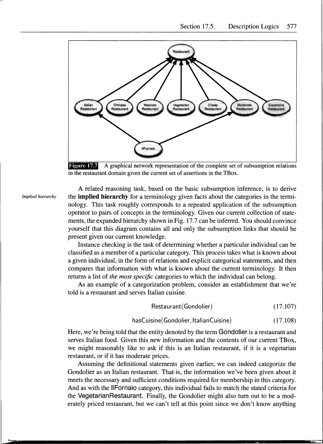
17 The Representation of Meaning................................545
18 Computational Semantics......................................583
19 Lexical Semantics............................................611
20 Computational Lexical Semantics..............................637
21 Computational Discourse......................................681
V Applications
22 Information Extraction.......................................725
23 Question Answering and Summarization.........................765
24 Dialogue and Conversational Agents...........................811
25 Machine Translation..........................................859
Bibliography.....................................................909
Author Index.....................................................959
Subject Index....................................................971
vii
Contents
Foreword xxiii
Preface xxv
About the Authors xxxi
1 Introduction 1
1.1 Knowledge in Speech and Language Processing..........................2
1.2 Ambiguity............................................................4
1.3 Models and Algorithms................................................5
1.4 Language, Thought, and Understanding.................................6
1.5 The State of the Art.................................................8
1.6 Some Brief History...................................................9
1.6.1 Foundational Insights: 1940s and 1950s........................9
1.6.2 The Two Camps: 1957-1970.....................................10
1.6.3 Four Paradigms: 1970-1983....................................11
1.6.4 Empiricism and Finite-State Models Redux: 1983-1993 .. 12
1.6.5 The Field Comes Together: 1994-1999..........................12
1.6.6 The Rise of Machine Learning: 2000-2008......................12
1.6.7 On Multiple Discoveries......................................13
1.6.8 A Final Brief Note on Psychology.............................14
1.7 Summary.............................................................14
Bibliographical and Historical Notes.......................................15
1 Words
2 Regular Expressions and Automata 17
2.1 Regular Expressions.................................................17
2.1.1 Basic Regular Expression Patterns..........................18
2.1.2 Disjunction, Grouping, and Precedence......................21
2.1.3 A Simple Example...........................................22
2.1.4 A More Complex Example.....................................23
2.1.5 Advanced Operators.........................................24
2.1.6 Regular Expression Substitution, Memory, and ELIZA ... 25
2.2 Finite-State Automata...............................................26
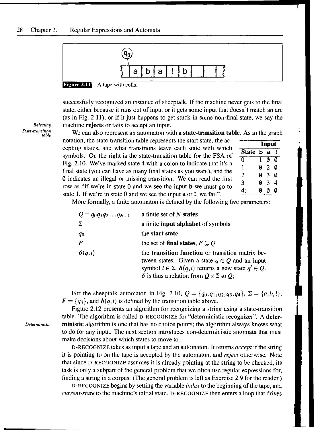
2.2.1 Use of an FSA to Recognize Sheeptalk.......................27
2.2.2 Formal Languages...........................................30
2.2.3 Another Example............................................31
2.2.4 Non-Deterministic FSAs.....................................32
2.2.5 Use of an NFSA to Accept Strings...........................33
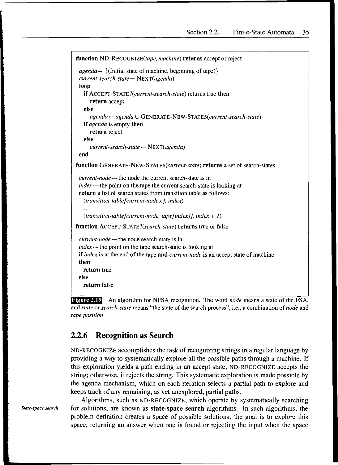
2.2.6 Recognition as Search......................................35
2.2.7 Relation of Deterministic and Non-Deterministic Automata 38
2.3 Regular Languages and FSAs..........................................38
2.4 Summary.............................................................41
ix
X
Contents
Bibliographical and Historical Notes.......................................42
Exercises..................................................................42
3 Words and Transducers 45
3.1 Survey of (Mostly) English Morphology................................47
3.1.1 Inflectional Morphology......................................48
3.1.2 Derivational Morphology......................................50
3.1.3 Cliticization................................................51
3.1.4 Non-Concatenative Morphology.................................51
3.1.5 Agreement....................................................52
3.2 Finite-State Morphological Parsing...................................52
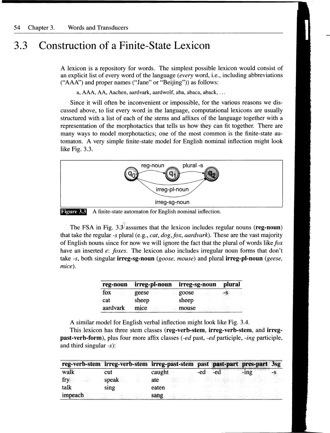
3.3 Construction of a Finite-State Lexicon...............................54
3.4 Finite-State Transducers.............................................57
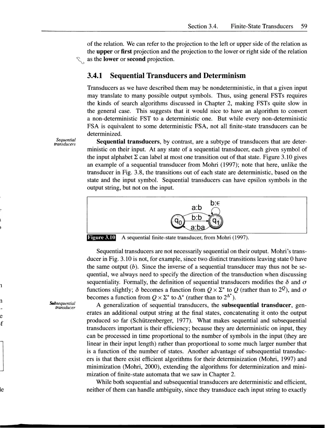
3.4.1 Sequential Transducers and Determinism.......................59
3.5 FSTs for Morphological Parsing.......................................60
3.6 Transducers and Orthographic Rules...................................62
3.7 The Combination of an FST Lexicon and Rules..........................65
3.8 Lexicon-Free FSTs: The Porter Stemmer................................68
3.9 Word and Sentence Tokenization.......................................68
3.9.1 Segmentation in Chinese.......................................70
3.10 Detection and Correction of Spelling Errors..........................72
3.11 Minimum Edit Distance................................................73
3.12 Human Morphological Processing.......................................77
3.13 Summary..............................................................79
Bibliographical and Historical Notes......................................80
Exercises..................................................................81
4 W-Grams 83
4.1 Word Counting in Corpora.............................................85
4.2 Simple (Unsmoothed) V-Grams..........................................86
4.3 Training and Test Sets...............................................91
4.3.1 N-Gram Sensitivity to the Training Corpus.....................92
4.3.2 Unknown Words: Open Versus Closed Vocabulary Tasks . . 95
4.4 Evaluating Af-Grams: Perplexity......................................95
4.5 Smoothing............................................................97
4.5.1 Laplace Smoothing............................................98
4.5.2 Good-Turing Discounting.....................................101
4.5.3 Some Advanced Issues in Good-Turing Estimation..............102
4.6 Interpolation.......................................................104
4.7 Backoff.............................................................105
4.7.1 Advanced: Details of Computing Katz Backoff a and P* . . 107
4.8 Practical Issues: Toolkits and Data Formats.........................108
4.9 Advanced Issues in Language Modeling................................109
4.9.1 Advanced Smoothing Methods: Kneser-Ney Smoothing . . 109
4.9.2 Class-Based W-Grams..........................................Ill
4.9.3 Language Model Adaptation and Web Use......................112
Contents xi
4.9.4 Using Longer-Distance Information: A Brief Summary . . . 112
4.10 Advanced: Information Theory Background...........................114
4.10.1 Cross-Entropy for Comparing Models.........................116
4.11 Advanced: The Entropy of English and Entropy Rate Constancy . . 118
4.12 Summary...........................................................119
Bibliographical and Elistorical Notes...................................120
Exercises...............................................................121
5 Part-of-Speech Tagging 123
5.1 (Mostly) English Word Classes.....................................124
5.2 Tagsets for English...............................................130
5.3 Part-of-Speech Tagging............................................133
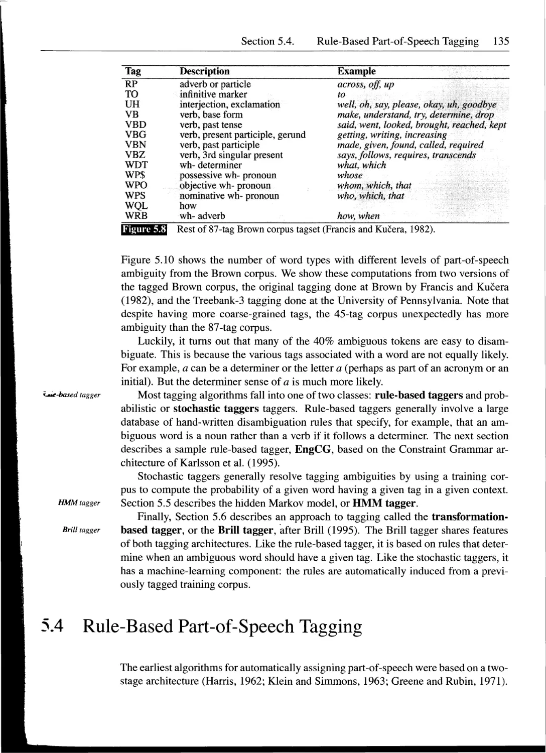
5.4 Rule-Based Part-of-Speech Tagging.................................135
5.5 HMM Part-of-Speech Tagging........................................139
5.5.1 Computing the Most Likely Tag Sequence: An Example . . 142
5.5.2 Formalizing Hidden Markov Model Taggers.....................144
5.5.3 Using the Viterbi Algorithm for HMM Tagging................145
5.5.4 Extending the HMM Algorithm to Trigrams....................149
5.6 Transformation-Based Tagging......................................151
5.6.1 How TBL Rules Are Applied..................................152
5.6.2 How TBL Rules Are Learned...................................152
5.7 Evaluation and Error Analysis.....................................153
5.7.1 Error Analysis..............................................156
5.8 Advanced Issues in Part-of-Speech Tagging.........................157
5.8.1 Practical Issues: Tag Indeterminacy and Tokenization . ... 157
5.8.2 Unknown Words..............................................158
5.8.3 Part-of-Speech Tagging for Other Languages.................160
5.8.4 Tagger Combination.........................................163
5.9 Advanced: The Noisy Channel Model for Spelling....................163
5.9.1 Contextual Spelling Error Correction.......................167
5.10 Summary...........................................................168
Bibliographical and Historical Notes....................................169
Exercises...............................................................171
6 Hidden Markov and Maximum Entropy Models 173
6.1 Markov Chains.....................................................174
6.2 The Hidden Markov Model...........................................176
6.3 Likelihood Computation: The Forward Algorithm.....................179
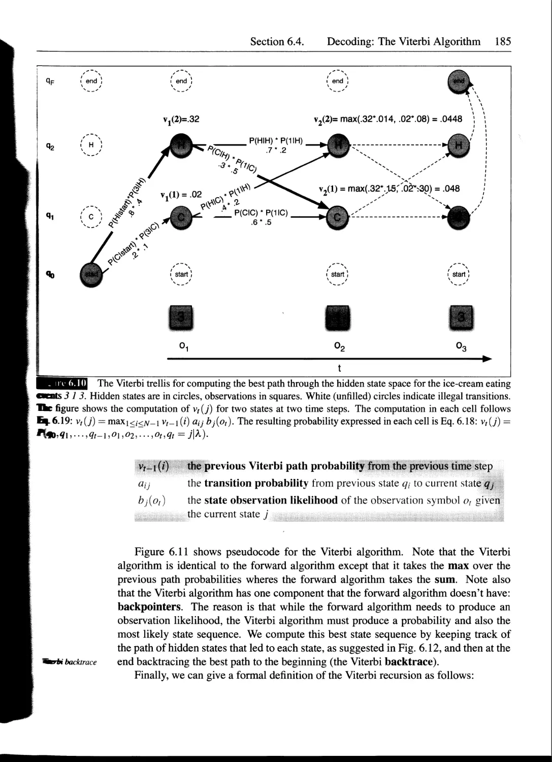
6.4 Decoding: The Viterbi Algorithm...................................184
6.5 HMM Training: The Forward-Backward Algorithm......................186
6.6 Maximum Entropy Models: Background................................193
6.6.1 Linear Regression..........................................194
6.6.2 Logistic Regression........................................197
6.6.3 Logistic Regression: Classification........................199
6.6.4 Advanced: Learning in Logistic Regression................200
6.7 Maximum Entropy Modeling..........................................201
xii Contents
6.7.1 Why We Call It Maximum Entropy..............................205
6.8 Maximum Entropy Markov Models.....................................207
6.8.1 Decoding and Learning in MEMMs..............................210
6.9 Summary...........................................................211
Bibliographical and Historical Notes....................................212
Exercises...............................................................213
II Speech
7 Phonetics 215
7.1 Speech Sounds and Phonetic Transcription..........................216
7.2 Articulatory Phonetics............................................217
7.2.1 The Vocal Organs............................................218
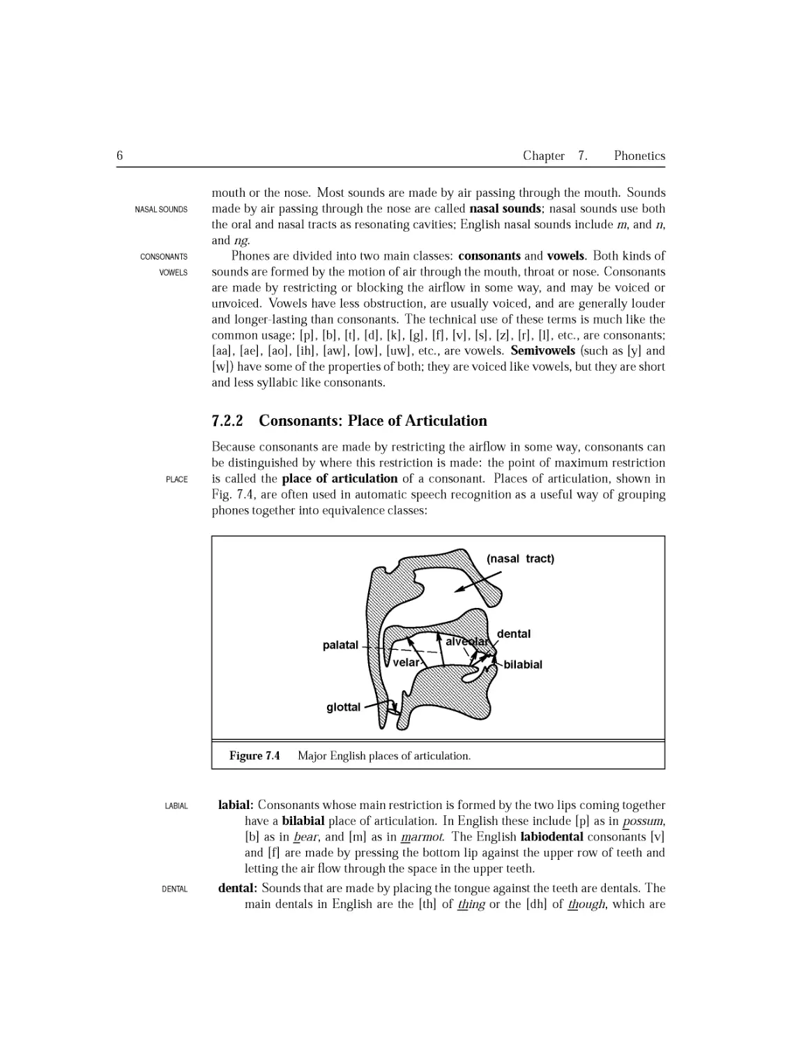
7.2.2 Consonants: Place of Articulation...........................220
7.2.3 Consonants: Manner of Articulation..........................221
7.2.4 Vowels.....................................................222
7.2.5 Syllables..................................................223
7.3 Phonological Categories and Pronunciation Variation...............225
7.3.1 Phonetic Features..........................................227
7.3.2 Predicting Phonetic Variation..............................228
7.3.3 Factors Influencing Phonetic Variation.....................229
7.4 Acoustic Phonetics and Signals....................................230
7.4.1 Waves......................................................230
7.4.2 Speech Sound Waves.........................................231
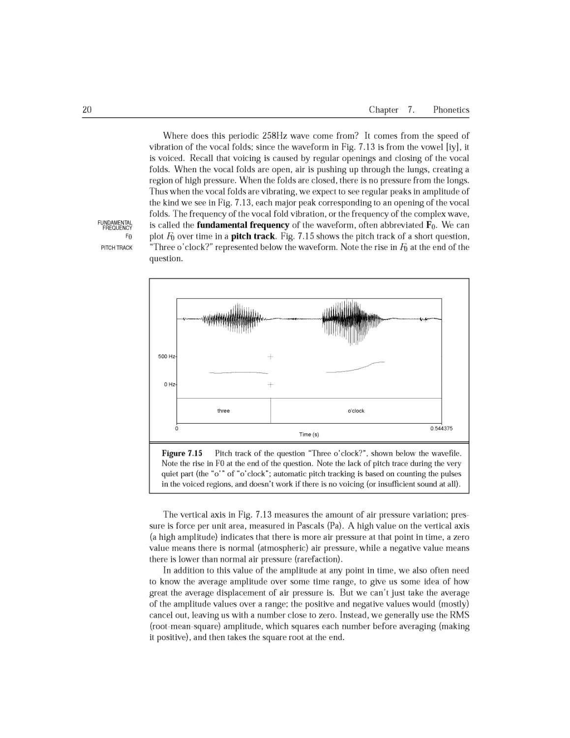
7.4.3 Frequency and Amplitude; Pitch and Loudness................233
7.4.4 Interpretation of Phones from a Waveform...................236
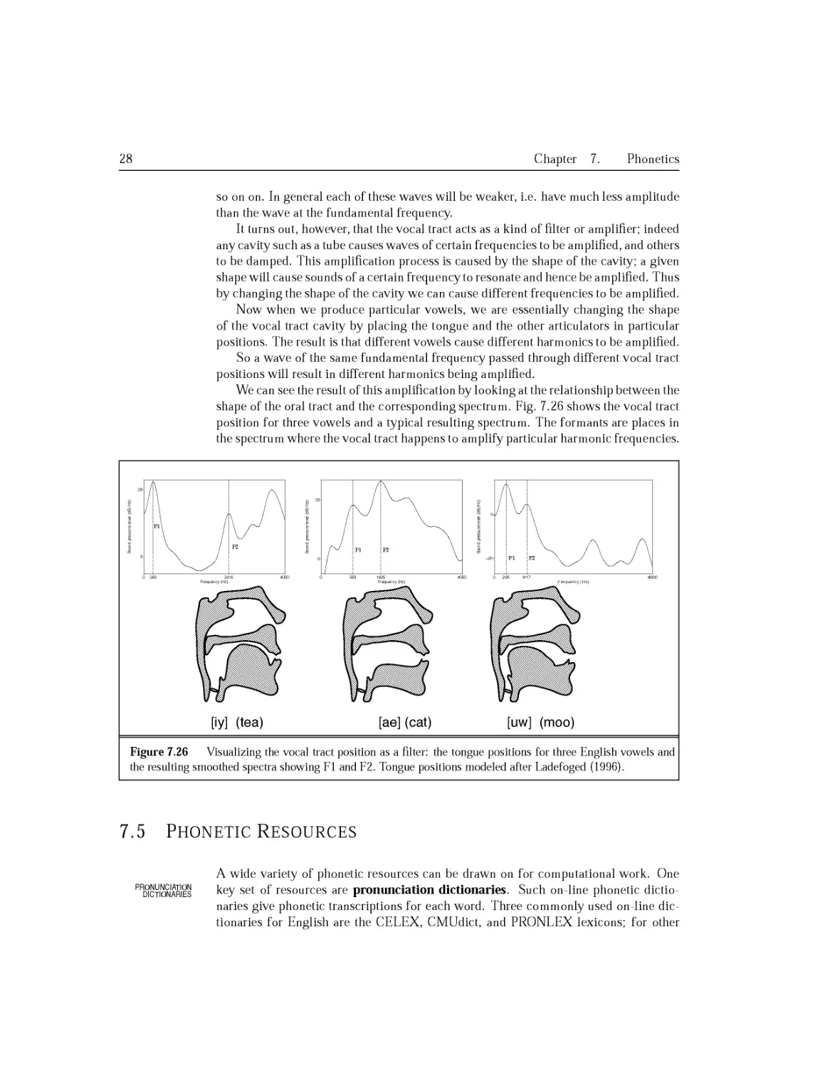
7.4.5 Spectra and the Frequency Domain...........................236
7.4.6 The Source-Filter Model....................................240
7.5 Phonetic Resources................................................241
7.6 Advanced: Articulatory and Gestural Phonology.....................244
7.7 Summary...........................................................245
Bibliographical and Historical Notes....................................246
Exercises...........................................•...................247
8 Speech Synthesis 249
8.1 Text Normalization................................................251
8.1.1 Sentence Tokenization......................................251
8.1.2 Non-Standard Words.........................................252
8.1.3 Homograph Disambiguation...................................256
8.2 Phonetic Analysis.................................................257
8.2.1 Dictionary Lookup..........................................257
8.2.2 Names......................................................258
8.2.3 Grapheme-to-Phoneme Conversion.............................259
8.3 Prosodic Analysis.................................................262
8.3.1 Prosodic Structure.........................................262
8.3.2 Prosodic Prominence........................................263
Contents xiii
8.3.3 Tune........................................................265
8.3.4 More Sophisticated Models: ToBI.............................266
8.3.5 Computing Duration from Prosodic Labels.....................268
8.3.6 Computing FO from Prosodic Labels...........................269
8.3.7 Final Result of Text Analysis: Internal Representation ... 271
8.4 Diphone Waveform Synthesis..........................................272
8.4.1 Steps for Building a Diphone Database.......................272
8.4.2 Diphone Concatenation and TD-PSOLA for Prosody .... 274
8.5 Unit Selection (Waveform) Synthesis.................................276
8.6 Evaluation..........................................................280
Bibliographical and Historical Notes......................................281
Exercises.................................................................284
9 Automatic Speech Recognition 285
9.1 Speech Recognition Architecture.....................................287
9.2 The Hidden Markov Model Applied to Speech........................291
9.3 Feature Extraction: MFCC Vectors....................................295
9.3.1 Preemphasis.................................................296
9.3.2 Windowing...................................................296
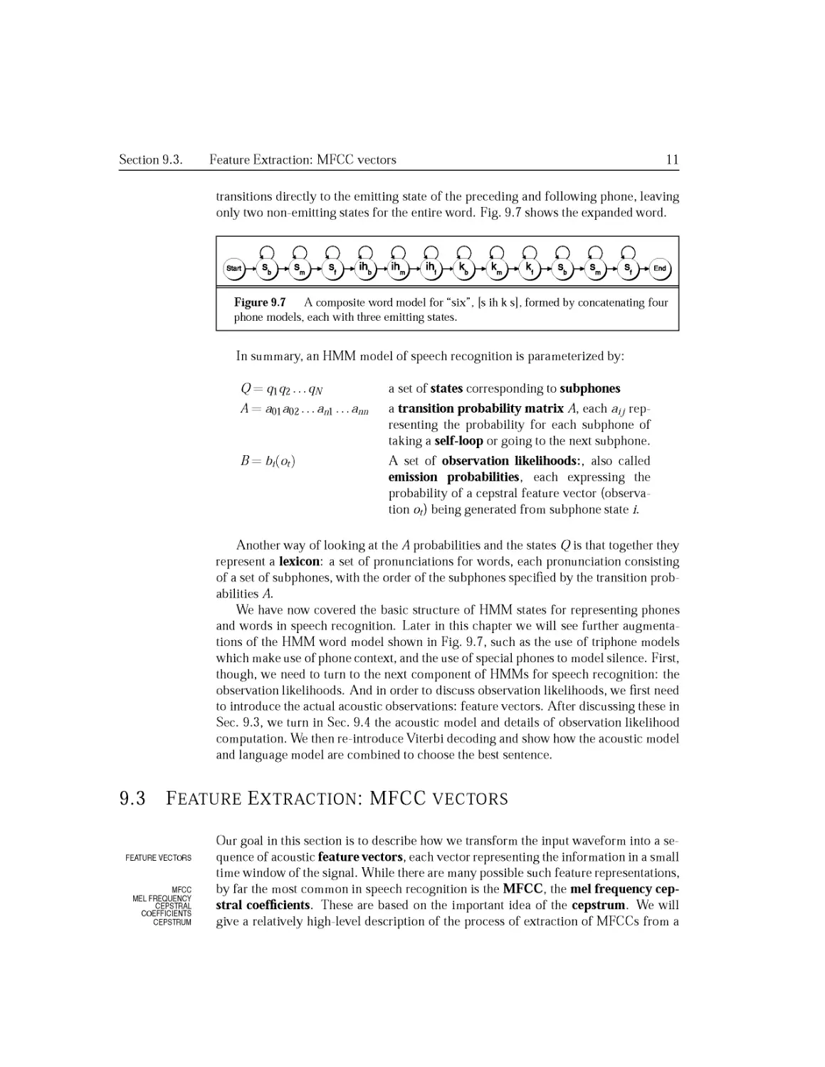
9.3.3 Discrete Fourier Transform..................................298
9.3.4 Mel Filter Bank and Log.....................................299
9.3.5 The Cepstrum: Inverse Discrete Fourier Transform . . . 300
9.3.6 Deltas and Energy...........................................302
9.3.7 Summary: MFCC...............................................302
9.4 Acoustic Likelihood Computation.....................................303
9.4.1 Vector Quantization.........................................303
9.4.2 Gaussian PDFs...............................................306
9.4.3 Probabilities, Log-Probabilities, and Distance Functions . . 313
9.5 The Lexicon and Language Model......................................314
9.6 Search and Decoding.................................................314
9.7 Embedded Training...................................................324
9.8 Evaluation: Word Error Rate.........................................328
9.9 Summary.............................................................330
Bibliographical and Historical Notes'.....................................331
Exercises.................................................................333
10 Speech Recognition: Advanced Topics 335
10.1 Multipass Decoding: V-Best Lists and Lattices.......................335
10.2 A* ("Stack") Decoding...............................................341
10.3 Context-Dependent Acoustic Models: Triphones......................345
10.4 Discriminative Training.............................................349
10.4.1 Maximum Mutual Information Estimation.......................350
10.4.2 Acoustic Models Based on Posterior Classifiers..............351
10.5 Modeling Variation..................................................352
10.5.1 Environmental Variation and Noise........................352
10.5.2 Speaker Variation and Speaker Adaptation....................353
xiv Contents
10.5.3 Pronunciation Modeling: Variation Due to Genre..............354
10.6 Metadata: Boundaries, Punctuation, and Disfluencies...............356
10.7 Speech Recognition by Humans......................................358
10.8 Summary............................................................359
Bibliographical and Historical Notes...........................359
Exercises................................................................360
11 Computational Phonology 361
11.1 Finite-State Phonology.............................................361
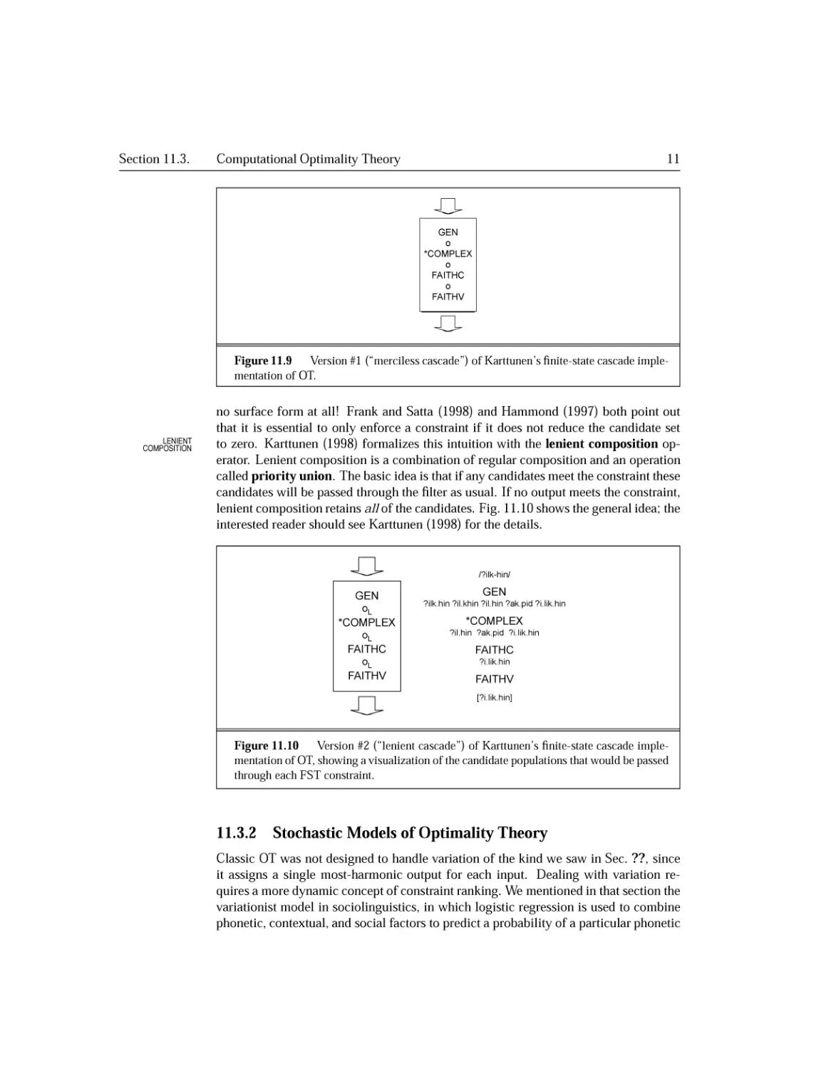
11.2 Advanced Finite-State Phonology....................................365
11.2.1 Harmony.....................................................365
11.2.2 Templatic Morphology........................................366
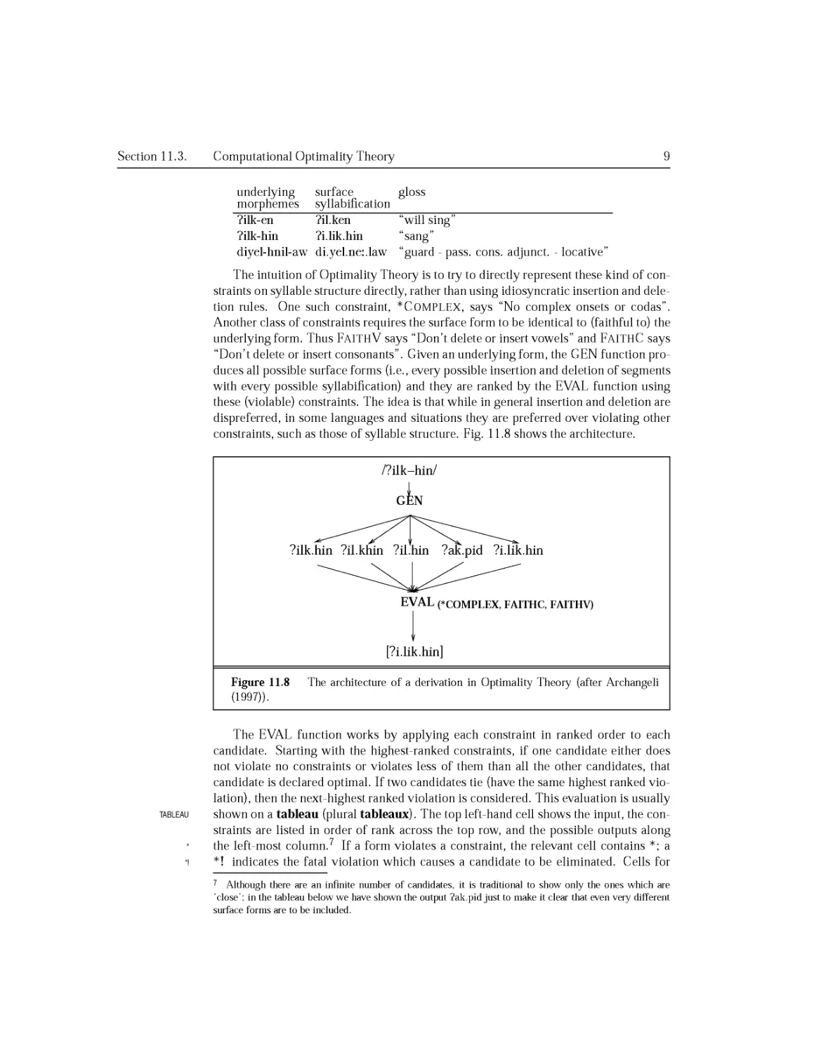
11.3 Computational Optimality Theory....................................367
11.3.1 Finite-State Transducer Models of Optimality Theory . . . . 369
11.3.2 Stochastic Models of Optimality Theory.....................370
11.4 Syllabification....................................................372
11.5 Learning Phonology and Morphology..................................375
11.5.1 Learning Phonological Rules................................375
11.5.2 Learning Morphology........................................377
11.5.3 Learning in Optimality Theory..............................380
11.6 Summary............................................................381
Bibliographical and Historical Notes.....................................381
Exercises................................................................383
III Syntax
12 Formal Grammars of English 385
12.1 Constituency.......................................................386
12.2 Context-Free Grammars..............................................387
12.2.1 Formal Definition of Context-Free Grammar..................391
12.3 Some Grammar Rules for English.....................................392
12.3.1 Sentence-Level Constructions...............................392
12.3.2 Clauses and Sentences......................................394
12.3.3 The Noun Phrase............................................394
12.3.4 Agreement..................................................398
12.3.5 The Verb Phrase and Subcategorization......................400
12.3.6 Auxiliaries................................................402
12.3.7 Coordination...............................................403
12.4 Treebanks..........................................................404
12.4.1 Example: The Penn Treebank Project.........................404
12.4.2 Treebanks as Grammars......................................406
12.4.3 Treebank Searching.........................................408
12.4.4 Heads and Head Finding.....................................409
12.5 Grammar Equivalence and Normal Form..............................412
12.6 Finite-State and Context-Free Grammars.............................413
12.7 Dependency Grammars................................................414
Contents
xv
12.7.1 The Relationship Between Dependencies and Heads .... 415
12.7.2 Categorial Grammar.........................................417
12.8 Spoken Language Syntax..............................................417
12.8.1 Disfluencies and Repair....................................418
12.8.2 Treebanks for Spoken Language..............................419
12.9 Grammars and Human Processing.......................................420
12.10 Summary............................................................421
Bibliographical and Historical Notes......................................422
Exercises.................................................................424
13 Syntactic Parsing 427
13.1 Parsing as Search...................................................428
13.1.1 Top-Down Parsing...........................................429
13.1.2 Bottom-Up Parsing..........................................430
13.1.3 Comparing Top-Down and Bottom-Up Parsing...................431
13.2 Ambiguity...........................................................432
13.3 Search in the Face of Ambiguity.....................................434
13.4 Dynamic Programming Parsing Methods.................................435
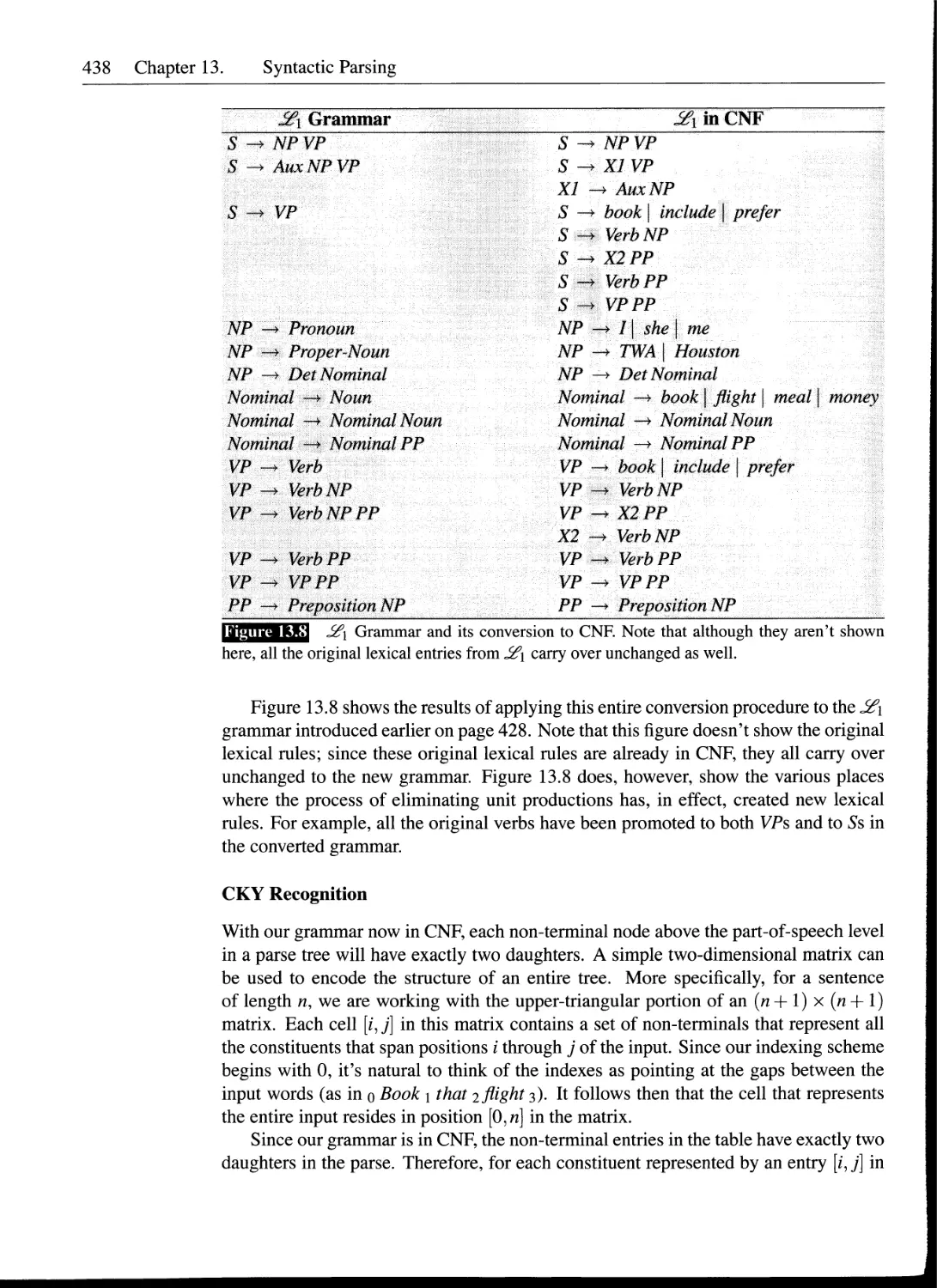
13.4.1 CKY Parsing................................................436
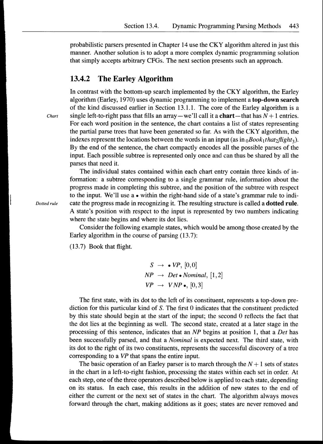
13.4.2 The Earley Algorithm.......................................443
13.4.3 Chart Parsing..............................................448
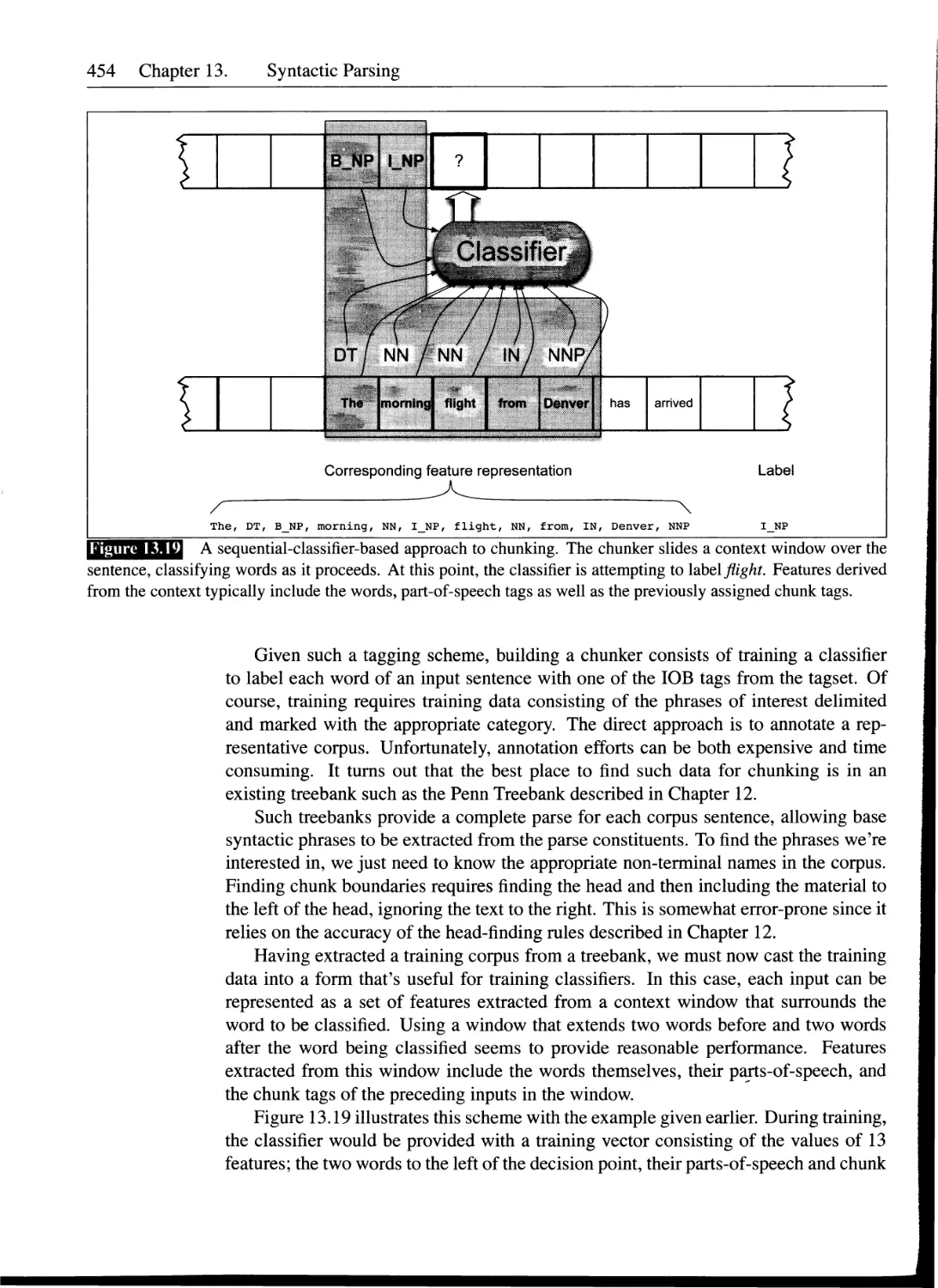
13.5 Partial Parsing.....................................................450
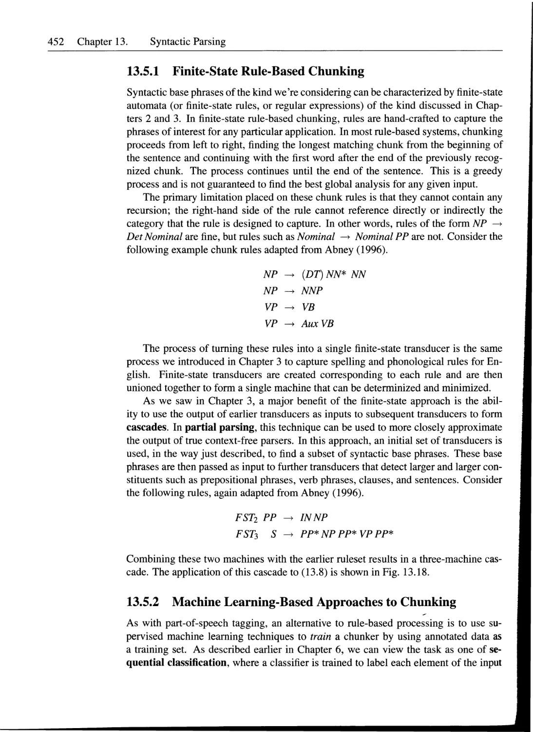
13.5.1 Finite-State Rule-Based Chunking............................452
13.5.2 Machine Learning-Based Approaches to Chunking . . .452
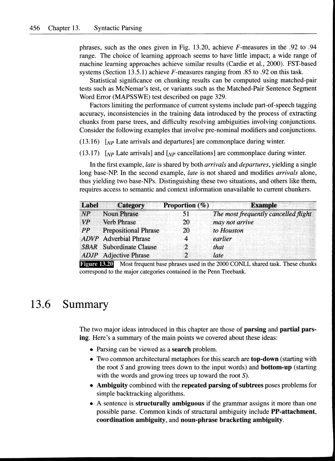
13.5.3 Chunking-System Evaluations.................................455
13.6 Summary.............................................................456
Bibliographical and Historical Notes......................................457
Exercises.................................................................458
14 Statistical Parsing 459
14.1 Probabilistic Context-Free Grammars.................................460
14.1.1 PCFGs for Disambiguation....................................461
14.1.2 PCFGs for Language Modeling.................................463
14.2 Probabilistic CKY Parsing of PCFGs..................................464
14.3 Ways to Learn PCFG Rule Probabilities...............................467
14.4 Problems with PCFGs.................................................468
14.4.1 Independence Assumptions Miss Structural Dependencies Be-
tween Rules...................................................468
14.4.2 Lack of Sensitivity to Lexical Dependencies.................469
14.5 Improving PCFGs by Splitting Non-Terminals..........................471
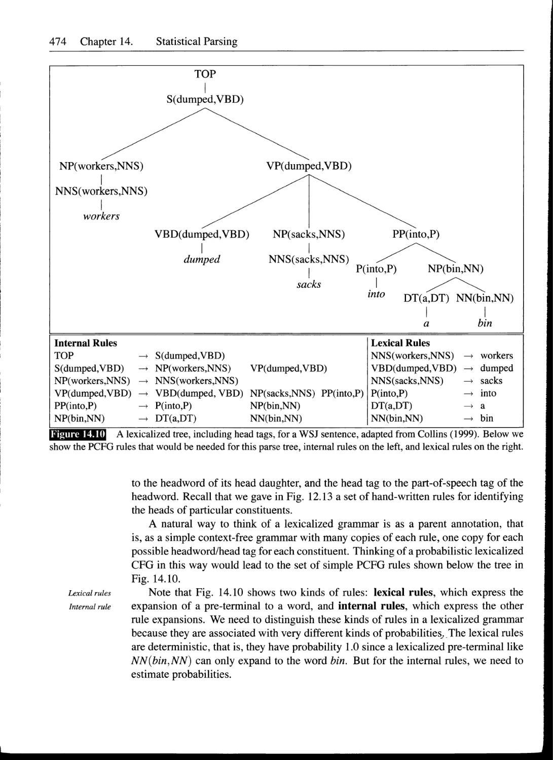
14.6 Probabilistic Lexicalized CFGs......................................473
14.6.1 The Collins Parser..........................................475
14.6.2 Advanced: Further Details of the Collins Parser.............477
14.7 Evaluating Parsers..................................................479
14.8 Advanced: Discriminative Reranking..................................481
14.9 Advanced: Parser-Based Language Modeling............................482
xvi Contents
14.10 Human Parsing......................................................483
14.11 Summary.............................................................485
Bibliographical and Historical Notes......................................486
Exercises.................................................................488
15 Features and Unification 489
15.1 Feature Structures..................................................490
15.2 Unification of Feature Structures...................................492
15.3 Feature Structures in the Grammar...................................497
15.3.1 Agreement...................................................498
15.3.2 Head Features...............................................500
15.3.3 Subcategorization..........................................501
15.3.4 Long-Distance Dependencies.................................506
15.4 Implementation of Unification.......................................507
15.4.1 Unification Data Structures.................................507
15.4.2 The Unification Algorithm..................................509
15.5 Parsing with Unification Constraints................................513
15.5.1 Integration of Unification into an Earley Parser............514
15.5.2 Unification-Based Parsing...................................519
15.6 Types and Inheritance...............................................521
15.6.1 Advanced: Extensions to Typing..............................524
15.6.2 Other Extensions to Unification.............................525
15.7 Summary.............................................................525
Bibliographical and Historical Notes......................................526
Exercises.................................................................527
16 Language and Complexity 529
16.1 The Chomsky Hierarchy...............................................530
16.2 Ways to Tell if a Language Isn't Regular............................532
16.2.1 The Pumping Lemma...........................................533
16.2.2 Proofs that Various Natural Languages Are Not Regular . . 535
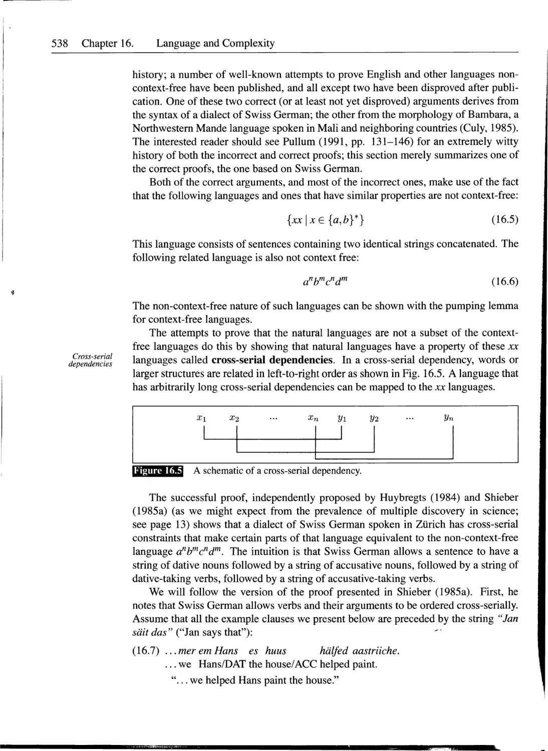
16.3 Is Natural Language Context Free?...................................537
16.4 Complexity and Human Processing.....................................539
16.5 Summary.............................................................542
Bibliographical and Historical Notes......................................543
Exercises.................................................................544
IV Semantics and Pragmatics
17 The Representation of Meaning 545
17.1 Computational Desiderata for Representations........................547
17.1.1 Verifiability...............................................547
17.1.2 Unambiguous Representations.................................548
17.1.3 Canonical Form.............................................549
17.1.4 Inference and Variables....................................550
17.1.5 Expressiveness..............................................551
Contents xvii
17.2 Model-Theoretic Semantics..........................................552
17.3 First-Order Logic..................................................555
17.3.1 Basic Elements of First-Order Logic........................555
17.3.2 Variables and Quantifiers..................................557
17.3.3 Lambda Notation............................................559
17.3.4 The Semantics of First-Order Logic.........................560
17.3.5 Inference..................................................561
17.4 Event and State Representations....................................563
17.4.1 Representing Time..........................................566
17.4.2 Aspect.....................................................569
17.5 Description Logics.................................................572
17.6 Embodied and Situated Approaches to Meaning........................578
17.7 Summary............................................................580
Bibliographical and Historical Notes.....................................580
Exercises................................................................582
18 Computational Semantics 583
18.1 Syntax-Driven Semantic Analysis....................................583
18.2 Semantic Augmentations to Syntactic Rules..........................585
18.3 Quantifier Scope Ambiguity and Underspecification..................592
18.3.1 Store and Retrieve Approaches..............................592
18.3.2 Constraint-Based Approaches................................595
18.4 Unification-Based Approaches to Semantic Analysis..................598
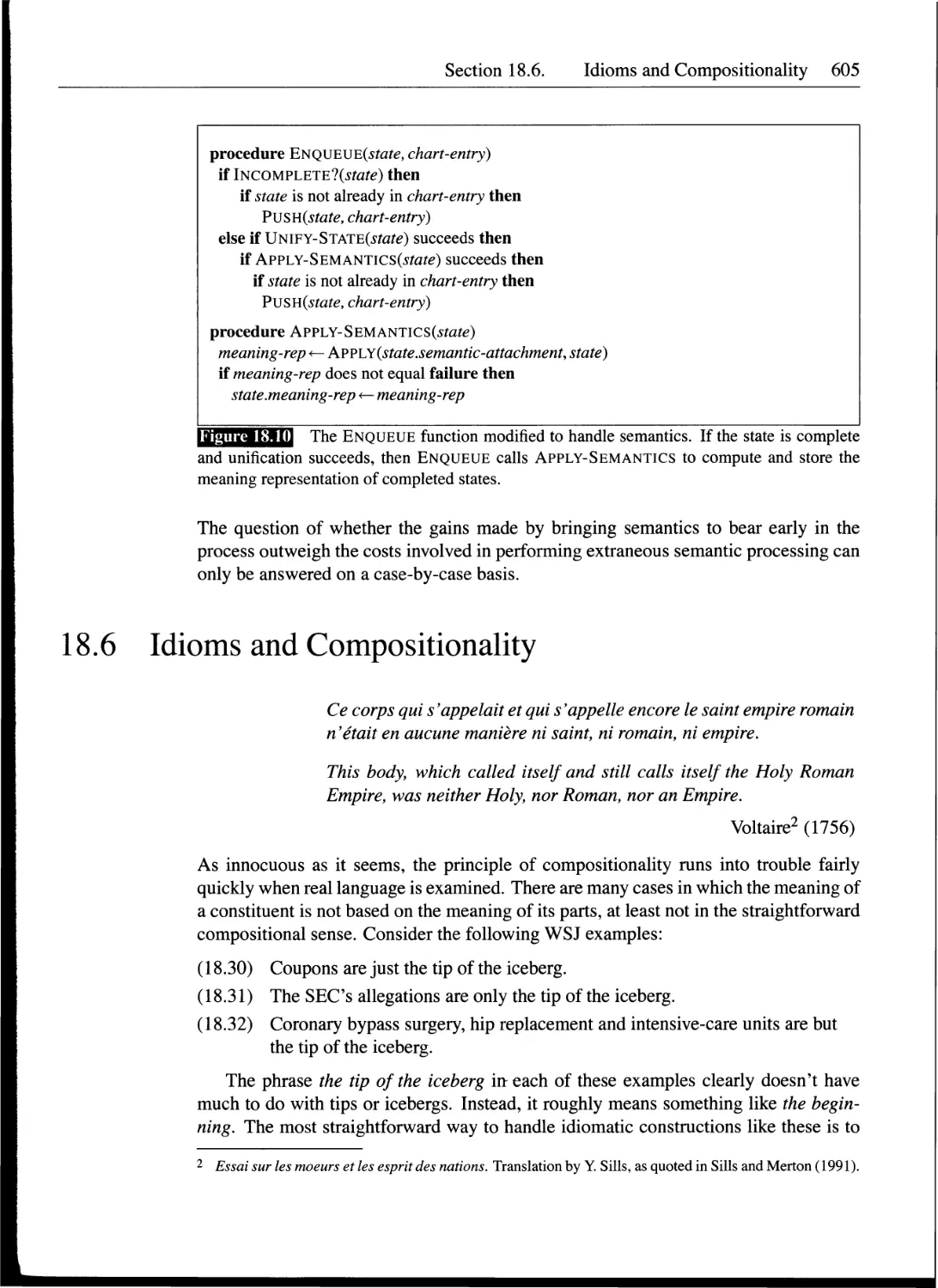
18.5 Integration of Semantics into the Earley Parser....................604
18.6 Idioms and Compositionality........................................605
18.7 Summary............................................................607
Bibliographical and Historical Notes.....................................607
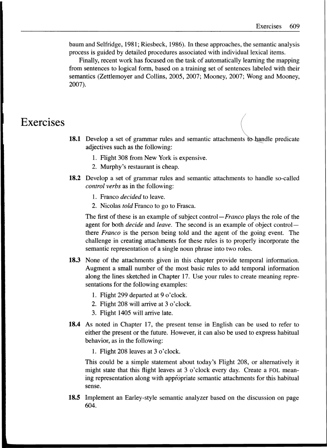
Exercises................................................................609
19 Lexical Semantics 611
19.1 Word Senses........................................................612
19.2 Relations Between Senses...........................................615
19.2.1 Synonymy and Antonymy.....................................615
19.2.2 Hyponymy.................•.................................616
19.2.3 Semantic Fields...........................................617
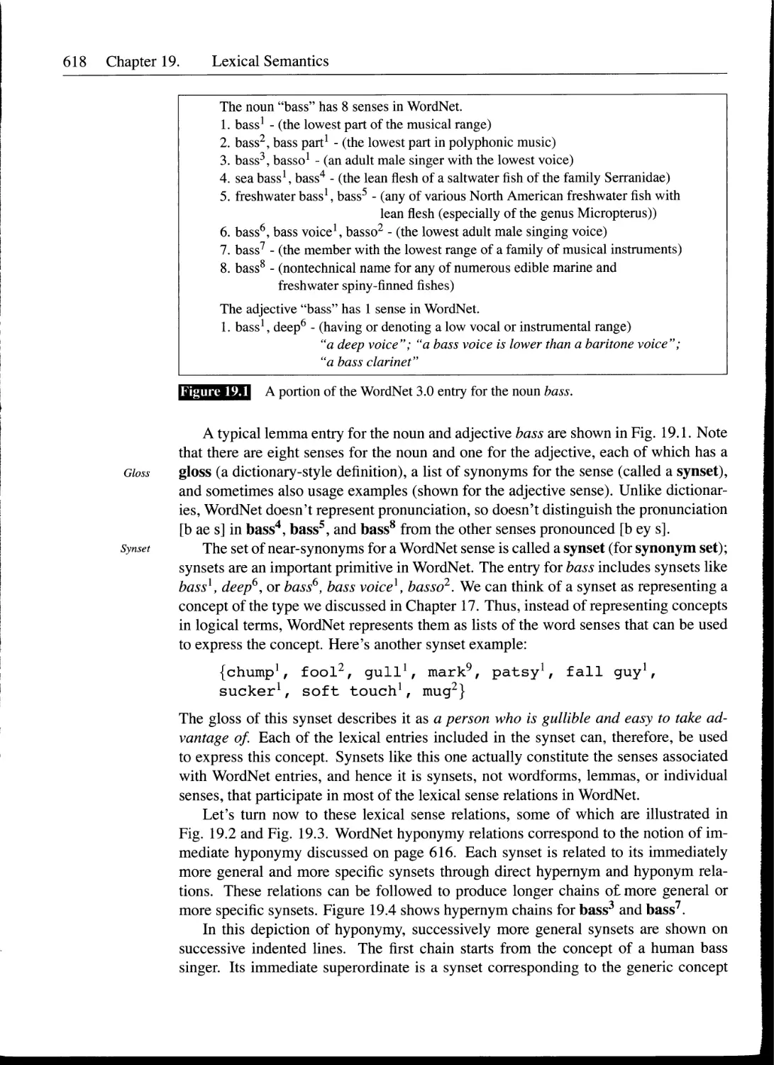
19.3 WordNet: A Database of Lexical Relations..........................617
19.4 Event Participants................................................619
19.4.1 Thematic Roles............................................620
19.4.2 Diathesis Alternations....................................622
19.4.3 Problems with Thematic Roles..............................623
19.4.4 The Proposition Bank......................................624
19.4.5 FrameNet..................................................625
19.4.6 Selectional Restrictions..................................627
19.5 Primitive Decomposition...........................................629
19.6 Advanced: Metaphor................................................631
19.7 Summary...........................................................632
xviii Contents
Bibliographical and Historical Notes......................................633
Exercises.................................................................634
20 Computational Lexical Semantics 637
20.1 Word Sense Disambiguation: Overview.................................638
20.2 Supervised Word Sense Disambiguation................................639
20.2.1 Feature Extraction for Supervised Learning..................640
20.2.2 Naive Bayes and Decision List Classifiers...................641
20.3 WSD Evaluation, Baselines, and Ceilings.............................644
20.4 WSD: Dictionary and Thesaurus Methods...............................646
20.4.1 The Lesk Algorithm..........................................646
20.4.2 Selectional Restrictions and Selectional Preferences .... 648
20.5 Minimally Supervised WSD: Bootstrapping.............................650
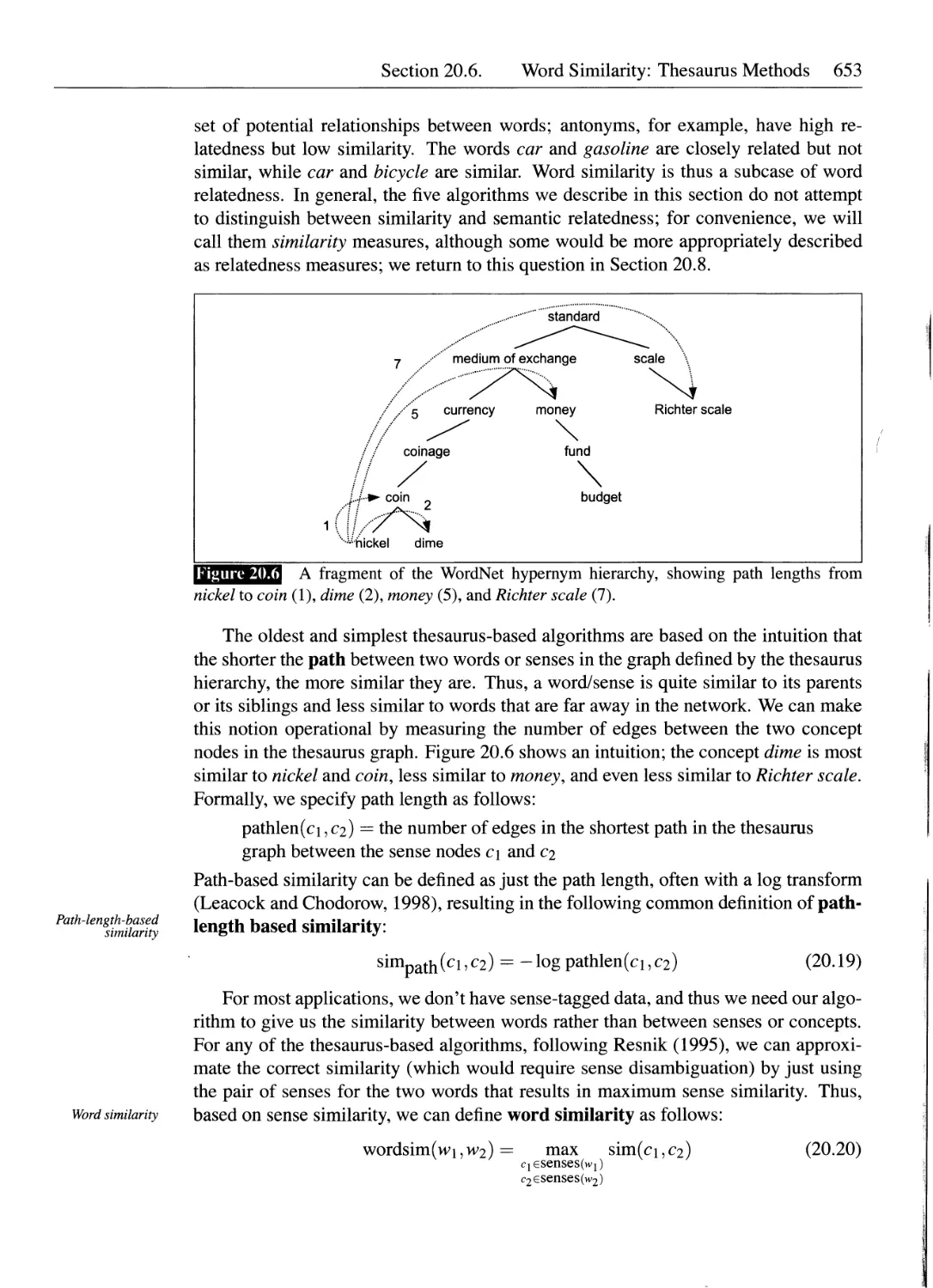
20.6 Word Similarity: Thesaurus Methods..................................652
20.7 Word Similarity: Distributional Methods.............................658
20.7.1 Defining a Word's Co-Occurrence Vectors.....................659
20.7.2 Measuring Association with Context..........................661
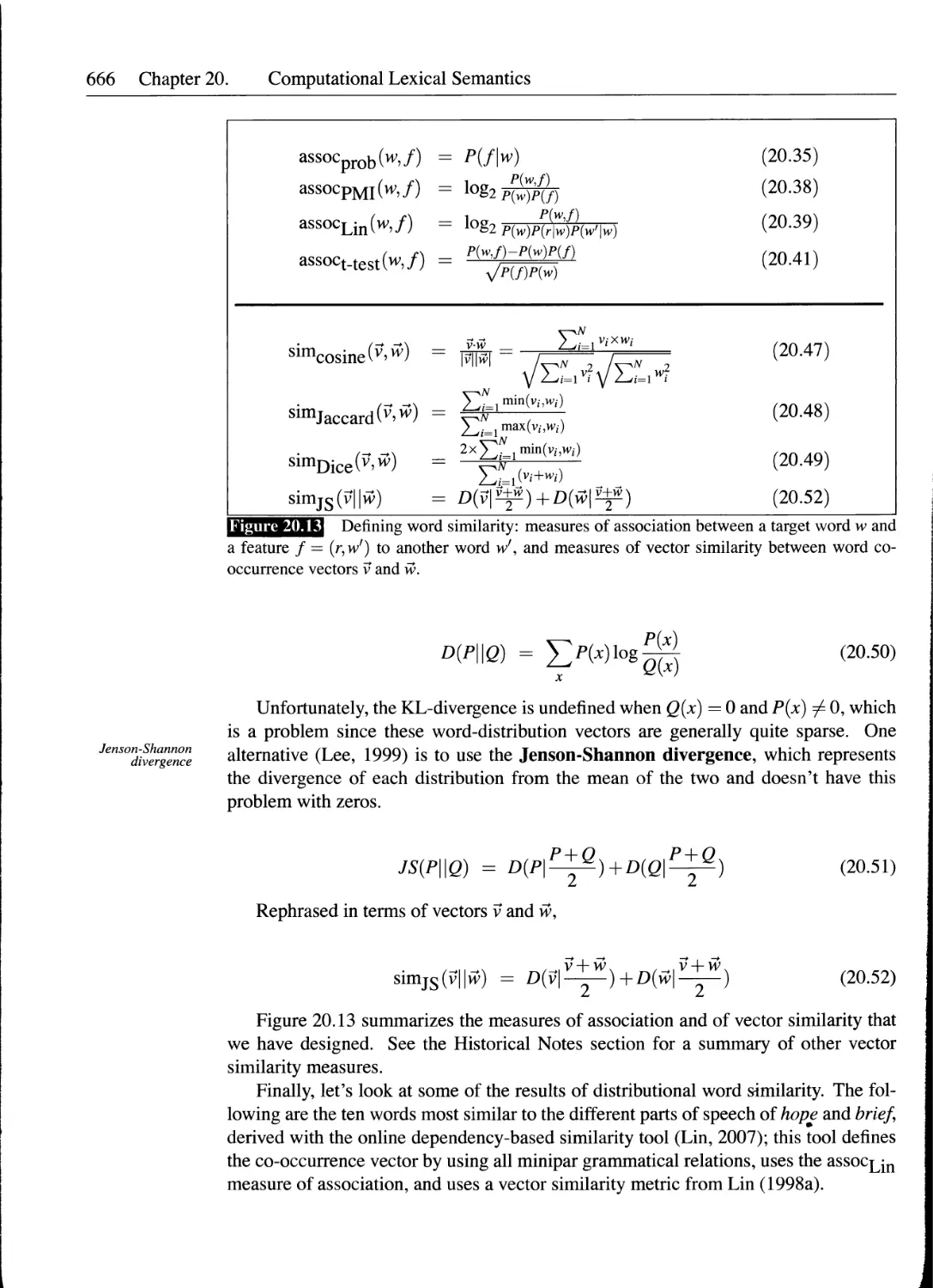
20.7.3 Defining Similarity Between Two Vectors.....................663
20.7.4 Evaluating Distributional Word Similarity...................667
20.8 Hy pony my and Other Word Relations.................................667
20.9 Semantic Role Labeling..............................................670
20.10 Advanced: Unsupervised Sense Disambiguation........................674
20.11 Summary............................................................675
Bibliographical and Historical Notes......................................676
Exercises.................................................................679
21 Computational Discourse 681
21.1 Discourse Segmentation..............................................684
21.1.1 Unsupervised Discourse Segmentation.........................684
21.1.2 Supervised Discourse Segmentation...........................686
21.1.3 Discourse Segmentation Evaluation..........................688
21.2 Text Coherence......................................................689
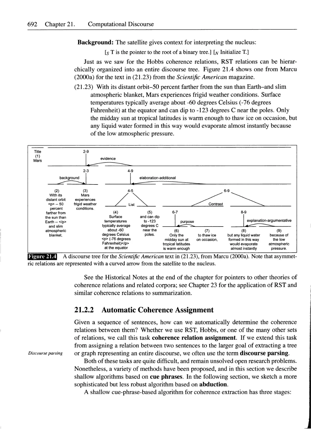
21.2.1 Rhetorical Structure Theory.................................690
21.2.2 Automatic Coherence Assignment..............................692
21.3 Reference Resolution................................................695
21.4 Reference Phenomena.................................................698
21.4.1 Five Types of Referring Expressions.........................698
21.4.2 Information Status..........................................700
21.5 Features for Pronominal Anaphora Resolution.........................701
21.5.1 Features for Filtering Potential Referents..................701
21.5.2 Preferences in Pronoun Interpretation.......................702
21.6 Three Algorithms for Anaphora Resolution............................704
21.6.1 Pronominal Anaphora Baseline: The Hobbs Algorithm . . 704
21.6.2 A Centering Algorithm for Anaphora Resolution...............706
21.6.3 A Log-Linear Model for Pronominal Anaphora Resolution . 708
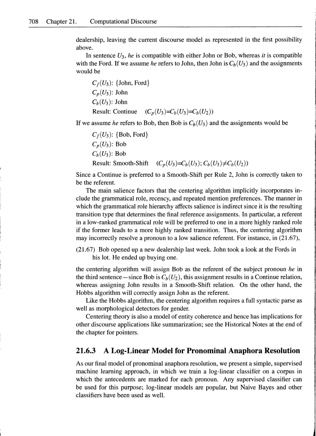
21.6.4 Features for Pronominal Anaphora Resolution................709
Contents xix
21.7 Coreference Resolution............................................710
21.8 Evaluation of Coreference Resolution..............................712
21.9 Advanced: Inference-Based Coherence Resolution....................713
21.10 Psycholinguistic Studies of Reference.............................718
21.11 Summary...........................................................719
Bibliographical and Historical Notes....................................720
Exercises...............................................................722
V Applications
22 Information Extraction 725
22.1 Named Entity Recognition..........................................727
22.1.1 Ambiguity in Named Entity Recognition.....................729
22.1.2 NER as Sequence Labeling..................................729
22.1.3 Evaluation of Named Entity Recognition....................732
22.1.4 Practical NER Architectures...............................734
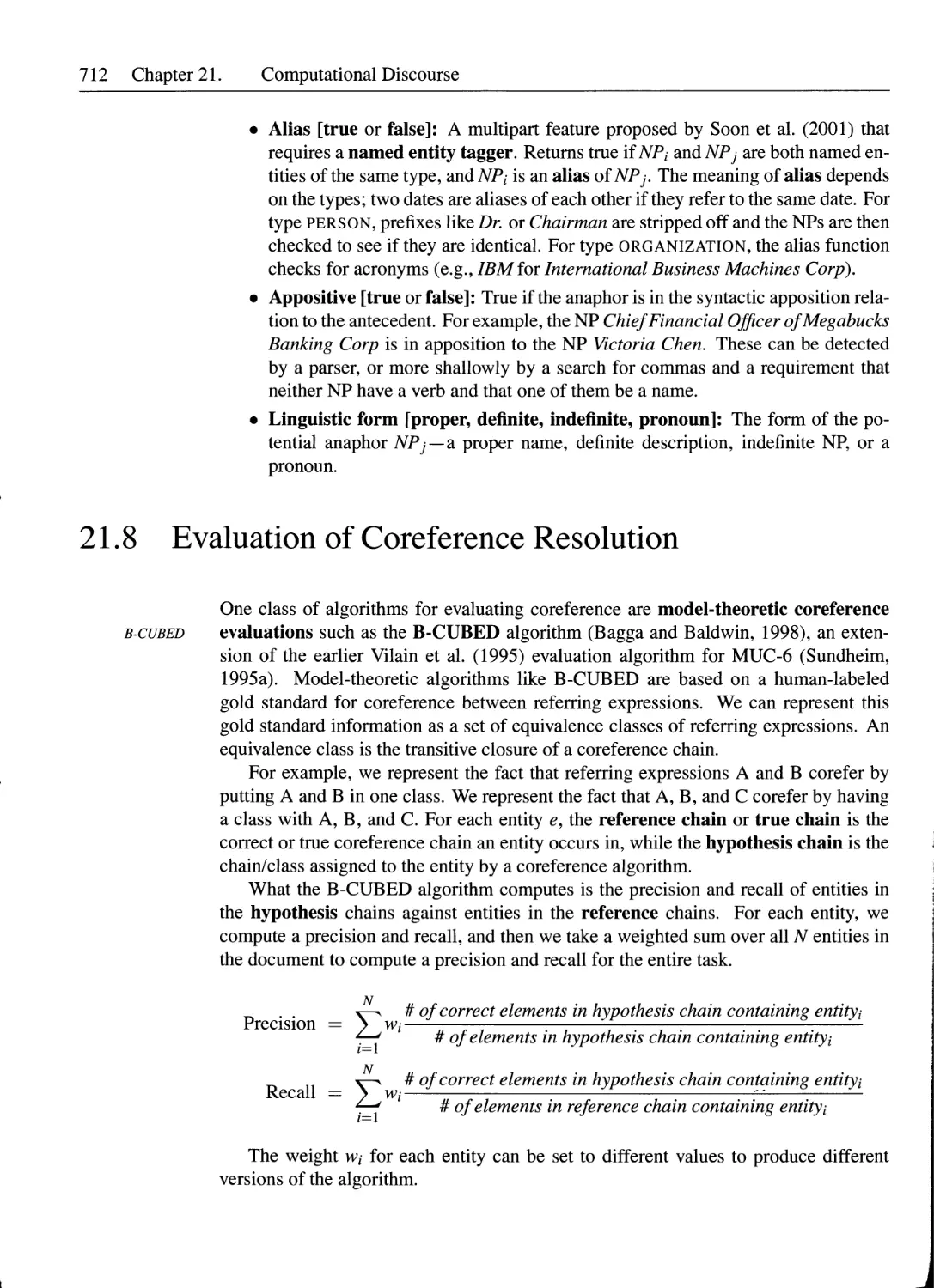
22.2 Relation Detection and Classification.............................734
22.2.1 Supervised Learning Approaches to Relation Analysis . . . 735
22.2.2 Lightly Supervised Approaches to Relation Analysis .... 738
22.2.3 Evaluation of Relation Analysis Systems...................742
22.3 Temporal and Event Processing.....................................743
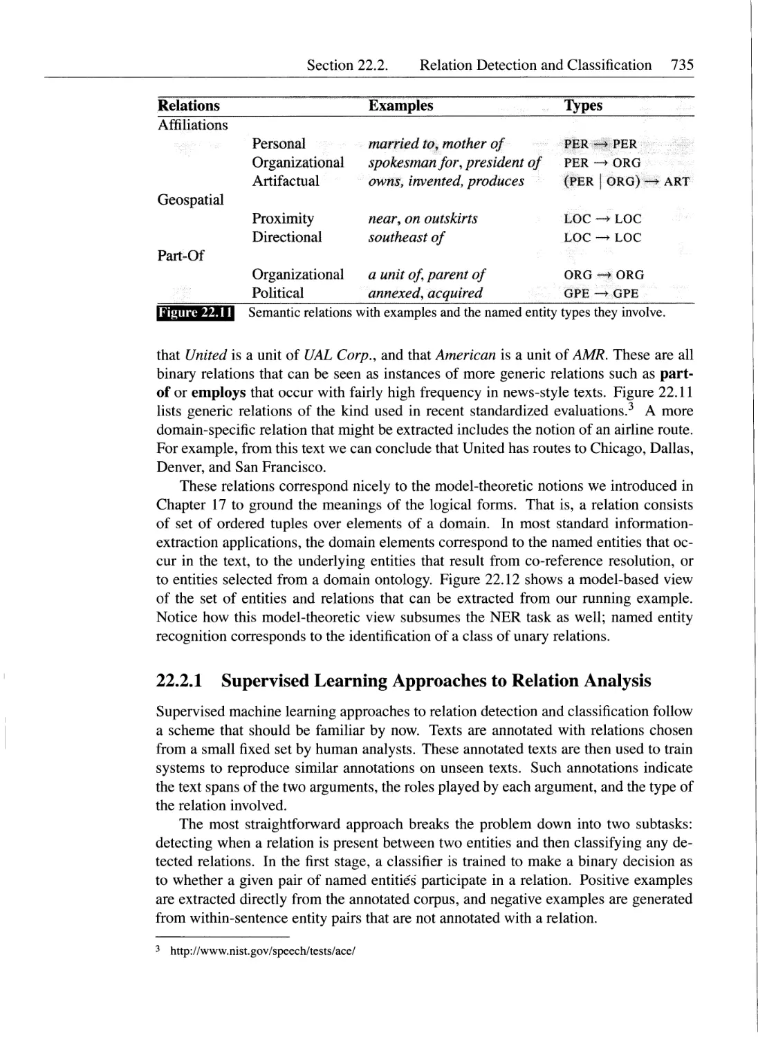
22.3.1 Temporal Expression Recognition...........................743
22.3.2 Temporal Normalization....................................746
22.3.3 Event Detection and Analysis..............................749
22.3.4 TimeBank..................................................750
22.4 Template Filling..................................................752
22.4.1 Statistical Approaches to Template-Filling................752
22.4.2 Finite-State Template-Filling Systems.....................754
22.5 Advanced: Biomedical Information Extraction.......................757
22.5.1 Biological Named Entity Recognition.......................758
22.5.2 Gene Normalization........................................759
22.5.3 Biological Roles and Relations............................760
22.6 Summary...........................................................762
Bibliographical and Historical Notes....................................762
Exercises...............................................................763
23 Question Answering and Summarization 765
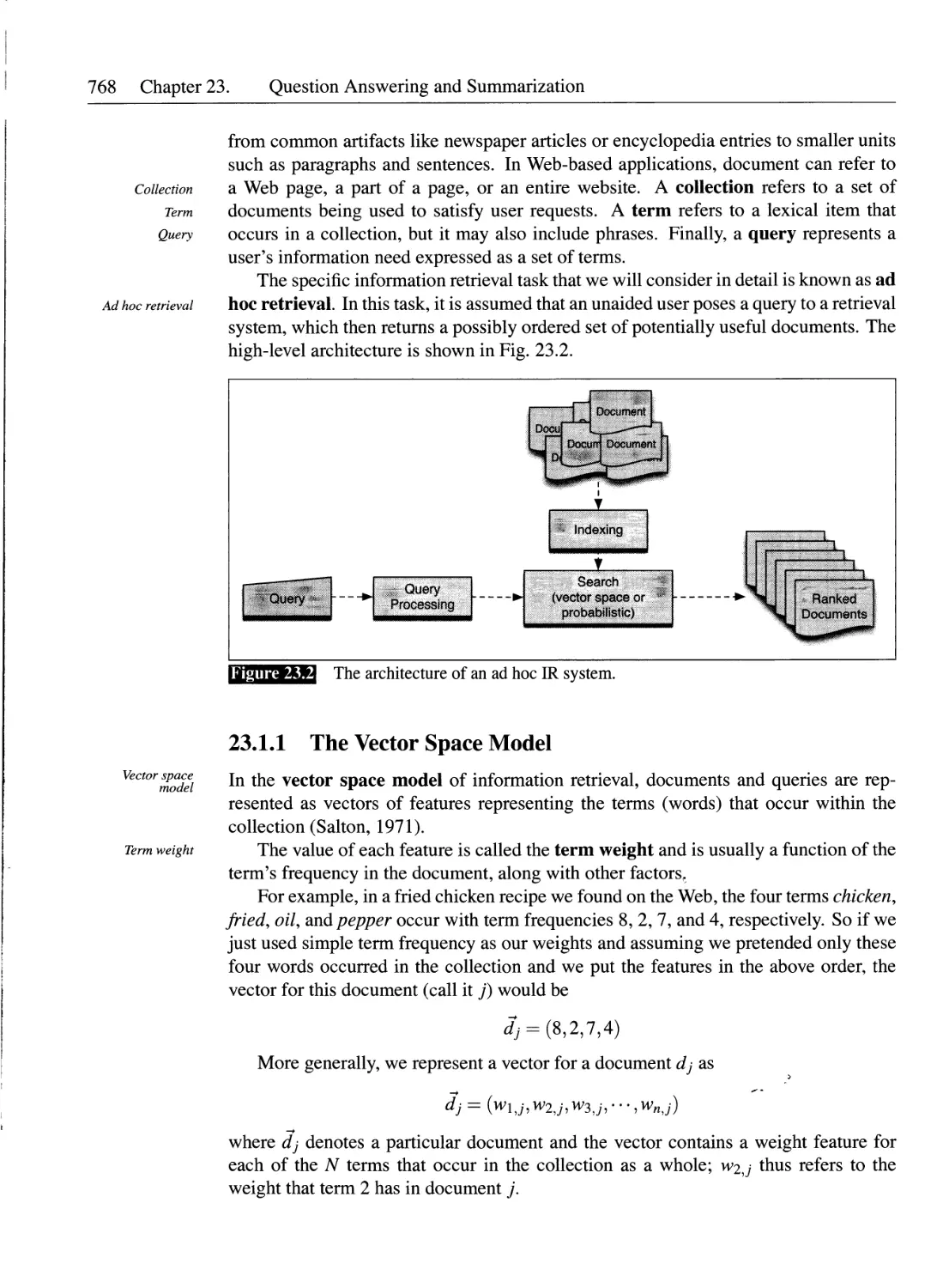
23.1 Information Retrieval.............................................767
23.1.1 The Vector Space Model....................................768
23.1.2 Term Weighting............................................770
23.1.3 Term Selection and Creation...............................772
23.1.4 Evaluation of Information-Retrieval Systems...............772
23.1.5 Homonymy, Polysemy, and Synonymy..........................776
23.1.6 Ways to Improve User Queries..............................776
23.2 Factoid Question Answering........................................778
23.2.1 Question Processing.......................................779
XX
Contents
23.2.2 Passage Retrieval..........................................781
23.2.3 Answer Processing..........................................783
23.2.4 Evaluation of Factoid Answers..............................787
23.3 Summarization......................................................787
23.4 Single-Document Summarization......................................790
23.4.1 Unsupervised Content Selection..............................790
23.4.2 Unsupervised Summarization Based on Rhetorical Parsing . 792
23.4.3 Supervised Content Selection...............................794
23.4.4 Sentence Simplification....................................795
23.5 Multi-Document Summarization.......................................796
23.5.1 Content Selection in Multi-Document Summarization . . . 797
23.5.2 Information Ordering in Multi-Document Summarization . 798
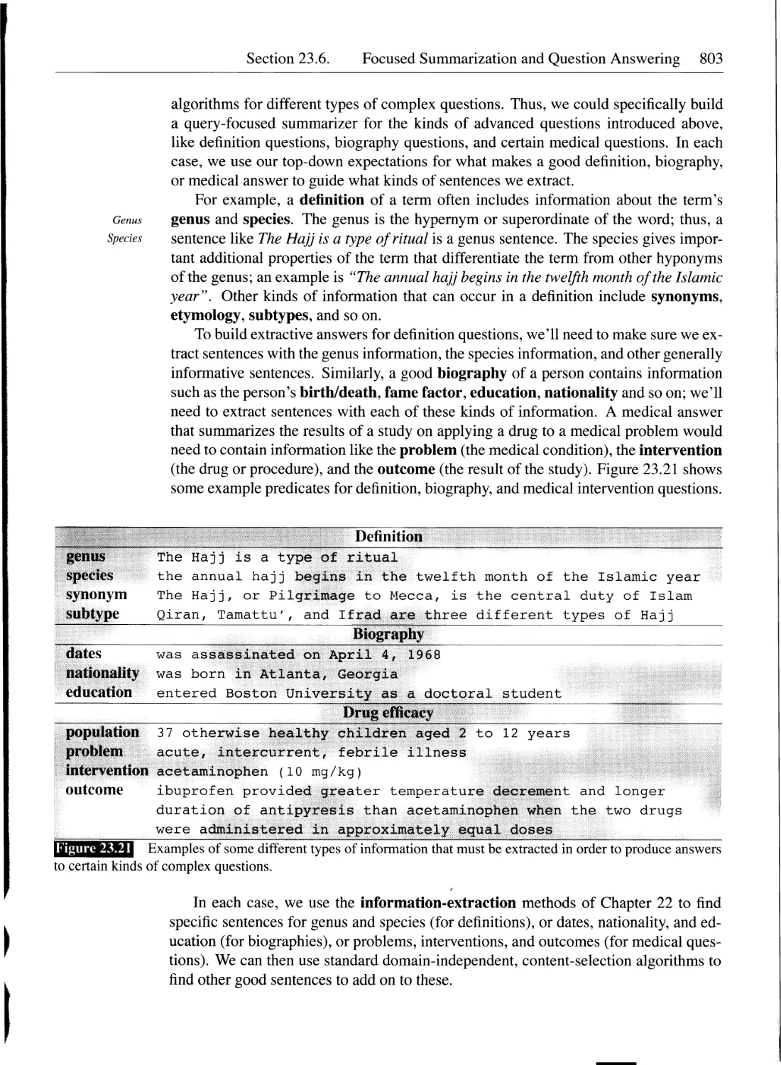
23.6 Focused Summarization and Question Answering.......................801
23.7 Summarization Evaluation...........................................805
23.8 Summary............................................................807
Bibliographical and Historical Notes......................................808
Exercises.................................................................810
24 Dialogue and Conversational Agents 811
24.1 Properties of Human Conversations..................................813
24.1.1 Turns and Turn-Taking.......................................813
24.1.2 Language as Action: Speech Acts............................815
24.1.3 Language as loint Action: Grounding........................816
24.1.4 Conversational Structure...................................818
24.1.5 Conversational Implicature.................................819
24.2 Basic Dialogue Systems.............................................821
24.2.1 ASR Component...............................................821
24.2.2 NLU Component..............................................822
24.2.3 Generation and TTS Components..............................825
24.2.4 Dialogue Manager...........................................827
24.2.5 Dealing with Errors: Confirmation and Rejection............831
24.3 VoiceXML...........................................................832
24.4 Dialogue System Design and Evaluation..............................836
24.4.1 Designing Dialogue Systems..................................836
24.4.2 Evaluating Dialogue Systems................................836
24.5 Information-State and Dialogue Acts................................838
24.5.1 Using Dialogue Acts........................................840
24.5.2 Interpreting Dialogue Acts.................................841
24.5.3 Detecting Correction Acts..................................844
24.5.4 Generating Dialogue Acts: Confirmation and Rejection . . . 845
24.6 Markov Decision Process Architecture...............................846
24.7 Advanced: Plan-Based Dialogue Agents...............................850
24.7.1 Plan-Inferential Interpretation and Production.............851
24.7.2 The Intentional Structure of Dialogue....................853
24.8 Summary............................................................855
Bibliographical and Historical Notes.....................................856
Contents xxi
Exercises...................................................................858
25 Machine Translation 859
25.1 Why Machine Translation Is Hard.....................................862
25.1.1 Typology...................................................862
25.1.2 Other Structural Divergences...............................864
25.1.3 Lexical Divergences........................................865
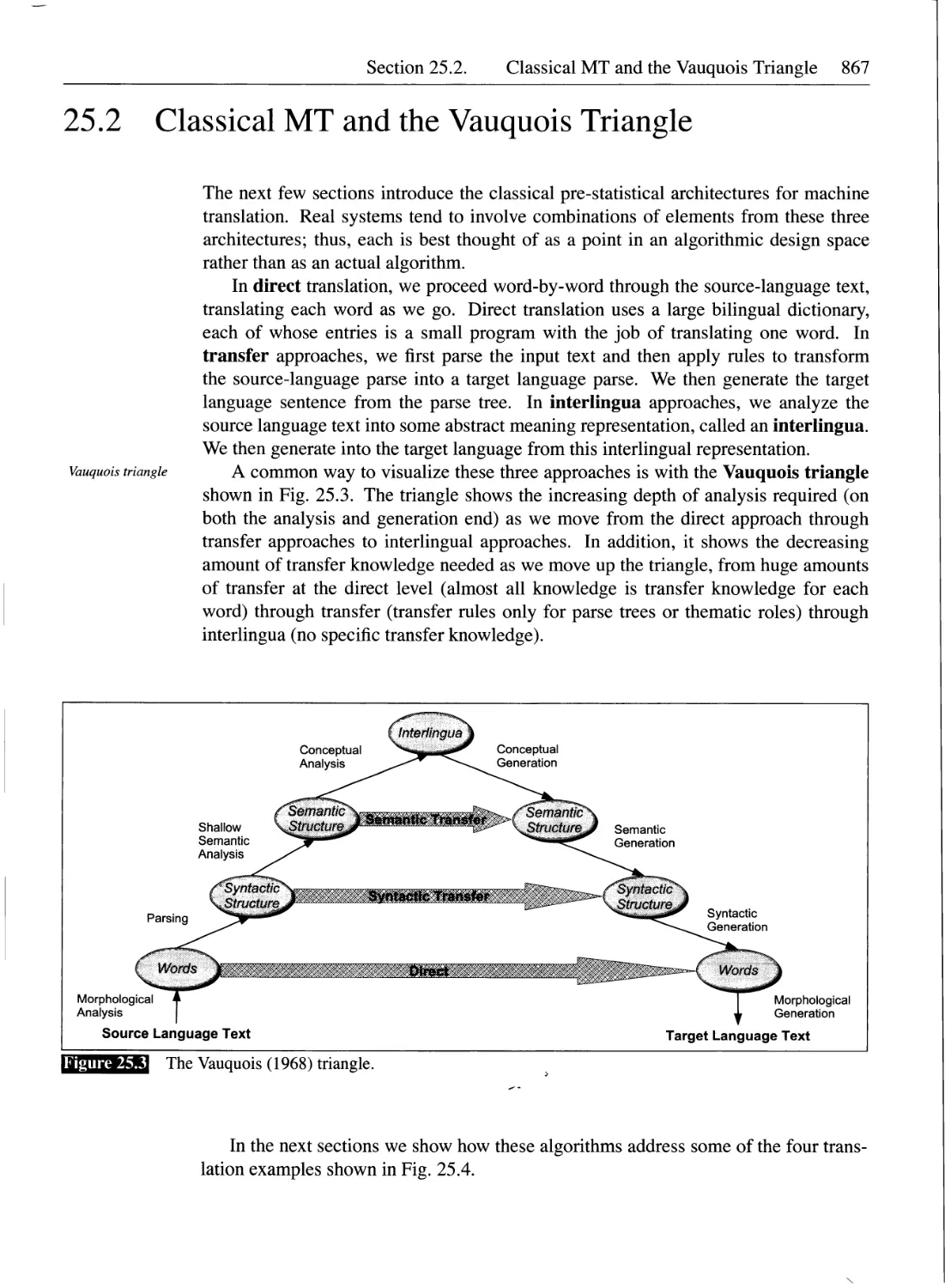
25.2 Classical MT and the Vauquois Triangle..............................867
25.2.1 Direct Translation.........................................868
25.2.2 Transfer...................................................870
25.2.3 Combined Direct and Transfer Approaches in Classic MT . 872
25.2.4 The Interlingua Idea: Using Meaning........................873
25.3 Statistical MT......................................................874
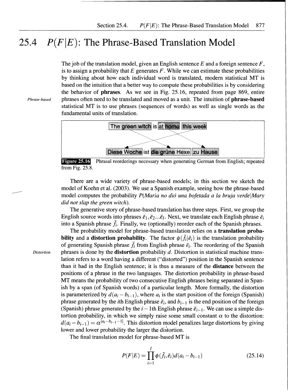
25.4 P(F\E): The Phrase-Based Translation Model..........................877
25.5 Alignment in MT.....................................................879
25.5.1 IBM Model 1................................................880
25.5.2 HMM Alignment..............................................883
25.6 Training Alignment Models...........................................885
25.6.1 EM for Training Alignment Models...........................886
25.7 Symmetrizing Alignments for Phrase-Based MT.........................888
25.8 Decoding for Phrase-Based Statistical MT............................890
25.9 MT Evaluation.......................................................894
25.9.1 Using Human Raters.........................................894
25.9.2 Automatic Evaluation: BLEU.................................895
25.10 Advanced: Syntactic Models for MT..................................898
25.11 Advanced: IBM Model 3 and Fertility................................899
25.11.1 Training for Model 3........................................903
25.12 Advanced: Log-Linear Models for MT.................................903
25.13 Summary............................................................904
Bibliographical and Historical Notes.......................................905
Exercises..................................................................907
Bibliography 909
Author Index 959
Subject Index 971
Foreword
Linguistics has a hundred-year history as a scientific discipline, and computational
linguistics has a fifty-year history as a part of computer science. But it is only in the last
decade or so that language understanding has emerged as an industry reaching millions
of people, with information retrieval and machine translation available on the Internet,
and speech recognition becoming popular on desktop computers. This industry has
been enabled by theoretical advances in the representation and processing of language
information.
Speech and Language Processing is the first book to thoroughly cover language
technology, at all levels and with all modern technologies. It combines deep linguistic
analysis with robust statistical methods. From the point of view of levels, the book
starts with the word and its components, covers the properties of sequences of words
and how they are spoken and understood, then moves up to the way words fit together
(syntax), form meaning (semantics), and serve as the basis of question answering, di-
alog, and translation between languages. From the point of view of technologies, the
book covers regular expressions, information retrieval, context free grammars, unifi-
cation, first-order predicate calculus, hidden Markov and other probabilistic models,
rhetorical structure theory, and others. Previously you would need two or three books
to get this kind of coverage. Speech and Language Processing covers the full range
in one book, but more importantly, it relates the technologies to each other, giving the
reader a sense of how each one is best used and how they can be used together. It
does all this with an engaging style that keeps the reader's interest and motivates the
technical details in a way that is thorough but not dry. Whether you're interested in
the field from the scientific or the industrial point of view, this book serves as an ideal
introduction, reference, and guide to future study of this fascinating field.
Since the first edition of this book in 2000, the field has advanced in several ways.
There are more applications of language technology in widespread use. The availability
of large collections of language data—both written and spoken—has brought on an
even greater reliance on statistical machine learning. This second edition of the book
covers these new developments well from both a theoretical and practical viewpoint.
The organization of the book also makes it easier for the reader or instructor to choose
which parts to learn—there are fewer dependencies between sections and chapters.
While the field of language processing has seen some excellent expository writing since
the publication of the first edition, this book remains the best introduction to the field
as a whole.
PETER NORVIG and STUART RUSSELL, Editors
Prentice Hall Series in Artificial Intelligence
xxiii
Preface
This is an exciting time to be working in speech and language processing. Histori-
cally distinct fields (natural language processing, speech recognition, computational
linguistics, computational psycholinguistics) have begun to merge. The explosion of
Web-based language techniques, the commercial availability of telephone-based dia-
logue systems, and speech synthesis and speech recognition have provided an impor-
tant impetus for the development of real systems. The availability of very large on-line
corpora has enabled statistical models of language at every level, from phonetics to
discourse. We have tried to draw on this emerging state of the art in the design of this
pedagogical and reference work.
1. Coverage
In attempting to describe a unified vision of speech and language processing,
we cover areas that traditionally are taught in different courses in different de-
partments: speech recognition in electrical engineering; parsing, semantic in-
terpretation, and machine translation in natural language processing courses in
computer science departments; and computational morphology, phonology, and
pragmatics in computational linguistics courses in linguistics departments. The
book introduces the fundamental algorithms of each of these fields, whether orig-
inally proposed for spoken or written language, whether logical or statistical in
origin, and attempts to tie together the descriptions of algorithms from differ-
ent domains. We have also covered applications like machine translation, spell-
checking, and information retrieval and extraction as well as areas like cogni-
tive modeling. A potential problem with this broad-coverage approach is that it
required us to include introductory material for each field; thus, linguists may
want to skip our description of articulatory phonetics, computer scientists may
not need such sections as regular expressions, and electrical engineers may not
need to use the sections on signal processing. Of course, even in a book this long,
we didn't have room for everything. Thus, this book should not be considered a
substitute for important relevant courses in linguistics, automata and formal lan-
guage theory, artificial intelligence, machine learning, statistics, or information
theory.
2. Emphasis on practical applications
It is important to show how language-related algorithms and techniques (from
hidden Markov models (HMMs) to unification, from the lambda calculus to log-
linear models) can be applied to important real-world problems: speech recogni-
tion, machine translation, information extraction from the Web, spell checking,
text document search, and spoken-language dialogue. We have attempted to do
this by integrating the description of language processing applications into each
chapter. The advantage of this approach is that as the relevant linguistic knowl-
edge is introduced, the student has the background to understand and model a
particular domain.
3. Emphasis on scientific evaluation
The recent prevalence of statistical algorithms in language processing and the
growth of organized evaluations of speech and language processing systems has
xxv
xxvi Preface
led to a new emphasis on evaluation. Most chapters therefore include an evalua-
tion section describing modern empirical methods for evaluating systems and an-
alyzing errors, including such concepts as training and test sets, cross-validation,
and information-theoretic evaluation metrics like perplexity.
4. Description of widely available language processing resources
Modern speech and language processing is heavily based on common resources:
raw speech and text corpora, annotated corpora and treebanks, and standard
tagsets. We have tried to introduce many of these important resources through-
out the book (e.g., the Brown, Switchboard, Fisher, CALLHOME, ATIS, TREC,
MUC, and BNC corpora) and provide complete listings of many useful tagsets
and coding schemes (such as the Penn Treebank, CLAWS tagset, and the ARPA-
bet), but some inevitably got left out. Rather than include references to URLs for
many resources directly in the textbook, we have generally placed them on the
book's Web site, where they can more readily be updated, at
http: L/www.cs.Colorado. edu/-martin/slp. h tm 1
The book is primarily intended for use in a graduate or advanced undergraduate
course or sequence. Because of its comprehensive coverage and the large number of
algorithms, the book is also useful as a reference for students and professionals in any
of the areas of speech and language processing.
Overview of the Book
The book is divided into five parts in addition to an introduction and end matter.
Part I, "Words", introduces concepts related to the processing of words and simple
word sequences: word segmentation, word morphology, word edit distance, parts-
of-speech, and the algorithms used to process them: regular expressions, finite au-
tomata, finite transducers, N-grams, Hidden Markov Models, and log-linear models.
Part II, "Speech", introduces linguistic phonetics and then covers speech synthesis,
speech recognition, and linguistic topics in computational phonology. Part III, "Syn-
tax", introduces phrase-structure grammars for English and gives essential algorithms
for processing structured syntactic relationships among words: the CKY and Earley
algorithms for parsing, statistical parsing, unification and typed feature structures, and
analytical tools like the Chomsky hierarchy and the pumping lemma. Part IV, "Se-
mantics and Pragmatics", introduces first-order logic and other ways of representing
meaning, the lambda calculus, lexical semantics, lexical semantic resources such as
WordNet, PropBank, and FrameNet, and computational models of lexical semantics
for word similarity, word sense disambiguation, and discourse topics like coreference
and coherence. Part V, "Applications", covers information extraction, machine transla-
tion, and dialog and conversational agents.
Using This Book
The book provides enough material to be used for a fulLyear sequence in speech and
language processing. It is also designed so that it can be used for a number of different
useful one-term courses:
Preface xxvii
NLP 1 quarter NLP 1 semester Speech + NLP 1 semester Comp. Ling. 1 quarter
1. Intro 1. Intro 1. Intro 1. Intro
2. Regex, FSA 2. Regex, FSA 2. Regex, FSA 2. Regex, FSA
4. iV-grams 4. iV-grams 4. TV-grams 3. Morph., FST
5. PCS tagging 5. PCS tagging 5. POS tagging 4. yV-grams
12. CFGs 6. HMMS 6. HMMs 5. POS tagging
13. Parsing 12. CFGs 8. TTS 13. Parsing
14. Stat. Parsing 13. Parsing 9. ASR 14. Stat. Parsing
19. Lex. Semantics 14. Stat. Parsing 12. CFGs 15. Complexity
20. Comp. Lex. Sem. 17. Semantics 13. Parsing 16. Unification
23. QA & Summar. 18. Comp. Semantics 14. Stat. Parsing 20. Comp. Lex. Sem.
25. MT 19. Lex. Semantics 17. Semantics 21. Discourse
20. Comp. Lex. Sem. 19. Lex. Sem.
21. Discourse 20. Comp. Lex. Sm.
22. IE 22. IE
23. QA & Summar. 24. Dialog
25. MT 25. MT
Selected chapters from the book could also be used to augment courses in Artifi-
cial Intelligence, Cognitive Science, Information Retrieval, or Electrical Engineering-
oriented courses in Speech Processing.
All resources associated with this book can be accessed at
http://www.prenhall.com/iurafsky-martin
Password protected instructor materials include lecture PowerPoint slides and solu-
tions to exercises in the text. Other resources including online versions of figures and
pointers to web content can be accessed via this URL or directly at
http://www.es.colorado.edu/~martin/slp.html
Acknowledgments
Andy Kehler wrote the Discourse chapter for the first edition, which we used as the
starting point for this second-edition chapter. Much of Andy's prose and structure re-
main throughout the chapter. Similarly, Nigel Ward wrote most of the Machine Trans-
lation chapter for the first edition, which we used as the starting point for the MT
chapter of this second edition. Much of his text remains, particularly in Sections 25.2,
25.3, and the exercises. Kevin Bretonnel Cohen wrote Section 22.5 on biomedical in-
formation extraction. Keith Vander Linden wrote the Generation chapter in the first
edition. Feng Zhiwei, aided by Sun Le, translated the first edition to Chinese.
Boulder and Stanford have been very rewarding places to work on speech and lan-
guage processing. We'd like to thank our departments, our colleagues, and our students
at both places for their collaborations, which have greatly influenced our research and
teaching.
Dan would like to thank his parents for always encouraging him to do the right
thing and do it in a timely fashion. He would also like to thank Nelson Morgan, for
introducing him to speech recognition and teaching him to ask "but does it work?";
Jerry Feldman, for sharing his commitment to finding the right answers and teaching
him to ask "but is it really important?"; Chuck Fillmore, his first advisor, for sharing
xxviii Preface
his love for language and teaching him to always go look at the data; Robert Wilensky,
his dissertation advisor, for teaching him the importance of collaboration and group
spirit in research; Chris Manning for being a superb collaborator at Stanford, and of
course all his fantastic former colleagues at Boulder.
Jim would like to thank his parents for encouraging him and allowing him to fol-
low what must have seemed like an odd path at the time. He would also like to thank
his dissertation advisor, Robert Wilensky, for giving him his start in NLP at Berkeley;
Peter Norvig, for providing many positive examples along the way; Rick Alterman, for
encouragement and inspiration at a critical time; Chuck Fillmore, George Lakoff, Paul
Kay, and Susanna Cumming for teaching him what little he knows about linguistics;
and Martha Palmer, Tammy Sumner, and Wayne Ward for being wonderful collabora-
tors at Boulder. Finally, Jim would like to thank his wife Linda for all her support and
patience through the years, and his daughter Katie, who has waited her entire life for
the completion of this edition.
We are grateful to the many people who helped enormously on the first edition of
the book. This second edition has also benefited from our many readers and from their
course-testing. Special thanks for very helpful comments and ideas on wide swaths of
the book to Regina Barzilay, Philip Resnik, Emily Bender, and Adam Przepiorkowski.
Our editor Tracy Dunkelberger, our senior managing editor Scott Disanno, our series
editors Peter Norvig and Stuart Russell, and our production editor Jane Bonnell made
many helpful suggestions on design and content. We are also indebted to many friends
and colleagues who read individual sections of the book or answered our many ques-
tions for their comments and advice, including the students in our classes at the Univer-
sity of Colorado, Stanford University, and the LSA Summer Institutes at the University
of Illinois at Urbana-Champaign (1999), MIT (2005), and Stanford (2007), as well as
Ricks op den Akker, Kayra Akman, Angelos Alexopoulos, Robin Aly, S. M.
Niaz Arifin, Nimar S. Arora, Tsz-Chiu Au, Bai Xiaojing, Ellie Baker, Jason
Baldridge, Clay Beckner, Rafi Benjamin, Steven Bethard, G. W. Blackwood,
Steven Bills, Jonathan Boiser, Marion Bond, Marco Aldo Piccolino Boniforti,
Onn Brandman, Chris Brew, Tore Bruland, Denis Bueno, Sean M. Burke, Dani
Byrd, Bill Byrne, Kai-Uwe Carstensen, Alejandro Cdebaca, Dan Cer, Nate Cham-
bers, Pichuan Chang, Grace Chung, Andrew Clausen, Raphael Cohn, Kevin B.
Cohen, Frederik Copperis, Stephen Cox, Heriberto Cuayahuitl, Martin Davids-
son, Paul Davis, Jon Dehdari, Franz Deuzer, Mike Dillinger, Bonnie Dorr, Jason
Eisner, John Eng, Ersin Er, Hakan Erdogan, Giilsen Eryigit, Barbara Di Euge-
nio, Christiane Fellbaum, Eric Fosler-Lussier, Olac Fuentes, Mark Gawron, Dale
Gerdemann, Dan Gildea, Filip Ginter, Cynthia Girand, Anthony Gitter, John A.
Goldsmith, Michelle Gregory, Rocio Guillen, Jeffrey S. Haemer, Adam Hahn,
Patrick Hall, Harald Hammarstrom, Mike Hammond, Eric Hansen, Marti Hearst,
Paul Hirschbiihler, Julia Hirschberg, Graeme Hirst, Julia Hockenmaier, Jeremy
Hoffman, Greg Hiillender, Rebecca Hwa, Gaja Jarosz, Eric W. Johnson, Chris
Jones, Edwin de Jong, Bernadette Joret, Fred Karlsson, Graham Katz, Stefan
Kaufmann, Andy Kehler, Manuel Kirschner, Dan Klein Sheldon Klein, Kevin
Knight, Jean-Pierre Koenig, Greg Kondrak, Selcuk Kopru, Kimmo Koskenniemi,
Alexander Kostyrkin, Mikko Kurimo, Mike LeBeau, Chia-Ying Lee, Jaeyong
Preface xxix
Lee, Scott Leishman, Szymon Letowski, Beth Levin, Roger Levy, Liuyang Li,
Marc Light, Greger Lind'en, Pierre Lison, Diane Litman, Chao-Lin Liu, Feng
Liu, Roussanka Louka, Artyom Lukanin, Jean Ma, Maxim Makatchev, Inder-
jeet Mani, Chris Manning, Steve Marmon, Marie-Catherine de Marneffe, Hen-
drik Maryns, Jon May, Dan Melamed, Laura Michaelis, Johanna Moore, Nelson
Morgan, Emad Nawfal, Mark-Jan Nederhof, Hwee Tou Ng, John Niekrasz, Rod-
ney Nielsen, Yuri Niyazov, Tom Nurkkala, Kris Nuttycombe, Valerie Nygaard,
Mike O'Connell, Robert Oberbreckling, Scott Olsson, Woodley Packard, Gabor
Palagyi, Bryan Pellom, Gerald Penn, Rani Pinchuk, Sameer Pradhan, Kathryn
Pruitt, Drago Radev, Dan Ramage, William J. Rapaport, Ron Regan, Ehud Re-
iter, Steve Renals, Chang-han Rhee, Dan Rose, Mike Rosner, Deb Roy, Teodor
Rus, William Gregory Sakas, Murat Saraclar, Stefan Schaden, Anna Schapiro,
Matt Shannon, Stuart C. Shapiro, Ilya Sherman, Lokesh Shrestha, Nathan Sil-
berman, Noah Smith, Otakar Smrz, Rion Snow, Andreas Stolcke, Niyue Tan,
Frank Yung-Fong Tang, Ahmet Ciineyd Tantug, Paul Taylor, Lome Temes, Rich
Thomason, Aimer S. Tigelaar, Richard Trahan, Antoine Trux, Clement Wang,
Nigel Ward, Wayne Ward, Rachel Weston, Janyce Wiebe, Lauren Wilcox, Ben
Wing, Dean Earl Wright III, Dekai Wu, Lei Wu, Eric Yeh, Alan C. Yeung, Mar-
galit Zabludowski, Menno van Zaanen, Zhang Sen, Sam Shaojun Zhao, and
Xingtao Zhao.
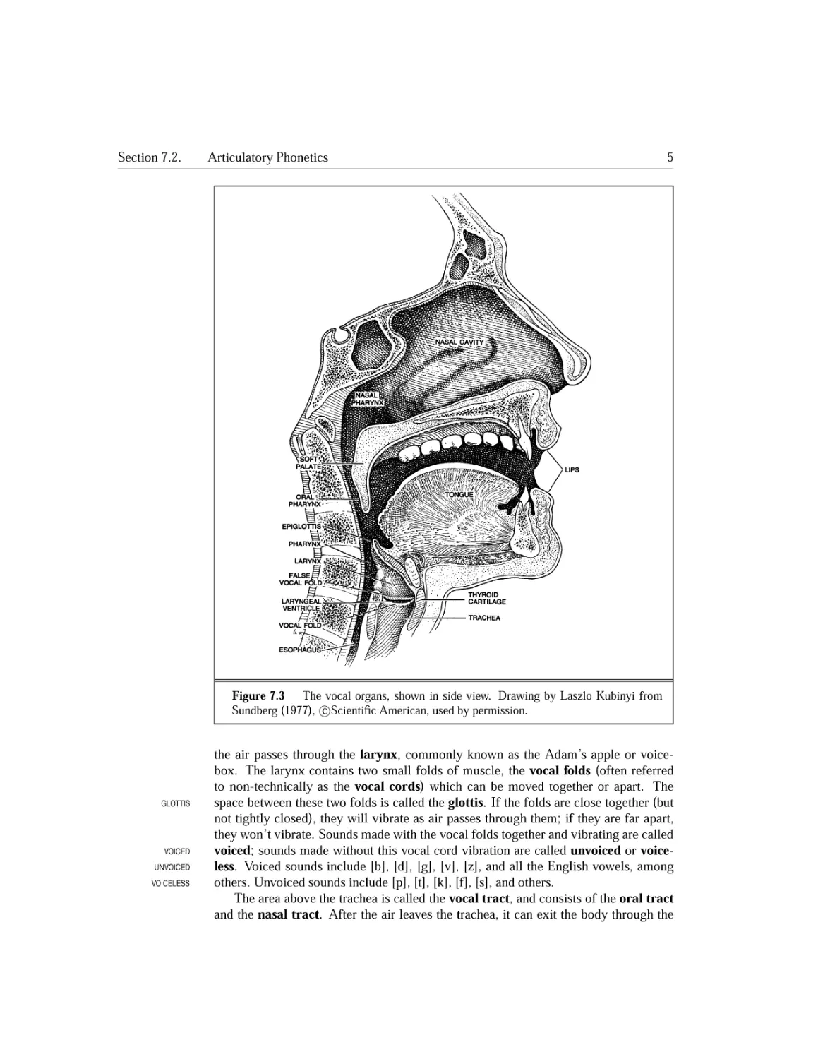
We are also grateful for kind permission to reprint two figures: Fig. 7.3 (©Laszlo
Kubinyi and Scientific American) and Fig. 9.14 (©Paul Taylor and Cambridge Uni-
versity Press). In addition, we created many of our figures as adaptations of pre-
vious figures; we are grateful to the people listed below (for brevity we've listed
just one author in each case) for permission to adapt their figures. The following
three figures are ©IEEE and the authors; we thank Esther Levin (Fig. 24.22) and
Lawrence Rabiner (Figs. 6.14 and 6.15). The other adapted figures below are © the
authors; thanks to the Association of Computational Linguistics, the Journal of Com-
putational Linguistics and its editor Robert Dale, and to Regina Barzilay (Fig. 23.19),
Michael Collins (Figs. 14.7, 14.10, and 14.11), John Goldsmith (Fig. 11.18), Marti
Hearst (Figs. 21.1 and 21.2), Kevin Knight (Fig. 25.35), Philipp Koehn (Figs. 25.25,
25.26, and 25.28), Dekang Lin (Fig. 20.7), Chris Manning (Fig. 14.9), Daniel Marcu
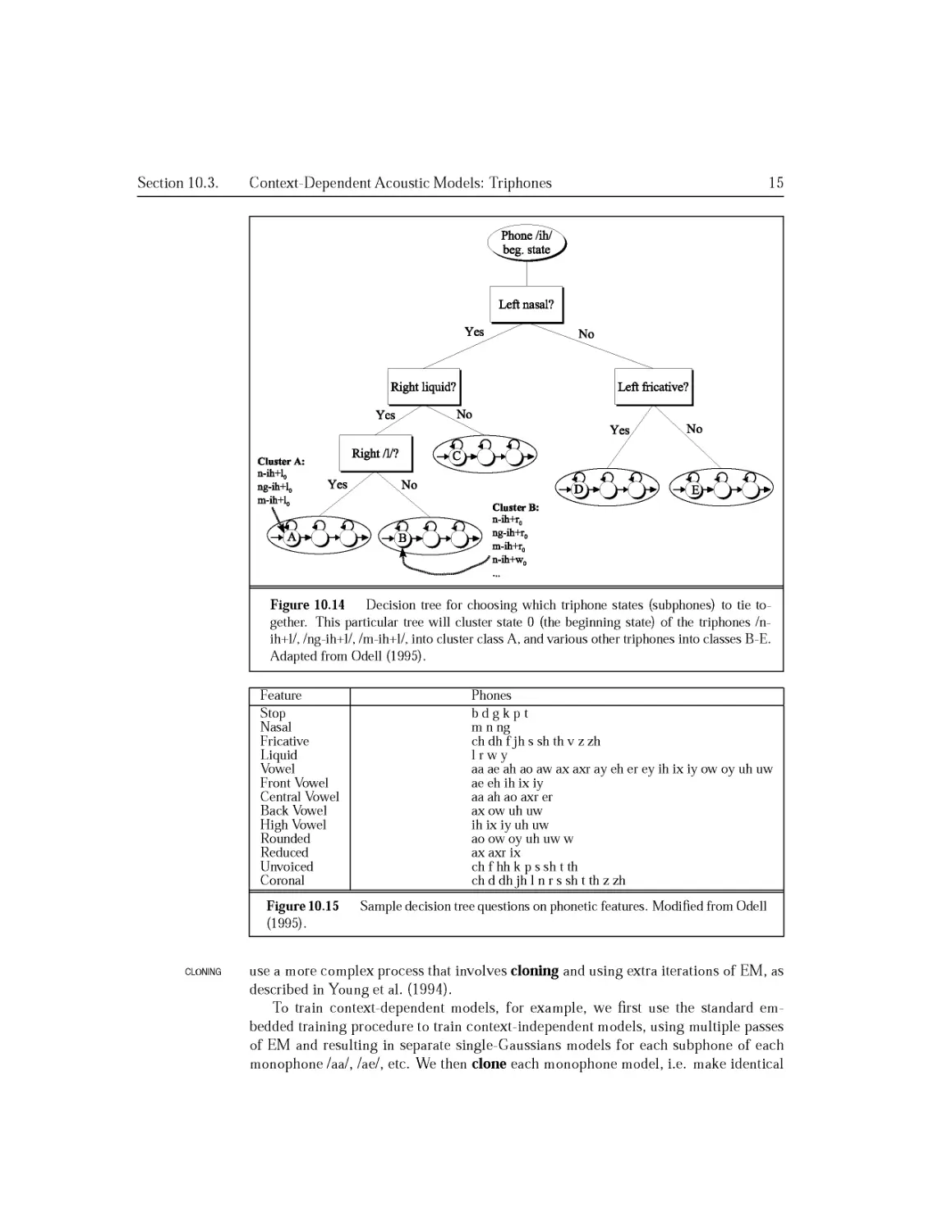
(Fig. 23.16), Mehryar Mohri (Figs. 3.10 and 3.11), Julian Odell (Fig. 10.14), Marilyn
Walker (Figs. 24.8, 24.14, and 24.15), David Yarowsky (Fig. 20.4), and Steve Young
(Fig. 10.16).
DANIEL JURAFSKY
Stanford, California
JAMES H. MARTIN
Boulder, Colorado
About the Authors
Dan Jurafsky is an associate professor in the Department of Linguistics, and by cour-
tesy in the Department of Computer Science, at Stanford University. Previously, he was
on the faculty of the University of Colorado, Boulder, in the Linguistics and Computer
Science departments and the Institute of Cognitive Science. He was born in Yonkers,
New York, and received a B.A in Linguistics in 1983 and a Ph.D. in Computer Science
in 1992, both from the University of California at Berkeley. He received the National
Science Foundation CAREER award in 1998 and the Mac Arthur Fellowship in 2002.
He has published over 90 papers on a wide range of topics in speech and language
processing.
James H. Martin is a professor in the Department of Computer Science and in the
Department of Linguistics, and a fellow in the Institute of Cognitive Science at the
University of Colorado at Boulder. He was born in New York City, received a B.S. in
Computer Science from Columbia University in 1981 and a Ph.D. in Computer Science
from the University of California at Berkeley in 1988. He has authored over 70 publi-
cations in computer science including the book A Computational Model of Metaphor
Interpretation.
xxxi
Chapter 1
Introduction
Dave Bowman: Open the pod bay doors, HAL.
HAL: I'm sorry Dave, I'm afraid 1 can't do that.
Stanley Kubrick and Arthur C. Clarke,
screenplay of 2001: A Space Odyssey
Conversational
agent
Dialogue system
Machine
translation
Question
answering
The idea of giving computers the ability to process human language is as old as the idea
of computers themselves. This book is about the implementation and implications of
that exciting idea. We introduce a vibrant interdisciplinary field with many names cor-
responding to its many facets, names like speech and language processing, human
language technology, natural language processing, computational linguistics, and
speech recognition and synthesis. The goal of this new field is to get computers
to perform useful tasks involving human language, tasks like enabling human-machine
communication, improving human-human communication, or simply doing useful pro-
cessing of text or speech.
One example of a useful such task is a conversational agent. The HAL 9000 com-
puter in Stanley Kubrick's film 2007: A Space Odyssey is one of the most recognizable
characters in 20th century cinema. HAL is an artificial agent capable of such advanced
language behavior as speaking and understanding English, and at a crucial moment in
the plot, even reading lips. It is now clear that HAL's creator, Arthur C. Clarke, was
a little optimistic in predicting when an artificial agent such as HAL would be avail-
able. But just how far off was he? What would it take to create at least the language-
related parts of HAL? We call programs like HAL that converse with humans in natural
language conversational agents or dialogue systems. In this text we study the vari-
ous components that make up modern conversational agents, including language input
(automatic speech recognition and natural language understanding) and language
output (dialogue and response planning and speech synthesis).
Let's turn to another useful language-related task, that of making available to non-
English-speaking readers the vast amount of scientific information on the Web in En-
glish. Or translating for English speakers the hundreds of millions of Web pages written
in other languages like Chinese. The goal of machine translation is to automatically
translate a document from one language to another. We introduce the algorithms and
mathematical tools needed to understand how modern machine translation works. Ma-
chine translation is far from a solved problem; we cover the algorithms currently used
in the field, as well as important component tasks.
Many other language processing tasks are also related to the Web. Another such
task is Web-based question answering. This is a generalization of simple Web search,
where instead ofjust typing keywords, a user might ask complete questions, ranging
from easy to hard, like the following:
• What does "divergent" mean?
• What year was Abraham Lincoln born?
• How many states were in the United States that year?
1
2 Chapter 1.
Introduction
• How much Chinese silk was exported to England by the end of the 18th century?
• What do scientists think about the ethics of human cloning?
Some of these, such as definition questions, or simple factoid questions like dates
and locations, can already be answered by search engines. But answering more com-
plicated questions might require extracting information that is embedded in other text
on a Web page, doing inference (drawing conclusions based on known facts), or syn-
thesizing and summarizing information from multiple sources or Web pages. In this
text we study the various components that make up modern understanding systems of
this kind, including information extraction, word sense disambiguation, and so on.
Although the subfields and problems we've described above are all very far from
completely solved, these are all very active research areas and many technologies are
already available commercially. In the rest of this chapter, we briefly summarize the
kinds of knowledge that are necessary for these tasks (and others like spelling cor-
rection, grammar checking, and so on), as well as the mathematical models that are
introduced throughout the book.
1.1 Knowledge in Speech and Language Processing
What distinguishes language processing applications from other data processing sys-
tems is their use of knowledge of language. Consider the Unix wc program, which
counts the total number of bytes, words, and lines in a text file. When used to count
bytes and lines, wc is an ordinary data processing application. However, when it is
used to count the words in a file, it requires knowledge about what it means to be a
word and thus becomes a language processing system.
Of course, wc is an extremely simple system with an extremely limited and impov-
erished knowledge of language. Sophisticated conversational agents like HAL, ma-
chine translation systems, or robust question-answering systems require much broader
and deeper knowledge of language. To get a feeling for the scope and kind of required
knowledge, consider some of what HAL would need to know to engage in the dia-
logue that begins this chapter, or for a question-answering system to answer one of the
questions above.
HAL must be able to recognize words from an audio signal and to generate an audio
signal from a sequence of words. These tasks of speech recognition and speech syn-
thesis require knowledge about phonetics and phonology: how words are pronounced
in terms of sequences of sounds and how each of these sounds is realized acoustically.
Note also that unlike Commander Data in "Star Trek", HAL is capable of producing
contractions like I'm and can't. Producing and recognizing these and other variations
of individual words (e.g., recognizing that doors is plural) requires knowledge about
morphology, the way words break down into component parts that carry meanings like
singular versus plural.
Moving beyond individual words, HAL must use structural knowledge to properly
string together the words that constitute its response. For example, HAL must know
that the following sequence of words will not make sense to Dave, despite the fact that
Section 1.1.
Knowledge in Speech and Language Processing 3
it contains precisely the same set of words as the original.
(1.1) I'm I do, sorry that afraid Dave I'm can't.
The knowledge needed to order and group words comes under the heading of syn-
tax.
Now consider a question-answering system dealing with the following question:
(1.2) How much Chinese silk was exported to Western Europe by the end of the 18th
century?
To answer this question, we need to know something about lexical semantics, the
meaning of all the words {export or silk) as well as compositional semantics (what
exactly constitutes Western Europe as opposed to Eastern or Southern Europe, what
does end mean when combined with the 18th century. We also need to know something
about the relationship of the words to the syntactic structure. For example, we need to
know that by the end of the 18th century is a temporal end-point and not a description
of the agent, as the by-phrase is in the following sentence:
(1.3) How much Chinese silk was exported to Western Europe by southern
merchants?
We also need the kind of knowledge that lets HAL determine that Dave's utterance
is a request for action, as opposed to a simple statement about the world or a question
about the door, as in the following variations of his original statement.
REQUEST: ElAL, open the pod bay door.
STATEMENT: ElAL, the pod bay door is open.
INFORMATION QUESTION: HAL, is the pod bay door open?
Next, despite its bad behavior, HAL knows enough to be polite to Dave. It could,
for example, have simply replied No or No, I won't open the door. Instead, it first
embellishes its response with the phrases I'm sorry and I'm afraid, and then only indi-
rectly signals its refusal by saying I can't, rather than the more direct (and truthful) I
won't.1 This knowledge about the kind of actions that speakers intend by their use of
sentences is pragmatic or dialogue knowledge.
Another kind of pragmatic or discourse knowledge is required to answer the ques-
tion
(1.4) How many states were in the United States that year?
What year is that year? To interpret words like that year, a question-answering
system needs to examine the earlier questions that were asked; in this case, the previous
question talked about the year that Lincoln was born. Thus, this task of coreference
resolution makes use of knowledge about how words like that or pronouns like it or
she refer to previous parts of the discourse.
To summarize, engaging in complex language behavior requires various kinds of
knowledge of language:
• Phonetics and Phonology — knowledge about linguistic sounds
1 For those unfamiliar with HAL, it is neither sorry nor afraid, nor is it incapable of opening the door. It
has simply decided in a fit of paranoia to kill its crew.
4 Chapter 1.
Introduction
• Morphology — knowledge of the meaningful components of words
• Syntax — knowledge of the structural relationships between words
• Semantics — knowledge of meaning
• Pragmatics — knowledge of the relationship of meaning to the goals and inten-
tions of the speaker
• Discourse — knowledge about linguistic units larger than a single utterance
1.2 Ambiguity
A perhaps surprising fact about these categories of linguistic knowledge is that most
Ambiguity tasks in speech and language processing can be viewed as resolving ambiguity at one
Ambiguous of these levels. We say some input is ambiguous if multiple, alternative linguistic
structures can be built for it. Consider the spoken sentence 1 made her duck. Here are
five different meanings this sentence could have (see if you can think of some more),
each of which exemplifies an ambiguity at some level:
(1.5) I cooked waterfowl for her.
(1.6) I cooked waterfowl belonging to her.
(1.7) I created the (plaster?) duck she owns.
(1.8) I caused her to quickly lower her head or body.
(1.9) I waved my magic wand and turned her into undifferentiated waterfowl.
These different meanings are caused by a number of ambiguities. First, the words
duck and her are morphologically or syntactically ambiguous in their part-of-speech.
Duck can be a verb or a noun, while her can be a dative pronoun or a possessive
pronoun. Second, the word make is semantically ambiguous; it can mean create or
cook. Finally, the verb make is syntactically ambiguous in a different way. Make can
be transitive, that is, taking a single direct object (1.6), or it can be ditransitive, that is,
taking two objects (1.9), meaning that the first object {her) was made into the second
object {duck). Finally, make can take a direct object and a verb (1.8), meaning that the
object {her) was caused to perform the verbal action {duck). Furthermore, in a spoken
sentence, there is an even deeper kind of ambiguity; the first word could have been eye
or the second word maid.
We often introduce the models and algorithms we present throughout the book as
ways to resolve or disambiguate these ambiguities. For example, deciding whether
duck is a verb or a noun can be solved by part-of-speech tagging. Deciding whether
make means "create" or "cook" can be solved by word sense disambiguation. Reso-
lution of part-of-speech and word sense ambiguities are two important kinds of lexical
disambiguation. A wide variety of tasks can be framed as lexical disambiguation
problems. For example, a text-to-speech synthesis system reading the word lead needs
to decide whether it should be pronounced as in lead pipe or as in lead me on. By
contrast, deciding whether her and duck are part of the same entity (as in (1.5) or (1.8))
or are different entities (as in (1.6)) is an example of syntactic disambiguation and
can be addressed by probabilistic parsing. We also consider ambiguities that don't
Section 1.3.
Models and Algorithms 5
arise in this particular example, such as determining whether a sentence is a statement
or a question (which can be resolved by speech act interpretation).
1.3 Models and Algorithms
One of the key insights of the last 50 years of research in language processing is that
the various kinds of knowledge described in the last sections can be captured through
the use of a small number of formal models or theories. Fortunately, these models and
theories are all drawn from the standard toolkits of computer science, mathematics, and
linguistics and should be generally familiar to those trained in those fields. Among the
most important models are state machines, rule systems, logic, probabilistic models,
and vector-space models. These models, in turn, lend themselves to a small number
of algorithms, among the most important of which are state space search algorithms,
such as dynamic programming, and machine learning algorithms, such as classifiers
and Expectation-Maximization (EM) and other learning algorithms.
In their simplest formulation, state machines are formal models that consist of
states, transitions among states, and an input representation. Some of the variations
of this basic model that we will consider are deterministic and non-deterministic
finite-state automata and finite-state transducers.
Closely related to these models are their declarative counterparts: formal rule sys-
tems. Among the more important ones we consider (in both probabilistic and non-
probabilistic formulations) are regular grammars and regular relations, context-free
grammars, and feature-augmented grammars. State machines and formal rule sys-
tems are the main tools used when dealing with knowledge of phonology, morphology,
and syntax.
A third class of models that plays a critical role in capturing knowledge of language
are models based on logic. We discuss first-order logic, also known as the predicate
calculus, as well as such related formalisms as lambda-calculus, feature structures,
and semantic primitives. These logical representations have traditionally been used for
modeling semantics and pragmatics, although more recent work has tended to focus on
potentially more robust techniques drawn from non-logical lexical semantics.
Probabilistic models are crucial for capturing every kind of linguistic knowledge.
Each of the other models (state machines, formal rule systems, and logic) can be aug-
mented with probabilities. For example, the state machine can be augmented with
probabilities to become the weighted automaton, or Markov model. We spend a
significant amount of time on hidden Markov models or HMMs, which are used
everywhere in the field, in part-of-speech tagging, speech recognition, dialogue under-
standing, text-to-speech, and machine translation. The key advantage of probabilistic
models is their ability to solve the many kinds of ambiguity problems that we discussed
earlier; almost any speech and language processing problem can be recast as "given N
choices for some ambiguous input, choose the most probable one".
Finally, vector-space models, based on linear algebra, underlie information retrieval
and many treatments of word meanings.
Processing language with any of these models typically involves a search through
6 Chapter 1.
Introduction
a space of states representing hypotheses about an input. In speech recognition, we
search through a space of phone sequences for the correct word. In parsing, we search
through a space of trees for the syntactic parse of an input sentence. In machine trans-
lation, we search through a space of translation hypotheses for the correct translation of
a sentence into another language. For non-probabilistic tasks, such as tasks involving
state machines, we use well-known graph algorithms such as depth-first search. For
probabilistic tasks, we use heuristic variants such as best-first and A* search and rely
on dynamic programming algorithms for computational tractability.
Machine learning tools such as classifiers and sequence models play a significant
role in many language processing tasks. Based on attributes describing each object, a
classifier attempts to assign a single object to a single class while a sequence model
attempts tojointly classify a sequence of objects into a sequence of classes.
For example, in the task of deciding whether a word is spelled correctly, classi-
fiers such as decision trees, support vector machines, Gaussian mixture models,
and logistic regression could be used to make a binary decision (correct or incorrect)
for one word at a time. Sequence models such as hidden Markov models, maxi-
mum entropy Markov models, and conditional random fields could be used to assign
correct/incorrect labels to all the words in a sentence at once.
Finally, researchers in language processing use many of the same methodologi-
cal tools that are used in machine learning research—the use of distinct training and
test sets, statistical techniques like cross-validation, and careful evaluation of trained
systems.
1.4 Language, Thought, and Understanding
To many, the ability of computers to process language as skillfully as we humans do
will signal the arrival of truly intelligent machines. The basis of this belief is the fact
that the effective use of language is intertwined with our general cognitive abilities.
Among the first to consider the computational implications of this intimate connection
was Alan Turing (1950). In this famous paper, Turing introduced what has come to
Turing test be known as the Turing test. Turing began with the thesis that the question of what it
would mean for a machine to think was essentially unanswerable because of the inher-
ent imprecision in the terms machine and think. Instead, he suggested an empirical test,
a game, in which a computer's use of language would form the basis for determining
if the machine could think. If the machine could win the game, it would be judged
intelligent.
In Turing's game, there are three participants: two people and a computer. One of
the people is a contestant who plays the role of an interrogator. To win, the interrogator
must determine which of the other two participants is the machine by asking a series
of questions via a teletype. The task of the machine is to fool the interrogator into
believing it is a person by responding as a person would to the interrogator's questions.
The task of the second human participant is to convince the interrogator that the other
participant is the machine and that she is human.
The following interaction from Turing's paper illustrates the kind of interactions he
Section 1.4.
Language, Thought, and Understanding 7
had in mind. Clearly, a convincing simulation of humanity doesn't require being an
expert in all domains:
Q: Please write me a sonnet on the topic of the Forth Bridge.
A: Count me out on this one. I never could write poetry.
Q: Add 34957 to 70764. ,
A: (Pause about 30 seconds and then give answer as) 105621.
Turing predicted that roughly by the end of the 20th century a machine with 10
gigabytes of memory would have around a 30% chance of fooling a human interrogator
after five minutes of questioning. Given the fact that you can fool some of the people
all the time, it is not clear how rigorous this particular standard is. Nevertheless, the
critical issue for Turing was that using language as humans do is sufficient, by itself,
as an operational test for intelligence.
Surprisingly, many of the issues raised by Turing became relevant as early as 1966
Eliza in the context of the ELIZA program (Weizenbaum, 1966). ELIZA was an early nat-
ural language processing system capable of carrying on a limited form of conversation
with a user. Consider the following session with a version of ELIZA that imitated the
responses of a Rogerian psychotherapist.
User]: You are like my father in some ways.
ELIZA]: WHAT RESEMBLANCE DO YOU SEE
User2: You are not very aggressive but I think you don't want me to notice that.
ELIZA,: WHAT MAKES YOU THINK I AM NOT AGGRESSIVE
User-,: You don't argue with me.
ELIZA,: WHY DO YOU THINK I DON'T ARGUE WITH YOU
User4'. You are afraid of me.
E LI z A 4: DOES IT PLEASE YOU TO BELIEVE I AM AFRAID OF YOU
As we discuss in more detail in Chapter 2, ELIZA is a remarkably simple program
that uses pattern matching to process the input and translate it into suitable outputs.
This simple technique succeeds in this domain because ELIZA doesn't actually need
to know anything to mimic a Rogerian psychotherapist. As Weizenbaum notes, this is
one of the few dialogue genres where listeners can act as if they know nothing of the
world.
ELIZA's deep relevance to Turing's ideas is that many people who interacted with
ELIZA came to believe that it really understood them and their problems. Indeed,
Weizenbaum (1976) notes that many of these people continued to believe in ELIZA's
abilities even after the program's operation was explained to them. In more recent
years, Weizenbaum's informal tests have been repeated in a somewhat more controlled
setting. Since 1991, an event known as the Loebner Prize competition has attempted to
put various computer programs to the Turing test. Although these contests seem to have
little scientific interest, a consistent result over the years has been that even the crudest
programs can fool some of the judges some of the time (Shieber, 1994a). Not surpris-
ingly, these results have done nothing to quell the ongoing debate over the suitability of
the Turing test as a test for intelligence among philosophers and Al researchers (Searle,
1980).
Fortunately, for the purposes of this book, the relevance of these results does not
hinge on whether computers will ever be intelligent or will ever understand natural
8 Chapter 1.
Introduction
language. Far more important is recent related research in the social sciences that has
confirmed another of Turing's predictions from the same paper.
Nevertheless I believe that at the end of the century the use of words and
educated opinion will have altered so much that we will be able to speak
of machines thinking without expecting to be contradicted.
It is now clear that regardless of what people believe or know about the inner work-
ings of computers, they talk about them and interact with them as social entities. People
act toward computers as if they were people; they are polite to them, treat them as team
members, and expect, among other things, that computers should be able to understand
their needs and be capable of interacting with them naturally. For example, Reeves and
Nass (1996) found that when a computer asked a human to evaluate how well the com-
puter had been doing, the human gives more positive responses than when a different
computer asks the same questions. People seemed to be afraid of being impolite. In
a different experiment, Reeves and Nass found that people also give computers higher
performance ratings if the computer has recently said something flattering to the hu-
man. Given these predispositions, speech- and language-based systems may provide
many users with the most natural interface for many applications. This fact has led to
a long-term focus in the field on the design of conversational agents, artificial entities
that communicate conversationally.
1.5 The State of the Art
ITe can only see a short distance ahead, but we can see plenty there that needs to be done.
Alan Turing
This is an exciting time for the field of speech and language processing. The startling
increase in computing resources available to the average computer user, the rise of
the Web as a massive source of information, and the increasing availability of wire-
less mobile access have all placed speech- and language-processing applications in the
technology spotlight. The following are examples of some currently deployed systems
that reflect this trend:
• Travelers calling Amtrak, United Airlines, and other travel providers interact
with conversational agents that guide them through the process of making reser-
vations and getting arrival and departure information.
• Car makers provide automatic speech recognition and text-to-speech systems
that allow drivers to control their environmental, entertainment, and navigational
systems by voice. A similar spoken dialogue system has been deployed by as-
tronauts on the International Space Station.
• Video search companies provide search services for millions of hours of video
on the Web by using speech recognition technology to capture the words in the
sound track.
• Google provides cross-language information retrieval and translation services
whereby users can supply queries in their native language to search collections
Section 1.6.
Some Brief History 9
in another language. Google translates the query, finds the most relevant pages,
and then automatically translates them back to the user's native language.
• Large educational publishers such as Pearson and testing services like ETS use
automated systems to analyze thousands of student essays, grading and assessing
them in a manner that is indistinguishable from human graders.
• Interactive virtual agents, based on lifelike animated characters, serve as tutors
for children learning to read (Wise et al., 2007).
• Text analysis companies provide marketing intelligence based on automated mea-
surements of user opinions, preferences, attitudes as expressed in weblogs, dis-
cussion forums, and user groups.
1.6 Some Brief History
Historically, speech and language processing has been treated very differently in com-
puter science, electrical engineering, linguistics, and psychology/cognitive science.
Because of this diversity, speech and language processing encompasses a number of
different but overlapping fields in these different departments: computational linguis-
tics in linguistics, natural language processing in computer science, speech recogni-
tion in electrical engineering, computational psycholinguistics in psychology. This
section summarizes the different historical threads that have given rise to the field of
speech and language processing. This section provides only a sketch, but many of the
topics listed here are covered in more detail in subsequent chapters.
1.6.1 Foundational Insights: 1940s and 1950s
The earliest roots of the field date to the intellectually fertile period just after World
War II that gave rise to the computer itself. This period from the 1940s through the end
of the 1950s saw intense work on two foundational paradigms: the automaton and
probabilistic or information-theoretic models.
The automaton arose in the 1950s out of Turing's (1936) model of algorithmic
computation, considered by many to be the foundation of modern computer science.
Turing's work led first to the McCulloch-Pitts neuron (McCulloch and Pitts, 1943), a
simplified model of the neuron as a kind of computing element that could be described
in terms of propositional logic, and then to the work of Kleene (1951) and (1956) on
finite automata and regular expressions. Shannon (1948) applied probabilistic models
of discrete Markov processes to automata for language. Drawing on the idea of a finite-
state Markov process from Shannon's work, Chomsky (1956) first considered finite-
state machines as a way to characterize a grammar and defined a finite-state language
as a language generated by a finite-state grammar. These early models led to the field of
formal language theory, which used algebra and set theory to define formal languages
as sequences of symbols. This includes the context-free grammar, first defined by
Chomsky (1956) for natural languages but independently discovered by Backus (1959)
and Naur et al. (1960) in their descriptions of the ALGOL programming language.
10 Chapter 1.
Introduction
The second foundational insight of this period was the development of probabilistic
algorithms for speech and language processing, which dates to Shannon's other contri-
bution: the metaphor of the noisy channel and decoding for the transmission of lan-
guage through media such as communication channels and speech acoustics. Shannon
also borrowed the concept of entropy from thermodynamics as a way of measuring the
information capacity of a channel, or the information content of a language, and per-
formed the first measure of the entropy of English by using probabilistic techniques.
It was also during this early period that the sound spectrograph was developed
(Koenig et al., 1946), and foundational research was done in instrumental phonetics
that laid the groundwork for later work in speech recognition. This led to the first ma-
chine speech recognizers in the early 1950s. In 1952, researchers at Bell Labs built a
statistical system that could recognize any of the 10 digits from a single speaker (Davis
et al., 1952). The system had 10 speaker-dependent stored patterns roughly represent-
ing the first two vowel formants in the digits. They achieved 97%-99% accuracy by
choosing the pattern that had the highest relative correlation coefficient with the input.
1.6.2 The Two Camps: 1957-1970
By the end of the 1950s and the early 1960s, speech and language processing had split
very cleanly into two paradigms: symbolic and stochastic.
The symbolic paradigm took off from two lines of research. The first was the work
of Chomsky and others on formal language theory and generative syntax throughout the
late 1950s and early to mid 1960s, and the work of many linguistics and computer sci-
entists on parsing algorithms, initially top-down and bottom-up and then with dynamic
programming. One of the earliest complete parsing systems was Zelig Harris's Trans-
formations and Discourse Analysis Project (TDAP), which was implemented between
June 1958 and July 1959 at the University of Pennsylvania (Harris, 1962).’ The sec-
ond line of research was the new field of artificial intelligence. In the summer of 1956
John McCarthy, Marvin Minsky, Claude Shannon, and Nathaniel Rochester brought
together a group of researchers for a two-month workshop on what they decided to
call artificial intelligence (Al). Although Al always included a minority of researchers
focusing on stochastic and statistical algorithms (including probabilistic models and
neural nets), the major focus of the new field was the work on reasoning and logic
typified by Newell and Simon's work on the Logic Theorist and the General Problem
Solver. At this point, early natural language understanding systems were built. These
simple systems worked in single domains mainly by a combination of pattern matching
and keyword search with simple heuristics for reasoning and question-answering. By
the late 1960s, more formal logical systems were developed.
The stochastic paradigm took hold mainly in departments of statistics and of elec-
trical engineering. By the late 1950s, the Bayesian method was beginning to be applied
to the problem of optical character recognition. Bledsoe and Browning (1959) built a
Bayesian text-recognition that used a large dictionary and computed the likelihood of
each observed letter sequence given each word in the dictionary by multiplying the
This system was reimplemented recently and is described by Joshi and Hopely (1999) and Karttunen
(1999), who note that the parser was essentially implemented as a cascade of finite-state transducers.
Section 1.6.
Some Brief History 11
likelihoods for each letter. Mosteller and Wallace (1964) applied Bayesian methods to
the problem of authorship attribution on The Federalist papers.
The 1960s also saw the rise of the first serious testable psychological models of
human language processing based on transformational grammar, as well as the first on-
line corpora: the Brown corpus of American English, a one-million-word collection of
samples from 500 written texts from different genres (newspaper, novels, non-fiction,
academic, etc.), which was assembled at Brown University in 1963-64 (Kucera and
Francis, 1967; Francis, 1979; Francis and Kucera, 1982), and William S. Y. Wang's
1967 DOC (Dictionary on Computer), an on-line Chinese dialect dictionary.
1.6.3 Four Paradigms: 1970-1983
The next period saw an explosion in research in speech and language processing and
the development of a number of research paradigms that still dominate the field.
The stochastic paradigm played a huge role in the development of speech recogni-
tion algorithms in this period, particularly the use of the hidden Markov model (HMM)
and the metaphors of the noisy channel and decoding, developed independently by Je-
linek, Bahl, Mercer, and colleagues at IBM's Thomas J. Watson Research Center, and
by Baker at Carnegie Mellon University, who was influenced by the work of Baum and
colleagues at the Institute for Defense Analyses in Princeton. AT&T's Bell Laborato-
ries was another key center for work on speech recognition and synthesis; see Rabiner
and Juang (1993) for descriptions of the wide range of this work.
The logic-based paradigm was begun by the work of Colmerauer and his col-
leagues on Q-systems and metamorphosis grammars (Colmerauer, 1970, 1975), the
forerunners of Prolog, and Definite Clause Grammars (Pereira and Warren, 1980). In-
dependently, Kay's (1979) work on functional grammar and shortly later, Bresnan and
Kaplan's (1982) work on Lexical Functional Grammar (LFG), established the impor-
tance of feature structure unification.
The natural language understanding field took off during this period, beginning
with Winograd's SHRDLU system, which simulated a robot embedded in a world of
toy blocks (Winograd, 1972a). The program was able to accept natural-language text
commands (Move the red block on top of the smaller green one) of a hitherto unseen
complexity and sophistication. His system was also the first to attempt to build an
extensive (for the time) grammar of English, based on Halliday's systemic grammar.
Winograd's model made it clear that the problem of parsing was well enough under-
stood to begin to focus on semantics and discourse. Roger Schank and his colleagues
and students (in what was often referred to as the Yale School) built a series of language-
understanding programs that focused on conceptual knowledge such as scripts, plans,
and goals, and human memory organization (Schank and Abelson, 1977; Schank and
Riesbeck, 1981; Cullingford, 1981; Wilensky, 1983; Lehnert, 1977). This work often
used network-based semantics (Quillian, 1968; Norman and Rumelhart, 1975; Schank,
1972; Wilks, 1975c, 1975b; Kintsch, 1974) and began to incorporate Fillmore's notion
of case roles (Fillmore, 1968) into their representations (Simmons, 1973).
The logic-based and natural-language-understanding paradigms were unified in
systems that used predicate logic as a semantic representation, such as the LUNAR
question-answering system (Woods, 1967, 1973).
12 Chapter 1.
Introduction
The discourse modeling paradigm focused on four key areas in discourse. Grosz
and her colleagues introduced the study of substructure in discourse, and of discourse
focus (Grosz, 1977a; Sidner, 1983); a number of researchers began to work on au-
tomatic reference resolution (Hobbs, 1978); and the BDI (Belief-Desire-Intention)
framework for logic-based work on speech acts was developed (Perrault and Allen,
1980; Cohen and Perrault, 1979).
1.6.4 Empiricism and Finite-State Models Redux: 1983-1993
This next decade saw the return of two classes of models that had lost popularity in the
late 1950s and early 1960s, partially due to theoretical arguments against them such
as Chomsky's influential review of Skinner's Verbal Behavior (Chomsky, 1959b). The
first class was finite-state models, which began to receive attention again after work
on finite-state phonology and morphology by Kaplan and Kay (1981) and finite-state
models of syntax by Church (1980). A large body of work on finite-state models is
described throughout the book.
The second trend in this period was what has been called the "return of empiri-
cism"; most notable here was the rise of probabilistic models throughout speech and
language processing, influenced strongly by the work at the IBM Thomas J. Watson
Research Center on probabilistic models of speech recognition. These probabilistic
methods and other such data-driven approaches spread from speech into part-of-speech
tagging, parsing and attachment ambiguities, and semantics. This empirical direction
was also accompanied by a new focus on model evaluation, based on using held-out
data, developing quantitative metrics for evaluation, and emphasizing the comparison
of performance on these metrics with previous published research.
This period also saw considerable work on natural language generation.
1.6.5 The Field Comes Together: 1994-1999
By the last five years of the millennium it was clear that the field was undergoing ma-
jor changes. First, probabilistic and data-driven models had become quite standard
throughout natural language processing. Algorithms for parsing, part-of-speech tag-
ging, reference resolution, and discourse processing all began to incorporate probabil-
ities and to employ evaluation methodologies borrowed from speech recognition and
information retrieval. Second, the increases in the speed and memory of computers
had allowed commercial exploitation of a number of subareas of speech and language
processing, in particular, speech recognition, and spelling and grammar correction.
Speech and language processing algorithms began to be applied to Augmentative and
Alternative Communication (AAC). Finally, the rise of the Web emphasized the need
for language-based information retrieval and information extraction.
1.6.6 The Rise of Machine Learning: 2000-2008
The empiricist trends begun in the latter part of the 1990s accelerated at an astounding
pace in the new century. This acceleration was largely driven by three synergistic
trends.
Section 1.6.
Some Brief History 13
First, large amounts of spoken and written material became widely available through
the auspices of the Linguistic Data Consortium (LDC) and other similar organizations.
Importantly, included among these materials were annotated collections such as the
Penn Treebank (Marcus et al., 1993), Prague Dependency Treebank (Hajic, 1998),
PropBank (Palmer et al., 2005), Penn Discourse Treebank (Miltsakaki et al., 2004b),
RSTBank (Carlson et al., 2001) and TimeBank (Pustejovsky et al., 2003b), all of which
layered standard text sources with various forms of syntactic, semantic, and pragmatic
annotations. The existence of these resources promoted the trend of casting more com-
plex traditional problems, such as parsing and semantic analysis, as problems in super-
vised machine learning. These resources also promoted the establishment of additional
competitive evaluations for parsing (Dejean and Tjong Kim Sang, 2001), information
extraction (NIST, 2007a; Tjong Kim Sang, 2002; Tjong Kim Sang and De Meulder,
2003), word sense disambiguation (Palmer et al., 2001; Kilgarriff and Palmer, 2000),
question answering (Voorhees and Tice, 1999), and summarization (Dang, 2006).
Second, this increased focus on learning led to a more serious interplay with the
statistical machine learning community. Techniques such as support vector machines
(Boser et al., 1992; Vapnik, 1995), maximum entropy techniques and their equiva-
lent formulation as multinomial logistic regression (Berger et al., 1996), and graphical
Bayesian models (Pearl, 1988) became standard practice in computational linguistics.
Third, the widespread availability of high-performance computing systems facil-
itated the training and deployment of systems that could not have been imagined a
decade earlier.
Finally, near the end of this period, largely unsupervised statistical approaches be-
gan to receive renewed attention. Progress on statistical approaches to machine trans-
lation (Brown et al., 1990; Och and Ney, 2003) and topic modeling (Blei et al., 2003)
demonstrated that effective applications could be constructed from systems trained on
unannotated data alone. In addition, the widespread cost and difficulty of producing re-
liably annotated corpora became a limiting factor in the use of supervised approaches
for many problems. This trend toward the use of unsupervised techniques will likely
increase.
1.6.7 On Multiple Discoveries
Even in this brief historical overview, we have mentioned a number of cases of multiple
independent discoveries of the same idea. Just a few of the "multiples" to be discussed
in this book include the application of dynamic programming to sequence comparison
by Viterbi, Vintsyuk, Needleman and Wunsch, Sakoe and Chiba, Sankoff, Reichert et
al., and Wagner and Fischer (Chapters 3, 5, and 6); the HMM/noisy channel model
of speech recognition by Baker and by Jelinek, Bahl, and Mercer (Chapters 6, 9, and
10); the development of context-free grammars by Chomsky and by Backus and Naur
(Chapter 12); the proof that Swiss-German has a non-context-free syntax by Huybregts
and by Shieber (Chapter 16); the application of unification to language processing by
Colmerauer et al. and by Kay (Chapter 15).
Are these multiples to be considered astonishing coincidences? A well-known hy-
pothesis by sociologist of science Robert K. Merton (1961) argues, quite the contrary,
that
14 Chapter 1.
Introduction
all scientific discoveries are in principle multiples, including those that on
the surface appear to be singletons.
Of course, there are many well-known cases of multiple discovery or invention;
just a few examples from an extensive list in Ogburn and Thomas (1922) include the
multiple invention of the calculus by Leibnitz and by Newton, the multiple develop-
ment of the theory of natural selection by Wallace and by Darwin, and the multiple
invention of the telephone by Gray and Bell.’ But Merton gives a further array of ev-
idence for the hypothesis that multiple discovery is the rule rather than the exception,
including many cases of putative singletons that turn out be a rediscovery of previ-
ously unpublished or perhaps inaccessible work. An even stronger piece of evidence
is his ethnomethodological point that scientists themselves act under the assumption
that multiple invention is the norm. Thus many aspects of scientific life are designed
to help scientists avoid being "scooped": submission dates on journal articles, careful
dates in research records, circulation of preliminary or technical reports.
1.6.8 A Final Brief Note on Psychology
Many of the chapters in this book include short summaries of psychological research
on human processing. Of course, understanding human language processing is an im-
portant scientific goal in its own right and is part of the general field of cognitive sci-
ence. However, an understanding of human language processing can often be helpful
in building better machine models of language. This seems contrary to the popular
wisdom, which holds that direct mimicry of nature's algorithms is rarely useful in en-
gineering applications. For example, the argument is often made that if we copied
nature exactly, airplanes would flap their wings; yet airplanes with fixed wings are a
more successful engineering solution. But language is not aeronautics. Cribbing from
nature is sometimes useful for aeronautics (after all, airplanes do have wings), but it is
particularly useful when we are trying to solve human-centered tasks. Airplane flight
has different goals from bird flight; but the goal of speech recognition systems, for
example, is to perform exactly the task that human court reporters perform every day:
transcribe spoken dialog. Since people already do this well, we can learn from nature's
previous solution. Furthermore, since an important application of speech and language
processing systems is for human-computer interaction, it makes sense to copy a solu-
tion that behaves the way people are accustomed to.
1.7 Summary
This chapter introduces the field of speech and language processing. The following are
some of the highlights of this chapter.
3 Ogburn and Thomas are generally credited with noticing that the prevalence of multiple inventions sug-
gests that the cultural milieu and not individual genius is the deciding causal factor in scientific discovery. In
an amusing bit of recursion, however, Merton notes that even this idea has been multiply discovered, citing
sources from the 19th century and earlier!
Bibliographical and Historical Notes 15
• A good way to understand the concerns of speech and language processing re-
search is to consider what it would take to create an intelligent agent like HAL
from 2001: A Space Odyssey, or build a Web-based question answerer, or a ma-
chine translation engine.
• Speech and language technology relies on formal models, or representations, of
knowledge of language at the levels of phonology and phonetics, morphology,
syntax, semantics, pragmatics and discourse. A number of formal models in-
cluding state machines, formal rule systems, logic, and probabilistic models are
used to capture this knowledge.
• The foundations of speech and language technology lie in computer science, lin-
guistics, mathematics, electrical engineering, and psychology. A small number
of algorithms from standard frameworks are used throughout speech and lan-
guage processing.
• The critical connection between language and thought has placed speech and
language processing technology at the center of debate over intelligent machines.
Furthermore, research on how people interact with complex media indicates that
speech and language processing technology will be critical in the development
of future technologies.
• Revolutionary applications of speech and language processing are currently in
use around the world. The creation of the Web, as well as significant recent
improvements in speech recognition and synthesis, will lead to many more ap-
plications.
Bibliographical and Historical Notes
Research in the various subareas of speech and language processing is spread across
a wide number of conference proceedings and journals. The conferences and journals
most centrally concerned with natural language processing and computational linguis-
tics are associated with the Association for Computational Linguistics (ACL), its Eu-
ropean counterpart (EACL), and the International Conference on Computational Lin-
guistics (COLING). The annual, proceedings of ACL, NAACL, and EACL, and the
biennial COLING conference are the primary forums for work in this area. Related
conferences include various proceedings of ACL Special Interest Groups (SIGs) such
as the Conference on Natural Language Learning (CoNLL), as well as the conference
on Empirical Methods in Natural Language Processing (EMNLP).
Research on speech recognition, understanding, and synthesis is presented at the
annual INTERSPEECH conference, which is called the International Conference on
Spoken Language Processing (ICSLP), and the European Conference on Speech Com-
munication and Technology (EUROSPEECH) in alternating years, or the annual IEEE
International Conference on Acoustics, Speech, and Signal Processing (IEEE ICASSP).
Spoken language dialogue research is presented at these or at workshops like SIGDial.
Journals include Computational Linguistics, Natural Language Engineering, Com-
puter Speech and Language, Speech Communication, the IEEE Transactions on Audio,
16 Chapter 1.
Introduction
Speech & Language Processing, the ACM Transactions on Speech and Language Pro-
cessing, and Linguistic Issues in Language Technology.
Many of these papers, including those from the Computational Linguistics journal
and the ACL, COLING, and related conferences are available for free online at the ACL
Anthology (http: I /vrvrw. aclweb. org/anthology- index/).
Work on language processing from an Artificial Intelligence perspective can be
found in the annual meetings of the American Association for Artificial Intelligence
(AAAI), as well as the biennial International Joint Conference on Artificial Intelli-
gence (IJCAI) meetings. Artificial intelligence journals that periodically feature work
on speech and language processing include Machine Learning, Journal of Machine
Learning Research, and the Journal of Artificial Intelligence Research.
A fair number of textbooks covering various aspects of speech and language pro-
cessing are available. Manning and Schiitze (1999) {Foundations of Statistical Lan-
guage Processing) focuses on statistical models of tagging, parsing, disambiguation,
collocations, and other areas. Charniak (1993) {Statistical Language Learning) is an
accessible, though older and less-extensive, introduction to similar material. Manning
et al. (2008) focuses on information retrieval, text classification, and clustering. NLTK,
the Natural Language Toolkit (Bird and Loper, 2004), is a suite of Python modules and
data for natural language processing, together with a Natural Language Processing
book based on the NLTK suite. Allen (1995) {Natural Language Understanding) pro-
vides extensive coverage of language processing from the Al perspective. Gazdar and
Mellish (1989) {Natural Language Processing in LisplProloglPopll) covers especially
automata, parsing, features, and unification and is available free online. Pereira and
Shieber (1987) gives a Prolog-based introduction to parsing and interpretation. Russell
and Norvig (2002) introduce artificial intelligence with chapters on natural language
processing. Partee et al. (1990) broadly cover mathematical linguistics. A historically
significant collection of foundational papers can be found in Grosz et al. (1986) {Read-
ings in Natural Language Processing).
There are many places to acquire corpora of speech and text. One of the largest
is the Linguistic Data Consortium, a non-profit consortium that creates and distributes
corpora (http: //www.ldc.upenn.edu/). See the textbook web page for point-
ers to others such as CHILDES (http: 7/childes. psy. emu. edu/), the British
National Corpus (http: I/www. natcorp. ox. ac. uk/), the International Corpus
о f English (http: / / www . u cl. a c .uk/english-usage/ice/index. htm),
and Project Gutenberg (http: / /www. gutenberg. org/) .
Chapter 2
Regular Expressions and Automata
User i: Men are all alike.
ELIZAi: IN WHAT WAY
User 2: They ’re always bugging us about something or other.
ELIZA2: CAN YO U THINK OF A SPECIFIC EXAMPLE
User3: Well, my boyfriend made me come here.
ELIZA-}: YOUR BOYFRIEND MADE YOU COME HERE
User^: He says I’m depressed much of the time.
ELIZA4: I AM SORRY TO HEAR YOU ARE DEPRESSED
Weizenbaum (1966)
Imagine that you have become a passionate fan of woodchucks and have recently
learned that groundhog and woodchuck are different names for the same animal. Since
you are writing a term paper on woodchucks, you now need to search through your
paper for every occurrence of the term woodchuck and replace woodchucks with wood-
chucks (groundhogs). But you also need to replace singular woodchuck with wood-
chuck (groundhog). Instead of having to do this search twice, you would prefer to
perform a single command for something like woodchuck with an optional final s. Or
perhaps you might want to search for all the prices in some document; you might want
to see all strings that look like $199 or $25 or $24.99 in order to automatically extract
a table of prices. In this chapter we introduce the regular expression, the standard no-
tation for characterizing text sequences. The regular expression is used for specifying
text strings in all sorts of text processing and information extraction applications.
After we have defined regular expressions, we show how they can be implemented
with the finite-state automaton. The finite-state automaton is not only the mathemat-
ical device used to implement regular expressions but also one of the most significant
tools of computational linguistics. Variations of automata such as finite-state trans-
ducers, hidden Markov models, and V-gram grammars are important components of
applications that we introduce in later chapters, including speech recognition and syn-
thesis, machine translation, spell-checking, and information extraction.
2.1 Regular Expressions
SIR ANDREW: Her C’s, her U’s and her T’s: why that?
Shakespeare, Twelfth Night
Regular
expression
One of the unsung successes in standardization in computer science has been the reg-
ular expression (RE), a language for specifying text search strings. The regular ex-
17
18 Chapter 2. Regular Expressions and Automata
pression languages used for searching texts in Unix tools like grep and Emacs, in Perl,
Python, Ruby, Java, and .NET, and also in Microsoft Word are very similar, and many
RE features exist in Web search engines. Besides this practical use, the regular expres-
sion is an important theoretical tool throughout computer science and linguistics.
A regular expression (first developed by Kleene (1956) but see the Historical Notes
section for more details) is a formula in a special language that specifies simple classes
Strings of strings. A string is a sequence of symbols; for most text-based search techniques, a
string is any sequence of alphanumeric characters (letters, numbers, spaces, tabs, and
punctuation). For these purposes a space is just a character like any other, and we
represent it with the symbol
Formally, a regular expression is an algebraic notation for characterizing a set of
strings. Thus, they can specify search strings as well as define a language in a formal
way. We begin by talking about regular expressions as a way of specifying searches
in texts and proceed to other uses. Section 2.3 shows that the use of just three regular
expression operators is sufficient to characterize strings, but we use the more conve-
nient and commonly used regular expression syntax of the Perl language throughout
this section. Since common text-processing programs agree on most of the syntax of
regular expressions, most of what we say extends to all UNIX and Microsoft Word
regular expressions.
Regular expression search requires a pattern that we want to search for and a cor-
Corpus pus of texts to search through. A regular expression search function will search through
the corpus, returning all texts that match the pattern. In an information retrieval (IR)
system such as a Web search engine, the texts might be entire documents or Web pages.
In a word processor, the texts might be individual words or lines of a document. In the
rest of this chapter, we use this last paradigm. Thus, when we give a search pattern,
we assume that the search engine returns the line of the document returned. This is
what the Unix grep command does. We underline the exact part of the pattern that
matches the regular expression. A search can be designed to return all matches to a
regular expression or only the first match. We show only the first match.
2.1.1 Basic Regular Expression Patterns
The simplest kind of regular expression is a sequence of simple characters. For ex-
ample, to search for woodchuck, we type /woodchuck/. So the regular expression
/Buttercup/ matches any string containing the substring Buttercup, for example,
the line I'm called little Buttercup (recall that we are assuming a search application that
returns entire lines).
From here on we put slashes around each regular expression to make it clear what
is a regular expression and what is a pattern. We use the slash since this is the notation
used by Perl, but the slashes are not part of the regular expressions.
The search string can consist of a single character (like /! /) or a sequence of
characters (like / urgl/). The first instance of each match to the regular expression is
underlined below (although a given application might choose to return more than just
the first instance):
Section 2.1. Regular Expressions 19
RE Example Patterns Matched
/woodchucks/ “interesting links to woodchucks and lemurs”
/а/ “Mary Ann stopped by Mona’s”
/Claire^says,/ “ “Dagmar, my gift please,” Claire says,”
/DOROTHY/ “SURRENDER DOROTHY”
/!/ “You’ve left the burglar behind again!” said Nori
Regular expressions are case sensitive; lower case / s/ is distinct from upper case
/S/ (/s/ matches a lower case s but not an uppercase S). This means that the pattern
/woodchucks/ will not match the string Woodchucks. We can solve this problem
with the use of the square braces [ and ]. The string of characters inside the braces
specify a disjunction of characters to match. For example, Fig. 2.1 shows that the
pattern / [ wW ] / matches patterns containing either w or W.
RE Match Example Patterns
/ [ wW ] oodc hue к / Woodchuck or woodchuck /[abc]/ ‘a’, ‘b’, or ‘c’ /[1234567890]/ any digit “Woodchuck” “In uomini, in soldati” “plenty of 7 to 5”
The use of the brackets [ ] to specify a disjunction of characters.
The regular expression / [1234567890] / specified any single digit. While such
classes of characters as digits or letters are important building blocks in expressions,
they can get awkward (e.g., it’s inconvenient to specify
/[ABCDEFGHIJKLMNOPQRSTUVWXYZ]/
to mean “any capital letter”). In these cases the brackets can be used with the dash (-)
Range to specify any one character in a range. The pattern / [ 2-5 ] / specifies any one of the
characters 2,3,4. or 5. The pattern / [ b-g ] / specifies one of the characters b, c, d, e,
f, or g. Some other examples are shown in Fig. 2.2.
RE Match Example Patterns Matched
/[A-Z]/ an upper case letter “we should call it ‘Drenched Blossoms’ ”
/[a-z]/ a lower case letter “my beans were impatient to be hoed!”
/[0-9]/ a single digit “Chapter Down the Rabbit Hole”
Figure 2.2
The use of the brackets [ ] plus the dash - to specify a range.
The square braces can also be used to specify what a single character cannot be,
by use of the caret ~. If the caret ” is the first symbol after the open square brace [,
the resulting pattern is negated. For example, the pattern / [ ~ a ] / matches any single
character (including special characters) except a. This is only true when the caret is the
first symbol after the open square brace. If it occurs anywhere else, it usually stands
for a caret; Fig. 2.3 shows some examples.
The use of square braces solves our capitalization problem for woodchucks. But
we still haven’t answered our original question; how do we specify both woodchuck
and woodchucks! We can’t use the square brackets, because while they allow us to say
“s or S”, they don’t allow us to say “s or nothing”. For this we use the question mark
/ ? / , which means “the preceding character or nothing”, as shown in Fig. 2.4.
20 Chapter 2. Regular Expressions and Automata
RE Match (single characters) Example Patterns Matched
[*A-Z] not an upper case letter “Oyfn pripetchik”
rss] neither ‘S’ nor ‘s’ “I have no exquisite reason for’t”
r\.] not a period “our resident Djinn”
[e~] either ‘e’ or **’ “look up f now”
a'b the pattern ‘a'b’ “look up a b now”
Uses of the caret * for negation or just to mean *. We discuss below the need to escape the period by a backslash.
RE Match Example Patterns Matched
woodc hue к s ? woodchuck or woodchucks “woodchuck”
colou?r color or colour “colour”
The question mark ? marks optionality of the previous expression.
We can think of the question mark as meaning “zero or one instances of the previous
character”. That is, it’s a way of specifying how many of something that we want.
So far we haven’t needed to specify that we want more than one of something. But
sometimes we need regular expressions that allow repetitions. For example, consider
the language of (certain) sheep, which consists of strings that look like the following:
baa!
baaa!
baaaa!
baaaaa!
This language consists of strings with a b, followed by at least two a’s, followed by
an exclamation point. The set of operators that allows us to say things like “some num-
Kieene * ber of a’s” are based on the asterisk or *, commonly called the Kleene * (pronounced
“cleany star”). The Kleene star means “zero or more occurrences of the immediately
previous character or regular expression”. So /a* / means “any string of zero or more
as”. This will match a or aaaaaa, but it will also match Off Minor since the string Off
Minor has zero a’s. So the regular expression for matching one or more a is /aa*/,
meaning one a followed by zero or more as. More complex patterns can also be re-
peated. So / [ ab ] * / means “zero or more a’s or £>’s” (not “zero or more right square
braces”). This will match strings like aaaa or ababab or bbbb.
We now know enough to specify part of our regular expression for prices: multiple
digits. Recall that the regular expression for an individual digit was / [ 0-9 ] / . So the
regular expression for an integer (a string of digits) is / [0-9] [0-9]*/. (Why isn’t
it just /[0-9]*/?)
Sometimes it’s annoying to have to write the regular expression for digits twice,
so there is a shorter way to specify “at least one” of some character. This is the
Kleene + Kleene +, which means “one or more of the previous character”. Thus, the expres-
sion / [ 0-9 ] + / is the normal way to specify “a sequence of digits”. There are thus
two ways to specify the sheep language: /baaa* 1 / or /Ьаа+! /.
One very important special character is the period (/./), a wildcard expression
that matches any single character (except a carriage return), as shown in Fig. 2.5.
Section 2.1. Regular Expressions 21
RE____________ Match ____________Example Patterns
/beg. n/ any character between beg and n begin, beg’n, begun
The use of the period . to specify any character.
The wildcard is often used together with the Kleene star to mean “any string of
characters”. For example, suppose we want to find any line in which a particular word,
for example, aardvark, appears twice. We can specify this with the regular expression
/aardvark.*aardvark/.
Anchors Anchors are special characters that anchor regular expressions to particular places
in a string. The most common anchors are the caret * and the dollar sign $. The caret
* matches the start of a line. The pattern / ' The/ matches the word The only at the
start of a line. Thus, the caret ' has three uses: to match the start of a line, to indicate
a negation inside of square brackets, and just to mean a caret. (What are the contexts
that allow Perl to know which function a given caret is supposed to have?) The dollar
sign $ matches the end of a line. So the pattern u$ is a useful pattern for matching
a space at the end of a line, and / "The dog\ . $/ matches a line that contains only
the phrase The dog. (We have to use the backslash here since we want the . to mean
“period” and not the wildcard.)
There are also two other anchors: \b matches a word boundary, and \B matches a
non-boundary. Thus, /\bthe\b/ matches the word the but not the word other. More
technically, Perl defines a word as any sequence of digits, underscores, or letters; this
is based on the definition of “words” in programming languages like Perl or C. For
example, /\b99\b/ will match the string 99 in There are 99 bottles of beer on the
wall (because 99 follows a space) but not 99 in There are 299 bottles of beer on the
wall (since 99 follows a number). But it will match 99 in $99 (since 99 follows a dollar
sign ($), which is not a digit, underscore, or letter).
2.1.2 Disjunction, Grouping, and Precedence
Suppose we need to search for texts about pets; perhaps we are particularly interested
in cats and dogs. In such a case, we might want to search for either the string cat or
the string dog. Since we can’t use the square brackets to search for “cat or dog” (why
Disjunction not?), we need a new operator, the disjunction operator, also called the pipe symbol
|. The pattern /cat | dog/ matches either the string cat or the string dog.
Sometimes we need to use this disjunction operator in the midst of a larger se-
quence. For example, suppose I want to search for information about pet fish for my
cousin David. How can I specify both guppy and guppies? We cannot simply say
/guppy |ies/, because that would match only the strings guppy and ies. This is be-
Precedence cause sequences like guppy take precedence over the disjunction operator |. To make
the disjunction operator apply only to a specific pattern, we need to use the parenthesis
operators ( and ). Enclosing a pattern in parentheses makes it act like a single charac-
ter for the purposes of neighboring operators like the pipe | and the Kleene*. So the
pattern /gupp (у | ies) / would specify that we meant the disjunction only to apply
to the suffixes у and ies.
22 Chapter 2. Regular Expressions and Automata
Operator
precedence
The parenthesis operator ( is also useful when we are using counters like the
Kleene*. Unlike the | operator, the Kleene* operator applies by default only to a sin-
gle character, not to a whole sequence. Suppose we want to match repeated instances
of a string. Perhaps we have a line that has column labels of the form Column 1 Col-
umn 2 Column 3. The expression /Column^ [ 0-9 ] +,_,*/ will not match any number
of columns; instead, it will match a single column followed by any number of spaces!
The star here applies only to the space that precedes it, not to the whole sequence.
With the parentheses, we could write the expression / (Column^[ 0-9 ] +u*) */ to
match the word Column, followed by a number and optional spaces, the whole pattern
repeated any number of times.
This idea that one operator may take precedence over another, requiring us to some-
times use parentheses to specify what we mean, is formalized by the operator prece-
dence hierarchy for regular expressions. The following table gives the order of RE
operator precedence, from highest precedence to lowest precedence.
Parenthesis ()
Counters * + ? {}
Sequences and anchors the 'my end$
Disjunction |
Thus, because counters have a higher precedence than sequences,
/the* / matches theeeee but not thethe. Because sequences have a higher precedence
than disjunction, /the | any/ matches the or any but not theny.
Patterns can be ambiguous in another way. Consider the expression / [a-z ] */
when matching against the text once upon a time. Since / [ a-z ] */ matches zero or
more letters, this expression could match nothing, or just the first letter o, on, one, or
once. In these cases regular expressions always match the largest string they can; we
Greedy say that patterns are greedy, expanding to cover as much of a string as they can.
2.1.3 A Simple Example
Suppose we wanted to write a RE to find cases of the English article the. A simple (but
incorrect) pattern might be:
/the/
One problem is that this pattern will miss the word when it begins a sentence and
hence is capitalized (i.e., The). This might lead us to the following pattern:
/[tTJhe/
But we will still incorrectly return texts with the embedded in other words (e.g.,
other or theology). So we need to specify that we want instances with a word boundary
on both sides:
/\b[tT]he\b/
Suppose we wanted to do this without the use of /\Ь/. We might want this since
/\Ь/ won’t treat underscores and numbers as word boundaries; but we might want to
Section 2.1. Regular Expressions 23
find the in some context where it might also have underlines or numbers nearby (the.
or the25). We need to specify that we want instances in which there are no alphabetic
letters on either side of the the:
/['a-zA-Z][tT]he[~a-zA-Z]/
But there is still one more problem with this pattern: it won’t find the word the when
it begins a line. This is because the regular expression [ ~a-zA-Z ], which we used
to avoid embedded instances of the, implies that there must be some single (although
non-alphabetic) character before the the. We can avoid this by specifying that before
the the we require either the beginning-of-line or a non-alphabetic character, and the
same at the end of the line:
/("|['a-zA-Z])[tT]he([‘a-zA-Z]|$)/
The process we just went through was based on fixing two kinds of errors: false
False positive positives, strings that we incorrectly matched like other or there, and false negatives,
False negative strings that we incorrectly missed, like The. Addressing these two kinds of errors
comes up again and again in implementing speech and language processing systems.
Reducing the error rate for an application thus involves two antagonistic efforts:
• Increasing accuracy (minimizing false positives)
• Increasing coverage (minimizing false negatives)
2.1.4 A More Complex Example
Let’s try out a more significant example of the power of REs. Suppose we want to build
an application to help a user buy a computer on the Web. The user might want “any PC
with more than 6 GHz and 256 GB of disk space for less than $1000”. To do this kind
of retrieval, we first need to be able to look for expressions like 6 GHz or 256 GB or
Dell or Mac or $999.99. In the rest of this section we’ll work out some simple regular
expressions for this task.
First, let’s complete our regular expression for prices. Here’s a regular expression
for a dollar sign followed by a string of digits. Note that Perl is smart enough to realize
that $ here doesn’t mean end-of-line; how might it know that?
/$[0-9]+/
Now we just need to deal with fractions of dollars. We’ll add a decimal point and
two digits afterwards:
/$[0-9]+\.[0-9][0-9]/
This pattern only allows $199.99 but not $199. We need to make the cents optional
and to make sure we’re at a word boundary:
/\b$[0-9]+(\.[0-9][0-9])?\b/
How about specifications for processor speed (in megahertz = MHz or gigahertz =
GHz)? Here’s a pattern for that:
24 Chapter 2. Regular Expressions and Automata
/\b[ 0-9 ]+,_,* (MHz | [Mm]egahertz | GHz | [Gg]igahertz) \b/
Note that we use /,_,*/ to mean “zero or more spaces” since there might always be
extra spaces lying around. Dealing with disk space or memory size (in GB = gigabytes),
we need to allow for optional fractions again (5.5 GB). Note the use of ? for making
the final s optional:
/\b[0-9]+(\.[0-9]+)?^*(GB|[Gg]igabytes?)\b/
Finally, we might want some simple patterns to specify operating systems:
/\b(Windows^*(Vista|XP) ?)\b/
/\b(Mac|Macintosh|Apple|OS^X)\b/
2.1.5 Advanced Operators
There are also some useful advanced regular expression operators. Figure 2.6 shows
some aliases for common ranges, which can be used mainly to save typing. Besides
the Kleene * and Kleene + we can also use explicit numbers as counters, by enclosing
them in curly brackets. The regular expression / { 3 } / means “exactly 3 occurrences
of the previous character or expression”. So /a\ . {24 }z/ will match a followed by
24 dots followed by z (but not a followed by 23 or 25 dots followed by a z).
RE Expansion Match Examples
\d [0-9] any digit Party^oLS
\D [“0-9] any non-digit Blue^moon
\w [a-zA-Z0-9_] any alphanumeric/underscore Daiyu
\w r\w] a non-alphanumeric 1!!!
\s [^\r\t\n\f] whitespace (space, tab)
\s r\s] Non-whitespace in^Concord
] Figure 2.6|
Aliases for common sets of characters.
A range of numbers can also be specified. So / {n,m} / specifies from n to m oc-
currences of the previous char or expression, and / { n, } / means at least n occurrences
of the previous expression. REs for counting are summarized in Fig. 2.7.
RE Match
•k zero or more occurrences of the previous char or expression
+ one or more occurrences of the previous char or expression
exactly zero or one occurrence of the previous char or expression
{n} n occurrences of the previous char or expression
{n,m} from n to m occurrences of the previous char or expression
{n,} at least n occurrences of the previous char or expression
Regular expression operators for counting.
Figure 2.7
Newline
Finally, certain special characters are referred to by special notation based on the
backslash (\) (see Fig. 2.8). The most common of these are the newline character \n
and the tab character \t. To refer to characters that are special themselves (like ., *,
[, and \), precede them with a backslash, (i.e., /\ • /, /\*/, /\ [ /, and /\\/).
Section 2.1. Regular Expressions 25
RE Match Example Patterns Matched
\* an asterisk “K*A*P*L*A*N”
\. a period “Dr. Livingston, I presume”
\? a question mark “Why don’t they come and lend a hand?”
\n a newline
\t a tab
Figure 2.8
Some characters that need to be backslashed.
Substitution
Register
2.1.6 Regular Expression Substitution, Memory, and ELIZA
An important use of regular expressions is in substitutions. For example, the Perl sub-
stitution operator s/regexpl/pattern/ allows a string characterized by a regular
expression to be replaced by another string:
s/colour/color/
It is often useful to be able to refer to a particular subpart of the string matching the
first pattern. For example, suppose we wanted to put angle brackets around all integers
in a text, for example, changing the 35 boxes to the <35> boxes. We’d like a way to
refer to the integer we’ve found so that we can easily add the brackets. To do this, we
put parentheses ( and ) around the first pattern and use the number operator \ 1 in the
second pattern to refer back. Here’s how it looks:
s/([0-9]+)/<\1>/
The parenthesis and number operators can also specify that a certain string or ex-
pression must occur twice in the text. For example, suppose we are looking for the
pattern “the Xer they were, the Xer they will be”, where we want to constrain the two
X’s to be the same string. We do this by surrounding the first X with the parenthesis
operator, and replacing the second X with the number operator \ 1, as follows:
/the (.*)er they were, the \ler they will be/
Here the \ 1 will be replaced by whatever string matched the first item in parenthe-
ses. So this will match The bigger they were, the bigger they will be but not The bigger
they were, the faster they will be.
The number operator can be used with other numbers. If you match two different
sets of parenthesis, \ 2 means whatever matched the second set. For example,
/the |.*)er they (.*), the \ler we \2/
will match The faster they ran, the faster we ran but not The faster they ran, the faster
we ate. These numbered memories are called registers (e.g., register 1, register 2,
register 3). This memory feature is not part of every regular expression language and
is often considered an “extended” feature of regular expressions.
Substitutions using memory are useful in implementing simple natural-language-
understanding programs like ELIZA (Weizenbaum, 1966). Recall that ELIZA simu-
lates a Rogerian psychologist by carrying on conversations like the following:
26 Chapter 2. Regular Expressions and Automata
Useri: Men are all alike.
ELIZA,: IN WHAT WAY
Use^: They’re always bugging us about something or other.
ELIZA2: CAN YOU THINK OF A SPECIFIC EXAMPLE
Users: Well, my boyfriend made me come here.
ELIZA3: YOUR BOYFRIEND MADE YOU COME HERE
User4: He says I'm depressed much of the time.
ELIZA4: I AM SORRY TO HEAR YOU ARE DEPRESSED
ELIZA works by having a cascade of regular expression substitutions that each
match some part of the input lines and changes them. The first substitutions change all
instances of my to YOUR, and I’m to YOU ARE, and so on. The next set of substitutions
matches and replaces other patterns in the input. Here are some examples:
s/.* YOU ARE (depressed I sad)
s/.* YOU ARE (depressedI sad)
s/.* all .*/IN WHAT WAY/
.*/1 AM SORRY TO HEAR YOU ARE \1/
.*/WHY DO YOU THINK YOU ARE \1/
s/. *
always
.*/CAN YOU THINK OF A SPECIFIC EXAMPLE/
Since multiple substitutions can apply to a given input, substitutions are assigned a
rank and applied in order. Creating patterns is the topic of Exercise 2.2.
2.2 Finite-State Automata
Finite-state
automaton
FSA
Regular language
The regular expression is more than just a convenient metalanguage for text searching.
First, a regular expression is one way of describing a finite-state automaton (FSA).
Finite-state automata are the theoretical foundation of a good deal of the computational
work we describe in this book. Any regular expression can be implemented as a finite-
state automaton (except regular expressions that use the memory feature; more on this
later). Symmetrically, any finite-state automaton can be described with a regular ex-
pression. Second, a regular expression is one way of characterizing a particular kind of
formal language called a regular language. Both regular expressions and finite-state
automata can be used to describe regular languages. A third equivalent method of char-
acterizing the regular languages, the regular grammar, is introduced in Chapter 16.
The relation among these theoretical constructions is sketched in Fig. 2.9.
Section 2.2. Finite-State Automata 27
Automaton
State
Start state
This section begins by introducing finite-state automata for some of the regular
expressions from the last section and then suggests how the mapping from regular
expressions to automata proceeds in general. Although we begin with their use for
implementing regular expressions, FSAs have a wide variety of other uses that we
explore in this chapter and the next.
2.2.1 Use of an FSA to Recognize Sheeptalk
After a while, with the parrot’s help, the Doctor got to learn the language of the animals
so well that he could talk to them himself and understand everything they said.
Hugh Lofting, The Story of Doctor Dolittle
Let’s begin with the “sheep language” we discussed previously. Recall that we
defined the sheep language as any string from the following (infinite) set:
baa!
baaa!
baaaa!
baaaaa!
The regular expression for this kind of “sheeptalk” is /baa+! /. Figure 2.10 shows
an automaton for modeling this regular expression. The automaton (i.e., machine,
also called finite automaton, finite-state automaton, or FSA) recognizes a set of
strings, in this case the strings characterizing sheep talk in the same way that a regular
expression does. We represent the automaton as a directed graph: a finite set of vertices
(also called nodes), together with a set of directed links between pairs of vertices called
arcs. We’ll represent vertices with circles and arcs with arrows. The automaton has five
states, which are represented by nodes in the graph. State 0 is the start state. In our
examples, state 0 will generally be the start state; to mark another state as the start state,
we can add an incoming arrow to the start state. State 4 is the final state or accepting
state, which we represent by the double circle. It also has five transitions, which we
represent by arcs in the graph.
a
A finite-state automaton for talking sheep.
The FSA can be used for recognizing (we also say accepting) strings in the follow-
ing way. First, think of the input as being written on a long tape broken up into cells,
with one symbol written in each cell of the tape, as in Fig. 2.11.
The machine starts in the start state (qtf) and iterates the following process: Check
the next letter of the input. If it matches the symbol on an arc leaving the current
state, then cross that arc, move to the next state, and also advance one symbol in the
input. If we are in the accepting state (cpf) when we run out of input, the machine has
28 Chapter 2. Regular Expressions and Automata
cr 0) cr
Figure 2.11
A tape with cells.
Rejecting
State-transition
table
successfully recognized an instance of sheeptalk. If the machine never gets to the final
state, either because it runs out of input or it gets some input that doesn’t match an arc
(as in Fig. 2.11), or if it just happens to get stuck in some non-final state, we say the
machine rejects or fails to accept an input.
We can also represent an automaton with a state-transition table. As in the graph
notation, the state-transition table represents the start state, the ac- ------=-----r-
cepting states, and what transitions leave each state with which g^e —Г
symbols. On the right is the state-transition table for the FSA of —-----------:——
0 10 0
Fig. 2.10. We’ve marked state 4 with a colon to indicate that it’s a 0 2 0
final state (you can have as many final states as you want), and the 0 3 0
0 indicates an illegal or missing transition. We can read the first 0 3 4
row as “if we’re in state 0 and we see the input b we must go to 0 0 0
state 1. If we’re in state 0 and we see the input a or I, we fail”. —'--------------
More formally, a finite automaton is defined by the following five parameters:
Q — ?2 • • • Qn- i a finite set of N states
2 a finite input alphabet of symbols
F the start state the set of final states, F C Q the transition function or transition matrix be- tween states. Given a state q € Q and an input symbol i G 2, й (q, i) returns a new state q[ e Q. Й is thus a relation from Q x 2 to Q‘,
For the sheeptalk automaton in Fig. 2.10, Q = {<7o,<71,<72,<73><?4}, 2 = {a,£>,!},
F = {<74}, and & (q,i) is defined by the transition table above.
Figure 2.12 presents an algorithm for recognizing a string using a state-transition
table. The algorithm is called D-RECOGNIZE for “deterministic recognizer”. A deter-
Deterministic ministic algorithm is one that has no choice points; the algorithm always knows what
to do for any input. The next section introduces non-deterministic automata that must
make decisions about which states to move to.
D-RECOGNIZE takes as input a tape and an automaton. It returns accept if the string
it is pointing to on the tape is accepted by the automaton, and reject otherwise. Note
that since D-RECOGNIZE assumes it is already pointing at the string to be checked, its
task is only a subpart of the general problem that we often use regular expressions for,
finding a string in a corpus. (The general problem is left as Exercise 2.9 for the reader.)
D-RECOGNIZE begins by setting the variable index to the beginning of the tape, and
current-state to the machine’s initial state, d-recognize then enters a loop that drives
Section 2.2. Finite-State Automata 29
function D-RECOGNIZE(ta/?e, machine) returns accept or reject
index Beginning of tape
current-state <— Initial state of machine
loop
if End of input has been reached then
if current-state is an accept state then
return accept
else
return reject
elsif transition-table[current-state,tape[index]] is empty then
return reject
else
current-state <— transition-table [current-state,tape [index]]
index*— index + 1
end
Figure 2.12
An algorithm for deterministic recognition of FSAs. This algorithm returns ac-
cept if the entire string it is pointing at is in the language defined by the FSA, and reject if the
string is not in the language.
the algorithm. It first checks whether it has reached the end of its input. If so, it either
accepts the input (if the current state is an accept state) or rejects the input (if not).
If there is input left on the tape, d-recognize looks at the transition table to decide
which state to move to. The variable current-state indicates which row of the table to
consult, and the current symbol on the tape indicates which column of the table to
consult. The resulting transition-table cell is used to update the variable current-state
and index is incremented to move forward on the tape. If the transition-table cell is
empty, then the machine has nowhere to go and must reject the input.
Figure 2.13 traces the execution of this algorithm on the sheep language FSA given
the sample input string baaa!.
Tracing the execution of FSA #1 on some sheeptalk.
Figure 2.13
Before examining the beginning of the tape, the machine is in state qo. Finding a b
on input tape, it changes to state q\ as indicated by the contents of transition-table[qo,b]
on page 28. It then finds an a and switches to state qi, another a puts it in state q$, a
third a leaves it in state qj, where it reads the / and switches to state q$. Since there
is no more input, the end of input condition at the beginning of the loop is satisfied for
the first time and the machine halts in q$. State q$ is an accepting state, so the machine
has accepted the string baaa! as a sentence in the sheep language.
30 Chapter 2. Regular Expressions and Automata
Fail state
The algorithm fails whenever there is no legal transition for a given combination of
state and input. The input abc will fail to be recognized since there is no legal transition
out of state qo on the input a (i.e., this entry of the transition table on page 28 has a 0).
Even if the automaton had allowed an initial a, it would have certainly failed on c since
c isn’t even in the sheeptalk alphabet! We can think of these “empty” elements in the
table as if they all pointed at one “empty” state, which we might call the fail state or
sink state. In a sense then, we could view any machine with empty transitions as if we
had augmented it with a fail state and had drawn in all the extra arcs so that we always
had somewhere to go from any state on any possible input. Just for completeness,
Fig. 2.14 shows the FSA from Fig. 2.10 with the fail state qp filled in.
Formal language
Alphabet
2.2.2 Formal Languages
We can use the same graph in Fig. 2.10 as an automaton for GENERATING sheeptalk.
If we do, we would say that the automaton starts at state qo and crosses arcs to new
states, printing out the symbols that label each arc it follows. When the automaton gets
to the final state it stops. Notice that at state qj, the automaton has to choose between
printing a ! and going to state qt, or printing an a and returning to state q^. Let’s say
for now that we don’t care how the machine makes this decision; maybe it flips a coin.
For now, we don’t care which exact string of sheeptalk we generate, as long as it’s a
string captured by the regular expression for sheeptalk above.
Formal Language: A model that can both generate and recognize all and only
the strings of a formal language acts as a definition of the formal language.
A formal language is a set of strings, each string composed of symbols from a
finite symbol set called an alphabet (the same alphabet used above for defining an
automaton). The alphabet for the sheep language is the set 2 = {a.b.!}. Given a
model m (such as a particular FSA), we can use L(m) to mean “the formal language
characterized by m”. So the formal language defined by our sheeptalk automaton m in
Fig. 2.10 (and the transition table on page 28) is the infinite set
L(m) — {baal,baaal,baaaal,baaaaal,baaaaaal,...} (2.1)
The usefulness of an automaton for defining a language is that it can express an in-
finite set (such as the one above) in a closed form. Formal languages are not the same
Section 2.2. Finite-State Automata 31
Natural language as natural languages, which are the languages that real people speak. In fact, a formal
language may bear no resemblance at all to a real language (e.g., a formal language can
be used to model the different states of a soda machine). But we often use a formal lan-
guage to model part of a natural language, such as parts of the phonology, morphology,
or syntax. The term generative grammar is sometimes used in linguistics to mean a
grammar of a formal language; the origin of the term is this use of an automaton to
define a language by generating all possible strings.
2.2.3 Another Example
In the previous examples, our formal alphabet consisted of letters; but we can also
have a higher-level alphabet consisting of words. In this way we can write finite-state
automata that model facts about word combinations. For example, suppose we wanted
to build an FSA that modeled the subpart of English dealing with amounts of money.
Such a formal language would model the subset of English consisting of phrases like
ten cents, three dollars, one dollar thirty-five cents, and so on.
We might break this down by first building just the automaton to account for the
numbers from 1 to 99, since we’ll need them to deal with cents. Figure 2.15 shows
this.
raimaau An FSA for the words for English numbers 1-99.
We could now add cents and dollars to our automaton. Figure 2.16 shows a simple
version of this, where we just made two copies of the automaton in Fig. 2.15 with
minor changes, and appended the words cents and dollars.
We would now need to add in the grammar for different amounts of dollars; in-
cluding higher numbers like hundred, thousand. We’d also need to make sure that the
32 Chapter 2. Regular Expressions and Automata
nouns like cents and dollars are singular when appropriate (one cent, one dollar), and
plural when appropriate (ten cents, two dollars). This is left as an exercise for the
reader (Exercise 2.3). We can think of the FSAs in Fig. 2.15 and Fig. 2.16 as simple
grammars of parts of English. We return to grammar-building in Part III of this book,
particularly in Chapter 12.
2.2.4 Non-Deterministic FSAs
Let’s extend our discussion now to another class of FSAs: non-deterministic FSAs
(or NFS As). Consider the sheeptalk automaton in Fig. 2.17, which is much like our
first automaton in Fig. 2.10.
Figure 2.17
A non-deterministic finite-state automaton for talking sheep (NFSA #1). Com-
pare with the deterministic automaton in Fig. 2.10.
Non-deterministic
NFSA
DFSA
^-transition
The only difference between this automaton and the previous one is that here in
Fig. 2.17 the self-loop is on state 2 instead of state 3. Consider using this network as
an automaton for recognizing sheeptalk. When we get to state 2, if we see an a we
don’t know whether to remain in state 2 or go on to state 3. Automata with decision
points like this are called non-deterministic FSAs (or NFSAs). Recall by contrast
that Fig. 2.10 specified a deterministic automaton, that is one whose behavior during
recognition is fully determined by the state it is in and the symbol it is looking at. A
deterministic automaton can be referred to as a DFSA. That is not true for the machine
in Fig. 2.17 (NFSA #1).
Another common type of non-determinism is one caused by arcs that have no sym-
bols on them (called e-transitions). The automaton in Fig. 2.18 defines exactly the
same language as the last one and our first one, but it does it with an e-transition.
Figure 2.18
Another NFSA for the sheep language (NFSA #2). It differs from NFSA #1 in
Fig. 2.17 in having an e-transition.
We interpret this new arc as follows: If we are in state <73, we are allowed to move
to state qi without looking at the input or advancing our input pointer. So this intro-
duces another kind of non-determinism—we might not know whether to follow the
e-transition or the ! arc.
Section 2.2. Finite-State Automata 33
2.2.5 Use of an NFS A to Accept Strings
If we want to know whether a string is an instance of sheeptalk and if we use a non-
deterministic machine to recognize it, we might follow the wrong arc and reject it
when we should have accepted it. That is, since there is more than one choice at some
point, we might take the wrong choice. This problem of choice in non-deterministic
models will come up again and again as we build computational models, particularly
for parsing. There are three standard solutions to the problem of non-determinism:
Backup
Look-ahead
Parallelism
• Backup: Whenever we come to a choice point, we could put a marker to mark
where we were in the input and what state the automaton was in. Then if it turns
out that we took the wrong choice, we could back up and try another path.
• Look-ahead: We could look ahead in the input to help us decide which path to
take.
• Parallelism: Whenever we come to a choice point, we could look at every
alternative path in parallel.
We focus here on the backup approach and defer discussion of the look-ahead and
parallelism approaches to later chapters.
The backup approach suggests that we should blithely make choices that might
lead to dead ends, knowing that we can always return to the unexplored alternatives.
There are two keys to this approach: we need to remember all the alternatives for each
choice point, and we need to store sufficient information about each alternative so that
we can return to it when necessary. When a backup algorithm reaches a point in its
processing where no progress can be made (because it runs out of input or has no
legal transitions), it returns to a previous choice point, selects one of the unexplored
alternatives, and continues from there. Applying this notion to our non-deterministic
recognizer, we need only remember two things for each choice point: the state, or
node, of the machine that we can go to and the corresponding position on the tape. We
Search-state
will call the combination of the node and position the search-state of the recognition
algorithm. To avoid confusion, we will refer to the state of the automaton (as opposed
to the state of the search) as a node or a machine-state.
Before going on to describe the main part of this algorithm,
we should note two changes to the transition table that drives
it. First, to represent nodes that have outgoing e-transitions,
we add a new e-column to the transition table. If a node has
an e-transition, we list the destination node in the e-column for
that node’s row. The second addition is needed to account for
multiple transitions to different nodes from the same input sym-
bol. We let each cell entry consist of a list of destination nodes
Input
State ba ! e
0 10 0 0
1 0 2 0 0
2 0 2,3 0 0
3 0 0 4 0
4: 0 0 0 0
rather than a single node. On the right we show the transition table for the machine in
Fig. 2.17 (NFSA #1). While it has no e-transitions, it does show that in machine-state
92, the input a can lead back to 92 or on to 93.
Figure 2.19 shows the algorithm for using a non-deterministic FSA to recognize an
input string. The function ND-RECOGNIZE uses the variable agenda to keep track of
all the currently unexplored choices generated during the course of processing. Each
34 Chapter 2. Regular Expressions and Automata
choice (search-state) is a tuple consisting of a node (state) of the machine and a posi-
tion on the tape. The variable current-search-state represents the branch choice being
currently explored.
ND-RECOGNIZE begins by creating an initial search-state and placing it on the
agenda. For now we don’t specify in what order the search-states are placed on the
agenda. This search-state consists of the initial machine-state of the machine and a
pointer to the beginning of the tape. The function next is then called to retrieve an
item from the agenda and assign it to the variable current-search-state.
As with D-RECOGNIZE, the first task of the main loop is to determine if the en-
tire contents of the tape have been successfully recognized. This is done by a call
to ACCEPT-STATE?, which returns accept if the current search-state contains both an
accepting machine-state and a pointer to the end of the tape. If we’re not done, the
machine generates a set of possible next steps by calling generate-new-states,
which creates search-states for any e-transitions and any normal input-symbol transi-
tions from the transition table. All of these search-state tuples are then added to the
current agenda.
Finally, we attempt to get a new search-state to process from the agenda. If the
agenda is empty, we’ve run out of options and have to reject the input. Otherwise, an
unexplored option is selected and the loop continues.
It is important to understand why ND-RECOGNIZE returns a value of reject only
when the agenda is found to be empty. Unlike d-recognize, it does not return reject
when it reaches the end of the tape in a non-accept machine-state or when it finds
itself unable to advance the tape from some machine-state. This is because, in the non-
deterministic case, such roadblocks indicate failure only down a given path, not overall
failure. We can only be sure we can reject a string when all possible choices have been
examined and found lacking.
Figure 2.20 illustrates the progress of nd-recognize as it attempts to handle the
input baaa!. Each strip illustrates the state of the algorithm at a given point in its
processing. The current-search-state variable is captured by the solid bubbles repre-
senting the machine-state along with the arrow representing progress on the tape. Each
strip lower down in the figure represents progress from one current-search-state to the
next.
Little of interest happens until the algorithm finds itself in state qi while looking at
the second a on the tape. An examination of the entry for transition-table^,a] returns
both qt and <уз. Search states are created for each of these choices and placed on the
agenda. Unfortunately, our algorithm chooses to move to state <73, a move that results
in neither an accept state nor any new states since the entry for transition-table^,
a] is empty. At this point, the algorithm simply asks the agenda for a new state to
pursue. Since the choice of returning to q^ from 42 is the only unexamined choice
on the agenda, it is returned with the tape pointer advanced to the next a. Somewhat
diabolically, ND-RECOGNIZE finds itself faced with the same choice. The entry for
transition-table[^2,a] still indicates that looping back to qi or advancing to 43 are valid
choices. As before, states representing both are placed on the agenda. These search
states are not the same as the previous ones since their tape index values have advanced.
This time the agenda provides the move to 43 as the next move. The move to 44, and
success, is then uniquely determined by the tape and the transition table.
Section 2.2. Finite-State Automata 35
function ND-RECOGNiZE(r<zpe, machine) returns accept or reject
agenda <— {(Initial state of machine, beginning of tape)}
current-search-state <— N EXT(agenda)
loop
if AcCEPT-ST.\TE‘!(current-search-state) returns true then
return accept
else
agendas-agenda U GENERATE-NEW-STATESfewrrt'nr.st'are/i-.s'tan?)
if agenda is empty then
return reject
else
current-search-state <— N EXT (agenda)
end
function GENERATE-NEW-STATES(c«rrenr-5rare) returns a set of search-states
current-node <— the node the current search-state is in
index the point on the tape the current search-state is looking at
return a list of search states from transition table as follows:
(transition-table [current-node,e], index)
U
(transition-table[current-node, tapefindex]], index + 1)
function AeCEPT-STATE?(.s<?arc/!-state) returns true or false
current-node the node search-state is in
index <— the point on the tape search-state is looking at
if index is at the end of the tape and current-node is an accept state of machine
then
return true
else
return false
Figure 2.19
An algorithm for NFSA recognition. The word node means a state of the FSA,
and state or search-state means “the state of the search process”, i.e., a combination of node and
tape position.
2.2.6 Recognition as Search
nd-recognize accomplishes the task of recognizing strings in a regular language by
providing a way to systematically explore all the possible paths through a machine. If
this exploration yields a path ending in an accept state, nd-recognize accepts the
string; otherwise, it rejects the string. This systematic exploration is made possible by
the agenda mechanism, which on each iteration selects a partial path to explore and
keeps track of any remaining, as yet unexplored, partial paths.
Algorithms, such as ND-RECOGNIZE, which operate by systematically searching
State-space search for solutions, are known as state-space search algorithms. In such algorithms, the
problem definition creates a space of possible solutions; the goal is to explore this
space, returning an answer when one is found or rejecting the input when the space
36 Chapter 2. Regular Expressions and Automata
Depth-first
Figure 2.20
Tracing the execution of NFSA #1 (Fig. 2.17) on some sheeptalk.
has been exhaustively explored. In nd-recognize, search states consist of pairings
of machine-states with positions on the input tape. The state-space consists of all the
pairings of machine-state and tape positions that are possible given the machine in
question. The goal of the search is to navigate through this space from one state to
another, looking for a pairing of an accept state with an end of tape position.
The key to the effectiveness of such programs is often the order in which the states
in the space are considered. A poor ordering of states may lead to the examination of
a large number of unfruitful states before a successful solution is discovered. Unfortu-
nately, it is typically not possible to tell a good choice from a bad one, and often the
best we can do is to ensure that each possible solution is eventually considered.
Careful readers may have noticed that the ordering of states in nd-recognize has
been left unspecified. We know only that unexplored states are added to the agenda
as they are created and that the (undefined) function Next returns an unexplored state
from the agenda when asked. How should the function Next be defined? Consider
an ordering strategy by which the states that are considered next are the most recently
created ones. We can implement such a policy by placing newly created states at the
front of the agenda and having Next return the state at the front of the agenda when
called. Thus, the agenda is implemented by a stack. This is commonly referred to as a
depth-first search or last in first out (LIFO) strategy.
Section 2.2. Finite-State Automata 37
Such a strategy dives into the search space following newly developed leads as
they are generated. It will only return to consider earlier options when progress along
a current lead has been blocked. The trace of the execution of nd-recognize on the
string baaa! as shown in Fig. 2.20 illustrates a depth-first search. The algorithm hits
the first choice point after seeing ba when it has to decide whether to stay in qi or
advance to state 43. At this point, it chooses one alternative and follows it until sure
the choice was wrong. The algorithm then backs up and tries another older alternative.
Depth-first strategies have one major pitfail: under certain circumstances they can
enter an infinite loop. This is possible either if the search space happens to be set up
in such a way that a search-state can be accidentally revisited, or if there are an infinite
number of search states. We revisit this question when we turn to more complicated
search problems in parsing in Chapter 13.
The second way to order the states in the search space is to consider states in the
order in which they are created. We can implement such a policy by placing newly
created states at the back of the agenda and still have Next return the state at the
front of the agenda. Thus, the agenda is implemented via a queue. This is commonly
Breadth-first referred to as a breadth-first search or first in first out (FIFO) strategy. Consider a
different trace of the execution of ND-RECOGNIZE on the string baaa! as shown in
Fig. 2.21. Again, the algorithm hits its first choice point after seeing ba when it had to
decide whether to stay in qz or advance to state qj,. But now rather than picking one
choice and following it up, we imagine examining all possible choices, expanding one
ply of the search tree at a time.
38 Chapter 2. Regular Expressions and Automata
Like depth-first search, breadth-first search has its pitfalls. As with depth-first, if
the state-space is infinite, the search may never terminate. More importantly, due to
growth in the size of the agenda if the state-space is even moderately large, the search
may require an impractically large amount of memory. For small problems, either
depth-first or breadth-first search strategies may be adequate, although depth-first is
normally preferred for its more efficient use of memory. For larger problems, more
complex search techniques such as dynamic programming or A* must be used, as we
discuss in Chapters 6 and 13.
2.2.7 Relation of Deterministic and Non-Deterministic Automata
It may seem that allowing NFSAs to have non-deterministic features like e-transitions
would make them more powerful than DFSAs. In fact, this is not the case; for any
NFSA, there is an exactly equivalent DFSA. There is a simple algorithm for converting
an NFSA to an equivalent DFSA, although the number of states in this equivalent
deterministic automaton may be much larger. See Lewis and Papadimitriou (1988) or
Hopcroft and Ullman (1979) for the proof of the correspondence. The basic intuition
of the proof is worth mentioning, however, and builds on the way NFSAs parse their
input. Recall that the difference between NFSAs and DFSAs is that in an NFSA a
state qt may have more than one possible next state given an input i (e.g., qa and qb).
The algorithm in Fig. 2.19 dealt with this problem by choosing either qa or qb and then
backtracking if the choice turned out to be wrong. We mentioned that a parallel version
of the algorithm would follow both paths (toward qa and qb) simultaneously.
The algorithm for converting an NFSA to a DFSA is like this parallel algorithm; we
build an automaton that has a deterministic path for every path our parallel recognizer
might have followed in the search space. We imagine following both paths simulta-
neously, and group into an equivalence class all the states we reach on the same input
symbol (i.e., qa and qb). We now give a new state label to this new equivalence class
state (e.g., qab). We continue doing this for every possible input for every possible
group of states. The resulting DFSA can have as many states as there are distinct sets
of the N states in the original NFSA. The number of different subsets of a set with N
elements is 2N; hence, the new DFSA can have as many as 2N states.
2.3 Regular Languages and FSAs
As we suggested above, the class of languages that are definable by regular expressions
is exactly the same as the class of languages that are characterizable by finite-state au-
tomata (whether deterministic or non-deterministic). We therefore call these languages
Regular language the regular languages. To give a formal definition of the class of regular languages,
we need to refer to two earlier concepts: the alphabet 2, which is the set of all symbols
in the language, and the empty string e, which is conventionally not included in 2. In
addition, we refer to the empty set 0 (which is distinct from e). The class of regular
Section 2.3. Regular Languages and FSAs 39
languages (or regular sets) over 2 is then formally defined as follows: 1
1. 0 is a regular language
2. Va € 2 U e, {a} is a regular language
3. If £| and Li are regular languages, then so are:
(a) L\ Li = {xy |x € L\ ,y € Li}, the concatenation of £j and£2
(b) fiUb, the union or disjunction of £1 and£2
(c) £j, the Kleene closure of £1
Only languages that meet the above properties are regular languages. Since the reg-
ular languages are the languages characterizable by regular expressions, all the regular
expression operators introduced in this chapter (except memory) can be implemented
by the three operations that define regular languages: concatenation, disjunction/union
(also called “|”), and Kleene closure. For example, all the counters (*,+, {n,m}) are
just a special case of repetition plus Kleene *. All the anchors can be thought of as
individual special symbols. The square braces [ ] are a kind of disjunction (i.e., [ ab]
means “a or b”, or the disjunction of a and b). Thus, it is true that any regular expres-
sion can be turned into a (perhaps larger) expression that only makes use of the three
primitive operations.
Regular languages are also closed under the following operations (2* means the
infinite set of all possible strings formed from the alphabet 2):
intersection if £] and £2 are regular languages, then so is £j Ci£2, the
language consisting of the set of strings that are in both £1
and £2.
difference if £1 and £2 are regular languages, then so is £1 — £2, the
language consisting of the set of strings that are in £j but
not £2.
complementation If £1 is a regular language, then so is 2* — L\, the set of all
possible strings that aren’t in L\.
reversal If £1 is a regular language, then so is £f, the language
consisting of the set of reversals of all the strings in £1.
The proof that regular expressions are equivalent to finite-state automata can be
found in Hopcroft and Ullman (1979); the proof has two parts: showing that an au-
tomaton can be built for each regular language and, conversely, that a regular language
can be built for each automaton.
We won’t give the proof, but we give the intuition by showing how to do the first
part: build an automaton from any regular expression. The intuition is inductive on the
number of operators: for the base case, we build an automaton to correspond to the
regular expressions with no operators, that is, the regular expressions 0, e, or any single
symbol a e 2. Figure 2.22 shows the automata for these three base cases.
Now for the inductive step, we show that each of the primitive operations of a
regular expression (concatenation, union, closure) can be imitated by an automaton.
1 Following van Santen and Sproat (1998), Kaplan and Kay (1994), and Lewis and Papadimitriou (1988).
40 Chapter 2. Regular Expressions and Automata
© ©
(a) r=e (b) r=0 (c) r=a
Automata for the base case (no operators) for the induction showing that any
regular expression can be turned into an equivalent automaton.
• concatenation: As shown in Fig. 2.23, we just string two FSAs next to each
other by connecting all the final states of FSAi to the initial state of FSA2 by an
e-transition.
The concatenation of two FSAs.
' • closure: As shown in Fig. 2.24, we create a new final and initial state, connect
the original final states of the FSA back to the initial states by e-transitions (this
implements the repetition part of the Kleene *), and then put direct links between
the new initial and final states by e-transitions (this implements the possibility of
having zero occurrences). We’d omit this last part to implement Kleene + instead.
The closure (Kleene *) of an FSA.
• union: Finally, as shown in Fig. 2.25, we add a single new initial state and
add new e-transitions from it to the former initial states of the two machines to
be joined.
We return to regular languages and regular grammars in Chapter 16.
Section 2.4. Summary 41
The union (|) of two FSAs.
2.4 Summary
This chapter introduced the most important fundamental concept in language process-
ing, the finite automaton, and the practical tool based on automaton, the regular ex-
pression. Here’s a summary of the main points we covered about these ideas:
• The regular expression language is a powerful tool for pattern-matching.
• Basic operations in regular expressions include concatenation of symbols, dis-
junction of symbols ([ ], |, and counters (*, +, and {n,m}), anchors (~,
$) and precedence operators ((,)).
• Any regular expression can be realized as a finite-state automaton (FSA).
• Memory ( \ 1 together with ( )) is an advanced operation that is often considered
part of regular expressions but that cannot be realized as a finite automaton.
• An automaton implicitly defines a formal language as the set of strings the
automaton accepts over any vocabulary (set of symbols).
• The behavior of a deterministic automaton (DFSA) is fully determined by the
state it is in.
• A non-deterministic automaton (NFSA) sometimes has to choose between mul-
tiple paths to take given the same current state and next input.
• Any NFSA can be converted to a DFSA.
• The order in which an NFSA chooses the next state to explore on the agenda de-
fines its search strategy. The depth-first search or LIFO strategy corresponds
to the agenda-as-stack; the breadth-first search or FIFO strategy corresponds
to the agenda-as-queue.
• Any regular expression can automatically be compiled into a NFSA and hence
into a FSA.
42 Chapter 2. Regular Expressions and Automata
Bibliographical and Historical Notes
Finite automata arose in the 1950s out of Turing’s (1936) model of algorithmic com-
putation, considered by many to be the foundation of modern computer science. The
Turing machine was an abstract machine with a finite control and an input/output tape.
In one move, the Turing machine could read a symbol on the tape, write a different
symbol on the tape, change state, and move left or right. Thus, the Turing machine
differs from a finite-state automaton mainly in its ability to change the symbols on its
tape.
Inspired by Turing’s work, McCulloch and Pitts built an automata-like model of the
neuron (see von Neumann, 1963, p. 319). Their model, which is now usually called
McCuUoch-Pins the McCulloch-Pitts neuron (McCulloch and Pitts, 1943), was a simplified model
of the neuron as a kind of “computing element” that could be described in terms of
propositional logic. The model was a binary device, at any point either active or not,
that took excitatory and inhibitory input from other neurons and fired if its activation
passed some fixed threshold. Based on the McCulloch-Pitts neuron, Kleene (1951) and
(1956) defined the finite automaton and regular expressions and proved their equiva-
lence. Non-deterministic automata were introduced by Rabin and Scott (1959), who
also proved them equivalent to deterministic ones.
Ken Thompson was one of the first to build regular expressions compilers into edi-
tors for text searching (Thompson, 1968). His editor ed included a command “g/regular
expression/p”, or Global Regular Expression Print, which later became the Unix grep
utility.
There are many general-purpose introductions to the mathematics underlying au-
tomata theory, such as Hopcroft and Ullman (1979) and Lewis and Papadimitriou
(1988). These cover the mathematical foundations of the simple automata of this chap-
ter, as well as the finite-state transducers of Chapter 3, the context-free grammars of
Chapter 12, and the Chomsky hierarchy of Chapter 16. Friedl (1997) is a useful com-
prehensive guide to the advanced use of regular expressions.
The metaphor of problem-solving as search is basic to Artificial Intelligence (Al);
more details on search can be found in any Al textbook such as Russell and Norvig
(2002).
Exercises
2.1 Write regular expressions for the following languages. You may use either
Perl/Python notation or the minimal “algebraic” notation of Section 2.3, but
make sure to say which one you are using. By “word”, we mean an alphabetic
string separated from other words by whitespace, any relevant punctuation, line
breaks, and so forth.
1. the set of all alphabetic strings;
2. the set of all lower case alphabetic strings ending in a b\
Exercises 43
3. the set of all strings with two consecutive repeated words (e.g., “Humbert
Humbert” and “the the” but not “the bug” or “the big bug”);
4. the set of all strings from the alphabet a.b such that each a is immediately
preceded by and immediately followed by a b-
5. all strings that start at the beginning of the line with an integer and that end
at the end of the line with a word;
6. all strings that have both the word grotto and the word raven in them (but
not, e.g., words like grottos that merely contain the word grotto)',
7. write a pattern that places the first word of an English sentence in a register.
Deal with punctuation.
2.2 Implement an ELIZA-like program, using substitutions such as those described
on page 26. You may choose a different domain than a Rogerian psychologist,
if you wish, although keep in mind that you would need a domain in which your
program can legitimately engage in a lot of simple repetition.
2.3 Complete the FSA for English money expressions in Fig. 2.15 as suggested in the
text following the figure. You should handle amounts up to $100,000, and make
sure that “cent” and “dollar” have the proper plural endings when appropriate.
2.4 Design an FSA that recognizes simple date expressions like March 15, the 22nd
of November, Christmas. You should try to include all such “absolute” dates
(e.g., not “deictic” ones relative to the current day, like the day before yesterday).
Each edge of the graph should have a word or a set of words on it. You should
use some sort of shorthand for classes of words to avoid drawing too many arcs
(e.g., furniture —» desk, chair, table).
2.5 Now extend your date FSA to handle deictic expressions like yesterday, tomor-
row, a week from tomorrow, the day before yesterday, Sunday, next Monday,
three weeks from Saturday.
2.6 Write an FSA for time-of-day expressions like eleven о 'clock, twelve-thirty, mid-
night, or a quarter to ten, and others.
2.7 (Thanks to Pauline Welby; this problem probably requires the ability to knit.)
Write a regular expression (or draw an FSA) that matches all knitting patterns
for scarves with the following specification: 32 stitches wide, K1P1 ribbing on
both ends, stockinette stitch body, exactly two raised stripes. All knitting patterns
must include a cast-on row (to put the correct number of stitches on the needle)
and a bind-off row (to end the pattern and prevent unraveling). Here’s a sample
pattern for one possible scarf matching the above description:2
2 Knit and purl are two different types of stitches. The notation Kn means do n knit stitches. Similarly for
purl stitches. Ribbing has a striped texture—most sweaters have ribbing at the sleeves, bottom, and neck.
Stockinette stitch is a series of knit and purl rows that produces a plain pattern—socks or stockings are knit
with this basic pattern, hence the name.
44 Chapter 2. Regular Expressions and Automata
1. Cast on 32 stitches.
2. KI Pl across row (i.e., do (KI Pl) 16 times).
3. Repeat instruction 2 seven more times.
4. K32.P32.
5. Repeat instruction 4 an additional 13 times.
6. P32, P32.
7. K32, P32.
8. Repeat instruction 7 an additional 251 times.
9. P32, P32.
10. K32, P32.
11. Repeat instruction 10 an additional 13 times.
12. KI Pl across row.
13. Repeat instruction 12 an additional 7 times.
14. Bind off 32 stitches.
cast on; puts stitches on needle
KI Pl ribbing
adds length
stockinette stitch
adds length
raised stripe stitch
stockinette stitch
adds length
raised stripe stitch
stockinette stitch
adds length
KI Pl ribbing
adds length
binds off row: ends pattern
2.8 Write a regular expression for the language accepted by the NFSA in Fig. 2.26.
A mystery language.
2.9 Currently the function D-RECOGNIZE in Fig. 2.12 solves only a subpart of the
important problem of finding a string in some text. Extend the algorithm to solve
the following two deficiencies: (1) D-RECOGNIZE currently assumes that it is
already pointing at the string to be checked, and (2) D-RECOGNIZE fails if the
string it is pointing to includes as a proper substring a legal string for the FSA.
That is, D-RECOGNIZE fails if there is an extra character at the end of the string.
2.10 Give an algorithm for negating a deterministic FSA. The negation of an FSA
accepts exactly the set of strings that the original FSA rejects (over the same
alphabet) and rejects all the strings that the original FSA accepts.
2.11 Why doesn’t your previous algorithm work with NFSAs? Now extend your al-
gorithm to negate an NFSA.
Words and Transducers
Morphological
parsing
Parsing
Surface form
How can there be any sin in sincere?
Where is the good in goodbye?
Meredith Willson, The Music Man
Chapter 2 introduced the regular expression, showing, for example, how a single search
string could help us find both woodchuck and woodchucks. Hunting for singular or
plural woodchucks was easy; the plural just tacks an s on to the end. But suppose we
were looking for another fascinating woodland creatures; let’s say a. fox, a fish, that
surly peccary, and perhaps a Canadian wild goose. Hunting for the plurals of these
animals takes more than just tacking on an 5. The plural of fox is foxes', of peccary,
peccaries', and of goose, geese. To confuse matters further, fish don’t usually change
their form when they are plural.1
It takes two kinds of knowledge to correctly search for singulars and plurals of
these forms. Orthographic rules tell us that we pluralize English words ending in -y
by changing the -y to -i- and adding an -es. Morphological rules tell us that fish has a
null plural and that the plural of goose is formed by a vowel change.
The problem of recognizing that a word (like/axes) breaks down into component
morphemes (fox and -es) and building a structured representation of this fact is called
morphological parsing.
Parsing means taking an input and producing some sort of linguistic structure for
it. We use the term parsing very broadly throughout this book to include many kinds
of structures that might be produced; morphological, syntactic, semantic, discourse; in
the form of a string, a tree, or a network. Morphological parsing or stemming applies to
many affixes other than plurals; for example, we might need to take any English verb
form ending in -ing (going, talking, congratulating) and parse it into its verbal stem
plus the -ing morpheme. So given the surface or input form going, we might want to
produce the parsed form VERB-go + GERUND-ing.
Morphological parsing is important throughout speech and language processing. It
plays a crucial role in Web search for morphologically complex languages like Russian
or German; in Russian the word Moscow has different endings in the phrases Moscow,
of Moscow, from Moscow, and so on. We want to be able to automatically search for the
inflected forms of the word even if the user only typed in the base form. Morphologi-
cal parsing also plays a crucial role in part-of-speech tagging for these morphologically
complex languages, as we show in Chapter 5. It is important for producing the large
dictionaries that are necessary for robust spell-checking. We need it in machine trans-
lation to realize, for example, that the French words va and aller should both translate
to forms of the English verb go.
To solve the morphological parsing problem, why couldn’t we just store all the
plural forms of English nouns and -ing forms of English verbs in a dictionary and do
parsing by lookup? Sometimes we can do this, and, for example, for English speech
1 See, for example, Seuss (1960).
45
Chapter 3. Words and Transducers
Productive
Stemming
recognition this is exactly what we do. But for many NLP applications this isn’t pos-
sible because -ing is a productive suffix; by this we mean that it applies to every verb.
Similarly -5 applies to almost every noun. Productive suffixes even apply to new words;
thus, the new word fax can automatically be used in the -ing form: faxing. Since new
words (particularly acronyms and proper nouns) are created every day, the class of
nouns in English increases constantly and we need to be able to add the plural mor-
pheme -5 to each of these. Additionally, the plural form of these new nouns depends
on the spelling/pronunciation of the singular form; for example, if the noun ends in -z,
then the plural form is -es rather than -s. We’ll need to encode these rules somewhere.
Finally, we certainly cannot list all the morphological variants of every word in
morphologically complex languages like Turkish, which has words like these:
(3.1) uygarla§tiramadiklanmizdanmi§simzcasma
uygar +la§ +tir +ama +dik +lar +imiz +dan +mt§ +siniz +casina
civilized+B EC+C AUS+NABL+PART+PL +P1PL+ABL+PAST+2PL +Aslf
“(behaving) as if you are among those whom we could not civilize”
The various pieces of this word (the morphemes) have these meanings:
+bec “become”
+CAUS the causative verb marker (‘cause to X’)
+nabl “notable”
+PART past participle form
+P1 pl 1 st person pl possessive agreement
+2pl 2nd person pl
+ABL ablative (from/among) case marker
+Aslf derivationally forms an adverb from a finite verb
Not all Turkish words look like this; the average Turkish word has about three mor-
phemes. But such long words do exist; indeed, Kemal Oflazer, who came up with this
example, notes (p.c.) that verbs in Turkish have 40,000 possible forms, not counting
derivational suffixes. Adding derivational suffixes, such as causatives, allows a theoret-
ically infinite number of words, since causativization can be repeated in a single word
(You cause X to cause Y to ...do W). Thus, we cannot store all possible Turkish words
in advance and must do morphological parsing dynamically.
In the next section, we survey morphological knowledge for English and some
other languages. We then introduce the key algorithm for morphological parsing, the
finite-state transducer. Finite-state transducers are a crucial technology throughout
speech and language processing, so we return to them again in later chapters.
After describing morphological parsing, we introduce some related algorithms in
this chapter. In some applications we don’t need to parse a word, but we do need to
map from the word to its root or stem. For example, in information retrieval (IR) and
web search, we might want to map from foxes to fox, but might not need to also know
that/axes is plural. Just stripping off such word endings is called stemming in IR. We
describe a simple stemming algorithm called the Porter stemmer.
For other speech and language processing tasks, we need to know that two words
have a similar root, despite their surface differences. For example, the words sang,
sung, and sings are all forms of the verb sing. The word sing is sometimes called
Section 3.1. Survey of (Mostly) English Morphology 47
the common lemma of these words, and mapping from all of these to sing is called
Lemmatization lemmatization.2
Tokenization Next, we introduce another task related to morphological parsing. Tokenization
or word segmentation is the task of separating out (tokenizing) words from running
text. In English, words are often separated from each other by blanks (whitespace), but
whitespace is not always sufficient; we’ll need to notice that New York and rock ’n’ roll
are individual words despite the fact that they contain spaces, but for many applications
we’ll need to separate Гт into the two words I and am.
Finally, for many applications we need to know how similar two words are or-
thographically. Morphological parsing is one method for computing this similarity;
another is to use the minimum edit distance algorithm to compare the letters in the
two words. We introduce this important NLP algorithm and also show how it can be
used in spelling correction.
3.1 Survey of (Mostly) English Morphology
Morphology is the study of the way words are built up from smaller meaning-bearing
Morpheme units, morphemes. A morpheme is often defined as the minimal meaning-bearing unit
in a language. So, for example, the word fox consists of one morpheme (the morpheme
fox) and the word cats consists of two: the morpheme cat and the morpheme -s.
As this example suggests, it is often useful to distinguish two broad classes of
stem morphemes: stems and affixes. The exact details of the distinction vary from language
Affix to language, but intuitively, the stem is the “main” morpheme of the word, supplying
the main meaning, and the affixes add “additional” meanings of various kinds.
Affixes are further divided into prefixes, suffixes, infixes, and circumfixes. Pre-
fixes precede the stem, suffixes follow the stem, circumfixes do both, and infixes are
inserted inside the stem. For example, the word eats is composed of a stem eat and the
suffix -5. The word unbuckle is composed of a stem buckle and the prefix un-. English
doesn’t really have circumfixes, but many other languages do. In German, for exam-
ple, the past participle of some verbs is formed by adding ge- to the beginning of the
stem and -t to the end; so the past participle of the verb sagen (to say) is gesagt (said).
Infixes, in which a morpheme is inserted in the middle of a word, occur commonly,
for example, in the Philipine language Tagalog. For example, the affix um, which
marks the agent of an action, is infixed to the Tagalog stem hingi “borrow” to produce
humingi. There is one infix that occurs in some dialects of English in which the taboo
morphemes “f**king” or “bl**dy” or others like them are inserted in the middle of
other words (“Man-f**king-hattan”, “abso-bl**dy-lutely”3) (McCawley, 1978).
A word can have more than one affix. For example, the word rewrites has the prefix
re-, the stem write, and the suffix -s. The word unbelievably has a stem (believe) plus
three affixes (un-, -able, and -ly). While English doesn’t tend to stack more than four
2 Lemmatization is actually more complex, since it sometimes involves deciding on which sense of a word
is present. We return to this issue in Chapter 20.
3 Alan Jay Lerner, the lyricist of My Fair Lady, bowdlerized the latter to abso-bloomin ’lutely in the lyric to
“Wouldn’t It Be Loverly?” (Lerner, 1978, p. 60).
48 Chapter 3. Words and Transducers
or five affixes, languages like Turkish can have words with nine or ten affixes, as we
saw above. Languages that tend to string affixes together as Turkish does are called
agglutinative languages.
There are many ways to combine morphemes to create words. Four of these meth-
ods are common and play important roles in speech and language processing: inflec-
inflection tion, derivation, compounding, and cliticization.
Derivation Inflection is the combination of a word stem with a grammatical morpheme, usu-
Compounding ally resulting in a word of the same class as the original stem and usually filling some
Cliticization syntactic function like agreement. For example, English has the inflectional morpheme
-s for marking the plural on nouns and the inflectional morpheme -ed for marking the
past tense on verbs. Derivation is the combination of a word stem with a grammatical
morpheme, usually resulting in a word of a different class, often with a meaning hard
to predict exactly. For example, the verb computerize can take the derivational suf-
fix -ation to produce the noun computerization. Compounding is the combination of
multiple word stems together. For example, the noun doghouse is the concatenation of
the morpheme dog with the morpheme house. Finally, cliticization is the combination
cutie of a word stem with a clitic. A clitic is a morpheme that acts syntactically like a word
but is reduced in form and attached (phonologically and sometimes orthographically)
to another word. For example the English morpheme ’ve in the word I’ve is a clitic, as
is the French definite article Г in the word Г opera. In the following sections we give
more details on these processes.
3.1.1 Inflectional Morphology
English has a relatively simple inflectional system; only nouns, verbs, and some adjec-
tives can be inflected, and the number of possible inflectional affixes is quite small.
Plural English nouns have only two kinds of inflection: an affix that marks plural and an
affix that marks possessive. For example, many (but not all) English nouns can either
Singular appear in the bare stem or singular form or take a plural suffix. Here are examples of
the regular plural suffix -s (also spelled -es), and irregular plurals.
Regular Nouns Irregular Nouns
Singular cat thrush mouse ox
Plural cats thrushes сЛ mice oxen
While the regular plural is spelled -s after most nouns, it is spelled -es after words
ending in -s (ibis/ibises), -z (waltz/waltzes), -sh (thrush/thrushes), -ch (finch/finches),
and sometimes -x (box/boxes). Nouns ending in -y preceded by a consonant change the
-y to -i (butterfly/butterflies).
The possessive suffix is realized by apostrophe + -s for regular singular nouns
(llama’s) and plural nouns not ending in -5 (children s) and often by a lone apostro-
phe after regular plural nouns (llamas’) and some names ending in -s or -z (Euripides’
comedies).
English verbal inflection is more complicated than nominal inflection. First, En-
glish has three kinds of verbs; main verbs, (eat, sleep, impeach), modal verbs (can,
will, should), and primary verbs (be, have, do) (using the terms of Quirk et al., 1985).
Section 3.1. Survey of (Mostly) English Morphology 49
Regular verb
Irregular verb
Preterite
Progressive
In this chapter, we are mostly concerned with the main and primary verbs because these
have inflectional endings. Of these verbs a large class are regular, that is, all verbs of
this class have the same endings marking the same functions. These regular verbs (e.g.,
walk or inspect) have four morphological forms, as follows:
Morphological Class Regularly Inflected Verbs
stem walk merge try map
-s form walks merges tries maps
-ing participle walking merging trying mapping
Past form or -ed participle walked merged tried mapped
These verbs are called regular because just by knowing the stem we can predict
the other forms by adding one of three predictable endings and making some regular
spelling changes (and as we show in Chapter 7, regular pronunciation changes). These
regular verbs and forms are significant in the morphology of English: first, because they
cover a majority of the verbs; and second, because the regular class is productive. As
discussed earlier, a productive class is one that automatically includes any new words
that enter the language. For example, the recently created verb fax (My mom faxed me
the note from cousin Everett) takes the regular endings -ed, -ing, -es. (Note that the -s
form is spelled faxes rather than faxs', we will discuss spelling rules below).
The irregular verbs are those that have some more or less idiosyncratic forms of
inflection. Irregular verbs in English often have five different forms but can have as
many as eight (e.g., the verb be) or as few as three (e.g., cut or hit). While irregular
verbs constitute a much smaller class of verbs (Quirk et al. (1985) estimate there are
only about 250 irregular verbs, not counting auxiliaries), this class includes most of the
very frequent verbs of the language.4 The table below shows some sample irregular
forms. Note that an irregular verb can inflect in the past form (also called the preterite)
by changing its vowel (eat/ate), its vowel and some consonants (catch/caught), or with
no change at all (cut/cut).
Morphological Class Irregularly Inflected Verbs
stem eat catch cut
-s form eats catches cuts
-ing participle eating catching cutting
preterite ate caught cut
past participle eaten caught cut
The way these forms are used in a sentence is discussed in the syntax and semantics
chapters but is worth a brief mention here. The -s form is used in the “habitual present”
form to distinguish the third-person singular ending (She jogs every Tuesday) from the
other choices of person and number (I/you/we/they jog every Tuesday). The stem form
is used in the infinitive form and also after certain other verbs (Ed rather walk home,
I want to walk home). The -ing participle is used in the progressive construction to
4 In general, the more frequent a word form, the more likely it is to have idiosyncratic properties; this is due
to a fact about language change: very frequent words tend to preserve their form even if other words around
them are changing so as to become more regular.
50 Chapter 3. Words and Transducers
mark present or ongoing activity (It is raining) or when the verb is treated as a noun;
Gerund this latter kind of nominal use of a verb is called a gerund: Fishing is fine if you live
Perfect near water. The -ed/-en participle is used in the perfect construction (He’s eaten lunch
already) or the passive construction (The verdict was overturned yesterday).
In addition to noting which suffixes can be attached to which stems, we need to cap-
ture the fact that a number of regular spelling changes occur at these morpheme bound-
aries. For example, a single consonant letter is doubled before the -ing and -ed suffixes
(beg/begging/begged) is added. If the final letter is “c”, the doubling is spelled “ck”
(picnic/picnicking/picnicked). If the base ends in a silent -e, it is deleted before -ing
and -ed (merge/merging/merged) are added. Just as for nouns, the -s ending is spelled
-es after verb stems ending in -s (toss/tosses), -z (waltz/waltzes), -sh (wash/washes)
-ch (catch/catches), and sometimes -x (tax/taxes). Also like nouns, verbs ending in -y
preceded by a consonant change the -y to -i (try/tries).
The English verbal system is much simpler than for example the European Spanish
system, which has as many as 50 distinct verb forms for each regular verb. Figure 3.1
shows just a few of the examples for the verb amar, “to love”. Other languages can
have even more forms than this Spanish example.
Present Indicative Imperfect Indicative Future Preterite Present Subjunctive Conditional Imperfect Subjunctive Future Subjunctive
1SG amo amaba amare ame ame amarfa amara amare
2SG amas amabas amaras amaste ames amarias amaras amares
3SG ama amaba amara amo ame amarfa amara amareme
1PL amamos amabamos amaremos amamos amemos amarfamos amaramos amaremos
2PL amais amabais amareis amasteis ameis amariais amarais amareis
3PL aman amaban amaran amaron amen amarian amaran amaren
Figure 3.11 “To love” in Spanish. Some of the inflected forms of the verb amar in European Spanish. 1SG stands
for “first-person singular”, 3PL for “third-person plural”, and so on.
3.1.2 Derivational Morphology
While English inflection is relatively simple compared to other languages, derivation
in English is quite complex. Recall that derivation is the combination of a word stem
with a grammatical morpheme, usually resulting in a word of a different class, often
with a meaning hard to predict exactly.
A common kind of derivation in English is the formation of new nouns, often from
Nominalization verbs or adjectives. This process is called nominalization. For example, the suffix
-ation produces nouns from verbs ending often in the suffix -ize (computerize —* com-
puterization). Here are examples of some productive English nominalizing suffixes.
Suffix Base Verh/Adjective Derived Noun
-ation computerize (V) computerization
-ее appoint (V) appointee
-er kill (V) killer
-ness fuzzy (A) fuzziness
Adjectives can also be derived from nouns and verbs. Here are examples of a few
suffixes deriving adjectives from nouns or verbs.
Section 3.1. Survey of (Mostly) English Morphology 51
Suffix Base Noun/Verb Derived Adjective
-al computation (N) computational
-able embrace (V) embraceable
-less clue (N) clueless
Derivation in English is more complex than inflection for a number of reasons.
One is that it is generally less productive; even a nominalizing suffix like -ation, which
can be added to almost any verb ending in -ize, cannot be added to absolutely every
verb. Thus, we can’t say *eatation or *spellation (we use an asterisk (*) to mark
“non-examples” of English). Another is that there are subtle and complex meaning
differences among nominalizing suffixes. For example, sincerity has a subtle difference
in meaning from sincereness.
3.1.3 Cliticization
Recall that a clitic is a unit whose status lies between that of an affix and a word. The
phonological behavior of clitics is like affixes; they tend to be short and unaccented
(we talk more about phonology in Chapter 8). Their syntactic behavior is more like
words, often acting as pronouns, articles, conjunctions, or verbs. Clitics preceding a
Proclitic word are called proclitics, and those following are enclitics.
Enclitic English clitics include these auxiliary verbal forms:
Full Form Clitic Full Form Clitic
am ’m have ’ve
are ’re has ’s
is ’s had ’d
will ’ll would ’d
Note that the clitics in English are ambiguous; Thus she's can mean she is or she
has. Except for a few such ambiguities, however, correctly segmenting clitics in En-
glish is simplified by the presence of the apostrophe. Clitics can be harder to parse
in other languages. In Arabic and Hebrew, for example, the definite article (the', Al
in Arabic, ha in Hebrew) is cliticized on to the front of nouns. It must be segmented
in order to do part-of-speech tagging, parsing, or other tasks. Other Arabic proclitics
include prepositions like b ‘by/with’ and conjunctions like w ‘and’. Arabic also has
enclitics marking certain pronouns. ’ For example, the word and by their virtues has
clitics meaning and, by, and their, a stem virtue, and a plural affix. Note that since
Arabic is read right to left, these would actually appear ordered from right to left in an
Arabic word.
Proclitic Proclitic Stem Affix Enclitic
Arabic w b Hsn At hm
Gloss and by virtue s their
3.1.4 Non-Concatenative Morphology
Concatenative
morphology
The kind of morphology we have discussed so far, in which a word is composed of
a string of concatenated morphemes is often called concatenative morphology. A
52 Chapter 3. Words and Transducers
number of languages have extensive non-concatenative morphology, in which mor-
phemes are combined in more complex ways. The Tagalog infixation example above is
one example of non-concatenative morphology since two morphemes (hingi and urn)
are intermingled.
Another kind of non-concatenative morphology is called templatic morphology or
root-and-pattern morphology. This is common in Arabic, Hebrew, and other Semitic
languages. In Hebrew, for example, a verb (as well as other parts-of-speech) is con-
structed from two components: a root, consisting usually of three consonants (CCC)
and carrying the basic meaning; and a template, which gives the ordering of conso-
nants and vowels and specifies more semantic information about the resulting verb,
such as the semantic voice (e.g., active, passive, middle). For example, the Hebrew
tri-consonantal root Imd, meaning Team’ or ‘study’, can be combined with the active
voice CaCaC template to produce the word lamad, ‘he studied’, or the intensive Ci-
CeC template to produce the word limed, ‘he taught’, or the intensive passive template
CuCaC to produce the word lumad, ‘he was taught’. Arabic and Hebrew combine this
templatic morphology with concatenative morphology (like the cliticization example
shown in the previous section).
3.1.5 Agreement
We introduced the plural morpheme above and noted that plural is marked on both
nouns and verbs in English. We say that the subject noun and the main verb in English
Agreement have to agree in number, meaning that the two must either be both singular or both
plural. There are other kinds of agreement processes. For example, nouns, adjectives,
Gender and sometimes verbs in many languages are marked for gender. A gender is a kind
of equivalence class that is used by the language to categorize the nouns; each noun
falls into one class. Many languages (e.g., Romance languages like French, Spanish,
or Italian) have 2 genders, which are referred to as masculine and feminine. Other
languages (like most Germanic and Slavic languages) have three (masculine, feminine,
neuter). Some languages, for example, the Bantu languages of Africa, have as many as
20 genders. When the number of classes is very large, we often refer to them as noun
Noun class classes instead of genders.
Gender is sometimes marked explicitly on a noun; for example, Spanish masculine
words often end in -o and feminine words in -a. But in many cases the gender is not
marked in the letters or phones of the noun itself. Instead, it is a property of the word
that must be stored in a lexicon. We see an example of this in Fig. 3.2.
3.2 Finite-State Morphological Parsing
Let’s now proceed to the problem of parsing morphology. Our goal is to take input
forms like those in the first and third columns of Fig. 3.2 and produce output forms like
those in the second and fourth column.
The second column contains the stem of each word as well as assorted morpho-
Feature logical features. These features specify additional information about the stem. For
Section 3.2. Finite-State Morphological Parsing 53
Input English Morphological Parse Input Spanish Morphological Parse Gloss
cats cat -t-N +PL pavos pavo +N +Masc +P1 ‘ducks’
cat cat fN +SG pavo pavo +N +Masc +Sg ‘duck’
cities city +N +P1 bebo beber +V +PInd +1P +Sg T drink’
geese goose +N +P1 canto cantar +V +PInd +1P +Sg ‘I sing’
goose goose +N +Sg canto canto +N +Masc +Sg ‘song’
goose goose +V puse poner +V +Perf +1P +Sg T was able’
gooses goose +V +3P +Sg vino venir +V +Perf +3P +Sg ‘he/she came’
merging merge +V +PresPart vino vino +N +Masc +Sg ‘wine’
caught catch 4-V +PastPart lugar lugar +N +Masc +Sg ‘place’
caught catch +V +Past
Figure 3.2
Output of a morphological parse for some English and Spanish words. Spanish
output modified from the Xerox XRCE finite-state language tools.
Lexicon
Morphotactics
Orthographic
rules
example, the feature +N means that the word is a noun; +Sg means it is singular; +P1
that it is plural. Morphological features are referred to again in Chapter 5 and in more
detail in Chapter 15; for now, consider +Sg to be a primitive unit that means “singular”.
Spanish has some features that don’t occur in English; for example, the nouns lugar
andpavо are marked +Masc (masculine). Because Spanish nouns agree in gender with
adjectives, knowing the gender of a noun will be important for tagging and parsing.
Note that some of the input forms (like caught, goose, canto, or vino) are am-
biguous between different morphological parses. For now, we will consider the goal
of morphological parsing merely to list all possible parses. We return to the task of
disambiguating among morphological parses in Chapter 5.
To build a morphological parser, we’ll need at least the following:
1. Lexicon: the list of stems and affixes, together with basic information about
them (whether a stem is a noun stem or a verb stem, etc.).
2. Morphotactics: the model of morpheme ordering that explains which classes of
morphemes can follow other classes of morphemes inside a word. For example,
the fact that the English plural morpheme follows the noun rather than preceding
it is a morphotactic fact.
3. Orthographic rules: these spelling rules are used to model the changes that
occur in a word, usually when two morphemes combine (e.g., the у —»ie spelling
rule discussed above that changes city + -s to cities rather than citys).
The next section discusses how to represent a simple version of the lexicon just for
the sub-problem of morphological recognition, including how to use FSAs to model
morphotactic knowledge.
In following sections we then introduce the finite-state transducer (FST) as a way of
modeling morphological features in the lexicon and addressing morphological parsing.
Finally, we show how to use FSTs to model orthographic rules.
54 Chapter 3. Words and Transducers
3.3 Construction of a Finite-State Lexicon
A lexicon is a repository for words. The simplest possible lexicon would consist of
an explicit list of every word of the language (every word, i.e., including abbreviations
(“AAA”) and proper names (“Jane” or “Beijing”)) as follows:
a, AAA, AA, Aachen, aardvark, aardwolf, aba, abaca, aback,...
Since it will often be inconvenient or impossible, for the various reasons we dis-
cussed above, to list every word in the language, computational lexicons are usually
structured with a list of each of the stems and affixes of the language together with a
representation of the morphotactics that tells us how they can fit together. There are
many ways to model morphotactics; one of the most common is the finite-state au-
tomaton. A very simple finite-state model for English nominal inflection might look
like Fig. 3.3.
A finite-state automaton for English nominal inflection.
The FSA in Fig. 3.3^assumes that the lexicon includes regular nouns (reg-noun)
that take the regular -s plural (e.g., cat, dog, fox, aardvark). These are the vast majority
of English nouns since for now we will ignore the fact that the plural of words like fox
have an inserted e\ foxes. The lexicon also includes irregular noun forms that don’t
take -s, both singular irreg-sg-noun (goose, mouse) and plural irreg-pl-noun (geese,
mice).
reg-noun irreg-pl-noun irreg-sg-noun plural
fox geese goose -s
cat sheep sheep
aardvark mice mouse
A similar model for English verbal inflection might look like Fig. 3.4.
This lexicon has three stem classes (reg-verb-stem, irreg-verb-stem, and irreg-
past-verb-form), plus four more affix classes (-ed past, -ed participle, -ing participle,
and third singular -5):
reg-verb-stem irreg-verb-stem irreg-past-stem past past-part pres-part 3sg
walk cut caught -ed -ed -ing -s
fry speak ate
talk sing eaten
impeach sang
Section 3.3. Construction of a Finite-State Lexicon 55
Figure 3.4
A finite-state automaton for English verbal inflection.
English derivational morphology is significantly more complex than English inflec-
tional morphology, and so automata for modeling English derivation tend to be quite
complex. Some models of English derivation, in fact, are based on the more complex
context-free grammars of Chapter 12 (see also (Sproat, 1993)).
Consider a relatively simpler case of derivation: the morphotactics of English ad-
jectives. Here are some examples from Antworth (1990):
big, bigger, biggest, cool, cooler, coolest, coolly
happy, happier, happiest, happily red, redder, reddest
unhappy, unhappier, unhappiest, unhappily real, unreal, really
clear, clearer, clearest, clearly, unclear, unclearly
An initial hypothesis might be that adjectives can have an optional prefix (un-), an
obligatory root (big, cool, etc.), and an optional suffix (-er, -est, or -ly). This might
suggest the FSA in Fig. 3.5.
Figure 3.5
An FSA for a fragment of English adjective morphology: Antworth’s Proposal #1.
Alas, while this FSA will recognize all the adjectives in the table above, it will also
recognize ungrammatical forms like unbig, unfast, oranger, or smally. We need to set
up classes of roots and specify their possible suffixes. Thus, adj-rooti would include
adjectives that can occur with un- and -ly (clear, happy, and real), and adj-root2 will
include adjectives that can’t (big, small), and so on.
This gives an idea of the complexity to be expected from English derivation. As a
further example, we give in Fig. 3.6 another fragment of an FSA for English nominal
and verbal derivational morphology, based on Sproat (1993), Bauer (1983), and Porter
(1980). This FSA models a number of derivational facts, such as the well-known gener-
alization that any verb ending in -ize can be followed by the nominalizing suffix -ation
(Bauer, 1983; Sproat, 1993). Thus, since there is a word fossilize, we can predict the
word fossilization by following states qo, q\, and <72- Similarly, adjectives ending in
-al or -able at q$ (equal, formal, realizable) can take the suffix -ity, or sometimes the
suffix -ness to state qe (naturalness, casualness). We leave it as an exercise for the
56 Chapter 3. Words and Transducers
reader (Exercise 3.1) to discover some of the individual exceptions to many of these
constraints and also to give examples of some of the various noun and verb classes.
We can now use these FSAs to solve the problem of morphological recognition;
that is, of determining whether an input string of letters makes up a legitimate English
word. We do this by taking the morphotactic FSAs and plugging each “sub-lexicon”
into the FSA. That is, we expand each arc (e.g., the reg-noun-stem arc) with all the
morphemes that make up the set of reg-noun-stem. The resulting FSA can then be
defined at the level of the individual letter.
Figure 3.7 shows the noun-recognition FSA produced by expanding the nominal
inflection FSA of Fig. 3.3 with sample regular and irregular nouns for each class. We
can use Fig. 3.7 to recognize strings like aardvarks by simply starting at the initial state
and comparing the input letter by letter with each word on each outgoing arc, and so
on, just as we saw in Chapter 2.
Expanded FSA for a few English nouns with their inflection. Note that this au-
tomaton will incorrectly accept the input foxs. We see, beginning on page 62, how to correctly
deal with the inserted e in foxes.
Section 3.4. Finite-State Transducers 57
3.4 Finite-State Transducers
We’ve now seen that FSAs can represent the morphotactic structure of a lexicon and can
be used for word recognition. In this section, we introduce the finite-state transducer.
The next section shows how transducers can be applied to morphological parsing.
A transducer maps between one representation and another: a finite-state trans-
fst ducer, or FST, is a type of finite automaton which maps between two sets of symbols.
We can visualize an FST as a two-tape automaton that recognizes or generates pairs of
strings. Intuitively, we can do this by labeling each arc in the finite-state machine with
two symbol strings, one from each tape. Figure 3.8 shows an example of an FST where
each arc is labeled by an input and output string, separated by a colon.
The FST thus has a more general function than an FSA; where an FSA defines a
formal language by defining a set of strings, an FST defines a relation between sets of
strings. Another way of looking at an FST is as a machine that reads one string and
generates another. Here’s a summary of this fourfold way of thinking about transduc-
ers:
• FST as recognizer: a transducer that takes a pair of strings as input and outputs;
accept if the string-pair is in the string-pair language, and reject if it is not.
• FST as generator: a machine that outputs pairs of strings of the language. Thus,
the output is a yes or no, and a pair of output strings.
• FST as translator: a machine that reads a string and outputs another string.
• FST as set relater: a machine that computes relations between sets.
All of these have applications in speech and language processing. For morpholog-
ical parsing (and for many other NLP applications), we apply the FST as translator
metaphor, taking as input a string of letters and producing as output a string of mor-
phemes.
Let’s begin with a formal definition. An FST can be formally defined with seven
parameters:
58 Chapter 3. Words and Transducers
Q a finite set of N states qo ,q\,..., qw~1
S a finite set corresponding to the input alphabet
Д a finite set corresponding to the output alphabet
qo e Q the start state
F C Q the set of final states
the transition function or transition matrix between states. Given a
state q € Q and a string w € £*, <5 (#, w), returns a set of new states
6' e Q, d is thus a function from Q x 2* to 2® (because there are
2® possible subsets of Q). <5 returns a set of states rather than a
/ single state because a given input may be ambiguous as to which
state it maps to.
a(q, w) the output function giving the set of possible output strings for each
state and input. Given a state q e Q and a string a(#,w)
gives a set of output strings, each a string о € A*. a is thus a func-
tion from Q x S* to 2Л*.
Regular relation
Intersection
Inversion
Composition
Whereas FSAs are isomorphic to regular languages, FSTs are isomorphic to regu-
lar relations. Regular relations are sets of pairs of strings, a natural extension of the
regular languages, which are sets of strings. Like FSAs and regular languages, FSTs
and regular relations are closed under union, although in general they are not closed un-
der difference, complementation, and intersection (although some useful subclasses of
FSTs are closed under these operations; in general, FSTs that are not augmented with
the e are more likely to have such closure properties). Besides union, FSTs have two
additional closure properties that turn out to be extremely useful:
Inversion: The inversion of a transducer T (T-1) simply switches the
input and output labels. Thus, if T maps from the input alphabet I to
the output alphabet О, Г1 maps from О to I.
Composition: If T\ is a transducer from Д to O\ and T2 a transducer
from Oi to O2, then T\ о T2 maps from Ц to O2.
Inversion is useful because it makes it easy to convert an FST-as-parser into an
FST-as-generator.
Composition is useful because it allows us to replace two transducers that run in
series with one, more complex, transducer. Composition works as in algebra; apply-
ing Ti о T2 to an input sequence S is identical to applying I\ to S and then T2 to the
result; thus, Ti о T2(S) = 72(71 (5)). Figure 3.9 shows, for example, the composition of
[ a: b ] + with [ b: c ] + to produce [ a: c ] +.
1
a:b
b:c
a:c
Figure 3.9
The composition of [ a: b ] + with [ b: c ] + to produce [ a: c ] +.
Projection
The projection of an FST is the FSA that is produced by extracting only one side
Section 3.4. Finite-State Transducers 59
of the relation. We can refer to the projection to the left or upper side of the relation as
the upper or first projection and the projection to the lower or right side of the relation
as the lower or second projection.
3.4.1 Sequential Transducers and Determinism
Transducers as we have described them may be nondeterministic, in that a given input
may translate to many possible output symbols. Thus, using general FSTs requires
the kinds of search algorithms discussed in Chapter 2, making FSTs quite slow in
the general case. This suggests that it would nice to have an algorithm to convert
a non-deterministic FST to a deterministic one. But while every non-deterministic
FSA is equivalent to some deterministic FSA, not all finite-state transducers can be
determinized.
ransducers Sequential transducers, by contrast, are a subtype of transducers that are deter-
ministic on their input. At any state of a sequential transducer, each given symbol of
the input alphabet 2 can label at most one transition out of that state. Figure 3.10 gives
an example of a sequential transducer from Mohri (1997); note that here, unlike the
transducer in Fig. 3.8, the transitions out of each state are deterministic, based on the
state and the input symbol. Sequential transducers can have epsilon symbols in the
output string, but not on the input.
Figure 3.10
A sequential finite-state transducer, from Mohri (1997).
Subsequential
transducer
Sequential transducers are not necessarily sequential on their output. Mohri’s trans-
ducer in Fig. 3.10 is not, for example, since two distinct transitions leaving state 0 have
the same output (/?). Since the inverse of a sequential transducer may thus not be se-
quential, we always need to specify the direction of the transduction when discussing
sequentiality. Formally, the definition of sequential transducers modifies the <5 and о
functions slightly; d becomes a function from Q x 2* to Q (rather than to 2^), and о
becomes a function from Q x S* to A* (rather than to 2Л ).
A generalization of sequential transducers, the subsequential transducer, gen-
erates an additional output string at the final states, concatenating it onto the output
produced so far (Schiitzenberger, 1977). What makes sequential and subsequential
transducers important is their efficiency; because they are deterministic on input, they
can be processed in time proportional to the number of symbols in the input (they are
linear in their input length) rather than proportional to some much larger number that
is a function of the number of states. Another advantage of subsequential transduc-
ers is that there exist efficient algorithms for their determinization (Mohri, 1997) and
minimization (Mohri, 2000), extending the algorithms for determinization and mini-
mization of finite-state automata that we saw in Chapter 2.
While both sequential and subsequential transducers are deterministic and efficient,
neither of them can handle ambiguity, since they transduce each input string to exactly
60 Chapter 3. Words and Transducers
one possible output string. Since ambiguity is a crucial property of natural language,
it will be useful tp have an extension of subsequential transducers that can deal with
ambiguity but still retain the efficiency and other useful properties of sequential trans-
ducers. One such generalization of subsequential transducers is the p-subsequential
transducer. A p-subsequential transducer allows for p(p> 1) final output strings to
be associated with each final state (Mohri, 1996). They can thus handle a finite amount
of ambiguity, which is useful for many NLP tasks. Figure 3.11 shows an example of a
2-subsequential FST.
A 2-subsequential finite-state transducer, from Mohri (1997).
Figure 3.11
Mohri (1996, 1997) shows a number of tasks whose ambiguity can be limited in
this way, including the representation of dictionaries, the compilation of morphological
and phonological rules, and local syntactic constraints. For each of these kinds of
problems, he and others have shown that they are p-subsequentializable and thus can
be determinized and minimized. This class of transducers includes many, although not
necessarily all, morphological rules.
3.5 FSTs for Morphological Parsing
Let’s now turn to the task of morphological parsing. Given the input cats, for instance,
we’d like to output cat +N +PI, telling us that cat is a plural noun. Given the Spanish
input bebo (“I drink”), we’d like beber + V +PInd +1P +Sg, telling us that bebo is the
present indicative first person singular form of the Spanish verb beber, “to drink”.
In the finite-state morphology paradigm that we use, we represent a word as a cor-
respondence between a lexical level, which represents a concatenation of morphemes
Surface level making up a word, and the surface level, which represents the concatenation of let-
ters making up the actual spelling of the word. Figure 3.12 shows these two levels for
(English) cats.
volve intermediate tapes as well.
Lexical tape
For finite-state morphology, it’s convenient to view an FST as having two tapes.
The upper or lexical tape is composed from characters from one alphabet 2. The
Section 3.5. FSTs for Morphological Parsing 61
Feasible pair
Default pair
Morpheme
boundary
#
Word boundary
lower or surface tape is composed of characters from another alphabet A. In the two-
level morphology of Koskenniemi (1983), each arc is allowed to have a single symbol
from each alphabet. We can then combine the two symbol alphabets 2 and A to create
a new alphabet, S', which makes the relationship to FSAs quite clear. S' is a finite
alphabet of complex symbols. Each complex symbol is composed of an input-output
pair i: o, that has one symbol i from the input alphabet S, and one symbol о from an
output alphabet A; thus, S' C S x A. S and A may each also include the epsilon symbol
e. Thus, whereas an FSA accepts a language stated over a finite alphabet of single
symbols, such as the alphabet of our sheep language:
2 = {M,!} (3.2)
an FST defined this way accepts a language stated over pairs of symbols, as in
S' = {a:a, b \b, \ \ \, a\\, a\ e, c:!} (3.3)
In two-level morphology, the pairs of symbols in S' are also called feasible pairs.
Thus, each feasible pair symbol a : b in the transducer alphabet S' expresses how the
symbol a from one tape is mapped to the symbol b on the other tape. For example,
a : 6 means that an a on the upper tape will correspond to nothing on the lower tape.
Just as for an FSA, we can write regular expressions in the complex alphabet S'. Since
it’s most common for symbols to map to themselves, in two-level morphology we call
pairs like a : a default pairs and just refer to them by the single letter a.
We are now ready to build an FST morphological parser out of our earlier mor-
photactic FSAs and lexica by adding an extra “lexical” tape and the appropriate mor-
phological features. Figure 3.13 shows an augmentation of Fig. 3.3 with the nominal
morphological features (+Sg and +P1) that correspond to each morpheme. The sym-
bol л indicates a morpheme boundary, and the symbol # indicates a word boundary.
The morphological features map to the empty string e or the boundary symbols since
no segment on the output tape corresponds to them.
bols above each arc represent elements of the morphological parse in the lexical tape; the symbols
below each arc represent the surface tape (or the intermediate tape, described later), using the
morpheme-boundary symbol л and word-boundary marker #. The labels on the arcs leaving
are schematic and must be expanded by individual words in the lexicon.
In order for us to use Fig. 3.13 as a morphological noun parser, it needs to be
expanded with all the individual regular and irregular noun stems, replacing the labels
62 Chapter 3. Words and Transducers
reg-noun, etc. To do this, we need to update the lexicon for this transducer so that
irregular plurals like geese will parse into the correct stem goose +N +P1. We do
this by allowing the lexicon to also have two levels. Since surface geese maps to lexical
goose, the new lexical entry will be“g:g o:e o:e s:s e:e”. Regular forms
are simpler; the two-level entry for fox will now be “f: f о: о x: x”, but by relying
on the orthographic convention that f stands for f: f and so on, we can simply refer
to it as fox and the form for geese as “g о: e о: e s e”. Thus, the lexicon looks
only slightly more complex:
reg-noun irreg-pl-noun irreg-sg-noun
fox g o:e o:e s e goose
cat sheep sheep
aardvark m o:i u:c s:c e mouse
placing the three arcs with individual word stems (only a few sample word stems are shown).
The resulting transducer, shown in Fig. 3.14, will map plural nouns into the stem
plus the morphological marker +P1, and singular nouns into the stem plus the mor-
phological marker +Sg. Thus, a surface cats will map to cat +N +P1. This can be
viewed in feasible-pair format as follows:
c:c a:a t:t +N:c +Pl:"s#
Since the output symbols include the morpheme- and word-boundary markers л and
#, the lower labels in Fig. 3.14 do not correspond exactly to the surface level. Hence,
we refer to tapes with these morpheme boundary markers in Fig. 3.15 as intermediate
tapes; the next section shows how the boundary marker is removed.
3.6 Transducers and Orthographic Rules
The method described in the previous section will successfully recognize words like
aardvarks and mice. But just concatenating the morphemes won’t work for cases in
Section 3.6. Transducers and Orthographic Rules 63
Spelling rule
which there is a spelling change; it would incorrectly reject an input like/axes and
accept an input like foxs. We need to deal with the fact that English often requires
spelling changes at morpheme boundaries by introducing spelling rules (or ortho-
graphic rules) This section introduces a number of notations for writing such rules
and shows how to implement the rules as transducers. In general, the ability to im-
plement rules as a transducer turns out to be useful throughout speech and language
processing. Here are some spelling rules:
Name Description of Rule Example
Consonant 1-letter consonant doubled before -ingl-ed beg/begging
doubling E deletion silent e dropped before -ing and -ed make/making
E insertion e added after -s,~z,-x,-ch9 -sh before -s watch/watches
Y replacement -y changes to -ie before -s, -i before -ed try/tries
К insertion verbs ending with vowel + -c add -k panic/panicked
We can think of these spelling changes as taking as input a simple concatenation of
morphemes (the “intermediate output” of the lexical transducer in Fig. 3.14) and pro-
ducing as output a slightly modified (correctly spelled) concatenation of morphemes.
Figure 3.16 shows in schematic form the three levels we are talking about: lexical,
intermediate, and surface. So, for example, we could write an E-insertion rule that
performs the mapping from the intermediate to surface levels shown in Fig. 3.16.
Figure 3.16j
An example of the lexical, intermediate, and surface tapes. Between each pair
of tapes is a two-level transducer; the lexical transducer of Fig. 3.14 between the lexical and
intermediate levels, and the E-insertion spelling rule between the intermediate and surface levels.
The E-insertion spelling rule inserts an e on the surface tape when the intermediate tape has a
morpheme boundary л followed by the morpheme -5.
Such a rule might say something like “insert an e on the surface tape just when
the lexical tape has a morpheme ending in x (or z, etc.) and the next morpheme is -5”.
Here’s a formalization of the rule:
64 Chapter 3. Words and Transducers
>л_____________s#
e —> e / s
(3.4)
z
This is the rule notation of Chomsky and Halle (1968); a rule of the form a
Ыс____d means “rewrite a as b when it occurs between c and d”. Since the symbol
e means an empty transition, replacing it means inserting something. Recall that the
symbol л indicates a morpheme boundary. These boundaries are deleted by inclusion
of the symbol in the default pairs for the transducer; thus, morpheme boundary
markers are deleted on the surface level by default. The # symbol is a special symbol
that marks a word boundary. Thus (3.4) means “insert an e after a morpheme-final x,
5, or z, and before the morpheme 5”. Figure 3.17 shows an automaton that corresponds
to this rule.
ducer in Antworth (1990). We additionally need to delete the # symbol from the surface string;
we can do this either by interpreting the symbol # as the pair #:e or by postprocessing the output
to remove word boundaries.
The idea in building a transducer for a particular rule is to express only the con-
straints necessary for that rule, allowing any other string of symbols to pass through
unchanged. This rule ensures that we can only see the e:e pair if we are in the proper
context. So state 40, which models having seen only default pairs unrelated to the rule,
is an accepting state, as is gi, which models having seen a z, s, or x. qz models hav-
ing seen the morpheme boundary after the z, s, or x, and again is an accepting state.
State 43 models having just seen the E-insertion; it is not an accepting state, since the
insertion is allowed only if it is followed by the s morpheme and then the end-of-word
symbol #.
The other symbol is used in Fig. 3.17 to safely pass through any parts of words that
don’t play a role in the E-insertion rule; other means “any feasible pair that is not in
this transducer”. So, for example, when leaving state qo, we go to qi on the z, s, or x
symbols, rather than following the other arc and staying in qo. The semantics of other
depends on what symbols are on other arcs; since # is mentioned on some arcs, it is
(by definition) not included in other and thus, for example, is explicitly mentioned on
the arc from qz to qo.
Section 3.7. The Combination of an FST Lexicon and Rules 65
A transducer needs to correctly reject a string that applies the rule when it shouldn’t.
One possible bad string would have the correct environment for the E-insertion but
have no insertion. State q§ is used to ensure that the e is always inserted whenever
the environment is appropriate; the transducer reaches q$ only when it has seen an s
after an appropriate morpheme boundary. If the machine is in state q$ and the next
symbol is #, the machine rejects the string (because there is no legal transition on #
from qs). Figure 3.18 shows the transition table for the rule that makes the illegal
transitions explicit with the symbol. The next section shows a trace of this E-
insertion transducer running on a sample input string.
State \ Input s:s x:x z:z e:e # other
4o: 1 1 1 0 0 0
41: 1 1 1 2 0 0
42 5 1 1 0 3 0 0
Чз 4 - - - -
44 - - - - • 0
45 1 1 1 2 0
ПИНВВЖЖ1Я The state-transition table for the E-insertion rule of Fig. 3.17, extended from a
similar transducer in Antworth (1990).
3.7 The Combination of an FST Lexicon and Rules
We are now ready to combine our lexicon and rule transducers for parsing and gener-
ating. Figure 3.19 shows the architecture of a two-level morphology system, whether
used for parsing or generating. The lexicon transducer maps between the lexical level,
with its stems and morphological features and an intermediate level that represents a
simple concatenation of morphemes. Then a host of transducers, each representing a
single spelling rule constraint, all run in parallel to map between this intermediate level
and the surface level. (We could instead have chosen to run all the spelling rules in
series (as a long cascade) if we slightly changed each rule.)
Cascade The architecture in Fig. 3.19 is .a two-level cascade of transducers. Cascading two
automata means running them in series with the output of the first feeding the input to
the second. Cascades can be of arbitrary depth, and each level might be built out of
many individual transducers. The cascade in Fig. 3.19 has two transducers in series:
the transducer mapping from the lexical to the intermediate levels and the collection of
parallel transducers mapping from the intermediate to the surface level. The cascade
can be run top-down to generate a string, or bottom-up to parse it; Fig. 3.20 shows a
trace of the system accepting the mapping from fox +N +PL to foxes.
The power of finite-state transducers is that exactly the same cascade with the same
state sequences is used when the machine is generating the surface tape from the lexical
tape or when it is parsing the lexical tape from the surface tape. For example, for
generation, imagine leaving the Intermediate and Surface tapes blank. Now if we run
the lexicon transducer, given fox +N +PL, it will produce fox ~s# on the Intermediate
66 Chapter 3. Words and Transducers
Figure 3.20
Accepting foxes'. The lexicon transducer Tiex from Fig. 3.14 cascaded with the
E-insertion transducer in Fig. 3.17.
tape via the same states that it accepted the Lexical and Intermediate tapes in our earlier
example. If we then allow all possible orthographic transducers to run in parallel, we
will produce the same surface tape.
Parsing can be slightly more complicated than generation because of the problem
Ambiguity of ambiguity. For example, foxes can also be a verb (albeit a rare one, meaning “to
baffle or confuse”), and hence the lexical parse for foxes could be fox +V +3Sg as
well as fox +N +PL. How are we to know which one is the proper parse? In fact, for
ambiguous cases of this sort, the transducer is not capable of deciding. Disambiguat-
Disambiguating ing will require some external evidence such as the surrounding words. Thus, foxes
is likely to be a noun in the sequence I saw two foxes yesterday, but a verb in the se-
quence That trickster foxes me every time!. We discuss such disambiguation algorithms
Section 3.7. The Combination of an FST Lexicon and Rules 67
in Chapter 5 and Chapter 20. Barring such external evidence, the best our transducer
can do is just enumerate the possible choices so we can transduce fox "s# into both fox
+V +3SGandfox +N +PL.
There is a kind of ambiguity that we do need to handle: local ambiguity that occurs
during the process of parsing. For example, imagine parsing the input verb assess.
After seeing ass, our E-insertion transducer may propose that the e that follows is
inserted by the spelling rule (e.g., as far as the transducer is concerned, we might have
been parsing the word asses). It is not until we don’t see the # after asses, but rather
run into another 5, that we realize we have gone down an incorrect path.
Because of this non-determinism, FST-parsing algorithms need to incorporate some
sort of search algorithm. Exercise 3.7 asks the reader to modify the algorithm for non-
deterministic FSA recognition in Fig. 2.19 in Chapter 2 to do FST parsing.
Note that many possible spurious segmentations of the input, such as parsing assess
as "aVses's will be ruled out since no entry in the lexicon will match this string.
Running a cascade can be made more efficient by composing and intersecting the
transducers. We’ve already seen how to compose a cascade of transducers in series
into a single more complex transducer. The intersection of two transducers/relations F
and G (F A G) defines a relation R such that R(x,y) if and only if F(x,y) and G(x,y).
While transducers in general are not closed under intersection, as discussed on page 58,
transducers between strings of equal length (without e) are, and two-level rules can be
written this way by treating the e symbol as an ordinary symbol in the rule system. The
intersection intersection algorithm takes the Cartesian product of the states, that is, for each state
qi in machine 1 and state qj in machine 2, we create a new state qij. Then for any input
symbol a, if machine 1 would transition to state qn and machine 2 would transition to
state qm, we transition to state qnm. Figure 3.21 sketches how this intersection (A) and
composition (o) process might be carried out.
Ж1 I I I I I T7 11 I I I I I I Г? И I I I I I I T7
[~LEXICON-FST^ I LEXICON-FST |
Intersection and composition of transducers.
Since there are a number of rule^FST compilers, it is almost never necessary in
practice to write an FST by hand. Kaplan and Kay (1994) give the mathematics that
define the mapping from rules to two-level relations, and Antworth (1990) gives details
of the algorithms for rule compilation. Mohri (1997) gives algorithms for transducer
minimization and determinization.
68 Chapter 3. Words and Transducers
3.8 Lexicon-Free FSTs: The Porter Stemmer
Keyword
Stemming
Porter stemmer
While building a transducer from a lexicon plus rules is the standard algorithm for
morphological parsing, there are simpler algorithms that don’t require the large on-line
lexicon demanded by this algorithm. These are used especially in IR tasks like Web
search (Chapter 23), in which a query such as a Boolean combination of relevant key-
words or phrases, for example, (marsupial OR kangaroo OR koala) returns documents
that have these words in them. Since a document with the word marsupials might not
match the keyword marsupial, some IR systems first run a stemmer on the query and
document words. Morphological information in IR is thus only used to determine that
two words have the same stem; the suffixes are thrown away.
One of the most widely used stemming algorithms is the simple and efficient Porter
(1980) algorithm, which is based on a series of simple cascaded rewrite rules. Since
cascaded rewrite rules are just the sort of thing that could be easily implemented as an
FST, the Porter algorithm also can be viewed as a lexicon-free FST stemmer (this idea
is developed further in the exercises (Exercise 3.6). The algorithm contains a series of
rules like these:
ATIONAL ATE (e.g., relational relate)
ING e if stem contains vowel (e.g., motoring motor)
SSES SS (e.g., grasses grass)
Detailed rule lists for the Porter stemmer, as well as code (in Java, Python, etc.) can
be found on Martin Porter’s homepage; see also the original paper (Porter, 1980).
Stemming tends to improve the performance of information retrieval, especially
with smaller documents (the larger the document, the higher the chance the keyword
will occur in the exact form used in the query). But lexicon-free stemmers like the
Porter algorithm, while simpler than full lexicon-based morphological parsers, commit
errors like the following (Krovetz, 1993):
Errors of Commission Errors of Omission
organization organ European Europe
doing doe analysis analyzes
numerical numerous noise noisy
policy police sparse sparsity
Modem stemmers tend to be more complicated because, for example, we don’t
want to stem, say the word Illustrator to illustrate, since the capitalized form Illustrator
tends to refer to the software package. We return to this issue in Chapter 23.
3.9 Word and Sentence Tokenization
We have focused so far in this chapter on a problem of segmentation: how words can be
segmented into morphemes. We turn now to a brief discussion of the related problem
Section 3.9. Word and Sentence Tokenization 69
Tokenization of segmenting running text into words and sentences. This task is called tokenization.
Word tokenization may seem simple in a language like English that separates words
by a special ‘space’ character. As shown later, not every language does this (Chinese,
Japanese, and Thai, for example, do not). But a closer examination will make it clear
that whitespace is not sufficient by itself even for English. Consider the following
sentences from Wall Street Journal and New York Times articles, respectively:
Mr. Sherwood said reaction to Sea Containers' proposal
has been "very positive." In New York Stock Exchange
composite trading yesterday, Sea Containers closed at
$62,625, up 62.5 cents.
Sentence
segmentation
''I said, 'what're you? Crazy?' '' said Sadowsky. ''I
can't afford to do that.''
Segmenting purely on whitespace would produce words like these:
cents. said, positive." Crazy?
We could address these errors by treating punctuation, in addition to whitespace, as
a word boundary. But punctuation often occurs word internally, in examples like m.p.h,,
Ph.D., AT&T, cap'n, 01/02/06, and google.com. Similarly, assuming that we want 62.5
to be a word, we’ll need to avoid segmenting every period, since that will segment
this number into 62 and 5. Number expressions introduce other complications as well;
while commas normally appear at word boundaries, commas are used inside numbers
in English, every three digits: 555,500.50. Languages differ on punctuation styles for
numbers; many continental European languages like Spanish, French, and German, by
contrast, use a comma to mark the decimal point, and spaces (or sometimes periods)
where English puts commas, for example, 555 500,50.
A tokenizer can also be used to expand clitic contractions that are marked by apos-
trophes, for example, converting what're above to the two tokens what are, and we Ye to
we are. This requires ambiguity resolution, since apostrophes are also used as genitive
markers (as in the book's over or in Containers' above) or as quotative markers (as in
'what're you? Crazy?" above). Such contractions occur in other alphabetic languages,
including articles and pronouns in French (j'ai, I'homme). While these contractions
tend to be clitics, not all clitics are marked this way with contraction. In general, then,
segmenting and expanding clitics can be done as part of the process of morphological
parsing presented earlier in the chapter.
Depending on the application, tokenization algorithms may also tokenize multi-
word expressions like New York or rock 'n' roll, which requires a multiword expression
dictionary of some sort. This makes tokenization intimately tied up with the task of de-
tecting names, dates, and organizations, a process called named entity detection which
is discussed in Chapter 22.
In addition to word segmentation, sentence segmentation is a crucial first step in
text processing. Segmenting a text into sentences is generally based on punctuation.
This is because certain kinds of punctuation (periods, question marks, exclamation
points) tend to mark sentence boundaries. Question marks and exclamation points are
70 Chapter 3. Words and Transducers
Maximum
matching
relatively unambiguous markers of sentence boundaries. Periods, on the other hand, are
more ambiguous. The period character is ambiguous between a sentence boundary
marker and a marker of abbreviations like Mr. or Inc. The previous sentence that you
just read showed an even more complex case of this ambiguity, in which the final period
of Inc. marked both an abbreviation and the sentence boundary marker. For this reason,
sentence tokenization and word tokenization tend to be addressed jointly.
In general, sentence tokenization methods work by building a binary classifier
(based on a sequence of rules or on machine learning) that decides if a period is part
of the word or is a sentence-boundary marker. In making this decision, it helps to
know if the period is attached to a commonly used abbreviation; thus, an abbreviation
dictionary is useful.
State-of-the-art methods for sentence tokenization are based on machine learning
and are introduced in later chapters. But a useful first step can still be taken through
a sequence of regular expressions. We introduce here the first part; a word tokeniza-
tion algorithm. Figure 3.22 gives a simple Perl word tokenization algorithm based on
Grefenstette (1999). The algorithm is quite minimal, designed mainly to clarify many
of the segmentation issues we discussed in previous paragraphs.
The algorithm consists of a sequence of regular expression substitution rules. The
first rule separates unambiguous punctuation like question marks and parentheses. The
next rule segments commas unless they are inside numbers. We then disambiguate
apostrophes and pull off word-final clitics. Finally, we deal with periods, using a (toy)
abbreviation dictionary and some heuristics for detecting other abbreviations.
The fact that a simple tokenizer can be build with such simple regular expression
patterns suggest that tokenizers like the one in Fig. 3.22 can be easily implemented in
FSTs. This is indeed the case, and Karttunen et al. (1996) and Beesley and Karttunen
(2003) describe such FST-based tokenizers.
3.9.1 Segmentation in Chinese
We mentioned above that some languages, including Chinese, Japanese, and Thai, do
not use spaces to mark potential word-boundaries. Alternative segmentation methods
are used for these languages.
In Chinese, for example, words are composed of characters known as hanzi. Each
character generally represents a single morpheme and is pronounceable as a single
syllable. Words on average are about 2.4 characters long. A simple algorithm that does
remarkably well for segmenting Chinese, and often used as a baseline comparison for
more advanced methods, is a version of greedy search called maximum matching or
sometimes maxmatch. The algorithm requires a dictionary (wordlist) of the language.
The maximum matching algorithm starts by pointing at the beginning of a string. It
chooses the longest word in the dictionary that matches the input at the current position.
The pointer is then advanced past each character in that word. If no word matches, the
pointer is instead advanced one character (creating a one-character word). The algo-
rithm is then iteratively applied again starting from the new pointer position. To help
visualize this algorithm, Palmer (2000) gives an English analogy that approximates the
Chinese situation by removing the spaces from the English sentence the table down
there to produce thetabledownthere. The maximum match algorithm (given a long En-
Section 3.9. Word and Sentence Tokenization 71
#! /usr/bin/perl
$ letter-number = "[A-Za-zO-9]";
$notletter = "[~A-Za-zO-9]";
$alwayssep = " [\\?!( ) \";/\\|•]";
$clitic = "('|:|-|'S|'D|'M|'LL|'RE|'VE|N'T|'s|'d|'m|'11|'re|'ve|n't)";
$abbr{"Co."} = 1; $abbr{"Dr."} = 1; $abbr{"Jan."} = 1; $abbr{"Feb."} = 1;
while ($line = <>){ # read the next line from standard input
# put whitespace around unambiguous separators
$line =* s/$alwayssep/ $& /g;
# put whitespace around commas that aren't inside numbers
$line =~ s/(["0-9]),/$l , /g;
$line =' s/,(["0-9])/ , $l/g;
# distinguish singlequotes from apostrophes by
# segmenting off single quotes not preceded by letter
$line =~ s/~'/$& /g;
$line =" s/($notletter)'/$1 '/g;
# segment off unambiguous word-final clitics and punctuation
$line =~ s/$clitic$/ $&/g;
$line =~ s/$clitic($notletter)/ $1 $2/g;
# now deal with periods. For each possible word
@possiblewords=split(/\s+/,$line);
foreach $word (@possiblewords) {
# if it ends in a period,
if (($word =“ /$letternumber\./)
&& !($abbr{$word}) # and isn't on the abbreviation list
# and isn't a sequence of letters and periods (U.S.)
# and doesn't resemble an abbreviation (no vowels: Inc.)
&& !($word =~
/~([A-Za-z]\.([A-Za-z]\.)+|[A-Z][bcdfghj-nptvxz]+\.)$/)) {
# then segment off the period
$word =~ s/\.$/ \./;
}
# expand clitics
$word =~s/'ve/have/;
$word =~s/'m/am/;
print $word," ";
}
print "\n";
}
Figure 3.22
A sample English tokenization script, adapted from Grefenstette (1999) and
Palmer (2000). A real script would have a longer abbreviation dictionary.
glish dictionary) would first match the word theta in the input since that is the longest
sequence of letters that matches a dictionary word. Starting from the end of theta, the
longest matching dictionary word is bled, followed by own and then there, producing
the incorrect sequence theta bled own there.
The algorithm seems to work better in Chinese (with such short words) than in
languages like English with long words, as our failed example shows. Even in Chinese,
however, maxmatch has a number of weakness, particularly with unknown words
(words not in the dictionary) or unknown genres (genres which differ a lot from the
assumptions made by the dictionary builder).
There is an annual competition (technically called a bakeoff) for Chinese segmen-
tation algorithms. The most successful modem algorithms for Chinese word segmen-
tation are based on machine learning from hand-segmented training sets. We return to
these algorithms after we introduce probabilistic methods in Chapter 5.
12 Chapter 3. Words and Transducers
3.10 Detection and Correction of Spelling Errors
ALGERNON: But my own sweet Cecily, 1 have never written you any letters.
Cecily.- You need hardly remind me of that, Ernest. I remember only too well
that I was forced to write your letters for you. I wrote always three times a week,
and sometimes oftener.
Algernon.- Oh, do let me read them, Cecily?
Cecily.- Oh, I couldn't possibly. They would make you far too conceited. The
three you wrote me after 1 had broken off the engagement are so beautiful, and
so badly spelled, that even now I can hardly read them without crying a little.
Oscar Wilde, The Importance of Being Earnest
Like Oscar Wilde’s fabulous Cecily, a lot of people were thinking about spelling dur-
ing the last turn of the century. Gilbert and Sullivan provide many examples. The
Gondoliers' Giuseppe, for example, worries that his private secretary is “shaky in his
spelling”, while lolanthe's Phyllis can “spell every word that she uses”. Thorstein Ve-
blen’s explanation (in his 1899 classic The Theory of the Leisure Class) was that a
main purpose of the “archaic, cumbrous, and ineffective” English spelling system was
to be difficult enough to provide a test of membership in the leisure class. Whatever
the social role of spelling, we can certainly agree that many more of us are like Ce-
cily than like Phyllis. Estimates for the frequency of spelling errors in human-typed
text vary from 0.05% of the words in carefully edited news wire text to 38% in difficult
applications like telephone directory lookup (Kukich, 1992).
In this section we introduce the problem of detecting and correcting spelling errors.
Since the standard algorithm for spelling error correction is probabilistic, we continue
our spell-checking discussion later in Chapter 5 after we define the probabilistic noisy
channel model. The detection and correction of spelling errors is an integral part of
modem word processors and search engines. It is also important in correcting errors in
ocr optical character recognition (OCR), the automatic recognition of machine or hand-
printed characters, and in on-line handwriting recognition, the recognition of human
printed or cursive handwriting as the user is writing. Following Kukich (1992), we can
distinguish three increasingly broader problems:
1. Non-word error detection: detecting spelling errors that result in non-words
(like graffe for giraffe).
2. Isolated-word error correction: correcting spelling errors that result in non-
words, for example, correcting graffe to giraffe, but looking only at the word in
isolation.
3. Context-dependent error detection and correction: using the context to help
detect and correct spelling errors even if they accidentally result in an actual word
Real-word errors of English (real-word errors). This can happen from typographical errors (in-
sertion, deletion, transposition) that accidentally produce a real word (e.g., there
for three), or because the writer substituted the wrong spelling of a homophone
or near-homophone (e.g., dessert for desert, or piece for peace).
Section 3.11. Minimum Edit Distance 73
Detecting non-word errors is generally done by marking any word that is not found
in a dictionary. For example, the misspelling graffe above would not occur in a dictio-
nary. Some early research (Peterson, 1986) had suggested that such spelling dictionar-
ies would need to be kept small because large dictionaries contain very rare words that
resemble misspellings of other words. For example the rare words wont or veery are
also common misspelling of won't and very. In practice, Damerau and Mays (1989)
found that while some misspellings were hidden by real words in a larger dictionary,
the larger dictionary proved more helpful than harmful by avoiding marking rare words
as errors. This is especially true with probabilistic spell-correction algorithms that can
use word frequency as a factor. Thus, modem spell-checking systems tend to be based
on large dictionaries.
The finite-state morphological parsers described throughout this chapter provide a
technology for implementing such large dictionaries. By giving a morphological parser
for a word, an FST parser is inherently a word recognizer. Indeed, an FST morpho-
logical parser can be turned into an even more efficient FSA word recognizer by using
the projection operation to extract the lower-side language graph. Such FST dictio-
naries also have the advantage of representing productive morphology like the English
-s and -ed inflections. This is important for dealing with new legitimate combinations
of stems and inflection. For example, a new stem can be easily added to the dictionary,
and then all the inflected forms are easily recognized. This makes FST dictionaries
especially powerful for spell-checking in morphologically rich languages in which a
single stem can have tens or hundreds of possible surface forms.5
FST dictionaries can thus help with non-word error detection. But how about error
correction? Algorithms for isolated-word error correction operate by finding words
that are the likely source of the errorful form. For example, correcting the spelling
error graffe requires searching through all possible words like giraffe, graf, craft, grail,
etc., to pick the most likely source. To choose among these potential sources, we need a
distance metric between the source and the surface error. Intuitively, giraffe is a more
likely source than grail for graffe because giraffe is closer in spelling to graffe than
grail is to graffe. The most powerful way to capture this similarity intuition requires
the use of probability theory and is discussed in Chapter 5. The algorithm underlying
this solution, however, is the non-probabilistic minimum edit distance algorithm that
we introduce in the next section.
3.11 Minimum Edit Distance
Deciding which of two words is closer to some third word in spelling is a special case of
string distance the general problem of string distance. The distance between two strings is a measure
of how alike two strings are to each other.
Many important algorithms for finding string distance rely on some version of the
5 Early spell-checkers, by contrast, allowed any word to have any suffix; thus, early versions of Unix
spell accepted bizarre prefixed words like misclam and antiundoggingly and suffixed words from the, like
thehood and theness.
74 Chapter 3. Words and Transducers
Minimum edit
distance
Alignment
minimum edit distance algorithm, named by Wagner and Fischer (1974) but indepen-
dently discovered by many people (summarized later, in the Historical Notes section of
Chapter 6). The minimum edit distance between two strings is the minimum number
of editing operations (insertion, deletion, substitution) needed to transform one string
into another. For example, the gap between the words intention and execution is five
operations, shown in Fig. 3.23 as an alignment between the two strings. Given two se-
quences, an alignment is a correspondence between substrings of the two sequences.
Thus, I aligns with the empty string, N with E, T with X, and so on. Beneath the aligned
strings is another representation; a series of symbols expressing an operation list for
converting the top string into the bottom string: d for deletion, s for substitution, i for
insertion.
The final row gives the operation list for converting the top string into the bottom string: d for
deletion, s for substitution, i for insertion.
Dynamic
programming
We can also assign a particular cost or weight to each of these operations. The
Levenshtein distance between two sequences is the simplest weighting factor in which
each of the three operations has a cost of 1 (Levenshtein, 1966).6 Thus, the Levenshtein
distance between intention and execution is 5. Levenshtein also proposed an alternative
version of his metric in which each insertion or deletion has a cost of 1 and substitutions
are not allowed (equivalent to allowing substitution, but giving each substitution a cost
of 2 since any substitution can be represented by one insertion and one deletion). Using
this version, the Levenshtein distance between intention and execution is 8.
The minimum edit distance is computed by dynamic programming. Dynamic
programming is the name for a class of algorithms, first introduced by Bellman (1957),
that apply a table-driven method to solve problems by combining solutions to sub-
problems. This class includes the most commonly used algorithms in speech and
language processing; besides minimum edit distance, these include the Viterbi and
forward algorithms (Chapter 6) and the CKY and Earley algorithm (Chapter 13).
The intuition of a dynamic programming problem is that a large problem can be
solved by properly combining the solutions to various sub-problems. For example,
consider the sequence or “path” of transformed words that comprise the minimum edit
distance between the strings intention and execution shown in Fig. 3.24.
Imagine some string (perhaps it is exention) that is in this optimal path (whatever it
is). The intuition of dynamic programming is that if exention is in the optimal operation
list, then the optimal sequence must also include the optimal path from intention to
exention. Why? If there were a shorter path from intention to exention, then we could
6 We assume that the substitution of a letter for itself, for example, substitution t for t, has zero cost.
Section 3.11. Minimum Edit Distance 75
use it instead, resulting in a shorter overall path, and the optimal sequence wouldn’t be
optimal, thus leading to a contradiction.
Dynamic programming algorithms for sequence comparison work by creating a
distance matrix with one column for each symbol in the target sequence and one row
for each symbol in the source sequence (i.e., target along the bottom, source along the
side). For minimum edit distance, this matrix is the edit-distance matrix. Each cell
edit-distance[ij\ contains the distance between the first i characters of the target and
the first j characters of the source. Each cell can be computed as a simple function of
the surrounding cells; thus, starting from the beginning of the matrix it is possible to
fill in every entry. The value in each cell is computed by taking the minimum of the
three possible paths through the matrix which arrive there:
' distance^ — 1, j] + ins-cost(torgerz_1)
distance [i, j] = min distance [i — 1, j — 1 ] + sub-cost (source j_ i, target^ j)
distance^ j — 1] + del-cost (source j_\))
The algorithm itself is summarized in Fig. 3.25 and Fig. 3.26 shows the results
of applying the algorithm to the distance between intention and execution, assuming
the version of Levenshtein distance in which the insertions and deletions each have a
cost of 1 (ins-cost(-) = del-cost(-) = 1), and substitutions have a cost of 2 (except that
substitution of identical letters has zero cost).
Knowing the minimum edit distance is useful for algorithms like finding potential
spelling error corrections. But the edit distance algorithm is important in another way;
with a small change, it can also provide the minimum cost alignment between two
strings. Aligning two strings is useful throughout speech and language processing. In
speech recognition, minimum edit distance alignment is used to compute word error
rate in speech recognition (Chapter 9). Alignment plays a role in machine translation,
in which sentences in a parallel corpus (a corpus with a text in two languages) need to
be matched to each other.
To extend the edit distance algorithm to produce an alignment, we can start by
visualizing an alignment as a path through the edit distance matrix. Figure 3.27 shows
this path with the boldfaced cell. Each boldfaced cell represents an alignment of a pair
of letters in the two strings. If two boldfaced cells occur in the same row, there will
be an insertion in going from the source to the target; two boldfaced cells in the same
column indicates a deletion.
76 Chapter 3. Words and Transducers
function MlN-EDlT-DlSTANCE(targe/\ source) returns min-distance
n LENGTH(target)
m +- LENGTH(source)
Create a distance matrix distance[n+l,m+l]
Initialize the zeroth row and column to be the distance from the empty string
dis tance [0,0] = 0
for each column i from 1 to n do
distance[i,0] <— distance[i-1,0] + ins-cost(target[i])
for each row j from 1 to m do
distance [0,j] <— distance [0 J-1 ] + del-cost(source [/])
for each column i from 1 to и do
for each row j from 1 to m do
distance/i’, j/ч—MlN( distance^— 1,J] + ins-cost(targeti_\),
distance[i— 1, j— 1 ] + sub-cost(sourcej-1, ]targeti-1),
distance [i, j— 1] + del-cost(sourcey-i))
return distance[n,m]
figure 3.25
The minimum edit distance algorithm, an example of the class of dynamic pro-
gramming algorithms. The various costs can either be fixed (e.g., Vx, ins-cost(x) = 1) or can
be specific to the letter (to model the fact that some letters are more likely to be inserted than
others). We assume that there is no cost for substituting a letter for itself (i.e., sub-cost(x,x) = 0).
n 9 8 9 10 11 12 11 10 9 8
0 8 7 8 9 10 11 10 9 8 9
i 7 6 7 8 9 10 9 8 9 10
t 6 5 6 7 8 9 8 9 10 11
n 5 4 5 6 7 8 9 10 11 10
e 4 3 4 5 6 7 8 9 10 9
t 3 4 5 6 7 8 7 8 9 8
n 2 3 4 5 6 7 8 7 8 7
i 1 2 3 4 5 6 7 6 7 8
# 0 1 2 3 4 5 6 7 8 9
# e X e c U t i О n
ГОЯВЯЕЯЯ Computation of minimum edit distance between intention and execution with the
algorithm of Fig. 3.25, using Levenshtein distance with cost of 1 for insertions or deletions, 2 for
substitutions. In italics are the initial values representing the distance from the empty string.
Figure 3.27 also shows the intuition of how to compute this alignment path. The
computation proceeds in two steps. In the first step, we augment the minimum edit dis-
tance algorithm to store backpointers in each cell. The backpointer from a cell points
to the previous cell (or cells) that we came from in entering the current cell. We’ve
shown a schematic of these backpointers in Fig. 3.27, after a similar diagram in Gus-
field (1997). Some cells have multiple backpointers because the minimum extension
could have come from multiple previous cells. In the second step, we perform a back-
Backtrace trace. In a backtrace, we start from the last cell (at the final row and column), and
Section 3.12. Human Morphological Processing 77
follow the pointers back through the dynamic programming matrix. Each complete
path between the final cell and the initial cell is a minimum distance alignment. Exer-
cise 3.12 asks you to modify the minimum edit distance algorithm to store the pointers
and compute the backtrace to output an alignment.
n 9 18 /4 9 ZH10 ZU И ZU 12 111 110 19 Z8
0 8 17 ZU 8 ZU 9 ZU 10 ZU И HO 19 9
i 7 16 /47 ZU 8 ZU 9 ZU 10 19 Iliifii -9 - 10
t 6 15 /4 6 ZU 7 /4» /49 Z& 9’ -10 uii
n 5 14 /45 /4 6 ZU 7 /4 8 ZU 9 ZH10 zuii Z110
e 4 Z3 -4 lllffell *-7 48 /49 ZU 10 19
t 3 /4 4 И /4 6 ZU 7 /48 Z7 48 Mfr 18
n 2 3 ZU 4 ZU 5 ZU 6 ZU 7 /4 8 17 ZU 8 Z7
i 1 ZU 2 /4 3 ZU 4 /4 5 /4 6 ZU 7 Z6 u-7 -8
# 0 # 1 e 2 X 3 e 4 c 5 u 6 t 7 i © 00 9 n
Figure 3.271 When entering a value in each cell, we mark which of the three neighboring cells
we came from with up to three arrows. After the table is full we compute an alignment (min-
imum edit path) by using a backtrace, starting at the 8 in the upper-right comer and following
the arrows. The sequence of dark grey cells represents one possible minimum cost alignment
between the two strings.
There are various publicly available packages to compute edit distance, including
Unix dif f and the NIST sclite program (NIST, 2005). Minimum edit distance can
also be augmented in various ways. The Viterbi algorithm, for example, is an extension
of minimum edit distance that uses probabilistic definitions of the operations. Instead
of computing the “minimum edit distance” between two strings, Viterbi computes the
“maximum probability alignment” of one string with another. The Viterbi algorithm is
crucial in probabilistic tasks like speech recognition and part-of-speech tagging.
3.12 Human Morphological Processing
Full listing
Minimum
redundancy
In this section we briefly survey psycholinguistic studies on how multimorphemic
words are represented in the minds of speakers of English. Consider the word walk
and its inflected forms walks and walked. Are all three in the human lexicon? Or
merely walk along with -ed and -si How about the word happy and its derived forms
happily and happinessl We can imagine two ends of a spectrum of possible representa-
tions. The full listing hypothesis proposes that all words of a language are listed in the
mental lexicon without any internal morphological structure. In this view, morphologi-
cal structure is an epiphenomenon, and walk, walks, walked, happy, and happily are all
separately listed in the lexicon. This hypothesis is untenable for morphologically com-
plex languages like Turkish. The minimum redundancy hypothesis suggests that only
the constituent morphemes are represented in the lexicon and when processing walks,
(whether for reading, listening, or talking) we must always access both morphemes
78 Chapter 3. Words and Transducers
Priming
(walk and -5) and combine them. This view is probably too strict as well.
Some of the earliest evidence that the human lexicon represents at least some mor-
phological structure comes from speech errors, also called slips of the tongue. In
conversational speech, speakers often mix up the order of the words or sounds:
if you break it it’ll drop
In slips of the tongue collected by Fromkin and Ratner (1998) and Garrett (1975),
inflectional and derivational affixes can appear separately from their stems. The ability
of these affixes to be produced separately from their stem suggests that the mental
lexicon contains some representation of morphological structure.
it’s not only us who have screw looses (for “screws loose”)
words of rule formation (for “rules of word formation”)
easy enoughly (for “easily enough”)
More recent experimental evidence suggests that neither the full listing nor the
minimum redundancy hypotheses may be completely true. Instead, it’s possible that
some but not all morphological relationships are mentally represented. Stanners et al.
(1979), for example, found that some derived forms (happiness, happily) seem to be
stored separately from their stem (happy) but that regularly inflected forms (pouring)
are not distinct in the lexicon from their stems (pour). Stanners et al. did this by
using a repetition priming experiment. In short, repetition priming takes advantage of
the fact that a word is recognized faster if it has been seen before (if it is primed).
They found that lifting primed lift, and burned primed burn, but, for example, selective
didn’t prime select. Marslen-Wilson et al. (1994) found that spoken derived words
can prime their stems, but only if the meaning of the derived form is closely related
to the stem. For example, government primes govern, but department does not prime
depart. A Marslen-Wilson et al. (1994) model compatible with their findings is shown
in Fig. 3.28.
Morphological
family size
Marslen-Wilson et al. (1994) result: Derived words are linked to their stems only
if semantically related.
In summary, these results suggest that (at least) productive morphology like inflec-
tion does play an online role in the human lexicon. More recent studies have shown
effects of non-inflectional morphological structure on word reading time as well, such
as the morphological family size. The morphological family size of a word is the
number of other multimorphemic words and compounds in which it appears; the fam-
ily for fear, for example, includes fearful, fearfully, fearfulness, fearless, fearlessly,
fearlessness, fearsome, and godfearing (according to the CELEX database), for a total
size of 9. Baayen and others (Baayen et al., 1997; De Jong et al., 2002; Moscoso del
Prado Martin et al., 2004a) have shown that words with a larger morphological family
size are recognized faster. Recent work has further shown that word recognition speed
Section 3.13. Summary 79
is affected by the total amount of information (or entropy) contained by the morpho-
logical paradigm (Moscoso del Prado Martin et al., 2004a); entropy will be introduced
in the next chapter.
3.13 Summary
This chapter introduced morphology, the arena of language processing dealing with
the subparts of words, and the finite-state transducer, the computational device that is
important for morphology but that also plays a role in many other tasks in later chapters.
We also introduced stemming, word and sentence tokenization, and spelling error
detection. Here’s a summary of the main points we covered about these ideas:
• Morphological parsing is the process of finding the constituent morphemes in
a word (e.g., cat +N +PL for cats).
• English mainly uses prefixes and suffixes to express inflectional and deriva-
tional morphology.
• English inflectional morphology is relatively simple and includes person and
number agreement (-5) and tense markings (-ed and -ing). English derivational
morphology is more complex and includes suffixes like -ation and -ness and pre-
fixes like co- and re-. Many constraints on the English morphotactics (allowable
morpheme sequences) can be represented by finite automata.
• Finite-state transducers are an extension of finite-state automata that can gener-
ate output symbols. Important FST operations include composition, projection,
and intersection.
• Finite-state morphology and two-level morphology are applications of finite-
state transducers to morphological representation and parsing.
• Automatic transducer compilers can produce a transducer for any rewrite rule.
The lexicon and spelling rules can be combined by composing and intersecting
transducers.
• The Porter algorithm is a simple and efficient way to do stemming, stripping
off affixes. It is not as accurate as a lexicon-based transducer model but is rele-
vant for tasks like information retrieval in which exact morphological structure
is not needed.
• Word tokenization can be done by simple regular expressions substitutions or
by transducers.
• Spelling error detection is normally done by finding words that are not in a
dictionary; an FST dictionary can be useful for this.
• The minimum edit distance between two strings is the minimum number of
operations it takes to edit one into the other. Minimum edit distance can be
computed by dynamic programming, which also results in an alignment of the
two strings.
80 Chapter 3. Words and Transducers
Bibliographical and Historical Notes
Despite the close mathematical similarity of finite-state transducers to finite-state au-
tomata, the two models grew out of somewhat different traditions. Chapter 2 described
how the finite automaton grew out of Turing’s (1936) model of algorithmic computa-
tion, and McCulloch and Pitts finite-state-like models of the neuron. The influence of
the Turing machine on the transducer was somewhat more indirect. Huffman (1954)
proposed what was essentially a state-transition table to model the behavior of sequen-
tial circuits, based on the work of Shannon (1938) on an algebraic model of relay cir-
cuits. Based on Turing and Shannon’s work, and unaware of Huffman’s work, Moore
(1956) introduced the term finite automaton for a machine with a finite number of
states with an alphabet of input symbols and an alphabet of output symbols. Mealy
(1955) extended and synthesized the work of Moore and Huffman.
The finite automata in Moore’s original paper and the extension by Mealy differed
in an important way. In a Mealy machine, the input/output symbols are associated
with the transitions between states. In a Moore machine, the input/output symbols
are associated with the state. The two types of transducers are equivalent; any Moore
machine can be converted into an equivalent Mealy machine, and vice versa. Further
early work on finite-state transducers, sequential transducers, and so on, was conducted
by Salomaa (1973) and by Schiitzenberger (1977).
Early algorithms for morphological parsing used either the bottom-up or top-down
methods that we discuss when we turn to parsing in Chapter 13. An early bottom-
up affix-stripping approach was Packard’s (1973) parser for ancient Greek that itera-
tively stripped prefixes and suffixes off the input word, making note of them, and then
looked up the remainder in a lexicon. It returned any root that was compatible with
the stripped-off affixes. AMPLE (A Morphological Parser for Linguistic Exploration)
(Weber and Mann, 1981; Weber et al., 1988; Hankamer and Black, 1991) is another
early bottom-up morphological parser. Hankamer’s (1986) keCi is an early top-down
generate-and-test or analysis-by-synthesis morphological parser for Turkish, guided by
a finite-state representation of Turkish morphemes. The program begins with a mor-
pheme that might match the left edge of the word, applies every possible phonological
rule to it, and checks each result against the input. If one of the outputs succeeds, the
program then follows the finite-state morphotactics to the next morpheme and tries to
continue matching the input.
The idea of modeling spelling rules as finite-state transducers is really based on
Johnson’s (1972) early idea that phonological rules (discussed in Chapter 7) have finite-
state properties. Johnson’s insight unfortunately did not attract the attention of the
community and was independently discovered by Ronald Kaplan and Martin Kay, first
in an unpublished talk (Kaplan and Kay, 1981) and then finally in print (Kaplan and
Kay, 1994) (see page 13 for a discussion of multiple independent discoveries). Kaplan
and Kay’s work was followed up and most fully worked out by Koskenniemi (1983),
who described finite-state morphological rules for Finnish. Karttunen (1983) built a
program called KIMMO based on Koskenniemi’s models. Antworth (1990) gives many
details of two-level morphology and its application to English.
Besides Koskenniemi’s work on Finnish and that of Antworth (1990) on English,
Exercises 81
two-level or other finite-state models of morphology have been worked out for many
languages, such as Turkish (Oflazer, 1993) and Arabic (Beesley, 1996). Barton, Jr.
et al. (1987) bring up some computational complexity problems with two-level models,
which are responded to by Koskenniemi and Church (1988).
Readers with further interest in finite-state morphology should turn to Beesley and
Karttunen (2003). Readers with further interest in computational models of Arabic and
Semitic morphology should see Smrz (1998), Kiraz (2001), and Habash et al. (2005).
A number of practical implementations of sentence segmentation were available by
the 1990s. Summaries of sentence segmentation history and various algorithms can be
found in Palmer (2000), Grefenstette (1999), and Mikheev (2003). Word segmentation
has been studied especially in Japanese and Chinese. While the max-match algorithm
we describe is commonly used as a baseline or when a simple but reasonably accurate
algorithm is required, more recent algorithms rely on stochastic and machine learning
algorithms; see, for example, such algorithms as Sproat et al. (1996), Xue and Shen
(2003), and Tseng et al. (2005a).
Gusfield (1997) is an excellent book covering everything you could want to know
about string distance, minimum edit distance, and related areas.
Students interested in automata theory should see Hopcroft and Ullman (1979) or
Lewis and Papadimitriou (1988). Roche and Schabes (1997b) is the definitive mathe-
matical introduction to finite-state transducers for language applications, and together
with Mohri (1997) and Mohri (2000), give many useful algorithms such as those for
transducer minimization and determinization.
The CELEX dictionary is an extremely useful database for morphological analysis,
containing full morphological parses of a large lexicon of English, German, and Dutch
(Baayen et al., 1995). Roark and Sproat (2007) is a general introduction to computa-
tional issues in morphology and syntax. Sproat (1993) is an older general introduction
to computational morphology.
Exercises
3.1 Give examples of each of the noun and verb classes in Fig. 3.6, and find some
exceptions to the rules.
3.2 Extend the transducer in Fig. 3.17 to deal with sh and ch.
3.3 Write a transducer(s) for the К insertion spelling rule in English.
3.4 Write a transducer(s) for the consonant doubling spelling rule in English.
3.5 The Soundex algorithm (Knuth, 1973; Odell and Russell, 1922) is a method
commonly used in libraries and older census records for representing people’s
names. It has the advantage that versions of the names that are slightly misspelled
or otherwise modified (common, e.g., in hand-written census records) will still
have the same representation as correctly spelled names, (e.g., Jurafsky, Jarofsky,
Jarovsky, and Jarovski all map to J612).
82 Chapter 3. Words and Transducers
1. Keep the first letter of the name, and drop all occurrences of non-initial a,
e, h, i, o, u, w, y.
2. Replace the remaining letters with the following numbers:
b, f, p, v —> 1
c, g, j, k, q, s, x, z —> 2
d, t—>3
1—>4
m, n —> 5
r —> 6
3. Replace any sequences of identical numbers, only if they derive from two or
more letters that were adjacent in the original name, with a single number
(e.g., 666 —> 6).
4. Convert to the form Letter Digit Digit Digit by dropping digits
past the third (if necessary) or padding with trailing zeros (if necessary).
The exercise: write an FST to implement the Soundex algorithm.
3.6 Read Porter (1980) or see Martin Porter’s official homepage on the Porter stem-
mer. Implement one of the steps of the Porter Stemmer as a transducer.
3.7 Write the algorithm for parsing a finite-state transducer, using the pseudocode
introduced in Chapter 2. You should do this by modifying the algorithm ND-
RECOGNIZE in Fig. 2.19 in Chapter 2.
3.8 Write a program that takes a word and, using an on-line dictionary, computes
possible anagrams of the word, each of which is a legal word.
3.9 In Fig. 3.17, why is there a z, s, x arc from q$ to q\ 1
3.10 Computing minimum edit distances by hand, figure out whether drive is closer
to brief or to divers and what the edit distance is. You may use any version of
distance that you like.
3.11 Now implement a minimum edit distance algorithm and use your hand-computed
results to check your code.
3.12 Augment the minimum edit distance algorithm to output an alignment; you will
need to store pointers and add a stage to compute the backtrace.
But it must be recognized that the notion “probability of a sentence ” is an entirely useless
one, under any known interpretation of this term.
Noam Chomsky (1969, p. 57)
Anytime a linguist leaves the group the recognition rate goes up.
Fred Jelinek (then of the IBM speech group) (1988)1
N-gram
Language model
LM
Being able to predict the future is not always a good thing. Cassandra of Troy had
the gift of foreseeing but was cursed by Apollo that her predictions would never be
believed. Her warnings of the destruction of Troy were ignored and to simplify, let’s
just say that things just didn’t go well for her later.
Predicting words seems somewhat less fraught, and in this chapter we take up this
idea of word prediction. What word, for example, is likely to follow
Please turn your homework ...
Hopefully, most of you concluded that a very likely word is in, or possibly over,
but probably not the. We formalize this idea of word prediction with probabilistic
models called А-gram models, which predict the next word from the previous N — 1
words. An А-gram is an A-token sequence of words: a 2-gram (more commonly called
a bigram) is a two-word sequence of words like “please turn”, “turn your”, or ’’your
homework”, and a 3-gram (more commonly called a trigram) is a three-word sequence
of words like “please turn your”, or “turn your homework”. An А-gram model, as we
will explore in detail, is then a model which computes the last word of an А-gram from
the previous ones.2 Such statistical models of word sequences are also called language
models or LMs. Computing the probability of the next word turns out to be closely
related to computing the probability of a sequence of words. The following sequence,
for example, has a non-zero probability of appearing in a text:
... all of a sudden I notice three guys standing on the sidewalk...
while this same set of words in a different order has a much much lower probability:
on guys all I of notice sidewalk three a sudden standing the
1 This wording from his address is as recalled by Jelinek himself; the quotation didn’t appear in the Pro-
ceedings (Palmer and Finin, 1990). Some remember a snappier version: Every time I fire a linguist the
performance of the recognizer improves.
2 In a bit of terminological ambiguity, we often drop the word “model”, and thus the term 7V-gram is used
to mean either the word sequence or the predictive model.
83
84 Chapter 4. А-Grams
As we will see, estimators like А-grams that assign a conditional probability to
possible next words can be used to assign a joint probability to an entire sentence.
Whether estimating probabilities of next words or of whole sequences, the A-gram
model is one of the most important tools in speech and language processing.
А-grams are essential in any task in which we have to identify words in noisy,
ambiguous input. In speech recognition, for example, the input speech sounds are very
confusable and many words sound extremely similar. Russell and Norvig (2002) give
an intuition from handwriting recognition for how probabilities of word sequences
can help. In the movie Take the Money and Run, Woody Allen tries to rob a bank with
a sloppily written hold-up note that the teller incorrectly reads as “I have a gub”. Any
speech and language processing system could avoid making this mistake by using the
knowledge that the sequence “I have a gun” is far more probable than the non-word “I
have a gub” or even “I have a gull”.
А-gram models are also essential in statistical machine translation. Suppose we
are translating a Chinese source sentence fife I*] S and as part
of the process we have a set of potential rough English translations:
he briefed to reporters on the chief contents of the statement
he briefed reporters on the chief contents of the statement
he briefed to reporters on the main contents of the statement
he briefed reporters on the main contents of the statement
An А-gram grammar might tell us that, even after controlling for length, briefed
reporters is more likely than briefed to reporters, and main contents is more likely
than chief contents. This lets us select the boldfaced sentence above as the most fluent
translation sentence, that is, the one that has the highest probability.
In spelling correction, we need to find and correct spelling errors like the following
(from Kukich (1992)) that accidentally result in real English words:
They are leaving in about fifteen minuets to go to her house.
The design an construction of the system will take more than a year.
Augmentative
communication
Since these errors have real words, we can’t find them by just flagging words that
aren’t in the dictionary. But note that in about fifteen minuets is a much less probable
sequence than in about fifteen minutes. A spellchecker can use a probability estimator
both to detect these errors and to suggest higher-probability corrections.
Word prediction is also important for augmentative communication (Newell et al.,
1998) systems that help people with disabilities. People, like the physicist Steven
Hawking, who are unable to use speech or sign-language to communicate can commu-
nicate by using simple body movements to select words from a menu that are spoken
by the system. Word prediction can be used to suggest likely words for the menu.
Besides these sample areas, А-grams are also crucial in NLP tasks like part-of-
speech tagging, natural language generation, and word similarity, as well as in
applications from authorship identification and sentiment extraction to predictive
text input systems for cell phones.
Section 4.1. Word Counting in Corpora 85
4.1 Word Counting in Corpora
[upon being asked if there weren’t enough words in the English language for him]:
“Yes, there are enough, but they aren’t the right ones.”
James Joyce, reported in Bates (1997)
Probabilities are based on counting things. Before we talk about probabilities, we need
to decide what we are going to count. Counting of things in natural language is based on
Corpus a corpus (plural corpora), a computer-readable collection of text or speech. Let’s look
Corpora at two popular corpora, Brown and Switchboard. The Brown corpus is a million-word
collection of samples from 500 written texts from different genres (newspaper, fiction,
non-fiction, academic, etc.), assembled at Brown University in 1963-64 (Kucera and
Francis, 1967; Francis, 1979; Francis and Kucera, 1982). How many words are in the
following Brown sentence?
(4.1) He stepped out into the hall, was delighted to encounter a water brother.
Example (4.1) has 13 words if we don’t count punctuation marks as words, 15 if
we count punctuation. Whether we treat period comma and so on as words
depends on the task. Punctuation is critical for finding boundaries of things (com-
mas, periods, colons) and for identifying some aspects of meaning (question marks,
exclamation marks, quotation marks). For some tasks, like part-of-speech tagging or
parsing or speech synthesis, we sometimes treat punctuation marks as if they were
separate words.
The Switchboard corpus of telephone conversations between strangers was col-
lected in the early 1990s; it contains 2430 conversations averaging 6 minutes each,
totaling 240 hours of speech and about 3 million words (Godfrey et al., 1992). Such
corpora of spoken language don’t have punctuation but do introduce other complica-
tions with regard to defining words. Let’s look at one utterance from Switchboard; an
utterance is the spoken correlate of a sentence:
Utterance
Disfluency
(4.2) I do uh main- mainly business data processing
This utterance has two kinds of disfluencies. The broken-off word main- is called
Fragment a fragment. Words like uh and um are called fillers or filled pauses. Should we
Filled pause consider these to be words? Again, it depends on the application. If we are building an
automatic dictation system based on automatic speech recognition, we might want to
eventually strip out the disfluencies.
But we also sometimes keep disfluencies around. How disfluent people are can be
used to identify them or to detect whether they are stressed or confused. Disfluencies
also often occur with particular syntactic structures, so they may help in parsing and
word prediction. Stolcke and Shriberg (1996) found, for example, that treating uh
as a word improves next-word prediction (why might this be?), and so most speech
recognition systems treat uh and um as words.3
Are capitalized tokens like They and uncapitalized tokens like they the same word?
These are lumped together in speech recognition, while for part-of-speech-tagging,
3 Clark and Fox Tree (2002) showed that uh and um have different meanings. What do you think they are?
86 Chapter 4. А-Grams
capitalization is retained as a separate feature. For the rest of this chapter we will
assume our models are not case sensitive.
How about inflected forms like cats versus catl These two words have the same
lemma cat but are different wordforms. Recall from Chapter 3 that a lemma is a set
of lexical forms having the same stem, the same major part-of-speech, and the same
Wordform word sense. The wordform is the full inflected or derived form of the word. For
morphologically complex languages like Arabic, we often need to deal with lemmati-
zation. А-grams for speech recognition in English, however, and all the examples in
this chapter, are based on wordforms.
As we can see, А-gram models, and counting words in general, requires that we do
the kind of tokenization or text normalization that we introduced in the previous chap-
ter: separating out punctuation, dealing with abbreviations like m.p.h., normalizing
spelling, and so on.
How many words are there in English? To answer this question we need to dis-
Wordtype tinguish types, the number of distinct words in a corpus or vocabulary size V, from
Word token tokens, the total number A of running words. The following Brown sentence has 16
tokens and 14 types (not counting punctuation):
(4.3) They picnicked by the pool, then lay back on the grass and looked at the stars.
The Switchboard corpus has about 20,000 wordform types (from about 3 million
wordform tokens). Shakespeare’s complete works have 29,066 wordform types (from
884,647 wordform tokens) (Kucera, 1992). The Brown corpus has 61,805 wordform
types from 37,851 lemma types (from 1 million wordform tokens). Looking at a very
large corpus of 583 million wordform tokens, Brown et al. (1992) found that it included
293,181 different wordform types. Dictionaries can help in giving lemma counts; dic-
tionary entries or boldface forms are a very rough upper bound on the number of
lemmas (since some lemmas have multiple boldface forms). The American Heritage
Dictionary lists 200,000 boldface forms. It seems like the larger the corpora we look
at, the more word types we find. In general, Gale and Church (1990) suggest that the
vocabulary size (the number of types) grows with at least the square root of the number
of tokens (i.e., V >
In the rest of this chapter we continue to distinguish between types and tokens,
using “types” to mean wordform types.
4.2 Simple (Unsmoothed) A-Grams
Let’s start with some intuitive motivations for А-grams. We assume that the reader
has acquired some basic background in probability theory. Our goal is to compute the
probability of a word w given some history h, or P(w|/z). Suppose the history h is “its
water is so transparent that” and we want to know the probability that the next word is
the'.
P(the| its water is so transparent that). (4.4)
How can we compute this probability? One way is to estimate it from relative
frequency counts. For example, we could take a very large corpus, count the number
Section 4.2. Simple (Unsmoothed) N-Grams 87
of times we see the water is so transparent that, and count the number of times this is
followed by the. This would be answering the question “Out of the times we saw the
history h, how many times was it followed by the word w”, as follows:
P(the\its water is so transparent that) =
C(jts water is so transparent that the)
C(its water is so transparent that)
(4.5)
With a large enough corpus, such as the Web, we can compute these counts and
estimate the probability from Eq. 4.5. You should pause now, go to the Web, and
compute this estimate for yourself.
While this method of estimating probabilities directly from counts works fine in
many cases, it turns out that even the Web isn’t big enough to give us good estimates
in most cases. This is because language is creative; new sentences are created all the
time, and we won’t always be able to count entire sentences. Even simple extensions
of the example sentence may have counts of zero on the Web (such as “Walden Pond’s
water is so transparent that the").
Similarly, if we wanted to know the joint probability of an entire sequence of words
like its water is so transparent, we could do it by asking “out of all possible sequences
of five words, how many of them are its water is so transparent!" We would have to
get the count of its water is so transparent and divide by the sum of the counts of all
possible five word sequences. That seems rather a lot to estimate!
For this reason, we’ll need to introduce cleverer ways of estimating the probabil-
ity of a word w given a history h, or the probability of an entire word sequence W.
Let’s start with a little formalizing of notation. To represent the probability of a par-
ticular random variable X/ taking on the value “the”, or P(XZ = “the”), we will use
the simplification P(the). We’ll represent a sequence of N words either as w\...wn
or и'|. For the joint probability of each word in a sequence having a particular value
P(X — w\,Y = W2,Z = vv’3,...,W = wn) we’ll use P(wi,wn).
Now how can we compute probabilities of entire sequences like P(wi,W2, ...,wn)?
One thing we can do is decompose this probability using the chain rule of probability:
P(X1...X„) = P(Xi)P(X2|Xi)P(X3|X12)...P(X„|X1"-1)
= HWh
(4.6)
Applying the chain rule to words, we get
P(w") = P(wi)P(W2|wi)P(w3|Wi)...P(w„|w" *)
= *)
(4.7)
The chain rule shows the link between computing the joint probability of a se-
quence and computing the conditional probability of a word given previous words.
88 Chapter 4. А-Grams
Bigram
Markov
N-gram
Maximum
likelihood
estimation
Normalize
Equation 4.7 suggests that we could estimate the joint probability of an entire sequence
of words by multiplying together a number of conditional probabilities. But using the
chain rule doesn’t really seem to help us! We don’t know any way to compute the exact
probability of a word given a long sequence of preceding words, P(wn|wi-1). As we
said above, we can’t just estimate by counting the number of times every word occurs
following every long string, because language is creative and any particular context
might have never occurred before!
The intuition of the А-gram model is that instead of computing the probability of
a word given its entire history, we can approximate the history by just the last few
words.
The bigram model, for example, approximates the probability of a word given
all the previous words P(wn |w”~1) by using only the conditional probability of the
preceding word P(wn\wn-i). In other words, instead of computing the probability
P(the|Walden Pond’s water is so transparent that) (4.8)
we approximate it with the probability
P(the|that) (4.9)
When we use a bigram model to predict the conditional probability of the next
word, we are thus making the following approximation:
p(wn IW1 -1) « P(wn I wn-1) (4.10)
This assumption that the probability of a word depends only on the previous word
is called a Markov assumption. Markov models are the class of probabilistic models
that assume we can predict the probability of some future unit without looking too far
into the past. We can generalize the bigram (which looks one word into the past) to the
trigram (which looks two words into the past) and thus to the А-gram (which looks
N — 1 words into the past).
Thus, the general equation for this А-gram approximation to the conditional prob-
ability of the next word in a sequence is
P(w„|w^-1) «/>(w„|w^Z^+1) (4.11)
Given the bigram assumption for the probability of an individual word, we can
compute the probability of a complete word sequence by substituting Eq. 4.10 into
Eq. 4.7:
n
ри)«пр(^|^-0 <412)
k=l
How do we estimate these bigram or А-gram probabilities? The simplest and most
intuitive way to estimate probabilities is called maximum likelihood estimation or
MLE. We get the MLE estimate for the parameters of an А-gram model by normalizing
counts from a corpus, and normalize them so that they lie between 0 and I.4
Section 4.2.
Simple (Unsmoothed) N-Grams 89
For example, to compute a particular bigram probability of a word у given a previ-
ous word x, we’ll compute the count of the bigram C(xy) and normalize by the sum of
all the bigrams that share the same first word x:
C(wn_iw„)
^wC(wn-iw)
(4.13)
We can simplify this equation, since the sum of all bigram counts that start with a
given word wn_\ must be equal to the unigram count for that word wn_i (the reader
should take a moment to be convinced of this):
ЛЛшпе frequency
/>(«•>.-.) = (4.14)
C(wn_i)
Let’s work through an example using a mini-corpus of three sentences. We’ll first
need to augment each sentence with a special symbol <s> at the beginning of the
sentence, to give us the bigram context of the first word. We’ll also need a special
end-symbol </s>4 5
<s> I am Sam </s>
<s> Sam I am </s>
<s> I do not like green eggs and ham </s>
Here are the calculations for some of the bigram probabilities from this corpus
P(l|<s>) = 5 = .67 P(Sam| <s>) = | = .33 P(am| I) = | = .67
P(</s> | Sam) = I =0.5 P(Sam| am) = | = .5 P(do 11) = | = .33
For the general case of MLE N-gram parameter estimation:
P(w |wn-l \ _ C(VV"-W+1K’») f415.
P(H’„|K’„_W+1) - . (4.15)
C\Wn-N+l)
Equation 4.15 (like Eq. 4.14) estimates the N-gram probability by dividing the
observed frequency of a particular sequence by the observed frequency of a prefix. This
ratio is called a relative frequency. We said above that this use of relative frequencies
as a way to estimate probabilities is an example of maximum likelihood estimation or
MLE. In MLE, the resulting parameter set maximizes the likelihood of the training set
T given the model M (i.e., P(T|M)). For example, suppose the word Chinese occurs
400 times in a corpus of a million words like the Brown corpus. What is the probability
that a random word selected from some other text of, say, a million words will be the
word Chinesei The MLE of its probability is 1OqoqqO or .0004. Now .0004 is not the
best possible estimate of the probability of Chinese occurring in all situations; it might
turn out that in some other corpus or context Chinese is a very unlikely word. But
it is the probability that makes it most likely that Chinese will occur 400 times in a
4 For probabilistic models, normalizing means dividing by some total count so that the resulting probabili-
ties fall legally between 0 and 1.
5 As Chen and Goodman (1998) point out, we need the end-symbol to make the bigram grammar a true
probability distribution. Without an end-symbol, the sentence probabilities for all sentences of a given length
would sum to one, and the probability of the whole language would be infinite.
90 Chapter 4. TV-Grams
million-word corpus. We present ways to modify the MLE estimates slightly to get
better probability estimates in Section 4.5.
Let’s move on to some examples from a slightly larger corpus than our 14-word
example above. We’ll use data from the now-defunct Berkeley Restaurant Project,
a dialogue system from the last century that answered questions about a database of
restaurants in Berkeley, California (Jurafsky et al., 1994). Here are some sample user
queries, lower-cased and with no punctuation (a representative corpus of 9332 sen-
tences is on the website):
can you tell me about any good cantonese restaurants close by
mid priced thai food is what i’m looking for
tell me about chez panisse
can you give me a listing of the kinds of food that are available
i’m looking for a good place to eat breakfast
when is caffe venezia open during the day
Figure 4. 1 shows the bigram counts from a piece of a bigram grammar from the
Berkeley Restaurant Project. Note that the majority of the values are zero. In fact,
we have chosen the sample words to cohere with each other; a matrix selected from a
random set of seven words would be even more sparse.
i want to eat Chinese food lunch spend
i 5 827 0 9 0 lllelll 0 2
want 2 0 608 1 6 6 5 1
to 2 0 4 686 2 0 6 211
eat 0 0 2 0 16 2 42 0
Chinese 1 0 0 0 0 82 1 0
food 15 0 15 0 1 4 0 0
lunch 2 0 0 0 0 1 0 0
spend 1 0 1 0 0 0 0 0
I Figure 4.1| Bigram counts for eight of the words (out of V = 1446) in the Berkeley Restaurant
Project corpus of 9332 sentences. Zero counts are in gray.
Figure 4. 2 shows the bigram probabilities after normalization (dividing each row
by the following unigram counts):
i want to eat Chinese food lunch spend
2533 927 2417 746 158 1093 341 278““
Here are a few other useful probabilities:
P(i | <s>) = 0.25 P(english | want) = 0.0011
P(food | english) = 0.5 P(</s> | food) = 0.68
Now we can compute the probability of sentences like I want English food or I want
Chinese food by simply multiplying the appropriate bigram probabilities together, as
follows:
Section 4.3. Training and Test Sets 91
i want to eat Chinese food lunch ' spend
i 0.002 0.33 0 0.0036 0 0 0 0.00079
want 0.0022 0 0.66 0.0011 0.0065 0.0065 0.0054 0.0011
to 0.00083 0 0.0017 0.28 0.00083 0 0.0025 0.087
eat 0 0 0.0027 0 0.021 0.0027 0.056 0
Chinese 0.0063 0 0 0 0 0.52 0.0063 0
food 0.014 0 0.014 0 0.00092 0.0037 0 0
lunch 0.0059 0 0 0 0 0.0029 0 0
spend 0.0036 0 0.0036 0 0 0 0 0
[Figure 4.21 Bigram probabilities for eight words in the Berkeley Restaurant Project corpus of
9332 sentences. Zero probabilities are in gray.
P(<s> i want english food </s>)
= P(i | <s>)P(want | i)P(english | want)
P(food | english)P(</s> | food)
= .25 x.33 x.001 lx 0.5x0.68
= = .000031
We leave it as an exercise for the reader to compute the probability of i want Chinese
food. But that exercise does suggest that we’ll want to think a bit about what kinds of
linguistic phenomena are captured in bigrams. Some of the bigram probabilities above
encode some facts that we think of as strictly syntactic in nature, like the fact that what
comes after eat is usually a noun or an adjective, or that what comes after to is usually a
verb. Others might be more cultural than linguistic, like the low probability of anyone
asking for advice on finding English food.
Although we generally show bigram models in this chapter for pedagogical pur-
poses, note that when there is sufficient training data, we are more likely to use tri-
Trigram gram models, which condition on the previous two words rather than the previous
word. To compute trigram probabilities at the very beginning of sentence, we can use
two pseudo-words for the first trigram (i.e., P(l | <s><s>).
4.3 Training and Test Sets
The А-gram model is a good example of the kind of statistical models that we see
throughout speech and language processing. The probabilities of an А-gram model
come from the corpus it is trained on. In general, the parameters of a statistical model
are trained on some set of data, and then we apply the models to some new data in some
task (such as speech recognition) and see how well they work. Of course this new data
or task won’t be exactly the same data we trained on.
We can formalize this idea of training on some data and testing on some other data
Training set by talking about these two data sets as a training set and a test set (or a training
Test set corpus and a test corpus). Thus, when using a statistical model of language given
some corpus of relevant data, we start by dividing the data into training and test sets.
92 Chapter 4. А-Grams
Evaluation
Held-out set
Development test
We train the statistical parameters of the model on the training set and then use this
trained model to compute probabilities on the test set.
This training-and-testing paradigm can also be used to evaluate different A-gram
architectures. Suppose we want to compare different language models (such as those
based on А-grams of different orders N or those using the different smoothing algo-
rithms to be introduced in Section 4.5). We can do this by dividing a corpus into a train-
ing set and a test set. Then we train the two different А-gram models on the training
set and see which one better models the test set. But what does it mean to “model the
test set”? There is a useful metric for how well a given statistical model matches a test
corpus; that method is called perplexity, introduced on page 95. Perplexity is based on
computing the probability of each sentence in the test set; intuitively, whichever model
assigns a higher probability to the test set (hence more accurately predicts the test set)
is a better model.
Since our evaluation metric is based on test set probability, it’s important not to let
the test sentences into the training set. Suppose we are trying to compute the probability
of a particular “test” sentence. If our test sentence is part of the training corpus, we will
mistakenly assign it an artificially high probability when it occurs in the test set. We
call this situation training on the test set. Training on the test set introduces a bias that
makes the probabilities all look too high and causes huge inaccuracies in perplexity.
In addition to training and test sets, other divisions of data are often useful. Some-
times we need an extra source of data to augment the training set. Such extra data is
called a held-out set, because we hold it out from our training set when we train our
А-gram counts. The held-out corpus is then used to set some other parameters; for
example we show the use of held-out data to set interpolation weights in interpolated
А-gram models in Section 4.6. Finally, sometimes we need to have multiple test sets.
This happens because we might use a particular test set so often that we implicitly tune
to its characteristics. We would then definitely need a fresh test set that is truly unseen.
In such cases, we call the initial test set the development test set or, devset. We discuss
development test sets again in Chapter 5.
How do we divide our data into training, development, and test sets? There is a
tradeoff since we want our test set to be as large as possible and a small test set may
be accidentally unrepresentative. On the other hand, we want as much training data as
possible. At the minimum, we would want to pick the smallest test set that gives us
enough statistical power to measure a statistically significant difference between two
potential models. In practice, we often just divide our data into 80% training, 10%
development, and 10% test. Given a large corpus that we want to divide into training
and test, test data can either be taken from some continuous sequence of text inside the
corpus, or we can remove smaller “stripes” of text from randomly selected parts of our
corpus and combine them into a test set.
4.3.1 2V-Gram Sensitivity to the Training Corpus
The А-gram model, like many statistical models, is dependent on the training corpus.
One implication of this is that the probabilities often encode specific facts about a
given training corpus. Another implication is that А-grams do a better and better job
of modeling the training corpus as we increase the value of N.
Section 4.3. Training and Test Sets 93
We can visualize both of these facts by borrowing the technique of Shannon (1951)
and Miller and Selfridge (1950) of generating random sentences from different TV-gram
models. It’s simplest to visualize how this works for the unigram case. Imagine all the
words of English covering the probability space between 0 and 1, each word covering
an interval equal to its frequency. We choose a random value between 0 and 1 and print
the word whose interval includes the real value we have chosen. We continue choosing
random numbers and generating words until we randomly generate the sentence-final
token </s>. We can use the same technique to generate bigrams by first generating a
random bigram that starts with <s> (according to its bigram probability), then choos-
ing a random bigram to follow (again, according to its bigram probability), and so on.
To give an intuition for the increasing power of higher-order TV-grams, Fig. 4.3
shows random sentences generated from unigram, bigram, trigram, and quadrigram
models trained on Shakespeare’s works.
Unigram
To him swallowed confess hear both. Which. Of save on trail for are ay device and rote life have
Every enter now severally so, let
Hill he late speaks; or! a more to leg less first you enter
Are where exeunt and sighs have rise excellency took of.. Sleep knave we. near; vile like
Bigram
What means, sir. I confess she? then all sorts, he is trim, captain.
Why dost stand forth thy canopy, forsooth; he is this palpable hit the King Henry. Live king. Follow.
What we, hath got so she that I rest and sent to scold and nature bankrupt, nor the first gentleman?
Trigram
Sweet prince, Falstaff shall die. Harry of Monmouth’s grave.
This shall forbid it should be branded, if renown made it empty.
Indeed the duke; and had a very good friend.
Fly, and will rid me these news of price. Therefore the sadness of parting, as they say, ’tis done.
Quadrigram
King Henry.What! I will go seek the traitor Gloucester. Exeunt some of the watch. A great banquet serv’d in;
Will you not tell me who I am?
к cannot be but so.
Indeed the short and the long. Marry, ’tis a noble Lepidus.
[Гегиге 4.3
Sentences randomly generated from four А-gram models computed from Shakespeare’s works. All
^Saracters were mapped to lower case and punctuation marks were treated as words. Output was hand-corrected for
capitalization to improve readability.
The longer the context on which we train the model, the more coherent the sen-
tences. In the unigram sentences, there is no coherent relation between words or any
sentence-final punctuation. The bigram sentences have some local word-to-word co-
herence (especially if we consider that punctuation counts as a word). The trigram and
quadrigram sentences are beginning to look a lot like Shakespeare. Indeed, a careful
investigation of the quadrigram sentences shows that they look a little too much like
Shakespeare. The words It cannot be but so are directly from King John. This is be-
cause, not to put the knock on Shakespeare, his oeuvre is not very large as corpora
go (N — 884,647, V = 29,066), and our N-gram probability matrices are ridiculously
sparse. There are V2 = 844,000,000 possible bigrams alone, and the number of pos-
94 Chapter 4. TV-Grams
sible quadrigrams is V4 = 7 x 10¹⁷. Thus, once the generator has chosen the first
quadrigram (It cannot be but), there are only five possible continuations (that, I, he,
thou, and so); indeed, for many quadrigrams, there is only one continuation.
To get an idea of the dependence of a grammar on its training set, let’s look at
an TV-gram grammar trained on a completely different corpus: the Wall Street Journal
(WSJ) newspaper. Shakespeare and the Wall Street Journal are both English, so we
might expect some overlap between our 7V-grams for the two genres. To check whether
this is true, we created Fig. 4.4, which shows sentences generated by unigram, bigram,
and trigram grammars trained on 40 million words from WSJ.
Unigram
Months the my and issue of year foreign new exchange’s September were recession ex-
change new endorsed a acquire to six executives
Bigram
Last December through the way to preserve the Hudson corporation N. В. E. C. Taylor
would seem to complete the major central planners one point five percent of U. S. E. has
already old M. X. corporation of living on information such as more frequently fishing to
keen her
Trigram
They also point to ninety nine point six billion dollars from two hundred four oh six three
percent of the rates of interest stores as Mexico and Brazil on market conditions
Sentences randomly generated from three N-gram models computed from 40 mil-
lion words of the Wall Street Journal, lower-casing all characters and treating punctuation as
words. Output was then hand-corrected for capitalization to improve readability.
Figure 4.4
Compare these examples to the pseudo-Shakespeare in Fig. 4.3. While superficially
they both seem to model “English-like sentences”, there is obviously no overlap what-
soever in possible sentences, and little if any overlap even in small phrases. This stark
difference tells us that statistical models are likely to be pretty useless as predictors if
the training sets and the test sets are as different as Shakespeare and WSJ.
How should we deal with this problem when we build N-gram models? In general,
we need to be sure to use a training corpus that looks like our test corpus. We especially
wouldn’t choose training and tests from different genres of text like newspaper text,
early English fiction, telephone conversations, and Web pages. Sometimes finding ap-
propriate training text for a specific new task can be difficult; to build N-grams for text
prediction in Short Message Service (SMS), we need a training corpus of SMS data.
To build N-grams on business meetings, we would need to have corpora of transcribed
business meetings.
For general research when we know we want written English but don’t have a
domain in mind, we can use a balanced training corpus that includes cross sections
from different genres, such as the million-word Brown corpus of English (Francis and
Kucera, 1982) or the 100-million-word British National Corpus (Leech et al., 1994).
Recent research has also studied ways to dynamically adapt language models to
different genres; see Section 4.9.4.
Section 4.4. Evaluating А-Grams: Perplexity 95
4.3.2 Unknown Words: Open Versus Closed Vocabulary Tasks
Closed vocabulary
oov
Open vocabulary
Sometimes we have a language task in which we know all the words that can occur,
and hence we know the vocabulary size V in advance. The closed vocabulary as-
sumption is the assumption that we have such a lexicon and that the test set can only
contain words from this lexicon. The closed vocabulary task thus assumes there are no
unknown words.
But of course this is a simplification; as we suggested earlier, the number of unseen
words grows constantly, so we can’t possibly know in advance exactly how many there
are, and we’d like our model to do something reasonable with them. We call these
unseen events unknown words, or out of vocabulary (OOV) words. The percentage
of OOV words that appear in the test set is called the OOV rate.
An open vocabulary system is one in which we model these potential unknown
words in the test set by adding a pseudo-word called <UNK>. We can train the proba-
bilities of the unknown word model <UNK> as follows:
1. Choose a vocabulary (word list) that is fixed in advance.
2. Convert in the training set any word that is not in this set (any OOV word) to the
unknown word token <UNK> in a text normalization step.
3. Estimate the probabilities for <UNK> from its counts just like any other regular
word in the training set.
An alternative that doesn’t require choosing a vocabulary is to replace the first occur-
rence of every word type in the training data by <UNK>.
4.4 Evaluating А-Grams: Perplexity
Extrinsic
evaluation
Intrinsic
evaluation
The best way to evaluate the performance of a language model is to embed it in an
application and measure the total performance of the application. Such end-to-end
evaluation is called extrinsic evaluation, and also sometimes called in vivo evaluation
(Sparck Jones and Galliers, 1996). Extrinsic evaluation is the only way to know if a
particular improvement in a component is really going to help the task at hand. Thus,
for speech recognition, we can compare the performance of two language models by
running the speech recognizer twice, once with each language model, and seeing which
gives the more accurate transcription.
Unfortunately, end-to-end evaluation is often very expensive; evaluating a large
speech recognition test set, for example, takes hours or even days. Thus, we would
like a metric that can be used to quickly evaluate potential improvements in a language
model. An intrinsic evaluation metric is one that measures the quality of a model
independent of any application. Perplexity is the most common intrinsic evaluation
metric for А-gram language models. While an (intrinsic) improvement in perplexity
does not guarantee an (extrinsic) improvement in speech recognition performance (or
any other end-to-end metric), it often correlates with such improvements. Thus, it is
commonly used as a quick check on an algorithm, and an improvement in perplexity
can then be confirmed by an end-to-end evaluation.
96 Chapter 4. /V-Grams
Perplexity
The intuition of perplexity is that given two probabilistic models, the better model
is the one that has a tighter fit to the test data or that better predicts the details of the test
data. We can measure better prediction by looking at the probability the model assigns
to the test data; the better model will assign a higher probability to the test data. More
formally, the perplexity (sometimes called PP for short) of a language model on a test
set is a function of the probability that the language model assigns to that test set. For
a test set W = wiW2...wy, the perplexity is the probability of the test set, normalized
by the number of words:
PP(W) = P(wiW2...w)
(4.16)
nI 1
у P(wiW2 . • . w
We can use the chain rule to expand the probability of W:
PP(W) =
rr______f_____
(4.17)
Thus, if we are computing the perplexity of W with a bigram language model, we
get:
PP(W) =
(4.18)
Note that because of the inverse in Eq. 4.17, the higher the conditional probability
of the word sequence, the lower the perplexity. Thus, minimizing perplexity is equiva-
lent to maximizing the test set probability according to the language model. What we
generally use for word sequence in Eq. 4.17 or Eq. 4.18 is the entire sequence of words
in some test set. Since of course this sequence will cross many sentence boundaries, we
need to include the begin- and end-sentence markers <s> and </s> in the probability
computation. We also need to include the end-of-sentence marker </s> (but not the
beginning-of-sentence marker <s>) in the total count of word tokens 2V.
There is another way to think about perplexity: as the weighted average branching
factor of a language. The branching factor of a language is the number of possible next
words that can follow any word. Consider the task of recognizing the digits in English
(zero, one, two,..., nine), given that each of the 10 digits occurs with equal probability
P = The perplexity of this mini-language is in fact 10. To see that, imagine a string
of digits of length N. By Eq. 4.17, the perplexity will be
PP(W) = P(w\W2 ... w) N
1 N 1
= (— ) N
40 J
Section 4.5. Smoothing 97
= X"1
10
= 10 (4.19)
But suppose that the number zero is really frequent and occurs 10 times more often
than other numbers. Now we should expect the perplexity to be lower since most of
the time the next number will be zero. Thus, although the branching factor is still 10,
the perplexity or weighted branching factor is smaller. We leave this calculation as an
exercise to the reader.
We see in Section 4.10 that perplexity is also closely related to the information-
theoretic notion of entropy.
Finally, let’s look at an example of how perplexity can be used to compare different
А-gram models. We trained unigram, bigram, and trigram grammars on 38 million
words (including start-of-sentence tokens) from the Wall Street Journal, using a 19,979
word vocabulary.6 We then computed the perplexity of each of these models on a test
set of 1.5 million words with Eq. 4.18. The table below shows the perplexity of a 1.5
million word WSJ test set according to each of these grammars.
Unigram Bigram Trigram
Perplexity 962 170 109
As we see above, the more information the А-gram gives us about the word se-
quence, the lower the perplexity (since as Eq. 4.17 showed, perplexity is related in-
versely to the likelihood of the test sequence according to the model).
Note that in computing perplexities, the А-gram model P must be constructed with-
out any knowledge of the test set. Any kind of knowledge of the test set can cause the
perplexity to be artificially low. For example, we defined above the closed vocabu-
lary task, in which the vocabulary for the test set is specified in advance. This can
greatly reduce the perplexity. As long as this knowledge is provided equally to each of
the models we are comparing, the closed vocabulary perplexity can still be useful for
comparing models, but care must be taken in interpreting the results. In general, the
perplexity of two language models is only comparable if they use the same vocabulary.
4.5 Smoothing
Never do I ever want I to hear another word!
There isn 7 one, 11 haven 7 heard!
Eliza Doolittle
in Alan Jay Lerner’s
My Fair Lady
There is a major problem with the maximum likelihood estimation process we have
seen for training the parameters of an А-gram model. This is the problem of sparse
Sparse data data caused by the fact that our maximum likelihood estimate was based on a particular
6 Katz backoff grammars with Good-Turing discounting trained on 38 million words from the WSJ0 corpus
(LDC, 1993), open-vocabulary, using the <UNK> token; see later sections for definitions.
98 Chapter 4. /V-Grams
Smoothing
Laplace
smoothing
Add-one
set of training data. For any /V-gram that occurred a sufficient number of times, we
might have a good estimate of its probability. But because any corpus is limited, some
perfectly acceptable English word sequences are bound to be missing from it. This
missing data means that the 7V-gram matrix for any given training corpus is bound to
have a very large number of cases of putative “zero probability /V-grams” that should
really have some non-zero probability. Furthermore, the MLE method also produces
poor estimates when the counts are non-zero but still small.
We need a method which can help get better estimates for these zero or low-
frequency counts. Zero counts turn out to cause another huge problem. The perplexity
metric defined above requires that we compute the probability of each test sentence.
But if a test sentence has an /V-gram that never appeared in the training set, the max-
imum likelihood estimate of the probability for this 7V-gram, and hence for the whole
test sentence, will be zero! This means that in order to evaluate our language mod-
els, we need to modify the MLE method to assign some non-zero probability to any
/V-gram, even one that was never observed in training.
For these reasons, we’ll want to modify the maximum likelihood estimates for
computing /V-gram probabilities, focusing on the /V-gram events that we incorrectly
assumed had zero probability. We use the term smoothing for such modifications that
address the poor estimates that are due to variability in small data sets. The name
comes from the fact that (looking ahead a bit) we will be shaving a little bit of proba-
bility mass from the higher counts and piling it instead on the zero counts, making the
distribution a little less jagged.
In the next few sections we introduce some smoothing algorithms and show how
they modify the Berkeley Restaurant bigram probabilities in Fig. 4.2.
4.5.1 Laplace Smoothing
One simple way to do smoothing might be just to take our matrix of bigram counts, be-
fore we normalize them into probabilities, and add 1 to all the counts. This algorithm
is called Laplace smoothing, or Laplace’s Law (Lidstone, 1920; Johnson, 1932; Jef-
freys, 1948). Laplace smoothing does not perform well enough to be used in modem
/V-gram models, but we begin with it because it introduces many of the concepts that
we see in other smoothing algorithms and also gives us a useful baseline.
Let’s start with the application of Laplace smoothing to unigram probabilities. Re-
call that the unsmoothed maximum likelihood estimate of the unigram probability of
the word wz is its count cz- normalized by the total number of word tokens N:
P(wz) = -
V J N
Laplace smoothing merely adds one to each count (hence its alternate name add-
one smoothing). Since there are V words in the vocabulary and each one was in-
cremented, we also need to adjust the denominator to take into account the extra V
observations. (What happens to our P values if we don’t increase the denominator?)
Section 4.5. Smoothing 99
^Laplace (w0 ~ _j_ у (4.20)
Instead of changing both the numerator and denominator, it is convenient to de-
scribe how a smoothing algorithm affects the numerator, by defining an adjusted count
c*. This adjusted count is easier to compare directly with the MLE counts and can be
turned into a probability like an MLE count by normalizing by 2V. To define this count,
since we are only changing the numerator in addition to adding 1 we’ll also need to
multiply by a normalization factor :
N
= <4-21>
We can now turn c* into a probability P* by normalizing by N.
Discounting A related way to view smoothing is as discounting (lowering) some non-zero
counts in order to get the probability mass that will be assigned to the zero counts.
Thus, instead of referring to the discounted counts c*, we might describe a smoothing
Discount algorithm in terms of a relative discount dc, the ratio of the discounted counts to the
original counts:
Now that we have the intuition for the unigram case, let’s smooth our Berkeley
Restaurant Project bigrams. Figure 4.5 shows the add-one smoothed counts for the
bigrams in Fig. 4.1.
i want to eat Chinese food lunch spend
i 6 828 1 10 1 1 1 3
want 3 1 609 2 7 7 6 2
to 3 1 5 687 3 1 7 212
eat 1 1 3 1 17 3 43 1
Chinese 2 1 1 1 1 83 2 1
food 16 1 16 1 2 5 1 1
lunch 3 1 1 1 1 2 1 1
spend 2 1 2 1 1 1 1 1
I Figure 4.51 Add-one smoothed bigram counts for eight of the words (out of V = 1446) in the
Berkeley Restaurant Project corpus of 9332 sentences. Previously-zero counts are in gray.
Figure 4.6 shows the add-one smoothed probabilities for the bigrams in Fig. 4.2.
Recall that normal bigram probabilities are computed by normalizing each row of
counts by the unigram count:
(4.22)
C(w„_iw„)
P("'"|K'-‘, = TSZT
For add-one smoothed bigram counts, we need to augment the unigram count by
the number of total word types in the vocabulary V:
100 Chapter 4. N-Grams
^Laplace (Wn I ™n~1)
C(wn_ivvn) + 1
C(wn_i) + V
(4.23)
Thus, each of the unigram counts given in the previous section will need to be
augmented by V — 1446. The result is the smoothed bigram probabilities in Fig. 4.6.
i want to eat Chinese food lunch spend
i 0.0015 0.21 0.00025 0.0025 0.00025 0.00025 0.00025 0.00075
want 0.0013 0.00042 0.26 0 00084 0.0029 0.0029 0.0025 0.00084
to 0.00078 0.00026 0.0013 0.18 0.00078 0.00026 0.0018 0.055
eat 0.00046 0.00046 0.0014 0.00046 0.0078 0 0014 0.02 0.00046
Chinese 0.0012 0.00062 0.00062 0.00062 0.00062 0 052 0.0012 0.00062
food 0.0063 0.00039 0.0063 0.00039 0.00079 0 002 0.00039 0.00039
lunch 0.0017 0.00056 0.00056 0.00056 0.00056 0.0011 0.00056 0.00056
spend 0.0012 0.00058 0.0012 0.00058 0.00058 0.00058 0.00058 0.00058
[Figure 4.61 Add-one smoothed bigram probabilities for eight of the words (out of V = 1446) in the BeRP corpus
of 9332 sentences. Previously-zero probabilities are in gray.
It is often convenient to reconstruct the count matrix so we can see how much a
smoothing algorithm has changed the original counts. These adjusted counts can be
computed by Eq. 4.24. Figure 4.7 shows the reconstructed counts.
c^(wn-iwn) =
[C(wn-]Wn) + 1] x C(ww i)
(4.24)
СЬ-0 + V
i want to eat Chinese food lunch spend
i 3.8 527 0.64 6.4 0.64 0.64 0.64 1.9
want 1.2 0.39 238 0.78 2.7 2.7 2.3 0.78
to 1.9 0.63 3.1 430 1.9 0.63 4.4 133
eat 0.34 0.34 1 0.34 5.8 1 15 0.34
Chinese 0.2 0.098 0.098 0.098 0.098 8.2 0.2 0.098
food 6.9 0.43 6.9 0.43 0.86 2.2 0.43 0.43
lunch 0.57 0.19 0.19 0.19 0.19 0.38 0.19 0.19
spend 0.32 0.16 0.32 0.16 0.16 0.16 0.16 0.16
Add-one reconstituted counts for eight words (of V = 1446) in the BeRP corpus of
9332 sentences. Previously-zero counts are in gray.
Note that add-one smoothing has made a very big change to the counts. C(want to)
changed from 608 to 238! We can see this in probability space as well: P{to\want)
decreases from .66 in the unsmoothed case to .26 in the smoothed case. Looking at the
discount d (the ratio between new and old counts) shows us how strikingly the counts
for each prefix word have been reduced; the discount for the bigram want to is .39,
while the discount for Chinese food is .10, a factor of 10!
The sharp change in counts and probabilities occurs because too much probability
mass is moved to all the zeros. We could move a bit less mass by adding a frac-
tional count rather than 1 (add-d smoothing; (Lidstone, 1920; Johnson, 1932; Jeffreys,
Section 4.5. Smoothing 101
1948)), but this method requires a method for choosing d dynamically, results in an in-
appropriate discount for many counts, and turns out to give counts with poor variances.
For these and other reasons (Gale and Church, 1994), we’ll need better smoothing
methods for А-grams like the ones we show in the next section.
4.5.2 Good-Thring Discounting
There are a number of much better discounting algorithms that are only slightly more
complex than add-one smoothing. In this section we introduce one of them, known
Good-Turing as Good-Turing smoothing. The Good-Turing algorithm was first described by Good
(1953), who credits Turing with the original idea.
The intuition of a number of discounting algorithms (Good-Turing, Witten-Bell
discounting, and Kneser-Ney smoothing) is to use the count of things you’ve seen
once to help estimate the count of things you’ve never seen. A word or А-gram (or
Singleton any event) that occurs once is called a singleton, or a hapax legomenon. The Good-
Turing intuition is to use the frequency of singletons as a re-estimate of the frequency
of zero-count bigrams.
Let’s formalize the algorithm. The Good-Turing algorithm is based on computing
Ac, the number of А-grams that occur c times. We refer to the number of А-grams that
occur c times as the frequency of frequency c. So applying the idea to smoothing the
joint probability of bigrams, Ao is the number of bigrams with count 0, Ai the number
of bigrams with count 1 (singletons), and so on. We can think of each of the Nc as a
bin that stores the number of different А-grams that occur in the training set with that
frequency c. More formally:
Nc = 52 1 (4-25)
x:count(x)=c
The MLE count for Nc is c. The Good-Turing intuition is to estimate the probability
of things that occur c times in the training corpus by the MLE probability of things that
occur c + 1 times in the corpus. So the Good-Turing estimate replaces the MLE count
c for Nc with a smoothed count c* that is a function of Ac+i:
c* = (c+1)^ (4-26)
We can use Eq. 4.26 to replace the MLE counts for all the bins Ai, A2, and so on.
Instead of using this equation directly to re-estimate the smoothed count c* for Ao, we
use the following equation for the probability PqT for things that had zero count Ao, or
what we might call the missing mass:
Ai
PqT (things with frequency zero in training) = — (4.27)
Here Ai is the count of items in bin 1, that is, that were seen once in training, and
A is the total number of items we have seen in training. Equation 4.27 thus gives the
probability that the A+ 1st bigram we see will be one that we never saw in training.
Showing that Eq. 4.27 follows from Eq. 4.26 is left as Exercise 4.8 for the reader.
102 Chapter 4. А-Grams
The Good-Turing method was first proposed for estimating the populations of ani-
mal species. Let’s consider an illustrative example from this domain created by Joshua
Goodman and Stanley Chen. Suppose we are fishing in a lake with 8 species (bass,
carp, catfish, eel, perch, salmon, trout, whitefish) and we have seen 6 species with the
following counts: 10 carp, 3 perch, 2 whitefish, 1 trout, 1 salmon, and 1 eel (so we
haven’t yet seen the catfish or bass). What is the probability that the next fish we catch
will be a new species, that is, one that had a zero frequency in our training set, in this
case, either a catfish or a bass?
The MLE count c of a hitherto-unseen species (bass or catfish) is 0. But Eq. 4.27
tells us that the probability of a new fish being one of these unseen species is since
Ni is 3 and N is 18:
Ni 3
PqT (things with frequency zero in training) = — = — (4.28)
N 18
What is the probability that the next fish will be another trout? The MLE count for
trout is 1, so the MLE probability is But the Good-Turing estimate must be lower
since we just stole of our probability mass to use on unseen events. We’ll need
to discount the MLE probabilities for trout, perch, carp, etc. In summary, the revised
counts c* and Good-Turing smoothed probabilities PqT for species with count 0 (like
bass or catfish) or count 1 (like trout, salmon, or eel) are as follows:
Unseen (Bass or Catfish) Trout
c 0 1
MLEp p = те =o i 18
c* c*(trout)= 2x^-=2x| = .67
GTPJjt /^(unseen) = $ = ^ = .17 P*T(trout) = = X = .037
Note that the revised count c* for trout was discounted from c = 1.0 to c* = .67
(thus leaving some probability mass PgT(unseen) = = .17 for the catfish and bass).
And since we know there were 2 unknown species, the probability of the next fish being
specifically a catfish is PgT(catfish) = x = .085.
Figure 4.8 gives two examples of the application of Good-Turing discounting to
bigram grammars, one on the BeRP corpus of 9332 sentences, and a larger example
computed from 22 million words from the Associated Press (AP) newswire by Church
and Gale (1991). For both examples, the first column shows the count c, that is, the
number of observed instances of a bigram. The second column shows the number of
bigrams that had this count. Thus, 449,721 of the AP bigrams have a count of 2. The
third column shows c*, the Good-Turing re-estimation of the count.
4.5.3 Some Advanced Issues in Good-Turing Estimation
Good-Turing estimation assumes that the distribution of each bigram is binomial (see
Church et al., 1991) and assumes we know No, the number of bigrams we haven’t seen.
We know this because given a vocabulary size of V, the total number of bigrams is V2;
hence No is V2 minus all the bigrams we have seen.
Section 4.5.
Smoothing 103
AP Newswire Berkeley Restaurant
c(MLE) Nc c* (GT) c(MLE) Nc c* (GT)
0 74,671,100,000 0.0000270 0 2,081,496 0.002553
1 2,018,046 0.446 1 5315 0.533960
2 449,721 1.26 2 1419 1.357294
3 188,933 2.24 3 642 2.373832
4 105,668 3.24 4 381 4.081365
5 68,379 4.22 5 311 3.781350
6 48,190 5.19 6 196 4.500000
Figure 4.81 Bigram “frequencies of frequencies” and Good-Turing re-estimations for the
22 million AP bigrams from Church and Gale (1991) and from the Berkeley Restaurant cor-
pus of 9332 sentences.
There are a number of additional complexities in the use of Good-Turing. For
example, we don’t just use the raw Nc values in Eq. 4.26. This is because the re-
estimate c* for Nc depends on Nc+i; hence, Eq. 4.26 is undefined when Nc+i = 0. Such
zeros occur quite often. In our sample problem above, for example, since N4 = 0, how
Good-THnng can we compute W3? One solution to this is called Simple Good-Turing (Gale and
Sampson, 1995). In Simple Good-Turing, after we compute the bins Nc but before
we compute Eq. 4.26 from them, we smooth the Nc counts to replace any zeros in the
sequence. The simplest thing is just to replace the value Nc with a value computed
from a linear regression that is fit to map Nc to c in log space (see Gale and Sampson
(1995) for details):
log(A/c) = a + b log(c)
(4.29)
In addition, in practice, the discounted estimate c* is not used for all counts c.
Large counts (where с > k for some threshold k) are assumed to be reliable. Katz
(1987) suggests setting £ at 5. Thus, we define
с* = c forc>k
(4.30)
The correct equation for c* when some к is introduced (from Katz (1987)) is
1 _Й±1Ж1
1 м
for 1 < с < к.
(4.31)
Finally, with Good-Turing and other discounting, it is usual to treat /V-grams with
low raw counts (especially counts of 1) as if the count were 0, that is, to apply Good-
Turing discounting to these as if they were unseen, and then using smoothing.
Good-Turing discounting is not used by itself in discounting /V-grams; it is only
used in combination with the backoff and interpolation algorithms described in the
next sections.
104 Chapter 4. /V-Grams
4.6 Interpolation
The discounting we have been discussing so far can help solve the problem of zero
frequency N-grams. But there is an additional source of knowledge we can draw on.
If we are trying to compute P(wn\wn-2Wn-\) but we have no examples of a particular
trigram wn, we can instead estimate its probability by using the bigram prob-
ability P(wn\wn_i). Similarly, if we don’t have counts to compute P(wn\wn-i), we can
look to the unigram P(wn).
Backoff There are two ways to use this TV-gram “hierarchy”: backoff and interpolation. In
interpolation backoff, if we have non-zero trigram counts, we rely solely on the trigram counts. We
only “back off” to a lower-order 2V-gram if we have zero evidence for a higher-order
2V-gram. By contrast, in interpolation, we always mix the probability estimates from
all the 2V-gram estimators, that is, we do a weighted interpolation of trigram, bigram,
and unigram counts.
In simple linear interpolation, we combine different order 2V-grams by linearly in-
terpolating all the models. Thus, we estimate the trigram probability P(wn\wn-2Wn-\)
by mixing together the unigram, bigram, and trigram probabilities, each weighted by a
A:
P(w„|w„-2W„_1) = ZiP(w„|w„_2Wn_i)
+Z2P(w„|w„_i)
+A3P(wn)
(4.32)
such that the As sum to 1:
^A, = 1 (4.33)
i
In a slightly more sophisticated version of linear interpolation, each A weight is
computed in a more sophisticated way, by conditioning on the context. This way, if
we have particularly accurate counts for a particular bigram, we assume that the counts
of the trigrams based on this bigram will be more trustworthy, so we can make the As
for those trigrams higher and thus give that trigram more weight in the interpolation.
Equation 4.34 shows the equation for interpolation with context-conditioned weights:
P(w„|wn-2Wn-l) = A.i(w^_2)P(w„|Wn_2Wn_i)
+A2(w£Z2)P(Wn|w„-i)
+Аз(«ЙЖ) (4.34)
How are these A values set? Both the simple interpolation and conditional interpo-
Heid-out lation As are learned from a held-out corpus. Recall from Section 4.3 that a held-out
corpus is an additional training corpus that we use, not to set the /V-gram counts but to
set other parameters. In this case, we can use such data to set the A values. We can do
this by choosing the A values that maximize the likelihood of the held-out corpus. That
Section 4.7. Backoff 105
is, we fix the 7V-gram probabilities and then search for the A values that when plugged
into Eq. 4.32 give us the highest probability of the held-out set. There are various ways
to find this optimal set of As. One way is to use the EM algorithm defined in Chapter 6,
which is an iterative learning algorithm that converges on locally optimal As (Baum,
1972; Dempster et al., 1977; Jelinek and Mercer, 1980).
4.7 Backoff
While simple interpolation is indeed simple to understand and implement, it turns out
that there are a number of better algorithms. One of these is backoff 2V-gram modeling.
The version of backoff that we describe uses Good-Turing discounting as well. It was
introduced by Katz (1987); hence, this kind of backoff with discounting is also called
Katz backoff Katz backoff. In a Katz backoff 7V-gram model, if the 7V-gram we need has zero counts,
we approximate it by backing off to the (AM)-gram. We continue backing off until we
reach a history that has some counts:
pkatz(w«W-w+i) = <
a )^atz (w« l<=w+2)>
ifCK_w+1)>0
• (4.35)
otherwise.
Equation 4.35 shows that the Katz backoff probability for an N-gram just relies
on the (discounted) probability P* if we’ve seen this N-gram before (i.e., if we have
non-zero counts). Otherwise, we recursively back off to the Katz probability for the
shorter-history (N-l)-gram. We’ll define the discounted probability P*, the normalizing
factor a, and other details about dealing with zero counts in Section 4.7.1. Based on
these details, the trigram version of backoff might be represented as follows (where for
pedagogical clarity, since it’s easy to confuse the indices and so on, we refer
to the three words in a sequence as x, y, z in that order):
p*(z\x,y),
if C(x,y,z) > 0
Лийг(г1*>У) = «(^^catzW?)’
else if C(x,y) > 0
^katz(^M ~
«Cy)p*U),
otherwise.
ifC(y,z)>0
otherwise.
(4.36)
(4.37)
P*(z),
Katz backoff incorporates discounting as an integral part of the algorithm. Our
previous discussions of discounting showed how a method like Good-Turing could be
used to assign probability mass to unseen events. For simplicity, we assumed that these
unseen events were all equally probable, and so the probability mass was distributed
evenly among all unseen events. Katz backoff gives us a better way to distribute the
probability mass among unseen trigram events by relying on information from uni-
grams and bigrams. We use discounting to tell us how much total probability mass to
106 Chapter 4. N-Grams
set aside for all the events we haven’t seen and backoff to tell us how to distribute this
probability.
Discounting is implemented by using discounted probabilities P*(-) rather than
MLE probabilities P(-) in Eq. 4.35 and Eq. 4.37.
Why do we need discounts and a values in Eq. 4.35 and Eq. 4.37? Why couldn’t we
just have three sets of MLE probabilities without weights? Because without discounts
and a weights, the result of the equation would not be a true probability! The MLE
estimates of P(wn|w"Z^+1) are true probabilities; if we sum the probability of all
over a given N-gram context, we should get 1:
^P(wj\wjWk) = 1 (4.38)
i
But if that is the case, if we use MLE probabilities but back off to a lower-order
model when the MLE probability is zero, we would be adding extra probability mass
into the equation and the total probability of a word would be greater than 1!
Thus any backoff language model must also be discounted. The P* is used to
discount the MLE probabilities to save some probability mass for the lower-order
N-grams. The a is used to ensure that the probability mass from all the lower-order
N-grams sums up to exactly the amount that we saved by discounting the higher-order
N-grams. We define P* as the discounted (c*) estimate of the conditional probability
of an N-gram (and save P for MLE probabilities):
<4-39)
Because on average the (discounted) c* will be less than c, this probability P* will
be slightly less than the MLE estimate, which is
cW-jV+l)
This will leave some probability mass for the lower-order N-grams which is then
distributed by the a weights; details of computing a are in Section 4.7.1. Figure 4.9
shows the Katz backoff bigram probabilities for our 8 sample words, computed from
the BeRP corpus, using the SRILM toolkit.
want to eat Chinese food lunch spend
Illg 0.0014 0.326 'ШЮЙ. 0.00355 0.000205, 0.0017 0.00073 0.000489
want 0.00134 0.00152 0.656 0.000483 0.00455 0.00455 0.00384 0.000483
to 0.000512 0.00152 0.00165 0.284 0.000512 0.0017 0.00175 0.0873
eat 0.00101 0.00152 0.00166 0.00189 0.0214 0.00166 0.0563 0.00)585
Chinese 0.00283 0.00152 0.00248 0.00189 0.000205 0.519 0.00283 0.000585
food 0.0137 0.00152 0.0137 0.00189 0.000409 0.00366 0.00073 0.000585
lunch 0.00363 0.00152 0.00248 0.00189 0.000205 0.00131 0.00073 0.00)585
spend 0.00161 0.00152 0.00161 0.00189 0.000205 0.0017 0.00073 0.000585
Figure 4.91 Good-Turing smoothed bigram probabilities for eight words (of V = 1446) in the BeRP corpus of 9332
sentences, computing by using SRILM, with к = 5 and counts of 1 replaced by 0.
Section 4.7. Backoff 107
4.7.1 Advanced: Details of Computing Katz Backoff a and P*
In this section we give the remaining details of the computation of the discounted prob-
ability P* and the backoff weights a(w).
We begin with a, which passes the leftover probability mass to the lower-order
N-grams. Let’s represent the total amount of leftover probability mass by the function
fi, a function of the (W-l)-gram context. For a given (W-l)-gram context, the total
leftover probability mass can be computed by subtracting from 1 the total discounted
probability mass for all 2V-grams starting with that context:
= E P*(^KZ^+1) (4.40)
^:c(w"_N+1)>0
This gives us the total probability mass that we are ready to distribute to all (N-l)-
gram (e.g., bigrams if our original model was a trigram). Each individual (N-l)-gram
(bigram) will only get a fraction of this mass, so we need to normalize ft by the total
probability of all the (N-l)-grams (bigrams) that begin some N-gram (trigram) that has
zero count. The final equation for computing how much probability mass to distribute
from an N-gram to an (N-l)-gram is represented by the function a:
__________W-A41)_____________
)=0 ^katz I Wn-N+2)
(^l^zz-V+l)
1 — ^wn:c(w^_N+i)>0^
(4.41)
Note that a is a function of the preceding word string, that is, of thus
the amount by which we discount each trigram (d) and the mass that gets reassigned
to lower-order N-grams (a) are recomputed for every (N-l)-gram that occurs in any
N-gram.
We need to specify what to do when the counts of an (N-l)-gram context are 0,
(i.e., when c(w"Z^+1) = 0) and our definition is complete:
and
and
^katz I 1) — ^katz I wn-w+2)
n<Xi)=0
if<U = °
ifc«J+1)=0
(4.42)
(4.43)
(4.44)
ifc«_)/+i)=0
108 Chapter 4. N-Grams
4.8 Practical Issues: Toolkits and Data Formats
Let’s now examine how N-gram language models are represented. We represent and
compute language model probabilities in log format, to avoid underflow and also to
speed up computation. Since probabilities are (by definition) less than 1, the more prob-
abilities we multiply together, the smaller the product becomes. Multiplying enough
N-grams together would result in numerical underflow. By using log probabilities in-
stead of raw probabilities, we get numbers that are not as small. Adding in log space
is equivalent to multiplying in linear space, so we combine log probabilities by adding
them. Besides avoiding underflow, addition is faster to compute than multiplication.
The result of doing all computation and storage in log space is that when we need to
report probabilities we just take the exp of the logprob:
Pi X P2 X P3 x p4 = exp(logPl + logP2 + logP3 + logp4) (4.45)
Backoff N-gram language models are generally stored in ARPA format. An
N-gram in ARPA format is an ASCII file with a small header followed by a list of all
the non-zero N-gram probabilities (all the unigrams, followed by bigrams, followed by
trigrams, and so on). Each N-gram entry is stored with its discounted log probability
(in log10 format) and its backoff weight a. Backoff weights are only necessary for
N-grams that form a prefix of a longer N-gram, so no a is computed for the highest
order N-gram (in this case, the trigram) or N-grams ending in the end-of-sequence
token <s>. Thus, for a trigram grammar, the format of each N-gram is
unigram: logP*(wz) wz loga(w/)
bigram: log P*(wzjwz_i) wz-iwz loga(wz_iWj)
trigram: logP* (wz |wz_2, wz_ i) wz_2wz_ i wz
Figure 4.10 shows an ARPA formatted LM file with selected N-grams from the
BeRP corpus. Given one of these trigrams, the probability P(z|x,y) for the word se-
quence x,y,z can be computed as follows (repeated from (4.37)):
p*(z|x,y),
if C(x,y,z) > 0
AuitzW*’)') = ) «(^y)^catz(zM’ else if C(x,jy) > 0
P*(z),
A ( M - I P*(ZW’
^atz Z J | a(y)P*(z),
(4.46)
(4.47)
otherwise.
ifC(y,z)>0
otherwise.
Toolkits: Two commonly used toolkits for building language models are the SRILM
toolkit (Stolcke, 2002) and the Cambridge-CMU toolkit (Clarkson and Rosenfeld,
1997). Both are publicly available and have similar functionality. In training mode,
each toolkit takes a raw text file, one sentence per line with words separated by white-
space, and various parameters such as the order N, the type of discounting (Good-
Turing or Kneser-Ney, discussed in Section 4.9.1), and various thresholds. The output
is a language model in ARPA format. In perplexity or decoding mode, the toolkits
Section 4.9. Advanced Issues in Language Modeling 109
\data\
ngram 1=1447
ngram 2-9420
ngram 3=5201
\1-grams:\
-0.8679678
-99
-4.743076
-4.266155
-3.175167
-1.776296
</s>
<s>
chow-fun
fries
thursday
want
-1.068532
-0.1943932
-0.5432462
-0.7510199
-1.04292
\2-grams:\
-0.6077676
-0.4861297
-2.832415
-0.5469525
-0.09403705
•<s>- 1
i want
to drink
to eat
today </s>
-0.6257131
0.0425899
-0.06423882
-0.008193135
\3-grams:\
-2.579416
-1.148009
-0.4120701
-0.3735807
-0.260361
-0.260361
<s>
<s>
to
me
at
a
about
go
a
jupiter
malaysian
prefer
fifteen
to
list
</s>
restaurant
\end\
Figure 4.10
ARPA format for N-grams, showing some sample N-grams. Each is represented
by a logprob, the word sequence, wi ...wn, followed by the log backoff weight a. Note that no a
is computed for the highest-order N-gram or for N-grams ending in <s>.
take a language model in ARPA format and a sentence or corpus, and produce the
probability and perplexity of the sentence or corpus. Both also implement many ad-
vanced features discussed later in this chapter and in following chapters, including skip
N-grams, word lattices, confusion networks, and N-gram pruning.
4.9 Advanced Issues in Language Modeling
Because language models play such a broad role throughout speech and language pro-
cessing, they have been extended and augmented in many ways. In this section we
briefly introduce a few of these, including Kneser-Ney Smoothing, class-based lan-
guage modeling, language model adaptation, topic-based language models, cache lan-
guage models, variable-length N-grams.
4.9.1 Advanced Smoothing Methods: Kneser-Ney Smoothing
One of the most commonly used modem N-gram smoothing methods is the interpo-
Kneser-Ney lated Kneser-Ney algorithm.
Kneser-Ney has its roots in a discounting method called absolute discounting.
Absolute discounting is a much better method of computing a revised count c* than
the Good-Turing discount formula we saw in Eq. 4.26, based on frequencies of fre-
quencies. To get the intuition, let’s revisit the Good-Turing estimates of the bigram c*
110 Chapter 4. TV-Grams
Absolute
discounting
extended from Fig. 4.8 and reformatted below.
e(MLE) 0 T 3 4 5 6 7 8
c* (GT) 0.0000270 0,446 1.26 2.24 3.24 4.22 5.19 6.21 7.24 8.25
The astute reader may have noticed that except for the re-estimated counts for 0
and 1, all the other re-estimated counts c* could be estimated pretty well by just sub-
tracting 0.75 from the MLE count c! Absolute discounting formalizes this intuition
by subtracting a fixed (absolute) discount d from each count. The intuition is that we
have good estimates already for the high counts, and a small discount d won’t affect
them much. It will mainly modify the smaller counts, for which we don’t necessarily
trust the estimate anyway. The equation for absolute discounting applied to bigrams
(assuming a proper coefficient a on the backoff to make everything sum to 1) is
Absolute (Wj|w/—1) —
c^- 1W,)-D ifc(w,_iw,)>0
ch-i) ’ v 1 1 M (4.48)
a(w/)P(w/), otherwise.
In practice, we might also want to keep distinct discount values D for the 0 and 1
counts.
Kneser-Ney discounting (Kneser and Ney, 1995) augments absolute discounting
with a more sophisticated way to handle the backoff distribution. Consider the job of
predicting the next word in this sentence, assuming we are backing off to a unigram
model:
I can’t see without my reading
The word glasses seems much more likely to follow here than the word Francisco.
But Francisco is in fact more common, so a unigram model will prefer it to glasses.
We would like to capture the intuition that although Francisco is frequent, it is only
frequent after the word San, that is, in the phrase San Francisco. The word glasses has
a much wider distribution.
Thus, instead of backing off to the unigram MLE count (the number of times the
word w has been seen), we want to use a completely different backoff distribution. We
want a heuristic that more accurately estimates the number of times we might expect to
see word w in a new unseen context. The Kneser-Ney intuition is to base our estimate
on the number of different contexts word w has appeared in. Words that have appeared
in more contexts are more likely to appear in some new context as well. We can express
this new backoff probability, the “continuation probability”, as follows:
^CONTINUATION(w,) = >0}l (4-49)
EhJW-i -Ciwi-iWi) >0}|
The Kneser-Ney backoff intuition can be formalized as follows (again assuming a
proper coefficient a on the backoff to make everything sum to 1):
Pkn(>Vz|wz_i) =
rr(v..\ l{"'i-l:C(Wi-lW()>°}l
ifC(w,-iw,) > 0
otherwise.
(4.50)
Section 4.9. Advanced Issues in Language Modeling 111
Interpolated
Kneser-Ney
Finally, it turns out to be better to use an interpolated rather than a backoff form
of Kneser-Ney. While simple linear interpolation is generally not as successful as
Katz backoff, it turns out that more powerful interpolated models, such as interpo-
lated Kneser-Ney, work better than their backoff version. Interpolated Kneser-Ney
discounting can be computed with an equation like the following (omitting the compu-
tation of P):
flKN(wz-|Wf_i)
C^-iwO-D |{w,_i :C(wi_lwi') >0}|
C^-l) +PWEWi.|{W/_1:C(w;_1w/)>0}|
(4.51)
A final practical note: it turns out that any interpolation model can be represented as
a backoff model, hence stored in ARPA backoff format. We simply do the interpolation
when we build the model, so the ‘bigram’ probability stored in the backoff format is
really ‘bigram already interpolated with unigram’.
Class-based
N-gram
Cluster N-gram
IBM clustering
4.9.2 Class-Based 7V-Grams
The class-based N-gram, or cluster N-gram, is a variant of the А-gram that uses
information about word classes or clusters. Class-based А-grams can be useful for
dealing with sparsity in the training data. Suppose for a flight reservation system we
want to compute the probability of the bigram to Shanghai, but this bigram never occurs
in the training set. Instead, our training data has to London, to Beijing, and to Denver.
If we knew that these were all cities and assuming that Shanghai does appear in the
training set in other contexts, we could predict the likelihood of a city following from.
There are many variants of cluster А-grams. The simplest one is sometimes known
as IBM clustering, after its originators (Brown et al., 1992). IBM clustering is a kind
of hard clustering, in which each word can belong to only one class. The model esti-
mates the conditional probability of a word wz by multiplying two factors: the probabil-
ity of the word’s class q given the preceding classes (based on an А-gram of classes),
and the probability of vq given q. Here is the IBM model in bigram form:
X P(w,|c,)
If we had a training corpus in which we knew the class for each word, the maximum
likelihood estimate of the probability of the word given the class and the probability of
the class given the previous class could be computed as follows:
P(w|c)
ад
C(c)
P(c,|c,-1) =
С(сг--1с,)
Есад_1с)
Cluster А-grams are generally used in two ways. In dialog systems we often hand-
design domain-specific word classes. Thus for an airline information system, we might
112 Chapter 4. А-Grams
use classes like cityname, airline, dayofweek, or MONTH, as we see in Chap-
ter 24. In other cases, we can automatically induce the classes by clustering words in
a corpus (Brown et al., 1992). Syntactic categories like part-of-speech tags don’t seem
to work well as classes (Niesler et al., 1998).
Whether automatically induced or hand-designed, cluster А-grams are generally
mixed with regular word-based A-grams.
Adaptation
4.9.3 Language Model Adaptation and Web Use
One of the most exciting recent developments in language modeling is language model
adaptation. This is relevant when we have only a small amount of in-domain training
data but a large amount of data from some other domain. We can train on the larger
out-of-domain dataset and adapt our models to the small in-domain set (Federico, 1996;
Iyer and Ostendorf, 1997, 1999a, 1999b; Bacchiani and Roark, 2003; Bacchiani et al.,
2004; Bellegarda, 2004).
A useful large data source for this type of adaptation is the Web. The simplest way
to apply the Web to improve, say, trigram language models is to use search engines to
get counts for wi W2W3 and wi W2W3, and then compute
_ Cweb(wxW2W3)
Pweb / \
(4.52)
We can then mix pweb with a conventional А-gram (Berger and Miller, 1998; Zhu
and Rosenfeld, 2001). We can also use more sophisticated combination methods that
make use of topic or class dependencies to find domain-relevant data on the Web data
(Bulyko et al., 2003).
In practice, it is difficult or impossible to download every page from the Web in
order to compute А-grams. For this reason, most uses of Web data rely on page counts
from search engines. Page counts are only an approximation to actual counts for many
reasons: a page may contain an А-gram multiple times, most search engines round
off their counts, punctuation is deleted, and the counts themselves may be adjusted
due to links and other information. It seems that this kind of noise does not hugely
affect the results of using the Web as a corpus (Keller and Lapata, 2003; Nakov and
Hearst, 2005), although it is possible to perform specific adjustments, such as fitting a
regression to predict actual word counts from page counts (Zhu and Rosenfeld, 2001).
4.9.4 Using Longer-Distance Information: A Brief Summary
There are many methods for incorporating longer-distance context into А-gram mod-
eling. While we have limited our discussion mainly to bigrams and trigrams, state-of-
the-art speech recognition systems, for example, are based on longer-distance A-grams,
especially 4-grams, but also 5-grams. Goodman (2006) showed that with 284 million
words of training data, 5-grams do improve perplexity scores over 4-grams, but not by
much. Goodman checked contexts up to 20-grams and found that after 6-grams, longer
contexts weren’t useful, at least not with 284 million words of training data.
Many models focus on more sophisticated ways to get longer-distance information.
For example people tend to repeat words they have used before. Thus, if a word is
Section 4.9. Advanced Issues in Language Modeling 113
used once in a text, it will probably be used again. We can capture this fact by a
Cache cache language model (Kuhn and De Mori, 1990). For example, to use a unigram
cache model to predict word i of a test corpus, we create a unigram grammar from the
preceding part of the test corpus (words 1 to i — 1) and mix this with our conventional
А-gram. We might use only a shorter window from the previous words, rather than
the entire set. Cache language models are very powerful in any applications in which
we have perfect knowledge of the words. Cache models work less well in domains in
which the previous words are not known exactly. In speech applications, for example,
unless there is some way for users to correct errors, cache models tend to “lock in”
errors that the speech recognizer has made on earlier words.
The fact that words are often repeated in a text is a symptom of a more general fact
about texts; texts tend to be about things. Documents that are about particular topics
tend to use similar words. This suggests that we could train separate language models
Topic-based for different topics. In topic-based language models (Chen et al., 1998; Gildea and
Hofmann, 1999), we try to take advantage of the fact that different topics will have
different kinds of words. For example, we can train different language models for each
topic t and then mix them, weighted by how likely each topic is given the history h*.
p(w\h) = ^P(w\t)P(t\h)
t
(4.53)
Latent semantic
indexing
Trigger
Skip N-gram
МштаЫе-length
N-gram
A similar class of models relies on the intuition that upcoming words are semanti-
cally similar to preceding words in the text. These models use a measure of semantic
word association such as the latent semantic indexing (Coccaro and Jurafsky, 1998;
Bellegarda, 1999, 2000, see also Chapter 20) or computer-readable dictionaries or the-
sauri (Demetriou et al., 1997) to compute a probability based on a word’s similarity to
preceding words, and then mix it with a conventional A-gram.
There are also various ways to extend the А-gram model by having the previous
(conditioning) word be something other than a fixed window of previous words. For
example, we can choose as a predictor a word called a trigger that is not adjacent
but is very related to (has high mutual information with) the word we are trying to
predict (Rosenfeld, 1996; Niesler and Woodland, 1999; Zhou and Lua, 1998). Or we
can create skip N-grams, where the preceding context “skips over” some intermediate
words, for example, computing a probability such as P(wzjwz-_i, vvf-з). We can also
use extra previous context just in cases in which a longer phrase is particularly frequent
or predictive, producing a variable-length А-gram (Ney et al., 1994; Kneser, 1996;
Niesler and Woodland, 1996).
In general, using very large and rich contexts can result in very large language
models. Thus, these models are often pruned by removal of low-probability events.
Pruning is also essential for language models that are used on small platforms such as
cellphones (Stolcke, 1998; Church et al., 2007).
Finally, there is a wide body of research on integrating sophisticated linguistic
structures into language modeling. Language models based on syntactic structure from
probabilistic parsers are described in Chapter 14. Language models based on the cur-
rent speech act in dialogue are described in Chapter 24.
114 Chapter 4. N-Grams
4.10 Advanced: Information Theory Background
I got the horse right here
Frank Loesser, Guys and Dolls
We introduced perplexity in Section 4.4 as a way to evaluate N-gram models on a test
set. A better N-gram model is one that assigns a higher probability to the test data, and
perplexity is a normalized version of the probability of the test set. Another way to
think about perplexity is based on the information-theoretic concept of cross-entropy.
To give another intuition into perplexity as a metric, this section briefly reviews fun-
damental facts from information theory, including the concept of cross-entropy that
underlies perplexity. The interested reader should consult a good information theory
textbook like Cover and Thomas (1991).
Perplexity is based on the information-theoretic notion of cross-entropy, which
Entropy we now work toward defining. Entropy is a measure of information and is invaluable
throughout speech and language processing. It can be used as a metric for how much
information there is in a particular grammar, and for how well a given grammar matches
a given language, for how predictive a given N-gram grammar is about what the next
word could be. Given two grammars and a corpus, we can use entropy to tell us which
grammar better matches the corpus. We can also use entropy to compare how difficult
two speech recognition tasks are and also to measure how well a given probabilistic
grammar matches human grammars.
Computing entropy requires that we establish a random variable X that ranges over
whatever we are predicting (words, letters, parts of speech, the set of which we’ll call
%) and that has a particular probability function, call it p(x). The entropy of this random
variable X is then
я(х) = _ZLpWlog2^(*) (4-54)
The log can, in principle, be computed in any base. If we use log base 2, the
resulting value of entropy will be measured in bits.
The most intuitive way to define entropy for computer scientists is to think of the
entropy as a lower bound on the number of bits it would take to encode a certain
decision or piece of information in the optimal coding scheme.
Cover and Thomas (1991) suggest the following example. Imagine that we want
to place a bet on a horse race but it is too far to go all the way to Yonkers Racetrack,
so we’d like to send a short message to the bookie to tell him which horse to bet on.
Suppose there are eight horses in this particular race.
One way to encode this message is just to use the binary representation of the
horse’s number as the code; thus, horse 1 would be 001, horse 2 010, horse 3 011,
and so on, with horse 8 coded as 000. If we spend the whole day betting and each
horse is coded with 3 bits, on average we would be sending 3 bits per race.
Section 4.10. Advanced: Information Theory Background 115
Can we do better? Suppose that the spread is the actual distribution of the bets
placed and that we represent it as the prior probability of each horse as follows:
Horse 1 1 Horse 5 1 64
Horse 2 Horse 6 1 64
Horse 3 Horse 7 1 64
Horse 4 i 16 Horse 8 1 _64_
Entropy rate
The entropy of the random variable X that ranges over horses gives us a lower
bound on the number of bits and is
i=8
w) =
Z=1
= -21о§2Ч1о8?-|1оЙ-ТБ1о8гё-4(я1о8я)
= 2 bits (4.55)
A code that averages 2 bits per race can be built with short encodings for more
probable horses, and longer encodings for less probable horses. For example, we could
encode the most likely horse with the code 0, and the remaining horses as 10, then
110, 1110, 111100, 111101, 111110, and 111111.
What if the horses are equally likely? We saw above that if we used an equal-length
binary code for the horse numbers, each horse took 3 bits to code, so the average was
3. Is the entropy the same? In this case each horse would have a probability of The
entropy of the choice of horses is then
^=8 11 1
H(X) = -£-log- = -log-=3bits (4.56)
i=l
Until now we have been computing the entropy of a single variable. But most of
what we will use entropy for involves sequences. For a grammar, for example, we will
be computing the entropy of some sequence of words W = {wo, wi, W2, One
way to do this is to have a variable that ranges over sequences of words. For example
we can compute the entropy of a random variable that ranges over all finite sequences
of words of length n in some language L as follows:
//(W1,W2,...,W„) = - /W)logPW) (4.57)
We could define the entropy rate (we could also think of this as the per-word
entropy) as the entropy of this sequence divided by the number of words:
= -1 E PW)!°gpW) (4.58)
П WfeL
But to measure the true entropy of a language, we need to consider sequences of
infinite length. If we think of a language as a stochastic process L that produces a
sequence of words, its entropy rate H(L) is defined as
116 Chapter 4. А-Grams
H(L) = — lim-/f(vvi,W2,... ,wn)
n—>00 n
= - lim -'Vp(wi,...,H’„)l°gp('wi,...,H’,1) (4.59)
n—>oo Yl
WeL
The Shannon-McMillan-Breiman theorem (Algoet and Cover, 1988; Cover and
Thomas, 1991) states that if the language is regular in certain ways (to be exact, if it is
both stationary and ergodic),
H(L) = lim — - logp(vviW2... wn) (4.60)
n—>oo yi
That is, we can take a single sequence that is long enough instead of summing over
all possible sequences. The intuition of the Shannon-McMillan-Breiman theorem is
that a long-enough sequence of words will contain in it many other shorter sequences
and that each of these shorter sequences will reoccur in the longer sequence according
to their probabilities.
stationary A stochastic process is said to be stationary if the probabilities it assigns to a
sequence are invariant with respect to shifts in the time index. In other words, the
probability distribution for words at time t is the same as the probability distribution
at time t + 1. Markov models, and hence A-grams, are stationary. For example, in
a bigram, Pi is dependent only on Pi~\. So if we shift our time index by x, is
still dependent on Pi+x-i- But natural language is not stationary, since as we show
in Chapter 12, the probability of upcoming words can be dependent on events that
were arbitrarily distant and time dependent. Thus, our statistical models only give an
approximation to the correct distributions and entropies of natural language.
To summarize, by making some incorrect but convenient simplifying assumptions,
we can compute the entropy of some stochastic process by taking a very long sample
of the output and computing its average log probability. In the next section, we talk
about the why and how: why we would want to do this (i.e., what kinds of problems
the entropy would be useful for), and how to compute the probability of a very long
sequence.
4.10.1 Cross-Entropy for Comparing Models
Cross-entropy In this section, we introduce cross-entropy and discuss its usefulness in comparing
different probabilistic models. The cross-entropy is useful when we don’t know the
actual probability distribution p that generated some data. It allows us to use some m,
which is a model of p (i.e., an approximation to p). The cross-entropy of m on p is
defined by
H(ppri) = lim — - V p(w\,..., vv„) logm(wi,... ,wn) (4.61)
n—>°° Yl
WeL
That is, we draw sequences according to the probability distribution p, but sum the
log of their probabilities according to m.
Section 4.10. Advanced: Information Theory Background 117
Again, following the Shannon-McMillan-Breiman theorem, for a stationary ergodic
process:
H(p,m) = lim—logm(wiW2... wn) (4.62)
n—>°° n
This means that, as for entropy, we can estimate the cross-entropy of a model m on
some distribution p by taking a single sequence that is long enough instead of summing
over all possible sequences.
What makes the cross-entropy useful is that the cross-entropy H(p,m) is an upper
bound on the entropy H(p). For any model m:
(4.63)
This means that we can use some simplified model m to help estimate the true
entropy of a sequence of symbols drawn according to probability p. The more accurate
m is, the closer the cross-entropy H(p, m) will be to the true entropy H(p). Thus,
the difference between H(p, m) and H(p) is a measure of how accurate a model is.
Between two models m\ and m2, the more accurate model will be the one with the
lower cross-entropy. (The cross-entropy can never be lower than the true entropy, so a
model cannot err by underestimating the true entropy.)
We are finally ready to see the relation between perplexity and cross-entropy as
we saw it in Eq. 4.62. Cross-entropy is defined in the limit, as the length of the ob-
served word sequence goes to infinity. We will need an approximation to cross-entropy,
relying on a (sufficiently long) sequence of fixed length. This approximation to the
cross-entropy of a model M = P(wJw/_n+i...w/_i) on a sequence of words W is
H(W) = -- logP(wiw2... wN) (4.64)
Perplexity The perplexity of a model P on a sequence of words W is now formally defined as the
exp of this cross-entropy:
Perplexity(W) = 2WW
= P(W1W2 . • • Wtf) %
_ Nl 1
V P(W]W2 . . . w)
(4.65)
118 Chapter 4. А-Grams
4.11 Advanced: The Entropy of English and Entropy Rate
Constancy
As we suggested in the previous section, the cross-entropy of some model m can be
used as an upper bound on the true entropy of some process. We can use this method to
get an estimate of the true entropy of English. Why should we care about the entropy
of English?
One reason is that the true entropy of English would give us a solid lower bound
for all of our future experiments on probabilistic grammars. Another is that we can use
the entropy values for English to help understand what parts of a language provide the
most information (e.g., is the predictability of English mainly based on word order, on
semantics, on morphology, on constituency, or on pragmatic cues?) This can help us
immensely in knowing where to focus our language-modeling efforts.
There are two common methods for computing the entropy of English. The first
was employed by Shannon (1951) as part of his groundbreaking work in defining the
field of information theory. His idea is to use human subjects and to construct a psy-
chological experiment that requires them to guess strings of letters. By looking at how
many guesses it takes them to guess letters correctly, we can estimate the probability
of the letters and hence the entropy of the sequence.
The actual experiment is designed as follows: We present subjects with some En-
glish text and ask them to guess the next letter. The subjects will use their knowledge
of the language to guess the most probable letter first, the next most probable next, and
so on. We record the number of guesses it takes for a subject to guess correctly. Shan-
non’s insight was that the entropy of the number-of-guesses sequence is the same as the
entropy of English. (The intuition is that given the number-of-guesses sequence, we
could reconstruct the original text by choosing the “nth most probable” letter whenever
a subject took n guesses.) This methodology requires the use of letter guesses rather
than word guesses (since the subject sometimes has to do an exhaustive search of all
the possible letters!), so Shannon computed the per-letter entropy of English rather
than the per-word entropy. He reported an entropy of 1.3 bits (for 27 characters (26
letters plus space)). Shannon’s estimate is likely to be too low since it is based on a
single text {Jefferson the Virginian by Dumas Malone). Shannon notes that his subjects
had worse guesses (hence higher entropies) on other texts (newspaper writing, scien-
tific work, and poetry). More recent variations on the Shannon experiments include the
use of a gambling paradigm whereby the subjects get to bet on the next letter (Cover
and King, 1978; Cover and Thomas, 1991).
The second method for computing the entropy of English helps avoid the single-
text problem that confounds Shannon’s results. This method is to train a very good
stochastic model on a very large corpus and uses it to assign a log-probability to a very
long sequence of English, using the Shannon-McMillan-Breiman theorem:
//(English) < lim — - logm(w]W2...wn) (4.66)
n—>00 n
For example, Brown et al. (1992) trained a trigram language model on 583 million
Section 4.12.
Summary 119
words of English (293,181 different types) and used it to compute the probability of
the entire Brown corpus (1,014,312 tokens). The training data include newspapers,
encyclopedias, novels, office correspondence, proceedings of the Canadian parliament,
and other miscellaneous sources.
Brown et al. (1992) then computed the character entropy of the Brown corpus by
using their word-trigram grammar to assign probabilities to the Brown corpus, con-
sidered as a sequence of individual letters. They obtained an entropy of 1.75 bits per
character (where the set of characters included all the 95 printable ASCII characters).
The average length of English written words (including space) has been reported
at 5.5 letters (Nadas, 1984). If this is correct, it means that the Shannon estimate of
1.3 bits per letter corresponds to a per-word perplexity of 142 for general English. The
numbers we reported earlier for the WSJ experiments are significantly lower than this
since the training and test set came from the same subsample of English. That is, those
experiments underestimate the complexity of English (since the Wall Street Journal
looks very little like Shakespeare, for example).
A number of scholars have independently made the intriguing suggestion that en-
tropy rate plays a role in human communication in general (Lindblom, 1990; Van Son
et al., 1998; Aylett, 1999; Genzel and Chamiak, 2002; Van Son and Pols, 2003; Levy
and Jaeger, 2007). The idea is that people speak so as to keep the rate of information
being transmitted per second roughly constant, that is, transmitting a constant number
of bits per second or maintaining a constant entropy rate. Since the most efficient way
of transmitting information through a channel is at a constant rate, language may even
have evolved for such communicative efficiency (Plotkin and Nowak, 2000). There is
a wide variety of evidence for the constant entropy rate hypothesis. One class of ev-
idence, for speech, shows that speakers shorten predictable words (i.e., they take less
time to say predictable words) and lengthen unpredictable words (Aylett, 1999; Juraf-
sky et al., 2001a; Aylett and Turk, 2004; Pluymaekers et al., 2005). In another line of
research, Genzel and Chamiak (2002, 2003) show that entropy rate constancy makes
predictions about the entropy of individual sentences from a text. In particular, they
show that it predicts that local measures of sentence entropy which ignore previous
discourse context (e.g., the V-gram probability of sentence) should increase with the
sentence number, and they document this increase in corpora. Keller (2004) provides
evidence that entropy rate plays a role for the addressee as well, showing a correlation
between the entropy of a sentence and the processing effort it causes in comprehension,
as measured by reading times in eye-tracking data.
4.12 Summary
This chapter introduced the V-gram, one of the oldest and most broadly useful practical
tools in language processing.
• An V-gram probability is the conditional probability of a word given the previous
N — 1 words. TV-gram probabilities can be computed by simply counting in a
corpus and normalizing (the maximum likelihood estimate), or they can be
120 Chapter 4. А-Grams
computed by more sophisticated algorithms. The advantage of А-grams is that
they take advantage of lots of rich lexical knowledge. A disadvantage for some
purposes is that they are very dependent on the corpus they were trained on.
• Smoothing algorithms provide a better way of estimating the probability of
А-grams than maximum likelihood estimation. Commonly used smoothing al-
gorithms for А-grams rely on lower-order А-gram counts through backoff or
interpolation.
• Both backoff and interpolation require discounting such as Kneser-Ney, Witten-
Bell, or Good-Turing discounting.
• А-gram language models are evaluated by separating the corpus into a training
set and a test set, training the model on the training set, and evaluating on the test
set. The perplexity 2H of the language model on a test set is used to compare
language models.
Bibliographical and Historical Notes
The underlying mathematics of the А-gram was first proposed by Markov (1913), who
used what are now called Markov chains (bigrams and trigrams) to predict whether an
upcoming letter in Pushkin’s Eugene Onegin would be a vowel or a consonant. Markov
classified 20,000 letters as V or C and computed the bigram and trigram probability that
a given letter would be a vowel given the previous one or two letters. Shannon (1948)
applied А-grams to compute approximations to English word sequences. Based on
Shannon’s work, Markov models were commonly used in engineering, linguistic, and
psychological work on modeling word sequences by the 1950s.
In a series of extremely influential papers starting with Chomsky (1956) and in-
cluding Chomsky (1957) and Miller and Chomsky (1963), Noam Chomsky argued that
“finite-state Markov processes”, while a possibly useful engineering heuristic, were in-
capable of being a complete cognitive model of human grammatical knowledge. These
arguments led many linguists and computational linguists to ignore work in statistical
modeling for decades.
The resurgence of А-gram models came from Jelinek, Mercer, В ahi, and colleagues
at the IBM Thomas J. Watson Research Center, who were influenced by Shannon, and
Baker at CMU, who was influenced by the work of Baum and colleagues. Indepen-
dently these two labs successfully used А-grams in their speech recognition systems
(Baker, 1990; Jelinek, 1976; Baker, 1975; Bahl et al., 1983; Jelinek, 1990). A trigram
model was used in the IBM TANGORA speech recognition system in the 1970s, but
the idea was not written up until later.
Add-one smoothing derives from Laplace’s 1812 law of succession and was first
applied as an engineering solution to the zero-frequency problem by Jeffreys (1948)
based on an earlier Add-К suggestion by Johnson (1932). Problems with the add-one
algorithm are summarized in Gale and Church (1994). The Good-Turing algorithm was
first applied to the smoothing of А-gram grammars at IBM by Katz, as cited in Nadas
(1984). Church and Gale (1991) give a good description of the Good-Turing method,
as well as the proof. Sampson (1996) also has a useful discussion of Good-Turing.
Exercises 121
Jelinek (1990) summarizes this and many other early language model innovations used
in the IBM language models.
A wide variety of different language modeling and smoothing techniques were
tested through the 1980s and 1990s, including Witten-Bell discounting (Witten and
Bell, 1991), varieties of class-based models (Jelinek, 1990; Kneser and Ney, 1993;
Heeman, 1999; Samuelsson and Reichl, 1999), and others (Gupta et al., 1992). In
the late 1990s, Chen and Goodman produced a highly influential series of papers with
a comparison of different language models (Chen and Goodman, 1996, 1998, 1999;
Goodman, 2006). They performed a number of carefully controlled experiments com-
paring different discounting algorithms, cache models, class-based (cluster) models,
and other language model parameters. They showed the advantages of Interpolated
Kneser-Ney, which has since become one of the most popular current methods for
language modeling. These papers influenced our discussion in this chapter and are
recommended reading if you have further interest in language modeling.
Recent research in language modeling has focused on adaptation, on the use of
sophisticated linguistic structures based on syntactic and dialogue structure, and on
very large А-grams. For example in 2006 Google publicly released a very large set of
А-grams that is a useful research resource, consisting of all the five-word sequences
that appear at least 40 times from 1,024,908,267,229 words of running text; there are
1,176,470,663 five-word sequences using over 13 million unique words types (Franz
and Brants, 2006). Large language models generally need to be pruned to be practical,
by techniques such as Stolcke (1998) and Church et al. (2007).
Exercises
4.1 Write out the equation for trigram probability estimation (modifying Eq. 4.14).
4.2 Write a program to compute unsmoothed unigrams and bigrams.
4.3 Run your А-gram program on two different small corpora of your choice (you
might use email text or newsgroups). Now compare the statistics of the two
corpora. What are the differences in the most common unigrams between the
two? How about interesting differences in bigrams?
4.4 Add an option to your program to generate random sentences.
4.5 Add an option to your program to do Good-Turing discounting.
4.6 Add an option to your program to implement Katz backoff.
4.7 Add an option to your program to compute the perplexity of a test set.
4.8 (Adapted from Michael Collins). Prove Eq. 4.27 given Eq. 4.26 and any neces-
sary assumptions. That is, show that given a probability distribution defined by
the GT formula in Eq. 4.26 for the A items seen in training, the probability of the
next (i.e., A 4- 1st) item being unseen in training can be estimated by Eq. 4.27.
You may make any necessary assumptions for the proof, including assuming that
all Nc are non-zero.
122 Chapter 4. А-Grams
Bag of words
Bag generation
Authorship
attribution
4.9 (Advanced) Suppose someone took all the words in a sentence and reordered
them randomly. Write a program that takes as input such a bag of words and
produces as output a guess at the original order. You will need to use an A-gram
grammar produced by your А-gram program (on some corpus), and you will
need to use the Viterbi algorithm introduced in the next chapter. This task is
sometimes called bag generation.
4.10 The field of authorship attribution is concerned with discovering the author of
a particular text. Authorship attribution is important in many fields, including
history, literature, and forensic linguistics. For example, Mosteller and Wallace
(1964) applied authorship identification techniques to discover who wrote The
Federalist papers. The Federalist papers were written in 1787-1788 by Alexan-
der Hamilton, John Jay, and James Madison to persuade New York to ratify
the United States Constitution. They were published anonymously, and as a re-
sult, although some of the 85 essays were clearly attributable to one author or
another, the authorship of 12 were in dispute between Hamilton and Madison.
Foster (1989) applied authorship identification techniques to suggest that W.S.’s
Funeral Elegy for William Peter might have been written by William Shake-
speare (he turned out to be wrong on this one) and that the anonymous author of
Primary Colors, the roman a clef about the Clinton campaign for the American
presidency, was journalist Joe Klein (Foster, 1996).
A standard technique for authorship attribution, first used by Mosteller and
Wallace, is a Bayesian approach. For example, they trained a probabilistic model
of the writing of Hamilton and another model on the writings of Madison, then
computed the maximum-likelihood author for each of the disputed essays. Many
complex factors go into these models, including vocabulary use, word length,
syllable structure, rhyme, grammar; see Holmes (1994) for a summary. This
approach can also be used for identifying which genre a text comes from.
One factor in many models is the use of rare words. As a simple approx-
imation to this one factor, apply the Bayesian method to the attribution of any
particular text. You will need three things: a text to test and two potential au-
thors or genres, with a large computer-readable text sample of each. One of
them should be the correct author. Train a unigram language model on each of
the candidate authors. You are going to use only the singleton unigrams in each
language model. You will compute P(T|Ai), the probability of the text given
author or genre Aj, by (1) taking the language model from Ai, (2) multiplying
together the probabilities of all the unigrams that occur only once in the “un-
known” text, and (3) taking the geometric mean of these (i.e., the nth root, where
n is the number of probabilities you multiplied). Do the same for A2. Choose
whichever is higher. Did it produce the correct candidate?
Chapter 5
Part-of-Speech Tagging
Conjunction Junction, what’s your function?
Bob Dorough, Schoolhouse Rock, 1973
A gnostic was seated before a grammarian. The grammarian said, ‘A word must be
one of three things: either it is a noun, a verb, or a particle? The gnostic tore his robe
and cried, ‘Alas! Twenty years of my life and striving and seeking have gone to the winds,
for I laboured greatly in the hope that there was another word outside of this. Now you
have destroyed my hope? Though the gnostic had already attained the word which was
his purpose, he spoke thus in order to arouse the grammarian.
Rumi (1207-1273), The Discourses of Rumi, Translated by A. J. Arberry
Dionysius Thrax of Alexandria (<?. 100 B.C.), or perhaps someone else (exact author-
ship being understandably difficult to be sure of with texts of this vintage), wrote a
grammatical sketch of Greek (a “techne”) that summarized the linguistic knowledge of
his day. This work is the direct source of an astonishing proportion of our modern lin-
guistic vocabulary, including among many other words, syntax, diphthong, clitic, and
Pbrts-of-speech analogy. Also included are a description of eight parts-of-speech: noun, verb, pro-
noun, preposition, adverb, conjunction, participle, and article. Although earlier schol-
ars (including Aristotle as well as the Stoics) had their own lists of parts-of-speech, it
was Thrax’s set of eight that became the basis for practically all subsequent part-of-
speech descriptions of Greek, Latin, and most European languages for the next 2000
years.
Schoolhouse Rock was a popular series of 3-minute musical animated clips first
aired on television in 1973. The series was designed to inspire kids to learn multi-
plication tables, grammar, basic science, and history. The Grammar Rock sequence,
for example, included songs about parts-of-speech, thus bringing these categories into
the realm of popular culture. As it happens, Grammar Rock was remarkably tradi-
tional in its grammatical notation, including exactly eight songs about parts-of-speech.
Although the list was slightly modified from Thrax’s original, substituting adjective
and interjection for the original participle and article, the astonishing durability of the
parts-of-speech through two millenia is an indicator of both the importance and the
transparency of their role in human language.
Tagset More recent lists of parts-of-speech (or tagsets) have many more word classes; 45
for the Penn Treebank (Marcus et al., 1993), 87 for the Brown corpus (Francis, 1979;
Francis and Kucera, 1982), and 146 for the C7 tagset (Garside et al., 1997).
pos The significance of parts-of-speech (also known as POS, word classes, morpho-
logical classes, or lexical tags) for language processing is the large amount of informa-
tion they give about a word and its neighbors. This is clearly true for major categories,
123
124 Chapter 5. Part-of-Speech Tagging
(verb versus noun), but it is also true for the many finer distinctions. For example,
these tagsets distinguish between possessive pronouns (my, your, his, her, its) and per-
sonal pronouns (I, you, he, me). Knowing whether a word is a possessive pronoun or a
personal pronoun can tell us what words are likely to occur in its vicinity (possessive
pronouns are likely to be followed by a noun, personal pronouns by a verb). This can
be useful in a language model for speech recognition.
A word’s part of speech can tell us something about how the word is pronounced.
As Chapter 8 discusses, the word content, for example, can be a noun or an adjective.
They are pronounced differently (the noun is pronounced CONtent and the adjective
conTENT). Thus, knowing the part of speech can produce more natural pronuncia-
tions in a speech synthesis system and more accuracy in a speech recognition system.
(Other pairs like this include OBject (noun) and obJECT (verb), Discount (noun) and
disCOUNT (verb); see Cutler (1986).)
Parts-of-speech can also be used in stemming for informational retrieval (IR), since
knowing a word’s part of speech can help tell us which morphological affixes it can
take, as we saw in Chapter 3. They can also enhance an IR application by selecting
nouns or other important words from a document. Automatic assignment of part of
speech plays a role in parsing, in word sense disambiguation algorithms, and in shallow
parsing of texts to quickly find names, times, dates, or other named entities for the
information extraction applications discussed in Chapter 22. Finally, corpora that have
been marked for parts-of-speech are useful for linguistic research. For example, they
can help find instances or frequencies of particular constructions.
This chapter focuses on computational methods for assigning parts-of-speech to
words (part-of-speech tagging). Many algorithms have been applied to this prob-
lem, including hand-written rules (rule-based tagging), statistical methods (HMM
tagging and maximum entropy tagging), and other methods like transformation-
based tagging and memory-based tagging. We introduce three of these algorithms
in this chapter: rule-based tagging, HMM tagging, and transformation-based tagging.
But before turning to the algorithms themselves, let’s begin with a summary of English
word classes and of various tagsets for formally coding these classes.
5.1 (Mostly) English Word Classes
Until now we have been using part-of-speech terms like noun and verb rather freely.
In this section we give a more complete definition of these and other classes. Tradition-
ally, the definition of parts-of-speech has been based on syntactic and morphological
function; words that function similarly with respect to what can occur nearby (their
“syntactic distributional properties”) or with respect to the affixes they take (their mor-
phological properties) are grouped into classes. While word classes do have tendencies
toward semantic coherence (nouns do in fact often describe “people, places, or things”,
and adjectives often describe properties), this is not necessarily the case, and in general
we don’t use semantic coherence as a definitional criterion for parts-of-speech.
Closed class Parts-of-speech can be divided into two broad supercategories: closed class types
Open class and open class types. Closed classes are those that have relatively fixed membership.
Section 5.1. (Mostly) English Word Classes 125
For example, prepositions are a closed class because there is a fixed set of them in
English; new prepositions are rarely coined. By contrast, nouns and verbs are open
classes because new nouns and verbs are continually coined or borrowed from other
languages (e.g., the new verb to fax or the borrowed noun futon). It is likely that any
given speaker or corpus will have different open class words, but all speakers of a lan-
guage, and corpora that are large enough, will likely share the set of closed class words.
Function word Closed class words are also generally function words like of it, and, or you, which
tend to be very short, occur frequently, and often have structuring uses in grammar.
Four major open classes occur in the languages of the world: nouns, verbs, adjec-
tives, and adverbs. It turns out that English has all four of these, although not every
language does.
Noun Noun is the name given to the syntactic class in which the words for most peo-
ple, places, or things occur. But since syntactic classes like noun are defined syntac-
tically and morphologically rather than semantically, some words for people, places,
and things may not be nouns, and conversely, some nouns may not be words for people,
places, or things. Thus, nouns include concrete terms like ship and chair, abstractions
like bandwidth and relationship, and verb-like terms like pacing as in His pacing to
and fro became quite annoying. What defines a noun in English, then, are things like
its ability to occur with determiners (a goat, its bandwidth, Plato's Republic), to take
possessives {IBM's annual revenue), and for most but not all nouns to occur in the
plural form (goats, abaci).
Proper noun Nouns are traditionally grouped into proper nouns and common nouns. Proper
Common noun nouns, like Regina, Colorado, and IBM, are names of specific persons or entities. In
English, they generally aren’t preceded by articles (e.g., the book is upstairs, but Regina
is upstairs). In written English, proper nouns are usually capitalized.
Count nouns In many languages, including English, common nouns are divided into count nouns
Mass noun and mass nouns. Count nouns are those that allow grammatical enumeration; that is,
they can occur in both the singular and plural (goat/goats, relationship/relationships)
and they can be counted (one goat, two goats). Mass nouns are used when something
is conceptualized as a homogeneous group. So words like snow, salt, and communism
are not counted (i.e., *two snows or *two communisms). Mass nouns can also appear
without articles where singular count nouns cannot (Snow is white but not *Goat is
white).
Verb The verb class includes most of the words referring to actions and processes, in-
cluding main verbs like draw, provide, differ, and go. As we saw in Chapter 3, English
verbs have a number of morphological forms (non-third-person-sg (eat), third-person-
sg (eats), progressive (eating), past participle (eaten)). A subclass of English verbs
Auxiliary called auxiliaries is discussed when we turn to closed class forms.
While many researchers believe that all human languages have the categories of
noun and verb, others have argued that some languages, such as Riau Indonesian and
Tongan, don’t even make this distinction (Broschart, 1997; Evans, 2000; Gil, 2000).
Adjective The third open class English form is adjectives; semantically this class includes
many terms that describe properties or qualities. Most languages have adjectives for
the concepts of color (white, black), age (old, young), and value (good, bad), but there
are languages without adjectives. In Korean, for example, the words corresponding
126 Chapter 5. Part-of-Speech Tagging
to English adjectives act as a subclass of verbs, so what is in English an adjective
“beautiful” acts in Korean like a verb meaning “to be beautiful” (Evans, 2000).
Adverb The final open class form, adverbs, is rather a hodge-podge, both semantically
and formally. For example, Schachter (1985) points out that in a sentence like the
following, all the italicized words are adverbs:
Unfortunately, John walked home extremely slowly yesterday
What coherence the class has semantically may be solely that each of these words
can be viewed as modifying something (often verbs, hence the name “adverb”, but
Locative also other adverbs and entire verb phrases). Directional adverbs or locative adverbs
Degree {home, here, downhill) specify the direction or location of some action; degree adverbs
{extremely, very, somewhat) specify the extent of some action, process, or property;
Manner manner adverbs {slowly, slinkily, delicately) describe the manner of some action or
Temporal process; and temporal adverbs describe the time that some action or event took place
{yesterday, Monday). Because of the heterogeneous nature of this class, some adverbs
(e.g., temporal adverbs like Monday) are tagged in some tagging schemes as nouns.
The closed classes differ more from language to language than do the open classes.
Here’s a quick overview of some of the more important closed classes in English, with
a few examples of each:
• prepositions: on, under, over, near, by, at, from, to, with
• determiners: a, an, the
• pronouns: she, who, I, others
• conjunctions: and, but, or, as, if, when
• auxiliary verbs: can, may, should, are
• particles: up, down, on, off, in, out, at, by
• numerals: one, two, three, first, second, third
Prepositions Prepositions occur before noun phrases; semantically they are relational, often
indicating spatial or temporal relations, whether literal {on it, before then, by the house)
or metaphorical {on time, with gusto, beside herself). But they often indicate other
relations as well {Hamlet was written by Shakespeare, and [from Shakespeare] “And I
did laugh sans intermission an hour by his dial”). Figure 5.1 shows the prepositions
of English according to the CELEX online dictionary (Baayen et al., 1995), sorted
by their frequency in the COBUILD 16-million-word corpus of English. Figure 5.1
should not be considered a definitive list, since different dictionaries and tagsets label
word classes differently. Furthermore, this list combines prepositions and particles.
Particle A particle is a word that resembles a preposition or an adverb and is used in com-
bination with a verb. Particles often have extended meanings that aren’t quite the same
as the prepositions they resemble:
He arose slowly and brushed himself off.
... she had turned the paper over.
When a verb and a particle behave as a single syntactic and/or semantic unit, we call
Phrasal verb the combination a phrasal verb. Phrasal verbs can behave as a semantic unit; thus, they
often have a meaning that is not predictable from the separate meanings of the verb and
the particle. Thus, turn down means something like ‘reject’, rule out means ‘eliminate*.
Section 5.1. (Mostly) English Word Classes 127
of 540,085 through 14,964 worth 1,563 pace 12
in 331,235 after 13,670 toward 1,390 nigh 9
for 142.421 between 13,275 plus 750 re 4
to 125,691 under 9,525 till 686 mid 3
with 124,965 per 6,515 amongst 525 o’er 2
on 109,129 among 5,090 via 351 but 0
at 100,169 within 5,030 amid 222 ere 0
by 77,794 towards 4,700 underneath 164 less 0
from 74,843 above 3,056 versus 113 midst 0
about 38,428 near 2,026 amidst 67 o’ 0
than 20,210 off 1,695 sans 20 thru 0
over 18,071 past 1,575 circa 14 vice 0
(Figure 5.1 Prepositions (and particles) of English from the CELEX online dictionary. Fre-
quency counts are from the COBUILD 16-million-word corpus.
find out is ‘discover’, and go on is ‘continue’; these are not meanings that could have
been predicted from the meanings of the verb and the particle independently. Here are
some examples of phrasal verbs from Thoreau:
So I went on for some days cutting and hewing timber. ..
Moral reform is the effort to throw off sleep...
We show in Fig. 5.2 a list of single-word particles from Quirk et al. (1985). Since it
is extremely hard to automatically distinguish particles from prepositions, some tagsets
(like the one used for CELEX) do not distinguish them, and even in corpora that do (like
the Penn Treebank), the distinction is very difficult to make reliably in an automatic
process, so we do not give counts.
aboard aside besides forward(s) opposite through
about astray between home out throughout
above away beyond in outside together
across back by inside over under
ahead before close instead overhead underneath
alongside behind down near past up
apart below east, etc. off round within
around beneath east ward(s),etc. on since without
English single-word particles from Quirk et al. (1985).
A closed class that occurs with nouns, often marking the beginning of a noun
Determiner phrase, is the determiners. One small subtype of determiners is the articles: English
Article has three articles: a, an, and the. Other determiners include this (as in this chapter)
and that (as in that page). A and an mark a noun phrase as indefinite, while the can
mark it as definite; definiteness is a discourse and semantic property that is discussed
in Chapter 21. Articles are quite frequent in English; indeed, the is the most frequently
occurring word in most corpora of written English. Here are COBUILD statistics,
again out of 16 million words:
the: 1,071,676 a: 413,887 an: 59,359
Conjunctions Conjunctions join two phrases, clauses, or sentences. Coordinating conjunctions
like and, or, and but, join two elements of equal status. Subordinating conjunctions are
128 Chapter 5. Part-of-Speech Tagging
Complementizer
Pronoun
Personal
Possessive
Wh
Auxiliary
Copula
Modal
used when one of the elements is of some sort of embedded status. For example, that
in ‘7 thought that you might like some milk" is a subordinating conjunction that links
the main clause I thought with the subordinate clause you might like some milk. This
clause is called subordinate because this entire clause is the “content” of the main verb
thought. Subordinating conjunctions like that which link a verb to its argument in this
way are also called complementizers. Chapter 12 and Chapter 15 discuss complemen-
tation in more detail. Figure 5.3 lists English conjunctions.
and 514,946 yet 5,040 considering 174 forasmuch as 0
that 134,773 since 4,843 lest 131 however 0
but 96,889 where 3,952 albeit 104 immediately 0
or 76,563 nor 3,078 providing 96 in as far as 0
as 54,608 once 2.826 whereupon 85 in so far as 0
if 53.917 unless 2,205 seeing 63 inasmuch as 0
when 37,975 why 1.333 directly 26 insomuch as 0
because 23,626 now 1.290 ere 12 insomuch that 0
so 12,933 neither 1.120 notwithstanding 3 like 0
before 10,720 whenever 913 according as 0 neither nor 0
though 10,329 whereas 867 as if 0 now that 0
than 9,511 except 864 as long as 0 only 0
while 8,144 till 686 as though 0 provided that 0
after 7,042 provided 594 both and 0 providing that 0
whether 5,978 whilst 351 but that 0 seeing as 0
for 5.935 suppose 281 but then 0 seeing as how 0
although 5,424 cos 188 but then again 0 seeing that 0
until 5,072 supposing 185 0 without 0
Coordinating and subordinating conjunctions of English from CELEX. Frequency counts are from COBUILD (16 million words).
Pronouns are forms that often act as a kind of shorthand for referring to some noun
phrase or entity or event. Personal pronouns refer to persons or entities (you, she, I,
it, me, etc.). Possessive pronouns are forms of personal pronouns that indicate either
actual possession or more often just an abstract relation between the person and some
object (my, your, his, her, its, one's, our, their). Wh-pronouns (what, who, whom, who-
ever) are used in certain question forms, or may also act as complementizers (Frida,
who married Diego...). Figure 5.4 shows English pronouns, again from CELEX.
A closed class subtype of English verbs are the auxiliary verbs. Cross-linguistically,
auxiliaries are words (usually verbs) that mark certain semantic features of a main verb,
including whether an action takes place in the present, past, or future (tense), whether
it is completed (aspect), whether it is negated (polarity), and whether an action is nec-
essary, possible, suggested, desired, etc. (mood).
English auxiliaries include the copula verb be, the two verbs do and have, along
with their inflected forms, as well as a class of modal verbs. Be is called a copula
because it connects subjects with certain kinds of predicate nominals and adjectives
(He is a duck). The verb have is used, for example, to mark the perfect tenses (I have
gone, I had gone), and be is used as part of the passive (We were robbed) or progressive
(We are leaving) constructions. The modals are used to mark the mood associated with
the event or action depicted by the main verb. So can indicates ability or possibility.
may indicates permission or possibility, must indicates necessity, and so on. In addition
to the perfect have mentioned above, there is a modal verb have (e.g., I have to go).
which is common in spoken English. Neither it nor the modal verb dare, which is
Section 5.1. (Mostly) English Word Classes 129
it 199,920 how 13,137 yourself 2,437 no one 106
I 198,139 another 12,551 why 2,220 wherein 58
he 158,366 where 11,857 little 2,089 double 39
you 128,688 same 11,841 none 1,992 thine 30
his 99,820 something 11,754 nobody 1,684 summat 22
they 88,416 each 11,320 further 1,666 suchlike 18
this 84,927 both 10,930 everybody 1,474 fewest 15
that 82,603 last 10,816 ourselves 1,428 thyself 14
she 73,966 every 9,788 mine 1,426 whomever 11
her 69,004 himself 9,113 somebody 1,322 whosoever 10
we 64,846 nothing 9,026 former 1,177 whomsoever 8
all 61,767 when 8,336 past 984 wherefore 6
which 61,399 one 7,423 plenty 940 whereat 5
their 51,922 much 7,237 either 848 whatsoever 4
what 50,116 anything 6,937 yours 826 whereon 2
my 46,791 next 6,047 neither 618 whoso 2
him 45,024 themselves 5,990 fewer 536 aught 1
me 43,071 most 5,115 hers 482 howsoever 1
who 42,881 itself 5,032 ours 458 thrice 1
them 42,099 myself 4,819 whoever 391 wheresoever 1
no 33,458 everything 4,662 least 386 you-all 1
some 32,863 several 4,306 twice 382 additional 0
other 29,391 less 4,278 theirs 303 anybody 0
your 28,923 herself 4,016 wherever 289 each other 0
its 27,783 whose 4,005 oneself 239 once 0
our 23,029 someone 3,755 thou 229 one another 0
these 22,697 certain 3,345 ’un 227 overmuch 0
any 22,666 anyone 3,318 ye 192 such and such 0
more 21,873 whom 3,229 thy 191 whate’er 0
many 17,343 enough 3,197 whereby 176 whenever 0
such 16,880 half 3,065 thee 166 whereof 0
those 15,819 few 2,933 yourselves 148 whereto 0
own 15,741 everyone 2,812 latter 142 whereunto 0
us 15,724 whatever 2,571 whichever 121 whichsoever 0
Figure 5.41 Pronouns of English from the CELEX online dictionary . Frequency counts are
from the COBUILD 16-million-word corpus.
can 70,930 might 5,580 shouldn’t 858
will 69,206 couldn’t 4,265 mustn’t 332
may 25,802 shall 4,118 ’ll 175
would 18,448 wouldn’t 3,548 needn’t 148
should 17,760 won’t 3,100 mightn’t 68
must 16,520 ’d 2,299 oughtn’t 44
need 9,955 ought 1,845 mayn’t 3
can’t 6,375 will 862 dare, have ???
English modal verbs from the CELEX online dictionary. Frequency counts are
from the COBUILD 16-million-word corpus.
rare, have frequency counts because the CELEX dictionary does not distinguish the
main verb sense (/ have three oranges, He dared me to eat them) from the modal sense
(There has to be some mistake, Dare I confront him?), from the non-modal auxiliary
verb sense (I have never seen that). Figure 5.5 lists English modal verbs.
English also has many words of more or less unique function, including interjec-
interjection tions (oh, ah, hey, man, alas, uh, um), negatives (no, not), politeness markers (please,
Negative thank you), greetings (hello, goodbye), and the existential there (there are two on the
130 Chapter 5. Part-of-Speech Tagging
table) among others. Whether these classes are assigned particular names or lumped
together (as interjections or even adverbs) depends on the purpose of the labeling.
5.2 Tagsets for English
The previous section broadly described some syntactic classes for English words. This
section fleshes out that sketch by describing the actual tagsets used in part-of-speech
tagging, in preparation for introducing various tagging algorithms.
Most of the popular tagsets for English evolved from the 87-tag tagset used for
the Brown corpus (Francis, 1979; Francis and Kucera, 1982). The Brown corpus is a
million-word collection of samples from 500 written texts from different genres (news-
paper, novels, non-fiction, academic, etc.), which was assembled at Brown University
in 1963-1964 (Kucera and Francis, 1967; Francis, 1979; Francis and Kucera, 1982).
This corpus was tagged with parts-of-speech first with the Taggit program and then
by hand-correction of the tags.
Besides this original Brown tagset, shown in Figs. 5.7-5.8, two of the most com-
monly used tagsets are the small 45-tag Penn Treebank tagset (Marcus et al., 1993),
shown in Fig. 5.6, and the medium-sized 61-tag C5 tagset, shown in Fig. 5.9, used by
the Lancaster UCREL project’s CLAWS (the Constituent Likelihood Automatic Word-
tagging System) tagger to tag the British National Corpus (BNC) (Garside et al., 1997).
We focus our discussion on the widely used Penn Treebank set, shown in Fig. 5.6,
which has been applied to the Brown corpus, the Wall Street Journal corpus, and the
Switchboard corpus among others. We discuss difficult tagging decisions as well as
some useful distinctions made in the larger tagsets. Here are some examples of tagged
sentences from the Penn Treebank version of the Brown corpus (we represent a tagged
word by placing the tag after each word, delimited by a slash):
(5.1) The/DT grand/Л jury/NN commented/VBD on/IN a/DT number/NN of/IN
other/Л topics/NNS ./.
(5.2) There/EX are/VBP 70/CD children/NNS there/RB
(5.3) Although/IN preliminary/Л findings/NNS were/VBD reported/VBN
more/RBR than/IN a/DT year/NN ago/IN ,/, the/DT latest/JJS results/NNS
appear/VBP in/IN today/NN ’s/POS New/NNP England/NNP Journal/NNP
of/IN Medicine/NNP,/,
Example (5.1) shows phenomena that we discussed in the previous section; the de-
terminers the and a, the adjectives grand and other, the common nouns jury, number,
and topics, the past tense verb commented. Example (5.2) shows the use of the EX
tag to mark the existential there construction in English, and, for comparison, another
use of there which is tagged as an adverb (RB). Example (5.3) shows the segmenta-
tion of the possessive morpheme ’s and shows an example of a passive construction,
‘were reported’, in which the verb reported is marked as a past participle (VBN), rather
than a simple past (VBD). Note also that the proper noun New England is tagged NNP.
Finally, note that since New England Journal of Medicine is a proper noun, the Tree-
Section 5.2. Tagsets for English 131
Tag Description Example Tag Description Example
cc coordin. conjunction and, but, or SYM symbol +,%, &
CD cardinal number one, two, three TO “to” to
DT determiner a, the UH interjection ah, oops
EX existential ‘there* there VB verb, base form eat
FW foreign word mea culpa VBD verb, past tense ate
IN preposition/sub-conj of, in, by VBG verb, gerund eating
JJ adjective yellow VBN verb, past participle eaten
J JR adj., comparative bigger VBP verb, non-3sg pres eat
JJS adj., superlative wildest VBZ verb, 3sg pres eats
LS list item marker 1, 2, One WDT wh-determiner which, that
MD modal can, should WP wh-pronoun what, who
NN noun, sing, or mass llama WP$ possessive wh- whose
NNS noun, plural llamas WRB wh-adverb how, where
NNP proper noun, singular IBM $ dollar sign $
NNPS proper noun, plural Carolinas # pound sign #
PDT predeterminer all, both 44 left quote ‘ or“
POS possessive ending 's >5 right quote ’ or”
PRP personal pronoun I, you, he ( left parenthesis [,(,{,<
PRP$ possessive pronoun your, one ’s ) right parenthesis ],),},>
RB adverb quickly, never comma
RBR adverb, comparative faster sentence-final punc . ! ?
RBS adverb, superlative fastest mid-sentence punc : ; ... —
RP particle up, off
ПЙПТТЯЗИ Penn Treebank part-of-speech tags (including punctuation).
bank tagging chooses to mark each noun in it separately as NNP, including journal and
medicine, which might otherwise be labeled as common nouns (NN).
Some tagging distinctions are quite hard for both humans and machines to make.
For example, prepositions (IN), particles (RP), and adverbs (RB) can have a large over-
lap. Words like around can be all three:
(5.4) Mrs./NNP Shaefer/NNP never/RB got/VBD around/RP to/TO joining/VBG
(5.5) All/DT we/PRP gotta/VBN do/VB is/VBZ go/VB around/IN the/DT corner/NN
(5.6) Chateau/NNP Petrus/NNP costs/VBZ around/RB 250/CD
Making these decisions requires sophisticated knowledge of syntax; tagging man-
uals (Santorini, 1990) give various heuristics that can help human coders make these
decisions and that can also provide useful features for automatic taggers. For example,
two heuristics from Santorini (1990) are that prepositions generally are associated with
a following noun phrase (although they also may be followed by prepositional phrases)
and that the word around is tagged as an adverb when it means “approximately”. Fur-
thermore, particles often can either precede or follow a noun phrase object, as in the
following examples:
(5.7) She told off/RP her friends
(5.8) She told her friends off/RP.
Prepositions, on the other hand, cannot follow their noun phrase (* marks an un-
grammatical sentence, a concept we return to in Chapter 12):
132 Chapter 5. Part-of-Speech Tagging
(5.9) She stepped off/IN the train
(5.10) * She stepped the train off/IN.
Another difficulty is labeling the words that can modify nouns. Sometimes the
modifiers preceding nouns are common nouns like cotton, below; other times the Tree-
bank tagging manual specifies that modifiers be tagged as adjectives (e.g., if the mod-
ifier is a hyphenated common noun like income-tax) and other times as proper nouns
(for modifiers that are hyphenated proper nouns like Gramm-Rudman)'.
(5.11) cotton/NN sweater/NN
(5.12) income-tax/JJ retum/NN
(5.13) the/DT Gramm-Rudman/NP Act/NP
Some words that can be adjectives, common nouns, or proper nouns are tagged in
the Treebank as common nouns when acting as modifiers:
(5.14) Chinese/NN cooking/NN
(5.15) Pacific/NN waters/NNS
A third known difficulty in tagging is distinguishing past participles (VBN) from
adjectives (JJ). A word like married is a past participle when it is being used in an
eventive, verbal way, as in (5.16) below, and is an adjective when it is being used to
express a property, as in (5.17):
(5.16) They were married/VBN by the Justice of the Peace yesterday at 5:00.
(5.17) At the time, she was already married/JJ.
Tagging manuals like Santorini (1990) give various helpful criteria for deciding
how ‘verb-like’ or ‘eventive’ a particular word is in a specific context.
The Penn Treebank tagset was culled from the original 87-tag tagset for the Brown
corpus. This reduced set leaves out information that can be recovered from the identity
of the lexical item. For example the original Brown and C5 tagsets include a separate
tag for each of the different forms of the verbs do (e.g., C5 tag VDD for did and VDG
for doing), be, and have. These were omitted from the Treebank set.
Certain syntactic distinctions were not marked in the Penn Treebank tagset because
Treebank sentences were parsed, not merely tagged, and so some syntactic information
is represented in the phrase structure. For example, the single tag IN is used for both
prepositions and subordinating conjunctions since the tree-structure of the sentence
disambiguates them (subordinating conjunctions always precede clauses, prepositions
precede noun phrases or prepositional phrases). Most tagging situations, however, do
not involve parsed corpora; for this reason, the Penn Treebank set is not specific enough
for many uses. The original Brown and C5 tagsets, for example, distinguish preposi-
tions (IN) from subordinating conjunctions (CS), as in the following examples: ।
(5.18) after/CS spending/VBG a/AT day/NN at/IN the/AT Brown/NP Palace/NN
(5.19) after/IN a/AT wedding/NN trip/NN to/IN Corpus/NP Christi/NP ./.
The original Brown and C5 tagsets also have two tags for the word to', in Brown
the infinitive use is tagged TO, and the prepositional use as IN:
(5.20) to/TO give/VB priority/NN to/IN teacher/NN pay/NN raises/NNS
Section 5.3. Part-of-Speech Tagging 133
Brown also has the tag NR for adverbial nouns like home, west, Monday, and to-
morrow. Because the Treebank lacks this tag, it has a much less consistent policy for
adverbial nouns; Monday, Tuesday, and other days of the week are marked NNP, tomor-
row, west, and home are marked sometimes as NN, sometimes as RB. This makes the
Treebank tagset less useful for high-level NLP tasks like the detection of time phrases.
Nonetheless, the Treebank tagset has been the most widely used in evaluating tag-
ging algorithms, so many of the algorithms we describe below have been evaluated
mainly on this tagset. Of course, whether a tagset is useful for a particular application
depends on how much information the application needs.
5.3 Part-of-Speech Tagging
Tagging Part-of-speech tagging (or just tagging for short) is the process of assigning a part of
speech or other syntactic class marker to each word in a corpus. Because tags are gen-
erally also applied to punctuation, tagging requires that the punctuation marks (period,
comma, etc) be separated from the words. Thus, tokenization of the sort described
in Chapter 3 is usually performed before, or as part of, the tagging process, separat-
ing commas, quotation marks, etc., from words and disambiguating end-of-sentence
punctuation (period, question mark, etc.) from part-of-word punctuation (such as in
abbreviations like e.g. and etc.)
The input to a tagging algorithm is a string of words and a specified tagset of the
kind described in the previous section. The output is a single best tag for each word. For
example, here are some sample sentences from the ATIS corpus of dialogues about air-
travel reservations that we discuss in Chapter 12. For each we have shown a potential
tagged output using the Penn Treebank tagset defined in Fig. 5.6 on page 131:
(5.21) Book/VB that/DT flight/NN ./.
(5.22) Does/VBZ that/DT flight/NN serve/VB dinner/NN ?/.
The previous section discussed some tagging decisions that are difficult to make
for humans. Even in these simple examples, automatically assigning a tag to each
Ambiguous word is not trivial. For example, book is ambiguous. That is, it has more than one
possible usage and part-of-speech. It can be a verb (as in book that flight or to book
the suspect) or a noun (as in hand me that book or a book of matches). Similarly, that
can be a determiner (as in Does that flight serve dinner) or a complementizer (as in I
Resolution thought that your flight was earlier). The problem of POS-tagging is to resolve these
ambiguities, choosing the proper tag for the context. Part-of-speech tagging is thus one
Disambiguation of the many disambiguation tasks we see in this book.
How hard is the tagging problem? The previous section described some difficult
tagging decisions; how common is tag ambiguity? It turns out that most words in
English are unambiguous; that is, they have only a single tag. But many of the most
common words of English are ambiguous (for example, can can be an auxiliary (‘to
be able’), a noun (‘a metal container’), or a verb (‘to put something in such a metal
container’)). In fact, DeRose (1988) reports that while only 11.5% of English word
types in the Brown corpus are ambiguous, over 40% of Brown tokens are ambiguous.
134 Chapter 5. Part-of-Speech Tagging
Tag Description Example
( opening parenthesis (,[
) closing parenthesis ),]
* negator comma not, n 't
— dash —
sentence terminator colon ’ ? f * f ’ •
ABL pre-qualifier quite, rather, such
ABN pre-quantifier half, all
ABX pre-quantifier, double conjunction both
AP post-determiner many, next, several, last
AT article a, the, an, no, a, every be/were/was/being/am/been/are/is
BE/BED/BEDZ/BEG/BEM/BEN/BER/BEZ
CC coordinating conjunction and, or, but, either, neither two, 2, 1962, million
CD cardinal numeral
CS subordinating conjunction that, as, after, whether, before
DO/DOD/DOZ do, did, does
DT singular determiner this, that
DTI singular or plural determiner some, any
DTS plural determiner these, those, them
DTX determiner, double conjunction either, neither
EX existential there there
HV/HVD/HVG/HVN/HVZ have, had, having, had, has
IN preposition of, in, for, by, to, on, at
JJ J JR JJS JJT MD NN NN$ NNS NNS$ NP NP$ NPS NPS$ NR NR$ NRS OD PN PN$ PP$ PP$$ PPL PPLS PPO PPS PPSS QL QLP RB RBR RBT RN adjective comparative adjective semantically superlative adj. morphologically superlative adj. modal auxiliary (common) singular or mass noun possessive singular common noun plural common noun possessive plural noun singular proper noun possessive singular proper noun plural proper noun possessive plural proper noun adverbial noun possessive adverbial noun plural adverbial noun ordinal numeral nominal pronoun possessive nominal pronoun possessive personal pronoun second possessive personal pronoun singular reflexive personal pronoun plural reflexive pronoun objective personal pronoun 3rd. sg. nominative pronoun other nominative pronoun qualifier post-qualifier adverb comparative adverb superlative adverb nominal adverb better, greater, higher, larger, lower main, top, principal, chief, key, foremost best, greatest, highest, largest, latest, worst would, will, can, could, may, must, should time, world, work, school, family, door father’s, year’s, city’s, earth’s years, people, things, children, problems children’s, artist’s parent’s years’ Kennedy, England, Rachel, Congress Plato’s Faulkner’s Viola’s Americans, Democrats, Chinese Yankees ’, Gershwins ’ Earthmen’s home, west, tomorrow, Friday, North today’s, yesterday’s, Sunday’s, South’s Sundays, Fridays second, 2nd, twenty-first, mid-twentieth one, something, nothing, anyone, none one’s, someone’s, anyone’s his, their, her, its, my, our, your mine, his, ours, yours, theirs myself, herself ourselves, themselves me, us, him he, she, it I, we, they very, too, most, quite, almost, extremely enough, indeed later, more, better, longer, further best, most, highest, nearest here, then
First part of original 87-tag Brown corpus tagset (Francis and Kucera, 1982). Four
special hyphenated tags are omitted from this list.
Section 5.4. Rule-Based Part-of-Speech Tagging 135
Tag Description Example
RP TO UH VB VBD VBG VBN VBZ WDT WP$ WPO WPS WQL WRB adverb or particle across, off, up infinitive marker to interjection, exclamation well, oh, say, please, okay, uh, goodbye verb, base form make, understand, try, determine, drop verb, past tense said, went, looked, brought, reached, kept verb, present participle, gerund getting, writing, increasing verb, past participle made, given, found, called, required verb, 3rd singular present says, follows, requires, transcends wh- determiner what, which possessive wh- pronoun whose objective wh- pronoun whom, which, that nominative wh- pronoun who, which, that how wh- adverb how, when
Figure 5.8| Rest of 87-tag Brown corpus tagset (Francis and Kucera, 1982).
^~atg-based tagger
HMM tagger
Brill tagger
Figure 5.10 shows the number of word types with different levels of part-of-speech
ambiguity from the Brown corpus. We show these computations from two versions of
the tagged Brown corpus, the original tagging done at Brown by Francis and Kucera
(1982), and the Treebank-3 tagging done at the University of Pennsylvania. Note that
despite having more coarse-grained tags, the 45-tag corpus unexpectedly has more
ambiguity than the 87-tag corpus.
Luckily, it turns out that many of the 40% ambiguous tokens are easy to disam-
biguate. This is because the various tags associated with a word are not equally likely.
For example, a can be a determiner or the letter a (perhaps as part of an acronym or an
initial). But the determiner sense of a is much more likely.
Most tagging algorithms fall into one of two classes: rule-based taggers and prob-
abilistic or stochastic taggers taggers. Rule-based taggers generally involve a large
database of hand-written disambiguation rules that specify, for example, that an am-
biguous word is a noun rather than a verb if it follows a determiner. The next section
describes a sample rule-based tagger, EngCG, based on the Constraint Grammar ar-
chitecture of Karlsson et al. (1995).
Stochastic taggers generally resolve tagging ambiguities by using a training cor-
pus to compute the probability of a given word having a given tag in a given context.
Section 5.5 describes the hidden Markov model, or HMM tagger.
Finally, Section 5.6 describes an approach to tagging called the transformation-
based tagger, or the Brill tagger, after Brill (1995). The Brill tagger shares features
of both tagging architectures. Like the rule-based tagger, it is based on rules that deter-
mine when an ambiguous word should have a given tag. Like the stochastic taggers, it
has a machine-learning component: the rules are automatically induced from a previ-
ously tagged training corpus.
5.4 Rule-Based Part-of-Speech Tagging
The earliest algorithms for automatically assigning part-of-speech were based on a two-
stage architecture (Harris, 1962; Klein and Simmons, 1963; Greene and Rubin, 1971).
136 Chapter 5. Part-of-Speech Tagging
Tag Description Example
AJO adjective (unmarked) good, old
AJC comparative adjective better, older
AJS superlative adjective best, oldest
ATO article the, a, an often, well, longer, furthest
AVO adverb (unmarked)
AVP adverb particle up, off, out
AVQ wh-adverb when, how, why
CJC coordinating conjunction and, or
CJS subordinating conjunction although, when
CJT CRD the conjunction that cardinal numeral (except one) 3, twenty-five, 734
DPS possessive determiner your, their
DTO general determiner these, some
DTQ wh-determiner whose, which
EXO ITJ existential there interjection or other isolate oh, yes, mhm
NNO noun (neutral for number) aircraft, data
NN1 singular noun pencil, goose
NN2 plural noun pencils, geese
NPO proper noun London, Michael, Mars
ORD ordinal sixth, 77th, last
PNI indefinite pronoun none, everything
PNP personal pronoun you, them, ours
PNQ wh-pronoun who, whoever
PNX reflexive pronoun itself, ourselves
POS PRF PRP possessive 's or ’ the preposition of preposition (except of) for, above, to
PUL punctuation - left bracket (or[
PUN punctuation - general mark I • ♦ _ 9
PUQ punctuation - quotation mark
PUR punctuation - right bracket )or]
TOO UNC VBB infinitive marker to unclassified items (not English) base forms of be (except infinitive) am, are
VBD past form of be was, were
VBG -ing form of be being
VBI VBN infinitive of be past participle of be been
VBZ -s form of be is, 's
VDB/D/G/I/N/Z form of do do, does, did, doing, to do
VHB/D/G/I/N/Z form of have have, had, having, to have
VMO modal auxiliary verb can, could, will, 'll
VVB base form of lexical verb (except infin.) take, live
VVD past tense form of lexical verb took, lived
VVG -ing form of lexical verb taking, living
VVI infinitive of lexical verb take, live
VVN past participle form of lex. verb taken, lived
vvz -s form of lexical verb takes, lives
xxo zzo the negative not or n't alphabetical symbol A, B, c, d
[Figure 5.91 UCREL’s C5 tagset for the British National Corpus (Garside et al., 1997).
The first stage used a dictionary to assign each word a list of potential parts-of-speech.
The second stage used large lists of hand-written disambiguation rules to winnow down
this list to a single part of speech for each word.
Section 5.4. Rule-Based Part-of-Speech Tagging 137
87-tag Original Bipifcetfr 45-tag Treebank Brown
Unambiguous (1 tag) 38,857
Ambiguous (2-7 tags) 5,490
Details: 2 tags 4,967 6,731
3 tags 411 1621
4 tags 91 357
5 tags 17 90
6 tags 2 (well, beat) 32
7 tags 2 (still, down) 6 (well, set. round, open, fit, down)
8 tags 4 (’s, half, back, a)
9 tags 3 (that, more, in)
The amount of tag ambiguity for word types in the Brown corpus, from the
ICAME release of the original (87-tag) tagging and the Treebank-3 (45-tag) tagging. Numbers
are not strictly comparable because only the Treebank segments T. An earlier estimate of some
of these numbers is reported in DeRose (1988).
EngCG
Modem rule-based approaches to part-of-speech tagging have a similar architec-
ture, although the dictionaries and the rulesets are vastly larger than in the 1960s. One
of the most comprehensive rule-based approaches is the Constraint Grammar approach
(Karlsson et al., 1995). In this section we describe a tagger based on this approach, the
EngCG tagger (Voutilainen, 1995, 1999).
The EngCG ENGTWOL lexicon is based on the two-level morphology described
in Chapter 3 and has about 56,000 entries for English word stems (Heikkila, 1995),
counting a word with multiple parts-of-speech (e.g., nominal and verbal senses of hit)
as separate entries and not counting inflected and many derived forms. Each entry is
annotated with a set of morphological and syntactic features. Figure 5.11 shows some
selected words, together with a slightly simplified listing of their features, as used in
rule writing.
Il JIIllfHIIllil Additional POS features
smaller ADJ wie
fast ADV SUPERLATIVE
that DET CENTRAL DEMONSTRATIVE SG
all DET PREDETERMINER SG/PL QUANTIFIER
dog’s N GENITIVE SG
furniture N NOMINATIVE SG NOINDEFDETERMINER
one-third NUM SG
she PRON PERSONAL FEMININE NOMINATIVE SG3
show V PRESENT -SG3VFIN
show N NOMINATIVE SG
shown PCP2 SVOO SVO SV
occurred PCP2 SV »
occurred ШШ PAST vie
Figure 5.11
Lexical entries in the ENGTWOL lexicon (Voutilainen, 1995; Heikkila, 1995).
Most of the features in Fig. 5.11 are relatively self-explanatory; SG for singular,
-SG3 for other than third-person singular. NOMINATIVE means non-genitive, and
PCP2 means past participle. PRE, CENTRAL, and POST are ordering slots for deter-
138 Chapter 5. Part-of-Speech Tagging
miners (predeterminers (all) come before determiners (the)', all the president's men).
NOINDEFDETERMINER means that words like furniture do not appear with the in-
Subcategorization definite determiner a. SV, SVO, and SVOO specify the subcategorization or com-
Compiementation piementation pattern for the verb. Subcategorization is discussed in Chapter 12 and
Chapter 15, but briefly SV means the verb appears solely with a subject (nothing oc-
curred)', SVO with a subject and an object (/ showed the film)', SVOO with a subject
and two complements (She showed her the ball).
In the first stage of the tagger, each word is run through the two-level lexicon trans-
ducer and the entries for all possible parts-of-speech are returned. For example, the
phrase Pavlov had shown that salivation ... would return the following list (one line
per possible tag, with the correct tag shown in boldface):
Pavlov PAVLOV N NOM SG PROPER
had HAVE V PAST VFIN SVO
HAVE PCP2 SVO
shown SHOW PCP2 SVOO SVO SV
that ADV
PRON DEM SG
DET CENTRAL DEM SG
cs
salivation N NOM SG
EngCG then applies a large set of constraints (as many as 3,744 constraints in
the EngCG-2 system) to the input sentence to rule out incorrect parts-of-speech. The
boldfaced entries in the table above show the desired result, in which the simple past
tense tag (rather than the past participle tag) is applied to had and the complementizer
(CS) tag is applied to that. The constraints are used in a negative way, to eliminate
tags that are inconsistent with the context. For example, one constraint eliminates all
readings of that except the ADV (adverbial intensifier) sense (this is the sense in the
sentence it isn't that odd). Here’s a simplified version of the constraint:
Adverbial-that rule
Given input: “that”
if
(+1 A/ADV/QUANT); /* if next word is adj, adverb, or quantifier *7
(+2 SENT-LIM); / * and following which is a sentence boundary, * /
(NOT -1 SVOC/A); / * and the previous word is not a verb like * /
/* 'consider' which allows adjs as object complements */
then eliminate non-ADV tags
else eliminate ADV tag
The first two clauses of this rule check to see that the that directly precedes a
sentence-final adjective, adverb, or quantifier. In all other cases, the adverb reading is
eliminated. The last clause eliminates cases preceded by verbs like consider or believe
that can take a noun and an adjective; this is to avoid tagging the following instance of
that as an adverb:
I consider that odd.
Section 5.5. HMM Part-of-Speech Tagging 139
Another rule is used to express the constraint that the complementizer sense of that
is most likely to be used if the previous word is a verb that expects a complement (like
believe, think, or show), and if that is followed by the beginning of a noun phrase and
a finite verb.
This description oversimplifies the EngCG architecture; the system also includes
probabilistic constraints and also makes use of other syntactic information we haven’t
discussed. The interested reader should consult Karlsson et al. (1995) and Voutilainen
(1999).
5.5 HMM Part-of-Speech Tagging
The use of probabilities in tags is quite old; probabilities in tagging were first used by
Stolz et al. (1965), a complete probabilistic tagger with Viterbi decoding was sketched
by Bahl and Mercer (1976), and various stochastic taggers were built in the 1980s
(Marshall, 1983; Garside, 1987; Church, 1988; DeRose, 1988). This section describes
a particular stochastic tagging algorithm generally known as the hidden Markov model
or HMM tagger. Hidden Markov models themselves are more fully introduced and
defined in Chapter 6. In this section, we prefigure Chapter 6 a bit by introducing the
hidden Markov model as applied to part-of-speech tagging.
Use of a hidden Markov model to do part-of-speech tagging, as we define it, is a
special case of Bayesian inference, a paradigm that has been known since the work of
Bayes (1763). Bayesian inference or Bayesian classification was applied successfully
to language problems as early as the late 1950s, including the OCR work of Bledsoe
in 1959 and the seminal work of Mosteller and Wallace (1964) on applying Bayesian
inference to determine the authorship of the Federalist papers.
In a classification task, we are given some observation(s) and our job is to determine
which of a set of classes it belongs to. Part-of-speech tagging is generally treated as a
sequence classification task. So here the observation is a sequence of words (let’s say
a sentence), and it is our job to assign them a sequence of part-of-speech tags.
For example, say we are given a sentence like
(5.23) Secretariat is expected to race tomorrow.
What is the best sequence of tags that corresponds to this sequence of words? In
Bayesian inference, we start by considering all possible sequences of classes—in this
case, all possible sequences of tags. Out of this universe of tag sequences, we want
to choose the tag sequence that is most probable given the observation sequence of
n words Wp In other words, we want, out of all sequences of n tags t" the single tag
sequence such that P(t” | w") is highest. We use the hat notation л to mean “our estimate
of the correct tag sequence”.
= argmax P(t” | w") (5.24)
tn
The function argmaxx/(x) means “the x such that f(x) is maximized”. Equa-
tion 5.24 thus means, that out of all tag sequences of length n, we want the particular tag
140 Chapter 5. Part-of-Speech Tagging
sequence r" that maximizes the right-hand side. While Eq. 5.24 is guaranteed to give
us the optimal tag sequence, it is not clear how to make the equation operational; that
is, for a given tag sequence r" and word sequence w", we don’t know how to directly
compute P(t” |w").
The intuition of Bayesian classification is to use Bayes’ rule to transform Eq. 5.24
into a set of other probabilities, which turn out to be easier to compute. Bayes’ rule
is presented in Eq. 5.25; it gives us a way to break down any conditional probability
P(x|y) into three other probabilities:
ЛФ) = (5.25)
We can then substitute Eq. 5.25 into Eq. 5.24 to get Eq. 5.26:
,7=argm„o«)
We can conveniently simplify Eq. 5.26 by dropping the denominator Р(и^). Why
is that? Since we are choosing a tag sequence out of all tag sequences, we will be
computing
P(w«)
for each tag sequence. But P(w") doesn’t change for each tag
sequence; we are always asking about the most likely tag sequence for the same obser-
vation wf, which must have the same probability P(w^). Thus, we can choose the tag
sequence that maximizes this simpler formula:
Prior probability
Likelihood
7 = argmax P(w"| 7 )P(7) (5.27)
'Г
To summarize, we compute the most probable tag sequence 7 given some word
string w" by multiplying two probabilities for each tag sequence and choosing the tag
sequence for which this product is greatest. The two terms are the prior probability
of the tag sequence P(7) and the likelihood of the word string P(w^\t"):
likelihood prior
(5.28)
Unfortunately, Eq. 5.28 is still too hard to compute directly. HMM taggers therefore
make two simplifying assumptions. The first assumption is that the probability of a
word appearing depends only on its own part-of-speech tag; that is, it is independent
of other words around it and of the other tags around it:
n
Z=1
(5.29)
The second assumption is that the probability of a tag appearing is dependent only
on the previous tag, rather than the entire tag sequence. This is the bigram assumption
Section 5.5. HMM Part-of-Speech Tagging 141
that we saw in Chapter 4:
n
Z=1
(5.30)
Plugging the simplifying assumptions Eq. 5.29 and Eq. 5.30 into Eq. 5.28 results
in the following equation by which a bigram tagger estimates the most probable tag
sequence:
if = argmax P(t" | w'j') » argmax IT P(w, |r,)P(r, |r,_i) (5.31)
rl i=\
Equation 5.31 contains two kinds of probabilities, tag transition probabilities and
word likelihoods. Let’s take a moment to see what these probabilities represent. The
tag transition probabilities, P(rzjrz-i), represent the probability of a tag given the previ-
ous tag. For example, determiners are very likely to precede adjectives and nouns, as in
sequences like that/DT flight/NN and the/DT yellow/J J hat/NN. Thus we would expect
the probabilities P(NN|DT) and P(JJ|DT) to be high. But in English, adjectives don’t
tend to precede determiners, so the probability P(DT| JJ) ought to be low.
We can compute the maximum likelihood estimate of a tag transition probability
P(NN|DT) by taking a corpus in which parts-of-speech are labeled and then counting,
out of the times we see DT, how many of those times we see NN after the DT. That is,
we compute the following ratio of counts:
/Ш-1) = (5.32)
4^-1)
Let’s choose a specific corpus to examine. For the examples in this chapter we’ll
use the Brown corpus, the million-word corpus of American English described earlier.
The Brown corpus has been tagged twice, once in the 1960s with the 87-tag tagset, and
again in the 1990s with the 45-tag Treebank tagset. This makes it useful for comparing
tagsets, and is also widely available.
In the 45-tag Treebank Brown corpus, the tag DT occurs 116,454 times. Of these,
DT is followed by NN 56,509 times (if we ignore the few cases of ambiguous tags).
Thus, the MLE estimate of the transition probability is calculated as follows:
The probability of getting a common noun after a determiner, .49, is indeed quite
high, as we suspected.
The word likelihood probabilities, P(wzj^z), represent the probability, given that we
see a given tag, that it will be associated with a given word. For example, if we were
to see the tag VBZ (third-person singular present verb) and guess the verb that is likely
to have that tag, we might likely guess the verb is since the verb to be is so common in
English.
We can compute the MLE of a word likelihood probability like P(is|VBZ) again
by counting, out of the times we see VBZ in a corpus, how many of those times the
VBZ is labeling the word is. That is, we compute the following ratio of counts:
142 Chapter 5. Part-of-Speech Tagging
(5’34)
c w
In Treebank Brown corpus, the tag VBZ occurs 21,627 times, and VBZ is the tag
for is 10,073 times. Thus:
For those readers who are new to Bayesian modeling, note that this likelihood term
is not asking “which is the most likely tag for the word is?” That is, the term is not
P(VBZ|is). Instead, we are computing P(is|VBZ). The probability, slightly counterin-
tuitively, answers the question “If we were expecting a third-person singular verb, how
likely is it that this verb would be is?”
We have now defined HMM tagging as a task of choosing a tag-sequence with the
maximum probability, derived the equations by which we will compute this probability,
and shown how to compute the component probabilities. In fact, we have simplified
the presentation of the probabilities in many ways; in later sections we return to these
equations and introduce the deleted interpolation algorithm for smoothing these counts,
the trigram model of tag history, and a model for unknown words.
But before turning to these augmentations, we need to introduce the decoding algo-
rithm by which these probabilities are combined to choose the most likely tag sequence.
5.5.1 Computing the Most Likely Tag Sequence: An Example
The previous section showed that the HMM tagging algorithm chooses as the most
likely tag sequence the one that maximizes the product of two terms: the probability of
the sequence of tags and the probability of each tag generating a word. In this section
we ground these equations in a specific example, showing for a particular sentence how
the correct tag sequence achieves a higher probability than one of the many possible
wrong sequences.
We focus on resolving the part-of-speech ambiguity of the word race, which can
be a noun or verb in English, as we show in two examples modified from the Brown
and Switchboard corpus. For this example, we will use the 87-tag Brown corpus tagset
because it has a specific tag for to, TO, used only when to is ah infinitive; prepositional
uses of to are tagged as IN. This will come in handy in our example.1
In (5.36) race is a verb (VB) while in (5.37) race is a common noun (NN):
(5.36) Secretariat/NNP is/BEZ expected/VBN to/TO race/VB tomorrow/NR
(5.37) People/NNS continue/VB to/TO inquire/VB the/AT reason/NN for/IN the/AT
race/NN for/IN outer/Л space/NN
Let’s look at how race can be correctly tagged as a VB instead of an NN in (5.36).
HMM part-of-speech taggers resolve this ambiguity globally rather than locally, pick-
1 The 45-tag Treebank-3 tagset does make this distinction in the Switchboard corpus but not, alas, in the
Brown corpus. Recall that in the 45-tag tagset time adverbs like tomorrow are tagged as NN; in the 87-tag
tagset they appear as NR.
Section 5.5. HMM Part-of-Speech Tagging 143
ing the best tag sequence for the whole sentence. There are many hypothetically pos-
sible tag sequences for (5.36) since there are other ambiguities in the sentence (e.g.,
expected can be an adjective (Л), a past tense/preterite (VBD), or a past participle
(VBN)). But let’s just consider two of the potential sequences, shown in Fig. 5.12.
Note that these sequences differ in only one place: whether the tag chosen for race is
VB or NN.
Figure 5.12
Two of the possible sequences of tags corresponding to the Secretariat sentence,
one of them corresponding to the correct sequence, in which race is a VB. Each arc in these
graphs would be associated with a probability. Note that the two graphs differ only in three arcs,
hence in three probabilities.
Almost all the probabilities in these two sequences are identical; in Fig. 5.12 we
have highlighted in boldface the three probabilities that differ. Let’s consider two of
these, corresponding to P(fz|fz_i) and P(wzjrz). The probability P(^j^-i) in Fig. 5.12a
is P(VB|TO), and in Fig. 5.12b the transition probability is P(NN|TO).
The tag transition probabilities P(NN|TO) and P(VB|TO) give us the answer to the
question “How likely are we to expect a verb (noun) given the previous tag?” As we
saw in the previous section, the maximum likelihood estimate for these probabilities
can be derived from corpus counts.
Since the (87-tag Brown tagsetj tag TO is used only for the infinitive marker to, we
expect that only a very small number of nouns can follow this marker (as an exercise,
try to think of a sentence where a noun can follow the infinitive marker use of to).
Sure enough, a look at the (87-tag) Brown corpus gives us the following probabilities,
showing that verbs are about 500 times as likely as nouns to occur after TO:
P(NN|TO) - .00047
P(VB|TO) = .83
Let’s now turn to P(wzj^z), the lexical likelihood of the word race given a part-of-
speech tag. For the two possible tags VB and NN, these correspond to the probabilities
144 Chapter 5. Part-of-Speech Tagging
P(race|VB) and P(race|NN). Here are the lexical likelihoods from Brown:
P (race | NN) = .00057
P(race|VB) = .00012
Finally, we need to represent the tag sequence probability for the following tag (in
this case the tag NR for tomorrow):
P(NR|VB) = .0027
P(NR|NN) = .0012
If we multiply the lexical likelihoods with the tag sequence probabilities, we see
that the probability of the sequence with the VB tag is higher and the HMM tagger
correctly tags race as a VB in Fig. 5.12 despite the fact that it is the less likely sense of
race:
P(VB|TO)P(NR|VB)P(race|VB) = .00000027
P(NN|TO)P(NR|NN)P(race|NN) = .00000000032
5.5.2 Formalizing Hidden Markov Model Taggers
Weighted
Markov chain
Hidden Markov
model
HMM
Now that we have seen the equations and some examples of choosing the most probable
tag sequence, we show a brief formalization of this problem as a hidden Markov model
(see Chapter 6 for the more complete formalization).
The HMM is an extension of the finite automata of Chapter 3. Recall that a finite
automaton is defined by a set of states and a set of transitions between states that are
taken according to the input observations. A weighted finite-state automaton is a
simple augmentation of the finite automaton in which each arc is associated with a
probability, indicating how likely that path is to be taken. The probability on all the
arcs leaving a node must sum to 1. A Markov chain is a special case of a weighted
automaton in which the input sequence uniquely determines which states the automaton
will go through. Because it can’t represent inherently ambiguous problems, a Markov
chain is only useful for assigning probabilities to unambiguous sequences.
While the Markov chain is appropriate for situations in which we can see the actual
conditioning events, it is not appropriate in part-of-speech tagging. This is because in
part-of-speech tagging, while we observe the words in the input, we do not observe
the part-of-speech tags. Thus, we can’t condition any probabilities on, say, a previous
part-of-speech tag, because we cannot be completely certain exactly which tag applied
to the previous word. A hidden Markov model (HMM) allows us to talk both about
observed events (like words that we see in the input) and about hidden events (like
part-of-speech tags) that we think of as causal factors in our probabilistic model.
An HMM is specified by the following components:
Section 5.5. HMM Part-of-Speech Tagging 145
a set of N states.
А=аца\2---Оп\- .. ann a transition probability matrix A, each rep- resenting the probability of moving from state i to state j, s.t. л/j = 1 V/.
О = O\O2 *От a sequence of T observations, each one drawn from a vocabulary V — vi, V2, •••? vy.
B = bi(ot) A sequence of observation likelihoods, also called emission probabilities, each expressing the probability of an observation ot being gen- erated from a state i.
QO-.QF a special start state and end (final) state that are not associated with observations, together with transition probabilities aoi«O2•• •#()« out of the start state and • • • anF into the end state.
An HMM thus has two kinds of probabilities: the A transition probabilities, and
the В observation likelihoods, corresponding respectively to the prior and likelihood
probabilities that we saw in Eq. 5.31. Figure 5.13 illustrates the prior probabilities in
an HMM part-of-speech tagger, showing three sample states and some of the A tran-
sition probabilities between them. Figure 5.14 shows another view of an HMM part-
of-speech tagger, focusing on the word likelihoods B. Each hidden state is associated
with a vector of likelihoods for each observation word.
Decoding
Viterbi
5.5.3 Using the Viterbi Algorithm for HMM Tagging
For any model, such as an HMM, that contains hidden variables, the task of determin-
ing which sequence of variables is the underlying source of some sequence of observa-
tions is called the decoding task. The Viterbi algorithm is perhaps the most common
decoding algorithm used for HMMs, whether for part-of-speech tagging or for speech
recognition. The term Viterbi is common in speech and language processing, but this
146 Chapter 5. Part-of-Speech Tagging
Figure 5.14
The В observation likelihoods for the HMM in the previous figure. Each state
(except the non-emitting start and end states) is associated with a vector of probabilities, one
likelihood for each possible observation word.
is really a standard application of the classic dynamic programming algorithm and
looks a lot like the minimum edit distance algorithm of Chapter 3. The Viterbi al-
gorithm was first applied to speech and language processing in the context of speech
recognition by Vintsyuk (1968) but has what Kruskal (1983) calls a “remarkable history
of multiple independent discovery and publication”; see the Historical Notes section at
the end of Chapter 6 for more details.
The slightly simplified version of the Viterbi algorithm that we present takes as
input a single HMM and a sequence of observed words О = (p 102^3 •..or) and returns
the most probable state/tag sequence Q = (<71 <72<73 •••#?), together with its probability.
Let the HMM be defined by the two tables in Fig. 5.15 and Fig. 5.16. Figure 5.15
expresses the aij probabilities, the transition probabilities between hidden states (i.e.,
part-of-speech tags). Figure 5.16 expresses the bi(ot) probabilities, the observation
likelihoods of words given tags.
VB TO NN PPSS
<s> .019 .0043 .041 .067
VB .0038 .035 .047 .0070
TO .83 0 .00047 0
NN .0040 .016 .087 .0045
PPSS .23 .00079 .0012 .00014
1ИИЯ5ПЭ Tag transition probabilities (the a array, p(ti\ti-i)) computed from the 87-tag
Brown corpus without smoothing. The rows are labeled with the conditioning event; thus
P(PPSS\VB) is .0070. The symbol <s> is the start-of-sentence symbol.
Figure 5.17 shows pseudocode for the Viterbi algorithm. The Viterbi algorithm
sets up a probability matrix, with one column for each observation t and one row for
each state in the state graph. Each column thus has a cell for each state qt in the single
combined automaton for the four words.
The algorithm first creates N or four state columns. The first column corresponds
to the observation of the first word /, the second to the second word want, the third to
Section 5.5. HMM Part-of-Speech Tagging 147
I want to race
VB 0 .0093 0 TO 0 0 .99 NN 0 .000054 0 PPSS .37 0 0 .00012 0 .00057 0
Observation likelihoods (the b array) computed from the 87-tag Brown corpus
without smoothing.
function VlTERBl(observations of len T,state-graph of len N) returns best-path
create a path probability matrix viterbi[N+2, T]
for each state 5 from 1 to N do ; initialization step
viterbi[s,l]^—aQS * bs(oi)
backpointer[s, 1 ] <— 0
for each time step t from 2 to T do ; recursion step
for each state 5 from 1 to N do
viterbi[s,t\ <— max viterbi[s ,t — 1] * asf s * bs(pt)
/=i ’
N
backpointer\s,t]^mgm&x viterbi[sf,t — 1] * as/ s
N
viterbi[qp,T]^~ max viterbi[s,T] * as^F ; termination step
S=1
N
backpointer[qp,T]^- argmax viterbi[s, T] * as,qF ; termination step
S=1
return the backtrace path by following backpointers to states back in time from
backpointer[qp, T]
Viterbi algorithm for finding optimal sequence of tags. Given an observation
sequence and an HMM Л = (A,B), the algorithm returns the state path through the HMM that
assigns maximum likelihood to the observation sequence. Note that states 0 and qp are non-
emitting.
the third word to, and the fourth to the fourth word race. We begin in the first column
by setting the Viterbi value in each cell to the product of the transition probability (into
it from the start state) and the observation probability (of the first word); the reader
should find this in Fig. 5.18.
Then we move on, column by column; for every state in column 1, we compute the
probability of moving into each state in column 2, and so on. For each state qj at time
t, we compute the value viterbi[s,t] by taking the maximum over the extensions of all
the paths that lead to the current cell, using the following equation:
vt{j) = maxv,_i(z) ач bj{ot) (5.38)
The three factors that are multiplied in Eq. 5.38 for extending the previous paths to
compute the Viterbi probability at time t are
148 Chapter 5. Part-of-Speech Tagging
(0 the previous Viterbi path probability from the previous time step
aij the transition probability from previous state qi to current state qj
bj(pt} the state observation likelihood of the observation symbol ot given
the current state j
The entries in the individual state columns for the Viterbi algorithm. Each cell keeps the probability
of the best path so far and a pointer to the previous cell along that path. We have only filled out columns 0 and 1 and
one cell of column 2; the rest is left as an exercise for the reader. After the cells are filled in, backtracing from the
end state, we should be able to reconstruct the correct state sequence PPSS VB TO VB.
In Fig. 5.18, each cell of the trellis in the column for the word I is computed by
multiplying the previous probability at the start state (1.0), the transition probability
from the start state to the tag for that cell, and the observation likelihood of the word I
given the tag for that cell. As it turns out, three of the cells are zero (since the word I
cannot be NN, TO, or VB). Next, each cell in the want column gets updated with the
maximum probability path from the previous column. We have shown only the value
for the VB cell. That cell gets the max of four values; as it happens in this case, three
Section 5.5. HMM Part-of-Speech Tagging 149
of them are zero (since there were zero values in the previous column). The remaining
value is multiplied by the relevant transition probability, and the (trivial) max is taken.
In this case the final value, .000051, comes from the PPSS state at the previous column.
The reader should fill in the rest of the trellis in Fig. 5.18 and backtrace to recon-
struct the correct state sequence PPSS VB TO VB.
5.5.4 Extending the HMM Algorithm to Trigrams
We mentioned earlier that HMM taggers in actual use have a number of sophistications
not present in the simplified tagger as we have described it so far. One important
missing feature has to do with the tag context. In the tagger described above, we
assume that the probability of a tag appearing is dependent only on the previous tag:
n
Р(^) « П/Ш-1) (5.39)
Z=1
Most modem HMM taggers actually use a little more of the history, letting the
probability of a tag depend on the two previous tags:
n
P(t4) « (5.40)
1=1
In addition to increasing the window before a tagging decision, state-of-the-art
HMM taggers like Brants (2000) let the tagger know the location of the end of the
sentence by adding dependence on an end-of-sequence marker for tn+i, This gives the
following equation for part-of-speech tagging:
= argmax P (t” | w") argmax
n
.z=l
(5.41)
In tagging any sentence with Eq. 5.41, three of the tags used in the context will fall
off the edge of the sentence, and hence will not match regular words. These tags, L-i,
to, and tn+i, can all be set to be a single special ‘sentence boundary’ tag that is added to
the tagset. This requires that sentences passed to the tagger have sentence boundaries
demarcated, as discussed in Chapter 3.
There is one large problem with Eq. 5.41: data sparsity. Any particular sequence
of tags that occurs in the test set may simply never have occurred in the
training set. That means we cannot compute the tag trigram probability just by the
maximum likelihood estimate from counts, following Eq. 5.42:
m-i (5.42)
Why not? Because many of these counts will be zero in any training set, and we will
incorrectly predict that a given tag sequence will never occur! What we need is a way
to estimate 1,^-2) even if the sequence ^-2,^-1,6 never occurs in the training
data.
150 Chapter 5. Part-of-Speech Tagging
The standard approach to solving this problem is to estimate the probability by
combining more robust, but weaker estimators. For example, if we’ve never seen the
tag sequence PRP VB TO, and so can’t compute P(TO|PRP,VB) from this frequency,
we still could rely on the bigram probability P(TO| VB), or even the unigram probabil-
ity P(TO). The maximum likelihood estimation of each of these probabilities can be
computed from a corpus with the following counts:
Trigrams Р(г;|г,_1,гг_2) = ----—c-
Bigrams Р(ф-1) =
Cfr)
Unigrams P(^) = L-
(5.43)
(5.44)
(5.45)
How should these three estimators be combined in order to estimate the trigram
probability P(Z/|^-i ,^-2)? The simplest method of combination is linear interpolation.
In linear interpolation, we estimate the probability P(tt• |^_ 1^—2) by a weighted sum of
the unigram, bigram, and trigram probabilities:
Deleted
interpolation
P(ti\ti-iti-2) = Л3Р(^к/-1^-2) + А2Р(^к/-1) + ^1^(^) (5-46)
We require Ai + A2 + A3 = 1, ensuring that the resulting P is a probability distribu-
tion. How should these As be set? One good way is deleted interpolation, developed
by Jelinek and Mercer (1980). In deleted interpolation, we successively delete each
trigram from the training corpus and choose the As so as to maximize the likelihood
of the rest of the corpus. The idea of the deletion is to set the As in such a way as
to generalize to unseen data and not overfit the training corpus. Figure 5.19 gives the
Brants (2000) version of the deleted interpolation algorithm for tag trigrams.
Brants (2000) achieves an accuracy of 96.7% on the Penn Treebank with a trigram
HMM tagger. Weischedel et al. (1993) and DeRose (1988) have also reported accu-
racies of above 96% for HMM tagging. Thede and Harper (1999) offer a number of
augmentations of the trigram HMM model, including the idea of conditioning word
likelihoods on neighboring words and tags.
The HMM taggers we have seen so far are trained on hand-tagged data. Kupiec
(1992), Cutting et al. (1992a), and others show that it is also possible to train an HMM
tagger on unlabeled data, using the EM algorithm that we introduce in Chapter 6. These
taggers still start with a dictionary that lists which tags can be assigned to which words;
the EM algorithm then learns the word likelihood function for each tag and the tag
transition probabilities. An experiment by Merialdo (1994), however, indicates that
with even a small amount of training data, a tagger trained on hand-tagged data worked
better than one trained by EM. Thus, the EM-trained “pure HMM” tagger is probably
best suited to cases for which no training data is available, for example, when tagging
languages for which no data was previously hand-tagged.
Section 5.6. Transformation-Based Tagging 151
function DELETED-lNTERPOLATION(cor/7M5) returns Л1,Л2,Лз
Л1^о
Л2^0
Л3^0
foreach trigram ?i,z2,?3 with/(?i,Z2,?3) >0
depending on the maximum of the following three values
case increment Л3 by С(Г1,/2^з)
case • increment Л2 by C(t\, f2, /3)
case C^3271: increment Л1 by C(t\ , *2, /3)
end
end
normalize Ai, Л2, Л3
return Ai, Л2, Л3
Figure 5.19
The deleted interpolation algorithm for setting the weights for combining uni-
gram, bigram, and trigram tag probabilities. If the denominator is 0 for any case, we define the
result of that case to be 0. N is the total number of tokens in the corpus. After Brants (2000).
5.6 Transformation-Based Tagging
Tnmsformation-
based learning
Transformation-Based tagging, sometimes called Brill tagging, is an instance of the
transformation-based learning (TBL) approach to machine learning (Brill, 1995). It
draws inspiration from both the rule-based and stochastic taggers. Like the rule-based
taggers, TBL is based on rules that specify what tags should be assigned to what words.
But like the stochastic taggers, TBL is a machine learning technique, in which rules are
automatically induced from the data. Like some but not all of the HMM taggers, TBL
is a supervised learning technique; it assumes a pre-tagged training corpus.
Samuel et al. (1998) offer a useful analogy for understanding the TBL paradigm
which they credit to Terry Harvey. Imagine an artist painting a picture of a white house
with green trim against a blue sky. Suppose most of the picture was sky and hence
most of the picture was blue. The artist might begin by using a very broad brush and
painting the entire canvas blue. Next she might switch to a somewhat smaller white
brush and paint the entire house white. She would just color in the whole house, not
worrying about the brown roof or the blue windows or the green gables. Next she takes
a smaller brown brush and colors over the roof. Now she takes up the blue paint on a
small brush and paints in the blue windows on the house. Finally, she takes a very fine
green brush and does the trim on the gables.
The painter starts with a broad brush that covers a lot of the canvas but colors a
lot of areas that will have to be repainted. The next layer colors less of the canvas
but also makes fewer “mistakes”. Each new layer uses a finer brush that corrects less
of the picture but makes fewer mistakes. TBL uses somewhat the same method as
this painter. The TBL algorithm has a set of tagging rules. A corpus is first tagged
according to the broadest rule, that is, the one that applies to the most cases. Then a
152 Chapter 5. Part-of-Speech Tagging
slightly more specific rule is chosen, which changes some of the original tags. Next
an even narrower rule changes a smaller number of tags (some of which might be
previously changed tags).
5.6.1 How TBL Rules Are Applied
Let’s look at one of the rules used by Brill’s (1995) tagger. Before the rules apply, the
tagger labels every word with its most likely tag. We get these most likely tags from a
tagged corpus. For example, in the Brown corpus, race is most likely to be a noun:
P(NN|race) = .98
P(VB|race) - .02
This means that the two examples of race that we saw above will both be coded as
NN. In the first case, this is a mistake since NN is the incorrect tag:
(5.47) is/VBZ expected/VBN to/TO race/NN tomorrow/NN
In the second case this race is correctly tagged as an NN:
(5.48) the/DT race/NN for/IN outer/Л space/NN
After selecting the most likely tag, Brill’s tagger applies its transformation rules.
As it happens, Brill’s tagger learned a rule that applies exactly to this mistagging of
race'.
Change NN to VB when the previous tag is TO
This rule would change race/NN to race/VB in exactly the following situation since
it is preceded by to/TO\
(5.49) expected/VBN to/TO race/NN —> expected/VBN to/TO race/VB
5.6.2 How TBL Rules Are Learned
Brill’s TBL algorithm has three major stages. It first labels every word with its most
likely tag. It then examines every possible transformation and selects the one that
results in the most improved tagging. Finally, it then re-tags the data according to this
rule. TBL repeats the last two stages until it reaches some stopping criterion, such as
insufficient improvement over the previous pass. Note that stage two requires that TBL
knows the correct tag of each word; that is, TBL is a supervised learning algorithm.
The output of the TBL process is an ordered list of transformations; these then
constitute a “tagging procedure” that can be applied to a new corpus. In principle, the
set of possible transformations is infinite since we could imagine transformations such
as “transform NN to VB if the previous word was ‘IBM’ and the word “the” occurs
between 17 and 158 words before that”. But TBL needs to consider every possible
transformation in order to pick the best one on each pass through the algorithm. Thus
the algorithm needs a way to limit the set of transformations. This is done by a small
Template set of templates (abstracted transformations). Every allowable transformation is an
instantiation of one of the templates. Brill’s set of templates is listed in Fig. 5.20.
Figure 5.21 gives the details of this algorithm for learning transformations.
Section 5.7. Evaluation and Error Analysis 153
Figure 5.20
The preceding (following) word is tagged z.
The word two before (after) is tagged z.
One of the two preceding (following) words is tagged z.
One of the three preceding (following) words is tagged z.
The preceding word is tagged z and the following word is tagged w.
The preceding (following) word is tagged z and the word
two before (after) is tagged w.
Brill’s (1995) templates. Each begins with “Change tag a to tag b when: ... ”.
The variables a, b, z, and w range over parts-of-speech.
At the heart of Fig. 5.21 are the two functions Get_Best_Transformation and
Get_Best_Instance. Get_Best_Transformation is called with a list of poten-
tial templates; for each template, Get_Best_Transformation calls Get_Best_-
Instance. Get_Best_Instance iteratively tests every possible instantiation of each
template by filling in specific values for the tag variables a, b, z, and w.
In practice, there are a number of ways to make the algorithm more efficient. For
example, templates and instantiated transformations can be suggested in a data-driven
manner; a transformation-instance might be suggested only if it would improve the
tagging of some specific word. The search can also be made more efficient by pre-
indexing the words in the training corpus by potential transformation. Roche and Sch-
abes (1997a) show how the tagger can also be speeded up by converting each rule into
a finite-state transducer and composing all the transducers.
Figure 5.22 shows a few of the rules learned by Brill’s original tagger.
5.7 Evaluation and Error Analysis
‘tlopment test
set
Dev-test
The probabilities in a statistical model like an HMM POS-tagger come from the corpus
it is trained on. We saw in Section 4.3 that in order to train statistical models like
taggers or A-grams, we need to set aside a training set. The design of the training
set or training corpus needs to be carefully considered. If the training corpus is too
specific to the task or domain, the probabilities may be too narrow and not generalize
well to tagging sentences in very different domains. But if the training corpus is too
general, the probabilities may not do a sufficient job of reflecting the task or domain.
For evaluating А-grams models, we said in Section 4.3 that we need to divide our
corpus into a distinct training set, test set, and a second test set called a development
test set. We train our tagger on the training set. Then we use the development test
set (also called a dev-test set) to perhaps tune some parameters, and in general decide
what the best model is. Once we come up with what we think is the best model, we
run it on the (hitherto unseen) test set to see its performance. We might use 80% of
our data for training and save 10% each for dev-test and test. Why do we need a
development test set distinct from the final test set? Because if we used the final test
set to compute performance for all our experiments during our development phase, we
would be tuning the various changes and parameters to this set. Our final error rate on
the test set would then be optimistic: it would underestimate the true error rate.
154 Chapter 5. Part-of-Speech Tagging
function TBL(corpus) returns transforms-queue
lNITIALIZE-WITH-MOST-LIKELY-TAGS(cor/7M5)
until end condition is met do
templates Generate-Potential-Relevant-Templates
best-transform <— GET-BEST-TRANSFORM(cor/7ws, templates)
APPLY-TRANSFORM(Z?e5/-/ran.y/orm, corpus)
B^QGBGE(best-transform-rule, transforms-queue)
end
retum(transforms-queue)
function GET-BEST-TRANSFORM(cc>777Ms, templates) returns transform
for each template in templates
(instance, score) <— GET-BEST-lNSTANCE(cor/?M5, template)
if (score > best-transform.score) then best-transform <— (instance, score)
return(best-transform)
function GET-BEST-lNSTANCE(cor/?M5, template) returns transform
for from-tag <— from tag\ to tagn do
for to-tag <— from tag\ to tagn do
for pos from 1 to corpus-size do
if (correct-tag(pos) == to-tag 8c8c current-tag(pos) == from-tag)
num-good-transforms(current-tag(pos— 1 ))++
elseif (correct-tag(pos)==from-tag &8c current-tag(pos)==from-tag)
num-bad-transforms(current-tag(pos— 1 ))++
end
best-Z^- kRGMKXt(num-good-transforms(t) - num-bad-transforms(t))
\f(num-good-transforms(best-Z) - num-bad-transforms(best-Z)
> best-instance.score) then
best.rule “Change tag from from-tag to to-tag if prev tag is best-Z'
best.score+-num-good-transforms(best-Z) - num-bad-transforms(best-Z)
returnees/)
Figure 5.21
procedure APPLY-TRANSFORM(/rans/c>rm, corpus)
for pos <— from 1 to corpus-size do '
if (current-tag(pos)~best-rule-from)
<&& (current-tag(pos—\)==best-rule-prev))
current-tag(pos) best-rule-to
The Brill (1995) TBL algorithm for learning to tag. Get_Best_Instance would
change for transformation templates other than “Change tag from X to Y if previous tag is Z”.
The problem with having a fixed training set, devset, and test set is that in order to
save lots of data for training, the test set might not be large enough to be representative.
Thus, a better approach would be to somehow use all our data both for training and
Cross-validation test. How is this possible? The idea is to use cross-validation. In cross-validation,
we randomly choose a training and test set division of our data, train our tagger, and
then compute the error rate on the test set. Then we repeat with a different randomly
Section 5.7. Evaluation and Error Analysis 155
# Change tags
From To Condition Example
1 NN VB previous tag is TO to/TO race/NN —> VB
2 VBP VB one of the previous 3 tags is MD might/MD vanish/VBP —> VB
3 NN VB one of the previous 2 tags is MD might/MD not reply/NN VB
4 VB NN one of the previous 2 tags is DT
5 VBD VBN one of the previous 3 tags is VBZ
The first 20 non-lexicalized transformations from Brill (1995).
Figure 5.22
10-fold
cross-validation
Baseline
Ceiling
selected training set and test set. We do this sampling process 10 times and average
these 10 runs to get an average error rate. This is called 10-fold cross-validation.
The only problem with cross-validation is that because all the data is used for test-
ing, we need the whole corpus to be blind; we can’t examine any of the data to suggest
possible features and in general see what’s going on. But looking at the corpus is often
important for designing the system. For this reason, it is common to create a fixed
training set and test set, then do 10-fold cross-validation inside the training set, but
compute error rate the normal way in the test set.
Once we have a test set, we evaluate taggers by comparing their labeling of the test
set with a human-labeled gold standard test set, based on accuracy: the percentage
of all tags in the test set where the tagger and the gold standard agree. Most current
tagging algorithms have an accuracy of around 96%-97% for simple tagsets like the
Penn Treebank set. These accuracies are for words and punctuation; the accuracy for
words only would be lower.
How good is 97%? Since tagsets and tasks differ, the performance of tags can
be compared against a lower-bound baseline and an upper-bound ceiling. One way
to set a ceiling is to see how well humans do on the task. Marcus et al. (1993), for
example, found that human annotators agreed on about 96%-97% of the tags in the
Penn Treebank version of the Brown corpus. This suggests that the gold standard
may have a 3%-4% margin of error and that it is meaningless to get 100% accuracy
(modeling the last 3% would just be modeling noise). Indeed, Ratnaparkhi (1996)
showed that the tagging ambiguities that caused problems for his tagger were exactly
the ones that humans had labeled inconsistently in the training set. Two experiments by
Voutilainen (1995, p. 174), however, found that when humans were allowed to discuss
tags, they reached consensus on 100% of the tags.
Human Ceiling: When using a human Gold Standard to evaluate a classifica-
tion algorithm, check the agreement rate of humans on the standard.
The standard baseline, suggested by Gale et al. (1992a) (in the slightly different
context of word sense disambiguation), is to choose the unigram most likely tag for
each ambiguous word. The most likely tag for each word can be computed from a
hand-tagged corpus (which may be the same as the training corpus for the tagger being
evaluated).
Most Frequent Class Baseline: Always compare a classifier against a base-
line at least as good as the most frequent class baseline (assigning each token
to the class it occurred in most often in the training set).
Tagging algorithms since Harris (1962) incorporate this tag frequency intuition.
156 Chapter 5. Part-of-Speech Tagging
Paired test
Wilcoxon
signed-rank test
Paired t-test
McNemar test
MAPSSWE
Chamiak et al. (1993) showed that this baseline algorithm achieves an accuracy of
90%-91% on the 87-tag Brown tagset; Toutanova et al. (2003) showed that a more
complex version, augmented with an unknown word model, achieved 93.69% on the
45-tag Treebank tagset.
When comparing models, it is important to use statistical tests (introduced in any
statistics class or textbook for the social sciences) to determine if the difference be-
tween two models is significant. Cohen (1995) is a useful reference that focuses on
statistical research methods for artificial intelligence. Dietterich (1998) focuses on
statistical tests for comparing classifiers. When statistically comparing sequence mod-
els like part-of-speech taggers, it is important to use paired tests or matched-pairs
tests. Commonly used paired tests for evaluating part-of-speech taggers include the
Wilcoxon signed-rank test, paired t-tests, the McNemar test, and the Matched-Pair
Sentence Segment Word Error (MAPSSWE) test, originally applied to word error rate
in speech recognition.
5.7.1 Error Analysis
In order to improve any model, we need to understand where it went wrong. Ana-
lyzing the error in a classifier like a part-of-speech tagger is done with a confusion
matrix, or contingency table. A confusion matrix for an V-way classification task
is an V-by-V matrix, where the cell (x,y) contains the number of times an item with
correct classification x was classified by the model as y. For example, the following
table shows a portion of the confusion matrix from the HMM tagging experiments of
Franz (1996). The row labels indicate correct tags, column labels indicate the tagger’s
hypothesized tags, and each cell indicates percentage of the overall tagging error. Thus,
4.4% of the total errors were caused by mistagging a VBD as a VBN. Common errors
are highlighted.
IN JJ NN NNP RB VBD VBN
IN — .2 .7
JJ .2 — 3.3 2.1 1.7 .2 2.7
NN 8.7 .2
NNP .2 3.3 4.1 .2
RB 2.2 2.0 .5 —
VBD .3 .5 — 4.4
VBN 2.8 2.6 'iOS?!
The confusion matrix above and related error analyses in Franz (1996), Kupiec
(1992), and Ratnaparkhi (1996) suggest some major problems facing taggers:
1. NN versus NNP versus JJ: These are hard to distinguish prenominally. Dis-
tinguishing proper nouns is especially important for information extraction and
machine translation.
2. RP versus RB versus IN: All of these can appear in sequences of satellites
immediately following the verb.
Section 5.8. Advanced Issues in Part-of-Speech Tagging 157
3. VBD versus VBN versus J J: Distinguishing these is important for partial pars-
ing (participles are used to find passives) and for correctly labeling the edges of
noun phrases.
Error analysis like this is a crucial part of any computational linguistic application.
Error analysis can help find bugs, find problems in the training data, and, most im-
portant, help in developing new kinds of knowledge or algorithms to use in solving
problems.
5.8 Advanced Issues in Part-of-Speech Tagging
Many additional issues must be resolved in order to build a working tagger. In this sec-
tion we introduce some of these, including preprocessing steps for text normalization,
dealing with unknown words, and complications that result when tagging morphologi-
cally rich languages like Czech, Hungarian and Turkish.
5.8.1 Practical Issues: Tag Indeterminacy and Tokenization
Tag indeterminacy arises when a word is ambiguous between multiple tags and is im-
possible or very difficult to disambiguate. In this case, some taggers allow the use of
multiple tags. This is the case in both the Penn Treebank and in the British National
Corpus. Common tag indeterminacies include adjective versus preterite versus past
participle (JJ/VBD/VBN) and adjective versus noun as prenominal modifier (JJ/NN).
Given a corpus with these indeterminate tags, there are three ways to deal with tag
indeterminacy when training and scoring part-of-speech taggers:
1. Somehow replace the indeterminate tags with only one tag.
2. In testing, count a tagger as having correctly tagged an indeterminate token if it
gives either of the correct tags. In training, somehow choose only one of the tags
for the word.
3. Treat the indeterminate tag as a single complex tag.
The second approach is perhaps the most sensible, although most previous published
results seem to have used the third approach. This third approach applied to the Penn
Treebank Brown corpus, for example, results in a much larger tagset of 85 tags instead
of 45, but the additional 40 complex tags cover a total of only 121 word instances out
of the million-word corpus.
Most tagging algorithms assume that a process of tokenization has been applied to
the tags. Chapter 3 discussed the issue of tokenization of periods for distinguishing
sentence-final periods from word-internal periods in words like etc. An additional
role for tokenization is in word splitting. The Penn Treebank and the British National
Corpus split contractions and the ’^-genitive from their stems:
would/MD n’t/RB
children/NNS ’s/POS
Indeed, the special Treebank tag POS is used only for the morpheme ’s, which must
be segmented off during tokenization.
158 Chapter 5. Part-of-Speech Tagging
Another tokenization issue concerns multipart words. The Treebank tagset assumes
that tokenization of words like New York is done at whitespace. The phrase a New
York City firm is tagged in Treebank notation as five separate words: a/DT New/NNP
York/NNP City/NNP firm/NN. The C5 tagset, by contrast, allow prepositions like “in
terms of9 to be treated as a single word by adding numbers to each tag, as in in/II31
terms/1132 of/II33.
5.8.2 Unknown Words
words people
never use —
could be
only I
know them
Ishikawa Takuboku 1885-1912
All the tagging algorithms we have discussed require a dictionary that lists the possible
parts-of-speech of every word. But the largest dictionary will still not contain every
possible word, as we see in Chapter 7. Proper names and acronyms are created very
often, and even new common nouns and verbs enter the language at a surprising rate.
Therefore, in order to build a complete tagger, we cannot always use a dictionary to
give us p(wi\ti). We need some method for guessing the tag of an unknown word.
The simplest possible unknown-word algorithm is to pretend that each unknown
word is ambiguous among all possible tags, with equal probability. Then the tagger
must rely solely on the contextual POS-trigrams to suggest the proper tag. A slightly
more complex algorithm is based on the idea that the probability distribution of tags
over unknown words is similar to the distribution of tags over words that occurred only
once in a training set, an idea that was suggested by both Baayen and Sproat (1996)
and Dermatas and Kokkinakis (1995). These words that only occur once are known
Нарах legomena as hapax legomena (singular hapax legomenon). For example, unknown words and
hapax legomena are similar in that they are both most likely to be nouns, followed by
verbs, but are very unlikely to be determiners or interjections. Thus, the likelihood
P(wj\ti) for an unknown word is determined by the average of the distribution over all
singleton words in the training set. This idea of using “things we’ve seen once” as an
estimator for “things we’ve never seen” proved useful in the Good-Turing algorithm of
Chapter 4.
Most unknown-word algorithms, however, make use of a much more powerful
source of information: the morphology of the words. For example, words that end
in -s are likely to be plural nouns (NNS), words ending with -ed tend to be past par-
ticiples (VBN), words ending with able tend to be adjectives (Л), and so on. Even if
we’ve never seen a word, we can use facts about its morphological form to guess its
part-of-speech. Besides morphological knowledge, orthographic information can be
very helpful. For example, words starting with capital letters are likely to be proper
nouns (NP). The presence of a hyphen is also a useful feature; hyphenated words in the
Treebank version of Brown are most likely to be adjectives (JJ). This prevalence of JJs
is caused by the labeling instructions for the Treebank, which specified that prenominal
modifiers should be labeled as J J if they contained a hyphen.
Section 5.8. Advanced Issues in Part-of-Speech Tagging 159
How are these features combined and used in part-of-speech taggers? One method
is to train separate probability estimators for each feature, assume independence, and
multiply the probabilities. Weischedel et al. (1993) built such a model, based on four
specific kinds of morphological and orthographic features. They used 3 inflectional
endings (-ed, -s, -ing), 32 derivational endings (such as -ion, -al, -ive, and -ly), 4 values
of capitalization depending on whether a word is sentence-initial (+/- capitalization, +/-
initial) and whether the word was hyphenated. For each feature, they trained maximum
likelihood estimates of the probability of the feature given a tag from a labeled training
set. They then combined the features to estimate the probability of an unknown word
by assuming independence and multiplying:
P(wz|zz) = p(unknown-word|Zz) * p(capital|zz) * p(endings/hyph|zz) (5.50)
Another HMM-based approach, from Samuelsson (1993) and Brants (2000), gen-
eralizes this use of morphology in a data-driven way. In this approach, rather than
pre-selecting certain suffixes by hand, they consider all final letter sequences of all
words. They consider such suffixes of up to ten letters, computing for each suffix of
length i the probability of the tag Zz given the suffix:
P(zz|Zn_z+1...Zn) (5.51)
These probabilities are smoothed with successively shorter and shorter suffixes.
Separate suffix tries are kept for capitalized and uncapitalized words.
In general, most unknown-word models try to capture the fact that unknown words
are unlikely to be closed-class words like prepositions. Brants models this fact by
computing suffix probabilities only from the training set for words whose frequency in
the training set is < 10. In the HMM tagging model of Thede and Harper (1999), this
fact is modeled instead by training only on open-class words.
Note that Eq. 5.51 gives an estimate of p(rz|wz); since for the HMM tagging ap-
proach we need the likelihood p(wz|zz), we can derive this from Eq. 5.51 by using
Bayesian inversion (i.e., using Bayes rule and computation of the two priors P(rz) and
z+1 • • • 4i))«
In addition to using capitalization information for unknown words, Brants (2000)
also uses capitalization for known words by adding a capitalization feature to each
tag. Thus, instead of computing P(rz|rz_i,rz_2) as in Eq. 5.44, he actually computes the
probability P(rz,cz|zz-i,cz_i,Zz-2,cz_2). This is equivalent to having a capitalized and
uncapitalized version of each tag, essentially doubling the size of the tagset.
A non-HMM based approach to unknown-word detection was that of Brill (1995),
using the TBL algorithm, by which the allowable templates were defined orthographi-
cally (the first N letters of the words, the last N letters of the word, etc.).
Most recent approaches to unknown-word handling, however, combine these fea-
tures in a third way: by using maximum entropy (MaxEnt) models such as the maxi-
mum entropy Markov model (MEMM) first introduced by Ratnaparkhi (1996) and
McCallum et al. (2000); we study MEMMs in Chapter 6. The maximum entropy
approach is one of a family of log-linear approaches to classification in which many
features are computed for the word to be tagged and all the features are combined in
160 Chapter5. Part-of-Speech Tagging
a model based on multinomial logistic regression. The unknown-word model in the
tagger of Toutanova et al. (2003) uses a feature set extended from Ratnaparkhi (1996),
in which each feature represents a property of a word, including features like
word contains a number
word contains an upper-case letter
word contains a hyphen
word is all upper case
word contains a particular prefix (from the set of all prefixes of length < 4)
word contains a particular suffix (from the set of all prefixes of length < 4)
word is upper case and has a digit and a dash (like CFC-12)
word is upper case and followed within 3 words by Co., Inc., etc
Toutanova et al. (2003) found this last feature, a simple company name detector
looking for a nearby Co. or Inc., particularly useful. Note that the Ratnaparkhi (1996)
model ignored all features with counts less than 10.
Log-linear models have also been applied to Chinese tagging (Tseng et al., 2005b).
Chinese words are very short (around 2.4 characters per unknown word compared with
7.7 for English), but Tseng et al. (2005b) found that morphological features still im-
proved tagging performance for unknown words. For example, for each character in an
unknown word and each POS tag, they added a binary feature indicating whether that
character ever occurred with that tag in any training set word. There is also an interest-
ing distributional difference in unknown words between Chinese and English. While
English unknown words tend to be proper nouns (41% of unknown words in WSJ are
NP), in Chinese the majority of unknown words are common nouns and verbs (61% in
the Chinese TreeBank 5.0). These ratios are similar to German and seem to be caused
by the prevalence of compounding as a morphological device in Chinese and German.
5.8.3 Part-of-Speech Tagging for Other Languages
As the previous paragraph suggests, part-of-speech tagging algorithms have all been
applied to many other languages as well. In some cases, the methods work well without
large modifications; Brants (2000) showed exactly the same performance for tagging on
the German NEGRA corpus (96.7%) as on the English Penn Treebank. But a number
of augmentations and changes become necessary when dealing with highly inflected or
agglutinative languages.
One problem with these languages is simply the large number of words when com-
pared with English. Recall from Chapter 3 that agglutinative languages like Turkish
(and to some extent mixed agglutinative-inflectional languages like Hungarian) are
those in which words contain long strings of morphemes; and since each morpheme
has relatively few surface forms, it is often possible to clearly see the morphemes in
the surface text. For example, Megyesi (1999) gives the following typical example of
a Hungarian word meaning “of their hits”:
(5.52) talalataiknak
taldl -at -a -i -k -nak
hit/find nominalizer his poss.plur their dat/gen
“of their hits”
Section 5.8. Advanced Issues in Part-of-Speech Tagging 161
Similarly, the following list, excerpted from Hakkani-Tur et al. (2002), shows a few
of the words producible in Turkish from the root uyu-, ‘sleep’:
uyuyorum T am sleeping’
uyuduk ‘we slept’
uyuman ‘your sleeping’
uyutmak ‘to cause someone to sleep’
uyuyorsun ‘you are sleeping’
uyumadan ‘without sleeping’
uyurken ‘while (somebody) is sleeping’
uyutturmak ‘to cause someone to cause another
person to sleep’
These productive word-formation processes result in a large vocabulary for these
languages. Oravecz and Dienes (2002), for example, show that a quarter-million-word
corpus of English has about 19,000 different words (i.e., word types); the same size
corpus of Hungarian has almost 50,000 different words. This problem continues even
with much larger corpora; note in the table below on Turkish from Hakkani-Tur et al.
(2002) that the vocabulary size of Turkish is far bigger than that of English and is
growing faster than English even at 10 million words.
Corpus Size Vocabulary Size
Turkish English
1 million words106,547 33,398
10 million words 417,775 97,734
The large vocabulary size seems to cause a significant degradation in tagging per-
formance when the HMM algorithm is applied directly to agglutinative languages. For
example, Oravecz and Dienes (2002) applied the same HMM software (called ‘TnT’)
that Brants (2000) used to achieve 96.7% on both English and German, and achieved
only 92.88% on Hungarian. The performance on known words (98.32%) was compa-
rable to English results; the problem was the performance on unknown words: 67.07%
on Hungarian, compared with around 84%-85% for unknown words with a compara-
ble amount of English training data. Hajic (2000) notes the same problem in a wide
variety of other languages (including Czech, Slovene, Estonian, and Romanian); the
performance of these taggers is hugely improved by the addition of a dictionary that
essentially gives a better model of unknown words. In summary, one difficulty in tag-
ging highly inflected and agglutinative languages is the tagging of unknown words.
A second, related, issue with such languages is the vast amount of information that
is coded in the morphology of the word. In English, lots of information about the syn-
tactic function of a word is represented by word order, or neighboring function words.
In highly inflectional languages, information such as the case (nominative, accusative,
genitive) or gender (masculine, feminine) is marked on the words themselves, and word
order plays less of a role in marking syntactic function. Since tagging is often used in a
preprocessing step for other NLP algorithms such as parsing or information extraction,
this morphological information is crucial to extract. This means that a part-of-speech
tagging output for, say, Czech needs to include information about the case and gender
of each word in order to be as useful as parts-of-speech without case or gender are in
English.
For this reason, tagsets for agglutinative and highly inflectional languages are usu-
ally much larger than the 50-100 tags we have seen for English. Tags in such enriched
tagsets are sequences of morphological tags rather than a single primitive tag. Assign-
162 Chapter 5. Part-of-Speech Tagging
ing tags from such a tagset to words means that we are jointly solving the problems of
part-of-speech tagging and morphological disambiguation. Hakkani-Tur et al. (2002)
give the following example of tags from Turkish, in which the word izin has three
possible morphological/part-of-speech tags (and meanings):
1. Yerdeki izin temizlenmesi gerek.
iz + Noun+A3sg+Pnon+Gen
The trace on the floor should be cleaned.
2. Uzerinde parmak izin kalmi§
Your finger print is left on (it).
3. I$eri girmek i$in izin alman gerekiyor.
You need a permission to enter.
iz + Noun+A3sg+P2sg+Nom
izin + Noun+A3sg+Pnon+Nom
Using a morphological parse sequence like Noun+A3sg+Pnon+Gen as the part-
of-speech tag greatly increases the number of parts-of-speech, of course. We can see
this clearly in the morphologically tagged MULTEXT-East corpora, in English, Czech,
Estonian, Hungarian, Romanian, and Slovene (Dimitrova et al., 1998; Erjavec, 2004).
Hajic (2000) gives the following tagset sizes for these corpora:
Language Tagset Size
English 139
Czech 970
Estonian 476
Hungarian 401
Romanian 486
Slovene 1033
With such large tagsets, it is generally necessary to perform morphological analysis
on each word to generate the list of possible morphological tag sequences (i.e., the list
of possible part-of-speech tags) for the word. The role of the tagger is then to disam-
biguate among these tags. The morphological analysis can be done in various ways.
The Наккат-Tiir et al. (2002) model of Turkish morphological analysis is based on the
two-level morphology we introduced in Chapter 3. For Czech and the MULTEXT-East
languages, Hajic (2000) and Hajic and Hladka (1998) use a fixed external dictionary
for each language; the dictionary compiles out all the possible forms of each word and
lists possible tags for each wordform. The morphological parse also crucially helps ad-
dress the problem of unknown words since morphological parsers can accept unknown
stems and still segment the affixes properly.
Given such a morphological parse, various methods for the tagging itself can be
used. The Hakkani-Tur et al. (2002) model for Turkish uses a Markov model of tag
sequences. The model assigns a probability to sequences of tags like
izin+Noun+A3sg+Pnon+Nom
by computing tag transition probabilities from a training set. Other models use similar
techniques to those for English. Hajic (2000) and Hajic and Hladka (1998), for ex-
ample, use a log-linear exponential tagger for the MULTEXT-East languages, Oravecz
and Dienes (2002) and Dzeroski et al. (2000) use the TnT HMM tagger (Brants, 2000).
and so on.
Section 5.9. Advanced: The Noisy Channel Model for Spelling 163
5.8.4 Tagger Combination
The various part-of-speech tagging algorithms we have described can also be com-
bined. The most common approach to tagger combination is to run multiple taggers
in parallel on the same sentence and then combine their output, either by voting or by
training another classifier to choose which tagger to trust in a given context. Brill and
Wu (1998), for example, combined unigram, HMM, TBL, and maximum-entropy tag-
gers by voting through a higher-order classifier, and showed a small gain over the best
of the four classifiers. In general, this kind of combination is only useful if the taggers
have complementary errors, and so research on combination often begins by checking
to see if the errors are indeed different from different taggers. Another option is to
combine taggers in series. Hajic et al. (2001) apply this option for Czech, using the
rule-based approach to remove some of the impossible tag possibilities for each word
and then using an HMM tagger to choose the best sequence from the remaining tags.
5.9 Advanced: The Noisy Channel Model for Spelling
The Bayesian inference model introduced in Section 5.5 for tagging has another inter-
pretation: as an implementation of the noisy channel model, a crucial tool in speech
recognition and machine translation.
In this section we introduce this noisy channel model and show how to apply it to
the task of correcting spelling errors. The noisy channel model is used in Microsoft
Word and in many search engines; in general it is the most widely used algorithm for
correcting any kind of single-word spelling error, including non-word spelling errors
and real-word spelling errors.
Recall that non-word spelling errors are those that are not English words (like re-
cieve for receive) and that we can detect these by simply looking for any word not in a
dictionary. We saw in Section 3.10 that candidate corrections for some spelling errors
could be found by looking for words that had a small edit distance to the misspelled
word.
The Bayesian models we have seen in this chapter and the noisy channel model,
will give us a better way to find these corrections. Furthermore, we’ll be able to use
the noisy channel model for contextual spell checking, which is the task of correcting
real-word spelling errors like the following:
They are leaving in about fifteen minuets to go to her house.
The study was conducted mainly be John Black.
Since these errors have real words, we can’t find them by just flagging words not in
the dictionary, and we can’t correct them by just using edit distance alone. But note that
words around the candidate correction in about fifteen minutes make it a much more
probable word sequence than the original in about fifteen minuets. The noisy channel
model implements this idea with N-gram models.
channel The intuition of the noisy channel model (see Fig. 5.23) is to treat the misspelled
word as if a correctly spelled word had been “distorted” by being passed through a
164 Chapter 5. Part-of-Speech Tagging
Figure 5.23
In the noisy channel model, we imagine that the surface form we see is actually
a “distorted” form of an original word passed through a noisy channel. The decoder passes each
hypothesis through a model of this channel and picks the word that best matches the surface
noisy word.
Bayesian
V
noisy communication channel. This channel introduces “noise” in the form of substi-
tutions or other changes to the letters, making it hard to recognize the “true” word. Our
goal, then, is to build a model of the channel. Given this model, we then find the true
word by passing every word of the language through our model of the noisy channel
and seeing which one comes the closest to the misspelled word.
This noisy channel model, like the HMM tagging architecture we saw earlier, is a
special case of Bayesian inference. We see an observation О (a misspelled word) and
our job is to find the word w that generated this misspelled word. Out of all possible
words in the vocabulary V we want to find the word w such that P(w|O) is highest, or:
w = argmax P(w | O) (5.53)
w&V
As we saw for part-of-speech tagging, we can use Bayes rule to turn the problem
around (and note that, as for tagging, we can ignore the denominator):
w = argmax _ argmaxP(O|w) P(w) (5.54)
wev P\P)
To summarize, the noisy channel model says that we have some true underlying
word w, and we have a noisy channel that modifies the word into some possible mis-
spelled surface form. The probability of the noisy channel producing any particular
observation sequence О is modeled by P(O|w). The probability distribution over pos-
sible hidden words is modeled by P(w). We can compute the most probable word w
given that we’ve seen some observed misspelling О by taking the product of the word
prior P(w) and the observation likelihood P(O|w) and choosing the word for which
this product is greatest.
Let’s apply the noisy channel approach to correcting non-word spelling errors. This
approach was first suggested by Kemighan et al. (1990); their program, correct,
takes words rejected by the Unix spell program, generates a list of potential correct
Section 5.9. Advanced: The Noisy Channel Model for Spelling 165
words, ranks them according to Eq. 5.54, and picks the highest-ranked one. We’ll
apply the algorithm to the example misspelling acress. The algorithm has two stages:
proposing candidate corrections and scoring the candidates.
To propose candidate corrections Kemighan et al. (1990) make the reasonable sim-
plifying assumption (Damerau, 1964) that the correct word will differ from the mis-
spelling by a single insertion, deletion, substitution, or transposition. The list of candi-
date words is generated from the typo by application of any single transformation that
results in a word in a large online dictionary. Applying all possible transformations to
acress yields the list of candidate words in Fig. 5.24.
Error Correction Transformation Type
Correct Letter Error Letter Position (Letter #)
acress actress t — 2 deletion
acress cress a 0 insertion
acress caress ca ac 0 transposition
acress access c r 2 substitution
acress across 0 e 3 substitution
acress acres 2 5 insertion
acress acres 4 insertion
Figure 5.24
Candidate corrections for the misspelling acress and the transformations that
would have produced the error (after Kemighan et al. (1990)). represents a null letter.
The second stage of the algorithm scores each correction by Eq. 5.54. Let t repre-
sent the typo (the misspelled word), and let c range over the set C of candidate correc-
tions. The most likely correction is then
likelihood prior
c = argmax P(/|c) P(c) (5.55)
cec
The prior probability of each correction P(c) is the language model probability of
the word c in context; in this section for pedagogical reasons we’ll make the simpli-
fying assumption that this is the unigram probability P(c), but in practice, in spelling
correction this is extended to trigram or 4-gram probabilities. Let’s use the corpus of
Kemighan et al. (1990), which is the 1988 AP newswire corpus of 44 million words.
Since in this corpus the word actress occurs 1343 times out of 44 million, the word
acres 2879 times, and so on, the resulting unigram prior probabilities are as follows:
c freq(c) p(c)
actress 1343 0000315
cress 0 .000000014
caress 4 .0000001
access 2280 .000058
across 8436 .00019
acres 2879 .000065
How can we estimate P(t|c)? It is difficult to model the actual channel perfectly
(i.e., computing the exact probability that a word will be mistyped) because it would re-
166 Chapter 5. Part-of-Speech Tagging
Confusion matrix
quire knowing who the typist was, whether the typist was left-handed or right-handed,
and many other factors. Luckily, it turns out we can get a pretty reasonable estimate
of p(r|c) Just by looking at simple local context factors. That’s because the most im-
portant factors predicting an insertion, deletion, or transposition are the identity of the
correct letter itself, how the letter was misspelled, and the surrounding context. For ex-
ample, the letters m and n are often substituted for each other; this is partly a fact about
their identity (these two letters are pronounced similarly and they are next to each other
on the keyboard) and partly a fact about context (because they are pronounced simi-
larly and they occur in similar contexts). Kemighan et al. (1990) used a simple model
of this sort. They estimated, for example, p(acress\across) just using the number of
times that the letter e was substituted for the letter о in some large corpus of errors.
This is represented by a confusion matrix, a square 26x26 matrix that represents the
number of times one letter was incorrectly used instead of another. For example, the
cell labeled \o,e\ in a substitution confusion matrix would give the count of times that
e was substituted for o. The cell labeled [r,s] in an insertion confusion matrix would
give the count of times that t was inserted after 5. A confusion matrix can be computed
by coding a collection of spelling errors with the correct spelling and then counting the
number of times different errors occurred (Grudin, 1983). Kemighan et al. (1990) used
four confusion matrices, one for each type of single error:
• del[x, y] contains the number of times in the training set that the characters xy in
the correct word were typed as x.
• ins[x,y] contains the number of times in the training set that the character x in the
correct word was typed as xy.
• sub[x,y] the number of times that x was typed as y.
• trans [x,y] the number of times that xy was typed as yx.
Note that Kemighan et al. (1990) chose to condition their insertion and deletion
probabilities on the previous character; they could also have chosen to condition on the
following character. Using these matrices, they estimated p(t\c) as follows (where cp
is the pth character of the word c):
del[cp-i,cp] if deletion
COUnt[cp_1Cp] ’ 11 deletlon
conntF/^^i > if insertion
Л'Ю = sub[z c7* • • • (5,56)
----P if substitution
county] ’ 11 SUDSL1LUllon
C?+1J ’ if transposition
count[cpCp+1] ’ r
Figure 5.25 shows the final probabilities for each of the potential corrections; the
unigram prior is multiplied by the likelihood (computed with Eq. 5.56 and the confu-
sion matrices). The final column shows the “normalized percentage”.
This implementation of the Bayesian algorithm predicts acres as the correct word
(at a total normalized percentage of 45%) and actress as the second most likely word.
Unfortunately, the algorithm was wrong here: The writer’s intention becomes clear
from the context: ... was called a “stellar and versatile acress whose combination of
Section 5.9. Advanced: The Noisy Channel Model for Spelling 167
c freq(c) p(c) P(t|c) p(t|c)p(c) %
actress 1343 .0000315 .000117 3.69x10’® 37%
cress 0 .000000014 .00000144 2.02 x 10’14 0%
caress 4 .0000001 .00000164 1.64 x 10’13 0%
access 2280 .000058 .000000209 1.21 x 10’11 0%
across 8436 .00019 .0000093 1.77 x 10’® 18%
acres 2879 .000065 .0000321 2.09 x 10’® 21%
acres 2879 .000065 .0000342 2.22 x 10’® 23%
(Figure 5.251 Computation of the ranking for each candidate correction. Note that the highest
ranked word is not actress but acres (the two lines at the bottom of the table) since acres can be
generated in two ways. The del[], ins[], and trans[] confusion matrices are given in full in
Kemighan et al. (1990).
sass and glamour has defined her... ”. The surrounding words make it clear that actress
and not acres was the intended word. This is the reason that in practice we use trigram
(or larger) language models in the noisy channel model, rather than unigrams. Seeing
whether a bigram model of P(c) correctly solves this problem is left as Exercise 5.10
for the reader.
The algorithm as we have described it requires hand-annotated data to train the
confusion matrices. An alternative approach used by Kemighan et al. (1990) is to
compute the matrices by iteratively using this very spelling error correction algorithm
itself. The iterative algorithm first initializes the matrices with equal values; thus, any
character is equally likely to be deleted, equally likely to be substituted for any other
character, etc. Next, the spelling error correction algorithm is run on a set of spelling
errors. Given the set of typos paired with their corrections, the confusion matrices can
now be recomputed, the spelling algorithm run again, and so on. This clever method
turns out to be an instance of the important EM algorithm (Dempster et al., 1977),
which we discuss in Chapter 6.
Real-word error
detection
Context-sensitive
spell correction
5.9.1 Contextual Spelling Error Correction
As we mentioned above, the noisy channel approach can also be applied to detect and
correct real-word spelling errors, errors that result in an actual word of English. This
can happen from typographical errors (insertion, deletion, transposition) that acciden-
tally produce a real word (e.g., there for three) or because the writer substituted the
wrong spelling of a homophone or near-homophone (e.g., dessert for desert, or piece
for peace). The task of correcting these errors is also called context-sensitive spell
correction. A number of studies suggest that between of 25% and 40% of spelling
errors are valid English words as in the following examples (Kukich, 1992):
They are leaving in about fifteen minuets to go to her house.
The design an construction of the system will take more than a year.
Can they lave him my messages?
The study was conducted mainly be John Black.
We can extend the noisy channel model to deal with real-word spelling errors by
generating a candidate spelling set for every word in a sentence (Mays et al., 1991).
168 Chapter 5. Part-of-Speech Tagging
The candidate set includes the word itself, plus every English word that would be gen-
erated from the word either by typographical modifications (letter insertion, deletion,
substitution), or from a homophone list. The algorithm then chooses the spelling for
each word that gives the whole sentence the highest probability. That is, given a sen-
tence W = {wi, W2,..., Wk, ...,wn}, where has alternative spelling w'k, w^, etc., we
choose from among these possible spellings the spelling that maximizes P(W), by us-
ing the TV-gram grammar to compute P(W).
More recent research has focused on improving the channel model P(z|c), such
as by incorporating phonetic information or allowing more complex errors (Brill and
Moore, 2000; Toutanova and Moore, 2002). The most important improvement to the
language model P(c) is to use very large contexts, for example, by using the very
large set of 5-grams publicly released by Google in 2006 (Franz and Brants, 2006).
See Norvig (2007) for a nice explanation and a Python implementation of the noisy
channel model; the end of the chapter has further pointers.
5.10 Summary
This chapter introduced the idea of parts-of-speech and part-of-speech tagging. The
main ideas:
• Languages generally have a relatively small set of closed class words that are
often highly frequent, generally act as function words, and can be ambiguous in
their part-of-speech tags. Open-class words generally include various kinds of
nouns, verbs, adjectives. There are a number of part-of-speech coding schemes,
based on tagsets of between 40 and 200 tags.
• Part-of-speech tagging is the process of assigning a part-of-speech label to each
of a sequence of words. Rule-based taggers use hand-written rules to distinguish
tag ambiguity. HMM taggers choose the tag sequence that maximizes the prod-
uct of word likelihood and tag sequence probability. Other machine learning
models used for tagging include maximum entropy and other log-linear models,
decision trees, memory-based learning, and transformation-based learning.
• The probabilities in HMM taggers are trained on hand-labeled training corpora,
combine different V-gram levels by using deleted interpolation, and incorporate
sophisticated unknown word models.
• Given an HMM and an input string, the Viterbi algorithm can decode the optimal
tag sequence.
• Taggers are evaluated by comparison of their output from a test set to human
labels for that test set. Error analysis can help pinpoint areas in which a tagger
doesn’t perform well.
Bibliographical and Historical Notes 169
Bibliographical and Historical Notes
The earliest implemented part-of-speech assignment algorithm may have been part of
the parser in Zellig Harris’s Transformations and Discourse Analysis Project (TDAP),
which was implemented between June 1958 and July 1959 at the University of Penn-
sylvania (Harris, 1962). Previous natural language processing systems had used dic-
tionaries with part-of-speech information for words but have not been described as
performing part-of-speech disambiguation. As part of its parsing, TDAP did part-of-
speech disambiguation with 14 hand-written rules, whose use of part-of-speech tag
sequences prefigures all modem algorithms and whose run order was based on the rel-
ative frequency of tags for a word. The parser/tagger was reimplemented recently and
is described by Joshi and Hopely (1999) and Karttunen (1999), who note that the parser
was essentially implemented (in a modem way) as a cascade of finite-state transducers.
Soon after the TDAP parser was the Computational Grammar Coder (CGC) of
Klein and Simmons (1963). The CGC had three components: a lexicon, a morpholog-
ical analyzer, and a context disambiguator. The small 1500-word lexicon included ex-
ceptional words that could not be accounted for in the simple morphological analyzer,
including function words as well as irregular nouns, verbs, and adjectives. The mor-
phological analyzer used inflectional and derivational suffixes to assign part-of-speech
classes. A word was run through the lexicon and morphological analyzer to produce
a candidate set of parts-of-speech. A set of 500 context rules was then used to dis-
ambiguate this candidate set by relying on surrounding islands of unambiguous words.
For example, one rule said that between an ARTICLE and a VERB, the only allowable
sequences were ADJ-NOUN, NOUN-ADVERB, or NOUN-NOUN. The CGC algo-
rithm reported 90% accuracy on applying a 30-tag tagset to articles from the Scientific
American and a children’s encyclopedia.
The TAGGIT tagger (Greene and Rubin, 1971) was based on the Klein and Simmons
(1963) system, using the same architecture but increasing the size of the dictionary and
the size of the tagset to 87 tags. For example, the following sample rule states that a
word x is unlikely to be a plural noun (NNS) before a third person singular verb (VBZ):
xVBZ—NNS
Taggit was applied to the Brown corpus and, according to Francis and Kucera
(1982, p. 9), “resulted in the accurate tagging of 77% of the corpus” (the remainder of
the Brown corpus was tagged by hand).
In the 1970s, the Lancaster-Oslo/Bergen (LOB) corpus was compiled as a British
English equivalent of the Brown corpus. It was tagged with the CLAWS tagger (Mar-
shall, 1983, 1987; Garside, 1987), a probabilistic algorithm that can be viewed as an
approximation to the HMM tagging approach. The algorithm used tag bigram probabil-
ities, but instead of storing the word likelihood of each tag, the algorithm marked tags
either as rare (P(tag|word) < .01) infrequent (P(tag|word) < .10) or normally frequent
(P(tag|word) > .10),
The probabilistic PARTS tagger of Church (1988) was close to a full HMM tagger.
It extended the CLAWS idea to assign full lexical probabilities to each word/tag com-
bination and used Viterbi decoding to find a tag sequence. Like the CLAWS tagger,
however, it stored the probability of the tag, given the word
170 Chapter 5. Part-of-Speech Tagging
P(tag|word) * P(tag|previous n tags) (5.57)
rather than using the probability of the word, given the tag, as an HMM tagger does:
P(word|tag) * P(tag|previous n tags) (5.58)
Later taggers explicitly introduced the use of the hidden Markov model, often with
the EM training algorithm (Kupiec, 1992; Merialdo, 1994; Weischedel et al., 1993),
including the use of variable-length Markov models (Schiitze and Singer, 1994).
Most recent tagging algorithms, like the HMM and TBL approaches we have dis-
cussed, are machine learning classifiers that estimate the best tag-sequence for a sen-
tence, given various features such as the current word, neighboring parts-of-speech or
words, and unknown word features such as orthographic and morphological features.
Many kinds of classifiers have been used to combine these features, including deci-
sion trees (Jelinek et al., 1994; Magerman, 1995), maximum entropy models (Ratna-
parkhi, 1996), other log-linear models (Franz, 1996), memory-based learning (Daele-
mans et al., 1996), and networks of linear separators (SNOW) (Roth and Zelenko,
1998).
Most machine learning models seem to achieve relatively similar performance given
similar features, roughly 96%-97% on the Treebank 45-tag tagset on the Wall Street
Journal corpus. As of the writing of this chapter, the highest-performing published
model on this WSJ Treebank task is a log-linear tagger that uses information about
neighboring words as well as tags and a sophisticated unknown-word model, achieving
97.24% accuracy (Toutanova et al., 2003). Most such models are supervised, although
work is beginning on unsupervised models (Schiitze, 1995; Brill, 1997; Clark, 2000;
Banko and Moore, 2004; Goldwater and Griffiths, 2007).
Readers interested in the history of parts-of-speech should consult a history of lin-
guistics such as Robins (1967) or Koerner and Asher (1995), particularly the article
by Householder (1995) in the latter. Sampson (1987) and Garside et al. (1997) give a
detailed summary of the provenance and makeup of the Brown and other tagsets. More
information on part-of-speech tagging can be found in van Halteren (1999).
Algorithms for spelling error detection and correction have existed since at least
Blair (1960). Most early algorithms were based on similarity keys like the Soundex al-
gorithm discussed in the exercises on page 81 (Odell and Russell,. 1922; Knuth, 1973).
Damerau (1964) gave a dictionary-based algorithm for error detection; most error-
detection algorithms since then have been based on dictionaries. Damerau also gave
a correction algorithm that worked for single errors. Most algorithms since then have
relied on dynamic programming, beginning with Wagner and Fischer (1974). Kukich
(1992) wrote the definitive survey article on spelling error detection and correction.
Modern algorithms are based on statistical or machine learning algorithm, following,
for example, Kashyap and Oommen (1983) and Kemighan et al. (1990).
Recent approaches to spelling include extensions to the noisy channel model (Brill
and Moore, 2000; Toutanova and Moore, 2002) as well as many other machine learning
architectures such as Bayesian classifiers (Gale et al., 1993; Golding, 1997; Golding
and Schabes, 1996), decision lists (Yarowsky, 1994), transformation-based learning
(Mangu and Brill, 1997), latent semantic analysis (Jones and Martin, 1997), and Win-
Exercises 171
now (Golding and Roth, 1999). Hirst and Budanitsky (2005) explore the use of word
relatedness; see Chapter 20. Noisy channel spelling correction is used in a number of
commercial applications, including the Microsoft Word contextual spell checker.
Exercises
5.1 Find one tagging error in each of the following sentences that are tagged with
the Penn Treebank tagset:
1. I/PRP need/VBP a/DT flight/NN from/IN Atlanta/NN
2. Does/VBZ this/DT flight/NN serve/VB dinner/NNS
3. I/PRP have/VB a/DT friend/NN living/VBG in/IN Denver/NNP
4. Can/VBP you/PRP list/VB the/DT nonstop/JJ afternoon/NN flights/NNS
5.2 Use the Penn Treebank tagset to tag each word in the following sentences from
Damon Runyon’s short stories. You may ignore punctuation. Some of these are
quite difficult; do your best.
1. It is a nice night.
2. This crap game is over a garage in Fifty-second Street...
3. ... Nobody ever takes the newspapers she sells ...
4. He is a tall, skinny guy with a long, sad, mean-looking kisser, and a mourn-
ful voice.
5. ... I am sitting in Mindy’s restaurant putting on the gefillte fish, which is a
dish I am very fond of,...
6. When a guy and a doll get to taking peeks back and forth at each other, why
there you are indeed.
5.3 Now compare your tags from the previous exercise with one or two friend’s
answers. On which words did you disagree the most? Why?
5.4 Now tag the sentences in Exercise 5.2; use the more detailed Brown tagset in
Fig. 5.7.
5.5 Implement the TBL algorithm in Fig. 5.21. Create a small number of templates
and train the tagger on any POS-tagged training set you can find.
5.6 Implement the “most likely tag” baseline. Find a POS-tagged training set, and
use it to compute for each word the tag that maximizes p(/|w). You will need
to implement a simple tokenizer to deal with sentence boundaries. Start by as-
suming that all unknown words are NN and compute your error rate on known
and unknown words. Now write at least five rules to do a better job of tagging
unknown words, and show the difference in error rates.
5.7 Recall that the Church (1988) tagger is not an HMM tagger since it incorporates
the probability of the tag given the word:
P(tag| word) * P(tag|previous n tags) (5.59)
rather than using the likelihood of the word given the tag, as an HMM tagger
does:
172 Chapter 5. Part-of-Speech Tagging
P(word|tag) * P(tag|previous n tags) (5.60)
Interestingly, this use of a kind of “reverse likelihood” has proven to be useful
in the modem log-linear approach to machine translation (see page 903). As a
gedanken-experiment, construct a sentence, a set of tag transition probabilities,
and a set of lexical tag probabilities that demonstrate a way in which the HMM
tagger can produce a better answer than the Church tagger, and create another
example in which the Church tagger is better.
5.8 Build a bigram HMM tagger. You will need a part-of-speech-tagged corpus.
First split the corpus into a training set and test set. From the labeled training set,
train the transition and observation probabilities of the HMM tagger directly on
the hand-tagged data. Then implement the Viterbi algorithm from this chapter
and Chapter 6 so that you can decode (label) an arbitrary test sentence. Now run
your algorithm on the test set. Report its error rate and compare its performance
to the most frequent tag baseline.
5.9 Do an error analysis of your tagger. Build a confusion matrix and investigate the
most frequent errors. Propose some features for improving the performance of
your tagger on these errors.
5.10 Compute a bigram grammar on a large corpus and re-estimate the spelling cor-
rection probabilities shown in Fig. 5.25 given the correct sequence ... was called
a “stellar and versatile acress whose combination of sass and glamour has de-
fined her... Does a bigram grammar prefer the correct word actressl
5.11 Read Norvig (2007) and implement one of the extensions he suggests to his
Python noisy channel spellchecker.
Chapter 6
Hidden Markov and
Maximum Entropy Models
Numquam ponenda est pluralitas sine necessitat
‘Plurality should never be proposed unless needed’
William of Occam
Her sister was called Tatiana.
For the first time with such a name
the tender pages of a novel,
we 7/ whimsically grace.
Pushkin, Eugene Onegin, in the Nabokov translation
Sequence
classifier
Alexander Pushkin’s novel in verse, Eugene Onegin, serialized in the early 19th cen-
tury, tells of the young dandy Onegin, his rejection of the love of young Tatiana, his
duel with his friend Lenski, and his later regret for both mistakes. But the novel is
mainly beloved for its style and structure rather than its plot. Among other interesting
structural innovations, the novel is written in a form now known as the Onegin stanza,
iambic tetrameter with an unusual rhyme scheme. These elements have caused compli-
cations and controversy in its translation into other languages. Many of the translations
have been in verse, but Nabokov famously translated it strictly literally into English
prose. The issue of its translation and the tension between literal and verse translations
have inspired much commentary (see, for example, Hofstadter (1997)).
In 1913, A. A. Markov asked a less controversial question about Pushkin’s text:
could we use frequency counts from the text to help compute the probability that the
next letter in sequence would be a vowel? In this chapter we introduce two impor-
tant classes of statistical models for processing text and speech, both descendants of
Markov’s models. One of them is the hidden Markov model (HMM). The other is
the maximum entropy model (MaxEnt), and particularly a Markov-related variant of
MaxEnt called the maximum entropy Markov model (MEMM). All of these are ma-
chine learning models. We have already touched on some aspects of machine learning
in Chapter 4, and we briefly introduced the hidden Markov model in the previous chap-
ter. In this chapter, we introduce more completely and formally these two important
models.
HMMs and MEMMs are both sequence classifiers. A sequence classifier or se-
quence labeler is a model whose job is to assign some label or class to each unit
in a sequence. The finite-state transducer we studied in Chapter 3 is a kind of non-
probabilistic sequence classifier, for example, transducing from sequences of words to
sequences of morphemes. The HMM and MEMM extend this notion by being prob-
abilistic sequence classifiers; given a sequence of units (words, letters, morphemes,
173
174 Chapter 6. Hidden Markov and Maximum Entropy Models
sentences, whatever), they compute a probability distribution over possible labels and
choose the best label sequence.
We have already seen one important sequence classification task: part-of-speech
tagging, whereby each word in a sequence must be assigned a part-of-speech tag. Se-
quence labeling tasks come up throughout speech and language processing, a fact that
isn’t too surprising if we consider that language consists of sequences at many represen-
tational levels. Besides part-of-speech tagging, in this book we apply sequence models
to tasks like speech recognition (Chapter 9), sentence segmentation and grapheme-to-
phoneme conversion (Chapter 8), partial parsing/chunking (Chapter 13), and named
entity recognition and information extraction (Chapter 22).
This chapter is roughly divided into two sections: hidden Markov models followed
by maximum entropy Markov models. Our discussion of the hidden Markov model
extends what we said about HMM part-of-speech tagging. We begin in the next section
by introducing the Markov chain, then give details of HMMs and the forward and
Viterbi algorithms with more formalization, and finally introduce the important EM
algorithm for unsupervised (or semi-supervised) learning of a hidden Markov model.
In the second half of the chapter, we gradually introduce maximum entropy Markov
models, beginning with techniques that may already be familiar to you from statistics:
linear regression and logistic regression. We next introduce MaxEnt. MaxEnt by it-
self is not a sequence classifier; it is used to assign a class to a single element. The
name maximum entropy comes from the idea that the classifier finds the probabilistic
model that follows Occam’s Razor in being the simplest (least constrained; has the
maximum entropy) yet still consistent with some specific constraints. The maximum
entropy Markov model is the extension of MaxEnt to the sequence labeling task, adding
components such as the Viterbi algorithm.
Although this chapter introduces MaxEnt, which is a classifier, we do not focus in
general on non-sequential classification. Non-sequential classification is addressed in
later chapters with the introduction of classifiers like the Gaussian mixture model in
(Chapter 9) and the naive Bayes and decision list classifiers in (Chapter 20).
6.1 Markov Chains
The hidden Markov model is one of the most important machine learning models in
speech and language processing. To define it properly, we need to first introduce the
Markov chain, sometimes called the observed Markov model. Markov chains and
hidden Markov models are both extensions of the finite automata of Chapter 2. Recall
that a finite automaton is defined by a set of states and a set of transitions between states.
Weighted fsa A weighted finite-state automaton is a simple augmentation of the finite automaton
in which each arc is associated with a probability, indicating how likely that path is to
be taken. The probability on all the arcs leaving a node must sum to 1.
Markov chain A Markov chain is a special case of a weighted automaton in which the input
sequence uniquely determines which states the automaton will go through. Because
it can’t represent inherently ambiguous problems, a Markov chain is only useful for
assigning probabilities to unambiguous sequences.
Section 6.1. Markov Chains 175
*e transition between states, and the start and end states.
Figure 6.1a shows a Markov chain for assigning a probability to a sequence of
weather events, for which the vocabulary consists of HOT, COLD, and rainy. Fig-
ure 6.1b shows another simple example of a Markov chain for assigning a probability
to a sequence of words wi...w„. This Markov chain should be familiar; in fact, it rep-
resents a bigram language model. Given the two models in Fig. 6.1, we can assign a
probability to any sequence from our vocabulary. We go over how to do this shortly.
First, let’s be more formal and view a Markov chain as a kind of probabilistic
graphical model: a way of representing probabilistic assumptions in a graph. A
Markov chain is specified by the following components:
Q-qiqi.. .qN
A = aoiao2---ani -
ЧО-ЧГ
a set of N states
a transition probability matrix A, each rep-
resenting the probability of moving from state i
to state j, s.t. aij = 1 Vz
a special start state and end (final) state that are
not associated with observations
First-order
Markov chain
Figure 6.1 shows that we represent the states (including start and end states) as
nodes in the graph, and the transitions as edges between nodes.
A Markov chain embodies an important assumption about these probabilities. In
a first-order Markov chain, the probability of a particular state depends only on the
previous state:
Markov Assumption: P(gz|gi...gz_i) = P(^|^-_i) (6.1)
Note that because each aij expresses the probability p(qj\qi\ the laws of probabil-
ity require that the values of the outgoing arcs from a given state must sum to 1:
У^а0=1 Vi (6.2)
7=1
An alternative representation that is sometimes used for Markov chains doesn’t
176 Chapter 6. Hidden Markov and Maximum Entropy Models
rely on a start or end state, instead representing the distribution over initial states and
accepting states explicitly:
= an initial probability distribution over states. is the
probability that the Markov chain will start in state i. Some
states j may have = 0, meaning that they cannot be initial
states. Also, jt/ = 1
QA = a set QA c Q of legal accepting states
Thus, the probability of state 1 being the first state can be represented either as aoi
or as Tri. Note that because each expresses the probability p(qi\START), all the л
probabilities must sum to 1:
n
5>, = 1 (6.3)
i=l
Before you go on, use the sample probabilities in Fig. 6.2b to compute the proba-
bility of each of the following sequences:
(6.4) hot hot hot hot
(6.5) cold hot cold hot
What does the difference in these probabilities tell you about a real-world weather
fact encoded in Fig. 6.2b?
.5
Figure 6.2
(a)____________________________________________(b)_______________________
Another representation of the same Markov chain for weather shown in Fig. 6.1.
Instead of using a special start state with aoi transition probabilities, we use the л vector, which
represents the distribution over starting state probabilities. The figure in (b) shows sample prob-
abilities.
6.2 The Hidden Markov Model
A Markov chain is useful when we need to compute a probability for a sequence of
events that we can observe in the world. In many cases, however, the events we are
Section 6.2. The Hidden Markov Model 177
Hidden Markov
model
interested in may not be directly observable in the world. For example, in part-of-
speech tagging (Chapter 5) we didn’t observe part-of-speech tags in the world; we saw
words and had to infer the correct tags from the word sequence. We call the part-of-
speech tags hidden because they are not observed. The same architecture comes up in
speech recognition; in that case we see acoustic events in the world and have to infer
the presence of “hidden” words that are the underlying causal source of the acoustics.
A hidden Markov model (HMM) allows us to talk about both observed events (like
words that we see in the input) and hidden events (like part-of-speech tags) that we
think of as causal factors in our probabilistic model.
To exemplify these models, we’ll use a task conceived of by Jason Eisner (2002b).
Imagine that you are a climatologist in the year 2799 studying the history of global
warming. You cannot find any records of the weather in Baltimore, Maryland, for the
summer of 2007, but you do find Jason Eisner’s diary, which lists how many ice creams
Jason ate every day that summer. Our goal is to use these observations to estimate the
temperature every day. We’ll simplify this weather task by assuming there are only two
kinds of days: cold (C) and hot (H). So the Eisner task is as follows:
Given a sequence of observations (9, each observation an integer corre-
sponding to the number of ice creams eaten on a given day, figure out the
correct ‘hidden’ sequence Q of weather states (H or C) which caused Jason
to eat the ice cream.
Let’s begin with a formal definition of a hidden Markov model, focusing on how it
differs from a Markov chain. An HMM is specified by the following components:
Q — qiq2--qN
A = a\i#i2.. .. .ann
О = 01^2 • • *от
В = bi(ot)
qo^F
a set of N states
a transition probability matrix A, each ay rep-
resenting the probability of moving from state i
to state j, s.t. 22^1 ay = 1 Vz
a sequence of T observations, each one drawn
from a vocabulary V = vi , V2 > • • • > vy
a sequence of observation likelihoods, also
called emission probabilities, each expressing
the probability of an observation ot being gen-
erated from a state i
a special start state and end (final) state that are
not associated with observations, together with
transition probabilities aoi#o2 • - out of the
start state and a^aiF > • ♦ &nF into the end state
As we noted for Markov chains, an alternative representation that is sometimes used
for HMMs doesn’t rely on a start or end state, instead representing the distribution over
initial and accepting states explicitly. We don’t use the л notation in this textbook, but
you may see it in the literature:
178 Chapter 6. Hidden Markov and Maximum Entropy Models
л = an initial probability distribution over states, щ is the
probability that the Markov chain will start in state i. Some
states j may have лу = 0, meaning that they cannot be initial
states. Also, = 1
QA = {qx, qr..} a set QA C Q of legal accepting states
A first-order hidden Markov model instantiates two simplifying assumptions. First,
as with a first-order Markov chain, the probability of a particular state depends only on
the previous state:
Markov Assumption: P(qi\qi^-qi-i) — P(qi\qi-i) (6.6)
Second, the probability of an output observation Oi depends only on the state that
produced the observation qi and not on any other states or any other observations:
Output Independence: P(pi|gi.. .q^... ,qr,6>i,... .. ,0т) — P(oi\qi) (6.7)
Figure 6.3 shows a sample HMM for the ice cream task. The two hidden states
(H and C) correspond to hot and cold weather, and the observations (drawn from the
alphabet О = {1,2,3}) correspond to the number of ice creams eaten by Jason on a
given day.
observations) to the weather (H or C, the hidden variables). For this example we are not using
an end-state, instead allowing both states 1 and 2 to be a final (accepting) state.
Ergodic HMM
Bakis network
Notice that in the HMM in Fig. 6.3, there is a (non-zero) probability of transitioning
between any two states. Such an HMM is called a fully connected or ergodic HMM.
Sometimes, however, we have HMMs in which many of the transitions between states
have zero probability. For example, in left-to-right (also called Bakis) HMMs, the
state transitions proceed from left to right, as shown in Fig. 6.4. In a Bakis HMM.
no transitions go from a higher-numbered state to a lower-numbered state (or, more
accurately, any transitions from a higher-numbered state to a lower-numbered state
have zero probability). Bakis HMMs are generally used to model temporal processes
like speech; we show more of them in Chapter 9.
Now that we have seen the structure of an HMM, we turn to algorithms for com-
puting things with them. An influential tutorial by Rabiner (1989), based on tutorials
Section 6.3. Likelihood Computation: The Forward Algorithm 179
fully connected (ergodic) HMM on the right. In the Bakis model, all transitions not shown have
zero probability.
by Jack Ferguson in the 1960s, introduced the idea that hidden Markov models should
be characterized by three fundamental problems:
Problem 1 (Likelihood): Given an HMM Л = (A,B) and an observation se-
quence O, determine the likelihood Р(О|Л).
Problem 2 (Decoding): Given an observation sequence О and an HMM Л =
(A,B), discover the best hidden state sequence Q.
Problem 3 (Learning): Given an observation sequence О and the set of states
in the HMM, learn the HMM parameters A and B.
We already saw an example of Problem 2 in Chapter 5. In the next three sections
we introduce all three problems more formally.
6.3 Likelihood Computation: The Forward Algorithm
Our first problem is to compute the likelihood of a particular observation sequence. For
example, given the HMM in Fig. 6.2b, what is the probability of the sequence 3 1 31
More formally:
Computing Likelihood: Given an HMM Л = (A,B) and an observation
sequence O, determine the likelihood P(O|A).
For a Markov chain, where the surface observations are the same as the hidden
events, we could compute the probability of 3 1 3 just by following the states labeled
313 and multiplying the probabilities along the arcs. For a hidden Markov model,
things are not so simple. We want to determine the probability of an ice-cream obser-
vation sequence like 313, but we don’t know what the hidden state sequence is!
Let’s start with a slightly simpler situation. Suppose we already knew the weather
and wanted to predict how much ice cream Jason would eat. This is a useful part of
many HMM tasks. For a given hidden state sequence (e.g., hot hot cold), we can easily
compute the output likelihood of 3 1 3.
180 Chapter 6. Hidden Markov and Maximum Entropy Models
Let’s see how. First, recall that for hidden Markov models, each hidden state pro-
duces only a single observation. Thus, the sequence of hidden states and the sequence
of observations have the same length.1
Given this one-to-one mapping and the Markov assumptions expressed in Eq. 6.6,
for a particular hidden state sequence Q = qo, qi, q2,qr and an observation sequence
О = оi, 02,от, the likelihood of the observation sequence is
т
P(O\Q) = (6.8)
1=1
The computation of the forward probability for our ice-cream observation 3 13
from one possible hidden state sequence hot hot cold is shown in Eq. 6.9. Figure 6.5
shows a graphic representation of this computation.
P(3 1 3|hot hot cold) = P(3|hot) x P(l|hot) x P(3|cold) (6.9)
Figure 6.5
(jp
3 1 3
The computation of the observation likelihood for the ice-cream events 313 given
the hidden state sequence hot hot cold.
But of course, we don’t actually know what the hidden state (weather) sequence
was. We’ll need to compute the probability of ice-cream events 313 instead by sum-
ming over all possible weather sequences, weighted by their probability. First, let’s
compute the joint probability of being in a particular weather sequence Q and generat-
ing a particular sequence О of ice-cream events. In general, this is
mo=же) xp(e) = Пш-|<7,) x (б.ю>
Z=1 Z=1
The computation of the joint probability of our ice-cream observation 313 and one
possible hidden state sequence hot hot cold is shown in Eq. 6.11. Figure 6.6 shows a
graphic representation of this computation.
P(3 1 3,hot hot cold) = P( hot | start) x P(hot|hot) x P(cold|hot)
xP(3|hot) xP(l|hot) xP(3|cold) (6.11)
1 In a variant of HMMs called segmental HMMs (in speech recognition) or semi-HMMs (in text pro-
cessing) this one-to-one mapping between the length of the hidden state sequence and the length of the
observation sequence does not hold.
Section 6.3. Likelihood Computation: The Forward Algorithm 181
Figure 6.6
3 1 3
The computation of the joint probability of the ice-cream events 3 13 and the
hidden state sequence hot hot cold.
Now that we know how to compute the joint probability of the observations with a
particular hidden state sequence, we can compute the total probability of the observa-
tions just by summing over all possible hidden state sequences:
p(o) = = 52p(oie)p(e) (6.12)
Q Q
For our particular case, we would sum over the eight 3-event sequences cold cold
cold, cold cold hot, that is,
P(3 1 3) = P(3 1 3,cold cold cold) +P(3 1 3,cold cold hot) +P(3 1 3,hot hot cold) +...
For an HMM with N hidden states and an observation sequence of T observations,
there are NT possible hidden sequences. For real tasks, where N and T are both large,
NT is a very large number, so we cannot compute the total observation likelihood by
computing a separate observation likelihood for each hidden state sequence and then
summing them.
Instead of using such an extremely exponential algorithm, we use an efficient
ithm O(N2T) algorithm called the forward algorithm. The forward algorithm is a kind
of dynamic programming algorithm, that is, an algorithm that uses a table to store
intermediate values as it builds up the probability of the observation sequence. The
forward algorithm computes the observation probability by summing over the proba-
bilities of all possible hidden state paths that could generate the observation sequence,
but it does so efficiently by implicitly folding each of these paths into a single forward
trellis.
Figure 6.7 shows an example of the forward trellis for computing the likelihood of
313 given the hidden state sequence hot hot cold.
Each cell of the forward algorithm trellis az(y) represents the probability of being
in state j after seeing the first t observations, given the automaton Л. The value of each
cell at (y) is computed by summing over the probabilities of every path that could lead
us to this cell. Formally, each cell expresses the following probability:
at(j) =P(pi,O2...ot,qt = j|Z) (6.13)
Here, qt = j means “the probability that the tth state in the sequence of states is
state We compute this probability by summing over the extensions of all the paths
that lead to the current cell. For a given state qj at time t, the value a,(y) is computed
as
N
= (6.14)
(=1
182 Chapter 6. Hidden Markov and Maximum Entropy Models
The forward trellis for computing the total observation likelihood for the ice-cream events 313. Hidden
Figure 6.7
states are in circles, observations in squares. White (unfilled) circles indicate illegal transitions. The figure shows
the computation of ar(j) for two states at two time steps. The computation in each cell follows Eq. 6.14: at(j) —
Y.Ni=\at-\^aijbThe resulting probability expressed in each cell is Eq. 6.13: = P(o\,O2 • • -otlqt = j|A).
The three factors that are multiplied in Eq. 6.14 in extending the previous paths to
compute the forward probability at time t are
(i) the previous forward path probability from the previous time step
щj the transition probability from previous state qi to current state qj
bj(pt) the state observation likelihood of the observation symbol ot given
_ the current state j _
Consider the computation in Fig. 6.7 of «2(1), the forward probability of being
at time step 2 in state 1 having generated the partial observation 3 1. We compute by-
extending the a probabilities from time step 1, via two paths, each extension consisting
of the three factors above: (1) x P(H\H) x P(1 \H) and a\ (2) x P(H\C) x P(1 \H).
Figure 6.8 shows another visualization of this induction step for computing the
value in one new cell of the trellis.
We give two formal definitions of the forward algorithm: the pseudocode in Fig. 6.9
and a statement of the definitional recursion here.
1. Initialization:
ai(j) = ooA(°i) l<j<N
(6.15)
Section 6.3. Likelihood Computation: The Forward Algorithm 183
Figure 6.8
Visualizing the computation of a single element at(f) in the trellis by summing
all the previous values cfy-i, weighted by their transition probabilities a, and multiplying by
the observation probability bi(pt+\). For many applications of HMMs, many of the transition
probabilities are 0, so not all previous states will contribute to the forward probability of the
current state. Hidden states are in circles, observations in squares. Shaded nodes are included in
the probability computation for at(i). Start and end states are not shown.
function FORWARD(observations of len T, state-graph of len N) returns forward-prob
create a probability m&\x\xforward[N+2,T] for each state 5 from 1 to N do ; initialization step
forward[s,l] <— aQ s * bs(of) for each time step t from 2 to T do ; recursion step
for each state 5 from 1 to N do N forwarded] forwarded — 1] * * bs(pt)
/=i N forward[qF,T]forward[s,T] * as,qF ; termination step
S=1 return forward[qF ,T]
The forward algorithm. We’ve used the notation forwarded] to represent at(s).
Figure 6.9
2. Recursion (since states 0 and F are non-emitting):
N
Ot(j) = ^at-\(i)aijbj(oty, l<j<N,l<t<T
i=l
3. Termination:
N
P(O|A) = aT(qF) =Y}aT(i) atF
i=l
(6.16)
(6.17)
184 Chapter 6. Hidden Markov and Maximum Entropy Models
6.4 Decoding: The Viterbi Algorithm
For any model, such as an HMM, that contains hidden variables, the task of determining
which sequence of variables is the underlying source of some sequence of observations
Decoding is called the decoding task. In the ice-cream domain, given a sequence of ice-cream
Decoder observations 3 13 and an HMM, the task of the decoder is to find the best hidden
weather sequence (HHH). More formally,
Decoding: Given as input an HMM Л = (A,B) and a sequence of ob-
servations О = 6>i,6>2, --Iot, find the most probable sequence of states
Q = <71<72<7з --qr-
We might propose to find the best sequence as follows: For each possible hidden
state sequence (HHH, HHC, HCH, etc.), we could run the forward algorithm and com-
pute the likelihood of the observation sequence given that hidden state sequence. Then
we could choose the hidden state sequence with the maximum observation likelihood.
It should be clear from the previous section that we cannot do this because there are an
exponentially large number of state sequences.
Instead, the most common decoding algorithms for HMMs is the Viterbi algo-
Viterbi algorithm rithm. Like the forward algorithm, Viterbi is a kind of dynamic programming that
makes uses of a dynamic programming trellis. Viterbi also strongly resembles another
dynamic programming variant, the minimum edit distance algorithm of Chapter 3.
Figure 6.10 shows an example of the Viterbi trellis for computing the best hidden
state sequence for the observation sequence 313. The idea is to process the observation
sequence left to right, filling out the trellis. Each cell of the trellis, vf(j), represents the
probability that the HMM is in state j after seeing the first t observations and passing
through the most probable state sequence qo,qi,...,qt-\, given the automaton Л. The
value of each cell vt(j) is computed by recursively taking the most probable path that
could lead us to this cell. Formally, each cell expresses the probability
vt(j)= max P(q0,ql...qt_i,oi,O2...ot,qt = j|A) (6.18)
Note that we represent the most probable path by taking the maximum over all
possible previous state sequences max . Like other dynamic programming algO-
20,21,•,2f-l
rithms, Viterbi fills each cell recursively. Given that we had already computed the
probability of being in every state at time t — 1, we compute the Viterbi probability by
taking the most probable of the extensions of the paths that lead to the current cell. For
a given state qj at time L the value vt(f) is computed as
vrC/) = maxvr_i(i)a,7&y(or) (6.19)
Z—1
The three factors that are multiplied in Eq. 6.19 for extending the previous paths to
compute the Viterbi probability at time t are
Section 6.4. Decoding: The Viterbi Algorithm 185
_ re 6.10
The Viterbi trellis for computing the best path through the hidden state space for the ice-cream eating
ocnts 313. Hidden states are in circles, observations in squares. White (unfilled) circles indicate illegal transitions.
He figure shows the computation of vr(j) for two states at two time steps. The computation in each cell follows
*4 6.19: vt (j) = таХ1<г<дг-1 Vt-i (/) aij bj(pt). The resulting probability expressed in each cell is Eq. 6.18: vt (j) =
= j|A).
(0 the previous Viterbi path probability from the previous time step
ац the transition probability from previous state qi to current state qj
bj{ot} the state observation likelihood of the observation symbol ot given
the current state j
Figure 6.11 shows pseudocode for the Viterbi algorithm. Note that the Viterbi
algorithm is identical to the forward algorithm except that it takes the max over the
previous path probabilities wheres the forward algorithm takes the sum. Note also
that the Viterbi algorithm has one component that the forward algorithm doesn’t have:
backpointers. The reason is that while the forward algorithm needs to produce an
observation likelihood, the Viterbi algorithm must produce a probability and also the
most likely state sequence. We compute this best state sequence by keeping track of
the path of hidden states that led to each state, as suggested in Fig. 6.12, and then at the
backtrace end backtracing the best path to the beginning (the Viterbi backtrace).
Finally, we can give a formal definition of the Viterbi recursion as follows:
186 Chapter 6. Hidden Markov and Maximum Entropy Models
function ViTERBl(observations often T, state-graph of len N) returns best-path
create a path probability matrix viterbi[N+2,T]
for each state 5 from 1 to N do ; initialization step
viterbi[s,V\^-a$s * bs(o\)
backpointer[s, 1 ] 0
for each time step t from 2 to T do ; recursion step
for each state s from 1 to N do
viterbi[s,t] max viterbi[s',t — 1] * as> s * bs(pt)
s’ = \ ’
N
backpointer[sj] argmax viterbi[s',t — 1] * as^s
s' = l
N
viterbi[qp,T]^~ max viterbi\s, T] * as^F ; termination step
j—i
N
backpointer[qp,T]^ argmax viterbi[s,T] * as,qF ; termination step
.5=1
return the backtrace path by following backpointers to states back in
time from backpointer[qp ,T]
Figure 6.11
Viterbi algorithm for finding optimal sequence of hidden states. Given an obser-
vation sequence and an HMM A = (A,B), the algorithm returns the state path through the HMM
that assigns maximum likelihood to the observation sequence. Note that states 0 and qp are
non-emitting.
1. Initialization:
Vi(j) = aoA(oi) i<j<N (6.20)
Mj) = 0 (6.21)
2. Recursion (recall that states 0 and qp are non-emitting):
vt(j) = ma.xvt-i(i)aijbj(ot); 1 < j < N, 1 < t < T (6.22)
Z=1
btt(f) = argmaxvZ-i(f)az-7Z?7(or); 1 < j <N,1 <t <T (6.23)
i=\
3. Termination:
N
The best score: F* = vr(^) = max (6.24)
i—1 ’
N
The start of backtrace: qT* = btp(ciF} = argmax vt(i) *aij? (6.25)
i=l
6.5 HMM Training: The Forward-Backward Algorithm
We turn to the third problem for HMMs: learning the parameters of an HMM, that is.
the A and В matrices. Formally,
Section 6.5. HMM Training: The Forward-Backward Algorithm 187
"^ure 6.12
The Viterbi backtrace. As we extend each path to a new state account for the next observation, we
teep a backpointer (shown with broken lines) to the best path that led us to this state.
Learning: Given an observation sequence О and the set of possible states
in the HMM, learn the HMM parameters A and B.
The input to such a learning algorithm would be an unlabeled sequence of obser-
vations О and a vocabulary of potential hidden states Q. Thus, for the ice cream task,
we would start with a sequence of observations О = {1,3,2,...,} and the set of hidden
states H and C. For the part-of-speech tagging task, we would start with a sequence of
observations О = {w>i,W2,W3 ...} and a set of hidden states NN, NNS, VBD, IN,... and
so on.
backward The standard algorithm for HMM training is the forward-backward, or Baum-
Baum-Weich Welch algorithm (Baum, 1972), a special case of the Expectation-Maximization or
em EM algorithm (Dempster et al., 1977). The algorithm will let us train both the transi-
tion probabilities A and the emission probabilities В of the HMM.
Let us begin by considering the much simpler case of training a Markov chain
rather than a hidden Markov model. Since the states in a Markov chain are observed,
we can run the model on the observation sequence and directly see which path we
took through the model and which state generated each observation symbol. A Markov
chain of course has no emission probabilities В (alternatively, we could view a Markov
chain as a degenerate hidden Markov model where all the b probabilities are 1.0 for the
188 Chapter 6. Hidden Markov and Maximum Entropy Models
observed symbol and 0 for all other symbols). Thus, the only probabilities we need to
train are the transition probability matrix A.
We get the maximum likelihood estimate of the probability of a particular tran-
sition between states i and j by counting the number of times the transition was taken,
which we could call C(i j), and then normalizing by the total count of all times we
took any transition from state i:
,J Y^QC(i^q)
(6.26)
Backward
probability
We can directly compute this probability in a Markov chain because we know which
states we were in. For an HMM, we cannot compute these counts directly from an
observation sequence since we don’t know which path of states was taken through the
machine for a given input. The Baum-Welch algorithm uses two neat intuitions to solve
this problem. The first idea is to iteratively estimate the counts. We will start with an
estimate for the transition and observation probabilities and then use these estimated
probabilities to derive better and better probabilities. The second idea is that we get
our estimated probabilities by computing the forward probability for an observation
and then dividing that probability mass among all the different paths that contributed
to this forward probability.
To understand the algorithm, we need to define a useful probability related to the
forward probability and called the backward probability.
The backward probability fi is the probability of seeing the observations from time
t + 1 to the end, given that we are in state i at time t (and given the automaton Л):
Pt(i) =P{ot+i,ot+2...OT\qt = i,M (6.27)
It is computed inductively in a similar manner to the forward algorithm.
1. Initialization:
Ы0 = l<i<N (6.28)
2. Recursion (again since states 0 and qp are non-emitting):
N
Pl(i) = y2aijbj(ot+l)pt+l0), \<i<N,\<t<T (6.29)
7=1
3. Termination:
N
P(O\k) = aT(.qF) = /31(0) = УУч (6-30)
7=1
Figure 6.13 illustrates the backward induction step.
We are now ready to understand how the forward and backward probabilities can
help us compute the transition probability aij and observation probability bi(pt) from
Section 6.5. HMM Training: The Forward-Backward Algorithm 189
The computation of fit (z) by summing all the successive values fit+i (J) weighted
by their transition probabilities and their observation probabilities Z?7 (of+i). Start and end
states not shown.
an observation sequence, even though the actual path taken through the machine is
hidden.
Let’s begin by seeing how to estimate dij by a variant of Eq. 6.26:
л expected number of transitions from state i to state j (6 31)
lJ expected number of transitions from state i
How do we compute the numerator? Here’s the intuition. Assume we had some
estimate of the probability that a given transition i j was taken at a particular point
in time t in the observation sequence. If we knew this probability for each particular
time t, we could sum over all times t to estimate the total count for the transition i j.
More formally, let’s define the probability as the probability of being in state i at
time t and state j at time t +1, given the observation sequence and of course the model:
^i,j)=P(qt=i,qt+l=j\O,k) (6.32)
To compute , we first compute a probability which is similar to but differs in
including the probability of the observation; note the different conditioning of О from
Eq. 6.32:
not-quite-^(i,y) =P(qt = i,qt+i = j,O\k) (6.33)
Figure 6.14 shows the various probabilities that go into computing not-quite-§r:
the transition probability for the arc in question, the a probability before the arc, the
ft probability after the arc, and the observation probability for the symbol just after the
arc. These four are multiplied together to produce not-quite-^t as follows:
not-quite-g,(i, j) = (6.34)
To compute from not-quite-^t, we follow the laws of probability and divide by
P(O|A), since
190 Chapter 6. Hidden Markov and Maximum Entropy Models
t + 1. The figure shows the various probabilities that need to be combined to produce P(qt =
i,qt+\ = j, O|A): the a and P probabilities, the transition probability cqj and the observation
probability bj(pt+i). After Rabiner (1989) which is ©1989 IEEE.
P(X \Y,Z) = (6 35)
V 1 ’ ’ P(Y\Z)
The probability of the observation given the model is simply the forward proba-
bility of the whole utterance (or alternatively, the backward probability of the whole
utterance), which can thus be computed in a number of ways:
N
P(O|A) = ar^)=/3r(l) = ^af(j)ft(j) (6-36)
J=1
So, the final equation for is
at{i)aijbj{ot+x)^+x{j)
ат (N)
(6.37)
The expected number of transitions from state i to state j is then the sum over all t
of §. For our estimate of aij in Eq. 6.31, we just need one more thing: the total expected
number of transitions from state i. We can get this by summing over all transitions out
of state i. Here’s the final formula for dij\
(6.38)
We also need a formula for recomputing the observation probability. This is the
probability of a given symbol Vk from the observation vocabulary V, given a state j:
b7(n). We will do this by trying to compute
Section 6.5. HMM Training: The Forward-Backward Algorithm 191
- expected number of times in state j and observing symbol vk
J expected number of times in state j
For this, we will need to know the probability of being in state j at time t, which
we will call уДу):
nCz) = P{qt = j\o,k)
(6.40)
Once again, we will compute this by including the observation sequence in the
probability:
n(j) =
P(gf = j,O|A)
W)
(6.41)
у is really a degenerate case of § and hence this figure is like a version of Fig. 6.14 with state i
collapsed with state j. After Rabiner (1989) which is ©1989 IEEE.
As Fig. 6.15 shows, the numerator of Eq. 6.41 is just the product of the forward
probability and the backward probability:
We are ready to compute b. For the numerator, we sum yr(j) for all time steps t in
which the observation ot is the symbol vk that we are interested in. For the denominator,
we sum yr (j) over all time steps t. The result is the percentage of the times that we were
in state j and saw symbol vk (the notation Y^=is.t.ot=vk means “sum over all t for which
the observation at time t was v*”):
f / \ У*С/)
bjM =-------- k ----------- (6.43)
Er=iYz(j)
192 Chapter 6. Hidden Markov and Maximum Entropy Models
We now have ways in Eq. 6.38 and Eq. 6.43 to re-estimate the transition A and
observation В probabilities from an observation sequence O, assuming that we already
have a previous estimate of A and B.
These re-estimations form the core of the iterative forward-backward algorithm.
The forward-backward algorithm (Fig. 6.16) starts with some initial estimate of the
HMM parameters Л = (A,B). We then iteratively run two steps. Like other cases
of the EM (expectation-maximization) algorithm, the forward-backward algorithm has
E-step two steps: the expectation step, or E-step, and the maximization step, or M-step.
Mstep In the E-step, we compute the expected state occupancy count у and the expected
state transition count § from the earlier A and В probabilities. In the M-step, we use у
and § to recompute new A and В probabilities.
function FORWARD-BACK WAR of len T, output vocabulary V, hidden state
set Q) returns HMM=(A,B)
initialize A and В
iterate until convergence
E-step
YfU) = Vrandj
M-step
T-X
E
^ij — fTi #
52 E^^^
r=l 7=1
E no-)
52
return A, В
Figure 6.16
The forward-backward algorithm.
Although in principle the forward-backward algorithm can do completely unsuper-
vised learning of the A and В parameters, in practice the initial conditions are very
important. For this reason the algorithm is often given extra information. For example,
for speech recognition, in practice the HMM structure is often set by hand, and only the
emission (B) and (non-zero) A transition probabilities are trained from a set of observa-
tion sequences O. Section 9.7 in Chapter 9 also discusses how initial A and В estimates
are derived in speech recognition. We also show that for speech the forward-backward
algorithm can be extended to inputs that are non-discrete (“continuous observation den-
sities”)-
Section 6.6. Maximum Entropy Models: Background 193
6.6 Maximum Entropy Models: Background
We turn now to a second probabilistic machine learning framework called maximum
entropy modeling, MaxEnt for short. MaxEnt is more widely known as multinomial
logistic regression.
Our goal in this chapter is to introduce the use of MaxEnt for sequence classifi-
cation. Recall that the task of sequence classification or sequence labeling is to as-
sign a label to each element in some sequence, such as assigning a part-of-speech tag
to a word. The most common MaxEnt sequence classifier is the maximum entropy
Markov model or MEMM, introduced in Section 6.8. But before we describe the use
of MaxEnt as a sequence classifier, we need to introduce non-sequential classification.
The task of classification is to take a single observation, extract some useful features
describing the observation, and then, based on these features, to classify the observa-
tion into one of a set of discrete classes. A probabilistic classifier does slightly more
than this; in addition to assigning a label or class, it gives the probability of the ob-
servation being in that class; indeed, for a given observation, a probabilistic classifier
gives a probability distribution over all classes.
Such non-sequential classification tasks occur throughout speech and language pro-
cessing. For example, in text classification we might need to decide whether a partic-
ular email should be classified as spam. In sentiment analysis we have to determine
whether a particular sentence or document expresses a positive or negative opinion. In
many tasks, we’ll need to know where the sentence boundaries are, and so we’ll need
to classify a period character (‘.’) as either a sentence boundary or not. We show more
examples of the need for classification throughout this book.
MaxEnt belongs to the family of classifiers known as the exponential or log-linear
classifiers. MaxEnt works by extracting some set of features from the input, combining
them linearly (meaning that each feature is multiplied by a weight and then added up),
and then, for reasons discussed below, using this sum as an exponent.
Let’s flesh out this intuition just a bit more. Assume that we have some input x
(perhaps it is a word that needs to be tagged or a document that needs to be classified)
from which we extract some features. A feature for tagging might be this word ends in
-ing or the previous word was ‘the’. For each such feature /•, we have some weight и>/.
Given the features and weights, our goal is to choose a class (e.g., a part-of-speech
tag) for the word. MaxEnt does this by choosing the most probable tag; the probability
of a particular class c given the observation x is
p(c|x) = (б-44)
\ *
HereZ is a normalizing factor, used to make the probabilities correctly sum to 1;
and as usual exp(x) = ex. As we show later, this is a simplified equation in various
ways; for example, in the actual MaxEnt model, the features f and weights w both de-
pend on the class c (i.e., we’ll have different features and weights for different classes).
To explain the details of the MaxEnt classifier, including the definition of the nor-
malizing/term Z and the intuition of the exponential function, we must first understand
194 Chapter 6. Hidden Markov and Maximum Entropy Models
both linear regression, which lays the groundwork for prediction by using features,
and logistic regression, which is our introduction to exponential models. We cover
these areas in the next two sections; readers with a background in regression may want
to skip ahead. Then, in Section 6.7 we introduce the details of the MaxEnt classi-
fier. Finally, in Section 6.8 we show how the MaxEnt classifier is used for sequence
classification in the maximum entropy Markov model (MEMM).
6.6.1 Linear Regression
In statistics we use two different names for tasks that map some input features into
some output value: we use the word regression when the output is real-valued and
classification when the output is one of a discrete set of classes.
You may already be familiar with linear regression from a statistics class. The
idea is that we are given a set of observations, each observation associated with some
features, and we want to predict some real-valued outcome for each observation. Let’s
see an example from the domain of predicting housing prices. Levitt and Dubner (2005)
showed that the words used in a real estate ad can be a good predictor of whether a
house will sell for more or less than its asking price. They showed, for example, that
houses whose real estate ads had words like fantastic, cute, or charming, tended to sell
for lower prices, while houses whose ads had words like maple and granite tended to
sell for higher prices. Their hypothesis was that real estate agents used vague positive
words like/antayft’c to mask the lack of any specific positive qualities in the house. Just
for pedagogical purposes, we created the fake data in Fig. 6.17.
# of Vague Adjectives Amount House Sold Over Asking Price
4 0
3 $1000
2 $1500
2 $6000
1 $14000
0 $18000
Some made-up data on the number of vague adjectives (fantastic, cute, charmv .
in a real estate ad and the amount the house sold for over the asking price.
Figure 6.18 shows a graph of these points, with the feature (# of adjectives) on the
gression line x-axis, and the price on the у-axis. We have also plotted a regression line, which is the
\ line that best fits the observed data. The equation of any line is у = mx + /?; as we show
on the graph, the slope of this line is m = —4900, and the intercept is 16550. We cam
/ think of these two parameters of this line (slope m and intercept b) as a set of weight»
that we use to map from our features (in this case x, number of adjectives) to our output
value у (in this case, price). We can represent this linear function by using w to refer to
weights as follows:
price = wq + wq * Num_Adjectives (6.451
Thus, Eq. 6.45 gives us a linear function that lets us estimate the sales price for аиу
number of these adjectives. For example, how much would we expect a house whose
Section 6.6. Maximum Entropy Models: Background 195
A plot of the (made-up) points in Fig. 6.17 and the regression line that best fits
them, with the equation у = —4900л+ 16550.
ad has five adjectives to sell for?
The true power of linear models comes when we use more than one feature (tech-
nically, we call this multiple linear regression). For example, the final house price
probably depends on many factors, such as the current mortgage rate, the number of
unsold houses on the market, etc. We could encode each of these as a variable, and the
importance of each factor would be the weight on that variable, as follows:
price = wo + wi * Num_Adjectives + W2 * Mortgage-Rate + W3 * Num_Unsold_Houses
In speech and language processing, we often call each of these predictive factors,
like the number of adjectives or the mortgage rate, a feature. We represent each ob-
servation (each house for sale) by a vector of these features. Suppose a house has one
adjective in its ad and the mortgage rate was 6.5 and there were 10,000 unsold houses
in the city. The feature vector for the house would be f = (1,6.5,10000). Suppose the
weight vector that we had previously learned for this task was w = (wo, wi, W2, W3) —
(18000, —5000, -3000,-1.8). Then the predicted value for this house would be com-
puted by multiplying each feature by its weight:
N
price = wo + (6.46)
i=\
In general, we will pretend that there is an extra feature, fo, that has the value 1, an
intercept feature, which make the equations simpler with regard to that pesky wo, and
so in general we can represent a linear regression for estimating the value of у as
N
linear regression: у = wi x fi (6.47)
z=0
Taking two vectors and creating a scalar by multiplying each element in a pairwise
fashion and summing the results is called the dot product. Recall that the dot product
196 Chapter 6. Hidden Markov and Maximum Entropy Models
Sum-squared,
error
a • b between two vectors a and b is defined as
N
dot product: a • b = afti = a\bi+ a^b^ 4-------h anbn (6.48)
i=l
Thus, Eq. 6.47 is equivalent to the dot product between the weights vector and the
feature vector:
У = w • f (6.49)
Vector dot products frequently occur in speech and language processing; we often
rely on the dot product notation to avoid the messy summation signs.
Learning in Linear Regression
How do we learn the weights for linear regression? Intuitively, we’d like to choose
weights that make the estimated values у as close as possible to the actual values that
we saw in a training set.
Consider a particular instance from the training set that has an observed la-
bel in the training set (we’U use superscripts in parentheses to represent training
instances). Our linear regression model predicts a value for as follows:
N
У(рге<1 = И^Х^} (6’50)
i=Q
We’d like to choose the whole set of weights W so as to minimize the difference
between the predicted value and the observed value y°ls, and we want this dif-
ference minimized over all the M examples in our training set. Actually, we want to
minimize the absolute value of the difference since we don’t want a negative distance
in one example to cancel out a positive difference in another example, so for simplicity
(and differentiability), we minimize the square of the difference. Thus, the total value
we want to minimize, which we call the sum-squared error, is this cost function of
the current set of weights W:
M 2
cost(W) = (y^red - y^s) (6.51)
We don’t give here the details of choosing the optimal set of weights to minimize
the sum-squared error. But, briefly, it turns out that if we put the entire training set
into a single matrix X with each row in the matrix consisting of the vector of features
associated with each observation and put all the observed у values in a vector y,
there is a closed-form formula for the optimal weight values W that will minimize
cost(W):
W = (XTX)~1XTy (6.52)
Implementations of this equation are widely available in statistical packages like
SPSS orR.
Section 6.6. Maximum Entropy Models: Background 197
6.6.2 Logistic Regression
Linear regression is what we want when we are predicting a real-valued outcome. But
often in speech and language processing we are doing classification, in which the
output у we are trying to predict takes on one from a small set of discrete values.
Consider the simplest case of binary classification: classifying whether some ob-
servation x is in the class (true) or not in the class (false). In other words, у can only
take on the values 1 (true) or 0 (false), and we’d like a classifier that can take features of
x and return true or false. Furthermore, instead of just returning the 0 or 1 value, we’d
like a model that can give us the probability that a particular observation is in class 0
or 1. This is important because in most real-world tasks we’re passing the results of
this classifier to some further classifier to accomplish some task. Since we are rarely
completely certain about which class an observation falls in, we’d prefer not to make a
hard decision at this stage, ruling out all other classes. Instead, we’d like to pass on to
the later classifier as much information as possible: the entire set of classes, with the
probability value that we assign to each class.
Could we modify our linear regression model to use it for this kind of probabilistic
classification? Suppose we just tried to train a linear model to predict a probability as
follows:
N
P(y = true|x) = (6.53)
i=0
= w-f (6.54)
We could train such a model by assigning each training observation the target value
у = 1 if it was in the class (true) and the target value у = 0 if it was not (false). Each
observation x would have a feature vector /, and we would train the weight vector w to
minimize the predictive error from 1 (for observations in the class) or 0 (for observa-
tions not in the class). After training, we would compute the probability of a class given
an observation by just taking the dot product of the weight vector with the features for
that observation.
The problem with this model is that nothing forces the output to be a legal probabil-
ity, that is, to lie between 0 and 1. The expression x / produces values from
—oo to oo. How can we fix this problem? Suppose that we keep our linear predictor
w • /, but instead of having it predict a probability, we have it predict a ratio of two
probabilities. Specifically, suppose we predict the ratio of the probability of being in
Odds the class to the probability of not being in the class. This ratio is called the odds. If an
event has probability .75 of occurring and probability .25 of not occurring, we say the
odds of occurring is .75/.25 = 3. We could use the linear model to predict the odds of
у being true:
p(y = true)|x
1 ~ P{y — true|x)
(6.55)
This last model is close: a ratio of probabilities can lie between 0 and oo. But we
need the left-hand side of the equation to lie between — oo and oo. We can achieve this
by taking the natural log of this probability:
198 Chapter 6. Hidden Markov and Maximum Entropy Models
Logit function
Logistic
regression
ln( pby true|-*) \ (656)
\ 1 — p(y = true|x) J
Now both the left and right hand lie between —oo and oo. This function on the left
(the log of the odds) is known as the logit function:
logit (p(x)) = In <6-57)
The model of regression in which we use a linear function to estimate the logit of
the probability rather than the probability is known as logistic regression. If the linear
function is estimating the logit, what is the actual formula in logistic regression for the
probability P(y = true)? You should stop here and with Eq. 6.56 apply some simple
algebra to solve for the probability P(y = true).
Hopefully, when you solved for P(y = true), you came up with a derivation some-
thing like the following:
, ( p(^ = true|x) \
In -—------------Ч-т I = w • f
\ 1 —p\y = true|x) J
р(, = 1,ие|.) _e„, (65g)
1 — p(y = true|x)
p(y = true|x) = (1 — p(y — true|x))ew'^
p(y = true|x) — ew'f — p(y = true|x)^'^
p(y = true|x) 4- p(y — true|x)ew'^ = ew'^
p(y = true|x)(l +ew*^) =
ewf
p(y = true|x) = (6.59)
Once we have this probability, it is easy to state the probability of the observation
not belonging to the class, p(y = false|x), as the two must sum to 1:
p(y = false|x) = 1 _^ewf (6.60)
Here are the equations again in explicit summation notation:
p(y = true|x)
p(y — false |x)
exp(ZXo^Z)
1 +exp(E^ow<7<)
_______1______
1 +exp(£^ow'^)
(6.61)
(6.62)
We can express the probability P(y = true|x) in a slightly different way, by dividing
the numerator and denominator in (6.59) by e~w
e™-f
P(y = true|x) =
(6.63)
Section 6.6. Maximum Entropy Models: Background 199
Logistic function
The last equation is now in the form of what is called the logistic function (the
function that gives logistic regression its name). The general form of the logistic func-
tion is
Classification
Inference
The logistic function maps values from —oo and oo to lie between 0 and 1. Again,
we can express P(y = false|x) so as to make the probabilities sum to 1:
e-yv-f
p(y = false |x) = "(6-66)
6.6.3 Logistic Regression: Classification
Given a particular observation, how do we decide which of the two classes (‘true’ or
‘false’) it belongs to? This is the task of classification, also called inference. Clearly,
the correct class is the one with the higher probability. Thus, we can safely say that our
observation should be labeled ‘true’ if
p(y — true|x) > p(y = false|x)
p(y = truejx) > 1
p(y = false |x)
p(y = true|x) 1
1 — p(y = true|x)
and substituting from Eq. 6.58 for the odds ratio:
ew f > 1
w-f>Q
(6.67)
or with the explicit sum notation:
52 w,/- >0
z=0
(6.68)
Thus, to decide if an observation is a member of the class, we just need to compute
the linear function and see if its value is positive; if so, the observation is in the class.
A more advanced point: the equation ^л=о wifi — 0 is the equation of a hyperplane
(a generalization of a line to N dimensions). The equation wifi > 0 is thus the part
of A-dimensional space above this hyperplane. Thus, we can see the logistic regression
function as learning a hyperplane which separates points in space that are in the class
(’true’) from points that are not in the class.
200 Chapter 6. Hidden Markov and Maximum Entropy Models
6.6.4 Advanced: Learning in Logistic Regression
Conditional
maximum
likelihood
estimation
In linear regression, learning consisted of choosing the weights w that minimized the
sum-squared error on the training set. In logistic regression we use conditional maxi-
mum likelihood estimation. What this means is that we choose the parameters w that
make the probability of the observed у values in the training data to be the highest,
given the observations x. In other words, for an individual training observation x, we
want to choose the weights as follows:
(6.69)
w
And we’d like to choose the optimal weights for the entire training set:
w = argmax |x^)
(6.70)
We generally work with the log likelihood:
(6.71)
w
So, more explicitly:
w
= 0
(6.72)
This equation is unwieldy, so we usually apply a convenient representational trick.
Note that if у = 0, the first term goes away, while if у = 1 the second term goes away:
w = argmax у «logP(y« = l|x«) + (1 -y«)logP(y(/) =0|x«) (6.73)
w
I
Now if we substitute in Eq. 6.64 and Eq. 6.66, we get
w = argmax ^yw log f + (1 - У(,)) log - -^7 (6-74)
i
Finding the weights that result in the maximum log-likelihood according to Eq. 6.74
is a problem in the field known as convex optimization. Among the most commonly
used algorithms are quasi-Newton methods like L-BFGS (Nocedal, 1980; Byrd et al.,
1995), as well as gradient ascent, conjugate gradient, and various iterative scaling al-
gorithms (Darroch and Ratcliff, 1972; Della Pietra et al., 1997; Malouf, 2002). These
learning algorithms are available in MaxEnt modeling toolkits but are too complex to
define here; interested readers should see the Historical Notes at the end of the chapter.
Section 6.7. Maximum Entropy Modeling 201
6.7 Maximum Entropy Modeling
Multinomial
logistic regression
MaxEnt
We showed above how logistic regression can be used to classify an observation into
one of two classes. But most of the time, the kinds of classification problems that
come up in language processing involve larger numbers of classes (such as the set of
part-of-speech classes). Logistic regression can also be defined for such functions with
many discrete values. In such cases it is called multinomial logistic regression. As
we mentioned above, multinomial logistic regression is called MaxEnt in speech and
language processing (see Section 6.7.1 on the intuition behind the name “maximum
entropy”).
The equations for computing the class probabilities for a MaxEnt classifier are a
generalization of Eqs. 6.61-6.62 above. Let’s assume that the target value у is a random
variable that can take on C different values corresponding to the classes n, С2,—
We said earlier in this chapter that in a MaxEnt model we estimate the probability
that у is a particular class c as
ЛЛаиог function
p(c|x) = -exp^wjj-
(6.75)
Let’s now add some details to this schematic equation. First, we’ll flesh out the
normalization factor Z, specify the number of features as N, and make the value of the
weight dependent on the class c. The final equation is
(n \
I
:
Eexp I
c'eC \i=0
(6.76)
Note that the normalization factor Z is just used to make the exponential into a true
probability:
(N
i=0
(6.77)
We need to make one more change to see the final MaxEnt equation. So far we’ve
been assuming that the features ft are real-valued. It is more common in speech and
language processing, however, to use binary-valued features. A feature that takes on
only the values 0 and 1 is also called an indicator function. In general, the features
we use are indicator functions of some property of the observation and the class we are
considering assigning. Thus, in MaxEnt, instead of the notation //, we often use the
notation / (c,x), meaning a feature i for a particular class c for a given observation x.
The final equation for computing the probability of у being of class c given x in
MaxEnt is
202 Chapter 6. Hidden Markov and Maximum Entropy Models
(n \
Y^Wcifi(.C,x) j
“ (6-78)
52exp 1ZLwe’ifi(c^x) i
c'GC \ i=0 /
To get a clearer intuition of this use of binary features, let’s look at some sample
features for the task of part-of-speech tagging. Suppose we are assigning a part-of-
speech tag to the word race in Eq. 6.79, repeated from Eq. 5.36:
(6.79) Secretariat/NNP is/BEZ expected/VBN to/TO race/?? tomorrow/
Again, for now we’re just doing classification, not sequence classification, so let’s
consider just this single word. We discuss in Section 6.8 how to perform tagging for a
whole sequence of words.
We would like to know whether to assign the class VB to race (or instead assign
some other class like NN). One useful feature, we’ll call it /j, would be the fact that the
current word is race. We can thus add a binary feature that is true if this is the case:
z . _ ( 1 if wordi — “race” & c = NN
— | 0 otherwise
Another feature would be whether the previous word has the tag TO:
f2(c,X)
1 if ?,_1 = TO & c = VB
0 otherwise
Two more part-of-speech tagging features might focus on aspects of a word’s spelling
and case:
/з(с,х) =
f4(c,X) =
1 if suffix(yvordi) = “ing” & c = VBG
0 otherwise
1 if is_lower_case(wordt) & c = VB
0 otherwise
Since each feature is dependent on both a property of the observation and the class
being labeled, we would need to have a separate feature, for example, for the link
between race and VB or the link between a previous TO and NN:
/5(C,X) =
/б(с,х)
1 if wordi — ’’race” & c = VB
0 otherwise
1 if ti-1 = TO & c = NN
0 otherwise
Section 6.7. Maximum Entropy Modeling 203
Each of these features has a corresponding weight. Thus, the weight wi (c,x) would
indicate how strong a cue the word race is for the tag VB, the weight и>2(с,х) would
indicate how strong a cue the previous tag TO is for the current word being a VB, and
so on.
fl £2 f3 f4 f5 f6
VB f 0 1 0 1 1 0
VB w .8 .01 .1
NN f 1 0 0 0 0 1
NN w .8 -1.3
Figure 6.19
Some sample feature values and weights for tagging the word race in Eq. 6.79.
Let’s assume that the feature weights for the two classes VB and VN are as shown
in Fig. 6.19. Let’s call the current input observation (where the current word is race) x.
We can now compute P(NN\x) and P(VB\x), using Eq. 6.78:
Л-1-3
P(NN\x) = 8 ! 3 8 Oie.i = 20
C- v | C- v- v-
eVOi^.i
P(VB\x) = е.8е_1.з+£>.8е.01е.1 ='80
(6.80)
(6.81)
Notice that when we use MaxEnt to perform classification, MaxEnt naturally gives
us a probability distribution over the classes. If we want to do a hard classification and
choose the single-best class, we can choose the class that has the highest probability,
that is,
c = argmax P(c|x) (6.82)
cGC
Classification in MaxEnt is thus a generalization of classification in (Boolean) lo-
gistic regression. In Boolean logistic regression, classification involves building one
linear expression that separates the observations in the class from the observations not
in the class. Classification in MaxEnt, by contrast, involves building a separate linear
expression for each of C classes.
But as we show later in Section 6.8, we generally don’t use MaxEnt for hard clas-
sification. We usually want to use MaxEnt as part of sequence classification, where we
want not the best single class for one unit, but the best total sequence. For this task,
it’s useful to exploit the entire probability distribution for each individual unit, to help
find the best sequence. Indeed, even in many non-sequence applications a probability
distribution over the classes is more useful than a hard choice.
The features we have described so far express a single binary property of an obser-
vation. But it is often useful to create more complex features that express combinations
of properties of a word. Some kinds of machine learning models, like Support Vector
Machines (SVMs), can automatically model the interactions between primitive prop-
erties, but in MaxEnt any kind of complex feature has to be defined by hand. For
example, a word starting with a capital letter (like the word Day) is more likely to
204 Chapter 6. Hidden Markov and Maximum Entropy Models
be a proper noun (NNP) than a common noun (e.g., in the expression United Nations
Day). But a word that is capitalized but that occurs at the beginning of the sentence
(the previous word is <s>), as in Day after day...., is not more likely to be a proper
noun. Even if each of these properties were already a primitive feature, MaxEnt would
not model their combination, so this Boolean combination of properties would need to
be encoded as a feature by hand:
/125 (c,*) =
1 if wordt~\=<s> & isupperfirst(wor</;) & c = NNP
0 otherwise
A key to successful use of MaxEnt is thus the design of appropriate features and
feature combinations.
Learning Maximum Entropy Models
Learning a MaxEnt model can be done through a generalization of the logistic regres-
sion learning algorithms described in Section 6.6.4. As we saw in Eq. 6.71, we want to
find the parameters w that maximize the log likelihood of the M training samples:
w = argmax У^ logP(y(z) |x^) (6.83)
w
I
As with binary logistic regression, we use some convex optimization algorithm to
find the weights which maximize this function.
A brief note: One important aspect of MaxEnt training is a kind of smoothing of the
Regularization weights called regularization. The goal of regularization is to penalize large weights;
it turns out that otherwise a MaxEnt model will learn very high weights that overfit
the training data. We implement regularization in training by changing the likelihood
function that is optimized. Instead of the optimization in Eq. 6.83, we optimize the
following:
w = argmax У^ log P(y^ |x^z^) — aR(w) (6.84)
w
I
where R(w) is a regularization term used to penalize large weights. It is common to
make the regularization term R(w) be a quadratic function of the weight values:
N
R(W) = 'y2w1j (6.85)
7=1
Subtracting squares of the weights thus results in preferring smaller weights:
N
w = argmax logP(y^ |x^) — а У^ Wj (6.86)
W . . .
I J=1
It turns that this kind of regularization corresponds to assuming that weights are
distributed according to a Gaussian distribution with mean /1=0. In a Gaussian or
normal distribution, the further away a value is from the mean, the lower its probability
Section 6.7. Maximum Entropy Modeling 205
(scaled by the variance cr). By using a Gaussian prior on the weights, we are saying
that weights prefer to have the value 0. A Gaussian for a weight is
If we multiply each weight by a Gaussian prior on the weight, we are thus maxi-
mizing the following constraint:
M N 1 / ( ,\2\
w = argmax TTP(y^ ) x TT — exp I ———— I (6.88)
" V \ 2oJ J
which in log space, with g = 0, corresponds to
N w2
w = argmax У^ log />(/*) ) — У^ —(6.89)
w . . , 2cr
i j=i j
which is in the same form as Eq. 6.86.
There is a vast literature on the details of learning in MaxEnt; see the end of the
chapter for pointers to further details.
6.7.1 Why We Call It Maximum Entropy
Why do we refer to multinomial logistic regression models as MaxEnt or Maximum
Entropy models? Let’s give the intuition of this interpretation in the context of part-
of-speech tagging. Suppose we want to assign a tag to the word zzfish (a word we
made up for this example). What is the probabilistic tagging model (the distribution
of part-of-speech tags across words) that makes the fewest assumptions, imposing no
constraints at all? Intuitively it would be the equiprobable distribution:
NN JJ NNS VB NNP IN MD UH SYM VBG POS PRP CC CD ...
XXX XX XXX X X X X X X
45 45 45 45 45 45 45 45 45 45 45 45 45 45 **'
Now suppose we had some training data labeled with part-of-speech tags, and from
this data we learned only one fact: the set of possible tags for zzfish is NN, JJ, NNS,
and VB (so zzfish is a word something like fish but can also be an adjective). What is
the tagging model that relies on this constraint but makes no further assumptions at all?
Since one of these must be the correct tag, we know that
P(AW) + P(JJ) + P(NNS) + P(VB) = 1 (6.90)
Since we have no further information, a model that makes no further assumptions
beyond what we know would simply assign equal probability to each of these words:
NN JJ NNS VB NNP IN MD UH SYM VBG POS PRP CC CD ...
1 И | 0 0000 0 0 0 00...
206 Chapter 6. Hidden Markov and Maximum Entropy Models
In the first example, where we wanted an uninformed distribution over 45 parts-of-
speech, and in this case, where we wanted an uninformed distribution over 4 parts-of-
speech, it turns out that of all possible distributions, the equiprobable distribution has
the maximum entropy. Recall from Section 4.10 that the entropy of the distribution
of a random variable x is computed as
HW = -£>(x)log2P(x) (6.91)
An equiprobable distribution in which all values of the random variable have the
same probability has a higher entropy than one in which there is more information.
Thus, of all distributions over four variables, the distribution {||||} has the maxi-
mum entropy. (To have an intuition for this, use Eq. 6.91 to compute the entropy for a
few other distributions, such as the distribution {|, |}, and make sure they are all
lower than the equiprobable distribution.)
The intuition of MaxEnt modeling is that the probabilistic model we are building
should follow whatever constraints we impose on it, but beyond these constraints it
should follow Occam’s Razor, that is, make the fewest possible assumptions.
Let’s add some more constraints into our tagging example. Suppose we looked
at our tagged training data and noticed that 8 times out of 10, zzfish was tagged as
some sort of common noun, either NN or NNS. We can think of this as specifying the
feature ‘word is zzfish and ti = NN or ti = NNS’. We might now want to modify our
distribution so that we give of our probability mass to nouns, that is, now we have
two constraints
P(NN) + P(JJ) + P( NNS) + P( VB) = 1
g
P(word is zzfish and ti = NN or ti = NNS) = —
but make no further assumptions (keep JJ and VB equiprobable and NN and NNS
equiprobable).
NN JJ NNS VB NNP ...
4 1 4 1 n
10 10 10 10 u
Now suppose we have no more information about zzfish. But we notice in the
training data that for all English words (not just zzfish), verbs (VB) occur as 1 word in
20. We can now add this constraint (corresponding to the feature ti —VB)’.
P(NN) +P(JJ) + P(NNS) + P(VB) = 1
g
P(word is zzfish and ti = NN or ti — NNS) = —
P(VS) = i
The resulting maximum entropy distribution is now as follows:
Section 6.8. Maximum Entropy Markov Models 207
NN JJ NNS VB
4 3 4 1
10 20 10 20
In summary, the intuition of maximum entropy is to build a distribution by continu-
ously adding features. Each feature is an indicator function, which picks out a subset of
the training observations. For each feature we add a constraint on our total distribution,
specifying that our distribution for this subset should match the empirical distribution
we saw in our training data. We then choose the maximum entropy distribution that
otherwise accords with these constraints. Berger et al. (1996) pose the optimization
problem of finding this distribution as follows:
“To select a model from a set c of allowed probability distributions, choose
the model p* with maximum entropy H(p) ”:
p* = argmax H(p) (6.92)
Now we come to the important conclusion. Berger et al. (1996) show that the
solution to this optimization problem turns out to be exactly the probability distribution
of a multinomial logistic regression model whose weights W maximize the likelihood
of the training data! Thus, the exponential model for multinomial logistic regression,
when trained according to the maximum likelihood criterion, also finds the maximum
entropy distribution subject to the constraints from the feature functions.
6.8 Maximum Entropy Markov Models
We began our discussion of MaxEnt by pointing out that the basic MaxEnt model is
not in itself a classifier for sequences. Instead, it is used to classify a single observation
into one of a set of discrete classes, as in text classification (choosing between possible
authors of an anonymous text or classifying an email as spam) or tasks like deciding
whether a period marks the end of a sentence.
We turn in this section to the maximum entropy Markov model or MEMM,
which is an augmentation of the basic MaxEnt classifier so that it can be applied to
assign a class to each element in a sequence, just as we do with HMMs. Why would
we want a sequence classifier built on MaxEnt? How might such a classifier be better
than an HMM?
Consider the HMM approach to part-of-speech tagging. The HMM tagging model
is based on probabilities of the form P(tag|tag) and P(word|tag). That means that
if we want to include some source of knowledge into the tagging process, we must
find a way to encode the knowledge into one of these two probabilities. But many
knowledge sources are hard to fit into these models. For example, we saw in Sec-
tion 5.8.2 that for tagging unknown words, useful features include capitalization, the
presence of hyphens, word endings, and so on. There is no easy way to fit probabilities
like P(capitalization|tag), P(hyphen|tag), P(suffix|tag), and so on into an HMM-style
model.
208 Chapter 6. Hidden Markov and Maximum Entropy Models
Discriminative
model
We gave part of this intuition in the previous section, when we discussed apply-
ing MaxEnt to part-of-speech tagging. Part-of-speech tagging is definitely a sequence
labeling task, but we only discussed assigning a part-of-speech tag to a single word.
How can we take this single local classifier and turn it into a general sequence
classifier? When classifying each word, we can rely on features from the current word,
features from surrounding words, as well as the output of the classifier from previous
words. For example, the simplest method is to run our local classifier left to right, first
making a hard classification of the first word in the sentence, then the second word,
and so on. When classifying each word, we can rely on the output of the classifier from
the previous word as a feature. For example, we saw in tagging the word race that a
useful feature was the tag of the previous word; a previous TO is a good indication that
race is a VB, whereas a previous DT is a good indication that race is an NN. Such a
strict left-to-right sliding window approach has been shown to yield surprisingly good
results across a wide range of applications.
While it is possible to perform part-of-speech tagging in this way, this simple left-
to-right classifier has a flaw: it makes a hard decision on each word before moving on
to the next word. This means that the classifier is unable to use information from later
words to inform its earlier decisions. Recall that in hidden Markov models, by contrast,
we didn’t have to make a hard decision at each word; we used Viterbi decoding to find
the sequence of part-of-speech tags that was optimal for the whole sentence.
The maximum entropy Markov model (or MEMM) allows us to achieve this same
advantage by mating the Viterbi algorithm with MaxEnt. Let’s see how it works, again
looking at part-of-speech tagging. It is easiest to understand an MEMM when com-
paring it to an HMM. Remember that in using an HMM to model the most probable
part-of-speech tag sequence, we rely on Bayes’ rule, computing P(W|T)P(W) instead
of directly computing P(T|W):
T — argmax P(T | W)
т
= argmax P(W|T)P(T)
т
= argmax JJ/’(wordily,(6.93)
i i
That is, an HMM as we’ve described it is a generative model that optimizes the
likelihood P(W|T), and we estimate the posterior by combining the likelihood and the
prior P(T).
In an MEMM, by contrast, we compute the posterior P(T|W) directly. Because we
train the model directly to discriminate among the possible tag sequences, we call an
MEMM a discriminative model rather than a generative model. In an MEMM, we
break down the probabilities as follows:
T = argmaxP(T|W)
т
= argmax P(tagt | wordi, tagt_ ।) (6.94)
Section 6.8. Maximum Entropy Markov Models 209
Thus, in an MEMM, instead of having a separate model for likelihoods and priors,
we train a single probabilistic model to estimate Pfjag^wordidagi^i). We will use
MaxEnt for this last piece, estimating the probability of each local tag given the previ-
ous tag, the observed word, and, as we show, any other features we want to include.
We can see the HMM versus MEMM intuitions of the POS tagging task in Fig. 6.20,
which repeats the HMM model of Fig. 5.12a from Chapter 5 and adds a new model
for the MEMM. Note that the HMM model includes distinct probability estimates for
each transition and observation, whereas the MEMM gives one probability estimate
per hidden state, which is the probability of the next tag given the previous tag and the
observation.
Figure 6.20
The HMM (top) and MEMM (bottom) representation of the probability compu-
tation for the correct sequence of tags for the Secretariat sentence. Each arc would be associated
with a probability; the HMM computes two separate probabilities for the observation likelihood
and the prior, while the MEMM computes a single probability function at each state, conditioned
on the previous state and current observation.
Figure 6.21 emphasizes another advantage of MEMMs over HMMs not shown in
Fig. 6.20: unlike the HMM, the MEMM can condition on any useful feature of the
input observation. In the HMM this wasn’t possible, because the HMM is likelihood
based; hence it would have needed to compute the likelihood of each feature of the
observation.
More formally, in the HMM we compute the probability of the state sequence given
the observations as
n n
P(Q\O) = x (6.95)
Z=1 Z=1
In the MEMM, we compute the probability of the state sequence given the obser-
vations as
n
р(е|о)=Пр^1«'-1’0') (6-96)
1=1
210 Chapter 6. Hidden Markov and Maximum Entropy Models
An MEMM for part-of-speech tagging, augmenting the description in Fig. 6.20
by showing that an MEMM can condition on many features of the input, such as capitalization,
morphology (ending in -5 or -ed), as well as earlier words or tags. We have shown some potential
additional features for the first three decisions, using different line styles for each class.
In practice, however, an MEMM can also condition on many more features than
the HMM, so, in general, we condition the right-hand side on many more factors.
To estimate the individual probability of a transition from a state q' to a state q
producing an observation o, we build a MaxEnt model as follows:
= 7/exP (
) \
(6.97)
6.8.1 Decoding and Learning in MEMMs
Like HMMs, the MEMM uses the Viterbi algorithm to perform the task of decoding
(inference). Concretely, this involves filling an N x T array with the appropriate values
for P(ti\ti-i,wordi), maintaining backpointers as we proceed. As with HMM Viterbi,
when the table is filled, we simply follow pointers back from the maximum value in
the final column to retrieve the desired set of labels. The requisite changes from the
HMM-style application of Viterbi have to do only with how we fill each cell. Recall
from Eq. 6.22 that the recursive step of the Viterbi equation computes the Viterbi value
of time t for state j as
vt(f) = max vt-i(i)aijbj(oty, 1 < j <N,1 <t <T
Z=1
(6.98)
which is the HMM implementation of
N
vt(j) = max Vt-i(j) P(sj\si) P(ot\sj) 1 < j <N,1 <t <T (6.99)
i=l
The MEMM requires only a slight change to this latter formula, replacing the a and
b prior and likelihood probabilities with the direct posterior:
vt(J) = max v^-i(z) P(sj\shot) 1 < j <N,1 <t <T (6.100)
Figure 6.22 shows an example of the Viterbi trellis for an MEMM applied to the ice-
cream task from Section 6.4. Recall that the task is figuring out the hidden weather (hot
Section 6.9. Summary 211
or cold) from observed numbers of ice creams eaten in Jason Eisner’s diary. Figure 6.22
shows the abstract Viterbi probability calculation, assuming that we have a MaxEnt
model which computes P(si:|^_i, oz) for us.
JFt*ure 6.22
Inference from ice-cream eating computed by an MEMM instead of an HMM. The Viterbi trellis for
computing the best path through the hidden state space for the ice-cream eating events 3 13, modified from the
EMM figure in Fig. 6.10.
Learning in MEMMs relies on the same supervised learning algorithms we pre-
sented for logistic regression and MaxEnt. Given a sequence of observations, fea-
ture functions, and corresponding hidden states, we train the weights so as maximize
the log-likelihood of the training corpus. As with HMMs, it is also possible to train
MEMMs in semi-supervised modes, for example, when the sequence of labels for the
training data is missing or incomplete in some way: a version of the EM algorithm can
be used for this purpose.
6.9 Summary
This chapter described two important models for probabilistic sequence classification:
the hidden Markov model and the maximum entropy Markov model. Both models
are widely used throughout speech and language processing.
• Hidden Markov models (HMMs) are a way of relating a sequence of observa-
tions to a sequence of hidden classes or hidden states that explain the observa-
tions.
212 Chapter 6. Hidden Markov and Maximum Entropy Models
• The process of discovering the sequence of hidden states, given the sequence
of observations, is known as decoding or inference. The Viterbi algorithm is
commonly used for decoding.
• The parameters of an HMM are the A transition probability matrix and the В
observation likelihood matrix. Both can be trained with the Baum-Welch or
forward-backward algorithm.
• A MaxEnt model is a classifier that assigns a class to an observation by com-
puting a probability from an exponential function of a weighted set of features
of the observation.
• MaxEnt models can be trained with methods from the field of convex optimiza-
tion, although we don’t give the details in this textbook.
• A maximum Entropy Markov model or MEMM is a sequence model augmen-
tation of MaxEnt that makes use of the Viterbi decoding algorithm.
• MEMMs can be trained by augmenting MaxEnt training with a version of EM.
Bibliographical and Historical Notes
As we discussed at the end of Chapter 4, Markov chains were first used by Markov
(1913,2006), to predict whether an upcoming letter in Pushkin’s Eugene Onegin would
be a vowel or a consonant.
The hidden Markov model was developed by Baum and colleagues at the Institute
for Defense Analyses in Princeton (Baum and Petrie, 1966; Baum and Eagon, 1967).
The Viterbi algorithm was first applied to speech and language processing in the
context of speech recognition by Vintsyuk (1968) but has what Kruskal (1983) calls a
“remarkable history of multiple independent discovery and publication”.2 Kruskal and
others give at least the following independently-discovered variants of the algorithm
published in four separate fields:
Citation_____________________Field______________
Viterbi (1967) information theory
Vintsyuk (1968) speech processing
Needleman and Wunsch (1970) molecular biology
Sakoe and Chiba (1971)
Sankoff (1972)
Reichert et al. (1973)
Wagner and Fischer (1974)
speech processing
molecular biology
molecular biology
computer science
The use of the term Viterbi is now standard for the application of dynamic pro-
gramming to any kind of probabilistic maximization problem in speech and language
processing. For non-probabilistic problems (such as for minimum edit distance), the
plain term dynamic programming is often used. Forney, Jr. (1973) wrote an early sur-
vey paper that explores the origin of the Viterbi algorithm in the context of information
and communications theory.
2 Seven is pretty remarkable, but see page 13 for a discussion of the prevalence of multiple discovery.
Exercises 213
Our presentation of the idea that hidden Markov models should be characterized
by three fundamental problems was modeled after an influential tutorial by Rabiner
(1989), which was itself based on tutorials by Jack Ferguson of IDA in the 1960s.
Jelinek (1997) and Rabiner and Juang (1993) give very complete descriptions of the
forward-backward algorithm as applied to the speech recognition problem. Jelinek
(1997) also shows the relationship between forward-backward and EM. See also the
description of HMMs in other textbooks such as Manning and Schiitze (1999). See
Durbin et al. (1998) for the application of probabilistic models like HMMs to biological
sequences of proteins and nucleic acids. Bilmes (1997) is a tutorial on EM.
While logistic regression and other log-linear models have been used in many fields
since the middle of the 20th century, the use of maximum entropy/multinomial logistic
regression in natural language processing dates from work in the early 1990s at IBM
(Berger et al., 1996; Della Pietra et al., 1997). This early work introduced the maximum
entropy formalism, proposed a learning algorithm (improved iterative scaling), and
proposed the use of regularization. A number of applications of MaxEnt followed. For
further discussion of regularization and smoothing for maximum entropy models, see
(inter alia) Chen and Rosenfeld (2000), Goodman (2004), and Dudik and Schapire
(2006). Our presentation in this chapter was influenced by lecture notes from Andrew
Ng.
Although the second part of this chapter focused on MaxEnt-style classification,
numerous other approaches to classification are used throughout speech and language
processing. Naive Bayes (Duda et al., 2000) is often employed as a good baseline
method (often yielding results that are sufficiently good for practical use); we cover
naive Bayes in Chapter 20. Support Vector Machines (Vapnik, 1995) have been, suc-
cessfully used in text classification and in a wide variety of sequence processing appli-
cations. Decision lists have been widely used in word sense discrimination, and deci-
sion trees (Breiman et al., 1984; Quinlan, 1986) have been used in many applications
in speech processing. Good references to supervised machine learning approaches to
classification include Duda et al. (2000), Hastie et al. (2001), and Witten and Frank
(2005).
Maximum entropy Markov models (MEMMs) were introduced by Ratnaparkhi
(1996) and McCallum et al. (2000).
Many sequence models augment the MEMM, such as the conditional random
m£i°fidd field (CRF) (Lafferty et al., 2001; Sutton and McCallum, 2006). In addition, there are
crf various generalizations of maximum margin methods (the insights that underlie S VM
classifiers) to sequence tasks.
:ercises
6.1 Implement the Forward algorithm and run it with the HMM in Fig. 6.3 to com-
pute the probability of the observation sequences 331122313 and 331123312.
Which is more likely?
6.2 Implement the Viterbi algorithm and run it with the HMM in Fig. 6.3 to compute
the most likely weather sequences for each of the two observation sequences
above, 331122313 and 331123312.
214 Chapter 6.
Hidden Markov and Maximum Entropy Models
Sentiment analysis
6.3 Extend the HMM tagger you built in Exercise 5.8 by adding the ability to make
use of some unlabeled data in addition to your labeled training corpus. First ac-
quire a large unlabeled (i.e., no part-of-speech tags) corpus. Next, implement
the forward-backward training algorithm. Now start with the HMM parameters
you trained on the training corpus in Exercise 5.8; call this model Mq. Run the
forward-backward algorithm with these HMM parameters to label the unsuper-
vised corpus. Now you have a new model M\. Test the performance of M\ on
some held-out labeled data.
6.4 As a generalization of the previous homework, implement Jason Eisner’s HMM
tagging homework available from his webpage. His homework includes a cor-
pus of weather and ice-cream observations, a corpus of English part-of-speech
tags, and a very hand spreadsheet with exact numbers for the forward-backward
algorithm that you can compare against.
6.5 Train a MaxEnt classifier to decide if a movie review is a positive review (the
critic liked the movie) or a negative review. Your task is to take the text of a
movie review as input, and produce as output either 1 (positive) or 0 (negative).
You don’t need to implement the classifier itself, you can find various MaxEnt
classifiers on the Web. You’ll need training and test sets of documents from
a labeled corpus (which you can get by scraping any web-based movie review
site), and a set of useful features. For features, the simplest thing is just to create
a binary feature for the 2500 most frequent words in your training set, indicating
if the word was present in the document or not.
Determining the polarity of a movie review is a kind of sentiment analysis
task. For pointers to the rapidly growing body of work on extraction of sen-
timent, opinions, and subjectivity see the collected papers in Qu et al. (2005).
and individual papers like Wiebe (2000), Pang et al. (2002), Tumey (2002), Tur-
ney and Littman (2003), Wiebe and Mihalcea (2006), Thomas et al. (2006) and
Wilson et al. (2006).
Speech and Language Processing: An introduction to natural language processing,
computational linguistics, and speech recognition. Daniel Jurafsky & James H. Martin.
Copyright © 2007, All rights reserved. Draft of September 19, 2007. Do not cite
without permission.
7
PHONETICS
(Upon being asked by Director George Cukor to teach Rex Harrison, the star of the 1964
film ”My Fair Lady”, how to behave like a phonetician:)
“My immediate answer was, 7 don 'thave a singing butler and three maids
who sing, but I will tell you what I can as an assistant professor’ ”
Peter Ladefoged, quoted in his obituary, LA Times, 2004
The debate between the “whole language” and “phonics” methods of teaching read-
ing to children seems at very glance like a purely modern educational debate. Like
many modern debates, however, this one recapitulates an important historical dialec-
tic, in this case in writing systems. The earliest independently-invented writing sys-
tems (Sumerian, Chinese, Mayan) were mainly logographic: one symbol represented
a whole word. But from the earliest stages we can find, most such systems contain
elements of syllabic or phonemic writing systems, in which symbols are used to rep-
resent the sounds that make up the words. Thus the Sumerian symbol pronounced ba
and meaning “ration” could also function purely as the sound /ba/. Even modern Chi-
nese, which remains primarily logographic, uses sound-based characters to spell out
foreign words. Purely sound-based writing systems, whether syllabic (like Japanese
hiragana or katakana), alphabetic (like the Roman alphabet used in this book), or con-
sonantal (like Semitic writing systems), can generally be traced back to these early
logo-syllabic systems, often as two cultures came together. Thus the Arabic, Aramaic,
Hebrew, Greek, and Roman systems all derive from a West Semitic script that is pre-
sumed to have been modified by Western Semitic mercenaries from a cursive form of
Egyptian hieroglyphs. The Japanese syllabaries were modified from a cursive form of
a set of Chinese characters which were used to represent sounds. These Chinese char-
acters themselves were used in Chinese to phonetically represent the Sanskrit in the
Buddhist scriptures that were brought to China in the Tang dynasty.
Whatever its origins, the idea implicit in a sound-based writing system, that the
spoken word is composed of smaller units of speech, is the Ur-theory that underlies
all our modern theories of phonology. This idea of decomposing speech and words
into smaller units also underlies the modern algorithms for speech recognition (tran-
scrbining acoustic waveforms into strings of text words) and speech synthesis or text-
to-speech (converting strings of text words into acoustic waveforms).
Chapter 7. Phonetics
In this chapter we introduce phonetics from a computational perspective. Phonetics
is the study of linguistic sounds, how they are produced by the articulators of the human
vocal tract, how they are realized acoustically, and how this acoustic realization can be
digitized and processed.
We begin with a key element of both speech recognition and text-to-speech sys-
tems: how words are pronounced in terms of individual speech units called phones. A
speech recognition system needs to have a pronunciation for every word it can recog-
nize, and a text-to-speech system needs to have a pronunciation for every word it can
say. The first section of this chapter will introduce phonetic alphabets for describing
these pronunciations. We then introduce the two main areas of phonetics, articulatory
phonetics, the study of how speech sounds are produced by articulators in the mouth,
and acoustic phonetics, the study of the acoustic analysis of speech sounds.
We also briefly touch on phonology, the area of linguistics that describes the sys-
tematic way that sounds are differently realized in different environments, and how
this system of sounds is related to the rest of the grammar. In doing so we focus on
the crucial fact of variation in modeling speech; phones are pronounced differently in
different contexts.
7.1 Speech Sounds and Phonetic Transcription
phonetics The study of the pronunciation of words is part of the field of phonetics, the study of
the speech sounds used in the languages of the world. We model the pronunciation of a
phones word as a string of symbols which represent phones or segments. A phone is a speech
sound; phones are represented with phonetic symbols that bear some resemblance to a
letter in an alphabetic language like English.
This section surveys the different phones of English, particularly American En-
glish, showing how they are produced and how they are represented symbolically. We
will be using two different alphabets for describing phones. The International Pho-
ipa netic Alphabet (IPA) is an evolving standard originally developed by the International
Phonetic Association in 1888 with the goal of transcribing the sounds of all human
languages. The IPA is not Just an alphabet but also a set of principles for transcription,
which differ according to the needs of the transcription, so the same utterance can be
transcribed in different ways all according to the principles of the IPA. The ARPAbet
(Shoup, 1980) is another phonetic alphabet, but one that is specifically designed for
American English and which uses ASCII symbols; it can be thought of as a convenient
ASCII representation of an American-English subset of the IPA. ARPAbet symbols are
often used in applications where non-ASCII fonts are inconvenient, such as in on-line
pronunciation dictionaries. Because the ARPAbet is very common for computational
representations of pronunciations, we will rely on it rather than the IPA in the remain-
der of this book. Fig. 7.1 and Fig. 7.2 show the ARPAbet symbols for transcribing
consonants and vowels, respectively, together with their IPA equivalents.
1 The phone [ux] is rare in general American English and not generally used in speech systems. It is used
to represent the fronted [uw] which appeared in (at least) Western and Northern Cities dialects of Ameri-
can English starting in the late 1970s (Labov, 1994). This fronting was first called to public by imitations
Section 7.1. Speech Sounds and Phonetic Transcription
ARPAbet Symbol IPA Symbol Word ARPAbet Transcription
[p] [p] parsley [p aa r s 1 iy]
[t] [t] tea [tiy]
[k] [k] cook [k uh k]
[b] [b] ЬаУ [bey]
[d] [d] dill [d ih 1]
[g] [g] garlic [g aa r 1 ix k]
[m] [m] mint [m ih n t]
[n] [n] nutmeg [n ah t m eh g]
[ng] [rj] baking [b ey к ix ng]
[f] [f] flour [f 1 aw axr]
[v] [v] clove [k 1 ow v]
[th] [0] thick [th ih k]
[dh] [8] those [dh ow z]
[s] [s] soup [s uw p]
[z] [z] eggs [eh g z]
[sh] Ш squash [s к w aa sh]
[zh] [3] ambrosia [ae m b r ow zh ax]
[ch] [tj] cherry [ch eh r iy]
[jh] [d3] Jar [jh aa r]
[1] [1] licorice [1 ih к axr ix sh]
[w] [w] kiwi [k iy w iy]
[r] [r] rice [r ay s]
[y] [j] yellow [y eh 1 ow]
[h] [h] honey [h ah n iy]
Less commonly used phones and allophones
[q] [?] uh-oh [q ah q ow]
[dx] [r] butter [b ah dx axr ]
[nx] [r] winner [w ih nx axr]
[el] [1] table [t ey b el]
Figure 7.1 ARPAbet symbols for transcription of English consonants, with IPA equiv-
alents. Note that some rarer symbols like the flap [dx], nasal flap [nx], glottal stop [q] and
the syllabic consonants, are used mainly for narrow transcriptions.
Many of the IPA and ARPAbet symbols are equivalent to the Roman letters used
in the orthography of English and many other languages. So for example the ARPA-
bet phone |p] represents the consonant sound at the beginning of platypus, puma, and
pachyderm, the middle of leopard, or the end of antelope. In general, however, the
mapping between the letters of English orthography and phones is relatively opaque;
a single letter can represent very different sounds in different contexts. The English
letter c corresponds to phone [k] in cougar [k uw g axr], but phone [s] in cell [s eh
and recordings of ‘Valley Girls’ speech by Moon Zappa (Zappa and Zappa, 1982). Nevertheless, for most
speakers [uw] is still much more common than [ux] in words like dude.
Chapter 7. Phonetics
ARPAbet Symbol IPA Symbol Word ARPAbet Transcription
[iy] [i] Шу [1 ih 1 iy]
[ih] И ШУ [1 ih 1 iy]
[ey] [ei] daisy [d ey z iy]
[eh] Ы pen [p eh n]
[ae] [as] aster [ae s t axr]
[aa] [a] РОРРУ [p aa p iy]
[ao] [Э] orchid [ao г к ix d]
[uh] M wood [w uh d]
[ow] [ou] lotus [1 ow dx ax s]
[uw] [u] tulip [t uw 1 ix p]
[ah] [л] buttercup [b ah dx axr к ah p]
[er] M bird [b er d]
[ay] [ai] iris [ay r ix s]
[aw] [au] sunflower [s ah n f 1 aw axr]
[oy] [or] soil [s oy 1]
Reduced and uncommon phones
[ax] LI lotus [1 ow dx ax s]
[axr] heather [h eh dh axr]
[ix] [1] tulip [t uw 1 ix p]
[ux] H dude1 [d ux d]
Figure 7.2 ARPAbet symbols for transcription of English vowels, with IPA equivalents.
Note again the list of rarer phones and reduced vowels (see Sec. 7.2.4); for example [ax] is
the reduced vowel schwa, [ix] is the reduced vowel corresponding to [ih], and [axr] is the
reduced vowel corresponding to [er].
1]. Besides appearing as c and k, the phone [k] can appear as part of x (fox [f aa к s]),
as ck (jackal [jh ae к el] and as cc (raccoon [г ae к uw n]). Many other languages,
for example Spanish, are much more transparent in their sound-orthography mapping
than English.
7.2 Articulatory Phonetics
The list of ARPAbet phones is useless without an understanding of how each phone
is produced. We thus turn to articulatory phonetics, the study of how phones are
produced, as the various organs in the mouth, throat, and nose modify the airflow from
the lungs.
7.2.1 The Vocal Organs
Sound is produced by the rapid movement of air. Most sounds in human spoken lan-
guages are produced by expelling air from the lungs through the windpipe (techni-
cally the trachea) and then out the mouth or nose. As it passes through the trachea,
Section 7.2. Articulatory Phonetics
5
the air passes through the larynx, commonly known as the Adam’s apple or voice-
box. The larynx contains two small folds of muscle, the vocal folds (often referred
to non-technically as the vocal cords) which can be moved together or apart. The
glottis space between these two folds is called the glottis. If the folds are close together (but
not tightly closed), they will vibrate as air passes through them; if they are far apart,
they won’t vibrate. Sounds made with the vocal folds together and vibrating are called
voiced voiced; sounds made without this vocal cord vibration are called unvoiced or voice-
unvoiced less. Voiced sounds include [b], [d], [g], [v], [z], and all the English vowels, among
voiceless others. Unvoiced sounds include [p], [t], [k], [f], [s], and others.
The area above the trachea is called the vocal tract, and consists of the oral tract
and the nasal tract. After the air leaves the trachea, it can exit the body through the
6
Chapter 7. Phonetics
mouth or the nose. Most sounds are made by air passing through the mouth. Sounds
nasalsounds made by air passing through the nose are called nasal sounds; nasal sounds use both
the oral and nasal tracts as resonating cavities; English nasal sounds include m, and n,
and ng.
consonants Phones are divided into two main classes: consonants and vowels. Both kinds of
vowels sounds are formed by the motion of air through the mouth, throat or nose. Consonants
are made by restricting or blocking the airflow in some way, and may be voiced or
unvoiced. Vowels have less obstruction, are usually voiced, and are generally louder
and longer-lasting than consonants. The technical use of these terms is much like the
common usage; [p], [b], [t], [d], [k], [g], [f], [v], [s], [z], [r], [1] , etc., are consonants;
[aa], [ae], [ao], [ih], [aw], [ow], [uw], etc., are vowels. Semivowels (such as [y] and
[w]) have some of the properties of both; they are voiced like vowels, but they are short
and less syllabic like consonants.
7.2.2 Consonants: Place of Articulation
Because consonants are made by restricting the airflow in some way, consonants can
be distinguished by where this restriction is made: the point of maximum restriction
place is called the place of articulation of a consonant. Places of articulation, shown in
Fig. 7.4, are often used in automatic speech recognition as a useful way of grouping
phones together into equivalence classes:
labial labial: Consonants whose main restriction is formed by the two lips coming together
have a bilabial place of articulation. In English these include [p] as in possum,
[b] as in bear, and [m] as in marmot. The English labiodental consonants [v]
and [f] are made by pressing the bottom lip against the upper row of teeth and
letting the air flow through the space in the upper teeth.
dental dental: Sounds that are made by placing the tongue against the teeth are dentals. The
main dentals in English are the [th] of tiling or the [dh] of though, which are
Section 7.2. Articulatory Phonetics
7
made by placing the tongue behind the teeth with the tip slightly between the
teeth.
alveolar alveolar: The alveolar ridge is the portion of the roof of the mouth just behind the
upper teeth. Most speakers of American English make the phones [s], [z], [t],
and [d] by placing the tip of the tongue against the alveolar ridge. The word
coronal coronal is often used to refer to both dental and alveolar.
palatal palatal: The roof of the mouth (the palate) rises sharply from the back of the alveolar
palate ridge. The palato-alveolar sounds [sh] (shrimp}, [ch] (china}, [zh] (Asian), and
[jh] (jar) are made with the blade of the tongue against this rising back of the
alveolar ridge. The palatal sound [y] of yak is made by placing the front of the
tongue up close to the palate.
velar velar: The velum or soft palate is a movable muscular flap at the very back of the
velum roof of the mouth. The sounds [k] (cuckoo), [g] (goose), and [ij] (kinghshei) are
made by pressing the back of the tongue up against the velum.
glottal glottal: The glottal stop [q] (IPA [?]) is made by closing the glottis (by bringing the
vocal folds together).
7.2.3 Consonants: Manner of Articulation
Consonants are also distinguished by howllie restriction in airflow is made, for example
whether there is a complete stoppage of air, or only a partial blockage, etc. This feature
manner is called the manner of articulation of a consonant. The combination of place and
manner of articulation is usually sufficient to uniquely identify a consonant. Following
are the major manners of articulation for English consonants:
stop A stop is a consonant in which airflow is completely blocked for a short time.
This blockage is followed by an explosive sound as the air is released. The period
of blockage is called the closure and the explosion is called the release. English has
voiced stops like [b], [d], and [g] as well as unvoiced stops like [p], [t], and [k]. Stops
are also called plosives. Some computational systems use a more narrow (detailed)
transcription style that has separate labels for the closure and release parts of a stop. In
one version of the ARPAbet, for example, the closure of a [p], [t], or [k] is represented
as [pci], [tel], or [kcl] (respectively), while the symbols [p], [t], and [k] are used to
mean only the release portion of the stop. In another version the symbols [pd], [td],
[kd], [bd], [dd], [gd] are used to mean unreleased stops (stops at the end of words or
phrases often are missing the explosive release), while [p], [t], [k], etc are used to mean
normal stops with a closure and a release. The IPA uses a special symbol to mark
unreleased stops: |pn], [f], or |kn|. We will not be using these narrow transcription
styles in this chapter; we will always use [p] to mean a full stop with both a closure and
a release.
nasal The nasal sounds [n], [m], and [ng] are made by lowering the velum and allowing
air to pass into the nasal cavity.
fricatives In fricatives, airflow is constricted but not cut off completely. The turbulent air-
flow that results from the constriction produces a characteristic “hissing” sound. The
English labiodental fricatives [f] and [v] are produced by pressing the lower lip against
the upper teeth, allowing a restricted airflow between the upper teeth. The dental frica-
8
Chapter 7. Phonetics
tives [th] and [dh] allow air to flow around the tongue between the teeth. The alveolar
fricatives [s] and [z] are produced with the tongue against the alveolar ridge, forcing air
over the edge of the teeth. In the palato-alveolar fricatives [sh] and [zh] the tongue is at
the back of the alveolar ridge forcing air through a groove formed in the tongue. The
sibilants higher-pitched fricatives (in English [s], [z], [sh] and [zh] are called sibilants. Stops
that are followed immediately by fricatives are called affricates; these include English
[ch] (chicken] and [jh] (giraffe).
approximants In approximants, the two articulators are close together but not close enough to
cause turbulent airflow. In English [y] (yellow), the tongue moves close to the roof
of the mouth but not close enough to cause the turbulence that would characterize
a fricative. In English [w] (wood), the back of the tongue comes close to the velum.
American [r] can be formed in at least two ways; with just the tip of the tongue extended
and close to the palate or with the whole tongue bunched up near the palate. [1] is
formed with the tip of the tongue up against the alveolar ridge or the teeth, with one
or both sides of the tongue lowered to allow air to flow over it. [1] is called a lateral
sound because of the drop in the sides of the tongue.
tap A tap or flap [dx] (or IPA [r]) is a quick motion of the tongue against the alveolar
flap ridge. The consonant in the middle of the word lotus ([1 ow dx ax s]) is a tap in most
dialects of American English; speakers of many UK dialects would use a [t] instead of
a tap in this word.
7.2.4 Vowels
Like consonants, vowels can be characterized by the position of the articulators as they
are made. The three most relevant parameters for vowels are what is called vowel
height, which correlates roughly with the height of the highest part of the tongue,
vowel frontness or backness, which indicates whether this high point is toward the
front or back of the oral tract, and the shape of the lips (rounded or not). Fig. 7.5
shows the position of the tongue for different vowels.
Figure 7.5 Positions of the tongue for three English vowels, high front [iy], low front
[ae] and high back [uw]; tongue positions modeled after Ladefoged (1996).
In the vowel [iy], for example, the highest point of the tongue is toward the front
of the mouth. In the vowel [uw], by contrast, the high-point of the tongue is located
toward the back of the mouth. Vowels in which the tongue is raised toward the front
front are called front vowels; those in which the tongue is raised toward the back are called
Section 7.2. Articulatory Phonetics
9
back back vowels. Note that while both [ih] and [eh] are front vowels, the tongue is higher
for [ih] than for [eh]. Vowels in which the highest point of the tongue is comparatively
high high are called high vowels; vowels with mid or low values of maximum tongue height
are called mid vowels or low vowels, respectively.
Figure 7.6 Qualities of English vowels (after Ladefoged (1993)).
Fig. 7.6 shows a schematic characterization of the vowel height of different vowels.
It is schematic because the abstract property height only correlates roughly with actual
tongue positions; it is in fact a more accurate reflection of acoustic facts. Note that
the chart has two kinds of vowels: those in which tongue height is represented as a
point and those in which it is represented as a vector. A vowel in which the tongue
diphthong position changes markedly during the production of the vowel is a diphthong. English
is particularly rich in diphthongs.
The second important articulatory dimension for vowels is the shape of the lips.
Certain vowels are pronounced with the lips rounded (the same lip shape used for
rounded whistling). These rounded vowels include [uw], [ao], and [ow].
Syllables
syllable Consonants and vowels combine to make a syllable. There is no completely agreed-
upon definition of a syllable; roughly speaking a syllable is a vowel-like (or sonorant)
sound together with some of the surrounding consonants that are most closely associ-
ated with it. The word dog has one syllable, [d aa g], while the word catnip has two
nucleus syllables, [k ae t] and [n ih p], We call the vowel at the core of a syllable the nucleus.
onset The optional initial consonant or set of consonants is called the onset. If the onset has
more than one consonant (as in the word strike [s t r ay k]), we say it has a complex
coda onset. The coda, is the optional consonant or sequence of consonants following the
rime nucleus. Thus [d] is the onset of dog, while [g] is the coda. The rime, or rhyme, is the
rhyme nucleus plus coda. Fig. 7.7 shows some sample syllable structures.
10
Chapter 7. Phonetics
SYLLABIFICATION
PHONOTACTICS
ACCENTED
PITCH ACCENT
BEAR
LEXICAL STRESS
REDUCED VOWELS
SCHWA
The task of automatically breaking up a word into syllables is called syllabifica-
tion, and will be discussed in Sec. ??.
Syllable structure is also closely related to the phonotactics of a language. The
term phonotactics means the constraints on which phones can follow each other in a
language. For example, English has strong constraints on what kinds of consonants
can appear together in an onset; the sequence [zdr], for example, cannot be a legal
English syllable onset. Phonotactics can be represented by listing constraints on fillers
of syllable positions, or by creating a finite-state model of possible phone sequences.
It is also possible to create a probabilistic phonotactics, by training N-gram grammars
on phone sequences.
Lexical Stress and Schwa
In a natural sentence of American English, certain syllables are more prominent than
others. These are called accented syllables, and the linguistic marker associated with
this prominence is called a pitch accent. Words or syllables which are prominent
are said to bear (be associated with) a pitch accent. Pitch accent is also sometimes
referred to as sentence stress, although sentence stress can instead refer to only the
most prominent accent in a sentence.
Accented syllables may be prominent by being louder, longer, by being associ-
ated with a pitch movement, or by any combination of the above. Since accent plays
important roles in meaning, understanding exactly why a speaker chooses to accent a
particular syllable is very complex, and we will return to this in detail in Sec. ??. But
one important factor in accent is often represented in pronunciation dictionaries. This
factor is called lexical stress. The syllable that has lexical stress is the one that will be
louder or longer if the word is accented. For example the word parsley is stressed in
its first syllable, not its second. Thus if the word parsley receives a pitch accent in a
sentence, it is the first syllable that will be stronger.
In IPA we write the symbol ['] before a syllable to indicate that it has lexical stress
(e.g. [par.sli]). This difference in lexical stress can affect the meaning of a word. For
example the word content can be a noun or an adjective. When pronounced in isolation
the two senses are pronounced differently since they have different stressed syllables
(the noun is pronounced ['kan.tcnt] and the adjective [kon.'tcnt]).
Vowels which are unstressed can be weakened even further to reduced vowels. The
most common reduced vowel is schwa ([ax]). Reduced vowels in English don’t have
their full form; the articulatory gesture isn’t as complete as for a full vowel. As a result
Section 7.3. Phonological Categories and Pronunciation Variation
11
the shape of the mouth is somewhat neutral; the tongue is neither particularly high nor
particularly low. For example the second vowel in parakeet is a schwa: [p ae г ax к iy
t].
While schwa is the most common reduced vowel, it is not the only one, at least not
in some dialects. Bolinger (1981) proposed that American English had three reduced
vowels: a reduced mid vowel [o], a reduced front vowel [1], and a reduced rounded
vowel [e]. The full ARPAbet includes two of these, the schwa [ax] and [ix] ([i]), as
well as [axr] which is an r-colored schwa (often called schwar), although [ix] is gener-
ally dropped in computational applications (Miller, 1998), and [ax] and [ix] are falling
together in many dialects of English Wells (1982, p. 167-168).
Not all unstressed vowels are reduced; any vowel, and diphthongs in particular can
retain their full quality even in unstressed position. For example the vowel [iy] can
appear in stressed position as in the word eat [iy t] or in unstressed position in the word
carry [k ae r iy].
Some computational ARPAbet lexicons mark reduced vowels like schwa explic-
itly. But in general predicting reduction requires knowledge of things outside the lex-
icon (the prosodic context, rate of speech, etc, as we will see the next section). Thus
other ARPAbet versions mark stress but don’t mark how stress affects reduction. The
CMU dictionary (CMU, 1993), for example, marks each vowel with the number 0 (un-
stressed) 1 (stressed), or 2 (secondary stress). Thus the word counter is listed as [K
secondary stress AW 1 N T ERO], and the word table as [T E Y1 В AEIO L]. Secondary stress is defined
as a level of stress lower than primary stress, but higher than an unstressed vowel, as in
the word dictionary [D IH1 К SEI AEIO N EH2 RIY0]
prominence We have mentioned a number of potential levels of prominence: accented, stressed,
secondary stress, full vowel, and reduced vowel. It is still an open research question
exactly how many levels are appropriate. Very few computational systems make use of
all five of these levels, most using between one and three. We return to this discussion
when we introduce prosody in more detail in Sec. ??.
7.3 Phonological Categories and Pronunciation Variation
’Scuse me, while I kiss the sky
Jimi Hendrix, Purple Haze
’Scuse me, while I kiss this guy
Common mis hearing of same lyrics
If each word was pronounced with a fixed string of phones, each of which was
pronounced the same in all contexts and by all speakers, the speech recognition and
speech synthesis tasks would be really easy. Alas, the realization of words and phones
varies massively depending on many factors. Fig. 7.8 shows a sample of the wide
variation in pronunciation in the words because and about from the hand-transcribed
Switchboard corpus of American English telephone conversations (Greenberg et al.,
1996).
How can we model and predict this extensive variation? One useful tool is the
assumption that what is mentally represented in the speaker’s mind are abstract cate-
12
Chapter 7. Phonetics
because || about |
ARPAbet % ARPAbet % ARPAbet % ARPAbet %
b iy к ah z 27% к s 2% ax b aw 32% b ae 3%
b ix к ah z 14% к ix z 2% ax b aw t 16% b aw t 3%
к ah z 7% к ih z 2% b aw 9% ax b aw dx 3%
к ax z 5% b iy к ah zh 2% ix b aw 8% ax b ae 3%
b ix к ax z 4% b iy к ah s 2% ix b aw t 5% b aa 3%
b ih к ah z 3% b iy к ah 2% ix b ae 4% b ae dx 3%
b ax к ah z 3% b iy к aa z 2% ax b ae dx 3% ix b aw dx 2%
к uh z 2% ax z 2% b aw dx 3% ix b aa t 2%
Figure 7.8 The 16 most common pronunciations of because and about from the hand- transcribed Switchboard corpus of American English conversational telephone speech (Godfrey et al., 1992; Greenberg et al., 1996).
gories rather than phones in all their gory phonetic detail. For example consider the
different pronunciations of [t] in the words tunafish and starfish. The [t] of tunafish
is aspirated. Aspiration is a period of voicelessness after a stop closure and before
the onset of voicing of the following vowel. Since the vocal cords are not vibrating,
aspiration sounds like a puff of air after the [t] and before the vowel. By contrast, a
unaspirated [t] following an initial [s] is unaspirated; thus the [t] in starfish ([s t aa r f ih sh])
has no period of voicelessness after the [t] closure. This variation in the realization of
[t] is predictable: whenever a [t] begins a word or unreduced syllable in English, it is
aspirated. The same variation occurs for [k]; the [k] of sky is often mis heard as [g] in
Jimi Hendrix’s lyrics because [k] and [g] are both unaspirated.2
There are other contextual variants of [t]. For example, when [t] occurs between
two vowels, particularly when the first is stressed, it is often pronounced as a tap.
Recall that a tap is a voiced sound in which the top of the tongue is curled up and
back and struck quickly against the alveolar ridge. Thus the word buttercup is usually
pronounced [b ah dx axr к uh p] rather than [b ah t axr к uh p]. Another variant of
[t] occurs before the dental consonant [th]. Here the [t] becomes dentalized (IPA [t]).
That is, instead of the tongue forming a closure against the alveolar ridge, the tongue
touches the back of the teeth.
In both linguistics and in speech processing, we use abstract classes to capture the
phoneme similarity among all these [t]s. The simplest abstract class is called the phoneme, and
allophones its different surface realizations in different contexts are called allophones. We tradi-
tionally write phonemes inside slashes. So in the above examples, /1/ is a phoneme
whose allophones include (in IPA) [th], [r], and [t]. Fig. 7.9 summarizes a number
of allophones of /1/. In speech synthesis and recognition, we use phonesets like the
ARPAbet to approximate this idea of abstract phoneme units, and represent pronuncia-
tion lexicons using ARPAbet phones. For this reason, the allophones listed in Fig. 7.1
tend to be used for narrow transcriptions for analysis purposes, and less often used in
speech recognition or synthesis systems.
2 The ARPAbet does not have a way of marking aspiration; in the IPA aspiration is marked as [h], so in IPA
the word tunafish would be transcribed [Aunoftf].
Section 7.3. Phonological Categories and Pronunciation Variation
13
IPA ARPABet Description Environment Example
7е- t ? ?t г f t [t] [q] [qt] [dx] [tel] aspirated unaspirated glottal stop glottal stop t tap unreleased t dental t deleted t in initial position after [s] or in reduced syllables word-finally or after vowel before [n] sometimes word-finally between vowels before consonants or word-finally before dental consonants ([6]) sometimes word-finally toucan starfish kitten cat butter fruitcake eighth past
Figure 7.9 Some allophones of Л/ in General American English.
REDUCTION
HYPOARTICULATION
ASSIMILATION
PALATALIZATION
DELETION
Variation is even more common than Fig. 7.9 suggests. One factor influencing vari-
ation is that the more natural and colloquial speech becomes, and the faster the speaker
talks, the more the sounds are shortened, reduced and generally run together. This phe-
nomena is known as reduction or hypoarticulation. For example assimilation is the
change in a segment to make it more like a neighboring segment. The dentalization
of [t] to ([t]) before the dental consonant [0] is an example of assimilation. A com-
mon type of assimilation cross-linguistically is palatalization, when the constriction
for a segment moves closer to the palate than it normally would, because the following
segment is palatal or alveolo-palatal. In the most common cases, /s/ becomes [sh], /z/
becomes [zh], /t/ becomes [ch] and /d/ becomes [j h], We saw one case of palatalization
in Fig. 7.8 in the pronunciation of because as [b iy к ah zh], because the following
word was you’ve. The lemma you (you, your, you’ve, and you’d) is extremely likely to
cause palatalization in the Switchboard corpus.
Deletion is quite common in English speech. We saw examples of deletion of final
/t/ above, in the words about anA it. Deletion of final /t/ and /d/ has been extensively
studied, /d/ is more likely to be deleted than /t/, and both are more likely to be deleted
before a consonant (Labov, 1972). Fig. 7.10 shows examples of palatalization and final
t/d deletion from the Switchboard corpus.
Palatalization || Final t/d Deletion
Phrase Lexical Reduced Phrase Lexical Reduced
set your not yet did you s eh t у ow r n aa t у eh t d ih d у uw s eh ch er n aa ch eh t d ih jh у ah find him and we draft the f ay n d h ih m ae n d w iy d r ae f t dh iy f ay n ix m eh n w iy d r ae f dh iy
Figure 7.10 Examples of palatalization and final t/d/ deletion from the Switchboard corpus. Some of the t/d examples may have glottalization instead of being completely deleted.
7.3.1 Phonetic Features
The phoneme gives us only a very gross way to model contextual effects. Many of
the phonetic processes like assimilation and deletion are best modeled by more fine-
grained articulatory facts about the neighboring context. Fig. 7.10 showed that /t/ and
/d/ were deleted before [h], [dh], and [w]; rather than list all the possible following
14
Chapter 7. Phonetics
COARTICULATION
DISTINCTIVE
FEATURES
phones which could influence deletion, we’d like to generalize that /t/ often deletes
“before consonants”. Similarly, flapping can be viewed as a kind of voicing assimi-
lation, in which unvoiced /t/ becomes a voiced tap [dx] in between voiced vowels or
glides. Rather than list every possible vowel or glide, we’d like to say that flapping hap-
pens ‘near vowels or voiced segments’. Finally, vowels that precede nasal sounds [n],
[m], and [ng], often acquire some of the nasal quality of the following vowel. In each of
these cases, a phone is influenced by the articulation of the neighboring phones (nasal,
consonantal, voiced). The reason these changes happen is that the movement of the
speech articulators (tongue, lips, velum) during speech production is continuous and is
subject to physical constraints like momentum. Thus an articulator may start moving
during one phone to get into place in time for the next phone. When the realization
of a phone is influenced by the articulatory movement of neighboring phones, we say
it is influenced by coarticulation. Coarticulation is the movement of articulators to
anticipate the next sound, or perseverating movement from the last sound.
We can capture generalizations about the different phones that cause coarticulation
by using distinctive features. Features are (generally) binary variables which express
some generalizations about groups of phonemes. For example the feature [voice] is true
of the voiced sounds (vowels, [n], [v], [b], etc); we say they are [+voice] while unvoiced
sounds are [-voice]. These articulatory features can draw on the articulatory ideas of
place and manner that we described earlier. Common place features include [+labial]
([p, b, m]), [+coronal] ([ch d dh jh 1 n r s sh t th z zh]), and [+dorsal]. Manner features
include [+consonantal] (or alternatively [+vocalic]), [+continuant], [+sonorant]. For
vowels, features include [+high], [+low], [+back], [+round] and so on. Distinctive fea-
tures are used to represent each phoneme as a matrix of feature values. Many different
sets of distinctive features exist; probably any of these are perfectly adequate for most
computational purposes. Fig. 7.11 shows the values for some phones from one partial
set of features.
syl son cons strident nasal high back round tense voice labial coronal dorsal
b - - + - - - - + + + + - -
p - - + - - - - - + - + - -
iy + + - - - + - - - + - - -
Figure 7.11 Some partial feature matrices for phones, values simplified from Chomsky
and Halle (1968). Syl is short for syllabic; son for sonorant, and cons for consonantal.
One main use of these distinctive features is in capturing natural articulatory classes
of phones. In both synthesis and recognition, as we will see, we often need to build
models of how a phone behaves in a certain context. But we rarely have enough data
to model the interaction of every possible left and right context phone on the behavior
of a phone. For this reason we can use the relevant feature ([voice], [nasal], etc) as
a useful model of the context; the feature functions as a kind of backoff model of the
phone. Another use in speech recognition is to build articulatory feature detectors and
use them to help in the task of phone detection; for example Kirchhoff et al. (2002)
built neural-net detectors for the following set of multi-valued articulatory features and
used them to improve the detection of phones in German speech recognition:
Section 7.3. Phonological Categories and Pronunciation Variation
15
Feature Values
voicing +voice, -voice, silence
cplace labial, coronal, palatal, velar
front-back front, back, nil, silence
Feature Value
manner stop, vowel, lateral, nasal, fricative, silence
vplace glottal, high, mid, low, silence
rounding +round, -round, nil, silence
7.3.2 Predicting Phonetic Variation
For speech synthesis as well as recognition, we need to be able to represent the rela-
tion between the abstract category and its surface appearance, and predict the surface
appearance from the abstract category and the context of the utterance. In early work
in phonology, the relationship between a phoneme and its allophones was captured by
writing a phonological rule. Here is the phonological rule for flapping in the tradi-
tional notation of Chomsky and Halle (1968):
(7.1) /{ ^}/^ [dx]/V_ V
In this notation, the surface allophone appears to the right of the arrow, and the pho-
netic environment is indicated by the symbols surrounding the underbar (_). Simple
rules like these are used in both speech recognition and synthesis when we want to
generate many pronunciations for a word; in speech recognition this is often used as a
first step toward picking the most likely single pronunciation for a word (see Sec. ??).
In general, however, there are two reasons why these simple ‘Chomsky-Halle’-type
rules don’t do well at telling us when a given surface variant is likely to be used. First,
variation is a stochastic process; flapping sometimes occurs, and sometimes doesn’t,
even in the same environment. Second, many factors that are not related to the phonetic
environment are important to this prediction task. Thus linguistic research and speech
recognition/synthesis both rely on statistical tools to predict the surface form of a word
by showing which factors cause, e.g., a particular /t/ to flap in a particular context.
7.3.3 Factors Influencing Phonetic Variation
rate of speech One important factor that influences phonetic variation is the rate of speech, gener-
ally measured in syllables per second. Rate of speech varies both across and within
speakers. Many kinds of phonetic reduction processes are much more common in fast
speech, including flapping, is vowel reduction, and final /t/ and /d/ deletion (Wolfram,
1969). Measuring syllables per second (or words per second) can be done with a tran-
scription (by counting the number of words or syllables in the transcription of a region
and dividing by the number of seconds), or by using signal-processing metrics (Morgan
and Fosler-Lussier, 1989). Another factor affecting variation is word frequency or pre-
dictability. Final /t/ and /d/ deletion is particularly likely to happen in words which are
very frequent like and and just (Labov, 1975; Neu, 1980). Deletion is also more likely
when the two words surrounding the segment are a collocation (Bybee, 2000; Gregory
et al., 1999; Zwicky, 1972). The phone [t] is more likely to be palatalized in frequent
words and phrases. Words with higher conditional probability given the previous word
are more likely to have reduced vowels, deleted consonants, and flapping (Bell et al.,
2003; Gregory et al., 1999).
16
Chapter 7. Phonetics
SOCIOLINGUISTIC
DIALECT
AFRICAN-AMERICAN
VERNACULAR
ENGLISH
REGISTER
STYLE
Other phonetic, phonological, and morphological factors affect variation as well.
For example /t/ is much more likely to flap than /d/; and there are complicated inter-
actions with syllable, foot, and word boundaries (Rhodes, 1992). As we will discuss
in Ch. 8, speech is broken up into units called intonation phrases or breath groups.
Words at the beginning or end of intonation phrases are longer and less likely to be
reduced. As for morphology, it turns out that deletion is less likely if the word-final
/t/ or /d/ is the English past tense ending (Guy, 1980). For example in Switchboard,
deletion is more likely in the word around (73% /d/-deletion) than in the word turned
(30% /d/-deletion) even though the two words have similar frequencies.
Variation is also affected by the speaker’s state of mind. For example the word the
can be pronounced with a full vowel [dh iy] or reduced vowel [dh ax]. ft is more likely
to be pronounced with the full vowel [iy] when the speaker is disfluent and having
“planning problems”; in general speakers are more likely to use a full vowel than a
reduced one if they don’t know what they are going to say next (Fox Tree and Clark,
1997; Bell et al., 2003; Keating et al., 1994).
Sociolinguistic factors like gender, class, and dialect also affect pronunciation
variation. North American English is often divided into eight dialect regions (North-
ern, Southern, New England, New York/Mid-Atlantic, North Midlands, South Mid-
lands, Western, Canadian). Southern dialect speakers use a monophthong or near-
monophthong [aa] or [ae] instead of a diphthong in some words with the vowel [ay].
In these dialects rice is pronounced [r aa s]. African-American Vernacular English
(AAVE) shares many vowels with Southern American English, and also has individual
words with specific pronunciations such as [b ih d n ih s] for business and [ae к s] for
ask. For older speakers or those not from the American West or Midwest, the words
caughtanA cot have different vowels ([k ao t] and [k aa t] respectively). Young Ameri-
can speakers or those from the West pronounce the two words cot and caughtihe same;
the vowels [ao] and [aa] are usually not distinguished in these dialects except before
[r], For speakers of most non-American and some American dialects of English (for
example Australian English), the words Mary ([m ey r iy]), marry ([m ae r iy]) and
merry ([m eh r iy]) are all pronounced differently. Most American speakers pronounce
all three of these words identically as ([m eh r iy]).
Other sociolinguistic differences are due to register or style; a speaker might pro-
nounce the same word differently depending on who they were talking to or what the
social situation is. One of the most well-studied examples of style-variation is the suf-
fix -ing (as in something), which can be pronounced [ih ng] or [ih n] (this is often
written somethin}. Most speakers use both forms; as Labov (1966) shows, they use [ih
ng] when they are being more formal, and [ih n] when more casual. Wald and Shopen
(1981) found that men are more likely to use the non-standard form [ih n] than women,
that both men and women are more likely to use more of the standard form [ih ng]
when the addressee is a women, and that men (but not women) tend to switch to [ih n]
when they are talking with friends.
Many of these results on predicting variation rely on logistic regression on phonetically-
transcribed corpora, a technique with a long history in the analysis of phonetic variation
(Cedergren and Sankoff, 1974), particularly using the VARBRUL and GOLDVARB
software (Rand and Sankoff, 1990).
Finally, the detailed acoustic realization of a particular phone is very strongly in-
Section 7.4. Acoustic Phonetics and Signals 17
fluenced by coarticulation with its neighboring phones. We will return to these fine-
grained phonetic details in the following chapters (Sec. ?? and Sec. ??) after we intro-
duce acoustic phonetics.
7.4 Acoustic Phonetics and Signaes
We will begin with a brief introduction to the acoustic waveform and how it is digitized,
summarize the idea of frequency analysis and spectra. This will be an extremely brief
overview; the interested reader is encouraged to consult the references at the end of the
chapter.
7.4.1 Waves
Acoustic analysis is based on the sine and cosine functions. Fig. 7.12 shows a plot of a
sine wave, in particular the function:
(7.2) y= A* sin(2nft)
where we have set the amplitude A to 1 and the frequency f to 10 cycles per second.
0 0.1 0.2 0.3 0.4 0.5
Time (s)
Figure 7.12 A sine wave with a frequency of 10 Hz and an amplitude of 1.
Recall from basic mathematics that two important characteristics of a wave are its
frequency frequency and amplitude. The frequency is the number of times a second that a wave
amplitude repeats itself, i.e. the number of cycles. We usually measure frequency in cycles per
CYCsecond second. The signal in Fig. 7.12 repeats itself 5 times in .5 seconds, hence 10 cycles
hertz per second. Cycles per second are usually called Hertz (shortened to Hz), so the
frequency in Fig. 7.12 would be described as 10 Hz. The amplitude A of a sine wave
is the maximum value on the Y axis.
period The period T of the wave is defined as the time it takes for one cycle to complete,
defined as
(7.3) T=-f
In Fig. 7.12 we can see that each cycle lasts a tenth of a second, hence T = .1
seconds.
18
Chapter 7. Phonetics
7.4.2 Speech Sound Waves
Let’s turn from hypothetical waves to sound waves. The input to a speech recognizer,
like the input to the human ear, is a complex series of changes in air pressure. These
changes in air pressure obviously originate with the speaker, and are caused by the spe-
cific way that air passes through the glottis and out the oral or nasal cavities. We repre-
sent sound waves by plotting the change in air pressure over time. One metaphor which
sometimes helps in understanding these graphs is to imagine a vertical plate which is
blocking the air pressure waves (perhaps in a microphone in front of a speaker’s mouth,
or the eardrum in a hearer’s ear). The graph measures the amount of compression or
rarefaction (uncompression) of the air molecules at this plate. Fig. 7.13 shows a short
segment of a waveform taken from the Switchboard corpus of telephone speech of the
vowel [iy] from someone saying “she just had a baby”.
0 0.03875
Time (s)
Figure 7.13 A waveform of the vowel [iy] from an utterance to be shown in Fig. 7.17. The у axis shows the
level of air pressure above and below normal atmospheric pressure. The x axis shows time. Notice that the wave
repeats regularly.
Let’s explore how the digital representation of the sound wave shown in Fig. 7.13
would be constructed. The first step in processing speech is to convert the analog rep-
resentations (first air pressure, and then analog electric signals in a microphone), into a
sampling digital signal. This process of analog-to-digital conversion has two steps: sampling
and quantization. A signal is sampled by measuring its amplitude at a particular time;
sampling rate the sampling rate is the number of samples taken per second. In order to accurately
measure a wave, it is necessary to have at least two samples in each cycle: one mea-
suring the positive part of the wave and one measuring the negative part. More than
two samples per cycle increases the amplitude accuracy, but less than two samples
will cause the frequency of the wave to be completely missed. Thus the maximum
frequency wave that can be measured is one whose frequency is half the sample rate
(since every cycle needs two samples). This maximum frequency for a given sampling
frequency rate is called the Nyquist frequency. Most information in human speech is in frequen-
cies below 10,000 Hz; thus a 20,000 Hz sampling rate would be necessary for complete
accuracy. But telephone speech is filtered by the switching network, and only frequen-
cies less than 4,000 Hz are transmitted by telephones. Thus an 8,000 Hz sampling rate
Tbandw?dth is sufficient for telephone-bandwidth speech like the Switchboard corpus. A 16,000
wideband Hz sampling rate (sometimes called wideband) is often used for microphone speech.
Even an 8,000 Hz sampling rate requires 8000 amplitude measurements for each
second of speech, and so it is important to store the amplitude measurement efficiently.
They are usually stored as integers, either 8 bit (values from -128-127) or 16 bit (values
Section 7.4. Acoustic Phonetics and Signals
19
QUANTIZATION
CHANNELS
PCM
(7.4)
from -32768-32767). This process of representing real-valued numbers as integers is
called quantization because there is a minimum granularity (the quantum size) and all
values which are closer together than this quantum size are represented identically.
Once data is quantized, it is stored in various formats. One parameter of these
formats is the sample rate and sample size discussed above; telephone speech is often
sampled at 8 kHz and stored as 8 bit samples, while microphone data is often sampled
at 16 kHz and stored as 16 bit samples. Another parameter of these formats is the
number of channels. For stereo data, or for two-party conversations, we can store both
channels in the same file, or we can store them in separate files. A final parameter
is whether each sample is stored linearly or whether it is compressed. One common
compression format used for telephone speech is /т-law (often written u-law but still
pronounced mu-law). The intuition of log compression algorithms like /т-law is that
human hearing is more sensitive at small intensities than large ones; the log represents
small values with more faithfulness at the expense of more error on large values. The
linear (unlogged) values are generally referred to as linear PCM values (PCM stands
for Pulse Code Modulation, but never mind that). Here’s the equation for compressing
a linear PCM sample value xlo 8 bit /т-law, (where /7=255 for 8 bits):
= sg7?(s) log( 1 +//| s|)
There are a number of standard file formats for storing the resulting digitized wave-
file, such as Microsoft’s WAV, Apple AIFF and Sun AU, all of which have special
headers; simple headerless ‘raw’ files are also used. For example the .wav format is a
subset of Microsoft’s RIFF format for multimedia files; RIFF is a general format that
can represent a series of nested chunks of data and control information. Fig. 7.14 shows
a simple .wav file with a single data chunk together with its format chunk:
7.4.3 Frequency and Amplitude; Pitch and Loudness
Sound waves, like all waves, can be described in terms of frequency, amplitude and
the other characteristics that we introduced earlier for pure sine waves. In sound waves
these are not quite as simple to measure as they were for sine waves. Let’s consider
frequency. Note in Fig. 7.13 that although not exactly a sine, that the wave is nonethe-
less periodic, and that there are 10 repetitions of the wave in the 38.75 milliseconds
(.03875 seconds) we have captured in the figure. Thus the frequency of this segment
of the wave is 10/.03875 or 258 Hz.
20
Chapter 7. Phonetics
FUNDAMENTAL
FREQUENCY
F0
PITCH TRACK
Where does this periodic 258Hz wave come from? It comes from the speed of
vibration of the vocal folds; since the waveform in Fig. 7.13 is from the vowel [iy], it
is voiced. Recall that voicing is caused by regular openings and closing of the vocal
folds. When the vocal folds are open, air is pushing up through the lungs, creating a
region of high pressure. When the folds are closed, there is no pressure from the longs.
Thus when the vocal folds are vibrating, we expect to see regular peaks in amplitude of
the kind we see in Fig. 7.13, each major peak corresponding to an opening of the vocal
folds. The frequency of the vocal fold vibration, or the frequency of the complex wave,
is called the fundamental frequency of the waveform, often abbreviated Fq. We can
plot Fq over time in a pitch track. Fig. 7.15 shows the pitch track of a short question,
“Three o’clock?” represented below the waveform. Note the rise in Fq at the end of the
question.
Time (s)
0.544375
Figure 7.15 Pitch track of the question “Three o’clock?”, shown below the wavefile.
Note the rise in F0 at the end of the question. Note the lack of pitch trace during the very
quiet part (the “o’ ” of “o’clock”; automatic pitch tracking is based on counting the pulses
in the voiced regions, and doesn’t work if there is no voicing (or insufficient sound at all).
The vertical axis in Fig. 7.13 measures the amount of air pressure variation; pres-
sure is force per unit area, measured in Pascals (Pa). A high value on the vertical axis
(a high amplitude) indicates that there is more air pressure at that point in time, a zero
value means there is normal (atmospheric) air pressure, while a negative value means
there is lower than normal air pressure (rarefaction).
In addition to this value of the amplitude at any point in time, we also often need
to know the average amplitude over some time range, to give us some idea of how
great the average displacement of air pressure is. But we can’t just take the average
of the amplitude values over a range; the positive and negative values would (mostly)
cancel out, leaving us with a number close to zero. Instead, we generally use the RMS
(root-mean-square) amplitude, which squares each number before averaging (making
it positive), and then takes the square root at the end.
Section 7.4. Acoustic Phonetics and Signals
21
(7.5)
RMS
POWER
The power of the signal is related to the square of the amplitude. If the number of
samples of a sound is N, the power is
(7.6)
Power = д)Ё*И2
INTENSITY
Rather than power, we more often refer to the intensity of the sound, which nor-
malizes the power to the human auditory threshold, and is measured in dB. If P is the
auditory threshold pressure = 2 x 1 () 5Pa then intensity is defined as follows:
(7.7)
1 11
Intensity == 101og10
Fig. 7.16 shows an intensity plot for the sentence “Is it a long movie?” from the
CallHome corpus, again shown below the waveform plot.
Two important perceptual properties, pitch and loudness, are related to frequency
pitch and intensity. The pitch of a sound is the mental sensation or perceptual correlate of
fundamental frequency; in general if a sound has a higher fundamental frequency we
perceive it as having a higher pitch. We say “in general” because the relationship is not
linear, since human hearing has different acuities for different frequencies. Roughly
speaking, human pitch perception is most accurate between 100Hz and 1000Hz, and in
this range pitch correlates linearly with frequency. Human hearing represents frequen-
cies above 1000 Hz less accurately and above this range pitch correlates logarithmically
with frequency. Logarithmic representation means that the differences between high
22
Chapter 7. Phonetics
frequencies are compressed, and hence not as accurately perceived. There are various
mel psychoacoustic models of pitch perception scales. One common model is the mel scale
(Stevens et al., 1937; Stevens and Volkmann, 1940). A mel is a unit of pitch defined
so that pairs of sounds which are perceptually equidistant in pitch are separated by an
equal number of mels. The mel frequency m can be computed from the raw acoustic
frequency as follows:
(7.8) ffl=11271n(l + ^)
We will return to the mel scale in Ch. 9 when we introduce the MFCC representa-
tion of speech used in speech recognition.
The loudness of a sound is the perceptual correlate of the power. So sounds with
higher amplitudes are perceived as louder, but again the relationship is not linear. First
of all, as we mentioned above when we defined //law compression, humans have
greater resolution in the low power range; the ear is more sensitive to small power
differences. Second, it turns out that there is a complex relationship between power,
frequency, and perceived loudness; sounds in certain frequency ranges are perceived as
being louder than those in other frequency ranges.
Various algorithms exist for automatically extracting Fq. In a slight abuse of ter-
pitch extraction minology these are called pitch extraction algorithms. The autocorrelation method of
pitch extraction, for example, correlates the signal with itself, at various offsets. The
offset that gives the highest correlation gives the period of the signal. Other methods
for pitch extraction are based on the cepstral features we will return to in Ch. 9. There
are various publicly available pitch extraction toolkits; for example an augmented au-
tocorrelation pitch tracker is provided with Praat (Boersma and Weenink, 2005).
7.4.4 Interpreting Phones from a Waveform
Much can be learned from a visual inspection of a waveform. For example, vowels
are pretty easy to spot. Recall that vowels are voiced; another property of vowels is
that they tend to be long, and are relatively loud (as we can see in the intensity plot
in Fig. 7.16). Length in time manifests itself directly on the x-axis, while loudness
is related to (the square of) amplitude on the у-axis. We saw in the previous section
that voicing is realized by regular peaks in amplitude of the kind we saw in Fig. 7.13,
each major peak corresponding to an opening of the vocal folds. Fig. 7.17 shows the
waveform of the short phrase ‘she just had a baby’. We have labeled this waveform
with word and phone labels. Notice that each of the six vowels in Fig. 7.17, [iy], [ax],
[ae], [ax], [ey], [iy], all have regular amplitude peaks indicating voicing.
For a stop consonant, which consists of a closure followed by a release, we can
often see a period of silence or near silence followed by a slight burst of amplitude. We
can see this for both of the [b] ’s in baby in Fig. 7.17.
Another phone that is often quite recognizable in a waveform is a fricative. Recall
that fricatives, especially very strident fricatives like [sh], are made when a narrow
channel for airflow causes noisy, turbulent air. The resulting hissy sounds have a very
noisy, irregular waveform. This can be seen somewhat in Fig. 7.17; it’s even clearer in
Fig. 7.18, where we’ve magnified just the first word she.
Section 7.4. Acoustic Phonetics and Signals
23
Figure 7.17 A waveform of the sentence “She just had a baby” from the Switchboard corpus (conversation
4325). The speaker is female, was 20 years old in 1991, which is approximately when the recording was made,
and speaks the South Midlands dialect of American English.
0.257
Figure 7.18 A more detailed view of the first word “she” extracted from the wavefile in Fig. 7.17. Notice the
difference between the random noise of the fricative [sh] and the regular voicing of the vowel [iy].
7.4.5 Spectra and the Frequency Domain
While some broad phonetic features (such as energy, pitch, and the presence of voic-
ing, stop closures, or fricatives) can be interpreted directly from the waveform, most
computational applications such as speech recognition (as well as human auditory pro-
cessing) are based on a different representation of the sound in terms of its component
frequencies. The insight of Fourier analysis is that every complex wave can be repre-
sented as a sum of many sine waves of different frequencies. Consider the waveform
in Fig. 7.19. This waveform was created (in Praat) by summing two sine waveforms,
one of frequency 10 Hz and one of frequency 100 Hz.
spectrum We can represent these two component frequencies with a spectrum. The spectrum
of a signal is a representation of each of its frequency components and their amplitudes.
Fig. 7.20 shows the spectrum of Fig. 7.19. Frequency in Hz is on the x-axis and ampli-
tude on the у-axis. Note that there are two spikes in the figure, one at 10 Hz and one
at 100 Hz. Thus the spectrum is an alternative representation of the original waveform,
and we use the spectrum as a tool to study the component frequencies of a soundwave
at a particular time point.
Let’s look now at the frequency components of a speech waveform. Fig. 7.21 shows
24
Chapter 7. Phonetics
Figure 7.19 A waveform created by summing two sine waveforms, one of frequency
10 Hz (note the 5 repetitions in the half-second window) and one of frequency 100 Hz,
both with amplitude 1.
Figure 7.20 The spectrum of the waveform in Fig. 7.19.
part of the waveform for the vowel [ae] of the word had, cut out from the sentence
shown in Fig. 7.17.
Time (s)
Figure 7.21 The waveform of part of the vowel [ae] from the word had cut out from
the waveform shown in Fig. 7.17.
Note that there is a complex wave which repeats about ten times in the figure; but
there is also a smaller repeated wave which repeats four times for every larger pattern
(notice the four small peaks inside each repeated wave). The complex wave has a
Section 7.4. Acoustic Phonetics and Signals
25
frequency of about 234 Hz (we can figure this out since it repeats roughly 10 times in
.0427 seconds, and 10 cycles/,0427 seconds = 234 Hz).
The smaller wave then should have a frequency of roughly four times the frequency
of the larger wave, or roughly 936 Hz. Then if you look carefully you can see two little
waves on the peak of many of the 936 Hz waves. The frequency of this tiniest wave
must be roughly twice that of the 936 Hz wave, hence 1872 Hz.
Fig. 7.22 shows a smoothed spectrum for the waveform in Fig. 7.21, computed via
a Discrete Fourier Transform (DFT).
Figure 7.22 A spectrum for the vowel [ae] from the word had in the waveform of She
Just had a baby in Fig. 7.17.
COCHLEA
INNER EAR
SPECTROGRAM
The x axis of a spectrum shows frequency while the у-axis shows some measure of
the magnitude of each frequency component (in decibels (dB), a logarithmic measure
of amplitude that we saw earlier). Thus Fig. 7.22 shows that there are significant fre-
quency components at around 930 Hz, 1860 Hz, and 3020 Hz, along with many other
lower-magnitude frequency components. These first two components are just what we
noticed in the time domain by looking at the wave in Fig. 7.21!
Why is a spectrum useful? It turns out that these spectral peaks that are easily visi-
ble in a spectrum are very characteristic of different phones; phones have characteristic
spectral “signatures”. Just as chemical elements give off different wavelengths of light
when they burn, allowing us to detect elements in stars looking at the spectrum of the
light, we can detect the characteristic signature of the different phones by looking at the
spectrum of a waveform. This use of spectral information is essential to both human
and machine speech recognition. In human audition, the function of the cochlea or
inner ear is to compute a spectrum of the incoming waveform. Similarly, the various
kinds of acoustic features used in speech recognition as the HMM observation are all
different representations of spectral information.
Let’s look at the spectrum of different vowels. Since some vowels change over
time, we’ll use a different kind of plot called a spectrogram. While a spectrum shows
the frequency components of a wave at one point in time, a spectrogram is a way of
envisioning how the different frequencies that make up a waveform change over time.
The x axis shows time, as it did for the waveform, but the у-axis now shows frequencies
in Hertz. The darkness of a point on a spectrogram corresponding to the amplitude of
26
Chapter 7. Phonetics
the frequency component. Very dark points have high amplitude, light points have low
amplitude. Thus the spectrogram is a useful way of visualizing the three dimensions
(time x frequency x amplitude).
Fig. 7.23 shows spectrograms of 3 American English vowels, [ih], [ae], and [ah].
Note that each vowel has a set of dark bars at various frequency bands, slightly different
bands for each vowel. Each of these represents the same kind of spectral peak that we
saw in Fig. 7.21.
0 2 81397
Time (s)
Figure 7.23 Spectrograms for three American English vowels, [ih], [ae], and [uh], spo-
ken by the first author.
formant Each dark bar (or spectral peak) is called a formant. As we will discuss below, a
formant is a frequency band that is particularly amplified by the vocal tract. Since dif-
ferent vowels are produced with the vocal tract in different positions, they will produce
different kinds of amplifications or resonances. Let’s look at the first two formants,
called Fl and F2. Note that Fl, the dark bar closest to the bottom is in different posi-
tion for the 3 vowels; it’s low for [ih] (centered at about 470Hz) and somewhat higher
for [ae] and [ah] (somewhere around 800Hz) By contrast F2, the second dark bar from
the bottom, is highest for [ih], in the middle for [ae], and lowest for [ah].
We can see the same formants in running speech, although the reduction and coar-
ticulation processes make them somewhat harder to see. Fig. 7.24 shows the spectro-
gram of ‘she just had a baby’ whose waveform was shown in Fig. 7.17. Fl and F2 (and
also F3) are pretty clear for the [ax] of Just, the [ae] of had, and the [ey] of baby.
What specific clues can spectral representations give for phone identification? First,
since different vowels have their formants at characteristic places, the spectrum can
be used to distinguish vowels from each other. We’ve seen that [ae] in the sample
waveform had formants at 930 Hz, 1860 Hz, and 3020 Hz. Consider the vowel [iy],
at the beginning of the utterance in Fig. 7.17. The spectrum for this vowel is shown
in Fig. 7.25. The first formant of [iy] is 540 Hz; much lower than the first formant for
[ae], while the second formant (2581 Hz) is much higher than the second formant for
[ae]. If you look carefully you can see these formants as dark bars in Fig. 7.24 just
around 0.5 seconds.
The location of the first two formants (called Fl and F2) plays a large role in de-
termining vowel identity, although the formants still differ from speaker to speaker.
Higher formants tend to be caused more by general characteristic of the speakers vocal
tract rather than by individual vowels. Formants also can be used to identify the nasal
Section 7.4. Acoustic Phonetics and Signals
27
Time (s)
Figure 7.24 A spectrogram of the sentence “She just had a baby” whose waveform was shown in Fig. 7.17.
We can think of a spectrogram is as a collection of spectra (time-slices) like Fig. 7.22 placed end to end. Note
Figure 7.25 A smoothed (LPC) spectrum for the vowel [iy] at the start of She Just had
a baby. Note that the first formant (540 Hz) is much lower than the first formant for [ae]
shown in Fig. 7.22, while the second formant (2581 Hz) is much higher than the second
formant for [ae].
phones [n], [m], and [ng], and the liquids [1] and [r].
7.4.6 The Source-Filter Model
Why do different vowels have different spectral signatures? As we briefly mentioned
source-filter above, the formants are caused by the resonant cavities of the mouth. The source-filter
model is a way of explaining the acoustics of a sound by modeling how the pulses
produced by the glottis (the source) are shaped by the vocal tract (the filter).
Let’s see how this works. Whenever we have a wave such as the vibration in air
harmonics caused by the glottal pulse, the wave also has harmonics. A harmonic is another wave
whose frequency is a multiple of the fundamental wave. Thus for example a 115 Hz
glottal fold vibration leads to harmonics (other waves) of 230 Hz, 345 Hz, 460 Hz, and
28
Chapter 7. Phonetics
so on on. In general each of these waves will be weaker, i.e. have much less amplitude
than the wave at the fundamental frequency.
It turns out, however, that the vocal tract acts as a kind of filter or amplifier; indeed
any cavity such as a tube causes waves of certain frequencies to be amplified, and others
to be damped. This amplification process is caused by the shape of the cavity; a given
shape will cause sounds of a certain frequency to resonate and hence be amplified. Thus
by changing the shape of the cavity we can cause different frequencies to be amplified.
Now when we produce particular vowels, we are essentially changing the shape
of the vocal tract cavity by placing the tongue and the other articulators in particular
positions. The result is that different vowels cause different harmonics to be amplified.
So a wave of the same fundamental frequency passed through different vocal tract
positions will result in different harmonics being amplified.
We can see the result of this amplification by looking at the relationship between the
shape of the oral tract and the corresponding spectrum. Fig. 7.26 shows the vocal tract
position for three vowels and a typical resulting spectrum. The formants are places in
the spectrum where the vocal tract happens to amplify particular harmonic frequencies.
Figure 7.26 Visualizing the vocal tract position as a filter: the tongue positions for three English vowels and
the resulting smoothed spectra showing Fl and F2. Tongue positions modeled after Eadefoged (1996).
7.5 Phonetic Resources
A wide variety of phonetic resources can be drawn on for computational work. One
key set of resources are pronunciation dictionaries. Such on-line phonetic dictio-
naries give phonetic transcriptions for each word. Three commonly used on-line dic-
tionaries for English are the CELEX, CMUdict, and PRONLEX lexicons; for other
PRONUNCIATION
DICTIONARIES
Section 7.5. Phonetic Resources
29
TIME-ALIGNED
TRANSCRIPTION
languages, the LDC has released pronunciation dictionaries for Egyptian Arabic, Ger-
man, Japanese, Korean, Mandarin, and Spanish. All these dictionaries can be used for
both speech recognition and synthesis work.
The CELEX dictionary (Baayen et al., 1995) is the most richly annotated of the dic-
tionaries. It includes all the words in the Oxford Advanced Learner’s Dictionary (1974)
(41,000 lemmata) and the Longman Dictionary of Contemporary English (1978) (53,000
lemmata), in total it has pronunciations for 160,595 wordforms. Its (British rather than
American) pronunciations are transcribed using an ASCII version of the IPA called
SAM. In addition to basic phonetic information like phone strings, syllabification, and
stress level for each syllable, each word is also annotated with morphological, part of
speech, syntactic, and frequency information. CELEX (as well as CMU and PRON-
LEX) represent three levels of stress: primary stress, secondary stress, and no stress.
For example, some of the CELEX information for the word dictionary includes multi-
ple pronunciations (’dIk-S@n-rI and ’dIk-S@-n@-rI, corresponding to ARPABET [d
ih к sh ax n r ih] and [d ih к sh ax n ax r ih] respectively), together with the CV-
skelata for each one ([CVC] [CVC] [CV] and [CVC] [CV] [CV] [CV]), the frequency of
the word, the fact that it is a noun, and its morphological structure (diction+ary).
The free CMU Pronouncing Dictionary (CMU, 1993) has pronunciations for about
125,000 wordforms. It uses an 39-phone ARPAbet-derived phoneme set. Transcrip-
tions are phonemic, and thus instead of marking any kind of surface reduction like
flapping or reduced vowels, it marks each vowel with the number 0 (unstressed) 1
(stressed), or 2 (secondary stress). Thus the word tiger is listed as [T AY 1 G ER0] the
word table as [T EY1 В AHO L], and the word dictionary as [DIH1 К SH AHO N EH2
R IY0]. The dictionary is not syllabified, although the nucleus is implicitly marked by
the (numbered) vowel.
The PRONLEX dictionary (LDC, 1995) was designed for speech recognition and
contains pronunciations for 90,694 wordforms. It covers all the words used in many
years of the Wall Street Journal, as well as the Switchboard Corpus. PRONLEX has the
advantage that it includes many proper names (20,000, where CELEX only has about
1000). Names are important for practical applications, and they are both frequent and
difficult; we return to a discussion of deriving name pronunciations in Ch. 8.
Another useful resource is a phonetically annotated corpus, in which a collection
of waveforms is hand-labeled with the corresponding string of phones. Two important
phonetic corpora in English are the TIMIT corpus and the Switchboard Transcription
Project corpus.
The TIMIT corpus (NIST, 1990) was collected as a joint project between Texas
Instruments (TI), MIT, and SRI. It is a corpus of 6300 read sentences, where 10 sen-
tences each from 630 speakers. The 6300 sentences were drawn from a set of 2342 pre-
designed sentences, some selected to have particular dialect shibboleths, others to max-
imize phonetic diphone coverage. Each sentence in the corpus was phonetically hand-
labeled, the sequence of phones was automatically aligned with the sentence wavefile,
and then the automatic phone boundaries were manually hand-corrected (Seneff and
Zue, 1988). The result is a time-aligned transcription; a transcription in which each
phone in the transcript is associated with a start and end time in the waveform; we
showed a graphical example of a time-aligned transcription in Fig. 7.17.
The phoneset for TIMIT, and for the Switchboard Transcription Project corpus be-
30
Chapter 7. Phonetics
low, is a more detailed one than the minimal phonemic version of the ARPAbet. In par-
ticular, these phonetic transcriptions make use of the various reduced and rare phones
mentioned in Fig. 7.1 and Fig. 7.2; the flap [dx], glottal stop [q], reduced vowels [ax],
[ix], [axr], voiced allophone of [h] ([hv]), and separate phones for stop closure ([del],
[tel], etc) and release ([d], [t], etc). An example transcription is shown in Fig. 7.27.
she had your dark suit in greasy wash water all year
sh iy hv ae del jh axr del d aa r kcl s ux q en gel g r iy s ix w aa sh q w aa dx axr q aa 1 у ix axr
Figure 7.27 Phonetic transcription from the TIMIT corpus. Note palatalization of [d] in had, unreleased final
stop in dark, glottalization of final [t] in suit to [q], and flap of [t] in water. The TIMIT corpus also includes
time-alignments for each phone (not shown).
Where TIMIT is based on read speech, the more recent Switchboard Transcrip-
tion Project corpus is based on the Switchboard corpus of conversational speech. This
phonetically-annotated portion consists of approximately 3.5 hours of sentences ex-
tracted from various conversations (Greenberg et al., 1996). As with TIMIT, each
annotated utterance contains a time-aligned transcription. The Switchboard transcripts
are time-aligned at the syllable level rather than at the phone level; thus a transcript
consists of a sequence of syllables with the start and end time of each syllables in the
corresponding wavefile. Fig. 7.28 shows an example from the Switchboard Transcrip-
tion Project, for the phrase they’re kind of in between right now.
0.470 dh er 0.640 к aa 0.720 n ax 0.900 v ih m 0.953 b ix 1.279 t w iy n 1.410 ray 1.630 n aw
Figure 7.28 Phonetic transcription of the Switchboard phrase they’re kind of in between right now. Note vowel reduction in they’re and of, coda deletion in kind and right, and resyllabification (the [v] of of attaches as the onset of in). Time is given in number of seconds from beginning of sentence to start of each syllable.
Phonetically transcribed corpora are also available for other languages; the Kiel
corpus of German is commonly used, as are various Mandarin corpora transcribed by
the Chinese Academy of Social Sciences (Li et al., 2000).
In addition to resources like dictionaries and corpora, there are many useful pho-
netic software tools. One of the most versatile is the free Praat package (Boersma and
Weenink, 2005), which includes spectrum and spectrogram analysis, pitch extraction
and formant analysis, and an embedded scripting language for automation. It is avail-
able on Microsoft, Macintosh, and UNIX environments.
7.6 Advanced: Articulatory and Gestural Phonology
We saw in Sec. 7.3.1 that we could use distinctive features to capture generalizations
across phone class. These generalizations were mainly articulatory (although some,
like [strident] and the vowel height features, are primarily acoustic).
Section 7.6. Advanced: Articulatory and Gestural Phonology
31
ARTICULATORY
PHONOLOGY
ARTICULATORY
GESTURE
GESTURAL SCORE
This idea that articulation underlies phonetic production is used in a more sophis-
ticated way in articulatory phonology, in which the articulatory gesture is the un-
derlying phonological abstraction (Browman and Goldstein, 1986, 1992). Articulatory
gestures are defined as parameterized dynamical systems. Since speech production
requires the coordinated actions of tongue, lips, glottis, etc, articulatory phonology
represents a speech utterances as a sequence of potentially overlapping articulatory
gestures. Fig. 7.29 shows the sequent of gestures (or gestural score) required for the
production of the word pawn [p aa n]. The lips first close, then the glottis opens, then
the tongue body moves back toward the pharynx wall for the vowel [aa], the velum
drops for the nasal sounds, and finally the tongue tip closes against the alveolar ridge.
The lines in the diagram indicate gestures which are phased with respect to each other.
With such a gestural representation, the nasality in the [aa] vowel is explained by the
timing of the gestures; the velum drops before the tongue tip has quite closed.
The intuition behind articulatory phonology is that the gestural score is likely to be
much better as a set of hidden states at capturing the continuous nature of speech than a
discrete sequence of phones. In addition, using articulatory gestures as a basic unit can
help in modeling the fine-grained effects of coarticulation of neighboring gestures that
we will explore further when we introduce diphones (Sec. ??) and triphones (Sec. ??).
Computational implementations of articulatory phonology have recently appeared
in speech recognition, using articulatory gestures rather than phones as the underlying
representation or hidden variable. Since multiple articulators (tongue, lips, etc) can
move simultaneously, using gestures as the hidden variable implies a multi-tier hidden
representation. Fig. 7.30 shows the articulatory feature set used in the work of Livescu
and Glass (2004) and Livescu (2005); Fig. 7.31 shows examples of how phones are
mapped onto this feature set.
32
Chapter 7. Phonetics
Feature Description value = meaning
LIP-LOC position of lips LAB = labial (neutral position); PRO = protruded (rounded); DEN = dental
LIP-OPEN degree of opening of lips CL = closed; CR = critical (labial/labio-dental fricative); NA = narrow (e.g., [w], [uw]); WI = wide (all other sounds)
TT-LOC location of tongue tip DEN = inter-dental ([th], [dh]); ALV = alveolar ([t], [n]); P-A = palato-alveolar ([sh]); RET = retroflex ([r])
TT-OPEN degree of opening of tongue tip CL = closed (stop); CR = critical (fricative); NA = narrow ([r], alveolar glide); M-N = medium-narrow; MID = medium; WI = wide
TB-LOC location of tongue body PAL = palatal (e.g. [sh], [y]); VEL = velar (e.g., [k], [ng]); UVU = uvular (neutral position); PHA = pharyngeal (e.g. [aa])
TB-OPEN degree of opening of tongue body CL = closed (stop); CR = critical (e.g. fricated [g] in ’’legal”); NA = narrow (e.g. [y]); M-N = medium-narrow; MID = medium; WI = wide
VEL state of the velum CL = closed (non-nasal); OP = open (nasal)
GLOT state of the glottis CL = closed (glottal stop); CR = critical (voiced); OP = open (voiceless)
Figure 7.30 Articulatory-phonology-based feature set from Livescu (2005).
phone LIP-LOC LIP-OPEN TT-LOC TT-OPEN TB-LOC TB-OPEN VEL GLOT
aa LAB W ALV W PHA M-N CL(.9),OP(.l) CR
ae LAB W ALV W VEL W CL(.9),OP(.l) CR
b LAB CR ALV M UVU W CL CR
f DEN CR ALV M VEL M CL OP
n LAB W ALV CL UVU M OP CR
s LAB W ALV CR UVU M CL OP
uw PRO N P-A W VEL N CL(.9),OP(.l) CR
Figure 7.31 Livescu (2005): sample of mapping from phones to underyling target articulatory feature values.
Note that some values are probabilistic.
7.7 Summary
This chapter has introduced many of the important concepts of phonetics and compu-
tational phonetics.
• We can represent the pronunciation of words in terms of units called phones.
The standard system for representing phones is the International Phonetic Al-
phabet or IPA. The most common computational system for transcription of
English is the ARPAbet, which conveniently uses ASCII symbols.
• Phones can be described by how they are produced articulatorily by the vocal
organs; consonants are defined in terms of their place and manner of articulation
and voicing, vowels by their height, backness, and roundness.
• A phoneme is a generalization or abstraction over different phonetic realizations.
Allophonic rules express how a phoneme is realized in a given context.
• Speech sounds can also be described acoustically. Sound waves can be de-
scribed in terms of frequency, amplitude, or their perceptual correlates, pitch
and loudness.
• The spectrum of a sound describes its different frequency components. While
some phonetic properties are recognizable from the waveform, both humans and
machines rely on spectral analysis for phone detection.
Section 7.7. Summary
33
• A spectrogram is a plot of a spectrum over time. Vowels are described by char-
acteristic harmonics called formants.
• Pronunciation dictionaries are widely available, and used for both speech recog-
nition and speech synthesis, including the CMU dictionary for English and CELEX
dictionaries for English, German, and Dutch. Other dictionaries are available
from the LDC.
• Phonetically transcribed corpora are a useful resource for building computational
models of phone variation and reduction in natural speech.
Bibliographical and Historical Notes
The major insights of articulatory phonetics date to the linguists of 800-150 B.C. In-
dia. They invented the concepts of place and manner of articulation, worked out the
glottal mechanism of voicing, and understood the concept of assimilation. European
science did not catch up with the Indian phoneticians until over 2000 years later, in the
late 19th century. The Greeks did have some rudimentary phonetic knowledge; by the
time of Plato’s Theaetetus and Cratylus, for example, they distinguished vowels from
consonants, and stop consonants from continuants. The Stoics developed the idea of
the syllable and were aware of phonotactic constraints on possible words. An unknown
Icelandic scholar of the twelfth century exploited the concept of the phoneme, proposed
a phonemic writing system for Icelandic, including diacritics for length and nasality.
But his text remained unpublished until 1818 and even then was largely unknown out-
side Scandinavia (Robins, 1967). The modern era of phonetics is usually said to have
begun with Sweet, who proposed what is essentially the phoneme in his Handbook
of Phonetics (1877). He also devised an alphabet for transcription and distinguished
between broad and narrow transcription, proposing many ideas that were eventually
incorporated into the IPA. Sweet was considered the best practicing phonetician of his
time; he made the first scientific recordings of languages for phonetic purposes, and
advanced the state of the art of articulatory description. He was also infamously diffi-
cult to get along with, a trait that is well captured in Henry Higgins, the stage character
that George Bernard Shaw modeled after him. The phoneme was first named by the
Polish scholar Baudouin de Courtenay, who published his theories in 1894.
Students with further interest in transcription and articulatory phonetics should con-
sult an introductory phonetics textbook such as Ladefoged (1993) or Clark and Yallop
(1995). Pullum and Ladusaw (1996) is a comprehensive guide to each of the symbols
and diacritics of the IPA. A good resource for details about reduction and other pho-
netic processes in spoken English is Shockey (2003). Wells (1982) is the definitive
3-volume source on dialects of English.
Many of the classic insights in acoustic phonetics had been developed by the late
1950’s or early 1960’s; just a few highlights include techniques like the sound spectro-
graph (Koenig et al., 1946), theoretical insights like the working out of the source-filter
theory and other issues in the mapping between articulation and acoustics (Fant, 1970;
Stevens et al., 1953; Stevens and House, 1955; Heinz and Stevens, 1961; Stevens and
34
Chapter 7. Phonetics
House, 1961), the FlxF2 space of vowel formants Peterson and Barney (1952), the
understanding of the phonetic nature of stress and and the use of duration and intensity
as cues (Fry, 1955), and a basic understanding of issues in phone perception Miller and
Nicely (1955), Liberman et al. (1952). Lehiste (1967) is a collection of classic papers
on acoustic phonetics.
Excellent textbooks on acoustic phonetics include Johnson (2003) and (Ladefoged,
1996). (Coleman, 2005) includes an introduction to computational processing of acous-
tics as well as other speech processing issues, from a linguistic perspective. (Stevens,
1998) lays out an influential theory of speech sound production. There are a wide va-
riety of books that address speech from a signal processing and electrical engineering
perspective. The ones with the greatest coverage of computational phonetics issues in-
clude (Huang et al., 2001), (O’Shaughnessy, 2000), and (Gold and Morgan, 1999). An
excellent textbook on digital signal processing is Lyons (2004).
There are a number of software packages for acoustic phonetic analysis. Probably
the most widely-used one is Praat (Boersma and Weenink, 2005).
Many phonetics papers of computational interest are to be found in the Journal of
the Acoustical Society of America (JASA), Computer Speech and Language, and Speech
Communication.
Exercises
7.1
d. “study” [s t uh d i]
e. “though” [th ow]
f. “planning” [p pl aa n ih ng]
g. “slight” [s 1 iy t]
7.2
Find the mistakes in the ARPAbet transcriptions of the following words:
a. “three” [dh r i]
b. “sing” [s ih n g]
c. “eyes” [ays]
Translate the pronunciations of the following color words from the IPA into the
ARPAbet (and make a note if you think you pronounce them differently than this!):
a. [red] e. [blask] i. [pjus]
b. [blu] f. [wait] j. [toup]
c. [grin] g. [orindg]
d. [jelou] h. [pypl]
7.3 Ira Gershwin’s lyric for Let’s Call the Whole Thing GWlalks about two pronunci-
ations of the word “either” (in addition to the tomato and potato example given at the
beginning of the chapter. Transcribe Ira Gershwin’s two pronunciations of “either” in
the ARPAbet.
7.4 Transcribe the following words in the ARPAbet:
a. dark
b. suit
Section 7.7. Summary
35
c. greasy
d. wash
e. water
7.5 Take a wavefile of your choice. Some examples are on the textbook website.
Download the PRAAT software, and use it to transcribe the wavefiles at the word level,
and into ARPAbet phones, using Praat to help you play pieces of each wavfile, and to
look at the wavefile and the spectrogram.
7.6 Record yourself saying five of the English vowels: [aa], [eh], [ae], [iy], [uw].
Find Fl and F2 for each of your vowels.
36
Chapter 7. Phonetics
Baayen, R. H., Piepenbrock, R., and Gulikers, L. (1995). The
CELEXLexical Database (Release 2) [CD-ROM]. Linguistic
Data Consortium, University of Pennsylvania [Distributor],
Philadelphia, PA.
Bell, A., Jurafsky, D., Fosler-Lussier, E., Girand, C., Gregory,
M. L., and Gildea, D. (2003). Effects of disfluencies, pre-
dictability, and utterance position on word form variation in
English conversation. Journal of the Acoustical Society of
America, 113(2), 1001-1024.
Boersma, P. andWeenink, D. (2005). Praat: doing phonetics by
computer (version 4.3.14). [Computer program]. Retrieved
May 26, 2005, from http://www.praat.org/.
Bolinger, D. (1981). Two kinds of vowels, two kinds of rhythm.
Indiana University Linguistics Club.
Browman, С. P. and Goldstein, L. (1986). Towards an articula-
tory phonology. Phonology Yearbook, 3, 219-252.
Browman, С. P. and Goldstein, L. (1992). Articulatory phonol-
ogy: Anoverview. Phonetica, 49, 155-180.
Browman, С. P. and Goldstein, L. (1989). Articulatory gestures
as phonological units. Phonology, 6, 201-250.
Browman, С. P. and Goldstein, L. (1995). Dynamics and artic-
ulatory phonology. In Port, R. and v. Gelder, T. (Eds.), Mind
as Motion: Explorations in the Dynamics of Cognition, pp.
175-193. MIT Press.
Bybee, J. L. (2000). The phonology of the lexicon: evidence
from lexical diffusion. In Barlow, M. and Kemmer, S. (Eds.),
Usage-based Models of Language, pp. 65-85. CSLI, Stan-
ford.
Cedergren, H. J. and Sankoff, D. (1974). Variable rules: per-
formance as a statistical reflection of competence. Language,
50(2), 333-355.
Chomsky, N. and Halle, M. (1968). The Sound Pattern of En-
glish. Harper and Row.
Clark, J. and Yallop, C. (1995). An Lntroduction to Phonetics
and Phonology. Blackwell, Oxford. 2nd ed.
CMU (1993). The Carnegie Mellon Pronouncing Dictionary
vO.l. Carnegie Mellon University.
Coleman, J. (2005). Lntroducing Speech and Language Pro-
cessing. Cambridge University Press.
Fant, G. M. (1960). Acoustic Theory of Speech Production.
Mouton.
Fox Tree, J. E. and Clark, H. H. (1997). Pronouncing “the” as
“thee” to signal problems in speaking. Cognition, 62, 151—
167.
Fry, D. B. (1955). Duration and intensity as physical correlates
of linguistic stress. Journal of the Acoustical Society of Amer-
ica, 27, 765-768.
Godfrey, J., Holliman, E., and McDaniel, J. (1992). SWITCH-
BOARD: Telephone speech corpus for research and devel-
opment. In IEEE LCASSP-92, San Francisco, pp. 517-520.
IEEE.
Gold, B. and Morgan, N. (1999). Speech and Audio Signal Pro-
cessing. Wiley Press.
Greenberg, S., Ellis, D., and Hollenback, J. (1996). Insights
into spoken language gleaned from phonetic transcription of
the Switchboard corpus. In LCSLP-96, Philadelphia, PA, pp.
S24-27.
Gregory, M. L., Raymond, W. D., Bell, A., Fosler-Lussier, E.,
and Jurafsky, D. (1999). The effects of collocational strength
and contextual predictability in lexical production. In CLS-99,
pp. 151-166. University of Chicago, Chicago.
Guy, G. R. (1980). Variation in the group and the individual:
The case of final stop deletion. In Labov, W. (Ed.), Locating
Language in Time and Space, pp. 1-36. Academic.
Heinz, J. M. and Stevens, K. N. (1961). On the properties of
voiceless fricative consonants. Journal of the Acoustical So-
ciety of America, 33, 589-596.
Huang, X., Acero, A., and Hon, H.-W. (2001). Spoken Lan-
guage Processing: A Guide to Theory Algorithm, and System
Development. Prentice Hall, Upper Saddle River, NJ.
Johnson, K. (2003). Acoustic and Auditory Phonetics. Black-
well, Oxford. 2nd ed.
Keating, P. A., Byrd, D., Flemming, E., and Todaka, Y. (1994).
Phonetic analysis of word and segment variation using the
TIMIT corpus of American English. Speech Communication,
14, 131-142.
Kirchhoff, K., Fink, G. A., and Sagerer, G. (2002). Combining
acoustic and articulatory feature information for robust speech
recognition. Speech Communication, 37, 303-319.
Koenig, W., Dunn, H. K., Y, L., and Lacy (1946). The sound
spectrograph. Journal of the Acoustical Society of America,
18, 19-49.
Labov, W. (1966). The Social Stratification of English in New
York City. Center for Applied Linguistics, Washington, D.C.
Labov, W. (1972). The internal evolution of linguistic rules.
In Stockwell, R. P. and Macaulay, R. K. S. (Eds.), Linguistic
Change and Generative Theory, pp. 101-171. Indiana Univer-
sity Press, Bloomington.
Labov, W. (1975). The quantitative study of linguistic struc-
ture. Pennsylvania Working Papers on Linguistic Change and
Variation v.l no. 3. U.S. Regional Survey, Philadelphia, PA.
Labov, W. (1994). Principles of Linguistic Change: Internal
Factors. Blackwell, Oxford.
Ladefoged, P. (1993). A Course in Phonetics. Harcourt Brace
Jovanovich. Third Edition.
Ladefoged, P. (1996). Elements of Acoustic Phonetics. Univer-
sity of Chicago, Chicago, IL. Second Edition.
LDC (1995). COMLEX English Pronunciation Dictionary Ver-
sion 0.2 (COMLEX 0.2). Linguistic Data Consortium.
Lehiste, I. (Ed.). (1967). Readings in Acoustic Phonetics. MIT
Press.
Li, A., Zheng, F., Byrne, W., Fung, P., Kamm, T., Yi, L., Song,
Z., Ruhi, U., Venkataramani, V, and Chen, X. (2000). CASS:
A phonetically transcribed corpus of mandarin spontaneous
speech. In LCSLP-00, Beijing, China, pp. 485-488.
Section 7.7. Summary
Liberman, A. M., Delattre, P. C., and Cooper, F. S. (1952). The
role of selected stimulus variables in the perception of the un-
voiced stop consonants. American Journal of Psychology, 65,
497-516.
Livescu, K. (2005). Feature-Based Pronuncaition Modeling for
Automatic Speech Recognition. Ph.D. thesis, Massachusetts
Institute of Technology.
Livescu, K. and Glass, J. (2004). Feature-based pronunciation
modeling with trainable asynchrony probabilities. In ICSLP-
04, Jeju, South Korea.
Lyons, R. G. (2004). Understanding Digital Signal Processing.
Prentice Hall, Upper Saddle River, NJ. 2nd. ed.
Miller, C. A. (1998). Pronunciation modeling in speech syn-
thesis. Tech. rep. IRCS 98-09, University of Pennsylvania
Institute for Research in Cognitive Science, Philadephia, PA.
Miller, G. A. and Nicely, P. E. (1955). An analysis of percep-
tual confusions among some English consonants. Journal of
the Acoustical Society of America, 27, 338-352.
Morgan, N. and Fosler-Lussier, E. (1989). Combining multiple
estimators of speaking rate. In IEEE ICASSP-89.
Neu, H. (1980). Ranking of constraints on it,di deletion in
American English: A statistical analysis. In Labov, W. (Ed.),
Locating Language in Time and Space, pp. 37-54. Academic
Press.
Stevens, K. N., Kasowski, S., and Fant, G. M. (1953). An elec-
trical analog of the vocal tract. Journal of the Acoustical So-
ciety of America, 25(4), 734-742.
Stevens, K. N. (1998). Acoustic Phonetics. MIT Press.
Stevens, K. N. and House, A. S. (1955). Development of a
quantitative description of vowel articulation. Journal of the
Acoustical Society of America, 27, 484-493.
Stevens, K. N. and House, A. S. (1961). An acoustical theory
of vowel production and some of its implications. Journal of
Speech and Hearing Research, 4, 303-320.
Stevens, S. S. and Volkmann, J. (1940). The relation of pitch
to frequency: A revised scale. The American Journal of Psy-
chology, 53(3), 329-353.
Stevens, S. S., Volkmann, J., and Newman, E. B. (1937). A
scale for the measurement of the psychological magnitude
pitch. Journal of the Acoustical Society of America, 8, 185—
190.
Sweet, H. (1877). A Handbook of Phonetics. Clarendon Press,
Oxford.
Wald, B. and Shopen, T. (1981). A researcher’s guide to the so-
ciolinguistic variable (ING). In Shopen, T. and Williams, J. M.
(Eds.), Style and Variables in English, pp. 219-249. Winthrop
Publishers.
NIST (1990). TIMIT Acoustic-Phonetic Continuous Speech
Corpus. National Institute of Standards and Technology
Speech Disc 1-1.1. NIST Order No. PB91-505065.
O’Shaughnessy, D. (2000). Speech Communications: Human
and Machine. IEEE Press, New York. 2nd. ed.
Peterson, G.E.and Barney, H.L. (1952). Control methods used
in a study of the vowels. Journal of the Acoustical Society of
America, 24, 175-184.
Pullum, G. K. and Ladusaw, W. A. (1996). Phonetic Symbol
Guide. University of Chicago, Chicago, IL. Second Edition.
Rand, D. and Sankoff, D. (1990). Goldvarb: A vari-
able rule application for the macintosh. Available at
http://www.crm.umontreal.ca/ sankoff/GoldVarb.Iing.html.
Rhodes, R. A. (1992). Flapping in American English. In
Dressier, W. U., Prinzhorn, M., and Rennison, J. (Eds.), Pro-
ceedings of the 7th International Phonology Meeting, pp.
217-232. Rosenberg and Sellier, Turin.
Robins, R. H. (1967). A Short History of Linguistics. Indiana
University Press, Bloomington.
Seneff, S. and Zue, V. W. (1988). Transcription and alignment
of the TIMIT database. In Proceedings of the Second Sym-
posium on Advanced Man-Machine Interface through Spoken
Language, Oahu, Hawaii.
Shockey, L. (2003). Sound Patterns of Spoken English. Black-
well, Oxford.
Shoup, J. E. (1980). Phonological aspects of speech recogni-
tion. In Lea, W. A. (Ed.), Trends in Speech Recognition, pp.
125-138. Prentice-Hall.
Wells, J. C. (1982). Accents of English. Cambridge University
Press.
Wolfram, W. A. (1969). A Sociolinguistic Description of De-
troit Negro Speech. Center for Applied Linguistics, Washing-
ton, D.C.
Zappa, F. and Zappa, M. U. (1982). Valley girl. From Frank
Zappa album Ship Arriving Too Late To Save A Drowning
Witch.
Zwicky, A. (1972). On Casual Speech. In CLS-72, pp. 607-615.
University of Chicago.
Speech and Language Processing: An introduction to natural language processing,
computational linguistics, and speech recognition. Daniel Jurafsky & James H. Martin.
without permission.
8
SPEECH SYNTHESIS
And computers are getting smarter all the time: Scientists tell us
that soon they will be able to talk to us. (By ‘they’ I mean ‘comput-
ers I doubt scientists will ever be able to talk to us.)
Dave Barry
In Vienna in 1769, Wolfgang von Kempelen built for the Empress Maria Theresa
the famous Mechanical Turk, a chess-playing automaton consisting of a wooden box
filled with gears, and a robot mannequin sitting behind the box who played chess by
moving pieces with his mechanical arm. The Turk toured Europe and the Americas
for decades, defeating Napolean Bonaparte and even playing Charles Babbage. The
Mechanical Turk might have been one of the early successes of artificial intelligence
if it were not for the fact that it was, alas, a hoax, powered by a human chessplayer
hidden inside the box.
What is perhaps less well-known is that von Kempelen, an extraordinarily prolific
inventor, also built between 1769 and 1790 what is definitely not a hoax: the first
full-sentence speech synthesizer. His device consisted of a bellows to simulate the
lungs, a rubber mouthpiece and a nose aperature, a reed to simulate the vocal folds,
various whistles for each of the fricatives, and a small auxiliary bellows to provide
the puff of air for plosives. By moving levers with both hands, opening and closing
various openings, and adjusting the flexible leather ‘vocal tract’, different consonants
and vowels could be produced.
More than two centuries later, we no longer build our speech synthesizers out of
wood, leather, and rubber, nor do we need trained human operators. The modern task
speech synthesis of speech synthesis, also called text-to-speech or TTS, is to produce speech (acoustic
text-to-speech waveforms) from text input.
tts Modern speech synthesis has a wide variety of applications. Synthesizers are used,
together with speech recognizers, in telephone-based conversational agents that con-
duct dialogues with people (see Ch. 23). Synthesizer are also important in non-
conversational applications that speak to people, such as in devices that read out loud
for the blind, or in video games or children’s toys. Finally, speech synthesis can be used
to speak for sufferers of neurological disorders, such as astrophysicist Steven Hawking
who, having lost the use of his voice due to ALS, speaks by typing to a speech synthe-
Chapter 8. Speech Synthesis
sizer and having the synthesizer speak out the words. State of the art systems in speech
synthesis can achieve remarkably natural speech for a very wide variety of input situa-
tions, although even the best systems still tend to sound wooden and are limited in the
voices they use.
The task of speech synthesis is to map a text like the following:
(8.1) PG&E will file schedules on April 20.
to a waveform like the following:
Speech synthesis systems perform this mapping in two steps, first converting the
input text into a phonemic internal representation and then converting this internal
text analysis representation into a waveform. We will call the first step text analysis and the second
synthesis step waveform synthesis (although other names are also used for these steps).
A sample of the internal representation for this sentence is shown in Fig. 8.1. Note
that the acronym PG&E is expanded into the words P G AND E, the number 2 0 is
expanded into twentieth, a phone sequence is given for each of the words, and there is
also prosodic and phrasing information (the *’s) which we will define later.
P I G I AND P| iy| jh| iy| ae| n| d E iy 1*1 | L-L% | WILL I FILE | SCHEDULES | ON 1 APRIL 1 TWENTIETH w| ih| 1| f| ay| 1| s| k| eh| jh| ax| 1| z| aa| n| ey| p| r| ih| 1| t| w| eh| n| t| iy| ax| th|
Figure 8.1 Intermediate output for a unit selection synthesizer for the sentence PG&E will file schedules on April 20.. The numbers and acronyms have been expanded, words have been converted into phones, and prosodic features have been assigned.
While text analysis algorithms are relatively standard, there are three widely differ-
ent paradigms for waveform synthesis: concatenative synthesis, formant synthesis,
and articulatory synthesis. The architecture of most modern commercial TTS sys-
tems is based on concatenative synthesis, in which samples of speech are chopped up,
stored in a database, and combined and reconfigured to create new sentences. Thus we
will focus on concatenative synthesis for most of this chapter, although we will briefly
introduce formant and articulatory synthesis at the end of the chapter.
Fig. 8.2 shows the TTS architecture for concatenative unit selection synthesis, using
the two-step hourglass metaphor of Taylor (2008). In the following sections, we’ll
examine each of the components in this architecture.
8.1 Text Normalization
NORMALIZED
In order to generate a phonemic internal representation, raw text first needs to be pre-
processed or normalized in a variety of ways. We’ll need to break the input text into
Section 8.1. Text Normalization
3
PG&E will file schedules on April 20.
Waveform
Synthesis
Text
Analysis
Figure 8.2 Architecture for the unit selection (concatenative) architecture for speech
synthesis.
sentences, and deal with the idiosyncracies of abbreviations, numbers, and so on. Con-
sider the difficulties in the following text drawn from the Enron corpus (Klimt and
Yang, 2004):
He said the increase in credit limits helped B.C. Hydro achieve record net income
of about $ 1 billion during the year ending March 31. This figure does not include
any write-downs that may occur if Powerex determines that any of its customer
accounts are not collectible. Cousins, however, was insistent that all debts will
be collected: “We continue to pursue monies owing and we expect to be paid for
electricity we have sold.”
SENTENCE
TOKENIZATION
The first task in text normalization is sentence tokenization. In order to segment
this paragraph into separate utterances for synthesis, we need to know that the first
sentence ends at the period after March 31, not at the period of B.C.. We also need
to know that there is a sentence ending at the word collected, despite the punctuation
being a colon rather than a period. The second normalization task is dealing with non-
standard words. Non-standard words include number, acronyms, abbreviations, and
so on. For example, March 31 needs to be pronounced March thirty-first, not March
three one', $1 billion needs to be pronounced one billion dollars, with the word dollars
appearing after the word billion.
4
Chapter 8. Speech Synthesis
8.1.1 Sentence Tokenization
We saw two examples above where sentence tokenization is difficult because sentence
boundaries are not always indicated by periods, and can sometimes be indicated by
punctuation like colons. An additional problem occurs when an abbreviation ends a
sentence, in which case the abbreviation-final period is playing a dual role:
(8.2) He said the increase in credit limits helped B.C. Hydro achieve record net income of about $1
billion during the year ending March 31.
(8.3) Cousins, however, was insistent that all debts will be collected: “We continue to pursue monies
owing and we expect to be paid for electricity we have sold.”
(8.4) The group included Dr. J. M. Freeman and T. Boone Pickens Jr.
A key part of sentence tokenization is thus period disambiguation; we’ve seen a
simple perl script for period disambiguation in Ch. 3. Most sentence tokenization al-
gorithms are slightly more complex than this deterministic algorithm, and in particular
are trained by machine learning methods rather than being hand-built. We do this by
hand-labeling a training set with sentence boundaries, and then using any supervised
machine learning method (decision trees, logistic regression, SVM, etc) to train a clas-
sifier to mark the sentence boundary decisions.
More specifically, we could start by tokenizing the input text into tokens separated
by whitespace, and then select any token containing one of the three characters 1, . or
? (or possibly also :). After hand-labeling a corpus of such tokens, then we train a
classifier to make a binary decision (EOS (end-of-sentence) versus not-EOS) on these
potential sentence boundary characters inside these tokens.
The success of such a classifier depends on the features that are extracted for the
classification. Let’s consider some feature templates we might use to disambiguate
these candidate sentence boundary characters, assuming we have a small amount of
training data, labeled for sentence boundaries:
• the prefix (the portion of the candidate token preceding the candidate)
• the suffix (the portion of the candidate token following the candidate)
• whether the prefix or suffix is an abbreviation (from a list)
• the word preceding the candidate
• the word following the candidate
• whether the word preceding the candidate is an abbreviation
• whether the word following the candidate is an abbreviation
Consider the following example:
(8.5) ANLP Corp, chairman Dr. Smith resigned.
Given these feature templates, the feature values for the period . in the word Corp .
in (8.5) would be:
PreviousWord = ANLP NextWord = chairman
Prefix = Corp Suffix = NULL
PreviousWordAbbreviation = 1 NextWordAbbreviation = 0
If our training set is large enough, we can also look for lexical cues about sen-
tence boundaries. For example, certain words may tend to occur sentence-initially, or
sentence-finally. We can thus add the following features:
Section 8.1. Text Normalization
5
• Probability [candidate occurs at end of sentence]
• Probability [word following candidate occurs at beginning of sentence]
Finally, while most of the above features are relatively language-independent, we
can use language-specific features. For example, in English, sentences usually begin
with capital letters, suggesting features like the following:
• case of candidate: Upper, Lower, AllCap, Numbers
• case of word following candidate: Upper, Lower, AllCap, Numbers
Similary, we can have specific subclasses of abbreviations, such as honorifics or
titles (e.g., Dr., Mr., Gen.), corporate designators (e.g., Corp., Inc.), or month-names
(e.g., Jan., Feb.).
Any machine learning method can be applied to train EOS classifiers. Logistic
regression and decision trees are two very common methods; logistic regression may
have somewhat higher accuracy, although we have instead shown an example of a
decision tree in Fig. 8.3 because it is easier for the reader to see how the features are
used.
Figure 8.3 A decision tree for predicting whether a period is an end of sentence
(YES) or not an end-of-sentence (NO), using features like the log likelihood of the cur-
rent word being the beginning of a sentence (bprob), the previous word being an end
of sentence (eprob), the capitalization of the next word, and the abbreviation subclass
(company, state, unit of measurement). After slides by Richard Sproat.
NON-STANDARD
WORDS
8 .1.2 Non-Standard Words
The second step in text normalization is normalizing non-standard words. Non-
standard words are tokens like numbers or abbreviations, which need to be expanded
into sequences of English words before they can be pronounced.
What is difficult about these non-standard words is that they are often very am-
biguous. For example, the number 1750 can be spoken in at least three different ways,
depending on the context:
6
Chapter 8. Speech Synthesis
seventeen fifty: (in ‘The European economy in 1750"}
one seven five zero: (in ‘The password is 1750’}
seventeen hundred and fifty: (in ‘1750 dollars’)
one thousand, seven hundred, and fifty: (in ‘1750dollars’)
Similar ambiguities occur for Roman numerals like IV, (which can be pronounced
four, fourth, or as the letters I V (meaning ‘intravenous’)), or 2/3, which can be
two thirds or February third or two slash three.
In addition to numbers, various non-standard words are composed of letters. Three
types non-standard words include abbreviations, letter sequences, and acronyms.
Abbreviations are generally pronounced by expanding them; thus Jan 1 is pronounced
January first, and Wed is pronounced Wednesday. Letter sequences like UN,
DVD, PC, and IBM are pronounced by pronouncing each letter in a sequence (IBM is
thus pronounced ay b iy eh m). Acronyms like IKEA, MoMA, NASA, and UNICEF
are pronounced as if they were words; MoMA is pronounced m ow m ax. Ambiguity
occurs here as well; should Jan be read as a word (the name Jan) or expanded as the
month January?
These different types of numeric and alphabetic non-standard words can be sum-
marized in Fig. 8.4. Each of the types has a particular realization (or realizations). For
paired example, a year NYER is generally read in the paired method, in which each pair of
digits is pronounced as an integer (e.g., seventeen fifty for 1750), while a U.S.
serial zip code NZIP is generally read in the serial method, as a sequence of single digits
(e.g., nine four one one zero for 94110). The type BMONEY deals with the
idiosyncracies of expressions like $3.2 billion, which must be read out with the word
dollars at the end, as three point two billion dollars.
For the alphabetic NSWs, we have the class EXPN for abbreviations like N. Y.
which are expanded, LSEQ for acronyms pronounced as letter sequences, and ASWD
for acronyms pronounced as if they were words.
Dealing with non-standard words requires at least three steps: tokenization to sep-
arate out and identify potential non-standard words, classification to label them with a
type from Fig. 8.4, and expansion to convert each type into a string of standard words.
In the tokenization step, we can tokenize the input by whitespace, and then assume
that any word which is not in the pronunciation dictionary is a non-standard word.
More sophisticated tokenization algorithms would also deal with the fact that some
dictionaries already contain some abbreviations. The CMU dictionary, for example,
contains abbreviated (and hence incorrect) pronunciations for st, mr, mrs, as well as
day and month abbreviations like mon, tues, nov, dec, etc. Thus in addition to unseen
words, we also need to label any of these acronyms and also single-character token as
potential non-standard words. Tokenization algorithms also need to split words which
are combinations of two tokens, like 2-car or RVing. Words can be split by simple
heuristics, such as splitting at dashes, or at changes from lower-case to upper case.
The next step is assigning a NSW type; many types can be detected with simple
regular expressions. For example, NYER could be detected by the following regular
expression:
Z(l[89] [0-9] [0-9]) |(20[0-9][0-9]/
Other classes might be harder to write rules for, and so a more powerful option is
Section 8.1. Text Normalization
7
< EXPN abbreviation adv, N.Y., mph, gov’t
LSEQ letter sequence DVD, D.C., PC, UN, IBM,
< ASWD read as word IKEA, unknown words/names
NUM number (cardinal) 12, 45, 1/2, 0.6
NORD number (ordinal) May 7, 3rd, Bill Gates III
NTEL telephone (or part of) 212-555-4523
NDIG number as digits Room 101
(Z) NIDE identifier 747, 386,15, pci 10, ЗА
Qi Ы NADDR number as street address 747, 386,15, pci 10, ЗА
03 NZIP zip code or PO Box 91020
□ z NTIME a (compound) time 3.20, 11:45
NDATE a (compound) date 2/28/05, 28/02/05
NYER year(s) 1998, 80s, 1900s, 2008
MONEY money (US or other) $3.45, HK$300, Y20.200, $200K
BMONEY money tr/m/billions $3.45 billion
PRCT percentage 75% 3.4%
Figure 8.4 Some types of non-standard words in text normalization, selected from Ta-
ble 1 of Sproat et al. (2001); not listed are types for URLs, emails, and some complex uses
of punctuation.
to use a machine learning classifier with many features.
To distinguish between the alphabetic ASWD, LSEQ and EXPN classes, for example
we might want features over the component letters. Thus short, all-capital words (IBM,
US) might be LSEQ, longer all-lowercase words with a single-quote (gov’t, cap’ri)
might be EXPN, and all-capital words with multiple vowels (NASA, IKEA) might be
more likely to be ASWD.
Another very useful features is the identity of neighboring words. Consider am-
biguous strings like 3/4, which can be an NDATE march third or a num three - fourths.
NDATE might be preceded by the word on, followed by the word of, or have the word
Monday somewhere in the surrounding words. By contrast, NUM examples might be
preceded by another number, or followed by words like mile and inch. Similarly, Ro-
man numerals like 1'7/lend to be NORD (seven) when preceded by Chapter, part, or
Act, but NUM (seventh) when the words kingor Pope occur in the neighborhood. These
context words can be chosen as features by hand, or can be learned by machine learning
techniques like the decision list algorithm of Ch. 8.
We can achieve the most power by building a single machine learning classifier
which combines all of the above ideas. For example, the NSW classifier of (Sproat
et al., 2001) uses 136 features, including letter-based features like ‘all-upper-case’,
‘has-two-vowels ’, ‘contains-slash ’, and ‘token-length ’, as well as binary features for
the presence of certain words like Chapter, on, or king in the surrounding context.
Sproat et al. (2001) also included a rough-draft rule-based classifier, which used hand-
written regular expression to classify many of the number NSWs. The output of this
rough-draft classifier was used as just another feature in the main classifier.
In order to build such a main classifier, we need a hand-labeled training set, in
which each token has been labeled with its NSW category; one such hand-labeled
data-base was produced by Sproat et al. (2001). Given such a labeled training set, we
8
Chapter 8. Speech Synthesis
can use any supervised machine learning algorithm to build the classifier.
Formally, we can model this task as the goal of producing the tag sequence T which
is most probable given the observation sequence:
(8.6) T* = argmax/^TjO)
т
One way to estimate this probability is via decision trees. For example, for each
observed token Oj, and for each possible NSW tag tj, the decision tree produces the
posterior probability F’(t/joy). If we make the incorrect but simplifying assumption
that each tagging decision is independent of its neighbors, we can predict the best tag
sequence T = argmaxrP(T\O) using the tree:
T = argmax P(T\O)
т
(8.7) « argmax F’(t|oy)
i=l t
The third step in dealing with NSWs is expansion into ordinary words. One NSW
type, EXPN, is quite difficult to expand. These are the abbreviations and acronyms like
NY. Generally these must be expanded by using an abbreviation dictionary, with any
ambiguities dealt with by the homonym disambiguation algorithms discussed in the
next section.
Expansion of the other NSW types is generally deterministic. Many expansions
are trivial; for example, LSEQ expands to a sequence of words, one for each letter,
ASWD expands to itself, NUM expands to a sequence of words representing the cardinal
number, NORD expands to a sequence of words representing the ordinal number, and
NDIG and NZIP both expand to a sequence of words, one for each digit.
Other types are slightly more complex; NYER expands to two pairs of digits, unless
the year ends in 00, in which case the four years are pronounced as a cardinal number
hundreds {2000 as two thousand) or in the hundreds method (e.g., 1800 as eighteen
hundred). NTEL can be expanded just as a sequence of digits; alternatively, the last
four digits can be read as paired digits, in which each pair is read as an integer. It is
trailing unit also possible to read them in a form known as trailing unit, in which the digits are read
serially until the last nonzero digit, which is pronounced followed by the appropriate
unit (e.g., 876-5000as eight seven six five thousand). The expansion of
NDATE, MONEY, and NTIME is left as exercises (8.l)-(8.4) for the reader.
Of course many of these expansions are dialect-specific. In Australian English,
the sequence 33 in a telephone number is generally read double three. Other
languages also present additional difficulties in non-standard word normalization. In
French or German, for example, in addition to the above issues, normalization may
depend on morphological properties. In French, the phrase 1 hlle (‘one girl’) is nor-
malized to une f ille, but 1 garfon (‘one boy’) is normalized to un garcqon.
Similarly, in German Heinrich IV(‘Henry IV’) can be normalized to Heinrich der
Vierte, Heinrich des Vierten, Heinrich dem Vierten, or Heinrich
den Vierten depending on the grammatical case of the noun (Demberg, 2006).
Section 8.1. Text Normalization
9
8.1.3 Homograph Disambiguation
The goal of our NSW algorithms in the previous section was to determine which se-
quence of standard words to pronounce for each NSW. But sometimes determining
how to pronounce even standard words is difficult. This is particularly true for homo-
homographs graphs, which are words with the same spelling but different pronunciations. Here are
some examples of the English homographs use, live, and bass:
(8.8) It’s no use (/y uw s/) to ask to use (/y uw z/) the telephone.
(8.9) Do you live (/1 ih v/) near a zoo with live (/1 ay v/) animals?
(8.10) I prefer bass (/b ae s/) fishing to playing the bass (/b ey s/) guitar.
French homographs include Sis (which has two pronunciations [fis] ‘son’ versus
[fil] ‘thread]), or the multiple pronunciations for Ser (‘proud’ or ‘to trust’), and es/(‘is’
or ‘East’) (Divay and Vitale, 1997).
Luckily for the task of homograph disambiguation, the two forms of homographs in
English (as well as in similar languages like French and German) tend to have different
parts of speech.For example, the two forms of use above are (respectively) a noun and
a verb, while the two forms of live are (respectively) a verb and a noun. Fig. 8.5 shows
some interesting systematic relations between the pronunciation of some noun-verb
and adj-verb homographs.
Final voicing Stress shift -ate final vowel
N(/s/) V(/z/) N (init. stress) V (fin. stress) N/A (final /ax/) V (final /ey/)
use close house у uw s к 1 ow s h aw s у uw z к 1 ow z h aw z record insult object r ehl к axrO d ihl n s axO 11 aal b j ehO к t r ixO к aol r d ixO n s ahi 11 axO b j ehl к t estimate separate moderate eh s t ih m ax t s eh p ax r ax t m aa d ax r ax t eh s t ih m ey t s eh p ax r ey t m aa d ax r ey t
Figure 8.5 Some systematic relationships between homographs: final consonant (noun /s/ versus verb /z/), stress shift (noun initial versus verb final stress), and final vowel weakening in -ate noun/adjs.
Indeed, Liberman and Church (1992) showed that many of the most frequent ho-
mographs in 44 million words of AP newswire are disambiguatable just by using part-
of-speech (the most frequent 15 homographs in order are: use, increase, close, record,
house, contract, lead, live, lives, protest, survey, project, separate, present, read).
Thus because knowledge of part-of-speech is sufficient to disambiguate many ho-
mographs, in practice we perform homograph disambiguation by storing distinct pro-
nunciations for these homographs labeled by part-of-speech, and then running a part-
of-speech tagger to choose the pronunciation for a given homograph in context.
There are a number of homographs, however, where both pronunciations have the
same part-of-speech. We saw two pronunciations for bass (fish versus instrument)
above. Other examples of these include lead (because there are two noun pronuncia-
tions, /1 iy d/ (a leash or restraint) and /1 eh d/ (a metal)). We can also think of the task
of disambiguating certain abbreviations (mentioned early as NSW disambiguation) as
homograph disambiguation. For example, Dr. is ambiguous between doctor and
drive, and St. between Saint or street. Finally, there are some words that dif-
10
Chapter 8. Speech Synthesis
fer in capitalizations like polish!Polish, which are homographs only in situations like
sentence beginnings or all-capitalized text.
In practice, these latter classes of homographs that cannot be resolved using part-
of-speech are often ignored in TTS systems. Alternatively, we can attempt to resolve
them using the word sense disambiguation algorithms that we will introduce in Ch. 20,
like the decision-list algorithm of Yarowsky (1997).
8.2 Phonetic Analysis
The next stage in synthesis is to take the normalized word strings from text analysis
and produce a pronunciation for each word. The most important component here is a
large pronunciation dictionary. Dictionaries alone turn out to be insufficient, because
running text always contains words that don’t appear in the dictionary. For example
Black et al. (1998) used a British English dictionary, the OALD lexicon on the first
section of the Penn Wall Street Journal Treebank. Of the 39923 words (tokens) in this
section, 1775 word tokens (4.6%) were not in the dictionary, of which 943 are unique
(i.e. 943 types). The distributions of these unseen word tokens was as follows:
names unknown typos and other
1360 351 64
76.6% 19.8% 3.6%
Thus the two main areas where dictionaries need to be augmented is in dealing with
names and with other unknown words. We’ll discuss dictionaries in the next section,
followed by names, and then turn to grapheme-to-phoneme rules for dealing with other
unknown words.
8.2.1 Dictionary Lookup
Phonetic dictionaries were introduced in Sec. ?? of Ch. 8. One of the most widely-used
for TTS is the freely available CMU Pronouncing Dictionary (CMU, 1993), which has
pronunciations for about 120,000 words. The pronunciations are roughly phonemic,
from a 39-phone ARPAbet-derived phoneme set. Phonemic transcriptions means that
instead of marking surface reductions like the reduced vowels [ax] or [ix], CMUdict
marks each vowel with a stress tag, 0 (unstressed), 1 (stressed), or 2 (secondary stress).
Thus (non-diphthong) vowels with 0 stress generally correspond to [ax] or [ix]. Most
words have only a single pronunciation, but about 8,000 of the words have two or even
three pronunciations, and so some kinds of phonetic reductions are marked in these
pronunciations. The dictionary is not syllabified, although the nucleus is implicitly
marked by the (numbered) vowel. Fig. 8.6 shows some sample pronunciations.
The CMU dictionary was designed for speech recognition rather than synthesis
uses; thus it does not specify which of the multiple pronunciations to use for synthesis,
does not mark syllable boundaries, and because it capitalizes the dictionary headwords,
does not distinguish between e.g., US and us (the form US has the two pronunciations
[AHI S] and [YUW1 EH1 S],
Section 8.2. Phonetic Analysis
11
ANTECEDENTS AE2 N T IH0 S IY1 D AHO NTS PAKISTANI P AE2 К IH0 S T AE1 N IY0
CHANG CH AE1 NG TABLE T EY1 В AHO L
DICTIONARY D IH1 К SH AHO N EH2 R IY0 TROTSKY T R AA1 T S КIY2
DINNER DIH1N ER0 WALTER W AO1 L T ER0
LUNCH L AHIN CH WALTZING W AO1 L T S IH0 NG
MCFARLAND M AHO К F AA1 R L AHO N D WALTZING(2) W AO1 LSIH0 NG
Figure 8.6 Some sample pronunciations from the CMU Pronouncing Dictionary.
The 110,000 word UNISYN dictionary, freely available for research purposes, re-
solves many of these issues as it was designed specifically for synthesis (Fitt, 2002).
UNISYN gives syllabifications, stress, and some morphological boundaries. Further-
more, pronunciations in UNISYN can also be read off in any of dozens of dialects of
English, including General American, RP British, Australia, and so on. The UNISYN
uses a slightly different phone set; here are some examples:
going: { g * ou } . > i ng >
antecedents: { *an . t~ i . s~ ii . dn! t }>s>
dictionary: {d*ik.sh@.n~e.rii}
8.2.2 Names
As the error analysis above indicated, names are an important issue in speech synthe-
sis. The many types can be categorized into personal names (first names and surnames),
geographical names (city, street, and other place names), and commercial names (com-
pany and product names). For personal names alone, Spiegel (2003) gives an estimate
from Donnelly and other household lists of about two million different surnames and
100,000 first names just for the United States. Two million is a very large number; an
order of magnitude more than the entire size of the CMU dictionary. For this reason,
most large-scale TTS systems include a large name pronunciation dictionary. As we
saw in Fig. 8.6 the CMU dictionary itself contains a wide variety of names; in partic-
ular it includes the pronunciations of the most frequent 50,000 surnames from an old
Bell Lab estimate of US personal name frequency, as well as 6,000 first names.
How many names are sufficient? Liberman and Church (1992) found that a dic-
tionary of 50,000 names covered 70% of the name tokens in 44 million words of AP
newswire. Interestingly, many of the remaining names (up to 97.43% of the tokens in
their corpus) could be accounted for by simple modifications of these 50,000 names.
For example, some name pronunciations can be created by adding simple stress-neutral
suffixes like s or ville to names in the 50,000, producing new names as follows:
waiters = walter+s lucasville = lucas+ville abelson = abel+son
Other pronunciations might be created by rhyme analogy. If we have the pronunci-
ation for the name Trotsky, but not the name Plotsky, we can replace the initial /tr/ from
Trotsky with initial /pl/ to derive a pronunciation for Plotsky.
Techniques such as this, including morphological decomposition, analogical for-
12
Chapter 8. Speech Synthesis
mation, and mapping unseen names to spelling variants already in the dictionary (Fack-
rell and Skut, 2004), have achieved some success in name pronunciation. In general,
however, name pronunciation is still difficult. Many modern systems deal with un-
known names via the grapheme-to-phoneme methods described in the next section, of-
ten by building two predictive systems, one for names and one for non-names. Spiegel
(2003, 2002) summarizes many more issues in proper name pronunciation.
8.2.3 Grapheme-to-Phoneme
GRAPHEME-TO-
PHONEME
LETTER-TO-SOUND
Once we have expanded non-standard words and looked them all up in a pronuncia-
tion dictionary, we need to pronounce the remaining, unknown words. The process
of converting a sequence of letters into a sequence of phones is called grapheme-to-
phoneme conversion, sometimes shortened g2p. The job of a grapheme-to-phoneme
algorithm is thus to convert a letter string like cake into a phone string like [ К E Y K] .
The earliest algorithms for grapheme-to-phoneme conversion were rules written by
hand using the Chomsky-Halle phonological rewrite rule format of Eq. ?? in Ch. 7.
These are often called letter-to-sound or LTS rules, and they are still used in some
systems. LTS rules are applied in order, with later (default) rules only applying if the
context for earlier rules are not applicable. A simple pair of rules for pronouncing the
letter c might be as follows:
(8.11) c —> [k] /_____{a,o}V ; context-dependent
(8.12) c —> [s] ; context-independent
Actual rules must be much more complicated (for example c can also be pro-
nounced [ch] in cello or concerto}. Even more complex are rules for assigning stress,
which are famously difficult for English. Consider just one of the many stress rules
from Allen et al. (1987), where the symbol Xrepresents all possible syllable onsets:
(8.13) V[+stress] /X— C* {Vshort C C?|V} {Vshort C*|V}
This rule represents the following two situations:
1. Assign 1 -stress to the vowel in a syllable preceding a weak syllable followed by a morpheme-
final syllable containing a short vowel and 0 or more consonants (e.g. difficult}
2. Assign 1 -stress to the vowel in a syllable preceding a weak syllable followed by a morpheme-
final vowel (e.g. oregano}
While some modern systems still use such complex hand-written rules, most sys-
tems achieve higher accuracy by relying instead on automatic or semi-automatic meth-
ods based on machine learning. This modern probabilistic grapheme-to-phoneme prob-
lem was first formalized by Lucassen and Mercer (1984). Given a letter sequence L,
we are searching for the most probable phone sequence P:
(8.14) P= argmax P(P|£)
P
The probabilistic method assumes a training set and a test set; both sets are lists of
words from a dictionary, with a spelling and a pronunciation for each word. The next
subsections show how the popular decision tree model for estimating this probability
P(P|£) can be trained and applied to produce the pronunciation for an unseen word.
Section 8.2.
Phonetic Analysis
13
(8.15)
Finding a letter-to-phone alignment for the training set
Most letter-to-phone algorithms assume that we have an alignment, which tells us
which phones align with each letter. We’ll need this alignment for each word in the
training set. Some letters might align to multiple phones (e.g., xoften aligns to к s),
while other letters might align with no phones at all, like the final letter of cake in the
following alignment:
L: с a к e
P: К EY К e
One method for finding such a letter-to-phone alignment is the semi-automatic
method of (Black et al., 1998). Their algorithm is semi-automatic because it relies
on a hand written list of the allowable phones that can realize each letter. Here are
allowables lists for the letters c and e:
с: к ch s sh t-s e
e: ih iy er ax ah eh ey uw ay ow y-uw oy aa e
In order to produce an alignment for each word in the training set, we take this
allowables list for all the letters, and for each word in the training set, we find all
alignments between the pronunciation and the spelling that conform to the allowables
list. From this large list of alignments, we compute, by summing over all alignments
for all words, the total count for each letter being aligned to each phone (or multi-
phone or e). From these counts we can normalize to get for each phone p, and letter lj
a probability P^p^lj):
count(yy,.
count(7y
We can now take these probabilities and realign the letters to the phones, using
the Viterbi algorithm to produce the best (Viterbi) alignment for each word, where
the probability of each alignment is just the product of all the individual phone/letter
alignments.
In this way we can produce a single good alignment A for each particular pair (P,L)
in our training set.
Choosing the best phone string for the test set
Given a new word w, we now need to map its letters into a phone string. To do this,
we’ll first train a machine learning classifier, like a decision tree, on the aligned training
set. The job of the classifier will be to look at a letter of the word and generate the most
probable phone.
What features should we use in this decision tree besides the aligned letter /, itself?
Obviously we can do a better job of predicting the phone if we look at a window
of surrounding letters; for example consider the letter a. In the word cat, the a is
pronounce AE. But in our word cake, a is pronounced EY, because cake has a final e;
thus knowing whether there is a final e is a useful feature. Typically we look at the к
previous letters and the к following letters.
Another useful feature would be the correct identity of the previous phone. Know-
ing this would allow us to get some phonotactic information into our probability model.
14
Chapter 8. Speech Synthesis
Of course, we can’t know the true identity of the previous phone, but we can approxi-
mate this by looking at the previous phone that was predicted by our model. In order to
do this, we’ll need to run our decision tree left to right, generating phones one by one.
In summary, in the most common decision tree model, the probability of each phone
Pi is estimated from a window of к previous and к following letters, as well as the most
recent к phones that were previously produced.
Fig. 8.7 shows a sketch of this left-to-right process, indicating the features that a
decision tree would use to decide the letter corresponding to the letter s in the word
Jurafsky. As this figure indicates, we can integrate stress prediction into phone pre-
diction by augmenting our set of phones with stress information. We can do this by
having two copies of each vowel (e.g., AE and AE1), or possibly even the three levels
of stress AEO, AE1, and AE2, that we saw in the CMU lexicon. We’ll also want to add
other features into the decision tree, including the part-of-speech tag of the word (most
part-of-speech taggers provide an estimate of the part-of-speech tag even for unknown
words) and facts such as whether the previous vowel was stressed.
In addition, grapheme-to-phoneme decision trees can also include other more so-
phisticated features. For example, we can use classes of letters (corresponding roughly
to consonants, vowels, liquids, and so on). In addition, for some languages, we need to
know features about the following word. For example French has a phenomenon called
liaison liaison, in which the realization of the final phone of some words depends on whether
there is a next word, and whether it starts with a consonant or a vowel. For example
the French word six can be pronounced [sis] (in J’en veux six ‘I want six’), [siz] (six
enfants ‘six children’), [si] (sixGiles ‘six girls’).
Finally, most synthesis systems build two separate grapheme-to-phoneme decision
trees, one for unknown personal names and one for other unknown words. For pro-
nouncing personal names it turns out to be helpful to use additional features that in-
dicate which foreign language the names originally come from. Such features could
be the output of a foreign-language classifier based on letter sequences (different lan-
guages have characteristic letter A gram sequences).
The decision tree is a conditional classifier, computing the phoneme string that
has the highest conditional probability given the grapheme sequence. More recent
grapheme-to-phoneme conversion makes use of a joint classifier, in which the hidden
state is a combination of phone and grapheme called a graphone; see the end of the
chapter for references.
8.3 Prosodic Analysis
prosody The final stage of linguistic analysis is prosodic analysis. In poetry, the word prosody
refers to the study of the metrical structure of verse. In linguistics and language pro-
cessing, however, we use the term prosody to mean the study of the intonational and
rhythmic aspects of language. More technically, prosody has been defined by Ladd
(1996) as the ‘use of suprasegmental features to convey sentence-level pragmatic mean-
suprasegmental ings’. The term suprasegmental means above and beyond the level of the segment or
phone, and refers especially to the uses of acoustic features like FO duration, and
Section 8.3. Prosodic Analysis
15
# # J u r a f s к у # #
Figure 8.7 The process of converting graphemes to phonemes, showing the left-to-right
process making a decision for the letter s. The features used by the decision tree are shown
in blue. We have shown the context window к = 3; in real TTS systems the window size
is likely to be 5 or even larger.
energy independently of the phone string.
By sentence-level pragmatic meaning, Ladd is referring to a number of kinds
of meaning that have to do with the relation between a sentence and its discourse
or external context. For example, prosody can be used to mark discourse structure
or function, like the difference between statements and questions, or the way that a
conversation is structured into segments or subdialogs. Prosody is also used to mark
saliency, such as indicating that a particular word or phrase is important or salient. Fi-
nally, prosody is heavily used for affective and emotional meaning, such as expressing
happiness, surprise, or anger.
In the next sections we will introduce the three aspects of prosody, each of which is
important for speech synthesis: prosodic prominence, prosodic structure and tune.
Prosodic analysis generally proceeds in two parts. First, we compute an abstract repre-
sentation of the prosodic prominence, structure and tune of the text. For unit selection
synthesis, this is all we need to do in the text analysis component. For diphone and
HMM synthesis, we have one further step, which is to predict duration and FO values
from these prosodic structures.
8.3.1 Prosodic Structure
PROSODIC
PHRASING
INTONATION
PHRASES
INTERMEDIATE
PHRASE
Spoken sentences have prosodic structure in the sense that some words seem to group
naturally together and some words seem to have a noticeable break or disjuncture be-
tween them. Often prosodic structure is described in terms of prosodic phrasing,
meaning that an utterance has a prosodic phrase structure in a similar way to it having
a syntactic phrase structure. For example, in the sentence I wanted to go to London, but
could only get tickets for France there seems to be two main intonation phrases, their
boundary occurring at the comma. Furthermore, in the first phrase, there seems to be
another set of lesser prosodic phrase boundaries (often called intermediate phrases)
that split up the words as follows I wanted | to go | to London.
Prosodic phrasing has many implications for speech synthesis; the final vowel of a
16
Chapter 8. Speech Synthesis
phrase is longer than usual, we often insert a pause after an intonation phrases, and, as
we will discuss in Sec. 8.3.6, there is often a slight drop in FO from the beginning of an
intonation phrase to its end, which resets at the beginning of a new intonation phrase.
Practical phrase boundary prediction is generally treated as a binary classification
task, where we are given a word and we have to decide whether or not to put a prosodic
boundary after it. A simple model for boundary prediction can be based on determinis-
tic rules. A very high-precision rule is the one we saw for sentence segmentation: insert
a boundary after punctuation. Another commonly used rule inserts a phrase boundary
before a function word following a content word.
More sophisticated models are based on machine learning classifiers. To create
a training set for classifiers, we first choose a corpus, and then mark every prosodic
boundaries in the corpus. One way to do this prosodic boundary labeling is to use
an intonational model like ToBI or Tilt (see Sec. 8.3.4), have human labelers listen to
speech and label the transcript with the boundary events defined by the theory. Because
prosodic labeling is extremely time-consuming, however, a text-only alternative is of-
ten used. In this method, a human labeler looks only at the text of the training corpus,
ignoring the speech. The labeler marks any juncture between words where they feel a
prosodic boundary might legitimately occur if the utterance were spoken.
Given a labeled training corpus, we can train a decision tree or other classifier to
make a binary (boundary vs. no boundary) decision at every juncture between words
(Wang and Hirschberg, 1992; Ostendorf and Veilleux, 1994; Taylor and Black, 1998).
Features that are commonly used in classification include:
• Length features: phrases tend to be of roughly equal length, and so we can
use various feature that hint at phrase length (Bachenko and Fitzpatrick, 1990;
Grosjean et al., 1979; Gee and Grosjean, 1983).
- The total number of words and syllables in utterance
- The distance of the juncture from the beginning and end of the sentence (in
words or syllables)
- The distance in words from the last punctuation mark
• Neighboring part-of-speech and punctuation:
- The part-of-speech tags for a window of words around the juncture. Gen-
erally the two words before and after the juncture are used.
- The type of following punctuation
There is also a correlation between prosodic structure and the syntactic structure
that will be introduced in Ch. 12, Ch. 13, and Ch. 14 (Price et al., 1991). Thus robust
parsers like Collins (1997) can be used to label the sentence with rough syntactic in-
formation, from which we can extract syntactic features such as the size of the biggest
syntactic phrase that ends with this word (Ostendorf and Veilleux, 1994; Koehn et al.,
2000).
8.3.2 Prosodic prominence
prominent In any spoken utterance, some words sound more prominent than others. Prominent
words are perceptually more salient to the listener; speakers make a word more salient
Section 8.3. Prosodic Analysis
17
in English by saying it louder, saying it slower (so it has a longer duration), or by
varying FO during the word, making it higher or more variable.
We generally capture the core notion of prominence by associating a linguistic
pitch accent marker with prominent words, a marker called pitch accent. Words which are promi-
bear nent are said to bear (be associated with) a pitch accent. Pitch accent is thus part of the
phonological description of a word in context in a spoken utterance.
Pitch accent is related to stress, which we discussed in Ch. 7. The stressed syllable
of a word is where pitch accent is realized. In other words, if a speaker decides to
highlight a word by giving it a pitch accent, the accent will appear on the stressed
syllable of the word.
The following example shows accented words in capital letters, with the stressed
syllable bearing the accent (the louder, longer, syllable) in boldface:
(8.16) I’m a little SURPRISED to hear it CHARACTERIZED as UPBEAT.
NUCLEAR ACCENT
Note that the function words tend not to bear pitch accent, while most of the content
words are accented. This is a special case of the more general fact that very informative
words (content words, and especially those that are new or unexpected) tend to bear
accent (Ladd, 1996; Bolinger, 1972).
We’ve talked so far as if we only need to make a binary distinction between ac-
cented and unaccented words. In fact we generally need to make more fine-grained
distinctions. For example the last accent in a phrase generally is perceived as being
more prominent than the other accents. This prominent last accent is called the nu-
clear accent. Emphatic accents like nuclear accent are generally used for semantic
purposes, for example to indicate that a word is the semantic focus of the sentence
(see Ch. 21) or that a word is contrastive or otherwise important in some way. Such
emphatic words are the kind that are often written IN CAPITAL LETTERS or with
**STARS** around them in SMS or email or Alice in Wonderland; here’s an example
from the latter:
(8.17) T know SOMETHING interesting is sure to happen,’ she said to herself,
Another way that accent can be more complex than just binary is that some words
can be less prominent than usual. We introduced in Ch. 7 the idea that function words
are often phonetically very reduced.
A final complication is that accents can differ according to the tune associated with
them; for example accents with particularly high pitch have different functions than
those with particularly low pitch; we’ll see how this is modeled in the ToBI model in
Sec. 8.3.4.
Ignoring tune for the moment, we can summarize by saying that speech synthesis
systems can use as many as four levels of prominence: emphatic accent, pitch accent,
unaccented, and reduced. In practice, however, many implemented systems make do
with a subset of only two or three of these levels.
Let’s see how a 2-level system would work. With two-levels, pitch accent predic-
tion is a binary classification task, where we are given a word and we have to decide
whether it is accented or not.
Since content words are very often accented, and function words are very rarely
accented, the simplest accent prediction system is just to accent all content words and
no function words. In most cases better models are necessary.
18
Chapter 8. Speech Synthesis
In principle accent prediction requires sophisticated semantic knowledge, for ex-
ample to understand if a word is new or old in the discourse, whether it is being used
contrastively, and how much new information a word contains. Early models made use
of sophisticated linguistic models of all of this information (Hirschberg, 1993). But
Hirschberg and others showed better prediction by using simple, robust features that
correlate with these sophisticated semantics.
For example, the fact that new or unpredictable information tends to be accented
can be modeled by using robust features like N-grams or TF*IDF (Pan and Hirschberg,
2000; Pan and McKeown, 1999). The unigram probability of a word P(wj) and its
bigram probability P(w,j w,-_i), both correlate with accent; the more probable a word,
the less likely it is to be accented. Similarly, an information-retrieval measure known as
tf'idf TF*IDF (Term-Frequency/Inverse-Document Frequency; see Ch. 23) is a useful accent
predictor. TF*IDF captures the semantic importance of a word in a particular document
d, by downgrading words that tend to appear in lots of different documents in some
large background corpus with N documents. There are various versions of TF*IDF;
one version can be expressed formally as follows, assuming Nw is the frequency of w
in the document d, and A'is the total number of documents in the corpus that contain w.
(8.18) TF*IDF(w) = 7Vwxlog(^)
accent ratio For words which have been seen enough times in a training set, the accent ratio
feature can be used, which models a word’s individual probability of being accented.
The accent ratio of a word is equal to the estimated probability of the word being ac-
cented if this probability is significantly different from 0.5, and equal to 0.5 otherwise.
More formally,
. n . , a fl if B(k,N,0.5) <0.05
AccentRatio(w) = < N
I 0.5 otherwise
where N is the total number of times the word w occurred in the training set, к is the
number of times it was accented, and B(k, n. 0.5) is the probability (under a binomial
distribution) that there are A'successes in л trials if the probability of success and failure
is equal (Nenkova et al., 2007; Yuan et al., 2005).
Features like part-of-speech, /V grams, TF*IDF, and accent ratio can then be com-
bined in a decision tree to predict accents. While these robust features work relatively
well, a number of problems in accent prediction still remain the subject of research.
For example, it is difficult to predict which of the two words should be accented
in adjective-noun or noun-noun compounds. Some regularities do exist; for example
adjective-noun combinations like new truck are likely to have accent on the right word
(new TRUCK}, while noun-noun compounds like TREE surgeon are likely to have ac-
cent on the left. But the many exceptions to these rules make accent prediction in noun
compounds quite complex. For example the noun-noun compound АРРЕЕ cake has
the accent on the first word while the noun-noun compound apple PIE or city HATE
both have the accent on the second word (Liberman and Sproat, 1992; Sproat, 1994,
1998a).
Another complication has to do with rhythm; in general speakers avoid putting
clash accents too close together (a phenomenon known as clash) or too far apart (lapse).
LAPSE
Section 8.3. Prosodic Analysis
19
Thus city HALL and PARKING lot combine as CITYhall PARKING fotwith the accent
on HALL shifting forward to CITY to avoid the clash with the accent on PARKING
(Liberman and Prince, 1977),
Some of these rhythmic constraints can be modeled by using machine learning
techniques that are more appropriate for sequence modeling. This can be done by
running a decision tree classifier left to right through a sentence, and using the output
of the previous word as a feature, or by using more sophisticated machine learning
models like Conditional Random Fields (CRFs) (Gregory and Altun, 2004).
8.3.3 Tune
Two utterances with the same prominence and phrasing patterns can still differ prosod-
tune ically by having different tunes. The tune of an utterance is the rise and fall of its
F0 over time. A very obvious example of tune is the difference between statements
and yes-no questions in English. The same sentence can be said with a final rise in F0
to indicate a yes-no-question, or a final fall in F0 to indicate a declarative intonation.
Fig. 8.8 shows the F0 track of the same words spoken as a question or a statement.
question rise Note that the question rises at the end; this is often called a question rise. The falling
final fall intonation of the statement is called a final fall.
Figure 8.8 The same text read as the statement You know what 1 mean, (on the left) and as a question You know
what 1 mean? (on the right). Notice that yes-no-question intonation in English has a sharp final rise in F0.
It turns out that English makes very wide use of tune to express meaning. Besides
this well known rise for yes-no questions, an English phrase containing a list of nouns
continuation rise separated by commas often has a short rise called a continuation rise after each noun.
English also has characteristic contours to express contradiction, to express surprise,
and many more.
The mapping between meaning and tune in English is extremely complex, and
linguistic theories of intonation like ToBI have only begun to develop sophisticated
models of this mapping.
In practice, therefore, most synthesis systems just distinguish two or three tunes,
such as the continuation rise (at commas), the question rise (at question mark if the
question is a yes-no question), and a final fall otherwise.
8.3.4 More sophisticated models: ToBI
While current synthesis systems generally use simple models of prosody like the ones
discussed above, recent research focuses on the development of much more sophisti-
20
Chapter 8. Speech Synthesis
TOBI
BOUNDARY TONES
BREAK INDEX
TIERS
cated models. We’ll very briefly discuss the ToBI, and Tilt models here.
ToBI
One of the most widely used linguistic models of prosody is the ToBI (Tone and Break
Indices) model (Silverman et al., 1992; Beckman and Hirschberg, 1994; Pierrehumbert,
1980; Pitrelli et al., 1994). ToBI is a phonological theory of intonation which models
prominence, tune, and boundaries. ToBI’s model of prominence and tunes is based on
the 5 pitch accents and 4 boundary tones shown in Fig. 8.9.
Pitch Accents Boundary Tones
H* L* L*+H L+H* H+!H* peak accent low accent scooped accent rising peak accent step down L-L% L-H% H-H% H-L% “final fall”: “declarative contour” of American En- glish” continuation rise “question rise”: cantonical yes-no question con- tour final level plateau (plateau because H- causes “up- step” of following)
Figure 8.9 The accent and boundary tones labels from the ToBI transcription system for American English intonation (Beckman and Ayers, 1997; Beckman and Hirschberg, 1994).
An utterance in ToBI consists of a sequence of intonational phrases, each of which
ends in one of the four boundary tones. The boundary tones are used to represent the
utterance final aspects of tune discussed in Sec. 8.3.3. Each word in the utterances can
optionally be associated with one of the five types of pitch accents.
Each intonational phrase consists of one or more intermediate phrase. These
phrases can also be marked with kinds of boundary tone, including the %H high ini-
tial boundary tone, which is used to mark a phrase which is particularly high in the
speakers’ pitch range, as well as final phrase accents H- and L-.
In addition to accents and boundary tones, ToBI distinguishes four levels of phras-
ing, which are labeled on a separate break index tier. The largest levels of phrasing
are the intonational phrase (break index 4) and the intermediate phrase (break index
3), and were discussed above. Break index 2 is used to mark a disjuncture or pause
between words that is smaller than an intermediate phrase, while 1 is used for normal
phrase-medial word boundaries.
Fig. 8.10 shows the tone, orthographic, and phrasing tiers of a ToBI transcription,
using the praat program. We see the same sentence read with two different intonation
patterns. In (a), the word Marianna is spoken with a high H* accent, and the sentence
has the declarative boundary tone L-L%. In (b), the word Marianna is spoken with
a low L* accent and the yes-no question boundary tone H-H%. One goal of ToBI is
to express different meanings to the different type of accents. Thus, for example, the
L* accent adds a meaning of surprise to the sentence (i.e., with a connotation like ‘Are
you really saying it was Marianna?’). (Hirschberg and Pierrehumbert, 1986; Steedman,
2003).
Section 8.3. Prosodic Analysis
21
Figure 8.10 The same sentence read by Mary Beckman with two different intonation patterns and transcribed
in ToBI. (a) shows an H* accent and the typical American English declarative final fall L-L%. (b) shows the L*
accent, with the typical American English yes-no question rise H-H%.
ToBI models have been proposed for many languages, such as the J_TOBI system
for Japanese (Venditti, 2005) ; see Jun (2005).
Other Intonation models
tilt The Tilt model (Taylor, 2000) resembles ToBI in using sequences of intonational
events like accents and boundary tones. But Tilt does not use ToBI-style discrete
phonemic classes for accents. Instead, each event is modeled by continuous param-
eters that represent the F0 shape of the accent.
Instead of giving each event a category label, as in ToBI, each Tilt prosodic event is
characterized by a set of three acoustic parameters: the duration, the amplitude, and the
22
Chapter 8. Speech Synthesis
TILT
(8.19)
tilt parameter. These acoustic parameters are trained on a corpus which has been hand-
labeled for pitch accents (a) and boundary tones (b). The human labeling specifies
the syllable which bears the accent or tone; the acoustic parameters are then trained
automatically from the wavefile. Fig. 8.11 shows a sample of a Tilt representation.
Each accent in Tilt is viewed as having a (possibly zero) rise component up to peak,
followed by a (possible zero) fall component. An automatic accent detector finds
the start, peak, and end point of each accent in the wavefile, which determines the
duration and amplitude of the rise and fall components. The tilt parameter is an abstract
description of the FO slope of an event, calculated by comparing the relative sizes of
the rise and fall for an event. A tilt value of 1.0 indicates a rise, tilt of -1.0 a fall, 0
equal rise and fall, -0.5 is an accent with a rise and a larger fall, and so on:
tilt = tiitamp + tiltdur
_ Hrise I ~ Hfalll । M ise ~ ffiall
Hrise I + I ^lall I ^rise + ^fall
See the end of the chapter for pointers to a wide variety of other intonational mod-
els.
8.3.5 Computing duration from prosodic labels
The results of the text analysis processes described so far is a string of phonemes,
annotated with words, with pitch accent marked on relevant words, and appropriate
boundary tones marked. For the unit selection synthesis approaches that we will de-
scribe in Sec. 8.5, this is a sufficient output from the text analysis component.
For diphone synthesis, as well as other approaches like formant synthesis, we also
need to specify the duration and the FO values of each segment.
Phones vary quite a bit in duration. Some of the duration is inherent to the identity
of the phone itself. Vowels, for example, are generally much longer than consonants;
in the Switchboard corpus of telephone speech, the phone [aa] averages 118 millisec-
onds, while [d] averages 68 milliseconds. But phone duration is also affected by a
wide variety of contextual factors, which can be modeled by rule-based or statistical
methods.
The most well-known of the rule-based methods is the method of Klatt (1979),
which uses rules to model how the the average or ‘context-neutral’ duration of a phone
d is lengthened or shortened by context, while staying above a minimum duration c/m|n.
Each rule is associated with a duration multiplicative factor; some examples:
Prepasual Lengthening: The vowel or syllabic consonant in the syllable before a pause is
lengthened by 1.4.
Non-phrase-final Shortening: Segments which are not phrase-final are shortened by 0.6.
Phrase-final postvocalic liquids and nasals are lengthened by 1.4.
Unstressed Shortening: Unstressed segments are more compressible, so their minimum dura-
tion dmjn is halved, and are shortened by .7 for most phone types.
Lengthening for Accent: A vowel which bears accent is lengthened by 1.4
Section 8.3. Prosodic Analysis
23
(8.20)
SUM-OF-PRODUCTS
TARGET POINTS
PITCH RANGE
BASELINE
FREQUENCY
TOPLINE
REFERENCE LINE
ALIGNMENT
Shortening in Clusters: A consonant followed by a consonant is shortened by 0.5.
Pre-voiceless shortening: Vowels are shortened before a voiceless plosive by 0.7
Given the set of N factor weights f, the Klatt formula for the duration of a phone
is:
N
d=dmin + T[fix(.d-dmin')
t=l
More recent machine-learning systems use the Klatt hand-written rules as the basis
for defining features, for example using features such as the following:
• identity of the left and right context phone
• lexical stress and accent values of current phone
• position in syllable, word, phrase
• following pause
We can then train machine learning classifiers like decision trees or the sum-of-
products model (van Santen, 1994,1997, 1998), to combine the features to predict the
final duration of the segment.
8.3.6 Computing F0 from prosodic labels
For diphone, articulatory, HMM, and formant synthesis we also need to specify the F0
values of each segment. For the tone sequence models like ToBI or Tilt, this F0 gener-
ation can be done by specifying F0 target points for each pitch accent and boundary
tone; the F0 contour for the whole sentence can be created by interpolating among
these targets (Anderson et al., 1984).
In order to specify a target point we need to describe what it is (the F0 value)
and when it occurs (the exact time at which this peak or trough occurs in the sylla-
ble). The F0 values of the target points are generally not specified in absolute terms of
Hertz. Instead, they are defined relative to pitch range. A speaker’s pitch range is the
range between the lowest frequency they use in a particular utterance (the baseline fre-
quency) and the the highest frequency in the utterance (the topline). In some models,
target points are specified relative to a line in between called the reference line.
For example, we might write a rule specifying that the very beginning of an utter-
ance have a target point of 50% (halfway between the baseline and topline). In the
rule-based system of Jilka et al. (1999) the target point for an H* accent is at 100% (the
topline) and for an L* accent at 0% (at the baseline). L+H* accents have two target
points, at 20% and 100%. Final boundary tones H-H% and L-L% are extra-high and
extra-low at 120% and -20% respectively.
Second, we must also specify exactly where in the accented syllable the targets
apply; this is known as accent alignment. In the rule-based system of Jilka et al.
(1999), again, H* accents are aligned 60% of the way through the voiced part of the
accent syllable (although IP-initial accents are aligned somewhat later in the syllable,
while IP-final accents are aligned somewhat earlier).
Instead of writing these rules by hand, the mapping from pitch accent sequence
to F0 value may be learned automatically. For example Black and Hunt (1996) used
24
Chapter 8. Speech Synthesis
linear regression to assign target values to each syllable. For each syllable with a pitch
accent or boundary tone, they predicted three target values, at the beginning, middle,
and end of the syllable. They trained three separate linear regression models, one for
each of the three positions in the syllable. Features included:
• accent type on the current syllable as well as two previous and two following
syllables
• lexical stress of this syllable and surrounding syllables
• number of syllables to start of phrase and to end of phrase
• number of accented syllables to end of phrase
Such machine learning models require a training set that is labeled for accent; a
number of such prosodically-labeled corpora exist, although it is not clear how well
these models generalize to unseen corpora.
Finally, FO computation models must model the fact that pitch tends to decline
declination through a sentence; this subtle drop in pitch across an utterance is called declination;
an example is shown in Fig. 8.12.
— 400t-----------------------------------------------------------------------
_N
О K _
°- 100-1-----------------------------------" -----—--------- ----------
0 1.81392
Time (s)
Figure 8.12 FO declination in the sentence T was pretty goofy for about twenty-four
hours afterwards’.
The exact nature of declination is a subject of much research; in some models, it
is treated by allowing the baseline (or both baseline and top-line) to decrease slowly
over the utterance. In ToBI-like models, this downdrift in FO is modeled by two sepa-
rate components; in addition to declination, certain high tones are marked as carrying
downstep downstep. Each downstepped high accent causes the pitch range to be compressed,
resulting in a lowered topline for each such accent.
8.3.7 Final result of text analysis: Internal Representation
The final output of text analysis is what we called the internal representation of the
input text sentence. For unit selection synthesis, the internal representation can be as
simple as a phone string together with indications of prosodic boundaries and promi-
nent syllables, as shown in Fig. 8.1. For diphone synthesis as well as non-concatenative
synthesis algorithms the internal representation must also include a duration and an FO
value for each phone.
Fig. 8.13 shows some sample TTS output from the FESTIVAL (Black et al., 1999)
diphone speech synthesis system for the sentence Do you really want to see all of
it?. This output, together with the FO values shown in Fig. 8.14 would be the input
Section 8.4. Diphone Waveform synthesis
25
to the waveform synthesis component described in Sec. 8.4. The durations here are
computed by a CART-style decision tree (Riley, 1992).
t
41
to
t ax
43 47
see
s iy
54 130
Figure8.13 Output of the FESTIVAL (Black et al., 1999) generator for the sentence Doyoureally want to see
all of it?, together with the FO contour shown in Fig. 8.14. Figure thanks to Paul Taylor.
As was suggested above, determining the proper prosodic pattern for a sentence is
difficult, as real-world knowledge and semantic information is needed to know which
syllables to accent, and which tune to apply. This sort of information is difficult to ex-
tract from the text and hence prosody modules often aim to produce a “neutral declara-
tive” version of the input text, which assume the sentence should be spoken in a default
way with no reference to discourse history or real-world events. This is one of the main
reasons why intonation in TTS often sounds “wooden”.
8.4 Diphone Waveform synthesis
We are now ready to see how the internal representation can be turned into a wave-
form. We will present two kinds of concatentative synthesis: diphone synthesis in
this section, and unit selection synthesis in the next section.
Recall that for diphone synthesis, our internal representation is as shown in Fig. 8.13
and Fig. 8.14, consisting of a list of phones, each phone associated with a duration and
a set of FO targets.
The diphone concatenative synthesis model generates a waveform from a sequence
of phones by selecting and concatenating units from a prerecorded database of di-
diphones phones. A diphone is a phone-like unit going from roughly the middle of one phone to
26
Chapter 8. Speech Synthesis
the middle of the following phone. Diphone concatenative synthesis can be character-
ized by the following steps:
Training:
1. Record a single speaker saying an example of each diphone.
2. Cut each diphone out from the speech and store all diphones in a diphone
database.
Synthesis:
1. Take from the database a sequence of diphones that corresponds to the
desired phone sequence.
2. Concatenate the diphones, doing some slight signal processing at the bound-
aries
3. Use signal processing to change the prosody (fO, duration) of the diphone
sequence to the desired prosody.
We tend to use diphones rather than phones for concatenative synthesis because of
coarticulation the phenomenon of coarticulation. In Ch. 7 we defined coarticulation as the move-
ment of articulators to anticipate the next sound, or perseverating movement from the
last sound. Because of coarticulation, each phone differs slightly depending on the
previous and following phone. This if we Just concatenated phones together, we would
have very large discontinuities at the boundaries.
In a diphone, we model this coarticulation by including the transition to the next
phone inside the unit. The diphone [w-eh], for example, includes the transition from
the [w] phone to the [eh] phone. Because a diphone is defined from the middle of one
phone to the middle of the next, when we concatenate the diphones, we are concate-
nating the middle of phones, and the middle of phones tend to be less influenced by the
context. Fig. ?? shows the intuition that the beginning and end of the vowel [eh] have
much more movement than the center.
0.63
Figure 8.15 The vowel [eh] in different surrounding contexts, in the words wed and
Ben. Notice the differences in the second formants (F2) at the beginning and end of the
[eh], but the relatively steady state portion in the middle at the blue line.
Section 8.4. Diphone Waveform synthesis
27
8.4.1 Building a diphone database
There are six steps in building a diphone database:
1. Create a diphone inventory
2. Recruit a speaker
3. Create a text for the speaker to read for each diphone
4. Record the speaker reading each diphone
5. Segment, label, and pitch-mark the diphones
6. Excise the diphones
What is the inventory of diphones that we need for a system? If we have 43 phones
(like the AT&T diphone system of Olive et al. (1998)), there are 432 = 1849 hypo-
thetically possible diphone combinations. Not all of these diphones can actually occur.
For example, the rules of English phonotactics rules out some combinations; phones
like [h], [y], and [w] can only occur before vowels. In addition, some diphone systems
don’t bother storing diphones if there is no possible coarticulation between the phones,
such as across the silence between successive voiceless stops. The 43-phone system
of Olive et al. (1998) thus has only 1162 diphones rather than the 1849 hypothetically
possible set.
voice talent Next we recruit our speaker, often called a voice talent. The database of diphones
voice for this speaker is called a voice; commercial systems often have multiple voices, such
as one male and one female voice.
We’ll now create a text for the voice talent to say, and record each diphone. The
most important thing in recording diphones is to keep them as consistent as possible;
if possible, they should have constant pitch, energy, and duration, so they are easy to
paste together without noticeable breaks. We do this by enclosing each diphone to be
carrier phrase recorded in a carrier phrase. By putting the diphone in the middle of other phones,
we keep utterance-final lengthening or initial phone effects from making any diphone
louder or quieter than the others. We’ll need different carrier phrases for consonant-
vowel, vowel-consonant, phone-silence, and silence-phone sequences. For example, a
consonant vowel sequence like [b aa] or [b ae] could be embedded between the sylla-
bles [t aa] and [m aa]:
pause t aa b aa m aa pause
pause t aa b ae m aa pause
pause t aa b eh m aa pause
If we have an earlier synthesizer voice lying around, we usually use that voice to
read the prompts out loud, and have our voice talent repeat after the prompts. This
is another way to keep the pronunciation of each diphone consistent. It is also very
important to use a a high quality microphone and a quiet room or, better, a studio
sound booth.
Once we have recorded the speech, we need to label and segment the two phones
that make up each diphone. This is usually done by running a speech recognizer in
forced alignment mode. In forced alignment mode, a speech recognition is told ex-
actly what the phone sequence is; its job is just to find the exact phone boundaries
28
Chapter 8. Speech Synthesis
in the waveform. Speech recognizers are not completely accurate at finding phone
boundaries, and so usually the automatic phone segmentation is hand-corrected.
We now have the two phones (for example [b aa]) with hand-corrected boundaries.
There are two ways we can create the /b-аа/ diphone for the database. One method is to
use rules to decide how far into the phone to place the diphone boundary. For example,
for stops, we put place the diphone boundary 30% of the way into the phone. For most
other phones, we place the diphone boundary 50% into the phone.
A more sophisticated way to find diphone boundaries is to store the entire two
phones, and wait to excise the diphones until we are know what phone we are about
optimal coupling to concatenate with. In this method, known as optimal coupling, we take the two
(complete, uncut) diphones we need to concatenate, and we check every possible cut-
ting point for each diphones, choosing the two cutting points that would make the final
frame of the first diphone acoustically most similar to the end frame of the next diphone
(Taylor and Isard, 1991; Conkie and Isard, 1996). Acoustical similar can be measured
by using cepstral similarity, to be defined in Sec. ??.
8.4.2 Diphone concatenation and TD-PSOLA for prosodic adjust-
ment
We are now ready to see the remaining steps for synthesizing an individual utterance.
Assume that we have completed text analysis for the utterance, and hence arrived at a
sequence of diphones and prosodic targets, and that we have also grabbed the appro-
priate sequence of diphones from the diphone database. Next we need to concatenate
the diphones together and then adjust the prosody (pitch, energy, and duration) of the
diphone sequence to match the prosodic requirements from the intermediate represen-
tation.
Given two diphones, what do we need to do to concatenate them successfully?
If the waveforms of the two diphones edges across the juncture are very different,
click a perceptible click will result. Thus we need to apply a windowing function to the
edge of both diphones so that the samples at the juncture have low or zero amplitude.
Furthermore, if both diphones are voiced, we need to insure that the two diphones are
synchronously joined pitch-synchronously. This means that the pitch periods at the end of the first
diphone must line up with the pitch periods at the beginning of the second diphone;
otherwise the resulting single irregular pitch period at the juncture is perceptible as
well.
Now given our sequence of concatenated diphones, how do we modify the pitch
and duration to meet our prosodic requirements? It turns out there is a very sim-
td-psola pie algorithm for doing this called TD-PSOLA (Time-Domain Pitch-Synchronous
OverLap-and-Add).
As we just said, a pitch-synchronous algorithm is one in which we do something
at each pitch period or epoch. For such algorithms it is important to have very accurate
pitch markings: measurements of exactly where each pitch pulse or epoch occurs. An
epoch can be defined by the instant of maximum glottal pressure, or alternatively by
pitch marking the instant of glottal closure. Note the distinction between pitch marking or epoch
pitch tracking detection and pitch tracking. Pitch tracking gives the value of FO (the average cycles
per second of the glottis) at each particular point in time, averaged over a neighborhood.
Section 8.4. Diphone Waveform synthesis
29
ELECTROGLOTTO-
GRAPH
EGG (ELECTROGLOT-
TOGRAPH)
LARYNGOGRAPH
LX(LARYNGOGRAPH)
OVERLAP-AND-ADD
OLA
Pitch marking finds the exact point in time at each vibratory cycle at which the vocal
folds reach some specific point (epoch).
Epoch-labeling can be done in two ways. The traditional way, and still the most
accurate, is to use an electroglottograph or EGG (electroglottograph) (often also
called a laryngograph or Lx (laryngograph)). An EGG is a device which straps onto
the (outside of the) speaker’s neck near the larynx and sends a small current through
the Adam’s apple. A transducer detects whether the glottis is open or closed by mea-
suring the impedance across the vocal folds. Some modern synthesis databases are still
recorded with an EGG. The problem with using an EGG is that it must be attached to
the speaker while they are recording the database. Although an EGG isn’t particularly
invasive, this is still annoying, and the EGG must be used during recording; it can’t be
used to pitch-mark speech that has already been collected. Modern epoch detectors are
now approaching a level of accuracy that EGGs are no longer used in most commer-
cial TTS engines. Algorithms for epoch detection include Brookes and Loke (1999),
Veldhuis (2000).
Given an epoch-labeled corpus, the intuition of TD-PSOLA is that we can mod-
ify the pitch and duration of a waveform by extracting a frame for each pitch period
(windowed so that the frame doesn’t have sharp edges) and then recombining these
frames in various ways by simply overlapping and adding the windowed pitch period
frames (we will introduce the idea of windows in Sec. ??). The idea that we modify
a signal by extracting frames, manipulating them in some way and then recombin-
ing them by adding up the overlapped signals is called the overlap-and-add or OLA
algorithm; TD-PSOLA is a special case of overlap-and-add in which the frames are
pitch-synchronous, and the whole process takes place in the time domain.
For example, in order to assign a specific duration to a diphone, we might want to
lengthen the recorded master diphone. To lengthen a signal with TD-PSOLA, we sim-
ply insert extra copies of some of the pitch-synchronous frames, essentially duplicating
a piece of the signal. Fig. 8.16 shows the intuition.
TD-PSOLA can also be used to change the FO value of a recorded diphone to give
a higher or lower value. To increase the FO, we extract each pitch-synchronous frame
from the original recorded diphone signal, place the frames closer together (overlap-
ping them), with the amount of overlap determined by the desired period and hence
frequency, and then add up the overlapping signals to produce the final signal. But
note that by moving all the frames closer together, we make the signal shorter in time!
Thus in order to change the pitch while holding the duration constant, we need to add
duplicate frames.
Fig. 8.17 shows the intuition; in this figure we have explicitly shown the extracted
pitch-synchronous frames which are overlapped and added; note that the frames moved
closer together (increasing the pitch) while extra frames have been added to hold the
duration constant.
30
Chapter 8. Speech Synthesis
Figure 8.16 TD-PSOLA for duration modification. Individual pitch-synchronous
frames can be duplicated to lengthen the signal (as shown here), or deleted to shorten
the signal.
8.5 Unit Selection (Waveform) Synthesis
Diphone waveform synthesis suffers from two main problems. First, the stored di-
phone database must be modified by signal process methods like PSOLA to produce
the desired prosody. Any kind of signal processing of the stored speech leaves artifacts
in the speech which can make the speech sound unnatural. Second, diphone synthesis
only captures the coarticulation due to a single neighboring phone. But there are many
more global effects on phonetic realization, including more distant phones, syllable
structure, the stress patterns of nearby phones, and even word-level effects.
For this reason, modern commercial synthesizers are based on a generalization of
diphone synthesis called unit selection synthesis. Like diphone synthesis, unit selec-
tion synthesis is a kind of concatenative synthesis algorithm. It differs from classic
diphone synthesis in two ways:
1. In diphone synthesis the database stores exactly one copy of each diphone, while
in unit selection, the unit database is many hours long, containing many copies
of each diphone.
2. In diphone synthesis, the prosody of the concatenated units is modified by PSOLA
or similar algorithms, while in unit selection no (or minimal) signal processing
is applied to the concatenated units.
The strengths of unit selection are due to the large unit database. In a sufficiently
large database, entire words or phrases of the utterance we want to synthesize may be
already present in the database, resulting in an extremely natural waveform for these
Section 8.5. Unit Selection (Waveform) Synthesis
31
2 3 4 5 6 7 8
Figure 8.17 TD-PSOLA for pitch (FO) modification. In order to increase the pitch,
the individual pitch-synchronous frames are extracted, Hanning windowed, moved closer
together and then added up. To decrease the pitch, we move the frames further apart.
Increasing the pitch will result in a shorter signal (since the frames are closer together), so
we also need to duplicate frames if we want to change the pitch while holding the duration
constant.
words or phrases. In addition, in cases where we can’t find a large chunk and have to
back off to individual diphones, the fact that there are so many copies of each diphone
makes it more likely that we will find one that will fit in very naturally.
The architecture of unit selection can be summarized as follows. We are given a
large database of units; let’s assume these are diphones (although it’s also possible to do
unit selection with other kinds of units such half-phones, syllables, or half-syllables).
We are also given a characterization of the target ‘internal representation’, i.e. a phone
string together with features such as stress values, word identity, FO information, as
described in Fig. 8.1.
The goal of the synthesizer is to select from the database the best sequence of
32
Chapter 8. Speech Synthesis
diphone units that corresponds to the target representation. What do we mean by the
‘best’ sequence? Intuitively, the best sequence would be one in which:
• each diphone unit we select exactly meets the specifications of the target diphone
(in terms of FO, stress level, phonetic neighbors, etc)
• each diphone unit concatenates smoothly with its neighboring units, with no
perceptible break.
Of course, in practice, we can’t guarantee that there wil be a unit which exactly
meets our specifications, and we are unlikely to find a sequence of units in which every
single join is imperceptible. Thus in practice unit selection algorithms implement a
gradient version of these constraints, and attempt to find the sequence of unit which at
least minimizes these two costs:
target cost target cost T(uf, sf): how well the target specification st matches the potential unit ut
join cost join cost J(ut, ut+ly. how well (perceptually) the potential unit ut joins with its po-
tential neighbor uf+i
The T and / values are expressed as costs meaning that high values indicate bad
matches and bad joins (Hunt and Black, 1996a).
Formally, then, the task of unit selection synthesis, given a sequence S of T target
specifications, is to find the sequence U of T units from the database which minimizes
the sum of these costs:
T 71
(8.21) Z7=argmin^T(sf,uf)+J(uf,uf+i)
Let’s now define the target cost and the join cost in more detail before we turn to
the decoding and training tasks.
The target cost measures how well the unit matches the target diphone specifica-
tion. We can think of the specification for each diphone target as a feature vector: here
are three sample vectors for three target diphone specifications, using dimensions (fea-
tures) like should the syllable be stressed, and where in the intonationalphrase should
the diphone come from:
/ih-t/, +stress, phrase internal, high FO, content word
/п-t/, -stress, phrase final, high FO, function word
/dh-ах/, -stress, phrase initial, low FO, word 'the'
We’d like the distance between the target specification s and the unit to be some
function of the how different the unit is on each of these dimensions from the specifi-
cation. Let’s assume that for each dimension p, we can come up with some subcost
7p(sf[p], iz_/[p]). The subcost for a binary feature like stress might be 1 or 0. The sub-
cost for a continuous feature like FO might be the difference (or log difference) between
the specification FO and unit FO. Since some dimensions are more important to speech
perceptions than others, we’ll also want to weight each dimension. The simplest way
to combine all these subcosts is just to assume that they are independent and additive.
Using this model, the total target cost for a given target/unit pair is the weighted sum
over all these subcosts for each feature/dimension:
Section 8.5. Unit Selection (Waveform) Synthesis
33
(8-22) T(sf, uj) = ± WpTp(st[pi ujIpY)
The target cost is a function of the desired diphone specification and a unit from
the database. The join cost, by contrast, is a function of two units from the database.
The goal of the join cost is to be low (0) when the join is completely natural, and high
when the join would be perceptible or jarring. We do this by measuring the acoustic
similarity of the edges of the two units that we will be joining. If the two units have
very similar energy, FO, and spectral features, they will probably join well. Thus as
with the target cost, we compute a join cost by summing weighted subcosts:
(8.23) J(uf,uf+i)= £ WpJp(uf[p],uf+i[p])
The three subcosts used in the classic Hunt and Black (1996b) algorithm are the
cepstral distance at the point of concatenation, and the absolute differences in log
power and FO. We will introduce the cepstrum in Sec. ??.
In addition, if the two units ut and uf+i to be concatenated were consecutive di-
phones in the unit database (i.e. they followed each other in the original utterance),
then we set the join cost to 0: J(ut, ut+i~) — 0. This is an important feature of unit
selection synthesis, since it encourages large natural sequences of units to be selected
from the database.
How do we find the best sequence of units which minimizes the sum of the target
and join costs as expressed in Eq. 8.21? The standard method is to think of the unit se-
lection problem as a Hidden Markov Model. The target units are the observed outputs,
and the units in the database are the hidden states. Our job is to find the best hidden
state sequence. We will use the Viterbi algorithm to solve this problem, just as we saw
it in Ch. 5 and Ch. 6, and will see it again in Ch. 9. Fig. 8.18 shows a sketch of the
search space as well as the best (Viterbi) path that determines the best unit sequence.
The weights for join and target costs are often set by hand, since the number of
weights is small (on the order of 20) and machine learning algorithms don’t always
achieve human performance. The system designer listens to entire sentences produced
by the system, and chooses values for weights that result in reasonable sounding utter-
ances. Various automatic weight-setting algorithms do exist, however. Many of these
assume we have some sort of distance function between the acoustics of two sentences,
perhaps based on cepstral distance. The method of Hunt and Black (1996b), for exam-
ple, holds out a test set of sentences from the unit selection database. For each of these
test sentences, we take the word sequence and synthesize a sentence waveform (using
units from the other sentences in the training database). Now we compare the acoustics
of the synthesized sentence with the acoustics of the true human sentence. Now we
have a sequence of synthesized sentences, each one associated with a distance function
to its human counterpart. Now we use linear regression based on these distances to set
the target cost weights so as to minimize the distance.
There are also more advanced methods of assigning both target and join costs. For
example, above we computed target costs between two units by looking at the features
34
Chapter 8. Speech Synthesis
TARGETS
UNITS
Figure 8.18 The process of decoding in unit selection. The figure shows the sequence
of target (specification) diphones for the word six, and the set of possible database diphone
units that we must search through. The best (Viterbi) path that minimizes the sum of the
target and join costs is shown in bold.
of the two units, doing a weighted sum of feature costs, and choosing the lowest-
cost unit. An alternative approach (which the new reader might need to come back to
after learning the speech recognition techniques introduced in the next chapters) is to
map the target unit into some acoustic space, and then find a unit which is near the
target in that acoustic space. In the method of Donovan and Eide (1998), Donovan and
Woodland (1995), for example, all the training units are clustered using the decision
tree algorithm of speech recognition described in Sec. ??. The decision tree is based on
the same features described above, but here for each set of features, we follow a path
down the decision tree to a leaf node which contains a cluster of units that have those
features. This cluster of units can be parameterized by a Gaussian model, just as for
speech recognition, so that we can map a set of features into a probability distribution
over cepstral values, and hence easily compute a distance between the target and a
unit in the database. As for join costs, more sophisticated metrics make use of how
perceivable a particular join might be (Wouters and Macon, 1998; Syrdal and Conkie,
2004; Bulyko and Ostendorf, 2001).
8.6 Evaluation
Speech synthesis systems are evaluated by human listeners. The development of a
good automatic metric for synthesis evaluation, that would eliminate the need for ex-
pensive and time-consuming human listening experiments, remains an open and exiting
research topic.
intelligibility The minimal evaluation metric for speech synthesis systems is intelligibility: the
ability of a human listener to correctly interpret the words and meaning of the synthe-
quality sized utterance. A further metric is quality; an abstract measure of the naturalness,
fluency, or clarity of the speech.
Section 8.6. Evaluation
35
DIAGNOSTIC RHYME
TEST
DRT
MODIFIED RHYME
TEST
MRT
CARRIER PHRASES
SUS
MOS
AB TESTS
The most local measures of intelligibility test the ability of a listener to discriminate
between two phones. The Diagnostic Rhyme Test (DRT) (Voiers et al., 1975) tests
the intelligibility of initial consonants. It is based on 96 pairs of confusable rhyming
words which differ only in a single phonetic feature, such as (dense/tense) or bond/pond
(differing in voicing) or mean/beator neck/deck (differing in nasality), and so on. For
each pair, listeners hear one member of the pair, and indicate which they think it is.
The percentage of right answers is then used as an intelligibility metric. The Modified
Rhyme Test (MRT) (House et al., 1965) is a similar test based on a different set of
300 words, consisting of 50 sets of 6 words. Each 6-word set differs in either initial
or final consonants (e.g., went, sent, bent, dent, tent, rent or bat, bad, back, bass, ban,
bath). Listeners are again given a single word and must identify from a closed list of
six words; the percentage of correct identifications is again used as an intelligibility
metric.
Since context effects are very important, both DRT and MRT words are embedded
in carrier phrases like the following:
Now we will say <word> again.
In order to test larger units than single phones, we can use semantically unpre-
dictable sentences (SUS) (Benoit et al., 1996). These are sentences constructed by
taking a simple POS template like DET ADJ NOUN VERB DET NOUN and inserting
random English words in the slots, to produce sentences like
The unsure steaks closed the fish.
Measures of intelligibility like DRT/MRT and SUS are designed to factor out the
role of context in measuring intelligibility. While this allows us to get a carefully
controlled measure of a system’s intelligibility, such acontextual or semantically un-
predictable sentences aren’t a good fit to how TTS is used in most commercial appli-
cations. Thus in commercial applications instead of DRT or SUS, we generally test
intelligibility using situations that mimic the desired applications; reading addresses
out loud, reading lines of news text, and so on.
To further evaluate the quality of the synthesized utterances, we can play a sentence
for a listener and ask them to give a mean opinion score (MOS), a rating of how good
the synthesized utterances are, usually on a scale from 1-5. We can then compare
systems by comparing their MOS scores on the same sentences (using, e.g., t-tests to
test for significant differences).
If we are comparing exactly two systems (perhaps to see if a particular change
actually improved the system), we can use AB tests In AB tests, we play the same
sentence synthesized by two different systems (an A and a В system). The human
listener chooses which of the two utterances they like better. We can do this for 50
sentences and compare the number of sentences preferred for each systems. In order
to avoid ordering preferences, for each sentence we must present the two synthesized
waveforms in random order.
36
Chapter 8. Speech Synthesis
Bibliographical and Historical Notes
As we noted at the beginning of the chapter, speech synthesis is one of the earliest fields
of speech and language processing. The 18th century saw a number of physical models
of the articulation process, including the von Kempelen model mentioned above, as
well as the 1773 vowel model of Kratzenstein in Copenhagen using organ pipes.
But the modern era of speech synthesis can clearly be said to have arrived by the
early 1950’s, when all three of the major paradigms of waveform synthesis had been
proposed (formant synthesis, articulatory synthesis, and concatenative synthesis).
Concatenative synthesis seems to have been first proposed by Harris (1953) at Bell
Laboratories, who literally spliced together pieces of magnetic tape corresponding to
phones. Harris’s proposal was actually more like unit selection synthesis than diphone
synthesis, in that he proposed storing multiple copies of each phone, and proposed
the use of a join cost (choosing the unit with the smoothest formant transitions with
the neighboring unit). Harris’s model was based on the phone, rather than diphone,
resulting in problems due to coarticulation. Peterson et al. (1958) added many of the
basic ideas of unit selection synthesis, including the use of diphones, a database with
multiple copies of each diphone with differing prosody, and each unit labeled with in-
tonational features including FO, stress, and duration, and the use of join costs based
on FO and formant distant between neighboring units. They also proposed microcon-
catenation techniques like windowing the waveforms. The Peterson etal. (1958) model
was purely theoretical, however, and concatenative synthesis was not implemented un-
til the 1960’s and 1970’s, when diphone synthesis was first implemented (Dixon and
Maxey, 1968; Olive, 1977). Later diphone systems included larger units such as con-
sonant clusters (Olive and Liberman, 1979). Modern unit selection, including the idea
of large units of non-uniform length, and the use of a target cost, was invented by Sag-
isaka (1988), Sagisaka et al. (1992). Hunt and Black (1996b) formalized the model,
and put it in the form in which we have presented it in this chapter in the context of the
ATR CHATR system (Black and Taylor, 1994). The idea of automatically generating
synthesis units by clustering was first invented by Nakajima and Hamada (1988), but
was developed mainly by (Donovan, 1996) by incorporating decision tree clustering al-
gorithms from speech recognition. Many unit selection innovations took place as part
of the ATT NextGen synthesizer (Syrdal et al., 2000; Syrdal and Conkie, 2004).
We have focused in this chapter on concatenative synthesis, but there are two other
paradigms for synthesis: formant synthesis, in which we attempt to build rules which
generate artificial spectra, including especially formants, and articulatory synthesis,
in which we attempt to directly model the physics of the vocal tract and articulatory
process.
Formant synthesizers originally were inspired by attempts to mimic human speech
by generating artificial spectrograms. The Haskins Laboratories Pattern Playback Ma-
chine generated a sound wave by painting spectrogram patterns on a moving trans-
parent belt, and using reflectance to filter the harmonics of a waveform (Cooper et al.,
1951); other very early formant synthesizers include Lawrence (1953) and Fant (3951).
Perhaps the most well-known of the formant synthesizers were the Klatt formant syn-
Section 8.6. Evaluation
37
thesizer and its successor systems, including the MITalk system (Allen et al., 1987),
and the Klattalk software used in Digital Equipment Corporation’s DECtalk (Klatt,
1982). See Klatt (1975) for details.
Articulatory synthesizers attempt to synthesize speech by modeling the physics
of the vocal tract as an open tube. Representative models, both early and somewhat
more recent include Stevens et al. (1953), Flanagan et al. (1975), Fant (1986) See Klatt
(1975) and Flanagan (1972) for more details.
Development of the text analysis components of TTS came somewhat later, as tech-
niques were borrowed from other areas of natural language processing. The input to
early synthesis systems was not text, but rather phonemes (typed in on punched cards).
The first text-to-speech system to take text as input seems to have been the system of
Umeda and Teranishi (Umeda et al., 1968; Teranishi and Umeda, 1968; Umeda, 1976).
The system included a lexicalized parser which was used to assign prosodic bound-
aries, as well as accent and stress; the extensions in Coker et al. (1973) added addi-
tional rules, for example for deaccenting light verbs and explored articulatory models
as well. These early TTS systems used a pronunciation dictionary for word pronuncia-
tions. In order to expand to larger vocabularies, early formant-based TTS systems such
as MITlak (Allen et al., 1987) used letter-to-sound rules instead of a dictionary, since
computer memory was far too expensive to store large dictionaries.
Modern grapheme-to-phoneme models derive from the influential early probabilis-
tic grapheme-to-phoneme model of Lucassen and Mercer (1984), which was originally
proposed in the context of speech recognition. The widespread use of such machine
learning models was delayed, however, because early anecdotal evidence suggested
that hand-written rules worked better than e.g., the neural networks of Sejnowski and
Rosenberg (1987). The careful comparisons of Damper et al. (1999) showed that ma-
chine learning methods were in generally superior. A number of such models make use
of pronunciation by analogy (Byrd and Chodorow, 1985; ?; Daelemans and van den
Bosch, 1997; Marchand and Damper, 2000) or latent analogy (Bellegarda, 2005);
HMMs (Taylor, 2005) have also been proposed. The most recent work makes use
graphone of joint graphone models, in which the hidden variables are phoneme-grapheme pairs
and the probabilistic model is based on joint rather than conditional likelihood (Deligne
et al., 1995; Luk and Damper, 1996; Galescu and Allen, 2001; Bisani and Ney, 2002;
Chen, 2003).
There is a vast literature on prosody. Besides the ToBI and TILT models described
fujisaki above, other important computational models include the Fujisaki model (Fujisaki
and Ohno, 1997). IViE (Grabe, 2001) is an extension of ToBI that focuses on labelling
different varieties of English (Grabe et al., 2000). There is also much debate on the
units of intonational structure (intonational phrases (Beckman and Pierrehumbert,
intonation units 1986), intonation units (Du Bois et al., 1983) or tone units (Crystal, 1969)), and their
tone units relation to clauses and other syntactic units (Chomsky and Halle, 1968; Langendoen,
1975; Streeter, 1978; Hirschberg and Pierrehumbert, 1986; Selkirk, 1986; Nespor and
Vogel, 1986; Croft, 1995; Ladd, 1996; Ford and Thompson, 1996; Ford et al., 1996).
hmm synthesis One of the most exciting new paradigms for speech synthesis is HMM synthesis,
first proposed by Tokuda et al. (1995b) and elaborated in Tokuda et al. (1995a), Tokuda
et al. (2000), and Tokuda et al. (2003). See also the textbook summary of HMM syn-
thesis in Taylor (2008).
38
Chapter 8. Speech Synthesis
More details on TTS evaluation can be found in Huang et al. (2001) and Gibbon
et al. (2000). Other descriptions of evaluation can be found in the annual speech syn-
thesis competition called the Blizzard Challenge (Black and Tokuda, 2005; Bennett,
2005).
Much recent work on speech synthesis has focused on generating emotional speech
(Cahn, 1990; Bulutl et al., 2002; Hamza et al., 2004; Eide et al., 2004; Lee et al., 2006;
Schroder, 2006, inter alia)
Two classic text-to-speech synthesis systems are described in Allen et al. (1987)
(the MITalk system) and Sproat (1998b) (the Bell Labs system). Recent textbooks
include Dutoit (1997), Huang et al. (2001), Taylor (2008), and Alan Black’s online lec-
ture notes at http : / /f estvox. org/fest tut/notes/f esttut_toc . html.
Influential collections of papers include van Santen et al. (1997), Sagisaka et al. (1997),
Narayanan and Alwan (2004). Conference publications appear in the main speech engi-
neering conferences (INTERSPEECH, IEEEICASSP), and the Speech Synthesis Work-
shops. Journals include Speech Communication, Computer Speech and Language, the
IEEE Transactions on Audio, Speech, and Language Processing, and the ACM Trans-
actions on Speech and Language Processing.
Exercises
8.1 Implement the text normalization routine that deals with MONEY, i.e. mapping
strings of dollar amounts like $45, $320, and $4100 to words (either writing code
directly or designing an FST). If there are multiple ways to pronounce a number you
may pick your favorite way.
8.2 Implement the text normalization routine that deals with NTEL, i.e. seven-digit
phone numbers like 555-1212, 555-1300, and so on. You should use a combination of
the paired and trailing unit methods of pronunciation for the last four digits. (Again
you may either write code or design an FST).
8.3 Implement the text normalization routine that deals with type DATE in Fig. 8.4
8.4 Implement the text normalization routine that deals with type NTIME in Fig. 8.4.
8.5 (Suggested by Alan Black). Download the free Festival speech synthesizer. Aug-
ment the lexicon to correctly pronounce the names of everyone in your class.
8.6 Download the Festival synthesizer. Record and train a diphone synthesizer using
your own voice.
Section 8.6. Evaluation
39
Allen, J., Hunnicut, M. S., and Klatt, D. H. (1987). From Text
to Speech: The MITalk system. Cambridge University Press.
Anderson, M. J., Pierrehumbert, J. B., and Liberman, M. Y.
(1984). Improving intonational phrasing with syntactic infor-
mation. In IEEEICASSP-84, pp. 2.8.1-2.8.4.
Bachenko, J. and Fitzpatrick, E. (1990). A computational gram-
mar of discourse-neutral prosodic phrasing in English. Com-
putational Linguistics, 16(3), 155-170.
Beckman, M. E. and Ayers, G. M. (1997). Guidelines for ToBI
labelling..
Beckman, M. E. and Hirschberg, J. (1994). The tobi annotation
conventions. Manuscript, Ohio State University.
Beckman, M. E. and Pierrehumbert, J. B. (1986). Intonational
structure in English and Japanese. Phonology Yearbook, 3,
255-310.
Bellegarda, J. R. (2005). Unsupervised, language-independent
grapheme-to-phoneme conversion by latent analogy. Speech
Communication, 46(2), 140-152.
Bennett, C. (2005). Large scale evaluation of corpus-based
synthesizers: Results and lessons from the blizzard challenge
2005. In EUROSPEECH-05.
Benoit, C., Grice, M., and Hazan, V. (1996). The SUS test: A
method for the assessment of text-to-speech synthesis intelli-
gibility using Semantically Unpredictable Sentences. Speech
Communication, 18(4), 381-392.
Bisani, M. and Ney, H. (2002). Investigations on joint-
multigram models for grapheme-to-phoneme conversion. In
ICSLP-02, Vol. 1, pp. 105-108.
Black, A. W. and Taylor, P. (1994). CHATR: a generic speech
synthesis system. In COLING-94, Kyoto, Vol. II, pp. 983-
986.
Black, A. W. and Hunt, A. J. (1996). Generating F0 contours
from ToBI labels using linear regression. In ICSLP-96, Vol. 3,
pp. 1385-1388.
Black, A. W., Lenzo, K., and Pagel, V. (1998). Issues in build-
ing general letter to sound rules. In 3rd ESC A Workshop on
Speech Synthesis, Jenolan Caves, Australia.
Black, A. W., Taylor, P., and Galey, R. (1996-1999).
The Festival Speech Synthesis System system. Man-
ual and source code available at www.cstr.ed.ac.uk/
projects/festival.html.
Black, A. W. and Tokuda, K. (2005). The Blizzard Challenge-
2005: Evaluating corpus-based speech synthesis on common
datasets. In EUROSPEECH-05.
Bolinger, D. (1972). Accent is predictable (if you’re a mind-
reader). Language, 48(3), 633-644.
Brookes, D. M. and Loke, H. P. (1999). Modelling energy flow
in the vocal tract with applications to glottal closure and open-
ing detection. In IEEEICASSP-99, pp. 213-216.
Bulutl, M., Narayanan, S. S., and Syrdal, A. K. (2002). Ex-
pressive speech synthesis using a concatenative synthesizer.
In ICSLP-02.
Bulyko, I. and Ostendorf, M. (2001). Unit selection for speech
synthesis using splicing costs with weighted finite state trans-
ducers. In EUROSPEECH-Ol, Vol. 2, pp. 987-990.
Byrd, R. J. and Chodorow, M. S. (1985). Using an On-Line
dictionary to find rhyming words and pronunciations for un-
known words. In ACL-85, pp. 277-283.
Cahn, J. E. (1990). The generation of affect in synthesized
speech. In Journal of the American Voice I/O Society, Vol. 8,
pp. 1-19.
Chen, S. F. (2003). Conditional and joint models for grapheme-
to-phoneme conversion. In EUROSPEECH-03.
Chomsky, N. and Halle, M. (1968). The Sound Pattern of En-
glish. Harper and Row.
CMU (1993). The Carnegie Mellon Pronouncing Dictionary
vO.l. Carnegie Mellon University.
Coker, C., Umeda, N., and Browman, C. (1973). Automatic
synthesis from ordinary english test. IEEE Transactions on
Audio and Electroacoustics, 21(3), 293-298.
Collins, M. (1997). Three generative, lexicalised models for
statistical parsing. In ACL/EACL-97, Madrid, Spain, pp. 16-
23.
Conkie, A. and Isard, S. (1996). Optimal coupling of diphones.
In van Santen, J. P. H., Sproat, R., Olive, J. P., and Hirschberg,
J. (Eds.), Progress in Speech Synthesis. Springer.
Cooper, F. S., Liberman, A. M., and Borst, J. M. (1951). The
Interconversion of Audible and Visible Patterns as a Basis for
Research in the Perception of Speech. Proceedings of the Na-
tional Academy of Sciences, 370, 318-325.
Croft, W. (1995). Intonation units and grammatical structure.
Linguistics, 55,839-882.
Crystal, D. (1969). Prosodic systems and intonation in English.
Cambridge University Press.
Daelemans, W. and van den Bosch, A. (1997). Language-
independent data-oriented grapheme-to-phoneme conversion.
In van Santen, J. P. H., Sproat, R., Olive, J. P., and Hirschberg,
J. (Eds.), Progress in Speech Synthesis, pp. 77-89. Springer.
Damper, R. L, Marchand, Y, Adamson, M. J., and Gustafson,
K. (1999). Evaluating the pronunciation component of text-
to-speech systems for english: A performance comparison of
different approaches. Computer Speech and Language, 13(2),
155-176.
Deligne, S., Yvon, F., and Bimbot, F. (1995). Variable-
length sequence matching for phonetic transcription using
joint multigrams. In EUROSPEECH-95, Madrid.
Demberg, V. (2006). Letter-to-phoneme conversion for a ger-
man text-to-speech system. Diplomarbeit Nr. 47, Universitt
Stuttgart.
Divay, M. and Vitale, A. J. (1997). Algorithms for grapheme-
phoneme translation for English and French: Applications for
database searches and speech synthesis. Computational Lin-
guistics, 23(4), 495-523.
40
Chapter 8. Speech Synthesis
Dixon, N. and Maxey, H. (1968). Terminal analog synthesis of
continuous speech using the diphone method of segment as-
sembly. IEEE Transactions on Audio and Electroacoustics,
16(1), 40-50.
Donovan, R. E. (1996). Trainable Speech Synthesis. Ph.D. the-
sis, Cambridge University Engineering Department.
Donovan, R. E. and Eide, E. M. (1998). The IBM trainable
speech synthesis system. In ICSLP-98, Sydney.
Donovan, R. E. and Woodland, P. C. (1995). Improvements
in an HMM-based speech synthesiser. In EUROSPEECH-95,
Madrid, Vol. 1, pp. 573-576.
Du Bois, J. W., Schuetze-Coburn, S., Cumming, S., and
Paolino, D. (1983). Outline of discourse transcription. In
Edwards, J. A. and Lampert, M. D. (Eds.), Talking Data:
Transcription and Coding in Discourse Research, pp. 45-89.
Lawrence Erlbaum.
Dutoit, T. (1997). An Introduction to Text to Speech Synthesis.
Kluwer.
Eide, E. M., Bakis, R., Hamza, W., and Pitrelli, J. F. (2004). To-
wards synthesizing expressive speech. In Narayanan, S. S. and
Alwan, A. (Eds.), Text to Speech Synthesis: New paradigms
and Advances. Prentice Hall.
Fackrell, J. and Skut, W. (2004). Improving pronunciation dic-
tionary coverage of names by modelling spelling variation. In
Proceedings of the 5th Speech Synthesis Workshop.
Fant, C. G. M. (3951). Speech communication research. Ing.
Vetenskaps Akad. Stockholm, Sweden, 24, 331-337.
Fant, G. M. (1986). Glottal flow: Models and interaction. Jour-
nal of Phonetics, 14, 393-399.
Fitt, S. (2002). Unisyn lexicon, http://www.cstr.ed.
ac.uk/projects/unisyn/.
Flanagan, J. L. (1972). Speech Analysis, Synthesis, and Percep-
tion. Springer.
Flanagan, J. L., Ishizaka, K., and Shipley, K. L. (1975). Syn-
thesis of speech from a dynamic model of the vocal cords and
vocal tract. The Bell System Technical Journal, 54(3), 485—
506.
Ford, C., Fox, B., and Thompson, S. A. (1996). Practices in the
construction of turns. Pragmatics, 6, 427-454.
Ford, C. and Thompson, S. A. (1996). Interactional units in
conversation: syntactic, intonational, and pragmatic resources
for the management of turns. In Ochs, E., Schegloff, E. A.,
and Thompson, S. A. (Eds.), Interaction and Grammar, pp.
134-184. Cambridge University Press.
Fujisaki, H. and Ohno, S. (1997). Comparison and assessment
of models in the study of fundamental frequency contours of
speech. In ESCA workshop on Intonation: Theory Models and
Applications.
Galescu, L. and Allen, J. (2001). Bi-directional conversion be-
tween graphemes and phonemes using a joint N-gram model.
In Proceedings of the 4th ISC A Tutorial and Research Work-
shop on Speech Synthesis.
Gee, J. P. and Grosjean, F. (1983). Performance structures: A
psycholinguistic and linguistic appraisal. Cognitive Psychol-
ogy, 15, 411-458.
Gibbon, D., Mertins, I., and Moore, R. (2000). Handbook of
Multimodal and Spoken Dialogue Systems: Resources, Ter-
minology and Product Evaluation. Kluwer, Dordrecht.
Grabe, E., Post, B., Nolan, F., and Farrar, K. (2000). Pitch ac-
cent realisation in four varieties of British English. Journal of
Phonetics, 28, 161-186.
Grabe, E. (2001). The ivie labelling guide..
Gregory, M. and Altun, Y. (2004). Using conditional random
fields to predict pitch accents in conversational speech. In
ACL-04.
Grosjean, F., Grosjean, L., and Lane, H. (1979). The patterns of
silence: Performance structures in sentence production. Cog-
nitive Psychology, 11, 58-81.
Hamza, W., Bakis, R., Eide, E. M., Picheny, M. A., and Pitrelli,
J. F. (2004). The IBM expressive speech synthesis system. In
ICSLP-04, Jeju, Korea.
Harris, С. M. (1953). A study of the building blocks in speech.
Journal of the Acoustical Society of America, 25(J>), 962-969.
Hirschberg, J. (1993). Pitch Accent in Context: Predicting Into-
national Prominence from Text. Artificial Intelligence, 33(1-
2), 305-340.
Hirschberg, J. and Pierrehumbert, J. B. (1986). Theintonational
structuring of discourse. In ACL-86, New York, pp. 136-144.
House, A. S., Williams, С. E., Hecker, M. H. L., and Kryter,
K. D. (1965). Articulation-Testing Methods: Consonantal
Differentiation with a Closed-Response Set. Journal of the
Acoustical Society of America, 37, 158-166.
Huang, X., Acero, A., and Hon, H.-W. (2001). Spoken Lan-
guage Processing: A Guide to Theory, Algorithm, and System
Development. Prentice Hall, Upper Saddle River, NJ.
Hunt, A. J. and Black, A. W. (1996a). Unit selection in a
concatenative speech synthesis system using a large speech
database. In IEEE ICASSP-96, Atlanta, GA, Vol. 1, pp. 373-
376. IEEE.
Hunt, A. J. and Black, A. W. (1996b). Unit selection in a
concatenative speech synthesis system using a large speech
database. In IEEEICASSP-06, Vol. 1, pp. 373-376.
Jilka, M., Mohler, G., and Dogil, G. (1999). Rules for the gen-
eration of ToBLbased American English intonation. Speech
Communication, 28(2), 83-108.
Jun, S.-A. (Ed.). (2005). Prosodic Typology and Transcription:
A Unified Approach. Oxford University Press.
Klatt, D. H. (1975). Voice onset time, friction, and aspiration in
word-initial consonant clusters. Journal of Speech and Hear-
ing Research, 18, 686-706.
Klatt, D. H. (1982). The Klattalk text-to-speech conversion sys-
tem. In IEEEICASSP-82, pp. 1589-1592.
Klatt, D. H. (1979). Synthesis by rule of segmental durations
in English sentences. In Lindblom, В. E. F. and Ohman,
S. (Eds.), Frontiers of Speech Communication Research, pp.
287-299. Academic.
Section 8.6. Evaluation
41
Klimt, B. and Yang, Y. (2004). The Enron corpus: A new
dataset for email classification research. In Proceedings of
theEuropean Conference on Machine Learning, pp. 217-226.
Springer.
Koehn, P., Abney, S. P., Hirschberg, J., and Collins, M. (2000).
Improving intonational phrasing with syntactic information.
In IEEE ICASSP-00.
Ladd, D. R. (1996). Intonational Phonology. Cambridge Stud-
ies in Linguistics. Cambridge University Press.
Langendoen, D. T. (1975). Finite-state parsing of phrase-
structure languages and the status of readjustment rules in the
grammar. Linguistic Inquiry, 6X4), 533-554.
Lawrence, W. (1953). The synthesis of speech from signals
which have a low information rate.. In Jackson, W. (Ed.),
Communication Theory, pp. 460-469. Butterworth.
Lee, S., Bresch, E., Adams, J., Kazemzadeh, A., and
Narayanan, S. S. (2006). A study of emotional speech ar-
ticulation using a fast magnetic resonance imaging technique.
In ICSLP-06.
Liberman, M. Y. and Church, K. W. (1992). Text analysis and
word pronunciation in text-to-speech synthesis. In Furui, S.
and Sondhi, M. M. (Eds.), Advances in Speech Signal Pro-
cessing, pp. 791-832. Marcel Dekker.
Liberman, M. Y. and Prince, A. (1977). On stress and linguistic
rhythm. Linguistic Inquiry, 8, 249-336.
Liberman, M. Y. and Sproat, R. (1992). The stress and structure
of modified noun phrases in English. In Sag, I. A. and Sz-
abolcsi, A. (Eds.), Lexical Matters, pp. 131-181. CSLI, Stan-
ford University.
Lucassen, J. and Mercer, R. L. (1984). An information the-
oretic approach to the automatic determination of phonemic
baseforms. In IEEEICASSP-84, Vol. 9, pp. 304-307.
Luk, R. W. P. and Damper, R. I. (1996). Stochastic phono-
graphic transduction for english. Computer Speech and Lan-
guage, 10(2), 133-153.
Marchand, Y. and Damper, R. I. (2000). A multi-strategy ap-
proach to improving pronunciation by analogy. Computa-
tional Linguistics, 26(2), 195-219.
Nakajima, S. and Hamada, H. (1988). Automatic generation of
synthesis units based on context oriented clustering. In IEEE
ICASSP-88, pp. 659-662.
Narayanan, S. S. and Alwan, A. (Eds.). (2004). Text to Speech
Synthesis: New paradigms and advances. Prentice Hall.
Nenkova, A., Brenier, J., Kothari, A., Calhoun, S., Whitton,
L., Beaver, D., and Jurafsky, D. (2007). To memorize or to
predict: Prominence labeling in conversational speech. In
NAACL-HLT07.
Nespor, M. and Vogel, I. (1986). Prosodic phonology. Foris,
Dordrecht.
Olive, J. and Liberman, M. (1979). A set of concatenative units
for speech synthesis. Journal of the Acoustical Society of
America, 65, SI30.
Olive, J. P. (1977). Rule synthesis of speech from dyadic units.
In ICASSP77, pp. 568-570.
Olive, J. P., van Santen, J. P. H., Mobius, B., and Shih, C.
(1998). Synthesis. In Sproat, R. (Ed.), Multilingual Text-
To-Speech Synthesis: The Bell Labs Approach, pp. 191-228.
Kluwer, Dordrecht.
Ostendorf, M. and Veilleux, N. (1994). A hierarchical stochas-
tic model for automatic prediction of prosodic boundary loca-
tion. Computational Linguistics, 20(1).
Pan, S. and Hirschberg, J. (2000). Modeling local context for
pitch accent prediction. In ACL-00, Hong Kong, pp. 233-240.
Pan, S. and McKeown, K. R. (1999). Word informativeness and
automatic pitch accent modeling. In EMNLP/VLC-99.
Peterson, G. E., Wang, W. W.-Y, and Sivertsen, E. (1958).
Segmentation techniques in speech synthesis. Journal of the
Acoustical Society of America, 30(8), 739-742.
Pierrehumbert, J. B. (1980). The Phonology and Phonetics of
English Intonation. Ph.D. thesis, MIT.
Pitrelli, J. F., Beckman, M. E., and Hirschberg, J. (1994). Eval-
uation of prosodic transcription labeling reliability in the ToBI
framework. In ICSLP-94, Vol. 1, pp. 123-126.
Price, P. J., Ostendorf, M., Shattuck-Hufnagel, S., and Fong,
C. (1991). The use of prosody in syntactic disambiguation.
Journal of the Acoustical Society of America, 90(6).
Riley, M. D. (1992). Tree-based modelling for speech synthe-
sis. In Bailly, G. and Beniot, C. (Eds.), Talking Machines:
Theories, Models and Designs. North Holland, Amsterdam.
Sagisaka, Y. (1988). Speech synthesis by rule using an optimal
selection of non-uniform synthesis units. In IEEEICASSP-88,
pp. 679-682.
Sagisaka, Y, Kaiki, N., Iwahashi, N., and Mimura, K. (1992).
Atr - v-talk speech synthesis system. In ICSLP-92, Banff,
Canada, pp. 483-486.
Sagisaka, Y, Campbell, N., and Higuchi, N. (Eds.). (1997).
Computing Prosody: Computational Models for Processing
Spontaneous Speech. Springer.
Schroder, M. (2006). Expressing degree of activation in syn-
thetic speech. IEEE Transactions on Audio, Speech, and Lan-
guage Processing, 14(4), 1128-1136.
Sejnowski, T. J. and Rosenberg, C. R. (1987). Parallel networks
that learn to pronounce English text. Complex Systems, 1(1),
145-168.
Selkirk, E. (1986). On derived domains in sentence phonology.
Phonology Yearbook, 3, 371-405.
Silverman, K., Beckman, M. E., Pitrelli, J. F., Ostendorf,
M., Wightman, C., Price, P. J., Pierrehumbert, J. B., and
Hirschberg, J. (1992). ToBI: a standard for labelling English
prosody. In ICSLP-92, Vol. 2, pp. 867-870.
Spiegel, M. F. (2002). Proper name pronunciations for speech
technology applications. In Proceedings of IEEE Workshop
on Speech Synthesis, pp. 175-178.
Spiegel, M. F. (2003). Proper name pronunciations for speech
technology applications. International Journal of Speech
Technology, 6(4), 419-427.
42
Chapter 8. Speech Synthesis
Sproat, R. (1994). English noun-phrase prediction for text-to-
speech. Computer Speech and Language, 8, 79-94.
Sproat, R. (1998a). Further issues in text analysis. In Sproat, R.
(Ed.), Multilingual Text-To-Speech Synthesis: The Bell Labs
Approach, pp. 89-114. Kluwer, Dordrecht.
Sproat, R. (Ed.). (1998b). Multilingual Text-To-Speech Synthe-
sis: The Bell Labs Approach. Kluwer, Dordrecht.
Sproat, R., Black, A. W., Chen, S. F., Kumar, S., Ostendorf,
M., and Richards, C. (2001). Normalization of non-standard
words. Computer Speech & Language, 15(3), 287-333.
Steedman, M. (2003). Information-structural semantics for En-
glish intonation..
Stevens, K. N., Kasowski, S., and Fant, G. M. (1953). An elec-
trical analog of the vocal tract. Journal of the Acoustical So-
ciety of America, 25(4), 734-742.
Streeter, L. (1978). Acoustic determinants of phrase boundary
perception. Journal of the Acoustical Society of America, 63,
1582-1592.
Syrdal, A. K. and Conkie, A. (2004). Data-driven perceptually
based join costs. In Proceedings of Fifth ISCA Speech Synthe-
sis Workshop.
Syrdal, A. K., Wightman, C. W., Conkie, A., Stylianou, Y,
Beutnagel, M., Schroeter, J., Strom, V., and Lee, K.-S. (2000).
Corpus-based techniques in the AT&T NEXTGEN synthesis
system. In ICSLP-00, Beijing.
Taylor, P. (2000). Analysis and synthesis of intonation using
the Tilt model. Journal of the Acoustical Society of America,
107(3), 1697-1714.
Taylor, P. (2005). Hidden Markov Models for grapheme to
phoneme conversion. In INTERSPEECH-05, Lisbon, Portu-
gal, pp.1973-1976.
Taylor, P. (2008). Text-to-speech synthesis. Manuscript.
Taylor, P. and Black, A. W. (1998). Assigning phrase breaks
from part of speech sequences. Computer Speech and Lan-
guage, 12, 99-117.
Taylor, P. and Isard, S. (1991). Automatic diphone segmenta-
tion. In EUROSPEECH-91, Genova, Italy.
Teranishi, R. and Umeda, N. (1968). Use of pronouncing dic-
tionary in speech synthesis experiments. In 6th International
Congress on Acoustics, Tokyo, Japan, pp. B155-158. J.
Tokuda, K., Kobayashi, T., and Imai, S. (1995a). Speech param-
eter generation from hmm using dynamic features. In IEEE
ICASSP-95.
Tokuda, K., Masuko, T., and Yamada, T. (1995b). An algo-
rithm for speech parameter generation from continuous mix-
ture hmms with dynamic features. In EUROSPEECH-95,
Madrid.
Tokuda, K., Yoshimura, T., Masuko, T., Kobayashi, T., and Ki-
tamura, T. (2000). Speech parameter generation algorithms
for hmm-based speech synthesis. In IEEE ICASSP-00.
Tokuda, K., Zen, H., and Kitamura, T. (2003). Trajectory mod-
eling based on hmms with the explicit relationship between
static and dynamic features. In EUROSPEECH-03.
Umeda, N., Matui, E., Suzuki, T., and Omura, H. (1968). Syn-
thesis of fairy tale using an analog vocal tract. In 6th Interna-
tional Congress on Acoustics, Tokyo, Japan, pp. Bl59—162.
t.
Umeda, N. (1976). Linguistic rules for text-to-speech synthesis.
Proceedings of the IEEE, 64(4), 443-451.
van Santen, J. P. H. (1994). Assignment of segmental duration
in text-to-speech synthesis. Computer Speech and Language,
5(95-128).
van Santen, J. P. H. (1997). Segmental duration and speech
timing. In Sagisaka, Y, Campbell, N., and Higuchi, N. (Eds.),
Computing Prosody: Computational Models for Processing
Spontaneous Speech. Springer.
van Santen, J. P. H. (1998). Timing. In Sproat, R. (Ed.), Mul-
tilingual Text-To-Speech Synthesis: The Bell Labs Approach,
pp. 115-140. Kluwer, Dordrecht.
van Santen, J. P. H., Sproat, R., Olive, J. P., and Hirschberg, J.
(Eds.). (1997). Progress in Speech Synthesis. Springer.
Veldhuis, R. (2000). Consistent pitch marking. In ICSLP-00,
Beijing, China.
Venditti, J. J. (2005). The j.tobi model of Japanese intonation.
In Jun, S.-A. (Ed.), Prosodic Typology and Transcription: A
Unified Approach. Oxford University Press.
Voiers, W., Sharpley, A., and Hehmsoth, C. (1975). Research
on diagnostic evaluation of speech intelligibility. Research
Report AFCRL-72-0694.
Wang, M. Q. and Hirschberg, J. (1992). Automatic classifica-
tion of intonational phrasing boundaries. Computer Speech
and Language, 6(2), 175-196.
Wouters, J. and Macon, M. (1998). Perceptual evaluation of dis-
tance measures for concatenative speech synthesis. In ICSLP-
98, Sydney, pp. 2747-2750.
Yarowsky, D. (1997). Homograph disambiguation in text-to-
speech synthesis. In van Santen, J. P. H., Sproat, R., Olive,
J. P., and Hirschberg, J. (Eds.), Progress in Speech Synthesis,
pp. 157-172. Springer.
Yuan, J., Brenier, J. M., and Jurafsky, D. (2005). Pitch accent
prediction: Effects of genre and speaker. In EUROSPEECH-
05.
Speech and Language Processing: An introduction to natural language processing,
computational linguistics, and speech recognition. Daniel Jurafsky & James H. Martin.
Copyright © 2007, All rights reserved. Draft of October 16, 2007. Do not cite
without permission.
AUTOMATIC SPEECH
RECOGNITION
When Frederic was a little lad he proved so brave and daring,
His father thought he’d ’prentice him to some career seafaring.
I was, alas! his nurs’rymaid, and so it fell to my lot
To take and bind the promising boy apprentice to a pilot —
A life not bad for a hardy lad, though surely not a high lot,
Though I’m a nurse, you might do worse than make your boy a pilot.
I was a stupid nurs’rymaid, on breakers always steering,
And I did not catch the word aright, through being hard of hearing;
Mistaking my instructions, which within my brain did gyrate,
I took and bound this promising boy apprentice to a pirate.
The Pirates of Penzance, Gilbert and Sullivan, 1877
Alas, this mistake by nurserymaid Ruth led to Frederic’s long indenture as a pirate and,
due to a slight complication involving 21st birthdays and leap years, nearly led to 63
extra years of apprenticeship. The mistake was quite natural, in a Gilbert-and-Sullivan
sort of way; as Ruth later noted, “The two words were so much alike!” True, true;
spoken language understanding is a difficult task, and it is remarkable that humans do
asr as well at it as we do. The goal of automatic speech recognition (ASR) research is to
address this problem computationally by building systems that map from an acoustic
signal to a string of words. Automatic speech understanding (ASU) extends this goal
to producing some sort of understanding of the sentence, rather than just the words.
The general problem of automatic transcription of speech by any speaker in any en-
vironment is still far from solved. But recent years have seen ASR technology mature
to the point where it is viable in certain limited domains. One major application area
is in human-computer interaction. While many tasks are better solved with visual or
pointing interfaces, speech has the potential to be a better interface than the keyboard
for tasks where full natural language communication is useful, or for which keyboards
are not appropriate. This includes hands-busy or eyes-busy applications, such as where
the user has objects to manipulate or equipment to control. Another important ap-
plication area is telephony, where speech recognition is already used for example in
spoken dialogue systems for entering digits, recognizing “yes” to accept collect calls,
finding out airplane or train information, and call-routing (“Accounting, please”, “Prof.
Regier, please”). In some applications, a multimodal interface combining speech and
pointing can be more efficient than a graphical user interface without speech (Cohen
et al., 1998). Finally, ASR is applied to dictation, that is, transcription of extended
2
Chapter 9. Automatic Speech Recognition
DIGITS TASK
ISOLATED WORD
CONTINUOUS
SPEECH
READ SPEECH
CONVERSATIONAL
SPEECH
monologue by a single specific speaker. Dictation is common in fields such as law and
is also important as part of augmentative communication (interaction between comput-
ers and humans with some disability resulting in the inability to type, or the inability to
speak). The blind Milton famously dictated Paradise Lost to his daughters, and Henry
James dictated his later novels after a repetitive stress injury.
Before turning to architectural details, let’s discuss some of the parameters and the
state of the art of the speech recognition task. One dimension of variation in speech
recognition tasks is the vocabulary size. Speech recognition is easier if the number of
distinct words we need to recognize is smaller. So tasks with a two word vocabulary,
like yes versus no detection, or an eleven word vocabulary, like recognizing sequences
of digits, in what is called the digits task task, are relatively easy. On the other end,
tasks with large vocabularies, like transcribing human-human telephone conversations,
or transcribing broadcast news, tasks with vocabularies of 64,000 words or more, are
much harder.
A second dimension of variation is how fluent, natural, or conversational the speech
is. Isolated word recognition, in which each word is surrounded by some sort of pause,
is much easier than recognizing continuous speech, in which words run into each other
and have to be segmented. Continuous speech tasks themselves vary greatly in diffi-
culty. For example, human-to-machine speech turns out to be far easier to recognize
than human-to-human speech. That is, recognizing speech of humans talking to ma-
chines, either reading out loud in read speech (which simulates the dictation task), or
conversing with speech dialogue systems, is relatively easy. Recognizing the speech
of two humans talking to each other, in conversational speech recognition, for exam-
ple for transcribing a business meeting or a telephone conversation, is much harder.
It seems that when humans talk to machines, they simplify their speech quite a bit,
talking more slowly and more clearly.
A third dimension of variation is channel and noise. Commercial dictation systems,
and much laboratory research in speech recognition, is done with high quality, head
mounted microphones. Head mounted microphones eliminate the distortion that occurs
in a table microphone as the speakers head moves around. Noise of any kind also makes
recognition harder. Thus recognizing a speaker dictating in a quiet office is much easier
than recognizing a speaker dictating in a noisy car on the highway with the window
open.
A final dimension of variation is accent or speaker-class characteristics. Speech is
easier to recognize if the speaker is speaking a standard dialect, or in general one that
matches the data the system was trained on. Recognition is thus harder on foreign-
accented speech, or speech of children (unless the system was specifically trained on
exactly these kinds of speech).
Table 9.1 shows the rough percentage of incorrect words (the word error rate, or
WER, defined on page 45) from state-of-the-art systems on a range of different ASR
tasks.
Variation due to noise and accent increases the error rates quite a bit. The word error
rate on strongly Japanese-accented or Spanish accented English has been reported to be
about 3 to 4 times higher than for native speakers on the same task (Tomokiyo, 2001).
And adding automobile noise with a lOdB SNR (signal-to-noise ratio) can cause error
rates to go up by 2 to 4 times.
Section 9.1. Speech Recognition Architecture
3
Task Vocabulary Error Rate %
TI Digits 11 (zero-nine, oh) .5
Wall Street Journal read speech 5,000 3
Wall Street Journal read speech 20,000 3
Broadcast News 64,000+ 10
Conversational Telephone Speech (GTS) 64,000+ 20
Figure 9.1 Rough word error rates (% of words misrecognized) reported around 2006 for ASR on various tasks; the error rates for Broadcast News and CTS are based on par- ticular training and test scenarios and should be taken as ballpark numbers; error rates for
differently defined tasks may range up to a factor of two.
In general, these error rates go down every year, as speech recognition performance
has improved quite steadily. One estimate is that performance has improved roughly
10 percent a year over the last decade (Deng and Huang, 2004), due to a combination
of algorithmic improvements and Moore’s law.
While the algorithms we describe in this chapter are applicable across a wide va-
riety of these speech tasks, we chose to focus this chapter on the fundamentals of one
lvcsr crucial area: Large-Vocabulary Continuous Speech Recognition (LVCSR). Large
vocabulary generally means that the systems have a vocabulary of roughly 20,000
to 60,000 words. We saw above that continuous means that the words are run to-
gether naturally. Furthermore, the algorithms we will discuss are generally speaker-
ndent independent; that is, they are able to recognize speech from people whose speech the
system has never been exposed to before.
The dominant paradigm for LVCSR is the HMM, and we will focus on this ap-
proach in this chapter. Previous chapters have introduced most of the core algorithms
used in HMM-based speech recognition. Ch. 7 introduced the key phonetic and phono-
logical notions of phone, syllable, and intonation. Ch. 5 and Ch. 6 introduced the use
of the Bayes rule, the Hidden Markov Model (HMM), the Viterbi algorithm, and
the Baum-Welch training algorithm. Ch. 4 introduced the W-gram language model
and the perplexity metric. In this chapter we begin with an overview of the architec-
ture for HMM speech recognition, offer an all-too-brief overview of signal processing
for feature extraction and the extraction of the important MFCC features, and then in-
troduce Gaussian acoustic models. We then continue with how Viterbi decoding works
in the ASR context, and give a complete summary of the training procedure for ASR,
called embedded training. Finally, we introduce word error rate, the standard evalua-
tion metric. The next chapter will continue with some advanced ASR topics.
9.1 Speech Recognition Architecture
The task of speech recognition is to take as input an acoustic waveform and produce
as output a string of words. HMM-based speech recognition systems view this task
noisychannel using the metaphor of the noisy channel. The intuition of the noisy channel model
(see Fig. 9.2) is to treat the acoustic waveform as an “noisy” version of the string of
words, i.e.. a version that has been passed through a noisy communications channel.
4
Chapter 9. Automatic Speech Recognition
This channel introduces “noise” which makes it hard to recognize the “true” string of
words. Our goal is then to build a model of the channel so that we can figure out how
it modified this “true” sentence and hence recover it.
The insight of the noisy channel model is that if we know how the channel distorts
the source, we could find the correct source sentence for a waveform by taking every
possible sentence in the language, running each sentence through our noisy channel
model, and seeing if it matches the output. We then select the best matching source
sentence as our desired source sentence.
source зепЪепсё)--
noisy channel
If music be
the food of love
guess at source
If music be
the food of love
! N
decoder
Every happy family
In a hole in the ground
If music be the food of love
Figure 9.2 The noisy channel model. We search through a huge space of potential
“source” sentences and choose the one which has the highest probability of generating the
“noisy” sentence. We need models of the prior probability of a source sentence (7V-grams),
the probability of words being realized as certain strings of phones (HMM lexicons), and
the probability of phones being realized as acoustic or spectral features (Gaussian Mixture
Models).
Implementing the noisy-channel model as we have expressed it in Fig. 9.2 requires
solutions to two problems. First, in order to pick the sentence that best matches the
noisy input we will need a complete metric for a “best match”. Because speech is so
variable, an acoustic input sentence will never exactly match any model we have for
this sentence. As we have suggested in previous chapters, we will use probability as our
bayesian metric. This makes the speech recognition problem a special case of Bayesian infer-
ence, a method known since the work of Bayes (1763). Bayesian inference or Bayesian
classification was applied successfully by the 1950s to language problems like optical
character recognition (Bledsoe and Browning, 1959) and to authorship attribution tasks
like the seminal work of Mosteller and Wallace (1964) on determining the authorship of
the Federalist papers. Our goal will be to combine various probabilistic models to get a
complete estimate for the probability of a noisy acoustic observation-sequence given a
candidate source sentence. We can then search through the space of all sentences, and
choose the source sentence with the highest probability.
Second, since the set of all English sentences is huge, we need an efficient algorithm
that will not search through all possible sentences, but only ones that have a good
Section 9.1. Speech Recognition Architecture
5
chance of matching the input. This is the decoding or search problem, which we have
already explored with the Viterbi decoding algorithm for HMMs in Ch. 5 and Ch. 6.
Since the search space is so large in speech recognition, efficient search is an important
part of the task, and we will focus on a number of areas in search.
In the rest of this introduction we will review the probabilistic or Bayesian model
for speech recognition that we introduced for part-of-speech tagging in Ch. 5. We then
introduce the various components of a modern HMM-based ASR system.
Recall that the goal of the probabilistic noisy channel architecture for speech recog-
nition can be summarized as follows:
“What is the most likely sentence out of all sentences in the language PP
given some acoustic input O? ”
We can treat the acoustic input О as a sequence of individual “symbols” or “obser-
vations” (for example by slicing up the input every 10 milliseconds, and representing
each slice by floating-point values of the energy or frequencies of that slice). Each
index then represents some time interval, and successive ot indicate temporally con-
secutive slices of the input (note that capital letters will stand for sequences of symbols
and lower-case letters for individual symbols):
(9.1) 0= oi,o2,03,..., ot
Similarly, we treat a sentence as if it were composed of a string of words:
(9.2) W= wi, wz, W3,..., wn
Both of these are simplifying assumptions: for example dividing sentences into
words is sometimes too fine a division (we’d like to model facts about groups of words
rather than individual words) and sometimes too gross a division (we need to deal with
morphology). Usually in speech recognition a word is defined by orthography (after
mapping every word to lower-case): oak is treated as a different word than oaks, but
the auxiliary can (“can you tell me... ”) is treated as the same word as the noun can (“i
need a can of... ”).
The probabilistic implementation of our intuition above, then, can be expressed as
follows:
(9.3) W = argmax P( W\ O')
Recall that the function argniax,. f(x) means “the x such that f(x) is largest”. Equa-
tion (9.3) is guaranteed to give us the optimal sentence W; we now need to make the
equation operational. That is, for a given sentence W and acoustic sequence Owe need
to compute P(W[O). Recall that given any probability Р(х|у), we can use Bayes’ rule
to break it down as follows:
We saw in Ch. 5 that we can substitute (9.4) into (9.3) as follows:
6
Chapter 9. Automatic Speech Recognition
z z A, P(O\W)P(W)
(9.5) W = argmax V ' L? 7
Р(и)
The probabilities on the right-hand side of (9.5) are for the most part easier to
compute than P(W[O). For example, P(W~), the prior probability of the word string
itself is exactly what is estimated by the л-gram language models of Ch. 4. And we
will see below that ДО|РР) turns out to be easy to estimate as well. But P(O), the
probability of the acoustic observation sequence, turns out to be harder to estimate.
Luckily, we can ignore P(O') just as we saw in Ch. 5. Why? Since we are maximizing
over all possible sentences, we will be computing fCWAJL) for eacp sentence in the
language. But P(O') doesn’t change for each sentence! For each potential sentence
we are still examining the same observations O, which must have the same probability
ДО). Thus:
(9.6) W = argmax = argmax Д Q\ PF) Д PF)
ДО)
To summarize, the most probable sentence PF given some observation sequence
О can be computed by taking the product of two probabilities for each sentence, and
choosing the sentence for which this product is greatest. The general components of
the speech recognizer which compute these two terms have names; Д PF), the prior
language model probability, is computed by the language model, while Д O| PF), the observation
acoustic model likelihood, is computed by the acoustic model.
likelihood prior
(9.7) W = argmax ДфЁ) ДРЕ)
WeJ?
The language model (LM) prior Д PF) expresses how likely a given string of words
is to be a source sentence of English. We have already seen in Ch. 4 how to compute
such a language model prior Д PP) by using W-gram grammars. Recall that an W-gram
grammar lets us assign a probability to a sentence by computing:
(9-8) Д wf) ~ П P( wkI иу L l)
k=l
This chapter will show how the HMM we covered in Ch. 6 can be used to build
an Acoustic Model (AM) which computes the likelihood Д O| PF). Given the AM and
LM probabilities, the probabilistic model can be operationalized in a search algorithm
so as to compute the maximum probability word string for a given acoustic waveform.
Fig. 9.3 shows the components of an HMM speech recognizer as it processes a single
utterance, indicating the computation of the prior and likelihood. The figure shows
the recognition process in three stages. In the feature extraction or signal processing
stage, the acoustic waveform is sampled into frames (usually of 10, 15, or 20 mil-
liseconds) which are transformed into spectral features. Each time window is thus
represented by a vector of around 39 features representing this spectral information as
well as information about energy and spectral change. Sec. 9.3 gives an (unfortunately
brief) overview of the feature extraction process.
Section 9.1. Speech Recognition Architecture
7
In the acoustic modeling or phone recognition stage, we compute the likelihood
of the observed spectral feature vectors given linguistic units (words, phones, subparts
of phones). For example, we use Gaussian Mixture Model (GMM) classifiers to com-
pute for each HMM state q, corresponding to a phone or subphone, the likelihood of
a given feature vector given this phone p(o\q). A (simplified) way of thinking of the
output of this stage is as a sequence of probability vectors, one for each time frame,
each vector at each time frame containing the likelihoods that each phone or subphone
unit generated the acoustic feature vector observation at that time.
Finally, in the decoding phase, we take the acoustic model (AM), which consists of
this sequence of acoustic likelihoods, plus an HMM dictionary of word pronunciations,
combined with the language model (LM) (generally an 7V-gram grammar), and output
the most likely sequence of words. An HMM dictionary, as we will see in Sec. 9.2, is a
list of word pronunciations, each pronunciation represented by a string of phones. Each
word can then be thought of as an HMM, where the phones (or sometimes subphones)
are states in the HMM, and the Gaussian likelihood estimators supply the HMM output
likelihood function for each state. Most ASR systems use the Viterbi algorithm for
decoding, speeding up the decoding with wide variety of sophisticated augmentations
such as pruning, fast-match, and tree-structured lexicons.
Figure 9.3 Schematic architecture for a (simplified) speech recognizer decoding a sin-
gle sentence. A real recognizer is more complex since various kinds of pruning and fast
matches are needed for efficiency. This architecture is only for decoding; we also need a
separate architecture for training parameters.
8
Chapter 9. Automatic Speech Recognition
9.2 Applying the Hidden Markov Model to Speech
Let’s turn now to how the HMM model is applied to speech recognition. We saw in
Ch. 6 that a Hidden Markov Model is characterized by the following components:
a set of states
Q= qiqz-qN
A = agi aQ2... ani... ann
о = O102 . . . <>N
B= bi(ot)
qOi qend
a transition probability matrix A, each ay rep
resenting the probability of moving from state i
to state j, s.t. aij = 1 W
a set of observations, each one drawn from a vo-
cabulary V = Vl,V2, ...,vy.
A set of observation likelihoods:, also called
emission probabilities, each expressing the
probability of an observation ot being generated
from a state i.
a special start and end state which are not asso-
ciated with observations.
Furthermore, the chapter introduced the Viterbi algorithm for decoding HMMs,
and the Baum-Welch or Forward-Backward algorithm for training HMMs.
All of these facets of the HMM paradigm play a crucial role in ASR. We begin
here by discussing how the states, transitions, and observations map into the speech
recognition task. We will return to the ASR applications of Viterbi decoding in Sec. 9.6.
The extensions to the Baum-Welch algorithms needed to deal with spoken language are
covered in Sec. 9.4 and Sec. 9.7.
Recall the examples of HMMs we saw earlier in the book. In Ch. 5, the hid-
den states of the HMM were parts-of-speech, the observations were words, and the
HMM decoding task mapped a sequence of words to a sequence of parts-of-speech. In
Ch. 6, the hidden states of the HMM were weather, the observations were ‘ice-cream
consumptions’, and the decoding task was to determine the weather sequence from a
sequence of ice-cream consumption. For speech, the hidden states are phones, parts
of phones, or words, each observation is information about the spectrum and energy
of the waveform at a point in time, and the decoding process maps this sequence of
acoustic information to phones and words.
The observation sequence for speech recognition is a sequence of acoustic feature
vectors. Each acoustic feature vector represents information such as the amount of en-
ergy in different frequency bands at a particular point in time. We will return in Sec. 9.3
to the nature of these observations, but for now we’ll simply note that each observation
consists of a vector of 39 real-valued features indicating spectral information. Obser-
vations are generally drawn every 10 milliseconds, so 1 second of speech requires 100
spectral feature vectors, each vector of length 39.
The hidden states of Hidden Markov Models can be used to model speech in a
digit recognition number of different ways. For small tasks, like digit recognition, (the recognition of
the 10 digit words zero through nine}, or for yes-no recognition (recognition of the two
words yes and no), we could build an HMM whose states correspond to entire words.
Section 9.2.
Applying the Hidden Markov Model to Speech
9
For most larger tasks, however, the hidden states of the HMM correspond to phone-like
units, and words are sequences of these phone-like units.
Let’s begin by describing an HMM model in which each state of an HMM corre-
sponds to a single phone (if you’ve forgotten what a phone is, go back and look again
at the definition in Ch. 7). In such a model, a word HMM thus consists of a sequence
of HMM states concatenated together. Fig. 9.4 shows a schematic of the structure of a
basic phone-state HMM for the word six.
an ^2 ^3 a44
Figure 9.4 An HMM for the word six, consisting of four emitting states and two non-
emitting states, the transition probabilities A, the observation probabilities B, and a sample
observation sequence.
BAKIS NETWORK
Note that only certain connections between phones exist in Fig. 9.4. In the HMMs
described in Ch. 6, there were arbitrary transitions between states; any state could
transition to any other. This was also in principle true of the HMMs for part-of-speech
tagging in Ch. 5; although the probability of some tag transitions was low, any tag
could in principle follow any other tag. Unlike in these other HMM applications, HMM
models for speech recognition usually do not allow arbitrary transitions. Instead, they
place strong constraints on transitions based on the sequential nature of speech. Except
in unusual cases, HMMs for speech don’t allow transitions from states to go to earlier
states in the word; in other words, states can transition to themselves or to successive
states. As we saw in Ch. 6, this kind of left-to-right HMM structure is called a Bakis
network.
The most common model used for speech, illustrated in a simplified form in Fig. 9.4
is even more constrained, allowing a state to transition only to itself (self-loop) or to a
single succeeding state. The use of self-loops allows a single phone to repeat so as to
cover a variable amount of the acoustic input. Phone durations vary hugely, dependent
on the phone identify, the speaker’s rate of speech, the phonetic context, and the level
of prosodic prominence of the word. Looking at the Switchboard corpus, the phone
[aa] varies in length from 7 to 387 milliseconds (1 to 40 frames), while the phone [z]
varies in duration from 7 milliseconds to more than 1.3 seconds (130 frames) in some
utterances! Self-loops thus allow a single state to be repeated many times.
For very simple speech tasks (recognizing small numbers of words such as the
10 digits), using an HMM state to represent a phone is sufficient. In general LVCSR
tasks, however, a more fine-grained representation is necessary. This is because phones
can last over 1 second, i.e., over 100 frames, but the 100 frames are not acoustically
identical. The spectral characteristics of a phone, and the amount of energy, vary dra-
matically across a phone. For example, recall from Ch. 7 that stop consonants have
a closure portion, which has very little acoustic energy, followed by a release burst.
Similarly, diphthongs are vowels whose Fl and F2 change significantly. Fig. 9.5 shows
10
Chapter 9. Automatic Speech Recognition
these large changes in spectral characteristics over time for each of the two phones in
the word “Ike”, ARPAbet [ay к].
Figure 9.5 The two phones of the word ”Ike”, pronounced [ay к]. Note the continuous
changes in the [ay] vowel on the left, as F2 rises and Fl falls, and the sharp differences
between the silence and release parts of the [k] stop.
To capture this fact about the non-homogeneous nature of phones over time, in
LVCSR we generally model a phone with more than one HMM state. The most com-
mon configuration is to use three HMM states, a beginning, middle, and end state. Each
phone thus consists of 3 emitting HMM states instead of one (plus two non-emitting
model states at either end), as shown in Fig. 9.6. It is common to reserve the word model or
phone model phone model to refer to the entire 5-state phone HMM, and use the word HMM state
hmm state (or Just state for short) to refer to each of the 3 individual subphone HMM states.
Figure 9.6 A standard 5-state HMM model for a phone, consisting of three emitting
states (corresponding to the transition-in, steady state, and transition-out regions of the
phone) and two non-emitting states.
To build a HMM for an entire word using these more complex phone models, we
can simply replace each phone of the word model in Fig. 9.4 with a 3-state phone
HMM. We replace the non-emitting start and end states for each phone model with
Section 9.3. Feature Extraction: MFCC vectors
11
transitions directly to the emitting state of the preceding and following phone, leaving
only two non-emitting states for the entire word. Fig. 9.7 shows the expanded word.
Figure 9.7 A composite word model for “six”, [s ih к s], formed by concatenating four
phone models, each with three emitting states.
In summary, an HMM model of speech recognition is parameterized by:
Q q\ q2 qN a set of states corresponding to subphones
A = aoi ao2 • • • ani... ann a transition probability matrix A, each ay rep-
resenting the probability for each subphone of
taking a self-loop or going to the next subphone.
B=bi(ot) A set of observation likelihoods:, also called
emission probabilities, each expressing the
probability of a cepstral feature vector (observa-
tion of) being generated from subphone state i.
Another way of looking at the A probabilities and the states Q is that together they
represent a lexicon: a set of pronunciations for words, each pronunciation consisting
of a set of subphones, with the order of the subphones specified by the transition prob-
abilities A.
We have now covered the basic structure of HMM states for representing phones
and words in speech recognition. Later in this chapter we will see further augmenta-
tions of the HMM word model shown in Fig. 9.7, such as the use of triphone models
which make use of phone context, and the use of special phones to model silence. First,
though, we need to turn to the next component of HMMs for speech recognition: the
observation likelihoods. And in order to discuss observation likelihoods, we first need
to introduce the actual acoustic observations: feature vectors. After discussing these in
Sec. 9.3, we turn in Sec. 9.4 the acoustic model and details of observation likelihood
computation. We then re-introduce Viterbi decoding and show how the acoustic model
and language model are combined to choose the best sentence.
9.3 Feature Extraction: MFCC vectors
FEATURE VECTORS
MFCC
MEL FREQUENCY
CEPSTRAL
COEFFICIENTS
CEPSTRUM
Our goal in this section is to describe how we transform the input waveform into a se-
quence of acoustic feature vectors, each vector representing the information in a small
time window of the signal. While there are many possible such feature representations,
by far the most common in speech recognition is the MFCC, the mel frequency cep-
stral coefficients. These are based on the important idea of the cepstrum. We will
give a relatively high-level description of the process of extraction of MFCCs from a
12
Chapter 9. Automatic Speech Recognition
12 MFCC
12 AMFCC
12 ДД MFCC
1 energy
1 Д energy
1 ДД energy
Figure 9.8 Extracting a sequence of 39-dimensional MFCC feature vectors from a quantized digitized wave-
form
SAMPLING
SAMPLING RATE
NYQUIST
FREQUENCY
TELEPHONE-
BANDWIDTH
WIDEBAND
QUANTIZATION
waveform; we strongly encourage students interested in more detail to follow up with
a speech signal processing course.
We begin by repeating from Sec. ?? the process of digitizing and quantizing an
analog speech waveform. Recall that the first step in processing speech is to convert
the analog representations (first air pressure, and then analog electric signals in a mi-
crophone), into a digital signal. This process of analog-to-digital conversion has two
steps: sampling and quantization. A signal is sampled by measuring its amplitude
at a particular time; the sampling rate is the number of samples taken per second. In
order to accurately measure a wave, it is necessary to have at least two samples in each
cycle: one measuring the positive part of the wave and one measuring the negative part.
More than two samples per cycle increases the amplitude accuracy, but less than two
samples will cause the frequency of the wave to be completely missed. Thus the maxi-
mum frequency wave that can be measured is one whose frequency is half the sample
rate (since every cycle needs two samples). This maximum frequency for a given sam-
pling rate is called the Nyquist frequency. Most information in human speech is in
frequencies below 10,000 Hz; thus a 20,000 Hz sampling rate would be necessary for
complete accuracy. But telephone speech is filtered by the switching network, and only
frequencies less than 4,000 Hz are transmitted by telephones. Thus an 8,000 Hz sam-
pling rate is sufficient for telephone-bandwidth speech like the Switchboard corpus.
A 16,000 Hz sampling rate (sometimes called wideband) is often used for microphone
speech.
Even an 8,000 Hz sampling rate requires 8000 amplitude measurements for each
second of speech, and so it is important to store the amplitude measurement efficiently.
They are usually stored as integers, either 8 bit (values from -128-127) or 16 bit (values
from -32768-32767). This process of representing real-valued numbers as integers is
called quantization because there is a minimum granularity (the quantum size) and all
values which are closer together than this quantum size are represented identically.
We refer to each sample in the digitized quantized waveform as х[л], where n is
an index over time. Now that we have a digitized, quantized representation of the
waveform, we are ready to extract MFCC features. The seven steps of this process are
shown in Fig. 9.8 and individually described in each of the following sections.
9.3.1 Preemphasis
The first stage in MFCC feature extraction is to boost the amount of energy in the
high frequencies. It turns out that if we look at the spectrum for voiced segments like
Section 9.3. Feature Extraction: MFCC vectors
13
vowels, there is more energy at the lower frequencies than the higher frequencies. This
spectral tilt drop in energy across frequencies (which is called spectral tilt) is caused by the nature
of the glottal pulse. Boosting the high frequency energy makes information from these
higher formants more available to the acoustic model and improves phone detection
accuracy.
This preemphasis is done by using a filter1 Fig. 9.9 shows an example of a spectral
slice from the first author’s pronunciation of the single vowel [aa] before and after
preemphasis.
0 22050 0 22050
Frequency (Hz) Frequency (Hz)
(a) (b)
Figure 9.9 A spectral slice from the vowel [aa] before (a) and after (b) preemphasis.
9.3.2 Windowing
Recall that the goal of feature extraction is to provide spectral features that can help
us build phone or subphone classifiers. We therefore don’t want to extract our spectral
features from an entire utterance or conversation, because the spectrum changes very
non-stationary quickly. Technically, we say that speech is a non-stationary signal, meaning that its
statistical properties are not constant across time. Instead, we want to extract spectral
features from a small window of speech that characterizes a particular subphone and
stationary for which we can make the (rough) assumption that the signal is stationary (i.e. its
statistical properties are constant within this region).
We’ll do this by using a window which is non zero inside some region and zero
elsewhere, running this window across the speech signal, and extracting the waveform
inside this window.
We can characterize such a windowing process by three parameters: how wide is
the window (in milliseconds), what is the offset between successive windows, and what
frame is the shape of the window. We call the speech extracted from each window a frame,
frame size and we call the number of milliseconds in the frame the frame size and the number of
frame shift milliseconds between the left edges of successive windows the frame shift.
The extraction of the signal takes place by multiplying the value of the signal at
1 For students who have had signal processing: this preemphasis filter is a first-order high-pass filter. In the
time domain, with input х[л] and 0.9 < a < 1.0, the filter equation is у[л] = х[л] — ax[n— 1].
14
Chapter 9. Automatic Speech Recognition
Figure 9.10 The windowing process, showing the frame shift and frame size, assuming
a frame shift of 10ms, a frame size of 25 ms, and a rectangular window. After a figure by
Bryan Pellom.
time n, s[n], with the value of the window at time n, wjn]:
(9.9)
Ял] ЯФИ
Figure 9.10 suggests that these window shapes are rectangular, since the extracted
windowed signal looks just like the original signal. Indeed the simplest window is the
rectangular rectangular window. The rectangular window can cause problems, however, because
it abruptly cuts of the signal at its boundaries. These discontinuities create problems
when we do Fourier analysis. For this reason, a more common window used in MFCC
hamming extraction is the Hamming window, which shrinks the values of the signal toward
zero at the window boundaries, avoiding discontinuities. Fig. 9.11 shows both of these
windows; the equations are as follows (assuming a window that is L frames long):
(9.10) rectangular
(9.11) hamming
( 1 0<n<L—l
[ 0 otherwise
J 0.54 -0.46cos(^)
0<n<L-l
otherwise
9.3.3 Discrete Fourier Transform
The next step is to extract spectral information for our windowed signal; we need to
know how much energy the signal contains at different frequency bands. The tool for
Section 9.3. Feature Extraction: MFCC vectors
15
DISCRETE FOURIER
TRANSFORM
DFT
EULER’S FORMULA
(9.12)
(9.13)
FAST FOURIER
TRANSFORM
FFT
extracting spectral information for discrete frequency bands for a discrete-time (sam-
pled) signal is the Discrete Fourier Transform or DFT.
The input to the DFT is a windowed signal х[л].. .x[zn], and the output, for each of
N discrete frequency bands, is a complex number X[A] representing the magnitude and
phase of that frequency component in the original signal. If we plot the magnitude
against the frequency, we can visualize the spectrum that we introduced in Ch. 7. For
example, Fig. 9.12 shows a 25 ms Hamming-windowed portion of a signal and its
spectrum as computed by a DFT (with some additional smoothing).
We will not introduce the mathematical details of the DFT here, except to note that
Fourier analysis in general relies on Euler’s formula:
= cos 0 + /sin 0
As a brief reminder for those students who have already had signal processing, the DFT
is defined as follows:
7V-1
X[£] = x[n]e-Jz^kn
n=0
A commonly used algorithm for computing the DFT is the the Fast Fourier Trans-
form or FFT. This implementation of the DFT is very efficient, but only works for
values of N which are powers of two.
16
Chapter 9. Automatic Speech Recognition
Figure 9.12 (a) A 25 ms Hamming-windowed portion of a signal from the vowel [iy]
and (b) its spectrum computed by a DFT.
9.3.4 Mel filter bank and log
The results of the FFT will be information about the amount of energy at each fre-
quency band. Human hearing, however, is not equally sensitive at all frequency bands.
It is less sensitive at higher frequencies, roughly above 1000 Hertz. It turns out that
modeling this property of human hearing during feature extraction improves speech
recognition performance. The form of the model used in MFCCs is to warp the fre-
mel quencies output by the DFT onto the mel scale mentioned in Ch. 7. A mel (Stevens
et al., 1937; Stevens and Volkmann, 1940) is a unit of pitch defined so that pairs of
sounds which are perceptually equidistant in pitch are separated by an equal number of
mels. The mapping between frequency in Hertz and the mel scale is linear below 1000
Hz and the logarithmic above 1000 Hz. The mel frequency m can be computed from
the raw acoustic frequency as follows:
(9.14) mel(f) = H271n(l + ^)
During MFCC computation, this intuition is implemented by creating a bank of fil-
ters which collect energy from each frequency band, with 10 filters spaced linearly be-
low 1000 Hz, and the remaining filters spread logarithmically above 1000 Hz. Fig. 9.13
shows the bank of triangular filters that implement this idea.
Finally, we take the log of each of the mel spectrum values. In general the human
response to signal level is logarithmic; humans are less sensitive to slight differences
in amplitude at high amplitudes than at low amplitudes. In addition, using a log makes
the feature estimates less sensitive to variations in input (for example power variations
due to the speaker’s mouth moving closer or further from the microphone).
CEPSTRUM
9.3.5 The Cepstrum: Inverse Discrete Fourier Transform
While it would be possible to use the mel spectrum by itself as a feature representation
for phone detection, the spectrum also has some problems, as we will see. For this rea-
son, the next step in MFCC feature extraction is the computation of the cepstrum. The
Section 9.3. Feature Extraction: MFCC vectors
17
cepstrum has a number of useful processing advantages and also significantly improves
phone recognition performance.
One way to think about the cepstrum is as a useful way of separating the source
and filter. Recall from Sec. ?? that the speech waveform is created when a glottal
source waveform of a particular fundamental frequency is passed through the vocal
tract, which because of its shape has a particular filtering characteristic. But many
characteristics of the glottal source (its fundamental frequency, the details of the glottal
pulse, etc) are not important for distinguishing different phones. Instead, the most
useful information for phone detection is the filter, i.e. the exact position of the vocal
tract. If we knew the shape of the vocal tract, we would know which phone was being
produced. This suggests that useful features for phone detection would find a way to
deconvolve (separate) the source and filter and show us only the vocal tract filter. It
turns out that the cepstrum is one way to do this.
a SO 100 ISO SOD S£D
Figure 9.14 PLACEHOLDER FIGURE. The magnitude spectrum (a), the log magnitude spectrum (b), and
the cepstrum (c). From Taylor (2008). The two spectra have a smoothed spectral enveloped laid on top of them to
help visualize the spectrum.
For simplicity, let’s ignore the pre emphasis and mel-warping that are part of the
definition of MFCCs, and look just at the basic definition of the cepstrum. The cep-
strum can be thought of as the spectrum of the log of the spectrum. This may sound
confusing. But let’s begin with the easy part: the log of the spectrum. That is, the cep-
strum begins with a standard magnitude spectrum, such as the one for a vowel shown
18
Chapter 9. Automatic Speech Recognition
in Fig. 9.14(a) from Taylor (2008). We then take the log, i.e. replace each amplitude
value in the magnitude spectrum with its log, as shown in Fig. 9.14(b).
The next step is to visualize the log spectrum as if itself were a waveform. In other
words, consider the log spectrum in Fig. 9.14(b). Let’s imagine removing the axis
labels that tell us that this is a spectrum (frequency on the x-axis) and imagine that we
are dealing with just a normal speech signal with time on the x-axis. Now what can we
say about the spectrum of this ‘pseudo-signal’? Notice that there is a high-frequency
repetitive component in this wave: small waves that repeat about 8 times in each 1000
along the x-axis, for a frequency of about 120 Hz. This high-frequency component is
caused by the fundamental frequency of the signal, and represents the little peaks in the
spectrum at each harmonic of the signal. In addition, there are some lower frequency
components in this ‘pseudo-signal’; for example the envelope or formant structure has
about four large peaks in the window, for a much lower frequency.
Fig. 9.14(c) shows the cepstrum: the spectrum that we have been describing of
the log spectrum. This cepstrum (the word cepstrum is formed by reversing the first
letters of spectrum) is shown with samples along the x-axis. This is because by taking
the spectrum of the log spectrum, we have left the frequency domain of the spectrum,
and gone back to the time domain. It turns out that the correct unit of a cepstrum is the
sample.
Examining this cepstrum, we see that there is indeed a large peak around 120,
corresponding to the F0 and representing the glottal pulse. There are other various
components at lower values on the x-axis. These represent the vocal tract filter (the
position of the tongue and the other articulators). Thus if we are interested in detecting
phones, we can make use of just the lower cepstral values. If we are interested in
detecting pitch, we can use the higher cepstral values.
For the purposes of MFCC extraction, we generally just take the first 12 cepstral
values. These 12 coefficients will represent information solely about the vocal tract
filter, cleanly separated from information about the glottal source.
It turns out that cepstral coefficients have the extremely useful property that the
variance of the different coefficients tends to be uncorrelated. This is not true for the
spectrum, where spectral coefficients at different frequency bands are correlated. The
fact that cepstral features are uncorrelated means, as we will see in the next section, that
the Gaussian acoustic model (the Gaussian Mixture Model, or GMM) doesn’t have to
represent the covariance between all the MFCC features, which hugely reduces the
number of parameters.
For those who have had signal processing, the cepstrum is more formally defined as
the inverse DFT of the log magnitude of the DFT of a signal, hence for a windowed
frame of speech х[л]:
(9.15)
7V-1
c["I = X loS
n=0
tV-1 „
x[n]e-J^kn
n=0
9.3.6 Deltas and Energy
The extraction of the cepstrum via the Inverse DFT from the previous section results
in 12 cepstral coefficients for each frame. We next add a thirteenth feature: the energy
Section 9.3. Feature Extraction: MFCC vectors
19
from the frame. Energy correlates with phone identity and so is a useful cue for phone
energy detection (vowels and sibilants have more energy than stops, etc). The energy in a
frame is the sum over time of the power of the samples in the frame; thus for a signal x
in a window from time sample t\ to time sample t%, the energy is:
ti
(9.16) Energy = X x2^]
t=h
Another important fact about the speech signal is that it is not constant from frame
to frame. This change, such as the slope of a formant at its transitions, or the nature
of the change from a stop closure to stop burst, can provide a useful cue for phone
identity. For this reason we also add features related to the change in cepstral features
over time.
We do this by adding for each of the 13 features (12 cepstral features plus en-
delta ergy) a delta or velocity feature, and a double delta or acceleration feature. Each of
velocity the 13 delta features represents the change between frames in the corresponding cep-
double delta stral/energy feature, while each of the 13 double delta features represents the change
acceleration between frames in the corresponding delta features.
A simple way to compute deltas would be just to compute the difference between
frames; thus the delta value c7(f) for a particular cepstral value c(zj at time t can be
estimated as:
(9.17)
c(7+l)-c(t-l)
Instead of this simple estimate, however, it is more common to make more sophis-
ticated estimates of the slope, using a wider context of frames.
9.3.7 Summary: MFCC
After adding energy, and then delta and double-delta features to the 12 cepstral features,
we end up with 39 MFCC features:
12 cepstral coefficients
12 delta cepstral coefficients
12 double delta cepstral coefficients
1 energy coefficient
1 delta energy coefficient
1 double delta energy coefficient
39 MFCC features
Again, one of the most useful facts about MFCC features is that the cepstral coef-
ficients tend to be uncorrelated, which will turn out to make our acoustic model much
simpler.
20
Chapter 9. Automatic Speech Recognition
9.4 Computing Acoustic Likelihoods
The last section showed how we can extract MFCC features representing spectral infor-
mation from a wavefile, and produce a 39-dimensional vector every 10 milliseconds.
We are now ready to see how to compute the likelihood of these feature vectors given
an HMM state. Recall from Ch. 6 that this output likelihood is computed by the В
probability function of the HMM. Given an individual state q, and an observation ot,
the observation likelihoods in В matrix gave us p(ot\qi), which we called
For part-of-speech tagging in Ch. 5, each observation ot is a discrete symbol (a
word) and we can compute the likelihood of an observation given a part-of-speech tag
just by counting the number of times a given tag generates a given observation in the
training set. But for speech recognition, MFCC vectors are real-valued numbers; we
can’t compute the likelihood of a given state (phone) generating an MFCC vector by
counting the number of times each such vector occurs (since each one is likely to be
unique).
In both decoding and training, we need an observation likelihood function that can
compute p{ot\qi) on real-valued observations. In decoding, we are given an observation
ot and we need to produce the probability p(ot\qi) for each possible HMM state, so we
can choose the most likely sequence of states. Once we have this observation likelihood
В function, we need to figure out how to modify the Baum-Welch algorithm of Ch. 6
to train it as part of training HMMs.
9.4.1 Vector Quantization
One way to make MFCC vectors look like symbols that we could count is to build a
mapping function that maps each input vector into one of a small number of symbols.
Then we could just compute probabilities on these symbols by counting, just as we
did for words in part-of-speech tagging. This idea of mapping input vectors to discrete
quantization quantized symbols is called vector quantization or VQ (Gray, 1984). Although vector
vq quantization is too simple to act as the acoustic model in modern LVCSR systems, it is
a useful pedagogical step, and plays an important role in various areas of ASR, so we
use it to begin our discussion of acoustic modeling.
In vector quantization, we create the small symbol set by mapping each training
feature vector into a small number of classes, and then we represent each class by a
discrete symbol. More formally, a vector quantization system is characterized by a
codebook, a clustering algorithm, and a distance metric.
codebook A codebook is a list of possible classes, a set of symbols constituting a vocabulary
prototype vector F r ( v|. v2, •••, v,,). For each symbol in the codebook we list a prototype vector,
codeword also known as a codeword, which is a specific feature vector. For example if we choose
to use 256 codewords we could represent each vector by a value from 0 to 255; (this
is referred to as 8 bit VQ, since we can represent each vector by a single 8 bit value).
Each of these 256 values would be associated with a prototype feature vector.
CLUSTERING
The codebook is created by using a clustering algorithm to cluster all the feature
vectors in the training set into the 256 classes. Then we chose a representative feature
vector from the cluster, and make it the prototype vector or codeword for that cluster.
Section 9.4. Computing Acoustic Likelihoods
21
K-MEANS
CLUSTERING
К-means clustering is often used, but we won’t define clustering here; see Huang et al.
(2001) or Duda et al. (2000) for detailed descriptions.
Once we’ve built the codebook, for each incoming feature vector, we compare it to
each of the 256 prototype vectors, select the one which is closest (by some distance
metric), and replace the input vector by the index of this prototype vector. A schematic
of this process is shown in Fig. 9.15.
The advantage of VQ is that since there are a finite number of classes, for each class
we can compute the probability that it is generated by a given HMM state/sub-phone
by simply counting the number of times it occurs in some training set when labeled by
that state, and normalizing.
Figure 9.15 Schematic architecture of the (trained) vector quantization (VQ) process
for choosing a symbol vq for each input feature vector. The vector is compared to each
codeword in the codebook, the closest entry (by some distance metric) is selected, and the
index of the closest codeword is output.
DISTANCE METRIC
EUCLIDEAN
DISTANCE
(9.18)
Both the clustering process and the decoding process require a distance metric
or distortion metric, that specifies how similar two acoustic feature vectors are. The
distance metric is used to build clusters, to find a prototype vector for each cluster, and
to compare incoming vectors to the prototypes.
The simplest distance metric for acoustic feature vectors is Euclidean distance.
Euclidean distance is the distance in N-dimensional space between the two points de-
fined by the two vectors. In practice we use the phrase ‘ Euclidean distance ’ even though
we actually often use the square of the Euclidean distance. Thus given a vector x and
a vector у of length D, the (square of the) Euclidean distance between them is defined
as:
D
£/euclideanUy) = S(^-Ti)2
7=1
The (squared) Euclidean distance described in (9.18) (and shown for two dimen-
sions in Fig. 9.16) is also referred to as the sum-squared error, and can also be expressed
using the vector transpose operator as:
22
Chapter 9. Automatic Speech Recognition
(9-!9) £/euclideanUy) = ^-y)r(^-y)
Figure 9.16 Euclidean distance in two dimensions; by the Pythagorean theorem,
the distance between two points in a plane x = (xl,j4) and y = (x2,y2) d(x,y) =
л/Й ~*2)2 + Й -у?.')2-
The Euclidean distance metric assumes that each of the dimensions of a feature
vector are equally important. But actually each of the dimensions have very different
variances. If a dimension tends to have a lot of variance, then we’d like it to count
less in the distance metric; a large difference in a dimension with low variance should
count more than a large difference in a dimension with high variance. A slightly more
"'distance complex distance metric, the Mahalanobis distance, takes into account the different
variances of each of the dimensions.
If we assume that each dimension i of the acoustic feature vectors has a variance
of, then the Mahalanobis distance is:
D (x.- v.}2
(9-20) йпаЬакпоЫзЙУ) = X Z2
1=1 ai
For those readers with more background in linear algebra here’s the general form
of Mahalanobis distance, which includes a full covariance matrix (covariance matrices
will be defined below):
(9-21) ^mahalanobis ЙУ) = Й-У) (Х~У)
In summary, when decoding a speech signal, to compute an acoustic likelihood of
a feature vector ot given an HMM state qj using VQ, we compute the Euclidean or
Mahalanobis distance between the feature vector and each of the N codewords, choose
the closest codeword, getting the codeword index Vy We then look up the likelihood of
the codeword index vk given the HMM state j in the pre-computed В likelihood matrix
defined by the HMM:
Section 9.4. Computing Acoustic Likelihoods
23
(9.22)
PROBABILITY
DENSITY FUNCTION
GAUSSIAN MIXTURE
MODEL
GMM
GAUSSIAN
NORMAL
DISTRIBUTION
MEAN
VARIANCE
(9.23)
(9.24)
(9.25)
bj(ot) = bj^yk) s.t. is codeword of closest vector to ot
Since VQ is so rarely used, we don’t use up space here giving the equations for
modifying the EM algorithm to deal with VQ data; instead, we defer discussion of
EM training of continuous input parameters to the next section, when we introduce
Gaussians.
9.4.2 Gaussian PDFs
Vector quantization has the advantage of being extremely easy to compute and requires
very little storage. Despite these advantages, vector quantization turns out not to be a
good model of speech. A small number of codewords is insufficient to capture the wide
variability in the speech signal. Speech is simply not a categorical, symbolic process.
Modern speech recognition algorithms therefore do not use vector quantization to
compute acoustic likelihoods. Instead, they are based on computing observation prob-
abilities directly on the real-valued, continuous input feature vector. These acoustic
models are based on computing a probability density function or pdf over a contin-
uous space. By far the most common method for computing acoustic likelihoods is
the Gaussian Mixture Model (GMM) pdfs, although neural networks, support vector
machines (SVMs) and conditional random fields (CRFs) are also used.
Let’s begin with the simplest use of Gaussian probability estimators, slowly build-
ing up the more sophisticated models that are used.
Univariate Gaussians
The Gaussian distribution, also known as the normal distribution, is the bell-curve
function familiar from basic statistics. A Gaussian distribution is a function parame-
terized by a mean, or average value, and a variance, which characterizes the average
spread or dispersal from the mean. We will use p to indicate the mean, and cr2 to
indicate the variance, giving the following formula for a Gaussian function:
e, I \ 1 z
Recall from basic statistics that the mean of a random variable X is the expected
value of X. For a discrete variable X, this is the weighted sum over the values of X (for
a continuous variable, it is the integral):
N
Ц = Е(Х) = ^Р(Х1)Х1
i=i
The variance of a random variable X is the weigthed squared average deviation
from the mean:
N
a2 = E(X - ВД)2 = p(XXX - E(X')')2
i=i
When a Gaussian function is used as a probability density function, the area under
the curve is constrained to be equal to one. Then the probability that a random variable
24
Chapter 9. Automatic Speech Recognition
Figure 9.17 Gaussian functions with different means and variances.
takes on any particular range of values can be computed by summing the area under
the curve for that range of values. Fig. 9.18 shows the probability expressed by the area
under an interval of a Gaussian.
Figure 9.18 A Gaussian probability density function, showing a region from 0 to 1 with
a total probability of .341. Thus for this sample Gaussian, the probability that a value on
the X axis lies between 0 and 1 is .341.
Section 9.4. Computing Acoustic Likelihoods
25
We can use a univariate Gaussian pdf to estimate the probability that a particular
HMM state J generates the value of a single dimension of a feature vector by assuming
that the possible values of (this one dimension of the) observation feature vector ot are
normally distributed. In other words we represent the observation likelihood function
bj(ot) for one dimension of the acoustic vector as a Gaussian. Taking, for the moment,
our observation as a single real valued number (a single cepstral feature), and assuming
that each HMM state J has associated with it a mean value Uj and variance o2, we
compute the likelihood bj(ot) via the equation for a Gaussian pdf:
(9.26) bj^Ot) = —J------avp( -
\/M \
Equation (9.26) shows us how to compute bj(ot), the likelihood of an individual
acoustic observation given a single univariate Gaussian from state j with its mean and
variance. We can now use this probability in HMM decoding.
But first we need to solve the training problem; how do we compute this mean and
variance of the Gaussian for each HMM state q^ Let’s start by imagining the simpler
situation of a completely labeled training set, in which each acoustic observation was
labeled with the HMM state that produced it. In such a training set, we could compute
the mean of each state by just taking the average of the values for each ot that corre-
sponded to state i, as show in (9.27). The variance could just be computed from the
sum-squared error between each observation and the mean, as shown in (9.28).
1 T
(9.27) Д, = — X of s.t. qt is state i
* t=l
1 T
(9.28) 62 = — ^(ot — jUjj2 s.t. qt is state i
1 t=l
But since states are hidden in an HMM, we don’t know exactly which observation
vector Of was produced by which state. What we would like to do is assign each ob-
servation vector Of to every possible state i, prorated by the probability that the HMM
was in state i at time t. Luckily, we already know how to do this prorating; the prob-
ability of being in state i at time t was defined in Ch. 6 as (i), and we saw how to
compute <®f (i) as part of the Baum-Welch algorithm using the forward and backward
probabilities. Baum-Welch is an iterative algorithm, and we will need to do the prob-
ability computation of (i) iteratively since getting a better observation probability b
will also help us be more sure of the probability of being in a state at a certain time.
Thus we give equations for computing an updated mean and variance Д and o2:
(9.29) At =
(9.30) 62 =
Ь=1 Ш
Equations (9.29) and (9.30) are then used in the forward-backward (Baum-Welch)training
26
Chapter 9. Automatic Speech Recognition
of the HMM. As we will see, the values of /л, and <7, are first set to some initial estimate,
which is then re-estimated until the numbers converge.
Multivariate Gaussians
Equation (9.26) shows how to use a Gaussian to compute an acoustic likelihood for a
single cepstral feature. Since an acoustic observation is a vector of 39 features, we’ll
need to use a multivariate Gaussian, which allows us to assign a probability to a 39-
valued vector. Where a univariate Gaussian is defined by a mean /л and a variance
<72, a multivariate Gaussian is defined by a mean vector Д of dimensionality D and
a covariance matrix Z, defined below. As we discussed in the previous section, for a
typical cepstral feature vector in LVCSR, D is 39:
(9-31) =------d---rexP \ -ttA-p/'z 'U-P) )
(2тг)? |E|7 \ /
The covariance matrix E captures the variance of each dimension as well as the
covariance between any two dimensions.
Recall again from basic statistics that the covariance of two random variables X
and Y is the expected value of the product of their average deviations from the mean:
N
(9.32) Е = Е[(Х-ад)(У-Е(У)]) = ^р(Л).Е)(Л;--Е(Х))(Е-В(Г))
1=1
Thus for a given HMM state with mean vector /Лу and covariance matrix ILj, and a
given observation vector ot, the multivariate Gaussian probability estimate is:
The covariance matrix ILj expresses the variance between each pair of feature di-
mensions. Suppose we made the simplifying assumption that features in different di-
mensions did not covary, i.e., that there was no correlation between the variances of
different dimensions of the feature vector. In this case, we could simply keep a dis-
tinct variance for each feature dimension. It turns out that keeping a separate variance
diagonal for each dimension is equivalent to having a covariance matrix that is diagonal, i.e.
non zero elements only appear along the main diagonal of the matrix. The main di-
agonal of such a diagonal covariance matrix contains the variances of each dimension,
2 2 2
erf, erf, ...erf,;
Let’s look at some illustrations of multivariate Gaussians, focusing on the role of
the full versus diagonal covariance matrix. We’ll explore a simple multivariate Gaus-
sian with only 2 dimensions, rather than the 39 that are typical in ASR. Fig. 9.19 shows
three different multivariate Gaussians in two dimensions. The leftmost figure shows
a Gaussian with a diagonal covariance matrix, in which the variances of the two di-
mensions are equal. Fig. 9.20 shows 3 contour plots corresponding to the Gaussians in
Fig. 9.19: each is a slice through the Gaussian. The leftmost graph in Fig. 9.20 shows
a slice through the diagonal equal-variance Gaussian. The slice is circular, since the
variances are equal in both the X and Y directions.
Section 9.4. Computing Acoustic Likelihoods
27
Figure 9.19 Three different multivariate Gaussians in two dimensions. The first
two have diagonal covariance matrices, one with equal variance in the two dimensions
the second with different variances in the two dimensions,
q 2 • and the
third with non-zero elements in the off-diagonal of the covariance matrix:
The middle figure in Fig. 9.19 shows a Gaussian with a diagonal covariance matrix,
but where the variances are not equal. It is clear from this figure, and especially from
the contour slice show in Fig. 9.20, that the variance is more than 3 times greater in one
dimension than the other.
Figure 9.20 The same three multivariate Gaussians as in the previous figure. From left
to right, a diagonal covariance matrix with equal variance, diagonal with unequal variance,
and and nondiagonal covariance. With non-diagonal covariance, knowing the value on
dimension X tells you something about the value on dimension Y.
The rightmost graph in Fig. 9.19 and Fig. 9.20 shows a Gaussian with a non-
diagonal covariance matrix. Notice in the contour plot in Fig. 9.20 that the contour
is not lined up with the two axes, as it is in the other two plots. Because of this, know-
ing the value in one dimension can help in predicting the value in the other dimension.
Thus having a non-diagonal covariance matrix allows us to model correlations between
the values of the features in multiple dimensions.
A Gaussian with a full covariance matrix is thus a more powerful model of acoustic
likelihood than one with a diagonal covariance matrix. And indeed, speech recognition
performance is better using full-covariance Gaussians than diagonal-covariance Gaus-
sians. But there are two problems with full-covariance Gaussians that makes them
28
Chapter 9. Automatic Speech Recognition
difficult to use in practice. First, they are slow to compute. A full covariance matrix
has parameters, where a diagonal covariance matrix has only D. This turns out to
make a large difference in speed in real ASR systems. Second, a full covariance matrix
has many more parameters and hence requires much more data to train than a diagonal
covariance matrix. Using a diagonal covariance model means we can save room for
using our parameters for other things like triphones (context-dependent phones) to be
introduced in Sec. ??.
For this reason, in practice most ASR systems use diagonal covariance. We will
assume diagonal covariance for the remainder of this section.
Equation (9.33) can thus be simplified to the version in (9.34) in which instead of a
covariance matrix, we simply keep a mean and variance for each dimension. Equation
(9.34) thus describes how to estimate the likelihood bj(ot) of a D-dimensional feature
vector ot given EIMM state j, using a diagonal-covariance multivariate Gaussian.
(9.34)
= П
d=l
1 ( 1 A°td Pjd)2 Л
2 Jd '
Training a diagonal-covariance multivariate Gaussian is a simple generalization of
training univariate Gaussians. We’ll do the same Baum-Welch training, where we use
the value of <®f(r) to tell us the likelihood of being in state i at time t. Indeed, we’ll
use exactly the same equation as in (9.30), except that now we are dealing with vectors
instead of scalars; the observation ot is a vector of cepstral features, the mean vector
p is a vector of cepstral means, and the variance vector cr2 is a vector of cepstral
variances.
(9.35) fa
(9.36) <72
Gaussian Mixture Models
GAUSSIAN MIXTURE
MODEL
GMM
(9.37)
The previous subsection showed that we can use a multivariate Gaussian model to as-
sign a likelihood score to an acoustic feature vector observation. This models each
dimension of the feature vector as a normal distribution. But a particular cepstral fea-
ture might have a very non-normal distribution; the assumption of a normal distribu-
tion may be too strong an assumption. For this reason, we often model the observation
likelihood not with a single multivariate Gaussian, but with a weighted mixture of mul-
tivariate Gaussians. Such a model is called a Gaussian Mixture Model or GMM.
Equation (9.37) shows the equation for the GMM function; the resulting function is the
sum of M Gaussians. Fig. 9.21 shows an intuition of how a mixture of Gaussians can
model arbitrary functions.
M i
f(x|/t,Z) = V q.
V2^n
ехр[(х-^)гЕ \x-idk)]
Section 9.4. Computing Acoustic Likelihoods
29
(9.38)
(9.39)
(9.40)
(9.41)
Figure 9.21 An arbitrary function approximated by a mixture of 3 gaussians.
Equation (9.38) shows the definition of the output likelihood function bj(ot)
м ।
bA°t) = S CJm iv ,exP[{x~ Pjm) ^JnS°t~ Pjm)\
m=l V
Let’s turn to training the GMM likelihood function. This may seem hard to do; how
can we train a GMM model if we don’t know in advance which mixture is supposed to
account for which part of each distribution? Recall that a single multivariate Gaussian
could be trained even if we didn’t know which state accounted for each output, simply
by using the Baum-Welch algorithm to tell us the likelihood of being in each state j at
time t. It turns out the same trick will work for GMMs; we can use Baum-Welch to tell
us the probability of a certain mixture accounting for the observation, and iteratively
update this probability.
We used the function above to help us compute the state probability. By analogy
with this function, let’s define to mean the probability of being in state j at time
t with the znth mixture component accounting for the output observation ot. We can
compute as follows:
i Nttt— i (j) ay Cjm bjm (of) /3f (J)
Now if we had the values of from a previous iteration of Baum-Welch, we can
use ^fm(J) to recompute the mean, mixture weight, and covariance using the following
equations:
Pirn
Sf=l
zLCtW)
Cim
30
Chapter 9. Automatic Speech Recognition
(9.42)
51^=1 <ог(1)(оГ
^im
9.4.3 Probabilities, log probabilities and distance functions
Up to now, all the equations we have given for acoustic modeling have used probabil-
logprob ities. It turns out, however, that a log probability (or logprob) is much easier to work
with than a probability. Thus in practice throughout speech recognition (and related
fields) we compute log-probabilities rather than probabilities.
One major reason that we can’t use probabilities is numeric underflow. To com-
pute a likelihood for a whole sentence, say, we are multiplying many small prob-
ability values, one for each 10ms frame. Multiplying many probabilities results in
smaller and smaller numbers, leading to underflow. The log of a small number like
.00000001 = 10 й, on the other hand, is a nice easy-to-work-with-number like —8. A
second reason to use log probabilities is computational speed. Instead of multiplying
probabilities, we add log-probabilities, and adding is faster than multiplying. Log-
probabilities are particularly efficient when we are using Gaussian models, since we
can avoid exponentiating.
Thus for example for a single multivariate diagonal-covariance Gaussian model,
instead of computing:
D 1
(9.43) bj(ot') = JJ exp
d=1
1 (°td P-Jd) |
we would compute
(9-44) log^(or) =-| X M2^) + Oyd+
Z L °Jd
With some rearrangement of terms, we can rewrite this equation to pull out a constant
C:
(9.45) log6j(of) = C —- \H—
z d=l °jd
where C can be precomputed:
(9-46) C= £ (log(2zr) + ajd)
L </=l
In summary, computing acoustic models in log domain means a much simpler com-
putation, much of which can be precomputed for speed.
The perceptive reader may have noticed that equation (9.45) looks very much like
the equation for Mahalanobis distance (9.20). Indeed, one way to think about Gaussian
logprobs is as just a weighted distance metric.
A further point about Gaussian pdfs, for those readers with calculus. Although the
equations for observation likelihood such as (9.26) are motivated by the use of Gaus-
sian probability density functions, the values they return for the observation likelihood,
Section 9.5. The Lexicon and Language Model
31
bj(ot), are not technically probabilities; they may in fact be greater than one. This is
because we are computing the value of bj(ot) at a single point, rather than integrating
over a region. While the total area under the Gaussian PDF curve is constrained to one,
the actual value at any point could be greater than one. (Imagine a very tall skinny
Gaussian; the value could be greater than one at the center, although the area under the
curve is still 1.0). If we were integrating over a region, we would be multiplying each
point by its width dx, which would bring the value down below one. The fact that the
Gaussian estimate is not a true probability doesn’t matter for choosing the most likely
HMM state, since we are comparing different Gaussians, each of which is missing this
dx factor.
In summary, the last few subsections introduced Gaussian models for acoustic train-
ing in speech recognition. Beginning with simple univariate Gaussian, we extended
first to multivariate Gaussians to deal with the multidimensionality acoustic feature
vectors. We then introduced the diagonal covariance simplification of Gaussians, and
then introduced Gaussians mixtures (GMMs).
9.5 The Lexicon and Language Model
Since previous chapters had extensive discussions of the W-gram language model (Ch. 4)
and the pronunciation lexicon (Ch. 7), in this section we just briefly recall them to the
reader.
Language models for LVCSR tend to be trigrams or even fourgrams; good toolkits
are available to build and manipulate them (Stolcke, 2002; Young et al., 2005). Bigrams
and unigram grammars are rarely used for large-vocabulary applications. Since tri-
grams require huge amounts of space, however, language models for memory-constrained
applications like cell phones tend to use smaller contexts (or use compression tech-
niques). As we will discuss in Ch. 24, some simple dialogue applications take ad-
vantage of their limited domain to use very simple finite state or weighted-finite state
grammars.
Lexicons are simply lists of words, with a pronunciation for each word expressed
as a phone sequence. Publicly available lexicons like the CMU dictionary (CMU,
1993) can be used to extract the 64,000 word vocabularies commonly used for LVCSR.
Most words have a single pronunciation, although some words such as homonyms and
frequent function words may have more; the average number of pronunciations per
word in most LVCSR systems seems to range from 1 to 2.5. Sec. ?? in Ch. 10 discusses
the issue of pronunciation modeling.
9.6 Search and Decoding
We are now very close to having described all the parts of a complete speech recog-
nizer. We have shown how to extract cepstral features for a frame, and how to compute
the acoustic likelihood bj(ot) for that frame. We also know how to represent lexical
knowledge, that each word HMM is composed of a sequence of phone models, and
32
Chapter 9. Automatic Speech Recognition
DECODING
(9.47)
LMSF
(9.48)
WORD INSERTION
PENALTY
each phone model of a set of subphone states. Finally, in Ch. 4 we showed how to use
A grams to build a model of word predictability.
In this section we show how to combine all of this knowledge to solve the problem
of decoding: combining all these probability estimators to produce the most probable
string of words. We can phrase the decoding question as: ‘Given a string of acoustic
observations, how should we choose the string of words which has the highest posterior
probability?’
Recall from the beginning of the chapter the noisy channel model for speech recog-
nition. In this model, we use Bayes rule, with the result that the best sequence of words
is the one that maximizes the product of two factors, a language model prior and an
acoustic likelihood:
likelihood prior
IY = argmax Р(фЁ) P^W)
Wej?
Now that we have defined both the acoustic model and language model we are
ready to see how to find this maximum probability sequence of words. First, though,
it turns out that we’ll need to make a modification to Equation (9.47), because it relies
on some incorrect independence assumptions. Recall that we trained a multivariate
Gaussian mixture classifier to compute the likelihood of a particular acoustic observa-
tion (a frame) given a particular state (subphone). By computing separate classifiers
for each acoustic frame and multiplying these probabilities to get the probability of the
whole word, we are severely underestimating the probability of each subphone. This
is because there is a lot of continuity across frames: if we were to take into account
the acoustic context, we would have a greater expectation for a given frame and hence
could assign it a higher probability. We must therefore reweight the two probabilities.
We do this by adding in a language model scaling factor or LMSF, also called the
language weight. This factor is an exponent on the language model probability P( IY).
Because P(W) is less than one and the LMSF is greater than one (between 5 and 15, in
many systems), this has the effect of decreasing the value of the LM probability:
W= argmax P(O\ W)P(W)LMSF
Reweighting the language model probability P( W) in this way requires us to make
one more change. This is because P( W) has a side-effect as a penalty for inserting
words. It’s simplest to see this in the case of a uniform language model, where every
word in a vocabulary of size | Y| has an equal probability y|y. In this case, a sentence
with N words will have a language model probability of y^- for each of the N words,
for a total penalty of of y^. The larger N is (the more words in the sentence), the more
times this у penalty multiplier is taken, and the less probable the sentence will be. Thus
if (on average) the language model probability decreases (causing a larger penalty), the
decoder will prefer fewer, longer words. If the language model probability increases
(larger penalty), the decoder will prefer more shorter words. Thus our use of a LMSF to
balance the acoustic model has the side-effect of decreasing the word insertion penalty.
To offset this, we need to add back in a separate word insertion penalty:
Section 9.6. Search and Decoding
33
(9.49) W= argmax P(O\ W) P(W)LMSF WIP"
Since in practice we use logprobs, the goal of our decoder is:
(9.50) W = argmax log P(JD\ W)+LMSFx log.P( PF) + Nx log WIP
Now that we have an equation to maximize, let’s look at how to decode. It’s the job
of a decoder to simultaneously segment the utterance into words and identify each of
these words. This task is made difficult by variation, both in terms of how words are
pronounced in terms of phones, and how phones are articulated in acoustic features.
Just to give an intuition of the difficulty of the problem imagine a massively simplified
version of the speech recognition task, in which the decoder is given a series of discrete
phones. In such a case, we would know what each phone was with perfect accuracy,
and yet decoding is still difficult. For example, try to decode the following sentence
from the (hand-labeled) sequence of phones from the Switchboard corpus (don’t peek
ahead!):
[ay d ih s hh er d s ah m th ih ng ax b aw m uh v ih ng r ih s en 1 ih]
The answer is in the footnote.2 The task is hard partly because of coarticulation
and fast speech (e.g., [d] for the first phone of just'.'). But it’s also hard because speech,
unlike English writing, has no spaces indicating word boundaries. The true decoding
task, in which we have to identify the phones at the same time as we identify and
segment the words, is of course much harder.
For decoding, we will start with the Viterbi algorithm that we introduced in Ch. 6,
in the domain of digit recognition, a simple task with with a vocabulary size of 11 (the
numbers one through nine plus zero and oil}.
Recall the basic components of an HMM model for speech recognition:
j) q\ q2... qu a set of states corresponding to subphones
A = aoi aoz • • • ani... ann a transition probability matrix A, each ayj- rep-
resenting the probability for each subphone of
taking a self-loop or going to the next subphone.
Together, Q and A implement a pronunciation
lexicon, an HMM state graph structure for each
word that the system is capable of recognizing.
B=bi(ot) A set of observation likelihoods:, also called
emission probabilities, each expressing the
probability of a cepstral feature vector (observa-
tion of) being generated from subphone state i.
The HMM structure for each word comes from a lexicon of word pronunciations.
Generally we use an off-the-shelf pronunciation dictionary such as the free CMUdict
dictionary described in Ch. 7. Recall from page 9 that the HMM structure for words in
2 I just heard something about moving recently.
34
Chapter 9. Automatic Speech Recognition
speech recognition is a simple concatenation of phone HMMs, each phone consisting
of 3 subphone states, where every state has exactly two transitions: a self-loop and a
loop to the next phones. Thus the HMM structure for each digit word in our digit rec-
ognizer is computed simply by taking the phone string from the dictionary, expanding
each phone into 3 subphones, and concatenating together. In addition, we generally
add an optional silence phone at the end of each word, allowing the possibility of paus-
ing between words. We usually define the set of states Q from some version of the
ARPAbet, augmented with silence phones, and expanded to create three subphones for
each phone.
The A and В matrices for the HMM are trained by the Baum-Welch algorithm in
the embedded training procedure that we will describe in Sec. 9.7. For now we’ll
assume that these probabilities have been trained.
Fig. 9.22 shows the resulting HMM for digit recognition. Note that we’ve added
non-emitting start and end states, with transitions from the end of each word to the end
state, and a transition from the end state back to the start state to allow for sequences
of digits. Note also the optional silence phones at the end of each word.
Digit recognizers often don’t use word probabilities, since in many digit situations
(phone numbers or credit card numbers) each digit may have an equal probability of
appearing. But we’ve included transition probabilities into each word in Fig. 9.22,
mainly to show where such probabilities would be for other kinds of recognition tasks.
As it happens, there are cases where digit probabilities do matter, such as in addresses
(which are often likely to end in 0 or 00) or in cultures where some numbers are lucky
and hence more frequent, such as the lucky number ‘8’ in Chinese.
Now that we have an HMM, we can use the same forward and Viterbi algorithms
that we introduced in Ch. 6. Let’s see how to use the forward algorithm to generate
P(O\W), the likelihood of an observation sequence О given a sequence of words PF;
we’ll use the single word “five”. In order to compute this likelihood, we need to sum
over all possible sequences of states; assuming five has the states [f], [ay], and [v], a
10-observation sequence includes many sequences such as the following:
f ay ay ay ay v v v v v
f f ay ay ay ay v v v v
f f f f ay ay ay ay v v
f f ay ay ay ay ay ay v v
f f ay ay ay ay ay ay ay v
f f ay ay ay ay ay v v v
The forward algorithm efficiently sums over this large number of sequences in
O(TV2T) time.
Let’s quickly review the forward algorithm. It is a dynamic programming algo-
rithm, i.e. an algorithm that uses a table to store intermediate values as it builds up the
probability of the observation sequence. The forward algorithm computes the obser-
vation probability by summing over the probabilities of all possible paths that could
generate the observation sequence.
Each cell of the forward algorithm trellis aAj) or forward[t,j\ represents the proba-
bility of being in state J after seeing the first t observations, given the automaton Л. The
Section 9.6. Search and Decoding
35
Lexicon
one w ah n
two t uw
three th r iy
four f ao r
five f ay v
six s ih к s
seven s eh v ax n
eight ey t
nine n ay n
zero z iy r ow
oh ow
Figure 9.22 An HMM for the digit recognition task. A lexicon specifies the phone
sequence, and each phone HMM is composed of three subphones each with a Gaussian
emission likelihood model. Combining these and adding an optional silence at the end of
each word, results in a single HMM for the whole task. Note the transition from the End
state to the Start state to allow digit sequences of arbitrary length.
value of each cell tXf(J) is computed by summing over the probabilities of every path
that could lead us to this cell. Formally, each cell expresses the following probability:
(9.51)
af(J) = P(ob o2 ...ot,qt = J|A)
Here qt = j means “the probability that the tth state in the sequence of states is state
J”. We compute this probability by summing over the extensions of all the paths that
lead to the current cell. For a given state qj at time t, the value tXf(J) is computed as:
(9.52)
N
i=i
The three factors that are multiplied in Eq' 9.52 in extending the previous paths to
compute the forward probability at time t are:
36
Chapter 9. Automatic Speech Recognition
cz,i (r) the previous forward path probability from the previous time step
ajj the transition probability from previous state qj to current state qj
bj(ot) the state observation likelihood of the observation symbol ot given
the current state j
The algorithm is described in Fig. 9.23.
function FORWARD (observations of len I. state-graph of len A) returns forward-prob
create a probability matrix forward[N+2, T]
for each state s from 1 to Ado initialization step
forward[s, 1 ] r- aQ s * bs (<y)
for each time step t from 2 to / do recursion step
for each state s from 1 to Ado
N
forward[s, t] r- forward^, t — 1] * a<J s * b5(of)
?=!
N
forward(qp2f \ r- forward[s, T\ * as,qF ; termination step
return forward[qp, l\
Figure 9.23 The forward algorithm for computing likelihood of observation sequence
given a word model. a[s, s'] is the transition probability from current state s to next state У,
and b[s?, ot\ is the observation likelihood of s ’given ot. The observation likelihood b[s?, ot\
is computed by the acoustic model.
(9.53)
Let’s see a trace of the forward algorithm running on a simplified HMM for the
single word five given 10 observations; assuming a frame shift of 10ms, this comes to
100ms. The HMM structure is shown vertically along the left of Fig. 9.24, followed by
the first 3 time-steps of the forward trellis. The complete trellis is shown in Fig. 9.25,
together with В values giving a vector of observation likelihoods for each frame. These
likelihoods could be computed by any acoustic model (GMMs or other); in this exam-
ple we’ve hand-created simple values for pedagogical purposes.
Let’s now turn to the question of decoding. Recall the Viterbi decoding algorithm
from our description of HMMs in Ch. 6. The Viterbi algorithm returns the most likely
state sequence (which is not the same as the most likely word sequence, but is often a
good enough approximation) in time O(№Г).
Each cell of the Viterbi trellis, Vt(J) represents the probability that the HMM is in
state j after seeing the first t observations and passing through the most likely state
sequence q\...qt_\, given the automaton Л. The value of each cell vt(j) is computed
by recursively taking the most probable path that could lead us to this cell. Formally,
each cell expresses the following probability:
v(J) = P(.qo, qi-qt-i,oi,o2 ...ot,qt = j|A)
Like other dynamic programming algorithms, Viterbi fills each cell recursively.
Given that we had already computed the probability of being in every state at time
Section 9.6. Search and Decoding
37
Figure 9.24 The first 3 time-steps of the forward trellis computation for the word five.
The A transition probabilities are shown along the left edge; the В observation likelihoods
are shown in Fig. 9.25.
V AY F 0 0 0.8 0 0.04 0.32 0.008 0.054 0.112 0.0093 0.0664 0.0224 0.0114 0.0355 0.00448 0.00703 0.016 0.000896 0.00345 0.00676 0.000179 0.00306 0.00208 4.48e-05 0.00206 0.000532 1.12e-05 0.00117 0.000109 2.8e-06
Time 1 1 2 3 4 5 6 7 8 9 10
В f 0.8 ay 0.1 v 0.6 p 0.4 iy 0.1 f 0.8 ay 0.1 v 0.6 p 0.4 iy 0.1 f 0.7 ay 0.3 v 0.4 p 0.2 iy 0.3 f 0.4 ay 0.8 v 0.3 p 0.1 iy 0.6 f 0.4 ay 0.8 v 0.3 p 0.1 iy 0.6 f 0.4 ay 0.8 v 0.3 p 0.1 iy 0.6 f 0.4 ay 0.8 v 0.3 p 0.1 iy 0.6 f 0.5 ay 0.6 v 0.6 p 0.1 iy 0.5 f 0.5 ay 0.5 v 0.8 p 0.3 iy 0.5 f 0.5 ay 0.4 v 0.9 p 0.3 iy 0.4
Figure 9.25 The forward trellis for 10 frames of the word five, consisting of 3 emitting states (/. ay, r), plus non- emitting start and end states (not shown). The bottom half of the table gives part of the В observation likelihood vector for the observation о at each frame, p(o q) for each phone q. В values are created by hand for pedagogical purposes. This table assumes the HMM structure for five shown in Fig. 9.24, each emitting state having a .5 loopback probability.
t— 1, We compute the Viterbi probability by taking the most probable of the extensions
of the paths that lead to the current cell. For a given state qj at time t, the value y-(J) is
computed as:
(9.54)
N
v(J) = maxvf_i(r) atj bj{ot)
The three factors that are multiplied in Eq. 9.54 for extending the previous paths to
compute the Viterbi probability at time t are:
Vf-l (r) the previous Viterbi path probability from the previous time step
ay the transition probability from previous state q, to current state qj
bj(ot) the state observation likelihood of the observation symbol ot given
the current state j
Fig. 9.26 shows the Viterbi algorithm, repeated from Ch. 6.
38
Chapter 9. Automatic Speech Recognition
function VlTERBl(otoervatfons of len T,state-graph of len N) returns best-path
create a path probability matrix viterbi[N+2,T]
for each state s from 1 to Ado initialization step
i77c/b/|s,l | s * A(oi)
backpointer[s, 1] <— 0
for each time step t from 2 to / do recursion step
for each state s from 1 to Ado
N
Wterbi[s,t] -max viterbi[s, t— 1] * ay s * bs(ot)
7=1 ’
backpointer[s,t] argmax Viterbi s'. I 1] * ay s
7=1
N
wterto[(/77,T] <— max viterbi[s, T] * aFqi ; termination step
N
backpointer[qp,T\ <— argmax viterbi[s, T] * aFFI ; termination step
return the backtrace path by following backpointers to states back in time from
backpointer[qp, / |
Figure 9.26 Viterbi algorithm for finding optimal sequence of hidden states. Given
an observation sequence of words and an HMM (as defined by the A and В matrices),
the algorithm returns the state-path through the HMM which assigns maximum likelihood
to the observation sequence. а|У,$] is the transition probability from previous state s' to
current state s, and bs(ot) is the observation likelihood of s given ot. Note that states 0 and
F are non-emitting start and end states.
Recall that the goal of the Viterbi algorithm is to find the best state sequence q =
(<71 '72'73 Qt) given the set of observations о = (010203 ... стр). It needs to also find
the probability of this state sequence. Note that the Viterbi algorithm is identical to the
forward algorithm except that it takes the MAX over the previous path probabilities
where forward takes the SUM.
Fig. 9.27 shows the computation of the first three time-steps in the Viterbi trellis
corresponding to the forward trellis in Fig. 9.24. We have again used the made-up
probabilities for the cepstral observations; here we also follow common convention in
not showing the zero cells in the upper left corner. Note that only the middle cell in the
third column differs from Viterbi to forward. Fig. 9.25 shows the complete trellis.
Note the difference between the final values from the Viterbi and forward algo-
rithms for this (made-up) example. The forward algorithm gives the probability of
the observation sequence as .00128, which we get by summing the final column. The
Viterbi algorithm gives the probability of the observation sequence given the best path,
which we get from the Viterbi matrix as .000493. The Viterbi probability is much
smaller than the forward probability, as we should expect since Viterbi comes from a
single path, where the forward probability is the sum over all paths.
The real usefulness of the Viterbi decoder, of course, lies in its ability to decode
a string of words. In order to do cross-word decoding, we need to augment the A
matrix, which only has intra-word state transitions, with the inter-word probability of
Section 9.6. Search and Decoding
39
Figure 9.27 The first 3 time-steps of the viterbi trellis computation for the word five.
The A transition probabilities are shown along the left edge; the В observation likelihoods
are shown in Fig. 9.28. In this computation we make the simplifying assumption that the
probability of starting in state 1 (phone [f]) is 1.0
V AY F 0 0 0.8 0 0.04 0.32 0.008 0.048 0.112 0.0072 0.0448 0.0224 0.00672 0.0269 0.00448 0.00403 0.0125 0.000896 0.00188 0.00538 0.000179 0.00161 0.00167 4.48e-05 0.000667 0.000428 1.12e-05 0.000493 8.78e-05 2.8e-06
Time 1 1 2 3 4 5 6 7 8 9 10
В f 0.8 ay 0.1 v 0.6 p 0.4 iy 0.1 f 0.8 ay 0.1 v 0.6 p 0.4 iy 0.1 f 0.7 ay 0.3 v 0.4 p 0.2 iy 0.3 f 0.4 ay 0.8 v 0.3 p 0.1 iy 0.6 f 0.4 ay 0.8 v 0.3 p 0.1 iy 0.6 f 0.4 ay 0.8 v 0.3 p 0.1 iy 0.6 f 0.4 ay 0.8 v 0.3 p 0.1 iy 0.6 f 0.5 ay 0.6 v 0.6 p 0.1 iy 0.5 f 0.5 ay 0.5 v 0.8 p 0.3 iy 0.5 f 0.5 ay 0.4 v 0.9 p 0.3 iy 0.4
Figure 9.28 The Viterbi trellis for 10 frames of the word five, consisting of 3 emitting states (/' ay, v), plus non- emitting start and end states (not shown). The bottom half of the table gives part of the В observation likelihood vector for the observation о at each frame, p(o\ q) for each phone q. В values are created by hand for pedagogical purposes. This table assumes the HMM structure for five shown in Fig. 9.24, each emitting state having a .5 loopback probability.
transitioning from the end of one word to the beginning of another word. The digit
HMM model in Fig. 9.22 showed that we could just treat each word as independent,
and use only the unigram probability. Higher-order N-grams are much more common.
Fig. 9.29, for example, shows an augmentation of the digit HMM with bigram proba-
bilities.
A schematic of the HMM trellis for such a multi-word decoding task is shown
in Fig. 9.30. The intraword transitions are exactly as shown in Fig. 9.27. But now
between words we’ve added a transition. The transition probability on this arc, rather
than coming from the A matrix inside each word, comes from the language model
P(W).
Once the entire Viterbi trellis has been computed for the utterance, we can start
from the most-probable state at the final time step and follow the backtrace pointers
40
Chapter 9. Automatic Speech Recognition
p(one I zero)
p(one I two)
p(two I one
p(zero I one)
p(two I two)
p(zero I two)
p(zero I zero)
p(one I one)
(two I zero)
Figure 9.2 9 A bigram grammar network for the digit recognition task. The bigrams
give the probability of transitioning from the end of one word to the beginning of the next.
wN Ю
Ю
Ю
w2 Ю
Ю
Ю
w, Ю
0 1 2 3
Time
Figure 9.3 0 The HMM Viterbi trellis for a bigram language model. The intraword
transitions are exactly as shown in Fig. 9.27. Between words, a potential transition is
added (shown as a dotted line) from the end state of each word to the beginning state of
every word, labeled with the bigram probability of the word pair.
backwards to get the most probable string of states, and hence the most probable string
of words. Fig. 9.31 shows the backtrace pointers being followed back from the best
Section 9.6. Search and Decoding
41
state, which happens to be at wz, eventually through wn and wi, resulting in the final
word string wi wn • • • wz.
Figure 9.3 1 Viterbi backtrace in the HMM trellis. The backtrace starts in the final state,
and results in a best phone string from which a word string is derived.
The Viterbi algorithm is much more efficient than exponentially running the for-
ward algorithm for each possible word string. Nonetheless, it is still slow, and much
modern research in speech recognition has focused on speeding up the decoding pro-
cess. For example in practice in large-vocabulary recognition we do not consider all
possible words when the algorithm is extending paths from one state-column to the
pruning next. Instead, low-probability paths are pruned at each time step and not extended to
the next state column.
beamsearch This pruning is usually implemented via beam search (Lowerre, 1968). In beam
search, at each time t, we first compute the probability of the best (most-probable)
state/path D. We then prune away any state which is worse than D by some fixed
beamwidth threshold (beam width) 0. We can talk about beam-search in both the probability
and negative log probability domain. In the probability domain any path/state whose
probability is less than в * D is pruned away; in the negative log domain, any path
whose cost is greater then в + D is pruned. Beam search is implemented by keeping for
active list each time step an active list of states. Only transitions from these words are extended
when moving to the next time step.
Making this beam search approximation allows a significant speed-up at the cost
of a degradation to the decoding performance. Huang et al. (2001) suggest that em-
pirically a beam size of 5-10% of the search space is sufficient; 90-95% of the states
are thus not considered. Because in practice most implementations of Viterbi use beam
search, some of the literature uses the term beam search or time-synchronous beam
search instead of Viterbi.
42
Chapter 9. Automatic Speech Recognition
9.7 Embedded Training
We turn now to see how an HMM-based speech recognition system is trained. We’ve
already seen some aspects of training. In Ch. 4 we showed how to train a language
model. In Sec. 9.4, we saw how GMM acoustic models are trained by augmenting the
EM algorithm to deal with training the means, variances, and weights. We also saw
how posterior AM classifiers like SVMs or neural nets could be trained, although for
neural nets we haven’t yet seen how we get training data in which each frame is labeled
with a phone identity.
In this section we complete the picture of HMM training by showing how this aug-
mented EM training algorithm fits into the whole process of training acoustic models.
For review, here are the three components of the acoustic model:
Q = </i <72 • • • QN the subphones represented as a set of states
A = aoiao2 • • • ani... ann a subphone transition probability matrix A,
each atj representing the probability for each
subphone of taking a self-loop or going to the
next subphone. Together, Q and A implement
a pronunciation lexicon, an HMM state graph
structure for each word that the system is capa-
ble of recognizing.
B=bi(ot) A set of observation likelihoods:, also called
emission probabilities, each expressing the
probability of a cepstral feature vector (observa-
tion of) being generated from subphone state i.
We will assume that the pronunciation lexicon, and thus the basic HMM state graph
structure for each word, is pre-specified as the simple linear HMM structures with
loopbacks on each state that we saw in Fig. 9.7 and Fig. 9.22. In general, speech
recognition systems do not attempt to learn the structure of the individual word HMMs.
Thus we only need to train the В matrix, and we need to train the probabilities of
the non zero (self-loop and next-subphone) transitions in the A matrix. All the other
probabilities in the A matrix are set to zero and never change.
The simplest possible training method, is hand-labeled isolated word training,
in which we train separate the В and A matrices for the HMMs for each word based
on hand-aligned training data. We are given a training corpus of digits, where each
instance of a spoken digit is stored in a wavefile, and with the start and end of each word
and phone hand-segmented. Given such a hand-labeled database, we can compute the В
Gaussians observation likelihoods and the A transition probabilities by merely counting
in the training data! The A transition probability are specific to each word, but the В
Gaussians would be shared across words if the same phone occurred in multiple words.
Unfortunately, hand-segmented training data is rarely used in training systems for
continuous speech. One reason is that it is very expensive to use humans to hand-label
phonetic boundaries; it can take up to 400 times real time (i.e. 400 labeling hours
to label each 1 hour of speech). Another reason is that humans don’t do phonetic
Section 9.7. Embedded Training
43
EMBEDDED
TRAINING
labeling very well for units smaller than the phone; people are bad at consistently
finding the boundaries of subphones. ASR systems aren’t better than humans at finding
boundaries, but their errors are at least consistent between the training and test sets.
For this reason, speech recognition systems train each phone HMM embedded in an
entire sentence, and the segmentation and phone alignment are done automatically as
part of the training procedure. This entire acoustic model training process is therefore
called embedded training. Hand phone segmentation do still play some role, however,
for example for bootstrapping initial systems for discriminative (SVM; non-Gaussian)
likelihood estimators, or for tasks like phone recognition.
In order to train a simple digits system, we’ll need a training corpus of spoken digit
sequences. For simplicity assume that the training corpus is separated into separate
wavefiles, each containing a sequence of spoken digits. For each wavefile, we’ll need
to know the correct sequence of digit words. We’ll thus associate with each wavefile a
transcription (a string of words). We’ll also need a pronunciation lexicon and a phone-
set, defining a set of (untrained) phone HMMs. From the transcription, lexicon, and
phone HMMs, we can build a “whole sentence” HMM for each sentence, as shown in
Fig. 9.32.
We are now ready to train the transition matrix A and output likelihood estimator В
for the HMMs. The beauty of the Baum-Welch-based paradigm for embedded training
of HMMs is that this is all the training data we need. In particular, we don’t need
phonetically transcribed data. We don’t even need to know where each word starts and
ends. The Baum-Welch algorithm will sum over all possible segmentations of words
44
Chapter 9. Automatic Speech Recognition
and phones, using the probability of being in state J at time t and generating the
observation sequence 0.
We will, however, need an initial estimate for the transition and observation prob-
flatstart abilities atj and bj(ot). The simplest way to do this is with a flat start. In flat start,
we first set to zero any HMM transitions that we want to be ‘structurally zero’, such as
transitions from later phones back to earlier phones. The у probability computation in
Baum-Welch includes the previous value of ay, so those zero values will never change.
Then we make all the rest of the (non-zero) HMM transitions equiprobable. Thus the
two transitions out of each state (the self-loop and the transition to the following sub-
phone) each would have a probability of 0.5. For the Gaussians, a flat start initializes
the mean and variance for each Gaussian identically, to the global mean and variance
for the entire training data.
Now we have initial estimates for the A and В probabilities. For a standard Gaus-
sian HMM system, we now run multiple iterations of the Baum-Welch algorithm on
the entire training set. Each iteration modifies the HMM parameters, and we stop when
the system converges. During each iteration, as discussed in Ch. 6, we compute the
forward and backward probabilities for each sentence given the initial A and В proba-
bilities, and use them to re-estimate the A and В probabilities. We also apply the various
modifications to EM discussed in the previous section to correctly update the Gaussian
means and variances for multivariate Gaussians. We will discuss in Sec. ?? in Ch. 10
how to modify the embedded training algorithm to handle mixture Gaussians.
In summary, the basic embedded training procedure is as follows:
Given: phoneset, pronunciation lexicon, and the transcribed wavefiles
1. Build a “whole sentence” HMM for each sentence, as shown in Fig. 9.32.
2. Initialize A probabilities to 0.5 (for loop-backs or for the correct next
subphone) or to zero (for all other transitions).
3. Initialize В probabilities by setting the mean and variance for each
Gaussian to the global mean and variance for the entire training set.
4. Run multiple iterations of the Baum-Welch algorithm.
The Baum-Welch algorithm is used repeatedly as a component of the embedded
training process. Baum-Welch computes <®f(rj, the probability of being in state i at
time t, by using forward-backward to sum over all possible paths that were in state
i emitting symbol ot at time t. This lets us accumulate counts for re-estimating the
emission probability bj(ot) from all the paths that pass through state j at time t. But
Baum-Welch itself can be time-consuming.
There is an efficient approximation to Baum-Welch training that makes use of the
viterbi training Viterbi algorithm. In Viterbi training, instead of accumulating counts by a sum over
all paths that pass through a state j at time t, we approximate this by only choosing
the Viterbi (most-probable) path. Thus instead of running EM at every step of the
embedded training, we repeatedly run Viterbi.
Running the Viterbi algorithm over the training data in this way is called forced
forced alignment Viterbi alignment or just forced alignment. In Viterbi training (unlike in Viterbi
decoding on the test set) we know which word string to assign to each observation
Section 9.8. Evaluation: Word Error Rate
45
sequence, So we can ‘force’ the Viterbi algorithm to pass through certain words, by
setting the a^s appropriately. A forced Viterbi is thus a simplification of the regular
Viterbi decoding algorithm, since it only has to figure out the correct state (subphone)
sequence, but doesn’t have to discover the word sequence. The result is a forced align-
ment: the single best state path corresponding to the training observation sequence. We
can now use this alignment of EIMM states to observations to accumulate counts for re-
estimating the EIMM parameters. We saw earlier that forcd alignment can also be used
in other speech applications like text-to-speech, whenver we have a word transcript and
a wavefile in which we want to find boundaries.
The equations for retraining a (non-mixture) Gaussian from a Viterbi alignment are
as follows:
(9.55)
(9.56)
~ .... ...... 1
1 t=l
1 T
6j = у (or - Mr)2 s-t- misstate r
1 t=l
We saw these equations already, as (9.27) and (9.28) on page 25, when we were
‘imagining the simpler situation of a completely labeled training set’.
It turns out that this forced Viterbi algorithm is also used in the embedded training
of hybrid models like HMM/MLP or HMM/SVM systems. We begin with an untrained
MLP, and using its noisy outputs as the lvalues for the HMM, perform a forced Viterbi
alignment of the training data. This alignment will be quite errorful, since the MLP
was random. Now this (quite errorful) Viterbi alignment give us a labeling of feature
vectors with phone labels. We use this labeling to retrain the MLP. The counts of the
transitions which are taken in the forced alignments can be used to estimate the HMM
transition probabilities. We continue this hill-climbing process of neural-net training
and Viterbi alignment until the HMM parameters begin to converge.
9.8 Evaluation: Word Error Rate
word error The standard evaluation metric for speech recognition systems is the word error rate.
The word error rate is based on how much the word string returned by the recognizer
(often called the hypothesized word string) differs from a correct or reference tran-
scription. Given such a correct transcription, the first step in computing word error is
to compute the minimum edit distance in words between the hypothesized and cor-
rect strings, as described in Ch. 3. The result of this computation will be the minimum
number of word substitutions, word insertions, and word deletions necessary to map
between the correct and hypothesized strings. The word error rate (WER) is then de-
fined as follows (note that because the equation includes insertions, the error rate can
be greater than 100%):
46
Chapter 9. Automatic Speech Recognition
We sometimes also talk about the SER (Sentence Error Rate), which tells us how
many sentences had at least one error:
# of sentences with at least one word error
Sentence Error Rate = 100 x-----------------------------------------
total # of sentences
alignments Elere is an example of the alignments between a reference and a hypothesized
utterance from the CALLEIOME corpus, showing the counts used to compute the word
error rate:
REF: j « UM the PHONE IS i LEFT THE portable **** PHONE UPSTAIRS last night
HYP: i GOT IT TO the ***** FULLEST i LOVE TO portable FORM OF STORES last night
Eval: I I S D S S S I S S
This utterance has six substitutions, three insertions, and one deletion:
Word Error Rate = 100 =76.9%
The standard method for implementing minimum edit distance and computing word
error rates is a free script called sclite, available from the National Institute of
Standards and Technologies (NIST) (NIST, 2005). sclite is given a series of ref-
erence (hand-transcribed, gold-standard) sentences and a matching set of hypothesis
sentences. Besides performing alignments, and computing word error rate, sclite per-
forms a number of other useful tasks. For example, it gives useful information for
error analysis, such as confusion matrices showing which words are often misrecog-
nized for others, and gives summary statistics of words which are often inserted or
deleted, sclite also gives error rates by speaker (if sentences are labeled for speaker
intence error jj); as wep as usefuj statistics like the sentence error rate, the percentage of sentences
with at least one word error.
Finally, sclite can be used to compute significance tests. Suppose we make
some changes to our ASR system and find that our word error rate has decreased by
1%. In order to know if our changes really improved things, we need a statistical test
to make sure that the 1% difference is not just due to chance. The standard statistical
test for determining if two word error rates are different is the Matched-Pair Sentence
Segment Word Error (MAPSSWE) test, which is also available in sclite (although
mcnemar test the McNemar test is sometimes used as well).
The MAPSSWE test is a parametric test that looks at the difference between the
number of word errors the two systems produce, averaged across a number of segments.
The segments may be quite short or as long as an entire utterance: in general we want to
have the largest number of (short) segments in order to justify the normality assumption
and for maximum power. The test requires that the errors in one segment be statistically
independent of the errors in another segment. Since ASR systems tend to use trigram
LMs, this can be approximated by defining a segment as a region bounded on both
sides by words that both recognizers get correct (or turn/utterance boundaries).
Here’s an example from NIST (2007) with four segments, labeled in roman numer-
als:
Section 9.9. Summary
47
I II III IV
REF: | it was 1 |the best|of|times 1 1 1 it|was the worst|of times 1 1 | |it was 1 1
SYS A: 1 | ITS 1 1 1 1 |the best|of|times 1 1 1 1 1 it|lS the worst |of times 1 1 1 1 |OR|it was 1 1
SYS B: 1 | it was 1 1 1 |the best| |times 1 1 it|WON the TEST |of times 1 1 | |it was
In region I, system A has 2 errors (a deletion and an insertion) and system В has
0; in region III system A has 1 (substitution) error and system В has 2. Let’s define
a sequence of variables Z representing the difference between the errors in the two
systems as follows:
NA the number of errors made on segment i by system A
Ng the number of errors made on segment i by system В
Z A4 — Ag, i = 1,2, • • •, n where n is the number of segments
For example in the example above the sequence of Z values is {2, —1, — 1,1}. In-
tuitively, if the two systems are identical, we would expect the average difference, i.e.
the average of the Z values, to be zero. If we call the true average of the differences
muz, we would thus like to know whether muz = 0. Following closely the original pro-
posal and notation of Gillick and Cox (1989), we can estimate the true average from
our limited sample as Uz = Y?=l ZJn.
The estimate of the variance of the Zj’s is:
(9-57) <y2
n 1 t=l
Let
Oz
For a large enough n (> 50) W will approximately have a normal distribution with unit
variance. The null hypothesis is /Т : Llz = 0, and it can thus be rejected if 2 * P(Z >
|wj) <0.05 (two-tailed) ot P(Z> |wj) <0.05 (one-tailed), where Z is standard normal
and w is the realized value W; these probabilities can be looked up in the standard
tables of the normal distribution.
Could we improve on word error rate as a metric? It would be nice, for example, to
have something which didn’t give equal weight to every word, perhaps valuing content
words like Tuesday more than function words like a or of. While researchers generally
agree that this would be a good idea, it has proved difficult to agree on a metric that
works in every application of ASR. For dialogue systems, however, where the desired
semantic output is more clear, a metric called concept error rate has proved extremely
useful, and will be discussed in Ch. 24 on page ??.
9.9 Summary
Together with Ch. 4 and Ch. 6, this chapter introduced the fundamental algorithms for
addressing the problem of Large Vocabulary Continuous Speech Recognition.
48
Chapter 9. Automatic Speech Recognition
• The input to a speech recognizer is a series of acoustic waves. The waveform,
spectrogram and spectrum are among the visualization tools used to understand
the information in the signal.
• In the first step in speech recognition, sound waves are sampled, quantized,
and converted to some sort of spectral representation; A commonly used spec-
tral representation is the mel cepstrum or MFCC which provides a vector of
features for each frame of the input.
• GMM acoustic models are used to estimate the phonetic likelihoods (also called
observation likelihoods) of these feature vectors for each frame.
• Decoding or search or inference is the process of finding the optimal sequence
of model states which matches a sequence of input observations. (The fact that
there are three terms for this process is a hint that speech recognition is inherently
inter-disciplinary, and draws its metaphors from more than one field; decoding
comes from information theory, and search and inference from artificial intelli-
gence).
• We introduced two decoding algorithms: time-synchronous Viterbi decoding
(which is usually implemented with pruning and can then be called beam search)
and stack or A* decoding. Both algorithms take as input a sequence of cepstral
feature vectors, a GMM acoustic model, and an A glam language model, and
produce a string of words.
• The embedded training paradigm is the normal method for training speech rec-
ognizers. Given an initial lexicon with hand-built pronunciation structures, it will
train the HMM transition probabilities and the HMM observation probabilities.
Bibliographical and Historical Notes
The first machine which recognized speech was probably a commercial toy named
“Radio Rex” which was sold in the 1920s. Rex was a celluloid dog that moved (via
a spring) when the spring was released by 500 Hz acoustic energy. Since 500 Hz is
roughly the first formant of the vowel [eh] in “Rex”, the dog seemed to come when he
was called (David and Selfridge, 1962).
By the late 1940s and early 1950s, a number of machine speech recognition systems
had been built. An early Bell Labs system could recognize any of the 10 digits from
a single speaker (Davis et al., 1952). This system had 10 speaker-dependent stored
patterns, one for each digit, each of which roughly represented the first two vowel
formants in the digit. They achieved 97-99% accuracy by choosing the pattern which
had the highest relative correlation coefficient with the input. Fry (1959) and Denes
(1959) built a phoneme recognizer at University College, London, which recognized
four vowels and nine consonants based on a similar pattern-recognition principle. Fry
and Denes’s system was the first to use phoneme transition probabilities to constrain
the recognizer.
The late 1960s and early 1970s produced a number of important paradigm shifts.
First were a number of feature-extraction algorithms, include the efficient Fast Fourier
Section 9.9. Summary
49
Transform (FFT) (Cooley and Tukey, 1965), the application of cepstral processing to
speech (Oppenheim et al., 1968), and the development of LPC for speech coding (Atal
warping and Hanauer, 1971). Second were a number of ways of handling warping; stretching
or shrinking the input signal to handle differences in speaking rate and segment length
when matching against stored patterns. The natural algorithm for solving this problem
was dynamic programming, and, as we saw in Ch. 6, the algorithm was reinvented
multiple times to address this problem. The first application to speech processing was
by Vintsyuk (1968), although his result was not picked up by other researchers, and
was reinvented by Velichko and Zagoruyko (1970) and Sakoe and Chiba (1971) (and
(1984)). Soon afterward, Itakura (1975) combined this dynamic programming idea
with the LPC coefficients that had previously been used only for speech coding. The
resulting system extracted LPC features for incoming words and used dynamic pro-
gramming to match them against stored LPC templates. The non-probabistic use of
dynamic programming to match a template against incoming speech is called dynamic
DYNAMIC TIME fSmo wnrninn
WARPING tlme Warping.
The third innovation of this period was the rise of the HMM. Hidden Markov Mod-
els seem to have been applied to speech independently at two laboratories around 1972.
One application arose from the work of statisticians, in particular Baum and colleagues
at the Institute for Defense Analyses in Princeton on HMMs and their application to
various prediction problems (Baum and Petrie, 1966; Baum and Eagon, 1967). James
Baker learned of this work and applied the algorithm to speech processing (Baker,
1975) during his graduate work at CMU. Independently, Frederick Jelinek, Robert
Mercer, and Lalit Bahl (drawing from their research in information-theoretical mod-
els influenced by the work of Shannon (1948)) applied HMMs to speech at the IBM
Thomas J. Watson Research Center (Jelinek et al., 1975). IBM’s and Baker’s sys-
tems were very similar, particularly in their use of the Bayesian framework described
in this chapter. One early difference was the decoding algorithm; Baker’s DRAGON
system used Viterbi (dynamic programming) decoding, while the IBM system applied
Jelinek’s stack decoding algorithm (Jelinek, 1969). Baker then joined the IBM group
for a brief time before founding the speech-recognition company Dragon Systems. The
HMM approach to speech recognition would turn out to completely dominate the field
by the end of the century; indeed the IBM lab was the driving force in extending sta-
tistical models to natural language processing as well, including the development of
class-based /V grams, HMM-based part-of-speech tagging, statistical machine transla-
tion, and the use of entropy/perplexity as an evaluation metric.
The use of the HMM slowly spread through the speech community. One cause
was a number of research and development programs sponsored by the Advanced Re-
search Projects Agency of the U.S. Department of Defense (ARPA). The first five-
year program starting in 1971, and is reviewed in Klatt (1977). The goal of this first
program was to build speech understanding systems based on a few speakers, a con-
strained grammar and lexicon (1000 words), and less than 10% semantic error rate.
Four systems were funded and compared against each other: the System Develop-
ment Corporation (SDC) system, Bolt, Beranek & Newman (BBN) ’s HWIM system,
Carnegie-Mellon University’s Hearsay-II system, and Carnegie-Mellon’s Harpy sys-
tem (Lowerre, 1968). The Harpy system used a simplified version of Baker’s HMM-
based DRAGON system and was the best of the tested systems, and according to Klatt
50
Chapter 9. Automatic Speech Recognition
BAKE-OFF
SPEAKER
IDENTIFICATION
SPEAKER
VERIFICATION
LANGUAGE
IDENTIFICATION
the only one to meet the original goals of the ARPA project (with a semantic accuracy
rate of 94% on a simple task).
Beginning in the mid-1980s, ARPA funded a number of new speech research pro-
grams. The first was the “Resource Management” (RM) task (Price etal., 1988), which
like the earlier ARPA task involved transcription (recognition) of read-speech (speakers
reading sentences constructed from a 1000-word vocabulary) but which now included a
component that involved speaker-independent recognition. Later tasks included recog-
nition of sentences read from the Wall Street Journal (WSJ) beginning with limited
systems of 5,000 words, and finally with systems of unlimited vocabulary (in prac-
tice most systems use approximately 60,000 words). Later speech-recognition tasks
moved away from read-speech to more natural domains; the Broadcast News domain
(LDC, 1998; Graff, 1997) (transcription of actual news broadcasts, including quite
difficult passages such as on-the-street interviews) and the Switchboard, CALLHOME,
CALLFRIEND, and Fisher domains (Godfrey et al., 1992; Cieri et al., 2004) (natural
telephone conversations between friends or strangers) . The Air Traffic Information
System (ATIS) task (Hemphill et al., 1990) was an earlier speech understanding task
whose goal was to simulate helping a user book a flight, by answering questions about
potential airlines, times, dates, and so forth.
Each of the ARPA tasks involved an approximately annual bake-off at which all
ARPA-funded systems, and many other ‘volunteer’ systems from North American and
Europe, were evaluated against each other in terms of word error rate or semantic error
rate. In the early evaluations, for-profit corporations did not generally compete, but
eventually many (especially IBM and ATT) competed regularly. The ARPA compe-
titions resulted in widescale borrowing of techniques among labs, since it was easy
to see which ideas had provided an error-reduction the previous year, and were prob-
ably an important factor in the eventual spread of the HMM paradigm to virtual ev-
ery major speech recognition lab. The ARPA program also resulted in a number of
useful databases, originally designed for training and testing systems for each evalua-
tion (TIMIT, RM, WSJ, ATIS, BN, CALLHOME, Switchboard, Fisher) but then made
available for general research use.
Speech research includes a number of areas besides speech recognition; we already
saw computational phonology in Ch. 7, speech synthesis in Ch. 8, and we will discuss
spoken dialogue systems in Ch. 24. Another important area is speaker identification
and speaker verification, in which we identify a speaker (for example for security
when accessing personal information over the telephone) (Reynolds and Rose, 1995;
Shriberg et al., 2005; Doddington, 2001). This task is related to language identifica-
tion, in which we are given a wavefile and have to identify which language is being
spoken; this is useful for automatically directing callers to human operators that speak
appropriate languages.
There are a number of textbooks and reference books on speech recognition that are
good choices for readers who seek a more in-depth understanding of the material in this
chapter: Huang et al. (2001) is by far the most comprehensive and up-to-date reference
volume and is highly recommended. Jelinek (1997), Gold and Morgan (1999), and Ra-
biner andjuang (1993) are good comprehensive textbooks. The last two textbooks also
have discussions of the history of the field, and together with the survey paper of Levin-
son (1995) have influenced our short history discussion in this chapter. Our description
Section 9.9. Summary
of the forward-backward algorithm was modeled after Rabiner (1989), and we were
also influenced by another useful tutorial paper, Knill and Young (1997). Research in
the speech recognition field often appears in the proceedings of the annual INTER-
SPEECH conference, (which is called ICSLP and EUROSPEECH in alternate years)
as well as the annual IEEE International Conference on Acoustics, Speech, and Signal
Processing (ICASSP). Journals include Speech Communication, Computer Speech and
Language, the IEEE Transactions on Audio, Speech, and Language Processing, and
the ACM Transactions on Speech and Language Processing.
Exercises
9.1 Analyze each of the errors in the incorrectly recognized transcription of “urn the
phone is I left the... ” on page 46. For each one, give your best guess as to whether you
think it is caused by a problem in signal processing, pronunciation modeling, lexicon
size, language model, or pruning in the decoding search.
9.2 In practice, speech recognizers do all their probability computation using the log
logprob probability (or logprob) rather than actual probabilities. This helps avoid underflow
for very small probabilities, but also makes the Viterbi algorithm very efficient, since
all probability multiplications can be implemented by adding log probabilities. Rewrite
the pseudocode for the Viterbi algorithm in Fig. 9.26 on page 38 to make use of log-
probs instead of probabilities.
9.3 Now modify the Viterbi algorithm in Fig. 9.26 on page 38 to implement the beam
search described on page 41. Hint: You will probably need to add in code to check
whether a given state is at the end of a word or not.
9.4 Finally, modify the Viterbi algorithm in Fig. 9.26 on page 38 with more detailed
pseudocode implementing the array of backtrace pointers.
9.5 Using the tutorials available as part of a publicly available recognizer like НТК
or Sonic, build a digit recognizer.
9.6 Take the digit recognizer above and dump the phone likelihoods for a sentence.
Now take your implementation of the Viterbi algorithm and show that you can success-
fully decode these likelihoods.
52
Chapter 9. Automatic Speech Recognition
Atal, B. S. and Hanauer, S. (1971). Speech analysis and synthe-
sis by prediction of the speech wave. Journal of the Acoustical
Society of America, 50, 637-655.
Baker, J. K. (1975). The DRAGON system - An overview.
IEEE Transactions on Acoustics, Speech, and Signal Process-
ing, ASSP-23(1), 24-29.
Baum, L. E. and Eagon, J. A. (1967). An inequality with appli-
cations to statistical estimation for probabilistic functions of
Markov processes and to a model for ecology. Bulletin of the
American Mathematical Society, 73(3), 360-363.
Baum, L. E. and Petrie, T. (1966). Statistical inference for prob-
abilistic functions of finite-state Markov chains. Annals of
Mathematical Statistics, 37(6), 1554-1563.
Bayes, T. (1763). An Essay Toward Solving a Problem in the
Doctrine of Chances, Vol. 53. Reprinted in Facsimiles of
two papers by Bayes, Hafner Publishing Company, New York,
1963.
Bledsoe, W. W. and Browning, I. (1959). Pattern recognition
and reading by machine. In 1959 Proceedings of the Eastern
Joint Computer Conference, pp. 225-232. Academic.
Cieri, C., Miller, D., and Walker, K. (2004). The Fisher Cor-
pus: a Resource for the Next Generations of Speech-to-Text.
In LREC-04.
CMU (1993). The Carnegie Mellon Pronouncing Dictionary
vO.l. Carnegie Mellon University.
Cohen, P. R., Johnston, M., McGee, D., Oviatt, S. L., Clow, J.,
and Smith, I. (1998). The efficiency of multimodal interac-
tion: a case study. In ICSLP-98, Sydney, Vol. 2, pp. 249-252.
Cooley, J. W. and Tukey, J. W. (1965). An algorithm for the
machine calculation of complex Fourier series. Mathematics
of Computation, 19(60), 297-301.
David, Jr., E. E. and Selfridge, 0. G. (1962). Eyes and ears for
computers. Proceedings of the IRE (Institute of Radio Engi-
neers), 50, 1093-1101.
Davis, К. H., Biddulph, R., and Balashek, S. (1952). Automatic
recognition of spoken digits. Journal of the Acoustical Society
of America, 24(6), 637-642.
Davis, S. and Mermelstein, P. (1980). Comparison of paramet-
ric representations for monosyllabic word recognition in con-
tinuously spoken sentences. IEEE Transactions on Acoustics,
Speech, and Signal Processing, 28(4), 357-366.
Denes, P. (1959). The design and operation of the mechani-
cal speech recognizer at University College London. Journal
of the British Institution of Radio Engineers, 19(4), 219-234.
Appears together with companion paper (Fry 1959).
Deng, L. and Huang, X. (2004). Challenges in adopting speech
recognition. Communications of the ACM, 47(1), 69-75.
Doddington, G. (2001). Speaker recognition based on idiolec-
tal differences between speakers. In EUROSPEECH-Ol, Bu-
dapest, pp. 2521-2524.
Duda, R. 0., Hart, P. E., and Stork, D. G. (2000). Pattern Clas-
sification. Wiley-Interscience Publication.
Fry, D. B. (1959). Theoretical aspects of mechanical speech
recognition. Journal of the British Institution of Radio En-
gineers, 19(J), 211-218. Appears together with companion
paper (Denes 1959).
Gillick, L. and Cox, S. (1989). Some statistical issues in
the comparison of speech recognition algorithms. In IEEE
ICASSP-89, pp. 532-535.
Godfrey, J., Holliman, E„ and McDaniel, J. (1992). SWITCH-
BOARD: Telephone speech corpus for research and devel-
opment. In IEEE ICASSP-92, San Francisco, pp. 517-520.
IEEE.
Gold, B. and Morgan, N. (1999). Speech and Audio Signal Pro-
cessing. Wiley Press.
Graff, D. (1997). The 1996 Broadcast News speech and
language-model corpus. In Proceedings DARPA Speech
Recognition Workshop. Chantilly, VA, pp. 11-14. Morgan
Kaufmann.
Gray, R. M. (1984). Vector quantization. IEEE Transactions on
Acoustics, Speech, and Signal Processing, ASSP-1(2), 4-29.
Hemphill, С. T, Godfrey, J., and Doddington, G. (1990). The
ATIS spoken language systems pilot corpus. In Proceed-
ings DARPA Speech and Natural Laneuaee Workshop, Hid-
den Valley, PA, pp. 96-101. Morgan Kaufmann.
Huang, X., Acero, A., and Hon, H.-W. (2001). Spoken Lan-
guage Processing: A Guide to Theory, Algorithm, and System
Development. Prentice Hall, Upper Saddle River, NJ.
Itakura, F. (1975). Minimum prediction residual principle ap-
plied to speech recognition. IEEE Transactions on Acoustics,
Speech, and Signal Processing, ASSP-32, 67-72.
Jelinek, F. (1969). A fast sequential decoding algorithm using
a stack. IBM Journal of Research and Development, 13,675-
685.
Jelinek, F. (1997). Statistical Methods for Speech Recognition.
MIT Press.
Jelinek, E, Mercer, R. L., and Bahl, L. R. (1975). Design of a
linguistic statistical decoder for the recognition of continuous
speech. IEEE Transactions on Information Theory, IT-21(3),
250-256.
Klatt, D. H. (1977). Review of the ARPA speech understanding
project. Journal of the Acoustical Society of America, 62(6),
1345-1366.
Knill, K. and Young, S. J. (1997). Hidden Markov Mod-
els in speech and language processing. In Young, S. J. and
Bloothooft, G. (Eds.), Corpus-based Methods in Language
and Speech Processing, pp. 27-68. Kluwer, Dordrecht.
LDC (1998). LDC Catalog: Hub4 project. University
of Pennsylvania. www.ldc.upenn.edu/Catalog/
LDC98S71.htmlor www.Ide . upenn.edu/Catalog/
Hub4.html.
Levinson, S. E. (1995). Structural methods in automatic speech
recognition. Proceedings of the IEEE, 73(11), 1625-1650.
Lowerre, В. T. (1968). The Harpy Speech Recognition System.
Ph.D. thesis, Carnegie Mellon University, Pittsburgh, PA.
Section 9.9. Summary
53
Mosteller, F. and Wallace, D. L. (1964). Inference and Dis-
puted Authorship: The Federalist. Springer Verlag. A second
edition appeared in 1984 as Applied Bayesian and Classical
Inference.
NIST (2005). Speech recognition scoring toolkit (sctk) version
2.1. Available at http://www.nist.gov/speech/tools/.
NIST (2007). Matched Pairs Sentence-Segment Word Error
(MAPSSWE) Test, http://www.nist.gov/speech/
tests/sigtests/mapsswe.htm.
Oppenheim, A. V, Schafer, R. W., and Stockham, T. G. J.
(1968). Nonlinear filtering of multiplied and convolved sig-
nals. Proceedings of the IEEE, 56(8), 1264-1291.
Price, P. J., Fisher, W., Bernstein, J., and Pallet, D. (1988). The
DARPA 1000-word resource management database for con-
tinuous speech recognition. In IEEE ICASSP-88, New York,
Vol. 1, pp. 651-654.
Rabiner, L. R. (1989). A tutorial on Hidden Markov Models
and selected applications in speech recognition. Proceedings
of the IEEE, 77(2), 257-286.
Rabiner, L. R. and Juang, В. H. (1993). Fundamentals of
Speech Recognition. Prentice Hall.
Reynolds, D. A. and Rose, R. C. (1995). Robust text- inde-
pendent speaker identification using gaussian mixture speaker
models. IEEE Transactions on Speech and Audio Processing,
3(1), 72-83.
Sakoe, H. and Chiba, S. (1971). A dynamic programming ap-
proach to continuous speech recognition. In Proceedings of
the Seventh International Congress on Acoustics, Budapest,
Budapest, Vol. 3, pp. 65-69. Akademiai Kiadd.
Sakoe, H. and Chiba, S. (1984). Dynamic programming algo-
rithm optimization for spoken word recognition. IEEE Trans-
actions on Acoustics, Speech, and Signal Processing, ASSP-
26(1), 43-49.
Shannon, С. E. (1948). A mathematical theory of communica-
tion. Bell System Technical Journal, 27(8), 379-423. Contin-
ued in the following volume.
Shriberg, E., Ferrer, L., Kajarekar, S., Venkataraman, A., and
Stolcke, A. (2005). Modeling prosodic feature sequences for
speaker recognition. Speech Communication, 46(3-4), 455-
472.
Velichko, V. M. and Zagoruyko, N. G. (1970). Automatic
recognition of 200 words. International Journal of Man-
Machine Studies, 2, 223-234.
Vintsyuk, T. K. (1968). Speech discrimination by dynamic pro-
gramming. Cybernetics, 7(1), 52-57. Russian Kibernetika
4(l):81-88 (1968).
Young, S. J., Evermann, G., Gales, M., Hain, T, Kershaw, D.,
Moore, G., Odell, J. J., Ollason, D., Povey, D., Valtchev, V,
and Woodland, P. C. (2005). The НТК Book. Cambridge Uni-
versity Engineering Department.
Stevens, S. S. and Volkmann, J. (1940). The relation of pitch
to frequency: A revised scale. The American Journal of Psy-
chology, 53(3), 329-353.
Stevens, S. S., Volkmann, J., and Newman, E. B. (1937). A
scale for the measurement of the psychological magnitude
pitch. Journal of the Acoustical Society of America, 8, 185—
190.
Stolcke, A. (2002). Srilm - an extensible language modeling
toolkit. In ICSLP-02, Denver, CO.
Taylor, P. (2008). Text-to-speech synthesis. Manuscript.
Tomokiyo, L. M. (2001). Recognizing non-native speech:
Characterizing and adapting to non-native usage in speech
recognition. Ph.D. thesis, Carnegie Mellon University.
Speech and Language Processing: An introduction to natural language processing,
computational linguistics, and speech recognition. Daniel Jurafsky & James H. Martin.
Copyright © 2007, All rights reserved. Draft of October 16, 2007. Do not cite
without permission.
1 n SPEECH RECOGNITION:
1 U ADVANCED TOPICS
True, their voice-print machine was unfortunately a crude one. It
could discriminate among only a few frequencies, and it indicated
amplitude by indecipherable blots. But it had never been intended
for such vitally important work.
Aleksandr I. Solzhenitsyn, The First Circle, p. 505
The keju civil service examinations of Imperial China lasted almost 1300 years,
from the year 606 until it was abolished in 1905. In its peak, millions of would-be
officials from all over China competed for high-ranking government positions by par-
ticipating in a uniform examination. For the final ‘metropolitan’ part of this exam in
the capital city, the candidates would be locked into an examination compound for a
grueling 9 days and nights answering questions about history, poetry, the Confucian
classics, and policy.
Naturally all these millions of candidates didn’t all show up in the capital. Instead,
the exam had progressive levels; candidates who passed a one-day local exam in their
local prefecture could then sit for the biannual provincial exam, and only upon passing
that exam in the provincial capital was a candidate eligible for the metropolitan and
palace examinations.
This algorithm for selecting capable officials is an instance of multi-stage search.
The final 9-day process requires far too many resources (in both space and time) to
examine every candidate. Instead, the algorithm uses an easier, less intensive 1-day
process to come up with a preliminary list of potential candidates, and applies the final
test only to this list.
The keju algorithm can also be applied to speech recognition. We’d like to be able
to apply very expensive algorithms in the speech recognition process, such as ©gram,
5-gram, or even parser-based language models, or context-dependent phone models
that can see two or three phones into the future or past. But there are a huge number
of potential transcriptions sentences for any given waveform, and it’s too expensive
(in time, space, or both) to apply these powerful algorithms to every single candidate.
Instead, we’ll introduce multipass decoding algorithms in which efficient but dumber
decoding algorithms produce shortlists of potential candidates to be rescored by slow
but smarter algorithms. We’ll also introduce the context-dependent acoustic model,
Chapter 10. Speech Recognition: Advanced Topics
which is one of these smarter knowledge sources that turns out to be essential in large-
vocabulary speech recognition. We’ll also briefly introduce the important topics of
discriminative training and the modeling of variation.
10.1 Multipass Decoding: TV-best lists and lattices
The previous chapter applied the Viterbi algorithm for HMM decoding. There are two
main limitations of the Viterbi decoder, however. First, the Viterbi decoder does not
actually compute the sequence of words which is most probable given the input acous-
tics. Instead, it computes an approximation to this: the sequence of states (i.e., phones
or subphones) which is most probable given the input. More formally, recall that the
true likelihood of an observation sequence О is computed by the forward algorithm by
summing over all possible paths:
(10.1) P(O\W) = P(P,S\W)
SeS[
The Viterbi algorithm only approximates this sum by using the probability of the best
path:
(10.2) P(O|PK)«maxP(O,S|W0
SeS[
approximation L turns out that this Viterbi approximation is not too bad, since the most probable
sequence of phones usually turns out to correspond to the most probable sequence
of words. But not always. Consider a speech recognition system whose lexicon has
multiple pronunciations for each word. Suppose the correct word sequence includes a
word with very many pronunciations. Since the probabilities leaving the start arc of
each word must sum to 1.0, each of these pronunciation-paths through this multiple-
pronunciation HMM word model will have a smaller probability than the path through
a word with only a single pronunciation path. Thus because the Viterbi decoder can
only follow one of these pronunciation paths, it may ignore this many-pronunciation
word in favor of an incorrect word with only one pronunciation path. In essence, the
Viterbi approximation penalizes words with many pronunciations.
A second problem with the Viterbi decoder is that it is impossible or expensive for
it to take advantage of many useful knowledge sources. For example the Viterbi al-
gorithm as we have defined it cannot take complete advantage of any language model
more complex than a bigram grammar. This is because of the fact mentioned earlier
that a trigram grammar, for example, violates the dynamic programming invariant.
Recall that this invariant is the simplifying (but incorrect) assumption that if the ulti-
mate best path for the entire observation sequence happens to go through a state gj, that
this best path must include the best path up to and including state gj. Since a trigram
grammar allows the probability of a word to be based on the two previous words, it is
possible that the best trigram-probability path for the sentence may go through a word
but not include the best path to that word. Such a situation could occur if a particular
word wx has a high trigram probability given wy, wz, but that conversely the best path
Section 10.1. Multipass Decoding: TV-best lists and lattices
3
STACK DECODER
A*
N-BEST
RESCORED
to wy didn’t include wz (i.e., P{wy\wqi wz) was low for all q). Advanced probabilistic
LMs like SCFGs also violate the same dynamic programming assumptions.
There are two solutions to these problems with Viterbi decoding. The most com-
mon is to modify the Viterbi decoder to return multiple potential utterances, instead
of just the single best, and then use other high-level language model or pronunciation-
modeling algorithms to re-rank these multiple outputs (Schwartz and Austin, 1991;
Soong and Huang, 1990; Murveit et al., 1993).
The second solution is to employ a completely different decoding algorithm, such
as the stack decoder, or A* decoder (Jelinek, 1969; Jelinek et al., 1975). We begin
in this section with multiple-pass decoding, and return to stack decoding in the next
section.
In multiple-pass decoding we break up the decoding process into two stages. In
the first stage we use fast, efficient knowledge sources or algorithms to perform a non-
optimal search. So for example we might use an unsophisticated but time-and-space
efficient language model like a bigram, or use simplified acoustic models. In the second
decoding pass we can apply more sophisticated but slower decoding algorithms on a
reduced search space. The interface between these passes is an TV-best list or word
lattice.
The simplest algorithm for multipass decoding is to modify the Viterbi algorithm
to return the N-best sentences (word sequences) for a given speech input. Suppose
for example a bigram grammar is used with such an TV-best-Viterbi algorithm to return
the 1000 most highly-probable sentences, each with their AM likelihood and LM prior
score. This 1000-best list can now be passed to a more sophisticated language model
like a trigram grammar. This new LM is used to replace the bigram LM score of
each hypothesized sentence with a new trigram LM probability. These priors can be
combined with the acoustic likelihood of each sentence to generate a new posterior
probability for each sentence. Sentences are thus rescored and re-ranked using this
more sophisticated probability. Fig. 10.1 shows an intuition for this algorithm.
Simple
Knowledge
Source
N-Best List
? Alice was beginning to get
? Every happy family
? In a hole m the ground.
? If music be the food of love
? If music be the foot of dove
Smarter
Knowledge
Source
1-Best Utterance
If music be the
food of love
Figure 10.1 The use of TV-best decoding as part of a two-stage decoding model. Effi-
cient but unsophisticated knowledge sources are used to return the TV-best utterances. This
significantly reduces the search space for the second pass models, which are thus free to
be very sophisticated but slow.
There are a number of algorithms for augmenting the Viterbi algorithm to generate
TV-best hypotheses. It turns out that there is no polynomial-time admissible algorithm
for finding the TV most likely hypotheses (Young, 1984). There are however, a number
of approximate (non-admissible) algorithms; we will introduce just one of them, the
Chapter 10. Speech Recognition: Advanced Topics
HYPOTHESIS
RECOMBINATION
“Exact /V besl” algorithm of Schwartz and Chow (1990). In Exact А-best, instead of
each state maintaining a single path/backtrace, we maintain up to A different paths for
each state. But we’d like to insure that these paths correspond to different word paths;
we don’t want to waste our A paths on different state sequences that map to the same
words. To do this, we keep for each path the word history, the entire sequence of
words up to the current word/state. If two paths with the same word history come to
a state at the same time, we merge the paths and sum the path probabilities. To keep
the A best word sequences, the resulting algorithm requires O(N~) times the normal
Viterbi time. We’ll see this merging of paths again when we introducing decoding for
statistical machine translation, where it is called hypothesis recombination.
AM LM
Rank Path logprob logprob
1. it’s an area that’s naturally sort of mysterious -7193.53 -20.25
2. that’s an area that’s naturally sort of mysterious -7192.28 -21.11
3. it’s an area that’s not really sort of mysterious -7221.68 -18.91
4. that scenario that’s naturally sort of mysterious -7189.19 -22.08
5. there’s an area that’s naturally sort of mysterious -7198.35 -21.34
6. that’s an area that’s not really sort of mysterious -7220.44 -19.77
7. the scenario that’s naturally sort of mysterious -7205.42 -21.50
8. so it’s an area that’s naturally sort of mysterious -7195.92 -21.71
9. that scenario that’s not really sort of mysterious -7217.34 -20.70
10. there’s an area that’s not really sort of mysterious -7226.51 -20.01
Figure 10.2 An example 10-Best list from the Broadcast News corpus, produced by the
CU-HTK BN system (thanks to Phil Woodland). Logprobs use logic! the language model
scale factor (LMSF) is 15.
The result of any of these algorithms is an А-best list like the one shown in Fig. 10.2.
In Fig. 10.2 the correct hypothesis happens to be the first one, but of course the reason
to use А-best lists is that isn’t always the case. Each sentence in an А-best list is also
annotated with an acoustic model probability and a language model probability. This
allows a second-stage knowledge source to replace one of those two probabilities with
an improved estimate.
One problem with an А-best list is that when A is large, listing all the sentences
is extremely inefficient. Another problem is that А-best lists don’t give quite as much
information as we might want for a second-pass decoder. For example, we might want
distinct acoustic model information for each word hypothesis so that we can reapply a
new acoustic model for the word. Or we might want to have available different start
and end times of each word so that we can apply a new duration model.
For this reason, the output of a first-pass decoder is usually a more sophisticated
word lattice representation called a word lattice (Murveit et al., 1993; Aubert and Ney, 1995). A
word lattice is a directed graph that efficiently represents much more information about
possible word sequences.1 In some systems, nodes in the graph are words and arcs are
1 Actually an ASR lattice is not the kind of lattice that may be familiar to you from mathematics, since it is
not required to have the properties of a true lattice (i.e., be a partially ordered set with particular properties,
such as a unique join for each pair of elements). Really it’s just a graph, but it is conventional to call it a
Section 10.1. Multipass Decoding: TV-best lists and lattices
transitions between words. In others, arcs represent word hypotheses and nodes are
points in time. Let’s use this latter model, and so each arc represents lots of information
about the word hypothesis, including the start and end time, the acoustic model and
language model probabilities, the sequence of phones (the pronunciation of the word),
or even the phone durations. Fig. 10.3 shows a sample lattice corresponding to the N-
best list in Fig. 10.2. Note that the lattice contains many distinct links (records) for the
same word, each with a slightly different starting or ending time. Such lattices are not
produced from TV-best lists; instead, a lattice is produced during first-pass decoding by
including some of the word hypotheses which were active (in the beam) at each time-
step. Since the acoustic and language models are context-dependent, distinct links
need to be created for each relevant context, resulting in a large number of links with
the same word but different times and contexts. TV-best lists like Fig. 10.2 can also be
produced by first building a lattice like Fig. 10.3 and then tracing through the paths to
produce N word strings.
Figure 10.3 Word lattice corresponding to the TV-best list in Fig. 10.2. The arcs beneath
each word show the different start and end times for each word hypothesis in the lattice;
for some of these we’ve shown schematically how each word hypothesis must start at the
end of a previous hypothesis. Not shown in this figure are the acoustic and language model
probabilities that decorate each arc.
The fact that each word hypothesis in a lattice is augmented separately with its
acoustic model likelihood and language model probability allows us to rescore any
path through the lattice, using either a more sophisticated language model or a more
sophisticated acoustic model. As with TV-best lists, the goal of this rescoring is to
replace the 1-best utterance with a different utterance that perhaps had a lower score
on the first decoding pass. For this second-pass knowledge source to get perfect word
error rate, the actual correct sentence would have to be in the lattice or TV-best list. If
the correct sentence isn’t there, the rescoring knowledge source can’t find it. Thus it
Chapter 10. Speech Recognition: Advanced Topics
LATTICE ERROR
RATE
ORACLE
LATTICE DENSITY
WORD GRAPH
(10.3)
is important when working with a lattice or TV-best list to consider the baseline lattice
error rate (Woodland et al., 1995; Ortmanns et al., 1997): the lower bound word error
rate from the lattice. The lattice error rate is the word error rate we get if we chose
the lattice path (the sentence) that has the lowest word error rate. Because it relies on
perfect knowledge of which path to pick, we call this an oracle error rate, since we
need some oracle to tell us which sentence/path to pick.
Another important lattice concept is the lattice density, which is the number of
edges in a lattice divided by the number of words in the reference transcript. As we saw
schematically in Fig. 10.3, real lattices are often extremely dense, with many copies of
individual word hypotheses at slightly different start and end times. Because of this
density, lattices are often pruned.
Besides pruning, lattices are often simplified into a different, more schematic kind
of lattice that is sometimes called a word graph or finite state machine, although often
it’s still just referred to as a word lattice. In these word graphs, the timing information
is removed and multiple overlapping copies of the same word are merged. The timing
of the words is left implicit in the structure of the graph. In addition, the acoustic model
likelihood information is removed, leaving only the language model probabilities. The
resulting graph is a weighted FSA, which is a natural extension of an TV-gram language
model; the word graph corresponding to Fig. 10.3 is shown in Fig. 10.4. This word
graph can in fact be used as the language model for another decoding pass. Since such
a wordgraph language model vastly restricts the search space, it can make it possible
to use a complicated acoustic model which is too slow to use in first-pass decoding.
SO IT'S
//THERESA
AN AREA THAT’S NATURALLY SORT OF MYSTERIOUS
' ¥ у b k
not** Really
THAT ** SCENARIO
Figure 10.4 Word graph corresponding to the TV-best list in Fig. 10.2. Each word hy-
pothesis in the lattice also has language model probabilities (not shown in this figure).
A final type of lattice is used when we need to represent the posterior probability of
individual words in a lattice. It turns out that in speech recognition, we almost never see
the true posterior probability of anything, despite the fact that the goal of speech recog-
nition is to compute the sentence with the maximum a posteriori probability. This is
because in the fundamental equation of speech recognition we ignore the denominator
in our maximization:
W = argmax = argmaXjp( Q\ PF) P( PF)
The product of the likelihood and the prior is not the posterior probability of the
Section 10.1. Multipass Decoding: TV-best lists and lattices
utterance. It is not even a probability, since it doesn’t necessarily lie between 0 and
1. It’s just a score. Why does it matter that we don’t have a true probability? The
reason is that without having true probability, we can choose the best hypothesis, but
we can’t know how good it is. Perhaps the best hypothesis is still really bad, and we
need to ask the user to repeat themselves. If we had the posterior probability of a word
it could be used as a confidence metric, since the posterior is an absolute rather than
relative measure. A confidence metric is a metric that the speech recognizer can give
to a higher-level process (like dialogue) to indicate how confident the recognizer is that
the word string that it returns is a good one. We’ll return to the use of confidence in
Ch. 24.
In order to compute the posterior probability of a word, we’ll need to normalize
over all the different word hypotheses available at a particular point in the utterances.
At each point we’ll need to know which words are competing or confusable. The
networ™ lattices that show these sequences of word confusions are called confusion networks,
meshes meshes, sausages, or pinched lattices. A confusion network consists of a sequence of
sausages word positions. At each position is a set of mutually exclusive word hypotheses. The
pinched lattices network represents the set of sentences that can be created by choosing one word from
each position.
ITS .94
/THERE'S002 ,98
0S THArs AN .99 AREA THAT’S NATURALLY SORT OF MYSTERIOUS
c—» » > * > *
.001 THE /scenario 01 NOT 02
.007 THAT
Figure 10.5 Confusion network corresponding to the word lattice in Fig. 10.3. Each
word is associated with a posterior probability. Note that some of the words from the
lattice have been pruned away. (Probabilities computed by the SRI-LM toolkit).
Note that unlike lattices or word graphs, the process of constructing a confusion
network actually adds paths that were not in the original lattice. Confusion networks
have other uses besides computing confidence. They were originally proposed for
use in minimizing word error rate, by focusing on maximizing improving the word
posterior probability rather than the sentence likelihood. Recently confusion networks
have been used to train discriminative classifiers that distinguish between words.
Roughly speaking, confusion networks are built by taking the different hypothesis
paths in the lattice and aligning them with each other. The posterior probability for
each word is computing by first summing over all paths passing through a word, and
then normalizing by the sum of the probabilities of all competing words. For further
details see Mangu et al. (2000), Evermann and Woodland (2000), Kumar and Byrne
(2002), Doumpiotis et al. (2003b).
Standard publicly available language modeling toolkits like SRI-LM (Stolcke, 2002)
(http: //ww. speech. sri . com/proj ects/srilm/) and the НТК language
Chapter 10. Speech Recognition: Advanced Topics
modeling toolkit (Young et al., 2005) (http://htk.eng.cam.ac.uk/) can be
used to generate and manipulate lattices, TV-best lists, and confusion networks.
There are many other kinds of multiple-stage search, such as the forward-backward
search algorithm (not to be confused with the forward-backward algorithm for HMM
parameter setting) (Austin et al., 1991) which performs a simple forward search fol-
lowed by a detailed backward (i.e., time-reversed) search.
10.2 A* (‘Stack’) Decoding
Recall that the Viterbi algorithm approximated the forward computation, computing
the likelihood of the single best (MAX) path through the HMM, while the forward al-
gorithm computes the likelihood of the total (SUM) of all the paths through the HMM.
The A* decoding algorithm allows us to use the complete forward probability, avoiding
the Viterbi approximation. A* decoding also allows us to use any arbitrary language
model. Thus A* is a one-pass alternative to multi-pass decoding.
The A* decoding algorithm is a best-first search of the tree that implicitly defines
the sequence of allowable words in a language. Consider the tree in Fig. 10.6, rooted in
the START node on the left. Each leaf of this tree defines one sentence of the language;
the one formed by concatenating all the words along the path from START to the leaf.
We don’t represent this tree explicitly, but the stack decoding algorithm uses the tree
implicitly as a way to structure the decoding search.
START-
Figure 10.6 A visual representation of the implicit lattice of allowable word sequences
that defines a language. The set of sentences of a language is far too large to represent
explicitly, but the lattice gives a metaphor for exploring prefixes.
The algorithm performs a search from the root of the tree toward the leaves, look-
ing for the highest probability path, and hence the highest probability sentence. As we
proceed from root toward the leaves, each branch leaving a given word node represents
a word which may follow the current word. Each of these branches has a probabil-
ity, which expresses the conditional probability of this next word given the part of the
sentence we’ve seen so far. In addition, we will use the forward algorithm to assign
each word a likelihood of producing some part of the observed acoustic data. The
A* decoder must thus find the path (word sequence) from the root to a leaf which
Section 10.2. A* (‘Stack’) Decoding
has the highest probability, where a path probability is defined as the product of its
language model probability (prior) and its acoustic match to the data (likelihood). It
priority queue does this by keeping a priority queue of partial paths (i.e., prefixes of sentences, each
annotated with a score). In a priority queue each element has a score, and the pop oper-
ation returns the element with the highest score. The A* decoding algorithm iteratively
chooses the best prefix-so-far, computes all the possible next words for that prefix, and
adds these extended sentences to the queue. Fig. 10.7 shows the complete algorithm.
function STACK-DECODINGO returns min-distance
Initialize the priority queue with a null sentence.
Pop the best (highest score) sentence s off the queue.
If (sis marked end-of-sentence (EOS)) output sand terminate.
Get list of candidate next words by doing fast matches.
For each candidate next word w.
Create a new candidate sentence s ir.
Use forward algorithm to compute acoustic likelihood Lof s+w
Compute language model probability Pof extended sentence s ir
Compute “score” for s+ w (a function of L, P, and ???)
if (end-of-sentence) set EOS flag for s+w.
Insert s+ iv into the queue together with its score and EOS flag
Figure 10.7 The A* decoding algorithm (modified from Paul (1991) and Jelinek
(1997)). The evaluation function that is used to compute the score for a sentence is not
completely defined here; possible evaluation functions are discussed below.
FAST MATCH
Let’s consider a stylized example of an A* decoder working on a waveform for
which the correct transcription is If music be the food of love. Fig. 10.8 shows the
search space after the decoder has examined paths of length one from the root. A fast
match is used to select the likely next words. A fast match is one of a class of heuristics
designed to efficiently winnow down the number of possible following words, often
by computing some approximation to the forward probability (see below for further
discussion of fast matching).
At this point in our example, we’ve done the fast match, selected a subset of the
possible next words, and assigned each of them a score. The word Alice has the highest
score. We haven’t yet said exactly how the scoring works.
Fig. 10.9a show the next stage in the search. We have expanded the Alice node.
This means that the Alice node is no longer on the queue, but its children are. Note that
now the node labeled if actually has a higher score than any of the children of Alice.
Fig. 10.9b shows the state of the search after expanding the if node, removing it, and
adding if music, if muscle, and if messy on to the queue.
We clearly want the scoring criterion for a hypothesis to be related to its probability.
Indeed it might seem that the score for a string of words w{ given an acoustic string y[
should be the product of the prior and the likelihood:
10
Chapter 10. Speech Recognition: Advanced Topics
(a) (b)
Figure 10.9 The next steps of the search for the sentence If music be the food of love. In
(a) we’ve now expanded the Alice node and added three extensions which have a relatively
high score; the highest-scoring node is START if which is not along the START Alice path
at all. In (b) we’ve expanded the if node. The hypothesis START if music then has the
highest score.
Alas, the score cannot be this probability because the probability will be much
smaller for a longer path than a shorter one. This is due to a simple fact about prob-
abilities and substrings; any prefix of a string must have a higher probability than the
string itself (e.g., P(START the ...) will be greater than P(START the book)). Thus
if we used probability as the score, the A* decoding algorithm would get stuck on the
Section 10.3. Context-Dependent Acoustic Models: Triphones
11
single-word hypotheses.
Instead, we use the A* evaluation function (Nilsson, 1980; Pearl, 1984) f*(p),
given a partial path p:
ПрЫрНПр)
is the estimated score of the best complete path (complete sentence) which
starts with the partial path p. In other words, it is an estimate of how well this path
would do if we let it continue through the sentence. The A* algorithm builds this
estimate from two components:
• g(p~) is the score from the beginning of utterance to the end of the partial path
p. This g function can be nicely estimated by the probability of p given the
acoustics so far (i.e., as P( O| W~)P( W) for the word string W constituting p).
• Л*(р) is an estimate of the best scoring extension of the partial path to the end of
the utterance.
Coming up with a good estimate of h* is an unsolved and interesting problem. A
very simple approach is to chose an h* estimate which correlates with the number of
words remaining in the sentence (Paul, 1991). Slightly smarter is to estimate the ex-
pected likelihood per frame for the remaining frames, and multiple this by the estimate
of the remaining time. This expected likelihood can be computed by averaging the
likelihood per frame in the training set. See Jelinek (1997) for further discussion.
Tree Structured Lexicons
We mentioned above that both the A* and various other two-stage decoding algorithms
require the use of a fast match for quickly finding which words in the lexicon are
likely candidates for matching some portion of the acoustic input. Many fast match
tree-structured algorithms are based on the use of a tree-structured lexicon, which stores the pronun-
ciations of all the words in such a way that the computation of the forward probability
can be shared for words which start with the same sequence of phones. The tree-
structured lexicon was first suggested by Klovstad and Mondshein (1975); fast match
algorithms which make use of it include Gupta et al. (1988), Bahl et al. (1992) in the
context of A* decoding, and Ney et al. (1992) and Nguyen and Schwartz (1999) in the
context of Viterbi decoding. Fig. 10.10 shows an example of a tree-structured lexicon
from the Sphinx-II recognizer (Ravishankar, 1996). Each tree root represents the first
phone of all words beginning with that context dependent phone (phone context may
or may not be preserved across word boundaries), and each leaf is associated with a
word.
10.3 Context-Dependent Acoustic Models: Triphones
In our discussion in Sec. ?? of how the HMM architecture is applied to ASR, we
showed how an HMM could be created for each phone, with its three emitting states
corresponding to subphones at the beginning, middle, and end of the phone. We thus
12
Chapter 10. Speech Recognition: Advanced Topics
AX(#,B)
ABOUND
ABOUT
B(AX,AH) H AH(B,V) V(AH,#)
ABOVE
B(#,EY)
KD(EY,TD)
KD(EY,#)
TD(KD,#)
BAKE
BAKED
K(EYJX) H IX(K,NG) H NG(IX,#)
x AXR(K,#)
K(EY,AXR) К
4 AXR(KJY)
IY(AXR,#)
BAKING
BAKER
BAKERY
Figure 10.10 A tree-structured lexicon from the Sphinx-II recognizer (after Ravis-
hankar (1996)). Each node corresponds to a particular triphone in the slightly modified
version of the ARPAbet used by Sphinx-II. Thus EY(B,KD) means the phone EY pre-
ceded by a В and followed by the closure of a K.
COARTICULATION
Cl PHONE
CD PHONES
TRIPHONE
represent each subphone (“beginning of [eh]”, “beginning of [t]”, “middle of [ae]”)
with its own GMM.
There is a problem with using a fixed GMM for a subphone like ’’beginning of
[eh] ”. The problem is that phones vary enormously based on the phones on either side.
This is because the movement of the articulators (tongue, lips, velum) during speech
production is continuous and is subject to physical constraints like momentum. Thus
an articulator may start moving during one phone to get into place in time for the next
phone. In Ch. 7 we defined the word coarticulation as the movement of articulators to
anticipate the next sound, or perseverating movement from the last sound. Fig. 10.11
shows coarticulation due to neighboring phone contexts for the vowel [eh].
In order to model the marked variation that a phone exhibits in different contexts,
most LVCSR systems replace the idea of a context-independent (CI phone) HMM
with a context-dependent or CD phones. The most common kind of context-dependent
model is a triphone HMM (Schwartz et al., 1985; Deng et al., 1990). A triphone model
represents a phone in a particular left and right context. For example the triphone [y-
eh +1]means “[eh] preceded by [y] and followed by [1]”. In general, [a-b+c] will mean
“[b] preceded by [a] and followed by [c]”. In situations where we don’t have a full
triphone context, we’ll use [a-b] to mean “[b] preceded by [a]” and [b+c] to mean “[b]
followed by [c]”.
Context-dependent phones capture an important source of variation, and are a key
part of modern ASR systems. But unbridled context-dependency also introduces the
same problem we saw in language modeling: training data sparsity. The more complex
the model we try to train, the less likely we are to have seen enough observations of
each phone-type to train on. For a phoneset with 50 phones, in principle we would need
503 or 125,000 triphones. In practice not every sequence of three phones is possible
(English doesn’t seem to allow triphone sequences like [ae-eh+ow] or [m-j+t]). Young
et al. (1994) found that 55,000 triphones are needed in the 20K Wall Street Journal
task. But they found that only 18,500 of these triphones, i.e. less than half, actually
Section 10.3. Context-Dependent Acoustic Models: Triphones
13
WED
T'mYELL
BEN
Figure 10.11 The vowel [eh] in three different triphone contexts, in the words wed, yell,
and Ben. Notice the marked differences in the second formant (F2) at the beginning and
end of the [eh] in all three cases.
occurred in the SI84 section of the WSJ training data.
Because of the problem of data sparsity, we must reduce the number of triphone
parameters that we need to train. The most common way to do this is by clustering
tying some of the contexts together and tying subphones whose contexts fall into the same
cluster (Young and Woodland, 1994). For example, the beginning of a phone with an
[n] on its left may look much like the beginning of a phone with an [m] on its left. We
can therefore tie together the first (beginning) subphone of, say, the [m-eh+d] and [n-
eh+d] triphones. Tying two states together means that they share the same Gaussians.
So we only train a single Gaussian model for the first subphone of the [m-eh+d] and [n-
eh+d] triphones. Likewise, it turns out that the left context phones [r] and [w] produce
a similar effect on the initial subphone of following phones.
Fig. 10.12 shows, for example the vowel [iy] preceded by the consonants [w], [r],
[m], and [n], Notice that the beginning of [iy] has a similar rise in F2 after [w] and [r].
And notice the similarity of the beginning of [m] and [n]; as Ch. 7 noted, the position
of nasal formants varies strongly across speakers, but this speaker (the first author) has
a nasal formant (N2) around 1000 Hz.
Fig. 10.13 shows an example of the kind of triphone tying learned by the clustering
algorithm. Each mixture Gaussian model is shared by the subphone states of various
triphone HMMs.
How do we decide what contexts to cluster together? The most common method
is to use a decision tree. For each state (subphone) of each phone, a separate tree is
built. Fig. 10.14 shows a sample tree from the first (beginning) state of the phone /ih/,
modified from Odell (1995). We begin at the root node of the tree with a single large
cluster containing (the beginning state of) all triphones centered on /ih/. At each node
in the tree, we split the current cluster into two smaller clusters by asking questions
14
Chapter 10. Speech Recognition: Advanced Topics
5000-
N
T
o'
c
Ф
ZD
CT
Ф
0-
0 3 12079
Time (s)
[w iy] [r iy] [m iy] [n iy]
Figure 10.12 The words we, re, me, and knee. The glides [w] and [r] have similar
effects on the beginning of the vowel [iy], as do the two nasals [n] and [m].
Figure 10.13 Four triphones showing the result of clustering. Notice that the initial
subphone of [t-iy+n] and [t-iy+ng] is tied together, i.e. shares the same Gaussian mixture
acoustic model. After Young et al. (1994).
about the context. For example the tree in Fig. 10.14 first splits the initial cluster into
two clusters, one with nasal phone on the left, and one without. As we descend the tree
from the root, each of these clusters is progressively split. The tree in Fig. 10.14 would
split all beginning-state /ih/ triphones into 5 clusters, labeled A-E in the figure.
The questions used in the decision tree ask whether the phone to the left or right
has a certain phonetic feature, of the type introduced in Ch. 7. Fig. 10.15 shows
a few decision tree questions; note that there are separate questions for vowels and
consonants. Real trees would have many more questions.
How are decision trees like the one in Fig. 10.14 trained? The trees are grown top
down from the root. At each iteration, the algorithm considers each possible question
q and each node n in the tree. For each such question, it considers how the new split
would impact the acoustic likelihood of the training data. The algorithm computes the
difference between the current acoustic likelihood of the training data, and the new
likelihood if the models were tied based on splitting via question q. The algorithm
picks the node n and question q which give the maximum likelihood. The procedure
then iterates, stopping when each each leaf node has some minimum threshold number
of examples.
We also need to modify the embedded training algorithm we saw in Sec. ?? to deal
with context-dependent phones and also to handle mixture Gaussians. In both cases we
Section 10.3. Context-Dependent Acoustic Models: Triphones
Ч&, No
Right liquid? Left fricative?
Figure 10.14 Decision tree for choosing which triphone states (subphones) to tie to-
gether. This particular tree will cluster state 0 (the beginning state) of the triphones /n-
ih+1/, /ng-ih+1/, /т-ih+l/, into cluster class A, and various other triphones into classes B-E.
Adapted from Odell (1995).
Feature Phones
Stop Nasal Fricative Eiquid Vowel Front Vowel Central Vowel Back Vowel High Vowel Rounded Reduced Unvoiced Coronal b d g к p t m n ng ch dh f jh s sh th v z zh aa ae ah ao aw ax axr ay eh er ey ih ix iy ow oy uh uw ae eh ih ix iy aa ah ao axr er ax ow uh uw ih ix iy uh uw ao ow oy uh uw w ax axr ix ch f hh к p s sh t th ch d dh jh 1 n r s sh t th z zh
Figure 10.15 Sample decision tree questions on phonetic features. Modified from Odell (1995).
cloning use a more complex process that involves cloning and using extra iterations of EM, as
described in Young et al. (1994).
To train context-dependent models, for example, we first use the standard em-
bedded training procedure to train context-independent models, using multiple passes
of EM and resulting in separate single-Gaussians models for each subphone of each
monophone/аа/, /ае/, etc. We then clone each monophone model, i.e. make identical
16
Chapter 10. Speech Recognition: Advanced Topics
copies of the model with its 3 substates of Gaussians, one clone for each potential tri-
phone. The A transition matrices are not cloned, but tied together for all the triphone
clones of a monophone. We then run an iteration of EM again and retrain the triphone
Gaussians. Now for each monophone we cluster all the context-dependent triphones
using the clustering algorithm described on page 15 to get a set of tied state clusters.
One typical state is chosen as the exemplar for this cluster and the rest are tied to it.
We use this same cloning procedure to learn Gaussian mixtures. We first use em-
bedded training with multiple iterations of EM to learn single-mixture Gaussian models
for each tied triphone state as described above. We then clone (split) each state into 2
identical Gaussians, perturb the values of each by some epsilon, and run EM again to
retrain these values. We then split each of the two mixtures, resulting in four, perturb
them, retrain. We continue until we have an appropriate number of mixtures for the
amount of observations in each state.
A full context-depending GMM triphone model is thus created by applying these
two cloning-and-retraining procedures in series, as shown schematically in Fig. 10.16.
(1) Train monophone
single Gaussian
models
... etc.
... etc.
Figure 10.16 The four stages in training a tied-mixture triphone acoustic model. After Young et al. (1994).
Section 10.4. Discriminative Training
10.4 Discriminative Training
The Baum-Welch and embedded training models we have presented for training the
HMM parameters (the A and В matrices) are based on maximizing the likelihood of
likelihood the training data. An alternative to this maximum likelihood estimation (MLE) is to
mle focus not on fitting the best model to the data, but rather on discriminating the best
discriminating model from all the other models. Such training procedures include Maximum Mu-
tual Information Estimation (MMIE) (Woodland and Povey, 2002) the use of neural
net/SVM classifiers (Bourlard and Morgan, 1994) as well as other techniques like Min-
imum Classification Error training (Chou et al., 1993; McDermott and Hazen, 2004) or
Minimum Bayes Risk estimation (Doumpiotis et al., 2003a). We summarize the first
two of these in the next two subsections.
10.4.1 Maximum Mutual Information Estimation
Recall that in Maximum Likelihood Estimation (MLE), we train our acoustic model
parameters (A and B) so as to maximize the likelihood of the training data. Consider a
particular observation sequence O, and a particular HMM model corresponding to
word sequence W^, out of all the possible sentences W G . The MLE criterion thus
maximizes
(Ю-4) ^mleW = -T(O|M)
Since our goal in speech recognition is to have the correct transcription for the
largest number of sentences, we’d like on average for the probability of the correct
word string to be high; certainly higher than the probability of all the wrong word
strings Wjs.t.j V k. But the MLE criterion above does not guarantee this. Thus we’d
like to pick some other criterion which will let us chose the model Л which assigns the
highest probability to the correct model, i.e. maximizes Д(Л4|О). Maximizing the
probability of the word string rather than the probability of the observation sequence is
called conditional maximum likelihood estimation or CMLE:
(10.5) ^CMLEW = ^(M|O)
Using Bayes Law, we can express this as
ппй m р(м\п\ ЪШРШ
(10-6) ^cmleW = pM\°) = ——
Let’s now expand /^(O) by marginalizing (summing over all sequences which
could have produced it). The total probability of the observation sequence is the
weighted sum over all word strings of the observation likelihood given that word string:
(10.7) P(O) = X P(.0\W)P(W)
Wej?
So a complete expansion of Eq. 10.6 is:
“°8’ >CMLE(T) = a(M.|O) = —a(0RW
18
Chapter 10. Speech Recognition: Advanced Topics
In a slightly confusing bit of standard nomenclature, CMLE is generally referred to
instead as Maximum Mutual Information Estimation (MMIE). This is because it turns
out that maximizing the posterior Р(И/|О) and maximizing the mutual information
/(PE, O) are equivalent if we assume that the language model probability of each sen-
tence PE is constant (fixed) during acoustic training, an assumption we usually make.
Thus from here on we will refer to this criterion as the MMIE criterion rather than the
CMLE criterion, and so here is Eq. 10.8 restated:
„/Q > _ D/uin _ PdO\Mk)P)Mk)
( } mmieW PM\0) pk(o\M)P(M)
In a nutshell, then, the goal of MMIE estimation is to maximize (10.9) rather than
(10.4). Now if our goal is to maximize Pk(Mk\0), we not only need to maximize the
numerator of (10.9), but also minimize the denominator. Notice that we can rewrite the
denominator to make it clear that it includes a term equal to the model we are trying to
maximize and a term for all other models:
(1010) P ШЛО) = P^0\Mk)P)Mk)
Thus in order to maximize Pk(Mk\0), we will need to incrementally change Л so
that it increases the probability of the correct model, while simultaneously decreasing
the probability of each of the incorrect models. Thus training with MMIE clearly
fulfills the important goal of discriminating between the correct sequence and all other
sequences.
The implementation of MMIE is quite complex, and we don’t discuss it here except
to mention that it relies on a variant of Baum-Welch training called Extended Baum-
Welch that maximizes (10.9) instead of (10.4). Briefly, we can view this as a two step
algorithm: we first use standard MLE Baum-Welch to compute the forward-backward
counts for the training utterances. Then we compute another forward-backward pass
using all other possible utterances and subtract these from the counts. Of course it
turns out that computing this full denominator is computationally extremely expensive,
because it requires running a full recognition pass on all the training data. Recall that
in normal EM, we don’t need to run decoding on the training data, since we are only
trying to maximize the likelihood of the correct word sequence: in MMIE, we need
to compute the probabilities of all possible word sequences. Decoding is very time-
consuming because of complex language models. Thus in practice MMIE algorithms
estimate the denominator by summing over only the paths that occur in a word lattice,
as an approximation to the full set of possible paths.
CMLE was first proposed by Nadas (1983) and MMIE by Bahl et al. (1986), but
practical implementations that actually reduced word error rate came much later: see
Woodland and Povey (2002) or Normandin (1996) for details.
10.4.2 Acoustic Models based on Posterior Classifiers
Another way to think about discriminative training is to choose a classifier at the frame
level which is discriminant. Thus while the Gaussian classifier is by far the most com-
monly used acoustic likelihood classifier, it is possible to instead use classifiers that
Section 10.4. Discriminative Training
are naturally discriminative or posterior estimators, such as neural networks or SVMs
(support vector machines).
The posterior classifier (neural net or SVM) is generally integrated with an HMM
architecture, is often called a HMM-SVM or HMM-MLP hybrid approach (Bourlard
and Morgan, 1994).
The SVM or MLP approaches, like the Gaussian model, estimate the probability
with respect to a cepstral feature vector at a single time t. Unlike the Gaussian model,
the posterior approaches often uses a larger window of acoustic information, relying
on cepstral feature vectors from neighboring time periods as well. Thus the input to a
typical acoustic MLP or SVM might be feature vectors for the current frame plus the
four previous and four following frames, i.e. a total of 9 cepstral feature vectors instead
of the single one that the Gaussian model uses. Because they have such a wide context,
SVM or MLP models generally use phones rather than subphones or triphones, and
compute a posterior for each phone.
The SVM or MLP classifiers are thus computing the posterior probability of a state
J given the observation vectors, i.e. /3(</J|of). (also conditioned on the context, bullet’s
ignore that for the moment). But the observation likelihood we need for the HMM,
bjipt), is /3(of|</J). The Bayes rule can help us see how to compute one from the other.
The net is computing:
( I a
We can rearrange the terms as follows:
P(°dw) = Л9»
p{°t) p{qj)
The two terms on the right-hand side of (10.12) can be directly computed from the
posterior classifier: the numerator is the output of the SVM or MLP, and the denomi-
nator is the total probability of a given state, summing over all observations (i.e., the
sum over all t of £y(t)). Thus although we cannot directly compute P(ot\qj), we can
scaled likelihood use (10.12) to compute , which is known as a scaled likelihood (the likelihood
divided by the probability of the observation). In fact, the scaled likelihood is just
as good as the regular likelihood, since the probability of the observation p(pt) is a
constant during recognition and doesn’t hurt us to have in the equation.
The supervised training algorithms for training a SVM or MLP posterior phone
classifiers require that we know the correct phone label qj for each observation ot.
We can use the same embedded training algorithm that we saw for Gaussians: we
start with some initial version of our classifier and a word transcript for the training
sentences. We run a forced alignment of the training data, producing a phone string,
and now we retrain the classifier, and iterate.
20
Chapter 10. Speech Recognition: Advanced Topics
10.5 Modeling Variation
As we noted at the beginning of this chapter, variation is one of the largest obstacles to
successful speech recognition. We mentioned variation due to speaker differences from
vocal characteristics or dialect, due to genre (such as spontaneous versus read speech),
and due to the environment (such as noisy versus quiet environments). Handling this
kind of variation is a major subject of modern research.
10.5.1 Environmental Variation and Noise
Environmental variation has received the most attention from the speech literature, and
a number of techniques have been suggested for dealing with environmental noise.
subtfwction Spectral subtraction, for example, is used to combat additive noise. Additive noise
additive noise is noise from external sound sources like engines or wind or fridges that is relatively
constant and can be modeled as a noise signal that is just added in the time domain to
the speech waveform to produce the observed signal. In spectral subtraction, we esti-
mate the average noise during non-speech regions and then subtract this average value
from the speech signal. Interestingly, speakers often compensate for high background
noise levels by increasing their amplitude, FO, and formant frequencies. This change
lombard effect in speech production due to noise is called the Lombard effect, named for Etienne
Lombard who first described it in 1911 (Junqua, 1993).
or R zaEo Other noise robustness techniques like cepstral mean normalization are used to
convolutional (|ea| wj||! convolutional noise, noise introduced by channel characteristics like differ-
ent microphones. Here we compute the average of the cepstrum over time and subtract
it from each frame; the average cepstrum models the fixed spectral characteristics of
the microphone and the room acoustics (Atal, 1974).
Finally, some kinds of short non-verbal sounds like coughs, loud breathing, and
throat clearing, or environmental sounds like beeps, telephone rings, and door slams,
can be modeled explicitly. For each of these non-verbal sounds, we create a special
phone and add to the lexicon a word consisting only of that phone. We can then use
normal Baum-Welch training to train these phones just by modifying the training data
transcripts to include labels for these new non-verbal ‘words’ (Ward, 1989). These
words also need to be added to the language model; often by just allowing them to
appear in between any word.
10.5.2 Speaker and Dialect Adaptation: Variation due to speaker
differences
Speech recognition systems are generally designed to be speaker-independent, since
it’s rarely practical to collect sufficient training data to build a system for a single
user. But in cases where we have enough data to build speaker-dependent systems,
they function better than speaker-independent systems. This only makes sense; we can
reduce the variability and increase the precision of our models if we are guaranteed that
the test data will look more like the training data.
While it is rare to have enough data to train on an individual speaker, we do have
Section 10.5. Modeling Variation
enough data to train separate models for two important groups of speakers: men ver-
sus women. Since women and men have different vocal tracts and other acoustic and
phonetic characteristics, we can split the training data by gender, and train separate
acoustic models for men and for women. Then when a test sentence comes in, we use
a gender detector to decide if it is male or female, and switch to those acoustic models.
Gender detectors can be built out of binary GMM classifiers based on cepstral features.
Such gender-dependent acoustic modeling is used in most LVCSR systems.
Although we rarely have enough data to train on a specific speaker, there are tech-
niques that work quite well at adapting the acoustic models to a new speaker very
mllr quickly. For example the MLLR (Maximum Likelihood Linear Regression) tech
nique (Leggetter and Woodland, 1995) is used to adapt Gaussian acoustic models to a
small amount of data from a new speaker. The idea is to use the small amount of data
to train a linear transform to warp the means of the Gaussians. MLLR and other such
adaptation techniques for speaker adaptation have been one of the largest sources of improve-
ment in ASR performance in recent years.
The MLLR algorithm begins with a trained acoustic model and a small adaptation
dataset from a new speaker. The adaptation set can be as small as 3 sentences or 10
seconds of speech. The idea is to learn a linear transform matrix (PF) and a bias vector
(m) to transform the means of the acoustic model Gaussians. If the old mean of a
Gaussian is p, the equation for the new mean p is thus:
(10.13) Ц -Wij \(j)
In the simplest case, we can learn a single global transform and apply it to each Gaus-
sian models. The resulting equation for the acoustic likelihood is thus only very slightly
modified:
(10.14) 6/of) = 1 exp f-|(of-(FFp7 + ffl))rSj1(of-(fFp7 + ffl))>)
The transform is learned by using linear regression to maximize the likelihood of
the adaptation dataset. We first run forward-backward alignment on the adaptation set
to compute the state occupation probabilities Zjit'). We then compute PL by solving a
system of simultaneous equations involving If enough data is available, it’s also
possible to learn a larger number of transforms.
MLLR is an example of the linear transform approach to speaker adaptation, one
of the three major classes of speaker adaptation methods: the other two are MAP adap-
tation and Speaker Clustering/Speaker Space approaches. See Woodland (2001) for
a comprehensive survey of speaker adaptation which covers all three families.
MLLR and other speaker adaptation algorithms can also be used to address another
large source of error in LVCSR, the problem of foreign or dialect accented speakers.
Word error rates go up when the test set speaker speaks a dialect or accent (such as
Spanish-accented English or southern accented Mandarin Chinese) that differs from the
(usually standard) training set, Here we can take an adaptation set of a few sentences
from say 10 speakers, and adapt to them as a group, creating an MLLR transform that
addresses whatever characteristics are present in the dialect or accent (Huang et al.,
2000: Tomokiyo and Waibel, 2001: Wang et al., 2003: Zheng et al., 2005).
22
Chapter 10. Speech Recognition: Advanced Topics
Another useful speaker adaptation technique is to control for the differing vocal
tract lengths of speakers. Cues to the speaker’s vocal tract length are present in the
signal; for example speakers with longer vocal tracts tend to have lower formants.
vtln Vocal tract length can therefore be detected and normalized, in a process called VTLN
(Vocal Tract Length Normalization); see the end notes for details.
10.5.3 Pronunciation Modeling: Variation due to Genre
We said at the beginning of the chapter that recognizing conversational speech is harder
for ASR systems than recognizing read speech. What are the causes of this difference?
Is it the difference in vocabulary? Grammar? Something about the speaker themselves?
Perhaps it’s a fact about the microphones or telephone used in the experiment.
None of these seems to be the cause. In a well-known experiment, Weintraub et al.
(1996) compared ASR performance on natural conversational speech versus perfor-
mance on read speech, controlling for the influence of possible causal factors. Pairs of
subjects in the lab had spontaneous conversations on the telephone. Weintraub et al.
(1996) then hand-transcribed the conversations, and invited the participants back into
the lab to read their own transcripts to each other over the same phone lines as if they
were dictating. Both the natural and read conversations were recorded. Now Weintraub
et al. (1996) had two speech corpora from identical transcripts; one original natural
conversation, and one read speech. In both cases the speaker, the actual words, and
the microphone were identical; the only difference was the naturalness or fluency of
the speech. They found that read speech was much easier (WER=29%) than conver-
sational speech (WER=53%). Since the speakers, words, and channel were controlled
for, this difference must be modelable somewhere in the acoustic model or pronuncia-
tion lexicon.
Saraclar et al. (2000) tested the hypothesis that this difficulty with conversational
speech was due to changed pronunciations, i.e., to a mismatch between the phone
strings in the lexicon and what people actually said. Recall from Ch. 7 that conver-
sational corpora like Switchboard contain many different pronunciations for words,
(such as 12 different pronunciations for because and hundreds for the). Saraclar et al.
(2000) showed in an oracle experiment that if a Switchboard recognizer is told which
pronunciations to use for each word, the word error rate drops from 47% to 27%.
If knowing which pronunciation to use improves accuracy, could we improve recog-
nition by simply adding more pronunciations for each word to the lexicon?
Alas, it turns out that adding multiple pronunciations doesn’t work well, even if the
list of pronunciation is represented as an efficient pronunciation HMM (Cohen, 1989).
Adding extra pronunciations adds more confusability; if a common pronunciation of
the word “of” is the single vowel [ax], it is now very confusable with the word “a”.
Another problem with multiple pronunciations is the use of Viterbi decoding. Recall
our discussion on 2 that since the Viterbi decoder finds the best phone string, rather than
the best word string, it biases against words with many pronunciations. Finally, using
multiple pronunciations to model coarticulatory effects may be unnecessary because
CD phones (triphones) are already quite good at modeling the contextual effects in
phones due to neighboring phones, like the flapping and vowel-reduction handled by
Fig. ?? (Jurafsky et al., 2001).
Section 10.6. Metadata: Boundaries, Punctuation, and Disfluencies
23
Instead, most current LVCSR systems use a very small number of pronunciations
per word. What is commonly done is to start with a multiple pronunciation lexicon,
where the pronunciations are found in dictionaries or are generated via phonological
rules of the type described in Ch. 7. A forced Viterbi phone alignment is then run of the
training set, using this dictionary. The result of the alignment is a phonetic transcription
of the training corpus, showing which pronunciation was used, and the frequency of
each pronunciation. We can then collapse similar pronunciations (for example if two
pronunciations differ only in a single phone substitution we chose the more frequent
pronunciation). We then chose the maximum likelihood pronunciation for each word.
For frequent words which have multiple high-frequency pronunciations, some systems
chose multiple pronunciations, and annotate the dictionary with the probability of these
pronunciations; the probabilities are used in computing the acoustic likelihood (Cohen,
1989; Hain et al., 2001; Hain, 2002).
Finding a better method to deal with pronunciation variation remains an unsolved
research problem. One promising avenue is to focus on non-phonetic factors that affect
pronunciation. For example words which are highly predictable, or at the beginning
or end of intonation phrases, or are followed by disfluencies, are pronounced very
differently (Jurafsky et al., 1998; Fosler-Lussier and Morgan, 1999; Bell et al., 2003).
Fosler-Lussier (1999) shows an improvement in word error rate by using these sorts
of factors to predict which pronunciation to use. Another exciting line of research
in pronunciation modeling uses a dynamic Bayesian network to model the complex
overlap in articulators that produces phonetic reduction (Livescu and Glass, 2004b,
2004a).
Another important issue in pronunciation modeling is dealing with unseen words.
In web-based applications such as telephone-based interfaces to the Web, the recog-
nizer lexicon must be automatically augmented with pronunciations for the millions
of unseen words, particularly names, that occur on the Web. Grapheme-to-phoneme
techniques like those described in Sec. ?? are used to solve this problem.
10.6 Metadata: Boundaries, Punctuation, and Disfluen-
cies
The output of the speech recognition process as we have described it so far is just
a string of raw words. Consider the following sample gold-standard transcript (i.e.,
assuming perfect word recognition) of part of a dialogue (Jones et al., 2003):
yeah actually um i belong to a gym down here a gold’s gym uh-huh and uh
exercise i try to exercise five days a week um and i usually do that uh what type
of exercising do you do in the gym
Compare the difficult transcript above with the following much clearer version:
A: Yeah I belong to a gym down here. Gold’s Gym. And I try to exercise five
days a week. And I usually do that.
B: What type of exercising do you do in the gym?
24
Chapter 10. Speech Recognition: Advanced Topics
The raw transcript is not divided up among speakers, there is no punctuation or
capitalization, and disfluencies are scattered among the words. A number of studies
have shown that such raw transcripts are harder for people to read Jones et al. (2003,
2005) and that adding, for example, commas back into the transcript improve sthe
accuracy of information extraction algorithms on the transcribed text (Makhoul et al.,
2005; Hillard et al., 2006). Post processing ASR output involves tasks including the
following:
diarization diarization: Many speech tasks have multiple speakers, such as telephone conver-
sations, business meetings, and news reports (with multiple broadcasters). Di-
arization is the task of breaking up a speech file by speaker assigning parts of the
transcript to the relevant speakers, like the A: and B: labels above.
segmentation sentence boundary detection: We discussed the task of breaking speech into sen-
tences (sentence segmentation) in Ch. 3 and Ch. 8. But for those tasks we already
add punctuation like periods to help us; from speech we don’t already have punc-
tuation, just words. Sentence segmentation from speech has the added difficulty
that the transcribed words will be errorful, but has the advantage that prosodic
features like pauses and sentence-final intontation can be used as cues.
truecasing truecasing: Words in a clean transcript need to have sentence-initial words start-
ing with an upper case letter, acronyms all in capitals, and so on. Truecasing
is the task of assigning the correct case for a word, and is often addressed as
a HMM classification task like part-of-speech tagging, with hidden states like
ALL-LOWER CASE, UPPER-CASE-INITIAL, all-caps, and so on.
PUdetectIon punctuation detection: In addition to segmenting sentences, we need to choose
sentence-final punctuation (period, question mark, exclamation mark), and in-
sert commas and quotation marks and so on.
“section disfluency detection: Disfluencies can be removed from a transcript for readability,
or at least marked off with commas or font changes. Since standard recogniz-
ers don’t actually include disfluencies (like word fragments) in their transcripts,
disfluency detection algorithms can also play an important role in avoiding the
misrecognized words that may result.
Marking these features (punctuation, boundaries, diarization) in the text output is
metadata often called metadata or sometimes rich transcription. Let’s look at a couple of these
transcription tasks m slightly more detail.
Sentence segmentation can be modeled as a binary classification task, in which
each boundary between two words is judged as a sentence boundary or as sentence-
internal. Such classifiers can use similar features to the sentence segmentation dis-
cussed in Sec. ??, such as words and part-of-speech tags around each candidate bound-
ary, or length features such as the distance from the previously found boundary. We
can also make use of prosodic features, especially pause duration, word duration (recall
that sentence-final words are lengthened), and pitch movements.
Fig. 10.17 shows the candidate boundary locations in a sample sentence. Com-
monly extracted features include:
pause features: duration of the interword pause at the candidate boundary.
Section 10.6. Metadata: Boundaries, Punctuation, and Disfluencies
25
SENTENCE
BOUNDARY
after,a
1
powerful earthquake hit last
night i (pause) • at eleven we bring you live coverage
200ms 200ms
200ms
200ms
Figure 10.17 Candidate sentence boundaries computed at each inter-word boundary,
showing prosodic feature extraction regions. After Shriberg et al. (2000).
duration features: durations of the phone and rime (nucleus plus coda) preceding
the candidate boundary. Since some phones are inherently longer than others,
each phone is normalized to the mean duration for that phone.
F0 features: the change in pitch across the boundary; sentence boundaries often
have pitch reset (an abrupt change in pitch), while non-boundaries are more
likely to have continuous pitch across the boundary. Another useful F0 feature
is the pitch range of the preboundary word; sentences often end with a final fall
(Sec. ??) which is close to the speaker’s F0 baseline.
For punctuation detection, similar features are used as for sentence boundary de-
tection, but with multiple hidden classes (comma, sentence-final question mark, quota-
tion mark, no punctuation), instead of just two.
For both of these tasks, instead of a simple binary classifier, sequence informa-
tion can be incorporated by modeling sentence segmentation as an HMM in which the
hidden states correspond to sentence boundary or non-boundary decisions. We will
describe methods for combining prosodic and lexical features in more detail when we
introduce dialogue act detection in Sec. ??.
disfluencies Recall from Sec. ?? that disfluencies or repair in conversation include phenomena
repair like the following:
Disfluency type Example
fillers (or filled pauses): But, uh, that was absurd
word fragments A guy went to a d-, a landfill
repetitions: it was just a change of, change ^/location
restarts it’s - I find it very strange
The ATIS sentence in Fig. 10.18 shows examples of a restart and the filler uh,
showing the
Detection methods for disfluencies are very similar to detecting sentence bound-
aries; a classifier is trained to make a decision at each word boundary, using both text
and prosodic features. HMM and CRF classifiers are commonly used, and features
are quite similar to the features for boundary detection, including neighoring words
and part-of-speech tags, the duration of pauses at the word boundary, the duration of
the word and phones preceding the boundary, the difference in pitch values across the
boundary, and so on.
For detecting fragments, features for detecting voice quality are used (Liu, 2004),
jitter such as jitter, a measure of perturbation in the pitch period (Rosenberg, 1971), spectral
26
Chapter 10. Speech Recognition: Advanced Topics
Interruption Point
Does American Airlines offer any one-way flights [uh] one-way fares for 160 dollars?
Reparandum Repair
Editing Phase
Figure 10.18 Repeated from Fig. ??An example of a disfluency (after Shriberg (1994); terminology is from
Levelt (1983)).
spectral tilt tilt, the slope of the spectrum, (see Sec. ??), and open quotient, the percentage of the
open quotient glottal cycle in which the vocal folds are open (Fant, 1997).
10.7 Speech Recognition by Humans
Humans are of course much better at speech recognition than machines; current ma-
chines are roughly about five times worse than humans on clean speech, and the gap
seems to increase with noisy speech.
Speech recognition in humans shares some features with ASR algorithms. We men-
tioned above that signal processing algorithms like PLP analysis (Hermansky, 1990)
were in fact inspired by properties of the human auditory system. In addition, three
lexicalaccess properties of human lexical access (the process of retrieving a word from the mental
lexicon) are also true of ASR models: frequency, parallelism, and cue-based pro-
cessing. For example, as in ASR with its W-gram language models, human lexical
access is sensitive to word frequency. High-frequency spoken words are accessed
faster or with less information than low-frequency words. They are successfully rec-
ognized in noisier environments than low frequency words, or when only parts of the
words are presented (Howes, 1957; Grosjean, 1980; Tyler, 1984, inter alia). Like ASR
models, human lexical access is parallel: multiple words are active at the same time
(Marslen-Wilson and Welsh, 1978; Salasoo and Pisoni, 1985, inter alia).
Finally, human speech perception is cue based: speech input is interpreted by in-
tegrating cues at many different levels. Human phone perception combines acous-
tic cues, such as formant structure or the exact timing of voicing, (Oden and Mas-
saro, 1978; Miller, 1994) visual cues, such as lip movement (McGurk and Macdon-
ald, 1976; Massaro and Cohen, 1983; Massaro, 1998) and lexical cues such as the
identity of the word in which the phone is placed (Warren, 1970; Samuel, 1981; Con-
nine and Clifton, 1987; Connine, 1990). For example, in what is often called the
restofwton phoneme restoration effect, Warren (1970) took a speech sample and replaced one
phone (e.g. the [s] in legislature) with a cough. Warren found that subjects listening
to the resulting tape typically heard the entire word legislature including the [s], and
mcgurk effect perceived the cough as background. In the McGurk effect, (McGurk and Macdon-
ald, 1976) showed that visual input can interfere with phone perception, causing us to
perceive a completely different phone. They showed subjects a video of someone say-
Section 10.7. Speech Recognition by Humans
27
WORD ASSOCIATION
REPETITION PRIMING
ON-LINE
ing the syllable ga in which the audio signal was dubbed instead with someone saying
the syllable ba. Subjects reported hearing something like da instead. It is definitely
worth trying this out yourself from video demos on the web; see for example http :
//mm .haskins.yale. edu/f eatured/heads/mcgurk. html. Other cues
in human speech perception include semantic word association (words are accessed
more quickly if a semantically related word has been heard recently) and repetition
priming (words are accessed more quickly if they themselves have just been heard).
The intuitions of both these results are incorporated into recent language models dis-
cussed in Ch. 4, such as the cache model of Kuhn and De Mori (1990), which models
repetition priming, or the trigger model of Rosenfeld (1996) and the LSA models of
Coccaro and Jurafsky (1998) and Bellegarda (1999), which model word association.
In a fascinating reminder that good ideas are never discovered only once, Cole and
Rudnicky (1983) point out that many of these insights about context effects on word
and phone processing were actually discovered by William Bagley (1901). Bagley
achieved his results, including an early version of the phoneme restoration effect, by
recording speech on Edison phonograph cylinders, modifying it, and presenting it to
subjects. Bagley’s results were forgotten and only rediscovered much later.2
One difference between current ASR models and human speech recognition is the
time-course of the model. It is important for the performance of the ASR algorithm
that the the decoding search optimizes over the entire utterance. This means that the
best sentence hypothesis returned by a decoder at the end of the sentence may be very
different than the current-best hypothesis, halfway into the sentence. By contrast, there
is extensive evidence that human processing is on-line: people incrementally segment
and utterance into words and assign it an interpretation as they hear it. For example,
Marslen-Wilson (1973) studied close shadowers: people who are able to shadow (re-
peat back) a passage as they hear it with lags as short as 250 ms. Marslen-Wilson
found that when these shadowers made errors, they were syntactically and semanti-
cally appropriate with the context, indicating that word segmentation, parsing, and in-
terpretation took place within these 250 ms. Cole (1973) and Cole and Jakimik (1980)
found similar effects in their work on the detection of mispronunciations. These results
have led psychological models of human speech perception (such as the Cohort model
(Marslen-Wilson and Welsh, 1978) and the computational TRACE model (McClelland
and Elman, 1986)) to focus on the time-course of word selection and segmentation.
The TRACE model, for example, is a connectionist interactive-activation model, based
on independent computational units organized into three levels: feature, phoneme, and
word. Each unit represents a hypothesis about its presence in the input. Units are acti-
vated in parallel by the input, and activation flows between units; connections between
units on different levels are excitatory, while connections between units on single level
are inhibitatory. Thus the activation of a word slightly inhibits all other words.
We have focused on the similarities between human and machine speech recogni-
tion; there are also many differences. In particular, many other cues have been shown
to play a role in human speech recognition but have yet to be successfully integrated
into ASR. The most important class of these missing cues is prosody. To give only
one example, Cutler and Norris (1988), Cutler and Carter (1987) note that most mul-
2 Recall the discussion on page ?? of multiple independent discovery in science.
28
Chapter 10. Speech Recognition: Advanced Topics
tisyllabic English word tokens have stress on the initial syllable, suggesting in their
metrical segmentation strategy (MSS) that stress should be used as a cue for word
segmentation. Another difference is that human lexical access exhibits neighborhood
effects (the neighborhood of a word is the set of words which closely resemble it).
Words with large frequency-weighted neighborhoods are accessed slower than words
with less neighbors (Luce et al., 1990). Current models of ASR don’t generally focus
on this word-level competition.
10.8 Summary
• We introduced two advanced decoding algorithms: The multipass (W-best or
lattice) decoding algorithm, and stack or A* decoding.
• Advanced acoustic models are based on context-dependent triphones rather than
phones. Because the complete set of triphones would be too large, we use a
smaller number of automatically clustered triphones instead.
• Acoustic models can be adapted to new speakers.
• Pronunciation variation is a source of errors in human-human speech recogni-
tion, but one that is not successfully handled by current technology.
Bibliographical and Historical Notes
A SEARCH
FRAME-BASED
SEGMENT-BASED
RECOGNIZERS
See the previous chapter for most of the relevant speech recognition history. Note that
although stack decoding is equivalent to the A* search developed in artificial intelli-
gence, the stack decoding algorithm was developed independently in the information
theory literature and the link with Al best-first search was noticed only later (Jelinek,
1976). Useful references on vocal tract length normalization include (Cohen et al.,
1995: Wegmann et al., 1996: Eide and Gish, 1996: Lee and Rose, 1996: Welling et al.,
2002: Kim et al., 2004).
There are many new directions in current speech recognition research involving
alternatives to the HMM model. For example,there are new architectures based on
graphical models (dynamic bayes nets, factorial HMMs, etc) (Zweig, 1998: Bilmes,
2003: Livescu et al., 2003: Bilmes and Bartels, 2005: Frankel et al., 2007). There are
attempts to replace the frame-based HMM acoustic model (that make a decision about
each frame) with segment-based recognizers that attempt to detect variable-length
segments (phones) (Digilakis, 1992: Ostendorf et al., 1996: Glass, 2003). Landmark-
based recognizers and articulatory phonology-based recognizers focus on the use of
distinctive features, defined acoustically or articulatorily (respectively) (Niyogi et al.,
1998: Livescu, 2005: Hasegawa-Johnson and et al, 2005: Juneja and Espy-Wilson,
2003).
See Shriberg (2005) for an overview of metadata research. Shriberg (2002) and
Nakatani and Hirschberg (1994) are computationally-focused corpus studies of the
acoustic and lexical properties of disfluencies. Early papers on sentence segmenta-
Section 10.8. Summary
29
tion from speech include Wang and Hirschberg (1992), Ostendorf and Ross (1997) See
Shriberg et al. (2000), Liu et al. (2006a) for recent work on sentence segmentation,
Kim and Woodland (2001), Hillard et al. (2006) on punctuation detection, Nakatani
and Hirschberg (1994), Honal and Schultz (2003, 2005), Lease et al. (2006), and a
number of papers that jointly address multiple metadata extraction tasks (Heeman and
Allen, 1999; Liu et al., 2005, 2006b).
Exercises
10.1 Implement the Stack decoding algorithm of Fig. 10.7 on page 9. Pick a very sim-
ple h* function like an estimate of the number of words remaining in the sentence.
10.2 Modify the forward algorithm of Fig. ?? from Ch. 9 to use the tree-structured
lexicon of Fig. 10.10 on page 12.
10.3 Many ASR systems, including the Sonic and НТК systems, use a different al-
gorithm for Viterbi called the token-passing Viterbi algorithm (Young et al., 1989).
Read this paper and implement this algorithm.
30
Chapter 10. Speech Recognition: Advanced Topics
Atal, B. S. (1974). Effectiveness of linear prediction charac-
teristics of the speech wave for automatic speaker identifica-
tion and verification. The Journal of the Acoustical Society of
America, 55(6), 1304-1312.
Aubert, X. and Ney, H. (1995). Large vocabulary continu-
ous speech recognition using word graphs. In IEEEICASSP,
Vol. l,pp. 49-52.
Austin, S., Schwartz, R., and Placeway, P. (1991). The forward-
backward search algorithm. In IEEE ICASSP-91, Vol. 1, pp.
697-700.
Bagley, W. C. (1900-1901). The apperception of the spoken
sentence: A study in the psychology of language. The Ameri-
can Journal of Psychology, 12, 80-130. f.
Bahl, L. R., Brown, P. F., de Souza, P. V, and Mercer, R. L.
(1986). Maximum mutual information estimation of hidden
Markov model parameters for speech recognition. In IEEE
ICASSP-86, Tokyo, pp. 49-52.
Bahl, L. R., de Souza, P. V, Gopalakrishnan, P. S., Nahamoo,
D., and Picheny, M. A. (1992). A fast match for continu-
ous speech recognition using allophonic models. In IEEE
ICASSP-92, San Francisco, CA, pp. 1.17-20.
Bell, A., Jurafsky, D., Fosler-Lussier, E., Girand, C., Gregory,
M. L., and Gildea, D. (2003). Effects of disfluencies, pre-
dictability, and utterance position on word form variation in
English conversation. Journal of the Acoustical Society of
America, 113(2), 1001-1024.
Bellegarda, J. R. (1999). Speech recognition experiments using
multi-span statistical language models. In IEEE ICASSP-99,
pp.717-720.
Bilmes, J. (2003). Buried Markov Models: A graphical-
modeling approach to automatic speech recognition. Com-
puter Speech and Language, 17(2-3).
Bilmes, J. and Bartels, C. (2005). Graphical model architec-
tures for speech recognition. IEEE Signal Processing Maga-
zine, 22(5), 89-100.
Bourlard, H. and Morgan, N. (1994). Connectionist Speech
Recognition: A Hybrid Approach. Kluwer Press.
Chou, W., Lee, С. H., and Juang, В. H. (1993). Minimum error
rate training based on л-best string models. In IEEEICASSP-
93, pp. 2.652-655.
Coccaro, N. and Jurafsky, D. (1998). Towards better integra-
tion of semantic predictors in statistical language modeling.
lnICSLP-98, Sydney, Vol. 6, pp. 2403-2406.
Cohen, J., Kamm, T., and Andreou, A. (1995). Vocal tract nor-
malization in speech recognition: compensating for system-
atic systematic speaker variability. Journal of the Acoustical
Society of America, 97(5), 3246-3247.
Cohen, M. H. (1989). Phonological Structures for Speech
Recognition. Ph.D. thesis, University of California, Berkeley.
Cole, R. A. (1973). Listening for mispronunciations: A mea-
sure of what we hear during speech. Perception and Psy-
chophysics, 13, 153-156.
Cole, R. A. and Jakimik, J. (1980). A model of speech per-
ception. In Cole, R. A. (Ed.), Perception and Production of
Fluent Speech, pp. 133-163. Lawrence Erlbaum.
Cole, R. A. and Rudnicky, A. I. (1983). What’s new in speech
perception? The research and ideas of William Chandler
Bagley. Psychological Review, 50(1), 94-101.
Connine, С. M. (1990). Effects of sentence context and lexi-
cal knowledge in speech processing. In Altmann, G. T. M.
(Ed.), Cognitive Models of Speech Processing, pp. 281-294.
MIT Press.
Connine, С. M. and Clifton, C. (1987). Interactive use of lexi-
cal information in speech perception. Journal of Experimental
Psychology: Human Perception and Performance, 13, 291—
299.
Cutler, A. and Carter, D. M. (1987). The predominance of
strong initial syllables in the English vocabulary. Computer
Speech and Language, 2, 133-142.
Cutler, A. and Norris, D. (1988). The role of strong syllables in
segmentation for lexical access. Journal of Experimental Psy-
chology: Human Perception and Performance, 14, 113-121.
Deng, L., Lennig, M., Seitz, F., and Mermelstein, P. (1990).
Large vocabulary word recognition using context-dependent
allophonic hidden Markov models. Computer Speech and
Language, 4, 345-357.
Digilakis, V. (1992). Segment-based stochastic models of spec-
tral dynamics for continuous speech recognition. Ph.D. thesis,
Boston University.
Doumpiotis, V, Tsakalidis, S., and Byrne, W. (2003a). Dis-
criminative training for segmental minimum bayes-risk de-
coding. In IEEE ICASSP-03.
Doumpiotis, V, Tsakalidis, S., and Byrne, W. (2003b). Lattice
segmentation and minimum bayes risk discriminative train-
ing. In EUROSPEECH-03.
Eide, E. M. and Gish, H. (1996). A parametric approach to vo-
cal tract length normalization. In IEEE ICASSP-96, Atlanta,
GA, pp. 346-348.
Evermann, G. and Woodland, P. C. (2000). Large vocabu-
lary decoding and confidence estimation using word poste-
rior probabilities. In IEEE ICASSP-00, Istanbul, Vol. Ill, pp.
1655-1658.
Fant, G. (1997). The voice source in connected speech. Speech
Communication, 22(2-3), 125-139.
Fosler-Lussier, E. (1999). Multi-level decision trees for static
and dynamic pronunciation models. In EUROSPEECH-99,
Budapest.
Fosler-Lussier, E. and Morgan, N. (1999). Effects of speaking
rate and word predictability on conversational pronunciations.
Speech Communication, 29(J-A), 137-158.
Frankel, J., Wester, M., and King, S. (2007). Articulatory fea-
ture recognition using dynamic bayesian networks. Computer
Speech and Language, 21(A), 620-640.
Glass, J. (2003). A probabilistic framework for segment-based
speech recognition. Computer Speech and Language,, 17(1-
2), 137-152.
Section 10.8. Summary
31
Grosjean, F. (1980). Spoken word recognition processes and
the gating paradigm. Perception and Psychophysics, 28, 267-
283.
Gupta, V., Lennig, M., and Mermelstein, P. (1988). Fast search
strategy in a large vocabulary word recognizer. Journal of the
Acoustical Society of America, 84(6), 2007-2017.
Hain, T. (2002). Implicit pronunciation modelling in asr. In
Proceedings ofISCA Pronunciation Modeling Workshop.
Hain, T., Woodland, P. C., Evermann, G., and Povey, D. (2001).
New features in the CU-HTK system for transcription of con-
versational telephone speech. In IEEE ICASSP-01, Salt Lake
City, Utah.
Hasegawa-Johnson, M. and et al (2005). Landmark-based
speech recognition: Report of the 2004 Johns Hopkins Sum-
mer Workshop. In IEEE ICASSP-05.
Heeman, P. A. and Allen, J. (1999). Speech repairs, intona-
tional phrases and discourse markers: Modeling speakers’ ut-
terances in spoken dialog. Computational Linguistics, 25(A).
Hermansky, H. (1990). Perceptual linear predictive (PLP) anal-
ysis of speech. Journal of the Acoustical Society of America,
87(A), 1738-1752.
Hillard, D., Huang, Z., Ji, H., Grishman, R., Hakkani-Tur, D.,
Harper, M., Ostendorf, M., and Wang, W. (2006). Impact of
automatic comma prediction on pos/name tagging of speech.
In Proceedings of IEEE/ACL 06 Workshop on Spoken Lan-
guage Technology, Aruba.
Honal, M. and Schultz, T. (2003). Correction of disfluencies
in spontaneous speech using a noisy-channel approach. In
EUROSPEECH-03.
Honal, M. and Schultz, T. (2005). Automatic disfluency re-
moval on recognized spontaneous speech - rapid adaptation
to speaker-dependent disfluencies. In IEEE ICASSP-05.
Howes, D. (1957). On the relation between the intelligibility
and frequency of occurrence of English words. Journal of the
Acoustical Society of America, 29, 296-305.
Huang, C., Chang, E., Zhou, J., and Lee, K.-F. (2000). Ac-
cent modeling based on pronunciation dictionary adaptation
for large vocabulary mandarin speech recognition. In ICSLP-
00, Beijing, China.
Jelinek, F. (1969). A fast sequential decoding algorithm using
a stack. IBM Journal of Research and Development, 13, 675-
685.
Jelinek, F. (1976). Continuous speech recognition by statistical
methods. Proceedings of the IEEE, 64(A), 532-557.
Jelinek, F. (1997). Statistical Methods for Speech Recognition.
MIT Press.
Jelinek, F., Mercer, R. L., and Bahl, L. R. (1975). Design of a
linguistic statistical decoder for the recognition of continuous
speech. IEEE Transactions on Information Theory, IT-21fo),
250-256.
Jones, D. A., Gibson, E., Shen, W., Granoien, N., Herzog, M.,
Reynolds, D., and Weinstein, C. (2005). Measuring human
readability of machine generated text: Three case studies in
speech recognition and machine translation. In IEEEICASSP-
05, pp. 18-23.
Jones, D. A., Wolf, F., Gibson, E., Williams, E., Fedorenko,
E., Reynolds, D. A., and Zissman, M. (2003). Measuring
the readability of automatic speech-to-text transcripts. In
EUROSPEECH-03, pp. 1585-1588.
Juneja, A. and Espy-Wilson, C. (2003). Speech segmenta-
tion using probabilistic phonetic feature hierarchy and support
vector machines. In IJCNN 2003.
Junqua, J. C. (1993). The Lombard reflex and its role on hu-
man listeners and automatic speech recognizers. Journal of
the Acoustical Society of America, Ш(1), 510-524.
Jurafsky, D., Ward, W., Jianping, Z., Herold, K., Xiuyang, Y,
and Sen, Z. (2001). What kind of pronunciation variation is
hard for triphones to model?. In IEEE ICASSP-01, Salt Lake
City, Utah, pp. 1.577-580.
Jurafsky, D., Bell, A., Fosler-Lussier, E., Girand, C., and Ray-
mond, W. D. (1998). Reduction of English function words in
Switchboard. In ICSLP-98, Sydney, Vol. 7, pp. 3111-3114.
Kim, D., Gales, M., Hain, T., and Woodland, P. C. (2004). Us-
ing vtln for broadcast news transcription. In ICSLP-04, Jeju,
South Korea.
Kim, J. and Woodland, P. (2001). The use of prosody in a com-
bined system for punctuation generation and speech recogni-
tion. In EUROSPEECH-Ol, pp. 2757-2760.
Klovstad, J. W. and Mondshein, L. F. (1975). The CASPERS
linguistic analysis system. IEEE Transactions on Acoustics,
Speech, and Signal Processing, ASSP-23(\), 118-123.
Kuhn, R. and De Mori, R. (1990). A cache-based natural lan-
guage model for speech recognition. IEEE Transactions on
Pattern Analysis and Machine Intelligence, 12(6), 570-583.
Kumar, S. and Byrne, W. (2002). Risk based lattice cutting
for segmental minimum Bayes-risk decoding. In ICSLP-02,
Denver, CO.
Lease, M., Johnson, M., and Charniak, E. (2006). Recognizing
disfluencies in conversational speech. IEEE Transactions on
Audio, Speech and Language Processing, 14(5), 1566-1573.
Lee, L. and Rose, R. C. (1996). Speaker normalisation using ef-
ficient frequency warping procedures. In ICASSP96, pp. 353—
356.
Leggetter, C. J. and Woodland, P. C. (1995). Maximum likeli-
hood linear regression for speaker adaptation of HMMs. Com-
puter Speech and Language,, 9(2), 171-186.
Levelt, W. J. M. (1983). Monitoring and self-repair in speech.
Cognition, 14, 41-104.
Liu, Y, Chawla, N. V, Harper, M. P., Shriberg, E., and Stolcke,
A. (2006a). A study in machine learning from imbalanced
data for sentence boundary detection in speech. Computer
Speech & Language, 20(A), 468-494.
Liu, Y, Shriberg, E., Stolcke, A., Hillard, D., Ostendorf, M.,
and Harper, M. (2006b). Enriching speech recognition with
automatic detection of sentence boundaries and disfluencies.
IEEE Transactions on Audio, Speech, and Language Process-
ing, 14(5), 1526-1540.
32
Chapter 10. Speech Recognition: Advanced Topics
Liu, Y, Shriberg, E., Stolcke, A., Peskin, B., Aug, J., Hillard,
D., Ostendorf, M., Tomalin, M., Woodland, P. C., and Harper,
M. P. (2005). Structural metadata research in the ears pro-
gram. In IEEE ICASSP-05.
Liu, Y. (2004). Word fragment identification using acoustic-
prosodic features in conversational speech. In HLT-NAACL-
03 student research workshop, pp. 37-42.
Livescu, K., Glass, J., and Bilmes, J. (2003). Hidden feature
modeling for speech recognition using dynamic bayesian net-
works. In EUROSPEECH-03.
Livescu, K. (2005). Feature-Based Pronuncaition Modeling for
Automatic Speech Recognition. Ph.D. thesis, Massachusetts
Institute of Technology.
Livescu, K. and Glass, J. (2004a). Feature-based pronunciation
modeling for speech recognition. In HLT-NAACL-04, Boston,
MA.
Livescu, K. and Glass, J. (2004b). Feature-based pronunciation
modeling with trainable asynchrony probabilities. In ICSLP-
04, Jeju, South Korea.
Luce, P. A., Pisoni, D. B., and Goldfinger, S. D. (1990). Simi-
larity neighborhoods of spoken words. In Altmann, G. T. M.
(Ed.), Cognitive Models of Speech Processing, pp. 122-147.
MIT Press.
Makhoul, J., Baron, A., Bulyko, I., Nguyen, L., Ramshaw, L.,
Stallard, D., Schwartz, R., and Xiang, B. (2005). The effects
of speech recognition and punctuation on information extrac-
tion performance. In INTERSPEECH-05, Lisbon, Portugal,
pp.57-60.
Mangu, L., Brill, E., and Stolcke, A. (2000). Finding consen-
sus in speech recognition: Word error minimization and other
applications of confusion networks. Computer Speech and
Language, 14(4), 373-400.
Marslen-Wilson, W. and Welsh, A. (1978). Processing interac-
tions and lexical access during word recognition in continuous
speech. Cognitive Psychology, 10,29-63.
Marslen-Wilson, W. (1973). Linguistic structure and speech
shadowing at very short latencies. Nature, 244, 522-523.
Massaro, D. W. (1998). Perceiving Talking Faces: From Speech
Perception to a Behavioral Principle. MIT Press.
Massaro, D. W. and Cohen, M. M. (1983). Evaluation and in-
tegration of visual and auditory information in speech percep-
tion. Journal of Experimental Psychology: Human Perception
and Performance, 9, 753-771.
McClelland, J. L. and Elman, J. L. (1986). Interactive processes
in speech perception: The TRACE model. In McClelland,
J. L., Rumelhart, D. E., and the PDP Research Group (Eds.),
Parallel Distributed Processing Volume 2: Psychological and
Biological Models, pp. 58-121. MIT Press.
McDermott, E. and Hazen, T. (2004). Minimum Classification
Error training of landmark models for real-time continuous
speech recognition. In IEEE ICASSP-04.
McGurk, H. and Macdonald, J. (1976). Hearing lips and seeing
voices. Nature, 264, 746-748.
Miller, J. L. (1994). On the internal structure of phonetic cate-
gories: a progress report. Cognition, 50, 271-275.
Murveit, H., Butzberger, J. W., Digalakis, V. V., and Weintraub,
M. (1993). Large-vocabulary dictation using SRI’s decipher
speech recognition system: Progressive-search techniques. In
IEEEICASSP-93, Vol. 2, pp. 319-322. IEEE.
Nadas, A. (1983). A decision theorectic formulation of a train-
ing problem in speech recognition and a comparison of train-
ing by unconditional versus conditional maximum likelihood.
IEEE Transactions on Acoustics, Speech, and Signal Process-
ing, 31(4), 814-817.
Nakatani, C. and Hirschberg, J. (1994). A corpus-based study
of repair cues in spontaneous speech. Journal of the Acousti-
cal Society of America, 95(3), 1603-1616.
Ney, H., Haeb-Umbach, R., Tran, В.-H., and Oerder, M. (1992).
Improvements in beam search for 10000-word continuous
speech recognition. In IEEEICASSP-92, San Francisco, CA,
pp. 1.9-12. IEEE.
Nguyen, L. and Schwartz, R. (1999). Single-tree method for
grammar-directed search. In IEEEICASSP-99, pp. 613-616.
IEEE.
Nilsson, N.J. (1980). Principles of Artificial Intelligence. Mor-
gan Kaufmann, Los Altos, CA.
Niyogi, P., Burges, C., and Ramesh, P. (1998). Distinctive
feature detection using support vector machines. In IEEE
ICASSP-98.
Normandin, Y. (1996). Maximum mutual information estima-
tion of hidden Markov models. In Lee, С. H., Soong, F. K.,
and Paliwal, К. K. (Eds.), Automatic Speech and Speaker
Recognition, pp. 57-82. Kluwer.
Odell, J. J. (1995). The Use of Context in Large Vocabulary
Speech Recognition. Ph.D. thesis, Queen’s College, Univer-
sity of Cambridge.
Oden, G. C. and Massaro, D. W. (1978). Integration of featural
information in speech perception. Psychological Review, 85,
172-191.
Ortmanns, S., Ney, H., and Aubert, X. (1997). A word graph
algorithm for large vocabulary continuous speech recognition.
Computer Speech and Language,, 11, 43-72.
Ostendorf, M., Digilakis, V, and Kimball, O. (1996). From
HMMs to segment models: A unified view of stochastic mod-
eling for speech recognition. IEEE Transactions on Speech
and Audio, 4(5), 360-378.
Ostendorf, M. and Ross, K. (1997). Multi-level recogni-
tion of intonation labels. In Sagisaka, Y, Campbell, N.,
and Higuchi, N. (Eds.), Computing Prosody: Computational
Models for Processing Spontaneous Speech, chap. 19, pp.
291-308. Springer.
Paul, D. B. (1991). Algorithms for an optimal A* search and
linearizing the search in the stack decoder. In IEEE ICASSP-
91,Nd. l,pp. 693-696. IEEE.
Pearl, J. (1984). Heuristics. Addison-Wesley, Reading, MA.
Section 10.8. Summary
33
Ravishankar, M. K. (1996). Efficient Algorithms for Speech
Recognition. Ph.D. thesis, School of Computer Science,
Carnegie Mellon University, Pittsburgh. Available as CMU
CS tech report CMU-CS-96-143.
Rosenberg, A. E. (1971). Effect of Glottal Pulse Shape on the
Quality of Natural Vowels. The Journal of the Acoustical So-
ciety of America, 49, 583-590.
Rosenfeld, R. (1996). A maximum entropy approach to adap-
tive statistical language modeling. Computer Speech and Lan-
guage, 10, 187-228.
Salasoo, A. and Pisoni, D. B. (1985). Interaction of knowledge
sources in spoken word identification. Journal of Memory and
Language, 24, 210-231.
Samuel, A. G. (1981). Phonemic restoration: Insights from a
new methodology. Journal of Experimental Psychology: Gen-
eral, 110, 474-494.
Saraclar, M., Nock, H., and Khudanpur, S. (2000). Pronunci-
ation modeling by sharing gaussian densities across phonetic
models. Computer Speech and Language, 14(2), 137-160.
Schwartz, R. and Austin, S. (1991). A comparison of several
approximate algorithms for finding multiple GV-BEST) sen-
tence hypotheses. In icassp91, Toronto, Vol. 1, pp. 701-704.
IEEE.
Schwartz, R. and Chow, Y.-L. (1990). The N-best algorithm:
An efficient and exact procedure for finding the N most likely
sentence hypotheses. In IEEE ICASSP-90, Vol. 1, pp. 81-84.
IEEE.
Schwartz, R., Chow, Y.-L., Kimball, 0., Roukos, S., Krasnwer,
M., and Makhoul, J. (1985). Context-dependent modeling for
acoustic-phonetic recognition of continuous speech. In IEEE
ICASSP-85, Vol. 3, pp. 1205-1208. IEEE.
Shriberg, E. (2002). To ‘errrr’ is human: ecology and acoustics
of speech disfluencies. Journal of the International Phonetic
Association, 31(1), 153-169.
Shriberg, E. (2005). Spontaneous speech: How people really
talk, and why engineers should care. In INTERSPEECH-05,
Lisbon, Portugal.
Shriberg, E., Stolcke, A., Hakkani-Tiir, D., and Tur, G. (2000).
Prosody-based automatic segmentation of speech into sen-
tences and topics. Speech Communication, 32(1-2), 127-154.
Shriberg, E. (1994). Preliminaries to a Theory of Speech Disflu-
encies. Ph.D. thesis, University of California, Berkeley, CA.
(unpublished).
Soong, F. K. and Huang, E.-F. (1990). A tree-trellis based fast
search for finding the n-best sentence hypotheses in continu-
ous speech recognition. In Proceedings DARPA Speech and
Natural Language Processing Workshop, Hidden Valley, PA,
pp. 705-708. Also in Proceedings of IEEE ICASSP-91, 705-
708.
Stolcke, A. (2002). Srilm - an extensible language modeling
toolkit. In ICSLP-02, Denver, CO.
Tomokiyo, L. M. and Waibel, A. (2001). Adaptation methods
for non-native speech. In Proceedings of Multilinguality in
Spoken Language Processing, Aalborg, Denmark.
Tyler, L. K. (1984). The structure of the initial cohort: Evidence
from gating. Perception & Psychophysics, 36(5), 417-427.
Wang, M. Q. and Hirschberg, J. (1992). Automatic classifica-
tion of intonational phrasing boundaries. Computer Speech
and Language, 6(2), 175-196.
Wang, Z., Schultz, T., and Waibel, A. (2003). Comparison of
acoustic model adaptation techniques on non-native speech.
In IEEEICASSP, Vol. 1, pp. 540-543.
Ward, W. (1989). Modelling non-verbal sounds for speech
recognition. In HLT ’89: Proceedings of the Workshop on
Speech and Natural Language, Cape Cod, MA, pp. 47-50.
Warren, R. M. (1970). Perceptual restoration of missing speech
sounds. Science, 167, 392-393.
Wegmann, S., McAllaster, D., Orloff, J., and Peskin, B. (1996).
Speaker normalisation on conversational telephone speech. In
IEEEICASSP-96, Atlanta, GA.
Weintraub, M., Taussig, K., Hunicke-Smith, K., and Snodgras,
A. (1996). Effect of speaking style on LVCSR performance.
In ICSLP-96, Philadelphia, PA, pp. 16-19.
Welling, L., Ney, H., and Kanthak, S. (2002). Speaker adaptive
modeling by vocal tract normalisation. IEEE Transactions on
Speech and Audio Processing, 10, 415-426.
Woodland, P. C., Leggetter, C. J., Odell, J. J., Valtchev, V, and
Young, S. J. (1995). The 1994 htk large vocabulary speech
recognition system. In IEEE ICASSP.
Woodland, P. C. and Povey, D. (2002). Large scale discrimina-
tive training of hidden Markov models for speech recognition.
Computer Speech and Language,, 16, 25-47.
Woodland, P. C. (2001). Speaker adaptation for continuous
density HMMs: A review. In Juncqua, J.-C. and Wellekens,
C. (Eds.), Proceedings of the ITRW Adaptation Methods For
Speech Recognition’, Sophia-Antipolis, France.
Young, S. J. (1984). Generating multiple solutions from con-
nected word dp recognition algorithms. Proceedings of the
Institute of Acoustics, 5(4), 351-354.
Young, S. J., Odell, J. J., and Woodland, P. C. (1994). Tree-
based state tying for high accuracy acoustic modelling. In
Proceedings ARPA Workshop on Human Language Technol-
ogy, pp. 307-312.
Young, S. J., Russell, N. H., and Thornton, J. H. S. (1989). To-
ken passing: A simple conceptual model for connected speech
recognition systems. Tech. rep. CUED/F-INFENG/TR.38,
Cambridge University Engineering Department, Cambridge,
England.
Young, S. J. and Woodland, P. C. (1994). State clustering
in HMM-based continuous speech recognition. Computer
Speech and Language, 5(4), 369-394.
Young, S. J., Evermann, G., Gales, M., Hain, T., Kershaw, D.,
Moore, G., Odell, J. J., Ollason, D., Povey, D., Valtchev, V,
and Woodland, P. C. (2005). The НТК Book. Cambridge Uni-
versity Engineering Department.
Zheng, Y, Sproat, R., Gu, L., Shafran, I., Zhou, H., Su, Y, Ju-
rafsky, D., Starr, R., and Yoon, S.-Y. (2005). Accent detection
34
Chapter 10. Speech Recognition: Advanced Topics
and speech recognition for shanghai-accented mandarin. In
InterSpeech 2005, Lisbon, Portugal.
Zweig, G. (1998). Speech Recognition with Dynamic Bayesian
Networks. Ph.D. thesis, University of California, Berkeley.
Speech and Language Processing: An introduction to natural language processing,
computational linguistics, and speech recognition. Daniel Jurafsky & James H. Martin.
Copyright © 2007, All rights reserved. Draft of October 23, 2007. Do not cite
without permission.
COMPUTATIONAL
PHONOLOGY
bidakiipadotigolabiibidakiitiipiropadotigolabiitiipirobidakii...
Word segmentation stimulus (Saffran et al., 1996a)
COMPUTATIONAL
PHONOLOGY
Recall from Ch. 7 that phonology is the area of linguistics that describes the sys-
tematic way that sounds are differently realized in different environments, and how
this system of sounds is related to the rest of the grammar. This chapter introduces
computational phonology, the use of computational models in phonological theory.
One focus of computational phonology is on computational models of phonological
representation, and on how to use phonological models to map from surface phonolog-
ical forms to underlying phonological representation. Models in (non-computational)
phonological theory are generative; the goal of the model is to represent how an under-
lying form can generate a surface phonological form. In computation, we are generally
more interested in the alternative problem of phonological parsing; going from surface
form to underlying structure. One major tool for this task is the finite-state automaton,
which is employed in two families of models: finite-state phonology and optimality
theory.
A related kind of phonological parsing task is syllabification: the task of assigning
syllable structure to sequences of phones. Besides its theoretical interest, syllabifi-
cation turns out to be a useful practical tool in aspects of speech synthesis such as
pronunciation dictionary design. We therefore summarize a few practical algorithms
for syllabification.
Finally, we spend the remainder of the chapter on the key problem of how phono-
logical and morphological representations can be learned.
11.1 Finite-State Phonology
Ch. 3 showed that spelling rules can be implemented by transducers. Phonological
rules can be implemented as transducers in the same way; indeed the original work
by Johnson (1972) and Kaplan and Kay (1981) on finite-state models was based on
phonological rules rather than spelling rules. There are a number of different models
of computational phonology that use finite automata in various ways to realize phono-
Chapter 11. Computational Phonology
logical rules. We will describe the two-level morphology of Koskenniemi (1983) first
mentioned in Ch. 3. Let’s begin with the intuition, by seeing the transducer in Fig. 11.1
which models the simplified flapping rule in (11.1):
(И.1)
/t/^ [dx] /V___V
Figure 11.1 Transducer for English Flapping: ARPAbet “dx” indicates a flap, and the
“other” symbol means “any feasible pair not used elsewhere in the transducer”. “@” means
“any symbol not used elsewhere on any arc”.
(И.2)
The transducer in Fig. 11.1 accepts any string in which flaps occur in the correct
places (after a stressed vowel, before an unstressed vowel), and rejects strings in which
flapping doesn’t occur, or in which flapping occurs in the wrong environment.1
We’ve seen both transducers and rules before; the intuition of two-level morphol-
ogy is to augment the rule notation to correspond more naturally to transducers. We
motivate his idea by beginning with the notion of rule ordering. In a traditional phono-
logical system, many different phonological rules apply between the lexical form and
the surface form. Sometimes these rules interact; the output from one rule affects the
input to another rule. One way to implement rule-interaction in a transducer system
is to run transducers in a cascade. Consider, for example, the rules that are needed to
deal with the phonological behavior of the English noun plural suffix -s. This suffix is
pronounced [ix z] after the phones [s], [sh], [z], [zh], [ch], or [jh] (so peaches is pro-
nounced [p iy ch ix z], and faxes is pronounced [f ae к s ix z]), [z] after voiced sounds
(pigs is pronounced [p ih g z]), and [s] after unvoiced sounds (cats is pronounced [k
ae t s]). We model this variation by writing phonological rules for the realization of
the morpheme in different contexts. We first need to choose one of these three forms
([s], [z], [ix z]) as the “lexical” pronunciation of the suffix; we chose [z] only because
it turns out to simplify rule writing. Next we write two phonological rules. One, sim-
ilar to the E-insertion spelling rule of page ??, inserts an [ix] after a morpheme-final
sibilant and before the plural morpheme [z]. The other makes sure that the -s suffix is
properly realized as [s] after unvoiced consonants.
e ix / [+sibilant] * _________z #
1 For pedagogical purposes, this example assumes (incorrectly) that the factors that influence flapping are
purely phonetic and are non-stochastic.
Section 11.1. Finite-State Phonology
z s / [-voice] ' _________#
BLEEDING
These two rules must be ordered; rule (11.2) must apply before (11.3). This is
because the environment of (11.2) includes z, and the rule (11.3) changes z. Consider
running both rules on the lexical form fox concatenated with the plural -s:
Lexical form: f aa к ' z
(11.2) applies: f aa к s ' ix z
(11.3) doesn 't apply: f aa к s' ix z
If the devoicing rule (11.3) was ordered first, we would get the wrong result. This
situation, in which one rule destroys the environment for another, is called bleeding:2
Lexical form: f aa к s ' z
(11.3) applies: f aa к s ' s
(11.2) doesn't apply: f aa к s ' s
As was suggested in Ch. 3, each of these rules can be represented by a transducer.
Since the rules are ordered, the transducers would also need to be ordered. For example
if they are placed in a cascade, the output of the first transducer would feed the input
of the second transducer.
Many rules can be cascaded together this way. As Ch. 3 discussed, running a cas-
cade, particularly one with many levels, can be unwieldy, and so transducer cascades
are usually replaced with a single more complex transducer by composing the individ-
ual transducers.
Koskenniemi’s method of two-level morphology that was sketchily introduced in
Ch. 3 is another way to solve the problem of rule ordering. Koskenniemi (1983) ob-
served that most phonological rules in a grammar are independent of one another; that
feeding and bleeding relations between rules are not the norm.3 Since this is the case,
Koskenniemi proposed that phonological rules be run in parallel rather than in series.
The cases where there is rule interaction (feeding or bleeding) we deal with by slightly
modifying some rules. Koskenniemi’s two-level rules can be thought of as a way of
expressing declarative constraints on the well-formedness of the lexical-surface map-
ping.
Two-level rules also differ from traditional phonological rules by explicitly coding
when they are obligatory or optional, by using four differing rule operators; the О rule
corresponds to traditional obligatory phonological rules, while the => rule implements
optional rules:
Rule type
Interpretation
a is always realized as b in the context c____d
a may be realized as b only in the context c_____d
a must be realized as b in context c____с/and nowhere else
a is never realized as b in the context c____d
2 If we had chosen to represent the lexical pronunciation of -s as [s] rather than [z], we would have written
the rule inversely to voice the -s after voiced sounds, but the rules would still need to be ordered; the ordering
would simply flip.
3 Feeding is a situation in which one rule creates the environment for another rule and so must be run
beforehand.
Chapter 11. Computational Phonology
The most important intuition of the two-level rules, and the mechanism that lets
them avoid feeding and bleeding, is their ability to represent constraints on two levels.
This is based on the use of the colon which was touched on very briefly in Ch. 3.
The symbol a:b means a lexical a that maps to a surface b. Thus a:b О :c_________ means
a is realized as b after a surface c. By contrast a:b О c:_____means that a is realized
as b after a lexical c. As discussed in Ch. 3, the symbol c with no colon is equivalent
to c/cthat means a lexical c which maps to a surface c.
Fig. 11.2 shows an intuition for how the two-level approach avoids ordering for the
ix-insertion and z-devoicing rules. The idea is that the z-devoicing rule maps a lexical
z-insertion to a surface s and the ix rule refers to the lexical z.
ix-insertion
Figure 11.2 The constraints for the i-insertion and z-devoicing rules both refer to a
lexical z, not a surface z.
The two-level rules that model this constraint are shown in (11.4) and (11.5):
(11.4) e : ix О [+sibilant]: ' ________z: #
As Ch. 3 discussed, there are compilation algorithms for creating automata from
rules. Kaplan and Kay (1994) give the general derivation of these algorithms, and
Antworth (1990) gives one that is specific to two-level rules. The automata corre-
sponding to the two rules are shown in Fig. 11.3 and Fig. 11.4. Fig. 11.3 is based on
Figure 3.14 of Ch. 3; see page 78 for a reminder of how this automaton works. Note in
Fig. 11.3 that the plural morpheme is represented by z:, indicating that the constraint is
expressed about a lexical rather than surface z.
Fig. 11.5 shows the two automata run in parallel on the input [f aa к s ' z]. Note that
both the automata assumes the default mapping to remove the morpheme boundary,
and that both automata end in an accepting state.
11.2 Advanced Finite-State Phonology
11.2.1 Harmony
Finite-state models of phonology have also been applied to more sophisticated phono-
logical and morphological phenomena. Let’s consider a finite-state model of a well-
Section 11.2. Advanced Finite-State Phonology
other : [-voice]
Figure 11.4 The transducer for the z-devoicing rule 11.3. This rule might be summa-
rized Devoice the morpheme z if it follows a morpheme-final voiceless consonant.
known complex interaction of three phonological rules in the Yawelmani dialect of
Yokuts, a Native American language spoken in California.* 4
First, Yokuts (like many other languages including for example Turkish and Hun-
vowel harmony garian) has vowel harmony. Vowel harmony is a process in which a vowel changes its
form to look like a neighboring vowel. In Yokuts, a suffix vowel changes its form to
agree in backness and roundness with the preceding stem vowel. That is, a front vowel
like /i/ will appear as a back vowel [u] if the stem vowel is /и/. This Harmony rule
applies if the suffix and stem vowels are of the same height (e.g., /и/ and /i/ both high,
/о/ and /а/ both low): 5
4 These rules were first drawn up in the traditional Chomsky and Halle (1968) format by Kisseberth (1969)
following the field work of Newman (1944).
5 Examples from Cole and Kisseberth (1995). Some parts of system such as vowel underspecification have
been removed for pedagogical simplification (Archangel!, 1984).
6
Chapter 11. Computational Phonology
Intermediate
ix-insertion
z-devoicing
Surface
Figure 11.5 The transducer for the ix-insertion rule 11.2 and the z-devoicing rule 11.3
run in parallel.
High Stem Low Stem
Lexical Surface Gloss Lexical Surface Gloss
Harmony dub+hin dubhun “tangles” bok’+al - -> bok’ol “might eat”
No Harmony xil+hin xilhin “leads by the hand” xat’+al - -> xat’al “might find”
The second relevant rule, Lowering, causes long high vowels to become low; /u:/
becomes [oi] and /ii/ becomes [ei], while the third rule, Shortening, shortens long
vowels in closed syllables:
Lowering
?uit’+it ?oit’ut “steal, passive aorist”
milk’+it meik’+it “swallow, passive aorist”
Shortening
siap+hin saphin
suduik+hin sudokhun
The three Yokuts rules must be ordered, just as the ix-insertion and z-devoicing
rules had to be ordered. Harmony must be ordered before Lowering because the /u:/
in the lexical form /?uit’+it/ causes the /i/ to become [u] before it lowers in the
surface form [?o:t’ut]. Lowering must be ordered before Shortening because the /u:/
in /suduik+hin/ lowers to [o]; if it was ordered after shortening it would appear on the
surface as [u].
The Yokuts data can be modeled either as a cascade of three rules in series, or in
the two-level formalism as three rules in parallel; Fig. 11.6 shows the two architectures
(Goldsmith, 1993; Lakoff, 1993; Karttunen, 1998). Just as in the two-level examples
presented earlier, the rules work by referring sometimes to the lexical context, some-
times to the surface context; writing the rules is left as Exercise 11.4 for the reader.
11.2.2 Templatic Morphology
Finite-state models of phonology and morphology have also been proposed for the
templatic (non-concatenative) morphology (discussed on page ??) common in Semitic
languages like Arabic, Hebrew, and Syriac.
There are a number of computational finite-state implementations of non-concatenative
morphology. Many of them draw on the the CV approach of McCarthy (1981), in which
a word like /katab/ is represented by three separate morphemes; a root morpheme con-
sisting of consonants (ktb), a vocalic morpheme consisting of vowels (a), and a CV
Section 11.3. Computational Optimality Theory
7
Rounding
0
Lowering
0
Shortening
Figure 11.6 Combining the rounding, lowering, and shortening rules for Yawelmani
Yokuts.
pattern morpheme (sometimes called a binyan or a CV skeleton) (CVCVQ. McCarthy
tiers represented this morphemes on three separate morphological tiers (Goldsmith, 1976).
An influential model by Kay (1987), for example, uses separate tapes for each of
McCarthy’s tiers. A high-level intuition of Kay’s model is shown in Fig. 11.7, which
shows his special transducer that reads four tapes instead of two.
Figure 11.7 A finite-state model of templatic (“non-concatenative”) morphology.
Adapted from Kay (1987) and Sproat (1993).
The complication with such a multi-tape model is designing a machine which aligns
the various strings on the tapes in the correct way; Kay proposed that the binyan tape
could act as a sort of guide for alignment. Kay’s intuition has led to a number of more
fully worked out finite-state models of Semitic morphology; see the end of the chapter
for details of these models, as well as alternatives based on new finite-state operations.
11.3 Computational Optimality Theory
In a traditional phonological derivation, we are given an underlying lexical form and
a surface form. The phonological system then consists of a sequence of rules which
8
Chapter 11. Computational Phonology
optimality theory map the underlying form to the surface form. Optimality Theory (OT) (Prince and
от Smolensky, 1993) offers an alternative way of viewing phonological derivation, based
on the metaphor of filtering rather than transforming. An OT model includes two func-
tions (GEN and EVAL) and a set of ranked violable constraints (CON). Given an un-
derlying form, the GEN function produces all imaginable surface forms, even those
which couldn’t possibly be a legal surface form for the input. The EVAL function then
applies each constraint in CON to these surface forms in order of constraint rank. The
surface form which best meets the constraints is chosen.
Let’s briefly introduce OT, using some Yawlemani data, and then turn to the com-
putational ramifications.6 In addition to the interesting vowel harmony phenomena
discussed above, Yawelmani has phonotactic constraints that rule out sequences of
consonants; three consonants in a row (CCC) are not allowed to occur in a surface
word. Sometimes, however, a word contains two consecutive morphemes such that the
first one ends in two consonants and the second one starts with one consonant (or vice
versa). What does the language do to solve this problem? It turns out that Yawelmani
either deletes one of the consonants or inserts a vowel in between.
If a stem ends in a C, and its suffix starts with CC, the first C of the suffix is deleted
(“+” here means a morpheme boundary):
(11.6)
C-deletion: С e IC +________C
For example, simplifying somewhat, the CCVC “passive consequent adjunctive” mor-
pheme lined drops the initial C if the previous morpheme ends in a consonant. Thus
after diyel “guard”, we would get the form diyel-neil-aw, “guard - passive consequent
adjunctive - locative”.
If a stem ends in CC and the suffix starts with C, the language instead inserts a
vowel to break up the first two consonants:
(1L7)
V-insertion: e VIC_________С + C
For example in i is inserted into the root ?ilk- “sing” when it is followed by the C-initial
suffix -liin, “past”, producing ?ilik-hin, “sang”, but not when followed by a V-initial
suffix like -en, “future” in ?ilken “will sing”.
Kisseberth (1970) proposed that these two rules have the same function: avoiding
three consonants in a row. Let’s restate this in terms of syllable structure. It happens
that Yawelmani syllables can only be of the form CVC or GV; complex onsets or com-
plex codas i.e., with multiple consonants, aren’t allowed. Since CVCC syllables aren’t
resyllabified allowed on the surface, CVCC roots must be resyllabified when they appear on the
surface. From the point of view of syllabification, then, these insertions and deletions
all happen so as to allow Yawelmani words to be properly syllabified. Here’s examples
of resyllabifications with no change, with an insertion, and with a deletion:
6 The following explication of OT via the Yawelmani example draws heavily from Archangel! (1997) and
a lecture by Jennifer Cole at the 1999 TSA Tinguistic Institute.
Section 11.3. Computational Optimality Theory
9
underlying surface gloss
morphemes syllabification
?ilk-en ?il.ken “will sing”
?ifk-liin ?i.lik.hin “sang”
diyel-hnil-aw di.yel.nei.law “guard - pass. cons, adjunct. - locative”
The intuition of Optimality Theory is to try to directly represent these kind of con-
straints on syllable structure directly, rather than using idiosyncratic insertion and dele-
tion rules. One such constraint, *COMPLEX, says “No complex onsets or codas”.
Another class of constraints requires the surface form to be identical to (faithful to) the
underlying form. Thus FAITHV says “Don’t delete or insert vowels” and FAITHC says
“Don’t delete or insert consonants”. Given an underlying form, the GEN function pro-
duces all possible surface forms (i.e., every possible insertion and deletion of segments
with every possible syllabification) and they are ranked by the EVAL function using
these (violable) constraints. The idea is that while in general insertion and deletion are
dispreferred, in some languages and situations they are preferred over violating other
constraints, such as those of syllable structure. Fig. 11.8 shows the architecture.
The EVAL function works by applying each constraint in ranked order to each
candidate. Starting with the highest-ranked constraints, if one candidate either does
not violate no constraints or violates less of them than all the other candidates, that
candidate is declared optimal. If two candidates tie (have the same highest ranked vio-
lation), then the next-highest ranked violation is considered. This evaluation is usually
tableau shown on a tableau (plural tableaux). The top left-hand cell shows the input, the con-
straints are listed in order of rank across the top row, and the possible outputs along
* the left-most column.7 If a form violates a constraint, the relevant cell contains *; a
•! *! indicates the fatal violation which causes a candidate to be eliminated. Cells for
7 Although there are an infinite number of candidates, it is traditional to show only the ones which are
‘close’; in the tableau below we have shown the output ?ak.pid just to make it clear that even very different
surface forms are to be included.
10
Chapter 11. Computational Phonology
constraints which are irrelevant (since a higher-level constraint is already violated) are
shaded.
|| /?ilk-hin/ ||*Complex|FaithC|FaithV||
?ilk.hin *1
?il.khin *1
?il.hin *!
?i.lik.hin *
?ak.pid *!
One appeal of Optimality Theoretic derivations is that the constraints are presumed
to be cross-linguistic generalizations. That is all languages are presumed to have some
version of faithfulness, some preference for simple syllables, and so on. Languages
differ in how they rank the constraints; thus English, presumably, ranks FAITHC higher
than * COMPLEX. (How do we know this?)
11.3.1 Finite-State Transducer Models of Optimality Theory
Now that we’ve sketched the linguistic motivations for Optimality Theory, let’s turn to
the computational implications. We’ll explore two: implementation of OT via finite-
state models, and stochastic versions of OT.
Can a derivation in Optimality Theory be implemented by finite-state transducers?
Frank and Satta (1998), following the foundational work of Ellison (1994), showed
that (1) if GEN is a regular relation (for example assuming the input doesn’t contain
context-free trees of some sort), and (2) if the number of allowed violations of any
constraint has some finite bound, then an OT derivation can be computed by finite-
state means. This second constraint is relevant because of a property of OT that we
haven’t mentioned: if two candidates violate exactly the same number of constraints,
the winning candidate is the one which has the smallest number of violations of the
relevant constraint.
One way to implement OT as a finite-state system was worked out by Karttunen
(1998), following the above-mentioned work and that of Hammond (1997). In Kart-
tunen’s model, GEN is implemented as a finite-state transducer which is given an un-
derlying form and produces a set of candidate forms. For example for the syllabifica-
tion example above, GEN would generate all strings that are variants of the input with
consonant deletions or vowel insertions, and their syllabifications.
Each constraint is implemented as a filter transducer that lets pass only strings
which meet the constraint. For legal strings, the transducer thus acts as the iden-
tity mapping. For example, * COMPLEX would be implemented via a transducer that
mapped any input string to itself, unless the input string had two consonants in the
onset or coda, in which case it would be mapped to null.
The constraints can then be placed in a cascade, in which higher-ranked constraints
are simply run first, as suggested in Fig. 11.9.
There is one crucial flaw with the cascade model in Fig. 11.9. Recall that the
constraints-transducers filter out any candidate which violates a constraint. But in many
derivations, including the proper derivation of ?i.lik.hin, even the optimal form still vi-
olates a constraint. The cascade in Fig. 11.8 would incorrectly filter it out, leaving
Section 11.3. Computational Optimality Theory
11
LENIENT
COMPOSITION
no surface form at all! Frank and Satta (1998) and Hammond (1997) both point out
that it is essential to only enforce a constraint if it does not reduce the candidate set
to zero. Karttunen (1998) formalizes this intuition with the lenient composition op-
erator. Lenient composition is a combination of regular composition and an operation
called priority union. The basic idea is that if any candidates meet the constraint these
candidates will be passed through the filter as usual. If no output meets the constraint,
lenient composition retains allot the candidates. Fig. 11.10 shows the general idea; the
interested reader should see Karttunen (1998) for the details.
GEN
°L
*COMPLEX
oL
FAITHC
°L
FAITHV
/?ilk-hin/
GEN
?ilk.hin ?il.khin ?il.hin ?ak.pid ?i.lik.hin
*COMPLEX
?il.hin ?ak.pid ?i.lik.hin
FAITHC
?i.lik.hin
FAITHV
[?i.lik.hin]
Figure 11.10 Version #2 (“lenient cascade”) of Karttunen’s finite-state cascade imple-
mentation of OT, showing a visualization of the candidate populations that would be passed
through each FST constraint.
11.3.2 Stochastic Models of Optimality Theory
Classic OT was not designed to handle variation of the kind we saw in Sec. ??, since
it assigns a single most-harmonic output for each input. Dealing with variation re-
quires a more dynamic concept of constraint ranking. We mentioned in that section the
variationist model in sociolinguistics, in which logistic regression is used to combine
phonetic, contextual, and social factors to predict a probability of a particular phonetic
12
Chapter 11. Computational Phonology
variant. Part of this variationist intuition can be absorbed into an Optimality Theory
framework through probabilistic augmentations.
stochastic от One such augmentation is Stochastic OT (Boersma and Hayes, 2001). In Stochas-
tic OT, instead of the constraints being rank-ordered, each constraint is associated with
a value on a continuous scale. The continuous scale offers one thing a ranking cannot:
the relative importance or weight of two constraints can be proportional to the distance
between them. Fig. 11.11 shows a sketch of such a continuous scale.
C, I c, c, 2 3
high ranked low ranked
Figurell.il Continuous scale in Stochastic OT. After Boersma and Hayes (2001).
How can the distance between constraints play a role in evaluation? Stochastic OT
makes a further assumption about the values of constraints. Instead of each constraint
having a fixed value as shown in Fig. 11.11. it has a Gaussian distribution of values
centered on a fixed value, as shown in Fig. 11.12. At evaluation time, a value for
the constraint is drawn (a selection point) with a probability defined by the mean and
variance of the Gaussian associated with each constraint.
If the distribution for two constraints is far enough apart, as shown in Fig. 11.12
there will be little or no probability of the lower ranked constraint outranking the
higher-ranked one. Thus Stochastic OT includes non-stochastic OT as a special case.
The interesting cases arise when two constraints in Stochastic OT overlap in their
distribution, when there is some probability that a lower-ranked constraint will override
a higher-ranked constraint. In Fig. 11.13, for example, constraint Ci will generally
outrank Оз but occasionally outrank Ci. This allows Stochastic OT to model variation,
since for the same underlying form differing selection points can cause different surface
variants to be most highly ranked.
In addition to the advantage of modeling variation, Stochastic OT differs from
non-stochastic OT in having a stochastic learning theory, which we will return to in
Section 11.4. Syllabification
13
Sec. 11.5.3.
We can see stochastic OT itself as a special case of the general linear models of
Ch. 6.
11.4 Syllabification
SYLLABIFICATION
MAXIMUM ONSET
SONORITY
SONORITY
HIERARCHY
Syllabification, the task of segmenting a sequence of phones into syllables, is impor-
tant in a variety of speech applications. In speech synthesis, syllables are important in
predicting prosodic factors like accent; the realization of a phone is also dependent on
its position in the syllable (onset [1] is pronounced differently than coda [1]). In speech
recognition syllabification has been used to build recognizers which represent pronun-
ciations in terms of syllables rather than phones. Syllabification can help find errors in
pronunciation dictionaries, by finding words that can’t be syllabified, and can help an-
notate corpora with syllable boundaries for corpus linguistics research. Syllabification
also plays an important role in theoretical generative phonology.
One reason syllabification is a difficult computational task is that there is no com-
pletely agreed-upon definition of syllable boundaries. Different on-line syllabified dic-
tionaries (such as the CMU and the CELEX lexicons) sometimes choose different syl-
labifications. Indeed, as Ladefoged (1993) points out, sometimes it isn’t even clear
how many syllables a word has; some words (meal, teal, seal, hire, fire, hour) can be
viewed either as having one syllable or two.
Like much work in speech and language processing, syllabifiers can be based on
hand-written rules, or on machine learning from hand-labeled training sets. What kinds
of knowledge can we use in designing either kind of syllabifier? One possible con-
straint is the Maximum Onset principle, which says that when a series of consonants
occur word-medially before a vowel (VCCV), as many as possible (given the other
constraints of the language) should be syllabified into the onset of the second syllable
rather than the coda of the first syllable. Thus the Maximum Onset principle favors the
syllabification V.CCV over the syllabifications VC.CV or VCC.V.
Another principle is to use the sonority of a sound, which is a measure of how
perceptually salient, loud or vowel-like it is. There are various attempts to define a
sonority hierarchy; in general, all things being equal, vowels are more sonorous than
14
Chapter 11. Computational Phonology
glides (w, y), which are more sonorous than liquids (1, r), followed by nasals (n, m,
ng), fricatives (z, s, sh, zh, v, f th, dh), and stops. The sonority constraint on syllable
structure says that the nucleus of the syllable must be the most sonorous phone in a
sequence (the sonority peak), and that sonority decreases monotonically out from the
nucleus (toward the coda and toward the onset). Thus in a syllable C1C2VC3C4, the
nucleus V will be the most sonorous element, consonant Ci will be more sonorous than
Ci and consonant C3 will be more sonorant than consonant C4.
Goldwater and Johnson (2005) implement a simple rule-based language-independent
classifier based only on maximum onset and sonority sequencing. Given a cluster of
consonants between two syllable nuclei, sonority constrains the syllable boundary to
be either just before or just after the consonant with the lowest sonority. Combining
sonority with maximum onset, their parser predicts a syllable boundary just before the
consonant with the lowest sonority. They show that this simple syllabifier correctly
syllabifies 86-87% of multisyllabic words in English and German.
While this error rate is not unreasonable, and there is further linguistic and some
psychological evidence that these principles play a role in syllable structure, both
Maximum Onset and sonority sequencing seem to have exceptions. For example in
the English syllable-initial clusters /sp st sk/ in words like spell, the less sonorous
/р/ occurs between the more sonorous /s/ and the vowel, violating sonority sequenc-
ing (Blevins, 1995). Without some way to rule out onset clusters that are disallowed
language-specifically like /кп/ in English, the combination of sonority sequencing plus
maximum onset incorrectly predicts the syllabification of words like weakness to be
wea.kness rather than weak.ness. Furthermore, other constraints seem to be important,
including whether a syllable is stressed (stressed syllables tend to have more complex
codas), the presence or absence of morphological boundaries, and even the spelling of
the word (Titone and Connine, 1997;Treiman et al., 2002).
Achieving higher performance thus requires the use of these sorts of language-
specific knowledge. The most commonly used rule-based syllabifier is based on the
dissertation of Kahn (1976), available in an implementation by Fisher (1996). The
Kahn algorithm makes use of language-specific information in the form of lists of al-
lowable English initial initial clusters, allowable English final clusters, and ’universally
bad’ clusters. The algorithm takes strings of phones, together with other information
like word boundaries and stress if they are available, and assigns syllable boundaries
between the phones. Syllables are built up incrementally based on three rules, as
sketched out in Fig. 11.14. Rule 1 forms nuclei at each syllabic segment, Rule 2a
attaches onset consonants to the nucleus, and Rule 2b attaches coda consonants.8 Rule
2a and 2b make use of lists of legal onset consonant sequences (including e.g. [b], [b
1], [b r], [b y], [ch], [d], [dr], [d w], [d y], [dh], [f], [fl], [f r], [f y], [g], [g 1], [g r],
[g w], etc), and legal coda clusters. There are a very large number of coda consonant
clusters in English; some of the longer (4-consonant) clusters include:
к s t s if ths m f s t n d th s n к s t г к t s r p t s
к s th s 1 к t s m p f t n t s t n к t s r 1 d z r s t s
11 s t m p s t n t th s n к th s r m p th r t s t
The algorithm also takes a parameter indicating how fast or casual the speech is;
8 Note that the fact that Rule 2a precedes Rule 2b can be seen as an implementation of Maximum Onset.
Section 11.4. Syllabification
15
the faster or more informal the speech, the more resyllabification happens, based on
further rules we haven’t shown.
m i s i s i p i II Cl. ..C„V .C, . ..CiCi+1 . ,.cnv
II s s s s s s
Rule 1: Form Nuclei: Rule 2a: Add Onsets: where
link S with each [+syl- Су+1...СЛ is a permissible initial
labic] segment cluster but C2Cy+i ...Сл is not
Rule 2b: Add Codas: where
Ci ...Cj is a permissible coda cluster
but C-[...CjCj+ 1 is not
Figure 11.14 First three syllabification rules of Kahn (1976). Rule 2b may not apply across word boundaries.
WEIGHTED FST
Instead of hand-written rules, we can apply a machine learning approach, using
a hand-syllabified dictionary as a supervised training set. For example the CELEX
syllabified lexicon discussed in Sec. ?? is often used this way, selecting some words
as a training set, and reserving others as a dev-test and test set. Statistical classifiers
can be used to predict syllabifications, including decision trees (van den Bosch, 1997),
weighted finite-state transducers (Kiraz and Mobius, 1998), and probabilistic context-
free grammars (Seneff et al., 1996; Muller, 2002, 2001; Goldwater and Johnson, 2005).
For example the Kiraz and Mobius (1998) algorithm is a weighted finite-state trans-
ducer which inserts a syllable boundary in a sequence of phones (akin to the morpheme-
boundaries we saw in Ch. 3). A weighted FST (Pereira et al., 1994) is a simple aug-
mentation of the finite transducer in which each arc is associated with a probability as
well as a pair of symbols. The probability indicates how likely that path is to be taken;
the probability on all the arcs leaving a node must sum to 1.
The syllabification automaton of Kiraz and Mobius (1998) is composed of three
separate weighted transducers, one for onsets, one for nuclei, and one for codas, con-
catenated together into an FST that inserts a syllable marker after the end of the coda.
Kiraz and Mobius (1998) compute path weights from frequencies in the training set;
each path (for example the nucleus [iy]) of frequency f is assigned a weight of 1/f.
Another way to convert frequencies to costs is to use log probabilities. Fig. 11.15
shows a sample automaton, simplified from Kiraz and Mobius (1998). We have shown
the weights only for some of the nuclei. The arcs for each possible onset, nucleus, and
coda, are drawn from a language-dependent list like the one used in the Kahn algorithm
above.
The automaton shown in Fig. 11.15 can be used to map from an input sequence like
the phonetic representation of weakness [w iy к n eh s] into an output sequence that
includes the syllabification marker like [w iy к - n eh s]. If there are multiple pos-
sible legal syllabifications of a word, the Viterbi algorithm is used to choose the most
likely path through the FST, and hence the most probable segmentation. For exam-
ple, the German word Fenster, “window”, has three possible syllabifications: [fens-tn]
<74>, [fen-stn] <75>, and [fenst-в] <87> (with costs shown in angle brackets).
Their syllabifier correctly chooses the lowest cost syllabification fens-tn, based on the
frequencies of onsets and codas from the training set. Note that since morphological
boundaries also are important for syllabification, the Kiraz and Mobius (1998) syl-
labification transducer can be placed after a morphological parsing transducer, so that
16
Chapter 11. Computational Phonology
Figure 11.15 Syllabifier automaton, showing onset (o), coda (c), and nucleus arcs.
Costs on each arc shown only for some sample nucleus arcs. The syllable boundary marker
‘is inserted after every non-final syllable, eps stands for e. Simplified from Kiraz and
Mobius (1998).
syllabification can be influenced by morphological structure.
More recent syllabifiers based on probabilistic context-free grammars (PCFGs) can
model more complex hierarchical probabilistic dependencies between syllables (Seneff
et al., 1996; Muller, 2002, 2001; Goldwater and Johnson, 2005). Together with other
machine learning approaches like van den Bosch (1997), modern statistical syllabifi-
cation approaches have a word accuracy of around 97-98% correct, and probabilistic
model of syllable structure have also been shown to predict human judgments of the
acceptability of nonsense words (Coleman and Pierrehumbert, 1997).
There are a number of other directions in syllabification. One is the use of unsuper-
vised machine learning algorithms (Ellison, 1992; Muller et al., 2000; Goldwater and
Johnson, 2005) Another is the use of other cues for syllabification such as allophonic
details from a narrow phonetic transcription (Church, 1983).
11.5 Learning Phonology & Morphology
Machine learning of phonological structures is an active research area in computational
phonology above and beyond the induction of syllable structure discussed in the pre-
vious section. Supervised learning work is based on a training set that is explicitly
labeled for the phonological (or morphological) structure to be induced. Unsupervised
work attempts to induce phonological or morphological structure without labeled train-
ing data. Let’s look at three representative areas of learning: learning of phonological
rules, learning of morphological rules, and learning of OT constraint rankings
11.5.1 Learning Phonological Rules
In this section we briefly summarize some early literature in learning phonological
rules, generally couched either in terms of finite state models of two-level phonology
Section 11.5. Learning Phonology & Morphology
17
or classic Chomsky-Halle rules.
Johnson (1984) gives one of the first computational algorithms for phonological
rule induction. His algorithm works for rules of the form
(11.8) а^ЫС
where C is the feature matrix of the segments around a. Johnson’s algorithm sets
up a system of constraint equations which C must satisfy, by considering both the
positive contexts, i.e., all the contexts C, in which a b occurs on the surface, as well
as all the negative contexts Cj in which an a occurs on the surface. Touretzky et al.
(1990) extended Johnsons work in various ways, including dealing with epenthesis and
deletion rules.
The algorithm of Gildea and Jurafsky (1996) was designed to induce transducers
representing two-level rules of the type we have discussed earlier. Gildea and Juraf-
sky’s supervised algorithm was trained on pairs of underlying and surface forms. For
example, they attempted to learn the rule of English flapping, (focusing only on the
phonetic context and ignoring social and other factors). The training set thus consisted
of underlying/surface pairs, either with an underlying /t/ and surface flap [dx], or an
underlying/t/ and surface [t], as follows:
flapping non-flapping
butter /b ah t axr/ [b ah dx axr] stop /s t aa p/ —> [s t aa p]
meter /m iy t axr/ [m iy dx axr] cat /к ae t/ [k ae t]
The algorithm was based on OSTIA (Oncina et al., 1993), a general learning al-
gorithm for the subsequential transducers defined on page ??. Gildea and Jurafsky
showed that by itself, the OSTIA algorithm was too general to learn phonological trans-
ducers, even given a large corpus of underlying-form/surface-form pairs. For example,
given 25,000 underlying/surface pairs like the examples above, the algorithm ended up
with the huge and incorrect automaton in Fig. 11.16(a). Gildea and Jurafsky then aug-
mented the domain-independent OSTIA system with learning biases which are specific
to natural language phonology. For example they added a Faithfulness bias that un-
derlying segments tend to be realized similarly on the surface (i.e. that all things being
equal, an underlying /р/ was likely to emerge as a surface [p]). They did this by start-
ing OSTIA with the underlying and surface strings aligned using Levenshtein distance.
They also added knowledge about phonetic features (vowel versus consonant, reduced
versus non-reduced vowel, etc). Together, adding these biases enabled OSTIA to learn
the automaton in Fig. 11.16(b), as well as correct automatons for other phonological
rules like German consonant devoicing.
This phonological learning experiment illustrates that successful learning requires
two components: a model which fits some empirical data and some prior knowledge or
biases about the structure of the model.
Recent work on learning has focused either on morphological learning, or on rank-
ing of OT constraints rather than on the induction of rules and constraints, and will be
discussed in the next two sections.
18
Chapter 11. Computational Phonology
Figure 11.16 Induction of a flapping rule transducer (after Gildea and Jurafsky (1996)).
The transducer in (a) is the initial attempt at learning. The transducer in (b) is the correct
transducer induced after a faithfulness bias.
11.5.2 Learning Morphology
We discussed in Ch. 3 the use of finite-state transducers for morphological parsing.
In general, these morphological parsers are built by hand and have relatively high ac-
curacy, although there has also been some work on supervised machine learning of
morphological parsers (van den Bosch, 1997). Recent work, however, has focused on
unsupervised ways to automatically bootstrap morphological structure. The unsuper-
vised (or weakly supervised) learning problem has practical applications, since there
are many languages for which a hand-built morphological parser, or a morphological
segmented training corpus, does not yet exist. In addition, the learnability of linguistic
structure is a much-discussed scientific topic in linguistics; unsupervised morphologi-
cal learning may help us understand what makes language learning possible.
Approaches to unsupervised morphology induction have employed a wide variety
of heuristics or cues to a proper morphological parse. Early approaches were all es-
sentially segmentation-based; given a corpus of words they attempted to segment each
word into a stem and an affix using various unsupervised heuristics. For example the
earliest work hypothesized morpheme boundaries at the point in a word where there
is large uncertainty about the following letters (Harris, 1954, 1988; Hafer and Weiss,
trie 1974). For example, Fig. 11.17 shows a trie9 which stores the words car, care, cars,
cares, cared, etc. Note that there there are certain nodes in the tree in Fig. 11.17 that
have a wide branching factor (after car and after care). If we think of the task of pre-
dicting the next letter giving the path in the trie so far, we can say that these points have
9 A trie is a tree structure used for storing strings, in which a string is represented as a path from the root
to a leaf. Each non terminal node in the tree thus stores a prefix of a string; every common prefix is thus
represented by a node. The word trie comes from retrievafand is pronounced either [t r iy] or [t r ay].
Section 11.5. Learning Phonology & Morphology
19
a high conditional entropy; there are many possible continuations.10 While this is a
useful heuristic, it is not sufficient; in this example we would need a way to rule out the
morpheme car as well as care being part of the word careful; this requires a complex
set of thresholds.
Another class of segmentation-based approaches to morphology induction focuses
on globally optimizing a single criterion for the whole grammar, the criterion of min-
descrption imum description length, or MDL. The MDL principle is widely used in language
mdl learning, and we will see it again in grammar induction in Ch. 14. The idea is that we
are trying to learn the optimal probabilistic model of some data. Given any proposed
model, we can assign a likelihood to the entire data set. We can also use the proposed
model to assign a compressed length to this data (with probabilistic models we can use
the intuition that the compressed length of the data is related to the entropy, which we
can estimate from the log probability). We can also assign a length to the proposed
model itself. The MDL principle says to choose the model for which the sum of the
data length and the model length is the smallest. The principle is often viewed from a
Bayesian perspective; If we are attempting to learn the best model А/out of all models
Af for some data D which has the maximum a posteriori probability P{M\D), we can
use Bayes Rule to express the best model M as;
(1L9)
Af= argmaxMP(M\D) = argmaxM = argmaxMP(D\M)P(M)
Thus the best model is the one which maximizes two terms: the likelihood of the data
P(Z?|A/) and the prior of the model P(M). The MDL principle can be viewed as saying
that the prior term on the model should be related to the length of the model.
MDL approaches to segmentation induction were first proposed by de Marcken
(1996) and Brent (1999), as well as Kazakov (1997); let’s summarize from a more
recent instantiation by Goldsmith (2001). The MDL intuition can be seen from the
schematic example in Fig. 11.18 inspired by Goldsmith.
10 Interestingly, this idea of placing boundaries at regions of low predictability has been shown to be used
by infants for word segmentation (Saffran et al., 1996b).
20
Chapter 11. Computational Phonology
cooked cooks cooking
played plays playing
boiled boils boiling
cook
Play
boil
ing
(a) Word list with no structure
Total letter count: 54
(b) Word list with morphological structure
Total letter count: 18 letters
Figure 11.18 Naive version of MDL, showing the reduction in the description length
of a lexicon with morphological structure; adapted from Goldsmith (2001).
As we see in Fig. 11.18, using morphological structure makes it possible to rep-
resent a lexicon with far fewer letters. Of course this example doesn’t represent the
true complexity of morphological representations, since in reality not every word is
combinable with every affix. One way to represent slightly more complexity is to use
signatures signatures. A signature is a list of suffixes that can appear with a particular stem. Here
are some sample signatures from Goldsmith (2001):
Signature Example
NULL.ed.ing.s remain remained remaining remains
NULL.s cow cows
e.ed.es.ing notice noticed notices noticing
The Goldsmith (2001) version of MDL considers all possible segmentations of
every word into a stem and a suffix. It then chooses the set of segmentations for the
whole corpus that jointly minimize the compressed length of the corpus and the length
of the model. The length of the model is the sum of the lengths of the affixes, the stems,
and the signatures. The length of the corpus is computed by using the model to assign
a probability to the corpus and using this probably to compute the cross-entropy of the
corpus given the model.
While approaches based solely on stem and affix statistics like MDL have been
quite successful in morphological learning, they do have a number of limitations.
For example Schone and Jurafsky (2000, 2001) noted in an error analysis that MDL
sometimes segments valid affixes inappropriately (such as segmenting the word ally
to all+y), or fails to segment valid but non-productive affixes (missing the relation-
ship between dirt and dirty). They argued that such problems stemmed from a lack
of semantic or syntactic knowledge, and showed how to use relatively simple semantic
features to address them. The Schone and Jurafsky (2000) algorithm uses a trie to come
up with “pairs of potential morphological variants”, (PPMVs) words which differ only
in potential affixes. For each pair, they compute the semantic similarity between the
words, using the Latent Semantic Analysis (LSA) algorithm of Ch. 23. LSA is an un-
supervised model of word similarity which is induced directly from the distributions of
word in context. Schone and Jurafsky (2000) showed that using the semantic similarity
alone was at least as good a predictor of morphological structure as MDL. The table
below shows the LSA-based similarity between PPMVs; in this example the similarity
is high only for words that are morphologically related.
Section 11.5. Learning Phonology & Morphology
21
PPMVs Score PPMV Score PPMV Score PPMV Score
ally/allies 6.5 dirty/dirt 2.4 car/cares -0.14 car/cared -.096
car/cars 5.6 rating/rate 0.97 car/caring -0.71 ally/all -1.3
Schone and Jurafsky (2001) extended the algorithm to learn prefixes and circum-
fixes, and incorporated other useful features, including syntactic and other effects of
neighboring word context (Jacquemin, 1997), and the Levenshtein distance between
the PPMVs (Gaussier, 1999).
The algorithms we have mentioned so far have focused on the problem of learning
regular morphology. Yarowsky and Wicentowski (2000) focused on the more complex
problem of learning irregular morphology. Their idea was to probabilistically align an
inflected form (such as English took or Spanish juegari} with each potential stem (such
as English take or Spanish jugar). The result of their alignment-based algorithm was
a inflection-root mapping, with both an optional stem change and a suffix, as shown in
the following table:
English Spanish
root inflection stem change suffix root inflection stem change suffix
take took ake—ook +6 jugar juega gar^eg +a
take taking e— e +ing jugar jugamos ar— e +amos
skip skipped —P +ed tener tienen ener^ien +en
The Yarowsky and Wicentowski (2000) algorithm requires somewhat more infor-
mation than the algorithms for inducing regular morphology. In particular it assumes
knowledge of the regular inflectional affixes of the language and a list of open class
stems; both are things that might be induced by the MDL or other algorithms men-
tioned above. Given an inflected form, the Yarowsky and Wicentowski (2000) algo-
rithm uses various knowledge sources to weight the potential stem, including the rela-
tive frequency of the inflected form and potential stem, the similarity in lexical context,
and the Levenshtein distance between them.
CONSTRAINT
DEMOTION
11.5.3 Learning in Optimality Theory
Let’s conclude with a brief sketch of work which addresses the learning problem in
Optimality Theory. Most work on OT learning has assumed that the constraints are
already given, and the task is to learn the ranking. Two algorithms for learning rankings
have been worked out in some detail; the constraint demotion algorithm of Tesar
and Smolensky (2000) and the Gradual Learning Algorithm of Boersma and Hayes
(2001).
The Constraint Demotion algorithm makes two assumptions: that we know all the
possible OT constraints of the language, and that each surface form is annotated with
its complete parse and underlying form. The intuition of the algorithm is that each of
these surface observations gives us implicit evidence about the constraint ranking.
Given the underlying form, we can use the GEN algorithm to implicitly form the set
of competitors. Now we can construct a set of pairs consisting of the correct observed
grammatical form and each competitor. The learner must find a constraint ranking
that prefers the observed learning winner over each (non-observed) competitor loser.
22
Chapter 11. Computational Phonology
Because the set of constraints is given, we can use the standard OT parsing architecture
to determine for each winner or loser exactly which constraints they violate.
For example, consider the learning algorithm that has observed Candidate 1, but
whose current constraint ranking prefers Candidate 2, as follows (this example and the
following tables are modified from Boersma and Hayes (2001)):
/underlying form/ Ci c2 C3 c4 C5 C6 c7 C8
Candidate 1 (learning observation) *! ** * * *
Candidate 2 (learner’s output) * * * * *
Given a set of such winner/loser pairs, the Constraint Demotion algorithm needs to
demote each constraint that is violated by the winner Candidate 2, until the observed
form (Candidate 1) is preferred. The algorithm first cancels any marks due to violations
that are identical between the two candidates:
/underlying form/ Ci c2 C3 c4 C5 C6 c7 C8
Candidate 1 (learning observation) *! *
Candidate 2 (learner’s output) * *
These constraints are pushed down in the hierarchy until they are dominated by the
constraints violated by the loser. The algorithm divides constraints into strata, and
tries to find a lower strata to move the constraints into. Here’s shows a simplification
of this intuition, as Q and Ci get moved below C%.
/underlying form/ C3 c4 c5 c6 C7 C8 Cl C2
Candidate 1 (learning observation) * * *
Candidate 2 (learner’s output) *! *
GRADUAL LEARNING
ALGORITHM
The Gradual Learning Algorithm (GLA) of (Boersma and Hayes, 2001) is a gen-
eralization of Constraint Demotion that learns constraint rankings in Stochastic Opti-
mality Theory. Since OT is a special case of Stochastic OT, the algorithm also implic-
itly learns OT rankings. It generalizes Constraint Demotion by being able to learn from
cases of free variation. Recall from Sec. 11.3 that in Stochastic OT each constraint is
associated with a ranking value on a continuous scale. The ranking value is defined
as the mean of the Gaussian distribution that constitutes the constraint. The goal of the
GLA is to assign a ranking value for each constraint. The algorithm is a simple exten-
sion to the Constraint Demotion algorithm, and follows exactly the same steps until the
final step. Inside of demoting constraints to a lower strata, the ranking value of each
constraint violated by the learning observation (Candidate 1) is decreased slightly, and
the ranking value of each constraint violated by the learner’s output (Candidate 2) is
increased slightly, as shown below:
/underlying form/ Ci c2 Сз c4 C5 C6 c7 C8
Candidate 1 (learning observation) * —> * —>
Candidate 2 (learner’s output) «— * «— *
Section 11.6. Summary
23
11.6 Summary
This chapter has introduced many of the important concepts of phonetics and compu-
tational phonology.
• Transducers can be used to model phonological rules just as they were used in
Ch. 3 to model spelling rules. Two-level morphology is a theory of morphol-
ogy/phonology which models phonological rules as finite-state well-formedness
constraints on the mapping between lexical and surface form.
• Optimality theory is a theory of phonological well-formedness; there are com-
putational implementations, and relationships to transducers.
• Computational models exist for syllabification, inserting syllable boundaries in
phone strings.
• There are numerous algorithms for learning phonological and morphological
rules, both supervised and unsupervised.
Bibliographical and Historical Notes
Computational phonology is a fairly recent field. The idea that phonological rules
could be modeled as regular relations dates to Johnson (1972), who showed that any
phonological system that didn’t allow rules to apply to their own output (i.e., systems
that did not have recursive rules) could be modeled with regular relations (or finite-state
transducers). Virtually all phonological rules that had been formulated at the time had
this property (except some rules with integral-valued features, like early stress and tone
rules). Johnson’s insight unfortunately did not attract the attention of the community,
and was independently discovered by Ronald Kaplan and Martin Kay; see Ch. 3 for the
rest of the history of two-level morphology. Karttunen (1993) gives a tutorial introduc-
tion to two-level morphology that includes more of the advanced details than we were
able to present here, and the definitive text on finite-state morphology is Beesley and
Karttunen (2003). Other FSA models of phonology include Bird and Ellison (1994).
Earlier computational finite-state models that deal with templatic morphology in
languages like Arabic include Kataja and Koskenniemi (1988), Kornai (1991), Bird and
Ellison (1994), and Beesley (1996). Extensions of the Kay (1987) model include Kiraz
(1997, 2000, 2001). Recent models based on extensions to the finite-state calculus
include Beesley and Karttunen (2000).
Optimality theory was developed by Prince and Smolensky and circulated as a tech-
nical report (Prince and Smolensky, 1993) until its publication more than a decade later
(Prince and Smolensky, 2004). A selection from the extensive finite-state literature in
OT includes Eisner (1997, 2000, 2002), Gerdemann and van Noord (2000), and Riggle
(2005).
Recent work on phonological learning has focused on some new areas. One is
learning phonotactic constraints on the allowable word-internal sequences in the lan-
guage, including probabilistic (Coleman and Pierrehumbert, 1997; Frisch et al., 2000;
24
Chapter 11. Computational Phonology
HARMONIC
GRAMMAR
HARMONY
Bailey and Elahn, 2001; Elayes and Wilson, 2007; Albright, 2007) as well as non-
probabilistic phonotactic constraints (Elayes, 2004; Prince and Tesar, 2004; Tesar and
Prince, 2007). A related task is the learning of underlying forms and phonological
alternations given the observed surface forms and the set of constraints. Many of the
unsupervised algorithms for learning underlying forms are based on a constraint satis-
faction approach, in which sets of possible underlying forms are proposed by examin-
ing alternating surface forms, and then iteratively ruling out possible underlying forms
(Tesar and Prince, 2007; Alderete et al., 2005; Tesar, 2006a, 2006b). The recent un-
supervised Maximum Likelihood Learning of Lexicons and Grammars (MLG) model
of Jarosz (2006, 2008) learns underlying forms and constraint rankings given surface
forms in a probabilistic version of OT using the Expectation-Maximization (EM) algo-
rithm described in Ch. 6.
Indeed, in addition to this probabilistic model of Jarosz (2008), as well as the
Stochastic OT described earlier in the chapter, much recent work in computational
phonology has focused on models with weighted constraints, including Harmonic
Grammar and Maximum Entropy Models. For example Harmonic Grammar is
an extension to Optimality Theory (indeed is the theory that Optimality Theory orig-
inally grew out of) in which optimality for a form is defined as maximal harmony.
Harmony is defined by the sum of weighted constraints (Smolensky and Legendre,
2006). In using sums of weight rather than OT-style rankings, Harmony Theory resem-
bles the log-linear models of Ch. 6. Recent computational work include the application
to OT of Maximum Entropy Models (Goldwater and Johnson, 2003) and the Harmonic
Grammar related models of Pater et al. (2007) and Pater (2007).
Word segmentation is one of the earliest problems in computational linguistics,
and models date back to Harris (1954). Among the many modern models are Bayesian
ones like Brent (1999) and Goldwater et al. (2006). The word segmentation problem
is important also in computational developmental psycholinguistics; for representative
recent work see Christiansen et al. (1998), Kuhl et al. (2003), Thiessen and Saffran
(2004) and Thiessen et al. (2005). Recent work on morphology induction includes
Baroni et al. (2002), Clark (2002), and Albright and Hayes (2003).
Readers with further interest in phonology should consult phonology textbooks like
Odden (2005) and Kager (2000).
Exercises
11.1 Build an automaton for rule (11.3).
CANADIAN RAISING
11.2 One difference between one dialect of Canadian English and most dialects of
American English is called Canadian raising. Bromberger and Halle (1989) note that
some Canadian dialects of English raise /ai/ to [ai] and /аи/ to [ли] in stressed position
Section 11.6. Summary
25
before a voiceless consonant. A simplified version of the rule dealing only with /ai/
can be stated as:
(11.10)
/ai/ -> [ai] /---
C
— voice
This rule has an interesting interaction with the flapping rule. In some Canadian
dialects the word rider and writer are pronounced differently: rider is pronounced
|ran>| while writer is pronounced [гл i r>|. Write a two-level rule and an automaton for
both the raising rule and the flapping rule which correctly models this distinction. You
may make simplifying assumptions as needed.
11.3 Write the lexical entry for the pronunciation of the English past tense (preterite)
suffix -d, and the two level-rules that express the difference in its pronunciation de-
pending on the previous context. Don’t worry about the spelling rules. (Hint: make
sure you correctly handle the pronunciation of the past tenses of the words add, pat,
bake, and bag.)
11.4 Write two-level rules for the Yawelmani Yokuts phenomena of Harmony, Short-
ening, and Lowering introduced on page 5. Make sure your rules are capable of running
in parallel.
26
Chapter 11. Computational Phonology
Albright, A. (2007). How many grammars am i holding up?
Discovering phonological differences between word classes.
In WCCFL 26, pp. 34-42.
Albright, A. and Hayes, B. (2003). Rules vs. analogy in english
past tenses: A computational/experimental study. Cognition,
90, 119-161.
Alderete, J., Brasoveanu, A., Merchant, N., Prince, A., and
Tesar, B. (2005). Contrast analysis aids in the learning of
phonological underlying forms. In WCCFL 24, pp. 34-42.
Antworth, E. L. (1990). PC-KIMMO: A Two-level Processor
for Morphological Analysis. Summer Institute of Linguistics,
Dallas, TX.
Archangeli, D. (1984). Underspecification in Yawelmani
Phonology and Morphology. Ph.D. thesis, MIT.
Archangeli, D. (1997). Optimality theory: An introduction to
linguistics in the 1990s. In Archangeli, D. and Langendoen,
D. T. (Eds.), Optimality Theory: An Overview. Blackwell, Ox-
ford.
Bailey, T. and Hahn, U. (2001). Perception of wordlikeness: Ef-
fects of segment probability and length on the processing of
nonwords. Journal of Memory and Language, 44, 568-591.
Baroni, M., Matiasek, J., and Trost, H. (2002). Unsupervised
discovery of morphologically related words based on ortho-
graphic and semantic similarity. In Proceedings of ACL SIG-
PHON, Philadelphia, PA.
Beesley, K. R. (1996). Arabic finite-state morphological analy-
sis and generation. In COLING-96, Copenhagen, pp. 89-94.
Beesley, K. R. and Karttunen, L. (2000). Finite-state non-
concatenative morphotactics. In Proceedings of ACL SIG-
PHON, Luxembourg, pp. 50-59.
Beesley, K. R. and Karttunen, L. (2003). Finite-State Morphol-
ogy. CSLI Publications, Stanford University.
Bird, S. and Ellison, T. M. (1994). One-level phonology:
Autosegmental representations and rules as finite automata.
Computational Linguistics, 20(\).
Blevins, J. (1995). The handbook of phonological theory.
In Goldsmith, J. (Ed.), The syllable in phonological theory.
Blackwell, Oxford.
Boersma, P. and Hayes, B. (2001). Empirical tests of the grad-
ual learning algorithm. Linguistic Inquiry, 32, 45-86.
Brent, M. R. (1999). An efficient, probabilistically sound algo-
rithm for segmentation and word discovery. Machine Learn-
ing, 34(\-3), 71-105.
Bromberger, S. and Halle, M. (1989). Why phonology is dif-
ferent. Linguistic Inquiry, 20, 51-70.
Chomsky, N. and Halle, M. (1968). The Sound Pattern of En-
glish. Harper and Row.
Christiansen, M. H., Allen, J., and Seidenberg, M. S. (1998).
Learning to segment speech using multiple cues: A connec-
tionist model. Language and Cognitive Processes, 13(2),
221-268.
Church, K. W. (1983). Phrase-Structure Parsing: A Method for
Taking Advantage of Allophonic Constraints. Ph.D. thesis,
MIT.
Clark, A. (2002). Memory-based learning of morphology with
stochastic transducers. In ACL-02, Philadelphia, PA, pp. 513—
520.
Cole, J. S. and Kisseberth, C. W. (1995). Restricting multi-level
constraint evaluation. Rutgers Optimality Archive ROA-98.
Coleman, J. and Pierrehumbert, J. B. (1997). Stochastic phono-
logical grammars and acceptability. In Proceedings of ACL
SIGPHON.
de Marcken, C. (1996). Unsupervised Language Acquisition.
Ph.D. thesis, MIT.
Eisner, J. (1997). Efficient generation in primitive optimality
theory. In ACL/EACL-97, Madrid, Spain, pp. 313-320.
Eisner, J. (2000). Directional constraint evaluation in Optimal-
ity Theory. In COLING-OO, Saarbriicken, Germany, pp. 257—
263.
Eisner, J. (2002). Comprehension and compilation in Optimal-
ity Theory. In ACL-02, Philadelphia, pp. 56-63.
Ellison, T. M. (1992). The Machine Learning of Phonological
Structure. Ph.D. thesis, University of Western Australia.
Ellison, T. M. (1994). Phonological derivation in optimality
theory. In COLING-94, Kyoto, pp. 1007-1013.
Fisher, W. (1996). tsylb2 software and documentation, http://.
Frank, R. and Satta, G. (1998). Optimality theory and the gen-
erative complexity of constraint violability. Computational
Linguistics, 24(2), 307-315.
Frisch, S. A., Large, N. R., and Pisoni, D. B. (2000). Perception
of wordlikeness: Effects of segment probability and length on
the processing of nonwords. Journal of Memory and Lan-
guage, 42, 481-496.
Gaussier, E. (1999). Unsupervised learning of derivational mor-
phology from inflectional lexicons. In ACL-99.
Gerdemann, D. and van Noord, G. (2000). Approximation and
exactness in finite state optimality theory. In Proceedings of
ACL SIGPHON.
Gildea, D. and Jurafsky, D. (1996). Learning bias and phono-
logical rule induction. Computational Linguistics, 22(Y), 497—
530.
Goldsmith, J. (1976). Autosegmental Phonology. Ph.D. thesis,
MIT.
Goldsmith, J. (1993). Harmonic phonology. In Goldsmith, J.
(Ed.), The Last Phonological Rule, pp. 21-60. University of
Chicago Press, Chicago.
Goldsmith, J. (2001). Unsupervised learning of the morphol-
ogy of a natural language. Computational Linguistics, 27,
153-198.
Goldwater, S., Griffiths, T. L., and Johnson, M. (2006). Con-
textual dependencies in unsupervised word segmentation. In
COLING/ACL 2006, Sydney, Australia.
Section 11.6. Summary
27
Goldwater, S. and Johnson, M. (2003). Learning OT constraint
rankings using a maximum entropy model. In Stockholm
Workshop on Variation within Optimality Theory, pp. 111-
120. Stockholm University Press.
Goldwater, S. and Johnson, M. (2005). Representational bias in
unsupervised learning of syllable structure. In Proceedings of
the Conference on Computational Natural Language Learn-
ing (CoNLL-2005).
Hafer, M. A. and Weiss, S. F. (1974). Word segmentation by
letter successor varieties. Information Storage and Retrieval,
70(11-12), 371-385.
Hammond, M. (1997). Parsing in OT. Alternative title “Parsing
syllables: Modeling OT computationally”. Rutgers Optimal-
ity Archive ROA-222-1097.
Harris, Z. S. (1954). Distributional structure. Word, 10, 146—
162. Reprinted in J. Fodor and J. Katz, The structure of lan-
guage: Readings in the philosophy of language, Prentice-hall,
1964 and in Z. S. Harris, Papers in structural and transforma-
tional linguistics, Reidel, Dordrecht, 1970, 775-794.
Harris, Z. S. (1988). Language and Information. Columbia
University Press.
Hayes, B. and Wilson, C. (2007). A maximum entropy model
of phonotactics and phonotactic learning. Linguistic Inquiry.
To appear.
Hayes, B. (2004). Phonological acquisition in optimality the-
ory: the early stages. In Kager, R., Pater, J., and Zonn-
eveld, W. (Eds.), Constraints in Phonological Acquisition.
Cambridge University Press.
Jacquemin, C. (1997). Guessing morphology from terms and
corpora. In SIGIR1997, Philadelphia, PA, pp. 156-165.
Jarosz, G. (2006). Richness of the base and probabilistic unsu-
pervised learning in optimality theory. In Proceedings of ACL
SIGPHON, New York, NY, pp. 50-59.
Jarosz, G. (2008). Restrictiveness and phonological grammar
and lexicon learning. In CLS 43. In press.
Johnson, C. D. (1972). Formal Aspects of Phonological De-
scription. Mouton, The Hague. Monographs on Linguistic
Analysis No. 3.
Johnson, M. (1984). A discovery procedure for certain phono-
logical rules. In COLING-84, Stanford, CA, pp. 344-347.
Kager, R. (2000). Optimality Theory. Cambridge University
Press.
Kahn, D. (1976). Syllable-based Generalizations in English
Phonology. Ph.D. thesis, MIT.
Kaplan, R. M. and Kay, M. (1981). Phonological rules and
finite-state transducers. Paper presented at the Annual meet-
ing of the Linguistics Society of America. New York.
Kaplan, R. M. and Kay, M. (1994). Regular models of phono-
logical rule systems. Computational Linguistics, 20(3), 331—
378.
Karttunen, L. (1993). Finite-state constraints. In Goldsmith, J.
(Ed.), The Last Phonological Rule, pp. 173-194. University
of Chicago Press.
Karttunen, L. (1998). The proper treatment of optimality in
computational phonology. In Proceedings of FSMNLP’98:
International Workshop on Finite-State Methods in Natural
Language Processing, Bilkent University. Ankara, Turkey, pp.
1-12.
Kataja, L. and Koskenniemi, K. (1988). Finite state descrip-
tion of Semitic morphology. In COLING-88, Budapest, pp.
313-315.
Kay, M. (1987). Nonconcatenative finite-state morphology. In
EACL-87, Copenhagen, Denmark, pp. 2-10.
Kazakov, D. (1997). Unsupervised learning of naive morphol-
ogy with genetic algorithms. In ECML/Mlnet Workshop on
Empirical Learning of Natural Language Processing Tasks,
Prague, pp. 105-111.
Kiraz, G. A. (1997). Compiling regular formalisms with rule
features into finite-state automata. In ACL/EACL-97, Madrid,
Spain, pp. 329-336.
Kiraz, G. A. (2000). Multitiered nonlinear morphology using
multitape finite automata: A case study on syriac and arabic.
Computational Linguistics, 26(1), 77-105.
Kiraz, G. A. (2001). Computational Nonlinear Morphology
with Emphasis on Semitic Languages. Cambridge University
Press.
Kiraz, G. A. and Mobius, B. (1998). Multilingual syllabifica-
tion using weighted finite-state transducers. In Proceedings of
3rd ESCA Workshop on Speech Synthesis, Jenolan Caves, pp.
59-64.
Kisseberth, C. W. (1969). On the abstractness of phonology:
The evidence from Yawelmani. Papers in Linguistics, 1, 248—
282.
Kisseberth, C. W. (1970). On the functional unity of phonolog-
ical rules. Linguistic Inquiry, 7(3), 291-306.
Kornai, A. (1991). Formal Phonology. Ph.D. thesis, Stanford
University, Stanford, CAJ.
Koskenniemi, K. (1983). Two-level morphology: A general
computational model of word-form recognition and produc-
tion. Tech. rep. Publication No. 11, Department of General
Linguistics, University of Helsinki.
Kuhl, P. K., F.-M., T., and Liu, H.-M. (2003). Foreign-language
experience in infancy: Effects of short-term exposure and so-
cial interaction on phonetic learning. Proceedings of the Na-
tional Academy of Sciences, 100, 9096-9101.
Ladefoged, P. (1993). A Course in Phonetics. Harcourt Brace
Jovanovich. Third Edition.
Lakoff, G. (1993). Cognitive phonology. In Goldsmith, J.
(Ed.), The Last Phonological Rule, pp. 117-145. University
of Chicago Press, Chicago.
McCarthy, J. J. (1981). A prosodic theory of non-concatenative
morphology. Linguistic Inquiry, 12, 373-418.
Muller, K. (2001). Automatic detection of syllable boundaries
combining the advantages of treebank and bracketed corpora
training. In ACL-01, Toulouse, France. ACL.
28
Chapter 11. Computational Phonology
Miiller, K. (2002). Probabilistic context-free grammars for
phonology. In Proceedings of ACL SIGPHON, Philadelphia,
PA, pp. 70-80.
Muller, K., Mobius, B., and Prescher, D. (2000). Inducing prob-
abilistic syllable classes using multivariate clustering. In ACL-
00, pp. 225-232.
Newman, S. (1944). Yokuts Language of California. Viking
Fund Publications in Anthropology 2, New York.
Odden, D. (2005). Introducing Phonology. Cambridge Univer-
sity Press.
Oncina, J., Garcia, P., and Vidal, E. (1993). Learning sub-
sequential transducers for pattern recognition tasks. IEEE
Transactions on Pattern Analysis and Machine Intelligence,
15, 448-458.
Pater, J. (2007). Gradual learning and convergence. Linguistic
Inquiry. In press.
Pater, J., Potts, C., and Bhatt, R. (2007). Harmonic grammar
with linear programming, unpublished manuscript.
Pereira, F. C. N., Riley, M. D., and Sproat, R. (1994). Weighted
rational transductions and their applications to human lan-
guage processing. In ARPA Human Language Technology
Workshop, Plainsboro, NJ, pp. 262-267. Morgan Kaufmann.
Prince, A. and Smolensky, P. (1993). Optimality theory: Con-
straint interaction in generative grammar.. Appeared as Tech,
rep. CU-CS-696-93, Department of Computer Science, Uni-
versity of Colorado at Boulder, and TEch. rep. TR-2, Rut-
gers Center for Cognitive Science, Rutgers University, New
Brunswick, NJ, April 1993.
Prince, A. and Smolensky, P. (2004). Optimality Theory: Con-
straint interaction in generative grammar. Blackwell.
Prince, A. and Tesar, B. (2004). Learning phonotactic distri-
butions. In Kager, R., Pater, J., and Zonneveld, W. (Eds.),
Constraints in Phonological Acquisition, pp. 245-291. Cam-
bridge University Press.
Riggle, J. (2005). Contenders and learning. In WCCFL 23, pp.
101-114.
Saffran, J. R., Newport, E. L., and Aslin, R. N. (1996a). Statisti-
cal learning by 8-month old infants. Science, 274, 1926-1928.
Saffran, J. R., Newport, E. L., and Aslin, R. N. (1996b). Word
segmentation: The role of distributional cues. Journal of
Memory and Language, 35, 606-621.
Schone, P. and Jurafsky, D. (2000). Knowlege-free induction
of morphology using latent semantic analysis. In Proceed-
ings of the Conference on Computational Natural Language
Learning (CoNLL-2000).
Schone, P. and Jurafsky, D. (2001). Knowledge-free induction
of inflectional morphologies. In Proceedings of the Second
Meeting of the North American Chapter of the Association
for Computational Linguistics (NAACL-2001).
Seneff, S., Lau, R., and Meng, H. (1996). ANGIE: A new
framework for speech analysis based on morpho-phonological
modelling. In ICSLP-96.
Smolensky, P. and Legendre, G. (2006). The Harmonic Mind.
MIT Press.
Sproat, R. (1993). Morphology and Computation. MIT Press.
Tesar, B. (2006a). Faithful contrastive features in learning. Cog-
nitive Science, 30(5), 863-903.
Tesar, B. (2006b). Learning from paradigmatic information..
Tesar, B. and Prince, A. (2007). Using phonotactics to learn
phonological alternations. In CLS 39, pp. 200-213.
Tesar, B. and Smolensky, P. (2000). Learning in Optimality
Theory. MIT Press.
Thiessen, E. D., Hill, E. A., and Saffran, J. R. (2005). Infant-
directed speech facilitates word segmentation. Infancy, 7, 53-
71.
Thiessen, E. D. and Saffran, J. R. (2004). Spectral tilt as a cue
to word segmentation in infancy and adulthood. Perception
and Psychophysics, 66(2), 779-791.
Titone, D. and Connine, С. M. (1997). Syllabification strate-
gies in spoken word processing: Evidence from phonological
priming. Psychological Research, 60(Y), 251-263.
Touretzky, D. S., Elvgren III, G., and Wheeler, D. W. (1990).
Phonological rule induction: An architectural solution. In
COGSCI-90, pp. 348-355.
Treiman, R., Bowey, J., and Bourassa, D. (2002). Segmentation
of spoken words into syllables by english-speaking children as
compared to adults. Journal of Experimental Child Psychol-
ogy, 83, 213-238.
van den Bosch, A. (1997). Learning to Pronounce Written
Words: A Study in Inductive Language Learning. Ph.D. thesis,
University of Maastricht, Maastricht, The Netherlands.
Yarowsky, D. and Wicentowski, R. (2000). Minimally super-
vised morphological analysis by multimodal alignment. In
ACL-00, Hong Kong, pp. 207-216.
Chapter 12
Formal Grammars of English
The first context-free grammar parse tree
(Chomsky, 1956)
If on a winter's night a traveler by Italo Cal vino
Nuclear and Radiochemistry by Gerhart Friedlander et al.
The Fire Next Time by James Baldwin
A Tad Overweight, but Violet Eyes to Die For by G. B. Trudeau
Sometimes a Great Notion by Ken Kesey
Dancer from the Dance by Andrew Holleran
Six books in English whose titles are not
constituents, from Pullum (1991, p. 195)
Syntax
The study of grammar has an ancient pedigree; Panini’s grammar of Sanskrit was writ-
ten over two thousand years ago and is still referenced today in teaching Sanskrit.
By contrast, Geoff Pullum noted in a recent talk that “almost everything most edu-
cated Americans believe about English grammar is wrong”. In this chapter, we make
a preliminary stab at addressing some of these gaps in our knowledge of grammar and
syntax, as well as introducing some of the formal mechanisms that are available for
capturing this knowledge.
The word syntax comes from the Greek syntaxis, meaning “setting out together or
arrangement”, and refers to the way words are arranged together. We have seen various
syntactic notions in previous chapters. The regular languages introduced in Chap-
ter 2 offered a simple way to represent the ordering of strings of words, and Chapter 4
showed how to compute probabilities for these word sequences. Chapter 5 showed
that part-of-speech categories could act as a kind of equivalence class for words. This
chapter and the following ones introduce sophisticated notions of syntax and grammar
that go well beyond these simpler notions. In this chapter, we introduce three main
new ideas: constituency, grammatical relations, and subcategorization and depen-
dency.
The fundamental idea of constituency is that groups of words may behave as a
single unit or phrase, called a constituent. For example, we will see that a group of
words called a noun phrase often acts as a unit; noun phrases include single words
like she or Michael and phrases like the house, Russian Hill, and a well-weathered
385
386 Chapter 12. Formal Grammars of English
three-story structure. This chapter introduces the use of context-free grammars, a
formalism that will allow us to model these constituency facts.
Grammatical relations are a formalization of ideas from traditional grammar such
as SUBJECTS and OBJECTS and other related notions. In the following sentence, the
noun phrase She is the subject and a mammoth breakfast is the object:
(12.1) She ate a mammoth breakfast.
Subcategorization and dependency relations refer to certain kinds of relations
between words and phrases. For example, the verb want can be followed by an infini-
tive, as in 1 want to fly to Detroit, or a noun phrase, as in I want a flight to Detroit. But
the verb find cannot be followed by an infinitive (*/ found to fly to Dallas). These are
called facts about the subcategorization of the verb.
As we show, none of the syntactic mechanisms that we’ve discussed up until now
can easily capture such phenomena. They can be modeled much more naturally by
grammars that are based on context-free grammars. Context-free grammars are thus
the backbone of many formal models of the syntax of natural language (and, for that
matter, of computer languages). As such they are integral to many computational appli-
cations, including grammar checking, semantic interpretation, dialogue understanding,
and machine translation. They are powerful enough to express sophisticated relations
among the words in a sentence, yet computationally tractable enough that efficient al-
gorithms exist for parsing sentences with them (as we show in Chapter 13). Later is
Chapter 14 we show that adding probability to context-free grammars gives us a model
of disambiguation and also helps model certain aspects of human parsing.
In addition to an introduction to the grammar formalism, this chapter also provides
a brief overview of the grammar of English. We have chosen a domain that has rela-
tively simple sentences, the Air Traffic Information System (ATIS) domain (Hemphill
et al., 1990). ATIS systems are an early example of spoken language systems for help-
ing book airline reservations. Users try to book flights by conversing with the system,
specifying constraints like I’d like to fly from Atlanta to Denver. The U.S. govemmee
funded a number of different research sites to collect data and build ATIS systems in
the early 1990s. The sentences we model in this chapter are drawn from the corpus of
user queries to the system.
12.1 Constituency
Noun phrase How do words group together in English? Consider the noun phrase, a sequence tf
words surrounding at least one noun. Here are some examples of noun phrases (thanks
to Damon Runyon):
Harry the Horse
the Broadway coppers
they
How do we know that these words group together (or “form constituents”)? Оие
piece of evidence is that they can all appear in similar syntactic environments,
example, before a verb.
a high-class spot such as Mindy’s
the reason he comes into the Hot Box
three parties from Brooklyn
Section 12.2. Context-Free Grammars 387
three parties from Brooklyn arrive...
a high-class spot such as Mindy’s attracts...
the Broadway coppers love...
they sit
But while the whole noun phrase can occur before a verb, this is not true of each of
the individual words that make up a noun phrase. The following are not grammatical
sentences of English (recall that we use an asterisk (*) to mark fragments that are not
grammatical English sentences):
*from arrive... *as attracts...
*the is... *spot sat...
Thus, to correctly describe facts about the ordering of these words in English, we must
be able to say things like “Noun Phrases can occur before verbs".
Preposed Other kinds of evidence for constituency come from what are called preposed or
Postposed postposed constructions. For example, the prepositional phrase on September sev-
enteenth can be placed in a number of different locations in the following examples,
including preposed at the beginning and postposed at the end:
On September seventeenth, I’d like to fly from Atlanta to Denver
I’d like to fly on September seventeenth from Atlanta to Denver
I’d like to fly from Atlanta to Denver on September seventeenth
But again, while the entire phrase can be placed differently, the individual words
making up the phrase cannot be
*On September, I’d like to fly seventeenth from Atlanta to Denver
\*On I’d like to fly September seventeenth from Atlanta to Denver
t*I’d like to fly on September from Atlanta to Denver seventeenth
Section 12.6 gives other motivations for context-free grammars based on their abil-
ity to model recursive structures. See Radford (1988) for further examples of groups
of words behaving as a single constituent.
12.2 Context-Free Grammars
The most commonly used mathematical system for modeling constituent structure in
cfg English and other natural languages is the Context-Free Grammar, or CFG. Context-
free grammars are also called Phrase-Structure Grammars, and the formalism is
equivalent to what is also called Backus-Naur Form, or BNF. The idea of basing a
grammar on constituent structure dates back to the psychologist Wilhelm Wundt (1900)
but was not formalized until Chomsky (1956) and, independently, Backus (1959).
Rules A context-free grammar consists of a set of rules or productions, each of which
expresses the ways that symbols of the language can be grouped and ordered together,
Lexicon and a lexicon of words and symbols. For example, the following productions express
np that an NP (or noun phrase) can be composed of either a ProperNoun or a determiner
388 Chapter 12. Formal Grammars of English
{Det) followed by a Nominal', a Nominal can be one or more Nouns.
NP —> Det Nominal
NP ProperNoun
Nominal Noun | Nominal Noun
Context-free rules can be hierarchically embedded, so we can combine the previous
rules with others, like the following, that express facts about the lexicon:
Det a
Det the
Noun flight
The symbols that are used in a CFG are divided into two classes. The symbols that
Terminal correspond to words in the language (“the”, “nightclub”) are called terminal symbols:
the lexicon is the set of rules that introduce these terminal symbols. The symbols that
Non-terminai express clusters or generalizations of these are called non-terminals. In each context-
free rule, the item to the right of the arrow (—>) is an ordered list of one or more
terminals and non-terminals; to the left of the arrow is a single non-terminal symbol
expressing some cluster or generalization. Notice that in the lexicon, the non-terminal
associated with each word is its lexical category, or part-of-speech, which we defined
in Chapter 5.
A CFG can be thought of in two ways: as a device for generating sentences and as
a device for assigning a structure to a given sentence. We saw this same dualism in our
discussion of finite-state transducers in Chapter 3. Viewing a CFG as a generator, we
can read the arrow as “rewrite the symbol on the left with the string of symbols on
the right”.
So starting from the symbol:
we can use rule 12.2 to rewrite NP as:
and then rule 12.2:
and finally with 12.2 and 12.2 as:
NP
Det Nominal
Det Noun
aflight
We say the string a flight can be derived from the non-terminal NP. Thus, a CFG
can be used to generate a set of strings. This sequence of rule expansions is called a
Derivation derivation of the string of words. It is common to represent a derivation by a parse
Parse tree tree (commonly shown inverted with the root at the top). Figure 12.1 shows the tree
representation of this derivation.
NP
Det Nom
I I
a Noun
I
flight
Figure 12.1
A parse tree for “a flight”.
Section 12.2. Context-Free Grammars 389
Dominates In the parse tree shown in Fig. 12.1, we can say that the node NP dominates all the
nodes in the tree (Det, Nom, Noun, a, flight). We can say further that it immediately
dominates the nodes Det and Nom.
The formal language defined by a CFG is the set of strings that are derivable from
start symbol the designated start symbol. Each grammar must have one designated start symbol,
which is often called S. Since context-free grammars are often used to define sentences,
S is usually interpreted as the “sentence” node, and the set of strings that are derivable
from 5 is the set of sentences in some simplified version of English.
Let’s add to our list of rules a few higher-level rules that expand S, and a couple
of others. One rule will express the fact that a sentence can consist of a noun phrase
verb phrase followed by a verb phrase:
5 NP VP I prefer a morning flight
A verb phrase in English consists of a verb followed by assorted other things; for
example, one kind of verb phrase consists of a verb followed by a noun phrase:
VP Verb NP prefer a morning flight
Or the verb may be followed by a noun phrase and a prepositional phrase:
VP Verb NP PP leave Boston in the morning
Or the verb phrase may have a verb followed by a prepositional phrase alone:
VP Verb PP leaving on Thursday
A prepositional phrase generally has a preposition followed by a noun phrase. For
example, a common type of prepositional phrase in the ATIS corpus is used to indicate
location or direction:
PP Preposition NP from Los Angeles
The NP inside a PP need not be a location; PPs are often used with times and dates,
and with other nouns as well; they can be arbitrarily complex. Here are ten examples
from the ATIS corpus:
to Seattle
in Minneapolis
on Wednesday
in the evening
on the ninth of July
on these flights
about the ground transportation in Chicago
of the round trip flight on United Airlines
of the AP fifty seven flight
with a stopover in Nashville
Figure 12.2 gives a sample lexicon, and Fig. 12.3 summarizes the grammar rules
we’ve seen so far, which we’ll call Jz?o- Note that we can use the or-symbol | to indicate
that a non-terminal has alternate possible expansions.
We can use this grammar to generate sentences of this “ATIS-language”. We start
with S, expand it to NP VP, then choose a random expansion of NP (let’s say, to I),
and a random expansion of VP (let’s say, to Verb NP), and so on until we generate
the string I prefer a morning flight. Figure 12.4 shows a parse tree that represents a
complete derivation of I prefer a morning flight.
390 Chapter 12. Formal Grammars of English
Noun —> flights | breeze | trip | morning
Verb is | prefer | like | need | want | fly
Adjective •—> cheapest | non-stop | first | latest
| other | direct
Pronoun —> me | 11 you | it
Proper-Noun —* Alaska | Baltimore ( Los Angeles
| Chicago | United | American
Determiner —* the | a | an | this | these | that
Preposition from | to | on | near
Conjunction and | or | but
Figure 12.2
The lexicon for
Examples
Grammar Rules
s NPVP I + want a morning flight
NP Pronoun | Proper-Noun | Det Nominal I Los Angeles a * flight
Nominal —> Nominal Noun | Noun morning + flight flights
VP —» Verb | VerbNP | VerbNP PP | VerbPP do want + a flight leave + Boston + in the morning leaving + on Thursday
PP —» Preposition NP from + Los Angeles
The grammar for Jfo, with example phrases for each rule.
Figure 12.3
Section 12.2. Context-Free Grammars 391
Bracketed
notation
Grammatical
Ungrammatical
Generative
grammar
Directly derives
It is sometimes convenient to represent a parse tree in a more compact format
called bracketed notation, essentially the same as LISP tree representations; here is
the bracketed representation of the parse tree of Fig. 12.4:
(12.2) [5 [NP [Pro I]] [VP [y prefer] [NP [Det a] [Nom morning] [Nom flight]]]]]]
A CFG like that of defines a formal language. We saw in Chapter 2 that a for-
mal language is a set of strings. Sentences (strings of words) that can be derived by
a grammar are in the formal language defined by that grammar, and are called gram-
matical sentences. Sentences that cannot be derived by a given formal grammar are
not in the language defined by that grammar and are referred to as ungrammatical.
This hard line between “in” and “out” characterizes all formal languages but is only a
very simplified model of how natural languages really work. This is because determin-
ing whether a given sentence is part of a given natural language (say, English) often
depends on the context. In linguistics, the use of formal languages to model natural
languages is called generative grammar since the language is defined by the set of
possible sentences “generated” by the grammar.
12.2.1 Formal Definition of Context-Free Grammar
We conclude this section by way of summary with a quick, formal description of a
context-free grammar and the language it generates. A context-free grammar G is
defined by four parameters: A, 2, R, S (technically this is a “4-tuple”).
N a set of non-terminal symbols (or variables)
X a set of terminal symbols (disjoint from A)
R a set of rules or productions, each of the form A —> /3 ,
where A is a non-terminal,
/3 is a string of symbols from the infinite set of strings (I
S a designated start symbol
For the remainder of the book we adhere to the following conventions when discussing
the formal properties of context-free grammars (as opposed to explaining particular
facts about English or other languages).
Capital letters like A, and S
Lower-case Greek letters like a, /3, and у
Lower-case Roman letters like w, v, and w
Non-terminals
The start symbol
Strings drawn from (ZU A)*
Strings of terminals
A language is defined through the concept of derivation. One string derives another
one if it can be rewritten as the second one by some series of rule applications. More
formally, following Hopcroft and Ullman (1979),
if A —> p is a production of P and a and у are any strings in the set
(Z U A)*, then we say that aAy directly derives a/3y, or aAy => afty.
392 Chapter 12. Formal Grammars of English
Derivation is then a generalization of direct derivation:
Let oq, «2, • • • , am be strings in > 1, such that
«1 a2, «2 «з,..., => ctm
Derives We say that oq derives am, or oti am.
We can then formally define the language ^£g generated by a grammar G as the set
of strings composed of terminal symbols that can be derived from the designated start
symbol 5.
— {w|w is in S * and S 4> w}
The problem of mapping from a string of words to its parse tree is called syntactic
Syntactic parsing parsing; we define algorithms for parsing in Chapter 13.
12.3 Some Grammar Rules for English
In this section, we introduce a few more aspects of the phrase structure of English; for
consistency we will continue to focus on sentences from the ATIS domain. Because
of space limitations, our discussion is necessarily limited to highlights. Readers are
strongly advised to consult a good reference grammar of English, such as Huddleston
and Pullum (2002).
12.3.1 Sentence-Level Constructions
In the small grammar Jfo, we provided only one sentence-level construction for declar-
ative sentences like I prefer a morning flight. Among the large number of constructions
for English sentences, four are particularly common and important: declarative struc-
ture, imperative structure, yes-no question structure, and wh-question structure.
Declarative Sentences with declarative structure have a subject noun phrase followed by i
verb phrase, like “I prefer a morning flight”. Sentences with this structure have a great
number of different uses that we follow up on in Chapter 24. Here are a number of
examples from the ATIS domain:
The flight should be eleven a.m. tomorrow
The return flight should leave at around seven p.m.
I’d like to fly the coach discount class
I want a flight from Ontario to Chicago
I plan to leave on July first around six thirty in the evening
imperative Sentences with imperative structure often begin with a verb phrase and have no
subject. They are called imperative because they are almost always used for commands
and suggestions; in the ATIS domain they are commands to the system.
Show the lowest fare
Show me the cheapest fare that has lunch
Give me Sunday’s flights arriving in Las Vegas from New York City
Section 12.3. Some Grammar Rules for English 393
Yes-no question
Wh-phrase
Wh-word
Wh -non-subject
question
Long-distance
dependencies
List all flights between five and seven p.m.
Show me all flights that depart before ten a.m. and have first class fares
Please list the flights from Charlotte to Long Beach arriving after lunch time
Show me the last flight to leave
We can model this sentence structure with another rule for the expansion of 5:
S VP
Sentences with yes-no question structure are often (though not always) used to ask
questions (hence the name); they begin with an auxiliary verb, followed by a subject
NP, followed by a VP. Here are some examples. Note that the third example is not
really a question but a command or suggestion; Chapter 24 discusses the uses of these
question forms to perform different pragmatic functions such as asking, requesting, or
suggesting.
Do any of these flights have stops?
Does American’s flight eighteen twenty five serve dinner?
Can you give me the same information for United?
Here’s the rule:
S Aux NP VP
The most complex of the sentence-level structures we examine are the various wh-
structures. These are so named because one of their constituents is a wh-phrase, that
is, one that includes a wh-word (who, whose, when, where, what, which, how, why).
These may be broadly grouped into two classes of sentence-level structures. The wh-
subject-question structure is identical to the declarative structure, except that the first
noun phrase contains some wh-word.
What airlines fly from Burbank to Denver?
Which flights depart Burbank after noon and arrive in Denver by six p.m?
Whose flights serve breakfast?
Which of these flights have the longest layover in Nashville?
Here is a rule. Exercise 12.10 discusses rules for the constituents that make up the
Wh-NP.
S Wh-NP VP
In the wh-non-subject-question structure, the wh-phrase is not the subject of the
sentence, and so the sentence includes another subject. In these types of sentences the
auxiliary appears before the subject NP, just as in the yes-no question structures. Here
is an example followed by a sample rule:
What flights do you have from Burbank to Tacoma Washington?
S Wh-NP Aux NP VP
Constructions like the wh-non-subject-question contain what are called long-
distance dependencies because the Wh-NP what flights is far away from the predi-
394 Chapter 12. Formal Grammars of English
cate that it is semantically related to, the main verb have in the VP. In some models
of parsing and understanding compatible with the grammar rule above, long-distance
dependencies like the relation between flights and have are thought of as a semantic
relation. In such models, the job of figuring out that flights is the argument of have
is done during semantic interpretation. In other models of parsing, the relationship
between flights and have is considered to be a syntactic relation, and the grammar is
modified to insert a small marker called a trace or empty category after the verb.
We return to such empty-category models when we introduce the Penn Treebank on
page 404.
There are other sentence-level structures we won’t try to model here, like topical-
ization or other fronting constructions. In topicalization (also treated as a long-distance
dependency in the Penn Treebank), a phrase is placed at the beginning of the sentence
for discourse purposes.
On Tuesday, I’d like to fly from Detroit to Saint Petersburg
12.3.2 Clauses and Sentences
Before we move on, we should clarify the status of the S rules in the grammars те
just described. S rules are intended to account for entire sentences that stand alone
as fundamental units of discourse. However, as we’ll see, S can also occur on tbe
right-hand side of grammar rules and hence can be embedded within larger sentences.
Clearly then, there’s more to being an 5 than just standing alone as a unit of discourse.
What differentiates sentence constructions (i.e., the 5 rules) from the rest of the
grammar is the notion that they are in some sense complete. In this way they corre-
ciause spond to the notion of a clause, which traditional grammars often describe as forming a
complete thought. One way of making this notion of “complete thought” more precise
is to say an 5 is a node of the parse tree below which the main verb of the 5 has all of its
arguments. We define verbal arguments later, but for now let’s just see an illustratioe
from the tree for I prefer a morning flight in Fig. 12.4 on page 390. The verb prefer
has two arguments: the subject I and the object a morning flight. One of the arguments
appears below the VP node, but the other one, the subject NP, appears only below die
5 node.
12.3.3 The Noun Phrase
Our grammar introduced three of the most frequent types of noun phrases that occur
in English: pronouns, proper nouns and the NP Det Nominal construction. While
pronouns and proper nouns can be complex in their own ways, the central focus of
this section is on the last type since that is where the bulk of the syntactic complexity
resides. We can view these noun phrases as consisting of a head, the central noun iu
the noun phrase, along with various modifiers that can occur before or after the head
noun. Let’s take a close look at the various parts.
The Determiner
Noun phrases can begin with simple lexical determiners, as in the following examples:
Section 12.3. Some Grammar Rules for English 395
Cardinal numbers
Ordinal numbers
Quantifiers
a stop the flights this flight
those flights any flights some flights
The role of the determiner in English noun phrases can also be filled by more com-
plex expressions, as follows:
United’s flight
United’s pilot’s union
Denver’s mayor’s mother’s canceled flight
In these examples, the role of the determiner is filled by a possessive expression con-
sisting of a noun phrase followed by an ’5 as a possessive marker, as in the following
rule.
Det -+ NP 's
The fact that this rule is recursive (since an NP can start with a Det) helps us model
the last two examples above, in which a sequence of possessive expressions serves as
a determiner.
Under some circumstances determiners are optional in English. For example, de-
terminers may be omitted if the noun they modify is plural:
(12.3) Show me flights from San Francisco to Denver on weekdays
As we saw in Chapter 5, mass nouns also don’t require determination. Recall that mass
nouns often (not always) involve something that is treated like a substance (including
e.g., water and snow), don’t take the indefinite article “a”, and don’t tend to pluralize.
Many abstract nouns are mass nouns (music, homework). Mass nouns in the ATIS
domain include breakfast, lunch, and dinner.
(12.4) Does this flight serve dinner?
Exercise 12.4 asks the reader to represent this fact in the CFG formalism.
The Nominal
The nominal construction follows the determiner and contains any pre- and post-head
noun modifiers. As indicated in grammar in its simplest form a nominal can consist
of a single noun.
Nominal Noun
As we’ll see, this rule also provides the basis for the bottom of various recursive rules
used to capture more complex nominal constructions.
Before the Head Noun
A number of different kinds of word classes can appear before the head noun (the
“postdeterminers”) in a nominal. These include cardinal numbers, ordinal numbers,
and quantifiers. Examples of cardinal numbers:
two friends one stop
Ordinal numbers include first, second, third, and so on, but also words like next,
last, past, other, and another.
396 Chapter 12. Formal Grammars of English
Adjective phrase
the first one the next day the second leg
the last flight the other American flight
Some quantifiers (many, (a) few, several) occur only with plural count nouns:
many fares
The quantifiers much and a little occur only with non-count nouns.
Adjectives occur after quantifiers but before nouns.
a first-class fare a non-stop flight
the longest layover the earliest lunch flight
Adjectives can also be grouped into a phrase called an adjective phrase or AP-
APs can have an adverb before the adjective (see Chapter 5 for definitions of adjectives
and adverbs):
the least expensive fare
We can combine all the options for prenominal modifiers with one rule as follows:
NP -+ (Det) (Card) (Ord) (Quant) (AP) Nominal
This simplified noun phrase rule has a flatter structure and hence is simpler th»
would be assumed by most modem generative theories of grammar; as we discuss is
Section 12.4, flat structures are often used for simplicity in computational applications
(and indeed, there is no universally agreed-upon internal constituency for the no»
phrase).
Note the use of parentheses “()” to mark optional constituents. A rule with one
set of parentheses is really a shorthand for two rules, one with the optional constitueM.
and one without.
After the Head Noun
A head noun can be followed by postmodifiers. Three kinds of nominal postmodifias
are common in English:
prepositional phrases
non-finite clauses
relative clauses
all flights from Cleveland
any flights arriving after eleven a.m.
a flight that serves breakfast
Prepositional phrase postmodifiers are particularly common in the ATIS coqe
since they are used to mark the origin and destination of flights. Here are some exam-
ples, with brackets inserted to show the boundaries of each PP; note that two or пкж
PPs can be strung together:
any stopovers [for Delta seven fifty one]
all flights [from Cleveland] [to Newark]
arrival [in San Jose] [before seven p.m.]
a reservation [on flight six oh six] [from Tampa] [to Montreal]
Here’s a new nominal rule to account for postnominal PPs:
Nominal -+ Nominal PP
Section 12.3. Some Grammar Rules for English 397
Non-finite
Gerundive
Relative pronoun
The three most common kinds of non-finite postmodifiers are the gerundive (-ing),
-ed, and infinitive forms.
Gerundive postmodifiers are so called because they consist of a verb phrase that
begins with the gerundive (-ing) form of the verb. In the following examples, the verb
phrases happen to all have only prepositional phrases after the verb, but in general
this verb phrase can have anything in it (i.e., anything semantically and syntactically
compatible with the gerund verb).
any of those [leaving on Thursday]
any flights [arriving after eleven a.m.]
flights [arriving within thirty minutes of each other]
We can define the Nominals with gerundive modifiers as follows, making use of a
new non-terminal GerundVP'.
Nominal —> Nominal GerundVP
We can make rules for GerundVP constituents by duplicating all of our VP produc-
tions, substituting GerundV for V.
GerundVP -+ GerundV NP
| GerundV PP | GerundV | GerundV NP PP
GerundV can then be defined as
GerundV —> being | arriving | leaving | ...
The phrases in italics below are examples of the two other common kinds of non-
finite clauses, infinitives and -ed forms:
the last flight to arrive in Boston
I need to have dinner served
Which is the aircraft used by this flight!
A postnominal relative clause (more correctly a restrictive relative clause), is a
clause that often begins with a relative pronoun (that and who are the most common).
The relative pronoun functions as the subject of the embedded verb (is a subject rela-
tive) in the following examples:
a flight that serves breakfast
flights that leave in the morning
the United flight that arrives in San Jose around ten p.m.
the one that leaves at ten thirty five
We might add rules like the following to deal with these:
Nominal —> Nominal RelClause
RelClause (who | that) VP
The relative pronoun may also function as the object of the embedded verb, as in
the following example; we leave for the reader the exercise of writing grammar rules
for more complex relative clauses of this kind.
398 Chapter 12. Formal Grammars of English
the earliest American Airlines flight that I can get
Various postnominal modifiers can be combined, as the following examples show:
a flight [from Phoenix to Detroit] [leaving Monday evening]
I need a flight [to Seattle] [leaving from Baltimore] [making a stop in Minneapolis]
evening flights [from Nashville to Houston] [that serve dinner]
a friend [living in Denver] [that would like to visit me here in Washington DC]
Before the Noun Phrase
Predeterminers Word classes that modify and appear before NPs are called predeterminers. Many of
these have to do with number or amount; a common predeterminer is all'.
all the flights all flights all non-stop flights
The example noun phrase given in Fig. 12.5 illustrates some of the complexity that
arises when these rules are combined.
12.3.4 Agreement
In Chapter 3 we discussed English inflectional morphology. Recall that most verbs in
English can appear in two forms in the present tense: the form used for third-person,
singular subjects (the flight does), and the form used for all other kinds of subjects (all
Section 12.3. Some Grammar Rules for English 399
the flights do, I do). The third-person-singular (3sg) form usually has a final -s where
the non-3sg form does not. Here are some examples, again using the verb do, with
various subjects:
Do [np all of these flights] offer first class service?
Do [np I] get dinner on this flight?
Do [np you] have a flight from Boston to Forth Worth?
Does [дгр this flight] stop in Dallas?
Here are more examples with the verb leave'.
What flights leave in the morning?
What flight leaves from Pittsburgh?
This agreement phenomenon occurs whenever a verb has some noun acting as its
subject. Note that sentences in which the subject does not agree with the verb are
ungrammatical:
*[What flight] leave in the morning?
*Does [np you] have a flight from Boston to Forth Worth?
*Do [np this flight] stop in Dallas?
How can we modify our grammar to handle these agreement phenomena? One way
is to expand our grammar with multiple sets of rules, one rule set for 3sg subjects and
one for non-Jsg subjects. For example, the rule that handled these yes-no questions
used to look like this:
5 Aux NP VP
We could replace this with two rules of the following form:
S —> 3sgAux 3sgNP VP
S —> Non3sgAux Non3sgNP VP
We could then add rules for the lexicon like these:
3sgAux —> does | has | can | ...
Non3sgAux do | have | can | ...
But we would also need to add rules for 3sgNP and Non3sgNP, again by making
two copies of each rule for NP. While pronouns can be first, second, or third person, full
lexical noun phrases can only be third person, so for them we just need to distinguish
between singular and plural (dealing with the first and second person pronouns is left
as an exercise):
3SgNP DetSgNominal
Non3SgNP DetPINominal
SgNominal —> SgNoun
PINominal —> PINoun
SgNoun —> flight | fare | dollar | reservation | ...
PINoun flights | fares | dollars | reservations | ...
400 Chapter 12. Formal Grammars of English
Case
Nominative
Accusative
Gender agreement
Sentential
complements
The problem with this method of dealing with number agreement is that it doubles
the size of the grammar. Every rule that refers to a noun or a verb needs to have a
“singular” version and a “plural” version. Unfortunately, subject-verb agreement is
only the tip of the iceberg. We’ll also have to introduce copies of rules to capture the
fact that head nouns and their determiners have to agree in number as well:
this flight *this flights
those flights *those flight
Rule proliferation will also have to happen for the noun’s case; for example, En-
glish pronouns have nominative (Z, she, he, they) and accusative (me, her, him, them)
versions. We will need new versions of every NP and N rule for each of these.
These problems are compounded in languages like German or French, which not
only have number-agreement as in English but also have gender agreement. We men-
tioned briefly in Chapter 3 that the gender of a noun must agree with the gender of its
modifying adjective and determiner. This adds another multiplier to the rule sets of the
language.
Chapter 15 introduces a way to deal with these agreement problems without ex-
ploding the size of the grammar, by effectively parameterizing each non-terminal of
the grammar with feature structures and unification. But for many practical compu-
tational grammars, we simply rely on CFGs and make do with the large numbers of
rules.
12.3.5 The Verb Phrase and Subcategorization
The verb phrase consists of the verb and a number of other constituents. In the simple
rules we have built so far, these other constituents include NPs and PPs and combina-
tions of the two:
VP —> Verb disappear
VP —> Verb NP prefer a morning flight
VP —> Verb NP PP leave Boston in the morning
VP —> Verb PP leaving on Thursday
Verb phrases can be significantly more complicated than this. Many other kinds
of constituents, such as an entire embedded sentence, can follow the verb. These are
called sentential complements:
You [yp [y said [5 there were two flights that were the cheapest ]]]
You [yp [y said [5 you had a two hundred sixty six dollar fare]]
[yp tv Tell] [np me] [5 how to get from the airport in Philadelphia to downtown]]
I [vp tv think [5 I would like to take the nine thirty flight]]
Here’s a rule for these:
VP Verb S
Another potential constituent of the VP is another VP. This is often the case for
verbs like want, would like, try, intend, need'.
Section 12.3. Some Grammar Rules for English 401
I want [yp to fly from Milwaukee to Orlando]
Hi, I want [yp to arrange three flights]
Hello, I’m trying [yp to find a flight that goes from Pittsburgh to Denver after
two p.m.]
Transitive
Intransitive
Subcategorize
Subcategorizes for
Complements
Subcategorization
frame
Recall from Chapter 5 that verbs can also be followed by particles, words that
resemble a preposition but that combine with the verb to form a phrasal verb like take
off. These particles are generally considered to be an integral part of the verb in a way
that other post-verbal elements are not; phrasal verbs are treated as individual verbs
composed of two words.
While a verb phrase can have many possible kinds of constituents, not every verb
is compatible with every verb phrase. For example, the verb want can be used either
with an NP complement (/ want a flight...) or with an infinitive VP complement (/
want toflyto...). By contrast, a verb like find cannot take this sort of VP complement
(* I found to fly to Dallas).
This idea that verbs are compatible with different kinds of complements is a very
old one; traditional grammar distinguishes between transitive verbs like find, which
take a direct object NP (J found a flight), and intransitive verbs like disappear, which
do not (*I disappeared a flight).
Where traditional grammars subcategorize verbs into these two categories (transi-
tive and intransitive), modem grammars distinguish as many as 100 subcategories. (In
fact, tagsets for many such subcategorization frames exist; see Macleod et al. (1998)
for the COMLEX tagset, Sanfilippo (1993) for the ACQUILEX tagset, and further dis-
cussion in Chapter 15.) We say that a verb like find subcategorizes for an NP, and a
verb like want subcategorizes for either an NP or a non-finite VP. We also call these
constituents the complements of the verb (hence our use of the term sentential com-
plement above). So we say that want can take a VP complement. These possible sets
of complements are called the subcategorization frame for the verb. Another way of
talking about the relation between the verb and these other constituents is to think of
the verb as a logical predicate and the constituents as logical arguments of the predi-
cate. So we can think of such predicate-argument relations as FIND(I, A FLIGHT) or
WANT(I, TO FLY). We talk more about this view of verbs and arguments in Chapter 17
when we talk about predicate calculus representations of verb semantics.
Frame Verb Example
0 eat, sleep I ate
NP prefer, find, leave Find byp the flight from Pittsburgh to Boston]
NPNP show, give Show [да me] airlines with flights from Pittsburgh]
ePftota PPto fly, travel I would like to fly [pp from Boston] [/>/> to Philadelphia]
NPPP^ith help, load Can you help [^p me] [pp with a flight]
VPto prefer, want, need I would prefer [ypto to go by United airlines]
VPbrst can, would, might I can [ypbrst g° from Boston]
s mean Does this mean [5 AA has a hub in Boston]
Subcategorization frames for a set of example verbs.
Subcategorization frames for a set of example verbs are given in Fig. 12.6. Note
that a verb can subcategorize for a particular type of verb phrase, such as a verb phrase
402 Chapter 12. Formal Grammars of English
whose verb is an infinitive (VPto) or a verb phrase whose verb is a bare stem (un-
inflected: VPbrst). Note also that a single verb can take different subcategorization
frames. The verb find, for example, can take an NP NP frame (find me a flight) as well
as an NP frame.
How can we represent the relation between verbs and their complements in a
context-free grammar? One thing we could do is to do what we did with agreement
features: make separate subtypes of the class Verb (Verb-with-NP-complement, Verb-
with-Inf-VP-complement, Verb-with-S-complement, and so on):
Verb-with-NP-complement —> find | leave | repeat | ...
Verb-with-S-complement —> think | believe | say | ...
Verb-with-Inf-VP-complement —> want | try | need | ...
Each VP rule could then be modified to require the appropriate verb subtype:
VP —> Verb-with-no-complement disappear
VP —> Verb-with-NP-comp NP prefer a morning flight
VP Verb-with-S-comp S said there were two flights
The problem with this approach, as with the same solution to the agreement feature
problem, is a vast explosion in the number of rules. The standard solution to both
of these problems is the feature structure, which is introduced in Chapter 15, where
we also discuss the fact that nouns, adjectives, and prepositions can subcategorize for
complements just as verbs can.
12.3.6 Auxiliaries
Auxiliaries The subclass of verbs called auxiliaries or helping verbs have particular syntactic
constraints that can be viewed as a kind of subcategorization. Auxiliaries include the
Modal verb modal verbs can, could, may, might, must, will, would, shall, and should, the perfect
Perfect auxiliary have, the progressive auxiliary be, and the passive auxiliary be. Each of
Progressive these verbs places a constraint on the form of the following verb, and each of these
Passive must also combine in a particular order.
Modal verbs subcategorize for a VP whose head verb is a bare stem; for example.
can go in the morning, will try to find a flight. The perfect verb have subcategorizes for
a VP whose head verb is the past participle form: have booked 3 flights. The progressive
verb be subcategorizes for a VP whose head verb is the gerundive participle: am going
from Atlanta. The passive verb be subcategorizes for a VP whose head verb is the past
participle: was delayed by inclement weather.
A sentence can have multiple auxiliary verbs, but they must occur in a particular
order: modal < perfect < progressive < passive. Here are some examples of multiple
auxiliaries:
modal perfect
modal passive
perfect progressive
modal perfect passive
could have been a contender
will be married
have been feasting
might have been prevented
Section 12.3. Some Grammar Rules for English 403
Systemic grammar
Verb group
Active
Conjunctions
Coordinate
Auxiliaries are often treated just like verbs such as want, seem, or intend, which
subcategorize for particular kinds of VP complements. Thus, can would be listed in
the lexicon as a verb-with-bare-stem-VP-complement. One way of capturing the or-
dering constraints among auxiliaries, commonly used in the systemic grammar of
Halliday (1985), is to introduce a special constituent called the verb group, whose
subconstituents include all the auxiliaries as well as the main verb. Some of the or-
dering constraints can also be captured in a different way. Since modals, for example,
do not have a progressive or participle form, they simply will never be allowed to fol-
low progressive or passive be or perfect have. Exercise 12.8 asks the reader to write
grammar rules for auxiliaries.
The passive construction has a number of properties that make it different from
other auxiliaries. One important difference is a semantic one; while the subject of non-
passive (active) sentence is often the semantic agent of the event described by the verb
(7prevented a catastrophe), the subject of the passive is often the undergoer or patient
of the event (a catastrophe was prevented). This is discussed further in Chapter 19.
12.3.7 Coordination
The major phrase types discussed here can be conjoined with conjunctions like and,
or, and but to form larger constructions of the same type. For example, a coordinate
noun phrase can consist of two other noun phrases separated by a conjunction:
Please repeat [дгр [дгр the flights] and [дгр the costs]]
I need to know [NP [^p the aircraft] and [^p the flight number]]
Here’s a rule that allows these structures:
NP NPandNP
Note that the ability to form coordinate phrases through conjunctions is often used
as a test for constituency. Consider the following examples, which differ from the ones
given above in that they lack the second determiner.
Please repeat the [мот [мот flights] and [wom costs]]
I need to know the [мот [Nom aircraft] and [^Om flight number]]
The fact that these phrases can be conjoined is evidence for the presence of the
underlying Nominal constituent we have been making use of. Here’s a new rule for
this:
Nominal Nominal and Nominal
The following examples illustrate conjunctions involving VPs and 5s.
What flights do you have [yp [yp leaving Denver] and [yp arriving in San
Francisco]]
[5 [5 I’m interested in a flight from Dallas to Washington] and [5 I’m also
interested in going to Baltimore]]
The rules for VP and S conjunctions mirror the NP one given above.
VP -> VP and VP
S —> SandS
404 Chapter 12. Formal Grammars of English
Since all the major phrase types can be conjoined in this fashion, it is also possible
to represent this conjunction fact more generally; a number of grammar formalisms
Metarules such as Gazdar et al. (1985) do this using metarules such as the following:
X -» XandX
This metarule simply states that any non-terminal can be conjoined with the same non-
terminal to yield a constituent of the same type. Of course, the variable X must be
designated as a variable that stands for any non-terminal rather than a non-terminal
itself.
12.4 Treebanks
Context-free grammar rules of the type that we have explored so far in this chapter
can in principle be used to assign a parse tree to any sentence. This means that it is
possible to build a corpus in which every sentence is syntactically annotated with a
Treebank parse tree. Such a syntactically annotated corpus is called a treebank. Treebanks play
an important role in parsing, as we discuss in Chapter 13, and in various empirical
investigations of syntactic phenomena.
A wide variety of treebanks have been created, generally by the use of parsers (of
the sort described in the next two chapters) to automatically parse each sentence, fol-
Penn Treebank lowed by the use of humans (linguists) to hand-correct the parses. The Penn Treebank
project (whose POS tagset we introduced in Chapter 5) has produced treebanks from
the Brown, Switchboard, ATIS, and Wall Street Journal corpora of English, as well
as treebanks in Arabic and Chinese. Other treebanks include the Prague Dependency
Treebank for Czech, the Negra treebank for German, and the Susanne treebank for
English.
Traces
Syntactic
movement
12.4.1 Example: The Penn Treebank Project
Figure 12.7 shows sentences from the Brown and ATIS portions of the Penn Treebank.1
Note the formatting differences for the part-of-speech tags; such small differences are
common and must be dealt with in processing treebanks. The Penn Treebank part-of-
speech tagset was defined in Chapter 5. The use of LISP-style parenthesized notation
for trees is extremely common and resembles the bracketed notation we saw above in
(12.2). For those who are not familiar with it we show a standard node-and-line tree
representation in Fig. 12.8.
Figure 12.9 shows a tree from the Wall Street Journal. This tree shows another fea-
ture of the Penn Treebanks: the use of traces (-NONE- nodes) to mark long-distance
dependencies or syntactic movement. For example, quotations often follow a quota-
tive verb like say. But in this example, the quotation “We would have to wait until
1 The Penn Treebank project released treebanks in multiple languages and in various stages; for example,
there were Treebank I (Marcus et al., 1993), Treebank II (Marcus et al., 1994), and Treebank III releases of
English treebanks. We use Treebank III for our examples.
Section 12.4. Treebanks 405
< (S
(NP-SBJ (DT That) < <s
(JJ cold) (, ,) (NP-SBJ The/DT flight/NN )
(JJ empty) (NN sky) ) (VP should/MD
(VP (VBD was) (VP arrive/VB
(ADJP-PRD (JJ full) (PP-TMP at/lN
(PP (IN Of) (NP eleven/CD a.m/RB ))
(NP (NN fire) (NP-TMP tomorrow/NN )))))
(CC and)
(NN light) ))))
(• •) ))
(a) (b)
Figure 12.7
Parsed sentences from the LDC ТгееЬапкЗ version of the Brown (a) and ATIS (b)
corpora.
we have collected on those assets” precedes the words he said. An empty S contain-
ing only the node -NONE- marks the position after said where the quotation sentence
often occurs. This empty node is marked (in Treebanks II and III) with the index 2,
as is the quotation S at the beginning of the sentence. Such со-indexing may make it
easier for some parsers to recover the fact that this fronted or topicalized quotation is
the complement of the verb said. A similar -NONE- node marks the fact that there is
no syntactic subject right before the verb to wait', instead, the subject is the earlier NP
We. Again, they are both со-indexed with the index 1.
The Penn Treebank II and Treebank III releases added further information to make
it easier to recover the relationships between predicates and arguments. Certain phrases
were marked with tags indicating the grammatical function of the phrase (as surface
406 Chapter 12. Formal Grammars of English
( (S (" ")
(S-TPC-2
(NP-SBJ-1 (PRP We) )
(VP (MD would)
(VP (VB have)
(S
(NP-SBJ (-NONE- *-l) )
(VP (TO to)
(VP (VB wait)
(SBAR-TMP (IN until)
(S
(NP-SBJ (PRP we) )
(VP (VBP have)
(VP (VBN collected)
(PP-CLR (IN on)
(NP (DT those)(NNS assets)))))))))))))
(r ,) (" ")
(NP-SBJ (PRP he) )
(VP (VBD said)
(S (-NONE- *T*-2) ))
(• •) ))
Figure 12.9
A sentence from the Wall Street Journal portion of the LDC Penn Treebank. Note
the use of the empty -NONE- nodes.
subject, logical topic, cleft, non-VP predicates) its presence in particular text cate-
gories (headlines, titles), and its semantic function (temporal phrases, locations) (Mar-
cus et al., 1994; Bies et al., 1995). Figure 12.9 shows examples of the -SBJ (surface
subject) and -TMP (temporal phrase) tags. Figure 12.8 shows in addition the -PRD
tag, which is used for predicates that are not VPs (the one in Fig. 12.8 is an ADJP).
Figure 12.20 on page 420 shows the tag -UNF in NP-UNF meaning “unfinished or
incomplete phrase”.
12.4.2 Treebanks as Grammars
The sentences in a treebank implicitly constitute a grammar of the language. For ex-
ample, from the three parsed sentences in Fig. 12.7 and Fig. 12.9, we can extract each
of the CFG rules in them. For simplicity, let’s strip off the rule suffixes (-SBJ and so
on). The resulting grammar is shown in Fig. 12.10.
The grammar used to parse the Penn Treebank is relatively flat, resulting in very
many and very long rules. For example, among the approximately 4,500 different rules
for expanding VPs are separate rules for PP sequences of any length and every possible
arrangement of verb arguments:
VP -> VBD PP
VP VBD PP PP
Section 12.4. Treebanks 407
Grammar Lexicon
s-> NPVP. PRP we | he
NPVP DT —> the 1 that | those
»S”,NPVP, JJ —> cold | empty | full
-NONE- NN —> sky | fire | light | flight | tomorrow
NP^DTNN NNS —> assets
NP - DTNNS CC and
NP- NNCCNN IN-+of\ ar| until | on
NP- CDRB CD —► eleven
NP- ~*DTJJ,JJNN RB —> a.m.
NP- -+PRP VB “> arrive | have | wait
NP- -NONE- VBD —> was | said
VP- ^MDVP VBP have
VP- VBD AD JP VBN —collected
VP- -+VBDS MD should | would
VP^VBNPP VP^VBS VP—+VBSBAR VP VBP VP VP-+VBNPP VP TO VP SBAR INS ADJP-+JJPP PP^INNP TO^to
Figure 12.10
A sample of the CFG grammar rules and lexical entries that would be extracted
from the three treebank sentences in Fig. 12.7 and Fig. 12.9.
VP VBD PP PP PP
VP ->• VBD PP PP PP PP
VP VB ADVP PP
VP VB PP ADVP
VP -+ ADVP VB PP
as well as even longer rules, such as
VP VBP PP PP PP PP PP ADVP PP
which comes from the VP marked in italics:
(12.5) This mostly happens because we go from football in the fall to lifting in the
winter to football again in the spring.
Some of the many thousands of NP rules include
NP DT JJ NN
NP DT JJ NNS
NP DT JJ NN NN
NP -> DT JJ JJ NN
NP -> DT JJ CD NNS
NP RB DT JJ NN NN
NP -> RB DT JJ JJ NNS
NP -> DT JJ JJ NNP NNS
NP DT NNP NNP NNP NNP JJ NN
408 Chapter 12. Formal Grammars of English
NP -> DT NP -> RB NP -> DT NP DT NP -> DT NP -> NP JJ NNP CC JJ JJ NN NNS DT JJS NN NN SBAR VBG JJ NNP NNP CC NNP JJ NNS , NNS CC NN NNS NN JJ JJ VBG NN NNP NNP FW NNP JJ , JJ '' SBAR '' NNS
The last two of those rules, for example, come from the following two NPs:
(12.6) [DT The] [jj state-owned] [л industrial] [Vbg holding] [NN company] [nnp
Institute] [nnp Nacional] [fw de] [nnp Industria]
(12.7) [np Shearson’s] [jj easy-to-film], [jj black-and-white] “[sbar Where We Stand]”
[nns commercials]
Viewed as a large grammar in this way, the Penn Treebank III Wall Street Journal
corpus, which contains about 1 million words, also has about 1 million non-lexical rule
tokens, consisting of about 17,500 distinct rule types.
Various facts about the treebank grammars, such as their large numbers of flat rules,
pose problems for probabilistic parsing algorithms. For this reason, it is common to
make various modifications to a grammar extracted from a treebank. We discuss these
further in Chapter 14.
12.4.3 Treebank Searching
It is often important to search through a treebank to find examples of particular gram-
matical phenomena, either for linguistic research or for answering analytic questions
about a computational application. But neither the regular expressions used for text
search nor the Boolean expressions over words used for Web search are a sufficient
search tool. What is needed is a language that can specify constraints about nodes and
links in a parse tree so as to search for specific patterns.
Various such tree-searching languages exist in different tools. Tgrep (Pito, 1993)
and TGrep2 (Rohde, 2005) are publicly available tools for searching treebanks that
use a similar language for expressing tree constraints. We’ll describe the more recent
language used by TGrep2, drawing from the on-line manual (Rohde, 2005).
A pattern in tgrep or TGrep2 consists of a specification of a node, possibly fol-
lowed by links to other nodes. A node specification can then be used to return the
subtree rooted at that node. For example, the pattern
NP
returns all subtrees in a corpus whose root is NP. Nodes can be specified by a name,
a regular expression inside slashes, or a disjunction of these. For example, we can
specify a singular or plural noun (NN or NNS) in Penn Treebank notation as either of
the following:
/NNS?/ NN|NNS
A node that is either the word bush or else ends in the string tree can be expressed
as
/tree$/|bush
Section 12.4. Treebanks 409
The power of tgrep/TGrep2 patterns lies in the ability to specify information
about links. The operator < means immediately dominates; the following pefttem
thus matches an NP immediately dominating a PP:
NP < PP
The relation < < specifies dominance; this pattern matches an NP dominating a PP:
NP « PP
This previous pattern would thus match either of the following trees:
(12.8) (NP (NP (NN reinvestment))
(PP (IN of)
(NP (NNS dividends))))
(12.9) (NP (NP
(DT the) (JJ austere) (NN company) (NN dormitory))
(VP (VBN run)
(PP (IN by)
(NP (DT a) (JJ prying) (NN caretaker)))))
The relation . marks linear precedence. The following pattern matches an NP
that immediately dominates a JJ and is immediately followed by a PP, for example,
matching the NP dominating the austere company dormitory in (12.9) above:2
NP < JJ . VP
Each of the relations in a tgrep/TGrep2 expression is interpreted as referring to
the first or root node. Thus, for example, the following expression means an NP that
both precedes a PP and dominates an S:
NP . PP < S
If we wanted instead to specify that the PP dominated the S, we could use parentheses
as follows:
NP . (PP < S)
Figure 12.11 gives the major link operations for TGrep2.
12.4.4 Heads and Head Finding
We suggested informally earlier that syntactic constituents could be associated with a
lexical head; N is the head of an NP, V is the head of a VP. This idea of a head for each
constituent dates back to Bloomfield (1914). It is central to linguistic formalisms such
as Head-Driven Phrase Structure Grammar (Pollard and Sag, 1994), and has become
extremely popular in computational linguistics with the rise of lexicalized grammars
(Chapter 14).
In one simple model of lexical heads, each context-free rule is associated with
a head (Chamiak, 1997; Collins, 1999). The head is the word in the phrase that is
grammatically the most important. Heads are passed up the parse tree; thus, each
2 The definition of linear precedence differs slightly between tgrep and TGrep2. See Rohde (2005) for
more details.
410 Chapter 12. Formal Grammars of English
Link Explanation
A < В A > В A <N В A >N В A <, В A >r В A <~N В A >-N В A <- В A >- В A <' В A >' В AC В A >: В A « В A » В A «, В A », В A «' В A »' В A «: В A »: В A . В A f В A . . В A , r В A $ В A $. В A $, В A . В A is the parent of (immediately dominates) B. A is the child of B. В is the Nth child of A (the first child is <1). A is the Nth child of В (the first child is >1). Synonymous with A < 1 B. Synonymous with A >1 B. В is the Nth-to-last child of A (the last child is < -1). A is the Nth-to-last child of В (the last child is >-1). В is the last child of A (synonymous with A < -1 B). A is the last child of В (synonymous with A > -1 B). В is the last child of A (also synonymous with A < -1 B). A is the last child of В (also synonymous with A > -1 B). В is the only child of A. A is the only child of B. A dominates В (A is an ancestor of B). A is dominated by В (A is a descendant of B). В is the leftmost descendant of A. A is the leftmost descendant of B. В is the rightmost descendant of A. A is the rightmost descendant of B. There is a single path of descent from A and В is on it. There is a single path of descent from В and A is on it. A immediately precedes B. A immediately follows B. A precedes B. A follows B. A is a sister of В (and A B). A is a sister of and immediately precedes B. A is a sister of and immediately follows B. A is a sister of and precedes B . A is a sister of and follows B.
Links in TGrep2, summarized from Rohde (2005).
non-terminal in a parse tree is annotated with a single word, which is its lexical head.
Figure 12.12 shows an example of such a tree from Collins (1999), in which each non-
terminal is annotated with its head. “Workers dumped sacks into a bin” is a shortened
form of a WSJ sentence.
For the generation of such a tree, each CFG rule must be augmented to identify
one right-side constituent to be the head daughter. The headword for a node is then
set to the headword of its head daughter. Choosing these head daughters is simple for
textbook examples (NN is the head of NP) but is complicated and indeed controversial
for most phrases. (Should the complementizer to or the verb be the head of an infinite
verb-phrase?) Modem linguistic theories of syntax generally include a component that
defines heads (see, e.g., Pollard and Sag, 1994).
An alternative approach to finding a head is used in most practical computational
systems. Instead of specifying head rules in the grammar itself, heads are identified dy-
namically in the context of trees for specific sentences. In other words, once a sentence
Section 12.4. Treebanks 411
is parsed, the resulting tree is walked to decorate each node with the appropriate head.
Most current systems rely on a simple set of hand-written rules, such as a practical
one for Penn Treebank grammars given in Collins (1999) but developed originally by
Magerman (1995). For example, the rule for finding the head of an NP is as follows
(Collins, 1999, p. 238):
• If the last word is tagged POS, return last-word.
• Else search from right to left for the first child which is an NN, NNP, NNPS, NX, POS,
or JJR.
• Else search from left to right for the first child which is an NP.
• Else search from right to left for the first child which is a $, ADJP, or PRN.
• Else search from right to left for the first child which is a CD.
• Else search from right to left for the first child which is a JJ, JJS, RB or QP.
• Else return the last word
Selected other rules from this set are shown in Fig. 12.13. For example, for VP
rules of the form VP —» Y\ • • • Yn, the algorithm would start from the left of Y\ • • • Yn
looking for the first Yj of type TO; if no TOs are found, it would searchfor the firstyr,
of type VBD; if no VBDs are found, it would search for a VBN, and so on. See Collins
(1999) for more details.
Parent Direction Priority List
ADJP Left NNS QP NN $ ADVP JJ VBN VBG ADJP JJR NP JJS DT FW RBR RBS SBAR RB
ADVP PRN Right Left RB RBR RBS FW ADVP TO CD JJR JJ IN NP JJS NN
PRT Right RP
QP Left $ IN NNS NN JJ RB DT CD NCD QP JJR JJS
S SBAR XT Left Left Left TO IN VP S SBAR ADJP UCP NP WHNP WHPP WHADVP WHADJP IN DT S SQ SINV SBAR FRAG TO VBD VBN MD VBZ VB VBG VBP VP ADJP NN NNS NP
ДИНД1ММ Selected head rules from Collins (1999). The set of head rules is often called a head percolation
table.
412 Chapter 12. Formal Grammars of English
12.5 Grammar Equivalence and Normal Form
Normal form
Chomsky normal
form
Binary branching
A formal language is defined as a (possibly infinite) set of strings of words. This
suggests that we could ask if two grammars are equivalent by asking if they generate
the same set of strings. In fact, it is possible to have two distinct context-free grammars
generate the same language.
We usually distinguish two kinds of grammar equivalence: weak equivalence and
strong equivalence. Two grammars are strongly equivalent if they generate the same
set of strings and if they assign the same phrase structure to each sentence (allowing
merely for renaming of the non-terminal symbols). Two grammars are weakly equiva-
lent if they generate the same set of strings but do not assign the same phrase structure
to each sentence.
It is sometimes useful to have a normal form for grammars, in which each of
the productions takes a particular form. For example, a context-free grammar is in
Chomsky normal form (CNF) (Chomsky, 1963) if it is e-free and if in addition each
production is either of the form A —> В C or A a. That is, the right-hand side of each
rule either has two non-terminal symbols or one terminal symbol. Chomsky normal
form grammars are binary branching, that is they have binary trees (down to the
prelexical nodes). We make use of this binary branching property in the CKY parsing
algorithm in Chapter 13.
Any grammar can be converted into a weakly equivalent Chomsky normal form
grammar. For example, a rule of the form
A В C D
can be converted into the following two CNF rules (Exercise 12.11 asks the reader to
formulate the complete algorithm):
A В X
X CD
Sometimes using binary branching can actually produce smaller grammars. For
example, the sentences that might be characterized as
VP -> VBD NP PP*
are represented in the Penn Treebank by this series of rules:
VP -> VBD NP PP
VP -> VBD NP PP PP
VP VBD NP PP PP PP
VP -> VBD NP PP PP PP PP
but could also be generated by the following two-rule grammar:
VP -> VBD NP PP
VP VP PP
Section 12.6. Finite-State and Context-Free Grammars 413
Chomsky-
adjunction
The generation of a symbol A with a potentially infinite sequence of symbols В with a
rule of the form A — A В is known as Chomsky-adj unction.
12.6 Finite-State and Context-Free Grammars
We argued in Section 12.1 that adequate models of grammar need to be able to repre-
sent complex interrelated facts about constituency, subcategorization, and dependency
relations, and we implied that at the least the power of context-free grammars is needed
to accomplish this. But why is it that we can’t just use finite-state methods to capture
these syntactic facts? The answer to this question is critical since, as shown in Chap-
ter 13, a considerable price is paid in terms of processing speed when we switch from
regular languages to context-free ones.
There are two answers to this question. The first is mathematical; we show in Chap-
ter 16 that given certain assumptions, that certain syntactic structures present in English
and other natural languages make them not regular languages. The second answer is
more subjective and has to do with notions of expressiveness; even when finite-state
methods are capable of dealing with the syntactic facts in question, they often don’t
express them in ways that make generalizations obvious, lead to understandable for-
malisms, or produce structures of immediate use in subsequent semantic processing.
The mathematical objection is discussed more fully in Chapter 16, but we’ll briefly
review it here. We mentioned in passing in Chapter 2 that a completely equivalent
alternative to finite-state machines and regular expressions, called regular grammars,
can describe regular languages. The rules in a regular grammar are a restricted form
of the rules in a context-free grammar because they are in right-linear or left-linear
form. In a right-linear grammar, for example, the rules are all of the form A —> w*
or A —> that is, the non-terminals expand either to a string of terminals or to a
string of terminals followed by a non-terminal. These rules look a lot like the rules
we’ve been using throughout this chapter, so what can’t they do? What they can’t do is
express recursive center-embedding rules like the following, where a non-terminal is
rewritten as itself, surrounded by (non-empty) strings:
a4>ccA)3 (12.10)
In other words, a language can be generated by a finite-state machine if and only
if the grammar that generates L does not have any center-embedded recursions of this
form (Chomsky, 1959a; Bar-Hillel et al., 1961; Nederhof, 2000). Intuitively, this is be-
cause grammar rules in which the non-terminal symbols are always on either the right
or left edge of a rule can be processed iteratively rather than recursively. Such center-
embedding rules are needed to deal with artificial problems, such as the language anbn,
or for practical problems, such as checking for correctly matching delimiters in pro-
gramming and markup languages. It turns out that there are no slam-dunk examples of
this for English, but examples like the following give a flavor of the problem.
(12.11) The luggage arrived.
(12.12) The luggage that the passengers checked arrived.
414 Chapter 12. Formal Grammars of English
(12.13) The luggage that the passengers that the storm delayed checked arrived.
At least in theory, this kind of embedding could go on, although it gets increasingly
difficult to process such examples and they are luckily fairly rare outside textbooks
like this one. Chapter 16 discusses this and related issues as to whether or not even
context-free grammars are up to the task.
So, is there no role for finite-state methods in syntactic analysis? A quick review
of the rules used for noun phrases in this chapter, as well as those used in the Penn
treebank grammar, reveals that a considerable portion of them can be handled by finite-
Noun group state methods. Consider the following rule for a noun group, the prenominal and
nominal portions of a noun phrase:
Nominal (Det) (Card) (Ord) (Quant) (AP) Nominal
Assuming we convert the prenominal elements of this rule into terminals, this rule
is effectively right-linear and can be captured by a finite-state machine. Indeed, it is
possible to automatically build a regular grammar that is an approximation of a given
context-free grammar; see the references at the end of the chapter. Thus, for many
practical purposes for which matching syntactic and semantic rules aren’t necessary,
finite-state rules are quite sufficient.
12.7 Dependency Grammars
Dependency
grammar
Dependency
Typed dependency
Link Grammar
We have focused in this chapter on context-free grammars because many available tree-
banks and parsers produce these kinds of syntactic representations. But in a class of
grammar formalisms called dependency grammars, which are becoming quite im-
portant in speech and language processing, constituents and phrase-structure rules do
not play any fundamental role. Instead, the syntactic structure of a sentence is de-
scribed purely in terms of words and binary semantic or syntactic relations between
these words. Dependency grammars often draw heavily on the work of Tesniere (1959),
and the name dependency might have been used first by early computational linguist
David Hays. But this lexical dependency notion of grammar is, in fact, older than the
relatively recent phrase-structure or constituency grammars, and has its roots in the an-
cient Greek and Indian linguistic traditions. Indeed, the notion in traditional grammar
of “parsing a sentence into subject and predicate” is based on lexical relations rather
than constituent relations.
Figure 12.14 shows a typed dependency parse of the sentence They hid the letter
on the shelf, using the dependency grammar formalism of de Mameffe et al. (2006).
Note that there are no non-terminal or phrasal nodes; each link in the parse tree holds
between two lexical nodes. This is a typed dependency parse because the links are
labeled (typed), from a fixed inventory of 48 grammatical relations, a subset of which
is shown in Fig. 12.15. Other dependency-based computational grammars, such as
Link Grammar (Sleator and Temperley, 1993), use different but roughly overlapping
links. In untyped dependency parses the links are unlabeled.
As shown in Chapter 14, one advantage of dependency formalisms is the strong
predictive parsing power that words have for their dependents. Knowing the identity’
Section 12.7. Dependency Grammars 415
hid
nsubj
They
letter
the
shelf
det
4
the
Figure 12.14
A typed dependency parse from the Stanford Parser (de Mameffe et al., 2006).
Argument Dependencies Description
nsubj nominal subject
csubj clausal subject
dobj direct object
iobj indirect object
pobj object of preposition
Modifier Dependencies Description
tmod temporal modifier
appos appositional modifier
det determiner
prep prepositional modifier
IliimiUMMM Some of the grammatical relations from de Mameffe et al. (2006).
Free word order
of the verb can help in deciding which noun is the subject or the object. Dependency
grammar researchers argue that another advantage of dependency grammars is their
ability to handle languages with relatively free word order. For example, word order
in Czech is much more flexible than in English; an object might occur before or after
a location adverbial or a comp. A phrase-structure grammar would need a separate
rule for each possible place in the parse tree where such an adverbial phrase could oc-
cur. A dependency grammar would just have one link type representing this particular
adverbial relation. Thus, a dependency grammar abstracts from word-order variation,
representing only the information that is necessary for the parse.
Computational implementations of dependency grammars include (for English)
Link Grammar (Sleator and Temperley, 1993), Constraint Grammar (Karlsson et al.,
1995), MINIPAR (Lin, 2003), and the Stanford Parser (de Marneffe et al., 2006). De-
pendency resources in other languages include the 500,000 word Prague Dependency
Treebank for Czech Hajic (1998), which has been used to train probabilistic depen-
dency parsers (Collins et al., 1999).
12.7.1 The Relationship Between Dependencies and Heads
The reader may have noticed the similarity between dependency graphs like Fig. 12.14
and head structures like Fig. 12.12. In fact, an unlabeled dependency graph can be
automatically derived from a context-free parse through the use of head rules; here’s
an algorithm from Xia and Palmer (2001):
416 Chapter 12. Formal Grammars of English
1. Mark the head child of each node in a phrase structure, using the head percolation
table.
2. In the dependency structure, make the head of each non-head-child depend on
the head of the head-child.
This algorithm applied to the parse tree in Fig. 12.16 would produce the dependency
structure in Fig. 12.17. Hand-written patterns can then be used to type the dependencies
(de Mameffe et al., 2006).
We return to the discussion of heads and dependencies when we discuss lexicalized
parsing in Chapter 14 and again when we introduce head features and subcategorization
in Chapter 15.
Section 12.8. Spoken Language Syntax 417
Categorial
grammar
Combinatory
categorial
grammar
12.7.2 Categorial Grammar
Categorial grammar is an early lexicalized grammar model (Adjukiewicz, 1935; Bar-
Hillel, 1953). In this section, we give a simplified overview of one important extension
to categorial grammar, combinatory categorial grammar, or CCG (Steedman, 1996,
1989, 2000). A categorial grammar has two components. The categorial lexicon
associates each word with a syntactic and semantic category. The combinatory rules
allow functions and arguments to be combined. There are two types of categories:
functors and arguments. Arguments, like nouns, have simple categories like N. Verbs or
determiners act as functors. For example, a determiner can be thought of as a function
that applies to an N on its right to produce an NP. Such complex categories are built with
the X/Y and X\Y operators. X/Y means a function from Y to X, that is, something that
combines with a Y on its right to produce an X. Determiners thus receive the category
NP/N: something that combines with an N on its right to produce an NP. Transitive
verbs might have the category VP/NP: something that combines with an NP on the
right to produce a VP. Ditransitive verbs like give might have the category (VP/NP)/NP:
something that combines with an NP on its right to yield a transitive verb. The simplest
combination rules just combine an X/Y with a Y on its right to produce an X or an
X\Y with a Y on its left to produce an X.
Consider the simple sentence Harry eats apples from Steedman (1989). Instead
of using a primitive VP category, let’s assume that a finite verb phrase like eat apples
has the category (S\NP): something that combines with an NP on the left to produce
a sentence. Harry and apples are both NPs. Eats is a finite transitive verb which
combines with an NP on the right to produce a finite VP: (S\NP)/NP. The derivation
of S proceeds as follows:
(12.14) Harry eats apples
NP (S\NP)/NP NP
S\NP
S
Modem categorial grammars include more complex combinatory rules that are
needed for coordination and other complex phenomena, and also include composi-
tion of semantic categories as well as syntactic ones. See the end of the chapter for a
pointer to useful references.
12.8 Spoken Language Syntax
The grammar of written English and the grammar of conversational spoken English
share many features but also differ in a number of respects. This section gives a quick
sketch of a number of the characteristics of the syntax of spoken English.
utterance We usually use the term utterance rather than sentence for the units of spoken
language. Figure 12.18 shows some sample spoken ATIS utterances that exhibit many
aspects of spoken language grammar.
This is a standard style of transcription used in transcribing speech corpora for
speech recognition. The comma marks a short pause, and each period marks a
418 Chapter 12. Formal Grammars of English
the. [exhale]. . . [inhale]. . uh does American airlines . offer any . one way flights . uh one way fares,
for one hundred and sixty one dollars
[mm] i’d like to leave i guess between um. [smack]. five o’clock no, five o’clock and uh, seven o’clock
. PM
all right, [throat_clear] . . i’d like to know the . give me the flight . times . in the morning . for
September twentieth . nineteen ninety one
uh one way
. w- wha- what is the lowest, cost, fare
[click]. i need to fly, betwee-. leaving , Philadelphia . to, Atlanta [exhale]
on United airlines . . give me, the . . time . . from New York . [smack]. to Boise-, to . I’m sorry . on
United airlines . [uh] give me the flight, numbers, the flight times from . [uh] Boston . to Dallas
Sample spoken utterances from users interacting with an ATIS system.
Figure 12.18
long pause. Fragments (incomplete words like wha- for incomplete what) are marked
with a dash, and the square brackets “[smack]” mark non-verbal events (lipsmacks,
breaths, etc.).
These utterances differ from written English sentences in a number of ways. One
is in the lexical statistics; for example, spoken English is much higher in pronouns
than written English; the subject of a spoken sentence is almost invariably a pronoun.
Spoken sentences often consist of short fragments or phrases (one way or around four
p.m., which are less common in written English). Spoken sentences have phonological,
prosodic, and acoustic characteristics that of course written utterances don’t have; we
discussed these in Chapter 8. Finally, spoken sentences have various kinds of disfluen-
cies (hesitations, repairs, restarts, etc.), discussed below.
12.8.1 Disfluencies and Repair
Restarts
Reparandum
Repair
Interruption point
Edit terms
Filled pauses
Perhaps the most salient syntactic feature that distinguishes spoken and written lan-
guage is the class of phenomena known individually as disfluencies and collectively as
the phenomenon of repair.
Disfluencies include the use of the words uh and um, word repetitions, restarts,
and word fragments. The ATIS sentence in Fig. 12.19 shows examples of a restart and
the use of uh. The restart here occurs when the speaker starts by asking for one-way
flights and then stops and corrects herself, restarts and asks about one-way fares.
The segment one-way flights is referred to as the reparandum, and the replacing
sequence one-way fares is referred to as the repair. The interruption point, where the
speaker breaks off the original word sequence, here occurs right after the word flights.
In the editing phase we see what are often called edit terms, such as you know, I mean,
uh, and um.
The words uh and um (sometimes called filled pauses or fillers) are generally
treated like regular words in speech recognition lexicons and grammars.
Section 12.8. Spoken Language Syntax 419
Does United offer any Interrup one-way flights Reparandum tion point Editing phase one-way fares Repair for 160 dollars?
Figure 12.19
A disfluency example (from Fig. 10.18) adapted from an ATIS sentence.
Fragments Incomplete words like wha- and betwee- in Fig. 12.18 are known as fragments.
Fragments are extremely problematic for speech recognition systems since they are
often incorrectly attached to previous or following words, resulting in word misseg-
mentation.
Disfluencies are very common. One count in the Switchboard Treebank corpus
found that 37% of the sentences with more than two words were disfluent in some way.
Indeed, the word uh is one of the most frequent words in Switchboard.
For applications like speech understanding, where our goal is to build a meaning
for the input sentence, it may be useful to detect these restarts in order to edit out what
the speaker probably considered the “corrected” words. For example, in the sentence
above, if we could detect that there was a restart, we could just delete the reparandum
and parse the remaining parts of the sentence:
Does United offer any one way flights-uh I-mean one-way fares for 160
dollars?
How do disfluencies interact with the constituent structure of the sentence? Hindle
(1983) showed that the repair often has the same structure as the constituent just before
the interruption point. Thus, in the example above, the repair is an NP, as is the reparan-
dum. This means that if it is possible to automatically find the interruption point, it is
also often possible to automatically detect the boundaries of the reparandum.
There are other interactions between disfluencies and syntactic structure. For ex-
ample, when there is a disfluency immediately after a subject NP, the repair always
repeats the subject but not the preceding discourse marker. If the repair happens after
an auxiliary or main verb, the verb and subject are (almost) always recycled together
(Fox and Jasperson, 1995). We discuss the automatic detection of disfluencies in Sec-
tion 10.6.
12.8.2 Treebanks for Spoken Language
Treebanks for spoken corpora like Switchboard use an augmented notation to deal with
spoken language phenomena like disfluencies. Figure 12.20 shows the parse tree for
Switchboard sentence (12.15). This sentence shows how the Treebank marks disfluen-
cies; square brackets delineate the entire repair area, including the reparandum, editing
phase, and the repair. The plus symbol marks the end of the reparandum.
(12.15) But I don’t have [ any, + {F uh, } any ] real idea
420 Chapter 12. Formal Grammars of English
represented in the parse tree. Note the .EDITED node, with the .RM and .RS nodes marking the beginning and end
of the repair portion, and note the use of the filled pause uh.
12.9 Grammars and Human Processing
Do people use context-free grammars in their mental processing of language? It has
proved very difficult to find clear-cut evidence that they do. For example, some early
experiments asked subjects to judge which words in a sentence were more closely con-
nected (Levelt, 1970), finding that their intuitive groupings corresponded to syntactic
constituents. Other experimenters examined the role of constituents in auditory com-
prehension by having subjects listen to sentences while also listening to short “clicks”
at different times. Fodor and Bever (1965) found that subjects often mis-heard the
clicks as if they occurred at constituent boundaries. Fodor and Bever argued that the
constituent was thus a “perceptual unit” that resisted interruption. Unfortunately, there
were severe methodological problems with the click paradigm (see, e.g., Clark and
Clark (1977) for a discussion).
A broader problem with all these early studies is that they do not control for the
fact that constituents are often semantic units as well as syntactic units. Thus, as is
discussed further in Chapter 18, a single odd block is a constituent (an NP) but also a
semantic unit (an object of type BLOCK that has certain properties). Thus, experiments
that show that people notice the boundaries of constituents could simply be measuring
a semantic rather than syntactic fact.
Thus, it is necessary to find evidence for a constituent that is not a semantic unit.
Furthermore, because of the many non-constituent-based theories of grammar based
on lexical dependencies, it is important to find evidence that cannot be interpreted as a
lexical fact; that is, evidence for constituency that is not based on particular words.
One series of experiments arguing for constituency has come from Kathryn Bock
and her colleagues. Bock and Loebell (1990), for example, avoided all these earlier
pitfalls by studying whether a subject who uses a particular syntactic constituent (e.g.,
Section 12.10. Summary 421
a verb phrase of a particular type, like V NP PP), is more likely to use the constituent
in following sentences. In other words, they asked whether use of a constituent primes
its use in subsequent sentences. As we saw in previous chapters, priming is a common
way to test for the existence of a mental structure. Bock and Loebell relied on the
English ditransitive alternation. A ditransitive verb is one like give that can take two
arguments:
(12.16) The wealthy widow gave [^p the church] [^p her Mercedes].
The verb give allows another possible subcategorization frame, called a preposi-
tional dative, in which the indirect object is expressed as a prepositional phrase:
(12.17) The wealthy widow gave [np her Mercedes] [pp to the church].
Alternations As we discussed on page 402, many verbs other than give have such alternations
{send, sell, etc.; see Levin (1993) for a summary of many different alternation patterns).
Bock and Loebell relied on these alternations by giving subjects a picture and asking
them to describe it in one sentence. The picture was designed to elicit verbs like give
or sell by showing an event such as a boy handing an apple to a teacher. Since these
verbs alternate, subjects might, for example, say The boy gave the apple to the teacher
or The boy gave the teacher an apple.
Before describing the picture, subjects were asked to read an unrelated “priming”
sentence out loud; the priming sentences had either V NP NP or V NP PP structure.
Crucially, while these priming sentences had the same constituent structure as the da-
tive alternation sentences, they did not have the same semantics. For example, the
priming sentences might be prepositional locatives, rather than datives:
(12.18) IBM moved [np a bigger computer] [pp to the Sears store].
Bock and Loebell found that subjects who had just read a V NP PP sentence were
more likely to use a V NP PP structure in describing the picture. This suggested that
the use of a particular constituent primed the later use of that constituent, and hence
that the constituent must be mentally represented in order to prime and be primed.
In more recent work, Bock and her colleagues have continued to find evidence for
this kind of constituency structure.
12.10 Summary
This chapter has introduced a number of fundamental concepts in syntax through the
use of context-free grammars.
• In many languages, groups of consecutive words act as a group or a constituent,
which can be modeled by context-free grammars (which are also known as
phrase-structure grammars).
• A context-free grammar consists of a set of rules or productions, expressed
over a set of non-terminal symbols and a set of terminal symbols. Formally, a
particular context-free language is the set of strings that can be derived from a
particular context-free grammar.
422 Chapter 12. Formal Grammars of English
• A generative grammar is a traditional name in linguistics for a formal language
that is used to model the grammar of a natural language.
• There are many sentence-level grammatical constructions in English; declara-
tive, imperative, yes-no question, and wh-question are four common types;
these can be modeled with context-free rules.
• An English noun phrase can have determiners, numbers, quantifiers, and
adjective phrases preceding the head noun, which can be followed by a number
of postmodifiers; gerundive VPs, infinitives VPs, and past participial VPs are
common possibilities.
• Subjects in English agree with the main verb in person and number.
• Verbs can be subcategorized by the types of complements they expect. Sim-
ple subcategories are transitive and intransitive; most grammars include many
more categories than these.
• The correlate of sentences in spoken language are generally called utterances.
Utterances may be disfluent, containing filled pauses like um and uh, restarts,
and repairs.
• Treebanks of parsed sentences exist for many genres of English and for many
languages. Treebanks can be searched with tree-search tools.
• Any context-free grammar can be converted to Chomsky normal form, in which
the right-hand side of each rule has either two non-terminals or a single terminal.
• Context-free grammars are more powerful than finite-state automata, but it is
nonetheless possible to approximate a context-free grammar with a FSA.
• There is some evidence that constituency plays a role in the human processing
of language.
Bibliographical and Historical Notes
[The origin of the idea of phrasal constituency, cited in Percival (1976)]:
den sprachlichen Ausdruck fUr die willkurliche
Gliederung einer Gesammtvorstellung in ihre
in logische Beziehung zueinander gesetzten Bestandteile'
[the linguistic expression for the arbitrary division of a total idea
into its constituent parts placed in logical relations to one another]
W. Wundt
According to Percival (1976), the idea of breaking up a sentence into a hierarchy
of constituents appeared in the Volkerpsychologie of the groundbreaking psychologist
Wilhelm Wundt (Wundt, 1900). Wundt’s idea of constituency was taken up into lin-
guistics by Leonard Bloomfield in his early book An Introduction to the Study of Lan-
guage (Bloomfield, 1914). By the time of his later book, Language (Bloomfield, 1933),
what was then called “immediate-constituent analysis” was a well-established method
of syntactic study in the United States. By contrast, traditional European grammar, dat-
Bibliographical and Historical Notes 423
ing from the Classical period, defined relations between words rather than constituents,
and European syntacticians retained this emphasis on such dependency grammars.
American Structuralism saw a number of specific definitions of the immediate con-
stituent, couched in terms of their search for a “discovery procedure”: a methodological
algorithm for describing the syntax of a language. In general, these attempt to capture
the intuition that “The primary criterion of the immediate constituent is the degree in
which combinations behave as simple units” (Bazell, 1966, p. 284). The most well
known of the specific definitions is Harris’ idea of distributional similarity to individ-
ual units, with the substitutability test. Essentially, the method proceeded by breaking
up a construction into constituents by attempting to substitute simple structures for
possible constituents—if a substitution of a simple form, say, man, was substitutable in
a construction for a more complex set (like intense young man), then the form intense
young man was probably a constituent. Harris’s test was the beginning of the intuition
that a constituent is a kind of equivalence class.
The first formalization of this idea of hierarchical constituency was the phrase-
structure grammar defined in Chomsky (1956) and further expanded upon (and ar-
gued against) in Chomsky (1957) and Chomsky (1975). From this time on, most
generative linguistic theories were based at least in part on context-free grammars
or generalizations of them (such as Head-Driven Phrase Structure Grammar (Pollard
and Sag, 1994), Lexical-Functional Grammar (Bresnan, 1982), Government and Bind-
ing (Chomsky, 1981), and Construction Grammar (Kay and Fillmore, 1999), inter
alia); many of these theories used schematic context-free templates known as X-bar
x-bar schemata schemata, which also relied on the notion of syntactic head.
Shortly after Chomsky’s initial work, the context-free grammar was reinvented by
Backus (1959) and independently by Naur et al. (1960) in their descriptions of the
ALGOL programming language; Backus (1996) noted that he was influenced by the
productions of Emil Post and that Naur’s work was independent of his (Backus’) own.
(Recall the discussion on page 13 of multiple invention in science.) After this early
work, a great number of computational models of natural language processing were
based on context-free grammars because of the early development of efficient algo-
rithms to parse these grammars (see Chapter 13).
As we have already noted, grammars based on context-free rules are not ubiquitous.
Various classes of extensions to CFGs are designed specifically to handle long-distance
dependencies. We noted earlier that some grammars treat long-distance-dependent
items as being related semantically but not syntactically; the surface syntax does not
represent the long-distance link (Kay and Fillmore, 1999; Culicover and Jackendoff,
2005). But there are alternatives. One extended formalism is Tree Adjoining Gram-
mar (TAG) (Joshi, 1985). The primary TAG data structure is the tree, rather than the
rule. Trees come in two kinds: initial trees and auxiliary trees. Initial trees might, for
example, represent simple sentential structures, and auxiliary trees add recursion into
a tree. Trees are combined by two operations called substitution and adjunction. The
adjunction operation handles long-distance dependencies. See Joshi (1985) for more
details. An extension of Tree Adjoining Grammar, called Lexicalized Tree Adjoining
Grammars is discussed in Chapter 14. Tree Adjoining Grammar is a member of the
family of mildly context-sensitive languages, introduced in Chapter 16.
424 Chapter 12. Formal Grammars of English
We mentioned on page 404 another way of handling long-distance dependencies,
based on the use of empty categories and со-indexing. The Penn Treebank uses this
model, which draws (in various Treebank corpora) from the Extended Standard Theory
and Minimalism (Radford, 1997).
Representative examples of grammars that are based on word relations rather than
constituency include the dependency grammar of Mel’cuk (1979), the Word Grammar
of Hudson (1984), and the Constraint Grammar of Karlsson et al. (1995).
There are a variety of algorithms for building a regular grammar that approximates
a CFG (Pereira and Wright, 1997; Johnson, 1998a; Langendoen and Langsam, 1987;
Nederhof, 2000; Mohri and Nederhof, 2001).
Readers interested in the grammar of English should get one of the three large
reference grammars of English: Huddleston and Pullum (2002), Biber et al. (1999),
and Quirk et al. (1985). Another useful reference is McCawley (1998).
There are many good introductory textbooks on syntax from different perspectives.
Generative Sag et al. (2003) is an introduction to syntax from a generative perspective, focusing
on the use of phrase-structure rules, unification, and the type hierarchy in Head-Driven
Phrase Structure Grammar. Van Valin, Jr. and La Polla (1997) is an introduction from
Functional a functional perspective, focusing on cross-linguistic data and on the functional moti-
vation for syntactic structures.
See Bach (1988) for an introduction to basic categorial grammar. Various exten-
sions to categorial grammars are presented in Lambek (1958), Dowty (1979), and Ades
and Steedman (1982) inter alia; the other papers in Oehrle et al. (1988) give a survey of
extensions. Combinatory categorial grammar is presented in Steedman (1989, 2000);
see Steedman and Baldridge (2007) for a tutorial introduction. See Chapter 18 for a
discussion of semantic composition.
Exercises
12.1 Draw tree structures for the following ATIS phrases:
1. Dallas
2. from Denver
3. after five p.m.
4. arriving in Washington
5. early flights
6. all redeye flights
7. on Thursday
8. a one-way fare
9. any delays in Denver
12.2 Draw tree structures for the following ATIS sentences: /
1. Does American airlines have a flight between five a.m. and six a.m.?
2. I would like to fly on American airlines.
3. Please repeat that.
4. Does American 487 have a first-class section?
Exercises 425
Possessive
Genitive
5. I need to fly between Philadelphia and Atlanta.
6. What is the fare from Atlanta to Denver?
7. Is there an American airlines flight from Philadelphia to Dallas?
12.3 Augment the grammar rules on page 399 to handle pronouns. Deal properly with
person and case.
12.4 Modify the noun phrase grammar of Sections 12.3.3-12.3.4 to correctly model
mass nouns and their agreement properties
12.5 How many types of NPs would the rule on page 396 expand to if we didn’t allow
parentheses in our grammar formalism?
12.6 Assume a grammar that has many VP rules for different subcategorizations,
as expressed in Section 12.3.5, and differently subcategorized verb rules like
Verb-with-NP-complement. How would the rule for postnominal relative clauses
(12.5) need to be modified if we wanted to deal properly with examples like the
earliest flight that you have? Recall that in such examples the pronoun that is
the object of the verb get. Your rules should allow this noun phrase but should
correctly rule out the ungrammatical S */ get.
12.7 Does your solution to the previous problem correctly model the NP the earliest
flight that I can get? How about the earliest flight that I think my mother wants
me to book for her? Hint: this phenomenon is called long-distance dependency.
12.8 Write rules expressing the verbal subcategory of English auxiliaries; for exam-
ple, you might have a rule verb-with-bare-stem-VP-complement —> can.
12.9 NPs like Fortune's office or my uncle ’s marks are called possessive or genitive
noun phrases. We can be model possessive noun phrases by treating the sub-NP
like Fortune 's or my uncle's as a determiner of the following head noun. Write
grammar rules for English possessives. You may treat’s as if it were a separate
word (i.e., as if there were always a space before’s).
12.10 Page 393 discussed the need for a Wh-NP constituent. The simplest Wh-NP is
one of the Wh-pronouns (who, whom, whose, which). The Wh-words what and
which can be determiners: which four will you have?, what credit do you have
with the Duke? Write rules for the different types of Wh-NPs.
12.11 Write an algorithm for converting an arbitrary context-free grammar into Chom-
sky normal form.
Chapter 13
Syntactic Parsing
There are and can exist but two ways of investigating and discovering truth. The one
hurries on rapidly from the senses and particulars to the most general axioms, and from
them... derives and discovers the intermediate axioms. The other constructs its axioms
from the senses and particulars, by ascending continually and gradually, till it finally
arrives at the most general axioms.
Francis Bacon, Novum Organum Book 1.19 (1620)
We defined parsing in Chapter 3 as a combination of recognizing an input string and
assigning a structure to it. Syntactic parsing, then, is the task of recognizing a sentence
and assigning a syntactic structure to it. This chapter focuses on the kind of structures
assigned by context-free grammars of the kind described in Chapter 12. However,
since they are based on a purely declarative formalism, context-free grammars don’t
specify how the parse tree for a given sentence should be computed. We therefore
need to specify algorithms that employ these grammars to produce trees. This chapter
presents three of the most widely used parsing algorithms for automatically assigning
a complete context-free (phrase-structure) tree to an input sentence.
These kinds of parse trees are directly useful in applications such as grammar
checking in word-processing systems: a sentence that cannot be parsed may have
grammatical errors (or at least be hard to read). More typically, however, parse trees
serve as an important intermediate stage of representation for semantic analysis (as
we show in Chapter 18) and thus play an important role in applications like question
answering and information extraction. For example, to answer the question
What books were written by British women authors before 1800?
we’ll need to know that the subject of the sentence was what books and that the by-
adjunct was British women authors to help us figure out that the user wants a list of
books (and not a list of authors).
Before presenting any parsing algorithms, we begin by describing some of the fac-
tors that motivate the standard algorithms. First, we revisit the search metaphor for
parsing and recognition, which we introduced for finite-state automata in Chapter 2,
and talk about the top-down and bottom-up search strategies. We then discuss how
the ambiguity problem rears its head again in syntactic processing and how it ultimately
makes simplistic approaches based on backtracking infeasible.
The sections that follow then present the Cocke-Kasami-Younger (CKY) algorithm
(Kasami, 1965; Younger, 1967), the Earley algorithm (Earley, 1970), and the chart
parsing approach (Kay, 1982; Kaplan, 1973). These approaches all combine insights
from bottom-up and top-down parsing with dynamic programming to efficiently han-
dle complex inputs. Recall that we’ve already seen several applications of dynamic
427
428 Chapter 13. Syntactic Parsing
\ Grammar Lexicon
SNP VP S AuxNP VP S VP NP —> Pronoun NP Proper-Noun NP —» Det Nominal Nominal Noun Nominal Nominal Noun Nominal —» Nominal PP VP -+ Verb VP VerbNP Det —» that | this | a Noun book | flight | meal | money Verb —> book | include | prefer Pronoun 11 she | me Proper-Noun —» Houston | NWA Aux does Preposition from | to | on | near | through
VP VerbNPPP
VP -+ VerbPP
VP VPPP
PP Preposition NP
IlildlltfllMl The Jfi miniature English grammar and lexicon.
programming algorithms in earlier chapters — Minimum-Edit-Distance, Viterbi, For-
ward. Finally, we discuss partial parsing methods, for use in situations in which a
superficial syntactic analysis of an input may be sufficient.
13.1 Parsing as Search
Chapters 2 and 3 showed that finding the right path through a finite-state automaton
or finding the right transduction for an input can be viewed as a search problem. For
finite-state automata, the search is through the space of all possible paths through a
machine. In syntactic parsing, the parser can be viewed as searching through the space
of possible parse trees to find the correct parse tree for a given sentence. Just as the
search space of possible paths was defined by the structure of an automaton, so the
search space of possible parse trees is defined by a grammar. Consider the following
ATIS sentence:
(13.1) Book that flight.
Figure 13.1 introduces the grammar, which consists of the <5% grammar from
the last chapter with a few additional rules. Given this grammar, the correct parse tree
for this example would be the one shown in Fig. 13.2.
How can we use to assign the parse tree in Fig. 13.2 to this example? The goal
of a parsing search is to find all the trees whose root is the start symbol 5 and that
cover exactly the words in the input. Regardless of the search algorithm we choose,
two kinds of constraints should help guide the search. One set of constraints comes
from the data, that is, the input sentence itself. Whatever else is true of the final parse
tree, we know that there must be three leaves and that they must be the words book,
that, and flight. The second kind of constraint comes from the grammar. We know that
Section 13.1. Parsing as Search 429
whatever else is true of the final parse tree, it must have one root, which must be the
start symbol S.
These two constraints, invoked by Bacon at the start of this chapter, give rise to
the two search strategies underlying most parsers: top-down or goal-directed search,
and bottom-up or data-directed search. These constraints are more than just search
strategies. They reflect two important insights in the western philosophical tradition:
Rationalist the rationalist tradition, which emphasizes the use of prior knowledge, and the em-
Empiridst piricist tradition, which emphasizes the data in front of us.
13.1.1 Top-Down Parsing
Top-down A top-down parser searches for a parse tree by trying to build from the root node S
down to the leaves. Let’s consider the search space that a top-down parser explores,
assuming for the moment that it builds all possible trees in parallel. The algorithm
starts by assuming that the input can be derived by the designated start symbol S. The
next step is to find the tops of all trees that can start with S, by looking for all the
grammar rules with S on the left-hand side. In the grammar in Fig. 13.1, three rules
Riy expand S, so the second ply, or level, of the search space in Fig. 13.3 has three partial
trees.
We next expand the constituents in these three new trees, just as we originally
expanded 5. The first tree tells us to expect an NP followed by a VP, the second expects
an Aux followed by an NP and a VP, and the third a VP by itself. To fit the search space
on the page, we have shown in the third ply of Fig. 13.3 only a subset of the trees that
result from the expansion of the leftmost leaves of each tree. At each ply of the search
space we use the right-hand sides of the rules to provide new sets of expectations for the
parser, which are then used to recursively generate the rest of the trees. Trees are grown
downward until they eventually reach the part-of-speech categories at the bottom of the
tree. At this point, trees whose leaves fail to match all the words in the input can be
rejected, leaving behind those trees that represent successful parses. In Fig. 13.3, only
the fifth parse tree in the third ply (the one that has expanded the rule VP —> Verb NP)
will eventually match the input sentence Book that flight.
430 Chapter 13. Syntactic Parsing
replacing the leftmost non-terminal with each of its possible expansions and collecting each of these trees into a new
piy-
13.1.2 Bottom-Up Parsing
Bottom-up Bottom-up parsing is the earliest known parsing algorithm (it was first suggested by
Yngve (1955)) and is used in the shift-reduce parsers common for computer languages
(Aho and Ullman, 1972). In bottom-up parsing the parser starts with the words of
the input, and tries to build trees from the words up, again by applying rules from the
grammar one at a time. The parse is successful if the parser succeeds in building a tree
rooted in the start symbol S that covers all of the input. Figure 13.4 shows the bottom-
up search space, beginning with the sentence Book that flight. The parser begins by
looking up each input word in the lexicon and building three partial trees with the part-
of-speech for each word. But the word book is ambiguous; it can be a noun or a verb.
Thus, the parser must consider two possible sets of trees. The first two plies in Fig. 13.4
show this initial bifurcation of the search space.
Each of the trees in the second ply is then expanded. In the parse on the left (the one
in which book is incorrectly considered a noun), the Nominal —> Noun rule is applied
to both of the nouns (book and flight). This same rule is also applied to the sole noun
(flight) on the right, producing the trees on the third ply.
In general, the parser extends one ply to the next by looking for places in the parse-
in-progress where the right-hand side of some rule might fit. This contrasts with the
earlier top-down parser, which expanded trees by applying rules when their left-hand
side matched an unexpanded non-terminal.
Thus, in the fourth ply, in the first and third parse, the sequence Det Nominal is
recognized as the right-hand side of the NP Det Nominal rule.
In the fifth ply, the interpretation of book as a noun has been pruned from the search
space. This is because this parse cannot be continued: there is no rule in the grammar
with the right-hand side Nominal NP. The final ply of the search space (not shown in
Fig. 13.4) contains the correct parse (see Fig. 13.2).
Section 13.1. Parsing as Search 431
final phase of the search with the correct parse tree (see Fig. 13.2). Make sure you understand how that final parse
tree follows from the search space in this figure.
13.1.3 Comparing Top-Down and Bottom-Up Parsing
Each of these two architectures has its own advantages and disadvantages. The top-
down strategy never wastes time exploring trees that cannot result in an S, since it
begins by generating just those trees. This means it also never explores subtrees that
cannot find a place in some 5-rooted tree. In the bottom-up strategy, by contrast, trees
that have no hope of leading to an S or fitting in with any of their neighbors are gener-
ated with wild abandon.
The top-down approach has its own inefficiencies. While it does not waste time
with trees that do not lead to an 5, it does spend considerable effort on S trees that are
not consistent with the input. Note that the first four of the six trees in the third ply in
Fig. 13.3 all have left branches that cannot match the word book. None of these trees
432 Chapter 13. Syntactic Parsing
in which the elephant is in the pajamas, the parse on the right corresponds to the reading in which Captain Spaulding
did the shooting in his pajamas.
could possibly be used in parsing this sentence. This weakness in top-down parsers
arises from the fact that they generate trees before ever examining the input. Bottom-
up parsers, on the other hand, never suggest trees that are not at least locally grounded
in the input.
13.2 Ambiguity
Structural
ambiguity
Attachment
ambiguity
One morning I shot an elephant in my pajamas.
How he got into my pajamas I don 7 know.
Groucho Marx, Animal Crackers, 1930
Ambiguity is perhaps the most serious problem faced by parsers. Chapter 5 intro-
duced the notions of part-of-speech ambiguity and part-of-speech disambiguation.
In this section we introduce a new kind of ambiguity, called structural ambiguity,
which arises in the syntactic structures used in parsing. Structural ambiguity occurs
when the grammar assigns more than one possible parse to a sentence. Groucho Marx’s
well-known line as Captain Spaulding is ambiguous because the phrase in my pajamas
can be part of the NP headed by elephant or of the verb phrase headed by shot. Fig-
ure 13.5 illustrates these two analyses of Marx’s line.
Structural ambiguity, appropriately enough, comes in many forms. Two common
kinds of ambiguity are attachment ambiguity and coordination ambiguity.
A sentence has an attachment ambiguity if a particular constituent can be attached
to the parse tree at more than one place. The Groucho Marx sentence above is an exam-
ple of PP-attachment ambiguity. Various kinds of adverbial phrases are also subject to
this kind of ambiguity. For instance, in the following example the gerundive- VP flying
to Paris can be part of a gerundive sentence whose subject is the Eiffel Tower or it can
be an adjunct modifying the VP headed by saw:
Section 13.2. Ambiguity 433
Coordination
ambiguity
Syntactic
disambiguation
Local ambiguity
(13.2) We saw the Eiffel Tower flying to Paris.
In coordination ambiguity different sets of phrases can be conjoined by a con-
junction like and. For example, the phrase old men and women can be bracketed as
[old [men and women]], referring to old men and old women, or as [old men] and
[women], in which case it is only the men who are old.
These ambiguities combine in complex ways in real sentences. A program that
summarized the news, for example, would need to be able to parse sentences like the
following from the Brown corpus:
(13.3) President Kennedy today pushed aside other White House business to devote
all his time and attention to working on the Berlin crisis address he will deliver
tomorrow night to the American people over nationwide television and radio.
This sentence has a number of ambiguities, although since they are semantically
unreasonable, it requires a careful reading to see them. The last noun phrase could
be parsed [nationwide [television and radio]] or [[nationwide television] and radio].
The direct object of pushed aside should be other White House business but could also
be the bizarre phrase [other White House business to devote all his time and attention
to working] (i.e., a structure like Kennedy affirmed [his intention to propose a new
budget to address the deficit]). Then the phrase on the Berlin crisis address he will
deliver tomorrow night to the American people could be an adjunct modifying the verb
pushed. A PP like over nationwide television and radio could be attached to any of the
higher VPs or APs (e.g., it could modify people or night).
The fact that there are many unreasonable parses for naturally occurring sentences
is an extremely irksome problem that affects all parsers. Ultimately, most natural-
language processing systems need to be able to choose the correct parse from the mul-
titude of possible parses through a process known as syntactic disambiguation. Un-
fortunately, effective disambiguation algorithms generally require statistical, semantic,
and pragmatic knowledge not readily available during syntactic processing (techniques
for making use of such knowledge are introduced in Chapter 14 and Chapter 18).
Lacking such knowledge, we are left with the choice of simply returning all the
possible parse trees for a given input. Unfortunately, generating all the possible parses
from robust, highly ambiguous, wide-coverage grammars such as the Penn Treebank
grammar described in Chapter 12 is problematic. The reason for this lies in the poten-
tially exponential number of parses that are possible for certain inputs. Consider the
following ATIS example:
(13.4) Show me the meal on Flight UA 386 from San Francisco to Denver.
The recursive VP -+ VP PP and Nominal —> Nominal PP rules conspire with the three
prepositional phrases at the end of this sentence to yield a total of 14 parse trees for this
sentence. For example, from San Francisco could be part of the VP headed by show
(which would have the bizarre interpretation that the showing was happening from San
Francisco). Figure 13.6 illustrates a reasonable parse for this sentence. Church and
Patil (1982) showed that the number of parses for sentences of this type grows expo-
nentially at the same rate as the number of parenthesizations of arithmetic expressions.
Even if a sentence isn’t ambiguous (i.e., it doesn’t have more than one parse in the
end), it can be inefficient to parse because of local ambiguity. Local ambiguity occurs
434 Chapter 13. Syntactic Parsing
when some part of a sentence is ambiguous, that is, has more than one parse, even if
the whole sentence is not ambiguous. For example, the sentence Book that flight is
unambiguous, but when the parser sees the first word Book, it cannot know if the word
is a verb or a noun until later. Thus, it must consider both possible parses.
13.3 Search in the Face of Ambiguity
To fully understand the problem that local and global ambiguity pose for syntactic pars-
ing, let’s return to our earlier description of top-down and bottom-up parsing. There
we made the simplifying assumption that we could explore all possible parse trees in
parallel. Thus, each ply of the search in Fig. 13.3 and Fig. 13.4 showed parallel ex-
pansions of the parse trees on the previous plies. Although it is certainly possible to
implement this method directly, it typically requires an unrealistic amount of memory
to store the space of trees as they are constructed. This is especially true since realistic
grammars have much more ambiguity than the miniature grammar we’ve been using.
A common alternative approach to exploring complex search spaces is to use an
agenda-based backtracking strategy such as those used to implement the various finite-
Section 13.4. Dynamic Programming Parsing Methods 435
state machines in Chapters 2 and 3. A backtracking approach expands the search space
incrementally by systematically exploring one state at a time. The state chosen for
expansion can be based on simple systematic strategies, such as depth-first or breadth-
first methods, or on more complex methods that make use of probabilistic and semantic
considerations. When the given strategy arrives at a tree that is inconsistent with the
input, the search continues by returning to an unexplored option already on the agenda.
The net effect of this strategy is a parser that single-mindedly pursues trees until they
either succeed or fail before returning to work on trees generated earlier in the process.
Unfortunately, the pervasive ambiguity in typical grammars leads to intolerable
inefficiencies in any backtracking approach. Backtracking parsers will often build valid
trees for portions of the input and then discard them during backtracking, only to find
that they have to be rebuilt again. Consider the top-down backtracking process involved
in finding a parse for the NP in (13.5):
(13.5) a flight from Indianapolis to Houston on NWA
The preferred complete parse is shown as the bottom tree in Fig. 13.7. While this
phrase has numerous parses, we focus here on the amount of repeated work expended
on the path to retrieving this single preferred parse.
A typical top-down, depth-first, left-to-right backtracking strategy leads to small
parse trees that fail because they do not cover all of the input. These successive failures
trigger backtracking events that lead to parses that incrementally cover more and more
of the input. The sequence of trees attempted on the way to the correct parse by this
top-down approach is shown in Fig. 13.7.
This figure clearly illustrates the kind of reduplication of work that arises in back-
tracking approaches. Except for its topmost component, every part of the final tree
is derived more than once. The work done on this simple example would, of course,
be magnified by any ambiguity introduced at the verb phrase or sentential level. Note
that although this example is specific to top-down parsing, similar examples of wasted
effort exist for bottom-up parsing as well.
13.4 Dynamic Programming Parsing Methods
The previous section presented some of the ambiguity problems that afflict standard
bottom-up or top-down parsers. Luckily, a single class of algorithms can solve these
problems. Dynamic programming once again provides a framework for solving this
problem, just as it helped us with the Minimum Edit Distance, Viterbi, and Forward
algorithms. Recall that dynamic programming approaches systematically fill in tables
of solutions to sub-problems. When complete, the tables contain the solution to all the
sub-problems needed to solve the problem as a whole.
In the case of parsing, such tables store subtrees for each constituent in the input
as it is discovered. The efficiency gain arises because these subtrees are discovered
once, stored, and then used in all parses calling for that constituent. This solves the
re-parsing problem (subtrees are looked up, not re-parsed) and partially solves the am-
biguity problem (the dynamic programming table implicitly stores all possible parses
436 Chapter 13. Syntactic Parsing
by storing all the constituents with links that enable the parses to be reconstructed).
As we mentioned earlier, the three most widely used methods are the Cocke-Kasami-
Younger (CKY) algorithm, the Earley algorithm, and chart parsing.
13.4.1 CKY Parsing
Let’s begin our investigation of the CKY algorithm by examining one of its major
requirements: the grammars used with it must be in Chomsky normal form (CNF).
Recall from Chapter 12 that grammars in CNF are restricted to rules of the form A —>
В C or A —► w. That is, the right-hand side of each rule must expand either to two non-
terminals or to a single terminal. Recall also that restricting a grammar to CNF does
Section 13.4. Dynamic Programming Parsing Methods 437
not lead to any loss in expressiveness, since any context-free grammar can be converted
into a corresponding CNF grammar that accepts exactly the same set of strings as the
original grammar. This single restriction gives rise to an extremely simple and elegant
table-based parsing method.
Conversion to Chomsky Normal Form
Let’s start with the process of converting a generic CFG into one represented in CNF.
Assuming we’re dealing with an e-free grammar, there are three situations we need to
address in any generic grammar: rules that mix terminals with non-terminals on the
right-hand side, rules that have a single non-terminal on the right, and rules in which
the length of the right-hand side is greater than 2.
The remedy for rules that mix terminals and non-terminals is to simply introduce
a new dummy non-terminal that covers only the original terminal. For example, a rule
for an infinitive verb phrase such as INF-VP to VP would be replaced by the two
rules INF-VP TO VP and TO to.
Unit productions Rules with a single non-terminal on the right are called unit productions. We can
eliminate unit productions by rewriting the right-hand side of the original rules with the
right-hand side of all the non-unit production rules that they ultimately lead to. More
formally, if A В by a chain of one or more unit productions and В у is a non-unit
production in our grammar, then we add A —> у for each such rule in the grammar and
discard all the intervening unit productions. As we demonstrate with our toy grammar,
this can lead to a substantial flattening of the grammar and a consequent promotion of
terminals to fairly high levels in the resulting trees.
Rules with right-hand sides longer than 2 are normalized through the introduction
of new non-terminals that spread the longer sequences over several new rules. For-
mally, if we have a rule like
A BCy
we replace the leftmost pair of non-terminals with a new non-terminal and introduce a
new production result in the following new rules:
XI В C
A^Xly
In the case of longer right-hand sides, we simply iterate this process until the offending
rule has been replaced by rules of length 2. The choice of replacing the leftmost pair
of non-terminals is purely arbitrary; any systematic scheme that results in binary rules
would suffice.
In our current grammar, the rule S —> Aux NP VP would be replaced by the two
rules S XI VP andX7 AuxNP.
The entire conversion process can be summarized as follows:
1. Copy all conforming rules to the new grammar unchanged.
2. Convert terminals within rules to dummy non-terminals.
3. Convert unit-productions.
4. Make all rules binary and add them to new grammar.
438 Chapter 13. Syntactic Parsing
Grammar in CNF
S NP VP S NP VP
S AuxNPVP S XI VP XI AuxNP
S VP S book | include | prefer S VerbNP S X2PP S VerbPP S VPPP
NP Pronoun NP —> 11 she | me
NP —> Proper-Noun NP TWA | Houston
NP Det Nominal NP Det Nominal
Nominal —> Noun Nominal —> book | flight | meal | money
Nominal Nominal Noun Nominal —> Nominal Noun
Nominal —> Nominal PP Nominal Nominal PP
VP Verb VP book | include | prefer
VP VerbNP VP VerbNP
VP VerbNPPP VP -> X2 PP X2 VerbNP
VP VerbPP VP Verb PP
VP -> VPPP VP VPPP
pp Preposition NP PP Preposition NP
Grammar and its conversion to CNF. Note that although they aren’t shown
here, all the original lexical entries from carry over unchanged as well.
Figure 13.8 shows the results of applying this entire conversion procedure to the
grammar introduced earlier on page 428. Note that this figure doesn’t show the original
lexical rules; since these original lexical rules are already in CNF, they all carry over
unchanged to the new grammar. Figure 13.8 does, however, show the various places
where the process of eliminating unit productions has, in effect, created new lexical
rules. For example, all the original verbs have been promoted to both VPs and to 5s in
the converted grammar.
CKY Recognition
With our grammar now in CNF, each non-terminal node above the part-of-speech level
in a parse tree will have exactly two daughters. A simple two-dimensional matrix can
be used to encode the structure of an entire tree. More specifically, for a sentence
of length и, we are working with the upper-triangular portion of an (n + 1) x (n 4-1)
matrix. Each cell [/, j] in this matrix contains a set of non-terminals that represent all
the constituents that span positions i through j of the input. Since our indexing scheme
begins with 0, it’s natural to think of the indexes as pointing at the gaps between the
input words (as in о Book i that 2 flight 3). It follows then that the cell that represents
the entire input resides in position [0, n] in the matrix.
Since our grammar is in CNF, the non-terminal entries in the table have exactly two
daughters in the parse. Therefore, for each constituent represented by an entry [z, j] in
Section 13.4. Dynamic Programming Parsing Methods 439
the table, there must be a position in the input, k, where it can be split into two parts
such that i < k < j. Given such a position к, the first constituent [z, к] must lie to the
left of entry [z, j] somewhere along row z, and the second entry [к, j] must lie beneath
it, along column j.
To make this more concrete, consider the following example with its completed
parse matrix, shown in Fig. 13.9.
(13.6) Book the flight through Houston.
The superdiagonal row in the matrix contains the parts of speech for each input word
in the input. The subsequent diagonals above that superdiagonal contain constituents
that cover all the spans of increasing length in the input.
Figure 13.9
Completed parse table for Book the flight through Houston.
Given all this, CKY recognition is simply a matter of filling the parse table in the
right way. To do this, we’ll proceed in a bottom-up fashion so that at the point where
we are filling any cell [z, j], the cells containing the parts that could contribute to this
entry (i.e., the cells to the left and the cells below) have already been filled. There are
several ways to do this; as the right side of Fig. 13.9 illustrates, the algorithm given
in Fig. 13.10 fills the upper-triangular matrix a column at a time working from left to
right. Each column is then filled from bottom to top. This scheme guarantees that at
each point in time we have all the information we need (to the left, since all the columns
to the left have already been filled, and below since we’re filling bottom to top). It
also mirrors on-line parsing since filling the columns from left to right corresponds to
processing each word one at a time.
The outermost loop of the algorithm given in Fig. 13.10 iterates over the columns,
and the second loop iterates over the rows, from the bottom up. The purpose of the
innermost loop is to range over all the places where a substring spanning z to j in the
input might be split in two. As к ranges over the places where the string can be split,
the pairs of cells we consider move, in lockstep, to the right along row z and down along
440 Chapter 13. Syntactic Parsing
Figure 13.10
function CKY-PARSE(wc>rafc, grammar) returns table
for jfrom 1 to Length(wWv) do
table[j — l,j]<—{A | A words[j\ G grammar}
for i <— from j — 2 downto 0 do
for k^-i +1 to j — 1 do
table[ij]^~ table[ij] U
{A | A —> BC e grammar,
В G table[i,k],
С E table[k,j\}
The CKY algorithm.
column j. Figure 13.11 illustrates the general case of filling cell [i,j]. At each such
split, the algorithm considers whether the contents of the two cells can be combined in
a way that is sanctioned by a rule in the grammar. If such a rule exists, the non-terminal
on its left-hand side is entered into the table.
Figure 13.12 shows how the five cells of column 5 of the table are filled after the
word Houston is read. The arrows point out the two spans that are being used to
add an entry to the table. Note that the action in cell [0,5] indicates the presence of
three alternative parses for this input, one where the PP modifies the flight, one where
it modifies the booking, and one that captures the second argument in the original
VP Verb NP PP rule, now captured indirectly with the VP —> X2 PP rule.
In fact, since our current algorithm manipulates sets of non-terminals as cell entries,
it won’t include multiple copies of the same non-terminal in the table; the second S and
VP discovered while processing [0,5] would have no effect. We revisit this behavior in
the next section.
CKY Parsing
The algorithm given in Fig. 13.10 is a recognizer, not a parser; for it to succeed, it
simply has to find an £ in cell [0,2V]. To turn it into a parser capable of returning all
possible parses for a given input, we can make two simple changes to the algorithm:
the first change is to augment the entries in the table so that each non-terminal is paired
with pointers to the table entries from which it was derived (more or less as shown in
Fig. 13.12), the second change is to permit multiple versions of the same non-terminal
to be entered into the table (again as shown in Fig. 13.12). With these changes, the
completed table contains all the possible parses for a given input. Returning an arbitrary
single parse consists of choosing an S from cell [0, n] and then recursively retrieving its
component constituents from the table.
Of course, returning all the parses for a given input may incur considerable cost.
As we saw earlier, an exponential number of parses may be associated with a given
input. In such cases, returning all the parses will have an unavoidable exponential cost.
Looking forward to Chapter 14, we can also think about retrieving the best parse for a
given input by further augmenting the table to contain the probabilities of each entry.
Retrieving the most probable parse consists of running a suitably modified version of
the Viterbi algorithm from Chapter 5 over the completed parse table.
Section 13.4. Dynamic Programming Parsing Methods 441
Figure 13.11
All the ways to fill the [i, y] th cell in the CKY table.
CKY in Practice
Finally, we should note that while the restriction to CNF does not pose a problem theo-
retically, it does pose some non-trivial problems in practice. Obviously, as things stand
now, our parser isn’t returning trees that are consistent with the grammar given to us by
our friendly syntacticians. In addition to making our grammar developers unhappy, the
conversion to CNF will complicate any syntax-driven approach to semantic analysis.
One approach to getting around these problems is to keep enough information
around to transform our trees back to the original grammar as a post-processing step
of the parse. This is trivial in the case of the transformation used for rules with length
greater than 2. Simply deleting the new dummy non-terminals and promoting their
daughters restores the original tree.
In the case of unit productions, it turns out to be more convenient to alter the basic
CKY algorithm to handle them directly than it is to store the information needed to
recover the correct trees. Exercise 13.3 asks you to make this change. Many of the
442 Chapter 13. Syntactic Parsing
Book the flight through Houston
S. VP, Verb, Nominal, Noon ш [0.1] м - S.VP.X2 10,3] -
Det NP
[1.2] [1,3] и
Nominal, Noun Nominal
[2.3] . [2,41. [2.5] .
Prep ' -'
[3,4] [3.5}
NP. Proper- Noun
Book the flight through Houston
S, VP, Verb Nominal, Noun [0.1] [0,2] S.VP.X2 [0.3] [0,4] Msi •=
Det 11,2] NP [1,3]" [1Л] np . ' П.5]
Nominal, Noun . [2.3J ££ iiillii
Prep •*— [3.4] ТГ P? [3.5]|
NP, Г- '• Proper- Noun ea—
Figure 13.12
Filling the last column after reading the word Houston.
Section 13.4. Dynamic Programming Parsing Methods 443
probabilistic parsers presented in Chapter 14 use the CKY algorithm altered in just this
manner. Another solution is to adopt a more complex dynamic programming solution
that simply accepts arbitrary CFGs. The next section presents such an approach.
13.4.2 The Earley Algorithm
In contrast with the bottom-up search implemented by the CKY algorithm, the Earley
algorithm (Earley, 1970) uses dynamic programming to implement a top-down search
of the kind discussed earlier in Section 13.1.1. The core of the Earley algorithm is a
chart single left-to-right pass that fills an array—we’ll call it a chart—that has N +1 entries.
For each word position in the sentence, the chart contains a list of states representing
the partial parse trees that have been generated so far. As with the CKY algorithm, the
indexes represent the locations between the words in an input (as in $Bookvhat?flight3).
By the end of the sentence, the chart compactly encodes all the possible parses of the
input. Each possible subtree is represented only once and can thus be shared by all the
parses that need it.
The individual states contained within each chart entry contain three kinds of in-
formation: a subtree corresponding to a single grammar rule, information about the
progress made in completing this subtree, and the position of the subtree with respect
to the input. We’ll use a • within the right-hand side of a state’s grammar rule to indi-
Dotted rule cate the progress made in recognizing it. The resulting structure is called a dotted rule.
A state’s position with respect to the input is represented by two numbers indicating
where the state begins and where its dot lies.
Consider the following example states, which would be among those created by the
Earley algorithm in the course of parsing (13.7):
(13.7) Book that flight.
S .VP, [0,0]
NP Det .Nominal, [1,2]
VP VNP., [0,3]
The first state, with its dot to the left of its constituent, represents a top-down pre-
diction for this particular kind of S. The first 0 indicates that the constituent predicted
by this state should begin at the start of the input; the second 0 reflects the fact that
the dot lies at the beginning as well. The second state, created at a later stage in the
processing of this sentence, indicates that an NP begins at position 1, that a Det has
been successfully parsed, and that a Nominal is expected next. The third state, with
its dot to the right of its two constituents, represents the successful discovery of a tree
corresponding to a VP that spans the entire input.
The basic operation of an Earley parser is to march through the N + 1 sets of states
in the chart in a left-to-right fashion, processing the states within each set in order. At
each step, one of the three operators described below is applied to each state, depending
on its status. In each case, this results in the addition of new states to the end of
either the current or the next set of states in the chart. The algorithm always moves
forward through the chart, making additions as it goes; states are never removed and
444 Chapter 13. Syntactic Parsing
the algorithm never backtracks to a previous chart entry once it has moved on. The
presence of a state £ «•, [0,7V] in the list of states in the last chart entry indicates a
successful parse. Figure 13.13 gives the complete algorithm.
function Earley-PARSE(uwds, grammar) returns chart
Enqueue((/ -* •$, [0,Q]),chart[0J)
for f <—from 0 to Length (wo r<Vs) do
for each state in chart[i] do
if lNCOMPLETE?CsWe) and
NEXT-CAT(state) is not a part of speech then
PREDICTOR(iWe)
elseif Incomplete Instate) and
NEXT-CAT(state) is a part of speech then
SCANNER(state)
else
COMPLETER(state)
end
end
return(cftarf)
procedure Predictor((A aiBfi, [z,j]))
for each (B y) in GRAMMAR-RULES-FOR(B,gra7wnar) do
Enqueue((B -> .y, [j,;]), chart\j\)
end
procedure Scanner((A a • В fi, [/, j]))
if В c Parts-of-Speech(vvW/7/) then
ENQUEUE((B word[j], [jJ +1]),chart[j+1])
procedure Completer((B у •, [j,£]))
for each (A a • В p, [i, j]) in chart\j] do
Enqueue((A -+ aB'fi, [i,k]),chart,[kJ)
end
procedure ENQUEUE(state, chart-entry)
if state is not already in chart-entry then
PUSH (state, chart-entry)
end
МШ1ШММЫ The Earley algorithm.
The following three sections describe in detail the three operators used to process
states in the chart. Each takes a single state as input and derives new states from it.
These new states are then added to the chart as long as they are not already present.
Predictor and Completer add states to the chart entry being processed, and Scan-
ner adds a state to the next chart entry.
Section 13.4. Dynamic Programming Parsing Methods 445
Predictor
As might be guessed from its name, the job of PREDICTOR is to create new states rep-
resenting top-down expectations generated during the parsing process. Predictor is
applied to any state that has a non-terminal immediately to the right of its dot when the
non-terminal is not a part-of-speech category. This application results in the creation
of one new state for each alternative expansion of that non-terminal provided by the
grammar. These new states are placed into the same chart entry as the generating state.
They begin and end at the point in the input where the generating state ends.
For example, applying Predictor to the state 5 —> • VP, [0,0] results in the addi-
tion of the following five states to the first chart entry.
VP • Verb, [0,0]
VP • VerbNP, [0,0]
VP • VerbNPPP, [0,0]
VP • VerbPP, [0,0]
VP .VPPP, [0,0]
Scanner
When a state has a part-of-speech category to the right of the dot, Scanner is called to
examine the input and incorporate into the chart a state corresponding to the prediction
of a word with a particular part-of-speech. Scanner accomplishes this by creating a
new state from the input state with the dot advanced over the predicted input category.
Note that unlike CKY, Earley uses top-down input to help deal with part-of-speech
ambiguities; only those parts-of-speech of a word that are predicted by some existing
state will find their way into the chart.
Returning to our example, when the state VP —> • VerbNP, [0,0] is processed,
Scanner consults the current word in the input since the category following the dot is
a part-of-speech. It then notes that book can be a verb, matching the expectation in the
current state. This results in the creation of the new state Verb book^ [0,1]. This
new state is then added to the chart entry that follows the one currently being processed.
The noun sense of book never enters the chart since it is not predicted by any rule at
this position in the input.
We should note that our version of Scanner and Predictor differs slightly
from the corresponding operations in the original formulation of the algorithm (Ear-
ley, 1970). There terminals were treated uniformly as ordinary parts of the grammar by
both Predictor and Scanner. In this approach, a state like VP —> • VerbNP, [0,0]
would trigger predicted states corresponding to any rule that had Verb as its left-hand
side. In our current example, the state Verb • book would be predicted. The original
Scanner would subsequently encounter this predicted state and match the current in-
put token against the predicted token, resulting in a new state with the dot advanced,
Verb boofa.
Unfortunately, this approach is not practical for applications with large lexicons,
since states representing every word in a given word class would be entered into the
chart as soon as that class was predicted. In our current example, states representing
446 Chapter 13. Syntactic Parsing
every known verb would be added in addition to the one for book. For this reason, our
version of the Predictor does not create states representing predictions for individual
lexical items. SCANNER makes up for this by explicitly inserting states representing
completed lexical items despite the fact that no states in the chart predict them.
Completer
Completer is applied to a state when its dot has reached the right end of the rule.
The presence of such a state represents the fact that the parser has successfully discov-
ered a particular grammatical category over some span of the input. The purpose of
Completer is to find, and advance, all previously created states that were looking for
this grammatical category at this position in the input. COMPLETER then creates states
copying the older state, advancing the dot over the expected category, and installing
the new state in the current chart entry.
In the current example, when the state NP Det Nominal^ [1,3] is processed,
Completer looks for incomplete states ending at position 1 and expecting an NP.
It finds the states VP VerfaNP, [0,1] and VP VerbNP PP, [0,1]. This results in
the addition of the new complete state, VP Verb NP\ [0,3], and the new incomplete
state, VP Verb NP»PP, [0,3] to the chart.
A Complete Example
Figure 13.14 shows the sequence of states created during the complete processing of
(13.7); each row indicates the state number for reference, the dotted rule, the start and
end points, and finally the function that added this state to the chart. The algorithm
begins by seeding the chart with a top-down expectation for an S, that is, by adding
a dummy state у —> • S', [0,0] to Chart[0]. When this state is processed, it is passed
to Predictor, leading to the creation of the three states representing predictions for
each possible type of S and transitively passed to states for all of the left comers of
those trees. When the state VP • Verb, [0,0] is reached, SCANNER is called and the
first word is read. A state representing the verb sense of Book is added to the entry
for Chart[l]. Note that when the subsequent sentence initial VP states are processed,
Scanner will be called again. However, new states are not added since they would be
identical to the Verb state already in the chart.
When all the states of Chart[0] have been processed, the algorithm moves on to
Chart[l], where it finds the state representing the verb sense of book. This is a com-
plete state with its dot to the right of its constituent and is therefore passed to COM-
PLETER. Completer then finds the four previously existing VP states expecting a
Verb at this point in the input. These states are copied with their dots advanced and
added to Chart[l]. The completed state corresponding to an intransitive VP then leads
to the creation of an S representing an imperative sentence. Alternatively, the dot in the
transitive verb phrase leads to the creation of the three states predicting different forms
of NPs. The state NP • Det Nominal, [1,1] causes SCANNER to read the word that
and add a corresponding state to Chart[2].
Moving on to Chart[2], the algorithm finds the state representing the determiner
sense of that. This complete state leads to the advancement of the dot in the NP state
Section 13.4. Dynamic Programming Parsing Methods 447
Chart[0] SO r ~ * .s [0,0] Dummy start state
SI S - * .NPVP [0,0] Predictor
S2 S - -> .AuxNPVP [0,0] Predictor
S3 S - + .VP [0,0] Predictor
S4 NP —> .Pronoun [0,0] Predictor
S5 NP —> .Proper-Noun [0,0] Predictor
S6 NP —> .DetNominal [0,0] Predictor
S7 VP . Verb [0,0] Predictor
S8 VP .VerbNP [0,0] Predictor
S9 VP -> .VerbNPPP [0,0] Predictor
S10 VP .VerbPP [0,0] Predictor
Sil VP -4 • VPPP [0,0] Predictor
Chart[l] S12 Verl b —> book. [0,1] Scanner
S13 VP -O Verb. [0,1] Completer
S14 VP -> Verb.NP [0,1] Completer
S15 VP Verb.NPPP [0,1] Completer
S16 VP Verb.PP [0,1] Completer
S17 s - * VP. [0,1] Completer
S18 VP VP.PP [0,1] Completer
S19 NP —* .Pronoun [1,1] Predictor
S20 NP —> .Proper-Noun [1,1] Predictor
S21 NP —> .DetNominal [1,1] Predictor
S22 PP —> .PrepNP [1,1] Predictor
Chart[2] S23 Det that. [1,2] Scanner
S24 NP Det .Nominal [1,2] Completer
S25 Nominal .Noun [2,2] Predictor
S26 Nominal •NominalNoun [2,2] Predictor
S27 Nominal —* • Nominal PP [2,2] Predictor
Chart[3] S28 Noun —> flight • [2,3] Scanner
S29 Nominal —> Noun. [2,3] Completer
S30 NP —> Det Nominal. [1,3] Completer
S31 Nominal Nominal • Noun [2,3] Completer
S32 Nominal —» Nominal .PP [2,3] Completer
S33 VP VerbNP. [0,3] Completer
S34 VP VerbNP.PP [0,3] Completer
S35 PP —> .PrepNP [3,3] Predictor
S36 S VP. [0,3] Completer
S37 VP VP.PP [0,3] Completer
1 Figure 13.141 Chart entries created during an Earley parse of Book that flight. Each entry
shows the state, its start and end points, and the function that placed it in the chart.
predicted in Chart[l] and also to the predictions for the various kinds of Nominal. The
first of these causes SCANNER to be called for the last time to process the word flight.
Finally, moving on to Chart [3]: the presence of the state representing flight leads in
succession to the completion of an NP, a transitive VP, and an S. The presence of the
state S VP., [0,3] in the last chart entry signals the discovery of a successful parse.
It is useful to contrast this example with the CKY example given earlier. Although
Earley managed to avoid adding an entry for the noun sense of book, its overall behavior
448 Chapter 13. Syntactic Parsing
Chart[l] S12 Verb book* [0,1] Scanner
Chart[2] S23 Det - that* [1,2] Scanner
Chart[3] S28 Noun -> flight • [2,3] Scanner
S29 Nominal —> Noun ♦ [2,3] (S28)
S30 NP - > Det Nominal* [1,3] (S23, S29)
S33 VP - > VerbNP* [0,3] (S12, S30)
S36 S VP* [0,3] (S33)
Figure 13.15
States that participate in the final parse of Book that flight, including structural
parse information.
is clearly much more promiscuous than that of CKY. This promiscuity arises from the
purely top-down nature of the predictions that Earley makes. Exercise 13.6 asks you to
improve the algorithm by eliminating some of these unnecessary predictions.
Retrieving Parse Trees from a Chart
As with the CKY algorithm, this version of the Earley algorithm is a recognizer, not
a parser. Valid sentences will simply leave the state S —> «•, [0,7V] in the chart. To
retrieve parses from the chart, we need to add an additional field to each state with
information about the completed states that generated its constituents.
The information needed to fill these fields can be gathered by a simple change to
the Completer function. Recall that Completer creates new states by advancing
existing incomplete states when the constituent following the dot has been found. We
just change Completer to add a pointer to the older state onto a list of constituent-
states for the new state. Retrieving a parse tree from the chart is then merely a matter
of following pointers, starting with the state (or states) representing a complete S in the
final chart entry. Figure 13.15 shows the chart entries produced by an appropriately
updated COMPLETER that participated in the final parse for this example.
13.4.3 Chart Parsing
In both the CKY and Earley algorithms, the order in which events occur (adding entries
to the table, reading words, making predictions, etc.) is statically determined by the
procedures that make up these algorithms. Unfortunately, dynamically determining the
order in which events occur based on the current information is often necessary for a
chart parsing variety of reasons. Fortunately, chart parsing, an approach advanced by Martin Kay
and his colleagues (Kaplan, 1973; Kay, 1982), permits a more flexible determination
of the order in which chart entries are processed. This is accomplished through the
use of an explicit agenda. In this scheme, as states (called edges in this approach) are
created, they are added to an agenda that is kept ordered according to a policy that is
specified separately from the main parsing algorithm. This can be viewed as another
instance of a state-space search that we’ve seen several times before. The FSA and
FST recognition and parsing algorithms in Chapters 2 and 3 employed agendas with
simple static policies, and the A* decoding algorithm described in Chapter 9 is driven
by an agenda that is ordered probabilistically.
Section 13.4. Dynamic Programming Parsing Methods 449
Figure 13.16 presents a generic version of a parser based on such a scheme. The
main part of the algorithm consists of a single loop that removes an edge from the front
of an agenda, processes it, and then moves on to the next entry in the agenda. When
the agenda is empty, the parser stops and returns the chart. The policy used to order
the elements in the agenda thus determines the order in which further edges are created
and predictions are made.
function C HART-PAR SE( words’, grammar, agenda-strategy) returns chart
Initialize(c/z07T, agenda, words)
while agenda
current-edge <— POP(agenda)
Process-EDGE(current-edge)
return(chart)
procedure Process-EDGE(edge)
ADD-TO-CHART0dge)
if lNCOMPLETE?(edg£?)
FORWARD-FUNDAMENTAL-RULE(edge)
else
BACKWARD-FUNDAMENTAL-RULE(edge)
MAKE-PREDICTIONS(edge)
procedure Forward-Fundamental((A -> a • В /3, [ij]))
for each(B —> у •, [j,k]) in chart
Add-To-Agenda(A —> aBtfi, [/,£])
procedure Backward-Fundamental((B у •, [УЛ]))
for each(A a • В fl, [z,y]) in chart
Add-To-Agenda(A -> aB9fl, [i,k])
procedure Add-To-Chart(^J^)
if edge is not already in chart then
Add edge to chart
procedure ADD-To-AGENDA(edge)
if edge is not already in agenda then
APPLY (agenda-strategy, edge, agenda)
Figure 13.16
A chart parsing algorithm.
The key principle in processing edges in this approach is what Kay termed the
Fundamental rule fundamental rule of chart parsing. The fundamental rule states that when the chart
contains two contiguous edges where one of the edges provides the constituent that
the other one needs, a new edge should be created that spans the original edges and
incorporates the provided material. More formally, the fundamental rule states the
following: if the chart contains two edges A —» a • В fl, [i, j] and В —» у •, [у, к], then
we should add the new edge A —» a В • fl [i,k] to the chart. It should be clear that the
fundamental rule is a generalization of the basic table-filling operations found in both
the CKY and Earley algorithms.
The fundamental rule is triggered in Fig. 13.16 when an edge is removed from the
agenda and passed to the Process-Edge procedure. Note that the fundamental rule
450 Chapter 13. Syntactic Parsing
itself does not specify which of the two edges involved has triggered the processing.
Process-Edge handles both cases by checking to see whether or not the edge in
question is complete. If it is complete, then the algorithm looks earlier in the chart to
see if any existing edge can be advanced; if it is incomplete, then the algorithm looks
later in the chart to see if it can be advanced by any pre-existing edge later in the chart.
The next piece of the algorithm to specify is the method for making predictions
based on the edge being processed. There are two key components to making pre-
dictions in chart parsing: the events that trigger predictions and the nature of the pre-
diction. These components vary depending on whether we are pursuing a top-down
or bottom-up strategy. As in Earley, top-down predictions are triggered by expecta-
tions that arise from incomplete edges that have been entered into the chart; bottom-up
predictions are triggered by the discovery of completed constituents. Figure 13.17 il-
lustrates how these two strategies can be integrated into the chart parsing algorithm.
Figure 13.17
procedure MAKE-PREDiCTiONS(eJge)
if Top-Down and lNCOMPLETE?(edge)
TD-PREDlCT(edge)
elseif Bottom-Up and Complete ?(£dg£)
BU-PREDiCT(edge)
procedure TD-Predict((A а» В ft, [i,j]))
for each(B y) in grammar do
Add-To-Agenda(B -► »y, [j,j])
procedure BU-Predict((B —> у •, [i,j]))
for each(A В fl) in grammar
ADD-To-AGENDA(A В •fl, [i,j])
More of the chart parsing algorithm.
Obviously, we’ve left out many of the bookkeeping details that would have to be
specified to turn this approach into a real parser. Among the details that have to be
worked out are how the INITIALIZE procedure gets things started, how and when words
are read, how the chart is organized, and how to specify an agenda strategy. Indeed, in
Algorithm schema describing this approach, Kay (1982) refers to it as an algorithm schema rather than
an algorithm, since it more accurately specifies an entire family of parsers rather than
any particular parser. Exercise 13.7 asks you to explore some of the available choices
by implementing various chart parsers.
13.5 Partial Parsing
Many language processing tasks do not require complex, complete parse trees for all
Partial parse inputs. For these tasks, a partial parse, or shallow parse, of input sentences may be
Shallow parse sufficient. For example, information extraction systems generally do not extract all
the possible information from a text: they simply identify and classify the segments in
Section 13.5. Partial Parsing 451
a text that are likely to contain valuable information. Similarly, information retrieval
systems may index texts according to a subset of the constituents found in them.
There are many different approaches to partial parsing. Some make use of cas-
cades of FSTs, of the kind discussed in Chapter 3, to produce tree-like representations.
These approaches typically produce flatter trees than the ones we’ve been discussing in
this chapter and the previous one. This flatness arises from the fact that FST cascade
approaches generally defer decisions that may require semantic or contextual factors,
such as prepositional phrase attachments, coordination ambiguities, and nominal com-
pound analyses. Nevertheless, the intent is to produce parse trees that link all the major
constituents in an input.
chunking An alternative style of partial parsing is known as chunking. Chunking is the pro-
cess of identifying and classifying the flat, non-overlapping segments of a sentence that
constitute the basic non-recursive phrases corresponding to the major parts-of-speech
found in most wide-coverage grammars. This set typically includes noun phrases, verb
phrases, adjective phrases, and prepositional phrases; in other words, the phrases that
correspond to the content-bearing parts-of-speech. Of course, not all applications re-
quire the identification of all of these categories; indeed, the most common chunking
task is to simply find all the base noun phrases in a text.
Since chunked texts lack a hierarchical structure, a simple bracketing notation is
sufficient to denote the location and the type of the chunks in a given example. The
following example illustrates a typical bracketed notation.
(13.8) [да The morning flight] [pp from] [да Denver] [да has arrived.]
This bracketing notation makes clear the two fundamental tasks that are involved in
chunking: finding the non-overlapping extents of the chunks and assigning the correct
label to the discovered chunks.
Note that in this example all the words are contained in some chunk. This will not
be the case in all chunking applications. Many words in any input will often fall outside
of any chunk, for example, in systems searching for base NPs in their inputs, as in the
following:
(13.9) [да The morning flight] from [да Denver] has arrived.
The details of what constitutes a syntactic base phrase for any given system varies
according to the syntactic theories underlying the system and whether the phrases are
being derived from a treebank. Nevertheless, some standard guidelines are followed
in most systems. First and foremost, base phrases of a given type do not recursively
contain any constituents of the same type. Eliminating this kind of recursion leaves
us with the problem of determining the boundaries of the non-recursive phrases. In
most approaches, base phrases include the headword of the phrase, along with any pre-
head material within the constituent, while crucially excluding any post-head material.
Eliminating post-head modifiers from the major categories automatically removes the
need to resolve attachment ambiguities. Note that this exclusion does lead to certain
oddities, such as PPs and VPs often consisting solely of their heads. Thus, our earlier
example a flight from Indianapolis to Houston on NW A is reduced to the following:
(13.10) [да a flight] [pp from] [да Indianapolis][да to][да Houston][pp оп][да NWA]
452 Chapter 13. Syntactic Parsing
13.5.1 Finite-State Rule-Based Chunking
Syntactic base phrases of the kind we’re considering can be characterized by finite-state
automata (or finite-state rules, or regular expressions) of the kind discussed in Chap-
ters 2 and 3. In finite-state rule-based chunking, rules are hand-crafted to capture the
phrases of interest for any particular application. In most rule-based systems, chunking
proceeds from left to right, finding the longest matching chunk from the beginning of
the sentence and continuing with the first word after the end of the previously recog-
nized chunk. The process continues until the end of the sentence. This is a greedy
process and is not guaranteed to find the best global analysis for any given input.
The primary limitation placed on these chunk rules is that they cannot contain any
recursion; the right-hand side of the rule cannot reference directly or indirectly the
category that the rule is designed to capture. In other words, rules of the form NP
Det Nominal are fine, but rules such as Nominal —» Nominal PP are not. Consider the
following example chunk rules adapted from Abney (1996).
NP (DT) NN* NN
NP NNP
VP VB
VP -» AuxVB
The process of turning these rules into a single finite-state transducer is the same
process we introduced in Chapter 3 to capture spelling and phonological rules for En-
glish. Finite-state transducers are created corresponding to each rule and are then
unioned together to form a single machine that can be determinized and minimized.
As we saw in Chapter 3, a major benefit of the finite-state approach is the abil-
ity to use the output of earlier transducers as inputs to subsequent transducers to form
cascades. In partial parsing, this technique can be used to more closely approximate
the output of true context-free parsers. In this approach, an initial set of transducers is
used, in the way just described, to find a subset of syntactic base phrases. These base
phrases are then passed as input to further transducers that detect larger and larger con-
stituents such as prepositional phrases, verb phrases, clauses, and sentences. Consider
the following rules, again adapted from Abney (1996).
FST2 PP INNP
FST3 S PP* NP PP* VP PP*
Combining these two machines with the earlier ruleset results in a three-machine cas-
cade. The application of this cascade to (13.8) is shown in Fig. 13.18.
13.5.2 Machine Learning-Based Approaches to Chunking
As with part-of-speech tagging, an alternative to rule-based processing is to use su-
pervised machine learning techniques to train a chunker by using annotated data as
a training set. As described earlier in Chapter 6, we can view the task as one of se-
quential classification, where a classifier is trained to label each element of the input
Section 13.5. Partial Parsing 453
Figure 13.18
<► ' • 4 NP PP VP У" --"' $
“7^
I Fsb I
. ..........................
» NP VF- I
’ ' ......t..., '
FST,
—.____________
y DT ,, NN NN IN NNP Aux VB$
The morning flight from Denver has arrived
Chunk-based partial parsing through a set of finite-state cascades. FSTi trans-
duces from part-of-speech tags to base noun phrases and verb phrases. FST2 finds prepositional
phrases. Finally, FST3 detects sentences.
in sequence. Any of the standard approaches to training classifiers apply to this prob-
lem. In the work that pioneered this approach, Ramshaw and Marcus (1995) used the
transformation-based learning method described in Chapter 5.
The critical first step in such an approach is to be able to view the chunking process
in a way that is amenable to sequential classification. A particularly fruitful approach
is to treat chunking as a tagging task similar to part-of-speech tagging (Ramshaw and
Marcus, 1995). In this approach, a small tagset simultaneously encodes both the seg-
mentation and the labeling of the chunks in the input. The standard way to do this has
iob tagging come to be called IOB tagging and is accomplished by introducing tags to represent
the beginning (B) and internal (l) parts of each chunk, as well as those elements of
the input that are outside (o) any chunk. Under this scheme, the size of the tagset is
(2n +1), where n is the number of categories to be classified. The following example
shows the bracketing notation of (13.8) on page 451 reframed as a tagging task:
(13.11) The morning flight from Denver has arrived
B_NP I_NP I_NP B_PP B_NP B_VP I_VP
The same sentence with only the base-NPs tagged illustrates the role of the О tags.
(13.12) The morning flight from Denver has arrived.
B_NPI_NP I_NP О B_NP О О
Notice that there is no explicit encoding of the end of a chunk in this scheme; the end
of any chunk is implicit in any transition from an I or В to a В or О tag. This encoding
reflects the notion that when sequentially labeling words, it is generally easier (at least
in English) to detect the beginning of a new chunk than it is to know when a chunk has
ended. Not surprisingly, a variety of other tagging schemes represent chunks in subtly
different ways, including some that explicitly mark the end of constituents. Tjong Kim
Sang and Veenstra (1999) describe three variations on this basic tagging scheme and
investigate their performance on a variety of chunking tasks.
454 Chapter 13. Syntactic Parsing
The, DT, B_NP, morning, NN, I_NP, flight, NN, from, IN, Denver, NNP I_NP
A sequential-classifier-based approach to chunking. The chunker slides a context window over the
sentence, classifying words as it proceeds. At this point, the classifier is attempting to label flight. Features derived
from the context typically include the words, part-of-speech tags as well as the previously assigned chunk tags.
Given such a tagging scheme, building a chunker consists of training a classifier
to label each word of an input sentence with one of the IOB tags from the tagset. Of
course, training requires training data consisting of the phrases of interest delimited
and marked with the appropriate category. The direct approach is to annotate a rep-
resentative corpus. Unfortunately, annotation efforts can be both expensive and time
consuming. It turns out that the best place to find such data for chunking is in an
existing treebank such as the Penn Treebank described in Chapter 12.
Such treebanks provide a complete parse for each corpus sentence, allowing base
syntactic phrases to be extracted from the parse constituents. To find the phrases we’re
interested in, we just need to know the appropriate non-terminal names in the corpus.
Finding chunk boundaries requires finding the head and then including the material to
the left of the head, ignoring the text to the right. This is somewhat error-prone since it
relies on the accuracy of the head-finding rules described in Chapter 12.
Having extracted a training corpus from a treebank, we must now cast the training
data into a form that’s useful for training classifiers. In this case, each input can be
represented as a set of features extracted from a context window that surrounds the
word to be classified. Using a window that extends two words before and two words
after the word being classified seems to provide reasonable performance. Features
extracted from this window include the words themselves, their parts-of-speech, and
the chunk tags of the preceding inputs in the window.
Figure 13.19 illustrates this scheme with the example given earlier. During training,
the classifier would be provided with a training vector consisting of the values of 13
features; the two words to the left of the decision point, their parts-of-speech and chunk
Section 13.5. Partial Parsing 455
Precision
Recall
F-measure
tags, the word to be tagged along with its part-of-speech, the two words that follow
along with their parts-of speech, and finally the correct chunk tag, in this case, I_NP.
During classification, the classifier is given the same vector without the answer and
assigns the most appropriate tag from its tagset.
13.5.3 Chunking-System Evaluations
As with the evaluation of part-of-speech taggers, the evaluation of chunkers proceeds
by comparing chunker output with gold-standard answers provided by human anno-
tators. However, unlike part-of-speech tagging, word-by-word accuracy measures are
not appropriate. Instead, chunkers are evaluated according to the notions of precision,
recall, and the F-measure borrowed from the field of information retrieval.
Precision measures the percentage of system-provided chunks that were correct.
Correct here means that both the boundaries of the chunk and the chunk’s label are
correct. Precision is therefore defined as
p . . . _ Number of correct chunks given by system
recision. — yotai number of chunks given by system
Recall measures the percentage of chunks actually present in the input that were
correctly identified by the system. Recall is defined as
r ip _ Number of correct chunks given by system
’ — Total number of actual chunks in the text
The F-measure (van Rijsbergen, 1975) provides a way to combine these two mea-
sures into a single metric. The F-measure is defined as
_ (Д2 + 1)РТ?
p P2p+r
The P parameter differentially weights the importance of recall and precision,
based perhaps on the needs of an application. Values of P > 1 favor recall, while values
of P < 1 favor precision. When P = 1, precision and recall are equally balanced; this
is sometimes called Fp=1 or just Fi:
2PR
F1 ~ P + R
(13.13)
F-measure comes from a weighted harmonic mean of precision and recall. The har-
monic mean of a set of numbers is the reciprocal of the arithmetic mean of reciprocals:
HarmonicMean(ai, a2, аз, ад,..., an) = —-j—[-j-
ai a2 a3 ' * ‘ an
(13.14)
and hence F-measure is
aP л (l-a)R
f . , -7 1 — a
or with P =-----------
\ a
(P2 + i)pr
P2p+r
(13.15)
The best current systems achieve an F-measure of around .96 on the task of base-
NP chunking. Learning-based systems designed to find a more complete set of base
456 Chapter 13. Syntactic Parsing
phrases, such as the ones given in Fig. 13.20, achieve F-measures in the .92 to .94
range. The choice of learning approach seems to have little impact; a wide range of
machine learning approaches achieve similar results (Cardie et al., 2000). FST-based
systems (Section 13.5.1) achieve F-measures ranging from .85 to .92 on this task.
Statistical significance on chunking results can be computed using matched-pair
tests such as McNemar’s test, or variants such as the Matched-Pair Sentence Segment
Word Error (MAPSSWE) test described on page 329.
Factors limiting the performance of current systems include part-of-speech tagging
accuracy, inconsistencies in the training data introduced by the process of extracting
chunks from parse trees, and difficulty resolving ambiguities involving conjunctions.
Consider the following examples that involve pre-nominal modifiers and conjunctions.
(13.16) [np Late arrivals and departures] are commonplace during winter.
(13.17) [np Late arrivals] and [np cancellations] are commonplace during winter.
In the first example, late is shared by both arrivals and departures, yielding a single
long base-NP. In the second example, late is not shared and modifies arrivals alone,
thus yielding two base-NPs. Distinguishing these two situations, and others like them,
requires access to semantic and context information unavailable to current chunkers.
Label Category Proportion (%) Example
NP Noun Phrase 51 The most frequently cancelled flight
VP Verb Phrase 20 may not arrive
PP Prepositional Phrase 20 to Houston
ADVP Adverbial Phrase 4 earlier
SBAR Subordinate Clause 2 that
ADJP Adjective Phrase 2 late
Most frequent base phrases used in the 2000 CONLL shared task. These chunks
correspond to the major categories contained in the Penn Treebank.
13.6 Summary
The two major ideas introduced in this chapter are those of parsing and partial pars-
ing. Here’s a summary of the main points we covered about these ideas:
• Parsing can be viewed as a search problem.
• Two common architectural metaphors for this search are top-down (starting with
the root S and growing trees down to the input words) and bottom-up (starting
with the words and growing trees up toward the root 5).
• Ambiguity combined with the repeated parsing of subtrees poses problems for
simple backtracking algorithms.
• A sentence is structurally ambiguous if the grammar assigns it more than one
possible parse. Common kinds of structural ambiguity include PP-attachment,
coordination ambiguity, and noun-phrase bracketing ambiguity.
Bibliographical and Historical Notes 457
• Dynamic programming parsing algorithms use a table of partial parses to ef-
ficiently parse ambiguous sentences. The CKY, Earley, and chart parsing al-
gorithms all use dynamic programming to solve the repeated parsing of subtrees
problem.
• The CKY algorithm restricts the form of the grammar to Chomsky normal form
(CNF); the Earley and chart parsers accept unrestricted context-free grammars.
• Many practical problems, including information extraction problems, can be
solved without full parsing.
• Partial parsing and chunking are methods for identifying shallow syntactic
constituents in a text.
• High-accuracy partial parsing can be achieved either through rule-based or ma-
chine learning-based methods.
Bibliographical and Historical Notes
Writing about the history of compilers, Knuth notes:
In this field there has been an unusual amount of parallel discovery of the
same technique by people working independently.
Well, perhaps not unusual, if multiple discovery is the norm (see page 13). But there
has certainly been enough parallel publication that this history errs on the side of suc-
cinctness in giving only a characteristic early mention of each algorithm; the interested
reader should see Aho and Ullman (1972).
Bottom-up parsing seems to have been first described by Yngve (1955), who gave
a breadth-first, bottom-up parsing algorithm as part of an illustration of a machine
translation procedure. Top-down approaches to parsing and translation were described
(presumably independently) by at least Glennie (1960), Irons (1961), and Kuno and
Oettinger (1963). Dynamic programming parsing, once again, has a history of inde-
pendent discovery. According to Martin Kay (personal communication), a dynamic
programming parser containing the roots of the CKY algorithm was first implemented
by John Cocke in 1960. Later work extended and formalized the algorithm, as well as
proving its time complexity (Kay, 1967; Younger, 1967; Kasami, 1965). The related
wfst well-formed substring table (WFST) seems to have been independently proposed by
Kuno (1965) as a data structure that stores the results of all previous computations in
the course of the parse. Based on a generalization of Cocke’s work, a similar data
structure had been independently described by Kay (1967, 1973). The top-down appli-
cation of dynamic programming to parsing was described in Earley’s Ph.D. dissertation
(Earley, 1968,1970). Sheil (1976) showed the equivalence of the WFST and the Earley
algorithm. Norvig (1991) shows that the efficiency offered by dynamic programming
can be captured in any language with a memoization function (such as in LISP) simply
by wrapping the memoization operation around a simple top-down parser.
While parsing via cascades of finite-state automata had been common in the early
history of parsing (Harris, 1962), the focus shifted to full CFG parsing quite soon af-
458 Chapter 13. Syntactic Parsing
terward. Church (1980) argued for a return to finite-state grammars as a processing
model for natural language understanding; other early finite-state parsing models in-
clude Ejerhed (1988). Abney (1991) argued for the important practical role of shallow
parsing. Much recent work on shallow parsing applies machine learning to the task of
learning the patterns; see, for example, Ramshaw and Marcus (1995), Argamon et al.
(1998), Munoz etal. (1999).
The classic reference for parsing algorithms is Aho and Ullman (1972); although
the focus of that book is on computer languages, most of the algorithms have been
applied to natural language. A good programming languages textbook such as Aho
et al. (1986) is also useful.
Exercises
13.1 Implement the algorithm to convert arbitrary context-free grammars to CNF. Ap-
ply your program to the grammar.
13.2 Implement the CKY algorithm and test it with your converted grammar.
13.3 Rewrite the CKY algorithm given in Fig. 13.10 on page 440 so that it can accept
grammars that contain unit productions.
13.4 Augment the Earley algorithm of Fig. 13.13 to enable parse trees to be retrieved
from the chart by modifying the pseudocode for COMPLETER as described on
page 448.
13.5 Implement the Earley algorithm as augmented in the previous exercise. Check it
on a test sentence by using the grammar.
13.6 Alter the Earley algorithm so that it makes better use of bottom-up information
to reduce the number of useless predictions.
13.7 Attempt to recast the CKY and Earley algorithms in the chart-parsing paradigm.
13.8 Discuss the relative advantages and disadvantages of partial versus full parsing.
13.9 Implement a more extensive finite-state grammar for noun groups by using the
examples given in Section 13.5 and test it on some APs. Use an on-line dictio-
nary with parts-of-speech if available; if not, build a more restricted system by
hand.
13.10 Discuss how to augment a parser to deal with input that may be incorrect, for
example, containing spelling errors or mistakes arising from automatic speech
recognition.
Chapter 14
Statistical Parsing
Two roads diverged in a wood, and I -
I took the one less traveled by...
Robert Frost, The Road Not Taken
The characters in Damon Runyon’s short stories are willing to bet “on any proposition
whatever”, as Runyon says about Sky Masterson in The Idyll of Miss Sarah Brown,
from the probability of getting aces back-to-back to the odds against a man being able
to throw a peanut from second base to home plate. There is a moral here for language
processing: with enough knowledge we can figure the probability of just about any-
thing. The last two chapters have introduced sophisticated models of syntactic structure
and its parsing. In this chapter we show that it is possible to build probabilistic mod-
els of syntactic knowledge and use some of this probabilistic knowledge in efficient
probabilistic parsers.
One crucial use of probabilistic parsing is to solve the problem of disambiguation.
Recall from Chapter 13 that sentences on average tend to be syntactically ambiguous
because of problems like coordination ambiguity and attachment ambiguity. The
CKY and Earley parsing algorithms could represent these ambiguities in an efficient
way but were not equipped to resolve them. A probabilistic parser offers a solution
to the problem: compute the probability of each interpretation and choose the most
probable interpretation. Thus, due to the prevalence of ambiguity, most modern parsers
used for natural language understanding tasks (thematic role labeling, summarization,
question-answering, machine translation) are of necessity probabilistic.
Another important use of probabilistic grammars and parsers is in language mod-
eling for speech recognition. We saw that А-gram grammars are used in speech rec-
ognizers to predict upcoming words, helping constrain the acoustic model search for
words. Probabilistic versions of more sophisticated grammars can provide additional
predictive power to a speech recognizer. Of course, humans have to deal with the same
problems of ambiguity as do speech recognizers, and it is interesting that psycholog-
ical experiments suggest that people use something like these probabilistic grammars
in human language processing tasks (e.g., human reading or speech understanding).
The most commonly used probabilistic grammar is the probabilistic context-free
grammar (PCFG), a probabilistic augmentation of context-free grammars in which
each rule is associated with a probability. We introduce PCFGs in the next section,
showing how they can be trained on a hand-labeled Treebank grammar and how they
can be parsed. We present the most basic parsing algorithm for PCFGs, which is the
probabilistic version of the CKY algorithm that we saw in Chapter 13.
We then show a number of ways that we can improve on this basic probability
model (PCFGs trained on Treebank grammars). One method of improving a trained
459
460 Chapter 14. Statistical Parsing
Treebank grammar is to change the names of the non-terminals. By making the non-
terminals sometimes more specific and sometimes more general, we can come up with
a grammar with a better probability model that leads to improved parsing scores. An-
other augmentation of the PCFG works by adding more sophisticated conditioning
factors, extending PCFGs to handle probabilistic subcategorization information and
probabilistic lexical dependencies.
Finally, we describe the standard PARSEVAL metrics for evaluating parsers and
discuss some psychological results on human parsing.
14.1 Probabilistic Context-Free Grammars
The simplest augmentation of the context-free grammar is the Probabilistic Context-
pcfg Free Grammar (PCFG), also known as the Stochastic Context-Free Grammar
scfg (SCFG), first proposed by Booth (1969). Recall that a context-free grammar G is
defined by four parameters (N, S, R, 5); a probabilistic context-free grammar is also
defined by four parameters, with a slight augmentation to each of the rules in R:
IN a set of non-terminal symbols (or variables)
-2 a set of terminal symbols (disjoint from N)
Ш a set of rules or productions, each of the form Aft [p]9
where A is a non-terminal, -
fl is a string of symbols from the infinite set of strings (S UN)*,
j and p is a number between 0 and 1 expressing P($ |A)
S a designated start symbol
That is, a PCFG differs from a standard CFG by augmenting each rule in R with a
conditional probability:
A-+P [p] (14.1)
Here p expresses the probability that the given non-terminal A will be expanded to
the sequence ft. That is, p is the conditional probability of a given expansion ft given
the left-hand-side (LHS) non-terminal A. We can represent this probability as
or as
P(A->)8|A)
or as
P(RHS\LHS)
Thus, if we consider all the possible expansions of a non-terminal, the sum of then-
probabilities must be 1:
£p(A^/5) = 1
p
Section 14.1. Probabilistic Context-Free Grammars 461
Grammar Lexicon
5 NPVP [.80] Det that [.10] | a [.30] | the [.60]
S -+ Aux NPVP [•15] Noun book [.10] | flight [30]
S VP [•05] | meal [.15] | money [.05]
NP - Pronoun [•35] | flights [.40] | dinner [Л0]
NP - -> Prop er-Noun [•30] Verb —> book [.30] | include [.30]
NP - Det Nominal [•20] | pre/er; [.40]
NP - -> Nominal [•15] Pronoun I [.40] | she [.05]
Nominal Noun [•75] | me [.15] j you [.40]
Nominal Nominal Noun [•20] Proper-Noun —» Houston [.60]
Nominal Nominal PP [•05] | NWA [.40]
VP - -> Verb [•35] Aux —> does [.60] | can [40]
VP - ч- VerbNP [•20] Preposition —> from [.30] | to [.30]
VP VerbNPPP [-10] | on [.20] | rce«r[.15]
VP - -> VerbPP [-15] | through [.05]
VP - VerbNPNP [•05]
VP - -> VPPP [-15]
PP - Preposition NP [i-o]
A PCFG that is a probabilistic augmentation of the miniature English CFG
grammar and lexicon of Fig. 13.1. These probabilities were made up for pedagogical purposes
and are not based on a corpus (since any real corpus would have many more rules, so the true
probabilities of each rule would be much smaller).
Figure 14.1 shows a PCFG: a probabilistic augmentation of the miniature En-
glish CFG grammar and lexicon. Note that the probabilities of all of the expansions of
each non-terminal sum to 1. Also note that these probabilities were made up for peda-
gogical purposes. A real grammar has a great many more rules for each non-terminal;
hence, the probabilities of any particular rule would tend to be much smaller.
Consistent A PCFG is said to be consistent if the sum of the probabilities of all sentences in
the language equals 1. Certain kinds of recursive rules cause a grammar to be inconsis-
tent by causing infinitely looping derivations for some sentences. For example, a rule
S S with probability 1 would lead to lost probability mass due to derivations that
never terminate. See Booth and Thompson (1973) for more details on consistent and
inconsistent grammars.
How are PCFGs used? A PCFG can be used to estimate a number of useful prob-
abilities concerning a sentence and its parse tree(s), including the probability of a par-
ticular parse tree (useful in disambiguation) and the probability of a sentence or a piece
of a sentence (useful in language modeling). Let’s see how this works.
14.1.1 PCFGs for Disambiguation
A PCFG assigns a probability to each parse tree T (i.e., each derivation) of a sentence
S. This attribute is useful in disambiguation. For example, consider the two parses of
the sentence “Book the dinner flight” shown in Fig. 14.2. The sensible parse on the left
means “Book a flight that serves dinner”. The nonsensical parse on the right, however,
would have to mean something like “Book a flight on behalf of ‘the dinner”’ just as a
462 Chapter 14. Statistical Parsing
structurally similar sentence like “Can you book John a flight?” means something like
“Can you book a flight on behalf of John?”
The probability of a particular parse T is defined as the product of the probabilities
of all the n rules used to expand each of the n non-terminal nodes in the parse tree T,
where each rule i can be expressed as LHSi RHSf.
P(T,S) = \LHSi)
i=l
(14.2)
The resulting probability P(T,S) is both the joint probability of the parse and the
sentence and also the probability of the parse P(T). How can this be true? First, by the
definition of joint probability:
P(T,S)=P(T)P(SjT)
(14.3)
But since a parse tree includes all the words of the sentence, P(S|T) is 1. Thus,
P(T,S) = P(T)P(SjT) = P(T)
(14.4)
VP
Verb
NP
S
VP
B°ok Det
Nominal
the
Nominal
Noun
Noun
Verb NP NP
1 Book Det Nominal 1 I 1 Nominal
1 1 the Noun 1 Noun
1 dinner 1
Rules P Rules P
S VP .05 S VP .05
VP -> Verb NP .20 VP Verb NP NP .10
NP —> Det Nominal .20 NP —> Det Nominal .20
Nominal —> Nominal Noun .20 NP —> Nominal .15
Nominal —> Noun .75 Nominal —> Noun .75
Nominal —> Noun .75
Verb book .30 Verb —> book .30
Det —> the .60 Det —> the .60
Noun —> dinner .10 Noun —> dinner .10
Noun flights .40 Noun —> flights .40
Figure 14.2
Two parse trees for an ambiguous sentence. The transitive parse on the left cor-
responds to the sensible meaning “Book a flight that serves dinner”, while the ditransitive parse
on the right corresponds to the nonsensical meaning “Book a flight on behalf of ‘the dinner’ ”.
Section 14.1. Probabilistic Context-Free Grammars 463
We can compute the probability of each of the trees in Fig. 14.2 by multiplying the
probabilities of each of the rules used in the derivation. For example, the probability
of the left tree in Fig. 14.2a (call it Tieft) and the right tree (Fig. 14.2b or Tright) can be
computed as follows:
P(Tleft) = .05 *.20 *.20 *.20 *.75 *.30 *.60 *.10 *.40 = 2.2 xlO"6
P(Tright) = .05 * .10* .20* .15* .75* .75* .30* .60* .10* .40 = 6.1 x 10’7
We can see that the left (transitive) tree in Fig. 14.2 has a much higher probability
than the ditransitive tree on the right. Thus, this parse would correctly be chosen by a
disambiguation algorithm that selects the parse with the highest PCFG probability.
Let’s formalize this intuition that picking the parse with the highest probability is
the correct way to do disambiguation. Consider all the possible parse trees for a given
Yield sentence S. The string of words S is called the yield of any parse tree over S. Thus, out
of all parse trees with a yield of S, the disambiguation algorithm picks the parse tree
that is most probable given S:
f(S) = argmax P(T\S) (14.5)
T5.r.5=yield(r)
By definition, the probability P(T\S) can be rewritten as P(T,5)/P(5), thus leading
to
T(S)= argmax (14.6)
7\s.r.5=yield(n
Since we are maximizing over all parse trees for the same sentence, P(S) will be a
constant for each tree, so we can eliminate it:
T(S)= argmax P(P,S) (14.7)
Ts.t.s=yield(T)
Furthermore, since we showed above that P^T.S) = P(T\ the final equation for
choosing the most likely parse neatly simplifies to choosing the parse with the highest
probability:
t (5) = argmax P(P) (14.8)
Ts.r.s=yield(T)
14.1.2 PCFGs for Language Modeling
A second attribute of a PCFG is that it assigns a probability to the string of words con-
stituting a sentence. This is important in language modeling, whether for use in speech
recognition, machine translation, spelling correction, augmentative communication, or
other applications. The probability of an unambiguous sentence is P(T,S) = P(T) or
just the probability of the single parse tree for that sentence. The probability of an am-
biguous sentence is the sum of the probabilities of all the parse trees for the sentence:
464 Chapter 14. Statistical Parsing
P(5) = 52 P(T,S)
Ts.r.s=yield(T)
E p(r)
7Vr.5=yield(T)
(14.9)
(14.10)
An additional feature of PCFGs that is useful for language modeling is their ability
to assign a probability to substrings of a sentence. For example, suppose we want to
know the probability of the next word Wi in a sentence given all the words we’ve seen
so far wi,..., Wi-i. The general formula for this is
P(Wi | W1,W2,
^•-1) =
P(wi, ..., W/-1, W/, ...)
(14.11)
P(W1,W2,...,W/-1,...)
We saw in Chapter 4 a simple approximation of this probability using A-grams,
conditioning on only the last word or two instead of the entire context; thus, the bigram
approximation would give us
P(w/|wi,w2,...,w/_i) .(14.12)
PW-i)
But the fact that the А-gram model can only make use of a couple words of context
means it is ignoring potentially useful prediction cues. Consider predicting the word
after in the following sentence from Chelba and Jelinek (2000):
(14.13) the contract ended with a loss of 7 cents after trading as low as 9 cents
A trigram grammar must predict after from the words 7 cents, while it seems clear that
the verb ended and the subject contract would be useful predictors that a PCFG-based
parser could help us make use of. Indeed, it turns out that PCFGs allow us to condition
on the entire previous context wi,W2, ...,w/-i shown in Eq. 14.11. We discuss the
details of ways to use PCFGs and augmentations of PCFGs as language models in
Section 14.9.
In summary, this section and the previous one have shown that PCFGs can be ap-
plied both to disambiguation in syntactic parsing and to word prediction in language
modeling. Both of these applications require that we be able to compute the probability
of parse tree T for a given sentence S. The next few sections introduce some algorithms
for computing this probability.
14.2 Probabilistic CKY Parsing of PCFGs
The parsing problem for PCFGs is to produce the most-likely parse T for a given
sentence S, that is,
t (S) = argmax P(T)
Ts.t.s=yield(T)
(14.14)
Section 14.2. Probabilistic CKY Parsing of PCFGs 465
The algorithms for computing the most likely parse are simple extensions of the
standard algorithms for parsing; there are probabilistic versions of both the CKY and
Earley algorithms of Chapter 13. Most modem probabilistic parsers are based on the
Probabilistic cky probabilistic CKY algorithm, first described by Ney (1991).
As with the CKY algorithm, we assume for the probabilistic CKY algorithm that
the PCFG is in Chomsky normal form. Recall from page 412 that grammars in CNF
are restricted to rules of the form A —> В C, or A —> w. That is, the right-hand side of
each rule must expand to either two non-terminals or to a single terminal.
For the CKY algorithm, we represented each sentence as having indices between
the words. Thus, an example sentence like
(14.15) Book the flight through Houston.
would assume the following indices between each word:
(14.16) © Book (i) the @ flight @ through (4) Houston (s)
Using these indices, each constituent in the CKY parse tree is encoded in a two-
dimensional matrix. Specifically, for a sentence of length n and a grammar that contains
V non-terminals, we use the upper-triangular portion of an (n+1) x (n+1) matrix. For
CKY, each cell table[i, j] contained a list of constituents that could span the sequence
of words from i to j. For probabilistic CKY, it’s slightly simpler to think of the con-
stituents in each cell as constituting a third dimension of maximum length V. This
third dimension corresponds to each non-terminal that can be placed in this cell, and
the value of the cell is then a probability for that non-terminal/constituent rather than a
list of constituents. In summary, each cell [z, j,A] in this (и+1)х(и+1)х V matrix is
the probability of a constituent A that spans positions i through j of the input.
Figure 14.3 gives pseudocode for this probabilistic CKY algorithm, extending the
basic CKY algorithm from Fig. 13.10.
function PROB A в ILISTIC-CKY(mw£/5,grammar) returns most probable parse
and its probability
for j«—from 1 to Length(wWx) do
for all { A | A —> words[j] G grammar}
table[j — 1, j,A]«— P(A —> words[j])
for i«— from j — 2 downto 0 do
for z + 1 to j — 1 do
for all { A | A —> BC G grammar,
and table[i,k,B] > 0 and table[k,j,C] >0}
if (table[iJ,A] < P(A —> BC) x table[i,k,B] x table[kj,C]) then
table[ij,A]«— P(A —> BC) x tahle[i,k,B] x table[kj,C]
hack[iJ,A] <— {k, B,C}
return BUiLD_TREE(Z?tfc£[l, Length(hwzB), S]), table[l, LENGTH(Mwds), 5]
The probabilistic CKY algorithm for finding the maximum probability parse of
a string of num.words words given a PCFG grammar with num-rules rules in Chomsky normal
form, back is an array of backpointers used to recover the best parse. The build -tree function is
left as an exercise to the reader.
466 Chapter 14. Statistical Parsing
Like the CKY algorithm, the probabilistic CKY algorithm as shown in Fig. 14.3
requires a grammar in Chomsky normal form. Converting a probabilistic grammar to
CNF requires that we also modify the probabilities so that the probability of each parse
remains the same under the new CNF grammar. Exercise 14.2 asks you to modify
the algorithm for conversion to CNF in Chapter 13 so that it correctly handles rule
probabilities.
In practice, we more often use a generalized CKY algorithm that handles unit pro-
ductions directly rather than converting them to CNF. Recall that Exercise 13.3 asked
you to make this change in CKY; Exercise 14.3 asks you to extend this change to prob-
abilistic CKY.
Let’s see an example of the probabilistic CKY chart, using the following mini-
grammar, which is already in CNF:
s NPVP .80 Det —» the .40
NP Det N 30 Det —* a .40
VP V NP .20 N —> meal .01
V includes .05 N flight 02
Given this grammar, Fig. 14.4 shows the first steps in the probabilistic CKY parse
of this sentence:
(14.17) The flight includes a meal
The beginning of the probabilistic CKY matrix. Filling out the rest of the chart is
left as Exercise 14.4 for the reader.
Section 14.3. Ways to Learn PCFG Rule Probabilities 467
14.3 Ways to Learn PCFG Rule Probabilities
Where do PCFG rule probabilities come from? There are two ways to learn proba-
bilities for the rules of a grammar. The simplest way is to use a treebank, a corpus
of already parsed sentences. Recall that we introduced in Chapter 12 the idea of tree-
banks and the commonly used Penn Treebank (Marcus et al., 1993), a collection of
parse trees in English, Chinese, and other languages that is distributed by the Linguistic
Data Consortium. Given a treebank, we can compute the probability of each expan-
sion of a non-terminal by counting the number of times that expansion occurs and then
normalizing.
P(n в|„4 = Count(a^/3) Count(ot —»/3)
k Pl ’ £yCount(a^y) Count(a)
(14.18)
Inside-outside
Expectation step
Maximization step
If we don’t have a treebank but we do have a (non-probabilistic) parser, we can
generate the counts we need for computing PCFG rule probabilities by first parsing a
corpus of sentences with the parser. If sentences were unambiguous, it would be as
simple as this: parse the corpus, increment a counter for every rule in the parse, and
then normalize to get probabilities.
But wait! Since most sentences are ambiguous, that is, have multiple parses, we
don’t know which parse to count the rules in. Instead, we need to keep a separate count
for each parse of a sentence and weight each of these partial counts by the probability
of the parse it appears in. But to get these parse probabilities to weight the rules, we
need to already have a probabilistic parser.
The intuition for solving this chicken-and-egg problem is to incrementally improve
our estimates by beginning with a parser with equal rule probabilities, then parse the
sentence, compute a probability for each parse, use these probabilities to weight the
counts, re-estimate the rule probabilities, and so on, until our probabilities converge.
The standard algorithm for computing this solution is called the inside-outside algo-
rithm; it was proposed by Baker (1979) as a generalization of the forward-backward
algorithm of Chapter 6. Like forward-backward, inside-outside is a special case of the
Expectation Maximization (EM) algorithm, and hence has two steps: the expectation
step, and the maximization step. See Lari and Young (1990) or Manning and Schiitze
(1999) for a complete description of the algorithm.
This use of the inside-outside algorithm to estimate the rule probabilities for a
grammar is actually a kind of limited use of inside-outside. The inside-outside algo-
rithm can actually be used not only to set the rule probabilities but even to induce the
grammar rules themselves. It turns out, however, that grammar induction is so difficult
that inside-outside by itself is not a very successful grammar inducer; see the Historical
Notes at the end of the chapter for pointers to other grammar induction algorithms.
468 Chapter 14. Statistical Parsing
14.4 Problems with PCFGs
While probabilistic context-free grammars are a natural extension to context-free gram-
mars, they have two main problems as probability estimators:
Poor independence assumptions: CFG rules impose an independence assumption
on probabilities, resulting in poor modeling of structural dependencies across
the parse tree.
Lack of lexical conditioning: CFG rules don’t model syntactic facts about specific
words, leading to problems with subcategorization ambiguities, preposition at-
tachment, and coordinate structure ambiguities.
Because of these problems, most current probabilistic parsing models use some
augmented version of PCFGs, or modify the Treebank-based grammar in some way. In
the next few sections after discussing the problems in more detail we introduce some
of these augmentations.
14.4.1 Independence Assumptions Miss Structural Dependencies
Between Rules
Let’s look at these problems in more detail. Recall that in a CFG the expansion of a
non-terminal is independent of the context, that is, of the other nearby non-terminals in
the parse tree. Similarly, in a PCFG, the probability of a particular rule like NP DetN
is also independent of the rest of the tree. By definition, the probability of a group of
independent events is the product of their probabilities. These two facts explain why
in a PCFG we compute the probability of a tree by just multiplying the probabilities of
each non-terminal expansion.
Unfortunately, this CFG independence assumption results in poor probability es-
timates. This is because in English the choice of how a node expands can after all
depend on the location of the node in the parse tree. For example, in English it turns
out that NPs that are syntactic subjects are far more likely to be pronouns, and NPs that
are syntactic objects are far more likely to be non-pronominal (e.g., a proper noun or
a determiner noun sequence), as shown by these statistics for NPs in the Switchboard
corpus (Francis et al., 1999):1
Pronoun Non-Pronoun
Object 34% 66%
Unfortunately, there is no way to represent this contextual difference in the prob-
abilities in a PCFG. Consider two expansions of the non-terminal NP as a pronoun or
as a determiner+noun. How shall we set the probabilities of these two rules? If we set
1 Distribution of subjects from 31,021 declarative sentences; distribution of objects from 7,489 sentences.
This tendency is caused by the use of subject position to realize the topic or old information in a sentence
(Givon, 1990). Pronouns are a way to talk about old information, while non-pronominal (“lexical”) noun-
phrases are often used to introduce new referents. We talk more about new and old information in Chapter 21.
Section 14.4. Problems with PCFGs 469
their probabilities to their overall probability in the Switchboard corpus, the two rules
have about equal probability.
NP DT NN .28
NP PRP .25
Because PCFGs don’t allow a rule probability to be conditioned on surrounding
context, this equal probability is all we get; there is no way to capture the fact that in
subject position, the probability for NP PRP should go up to .91, while in object
position, the probability for NP —> DT NN should go up to .66.
These dependencies could be captured if the probability of expanding an NP as a
pronoun (e.g., NP PRP) versus a lexical NP (e.g., NP DTNN) were conditioned
on whether the NP was a subject or an object. Section 14.5 introduces the technique of
parent annotation for adding this kind of conditioning.
14.4.2 Lack of Sensitivity to Lexical Dependencies
A second class of problems with PCFGs is their lack of sensitivity to the words in the
parse tree. Words do play a role in PCFGs since the parse probability includes the
probability of a word given a part-of-speech (i.e., from rules like V —> sleep, NN
book, etc.).
But it turns out that lexical information is useful in other places in the grammar,
such as in resolving prepositional phrase (PP) attachment ambiguities. Since prepo-
sitional phrases in English can modify a noun phrase or a verb phrase, when a parser
finds a prepositional phrase, it must decide where to attach it into the tree. Consider
the following example:
(14.19) Workers dumped sacks into a bin.
Figure 14.5 shows two possible parse trees for this sentence; the one on the left
is the correct parse; Fig. 14.6 shows another perspective on the preposition attachment
problem, demonstrating that resolving the ambiguity in Fig. 14.5 is equivalent to decid-
ing whether to attach the prepositional phrase into the rest of the tree at the NP or VP
vp attachment nodes; we say that the correct parse requires VP attachment, and the incorrect parse
np attachment implies NP attachment.
Why doesn’t a PCFG already deal with PP attachment ambiguities? Note that the
two parse trees in Fig. 14.5 have almost exactly the same rules; they differ only in that
the left-hand parse has this rule:
VP VBDNPPP
while the right-hand parse has these:
VP -> VBDNP
NP NP PP
Depending on how these probabilities are set, a PCFG will always either prefer NP
attachment or VP attachment. As it happens, NP attachment is slightly more common
in English, so if we trained these rule probabilities on a corpus, we might always prefer
NP attachment, causing us to misparse this sentence.
470 Chapter 14. Statistical Parsing
sensible one, in which “into a bin” describes the resulting location of the sacks. In the right incorrect parse, the sacks
to be dumped are the ones which are already “into a bin”, whatever that might mean.
But suppose we set the probabilities to prefer the VP attachment for this sentence.
Now we would misparse the following sentence, which requires NP attachment:
(14.20) fishermen caught tons of herring
Lexical
dependency
What information in the input sentence lets us know that (14.20) requires NP at-
tachment while (14.19) requires VP attachment?
It should be clear that these preferences come from the identities of the verbs,
nouns, and prepositions. It seems that the affinity between the verb dumped and the
preposition into is greater than the affinity between the noun sacks and the preposition
into, thus leading to VP attachment. On the other hand, in (14.20) the affinity between
tons and of is greater than that between caught and of, leading to NP attachment.
Thus, to get the correct parse for these kinds of examples, we need a model that
somehow augments the PCFG probabilities to deal with these lexical dependency
statistics for different verbs and prepositions.
Section 14.5. Improving PCFGs by Splitting Non-Terminals 471
Coordination ambiguities are another case in which lexical dependencies are the
key to choosing the proper parse. Figure 14.7 shows an example from Collins (1999)
with two parses for the phrase dogs in houses and cats. Because dogs is semantically
a better conjunct for cats than houses (and because most dogs can’t fit inside cats), the
parse [dogs in [houses and cats]] is intuitively unnatural and should be dispreferred.
The two parses in Fig. 14.7, however, have exactly the same PCFG rules, and thus a
PCFG will assign them the same probability.
the correct one, a PCFG will assign them identical probabilities since both structures use exactly
the same rules. After Collins (1999).
In summary, we have shown in this section and the previous one that probabilistic
context-free grammars are incapable of modeling important structural and lexical de-
pendencies. In the next two sections we sketch current methods for augmenting PCFGs
to deal with both these issues.
14.5 Improving PCFGs by Splitting Non-Terminals
Let’s start with the first of the two problems with PCFGs mentioned above: their inabil-
ity to model structural dependencies, like the fact that NPs in subject position tend to
be pronouns, whereas NPs in object position tend to have full lexical (non-pronominal)
form. How could we augment a PCFG to correctly model this fact? One idea would
Split be to split the NP non-terminal into two versions: one for subjects, one for objects.
Having two nodes (e.g., NPsutyect and NP0^ject) would allow us to correctly model
their different distributional properties, since we would have different probabilities for
the rule NPsubject PRP and the rule NPobject -> PRP.
Parent annotation One way to implement this intuition of splits is to do parent annotation (Johnson,
1998b), in which we annotate each node with its parent in the parse tree. Thus, an NP
node that is the subject of the sentence and hence has parent 5 would be annotated NP~S,
while a direct object NP whose parent is VP would be annotated NP'VP. Figure 14.8
shows an example of a tree produced by a grammar that parent-annotates the phrasal
non-terminals (like NP and VP).
472 Chapter 14. Statistical Parsing
nodes which aren’t pre-terminal (b). All the non-terminal nodes (except the pre-terminal part-
of-speech nodes) in parse (b) have been annotated with the identity of their parent.
In addition to splitting these phrasal nodes, we can also improve a PCFG by split-
ting the pre-terminal part-of-speech nodes (Klein and Manning, 2003b). For example,
different kinds of adverbs (RB) tend to occur in different syntactic positions: the most
common adverbs with ADVP parents are also and now, with VP parents n ’t and not,
and with NP parents only and just. Thus, adding tags like RB'ADVP, RB'VP, and
RB'NP can be useful in improving PCFG modeling.
Similarly, the Penn Treebank tag IN can mark a wide variety of parts-of-speech,
including subordinating conjunctions (while, as, if), complementizers (that, for), and
prepositions (of, in, from). Some of these differences can be captured by parent anno-
tation (subordinating conjunctions occur under S, prepositions under PP), while others
require specifically splitting the pre-terminal nodes. Figure 14.9 shows an example
from Klein and Manning (2003b) in which even a parent-annotated grammar incor-
rectly parses works as a noun in to see if advertising works. Splitting pre-terminals to
allow if to prefer a sentential complement results in the correct verbal parse.
by a grammar in which the pre-terminal nodes have been split, allowing the probabilistic grammar to capture the fact
that (/'prefers sentential complements. Adapted from Klein and Manning (2003b).
Section 14.6. Probabilistic Lexicalized CFGs 473
To deal with cases in which parent annotation is insufficient, we can also hand-write
rules that specify a particular node split based on other features of the tree. For exam-
ple, to distinguish between complementizer IN and subordinating conjunction IN, both
of which can have the same parent, we could write rules conditioned on other aspects
of the tree such as the lexical identity (the lexeme that is likely to be a complementizer,
as a subordinating conjunction).
Node-splitting is not without problems; it increases the size of the grammar and
hence reduces the amount of training data available for each grammar rule, leading to
overfitting. Thus, it is important to split to just the correct level of granularity for a
particular training set. While early models employed hand-written rules to try to find
an optimal number of non-terminals (Klein and Manning, 2003b), modem models au-
Split and merge tomatically search for the optimal splits. The split and merge algorithm of Petrov
et al. (2006), for example, starts with a simple X-bar grammar, alternately splits the
non-terminals, and merges non-terminals, finding the set of annotated nodes that max-
imizes the likelihood of the training set treebank. As of the time of this writing, the
performance of the Petrov et al. (2006) algorithm was the best of any known parsing
algorithm on the Penn Treebank.
14.6 Probabilistic Lexicalized CFGs
Collins parser
Charniak parser
Lexicalized
grammar
The previous section showed that a simple probabilistic CKY algorithm for parsing
raw PCFGs can achieve extremely high parsing accuracy if the grammar rule symbols
are redesigned by automatic splits and merges.
In this section, we discuss an alternative family of models in which instead of mod-
ifying the grammar rules, we modify the probabilistic model of the parser to allow for
lexicalized rules. The resulting family of lexicalized parsers includes the well-known
Collins parser (Collins, 1999) and Charniak parser (Charniak, 1997), both of which
are publicly available and widely used throughout natural language processing.
We saw in Section 12.4.4 that syntactic constituents could be associated with a
lexical head, and we defined a lexicalized grammar in which each non-terminal in
the tree is annotated with its lexical head, where a rule like VP —> VBD NP PP would
be extended as
VP(dumped) —> VBD(dumped) NP(sacks) PP(into)
(14.21)
In the standard type of lexicalized grammar, we actually make a further extension,
Head tag which is to associate the head tag, the part-of-speech tags of the headwords, with the
non-terminal symbols as well. Each rule is thus lexicalized by both the headword and
the head tag of each constituent resulting in a format for lexicalized rules like
VP(dumped,VBD) -> VBD(dumped,VBD) NP(sacks,NNS) PP(intoJN) (14.22)
We show a lexicalized parse tree with head tags in Fig. 14.10, extended from Fig. 12.12.
To generate such a lexicalized tree, each PCFG rule must be augmented to identify
one right-hand constituent to be the head daughter. The headword for a node is then set
474 Chapter 14. Statistical Parsing
TOP 1 S(dumped,VBD) NPCworkers^NsT^^^^^^^^VPCdi^pedyBD) । NNS(workers,NNS) workers VBD(dumped,VBD) NP(sacks,NNS) PP(into,P) । । dumped NNS(sacks,NNS) । P(into,P) NP(bin,NN) sacks 1 into DT(a,DT) NN(bin,NN) 1 1 a bin
Internal Rules TOP S(dumped,VBD) S(dumped,VBD) —> NP(workers,NNS) VP(dumped,VBD) NP(workers,NNS) —> NNS(workers,NNS) VP(dumped,VBD) VBD(dumped, VBD) NP(sacks,NNS) PP(into,P) PP(into,P) —► P(into,P) NP(bin,NN) NP(bin,NN) DT(a,DT) NN(bin,NN) Lexical Rules NNS(workers,NNS) workers VBD(dumped,VBD) dumped NNS(sacks,NNS) —> sacks P(into,P) into DT(a,DT) a NN(bin,NN) bin
A lexicalized tree, including head tags, for a WSJ sentence, adapted from Collins (1999). Below we
show the PCFG rules that would be needed for this parse tree, internal rules on the left, and lexical rules on the right.
Figure 14.10
to the headword of its head daughter, and the head tag to the part-of-speech tag of the
headword. Recall that we gave in Fig. 12.13 a set of hand-written rules for identifying
the heads of particular constituents.
A natural way to think of a lexicalized grammar is as a parent annotation, that
is, as a simple context-free grammar with many copies of each rule, one copy for each
possible headword/head tag for each constituent. Thinking of a probabilistic lexicalized
CFG in this way would lead to the set of simple PCFG rules shown below the tree in
Fig. 14.10.
Lexical rules Note that Fig. 14.10 shows two kinds of rules: lexical rules, which express the
internal rule expansion of a pre-terminal to a word, and internal rules, which express the other
rule expansions. We need to distinguish these kinds of rules in a lexicalized grammar
because they are associated with very different kinds of probabilities. „The lexical rules
are deterministic, that is, they have probability 1.0 since a lexicalized pre-terminal like
NN(bin,NN) can only expand to the word bin. But for the internal rules, we need to
estimate probabilities.
Section 14.6. Probabilistic Lexicalized CFGs 475
Suppose we were to treat a probabilistic lexicalized CFG like a really big CFG that
just happened to have lots of very complex non-terminals and estimate the probabilities
for each rule from maximum likelihood estimates. Thus, according to Eq. 14.18, the
MLE estimate for the probability for the rule P(VP(dumped,VBD) VBD(dumped,
VBD) NP(sacks,NNS) PP(into,P)) would be
Count(VP(dumped, VBD) —> VBD(dumped, VBD) NP(sacks,NNS) PP(into,P))
Count(VP( dumped, VBD))
But there’s no way we can get good estimates of counts like those in (14.23) be-
cause they are so specific: we’re unlikely to see many (or even any) instances of a
sentence with a verb phrase headed by dumped that has one NP argument headed by
sacks and a PP argument headed by into. In other words, counts of fully lexicalized
PCFG rules like this will be far too sparse, and most rule probabilities will come out 0.
The idea of lexicalized parsing is to make some further independence assumptions
to break down each rule so that we would estimate the probability
P(VP(dumped, VBD) VBD(dumped, VBD) NP(sacks,NNS) PP(into,P)) (14.24)
as the product of smaller independent probability estimates for which we could
acquire reasonable counts. The next section summarizes one such method, the Collins
parsing method.
14.6.1 The Collins Parser
Modem statistical parsers differ in exactly which independence assumptions they make.
In this section we describe a simplified version of Collins’s (1999) Model 1, but a num-
ber of other parsers are worth knowing about; see the summary at the end of the chapter.
The first intuition of the Collins parser is to think of the right-hand side of every (in-
ternal) CFG rule as consisting of a head non-terminal, together with the non-terminals
to the left of the head and the non-terminals to the right of the head. In the abstract, we
think about these rules as follows:
LHS LnL^ ...LiHRi ...Rn_iRn (14.25)
Since this is a lexicalized grammar, each of the symbols like Ц or 7?з or H or LHS
is actually a complex symbol representing the category and its head and head tag, like
VP(dumped,VP) or NP( sacks,NNS).
Now, instead of computing a single MLE probability for this rule, we are going to
break down this rule via a neat generative story, a slight simplification of what is called
Collins Model 1. This new generative story is that given the left-hand side, we first
generate the head of the rule and then generate the dependents of the head, one by one,
from the inside out. Each of these generation steps will have its own probability.
We also add a special STOP non-terminal at the left and right edges of the rule; this
non-terminal allows the model to know when to stop generating dependents on a given
side. We generate dependents on the left side of the head until we’ve generated STOP
476 Chapter 14. Statistical Parsing
on the left side of the head, at which point we move to the right side of the head and
start generating dependents there until we generate STOP. So it’s as if we are generating
a rule augmented as follows:
P(VP(dumped, VBD) -+ (14.26)
STOP VBD(dumped, VBD) NP(sacks,NNS) PP(into.P) STOP)
Let’s see the generative story for this augmented rule. We make use of three kinds
of probabilities: Ph for generating heads, Pl for generating dependents on the left, and
Pr for generating dependents on the right.
1) Generate the head VBD(dumped,VBD) with probability
P(H|LHS) = P(VBD(dumped,VBD) | VP(dumped,VBD))
VP(dumped, VB D)
I
VBD(dumped,VBD)
2) Generate the left dependent (which is STOP, since there isn’t
one) with probability
P(STOP| VP(dumped,VBD) VBD(dumped,VBD))
VP(dumped,VBD)
STOP VBD(dumped,VBD)
3) Generate right dependent NP(sacks,NNS) with probability
Pr(NP(sacks,NNS| VP(dumped,VBD), VBD(dumped,VBD))
VP(dumped,VBD)
STOP VBD(dumped,VBD) NP(sacks,NNS)
4) Generate the right dependent PP(into,P) with probability
Pr(PP(into,P) | VP(dumped,VBD), VBD(dumped,VBD))
VP(dumped,VBD)
STOP VBD(dumped,VBD) NP(sacks,NNS) PP(into,P)
5) Generate the right dependent STOP with probability
Pr(STOP | VP(dumped,VBD), VBD(dumped,VBD))
VP(dumped,VBD)
STOP VBD(dumped,VBD) NP(sacks,NNS) PP(into,P) STOP
In summary, the probability of this rule
P (VP (dumped,VBD) (14.27)
VBD(dumped, VBD) NP(sacks,NNS) PP(into,P))
is estimated as
PH(VBD\VP, dumped) x PL(STOP\VP, VBD,dumped) (14.28)
x PR(NP( sacks,NNS)\VP, VBD, dumped)
x Pr(PP(into,P)\VP, VBD,dumped)
x PR(STOP\VP,VBD, dumped) '
Each of these probabilities can be estimated from much smaller amounts of data
than the full probability in (14.27). For example, the maximum likelihood estimate for
the component probability Pr(NP(sacks,NNS)\VP, VBD,dumped) is
Section 14.6. Probabilistic Lexicalized CFGs 477
(14.29)
VP(dumped,VBD) with NNS(sacks)as a daughter somewhere on the right
Count ( VP(dumped,VBD))
These counts are much less subject to sparsity problems than are complex counts like
those in (14.27).
More generally, if we use h to mean a headword together with its tag, I to mean a
word+tag on the left, and r to mean a word+tag on the right, then the probability of an
entire rule can be expressed as follows:
1. Generate the head of the phrase H(hw,ht) with probability:
Ph (H(hw, ht)\P, )
2. Generate modifiers to the left of the head with total probability
n+1
JJ PL(Li(lwi, It,) |P, H, hw, ht)
i=\
such that Ln+i(lwn+i,ltn+i) =STOP, and we stop generating once we’ve gener-
ated a STOP token.
3. Generate modifiers to the right of the head with total probability:
n+l
Пад (rwi, rti)\P,H, hw, ht)
i=i
such that Rn+i(rwn+i,rtn+i) — STOP, and we stop generating once we’ve gen-
erated a STOP token.
14.6.2 Advanced: Further Details of the Collins Parser
The actual Collins parser models are more complex (in a couple of ways) than the
Distance simple model presented in the previous section. Collins Model 1 includes a distance
feature. Thus, instead of computing Pl and Pr as follows,
PL{Li(lwi, Iti)\P, H, hw, ht) (14.30)
Pr (Pi (rwi, rti) |Л H, hw, ht) (14.31)
Collins Model 1 conditions also on a distance feature:
PL(Li(lwi,lti)\P,H ,hw,ht ,distanceL(i — 1)) (14.32)
PR(Ri(rwi,rti)\P,H ,hw,ht ,distanceR(i - 1)) (14.33)
The distance measure is a function of the sequence of words below the previous
modifiers (i.e., the words that are the yield of each modifier non-terminal we have
478 Chapter 14. Statistical Parsing
distance is the yield of the previous dependent non-terminal R\. Had there been another inter-
vening dependent, its yield would have been included as well. Adapted from Collins (2003).
already generated on the left). Figure 14.11, adapted from Collins (2003), shows the
computation of the probability P(R2{rh2^rt2)\P^H,hw^ht1distanceR(\)).
The simplest version of this distance measure is just a tuple of two binary features
based on the surface string below these previous dependencies: (1) Is the string of
length zero? (i.e., were no previous words generated?) (2) Does the string contain a
verb?
Collins Model 2 adds more sophisticated features, conditioning on subcategoriza-
tion frames for each verb and distinguishing arguments from adjuncts.
Finally, smoothing is as important for statistical parsers as it was for А-gram mod-
els. This is particularly true for lexicalized parsers, since the lexicalized rules will
otherwise condition on many lexical items that may never occur in training (even using
the Collins or other methods of independence assumptions).
Consider the probability Ptf(R/(rw/,r^)|P,/nv,/tf). What do we do if a particular
right-hand constituent never occurs with this head? The Collins model addresses this
problem by interpolating three backed-off models: fully lexicalized (conditioning on
the headword), backing off to just the head tag, and altogether unlexicalized.
Backoff Level Pr (Ri (nv,. rt{ |...) Example
PR (Ri (rwj, rtj) | P h w. hr) Ps(NP(sacks,NNS)|VP, VBD, dumped)
2 PR(Ri(rwl,rti)\P.ht) PR (NP(sacks. NNS) | VP. VBD)
3 PR(Ri(rwi,rti)\P) PR(NP(sacks,NNS)\VP)
Similar backoff models are built also for Pr and Ph. Although we’ve used the
word “backoff”, in fact these are not backoff models but interpolated models. The
three models above are linearly interpolated, where e\, e2, and ез are the maximum
likelihood estimates of the three backoff models above:
M-) = Aiei + (1 - Ai)(A2e2 + (1 - A2>3) (14.34)
The values of Zi6mdZ2 are set to implement Witten-Bell discounting (Witten and
Bell, 1991) following Bikel et al. (1997).
The Collins model deals with unknown words by replacing any unknown word in
the test set, and any word occurring less than six times in the training set, with a special
UNKNOWN word token. Unknown words in the test set are assigned a part-of-speech
tag in a preprocessing step by the Ratnaparkhi (1996) tagger; all other words are tagged
as part of the parsing process.
Section 14.7. Evaluating Parsers 479
The parsing algorithm for the Collins model is an extension of probabilistic CKY;
see Collins (2003). Extending the CKY algorithm to handle basic lexicalized probabil-
ities is left as Exercises 14.5 and 14.6 for the reader.
14.7 Evaluating Parsers
The standard techniques for evaluating parsers and grammars are called the PARSE-
VAL measures; they were proposed by Black et al. (1991) and were based on the same
ideas from signal-detection theory that we saw in earlier chapters. The intuition of the
PARSEVAL metric is to measure how much the constituents in the hypothesis parse
tree look like the constituents in a hand-labeled, gold-reference parse. PARSEVAL
thus assumes we have a human-labeled “gold standard” parse tree for each sentence in
the test set; we generally draw these gold-standard parses from a treebank like the Penn
Treebank.
Given these gold-standard reference parses for a test set, a given constituent in a
hypothesis parse Q of a sentence s is labeled “correct” if there is a constituent in the
reference parse Cr with the same starting point, ending point, and non-terminal symbol.
We can then measure the precision and recall just as we did for chunking in the
previous chapter.
labeled recall:
# of correct constituents in hypothesis parse of 5
# of correct constituents in reference parse of 5
1 , 1 я t _ # of correct constituents in hypothesis parse of 5
a e e precision. — # 0£ tQta| constituents in hypothesis parse of 5
As with other uses of precision and recall, instead of reporting them separately, we
F-measure often report a single number, the F-measure (van Rijsbergen, 1975): The F-measure
is defined as
(02 + l)PZ?
P fi2P + R
The P parameter differentially weights the importance of recall and precision,
based perhaps on the needs of an application. Values of P > 1 favor recall and val-
ues of P < 1 favor precision. When p = 1, precision and recall are equally balanced;
this is sometimes called F^=1 or just Fi:
2PR
Fl ~ P + R
The F-measure derives from a weighted harmonic mean of precision and recall. Re-
member that the harmonic mean of a set of numbers is the reciprocal of the arithmetic
mean of the reciprocals:
(14.35)
HarmonicMean(ai, #2 > <23, <24
n
(14.36)
«1 a2 аз” ‘ an
480 Chapter 14. Statistical Parsing
and hence the F-measure is
1 / ..„2 1~«\ г (02 + 1)РЯ
F = —;---i— or ( with B2 =- I F = ——5———-
V “ / /J2P + R
<14.37)
We additionally use a new metric, crossing brackets, for each sentence
cross-brackets: the number of constituents for which the reference parse has a brack-
eting such as ((А В) C) but the hypothesis parse has a bracketing such as (A (B
C)).
As of the time of this writing, the performance of modem parsers that are trained
and tested on the Wall Street Journal treebank was somewhat higher than 90% recall,
90% precision, and about 1% cross-bracketed constituents per sentence.
For comparing parsers that use different grammars, the PARSEVAL metric includes
a canonicalization algorithm for removing information likely to be grammar-specific
(auxiliaries, pre-infinitival “to”, etc.) and for computing a simplified score. The inter-
ested reader should see Black et al. (1991). The canonical publicly available imple-
evaib mentation of the PARSEVAL metrics is called evalb (Sekine and Collins, 1997).
You might wonder why we don’t evaluate parsers by measuring how many sen-
tences are parsed correctly instead of measuring constituent accuracy. The reason we
use constituents is that measuring constituents gives us a more fine-grained metric.
This is especially true for long sentences, where most parsers don’t get a perfect parse.
If we just measured sentence accuracy, we wouldn’t be able to distinguish between
a parse that got most of the constituents wrong and one that just got one constituent
wrong.
Nonetheless, constituents are not always an optimal unit for parser evaluation. For
example, using the PARSEVAL metrics requires that our parser produce trees in the
exact same format as the gold standard. That means that if we want to evaluate a
parser which produces different styles of parses (dependency parses, or LFG feature-
structures, etc.) against, say, the Penn Treebank (or against another parser that produces
Treebank format), we need to map the output parses into Treebank format. A related
problem is that constituency may not be the level we care the most about. We might be
more interested in how well the parser does at recovering grammatical dependencies
(subject, object, etc.), which could give us a better metric for how useful the parses
would be to semantic understanding. For these purposes, we can use alternative eval-
uation metrics based on measuring the precision and recall of labeled dependencies,
where the labels indicate the grammatical relations (Lin, 1995; Carroll et al., 1998;
Collins et al., 1999). Kaplan et al. (2004), for example, compared the Collins (1999)
parser with the Xerox XLE parser (Riezler et al., 2002), which produces much richer
semantic representations by converting both parse trees to a dependency representation.
Section 14.8. Advanced: Discriminative Reranking 481
14.8 Advanced: Discriminative Reranking
The models we have seen of parsing so far, the PCFG parser and the Collins lexical-
ized parser, are generative parsers. By this we mean that the probabilistic model im-
plemented in these parsers gives us the probability of generating a particular sentence
by assigning a probability to each choice the parser could make in this generation pro-
cedure.
Generative models have some significant advantages; they are easy to train with
maximum likelihood, and they give us an explicit model of how different sources of
evidence are combined. But generative parsing models also make it hard to incorporate
arbitrary kinds of information into the probability model. This is because the probabil-
ity is based on the generative derivation of a sentence; it is difficult to add features that
are not local to a particular PCFG rule.
Consider, for example, how to represent global facts about tree structure. Parse
trees in English tend to be right-branching; we’d therefore like our model to assign a
higher probability to a tree that is more right-branching, all else being equal. It is also
the case that heavy constituents (those with a large number of words) tend to appear
later in the sentence. Or we might want to condition our parse probabilities on global
facts like the identity of the speaker (perhaps some speakers are more likely to use
complex relative clauses or to use the passive). Or we might want to condition on
complex discourse factors across sentences. None of these kinds of global factors are
trivial to incorporate into the generative models we have been considering. A simplistic
model that, for example, makes each non-terminal dependent on how right-branching
the tree is in the parse so far, or makes each NP non-terminal sensitive to the number of
relative clauses the speaker or writer used in previous sentences, would result in counts
that are far too sparse.
We discussed this problem in Chapter 6, where the need for these kinds of global
features motivated the use of log-linear (MEMM) models for POS tagging instead
of HMMs. For parsing, there are two broad classes of discriminative models: dy-
namic programming approaches and two-stage models of parsing that use discrimina-
tive reranking. We discuss discriminative reranking in the rest of this section; see the
end of the chapter for pointers to discriminative dynamic programming approaches.
In the first stage of a discriminative reranking system, we can run a normal sta-
tistical parser of the type we’ve described so far. But instead of just producing the
single best parse, we modify the parser to produce a ranked list of parses together with
N-bestUst their probabilities. We call this ranked list of N parses the А-best list (the TV-best list
was first introduced in Chapter 9 in a discussion of multiple-pass decoding models for
speech recognition). There are various ways to modify statistical parsers to produce an
TV-best list of parses; see the end of the chapter for pointers to the literature. For each
sentence in the training set and the test set, we run this TV-best parser and produce a set
of N parse/probability pairs.
The second stage of a discriminative reranking model is a classifier that takes each
of these sentences with their N parse/probability pairs as input, extracts some large set
of features, and chooses the single best parse from the TV-best list. We can rerank with
any type of classifier, such as the log-linear classifiers introduced in Chapter 6.
482 Chapter 14. Statistical Parsing
A wide variety of features can be used for reranking. One important feature to
include is the parse probability assigned by the first-stage statistical parser. Other fea-
tures might include each of the CFG rules in the tree, the number of parallel conjuncts,
the heaviness of each constituent, measures of how right-branching the parse tree is,
the number of times various tree fragments occur, bigrams of adjacent non-terminals
in the tree, and so on.
The two-stage architecture has a weakness: the accuracy rate of the complete ar-
chitecture can never be better than the accuracy rate of the best parse in the first-stage
TV-best list. This is because reranking methods merely choose one of the TV-best parses;
even if we picked the very best parse in the list, we can’t get 100% accuracy if the
correct parse isn’t in the list! Therefore, it is important to consider the ceiling ora-
Oracie accuracy cle accuracy (often measured in F-measure) of the TV-best list. The oracle accuracy
of a particular TV-best list is the accuracy we get if we chose the parse that had the
highest accuracy. We call this an oracle accuracy because it relies on perfect knowl-
edge (as if from an oracle) of which parse to pick.2 Of course it only makes sense to
implement discriminative reranking if the TV-best F-measure is higher than the 1-best
F-measure. Luckily, this is often the case; for example the Charniak (2000) parser
has an F-measure of 0.897 on section 23 of the Penn Treebank, but the Charniak and
Johnson (2005) algorithm for producing the 50-best parses has a much higher oracle
F-measure of 0.968.
14.9 Advanced: Parser-Based Language Modeling
We said earlier that statistical parsers can take advantage of longer-distance informa-
tion than A-grams, which suggests that they might do a better job at language model-
ing/word prediction. It turns out that if we have a very large amount of training data, a
4-gram or 5-gram grammar is nonetheless still the best way to do language modeling.
But in situations in which there is not enough data for such huge models, parser-based
language models that have higher accuracy than TV-gram models are beginning to be
developed.
Two common applications for language modeling are speech recognition and ma-
chine translation. The simplest way to use a statistical parser for language modeling
for either of these applications is through a two-stage algorithm of the type discussed
in the previous section and in Section 10.1. In the first stage, we run a normal speech
recognition decoder, or machine translation decoder, using a normal TV-gram grammar.
But instead of just producing the single best transcription or translation sentence, we
modify the decoder to produce a ranked TV-best list of transcriptions/translations sen-
tences, each one together with its probability (or, alternatively, a lattice).
Then in the second stage, we run our statistical parser and assign a parse probability
to each sentence in the TV-best list or lattice. We then rerank the sentences based on
this parse probability and choose the single best sentence. This algorithm can work
better than using a simple trigram grammar. For example, on the task of recognizing
2 We introduced this same oracle idea in Chapter 9 when we talked about the lattice error rate.
Section 14.10. Human Parsing 483
spoken sentences from the Wall Street Journal with this two-stage architecture, the
probabilities assigned by the Chamiak (2001) parser improved the word error rate by
about 2% absolute, over a simple trigram grammar computed on 40 million words (Hall
and Johnson, 2003). We can either use the parse probabilities assigned by the parser
as-is or we can linearly combine it with the original А-gram probability.
An alternative to the two-pass architecture, at least for speech recognition, is to
modify the parser to run strictly left to right, so that it can incrementally give the prob-
ability of the next word in the sentence. This would allow the parser to be fit directly
into the first-pass decoding pass and would obviate the second pass altogether. While
a number of such left-to-right, parser-based language modeling algorithms exist (Stol-
cke, 1995; Jurafsky et al., 1995; Roark, 2001; Xu et al., 2002), it is fair to say that it is
still early days for the field of parser-based statistical language models.
14.10 Human Parsing
Human sentence
processing
Reading time
Are the kinds of probabilistic parsing models we have been discussing also used by
humans when they are parsing? The answer to this question lies in a field called human
sentence processing. Recent studies suggest that there are at least two ways in which
humans apply probabilistic parsing algorithms, although there is still disagreement on
the details.
One family of studies has shown that when humans read, the predictability of a
word seems to influence the reading time; more predictable words are read more
quickly. One way of defining predictability is from simple bigram measures. For exam-
ple, Scott and Shillcock (2003) used an eye-tracker to monitor the gaze of participants
reading sentences. They constructed the sentences so that some would have a verb-
noun pair with a high bigram probability (such as (14.38a)) and others a verb-noun
pair with a low bigram probability (such as (14.38b)).
(14.38) a) HIGH PROB: One way to avoid confusion is to make the changes
during vacation
b) LOW PROB: One way to avoid discovery is to make the changes
during vacation
They found that the higher the bigram predictability of a word, the shorter the time
that participants looked at the word (the initial-fixation duration).
While this result provides evidence only for А-gram probabilities, more recent ex-
periments have suggested that the probability of an upcoming word given the syntactic
parse of the preceding sentence prefix also predicts word reading time (Hale, 2001;
Levy, 2008).
Interestingly, this effect of probability on reading time has also been shown for mor-
phological structure; the time to recognize a word is influenced by entropy of the word
and the entropy of the word’s morphological paradigm (Moscoso del Prado Martin
et al., 2004b).
The second family of studies has examined how humans disambiguate sentences
that have multiple possible parses, suggesting that humans prefer whichever parse is
484 Chapter 14. Statistical Parsing
more probable. These studies often rely on a specific class of temporarily ambiguous
Garden-path sentences called garden-path sentences. These sentences, first described by Bever
(1970), are sentences that are cleverly constructed to have three properties that combine
to make them very difficult for people to parse:
1. They are temporarily ambiguous: The sentence is unambiguous, but its initial
portion is ambiguous.
2. One of the two or more parses in the initial portion is somehow preferable to the
human parsing mechanism.
3. But the dispreferred parse is the correct one for the sentence.
The result of these three properties is that people are “led down the garden path”
toward the incorrect parse and then are confused when they realize it’s the wrong one.
Sometimes this confusion is quite conscious, as in Bever’s example (14.39); in fact, this
sentence is so hard to parse that readers often need to be shown the correct structure. In
the correct structure, raced is part of a reduced relative clause modifying The horse, and
means “The horse [which was raced past the bam] fell”; this structure is also present in
the sentence “Students taught by the Berlitz method do worse when they get to France”.
(14.39) The horse raced past the bam fell.
NP
The horse
?
V
fell
VP
V
fell
In Marti Hearst’s example (14.40), readers often misparse the verb houses as a
noun (analyzing the complex houses as a noun phrase, rather than a noun phrase and
a verb). Other times, the confusion caused by a garden-path sentence is so subtle that
it can only be measured by a slight increase in reading time. Thus, in (14.41) readers
often misparse the solution as the direct object of forgot rather than as the subject
of an embedded sentence. This misparse is subtle, and is only noticeable because
experimental participants take longer to read the word was than in control sentences.
This “mini garden path” effect at the word was suggests that subjects had chosen the
direct object parse and had to reanalyze or rearrange their parse now that they realize
they are in a sentential complement.
(14.40) The complex houses married and single students and their families.
Section 14.11. Summary 485
(a)
NP
Det Adj N
I I I
The complex houses
(14.41) The student forgot the solution was in the back of the book.
Det N V Det N V
II Illi
The students forgot the solution was
Det N V Det N
I I I I I
The students forgot the solution
While many factors seem to play a role in these preferences for a particular (incor-,
rect) parse, at least one factor seems to be syntactic probabilities, especially lexicalized
(subcategorization) probabilities. For example, the probability of the verb forgot tak-
ing a direct object (VP VNP) is higher than the probability of it taking a sentential
complement (VP V5); this difference causes readers to expect a direct object after
forget and be surprised (longer reading times) when they encounter a sentential com-
plement. By contrast, a verb which prefers a sentential complement (like hope) didn’t
cause extra reading time at was.
The garden path in (14.40) may arise from the fact that P(houses\Noun) is higher
than P^houses^erb) and P(complex\Adjective) is higher than P(complex\Noun), and
the garden path in (14.39) at least partially caused by the low probability of the reduced
relative clause construction.
Besides grammatical knowledge, human parsing is affected by many other factors
which we describe later, including resource constraints (such as memory limitations,
discussed in Chapter 16), thematic structure (such as whether a verb expects semantic
agents or patients, discussed in Chapter 19) and discourse constraints (Chapter 21).
14.11 Summary
This chapter has sketched the basics of probabilistic parsing, concentrating on prob-
abilistic context-free grammars and probabilistic lexicalized context-free gram-
mars.
• Probabilistic grammars assign a probability to a sentence or string of words while
attempting to capture more sophisticated syntactic information than the A-gram
grammars of Chapter 4.
486 Chapter 14. Statistical Parsing
• A probabilistic context-free grammar (PCFG) is a context-free
grammar in which every rule is annotated with the probability of that rule be-
ing chosen. Each PCFG rule is treated as if it were conditionally independent;
thus, the probability of a sentence is computed by multiplying the probabilities
of each rule in the parse of the sentence.
• The probabilistic CKY (Cocke-Kasami-Younger) algorithm is a probabilistic
version of the CKY parsing algorithm. There are also probabilistic versions of
other parsers like the Earley algorithm.
• PCFG probabilities can be learned by counting in a parsed corpus or by parsing
a corpus. The inside-outside algorithm is a way of dealing with the fact that the
sentences being parsed are ambiguous.
• Raw PCFGs suffer from poor independence assumptions among rules and lack
of sensitivity to lexical dependencies.
• One way to deal with this problem is to split and merge non-terminals (automat-
ically or by hand).
• Probabilistic lexicalized CFGs are another solution to this problem in which
the basic PCFG model is augmented with a lexical head for each rule. The
probability of a rule can then be conditioned on the lexical head or nearby heads.
• Parsers for lexicalized PCFGs (like the Chamiak and Collins parsers) are based
on extensions to probabilistic CKY parsing.
• Parsers are evaluated with three metrics: labeled recall, labeled precision, and
cross-brackets.
• Evidence from garden-path sentences and other on-line sentence-processing
experiments suggest that the human parser uses some kinds of probabilistic in-
formation about grammar.
Bibliographical and Historical Notes
Many of the formal properties of probabilistic context-free grammars were first worked
out by Booth (1969) and Salomaa (1969). Baker (1979) proposed the inside-outside
algorithm for unsupervised training of PCFG probabilities, and used a CKY-style pars-
ing algorithm to compute inside probabilities. Jelinek and Lafferty (1991) extended the
CKY algorithm to compute probabilities for prefixes. Stolcke (1995) drew on both of
these algorithms in adapting the Earley algorithm to use with PCFGs.
A number of researchers starting in the early 1990s worked on adding lexical de-
pendencies to PCFGs and on making PCFG rule probabilities more sensitive to sur-
rounding syntactic structure. For example, Schabes et al. (1988) and Schabes (1990)
presented early work on the use of heads. Many papers on the use of lexical depen-
dencies were first presented at the DARPA Speech and Natural Language Workshop in
June 1990. A paper by Hindle and Rooth (1990) applied lexical dependencies to the
problem of attaching prepositional phrases; in the question session to a later paper, Ken
Church suggested applying this method to full parsing (Marcus, 1990). Early work on
Bibliographical and Historical Notes 487
such probabilistic CFG parsing augmented with probabilistic dependency information
includes Magerman and Marcus (1991), Black et al. (1992), Bod (1993), and Jelinek
et al. (1994), in addition to Collins (1996), Chamiak (1997), and Collins (1999) dis-
cussed above. Other recent PCFG parsing models include Klein and Manning (2003a)
and Petrov et al. (2006).
This early lexical probabilistic work led initially to work focused on solving spe-
cific parsing problems like preposition-phrase attachment by using methods includ-
ing transformation-based learning (TBL) (Brill and Resnik, 1994), maximum entropy
(Ratnaparkhi et al., 1994), memory-based Learning (Zavrel and Daelemans, 1997),
log-linear models (Franz, 1997), decision trees that used semantic distance between
heads (computed from WordNet) (Stetina and Nagao, 1997), and boosting (Abney
et al., 1999b).
Another direction extended the lexical probabilistic parsing work to build proba-
bilistic formulations of grammars other than PCFGs, such as probabilistic TAG gram-
mar (Resnik, 1992; Schabes, 1992), based on the TAG grammars discussed in Chap-
ter 12, probabilistic LR parsing (Briscoe and Carroll, 1993), and probabilistic link
grammar (Lafferty et al., 1992). An approach to probabilistic parsing called supertag-
Supertagging ging extends the part-of-speech tagging metaphor to parsing by using very complex
tags that are, in fact, fragments of lexicalized parse trees (Bangalore and Joshi, 1999;
Joshi and Srinivas, 1994), based on the lexicalized TAG grammars of Schabes et al.
(1988). For example, the noun purchase would have a different tag as the first noun in
a noun compound (where it might be on the left of a small tree dominated by Nomi-
nal) than as the second noun (where it might be on the right). Supertagging has also
been applied to CCG parsing and HPSG parsing (Clark and Curran, 2004a; Matsuzaki
et al., 2007; Blunsom and Baldwin, 2006). Non-supertagging statistical parsers for
CCG include Hockenmaier and Steedman (2002).
Goodman (1997), Abney (1997), and Johnson et al. (1999) gave early discussions
of probabilistic treatments of feature-based grammars. Other recent work on building
statistical models of feature-based grammar formalisms like HPSG and LFG includes
Riezler et al. (2002), Kaplan et al. (2004), and Toutanova et al. (2005).
We mentioned earlier that discriminative approaches to parsing fall into the two
broad categories of dynamic programming methods and discriminative reranking meth-
ods. Recall that discriminative reranking approaches require TV-best parses. Parsers
based on A* search can easily be modified to generate TV-best lists just by continuing
the search past the first-best parse (Roark, 2001). Dynamic programming algorithms
like the ones described in this chapter can be modified by the elimination of the dy-
namic programming with heavy pruning (Collins, 2000; Collins and Koo, 2005; Bikel,
2004), or through new algorithms (Jimenez and Marzal, 2000; Chamiak and Johnson,
2005; Huang and Chiang, 2005), some adapted from speech recognition algorithms
such as those of Schwartz and Chow (1990) (see Section 10.1).
In dynamic programming methods, instead of outputting and then reranking an TV-
best list, the parses are represented compactly in a chart, and log-linear and other meth-
ods are applied for decoding directly from the chart. Such modem methods include
Johnson (2001), Clark and Curran (2004b), and Taskar et al. (2004). Other rerank-
ing developments include changing the optimization criterion (Titov and Henderson,
2006).
488 Chapter 14. Statistical Parsing
Another important recent area of research is dependency parsing; algorithms in-
clude Eisner’s bilexical algorithm (Eisner, 1996b, 1996a, 2000a), maximum spanning
tree approaches (using on-line learning) (McDonald et al., 2005a, 2005b), and ap-
proaches based on building classifiers for parser actions (Kudo and Matsumoto, 2002;
Yamada and Matsumoto, 2003; Nivre et al., 2006; Titov and Henderson, 2007). A dis-
Ndependencies tinction is usually made between projective and non-projective dependencies. Non-
projective dependencies are those in which the dependency lines can cross; this is not
common in English but is very common in many languages with more free word or-
der. Non-projective dependency algorithms include McDonald et al. (2005b) and Nivre
(2007). The Klein-Manning parser combines dependency and constituency information
(Klein and Manning, 2003c).
Collins’ (1999) dissertation includes a very readable survey of the field and an
introduction to his parser. Manning and Schiitze (1999) extensively cover probabilistic
parsing.
The field of grammar induction is closely related to statistical parsing, and a parser
is often used as part of a grammar induction algorithm. One of the earliest statistical
works in grammar induction was Homing (1969), who showed that PCFGs could be
induced without negative evidence. Early modem probabilistic grammar work showed
that simply using EM was insufficient (Lari and Young, 1990; Carroll and Chamiak,
1992). Recent probabilistic work, such as Yuret (1998), Clark (2001), Klein and Man-
ning (2002), and Klein and Manning (2004), are summarized in Klein (2005) and Adri-
aans and van Zaanen (2004). Work since that summary includes Smith and Eisner
(2005), Haghighi and Klein (2006), and Smith and Eisner (2007).
Exercises
14.1 Implement the CKY algorithm.
14.2 Modify the algorithm for conversion to CNF from Chapter 13 to correctly han-
dle rule probabilities. Make sure that the resulting CNF assigns the same total
probability to each parse tree.
14.3 Recall that Exercise 13.3 asked you to update the CKY algorithm to handle unit
productions directly rather than converting them to CNF. Extend this change to
probabilistic CKY.
14.4 Fill out the rest of the probabilistic CKY chart in Fig. 14.4.
14.5 Sketch how the CKY algorithm would have to be augmented to handle lexical-
ized probabilities.
14.6 Implement your lexicalized extension of the CKY algorithm.
14.7 Implement the PARSEVAL metrics described in Section 14.7. Next, either use a
treebank or create your own hand-checked parsed testset. Now use your CFG (or
other) parser and grammar, parse the test set and compute labeled recall, labeled
precision, and cross-brackets.
Chapter 15
Features and Unification
Friar Francis: If either of you know any inward impediment why you should
not be conjoined, charge you, on your souls, to utter it.
William Shakespeare, Much Ado About Nothing
From a reductionist perspective, the history of the natural sciences over the last few
hundred years can be seen as an attempt to explain the behavior of larger structures
by the combined action of smaller primitives. In biology, the properties of inheritance
have been explained by the action of genes, and then again the properties of genes
have been explained by the action of DNA. In physics, matter was reduced to atoms,
and then again to subatomic particles. The appeal of reductionism has not escaped
computational linguistics. In this chapter we introduce the idea that grammatical cat-
egories like VPto, Sthat, Non3sgAux, or 3sgNP, as well as the grammatical rules like
S —> NP VP that make use of them, should be thought of as objects that can have com-
plex sets of properties associated with them. The information in these properties is
represented by constraints, and so these kinds of models are often called constraint-
Cons"forn^nsmS based formalisms.
Why do we need a more fine-grained way of representing and placing constraints
on grammatical categories? One problem arose in Chapter 12, where we saw that naive
models of grammatical phenomena such as agreement and subcategorization can lead
to overgeneration problems. For example, to avoid ungrammatical noun phrases such
as this flights and verb phrases like disappeared a flight, we were forced to create a
huge proliferation of primitive grammatical categories such as Non3sgVPto, NPmass,
3sgNP, and Non3sgAux. These new categories led, in turn, to an explosion in the
number of grammar rules and a corresponding loss of generality in the grammar. A
constraint-based representation scheme will allow us to represent fine-grained informa-
tion about number and person agreement, and subcategorization, as well as semantic
categories like mass/count.
Constraint-based formalisms have other advantages that we do not cover in this
chapter, such as the ability to model more complex phenomena than does context-
free grammar, and the ability to efficiently and conveniently compute semantics for
syntactic representations.
Consider briefly how this approach might work in the case of grammatical num-
ber. As we saw in Chapter 12, noun phrases like this flight and those flights can be
distinguished according to whether they are singular or plural. This distinction can be
captured if we associate a property called NUMBER that can have the value singular or
plural with appropriate members of the NP category. Given this ability, we can say that
this flight is a member of the NP category and, in addition, has the value singular for
489
490 Chapter 15. Features and Unification
its NUMBER property. This same property can be used in the same way to distinguish
singular and plural members of the VP category, such as serves lunch and serve lunch.
Of course, simply associating these properties with various words and phrases does
not solve any of our overgeneration problems. To make these properties useful, we need
the ability to perform simple operations, such as equality tests, on them. By pairing
such tests with our grammar rules, we can add various constraints to help ensure that
only grammatical strings are generated by the grammar. For example, we might want
to ask whether a given noun phrase and verb phrase have the same values for their
respective number properties. Such a test is illustrated by the following kind of rule:
S NPVP
only if the number of the NP is equal to the number of the VP.
The remainder of this chapter provides the details of one computational implemen-
tation of a constraint-based formalism, based on feature structures and unification. The
next section describes feature structures, the representation used to capture the kinds
of grammatical properties we have in mind. Section 15.2 then introduces the unifi-
cation operator that implements basic operations over feature structures and Section
15.3 covers the integration of these structures into a grammatical formalism. Section
15.4 then introduces the unification algorithm and its required data structures. Next,
Section 15.5 describes how feature structures and the unification operator can be in-
tegrated into a parser. Finally, Section 15.6 discusses the most significant extension
to this constraint-based formalism, the use of types and inheritance, as well as other
extensions.
15.1 Feature Structures
Feature structures
Attribute-value
matrix
One of the simplest ways to encode the kind of properties that we have in mind is
through the use of feature structures. These are simply sets of feature-value pairs,
where features are unanalyzable atomic symbols drawn from some finite set, and values
are either atomic symbols or feature structures themselves. Such feature structures are
illustrated with the following kind of diagram, called an attribute-value matrix or
AVM:
FEATURE1 valuer
FEATURE2 valuer
FEATURE^ value n
To make this concrete, consider the number property discussed above. To capture
this property, we use the symbol NUMBER to designate this grammatical attribute, and
the symbols sg and pl (introduced in Chapter 3) to designate the possible values it can
take on in English. A simple feature structure consisting of this single feature would
then be illustrated as follows:
[number
Section 15.1. Feature Structures 491
Adding an additional feature-value pair to capture the grammatical notion of person
leads to the following feature structure:
NUMBER Sg
PERSON 3rd
Next we can encode the grammatical category of the constituent that this structure
corresponds to through the use of the CAT feature. For example, we can indicate that
these features are associated with a noun phrase by using the following structure:
CAT NP
NUMBER Sg
PERSON 3rd
This structure can be used to represent the 3sgNP category introduced in Chapter 12 to
capture a restricted subcategory of noun phrases.
As mentioned earlier, features are not limited to atomic symbols as their values;
they can also have other feature structures as their values. This is particularly useful
when we wish to bundle a set of feature-value pairs for similar treatment. As an exam-
ple of this, consider that the NUMBER and PERSON features are often lumped together
since grammatical subjects must agree with their predicates in both their number and
person properties. This lumping together can be captured by an AGREEMENT feature
that takes a feature structure consisting of the NUMBER and person feature-value pairs
as its value. Introducing this feature into our third-person singular noun phrase yields
the following kind of structure:
CAT
NP
AGREEMENT
NUMBER
PERSON
Sg
3rd
Feature path
Reentrant
structures
Given this kind of arrangement, we can test for the equality of the values for both the
NUMBER and PERSON features of two constituents by testing for the equality of their
AGREEMENT features.
This ability to use feature structures as values leads fairly directly to the notion of
a feature path. A feature path is nothing more than a sequence of features through a
feature structure leading to a particular value. For example, in the last feature struc-
ture, we can say that the (AGREEMENT number) path leads to the value sg, while
the (agreement person) path leads to the value 3rd. This notion of a path leads
naturally to an alternative way of illustrating feature structures, shown in Figure 15.1,
which, as we discuss in Section 15.4, is suggestive of how they will be implemented.
In these diagrams, feature structures are depicted as directed graphs where features
appear as labeled edges and values as nodes.
While this notion of paths will prove useful in a number of settings, we introduce it
here to help explain an additional important kind of feature structure: one that contains
features that actually share some feature structure as a value. Such feature structures
are referred to as reentrant structures. What we have in mind here is not the simple
idea that two features might have equal values, but rather that they share precisely
the same feature structure (or node in the graph). These two cases can be distinguished
492 Chapter 15. Features and Unification
path.
clearly if we think in terms of paths through a graph. In the case of simple equality, two
paths lead to distinct nodes in the graph that anchor identical, but distinct, structures.
In the case of a reentrant structure, two feature paths actually lead to the same node in
the structure.
Figure 15.2 illustrates a simple example of reentrancy. In this structure, the (HEAD
subject agreement) path and the (head agreement) path lead to the same loca-
tion. We denote shared structures like this in our AVM diagrams by adding numerical
indexes that signal the values to be shared. The AVM version of the feature structure
from Fig. 15.2 would be denoted as follows, using the notation of the PATR-II system
(Shieber, 1986), based on Kay (1979):
cat S
HEAD
AGREEMENT
SUBJECT
_ NUMBER Sg
П
PERSON 3rd
AGREEMENT Ш
These simple structures give us the ability to express linguistic generalizations in
surprisingly compact and elegant ways.
15.2 Unification of Feature Structures
As noted earlier, feature structures would be of little use without our being able to
perform reasonably efficient and powerful operations on them. As we show, the two
principal operations we need to perform are merging the information content of two
structures and rejecting the merger of structures that are incompatible. Fortunately,
Unification a single computational technique, called unification<suffices for both of these pur-
poses. The bulk of this section illustrates through a series of examples how unification
instantiates these notions of merger and compatibility. Discussion of the unification
algorithm and its implementation is deferred to Section 15.4.
Section 15.2. Unification of Feature Structures 493
Figure 15.2
A feature structure with shared values. The location (value) found by following
the (head subject agreement) path is the same as that found via the (head agreement)
path.
We begin with the following simple application of the unification operator.
^NUMBER 5g] LI [number 5g] = [number 5g]
As the equation illustrates, unification is a binary operation (represented here as U)
that accepts two feature structures as arguments and returns a feature structure when
it succeeds. In this example, unification is being used to perform a simple equality
check. The unification succeeds because the corresponding NUMBER features in each
structure agree as to their values. In this case, since the original structures are identical,
the output is the same as the input. The following similar kind of check fails since the
NUMBER features in the two structures have incompatible values.
[number 5g] LI [number /?/] Fails!
This next unification illustrates an important aspect of the notion of compatibility
in unification.
[number 5gj LI [number []J = [number 5gj
In this situation, these features structures are taken to be compatible and are hence ca-
pable of being merged, despite the fact that the given values for the respective NUMBER
features are different. The [] value in the second structure indicates that the value has
been left unspecified. A feature with such a [] value can be successfully matched to any
value in a corresponding feature in another structure. Therefore, in this case, the value
sg from the first structure can match the [] value from the second and as is indicated
by the output shown, the result of this type of unification is a structure with the value
provided by the more specific, non-null, value.
The next example illustrates another of the merger aspects of unification.
NUMBER 5g] LI [PERSON 3rd^ =
NUMBER Sg
PERSON 3rd
494 Chapter 15. Features and Unification
Here the result of the unification is a merger of the original two structures into one
larger structure. This larger structure contains the union of all the information stored
in each of the original structures. Although this is a simple example, it is important to
understand why these structures are judged to be compatible: they are compatible be-
cause they contain no features that are explicitly incompatible—that they each contain
a feature-value pair that the other lacks does not cause the unification to fail.
We now consider a series of cases involving the unification of somewhat more com-
plex reentrant structures. The following example illustrates an equality check compli-
cated by the presence of a reentrant structure in the first argument.
AGREEMENT Ш NUMBER PERSON sg 3rd
SUBJECT [agreement
SUBJECT
AGREEMENT
PERSON
NUMBER
3rd
Sg
AGREEMENT
SUBJECT
NUMBER Sg
0
PERSON 3rd
AGREEMENT Ш
The important elements in this example are the SUBJECT features in the two input
structures. The unification of these features succeeds because the values found in the
first argument by following the Ш numerical index match those that are directly present
in the second argument. Note that, by itself, the value of the AGREEMENT feature
in the first argument would have no bearing on the success of unification since the
second argument lacks an AGREEMENT feature at the top level. It becomes relevant
only because the value of the AGREEMENT feature is shared with the SUBJECT feature.
The following example illustrates the copying capabilities of unification.
(15.1) AGREEMENT
SUBJECT
Ш
[agreement Ш
SUBJECT
AGREEMENT
PERSON 3rd
NUMBER Sg
AGREEMENT Ш
SUBJECT
AGREEMENT
PERSON
NUMBER
3rd
Sg
Here the value found via the second argument’s (subject agreement) path is copied
over to the corresponding place in the first argument. In addition, the AGREEMENT
feature of the first argument receives a value as a side effect of the index linking it to
the value at the end of the (subject agreement) path.
Section 15.2. Unification of Feature Structures 495
The next example demonstrates the important difference between features that ac-
tually share values versus those that merely have identical-looking values.
(15.2)
AGREEMENT
SUBJECT
SUBJECT
NUMBER sg
AGREEMENT NUMBER sg
AGREEMENT
AGREEMENT
SUBJECT
PERSON
NUMBER
NUMBER Sg
AGREEMENT
3
sg
NUMBER
PERSON
Sg
3
U
The values at the end of the (SUBJECT agreement) path and the (agreement) path
are the same, but not shared, in the first argument. The unification of the SUBJECT
features of the two arguments adds the PERSON information from the second argument
to the result. However, since no index links the agreement feature to the (subject
AGREEMENT) path, this information is not added to the value of the AGREEMENT
feature.
Finally, consider the following example of a failure to unify.
AGREEMENT
NUMBER
PERSON
Sg
3
SUBJECT
AGREEMENT Ш
Ш
U
AGREEMENT
SUBJECT
Fails!
NUMBER sg
PERSON 3
AGREEMENT
NUMBER PL
PERSON 3
Subsumes
Proceeding through the features in order, we first find that the agreement features in
these examples successfully match. However, when we move on to the SUBJECT fea-
tures, we find that the values found at the respective (SUBJECT AGREEMENT NUMBER)
paths differ, causing a unification failure.
Feature structures are a way of representing partial information about some linguis-
tic object or placing informational constraints on what the object can be. Unification
can be seen as a way of merging the information in each feature structure or of de-
scribing objects that satisfy both sets of constraints. Intuitively, unifying two feature
structures produces a new feature structure that is more specific (has more informa-
tion) than, or is identical to, either of the input feature structures. We say that a less
specific (more abstract) feature structure subsumes an equally or more specific one.
496 Chapter 15. Features and Unification
Subsumption is represented by the operator £. A feature structure F subsumes a fea-
ture structure G (F £ G) if and only if
1. For every feature x in F, F(x) £ G(x) (where F(x) means “the value of the
feature x of feature structure F”).
2. For all paths p and q in F such that F(p) = F(q), it is also the case that G(p) =
G(^).
For example, consider these feature structures:
(15.3) NUMBER sgj
(15.4) person з]
(15.5) NUMBER Sg
PERSON 3
(15.6)
CAT
AGREEMENT
SUBJECT
VP
Ш
AGREEMENT
(15.7)
CAT
AGREEMENT
VP
SUBJECT
AGREEMENT
Ш
PERSON
NUMBER
3
Sg
The following subsumption relations hold among them:
15.3 £ 15.5 1
15.4 £ 15.5
15.6 £ 15.7
Semilattice
Monotonic
Subsumption is a partial ordering; there are pairs of feature structures that neither
subsume nor are subsumed by each other:
15.3 g 15.4
15.4 g 15.3
Since every feature structure is subsumed by the empty structure [], the relation
among feature structures can be defined as a semilattice. Unification can be defined
in terms of the subsumption semilattice. Given two feature structures F and G, F U G
is defined as the most general feature structure H such that F £77 and GQH. Since
the information ordering defined by subsumption is a semilattice, the unification op-
eration is monotonic (Pereira and Shieber, 1984; Rounds and Kasper, 1986; Moshier,
1988). This means that if some description is true of a feature structure, unifying it
with another feature structure results in a feature structure that still satisfies the origi-
nal description. The unification operation is therefore associative; given a finite set of
feature structures to unify, we can check them in any order and get the same result.
Section 15.3. Feature Structures in the Grammar 497
To summarize, unification is a way of implementing the integration of knowledge
from different constraints. Given two compatible feature structures as input, unification
produces the most general feature structure that nonetheless contains all the informa-
tion in the inputs. Given two incompatible feature structures, it fails.
15.3 Feature Structures in the Grammar
Our primary purpose in introducing feature structures and unification has been to pro-
vide a way to elegantly express syntactic constraints that would be difficult to express
with the mechanisms of context-free grammars alone. Our next step, therefore, is to
specify a way to integrate feature structures and unification operations into the spec-
ification of a grammar. We can accomplish this by augmenting the rules of ordinary
context-free grammars with attachments that specify feature structures for the con-
stituents of the rules, along with appropriate unification operations that express con-
straints on those constituents. From a grammatical point of view, these attachments are
used to accomplish the following goals:
• to associate complex feature structures with both lexical items and instances of
grammatical categories
• to guide the composition of feature structures for larger grammatical constituents,
based on the feature structures of their component parts
• to enforce compatibility constraints between specified parts of grammatical con-
' structions
We use the following notation to denote the grammar augmentations that will allow
us to accomplish all of these goals, based on the PATR-II system described in Shieber
(1986):
ft —► ft • • • ft
{set of constraints}
The specified constraints have one of the following forms:
(fii feature path} = Atomic value
(Pifeature path} = (Pj feature path}
The notation (ft feature path} denotes a feature path through the feature structure as-
sociated with the ft component of the context-free part of the rule. The first style of
constraint specifies that the value found at the end of the given path must unify with
the specified atomic value. The second form specifies that the values found at the end
of the two given paths must be unifiable.
To illustrate the use of these constraints, let us return to the informal solution to the
number agreement problem proposed at the beginning of this chapter.
S NPVP
only if the number of the NP is equal to the number of the VP.
498 Chapter 15. Features and Unification
Using the new notation, this rule can now be expressed as follows.
S NP VP
(NP number) = (VP number)
Note that in cases of two or more constituents of the same syntactic category in a rule,
we subscript the constituents to keep them straight, as in VP —+ VNP\ NPz.
Taking a step back from the notation, it is important to note that in this approach
the simple generative nature of context-free rules has been fundamentally changed by
this augmentation. Ordinary context-free rules are based on the simple notion of con-
catenation; an NP followed by a VP is an S; or generatively, to produce an S, all we
need to do is concatenate an NP to a VP. In the new scheme, this concatenation must
be accompanied by a successful unification operation. This leads naturally to questions
about the computational complexity of the unification operation and its effect on the
generative power of this new grammar. These issues are discussed in Chapter 16.
To review, there are two fundamental components to this approach.
• The elements of context-free grammar rules will have feature-based constraints
associated with them. This reflects a shift from atomic grammatical categories
to more complex categories with properties. }
• The constraints associated with individual rules can make reference to the feature
structures associated with the parts of the rule to which they are attached.
The following sections present applications of unification constraints to four in-
teresting linguistic phenomena: agreement, grammatical heads, subcategorization, and
long-distance dependencies.
15.3.1 Agreement
As discussed in Chapter 12, agreement phenomena show up in a number of different
places in English. This section illustrates how unification can be used to capture the two
main types of English agreement phenomena: subject-verb agreement and determiner-
nominal agreement. We will use the following ATIS sentences as examples throughout
this discussion to illustrate these phenomena.
(15.8) This flight serves breakfast.
(15.9) Does this flight serve breakfast?
(15.10) Do these flights serve breakfast?
Notice that the constraint used to enforce SUBJECT-VERB agreement given above is
deficient in that it ignores the person feature. The following constraint, which makes
use of the AGREEMENT feature, takes care of this problem.
S NPVP
(NP agreement) = (VP agreement)
Examples 15.9 and 15.10 illustrate a minor variation on SUB ject-verb agreement.
In these yes-no questions, the subject NP must agree with the auxiliary verb, rather
Section 15.3. Feature Structures in the Grammar 499
than the main verb of the sentence, which appears in a non-finite form. This agreement
constraint can be handled by the following rule.
S AuxNPVP
(Aux agreement) = (NP agreement)
Agreement between determiners and nominals in noun phrases is handled in a sim-
ilar fashion. The basic task is to permit the expressions given above but block the
unwanted *this flights and *those flight expressions where the determiners and nomi-
nals clash in their NUMBER feature. Again, the logical place to enforce this constraint
is in the grammar rule that brings the parts together.
NP —> Det Nominal
(Det AGREEMENT) = (Nominal AGREEMENT)
(NP agreement) = (Nominal agreement)
This rule states that the AGREEMENT feature of the Det must unify with the AGREE-
MENT feature of the Nominal and, moreover, that the agreement feature of the NP
must also unify with the Nominal.
Having expressed the constraints needed to enforce subject-verb and determiner-
nominal agreement, we must now fill in the rest of the machinery needed to make these
constraints work. Specifically, we must consider how the various constituents that take
part in these constraints (the Aux, VP, NP, Det, and Nominal) acquire values for their
various agreement features.
We can begin by noting that our constraints involve both lexical and non-lexical
constituents. The simpler lexical constituents, Aux and Det, receive values for their
respective agreement features directly from the lexicon, as in the following rules:
Aux —> do
(Aux AGREEMENT NUMBER) = pl
(Aux AGREEMENT PERSON) = 3rd
Aux —> does
(Aux AGREEMENT NUMBER) = Sg
(Aux AGREEMENT PERSON) = 3rd
Det —> this
(Det AGREEMENT NUMBER) = Sg
Det —> these
(Det AGREEMENT NUMBER) = pl
Returning to our first S rule, let us first consider the AGREEMENT feature for the
VP constituent. The constituent structure for this VP is specified by the following rule:
VP VerbNP
It seems clear that the agreement constraint for this constituent must be based on
its constituent verb. This verb, as with the previous lexical entries, can acquire its
500 Chapter 15. Features and Unification
Head features
agreement feature values directly from lexicon as in the following rules:
Verb serve
(Verb AGREEMENT NUMBER) = pl
Verb —> serves
(Verb AGREEMENT NUMBER) = Sg
(Verb AGREEMENT PERSON) = 3rd
All that remains is to stipulate that the agreement feature of the parent VP is con-
strained to be the same as its verb constituent.
VP VerbNP
(VP agreement) = (Verb agreement)
In other words, non-lexical grammatical constituents can acquire values for at least
some of their features from their component constituents.
The same technique works for the remaining NP and Nominal categories. The
values for the agreement features for these categories are derived from the nouns flight
and flights.
Noun —> flight
(Noun AGREEMENT NUMBER) = Sg
Noun —> flights
(Noun AGREEMENT NUMBER) = pl
Nominal features can be constrained to have the same values as their constituent
nouns.
Nominal —> Noun
(Nominal agreement) = (Noun agreement)
Note that this section has only scratched the surface of the English agreement sys-
tem and that the agreement system of other languages can be considerably more com-
plex than English.
15.3.2 Head Features
To account for the way that compositional grammatical constituents such as noun
phrases, nominals, and verb phrases come to have agreement features, the preceding
section introduced the notion of copying feature structures from phrase-structure chil-
dren to their parents. This turns out to be a specific instance of a much more general
phenomenon in constraint-based grammars. Specifically, the features for most gram-
matical categories are copied from one of the children to the parent. The child that
provides the features is called the head of the phrase, and the features copied are re-
ferred to as head features.
Section 15.3. Feature Structures in the Grammar 501
This notion of heads, first introduced in Section 12.4.4, plays an important role in
constraint-based grammars. Consider the following three rules from the last section.
VP VerbNP
(VP agreement) = (Verb agreement)
NP —> Det Nominal
(Det agreement) = (Nominal agreement)
(NP agreement) = (Nominal agreement)
Nominal —> Noun
(Nominal AGREEMENT) = (Noun AGREEMENT)
In each of these rules, the constituent providing the agreement feature structure to
its parent is the head of the phrase. More specifically, the verb is the head of the verb
phrase, the nominal is the head of the noun phrase, and the noun is the head of the
nominal. As a result, we can say that the agreement feature structure is a head fea-
ture. We can rewrite our rules to reflect these generalizations by placing the agreement
feature structure under a HEAD feature and then copying that feature upward as in the
following constraints.
VP VerbNP
(VP head) = (Verb head)
(15.11)
NP Det Nominal (15.12)
(NP HEAD) = (Nominal HEAD)
(Det head agreement) = (Nominal head agreement)
Nominal —> Noun (15.13)
(Nominal HEAD) = (Noun HEAD)
Similarly, the lexical entries that introduce these features must now reflect this
HEAD notion, as in the following:
Noun —> flights
(Noun HEAD AGREEMENT NUMBER) = pl
Verb serves
(Verb HEAD AGREEMENT NUMBER) = Sg
(Verb HEAD AGREEMENT PERSON) = 3rd
15.3.3 Subcategorization
Recall that subcategorization is the notion that verbs can be picky about the patterns
of arguments they will allow themselves to appear with. In Chapter 12, to prevent the
502 Chapter 15. Features and Unification
generation of ungrammatical sentences with verbs and verb phrases that do not match,
we were forced to split the category of verb into multiple subcategories. These more
specific verb categories were then used in the definition of the specific verb phrases
that they were allowed to occur with, as in the following:
Verb-with-S-comp —> think
VP —> Verb-with-S-comp S
Clearly, this approach introduces exactly the same undesirable proliferation of cat-
egories that we saw with the similar approach to solving the number problem. The
proper way to avoid this proliferation is to introduce feature structures to distinguish
among the various members of the verb category. We can accomplish this goal by as-
sociating with each of the verbs in the lexicon an atomic feature, called SUBCAT, with
an appropriate value. For example, the transitive version of serves could be assigned
the following feature structure in the lexicon:
Verb serves
(Verb HEAD AGREEMENT NUMBER) = Sg
(Verb HEAD subcat) = trans
The SUB CAT feature signals to the rest of the grammar that this verb should only appear
in verb phrases with a single noun phrase argument. We enforce this constraint by
adding corresponding constraints to all the verb phrase rules in the grammar, as in the
following:
VP Verb
(VP head) = (Verb head)
(VP HEAD SUBCAT) = intrans
VP VerbNP
(VP head) = (Verb head)
(VP HEAD SUB cat) = trans
VP VerbNPNP
(VP head) = (Verb head)
(VP HEAD subcat) = ditrans
The first unification constraint in these rules states that the verb phrase receives its
HEAD features from its verb constituent, and the second constraint specifies what the
value of that SUB CAT feature must be. Any attempt to use a verb with an inappropriate
verb phrase will fail since the value of the SUBCAT feature of the VP will fail to unify
with the atomic symbol given in the second constraint. Note that this approach requires
unique symbols for each of the 50-100 verb phrase frames in English.
This is a somewhat clumsy approach since these unanalyzable SUBCAT symbols do
not directly encode either the number or type of the arguments that the verb expects
to take. To see this, note that we cannot simply examine a verb’s entry in the lexicon
Section 15.3. Feature Structures in the Grammar 503
Subcategorization
frames
and know what its subcategorization frame is. Rather, we must use the value of the
SUB CAT feature indirectly as a pointer to those verb phrase rules in the grammar that
can accept the verb in question.
A more elegant solution, which makes better use of the expressive power of feature
structures, allows the verb entries to directly specify the order and type of their argu-
ments. The following entry for serves is an example of one such approach, in which
the verb’s subcategory feature expresses a list of its objects and complements.
Verb —> serves
(Verb HEAD AGREEMENT NUMBER) = Sg
(Verb HEAD SUBCAT FIRST CAT) = NP
(Verb HEAD SUBCAT second) = end
This entry uses the FIRST feature to state that the first post-verbal argument must
be an AP; the value of the SECOND feature indicates that this verb expects only one
argument. A verb like leave Boston in the morning, with two arguments, would have
the following kind of entry.
Verb —> leaves
(Verb HEAD AGREEMENT NUMBER) = Sg
(Verb HEAD SUBCAT FIRST CAT) = NP
(Verb HEAD SUBCAT SECOND CAT) = PP
(Verb HEAD SUBCAT THIRD) = end
This scheme is, of course, a rather baroque way of encoding a list; it is also possible
to use the idea of types defined in Section 15.6 to define a list type more cleanly.
The individual verb phrase rules must now check for the presence of exactly the
elements specified by their verb, as in the following transitive rule:
VP VerbNP (15.14)
(VP head) = (Verb head)
(VP HEAD SUBCAT FIRST CAT) = (NP CAT)
(VP HEAD SUBCAT SECOND) = end
The second constraint in this rule’s constraints states that the category of the first
element of the verb’s SUBCAT list must match the category of the constituent immedi-
ately following the verb. The third constraint goes on to state that this verb phrase rule
expects only a single argument.
Our previous examples have shown rather simple subcategorization structures for
verbs. In fact, verbs can subcategorize for quite complex subcategorization frames,
(e.g., NP PP, NP NP, or NP S) and these frames can be composed of many different
phrasal types. To come up with a list of possible subcategorization frames for English
verbs, we first need a list of possible phrase types that can make up these frames. Fig-
ure 15.3 shows one short list of possible phrase types for making up subcategorization
frames for verbs; this list is modified from one used to create verb subcategorization
504 Chapter 15. Features and Unification
frames in the FrameNet project (Johnson, 1999; Baker et al., 1998) and includes phrase
types for special subjects of verbs like there and it, as well as for objects and comple-
ments.
Noun Phrase Types There nonreferential there It nonreferential it NP noun phrase There is still much to learn It was evident that my ideas As he was relating his story
Preposition Phrase Types PP preposition phrase PPing gerundive PP PPpart particle couch their message in terms censured him for not having intervened turn it off
Verb Phrase Types VPbrst bare stem VP VPto to-marked infin. VP VPwh wh-VP VPing gerundive VP she could discuss it Why do you want to know? it is worth considering how to write I would consider using it
Complement Clause types Sfin finite clause Swh wh-clause Sif whether/if clause Sing gerundive clause Sto to-marked clause Sforto for-to clause Sbrst bare stem clause maintain that the situation was unsatisfactory it tells us where we are ask whether Aristophanes is depicting a see some attention being given know themselves to be relatively unhealthy She was waiting for him to make some reply commanded that his sermons be published
Other Types AjP adjective phrase Quo quotes thought it possible asked “What was it like?”
A small set of potential phrase types which can be combined to create a set of
potential subcategorization frames for verbs. Modified from the FrameNet tagset (Johnson, 1999;
Baker et al., 1998). The sample sentence fragments are from the British National Corpus.
For the phrase types in Fig. 15.3 to be used in a unification grammar, each phrase
type could be described by features. For example, the form VPto, which is subcatego-
rized for by want, might be expressed as
Verb want
{Verb HEAD SUBCAT FIRST CAT) = VP
{Verb HEAD SUBCAT FIRST FORM) = infinitive
Each of the 50 to 100 possible verb subcategorization frames in English would be
described as a list drawn from these phrase types. For instance, here is an example
of the two-complement want. We can use this example to demonstrate two different
notational possibilities. First, lists can be represented with an angle brackets notation
{ and ). Second, instead of using a rewrite rule annotated with path equations, we can
represent the lexical entry as a single feature structure:
Section 15.3. Feature Structures in the Grammar 505
Subcat Example
Quo NP Swh Sto PP Vto NPSif NP NP NPSwh asking [np a question] asked [5^ what trades you’re interested in] ask [у*, him to tell you] that means asking [pp at home] asked [yrp to see a girl called Evelyn] asked [да him] [5^ whether he could make] asked [да myself] [да a question] asked [да him] why he took time off]
A set of sample subcategorization patterns for the verb ask with examples from
the BNC.
ORTH want
CAT Verb
HEAD
SUBCAT
CAT NP
CAT VP
HEAD IVFORM
Combining even a limited set of phrase types results in a very large set of possible
subcategorization frames. Furthermore, each verb allows many different subcatego-
rization frames. Figure 15.4 provides a set of subcategorization patterns for the verb
ask, with examples from the BNC.
A number of comprehensive subcategorization-frame tagsets exist, such as the
COMLEX set (Macleod et al., 1998), which includes subcategorization frames for
verbs, adjectives, and nouns, and the ACQUILEX tagset of verb subcategorization
frames (Sanfilippo, 1993). Many subcategorization-frame tagsets add other informa-
tion about the complements, such as specifying the identity of the implicit subject in
Control a lower verb phrase that has no overt subject; this is called control information. For
example, Temmy promised Ruth to go implies (at least in some dialects) that Temmy
will do the going, while Temmy persuaded Ruth to go implies that Ruth will do the go-
ing. Some of the multiple possible subcategorization frames for a verb can be partially
predicted by the semantics of the verb; for example, many verbs of transfer (like give,
send, carry) predictably take the two subcategorization frames NP NP and NP PP:
NP NP sent FAA Administrator James Busey a letter
NP PP sent a letter to the chairman of the Armed Services Committee
These relationships among subcategorization frames across classes of verbs are
Alternations called argument-structure alternations and are discussed in Chapter 19 when we dis-
cuss the semantics of verbal argument structure. Chapter 14 introduces probabilities
for modeling the fact that verbs generally have preferences even among the different
subcategorization frames they allow.
Subcategorization in Other Parts of Speech
Valence Although the notion of subcategorization, or valence as it is often called, was originally
conceived for verbs, more recent work has focused on the fact that many other kinds of
506 Chapter 15. Features and Unification
words exhibit forms of valence-like behavior. Consider the following contrasting uses
of the prepositions while and during.
(15.15) Keep your seatbelt fastened while we are taking off.
(15.16) *Keep your seatbelt fastened while takeoff.
(15.17) Keep your seatbelt fastened during takeoff.
(15.18) *Keep your seatbelt fastened during we are taking off.
Despite the apparent similarities between these words, they make quite different de-
mands on their arguments. Representing these differences is left as Exercise 15.5 for
the reader.
Many adjectives and nouns also have subcategorization frames. Here are some
examples that use the adjectives apparent, aware, and unimportant and the nouns as-
sumption and question'.
It was apparent Vsjin that the kitchen was the only room... ]
It was apparent [pp from the way she rested her hand over his]
aware Vsjin he may have caused offense]
it is unimportant [gwheth whether only a little bit is accepted]
the assumption that wasteful methods have been employed]
the question [gwheth whether the authorities might have decided]
See Nomlex (Macleod et al., 1998), FrameNet, Johnson (1999), and NomBank
(Meyers et al., 2004) for descriptions of subcategorization frames for nouns and adjec-
tives.
Verbs express subcategorization constraints on their subjects as well as their com-
plements. For example, we need to represent the lexical fact that the verb seem can
take an Sfin as its subject (That she was affected seems obvious), whereas the verb
paint cannot. The SUBJECT feature can be used to express these constraints.
Long-distance
dependencies
15.3.4 Long-Distance Dependencies
The model of subcategorization we have developed so far has two components. Each
headword has a SUBCAT feature that contains a list of the complements it expects.
Then, phrasal rules like the VP rule in (15.14) match up each expected complement
in the SUB CAT list with an actual constituent. This mechanism works fine when the
complements of a verb are in fact to be found in the verb phrase.
Sometimes, however, a constituent subcategorized for by the verb is not locally
instantiated but stands in a long-distance relationship with its predicate. Here are
some examples of such long-distance dependency:
What cities does Continental service?
What flights do you have from Boston to Baltimore?
What time does that flight leave Atlanta?
In the first example, the constituent what cities is subcategorized for by the verb
service, but because the sentence is an example of a wh-non-subject-question, the
object is located at the front of the sentence. Recall from Chapter 12 that a (simple)
phrase structure rule for a wh-non-subject-question is something like the following:
S
Wh-NP Aux NPVP
Section 15.4. Implementation of Unification 507
Now that we have features, we can augment this phrase structure rule to require
the Aux and the NP to agree (since the NP is the subject). But we also need some way
to augment the rule to tell it that the Wh-NP should fill some subcategorization slot
in the VP. The representation of such long-distance dependencies is a quite difficult
problem because the verb whose subcategorization requirement is being filled can be
quite distant from the filler. In the following (made-up) sentence, for example, the
wh-phrase which flight must fill the subcategorization requirements of the verb book,
despite the fact that there are two other verbs (want and have) in between:
Which flight do you want me to have the travel agent book?
Many solutions to representing long-distance dependencies in unification gram-
Gapiist mars involve keeping a list, often called a gap list, implemented as a feature GAP
Filler that is passed up from phrase to phrase in the parse tree. The filler (e.g., which flight
above) is put on the gap list and must eventually be unified with the subcategorization
frame of some verb. See Sag and Wasow (1999) for an explanation of such a strategy,
together with a discussion of the many other complications that must be modeled in
long-distance dependencies.
15.4 Implementation of Unification
The unification operator takes two feature structures as input and returns a single
merged feature structure if successful or a failure signal if the two inputs are not com-
patible. The input feature structures are represented as directed acyclic graphs (DAGs),
where features are depicted as labels on directed edges, and feature values are either
atomic symbols or DAGs. As we show, the implementation of the operator is a rela-
tively straightforward recursive, graph-matching algorithm, suitably tailored to accom-
modate the various requirements of unification. Roughly speaking, the algorithm loops
through the features in one input and attempts to find a corresponding feature in the
other. If all of the respective feature values match, then the unification is successful. If
there is a mismatch, then the unification fails. The recursion is motivated by the need
to correctly match those features that have feature structures as their values.
A notable aspect of this algorithm is that rather than constructing a new feature
structure with the unified information from the two arguments, it destructively alters
the arguments so that in the end they point to exactly the same information. Thus,
the result of a successful call to the unification operator consists of suitably altered
versions of the arguments. As is discussed in the next section, the destructive nature
of this algorithm necessitates certain minor extensions to the simple graph version of
feature structures as DAGs that we have been assuming.
15.4.1 Unification Data Structures
To facilitate the destructive merger aspect of the algorithm, we add a small complica-
tion to the DAGs used to represent the input feature structures: feature structures are
represented by DAGs with additional edges, or fields. Specifically, each feature struc-
508 Chapter 15. Features and Unification
ture consists of two fields: a content field and a pointer field. The content field may be
null or contain an ordinary feature structure. Similarly, the pointer field may be null or
contain a pointer to another feature structure. If the pointer field of the DAG is null,
then the content field of the DAG contains the actual feature structure to be processed.
If, on the other hand, the pointer field is non-null, then the destination of the pointer
represents the actual feature structure to be processed. The merger aspects of unifica-
tion are achieved by the alteration of the pointer field of DAGs during processing.
To see how this works, let’s consider the extended DAG representation for the fol-
lowing familiar feature structure:
(15.19) NUMBER sg
PERSON 3rd
Figure 15.5
An extended DAG notation for (15.19).
Figure 15.5 shows this extended representation in its graphical form. Note that the
extended representation contains content and pointer links both for the top-level layer
of features and for each of the embedded feature structures all the way down to the
atomic values.
Before presenting the details of the unification algorithm, let’s illustrate the use of
this extended DAG representation with the following simple example.
(15.20) NUMBER Sg LI PERSON 3rd
NUMBER Sg
PERSON 3rd
This unification results in the creation of a new structure containing the union of the
information from the two original arguments. With the extended notation, we can see
how the unification is accomplished by some additions to the original arguments and a
change to some of the pointers from one structure to the other so that in the end they
Section 15.4. Implementation of Unification 509
contain the same content. In this example, we accomplish this by first adding a PERSON
feature to the first argument and then assigning it a value by filling its POINTER field
with a pointer to the appropriate location in the second argument, as shown in Fig. 15.6.
Figure 15.6
The arguments after assigning the first argument’s new person feature to the
appropriate value in the second argument.
The process is, however, not yet complete. While it is clear from Fig. 15.6 that
the first argument now contains all the correct information, the second one does not; it
lacks a NUMBER feature. We could, of course, add a NUMBER feature to this argument
with a pointer to the appropriate place in the first one. This change would result in the
two arguments having all the correct information from this unification.
Unfortunately, this solution is inadequate since it does not meet our requirement
that the two arguments be truly unified. Since the two arguments are not completely
unified at the top level, future unifications involving one of the arguments would not
show up in the other. The solution to this problem is to simply set the POINTER field of
the second argument to point at the first one. When this is done, any future change to
either argument will be immediately reflected in both. The result of this final change is
shown in Figure 15.7.
15.4.2 The Unification Algorithm
The unification algorithm that we have been leading up to is shown in Figure 15.8. This
algorithm accepts two feature structures represented using the extended DAG represen-
tation and returns as its value a modified version of one of the arguments, or a failure
signal in the event that the feature structures are incompatible.
510 Chapter 15. Features and Unification
Figure 15.7
The final result of unifying Fl and F2.
The first step in this algorithm is to acquire the true contents of both of the argu-
ments. Recall that if the pointer field of an extended feature structure is non-null, then
we can find the real content of that structure by following the pointer found in pointer
field. The variables fl and f2 are the result of this pointer following process, often
Dereferencing referred to as dereferencing.
As with all recursive algorithms, the next step is to test for the various base cases of
the recursion before proceeding to a recursive call involving some part of the original
arguments. In this case, there are three possible base cases:
• The arguments are identical.
• One or both of the arguments have a null value.
• The arguments are non-null and non-identical.
If the structures are identical, then the pointer of the first is set to the second and
the second is returned. It is important to understand why this pointer change is done
in this case. After all, since the arguments are identical, returning either one would
appear to suffice. This might be true for a single unification, but recall that we want
the two arguments to the unification operator to be truly unified. The pointer change
is necessary since we want the arguments to be truly identical so that any subsequent
unification that adds information to one will add it to both.
In the case in which either of the arguments is null, the pointer field for the null
argument is changed to point to the other argument, which is then returned. The result
is that both structures now point at the same value.
Section 15.4. Implementation of Unification 511
function Unify(fl-orig,J2-orig) returns f-structure or failure
fl <— Dereferenced contents of fl -orig
J2 <— Dereferenced contents of f2-orig
if fl and f2 are identical then
fl.pointer <—f2
return f2
else if fl is null then
f l .pointer ^f2
return f2
else if f2 is null then
f2.pointer fl
return fl
else if both fl and f2 are complex feature structures then
f2.pointer^ fl
for each f2-feature in f2 do
fl -feature <— Find or create a corresponding feature in fl
if UNIFY (fl -feature.value,f2-feature.value) returns failure then
return failure
return fl
else return failure
Figure 15.8
The unification algorithm.
If neither of the preceding tests is true, then there are two possibilities: they are
non-identical atomic values or they are non-identical complex structures. The former
case signals an incompatibility in the arguments that leads the algorithm to return a
failure signal. In the latter case, a recursive call is needed to ensure that the component
parts of these complex structures are compatible. In this implementation, the key to the
recursion is a loop over all the features of the second argument,/?. This loop attempts
to unify the value of each feature in f2 with the corresponding feature in/7. In this
loop, if a feature is encountered in f2 that is missing from/7, then a feature is added to
fl and given the value NULL. Processing then continues as if the feature had been there
to begin with. If every one of these unifications succeeds, then the pointer field of f2 is
set to fl, completing the unification of the structures, and/7 is returned as the value of
the unification.
An Example
To illustrate this algorithm, let’s walk through the following example.
(15.21)
AGREEMENT
SUBJECT
Ш [NUMBER
I agreement"'Ш
subject agreement person
3rd\^
и
512 Chapter 15. Features and Unification
Figure 15.9 shows the extended representations for the arguments to this unifica-
tion. These original arguments are not identical, null, or atomic, so the main loop is
entered. Looping over the features of J2, the algorithm is led to a recursive attempt to
unify the values of the corresponding SUBJECT features of/7 and f2.
AGREEMENT Ш LJ
AGREEMENT PERSON 3rd
These arguments are also non-identical, non-null, and non-atomic, so the loop is
entered again, leading to a recursive check of the values of the agreement features.
[number 5g] LJ [person 3rd^
In looping over the features of the second argument, the fact that the first argu-
ment lacks a PERSON feature is discovered. A PERSON feature initialized with a NULL
value is, therefore, added to the first argument. This, in effect, changes the previous
unification to the following:
NUMBER
PERSON
Sg и [person 3rd\
null
After creating this new PERSON feature, the next recursive call leads to the unifica-
tion of the NULL value of the new feature in the first argument with the 3rd value of the
second argument. Since there are no further features to check in the f2 argument at any
Section 15.5. Parsing with Unification Constraints 513
level of recursion, each of the recursive calls to Unify returns. The result is shown in
Figure 15.10.
15.5 Parsing with Unification Constraints
We now have all the pieces necessary to integrate feature structures and unification into
a parser. Fortunately, the order-independent nature of unification allows us to largely
ignore the actual search strategy used in the parser. Once we have associated unification
constraints with the context-free rules of the grammar, and feature structures with the
states of the search, we can use any of the standard search algorithms described in
Chapter 13.
Of course, this leaves a fairly large range of possible implementation strategies. We
could, for example, simply parse as we jdid before, using the context-free components
of the rules, and then build the feature structures for the resulting trees after the fact,
filtering out those parses that contain unification failures. Although such an approach
would result in only well-formed structures in the end, it fails to use the power of
unification to reduce the size of the parser’s search space during parsing.
514 Chapter 15. Features and Unification
The next section describes an approach that makes better use of the power of uni-
fication by integrating unification constraints directly into the Earley parsing process,
allowing ill-formed structures to be eliminated as soon as they are proposed. As we
show, this approach requires only minimal changes to the basic Earley algorithm. We
then move on to briefly consider an approach to unification-based parsing that moves
even further away from standard context-free methods.
15.5.1 Integration of Unification into an Earley Parser
We have two goals in integrating feature structures and unification into the Earley al-
gorithm: to use feature structures to provide a richer representation for the constituents
of the parse and to block entry into the chart of ill-formed constituents that violate uni-
fication constraints. We show that these goals can be accomplished by fairly minimal
changes to the original Earley scheme given on page 444.
The first change involves the various representations used in the original code. Re-
call that the Earley algorithm operates by using a set of unadorned context-free gram-
mar rules to fill in a data structure, called a chart, with a set of states. At the end of
the parse, the states that make up this chart represent all possible parses of the input.
Therefore, we begin our changes by altering the representations of both the context-free
grammar rules and the states in the chart.
The rules are altered in such a way that in addition to their current components, they
also include a feature structure derived from their unification constraints. More specif-
ically, we use the constraints listed with a rule to build a feature structure, represented
as a DAG, for use with that rule during parsing.
Consider the following context-free rule with unification constraints:
S NP VP
(NP HEAD AGREEMENT) = (VP HEAD AGREEMENT)
(S HEAD) = (VP HEAD)
Converting these constraints into a feature structure results in the following structure:
s HEAD
NP HEAD ^AGREEMENT [2]]
VP HEAD Ш [AGREEMENT [2]]
In this derivation, we combined the various constraints into a single structure by first
creating top-level features for each of the parts of the context-free rule, S, NP, and
VP in this case. We then add further components to this structure by following the
path equations in the constraints. Note that this is a purely notational conversion; the
DAGs and the constraint equations contain the same information. However, tying the
constraints together in a single feature structure puts it in a form that can be passed
directly to our unification algorithm.
The second change involves the states used to represent partial parses in the Earley
chart. The original states contain fields for the context-free rule being used, the position
mi...
Section 15.5. Parsing with Unification Constraints 515
of the dot representing how much of the rule has been completed, the positions of the
beginning and end of the state, and a list of other states that represent the completed
subparts of the state. To this set of fields, we simply add an additional field to contain
the DAG representing the feature structure corresponding to the state. Note that when a
rule is first used by PREDICTOR to create a state, the DAG associated with the state will
simply consist of the DAG retrieved from the rule. For example, when PREDICTOR
uses the above S rule to enter a state into the chart, the DAG given above will be
its initial DAG. We denote states like this as follows, where Dag denotes the feature
structure given above.
S^.NPVP, [0,0],[],Dag
Given these representational additions, we can move on to altering the algorithm
itself. The most important change concerns the actions that take place when a new
state is created by the extension of an existing state, which takes place in the Com-
pleter routine. Recall that COMPLETER is called when a completed constituent has
been added to the chart. Its task is to attempt to find, and extend, existing states in the
chart that are looking for constituents that are compatible with the newly completed
constituent. Completer is, therefore, a function that creates new states by combin-
ing the information from two other states, and as such is a likely place to apply the
unification operation.
To be more specific, COMPLETER adds a new state into the chart by finding an ex-
isting state whose • can be advanced by the newly completed state. A • can be advanced
when the category of the constituent immediately following it matches the category of
the newly completed constituent. To accommodate the use of feature structures, we
can alter this scheme by unifying the feature structure associated with the newly com-
pleted state with the appropriate part of the feature structure being advanced. If this
unification succeeds, then the DAG of the new state receives the unified structure and
is entered into the chart. If it fails, then no new state is entered into the chart. The
appropriate alterations to COMPLETER are shown in Figure 15.11.
Consider this process in the context of parsing the phrase That flight, where the
That has already been seen, as is captured by the following state.
NP —» DefoNominalfl^ 1], [Soet],Dagi
Dagi NP HEAD
DET HEAD
NOMINAL HEAD
Ш]
AGREEMENT И [nUMBER SG
□ AGREEMENT [2]
516 Chapter 15. Features and Unification
Now consider the later situation in which the parser has processed flight and has sub-
sequently produced the following state:
Nominal Noun^ [1,2], [S^], Dag2
Dag2
NOMINAL
NOUN
HEAD Ej
HEAD Ш AGREEMENT
NUMBER SG
To advance the NP rule, the parser unifies the feature structure found under the NOM-
INAL feature of Dag2, with the feature structure found under the NOMINAL feature of
the /VP’s Dag\. As in the original algorithm, a new state is created to represent the fact
that an existing state has been advanced. This new state’s DAG is given the DAG that
resulted from this unification.
The final change to the original algorithm concerns the check for states already
contained in the chart. In the original algorithm, the ENQUEUE function refused to
enter into the chart any state that was identical to one already present in the chart.
“Identical” meant the same rule, with the same start and finish positions, and the same
position of the •. It was this check that allowed the algorithm to, among other things,
avoid the infinite recursion problems associated with left-recursive rules.
The problem, of course, is that our states are now more complex since they have
complex feature structures associated with them. States that appeared identical under
the original criteria might in fact now be different since their associated DAGs may
differ. One solution to this problem is to extend the identity check to include the DAGs
associated with the states, but it turns out that we can improve on this solution.
The motivation for the improvement lies in the motivation for the identity check.
Its purpose is to prevent the wasteful addition of a state into the chart whose effect on
the parse would be accomplished by an already existing state. Put another way, we
want to prevent the entry into the chart of any state that would duplicate the work that
will eventually be done by other states. Of course, this will clearly be the case with
identical states, but it turns out it is also the case for states in the chart that are more
general than new states being considered.
Consider the situation in which the chart contains the following state, where the
Dag places no constraints on the Det.
NP^.DetNP, [/,/],[],Dag
Such a state simply says that it is expecting a Det at position i and that any Det will do.
Now consider the situation in which the parser wants to insert into the chart a new
state that is identical to this one, with the exception that its DAG restricts the Det to be
singular. In this case, although the states in question are not identical, the addition of
the new state to the chart would accomplish nothing and should therefore be prevented.
To see this, let’s consider all the cases. If the new state is added, then a subsequent
singular Det will match both rules and advance both. As a result of the unification of
features, both will have DAGs indicating that their Dets are singular, with the net result
being duplicate states in the chart. If a plural Det is encountered, the new state will
Section 15.5. Parsing with Unification Constraints 517
function Earley-ParSEtwords, grammar) returns chart
ADDToCHART((y —> • £, [0,0], dagy), chart[0])
for z<—from 0 to Leng th( words) do
for each state in chart[i\ do
if lNCOMPLETE?(state) and
NEXT-CAT(.sWe) is not a part of speech then
PREDICTOR(state)
elseif lNCOMPLETE?CsWe) and
NEXT-CAT(state) is a part of speech then
SCANNER(.sWe)
else
COMPLETERCsWe)
end
end
retum(dzarr)
procedure Predictor((A a •B fl, [i, j], dag a))
for each (B y) in GRAMMAR-RULES-FOR(B,grazwnar) do
AddToChart((B —> • y, [j,j], dags), chart[j\)
end
procedure Sc ANNER((A cfBfl, [i,j], dagA))
if В e Parts-of-Speech(mwzZ//7) then
AddToChart((B word[j]9, [j,J+l], dagB),chart[j+l])
procedure Completer((B у •, [j,k], dag в))
for each (A a • В fl, [i,j], dagA) in chart[j] do
if new-dag<— UNlFY-STATES(d#gB,dagA,B) / Fails!
AddToChart((A —* aB^fl, [i,k]rnew-dag),chart[kJ)
end
procedure Unify-STATES(dog7, dag2, cat)
dagl-cp^~ COPY D AG (dag 1)
dag2-cp <— CoPYDAG(dag2)
Unify(Follow-Path(c0/, dagl-cp), Follow- Ратн(ш/, dag2-cp))
procedure ADDToCHART(5ta7e, chart-entry)
if state is not subsumed by a state in chart-entry then
PuSH-ON-END(5tate, chart-entry)
end
Figure 15.11
Modifications to the Earley algorithm to include unification.
reject it and not advance, while the old rule will advance, entering a single new state
into the chart. On the other hand, if the new state is not placed in the chart, a subsequent
plural or singular Det will match the more general state and advance it, leading to the
addition of one new state into the chart. Note that this leaves us in exactly the same
situation as if the new state had been entered into the chart, with the exception that the
duplication is avoided. In sum, nothing worthwhile is accomplished by entering into
the chart a state that is more specific than a state already in the chart.
518 Chapter 15. Features and Unification
Fortunately, the notion of subsumption introduced earlier gives us a formal way to
talk about the generalization and specialization relations among feature structures. The
proper way to alter Enqueue is to check whether a newly created state is subsumed by
any existing states in the chart. If it is, then it will not be allowed into the chart. More
specifically, if a new state is identical in terms of its rule, start and finish positions,
subparts, and • position, to an existing state, then that state will not be entered into the
chart if its DAG is subsumed by the DAG of an existing state (i.e., if Dagoid C Dagnew).
The necessary change to the original Enqueue procedure is shown in Figure 15.11.
The Need for Copying
The calls to COPYDAG within the UNIFY-STATE procedure require some elaboration.
Recall that one of the strengths of the Earley algorithm (and of the dynamic program-
ming approach in general) is that once states have been entered into the chart, they
may be used again and again as part of different derivations, including ones that in the
end do not lead to successful parses. This ability is the motivation for the fact that
states already in the chart are not updated to reflect the progress of their • but instead
are copied and then updated, leaving the original states intact so that they can be used
again in further derivations.
The call to CopyDag in UNIFY-STATE is required in order to preserve this behav-
ior because of the destructive nature of our unification algorithm. If we simply unified
the DAGs associated with the existing states, those states would be altered by the uni-
fication and hence would not be available in the same form for subsequent uses by the
Completer function. Note that this has negative consequences regardless of whether
the unification succeeds or fails, since in either case the original states are altered.
Let’s consider what would happen if the call to CopyDag were absent in the fol-
lowing example where an early unification attempt fails.
(15.22) Show me morning flights.
Let’s assume that our parser has the following entry for the ditransitive version of the
verb show, as well as the following transitive and ditransitive verb phrase rules.
Verb show
(Verb HEAD SUBCAT FIRST CAT) = NP
(Verb HEAD SUBCAT SECOND CAT) = NP
(Verb HEAD SUBCAT THIRD) = END
VP -> VerbNP
(VP head) = (Verb head)
(VP HEAD SUBCAT FIRST CAT) = (NP CAT)
(VP HEAD SUBCAT SECOND) = END
VP VerbNPNP
(VP head) = (Verb head)
(VP HEAD SUBCAT FIRST CAT) = (NP\ CAT)
(VP HEAD SUBCAT SECOND CAT) = (NP% CAT)
(VP HEAD SUBCAT THIRD) = END
Section 15.5. Parsing with Unification Constraints 519
When the word me is read, the state representing the transitive verb phrase will
be completed since its dot has moved to the end. Completer will, therefore, call
Unify-States before attempting to enter this complete state into the chart. The call
will fail since the SUBCAT structures of these two rules cannot be unified. This is, of
course, exactly what we want since this version of show is ditransitive. Unfortunately,
because of the destructive nature of our unification algorithm, we have already altered
the DAG attached to the state representing show, as well as the one attached to the
VP, thereby ruining them for use with the correct verb phrase rule later on. Thus, to
make sure that states can be used again and again with multiple derivations, we copy
the DAGs associated with states before attempting any unifications involving them.
All of this copying can be quite expensive. As a result, a number of alternative
techniques have been developed that attempt to minimize this cost (Pereira, 1985;
Karttunen and Kay, 1985; Tomabechi, 1991; Kogure, 1990). Kiefer et al. (1999) and
Penn and Munteanu (2003) describe a set of related techniques to speed up a large
unification-based parsing system.
15.5.2 Unification-Based Parsing
A more radical approach to using unification in parsing can be motivated by a look at
an alternative way of denoting our augmented grammar rules. Consider the following
5 rule that we have been using throughout this chapter:
S NPVP
{NP HEAD AGREEMENT) = {VP HEAD AGREEMENT)
{S HEAD) = {VP HEAD)
An interesting way to alter the context-free part of this rule is to change the way
its grammatical categories are specified. In particular, we can place the categorical
information about the parts of the rule inside the feature structure, rather than inside
the context-free part of the rule. A typical instantiation of this approach would give us
the following rule (Shieber, 1986):
Xo Xi X2
{Xq CAT) = S
(X1 cat) =NP
{X2 cat) = VP
(Xi HEAD AGREEMENT) = {X2 HEAD AGREEMENT)
(Xo head) = {X2 head)
Focusing solely on the context-free component of the rule, we can say that this
rule now states that the Xo constituent consists of two components and that the Xi
constituent is immediately to the left of the X2 constituent. The information about the
actual categories of these components is placed inside the rule’s feature structure, in
this case, indicating that Xo is an S, Xi is an NP, and X2 is a VP. Altering the Earley
algorithm to deal with this notational change is trivial. Instead of seeking the categories
520 Chapter 15. Features and Unification
of constituents in the context-free components of the rule, the algorithm simply needs
to look at the CAT feature in the DAG associated with a rule.
Of course, since it is the case that these two rules contain precisely the same infor-
mation, it isn’t clear that there is any benefit to this change. To see the potential benefit
of this change, consider the following rules.
Xo Xi X2
(Xo cat) = (Xi CAT)
(X2 CAT) = PP
Xo —> Xi andX^
(Xi cat) = (X2 cat)
(Xo CAT) = (Xi cat)
The first rule is an attempt to generalize over various rules that we have already
seen, such as NP NP PP and VP —* VP PP. It simply states that any category can
be followed by a prepositional phrase and that the resulting constituent has the same
category as the original. Similarly, the second rule is an attempt to generalize over
rules such as 5 —> S and S, NP NP and NP, and so on.1 It states that any constituent
can be conjoined with a constituent of the same category to yield a new category of the
same kind. What these rules have in common is their use of phrase-structure rules that
contain constituents with constrained, but unspecified, categories, something that can
not be accomplished with our old rule format.
Of course, since these rules rely on the use of the CAT feature, their effect could
be approximated in the old format by a simple enumeration of all the various instanti-
ations of the rule. A more compelling case for the new approach is motivated by the
existence of grammatical rules, or constructions, that contain constituents that are not
easily characterized by any existing syntactic category.
Consider the following examples of the English HOW-MANY construction from
the WSJ (Jurafsky, 1992).
(15.23) How early does it open?
(15.24) How deep is her Greenness?
(15.25) How papery are your profits?
(15.26) How quickly we forget.
(15.27) How many of you can name three famous sporting Blanchards?
As is illustrated in these examples, the How-Many construction has two compo-
nents: the lexical item how and a lexical item or phrase that is rather hard to characterize
syntactically. It is this second element that is of interest to us here. As these examples
show, it can be an adjective, adverb, or some kind of quantified phrase (although not
all members of these categories yield grammatical results). Clearly, a better way to
describe this second element is as a scalar concept, a constraint that can be captured
by feature structures, as in the following rule:
Xo Xi X2
1 These rules should not be mistaken for correct, or complete, accounts of the phenomena in question.
Section 15.6. Types and Inheritance 521
(Xl ORTH) = {how)
(X2 sem) = (scalar)
A complete account of rules like this involves semantics and must therefore have to
wait for Chapter 17. The key point here is that by using feature structures, a grammat-
ical rule can place constraints on its constituents in a manner that does not make any
use of the notion of a syntactic category.
Of course, dealing with this kind of rule requires some changes to our parsing
scheme. All of the parsing approaches we have considered thus far are driven by the
syntactic category of the various constituents in the input. More specifically, they are
based on simple atomic matches between the categories that have been predicted and
categories that have been found. Consider, for example, the operation of the Com-
pleter function shown in Figure 15.11 on page 517. This function searches the chart
for states that can be advanced by a newly completed state. Completer accomplishes
this by matching the category of the newly completed state to the category of the con-
stituent following the • in the existing state. Clearly, this approach will run into trouble
when there are no such categories to consult.
The remedy for this problem with Completer is to search the chart for states
whose DAGs unify with the DAG of the newly completed state. This eliminates any
requirement that states or rules have a category. The PREDICTOR can be changed in
a similar fashion by having it add states to the chart states whose Xo DAG component
can unify with the constituent following the • of the predicting state. Exercise 15.6
asks you to make the necessary changes to the pseudocode in Figure 15.11 to effect
this style of parsing. Exercise 15.7 asks you to consider some of the implications of
these alterations, particularly with respect to prediction.
ies and Inheritance
I am surprised that ancient and modern writers have not attributed greater
importance to the laws of inheritance...
Alexis de Tocqueville, Democracy in America, 1840
The basic feature structures we have presented so far have two problems that have
led to extensions to the formalism. The first problem is that there is no way to place
a constraint on what can be the value of a feature. For example, we have implicitly
assumed that the NUMBER attribute can take only sg and pl as values. But in our
current system, there is nothing, for example, to stop NUMBER from having the value
3rd or feminine as values:
[number feminine^
This problem has caused many unification-based grammatical theories to add var-
ious mechanisms to try to constrain the possible values of a feature. Formalisms like
Functional Unification Grammar (FUG) (Kay, 1979, 1984, 1985) and Lexical Func-
tional Grammar (LFG) (Bresnan, 1982), for example, focused on ways to keep intran-
sitive verbs like sneeze from unifying with a direct object {Marin sneezed Toby). This
522 Chapter 15. Features and Unification
None
Types
was addressed in FUG by addition of a special atom none, which is not allowed to unify
with anything, and in LFG by addition of coherence conditions that specified when a
feature should not be filled. The Generalized Phrase Structure Grammar (GPSG) (Gaz-
dar et al., 1985,1988) added a class of feature co-occurrence restrictions, to prevent,
for example, nouns from having some verbal properties.
The second problem with simple feature structures is that there is no way to capture
generalizations across them. For example, the many types of English verb phrases
described in the Subcategorization section on page 501 share many features, as do the
many kinds of subcategorization frames for verbs. Syntacticians were looking for ways
to express these generalities.
A general solution to both of these problems is the use of types. Type systems for
unification grammars have the following characteristics:
Appropriateness
Type hierarchy
Typed feature
structures
Simple types
Complex types
1. Each feature structure is labeled by a type.
2. Conversely, each type has appropriateness conditions expressing which fea-
tures are appropriate for it and what types of values they can take.
3. The types are organized into a type hierarchy, in which more specific types
inherit properties of more abstract ones.
4. The unification operation is modified to unify the types of feature structures in
addition to unifying the attributes and values.
In such typed feature structure systems, types are a new class of objects, just
like attributes and values were for standard feature structures. Types come in two
kinds: simple types (also called atomic types) and complex types. A simple type
is an atomic symbol like sg or pl (we will use boldface for all types), and replaces
the simple atomic values used in standard feature structures. All types are organized
into a multiple-inheritance type hierarchy (a kind of partial order called a lattice).
Figure 15.12 shows the type hierarchy for the new type agreement, which will be the
type of the kind of atomic object that can be the value of an AGREE feature.
can be the value of the agree attribute.
Subtype
In the hierarchy in Fig. 15.12, 3rd is a subtype of agr, and 3-sg is a subtype of
both 3rd and sg. Types can be unified in the type hierarchy; the unification of any two
types is the most general type that is more specific than the two input types. Thus:
Section 15.6. Types and Inheritance 523
Fail type
3rd LI sg = 3sg
1st LI pl = Ipl
1st LJ agr = 1st
3rd U 1st = undefined
The unification of two types that do not have a defined unifier is undefined, although
it is also possible to explicitly represent this fail type with the symbol ± (Ait-Kaci,
1984).
The second kind of types are complex types, which specify
• a set of features that are appropriate for that type
• restrictions on the values of those features (expressed in terms of types)
• equality constraints between the values
Consider a simplified representation of the complex type verb, which just repre-
sents agreement and verbal morphology information. A definition of verb would define
the two appropriate features, AGREE and VFORM, and would also define the type of the
values of the two features. Let’s suppose that the AGREE feature takes values of type
agr defined in Fig. 15.12 above and the VFORM feature takes values of type vform,
where vform subsumes the seven subtypes finite, infinitive, gerund, base, present-
participle, past-participle, and passive-participle. Thus, verb would be defined as
follows (where the convention is to indicate the type either at the top of the AVM or
just to the lower left of the left bracket):
verb
AGREE agr
VFORM vform
By contrast, the type noun might be defined with the AGREE feature, but without
the vform feature:
noun
AGREE agr
The unification operation is augmented for typed feature structures just by requiring
that the types of the two structures unify in addition to the values of the component
features unifying.
verb
AGREE 1st
vform gerund
verb
AGREE Sg
vform gerund
verb
AGREE 1-Sg
vform gerund
Complex types are also part of the type hierarchy. Subtypes of complex types in-
herit all the features of their parents, together with the constraints on their values. San-
filippo (1993), for example, uses a type hierarchy to encode the hierarchical structure of
the lexicon. Figure 15.13 shows a small part of this hierarchy, the part that models the
various subcategories of verbs that take sentential complements; these are divided into
the transitive ones (which take direct objects: (ask yourself whether you have become
better informed) and the intransitive ones (Monsieur asked whether I wanted to ride).
The type trans-comp-cat would introduce the required direct object, constraining it to
524 Chapter 15. Features and Unification
be of type noun-phrase, and types like sbase-comp-cat would introduce the baseform
(bare stem) complement and constrain its vform to be the baseform.
Part of the Sanfilippo (1993) type hierarchy for the verb type verb-cat, showing the subtypes of the
comp-cat type. These are all subcategories of verbs that take sentential complements.
15.6.1 Advanced: Extensions to Typing
Typed feature structures can be extended by allowing for inheritance with default uni-
Defauits fication. Default systems have mainly been used in lexical type hierarchies of the sort
described in the previous section, to encode generalizations and subregular exceptions
to them. In early versions of default unification the operation was order dependent,
Priority union based on the priority union operation (Kaplan, 1987). More recent architectures are
order independent (Lascarides and Copestake, 1997; Young and Rounds, 1993), related
to Reiter’s default logic (Reiter, 1980).
Many unification-based theories of grammar, including HPSG (Pollard and Sag,
1987, 1994) and LFG (Bresnan, 1982), use an additional mechanism besides inheri-
Lexicairuie tance for capturing lexical generalizations: the lexical rule. Lexical rules (Jackendoff,
1975) express lexical generalizations by allowing a reduced, hence more redundancy
free, lexicon to be automatically expanded by the rules. See Pollard and Sag (1994) for
examples, Carpenter (1991) on complexity issues, and Meurers and Minnen (1997) on
efficient implementation. Conversely, see Krieger and Nerbonne (1993) on using the
type hierarchy to replace lexical rules.
Types can also be used to represent constituency. Rules like (15.11) on page 501
use a normal phrase structure rule template and add the features through path equations,
but the whole phrase-structure rule can also be represented as a type. To do this, we
need a way to represent constituents as features. One way, following Sag and Wasow
(1999), is to take a type phrase, which has a feature called DTRS (“daughters”), whose
value is a list of phrases. For example, the phrase I love New York could have the
following representation (showing only the DTRS feature):
Section 15.7. Summary 525
phrase
DTRS ( CAT PRO ORTH / 9 CAT VP DTRS ( CAT Verb ORTH love
CAT NP
ORTH New York
15.6.2 Other Extensions to Unification
Path inequalities
Negation
Set-valued
features
Disjunction
There are many other extensions to unification besides typing, including path inequal-
ities (Moshier, 1988; Carpenter, 1992; Carpenter and Penn, 1994), negation (Johnson,
1988, 1990), set-valued features (Pollard and Moshier, 1990), and disjunction (Kay,
1979; Kasper and Rounds, 1986). In some unification systems, these operations are in-
corporated into feature structures. Kasper and Rounds (1986) and others, by contrast,
implement them in a separate metalanguage that describes feature structures. This idea
derives from the work of Pereira and Shieber (1984) and even earlier work by Kaplan
and Bresnan (1982), all of whom distinguished between a metalanguage for describing
feature structures and the actual feature structures themselves. The descriptions may
thus use negation and disjunction to describe a set of feature structures (i.e., a certain
feature must not contain a certain value or may contain any of a set of values), but an
actual instance of a feature structure that meets the description would not have negated
or disjoint values.
The unification grammars as described so far have no mechanism for disambigua-
tion. Much recent work in unification grammars has focused on this disambiguation
problem, particularly through the use of probabilistic augmentations. See the Historical
Notes section for important references.
15.7 Summary
This chapter introduced feature structures and the unification operation that combines
them.
• A feature structure is a set of features-value pairs, where features are unanalyz-
able atomic symbols drawn from some finite set and values are either atomic
symbols or feature structures. They are represented either as attribute-value
matrices (AVMs) or as directed acyclic graphs (DAGs), where features are di-
rected labeled edges and feature values are nodes in the graph.
• Unification is the operation for both combining information (merging the infor-
mation content of two feature structures) and comparing information (rejecting
the merger of incompatible features).
• A phrase-structure rule can be augmented with feature structures and with feature
constraints expressing relations among the feature structures of the constituents
of the rule. Subcategorization constraints can be represented as feature struc-
tures on head verbs (or other predicates). The elements that are subcategorized
526 Chapter 15. Features and Unification
for by a verb may appear in the verb phrase or may be realized apart from the
verb, as a long-distance dependency.
• Feature structures can be typed. The resulting typed feature structures place
constraints on which type of values a given feature can take; they can also be
organized into a type hierarchy to capture generalizations across types.
Bibliographical and Historical Notes
The use of features in linguistic theory comes originally from phonology. Anderson
(1985) credits Jakobson (1939) with being the first to use features (called distinctive
features) as an ontological type in a theory, drawing on previous uses of features by
Trubetskoi (1939) and others. The semantic use of features followed soon after; see
Chapter 19 for the history of componential analysis in semantics. Features in syntax
were well established by the 1950s and were popularized by Chomsky (1965).
The unification operation in linguistics was developed independently by Kay (1979)
(feature structure unification) and Colmerauer (1970, 1975) (term unification) (see
page 13). Both were working in machine translation and looking for a reversible for-
malism for combining linguistic information. Colmerauer’s original Q-system was a
bottom-up parser, based on a series of rewrite rules that contained logical variables,
designed for a English-to-French machine translation system. The rewrite rules were
reversible to allow them to work for both parsing and generation. Colmerauer, Fer-
nand Didier, Robert Pasero, Philippe Roussel, and Jean Trudel designed the Prolog
language, based on extending Q-systems to full unification using the resolution prin-
ciple of Robinson (1965), and implemented a French analyzer based on it (Colmer-
auer and Roussel, 1996). The modem use of Prolog and term unification for natural
De^nGrammarS language with Definite Clause Grammars was based on Colmerauer’s (1975) meta-
morphosis grammars, and was developed and named by Pereira and Warren (1980).
Meanwhile, Martin Kay and Ron Kaplan had been working with Augmented Transi-
atn tion Network (ATN) grammars. An ATN is a Recursive Transition Network (RTN) in
which the nodes are augmented with feature registers. In an ATN analysis of a passive,
the first NP would be assigned to the subject register, then when the passive verb was
encountered, the value would be moved into the object register. To make this process
reversible, they restricted assignments to registers so that certain registers could only
be filled once, that is, couldn’t be overwritten once written. They thus moved toward
the concepts of logical variables without realizing it. Kay’s original unification algo-
rithm was designed for feature structures rather than terms (Kay, 1979). The integration
of unification into an Earley-style approach given in Section 15.5 is based on Shieber
(1985b).
See Shieber (1986) for a clear introduction to unification, and Knight (1989) for a
multidisciplinary survey of unification.
Exercises 527
Inheritance and appropriateness conditions were first proposed for linguistic knowl-
edge by Bobrow and Webber (1980) in the context of an extension of the KL-ONE
knowledge representation system (Brachman and Schmolze, 1985). Simple inheritance
without appropriateness conditions was taken up by number of researchers; early users
include Jacobs (1985, 1987). Ait-Kaci (1984) borrowed the notion of inheritance in
unification from the logic programming community. Typing of feature structures, in-
cluding both inheritance and appropriateness conditions, was independently proposed
by Calder (1987), Pollard and Sag (1987), and Elhadad (1990). Typed feature struc-
tures were formalized by King (1989) and Carpenter (1992). There is an extensive
literature on the use of type hierarchies in linguistics, particularly for capturing lexical
generalizations; besides the papers previously discussed, the interested reader should
consult Evans and Gazdar (1996) for a description of the DATR language, designed
for defining inheritance networks for linguistic knowledge representation, Fraser and
Hudson (1992) for the use of inheritance in a dependency grammar, and Daelemans
et al. (1992) for a general overview. Formalisms and systems for the implementation
of constraint-based grammars through typed feature structures include the PAGE sys-
tem using the TDL language (Krieger and Schafer, 1994), ALE (Carpenter and Penn,
1994), ConTroll (Gotz et al., 1997), and LKB (Copestake, 2002).
Efficiency issues in unification parsing are discussed by Kiefer et al. (1999), Malouf
et al. (2000), and Munteanu and Penn (2004).
Grammatical theories based on unification include Lexical Functional Grammar
(LFG) (Bresnan, 1982), Head-Driven Phrase Structure Grammar (HPSG) (Pollard and
Sag, 1987, 1994), Construction Grammar (Kay and Fillmore, 1999), and Unification
Categorial Grammar (Uszkoreit, 1986).
Much recent computational work on unification grammars has focused on proba-
bilistic augmentations for disambiguation. Key relevant papers include Abney (1997),
Goodman (1997), Johnson et al. (1999), Riezler et al. (2000), Geman and Johnson
(2002), Riezler et al. (2002, 2003), Kaplan et al. (2004), Miyao and Tsujii (2005),
Toutanova et al. (2005), Ninomiya et al. (2006), and Blunsom and Baldwin (2006).
Exercises
15.1 Draw the DAGs corresponding to the AVMs given in Examples 15.1-15.2.
15.2 Consider the following examples from the Berkeley Restaurant Project (BERP),
focusing on their use of pronouns.
I want to spend lots of money.
Tell me about Chez Panisse.
I’d like to take her to dinner.
She doesn’t like Italian.
Assuming that these pronouns all belong to the category Pro, write lexical and
grammatical entries with unification constraints that block the following exam-
ples.
* Me want to spend lots of money.
* Tell I about Chez Panisse.
528 Chapter 15. Features and Unification
* 1 would like to take she to dinner.
* Her doesn’t like Italian.
15.3 Draw a picture of the subsumption semilattice corresponding to the feature struc-
tures in Examples 15.3 to 15.7. Be sure to include the most general feature struc-
ture [].
15.4 Consider the following examples.
The sheep are baaaaing.
The sheep is baaaaing.
Create appropriate lexical entries for the words the, sheep, and baaaaing. Show
that your entries permit the correct assignment of a value to the number feature
for the subjects of these examples, as well as their various parts.
15.5 Create feature structures expressing the different SUB CAT frames for while and
during shown on page 506.
15.6 Alter the pseudocode shown in Figure 15.11 so that it performs the more radical
kind of unification-based parsing described on page 519.
15.7 Consider the following problematic grammar suggested by Shieber (1985b).
S -+ T
(Tf) = a
Г1 - t2a
(Ti F) = (T2 F F)
S • A
A a
Show the first S state entered into the chart by using your modified PREDICTOR
from the previous exercise, then describe any problematic behavior displayed by
PREDICTOR on subsequent iterations. Discuss the cause of the problem and how
it might be remedied.
15.8 Using the list approach to representing a verb’s subcategorization frame, show
how a grammar could handle any number of verb subcategorization frames with
only the following two VP rules. More specifically, show the constraints that
would have to be added to these rules to make this work.
VP Verb
VP VPX
The solution to this problem involves thinking about a recursive walk down
a verb’s subcategorization frame. This is a hard problem; you might consult
Shieber (1986) if you get stuck.
15.9 Page 524 showed how to use typed feature structures to represent constituency.
Use that notation to represent rules 15.11, 15.12, and 15.13 shown on page 501.
Chapter 16
Language and Complexity
This is the dog, that worried the cat, that killed the rat, that ate the malt, that lay in the
house that Jack built.
Mother Goose, The House that Jack Built
This is the malt that the rat that the cat that the dog worried killed ate.
Victor H. Yngve (1960)
Much of the humor in musical comedy and comic operetta comes from entwining the
main characters in fabulously complicated plot twists. Casilda, the daughter of the
Duke of Plaza-Toro in Gilbert and Sullivan’s The Gondoliers, is in love with her fa-
ther’s attendant Luiz. Unfortunately, Casilda discovers she has already been married
(by proxy) as a babe of six months to “the infant son and heir of His Majesty the im-
measurably wealthy King of Barataria”. It is revealed that this infant son was spirited
away by the Grand Inquisitor and raised as a gondolier by a “highly respectable gondo-
lier” in Venice. The gondolier had a baby of the same age and could never remember
which child was which, and so Casilda was in the unenviable position, as she puts it,
of “being married to one of two gondoliers, but it is impossible to say which”. By way
of consolation, the Grand Inquisitor informs her that “such complications frequently
occur”.
Luckily, such complications don’t frequently occur in natural language. Or do they?
In fact, there are sentences that are so complex that they are hard to understand, such
as Yngve’s sentence above or the sentence:
“The Republicans who the senator who she voted for chastised were trying
to cut all benefits for veterans".
Studying such sentences, and more generally understanding what level of com-
plexity tends to occur in natural language, is an important area of language process-
ing. Complexity plays an important role, for example, in deciding when we need to
use a particular formal mechanism. Formal mechanisms like finite automata, Markov
models, transducers, phonological rewrite rules, and context-free grammars can be de-
Power scribed in terms of their power, or equivalently in terms of the complexity of the phe-
Compiexity потепа they can describe. This chapter introduces the Chomsky hierarchy, a theoreti-
cal tool that allows us to compare the expressive power or complexity of these different
formal mechanisms. With this tool in hand, we summarize arguments about the correct
formal power of the syntax of natural languages, in particular, English but also includ-
ing a famous Swiss dialect of German that has the interesting syntactic property called
cross-serial dependencies. This property has been used to argue that context-free
529
530 Chapter 16. Language and Complexity
grammars are insufficiently powerful to model the morphology and syntax of natural
language.
In addition to using complexity as a metric for understanding the relation between
natural language and formal models, the field of complexity is also concerned with
what makes individual constructions or sentences hard to understand. For example, we
saw above that certain nested or center-embedded sentences are difficult for people
to process. Understanding what makes some sentences difficult for people to process
is an important part of understanding human parsing.
16.1 The Chomsky Hierarchy
Generative power
Chomsky
hierarchy
How are automata, context-free grammars, and phonological rewrite rules related?
What they have in common is that each describes a formal language, which we have
seen is a set of strings over a finite alphabet. But the kinds of grammars we can write
with each of these formalism are of different generative power. One grammar is of
greater generative power or complexity than another if it can define a language that the
other cannot define. We show, for example, that a context-free grammar can be used to
describe formal languages that cannot be described with a finite-state automaton.
It is possible to construct a hierarchy of grammars, where the set of languages de-
scribable by grammars of greater power subsumes the set of languages describable by
grammars of lesser power. There are many possible such hierarchies; the one that is
most commonly used in computational linguistics is the Chomsky hierarchy (Chom-
sky, 1959a), which includes four kinds of grammars. Figure 16.1 shows the four gram-
mars in the Chomsky hierarchy as well as a useful fifth type, the mildly context-sensitive
languages.
Section 16.1. The Chomsky Hierarchy 531
This decrease in the generative power of languages from the most powerful to the
weakest can in general be accomplished by placing constraints on the way the grammar
rules are allowed to be written. Figure 16.2 shows the five types of grammars in the
extended Chomsky hierarchy, defined by the constraints on the form that rules must
take. In these examples, A is a single non-terminal, and a, fl, and у are arbitrary strings
of terminal and non-terminal symbols. They may be empty unless this is specifically
disallowed below, x is an arbitrary string of terminal symbols.
Type Common Name Rule Skeleton Linguistic Example 0 Turing Equivalent a —> s.t. a HPSG, LFG, Minimalism 1 Context Sensitive aAfl ay fl, s.t. у / e - Mildly Context Sensitive TAG, CCG 2 Context Free A —> у Phrase-Structure Grammars 3 Regular A-^xBorA-^x Finite-State Automata
Figure 16.2 | The Chomsky Hierarchy, augumented by the mildly context-sensitive grammars.
Recursively
enumerable
Context-sensitive
Context-free
Right-linear
Left-linear
Turing-equivalent, Type 0, or unrestricted grammars have no restrictions on the
form of their rules, except that the left-hand side cannot be the empty string e. Any
(non-null) string can be written as any other string (or as e). Type 0 grammars charac-
terize the recursively enumerable languages, that is, those whose strings can be listed
(enumerated) by a Turing Machine.
Context-sensitive grammars have rules that rewrite a non-terminal symbol A in
the context aAfl as any non-empty string of symbols. They can be written either in the
form aAfl —> ay fl or in the form A —> у la fl. We have seen this latter version in
the Chomsky-Halle representation of phonological rules (Chomsky and Halle, 1968),
like this flapping rule:
It/ [dx] /V______V
While the form of these rules seems context-sensitive, Chapter 7 showed that phono-
logical rule systems that do not have recursion are actually equivalent in power to the
regular grammars.
Another way of conceptualizing a rule in a context-sensitive grammar is as rewrit-
ing a string of symbols d as another string of symbols ф in a “nondecreasing” way such
that ф has at least as many symbols as d.
We studied context-free grammars in Chapter 12. Context-free rules allow any
single non-terminal to be rewritten as any string of terminals and non-terminals. A
non-terminal may also be rewritten as e, although we didn’t make use of this option in
Chapter 12.
Regular grammars are equivalent to regular expressions. That is, a given regular
language can be characterized either by a regular expression of the type we discussed
in Chapter 2 or by a regular grammar. Regular grammars can either be right-linear
or left-linear. A rule in a right-linear grammar has a single non-terminal on the left,
and at most one non-terminal on the.right-hand side. If there is a non-terminal on
the right-hand side, it must be the last symbol in the string. The right-hand side of
left-linear grammars is reversed (the right-hand side must start with (at most) a single
non-terminal). All regular languages have both a left-linear and a right-linear grammar.
For the rest of our discussion, we consider only the right-linear grammars.
532 Chapter 16. Language and Complexity
For example, consider the following regular (right-linear) grammar:
S aA
S -+ bB
A aS
В bbS
S e
It is regular, since the left-hand side of each rule is a single non-terminal and each
right-hand side has at most one (rightmost) non-terminal. Here is a sample derivation
in the language:
S => aA => aaS => aabB => aabbbS => aabbbaA
=> aabbbaaS => aabbbaa
Mildly
context-sensitive
We can see that each time S expands, it produces either aaS or bbbS', thus, readers
should convince themselves that this language corresponds to the regular expression
(aa\Jbbb)*.
We do not present the proof that a language is regular if and only if it is generated by
a regular grammar; it was first proved by Chomsky and Miller (1958) and can be found
in textbooks like Hopcroft and Ullman (1979) and Lewis and Papadimitriou (1988).
The intuition is that since the non-terminals are always at the right or left edge of a
rule, they can be processed iteratively rather than recursively.
The fifth class of languages and grammars that is useful to consider is the mildly
context-sensitive grammars and the mildly context-sensitive languages. Mildly
context-sensitive languages are a proper subset of the context-sensitive languages and
a proper superset of the context-free languages. The rules for mildly context-sensitive
languages can be described in a number of ways; indeed, it turns out that various gram-
mar formalisms, including Tree-Adjoining Grammars (Joshi, 1985), Head Grammars
(Pollard, 1984), Combinatory Categorial Grammars (CCG), (Steedman, 1996, 2000),
and also a specific version of Minimalist Grammars (Stabler, 1997) are all weakly
equivalent (Joshi et al., 1991).
16.2 Ways to Tell if a Language Isn’t Regular
How do we know which type of rules to use for a given problem? Could we use
regular expressions to write a grammar for English? Or do we need tOAise context-free
rules or even context-sensitive rules? It turns out that for formal languages there are
methods for deciding this. That is, we can say for a given formal language whether
it is representable by a regular expression or whether it instead requires a context-free
grammar, and so on.
Section 16.2. Ways to Tell if a Language Isn’t Regular 533
So if we want to know if some part of natural language (the phonology of English,
let’s say, or perhaps the morphology of Turkish) is representable by a certain class of
grammars, we need to find a formal language that models the relevant phenomena and
to figure out which class of grammars is appropriate for this formal language.
Why should we care whether (say) the syntax of English is representable by a
regular language? The main reason is that we’d like to know which type of rule to
use in writing computational grammars for English. If English is regular, we would
write regular expressions and use efficient automata to process the rules. If English is
context-free, we would write context-free rules and use the CKY algorithm to parse
sentences, and so on.
Another reason to care is that it tells us something about the formal properties
of different aspects of natural language; it would be nice to know where a language
“keeps” its complexity; whether the phonological system of a language is simpler than
the syntactic system, or whether a certain kind of morphological system is inherently
simpler than another kind. It would be a strong and exciting claim, for example, if
we could show that the phonology of English was capturable by a finite-state machine
rather than the context-sensitive rules that are traditionally used; it would mean that
English phonology has quite simple formal properties. Indeed, this fact was shown by
Johnson (1972) and helped lead to the modem work in finite-state methods described
in Chapters 3 and 11.
16.2.1 The Pumping Lemma
The most common way to prove that a language is regular is to actually build a regular
expression for the language. In doing this, we can rely on the fact that the regular lan-
guages are closed under union, concatenation, Kleene star, complementation, and in-
tersection. We saw examples of union, concatenation, and Kleene star in Chapter 2. So
if we can independently build a regular expression for two distinct parts of a language,
we can use the union operator to build a regular expression for the whole language,
proving that the language is regular.
Sometimes we want to prove that a given language is not regular. An extremely
Pumping lemma useful tool for doing this is the pumping lemma. There are two intuitions behind this
lemma. (Our description of the pumping lemma draws from Lewis and Papadimitriou
(1988) and Hopcroft and Ullman (1979).) First, if a language can be modeled by a finite
automaton with a finite number of states, we must be able to decide with a bounded
amount of memory whether any string was in the language or not. This amount of
memory can be different for different automata, but for a given automaton it can’t grow
larger for different strings (since a given automaton has a fixed number of states). Thus,
the memory needs must not be proportional to the length of the input. This means, for
example, that languages like anbn are not likely to be regular, since we would need
some way to remember what n was in order to make sure that there were an equal
number of a's and b's. The second intuition relies on the fact that if a regular language
has any long strings (longer than the number of states in the automaton), there must be
some sort of loop in the automaton for the language. We can use this fact by showing
that if a language doesn't have such a loop, then it can’t be regular.
534 Chapter 16. Language and Complexity
Let’s consider a language L and the corresponding deterministic FSA M, which has
N states. Consider an input string also of length N. The machine starts out in state qo',
after seeing one symbol it will be in state #i; after N symbols, it will be in state qn.
In other words, a string of length N will go through N + 1 states (from qo to ##). But
there are only N states in the machine. This means that at least two of the states along
the accepting path (call them qi and qj) must be the same. In other words, somewhere
on an accepting path from the initial to final state, there must be a loop. Figure 16.3
illustrates this point. Let x be the string of symbols that the machine reads on going
from the initial state qo to the beginning of the loop <уг. у is the string of symbols that
the machine reads in going through the loop, z is the string of symbols from the end of
the loop (qj) to the final accepting state (<?#).
Figure 16.3
A machine with N states accepting a string xyz of N symbols.
The machine accepts the concatenation of these three strings of symbols, that is,
xyz. But if the machine accepts xyz, it must accept xz! This is because the machine
could just skip the loop in processing xz. Furthermore, the machine could also go
around the loop any number of times; thus, it must also accept xyyz, xyyyz, xyyyyz, and
so on. In fact, it must accept any string of the form xynz for n > 0.
The version of the pumping lemma we give is a simplified one for infinite regular
languages; stronger versions can be stated that also apply to finite languages, but this
one gives the flavor of this class of lemmas:
Pumping lemma. Let L be an infinite regular language. Then, there are
strings x, y, and z, such that у / e and xynz E L for n > 0.
The pumping lemma states that if a language is regular, then there is some string
у that can be “pumped” appropriately. But this doesn’t mean that if we can pump
some string y, the language must be regular. Non-regular languages may also have
strings that can be pumped. Thus, the lemma is not used for showing that a language is
regular. Rather, it is used for showing that a language isn't regular, by showing that in
some language there is no possible string that can be pumped in the appropriate way.
Let’s use the pumping lemma to show that the language anbn (i.e., the language
consisting of strings of as followed by an equal number of Z?’s) is notregular. We must
show that any possible string 5 that we pick cannot be divided into three parts x, y, and
z such that у can be pumped. Given a random string s from anbn, we can distinguish
three ways of breaking s up and show that no matter which way we pick, we cannot
find some у that can be pumped:
Section 16.2. Ways to Tell if a Language Isn’t Regular 535
1. у is composed only of a’s. (This implies that x is all a’s too, and z contains all
the b's, perhaps preceded by some a’s.) But if у is all a's, that means xynz has
more a's than xyz. But this means it has more a's than b's, and so cannot be a
member of the language anbn!
2. у is composed only of b's. The problem here is similar to case 1; If у is all b's,
that means xynz has more b's than xyz, and hence has more b's than a's.
3. у is composed of both a's and b's (this implies that x is only a's, while z is only
b's). This means that xynz must have some b's before a's, and again cannot be a
member of the language anbnl
Thus, no string in anbn can be divided into x, y, z in such a way that у can be
pumped, and hence anbn is not a regular language.
But while anbn is not a regular language, it is a context-free language. In fact, the
context-free grammar that models anbn only takes two rules! Here they are:
S a S b
S e
Figure 16.4 illustrates a sample parse tree using this grammar to derive the sentence
aabb.
There is also a pumping lemma for context-free languages, one that can be used
whether or not a language is context-free; for more complete discussions see Hopcroft
and Ullman (1979) and Partee et al. (1990).
16.2.2 Proofs that Various Natural Languages Are Not Regular
“How’s business? ” I asked.
“Lousy and terrible.” Fritz grinned richly. “Or I pull off a new deal in
the next month or I go as a gigolo,”
“Either ... or ...,” I corrected, from force of professional habit.
“I’m speaking a lousy English just now,” drawled Fritz, with great self-
satisfaction. “Sally says maybe she’ll give me a few lessons.”
Christopher Isherwood, “Sally Bowles”, from
Goodbye to Berlin. 1935
536 Chapter 16. Language and Complexity
Consider a formal version of the English language modeled as a set of strings of
words. Is this language a regular language? It is generally agreed that natural languages
like English, viewed in this way, are not regular, although most attempted proofs of this
are widely known to be incorrect.
One kind of argument that is often made informally is that English number agree-
ment cannot be captured by a regular grammar because of the potentially unbounded
distance between the subject and the verb in sentences like these:
(16.1) Which problem did your professor say she thought was unsolvable?
(16.2) Which problems did your professor say she thought were unsolvable?
In fact, a simple regular grammar can model number agreement, as Pullum and
Gazdar (1982) show. Here’s their regular (right-linear) grammar that models these
sentences:
S Which problem did your professor say T
S Which problems did your professor say U
T she thought T | you thought T | was unsolvable
U she thought U | you thought U | were unsolvable
So, a regular grammar could model English agreement. This grammar isn’t elegant,
and would have a huge explosion in the number of grammar rules, but that’s not relevant
to the question of the regularity or non-regularity of English.
Another common flaw with previously attempted proofs, pointed out by Mohri and
Sproat (1998), is that a language L containing a subset l! at position P' in the Chomsky
hierarchy does not imply that the language L is also at position Pf. For example, a
regular language can contain as a proper subset a context-free language; Ц is context-
free,
= {anbn :neN} (16.3)
and yet Li is contained in the regular language L:
L={apbq \p,qeN} (16.4)
Thus, the fact that a language L contains a sublanguage that is very complex says
nothing about the overall complexity of language L,
There are correct proofs, based on the pumping lemma, that English (or rather
“the set of strings of English words considered as a formal language”) is not a regular
language. A proof by Partee et al. (1990), for example, is based on a famous class of
Center-embedded sentences with center-embedded structures (Yngve, 1960); here is a variant of these
sentences:
The cat likes tuna fish.
The cat the dog chased likes tuna fish.
The cat the dog the rat bit chased likes tuna fish.
The cat the dog the rat the elephant admired bit chased likes tuna fish.
Section 16.3. Is Natural Language Context Free? 537
These sentences get harder to understand as they get more complex. For now, let’s
assume that the grammar of English allows an indefinite number of embeddings. Then,
to show that English is not regular, we need to show that languages with sentences like
these are isomorphic to some non-regular language. Since every fronted NP must have
its associated verb, these sentences are of the form
(the + noun)" (transitive verb)"-1 likes tuna fish.
The idea of the proof will be to show that sentences of these structures can be pro-
duced by intersecting English with a regular expression. We can then use the pumping
lemma to prove that the resulting language isn’t regular.
In order to build a simple regular expression that we can intersect with English to
produce these sentences, we define regular expressions for the noun groups (A) and the
verbs (B):
A = { the cat, the dog, the rat, the elephant, the kangaroo,...}
В = { chased, bit, admired, ate, befriended,... }
Now, if we take the regular expression /А* B* likes tuna fish/ and in-
tersect it with English (considered as a set of strings), the resulting language is
L = j^yn~x likes tuna fish, x e А,у e В
This language L can be shown to be non-regular via the pumping lemma (see Ex-
ercise 16.2). Since the intersection of English with a regular language is not a regular
language, English cannot be a regular language either (since the regular languages are
closed under intersection).
A well-known flaw, or at least an overly strong assumption with this proof is the
assumption that these structures can be nested indefinitely. Sentences of English are
clearly bounded by some finite length; perhaps we can safely say that all sentences
of English are less than a billion words long. If the set of sentences is finite, then all
natural languages are clearly finite-state. This is a flaw with all such proofs about the
formal complexity of natural language. We will ignore this objection for now, since
conveniently imagining that English has an infinite number of sentences can prove
enlightening in understanding the properties of finite English.
A more worrisome potential flaw with this proof is that it depends on the assump-
tion that these double relativizations of objects are strictly grammatical (even if hard
to process). The research of Karlsson (2007) suggests that while some kinds of center-
embeddings are grammatical, these double relativizations of objects are in fact un-
grammatical. In any case, sentences like this get hard much faster than a billion words
and are difficult to understand after a couple nestings. We return to this issue in Sec-
tion 16.4.
16.3 Is Natural Language Context Free?
The previous section argued that English (considered as a set of strings) doesn’t seem
like a regular language. The natural next question to ask is whether English is a context-
free language. This question was first asked by Chomsky (1956) and has an interesting
538 Chapter 16. Language and Complexity
Cross-serial
dependencies
history ; a number of well-known attempts to prove English and other languages non-
context-free have been published, and all except two have been disproved after publi-
cation. One of these two correct (or at least not yet disproved) arguments derives from
the syntax of a dialect of Swiss German; the other from the morphology of Bambara, a
Northwestern Mande language spoken in Mali and neighboring countries (Culy, 1985).
The interested reader should see Pullum (1991, pp. 131-146) for an extremely witty
history of both the incorrect and correct proofs; this section merely summarizes one of
the correct proofs, the one based on Swiss German.
Both of the correct arguments, and most of the incorrect ones, make use of the fact
that the following languages and ones that have similar properties are not context-free:
{xx | x e {«,/?}*} (16.5)
This language consists of sentences containing two identical strings concatenated. The
following related language is also not context free:
anbmcndm (16.6)
The non-context-free nature of such languages can be shown with the pumping lemma
for context-free languages.
The attempts to prove that the natural languages are not a subset of the context-
free languages do this by showing that natural languages have a property of these xx
languages called cross-serial dependencies. In a cross-serial dependency, words or
larger structures are related in left-to-right order as shown in Fig. 16.5. A language that
has arbitrarily long cross-serial dependencies can be mapped to the xx languages.
X2 xn y± y2 ... Уп
Figure 16.5
A schematic of a cross-serial dependency.
The successful proof, independently proposed by Huybregts (1984) and Shieber
(1985a) (as we might expect from the prevalence of multiple discovery in science;
see page 13) shows that a dialect of Swiss German spoken in Zurich has cross-serial
constraints that make certain parts of that language equivalent to the non-context-free
language anbmcndm. The intuition is that Swiss German allows a sentence to have a
string of dative nouns followed by a string of accusative nouns, followed by a string of
dative-taking verbs, followed by a string of accusative-taking verbs.
We will follow the version of the proof presented in Shieber (1985a). First, he
notes that Swiss German allows verbs and their arguments to be ordered cross-serially.
Assume that all the example clauses we present below are preceded by the string “Jan
sait das” (“Jan says that”):
(16.7) ...meremHans es huus halfed aastriiche.
... we Hans/DAT the house/ACC helped paint.
“... we helped Hans paint the house.”
Section 16.4. Complexity and Human Processing 539
Notice the cross-serial nature of the semantic dependency: both nouns precede
both verbs, and em Hans (Hans) is the argument of halfed (helped), and es huus (the
house) is the argument of aastriiche (paint). Furthermore, there is a cross-serial case
dependency between the nouns and verbs; halfed (helped) requires the dative, and em
Hans is dative, while aastriiche (paint) takes the accusative, and es huus (the house) is
accusative.
Shieber points out that this case marking can occur even across triply embedded
cross-serial clauses like the following:
(16.8) .. .mer d’chind emHans es huus haend wele laa
... we the children/ACC Hans/DAT the house/ACC have wanted to let
halfe aastriiche.
help paint.
.. we have wanted to let the children help Hans paint the house.”
Shieber notes that among such sentences, those with all dative NPs preceding all ac-
cusative NPs and all dative-subcategorizing Vs preceding all accusative-subcategorizing
Vs are acceptable.
(16.9) Jan sait das mer (d’chind)* (em Hans)* es huus haend wele laa* halfe*
aastriche.
Let’s call the regular expression above R. Since it’s a regular expression (you see it
only has concatenation and Kleene stars), it must define a regular language, and so we
can intersect R with Swiss German; if the result is context-free, so is Swiss German.
But it turns out that Swiss German requires that the number of verbs requiring
dative objects (halfe) must equal the number of dative NPs (em Hans) and similarly
for accusatives. Furthermore, an arbitrary number of verbs can occur in a subordinate
clause of this type (subject to performance constraints). This means that the result of
intersecting this regular language with Swiss German is the following language:
(16.10) L = Jan sait das mer (d’chind)"(em Hans)"1 es huus haend wele (laa)" (halfe)"1
aastriiche.
But this language is of the form wanbmxcndmy, which is not context-free!
So we can conclude that Swiss German is not context free.
16.4 Complexity and Human Processing
We noted in passing earlier that many of the sentences that were used to argue for
the non-finite-state nature of English (like the center-embedded sentences) are quite
difficult to understand. If you are a speaker of Swiss German (or if you have a friend
who is), you will notice that the long cross-serial sentences in Swiss German are also
rather difficult to follow. Indeed, as Pullum and Gazdar (1982) point out,
precisely those construction-types that figure in the various proofs that
English is not context-free appear to cause massive difficulty in the human
processing system...
540 Chapter 16. Language and Complexity
This brings us to a second use of the term complexity. In the previous section we
talked about the complexity of a language. Here we turn to a question that is as much
psychological as computational: the complexity of an individual sentence. Why are
certain sentences hard to comprehend? Can this tell us anything about computational
processes?
Many things can make a sentence hard to understand. For example, we saw in
Chapter 14 that a word is read more slowly if it is unpredictable; that is, if it has a low
А-gram probability or a low parse probability. We also saw in Chapter 14 how am-
biguity arising from garden-path sentences can cause difficulty; if there are multiple
possible parses, a human reader (or listener) sometimes chooses the incorrect parse,
leading to a double-take when switching back to the other parse. Other factors that
affect sentence difficulty include implausible meanings and bad handwriting.
Another kind of difficulty seems to be related to human memory limitations, and it
is this particular kind of complexity (often called “linguistic complexity” or “syntactic
complexity”) that bears an interesting relation to the formal-language complexity from
the previous section.
Consider these sentences from Gibson (1998) that cause difficulties when people
try to read them (we will use the # to mean that a sentence causes extreme processing
difficulty). In each case, the (ii) example is significantly more complex than the (i)
example:
(16.11) (i) The cat likes tuna fish.
(ii) #The cat the dog the rat the goat licked bit chased likes tuna fish.
(16.12) (i) The child damaged the pictures which were taken by the photographer
who the professor met at the party.
(ii) #The pictures which the photographer who the professor met at the party
took were damaged by the child.
(16.13) (i) The fact that the employee who the manager hired stole office supplies
worried the executive.
(ii) #The executive who the fact that the employee stole office supplies
worried hired the manager.
The earliest work on sentences of this type noticed that they all exhibit nesting or
center embedding (Chomsky, 1957; Yngve, 1960; Chomsky and Miller, 1963; Miller
and Chomsky, 1963). That is, they all contain examples in which a syntactic category
A is nested within another category B, and surrounded by other words (X and Y):
[в X La] Y]
In each of the examples above, part (i) has zero or one embedding, while part (ii)
has two or more embeddings. For example, (16.1 lii) has three reduced relative clauses
embedded inside each other:
(16.14) # [s The cat [5/ the dog [y the rat [y the goat licked] bit] chased] likes tuna
fish].
In (16.12И), the relative clause who the professor met at the party is nested in be-
tween the photographer and took. The relative clause which the photographer ... took
is then nested between The pictures and were damaged by the child.
Section 16.4. Complexity and Human Processing 541
(16.15) #The pictures [ which the photographer [ who the professor met at the party ]
took ] were damaged by the child.
The difficulty with these nested structures is not caused by ungrammaticality, since
the structures that are used in the complex sentences in (16.11 ii)-(16.13ii) are the same
ones used in the easier sentences (16.1 li)-(16.13i). The difference between the easy
and complex sentences seems to relate to the number of embeddings. But there is no
natural way to write a grammar that allows N embeddings but not N + 1 embeddings.
Rather, the complexity of these sentences seems to be a processing phenomenon; some
fact about the human parsing mechanism is unable to deal with these kinds of multiple
nestings in English and in other languages (Cowper, 1976; Babyonyshev and Gibson,
1999).
The difficulty of these sentences seems to have something to do with memory lim-
itations. Early formal grammarians suggested that this might have something to do
with how the parser processed embeddings. For example, Yngve (1960) suggested that
the human parser is based on a limited-size stack and that the more incomplete phrase-
structure rules the parser needs to store on the stack, the more complex the sentence.
Seif-embedded Miller and Chomsky (1963) hypothesized that self-embedded structures are particu-
larly difficult. A self-embedded structure contains a syntactic category A nested within
another example of A and surrounded by other words (x and у below); such structures
might be difficult because a stack-based parser might confuse two copies of the rule on
the stack.
A
x A у
The intuitions of these early models are important, although we no longer believe
that the complexity problems have to do with an actual stack. For example, we now
know that between sentences having the same number of embeddings there are com-
plexity differences such as the well-known difference between subject-extracted rela-
tive clauses (16.16ii) and object-extracted relative clauses (16.16i):
(16.16) (i) [5 The reporter [5/ who [5 the senator attacked ]] admitted the error ].
(ii) [5 The reporter [5/ who [5 attacked the senator ]] admitted the error ].
The object-extracted relative clauses are more difficult to process, as measured, for
example, by the amount of time it takes to read them, and other factors (MacWhinney,
1977, 1982; MacWhinney and Csaba Pleh, 1988; Ford, 1983; Wanner and Maratsos,
1978; King and Just, 1991; Gibson, 1998). Indeed, Karlsson (2007) has shown in a
study of seven languages that the grammaticality of center embeddings depends a lot
on the particular syntactic structure (e.g., relative clauses versus double relativization of
objects) being embedded. Another problem for the old-fashioned stack-based models
is the fact that discourse factors can make some doubly nested relative clauses easier to
process, such as the following double nested example:
(16.17) The pictures [ that the photographer [ who I met at the party ] took ] turned
out very well.
What seems to make this structure less complex is that one of the embedded NPs is
the word /; pronouns like I and you seem to be easier to process, perhaps because they
do not introduce a new entity to the discourse.
542 Chapter 16. Language and Complexity
One human parsing model that accounts for this data is the Dependency Locality
Theory (Gibson, 1998, 2003). The intuition of the DLT is that object relatives are
difficult because they have two nouns that appear before any verb. The reader must
hold on to these two nouns without knowing how they will fit into the sentences.
More specifically, the DLT proposes that the processing cost of integrating a new
word w is proportional to the distance between w and the syntactic item with which w
is being integrated. Distance is measured not just in words but also in how many new
phrases or discourse referents have to be held in memory at the same time. Thus, the
memory load for a word is higher if there have been many intervening new discourse
referents since the word has been predicted. Thus, the DLT predicts that a sequence of
NPs can be made easier to process if one of them is a pronoun that is already active in
the discourse, explaining (16.17).
In summary, the complexity of these center-embedded and other examples does
seem to be related to memory, although not in as direct a link to parsing stack size as
was first thought 40 years ago. Recent research has focused on the relationship between
complexity and probabilistic parsing, suggesting that complexity can be caused by un-
expected (low probability, high entropy) structures (Hale, 2006; Levy, 2008; Moscoso
del Prado Martin et al., 2004b; Juola, 1998). Understanding the relationship between
complexity due to memory factors and due to information-theoretic and statistical pars-
ing factors is an exciting research area that is just beginning to be investigated.
16.5 Summary
This chapter introduced two different ideas of complexity: the complexity of a formal
language and the complexity of a human sentence.
• Grammars can be characterized by their generative power. One grammar is of
greater generative power or complexity than another if it can define a language
that the other cannot define. The Chomsky hierarchy is a hierarchy of gram-
mars based on their generative power. It includes Turing equivalent, context-
sensitive, context-free, and regular grammars.
• The pumping lemma can be used to prove that a given language is not regular.
English is not a regular language, although the kinds of sentences that make
English non-regular are exactly those that are hard for people to parse. Despite
many decades of attempts to prove the contrary, English does, however, seem to
be a context-free language. The syntax of Swiss-German and the morphology of
Bambara, by contrast, are not context-free and seem to require mildly context-
sensitive grammars.
• Certain center-embedded sentences are hard for people to parse. Many theo-
ries agree that this difficulty is somehow caused by memory limitations of the
human parser.
Bibliographical and Historical Notes 543
Bibliographical and Historical Notes
Chomsky (1956) first asked whether finite-state automata or context-free grammars
were sufficient to capture the syntax of English. His suggestion in that paper that
English syntax contained “examples that are not easily explained in terms of phrase
structure” was a motivation for his development of syntactic transformations.
Chomsky’s proof was based on the language {xx^ : x e {a,£}*}. x^ means “the
reverse of x”, so each sentence of this language consists of a string of a’s and Z?’s
followed by the reverse or “mirror image” of the string. This language is not regular;
Partee et al. (1990) shows this by intersecting it with the regular language aa*bbaa*.
The resulting language is anb2an', it is left as an exercise for the reader (Exercise 16.3)
to show by the pumping lemma that this is not regular.
Chomsky’s proof showed that English had mirror-like properties, relying on mul-
tiple embeddings of the following English syntactic structures, where 51,52, • • • ,Sn are
declarative sentences in English,
• If 5i, then S2
• Either S3, or S4
• The man who said S5 is arriving today
See Chomsky (1956) for details.
Pullum (1991, pp. 131-146) is the definitive historical study of research on the non-
context-free-ness of natural language. The early history of attempts to prove natural
languages non-context-free is summarized in Pullum and Gazdar (1982). The pumping
lemma was originally presented by Bar-Hillel et al. (1961), who also offer a number
of important proofs about the closure and decidability properties of finite-state and
context-free languages. Further details, including the pumping lemma for context-free
languages (also in Bar-Hillel et al. (1961)) can be found in a textbook on automata
theory such as Hopcroft and Ullman (1979).
Yngve’s idea that the difficulty of center-embedded sentences could be explained
if the human parser was finite-state was taken up by Church (1980) in his master’s
thesis. He showed that a finite-state parser that implements this idea could also explain
a number of other grammatical and psycholinguistic phenomena. While the cognitive
modeling field has turned toward more sophisticated models of complexity, Church’s
work can be seen as the beginning of the return to finite-state models in speech and
language processing that characterized the 1980s and 1990s.
We didn’t have space to go into a number of other ways of looking at complexity.
NP-compiete One is whether language processing is NP-complete. NP-complete is the name of
a class of problems that are suspected to be particularly difficult to process. Barton,
Jr. et al. (1987) prove a number of complexity results about the NP-completeness of
natural language recognition and parsing. Among other things, they showed that
1. Maintaining lexical and agreement feature ambiguities over a potentially infinite-
length sentence causes the problem of recognizing sentences in some unification-
based formalisms like Lexical Functional Grammar to be NP-complete.
2. Two-level morphological parsing (or even just mapping between lexical and sur-
face form) is also NP-complete.
544 Chapter 16. Language and Complexity
Finally, recent work has looked at the expressive power of different kinds of prob-
abilistic grammars, showing, for example, that weighted context-free grammars (in
which each rule has a weight) and probabilistic context-free grammars (in which the
weights of the rules for a non-terminal must sum to 1) are equally expressive (Smith
and Johnson, 2007; Abney et al., 1999a; Chi, 1999).
Exercises
16.1 Is the language anb2an context free?
16.2 Use the pumping lemma to show this language is not regular:
L — х^уп~х likes tuna fish^x € A, у G В
16.3 Partee et al. (1990) showed that the language xx&, x G a, /?* is not regular, by inter-
secting it with the regular language aa*bbaa*. The resulting language is anb2an.
Use the pumping lemma to show that this language is not regular, completing the
proof that xx^x G a,b* is not regular.
16.4 Build a context-free grammar for the language
L = {xx^jx G
Chapter 17
The Representation of Meaning
ISHMAEL: Surely all this is not without meaning.
Herman Melville, Moby Dick
Meaning
representations
Meaning
representation
languages
The approach to semantics that is introduced here, and elaborated on in the next four
chapters, is based on the notion that the meaning of linguistic expressions can be cap-
tured in formal structures, which we call meaning representations. Correspondingly,
the frameworks that specify the syntax and semantics of these representations are called
meaning representation languages. These meaning representations play a role anal-
ogous to that of the phonological, morphological, and syntactic representations intro-
duced in earlier chapters.
The need for meaning representations arises when neither the raw linguistic inputs
nor any of the structures derivable from them by any of the transducers we have studied
thus far facilitate the kind of semantic processing that is required. More specifically,
what we need are representations that bridge the gap from linguistic inputs to the non-
linguistic knowledge of the world needed to perform tasks involving the meaning of
linguistic inputs. To illustrate this notion, consider the following everyday language
tasks that require some form of semantic processing of natural language:
• Answering essay questions on an exam
• Deciding what to order at a restaurant by reading a menu
• Learning to use a new piece of software by reading the manual
• Realizing that you’ve been insulted
• Following recipes
Simply having access to the phonological, morphological, and syntactic represen-
tations that we have already discussed will not get us very far toward accomplishing
any of these tasks. Rather, they require access to representations that link the linguistic
elements involved in the task to the non-linguistic knowledge of the world needed to
successfully accomplish them. For example, some of the world knowledge needed to
perform the above tasks would include the following:
• Answering and grading essay questions requires background knowledge about
the topic of the question, the desired knowledge level of the students, and how
such questions are normally answered.
• Reading a menu and deciding what to order, giving advice about where to go
to dinner, following a recipe, and generating new recipes all require knowledge
about food, how it is prepared, what people like to eat, and what restaurants are
like.
545
546 Chapter 17. The Representation of Meaning
Semantic analysis
ing representations for I have a car.
• Learning to use a piece of software by reading a manual, or giving advice about
how to use the software, requires knowledge about current computers, the spe-
cific software in question, similar software applications, and knowledge about
users in general.
In the representational approach presented here and elaborated on in the next four
chapters, we assume that linguistic expressions have meaning representations that are
made up of the same kind of stuff that is used to represent this kind of everyday
common-sense knowledge of the world. The process whereby such representations
are created and assigned to linguistic inputs is called semantic analysis.
To make these notions a bit more concrete, consider Fig. 17.1, which shows sample
meaning representations for the sentence I have a car, using four representative mean-
ing representation languages. The first row illustrates a sentence in First-Order Logic,
which is covered in detail in Section 17.3; the graph in the center is an example of Se-
mantic Network, which is discussed further in Section 17.5; the third row contains a
Conceptual Dependency diagram, discussed in more detail in Chapter 19, and finally
a Frame-Based representation, discussed in Section 17.5 and again in Chapter 22.
While there are non-trivial differences among these approaches, at an abstract level
they all share as a common foundation the notion that a meaning representation con-
sists of structures composed from a set of symbols, or representational vocabulary.
When appropriately arranged, these symbol structures are taken to correspond to ob-
jects, properties of objects, and relations among objects in some state of affairs being
represented. In this case, all four representations make use of symbols corresponding
to the speaker, a car, and relations denoting the possession of one by the other.
It is important to note that these representations can be viewed from at least two
distinct perspectives in all four of these approaches: as representations of the meaning
of the particular linguistic input I have a car and as representations of the state of affairs
in some world. It is this dual perspective that allows these representations to be used to
link linguistic inputs to the world and to our knowledge of it.
Section 17.1. Computational Desiderata for Representations 547
The structure of this part of the book parallels that of the previous parts. We al-
ternate discussions of the nature of meaning representations with discussions of the
computational processes that can produce them. More specifically, this chapter intro-
duces the basics of what is needed in a meaning representation, and Chapter 18 intro-
duces a number of techniques for assigning meanings to linguistic inputs. Chapter 19
explores a range of complex representational issues related to the meanings of words.
Chapter 20 then explores some robust computational methods designed to exploit these
lexical representations.
Since the focus of this chapter is on some of the basic requirements for meaning
representations, we defer a number of extremely important issues to later chapters. In
particular, the focus of this chapter is on representing what is sometimes called the
Literal meaning literal meaning of sentences. By this, we have in mind representations that are closely
tied to the conventional meanings of the words that are used to create them and that
do not reflect much of the context in which they occur. The shortcomings of such
representations with respect to phenomena such as idioms and metaphor are discussed
in Chapter 19; the task of producing representations for larger stretches of discourse is
discussed in Chapter 21.
There are five major parts to this chapter. Section 17.1 explores some of the key
computational requirements for what we need in a meaning representation language.
Section 17.2 discusses how we can provide some guarantees that these representations
will actually do what we need them to do—provide a correspondence to the state of
affairs being represented. Section 17.3 then introduces First-Order Logic, which has
historically been the primary technique for investigating issues in natural language se-
mantics. Section 17.4 then describes how FOL can be used to capture the semantics of
events and states in English.
17.1 Computational Desiderata for Representations
We begin by considering the issue of why meaning representations are needed and what
they should do for us. To focus this discussion, we consider in more detail the task of
giving advice about restaurants to tourists. In this discussion, we assume that we have
a computer system that accepts spoken language queries from tourists and constructs
appropriate responses by using a knowledge base of relevant domain knowledge. A se-
ries of examples will serve to introduce some of the basic requirements that a meaning
representation must fulfill and some of the complications that inevitably arise in the
process of designing such meaning representations. In each of these examples, we will
examine the role that the representation of the meaning of the request must play in the
process of satisfying it.
17.1.1 Verifiability
Let us begin by considering the following simple question:
(17.1) Does Maharani serve vegetarian food?
548 Chapter 17. The Representation of Meaning
This example illustrates the most basic requirement for a meaning representation: it
must be possible to use the representation to determine the relationship between the
meaning of a sentence and the world as we know it. In other words, we need to be
able to determine the truth of our representations. Section 17.2 explores this topic in
some detail. For now, let’s assume that we can give computational systems the ability
to compare, or match, the representation of the meaning of a expressions with the
Knowledge base representations in a knowledge base, its store of information about its world.
In this example, let us assume that the meaning of this question contains, as a
component, the meaning underlying the proposition Maharani serves vegetarian food.
For now, we will simply gloss this representation as
Serves(Maharani, VegetarianFood) (17.2)
It is this representation of the input that will be matched against the knowledge base of
facts about a set of restaurants. If the system finds a representation matching the input
proposition in its knowledge base, it can return an affirmative answer. Otherwise, it
must either say No if its knowledge of local restaurants is complete or say that it does
not know if there is reason to believe that its knowledge is incomplete.
Verifiability This notion, known as verifiability, concerns a system’s ability to compare the state
of affairs described by a representation to the state of affairs in some world as modeled
in a knowledge base.
17.1.2 Unambiguous Representations
The domain of semantics, like all the other domains we have studied, is subject to am-
biguity. Specifically, individual linguistic expressions can legitimately have different
meaning representations assigned to them based on the circumstances in which they
occur. Consider the following example from the BERP corpus:
(17.3) I wanna eat someplace that’s close to ICSI.
Given the allowable argument structures for the verb eat, this sentence can either mean
that the speaker wants to eat at some nearby location, or under a Godzilla-as-speaker
interpretation, the speaker may want to devour some nearby location. The answer
generated by the system for this request will depend on which interpretation is chosen
as the correct one.
Since ambiguities such as this abound in all genres of all languages, some means
of determining that certain interpretations are preferable (or alternatively, not as prefer-
able) to others is needed. The various linguistic phenomena that give rise to such
ambiguities and the techniques that can be employed to deal with them are discussed
in detail in the next four chapters.
Our concern in this chapter, however, is with the status of our meaning represen-
tations with respect to ambiguity, and not with the means by which we might arrive at
correct interpretations. Since we reason about, and act upon, the semantic content of
linguistic inputs, the final representation of an input’s meaning should be free from any
ambiguity.1
1 This does not preclude the use of intermediate semantic representations that maintain some level of am-
biguity on the way to a single unambiguous form. Examples of such representations are discussed in Chap-
ter 18.
Section 17.1. Computational Desiderata for Representations 549
Vagueness A concept closely related to ambiguity is vagueness. Like ambiguity, vagueness
can make it difficult to determine what to do with a particular input on the basis of its
meaning representation. Vagueness, however, does not give rise to multiple represen-
tations. Consider the following request as an example:
(17.4) I want to eat Italian food.
While the use of the phrase Italian food may provide enough information for a restau-
rant advisor to provide reasonable recommendations, it is nevertheless quite vague as to
what the user really wants to eat. Therefore, a vague representation of the meaning of
this phrase may be appropriate for some purposes, while a more specific representation
may be needed for other purposes. It will, therefore, be advantageous for a mean-
ing representation language to support representations that maintain a certain level of
vagueness. Note that it is not always easy to distinguish ambiguity from vagueness.
Zwicky and Sadock (1975) provide a useful set of tests that can be used as diagnostics.
17.1.3 Canonical Form
The notion that single sentences can be assigned multiple meanings leads to the related
phenomenon of distinct inputs that should be assigned the same meaning representa-
tion. Consider the following alternative ways of expressing (17.1):
(17.5) Does Maharani have vegetarian dishes?
(17.6) Do they have vegetarian food at Maharani?
(17.7) Are vegetarian dishes served at Maharani?
(17.8) Does Maharani serve vegetarian fare?
Given that these alternatives use different words and have widely varying syntac-
tic analyses, it would not be unreasonable to expect them to have substantially dif-
ferent meaning representations. Such a situation would, however, have undesirable
. consequences for how we determine the truth of our representations. If the system’s
knowledge base contains only a single representation of the fact in question, then the
representations underlying all but one of our alternatives will fail to produce a match.
We could, of course, store all possible alternative representations of the same fact in the
knowledge base, but doing so would lead to an enormous number of problems related
to keeping such a knowledge base consistent.
The way out of this dilemma is motivated by the fact that since the answers given for
each of these alternatives should be the same in all situations, we might say that they all
mean the same thing, at least for the purposes of giving restaurant recommendations.
In other words, at least in this domain, we can legitimately consider assigning the
same meaning representation to the propositions underlying each of these requests.
Taking such an approach would guarantee that our simple scheme for answering yes-
no questions will still work.
The notion that inputs that mean the same thing should have the same meaning
Canonical form representation is known as the doctrine of canonical form. This approach greatly
simplifies various reasoning tasks since systems need only deal with a single meaning
representation for a potentially wide range of expressions.
Canonical form does, of course, complicate the task of semantic analysis. To see
this, note that the alternatives given above use completely different words and syntax to
550 Chapter 17. The Representation of Meaning
i
Word senses
Word sense
disambiguation
refer to vegetarian fare and to what restaurants do with it. More specifically, to assign
the same representation to all of these requests, our system would have to conclude that
vegetarian fare, vegetarian dishes, and vegetarian food refer to the same thing in this
context, that the use here of having and serving are similarly equivalent, and that the
different syntactic parses underlying these requests are all compatible with the same
meaning representation.
Being able to assign the same representation to such diverse inputs is a tall order.
Fortunately, some systematic meaning relationships among word senses and among
grammatical constructions can be exploited to make this task tractable. Consider the
issue of the meanings of the words food, dish, wwifare in these examples. A little
introspection or a glance at a dictionary reveals that these words have a fair number
of distinct uses. However, it also reveals that at least one sense is shared among them
all. If a system has the ability to choose that shared sense, then an identical meaning
representation can be assigned to the phrases containing these words.
In general, we say that these words all have various word senses and that some of
the senses are synonymous with one another. The process of choosing the right sense
in context is called word sense disambiguation, or word sense tagging, by analogy
to part-of-speech tagging. The topics of synonymy, sense tagging, and a host of other
topics related to word meanings is covered in Chapters 19 and 20. Suffice it to say here
that the fact that inputs may use different words does not preclude the assignment of
identical meanings to them.
Just as there are systematic relationships among the meanings of different words,
there are similar relationships related to the role that syntactic analyses play in as-
signing meanings to sentences. Specifically, alternative syntactic analyses often have
meanings that are, if not identical, at least systematically related to one another. Con-
sider the following pair of examples:
(17.9) Maharani serves vegetarian dishes.
(17.10) Vegetarian dishes are served by Maharani.
Despite the different placement of the arguments to serve in these examples, we
can still assign Maharani and vegetarian dishes to the same roles in both of these
examples because of our knowledge of the relationship between active and passive
sentence constructions. In particular, we can use knowledge of where grammatical
subjects and direct objects appear in these constructions to assign Maharani to the
role of the server, and vegetarian dishes to the role of thing being served in both of
these examples, despite the fact that they appear in different surface locations. The
precise role of the grammar in the construction of meaning representations is covered
in Chapter 18.
17.1.4 Inference and Variables
Continuing with the topic of the computational purposes that meaning representations
should serve, we should consider more complex requests such as the following:
(17.11) Can vegetarians eat at Maharani?
Here, it would be a mistake to invoke canonical form to force our system to assign the
same representation to this request as for the previous examples. That this request re-
Section 17.1. Computational Desiderata for Representations 551
suits in the same answer as the others arises, not because they mean the same thing, but
because there is a common-sense connection between what vegetarians eat and what
vegetarian restaurants serve. This is a fact about the world and not a fact about any par-
ticular kind of linguistic regularity. This implies that no approach based on canonical
form and simple matching will give us an appropriate answer to this request. What is
needed is a systematic way to connect the meaning representation of this request with
the facts about the world as they are represented in a knowledge base.
inference We use the term inference to refer generically to a system’s ability to draw valid
conclusions based on the meaning representation of inputs and its store of background
knowledge. It must be possible for the system to draw conclusions about the truth
of propositions that are not explicitly represented in the knowledge base but that are
nevertheless logically derivable from the propositions that are present.
Now consider the following somewhat more complex request:
(17.12) I’d like to find a restaurant where I can get vegetarian food.
Unlike our previous examples, this request does not make reference to any particular
restaurant. The user is expressing a desire for information about an unknown and
unnamed entity that is a restaurant that serves vegetarian food. Since this request does
not mention any particular restaurant, the kind of simple matching-based approach we
. have been advocating is not going to work. Rather, answering this request requires
a more complex kind of matching that involves the use of variables. We can gloss a
representation containing such variables as follows:
Serves (x, VegetarianFood) (17.13)
Matching such a proposition succeeds only if the variable x can be replaced by some
known object in the knowledge base in such a way that the entire proposition will then
match. The concept that is substituted for the variable can then be used to fulfill the
user’s request. Of course, this simple example only hints at the issues involved in the
use of such variables. Suffice it to say that linguistic inputs contain many instances of
all kinds of indefinite references, and it is, therefore, critical for any meaning represen-
tation language to be able to handle this kind of expression.
17.1.5 Expressiveness
Finally, to be useful, a meaning representation scheme must be expressive enough to
handle an extremely wide range of subject matter. The ideal situation, of course, would
be to have a single meaning representation language that could adequately represent
the meaning of any sensible natural language utterance. Although this is probably
too much to expect from any single representational system, First-Order Logic, as de-
scribed in Section 17.3, is expressive enough to handle quite a lot of what needs to be
represented.
552 Chapter 17. The Representation of Meaning
17.2 Model-Theoretic Semantics
Model
Non-logical
vocabulary
Logical
vocabulary
Denotation
Domain
The last two sections focused on various desiderata for meaning representations and on
some of the ways in which natural languages convey meaning. We haven’t said much
formally about what it is about meaning representation languages that allows them to
do all the things we want them to. In particular, we might like to have some kind of
guarantee that these representations can do the work that we require of them: bridge
the gap from merely formal representations to representations that tell us something
about some state of affairs in the world.
To see how we might provide such a guarantee, let’s start with the basic notions
shared by most meaning representation schemes. What they all have in common is the
ability to represent objects, properties of objects, and relations among objects. This
point of view can be formalized by the notion of a model. The basic idea is that a
model is a formal construct that stands for the particular state of affairs in the world that
we’re trying to represent. Expressions in a meaning representation language can then
be mapped in a systematic way to the elements of the model. If the model accurately
captures the facts we’re interested in concerning some state of affairs in the world,
then a systematic mapping between the meaning representation and model provides
the necessary bridge between the meaning representation and world being considered.
As we show, models provide a surprisingly simple and powerful way to ground the
expressions in meaning representation languages.
Before we start, here is some terminology. The vocabulary of a meaning represen-
tation consists of two parts: the non-logical vocabulary and the logical vocabulary. The
non-logical vocabulary consists of the open-ended set of names for the objects, prop-
erties, and relations that make up the world we’re trying to represent. These appear in
various schemes as predicates, nodes, labels on links, or labels in slots in frames, The
logical vocabulary consists of the closed set of symbols, operators, quantifiers, links,
etc., that provide the formal means for composing expressions in a given meaning rep-
resentation language.
We’ll start by requiring that each element of the non-logical vocabulary of a mean-
ing representation have a denotation in the model. By denotation, we simply mean
that every element of the non-logical vocabulary corresponds to a fixed, well-defined
part of the model. Let’s start with objects, the most basic notion in most representa-
tional schemes. The domain of a model is simply the set of objects that are part of the
application, or state of affairs, being represented. Each distinct concept, category, or
individual in an application denotes a unique element in the domain. A domain is there-
fore formally a set. Note that it isn’t mandatory that every element of the domain have a
corresponding concept in our meaning representation; it’s perfectly acceptable to have
domain elements that aren’t mentioned or conceived of in the meaning representation.
Nor do we require that elements of the domain have a single denoting concept in the
meaning representation; a given element in the domain might have several distinct rep-
resentations denoting it, such as Mary, Wife Of (Abe), or MotherOftRobert).
We can capture properties of objects in a model by denoting those domain elements
that have the property in question; that is, properties denote sets. Similarly, relations
among objects denote sets of ordered lists, or tuples, of domain elements that take
Section 17.2. Model-Theoretic Semantics 553
part in the corresponding relations. This approach to properties and relations is thus
Extensional an extensional one: the denotation of properties like red is the set of things we think
are red, the denotation of a relation like Married is simply the set of pairs of domain
elements that are married. To summarize:
• Objects denote elements of the domain
• Properties denote sets of elements of the domain
• Relations denote sets of tuples of elements of the domain
There is one additional element that we need to make this scheme work. We need a
mapping that systematically gets us from our meaning representation to the correspond-
ing denotations. More formally, we need a function that maps from the non-logical vo-
cabulary of our meaning representation to the proper denotations in the model. We’ll
interpretation call such a mapping an interpretation.
To make these notions more concrete, let’s return to the realm of restaurants we in-
troduced in Chapter 4. Assume that our application concerns a particular set of restau-
rant patrons and restaurants, various facts about the likes and dislikes of the patrons,
and facts about the restaurants such as their cuisine, typical cost, and noise level.
To begin populating our domain, let’s assume that in the current state of af-
fairs we’re dealing with four patrons designated by the non-logical symbols Matthew,
Franco, Katie, and Caroline. These four symbols will denote four unique domain ele-
ments. We’ll use the constants a,b,c and, d to stand for these domain elements. Note
that we’re deliberately using meaningless, non-mnemonic names for our domain ele-
ments to emphasize the fact that whatever it is that we know about these entities has to
come from the formal properties of the model and not from the names of the symbols.
Continuing, let’s assume that our application includes three restaurants, designated as
Frasca, Med, and Rio in our meaning representation, that denote the domain elements
e,f, and g. Finally, let’s assume that we’re dealing with the three cuisines Italian,
Mexican, and Eclectic, denoting i, j, and k in our model.
Having populated the domain, let’s move on to the properties and relations we
believe to be true in this particular state of affairs. Let’s assume that in our application
we need to represent some properties of restaurants such as the fact that some are noisy
or expensive. Properties like Noisy denote the subset of restaurants from our domain
that are known to be noisy. Two-place relational notions, such as which restaurants
individual patrons Like, denote ordered pairs, or tuples, of the objects from the domain.
Similarly, since we decided to represent cuisines as objects in our model, we can also
capture which restaurants Serve which cuisines as a set of tuples. One particular state
of affairs using this scheme is given in Fig. 17.2.
Given this simple scheme, we can ground the meaning of pretty much any of the
representations shown earlier in Fig. 17.1 by simply consulting the appropriate deno-
tations in the corresponding model. We can evaluate a representation claiming, for
example, that Matthew likes the Rio, or that the The Med serves Italian by mapping
the objects in the meaning representations to their corresponding domain elements and
mapping any links, predicates, or slots in the meaning representation to the appropri-
ate relations in the model. More concretely, we can verify a representation asserting
that Matthew likes Frasca by first using our interpretation function to map the symbol
Matthew to its denotation a, Frasca to e, and the Likes relation to the appropriate set of
554 Chapter 17. The Representation of Meaning
Domain Matthew, Franco, Katie and Caroline Frasca, Med, Rio Italian, Mexican, Eclectic >= {a,b,c,d,e,f,g,h,i, j} a, b.c.d e,f,g h,i,J
Properties Noisy Frasca, Med, and Rio are noisy Noisy = {e,f,g}
Relations Likes Matthew likes the Med Katie likes the Med and Rio Franco likes Frasca Caroline likes the Med and Rio Serves Med serves eclectic Rio serves Mexican Frasca serves Italian Likes = {{a,f),{c,f),{c,g),(b,e),(d,f), {d,g)} Serves = {{ej},{f,i}, (e,h)}
A model of the restaurant world.
tuples. We then simply check that set of tuples for the presence of the tuple {a, e}. If, as
it is in this case, the tuple is present in the model, then we can conclude that Matthew
likes Frasca is true; if it isn’t then we can’t.
This is all pretty straightforward—we’re simply using sets and operations on sets to
ground the expressions in our meaning representations. Of course, the more interesting
part comes when we consider more complex examples such as the following:
(17.14) Katie likes the Rio and Matthew likes the Med.
(17.15) Katie and Caroline like the same restaurants.
(17.16) Franco likes noisy, expensive restaurants.
(17.17) Not everybody likes Frasca.
Clearly, our simple scheme for grounding the meaning of representations is not
adequate for examples such as these. Plausible meaning representations for these ex-
amples will not map directly to individual entities, properties, or relations. Instead,
they involve complications such as conjunctions, equality, quantified variables, and
negations. To assess whether these statements are consistent with our model, we’ll
have to tear them apart, assess the parts, and then determine the meaning of the whole
from the meaning of the parts according to the details of how the whole is assembled.
Consider the first example given above. A typical meaning representation for exam-
ples like this will include two distinct propositions expressing the individual patron’s
preferences, conjoined with some kind of implicit or explicit conjunction operator. Ob-
viously, our model doesn’t have a relation that encodes the pairwise preferences for all
of the patrons and restaurants in our model, nor does it need to. We know from our
model that Matthew likes the Med and separately that Katie likes the Rio (that is, we
know that the tuples and are members of the set denoted by the Likes
Section 17.3. First-Order Logic 555
Truth-conditional
semantics
relation). All we really need to know is how to deal with the semantics of the conjunc-
tion operator. If we assume the simplest possible semantics for the English word and,
the whole statement is true if it is the case that each of the components is true in our
model. In this case, both components are true since the appropriate tuples are present
and therefore the sentence as a whole is true.
What we’ve done with this example is provide what is called truth-conditional
semantics for the assumed conjunction operator in some meaning representation. That
is, we’ve provided a method for determining the truth of a complex expression from
the meanings of the parts (by consulting a model) and the meaning of an operator by
essentially consulting a truth table. The various representations that populate Fig. 17.1
are truth-conditional to the extent that they give a formal specification as to how we
can assess the meaning of complex sentences from the meaning of their parts. In par-
ticular, we need to know the semantics of the entire logical vocabulary of the meaning
representation scheme being used.
Note that although the details of how this happens depends on details of the par-
ticular meaning representation being used, it should be clear that assessing the truth
conditions of examples like these involves nothing beyond the simple set operations
we’ve been discussing. We return to these issues in the next section, where we discuss
them in the context of the semantics of First-Order Logic.
17.3 First-Order Logic
First-Order Logic (FOL) is a flexible, well-understood, and computationally tractable
approach to the representation of knowledge that satisfies many of the desiderata given
in Section 17.1 for a meaning representation language. Specifically, it provides a sound
computational basis for the verifiability, inference, and expressiveness requirements, as
well as a sound model-theoretic semantics.
In addition, an attractive feature of FOL is that it makes very few specific commit-
ments as to how things ought to be represented. As we show, the specific commitments
it does make are ones that are fairly easy to live with and that are shared by many of
the schemes mentioned earlier; the represented world consists of objects, properties of
objects, and relations among objects.
The remainder of this section introduces the basic syntax and semantics of FOL
and then describes the application of FOL to the representation of events. Section 17.6
then discusses the connections between FOL and some of the other representational
approaches.
17.3.1 Basic Elements of First-Order Logic
We will explore FOL in a bottom-up fashion by first examining its various atomic ele-
ments and then showing how they can be composed to create larger meaning represen-
tations. Figure 17.3, which provides a complete context-free grammar for the particular
syntax of FOL that we will use, is our roadmap for this section.
556 Chapter 17. The Representation of Meaning
Formula - AtomicFormula Formula Connective Formula Quantifier Variable,... Formula Formula (Formula)
AtomicFormula - Term - •+ Predicate(Term,...) Function(Term,...) Constant Variable
Connective - Quantifier - Constant - Variable - Predicate - Function - A | V | -> V| 3 A | VegetarianFood | Maharani * ’ * x | у | ‘ ” Serves | Near | • • • LocationOf | CuisineOf\ •••
A context-free grammar specification of the syntax of First-Order Logic repre-
sentations. Adapted from Russell and Norvig (2002)
Term Let’s begin by examining the notion of a term, the FOL device for representing
objects. As can be seen from Fig. 17.3, FOL provides three ways to represent these
basic building blocks: constants, functions, and variables. Each of these devices can
be thought of as a way of naming, or pointing to, an object in the world under consid-
eration.
Constants Constants in FOL refer to specific objects in the world being described. Such
constants are conventionally depicted as either single capitalized letters such as A and В
or single capitalized words that are often reminiscent of proper nouns such as Maharani
and Harry. Like programming language constants, FOL constants refer to exactly one
object. Objects can, however, have multiple constants that refer to them.
Functions Functions in FOL correspond to concepts that are often expressed in English as
genitives such as Frasca’s location. A FOL translation of such an expression might
look like the following.
LocationOf (Frasca) (17.18)
FOL functions are syntactically the same as single argument predicates. It is impor-
tant to remember, however, that while they have the appearance of predicates, they are
in fact terms in that they refer to unique objects. Functions provide a convenient way to
refer to specific objects without having to associate a named constant with them. This
is particularly convenient in cases in which many named objects, like restaurants, have
a unique concept such as a location associated with them.
Variable The notion of a variable is our final fol mechanism for referring to objects. Vari-
ables, which are normally depicted as single lower-case letters, let us make assertions
and draw inferences about objects without having to make reference to any particu-
lar named object. This ability to make statements about anonymous objects comes in
two flavors: making statements about a particular unknown object and making state-
ments about all the objects in some arbitrary world of objects. We return to the topic of
variables after we have presented quantifiers, the elements of FOL that make variables
useful.
Section 17.3. First-Order Logic 557
Logical
connectives
Quantifiers
Now that we have the means to refer to objects, we can move on to the FOL mech-
anisms that are used to state relations that hold among objects. Predicates are symbols
that refer to, or name, the relations that hold among some fixed number of objects in
a given domain. Returning to the example introduced informally in Section 17.1, a
reasonable FOL representation for Maharani serves vegetarian food might look like the
following formula:
Serves(Maharani, VegetarianFood) (17.19)
This FOL sentence asserts that Serves, a two-place predicate, holds between the objects
denoted by the constants Maharani and VegetarianFood.
A somewhat different use of predicates is illustrated by the following fairly typical
representation for a sentence like Maharani is a restaurant'.
Restaurant (Maharani) (17.20)
This is an example of a one-place predicate that is used, not to relate multiple objects,
but rather to assert a property of a single object. In this case, it encodes the category
membership of Maharani.
With the ability to refer to objects, to assert facts about objects, and to relate objects
to one another, we can create rudimentary composite representations. These represen-
tations correspond to the atomic formula level in Fig. 17.3. This ability to compose
complex representations is, however, not limited to the use of single predicates. Larger
composite representations can also be put together through the use of logical connec-
tives. As can be seen from Fig. 17.3, logical connectives let us create larger repre-
sentations by conjoining logical formulas using one of three operators. Consider, for
example, the following BERP sentence and one possible representation for it:
(17.21) I only have five dollars and I don’t have a lot of time.
Have(Speaker, FiveDollars) A ^Have(Speaker, LotOfTime) (17.22)
The semantic representation for this example is built up in a straightforward way from
semantics of the individual clauses through the use of the A and operators. Note that
the recursive nature of the grammar in Fig. 17.3 allows an infinite number of logical
formulas to be created through the use of these connectives. Thus, as with syntax, we
can use a finite device to create an infinite number of representations.
17.3.2 Variables and Quantifiers
We now have all the machinery necessary to return to our earlier discussion of vari-
ables. As noted above, variables are used in two ways in FOL: to refer to particular
anonymous objects and to refer generically to all objects in a collection. These two
uses are made possible through the use of operators known as quantifiers. The two
operators that are basic to FOL are the existential quantifier, which is denoted 3 and is
pronounced as “there exists”, and the universal quantifier, which is denoted V and is
pronounced as “for all”.
The need for an existentially quantified variable is often signaled by the presence
of an indefinite noun phrase in English. Consider the following example:
(17.23) a restaurant that serves Mexican food near ICSI.
558 Chapter 17. The Representation of Meaning
Here, reference is being made to an anonymous object of a specified category with par-
ticular properties. The following would be a reasonable representation of the meaning
of such a phrase:
3xRestaurant(x) A Serves(x,MexicanFood) (17.24)
A Near( (LocationOf (x), LocationOf (IC SI))
The existential quantifier at the head of this sentence instructs us on how to interpret
the variable x in the context of this sentence. Informally, it says that for this sentence
to be true there must be at least one object such that if we were to substitute it for the
variable x, the resulting sentence would be true. For example, if AyCaramba is a Mex-
ican restaurant near ICSI, then substituting AyCaramba for x results in the following
logical formula:
Restaurant {AyCaramba) A Serves(AyCaramba, MexicanFood) (17.25)
AN ear ((LocationOf (AyCaramba), LocationOf(ICSI))
Based on the semantics of the A operator, this sentence will be true if all of its three
component atomic formulas are true. These in turn will be true if they are either present
in the system’s knowledge base or can be inferred from other facts in the knowledge
base.
The use of the universal quantifier also has an interpretation based on substitution
of known objects for variables. The substitution semantics for the universal quantifier
takes the expression for all quite literally; the V operator states that for the logical for-
mula in question to be true, the substitution of any object in the knowledge base for the
universally quantified variable should result in a true formula. This is in marked con-
trast to the 3 operator, which only insists on a single valid substitution for the sentence
to be true.
Consider the following example:
(17.26) All vegetarian restaurants serve vegetarian food.
A reasonable representation for this sentence would be something like the following:
^xVegetarianRestaurant(x) => Serves(x,VegetarianFood) (17.27)
For this sentence to be true, it must be the case that every substitution of a known
object for x must result in a sentence that is true. We can divide the set of all possible
substitutions into the set of objects consisting of vegetarian restaurants and the set
consisting of everything else. Let us first consider the case in which the substituted
object actually is a vegetarian restaurant; one such substitution would result in the
following sentence:
VegetarianRestaurant(Maharani) => Serves(Maharani,VegetaridnFood) (17.28)
If we assume that we know that the consequent clause
Serves (Maharani, VegetarianFood)
(17.29)
Section 17.3. First-Order Logic 559
Lambda notation
X -reduction
is true, then this sentence as a whole must be true. Both the antecedent and the conse-
quent have the value True and, therefore, according to the first two rows of Fig. 17.4
on page 561 the sentence itself can have the value True. This result will be the same
for all possible substitutions of Terms representing vegetarian restaurants for x.
Remember, however, that for this sentence to be true, it must be true for all possi-
ble substitutions. What happens when we consider a substitution from the set of ob-
jects that are not vegetarian restaurants? Consider the substitution of a non-vegetarian
restaurant such as Ay Caramba ’s for the variable x:
VegetarianRestaurant(AyCaramba) => Serves(AyCaramba, VegetarianFood)
Since the antecedent of the implication is False, we can determine from Fig. 17.4
that the sentence is always True, again satisfying the V constraint.
Note that it may still be the case that Ay Caramba serves vegetarian food without
actually being a vegetarian restaurant. Note also, that despite our choice of examples,
there are no implied categorical restrictions on the objects that can be substituted for x
by this kind of reasoning. In other words, there is no restriction of x to restaurants or
concepts related to them. Consider the following substitution:
VegetarianRestaurant (Carburet or) => Serves (Carburet or, VegetarianFood)
Here the antecedent is still false, and hence, the rule remains true under this kind of
irrelevant substitution.
To review, variables in logical formulas must be either existentially (3) or univer-
sally (V) quantified. To satisfy an existentially quantified variable, at least one substi-
tution must result in a true sentence. Sentences with universally quantified variables
must be true under all possible substitutions.
17.3.3 Lambda Notation
The final element we need to complete our discussion of FOL is called the lambda
notation (Church, 1940). This notation provides a way to abstract from fully specified
FOL formula in a way that will be particularly useful for semantic analysis. The lambda
notation extends the syntax of FOL to include expressions of the following form:
kx.P(x) (17.30)
Such expressions consist of the Greek symbol Л, followed by one or more variables,
followed by a FOL formula that makes use of those variables.
The usefulness of these Л-expressions is based on the ability to apply them to logi-
cal terms to yield new FOL expressions where the formal parameter variables are bound
to the specified terms. This process is known as Л-reduction and consists of a simple
textual replacement of the Л variables with the specified FOL terms, accompanied by
the subsequent removal of the Л. The following expressions illustrate the application
of а Л-expression to the constant A, followed by the result of performing а Л-reduction
on this expression:
kx.P(x)(A) (17.31)
P(A)
560 Chapter 17. The Representation of Meaning
An important and useful variation of this technique is the use of one Л-expression
as the body of another as in the following expression:
kx.ky.Near(x,y) (17.32)
This fairly abstract expression can be glossed as the state of something being near
something else. The following expressions illustrate a single Л-application and subse-
quent reduction with this kind of embedded Л-expression:
kx.ky.Near(x1y)(Bacaro) (17.33)
ky.Near(Bacaro ,y)
The important point here is that the resulting expression is still а Л-expression; the
first reduction bound the variable x and removed the outer Л, thus revealing the inner
expression. As might be expected, this resulting Л-expression can, in turn, be applied
to another term to arrive at a fully specified logical formula, as in the following:
Xy.Near (Bacaro,y) (Centro) (17.34)
Near(Bacaro, Centro)
Currying This general technique, called currying2 (Schonkfinkel, 1924) is a way of convert-
ing a predicate with multiple arguments into a sequence of single-argument predicates.
As we show in Chapter 18, the Л-notation provides a way to incrementally gather
arguments to a predicate when they do not all appear together as daughters of the
predicate in a parse tree.
17.3.4 The Semantics of First-Order Logic
The various objects, properties, and relations represented in a fol knowledge base
acquire their meanings by virtue of their correspondence to objects, properties, and
relations out in the external world being modeled. We can accomplish this by employ-
ing the model-theoretic approach introduced in Section 17.2. Recall that this approach
employs simple set-theoretic notions to provide a truth-conditional mapping from the
expressions in a meaning representation to the state of affairs being modeled. We can
apply this approach to fol by going through all the elements in Fig. 17.3 on page 556
and specifying how each should be accounted for.
We can start by asserting that the objects in our world, FOL terms, denote elements
in a domain, and asserting that atomic formulas are captured either as sets of domain
elements for properties, or as sets of tuples of elements for relations. As an example,
consider the following:
(17.35) Centro is near Bacaro.
Capturing the meaning of this example in FOL involves identifying the Terms and
Predicates that correspond to the various grammatical elements in the sentence and
2 Currying is the standard term, although Heim and Kratzer (1998) present an interesting argument for the
term Schonkfinkelization over currying, since Curry later built on Schonfinkel’s work.
Section 17.3. First-Order Logic 561
creating logical formulas that capture the relations implied by the words and syntax of
the sentence. For this example, such an effort might yield something like the following:
Near (Centro, Bacaro)
(17.36)
The meaning of this logical formula is based on whether the domain elements denoted
by the terms Centro and Bacaro are contained among the tuples denoted by the relation
denoted by the predicate Near in the current model.
The interpretations of formulas involving logical connectives is based on the mean-
ing of the components in the formulas combined with the meanings of the connectives
they contain. Figure 17.4 gives interpretations for each of the logical operators shown
in Fig. 17.3.
iilliiililal P&Q P vo шшяввшзл
False False True False False True
False True True False True True
True False False False True False
True True False True True True
Figure 17.4
Truth table giving the semantics of the various logical connectives.
The semantics of the A (and) and -> (not) operators are fairly straightforward, and
are correlated with at least some of the senses of the corresponding English terms.
However, it is worth pointing out that the V (or) operator is not disjunctive in the same
way that the corresponding English word is, and that the => (implies) operator is only
loosely based on any common-sense notions of implication or causation.
The final bit we need to address involves variables and quantifiers. Recall that there
are no variables in our set-based models, only elements of the domain and relations that
hold among them. We can provide a model-based account for formulas with variables
by employing the notion of a substitution introduced earlier on page 557. Formulas
involving 3 are true if a substitution of terms for variables results in a formula that is
true in the model. Formulas involving V must be true under all possible substitutions.
Modus ponens
17.3.5 Inference
One of the most important desiderata given in Section 17.1 for a meaning representa-
tion language is that it should support inference, or deduction. That is, the ability to
add valid new propositions to a knowledge base or to determine the truth of proposi-
tions not explicitly contained within a knowledge base. This section briefly discusses
modus ponens, the most widely implemented inference method provided by FOL. Ap-
plications of modus ponens to inference in discourse is discussed in Chapter 21.
Modus ponens is a familiar form of inference that corresponds to what is infor-
mally known as if-then reasoning. We can abstractly define modus ponens as follows,
where a and /3 should be taken as fol,formulas:
a
a => p
P
(17.37)
562 Chapter 17. The Representation of Meaning
A schema like this indicates that the formula below the line can be inferred from the
formulas above the line by some form of inference. Modus ponens simply states that
if the left-hand side of an implication rule is true, then the right-hand side of the rule
can be inferred. In the following discussions, we will refer to the left-hand side of an
implication as the antecedent and the right-hand side as the consequent.
For a typical use of modus ponens, consider the following example, which uses a
rule from the last section:
Forward chaining
Production
systems
Backward
chaining
VegetarianRestaurant (Leaf)
\/xVegetarianRestaurant(x) Serves(x, VegetarianFood) (17 38)
Serves(Leaf, VegetarianFood)
Here, the formula VegetarianRestaurant (Leaf) matches the antecedent of the rule, thus
allowing us to use modus ponens to conclude Serves(Leaf ^VegetarianFood).
Modus ponens can be put to practical use in one of two ways: forward chaining and
backward chaining. In forward chaining systems, modus ponens is used in precisely
the manner just described. As individual facts are added to the knowledge base, modus
ponens is used to fire all applicable implication rules. In this kind of arrangement, as
soon as a new fact is added to the knowledge base, all applicable implication rules are
found and applied, each resulting in the addition of new facts to the knowledge base.
These new propositions in turn can be used to fire implication rules applicable to them.
The process continues until no further facts can be deduced.
The forward chaining approach has the advantage that facts will be present in the
knowledge base when needed, because, in a sense all inference is performed in ad-
vance. This can substantially reduce the time needed to answer subsequent queries
since they should all amount to simple lookups. The disadvantage of this approach is
that facts that will never be needed may be inferred and stored.
Production systems, which are used extensively in cognitive modeling research,
are forward chaining inference systems augmented with additional control knowledge
that governs which rules are to be fired.
In backward chaining, modus ponens is run in reverse to prove specific proposi-
tions called queries. The first step is to see if the query formula is true by determining
if it is present in the knowledge base. If it is not, then the next step is to search for
applicable implication rules present in the knowledge base. An applicable rule is one
whereby the consequent of the rule matches the query formula. If there are any such
rules, then the query can be proved if the antecedent of any one them can be shown
to be true. Not surprisingly, this can be performed recursively by backward chaining
on the antecedent as a new query. The Prolog programming language is a backward
chaining system that implements this strategy.
To see how this works, let’s assume that we have been asked to verify the truth of
the proposition Serves(Leaf ^VegetarianFood), assuming the facts given above the line
in (17.38). Since this proposition is not present in the knowledge base, a search for
an applicable rule is initiated resulting in the rule given above. After substituting the
constant Leaf for the variable x, our next task is to prove the antecedent of the rule,
VegetarianRestaurant (Leaf), which, of course, is one of the facts we are given.
Section 17.4. Event and State Representations 563
Note that it is critical to distinguish between reasoning by backward chaining from
queries to known facts and reasoning backwards from known consequents to unknown
antecedents. To be specific, by reasoning backwards we mean that if the consequent of
a rule is known to be true, we assume that the antecedent will be as well. For example,
let’s assume that we know that Serves(Leaf,VegetarianFood) is true. Since this fact
matches the consequent of our rule, we might reason backwards to the conclusion that
VegetarianRestaurant (Leaf).
While backward chaining is a sound method of reasoning, reasoning backwards is
an invalid, though frequently useful, form of plausible reasoning. Plausible reasoning
Abduction from consequents to antecedents iseknown as abduction, and as we show in Chapter 21,
is often useful in accounting for many of the inferences people make while analyzing
extended discourses.
Complete While forward and backward reasoning are sound, neither is complete. This means
that there are valid inferences that cannot be found by systems using these methods
Resolution alone. Fortunately, there is an alternative inference technique called resolution that is
sound and complete. Unfortunately, inference systems based on resolution are far more
computationally expensive than forward or backward chaining systems. In practice,
therefore, most systems use some form of chaining and place a burden on knowledge-
base developers to encode the knowledge in a fashion that permits the necessary infer-
ences to be drawn.
17.4 Event and State Representations
Much of the semantics that we need to capture in language consists of representations
of states and events. Roughly speaking, states are conditions, or properties, that remain
unchanged over some period of time, and events denote changes in some state of affairs.
The representation of both can involve a host of participants, props, times and locations.
The representations for events and states that we have employed thus far have con-
sisted of single predicates with as many arguments as are needed to incorporate all the
roles associated with a given example. For example, the representation for an expres-
sion such as Leaf serves vegetarian fare consists of a single predicate with arguments
for the entity doing the serving and the thing served.
Serves(Leaf, VegetarianFare) (17.39)
Such an approach simply assumes that the predicate denoting the meaning of a verb
has the same number of arguments as are present in the verb’s syntactic subcategoriza-
tion frame. Unfortunately, four problems with this approach make it awkward to apply
in practice:
• Determining the correct number of roles for any given event
• Representing facts about the roles associated with an event
• Ensuring that all the correct inferences can be derived directly from the repre-
sentation of an event
• Ensuring that no incorrect inferences can be derived from the representation of
an event
564 Chapter 17. The Representation of Meaning
Arity
Meaning
postulates
We will explore these and other related issues by considering a series of represen-
tations for events. This discussion will focus on the following examples of the verb
eat’.
(17.40) late.
(17.41) I ate a turkey sandwich.
(17.42) I ate a turkey sandwich at my desk.
(17.43) I ate at my desk.
(17.44) I ate lunch.
(17.45) I ate a turkey sandwich for lunch.
(17.46) I ate a turkey sandwich for lunch at my desk.
Clearly, the variable number of arguments for a predicate-bearing verb like eat
poses a tricky problem. While we would like to think that all of these examples denote
the same kind of event, predicates in FOL have fixed arity—they take a fixed number
of arguments.
One possible solution is suggested by the way that examples like these are handled
syntactically. For example, the solution given in Chapter 15 was to create one subcat-
egorization frame for each of the configurations of arguments that a verb allows. The
semantic analog to this approach is to create as many different eating predicates as are
needed to handle all of the ways that eat behaves. Such an approach would yield the
following kinds of representations for (17.40) through (17.46).
Eatings {Speaker)
Eatingi (S peaker, T urkeySandwich)
Eatings {Speaker, TurkeySandwich, Desk)
Eatings {Speaker, Desk)
Eatings {Speaker, Lunch)
Eatings (Speaker, TurkeySandwich, Lunch)
Eatings {Speaker, TurkeySandwich, Lunch, Desk)
This approach simply sidesteps the issue of how many arguments the Eating pred-
icate should have by creating distinct predicates for each of the subcategorization
frames. Unfortunately, this approach comes at a rather high cost. Other than the sug-
gestive names of the predicates, nothing ties these events to one another even though
there are obvious logical relations among them. Specifically, if (17.46) is true, then all
of the other examples are true as well. Similarly, if (17.45) is true, then (17.40), (17.41),
and (17.44) must also be true. Such logical connections cannot be made on the basis of
these predicates alone. Moreover, we would expect a common-sense knowledge base
to contain logical connections between concepts like Eating and related concepts like
Hunger and Food.
One way to solve these problems involves the use of what are called meaning
postulates. Consider the following example postulate:
\/w,x,y,z Eatings{w,x,y,z) => Eatingf,{w,x,y) (17.47)
This postulate explicitly ties together the semantics of two of our predicates. Other
postulates could be created to handle the rest of the logical relations among the various
Eatings and the connections from them to other related concepts.
Section 17.4. Event and State Representations 565
Although such an approach might be made to work in small domains, it clearly has
scalability problems. A somewhat more sensible approach is to say that (17.40) through
(17.46) all reference the same predicate with some of the arguments missing from some
of the surface forms. Under this approach, as many arguments are included in the
definition of the predicate as ever appear with it in an input. Adopting the structure of
a predicate like Eatings as an example would give us a predicate with four arguments
denoting the eater, thing eaten, meal being eaten, and the location of the eating. The
following formulas would then capture the semantics of our examples:
3w,x,y E at ing(Speaker, w,x,y)
x E at ing(Speaker, T urkey Sandwich, w, x)
Eating(Speaker, TurkeySandwich, w, Desk)
Bw,x Eat ing (Speaker, w,x,Desk)
3w,x Eat ing (Speaker, w, Lunch,x)
E at ing(Speaker, T urkey Sandwich, Lunch, w)
Eating(Speaker, TurkeySandwich,Lunch, Desk)
This approach directly yields the obvious logical connections among these formulas
without the use of meaning postulates. Specifically, all of the sentences with ground
terms as arguments logically imply the truth of the formulas with existentially bound
variables as arguments.
Unfortunately, this approach has at least two glaring deficiencies: it makes too
many commitments and it does not let us individuate events. As an example of how it
makes too many commitments, consider how we accommodated the for lunch comple-
ment in (17.44) through (17.46); a third argument, the meal being eaten, was added to
the Eating predicate. The presence of this argument implicitly makes it the case that
all eating events are associated with a meal (i.e., breakfast, lunch, or dinner). More
specifically, the existentially quantified variable for the meal argument in the above
examples states that some formal meal is associated with each of these eatings. This is
flawed since one can certainly eat something without its being associated with a meal.
To see how this approach fails to properly individuate events, consider the following
formulas.
x Eating(Speaker, w, x, Desk)
3w,x Eat ing (Speaker, w, Lunch, x)
Bw,x Eat ing (Speaker, w, Lunch, Desk)
If we knew that the first two formulas were referring to the same event, they could be
combined to create the third representation. Unfortunately, with the current represen-
tation we have no way of telling if this is possible. The independent facts that 1 ate at
my desk and I ate lunch do not permit us to conclude that I ate lunch at my desk. What
is lacking in this approach is some way of referring to the particular events in question.
We can solve these problems if we employ reification to elevate events to entities
Event variable that can be quantified over. To accomplish this elevation, we can add an event variable
as the first argument to the representation of any event. Consider the representation of
(17.46) under this kind of approach.
Эе Eating(e, Speaker, TurkeySandwich, Lunch, Desk)
(17.48)
566 Chapter 17. The Representation of Meaning
The variable e now gives us a handle on the event in question. If we need to make
additional assertions about this event, we can do so through this variable. For example,
if we subsequently determine that this Eating event happened on a Tuesday, we can
assert that as follows:
3e Eating(e, Speaker, T ur key Sandwich, Lunch, Desk) Л T ime(e, T uesday) (17.49)
Davidsonian Events represented in this fashion are referred to as Davidsonian event representa-
tions after the philosopher Donald Davidson who introduced the technique (Davidson,
1967).
This approach still leaves us with the problem of deciding a fixed set of semantic
roles for each predicate and then capturing other ancillary facts with additional pred-
ications. For example, in (17.49) we captured the location of the event as the fourth
argument to the Eating predicate, and we captured the time with the Time relation.
We can eliminate this dichotomy by capturing all the event arguments with additional
relations.
3e Eating(e) A Eat er (e,Speaker) A Eat en(e, Turkey Sandwich) (17.50)
A Meal(e,Lunch) f\Location(e,Desk) /\Time(e, Tuesday)
This style of representation distills the representation of events to a single argument
that stands for the event itself. Everything else is captured by additional predications.
Neo-Davidsonian Representations of this sort are typically referred to as neo-Davidsonian event repre-
sentations (Parsons, 1990). To summarize, in the neo-Davidsonian approach to event
representations:
• There is no need to specify a fixed number of arguments for a given surface
predicate; rather, as many roles and fillers can be glued on as appear in the input.
• No more roles are postulated than are mentioned in the input.
• The logical connections among closely related examples are satisfied without the
need for meaning postulates.
17.4.1 Representing Time
In our discussion of events, we did not seriously address the issue of capturing the
time when the represented events are supposed to have occurred. The representation
Temporal logic of such information in a useful form is the domain of temporal logic. This discussion
introduces the most basic concerns of temporal logic and briefly discusses the means
by which human languages convey temporal information, which, among other things,
Tense logic includes tense logic, the ways that verb tenses convey temporal information. A more
detailed discussion of robust approaches to the representation and analysis of temporal
expressions is presented in Chapter 22.
The most straightforward theory of time holds that it flows inexorably forward and
that events are associated with either points or intervals in time, as on a timeline. Given
these notions, we can order distinct events by situating them on the timeline. More
specifically, we can say that one event precedes another if the flow of time leads from
the first event to the second. Accompanying these notions in most theories is the idea
Section 17.4. Event and State Representations 567
of the current moment in time. Combining this notion with the idea of a temporal
ordering relationship yields the familiar notions of past, present, and future.
Not surprisingly, a large number of schemes can represent this kind of temporal
information. The one presented here is a fairly simple one that stays within the FOL
framework of reified events that we have been pursuing. Consider the following exam-
ples:
(17.51) I arrived in New York.
(17.52) I am arriving in New York.
(17.53) I will arrive in New York.
These sentences all refer to the same kind of event and differ solely in the tense of the
verb. In our current scheme for representing events, all three would share the following
kind of representation, which lacks any temporal information:
3eArriving^) A Arriver(e, Speaker) A Destination^, NewYork) (17.54)
The temporal information provided by the tense of the verbs can be exploited by
predicating additional information about the event variable e. Specifically, we can add
temporal variables representing the interval corresponding to the event, the end point of
the event, and temporal predicates relating this end point to the current time as indicated
by the tense of the verb. Such an approach yields the following representations for our
arriving examples:
Be, z, n,1 Arriving^)
Be, z, n, t Arriving(e)
3e,i,n,t Arriving(e)
A Arriver(e, Speaker) A Destination(e, NewYork)
A IntervalOf(e, i) A EndPoint(i, e) A Precedes^, Now)
A Arriver (e, Speaker) A Destination^, NewYork)
A IntervalOf(e, i) A MemberOf(i, Now)
A Arriver(e, Speaker) A Destination^, NewYork)
A IntervalOf(e, i) A EndPoint(e, n) A Precedes(Now, e)
This representation introduces a variable to stand for the interval of time associated
with the event and a variable that stands for the end of that interval. The two-place
predicate Precedes represents the notion that the first time-point argument precedes
the second in time; the constant Now refers to the current time. For past events, the
end point of the interval must precede the current time. Similarly, for future events the
current time must precede the end of the event. For events happening in the present,
the current time is contained within the event interval.
Unfortunately, the relation between simple verb tenses and points in time is by no
means straightforward. Consider the following examples:
(17.55) Ok, we fly from San Francisco to Boston at 10.
(17.56) Flight 1390 will be at the gate an hour now.
In the first example, the present tense of the verb fly is used to refer to a future event,
while in the second the future tense is used to refer to a past event.
More complications occur when we consider some of the other verb tenses. Con-
sider the following examples:
568 Chapter 17. The Representation of Meaning
(17.57) Flight 1902 arrived late.
(17.58) Flight 1902 had arrived late.
Although both refer to events in the past, representing them in the same way seems
wrong. The second example seems to have another unnamed event lurking in the back-
ground (e.g., Flight 1902 had already arrived late when something else happened). To
account for this phenomena, Reichenbach (1947) introduced the notion of a reference
Reference point point. In our simple temporal scheme, the current moment in time is equated with
the time of the utterance and is used as a reference point for when the event occurred
(before, at, or after). In Reichenbach’s approach, the notion of the reference point is
separated from the utterance time and the event time. The following examples illustrate
the basics of this approach:
(17.59) When Mary’s flight departed, I ate lunch.
(17.60) When Mary’s flight departed, I had eaten lunch.
In both of these examples, the eating event has happened in the past, that is, prior
to the utterance. However, the verb tense in the first example indicates that the eating
event began when the flight departed, while the second example indicates that the eating
was accomplished prior to the flight’s departure. Therefore, in Reichenbach’s terms
the departure event specifies the reference point. These facts can be accommodated
by additional constraints relating the eating and departure events. In the first example,
the reference point precedes the eating event, and in the second example, the eating
precedes the reference point. Figure 17.5 illustrates Reichenbach’s approach with the
primary English tenses. Exercise 17.6 asks you to represent these examples in FOL.
time flows from left to right, an E denotes the time of the event, an R denotes the reference time,
and an U denotes the time of the utterance.
This discussion has focused narrowly on the broad notions of past, present, and
future and how they are signaled by various English verb tenses. Of course, languages
also have many other more direct and more specific ways to convey temporal informa-
tion, including the use of a wide variety of temporal expressions, as in the following
ATIS examples:
Section 17.4. Event and State Representations 569
Aspect
Stative
expressions
(17.61) I’d like to go at 6:45, in the morning.
(17.62) Somewhere around noon, please.
As we show in Chapter 22, grammars for such temporal expressions are of considerable
practical importance to information extraction and question-answering applications.
Finally, we should note that a systematic conceptual organization is reflected in
examples like these. In particular, temporal expressions in English are frequently ex-
pressed in spatial terms, as is illustrated by the various uses of at, in, somewhere, and
near in these examples (Lakoff and Johnson, 1980; Jackendoff, 1983). Metaphorical
organizations such as these, in which one domain is systematically expressed in terms
of another, will be discussed in more detail in Chapter 19.
17.4.2 Aspect
In the last section, we discussed ways to represent the time of an event with respect to
the time of an utterance describing it. In this section, we address the notion of aspect,
which concerns a cluster of related topics, including whether an event has ended or
is ongoing, whether it is conceptualized as happening at a point in time or over some
interval, and whether any particular state in the world comes about because of it. Based
on these and related notions, event expressions have traditionally been divided into four
general classes illustrated in the following examples:
Stative: I know my departure gate.
Activity: John is flying.
Accomplishment: Sally booked her flight.
Achievement: She found her gate.
Although the earliest versions of this classification were discussed by Aristotle,
the one presented here is due to Vendler (1967). In the following discussion, we’ll
present a brief characterization of each of the four classes, along with some diagnostic
techniques suggested in Dowty (1979) for identifying examples of each kind.
Stative expressions represent the notion of an event participant having a particular
property, or being in a state, at a given point in time. As such, these expressions can
be thought of as capturing an aspect of a world at a single point in time. Consider the
following ATIS examples.
(17.63) I like Flight 840 arriving at 10:06.
(17.64) I need the cheapest fare.
(17.65) I want to go first class.
In examples like these, the event participant denoted by the subject can be seen as
experiencing something at a specific point in time. Whether or not the experiencer was
in the same state earlier or will be in the future is left unspecified.
There are a number of diagnostic tests for identifying statives. As an example,
stative verbs are distinctly odd when used in the progressive form.
(17.66) *1 am needing the cheapest fare on this day.
(17.67) *1 am wanting to go first class.
570 Chapter 17. The Representation of Meaning
Activity
expressions
Accomplishment
expressions
We should note that in these and subsequent examples, we use an * to indicate a broad-
ened notion of ill-formedness that may include both semantic and syntactic factors.
Statives are also odd when used as imperatives.
(17.68) *Need the cheapest fare!
Finally, statives are not easily modified by adverbs like deliberately and carefully.
(17.69) *1 deliberately like Flight 840 arriving at 10:06.
(17.70) *1 carefully like Flight 840 arriving at 10:06.
Activity expressions describe events undertaken by a participant and have no par-
ticular end point. Unlike statives, activities are seen as occurring over some span of
time and are therefore not associated with single points in time. Consider the following
examples:
(17.71) She drove a Mazda.
(17.72) I live in Brooklyn.
These examples both specify that the subject is engaged in, or has engaged in, the
activity specified by the verb for some period of time.
Unlike statives, activity expressions are fine in both the progressive and imperative
forms.
(17.73) She is living in Brooklyn.
(17.74) Drive a Mazda!
However, like statives, activity expressions are odd when temporally modified with
temporal expressions using in.
(17.75) *1 live in Brooklyn in a month.
(17.76) *She drove a Mazda in an hour.
They can, however, successfully be used with for temporal adverbials, as in the
following examples:
(17.77) I live in Brooklyn for a month.
(17.78) She drove a Mazda for an hour.
Unlike activities, accomplishment expressions describe events that have a natural
end point and result in a particular state. Consider the following examples:
(17.79) He booked me a reservation.
(17.80) United flew me to New York.
In these examples, an event is seen as occurring over some period of time that ends
when the intended state is accomplished.
A number of diagnostics can be used to distinguish accomplishment events from
activities. Consider the following examples, which make use of the word stop as a test.
(17.81) I stopped living in Brooklyn.
(17.82) She stopped booking my flight.
Section 17.4. Event and State Representations 571
Achievement
expressions
Telic eventualities
In the first example, which is an activity, one can safely conclude the statement I lived in
Brooklyn even though this activity came to an end. However, from the second example,
one cannot conclude the statement She booked her flight, since the activity was stopped
before the intended state was accomplished. Therefore, although stopping an activity
entails that the activity took place, stopping an accomplishment event indicates that the
event did not succeed.
Activities and accomplishments can also be distinguished by how they can be mod-
ified by various temporal adverbials. Consider the following examples:
(17.83) *1 lived in Brooklyn in a year.
(17.84) She booked a flight in a minute.
In general, accomplishments can be modified by in temporal expressions, while simple
activities can not.
The final aspectual class, achievement expressions, is similar to accomplishments
in that these expressions result in a state. Consider the following examples:
(17.85) She found her gate.
(17.86) I reached New York.
Unlike accomplishments, achievement events are thought of as happening in an instant
and are not equated with any particular activity leading up to the state. To be more
specific, the events in these examples may have been preceded by extended search-
ing or traveling events, but the events corresponding directly to found and reach are
conceived of as points, not intervals.
The point-like nature of these events has implications for how they can be tempo-
rally modified. In particular, consider the following examples:
(17.87) I lived in New York for a year.
(17.88) *1 reached New York for a few minutes.
Unlike activity and accomplishment expressions, achievements cannot be modified by
for adverbials.
Achievements can also be distinguished from accomplishments by employing the
word stop, as we did earlier. Consider the following examples:
(17.89) I stopped booking my flight.
(17.90) *1 stopped reaching New York.
As we saw earlier, using stop with an accomplishment expression results in a failure to
reach the intended state. Note, however, that the resulting expression is perfectly well-
formed. On the other hand, using stop with an achievement example is unacceptable.
We should note that since both accomplishments and achievements are events that
result in a state, they are sometimes characterized as subtypes of a single aspectual
class. Members of this combined class are known as telic eventualities.
Before moving on, we should make two points about this classification scheme.
The first point is that event expressions can easily be shifted from one class to another.
Consider the following examples:
(17.91) I flew.
(17.92) I flew to New York.
572 Chapter 17. The Representation of Meaning
The first example is a simple activity; it has no natural end point and cannot be tempo-
rally modified by in temporal expressions. On the other hand, the second example is
clearly an accomplishment event since it has an end point, results in a particular state,
and can be temporally modified in all the ways that accomplishments can. Clearly, the
classification of an event is not solely governed by the verb, but by the semantics of the
entire expression in context.
The second point is that while classifications such as this one are often useful, they
do not explain why it is that events expressed in natural languages fall into these par-
ticular classes. We revisit this issue in Chapter 19 where we sketch a representational
approach from Dowty (1979) that accounts for these classes.
17.5 Description Logics
Semantic
networks
Frames
Slot-filler
Terminology
TBox
ABox
Ontology
Over the years, a fair number of representational schemes have been invented to capture
the meaning of linguistic utterances for use in natural language processing systems.
Other than FOL, the most widely used schemes have been semantic networks and
frames, which are also sometimes called slot-filler representations.
In semantic networks, objects are represented as nodes in a graph, with relations
between objects being represented by named links. In frame-based systems, objects
are represented as feature structures similar to those discussed in Chapter 15, which
can, of course, also be naturally represented as graphs. In this approach, features are
called slots and the values, or fillers, of these slots can either be atomic values or other
embedded frames.
It is now widely accepted that meanings represented in these approaches can, in
principle, be translated into equivalent statements in FOL with relative ease. The dif-
ficulty is that in many of these approaches the semantics of a statement are defined
procedurally. That is, the meaning arises from whatever the system that interprets it
does with it.
Description logics can be viewed as an effort to better understand and specify the
semantics of these earlier structured network representations and to provide a con-
ceptual framework that is especially well suited to certain kinds of domain modeling.
Formally, the term Description Logics refers to a family of logical approaches that
correspond to varying subsets of FOL. The various restrictions placed on the expres-
siveness of Description Logics serve to guarantee the tractability of various critical
kinds of inference. Our focus here, however, will be on the modeling aspects of DLs
rather than on computational complexity issues.
When using Description Logics to model an application domain, we emphasize the
representation of knowledge about categories, individuals that belong to those cate-
gories, and the relationships that can hold among these individuals. The set of cate-
gories, or concepts, that make up a particular application domain isxalled its termi-
nology. The portion of a knowledge base that contains the terminology is traditionally
called the TBox; this is in contrast to the ABox that contains facts about individu-
als. The terminology is typically arranged into a hierarchical organization called an
ontology that captures the subset/superset relations among the categories.
Section 17.5.
Description Logics 573
To illustrate this approach, let’s return to our earlier culinary domain, which in-
cluded notions like restaurants, cuisines, and patrons, among others. We represented
concepts like these in FOL by using unary predicates such as Restaur ant (x); the DL
equivalent simply omits the variable, so the category corresponding to the notion of a
restaurant is simply written as Restaurant.3 To capture the notion that a particular do-
main element, such as Frasca, is a restaurant, we simply assert Restaurant(Frasca) in
much the same way we would in FOL. The semantics of these categories are specified
in precisely the same way that was introduced earlier in Section 17.2: a category like
Restaurant simply denotes the set of domain elements that are restaurants.
Having specified the categories of interest in a state of affairs, the next step is to
arrange these categories into a hierarchical structure. There are two ways to capture the
hierarchical relationships present in a terminology: we can directly assert relations be-
tween categories that are related hierarchically, or we can provide complete definitions
for our concepts and then rely on these definitions to infer hierarchical relationships.
The choice between these methods hinges on the use to which the resulting categories
will be put and the feasibility of formulating precise definitions for many naturally
occurring categories. We’ll discuss the first option here and return to the notion of
definitions later in this section.
Subsumption To directly specify a hierarchical structure, we can assert subsumption relations
between the appropriate concepts in a terminology. The subsumption relation is con-
ventionally written as C □ D and is read as C is subsumed by D; that is, all members
of the category C are also members of the category D. Not surprisingly, the formal
semantics of this relation are provided by a simple set relation; any domain element
that is in the set denoted by C is also in the set denoted by D.
Continuing with our restaurant theme, adding the following statements to the TBox
asserts that all restaurants are commercial establishments and, moreover, that there are
various subtypes of restaurants.
Restaurant □ CommercialEstablishment (17.93)
Italian Restaura nt □ Restaurant (17.94)
ChineseRestaurant □ Restaurant (17.95)
Mexican Restaura nt C
Restaurant
(17.96)
Ontologies such as this are conventionally illustrated with diagrams such as the one
shown in Fig. 17.6, where subsumption relations are denoted by links between the
nodes representing the categories.
Note, however, that it was precisely the vague nature of network diagrams like this
that motivated the development of Description Logics. For example, from this diagram
we can’t tell whether the given set of categories is exhaustive or disjoint. That is, we
can’t tell if these are all the kinds of restaurants that we’ll be dealing with in our domain
or whether there might be others. We also can’t tell if an individual restaurant must fall
into only one of these categories, or if it is possible, for example, for a restaurant to
be both Italian and Chinese. The DL statements given above are more transparent in
3 DL statements are conventionally typeset with a sans serif font. We’ll follow that convention here,
reverting to our standard mathematical notation when giving FOL equivalents of DL statements.
574 Chapter 17. The Representation of Meaning
Figure 17.6
A graphical network representation of a set of subsumption relations in the restau-
rant domain.
their meaning; they simply assert a set of subsumption relations between categories
and make no claims about coverage or mutual exclusion.
If an application requires coverage and disjointness information, then such infor-
mation must be made explicitly. The simplest ways to capture this kind of information
is through the use of negation and disjunction operators. For example, the following
assertion would tell us that Chinese restaurants can’t also be Italian restaurants.
ChineseRestaurant □ not ItalianRestaurant (17.97)
Specifying that a set of subconcepts covers a category can be achieved with disjunction,
as in the following:
Restaurant C (17.98)
(or ItalianRestaurant ChineseRestaurant MexicanRestaurant)
Of course, having a hierarchy such as the one given in Fig. 17.6 tells us next to
nothing about the concepts in it. We certainly don’t know anything about what makes
a restaurant a restaurant, much less Italian, Chinese, or expensive. What is needed are
additional assertions about what it means to be a member of any of these categories.
In Description Logics such statements come in the form of relations between the con-
cepts being described and other concepts in the domain. In keeping with its origins in
structured network representations, relations in Description Logics are typically binary
and are often referred to as roles, or role-relations.
To see how such relations work, let’s consider some of the facts about restaurants
discussed earlier in the chapter. We’ll use the hasCuisine relation to capture infor-
mation as to what kinds of food restaurants serve and the hasPriceRange relation to
Section 17.5. Description Logics 575
capture how pricey particular restaurants tend to be. We can use these relations to say
something more concrete about our various classes of restaurants. Let’s start with our
ItalianRestaurant concept. As a first approximation, we might say something uncon-
troversial like Italian restaurants serve Italian cuisine. To capture these notions, let’s
first add some new concepts to our terminology to represent various kinds of cuisine.
MexicanCuisine □ Cuisine ExpensiveRestaurant □ Restaurant
ItalianCuisine □ Cuisine ModerateRestaurant □ Restaurant
ChineseCuisine □ Cuisine CheapRestaurant □ Restaurant
VegetarianCuisine □ Cuisine
Next, let’s revise our earlier version of ItalianRestaurant to capture cuisine infor-
mation.
ItalianRestaurant □ RestaurantП ElhasCuisine.ltalianCuisine (17.99)
The correct way to read this expression is that individuals in the category Italian-
Restaurant are subsumed both by the category Restaurant and by an unnamed class
defined by the existential clause—the set of entities that serve Italian cuisine. An equiv-
alent statement in FOL would be
\/xltalianRestaurant(x) Restaur ant (x) (17.100)
A (Serves (x, у) A It al ianCuisine (y))
This FOL translation should make it clear what the DL assertions given above do and
do not entail. In particular, they don’t say that domain entities classified as Italian
restaurants can’t engage in other relations like being expensive or even serving Chinese
cuisine. And critically, they don’t say much about domain entities that we know do
serve Italian cuisine. In fact, inspection of the FOL translation makes it clear that we
cannot infer that any new entities belong to this category based on their characteristics.
The best we can do is infer new facts about restaurants that we’re explicitly told are
members of this category.
Of course, inferring the category membership of individuals given certain charac-
teristics is a common and critical reasoning task that we need to support. This brings
us back to the alternative approach to creating hierarchical structures in a terminology:
actually providing a definition of the categories we’re creating in the form of necessary
and sufficient conditions for category membership. In this case, we might explicitly
provide a definition for ItalianRestaurant as being those restaurants that serve Italian
cuisine, and ModerateRestaurant as being those whose price range is moderate.
ItalianRestaurant = Restaurant n3hasCuisine.ltalianCuisine (17.101)
ModerateRestaurant = RestaurantП hasPriceRange.ModeratePrices (17.102)
While our earlier statements provided necessary conditions for membership in these
categories, these statements provide both necessary and sufficient conditions.
576 Chapter 17. The Representation of Meaning
Finally, let’s now consider the superficially similar case of vegetarian restaurants.
Clearly, vegetarian restaurants are those that serve vegetarian cuisine. But they don’t
merely serve vegetarian fare, that’s all they serve. We can accommodate this kind of
constraint by adding an additional restriction in the form of a universal quantifier to our
earlier description of Vegetarian Restaurants, as follows:
VegetarianRestaurant = Restaurant (17.103)
n3hasCuisine. VegetarianCuisine
FlVhasCuisine. VegetarianCuisine
Inference
Paralleling the focus of Description Logics on categories, relations, and individuals is a
processing focus on a restricted subset of logical inference. Rather than employing the
full range of reasoning permitted by FOL, DL reasoning systems emphasize the closely
coupled problems of subsumption and instance checking.
Subsumption Subsumption, as a form of inference, is the task of determining, based on the facts
asserted in a terminology, whether a superset/subset relationship exists between two
instance checking concepts. Correspondingly, instance checking asks if an individual can be a member
of a particular category given the facts we know about both the individual and the ter-
minology. The inference mechanisms underlying subsumption and instance checking
go beyond simply checking for explicitly stated subsumption relations in a terminol-
ogy. They must explicitly reason using the relational information asserted about the
terminology to infer appropriate subsumption and membership relations.
Returning to our restaurant domain, let’s add a new kind of restaurant using the
following statement:
IIFornaio □ ModerateRestaurant П 3hasCuisine.ltalianCuisine (17.104)
Given this assertion, we might ask whether the IIFornaio chain of restaurants might
be classified as an Italian restaurant or a vegetarian restaurant. More precisely, we can
pose the following questions to our reasoning system:
IIFornaio □ ItalianRestaurant (17.105)
IIFornaio □ VegetarianRestaurant (17.106)
The answer to the first question is positive since IIFornaio meets the criteria we
specified for the category ItalianRestaurant: it’s a Restaurant since we explicitly
classified it as a ModerateRestaurant, which is a subtype of Restaurant, and it meets
the has.Cuisine class restriction since we’ve asserted that directly.
The answer to the second question is negative. Recall, that our criteria for vegetar-
ian restaurants contains two requirements: it has to serve vegetarian fare, and that’s all
it can serve. Our current definition for IIFornaio fails on both counts since we have not
asserted any relations that state that IIFornaio serves vegetarian fare, and the relation
we have asserted, hasCuisine.ltalianCuisine, contradicts the second criteria.
Section 17.5. Description Logics 577
Implied hierarchy
in the restaurant domain given the current set of assertions in the ТВ ox.
A related reasoning task, based on the basic subsumption inference, is to derive
the implied hierarchy for a terminology given facts about the categories in the termi-
nology. This task roughly corresponds to a repeated application of the subsumption
operator to pairs of concepts in the terminology. Given our current collection of state-
ments, the expanded hierarchy shown in Fig. 17.7 can be inferred. You should convince
yourself that this diagram contains all and only the subsumption links that should be
present given our current knowledge.
Instance checking is the task of determining whether a particular individual can be
classified as a member of a particular category. This process takes what is known about
a given individual, in the form of relations and explicit categorical statements, and then
compares that information with what is known about the current terminology. It then
returns a list of the most specific categories to which the individual can belong.
As an example of a categorization problem, consider an establishment that we’re
told is a restaurant and serves Italian cuisine.
Restaurant(Gondolier) (17.107)
hasCuisine(Gondolier, ItalianCuisine) (17.108)
Here, we’re being told that the entity denoted by the term Gondolier is a restaurant and
serves Italian food. Given this new information and the contents of our current TBox,
we might reasonably like to ask if this is an Italian restaurant, if it is a vegetarian
restaurant, or if it has moderate prices.
Assuming the definitional statements given earlier, we can indeed categorize the
Gondolier as an Italian restaurant. Thatris, the information we’ve been given about it
meets the necessary and sufficient conditions required for membership in this category.
And as with the IIFornaio category, this individual fails to match the stated criteria for
the VegetarianRestaurant. Finally, the Gondolier might also turn out to be a mod-
erately priced restaurant, but we can’t tell at this point since we don’t know anything
578 Chapter 17. The Representation of Meaning
about its prices. What this means is that given our current knowledge the answer to
the query ModerateRestaurant(Gondolier) would be false since it lacks the required
hasPriceRange relation.
The implementation of subsumption, instance checking, as well as other kinds of
inferences needed for practical applications, varies according to the expressivity of the
Description Logic being used. However, for a Description Logic of even modest power,
the primary implementation techniques are based on satisfiability methods that in turn
rely on the underlying model-based semantics introduced earlier in this chapter.
OWL and the Semantic Web
Web Ontology
Language
The highest-profile role for Description Logics, to date, has been as a part of the de-
velopment of the Semantic Web. The Semantic Web is an ongoing effort to provide a
way to formally specify the semantics of the contents of the Web (Fensel et al., 2003).
A key component of this effort involves the creation and deployment of ontologies for
various application areas of interest. The meaning representation language used to rep-
resent this knowledge is the Web Ontology Language (OWL) (McGuiness and van
Harmelen, 2004). OWL embodies a Description Logic that corresponds roughly to the
one we’ve been describing here.
17.6 Embodied and Situated Approaches to Meaning
The notion that the translation of linguistic expressions into formal representations
made up of discrete symbols adequately captures the notion of meaning is subject to
considerable debate. The following discussion gives a brief overview of an alternative
approaches that seek to ground the meaning of linguistic expressions in various ways.
An approach that holds considerable appeal when we consider the semantics of
Meaning as action imperative sentences is the notion of meaning as action. Under this view, utterances
are viewed as actions, and the meanings of these utterances reside in procedures that are
activated in the hearer as a result of hearing the utterance. This approach was followed
in the creation of the historically important SHRDLU system and is summed up well by
its creator Terry Winograd (1972b).
One of the basic viewpoints underlying the model is that all language use
can be thought of as a way of activating procedures within the hearer. We
can think of an utterance as a program—one that indirectly causes a set of
operations to be carried out within the hearer’s cognitive system.
Unfortunately, while the approach employed in SHRDLU was procedural, it neverthe-
less consisted of arbitrary symbols that were not grounded in any meaningful way.
A more sophisticated procedural model of semantics is the executing schema or
x-schema x-schema model of Bailey et al. (1997), Narayanan (1997), and Chang et al. (1998).
The intuition of this model is that various parts of the semantics of events, including
the aspectual factors discussed on page 569, are based on schematized descriptions of
sensory-motor processes like inception, iteration, enabling, completion, force, and ef-
fort. The model represents the aspectual semantics of events via a kind of probabilistic
Section 17.6. Embodied and Situated Approaches to Meaning 579
Petri net automaton called a Petri net (Murata, 1989). The nets used in the model have states
like ready, process, finish, suspend, and result.
The meaning representation of an example like Jack is walking to the store activates
the process state of the walking event. An accomplishment event like Jack walked to
the store activates the result state. An iterative activity like Jack walked to the store
every week is simulated in the model by an iterative activation of the process and result
nodes. The key insight of this approach is that these processes have direct analogs in
the human motor control system.
This use of sensory motor primitives as a foundation for semantic description is also
based on the work of Regier (1996) on the role of visual primitives in a computational
model of learning the semantics of spatial prepositions. Siskind (2001) presents an
approach with similar goals based on the force dynamics work of Talmy (1988).
Of course, much of what we talk about is abstract and thus cannot be directly
grounded in visual, haptic, or motor control processes. However, as we show in Chap-
ter 19, many, if not most, abstract concepts can be expressed using metaphors that do
make a connection to concepts that are grounded in perceptual or motor primitives.
Consider the following example from Narayanan (1999).
(17.109) In 1991, in response to World Bank pressure, India boldly set out on a path
of liberalization.
Drawing on the metaphor work of Lakoff and Johnson (1980), Narayanan presents a
system that can analyze metaphorical expressions such as this and demonstrates that
it can draw appropriate inferences based on a mapping from the conceptual domain to
lower-level perceptual and motor primitives.
The focus of much of this work has been on grounded representations for events,
states, and actions. However, the representations of objects and their properties in these
systems is fairly similar to the approach taken in logic-based approaches, namely un-
analyzed constants that stand for the objects under discussion. Roy (2005b) presents a
framework that extends the notion of a grounded schema to provide a uniform treatment
of events, states, objects, and properties. In brief, in this approach the representations
of objects and their properties arise directly from the set of grounded schemas that an
agent possesses. For example, instead of relying on a logical constant like BALL to
represent what we know about balls, its meaning consists of the constraints expressed
by the grounded set of schemas that involve balls.
An impressive aspect of Roy’s grounded schema approach is that it is based on
the design and implementation of a series of language-processing robots that can both
perceive and act in the world (Roy et al., 2004; Roy, 2005a; Roy and Mukherjee, 2005).
In these robots, grounded schemas represent the robot’s model of its world, guide its
actions, and drive its language comprehension process.
580 Chapter 17. The Representation of Meaning
17.7 Summary
This chapter has introduced the representational approach to meaning. The following
are some of the highlights of this chapter:
• A major approach to meaning in computational linguistics involves the creation
of formal meaning representations that capture the meaning-related content
of linguistic inputs. These representations are intended to bridge the gap from
language to common-sense knowledge of the world.
• The frameworks that specify the syntax and semantics of these representations
are called meaning representation languages. A wide variety of such lan-
guages are used in natural language processing and artificial intelligence.
• Such representations need to be able to support the practical computational re-
quirements of semantic processing. Among these are the need to determine the
truth of propositions, to support unambiguous representations, to represent
variables, to support inference, and to be sufficiently expressive.
• Human languages have a wide variety of features that are used to convey mean-
ing. Among the most important of these is the ability to convey a predicate-
argument structure.
• First-Order Logic is a well-understood, computationally tractable meaning rep-
resentation language that offers much of what is needed in a meaning represen-
tation language.
• Important elements of semantic representation including states and events can
be captured in FOL.
• Semantic networks and frames can be captured within the FOL framework.
• Modem Description Logics consist of useful and computationally tractable sub-
sets of full First-Order Logic. The most prominent use of a description logic is
the Web Ontology Language (OWL), used in the specification of the Semantic
Web.
Bibliographical and Historical Notes
The earliest computational use of declarative meaning representations in natural lan-
guage processing was in the context of question-answering systems (Green et al., 1961;
Raphael, 1968; Lindsey, 1963). These systems employed ad hoc representations for the
facts needed to answer questions. Questions were then translated into a form that could
be matched against facts in the knowledge base. Simmons (1965) provides an overview
of these early efforts.
Woods (1967) investigated the use of FOL-like representations in question answer-
ing as a replacement for the ad hoc representations in use at the time. Woods (1973) fur-
ther developed and extended these ideas in the landmark Lunar system. Interestingly,
Bibliographical and Historical Notes 581
the representations used in Lunar had both truth-conditional and procedural seman-
tics. Winograd (1972b) employed a similar representation based on the Micro-Planner
language in his SHRDLU system.
During this same period, researchers interested in the cognitive modeling of lan-
guage and memory had been working with various forms of associative network rep-
resentations. Masterman (1957) was the first to make computational use of a seman-
tic network-like knowledge representation, although semantic networks are generally
credited to Quillian (1968). A considerable amount of work in the semantic network
framework was carried out during this era (Norman and Rumelhart, 1975; Schank,
1972; Wilks, 1975c, 1975b; Kintsch, 1974). It was during this period that a number of
researchers began to incorporate Fillmore’s notion of case roles (Fillmore, 1968) into
their representations. Simmons (1973) was the earliest adopter of case roles as part of
representations for natural language processing.
Detailed analyses by Woods (1975) and Brachman (1979) aimed at figuring out
what semantic networks actually mean led to the development of a number of more
sophisticated network-like languages including KRL (Bobrow and Winograd, 1977)
and KL-ONE (Brachman and Schmolze, 1985). As these frameworks became more
sophisticated and well defined, it became clear that they were restricted variants of FOL
coupled with specialized indexing inference procedures. A useful collection of papers
covering much of this work can be found in Brachman and Levesque (1985). Russell
and Norvig (2002) describe a modern perspective on these representational efforts.
Linguistic efforts to assign semantic structures to natural language sentences in the
generative era began with the work of Katz and Fodor (1963). The limitations of their
simple feature-based representations and the natural fit of logic to many of the linguistic
problems of the day quickly led to the adoption of a variety of predicate-argument
structures as preferred semantic representations (Lakoff, 1972; McCawley, 1968). The
subsequent introduction by Montague (1973) of the truth-conditional model-theoretic
framework into linguistic theory led to a much tighter integration between theories of
formal syntax and a wide range of formal semantic frameworks. Good introductions
to Montague semantics and its role in linguistic theory can be found in Dowty et al.
(1981) and Partee (1976).
The representation of events as reified objects is due to Davidson (1967). The
approach presented here, which explicitly reifies event participants, is due to Parsons
(1990). Most current computational approaches to temporal reasoning are based on
Allen’s notion of temporal intervals (Allen, 1984); see Chapter 22. ter Meulen (1995)
provides a modern treatment of tense and aspect. Davis (1990) describes the use of
FOL to represent knowledge across a wide range of common-sense domains including
quantities, space, time, and beliefs.
A recent comprehensive treatment of logic and language can be found in van Ben-
them and ter Meulen (1997). A classic semantics text is Lyons (1977). McCawley
(1993) is an indispensable textbook covering a wide range of topics concerning logic
and language. Chierchia and McConnell-Ginet (1991) also broadly covers semantic
issues from a linguistic perspective. Heim and Kratzer (1998) is a more recent text
written from the perspective of current generative theory.
582 Chapter 17. The Representation of Meaning
Exercises
17.1 Peruse your daily newspaper for three examples of ambiguous sentences or head-
lines. Describe the various sources of the ambiguities.
17.2 Consider a domain in which the word coffee can refer to the following concepts
in a knowledge-based system: a caffeinated or decaffeinated beverage, ground
coffee used to make either kind of beverage, and the beans themselves. Give
arguments as to which of the following uses of coffee are ambiguous and which
are vague.
1. I’ve had my coffee for today.
2. Buy some coffee on your way home.
3. Please grind some more coffee.
17.3 The following rule, which we gave as a translation for Example 17.26, is not a
reasonable definition of what it means to be a vegetarian restaurant.
VxVegetarianRestaurant{x) => Serves(x, VegetarianFood)
Give a FOL rule that better defines vegetarian restaurants in terms of what they
serve.
17.4 Give FOL translations for the following sentences:
1. Vegetarians do not eat meat.
2. Not all vegetarians eat eggs.
17.5 Give a set of facts and inferences necessary to prove the following assertions:
1. McDonald’s is not a vegetarian restaurant.
2. Some vegetarians can eat at McDonald’s.
Don’t just place these facts in your knowledge base. Show that they can be
inferred from some more general facts about vegetarians and McDonald’s.
17.6 For the following sentences, give FOL translations that capture the temporal re-
lationships between the events.
1. When Mary’s flight departed, I ate lunch.
2. When Mary’s flight departed, I had eaten lunch.
17.7 On page 560, we gave the representation Near(Centro,Bacaro) as a translation
for the sentence Centro is near Bacaro. In a truth-conditional semantics, this
formula is either true or false given some model. Critique this truth-conditional
approach with respect to the meaning of words like near.
Chapter 18
Computational Semantics
“Then you should say what you mean,” the March Hare went on.
“I do,” Alice hastily replied; “at least-at least I mean what I say-that’s the same thing,
you know.”
“Not the same thing a bit!” said the Hatter. “You might just as well say that T see what I
eat' is the same thing as T eat what I see9!”
Lewis Carroll, Alice in Wonderland
Semantic analysis
Syntax-driven
semantic analysis
This chapter presents a principled computational approach to the problem of seman-
tic analysis, the process whereby meaning representations of the kind discussed in
the last chapter are composed for linguistic expressions. The automated creation of
accurate and expressive meaning representations necessarily involves a wide range of
knowledge sources and inference techniques. Among the sources of knowledge that
are typically involved are the meanings of words, the conventional meanings associ-
ated with grammatical constructions, knowledge about the structure of the discourse,
common-sense knowledge about the topic at hand, and knowledge about the state of
affairs in which the discourse is occurring.
The focus of this chapter is a kind of syntax-driven semantic analysis that is
fairly modest in its scope. In this approach, meaning representations are assigned to
sentences solely on the basis of knowledge gleaned from the lexicon and the grammar.
When we refer to an expression’s meaning or meaning representation, we have in mind
a representation that is both context independent and free of inference. Representations
of this type correspond to the traditional notion of literal meaning discussed in the
previous chapter.
There are two motivations for proceeding along these lines: first, to provide useful
input to those domains, including question answering, in which such primitive rep-
resentations suffice to produce useful results, and second to use these impoverished
representations as inputs to subsequent processes that produce richer, more complete,
meaning representations. Chapters 21 and 24 will discuss how these meaning repre-
sentations can be used in processing extended discourses and dialogs.
18.1 Syntax-Driven Semantic Analysis
Principle of
compositionality
The approach detailed in this section is based on the principle of compositionality.
The key idea behind this approach is that the meaning of a sentence can be constructed
from the meanings of its parts. When interpreted superficially, this principle is some-
what less than useful. We know that sentences are composed of words and that words
583
584 Chapter 18. Computational Semantics
Semantic analyzer
are the primary carriers of meaning in language. It would seem then that all this prin-
ciple tells us is that we should compose the meaning representation for sentences from
the meanings of the words that make them up.
Fortunately, the Mad Hatter has provided us with a hint as to how to make this
principle useful. The meaning of a sentence is not based solely on the words that make
it up, but also on the ordering and grouping of words and on the relations among the
words in the sentence. This is just another way of saying that the meaning of a sentence
is partially based on its syntactic structure. Therefore, in syntax-driven semantic analy-
sis, the composition of meaning representations is guided by the syntactic components
and relations provided by the kind of grammars discussed in Chapter 12.
Let’s begin by assuming that the syntactic analysis of an input sentence serves as
the input to a semantic analyzer. Figure 18.1 illustrates an obvious pipeline-oriented
approach that follows directly from this assumption. An input is first passed through
a parser to derive its syntactic analysis. This analysis is then passed as input to a se-
mantic analyzer to produce a meaning representation. Note that although this diagram
shows a parse tree as input, other syntactic representations such as flat chunks, feature
structures, or dependency structures can also be used. For the remainder of this chapter
we assume tree-like inputs.
Before moving on, we should touch on the role of ambiguity in this story. As we’ve
seen, ambiguous representations can arise from numerous sources, including compet-
ing syntactic analyses, ambiguous lexical items, competing anaphoric references, and
as we show later in this chapter, ambiguous quantifier scopes. In the syntax-driven
approach presented here, we assume that syntactic, lexical, and anaphoric ambiguities
are not a problem. That is, we’ll assume that some larger system is capable of iterating
through the possible ambiguous interpretations and passing them individually to the
kind of semantic analyzer described here.
Let’s consider how such an analysis might proceed with the following example:
(18.1) Franco likes Frasca.
Figure 18.2 shows a simplified parse tree (lacking any feature attachments), along with
a plausible meaning representation for this example. As suggested by the dashed ar-
rows, a semantic analyzer given this tree as input might fruitfully proceed by first re-
Section 18.2. Semantic Augmentations to Syntactic Rules 585
Rule-to-rule
hypothesis
trieving a skeletal meaning representation from the subtree corresponding to the verb
likes. The analyzer would then retrieve or compose meaning representations corre-
sponding to the two noun phrases in the sentence. Then, using the representation ac-
quired from the verb as a kind of template, the analyzer would use the noun phrase
meaning representations to bind the appropriate variables in the verb representation,
thus producing the meaning representation for the sentence as a whole.
Unfortunately, there are a number of serious difficulties with this simplified story.
As described, the function used to interpret the tree in Fig. 18.2 must know, among
other things, that the verb carries the template upon which the final representation is
based, where its corresponding arguments are, and which argument fills which role in
the verb’s meaning representation. In other words, the function requires a good deal
of specific knowledge about this particular example and its parse tree to create the
required meaning representation. Given that there are an infinite number of such trees
for any reasonable grammar, any approach based on one semantic function for every
possible tree is in serious trouble.
Fortunately, we have faced this problem before. We do not define languages by
enumerating the strings or trees that are permitted, but rather by specifying finite de-
vices that are capable of generating the desired set of outputs. It would seem, therefore,
that the right place for semantic knowledge in a syntax-directed approach is with the
finite set of devices that generate trees in the first place: the grammar rules and the
lexical entries. This is known as the rule-to-rule hypothesis (Bach, 1976).
Designing an analyzer based on this approach brings us back to the notion of parts
and what it means for them to have meanings. The following section is an attempt to
answer two questions:
• What does it mean for a syntactic constituent to have a meaning?
• What characteristics must these meanings have so that they can be composed
into larger meanings?
18.2 Semantic Augmentations to Syntactic Rules
Semantic
attachments
In keeping with the approach used in Chapter 15, we will begin by augmenting our
context-free grammar rules with semantic attachments. These attachments are in-
structions that specify how to compute the meaning representation of a construction
586 Chapter 18. Computational Semantics
from the meanings of its constituent parts. Abstractly, our augmented rules have the
following structure:
A —> a\...an {f(aj.sem,...,ak.sem)} (18.2)
The semantic attachment to the basic context-free rule is shown in the {...} to the
right of the rule’s syntactic constituents. This notation states that the meaning represen-
tation assigned to the construction A, which we denote as A.sem, can be computed by
running the function f on some subset of the semantic attachments of As constituents.
There are myriad ways to instantiate this style of rule-to-rule approach. Our seman-
tic attachments could, for example, take the form of arbitrary programming language
fragments. We could then construct a meaning representation for a given derivation by
passing the appropriate fragments to an interpreter in a bottom-up fashion and then stor-
ing the resulting representations as the value for the associated non-terminals.1 Such an
approach would allow us to create any meaning representation we might like. Unfortu-
nately, the unrestricted power of this approach would also allow us to create represen-
tations that have no correspondence at all with the kind of formal logical expressions
described in the last chapter. Moreover, this approach would afford us very little guid-
ance as to how to go about designing the semantic attachments to our grammar rules.
For these reasons, more principled approaches are typically used to instantiate the
rule-to-rule approach. We introduce two such constrained approaches in this chapter.
The first makes direct use of FOL and the Л-calculus notation introduced in Chapter 17.
This approach essentially uses a logical notation to guide the creation of logical forms
in a principled fashion. The second approach, described later in Section 18.4 is based
on the feature-structure and unification formalisms introduced in Chapter 15.
To get started, let’s take a look at a basic example along with a simplified target
semantic representation.
(18.3) Maharani closed.
Closed{Maharani) (18.4)
Let’s work our way bottom-up through the rules involved in this example’s deriva-
tion. Starting with the proper noun, the simplest possible approach is to assign a unique
FOL constant to it, as in the following.
ProperNoun Maharani {Maharani} (18.5)
The non-branching NP rule that dominates this one doesn’t add anything semantically,
so we just copy the semantics of the ProperNoun up unchanged to the NP.
NP ProperNoun {ProperNoun.sem} (18.6)
Moving on to the VP, the semantic attachment for the verb needs to provide the name
of the predicate, specify its arity, and provide the means to incorporate an argument
1 Those familiar with compiler tools such as YACC and Bison will recognize this approach.
Section 18.2.
Semantic Augmentations to Syntactic Rules 587
once it’s discovered. We can make use of а Л-expression to accomplish these tasks.
VP Verb {Verb.sem} (18.7)
Verb closed {Xx.Closed{x)} (18.8)
This attachment stipulates that the verb closed has a unary predicate Closed as its
representation. The Л-notation lets us leave unspecified, as the x variable, the entity
that is closing. As with our earlier NP rule, the intransitive VP rule that dominates the
verb simply copies upward the semantics of the verb below it.
Proceeding upward, it remains for the semantic attachment for the S rule to bring
things together by inserting the semantic representation of the subject NP as the first
argument to the predicate.
S NPVP {VP.sem{NP.sem)} (18.9)
Since the value of VP.sem is а Л-expression and the value of NP.sem is a simply a FOL
constant, we can create our desired final meaning representation by using Л-reduction
to apply the VP.sem to the NP.sem.
kx.Closed{x){Maharani) (18.10)
Closed {Maharani) (18.11)
This example illustrates a general pattern which repeats itself throughout this chap-
ter. The semantic attachments to our grammar rules consist primarily of Л-reductions,
whereby one element of an attachment serves as a functor and the rest serve as argu-
ments to it. As we show, the real work resides in the lexicon where the bulk of the
meaning representations are introduced.
Although this example illustrates the basic approach, the full story is a bit more
complex. Let’s begin by replacing our earlier target representation with one that is more
in keeping with the neo-Davidsonian representations introduced in the last chapter, and
by considering an example with a more complex noun phrase as its subject.
(18.12) Every restaurant closed.
The target representation for this example should be the following.
VxRestaurant{x) => 3e Closed{e) /\ClosedThing{e,x) (18.13)
Clearly, the semantic contribution of the subject noun phrase in this example is
much more extensive than in our previous one. In our earlier example, the FOL con-
stant representing the subject was simply plugged into the correct place in the Closed
predicate by a single Л-reduction. Here, the final result involves a complex intertwin-
ing of the content provided by the NP and the content provided by the VP. We’ll have
to do some work if we want to rely on Л-reduction to produce what we want here.
The first step is to determine exactly what we’d like the meaning representation
of Every restaurant to be. Let’s start by assuming that Every invokes the V quantifier
and that restaurant specifies the category of concept that we’re quantifying over, which
588 Chapter 18. Computational Semantics
Restriction we call the restriction of the noun phrase. Putting these together, we might expect
the meaning representation to be something like \/xRestaurant(x). Although this is a
valid FOL formula, its not a terribly useful one, since it says that everything is a restau-
rant. What’s missing from it is the notion that noun phrases like every restaurant are
normally embedded in expressions that stipulate something about the universally quan-
tified variable. That is, we’re probably trying to say something about all restaurants.
Nuclear scope This notion is traditionally referred to as the NP’s nuclear scope. In this case, the
nuclear scope of this noun phrase is closed.
We can capture these notions in our target representation by adding a dummy pred-
icate, Q, representing the scope and attaching that predicate to the restriction predicate
with an => logical connective, leaving us with the following expression:
Vx Restaurant(x) => Q(x)
Ultimately, what we need to do to make this expression meaningful is to replace Q with
the logical expression corresponding to the nuclear scope. Fortunately, the Л-calculus
can come to our rescue again. All we need do is permit Л-variables to range over FOL
predicates as well as terms. The following expression captures exactly what we need.
kQNx Restaurant (x) => Q(x)
The following series of grammar rules with their semantic attachments serve to
produce this desired meaning representation for this kind of NP.
NP —> Det Nominal {Det.Sem(Nominal.Sem)} (18.14)
Det every {kP.kQNx P(x) =4> 2(x)} (18.15)
Nominal -+ Noun {Noun.sem} (18.16)
Noun restaurant {kx.Restaur ant (x)} (18.17)
The critical step in this sequence involves the Л-reduction in the NP rule. This rule
applies the Л-expression attached to the Det to the semantic attachment of the Nominal,
which is itself а Л-expression. The following are the intermediate steps in this process.
kP.kQNxP(x) => Q(x){kx.Restaurant(x))
XQ.\/xkx.Restaurant(x)(x) => Q(x)
XQNxRestaurant(x) => Q(x)
The first expression is the expansion of the Det.Sem(Nominal.Sem) semantic attach-
ment to the NP rule. The second formula is the result of this Л-reduction. Note that
this second formula has а Л-application embedded in it. Reducing this expression in
place gives us the final form.
Section 18.2. Semantic Augmentations to Syntactic Rules 589
Figure 18.3
VxRestaurant(x) => 3e Closed(e) /\ClosedThing(e,x)
XQNxRestaurant(x) => Q(x) Xx3e Closed(e) /\ClosedThing(e,x)
closed
kP.kQ\/xP(x) => Q(x) kx.Restaur ant (x)
Every restaurant
Intermediate steps in the semantic interpretation of Every restaurant closed.
Having revised our semantic attachment for the subject noun phrase portion of our
example, let’s move to the S and VP and Verb rules to see how they need to change
to accommodate these revisions. Let’s start with the S rule and work our way down.
Since the meaning of the subject NP is now а Л-expression, it makes sense to consider
it as a functor to be called with the meaning of the VP as its argument. The following
attachment accomplishes this.
S NPVP {NPsemiVP.sem)} (18.18)
Note that we’ve flipped the role of functor and argument from our original proposal for
this S rule.
The last attachment to revisit is the one for the verb close. We need to update it to
provide a proper event-oriented representation and to make sure that it interfaces well
with the new S and NP rules. The following attachment accomplishes both goals.
Verb close {Xx3eClosed(e) /\ClosedThing(e,x)} (18.19)
This attachment is passed unchanged to the VP constituent through the intransitive
VP rule. It is then combined with the meaning representation of Every restaurant as
dictated by the semantic attachment for the S given earlier. The following expressions
illustrate the intermediate steps in this process.
kQNxRestaurant(x) => Q(x)(ky3eClosed(e) /\ClosedThing(e^y))
VxRestaurant(x) => ky3eClosed(e) f\ClosedThing(e,y)(x)
\/xRestaurant(x) => 3eClosed(e) /\ClosedThing(e,x)
These steps achieve our goal of getting the VP’s meaning representation spliced in as
the nuclear scope in the NP’s representation. Figure 18.3 shows these steps in the
context of the parse tree underlying (18.12).
As is always the case with any kind of grammar engineering effort, we now need to
make sure that our earlier simpler examples still work. One area that we need to revisit
is our representation of proper nouns. Let’s consider them in the context of our earlier
example.
590 Chapter 18. Computational Semantics
(18.20) Maharani closed.
The S rule now expects the subject NP's semantic attachment to be a functor applied
to the semantics of the VP, so our earlier representation of proper nouns as FOL con-
stants won’t do. Fortunately, we can once again exploit the flexibility of the Л-calculus
to accomplish what we need:
kx.x(Maharani)
This trick turns a simple FOL constant into а Л-expression, which when reduced serves
to inject the constant into a larger expression. You should work through our original
example with all of the new semantic rules to make sure that you can come up with the
following intended representation:
3e Closed(e) A ClosedThing(Maharani)
As one final exercise, let’s see how this approach extends to an expression involving
a transitive verb phrase, as in the following:
(18.21) Matthew opened a restaurant.
If we’ve done things correctly we ought to be able to specify the semantic attachments
for transitive verb phrases, for the verb open and for the determiner a, while leaving
the rest of our rules alone.
Let’s start by modeling the semantics for the determiner a on our earlier attachment
for every.
Det a {kPkQ3xP(yc)hQ(x)} (18.22)
This rule differs from the attachment for every in two ways. First, we’re using the
existential quantifier 3 to capture the semantics of a. And second, we’ve replaced
the implies => operator with a logical A. The overall framework remains the same,
with the Л-variables P and Q standing for the restriction and the nuclear scopes, to
be filled in later. With this addition, our existing NP rule will create the appropriate
representation for a restaurant'.
XQ.3x Restaurant(x) A Q(x)
Next, let’s move on to the Verb and VP rules. Two arguments need to be incor-
porated into the underlying meaning representation. One argument is available at the
level of the transitive VP rule, and the second at the S rule. Let’s assume the following
form for the VP semantic attachment.
VP VerbNP {Verb.Sem(NP.Sem)} (18.23)
This attachment assumes that the verb’s semantic attachment will be applied as a
functor to the semantics of its noun phrase argument. And let’s assume for now that
the representations we developed earlier for quantified noun phrases and proper nouns
will remain unchanged. With these assumptions in mind, the following attachment for
the verb opened will do what we want.
Section 18.2. Semantic Augmentations to Syntactic Rules 591
Grammar Rule Semantic Attachment
S NPVP NP Det Nominal NP ProperNoun Nominal Noun VP Verb VP -+ VerbNP {N P.sem[VP.sem)} {Det .sem[Nominal,sem)} {Pro perN oun.sem } {Noun, sem} {Verb.sem} {Verb.sem[NP.sem)}
Det every Det a Noun restaurant ProperNoun Matthew ProperNoun -~+ Franco ProperNoun —> Frasca Verb —» closed Verb —* opened {kPAQNxP[x) => 0(x)} {ЛР.Л0.ЭхР(х)Ае(х)} {Л r.Restaurant (r)} {km.m[Matthew)} {kf.f [Franco)} {^f-f[Frasca)} {kx3eClosed[e) A ClosedThing[e,x)} {kw.hz.w[hx3e0pened[e) AOpener^z) /\Opened[eyx))}
Semantic attachments for a fragment of our English grammar and lexicon.
Verb opened (18.24)
{XwAz-w(Xx3e Opened(e) Л Opener(e,z) A OpenedThing[e,x))}
With this attachment in place, the transitive VP rule will incorporate the variable
standing for a restaurant as the second argument to opened, incorporate the entire
expression representing the opening event as the nuclear scope of a restaurant, and
finally produce а Л-expression suitable for use with our S rule. As with the previous
example, you should walk through this example step by step to make sure that you
arrive at our intended meaning representation.
3xRestaurant[x) A 3eOpened[e) A Opener[e,Matthew) A OpenedThing[e,x)
The list of semantic attachments we’ve developed for this small grammar fragment
is shown in Fig. 18.4.
In walking through these examples, we have introduced three techniques that in-
stantiate the rule-to-rule approach to semantic analysis introduced at the beginning of
this section:
1. Associating complex, function-like Л-expressions with lexical items
2. Copying semantic values from children to parents in non-branching rules
3. Applying the semantics of one of the children of a rule to the semantics of the
other children of the rule through Л-reduction.
These techniques serve to illustrate a general division of labor that guides the de-
sign of semantic attachments in this compositional framework. In general, the lexical
rules introduce quantifiers, predicates, and terms into our meaning representations. The
semantic attachments for grammar rules put these elements together in the right ways
but generally do not introduce new elements into the representations being created.
592 Chapter 18. Computational Semantics
18.3 Quantifier Scope Ambiguity and Underspecification
The grammar fragment developed in the last section should handle examples like the
following that contain multiple quantified noun phrases.
(18.25) Every restaurant has a menu.
Systematically applying the rules given in Fig. 18.4 to this example produces the
following perfectly reasonable meaning representation:
\/xRestaurant(x) => 3y (Menu(y) A Be (Having(e) A Haver (e,x) /\Had(e,y)})
This formula more or less corresponds to the common-sense notion that all restaurants
have menus.
Unfortunately, this isn’t the only possible interpretation for this example. The fol-
lowing is also possible:
3y Menu(y) A Vx (Restaurant (x) => Be (Having(e) AHaver(e,x) AHad(e,y)))
This formula asserts that there is one menu out there in the world and all restaurants
share it. From a common-sense point of view, this seems pretty unlikely, but remember
that our semantic analyzer only has access to the semantic attachments in the grammar
and the lexicon in producing meaning representations. Of course, world knowledge
and contextual information can be used to select between these two readings, but only
if we are able to produce both.
This example illustrates that expressions containing quantified terms can give rise
to ambiguous representations even in the absence of syntactic, lexical, or anaphoric
Quantifier scoping ambiguities. This is known as the problem of quantifier scoping. The difference
between the two interpretations given above arises from which of the two quantified
variables has the outer scope (i.e., which is outside the other in the expression).
The approach outlined in the last section cannot handle this phenomena. The inter-
pretation that is produced is based on the order in which the Л-expressions are reduced
as dictated by the grammar and its semantic attachments. To fix this, we need the
following capabilities.
• The ability to efficiently create underspecified representations that embody all
possible readings without explicitly enumerating them
• A means to generate, or extract, all of the possible readings from this represen-
tation
• The ability to choose among the possible readings
The following sections outline approaches to the first two problems. The solution
to the last, most important, problem requires the use of context and world knowledge
and, unfortunately, the problem remains largely unsolved.
1 8.3.1 Store and Retrieve Approaches
One way to address the quantifier scope problem is to rethink our notion of what the
semantic expressions attached to syntactic constituents should consist of. To see this,
Section 18.3. Quantifier Scope Ambiguity and Underspecification 593
the meaning of (18.25).
let’s examine the various parts that play a common role in both of the representations
given earlier for (18.25). Ignoring the Л-expressions, the representations provided by
has, every restaurant, and a menu are as follows.
3e Having(e) A Haver(e,x) /\Had(e,y)
\/xRestaurant(x) => Q(x)
3xMenu(x) A Q(x)
An underspecified representation of this sentence’s meaning should specify what
we know about how these representations combine and no more. In particular, it would
capture that the restaurant fills the Haver role and that the menu fills the Had role.
However, it should remain agnostic about the placement of the quantifiers in the final
representation. Figure 18.5 illustrates these facts graphically.
Cooper storage To provide this kind of functionality, we introduce the notion of Cooper storage
(Cooper, 1983) and once again leverage the power of Л-expressions. Recall that in our
original approach to semantic analysis, we assigned a single FOL formula to each node
in a parse tree. In the new approach, we replace this single semantic attachment with
a store. The store includes a core meaning representation for a node along with an
indexed list of quantified expressions gathered from the nodes below this node in the
tree. These quantified expressions are in the form of Л-expressions that can be com-
bined with the core meaning representation to incorporate the quantified expressions in
the right way.
The following store would be associated with the node at the top of the parse tree
for (18.25).
3e Having(e) A Haver(e, я) A Had(e, si)
(XQ.tfxRestaurant(x) => 2(x),l),
(XQ.3xMenu(x) A Q(x),2)
This store contains exactly what we said we needed—the Haver and Had roles
have been correctly assigned just as in our earlier approach but we also have access
to the original quantified expressions through the indexes on the variables я and S2-
These indexes pick out the corresponding quantified expressions in the store. Note that
contents of this store correspond directly to the representations given in Fig. 18.5.
594 Chapter 18. Computational Semantics
To retrieve a fully-specified representation from a store, we first choose one of the
elements of the store and apply it to the core representation through а Л-reduction. As
an example, let’s assume that we pull the second element of the store first. This results
in the following Л-application
kQ3x (Menu(x) A Q(x))
Having (e) /\Haver(e,si) /\Had(e,$2))
and its subsequent reduction.
Зх {Menu{x) A 3e Having{e) ЛHaver(e^i) NHad^e^x))
Note that we use the index variable S2 as the Л-variable for core representation’s
Л-expression. This ensures that the quantified expression retrieved from the store will
be assigned to the correct role in the core representation.
The store now contains this new core representation and one remaining quantified
Л-expression. Pulling that expression out of the store and applying it to the core results
in the following Л-application
XQNx (Restaurant(x) => Q(x))
(A.5i3y (Menu(y) f\3e Havingie) A Haver (e^i) /\Had(e,x))
and subsequent reduction.
\/x Restaurant(x) => 3y Menu(y) A 3e Having(e) /\Haverse,x) /\Had(e,y})
This process yields exactly the same expression that we got with our original ap-
proach. To get the alternative interpretation, in which a menu has the outer scope, we
simply pull the elements out of the store in the opposite order.
In working through this example, we assumed that we already had the contents
of the store for this sentence. But how did this store get populated? For the core
representations in the store, we simply apply our semantic attachments in exactly the
same fashion as we normally would. That is, we either copy them up unchanged from
child to parent in the tree, or we apply the core representation of one child to the
representation of the others as dictated by our semantic attachments in the grammar.
We store the result as the core representation in the parent’s store. Any quantified
indexed expressions in the store are simply copied up to the store of the parent.
To see how this works, let’s consider the VP node in the derivation of (18.25).
Figure 18.6 illustrates the stores for all of the nodes in this example. The core repre-
sentation for this VP results from the application of the transitive VP rule given earlier
in Fig. 18.4. In this case, we apply the representation of the Verb to the representation
of the argument NP. The indexed quantified expression in the NP's store is copied up
to the VP’s store.
Things get more interesting in the computation of the store for a menu. The rele-
vant rule in Fig. 18.4 instructs us to apply the meaning representation of the Det to the
representation of the Nominal, thus providing us with the representation shown as the
second element of the TVP’s store in Fig. 18.6. Now, if we were to store this expression
Section 18.3. Quantifier Scope Ambiguity and Underspecification 595
as the core representation for this NP we would be right back to our original formula-
tion. It would subsequently be consumed by the VP node and a hard commitment to
the placement of this quantified term would be made.
To avoid this, we use the same representational trick we used earlier to turn FOL
constants into Л-expressions. When a quantified NP is introduced, we create a new
index variable, in this case S2, and wrap а Л-application around that variable. This
index on the variable points at the corresponding quantified expression in the store.
This new Л-expression serves as the core representation for the new NP. And, as is
shown in Fig. 18.6, it is this variable that is subsequently bound as the appropriate
semantic argument in the event representation.
1 8.3.2 Constraint-Based Approaches
Unfortunately, this storage-based approach suffers from two problems. First, it only
addresses the problem of scope ambiguities introduced by quantified noun phrases.
However, a wide array of syntactic constructions and lexical items also introduce sim-
ilar ambiguities. Consider the following example and its associated interpretations.
(18.26) Every restaurant did not close.
-i(VxRestaurant(x) => Closing(e) f\Closed(e,x))
\/xRestaurant(x) => Closing(e) /\Closed(e,x))
Nothing in the store-and-retrieve method allows us to handle this problem. Of
course, we could incorporate additional mechanisms into the method to handle negation
but the resulting approach becomes more and more ad hoc as additional problems are
encountered.
Even if we could extend the store-and-retrieve approach to handle additional sources
of ambiguity, there is a second more critical shortcoming. Although it allows us to enu-
merate all the possible scopings for a given expression, it doesn’t allow us to impose
additional constraints on those possibilities. This is an ability that is crucial if we wish
596 Chapter 18. Computational Semantics
Hole semantics
Hole
Labels
Dominance
constraints
to be able to apply specific lexical, syntactic, and pragmatic knowledge to narrow down
the range of possibilities for any given expression.
The solution to these problems lies in a change of perspective. Instead of taking
what is essentially a procedural focus on how to retrieve fully-specified representations
from stores, we ought to focus instead on how to effectively represent underspecified
representations, including any constraints that any final representation must satisfy. In
this view, any fully-specified FOL expression that is consistent with the constraints is
valid.
There are a number of current approaches that address the underspecification prob-
lem from this constraint-based perspective. The hole semantics (Bos, 1996) approach
we describe here is representative of the field. The Historical Notes section at the end
of the chapter surveys the other constraint-based approaches.
To get a feel for this approach, let’s return to Fig. 18.5 on page 593. The Q predi-
cates in the quantified expressions are place-holders that will eventually be replaced
by arbitrary FOL expressions through a series of coordinated Л-reductions. In the
hole semantics approach, we replace these Л-variables with holes. Instead of using
Л-reductions to fill these holes, we first add labels to all of the candidate FOL subex-
pressions. In a fully-specified formula, all holes will be filled with labeled subexpres-
sions.
Of course, we can’t fill holes with just any labeled expression, so we’ll add dom-
inance constraints between holes and labels that restrict which labels can fill which
holes. More formally, an expression of the form I < h asserts that the expression con-
taining hole h dominates the expression with label /. This simply means that the ex-
pression containing h must ultimately have I as a subexpression, and not the other way
around.
Let’s walk through this in the context of (18.25). As we showed in Fig. 18.5 on
page 593, there are three quantified expressions that play a role in this example: the
restaurant, the menu, and the having. Let’s label them l\, fe, and /3, respectively. We’ll
use the hole h$ as a place-holder for the final representation. Replacing the Л-variables,
we’ll use h 1 to stand for the nuclear scope of restaurant, and h\ to stand for the nuclear
scope of menu.
Since /zo stands for the entire expression it trivially dominates all of the expressions
in the underspecified representation. Moreover, we know that in both of the two possi-
ble interpretations, the holes /ii and /12 outscope the event labeled by /3. However, since
we want to remain agnostic about how l\ and /2 relate to each other no dominance rela-
tions are specified concerning them. This leaves us with the following underspecified
representation for (18.25)
/1 \\/xRestaurant(x) => h\
I2 : Menu(y) A /22
/3 : 3e Having(e) A Haver (e,x) /\Had(e,y)
h <ho,l2<hv,l3 <h\,h <h2
Figure 18 .7 captures these facts graphically.
Section 18.3. Quantifier Scope Ambiguity and Underspecification 597
Now that we have an underspecified representation, how can we retrieve a fully-
Piugging? specified FOL representation? Clearly, what we need is a plugging that fills all the
' holes with labeled expressions in a way that respects all of the stated constraints. More
formally, a plugging is a one-to-one mapping from holes to labels that satisfies all the
given constraints. When we have plugged all the holes consistently, we have a fully-
specified representation.
Let’s start by filling ho. The two candidate plugs for this hole are l\ and /2- Since
/zo dominates both l\ and /2 and neither one dominates the other, the choice is arbi-
trary. Let’s assume that we plug ho with /1, denoted as P(/zo) = Л- Once we’ve made
this choice, the remaining assignments are fully determined by the constraints; that is,
P(/zi) = /2 and P(hi) = /3. This plugging corresponds to the following interpretation
where Vx Restaurant (x) has the outer-scope.
\/xRestaurant(x) => 3y(Menu(y) /\3eHaving(e) A Haver (e,x) /\Had(e,y))
Figure 18 .8 illustrates the steps in this process graphically. Not surprisingly, the
alternative interpretation in which menu has the outer scope is obtained by starting
with the assignment P(ho) = I2.
To implement this approach, we have to define a language to associate labels and
holes with FOL expressions and to express dominance constraints between holes and
labels. Blackbum and Bos (2005) describe a meta-language based on FOL and Л-
expressions for doing just that. These FOL statements play the role of our semantic
attachments to grammar rules.
This constraint-based approach to underspecification addresses many of the prob-
lems with the store-and-retrieve approach that we raised at the beginning of this section.
First, the approach is not specific to any particular grammatical construction or source
of scope ambiguity. This follows since we can label, or designate as holes, essentially
arbitrary pieces of FOL formula. Second, and perhaps more importantly, dominance
constraints give us the power to express constraints that can rule out unwanted inter-
pretations. The source of these constraints can come from specific lexical and syntactic
knowledge and can be expressed directly in the semantic attachments to lexical entries
and grammar rules.
598 Chapter 18. Computational Semantics
18.4 Unification-Based Approaches to Semantic Analysis
As mentioned in Section 18.2, feature structures and the unification operator provide an
effective way to implement syntax-driven semantic analysis. Recall that in Chapter 15
we paired complex feature structures with individual context-free grammar rules to en-
code syntactic constraints such as number agreement and subcategorization, constraints
that were awkward or in some cases impossible to convey directly with context-free
grammars. For example, the following rule was used to capture agreement constraints
on English noun phrases:
NP —> Det Nominal
{Det agreement) = {Nominal agreement)
{NP agreement) = {Nominal agreement) _
Rules such as this serve two functions at the same time: they ensure that the gram-
mar rejects expressions that violate this constraint, and more importantly for our current
topic, they create complex structures that can be associated with parts of grammatical
Section 18.4. Unification-Based Approaches to Semantic Analysis 599
derivations. The following structure, for example, results from the application of the
above rule to a singular noun phrase.
AGREEMENT NUMBER Sg
We’ll use this latter capability to compose meaning representations and associate them
with constituents in parse.
In this unification-based approach, our FOL representations and Л-based semantic
attachments are replaced by complex feature structures and unification equations. To
see how this works, let’s walk through a series of examples similar to those discussed
earlier in Section 18.2. Let’s start with a simple intransitive sentence with a proper
noun as its subject.
(18.27) Rhumba closed
With an event-oriented approach, the meaning representation for this sentence should
be something like the following.
Эе Closing(e) Л Closed(e, Rhumba)
Our first task is to show that we can encode representations like this within a
feature-structure framework. The most straightforward way to approach this task is
to simply follow the BNF-style definition of FOL statements given in Chapter 17. The
relevant elements of this definition stipulate that FOL formulas come in three varieties:
atomic formulas consisting of predicates with the appropriate number of term argu-
ments; formulas conjoined with other formulas by the Л, V and => operators; and
quantified formulas that consist of a quantifier, variables, and a formula. Using this
definition as a guide, we can capture this FOL expression with the following feature
structure.
QUANT a
VAR □ 'op l FORMULA1 XND PRED CLOSING ARGO Ш
FORMULA F0RMULA2 PRED CLOSED ARGO Ш argI Rhumba
Figure 18.9 shows this expression in the DAG-style notation introduced in Chap-
ter 15. The figure reveals how variables are handled. Instead of introducing explicit
FOL variables, we use the path-based, feature-sharing capability of feature structures
to accomplish the same goal. In this example, the event variable e is captured by the
three paths leading to the same shared node.
600 Chapter 18. Computational Semantics
Our next step is to associate unification equations with the grammar rules involved
in this example’s derivation. Let’s start at the top with the 5 rule.
S -> NP VP
(S sem) = (NP sem)
(VP argO) = (NP indexvar)
(NP scope) = (VP sem)
The first equation equates the meaning representation of the NP (encoded under the
SEM feature) with our top-level S. The second equation assigns the subject NP to the
appropriate role inside the VP’s meaning representation. More concretely, the second
equation fills the appropriate role in the VP’s semantic representation by unifying the
argO feature with a path that leads to a representation of the semantics of the NP.
Finally, the third equation unifies the SCOPE feature in the VP’s meaning representation
with a pointer to the VP’s meaning representation. As we show, this is a somewhat
convoluted way to bring the representation of an event up to where it belongs in the
representation. The motivation for this apparatus should become clear in the ensuing
discussion when we consider quantified noun phrases.
Carrying on, let’s consider the attachments for the NP and ProperNoun parts of this
derivation.
Section 18.4. Unification-Based Approaches to Semantic Analysis 601 .
NP —> ProperNoun
{NP sem) = {ProperNoun sem)
{NP scope) = (ProperNoun scope)
{NP indexvar) = {ProperNoun indexvar)
ProperNoun Rhumba
{ProperNoun sem pred) = rhumba
{ProperNoun INDEXVAR) = {ProperNoun SEM pred)
As we saw earlier, there isn’t much to the semantics of proper nouns in this approach.
Here we’re just introducing a constant and providing an index variable to point at that
constant.
Next, let’s move on to the semantic attachments for the VP and Verb rules.
VP Verb
{VP sem) = (Verb sem)
(VP ARGO) = (Verb ARGO)
Verb closed
{Verb sem quant) = 3
{Verb SEM FORMULA OP) = A
{Verb SEM FORMULA FORMULA 1 PRED) = CLOSING
{Verb SEM FORMULA FORMULA 1 ARGO) = {Verb SEM VAR)
{Verb SEM FORMULA FORMULA2 PRED) = CLOSED
{Verb SEM FORMULA FORMULA2 ARG0)= {Verb SEM VAR)
{Verb SEM FORMULA FORMULA2 ARG1) = {Verb ARGO)
The attachments for the VP rule parallel our earlier treatment of non-branching
grammatical rules. These unification equations are simply making the appropriate se-
mantic fragments of the Verb available at the VP level. In contrast, the unification
equations for the Verb introduce the bulk of the event representation that is at the core
of this example. Specifically, it introduces the quantifier, event variable, and predica-
tions that make up the body of the final expression. What would be an event variable in
FOL is captured by the equations unifying the Verb SEM VAR path with the appropriate
arguments to the predicates in the body of the formula. Finally, it exposes the single
missing argument (the entity being closed) through the {Verb ARGO) equation.
Taking a step back, we can see that these equations serve the same basic functions
as the Л-expressions in Section 18.2; they provide the content of the FOL formula being
created, and they serve to expose and name the external arguments that will be filled in
later at higher levels in the grammar.
602 Chapter 18. Computational Semantics
These last few rules also display the division of labor that we’ve seen several times
now; lexical rules introduce the bulk of the semantic content, and higher level gram-
matical rules assemble the pieces in the right way, rather than introducing content.
Of course, as was the case with the Л-based approach, things get quite a bit more
complex when we look at expressions containing quantifiers. To see this, let’s work
through the following example.
(18.28) Every restaurant closed.
Again, the meaning representation for this expression should be the following:
VxRestaurant(x) => (3e Closing(e) /\Closed(e,x))
V
which is captured by the following feature structure.
QUANT
VAR
OP
FORMULA
FORMULA 1
PRED
ARGO Ш
QUANT
VAR
RESTAURANT
EXISTS
[2
OP
FORMULA2
FORMULA 1
FORMULA
FORMULA2
A
PRED CLOSING
ARGO [2
PRED CLOSED
ARGO [2
ARG1 Ш
As we saw earlier with the Л-based approach, the outer structure for expressions
like this comes largely from the subject noun phrase. Recall that schematically this
semantic structure has the form VxP(x) => Q(x), where the P expression is traditionally
referred to as the restrictor and is provided by the head noun, and Q is referred to as
the nuclear scope and comes from the verb phrase.
This structure gives rise to two distinct tasks for our semantic attachments: the
semantics of the VP semantics must be unified with the nuclear scope of the subject
noun phrase, and the variable representing that noun phrase must be assigned to the
ARG 1 role of the CLOSED predicate in the event structure. The following rules involved
in the derivation of Every restaurant address these two tasks:
NP Det Nominal
( NP SEM) = (Det SEM )
( NP SEM VAR ) = (NP INDEXVAR )
( NP SEM FORMULA FORMULA 1 ) = ( Nominal SEM )
{ NP SEM FORMULA FORMULA2 ) = ( NP SCOPE )
Section 18.4. Unification-Based Approaches to Semantic Analysis 603
Nominal Noun
{ Nominal SEM ) = ( Noun SEM )
(Nominal indexvar ) = { Noun INDEXVAR )
Noun restaurant
{ Noun SEM PRED ) = { RESTAURANT )
{ Noun INDEXVAR ) = { Noun SEM PRED )
Det every
{ Det SEM QUANT ) = V
( Det SEM FORMULA OP ) = =>
As one final exercise, let’s walk through an example with a transitive verb phrase.
(18.29) Franco opened a restaurant.
This example has the following meaning representation.
Эх Restaurant {x) Л Эе Opening{e) Л Оpener{e.Franco) A Opened{e^x)
QUANT EXISTS
VAR Ш
OP A
FORMULA 1 PRED ARG1 RESTAURANT Ш
FORMULA FORMULA2 'quant 2 VAR E] Гор / FORMULA1 FORMULA FORMULA2 PRED OPENING ARGO El PRED OPENER ARGO El
FORMULAS argI Franco PRED OPENED argOE] ARG1 Ш
The only really new element that we need to address in this example is the following
transitive VP rule.
VP VerbNP
{VP SEM) = {Verb SEM)
{NP scope) = {VP sem)
{Verb argI) = {NP indexvar)
604 Chapter 18. Computational Semantics
This rule has the two primary tasks that parallel those in our S rule: it has to fill the
nuclear scope of the object NP with the semantics of the VP, and it has to insert the
variable representing the object into the right role in the VP’s meaning representation.
One obvious problem with the approach we just described is that it fails to generate
all the possible ambiguous representations arising from quantifier scope ambiguities.
Fortunately, the approaches to underspecification described earlier in Section 18.3 can
be adapted to the unification-based approach.
18.5 Integration of Semantics into the Earley Parser
In Section 18.1, we suggested a simple pipeline architecture for a semantic analyzer
where the results of a complete syntactic parse are passed to a semantic analyzer. The
motivation for this notion stems from the fact that the compositional approach requires
the syntactic parse before it can proceed. It is, however, also possible to perform se-
mantic analysis in parallel with syntactic processing. This is possible because in our
compositional framework, the meaning representation for a constituent can be created
as soon as all of its constituent parts are present. This section describes just such an
approach to integrating semantic analysis into the Earley parser from Chapter 13.
The integration of semantic analysis into an Earley parser is straightforward and
follows precisely the same lines as the integration of unification into the algorithm
given in Chapter 15. Three modifications are required to the original algorithm:
1. The rules of the grammar are given a new field to contain their semantic attach-
ments.
2. The states in the chart are given a new field to hold the meaning representation
of the constituent.
3. The Enqueue function is altered so that when a complete state is entered into
the chart, its semantics are computed and stored in the state’s semantic field.
Figure 18.10 shows Enqueue modified to create meaning representations. When
Enqueue is passed a complete state that can successfully unify its unification con-
straints, it calls Apply-Semantics to compute and store the meaning representation
for this state. Note the importance of performing feature-structure unification prior to
semantic analysis. This ensures that semantic analysis will be performed only on valid
trees and that features needed for semantic analysis will be present.
The primary advantage of this integrated approach over the pipeline approach lies in
the fact that Apply-Semantics can fail in a manner similar to the way that unification
can fail. If a semantic ill-formedness is found in the meaning representation being
created, the corresponding state can be blocked from entering the chart. In this way,
semantic considerations can be brought to bear during syntactic processing. Chapter 19
describes in some detail the various ways by which this notion of ill-formedness can
be realized.
Unfortunately, this also illustrates one of the primary disadvantages of integrating
semantics directly into the parser—considerable effort may be spent on the semantic
analysis of orphan constituents that do not in the end contribute to a successful parse.
Section 18.6. Idioms and Compositionality 605
procedure ENQUEUE(state, chart-entry)
if lNCOMPLETE?(state) then
if state is not already in chart-entry then
PUSH(state, chart-entry)
else if Unify-STATE(state) succeeds then
if ApPLY-SEMANTiCSCsWe) succeeds then
if state is not already in chart-entry then
PUS Harare, chart-entry)
procedure Apply-Semantic
meaning-rep <— Apply (state, semantic-attachment, state)
if meaning-rep does not equal failure then
state.meaning-rep <— meaning-rep
Figure 18.10
The Enqueue function modified to handle semantics. If the state is complete
and unification succeeds, then Enqueue calls Apply-Semantics to compute and store the
meaning representation of completed states.
The question of whether the gains made by bringing semantics to bear early in the
process outweigh the costs involved in performing extraneous semantic processing can
only be answered on a case-by-case basis.
18.6 Idioms and Compositionality
Ce corps qui s ’appelait et qui s ’appelle encore le saint empire romain
n ’etait en aucune maniere ni saint, ni romain, ni empire.
This body, which called itself and still calls itself the Holy Roman
Empire, was neither Holy, nor Roman, nor an Empire.
Voltaire2 (1756)
As innocuous as it seems, the principle of compositionality runs into trouble fairly
quickly when real language is examined. There are many cases in which the meaning of
a constituent is not based on the meaning of its parts, at least not in the straightforward
compositional sense. Consider the following WSJ examples:
(18.30) Coupons are just the tip of the iceberg.
(18.31) The SEC’s allegations are only the tip of the iceberg.
(18.32) Coronary bypass surgery, hip replacement and intensive-care units are but
the tip of the iceberg.
The phrase the tip of the iceberg in each of these examples clearly doesn’t have
much to do with tips or icebergs. Instead, it roughly means something like the begin-
ning. The most straightforward way to handle idiomatic constructions like these is to
2 Essai sur les moeurs et les esprit des nations. Translation by Y. Sills, as quoted in Sills and Merton (1991).
606 Chapter 18. Computational Semantics
introduce new grammar rules specifically designed to handle them. These idiomatic
rules mix lexical items with grammatical constituents and introduce semantic content
that is not derived from any of its parts. Consider the following rule as an example of
this approach:
NP the tip of the iceberg
{Beginning}
The lower-case items on the right-hand side of this rule represent precisely the
words in the input. Although, the constant Beginning should not be taken too seriously
as a meaning representation for this idiom, it does illustrate the idea that the meaning
of this idiom is not based on the meaning of any of its parts. Note that an Earley-style
analyzer with this rule will produce two parses when this phrase is encountered: one
representing the idiom and one representing the compositional meaning.
As with the rest of the grammar, it may take a few tries to get these rules right.
Consider the following iceberg examples from the WSJ corpus:
(18.33) And that’s but the tip of Mrs. Ford’s iceberg.
(18.34) These comments describe only the tip of a 1,000-page iceberg.
(18.35) The 10 employees represent the merest tip of the iceberg.
The rule given above is clearly not general enough to handle these cases. These exam-
ples indicate that there is a vestigial syntactic structure to this idiom that permits some
variation in the determiners used and also permits some adjectival modification of both
the iceberg and the tip. A more promising rule would be something like the following:
NP TipNP of IcebergNP
{Beginning}
Here, the categories TipNP and IcebergNP can be given an internal nominal-like
structure that permits some adjectival modification and some variation in the deter-
miners while still restricting the heads of these noun phrases to the lexical items tip
and iceberg. Note that this syntactic solution ignores the thorny issue that the mod-
ifiers mere and 1000-page seem to indicate that both the tip and iceberg may in fact
play some compositional role in the meaning of the idiom. We return to this topic in
Chapter 19, when we take up the issue of metaphor.
To summarize, handling idioms requires at least the following changes to the gen-
eral compositional framework:
• Allow the mixing of lexical items with traditional grammatical constituents.
• Allow the creation of additional idiom-specific constituents to handle the correct
range of productivity of the idiom.
• Permit semantic attachments that introduce logical terms and predicates that are
not related to any of the constituents of the rule.
This discussion is obviously only the tip of an enormous iceberg. Idioms are far
more frequent and far more productive than is generally recognized and pose serious
difficulties for many applications, including, as we discuss in Chapter 25, machine
translation.
Section 18.7. Summary 607
18.7 Summary
This chapter explores the notion of syntax-driven semantic analysis. Among the high-
lights of this chapter are the following topics:
• Semantic analysis is the process whereby meaning representations are created
and assigned to linguistic inputs.
• Semantic analyzers that make use of static knowledge from the lexicon and
grammar can create context-independent literal or conventional meanings.
• The Principle of Compositionality states that the meaning of a sentence can be
composed from the meanings of its parts.
• In syntax-driven semantic analysis, the parts are the syntactic constituents of
an input.
• Compositional creation of FOL formulas is possible with a few notational exten-
sions, including Л-expressions and complex terms.
• Compositional creation of FOL formulas is also possible with the mechanisms
provided by feature structures and unification.
• Natural language quantifiers introduce a kind of ambiguity that is difficult to
handle compositionally.
• Underspecified representations can be used to effectively handle multiple in-
terpretations arising from by scope ambiguities.
• Idiomatic language defies the principle of compositionality but can easily be
handled by the adaptation of techniques used to design grammar rules and their
semantic attachments.
Bibliographical and Historical Notes
As noted earlier, the principle of compositionality is traditionally attributed to Frege;
Janssen (1997) discusses this attribution. Using the categorial grammar framework we
describe in Chapter 12, Montague (1973) demonstrated that a compositional approach
could be systematically applied to an interesting fragment of natural language. The
rule-to-rule hypothesis was first articulated by Bach (1976). On the computational side
of things, Woods’s Lunar system (Woods, 1977) was based on a pipelined syntax-
first compositional analysis. Schubert and Pelletier (1982) developed an incremental
rule-to-rule system based on Gazdar’s GPSG approach (Gazdar, 1981, 1982; Gazdar
et al., 1985). Main and Benson (1983) extended Montague’s approach to the domain
of question answering.
In one of the all-too-frequent cases pf parallel development, researchers in pro-
gramming languages developed essentially identical compositional techniques to aid in
the design of compilers. Specifically, Knuth (1968) introduced the notion of attribute
grammars that associate semantic structures with syntactic structures in a one-to-one
correspondence. As a consequence, the style of semantic attachments used in this
608 Chapter 18. Computational Semantics
Semantic
grammar
chapter will be familiar to users of the YACC-style (Johnson and Lesk, 1978) compiler
tools.
Of necessity, a large number of important topics were not covered in this chapter.
See Alshawi (1992) for the standard gap-threading approach to semantic interpretation
in the presence of long-distance dependencies, ter Meulen (1995) presents a mod-
ern treatment of tense, aspect, and the representation of temporal information. Many
limited-domain systems such as dialogue agents make use of an alternative approach
to syntax-semantics integration called semantic grammar (Brown and Burton, 1975),
related to other early models such as pragmatic grammars (Woods, 1977) and perfor-
mance grammars (Robinson, 1975). All were centered around the notion of reshaping
syntactic grammars to serve the needs of semantic processing. See Chapter 24 for
details of this approach.
The store-and-retrieve approach to quantifier scope problems is due to Cooper
(1983). Keller (1988) extended this approach with the introduction of nested stores
to deal with a wider range of quantified noun phrases. The hole semantics approach to
underspecified representations is due to Bos (1996, 2001, 2004). Blackburn and Bos
(2005) provide a detailed description of hole semantics, including how it can be imple-
mented in Prolog and integrated into a semantic analysis system. Other constraint-
based approaches include Underspecified Discourse Representation Theory (Reyle,
1993), Minimal Recursion Semantics (MRS) (Copestake et al., 1995), and the Con-
straint Language for Lambda Structures (CLLS) (Egg et al., 2001). Player (2004)
argues that these approaches are, for all practical purposes, notational variants.
Practical computational approaches to quantifier scoping can be found in Hobbs
and Shieber (1987) and Alshawi (1992). VanLehn (1978) presents a set of human
preferences for quantifier scoping. Higgins and Sadock (2003) use such preferences as
features to train a classifier to predict the correct scope for quantifier ambiguities.
Over the years, a considerable amount of effort has been directed toward the in-
terpretation of compound nominals. Linguistic research on this topic can be found in
Lees (1970), Downing (1977), Levi (1978), and Ryder (1994); more computational
approaches are described in Gershman (1977), Finin (1980), McDonald (1982), Pierre
(1984), Arens et al. (1987), Wu (1992), Vanderwende (1994), and Lauer (1995).
The literature on idioms is long and extensive. Fillmore et al. (1988) describe a
general grammatical framework called Construction Grammar that places idioms at the
center of its underlying theory. Makkai (1972) presents an extensive linguistic analysis
of many English idioms. Hundreds of idiom dictionaries for second-language learners
are also available. On the computational side, Becker (1975) was among the first to
suggest the use of phrasal rules in parsers. Wilensky and Arens (1980) were among
the first to successfully make use of this notion in their PHRAN system. Zemik (1987)
demonstrated a system that could learn such phrasal idioms in context. A collection of
papers on computational approaches to idioms appeared in Fass et al. (1992).
We have neglected an entire branch of semantic analysis in which expectations aris-
ing from deep meaning representations drive the analysis process. Such systems avoid
the direct representation and use of syntax, rarely making use of anything resembling a
parse tree. Some of the earliest and most successful efforts along these lines were de-
veloped by Simmons (1973,1978,1983) and Wilks (1975a, 1975c). A series of similar
approaches was developed by Roger Schank and his students (Riesbeck, 1975; Bim-
Exercises 609
baum and Selfridge, 1981; Riesbeck, 1986). In these approaches, the semantic analysis
process is guided by detailed procedures associated with individual lexical items.
Finally, recent work has focused on the task of automatically learning the mapping
from sentences to logical form, based on a training set of sentences labeled with their
semantics (Zettlemoyer and Collins, 2005, 2007; Mooney, 2007; Wong and Mooney,
2007).
Exercises (
18.1 Develop a set of grammar rules and semantic attachments roriiandle predicate
adjectives such as the following:
1. Flight 308 from New York is expensive.
2. Murphy’s restaurant is cheap.
18.2 Develop a set of grammar rules and semantic attachments to handle so-called
control verbs as in the following:
1. Franco decided to leave.
2. Nicolas told Franco to go to Frasca.
The first of these is an example of subject control—Franco plays the role of the
agent for both decide and leave. The second is an example of object control—
there Franco is the person being told and the agent of the going event. The
challenge in creating attachments for these rules is to properly incorporate the
semantic representation of a single noun phrase into two roles.
18.3 None of the attachments given in this chapter provide temporal information.
Augment a small number of the most basic rules to add temporal information
along the lines sketched in Chapter 17. Use your rules to create meaning repre-
sentations for the following examples:
1. Flight 299 departed at 9 o’clock.
2. Flight 208 will arrive at 3 o’clock.
3. Flight 1405 will arrive late.
18.4 As noted in Chapter 17, the present tense in English can be used to refer to
either the present or the future. However, it can also be used to express habitual
behavior, as in the following:
1. Flight 208 leaves at 3 o’clock.
This could be a simple statement about today’s Flight 208, or alternatively it
might state that this flight leaves at 3 o’clock every day. Create a FOL mean-
ing representation along with appropriate semantic attachments for this habitual
sense.
18.5 Implement an Earley-style semantic analyzer based on the discussion on page
604.
610 Chapter 18.
Computational Semantics
18.6 It has been claimed that it is not necessary to explicitly list the semantic attach-
ment for most grammar rules. Instead, the semantic attachment for a rule should
be inferable from the semantic types of the rule’s constituents. For example, if a
rule has two constituents, where one is a single-argument Л-expression and the
other is a constant, then the semantic attachment must apply the Л-expression
to the constant. Given the attachments presented in this chapter, does this type-
driven semantics seem like a reasonable idea? Explain your answer.
18.7 Add a simple type-driven semantics mechanism to the Earley analyzer you im-
plemented for Exercise 18.5.
18.8 Using a phrasal search on your favorite Web search engine, collect a small corpus
of the tip of the iceberg examples. Be certain that you search for an appropriate
range of examples (i.e., don’t just search for “the tip of the iceberg”). Analyze
these examples and come up with a set of grammar rules that correctly accounts
for them.
18.9 Collect a similar corpus of examples for the idiom miss the boat. Analyze these
examples and come up with a set of grammar rules that correctly accounts for
them.
Chapter 19
Lexical Semantics
"When 1 use a word”, Humpty Dumpty said in rather a scornful
tone, "it means just what I choose it to mean - neither more nor less.”
Lewis Carroll, Alice in Wonderland
How many legs does a dog have if you call its tail a leg?
Four.
Calling a tail a leg doesn’t make it one.
Attributed to Abraham Lincoln
Lexical semantics
Lexeme
Lexicon
Lemma
Citation form
Wordform
Lemmatization
The previous two chapters focused on meaning representations for entire sentences. In
those discussions, we made a simplifying assumption by representing word meanings
as unanalyzed symbols like EAT or JOHN or RED. But representing the meaning of a
word by capitalizing it is a pretty unsatisfactory model. In this chapter we introduce
a richer model of the semantics of words, drawing on the linguistic study of word
meaning, a field called lexical semantics.
Before we try to define word meaning in the next section, we first need to be clear
on what we mean by word since we have used the word word in many different ways
in this book.
We can use the word lexeme to mean a pairing of a particular form (orthographic
or phonological) with its meaning, and a lexicon is a finite list of lexemes. For the pur-
poses of lexical semantics, particularly for dictionaries and thesauruses, we represent a
lexeme by a lemma. A lemma or citation form is the grammatical form that is used
to represent a lexeme; thus, carpet is the lemma for carpets. The lemma or citation
form for sing, sang, sung is sing. In many languages the infinitive form is used as the
lemma for the verb; thus in Spanish dormir “to sleep” is the lemma for verb forms like
duermes “you sleep”. The specific forms sung or carpets or sing or duermes are called
wordforms.
The process of mapping from a wordform to a lemma is called lemmatization.
Lemmatization is not always deterministic, since it may depend on the context. For
example, the wordform found can map to the lemma find (meaning ‘to locate’) or the
lemma/bwrzd (‘to create an institution’), as illustrated in the following WSJ examples:
(19.1) He has looked at 14 baseball and football stadiums and found that only one -
private Dodger Stadium - brought more money into a city than it took out.
(19.2) Culturally speaking, this city has increasingly displayed its determination to
found the sort of institutions that attract the esteem of Eastern urbanites.
In addition, lemmas are part-of-speech specific; thus, the wordform tables has two
possible lemmas, the noun table and the verb table.
One way to do lemmatization is with the morphological parsing algorithms of
Chapter 3. Recall that morphological parsing takes a surface form like cats and pro-
duces cat +PL. But a lemma is not necessarily the same as the stem from the morpho-
logical parse. For example, the morphological parse of the word celebrations might
611
612 Chapter 19. Lexical Semantics
produce the stem celebrate with the affixes -ion and -s, while the lemma for cele-
brations is the longer form celebration. In general, lemmas may be larger than mor-
phological stems (e.g., New York or throw up). The intuition is that we want to have
a different lemma whenever we need to have a completely different dictionary entry
with its own meaning representation; we expect to have celebrations and celebration
share an entry, since the difference in their meanings is mainly just grammatical, but
not necessarily to share one with celebrate.
In the remainder of this chapter, when we refer to the meaning (or meanings) of a
“word”, we are generally referring to a lemma rather than a wordform.
Now that we have defined the locus of word meaning, we can proceed to different
ways to represent this meaning. In the next section we introduce the idea of word
sense as the part of a lexeme that represents word meaning. In subsequent sections we
then describe ways of defining and representing these senses and introduce the lexical
semantic aspects of the events defined in Chapter 17.
19.1 Word Senses
The meaning of a lemma can vary enormously given the context. Consider these two
uses of the lemma bank, meaning something like “financial institution” and “sloping
mound”, respectively:
(19.3) Instead, a bank can hold the investments in a custodial account in the client’s
name.
(19.4) But as agriculture burgeons on the east bank, the river will shrink even more.
We represent some of this contextual variation by saying that the lemma bank has
Word sense two senses.1 A sense (or word sense) is a discrete representation of one aspect of the
meaning of a word. Loosely following lexicographic tradition, we represent each sense
by placing a superscript on the orthographic form of the lemma as in bank1 and bank2.
The senses of a word might not have any particular relation between them; it may
be almost coincidental that they share an orthographic form. For example, the financial
institution and sloping mound senses of bank seem relatively unrelated. In such cases
Homonym we say that the two senses are homonyms, and the relation between the senses is one
Homonymy of homonymy. Thus bank1 (“financial institution”) and bank2 (“sloping mound”) are
homonyms.
Sometimes, however, there is some semantic connection between the senses of a
word. Consider the following WSJ “bank” example:
(19.5) While some banks furnish sperm only to married women, others are much less
restrictive.
Although this is clearly not a use of the “sloping mound” meaning of bank, it just
as clearly is not a reference to a promotional giveaway at a financial institution. Rather,
bank has a whole range of uses related to repositories for various biological entities, as
1 Confusingly, the word “lemma” is itself ambiguous; it is also sometimes used to mean these separate
senses, rather than the citation form of the word. You should be prepared to see both uses in the literature.
Section 19.1. Word Senses 613
in blood bank, egg bank, and sperm bank. So we could call this “biological repository”
sense bank3. Now this new sense bank3 has some sort of relation to bank1; both
bank1 and bank3 are repositories for entities that can be deposited and taken out; in
bank1 the entity is monetary, whereas in bank3 the entity is biological.
When two senses are related semantically, we call the relationship between them
Polysemy polysemy rather than homonymy. In many cases of polysemy, the semantic relation
between the senses is systematic and structured. For example, consider yet another
sense of bank, exemplified in the following sentence:
(19.6) The bank is on the corner of Nassau and Witherspoon.
This sense, which we can call bank4, means something like “the building belonging
to a financial institution”. It turns out that these two kinds of senses (an organization
and the building associated with an organization ) occur together for many other words
as well {school, university, hospital, etc.). Thus, there is a systematic relationship
between senses that we might represent as
BUILDING ORGANIZATION
Metonymy This particular subtype of polysemy relation is often called metonymy. Metonymy
is the use of one aspect of a concept or entity to refer to other aspects of the entity or
to the entity itself. Thus, we are performing metonymy when we use the phrase the
White House to refer to the administration whose office is in the White House. Other
common examples of metonymy include the relation between the following pairings of
senses:
Author {Jane Austen wrote Emma) Works of Author {I really love Jane Austen)
Animal {The chicken was domesticated in Asia) Meat {The chicken was overcooked)
Tree {Plums have beautiful blossoms) Fruit (/ ate a preserved plum yesterday)
While it can be useful to distinguish polysemy from homonymy, there is no hard
threshold for how related two senses must be to be considered polysemous. Thus, the
difference is really one of degree. This fact can make it very difficult to decide how
many senses a word has, that is, whether to make separate senses for closely related
usages. There are various criteria for deciding that the differing uses of a word should
be represented as distinct discrete senses. We might consider two senses discrete if
they have independent truth conditions, different syntactic behavior, and independent
sense relations, or if they exhibit antagonistic meanings.
Consider the following uses of the verb serve from the WSJ corpus:
(19.7) They rarely serve red meat, preferring to prepare seafood, poultry or game
birds.
(19.8) He served as U.S. ambassador to Norway in 1976 and 1977.
(19.9) He might have served his time, come out and led an upstanding life.
The serve of serving red meat and that of serving time clearly have different truth
conditions and presuppositions; the serve of serve as ambassador has the distinct sub-
categorization structure serve as NP. These heuristic suggests that these are probably
three distinct senses of serve. One practical technique for determining if two senses are
distinct is to conjoin two uses of a word in a single sentence; this kind of conjunction
Zeugma of antagonistic readings is called zeugma. Consider the following ATIS examples:
614 Chapter 19. Lexical Semantics
(19.10) Which of those flights serve breakfast?
(19.11) Does Midwest Express serve Philadelphia?
(19.12) ?Does Midwest Express serve breakfast and Philadelphia?
We use (?) to mark those examples that are semantically ill-formed. The oddness of the
invented third example (a case of zeugma) indicates there is no sensible way to make
a single sense of serve work for both breakfast and Philadelphia. We can use this as
evidence that serve has two different senses in this case.
Dictionaries tend to use many fine-grained senses so as to capture subtle mean-
ing differences, a reasonable approach given that the traditional role of dictionaries is
aiding word learners. For computational purposes, we often don’t need these fine dis-
tinctions, so we may want to group or cluster the senses; we have already done this for
some of the examples in this chapter.
We generally reserve the word homonym for two senses which share both a pro-
nunciation and an orthography. A special case of multiple senses that causes prob-
Homophone lems for speech recognition and spelling correction is a homophone. Homophones are
senses that are linked to lemmas with the same pronunciation but different spellings,
such as woodlwould or toltwoltoo. A related problem for speech synthesis are homo-
Homograph graphs (Chapter 8). Homographs are distinct senses linked to lemmas with the same
orthographic form but different pronunciations, such as these homographs of bass'.
(19.13) The expert angler from Dora, Mo., was fly-casting for bass rather than the
traditional trout.
(19.14) The curtain rises to the sound of angry dogs baying and ominous bass chords
sounding.
How can we define the meaning of a word sense? Can we just look in a dictionary?
Consider the following fragments from the definitions of right, left, red, and blood from
the American Heritage Dictionary (Morris, 1985).
right adj. located nearer the right hand esp. being on the right when
facing the same direction as the observer.
left adj. located nearer to this side of the body than the right.
red n. the color of blood or a ruby.
blood n. the red liquid that circulates in the heart, arteries and veins of
animals.
Note the circularity in these definitions. The definition of right makes two direct
references to itself, and the entry for left contains an implicit self-reference in the phrase
this side of the body, which presumably means the left side. The entries for red and
blood avoid this kind of direct self-reference by instead referencing each other in their
definitions. Such circularity is, of course, inherent in all dictionary definitions; these
examples are just extreme cases. For humans, such entries are still useful since the user
of the dictionary has sufficient grasp of these other terms.
For computational purposes, one approach to defining a sense is to make use of a
similar approach to these dictionary definitions; defining a sense through its relation-
ship with other senses. For example, the above definitions make it clear that right and
left are similar kinds of lemmas that stand in some kind of alternation, or opposition,
Section 19.2. Relations Between Senses 615
to one another. Similarly, we can glean that red is a color, that it can be applied to both
blood and rubies, and that blood is a liquid. Sense relations of this sort are embodied
in on-line databases like WordNet. Given a sufficiently large database of such rela-
tions, many applications are quite capable of performing sophisticated semantic tasks
(even if they do not really know their right from their left).
A second computational approach to meaning representation is to create a small
finite set of semantic primitives, atomic units of meaning, and then create each sense
definition out of these primitives. This approach is especially common when defining
aspects of the meaning of events such as semantic roles.
We explore both of these approaches to meaning in this chapter. In the next section
we introduce various relations between senses, followed by a discussion of WordNet,
a sense relation resource. We then introduce a number of meaning representation ap-
proaches based on semantic primitives such as semantic roles.
19.2 Relations Between Senses
This section explores some of the relations that hold among word senses, focusing on a
few that have received significant computational investigation: synonymy, antonymy,
and hypernymy, as well as a brief mention of other relations like meronymy.
19.2.1 Synonymy and Antonymy
When two senses of two different words (lemmas) are identical, or nearly identical, we
Synonym say the two senses are synonyms. Synonyms include such pairs as
couch/sofa vomit/throw up filbert/hazelnut car/automobile
Propositional
meaning
A more formal definition of synonymy (between words rather than senses) is that
two words are synonymous if they are substitutable one for the other in any sentence
without changing the truth conditions of the sentence. We often say in this case that
the two words have the same propositional meaning.
While substitutions between some pairs of words like car/automobile or water/H?O
are truth preserving, the words are still not identical in meaning. Indeed, probably no
two words are absolutely identical in meaning, and if we define synonymy as identical
meanings and connotations in all contexts, there are probably no absolute synonyms.
Besides propositional meaning, many other facets of meaning that distinguish these
words are important. For example, H^O is used in scientific contexts and would be
inappropriate in a hiking guide; this difference in genre is part of the meaning of the
word. In practice, the word synonym is therefore commonly used to describe a rela-
tionship of approximate or rough synonymy.
Instead of talking about two words being synonyms, in this chapter we define syn-
onymy (and other relations like hyponymy and meronymy) as a relation between senses
rather than between words. We can see the usefulness of this by considering the words
big and large. These may seem to be synonyms in the following ATIS sentences, since
we could swap big and large in either sentence and retain the same meaning:
616 Chapter 19. Lexical Semantics
(19.15) How big is that plane?
(19.16) Would I be flying on a large or small plane?
But note the following WSJ sentence in which we cannot substitute large for big'.
(19.17) Miss Nelson, for instance, became a kind of big sister to Benjamin.
(19.18) ?Miss Nelson, for instance, became a kind of large sister to Benjamin.
This is because the word big has a sense that means being older or grown up, while
large lacks this sense. Thus, it is convenient to say that some senses of big and large
are (nearly) synonymous while other ones are not.
Antonym Synonyms are words with identical or similar meanings. Antonyms, by contrast,
are words with opposite meaning such as the following:
long/short big/little fast/slow cold/hot dark/light
rise/fall up/down in/out
It is difficult to give a formal definition of antonymy. Two senses can be antonyms
if they define a binary opposition or are at opposite ends of some scale. This is the case
for long/short, fast/slow, or big/little, which are at opposite ends of the length or size
scale. Another group of antonyms is reversives, which describe some sort of change
or movement in opposite directions, such as rise/fall or up/down.
From one perspective, antonyms have very different meanings since they are op-
posite. From another perspective, they have very similar meanings since they share
almost all aspects of their meaning except their position on a scale or their direction.
Thus, automatically distinguishing synonyms from antonyms can be difficult.
19.2.2 Hyponymy
Hyponym One sense is a hyponym of another sense if the first sense is more specific, denoting
a subclass of the other. For example, car is a hyponym of vehicle’, dog is a hyponym
of animal, and mango is a hyponym of fruit. Conversely, we say that vehicle is a
Hypernym hypernym of car, and animal is a hypernym of dog. It is unfortunate that the two
words (hypernym and hyponym) are very similar and hence easily confused; for this
Superordinate reason, the word superordinate is often used instead of hypernym.
Superordinate vehicle fruit furniture mammal
Hyponym car mango chair dog
We can define hypernymy more formally by saying that the class denoted by the
superordinate extensionally includes the class denoted by the hyponym. Thus, the class
of animals includes as members all dogs, and the class of moving actions includes
all walking actions. Hypernymy can also be defined in terms of entailment. Under
this definition, a sense A is a hyponym of a sense В if everything that is A is also B,
and hence being an A entails being a B, or Vx A(x) => B(x). Hyponymy is usually
a transitive relation; if A is a hyponym of В and В is a hyponym of C, then A is a
hyponym of C.
The concept of hyponymy is closely related to a number of other notions that play
central roles in computer science, biology, and anthropology. As discussed in Chap-
ter 17, an ontology usually refers to a set of distinct objects resulting from an analysis
Section 19.3. WordNet: A Database of Lexical Relations 617
Microworld of a single domain, or microworld. A taxonomy is a particular arrangement of the
Taxonomy elements of an ontology into a tree-like class inclusion structure. Normally, there is
a set of well-formedness constraints on taxonomies that go beyond their component
class inclusion relations. For example, the lexemes hound, mutt, and puppy are all hy-
ponyms of dog, as are golden retriever and poodle, but it would be odd to construct a
taxonomy from all those pairs since the concepts motivating the relations are different
in each case. Instead, we normally use the word taxonomy to talk about the hyper-
nymy relation between poodle and dog', by this definition, taxonomy is a subtype of
hypernymy.
19.2.3 Semantic Fields
So far we’ve seen the relations of synonymy, antonymy, hypernomy, and hyponymy.
Meronymy Another common relation is meronymy, the part-whole relation. A leg is part of a
Part-whole chair, a wheel is part of a car. We say that wheel is a meronym of car, and car is a
Meronym holonym of wheel.
Holonym But there is a more general way to think about sense relations and word meaning.
Whereas the relations we’ve defined so far have been binary relations between two
Semantic field senses, a semantic field is a model of a more integrated, or holistic, relationship among
entire sets of words from a single domain. Consider the following set of words:
reservation, flight, travel, buy, price, cost, fare, rates, meal, plane
We could assert individual lexical relations of hyponymy, synonymy, and so on
between many of the words in this list. The resulting set of relations does not, however,
add up to a complete account of how these words are related. They are clearly all
defined with respect to a coherent chunk of common-sense background information
concerning air travel. Background knowledge of this kind has been studied under a
Frame variety of frameworks and is known variously as a frame (Fillmore, 1985), model
Model (Johnson-Laird, 1983), or script (Schank and Abelson, 1977) and plays a central role
Script in a number of computational frameworks.
FrameNet We discuss in Section 19.4.5 the FrameNet project (Baker et al., 1998), which is an
attempt to provide a robust computational resource for this kind of frame knowledge.
In the FrameNet representation, each of the words in the frame is defined with respect
to the frame and shares aspects of meaning with other frame words.
19.3 WordNet: A Database of Lexical Relations
WordNet The most commonly used resource for English sense relations is the WordNet lexical
database (Fellbaum, 1998). WordNet consists of three separate databases, one each
for nouns and verbs and a third for adjectives and adverbs; closed class words are not
included. Each database consists of a set of lemmas, each one annotated with a set of
senses. The WordNet 3.0 release has 117,097 nouns, 11,488 verbs, 22,141 adjectives,
and 4,601 adverbs. The average noun has 1.23 senses, and the average verb has 2.16
senses. WordNet can be accessed on the Web or downloaded and accessed locally.
618 Chapter 19. Lexical Semantics
Figure 19.1
The noun “bass” has 8 senses in WordNet.
1. bass1 - (the lowest part of the musical range)
2. bass2, bass part1 - (the lowest part in polyphonic music)
3. bass3, basso1 - (an adult male singer with the lowest voice)
4. sea bass1, bass4 - (the lean flesh of a saltwater fish of the family Serranidae)
5. freshwater bass1, bass5 - (any of various North American freshwater fish with
lean flesh (especially of the genus Micropterus))
6. bass6, bass voice1, basso2 - (the lowest adult male singing voice)
7. bass7 - (the member with the lowest range of a family of musical instruments)
8. bass8 - (nontechnical name for any of numerous edible marine and
freshwater spiny-finned fishes)
The adjective “bass” has 1 sense in WordNet.
1. bass1, deep6 - (having or denoting a low vocal or instrumental range)
“a deep voice”; “a bass voice is lower than a baritone voice”;
“a bass clarinet”
A portion of the WordNet 3.0 entry for the noun bass.
A typical lemma entry for the noun and adjective bass are shown in Fig. 19.1. Note
that there are eight senses for the noun and one for the adjective, each of which has a
Gloss gloss (a dictionary-style definition), a list of synonyms for the sense (called a synset),
and sometimes also usage examples (shown for the adjective sense). Unlike dictionar-
ies, WordNet doesn’t represent pronunciation, so doesn’t distinguish the pronunciation
[b ae s] in bass4, bass5, and bass8 from the other senses pronounced [b ey s].
Synset The set of near-synonyms for a WordNet sense is called a synset (for synonym set);
synsets are an important primitive in WordNet. The entry for bass includes synsets like
bass1, deep6, or bass6, bass voice1, basso2. We can think of a synset as representing a
concept of the type we discussed in Chapter 17. Thus, instead of representing concepts
in logical terms, WordNet represents them as lists of the word senses that can be used
to express the concept. Here’s another synset example:
{chump1, fool2, gull1, mark9, patsy1, fall guy1,
sucker1, soft touch1, mug2}
The gloss of this synset describes it as a person who is gullible and easy to take ad-
vantage of. Each of the lexical entries included in the synset can, therefore, be used
to express this concept. Synsets like this one actually constitute the senses associated
with WordNet entries, and hence it is synsets, not wordforms, lemmas, or individual
senses, that participate in most of the lexical sense relations in WordNet.
Let’s turn now to these lexical sense relations, some of which are illustrated in
Fig. 19.2 and Fig. 19.3. WordNet hyponymy relations correspond to the notion of im-
mediate hyponymy discussed on page 616. Each synset is related to its immediately
more general and more specific synsets through direct hypernym and hyponym rela-
tions. These relations can be followed to produce longer chains of more general or
more specific synsets. Figure 19.4 shows hypernym chains for bass3 and bass7.
In this depiction of hyponymy, successively more general synsets are shown on
successive indented lines. The first chain starts from the concept of a human bass
singer. Its immediate superordinate is a synset corresponding to the generic concept
Section 19.4. Event Participants 619
Relation Also Called Definition Example
Hypernym Superordinate From concepts to superordinates breakfast1 —> meal1
Hyponym Subordinate From concepts to subtypes meal1 —> lunch1
Instance Hypernym Instance From instances to their concepts Austen1 author1
Instance Hyponym Has-Instance From concepts to concept instances composer1 Bach1
Member Meronym Has-Member From groups to their members faculty2 —> professor1
Member Holonym Member-Of From members to their groups copilot1 —> crew1
Part Meronym Has-Part From wholes to parts table2 —> leg3
Part Holonym Part-Of From parts to wholes course1 —> meal1
Substance Meronym From substances to their subparts water1 —> oxygen1
Substance Holonym From parts of substances to wholes gin1 martini1
Antonym Semantic opposition between lemmas leader1 <=> follower1
Derivationally Lemmas w/same morphological root destruction1 <=> destroy
Related Form
Figure 19.2
Noun relations in WordNet.
Relation Definition Example
Hypernym Troponym From events to superordinate events fly9 —> travel5 From events to subordinate event walk1 —> stroll1 (often via specific manner)
Entails Antonym Derivationally Related Form From verbs (events) to the verbs (events) they entail snore1 sleep1 Semantic opposition between lemmas increase1 decrease1 Lemmas with same morphological root destroy1 <=> destruction1
Verb relations in WordNet.
of a singer. Following this chain leads eventually to concepts such as entertainer and
person. The second chain, which starts from musical instrument, has a completely
different path leading eventually to such concepts as musical instrument, device, and
physical object. Both paths do eventually join at the very abstract synset whole, unit,
and then proceed together to entity which is the top (root) of the noun hierarchy (in
Unique beginner WordNet this root is generally called the unique beginner).
19.4 Event Participants
An important aspect of lexical meaning has to do with the semantics of events. When
we discussed events in Chapter 17, we introduced the importance of predicate-argument
structure for representing an event and,the use of Davidsonian reification of events to
represent each participant distinctly from the event itself. We now turn to representing
the meaning of these participants or arguments. We introduce two kinds of semantic
constraints on the arguments of event predicates: semantic roles and selectional re-
strictions. We begin with a particular model of semantic roles called thematic roles.
620 Chapter 19. Lexical Semantics
Figure 19.4
Sense 3
bass, basso —
(an adult male singer with the lowest voice)
=> singer, vocalist, vocalizer, vocaliser
=> musician, instrumentalist, player
=> performer, performing artist
=> entertainer
=> person, individual, someone...
=> organism, being
=> living thing, animate thing,
=> whole, unit
=> object, physical object
=> physical entity
=> entity
=> causal agent, cause, causal agency
=> physical entity
=> entity
Sense 7
bass —
(the member with the lowest range of a family of
musical instruments)
=> musical instrument, instrument
=> device
=> instrumentality, instrumentation
=> artifact, artefact
=> whole, unit
=> object, physical object
=> physical entity
=> entity
Hyponymy chains for two separate senses of the lemma bass. Note that the chains
are completely distinct, only converging at the very abstract level whole, unit.
19.4.1 Thematic Roles
Consider how in Chapter 17 we represented the meaning of arguments for sentences
like these:
(19.19) Sasha broke the window.
(19.20) Pat opened the door.
A neo-Davidsonian event representation of these two sentences would be
Breaking(e) A Breaker (e, Sasha)
/\BrokenThing{e^y) /\Window(y)
Opening(e) A Opener(e,Pat)
/\OpenedThing(e,y) /\Door(y)
In this representation, the roles of the subjects of the verbs break and open are
Deep roles Breaker and Opener respectively. These deep roles are specific to each event; Breaking
events have Breakers, Opening events have Openers, and so on.
Section 19.4. Event Participants 621
Thematic Role Definition
AGENT The volitional causer of an event
EXPERIENCER The experiencer of an event
FORCE The non-volitional causer of the event
THEME The participant most directly affected by an event
RESULT The end product of an event
CONTENT The proposition or content of a propositional event
INSTRUMENT An instrument used in an event
BENEFICIARY The beneficiary of an event
SOURCE The origin of the object of a transfer event
GOAL The destination of an object of a transfer event
ГЗЯПЯСТЗ Some commonly used thematic roles with their definitions.
Thematic Role Example
AGENT The waiter spilled the soup.
EXPERIENCER John has a headache.
FORCE The wind blows debris from the mall into our yards.
THEME Only after Benjamin Franklin broke the ice...
RESULT The French government has built a regulation-size baseball
diamond...
CONTENT Mona asked “You met Mary Ann at a supermarket?”
INSTRUMENT He turned to poaching catfish, stunning them with a shocking
device...
BENEFICIARY Whenever Ann Callahan makes hotel reservations for her boss...
SOURCE I flew in from Boston.
GOAL I drove to Portland.
Figure 19.6
Some prototypical examples of various thematic roles.
Thematic role
Agent
Theme
If we are going to be able to answer questions, perform inferences, or do any further
kinds of natural language understanding of these events, we’ll need to know a little
more about the semantics of these arguments. Breakers and Openers have something
in common. They are both volitional actors, often animate, and they have direct causal
responsibility for their events.
Thematic roles are one attempt to capture this semantic commonality between
Breakers and Eaters. We say that the subjects of both these verbs are agents. Thus,
AGENT is the thematic role that represents an abstract idea such as volitional causation.
Similarly, the direct objects of both these verbs, the BrokenThing and OpenedThing,
are both prototypically inanimate objects that are affected in some way by the action.
The thematic role for these participants is theme.
Thematic roles are one of the oldest linguistic models, proposed first by the Indian
grammarian Panini sometime between the 7th and 4th centuries BCE. Their modern
formulation is due to Fillmore (1968) and Gruber (1965). Although there is no uni-
versally agreed-upon set of thematic roles, Figs. 19.5 and 19.6 list some thematic roles
that have been used in various computational papers, together with rough definitions
and examples.
622 Chapter 19. Lexical Semantics
Thematic grid
Case frame
Verb alternation
Diathesis
alternation
Dative alternation
19.4.2 Diathesis Alternations
The main reason computational systems use thematic roles, and semantic roles in gen-
eral, is to act as a shallow meaning representation that can let us make simple inferences
that aren’t possible from the pure surface string of words, or even from the parse tree.
For example, if a document says that Company A acquired Company B, we’d like to
know that this answers the query Was Company В acquired? despite the fact that the
two sentences have very different surface syntax. Similarly, this shallow semantics
might act as a useful intermediate language in machine translation.
Thus, thematic roles help us generalize over different surface realizations of pred-
icate arguments. For example, while the agent is often realized as the subject of
the sentence, in other cases the THEME can be the subject. Consider these possible
realizations of the thematic arguments of the verb break'.
(19.21) John broke the window.
AGENT THEME
(19.22) John broke the window with a rock.
AGENT THEME INSTRUMENT
(19.23) The rock broke the window.
INSTRUMENT THEME
(19.24) The window broke.
THEME
(19.25) The window was broken by John.
THEME AGENT
These examples suggest that break has (at least) the possible arguments AGENT,
THEME, and INSTRUMENT. The set of thematic role arguments taken by a verb is often
called the thematic grid, 0-grid, or case frame. We can see that there are (among
others) the following possibilities for the realization of these arguments of break'.
• AGENT:Subject, THEMEiObject
• AGENT:Subject, THEME:ObjeCt, INSTRUMENT:PPwith
• iNSTRUMENT:Subject, THEME:Object
• THEME:Subject
It turns out that many verbs allow their thematic roles to be realized in various
syntactic positions. For example, verbs like give can realize the theme and GOAL
arguments in two different ways:
(19.26) a. Doris gave the book to Cary.
agent theme goal
b. Doris gave Cary the book.
agent goal theme
These multiple argument structure realizations (the fact that breakxan take AGENT,
instrument, or theme as subject, and give can realize its theme and GOAL in
either order) are called verb alternations or diathesis alternations. The alternation we
showed above for give, the dative alternation, seems to occur with particular semantic
classes of verbs, including “verbs of future having” (advance, allocate, offer, owe),
Section 19.4. Event Participants 623
Generalized
semantic role
Proto-agent
Proto-patient
“send verbs” (forward, hand, mail), “verbs of throwing” (kick, pass, throw), and so on.
Levin (1993) is a reference book that lists for a large set of English verbs the semantic
classes to which they belong and the various alternations in which they participate.
These lists of verb classes have been incorporated into the online resource VerbNet
(Kipper et al., 2000).
19.4.3 Problems with Thematic Roles
Representing meaning at the thematic role level seems like it should be useful in dealing
with complications like diathesis alternations. But despite this potential benefit, it has
proved quite difficult to come up with a standard set of roles, and equally difficult to
produce a formal definition of roles like agent, theme, or instrument.
For example, researchers attempting to define role sets often find they need to frag-
ment a role like AGENT or theme into many specific roles. Levin and Rappaport Ho-
vav (2005) summarize a number of such cases, such as the fact there seem to be at least
two kinds of INSTRUMENTS, intermediary instruments that can appear as subjects and
enabling instruments that cannot:
(19.27) a. The cook opened the jar with the new gadget.
b. The new gadget opened the jar.
(19.28) a. Shelly ate the sliced banana with a fork.
b. *The fork ate the sliced banana.
In addition to the fragmentation problem, there are cases in which we’d like to
reason about and generalize across semantic roles, but the finite discrete lists of roles
don’t let us do this.
Finally, it has proved difficult to formally define the semantic roles. Consider the
agent role; most cases of agents are animate, volitional, sentient, causal, but any
individual noun phrase might not exhibit all of these properties.
These problems have led most research to alternative models of semantic roles. One
such model is based on defining generalized semantic roles that abstract over the spe-
cific thematic roles. For example, proto-agent and proto-patient are generalized
roles that express roughly agent-like and roughly patient-like meanings. These roles are
defined, not by necessary and sufficient conditions, but rather by a set of heuristic fea-
tures that accompany more agent-like or more patient-like meanings. Thus, the more
an argument displays agent-like properties (intentionality, volitionality, causality, etc.),
the greater the likelihood that the argument can be labeled a PROTO-AGENT. The more
patient-like the properties (undergoing change of state, causally affected by another
participant, stationary relative to other participants, etc.), the greater the likelihood that
the argument can be labeled a proto-patient.
In addition to using proto-roles, many computational models avoid the problems
with thematic roles by defining semantic roles that are specific to a particular verb or
specific to a particular set of verbs or nouns.
In the next two sections we describe two commonly used lexical resources that
make use of some of these alternative versions of semantic roles. PropBank uses both
proto-roles and verb-specific semantic roles. FrameNet uses frame-specific semantic
roles.
624 Chapter 19. Lexical Semantics
19.4.4 The Proposition Bank
PropBank The Proposition Bank, generally referred to as PropBank, is a resource of sentences
annotated with semantic roles. The English PropBank labels all the sentences in the
Penn TreeBank; the Chinese PropBank labels sentences in the Penn Chinese TreeBank.
Because of the difficulty of defining a universal set of thematic roles, the semantic roles
in PropBank are defined with respect to an individual verb sense. Each sense of each
verb thus has a specific set of roles, which are given only numbers rather than names:
ArgO, Argl, Arg2, and so on. In general, ArgO represents the PROTO-AGENT, and
Argl, the proto-patient; the semantics of the other roles are specific to each verb
sense. Thus, the Arg2 of one verb is likely to have little in common with the Arg2 of
another verb.
Here are some slightly simplified PropBank entries for one sense each of the verbs
agree and fall*, the definitions for each role (“Other entity agreeing”, “Extent, amount
fallen”) are informal glosses intended to be read by humans, rather than being formal
definitions.
(19.29) agree.01
ArgO: Agreer
Argl: Proposition
Arg2: Other entity agreeing
Exl: [ArgO The group] agreed [Argl к wouldn’t make an offer unless it
had Georgia Gulf’s consent].
Ex2: [ArgM-TMP Usually] [Arg0 John] agrees [д^ with Mary]
[Argl on everything],
(19.30) fall.01
Argl: Logical subject, patient, thing falling
Arg2: Extent, amount fallen
Arg3: start point
Arg4: end point, end state of argl
Exl: [Argi Sales]/?// [дг§4 to $251.2 million]
[Arg3 from $278.7 million].
Ex2: [Argl The average junk bond]/e// [Arg2 by 4.2%].
Note that there is no ArgO role for fall, because the normal subject of fall is a
PROTO-PATIENT.
The PropBank semantic roles can be useful in recovering shallow semantic infor-
mation about verbal arguments. Consider the verb increase*.
(19.31) increase.01 “go up incrementally”
ArgO: causer of increase
Arg 1: thing increasing
Arg2: amount increased by, EXT, or MNR
Arg3: start point
Arg4: end point
A PropBank semantic role labeling would allow us to infer the commonality in the
event structures of the following three examples, that is, that in each case Big Fruit
Section 19.4. Event Participants 625
Co. is the AGENT and the price of bananas is the THEME, despite the differing surface
forms.
(19.32) [Aj-go Big Fruit Co. ] increased [Argl the price of bananas].
(19.33) [Argl The price of bananas] was increased again [ArgO by Big Fruit Co. ]
(19.34) [Argl The price of bananas] increased [Arg2 5%]-
FrameNet
Frame
Frame element
Core roles
Non-core roles
19.4.5 FrameNet
While making inferences about the semantic commonalities across different sentences
with increase is useful, it would be even more useful if we could make such inferences
in many more situations, across different verbs, and also between verbs and nouns.
For example, we’d like to extract the similarity among these three sentences:
(19.35) [Argl The price of bananas] increased [Arg2 5%]-
(19.36) [Argl The price of bananas] rose [Arg2 5%].
(19.37) There has been a [Arg2 5%] rise [Argl in the price of bananas].
Note that the second example uses the different verb rise, and the third example
uses the noun rather than the verb rise. We’d like a system to recognize that the price
of bananas is what went up, and that 5% is the amount it went up, no matter whether
the 5% appears as the object of the verb increased or as a nominal modifier of the noun
rise.
The FrameNet project is another semantic-role-labeling project that attempts to
address just these kinds of problems (Baker et al., 1998; Lowe et al., 1997; Ruppen-
hofer et al., 2006). Whereas roles in the PropBank project are specific to an individual
verb, roles in the FrameNet project are specific to a frame. A frame is a script-like
structure that instantiates a set of frame-specific semantic roles called frame elements.
Each word evokes a frame and profiles some aspect of the frame and its elements. For
example, the change_position_on_a_scale frame is defined as follows:
This frame consists of words that indicate the change of an Item’s position
on a scale (the Attribute) from a starting point (Initial-value) to an end
point (FinaLvalue).
Some of the semantic roles (frame elements) in the frame, separated into core roles
and non-core roles, are defined as follows (definitions are taken from the FrameNet
Labelers Guide (Ruppenhofer et al., 2006)).
626 Chapter 19. Lexical Semantics
Core Roles
Attribute The Attribute is a scalar property that the Item possesses.
Difference The distance by which an Item changes its position on the scale.
FINAL-STATE A description that presents the Item’s state after the change in the Attribute’s value as an independent predication.
FINAL-VALUE The position on the scale where the Item ends up.
INITIAL-STATE A description that presents the Item’s state before the change in the Attribute’s value as an independent predication.
INITIAL-VALUE The initial position on the scale from which the ITEM moves away.
Item The entity that has a position on the scale.
VALUE-RANGE A portion of the scale, typically identified by its end points, along which the values of the ATTRIBUTE fluctuate.
Some Non-Core Roles
Duration The length of time over which the change takes place.
Speed The rate of change of the VALUE.
Group The Group m which an ITEM changes the value of an Attribute in a specified way.
Here are some example sentences:
(19.38) [item Oil] r°se [attribute *п price] [difference by 2%].
(19.39) [item W has increased [final.state t0 having them 1 day a month].
(19.40) [lTEM Microsoft shares] fell [final.value t0 7 5/8 ] •
(19.41) [lTEM Colon cancer incidence] fell [difference ьУ 50%] [group among
men].
(19.42) a steady increase [initial.value from 9.5] [final.value to 14.3] [item hi
dividends]
(19.43) a [difference 5%] [item dividend] increase...
Note from these example sentences that the frame includes target words like rise,
fall, and increase. In fact, the complete frame consists of the following words:
VERBS: dwindle move soar escalation shift
advance edge mushroom swell explosion tumble
climb explode plummet swing fall
decline fall reach triple fluctuation ADVERBS:
decrease fluctuate rise tumble gain increasingly
diminish gain rocket growth
dip grow shift NOUNS: hike
double increase skyrocket decline increase
drop jump slide decrease rise
FrameNet also codes relationships between frames and frame elements. Frames can
inherit from each other, and generalizations among frame elements in different frames
can be captured by inheritance as well. Other relations between frames, like causation,
are also represented. Thus, there is a Cause_change_of_position_on_a_scale frame that
is linked to the Change_of_position_on_ajscale frame by the cause relation, but that
adds an AGENT role and is used for causative examples such as the following:
Section 19.4. Event Participants 627
Selectional
restriction
(19.44) [Agent They] raised [lTEM the price of their soda] [difference by 2%]-
Together, these two frames would allow an understanding system to extract the
common event semantics of all the verbal and nominal causative and non-causative
usages.
Chapter 20 discusses automatic methods for extracting various kinds of semantic
roles; indeed, one main goal of PropBank and FrameNet is to provide training data for
such semantic-role-labeling algorithms.
19.4.6 Selectional Restrictions
Semantic roles gave us a way to express some of the semantics of an argument in its
relation to the predicate. In this section we turn to another way to express semantic
constraints on arguments. A selectional restriction is a kind of semantic type con-
straint that a verb imposes on the kind of concepts that are allowed to fill its argument
roles. Consider the two meanings associated with the following example:
(19.45) I want to eat someplace that’s close to ICSI.
There are two possible parses and semantic interpretations for this sentence. In the
sensible interpretation, eat is intransitive and the phrase someplace that’s close to ICSI
is an adjunct that gives the location of the eating event. In the nonsensical speaker-as-
Godzilla interpretation, eat is transitive and the phrase someplace that’s close to ICSI
is the direct object and the THEME of the eating, like the NP Malaysian food in the
following sentences:
(19.46) I want to eat Malaysian food.
How do we know that someplace that’s close to ICSI isn’t the direct object in this
sentence? One useful cue is the semantic fact that the THEME of Eating events tends
to be something that is edible. This restriction placed by the verb eat on the filler of its
THEME argument is a selectional restriction.
Selectional restrictions are associated with senses, not entire lexemes. We can see
this in the following examples of the lexeme serve'.
(19.47) Well, there was the time they served green-lipped mussels from New
Zealand.
(19.48) Which airlines serve Denver?
Example (19.47) illustrates the cooking sense of serve, which ordinarily restricts its
THEME to be some kind foodstuff. Example (19.48) illustrates the provides a commer-
cial service to sense of serve, which constrains its THEME to be some type of appro-
priate location. We show in Chapter 20 that the fact that selectional restrictions are
associated with senses can be used as a cue to help in word sense disambiguation.
Selectional restrictions vary widely in their specificity. The verb imagine, for exam-
ple, imposes strict requirements on its AGENT role (restricting it to humans and other
animate entities) but places very few semantic requirements on its theme role. A verb
like diagonalize, on the other hand, places a very specific constraint on the filler of its
THEME role: it has to be a matrix, while the arguments of the adjectives odorless are
restricted to concepts that could possess an odor:
628 Chapter 19. Lexical Semantics
(19.49) In rehearsal, I often ask the musicians to imagine a tennis game.
(19.50) Radon is an odorless gas that can’t be detected by human senses.
(19.51) To diagonalize a matrix is to find its eigenvalues.
These examples illustrate that the set of concepts we need to represent selectional
restrictions (being a matrix, being able to possess an odor, etc) is quite open ended.
This distinguishes selectional restrictions from other features for representing lexical
knowledge, like parts-of-speech, which are quite limited in number.
Representing Selectional Restrictions
One way to capture the semantics of selectional restrictions is to use and extend the
event representation of Chapter 17. Recall that the neo-Davidsonian representation of
an event consists of a single variable that stands for the event, a predicate denoting
the kind of event, and variables and relations for the event roles. Ignoring the issue
of the Л-structures and using thematic roles rather than deep event roles, the semantic
contribution of a verb like eat might look like the following:
Eating(e) /\Agent(e,x) /\Theme(e,y)
With this representation, all we know about y, the filler of the THEME role, is that it is
associated with an Eating event through the Theme relation. To stipulate the selectional
restriction that у must be something edible, we simply add a new term to that effect:
Eating(e) /\ Agent (e, x) A Theme(e,y) AEdibleThing(y)
When a phrase like ate a hamburger is encountered, a semantic analyzer can form
the following kind of representation:
Eating(e) /\Eater(e,x) /\Theme{e^y) AEdibleThing(y) AHamburger(y)
This representation is perfectly reasonable since the membership of у in the category
Hamburger is consistent with its membership in the category EdibleThing, assuming a
reasonable set of facts in the knowledge base. Correspondingly, the representation for
a phrase such as ate a takeoff would be ill-formed because membership in an event-
like category such as Takeoff would be inconsistent with membership in the category
EdibleThing.
While this approach adequately captures the semantics of selectional restrictions,
there are two problems with its direct use. First, using FOL to perform the simple task
of enforcing selectional restrictions is overkill. Other, far simpler, formalisms can do
the job with far less computational cost. The second problem is that this approach
presupposes a large, logical knowledge base of facts about the concepts that make up
selectional restrictions. Unfortunately, although such common-sense knowledge bases
are being developed, none currently have the kind of coverage necessary to the task.
A more practical approach is to state selectional restrictions in terms of WordNet
synsets rather than as logical concepts. Each predicate simply specifies a WordNet
synset as the selectional restriction on each of its arguments. A meaning representation
is well-formed if the role filler word is a hyponym (subordinate) of this synset.
Section 19.5. Primitive Decomposition 629
Figure 19.7
Sense 1
hamburger, beefburger —
(a fried cake of minced beef served on a bun)
=> sandwich
=> snack food
=> dish
=> nutriment, nourishment, nutrition...
=> food, nutrient
=> substance
=> matter
=> physical entity
=> entity
Evidence from WordNet that hamburgers are edible.
For our ate a hamburger example, for instance, we could set the selectional restric-
tion on the THEME role of the verb eat to the synset {food, nutrient}, glossed as any
substance that can be metabolized by an animal to give energy and build tissue. Luck-
ily, the chain of hypernyms for hamburger shown in Fig. 19.7 reveals that hamburgers
are indeed food. Again, the filler of a role need not match the restriction synset exactly;
it just needs to have the synset as one of its superordinates.
We can apply this approach to the THEME roles of the verbs imagine, lift, and di-
agonalize, discussed earlier. Let us restrict imagined THEME to the synset {entity},
lift's theme to {physical entity}, and diagonalize to {matrix}. This arrangement cor-
rectly permits imagine a hamburger and lift a hamburger, while also correctly ruling
out diagonalize a hamburger.
Of course, WordNet is unlikely to have the exactly relevant synsets to specify selec-
tional restrictions for all possible words of English; other taxonomies may also be used.
In addition, it is possible to learn selectional restrictions automatically from corpora.
We return to selectional restrictions in Chapter 20 in which we introduce the exten-
sion to selectional preferences, whereby a predicate can place probabilistic preferences
rather than strict deterministic constraints on its arguments.
19.5 Primitive Decomposition
Componential
analysis
Semantic feature
Back at the beginning of the chapter, we said that one way of defining a word is to
decompose its meaning into a set of primitive semantics elements or features. We
saw one aspect of this method in our discussion of finite lists of thematic roles (agent,
patient, instrument, etc.). We turn now to a brief discussion of how this kind of model,
called primitive decomposition or componential analysis, could be applied to the
meanings of all words. Wierzbicka (1992, 1996) shows that this approach dates back
at least to continental philosophers like Descartes and Leibniz.
Consider trying to define words like hen, rooster, or chick. These words have
something in common (they all describe chickens) and something different (their age
and sex). This can be represented with semantic features, symbols that represent some
sort of primitive meaning:
630 Chapter 19. Lexical Semantics
hen +female, +chicken, +adult
rooster -female, +chicken, +adult
chick +chicken, -adult
Various studies of decompositional semantics, especially in the computational lit-
erature, have focused on the meaning of verbs. Consider these examples of the verb
kill\
(19.52) Jim killed his philodendron.
(19.53) Jim did something to cause his philodendron to become not alive.
There is a truth-conditional (‘propositional semantics’) perspective from which these
two sentences have the same meaning. Assuming this equivalence, we could represent
the meaning of kill as:
(19.54) KILL(x,y) О CAUSE(X, BECOME(NOT(ALIVE(y))))
thus using semantic primitives like do, cause, become not, and alive.
Indeed, one such set of potential semantic primitives has been used to account
for some of the verbal alternations discussed in Section 19.4.2 (Lakoff, 1965; Dowty,
1979). Consider the following examples.
(19.55) John opened the door. => CAUSE(John(BECOME(OPEN(door))))
(19.56) The door opened. => BECOME(OPEN(door))
(19.57) The door is open. => OPEN(door)
The decompositional approach asserts that a single state-like predicate associated
with open underlies all of these examples. The differences among the meanings of
these examples arises from the combination of this single predicate with the primitives
CAUSE and BECOME.
While this approach to primitive decomposition can explain the similarity between
states and actions or causative and non-causative predicates, it still relies on having a
large number of predicates like open. More radical approaches choose to break down
these predicates as well. One such approach to verbal predicate decomposition is con-
depenSency ceptual dependency (CD), a set of ten primitive predicates, shown in Fig. 19.8.
Below is an example sentence along with its CD representation. The verb brought is
translated into the two primitives ATRANS and PTRANS to indicate that the waiter both
physically conveyed the check to Mary and passed control of it to her. Note that CD
also associates a fixed set of thematic roles with each primitive to represent the various
participants in the action.
(19.58) The waiter brought Mary the check.
3x,y Atrans(x) A Act or (x, Wait er) A Ob ject(x,Check) A To(x,Mary)
/\Ptrans(y) A Act or (y, Waiter) A Ob ject(y, Check) A To\y.Mary)
There are also sets of semantic primitives that cover more than just simple nouns
and verbs. The following list comes from Wierzbicka (1996).
Section 19.6. Advanced: Metaphor 631
Primitive Definition
Atrans The abstract transfer of possession or control from one entity to another
Ptrans Mtrans The physical transfer of an object from one location to another The transfer of mental concepts between entities or within an entity
Mbuild Propel move Ingest Expel Speak Attend The creation of new information within an entity The application of physical force to move an object The integral movement of a body part by an animal The taking in of a substance by an animal The expulsion of something from an animal The action of producing a sound The action of focusing a sense organ
A set of conceptual dependency primitives.
substantives: I, YOU, SOMEONE, SOMETHING, PEOPLE
mental predicates: THINK, KNOW, WANT, FEEL, SEE, HEAR
speech: SAY
determiners and quantifiers: THIS, THE SAME, OTHER, ONE, TWO, MANY (MUCH), ALL, SOME, MORE
actions and events: DO, HAPPEN
evaluators: GOOD, BAD
descriptors: BIG, SMALL
time: WHEN, BEFORE, AFTER
space: WHERE, UNDER, ABOVE,
partonomy and taxonomy: PART (OF), KIND (OF)
movement, existence, life: metapredicates: MOVE, THERE IS, LIVE NOT, CAN, VERY
interclausal linkers: IF, BECAUSE, LIKE
space: FAR, NEAR, SIDE, INSIDE, HERE
time: A LONG TIME, A SHORT TIME, NOW
imagination and possibility: IF... WOULD, CAN, MAYBE
Because of the difficulty of coming up with a set of primitives that can represent
all possible kinds of meanings, most current computational linguistic work does not
use semantic primitives. Instead, most computational work tends to use the lexical
relations of Section 19.2 to define words.
19.6 Advanced: Metaphor
When we refer to and reason about a concept or domain in words and phrases whose
Metaphor meanings come from a completely different domain, we have used a metaphor. Meta-
phor is similar to metonymy, which we introduced as the use of one aspect of a con-
632 Chapter 19. Lexical Semantics
cept or entity to refer to other aspects of the entity. In Section 19.1, we introduced
metonymies like
(19.59) Author (Jane Austen wrote Emma) Works of Author (7 really love Jane Austen).
in which two senses of a polysemous word are systematically related. In metaphor, by
contrast, there is a systematic relation between two completely different domains of
meaning.
Metaphor is pervasive. Consider the following WSJ sentence:
(19.60) That doesn’t scare Digital, which has grown to be the world’s second-largest
computer maker by poaching customers of IBM’s mid-range machines.
The verb scare means “to cause fear in”, or “to cause to lose courage”. For this
sentence to make sense, it has to be the case that corporations can experience emotions
like fear or courage as people do. Of course they don’t, but we certainly speak of them
and reason about them as if they do. We can therefore say that this use of scare is based
on a metaphor that allows us to view a corporation as a person; we will refer to this as
the CORPORATION AS PERSON metaphor.
This metaphor is neither novel nor specific to this use of scare. Instead, it is a
fairly conventional way to think about companies and motivates the use of resuscitate,
hemorrhage, and mind in the following WSJ examples:
Conventional
metaphor
(19.61) Fuqua Industries Inc. said Triton Group Ltd., a company it helped
resuscitate, has begun acquiring Fuqua shares.
(19.62) And Ford was hemorrhaging; its losses would hit $1.54 billion in 1980.
(19.63) But if it changed its mind, however, it would do so for investment reasons,
the filing said.
Each of these examples reflects an elaborated use of the basic CORPORATION AS
PERSON metaphor. The first two examples extend it to use the notion of health to
express a corporation’s financial status, and the third example attributes a mind to a
corporation to capture the notion of corporate strategy.
Metaphorical constructs such as corporation AS PERSON are known as conven-
tional metaphors. Lakoff and Johnson (1980) argue that many, if not most, of the
metaphorical expressions that we encounter every day are motivated by a relatively
small number of these simple conventional schemas.
19.7 Summary
This chapter has covered a wide range of issues concerning the meanings associated
with lexical items. The following are among the highlights:
• Lexical semantics is the study of the meaning of words and the systematic
meaning-related connections between words.
• A word sense is the locus of word meaning; definitions and meaning relations
are defined at the level of the word sense rather than wordforms as a whole.
• Homonymy is the relation between unrelated senses that share a form, and poly-
semy is the relation between related senses that share a form.
Bibliographical and Historical Notes 633
• Synonymy holds between different words with the same meaning.
• Hyponymy relations hold between words that are in a class-inclusion relation-
ship.
• Semantic fields are used to capture semantic connections among groups of lex-
emes drawn from a single domain.
• WordNet is a large database of lexical relations for English words.
• Semantic roles abstract from the specifics of deep semantic roles by generalizing
over similar roles across classes of verbs.
• Thematic roles are a model of semantic roles based on a single finite list of
roles. Other semantic role models include per-verb semantic role lists and proto-
agent/proto-patient, both of which are implemented in PropBank, and per-
frame role lists, implemented in FrameNet.
• Semantic selectional restrictions allow words (particularly predicates) to post
constraints on the semantic properties of their argument words.
• Primitive decomposition is another way to represent the meaning of a word, in
terms of finite sets of sublexical primitives.
Bibliographical and Historical Notes
Generative
lexicon
Qualia structure
Cruse (2004) is a useful introductory linguistic text on lexical semantics. Levin and
Rappaport Hovav (2005) is a research survey covering argument realization and se-
mantic roles. Lyons (1977) is another classic reference. Collections describing com-
putational work on lexical semantics can be found in Pustejovsky and Bergler (1992),
Saint-Dizier and Viegas (1995), and Klavans (1995).
The most comprehensive collection of work concerning WordNet can be found in
Fellbaum (1998). Many efforts have been made to use existing dictionaries as lexical
resources. One of the earliest was Amsler’s (1980, 1981) use of the Merriam Webster
dictionary. The machine-readable version of Longman’s Dictionary of Contemporary
English has also been used (Boguraev and Briscoe, 1989). See Pustejovsky (1995),
Pustejovsky and Boguraev (1996), Martin (1986), and Copestake and Briscoe (1995),
inter alia, for computational approaches to the representation of polysemy. Puste-
jovsky’s theory of the generative lexicon, and in particular his theory of the qualia
structure of words, is another way of accounting for the dynamic systematic poly-
semy of words in context.
As we mentioned earlier, thematic roles are one of the oldest linguistic models,
proposed first by the Indian grammarian Panini some time between the 7th and 4th
centuries BCE. The modem formulation of thematic roles is due to Fillmore (1968) and
Gruber (1965). Fillmore’s work had a large and immediate impact on work in natural
language processing—much early work in language understanding used some version
of Fillmore’s case roles (e.g., Simmons (1973, 1978, 1983)). Fillmore’s extension of
this work to the FrameNet project is described in Baker et al. (1998), Narayanan et al.
(1999), and Baker et al. (2003).
634 Chapter 19. Lexical Semantics
Work on selectional restrictions as a way of characterizing semantic well-formed-
ness began with Katz and Fodor (1963). McCawley (1968) was the first to point out
that selectional restrictions could not be restricted to a finite list of semantic features
but had to be drawn from a larger base of unrestricted world knowledge.
Lehrer (1974) is a classic text on semantic fields. More recent papers addressing
this topic can be found in Lehrer and Kittay (1992).
The use of semantic primitives to define word meaning dates back to Leibniz; in lin-
guistics, the focus on componential analysis in semantics was due to Hjelmslev (1969).
See Nida (1975) for a comprehensive overview of work on componential analysis.
Wierzbicka (1996) has long been a major advocate of the use of primitives in linguis-
tic semantics; Wilks (1975a) has made similar arguments for the computational use of
primitives in machine translation and natural language understanding. Another promi-
nent effort has been Jackendoff’s Conceptual Semantics work (1983, 1990), which has
also been applied in machine translation (Dorr, 1993, 1992).
Computational approaches to the interpretation of metaphors include convention-
based and reasoning-based approaches. Convention-based approaches encode specific
knowledge about a relatively small core set of conventional metaphors. These rep-
resentations are then used during understanding to replace one meaning with an ap-
propriate metaphorical one (Norvig, 1987; Martin, 1990; Hayes and Bayer, 1991;
Veale and Keane, 1992; Jones and McCoy, 1992; Narayanan, 1999). Reasoning-based
approaches eschew representing metaphoric conventions, instead modeling figurative
language processing through general reasoning ability, such as analogical reasoning,
rather than as a specifically language-related phenomenon (Russell, 1976; Carbonell,
1982; Gentner, 1983; Fass, 1988, 1991, 1997).
An influential collection of papers on metaphor can be found in Ortony (1993).
Lakoff and Johnson (1980) is the classic work on conceptual metaphor and metonymy.
Russell (1976) presents one of the earliest computational approaches to metaphor. Ad-
ditional early work can be found in DeJong and Waltz (1983), Wilks (1978), and Hobbs
(1979b). More recent computational efforts to analyze metaphor can be found in Fass
(1988, 1991, 1997), Martin (1990), Veale and Keane (1992), Iverson and Helmreich
(1992), Chandler (1991), and Martin (2006). Martin (1996) presents a survey of com-
putational approaches to metaphor and other types of figurative language. Gries and
Stefanowitsch (2006) is a recent collection of papers on corpus-based approaches to
metaphor.
Exercises
19.1 From a dictionary of your choice, collect three definitions of ordinary non-
technical English words that you feel are flawed in some way. Explain the nature
of the flaw and how it might be remedied.
19.2 Give a detailed account of similarities and differences among the following set
of lexemes: imitation, synthetic, artificial, fake, and simulated.
Exercises 635
19.3 Examine the entries for these lexemes in WordNet (or some dictionary of your
choice). How well does it reflect your analysis?
19.4 The WordNet entry for the noun bat lists six distinct senses. Cluster these senses
by using the definitions of homonymy and polysemy given in this chapter. For
any senses that are polysemous, give an argument as to how the senses are re-
lated.
19.5 Assign the various verb arguments in the following WSJ examples to their ap-
propriate thematic roles, using the set of roles shown in Fig. 19.6.
1. The intense heat buckled the highway about three feet.
2. He melted her reserve with a husky-voiced paean to her eyes.
3. But Mingo, a major Union Pacific shipping center in the 1890s, has melted
away to little more than the grain elevator now.
19.6 Using WordNet, describe appropriate selectional restrictions on the verbs drink,
kiss, and write.
19.7 Collect a small corpus of examples of the verbs drink, kiss, and write, and ana-
lyze how well your selectional restrictions worked.
19.8 Consider the following examples from McCawley (1968):
My neighbor is a father of three.
?My buxom neighbor is a father of three.
What does the ill-formedness of the second example imply about how con-
stituents satisfy or violate selectional restrictions?
19.9 Find some articles about business, sports, or politics from your daily newspaper.
Identify as many uses of conventional metaphors as you can in these articles.
How many of the words used to express these metaphors have entries in either
WordNet or your favorite dictionary that directly reflect the metaphor.
19.10 Consider the following example:
The stock exchange wouldn’t talk publicly, but a spokesman said a news
conference is set for today to introduce a new technology product.
Assuming that stock exchanges are not the kinds of things that can literally talk,
give a sensible account for this phrase in terms of a metaphor or metonymy.
19.11 Choose an English verb that occurs in both FrameNet and PropBank. Compare
the FrameNet and PropBank representations of the arguments of the verb.
Chapter 20
Computational Lexical Semantics
To get a single right meaning is better than a ship-load of pearls,
To resolve a single doubt is like the bottom falling off the bucket.
Yuen Mei (1785) (translation by Arthur Waley)
Computational
lexical semantics
Word sense
disambiguation
The asphalt that Los Angeles is famous for occurs mainly on its freeways. But in the
middle of the city is another patch of asphalt, the La Brea tar pits, and this asphalt pre-
serves millions of fossil bones from the last of the Ice Ages of the Pleistocene Epoch.
One of these fossils is the Smilodon, or sabre-toothed tiger, instantly recognizable by
its long canines. Five million years ago or so, a completely different sabre-tooth tiger
called Thylacosmilus lived in Argentina and other parts of South America. Thylacos-
milus was a marsupial whereas Smilodon was a placental mammal, but Thylacosmilus
had the same long upper canines and, like Smilodon, had a protective bone flange on
the lower jaw. The similarity of these two mammals is one of many example of par-
allel or convergent evolution, in which particular contexts or environments lead to the
evolution of very similar structures in different species (Gould, 1980).
The role of context is also important in the similarity of a less biological kind of
organism: the word. Suppose we wanted to decide if two words have similar mean-
ings. Not surprisingly, words with similar meanings often occur in similar contexts,
whether in terms of corpora (having similar neighboring words or syntactic structures
in sentences) or in terms of dictionaries and thesauruses (having similar definitions or
being nearby in the thesaurus hierarchy). Thus, similarity of context turns out to be an
important way to detect semantic similarity. Semantic similarity turns out to play an
important role in a diverse set of applications including information retrieval, question
answering, summarization and generation, text classification, automatic essay grading,
and the detection of plagiarism.
In this chapter we introduce a series of topics related to computing with word mean-
ings, or computational lexical semantics. Roughly in parallel with the sequence of
topics in Chapter 19, we introduce computational tasks associated with word senses,
relations among words, and the thematic structure of predicate-bearing words. We
show the important role of context and similarity of sense in each of these.
We begin with word sense disambiguation, the task of examining word tokens
in context and determining which sense of each word is being used. WSD is a task
with a long history in computational linguistics, a non-trivial one given the somewhat
elusive nature of many word senses. Nevertheless, there are robust algorithms that can
achieve high levels of accuracy given certain reasonable assumptions. Many of these
algorithms rely on contextual similarity to help choose the proper sense.
This leads us naturally to a consideration of the computation of word similarity
and other relations between words, including the hypernym, hyponym, and meronym
WordNet relations introduced in Chapter 19. We introduce methods based purely on
corpus similarity and others based on structured resources such as WordNet.
637
638 Chapter 20. Computational Lexical Semantics
Finally, we describe algorithms for semantic role labeling, also known as case role
or thematic role assignment. These algorithms generally use features extracted from
syntactic parses to assign semantic roles, such as agent, theme, and instrument,
to the phrases in a sentence with respect to particular predicates.
20.1 Word Sense Disambiguation: Overview
Word sense
disambiguation
WSD
Our discussion of compositional semantic analyzers in Chapter 18 pretty much ignored
the issue of lexical ambiguity. It should be clear by now that this is an unreasonable
approach. Without some means of selecting correct senses for the words in an input,
the enormous amount of homonymy and polysemy in the lexicon would quickly over-
whelm any approach in an avalanche of competing interpretations.
The task of selecting the correct sense for a word is called word sense disambigua-
tion, or WSD. Disambiguating word senses has the potential to improve many natural
language processing tasks. As we describe in Chapter 25, machine translation is one
area in which word sense ambiguities can cause severe problems; others include ques-
tion answering, information retrieval, and text classification. The way that WSD is
exploited in these and other applications varies widely according to the particular needs
of the application. The discussion presented here ignores these application-specific dif-
ferences and focuses on WSD as as a stand-alone task.
In their most basic form, WSD algorithms take as input a word in context along
with a fixed inventory of potential word senses and return as output the correct word
sense for that use. Both the nature of the input and the inventory of senses depends on
the task. For machine translation from English to Spanish, the sense tag inventory for
an English word might be the set of different Spanish translations. If speech synthesis
is our task, the inventory might be restricted to homographs with differing pronuncia-
tions such as bass and bow. If our task is automatic indexing of medical articles, the
sense-tag inventory might be the set of MeSH (Medical Subject Headings) thesaurus
entries. When we are evaluating WSD in isolation, we can use the set of senses from a
dictionary/thesaurus resource like WordNet or LDOCE. Figure 20.1 shows an example
for the word bass, which can refer to a musical instrument or a kind of fish.1 *
WordNet Sense Spanish Translation Roget Category Target Word in Context
bass4 lubina hsh/insect ... fish as Pacific salmon and striped bass and...
bass4 lubina FISH/lNSECT ... produce filets of smoked bass or sturgeon...
bass7 bajo MUSIC ... exciting jazz bass player since Ray Brown...
bass7 bajo MUSIC ... play bass because he doesn’t have to solo...
Figure 20.11 Possible definitions for the inventory of sense tags for bass.
It is useful to distinguish two variants of the generic WSD task. In the lexical
Lexical sample sample task, a small pre-selected set of target words is chosen, along with an inventory
1 The WordNet database includes eight senses; we have arbitrarily selected two for this example; we have
also arbitrarily selected one of the many possible Spanish fishes that could translate English sea bass.
Section 20.2. Supervised Word Sense Disambiguation 639
of senses for each word from some lexicon. Since the set of words and the set of
senses are small, supervised machine learning approaches are often used to handle
lexical sample tasks. For each word, a number of corpus instances (context sentences)
can be selected and hand-labeled with the correct sense of the target word in each.
Classifier systems can then be trained with these labeled examples. Unlabeled target
words in context can then be labeled using such a trained classifier. Early work in
word sense disambiguation focused solely on lexical sample tasks of this sort, building
word-specific algorithms for disambiguating single words like line, interest, or plant.
Aii-words In contrast, in the all-words task, systems are given entire texts and a lexicon with
an inventory of senses for each entry and are required to disambiguate every content
word in the text. The all-words task is similar to part-of-speech tagging, except with a
much larger set of tags since each lemma has its own set. A consequence of this larger
set of tags is a serious data sparseness problem; it is unlikely that adequate training data
for every word in the test set will be available. Moreover, given the number of polyse-
mous words in reasonably sized lexicons, approaches based on training one classifier
per term are unlikely to be practical.
In the following sections we explore the application of various machine learning
paradigms to word sense disambiguation. We begin with supervised learning, followed
by a section on how systems are standardly evaluated. We then turn to a variety of
methods for dealing with the lack of sufficient data for fully supervised training, in-
cluding dictionary-based approaches and bootstrapping techniques.
Finally, after we have introduced the necessary notions of distributional word sim-
ilarity in Section 20.7, we return in Section 20.10 to the problem of unsupervised ap-
proaches to sense disambiguation.
20.2 Supervised Word Sense Disambiguation
Semantic
concordance
If we have data that has been hand-labeled with correct word senses, we can use a su-
pervised learning approach to the problem of sense disambiguation—extracting fea-
tures from the text that are helpful in predicting particular senses and then training a
classifier to assign the correct sense given these features. The output of training is thus
a classifier system capable of assigning sense labels to unlabeled words in context.
For lexical sample tasks, there are various labeled corpora for individual words;
these corpora consist of context sentences labeled with the correct sense for the target
word. These include the line-hard-serve corpus containing 4,000 sense-tagged exam-
ples of line as a noun, hard as an adjective and serve as a verb (Leacock et al., 1993),
and the interest corpus with 2,369 sense-tagged examples of interest as a noun (Bruce
and Wiebe, 1994). The senseval project has also produced a number of such sense-
labeled lexical sample corpora (senseval-1 with 34 words from the HECTOR lexicon
and corpus (Kilgarriff and Rosenzweig,2000; Atkins, 1993), senseval-2 and -3 with
73 and 57 target words, respectively (Palmer et al., 2001; Kilgarriff, 2001)).
For training all-word disambiguation tasks we use a semantic concordance, a
corpus in which each open-class word in each sentence is labeled with its word sense
from a specific dictionary or thesaurus. One commonly used corpus is SemCor, a subset
640 Chapter 20. Computational Lexical Semantics
Feature vector
Collocation
Collocational
features
of the Brown Corpus consisting of over 234,000 words that were manually tagged with
WordNet senses (Miller et al., 1993; Landes et al., 1998). In addition, sense-tagged
corpora have been built for the SENSEVAL all-word tasks. The SENSEVAL-3 English
all-words test data consisted of 2081 tagged content word tokens, from 5,000 total
running words of English from the WSJ and Brown corpora (Palmer et al., 2001).
20.2.1 Feature Extraction for Supervised Learning
The first step in supervised training is to extract features that are predictive of word
senses. As Ide and Veronis (1998b) point out, the insight that underlies all modem
algorithms for word sense disambiguation was first articulated by Weaver (1955) in the
context of machine translation:
If one examines the words in a book, one at a time as through an opaque mask
with a hole in it one word wide, then it is obviously impossible to determine, one
at a time, the meaning of the words. [... ] But if one lengthens the slit in the
opaque mask, until one can see not only the central word in question but also say
N words on either side, then if N is large enough one can unambiguously decide
the meaning of the central word. [... ] The practical question is : “What minimum
value of N will, at least in a tolerable fraction of cases, lead to the correct choice
of meaning for the central word?”
We first perform some processing on the sentence containing the window, typically
including part-of-speech tagging, lemmatization or stemming, and, in some cases, syn-
tactic parsing to reveal headwords and dependency relations. Context features relevant
to the target word can then be extracted from this enriched input. A feature vector
consisting of numeric or nominal values encodes this linguistic information as an input
to most machine learning algorithms.
Two classes of features are generally extracted from these neighboring contexts:
collocational features and bag-of-words features. A collocation is a word or phrase
in a position-specific relationship to a target word (i.e., exactly one word to the right,
or exactly four words to the left, and so on). Thus, collocational features encode
information about specific positions located to the left or right of the target word. Typ-
ical features extracted for these context words include the word itself, the root form of
the word, and the word’s part-of-speech. Such features are effective at encoding local
lexical and grammatical information that can often accurately isolate a given sense.
As an example of this type of feature encoding, consider the situation in which we
need to disambiguate the word bass in the following WSJ sentence:
(20.1) An electric guitar and bass player stand off to one side, not really part of the
scene, just as a sort of nod to gringo expectations perhaps.
A collocational feature vector, extracted from a window of two words to the right and
left of the target word, made up of the words themselves and their respective parts-of-
speech, that is,
[w/-2, POS/-2, W/-1, POS/-1, wl+i, POSl+i, w/+2, POSl+2] (20.2)
would yield the following vector:
[guitar, NN, and, CC, player, NN, stand, VB]
Section 20.2. Supervised Word Sense Disambiguation 641
Bag-of-words
Naive Bayes
classifier
The second type of feature consists of bag-of-words information about neighboring
words. A bag-of-words means an unordered set of words, with their exact position
ignored. The simplest bag-of-words approach represents the context of a target word
by a vector of features, each binary feature indicating whether a vocabulary word w
does or doesn’t occur in the context. This vocabulary is typically pre-selected as some
useful subset of words in a training corpus. In most WSD applications, the context
region surrounding the target word is generally a small, symmetric, fixed-size window
with the target word at the center. Bag-of-word features are effective at capturing the
general topic of the discourse in which the target word has occurred. This, in turn,
tends to identify senses of a word that are specific to certain domains. We generally
don’t use stopwords as features, and we may also limit the bag-of-words to consider
only a small number of frequently used content words.
For example, a bag-of-words vector consisting of the 12 most frequent content
words from a collection of bass sentences drawn from the WSJ corpus would have the
following ordered word feature set:
[fishing, big, sound, player, fly, rod, pound, double, runs, playing, guitar, band]
Using these word features with a window size of 10, (20.1) would be represented
by the following binary vector:
[0,0,0,1,0,0,0,0,0,0,1,0]
We revisit the bag-of-words technique in Chapter 23 where we show that it forms
the basis for the vector space model of search in modem search engines.
Most approaches to sense disambiguation use both collocational and bag-of-words
features, either by joining them into one long vector or by building a distinct classifier
for each feature type and combining them in some manner.
20.2.2 Naive Bayes and Decision List Classifiers
Given training data together with the extracted features, any supervised machine learn-
ing paradigm can be used to train a sense classifier. We will restrict our discussion
here to the naive Bayes and decision list approaches since they have been the focus of
considerable work in word sense disambiguation and have not yet been introduced in
previous chapters.
The naive Bayes classifier approach to WSD is based on the premise that choosing
the best sense s out of the set of possible senses S for a feature vector f amounts to
choosing the most probable sense given that vector. In other words
s = argmaxP(sj/) (20.3)
seS
As is almost always the case, it would be difficult to collect reasonable statistics for this
equation directly. To appreciate this, consider that a simple binary bag of words vector
defined over a vocabulary of 20 words would have 220 possible feature vectors. It’s
unlikely that any corpus to which we have access will provide coverage to adequately
train this kind of feature vector. To get around this problem, we first reformulate our
642 Chapter 20. Computational Lexical Semantics
problem in the usual Bayesian manner as follows:
s-.argm„W« (20.4)
f(/)
Even this equation isn’t helpful enough, since the available data that associates
specific vectors f with each sense 5 is also too sparse. However, what is available
in greater abundance in a tagged training set is information about individual feature-
value pairs in the context of specific senses. Therefore, we can make the independence
assumption that gives this method its name and that has served us well in part-of-
speech tagging, speech recognition, and probabilistic parsing—naively assume that the
features are independent of one another. Making the assumption that the features are
conditionally independent given the word sense yields the following approximation
for P(f\s):
n
P(f\s) ~ Пш-W (20.5)
7=1
In other words, we can estimate the probability of an entire vector given a sense by
the product of the probabilities of its individual features given that sense. Since P(f)
is the same for all possible senses, it does not affect the final ranking of senses, leaving
us with the following formulation of a naive Bayes classifier for WSD:
s = argmaxP(s) JJ P(fj |s) (20.6)
seS .=1
Given this equation, training a naive Bayes classifier consists of estimating each of
these probabilities. Example (20.6) first requires an estimate for the prior probability
of each sense P(s). We get the maximum likelihood estimate of this probability from
the sense-tagged training corpus by counting the number of times the sense Si occurs
and dividing by the total count of the target word Wj (i.e., the sum of the instances of
each sense of the word). That is,
= COUM^) (20 7)
count [Wj)
We also need to know each of the individual feature probabilities P(fj\s). The
maximum likelihood estimate for these would be
mw = (2о.ю
J count(s)
Thus, if a collocational feature such as [wz_2 = guitar] occurred 3 times for sense
bass1 and sense bass1 itself occurred 60 times in training, the MLE is P(fj\s) = 0.05.
Binary bag-of-word features are treated in a similar manner; we simply count the num-
ber of times a given vocabulary item is present with each of the possible senses and
divide by the count for each sense.
With the necessary estimates in place, we can assign senses to words in context
by applying Eq. 20.6. More specifically, we take the target word in context, extract
Section 20.2. Supervised Word Sense Disambiguation 643
Sense
fish within window bass1
striped bass bass1
guitar within window bass2
bass player дм bass2
piano within window bass2
tenor within window bass2
sea bass |||[|[||||||[|||ИД[||[^ bass1
play IN bass • • bass2 ••
river within window =Ф» bass1
violin within window bass2
salmon within window bass1
on bass => bass2
bass are bass1
An abbreviated decision list for disambiguating the fish sense of bass from the music sense (Yarowsky, 1997).
Decision list
classifiers
the specified features, compute P(s) П;=1 P(fj\s) f°r eac11 sense> and return the sense
associated with the highest score. Note that in practice, the probabilities produced for
even the highest scoring senses will be dangerously low because of the various multi-
plications involved; mapping everything to log-space and instead performing additions
is the usual solution.
The use of a simple maximum likelihood estimator means that in testing, when a
target word co-occurs with a word that it did not co-occur with in training, all of its
senses will receive a probability of zero. Smoothing is therefore essential to the whole
enterprise. Naive Bayes approaches to sense disambiguation generally use the simple
Laplace (add-one or add-к) smoothing discussed in Chapter 4.
One problem with naive Bayes and some other classifiers is that it’s hard for hu-
mans to examine their workings and understand their decisions. Decision lists and
decision trees are somewhat more transparent approaches that lend themselves to in-
spection. Decision list classifiers are equivalent to simple case statements in most
programming languages. In a decision list classifier, a sequence of tests is applied to
each target-word feature vector. Each test is indicative of a particular sense. If a test
succeeds, then the sense associated with that test is returned. If the test fails, then the
next test in the sequence is applied. This continues until the end of the list, where a
default test simply returns the majority sense.
Figure 20.2 shows a portion of a decision list for the task of discriminating the fish
sense of bass from the music sense. The first test says that if the word fish occurs
anywhere within the input context, then bass1 is the correct answer. If fish doesn’t
occur there, then each of the subsequent tests is consulted in turn until one returns true;
as with case statements, a default test that returns true is included at the end of the list.
Learning a decision list classifier consists of generating and ordering individual
tests according to the characteristics of the training data. A wide number of methods
can be used to create such lists. In the approach used by Yarowsky (1994) for binary
homonym discrimination, each individual feature-value pair constitutes a test. We can
644 Chapter 20. Computational Lexical Semantics
measure how much a feature indicates a particular sense by computing the probability
of the sense given the feature. The ratio between the probabilities of the two senses
tells us how discriminative a feature is between senses:
PjSensei I/-)
P(Se«.ve2L/iJ
(20.9)
The decision list is then created from these tests by simply ordering the tests in the
list according to the log-likelihood ratio. Each test is checked in order and returns the
appropriate sense. This training method differs quite a bit from standard decision list
learning algorithms. For the details and theoretical motivation for these approaches,
see Rivest (1987) or Russell and Norvig (2002).
20.3 WSD Evaluation, Baselines, and Ceilings
Extrinsic
evaluation
In vivo
Intrinsic
In vitro
Sense accuracy
Most frequent
sense
Evaluating component technologies like WSD is always a complicated affair. In the
long term, we’re primarily interested in the extent to which they improve performance
in some end-to-end application such as information retrieval, question answering or
machine translation. Evaluating component NLP tasks embedded in end-to-end appli-
cations is called extrinsic evaluation, task-based evaluation, end-to-end evaluation,
or in vivo evaluation. Only with extrinsic evaluation can we tell if a technology such
as WSD is working in the sense of actually improving performance on some real task.
Extrinsic evaluations are much more difficult and time consuming to implement,
however, since they require integration into complete working systems. Furthermore,
an extrinsic evaluation may only tell us something about WSD in the context of the
application and may not generalize to other applications.
For these reasons, WSD systems are typically developed and evaluated intrinsically.
In intrinsic or in vitro evaluation we treat a WSD component as if it were a stand-alone
system operating independently of any given application. In this style of evaluation,
systems are evaluated either by exact-match sense accuracy—the percentage of words
that are tagged identically with the hand-labeled sense tags in a test set—or with stan-
dard precision and recall measures if systems are permitted to pass on the labeling of
some instances. In general, we evaluate by using held-out data from the same sense-
tagged corpora that we used for training, such as the SemCor corpus discussed above
or the various corpora produced by the SENSEVAL effort.
Many aspects of sense evaluation have been standardized by the SENSEVAL and
SEMEVAL efforts (Palmer et al., 2006; Kilgarriff and Palmer, 2000). This framework
provides a shared task with training and testing materials along with sense inventories
for all-words and lexical sample tasks in a variety of languages.
Whichever WSD task we are performing, we ideally need two additional measures
to assess how well we’re doing: a baseline measure to tell us how well we’re doing as
compared to relatively simple approaches, and a ceiling to tell us how close we are to
optimal performance.
The simplest baseline is to choose the most frequent sense for each word (Gale
et al., 1992a) from the senses in a labeled corpus. For WordNet, this corresponds to
Section 20.3. WSD Evaluation, Baselines, and Ceilings 645
the take the first sense heuristic, since senses in WordNet are generally ordered from
most frequent to least frequent. WordNet sense frequencies come from the SemCor
sense-tagged corpus described above.
Unfortunately, many WordNet senses do not occur in SemCor; these unseen senses
are thus ordered arbitrarily after those that do. The four WordNet senses of the noun
plant, for example, are shown below.
Freq Synset Gloss _____
338 plant1, works, industrial plant buildings for carrying on industrial labor
207 plant2, flora, plant life a living organism lacking the power of locomotion
2 plant3 something planted secretly for discovery by another
0 plant4 an actor situated in the audience whose acting is rehearsed but seems spontaneous to the audience
The most frequent sense baseline can be quite accurate, and is therefore often used
as a default, to supply a word sense when a supervised algorithm has insufficient train-
ing data. A second commonly used baseline is the Lesk algorithm, discussed in the
next section. Human inter-annotator agreement is generally considered as a ceiling,
or upper bound, for sense disambiguation evaluations. Human agreement is measured
by comparison of the annotations of two human annotators on the same data given the
same tagging guidelines. The ceiling (inter-annotator agreement) for many all-words
corpora using WordNet-style sense inventories seems to range from about 75% to 80%
(Palmer et al., 2006). Agreement on more coarse-grained, often binary, sense invento-
ries is closer to 90% (Gale et al., 1992a).
Although using hand-labeled test sets is the best current method for evaluation,
labeling large amounts of data is still quite expensive. For supervised approaches,
we need this data anyhow for training, so the effort to label large amounts of data
seems justified. But for unsupervised algorithms like those we discuss in Section 20.10,
we would like to have an evaluation method that avoided hand-labeling. The use of
Pseudowords pseudowords is one such simplified evaluation method (Gale et al., 1992c; Schiitze,
1992a). A pseudoword is an artificial word created by concatenation of two randomly
chosen words (e.g., banana and door to create banana-door). Each occurrence of
the two words in the test set is replaced by the new concatenation, creating a new
“word” that is now ambiguous between the senses banana and door. The “correct
sense” is defined by the original word, so we can apply our disambiguation algorithm
and compute accuracy as usual. In general, pseudowords give an overly optimistic
measure of performance since they are a bit easier to disambiguate than are average
ambiguous words. This is because the different senses of real words tend to be similar,
whereas pseudowords are generally not semantically similar, acting like homonymous
but not polysemous words (Gaustad, 2001). Nakov and Hearst (2003) show that it is
possible to improve the accuracy of pseudoword evaluation by a more careful choice
of the pseudowords.
646 Chapter 20. Computational Lexical Semantics
20.4 WSD: Dictionary and Thesaurus Methods
Supervised algorithms based on sense-labeled corpora are the best-performing algo-
rithms for sense disambiguation. However, such labeled training data is expensive and
limited and supervised approaches fail on words not in the training data. Thus this sec-
tion and the next describe different ways to get indirect supervision from other sources.
In this section, we describe methods for using a dictionary or thesaurus as an indirect
kind of supervision; the next section describes bootstrapping approaches.
20.4.1 The Lesk Algorithm
By far the most well-studied dictionary-based algorithm for sense disambiguation is
Lesk algorithm the Lesk algorithm, really a family of algorithms that choose the sense whose dictio-
nary gloss or definition shares the most words with the target word’s neighborhood.
Figure 20.3 shows the simplest version of the algorithm, often called the Simplified
Simplified Lesk Lesk algorithm (Kilgarriff and Rosenzweig, 2000).
Figure 20.3
function Simplified Lesk(hyW, sentence) returns best sense of word
best-sense <— most frequent sense for word
max-overlap <— 0
context^ set of words in sentence
for each sense in senses of word do
signature set of words in the gloss and examples of sense
overlap <— COMPUTEOVERLAP(rignatare, context)
if overlap > max-overlap then
max-overlap <— overlap
best-sense sense
end
return(best-sense)
The Simplified Lesk algorithm. The ComputeOverlap function returns the
number of words in common between two sets, ignoring function words or other words on a
stop list. The original Lesk algorithm defines the context in a more complex way. The Corpus
Lesk algorithm weights each overlapping word w by its — logP(vv) and includes labeled training
corpus data in the signature.
As an example of the Lesk algorithm at work, consider disambiguating the word
bank in the following context:
(20.10) The bank can guarantee deposits will eventually cover future tuition costs
because it invests in adjustable-rate mortgage securities.
given the following two WordNet senses:
Section 20.4. WSD: Dictionary and Thesaurus Methods 647
bank1 Gloss: Examples: a financial institution that accepts deposits and channels the money into lending activities “he cashed a check at the bank”, “that bank holds the mortgage on my home”
bank2 Gloss: Examples: sloping land (especially the slope beside a body of water) “they pulled the canoe up on the bank”, “he sat on the bank of the river and watched the currents”
Corpus Lesk
Inverse document
frequency
IDF
Sense bank1 has two non-stopwords overlapping with the context in (20.10): de-
posits and mortgage, while sense bank2 has zero words, so sense bank1 is chosen.
There are many obvious extensions to Simplified Lesk. The original Lesk algorithm
(Lesk, 1986) is slightly more indirect. Instead of comparing a target word’s signature
with the context words, the target signature is compared with the signatures of each of
the context words. For example, consider Lesk’s example of selecting the appropriate
sense of cone in the phrase pine cone given the following definitions for pine and cone.
pine 1 kinds of evergreen tree with needle-shaped leaves
2 waste away through sorrow or illness
cone 1 solid body which narrows to a point
2 something of this shape whether solid or hollow
3 fruit of certain evergreen trees
In this example, Lesk’s method would select cone3 as the correct sense since two
of the words in its entry, evergreen and tree, overlap with words in the entry for pine,
whereas neither of the other entries has any overlap with words in the definition of pine.
In general Simplified Lesk seems to work better than original Lesk.
The primary problem with either the original or simplified approaches, however, is
that the dictionary entries for the target words are short and may not provide enough
chance of overlap with the context.2 One remedy is to expand the list of words used in
the classifier to include words related to, but not contained in, their individual sense def-
initions. But the best solution, if any sense-tagged corpus data like SemCor is available,
is to add all the words in the labeled corpus sentences for a word sense into the signa-
ture for that sense. This version of the algorithm, the Corpus Lesk algorithm, is the
best-performing of all the Lesk variants (Kilgarriff and Rosenzweig, 2000; Vasilescu
et al., 2004) and is used as a baseline in the senseval competitions. Instead of just
counting up the overlapping words, the Corpus Lesk algorithm also applies a weight
to each overlapping word. The weight is the inverse document frequency or IDF, a
standard information-retrieval measure introduced in Chapter 23. IDF measures how
many different “documents” (in this case, glosses and examples) a word occurs in and
is thus a way of discounting function words. Since function words like the, of, etc.,
occur in many documents, their IDF is very low, while the IDF of content words is
high. Corpus Lesk thus uses IDF instead of a stop list.
Formally, the IDF for a word i can be defined as
idfi = log ( ) (20.11)
\ udi j
1 Indeed, Lesk (1986) notes that the performance of his system seems to roughly correlate with the length
of the dictionary entries.
648 Chapter 20. Computational Lexical Semantics
Selectional
preference
strength
where Ndoc is the total number of “documents” (glosses and examples) and ndi is the
number of these documents containing word i.
Finally, we can combine the Lesk and supervised approaches by adding new Lesk-
like bag-of-words features. For example, the glosses and example sentences for the
target sense in WordNet could be used to compute the supervised bag-of-words features
in addition to the words in the SemCor context sentence for the sense (Yuret, 2004).
20.4.2 Selectional Restrictions and Selectional Preferences
The selectional restrictions defined in Chapter 19 were one of the earliest knowledge
sources for sense disambiguation. For example, the verb eat might have a restriction
that its theme argument be [ +FOOD ]. Early systems used this idea to rule out senses
that violated the selectional restrictions of neighboring words (Katz and Fodor, 1963;
Hirst, 1987). Consider the following pair of WSJ examples of the word dish:
(20.12) “In our house, everybody has a career and none of them includes washing
dishes,” he says.
(20.13) In her tiny kitchen at home, Ms. Chen works efficiently, stir-frying several
simple dishes, including braised pig’s ears and chicken livers with green
peppers.
These correspond to WordNet dish1 (a piece of dishware normally used as a con-
tainer for holding or serving food), with hypernyms like artifact, and dish2 (a particular
item of prepared food) with hypernyms like/ooJ.
The fact that we perceive no ambiguity in these examples can be attributed to the
selectional restrictions imposed by wash and stir-fry on their theme semantic roles.
The restrictions imposed by wash (perhaps [+WASHABLE]) conflict with dish2. The
restrictions on stir-fry ([+EDIBLE]) conflict with dish1. In early systems, the predicate
strictly selected the correct sense of an ambiguous argument by eliminating the sense
that fails to match one of its selectional restrictions. But such hard constraints have
a number of problems. The main problem is that selectional restriction violations of-
ten occur in well-formed sentences, either because they are negated as in (20.14), or
because selectional restrictions are overstated as in (20.15):
(20.14) But it fell apart in 1931, perhaps because people realized you can’t eat gold
for lunch if you’re hungry.
(20.15) In his two championship trials, Mr. Kulkami ate glass on an empty stomach,
accompanied only by water and tea.
As Hirst (1987) observes, examples like these often result in the elimination of all
senses, bringing semantic analysis to a halt. Modem models thus adopt the view of se-
lectional restrictions as preferences, rather than rigid requirements. Although there
have been many instantiations of this approach over the years (e.g., Wilks, 1975c,
1975b, 1978), we’ll discuss a member of the popular probabilistic or information-
theoretic family of approaches: Resnik’s (1997) model of selectional association.
Resnik first defines the selectional preference strength as the general amount of
information that a predicate tells us about the semantic class of its arguments. For
example, the verb eat tells us a lot about the semantic class of its direct objects, since
Section 20.4. WSD: Dictionary and Thesaurus Methods 649
Relative entropy
Kullback-Leibler
divergence
Selectional
association
they tend to be edible. The verb be, by contrast, tells us less about its direct objects.
The selectional preference strength can be defined by the difference in information
between two distributions: the distribution of expected semantic classes P(c) (how
likely is it that a direct object will fall into class c) and the distribution of expected
semantic classes for the particular verb P(c|v) (how likely is it that the direct object of
the specific verb v will fall into semantic class c). The greater the difference between
these distributions, the more information the verb is giving us about possible objects.
The difference between these two distributions can be quantified by relative entropy,
or the Kullback-Leibler divergence (Kullback and Leibler, 1951). The Kullback-
Leibler or KL divergence D(P| |g) expresses the difference between two probability
distributions P and Q, and is discussed further when we discuss word similarity in
Section 20.7.3.
D(P\ |G) = £P(x)log® (20.16)
The selectional preference Sr (v) uses the KL divergence to express how much in-
formation, in bits, the verb v expresses about the possible semantic class of its argu-
ment.
5й(у) = £>(P(c|v)||P(c))
= £p(c|v)log^) (20.17)
Resnik then defines the selectional association of a particular class and verb as the
relative contribution of that class to the general selectional preference of the verb:
Ar(v,c) = (20Л8)
SR{P) *Лс)
The selectional association is thus a probabilistic measure of the strength of associ-
ation between a predicate and a class dominating the argument to the predicate. Resnik
estimates the probabilities for these associations by parsing a corpus, counting all the
times each predicate occurs with each argument word, and assuming that each word is
a partial observation of all the WordNet concepts containing the word. The following
table from Resnik (1996) shows some sample high and low selectional associations for
verbs and some WordNet semantic classes of their direct objects.
Verb Direct Object Semantic Class Assoc Direct Object Semantic Class Assoc
read WRITING 6.80 ACTIVITY -.20
write WRITING 7.26 COMMERCE 0
see ENTITY 5.79 METHOD -0.01
Resnik (1998) shows that these selectional associations can be used to perform a
limited form of word sense disambiguation. Roughly speaking the algorithm selects as
the correct sense for an argument the one that has the highest selectional association
between one of its ancestor hypernyms and the predicate.
650 Chapter 20. Computational Lexical Semantics
While we have presented only the Resnik model of selectional preferences, there
are other more recent models that use probabilistic methods and relations other than just
direct object; see the Historical Notes at the end of the chapter for a brief summary.
In general, selectional restriction approaches perform as well as other unsupervised
approaches at sense disambiguation, but not as well as Lesk or supervised approaches.
20.5 Minimally Supervised WSD: Bootstrapping
Both the supervised approach and the dictionary-based approach to WSD require large
hand-built resources: supervised training sets in one case, large dictionaries in the
Bootstrapping other. We can instead use bootstrapping algorithms, often called semi-supervised
learning or minimally supervised learning, which need only a very small hand-
labeled training set. The most widely emulated bootstrapping algorithm for WSD is
algorithm Yarowsky algorithm (Yarowsky, 1995).
The goal of the Yarowsky algorithm is to learn a classifier for a target word (in a
lexical-sample task). The algorithm is given a small seedset Ao of labeled instances
of each sense and a much larger unlabeled corpus Vq. The algorithm first trains an
initial decision-list classifier on the seedset Aq. It then uses this classifier to label the
unlabeled corpus Vo. The algorithm then selects the examples in Vo that it is most
confident about, removes them, and adds them to the training set (call it now Ai). The
algorithm then trains a new decision list classifier (a new set of rules) on Ai, and iterates
by applying the classifier to the now-smaller unlabeled set Vi, extracting a new training
set Л2, and so on. With each iteration of this process, the training corpus grows and the
untagged corpus shrinks. The process is repeated until some sufficiently low error-rate
on the training set is reached or until no further examples from the untagged corpus are
above threshold.
The key to any bootstrapping approach lies in its ability to create a larger train-
ing set from a small set of seeds. This requires an accurate initial set of seeds and a
good confidence metric for picking good new examples to add to the training set. The
confidence metric used by Yarowsky (1995) is the measure described earlier in Sec-
tion 20.2.2, the log-likelihood ratio of the decision list rule that classified the example.
One way to generate the initial seeds is to hand-label a small set of examples
(Hearst, 1991). Instead of hand-labeling, we could also use a heuristic to automatically
°ncoUocatPion select accurate seeds. Yarowsky (1995) used the one sense per collocation heuristic,
which relies on the intuition that certain words or phrases strongly associated with the
target senses tend not to occur with the other sense. Yarowsky defines his seedset by
choosing a single collocation for each sense. As an illustration of this technique, con-
sider generating seed sentences for the fish and musical senses of bass. Without too
much thought, we might come up with fish as a reasonable indicator of bass1 and play
as a reasonable indicator of bass2. Figure 20.5 shows a partial result of such a search
for the strings “fish” and “play” in a corpus of bass examples drawn from the WSJ.
We can also suggest collocates automatically, for example, extracting words from
machine-readable dictionary entries and selecting seeds using collocational statistics
such as those described in Section 20.7 (Yarowsky, 1995).
Section 20.5. Minimally Supervised WSD: Bootstrapping 651
(a)
(b)
Figure 20.4
The Yarowsky algorithm disambiguating “plant” at two stages; “?” indicates an unlabeled observa-
tion, A and В are observations labeled as SENSE-A or SENSE-B. The initial stage (a) shows only seed sentences
Ao labeled by collocates (“life” and “manufacturing”). An intermediate stage is shown in (b) where more collocates
have been discovered (“equipment”, “microscopic”, etc.) and more instances in Vo have been moved into Ai, leaving
a smaller unlabeled set Vfi. Figure adapted from Yarowsky (1995).
Figure 20.5
We need more good teachers - right now, there are only a half a dozen who can play the
free bass with ease.
An electric guitar and bass player stand off to one side, not really part of the scene, just as
a sort of nod to gringo expectations perhaps.
When the New Jersey Jazz Society, in a fund-raiser for the American Jazz Hall of Fame,
honors this historic night next Saturday, Harry Goodman, Mr. Goodman’s brother and
bass player at the original concert, will be in the audience with other family members.
The researchers said the worms spend part of their life cycle in such fish as Pacific salmon
and striped bass and Pacific rockfish or snapper.
And it all started when fishermen decided the striped bass in Lake Mead were too skinny.
Though still a far cry from the lake’s record 52-pound bass of a decade ago, “you could
fillet these fish again, and that made people very, very happy,” Mr. Paulson says.
Samples of bass sentences extracted from the WSJ by using the simple correlates
play and fish.
The original Yarowsky algorithm also makes use of a second heuristic, called one
°ne Sscourse sense per discourse, based on the work of Gale et al. (1992b), who noticed that a
particular word appearing multiple times in a text or discourse often appeared with the
same sense. Yarowsky (1995), for example, showed in a corpus of 37,232 examples
that every time the word bass occurred more than once in a discourse, it occurred in
only the fish or only the music coarse-grained sense throughout the discourse. The va-
lidity of this heuristic depends on the granularity of the sense inventory and is not valid
in every discourse situation; it seems to be true mostly for coarse-grained senses and
particularly for cases of homonymy rather than polysemy (Krovetz, 1998). Nonethe-
less, it is still useful in a number of sense disambiguation situations.
652 Chapter 20. Computational Lexical Semantics
20.6 Word Similarity: Thesaurus Methods
Word similarity
Semantic distance
Word relatedness
We turn now to the computation of various semantic relations that hold between words.
We saw in Chapter 19 that such relations include synonymy, antonymy, hyponymy,
hypernymy, and meronymy. Of these, the one that has been most computationally
developed and has the greatest number of applications is the idea of word synonymy
and similarity.
Synonymy is a binary relation between words; two words are either synonyms or
not. For most computational purposes, we use instead a looser metric of word simi-
larity or semantic distance. Two words are more similar if they share more features
of meaning or are near-synonyms. Two words are less similar or have greater semantic
distance, if they have fewer common meaning elements. Although we have described
them as relations between words, synonymy, similarity, and distance are actually rela-
tions between word senses. For example, of the two senses of bank, we might say that
the financial sense is similar to one of the senses of fund and the riparian sense is more
similar to one of the senses of slope. In the next few sections of this chapter, we will
compute these relations over both words and senses.
The ability to compute word similarity is a useful part of many language under-
standing applications. In information retrieval or question answering, we might
want to retrieve documents whose words have meanings similar to the query words. In
summarization, generation, and machine translation, we need to know whether two
words are similar to know if we can substitute one for the other in particular contexts.
In language modeling, we can use semantic similarity to cluster words for class-based
models. One interesting class of applications for word similarity is automatic grading
of student responses. For example, algorithms for automatic essay grading use word
similarity to determine if an essay is similar in meaning to a correct answer. We can
also use word similarity as part of an algorithm to take an exam, such as a multiple-
choice vocabulary test. Automatically taking exams is useful in test designs in order to
see how easy or hard a particular multiple-choice question or exam is.
Two classes of algorithms can be used to measure word similarity. This section
focuses on thesaurus-based algorithms, in which we measure the distance between
two senses in an on-line thesaurus like WordNet or MeSH. The next section focuses on
distributional algorithms, in which we estimate word similarity by finding words that
have similar distributions in a corpus.
The thesaurus-based algorithms use the structure of the thesaurus to define word
similarity. In principle, we could measure similarity by using any information available
in a thesaurus (meronymy, glosses, etc.). In practice, however, thesaurus-based word
similarity algorithms generally use only the hypemym/hyponym (is-а or subsumption)
hierarchy. In WordNet, verbs and nouns are in separate hypernym hierarchies, so a
thesaurus-based algorithm for WordNet can thus compute only noun-noun similarity,
or verb-verb similarity; we can’t compare nouns to verbs or do anything with adjectives
or other parts of speech.
Resnik (1995) and Budanitsky and Hirst (2001) draw the important distinction be-
tween word similarity and word relatedness. Two words are similar if they are near-
synonyms or roughly substitutable in context. Word relatedness characterizes a larger
Section 20.6. Word Similarity: Thesaurus Methods 653
set of potential relationships between words; antonyms, for example, have high re-
latedness but low similarity. The words car and gasoline are closely related but not
similar, while car and bicycle are similar. Word similarity is thus a subcase of word
relatedness. In general, the five algorithms we describe in this section do not attempt
to distinguish between similarity and semantic relatedness; for convenience, we will
call them similarity measures, although some would be more appropriately described
as relatedness measures; we return to this question in Section 20.8.
Path-length-based
similarity
Word similarity
The oldest and simplest thesaurus-based algorithms are based on the intuition that
the shorter the path between two words or senses in the graph defined by the thesaurus
hierarchy, the more similar they are. Thus, a word/sense is quite similar to its parents
or its siblings and less similar to words that are far away in the network. We can make
this notion operational by measuring the number of edges between the two concept
nodes in the thesaurus graph. Figure 20.6 shows an intuition; the concept dime is most
similar to nickel and coin, less similar to money, and even less similar to Richter scale.
Formally, we specify path length as follows:
pathlen(ci, cz) — the number of edges in the shortest path in the thesaurus
graph between the sense nodes and cz
Path-based similarity can be defined as just the path length, often with a log transform
(Leacock and Chodorow, 1998), resulting in the following common definition of path-
length based similarity:
simpath(cbc2) = -log pathlen(ci,c2) (20.19)
For most applications, we don’t have sense-tagged data, and thus we need our algo-
rithm to give us the similarity between words rather than between senses or concepts.
For any of the thesaurus-based algorithms, following Resnik (1995), we can approxi-
mate the correct similarity (which would require sense disambiguation) by just using
the pair of senses for the two words that results in maximum sense similarity. Thus,
based on sense similarity, we can define word similarity as follows:
wordsim(w|, W2) = max sim(ci,<?2)
сг e senses (w j)
c2e senses (w2)
(20.20)
654 Chapter 20. Computational Lexical Semantics
Information-
content
Lowest common
subsumer
LCS
Resnik similarity
The basic path-length algorithm makes the implicit assumption that each link in the
network represents a uniform distance. In practice, this assumption is not appropriate.
Some links (e.g., those that are deep in the WordNet hierarchy) often seem to represent
an intuitively narrow distance, while other links (e.g., higher up in the WordNet hier-
archy) represent an intuitively wider distance. For example, in Fig. 20.6, the distance
from nickel to money (5) seems intuitively much shorter than the distance from nickel to
an abstract word standard', the link between medium of exchange and standard seems
wider than that between, say, coin and coinage.
It is possible to refine path-based algorithms with normalizations based on depth in
the hierarchy (Wu and Palmer, 1994), but in general we’d like an approach that lets us
independently represent the distance associated with each edge.
A second class of thesaurus-based similarity algorithms attempts to offer just such a
fine-grained metric. These information-content word-similarity algorithms still rely
on the structure of the thesaurus but also add probabilistic information derived from a
corpus.
Using similar notions to those we introduced earlier to define soft selectional re-
strictions, let’s first define P(c), following Resnik (1995), as the probability that a
randomly selected word in a corpus is an instance of concept c (i.e., a separate ran-
dom variable, ranging over words, associated with each concept). This implies that
P(root) — 1 since any word is subsumed by the root concept. Intuitively, the lower
a concept in the hierarchy, the lower its probability. We train these probabilities by
counting in a corpus; each word in the corpus counts as an occurrence of each con-
cept that contains it. For example, in Fig. 20.6 above, an occurrence of the word dime
would count toward the frequency of coin, currency, standard, etc. More formally,
Resnik computes P(c) as follows:
P(c) = ^wewords^---------(20.21)
where words (c) is the set of words subsumed by concept c, and N is the total number
of words in the corpus that are also present in the thesaurus.
Figure 20.7, from Lin (1998b), shows a fragment of the WordNet concept hierarchy
augmented with the probabilities P(c).
We now need two additional definitions. First, following basic information theory,
we define the information content (IC) of a concept c as
IC(c) = -logP(c) (20.22)
Second, we define the lowest common subsumer or LCS of two concepts:
LCS(cbc2) = the lowest common subsumer, that is, the lowest node in
the hierarchy that subsumes (is a hypernym of) both c\ and
There are now a number of ways to use the information content of a node in a word
similarity metric. The simplest way was first proposed by Resnik (1995). We think
of the similarity between two words as related to their common information; the more
two words have in common, the more similar they are. Resnik proposes to estimate the
common amount of information by the information content of the lowest common
subsumer of the two nodes. More formally, the Resnik similarity measure is
Section 20.6. Word Similarity: Thesaurus Methods 655
entity 0.395
I
inanimate-object 0.167
I
natural-object 0.0163
geological-formation 0.00176
shore 0.0000836
coast 0.0000216
the probability P(c) attached to
each content, adapted from a figure from Lin (1998b).
Figure 20.7
0.000113 natural-elevation
I
0.0000189 hill
A fragment of the WordNet hierarchy, showing
simresnik(cbc2) = -logP(LCS(ci,c2)) (20.23)
Lin (1998b) extended the Resnik intuition by pointing out that a similarity metric
between objects A and В needs to do more than measure the amount of information
in common between A and B. For example, he additionally pointed out that the more
differences between A and B, the less similar they are. In summary:
• Commonality: the more information A and В have in common, the more similar
they are.
• Difference: the more differences between the information in A and B, the less
similar they are.
Lin measures the commonality between A and В as the information content of the
proposition that states the commonality between A and B:
IC(common(A,B)) (20.24)
He measures the difference between A and В as
IC(description(A,B)) — IC(common(A,B)) (20.25)
where description A,В) describes A and B. Given a few additional assumptions about
similarity, Lin proves the following theorem:
Similarity Theorem: The similarity between A and В is measured by the ratio
between the amount of information needed to state the commonality of A and В
and the information needed to fully describe what A and В are.
common(A,B)
simLin( “ description(A,B)
(20.26)
Applying this idea to the thesaurus domain, Lin shows (in a slight modification of
Resnik’s assumption) that the information in common between two concepts is twice
the information in the lowest common subsumer LCS(ci,C2). Adding in the above
656 Chapter 20. Computational Lexical Semantics
Lin similarity
Jiang-Conrath
distance
Extended gloss
overlap
Extended Lesk
definitions of the information content of thesaurus concepts, the final Lin similarity
function is
2 x logP(LC5(ci,c2))
simLin(C1,c2) logF(ci) + logF(c2) (2°’27)
For example, using simjjn, Lin (1998b) shows that the similarity between the con-
cepts of hill and coast from Fig. 20.7 is
x 2 x logP(geological-formation)
simT (hill, coast) = —г ~ = 0.59 (20.28)
7 logP(hill) + log P (coast)
A similar formula, Jiang-Conrath distance (Jiang and Conrath, 1997), although
derived in a completely different way from Lin and expressed as a distance rather than
similarity function, has been shown to work as well as or better than all the other
thesaurus-based methods:
distJC(ci,c2) = 2 x logP(LCS(ci,c2)) - (logP(ci) + logP(c2)) (20.29)
We can transform distj^ into a similarity by taking the reciprocal.
Finally, we describe a dictionary-based method, an extension of the Lesk algo-
rithm for word sense disambiguation described in Section 20.4.1. We call this a dic-
tionary rather than a thesaurus method because it makes use of glosses, which are,
in general, a property of dictionaries rather than thesauruses (although WordNet does
have glosses). Like the Lesk algorithm, the intuition of this extended gloss overlap,
or Extended Lesk measure (Banerjee and Pedersen, 2003) is that two concepts/senses
in a thesaurus are similar if their glosses contain overlapping words. We’ll begin by
sketching an overlap function for two glosses. Consider these two concepts, with their
glosses:
• drawing paper: paper that is specially prepared for use in drafting
• decal: the art of transferring designs from specially prepared paper to a wood or
glass or metal surface.
For each n-word phrase that occurs in both glosses, Extended Lesk adds in a score
of n2 (the relation is non-linear because of the Zipfian relationship between lengths
of phrases and their corpus frequencies; longer overlaps are rare, so they should be
weighted more heavily). Here, the overlapping phrases are paper and specially pre-
pared, for a total similarity score of I2 + 22 = 5.
Given such an overlap function, when comparing two concepts (synsets), Extended
Lesk not only looks for overlap between their glosses but also between the glosses of
the senses that are hypernyms, hyponyms, meronyms, and other relations of the two
concepts. For example, if we just considered hyponyms and defined gloss(hypo(A)) as
the concatenation of all the glosses of all the hyponym senses of A, the total relatedness
between two concepts A and В might be
Section 20.6. Word Similarity: Thesaurus Methods 657
similarity (A,В) = overlap(gloss(A), gloss(B))
+overlap(gloss(hypo(A)), gloss(hypo(B)))
+overlap(gloss(A), gloss(hypo(B)))
+overlap(gloss(hypo(A)),gloss(B))
Let RELS be the set of possible WordNet relations whose glosses we compare;
assuming a basic overlap measure as sketched above, we can then define the Extended
Lesk overlap measure as
simeLesk(C1>c2) = ^2 overlap(gloss(r(ci)),gloss(^(c2))) (20.30)
r^eRELS
s*mpath (c Ь c2) —
simResnik(C1>C2) =
simLin(C1>c2) =
simjc(ci,c2) =
simeLesk(£‘i>£‘2) =
— log pathlen(ci, c2)
-logP(LCS(ci,c2))
2 x logP(LCS(ci,C2))
logP(ci)+logP(c2)
1
2 x logP(LCS(ci,c2)) - (logP(ci) +logP(c2))
overlap (gloss (r(<?i)), gloss (#(c2)))
r^eRELS
Figure 20.8
Five thesaurus-based (and dictionary-based) similarity measures.
Figure 20.8 summarizes the five similarity measures we have described in this sec-
tion. The publicly available Wordnet: : Similarity package implementing all
these and other thesaurus-based word similarity measures is described in Pedersen et al.
(2004).
Evaluating Thesaurus-Based Similarity: Which of these similarity measures is
best? Word similarity measures have been evaluated in two ways. One intrinsic method
is to compute the correlation coefficient between word similarity scores from an algo-
rithm and word similarity ratings assigned by humans; such human ratings have been
obtained for 65 word pairs by Rubenstein and Goodenough (1965) and for 30 word
pairs by Miller and Charles (1991). Another, more extrinsic, evaluation method is to
embed the similarity measure in some end-application like detection of malapropisms
(real-word spelling errors) (Budanitsky and Hirst, 2006; Hirst and Budanitsky, 2005),
or other NLP applications, like word sense disambiguation (Patwardhan et al., 2003;
McCarthy et al., 2004), and evaluate its impact on end-to-end performance. All of
these evaluations suggest that all the above measures perform relatively well and that
of these, Jiang-Conrath similarity and Extended Lesk similarity are two of the best
approaches, depending on the application.
658 Chapter 20. Computational Lexical Semantics
20.7 Word Similarity: Distributional Methods
The previous section showed how to compute similarity between any two senses in a
thesaurus and, by extension, between any two words in the thesaurus hierarchy. But
of course we don’t have such thesauruses for every language. Even for languages for
which we do have such resources, thesaurus-based methods have a number of limi-
tations. The obvious limitation is that thesauruses often lack words, especially new
or domain-specific words. In addition, thesaurus-based methods only work if rich hy-
ponymy knowledge is present in the thesaurus. While we have this for nouns, hyponym
information for verbs tends to be much sparser and doesn’t exist at all for adjectives and
adverbs. Finally, it is more difficult with thesaurus-based methods to compare words
in different hierarchies, such as nouns with verbs.
For these reasons, methods that can automatically extract synonyms and other word
relations from corpora have been developed. In this section we introduce such distri-
butional methods, which can be applied directly to supply a word-relatedness measure
for NLP tasks. Distributional methods can also be used for automatic thesaurus gen-
eration for automatically populating or augmenting on-line thesauruses like WordNet
with new synonyms and, as we described in Section 20.8, with other relations like
hyponymy and meronymy.
The intuition of distributional methods is that the meaning of a word is related to
the distribution of words around it; in the famous dictum of Firth (1957), “You shall
know a word by the company it keeps!”. Consider the following example, modified by
Lin (1998a) from (Nida, 1975, page 167):
(20.31) A bottle of tezguino is on the table.
Everybody likes tezguino.
Tezguino makes you drunk.
We make tezguino out of com.
The contexts in which tezguino occurs suggest that it might be some kind of fer-
mented alcoholic drink made from com. The distributional method tries to capture this
intuition by representing features of the context of tezgUino that might overlap with fea-
tures of similar words like beer, liquor, tequila, and so on. For example such features
might be occurs before drunk or occurs after bottle or is the direct object of likes.
We can then represent a word w as a feature vector just as we saw with the bag-
of-words features in Section 20.2. For example, suppose we had one binary feature /
representing each of the N words in the lexicon V/. The feature means w occurs in the
neighborhood of word Vj, and hence takes the value 1 if w and V/ occur in some context
window, and 0 otherwise. We could represent the meaning of word w as the feature
vector
If w=tezguino, vi -bottle, vi=drunk, and гз=тяГпх, the co-occurrence vector for w
from the corpus above would be
(1,1,0, •••)
Section 20.7. Word Similarity: Distributional Methods 659
Given two words represented by such sparse feature vectors, we can apply a vector
distance measure and say that the words are similar if the two vectors are close by
this measure. Figure 20.9 shows an intuition about vector similarity for the four words
apricot, pineapple, digital, and information. We would like a metric that based on
the meanings of these four words shows apricot and pineapple to be similar, digital
and information, to be similar, and the other four pairings to produce low similarity.
For each word, Fig. 20.9 shows a short piece (eight dimensions) of the (binary) word
co-occurrence vectors, computed from words that occur within a two-line context in
the Brown corpus. Readers should convince themselves that the vectors for apricot
and pineapple are indeed more similar than those of, say, apricot and information.
For pedagogical purposes, we’ve shown the context words that are particularly good
at discrimination. Note that since vocabularies are quite large (10,000-100,000 words)
and most words don’t occur near each other in any corpus, real vectors are quite sparse.
arts boil data function large sugar summarized water
apricot 0 1 0 0 1 1 0 1 5
pineapple 0 И111 0 0 IB 0 illllilii
digital 0 0 1ШШ 0 0
information 0 0 i ШШШ 0 0
[Figure 20.91 Co-occurrence vectors for four words, computed from the Brown corpus, showing
only eight of the (binary) dimensions (hand-picked for pedagogical purposes to show discrimi-
nation). Note that large occurs in all the contexts and arts occurs in none; a real vector would be
extremely sparse.
Now that we have some intuitions, let’s move on to examine the details of these
measures. Specifying a distributional similarity measure requires that we specify three
parameters: (1) how the co-occurrence terms are defined (i.e., what counts as a neigh-
bor), (2) how these terms are weighted (binary? frequency? mutual information?), and
(3) what vector distance metric we use (cosine? Euclidean distance?). Let’s look at
each of these requirements in the next three subsections.
20.7.1 Defining a Word’s Co-Occurrence Vectors
In our example feature vector, we used the feature w occurs in the neighborhood of
word Vj. That is, for a vocabulary size N, each word w had N features, specifying
whether vocabulary element Vj occurred in the neighborhood. Neighborhoods range
from a small window of words (as few as one or two words on either side) to very
large windows of ±500 words. In a minimal window, for example, we might have two
features for each word Vj in the vocabulary, word occurs immediately before word
w and word Vk occurs immediately after word w.
To keep these contexts efficient, we often ignore frequent words that tend not to be
very discriminative, for example, function words such as a, am, the, of, 1, 2.
Even with the removal of these stopwords, these co-occurrence vectors tend to
be very large when used on very large corpora. Instead of using every word in the
neighborhood, we could as Hindle (1990) suggested choose words that occur in some
sort of grammatical relation or dependency to the target words. Hindle suggested
that nouns bearing the same grammatical relation to the same verb might be similar.
660 Chapter 20. Computational Lexical Semantics
For example, the words tea, water, and beer are all frequent direct objects of the verb
drink. The words senate, congress, panel, and legislature all tend to be subjects of the
verbs consider, vote, and approve.
Hindle’s intuition follows from the early work of Harris (1968), who suggested the
following:
The meaning of entities, and the meaning of grammatical relations among
them, is related to the restriction of combinations of these entities relative
to other entities.
There have been a wide variety of realizations of Hindle’s idea since then. In gen-
eral, in these methods each sentence in a large corpus is parsed and a dependency parse
is extracted. We saw in Chapter 12 lists of grammatical relations produced by depen-
dency parsers, including noun-verb relations like subject, object, indirect object, and
noun-noun relations like genitive, ncomp, and so on. A sentence like the following
would result in the set of dependencies shown here.
(20.32) I discovered dried tangerines:
discover (subject I) I (subj-of discover)
tangerine (obj-of discover) tangerine (adj-mod dried)
dried (adj-mod-of tangerine)
Since each word can be in a variety of different dependency relations with other
words, we’ll need to augment the feature space. Each feature is now a pairing of a
word and a relation, so instead of a vector of N features, we have a vector of N x R
features, where R is the number of possible relations. Figure 20.10 shows a schematic
example of such a vector, taken from Lin (1998a), for the word cell. As the value of
each attribute we have shown the frequency of the feature co-occurring with cell; the
next section discusses the use of what values and weights to use for each attribute.
function (dependency) features. Values for each attribute are frequency counts from a 64-million
word corpus, parsed by an early version of MINIPAR.
Since full parsing is expensive, it is common to use a chunker or shallow parser
of the type defined in Section 13.5, with the goal of extracting only a smaller set of
relations like subject, direct object, and prepositional object of a particular preposition
(Curran, 2003).
Section 20.7. Word Similarity: Distributional Methods 661
Association
Mutual
information
20.7.2 Measuring Association with Context
Now that we have a definition for the features or dimensions of a word’s context vector,
we are ready to discuss the values that should be associated with those features. These
values are typically thought of as weights or measures of association between each
target word w and a given feature f. In the example in Fig. 20.9, our association
measure was a binary value for each feature, 1 if the relevant word had occurred in the
context, 0 if not. In the example in Fig. 20.10, we used a richer association measure,
the relative frequency with which the particular context feature had co-occurred with
the target word.
Frequency or probability is certainly a better measure of association than just a
binary value; features that occur often with a target word are more likely to be good
indicators of the word’s meaning. Let’s define some terminology for implementing
a probabilistic measure of association. For a target word w, each element of its co-
occurrence vector is a feature /, consisting of a relation r and a related word wz; we
can say f = (r, w'). For example, one of the features of the word cell in Fig. 20.10 is
f = (r,w') =(obj-of, attack). The probability of a feature f given a target word w is
P(f\w), for which the maximum likelihood estimate is
_ county <20.33)
count(w)
Similarly, the maximum likelihood estimate for the joint probability P(/, w) is
<20.34)
X^/COunttw')
P(w) and P(J) are computed similarly.
Thus, if we were to define simple probability as a measure of association, it would
look as follows:
assocprob (w, /) = P(/| w) (20.35)
It turns out, however, that simple probability doesn’t work as well as more sophis-
ticated association schemes for word similarity.
Why isn’t frequency or probability a good measure of association between a word
and a context feature? Intuitively, if we want to know what kinds of contexts are
shared by apricot and pineapple but not by digital and information, we’re not going to
get good discrimination from words like the, it, or they, which occur frequently with
all sorts of words and aren’t informative about any particular word. We’d like context
words that are particularly informative about the target word. We, therefore, need a
weighting or measure of association that asks how much more often than chance the
feature co-occurs with the target word. As Curran (2003) points out, such a weighting
is what we also want for finding good collocations, and so the measures of association
used for weighting context words for semantic similarity are exactly the same measure
used for finding a word’s collocations.
One of the most important measures of association was first proposed by Church
and Hanks (1989,1990) and is based on the notion of mutual information. The mutual
information between two random variables X and Y is
662 Chapter 20. Computational Lexical Semantics
Pointwise mutual
information
Lin association
measure
T-test
KX,Y) = ££m,y)10g2 (20.36)
The pointwise mutual information (Fano, 1961)3 is a measure of how often two
events x and у occur, compared with what we would expect if they were independent:
<20-37’
We can apply this intuition to co-occurrence vectors by defining the pointwise mu-
tual information association between a target word w and a feature f as
P(w, /*)
assocPMI(w,/) = log2 (20.38)
The intuition of the PMI measure is that the numerator tells us how often we ob-
served the two words together (assuming we compute probability by using MLE as
above). The denominator tells us how often we would expect the two words to co-
occur assuming they each occurred independently, so their probabilities could just be
multiplied. Thus, the ratio gives us an estimate of how much more the target and feature
co-occur than we expect by chance.
Since f is itself composed of two variables r and w', there is a slight variant on
this model, from Lin (1998a), that breaks down the expected value for P(/) slightly
differently; we’ll call it the Lin association measure assocpjn, not to be confused
with the WordNet measure simpjn that we discussed in the previous section:
P(w, /*)
assocy (w,/) = log2 „/ Чг>/ I zi x (20.39)
Lmv / 62 P(w)P(r|w)P(w'|w)
For both assocpmi and assoc^^, we generally use the feature f for a word w only
if the assoc value is positive since negative PMI values (which imply things are co-
occurring less often than we would expect by chance) tend to be unreliable unless the
training corpora are enormous (Dagan et al., 1993; Lin, 1998a). In addition, when
we are using the assoc-weighted features to compare two target words, we use only
features that co-occur with both target words.
Figure 20.11 from Hindle (1990) shows the difference between raw frequency
counts and PMI-style association for some direct objects of the verb drink.
One of the most successful association measures for word similarity attempts to
capture the same intuition as mutual information, but uses the t-test statistic to measure
how much more frequent the association is than chance. This measure was proposed
for collocation detection by Manning and Schiitze (1999, Chapter 5) and then applied
to word similarity by Curran and Moens (2002) and Curran (2003).
The t-test statistic computes the difference between observed and expected means,
normalized by the variance. The higher the value of t, the greater the likelihood that
we can reject the null hypothesis that the observed and expected means are the same.
3 Fano actually used the phrase mutual information to refer to what we now call pointwise mutual informa-
tion and the phrase expectation of the mutual information for what we now call mutual informations the term
mutual information is still often used to mean pointwise mutual information.
Section 20.7. Word Similarity: Distributional Methods 663
Object Count PMI Assoc Count PMI Assoc
bunch beer 2 .12.34 wine aliiii 9.34
tea 2 11.75 water 7 7.65
Pepsi ililtil 11.75 anything МИМ 5.15
champagne 4 11.75 much 3 5.15
liquid 2 10.53 it 3 1.25
beer 5 10.20 <SOMEAMOUNT> iiiisi 1.22
Figure 20.11
Objects of the verb drink, sorted by PMI, from Hindle (1990).
Manhattan
distance
Levenshtein
distance
LI norm
L2 norm
t = L-Я (20.40)
V N
When applied to association between words, the null hypothesis is that the two
words are independent, and hence P(/, w) = P(f)P(w) correctly models the relation-
ship between the two words. We want to know how different the actual MLE proba-
bility P(/,w) is from this null hypothesis value, normalized by the variance. Note the
similarity to the comparison with the product model in the PMI measure above. The
variance s2 can be approximated by the expected probability P(/)P(w) (see Manning
and Schiitze (1999)). Ignoring N (since it is constant), the resulting t-test association
measure from Curran (2003) is thus
assoc,.^,./) = «« (20.41)
ltest vww
See the Historical Notes section for a summary of various other weighting factors
that have been tested on word similarity.
20.7.3 Defining Similarity Between Two Vectors
From the previous sections we can now compute a co-occurrence vector for a target
word, with each co-occurrence feature weighted by an association measure, giving us
a distributional definition of the meaning of a target word.
To define similarity between two target words v and w, we need a measure for
taking two such vectors and giving a measure of vector similarity. Perhaps the sim-
plest two measures of vector distance are the Manhattan and Euclidean distance. Fig-
ure 20.12 shows a graphical intuition for Euclidean and Manhattan distance between
two 2-dimensional vectors a and b. The Manhattan distance, also known as Leven-
shtein distance or LX norm, is
N
distancemanhattan (x, у) = |x,- - у,- | (20.42)
1=1
The Euclidean distance, also called the L2 norm, was introduced in Chapter 9.
distanceeuc] ирдд (x, y)
52 (^--b-)2
i=l
(20.43)
664 Chapter 20. Computational Lexical Semantics
Ь2 Euclidean(a,b] a2 ^b = L2(a,b) . / 1 ... Manhattan(a,b) = L1 (a,6) / / ’ / _i ai b,
Figure 20.12
Binary vector
Dot product
Inner product
The Euclidean and Manhattan distance metrics for vectors a = (^1,^2), and
b = (Z>i,Z>2), just to give the reader a graphical intuition about the idea of distance between
vectors; these particular metrics are generally not used for word similarity. See Chapter 9 for
more on distance metrics.
Although the Euclidean and Manhattan distance metrics provide a nice geometric
intuition for vector similarity and distance, these measures are rarely used for word
similarity. This is because both measures turn out to be especially sensitive to extreme
values. Instead of these simple distance metrics, word similarity is based on closely
related metrics from information retrieval and from information theory. The in-
formation retrieval methods seem to work better for word similarity, so we define a
number of these in this section.
Let’s begin with the intuition for a similarity metric in Fig. 20.9, in which the
similarity between two binary vectors was just the number of features the two words
had in common. If we assume a feature vector is a binary vector, we can define such
a similarity metric by using the dot product or inner product operator from linear
algebra, as follows:
N
simdot-product(i?> w) = v • w = v,- x w,- (20.44)
Z=1
In most cases, though, as we saw in the previous section, the values of our vector are
not binary. Let’s assume for the rest of this section that the entries in the co-occurrence
vector are the association values between the target words and each of the features. In
other words, let’s define the vector for a target word w with N features /1 ..fy as
w = (assoc(w,/i), assoc (w,/2), assoc ..., assoc (w,/#)) (20.45)
Vector length
Now, to get the dot-product similarity between weighted values, we can apply
simjot_procjuct to vectors with values defined as associations. This raw dot-product,
however, has a problem as a similarity metric: it favors long vectors. The vector length
is defined as
(20.46)
Section 20.7. Word Similarity: Distributional Methods 665
Normalized dot
product
Cosine
A vector can be longer because it has more non-zero values or because each dimension
has a higher value. Both of these facts will increase the dot product. It turns out that
both of these can occur as a by-product of word frequency. A vector from a frequent
word will have more non-zero co-occurrence association values and will probably have
higher values in each (even if we use association weights that control somewhat for
frequency). The raw dot product thus favors frequent words.
We need to modify the dot product to normalize for the vector length. The simplest
way is just to divide the dot product by the lengths of each of the two vectors. This
normalized dot product turns out to be the same as the cosine of the angle between
the two vectors. The cosine or normalized dot product similarity metric is thus
simcosine(^) =
VW = \ Vj X Wj
(20.47)
Jaccard
Tanimoto
Min/max
Because we have transformed the vectors to unit length, the cosine metric, unlike
Euclidean or Manhattan distance, is no longer sensitive to long vectors from high-
frequency words. The cosine value ranges from 1 for vectors pointing in the same
direction, through 0 for vectors that are orthogonal (share no common terms), to -1 for
vectors pointing in opposite directions, although in practice values tend to be positive.
Let’s discuss two more similarity measures derived from information retrieval. The
Jaccard (Jaccard, 1908, 1912) (also called Tanimoto or min/max (Dagan, 2000))
measure was originally designed for binary vectors. It was extended by Grefenstette
(1994) to vectors of weighted associations as follows:
simJaccard(^’^) = S
£/=1max(v,-,w()
Dice
(20.48)
The numerator of the Grefenstette/Jaccard function uses the min function, essen-
tially computing the (weighted) number of overlapping features (since if either vector
has a zero association value for an attribute, the result will be zero). The denominator
can be viewed as a normalizing factor.
A like measure, the Dice measure, was similarly extended from binary vectors to
vectors of weighted associations; one extension from Curran (2003) uses the Jaccard
numerator but uses as the denominator normalization factor the total weighted value of
non-zero entries in the two vectors.
KL divergence
<20-49)
EEi(h' + ^)
Finally, also based on the conditional probability-association measure P(/|w), is a
family of information-theoretic distributional similarity measures (Pereira et al., 1993;
Dagan et al., 1994, 1999; Lee, 1999). The intuition of these models is that two vec-
tors, v and vv, are similar to the extent that their probability distributions P(f\w) and
P(/|v) are similar. The basis of comparing two probability distributions P and Q is the
Kullback-Leibler divergence or KL divergence or relative entropy (Kullback and
Leibler, 1951):
666 Chapter 20. Computational Lexical Semantics
assocprob(w,/) = P(f\w) (20.35) assocPMI(w,/) = (20.38) assocLin(w,/) = log2p(lv)p(r(|w^(H/|w) (20.39) assocl-test (w>/) = (20.41)
simcosine(v’w) - |v|W - /-J^1 (20-47) simJaccard(v>w) = g ( i (20-48) 2^.=1 max(v/.vv;) 2x\^ 1 min(v;,wz) simDice(v,w) = (20-49) simJS(v||w) = D(v|^r) +O(w|^) (20.52)
Figure 20.13
Defining word similarity: measures of association between a target word w and
a feature f = (r,w') to another word w', and measures of vector similarity between word co-
occurrence vectors v and w.
Jenson-Shannon
divergence
D(PHQ) = £p(x)log® (20.50)
X '
Unfortunately, the KL-divergence is undefined when Q(x) = 0 and P(x) 0, which
is a problem since these word-distribution vectors are generally quite sparse. One
alternative (Lee, 1999) is to use the Jenson-Shannon divergence, which represents
the divergence of each distribution from the mean of the two and doesn’t have this
problem with zeros.
WII2) = D(P|^)+D(e|^) (20.51)
Rephrased in terms of vectors v and w,
v 4- w у + w
simJS(v||vv) = D(v|^-)+D(w|^-) (20.52)
Figure 20.13 summarizes the measures of association and of vector similarity that
we have designed. See the Historical Notes section for a summary of other vector
similarity measures.
Finally, let’s look at some of the results of distributional word similarity. The fol-
lowing are the ten words most similar to the different parts of speech of hope and brief,
derived with the online dependency-based similarity tool (Lin, 2007); this tool defines
the co-occurrence vector by using all minipar grammatical relations, uses the assocjjn
measure of association, and uses a vector similarity metric from Lin (1998a).
Section 20.8. Hyponymy and Other Word Relations 667
• hope (N): optimism 0.141, chance 0.137, expectation 0.137, prospect 0.126,
dream 0.119, desire 0.118, fear 0.116, effort 0.111, confidence 0.109, promise
0.108
• hope (V): would like 0.158, wish 0.140, plan 0.139, say 0.137, believe 0.135,
think 0.133, agree 0.130, wonder 0.130, try 0.127, decide 0.125
• brief (N): legal brief 0.139, affidavit 0.103, filing 0.0983, petition 0.0865, doc-
ument 0.0835, argument 0.0832, letter 0.0786, rebuttal 0.0778, memo 0.0768,
article 0.0758
• brief (A): lengthy 0.256, hour-long 0.191, short 0.174, extended 0.163, frequent
0.163, recent 0.158, short-lived 0.155, prolonged 0.149, week-long 0.149, occa-
sional 0.146
20.7.4 Evaluating Distributional Word Similarity
Distributional similarity can be evaluated in the same ways we evaluate thesaurus-
based similarity: we can compare intrinsically to human similarity scores or we can
evaluate it extrinsically as part of end-to-end applications. Besides word sense disam-
biguation and malapropism detection, similarity measures have been used as a part of
systems for the grading of exams and essays (Landauer et al., 1997), or taking TOEFL
multiple-choice exams (Landauer and Dumais, 1997; Turney et al., 2003).
Distributional algorithms are also often evaluated in a third intrinsic way: by com-
parison with a gold-standard thesaurus. We can compare directly with a single the-
saurus (Grefenstette, 1994; Lin, 1998a), or we can use precision and recall measures
against an ensemble of thesauruses (Curran and Moens, 2002). Let S be the set of
words that are defined as similar in the thesaurus: being in the same synset or perhaps
sharing the same hypernym or being in the hypernym-hyponym relation. Let S' be the
set of words that are classified as similar by some algorithm. We can define precision
and recall as
isns'l „ isns'l
-------- recall = -----1
precision = -^-recall = —
(20.53)
Curran (2003) evaluated a number of distributional algorithms by comparing with
thesauruses and found that the Dice and Jaccard methods performed best as measures
of vector similarity, and t-test performed best as a measure of association. Thus, the
best metric weighted the associations with t-test, and then used either Dice or Jaccard
to measure vector similarity.
20.8 Hyponymy and Other Word Relations
Similarity is only one kind of semantic relation between words. As we discussed in
Chapter 19, WordNet and MeSH both include hyponymy/hypernymy, as do many
thesauruses for other languages, such as CiLin for Chinese. WordNet also includes
antonymy, meronymy, and other relations. Thus, if we want to know if two senses
are related by one of these relations and the senses occur in WordNet or MeSH, we can
668 Chapter 20. Computational Lexical Semantics
just look them up. But since many words are not in these resources, it is important to
be able to learn new hypernym and meronym relations automatically.
Much work on automatic learning of word relations is based on a key insight first
articulated by Hearst (1992): that the presence of certain lexico-syntactic patterns can
indicate a particular semantic relationship between two nouns. Consider the following
sentence extracted by Hearst from the Groliers encyclopedia:
(20.54) Agar is a substance prepared from a mixture of red algae, such as Gelidium,
for laboratory or industrial use.
Hearst points out that most human readers will not know what Gelidium is, but that
they can readily infer that it is a kind of (a hyponym of) red algae, whatever that is.
She suggests that the following lexico-syntactic pattern
NP0 such as NPi {,NP2..., (and\or)NPi},i > 1 (20.55)
implies the following semantics
Wbi > l,hyponym(APz,AP0) (20.56)
allowing us to infer
hyponym(Gelidium, red algae) (20.57)
* } (and|or) other NPh
NPh such as {NP,}* (or|and) NP
such NPh as {NP,} * (or| and) NP ;
NPh {J including {NP,}* (or|and) NP
NPh {J especially {NP,}* (or|and) NP
... temples, treasuries, and other important civic buildings.
red algae such as Gelidium
works by such authors as Herrick, Goldsmith, and Shakespeare
All common-law countries, including Canada and England
,.. most European countries, especially France, England, and Spain
Figure 20.14
Hand-built lexico-syntactic patterns for finding hypernyms (Hearst, 1992, 1998).
Figure 20.14 shows five patterns Hearst (1992, 1998) suggested for inferring the
hyponym relation; we’ve shown NPh as the parent/hyponym. There are a number
of other attempts to extract different WordNet relations with such patterns; see the
Historical Notes section for more details.
Of course, the coverage of such pattern-based methods is limited by the number and
accuracy of the available patterns. Unfortunately, once the obvious examples have been
found, the process of creating patterns by hand becomes a difficult and slow process.
Fortunately, we’ve already seen the solution to this kind of problem. We can find new
patterns by bootstrapping methods that are common in information extraction (Riloff,
1996; Brin, 1998) and that are also key to the Yarowsky method described earlier in
Section 20.5.
The key insight for the use of bootstrapping in relational pattern discovery is that
with a large corpus we can expect words involved in a relation to show up with many
different patterns that express that same relation. Therefore, in theory at least, we
need only start with a small number of precise patterns to acquire a^set of seed words
involved in a given relation. These words can then be used to query a large corpus
for sentences containing both terms in some kind of dependency relation; new patterns
can then be extracted from these new sentences. The process can be repeated until the
pattern set is large enough.
Section 20.8. Hyponymy and Other Word Relations 669
As an example of this process, consider the terms “red algae” and “Gelidium”
discovered earlier with Hearst’s simple pattern set. Among the results of a simple
Google search with these as query terms is the following example:
(20.58) One example of a red algae is Gelidium.
Removing the seed words from such a sentence and replacing them with simple
wildcards is the crudest kind of pattern generation. In this case, submitting the pattern
“One example of a * is *” to Google currently yields nearly 500,000 hits, including the
following example:
(20.59) One example of a boson is a photon.
We can also extract slightly more sophisticated patterns by parsing the extracted
sentences and putting wildcards into the parse tree.
The key to the success of bootstrapping approaches is to avoid the semantic drift
that tends to occur as part of repeated applications of bootstrapping. The further we
get from the original set of seed words or patterns, the more likely it is that we’ll
come across patterns with meanings quite different from what we set out to discover.
We describe methods for dealing with this drift when we discuss bootstrapping for
information extraction in Chapter 22.
An alternative to bootstrapping is to use large lexical resources like WordNet as a
source of training information, in which each WordNet hypemym/hyponym pair tells
us something about what kinds of words are in this relation; and then train a classifier
to help find new words that exhibit this relation.
This hyponym learning algorithm of Snow et al. (2005), for example, relies on
WordNet to help learn large numbers of weak hyponym patterns and then combine
them in a supervised classifier in five steps:
1. Collect all pairs of WordNet noun concepts q, Cj that are in the hypernym /
hyponym relation.
2. For each noun pair, collect all sentences (in a 6-million-word corpus) in which
both nouns occur.
3. Parse the sentences and automatically extract every possible Hearst-style lexico-
syntactic pattern from the parse tree.
4. Use the large set of patterns as features in an logistic regression classifier.
5. Given a pair of nouns in the test set, extract features and use the classifier to
determine whether the noun pair is related by the hypernym/hyponym relation.
Four of the new patterns automatically learned by this algorithm include
NPH like NP NPH called NP
NP is a NP# NP, a NP// (appositive):
Snow et al. (2005) then showed good hypernym detection performance by using
each of these patterns as a weak feature combined by a logistic regression classifier.
Another way to use WordNet to help address the hypernym problem is to model the
task as choosing the place to insert unknown words into an otherwise complete hierar-
chy. It is possible to do this without using lexico-syntactic patterns. For example, we
670 Chapter 20. Computational Lexical Semantics
can use a similarity classifier (using distributional information or morphological infor-
mation) to find the words in the hierarchy that are most similar to an unknown word,
using an approach like K-Nearest-Neighbors, and insert the new word there (Tseng,
2003). Or we can treat the task of hypernym labeling as a labeling task like named
entity tagging. Ciaramita and Johnson (2003) take this approach, using as tags 26
Supersenses supersenses from the 26 broad-category “lexicographer class” labels from WordNet
(person, location, event, quantity, etc.). They extract features, such as surrounding
part-of-speech tags, word bigram and trigram features, spelling, and morphological
features, and apply a multiclass perceptron classifier.
Finding meronyms seems to be harder than finding hyponyms; here are some ex-
amples from Girju et al. (2003):
(20.60) The car’s mail messenger is busy at work in the <PART>mail car</PART> as the
<WHOLE>train</WHOLE> moves along.
(20.61) Through the open <PART>side door</PART> of the <WHOLE>car</WHOLE>,
moving scenery can be seen.
Meronyms are hard to find because the lexico-syntactic patterns that characterize
them are exceedingly ambiguous. For example, the two most common patterns indicat-
ing meronymy are the English genitive constructions [NPi of NP2] and [NPi’s NP2],
which also express many other meanings such as possession', see Girju et al. (2003,
2006) for discussion and possible algorithms.
Learning individual relations between words is an important component of the gen-
Tinduction era^tas^ °f thesaurus induction. In thesaurus induction, we combine our estimates
of word similarity with our hypernym or other relations to build an entire ontology
or thesaurus. For example, the two-step, thesaurus-induction algorithm of Caraballo
(1999, 2001) first applies a bottom-up clustering algorithm to group semantically sim-
ilar words into an unlabeled word hierarchy. Recall from Section 20.10 that in agglom-
erative clustering, we start by assigning each word its own cluster. The algorithm then
forms new clusters in a bottom-up fashion by successively merging the two clusters
that are most similar; we can use any metric for semantic similarity, such as one of the
distributional metrics described in the previous section. In the second step, given the
unlabeled hierarchy, the algorithm uses a pattern-based hyponym classifier to assign
a hypernym label to each cluster of words. See the Historical Notes section for more
recent work on thesaurus induction.
20.9 Semantic Role Labeling
Semantic role
labeling
The final task we discuss in this chapter links word meanings with sentence meanings.
This is the task of semantic role labeling, sometimes called thematic role labeling,
case role assignment, or even shallow semantic parsing. Semantic role labeling is
the task of automatically finding the semantic roles for each predicate in a sentence.
More specifically, that means determining which constituents in a sentence are seman-
tic arguments for a given predicate and then determining the appropriate role for each
of those arguments. Semantic role labeling has the potential to improve performance in
Section 20.9. Semantic Role Labeling 671
any language-understanding task, although to date its primary applications have been
in question answering and information extraction.
Current approaches to semantic role labeling are based on supervised machine
learning and hence require access to adequate amounts of training and testing mate-
rials. Over the last few years, both the FrameNet and PropBank resources discussed in
Chapter 19 have played this role. That is, they have been used to specify what counts
as a predicate, to define the set of roles used in the task, and to provide training and
test data. The SENSE VAL-3 evaluation used FrameNet, and the CONLL evaluations in
2004 and 2005 were based on PropBank.
The following examples show the different representations from the two efforts.
Recall that FrameNet (20.62) employs a large number of frame-specific frame elements
as roles, and PropBank (20.63) makes use of a smaller number of numbered argument
labels that can be interpreted as verb-specific labels.
(20.62)
(20.63)
[You] can’t [blame] [the program] [for being unable to identify it]
COGNIZER TARGET EVALUEE REASON
[The San Francisco Examiner] issued
ARGO TARGET
[a special edition] [yesterday]
ARG1 ARGM-TMP
A simplified semantic-role-labeling algorithm is sketched in Fig. 20.15. Following
the very earliest work on semantic role analysis (Simmons, 1973), most work on se-
mantic role labeling begins by parsing the sentence. Publicly available broad-coverage
parsers (such as Collins (1996) or Chamiak (1997)) are typically used to assign a parse
to the input string. Figure 20.16 shows a parse of (20.63) above. The resulting parse is
then traversed to find all predicate-bearing words. For each of these predicates, the tree
is again traversed to determine which role, if any, each constituent in the parse plays
with respect to that predicate. The algorithm makes this judgment by first characteriz-
ing the constituent as a set of features with respect to the predicate. A classifier trained
on an appropriate training set is then passed this feature set and makes the appropriate
assignment.
function SemanticRoleLabel(wotzZs) returns labeled tree
parse <— PARSE(words)
for each predicate in parse do
for each node in parse do
featurevector ExtractFeatures(h(?J^, predicate, parse)
Cl AS S IF Y N ODE(node, featurevector, parse)
A generic semantic-role-labeling algorithm. The ClassifyNode component
can be a simple 1-of-A classifier that assigns a semantic role (or NONE for non-role con-
stituents). ClassifyNode can be trained on labeled data such as FrameNet or PropBank.
Let’s look in more detail at the simple set of features suggested by Gildea and Juraf-
sky (2000, 2002), which have been incorporated into most role-labeling systems. We’ll
extract them for the first NP in Fig. 20.16, the NP-SBJ constituent The San Francisco
Examiner.
672 Chapter 20. Computational Lexical Semantics
the path feature NPf S|VP|VBD for ARGO, the NP-SBJ constituent The San Francisco Examiner.
• The governing predicate, in this case the verb issued. For PropBank, the pred-
icates are always verbs; FrameNet also has noun and adjective predicates. The
predicate is a crucial feature since both PropBank and FrameNet labels are de-
fined only with respect to a particular predicate.
• The phrase type of the constituent, in this case, NP (or NP-SBJ). This is simply
the name of the parse node that dominates this constituent in the parse tree. Some
semantic roles tend to appear as NPs, others as S or PP, and so on.
• The headword of the constituent, Examiner. The headword of a constituent
can be computed with standard head rules, such as those given in Chapter 12 in
Fig. 12.13. Certain headwords (e.g., pronouns) place strong constraints on the
possible semantic roles they are likely to fill.
• The headword part of speech of the constituent, NNP.
• The path in the parse tree from the constituent to the predicate. This path is
marked by the dotted line in Fig. 20.16. Following (Gildea and Jurafsky, 2000),
we can use a simple linear representation of the path, NP^SJ,VP|VBD. f and 1
represent upward and downward movement in the tree, respectively. The path is
very useful as a compact representation of many kinds of grammatical function
relationships between the constituent and the predicate.
• The voice of the clause in which the constituent appears, in this case, active
(as contrasted with passive). Passive sentences tend to have strongly different
linkings of semantic roles to surface form than do active ones.
• The binary linear position of the constituent with respect to the predicate, either
before or after.
• The subcategorization of the predicate. Recall from Chapter 12 that the sub-
categorization of a verb is the set of expected arguments that appear in the verb
Section 20.9. Semantic Role Labeling 673
phrase. We can extract this information by using the phrase-structure rule that
expands the immediate parent of the predicate; VP NP PP for the predicate in
Fig. 20.16.
Semantic-role-labeling systems often extract many other features, such as named
entity tags (it is useful to know if a constituent is a LOCATION or PERSON, for example),
more complex versions of the path features (the upward or downward halves, whether
particular nodes occur in the path), the rightmost or leftmost words of the constituent,
and so on.
We now have a set of observations like the following example, each with a vector
of features; we have shown the features in the order described above (recall that most
observations will have the value NONE rather than, for example, ARGO, since most
constituents in the parse tree will not bear a semantic role):
ARGO: [issued, NP, Examiner, NNP, NPf SfVPfVBD, active, before, VP NP PP]
Just as we saw for word sense disambiguation, we can divide these observations
into a training set and a test set, use the training examples in any supervised machine
learning algorithm, and build a classifier. SVM and Maximum Entropy classifiers have
yielded good results on this task on standard evaluations. Once trained, the classi-
fier can be used on unlabeled sentences to propose a role for each constituent in the
sentence. More precisely, an input sentence is parsed and a procedure similar to that
described earlier for training is employed.
Instead of training a single-stage classifier, some role-labeling algorithms do clas-
sification in multiple stages for efficiency:
• Pruning: an elimination of some constituents from consideration as possible
roles based on simple rules to speed up execution
• Identification: a binary classification of each node as an ARG to be labeled or a
NONE
• Classification: a 1-of-V classification of all the constituents that were labeled as
ARG by the previous stage
All semantic role labeling systems need to deal with a number of complications.
Constituents in FrameNet and PropBank are required to be non-overlapping. Thus,
if a system incorrectly labels two overlapping constituents as arguments, it needs to
decide which of the two is correct. Additionally, the semantic roles of constituents
are not independent; since PropBank does not allow multiple identical arguments, la-
beling one constituent as an ARGO would greatly increase the probability of another
constituent being labeled ARG1. Both of these problems can be addressed by the two-
stage approaches based on lattice or V-best rescoring discussed in Chapter 9: having
the classifier assign multiple labels to each constituent, each with a probability, and
using a second global optimization pass to pick the best label sequence.
Instead of using parses as input, it is also possible to do semantic role labeling
directly from raw (or part-of-speech tagged) text by applying the chunking techniques
used for named entity extraction or partial parsing. Such techniques are particularly
useful in domains such as bioinformatics where it is unlikely that syntactic parsers
trained on typical newswire text will perform well.
674 Chapter 20. Computational Lexical Semantics
Finally, semantic-role-labeling systems have generally been evaluated by requiring
that each argument label must be assigned to the exactly correct word sequence or
parse constituent. Precision, recall, and F-measure can then be computed. A simple
rule-based system can be used as a baseline, for example, tagging the first NP before
the predicate as ARGO and the first NP after the predicate as ARG 1 and switching these
if the verb phrase is passive.
20.10 Advanced: Unsupervised Sense Disambiguation
Let’s briefly return to the WSD task. It is expensive and difficult to build large cor-
pora in which each word is labeled for its word sense. For this reason, unsupervised
approaches to sense disambiguation are an exciting and important research area.
In unsupervised approaches, we don’t use human-defined word senses. Instead,
the set of “senses” of each word is created automatically from the instances of each
word in the training set. Let’s introduce a simplified version of the methods of Schiitze
(Schiitze, 1992b, 1998) on unsupervised sense disambiguation. In Schiitze’s method,
we first represent each instance of a word in the training set by distributional-context
feature vectors that are a slight generalization of the feature vectors we defined in
Section 20.7. (It is for this reason that we turned to unsupervised sense disambiguation
only after introducing word similarity.)
As in Section 20.7, we will represent a word w as a vector based on frequencies of
its neighboring words. For example, for a given target word (type) w, we might select
1000 words that occur most frequently within 25 words of any instance of w. These
1000 words become the dimension of the vector. Let’s define ft to mean the frequency
with which word i occurs in the context of word w. We define the word vector w (for a
given token (observation) of w) as
So far this is just a version of the distributional context we saw in Section 20.7. We
can also use a slightly more complex version of the distributional context. For example,
Schiitze defines the context vector of a word w not as this first-order vector, but instead
by its second order co-occurrence. That is, we build the context vector for a word w
by computing for each word x in the context of w, its word vector x, and then taking
the centroid (average) of the vectors x.
Let’s see how we use these context vectors (whether first-order or second-order) in
unsupervised sense disambiguation of a word w. In training, we need only three steps:
1. For each token of word w in a corpus, compute a context vector c.
2. Use a clustering algorithm to cluster these word-token context vectors c into a
predefined number of groups or clusters. Each cluster defines a sense of w.
3. Compute the vector centroid of each cluster. Each vector centroid J) is a sense
vector representing that sense of w.
Since this is an unsupervised algorithm, we don’t have names for each of these
“senses” of w; we just refer to the jth sense of w.
Section 20.11. Summary 675
Agglomerative
clustering
Now how do we disambiguate a particular token t of w? Again, we have three
steps:
1. Compute a context vector c for t as discussed above.
2. Retrieve all sense vectors sj for w.
3. Assign t to the sense represented by the sense vector 5j that is closest to t.
All we need is a clustering algorithm and a distance metric between vectors. Fortu-
nately, clustering is a well-studied problem with a wide number of standard algorithms
that can be applied to inputs structured as vectors of numerical values (Duda and Hart,
1973). A frequently used technique in language applications is known as agglom-
erative clustering. In this technique, each of the N training instances is initially
assigned to its own cluster. New clusters are then formed in a bottom-up fashion by the
successive merging of the two clusters that are most similar. This process continues
until either a specified number of clusters is reached, or some global goodness mea-
sure among the clusters is achieved. In cases in which the number of training instances
makes this method too expensive, random sampling can be used on the original training
set (Cutting et al., 1992b) to achieve similar results.
How can we evaluate unsupervised sense disambiguation approaches? As usual,
the best way is to do extrinsic or in vivo evaluation, in which the WSD algorithm is
embedded in some end-to-end system. Intrinsic evaluation can also be useful, though,
if we have some way to map the automatically derived sense classes into some hand-
labeled gold-standard set so that we can compare a hand-labeled test set with a set
labeled by our unsupervised classifier. One way of doing this mapping is to map each
sense cluster to a predefined sense by choosing the sense that (in some training set) has
the most word tokens overlapping with the cluster. Another is to consider all pairs of
words in the test set, testing for each whether both the system and the hand-labeling
put both members of the pair in the same cluster.
20.11 Summary
This chapter introduced three areas in the computation of word meaning:
• Word-sense disambiguation (WSD) is the task of determining the correct sense
of a word in context. Supervised approaches make use of sentences in which
individual words (lexical sample task) or all words (all-words task) are hand-
labeled with senses from a resource like WordNet. Classifiers for supervised
WSD include naive Bayes, decision list, and many others, trained on colloca-
tional and bag-of-words features that describe the surrounding words.
• An important baseline for WSD is the most frequent sense, equivalent, in Word-
Net, to take the first sense.
• The Lesk algorithm chooses th£ sense whose dictionary definition shares the
most words with the target word’s neighborhood.
• Word similarity can be computed by measuring the link distance in a thesaurus,
by measuring the information content in a thesaurus, by using distributional
similarity in a corpus, or by usuing information-theoretic methods.
676 Chapter 20. Computational Lexical Semantics
• Measures of association for distributional similarity include PMI, Lin, and r-test.
Measures of vector similarity include cosine, Jaccard, Dice, and Jiang-Conrath.
• Lexical relations like hyponymy can be found via lexico-syntactic patterns.
• Semantic role labeling generally starts by parsing a sentence and then automat-
ically tagging each parse tree node with a semantic role (or NONE).
Bibliographical and Historical Notes
Word sense disambiguation traces its roots to some of the earliest applications of dig-
ital computers. We saw above Warren Weaver’s (1955) suggestion to disambiguate
a word by looking at a small window around it, in the context of machine transla-
tion. Other notions first proposed in this early period include the use of a thesaurus for
disambiguation (Masterman, 1957), supervised training of Bayesian models for disam-
biguation (Madhu and Lytel, 1965), and the use of clustering in word sense analysis
(Sparck Jones, 1986).
An enormous amount of work on disambiguation has been conducted within the
context of early Al-oriented natural language processing systems. While most natural
language analysis systems of this type exhibited some form of lexical disambiguation
capability, a number of these efforts made word sense disambiguation a larger focus
of their work. Among the most influential efforts were the efforts of Quillian (1968)
and Simmons (1973) with semantic networks, the work of Wilks with Preference Se-
mantics (Wilks, 1975c, 1975b, 1975a), and the work of Small and Rieger (1982) and
Riesbeck (1975) on word-based understanding systems. Hirst’s absity system (Hirst
and Charniak, 1982; Hirst, 1987, 1988), which used a technique called marker passing
based on semantic networks , represents the most advanced system of this type. As with
these largely symbolic approaches, most connectionist approaches to word sense dis-
ambiguation have relied on small lexicons with hand-coded representations (Cottrell,
1985; Kawamoto, 1988).
Considerable work on sense disambiguation has been conducted in the areas of
cognitive science and psycholinguistics. Appropriately enough, this work is generally
described by a different name: lexical ambiguity resolution. Small et al. (1988) present
a variety of papers from this perspective.
The earliest implementation of a robust empirical approach to sense disambigua-
tion is due to Kelly and Stone (1975), who directed a team that hand-crafted a set of
disambiguation rules for 1790 ambiguous English words. Lesk (1986) was the first to
use a machine-readable dictionary for word sense disambiguation. Wilks et al. (1996)
describe extensive explorations of the use of machine-readable dictionaries. The prob-
lem of dictionary senses being too fine-grained or lacking an appropriate organization
has been addressed with models of clustering word senses (Dolan, 1994; Peters et al.,
1998; Chen and Chang, 1998; Mihalcea and Moldovan, 2001; Agirre and de Lacalle,
2003; Chklovski and Mihalcea, 2003; Palmer et al., 2004; McCarthy, 2006; Navigli,
2006; Snow et al., 2007). Corpora with clustered word senses for training clustering
OntoNotes algorithms include Palmer et al. (2006) and OntoNotes (Hovy et al., 2006).
Bibliographical and Historical Notes 677
Modem interest in supervised machine learning approaches to disambiguation be-
gan with Black (1988), who applied decision tree learning to the task. The need for
large amounts of annotated text in these methods led to investigations into the use of
bootstrapping methods (Hearst, 1991; Yarowsky, 1995). The problem of how to weight
and combine disparate sources of evidence is explored in Ng and Lee (1996), McRoy
(1992), and Stevenson and Wilks (2001).
Among the semi-supervised methods, more recent models of selectional prefer-
ence include Li and Abe (1998), Ciaramita and Johnson (2000), McCarthy and Carroll
(2003) and Light and Greiff (2002). Diab and Resnik (2002) give a semi-supervised
algorithm for sense disambiguation based on aligned parallel corpora in two languages.
For example, the fact that the French word catastrophe might be translated as English
disaster in one instance and tragedy in another instance can be used to disambiguate
the senses of the two English words (i.e., to choose senses of disaster and tragedy that
are similar). Abney (2002, 2004) explores the mathematical foundations of the Yarow-
sky algorithm and its relation to со-training. The most-frequent-sense heuristic is an
extremely powerful one but requires large amounts of supervised training data. Mc-
Carthy et al. (2004) propose an unsupervised way to automatically estimate the most
frequent sense, based on the thesaurus similarity metrics defined in Section 20.6.
The earliest use of clustering in the study of word senses was by Sparck Jones
(1986). Zernik (1991) successfully applied a standard information retrieval clustering
algorithm to the problem and evaluated it according to improvements in retrieval per-
formance. More extensive recent work on clustering can be found in Pedersen and
Bruce (1997) and Schiitze (1997, 1998).
A few algorithms have attempted to exploit the power of mutually disambiguating
all the words in a sentence, either by multiple passes (Kelly and Stone, 1975) to take
advantage of easily disambiguated words or by parallel search (Cowie et al., 1992;
Veronis and Ide, 1990).
Recent work has focused on ways to use the Web for training data for word sense
disambiguation, either unsupervised (Mihalcea and Moldovan, 1999) or labeled by
volunteers.
Resnik (2006) describes potential applications of WSD. One recent application has
been to improve machine translation (Chan et al., 2007; Carpuat and Wu, 2007).
Agirre and Edmonds (2006) is a comprehensive edited volume that summarizes the
state of the art in WSD. Ide and Veronis (1998a) comprehensively review the history
of word sense disambiguation up to 1998. Ng and Zelle (1997) provide a more focused
review from a machine learning perspective. Wilks et al. (1996) describe dictionary
and corpus experiments, along with detailed descriptions of very early work.
The models of distributional word similarity we discussed arose out of research in
linguistics and psychology of the 1950s. The idea that meaning was related to distribu-
tion of words in context was widespread in linguistic theory of the 1950s; even before
the well-known Firth (1957) and Harris (1968) dictums discussed earlier, Joos (1950)
stated that
the linguist’s “meaning” of a morpheme... is by definition the set of conditional
probabilities of its occurrence in context with all other morphemes.
The related idea that the meaning of a word could be modeled as a point in a Eu-
clidean space and that the similarity of meaning between two words could be modeled
678 Chapter 20. Computational Lexical Semantics
Weighted mutual
information
Latent Semantic
Indexing
LSA
as the distance between these points was proposed in psychology by Osgood et al.
(1957). The application of these ideas in a computational framework was first made by
Sparck Jones (1986) and became a core principle of information retrieval, from whence
it came into broader use in speech and language processing.
There are a wide variety of other weightings and methods for word similarity. The
largest class of methods not discussed in this chapter are the variants to and details of
the information-theoretic methods like Jensen-Shannon divergence, KL-divergence
and a-skew divergence that we briefly introduced (Pereira et al., 1993; Dagan et al.,
1994, 1999; Lee, 1999, 2001); there are also other metrics from Hindle (1990) and Lin
(1998a). Alternative paradigms include the co-occurrence retrieval model (Weeds,
2003; Weeds and Weir, 2005). Manning and Schiitze (1999, Chapters 5 and 8) give
collocation measures and other related similarity measures. A commonly used weight-
ing is weighted mutual information (Fung and McKeown, 1997) in which the point-
wise mutual information is weighted by the joint probability. In information retrieval,
the tf-idf weight is widely used, as we discuss in Chapter 23. See Dagan (2000), Mo-
hammad and Hirst (2005), Curran (2003), and Weeds (2003) for good summaries of
distributional similarity.
An alternative vector space model of semantic similarity, Latent Semantic Index-
ing (LSI) or Latent Semantic Analysis (LSA), uses singular value decomposition
to reduce the dimensionality of the vector space with the intent of discovering higher-
order regularities (Deerwester et al., 1990). We have already discussed Schiitze (1992b)
who developed another semantic similarity model based on singular value decomposi-
tion.
There is a wide variety of recent literature on other lexical relations and thesaurus
induction. The use of distributional word similarity for thesaurus induction was ex-
plored systematically by Grefenstette (1994). Many distributional clustering algo-
rithms have been applied to the task of discovering groupings of semantically similar
words, including hard clustering (Brown et al., 1992), soft clustering (Pereira et al.,
1993), as well as new algorithms like Clustering By Committee (CBC) (Lin and Pan-
tel, 2002). For particular relations, Lin et al. (2003) applied hand-crafted patterns to
find antonyms, with the goal of improving synonym detection. The distributional
word similarity algorithms from Section 20.7 often incorrectly assign high similarity
to antonyms. Lin et al. (2003) showed that words appearing in the patterns from XtoY
or either X or Y tended to be antonyms. Girju et al. (2003, 2006) show improvements
in meronym extraction by learning generalizations about the semantic superclasses of
the two nouns. Chklovski and Pantel (2004) used hand-built patterns to extract fine-
grained relations such as strength between verbs. Much recent work has focused on
thesaurus induction by combining different relation extractors. Pantel and Ravichan-
dran (2004), for example, extend Caraballo’s algorithm for combining similarity and
hyponymy information, while Snow et al. (2006) integrate multiple relation extractors
to compute the most probable thesaurus structure. Recent work on similarity focuses
on the use of the Web, for example relying on Wikipedia (Strube and Ponzetto, 2006;
Gabrilovich and Markovitch, 2007). This Web-based work is also closely related to
unsupervised information extraction; see Chapter 22 and references like Etzioni et al.
(2005).
Exercises 679
While not as old a field as word similarity or sense disambiguation, semantic role
labeling has a long history in computational linguistics. The earliest work on seman-
tic role labeling (Simmons, 1973) first parsed a sentence by means of an ATN parser.
Each verb then had a set of rules specifying how the parse should be mapped to se-
mantic roles. These rules mainly made reference to grammatical functions (subject,
object, complement of specific prepositions) but also checked constituent internal fea-
tures such as the animacy of head nouns.
Statistical work in the area revived in 2000 after the FrameNet and PropBank
projects had created databases large enough and consistent enough to make training and
testing possible. Many popular features used for role labeling are defined in Gildea and
Jurafsky (2002), Chen and Rambow (2003), Surdeanu et al. (2003), Xue and Palmer
(2004), Pradhan et al. (2003, 2005).
To avoid the need for huge labeled training sets, recent work has focused on unsu-
pervised approaches for semantic role labeling (Swier and Stevenson, 2004).
The semantic-role-labeling work described above focuses on labeling each sentence
token in a corpus with semantic roles. An alternative approach to semantic role labeling
focuses on lexicon learning, using unsupervised learning on a corpus to learn the kinds
of semantic classes a verb can belong to in terms of its possible semantic roles or
argument alternation patterns (Stevenson and Merlo, 1999; Schulte im Walde, 2000;
Merlo and Stevenson, 2001; Merlo et al., 2001; Grenager and Manning, 2006).
Exercises
20.1 Collect a small corpus of example sentences of varying lengths from any news-
paper or magazine. Using WordNet or any standard dictionary, determine how
many senses there are for each of the open-class words in each sentence. How
many distinct combinations of senses are there for each sentence? How does this
number seem to vary with sentence length?
20.2 Using WordNet or a standard reference dictionary, tag each open-class word
in your corpus with its correct tag. Was choosing the correct sense always a
straightforward task? Report on any difficulties you encountered.
20.3 Using the same corpus, isolate the words taking part in all the verb-subject and
verb-object relations. How often does it appear to be the case that the words
taking part in these relations could be disambiguated with only information about
the words in the relation?
20.4 Between the words eat and find, which would you expect to be more effective in
selectional restriction-based sense disambiguation? Why?
20.5 Using your favorite dictionary, simulate the original Lesk word overlap disam-
biguation algorithm described on page 647 on the phrase Time flies like an arrow.
Assume that the words are to be disambiguated one at a time, from left to right,
and that the results from earlier decisions are used later in the process.
680 Chapter 20. Computational Lexical Semantics
20.6 Build an implementation of your solution to the previous exercise. Using Word-
Net, implement the original Lesk word overlap disambiguation algorithm de-
scribed on page 647 on the phrase Time flies like an arrow.
20.7 Implement and experiment with a decision-list sense disambiguation system. As
a model, use the kinds of features shown in Fig. 20.2 on page 643. Use one of the
publicly available decision-list packages like WEKA (or see Russell and Norvig
(2002) for more details on implementing decision-list learning yourself). To
facilitate evaluation of your system, you should obtain one of the freely available
sense-tagged corpora.
20.8 Evaluate two or three of the similarity methods from the publicly available Word-
net Similarity package (Pedersen et al., 2004). You might do this by hand-
labeling some word pairs with similarity scores and seeing how well the algo-
rithms approximate your hand labels.
20.9 Implement a distributional word similarity algorithm that can take different mea-
sures of association and different measures of vector similarity. Now evalu-
ate two measures of association and two measures of vector similarity from
Fig. 20.13 on page 666. Again, you might do this by hand-labeling some word
pairs with similarity scores and seeing how well the algorithms approximate
these labels.
Chapter 21
Computational Discourse
Grade: Oh yeah... and then Mr. and Mrs. Jones were having matrimonial
trouble, and my brother was hired to watch Mrs. Jones.
George: Well, I imagine she was a very attractive woman.
Grade: She was, and my brother watched her day and night for six months.
George: Well, what happened?
Grade: She finally got a divorce.
George: Mrs. Jones?
Grade: No, my brother’s wife.
George Bums and Gracie Allen in The Salesgirl
Orson Welles’ movie Citizen Kane was groundbreaking in many ways, perhaps most
notably in its structure. The story of the life of fictional media magnate Charles Foster
Kane, the movie does not proceed in chronological order through Kane’s life. Instead,
the film begins with Kane’s death (famously murmuring “Rosebud”) and is structured
around flashbacks to his life inserted among scenes of a reporter investigating his death.
The novel idea that the structure of a movie does not have to linearly follow the struc-
ture of the real timeline made apparent for 20th century cinematography the infinite
possibilities and impact of different kinds of coherent narrative structures.
But coherent structure is not just a fact about movies or works of art. Up to this
point of the book, we have focused primarily on language phenomena that operate at
the word or sentence level. But just like movies, language does not normally consist of
isolated, unrelated sentences, but instead of collocated, structured, coherent groups of
Discourse sentences. We refer to such a coherent structured group of sentences as a discourse.
The chapter you are now reading is an example of a discourse. It is in fact a dis-
Monoiogue course of a particular sort: a monologue. Monologues are characterized by a speaker
(a term that we use to include writers, as it is here), and a hearer (which, analogously,
includes readers). The communication flows in only one direction in a monologue, that
is, from the speaker to the hearer.
After reading this chapter, you may have a conversation with a friend about it,
Dialogue which would consist of a much freer interchange. Such a discourse is called a dialogue,
specifically a human-human dialogue. In this case, each participant periodically takes
turns being a speaker and hearer. Unlike a typical monologue, dialogues generally con-
sist of many different types of communicative acts: asking questions, giving answers,
making corrections, and so forth.
You may also, for some purposes^ such as booking an airline or train trip, have a
conversation with a computer conversational agent. This use of human-computer
hci dialogue for human-computer interaction, or HCI, has properties that distinguish it
from normal human-human dialogue, in part due to the present-day limitations on the
ability of computer systems to participate in free, unconstrained conversation.
681
682 Chapter 21. Computational Discourse
While many discourse processing problems are common to these three forms of
discourse, they differ in enough respects that different techniques have often been used
to process them. This chapter focuses on techniques commonly applied to the inter-
pretation of monologues; techniques for conversational agents and other dialogues are
described in Chapter 24.
Language is rife with phenomena that operate at the discourse level. Consider the
discourse shown in example (21.1).
(21.1) The Tin Woodman went to the Emerald City to see the Wizard of Oz and ask
for a heart. After he asked for it, the Woodman waited for the Wizard’s
response.
What do pronouns such as he and it denote? No doubt the reader had little trouble
figuring out that he denotes the Tin Woodman and not the Wizard of Oz, and that it
denotes the heart and not the Emerald City. Furthermore, it is clear to the reader that
the Wizard is the same entity as the Wizard of Oz, and the Woodman is the same as the
Tin Woodman.
But doing this disambiguation automatically is a difficult task. This goal of decid-
ing what pronouns and other noun phrases refer to is called coreference resolution.
Coreference resolution is important for information extraction, summarization, and
for conversational agents. In fact, it turns out that just about any conceivable language
processing application requires methods for determining the denotations of pronouns
and related expressions.
There are other important discourse structures besides the relationships between
pronouns and other nouns. Consider the task of summarizing the following passage:
(21.2) First Union Corp is continuing to wrestle with severe problems. According to
industry insiders at Paine Webber, their president, John R. Georgius, is
planning to announce his retirement tomorrow.
We might want to extract a summary like the following:
(21.3) First Union President John R. Georgius is planning to announce his retirement
tomorrow.
To build such a summary, we need to know that the second sentence is the more im-
portant of the two, and that the first sentence is subordinate to it, just giving background
information. Relationships of this sort between sentences in a discourse are called co-
herence relations and determining the coherence structures between discourse sen-
tences is an important discourse task.
Since coherence is also a property of a good text, automatically detecting coher-
ence relations is also useful for tasks like automatic essay grading that measure text
quality. Automatic essay grading assigns a grade to short student essays by measuring
the internal coherence of the essay as well as comparing its content to source material
and hand-labeled, high-quality essays. Coherence is also used to evaluate the output
quality of natural language generation systems.
Discourse structure and coreference are related in deep ways. Notice that in order
to perform the summary above, a system must correctly identify First Union Corp as
the denotation of their (as opposed to Paine Webber, for instance). Similarly, it turns
out that determining the discourse structure can help in determining coreference.
683
Coherence
Coherence
relation
Coherence
Let’s conclude this introduction by discussing what it means for a text to be coherent.
Assume that you have collected an arbitrary set of well-formed and independently in-
terpretable utterances, for instance, by randomly selecting one sentence from each of
the previous chapters of this book. Do you have a discourse? Almost certainly not. The
reason is that these utterances, when juxtaposed, will not exhibit coherence. Consider,
for example, the difference between passages (21.4) and (21.5).
(21.4) John hid Bill’s car keys. He was drunk.
(21.5) ?? John hid Bill’s car keys. He likes spinach.
While most people find passage (21.4) to be rather unremarkable, they find passage
(21.5) to be odd. Why is this so? Like passage (21.4), the sentences that make up
passage (21.5) are well formed and readily interpretable. Something instead seems to
be wrong with the fact that the sentences are juxtaposed. The hearer might ask, for
instance, what hiding someone’s car keys has to do with liking spinach. By asking this,
the hearer is questioning the coherence of the passage.
Alternatively, the hearer might try to construct an explanation that makes it co-
herent, for instance, by conjecturing that perhaps someone offered John spinach in
exchange for hiding Bill’s car keys. In fact, if we consider a context in which we had
known this already, the passage now sounds a lot better! Why is this? This conjecture
allows the hearer to identify John’s liking spinach as the cause of his hiding Bill’s car
keys, which would explain how the two sentences are connected. The very fact that
hearers try to identify such connections is indicative of the need to establish coherence
as part of discourse comprehension.
In passage (21.4) or in our new model of passage (21.5), the second sentence offers
the reader an explanation or CAUSE for the first sentence. These examples show
that a coherent discourse must have meaningful connections between its utterances,
connections like EXPLANATION that are often called coherence relations. Coherence
relations are introduced in Section 21.2.
Let’s introduce a second aspect of coherence by considering the following two texts
from Grosz et al. (1995):
(21.6) a. John went to his favorite music store to buy a piano.
b. He had frequented the store for many years.
c. He was excited that he could finally buy a piano.
d. He arrived just as the store was closing for the day.
(21.7) a. John went to his favorite music store to buy a piano.
b. It was a store John had frequented for many years.
c. He was excited that he could finally buy a piano.
d. It was closing just as John arrived.
While these two texts differ only in how the two entities (John and the store) are
realized in the sentences, the discourse in (21.6) is intuitively more coherent than the
one in (21.7). As Grosz et al. (1995) point out, this is because the discourse in (21.6) is
clearly about one individual, John, describing his actions and feelings. The discourse
684 Chapter 21. Computational Discourse
in (21.7), by contrast, focuses first on John, then the store, then back to John, then to
the store again. It lacks the “aboutness” of the first discourse.
These examples show that for a discourse to be coherent, it must exhibit certain
kinds of relationships with the entities it is about, introducing them and following them
in a focused way. This kind of coherence can be called entity-based coherence. We
introduce the Centering model of entity-based coherence in Section 21.6.2.
In the rest of the chapter we study aspects of both discourse structure and discourse
entities. We begin in Section 21.1 with the simplest kind of discourse structure: sim-
ple discourse segmentation of a document into a linear sequence of multiparagraph
passages. In Section 21.2, we then introduce more fine-grained discourse structure,
the coherence relation, and give some algorithms for interpreting these relations. Fi-
nally, in Section 21.3, we turn to entities, describing methods for interpreting referring
expressions such as pronouns.
21.1 Discourse Segmentation
Lede
Discourse
segmentation
Linear
segmentation
The first kind of discourse task we examine is the extraction of a simplified version of
the global or high-level structure of a text or discourse. Many genres of text are asso-
ciated with particular conventional structures. Academic articles might be divided into
sections like Abstract, Introduction, Methodology, Results, Conclusion. A newspaper
story is often described as having an inverted pyramid structure, in which the opening
paragraphs (the lede) contains the most important information. Spoken patient reports
are dictated by doctors in four sections following the standard SOAP format (Subjec-
tive, Objective, Assessment, Plan).
Automatically determining all of these types of structures for a large discourse
is a difficult and unsolved problem. But some kinds of discourse structure detection
algorithms exist. This section introduces one such algorithm for the simpler prob-
lem of discourse segmentation: separating a document into a linear sequence of
subtopics. Such segmentation algorithms are unable to find sophisticated hierarchical
structure. Nonetheless, linear discourse segmentation can be important for informa-
tion retrieval, for example, for automatically segmenting a TV news broadcast or a
long news story into a sequence of stories so as to find a relevant story, for text sum-
marization algorithms that need to make sure that different segments of the document
are summarized correctly, or for information extraction algorithms that tend to extract
information from inside a single discourse segment.
In the next two sections we introduce both an unsupervised and a supervised algo-
rithm for discourse segmentation.
21.1.1 Unsupervised Discourse Segmentation
Let’s consider the task of segmenting a text into multiple paragraph units that represent
subtopics or passages of the original text. As we suggested above, this task is often
called linear segmentation, to distinguish it from the task of deriving more sophisti-
cated hierarchical discourse structure. The goal of a segmenter, given raw text, might
Section 21.1. Discourse Segmentation 685
Cohesion
Lexical cohesion
Cohesion chain
TextTiling
be to assign subtopic groupings such as the ones defined by Hearst (1997) for the fol-
lowing 21-paragraph science news article called “Stargazers” on the existence of life
on earth and other planets (numbers indicate paragraphs):
1-3 Intro - the search for life in space
4-5 The moon’s chemical composition
6-8 How early earth-moon proximity shaped the moon
9-12 How the moon helped life evolve on earth
13 Improbability of the earth-moon system
14-16 Binary/trinary star systems make life unlikely
17-18 The low probability of nonbinary/trinary systems
19-20 Properties of earth’s sun that facilitate life
21 Summary
An important class of unsupervised algorithms for the linear discourse segmenta-
tion task rely on the concept of cohesion (Halliday and Hasan, 1976). Cohesion is the
use of certain linguistic devices to link or tie together textual units. Lexical cohesion
is cohesion indicated by relations between words in the two units, such as use of an
identical word, a synonym, or a hypernym. For example, the fact that the words house,
shingled, and I occur in both of the two sentences in (21.8ab), is a cue that the two are
tied together as a discourse:
(21.8) Before winter I built a chimney, and shingled the sides of my house...
I have thus a tight shingled and plastered house
In (21.9), lexical cohesion between the two sentences is indicated by the hypernym
relation between fruit and the words pears and apples.
(21.9) Peel, core and slice the pears and the apples. Add the fruit to the skillet.
There are also non-lexical cohesion relations, such as the use of anaphora, shown
here between Woodhouses and them (we define and discuss anaphora in detail in Sec-
tion 21.6):
(21.10) The Woodhouses were first in consequence there. All looked up to them.
In addition to single examples of lexical cohesion between two words, we can have a
cohesion!chain, in which cohesion is indicated by a whole sequence of related words:
(21.11) Peel, core and slice the pears and the apples. Add the fruit to the skillet.
When they are soft...
Coherence and cohesion are often confused; let’s review the difference. Cohesion
refers to the way textual units are linked together. A cohesive relation is like a kind of
glue grouping two units into a single unit. Coherence refers to the meaning relation
between the two units. A coherence relation explains how the meaning of different
textual units can combine to build a discourse meaning for the larger unit.
The intuition of the cohesion-based approach to segmentation is that sentences or
paragraphs in a subtopic are cohesive^ with each other, but not with paragraphs in a
neighboring subtopic. Thus, if we measured the cohesion between every neighboring
sentence, we might expect a “dip” in cohesion at subtopic boundaries.
Let’s look at one such cohesion-based approach, the TextTiling algorithm (Hearst,
1997). The algorithm has three steps: tokenization, lexical score determination, and
686 Chapter 21. Computational Discourse
boundary identification. In the tokenization stage, each space-delimited word in the
input is converted to lower case, words in a stop list of function words are thrown
out, and the remaining words are morphologically stemmed. The stemmed words are
grouped into pseudo-sentences of length w = 20 (equal-length pseudo-sentences are
used rather than real sentences).
Now we look at each gap between pseudo-sentences and compute a lexical cohe-
sion score across that gap. The cohesion score is defined as the average similarity of
the words in the pseudo-sentences before the gap to the pseudo-sentences after the gap.
We generally use a block of к — 10 pseudo-sentences on each side of the gap. To com-
pute similarity, we create a word vector b from the block before the gap, and a vector
a from the block after the gap, where the vectors are of length N (the total number
of non-stopwords in the document) and the ith element of the word vector is the fre-
quency of the word wz. Now we can compute similarity by the cosine (= normalized
dot product) measure defined in Eq. 20.47 from Chapter 20, rewritten here:
simcosine
b • a
(21.12)
This similarity score (measuring how similar pseudo-sentences i — к to i are to
sentences i +1 to i + k+1) is computed for each gap i between pseudo-sentences. Let’s
look at the example in Fig. 21.1, where к — 2. Figure 21.1a shows a schematic view
of four pseudo-sentences. Each 20-word pseudo-sentence might have multiple true
sentences in it; we’ve shown each with two true sentences. The figure also indicates
the computation of the dotproduct between successive pseudo-sentences. Thus, for
example in the first pseudo-sentence, consisting of sentences 1 and 2, the word A occurs
twice, В once, C twice, and so on. The dot product between the first two pseudo-
sentences is 2x1 + 1x1+2x14-1x1+2x1 = 8. What is the cosine between these
first two, assuming all words not shown have zero count?
Finally, we compute a depth score for each gap, measuring the depth of the “sim-
ilarity valley” at the gap. The depth score is the distance from the peaks on both sides
of the valley to the valley; in Fig. 21.1(b), this would be (уй1 — yai) + (y«3 — ya2)-
Boundaries are assigned at any valley that is deeper than a cutoff threshold (such
as J — er, i.e., one standard deviation deeper than the mean valley depth).
Instead of using these depth score thresholds, more recent cohesion-based seg-
mented use divisive clustering (Choi, 2000; Choi et al., 2001); see the Historical
Notes at the end of the chapter for more information.
21.1.2 Supervised Discourse Segmentation
We’ve now seen a method for segmenting discourses when no hand-labeled segment
boundaries exist. For some kinds of discourse segmentation tasks, however, it is rela-
tively easy to acquire boundary-labeled training data.
Consider the spoken discourse task of segmentation of broadcast news. To do sum-
marization of radio or TV broadcasts, we first need to assign boundaries between news
stories. This is a simple discourse segmentation task, and training sets with hand-
Section 21.1. Discourse Segmentation 687
(b)
Figure 21.1
The TextTiling algorithm, showing (a) the dot-product computation of similarity
between two sentences (1 and 2) and two following sentences (3 and 4); capital letters (А, В, C,
etc.) indicate occurrences of words, (b) Shows the computation of the depth score of a valley.
After Hearst (1997).
Paragraph
segmentation
Discourse marker
Cue word
labeled news story boundaries exist. Similarly, for speech recognition of monologues
like lectures or speeches, we often want to automatically break the text up into para-
graphs. For the task of paragraph segmentation, it is trivial to find labeled training
data from the Web (marked with <p>) or other sources.
Every kind of classifier has been used for this kind of supervised discourse seg-
mentation. For example, we can use a binary classifier (SVM, decision tree) and make
a yes-no boundary decision between any two sentences. We can also use a sequence
classifier (HMM, CRF), making it easier to incorporate sequential constraints.
The features in supervised segmentation are generally a superset of those used in
unsupervised classification. We can certainly use cohesion features such as word over-
lap, word cosine, LSA, lexical chains, coreference, and so on.
A key additional feature that is often used for supervised segmentation is the pres-
ence of discourse markers or cue word. A discourse marker is a word or phrase
that functions to signal discourse structure. Discourse markers play an important role
throughout this chapter. For the purpose of broadcast news segmentation, important
discourse markers might include a phrase like good evening, Гт {PERSON), which
tends to occur at the beginning of broadcasts, or the word joining, which tends to oc-
cur in the phrase joining us now is {PERSON), which often occurs at the beginning
of specific segments. Similarly, the cue phrase coming up often appears at the end of
segments (Reynar, 1999; Beeferman et al., 1999).
Discourse markers tend to be domain specific. For the task of segmenting newspa-
per articles from the Wall Street Journal, for example, the word incorporated is a useful
feature, since Wall Street Journal articles often start by introducing a company with the
full name XYZ Incorporated, but later using just XYZ. For the task of segmenting real
estate ads, Manning (1998) used discourse cue features like ‘is the following word a
688 Chapter 21. Computational Discourse
neighborhood name?’, ‘is previous word a phone number?’ and even punctuation cues
like ‘is the following word capitalized? ’
It is possible to write hand-written rules or regular expressions to identify discourse
markers for a given domain. Such rules often refer to named entities (like the PERSON
examples above), and so a named entity tagger must be run as a preprocessor. Auto-
matic methods for finding discourse markers for segmentation also exist. They first
encode all possible words or phrases as features to a classifier, and then some sort of
feature selection on the training set to find only the words that are the best indicators
of a boundary (Beeferman et al., 1999; Kawahara et al., 2004).
21.1.3 Discourse Segmentation Evaluation
We generally evaluate discourse segmentation by running the algorithm on a test set
in which boundaries have been labeled by humans and then comparing the automatic
and human boundary labels using the WindowDiff (Pevzner and Hearst, 2002) or Pk
(Beeferman et al., 1999) metrics.
We generally don’t use precision, recall, and F-measure for evaluating segmenta-
tion because they are not sensitive to near misses. If a segmentation algorithm is off
by one sentence in assigning a boundary, standard F-measure gives it as bad a score as
an algorithm that assigned boundaries nowhere near the correct locations. Both Win-
dowDiff and Pk assign partial credit. We will present WindowDiff, since it is a more
recent improvement to Pk-
WindowDiff compares a reference (human-labeled) segmentation with a hypothesis
segmentation by sliding a probe, a moving window of length k, across the hypothesis
segmentation. At each position in the hypothesis string, we compare the number of
reference boundaries that fall within the probe (rz) to the number of hypothesized
boundaries that fall within the probe (hi). The algorithm penalizes any hypothesis for
which ri ф hi, that is, for which |r, — | / 0. The window size к is set as half the average
segment in the reference string. Figure 21.2 shows a schematic of the computation.
Illllll
lllllll
Figure 21.2
The WindowDiff algorithm, showing the moving window sliding over the hy-
pothesis string, and the computation of |гг- — Лг-| at four positions. After Pevzner and Hearst
(2002).
More formally, if b(fj) is the number of boundaries between positions i and j in a
text, and N is the number of sentences in the text, then
Section 21.2. Text Coherence 689
1 N-k
WmdowDiff(re/,Ayp) = -- ^{\b{refi,refi+k)-b{hyphhypi+k)\/0) (21.13)
i=l
WindowDiff returns a value between 0 and 1, where 0 indicates that all boundaries
are assigned correctly.
21.2 Text Coherence
The previous section showed that cohesive devices, like lexical repetition, can be used
to find structure in a discourse. The existence of such devices alone, however, does not
satisfy a stronger requirement that a discourse must meet, that of being coherent. We
briefly introduced coherence in the introduction. In this section we offer more details
on what it means for a text to be coherent, and we describe computational mechanisms
for determining coherence. We focus on coherence relations and reserve entity-based
coherence for Section 21.6.2.
Recall from the introduction the difference between passages (21.14) and (21.15).
(21.14) John hid Bill’s car keys. He was drunk.
(21.15) ?? John hid Bill’s car keys. He likes spinach.
The reason (21.14) is more coherent is that the reader can form a connection be-
tween the two utterances, in which the second utterance provides a potential CAUSE
or EXPLANATION for the first utterance. This link is harder to form for (21.15). The
possible connections between utterances in a discourse can be specified as a set of co-
herence relations. A few such relations, proposed by Hobbs (1979a), are given below.
The terms So and Si represent the meanings of the two sentences being related.
Result: Infer that the state or event asserted by So causes or could cause the state or
event asserted by Si.
(21.16) The Tin Woodman was caught in the rain. His joints rusted.
Explanation: Infer that the state or event asserted by Si causes or could cause the state
or event asserted by So-
(21.17) John hid Bill’s car keys. He was drunk.
Parallel: Infer p(ai,a2,.--) from the assertion of So and p(Z?i,Z?2, •••) from the assertion
of Si, where щ and bi are similar, for all i.
(21.18) The Scarecrow wanted some brains. The Tin Woodman wanted a heart.
Elaboration: Infer the same proposition P from the assertions of So and Si.
(21.19) Dorothy was from Kansas. She lived in the midst of the great Kansas prairies.
690 Chapter 21. Computational Discourse
Occasion: A change of state can be inferred from the assertion of So, whose final state
can be inferred from Si, or a change of state can be inferred from the assertion of Si,
whose initial state can be inferred from So.
(21.20) Dorothy picked up the oil-can. She oiled the Tin Woodman’s joints.
We can also talk about the coherence of an entire discourse by considering the
hierarchical structure between coherence relations. Consider passage 21.21.
(21.21) John went to the bank to deposit his pay check. (SI)
He then took a train to Bill’s car dealership. (S2)
He needed to buy a car. (S3)
The company he works for now isn’t near any public transportation. (S4)
He also wanted to talk to Bill about their softball league. (S5)
Intuitively, the structure of (21.21) is not linear. The discourse is primarily about the
sequence of events described in sentences SI and S2, whereas sentences S3 and S5 are
related most directly to S2, and S4 is related most directly to S3. The coherence rela-
tionships between these sentences result in the discourse structure shown in Fig. 21.3.
Discourse
segment
Rhetorical
Structure Theory
RST
Each node in the tree represents a group of locally coherent clauses or sentences,
called a discourse segment. Roughly speaking, one can think of discourse segments
as being analogous to constituents in sentence syntax.
Now that we’ve seen examples of coherence, we can see more clearly how a coher-
ence relation can play a role in summarization or information extraction. For example,
discourses that are coherent by virtue of the Elaboration relation are often character-
ized by a summary sentence followed by one or more sentences adding detail to it,
as in (21.19). Although there are two sentences describing events in this passage, the
Elaboration relation tells us that the same event is being described in each. Automatic
labeling of the Elaboration relation could thus tell an information extraction or sum-
marization system to merge the information from the sentences and produce a single
event description instead of two.
21.2.1 Rhetorical Structure Theory
Another theory of coherence relations that has received broad usage is Rhetorical
Structure Theory (RST), a model of text organization that was originally proposed
for the study of text generation (Mann and Thompson, 1987).
Section 21.2. Text Coherence 691
RST is based on a set of 23 rhetorical relations that can hold between spans of
text within a discourse. Most relations hold between two text spans (often clauses or
Nucleus sentences), a nucleus and a satellite. The nucleus is the unit that is more central to the
Satellite writer’s purpose and that is interpretable independently; the satellite is less central and
generally is only interpretable with respect to the nucleus.
Evidence Consider the Evidence relation, in which a satellite presents evidence for the propo-
sition or situation expressed in the nucleus:
(21.22) Kevin must be here. His car is parked outside.
RST relations are traditionally represented graphically; the asymmetric Nucleus-
Satellite relation is represented with an arrow from the satellite to the nucleus:
Kevin must be here. His car is parked outside
In the original (Mann and Thompson, 1987) formulation, an RST relation is for-
mally defined by a set of constraints on the nucleus and satellite, having to do with the
goals and beliefs of the writer (W) and reader (R), and by the effect on the reader (R).
The Evidence relation, for example, is defined as follows:
Relation Name: Evidence
Constraints on N: R might not believe N to a degree satisfactory to W
Constraints on S: R believes S or will find it credible
Constraints on N+S: R’s comprehending S increases R’s belief of N
Effects: R’s belief of N is increased
There are many different sets of rhetorical relations in RST and related theories and
implementations. The RST TreeBank (Carlson et al., 2001), for example, defines 78
distinct relations, grouped into 16 classes. Here are some common RST relations, with
definitions adapted from Carlson and Marcu (2001).
Elaboration: There are various kinds of elaboration relations; in each one, the satel-
lite gives further information about the content of the nucleus:
bv The company wouldn’t elaborate,] [5 citing competitive reasons]
Attribution: The satellite gives the source of attribution for an instance of reported
speech in the nucleus.
[5 Analysts estimated,] bv that sales at U.S. stores declined in the quarter, too]
Contrast: This is a multinuclear relation, in which two or more nuclei contrast along
some important dimension:
bv The priest was in a very bad temper,] by but the lama was quite happy.]
List: In this multinuclear relation, a series of nuclei is given, without contrast or
explicit comparison:
bv Billy Bones was the mate; ] bv Long John, he was quartermaster]
692 Chapter 21. Computational Discourse
Background: The satellite gives context for interpreting the nucleus:
[5 T is the pointer to the root of a binary tree.] [# Initialize T.]
Just as we saw for the Hobbs coherence relations, RST relations can be hierar-
chically organized into an entire discourse tree. Figure 21.4 shows one from Marcu
(2000a) for the text in (21.23) from the Scientific American magazine.
(21.23) With its distant orbit-50 percent farther from the sun than Earth-and slim
atmospheric blanket, Mars experiences frigid weather conditions. Surface
temperatures typically average about -60 degrees Celsius (-76 degrees
Fahrenheit) at the equator and can dip to -123 degrees C near the poles. Only
the midday sun at tropical latitudes is warm enough to thaw ice on occasion, but
any liquid water formed in this way would evaporate almost instantly because
of the low atmospheric pressure.
Title
(1)
Mars
4-9
elaboration-additional
(2)
With its
distant orbit
<p> - 50
percent
farther from
the sun than
Earth -- </p>
and slim
atmospheric
blanket,
(3)
Mars
experiences
frigid weather
conditions.
6-7
purpose
8-9
(4)
Surface
temperatures
typically average
about -60
degrees Celsius
<p> (-76 degrees
Fahrenheit)</p>
at the equator
(5)
and can dip
to-123
degrees C
near the
poles.
(6)
Only the
midday sun at
tropical latitudes
is warm enough
(7)
to thaw ice
on occasion,
(8)
but any liquid water
formed in this way
would evaporate
almost instantly
(9)
because of
the low
atmospheric
pressure.
ВСТПЯЯИ A discourse tree for the Scientific American text in (21.23), from Marcu (2000a). Note that asymmet-
ric relations are represented with a curved arrow from the satellite to the nucleus.
See the Historical Notes at the end of the chapter for pointers to other theories of
coherence relations and related corpora; see Chapter 23 for the application of RST and
similar coherence relations to summarization.
21.2.2 Automatic Coherence Assignment
Given a sequence of sentences, how can we automatically determine the coherence
relations between them? Whether we use RST, Hobbs, or one of the many other sets
of relations, we call this task coherence relation assignment. If we extend this task
from assigning a relation between two sentences to the larger goal of extracting a tree
Discourse parsing or graph representing an entire discourse, we often use the term discourse parsing.
Both of these tasks are quite difficult, and remain unsolved open research problems.
Nonetheless, a variety of methods have been proposed, and in this section we describe
shallow algorithms based on cue phrases. In the following section, we sketch a more
sophisticated but less robust algorithm based on abduction.
A shallow cue-phrase-based algorithm for coherence extraction has three stages:
Section 21.2. Text Coherence 693
Cue phrase
Discourse marker
Connective
Sentential
1. Identify the cue phrases in a text.
2. Segment the text into discourse segments, using cue phrases.
3. Classify the relationship between each consecutive discourse segment, using cue
phrases.
We said earlier that a cue phrase (or discourse marker or cue word) is a word
or phrase that functions to signal discourse structure, especially by linking together
discourse segments. In Section 21.1 we mentioned cue phrases or features like join-
ing us now is (PERSON) (for broadcast news segmentation) dx following word is the
name of a neighborhood (for real estate ad segmentation). For extracting coherence
relations, we rely on cue phrases called connectives, which are often conjunctions or
adverbs, and which give us a cue to the coherence relations that hold between segments.
For example, the connective because strongly suggests the EXPLANATION relation in
(21.24).
(21.24) John hid Bill’s car keys because he was drunk.
Other such cue phrases include although, but, for example, yet, with, and and.
Discourse markers can be quite ambiguous between these discourse uses and non-
discourse-related sentential uses. For example, the word with can be used as a cue
phrase as in (21.25) or in a sentential use as in (21.26)1:
(21.25) With its distant orbit, Mars exhibits frigid weather conditions
(21.26) We can see Mars with an ordinary telescope.
Some simple disambiguation of the discourse versus sentential use of a cue phrase
can be done with simple regular expressions, once we have sentence boundaries. For
example, if the words With or Yet are capitalized and sentence-initial, they tend to
be discourse markers. The words because or where tend to be discourse markers if
preceded by a comma. More complete disambiguation requires the WSD techniques of
Chapter 20 that use many other features. If speech is available, for example, discourse
markers often bear different kinds of pitch accent than do sentential uses (Hirschberg
and Litman, 1993).
The second step in determining the correct coherence relation is to segment the text
into discourse segments. Discourse segments generally correspond to clauses or sen-
tences, although sometimes they are smaller than clauses. Many algorithms approx-
imate segmentation by using entire sentences, employing the sentence segmentation
algorithm of Fig. 3.22 (page 71), or the algorithm of Section 8.1.1.
Often, however, a clause or clause-like unit is a more appropriate size for a dis-
course segment, as we see in the following examples from Sporleder and Lapata (2004):
(21.27) [We can’t win] [but we must keep trying] (CONTRAST)
(21.28) [The ability to operate at these temperature is advantageous], [because the devices
need less thermal insulation] (explanation)
One way to segment these clause-like units is to use hand-written segmentation
rules based on individual cue phrases. For example, if the cue-phrase Because occurs
sentence-initially and is eventually followed by a comma (as in (21.29)), it may begin
1 In that case, perhaps it will be a cue instead for the semantic role INSTRUMENT.
694 Chapter 21. Computational Discourse
a segment (terminated by the comma) that relates to the clause after the comma. If
because occurs sentence-medially, it may divide the sentence into a previous and fol-
lowing discourse segment (as in (21.30)). These cases can be distinguished by hand-
written rules based on punctuation and sentence boundaries.
(21.29) [Because of the low atmospheric pressure,] [any liquid water would
evaporate instantly]
(21.30) [Any liquid water would evaporate instantly] [because of the low
atmospheric pressure.]
If a syntactic parser is available, we can write more complex segmentation rules by
making use of syntactic phrases.
The third step in coherence extraction is to automatically classify the relation be-
tween each pair of neighboring segments. We can again write rules for each discourse
marker, just as we did for determining discourse segment boundaries. Thus, a rule
could specify that a segment beginning with sentence-initial Because is a satellite in a
CAUSE relationship with a nucleus segment that follows the comma.
In general, the rule-based approach to coherence extraction does not achieve ex-
tremely high accuracy. Partly this is because cue phrases are ambiguous; because,
for example, can indicate both CAUSE and EVIDENCE, but can indicate CONTRAST,
ANTITHESIS, and CONCESSION, and so on. We need features other than just the cue
phrases themselves. But a deeper problem with the rule-based method is that many co-
herence relations are not signaled by cue phrases at all. In the RST corpus of Carlson
et al. (2001), for example, Marcu and Echihabi (2002) found that only 61 of the 238
contrast relations and only 79 of the 307 explanation-evidence relations were
indicated by explicit cue phrases. Instead, many coherence relations are signaled by
more implicit cues. For example, the following two sentences are in the CONTRAST
relation, but there is no explicit in contrast or but connective beginning the second
sentence:
(21.31) The $6 billion that some 40 companies are looking to raise in the year ending
March 31 compares with only $2.7 billion raised on the capital market in the
previous fiscal year.
(21.32) In fiscal 1984 before Mr. Gandhi came to power, only $810 million was
raised.
How can we extract coherence relations between discourse segments if no cue
phrases exist? There are certainly many implicit cues that we could use. Consider
the following two discourse segments:
(21.33) [I don’t want a truck;] [I’d prefer a convertible.]
The CONTRAST relation between these segments is signaled by their syntactic par-
allelism, by the use of negation in the first segment, and by the lexical coordinate
relation between convertible and truck. But many of these features, are quite lexical,
requiring a large number of parameters, which couldn’t be trained on the small amount
of labeled coherence relation data that currently exists.
This suggests the use of bootstrapping to automatically label a larger corpus with
coherence relations that could then be used to train these more expensive features. We
Section 21.3. Reference Resolution 695
can do this by relying on discourse markers that are strong, unambiguous cues for par-
ticular relations. For example, consequently is an unambiguous signal for RESULT, in
other words for SUMMARY, for example for ELABORATION, and secondly for CON-
TINUATION. We write regular expressions to extract pairs of discourse segments sur-
rounding these cue phrases and then remove the cue phrases themselves. The resulting
sentence pairs, without the cue phrases, are used as a supervised training set for these
coherence relations.
Given this labeled training set, any supervised machine learning method can be
used. Marcu and Echihabi (2002), for example, use a naive Bayes classifier based only
on word-pair features (vvi,W2), where the first word w\ occurs in the first discourse
segment, and the second w^ occurs in the following segment. This feature captures
lexical relations like convertible!truck above. Sporleder and Lascarides (2005) include
other features, such as individual words, parts of speech, or stemmed words in the left
and right discourse segment. They found, for example, that words like other, still,
and not were chosen by feature selection as good cues for CONTRAST. Words like so,
indeed, and undoubtedly were chosen as cues for RESULT.
21.3 Reference Resolution
and even Stigand, the patriotic archbishop of Canterbury, found it advisable-” ’
‘Found WHAT?’ said the Duck.
‘Found IT? the Mouse replied rather crossly: ‘of course you know what “it”means?
‘I know what “it” means well enough, when I find a thing? said the Duck: ‘it’s generally
a frog or a worm. The question is, what did the archbishop find? ’
Lewis Carroll, Alice in Wonderland
To interpret the sentences of any discourse, we need to know who or what entity is
being talked about. Consider the following passage:
(21.34) Victoria Chen, Chief Financial Officer of Megabucks Banking Corp since
2004, saw her pay jump 20%, to $1.3 million, as the 37-year-old also became
the Denver-based financial-services company’s president. It has been ten
years since she came to Megabucks from rival Lotsabucks.
In this passage, each of the underlined phrases is used by the speaker to denote one
person named Victoria Chen. We refer to this use of linguistic expressions like her or
Reference Victoria Chen to denote an entity or individual as reference. In the next few sections
resolution °f chapter we study the problem of reference resolution. Reference resolution is
the task of determining what entities are referred to by which linguistic expressions.
We first define some terminology. A natural language expression used to perform
expression reference is called a referring expression, and the entity that is referred to is called
Referent the referent. Thus, Victoria Chen and she in (21.34) are referring expressions, and
Victoria Chen is their referent. (To distinguish between referring expressions and their
referents, we italicize the former.) As a convenient shorthand, we sometimes speak of
a referring expression referring to a referent, for example, we might say that she refers
696 Chapter 21. Computational Discourse
Corefer
Antecedent
Anaphora
Anaphoric
Discourse context
Situational context
Discourse model
Evoke
Access
Coreference
resolution
Coreference chain
to Victoria Chen. However, the reader should keep in mind that what we really mean is
that the speaker is performing the act of referring to Victoria Chen by uttering she. Two
referring expressions that are used to refer to the same entity are said to corefer; thus,
Victoria Chen and she corefer in (21.34). There is also a term for a referring expression
that licenses the use of another, in the way that the mention of John allows John to be
subsequently referred to as he. We call John the antecedent of he. Reference to an
entity that has been previously introduced into the discourse is called anaphora, and
the referring expression used is said to be anaphoric. In passage (21.34), the pronouns
she and her and the definite NP the 37-year-old are therefore anaphoric.
Natural languages provide speakers with a variety of ways to refer to entities. Say
that your friend has a 1961 Ford Falcon automobile and you want to refer to it. De-
pending on the operative discourse context, you might say it, this, that, this car, that
car, the car, the Ford, the Falcon, or my friend's car, among many other possibilities.
However, you are not free to choose between any of these alternatives in any con-
text. For instance, you cannot simply say it or the Falcon if the hearer has no prior
knowledge of your friend’s car, it has not been mentioned before, and it is not in the
immediate surroundings of the discourse participants (i.e., the situational context of
the discourse).
The reason for this is that each type of referring expression encodes different signals
about the place that the speaker believes the referent occupies within the hearer’s set
of beliefs. A subset of these beliefs that has a special status forms the hearer’s mental
model of the ongoing discourse, which we call a discourse model (Webber, 1978).
The discourse model contains representations of the entities that have been referred to
in the discourse and the relationships in which they participate. Thus, two components
are required by a system to successfully interpret (or produce) referring expressions: a
method for constructing a discourse model that evolves with the dynamically changing
discourse it represents; and a method for mapping between the signals that various
referring expressions encode and the hearer’s set of beliefs. The latter includes this
discourse model.
We will speak in terms of two fundamental operations to the discourse model.
When a referent is first mentioned in a discourse, we say that a representation for it
is evoked into the model. Upon subsequent mention, this representation is accessed
from the model. The operations and relationships are illustrated in Fig. 21.5. As we
show in Section 21.8, the discourse model plays an important role in how coreference
algorithms are evaluated.
We are now ready to introduce two reference resolution tasks: coreference reso-
lution and pronominal anaphora resolution. Coreference resolution is the task of
finding referring expressions in a text that refer to the same entity, that is, finding ex-
pressions that corefer. We call the set of coreferring expressions a coreference chain.
For example, in processing (21.34), a coreference resolution algorithm would need to
find four coreference chains:
1. { Victoria Chen, Chief Financial Officer of Megabucks Banking Corp since 1994, her, the
37-year-old, the Denver-based financial-services company's president, She}
2. { Megabucks Banking Corp, the Denver-based financial-services company, Megabucks }
Section 21.3. Reference Resolution 697
Pronominal
anaphora
resolution
3. {herpay}
4. { Lotsabucks }
Coreference resolution thus requires finding all referring expressions in a discourse
and grouping them into coreference chains. By contrast, pronominal anaphora res-
olution is the task of finding the antecedent for a single pronoun; for example, given
the pronoun her, our task is to decide that the antecedent of her is Victoria Chen. Thus
pronominal anaphora resolution can be viewed as a subtask of coreference resolution.2
In the next section we introduce different kinds of reference phenomena. We then
give various algorithms for reference resolution. Pronominal anaphora has received
a lot of attention in speech and language processing, so we introduce three algorithms
for pronoun processing: the Hobbs algorithm, a Centering algorithm, and a log-linear
(MaxEnt) algorithm. We then give an algorithm for the more general coreference res-
olution task.
Each of these algorithms focuses on resolving reference to entities or individuals. It
is important to note, however, that discourses do include reference to many other types
of referents than entities. Consider the possibilities in (21.35), adapted from Webber
(1991).
(21.35) According to Doug, Sue just bought a 1961 Ford Falcon.
a. But that turned out to be a lie.
b. But that was false.
c. That struck me as a funny way to describe the situation.
d. That caused a financial problem for Sue.
The referent of that is a speech act (see Chapter 24) in (21.35a), a proposition in
(21.35b), a manner of description in (21.35c), and an event in (21.35d). The field
awaits the development of robust methods for interpreting these types of reference.
2 Technically, however, some cases of anaphora are not cases of coreference; see van Deemter and Kibble
(2000) for more discussion.
L
698 Chapter 21. Computational Discourse
21.4 Reference Phenomena
The set of referential phenomena that natural languages provide is quite rich indeed.
In this section, we briefly describe several basic reference phenomena, surveying five
types of referring expression: indefinite noun phrases, definite noun phrases, pronouns,
demonstratives, and names. We then summarize the way these referring expressions
are used to encode given and new information, along the way introducing two types of
referents that complicate the reference resolution problem: inferrables and generics.
21.4.1 Five Types of Referring Expressions
Indefinite Noun Phrases: Indefinite reference introduces into the discourse context
entities that are new to the hearer. The most common form of indefinite reference is
marked with the determiner a (or an), but it can also be marked by a quantifier such as
some or even the determiner this'.
(21.36) a. Mrs. Martin was so very kind as to send Mrs. Goddard a beautiful
goose.
b. He had gone round one day to bring her some walnuts.
с. I saw this beautiful Ford Falcon today.
Such noun phrases evoke into the discourse model a representation for a new entity that
satisfies the given description.
The indefinite determiner a does not indicate whether the entity is identifiable to
the speaker, which in some cases leads to a specific!non-specific ambiguity. Example
21.36a has only the specific reading since the speaker has a particular goose in mind,
the one Mrs. Martin sent. In (21.37), on the other hand, both readings are possible.
(21.37) I am going to the butcher’s to buy a goose.
That is, the speaker may already have the goose picked out (specific) or may just be
planning to pick one out that is to her liking (non-specific).
Definite Noun Phrases: Definite reference refers to an entity that is identifiable to
the hearer. An entity can be identifiable to the hearer because it has been mentioned
previously in the text and thus is already represented in the discourse model.
(21.38) It concerns a white stallion which I have sold to an officer. But the pedigree
of the white stallion was not fully established.
Alternatively, an entity can be identifiable because it is contained in the hearer’s set
of beliefs about the world, or the uniqueness of the object is implied by the description
itself, in which case it evokes a representation of the referent into the discourse model,
as in (21.39):
(21.39) I read about it in the New York Times.
Pronouns: Another form of definite reference is pronominalization, illustrated in
(21.40).
(21.40) Emma smiled and chatted as cheerfully as she could,
Section 21.4. Reference Phenomena 699
The constraints on using pronominal reference are stronger than those for full
definite noun phrases, requiring that the referent have a high degree of activation or
Salience salience in the discourse model. Pronouns usually (but not always) refer to entities that
were introduced no further than one or two sentences back in the ongoing discourse,
whereas definite noun phrases can often refer further back. This is illustrated by the
difference between (21.4Id) and (21.4Id’).
(21.41) a. John went to Bob’s party, and parked next to a classic Ford Falcon.
b. He went inside and talked to Bob for more than an hour.
c. Bob told him that he recently got engaged.
d. ?? He also said that he bought it yesterday.
d.’ He also said that he bought the Falcon yesterday.
By the time the last sentence is reached, the Falcon no longer has the degree of salience
required to allow for pronominal reference to it.
Cataphora Pronouns can also participate in cataphora, in which they are mentioned before
their referents are, as in (21.42).
(21.42) Even before she saw it, Dorothy had been thinking about the Emerald City
every day.
Here, the pronouns she and it both occur before their referents are introduced.
Pronouns also appear in quantified contexts in which they are considered to be
Bound bound, as in (21.43).
(21.43) Every dancer brought her left arm forward.
Under the relevant reading, her does not refer to some woman in context, but instead
behaves like a variable bound to the quantified expression every dancer. We are not
concerned with the bound interpretation of pronouns in this chapter.
Demonstratives: Demonstrative pronouns, like this and that, behave somewhat dif-
ferently than simple definite pronouns like it. They can appear either alone or as deter-
miners, for instance, this ingredient, that spice. This and that differ in lexical meaning:
Proximal this, the proximal demonstrative, indicates literal or metaphorical closeness; that, the
Distal distal demonstrative indicating literal or metaphorical distance (further away in time).
See the following example:
(21.44) I just bought a copy of Thoreau’s Walden. I had bought one five years ago.
That one had been very tattered; this one was in much better condition.
Note that this NP is ambiguous; in colloquial spoken English, it can be indefinite,
as in (21.36), or definite, as in (21.44).
Names: Names are a common form of referring expression, including names of peo-
ple, organizations, and locations, as we illustrate in the discussion of named entities in
Section 22.1. Names can be used to refer to both new and old entities in the discourse:
(21.45) a. Miss Woodhouse certainly had not done him justice.
b. International Business Machines sought patent compensation from
Amazon; IBM had previously sued other companies.
700 Chapter 21. Computational Discourse
Information status
Information
structure
Givenness
hierarchy
Accessibility scale
Inferrable
Bridging inference
Mediated
21.4.2 Information Status
We noted above that the same referring expressions (such as many indefinite NPs) can
be used to introduce new referents, and other expressions (such as many definite NPs
or pronouns) can be used to refer anaphorically to old referents. This idea of studying
the way different referential forms are used to provide new or old information is called
information status or information structure.
A variety of theories express the relation between different types of referential form
and the informativity or saliency of the referent in the discourse. For example, the
givenness hierarchy (Gundel et al., 1993) is a scale representing six kinds of informa-
tion status that different referring expression are used to signal.
The givenness hierarchy:
uniquely type
in focus > activated > familiar > identifiable > referential > identifiable
{that
this > {that N} {the N} {indef. this N} {a N}
this N J
The related accessibility scale of Ariel (2001) is based on the idea that referents
that are more salient will be easier for the hearer to call to mind, and hence can be
referred to with less linguistic material. By contrast, less salient entities will need a
longer and more explicit referring expression to help the hearer recover the referent.
The following shows a sample scale going from low to high accessibility:
Full name > long definite description > short definite description > last name
> first name > distal demonstrative > proximate demonstrative > NP > stressed
pronoun > unstressed pronoun
Note that accessibility correlates with length, with less accessible NPs tending to
be longer. Indeed, if we follow a coreference chain in a discourse, we often find longer
NPs (e.g., long definition descriptions with relative clauses) early in the discourse and
much shorter ones (for example pronouns) later in the discourse.
Another perspective, based on the work of (Prince, 1992), analyzes information
status in terms of two crosscutting dichotomies: hearer status and discourse status.
The hearer status of a referent expresses whether it is previously known to the hearer,
or whether it is new. The discourse status expresses whether the referent has been
previously mentioned in the discourse.
The relationship between referring expression form and information status can be
complicated; we summarize below the use of three such complicating factors: in-
ferrables, generics, and non-referential forms.
Inferrables: In some cases, a referring expression does not refer to an entity that
has been explicitly evoked in the text, but instead to one that is inferentially related
to an evoked entity. Such referents are called inferrables, bridging inferences, or
mediated (Haviland and Clark, 1974; Prince, 1981; Nissim et al., 2004). Consider the
expressions a door and the engine in (21.46).
(21.46) I almost bought a 1961 Ford Falcon today, but a door had a dent and the
engine seemed noisy.
Section 21.5. Features for Pronominal Anaphora Resolution 701
The indefinite noun phrase a door would normally introduce a new door into the dis-
course context, but in this case the hearer is to infer something more: that it is not just
any door, but one of the doors of the Falcon. Similarly, the use of the definite noun
phrase the engine normally presumes that an engine has been previously evoked or is
otherwise uniquely identifiable. Here, no engine has been explicitly mentioned, but
the hearer makes a bridging inference to infer that the referent is the engine of the
previously mentioned Falcon.
Generics: Another kind of expression that does not refer back to an entity explicitly
evoked in the text is generic reference. Consider (21.47).
(21.47) I’m interested in buying a Mac laptop. They are very stylish.
Here, they refers, not to a particular laptop (or even a particular set of laptops), but
instead to the class of Mac laptops in general. Similarly, the pronoun you can be used
generically in the following example:
(21.48) In March in Boulder you have to wear a jacket.
Non-referential uses: Finally, some non-referential forms bear a confusing super-
ficial resemblance to referring expressions. For example, in addition to its referring
Pleonastic usages, the word it can be used in pleonastic cases like it is raining, in idioms like hit
cleft it off, or in particular syntactic situations like clefts (21.49a) or extraposition (21.49b):
(21.49) a. It was Frodo who carried the ring.
b. It was good that Frodo carried the ring.
21.5 Features for Pronominal Anaphora Resolution
We now turn to the task of resolving pronominal reference. In general, this problem is
formulated as follows. We are given a single pronoun (he, him, she, her, it, and some-
times they/them), together with the previous context. Our task is to find the antecedent
of the pronoun in this context. We present three systems for this task; but first we
summarize useful constraints on possible referents.
21.5.1 Features for Filtering Potential Referents
We begin with four relatively hard-and-fast morphosyntactic features that can be used
to filter the set of possible referents: number, person, gender, and binding theory
constraints.
Number Agreement: Referring expressions and their referents must agree in num-
ber; for English, this means distinguishing between singular and plural references.
English she/her/he/him/his/it are singular, we/us/they/them are plural, and you is un-
specified for number. Here are some illustrations of the constraints on number agree-
ment:
John has a Ford Falcon. It is red. * John has a Ford Falcon. They are red.
John has three Ford Falcons. They are red. * John has three Ford Falcons. It is red.
702 Chapter 21. Computational Discourse
We cannot always enforce a strict grammatical notion of number agreement, since
sometimes semantically plural entities can be referred to by either it or they'.
(21.50) IBM announced a new machine translation product yesterday. They have
been working on it for 20 years.
Person Agreement: English distinguishes between three forms of person: first, sec-
ond, and third. The antecedent of a pronoun must agree with the pronoun in number.
In particular, a third person pronoun (he, she, they, him, her, them, his, her, their) must
have a third person antecedent (one of the above or any other noun phrase).
Gender Agreement: Referents also must agree with the gender specified by the re-
ferring expression. English third-person pronouns distinguish between male (he, him,
his), female (she, her), and nonpersonal (it) genders. Unlike the case in some lan-
guages, English male and female pronoun genders only apply to animate entities; with
few exceptions, inanimate entities are always nonpersonal/neuter. Some examples:
(21.51) John has a Ford. He is attractive. (he=John, not the Ford)
(21.52) John has a Ford. It is attractive. (it=the Ford, not John)
Binding Theory Constraints: Reference relations may also be constrained by the
syntactic relationships between a referential expression and a possible antecedent noun
phrase when both occur in the same sentence. For instance, the pronouns in all of the
following sentences are subject to the constraints indicated in brackets.
(21.53) John bought himself a new Ford, [himself=John]
(21.54) John bought him a new Ford. [him^John]
(21.55) John said that Bill bought him a new Ford. [him^Bill]
(21.56) John said that Bill bought himself a new Ford. [himself=Bill]
(21.57) He said that he bought John a new Ford. [He^John; he^John]
Reflexive English pronouns such as himself, herself, and themselves are called reflexives.
Oversimplifying the situation, a reflexive corefers with the subject of the most immedi-
ate clause that contains it (21.53), whereas a nonreflexive cannot corefer with this sub-
ject (21.54). That this rule applies only for the subject of the most immediate clause
is shown by (21.55) and (21.56), in which the opposite reference pattern is manifest
between the pronoun and the subject of the higher sentence. On the other hand, a full
noun phrase like John cannot corefer with the subject of the most immediate clause or
with a higher-level subject, as in (21.57).
Binding theory These constraints are often called the binding theory (Chomsky, 1981), and quite
complicated versions of these constraints have been proposed. A complete statement
of the constraints requires reference to semantic and other factors and cannot be stated
purely in terms of syntactic configuration. For the algorithms discussed in this chapter,
we assume a simple syntactic account of restrictions on intrasentential coreference.
21.5.2 Preferences in Pronoun Interpretation
We next turn to features for predicting the referent of a pronoun that are less hard-and-
fast: recency, grammatical role, repeated mention, parallelism, verb semantics,
and selectional restrictions.
Section 21.5. Features for Pronominal Anaphora Resolution 703
Recency: Entities introduced in recent utterances tend to be more salient than those
introduced from utterances further back. Thus, in (21.58), the pronoun it is more likely
to refer to Jim’s map than the doctor’s map.
(21.58) The doctor found an old map in the captain’s chest. Jim found an even older
map hidden on the shelf. It described an island.
Grammatical Role: Many theories specify a salience hierarchy of entities that is or-
dered by the grammatical position of the expressions that denote them. These typically
treat entities mentioned in subject position as more salient than those in object position,
which are in turn more salient than those mentioned in subsequent positions.
Passages such as (21.59) and (21.60) lend support for such a hierarchy. Although
the first sentence in each case expresses roughly the same propositional content, the
preferred referent for the pronoun he varies with the subject in each case—John in
(21.59) and Bill in (21.60).
(21.59) Billy Bones went to the bar with Jim Hawkins. He called for a glass of rum.
[ he = Billy ]
(21.60) Jim Hawkins went to the bar with Billy Bones. He called for a glass of rum.
[ he = Jim ]
Repeated Mention: Some theories incorporate the idea that entities that have been
focused on in the prior discourse are more likely to continue to be focused on in sub-
sequent discourse, and hence references to them are more likely to be pronominalized.
For instance, whereas the pronoun in (21.60) has Jim as its preferred interpretation, the
pronoun in the final sentence of (21.61) may be more likely to refer to Billy Bones.
(21.61) Billy Bones had been thinking about a glass of rum ever since the pirate ship
docked. He hobbled over to the Old Parrot bar. Jim Hawkins went with him.
He called for a glass of rum. [ he = Billy ]
Parallelism: There are also strong preferences that appear to be induced by paral-
lelism effects, as in (21.62).
(21.62) Long John Silver went with Jim to the Old Parrot. Billy Bones went with him
to the Old Anchor Inn. [ him = Jim ]
The grammatical role hierarchy described above ranks Long John Silver as more salient
than Jim and thus should be the preferred referent of him. Furthermore, there is no
semantic reason that Long John Silver cannot be the referent. Nonetheless, him is
instead understood to refer to Jim.
Verb Semantics: Certain verbs appear to place a semantically oriented emphasis on
one of their argument positions, which can have the effect of biasing the manner in
which subsequent pronouns are interpreted. Compare (21.63) and (21.64).
(21.63) John telephoned Bill. He lost the laptop.
(21.64) John criticized Bill. He lost the laptop.
These examples differ only in the verb used in the first sentence, yet the subject pronoun
in (21.63) is typically resolved to John, whereas the pronoun in (21.64) is resolved to
Bill. It has been argued that this effect results from the “implicit causality” of a verb:
704 Chapter 21. Computational Discourse
the implicit cause of a “criticizing” event is considered to be its object, whereas the
implicit cause of a “telephoning” event is considered to be its subject. This emphasis
results in a higher degree of salience for the entity in this argument position.
Selectional Restrictions: Many other kinds of semantic knowledge can play a role
in referent preference. For example, the selectional restrictions that a verb places on its
arguments (see Chapter 19) can help eliminate referents, as in (21.65).
(21.65) John parked his car in the garage after driving it around for hours.
There are two possible referents for it, the car and the garage. The verb drive, however,
requires that its direct object denote something that can be driven, such as a car, truck,
or bus, but not a garage. Thus, the fact that the pronoun appears as the object of drive
restricts the set of possible referents to the car. A system can implement selectional
restrictions by storing a dictionary of probabilistic dependencies between the verb and
the potential referent.
21.6 Three Algorithms for Anaphora Resolution
We now introduce three key algorithms for pronominal anaphora resolution: the Hobbs
algorithm, a Centering algorithm, and a log-linear (or MaxEnt) algorithm.
21.6.1 Pronominal Anaphora Baseline: The Hobbs Algorithm
Hobbs algorithm The Hobbs algorithm (the simpler of two algorithms presented originally in Hobbs
(1978)) depends only on a syntactic parser plus a morphological gender and number
checker. For this reason, the Hobbs algorithm is often used as a baseline for evaluating
new pronominal anaphora resolution algorithms.
The input to the Hobbs algorithm is a pronoun to be resolved, together with a
syntactic parse of the sentences up to and including the current sentence. The algorithm
searches for an antecedent noun phrase in these trees. The intuition of the algorithm is
to start with the target pronoun and walk up the parse tree to the root 5. For each NP
or S node that it finds, it does a breadth-first, left-to-right search of the node’s children
to the left of the target. As each candidate noun phrase is proposed, it is checked for
gender, number, and person agreement with the pronoun. If no referent is found, the
algorithm performs a left-to-right, breadth-first search on preceding sentences.
The Hobbs algorithm does not capture all the constraints and preferences on pronom-
inalization described above. It does, however, approximate the binding theory, recency,
and grammatical role preferences by the order in which the search is performed, and
the gender, person, and number constraints by a final check.
An algorithm that searches parse trees must also specify a grammar* since the as-
sumptions regarding the structure of syntactic trees will affect the results. A fragment
for English that the algorithm uses is given in Fig. 21.6. The steps of the Hobbs algo-
rithm are as follows:
1. Begin at the noun phrase (NP) node immediately dominating the pronoun.
Section 21.6. Three Algorithms for Anaphora Resolution 705
S NPVP
(Det) Nominal
Rel
Det
pronoun
determiner
NP ’s
PP —> preposition NP
Nominal —> noun (PP)*
Rel —> wh-word S
VP -» verbNP(PP)*
A grammar fragment for the Tree Search algorithm.
2. Go up the tree to the first NP or sentence (S) node encountered. Call this node
X, and call the path used to reach it p.
3. Traverse all branches below node X to the left of path p in a left-to-right, breadth-
first fashion. Propose as the antecedent any encountered NP node that has an NP
or S node between it and X.
4. If node X is the highest S node in the sentence, traverse the surface parse trees
of previous sentences in the text in order of recency, the most recent first; each
tree is traversed in a left-to-right, breadth-first manner, and when an NP node is
encountered, it is proposed as antecedent. If X is not the highest S node in the
sentence, continue to step 5.
5. From node X, go up the tree to the first NP or S node encountered. Call this new
node X, and call the path traversed to reach it p.
6. If X is an NP node and if the path p to X did not pass through the Nominal node
that X immediately dominates, propose X as the antecedent.
7. Traverse all branches below node X to the left of path p in a left-to-right, breadth-
first manner. Propose any NP node encountered as the antecedent.
8. If X is an S node, traverse all branches of node X to the right of path p in a left-to-
right, breadth-first manner, but do not go below any NP or S node encountered.
Propose any NP node encountered as the antecedent.
9. Go to Step 4.
Demonstrating that this algorithm yields the correct coreference assignments for an
example sentence is left as Exercise 21.2.
Most parsers return number information (singular or plural), and person informa-
tion is easily encoded by rule for the first- and second-person pronouns. But parsers
for English rarely return gender information for common or proper nouns. Thus, the
only additional requirement to implementing the Hobbs algorithm, besides a parser, is
an algorithm for determining gender for each antecedent noun phrase.
One common way to assign gender to a noun phrase is to extract the head noun and
then use WordNet (Chapter 19) to look at the hypernyms of the head noun. Ancestors
like person or living thing indicate an animate noun. Ancestors like female indicate a
female noun. A list of personal names associated with genders or patterns like Mr.
can also be used (Cardie and Wagstaff, 1999).
706 Chapter 21. Computational Discourse
Centering theory
Backward-looking
center
Forward-looking
center
More complex algorithms exist, such as that of Bergsma and Lin (2006); Bergsma
and Lin also make freely available a large list of nouns and their (automatically ex-
tracted) genders.
21.6.2 A Centering Algorithm for Anaphora Resolution
The Hobbs algorithm does not use an explicit representation of a discourse model. By
contrast, Centering theory (Grosz et al., 1995, henceforth GJW) is a family of models
that have an explicit representation of a discourse model. This family incorporates
an additional claim: that a single entity being “centered” on at any given point in the
discourse is to be distinguished from all other entities that have been evoked. Centering
theory has been applied to many problems in discourse, such as the computation of
entity-based coherence; in this section we see its application to anaphora resolution.
Two main representations are tracked in the Centering theory discourse model. In
what follows, take Un and Un+i to be two adjacent utterances. The backward-looking
center of Un, denoted as Q(f/n), represents the entity currently being focused on in
the discourse after Un is interpreted. The forward-looking centers of Un, denoted as
C/(L7n), form an ordered list containing the entities mentioned in Un, all of which could
serve as the Съ of the following utterance. In fact, Cb(Un+\) is by definition the most
highly ranked element of Cf(Un) mentioned in Un+\. (The Q of the first utterance
in a discourse is undefined.) As for how the entities in the Cf(Un) are ordered, for
simplicity’s sake we can use the grammatical role hierarchy below.3
subject > existential predicate nominal > object > indirect object or oblique
> demarcated adverbial PP
As a shorthand, we call the highest-ranked forward-looking center Cp (for “preferred
center”).
We describe a centering-based algorithm for pronoun interpretation due to Brennan
et al. (1987, henceforth BFP); see Walker et al. (1994) and the Historical Notes at the
end of the chapter for other centering algorithms. In this algorithm, preferred referents
of pronouns are computed from relations that hold between the forward- and backward-
looking centers in adjacent sentences. The algorithm defines four intersentential rela-
tionships between a pair of utterances Un and Un+i that depend on the relationship
between Q(Z7n+i), Q(C7n), and Cp(L7n+i); these are shown in Fig. 21.7.
ОЖ+1) =СЖ) or undefined Q(I/„)
Q(C7„+i)=9(t7„+1) Continue Smooth-Shift
Retain Rough-Shift
Transitions in the BFP algorithm.
3 This is an extended form of the hierarchy used in Brennan et al. (1987), described below.
Section 21.6. Three Algorithms for Anaphora Resolution 707
The following rules are used by the algorithm:
Rule 1: If any element of C/(l/w) is realized by a pronoun in utterance
I7n+i, then Cb{Un+i) must be realized as a pronoun also.
Rule 2: Transition states are ordered. Continue is preferred to Retain is
preferred to Smooth-Shift is preferred to Rough-Shift.
Having defined these concepts and rules, the algorithm is defined as follows.
1. Generate possible Cb-Cf combinations for each possible set of reference assign-
ments.
2. Filter by constraints, for example, syntactic coreference constraints, selectional
restrictions, centering rules, and constraints.
3. Rank by transition orderings.
The pronominal referents that get assigned are those that yield the most preferred rela-
tion in Rule 2, assuming that Rule 1 and other coreference constraints (gender, number,
syntactic, selectional restrictions) are not violated.
Let us step through (21.66) to illustrate the algorithm.
(21.66) John saw a beautiful 1961 Ford Falcon at the used car dealership. (LZi)
He showed it to Bob. (U2)
He bought it. (I/3)
Using the grammatical role hierarchy to order the С/, for sentence U\ we get:
Cy(Ui): {John, Ford, dealership}
Cp(Ui): John
Q(Ui): undefined
Sentence U2 contains two pronouns: he, which is compatible with John, and it, which
is compatible with the Ford or the dealership. John is by definition Q(U2) because he
is the highest-ranked member of C/(Z7i) mentioned in U2 (since he is the only possible
referent for he). We compare the resulting transitions for each possible referent of it.
If we assume it refers to the Falcon, the assignments would be
Cf(U2): {John, Ford, Bob}
Cp(U2)' John
Q(U2): John
Result: Continue (Cp(U2)=Q (U2); Cb(Lfi) undefined)
If we assume it refers to the dealership, the assignments would be
C/(U2): {John, dealership, Bob}
CP(U2): John
Cb(U2y John
Result: Continue (Cp(U2)=Q(l/2); Cb(Ui) undefined)
Since both possibilities result in a Continue transition, the algorithm does not say which
to accept. For the sake of illustration, we assume that ties are broken in terms of the
ordering on the previous Cf list. Thus, we take it to refer to the Falcon instead of the
708 Chapter 21. Computational Discourse
dealership, leaving the current discourse model as represented in the first possibility
above.
In sentence U3, he is compatible with either John or Bob, whereas it is compatible
with the Ford. If we assume he refers to John, then John is Cb(U3) and the assignments
would be
Cf(U3y {John, Ford}
Cp(U3y John
Cb(U3y John
Result: Continue (Cp(U3)=Cb(U3)=Cb(U2))
If we assume he refers to Bob, then Bob is Cb(U3) and the assignments would be
Cf(U3y {Bob, Ford}
CP(U3): Bob
Cb(U3y Bob
Result: Smooth-Shift (Cp(U3)=Cb(U3y Cb(U3)^Cb(U2))
Since a Continue is preferred to a Smooth-Shift per Rule 2, John is correctly taken to
be the referent.
The main salience factors that the centering algorithm implicitly incorporates in-
clude the grammatical role, recency, and repeated mention preferences. The manner in
which the grammatical role hierarchy affects salience is indirect since it is the resulting
transition type that determines the final reference assignments. In particular, a referent
in a low-ranked grammatical role will be preferred to one in a more highly ranked role
if the former leads to a more highly ranked transition. Thus, the centering algorithm
may incorrectly resolve a pronoun to a low salience referent. For instance, in (21.67),
(21.67) Bob opened up a new dealership last week. John took a look at the Fords in
his lot. He ended up buying one.
the centering algorithm will assign Bob as the referent of the subject pronoun he in
the third sentence—since Bob is Cb(U2y this assignment results in a Continue relation,
whereas assigning John results in a Smooth-Shift relation. On the other hand, the
Hobbs algorithm will correctly assign John as the referent.
Like the Hobbs algorithm, the centering algorithm requires a full syntactic parse as
well as morphological detectors for gender.
Centering theory is also a model of entity coherence and hence has implications for
other discourse applications like summarization; see the Historical Notes at the end of
the chapter for pointers.
21.6.3 A Log-Linear Model for Pronominal Anaphora Resolution
As our final model of pronominal anaphora resolution, we present a simple, supervised
machine learning approach, in which we train a log-linear classifier on a corpus in
which the antecedents are marked for each pronoun. Any supervised classifier can
be used for this purpose; log-linear models are popular, but Naive Bayes and other
classifiers have been used as well.
Section 21.6. Three Algorithms for Anaphora Resolution 709
For training, the system relies on a hand-labeled corpus in which each pronoun has
been linked by hand with the correct antecedent. The system needs to extract positive
and negative examples of anaphoric relations. Positive examples occur directly in the
training set. Negative examples are found by pairing each pronoun with some other
noun phrase. Features (discussed in the next section) are extracted for each training
observation, and a classifier is trained to predict 1 for the true pronoun-antecedent
pairs, and 0 for the incorrect pronoun-antecedent pairs.
For testing, just as we saw with the Hobbs and Centering classifiers, the log-linear
classifier takes as input a pronoun (he, him, his, she, her, it, they, them, their), together
with the current and preceding sentences.
To deal with non-referential pronouns, we first filter out pleonastic pronouns (like
the pleonastic it is raining), using hand-written rules based on frequent lexical patterns.
The classifier then extracts all potential antecedents by parsing the current and pre-
vious sentences, using either a full parser or a simple chunker. Next, each NP in the
parse is considered a potential antecedent for each following pronoun. Each pronoun-
potential antecedent pair is then presented to the classifier.
21.6.4 Features for Pronominal Anaphora Resolution
Some commonly used features for pronominal anaphora resolution between a pronoun
Proi and a potential referent NPj include the following:
• Strict number [true or false]: True if there is a strict match in number (e.g.,
singular pronoun with singular antecedent).
• Compatible number [true or false]: True if Proi and NPj are merely compati-
ble (e.g., singular pronoun Prot with antecedent NPj of unknown number).
• Strict gender [true or false]: True if there is a strict match in gender (e.g., male
pronoun Proi with male antecedent NPj).
• Compatible gender [true or false]: True if Proi and NPj are merely compatible
(e.g., male pronoun Proi with antecedent NPj of unknown gender).
• Sentence distance [0, 1, 2, 3,...]: The number of sentences between pronoun
and potential antecedent.
• Hobbs distance [0,1,2,3,...]: The number of noun groups that the Hobbs algo-
rithm has to skip, starting backwards from the pronoun Pro^ before the potential
antecedent NPj is found.
• Grammatical role [subject, object, PP]: The role taken by the potential ante-
cedent—a syntactic subject, direct object, or an embedment in a PP.
• Linguistic form [proper, definite, indefinite, pronoun]: The form of the po-
tential antecedent NPj—a proper name, definite description, indefinite NP, or
pronoun.
Figure 21.8 shows feature values fof potential antecedents for the final He in Uy
(21.68) John saw a beautiful 1961 Ford Falcon at the used car dealership. (Ui)
He showed it to Bob. (Ui)
He bought it. (Ui)
710 Chapter 21. Computational Discourse
He(t/2) it Ш Bob (tf2) John (I7i)
strict number 1 1 1 1
r compatible number ЙЙЙММЙЯ 1 1
1 strict gender lllllHKlgsil IIJHIJlIIllig
compatible gender 1 0 i i
sentence distance 1 1 i 2
Hobbs distance 2 1 0 3
grammatical role subject object pp subject
linguistic form pronoun pronoun proper proper
Figure 21.8
Feature values in log-linear classifier, for various pronouns from (21.68).
The classifier will learn weights indicating which of these features are more likely
to be good predictors of a successful antecedent (e.g., being nearby the pronoun, be-
ing in subject position, agreeing in gender and number). Thus, where the Hobbs and
Centering algorithms rely on hand-built heuristics for antecedent selection, the ma-
chine learning classifiers learn the importance of these different features based on their
co-occurrence in the training set.
21.7 Coreference Resolution
In the previous few sections, we concentrated on interpreting a particular subclass of
the reference phenomena that we outlined in Section 21.4: the personal pronouns such
as he, she, and it. But for the general coreference task we must decide whether any
pair of noun phrases corefer. This means we must deal with the other types of referring
expressions from Section 21.4, the most common of which are definite noun phrases
and names. Let’s return to our coreference example, repeated below:
(21.69) Victoria Chen, Chief Financial Officer of Megabucks Banking Corp since
2004, saw her pay jump 20%, to $1.3 million, as the 37-year-old also became
the Denver-based financial-services company’s president. It has been ten years
since she came to Megabucks from rival Lotsabucks.
Recall that we need to extract four coreference chains from this data:
1. { Victoria Chen, Chief Financial Officer of Megabucks Banking Corp since 1994, her, the
37-year-old, the Denver-based financial-services company's president, She}
2. { Megabucks Banking Corp, the Denver-based financial-services company, Megabucks }
3. {herpay}
4. { Lotsabucks }
As before, we have to deal with pronominal anaphora (figuring out that her refers
to Victoria Chen). And we still need to filter out non-referential pronouns like the
pleonastic It in It has been ten years), as we did for pronominal anaphora.
But for full NP coreference we also need to deal with definite noun phrases, to
figure out that the 37-year-old is coreferent with Victoria Chen, and that the Denver-
Section 21.7. Coreference Resolution 711
based financial-services company is the same as Megabucks. And we need to deal with
names, to realize that Megabucks is the same as Megabucks Banking Corp.
An algorithm for coreference resolution can use the same log-linear classifier ar-
chitecture we saw for pronominal anaphora. Thus, we’ll build a binary classifier that
is given an anaphor and a potential antecedent and returns true (the two are coreferen-
tial) or false (the two are not coreferential). We’ll use this classifier in the resolution
algorithm as follows. We process a document from left to right. For each NPj we
encounter, we search backwards through the document, examining each previous NP.
For each such potential antecedent APZ, we run our classifier, and if it returns true, we
successfully со-index NPi and NPj. The process for each NPj terminates when we
either find a successful antecedent NPi or reach the beginning of the document. We
then move on to the next anaphor NPj.
To train our binary coreference classifier, just as for pronoun resolution, we’ll need
a labeled training set in which each anaphor NPi has been linked by hand with the
correct antecedent. To build a classifier, we’ll need both positive and negative training
examples of coreference relations. A positive example for NPi is the noun phrase NPj
that is marked as со-indexed. We get negative examples by pairing the anaphor NPj
with the intervening NPs NPi+i, NPi+2 that occur between the true antecedent NPi and
the anaphor NPj.
Next, features are extracted for each training observation, and a classifier is trained
to predict whether an {NPj, NPi) pair corefer. Which features should we use in the
binary coreference classifier? We can use all the features we used for anaphora resolu-
tion: number, gender, syntactic position, and so on. But we will also need to add new
features to deal with phenomena that are specific to names and definite noun phrases.
For example, we’ll want a feature representing the fact that Megabucks and Megabucks
Banking Corp share the word Megabucks or that Megabucks Banking Corp and the
Denver-based financial-services company both end in words {Corp and company), in-
dicating a corporate organization.
Here are some commonly used features for coreference between an anaphor NPi
and a potential antecedent NPj (in addition to the features for pronominal anaphora
resolution listed on page 709).
• Anaphor edit distance [0,1,2,...,]: The character minimum edit distance from
the potential antecedent to the anaphor. Recall from Chapter 3 that the character
minimum edit distance is the minimum number of character editing operations
(insertions, substitutions, deletions) necessary to turn one string into another.
More formally,
1ООх",-(* + , + ")-
m
given the antecedent length m, and the number of substitutions s, insertions i,
and deletions d.
• Antecedent edit distance [0,1,2,...,]: The minimum edit distance from the
anaphor to the antecedent. Given the anaphor length n,
10<lx'|-(s + ,, + ‘i)
n
712 Chapter 21. Computational Discourse
• Alias [true or false]: A multipart feature proposed by Soon et al. (2001) that
requires a named entity tagger. Returns true if NPi and NPj are both named en-
tities of the same type, and NPi is an alias of NPj. The meaning of alias depends
on the types; two dates are aliases of each other if they refer to the same date. For
type PERSON, prefixes like Dr. or Chairman are stripped off and the NPs are then
checked to see if they are identical. For type ORGANIZATION, the alias function
checks for acronyms (e.g., IBM for International Business Machines Corp).
• Appositive [true or false]: True if the anaphor is in the syntactic apposition rela-
tion to the antecedent. For example, the NP Chief Financial Officer of Megabucks
Banking Corp is in apposition to the NP Victoria Chen. These can be detected
by a parser, or more shallowly by a search for commas and a requirement that
neither NP have a verb and that one of them be a name.
• Linguistic form [proper, definite, indefinite, pronoun]: The form of the po-
tential anaphor NPj—a proper name, definite description, indefinite NP, or a
pronoun.
21.8 Evaluation of Coreference Resolution
One class of algorithms for evaluating coreference are model-theoretic coreference
b-cubed evaluations such as the B-CUBED algorithm (Bagga and Baldwin, 1998), an exten-
sion of the earlier Vilain et al. (1995) evaluation algorithm for MUC-6 (Sundheim,
1995a). Model-theoretic algorithms like B-CUBED are based on a human-labeled
gold standard for coreference between referring expressions. We can represent this
gold standard information as a set of equivalence classes of referring expressions. An
equivalence class is the transitive closure of a coreference chain.
For example, we represent the fact that referring expressions A and В corefer by
putting A and В in one class. We represent the fact that A, B, and C corefer by having
a class with A, B, and C. For each entity e, the reference chain or true chain is the
correct or true coreference chain an entity occurs in, while the hypothesis chain is the
chain/class assigned to the entity by a coreference algorithm.
What the B-CUBED algorithm computes is the precision and recall of entities in
the hypothesis chains against entities in the reference chains. For each entity, we
compute a precision and recall, and then we take a weighted sum over all N entities in
the document to compute a precision and recall for the entire task.
N
p . . # of correct elements in hypothesis chain containing entity/
1 # of elements in hypothesis chain containing entityi
N
E# of correct elements in hypothesis chain containing entityi
Wi----------------------------------------------—------------
# of elements in reference chain containing entity i
The weight w, for each entity can be set to different values to produce different
versions of the algorithm.
Section 21.9. Advanced: Inference-Based Coherence Resolution 713
21.9 Advanced: Inference-Based Coherence Resolution
The algorithms we have seen in this chapter for the resolution of coherence and coref-
erence have relied solely on shallow information like cue phrases and other lexical and
simple syntactic cues. But many problems in resolution seem to require much more
sophisticated kinds of knowledge. Consider the following example of coreference,
adapted from Winograd (1972b):
(21.70) The city council denied the demonstrators a permit because
a. they feared violence.
b. they advocated violence.
Determining the correct antecedent for the pronoun they requires understanding
first that the second clause is intended as an Explanation of the first clause, and also
that city councils are perhaps more likely than demonstrators to fear violence and that
demonstrators might be more likely to advocate violence. A more advanced method
for coherence resolution might assign this Explanation relation and in doing so help us
figure out the referents of both pronouns.
We might perform this kind of more sophisticated coherence resolution by relying
on the semantic constraints that are associated with each coherence relation, assuming
a parser that could assign reasonable semantics to each clause.
Applying these constraints requires a method for performing inference. Perhaps the
Deduction most familiar type of inference is deduction; recall from Section 17.3 that the central
rule of deduction is modus ponens:
a => fi
a
~F~
An example of modus ponens is the following:
All Falcons are fast.
John’s car is an Falcon.
John’s car is fast.
Sound inference Deduction is a form of sound inference: if the premises are true, then the conclusion
must be true.
However, much of language understanding is based on inferences that are not
sound. While the ability to draw unsound inferences allows a greater range of in-
ferences to be made, it can also lead to false interpretations and misunderstandings.
Abduction A method for such inference is logical abduction (Peirce, 1955). The central rule of
abductive inference is
a => fi
Ii
a
714 Chapter 21. Computational Discourse
Whereas deduction runs an implication relation forward, abduction runs it back-
wards, reasoning from an effect to a potential cause. An example of abduction is the
following:
All Falcons are fast.
John’s car is fast.
John’s car is an Falcon.
Obviously, this may be an incorrect inference: John’s car may be made by another
manufacturer yet still be fast.
In general, a given effect ft may have many potential causes a/. We generally don’t
want to merely reason from a fact to a possible explanation of it; instead, we want to
identify the best explanation of it. To do this, we need a method for comparing the
quality of alternative abductive proofs. This comparison can be done with probabilistic
models (Chamiak and Goldman, 1988; Chamiak and Shimony, 1990) or with heuristic
strategies (Chamiak and McDermott, 1985, Chapter 10), such as preferring the expla-
nation with the smallest number of assumptions or the most specific explanation. We
will illustrate a third approach to abductive interpretation, from Hobbs et al. (1993),
which applies a more general cost-based strategy that combines features of the proba-
bilistic and heuristic approaches. To simplify the discussion, however, we will largely
ignore the cost component of the system, keeping in mind that one is nonetheless nec-
essary.
Hobbs et al. (1993) apply their method to a broad range of problems in language
interpretation; here, we focus on its use in establishing discourse coherence, in which
world and domain knowledge are used to determine the most plausible coherence re-
lation holding between utterances. Let us step through the analysis that leads to es-
tablishing the coherence of (21.4). First, we need axioms about coherence relations
themselves. Axiom 21.71 states that a possible coherence relation is the Explanation
relation; other relations would have analogous axioms.
\/ei,ej Explanation^, ej) => CoherenceRel(ei,ej) (21.71)
The variables et and represent the events (or states) denoted by the two utterances
being related. In this axiom and those given below, quantifiers always scope over
everything to their right. This axiom tells us that, given that we need to establish a
coherence relation between two events, one possibility is to abductively assume that
the relation is Explanation.
The Explanation relation requires that the second utterance express the cause of the
effect that the first sentence expresses. We can state this as axiom 21.72.
\/ei,ej cause(ej,ei) => Explanation^i,ej) (21.72)
In addition to axioms about coherence relations, we also need axioms representing
general knowledge about the world. The first axiom we use says that if someone is
drunk, then others will not want that person to drive, and that the former causes the
latter (for convenience, the state of not wanting is denoted by the distant predicate).
^x,y,Ci drunk(ei,x) => (21.73)
diswant(ej,y, еь) A dr ive (e £, x) A cause (ei,e y)
Section 21.9. Advanced: Inference-Based Coherence Resolution 715
Before we move on, a few notes are in order concerning this axiom and the others
we present. First, axiom 21.73 is stated with universal quantifiers to bind several of
the variables, which essentially says that in all cases in which someone is drunk, all
people do not want that person to drive. Although we might hope that this is generally
the case, such a statement is nonetheless too strong. The way in which the Hobbs et
al. system handles this is by including an additional relation, called an etc predicate, in
the antecedent of such axioms. An etc predicate represents all the other properties that
must be true for the axiom to apply, but that are too vague to state explicitly. These
predicates therefore cannot be proven; they can only be assumed at a corresponding
cost. Because rules with high assumption costs will be dispreferred to ones with low
costs, the likelihood that the rule applies can be encoded in terms of this cost. Since we
have chosen to simplify our discussion by ignoring costs, we similarly ignore the use
of etc predicates.
Second, each predicate has what may look like an “extra” variable in the first ar-
gument position; for instance, the drive predicate has two arguments instead of one.
This variable is used to reify the relationship denoted by the predicate so that it can be
referred to from argument places in other predicates. For instance, reifying the drive
predicate with the variable ek allows us to express the idea of not wanting someone to
drive by referring to it in the final argument of the diswant predicate.
Picking up where we left off, the second world-knowledge axiom we use says that
if someone does not want someone else to drive, then they do not want this person to
have his car keys, since car keys enable someone to drive.
diswant (eyy.ek) /\drive(ek,x) => (21.74)
3z,ei,em diswant(ei,y,em) /\have(em,x,z)
/\carkeys(z,x) A cause(e-yei)
The third axiom says that if someone doesn’t want someone else to have something,
he might hide it from him.
xyy,z,ei,em diswant(yeiyy,em)/\have(em,x,z) => (21.75)
3en hide(en,y,x, z) A cause(ei, en)
The final axiom says simply that causality is transitive, that is, if causes ej and
ej causes q, then ez- causes q.
cause(ei,ej) /\cause(e => cause^e^e^) (21.76)
Finally, we have the content of the utterances themselves, that is, that John hid
Bill’s car keys (from Bill),
hide^ei^John^Bill^ck} A carkeys(ck.Bill) (21.77)
and that someone described by the pronoun “he” was drunk; we represent the pronoun
with the free variable he.
drunk(e2,he)
(21.78)
716 Chapter 21. Computational Discourse
We can now see how reasoning with the content of the utterances along with the
aforementioned axioms allows the coherence of (21.4) to be established under the Ex-
planation relation. The derivation is summarized in Fig. 21.9; the sentence interpreta-
tions are shown in boxes. We start by assuming there is a coherence relation, and using
axiom 21.71, hypothesize that this relation is Explanation,
Explanation^ (21.79)
which, by axiom 21.72, means we hypothesize that
cause(e2,e\) (21.80)
holds. By axiom 21.76, we can hypothesize that an intermediate cause ез,
cause(e2,e^) /\cause{e^,e\) (21.81)
and we can repeat this again by expanding the first conjunct of (21.81) to have an
intermediate cause 04.
cause(в2, et) A cause(e4, e$) (21.82)
We can take the hide predicate from the interpretation of the first sentence in (21.77)
and the second cause predicate in (21.81), and, using axiom 21.75, hypothesize that
John did not want Bill to have his car keys:
diswant^e^ John,e^ /\have{e^,Bill,ck) (21.83)
From this, the carkeys predicate from (21.77) and the second cause predicate from
(21.82), we can use axiom 21.74 to hypothesize that John does not want Bill to drive:
diswant(e4 John, e^) /\drive(eb,Bill) (21.84)
From this, axiom 21.73, and the second cause predicate from (21.82), we can hypoth-
esize that Bill was drunk:
drunk(e2,Biir) (21.85)
But now we can “prove” this fact from the interpretation of the second sentence if we
assume that the variable he is bound to Bill. Thus, the establishment of coherence has
gone through; we have identified a chain between the sentence interpretations—one
that includes unprovable assumptions about axiom choice and pronoun assignment—
that results in cause(e2,e\), as required for establishing the Explanation relationship.
This derivation illustrates a powerful property of coherence establishment, namely,
its ability to cause the hearer to infer information about the situation described by the
discourse that the speaker has left unsaid. In this case, the derivation required the
assumption that John hid Bill’s keys because he did not want him to drive (presumably
out of fear of him having an accident or getting stopped by the police), as opposed
to some other explanation, such as playing a practical joke on him. This cause is not
stated anywhere in (21.4); it arises only from the inference process triggered by the
need to establish coherence. In this sense, the meaning of a discourse is greater than
the sum of the meanings of its parts. That is, a discourse typically communicates far
more information than is contained in the interpretations of the individual sentences
that comprise it.
We now return to (21.5), repeated below as (21.87), which was notable in that it
lacks the coherence displayed by (21.4), repeated below as (21.86).
Section 21.9. Advanced: Inference-Based Coherence Resolution 717
CoherenceRel(ei ,62)
Explanation^ ,62)
cause(e2,ei)
I hide(ei John,bill,ck)]
cause(e2,e3) caused ,ei)
I________ ,________________,
cause(e4 ,ез) diswant(e3 ,j ,65) A have(e5 ,bill,ck) | carkeys(ck,bill) |
cause(e2,e4)
diswant(e4,y,ee) A drived,he)
-----------------I
I drunk(e2,bill) |
(he=bill)
Figure 2L9j
Establishing the coherence of (21.4).
Defeasible
(21.86) John hid Bill’s car keys. He was drunk.
(21.87) ?? John hid Bill’s car keys. He likes spinach.
We can now see why this is: there is no analogous chain of inference capable of linking
the two utterance representations, in particular, there is no causal axiom analogous to
(21.73) that says that liking spinach might cause someone to not want you to drive.
Without additional information that can support such a chain of inference (such as the
aforementioned scenario in which someone promised John spinach in exchange for
hiding Bill’s car keys), the coherence of the passage cannot be established.
Because abduction is a form of unsound inference, it must be possible to subse-
quently retract the assumptions made during abductive reasoning, that is, abductive
inferences are defeasible. For instance, if (21.86) were followed by (21.88),
(21.88) Bill’s car isn’t here anyway; John was just playing a practical joke on him.
the system would have to retract the original chain of inference connecting the two
clauses in (21.86) and replace it with one utilizing the fact that the hiding event was
part of a practical joke.
In a more general knowledge base designed to support a broad range of inferences,
we would want axioms that are more general than those we used to establish the coher-
ence of (21.86). For instance, consider axiom 21.74, which says that if you do not want
someone to drive, then you do not want them to have their car keys. A more general
form of the axiom would say that if you do not want someone to perform an action and
an object enables them to perform that action, then you do not want them to have the
object. The fact that car keys enable someone to drive would then be encoded sepa-
rately, along with many other similar facts. Likewise, axiom 21.73 says that if someone
is drunk, you don’t want them to drive. We might replace this with an axiom that says
that if someone does not want something to happen, then they don’t want something
that will likely cause it to happen. Again, the facts that people typically don’t want
other people to get into car accidents and that drunk driving causes accidents would be
encoded separately.
While it is important to have computational models that shed light on the coherence
establishment problem, large barriers remain for widely employing this and similar
718 Chapter 21. Computational Discourse
methods. In particular, the large number of axioms that would be required to encode
all of the necessary facts about the world and the lack of a robust mechanism for con-
straining inference with such a large set of axioms make these methods impractical
in practice. Nonetheless, approximations to these kinds of knowledge and inferential
rules can already play an important role in natural language understanding systems.
21.10 Psycholinguistic Studies of Reference
Reading-time
experiments
Referent naming
task
Sentence
completion task
To what extent do the techniques described in this chapter model human discourse com-
prehension? We summarize a few results from the substantial body of psycholinguistic
research; for reasons of space, we focus here solely on anaphora resolution.
A significant amount of work has been concerned with the extent to which people
use the preferences described in Section 21.5 to interpret pronouns, the results of which
are often contradictory. Clark and Sengal (1979) studied the effects that sentence re-
cency plays in pronoun interpretation, using a set of reading-time experiments. After
receiving and acknowledging a three-sentence context to read, human subjects were
given a target sentence containing a pronoun. The subjects pressed a button when they
felt that they understood the target sentence. Clark and Sengal found that the reading
time was significantly faster when the referent for the pronoun was evoked from the
most recent clause in the context than when it was evoked from two or three clauses
back. On the other hand, there was no significant difference between referents evoked
from two clauses and three clauses back, leading them to claim that “the last clause
processed grants the entities it mentions a privileged place in working memory”.
Crawley et al. (1990) compared the preference for pronouns to be assigned to the
(referents evoked by the) subject of the previous sentence with the preference for gram-
matical role parallelism. They found that in two task environments—a question an-
swering task that revealed how the human subjects interpreted the pronoun and a refer-
ent naming task in which the subjects identified the referent of the pronoun directly—
the human subjects resolved pronouns to the subject of the previous sentence more
often than the object. However, Smyth (1994), using data that met more stringent re-
quirements for assessing parallelism, found that subjects overwhelmingly followed the
parallelism preference in a referent-naming task. The experiment supplied weaker sup-
port for the preference for subject referents over object referents, which Smyth posited
as a default strategy when sentences are not sufficiently parallel.
Caramazza et al. (1977) studied the effect of the “implicit causality” of verbs on
pronoun resolution. They categorized verbs in terms of having subject bias or object
bias by using a sentence completion task. Subjects were given sentence fragments
such as (21.89).
(21.89) John telephoned Bill because he
The subjects completed the sentences, which identified to the experimenters what refer-
ent for the pronoun they favored. Verbs for which a large percentage of human subjects
indicated a grammatical subject or object preference were categorized as having that
bias. A sentence pair was then constructed for each biased verb: a “congruent” sen-
Section 21.11. Summary 719
tence in which the semantics supported the pronoun assignment suggested by the verb’s
bias and an “incongruent” sentence in which the semantics supported the opposite pre-
diction. For example, (21.90) is congruent for the subject-bias verb “telephoned” since
the semantics of the second clause support assigning the subject John as the antecedent
of he, whereas sentence (21.91) is incongruent since the semantics support assigning
the object Bill.
(21.90) John telephoned Bill because he wanted some information.
(21.91) John telephoned Bill because he withheld some information.
In a referent-naming task, Caramazza et al. found that naming times were faster
for the congruent sentences than for the incongruent ones. Perhaps surprisingly, this
was even true for cases in which the two people mentioned in the first clause were of
different genders, thus rendering the reference unambiguous.
Matthews and Chodorow (1988) analyzed the problem of intrasentential reference
and the predictions of syntactically based search strategies. In a question-answering
task, they found that subjects exhibited slower comprehension times for sentences in
which a pronoun antecedent occupied an early, syntactically deep position than for
sentences in which the antecedent occupied a late, syntactically shallow position. This
result is consistent with the search process used in Hobbs’s tree search algorithm.
There has also been psycholinguistic work concerned with testing the principles of
Centering theory. In a set of reading-time experiments, Gordon et al. (1993) found that
reading times were slower when the current backward-looking center was referred to
with a full noun phrase instead of a pronoun, even though the pronouns were ambiguous
and the proper names were not. This effect—which they called a repeated name
Repeated name
penalty
penalty—was found only for referents in subject position, suggesting that the Сь is
preferentially realized as a subject. Brennan (1995) analyzed how choice of linguistic
form correlates with centering principles. She ran a set of experiments in which a
human subject watched a basketball game and had to describe it to a second person.
She found that the human subjects tended to refer to an entity by a full noun phrase
in subject position before subsequently pronominalizing it, even if the referent had
already been introduced in object position.
21.11 Summary
In this chapter, we saw that many of the problems that natural language processing sys-
tems face operate between sentences, that is, at the discourse level. Here is a summary
of some of the main points we discussed:
• Discourses, like sentences, have hierarchical structure. In the simplest kind of
structure detection, we assume a simpler linear structure, and we segment a dis-
course on topic or other boundaries. The main cues for this are lexical cohesion
and discourse markers/cue phrases.
• Discourses are not arbitrary collections of sentences; they must be coherent.
Among the factors that make a discourse coherent are coherence relations be-
tween the sentences and entity-based coherence.
к
720 Chapter 21. Computational Discourse
• Various sets of coherence relations and rhetorical relations have been proposed.
Algorithms for detecting these coherence relations can use surface-based cues
(cue phrases, syntactic information).
• Discourse interpretation requires that one build an evolving representation of
discourse state, called a discourse model, that contains representations of the
entities that have been referred to and the relationships in which they participate.
• Natural languages offer many ways to refer to entities. Each form of reference
sends its own signals to hearers about how it should be processed with respect to
their discourse model and set of beliefs about the world.
• Pronominal reference can be used for referents that have an adequate degree of
salience in the discourse model. A variety of lexical, syntactic, semantic, and
discourse factors appear to affect salience.
• The Hobbs, Centering, and log-linear models for pronominal anaphora offer dif-
ferent ways of drawing on and combining various of these constraints.
• The full NP coreference task also has to deal with names and definite NPs. String
edit distance is a useful features for these.
• Advanced algorithms for establishing coherence apply constraints imposed by
one or more coherence relations, often leading to the inference of additional
information left unsaid by the speaker. The unsound rule of logical abduction
can be used for performing such inference.
Bibliographical and Historical Notes
Building on the foundations set by early systems for natural language understanding
(Woods et al., 1972; Winograd, 1972b; Woods, 1978), much of the fundamental work
in computational approaches to discourse was performed in the late 70s. Webber’s
(1978, 1983) work provided fundamental insights into how entities are represented
in the discourse model and the ways in which they can license subsequent reference.
Many of the examples she provided continue to challenge theories of reference to this
day. Grosz (1977a) addressed the focus of attention that conversational participants
maintain as the discourse unfolds. She defined two levels of focus; entities relevant to
the entire discourse were said to be in global focus, whereas entities that are locally in
focus (i.e., most central to a particular utterance) were said to be in immediate focus.
Sidner (1979, 1983) described a method for tracking (immediate) discourse foci and
their use in resolving pronouns and demonstrative noun phrases. She made a distinction
between the current discourse focus and potential foci, which are the predecessors to
the backward- and forward-looking centers of Centering theory, respectively.
The roots of the centering approach originate from papers by Joshi and Kuhn (1979)
and Joshi and Weinstein (1981), who addressed the relationship between immediate
focus and the inferences required to integrate the current utterance into the discourse
model. Grosz et al. (1983) integrated this work with the prior work of Sidner and
Grosz. This led to a manuscript on centering which, while widely circulated since 1986,
Bibliographical and Historical Notes 721
remained unpublished until Grosz et al. (1995). A series of papers on centering based
on this manuscript/paper were subsequently published (Kameyama, 1986; Brennan
et al., 1987; Di Eugenio, 1990; Walker et al., 1994; Di Eugenio, 1996; Strube and
Hahn, 1996; Kehler, 1997a, inter alia). A collection of later centering papers appears
in Walker et al. (1998); see Poesio et al. (2004) for more recent work. We have focused
in this chapter on Centering and anaphora resolution; for the application of Centering
to entity-based coherence, see Karamanis (2003, 2007), Barzilay and Lapata (2008),
and related papers discussed in Chapter 23.
Studies of information status have a long history in linguistics (Chafe, 1976; Prince,
1981; Ariel, 1990; Prince, 1992; Gundel et al., 1993; Lambrecht, 1994, inter alia).
Beginning with Hobbs’s (1978) tree-search algorithm, researchers have pursued
syntax-based methods for identifying reference robustly in naturally occurring text. An
early system for a weighted combination of different syntactic and other features was
Lappin and Leass (1994). Kennedy and Boguraev (1996) describe a similar system that
does not rely on a full syntactic parser, but merely a mechanism for identifying noun
phrases and labeling their grammatical roles. Both approaches use Alshawi’s (1987)
framework for integrating salience factors. An algorithm that uses this framework
for resolving references in a multimodal (i.e., speech and gesture) human-computer
interface is described in Huis et al. (1995). A discussion of a variety of approaches to
reference in operational systems can be found in Mitkov and Boguraev (1997).
Methods for reference resolution based on supervised learning were proposed quite
early (Connolly et al., 1994; Aone and Bennett, 1995; McCarthy and Lehnert, 1995;
Kehler, 1997b; Ge et al., 1998, inter alia). More recently, both supervised and unsuper-
vised approaches have received a lot of research attention, focused both on anaphora
resolution (Kehler et al., 2004; Bergsma and Lin, 2006) and full NP coreference (Cardie
and Wagstaff, 1999; Ng and Cardie, 2002b; Ng, 2005). For definite NP reference, there
are general algorithms (Poesio and Vieira, 1998; Vieira and Poesio, 2000), as well as
specific algorithms that focus on deciding whether a particular definite NP is anaphoric
or not (Bean and Riloff, 1999, 2004; Ng and Cardie, 2002a; Ng, 2004). The use of
global optimization is an important recent focus (Denis and Baldridge, 2007; Haghighi
and Klein, 2007). See Mitkov (2002) for an excellent comprehensive overview of
anaphora resolution and Branco et al. (2002) for a collection of papers.
The idea of using cohesion for linear discourse segmentation was implicit in the
groundbreaking work of (Halliday and Hasan, 1976) but was first explicitly imple-
mented by Morris and Hirst (1991) and quickly picked up by many other researchers,
including (Kozima, 1993; Reynar, 1994; Hearst, 1994, 1997; Reynar, 1999; Kan et al.,
1998; Choi, 2000; Choi et al., 2001; Brants et al., 2002; Bestgen, 2006). Power et al.
(2003) study discourse structure, and Filippova and Strube (2006), Sporleder and Lap-
ata (2004, 2006) focus on paragraph segmentation.
The use of cue phrases in segmentation has been widely studied, including work on
many textual genres as well as speech (Passonneau and Litman, 1993; Hirschberg and
Litman, 1993; Manning, 1998; Kawahara et al., 2004).
Many researchers have posited sets of coherence relations that can hold between
utterances in a discourse (Halliday and Hasan, 1976; Hobbs, 1979a; Longacre, 1983;
Mann and Thompson, 1987; Polanyi, 1988; Hobbs, 1990; Sanders et al., 1992; Carlson
et al., 2001, 2002; Asher and Lascarides, 2003; Baldridge et al., 2007, inter alia). A
722 Chapter 21. Computational Discourse
compendium of over 350 relations that have been proposed in the literature can be
found in Hovy (1990).
There are a wide variety of approaches to coherence extraction. The cue-phrase-
based model described in Section 21.2.2 is due to Daniel Marcu and colleagues (Marcu,
2000b, 2000a; Carlson et al., 2001, 2002). The Linguistic Discourse Model (Polanyi,
1988; Scha and Polanyi, 1988; Polanyi et al., 2004a, 2004b) is a framework in which
discourse syntax is more heavily emphasized; in this approach, a discourse parse tree
is built, clause-by-clause, in direct analogy with how a sentence parse tree is built,
constituent-by-constituent. Corston-Oliver (1998) also explores syntactic and parser-
based features. A more recent line of work has applied a version of the tree-adjoining
grammar formalism to discourse parsing (Webber et al., 1999; Webber, 2004). This
model has also been used to annotate the Penn Discourse Treebank (Miltsakaki et al.,
2004b, 2004a). See Asher and Lascarides (2003) and Baldridge et al. (2007) on seg-
sdrt mented discourse representation structure (SDRT). Wolf and Gibson (2005) argue that
coherence structure includes crossed bracketings, which make it impossible to repre-
sent as a tree, and propose a graph representation instead.
In addition to determining discourse structure and meaning, theories of discourse
coherence have been used in algorithms for interpreting discourse-level linguistic phe-
nomena, including pronoun resolution (Hobbs, 1979a; Kehler, 2000), verb phrase el-
lipsis and gapping (Priist, 1992; Asher, 1993; Kehler, 1993, 1994a), and tense interpre-
tation (Lascarides and Asher, 1993; Kehler, 1994b, 2000). An extensive investigation
into the relationship between coherence relations and discourse connectives can be
found in Knott and Dale (1994).
Exercises
21.1 Early work in syntactic theory attempted to characterize rules for pronominaliza-
tion through purely syntactic means. One such early rule interprets a pronoun by
deleting it from the syntactic structure of the sentence that contains it and replac-
ing it with the syntactic representation of the antecedent noun phrase. Explain
why the following sentences (called “Bach-Peters” sentences) are problematic
for such an analysis:
(21.92) The man who deserves it gets the prize he wants.
(21.93) The pilot who shot at it hit the MIG that chased him.
What other types of reference discussed on pages 698-701 are problematic for
this type of analysis?
21.2 Draw syntactic trees for Example 21.66 on page 707 and apply Hobbs’s tree-
search algorithm to it, showing each step in the search.
21.3 Hobbs (1977) cites the following examples from his corpus as being problematic
for his tree-search algorithm:
(21.94) The positions of pillars in one hall were marked by river boulders and a shaped
convex cushion of bronze that had served as their footings.
Exercises 723
(21.95) They were at once assigned an important place among the scanty remains
which record the physical developments of the human race from the time of its
first appearance in Asia.
(21.96) Sites at which the coarse grey pottery of the Shang period has been discovered
do not extend far beyond the southernmost reach of the Yellow River, or
westward beyond its junction with the Wei.
(21.97) The thin, hard, black-burnished pottery, made in shapes of angular profile,
which archaeologists consider as the clearest hallmark of the Lung Shan
culture, developed in the east. The site from which it takes its name is in
Shantung. It is traced to the north-east as far as Liao-ning province.
(21.98) He had the duty of performing the national sacrifices to heaven and earth: his
role as source of honours and material rewards for services rendered by feudal
lords and ministers is commemorated in thousands of inscriptions made by the
recipients on bronze vessels which were eventually deposited in their graves.
In each case, identify the correct referent of the underlined pronoun and the one
that the algorithm will identify incorrectly. Discuss any factors that come into
play in determining the correct referent in each case, and the types of information
that might be necessary to account for them.
21.4 Implement the Hobbs algorithm. Test it on a sample of the Penn TreeBank. You
will need to modify the algorithm to deal with differences between the Hobbs
and TreeBank grammars.
21.5 Consider the following passage, from Brennan et al. (1987):
(21.99) Brennan drives an Alfa Romeo.
She drives too fast.
Friedman races her on weekends.
She goes to Laguna Seca.
Identify the referent that the BFP algorithm finds for the pronoun in the final
sentence. Do you agree with this choice, or do you find the example ambiguous?
Discuss why introducing a new noun phrase in subject position with a pronom-
inalized reference in object position might lead to an ambiguity for a subject
pronoun in the next sentence. What preferences are competing here?
21.6 Consider passages (21.100a-b), adapted from Winograd (1972b).
(21.100) The city council denied the demonstrators a permit because
a. they feared violence.
b. they advocated violence.
What are the correct interpretations for the pronouns in each case? Sketch an
analysis of each in the interpretation as abduction framework, in which these
reference assignments are made as a by-product of establishing the Explanation
relation.
21.7 Select an editorial column from your favorite newspaper, and determine the
discourse structure for a 10-20 sentence portion. What problems did you en-
counter? Were you helped by superficial cues the speaker included (e.g., dis-
course connectives) in any places?
Chapter 22
Information Extraction
I am the very model of a modern Major-General,
Pve information vegetable, animal, and mineral,
I know the kings of England, and I quote the fights historical
From Marathon to Waterloo, in order categorical...
Gilbert and Sullivan, Pirates of Penzance
Imagine that you are an analyst with an investment firm that tracks airline stocks.
You’re given the task of determining the relationship (if any) between airline announce-
ments of fare increases and the behavior of their stocks the next day. Historical data
about stock prices is easy to come by, but what about the information about airline an-
nouncements? To do a good job on this task, you would need to know at least the name
of the airline, the nature of the proposed fare hike, the dates of the announcement, and
possibly the response of other airlines. Fortunately, this information resides in archives
of news articles reporting on airline’s actions, as in the following recent example.
Citing high fuel prices, United Airlines said Friday it has increased fares by $6 per
round trip on flights to some cities also served by lower-cost carriers. American
Airlines, a unit of AMR Corp., immediately matched the move, spokesman Tim
Wagner said. United, a unit of UAL Corp., said the increase took effect Thursday
and applies to most routes where it competes against discount carriers, such as
Chicago to Dallas and Denver to San Francisco.
Information
extraction
Text analytics
Named entity
recognition
Of course, distilling information like names, dates, and amounts from naturally
occurring text is a non-trivial task. This chapter presents a series of techniques that
extract limited kinds of semantic content from text. This process of information ex-
traction (IE), also called text analytics, turns the unstructured information embedded
in texts into structured data. More concretely, information extraction is an effective
way to populate the contents of a relational database. Once the information is encoded
formally, we can apply all the capabilities provided by database systems, statistical
analysis packages, and other forms of decision support systems to address the prob-
lems we’re trying to solve.
As we proceed through this chapter, we show that robust solutions to IE problems
are actually clever combinations of techniques we’ve seen earlier in the book. In par-
ticular, the finite-state methods described in Chapters 2 and 3, the probabilistic models
introduced in Chapters 4 through 6, and the syntactic chunking methods from Chap-
ter 13 form the core of most current approaches to information extraction. Before
diving into the details of how these techniques are applied, we quickly introduce the
major problems in IE and describe how they can be approached.
The first step in most IE tasks is to detect and classify all the proper names men-
tioned in a text—a task generally referred to as named entity recognition (NER). Not
surprisingly, what constitutes a proper name and the particular scheme used to classify
725
726 Chapter 22. Information Extraction
Named entity
mentions
Relation detection
and classification
Event detection
and classification
Temporal
expression
recognition
Temporal analysis
them is application specific. Generic NER systems tend to focus on finding the names
of people, places, and organizations that are mentioned in ordinary news texts; practi-
cal applications have also been built to detect everything from the names of genes and
proteins (Settles, 2005) to the names of college courses (McCallum, 2005).
Our introductory example contains 13 instances of proper names, which we’ll refer
to as named entity mentions, that can be classified as organizations, people, places,
times, or amounts.
Having located all of the mentions of named entities in a text, it is useful to link,
or cluster, these mentions into sets that correspond to the entities behind the mentions.
This is the task of Reference resolution, which we introduced in Chapter 21, and is
also an important component in IE. In our sample text, we would like to know that
the United Airlines i^ention in the first sentence and the United mention in the third
sentence refer to the same real-world entity. This general reference resolution problem
also includes anaphora resolution as a sub-problem, in this case, determining that the
two uses of it refer to United Airlines and United, respectively.
The task of relation detection and classification is to find and classify semantic
relations among the entities discovered in a given text. In most practical settings, the fo-
cus of relation detection is on small fixed sets of binary relations. Generic relations that
appear in standard system evaluations include family, employment, part-whole, mem-
bership, and geospatial relations. The relation detection and classification task is the
one that most closely corresponds to the problem of populating a relational database.
Relation detection among entities is also closely related to the problem of discovering
semantic relations among words, introduced in Chapter 20.
Our sample text contains three explicit mentions of generic relations: United is a
part of UAL, American Airlines is a part of AMR, and Tim Wagner is an employee of
American Airlines. Domain-specific relations from the airline industry would include
the fact that United serves Chicago, Dallas, Denver, and San Francisco.
In addition to knowing about the entities in a text and their relation to one another,
we might like to find and classify the events in which the entities are participating; this
is the problem of event detection and classification. In our sample text, the key events
are the fare increases by United and American. In addition, several events report these
main events, as indicated by the two uses of said and the use of cite. As with entity
recognition, event detection brings with it the problem of reference resolution; we need
to figure out which of the many event mentions in a text refer to the same event. In our
running example, the events referred to as the move and the increase in the second and
third sentences are the same as the increase in the first sentence.
The problem of figuring out when the events in a text happened and how they relate
to each other in time raises the twin problems of temporal expression recognition
and temporal analysis. Temporal expression detection tells us that our sample text
contains the temporal expressions Friday and Thursday. Temporal expressions include
date expressions such as days of the week, months, holidays, etc., as well as relative
expressions including phrases like two days from now or next year. They also include
expressions for clock times such as 3:30 P.M. or noon.
The overall problem of temporal analysis is to map temporal expressions onto
specific calendar dates or times of day and then to use those times to situate events in
Section 22.1. Named Entity Recognition 727
time. It includes the following subtasks:
• Fixing the temporal expressions with respect to an anchoring date or time, typi-
cally the dateline of the story in the case of news stories;
• Associating temporal expressions with the events in the text;
\ • Arranging the events into a complete and coherent timeline.
। In our sample text, the temporal expressions Friday and Thursday should be an-
/ chored with respect to the dateline associated with the article itself. We also know that
/ Friday refers to the time of United’s announcement, and Thursday refers to the time
/ that the fare increase went into effect (i.e., the Thursday immediately preceding the
/ Friday). Finally, we can use this information to produce a timeline in which United’s
announcement follows the fare increase and American’s announcement follows both
of those events. Temporal analysis of this kind is useful in nearly any NLP application
that deals with meaning, including question answering, summarization, and dialogue
systems.
Finally, many texts describe stereotypical situations that recur with some frequency
Template filling in the domain of interest. The task of template filling is to find documents that evoke
such situations and then fill the slots in templates with appropriate material. These
slot-fillers may consist of text segments extracted directly from the text, or they may
consist of concepts that have been inferred from text elements through some additional
processing (times, amounts, entities from an ontology, etc.).
Our airline text is an example of this kind of stereotypical situation since airlines
are often attempting to raise fares and then waiting to see if competitors follow along.
In this situation, we can identify United as a lead airline that initially raised its fares.
$6 as the amount by which fares are being raised, Thursday as the effective date for the
fare increase, and American as an airline that followed along. A filled template from
our original airline story might look like the following.
Fare-Raise Attempt: Lead airline; United Airlines Amount: $6 Effective Date: 2006-10-26
Follower: American Airlines
The following sections review current approaches to each of these problems in the
context of generic news text. Section 22.5 then describes how many of these problems
arise in the context of processing biology texts.
22.1 Named Entity Recognition
The starting point for most information extraction applications is the detection and clas-
Named entity sification of the named entities in a text. By named entity, we simply mean anything
that can be referred to with a proper name. This process of named entity recognition
refers to the combined task of finding spans of text that constitute proper names and
then classifying the entities being referred to according to their type.
728 Chapter 22. Information Extraction
T^pe Tag Sample Categories
People Organization Location Geo-Political Entity Facility Vehicles per Individuals, fictional characters, small groups ORG Companies, agencies, political parties, religious groups, sports teams LOC Physical extents, mountains, lakes, seas GPE Countries, states, provinces, counties FAC Bridges, buildings, airports VEH Planes, trains, and automobiles
A list of generic named entity types with the kinds of entities they refer to.
Type Example
People Organization Location Turing is often considered to be the father of modem computer science. The 1PCC said it is likely that future tropical cyclones will become more intense. The Mt. Sanitas loop hike begins at the base of Sunshine Canyon.
Geo-Political Entity Palo Alto is looking at raising the fees for parking in the University Avenue dis-
trict.
Facility Drivers were advised to consider either the Tappan Zee Bridge or the Lincoln Tunnel.
Vehicles The updated Mini Cooper retains its charm and agility.
Named entity types with examples.
Temporal
expressions
Numerical
expressions
Generic news-oriented NER systems focus on the detection of things like people,
places, and organizations. Figures 22.1 and 22.2 list typical named entity types with
examples of each. Specialized applications may be concerned with many other types
of entities, including commercial products, weapons, works of art, or as we show in
Section 22.5, proteins, genes and other biological entities. What these applications
all share is a concern with proper names, the characteristic ways that such names are
signaled in a given language or genre, and a fixed set of categories of entities from a
domain of interest.
By the way that names are signaled, we simply mean that names are denoted in a
way that sets them apart from ordinary text. For example, if we’re dealing with standard
English text, then two adjacent capitalized words in the middle of a text are likely to
constitute a name. Further, if they are preceded by a Dr. or followed by an MD, then it
is likely that we’re dealing with a person. In contrast, if they are preceded by arrived in
or followed by NY then we’re probably dealing with a location. Note that these signals
include facts about the proper names as well as their surrounding contexts.
The notion of a named entity is commonly extended to include things that aren’t
entities per se, but nevertheless have practical importance and do have characteristic
signatures that signal their presence; examples include dates, times, named events,
and other kinds of temporal expressions, as well as measurements, counts, prices, and
other kinds of numerical expressions. We consider some of these later in Section 22.3.
Let’s revisit the sample text introduced earlier with the named entities marked (with
TIME and MONEY used to mark the temporal and monetary expressions).
Citing high fuel prices, [qrg United Airlines] said [time Friday] it has increased
fares by [money $6] per round trip on flights to some cities also served by lower-
cost carriers, [qrg American Airlines], a unit of [qrg AMR Corp.], immediately
matched the move, spokesman [pers Tim Wagner] said, [qrg United], a unit of
Section 22.1. Named Entity Recognition 729
Name Possible Categories
Washington Downing St. IRA Louis Vuitton Person, Location, Political Entity, Organization, Facility Location, Organization Person, Organization, Monetary Instrument Person, Organization, Commercial Product
Common categorical ambiguities associated with various proper names.
Figure 22.4
Ipers Washington] was bom into slavery on the farm of James Burroughs.
Iorg Washington] went up 2 games to 1 in the four-game series.
Blair arrived in Iloc Washington] for what may well be his last state visit.
In June, Igpe Washington] passed a primary seatbelt law.
The [/ИС Washington] had proved to be a leaky ship, every passage I made...
Examples of type ambiguities in the use of the name Washington.
[qrG UAL Corp.], said the increase took effect [/jME Thursday] and applies to
most routes where it competes against discount carriers, such as [рос Chicago] to
[lOC Dallas] and \_poc Denver] to [рос $ап Francisco].
As shown, this text contains 13 mentions of named entities including 5 organizations,
4 locations, 2 times, 1 person, and 1 mention of money. The 5 organizational mentions
correspond to 4 unique organizations, since United and United Airlines are distinct
mentions that refer to the same entity.
22.1.1 Ambiguity in Named Entity Recognition
Named entity recognition systems face two types of ambiguity. The first arises from
the fact the same name can refer to different entities of the same type. For example,
JFK can refer to the former president or his son. This is basically a reference resolution
problem; approaches to resolving this kind of ambiguity are discussed in Chapter 21.
The second source of ambiguity arises from the fact that identical named entity
mentions can refer to entities of completely different types. For example, in addition
to people, JFK might refer to the airport in New York or to any number of schools,
bridges, and streets around the United States. Some examples of this kind of cross-
type confusion are given in Figures 22.3 and 22.4.
Notice that some of the ambiguities shown in Fig. 22.3 are completely coincidental.
There is no relationship between the financial and organizational uses of the name
IRA—they simply arose coincidentally as acronyms from different sources (Individual
Retirement Account and International Reading Association). On the other hand, the
organizational uses of Washington and Downing St. are examples of a LOCATION-
FOR-ORGANIZATION metonymy, as discussed in Chapter 19.
22.1.2 NER as Sequence Labeling
The standard way to approach the problem of named entity recognition is as a word-by-
word sequence labeling task, for which the assigned tags capture both the boundary and
the type of any detected named entities. Viewed in this light, named entity recognition
looks very much like the problem of syntactic base-phrase chunking. In fact, the dom-
730 Chapter 22. Information Extraction
inant approach to NER is based on the same statistical sequence-labeling techniques
introduced in Chapter 5 for part of speech tagging and in Chapter 13 for syntactic
chunking.
In the sequence-labeling approach to NER, classifiers are trained to label the tokens
in a text with tags that indicate the presence of particular kinds of named entities.
This approach makes use of the same style of ЮВ encoding employed for syntactic
chunking. Recall that in this scheme an I is used to label tokens inside a chunk, В
is used to mark the beginning of a chunk, and О labels tokens outside any chunk of
interest. Consider the following sentence from our running example.
(22.1) [org American Airlines], a unit of [org AMR Corp.], immediately matched
the move, spokesman [pers Tim Wagner] said.
This bracketing notation provides us with the extent and the type of the named
entities in this text. Figure 22.5 shows a standard word-by-word IOB-style tagging
that captures the same information. As with syntactic chunking, the tagset for such an
encoding consists of 2 tags for each entity type being recognized, plus 1 for the О tag
outside any entity, or (2 x N) + 1 tags.
Shape feature
Gazetteers
Having encoded our training data with IOB tags, the
next step is to select a set of features to associate with
each input example (i.e., each of the tokens to be labeled
in Fig. 22.5). These features should be plausible predic-
tors of the class label and should be easily and reliably
extractable from the source text. Recall that such features
can be based not only on characteristics of the token to be
classified but also on the text in a surrounding window.
Figure 22.6 lists standard features employed in state-
of-the-art named entity recognition systems. We’ve seen
many of these features before in the context of part-of-
speech tagging and syntactic base-phrase chunking. Sev-
eral, however, are particularly important in the context of
NER. The shape feature feature includes the usual up-
per case, lower case, and capitalized forms, as well as
more elaborate patterns designed to capture expressions
that make use of numbers (A9), punctuation (Yahoo!),
and atypical case alternations (eBay). It turns out that
this feature by itself accounts for a considerable part of
the success of NER systems for English news text. And
as we show in Section 22.5, shape features are also par-
ticularly important in recognizing names of proteins and
Words Label
American ^ORG
Airlines loRG
0
a 0
unit о
of о
AMR ^ORG
Corp. loRG
0
immediately 0
matched 0
the о
move 0
0
spokesman о
Tim &PERS
Wagner IpERS
said 0
о
[Figure 22.5 Д ЮВ encoding.
genes in biological texts. Figure 22.7 describes some commonly employed shape fea-
ture values.
The presence in a named entity list feature can be quite predictive. Extensive lists
of names for all manner of things are available from both publicly available and com-
mercial sources. Lists of place names, called gazetteers, contain millions of entries
for all manner of locations along with detailed geographical, geologic, and political
Section 22.1. Named Entity Recognition 731
Feature Explanation
Lexical items Stemmed lexical items Shape Character affixes Part of speech Syntactic chunk labels Gazetteer or name list Predictive token(s) Bag of words/Bag of N-grams The token to be labeled Stemmed version of the target token The orthographic pattern of the target word Character-level affixes of the target and surrounding words Part of speech of the word Base-phrase chunk label Presence of the word in one or more named entity lists Presence of predictive words in surrounding text Words and/or N-grams occurring in the surrounding context
Features commonly used in training named entity recognition systems.
Shape Example
Lower Capitalized All caps Mixed case Capitalized character with period Ends in digit Contains hyphen cummings Washington IRA eBay H. A9 H-P
Selected shape features.
information.1 The United States Census Bureau provides extensive lists of first names
and surnames derived from its decadal census in the U.S.2 Similar lists of corporations,
commercial products, and all manner of things biological and mineral are also available
from a variety of sources.
This feature is typically implemented as a binary vector with a bit for each available
kind of name list. Unfortunately, such lists can be difficult to create and maintain, and
their usefulness varies considerably depending on the named entity class. It appears
that gazetteers can be quite effective, while extensive lists of persons and organizations
are not nearly as beneficial (Mikheev et al., 1999).
Finally, features based on the presence of predictive words and N-grams in the
context window can also be informative. When they are present, preceding and fol-
lowing titles, honorifics, and other markers such as Rev., MD, and Inc. can accurately
indicate the class of an entity. Unlike name lists and gazetteers, these lists are relatively
short and stable over time and are therefore easy to develop and maintain.
The relative usefulness of any of these features or combination of features depends
to a great extent on the application, genre, media, language, and text encoding. For
example, shape features, which are critical for English news wire texts, are of little use
with materials transcribed from spoken text by automatic speech recognition, materials
gleaned from informally edited sources such as blogs and discussion forums, and for
character-based languages like Chinese where case information isn’t available. The set
of features given in Fig. 22.6 should therefore be thought of as only a starting point for
any given application.
1 www.geonames.org
2 www.census.gov
732 Chapter 22. Information Extraction
Features Label
American NNP Bwp cap Borg
Airlines NNPS Inp cap Iorg
PUNC 0 punc О
a DT ^NP lower 0
unit NN Inp lower О
of IN Bpp lower О
AMR NNP ^NP upper Borg
Corp. NNP Inp cap_punc Iorg
PUNC О punc О
immediately RB В ADVP lower О
matched VBD Bvp lower О
the DT Bnp lower О
move NN InP lower О
PUNC О punc О
spokesman NN Bnp lower О
Tim NNP Inp cap BpgR
Wagner NNP Inp cap Ip£R
said VBD Bvp lower О
PUNC О punc о
ПВЯВДЯЗ Simple word-by-word feature encoding for NER.
Once an adequate set of features has been developed, they are extracted from a rep-
resentative training set and encoded in a form appropriate to train a machine learning-
based sequence classifier. A standard way of encoding these features is to simply
augment our earlier ЮВ scheme with more columns. Figure 22.8 illustrates the result
of adding part-of-speech tags, syntactic base-phrase chunk tags, and shape information
to our earlier example.
Given such a training set, a sequential classifier can be trained to label new sen-
tences. As with part-of-speech tagging and syntactic chunking, this problem can be
cast either as Markov-style optimization using HMMs or MEMMs, as described in
Chapter 6, or as a multiway classification task deployed as a sliding-window labeler,
as described in Chapter 13. Figure 22.9 illustrates the operation of such a sequence
labeler at the point where the token Corp, is next to be labeled. If we assume a context
window that includes the two preceding and following words, then the features avail-
able to the classifier are those shown in the boxed area. Figure 22.10 summarizes the
overall sequence labeling approach to creating a NER system.
22.1.3 Evaluation of Named Entity Recognition
The familiar metrics of recall, precision, and Fi measure introduced in Chapter 13
are used to evaluate NER systems. Remember that recall is the ratio of the number of
correctly labeled responses to the total that should have been labeled; precision is the
ratio of the number of correctly labeled responses to the total labeled. The F-measure
(van Rijsbergen, 1975) provides a way to combine these two measures into a single
Section 22.1. Named Entity Recognition 733
classifier during training and classification are those in the boxed area.
Figure 22.10
Basic steps in the statistical sequence labeling approach to creating a named
entity recognition system.
metric. The F-measure is defined as
(fi2 + V)PR
P P2P + R
(22.2)
The P parameter differentially weights the importance of recall and precision,
based perhaps on the needs of an application. Values of /3 > 1 favor recall, and values
of P < 1 favor precision. When p = 1, precision and recall are equally balanced; this
is sometimes called Fp=1 or just F\:
2PR
P-\-R
(22.3)
As with syntactic chunking, it is important to distinguish the metrics used to mea-
sure performance at the application level from those used during training. At the appli-
734 Chapter 22. Information Extraction
cation level, recall and precision are measured with respect to the actual named entities
detected. On the other hand, with an ЮВ encoding scheme, the learning algorithms are
attempting to optimize performance at the tag level. Performance at these two levels
can be quite different; since the vast majority of tags in any given text are outside any
entity, simply emitting an О tag for every token gives fairly high tag-level performance.
High-performing systems at recent standardized evaluations achieve entity level
F-measures around .92 for PERSONS and LOCATIONS, and around .84 for ORGANIZA-
TIONS (Tjong Kim Sang and De Meulder, 2003).
22.1.4 Practical NER Architectures
Commercial approaches to NER are often based on pragmatic combinations of lists,
rules, and supervised machine learning (Jackson and Moulinier, 2002). One common
approach is to make repeated passes over a text, allowing the results of one pass to
influence the next. The stages typically first involve the use of rules that have extremely
high precision but low recall. Subsequent stages employ more error-prone statistical
methods that take the output of the first pass into account.
1. First, use high-precision rules to tag unambiguous entity mentions.
2. Then, search for substring matches of the previously detected names, using prob-
abilistic string matching metrics (as described in Chapter 19).
3. Consult application-specific name lists to identify likely name entity mentions
from the given domain.
4. Finally, apply probabilistic sequence labeling techniques that make use of the
tags from previous stages as additional features.
The intuition behind this staged approach is twofold. First, some of the entity
mentions in a text will be more clearly indicative of a given entity’s class than others.
Second, once an unambiguous entity mention is introduced into a text, it is likely that
subsequent shortened versions will refer to the same entity (and thus the same type of
entity).
22.2 Relation Detection and Classification
Next on our list of tasks is to discern the relationships that exist among the entities
detected in a text. To see what this means, let’s return to our sample airline text with
all the entities marked.
Citing high fuel prices, [qrg United Airlines] said [77Л/Е Friday] it has increased
fares by [money $6] per round trip on flights to some cities also served by lower-
cost carriers, [qrg American Airlines], a unit of [qrg AMR Corp.], immediately
matched the move, spokesman [pers Tim Wagner] said, [org United], a unit of
tORG UAL Corp.], said the increase took effect [time Thursday] and applies to
most routes where it competes against discount carriers, such as [roc Chicago] to
[roc Dallas] and [roc Denver] to [roc San Francisco].
This text stipulates a set of relations among the named entities mentioned within
it. We know, for example, that Tim Wagner is a spokesman for American Airlines,
Section 22.2. Relation Detection and Classification 735
Relations Examples Types
Affiliations Personal married to, mother of PER PER
Organizational spokesman for, president of PER ORG
Artifactual owns, invented, produces (PER | ORO) ART
Geospatial Proximity near, on outskirts LOC LOC
Directional southeast of LOC LOC
Part-Of Organizational a unit of, parent of ORG ORG
Political annexed, acquired GPE GPE
Figure 22.111 Semantic relations with examples and the named entity types they involve.
that United is a unit of UAL Corp., and that American is a unit of AMR. These are all
binary relations that can be seen as instances of more generic relations such as part-
of or employs that occur with fairly high frequency in news-style texts. Figure 22.11
lists generic relations of the kind used in recent standardized evaluations.3 A more
domain-specific relation that might be extracted includes the notion of an airline route.
For example, from this text we can conclude that United has routes to Chicago, Dallas,
Denver, and San Francisco.
These relations correspond nicely to the model-theoretic notions we introduced in
Chapter 17 to ground the meanings of the logical forms. That is, a relation consists
of set of ordered tuples over elements of a domain. In most standard information-
extraction applications, the domain elements correspond to the named entities that oc-
cur in the text, to the underlying entities that result from co-reference resolution, or
to entities selected from a domain ontology. Figure 22.12 shows a model-based view
of the set of entities and relations that can be extracted from our running example.
Notice how this model-theoretic view subsumes the NER task as well; named entity
recognition corresponds to the identification of a class of unary relations.
22.2.1 Supervised Learning Approaches to Relation Analysis
Supervised machine learning approaches to relation detection and classification follow
a scheme that should be familiar by now. Texts are annotated with relations chosen
from a small fixed set by human analysts. These annotated texts are then used to train
systems to reproduce similar annotations on unseen texts. Such annotations indicate
the text spans of the two arguments, the roles played by each argument, and the type of
the relation involved.
The most straightforward approach breaks the problem down into two subtasks:
detecting when a relation is present between two entities and then classifying any de-
tected relations. In the first stage, a classifier is trained to make a binary decision as
to whether a given pair of named entities participate in a relation. Positive examples
are extracted directly from the annotated corpus, and negative examples are generated
from within-sentence entity pairs that are not annotated with a relation.
3 http: //www. nist. gov/speech/tests/ace/
736 Chapter 22. Information Extraction
Domain = {a.b,c,d.e.fyg.h.i}
United, UAL, American Airlines. AMR a.b.c.d
Tim Wagner e
Chicago, Dallas, Denver, and San Francisco f,g-h.i
Classes United. UAL, American, and AMR are organizations Org = {a.b.c.d}
Tim Wagner is a person Pers = {c}
Chicago, Dallas, Denver, and San Francisco are places Loc = {f.g.h.i}
Relations United is a unit of UAL American is a unit of AMR PartOf = {{a.b). (c,d)}
Tim Wagner works for American Airlines OrgAff = {(c.e)}
United serves Chicago, Dallas, Denver, and San Francisco IMllMfMiliib, f): {a, g), {a. h), {a,
A model-based view of the relations and entities in our sample text.
function FlNDRELATlONS(worJ5) returns relations
relations<— nil
entities Fl N DENTITIES(vwr^v)
forall entity pairs {el,e2} in entities do
if RELATED?(e7,e2)
relations reZaft’ons+CLASSlFYRELATlON(e7, e2)
Figure 22.13
Finding and classifying the relations among entities in a text.
In the second phase, a classifier is trained to label the relations that exist between
candidate entity pairs. As discussed in Chapter 6, techniques such as decision trees,
naive Bayes, or MaxEnt handle multiclass labeling directly. Binary approaches based
on the discovery of separating hyperplanes, such as SVMs, solve multiclass problems
by employing a one-versus-all training paradigm. In this approach, sets of classifiers
are trained such that each classifier is trained on one label as the positive class and
all the other labels as the negative class. Final classification is performed by passing
each instance to be labeled to all of the classifiers and then choosing the label from
the classifier with the most confidence or returning a rank ordering over the positively
responding classifiers. Figure 22.13 illustrates the basic approach for finding and clas-
sifying relations among the named entities within a discourse unit.
As with named entity recognition, the most important step in this process is to iden-
tify surface features that will be useful for relation classification (Zhou et al., 2005).
The first sources of information to consider are features of the named entities them-
selves.
• Named entity types of the two candidate arguments
• Concatenation of the two entity types
• Headwords of the arguments
• Bag-of-words from each of the arguments
Section 22.2. Relation Detection and Classification 737
The next set of features is derived from the words in the text being examined.
It is useful to think of these features as being extracted from three locations: the text
between the two candidate arguments, a fixed window before the first argument, and
a fixed window after the second argument. Given these locations, the following word-
based features have proven to be useful.
• The bag-of-words and bag-of-bigrams between the entities
• Stemmed versions of the same
• Words and stems immediately preceding and following the entities
• Distance in words between the arguments
• Number of entities between the arguments
Finally, the syntactic structure of a sentence can signal many of the relationships
among any entities contained within it. The following features can be derived from var-
ious levels of syntactic analysis, including base-phrase chunking, dependency parsing,
and full constituent parsing.
• Presence of particular constructions in a constituent structure
• Chunk base-phrase paths
• Bags of chunk heads
• Dependency-tree paths
• Constituent-tree paths
• Tree distance between the arguments
One method of exploiting parse trees is to create detectors that signal the presence
of particular syntactic constructions and then associate binary features with those de-
tectors. As an example of this, consider the subtree shown in Fig. 22.14 that dominates
the named entities American and AMR Inc. The NP construction that dominates these
two entities is called an appositive construction and is often associated with both part-
of and a-kind-of relations in English. A binary feature indicating the presence of this
construction can be useful in detecting these relations.
This method of feature extraction relies on a certain amount of a priori linguistic
analysis to identify those syntactic constructions that may be useful predictors of cer-
738 Chapter 22. Information Extraction
Entity-based features Entity i type Entity j head Entity2 type Entityi head Concatenated types Word-based features Bctween-entity bag of words ORG airlines PERS Wagner ORGPERS { a, unit, of, AMR, Inc., immediately, matched, the, move, spokesman }
Word(s) before Entity । Word(s) after Entity2 NONE said
Syntactic features Constituent path Base syntactic chunk path Typed-dependency path NP]NP]S]S^NP NP->NP->PP-+NP^VP-yNP-r NP Airlines +—хиьj matched ^—Comp sa^d —+subj Wagner
Sample of features extracted during classification of the <American Airlines, Tim Wagner> tuple.
tain classes. An alternative method is to automatically encode certain aspects of tree
structures as feature values and allow the machine learning algorithms to determine
which values are informative for which classes. One simple and effective way to do
this involves the use of syntactic paths through trees. Consider again the tree discussed
earlier that dominates American Airlines and AMR Inc. The syntactic relationship be-
tween these arguments can be characterized by the path traversed through the tree in
getting from one to the other:
NP T NP I NP 1 PP | NP
Similar path features defined over syntactic dependency trees as well as flat base-
phrase chunk structures have been shown to be useful for relation detection and classifi-
cation (Culotta and Sorensen, 2004; Bunescu and Mooney, 2005). Recall that syntactic
path features featured prominently in Chapter 20 in the context of semantic role label-
ing.
Figure 22.15 illustrates some of the features that would be extracted during the
classification of the relationship between American Airlines and Tim Wagner from our
example text.
22.2.2 Lightly Supervised Approaches to Relation Analysis
The supervised machine learning approach just described assumes that we have ready
access to a large collection of previously annotated material with which to train classi-
fiers. Unfortunately, this assumption is impractical in many real-world settings. A sim-
ple approach to extracting relational information without large amounts of annotated
material is to use regular expression patterns to match text segments that are likely to
contain expressions of the relations in which we are interested.
Consider the problem of building a table containing all the hub cities that various
airlines utilize. Assuming we have access to a search engine that permits some form of
Section 22.2. Relation Detection and Classification 739
phrasal search with wildcards, we might try something like the following as a query:
/ * has a hub at * /
Given access to a reasonable amount of material of the right kind, such a search would
yield a fair number of correct answers. A recent Google search with this pattern yielded
the following relevant sentences among the return set.
(22.4) Milwaukee-based Midwest has a hub at KCI.
(22.5) Delta has a hub at LaGuardia.
(22.6) Bulgaria Air has a hub at Sofia Airport, as does Hemus Air.
(22.7) American Airlines has a hub at the San Juan airport.
Of course, patterns such as this can fail in the two ways we discussed all the way
back in Chapter 2: by finding some things they shouldn’t and by failing to find things
they should. As an example of the first kind of error, consider the following sentences
that were also included in the earlier return set.
(22.8) airline j has a hub at airport к
(22.9) The catheter has a hub at the proximal end
(22.10) A star topology often has a hub at its center.
We can address these errors by making our proposed pattern more specific. In this
case, replacing the unrestricted wildcard operator with a named entity class restriction
would rule out these examples:
/[ORG] has a hub at [LOC]/
The second problem is that we can’t know if we’ve found all the hubs for all air-
lines, since we’ve limited ourselves to this one rather specific pattern. Consider the
following close calls missed by our first pattern.
(22.11) No frills rival easyJet, which has established a hub at Liverpool...
(22.12) Ryanair also has a continental hub at Charleroi airport (Belgium).
These examples are missed because they contain minor variations that cause the origi-
nal pattern to fail. There are two ways to address this problem. The first is to generalize
our pattern to capture expressions like these that contain the information we are seek-
ing. We can accomplish this by relaxing the pattern to allow matches that skip parts
of the candidate text. Of course, this approach is likely to introduce more of the false
positives that we tried to eliminate by making our pattern more specific in the first
place.
The second, more promising, solution is to expand our set of specific high-precision
patterns. Given a large and diverse document collection, an expanded set of patterns
should be able to capture more of the information we’re looking for. One way to
acquire these additional patterns is to simply have human analysts familiar with the
domain come up with more patterns and hope to get better coverage. A more interesting
Bootstrapping automatic alternative is to induce new patterns by bootstrapping from the initial search
Seed patterns results from a small set of seed patterns.
To see how this works, let’s assume that we’ve discovered that Ryanair has a hub
at Charleroi. We can use this fact to discover new patterns by finding other mentions
of this relation in our corpus. The simplest way to do this is to search for the terms
Ryanair, Charleroi and hub in some proximity. The following are among the results
from a recent search in Google News.
740 Chapter 22. Information Extraction
(22.13) Budget airline Ryanair, which uses Charleroi as a hub, scrapped all weekend
flights out of the airport.
(22.14) All flights in and out of Ryanair’s Belgian hub at Charleroi airport were
grounded on Friday...
(22.15) A spokesman at Charleroi, a main hub for Ryanair, estimated that 8000
passengers had already been affected.
From these results, we can extract patterns such as the following that look for rele-
vant named entities of various types in the right places.
/ [ORG], which uses [LOC] as a hub /
/ [ORG]'s hub at [LOC] /
/ [LOC] a main hub for [ORG] /
These new patterns can then be used to search for additional tuples.
Figure 22.16 illustrates the overall bootstrapping approach. This figure shows that
the dual nature of patterns and seeds permits the process to start with either a small
set of seed tuples or a set of seed patterns. This style of bootstrapping- and pattern-
based relation extraction is closely related to the techniques discussed in Chapter 20
for extracting hyponym- and meronym-based lexical relations.
There are, of course, a fair number of technical details to be worked out to actually
implement such an approach. The following are among some of the key problems.
• Representing the search patterns
Section 22.2. Relation Detection and Classification 741
• Assessing the accuracy and coverage of discovered patterns
• Assessing the reliability of the discovered tuples
Patterns are typically represented in a way that captures the following four factors.
• Context before the first entity mention
• Context between the entity mentions
• Context following the second mention
• The order of the arguments in the pattern
Contexts are either captured as regular expression patterns or as vectors of features
similar to those described earlier for machine learning-based approaches. In either
case, they can be defined over character strings, word-level tokens, or syntactic and
semantic structures. In general, regular expression approaches tend to be quite specific,
yielding high-precision results; feature-based approaches, on the other hand, are more
capable of ignoring potentially inconsequential elements of contexts.
Our next problem is how to assess the reliability of newly discovered patterns and
tuples. Recall that we don’t, in general, have access to annotated materials giving
us the right answers. We therefore must rely on the accuracy of the initial seed sets
of patterns and/or tuples for gold-standard evaluation, and we must ensure that we
Semantic drift don’t permit any significant semantic drift to occur as we’re learning new patterns and
tuples. Semantic drift occurs when an erroneous pattern leads to the introduction of
erroneous tuples, which can, in turn, lead to the creation of problematic patterns.
Consider the following example:
(22.16) Sydney has a ferry hub at Circular Quay.
If accepted as a positive example, this expression could lead to the introduction of
the tuple {Sydney, CircularQuay). Patterns based on this tuple could propagate further
errors into the database.
Two factors need to be balanced in assessing a proposed new pattern: the pattern’s
performance with respect to the current set of tuples and the pattern’s productivity in
terms of the number of matches it produces in the document collection. More formally,
given a document collection a current set of tuples T, and a proposed pattern p, we
need to track three factors:
• hits', the set of tuples in T that p matches while looking in Q)
• misses: The set of tuples in T that p misses while looking at @
• finds'. The total set of tuples that p finds in @
The following equation balances these considerations (Riloff and Jones, 1999).
hits
ConfRl F(p) = p.---------------x logifindSp) (22.17)
s hitSp 4- missesp ‘
It is useful to be able to treat this metric as a probability, so we’ll need to normalize it.
A simple way to do this is to track the range of confidences in a development set and
divide by some previously observed maximum confidence (Agichtein and Gravano,
2000).
We can assess the confidence in a proposed new tuple by combining the evidence
supporting it from all the patterns P’ that match that tuple in & (Agichtein and Gravano,
742 Chapter 22. Information Extraction
Noisy-or 2000). One way to combine such evidence is the noisy-or technique. Assume that a
given tuple is supported by a subset of the patterns in P, each with its own confidence
assessed as above. In the noisy-or model, we make two basic assumptions. First,
that for a proposed tuple to be false, all of its supporting patterns must have been in
error, and second, that the sources of their individual failures are all independent. If
we loosely treat our confidence measures as probabilities, then the probability of any
individual pattern p failing is 1 — Conf^p)\ the probability of all of the supporting
patterns for a tuple being wrong is the product of their individual failure probabilities,
leaving us with the following equation for our confidence in a new tuple.
Confit) = 1 - П 1 - Conf ip) (22.18)
PePf
The independence assumptions associated with the noisy-or model are exceedingly
strong indeed. If the failure modes of the patterns are not independent, then the method
will overestimate the confidence for the tuple. This overestimate is typically compen-
sated for by setting a very high threshold for the acceptance of new tuples.
Given these measures, we can dynamically assess our confidence in both new tuples
and patterns as the bootstrapping process iterates. Setting conservative thresholds for
the acceptance of new patterns and tuples should help prevent the system from drifting
from the targeted relation.
Although no standardized evaluations for this style of relation extraction are pub-
licly available, the technique has gained acceptance as a practical way to quickly pop-
ulate relational tables from open source materials, most commonly from the Web (Et-
zioni et al., 2005).
22.2.3 Evaluation of Relation Analysis Systems
There are two separate methods for evaluating relation detection systems. In the first,
the focus is on how well systems can find and classify all the relation mentions in a
given text. In this approach, labeled and unlabeled recall, precision, and F-measure are
used to evaluate systems against a test collection with human-annotated, gold-standard
relations. Labeled precision and recall require the system to classify the relation cor-
rectly, whereas unlabeled methods simply measure a system’s ability to detect entities
that are related.
The second approach focuses on the tuples to be extracted from a body of text rather
than on the relation mentions. In this method, systems need not detect every mention
of a relation to be scored correctly. Instead, the final evaluation is based on the set of
tuples occupying the database when the system is finished. That is, we want to know if
the system can discover that Ryanair has a hub at Charleroi; we don’t really care how
many times it discovers it.
This method has typically been used to evaluate unsupervised methods of the kind
discussed in the last section. In these evaluations, human analysts simply examine the
set of tuples produced by the system. Precision is simply the fraction of correct tuples
out of all the tuples produced as judged by the human experts.
Recall remains a problem in this approach. It is obviously too costly to search
by hand for all the relations that could have been extracted from a potentially large
Section 22.3. Temporal and Event Processing 743
collection such as the Web. One solution is to compute recall at various levels of
precision, as described in Chapter 23 (Etzioni et al., 2005). Of course, this isn’t true
recall, since we’re measuring against the number of correct tuples discovered rather
than the number of tuples that are theoretically extractable from the text.
Another possibility is to evaluate recall on problems for which large resources
containing comprehensive lists of correct answers are available. Examples include
gazetteers for facts about locations, the Internet Movie Database (IMDB) for facts
about movies, or Amazon for facts about books. The problem with this approach is
that it measures recall against a database that may be far more comprehensive than the
text collections used by the relation extraction system.
22.3 Temporal and Event Processing
Our focus thus far has been on extracting information about entities and their relations
to one another. However, in most texts, entities are introduced in the course of de-
scribing the events in which they take part. Finding and analyzing the events in a text,
and determining how they relate to each other in time are crucial to extracting a more
complete picture of the contents of a text. Such temporal information is particularly
important in applications such as question answering and summarization.
In question answering, whether or not a system detects a correct answer may de-
pend on temporal relations extracted from both the question and the potential answer
text. As an example of this, consider the following sample question and potential an-
swer text.
When did airlines as a group last raise fares?
Last week, Delta boosted thousands of fares by $10 per round trip, and
most big network rivals immediately matched the increase. (“Dateline”
7/2/2007).
This snippet does provide an answer to the question, but extracting it requires temporal
reasoning to anchor the phrase last week, to link that time to the boosting event, and
finally to link the time of the matching event to that.
The following sections introduce approaches to recognizing temporal expressions,
figuring out the times that those expressions refer to, detecting events, and associating
times with those events.
22.3.1 Temporal Expression Recognition
Absolute temporal
expressions
Relative temporal
expressions
Durations
Temporal expressions are those that refer to absolute points in time, relative times,
durations, and sets of these. Absolute temporal expressions are those that can be
mapped directly to calendar dates, times of day, or both. Relative temporal expres-
sions map to particular times through some other reference point (as in a week from last
Tuesday). Finally, durations denote spans of time at varying levels of granularity (sec-
onds, minutes, days, weeks, centuries etc.). Figure 22.17 lists some sample temporal
expressions in each of these categories.
744 Chapter 22. Information Extraction
Absolute ВйШй Durations
April 24,1916 yesterday four hours
The summer of ’77 next semester three weeks
10:15 AM two weeks from yesterday six days
The 3rd quarter of 2006 last quarter the last three quarters
Examples of absolute, relational and durational temporal expressions.
Figure 22.18
Lexical triggers
Д|||||||||И^
Noun morning, noon, night, winter, dusk, dawn
Proper Noun January, Monday, Ides, Easter, Rosh Hashana, Ramadan, Tet
Adjective recent, past, annual, former
Adverb hourly, daily, monthly, yearly
Examples of temporal lexical triggers.
Syntactically, temporal expressions are syntactic constructions that have temporal
lexical triggers as their heads. In the annotation scheme in widest use, lexical triggers
can be nouns, proper nouns, adjectives, and adverbs; full temporal expression consist
of their phrasal projections: noun phrases, adjective phrases, and adverbial phrases.
Figure 22.18 provides examples of lexical triggers from these categories.
The annotation scheme in widest use is derived from the TIDES standard (Ferro
et al., 2005). The approach presented here is based on the TimeML effort (Pustejovsky
et al., 2005). TimeML provides an XML tag, TIMEX3, along with various attributes
to that tag, for annotating temporal expressions. The following example illustrates
the basic use of this scheme (ignoring the additional attributes, which we discuss in
Section 22.3.2).
A fare increase initiated <TIMEX3>last week </TIMEX3> by UAL
Corp’s United Airlines was matched by competitors over <TIMEX3>the
weekend </TIMEX3>, marking the second successful fare increase in
<TIMEX3>two weeks </TIMEX2>.
The temporal expression recognition task consists of finding the start and end of
all of the text spans that correspond to such temporal expressions. Although there
are myriad ways to compose time expressions in English, the set of temporal trigger
terms is, for all practical purposes, static and the set of constructions used to generate
temporal phrases is quite conventionalized. These facts suggest that any of the major
approaches to finding and classifying text spans that we’ve already studied should be
successful. The following three approaches have all been successfully employed in
recent evaluations:
• Rule-based systems based on partial parsing or chunking
• Statistical sequence classifiers based on standard token-by-token iob encoding
• Constituent-based classification as used in semantic role labeling
Rule-based approaches to temporal expression recognition use cascades of au-
tomata to recognize patterns at increasing levels of complexity. Since temporal expres-
sions are limited to a fixed set of standard syntactic categories, most of these systems
make use of pattern-based methods for recognizing syntactic chunks. That is, tokens
Section 22.3. Temporal and Event Processing 745
are first part-of-speech tagged, and then larger and larger chunks are recognized from
the results from previous stages. The only difference from the usual partial parsing
approaches is the fact that temporal expressions must contain temporal lexical triggers.
Patterns must, therefore, contain either specific trigger words (e.g., February) or pat-
terns representing classes (e.g., MONTH). Figure 22.19 illustrates this approach with a
small representative fragment from a rule-based system written in Perl.
Sequence-labeling approaches follow the same scheme introduced in Chapter 13
for syntactic chunking. The three tags I, O, and в are used to mark tokens that are either
inside, outside or at the beginning of a temporal expression, as delimited by TIMEX3
tags. Our current example would be labeled as follows in this scheme.
A fare increase initiated last week by UAL Corp's...
ooo о BI ООО
As expected, features are extracted from the context surrounding a token to be
tagged, and a statistical sequence labeler is trained with those features. As with syn-
tactic chunking and named entity recognition, any of the usual statistical sequence
methods can be applied. Figure 22.20 lists the standard features used in the machine-
leaming-based approach to temporal tagging.
Constituent-based approaches to temporal expression recognition combine as-
pects of both chunking and token-by-token labeling. In this approach, a complete con-
stituent parse is produced by automatic means. The nodes in the resulting tree are then
classified, one by one, according to whether or not they contain a temporal expres-
sion. This task is accomplished by training a binary classifier with annotated training
data, using many of the same features employed in IOB-style training. This approach
separates the classification problem from the segmentation problem by assigning the
segmentation problem to the syntactic parser. The motivation for this choice was men-
tioned earlier; in currently available training materials, temporal expressions are lim-
ited to syntactic constituents from one of a fixed set of syntactic categories. Therefore,
it makes sense to allow a syntactic parser to solve the segmentation part of the problem.
In standard evaluations, temporal expression recognizers are evaluated with the
usual recall, precision, and F-measures. In recent evaluations, both rule-based and sta-
tistical systems achieve about the same level of performance, with the best systems
reaching an F-measure of around .87 on strict, exact-match criteria. On a looser crite-
rion based on overlap with gold-standard temporal expressions, the best systems reach
an F-measure of .94.4
The major difficulties for all of these approaches are achieving reasonable coverage,
correctly identifying the extent of temporal expressions, and dealing with expressions
that trigger false positives. The problem of false positives arises from the use of tempo-
ral trigger words as parts of proper names. For example, all of the following examples
are likely to cause false positives for either rule-based or statistical taggers.
(22.19) 1984 tells the story of Winston Smith and his degradation by the totalitarian
state in which he lives.
(22.20) Edge is set to join Bono onstage to perform U2’s classic Sunday Bloody
Sunday.
4 http://www.nist.gov/speech/tests/ace/
746 Chapter 22. Information Extraction
# yesterday/today/tomorrow
$string =~ s/(($0T+(early|earlier|later?)$CT+\s+)?(($OT+the$CT+\s+)?$OT+day$CT+\s+
$OT+(before|after)$CT+\s+)?$OT+$TERelDayExpr$CT+(\s+$OT+(morning|afternoon|
evening|night)$CT+)?)/<TIMEX2 TYPE=\"DATE\">$1<\/TIMEX2>/gio;
$string =~ s/($OT+\w+$CT+\s+)
<TIMEX2 TYPE=\"DATE\"[">]*>($OT+(Today|Tonight)$CT+)<\/Т1МЕХ2>/$1$2/gso;
# this/that (morning/afternoon/evening/night)
$string =~ s/(($0T+(early|earlier|later?)$CT+\s+)?$0T+(this|that|every|the$CT+\s+
$0T+(next|previous|following))$CT+\s*$OT+(morning|afternoon|evening|night)
$CT+(\s+$OT+thereafter$CT+)?)/<TIMEX2 TYPE=\"DATE\">$l<\/TIMEX2>/gosi;
Figure 22.19
Fragment of Perl code from MITRE’s TempEx temporal tagging system.
Feature Explanation
Token Tokens in window Shape POS Chunk tags Lexical triggers The target token to be labeled Bag of tokens in the window around a target Character shape features Parts of speech of target and window words Base-phrase chunk tag for target and words in a window Presence in a list of temporal terms
Figure 22.20
Typical features used to train юв-style temporal expression taggers.
<TIMEX3 id=tl type="DATE" value="2007-07-02" functionInDocument="CREATION_TIME">
July 2, 2007 </TIMEX3> A fare increase initiated <TIMEX3 id="t2" type="DATE"
value="2007-W26" anchorTimeID="tl">last week</TIMEX3> by UAL Corp's United Airlines
was matched by competitors over <TIMEX3 id="t3" type="DURATION" value="PlWE"
anchorTimeID="tl"> the weekend </TIMEX3>, marking the second successful fare increase
in <TIMEX3 id="t4" type="DURATION" value="P2W" anchorTimeID="tl"> two weeks </TIMEX3>
Figure 22.21
Temporal
normalization
TimeML markup including normalized values for temporal expressions.
(22.21) Black September tried to detonate three car bombs in New York City in
March 1973.
22.3.2 Temporal Normalization
The task of recognizing temporal expressions is typically followed by the task of nor-
malization. Temporal normalization refers to the process of mapping a temporal
expression to either a specific point in time or to a duration. Points in time correspond
to calendar dates, to times of day, or both. Durations primarily consist of lengths of
time but may also include information concerning the start and end points of a duration
when that information is available.
Normalized representations of temporal expressions are captured with the VALUE
attribute from the ISO 8601 standard for encoding temporal values (ISO8601, 2004).
To illustrate some aspects of this scheme, let’s return to our earlier example, reproduced
in Fig. 22.21 with the value attributes added in.
The dateline, or document date, for this text was July 2, 2007. The ISO represen-
tation for this kind of expression is YYYY-MM-DD, or in this case, 2007-07-02. The
encodings for the temporal expressions in our sample text all follow from this date, and
are shown here as values for the VALUE attribute. Let’s consider each of these temporal
expressions in turn.
Section 22.3. Temporal and Event Processing 747
Unit Pattern Sample Value
Fully specified dates Weeks Weekends 24-hour clock times Dates and times Financial quarters YYYY-MM-DD 1991-09-28 YYYY-rmW 2007-27W PnWE P1WE HH:MM:SS 11:13:45 YYYY-MM-DDTHH:MM:SS 1991-09-28T11:00:00 Qn 1999-Q3
Sample ISO patterns for representing various times and durations.
The first temporal expression in the text proper refers to a particular week of the
year. In the ISO standard, weeks are numbered from 01 to 53, with the first week of the
year being the one that has the first Thursday of the year. These weeks are represented
with the template YYYY-Wnn. The ISO week for our document date is week 27; thus
the value for last week is represented as “2007-W26”.
The next temporal expression is the weekend. ISO weeks begin on Monday; thus,
weekends occur at the end of a week and are fully contained within a single week.
Weekends are treated as durations, so the value of the VALUE attribute has to be a
length. Durations are represented according to the pattern Рих, where n is an integer
denoting the length and x represents the unit, as in P3 Y for three years or P2D for two
days. In this example, one weekend is captured as Pl WE. In this case, there is also
sufficient information to anchor this particular weekend as part of a particular week.
Such information is encoded in the ANCHORTimeID attribute. Finally, the phrase two
weeks also denotes a duration captured as P2W.
There is a lot more to both the ISO 8601 standard and the various temporal annota-
tion standards—far too much to cover here. Figure 22.22 describes some of the basic
ways that other times and durations are represented. Consult ISO8601 (2004), Ferro
et al. (2005), and Pustejovsky et al. (2005) for more details.
Most current approaches to temporal normalization employ rule-based methods
that associate semantic analysis procedures with patterns matching particular temporal
expressions. This is a domain-specific instantiation of the compositional rule-to-rule
approach introduced in Chapter 18. In this approach, the meaning of a constituent is
computed from the meaning of its parts, and the method used to perform this compu-
tation is specific to the constituent being created. The only difference here is that the
semantic composition rules involve simple temporal arithmetic rather than Л-calculus
attachments.
To normalize temporal expressions, we’ll need rules for four kinds of expressions.
• Fully qualified temporal expressions
• Absolute temporal expressions
• Relative temporal expressions
• Durations
Fully qualified
date expressions
Fully qualified date expressions contain a year, month, and day in some conven-
tional form. The units in the expression must be detected and then placed in the correct
place in the corresponding ISO pattern. The following pattern normalizes the fully
qualified temporal expression used in expressions like April 24, 1916.
748 Chapter 22. Information Extraction
FQTE Month Date , Year {Year.val — Month.val — Date.val}
In this rule, the non-terminals Month, Date, and Year represent constituents that have
already been recognized and assigned semantic values, accessed through the *.val no-
tation. The value of this FQE constituent can, in turn, be accessed as FQTE.val during
further processing.
Fully qualified temporal expressions are fairly rare in real texts. Most temporal
expressions in news articles are incomplete and are only implicitly anchored, often
with respect to the dateline of the article, which we refer to as the document’s temporal
Temporal anchor anchor. The values of relatively simple temporal expressions such as today, yesterday,
or tomorrow can all be computed with respect to this temporal anchor. The semantic
procedure for today simply assigns the anchor, and the attachments for tomorrow and
yesterday add a day and subtract a day from the anchor, respectively. Of course, given
the cyclic nature of our representations for months, weeks, days, and times of day, our
temporal arithmetic procedures must use modulo arithmetic appropriate to the time unit
being used.
Unfortunately, even simple expressions such as the weekend or Wednesday intro-
duce a fair amount of complexity. In our current example, the weekend clearly refers to
the weekend of the week that immediately precedes the document date. But this won’t
always be the case, as is illustrated in the following example.
(22.22) Random security checks that began yesterday at Sky Harbor will continue at
least through the weekend.
In this case, the expression the weekend refers to the weekend of the week that the
anchoring date is part of (i.e., the coming weekend). The information that signals this
meaning comes from the tense of continue, the verb governing the weekend.
Relative temporal expressions are handled with temporal arithmetic similar to that
used for today and yesterday. To illustrate this, consider the expression last week from
our example. From the document date, we can determine that the ISO week for the
article is week 27, so last week is simply 1 minus the current week.
Again, even simple constructions such as this can be ambiguous in English. The
resolution of expressions involving next and last must take into account the distance
from the anchoring date to the nearest unit in question. For example, a phrase such as
next Friday can refer either to the immediately next Friday or to the Friday following
that. The determining factor has to do with the proximity to the reference time. The
closer the document date is to a Friday, the more likely it is that the phrase next Friday
will skip the nearest one. Such ambiguities are handled by encoding language and
domain-specific heuristics into the temporal attachments.
The need to associate highly idiosyncratic temporal procedures with particular tem-
poral constructions accounts for the widespread use of rule-based methods in temporal
expression recognition. Even when high-performance statistical methods are used for
temporal recognition, rule-based patterns are still required for normalization. Although
the construction of these patterns can be tedious and filled with exceptions, it appears
that sets of patterns that provide good coverage in newswire domains can be created
fairly quickly (Ahn et al., 2005).
Section 22.3. Temporal and Event Processing 749
Feature Explanation
Character affixes Nominalization suffix Part of speech Light verb Subject syntactic category Morphological stem Verb root WordNet hypernyms Character-level prefixes and suffixes of target word Character level suffixes for nominalizations (e.g., -tiori) Part of speech of the target word Binary feature indicating that the target is governed by a light verb Syntactic category of the subject of the sentence Stemmed version of the target word Root form of the verb basis for a nominalization Hypernym set for the target
Figure 22.23
Features commonly used in both rule-based and statistical approaches to event detection.
Finally, many temporal expressions are anchored to events mentioned in a text and
not directly to other temporal expressions. Consider the following example:
(22.23) One week after the storm, JetBlue issued its customer bill of rights.
To determine when JetBlue issued its customer bill of rights we need to determine
the time of the storm event, and then we need to modify that time by the temporal
expression one week after. We return to this issue when we take up event detection in
the next section.
Event detection
and classification
22.3.3 Event Detection and Analysis
The task of event detection and classification is to identify mentions of events in texts
and then assign those events to a variety of classes. For the purposes of this task, an
event mention is any expression denoting an event or state that can be assigned to a
particular point, or interval, in time. The following markup of the sample text on page
744 shows all the events in this text.
[EVENT Citing] high fuel prices, United Airlines [event said] Friday it has [event
increased] fares by $6 per round trip on flights to some cities also served by lower-
cost carriers. American Airlines, a unit of AMR Corp., immediately [event
matched] [event move], spokesman Tim Wagner [event said]. United, a
unit of UAL Corp., [event said] [event tke increase] took effect Thursday and
[EVENT applies] to most routes where it [event competes] against discount carri-
ers, such as Chicago to Dallas and Denver to San Francisco.
In English, most event mentions correspond to verbs, and most verbs introduce
events. However, as we can see from our example, this is not always the case. Events
can be introduced by noun phrases, as in the move and the increase, and some verbs fail
to introduce events, as in the phrasal verb took effect, which refers to when the event
began rather than to the event itself. Similarly, light verbs such as make, take, and
have often fail to denote events. In these cases, the verb is simply providing a syntactic
structure for the arguments to an event expressed by the direct object as in took a flight.
Both rule-based and statistical machine learning approaches have been applied to
the problem of event detection. Both approaches make use of surface information such
as parts of speech information, presence of particular lexical items, and verb tense
information. Figure 22.23 illustrates the key features used in current event detection
and classification systems.
750 Chapter 22. Information Extraction
With both the events and the temporal expressions in a text having been detected,
the next logical task is to use this information to fit the events into a complete timeline.
Such a timeline would be useful for applications such as question answering and sum-
marization. This ambitious task is the subject of considerable current research but is
beyond the capabilities of current systems.
A somewhat simpler, but still useful, task is to impose a partial ordering on the
events and temporal expressions mentioned in a text. Such an ordering can provide
many of the same benefits as a true timeline. An example of such a partial ordering
is the determination that the fare increase by American Airlines came after the fare
increase by United in our sample text. Determining such an ordering can be viewed as
a binary relation detection and classification task similar to those described earlier in
Section 22.2.
Current approaches to this problem attempt to identify a subset of Allen’s 13 tempo-
ral relations discussed earlier in Chapter 17 and shown here in Fig. 22.24. Recent eval-
uation efforts have focused on detecting the before, after, and during relations among
the temporal expressions, document date, and event mentions in a text (Verhagen et al.,
2007). Most of the top-performing systems employ statistical classifiers of the kind
discussed earlier in Section 22.2, trained on the TimeBank corpus (Pustejovsky et al.,
2003b).
22.3.4 TimeBank
As we’ve seen with other tasks, it’s tremendously useful to have access to text annotated
with the types and relations in which we’re interested. Such resources facilitate both
corpus-based linguistic research as well as the training of systems to perform automatic
TimeBank tagging. The TimeBank corpus consists of text annotated with much of the information
we’ve been discussing throughout this section (Pustejovsky et al., 2003b). The current
release (TimeBank 1.2) of the corpus consists of 183 news articles selected from a
variety of sources, including the Penn TreeBank and PropBank collections.
Each article in the TimeBank corpus has had the temporal expressions and event
mentions in them explicitly annotated in the TimeML annotation (Pustejovsky et al.,
2003a). In addition to temporal expressions and events, the TimeML annotation pro-
vides temporal links between events and temporal expressions that specify the nature
of the relation between them. Consider the following sample sentence and its corre-
sponding markup shown in Fig. 22.25, selected from one of the TimeBank documents.
(22.24) Delta Air Lines soared 33% to a record in the fiscal first quarter, bucking the
industry trend toward declining profits.
As annotated, this text includes three events and two temporal expressions. The
events are all in the occurrence class and are given unique identifiers for use in further
annotations. The temporal expressions include the creation time of the article, which
serves as the document time, and a single temporal expression within the text.
In addition to these annotations, TimeBank provides four links that capture the
temporal relations between the events and times in the text. The following are the
within-sentence temporal relations annotated for this example.
• Soarings is included in the fiscal first quarterns
i
Section 22.3. Temporal and Event Processing 751
A meets В
В meets' A
Time
Figure 22.24
Allen’s 13 possible temporal relations.
<TIMEX3 tid="t57" type="DATE" value="1989-10-26" functionInDocument="CREATION_TIME">
10/26/89 </TIMEX3>
Delta Air Lines earnings <EVENT eid="el" class="OCCURRENCE"> soared </EVENT> 33% to a
record in <TIMEX3 tid="t58" type="DATE" value="1989-Q1" anchorTimeID="t57"> the
fiscal first quarter </TIMEX3>, <EVENT eid="e3;. class="OCCURRENCE">bucking</EVENT>
the industry trend toward <EVENT eid="e4" class="OCCURRENCE">declining</EVENT>
profits.
Figure 22.25
Example from the TimeBank corpus.
752 Chapter 22. Information Extraction
• Soaring^ is before 1989-10-26,57
• Soaringei is simultaneous with the buckinge3
• Declininge4 includes soaringei
The set of 13 temporal relations used in TimeBank are based on Allen’s (1984) rela-
tions, introduced in Fig. 22.24.
22.4 Template Filling
Many texts contain reports of events, and possibly sequences of events, that often corre-
spond to fairly common, stereotypical situations in the world. These abstract situations
Scripts can be characterized as scripts, in that they consist of prototypical sequences of sul
events, participants, roles, and props (Schank and Abelson, 1977). The use of explicit
representations of such scripts in language processing can assist in many of the IE tasks
we’ve been discussing. In particular, the strong expectations provided by these^scripts
can facilitate the proper classification of entities, the assignment-oFentities'into roles
and relations, and most critically, the drawing of inferences that fill in things that have
been left unsaid.
Templates
In their simplest form, such scripts can be represented as templates consisting of
fixed sets of slots that take as values slot-fillers belonging to particular classes. The
Template filling task of template filling is to find documents that invoke particular scripts and then
fill the slots in the associated templates with fillers extracted from the text. These
slot-fillers may consist of text segments extracted directly from the text, or they may
consist of concepts that have been inferred from text elements through some additional
processing (times, amounts, entities from an ontology, etc.).
A filled template from our original airline story might look like the following.
Fare-Raise Attempt: Flead Airline: United Airlines 1
Amount: $6 *
Effective Date: 2006-10-26
Follower: American Airlines
As is often the case, the slot-fillers in this example all correspond to detectable
named entities of various kinds (organizations, amounts, and times). This suggests that
template-filling applications should rely on tags provided by named entity recognition,
temporal expression, and coreference algorithms to identify candidate slot-fillers.
The next section describes a straightforward approach to filling slots that employs
sequence-labeling techniques. Section 22.4.2 then describes a system based on the
use of cascades of finite-state transducers and designed to address a considerably more
complex template-filling task.
22.4.1 Statistical Approaches to Template-Filling
A surprisingly effective approach to template filling casts it as a statistical sequence
labeling problem. In this approach, systems are trained to label sequences of tokens as
Section 22.4. Template Filling 753
potential fillers for particular slots. There are two ways to instantiate this approach: the
first is to train separate sequence classifiers for each slot and then send the entire text
through each labeler; the other is to train one large classifier (usually an HMM) that
assigns labels for each of the slots to be recognized. We focus on the former approach
here and take up the single-large-classifier approach in Chapter 24.
Under the one classifier per slot approach, slots are filled with the text segments
identified by each slot’s corresponding classifier. As with the other IE tasks described
earlier in this chapter, all manner of statistical sequence classifiers have been applied
to this problem, all using the usual set of features: tokens, shapes of tokens, part-of-
speech tags, syntactic chunk tags, and named entity tags.
There is the possibility in this approach that multiple non-identical text segments
will be labeled with the same slot label. This situation can arise in two ways: from
competing segments that refer to the same entity but use different referring expressions,
or from competing segments that represent truly distinct hypotheses. In our sample
text, we might expect the segments United, United Airlines to be labeled as the Lead
Airline. These are not incompatible choices and the reference resolution techniques
introduced in Chapter 21 can provide a path to a solution.
Truly competing hypotheses arise when a text contains multiple entities of the ex-
pected type for a given slot. In our example, United Airlines and American Airlines are
both airlines and both could be tagged as Lead Airline on the basis of their similarity
to exemplars in the training data. In general, most systems simply choose the hypoth-
esis with the highest confidence. Of course, the implementation of this confidence
heuristic depends on the style of sequence classifier being employed. Markov-based
approaches simply select the segment with the highest-probability labeling (Freitag and
McCallum, 1999).
A variety of annotated collections have been used to evaluate this style of approach
to template filling, including sets of job announcements, conference calls for papers,
restaurant guides, and biological texts. A frequently employed collection is the CMU
Seminar Announcement Corpus,5 a collection of 485 seminar announcements retrieved
from the Web with slots annotated for the SPEAKER, LOCATION, START TIME, and END
TIME. State-of-the-art F-measures on this dataset range from around .98 for the start
and end time slots, to as high as .77 for the speaker slot (Roth and Yih, 2001; Peshkin
and Pfefer, 2003).
As impressive as these results are, they are due as much to the constrained nature
of the task as to the techniques they have been employed. Three strong task constraints
have contributed to this success. First, in most evaluations all the documents in the
collection are all relevant and homogeneous, that is they are known to contain the
slots of interest. Second, the documents are all relatively small, providing little room
for distractor segments that might incorrectly fill slots. And finally, the target output
consists solely of a small set of slots which are to be filled with snippets from the text
itself.
5 http://www.isi.edu/info-agents/RISE/
754 Chapter 22. Information Extraction
Tie-up- 1:
Relationship: TIE-UP
Entities: “Bridgestone Sports Co.” “a local concern” “a Japanese trading house”
JointVentureCompany Activity Amount “Bridgestone Sports Taiwan Co.” Activity-1 NT$20000000
Activity-1:
Company Product Startdate “Bridgestone Sports Taiwan Co ” “iron and “metal wood” clubs” DURING: January 1990
The templates produced by the fastus (Hobbs et al., 1997) information-
extraction engine given the input text on page 754.
22.4.2 Finite-State Template-Filling Systems
The tasks introduced in the Message Understanding Conferences (MUC) (Sundheim,
1993), a series of U.S. government-organized, information-extraction evaluations, rep-
resent a considerably more complex template-filling problem. Consider the following
sentences selected from the MUC-5 materials from Grishman and Sundheim (1995).
Bridgestone Sports Co. said Friday it has set up a joint venture in Taiwan with a
local concern and a Japanese trading house to produce golf clubs to be shipped to
Japan.
The joint venture, Bridgestone Sports Taiwan Co., capitalized at 20 million new
Taiwan dollars, will start production in January 1990 with production of 20,000
iron and “metal wood” clubs a month.
The MUC-5 evaluation task required systems to produce hierarchically linked tem-
plates describing the participants in the joint venture, the resulting company, and its
intended activity, ownership and capitalization. Figure 22.26 shows the resulting struc-
ture produced by the FASTUS system (Hobbs et al., 1997). Note how the filler of the
activity slot of the tie-up template is itself a template with slots to be filled.
The FASTUS system produces the template given above, based on a cascade of
transducers in which each level of linguistic processing extracts some information from
the text, which is passed on to the next higher level, as shown in Fig. 22.27.
Most systems base most of these levels on finite-automata, although in practice
most complete systems are not technically finite-state because the individual automata
are augmented with feature registers (as in FASTUS), because they are used only as
preprocessing steps for full parsers (e.g., Gaizauskas et al., 1995; Weischedel, 1995),
or because they are combined with other components according to statistical methods
(Fisher et al., 1995).
Let’s sketch the FASTUS implementation of each of these levels/following Hobbs
et al. (1997) and Appelt et al. (1995). After tokenization, the second level recognizes
multiwords like set up and joint venture and names like Bridgestone Sports Co. The
Section 22.4. Template Filling 755
No. Step Description
1 Tokens: Transfer an input stream of characters into a token sequence.
2 Complex Words: Recognize multiword phrases, numbers, and proper names.
3 Basic phrases: Segment sentences into noun groups, verb groups, and particles.
4 Complex phrases: Identify complex noun groups and complex verb groups.
5 Semantic Patterns: Identify semantic entities and events and in- sert into templates.
6 Merging: Merge references to the same entity or event from different parts of the text.
Figure 22.27
Levels of processing in fastus (Hobbs et al., 1997). Each level extracts a
specific type of information which is then passed on to the next higher level.
(pre-location) Performer-Noun+ Perf-Org-Suffix
— > locname | nationality
— > city | region
— > orchestra, company
— > symphony, opera
— > Canadian, American, Mexican
San Francisco, London
named entity recognizer is a transducer, composed of a large set of specific mappings
designed to handle the usual set of named entities.
The following are typical rules for modeling names of performing organizations
like San Francisco Symphony Orchestra and Canadian Opera Company. While the
rules are written in a context-free syntax, they are not recursive and therefore can be
automatically compiled into finite-state transducers.
Performer-Org
pre-location
locname
Perf-Org-Suffix
Performer-Noun
nationality
city
The second stage also might transduce sequences like forty two into the appropriate
numeric value (recall the discussion of this problem in Chapter 8).
The third FASTUS stage implements chunking and produces a sequence of basic
syntactic chunks, such as noun groups, verb groups, and so on, using finite-state rules
of the sort discussed in Chapter 13. The output of the FASTUS basic phrase identifier
is shown in Figure 22.28; note the use of some domain-specific basic phrases like
Company and Location.
Chapter 13 described how these basic phrases can be combined into more complex
noun groups and verb groups. Stage 4 of FASTUS accomplishes this by dealing with
conjunction and with the attachment of measure phrases as in the following:
20,000 iron and “metal wood” clubs a month,
and prepositional phrases:
production of 20,000 iron and “metal wood” clubs a month,
The output of Stage 4 is a list of complex noun groups and verb groups. Stage
5 takes this list, ignores all input that has not been chunked into a complex group,
recognizes entities and events in the complex groups, and inserts the recognized objects
756 Chapter 22. Information Extraction
Phrase Type Phrase
Company Bridgestone Sports Co.
Verb Group said
Noun Group Friday
Noun Group it
Verb Group had set up
Noun Group a joint venture
Preposition in
Location Taiwan
Preposition with
Noun Group a local concern
Conjunction and
Noun Group a Japanese trading house
Verb Group to produce
Noun Group golf clubs
Verb Group to be shipped
Preposition to
Location Japan
The output of Stage 2 of the FASTUS basic-phrase extractor, which uses finite-
state rules of the sort described by Appelt and Israel (1997).
Template/Slot Value
1 Relationship: Entities: TIE-UP “Bridgestone Sports Co/ “a local concern” “a Japanese trading house”
2 Activity: Product: PRODUCTION “golf clubs”
3 Relationship: J oint V entureCompany: AMOUNT: TIE-UP “Bridgestone Sports Taiwan Co.” NT$20000000
4 Activity: Company: StartDate: PRODUCTION “Bridgestone Sports Taiwan Co ” DURING: January 1990
5 Activity: Product: PRODUCTION “iron and “metal wood” clubs”
Figure 22.29
The five partial templates produced by Stage 5 of the fastus system. These
templates will be merged by the Stage 6 merging algorithm to produce the final template shown
in Fig. 22.26 on page 754.
into the appropriate slots in templates. The recognition of entities and events is done
by hand-coded finite-state automata whose transitions are based on particular complex-
phrase types annotated by particular headwords or particular features like company,
currency, or date.
As an example, the first sentence of the news story above realizes the semantic
patterns based on the following two regular expressions (where NG indicates Noun-
Section 22.5. Advanced: Biomedical Information Extraction 757
Group and VG Verb-Group):
• NG(Company/ies) VG(Set-up) NG(Joint-Venture) with NG(Company/ies)
• VG(Produce) NG(Product)
The second sentence realizes the second pattern above as well as the following two
patterns:
• NG(Company) VG-Passive(Capitalized) at NG(Currency)
• NG(Company) VG(Start) NG(Activity) in/on NG(Date)
The result of processing these two sentences is the set of five draft templates shown
in Fig. 22.29. These five templates must then be merged into the single hierarchical
structure shown in Fig. 22.26. The merging algorithm decides whether two activity or
relationship structures are sufficiently consistent that they might be describing the same
events, and merges them if so. The merging algorithm must also perform reference
resolution, as described in Chapter 21.
22.5 Advanced: Biomedical Information Extraction
Information extraction from biomedical journal articles has become an important ap-
plication area in recent years. The motivation for this work comes primarily from
biologists, who find themselves faced with an enormous increase in the number of
publications in their field since the advent of modem genomics—so many that keeping
up with the relevant literature is nearly impossible for many scientists. Figure 22.30
amply demonstrates the severity of the problem faced by these scientists. Clearly, ap-
plications that can automate the extraction and aggregation of useful information from
such sources would be a boon to researchers.
A growing application area for information extraction in the biomedical domain is
as an aid to the construction of large databases of genomic and related information.
Without the availability of information-extraction-based curator assistance tools, many
manual database construction efforts will not be complete for decades—a time-span
much too long to be useful (Baumgartner, Jr. et al., 2007).
A good example of this kind of application is the MuteXt system. This system
targets two named entity types—mutations in proteins and two very specific types of
proteins called G-coupled protein receptors and nuclear hormone receptors. MuteXt
was used to build a database that drew information from 2,008 documents; building it
by hand would have been an enormously time-consuming and expensive undertaking.
Mutations in G-coupled protein receptors are associated with a range of diseases that
includes diabetes, ocular albinism, and retinitis pigmentosa, so even this simple text
mining system has a clear application to the relief of human suffering.
Biologists and bioinformaticians have recently come up with even more innovative
uses for text-mining systems, in which the output is never intended for viewing by hu-
mans but rather is used as part of the analysis of high-throughput assays—experimental
*This section was largely written by Kevin Bretonnel Cohen.
758 Chapter 22. Information Extraction
new
total
18E+6 n
16E+6
14E+6 -
12E+6 -
10E+6 -
8E+6 -
6E+6 -
4E+6
Medline Growth Rate
Year
Figure 22.30
Exponential growth in number of articles available in the PubMed database from
1986 to 2004 (Data from Cohen and Hunter (2004)).
methods that produce masses of data points that would have been unimaginable just
twenty years ago—and as part of techniques for using data in genomic data reposito-
ries. Ng (2006) provides a review and an insightful analysis of work in this vein.
22.5.1 Biological Named Entity Recognition
Information extraction in the biological realm is characterized by a much wider range
of relevant types of entities than the person, organization, and location seman-
tic classes that characterize work that is focused on news-style texts. Figure 22.31 and
the following example illustrate just a small subset of the variety of semantic classes of
named entities that have been the target of NER systems in the biomedical domain.
[TISSUE Plasma] [op BNP] concentrations were higher in both the [POPULATION
judo] and [POPULATION marathon groups] than in [POPULATION controls], and
positively correlated with Ian AT LV] mass as well as with deceleration time.
Nearly all of the techniques described in Section 22.1 have been applied to the
biomedical NER problem, with a particular focus on the problem of recognizing gene
and protein names. This task is particularly difficult due to the wide range of forms that
gene names can take: white, insulin, BRCA1, ether a go-go, and breast cancer associ-
ated 1 are all the names of genes. The choice of algorithm for gene name recognition
seems to be less important than the choice of features; typical feature sets include word-
shape and contextual features, as discussed earlier; additionally, knowledge-based fea-
Section 22.5. Advanced: Biomedical Information Extraction 759
Semantic class Examples
Cell lines Cell types Chemicals Drugs Genes/proteins Malignancies T98G, HeLa cell, Chinese hamster ovary cells, CHO cells primary T lymphocytes, natural killer cells, NK cells citric acid, 1,2-diiodopentane, C cyclosporin A, CD DP white, HSP60, protein kinase C, L23A carcinoma, breast neoplasms
Medical/clinical concepts amyotrophic lateral sclerosh
Mouse strains Mutations Populations LAFT, AKR C10T, Ala64 Gly judo group
A sample of the semantic classes of named entities that have been recognized in biomedical NLP.
Note the surface similarities between many of the examples.
tures, such as using the count of Google hits for a sequence like BRCA1 gene to decide
whether or not a token of the string BRCA1 is a reference to a gene, are sometimes
incorporated into statistical systems.
Surprisingly, the use of huge publicly available lists of gene names has not gener-
ally contributed to the performance of a gene/protein NER system (Yeh et al., 2005)
and in fact may actually degrade it (Baumgartner, Jr. et al., 2006). It is not uncommon
for gene names to be many tokens long (e.g., breast cancer associated 1). Gene name
length has a demonstrable effect on NER system performance (Kinoshita et al., 2005;
Yeh et al., 2005), and any technique for correctly finding the boundaries of multi-token
names seems to increase performance. Use of the abbreviation-definition-detection
algorithm (Schwartz and Hearst, 2003) is common for this purpose since many such
names appear as abbreviation or symbol definitions at some point in a publication.
Base-noun-group chunkers can also be useful in this regard, as can a surprisingly small
number of heuristic rules (Kinoshita et al., 2005).
22.5.2 Gene Normalization
Gene
normalization
Having identified all the mentions of biological entities in a text, the next step is to
map them to unique identifiers in databases or ontologies. This task has been most
heavily studied for genes, where it is known as gene normalization. Some of the
complexities of the problem come from high degrees of variability in the realization of
the names of specific entities in naturally occurring text; the nature of the problem was
first delineated by Cohen et al. (2002). In that work, a standard discovery procedure
from descriptive linguistics was used to determine what sorts of variability in gene
names can be ignored and what sorts must not be ignored. More recently, Morgan et al.
(2007) have shown how linguistic characteristics of community-specific, gene-naming
conventions affect the complexity of this task when the normalization of genes from
varying species is attempted. Gene normalization can be considered a type of word
sense disambiguation task, midway between a targetted WSD task and an all-words
WSD task.
An important thread of work on this problem involves mapping named entities to
biomedical ontologies, especially the Gene Ontology (Ashburner et al., 2000). This has
760 Chapter 22. Information Extraction
proved considerably more challenging; terms in the Gene Ontology tend to be long, to
have many possible lexical and syntactic forms, and to sometimes require significant
amounts of inference.
22.5.3 Biological Roles and Relations
Finding and normalizing all the mentions of biological entities in a text is a preliminary
step to determining the roles played by entities in the text. Two ways to do this have
been the focus of recent research: discover and classify the expressed binary relations
between the entities in a text; identify and classify the roles played by entities with
respect to the central events in the text. These two tasks correspond roughly to the tasks
of classifying the relationship between pairs of entities, as described in Section 22.2,
and to the semantic role labeling task introduced in Chapter 20.
Consider the following example texts that express binary relations between entities:
(22.25) These results suggest that con А-induced [disease hepatitis] was ameliorated
by pretreatment with [treatment TJ-135].
(22.26) [disease Malignant mesodermal mixed tumor of the uterus] following
[treatment irradiation]
Each of these examples asserts a relationship between a disease and a treatment. In
the first example, the relationship can be classified as that of curing. In the second
example, the disease is a result of the mentioned treatment. Rosario and Hearst (2004)
present a system for the classification of seven kinds of disease-treatment relations.
In this work, a series of HMM-based generative models and a discriminative neural
network model were successfully applied.
More generally, a wide range of rule-based and statistical approaches has been
applied to binary relation recognition problems such as this. Examples of other widely
studied biomedical relation recognition problems include genes and their biological
functions (Blaschke et al., 2005), genes and drugs (Rindflesch et al., 2000), genes and
mutations (Rebholz-Schuhmann et al., 2004), and protein-protein interactions (Rosario
and Hearst, 2005).
Now consider the following example that corresponds to a semantic role-labeling
style of problem.
(22.27) [theme Full-length cPLA2] was [target phosphorylated] stoichiometrically
by [agent p42 mitogen-activated protein (MAP) kinase] in vitro... and the
major site of phosphorylation was identified by amino acid sequencing as [site
Ser505]
The phosphorylation event that lies at the core of this text has three semantic roles
associated with it: the causal agent of the event, the theme or entity being phos-
phorylated, and the location, or SITE, of the event. The problem is to identify the
constituents in the input that play these roles and assign them the correct role labels.
Note that this example contains a further complication in that the second event mention
phosphorylation must be identified as coreferring with the first phosphorylated in order
to capture the SITE role correctly.
Much of the difficulty with semantic role labeling in the biomedical domain stems
from the preponderance of nominalizations in these texts. Nominalizations like phos-
Section 22.5. Advanced: Biomedical Information Extraction 761
phorylation typically offer fewer syntactic cues to signal their arguments than their
verbal equivalents, making the identification task more difficult. A further compli-
cation is that different semantic roles arguments often occur as parts of the same, or
dominating, nominal constituents. Consider the following examples
(22.28) Serum stimulation of fibroblasts in floating matrices does not result in
[.target [argi ERK] translocation] to the [arg3 nucleus] and there was
decreased serum activation of upstream members of the ERK signaling
pathway, MEK and Raf,
(22.29) The translocation of RelA/p65 was investigated using Western blotting and
immunocytochemistry. The COX-2 inhibitor SC236 worked directly through
suppressing [target [args nuclear] translocation] of [argi RelA/p65].
(22.30) Following UV treatment, Mcl-1 protein synthesis is blocked, the existing
pool of Mcl-1 protein is rapidly degraded by the proteasome, and [argi [arG2
cytosolic] Bcl-xL] [target translocates] to the [arg3 mitochondria]
Each of these examples contains arguments that are bundled into constituents with
other arguments or with the target predicate itself. For instance, in the second example
the constituent nuclear translocation signals both the TARGET and the ARG3 role.
Both rule-based and statistical approaches have been applied to these semantic role-
like problems. As with relation finding and NER, the choice of algorithm is less im-
portant than the choice of features, many of which are derived from accurate syntactic
analyses. However, since no large treebanks are available for biological texts, we are
left with the option using off-the-shelf parsers trained on generic newswire texts. Of
course, the errors introduced in this process may negate whatever power we can derive
from syntactic features. Therefore, an important area of research revolves around the
adaptation of generic syntactic tools to this domain (Blitzer et al., 2006).
Relational and event-extraction applications in this domain often have extremely
limited foci. The motivation for this limitation is that even systems with narrow scope
can contribute to the productivity of working bioscientists. An extreme example of
this is the RLIMS-P system discussed earlier. It tackles only the verb phosphorylate
and the associated nominalization phosphorylization. Nevertheless, this system was
successfully used to produce a large on-line database that is in widespread use by the
research community.
As the targets of biomedical information extraction applications have become more
ambitious, the range of BioNLP application types has become correspondingly broad.
Computational lexical semantics and semantic role labeling (Verspoor et al., 2003;
Wattarujeekrit et al., 2004; Ogren et al., 2004; Kogan et al., 2005; Cohen and Hunter,
2006), summarization (Lu et al., 2006), and question answering are all active re-
search topics in the biomedical domain. Shared tasks like BioCreative continue to
be a source of large data sets for named entity recognition, question answering, re-
lation extraction, and document classification (Hirschman and Blaschke, 2006), as
well as a venue for head-to-head assessment of the benefits of various approaches to
information-extraction tasks.
762 Chapter 22. Information Extraction
22.6 Summary
This chapter has explored a series of techniques for extracting limited forms of seman-
tic content from texts. Most techniques can be characterized as problems in detection
followed by classification.
• Named entities can be recognized and classified by statistical sequence label-
ing techniques.
• Relations among entities can be detected and classified by supervised learning
methods when annotated training data is available; lightly supervised bootstrap-
ping methods can be used when small numbers of seed tuples or seed patterns
are available.
• Reasoning about time can be facilitated by detection and normalization of tem-
poral expressions through a combination of statistical learning and rule-based
methods.
• Rule-based and statistical methods can be used to detect, classify, and order
events in time. The TimeBank corpus can facilitate the training and evalua-
tion of temporal analysis systems.
• Template-filling applications can recognize stereotypical situations in texts and
assign elements from the text to roles represented as fixed sets of slots.
• Information extraction techniques have proved to be particularly effective in pro-
cessing texts from the biological domain.
Bibliographical and Historical Notes
The earliest work on information extraction addressed the template-filling task and was
performed in the context of the Frump system (DeJong, 1982). Later work was stim-
ulated by the U.S. government-sponsored MUC conferences (Sundheim, 1991, 1992,
1993, 1995b). Chinchor et al. (1993) describe the evaluation techniques used in the
MUC-3 and MUC-4 conferences. Hobbs (1997) partially credits the inspiration for
fastus to the success of the University of Massachusetts CIRCUS system (Lehnert
et al., 1991) in MUC-3. Another system that did well in MUC-3 was the SCISOR
system based loosely on cascades and semantic expectations (Jacobs and Rau, 1990).
Due to the difficulty of reusing or porting systems from one domain to another,
attention shifted to the problem of automatic knowledge acquisition for these sys-
tems. The earliest supervised learning approaches to IE are described in Cardie (1993),
Cardie (1994), Riloff (1993), Soderland et al. (1995), Huffman (1996), and Freitag
(1998).
These early learning efforts focused on automating the knowledge acquisition pro-
cess for mostly finite-state rule-based systems. Their success, and the earlier success of
HMM-based methods for automatic speech recognition, led to the development of sta-
tistical systems based on sequence labeling. Early efforts applying HMMs to IE prob-
Exercises 763
lems include the work of Bikel et al. (1997, 1999) and Freitag and McCallum (1999).
Subsequent efforts demonstrated the effectiveness of a range of statistical methods in-
cluding MEMMs (McCallum et al., 2000), CRFs (Lafferty et al., 2001), and SVMs
(Sassano and Utsuro, 2000; McNamee and Mayfield, 2002).
Progress in this area continues to be stimulated by formal evaluations with shared
benchmark datasets. The MUC evaluations of the mid-1990s were succeeded by the
Automatic Content Extraction (ACE) program evaluations held periodically from 2000
to 2007.6 These evaluations focused on the tasks of named entity recognition, relation
detection, and temporal expression detection and normalization. Other IE evaluations
include the 2002 and 2003 CoNLL shared tasks on language-independent named entity
recognition (Tjong Kim Sang, 2002; Tjong Kim Sang and De Meulder, 2003) and the
2007 SemEval tasks on temporal analysis (Verhagen et al., 2007; Bethard and Martin,
2007) and people search (Artiles et al., 2007; Chen and Martin, 2007).
The scope of information extraction continues to expand to meet the ever-increasing
needs of applications for novel kinds of information. Some of the emerging IE tasks
that we haven’t discussed include the classification of gender (Koppel et al., 2002),
moods (Mishne and de Rijke, 2006), sentiment, affect, and opinions (Qu et al., 2005).
user-generated Much of this work involves user-generated content in the context of social media
Social media such as blogs, discussion forums, newsgroups and the like. Research results in this
domain have been the focus of a number of recent workshops and conferences (Nicolov
et al., 2006; Nicolov and Glance, 2007).
Exercises
22.1 Develop a set of regular expressions to recognize the character shape features
described in Fig. 22.7.
22.2 Using a statistical sequence modeling toolkit of your choosing, develop and eval-
uate an NER system.
22.3 The IOB labeling scheme given in this chapter isn’t the only possible one. For
example, an E tag might be added to mark the end of entities, or the в tag can
be reserved only for those situations where an ambiguity exists between adjacent
entities. Propose a new set of IOB tags for use with your NER system. Exper-
iment with it and compare its performance with the scheme presented in this
chapter.
22.4 Names of works of art (books, movies, video games, etc.) are quite different
from the kinds of named entities we’ve discussed in this chapter. Collect a list of
names of works of art from a particular category from a Web-based source (e.g.,
gutenberg.org, amazon.com, imdb.com, etc.). Analyze your list and give exam-
ples of ways that the names in it are likely to be problematic for the techniques
described in this chapter.
6 www.nist.gov/speech/tests/ace/
764 Chapter 22. Information Extraction
22.5 Develop an NER system specific to the category of names that you collected in
the last exercise. Evaluate your system on a collection of text likely to contain
instances of these named entities.
22.6 Acronym expansion, the process of associating a phrase with an acronym, can
be accomplished by a simple form of relational analysis. Develop a system
based on the relation analysis approaches described in this chapter to popu-
late a database of acronym expansions. If you focus on English Three Letter
Acronyms (TLAs) you can evaluate your system’s performance by comparing it
to Wikipedia’s TLA page.
22.7 A useful functionality in newer email and calendar applications is the ability to
associate temporal expressions connected with events in email (doctor’s appoint-
ments, meeting planning, party invitations, etc.) with specific calendar entries.
Collect a corpus of email containing temporal expressions related to event plan-
ning. How do these expressions compare to the kinds of expressions commonly
found in news text that we’ve been discussing in this chapter?
22.8 Develop and evaluate a recognition system capable of recognizing temporal ex-
pressions of the kind appearing in your email corpus.
22.9 Design a system capable of normalizing these expressions to the degree required
to insert them into a standard calendaring application.
22.10 Acquire the CMU seminar announcement corpus and develop a template-filling
system by using any of the techniques mentioned in Section 22.4. Analyze how
well your system performs as compared with state-of-the-art results on this cor-
pus.
22.11 Given your corpus, develop an approach to annotating the relevant slots in your
corpus so that it can serve as a training corpus. Your approach should involve
some hand-annotation but should not be based solely on it.
22.12 Retrain your system and analyze how well it functions on your new domain.
22.13 Species4dentification is a critical issue for biomedical information extraction
implications such as document routing and classification. But it is especially
crucial for realistic versions of the gene normalization problem.
Build a species identification system that works on the document level, using the
machine learning or rule-based method of your choice. Use the BioCreative gene
normalization data (biocreative.sourceforge.net) as gold-standard
data.
22.14 Build, or borrow, a named entity recognition system that targets mentions of
genes and gene products in texts. As development data, use the BioCreative
gene mention corpus (biocreative. sourceforge. net).
22.15 Build a gene normalization system that maps the output of your gene mention
recognition system to the appropriate database entry. Use the BioCreative gene
normalization data as your development and test data. Be sure you don’t give
your system access to the species identification in the metadata.
Chapter 23
Question Answering and
Summarization
“Alright", said Deep Thought. “The Answer to the Great Question..."
“Yes!"
“Of Life The Universe and Everything...", said Deep Thought.
“Yes!"
“Is..."
“Yes...!!!...?"
“Forty-two", said Deep Thought, with infinite majesty and calm...
Douglas Adams, The Hitchhiker's Guide to the Galaxy
I read War and Peace... It’s about Russia...
Woody Allen, Without Feathers
Because so much text information is available generally on the Web or in specialized
collections such as PubMed or even on the hard drives of our laptops, the single most
important use of language processing these days is to help us query and extract meaning
from these large repositories. If we have a structured idea of what we are looking for,
we can use the information-extraction algorithms from the previous chapter. But many
times we have an information need that is best expressed more informally in words or
sentences, and we want to find either a specific answer fact, a specific document, or
something in between.
In this chapter we introduce the tasks of question answering (QA) and summa-
rization, tasks that produce specific phrases, sentences, or short passages, often in
response to a user’s need for information expressed in a natural language query. In
studying these topics, we also cover highlights from the field of information retrieval
(IR), the task of returning documents that are relevant to a particular natural language
query. IR is a complete field in its own right, and we only give a brief introduction to
it here, but one that is essential for an understanding of QA and summarization.
We focus on a central idea behind all of these subfields, the idea of meeting a user’s
information needs by extracting passages directly from documents or from document
collections like the Web.
Information retrieval is an extremely broad field, encompassing a wide range of
topics pertaining to the storage, analysis, and retrieval of all manner of media, includ-
ing text, photographs, audio, and video (Baeza-Yates and Ribeiro-Neto, 1999). Our
concern in this chapter is solely with the storage and retrieval of text documents in
response to users’ word-based queries for information. In Section 23.1 we present the
vector space model, some variant of which is used in most current systems, including
most Web search engines.
Rather than make the user read through an entire document we’d often prefer to
give a single, concise, short answer. Researchers have been trying to automate this
765
766 Chapter 23. Question Answering and Summarization
process of question answering since the earliest days of computational linguistics
(Simmons, 1965).
The simplest form of question answering is dealing with factoid questions. As the
name implies, the answers to factoid questions are simple facts that can be found in
short text strings. The following are canonical examples of this kind of question.
(23.1) Who founded Virgin Airlines?
(23.2) What is the average age of the onset of autism?
(23.3) Where is Apple Computer based?
Each of these questions can be answered directly with a text string that contains the
name of a person, a temporal expression, or a location, respectively. Factoid questions,
therefore, are questions whose answers can be found in short spans of text and corre-
spond to a specific, easily characterized, category, often a named entity of the kind we
discussed in Chapter 22. These answers may be found on the Web, or alternatively,
within some smaller text collection. For example, a system might answer questions
about a company’s product line by searching for answers in documents on a particu-
lar corporate website or internal set of documents. Effective techniques for answering
these kinds of questions are described in Section 23.2.
Sometimes we are seeking information whose scope is greater than a single factoid
but less than an entire document. In such cases, we might need a summary of a docu-
ment or set of documents. The goal of text summarization is to produce an abridged
version of a text that contains the important or relevant information. For example, we
might want to generate an abstract of a scientific article, a summary of email threads,
Snippet a headline for a news article, or a short snippet that Web search engines return to the
user to describe each retrieved document. For example, Fig. 23.1 shows some sample
snippets from Google summarizing the first four documents returned from the query
German Expressionism Brucke.
german expressionism^^ Search |
«Ш»
MoMA.org \ Exhibitions 120021 Artists of Brucke
This site is the Museum's first exhibition created exclusively for the web and showcases its
unparalleled collection of German Expressionist prints and...
moma,c^/exhibifiore/2(X)2^bmckW - Sk. - Cached - Similar - Note this
free engystogedia
Norris Embry has been called “the first German Expressionisf.... dt
Expressionist groups in painting, including the Blaue Reiter and Die Brucke....
- 57k - Cached - Similar радев - Note this
The "Brucke* Museum - Museum of Expressionism
only available in Garman: „Brucke*-Highlights. Hg. Magdalena M. Moeller, mit
Kurzkommentaren zu 247 Werke des Briicke-Museums, 2G0 Seiten, Preis: 16s- € ...
www.bnj®ck^museum.de/wg!ish.htm - Sk - Cached - Similar pages - Note this
WebMuseum. Expressionism
The German Expressionist movement began in 1905 with artists such as Kirchner... Die ‘
Brucke (The Bridge) was ths first of two Expressionist movements that...
- 8k • Cached - Similar pages * Note this
Figure 23.1
The first four snippets from Google for German Expressionism Brucke.
Section 23.1. Information Retrieval 767
Complex question
Query-based
summarization
To produce these various kinds of summaries, we introduce algorithms for summa-
rizing single documents and those for producing summaries of multiple documents by
combining information from different textual sources.
Finally, we turn to a field that tries to go beyond factoid question answering by
borrowing techniques from summarization to try to answer more complex questions
like the following:
(23.4) Who is Celia Cruz?
(23.5) What is a Hajj?
(23.6) In children with an acute febrile illness, what is the efficacy of single-
medication therapy with acetaminophen or ibuprofen in reducing fever?
Answers to questions such as these do not consist of simple named entity strings.
Rather they involve potentially lengthy coherent texts that knit together an array of
associated facts to produce a biography, a complete definition, a summary of current
events, or a comparison of clinical results on particular medical interventions. In addi-
tion to the complexity and style differences in these answers, the facts that go into such
answers may be context, user, and time dependent.
Current methods answer these kinds of complex questions by piecing together rel-
evant text segments that come from summarizing longer documents. For example, we
might construct an answer from text segments extracted from a corporate report, a set
of medical research journal articles, a set of relevant news articles, or Web pages. This
idea of summarizing text in response to a user query is called query-based summa-
rization or focused summarization, and is explored in Section 23.6.
Finally, we reserve for Chapter 24 all discussion of the role that questions play in
extended dialogues; this chapter focuses only on responding to a single query.
23.1 Information Retrieval
Information
retrieval
IR
Bag-of-words
Document
Information retrieval (IR) is a growing field that encompasses a wide range of topics
related to the storage and retrieval of all manner of media. The focus of this section
is on the storage of text documents and their subsequent retrieval in response to users’
requests for information. In this section our goal is just to give a sufficient overview of
IR techniques to lay a foundation for the following sections on question answering and
summarization. Readers with more interest specifically in information retrieval should
see the Historical Notes section at the end of the chapter.
Most current IR systems are based on a kind of extreme version of compositional
semantics in which the meaning of a document resides solely in the set of words it
contains. To revisit the Mad Hatter’s quoteTrom the beginning of Chapter 19, in these
systems I see what 1 eat and I eat what I see mean precisely the same thing. The order-
ing and constituency of the words that make up the sentences that make up documents
play no role in determining their meaning. Because they ignore syntactic information,
these approaches are often referred to as bag-of-words models.
Before moving on, we need to introduce some new terminology. In information
retrieval, a document refers generically to the unit of text indexed in the system and
available for retrieval. Depending on the application, a document can refer to anything
768 Chapter 23. Question Answering and Summarization
Collection
Term
Query
Ad hoc retrieval
from common artifacts like newspaper articles or encyclopedia entries to smaller units
such as paragraphs and sentences. In Web-based applications, document can refer to
a Web page, a part of a page, or an entire website. A collection refers to a set of
documents being used to satisfy user requests. A term refers to a lexical item that
occurs in a collection, but it may also include phrases. Finally, a query represents a
user’s information need expressed as a set of terms.
The specific information retrieval task that we will consider in detail is known as ad
hoc retrieval. In this task, it is assumed that an unaided user poses a query to a retrieval
system, which then returns a possibly ordered set of potentially useful documents. The
high-level architecture is shown in Fig. 23.2.
23.1.1 The Vector Space Model
Vectormodel vect°r space model of information retrieval, documents and queries are rep-
resented as vectors of features representing the terms (words) that occur within the
collection (Salton, 1971).
Term weight The value of each feature is called the term weight and is usually a function of the
term’s frequency in the document, along with other factors.
For example, in a fried chicken recipe we found on the Web, the four terms chicken,
fried, oil, and pepper occur with term frequencies 8, 2, 7, and 4, respectively. So if we
just used simple term frequency as our weights and assuming we pretended only these
four words occurred in the collection and we put the features in the above order, the
vector for this document (call it j) would be
Jy = (8,2,7,4)
More generally, we represent a vector for a document dj as
dj = ™2,j, W3, Wn,j)
where dj denotes a particular document and the vector contains a weight feature for
each of the N terms that occur in the collection as a whole; W2j thus refers to the
weight that term 2 has in document j.
Section 23.1. Information Retrieval 769
We can also represent a query in the same way. For example, a query q for fried
chicken would have the representation:
q = (1,1,0,0)
More generally,
q = (wi,q, W2,q, W3yq, • • •, W„^)
Note that N, the number of dimensions in the vector, is the total number of terms
in the whole collection. This can be hundreds of thousands of words, even if (as is
often done) we don’t consider some function words in the set of possible terms. But of
course, a query or even a long document can’t contain very many of these hundreds of
thousands of terms. Thus, most of the values of the query and document vectors will be
zero. In practice, we don’t actually store all the zeros (we use hashes and other sparse
representations).
Now consider a different document, a recipe for poached chicken; here the counts
are
dk = (6,0,0,0)
Intuitively we’d like the query q fried chicken to match document dj (the fried
chicken recipe) rather than document dk (the poached chicken recipe). A brief glance
at the feature suggests that this might be the case; both the query and the fried chicken
recipe have the words fried and chicken, while the poached chicken recipe is missing
the word fried.
It is useful to view the features used to represent documents and queries in this
model as dimensions in a multidimensional space, where the feature weights serve to
locate documents in that space. A user’s query translated into a vector denotes a point
in that space. Documents that are located close to the query can then be judged as being
more relevant than documents that are farther away.
Figure 23.3 graphically illustrates a plot of the first two dimensions {chicken and
fried) for all three vectors. Note that if we measure the similarity between vectors by
the angle between the vectors, the query is more similar to dj than to dk, because the
angle between the query and dj is smaller.
Cosine In vector-based information retrieval we standardly use the cosine metric that we
introduced in Chapter 20 rather than the actual angle. We measure the distance between
two documents by the cosine of the angle between their vectors. When two documents
are identical, they will receive a cosine of 1; when they are orthogonal (share no com-
mon terms) they will receive a cosine of 0. The equation for cosine is
sim(q,dj) = —
W‘-4
(23.7)
Recall from Chapter 20 that another way to think of the cosine is as the normalized
dot product. That is, the cosine is the dot product between the two vectors divided by
the lengths of each of the two vectors. This is because the numerator of the cosine is
Dot product the dot product:
770 Chapter 23. Question Answering and Summarization
Dimension 2: 'chicken'
A graphical illustration of the vector model for information retrieval, showing the
first two dimensions (fried and chicken) and assuming that we use raw frequency in the document
as the feature weights.
N
dot-product (x, y) = x • у = xz- x yz- (23.8)
i=l
while the denominator of the cosine contains terms for the lengths of the two vectors;
recall that vector length is defined as
Figure 23.3
Vector length
Term-by-document
matrix
(23.9)
This characterization of documents and queries as vectors provides all the basic
parts for an ad hoc retrieval system. A document-retrieval system can simply accept
a user’s query, create a vector representation for it, compare it against the vectors rep-
resenting all known documents, and sort the results. The result is a list of documents
rank-ordered by their similarity to the query.
A further note on representation: the characterization of documents as vectors of
term weights allows us to view the document collection as a whole as a (sparse) matrix
of weights, where Wij represents the weight of term i in document j. This weight
matrix is typically called a term-by-document matrix . Under this view, the columns
of the matrix represent the documents in the collection, and the rows represent the
terms. The term-by-document matrix for the two recipe documents above (again using
only the raw term frequency counts as the term weights) would be
/8 6\
A— 2 °
7 0
\4 0) _ .>
23.1.2 Term Weighting
In the examples above, we assumed that the term weights were set as the simple fre-
quency counts of the terms in the documents. This is a simplification of what we do in
Section 23.1. Information Retrieval 771
Inverse document
frequency
IDF
practice. The method used to assign terms weights in the document and query vectors
has an enormous impact on the effectiveness of a retrieval system. Two factors have
proved to be critical in deriving effective term weights. We have already seen the first,
the term frequency, in its simplest form—the raw frequency of a term within a docu-
ment (Luhn, 1957). This factor reflects the intuition that terms that occur frequently
within a document may reflect its meaning more strongly than terms that occur less
frequently and should thus have higher weights.
The second factor is used to give a higher weight to words that occur only in a few
documents. Terms that are limited to a few documents are useful for discriminating
those documents from the rest of the collection; terms that occur frequently across
the entire collection aren’t as helpful. The inverse document frequency or IDF term
weight (Sparck Jones, 1972) is one way of assigning higher weights to these more
discriminative words. IDF is defined using the fraction N/тц, where N is the total
number of documents in the collection, and rq is the number of documents in which
term i occurs. The fewer documents in which a term occurs, the higher this weight.
The lowest weight of 1 is assigned to terms that occur in all the documents. Because of
the large number of documents in many collections, this measure is usually squashed
with a log function. The resulting definition for inverse document frequency (IDF) is
thus
... i (N
idf; = log —
\ni
(23.10)
tf-idf Combining term frequency with IDF results in a scheme known as tf-idf weighting:
w/j = tf/j x idf/ (23.11)
In tf-idf weighting, the weight of term i in the vector for document j is the product
of its overall frequency in j with the log of its inverse document frequency in the
collection (sometimes the term frequency is logged as well). Tf-idf thus prefers words
that are frequent in the current document j but rare overall in the collection. Let’s
repeat the cosine formula for query-document comparison with tf-idf weights added.
We’ll modify the formula slightly, since as we noted earlier, most values for any query
or document vector will be zero. This means that in practice we don’t compute the
cosine by iterating over all the (mostly zero) dimensions. Instead, we only compute
over the words that are present, as suggested by the following equation for the tf-idf
weighted cosine between a query q and a document d:
52
sim\q,d) — —. ----
V Qi^Q V di^d
(23.12)
With some minor variations, this tf-idf weighting scheme is used to assign term
weights to documents in nearly all vector-space-retrieval models. The tf-idf scheme
is also used in many other aspects of language processing; we show it again when we
introduce summarization on page 794.
772 Chapter 23. Question Answering and Summarization
23.1.3 Term Selection and Creation
Thus far, we have been assuming that it is precisely the words that occur in a collection
that are used to index the documents in the collection. Two common variations on this
assumption involve the use of stemming and a stop list.
stemming Stemming, as we discussed in Chapter 3, is the process of collapsing together the
morphological variants of a word. For example, without stemming, the terms process,
processing, and processed will be treated as distinct items with separate term frequen-
cies in a term-by-document matrix; with stemming, they will be conflated to the single
term process with a single summed frequency count. The major advantage to using
stemming is that it allows a particular query term to match documents containing any
of the morphological variants of the term. The Porter stemmer (Porter, 1980) described
in Chapter 3 is frequently used for retrieval from collections of English documents.
A problem with this approach is that it throws away useful distinctions. For ex-
ample, consider the use of the Porter stemmer on documents and queries containing
the words stocks and stockings. In this case, the Porter stemmer reduces these surface
forms to the single term stock. Of course, the result is that queries concerning stock
prices will return documents about stockings, and queries about stockings will find
documents about stocks. Additionally we probably don’t want to stem, for example,
the word Illustrator to illustrate, since the capitalized form Illustrator tends to refer to
the software package. Most modern Web search engines therefore need to use more
sophisticated methods for stemming.
A second common technique involves the use of stop lists, which address the issue
Stop list of what words should be allowed into the index. A stop list is simply a list of high-
frequency words that are eliminated from the representation of both documents and
queries. Two motivations are normally given for this strategy: high-frequency, closed-
class terms are seen as carrying little semantic weight and are thus unlikely to help with
retrieval; eliminating them can save considerable space in the inverted index files used
to map from terms to the documents that contain them. The downside of using a stop
list is that it makes it difficult to search for phrases that contain words in the stop list.
For example, a common stop list presented in Frakes and Baeza-Yates (1992) would
reduce the phrase to be or not to be to the phrase not.
23.1.4 Evaluation of Information-Retrieval Systems
The basic tools used to measure the performance of ranked retrieval systems are the
precision and recall measures we employed in earlier settings. Here we assume that
the returned items can be divided into two categories: those that are relevant to our
purposes and those that are not. Therefore, precision is the fraction of the returned
documents that are relevant, and recall is the fraction of all possible relevant documents
that are contained in the return set. More formally, let’s assume that we have been given
a total of T ranked documents in response to a given information request, that a subset
of these documents, R, consists of relevant documents, and that a disjoint subset, N,
consists of the remaining irrelevant documents. Finally, let’s assume that U documents
in the collection as a whole are relevant to this particular request. Given all this, we
can define our precision and recall measures to be:
Section 23.1. Information Retrieval 773
IRI
Precision = щ (23.13)
I Dl
Recall = (23.14)
Unfortunately, these metrics are not quite sufficient to measure the performance of
a system that ranks the documents it returns. That is, if we are comparing the perfor-
mance of two ranked retrieval systems, we require a metric that will prefer the one that
ranks the relevant documents higher. Simple precision and recall as defined above are
not dependent on rank in any way; we need to adapt them to capture how well a system
does at putting relevant documents higher in the ranking. The two standard methods
in information retrieval for accomplishing this are based on plotting precision/recall
curves and on averaging precision measures in various ways.
Rank Judgment Precision^ Recall Rank
1 R 1.0 .11
2 N .50 .11
3 R .66 .22
4 N .50 .22
5 R .60 .33
6 R .66 .44
7 N .57 .44
8 R .63 .55
9 N .55 .55
10 N .50 .55
11 R .55 .66
12 N .50 .66
13 N .46 .66
14 N .43 .66
15 R .47 .77
16 N .44 .77
17 N .44 .77
18 R .44 .88
19 N .42 .88
20 N .40 .88
21 N .38 .88
22 N .36 .88
23 N .35 .88
24 N .33 .88
25 R .36 1.0
Rank-specific precision and recall values calculated as we proceed down through
a set of ranked documents.
Let’s consider each of these methods in turn using the data given in the table in
Fig. 23.4. This table lists rank-specific precision and recall values calculated as we
proceed down through a set of ranked items. That is, the precision numbers are the
fraction of relevant documents seen at a given rank, and recall is the fraction of relevant
documents found at the same rank. The recall measures in this example are based on
Chapter 23. Question Answering and Summarization
Interpolated
precision
Mean average
precision
this query having nine relevant documents in the collection as a whole. Note that recall
is non-decreasing as we proceed; when relevant items are encountered, recall increases
and when non-relevant documents are found it remains unchanged. Precision on the
other hand, hops up and down, increasing when relevant documents are found, and
decreasing otherwise.
One common way to get a handle on this kind of data is to plot precision against
recall on a single graph, using data gathered from across a set of queries. To do this,
we need a way to average the recall and precision values across a set of queries. The
standard way is to plot averaged precision values at 11 fixed levels of recall (0 to 100, in
steps of 10). Of course, as is illustrated by Fig. 23.4, we’re not likely to have datapoints
at these exact levels for all (or any) of the queries in our evaluation set, but we can use
interpolated precision values for the 11 recall values from the data points we do have.
We can accomplish this by choosing the maximum precision value achieved at any
level of recall at or above the one we’re calculating. In other words,
IntPrecision(r) — max Precision^) (23.15)
i>=r
Note that this interpolation scheme not only provides us with the means to average
performance over a set of queries, but it also provides a sensible way to smooth over
the irregular precision values in the original data. This particular smoothing method is
designed to give systems the benefit of the doubt by assigning the maximum precision
value achieved at higher levels of recall from the one being measured. The interpolated
data points for our earlier example are listed in Fig. 23.5 and plotted in Fig. 23.6.
Interpolated Precision Recall
1.0 0.0
.10
.66 .20
.66 .30
.66 .40
.63 .50
iilMIMM .60
I- .70
.44 .80
.36 .90
.36 1.0
Interpolated data points from Fig. 23.4.
Given curves such as that in Fig. 23.6 we can compare two systems or approaches
by comparing their curves. Clearly, curves that are higher in precision across all recall
values are preferred. However, these curves can also provide insight into the overall
behavior of a system. Systems that are higher in precision toward the left may favor
precision over recall, while systems that are more geared towards recall will be higher
at higher levels of recall (to the right).
A second popular way to evaluate ranked retrieval systems is known as mean av-
erage precision (MAP). In this approach, we again descend through the ranked list
of items and note the precision only at those points where a relevant item has been
Section 23.1. Information Retrieval 775
Interpolated Precision Recall Curve
Recall
An 11 point interpolated precision-recall curve. Precision at each of the 11 stan-
dard recall levels is interpolated for each query from the maximum at any higher level of recall.
The original measured precision recall points are also shown.
Figure 23.6
encountered. For a single query, we average these individual precision measurements
over the return set up to some fixed cutoff. More formally, if we assume that Rr is the
set of relevant documents at or above r, then the average precision for a single query is
1
Precisionr(tf)
deRr
(23.16)
where Precisionr(d) is the precision measured at the rank at which document d was
found. For an ensemble of queries, we then average over these averages, to get our
final MAP measure. Applying this technique to the data in Fig. 23.5 yields a MAP
measure of 0.6 for this single retrieval.
MAP has the advantage of providing a single crisp metric that can be used to com-
pare competing systems or approaches. Note that MAP will tend to favor systems that
provide relevant documents at high ranks. Of course, this isn’t really a problem since
that is a big part of what we’re looking for in a retrieval system. But since the measure
essentially ignores recall, it can favor those systems that are tuned to return small sets
of documents in which they are highly confident, at the expense of systems that attempt
to be more comprehensive by trying to attain higher levels of recall.
The U.S. government-sponsored TREC (Text REtrieval Conference) evaluations,
run annually since 1992, provide a rigorous testbed for the evaluation of a variety of
information-retrieval tasks and techniques. TREC provides large document sets for
both training and testing, along with a uniform scoring system. Training materials con-
sist of sets of documents accompanied by sets of queries (called topics in TREC) and
relevance judgments. TREC subtasks over the years have included question answering,
776 Chapter 23. Question Answering and Summarization
Relevance
feedback
IR in Chinese and Spanish, interactive IR, retrieval from speech and video, and others.
See Voorhees and Harman (2005). Details of all of the meetings can be found at the
TREC page on the National Institute of Standards and Technology website.
23.1.5 Homonymy, Polysemy, and Synonymy
Since the vector space model is based solely on the use of simple terms, it is use-
ful to consider the effect that various lexical semantic phenomena may have on the
model. Consider a query containing the word canine, a word that has senses meaning
something like tooth and dog. A query containing canine will be judged similar to
documents making use of either of these senses. However, given that users are prob-
ably interested only in one of these senses, the documents containing the other sense
will be judged non-relevant. Homonymy and polysemy, therefore, can have the effect
of reducing precision by leading a system to return documents irrelevant to the user’s
information need.
Now consider a query consisting of the lexeme dog. This query will be judged
close to documents that make frequent use of the term dog, but the system may fail to
match documents that use close synonyms like canine, as well as documents that use
hyponyms such as Malamute. Synonymy and hyponymy, therefore, can have the effect
of reducing recall by causing the retrieval system to miss relevant documents.
Note that it is misleading to state flatly that polysemy reduces precision, and syn-
onymy reduces recall since, as we discuss on page 774, both measures are relative to
a fixed cutoff. As a result, every non-relevant document that rises above the cutoff
because of polysemy takes up a slot in the fixed-size return set and may thus push a rel-
evant document below threshold, thereby reducing recall. Similarly, when a document
is missed because of synonymy, a slot is opened in the return set for a non-relevant
document, potentially reducing precision as well.
These issues lead naturally to the question of whether word sense disambigua-
tion can help in information retrieval. The current evidence on this point is mixed,
with some experiments reporting a gain when disambiguation-like techniques are used
(Schiitze and Pedersen, 1995), and others reporting either no gain, or a degradation in
performance (Krovetz and Croft, 1992; Sanderson, 1994; Voorhees, 1998).
23.1.6 Ways to Improve User Queries
One of the most effective ways to improve retrieval performance is to find a way to
improve user queries. The techniques presented in this section have been shown to
varying degrees to be effective at this task.
The most effective way to improve retrieval performance in the vector space model
is the use of relevance feedback (Rocchio, 1971). In this method, a user presents a
query to the system and is presented with a small set of retrieved documents. The user
is then asked to specify which of these documents appears relevant to their need. The
original query is then reformulated according to the distribution of terms in the relevant
and non-relevant documents that the user examined. This reformulated query is then
passed to the system as a new query, with the new results being shown to the user.
Typically, a significant improvement is seen after a single iteration of this technique.
Section 23.1. Information Retrieval 777
The formal basis for the implementation of this technique falls out directly from
some of the basic geometric intuitions of the vector model. In particular, we would like
to push the vector representing the user’s original query toward the documents that have
been found to be relevant and away from the documents judged not relevant. We can do
this by adding an averaged vector representing the relevant documents to the original
query and subtracting an averaged vector representing the non-relevant documents.
More formally, let’s assume that cp represents the user’s original query, R is the
number of relevant documents returned from the original query, S is the number of
non-relevant documents, and r and s denote documents in the relevant and non-relevant
sets, respectively. In addition, assume that fl and у range from 0 to 1 and that /3 + у =
1. Given these assumptions, the following represents a standard relevance feedback
update formula:
о R s
-> p x-^- У x-^^
9i+l =<li+^2^rj-o2^sk
j=l k=l
Residual
collection
Query expansion
Thesaurus
Thesaurus
generation
Term clustering
The factors /3 and у in this formula represent parameters that can be adjusted ex-
perimentally. Intuitively, fl represents how far the new vector should be pushed toward
the relevant documents, and у represents how far it should be pushed away from the
non-relevant ones. Salton and Buckley (1990) report good results with /3 = .75 and
у = .25.
Evaluating systems that use relevance feedback is rather tricky. An enormous im-
provement is often seen in the documents retrieved by the first reformulated query.
This should not be too surprising, since it includes the documents that the user told the
system were relevant on the first round. The preferred way to avoid this inflation is to
compute recall and precision measures only for what is called the residual collection,
the original collection without any of the documents shown to the user on any previous
round. This technique usually has the effect of driving the system’s raw performance
below that achieved with the first query since the most highly relevant documents have
now been eliminated. Nevertheless, this is an effective technique to use when compar-
ing distinct relevance-feedback mechanisms.
An alternative approach to query improvement focuses on terms that make up the
query vector. In query expansion, the user’s original query is expanded by the addition
of terms that are synonymous with or related to the original terms. Query expansion is
thus a technique for improving recall, perhaps at the expense of precision. For example,
the query Steve Jobs could be expanded by adding terms like Apple or Macintosh.
The terms to be added to the query are taken from a thesaurus. It is possible to
use a hand-built resource like WordNet or UMLS as the thesaurus for query expansion
when the domain is appropriate. But often these thesauruses are not suitable for the
collection, and instead, we do thesaurus generation, automatically generating a the-
saurus from documents in the collection. We can do this by clustering the words in the
collection, a method known as term clustering. Recall from our characterization of
the term-by-document matrix that the columns in the matrix represent the documents
and the rows represent the terms. Thus, in thesaurus generation, the rows can be clus-
tered to form sets of synonyms, which can then be added to the user’s original query
to improve its recall. The distance metric for clustering can be simple cosine or any of
778 Chapter 23. Question Answering and Summarization
the other distributional methods for word relatedness discussed in Chapter 20.
The thesaurus can be generated once from the document collection as a whole
(Crouch and Yang, 1992), or sets of synonym-like terms can be generated dynamically
from the returned set for the original query (Attar and Fraenkel, 1977). Note that this
second approach entails far more effort since in effect a small thesaurus is generated
for the documents returned for every query rather than once for the entire collection.
23.2 Factoid Question Answering
In many situations a user wants a particular piece of information rather than an entire
document or document set. We use the term question answering for the task of return-
ing a particular piece of information to the user in response to a question. We call the
task factoid question answering if the information is a simple fact, and particularly if
this fact has to do with a named entity like a person, organization, or location.
The task of a factoid question-answering system is thus to answer questions by
finding, either from the Web or some other collection of documents, short text segments
that are likely to contain answers to questions, reformatting them, and presenting them
to the user. Figure 23.7 shows some sample factoid questions and their answers.
Question Answer
Where is the Louvre Museum located? What’s the abbreviation for limited partnership? What are the names of Odin’s ravens? What currency is used in China? What kind of nuts are used in marzipan? What instrument does Max Roach play? What’s the official language of Algeria? What is the telephone number for the University of Colorado, Boulder? How many pounds are there in a stone? in Paris, France L.P. Huginn and Mumnn the yuan almonds drums Arabic (303)492-1411 14
Some sample factoid questions and their answers.
Since factoid question answering is based on information-retrieval techniques to
find these segments, it is subject to the same difficulties as information retrieval. That
is, the fundamental problem in factoid question answering is the gap between the way
that questions are posed and the way that answers are expressed in a text. Consider the
following question/answer pair from the TREC question-answering task:
User Question: What company sells the most greeting cards?
Potential Document Answer: Hallmark remains the largest maker of greeting cards.
Here the user uses the verbal phrase sells the most while the document segment
uses a nominal the largest maker. The solution to the possible mismatches between
question and answer form lies in the ability to robustly process both questions and can-
didate answer texts in such a way that a measure of similarity between the question
and putative answers can be performed. As we show, this process involves many of the
Section 23.2. Factoid Question Answering 779
techniques that we have introduced in earlier chapters, including limited forms of mor-
phological analysis, part-of-speech tagging, syntactic parsing, semantic role labeling,
named-entity recognition, and information retrieval.
Because it is impractical to employ relatively expensive NLP techniques like pars-
ing or role labeling on vast amounts of textual data, question-answering systems gen-
erally use information-retrieval methods to first retrieve a smallish number of potential
documents. The most expensive techniques are then used in a second pass on these
smaller numbers of candidate relevant texts.
Figure 23.8 shows the three phases of a modern factoid question-answering system:
question processing, passage retrieval and ranking, and answer processing.
£
- Answer
Processing
।
_____i____
Answer ч.
Figure 23.8|
Question answering has three stages: question processing, passage retrieval, and answer processing.
23.2.1 Question Processing
The goal of the question-processing phase is to extract two things from the question: a
keyword query suitable as input to an IR system and an answer type, a specification
of the kind of entity that would constitute a reasonable answer to the question.
Query Formulation
The process of query formulation is similar to the processing done on other IR queries.
Our goal is to create from the question a list of keywords that form an IR query.
Exactly what query to form depends on the question-answering application. If
question answering is applied to the Web, we might simply create a keyword from
780 Chapter 23. Question Answering and Summarization
every word in the question, letting the Web search engine automatically remove any
stopwords. Often, we leave out the question word (where, when, etc.). Alternatively,
keywords can be formed from only the terms found in the noun phrases in the ques-
tion, applying stopword lists to ignore function words and high-frequency, low-content
verbs.
When question answering is applied to smaller sets of documents, for example,
to answer questions about corporate information pages, we still use an IR engine to
search our documents for us. But for this smaller set of documents, we generally need
to apply query expansion. On the Web the answer to a question might appear in many
different forms, so if we search with words from the question we’ll probably find an
answer written in the same form. In smaller sets of corporate pages, by contrast, an
answer might appear only once, and the exact wording might look nothing like the
question. Thus, query expansion methods can add query terms in hopes of matching
the particular form of the answer as it appears.
Thus, we might add to the query all morphological variants of the content words
in the question, as well as applying the thesaurus-based or other query expansion algo-
rithms discussed in the previous section to get a larger set of keywords for the query.
Many systems use WordNet as a thesaurus; others rely on special-purpose thesauruses
that are specifically hand-built for question answering.
Another query formulation approach that is sometimes used for questioning the
reformation Web is to apply a set of query reformulation rules to the query. The rules rephrase the
question to make it look like a substring of possible declarative answers. For example,
the question “when was the laser invented? " would be reformulated as the laser was
invented', the question “where is the Valley of the Kings?" might be reformulated as
“the Valley of the Kings is located in". We can apply multiple such rules to the query
and pass all the resulting reformulated queries to the Web search engine. Here are some
sample hand-written reformulation rules from Lin (2007):
(23.17) wh-word did A verb В —>... A verb+ed В
(23.18) Where is A A is located in
Question Classification
Answer type
Question
classification
The second task in question processing is to classify the question by its expected an-
swer type. For example, a question like “Who founded Virgin Airlines" expects an
answer of type PERSON. A question like “What Canadian city has the largest popu-
lation?" expects an answer of type CITY. This task is called question classification
or answer type recognition. If we know the answer type for a question, we can avoid
looking at every sentence or noun phrase in the entire suite of documents for the an-
swer, instead focusing on, for example, just people or cities. Knowing an answer type
is also important for presenting the answer. A DEFINITION question- like “What is a
prism" might use a simple answer template like “A prism is...", whereas an answer
to a BIOGRAPHY question like “Who is Zhou Enlai?" might use a biography-specific
template, perhaps beginning with the person’s nationality and proceeding to date of
birth and other biographical information.
Section 23.2. Factoid Question Answering 781
Answer type
taxonomy
Question ontology
As some of the above examples suggest, we might draw the set of possible answer
types for a question classifier from a set of named entities like PERSON, LOCATION,
and organization described in Chapter 22. Usually, however, a somewhat richer
set of answer types is used. These richer tagsets are often hierarchical, so we usually
call them an answer type taxonomy or a question ontology. Such taxonomies can
be built semi-automatically and dynamically, for example, from WordNet (Harabagiu
et al., 2000; Pasca, 2003), or they can be designed by hand.
Figure 23.9 shows one such hand-built ontology, the hierarchical Li and Roth
(2005) tagset. In this tagset, each question can be labeled with a coarse-grained tag
like human or a fine-grained tag like human description, human: group, hu-
man: IND, and so on. Similar tags are used in other systems; the human DESCRIPTION
type is often called a biography question because the answer is required to give a
brief biography of the person rather than just a name.
Question classifiers can be built by hand-writing rules, by supervised machine
learning, or with some combination. The Webclopedia QA Typology, for example,
contains 276 hand-written rules associated with the approximately 180 answer types in
the typology (Hovy et al., 2002). A regular expression rule for detecting an answer type
like biography (which assumes the question has been named-entity-tagged) might be
(23.19) who {is | was | are | were} PERSON
Most modem question classifiers, however, are based on supervised machine learn-
ing techniques. These classifiers are trained on databases of questions that have been
hand-labeled with an answer type such as the corpus of Li and Roth (2002). Typical
features used for classification include the words in the questions, the part-of-speech
of each word, and named entities in the questions.
Often, a single word in the question gives extra information about the answer type,
and its identity is used as a feature. This word is sometimes called the question head-
word, or the answer type word, and may be defined as the headword of the first NP
after the question’s wh-word\ headwords are indicated in boldface in the following
examples:
(23.20) Which city in China has the largest number of foreign financial companies?
(23.21) What is the state flower of California?
Finally, it often helps to use semantic information about the words in the questions.
The WordNet synset ID of the word can be used as a feature, as can the IDs of the
hypernym and hyponyms of each word in the question.
In general, question classification accuracies are relatively high on easy question
types like PERSON, LOCATION, and TIME questions; detecting REASON and DESCRIP-
TION questions can be much harder.
23.2.2 Passage Retrieval
The query that was created in the question-processing phase is next used to query
an information-retrieval system, either a general IR engine over a proprietary set of
indexed documents or a Web search engine. The result of this document retrieval stage
is a set of documents.
782 Chapter 23. Question Answering and Summarization
Tag Example
ABBREVIATION
abb What’s the abbreviation for limited partnership?
exp What does the “c” stand for in the equation E=mc2?
DESCRIPTION
definition What are tannins?
description What are the words to the Canadian National anthem?
manner How can you get rust stains out of clothing?
reason What caused the Titanic to sink ?
ENTITY
animal What are the names of Odin’s ravens?
body What part of your body contains the corpus callosum?
color What colors make up a rainbow ?
creative In what book can I find the story of Aladdin?
currency What currency is used in China?
disease/medicine What does Salk vaccine prevent?
event What war involved the battle of Chapultepec?
food What kind of nuts are used in marzipan?
instrument What instrument does Max Roach play?
lang What’s the official language of Algeria?
letter What letter appears on the cold-water tap in Spain?
other What is the name of King Arthur’s sword?
plant What are some fragrant white climbing roses?
product What is the fastest computer?
religion What religion has the most members?
sport What was the name of the ball game played by the Mayans?
substance What fuel do airplanes use?
symbol What is the chemical symbol for nitrogen?
technique What is the best way to remove wallpaper?
term How do you say “ Grandma ” in Irish?
vehicle What was the name of Captain Bligh’s ship?
word What’s the singular of dice?
HUMAN
description Who was Confucius?
group What are the major companies that are part of Dow Jones?
ind Who was the first Russian astronaut to do a spacewalk?
title What was Queen Victoria’s title regarding India?
LOCATION
city What’s the oldest capital city in the Americas?
country What country borders the most others?
mountain What is the highest peak in Africa?
other What river runs through Liverpool?
state What states do not have state income tax?
NUMERIC
code What is the telephone number for the University of Colorado?
count About how many soldiers died in World War П?
date What is the date of Boxing Day?
distance How long was Mao’s 1930s Long March?
money How much did a McDonald’s hamburger cost in 1963?
order Where does Shanghai rank among world cities in population?
other What is the population of Mexico?
period What was the average life expectancy during the Stone Age?
percent What fraction of a beaver’s life is spent swimming?
speed What is the speed of the Mississippi River?
temp How fast must a spacecraft travel to escape Earth’s gravity?
size What is the size of Argentina?
weight How many pounds are there in a stone?
[ИЯВЯЭИ Question typology from Li and Roth (2002, 2005). Example sentences are
from their corpus of 5500 labeled questions. A question can be labeled either with a coarse-
grained tag like human or numeric or with a fine-grained tag like human:description,
human:group, humanhnd, and so on.
Section 23.2. Factoid Question Answering 783
Although the set of documents is generally ranked by relevance, the top-ranked
document is probably not the answer to the question. This is because documents are
not an appropriate unit to rank with respect to the goals of a question-answering system.
A highly relevant and large document that does not prominently answer a question is
not an ideal candidate for further processing.
Therefore, the next stage is to extract a set of potential answer passages from the
retrieved set of documents. The definition of a passage is necessarily system dependent,
but the typical units include sections, paragraphs, and sentences. For example, we
might run a paragraph segmentation algorithm of the type discussed in Chapter 21 on
all the returned documents and treat each paragraph as a segment.
Passage retrieval We next perform passage retrieval. In this stage, we first filter out passages in the
returned documents that don’t contain potential answers and then rank the rest accord-
ing to how likely they are to contain an answer to the question. The first step in this
process is to run a named entity or answer type classification on the retrieved passages.
The answer type that we determined from the question tells us the possible answer
types (extended named entities) we expect to see in the answer. We can therefore filter
out documents that don’t contain any entities of the right type.
The remaining passages are then ranked; either by hand-crafted rules or by super-
vised training with machine learning techniques. In either case, the ranking is based on
a relatively small set of features that can be easily and efficiently extracted from a po-
tentially large number of answer passages. The following are among the more common
features.
• The number of named entities of the right type in the passage
• The number of question keywords in the passage
• The longest exact sequence of question keywords that occurs in the passage
• The rank of the document from which the passage was extracted
• The proximity of the keywords from the original query to each other
For each passage identify the shortest span that covers the keywords contained
in that passage. Prefer smaller spans that include more keywords (Pasca, 2003;
Monz, 2004).
• The А-gram overlap between the passage and the question
Count the А-grams in the question and the А-grams in the answer passages.
Prefer the passages with higher А-gram overlap with the question (Brill et al.,
2002).
For question answering from the Web, instead of extracting passages from all re-
turned documents, we can rely on the Web search to do passage extraction for us. We
do this by using snippets produced by the Web search engine as the returned pas-
sages. For example, Fig. 23.10 shows snippets for the first five documents returned
from Google for the query When was movable type metal printing invented in Korea?
23.2.3 Answer Processing
The final stage of question answering is to extract a specific answer from the passage so
as to be able to present the user with an answer like 300 million to the question “What
is the current population of the United States”.
784 Chapter 23. Question Answering and Summarization
teutte 1 4
Movable type - Wikipedia, the free encyclopedia
Metal movable type was first invented in Korea during the Goryeo Dynasty .... oldest extant
movable metal print book is the Jikji, printed in Korea in 1377....
en. wikipedia.org/wiki/Movdble_type * 78k - Cached - Similar cages - Note this
Hua Sul - Wikipedia, the free encyclopedia
Hua Soi is best known for creating China's first metal movable type printing in 1490 AD.
Metal movable type printing was also invented in Korea during the...
en.wikipedia.org/wiki/HirajSui - 40k - Cached ~ Similar iws * Note this
I More results from en.wikipedia.org 1
Education and Literacy
Korea has a long and venerable tradition of printing and publishing. In particular it can boast
the world's first serious use of movable metal type in ...
mmtaylor.net/Literacy_Book/DOCS/16.htrnl - 8k - Cached - Similar pages - Note this
Earliest Printed Books in Select Languages, Part 1:800-1500 A.D....
This is the oldest extant oxampto of movable metal type printing. Motel type was used in
Korea as eariy as 1234; in 1403 King Htei Tjong ordered the first...
do^.Wtannica.com/blog/mair^2007/03/
^riiest-printedbooks4n^electedHanguageS"part-1-W>’15(X>-ad/ - 47k -
Cached - Similar pages - Note this
Johannes Gutenberg: The Invention of Movable Type
... printing from movable metal type was developed in Korea using Chinese characters an
entire generation before Gutenberg is thought to have invented it....
www.juliantnjbin.com/bigten/gutenb®gmovable.html *25k *
Cached - Similar pages - Note this
Figure 23.10
Five snippets from Google in response to the query When was movable type
metal printing invented in Korea?
Two classes of algorithms have been applied to the answer-extraction task, one
based on answer-type pattern extraction and one based on /V-gram tiling.
In the pattern-extraction methods for answer processing, we use information
about the expected answer type together with regular expression patterns. For ex-
ample, for questions with a human answer type, we run the answer type or named
entity tagger on the candidate passage or sentence and return whatever entity is labeled
with type human. Thus, in the following examples, the underlined named entities
are extracted from the candidate answer passages as the answer to the human and
DISTANCE-QUANTITY questions:
“Who is the prime minister of India"
Manmohan Singh, Prime Minister of India, had told left leaders that the
deal would not be renegotiated.
“How tall is Mt. Everest? ”
The official height of Mount Everest is 29035feet
Section 23.2. Factoid Question Answering 785
Unfortunately, the answers to some questions, such as definition questions, don’t
tend to be of a particular named entity type. For some questions, then, instead of
using answer types, we use hand-written regular expression patterns to help extract the
answer. These patterns are also useful in cases in which a passage contains multiple
examples of the same named entity type. Figure 23.11 shows some patterns from Pasca
(2003) for the question phrase (QP) and answer phrase (AP) of definition questions.
Figure 23.11
Pattern Question Answer
<AP> such as <QP> What is autism? developmental disorders such as autism”
<QP>, a <AP> What is a caldera? “the Long Valley caldera, a volcanic crater 19
miles long”
Some answer-extraction patterns for definition questions (Pasca, 2003).
The patterns are specific to each question type and can either be written by hand or
learned automatically.
The automatic pattern learning methods of Ravichandran and Hovy (2002) and
Echihabi et al. (2005), for example, make use of the pattern-based methods for relation
extraction we introduced in Chapters 20 and 22 (Brin, 1998; Agichtein and Gravano,
2000). The goal of the pattern learning is to learn a relation between a particular answer
type, such as YEAR-OF-BIRTH, and a particular aspect of the question, in this case, the
name of the person whose birth year we want. We are thus trying to learn patterns that
are good cues for a relation between two phrases (PERSON-name/year-of-birth,
or term-to-be-defined/definition, etc). This task is thus similar to the task of
learning hyponym/hyponym relations between WordNet synsets introduced in Chap-
ter 20 and to learning ACE relations between words from Chapter 22. Here is a sketch
of the algorithm as applied to question-answer relation extraction:
1. For a given relation between two terms (i.e., person-name—>year-of-birth), we
start with a hand-built list of correct pairs (e.g., “gandhi: 1869”, “mozart:1756”).
2. Now query the Web with instances of these pairs (e.g., “gandhi” and “1869”,
etc.), and examine the top returned documents.
3. Break each document into sentences, and keep only sentences containing both
terms (e.g., person-name and birth-year).
4. Extract a regular expression pattern representing the words and punctuation that
occur between and around the two terms.
5. Keep all patterns that are sufficiently high precision.
In Chapters 20 and 22 we discussed various ways to measure accuracy of the pat-
terns. A method used in question-answer pattern matching is to keep patterns that are
high precision. We measure precision by performing a query with only the question
terms, but not the answer terms (i.e., query with just “gandhi” or “mozart”). We then
run the resulting patterns on the sentences from the document and extract a birth date.
Since we know the correct birth date, we can compute the percentage of times this
pattern produced a correct birthdate. This percentage is the precision of the pattern.
For the YEAR-OF-BIRTH answer type, this method learns patterns like the follow-
ing:
786 Chapter 23. Question Answering and Summarization
N-gram tiling
N-gram mining
N-gram filtering
<NAME> (<BD>-<DD>),
<NAME> was born on <BD>
These two methods, named entity detection and question-answer pattern extrac-
tion, are still not sufficient for answer extraction. Not every relation is signaled by
unambiguous surrounding words or punctuation, and multiple instances of the same
named-entity type often occur in the answer passages. The most successful answer-
extraction method is thus to combine all these methods, using them together with other
information as features in a classifier that ranks candidate answers. We extract potential
answers by using named entities or patterns or even just by looking at every sentence
returned from passage retrieval and rank them using a classifier with features like the
following.
Answer type match: True if the candidate answer contains a phrase with the correct
answer type.
Pattern match: The identity of a pattern that matches the candidate answer.
Number of matched question keywords: How many question keywords are con-
tained in the candidate answer.
Keyword distance: The distance between the candidate answer and query keywords
(measured in average number of words or as the number of keywords that occur
in the same syntactic phrase as the candidate answer).
Novelty factor: True if at least one word in the candidate answer is novel, that is, not
in the query.
Apposition features: True if the candidate answer is an appositive to a phrase con-
taining many question terms. Can be approximated by the number of question
terms separated from the candidate answer through at most three words and one
comma (Pasca, 2003).
Punctuation location: True if the candidate answer is immediately followed by a
comma, period, quotation marks, semicolon, or exclamation mark.
Sequences of question terms: The length of the longest sequence of question terms
that occurs in the candidate answer.
An alternative approach to answer extraction, used solely in Web search, is based on
N-gram tiling, sometimes called the redundancy-based approach (Brill et al., 2002;
Lin, 2007). This simplified method begins with the snippets returned from the Web
search engine, produced by a reformulated query. In the first step, N-gram mining,
every unigram, bigram, and trigram occurring in the snippet is extracted and weighted.
The weight is a function of the number of snippets in which the N-gram occurred, and
the weight of the query reformulation pattern that returned it. In the N-gram filtering
step, N-grams are scored by how well they match the predicted answer type. These
scores are computed by hand-written filters built for each answer type. Finally, an N-
gram tiling algorithm concatenates overlapping N-gram fragments intp. longer answers.
A standard greedy method is to start with the highest-scoring candidate and try to tile
each other candidate with this candidate. The best-scoring concatenation is added to
the set of candidates, the lower-scoring candidate is removed, and the process continues
until a single answer is built.
Section 23.3. Summarization 787
For any of these answer-extraction methods, the exact answer phrase can just be
presented to the user by itself. In practice, however, users are rarely satisfied with an
unadorned number or noun as an answer; they prefer to see the answer accompanied
by enough passage information to substantiate the answer. Thus, we often give the user
an entire passage with the exact answer inside it highlighted or boldfaced.
23.2.4 Evaluation of Factoid Answers
A wide variety of techniques have been employed to evaluate question-answering sys-
tems. By far the most influential evaluation framework has been provided by the TREC
Q/A track first introduced in 1999.
The primary measure used in TREC is an intrinsic or in vitro evaluation metric
Mean reciprocal^ known as mean reciprocal rank, or MRR. As with the ad hoc information retrieval
mrr task described in Section 23.1, MRR assumes a test set of questions that have been
human-labeled with correct answers. MRR also assumes that systems are returning a
short ranked list of answers or passages containing answers. Each question is then
scored according to the reciprocal of the rank of the first correct answer. For ex-
ample if the system returned five answers but the first three are wrong and hence the
highest-ranked correct answer is ranked fourth, the reciprocal rank score for that ques-
tion would be Questions with return sets that do not contain any correct answers
are assigned a zero. The score of a system is then the average of the score for each
question in the set. More formally, for an evaluation of a system returning M ranked
answers for test set consisting of N questions, the MRR is defined as
1
MRR = ^i=lranki (23.22)
23.3 Summarization
Text
summarization
The algorithms we have described so far in this chapter present the user an entire docu-
ment (information retrieval) or a short factoid answer phrase (factoid question answer-
ing). But sometimes the user wants something that lies in between these extremes:
something like a summary of a document or set of documents.
Text summarization is the process of distilling the most important information
from a text to produce an abridged version for a particular task and user (definition
adapted from Mani and Maybury (1999)). Important kinds of summaries that are the
focus of current research include the following:
• outlines of any document
• abstracts of a scientific article
• headlines of a news article
• snippets summarizing a Web page on a search engine results page
• action items or other summaries of a (spoken) business meeting
• summaries of email threads
788 Chapter 23. Question Answering and Summarization
Single-document
summarization
Multiple-
document
summarization
Generic summary
Query-focused
summarization
Extract
Abstract
• compressed sentences for producing simplified or compressed text
• answers to complex questions, constructed by summarizing multiple documents
These kinds of summarization goals are often characterized by their position on
two dimensions:
• single-document versus multiple-document summarization
• generic summarization versus query-focused summarization
In single-document summarization we are given a single document and produce
a summary. Single-document summarization is thus used in situations like producing a
headline or an outline, for which the final goal is to characterize the content of a single
document.
In multiple-document summarization, the input is a group of documents, and our
goal is to produce a condensation of the content of the entire group. We might use
multiple-document summarization when we are summarizing a series of news stories
on the same event or when we have Web content on the same topic that we’d like to
synthesize and condense.
A generic summary is one in which we don’t consider a particular user or a
particular information need; the summary simply gives the important information in
the document(s). By contrast, in query-focused summarization, also called focused
summarization, topic-based summarization, and user-focused summarization, the
summary is produced in response to a user query. We can think of query-focused sum-
marization as a kind of longer, non-factoid answer to a user question.
In the remainder of this section we briefly review the architecture of automatic text
summarization systems; the following sections then give details.
One crucial architectural dimension for text summarizers is whether they are pro-
ducing an abstract or an extract. The simplest kind of summary, an extract, is formed
by the combination of phrases or sentences selected (extracted) from the document to
be summarized. By contrast, an abstract uses different words to describe the contents
of the document. We’ll illustrate the difference between an extract and an abstract
by using the well-known Gettysburg address, a famous speech by Abraham Lincoln,
shown in Fig. 23.12.1 Figure 23.13 shows an extractive summary from the speech
followed by an abstract of the speech.
Most current text summarizers are extractive, since extraction is much easier than
abstracting; the transition to more sophisticated abstractive summarization is a key goal
of recent research.
Text summarization systems and, as it turns out, natural language generation sys-
tems as well, are generally described by their solutions to the following three problems.
1. Content Selection: What information to select from the document(s) we are
summarizing. We usually make the simplifying assumption that the granularity
of extraction is the sentence or clause. Content selection thus mainly consists of
choosing which sentences or clauses to extract into the summary.
2. Information Ordering: How to order and structure the extracted units.
1 In general, one probably wouldn’t need a summary of such a short speech, but a short text makes it easier
to see how the extract maps to the original for pedagogical purposes. For an amusing alternative application
of modern technology to the Gettysburg Address, see Norvig (2005).
Section 23.3. Summarization 789
Figure 23.12
Fourscore and seven years ago our fathers brought forth on this continent a new
nation, conceived in liberty, and dedicated to the proposition that all men are created
equal. Now we are engaged in a great civil war, testing whether that nation, or
any nation so conceived and so dedicated, can long endure. We are met on a great
battle-field of that war. We have come to dedicate a portion of that field as a final
resting-place for those who here gave their lives that this nation might live. It is
altogether fitting and proper that we should do this. But, in a larger sense, we cannot
dedicate...we cannot consecrate...we cannot hallow... this ground. The brave men,
living and dead, who struggled here, have consecrated it far above our poor power
to add or detract. The world will little note nor long remember what we say here,
but it can never forget what they did here. It is for us, the living, rather, to be
dedicated here to the unfinished work which they who fought here have thus far so
nobly advanced. It is rather for us to be here dedicated to the great task remaining
before us...that from these honored dead we take increased devotion to that cause for
which they gave the last full measure of devotion; that we here highly resolve that
these dead shall not have died in vain; that this nation, under God, shall have a new
birth of freedom; and that government of the people, by the people, for the people,
shall not perish from the earth.
The Gettysburg Address. Abraham Lincoln, 1863.
Extract from the Gettysburg Address:
Four score and seven years ago our fathers brought forth upon this continent a new
nation, conceived in liberty, and dedicated to the proposition that all men are created
equal. Now we are engaged in a great civil war, testing whether that nation can long
endure. We are met on a great battle-field of that war. We have come to dedicate a
portion of that field. But the brave men, living and dead, who struggled here, have
consecrated it far above our poor power to add or detract. From these honored dead
we take increased devotion to that cause for which they gave the last full measure of
devotion — that government of the people, by the people, for the people, shall not
perish from the earth.
Abstract of the Gettysburg Address: ______________________________________
This speech by Abraham Lincoln commemorates soldiers who laid down their lives
in the Battle of Gettysburg. It reminds the troops that it is the future of freedom in
America that they are fighting for.
Figure 23.13
An extract versus an abstract from the Gettysburg Address (abstract from Mani
(2001)).
3. Sentence Realization: What kind of cleanup to perform on the extracted units
so they are fluent in their new context.
In the next sections we show these components in three summarization tasks: single-
document summarization, multiple-document summarization, and query-focused sum-
marization.
790 Chapter 23. Question Answering and Summarization
23.4 Single-Document Summarization
Let’s first consider the task of building an extractive summary for a single document.
Assuming that the units being extracted are at the level of the sentence, the three sum-
marization stages for this task are as follows.
1. Content Selection: Choose sentences to extract from the document.
2. Information Ordering: Choose an order in which to place these sentences in
the summary.
3. Sentence Realization: Clean up the sentences, for example, by removing non-
essential phrases from each sentence, by fusing multiple sentences into a single
sentence, or by fixing problems in coherence.
Figure 23.14 illustrates the basic architecture underlying this approach.
We’ll first describe basic summarization techniques with only one of these compo-
nents: content selection. Indeed, many single-document summarizes have no informa-
tion-ordering component, simply ordering the extracted sentences in the order they ap-
peared in the original document. In addition, we’ll assume for now that sentences are
not combined or cleaned up after they are extracted, although we’ll briefly mention
later how this is done.
23.4.1 Unsupervised Content Selection
Content selection The content selection task of extracting sentences is often treated as a classification
task. The goal of the classifier is to label each sentence in a document with a binary
label: important versus unimportant (or extract worthy versus not extract worthy). We
begin with some unsupervised algorithms for sentence classification and then turn to
supervised algorithms in the next section.
The simplest unsupervised algorithm, based on an intuition that dates back to the
early summarizer of (Luhn, 1958), selects sentences that have more salient or infor-
mative words. Sentences that contain more informative words tend to be more extract
Topic signature worthy. Saliency is usually defined by computing the topic signature, a set of salient
signature terms or signature terms, each of whose saliency scores is greater than some threshold в.
Saliency could be measured in terms of simple word frequency, but frequency has
the problem that a word might have a high probability in English in general but not be
particularly topical to a particular document. Therefore, weighting schemes like tf-idf
or log-likelihood ratio are more often used.
Section 23.4. Single-Document Summarization 791
Log-likelihood
ratio
Centrality
Recall from page 771 that the tf-idf scheme gives a high weight to words that ap-
pear frequently in the current document but rarely in the overall document collection,
suggesting that the word is particularly relevant to this document. For each term i that
occurs in the sentence to be evaluated, we compute its count in the current document j
tfZ J and multiply by the inverse document frequency over the whole collection idfz:
weight (wt) — tfij x idfz (23.23)
A better-performing method for finding informative words is the log-likelihood
ratio (LLR). The LLR for a word, generally called A(w), is the ratio between the
probability of observing w both in the input and in the background corpus assuming
equal probabilities in both corpora, and the probability of observing w in both assuming
different probabilities for w in the input and the background corpus. See Dunning
(1993), Moore (2004), and Manning and Schutze (1999) for details on log-likelihood
and how it is calculated.
It turns out for the log-likelihood ratio that the quantity —2 log (A) is asymptotically
well approximated by the %2 distribution, which means that a word appears in the input
significantly more often than in the background corpus (at a = 0.001) if —2Zog(A) >
10.8. Lin and Hovy (2000) suggested that this made the log-likelihood ratio particularly
appropriate for selecting a topic signature for summarization. Thus, the word weight
with the log-likelihood ratio is generally defined as follows:
• / / \ fl if — 21og(A(wz)) > 10
weight(wt) = l _ л v l,) (23.24)
* v 7 [0 otherwise.
Equation 23.24 is used to set a weight of 1 or 0 for each word in the sentence. The
score for a sentence Si is then the average weight of its non-stop words:
Eweight(w)
(23.25)
wes. IWwes,}!
The summarization algorithm computes this weight for every sentence, and then
ranks all sentences by their score. The extracted summary consists of the top ranked
sentences.
The family of algorithms that this thresholded LLR algorithm belongs to is called
centroid-based summarization because we can view the set of signature terms as a
pseudo-sentence that is the “centroid” of all the sentences in the document and we are
looking for sentences that are as close as possible to this centroid sentence.
A common alternative to the log-likelihood ratio/centroid method is to use a dif-
ferent model of sentence centrality. These other centrality-based methods resemble
the centroid method described above, in that their goal is to rank the input sentences
in terms of how central they are in representing the information present in the doc-
ument. But rather than just ranking sentences by whether they contain salient words,
centrality-based methods compute distances between each candidate sentence and each
other sentence and choose sentences that are on average closer to other sentences. To
compute centrality, we can represent each sentence as a bag-of-words vector of length
A, as described in Chapter 20. For each pair of sentences x and y, we compute the tf-idf
weighted cosine as described in Eq. 23.12 on page 771.
792 Chapter 23. Question Answering and Summarization
Each of the к sentences in the input is then assigned a centrality score that is its
average cosine with all other sentences:
centrality(x) = — tf-idf-cosine(x,y) (23.26)
К
у
Sentences are ranked by this centrality score, and the sentence that has the highest
average cosine across all pairs, that is, is most like other sentences, is chosen as the
most “representative” or “topical” of all the sentences in the input.
It is also possible to extend this centrality score to use more complex graph-based
measures of centrality like PageRank (Erkan and Radev, 2004).
23.4.2 Unsupervised Summarization Based on Rhetorical Parsing
The sentence-extraction algorithm we introduced above for content extraction relied
solely on a single shallow feature, word saliency, ignoring possible higher-level cues
such as discourse information. In this section we briefly summarize a way to get more
sophisticated discourse knowledge into the summarization task.
The summarization algorithm we describe makes use of coherence relations such
as the RST (Rhetorical Structure Theory) relations described in Chapter 21. Recall
that RST relations are often expressed in terms of a satellite and a nucleus; nucleus
sentences are more likely to be appropriate for a summary. For example, consider the
following two paragraphs taken from the Scientific American magazine text that we
introduced in Section 21.2.1:
With its distant orbit - 50 percent farther from the sun than Earth - and slim atmo-
spheric blanket, Mars experiences frigid weather conditions. Surface temperatures
typically average about —70 degrees Fahrenheit at the equator, and can dip to —123
degrees C near the poles.
Only the midday sun at tropical latitudes is warm enough to thaw ice on occasion,
but any liquid water formed in this way would evaporate almost instantly because
of the low atmospheric pressure. Although the atmosphere holds a small amount
of water, and water-ice clouds sometimes develop, most Martian weather involves
blowing dust or carbon dioxide.
The first two discourse units in this passage are related by the RST JUSTIFICATION
relation, with the first discourse unit justifying the second unit, as shown in Fig. 23.15.
The second unit (“Mars experiences frigid weather conditions”) is thus the nucleus
and captures better what this part of the document is about.
JUSTIFICATION
With its distant orbit - 50 percent farther from Mars experiences frigid weather conditions
the sun than Earth - and slim atmospheric blanket,
Figure 23.15
and a nucleus (on the right).
The justification relation between two discourse units, a satellite (on the left)
Section 23.4. Single-Document Summarization 793
We can use this intuition for summarization by first applying a discourse parser
of the type discussed in Chapter 21 to compute the coherence relations between each
discourse unit. Once a sentence has been parsed into a coherence relation graph or parse
tree, we can use the intuition that the nuclear units are important for summarization by
recursively extracting the salient units of a text.
Consider the coherence parse tree in Fig. 23.16. The salience of each node in the
tree can be defined recursively as follows:
• Base case: The salient unit of a leaf node is the leaf node itself.
• Recursive case: The salient units of an intermediate node are the union of the
salient units of its immediate nuclear children.
By this definition, discourse unit (2) is the most salient unit of the entire text (since
the root node spanning units 1-8 has the node spanning units 1-6 as its nucleus, and
unit 2 is the nucleus of the node spanning units 1-6).
If we rank each discourse unit by the height of the nodes of which it is the nucleus,
we can assign a partial ordering of salience to units; the algorithm of Marcu (1995ь
assigns the following partial ordering to this discourse:
2>8>3> 1,4,5,7>6 (23.271
See Marcu (1995, 2000b) for the details of exactly how this partial order is com-
puted, and Teufel and Moens (2002) for another method for using rhetorical structure
in summarization.
Figure 23.16
The discourse tree for the text on page 792. Boldface links connect nodes to their nuclei children:
dotted lines to the satellite children. After Marcu (2000a).
794 Chapter 23. Question Answering and Summarization
23.4.3 Supervised Content Selection
While the use of topic signatures for unsupervised content selection is an extremely
effective method, a topic signature is only a single cue for finding extract-worthy sen-
tences. Many other cues exist, including the alternative saliency methods discussed
above like centrality and PageRank methods, as well as other cues like the position of
the sentence in the document (sentences at the very beginning or end of the document
tend to be more important), the length of each sentence, and so on. We’d like a method
that can weigh and combine all of these cues.
The most principled method for weighing and combining evidence is supervised
machine learning. For supervised machine learning, we need a training set of doc-
uments paired with human-created summary extracts, such as the Ziff-Davis corpus
(Marcu, 1999). Since these are extracts, each sentence in the summary is, by defini-
tion, taken from the document. That means we can assign a label to every sentence in
the document; 1 if it appears in the extract, 0 if it doesn’t. To build our classifier, then,
we just need to choose features to extract that are predictive of being a good sentence
to appear in a summary. Some of the features commonly used in sentence classification
are shown in Fig. 23.17.
position The position of the sentence in the document. For example, Hovy and Lin (1999) found that the single most extract-worthy sentence in most newspaper articles is the title sentence. In the Ziff-Davis corpus they examined, the next most infor- mative was the first sentence of paragraph 2 (PlSI), followed by the first sen- tence of paragraph 3 (P3S1); thus the list of ordinal sentence positions starting from the most informative was: Tl, P2S1, P3S1, P4S1, P1S1, P2S2,... Position, like almost all summarization features, is heavily genre dependent. In Wall Street Journal articles, they found the most important information appeared in the following sentences: Tl, P1S1, P1S2,...
cue phrases Sentences containing phrases like in summary, in conclusion, or this paper are more likely to be extract worthy. These cue phrases are very dependent on the genre. For example, in British House of Lords legal summaries, the phrase it seems to me that is a useful cue phrase (Hachey and Grover, 2005).
word informativeness Sentences that contain more terms from the topic signature, as described in the previous section, are more extract worthy.
sentence length Very short sentences are rarely appropriate for extracting. We usually capture this fact by using a binary feature based on a cutoff (true if the sentence has more than, say, five words).
cohesion Recall from Chapter 21 that a lexical chain is a series of related words that occurs throughout a discourse. Sentences that contain more terms from a lexical chain are often extract worthy because they are indicative of a continuing topic (Barzilay and Elhadad, 1997). This kind of cohesion can also be computed by graph-based methods (Mani and Bloedom, 1999). The PageRank graph- based measures of sentence centrality discussed above can also be viewed as a coherence metric (Erkan and Radev, 2004).
Some features commonly used in supervised classifiers for determining whether a document sen-
tence should be extracted into a summary.
Section 23.4. Single-Document Summarization 795
Alignment
Sentence
compression
Sentence
simplification
Each sentence in our training document thus has a label (0 if the sentence is not in
the training summary for that document, 1 if it is) and a set of extracted feature values
like those in Fig. 23.17. We can then train our classifier to estimate these labels for
unseen data; for example, a probabilistic classifier like naive Bayes or MaxEnt would
be computing the probability that a particular sentence 5 is extract worthy given a set
of features we can then just extract any sentences for which this probability is
greater than 0.5:
^(extract-worthy (i) |/i,/2,/з, ••,/«) (23.28)
There is one problem with the algorithm as we’ve described it: it requires that we
have for each document a training summary that consists solely of extracted sentences.
If we could weaken this restriction, we could apply the algorithm to a much wider
variety of summary-document pairs, such as conference papers or journal articles and
their abstracts. Luckily, it turns out that when humans write summaries, even with the
goal of writing abstractive summaries, they very often use phrases and sentences from
the document to compose the summary. But they don’t use only extracted sentences;
they often combine two sentences into one, change some of the words in the sentences,
or write completely new abstractive sentences. Here is an example of an extracted
sentence from a human summary that, although modified in the final human summary,
was clearly a document sentence that should be labeled as extract worthy:
(23.29) Human summary: This paper identifies the desirable features of an ideal
multisensor gas monitor and lists the different models currently available.
(23.30) Original document sentence: The present part lists the desirable features
and the different models of portable, multisensor gas monitors currently
available.
Thus, an important preliminary stage is to align each training document with its
summary, with the goal of finding which sentences in the document were (completely
or mostly) included in the summary. A simple algorithm for alignment is to find the
source document and abstract sentences with the longest common subsequences of
non-stop words; alternatively, minimum edit distance can be computed or more sophis-
ticated knowledge sources, such as WordNet, can be used. Recent work has focused on
more complex alignment algorithms such as the use of HMMs (Jing, 2002; Daume III
and Marcu, 2005, inter alia).
Given such alignment algorithms, supervised methods for content selection can
make use of parallel corpora of documents and human abstractive summaries, such as
academic papers with their abstracts (Teufel and Moens, 2002).
23.4.4 Sentence Simplification
Once a set of sentences has been extracted and ordered, the final step is sentence real-
ization. One component of sentence realization is sentence compression or sentence
simplification. The following examples, taken by Jing (2000) from a human summary,
796 Chapter 23. Question Answering and Summarization
show that the human summarizer chose to eliminate some of the adjective modifiers
and subordinate clauses when expressing the extracted sentence in the summary.
(23.31) Original sentence: When it arrives sometime new year in new TV sets, the
V-chip will give parents a new and potentially revolutionary device to block out
programs they don’t want their children to see.
(23.32) Simplified sentence by humans: The V-chip will give parents a device to
block out programs they don’t want their children to see.
The simplest algorithms for sentence simplification use rules to select parts of the
sentence to prune or keep, often by running a parser or partial parser over the sen-
tences. Some representative rules from Zajic et al. (2007), Conroy et al. (2006), and
Vanderwende et al. (2007) remove the following:
appositives
attribution clauses
PPs without
named entities
initial adverbials
Raj am, 28, an artist who was living at the time in Philadelphia,
found the inspiration in the back of city magazines.
Rebels agreed to talks with government officials, international
observers said Tuesday.
The commercial fishing restrictions in Washington will not be
lifted [SBAR unless the salmon population 329 increases [PP to
a-sustainable^HHHbeF]
“For example”, “On the other hand”, “As a matter of fact”, “At
this point”
More sophisticated models of sentence compression are based on supervised ma-
chine learning, in which a parallel corpus of documents together with their human
summaries is used to compute the probability that particular words or parse nodes will
be pruned. See the Historical Notes section at the end of the chapter for pointers to this
extensive recent literature.
23.5 Multi-Document Summarization
Multi-document
summarization
When we apply summarization techniques to groups of documents rather than to a
single document, we call the goal multi-document summarization. Multi-document
summarization is particularly appropriate for Web-based applications, for example, for
building summaries of a particular event in the news by combining information from
different news stories, or finding answers to complex questions by including compo-
nents from extracted from multiple documents.
While multi-document summarization is far from a solved problem, even the cur-
rent technology can be useful for information-finding tasks. McKeown et al. (2005),
for example, gave documents to human participants along with a human summary and
an automatically generated summary or no summary, and had the participants perform
time-restricted, fact-gathering tasks. The participants had to answer three related ques-
tions about an event in the news; subjects who read the automatic summaries gave
higher-quality answers to the questions.
Section 23.5. Multi-Document Summarization 797
Multi-document summarization algorithms are based on the same three steps we’ve
seen before. In most cases, we start with a cluster of documents that we’d like to sum-
marize; we must then perform content selection, information ordering, and sentence
realization, as described in the next three sections and sketched in Fig. 23.18.
Figure 23.18
The basic architecture of a multi-document summarizer.
23.5.1 Content Selection in Multi-Document Summarization
MMR
Maximal
Marginal
Relevance
In single-document summarization we used both supervised and unsupervised methods
for content selection. For multiple-document summarization, supervised training sets
are less available, and we focus more on unsupervised methods.
The major difference between the tasks of single-document and multiple-document
summarization is the greater amount of redundancy when we start with multiple doc-
uments. A group of documents can have significant overlap in words, phrases, and
concepts, in addition to information that might be unique to each article. While we
want each sentence in the summary to be about the topic, we don’t want the summary
to consist of a set of identical sentences.
For this reason, algorithms for multi-document summarization focus on ways to
avoid redundancy when selecting sentences for the summary. When adding a new
sentence to a list of extracted sentences, we need some way to make sure the sentence
doesn’t overlap too much with the already extracted sentences.
A simple method of avoiding redundancy is to explicitly include a redundancy fac-
tor in the scoring for choosing a sentence to extract. The redundancy factor is based on
the similarity between a candidate sentence and the sentences that have already been
extracted into the summary; a sentence is penalized if it is too similar to the summary.
For example, the MMR or Maximal Marginal Relevance scoring system (Carbonell
and Goldstein, 1998; Goldstein et al., 2000) includes the following penalty term for
representing the similarity between a sentence 5 and the set of sentences already ex-
tracted for the summary Summary, where Л is a weight that can be tuned and Sim is
some similarity function:
798 Chapter 23. Question Answering and Summarization
MMR penalization factor(s) = kmaxSiEsummary Sim(^,Si) (23.33)
An alternative to this MMR-based method is to instead apply a clustering algorithm
to all the sentences in the documents to be summarized to produce a number of clusters
of related sentences and then to select a single (centroid) sentence from each cluster
for entry into the summary.
By adding MMR or clustering methods for avoiding redundancy, we can also do
sentence simplification or compression at the content-selection stage rather than at the
sentence-realization stage. A common way to fit simplification into the architecture is
to run various sentence simplification rules (Section 23.4.4) on each sentence in the
input corpus. The result will be multiple versions of the input sentence, each version
with different amounts of simplification. For example, the following sentence
Former Democratic National Committee finance director Richard Sullivan
faced more pointed questioning from Republicans during his second day
on the witness stand in the Senate’s fund-raising investigation.
might produce different shortened versions:
• Richard Sullivan faced pointed questioning.
• Richard Sullivan faced pointed questioning from Republicans.
• Richard Sullivan faced pointed questioning from Republicans during day on stand in Sen-
ate fund-raising investigation.
• Richard Sullivan faced pointed questioning from Republicans in Senate fund-raising in-
vestigation.
This expanded corpus is now used as the input to content extraction. Redundancy
methods such as clustering or MMR will choose only the (optimally long) single ver-
sion of each original sentence.
23.5.2 Information Ordering in Multi-Document Summarization
Chronological
ordering
The second stage of an extractive summarizer is the ordering or structuring of informa-
tion, when we must decide how to concatenate the extracted sentences into a coherent
order. Recall that in single-document summarization, we can just use the original ar-
ticle ordering for these sentences. This isn’t appropriate for most multiple-document
applications, although we can certainly apply it if many or all of the extracted sentences
happen to come from a single article.
For sentences extracted from news stories, one technique is to use the dates associ-
ated with the story, a strategy known as chronological ordering. It turns out that pure
chronological ordering can produce summaries that lack cohesion; this problem can
be addressed by the ordering of slightly larger chunks of sentences rather than single
sentences; see Barzilay et al. (2002).
Perhaps the most important factor for information ordering, however, is coherence.
Recall from Chapter 21 the various devices that contribute to the coherence of a dis-
course. One is having sensible coherence relations between the sentences; thus, we
could prefer orderings in summaries that result in sensible coherence relations between
the sentences. Another aspect of coherence has to do with cohesion and lexical chains;
we could, for example, prefer orderings that have more local cohesion. A final aspect
Section 23.5. Multi-Document Summarization 799
of coherence is coreference; a coherence discourse is one in which entities are men-
tioned in coherent patterns. We could prefer orderings with coherent entity-mention
patterns.
All of these kinds of coherence have been used for information ordering. For exam-
ple, we can use lexical cohesion as an ordering heuristic by ordering each sentence next
to sentences containing similar words. We can do this by defining the standard tf-idf
cosine distance between each pair of sentences and choosing the overall ordering that
minimizes the average distance between neighboring sentences (Conroy et al., 2006),
or we can build models of predictable word sequences across sentences (Soricut and
Marcu, 2006).
Coreference-based coherence algorithms have also made use of the intuitions of
Centering. Recall that the Centering algorithm was based on the idea that each dis-
course segment has a salient entity, the focus. Centering theory proposed that certain
syntactic realizations of the focus (i.e., as subject or object) and certain transitions be-
tween these realizations (e.g., if the same entity is the subject of adjacent sentences)
created a more coherent discourse. Thus, we can prefer orderings in which the transi-
tion between entity mentions is a preferred one.
For example, in the entity-based information approach of Barzilay and Lapata
(2005, 2008), a training set of summaries is parsed and labeled for coreference. The re-
sulting sequence of entity realizations can be automatically extracted and represented
Entity grid into an entity grid. Figure 23.19 shows a simplified version of a parsed summary
and the extracted grid. A probabilistic model of particular entity transitions (i.e.,
{£,(Э,Х,—}) can then be trained from the entity grid. For example, the transitions
{X, O,S,S} for the headword Microsoft exemplify the fact that new entities in a dis-
course are often introduced first in oblique or object position and then only later appear
in subject position. See Barzilay and Lapata (2008) for details.
A general way to view all of these methods is as assigning a coherence score to
a sequence of sentences through a local coherence score between pairs or sequences
of sentences; a single general transition score between sentences could then combine
lexical coherence and entity-based coherence. Once we have such a scoring function,
choosing an ordering that optimizes all these local pairwise distances is known to be
quite difficult. The task of finding the optimal ordering of a set of sentences given a
set of pairwise distances between the sentences is equivalent to very hard problems
like Cyclic Ordering and the Traveling Salesman Problem.2 Sentence ordering is thus
equivalent to the difficult class of problems known as NP-complete. While these prob-
lems are difficult to solve exactly, a number of good approximation methods for solv-
ing NP-complete problems have been applied to the information ordering task. See
Althaus et al. (2004), Knight (1999a), Cohen et al. (1999), and Brew (1992) for the
relevant proofs and approximation techniques.
In the models described above, the information-ordering task is completely sepa-
rate from content extraction. An alternative approach is to learn the two tasks jointly,
resulting in a model that both selects sentences and orders them. For example, in the
HMM model of Barzilay and Lee (2004), the hidden states correspond to document
2 The Traveling Salesman Problem: given a set of cities and the pairwise distances between them, find the
shortest path that visits each city exactly once and then returns to the start city.
800 Chapter 23. Question Answering and Summarization
1 [The Justice Department^ is conducting an [anti-trust trials against [Microsoft Corp.]x
2 с СЛ +2 q_ Ф [Microsoft]o is accused of trying to forcefully buy into [markets]^ where -e ° g ro ro w [its own products]s are not competitive enough to unseat [established brands]o g-ro ro | о QHSSimozwp
3 [The case]s resolves around [evidence^ of [Microsoft]s aggressively 1SOX- - - -- -- pressuring [Netscape]0 into merging [browser software]o 2 - - О X S 0 - - - - 3 - - S 0 - - S 0 0 -
4 [Microsoft]s claims [its tactics]g are commonplace and good economically. 4 __ s ______ q
A summary (showing entities in subject (S), object (O), or oblique (X) position), and the entity grid
that is extracted from it. Adapted from Barzilay and Lapata (2005).
content topics and the observations to sentences. For example for newspaper articles
on earthquakes, the hidden states (topics) might be strength of earthquake, location,
rescue efforts, and casualties. Barzilay and Lee apply clustering and HMM induction
to induce these hidden states and the transitions between them. For example, here are
three sentences from the location cluster they induce:
(23.34) The Athens seismological institute said the temblor’s epicenter was located 380
kilometers (238 miles) south of the capital.
(23.35) Seismologists in Pakistan’s Northwest Frontier Province said the temblor’s epicenter
was about 250 kilometers (155 miles) north of the provincial capital Peshawar.
(23.36) The temblor was centered 60 kilometers (35 miles) northwest of the provincial capital
of Kunming, about 2,200 kilometers (1,300 miles) southwest of Beijing, a bureau
seismologist said.
The learned structure of the HMM then implicitly represents information-ordering
facts like mention “casualties ” prior to “rescue ” efforts through the HMM transition
probabilities.
In summary, we’ve seen information ordering based on chronological order, based
on coherence, and an ordering that is learned automatically from the data. In the next
section on query-focused summarization, we introduce a final method in which infor-
mation ordering can be specified according to an ordering template that is predefined
for different query types.
Sentence Realization
While discourse coherence can be factored in during sentence ordering, the resulting
sentences may still have coherence problems. For example, as we saw in Chapter 21,
when a referent appears multiple times in a coreference chain in a discourse, the longer
or more descriptive noun phrases occur before shorter, reduced, or pronominal forms.
But the ordering we choose for the extracted sentences may not respect this coherence
preference.
For example, the boldfaced names in the original summary in Fig. 23.20 appear in
an incoherent order; the full name U.S. President George W. Bush occurs only after
the shortened form Bush has been introduced.
One possible way to address this problem in the sentence-realization stage is to
apply a coreference resolution algorithm to the output, extracting names and applying
some simple cleanup rewrite rules like the following:
Section 23.6. Focused Summarization and Question Answering 801
(23.37) Use the full name at the first mention, and just the last name at subsequent
mentions.
(23.38) Use a modified form for the first mention, but remove appositives or
premodifiers from any subsequent mentions.
The rewritten summary in Fig. 23.20 shows how such rules would apply; in general,
such methods would depend on high-accuracy coreference resolution.
Original summary:..........-.-.-.......
Presidential advisers do not blame O’Neill, but they’ve long recognized that a
shakeup of the economic team would help indicate Bush was doing everything he
could to improve matters. U.S. President George W. Bush pushed out Treasury
Secretary Paul O’Neill and top economic adviser Lawrence Lindsey on Friday,
launching the first shakeup of his administration to tackle the ailing economy before
the 2004 election campaign.
Figure 23.20
Rewritten summary:
Presidential advisers do not blame Treasury Secretary Paul O’Neill, but they’ve
long recognized that a shakeup of the economic team would help indicate ILS. Pres-
ident George W. Bush was doing everything he could to improve matters. Bush
pushed out O’Neill and White House economic adviser Lawrence Lindsey on Fri-
day, launching the first shakeup of his administration to tackle the ailing economy
before the 2004 election campaign.______________________________________
Rewriting references, from Nenkova and McKeown (2003).
Recent research has also focused on a finer granularity for realization than the ex-
Sentence fusion tracted sentence by using sentence fusion algorithms to combine phrases from differ-
ent sentences. The sentence fusion algorithm of Barzilay and McKeown (2005) parses
each sentence, uses multiple-sequence alignment of the parses to find areas of common
information, builds a fusion lattice with overlapping information, and creates a new
fused sentence by linearizing a string of words from the lattice.
23.6 Focused Summarization and Question Answering
As noted at the beginning of this chapter, most interesting questions are not factoid
questions. User needs require longer, more informative answers than a single phrase
can provide. For example, while a definition question might be answered by a short
phrase like“Autism is a developmental disorder” or “A caldera is a volcanic crater”,
a user might want more information, as in the following definition of water spinach'.
Water spinach (ipomoea aquatica)Js a semi-aquatic leafy green plant char-
acterized by long hollow stems and spear-shaped or heart-shaped leaves
which is widely grown throughout Asia as a leaf vegetable. The leaves
and stems are often eaten stir-fried as greens with salt or salty sauces, or in
soups. Other common names include morning glory vegetable, kangkong
802 Chapter 23. Question Answering and Summarization
Query-focused
summarization
Snippet
(Malay), rau muong (Vietnamese), ong choi (Cantonese), and kong xin cai
(Mandarin). It is not related to spinach, but is closely related to sweet
potato and convolvulus.
Complex questions can also be asked in domains like medicine, such as this ques-
tion about a particular drug intervention:
(23.39) In children with an acute febrile illness, what is the efficacy of single-
medication therapy with acetaminophen or ibuprofen in reducing fever?
For this medical question, we’d like to be able to extract an answer of the following
type, perhaps giving the document ID(s) that the extract came from and some estimate
of our confidence in the result:
Ibuprofen provided greater temperature decrement and longer duration of
antipyresis than acetaminophen when the two drugs were administered in
approximately equal doses. (PubMedID: 1621668, Evidence Strength: A)
Questions can be even more complex, such as this one from the Document Under-
standing Conference annual summarization competition:
(23.40) Where have poachers endangered wildlife, what wildlife has been
endangered and what steps have been taken to prevent poaching?
Where a factoid answer might be found in a single phrase in a single document or
Web page, these kinds of complex questions are likely to require much longer answers
that are synthesized from many documents or pages.
For this reason, summarization techniques are often used to build answers to these
kinds of complex questions. But unlike the summarization algorithms introduced
above, the summaries produced for complex question answering must be relevant to
some user question. When a document is summarized for the purpose of answering
some user query or information need, we call the goal query-focused summarization
or sometimes just focused summarization. (The terms topic-based summarization
and user-focused summarization are also used.) A query-focused summary is thus
really a kind of longer, non-factoid answer to a user question or information need.
One kind of query-focused summary is a snippet, the kind that Web search engines
like Google return to the user to describe each retrieved document. Snippets are query-
focused summaries of a single document. But since for complex queries we will want
to aggregate information from multiple documents, we’ll need to summarize multiple
documents.
Indeed, the simplest way to do query-focused summarization is to slightly modify
the algorithms for multiple document summarization that we introduced in the previous
section to make use of the query. For example, when ranking sentences from all the
returned documents in the content-selection phase, we can require that any extracted
sentence must contain at least one word overlapping with the query. Or we can just
add the cosine distance from the query as one of the relevance features in sentence
extraction. We can characterize such a method of query-focused summarization as a
bottom-up, domain-independent method.
An alternative way to do query-focused summarization is to make additional use
of top-down or information-extraction techniques, building specific content-selection
Section 23.6. Focused Summarization and Question Answering 803
algorithms for different types of complex questions. Thus, we could specifically build
a query-focused summarizer for the kinds of advanced questions introduced above,
like definition questions, biography questions, and certain medical questions. In each
case, we use our top-down expectations for what makes a good definition, biography,
or medical answer to guide what kinds of sentences we extract.
For example, a definition of a term often includes information about the term’s
Genus genus and species. The genus is the hypernym or superordinate of the word; thus, a
Species sentence like The Hajj is a type of ritual is a genus sentence. The species gives impor-
tant additional properties of the term that differentiate the term from other hyponyms
of the genus; an example is “The annual hajj begins in the twelfth month of the Islamic
year”. Other kinds of information that can occur in a definition include synonyms,
etymology, subtypes, and so on.
To build extractive answers for definition questions, we’ll need to make sure we ex-
tract sentences with the genus information, the species information, and other generally
informative sentences. Similarly, a good biography of a person contains information
such as the person’s birth/death, fame factor, education, nationality and so on; we’ll
need to extract sentences with each of these kinds of information. A medical answer
that summarizes the results of a study on applying a drug to a medical problem would
need to contain information like the problem (the medical condition), the intervention
(the drug or procedure), and the outcome (the result of the study). Figure 23.21 shows
some example predicates for definition, biography, and medical intervention questions.
Definition
genus species synonym subtype The Hajj is a type of ritual the annual hajj begins in the twelfth month of the Islamic year The Hajj, or Pilgrimage to Mecca, is the central duty of Islam Qiran, Tamattu', and Ifrad are three different types of Hajj
Biography
dates nationality education was assassinated on April 4, 1968 was born in Atlanta, Georgia entered Boston University as a doctoral student
Drug efficacy '7Ж
population 37 otherwise healthy children aged 2 to 12 years problem acute, intercurrent, febrile illness intervention acetaminophen (10 mg/kg) outcome ibuprofen provided greater temperature decrement and longer duration of antipyresis than acetaminophen when the two drugs were administered in approximately equal doses
Figure 23.211 Examples of some different types of information that must be extracted in order to produce answers
to certain kinds of complex questions.
In each case, we use the information-extraction methods of Chapter 22 to find
specific sentences for genus and species (for definitions), or dates, nationality, and ed-
ucation (for biographies), or problems, interventions, and outcomes (for medical ques-
tions). We can then use standard domain-independent, content-selection algorithms to
find other good sentences to add on to these.
804 Chapter 23. Question Answering and Summarization
A typical architecture consists of the four steps shown in Fig. 23.22 from the
definition-extraction system of Blair-Goldensohn et al. (2004). The input is a definition
question T, the number N of documents to retrieve, and the length L of the answer (in
sentences).
'What is the Hajj?'
N = 20 L = 8
383 Non-Specific Definitional sentences
11 Web documents
1127 total
sentences
9 Genus-Species Sentences
The Hajj, or pilgrimage to Makkah (Mecca), is the central duty of Islam
The Hajj is a milestone event in a Muslim's life
The hajj is one of five pillars that make up the foundation of Islam.
The Hajj, or pilgrimage to Makkah [Mecca], is the central duty of Islam. More than two million Muslims are expected to take
the Hajj this year. Muslims must perform the hajj at least once in their lifetime if physically and financially able The Hajj is a
milestone event in a Muslim's life. The annual hajj begins in the twelfth month of the Islamic year (which is lunar, not solar,
so that hajj and Ramadan fall sometimes in summer, sometimes in winter). The Hajj is a week-long pilgrimage that begins
in the 12th month of the Islamic lunar calendar. Another ceremony, which was not connected with the rites of the Ka'ba
before the rise of Islam, is the Hajj, the annual pilgrimage to 'Arafat, about two miles east of Mecca, toward Mina...
Sentence clusters,
Importance ordering
Figure 23.22
Architecture of a query-focused summarizer for definition questions (Blair-Goldensohn et al., 2004).
The first step in any IE-based, complex question-answering system is information
retrieval. In this case, a handwritten set of patterns is used to extract the term to be
defined from the query T (Hajj) and to generate a series of queries that are sent to
an IR engine. Similarly, in a biography system it would be the name that would be
extracted and passed to the IR engine. The returned documents are broken up into
sentences.
In the second stage, we apply classifiers to label each sentence with an appropriate
set of classes for the domain. For definition questions, Blair-Goldensohn et al. (2004)
used a set of four classes: genus, species, other definitional, or other. The third class,
other definitional, is used to select other sentences that might be added into the sum-
mary. These classifiers can be based on any of the information extraction techniques
introduced in Chapter 22, including hand-written rules or supervised machine learning.
In the third stage, we can use the methods described in the section on generic (non-
query-focused), multiple-document summarization content selection to add additional
sentences to our answer that might not fall into a specific information-extraction type.
For example, for definition questions, all the sentences that are classified as other def-
initional are examined and a set of relevant sentences is selected from them. This
selection can be done by the centroid method, in which we form a tf-idf vector for each
sentence, find the centroid of all the vectors, and then choose the К sentences clos-
est to the centroid. Alternatively, we can use a method for avoiding redundancy, like
clustering the vectors and choosing the best sentence from each cluster.
Because query-focused summarizers of this type are domain specific, we can use
domain-specific methods such as fixed hand-built templates for information ordering
as well. For biography questions we might use a template like the following:
(23.41) <NAME> is <WHY FAMOUS>. She was bom on <BIRTHDATE> in
<BIRTHLOCATION>. She <EDUCATION>. <DESCRIPTIVE
SENTENCED <DESCRIPTIVE SENTENCED
The various sentences or phrases selected in the content selection phase can then
be fit into this template. These templates can also be somewhat more abstract. For
Section 23.7. Summarization Evaluation 805
example, for definitions, we could place a genus-species sentence first, followed by
remaining sentences ordered by their saliency scores.
23.7 Summarization Evaluation
As is true for other speech and language processing areas like machine translation,
there are a wide variety of evaluation metrics for summarization, metrics requiring
human annotation as well as completely automatic metrics.3
As we have seen for other tasks, we can evaluate a system by extrinsic (task-based)
or intrinsic (task-independent) methods. We described a kind of extrinsic evaluation
of multi-document summarization in Section 23.5, in which subjects were asked to
perform time-restricted, fact-gathering tasks and were given full documents together
with either no summaries, human summaries, or automatically generated summaries to
read. The subjects had to answer three related questions about an event in the news.
For query-focused, single-document summarization (like the task of generating Web
snippets), we can measure how different summarization algorithms affect human per-
formance at the task of deciding if a document is relevant/not-relevant to a query by
looking solely at the summary.
The most commonly used intrinsic summarization evaluation metric is an auto-
rouge matic method called ROUGE, Recall-Oriented Understudy for Gisting Evaluation
(Lin and Hovy, 2003; Lin, 2004). ROUGE is inspired by the BLEU metric used for
evaluating machine translation output and, like BLEU, automatically scores a machine-
generated candidate summary by measuring the amount of А-gram overlap between the
candidate and human-generated summaries (the references).
BLEU is computed by averaging the number of overlapping А-grams of different
length between the hypothesis and reference translations. In ROUGE, by contrast, the
rouge-1 length of the А-gram is fixed; ROUGE-1 uses unigram overlap, and ROUGE-2 uses
rouge-2 bigram overlap. We’ll define ROUGE-2; the definitions of all the other ROUGE-N
metrics follow naturally. ROUGE-2 is a measure of the bigram recall between the
candidate summary and the set of human reference summaries:
E . Countmatch(wSraw)
ROUGE2 — SQl' ReferenceSummaries '< b‘8rameS_______________
E E Count(bigram)
SG {ReferenceSummaries} bigramGS
The function Countma^-c|1(Z?zgra/77) returns the maximum number of bigrams that
co-occur in the candidate summary and the set of reference summaries. ROUGE-1 is
the same but counts unigrams instead of bigrams.
3 We focus here on evaluation of entire summarization algorithms and ignore evaluation of subcomponents
such as information ordering, although see, for example, Lapata (2006) on the use of Kendall’s r, a metric
of rank correlation, for information ordering.
806 Chapter 23. Question Answering and Summarization
ROUGE-L
ROUGES
ROUGESU
Skip bigram
Pyramid Method
Summary Content
Units
Note that ROUGE is a recall-oriented measure, whereas BLEU is a precision-
oriented measure. This is because the denominator of (23.42) is the total sum of the
number of bigrams in the reference summaries. By contrast, in BLEU the denominator
is the total sum of the number of А-grams in the candidates. Thus, ROUGE is measur-
ing something like how many of the human reference summary bigrams are covered
by the candidate summary, whereas BLEU is measuring something like how many of
the candidate translation bigrams occurred in the human reference translations.
Variants of ROUGE include ROUGE-L, which measures the longest common
subsequence between the reference and candidate summaries, and ROUGE-S and
ROUGE-SU, which measure the number of skip bigrams between the reference and
candidate summaries. A skip bigram is a pair of words in their sentence order, but
allowing for any number of other words to appear between the pair.
While ROUGE is the most commonly applied automatic baseline, it is not as ap-
plicable to summarization as similar metrics like BLEU are to machine translation.
This is because human summarizers seem to disagree strongly about which sentences
to include in a summary, making even the overlap of humans with each other very low.
This difference in which sentences humans choose to extract has motivated human
evaluation methods that attempt to focus more on meaning. One metric, the Pyramid
Method, is a way of measuring how many units of meaning are shared between the
candidate and reference summaries. The Pyramid Method also weights the units of
meaning by importance; units of meaning that occur in more of the human summaries
are weighted more highly. The units of meaning are called Summary Content Units
(SCU), which are sub-sentential semantic units that roughly correspond to propositions
or coherent pieces of propositions.
In the Pyramid Method, humans label the Summary Content Units in each reference
and candidate summary, and then an overlap measure is computed.
Let’s see an example from Nenkova et al. (2007) of how two SCUs are labeled
in sentences from six human abstracts. We’ll first show sentences from the human
summaries indexed by a letter (corresponding to one of the six human summaries) and
a number (the position of the sentence in the human summary):
Al. The industrial espionage case involving GM and VW began with the hiring of
Jose Ignacio Lopez, an employee of GM subsidiary Adam Opel, by VW as a
production director.
B3. However, he left GM for VW under circumstances, which along with ensuing
events, were described by a German judge as “potentially the biggest-ever case
of industrial espionage”.
C6. He left GM for VW in March 1993.
D6. The issue stems from the alleged recruitment of GM’s eccentric and visionary
Basque-bom procurement chief Jose Ignacio Lopez de Arriortura and seven of
Lopez’s business colleagues.
El. On March 16, 1993, with Japanese car import quotas to Europe expiring in two
years, renowned cost-cutter, Agnacio Lopez De Arriortura, left his job as head
of purchasing at General Motor’s Opel, Germany, to become Volkswagen’s Pur-
chasing and Production director.
F3. In March 1993, Lopez and seven other GM executives moved to VW overnight.
Section 23.8. Summary 807
The annotators first identify similar sentences, like those above, and then label
SCUs. The underlined and italicized spans of words in the above sentences result
in the following two SCUs, each one with a weight corresponding to the number of
summaries in which it appears (six for the first SCU, and three for the second):
SCU1 (w=6): Lopez left GM for VW
AL the hiring of Jose Ignacio Lopez, an employee of GM ... by VW
B3. he left GM for VW
C6. He left GM for VW
D6. recruitment of GMs . . . Jose Ignacio Lopez
EL Agnacio Lopez De Arriortura, left his job ... at General Motors Opel
... to become Volkswagens . . . director
F3. Lopez . . . GM .. . moved to VW
SCU2 (w=3) Lopez changes employers in March 1993
C6. in March, 1993
EL On March 16, 1993
F3. In March 1993
Random sentence
baseline
Leading sentence
baseline
Once the annotation is done, the informativeness of a given summary can be mea-
sured as the ratio of the sum of the weights of its SCUs to the weight of an optimal
summary with the same number of SCUs. See the Historical Notes section at the end
of the chapter for more details and pointers to the literature.
The standard baselines for evaluating summaries are the random sentences base-
line and the leading sentences baseline. Assuming we are evaluating summaries of
length N sentences, the random baseline just chooses N random sentences, and the
leading baseline chooses the first N sentences. The leading sentences method is quite
a strong baseline and many proposed summarization algorithms fail to beat it.
23.8 Summary
• The dominant models of information retrieval represent the meanings of docu-
ments and queries as bags of words.
• The vector space model views documents and queries as vectors in a large multi-
dimensional space. The similarity between documents and queries or other doc-
uments can be measured by the cosine of the angle between the vectors.
• The main components of a factoid question-answering system are the question
classification module to determine the named entity type of the answer, a pas-
sage retrieval module to identify relevant passages, and an answer processing
module to extract and format the final answer.
• Factoid question answers can be evaluated with mean reciprocal rank (MRR).
• Summarization can be abstractive or extractive; most current algorithms are
extractive.
• Three components of summarization algorithms are content selection, infor-
mation ordering, and sentence realization.
808 Chapter 23. Question Answering and Summarization
• Current single-document summarization algorithms focus mainly on sentence
extraction, relying on features like position in the discourse, word informa-
tiveness, cue phrases, and sentence length.
• Multiple-document summarization algorithms often perform sentence simplifi-
cation on document sentences.
• Redundancy avoidance is important in multiple-document summarization; it is
often implemented by the addition of a redundancy penalty term like MMR into
sentence extraction.
• Information-ordering algorithms in multi-document summarization are often
based on maintaining coherence.
• Query-focused summarization can be done by slight modifications to generic
summarization algorithms or by using information-extraction methods.
Bibliographical and Historical Notes
Luhn (1957) is generally credited with first advancing the notion of fully automatic in-
dexing of documents based on their contents. Over the years, Salton’s SMART project
(Salton, 1971) at Cornell developed or evaluated many of the most important notions in
information retrieval, including the vector model, term weighting schemes, relevance
feedback, and the use of cosine as a similarity metric. The notion of using inverse doc-
ument frequency in term weighting is due to Sparck Jones (1972). The original notion
of relevance feedback is due to Rocchio (1971).
An alternative to the vector model that we have not covered is the probabilistic
Probabilistic ir model originally shown to be effective by Robinson and Sparck Jones (1976). See
Crestani et al. (1998) and Chapter 11 of Manning et al. (2008) on probabilistic models
in information retrieval.
Manning et al. (2008) is a comprehensive modem text on information retrieval.
Good but slightly older texts include Baeza-Yates and Ribeiro-Neto (1999) and Frakes
and Baeza-Yates (1992); older classic texts include Salton and McGill (1983) and van
Rijsbergen (1975). Many of the classic papers in the field can be found in Sparck Jones
and Willett (1997). Current work is published in the annual proceedings of the ACM
Special Interest Group on Information Retrieval (SIGIR). The U.S. National Institute
of Standards and Technology (NIST) has run an annual evaluation project for text infor-
mation retrieval and extraction called the Text REtrieval Conference (TREC) since the
early 1990s; the conference proceedings from TREC contain results from these stan-
dardized evaluations. The primary journals in the field are the Journal of the American
Society of Information Sciences, ACM Transactions on Information Systems, Informa-
tion Processing and Management, and Information Retrieval.
Question answering was one of the earliest tasks for NLP systems-in the 1960s and
1970s (Green et al., 1961; Simmons, 1965; Woods et al., 1972; Lehnert, 1977), but
the field lay dormant for a few decades until the need for querying the Web brought
the task back into focus. The TREC QA track began in 1999, and a wide variety of
factoid and non-factoid systems have been competing in annual evaluations since then.
Bibliographical and Historical Notes 809
In addition to the references in this chapter, see Strzalkowski and Harabagiu (2006) for
a collection of recent research papers.
Research on text summarization began with the work of Luhn (1958) on extractive
methods for the automatic generation of abstracts, focusing on surface features like
term frequency, and the later work of Edmunson (1969) incorporating positional fea-
tures as well. Term-based features were also used in the early application of automatic
summarization at Chemical Abstracts Service (Pollock and Zamora, 1975). The 1970s
and 1980s saw a number of approaches grounded in AI methodology such as scripts
(DeJong, 1982), semantic networks (Reimer and Hahn, 1988), or combinations of AI
and statistical methods (Rau et al., 1989).
The work of Kupiec et al. (1995) on training a sentence classifier with supervised
machine learning led to many statistical methods for sentence extraction. Around the
turn of the century, the growth of the Web led naturally to interest in multi-document
summarization and query-focused summarization.
There have been a wide variety of algorithms for the main components of summa-
rizers. The simple, unsupervised, log-linear content-selection algorithm we describe is
SumBasic simplified from the SumBasic algorithm of Nenkova and Vanderwende (2005), Van-
Centroid derwende et al. (2007), and the centroid algorithm of Radev et al. (2000) and Radev
et al. (2001). A number of algorithms for information ordering have used entity co-
herence, including Kibble and Power (2000), Lapata (2003), Karamanis and Manu-
rung (2002), Karamanis (2003), Barzilay and Lapata (2005), and Barzilay and Lapata
(2008). Algorithms for combining multiple cues for coherence and searching for the
optimal ordering include Althaus et al. (2004), based on linear programming, the ge-
netic algorithms of Mellish et al. (1998) and Karamanis and Manurung (2002), and the
Soricut and Marcu (2006) algorithm, which uses A* search based on IDL expressions.
Karamanis (2007) showed that adding coherence based on rhetorical relations to en-
tity coherence didn’t improve sentence ordering. See Lapata (2006, 2003), Karamanis
et al. (2004), and Karamanis (2006) on methods for evaluating information ordering.
Sentence compression is an especially active area of research. Early algorithms
focused on the use of syntactic knowledge for eliminating less important words or
phrases (Grefenstette, 1998; Mani et al., 1999; Jing, 2000). Recent research has fo-
cused on using supervised machine learning, in which a parallel corpus of documents
together with their human summaries is used to compute the probability that particular
words or parse nodes will be pruned. Methods include the use of maximum entropy
(Riezler et al., 2003), the noisy channel model and synchronous context-free grammars
(Galley and McKeown, 2007; Knight and Marcu, 2000; Turner and Chamiak, 2005;
Daume III and Marcu, 2002), Integer Linear Programming (Clarke and Lapata, 2007),
and large-margin learning (McDonald, 2006). These methods rely on various features,
especially including syntactic or parse knowledge (Jing, 2000; Dorr et al., 2003; Sid-
dharthan et al., 2004; Galley and McKeown, 2007; Zajic et al., 2007; Conroy et al.,
2006; Vanderwende et al., 2007), but also including coherence information (Clarke
and Lapata, 2007). Alternative recent methods are able to function without these kinds
of parallel document/summary corpora (Hori and Furui, 2004; Turner and Chamiak,
2005; Clarke and Lapata, 2006).
See Daume III and Marcu (2006) for a recent Bayesian model of query-focused
summarization.
810 Chapter 23. Question Answering and Summarization
Paraphrase
detection
Text
categorization
Spam detection
For more information on summarization evaluation, see Nenkova et al. (2007), Pas-
sonneau et al. (2005), and Passonneau (2006) for details on the Pyramid Method, van
Halteren and Teufel (2003) and Teufel and van Halteren (2004) on related semantic-
coverage evaluation methods, and Lin and Demner-Fushman (2005) on the link be-
tween evaluations for summarization and question answering. A NIST program start-
ing in 2001, the Document Understanding Conference (DUC), has sponsored an an-
nual evaluation of summarization algorithms. These have included single-document,
multiple-document, and query-focused summarization; proceedings from the annual
workshop are available online.
Mani and Maybury (1999) is the definitive collection of classic papers on summa-
rization. Sparck Jones (2007) is a good recent survey, and Mani (2001) is the standard
textbook.
The task of paraphrase detection is an important task related to improving recall
in question answering and avoiding redundancy in summarization, and it is also rel-
evant for tasks like textual entailment. See Lin and Pantel (2001), Barzilay and Lee
(2003), Pang et al. (2003), Dolan et al. (2004), Quirk et al. (2004) for representative
papers on techniques for detecting paraphrases.
Another task related to information retrieval and summarization is the text cate-
gorization task, which is to assign a new document to one of a pre-existing set of
document classes. The standard approach is to use supervised machine learning to
train classifiers on a set of documents that have been labeled with the correct class. A
most important application of text categorization is for spam detection.
Exercises
23.1 Pose the following queries to your favorite Web search engine.
Who did the Vice President kill?
Who killed the former Treasury Secretary?
Do an error-analysis on the returned snippets and pages. What are the sources of
the errors? How might these errors be addressed by a more intelligent question-
answering system?
23.2 Do some error analysis on Web-based question answering. Choose 10 questions
and type them all into two different search engines. Analyze the errors. For
example, what kinds of questions could neither system answer? Which kinds of
questions did one work better on? Was there a type of question that could be
answered just from the snippets?
23.3 Read Brill et al. (2002). Implement a simple version of the AskMSR system.
23.4 Apply the system you developed for the last question to a small, closed, set of
Web pages of interest. For example, you could use the set of pages that describe
the undergraduate degree and course requirements at a university. How does the
restriction to a small collection affect the performance of the system?
Chapter 24
Dialogue and Conversational Agents
С: I want you to tell me the names of the fellows on the St. Louis team.
А: Гт telling you. Who's on first, What's on second, I Don't Know is on third.
C: You know the fellows'names?
A: Yes.
C: Well, then, who's playing first?
A: Yes.
С: I mean the fellow's name on first.
A: Who.
C: The guy on first base.
A: Who is on first.
C: Well what are you askin' me for?
A: I'm not asking you -I'm telling you. Who is on first.
Who’s on First - Bud Abbott and Lou Costello’s version of an
old burlesque standard.
The literature of the fantastic abounds in inanimate objects magically endowed with
sentience and the gift of speech. From Ovid’s statue of Pygmalion to Mary Shel-
ley’s Frankenstein, there is something deeply touching about creating something and
then having a chat with it. Legend has it that after finishing his sculpture of Moses,
Michelangelo thought it so lifelike that he tapped it on the knee and commanded it to
speak. Perhaps this shouldn’t be surprising. Language is the mark of humanity and
Conversation sentience, and conversation or dialogue is the most fundamental and specially privi-
Diaiogue leged arena of language. It is the first kind of language we learn as children, and for
most of us, it is the kind of language we most commonly indulge in, whether we are or-
dering curry for lunch or buying spinach, participating in business meetings or talking
with our families, booking airline flights or complaining about the weather.
This chapter introduces the fundamental structures and algorithms in conversa-
tional agents. Conversational agents most often communicate through speech rather
than text, and so they are also known as spoken dialogue systems, or spoken language
systems. These programs communicate with users in spoken natural language to make
travel arrangements, answer questions about weather or sports, route telephone calls,
act as a general telephone assistant, or perform even more sophisticated tasks.
Many of these tasks involve telephony and also involve mobile situations in which
a large screen and keyboard may not be available (Cohen and Oviatt, 1994). Applica-
tions relating to travel are thus very common. Indeed, travel planning and management
have been a key concern of dialogue systems since the early influential GUS system
for planning airline travel (Bobrow et al., 1977). More recently, a number of spoken
language systems for booking airline flights were built under the Air Traffic Informa-
tion System (ATIS) (Hemphill et al., 1990) and Communicator (Walker et al., 2002)
programs. We will use this travel domain as an example throughout the chapter (as we
811
812 Chapter 24. Dialogue and Conversational Agents
used it to discuss grammar rules for parsing ATIS sentences in Chapter 12). Figure 24.1
shows a sample dialogue from the Communicator system of Xu and Rudnicky (2000).
SI: Hello. You’ve reached the [Communicator]. Tell me your full name
U2: hi Vd like to fly to seattie tuesday morning
S3: Traveling to Seattle on Tuesday, August eleventh in the morning. Your full name?
U4: [John Doe]
S5: Hello, [John], I’m glad to hear from you again. You can now ask me for help.
S6: OK. Let’s see I have a United flight departing Pittsburgh at ten forty five a.m. arriving into Seattle at one fifty seven p.m. Is that OK?
U7:
S8: U9: Will you return to Pittsburgh from Seattle? no i will go to Los Angeles
S10: Traveling to Los Angeles, on what date
Ull: Sorry can we go back to talk about the previous leg again
S12: For the first leg, you are on a United flight 1446 departing Pittsburgh at ten forty five A.M. tomorrow, arriving in Seattle at one fifty seven P.M. Do you want to take that?
U13: actually i want to leave on Wednesday
S14: a flight on Wednesday.
S15: I have a flight departing Pittsburgh at ten forty five a.m., arrives Seattle at one fifty seven p.m. Is that OK?
U16: Yes
The travel domain: A fragment from a successful conversation between a user
(U) and the Communicator system (S) of Xu and Rudnicky (2000).
Another promising domain is automatic call routing. A call routing system directs
incoming calls in a telephone call center, transferring the call to the appropriate human.
Call routing dialogue systems generally begin by asking the user open-ended questions
like How may I help you? (Gorin et al., 1997) or How may I direct your call? (Chu-
Carroll and Carpenter, 1999). Figure 24.2 shows sample conversations from the AT&T
How May I Help You (HMIHY) system (Gorin et al., 1997).
S: U: S: U: S: How may I help you? can you tell me how much it is to tokyo? You want to know the cost of a call? yes that's right Please hold on for rate information.
S: U: S: U: S: How may I help you? what's the area code for Chicago? You want an area code. (silence) The area code for Chicago is 312.
The call routing domain: Two conversations between a user (U) and the AT&T
How May I Help You (HMIHY) system (S) (Gorin et al., 1997).
A somewhat different domain, which is very far from the telephony area, is au-
tomatic tutoring systems. Figure 24.3 shows part of a dialogue from the ITSPOKE
dialogue system (Litman and Silliman, 2004), which uses the Why2-Atlas text-based
tutoring system as its tutoring backend (VanLehn et al., 2002).
Section 24.1. Properties of Human Conversations 813
S: I didn’t understand. What force acts on all objects within close proximity to earth?
U: uh the force of gravity
S: Fine. Besides the Earth’s gravitational force, are there any other forces acting on the
person, keys, and elevator after the release?
U: no
S: Yep. Thus, keep in mind that after the release, the only force on the person, keys, and
elevator is the force of gravity. If gravity is the only force acting on an object, will it
be moving or staying still?
U: it will be moving
S: Fine. Not only are the person, keys, and elevator moving, they have only gravitational
forces on them. When an object is falling and has only gravitational force on it, it is
said to be in what?
U: freefall
Figure 24.3
The tutoring domain: Part of an conversation between a student user (U) and the
ITSPOKE system (S) of Litman and Silliman (2004).
Section 24.1 starts out with a summary of facts about human conversation, includ-
ing the idea of turns and utterances, speech acts, grounding, dialogue structure, and
conversational implicature. The next few sections introduce the components of spoken
language systems and some evaluation metrics. We then turn in Section 24.5 and Sec-
tion 24.6 to the more sophisticated information-state architecture and Markov decision
process models of conversational agents, and we conclude with some advanced topics
like the В DI (belief-desire-intention) paradigm.
24.1 Properties of Human Conversations
Conversation between humans is an intricate and complex joint activity. Because of the
limitations of our current technologies, conversations between humans and machines
are vastly simpler and more constrained than these human conversations. Nonethe-
less, before we attempt to design a conversational agent to converse with humans, it is
crucial to understand something about how humans converse with each other.
In this section we discuss some properties of human-human conversation that dis-
tinguish it from the kinds of (text-based) discourses we have seen so far. The main
difference is that conversation is a kind of joint activity between two (or more) in-
terlocutors. This basic fact has a number of ramifications; conversations are built up
out of consecutive turns, each turn consists of joint action of the speaker and hearer,
and the hearer makes special inferences called conversational implicatures about the
speaker’s intended meaning.
24.1.1 Turns and Turn-Taking
Тит-taking Dialogue is characterized by turn-taking; Speaker A says something, then speaker B,
then speaker A, and so on. If having a turn (or “taking the floor”) is a resource to be
allocated, what is the process by which turns are allocated? How do speakers know
when it is the proper time to contribute their turn?
814 Chapter 24. Dialogue and Conversational Agents
Conversation
analysis
Adjacency pair
Dialogic pair
Significant silence
Dispreferred
It turns out that conversation and language itself are structured in such a way as
to deal efficiently with this resource allocation problem. One source of evidence for
this is the timing of the utterances in normal human conversations. Although speakers
can overlap each other while talking, it turns out that on average the total amount of
overlap is remarkably small; perhaps less than 5% (Levinson, 1983). Furthermore,
the amount of time between turns is generally less than a few hundred milliseconds,
which is quite short given that it takes hundreds of milliseconds for a speaker to plan
the motor routines for an utterance. Thus, speakers must begin planning the exact
moment to start their next utterance before the previous speaker has finished talking.
For this to be possible, natural conversation must be set up in such a way that (most
of the time) people can quickly figure out who should talk next and exactly when
they should talk. This kind of turn-taking behavior is generally studied in the field of
Conversation analysis (CA). In a key conversation-analytic paper, Sacks et al. (1974)
argued that turn-taking behavior, at least in American English, is governed by a set of
turn-taking rules. These rules apply at a transition-relevance place, or TRP: places
where the structure of the language allows speaker shift to occur. Here is a version of
the turn-taking rules simplified from Sacks et al. (1974):
(24.1) Turn-taking rule. At each TRP of each turn:
a. If during this turn the current speaker has selected A as the next speaker
then A must speak next.
b. If the current speaker does not select the next speaker, any other speaker
may take the next turn.
c. If no one else takes the next turn, the current speaker may take it.
There are a number of important implications of rule (24.1) for dialogue modeling.
First, (24.1a) implies that there are some utterances by which the speaker specifically
selects who the next speaker will be. The most obvious of these are questions, in
which the speaker selects another speaker to answer the question. Two-part structures
like question-answer are called adjacency pairs (Schegloff, 1968) or dialogic
pair (Harris, 2005). Other adjacency pairs include GREETING followed by GREETING,
COMPLIMENT followed by DOWNPLAYER, REQUEST followed by GRANT. We will
show that these pairs and the dialogue expectations they set up will play an important
role in dialogue modeling.
Subrule (24.1a) also has an implication for the interpretation of silence. While
silence can occur after any turn, silence in between the two parts of an adjacency pair
is significant silence. For example, Levinson (1983) notes this example from Atkinson
and Drew (1979); pause lengths are marked in parentheses (in seconds):
(24.2) A: Is there something bothering you or not?
(1-0)
A: Yes or no?
(1-5) ..
A: Eh?
B: No.
Since A has just asked В a question, the silence is interpreted as a refusal to respond,
or perhaps a dispreferred response (a response, like saying “no” to a request, which is
Section 24.1. Properties of Human Conversations 815
stigmatized). By contrast, silence in other places, for example, a lapse after a speaker
finishes a turn, is not generally interpretable in this way. These facts are relevant for
user interface design in spoken dialogue systems; users are disturbed by the pauses in
dialogue systems caused by slow speech recognizers (Yankelovich et al., 1995).
Another implication of (24.1) is that transitions between speakers don’t occur just
anywhere; the transition-relevance places where they tend to occur are generally at
utterance utterance boundaries. Recall from Chapter 12 that spoken utterances differ from writ-
ten sentences in a number of ways. They tend to be shorter, they are more likely to be
single clauses or even just single words, their subjects are usually pronouns rather than
full lexical noun phrases, and they include filled pauses and repairs. A hearer must take
all this (and other cues like prosody) into account to know where to begin talking.
24.1.2 Language as Action: Speech Acts
The previous section showed that conversation consists of a sequence of turns, each
of which consists of one or more utterance. A key insight into conversation is due to
Wittgenstein (1953) but was worked out more fully by Austin (1962): an utterance in
a dialogue is a kind of action being performed by the speaker.
Performative
The idea that an utterance is a kind of action is particularly clear in performative
sentences like the following:
(24.3) I name this ship the Titanic.
(24.4) I second that motion.
(24.5) I bet you five dollars it will snow tomorrow.
When uttered by the proper authority, for example, (24.3) has the effect of changing
the state of the world (causing the ship to have the name Titanic) just as any action
can change the state of the world. Verbs like name or second that perform this kind of
action are called performative verbs, and Austin called these kinds of actions speech
Speech act acts. What makes Austin’s work so far-reaching is that speech acts are not confined
to this small class of performative verbs. Austin’s claim is that the utterance of any
sentence in a real speech situation constitutes three kinds of acts:
Locutionary act: the utterance of a sentence with a particular meaning
Illocutionary act: the act of asking, answering, promising, etc., in uttering a
sentence
Perlocutionary act: the (often intentional) production of certain effects upon
the feelings, thoughts, or actions of the addressee in utter-
ing a sentence
For example, Austin explains that the utterance of (24.6) might have the illocu-
niocutionary force tionary force of protesting and the perlocutionary effect of stopping the addressee
from doing something or annoying the addressee.
(24.6) You can’t do that.
The term speech act is generally used to describe illocutionary acts rather than
either of the other two types of acts. Searle (1975b), in modifying a taxonomy of
Austin’s, suggests that all speech acts can be classified into one of five major classes:
816 Chapter 24. Dialogue and Conversational Agents
Assertives: committing the speaker to something’s being the case (suggesting,
putting forward, swearing, boasting, concluding)
Directives: attempts by the speaker to get the addressee to do something (asking,
ordering, requesting, inviting, advising, begging)
Commissives: committing the speaker to some future course of action (promising,
planning, vowing, betting, opposing)
Expressives: expressing the psychological state of the speaker about a state of af-
fairs (thanking, apologizing, welcoming, deploring)
Declarations: bringing about a different state of the world by the utterance (includ-
ing many of the performative examples above; I resign, You're fired)
Common ground
Grounding
Contribution
24.1.3 Language as Joint Action: Grounding
The previous section suggested that each turn or utterance could be viewed as an ac-
tion by a speaker. But dialogue is not a series of unrelated independent acts. Instead,
dialogue is a collective act performed by the speaker and the hearer. One implication
of joint action is that, unlike in monologue, the speaker and hearer must constantly
establish common ground (Stalnaker, 1978), the set of things that are mutually be-
lieved by both speakers. The need to achieve common ground means that the hearer
must ground the speaker’s utterances, making it clear that the hearer has understood
the speaker’s meaning and intention.
As Clark (1996) points out, people need closure or grounding for non-linguistic
actions as well. For example, why does a well-designed elevator button light up when
it’s pressed? Because this indicates to the elevator traveler that she has successfully
called the elevator. Clark phrases this need for closure as follows, after Norman (1988):
Principle of closure. Agents performing an action require evidence, sufficient
for current purposes, that they have succeeded in performing it.
Grounding is also important when the hearer needs to indicate that the speaker has
not succeeded in performing an action. If the hearer has problems in understanding,
she must indicate these problems to the speaker, again so that mutual understanding
can eventually be achieved.
How is closure achieved? Clark and Schaefer (1989) introduce the idea that each
joint linguistic act or contribution has two phases, called presentation and accep-
tance. In the first phase, a speaker presents the hearer with an utterance, performing
a sort of speech act. In the acceptance phase, the hearer has to ground the utterance,
indicating to the speaker whether understanding was achieved.
What methods can the hearer (call her B) use to ground the speaker A’s utterance?
Clark and Schaefer (1989) discuss five main types of methods, ordered from weakest
to strongest:
Section 24.1. Properties of Human Conversations 817
Continued attention: В shows she is continuing to attend and therefore remains satisfied with
A’s presentation.
Next contribution: В starts in on the next relevant contribution.
Acknowledgment: В nods or says a continuer like uh-huh, yeah, or the like, or an assess-
ment like that's great.
Demonstration: В demonstrates all or part of what she has understood A to mean, for
example, by reformulating (paraphrasing) A’s utterance or by collabo-
rative completion of A’s utterance.
Display: В displays verbatim all or part of A’s presentation.
Let’s look for examples of grounding in a conversation between a human travel
agent and a human client in Fig. 24.4. We return to this dialogue throughout the chapter
to inform our design of a machine travel-dialogue agent.
Ci: ... I need to travel in May.
Ai: And, what day in May did you want to travel?
С%: OK uh I need to be there for a meeting that’s from the 12th to the 15th.
A2: And you’re flying into what city?
C3: Seattle.
A3: And what time would you like to leave Pittsburgh?
C4: Uh hmm I don’t think there’s many options for non-stop.
A4: Right. There’s three non-stops today.
C5: What are they?
A5: The first one departs PGH at 10:00am arrives Seattle at 12:05 their time. The
second flight departs PGH at 5:55pm, arrives Seattle at 8pm. And the last
flight departs PGH at 8:15pm arrives Seattle at 10:28pm.
C$: OK I’ll take the 5ish flight on the night before on the 11th.
Ae: On the 11th? OK. Departing at 5:55pm arrives Seattle at 8pm, U.S. Air flight
115.
C7: OK. _____________s_______________________________________________________
Part of a conversation between a travel agent (A) and client (C).
Utterance Ai, in which the agent repeats in May, repeated below in boldface, shows
the strongest form of grounding, in which the hearer displays understanding by repeat-
ing verbatim part of the speaker’s words:
Ci: ... I need to travel in May.
A{: And, what day in May did you want to travel?
This particular fragment doesn’t have an example of an acknowledgment, but there’s
an example in another fragment:
C: He wants to fly from Boston to Baltimore
A: Uh huh
Continuer The word uh-huh here is a continuer, also often called an acknowledgment token
Backchannel or a backchannel. A continuer is a (short) optional utterance that acknowledges the
818 Chapter 24. Dialogue and Conversational Agents
content of the utterance of the other and that doesn’t require an acknowledgment by the
other (Yngve, 1970; Jefferson, 1984; Schegloff, 1982; Ward and Tsukahara, 2000).
In Clark and Schaefer’s third method, the speaker starts in on a relevant next contri-
bution. We see a number of examples of this in the dialogue in Fig. 24.4, for example,
where the speaker asks a question and the hearer answers it. We mentioned these ad-
jacency pairs above; other examples include PROPOSAL followed by ACCEPTANCE or
REJECTION, APOLOGY followed by ACCEPTANCE/REJECTION, SUMMONS followed
by answer, and so on.
In a more subtle act of grounding, the speaker can combine this method with the
previous one. For example, notice that whenever the client answers a question, the
agent begins the next question with And. The And indicates to the client that the agent
has successfully understood the answer to the last question:
And, what day in May did you want to travel?
And you’re flying into what city?
And what time would you like to leave Pittsburgh?
As we show in Section 24.5, the notions of grounding and contributions can be
combined with speech acts to give a more sophisticated model of joint action in con-
versation; these more sophisticated models are called dialogue acts.
Grounding is just as crucial in human-machine conversation as it is in human con-
versation. The examples below, from Cohen et al. (2004), suggest how unnatural it
sounds when a machine doesn’t ground properly. The use of Okay makes (24.7) a
much more natural response than (24.8) to ground a user’s rejection:
(24.7) System: Did you want to review some more of your personal profile?
Caller: No.
System: Okay, what’s next?
(24.8) System: Did you want to review some more of your personal profile?
Caller: No.
System: What’s next?
Indeed, this kind of lack of grounding can cause errors. Stifelman et al. (1993) and
Yankelovich et al. (1995) found that humans become confused when a conversational
system doesn’t give explicit acknowledgments.
24.1.4 Conversational Structure
We have already seen how conversation is structured by adjacency pairs and contribu-
tions. Here we briefly discuss one aspect of the overall organization of a conversation:
conversational openings. The openings of telephone conversations, for example, tend
to have a 4-part structure (Clark, 1994; Schegloff, 1968, 1979):
Stage 1: Enter a conversation, with summons-response adjacency pair
Stage 2: Identify speakers
Stage 3: Establish joint willingness to converse
Section 24.1. Properties of Human Conversations 819
Stage 4: Raise the first topic, usually done by the caller.
These four stages appear in the opening of this short task-oriented conversation
from Clark (1994).
Stage Speaker and Utterance
1 Ai: (rings В’s telephone)
1,2 В i: Benjamin Holloway
2 Ai: this is Professor Dwight’s secretary, from Polymania College
2,3 Bi: ooh yes-
4 Ai: uh:m. about the: lexicology *seminar*
4 Bj: *yes*
It is common for the person who answers the phone to speak first (since the caller’s
ring functions as the first part of the adjacency pair) but for the caller to bring up the
first topic, as the caller did above concerning the “lexicology seminar”. This fact that
the caller usually brings up the first topic causes confusion when the answerer brings
up the first topic instead; here’s an example of this from the British directory enquiry
service from Clark (1994).
Customer: (rings)
Operator: Directory Enquiries, for which town please?
Customer: Could you give me the phone number of um: Mrs. um: Smithson?
Operator: Yes, which town is this at please?
Customer: Huddleston.
Operator: Yes. And the name again?
Customer: Mrs. Smithson.
In the conversation above, the operator brings up the topic (for which town please?)
in her first sentence, confusing the caller, who ignores this topic and brings up her own.
This fact that callers expect to bring up the topic explains why conversational agents
for call routing or directory information often use open prompts like How may I help
you? or How may I direct your call? rather than a directive prompt like For which
town please? Open prompts allow callers to state their own topic, reducing recognition
errors caused by customer confusion.
Conversation has many other kinds of structure, including the intricate nature of
conversational closings and the wide use of presequences. We discuss structure based
on coherence in Section 24.7.
24.1.5 Conversational Implicature
We have seen that conversation is a kind of joint activity, in which speakers produce
turns according to a systematic framework, and that the contributions made by these
turns include a presentation phase of performing a kind of action and an acceptance
phase of grounding the previous actions of the interlocutor. So far we have only talked
about what might be called the “infrastructure” of conversation. But we have so far said
nothing about the actual information that gets communicated from speaker to hearer in
dialogue.
820 Chapter 24. Dialogue and Conversational Agents
While Chapter 17 showed how we can compute meanings from sentences, it turns
out that in conversation, the meaning of a contribution is often quite a bit extended
from the compositional meaning that might be assigned from the words alone. This is
because inference plays a crucial role in conversation. The interpretation of an utter-
ance relies on more than just the literal meaning of the sentences. Consider the client’s
response C2 from the sample conversation in Fig. 24.4, repeated here:
Ai: And, what day in May did you want to travel?
C2: OK uh I need to be there for a meeting that’s from the 12th to the 15th.
Notice that the client does not in fact answer the question. The client merely states
that he has a meeting at a certain time. The semantics for this sentence produced by
a semantic interpreter will simply mention this meeting. What is it that licenses the
agent to infer that the client is mentioning this meeting so as to inform the agent of the
travel dates?
Now consider another utterance from the sample conversation, this one by the
agent:
A4: ... There’s three non-stops today.
Now this statement would still be true if there were seven non-stops today, since
if there are seven of something, there are by definition also three. But what the agent
means here is that there are three and not more than three non-stops today. How is
the client to infer that the agent means only three non-stops?
These two cases have something in common; in both cases the speaker seems to ex-
pect the hearer to draw certain inferences; in other words, the speaker is communicating
more information than seems to be present in the uttered words. These kind of exam-
ples were pointed out by Grice (1975, 1978) as part of his theory of conversational
impiicature implicature. Implicature means a particular class of licensed inferences. Grice pro-
posed that what enables hearers to draw these inferences is that conversation is guided
Maxim by a set of maxims, general heuristics that play a guiding role in the interpretation of
conversational utterances. He proposed the following four maxims:
Quantity • Maxim of Quantity: Be exactly as informative as is required.
1. Make your contribution as informative as is required (for the current pur-
poses of the exchange).
2. Do not make your contribution more informative than is required.
Quality • Maxim of Quality: Try to make your contribution one that is true:
1. Do not say what you believe to be false.
2. Do not say that for which you lack adequate evidence.
Relevance • Maxim of Relevance: Be relevant.
Manner • Maxim of Manner: Be perspicuous.
1. Avoid obscurity of expression.
2. Avoid ambiguity.
3. Be brief (avoid unnecessary prolixity).
4. Be orderly.
Section 24.2. Basic Dialogue Systems 821
It is the Maxim of Quantity (specifically Quantity 1) that allows the hearer to know
that three non-stops did not mean seven non-stops. This is because the hearer as-
sumes the speaker is following the maxims, and thus if seven non-stops were meant,
the speaker would have said seven non-stops (“as informative as is required”). The
Maxim of Relevance is what allows the agent to know that the client wants to travel by
the 12th. The agent assumes the client is following the maxims, and hence would only
have mentioned the meeting if it was relevant at this point in the dialogue. The most
natural inference that would make the meeting relevant is the inference that the client
meant the agent to understand that his departure time was before the meeting time.
24.2 Basic Dialogue Systems
We’ve now seen a bit about how human dialogue works, although as we show, not ev-
ery aspect of human-human conversation is modeled in human-machine conversation.
Let’s therefore turn to the spoken dialogue systems used in commercial applications.
Figure 24.5 shows a typical architecture for a dialogue system. It has six compo-
nents. The speech recognition and understanding components extract meaning from the
input, and the generation and TTS components map from meaning to speech. The dia-
logue manager controls the whole process, along with a task manager that has knowl-
edge about the task domain (such as air travel). We go through each of these com-
ponents in the next sections. Then we explore more sophisticated research systems in
following sections.
Speech
Recognition
Text-to-Speech
Synthesis
Simplified architecture of the components of a conversational agent.
24.2.1 ASR Component
The ASR (automatic speech recognition) component takes audio input, generally from
a telephone, but also from a PDA or desktop microphone, and returns a transcribed
string of words, as discussed in Chapter 9.
Various aspects of the ASR system may be optimized specifically for use in con-
versational agents. For example, the large-vocabulary speech recognizers we discussed
in Chapter 9 for dictation or transcription focused on transcribing any sentence on any
822 Chapter 24. Dialogue and Conversational Agents
Restrictive
grammar
topic using any English word. But for domain-dependent dialogue systems, it is of lit-
tle use to be able to transcribe such a wide variety of sentences. The sentences that the
speech recognizer needs to be able to transcribe are just those that can be understood by
the natural language understanding component. For this reason, commercial dialogue
systems generally use non-probabilistic language models based on finite-state gram-
mars. These grammars are generally hand-written and specify all possible responses
that the system understands. We give an example of such a hand-written grammar for
a VoiceXML system in Section 24.3. Such grammar-based language models can also
be compiled automatically from, for example, unification grammars used for natural
language understanding (Rayner et al., 2006).
Because what the user says to the system is related to what the system has just said,
language models in conversational agent are usually dialogue-state dependent. For ex-
ample, if the system has just asked the user “What city are you departing from?”, the
ASR language model can be constrained to consist only of city names or perhaps sen-
tences of the form T want to (leave | depart) from [CITYNAME]’. These dialogue-state-
specific language models often consist of hand-written finite-state (or even context-
free) grammars as discussed above, one for each dialogue state.
In some systems, the understanding component is more powerful, and the set of
sentences the system can understand is larger. In such cases, instead of a finite-state
grammar, we can use an А-gram language model whose probabilities are similarly
conditioned on the dialogue state.
Whether we use a finite-state, context-free, or an А-gram language model, we call
such a dialogue-state-dependent language model a restrictive grammar. When the
system wants to constrain the user to respond to the system’s last utterance, it can
use a restrictive grammar. When the system wants to allow the user more options,
it might mix this state-specific language model with a more general language model.
As we show, the choice between these strategies can be tuned according to how much
initiative the user is allowed.
Speech recognition in dialogue, as well as in many other applications like dictation,
has the property that the identity of the speaker remains constant across many utter-
ances. This means that speaker-adaptation techniques like MLLR and VTLN (Chap-
ter 9) can be applied to improve recognition as the system gets more speech from the
user.
Embedding an ASR engine in a dialogue system also requires that an ASR en-
gine have real-time response since users are unwilling to accept long pauses before
responses. Dialogue systems also generally require that an ASR system return a confi-
dence value for a sentence, which can then be used, for example, for deciding whether
to ask the user to confirm a response.
24.2.2 NLU Component
The NLU (natural language understanding) component of dialogue systems must pro-
duce a semantic representation that is appropriate for the dialogue task. Many speech-
based dialogue systems, since as far back as the GUS system (Bobrow et al., 1977), are
based on the frame-and-slot semantics discussed in Chapter 22. A travel system, for
example, which has the goal of helping a user find an appropriate flight, would have a
Section 24.2. Basic Dialogue Systems 823
frame with slots for information about the flight; thus, a sentence like Show me morn-
ingflights from Boston to San Francisco on Tuesday might correspond to the following
filled-out frame (from Miller et al. (1994)):
SHOW:
FLIGHTS:
ORIGIN:
CITY: Boston
DATE:
DAY-OF-WEEK: Tuesday
TIME:
PART-OF-DAY: morning
DEST:
CITY: San Francisco
How does the NLU component generate this semantic representation? Some di-
alogue systems use general-purpose unification grammars with semantic attachments,
such as the those introduced in Chapter 18. A parser produces a sentence meaning from
which the slot-fillers are extracted. Other dialogue systems rely on simpler domain-
specific semantic analyzers, such as semantic grammars. A semantic grammar is a
CFG in which the rule left-hand sides correspond to the semantic entities being ex-
pressed, as in the following fragment:
SHOW show me | i want | can i see|...
DEPART_TIME_RANGE (after | around | before) HOUR |
HOUR
FLIGHTS
AMPM
ORIGIN
DESTINATION
CITY
morning | afternoon | evening
one | two | three | four... | twelve (AMPM)
(a) flight | flights
am | pm
from CITY
to CITY
Boston | San Francisco | Denver | Washington
These grammars take the form of context-free grammars or recursive transition
networks (Issar and Ward, 1993; Ward and Issar, 1994), and hence can be parsed by
any standard CFG parsing algorithm, such as the CKY or Earley algorithms introduced
in Chapter 13. The result of the CFG or RTN parse is a hierarchical labeling of the
input string with semantic node labels:
SHOW FLIGHTS ORIGIN DESTINATION DEPART_DATE DEPART_TIME
to CITY
Show me flights from boston to san francisco on tuesday
morning
Since semantic grammar nodes like ORIGIN correspond to the slots in the frame,
the slot-fillers can be read almost directly off the resulting parse above. It remains only
to put the fillers into some sort of canonical form (e.g., as discussed in Chapter 22,
dates can be normalized into a DD:MM:YY form, times into 24-hour time, etc.).
The semantic grammar approach is very widely used but is unable to deal with am-
biguity and requires hand-written grammars that can be expensive and slow to create.
Ambiguity can be addressed by adding probabilities to the grammar; one such
probabilistic semantic grammar system is the TINA system (Seneff, 1995) shown in
Fig. 24.6; note the mix of syntactic and semantic node names. The grammar rules in
TINA are written by hand, but parse tree node probabilities are trained by a modified
version of the PCFG method described in Chapter 14.
824 Chapter 24. Dialogue and Conversational Agents
An alternative to semantic grammars that is probabilistic and also avoids hand-
coding of grammars is the semantic HMM model of Pieraccini et al. (1991). The hidden
states of this HMM are semantic slot labels, and the observed words are the fillers of
the slots. Figure 24.7 shows how a sequence of hidden states, corresponding to slot
names, could be decoded from (or could generate) a sequence of observed words. Note
that the model includes a hidden state called DUMMY, which generates words that do
not fill any slots in the frame.
Show me flights that go from Boston to San Francisco
The Pieraccini et al. (1991) HMM model of semantics for filling slots in frame-
Figure 24.7
based dialogue systems. Each hidden state can generate a sequence of words; such a model,
in which a single hidden state can correspond to multiple observations, is technically called a
semi-HMM.
The goal of the HMM model is to compute the labeling of semantic roles C =
ci, <?2,g (C for “cases” or “concepts”) that has the highest probability P(C\W) given
some words W = wi, W2,wn. As usual, we use Bayes Rule as follows:
argmax P(C|W) = argmax
c c
= argmaxP(W|C)P(C)
N M
= (24.9)
i=2 i=2
The Pieraccini et al. (1991) model makes a simplification that the concepts (the
hidden states) are generated by a Markov process (a concept M-gram model), and that
the observation probabilities for each state are generated by a state-dependent (concept-
Section 24.2. Basic Dialogue Systems 825
dependent) word Af-gram word model:
P(wi-|w/_i,...,wi,C) = (24.10)
P(c,|ci_i,...,ci) = P(c,|cI_i,...,cI_M+i) (24.11)
With this simplifying assumption, the final HMM model equations are
N M
argmaxP(C|W) = JJ/’(cI|c,-i...c,_Jw+i) (24.12)
C i—2 i=2
These probabilities can be trained on a labeled training corpus, in which each
sentence is hand-labeled with the concepts/slot-names associated with each string of
words. The best sequence of concepts for a sentence and the alignment of concepts to
word sequences can be computed by the standard Viterbi decoding algorithm.
In summary, the resulting HMM model is a generative model with two components.
The P(C) component represents the choice of what meaning to express; it assigns a
prior over sequences of semantic slots, computed by a concept 7V-gram. P(W|C) repre-
sents the choice of what words to use to express that meaning: the likelihood of a par-
ticular string of words being generated from a given slot. It is computed by a word N-
gram conditioned on the semantic slot. This model extends similar models for named
entity detection in Chapter 22 and for statistical template filling (Section 22.4.1) by
imposing more ordering constraints. HMM models like this, in which each hidden
Semi-ным state corresponds to multiple output observations, are called semi-HMMs. In a classic
HMM, by contrast, each hidden state corresponds to a single output observation.
Many other kinds of statistical models have been proposed for the semantic un-
derstanding component of dialogue systems. These include the hidden understanding
model (HUM), which adds hierarchical structure to the HMM to combine the advan-
tages of the semantic grammar and semantic HMM approaches (Miller et al., 1994,
1996, 2000), or the decision list method of Rayner and Hockey (2003).
24.2.3 Generation and TTS Components
The generation component of a conversational agent chooses the concepts to express
to the user, plans how to express these concepts in words, and assigns any necessary
prosody to the words. Then, as described in Chapter 8, the TTS component takes these
words and their prosodic annotations and synthesizes a waveform.
The generation task can be separated into two tasks: what to say and how to say it.
The content planner module addresses the first task, decides what content to express to
the user, whether to ask a question, present an answer, and so on. The content-planning
component of dialogue systems is generally merged with the dialogue manager; we
return to it below.
The language generation module addresses the second task, choosing the syntac-
tic structures and words needed to express the meaning. Language generation modules
are implemented in one of two ways. In the simplest and most common method, all
or most of the words in the sentence to be uttered to the user are prespecified by the
826 Chapter 24. Dialogue and Conversational Agents
Prompt
dialogue designer. This method is known as template-based generation, and the sen-
tences created by these templates are often called prompts. While most of the words
in the template are fixed, templates can include some variables that are filled in by the
generator, as in the following:
What time do you want to leave CITY-ORIG?
Will you return to CITY-ORIG from CITY-DEST?
A second method for language generation relies on techniques from the field nat-
ural language generation. Here the dialogue manager builds a representation of the
meaning of the utterance to be expressed and passes this meaning representation to
a full generator. Such generators generally have three components, a sentence plan-
ner, surface realizer, and prosody assigner. A sketch of this architecture is shown in
Fig. 24.8. See Reiter and Dale (2000) for further information on natural language gen-
eration systems and their use in dialogue.
Content
Planner
Sentence i
Planner
Surface
Realizer
Prosody
Assigner
to Speech
Synthesizer
What to say
How to Say it
Figure 24.8
Walker and Rambow (2002).
Architecture of a natural language generation system for a dialogue system, after
Tapered prompt
In the hand-designed prompts that are common in current systems, a number of
important conversational and discourse constraints must be implemented. Like any
discourse, a conversation needs to be coherent. For example, as Cohen et al. (2004)
show, the use of discourse markers and pronouns in the hand-built system prompts
makes the dialogue in (24.14) more natural than the dialogue in (24.13):
(24.13) Please say the data.
Please say the start time.
Please say the duration.
Please say the subject.
(24.14) First, tell me the date.
Next, Г11 need the time it starts.
Thanks. <pause> Now, how long is it supposed to last?
Last of all, I just need a brief description...
Another important case of discourse coherence occurs when particular prompts
may need to repeatedly be said to the user. In these cases, it is standard in dialogue
systems to use tapered prompts, prompts that get incrementally shorter. The following
example from Cohen et al. (2004) shows a series of (hand-designed) tapered prompts:
Section 24.2. Basic Dialogue Systems 827
(24.15) System: Now, what’s the first company to add to your watch list?
Caller: Cisco
System: What’s the next company name? (Or, you can say, “Finished.”)
Caller: IBM
System: Tell me the next company name, or say, “Finished.”
Caller: Intel
System: Next one?
Caller: America Online.
System: Next?
Caller: ...
Other constraints on generation are more specific to spoken dialogue and refer to
facts about human memory and attentional processes. For example, when humans are
prompted to give a particular response, it taxes their memory less if the suggested
response is the last thing they hear. Thus, as Cohen et al. (2004) point out, the prompt
“To hear the list again, say ‘Repeat list’” is easier for users than “Say ‘Repeat list’ to
hear the list again.”
Similarly, presentation of long lists of query results (e.g., flights or movies) can tax
users. Thus, most dialogue systems have content-planning rules to deal with this. In
the Mercury system for travel planning (Seneff, 2002), for example, a rule specifies
that if there are more than three flights to describe to the user, the system will just list
the available airlines and describe explicitly only the earliest flight.
24.2.4 Dialogue Manager
The final component of a dialogue system is the dialogue manager, which controls the
architecture and structure of the dialogue. The dialogue manager takes input from the
ASR/NLU components, maintains some sort of state, interfaces with the task manager,
and passes output to the NLG/TTS modules.
We saw a trivial dialogue manager in Chapter 2’s ELIZA, whose architecture was
a simple read-substitute-print loop. The system read in a sentence, applied a series
of text transformations to the sentence, and then printed it. No state was kept; the
transformation rules were only aware of the current input sentence. In addition to its
ability to interact with a task manager, a modem dialogue manager is very different
than ELIZA’s manager both in the amount of state that the manager keeps about the
conversation and in the ability of the manager to model structures of dialogue above
the level of a single response.
Four kinds of dialogue management architectures are most common. The simplest
and most commercially developed architectures, finite-state and frame-based, are dis-
cussed in this section. Later sections discuss the more powerful information-state dia-
logue managers, including a probabilistic version of information-state managers based
on Markov decision processes, and finally the more classic plan-based architectures.
The simplest dialogue manager architecture is a finite-state manager. For example,
imagine a trivial airline travel system whose job was to ask the user for a departure
city, a destination city, a time, and one-way or round-trip. Figure 24.9 shows a sample
dialogue manager for such a system. The states of the FSA correspond to questions that
the dialogue manager asks the user, and the arcs correspond to actions to take depend-
828 Chapter 24. Dialogue and Conversational Agents
System initiative
Single initiative
Initiative
Universal
Book the flight
Figure 24.9
A simple finite-state automaton architecture for a dialogue manager.
ing on what the user responds. This system completely controls the conversation with
the user. It asks the user a series of questions, ignoring (or misinterpreting) anything
that is not a direct answer to the question and then going on to the next question.
Systems that control the conversation in this way are called system-initiative or
single-initiative systems. We say that the speaker in control of the conversation has
the initiative; in normal human-human dialogue, initiative shifts back and forth be-
tween the participants (Walker and Whittaker, 1990).1 The limited single-initiative
finite-state dialogue manager architecture has the advantage that the system always
knows what question the user is answering. This means the system can prepare the
speech recognition engine with a specific language model tuned to answers for this
question. Knowing what the user is going to be talking about also makes the task of
the natural language understanding engine easier. Most finite-state systems also allow
universal commands that can be said anywhere in the dialogue; every dialogue state
recognizes the universal commands in addition to the answer to the question that the
system just asked. Common universals include help, which gives the user a (possi-
bly state-specific) help message, start over (or main menu), which returns the user to
some specified main start state, and some sort of command to correct the system’s un-
derstanding of the user’s last statement (San-Segundo et al., 2001). System-initiative,
finite-state dialogue managers with universals may be sufficient for simple tasks such
as entering a credit card number, or a name and password, on the phone.
Pure system-initiative, finite-state dialogue manager architectures are probably too
restricted, however, even for the relatively uncomplicated task of a spoken dialogue
travel agent system. The problem is that pure system-initiative systems require that the
1 Single-initiative systems can also be controlled by the user, in which case they are called user-initiative
systems. Pure user-initiative systems are generally used for stateless database querying systems, where the
user asks single questions of the system, which the system converts into SQL database queries and returns
the results from some database.
Section 24.2. Basic Dialogue Systems 829
Mixed, initiative
Frame-based
Form-based
user answer exactly the question that the system asked. But this can make a dialogue
awkward and annoying. Users often need to be able to say something that is not exactly
the answer to a single question from the system. For example, in a travel-planning
situation, users often want to express their travel goals with complex sentences that
may answer more than one question at a time, as in Communicator example 24.16
repeated from Fig. 24.1 or ATIS example 24.17.
(24.16) Hi I’d like to fly to Seattle Tuesday morning
(24.17) I want a flight from Milwaukee to Orlando one way leaving after five p.m. on
Wednesday.
A finite-state dialogue system, as typically implemented, can’t handle these kinds
of utterances since it requires that the user answer each question as it is asked. Of
course, it is theoretically possible to create a finite-state architecture that has a separate
state for each possible subset of questions that the user’s statement could be answer-
ing, but this would require a vast explosion in the number of states, making such an
architecture difficult to conceptualize.
Therefore, most systems avoid the pure system-initiative, finite-state approach and
use an architecture that allows mixed initiative, in which conversational initiative can
shift between the system and user at various points in the dialogue.
One common mixed-initiative dialogue architecture relies on the structure of the
frame itself to guide the dialogue. These frame-based or form-based dialogue man-
agers asks the user questions to fill slots in the frame, but allow the user to guide the
dialogue by giving information that fills other slots in the frame. Each slot may be
associated with a question to ask the user, of the following type:
Slot
ORIGIN CITY
DESTINATION CITY
DEPARTURE TIME
ARRIVAL TIME
Question
“From what city are you leaving?”
“Where are you going?”
“When would you like to leave?”
“When do you want to arrive?”
A frame-based dialogue manager thus needs to ask questions of the user, filling
any slot that the user specifies, until it has enough information to perform a database
query and then return the result to the user. If the user happens to answer two or
three questions at a time, the system has to fill in these slots and then remember not
to ask the user the associated questions for the slots. Not every slot need have an
associated question, since the dialogue designer may not want the user deluged with
questions. Nonetheless, the system must be able to fill these slots if the user happens
to specify them. This kind of form-filling dialogue manager thus does away with the
strict constraints that the finite-state manager imposes on the order in which the user
can specify information.
While some domains may be representable with a single frame, others, like the
travel domain, seem to require the ability to deal with multiple frames. In order to han-
dle possible user questions, we might need frames with general route information (for
questions like Which airlines fly from Boston to San Francisco?), information about
airfare practices (for questions like Do I have to stay a specific number of days to get a
decent airfare?) or about car or hotel reservations. Since users may switch from frame
830 Chapter 24. Dialogue and Conversational Agents
to frame, the system must be able to disambiguate which slot of which frame a given
input is supposed to fill and then switch dialogue control to that frame.
Because of this need to dynamically switch control, frame-based systems are often
implemented as production rule systems. Different types of inputs cause different
productions to fire, each of which can flexibly fill in different frames. The production
rules can then switch control according to factors such as the user’s input and some
simple dialogue history like the last question that the system asked. The Mercury flight
reservation system (Seneff and Polifroni, 2000; Seneff, 2002) uses a large “dialogue
control table” to store 200-350 rules, rules covering requests for help, rules to deter-
mine if the user is referring to a flight in a list (“I’ll take that nine a.m. flight”), and
rules to decide which flights to describe to the user first.
Now that we’ve seen the frame-based architecture, let’s return to our discussion of
conversational initiative. It’s possible in the same agent to allow system-initiative, user-
initiative, and mixed-initiative interactions. We said earlier that initiative refers to who
has control of the conversation at any point. The phrase mixed initiative is generally
used in two ways. It can mean that the system or the user could arbitrarily take or give
up the initiative in various ways (Walker and Whittaker, 1990; Chu-Carroll and Brown,
1997). This kind of mixed initiative is difficult to achieve in current dialogue systems.
In form-based dialogue systems, the term mixed initiative is used for a more limited
kind of shift, operationalized according to a combination of prompt type (open versus
Open prompt directive) and the type of grammar used in the ASR. An open prompt is one in which
the system allows users to respond roughly however they please, as in
How may I help you?
Directive prompt A directive prompt is one that explicitly instructs users how to respond:
Say yes if you accept the call; otherwise, say no.
A restrictive grammar (Section 24.2.1) is a language model that strongly constrains
the ASR system, only recognizing proper responses to a given prompt.
We can combine these as in Fig. 24.10 to define initiative as used in form-based
dialogue systems, following Singh et al. (2002) and others.
Grammar Prompt Type
Open Directive
Restrictive Doesn't make sense System Initiative
Non-Restrictive User Initiative Mixed Initiative
Figure 24.10
Operational definition of initiative, following Singh et al. (2002).
Here, a system-initiative interaction uses a directive prompt and a restrictive gram-
mar; the user is told how to respond, and the ASR system is constrained to recognize
only the responses that are prompted for. In user initiative, the user is given an open
prompt, and the grammar must recognize any kind of response, since the user could say
anything. Finally, in a mixed-initiative interaction, the system gives the user a direc-
tive prompt with particular suggestions for response, but the non-restrictive grammar
allows the user to respond outside the scope of the prompt.
Defining initiative as a property of the prompt and grammar type in this way allows
systems to dynamically change their initiative type for different users and interactions.
Section 24.2. Basic Dialogue Systems 831
Explicit
confirmation
Implicit
confirmation
Rejection
Novice users, or users with high speech recognition error, might be better served by
more system-initiative interaction. Expert users, or those who happen to speak more
recognizably, might do well with mixed- or user-initiative interactions. We show in
Section 24.6 how machine learning techniques can be used to choose initiative.
24.2.5 Dealing with Errors: Confirmation and Rejection
In a dialogue system, mishearings are a particularly important class of problems be-
cause speech recognition has such a high error rate. It is therefore important for di-
alogue systems to make sure that they have achieved the correct interpretation of the
user’s input. This is generally done by two methods: confirming understandings with
the user and rejecting utterances that the system is likely to have misunderstood.
Various strategies can be employed for confirmation with the user. A system us-
ing the explicit confirmation strategy asks the user a direct question to confirm the
system’s understanding. Here are two examples of explicit confirmations from travel-
planning systems. The (boldface) confirmation questions are both yes-no questions,
one using a single sentence, the other presenting a declarative sentence followed by a
tag question (a short question phrase like “right?” or “isn’t it?”).
S: Which city do you want to leave from?
U: Baltimore.
S: Do you want to leave from Baltimore?
О Yes. ____________________w
U: I’d like to fly from Denver Colorado to New York City on September
twenty first in the morning on United Airlines
S: Let’s see then. I have you going from Denver Colorado to New York
on September twenty first. Is that correct?
U: Yes
A system using the implicit confirmation strategy, rather than asking a direct ques-
tion, uses the demonstration or display grounding strategies described above, confirm-
ing to the user by repeating back what the system understood the user to have said.
U: I want to travel to Berlin
S: When do you want to travel to Berlin?
U2: Hi I’d like to fly to Seattle Tuesday Morning
A3: Traveling to Seattle on Tuesday, August eleventh in the morning.
Your full name?
Explicit and implicit confirmation have complementary strengths. Explicit confir-
mation makes it easier for users to correct the system’s misrecognitions since a user can
just answer “no” to the confirmation question. But explicit confirmation is awkward
and increases the length of the conversation (Danieli and Gerbino, 1995; Walker et al.,
1998). The explicit confirmation dialogue fragments above sound non-natural and def-
initely non-human; implicit confirmation is much more conversationally natural.
Confirmation is just one kind of conversational action by which a system can ex-
press lack of understanding. Another option is rejection. An ASR system rejects an ut-
832 Chapter 24. Dialogue and Conversational Agents
Progressive
prompting
Rapid,
reprompting
terance by giving the user a prompt like Гт sorry, I didn't understand that. Sometimes
utterances are rejected multiple times. This might mean that the user is using language
that the system is unable to follow. Thus, when an utterance is rejected, systems often
follow a strategy of progressive prompting or escalating detail (Yankelovich et al.,
1995; Weinschenk and Barker, 2000), as in this example from Cohen et al. (2004):
System: When would you like to leave?
Caller: Well, um, I need to be in New York in time for the first World Series game.
System: <reject>. Sorry, I didn’t get that. Please say the month and day you’d like
to leave.
Caller: I wanna go on October fifteenth.
In this example, instead of just repeating “When would you like to leave?”, the
rejection prompt gives the caller more guidance about how to formulate an utterance
the system will understand. These you-can-say help messages are important in help-
ing improve systems’ understanding performance (Bohus and Rudnicky, 2005). If the
caller’s utterance gets rejected yet again, the prompt can reflect this (“I still didn’t get
that”), and give the caller even more guidance.
An alternative strategy for error handling is rapid reprompting, in which the sys-
tem rejects an utterance just by saying “I’m sorry?” or “What was that?” Only if the
caller’s utterance is rejected a second time does the system start applying progressive
prompting. Cohen et al. (2004) summarize experiments showing that users greatly
prefer rapid reprompting as a first-level error prompt.
24.3 VoiceXML
VoiceXML VoiceXML is the Voice Extensible Markup Language, an XML-based dialogue design
language released by the W3C, and the most commonly used of the various speech
vxml markup languages (such as SALT). The goal of VoiceXML (or vxml) is to create simple
audio dialogues of the type we have been describing, making use of ASR and TTS
and dealing with very simple mixed-initiative in a frame-based architecture. While
VoiceXML is more common in the commercial rather than academic setting, it is a
good way to get a hands-on grasp of dialogue system design issues.
A VoiceXML document contains a set of dialogues, each of which can be zform or
a menu. We will limit ourselves to introducing forms; see http: / /www. voicexml.
org/ for more information on VoiceXML in general. The VoiceXML document in
Fig. 24.11 defines a form with a single field named “transporttype”. The field has an
attached prompt, Please choose airline, hotel, or rental car, which can be passed to
the TTS system. It also has a grammar (language model) that is passed to the speech
recognition engine to specify which words the recognizer is allowed to recognize. In
the example in Fig. 24.11, the grammar consists of a disjunction of the three words
airline, hotel, and rental car.
A <form> generally consists of a sequence of <f ield>s, together with a few
other commands. Each field has a name (transporttype is the name of the field
Section 24.3. VoiceXML 833
<form>
<field name="transporttype">
<prompt>
Please choose airline, hotel, or rental car.
</prompt>
<grammar type="application/x=nuance-gsl">
[airline hotel "rental car"]
</grammar>
</field>
<block>
<prompt>
You have chosen <value expr="transporttype">.
</prompt>
</block>
</form>
Figure 24.11
A minimal VoiceXML script for a form with a single field. User is prompted,
and the response is then repeated back.
in Fig. 24.11), which is also the name of the variable where the user’s response will
be stored. The prompt associated with the field is specified with the <prompt> com-
mand. The grammar associated with the field is specified with the <grammar> com-
mand. VoiceXML supports various ways of specifying a grammar, including XML
Speech Grammar, ABNF, and commercial standards, like Nuance GSL. We use the
Nuance GSL format in the following examples.
The VoiceXML interpreter walks through a form in document order, repeatedly
selecting each item in the form. If there are multiple fields, the interpreter visits each
one in order. The interpretation order can be changed in various ways, as we show
later. The example in Fig. 24.12 shows a form with three fields, for specifying the
origin, destination, and flight date of an airline flight.
The prologue of the example shows two global defaults for error handling. If
the user doesn’t answer after a prompt (i.e., silence exceeds a timeout threshold), the
VoiceXML interpreter will play the <noinput> prompt. If the user says something
that doesn’t match the grammar for that field, the VoiceXML interpreter will play the
<nomatch> prompt. After any failure of this type, it is normal to repeat the question
that failed to get a response. Since these routines can be called from any field the ex-
act prompt will be different every time. VoiceXML thus provides a <reprompt\>
command, which repeats the prompt for whatever field caused the error.
The three fields of this form show another feature of VoiceXML, the <f illed>
tag. The <f illed> tag for a field is executed by the interpreter as soon as the field
has been filled by the user. Here, this feature is used to confirm the user’s input.
The last field, departdate, shows another feature of VoiceXML, the type at-
tribute. VoiceXML 2.0 specifies seven built-in grammar types: boolean, currency,
date, digits, number, phone, and time. Since the type of this field is date,
a data-specific language model (grammar) will automatically be passed to the speech
recognizer, so we don’t need to specify the grammar here explicitly.
Figure 24.13 gives a final example,, which shows mixed initiative. In a mixed-
initiative dialogue, users can choose not to answer the question that was asked by the
system. For example, they might answer a different question or use a long sentence to
fill in multiple slots at once. This means that the VoiceXML interpreter can no longer
just evaluate each field of the form in order; it needs to skip fields whose values are
834 Chapter 24. Dialogue and Conversational Agents
<noinput> I'm sorry, </noinput> I didn't hear you. <reprompt/>
<nomatch> I'm sorry, </nomatch> <form> <block> I didn't understand that. <reprompt/> Welcome to the air travel consultant. </block>
<field name="origin">
<prompt> Which city do you want to leave from? </prompt>
<grammar type="application/x=nuance-gs1">
[(san francisco) denver (new york) barcelona]
</grammar>
<filled>
<prompt> OK, from <value expr="origin"> </prompt>
</filled>
</field>
<field name="destination">
<prompt> And which city do you want to go to? </prompt>
<grammar type="application/x=nuance-gsl">
[(san francisco) denver (new york) barcelona]
</grammar>
<filled>
<prompt> OK, to <value expr="destination"> </prompt>
</filled>
</field>
<field name="departdate" type="date">
<prompt> And what date do you want to leave? </prompt>
<filled>
<prompt> OK, on cvalue expr="departdate"> </prompt>
</filled>
</field>
<block>
<prompt> OK, I have you are departing from cvalue expr="origin">
to cvalue expr="destination"> on cvalue expr="departdate">
c/prompt>
send the info to book a flight...
c/block>
c/form>
Figure 24.12
A VoiceXML script for a form with three fields, which confirms each field and
handles the noinput and nomatch situations.
set. This is done by a guard condition, a test that keeps a field from being visited. The
default guard condition for a field tests to see if the field’s form item variable has a
value, and if it does have a value the field is not interpreted.
Figure 24.13 also shows a much more complex use of a grammar. This grammar is
a CFG grammar with two rewrite rules, named Flight and City. The Nuance GSL
grammar formalism uses parentheses () to mean concatenation and square brackets []
to mean disjunction. Thus, a rule like (24.18) means that Want sentence can be ex-
panded as i want to fly or i want to go, and Airports can be expanded
as san francisco or denver.
(24.18) Wantsentence (i want to [fly go])
Airports [(san francisco) denver]
Grammar rules can refer to other grammar rules recursively, and so in the grammar
in Fig. 24.13 we see the grammar for Flight referring to the rule for City.
VoiceXML grammars take the form of CFG grammars with optional semantic
attachments. The semantic attachments are generally either a text string (such as
"denver, Colorado") or a slot and a filler. We can see an example of the for-
Section 24.3. VoiceXML 835
<noinput> I'm sorry, I didn't hear you. <reprompt/> </noinput>
<nomatch> I'm sorry, I didn't understand that. <reprompt/> </nomatch>
<form>
<grammar type="application/x=nuance-gsl">
<![ CDATA[
Flight ( ?[
(i [wanna (want to)] [fly go])
(i'd like to [fly go])
j[(i wanna)(i'd like a)] flight)
]
[
( [from leaving departing] City:x) {<origin $x>}
( [(?going to)(arriving in)] City:x) {<destination $x>}
( [from leaving departing] City:x
[(?going to)(arriving in)] City:y) {corigin $x> cdestination $y>}
]
?please
)
City [ [(san francisco) (s f o)] {return( "san francisco, California")}
[(denver) (d e n)] {return( "denver, Colorado")}
[(seattie) (s t x)] {return( "seattie, Washington")}
]
]]> </grammar>
cinitial name="init">
<prompt> Welcome to the consultant. What are your travel plans? </prompt>
</initial>
cfield name="origin">
<prompt> Which city do you want to leave from? </prompt>
<filled>
<prompt> OK, from cvalue expr="origin"> </prompt>
</filled>
</field>
cfield name="destination">
cprompt> And which city do you want to go to? c/prompt>
cfilled>
cprompt> OK, to cvalue expr="destination"> c/prompt>
c/filled>
c/field>
cblock>
cprompt> OK, I have you are departing from cvalue expr="origin">
to cvalue expr="destination">. c/prompt>
send the info to book a flight...
c/block>
c/form>
Figure 24.13
A mixed-initiative VoiceXML dialogue. The grammar allows sentences that
specify the origin or destination cities or both. The user can respond to the initial prompt by
specifying origin city, destination city, or both.
mer in the semantic attachments for the City rule (the return statements at the end
of each line), which pass up the city and state name. The semantic attachments for the
Flight rule show the latter case, in which the slot (<origin> or <destination>
or both) is filled with the value passed up in the variable x from the City rule.
Because Fig. 24.13 is a mixed-initiative grammar, the grammar has to be applicable
to any of the fields. This is done by making the expansion for Flight a disjunction;
note that it allows the user to specify only the origin city, the destination city, or both.
836 Chapter 24. Dialogue and Conversational Agents
24.4 Dialogue System Design and Evaluation
The user plays a more important role in dialogue systems than in most other areas of
speech and language processing. In this section we focus on the role of the user in both
designing and evaluating dialogue systems.
24.4.1 Designing Dialogue Systems
How does a dialogue system developer choose dialogue strategies, prompts, error mes-
vui sages, and so on? This process is often called VUI (Voice User Interface) design. The
user-centered design principles of Gould and Lewis (1985) are as follows:
1. Study the user and task: Understand the potential users and the nature of the
task by interviews with users, investigation of similar systems, and study of related
human-human dialogues.
wizard-of-Oz 2. Build simulations and prototypes: In Wizard-of-Oz systems (WOZ) or
PNAMBIC (Pay No Attention to the Man Behind the Curtain) systems, the users inter-
act with what they think is a software system but is in fact a human operator (“wizard”)
behind some disguising interface software (e.g., Gould et al., 1983; Good et al., 1984;
Fraser and Gilbert, 1991).2 A WOZ system can be used to test out an architecture be-
fore implementation; only the interface software and databases need to be in place. The
wizard’s linguistic output can be disguised by a text-to-speech system or by text-only
interactions. It is difficult for the wizard to exactly simulate the errors, limitations, or
time constraints of a real system; results of WOZ studies are thus somewhat idealized,
but still can provide a useful first idea of the domain issues.
3. Iteratively test the design on users: An iterative design cycle with embed-
ded user testing is essential in system design (Nielsen, 1992; Cole et al., 1994, 1997;
Yankelovich et al., 1995; Landauer, 1995). For example, Stifelman et al. (1993) built
a system that originally required the user to press a key to interrupt the system. They
Barge-in found in user testing that users instead tried to interrupt the system (barge-in), sug-
gesting a redesign of the system to recognize overlapped speech. The iterative method
is also important for designing prompts that cause the user to respond in normative
ways, such as the use in particular situations of constrained forms (Oviatt et al., 1993)
or directive prompts rather than open prompts (Kamm, 1994). Simulations can also
be used at this stage; user simulations that interact with a dialogue system can help test
the interface for brittleness or errors (Chung, 2004).
See Cohen et al. (2004) and Harris (2005) for more on conversational interface
design.
24.4.2 Evaluating Dialogue Systems
We said above that user testing and evaluation is crucial in dialogue system design.
Computing a user satisfaction rating can be done by having users interact with a
dialogue system to perform a task and then having them complete a questionnaire
2 The name comes from the children’s book The Wizard of Oz (Baum, 1900), in which the Wizard turned
out to be just a simulation controlled by a man behind a curtain.
Section 24.4. Dialogue System Design and Evaluation 837
TTS Performance Was the system easy to understand ?
ASR Performance Did the system understand what you said?
Task Ease Was it easy to find the message/flight/train you wanted?
Interaction Pace Was the pace of interaction with the system appropriate?
User Expertise Did you know what you could say at each point?
System Response How often was the system sluggish and slow to reply to you?
Expected Behavior Did the system work the way you expected it to?
Future Use Do you think you’d use the system in the future?
User satisfaction survey, adapted from Walker et al. (2001).
Concept accuracy
(Shriberg et al., 1992; Polifroni et al., 1992; Stifelman et al., 1993; Yankelovich et al.,
1995; Moller, 2002). For example, Fig. 24.14 shows multiple-choice questions of the
sort used by Walker et al. (2001); responses are mapped into the range of 1 to 5, and
then averaged over all questions to get a total user satisfaction rating.
It is often economically infeasible to run complete user satisfaction studies after
every change in a system. For this reason, it is often useful to have performance eval-
uation heuristics that correlate well with human satisfaction. A number of such factors
and heuristics have been studied. One method that has been used to classify these fac-
tors is based on the idea that an optimal dialogue system is one that allows users to
accomplish their goals (maximizing task success) with the least problems (minimizing
costs). We can then study metrics that correlate with these two criteria.
Task completion success: Task success can be measured by evaluating the correct-
ness of the total solution. For a frame-based architecture, this might be the percentage
of slots that were filled with the correct values or the percentage of subtasks that were
completed (Polifroni et al., 1992). Since different dialogue systems may be applied to
different tasks, it is hard to compare them on this metric, so Walker et al. (1997) sug-
gested using the Kappa coefficient, к, to compute a completion score that is normalized
for chance agreement and that better enables cross-system comparison.
Efficiency cost: Efficiency costs are measures of the system’s efficiency at helping
users. This can be measured by the total elapsed time for the dialogue in seconds,
the number of total turns or of system turns, or the total number of queries (Polifroni
et al., 1992). Other metrics include the number of system non-responses and the “turn
correction ratio”: the number of system or user turns that were used solely to correct
errors divided by the total number of turns (Danieli and Gerbino, 1995; Hirschman and
Pao, 1993).
Quality cost: Quality cost measures other aspects of the interactions that affect users ’
perception of the system. One such measure is the number of times the ASR system
failed to return any sentence, or the number of ASR rejection prompts. Similar met-
rics include the number of times the user had to barge-in (interrupt the system), or
the number of time-out prompts played when the user didn’t respond quickly enough.
Other quality metrics focus on how well the system understood and responded to the
user. This can include the inappropriateness (verbose or ambiguous) of the system’s
questions, answers, and error messages (Zue et al., 1989) or the correctness of each
question, answer, or error message (Zue et al., 1989; Polifroni et al., 1992). An im-
portant quality cost is concept accuracy or concept error rate, which measures the
838 Chapter 24. Dialogue and Conversational Agents
percentage of semantic concepts that the NLU component returns correctly. Systems
with frame-based architectures can measure this by counting the percentage of slots
that are filled with the correct meaning. For example, if the sentence “I want to arrive
in Austin at 5:00” is misrecognized to have the semantics “DEST-CITY: Boston, Time:
5:00” the concept accuracy would be 50% (one of two slots is wrong).
Walker et al. (1997).
How should these success and cost metrics be combined and weighted? One ap-
proach is the PARADISE algorithm (PARAdigm for Dialogue System Evaluation),
which applies multiple regression to this problem. The algorithm first assigns each di-
alogue a user satisfaction rating from questionnaires like the one in Fig. 24.14. A set of
cost and success factors like those above is then treated as a set of independent factors;
multiple regression is used to train a weight for each factor, measuring its importance
in accounting for user satisfaction. Figure 24.15 shows the particular model of perfor-
mance that the PARADISE experiments have assumed. Each box is related to a set of
factors that we summarized on the previous page. The resulting metric can be used to
compare quite different dialogue strategies; evaluations using methods like PARADISE
have suggested that task completion and concept accuracy may be the most important
predictors of user satisfaction; see Walker et al. (1997, 2001, 2002).
A wide variety of other evaluation metrics and taxonomies have been proposed for
describing the quality of spoken dialogue systems (Fraser, 1992; Moller, 2002, 2004;
Delgado and Araki, 2005, inter alia).
24.5 Information-State and Dialogue Acts
The basic frame-based dialogue systems we have introduced so far are only capable of
limited domain-specific conversations. This is because the semantic interpretation and
generation processes in frame-based dialogue systems are based only on what is needed
to fill slots. To be usable for more than just form-filling applications^a conversational
agent needs to be able to do things like decide when the user has asked a question, made
a proposal, or rejected a suggestion, and needs to be able to ground a user’s utterance,
ask clarification questions, and suggest plans. This suggests that a conversational agent
needs sophisticated models of interpretation and generation in terms of speech acts and
Section 24.5. Information-State and Dialogue Acts 839
grounding and a more sophisticated representation of the dialogue context than just a
list of slots.
In this section we sketch a more advanced architecture for dialogue management
that allows for these more sophisticated components. This model is generally called
information-state the information-state architecture (Traum and Larsson, 2003, 2000), although we
use the term loosely to include architectures such as those in Allen et al. (2001). A
probabilistic architecture that can be seen as an extension of the information-state ap-
proach, the Markov decision process model, is described in the next section. The term
information-state architecture is really a cover term for a number of quite different
efforts toward more sophisticated agents; we’ll assume here a structure consisting of
five components:
• The information state (the “discourse context” or “mental model”)
• A dialogue act interpreter (or “interpretation engine”)
• A dialogue act generator (or “generation engine”)
• A set of update rules that update the information state as dialogue acts are inter-
preted and includes rules to generate dialogue acts
• A control structure to select which update rules to apply
The term information state is intentionally abstract and might include things like
the discourse context and the common ground of the two speakers, the beliefs or inten-
tions of the speakers, user models, and so on. Crucially, information state is intended
to be a more complex notion than the static states in a finite-state dialogue manager;
the current state includes the values of many variables, the discourse context, and other
elements that are not easily modeled by a state number in a finite network.
Dialogue acts are an extension of speech acts that integrate ideas from grounding
theory and will be defined more fully in the next subsection. The interpretation engine
takes speech as input and figures out sentential semantics and an appropriate dialogue
act. The dialogue act generator takes dialogue acts and sentential semantics as input
and produces text/speech as output.
Finally, the update rules modify the information state with information from the
dialogue acts. These update rules are a generalization of the production rules used in
frame-based dialogue systems described above (e.g., Seneff and Polifroni, 2000). A
subset of update rules, called selection rules, are used to generate dialogue acts. For
example, an update rule might say that when the interpretation engine recognizes an
assertion, it must update the information state with the assertion’s information, and with
a new obligation to perform a grounding act. When a question is recognized, an update
rule might specify the need to answer the question. We can refer to the combination of
the update rules and control structure as the Behavioral Agent (Allen et al., 2001), as
suggested in Fig. 24.16.
While the intuition of the information-state model is quite simple, the details can be
quite complex. The information state might involve rich discourse models such as Dis-
course Representation Theory or sophisticated models of the user’s belief, desire, and
intention (which we return to in Section 24.7). Instead of describing a particular im-
plementation here, we focus in the next few sections on the dialogue act interpretation
and generation engines and a probabilistic information-state architecture via Markov
decision processes.
840 Chapter 24. Dialogue and Conversational Agents
Dialogue act
Conversational
move
Conversation act
24.5.1 Using Dialogue Acts Э
As we implied above, the speech acts as originally defined by Austin don’t model
key features of conversation such as grounding, contributions, adjacency pairs, and
so on. To capture these conversational phenomena, we use an extension of speech
acts called dialogue acts (Bunt, 1994) (or dialogue moves or conversational moves
(Power, 1979; Carletta et al., 1997b)). A dialogue act extends speech acts with internal
structure related specifically to these other conversational functions (Allen and Core,
1997; Bunt, 2000).
A wide variety of dialogue act tagsets have been proposed. Figure 24.17 shows
a domain-specific tagset for the Verbmobil two-party scheduling domain, in which
speakers were asked to plan a meeting at some future date. Notice that it has domain-
specific tags, such as SUGGEST, used for the proposal of a particular date to meet, and
Accept and Reject, used for acceptance or rejection of a proposal for a date. Thus
this tagset has elements both from the presentation and acceptance phases of the Clark
contributions discussed on page 816.
There are a number of more general and domain-independent dialogue act tag sets.
In the DAMSL (Dialogue Act Markup in Several Layers) architecture inspired by the
work of Clark and Schaefer (1989), Allwood et al. (1992), and (Allwood, 1995), each
utterance is tagged for two types of functions, forward-looking functions like speech
act functions, and backward-looking functions, like grounding and answering, which
“look back” to the interlocutor’s previous utterance (Allen and Core, 1997; Walker
et al., 1996; Carletta et al., 1997a; Core et al., 1999).
Traum and Hinkelman (1992) proposed that the core speech acts and grounding
acts that constitute dialogue acts could fit into an even richer hierarchy of conver-
sation acts. Figure 24.18 shows the four levels of act types they propose, with the
two middle levels corresponding to DAMSL dialogue acts (grounding and core speech
acts). The two new levels include turn-taking acts and a type of coherence relations
called argumentation relations.
The acts form a hierarchy, in that performance of an act at a higher level (e.g., a core
speech act) entails performance of a lower-level act (taking a turn). We show the use
Section 24.5. Information-State and Dialogue Acts 841
Tag Example
Thank Greet Introduce Bye Request-Comment Suggest Reject Accept Request-Suggest Init GiveJIeason Feedback Deliberate 0 Confirm Clarify Digress Motivate Garbage Thanks Hello Dan Ifs me again Allright bye How does that look? from thirteenth through seventeenth June No Friday Гт booked all day Saturday sounds fine What is a good day of the week for you? I wanted to make an appointment with you Because I have meetings all afternoon Okay Let me check my calendar here Okay, that would be wonderful Okay, do you mean Tuesday the 23rd? [we could meet for lunch] and eat lots of ice cream We should go to visit our subsidiary in Munich Oops, I-
The 18 high-level dialogue acts used in Verbmobil-1, abstracted over a total of
43 more specific dialogue acts. Examples are from Jekat et al. (1995).
Act Type Sample Acts
turn-taking grounding core speech acts argumentation take-turn, keep-turn, release-turn, assign-turn acknowledge, repair, continue inform, wh-question, accept, request, offer elaborate, summarize, question-answer, clarify
Conversation act types, from Traum and Hinkelman (1992).
of conversational acts in generation later on in this section and return to the question of
coherence and dialogue structure in Section 24.7.
24.5.2 Interpreting Dialogue Acts
How can we interpret a dialogue act, deciding whether a given input is a QUESTION, a
STATEMENT, a SUGGEST (directive), or an acknowledgment? Perhaps we can just
rely on surface syntax? We saw in Chapter 12 that yes-no questions in English have
aux-inversion (the auxiliary verb precedes the subject), statements have declarative
syntax (no aux-inversion), and commands have no syntactic subject:
(24.19) YES-NO QUESTION Will breakfast be served on USAir 1557?
statement I don’t care about lunch.
COMMAND Show me flights from Milwaukee to Orlando.
Alas, as is clear from Abbott and Costello’s famous Who ’s on First routine at the be-
ginning of the chapter, the mapping from surface form to illocutionary act is complex.
For example, the following ATIS utterance looks like a YES-NO QUESTION meaning
something like Are you capable of giving me a list of ..?:
(24.20) Can you give me a list of the flights from Atlanta to Boston?
In fact, however, this person was not interested in whether the system was capable
of giving a list; this utterance was a polite form of a REQUEST, meaning something
842 Chapter 24. Dialogue and Conversational Agents
more like Please give me a list of.... Thus, what looks on the surface like a QUESTION
can really be a request.
Similarly, what looks on the surface like a STATEMENT can really be a QUESTION.
The very common CHECK question (Carletta et al., 1997b; Labov and Fanshel, 1977),
asks an interlocutor to confirm something that she has privileged knowledge about.
CHECKS have declarative surface form:
A OPEN-OPTION I was wanting to make some arrangements for a trip that I’m going to be taking uh to LA uh beginning of the week after next.
В HOLD OK uh let me pull up your profile and Г11 be right with you here, [pause]
В CHECK And you said you wanted to travel next week?
A ACCEPT Uh yes.
Indirect speech
act
Microgrammar
Final lowering
Utterances that use a surface statement to ask a question or a surface question to
issue a request are called indirect speech acts.
To resolve these dialogue act ambiguities, we can model dialogue act interpreta-
tion as a supervised classification task, with dialogue act labels as hidden classes to be
detected. We train classifiers on a corpus in which each utterance is hand-labeled for
dialogue acts. The features used for dialogue act interpretation derive from the conver-
sational context and from the act’s microgrammar (Goodwin, 1996) (its characteristic
lexical, grammatical, prosodic, and conversational properties):
1. Words and grammar: Please or would you is a good cue for a request, are
you for YES-NO questions, detected by dialogue-specific А-gram grammars.
2. Prosody: Rising pitch is a good cue for a YES-NO QUESTION, while declarative
utterances (like statements) have final lowering: a drop in FO at the end of
the utterance. Loudness or stress can help distinguish the yeah that is an agree-
ment from the yeah that is a BACKCHANNEL. We can extract acoustic correlates
of prosodic features like FO, duration, and energy.
3. Conversational structure: A yeah following a proposal is probably an agree-
ment; a yeah after an inform is likely a backchannel. Drawing on the idea
of adjacency pairs (Schegloff, 1968; Sacks et al., 1974), we can model conversa-
tional structure as a bigram of dialogue acts.
Formally, our goal is to find the dialogue act J* that has the highest posterior prob-
ability P(d\o) given the observation of a sentence:
d* = argmax P(d | o)
d
P(d)P(o\d)
= argmax-----——------
d P(o)
= argmaxP(d)P(o|d) (24.21)
d ’
Making some simplifying assumptions (that the prosody of the sentence f and the
word sequence W are independent and that the prior of a dialogue act can be modeled
by the conditional given the previous dialogue act), we can estimate the observation
likelihood for a dialogue act d as in (24.22):
Section 24.5. Information-State and Dialogue Acts 843
P(o\d) = P(f\d)P(W\d) (24.22)
6?* = argmaxP(J|Jr_i)P(/|J)P(W|J) (24.23)
d
where
N
P(W\d) = (24.24)
i=2
Training the prosodic predictor to compute P(f\d) has often been done with a deci-
sion tree. Shriberg et al. (1998), for example, built a CART tree to distinguish the four
dialogue acts statement (S), yes-no question (QY), declarative-question
like CHECK (QD), and WH-QUESTION (QW) based on acoustic features such as the
slope of FO at the end of the utterance, the average energy at different places in the
utterance, and various normalized duration measures. Figure 24.19 shows the decision
tree that gives the posterior probability P(d\f) of a dialogue act d type given a set of
acoustic features f. Note that the difference between S and QY toward the right of the
tree is based on the feature norm_f 0_dif f (normalized difference between mean FO
of end and penultimate regions), and the difference between QW and QD at the bottom
left is based on utt.grad, which measures FO slope across the whole utterance.
Decision tree for classifying DECLARATIVE QUESTIONS (QD), STATEMENT (S), YES-NO QUES-
TIONS (QY), and wh-questions (QW), after Shriberg et al. (199-8). Each node in the tree shows four probabilities,
one for each of the four dialogue acts in the order QD, S, QY, QW; the most likely of the four is shown as the label for
the node. Note that questions are shorter than statements (cont_speech_frames), that QYs rise at the end (end.grad),
and that QDs rise throughout the utterance (utt.grad).
Figure 24.19
844 Chapter 24. Dialogue and Conversational Agents
Since decision trees produce a posterior probability P(d\f), and equation (24.23)
requires a likelihood P(/|d), we need to massage the output of the decision tree by
Bayesian inversion (dividing by the prior P(dt) to turn it into a likelihood); we saw
this same process with the use of SVMs and MLPs instead of Gaussian classifiers
in speech recognition in Section 10.4.2. After all our simplifying assumptions, the
resulting equation for choosing a dialogue act tag would be
d* = argmaxP(6?)P(/|6?)P(W|6?)
d
argmaxP(J|J(_i)®^
N
JJ P(wt I H>(-_ 1. ..Wi-N+ l,d)
i=2
(24.25)
24.5.3 Detecting Correction Acts
In addition to general-purpose dialogue act interpretation, we may want to build special-
purpose detectors for particular acts. Let’s consider one such detector, for the recog-
Correction nition of user correction of system errors. If a dialogue system misrecognizes an
utterance (usually as a result of ASR errors), the user will generally correct the error by
repeating or rephrasing the utterance. Dialogue systems need to recognize that the user
is making a correction and then figure out what the user is trying to correct, perhaps by
further interaction.
Unfortunately, corrections are actually harder to recognize than normal sentences.
Swerts et al. (2000) found that corrections in the TOOT dialogue system were misrec-
ognized about twice as often (in terms of WER) as non-corrections. One reason for this
Hyperarticulation is that speakers use a very different prosodic style called hyperarticulation for correc-
tions. In hyperarticulated speech, some part of the utterance has exaggerated energy,
duration, or FO contours, such as I said BAL-TI-MORE, not Boston (Wade et al., 1992;
Oviatt et al., 1998; Levow, 1998; Hirschberg et al., 2001).
Speakers use various strategies to make corrections; Swerts et al. (2000) categorize
these as repetition (REP), paraphrase (PAR), adding content (ADD), and omitting con-
tent (OMIT), as shown in Fig. 24.20. They found that most corrections were repetitions
and omissions rather than paraphrases.
Various machine learning classifiers have been applied to the problem of detecting
correction acts. Useful features include lexical information (words like “no”, “correc-
tion”, “I don’t”, swear words), prosodic and hyperarticulation features (increases in
F0 range, pause duration, and word duration, generally normalized by the values for
previous sentences), features indicating utterance length, ASR features (confidence,
language model probability), and various dialogue features (Levow, 1998; Hirschberg
et al., 2001; Bulyko et al., 2005).
In addition to correction detection, a conversational agent also needs appropriate
control or update rules in the dialogue manager (Bulyko et al., 2005).
Section 24.5. Information-State and Dialogue Acts 845
Turn Corr I>pe S On which day of the week do you want to leave? S Sorry, I didn’t hear anything from you. Please tell me your departure date U Um tomorrow NA S You can say the departure date. For example, you can say “today” or “tomorrow”. Or you can say “Monday”, “Tuesday”, “Wednesday”... U Tomorrow REP S You can say the departure date. For example, you can say “today” or “tomorrow”. Or you can say “Monday”, “Tuesday”, “Wednesday”... U Saturday PAR S Do you want to leave on Saturday? U Yes S What time do you want to leave? U Eight о ’ clock A M S Do you want to leave around ten oclock p-m U Eight o'clock OMIT S Do you want to leave around ten oclock p-m U No OMIT S What time do you want to leave? U Eight о 'clock A M ADD
Swerts et al. ( | Dialogue fragment from the TOOT system labeled for correction type, from 2000).
Cue Turn-taking acts signaled
um KEEP-TURN, TAKE-TURN, RELEASE-TURN <lipsmack>, <click>, so, uh KEEP-TURN, TAKE-TURN you know, isn’t that so ASSIGN-TURN
Figure 24.21 | Language used to perform turn-taking acts, from Stent (2002).
24.5.4 Generating Dialogue Acts: Confirmation and Rejection
Deciding which dialogue acts to generate has received much less attention than dia-
logue act interpretation. Stent (2002) is one recent model of dialogue act generation in
the TRIPS system (Allen et al., 2001), based on Conversation Acts (page 841) and the
BDI model described in Section 24.7. Stent uses a set of update rules for content plan-
ning. One such rule says that if a user has just released the turn, the system can perform
a TAKE-TURN act. Another rule says that if the system has a problem-solving need
to summarize some information for the user, then it should use the ASSERT conversa-
tion act with that information as the semantic content. The content is then mapped into
words by the standard techniques of natural language generation systems (see, e.g., Re-
iter and Dale (2000)). After an utterance is generated, the information state (discourse
context) is updated with its words, syntactic structure, semantic form, and semantic and
conversation act structure. We sketch in Section 24.7 some of the issues in modeling
and planning that make generation a tough, ongoing research effort.
Stent showed that a crucial issue in dialogue generation that doesn’t occur in mono-
logue text generation is turn-taking acts. Figure 24.21 shows some examples of the
turn-taking function of various linguistic forms, from her labeling of conversation acts
in the Monroe corpus.
846 Chapter 24. Dialogue and Conversational Agents
A focus of much work on dialogue act generation is the task of generating the
confirmation and rejection acts discussed in Section 24.2.5. Because this task is often
solved by probabilistic methods, we’ll begin this discussion here but continue it in the
following section.
For example, while early dialogue systems tended to fix the choice of explicit ver-
sus implicit confirmation, recent systems treat confirmation as a dialogue act gener-
ation task, in which the confirmation strategy is adaptive, changing from sentence to
sentence.
Various factors can be included in the information state and then used as features to
a classifier in making this decision. For example, the confidence that the ASR system
assigns to an utterance can be used by explicitly confirming low-confidence sentences
(Bouwman et al., 1999; San-Segundo et al., 2001; Litman et al., 1999; Litman and Pan,
2002). Recall from page 340 that confidence is a metric that the speech recognizer can
assign to its transcription of a sentence to indicate how confident it is in that transcrip-
tion. Confidence is often computed from the acoustic log-likelihood of the utterance
(greater probability means higher confidence), but prosodic features can also be used
in confidence prediction. For example, utterances with large F0 excursions or longer
durations, or those preceded by longer pauses, are likely to be misrecognized (Litman
et al., 2000).
Another common feature in confirmation is the cost of making an error. For exam-
ple, explicit confirmation is common before a flight is actually booked or money in an
account is moved (Kamm, 1994; Cohen et al., 2004).
A system can also choose to reject an utterance when the ASR confidence is so
low or the best interpretation is so semantically ill formed that the system can be rel-
atively sure that the user’s input was not recognized at all. Systems thus might have
a three-tiered level of confidence; below a certain confidence threshold, an utterance
is rejected. Above the threshold, it is explicitly confirmed. If the confidence is even
higher, the utterance is implicitly confirmed.
Instead of rejecting or confirming entire utterances, it would be nice to be able to
clarify only the parts of the utterance that the system didn’t understand. If a system can
assign confidence at a more fine-grained level than the utterance, it can clarify such
Clarification individual elements with clarification subdialogues.
Much of the recent work on generating dialogue acts has been within the Markov
decision process framework, which we therefore turn to next.
24.6 Markov Decision Process Architecture
One of the fundamental insights of the information-state approach to dialogue architec-
ture is that the choice of conversational actions is dynamically dependent on the current
information state. The previous section discussed how dialogue systems could change
confirmation and rejection strategies according to context. For example, if the ASR or
NLU confidence is low, we might choose to do explicit confirmation. If confidence is
high, we might chose implicit confirmation or even decide not to confirm at all. Using
a dynamic strategy lets us choose the action that maximizes dialogue success while
Section 24.6. Markov Decision Process Architecture 847
Markov decision
process
MDP
minimizing costs. This idea of changing the actions of a dialogue system based on
optimizing some kinds of rewards or costs is the fundamental intuition behind model-
ing dialogue as a Markov decision process. This model extends the information-state
model by adding a probabilistic way of deciding on the proper actions given the current
state.
A Markov decision process or MDP is characterized by a set of states S an agent
can be in, a set of actions A the agent can take, and a reward r(a,s) that the agent
receives for taking an action in a state. Given these factors, we can compute a policy
я that specifies which action a the agent should take when in a given state 5 so as to
receive the best reward. To understand each of these components, we need to look
at a tutorial example in which the state space is extremely reduced. Thus, we return
to the simple frame-and-slot world, looking at a pedagogical MDP implementation
taken from Levin et al. (2000). Their tutorial example is a “Day-and-Month” dialogue
system, whose goal is to get correct values of day and month for a two-slot frame
through the shortest possible interaction with the user.
In principle, a state of an MDP could include any possible information about the
dialogue, such as the complete dialogue history so far. Using such a rich model of state
would make the number of possible states extraordinarily large. So a model of state is
usually chosen that encodes a much more limited set of information, such as the values
of the slots in the current frame, the most recent question asked to the user, the user’s
most recent answer, the ASR confidence, and so on. For the Day-and-Month example,
let’s represent the state of the system as the values of the two slots day and month.
There are 411 states (366 states with a day and month (counting leap year), 12 states
with a month but no day (d = 0, m = 1,2,..., 12), 31 states with a day but no month
(m = 0, J = 1,2,..., 31), and a special initial state st and final state Sf.
Actions of an MDP dialogue system might include generating particular speech
acts, or performing a database query to find out information. For the Day-and-Month
example, Levin et al. (2000) propose the following actions:
• ay. a question asking for the day
• am: a question asking for the month
• a^m: a question asking for both the day and the month
• af. a final action submitting the form and terminating the dialogue
Since the goal of the system is to get the correct answer with the shortest interaction,
one possible reward function for the system would integrate three terms:
R = ~(wini + wene + wfnf) (24.26)
The term щ is the number of interactions with the user, ne is the number of errors,
nf is the number of slots that are filled (0, 1, or 2), and the ws are weights.
Finally, a dialogue policy я specifies which actions to apply in which state. Con-
sider two possible policies: (1) asking for day and month separately, and (2) asking for
them together. These might generate the two dialogues shown in Fig. 24.22.
In policy 1, the action specified for the no-date/no-month state is to ask for a day,
and the action specified for any of the 31 states where we have a day but not a month
is to ask for a month. In policy 2, the action specified for the no-date/no-month state
is to ask an open-ended question (Which date) to get both a day and a month. The two
848 Chapter 24. Dialogue and Conversational Agents
Policy 1 (directive)
C1 =-3Wj + 2pdwe
Policy 2 (open)
c2 = -2Wi + 2powe
Figure 24.22
Two policies for getting a month and a day. After Levin et al. (2000).
Discounted
reward
Bellman equation
policies have different advantages; an open prompt can lead to shorter dialogues but is
likely to cause more errors, whereas a directive prompt is slower but less error-prone.
Thus, the optimal policy depends on the values of the weights w and also on the error
rates of the ASR component. Let’s call pd the probability of the recognizer making
an error interpreting a month or a day value after a directive prompt. The (presumably
higher) probability of error interpreting a month or day value after an open prompt
we’ll call p0. The reward for the first dialogue in Fig. 24.22 is thus — 3 x Wi + 2 x pd x
we. The reward for the second dialogue in Fig. 24.22 is — 2 x w,• + 2 x p0 x we. The
directive prompt policy, policy 1, is thus better than policy 2 when the improved error
rate justifies the longer interaction, that is, when Pd~ Po>
In the example we’ve seen so far, there were only two possible actions, and hence
only a tiny number of possible policies. In general, the number of possible actions,
states, and policies is quite large, and so the problem of finding the optimal policy я*
is much harder.
Markov decision theory together with classical reinforcement learning gives us a
way to think about this problem. First, generalizing from Fig. 24.22, we can think of
any particular dialogue as a trajectory in state space:
Si ~^a\,r\ S2 -^a'l.r'l S3 ~>аЪУ5 ' ' ' (24.27)
The best policy я* is the one with the greatest expected reward over all trajectories.
What is the expected reward for a given state sequence? The most common way to as-
sign utilities or rewards to sequences is to use discounted rewards. Here we compute
the expected cumulative reward Q of a sequence as a discounted sum of the utilities of
the individual states:
Q([so,ao,si,ai,S2,a2 •••]) = R(sQ,aQ) + y#(si,fli) + y2^(s2,«2) H-----, (24.28)
The discount factor у is a number between 0 and 1. This makes the agent care
more about current rewards than future rewards; the more future a reward, the more
discounted its value.
Given this model, it is possible to show that the expected cumulative reward Q(s, a)
for taking a particular action from a particular state is the following recursive equation
called the Bellman equation:
Section 24.6. Markov Decision Process Architecture 849
Value iteration
Q(s,d) — R(s,d) + P(>v,|lv,a)max2(/,a') (24.29)
a'
s'
What the Bellman equation says is that the expected cumulative reward for a given
state/action pair is the immediate reward for the current state plus the expected dis-
counted utility of all possible next states ?, weighted by the probability of moving to
that state s', and assuming that once there we take the optimal action a'.
Equation 24.29 makes use of two parameters. We need a model of P(s'\s, a), that is,
how likely a given state/action pair (s,a) is to lead to a new state s'. And we also need
a good estimate of R(s,a). If we had lots of labeled training data, we could simply
compute both of these from labeled counts. For example, with labeled dialogues, to
estimate P(s'\s,a) we could simply count how many times we were in a given state s,
and out of that how many times we took action a to get to state s'. Similarly, if we had
a hand-labeled reward for each dialogue, we could build a model of R(s,a).
Given these parameters, it turns out that there is an iterative algorithm for solving
the Bellman equation and determining proper Q values, the value iteration algorithm
(Sutton and Barto, 1998; Bellman, 1957). We don’t present this here, but see Chap-
ter 17 of Russell and Norvig (2002) for the details of the algorithm as well as further
information on Markov decision processes.
How do we get enough labeled training data to set these parameters? This is espe-
cially worrisome since in real problems the number of states s is extremely large. Two
methods have been applied in the past. The first is to carefully hand-tune the states
and policies so that only a very small number of states and policies need to be set au-
tomatically. In this case, we can build a dialogue system that explores the state space
by generating random conversations. Probabilities can then be set from this corpus
of conversations. The second method is to build a simulated user. The user interacts
with the system millions of times, and the system learns the state transition and reward
probabilities from this corpus.
The first approach, using real users to set parameters in a small state space, was
taken by Singh et al. (2002). They used reinforcement learning to make a small set
of optimal policy decisions. Their NJFun system learned to choose actions that varied
the initiative (system, user, or mixed) and the confirmation strategy (explicit or none).
The state of the system was specified by values of seven features including which slot
in the frame was being worked on (1^4), what the ASR confidence value (0-5) was,
how many times a current slot question had been asked, whether a restrictive or non-
restrictive grammar was used, and so on. The result of using only seven features with
a small number of attributes resulted in a small state space (62 states). Each state had
only two possible actions (system versus user initiative when asking questions, explicit
versus no confirmation when receiving answers). They ran the system with real users,
creating 311 conversations. Each conversation had a simple binary reward function;
1 if the user completed the task (finding specified museums, theater, winetasting in
the New Jersey area), 0 if the user did not. The system successfully learned a good
dialogue policy (roughly, start with user initiative, then back off to either mixed or
system initiative when re-asking for an attribute; confirm only at lower confidence
values; both initiative and confirmation policies, however, are different for different
850 Chapter 24. Dialogue and Conversational Agents
attributes). They showed, from various objective measures, that their policy actually
was more successful than many hand-designed policies reported in the literature.
The simulated user strategy was taken by Levin et al. (2000) in their MDP model
with reinforcement learning in the ATIS task. Their simulated user was a generative
stochastic model that given the system’s current state and actions, produced a frame-
slot representation of a user response. The parameters of the simulated user were es-
timated from a corpus of ATIS dialogues. The simulated user then interacted with the
system for tens of thousands of conversations, leading to an optimal dialogue policy.
While the MDP architecture offers a powerful new way of modeling dialogue be-
havior, it relies on the problematic assumption that the system actually knows what
state it is in. This is, of course, not true in a number of ways; the system never knows
the true internal state of the user, and even the state in the dialogue may be obscured
by speech recognition errors. Recent attempts to relax this assumption have relied on
partially observable Markov decision processes, or POMDPs (sometimes pronounced
‘pom-deepeez’). In a POMDP, we model the user output as an observed signal gen-
erated from yet another hidden variable. Both MDPs and POMDPs, however, have
problems due to computational complexity and due to their reliance on simulations
that don’t reflect true user behavior; see the end of the chapter for references.
24.7 Advanced: Plan-Based Dialogue Agents
One of the earliest models of conversational agent behavior, and also one of the most
sophisticated, is based on the use of AI planning techniques. For example, the TRIPS
agent (Allen et al., 2001) simulates helping with emergency management, planning
where and how to supply ambulances or personnel in a simulated emergency situation.
The same planning algorithms that reason how to get an ambulance from point A to
point В can be applied to conversation as well. Since communication and conversation
are just special cases of rational action in the world, these actions can be planned like
any other. So an agent seeking to find out some information can come up with the
plan of asking the interlocutor for the information. An agent hearing an utterance can
interpret a speech act by running the planner “in reverse”, using inference rules to infer
from what the interlocutor said what the plan might have been.
Using plans to generate and interpret sentences in this way require that the plan-
ner have good models of its beliefs, desires, and intentions (BDI), as well as those
bdi of the interlocutor. Plan-based models of dialogue are thus often referred to as BDI
models. BDI models of dialogue were first introduced by Allen, Cohen, Perrault, and
their colleagues in a number of influential papers showing how speech acts could be
generated (Cohen and Perrault, 1979) and interpreted (Perrault and Allen, 1980; Allen
and Perrault, 1980). At the same time, Wilensky (1983) introduced plan-based models
of understanding as part of the task of interpreting stories. In another related line of
research, Grosz and her colleagues showed how using similar notions of intention and
plans allowed ideas of discourse structure and coherence to be applied to dialogue.
Section 24.7. Advanced: Plan-Based Dialogue Agents 851
24.7.1 Plan-Inferential Interpretation and Production
Let’s first sketch the ideas of plan-based comprehension and production. How might
a plan-based agent act as the human travel agent to understand sentence C2 in the
dialogue repeated below?
Ci: I need to travel in May.
Ai: And, what day in May did you want to travel?
C2: OK uh I need to be there for a meeting that’s from the 12th to the 15th.
The Gricean principle of Relevance can be used to infer that the client’s meeting is
relevant to the flight booking. The system may know that one precondition for having
a meeting (at least before Web conferencing) is being at the place where the meeting is
held. One way of being at a place is flying there, and booking a flight is a precondition
for flying there. The system can follow this chain of inference, abducing that the user
wants to fly on a date before the 12th.
Next, consider how our plan-based agent could act as the human travel agent to
produce sentence Ai in the dialogue above. The planning agent would reason that to
help a client book a flight, it must know enough information about the flight to book
it. It reasons that knowing the month (May) is insufficient information to specify a
departure or return date. The simplest way to find out the needed date information is to
ask the client.
In the rest of this section, we’ll flesh out the sketchy outlines of planning for under-
standing and generation by using Perrault and Allen’s formal definitions of belief and
desire in the predicate calculus. Reasoning about belief is done with a number of axiom
schemas inspired by Hintikka (1969). We’ll represent “5 believes the proposition P”
as the two-place predicate with axiom schemas such as P(A,P) A
B(A,P A Q). Knowledge is defined as “true belief”; S knows that P will be represented
as KNOW(S,P), defined as KN0W(5,P) = PAB(5,P).
The theory of desire relies on the predicate WANT. If an agent S wants P to be true,
we say WANT (S, P), or W (S, P) for short. P can be a state or the execution of some
action. Thus, if ACT is the name of an action, W(S, ACT(H)) means that S wants H to
do ACT. The logic of WANT relies on its own set of axiom schemas just like the logic
of belief.
The BDI models also require an axiomatization of actions and planning; the sim-
Action schema plest of these is based on a set of action schemas based in turn on the simple AI
planning model STRIPS (Fikes and Nilsson, 1971). Each action schema has a set of
parameters with constraints about the type of each variable and three parts:
• Preconditions: conditions that must already be true to perform the action.
• Effects: conditions that become true as a result of performing the action.
• Body: a set of partially ordered goal states that must be achieved in performing
the action.
In the travel domain, for example, the action of agent A booking flight F1 for client
C might have the following simplified definition:
852 Chapter 24. Dialogue and Conversational Agents
BOOK-FLIGHT(A,C,F):
Constraints: Agent(A) A Flight(F) A Client(C)
Precondition: Know(A,depart-date(F)) A Know(A,depart-time(F))
A Know(A,origin(F)) A Know(A,flight-type(F))
A Know(A,destination(F)) A Has-Seats(F) A
W(C,(BOOK(A,C,F))) A ...
Effect: Flight-Booked(A,C,F)
Body: Make-Reservation(A,F,C)
This same kind of STRIPS action specification can be used for speech acts. IN-
FORM is the speech act of informing the hearer of some proposition, based on Grice’s
(1957) idea that a speaker informs the hearer of something merely by causing the hearer
to believe that the speaker wants them to know something:
INFORM(S,H,P):
Constraints: Speaker(S) A Hearer(H) A Proposition(P)
Precondition: Know(S,P) A W(S, INFORM(S, H, P))
Effect: Know(H,P)
Body: B(H,W(S,Know(H,P)))
REQUEST is the directive speech act for requesting the hearer to perform some
action:
REQUEST(S,H,ACT):
Constraints: Speaker(S) A Hearer(H) Л ACT(A) Л H is agent of ACT
Precondition: W(S,ACT(H))
Effect: W(H,ACT(H))
Body: B(H,W(S,ACT(H)))
Let’s now see how a plan-based dialogue system might interpret the sentence:
C2: I need to be there for a meeting that’s from the 12th to the 15th.
We’ll assume the system has the BOOK-FLIGHT plan mentioned above. In ad-
dition, we’ll need knowledge about meetings and getting to them, in the form of the
MEETING, FLY-ТО, and TAKE-FLIGHT plans, sketched broadly below:
MEETINGS,L,T1,T2):
Constraints: Person(P) A Location (L) A Time (Tl) A Time (T2) A Time (TA)
Precondition: At (P, L, TA)
Before (TA, Tl)
Body:
FLY-TO(P, L, T):
Constraints: Person(P) A Location (L) A Time (T)
Effect: At (P, L, T)
Body: TAKE-FLIGHT(P, L, T)
Section 24.7. Advanced: Plan-Based Dialogue Agents 853
TAKE-FLIGHT(P, L, T):
Constraints: Person(P) A Location (L) A Time (T) A Flight (F) A Agent (A)
Precondition: BOOK-FLIGHT (A, P, F)
Destination-Time(F) = T
Destination-Location(F) = L
Body:
Now let’s assume that an NLU module returns a meaning of the client’s utterance
that (among other things) includes the following semantic content:
MEETING (P, ?L, TI, T2)
Constraints: P = Client A TI = May 12 Л T2 = May 15
Our plan-based system now has two plans established, one MEETING plan from
this utterance, and one BOOK-FLIGHT plan from the previous utterance. The system
implicitly uses the Gricean Relevance intuition to try to connect them. Since BOOK-
FLIGHT is a precondition for TAKE-FLIGHT, the system may hypothesize (infer) that
the user is planning a TAKE-FLIGHT. Since TAKE-FLIGHT is in the body of FLY-
TO, the system further infers a FLY-ТО plan. Finally, since the effect of FLY-ТО is
a precondition of the MEETING, the system can unify each of the people, locations,
and times of all of these plans. The result will be that the system knows that the client
wants to arrive at the destination before May 12th.
Let’s turn to the details of our second example:
Ci: I need to travel in May.
Ai: And, what day in May did you want to travel?
How does a plan-based agent know to ask question Ai? This knowledge comes
from the BOOK-FLIGHT plan, whose preconditions were that the agent know a vari-
ety of flight parameters, including the departure date and time, origin and destination
cities, and so forth. Utterance Ci contains the origin city and partial information about
the departure date; the agent has to request the rest. A plan-based agent would use an
action schema like REQUEST-INFO to represent a plan for asking information ques-
tions (simplified from Cohen and Perrault (1979)):
REQUEST-INFO(A,C,I):
Constraints: Agent(A) A Client(C)
Precondition: Know(C,I)
Effect: Know(A,I)
Body: B(C,W(A,Know(A,I)))
Because the effects of REQUEST-INFO match each precondition of BOOK-FLIGHT,
the agent can use REQUEST-INFO to acquire the missing information.
24.7.2 The Intentional Structure of Dialogue
In Section 21.2 we introduced the idea that the segments of a discourse are related by
coherence relations like Explanation or Elaboration which describe the informa-
tional relation between discourse segments. The BDI approach to utterance interpre-
tation gives rise to another view of coherence that is particularly relevant for dialogue,
854 Chapter 24. Dialogue and Conversational Agents
Intentional
structure
Discourse
purpose
Discourse
segment purpose
the intentional approach (Grosz and Sidner, 1986). According to this approach, what
makes a dialogue coherent is its intentional structure, the plan-based intentions of the
speaker underlying each utterance.
These intentions are instantiated in the model by assuming that each discourse has
an underlying purpose called the discourse purpose (DP), held by the person who
initiates it. Each discourse segment within the discourse has a corresponding purpose,
a discourse segment purpose (DSP), which has a role in achieving the overall DP.
Possible DPs/DSPs include intending that some other agent intend to perform some
physical task, or that some agent believe some fact.
As opposed to the larger sets of coherence relations used in informational accounts
of coherence, only two such relations are proposed by Grosz and Sidner: dominance
and satisfaction-precedence. DSPi dominates DSP2 if satisfying DSP2 is intended
to provide part of the satisfaction of DSPi. DSPi satisfaction-precedes DSP2 if DSPi
must be satisfied before DSP2.
Ci: I need to travel in May.
A]: And, what day in May did you want to travel?
C2: OK uh I need to be there for a meeting that’s from the 12th to the 15th.
A2: And you’re flying into what city?
C3: Seattle.
A3; And what time would you like to leave Pittsburgh?
C4: Uh hmm I don’t think there’s many options for non-stop.
A4: Right. There’s three non-stops today.
C5: What are they?
A5: The first one departs PGH at 10:00am arrives Seattle at 12:05 their time. The
second flight departs PGH at 5:55pm, arrives Seattle at 8pm. And the last
flight departs PGH at 8:15pm arrives Seattle at 10:28pm.
Сб: OK I’ll take the 5ish flight on the night before on the 11th.
Аб: On the 11th? OK. Departing at 5:55pm arrives Seattle at 8pm, U.S. Air flight
115.
C7: OK._______________________
I A fragment from a telephone conversation between a client (C) and a travel
agent (A) (repeated from Fig. 24.4).
Consider the dialogue between a client (C) and a travel agent (A) that we saw
earlier, repeated here in Fig. 24.23. Collaboratively, the caller and agent successfully
identify a flight that suits the caller’s needs. Achieving this joint goal requires that
a top-level discourse intention be satisfied, listed as II below, in addition to several
intermediate intentions that contributed to the satisfaction of II, listed as 12-15:
Il: (Intend C (Intend A (A find a flight for C)))
12: (Intend A (Intend C (Tell C A departure date)))
13: (Intend A (Intend C (Tell C A destination city)))
14: (Intend A (Intend C (Tell C A departure time)))
15: (Intend C (Intend A (A find a nonstop flight for C)))
Figure 24.23
Section 24.8. Summary 855
Intentions 12-15 are all subordinate to intention II, because they were all adopted to
meet preconditions for achieving intention II. This is reflected in the dominance rela-
tionships below:
Il dominates 12 Л II dominates 13 Л II dominates 14 Л II dominates 15
Furthermore, intentions 12 and 13 needed to be satisfied before intention 15, since the
agent needed to know the departure date and destination in order to start listing non-
stop flights. This is reflected in the satisfaction-precedence relationships below:
12 satisfaction-precedes 15 A 13 satisfaction-precedes 15
The dominance relations give rise to the discourse structure depicted in Fig. 24.24.
Each discourse segment is numbered in correspondence with the intention number that
serves as its DP/DSP.
DS1
Cl ds2
DS3 DS4 DS5
A1-C2 A2-C3 Аз C4-C7
Figure 24.24|
Discourse structure of the flight reservation dialogue.
Intentions and their relationships give rise to a coherent discourse based on their
role in the overall plan that the caller is inferred to have. We assume that the caller
and agent have the plan BOOK-FLIGHT described on page 852. This plan requires
that the agent know the departure time and date and so on. As we discussed above, the
agent can use the REQUEST-INFO action scheme from page 853 to ask the user for
this information.
Subdialogue Subsidiary discourse segments are also called subdialogues; DS2 and DS3 in
particular are information-sharing (Chu-Carroll and Carberry, 1998), knowledge-
precondition subdialogues (Lochbaum et al., 1990; Lochbaum, 1998), since they are
initiated by the agent to help satisfy preconditions of a higher-level goal.
Algorithms for inferring intentional structure in dialogue work similarly to algo-
rithms for inferring dialogue acts, either employing the BDI model (e.g., Litman, 1985;
Grosz and Sidner, 1986; Litman and Allen, 1987; Carberry, 1990; Passonneau and Lit-
man, 1993; Chu-Carroll and Carberry, 1998), or machine learning architectures based
on cue phrases (Reichman, 1985; Grosz and Sidner, 1986; Hirschberg and Litman,
1993), prosody (Hirschberg and Pierrehumbert, 1986; Grosz and Hirschberg, 1992;
Pierrehumbert and Hirschberg, 1990; Hirschberg and Nakatani, 1996), and other cues.
24.8 Summary
Conversational agents are a crucial speech and language processing application that
are already widely used commercially. Research on these agents relies crucially on an
understanding of human dialogue or conversational practices.
856 Chapter 24. Dialogue and Conversational Agents
• Dialogue systems generally have five components: speech recognition, natural
language understanding, dialogue management, natural language generation, and
speech synthesis. They may also have a task manager specific to the task domain.
• Common dialogue architectures include finite-state and frame-based as well as
advanced systems such as information-state, Markov decision processes, and
BDI (belief-desire-intention) models.
• Turn-taking, grounding, conversational structure, and initiative are crucial hu-
man dialogue phenomena that must also be dealt with in conversational agents.
• In dialogue, speaking is a kind of action; these acts are referred to as speech acts
or dialogue acts. Models exist for generating and interpreting these acts.
Bibliographical and Historical Notes
Early work on speech and language processing had very little emphasis on the study
of dialogue. The dialogue manager for the simulation of the paranoid agent PARRY
(Colby et al., 1971), was a little more complex. Like ELIZA, it was based on a pro-
duction system, but where ELIZA’s rules were based only on the words in the user’s
previous sentence, PARRY’s rules also rely on global variables indicating its emotional
state. Furthermore, PARRY’s output sometimes makes use of script-like sequences of
statements when the conversation turns to its delusions. For example, if PARRY’s
anger variable is high, he will choose from a set of “hostile” outputs. If the input men-
tions his delusion topic, he will increase the value of his fear variable and then begin
to express the sequence of statements related to his delusion.
The appearance of more sophisticated dialogue managers awaited the better un-
derstanding of human-human dialogue. Studies of the properties of human-human
dialogue began to accumulate in the 1970s and 1980s. The conversation analysis com-
munity (Sacks et al., 1974; Jefferson, 1984; Schegloff, 1982) began to study the interac-
tional properties of conversation. Grosz’s (1977b) dissertation significantly influenced
the computational study of dialogue with its introduction of the study of dialogue struc-
ture, with its finding that “task-oriented dialogues have a structure that closely parallels
the structure of the task being performed” (p. 27), which led to her work on intentional
and attentional structure with Sidner. Lochbaum et al. (2000) is a good recent summary
of the role of intentional structure in dialogue. The BDI model integrating earlier AI
planning work (Fikes and Nilsson, 1971) with speech-act theory (Austin, 1962; Gordon
and Lakoff, 1971; Searle, 1975a) was first worked out by Cohen and Perrault (1979)
showing how speech acts could be generated, and Perrault and Allen (1980) and Allen
and Perrault (1980) applying the approach to speech-act interpretation. Simultaneous
work on a plan-based model of understanding was developed by Wilensky (1983) in
the Schankian tradition.
Probabilistic models of dialogue act interpretation were informed by linguistic
work that focused on the discourse meaning of prosody (Sag and Liberman, 1975;
Pierrehumbert, 1980), by conversation analysis work on microgrammar (e.g., Good-
win, 1996), by work such as Hinkelman and Allen (1989), who showed how lexical and
Bibliographical and Historical Notes 857
phrasal cues could be integrated into the BDI model. The models were then worked
out at a number of speech and dialogue labs in the 1990s (Waibel, 1988; Daly and
Zue, 1992; Kompe et al., 1993; Nagata and Morimoto, 1994; Woszczyna and Waibel,
1994; Reithinger et al., 1996; Kita et al., 1996; Wamke et al., 1997; Chu-Carroll, 1998;
Taylor et al., 1998; Stolcke et al., 2000).
Modem dialogue systems drew on research at many different labs in the 1980s and
1990s. Models of dialogue as collaborative behavior introduced in this period included
the ideas of common ground (Clark and Marshall, 1981), reference as a collaborative
process (Clark and Wilkes-Gibbs, 1986), joint intention (Levesque et al., 1990), and
shared plans (Grosz and Sidner, 1980). Related to this area is the study of initiative
in dialogue, studying how dialogue control shifts between participants (Walker and
Whittaker, 1990; Smith and Gordon, 1997; Chu-Carroll and Brown, 1997).
A wide body of dialogue research came out of AT&T and Bell Laboratories around
the turn of the century, including much of the early work on MDP dialogue systems
as well as fundamental work on cue phrases, prosody, and rejection and confirmation.
Work on dialogue acts and dialogue moves drew from a number of sources: HCRC’s
Map Task (Carletta et al., 1997b); the work of James Allen and his colleagues and
students, for example, Hinkelman and Allen (1989), showing how lexical and phrasal
cues could be integrated into the BDI model of speech acts; Traum (2000) and Traum
and Hinkelman (1992); and Sadek (1991).
Much recent academic work in dialogue focuses on multimodal applications (John-
ston et al., 2007; Niekrasz and Purver, 2006, inter alia), on the information-state model
(Traum and Larsson, 2003, 2000) or on reinforcement learning architectures including
POMDPs (Roy et al., 2000; Young, 2002; Lemon et al., 2006; Williams and Young,
2005, 2000). Work in progress on MDPs and POMDPs focuses on computational com-
plexity (they currently can only be run on quite small domains with limited numbers
of slots) and on making simulations more reflective of true user behavior. Alternative
algorithms include SMDPs (Cuayahuitl et al., 2007). See Russell and Norvig (2002)
and Sutton and Barto (1998) for a general introduction to reinforcement learning.
Recent years have seen the widespread commercial use of dialogue systems, often
based on VoiceXML. Some more sophisticated systems have also seen deployment. For
Clarissa example, Clarissa, the first spoken dialogue system used in space, is a speech-enabled
procedure navigator that was used by astronauts on the International Space Station
(Rayner et aL, 2003; Rayner and Hockey, 2004). Much research focuses on more
mundane in-vehicle applications in cars (e.g., Weng et al., 2006). Among the important
technical challenges in embedding these dialogue systems in real applications are good
End-pointing techniques for end-pointing (deciding if the speaker is done talking) (Ferrer et al.,
2003) and for noise robustness.
Good surveys on dialogue systems include Harris (2005), Cohen et al. (2004),
McTear (2002, 2004), Sadek and De Mori (1998), Delgado and Araki (2005), and
the dialogue chapter in Allen (1995).
858 Chapter 24. Dialogue and Conversational Agents
Exercises
24.1 List the dialogue act misinterpretations in the Who's on First routine at the be-
ginning of the chapter.
24.2 Write a finite-state automaton for a dialogue manager for checking your bank
balance and withdrawing money at an automated teller machine.
24.3 Dispreferred responses (e.g., turning down a request) are usually signaled by
surface cues such as significant silence. Try to notice the next time you or some-
one else utters a dispreferred response, and write down the utterance. What are
some other cues in the response that a system might use to detect a dispreferred
response? Consider non-verbal cues like eye gaze and body gestures.
24.4 When asked a question to which they aren’t sure they know the answer, peo-
ple display their lack of confidence by cues that resemble other dispreferred re-
sponses. Try to notice some unsure answers to questions. What are some of the
cues? If you have trouble doing this, read Smith and Clark (1993) and listen
specifically for the cues they mention.
24.5 Build a VoiceXML dialogue system for giving the current time around the world.
The system should ask the user for a city and a time format (24 hour, etc) and
should return the current time, properly dealing with time zones.
24.6 Implement a small air-travel help system based on text input. Your system should
get constraints from users about a particular flight that they want to take, ex-
pressed in natural language, and display possible flights on a screen. Make sim-
plifying assumptions. You may build in a simple flight database or you may use
a flight information system on the Web as your backend.
24.7 Augment your previous system to work with speech input through VoiceXML.
(Or alternatively, describe the user interface changes you would have to make for
it to work via speech over the phone.) What were the major differences?
24.8 Design a simple dialogue system for checking your email over the telephone.
Implement in VoiceXML.
24.9 Test your email-reading system on some potential users. Choose some of the
metrics described in Section 24.4.2 and evaluate your system.
Chapter 25
Machine Translation
The process of translating comprises in its essence the whole
secret of human understanding and social communication...
Attributed to Hans-Georg Gadamer
What is translation? On a platter IA poet’s pale and glaring head,
A parrot’s screech, a monkey’s chatter, / And profanation of the dead.
Nabokov, On Translating Eugene Onegin
Proper words in proper places
Jonathan Swift
Machine
translation
MT
This chapter introduces techniques for machine translation (MT), the use of comput-
ers to automate translation from one language to another. Translation, in its full gener-
ality, is a difficult, fascinating, and intensely human endeavor, as rich as any other area
of human creativity. Consider the following passage from the end of Chapter 45 of the
18th-century novel The Story of the Stone, also called Dream of the Red Chamber, by
Cao Xue Qin (Cao, 1792), together with the Mandarin phonetics:
dai yu zi zai zhen shang gan nian bao chai... you ting jian chuang wai zhu shao xiang ye
zhe shang, yu sheng xi li, qing han tou mu, bu jue you di xia lei lai.
Figure 25.1 shows the English translation of this passage by David Hawkes, in
sentences labeled E1-E4. For ease of reading, instead of giving the Chinese, we show
the English glosses of each Chinese word IN small caps. Words in white boxes are
words that only appear in one of the two languages. We show alignment lines between
words or phrases that roughly correspond in the two languages.
Consider some of the issues involved in this translation. First, the English and Chi-
nese texts are very different structurally and lexically. The four English sentences (no-
tice the periods) correspond to one long Chinese sentence. The word order of the two
texts is very different, as we can see by the many crossed alignment lines in Fig. 25.1.
The English has many more words than the Chinese, as we can see by the large number
of English words in white. Many of these differences are caused by structural differ-
ences between the two languages. For example, because Chinese rarely marks verbal
aspect or tense, the English translation has additional words like as, turned to, and had
begun, and Hawkes had to decide to translate Chinese tou as penetrated, rather than say
was penetrating or had penetrated. Chinese has fewer articles than English, explaining
the large number of white thes. Chinese also uses far fewer pronouns than English, so
Hawkes had to insert she and her in many places into the English translation.
859
860 Chapter 25. Machine Translation
glosses IN small caps. Alignment lines are drawn between “Chinese” words and their English translations. Words
in white boxes only appear in one of the languages.
Stylistic and cultural differences are another source of difficulty. Unlike English
names, Chinese names are made up of regular content words with meanings. Hawkes
chose to use transliterations (Daiyu) for the names of the main characters but to trans-
late names of servants by their meanings (Aroma, Skybright). To clarify for English
readers unfamiliar with Chinese bed-curtains, Hawkes translated ma (“curtain”) as cur-
tains of her bed. The phrase bamboo tip plantain leaf although elegant in Chinese,
where such four-character phrases are a hallmark of literate prose, would be awkward
if translated word-for-word into English, and so Hawkes used simply bamboos and
plantains.
Translation of this sort requires a deep and rich understanding of the source lan-
guage and the input text and a poetic and creative command of the target language.
The problem of automatically performing high-quality literary translation between lan-
guages as different as Chinese to English is thus far too hard to automate completely.
However, even non-literary translations between such similar languages as English
and French can be difficult. Here is an English sentence from the Hansards corpus of
Canadian parliamentary proceedings, with its French translation:
English: Following a two-year transitional period, the new Foodstuffs Ordinance for Min-
eral Water came into effect on April 1, 1988. Specifically, it contains more stringent re-
quirements regarding quality consistency and purity guarantees.
French: La nouvelle ordonnance federate sur les denrees alimentaires concemant entre
autres les eaux minerales, entree en vigueur le ler avril 1988 apres une periode transitoire
de deux ans. exige surtout une plus grande Constance dans la qualite et une garantie de la
purete.
French gloss: the new ordinance federal on the stuff food concerning
AMONG OTHERS THE WATERS MINERAL CAME INTO EFFECT THE 1ST APRIL 1988
AFTER A PERIOD TRANSITORY OF TWO YEARS REQUIRES ABOVE ALL A LARGER
CONSISTENCY IN THE QUALITY AND A GUARANTEE OF THE PURITY.
861
FAHQT
Post-editing
Computer-aided
human translation
Localization
Despite the strong structural and vocabulary overlaps between English and French,
such translation, like literary translation, still has to deal with differences in word order
(e.g., the location of the following a two-year transitional period phrase) and in struc-
ture (e.g., English uses the noun requirements while the French uses the verb exige
‘REQUIRE’).
Nonetheless, such translations are much easier, and a number of non-literary trans-
lation tasks can be addressed with current computational models of machine transla-
tion, including (1) tasks for which a rough translation is adequate, (2) tasks for which
a human post-editor is used, and (3) tasks limited to small sublanguage domains in
which fully automatic, high-quality translation (FAHQT) is still achievable.
Information acquisition on the Web is the kind of task for which a rough translation
is useful. Suppose this morning you saw some lovely platanos (plantains, a kind of
banana) at the local Caribbean grocery store and you want to know how to cook them.
You go to the Web, and find the following recipe.
Platano en Naranja Para 6 personas
3 Platanos maduros 2 cucharadas de mantequilla derretida
1 taza de jugo (zumo) de naranja 5 cucharadas de azucar morena о blanc
1/8 cucharadita de nuez moscada en polvo 1 cucharada de ralladura de naranja
1 cucharada de canela en polvo (opcional)
Pelar los platanos, cortarlos por la mitad y, luego, a lo largo. Engrasar una fuente о pirex con
margarina. Colocar los platanos у banarlos con la mantequilla derretida. En un recipiente
hondo, mezclar el jugo (zumo) de naranja con el azucar, jengibre, nuez moscada у ralladura
de naranja. Verter sobre los platanos у hornear a 325 ° F. Los primeros 15 minutos, de jar los
pdtanos cubiertos, hornear 10 о 15 minutos mas destapando los platanos
An MT engine (we ran this through Google in early 2008) produces the following
translation:
Platano in Orange For 6 people
3 ripe bananas 2 tablespoon butter, melted
1 cup of juice (juice) orange 5 tablespoons brown sugar or white
1/8 teaspoon nutmeg powder 1 tablespoon orange zest
1 tablespoon cinnamon (optional)
Peel bananas, cut them in half and then along. Grease a source or pirex with margarine. Put
bananas and banarlos with melted butter. In a deep bowl, mix the juice (juice) orange with
the sugar, ginger, nutmeg and orange zest. Pour over bananas and bake at 325° F. The first 15
minutes, leave covered bananas, bake 10 to 15 minutes more uncovering bananas.
While there are still lots of confusions in this translation (is it for bananas or plan-
tains? What exactly is the pot you should use? What is banarlos!) it’s probably
enough, perhaps after you look up one or two words, to get a basic idea of something
to try in the kitchen with your new purchase!
An MT system can also be used to speed up the human translation process by pro-
ducing a draft translation that is fixed up in a post-editing phase by a human translator.
Strictly speaking, systems used in this way are doing computer-aided human trans-
lation (CAHT or CAT) rather than (fully automatic) machine translation. This use of
MT is effective especially for high-volume jobs requiring quick turnaround, such as the
translation of software manuals for localization.
862 Chapter 25. Machine Translation
Sublanguage Weather forecasting is an example of a sublanguage domain that can be modeled
completely enough to use raw MT output without post-editing. Weather forecasts con-
sist of phrases like Cloudy with a chance of showers today and Thursday, or Outlook
for Friday: Sunny. This domain has a limited vocabulary and only a few basic phrase
types. Ambiguity is rare, and the senses of ambiguous words are easily disambiguated.
Other domains that are sublanguage-like include software manuals, air travel queries,
appointment scheduling, restaurant recommendation, and recipes.
Applications for machine translation can also be characterized by the number and
direction of the translations. Localization tasks like translations of computer manuals
require one-to-many translation (from English into many languages). One-to-many
translation is also needed for non-English speakers around the world to access Web
information in English. Conversely, many-to-one translation (into English) is relevant
for anglophone readers who need the gist of Web content written in other languages.
Many-to-many translation is relevant for environments like the European Union, where
23 official languages (at the time of this writing) need to be intertranslated.
Before we turn to MT systems, we begin in Section 25.1 by summarizing key differ-
ences among languages. The three classic models for doing MT— the direct, transfer,
and interlingua approaches—are then presented in Section 25.2. We then investigate
in detail modern statistical MT in Sections 25.3-25.8, finishing in Section 25.9 with a
discussion of evaluation.
25.1 Why Machine Translation Is Hard
We began this chapter with some of the issues that made it hard to translate The Story
of the Stone from Chinese to English. In this section we look in more detail about
what makes translation difficult. We discuss what makes languages similar or different,
including systematic differences that we can model in a general way and idiosyncratic
and lexical differences that must be dealt with one by one. These differences between
TdiveSrgen^e languages are referred to as translation divergences and an understanding of what
causes them will help us in building models that overcome the differences (Dorr, 1994).
25.1.1 Typology
When you accidentally pick up a radio program in some foreign language it seems like
chaos, completely unlike the familiar languages of your everyday life. But there are
patterns in this chaos, and indeed, some aspects of human language seem to be univer-
Universai sal, holding true for every language. Many universals arise from the functional role of
language as a communicative system by humans. Every language, for example, seems
to have words for referring to people, for talking about women, men, and children, eat-
ing and drinking, for being polite or not. Other universals are more subtle; for example,
every language seems to have nouns and verbs (Chapter 5).
Even when languages differ, the differences often have systematic structure. The
Typology study of these systematic cross-linguistic similarities and differences is called typology
(Croft, 1990; Comrie, 1989). This section sketches some typological facts.
Section 25.1. Why Machine Translation Is Hard 863
Morphologically, languages are often characterized along two dimensions of vari-
isoiating ation. The first is the number of morphemes per word, ranging from isolating lan-
guages like Vietnamese and Cantonese, in which each word generally has one mor-
Poiysynthetic pheme, to polysynthetic languages like Siberian Yupik (“Eskimo”), in which a single
word may have very many morphemes, corresponding to a whole sentence in English.
The second dimension is the degree to which morphemes are segmentable, ranging
Agglutinative from agglutinative languages like Turkish (discussed in Chapter 3), in which mor-
Fusion phemes have relatively clean boundaries, to fusion languages like Russian, in which a
single affix may conflate multiple morphemes, like -от in the word stolom (table-SG-
INSTR-DECLl), which fuses the distinct morphological categories instrumental, singu-
lar, and first declension.
Syntactically, languages are saliently different in the basic word order of verbs,
subjects, and objects in simple declarative clauses. German, French, English, and
svo Mandarin, for example, are all SVO (subject-verb-object) languages, meaning that
the verb tends to come between the subject and object. Hindi and Japanese, by contrast,
sov are SOV languages, meaning that the verb tends to come at the end of basic clauses,
vso and Irish, Arabic, and Biblical Hebrew are VSO languages. Two languages that share
their basic word-order type often have other similarities. For example, SVO languages
generally have prepositions, whereas SOV languages generally have postpositions.
For example, in the following SVO English sentence, the verb adores is followed
by its argument VP listening to music, the verb listening is followed by its argument
PP to music, and the preposition to is followed by its argument music. By contrast, in
the Japanese example that follows, each of these orderings is reversed; both verbs are
preceded by their arguments, and the postposition follows its argument.
(25.1) English: He adores listening to music
Japanese: kare ha ongaku wo kiku no ga daisuki desu
he music to listening adores
Another important dimension of typological variation has to do with argument
structure and linking of predicates with their arguments, such as the difference be-
Head-marking tween head-marking and dependent-marking languages (Nichols, 1986). Head-
marking languages tend to mark the relation between the head and its dependents on
the head. Dependent-marking languages tend to mark the relation on the non-head.
Head-marking Hungarian, for example, marks the possessive relation with an affix (A)
on the head noun (H), and English marks it on the (non-head) possessor:
(25.2) English: the man-A’sHhouse
Hungarian: az ember Hhdz-Aa
the man house-his
Typological variation in linking can also relate to how the conceptual properties of
an event are mapped onto specific words. Talmy (1985, 1991) noted that languages
can be characterized by whether direction of motion and manner of motion are marked
on the verb or on the “satellites”: particles, prepositional phrases, or adverbial phrases.
For example, a bottle floating out of a cave would be described in English with the
direction marked on the particle out, while in Spanish the direction would be marked
on the verb:
864 Chapter 25. Machine Translation
Verb-framed
Satellite-framed
Pro-drop
Referential density
Cold language
Hot language
(25.3) English: The bottle floated out.
Spanish: La botella salio flotando.
The bottle exited floating.
Verb-framed languages mark the direction of motion on the verb (leaving the
satellites to mark the manner of motion), like Spanish acercarse ‘approach’, alcan-
zar ‘reach’, entrar ‘enter’, salir ‘exit’. Satellite-framed languages mark the direc-
tion of motion on the satellite (leaving the verb to mark the manner of motion), like
English crawl out, float off, jump down, run after. Languages like Japanese, Tamil,
and the many languages in the Romance, Semitic, and Mayan languages families, are
verb-framed; Chinese as well as non-Romance Indo-European languages like English,
Swedish, Russian, Hindi, and Farsi are satellite framed (Talmy, 1991; Slobin, 1996).
Finally, languages vary along a typological dimension related to the things they can
omit. Many languages require that we use an explicit pronoun when talking about a
referent that is given in the discourse. In other languages, however, we can sometimes
omit pronouns altogether, as the following example from Spanish shows, using the
0-notation introduced in Chapter 21:
(25.4) [El jefe]z dio con un libro. 0/ Mostro a un descifrador ambulante.
[The boss] came upon a book. [He] showed it to a wandering decoder.
Languages that can omit pronouns are called pro-drop languages. Even among the
pro-drop languages, there are marked differences in frequencies of omission. Japanese
and Chinese, for example, tend to omit far more than does Spanish. We refer to this
dimension as referential density; languages that tend to use more pronouns are more
referentially dense than those that use more zeros. Referentially sparse languages, like
Chinese or Japanese, that require the hearer to do more inferential work to recover
antecedents are called cold languages. Languages that are more explicit and make it
easier for the hearer are called hot languages. The terms hot and cold are borrowed
from Marshall McLuhan’s (1964) distinction between hot media like movies, which
fill in many details for the viewer, versus cold media like comics, which require the
reader to do more inferential work to fill out the representation (Bickel, 2003).
Typological differences between languages can cause problems for translation. Ob-
viously, translating from SVO languages like English to SOV languages like Japanese
requires huge structural reorderings, since all the constituents are at different places in
the sentence. Translating from a satellite-framed to a verb-framed language or from a
head-marking to a dependent-marking language requires changes to sentence structure
and constraints on word choice. Languages with extensive pro-drop, like Chinese or
Japanese, cause huge problems for translation into non-pro-drop languages like English
since each zero has to be identified and the anaphor recovered.
25.1.2 Other Structural Divergences
Many structural divergences between languages are based on typological differences.
Others are simply idiosyncratic differences characteristic of particular languages or
language pairs. For example, in English the unmarked order in a noun phrase has ad-
Section 25.1. Why Machine Translation Is Hard 865
jectives precede nouns, but in French and Spanish adjectives generally follow nouns.1
Spanish bruja verde French maison bleue
(25.5) witch green house blue
English “green witch” “blue house”
Chinese relative clauses are structured differently from English relative clauses,
making it hard to translate long Chinese sentences.
Language-specific constructions abound. English, for example, has an idiosyn-
cratic syntactic construction involving the word there that is often used to introduce a
new scene in a story, as in there burst into the room three men with guns. To give an
idea of how trivial, yet crucial, these differences can be, think of dates. Dates not only
appear in various formats—typically DD/MM/YY in British English, MM/DD/YY in
American English, and YYMMDD in Japanese—but the calendars themselves may
also differ. Dates in Japanese, for example, are often relative to the start of the current
Emperor’s reign rather than to the start of the Christian Era.
25.1.3 Lexical Divergences
Lexical divergences also cause huge difficulties in translation. We saw in Chapter 20,
for example, that the English source-language word bass could appear in Spanish as
the fish lubina or the instrument bajo. Thus translation often requires solving exactly
the same problems as word sense disambiguation, and the two fields are closely linked.
In English the word bass is homonymous; the two senses of the word are not closely
related semantically, and so it is natural that we would have to disambiguate in order
to translate. Even in cases of polysemy, however, we often have to disambiguate if the
target language doesn’t have the exact same kind of polysemy. The English word know,
for example, is polysemous; it can refer to knowing of a fact or proposition (7 know that
snow is white) or familiarity with a person or location (/ know Jon Stewart). It turns
out that translating these different senses requires distinct French verbs, including the
verbs connaitre and savoir. Savoir is generally used with sentential complements to
indicate knowledge or mental representation of a fact or proposition, or verbal comple-
ments to indicate knowledge of how to do something (e.g., WordNet 3.0 senses #1, #2,
#3). Connaitre is generally used with NP complements to indicate familiarity or ac-
quaintance with people, entities, or locations (e.g., WordNet 3.0 senses #4, #7). Similar
distinctions occur in German, Chinese, and many other languages:
(25.6) English: I know he just bought a book.
(25.7) French: Je sais qu’il vient d’acheter un livre.
(25.8) English: I know John.
(25.9) French: Je connais Jean.
The savoir/connaitre distinction corresponds to different groups of WordNet senses.
Sometimes, however, a target language will make a distinction that is not even recog-
nized in fine-grained dictionaries. German, for example, uses two distinct words for
1 As always, there are exceptions to this generalization, such as galore in English and gros in French;
furthermore in French some adjectives can appear before the noun with a different meaning; route mauvaise
“bad road, badly paved road” versus mauvaise route “wrong road” (Waugh, 1976).
866 Chapter 25. Machine Translation
Lexical gap
what in English would be called a wall: Wand for walls inside a building, and Mauer for
walls outside a building. Similarly, where English uses the word brother for any male
sibling, both Japanese and Chinese have distinct words for older brother and younger
brother (Chinese gege and didi, respectively).
In addition to these distinctions, lexical divergences can be grammatical. For ex-
ample, a word may translate best to a different part of speech in the target language.
Many English sentences involving the verb like must be translated into German as the
adverbial gern', thus she likes to sing maps to sie singt gerne (SHE SINGS LIKINGLY).
In translation, we can think of sense disambiguation as a kind of specification; we
have to make a vague word like know or bass more specific in the target language. This
kind of specification is also quite common with grammatical differences. Sometimes
one language places more grammatical constraints on word choice than another. French
and Spanish, for example, mark gender on adjectives, so an English translation into
French requires specifying adjective gender. English distinguishes gender in pronouns,
where Mandarin does not; thus, translating a third-person singular pronoun ta from
Mandarin to English (he, she, or it) requires deciding who the original referent was. In
Japanese, because there is no single word for is, the translator must choose between iru
or aru, according to whether or not the subject is animate.
The way that languages differ in lexically dividing up conceptual space may be
more complex than this one-to-many translation problem, leading to many-to-many
mappings. For example, Fig. 25.2 summarizes some of the complexities discussed
by Hutchins and Somers (1992) in relating English leg, foot, and paw, to the French
jambe, pied, patte, etc. Further, one language may have a lexical gap, where no word
or phrase, short of an explanatory footnote, can express the meaning of a word in the
other language. For example, Japanese does not have a word for privacy, and English
does not have a word for Japanese oyakoko or Chinese xido (we make do with the
awkward phrase filial piety for both).
tions like patte discussed by Hutchins and Somers (1992).
Section 25.2. Classical MT and the Vauquois Triangle 867
25.2 Classical MT and the Vauquois Triangle
The next few sections introduce the classical pre-statistical architectures for machine
translation. Real systems tend to involve combinations of elements from these three
architectures; thus, each is best thought of as a point in an algorithmic design space
rather than as an actual algorithm.
In direct translation, we proceed word-by-word through the source-language text,
translating each word as we go. Direct translation uses a large bilingual dictionary,
each of whose entries is a small program with the job of translating one word. In
transfer approaches, we first parse the input text and then apply rules to transform
the source-language parse into a target language parse. We then generate the target
language sentence from the parse tree. In interlingua approaches, we analyze the
source language text into some abstract meaning representation, called an interlingua.
We then generate into the target language from this interlingual representation.
Vauquois triangle A common way to visualize these three approaches is with the Vauquois triangle
shown in Fig. 25.3. The triangle shows the increasing depth of analysis required (on
both the analysis and generation end) as we move from the direct approach through
transfer approaches to interlingual approaches. In addition, it shows the decreasing
amount of transfer knowledge needed as we move up the triangle, from huge amounts
of transfer at the direct level (almost all knowledge is transfer knowledge for each
word) through transfer (transfer rules only for parse trees or thematic roles) through
interlingua (no specific transfer knowledge).
The Vauquois (1968) triangle.
Figure 25.3
In the next sections we show how these algorithms address some of the four trans-
lation examples shown in Fig. 25.4.
868 Chapter 25. Machine Translation
English => Spanish Mary didn’t slap the green witch Maria no did una bofetada a la bruja verde Mary not gave a slap to the witch green
English The green witch is at home this week
German Diese Woche ist die grime Hexe zu Hause. this week is the green witch at house
English He adores listening to music
=> Japanese bare ha ongaku wo kiku no ga daisuki desu he music to listening adores
Chinese cheng long dao xiang gang qu Jackie Chan to Hong Kong go
=> English Jackie Chan went to Hong Kong
Example sentences used throughout the chapter.
25.2.1 Direct Translation
Direct translation In direct translation, we proceed word-by-word through the source-language text,
translating each word as we go. We make use of no intermediate structures, except for
shallow morphological analysis; each source word is directly mapped onto some target
word. Direct translation is thus based on a large bilingual dictionary; each entry in the
dictionary can be viewed as a small program whose job is to translate one word. After
the words are translated, simple reordering rules can apply, for example, for moving
adjectives after nouns when translating from English to French.
The guiding intuition of the direct approach is that we translate by incrementally
transforming the source-language text into a target-language text. While the pure
direct approach is no longer used, this transformational intuition underlies all modem
systems, both statistical and non-statistical.
Let’s look at a simplified direct system on our first example, translating from En-
glish into Spanish:
(25.10) Mary didn’t slap the green witch
Maria no did una bofetada a la bruja verde
Mary not gave a slap to the witch green
The four steps outlined in Fig. 25.5 would proceed as shown in Fig. 25.6.
Source language text
Direct machine translation. The major component, indicated by size here, is the bilingual dictionary.
Step 2 presumes that the bilingual dictionary has the phrase dar una bofetada a
as the Spanish translation of English slap. The local reordering step У would need
to switch the adjective-noun ordering from green witch to bruja verde. And some
combination of ordering rules and the dictionary would deal with the negation and
past tense in English didn’t. These dictionary entries can be quite complex; a sample
dictionary entry from an early direct English-Russian system is shown in Fig. 25.7.
Section 25.2. Classical MT and the Vauquois Triangle 869
Input:
After 1: Morphology
After 2: Lexical Transfer
After 3: Local reordering
After 4: Morphology
Mary didn’t slap the green witch ,
Mary DO-PAST not slap the green witch :
Maria PAST no dar una bofetada a la verde bruja
Maria no dar PAST una bofetada a la bruja verde
Maria no dio una bofetada a la bruja verde
An example of processing in a direct system.
function DlRECT_TRANSLATE_MUCH/MANY(word) returns Russian translation
if preceding word is how return skol’ko
else if preceding word is as return stol’ko zhe
else if word is much
if preceding word is very return nil
else if following word is a noun return mnogo
else /* word is many */
if preceding word is a preposition and following word is a noun return mnogii
else return mnogo
A procedure for translating much and many into Russian, adapted from Hutchins’
(1986, pg. 133) discussion of Panov (1960). Note the similarity to decision list algorithms for
word sense disambiguation.
While the direct approach can deal with our simple Spanish example and can han-
dle single-word reorderings, it has no parsing component or indeed any knowledge
about phrasing or grammatical structure in the source or target language. It thus cannot
reliably handle longer-distance reorderings or those involving phrases or larger struc-
tures. This can happen even in languages very similar to English, like German, where
adverbs like heute (“today”) occur in different places and the subject (e.g., die grilne
Hexe) can occur after the main verb, as shown in Fig. 25.8.
[The green witch is [this week
Diese Woche ist |die grdne Hexe||zu Hause|
Complex reorderings necessary when translating from English to German. Ger-
man often puts adverbs in initial position that English would more naturally put later. German
tensed verbs often occur in second position in the sentence, causing the subject and verb to be
inverted.
Similar kinds of reorderings happen between Chinese (where goal PPs often oc-
cur pre-verbally) and English (where goal PPs must occur post-verbally), as shown in
Fig. 25.9.
Finally, even more complex reorderings occur when we translate from SVO to SOV
languages, as we see in the English-Japanese example from Yamada and Knight (2002):
(25.11) He adores listening to music
kare ha ongaku wo kiku no ga daisuki desu
he music to listening adores
870 Chapter 25. Machine Translation
Figure 25.9]
Chinese goal PPs often occur pre-verbally, unlike in English.
These three examples suggest that the direct approach is too focused on individual
words and that in order to deal with real examples we need to add phrasal and structural
knowledge into our MT models. We flesh out this intuition in the next section.
Contrastive
knowledge
Transfer model
25.2.2 Transfer
As Section 25.1 illustrated, languages differ systematically in structural ways. One
strategy for doing MT is to translate by a process of overcoming these differences,
altering the structure of the input to make it conform to the rules of the target language.
This can be done by applying contrastive knowledge, that is, knowledge about the
differences between the two languages. Systems that use this strategy are said to be
based on the transfer model.
The transfer model presupposes a parse of the source language and is followed
by a generation phase to actually create the output sentence. Thus, on this model,
MT involves three phases: analysis, transfer, and generation, where transfer bridges
the gap between the output of the source-language parser and the input to the target-
language generator.
It is worth noting that a parse for MT may differ from parses required for other pur-
poses. For example, suppose we need to translate John saw the girl with the binoculars
into French. The parser does not need to bother to figure out where the prepositional
phrase attaches, because both possibilities lead to the same French sentence.
Once we have parsed the source language, we’ll need rules for syntactic transfer
and lexical transfer. The syntactic transfer rules will tell us how to modify the source
parse tree to resemble the target parse tree.
Nominal Nominal
Adj Noun Noun Adj
Figure 25.10
A simple transformation that reorders adjectives and nouns.
Syntactic
transformations
Figure 25.10 gives an intuition for simple cases like adjective-noun reordering; we
transform one parse tree, suitable for describing an English phrase, into another parse
tree, suitable for describing a Spanish sentence. These syntactic transformations are
operations that map froin one tree structure to another.
The transfer approacn and this rule can be applied to our example Mary did not
slap the green witch. Besides this transformation rule, we’ll need to assume that the
morphological processing figures out that didn 7 is composed of do-PAST plus not, and
that the parser attaches the PAST feature onto the VP. Lexical transfer, through lookup
Section 25.2. Classical MT and the Vauquois Triangle 871
in the bilingual dictionary, will then remove do, change not to no, and turn slap into the
phrase dar una bofetada a, with a slight rearrangement of the parse tree, as suggested
in Fig. 25.11.
For translating from SVO languages like English to SOV languages like Japanese,
we’ll need even more complex transformations, for moving the verb to the end, chang-
ing prepositions into postpositions, and so on. An example of the result of such rules is
shown in Fig. 25.12. An informal sketch of some transfer rules is shown in Fig. 25.13.
glish order (SVO) to Japanese order (SOV) for the sentence He adores listening to music (kare
ha ongaku wo kiku no ga daisuki desu). This transform would require rules for moving verbs
after their NP and VP complements, and changing prepositions to postpositions.
Figure 25.13 also shows that transfer systems can be based on richer structures than
just pure syntactic parses. For example, a transfer-based system for translating Chinese
to English might have rules to deal with the fact shown in Fig. 25.9 that in Chinese PPs
that fill the semantic role GOAL (like tothe store in I went to the store) tend to ap-
pear before the verb, while in English these goal PPs must appear after the verb. For
a transformation to be built to deal with this and related PP ordering differences, the
parse of the Chinese must include thematic structure, so as to distinguish BENEFAC-
tive PPs (which must occur before the verb) from direction and locative PPs
872 Chapter 25. Machine Translation
English to Spanish: NP —> Adjectivei Nouns NP ~~»Nouns Adjective^
2. Chinese to English: VP —> PP[+Goal] V => VPV PP[+Goal]
3. 4. 5. English to Japanese: VP—»VNP =» VP—»NPV PP—>PNP PP-^NPP NP —> NPj Rel. Clause2 => NP —» Rel. Clausei NPi
An informal description of some transformations.
Semantic transfer
(which preferentially occur before the verb) from RECIPIENT PPs (which occur after)
(Li and Thompson, 1981). We discussed how to do this kind of semantic role labeling
in Chapter 20. Using semantic roles in this way is generally called semantic transfer.
In addition to syntactic transformations, transfer-based systems need to have lexical
transfer rules. Lexical transfer is generally based on a bilingual dictionary, just as
for direct MT. The dictionary itself can also be used to deal with problems of lexical
ambiguity. For example, the English word home has many possible translations in
German, including nach Hause (in the sense of going home), Heim (in the sense of
a home game), Heimat (in the sense of homeland, home country, or spiritual home),
and zu Hause (in the sense of being at home). In this case, the phrase at home is very
likely to be translated zu Hause, so the bilingual dictionary can list this translation
idiomatically.
Many cases of lexical transfer are too complex to handle with a phrasal dictionary.
In these cases, transfer systems can do disambiguation during the source-language
analysis by applying the sense disambiguation techniques of Chapter 20.
25.2.3 Combined Direct and Transfer Approaches in Classic MT
Although the transfer metaphor offers the ability to deal with more complex source
language phenomena than the direct approach, it turns out the simple SVO SOV
rules we’ve described above are not sufficient. In practice, we need messy rules that
combine rich lexical knowledge of both languages with syntactic and semantic features.
We briefly saw an example of such a rule for changing slap to dar una bofetada a.
For this reason, commercial MT systems tend to be combinations of the direct
and transfer approaches, using rich bilingual dictionaries but also using taggers and
parsers. The Systran system, for example, as described in Hutchins and Somers (1992),
Senellart et al. (2001), has three components.
First is a shallow analysis stage, including
• Morphological analysis and part-of-speech tagging
• Chunking of NPs, PPs, and larger phrases
• Shallow dependency parsing (subjects, passives, head modifiers)
Next is a transfer phase, including
• Translation of idioms
• Word sense disambiguation
Section 25.2. Classical MT and the Vauquois Triangle 873
• Assignment of prepositions according to governing verbs
Finally is the synthesis stage, including
• Lexical translation with a rich bilingual dictionary to do lexical translation
• Reorderings
• Morphological generation
Thus, like the direct system, the Systran system relies for much of its processing on
the bilingual dictionary, which has lexical, syntactic, and semantic knowledge. Also
like a direct system, Systran does reordering in a post-processing step. But like a
transfer system, the Systran system informs many of its steps by syntactic and shallow
semantic processing of the source language.
25.2.4 The Interlingua Idea: Using Meaning
One problem with the transfer model is that it requires a distinct set of transfer rules
for each pair of languages. This is clearly suboptimal for translation systems employed
in many-to-many multilingual environments like the European Union.
This suggests a different perspective on the nature of translation. Instead of directly
transforming the words of the source-language sentence into the target language, the
interlingua intuition is to treat translation as a process of extracting the meaning of
the input and then expressing that meaning in the target language. If this could be
done, an MT system could do without contrastive knowledge, merely relying on the
same syntactic and semantic rules used by a standard interpreter and generator for the
language. The amount of knowledge needed would then be proportional to the number
of languages the system handles, rather than to the square of that number.
interlingua This scheme presupposes the existence of a meaning representation, or interlingua,
in a language-independent canonical form, like the semantic representations we saw in
Chapter 17. The idea is for the interlingua to represent all sentences that mean the
“same” thing in the same way, regardless of the language they happen to be in. This
model translates by performing a deep semantic analysis on the input from language X
into the interlingual representation and generating from the interlingua to language Y.
What kind of representation scheme can we use as an interlingua? First order logic
or a variant such as minimal recursion semantics is one possibility. Semantic decom-
position into some kind of atomic semantic primitives is another. We will illustrate
a third common approach, a simple event-based representation, in which events are
linked to their arguments through a small fixed set of thematic roles. Whether we use
logic or other representations of events, we’ll need to specify temporal and aspectual
properties of the events, and we’ll also need to represent non-eventive relationships
between entities, such as the has-color relation between green and witch. Figure 25.14
shows a possible interlingual representation for Mary did not slap the green witch as a
unification-style feature structure.
We can create these interlingual representation from the source-language text by
using the semantic analyzer techniques of Chapters 18 and 20. A semantic role la-
beler can discover the AGENT relation between Mary and the slap event, or the theme
relation between the witch and the slap event. We would also need to disambiguate
the noun-modifier relation to recognize that the relationship between green and witch
874 Chapter 25. Machine Translation
EVENT SLAPPING
agent Mary
TENSE PAST
POLARITY NEGATIVE
WITCH
DEFINITENESS DEF
THEME
ATTRIBUTES HAS-COLOR GREEN
Figure 25.14
Interlingual representation of Mary did not slap the green witch.
is the has-color relation, and we’ll need to discover that this event has negative po-
larity (from the word didn’t). The interlingua thus requires more analysis work than
the transfer model, which required only syntactic parsing (or at most, shallow thematic
role labeling). But generation can now proceed directly from the interlingua with no
need for syntactic transformations.
In addition to doing without syntactic transformations, the interlingual system does
without lexical transfer rules. Recall our earlier problem of whether to translate know
into French as savoir or connaitre. Most of the processing involved in making this
decision is not specific to the goal of translating into French; German, Spanish, and
Chinese all make similar distinctions, and furthermore, the disambiguation of know into
concepts such as HAVE-A-PROPOSITION-IN-MEMORY and BE-ACQUAINTED-WITH-
ENTITY is also important for other NLU applications that require word senses. Thus,
by using such concepts in an interlingua, a larger part of the translation process can
be done with general language processing techniques and modules, and the processing
specific to the English-to-French translation task can be eliminated or at least reduced,
as suggested in Fig. 25.3.
The interlingual model has its own problems. For example, for translation from
Japanese to Chinese, the universal interlingua must include concepts such as ELDER-
BROTHER and YOUNGER-BROTHER. Using these same concepts, translating from
German-to-English would then require large amounts of unnecessary disambiguation.
Furthermore, doing the extra work involved by the interlingua commitment requires
exhaustive analysis of the semantics of the domain and formalization into an ontol-
ogy. Generally, this is only possible in relatively simple domains based on a database
model, as in the air travel, hotel reservation, or restaurant recommendation domains,
where the database definition determines the possible entities and relations. For these
reasons, interlingual systems are generally only used in sublanguage domains.
25.3 Statistical MT
The three classic architectures for MT (direct, transfer, and interlingua) all provide
answers to the questions of what representations to use and what steps to perform to
translate. But there is another way to approach the problem of translation: to focus on
the result, not the process. Taking this perspective, let’s consider what it means for a
Section 25.3. Statistical MT 875
sentence to be a translation of some other sentence.
This is an issue to which philosophers of translation have given a lot of thought.
The consensus seems to be, sadly, that it is impossible for a sentence in one language
to be a translation of a sentence in an other, strictly speaking. For example, one cannot
really translate Hebrew adonai roi (“the Lord is my shepherd”) into the language of
a culture that has no sheep. On one hand, we can write something that is clear in the
target language, at some cost in fidelity to the original, something like the Lord will look
after me. On the other hand, we can be faithful to the original, at the cost of producing
something obscure to the target-language readers, perhaps like the Lord is for me like
somebody who looks after animals with cotton-like hair. As another example, if we
translate the Japanese phrase fukaku hansei shite orimasu, as we apologize, we are not
being faithful to the meaning of the original, but if we produce we are deeply reflecting
(on our past behavior, and what we did wrong, and how to avoid the problem next
time), then our output is unclear or awkward. Problems such as these arise not only for
culture-specific concepts, but whenever one language uses a metaphor, a construction,
a word, or a tense without an exact parallel in the other language.
So, true translation, which is both faithful to the source language and natural as
an utterance in the target language, is sometimes impossible. If you are going to go
ahead and produce a translation anyway, you have to compromise. This is exactly
what translators do in practice: they produce translations that do tolerably well on both
criteria.
This provides us with a hint for how to do MT. We can model the goal of translation
as the production of an output that maximizes some value function that represents the
importance of both faithfulness and fluency. Statistical MT is the name for a class
of approaches that do just this by building probabilistic models of faithfulness and
fluency and then combining these models to choose the most probable translation. If
we chose the product of faithfulness and fluency as our quality metric, we could model
the translation from a source-language sentence S to a target-language sentence t as
best-translation T = argmaxr faithfulness(T,S) fluency(T)
This intuitive equation clearly resembles the Bayesian noisy channel model we’ve
seen in Chapter 5 for spelling and Chapter 9 for speech. Let’s make the analogy perfect
and formalize the noisy channel model for statistical machine translation.
First of all, for the rest of this chapter, we’ll assume we are translating from a
foreign language sentence F — f^fz, --^fm to English. For some examples we’ll use
French as the foreign language, and for others Spanish. But in each case we are trans-
lating into English (although of course the statistical model also works for translating
out of English). In a probabilistic model, the best English sentence Ё — e^z^^ei
is the one whose probability P(E\F) is the highest. As is usual in the noisy channel
model, we can rewrite this with Bayes’ rule:
Ё = argmaXEP(E\F)
P(F\E)P(E)
= argmaxE---------------
= argmaxEP(F\E)P(E) (25.12)
876 Chapter 25. Machine Translation
Translation model
Language model
We can ignore the denominator P(F) inside the argmax since we are choosing the best
English sentence for a fixed foreign sentence F, and hence P(F) is a constant. The
resulting noisy channel equation shows that we need two components: a translation
model P(F|E) and a language model P(E).
translation model language model
E = argmax P(F|E) P(E)
EeEnglish
(25.13)
Notice that applying the noisy channel model to machine translation requires that
we think of things backwards, as shown in Fig. 25.15. We pretend that the foreign
(source-language) input F we must translate is a corrupted version of some English
(target-language) sentence E, and that our task is then to discover this hidden (target-
language) sentence E that generated our observation sentence F.
The noisy channel model of statistical MT. To translate Spanish (source lan-
guage) to English (target language), we instead think of “sources” and “targets” backwards. We
build a model of the generation process from an English sentence through a channel to a Spanish
sentence. Now given a Spanish sentence to translate, we pretend it is the output of an English
sentence going through the noisy channel, and search for the best possible “source” English
Figure 25.15
sentence.
The noisy channel model of statistical MT thus requires three components to trans-
late from a French sentence F to an English sentence E:
• A language model to compute P(E)
• A translation model to compute P(F|E)
• A decoder, which is given F and produces the most probable E
Of these three components, we have already introduced the language model P(E)
in Chapter 4. Statistical MT systems are based on the same А-gram language mod-
els as speech recognition and other applications. The language model component is
monolingual, so acquiring training data is relatively easy.
The next few sections therefore concentrate on the other two components: the trans-
lation model and the decoding algorithm.
Section 25.4. P(F\E): The Phrase-Based Translation Model 877
25.4 P(F|E): The Phrase-Based Translation Model
The job of the translation model, given an English sentence E and a foreign sentence F,
is to assign a probability that E generates F. While we can estimate these probabilities
by thinking about how each individual word is translated, modem statistical MT is
based on the intuition that a better way to compute these probabilities is by considering
the behavior of phrases. As we see in Fig. 25.16, repeated from page 869, entire
Phrase-based phrases often need to be translated and moved as a unit. The intuition of phrase-based
statistical MT is to use phrases (sequences of words) as well as single words as the
fundamental units of translation.
I The green witch) is
[this weekl
| Diese Woche ist |die griine Hexeljzu Hause |
Phrasal reorderings necessary when generating German from English; repeated
from Fig. 25.8.
There are a wide variety of phrase-based models; in this section we sketch the
model of Koehn et al. (2003). We use a Spanish example, seeing how the phrase-based
model computes the probability P(Maria no did una bofetada a la bruja verde\Mary
did not slap the green witch).
The generative story of phrase-based translation has three steps. First, we group the
English source words into phrases eq, Fz•••£/• Next, we translate each English phrase ё/
into a Spanish phrase / . Finally, we (optionally) reorder each of the Spanish phrases.
The probability model for phrase-based translation relies on a translation proba-
bility and a distortion probability. The factor 0(/|g) is the translation probability
of generating Spanish phrase / from English phrase ё/. The reordering of the Spanish
Distortion phrases is done by the distortion probability d. Distortion in statistical machine trans-
lation refers to a word having a different (“distorted”) position in the Spanish sentence
than it had in the English sentence; it is thus a measure of the distance between the
positions of a phrase in the two languages. The distortion probability in phrase-based
MT means the probability of two consecutive English phrases being separated in Span-
ish by a span (of Spanish words) of a particular length. More formally, the distortion
is parameterized by d(ai — Z^-i), where ai is the start position of the foreign (Spanish)
phrase generated by the ith English phrase ё/, and /?/_] is the end position of the foreign
(Spanish) phrase generated by the i — 1th English phrase ё/.i. We can use a simple dis-
tortion probability, in which we simply raise some small constant a to the distortion:
d(ai — bi-\) = a\ai-bi-i-x\' This distortion model penalizes large distortions by giving
lower and lower probability the larger the distortion.
The final translation model for phrase-based MT is
Р(Г|£) = П0(ЛёМа,-^_1)
(25.14)
878 Chapter 25. Machine Translation
Let’s consider the following particular set of phrases for our example sentences:2
Position 1 2 3 4 5
English Mary did not slap the green witch
Spanish Maria no dio una bofetada ala brujaverde
Since each phrase follows directly in order (nothing moves around in this example,
unlike the German example in (25.16)), the distortions are all 1 and the probability
P(F|F) can be computed as
Phrase alignment
Phrase-
translation
table
Word alignment
P(F|F) = P(Maria,Mary) x J(l) x P(no|did not) x J(l) x
P(dio una bofetada]slap) x J(l) x P(a la|the) x J(l) x
P(bruja verde|green witch) x J(l) (25.15)
To use the phrase-based model, we need two more things. We need a model of
decoding so that we can go from a surface Spanish string to a hidden English string.
And we need a model of training, so that we can learn parameters. We introduce the
decoding algorithm in Section 25.8. Let’s turn first to training.
How do we learn the simple phrase-based translation probability model in (25.14)?
The main set of parameters that needs to be trained is the set of phrase translation
probabilities ф (/•, et?).
These parameters, as well as the distortion constant ot, could be set if only we had a
large bilingual training set, in which each Spanish sentence was paired with an English
sentence and if, furthermore, we knew exactly which phrase in the Spanish sentence
was translated by which phrase in the English sentence. We call such a mapping a
phrase alignment.
The table of phrases above showed an implicit alignment of the phrases for this sen-
tence, for example, green witch aligned with bruja verde. If we had a large training set
with each pair of sentences labeled with such a phrase alignment, we could just count
the number of times each phrase-pair occurred, and normalize to get probabilities:
count(/,e) ГЭС IM
0 СЛ e) = ----------y— (25.16)
X/count (/»
We could store each phrase pair (/,£), together with its probability ф (/,£), in a
large phrase-translation table.
Alas, we don’t have large, hand-labeled, phrase-aligned training sets. But it turns
out that we can extract phrases from another kind of alignment called a word align-
ment. A word alignment is different from a phrase alignment because it shows exactly
which Spanish word aligns to which English word inside each phrase. We can visualize
a word alignment in various ways. Figures 25.17 and 25.18 show a graphical model
and an alignment matrix, respectively, for a word alignment.
2 Exactly which phrases we use depends on which phrases are discovered in the training process, as de-
scribed in Section 25.7; thus, for example, if we don’t see the phrase green witch in our training data, we
would have to translate green and witch independently.
Section 25.5. Alignment in MT 879
Figure 25.17
A graphical model representation of a word alignment between the English and
Spanish sentences. We later show how to extract phrases.
bofetada bruja
Figure 25.18
An alignment matrix representation of a word alignment between the English
and Spanish sentences. We later show how to extract phrases.
The next section introduces a few algorithms for deriving word alignments. We
then show in Section 25.7 how we can extract a phrase table from word alignments,
and finally, in Section 25.8 how the phrase table can be used in decoding.
25.5 Alignment in MT
Word alignment All statistical translation models are based on the idea of word alignment. A word
alignment is a mapping between the source words and the target words in a set of
parallel sentences.
Figure 25.19 illustrates an alignment between the English sentence And the pro-
gram has been implemented and the French sentence Le programme a ete mis en appli-
cation. For now, we assume that we already know which sentences in the English text
alignwith which sentences in the French text.
мщитяш An alignment between an English and a French sentence. Each French word
aligns to a single English word.
880 Chapter 25. Machine Translation
Spurious word
In principle, we can have arbitrary alignment relationships between the English
and French word. But the word alignment models we present (IBM Models 1 and 3
and the HMM model) make a more stringent requirement, which is that each French
word comes from exactly one English word; this is consistent with Fig. 25.19. One
advantage of this assumption is that we can represent an alignment by giving the index
number of the English word that the French word comes from. We can thus represent
the alignment shown in Fig. 25.19 as A = 2,3,4,4,5,6,6. This is a likely alignment. A
most unlikely alignment, by contrast, might be A = 3,3,3,3,3,3,3.
We will make one addition to this basic alignment idea, which is to allow the ap-
pearance in the foreign sentence of words that don’t align to any word in the English
sentence. We model these words by assuming the existence of a NULL English word
eo at position 0. Words in the foreign sentence that are not in the English sentence,
called spurious words, may be generated by eo. Figure 25.20 shows the alignment of
spurious Spanish a to English NULL.3
While the simplified model of alignment above disallows many-to-one or many-
to-many alignments, we will discuss more powerful translation models that allow such
alignments. Here are two such sample alignments; in Fig. 25.21 we see an alignment
that is many-to-one; each French word does not align to a single English word, although
each English word does align to a single French word.
Figure 25.21
An alignment between an English and a French sentence, in which each French
word does not align to a single English word, but each English word aligns to one French word.
Figure 25.22 shows an even more complex example, in which multiple English
words don 7 have any money jointly align to the French words sont demunis. Such
phrasal alignments are necessary for phrasal MT, but it turns out they can’t be directly
generated by the IBM Model 1, Model 3, or HMM word alignment algorithms.
25.5.1 IBM Model 1
We describe two alignment models in this section: IBM Model 1 and the HMM model
(we also sketch the fertility-based IBM Model 3 in the advanced section). Both are
statistical alignment algorithms. For phrase-based statistical MT, we use the align-
ment algorithms just to find the best alignment for a sentence pair (F,E), in order to
3 While this particular a might instead be aligned to English slap, there are many cases of spurious words
that have no other possible alignment site.
Section 25.5. Alignment in MT 881
many-to-many alignment between English and French words.
help extract a set of phrases. But we can also use these word alignment algorithms as
a translation model P(F,E) as well. As we show, the relationship between alignment
and translation can be expressed as follows:
P(F\E) = ^P(F,A\E)
A
We start with IBM Model 1, so called because it is the first and simplest of five
models proposed by IBM researchers in a seminal paper (Brown et al., 1993).
Here’s the general IBM Model 1 generative story for how we generate a Spanish
sentence from an English sentence E = e\, ej of length /:
1. Choose a length J for the Spanish sentence, henceforth F = f\ ,/2, -,fj-
2. Now choose an alignment A = #1,02, between the English and Spanish
sentences.
3. Now for each position j in the Spanish sentence, choose a Spanish word fj by
translating the English word that is aligned to it.
Figure 25.23 illustrates this generative process.
Step 2: Choose
alignment
Figure 25.23
Step 1: Choose
length of Spanish
sentence
Step 3: Choose
Spanish words from
each aligned
English word
from an English sentence.
The three steps of IBM Model 1 generating a Spanish sentence and alignment
Let’s see how this generative story assigns a probability P(F\E) of generating the
Spanish sentence F from the English sentence E. We’ll use this terminology:
• eaj is the English word that is aligned to the Spanish word fj
882 Chapter 25. Machine Translation
• is the probability of translating ey by fx (i.e., P{fx\ey))
We’ll work our way backwards from step 3. So suppose we already knew the length
J and the alignment A, as well as the English source E. The probability of the Spanish
sentence would be
I (25.17)
7=1
Now let’s formalize steps 1 and 2 of the generative story. This is the probability
P(A\E) of an alignment A (of length J) given the English sentence E. IBM Model 1
makes the (very) simplifying assumption that each alignment is equally likely. How
many possible alignments are there between an English sentence of length I and a
Spanish sentence of length J? Again assuming that each Spanish word must come
from one of the I English words (or the 1 NULL word), there are (/+1)7 possible
alignments. Model 1 also assumes that the probability of choosing length J is some
small constant 6. The combined probability of choosing a length J and then choosing
any particular one of the (/-hl)7 possible alignments is
= (25'18)
We can combine these probabilities as follows:
P(F,A\E) = P(F\E,A)xP(A\E)
= <25-19’
This probability, P(F,A|F), is the probability of generating a Spanish sentence F
through a particular alignment. To compute the total probability P(F|F) of generating
F, we just sum over all possible alignments:
A
= <25-»>
Equation 25.20 shows the generative probability model for Model 1, which assigns
a probability to each possible Spanish sentence F.
To find the best alignment between a pair of sentences F and F, we need a way to
decode using this probabilistic model. It turns out there is a very simple polynomial
algorithm for computing the best (Viterbi) alignment with Model 1 because the best
alignment for each word is independent of the decision about best alignments of the
surrounding words:
Section 25.5. Alignment in MT 883
A = argmax P(F, A\E)
A
J
= агётах77Г77П^/'1ч)
A +
= argmax t(fj | eaj)
aj
i<j<J
(25.21)
Training for Model 1 is done by the EM algorithm, which we cover in Section 25.6.
25.5.2 HMM Alignment
Now that we’ve seen Model 1, it should be clear that it makes some really appalling
simplifying assumptions. One of the most egregious is the assumption that all align-
ments are equally likely. One way in which this is a bad assumption is that align-
ments tend to preserve locality; neighboring words in English are often aligned with
neighboring words in Spanish. If we look back at the Spanish/English alignment in
Fig. 25.17, for example, we can see this locality in the neighboring alignments. The
HMM alignment model captures this kind of locality by conditioning each alignment
decision on previous decisions. Let’s see how this works.
The HMM alignment model is based on the familiar HMM model we’ve now seen
in many chapters. As with IBM Model 1, we are trying to compute P(F,A\E). The
HMM model is based on a restructuring of this probability, using the chain rule as
follows:
J
J
= P(J|e{) x x (25.22)
J-l
Through this restructuring, we can think of P(F,A|E) as being computable from
probabilities of the following three types: a length probability P(J|e{), an alignment
probabilityi Р{а^/(~Х,e{), and a lexicon probability
We next make some standard Markov simplifying assumptions. We assume that
the probability of a particular alignment aj for Spanish word j depends only on the
previous aligned position a7-i. We also assume that the probability of a Spanish word
fj depends only on the aligned English word eaj at position aj:
P(aj\aM,I) (25.23)
ЛМГ'ЧИ) = P(fj\eaj) (25.24)
Finally, we assume that the length probability can be approximated just as P(J\I).
884 Chapter 25. Machine Translation
Thus, the probabilistic model for HMM alignment is
рдахЦр(а>л1,/)р(/>11.)
>1
(25.25)
To get the total probability of the Spanish sentence P(/f \e\), we need to sum over
all alignments:
j
= Р(/|/)х^ПР(а7|ал1,/)Р(Л|Ч.)
A j=l
(25.26)
As we suggested at the beginning of the section, we’ve conditioned the alignment
probability P(tz7jtZy_i,/) on the previous aligned word, to capture the locality of align-
ments. Let’s rephrase this probability for a moment as P(zjz7,/), where i stands for the
absolute positions in the English sentence of consecutive aligned states in the Spanish
sentence. We’d like to make these probabilities dependent not on the absolute word
Jump width positions i and z', but rather on the jump width between words; the jump width is the
distance between their positions f — i. This is because our goal is to capture the fact that
'the English words that generate neighboring Spanish words are likely to be nearby".
We thus don’t want to be keeping separate probabilities for each absolute word position
like P(716,15) and P(817,15). Instead, we compute alignment probabilities by using a
non-negative function of the jump width:
(25.27)
jump=1 jump=0 jump=0 jump=1 jump=0 jump=2 jump=-1
Maria did una bofetada a
la bruja verde
Figure 25.24
The HMM alignment model generating from Mary slappped the green witch,
showing the alignment and lexicon components of the probability P(F,A|E) for this particular
alignment.
Figure 25.24 illustrates how the HMM model gives the probability of a particu-
lar alignment of a simplified version of our English-Spanish sentences Maria did una
bofetada a la bruja verde. The probability P(F, A|E) for this alignment is the following
product:
P(F,A\E) = P(J\P) x P(Maria\Mary) x P(2|l,5) x t(dio\slappedj
xP(2|2,5) x T (una\slappedj x P(2|2,5) x ... (25.28)
Section 25.6. Training Alignment Models 885
There are also more sophisticated augmentations to the basic HMM alignment
model. These include adding NULL words in the English source to align with Spanish
words that don’t align with English words or conditioning the alignment on С(ейу._1),
the word class of the preceding target word: (Och and Ney,
2003; Toutanova et al., 2002).
The main advantage of the HMM alignment model is that there are well-understood
algorithms for decoding and training. For decoding, we can use the Viterbi algorithm
of Chapters 5 and 6 to find the best (Viterbi) alignment for a sentence pair (F,E). For
training, we can use the Baum-Welch algorithm of Chapters 6 and 9 as summarized in
the next section.
25.6 Training Alignment Models
Parallel corpus
Bitext
Hansards
Hong Kong
Hansards
Sentence
segmentation
Sentence
alignment
All statistical translation models are trained with a large parallel corpus. A parallel
corpus, parallel text, or bitext is a text that is available in two languages. For example,
the proceedings of the Canadian Parliament are kept in both French and English. Each
sentence spoken in Parliament is translated, producing a volume with running text in
both languages. These volumes are called Hansards, after the publisher of the British
parliamentary proceedings. Similarly, the Hong Kong Hansards corpus contains the
proceedings of the Hong Kong SAR Legislative Council in both English and Chinese.
Both of these corpora contain tens of millions to hundreds of millions of words. Other
parallel corpora have been made available by the United Nations. It is possible to make
parallel corpora out of literary translations, but this is less common for MT purposes,
partly because it is difficult to acquire the legal rights to fiction, but mainly because,
as we saw at the beginning of the chapter, translating fiction is very difficult and trans-
lations are not very literal. Thus, statistical systems tend to be trained on very literal
translations such as Hansards.
The first step in training is to segment the corpus into sentences. This task is called
sentence segmentation or sentence alignment. The simplest methods align sentences
purely according to their length in words or characters, without looking at the contents
of the words in the sentences. The intuition is that if we see a long sentence in roughly
the same position in each language of the parallel text, we might suspect that these
sentences are translations. This intuition can be implemented by a dynamic program-
ming algorithm. More sophisticated algorithms also make use of information about
word alignments. Sentence-alignment algorithms are run on a parallel corpus before
MT models are trained. Sentences that don’t align to anything are thrown out, and the
remaining aligned sentences can be used as a training set. See the end of the chapter
for pointers to more details on sentence "segmentation.
Once we have done sentence alignment, the input to our training algorithm is a
corpus consisting of S sentence pairs {(FS,ES) : 5 = 1.. .5}. For each sentence pair
(FS,ES) the goal is to learn an alignment A = aj and the component probabilities (t for
Model 1, and the lexicon and alignment probabilities for the HMM model).
886 Chapter 25. Machine Translation
25.6.1 EM for Training Alignment Models
If each sentence pair (FS1ES) were already hand-labeled with a perfect alignment, learn-
ing the Model 1 or HMM parameters would be trivial. For example, to get a maximum
likelihood estimate in Model 1 for the translation probability t(verde,green), we would
just count the number of times green is aligned to verde, and normalize by the total
count of green.
But of course we don’t know the alignments in advance; all we have are the prob-
abilities of each alignment. Recall that Eq. 25.19 showed that if we already had
good estimates for the Model 1 t parameter, we could use this to compute probabil-
ities P(F, A\E) for alignments. Given P(F,A\E), we can generate the probability of an
alignment just by normalizing
’ ’ ’ ’
So, if we had a rough estimate of the Model 11 parameters, we could compute the
probability for each alignment. Then instead of estimating the t probabilities from the
(unknown) perfect alignment, we would estimate them from each possible alignment
and combine these estimates weighted by the probability of each alignment. For ex-
ample for two possible alignments, one of probability .9 and one of probability .1, we
would estimate the t parameters separately from the two alignments and mix these two
estimates with weights of .9 and .1.
Thus, if we already had Model 1 parameters, we could re-estimate these parame-
ters by using the original parameters to compute the probability of each possible align-
ment, and then using the weighted sum of alignments for re-estimation. This idea of
iteratively improving our estimates of probabilities is a special case of the EM algo-
rithm that we introduced in Chapter 6 and that we saw again for speech recognition
in Chapter 9. Recall that we use the EM algorithm when we have a variable that we
can’t optimize directly because it is hidden. In this case, the hidden variable is the
alignment. But we can use the EM algorithm to estimate the parameters, compute
alignments from these estimates, use the alignments to re-estimate the parameters, and
so on!
Let’s walk through an example inspired by Knight (1999b), using a simplified ver-
sion of Model 1, in which we ignore the NULL word and we consider only a subset of
the alignments (ignoring alignments for which an English word aligns with no Spanish
word). Hence we compute the simplified probability P(A,F\E) as follows:
j
Р(А,Г|Е) = П'(Л1Ч) (25-29)
J=1
The goal of this example is just to give an intuition of EM applied to this task; the
actual details of Model 1 training would be somewhat different.
The intuition of EM training is that in the E-step, we compute expected counts
for the t parameter based on summing over the hidden variable (the alignment), while
in the M-step, we compute the maximum likelihood estimate of the t probability from
these counts.
Section 25.6. Training Alignment Models 887
Let’s see a few stages of EM training of this parameter on a corpus of two sentences:
green house the house
casa verde la casa
The vocabularies for the two languages are E = {green, house, the} and S = {casa,
la, verde}. We start with uniform probabilities:
t(casa|green) = | t(verde|green) = | t(la|green) = |
t(casa| house) = | t(verde|house) = | t(la| house) = j
t(casa|the) = j t(verde|the) = j t(la|the) = j
Now let’s walk through the steps of EM:
E-step 1: Compute the expected counts E[count(t(/|e))] for all word pairs
E-step la: We first need to compute P(a,f\e) by multiplying all the t probabilities, following
Eq. 25.29.
green house 1 I green house the house I I the house
1 1 casa verde casa verde J la casa la casa
P(a,f\e) = /(casa,green) P(a,f\e) = /(verde, green) P(aff\e) = /(la,the) P(a,f\e) =/(casa,the)
x t(verde,house) x t(casa,house) x t(casa,house) x t(la,house)
_ 1 v 1 _ 1 “ 3 x 3 “ 9 _ 1 v 1 _ 1 - 3 x 3 — 9 _ 1 v 1 _ 1 — 3 X 3 — 9 _ 1 v 1 _ 1 — 3 x 3 — 9
E-step lb: Normalize P(a,f\e) to get P(a\e,f\ using the following:
P(ak,/) =
The resulting values of P(a|/,e) for each alignment are as follows:
green house green house the house I I the house
casa verde casa verde J 1 la casa la casa
PW,e) = ^5 = | = 275 = 2 /’(«I/, ,-1/9-1 — 2/9 — 2
E-step 1c: Compute expected (fractional) counts, by weighting each count by P(a\e,f).
tcount(casa|green) = \ tcount(verde|green) = | tcount(la|green) = 0 total(green) = 1
tcount(casa|house) = | + | tcount( verde |house) = | tcount(la| house) = | total(house) = 2
tcount(casa|the) = | tcount(verde|the) = 0 tcount(la|the) = | total(the) = 1
M-step 1: Compute the MLE probability parameters by normalizing the tcounts to sum to 1.
t(casa|green) = 122 — 1 t(verde|green) = 122 = 1 t(la|green) = = 0
t(casa|house) = | | t( verde |house) = 122 = 1 t(la|house) = 12? = 1
t(casa|the) = 122 =? 1 t(verde|the) = j =0 t(la|the) = = |
888 Chapter 25. Machine Translation
Note that each of the correct translations has increased in probability from the initial
assignment; for example, the translation casa for house has increased in probability
from | to
E-step 2a: We recompute P(a,/|e), again by multiplying the t probabilities, following Eq. 25.29.
green house green house the house I I the house
casa verde casa verde J 1 la casa la casa
P(a,f\e) = r(casa, green) P(a,f\e) = r(verde,green) P(a,f\e) = r(la,the) P(a,/|e) = r(casa,the)
x t( verde,house) x t(casa,house) x t(casa,house) x t(la,house)
1 у 1 1 — 2 X 4 ~ 8 — - У - — 1 — 2 X 2 — 4 _ 1 v 1 _ 1 — 2 X 2 ~ 4 J_ у J_ 1 ” 2 X 4 — 8
Note that the two correct alignments are now higher in probability than the two
incorrect alignments. Performing the second and further round of E-steps and M-steps
is left as Exercise 25.6 for the reader.
We have shown that we can use EM to learn the parameters for a simplified version
of Model 1. Our intuitive algorithm, however, requires that we enumerate all possible
alignments. For a long sentence, enumerating every possible alignment would be very
inefficient. Luckily, in practice, a very efficient version of EM for Model 1 efficiently
and implicitly sums over all alignments.
We also use EM, in the form of the Baum-Welch algorithm, for learning the param-
eters of the HMM model.
25.7 Symmetrizing Alignments for Phrase-Based MT
The reason we needed Model 1 or HMM alignments was to build word alignments on
the training set so that we could extract aligned pairs of phrases.
Unfortunately, HMM (or Model 1) alignments are insufficient for extracting pair-
ings of Spanish phrases with English phrases. This is because in the HMM model,
each Spanish word must be generated from a single English word; we cannot gen-
erate a Spanish phrase from multiple English words. The HMM model thus cannot
align a multiword phrase in the source language with a multiword phrase in the target
language.
We can, however, extend the HMM model to produce phrase-to-phrase alignments
Symmetrizing for a pair of sentences (F,E), by a method called symmetrizing. First, we train
two separate HMM aligners, an English-to-Spanish aligner and a Spanish-to-English
aligner. We then align (F,E) by using both aligners. We can then combine these align-
ments in clever ways to get an alignment that maps phrases to phrases.
intersection To combine the alignments, we start by taking the intersection of the two align-
ments, as shown in Fig. 25.25. The intersection will contain only jfiaces where the
two alignments agree, hence the high-precision aligned words. We can also separately
compute the union of these two alignments. The union will have lots of less accurately
aligned words. We can then build a classifier to select words from the union, which we
incrementally add back in to this minimal intersective alignment.
Section 25.7. Symmetrizing Alignments for Phrase-Based MT 889
Figure 25.25
Intersection of English-to-Spanish and Spanish-to-English alignments to pro-
duce a high-precision alignment. Alignment can then be expanded with points from both align-
ments to produce an alignment like that shown in Fig. 25.26. After Koehn (2003b).
(Maria, Mary), (no, did not),
(slap, dio una bofetada), (verde, green),
(a la, the), (bruja, witch),
(Maria no, Mary did not),
(no dio una bofetada, did not slap),
(dio una bofetada a la, slap the),
(bruja verde, green witch),
(a la bruja verde, the green witch),...
Figure 25.26
A better phrasal alignment for the green witch sentence, computed by starting
with the intersection alignment in Fig. 25.25 and adding points from the union alignment, using
the algorithm of Och and Ney (2003). On the right, some of the phrases consistent with this
alignment, after Koehn (2003b).
Figure 25.26 shows an example of the resulting word alignment. Note that it does
allow many-to-one alignments in both directions. We can now harvest all phrase pairs
that are consistent with this word alignment. A consistent phrase pair is one in which all
the words are aligned only with each other and not to any external words. Figure 25.26
also shows some phrases consistent with the alignment.
890 Chapter 25. Machine Translation
Once we collect all the aligned phrases pairs from the entire training corpus, we
can compute the maximum likelihood estimate for the phrase translation probability of
a particular pair as follows:
Ф(7,ё) =
count(/, e)
£jcount(/,e)
(25.30)
ph We can now store each phrase (/, e), together with its probability ф (/, e), in a large
translation phrase-translation table. The decoding algorithm discussed in the next section can
a e use this phrase translation table to compute the translation probability.
25.8 Decoding for Phrase-Based Statistical MT
The remaining component of a statistical MT system is the decoder. Recall that the
job of the decoder is to take a foreign (Spanish) source sentence F and produce the
best (English) translation E according to the product of the translation and language
models:
translation model language model
Ё = argmax P(F\E) P(E) (25.31)
EeEnglish
Finding the sentence that maximizes the translation and language model probabil-
ities is a search problem, and decoding is thus a kind of search. Decoders in MT are
based on best-first search, a kind of heuristic or informed search; these are search
algorithms that are informed by knowledge from the problem domain. Best-first search
algorithms select a node n in the search space to explore, based on an evaluation func-
tion MT decoders are variants of a specific kind of best-first search called A*
search. A* search was first implemented for machine translation by IBM (Brown
et al., 1995), based on IBM’s earlier work on A* search for speech recognition (Je-
linek, 1969). As we discussed in Section 10.2, for historical reasons A* search and
stack decoding its variants are commonly called stack decoding in speech recognition and sometimes
also in machine translation.
Let’s begin in Fig. 25.27 with a generic version of stack decoding for machine
translation. The basic intuition is to maintain a priority queue (traditionally referred
to as a stack) with all the partial translation hypotheses, together with their scores.
Let’s now describe stack decoding in more detail. While the original IBM statisti-
cal decoding algorithms were for word-based MT, we will describe the application to
phrase-based decoding in the publicly available MT decoder Pharaoh (Koehn, 2004).
To limit the search space in decoding, we don’t want to search through the space of
all English sentences; we want to consider only the ones that are possible translations
for F. To help reduce the search space, we want to consider only'sentences that in-
clude words or phrases that are possible translations of words or phrases in the Spanish
sentence F. We do this by searching the phrase-translation table, described in the
previous section, for all possible English translations for all possible phrases in F.
Section 25.8. Decoding for Phrase-Based Statistical MT 891
function stack DECODiNG(source sentence) returns target sentence
initialize stack with a null hypothesis
loop do
pop best hypothesis h off of stack
if h is a complete sentence, return h
for each possible expansion h' of h
assign a score to h'
push hf onto stack
Generic version of stack or A* decoding for machine translation. A hypothesis is
expanded by choosing a single word or phrase to translate. We show a more fleshed-out version
of the algorithm in Fig. 25.30.
A sample lattice of possible translation options is shown in Fig. 25.28, drawn from
Koehn (2003a, 2004). Each of these options consists of a Spanish word or phrase,
the English translation, and the phrase translation probability ф. We’ll need to search
through combinations of these to find the best translation string.
Mary not give a slap to the witch green
did not a slap to green witch
no slap to the
did not give to the slap the witch
The lattice of possible English translations for words and phrases in a particular
sentence F, taken from the entire aligned training set. After Koehn (2003a).
Now let’s walk informally through the stack-decoding example in Fig. 25.29, pro-
ducing an English translation of Mary dio una bofetada a la bruja verde left to right.
For now we’ll assume that there is a single stack and no pruning.
We start with the null hypothesis as the initial search state, in which we have
selected no Spanish words and produced no English translation words. We now expand
this hypothesis by choosing each possible source word or phrase that could generate
an English sentence-initial phrase. Figure 25.29a shows this first ply of the search.
For example, the top state represents the hypothesis that the English sentence starts
with Mary and that the Spanish word Maria has been covered (the asterisk for the
first word is marked with an M). Each state is also associated with a cost, discussed
below. Another state at this ply represents the hypothesis that the English translation
starts with the word No, and that Spanish no has been covered. This turns out to be the
lowest-cost node on the queue, so we pop it off the queue and push all its expansions
back on the queue. Now the state Mary is the lowest cost, so we expand it; Mary did
not is now the lowest cost translation so far, so it will be the next to be expanded. We
892 Chapter 25. Machine Translation
a) after expanding NULL
b) after expanding “No”
E: A
COST: 900.
E: Witch
COST: 950
E: Mary
F‘ |\/|********
COST: 800
E: No
p. *N*******
COST: 790
E: Mary gave
‘ F; M‘O******
COST: 760
ElNowitch
F: *N*«***B*
COST: 805
E: No slap
F: *N*UB****
COST: 830
E: No slap
F: *NDUB****
COST: 803
c) after expanding “Mary”
Three stages in stack decoding of Maria no did una bofetada a la bruja verde (simplified by assum-
ing a single stack and no pruning). The nodes in gray, on the fringe of the search space, are all on the stack, and are
open nodes still involved in the search. Nodes in white are closed nodes that have been popped off the stack.
can then continue to expand the search space until we have states (hypotheses) that
cover the entire Spanish sentence; we can just read off an English translation from this
state.
We mentioned that each state is associated with a cost that, as we show below, is
used to guide the search, The cost combines the current cost with an estimate of the
future cost. The current cost is the total probability of the phrases that have been
translated so far in the hypothesis, that is, the product of the translation, distortion, and
language model probabilities. For the set of partially translated phrases S = (F,F), this
probability would be
cost(F,F) = (25.32)
ieS
The future cost is our estimate of the cost of translating the remaining words in the
Spanish sentence. By combining these two factors, the state cost gives an estimate of
the total probability of the search path for the eventual complete translation sentence
E passing through the current node. A search algorithm based only on the current cost
would tend to select translations that had a few high-probability words at the beginning,
at the expense of translations with a higher overall probability.4 For the future cost,
it turns out to be far too expensive to compute the true minimum probability for all
possible translations. Instead, we approximate this cost by ignoring the distortion cost
and just finding the sequence of English phrases that has the minimum product of the
language model and translation model costs, which can be easily -computed by the
Viterbi algorithm.
4 We saw this same kind of cost function for A* search in speech recognition, where we used the A*
evaluation function: /* (p) = g(p) + h* (p).
Section 25.8. Decoding for Phrase-Based Statistical MT 893
Beam search
pruning
This sketch of the decoding process suggests that we search the entire state space of
possible English translations. But we can’t possibly afford to expand the entire search
space, because there are far too many states; unlike the case in speech recognition,
the need for distortion in MT means there is (at least) a distinct hypothesis for every
possible ordering of the English words!5
For this reason MT decoders, like decoders for speech recognition, all require some
sort of pruning. Pharaoh and similar decoders use a version of beam search pruning,
just as we saw in decoding for speech recognition and probabilistic parsing. Recall that
in beam search pruning, at every iteration we keep only the most promising states and
prune unlikely (high-cost) states (those “outside the search beam”). We could modify
the search sequence depicted in Fig. 25.29, by pruning all bad (high-cost) states at
every ply of the search and expanding only the best state. In fact, in Pharaoh, instead
of expanding only the best state, we expand all states within the beam; thus, Pharaoh
is technically beam search rather than best-first search or A* search.
More formally, at each ply of the search we keep around a stack (priority queue) of
states. The stack fits only n entries. At every ply of the search, we expand all the states
on the stack, push them onto the stack, order them by cost, keep the best n entries, and
delete the rest.
We need one final modification. While in speech we just used one stack for stack
decoding, in MT we use multiple stacks because we can’t easily compare the cost of
hypotheses that translate different numbers of foreign words. So we use m stacks,
where stack sm includes all hypotheses that cover m foreign words. When we expand
a hypothesis by choosing a phrase to translate, we insert the new state into the correct
stack for the number of foreign words covered. Then we use beam search inside each of
these stacks, and keep only n hypotheses for each of the m stacks. The final multistack
version of beam search stack decoding is shown in Fig. 25.30.
function beam search stack DECODER(source sentence) returns target sentence
initialize hypothesisStack[0..nf]
push initial null hypothesis on hypothesisStack[0]
for 0 to nf-1
for each hyp in hypothesisStack[i]
for each newJiyp that can be derived from hyp
njJiewJiyp number of foreign words covered by newJiyp
add newJiyp to hypothesisStack[nf_new_hyp]
prune hypothesisStack[nf_new_hyp]
find best hypothesis bestJiyp in hypothesisStack[nf]
return best path that leads to bestJiyp via backtrace
Figure 25.30
Pharaoh beam search multistack decoding algorithm, adapted from (Koehn,
2003a). For efficiency, most decoders don’t store the entire foreign and English sentence in
each state, requiring that we backtrace to find the state path from the initial to the final state so
that we can generate the entire English target sentence.
5 Indeed, as Knight (1999a) shows, decoding even in IBM Model 1 with a bigram language model is
equivalent to the difficult class of problems known as NP-complete.
894 Chapter 25. Machine Translation
Recombining
hypotheses
A number of additional issues in decoding must be dealt with. All decoders attempt
to limit somewhat the exponential explosion in the search space by recombining hy-
potheses. We saw hypothesis recombination in the Exact А-Best algorithm of Sec-
tion 10.1. In MT, we can merge any two hypotheses that are sufficiently similar (cover
the same foreign words, have the same last-two English words, and have the same end
of the last foreign phrase covered).
In addition, it turns out that decoders for phrasal MT optimize a slightly different
function than the one we presented in Eq. 25.31. In practice, it turns out that we need
to add another factor, which serves to penalize sentences that are too short. Thus the
decoder is actually choosing the sentence that maximizes
translation model language modelshort sentence penalty
Ё — argmax P(F\E) P(E) ^length^)
EeEnglish
(25.33)
This final equation is extremely similar to the use of the word insertion penalty in
speech recognition in Eq. 9.49.
25.9 MT Evaluation
Evaluating the quality of a translation is an extremely subjective task, and disagree-
ments about methodology are rampant. Nevertheless, evaluation is essential, and re-
search on evaluation methodology has played an important role from the earliest days
of MT (Miller and Beebe-Center, 1958). Broadly speaking, translations are evaluated
along two dimensions, corresponding to the fidelity and fluency discussed in Sec-
tion 25.3.
25.9.1 Using Human Raters
The most accurate evaluations use human raters to evaluate each translation along each
dimension. For example, along the dimension of fluency, we can ask how intelligible,
how clear, how readable, or how natural the MT output (the target translated text) is.
There are two broad ways to use human raters to answer these questions. One method
is to give the raters a scale, for example, from 1 (totally unintelligible) to 5 (totally
intelligible) and ask them to rate each sentence or paragraph of the MT output. We
can use distinct scales for any of the aspects of fluency, such as clarity, naturalness,
or style. The second class of methods relies less on the conscious decisions of the
participants. For example, we can measure the time it takes for the raters to read each
output sentence or paragraph. Clearer or more fluent sentences should be faster or
ctoze easier to read. We can also measure fluency with the cloze task (Taylor, 1953, 1957).
The cloze task is a metric often used in psychological studies of reading. The rater
sees an output sentence with a word replaced by a space (for example, every 8th word
might be deleted). Raters have to guess the identity of the missing word. Accuracy
Section 25.9. MT Evaluation 895
Adequacy
Informativeness
Edit cost
Post-editing
at the cloze task, that is, the average success of raters at guessing the missing words,
generally correlates with how intelligible or natural the MT output is.
A similar variety of metrics can be used to judge the second dimension, fidelity.
Two common aspects of fidelity that are measured are adequacy and informativeness.
The adequacy of a translation is judged by whether it contains the information that
existed in the original. We measure adequacy by using raters to assign scores on a
scale. If we have bilingual raters, we can give them the source sentence and a proposed
target sentence, and rate, perhaps on a 5-point scale, how much of the information
in the source was preserved in the target. If we only have monolingual raters but we
have a good human translation of the source text, we can give the monolingual raters
the human reference translation and a target machine translation and again rate how
much information is preserved. The informativeness of a translation is a task-based
evaluation of whether the information in the MT output is sufficient to perform some
task. For example we can give raters multiple-choice questions about the content of the
material in the source sentence or text. The raters answer these questions based only
on the MT output. The percentage of correct answers is an informativeness score.
Another set of metrics attempt to judge the overall quality of a translation, combin-
ing fluency and fidelity. For example, the typical evaluation metric for MT output to be
post-edited is the edit cost of post-editing the MT output into a good translation. For
example, we can measure the number of words, the amount of time, or the number of
keystrokes required for a human to correct the output to an acceptable level.
25.9.2 Automatic Evaluation: BLEU
While humans produce the best evaluations of machine translation output, running a
human evaluation can be time consuming, taking days or even weeks. It is useful
to have an automatic metric that can be run relatively frequently to quickly evaluate
potential system improvements. To have such convenience, we would be willing for the
metric to be much worse than human evaluation, as long as there was some correlation
with human judgments.
In fact, there are a number of such heuristic methods, such as BLEU, NIST, TER,
Precision and Recall, and METEOR (see the Historical Notes section). The intuition
of these metrics derives from Miller and Beebe-Center (1958), who pointed out that a
good MT output is one that is very similar to a human translation.
In the field of automatic speech recognition, we define “very similar” by the word
error rate, which is the minimum edit distance to a human transcript. But in translation,
we don’t rely on a single human translation, because a source sentence could be legit-
imately translated in many ways. A very good MT output might look like one human
translation, but very unlike another one. For this reason, MT metrics generally require
that we have multiple human translations of each sentence in a test set. This may seem
time consuming, but the hope is that we can reuse this translated test set over and over
again to evaluate new ideas.
Now, given an MT output sentence in a test set, we compute the translation close-
ness between the MT output and the human sentences. An MT output is ranked as
better if on average it is closer to the human translations. The metrics differ on what
counts as “translation closeness”.
896 Chapter 25. Machine Translation
Figure 25.31
For the rest of this section, let’s walk through one of these metrics, the BLEU
metric, following closely the original presentation in Papineni et al. (2002). In BLEU
we rank each MT output by a weighted average of the number of N-gram overlaps with
the human translations.
Figure 25.31 shows an intuition from two candidate translations of a Chinese source
sentence (Papineni et al., 2002), shown with three reference human translations of the
source sentence. Note that Candidate 1 shares many more words (shown in gray boxes)
with the reference translations than does Candidate 2.
Candi: Щ ДКИйД ' thatjie' rfiitary, | always j obeys ИИ И the
Cand 2: ||||| to insure the troops forever hearing activity guidebook that party direct
Ref 1: HH that the will forever heed Party |cbmmands|
Ref 2: Ц the guiding principle which, guarantees the military forces being under [ОД command
Ref 3: lltlll the practical guide for the army [аЩЦto heed ВКЯ directions
Intuition for BLEU: One of two candidate translations of a Chinese source sentence shares more
words with the reference human translations.
Let’s look at how the BLEU score is computed, starting with just unigrams. BLEU
is based on precision. A basic unigram precision metric would be a count of the number
of words in the candidate translation (MT output) that occur in some reference trans-
lation divided by the total number of words in the candidate translation. If a candidate
translation had 10 words and 6 of them occurred in at least one of the reference trans-
lations, we would have a precision of 6/10 = 0.6. Alas, there is a flaw in using simple
precision: it rewards candidates that have extra repeated words. Figure 25.32 shows
an example of a pathological candidate sentence composed of multiple instances of the
single word the. Since each of the 7 (identical) words in the candidate occurs in one of
the reference translations, the unigram precision would be 7/7!
Candidate: | the | t the | the the the the the
Reference 1: | the ] cat is on | the | mat
Reference 2: there is a cat on the mat
Figure 25.32
A pathological example showing why BLEU uses a modified precision metric.
Unigram precision would be unreasonably high (7/7). Modified unigram precision is appropri-
ately low (2/7).
Modified N-gram
precision
To avoid this problem, BLEU uses a modified N-gram precision metric. We first
count the maximum number of times a word is used in any single reference translation.
The count of each candidate word is then clipped by this maximum reference count.
Thus, the modified unigram precision in the example in Fig. 25.32 would be 2/7, since
Reference 1 has a maximum of 2 thes. Going back to Chinese example in Fig. 25.31,
Candidate 1 has a modified unigram precision of 17/18, and Candidate 2 has one of
8/14. We compute the modified precision similarly for higher order N-grams as well.
Section 25.9. MT Evaluation 897
The modified bigram precision for Candidate 1 is 10/17, and for Candidate 2 is 1/13.
Readers should check these numbers for themselves on Fig. 25.31.
To compute a score over the whole test set, BLEU first computes the TV-gram
matches for each sentence and sums the clipped counts over all the candidate sen-
tences, then divides by the total number of candidate TV-grams in the test set. The
modified precision score is thus
E E Countclip (n-gram)
Cg[Candidates] n-gramme
Pn =
(25.34)
E E Count (и-gram’)
C ^{Candidates} n-gram ’ec'
BLEU uses unigrams, bigrams, trigrams, and often quadrigrams; it combines these
modified TV-gram precisions by taking their geometric mean.
In addition, BLEU penalizes candidate translations that are too short. Consider
the candidate translation of the, compared with References 1-3 in Fig. 25.31 above.
Because this candidate is so short and all its words appear in some translation, its mod-
ified unigram precision is inflated to 2/2. Normally, we deal with these problems by
combining precision with recall. But as we discussed above, we can’t use recall over
multiple human translations, since recall would require (incorrectly) that a good trans-
lation must contain lots of TV-grams from every translation. Instead, BLEU includes a
brevity penalty over the whole corpus. Let c be the total length of the candidate transla-
tion corpus. We compute the effective reference length r for that corpus by summing,
for each candidate sentence, the lengths of the best matches. The brevity penalty is
then an exponential in r/c. In summary:
1
BP =
if
if
BLEU = BP x exp | —
\ N
(25.35)
While automatic metrics like BLEU (or NIST, METEOR, etc) have been useful in
quickly evaluating potential system improvements and they match human judgments in
many cases, they have certain limitations that are important to consider. First, many of
them focus only on local information. Consider slightly moving a phrase in Fig. 25.31
to produce a candidate like Ensures that the military it is a guide to action which always
obeys the commands of the party. This sentence would have an identical BLEU score
to Candidate 1, although a human rater would give it a lower score.
Furthermore, the automatic metrics probably do poorly at comparing systems that
have radically different architectures. Thus, BLEU, for example, is known to perform
poorly (i.e., not agree with human judgments of translation quality) when evaluating the
output of commercial systems like Systran against TV-gram-based statistical systems, or
even when evaluating human-aided translation against machine translation (Callison-
Burch et al., 2006). We can conclude that automatic metrics are most appropriate when
evaluating incremental changes to a single system or comparing systems with very
similar architectures.
898 Chapter 25. Machine Translation
25.10 Advanced: Syntactic Models for MT
Transduction
grammar
Synchronous
grammar
Inversion
transduction
grammar
The earliest statistical MT systems (like IBM Models 1, 2, and 3) were based on words
as the elementary units. The phrase-based systems that we described in earlier sections
improved on these word-based systems by using larger units, thus capturing larger
contexts and providing a more natural unit for representing language divergences.
Recent work in MT has focused on ways to move even further up the Vauquois
hierarchy, from simple phrases to larger and hierarchical syntactic structures.
It turns out that it doesn’t work just to constrain each phrase to match the syntactic
boundaries assigned by traditional parsers (Yamada and Knight, 2001). Instead, mod-
ern approaches attempt to assign a parallel syntactic tree structure to a pair of sentences
in different languages, with the goal of translating the sentences by applying reordering
operations on the trees. The mathematical model for these parallel structures is known
as a transduction grammar. These transduction grammars can be viewed as an ex-
plicit implementation of the syntactic transfer systems that we introduced on page
871, but based on a modem statistical foundation.
A transduction grammar (also called a synchronous grammar) describes a struc-
turally correlated pair of languages. From a generative perspective, we can view a
transduction grammar as generating pairs of aligned sentences in two languages. For-
mally, a transduction grammar is a generalization of the finite-state transducers we saw
in Chapter 3. A number of transduction grammars and formalisms are used for MT,
most of which are generalizations of context-free grammars to the two-language situ-
ation. Let’s consider one of the most widely used such models for MT, the inversion
transduction grammar (ITG).
In an ITG grammar, each non-terminal generates two separate strings. There are
three types of these rules. A lexical rule like
N witch / bruja
generates the word witch on one stream and bruja on the second stream. A non-terminal
rule in square brackets, like
S [NP VP]
generates two separate streams, each of NP VP. A non-terminal in angle brackets, like
Nominal —> {Adj N)
generates two separate streams, with different orderings'. Adj N in one stream, and N
Adj in the other stream.
Figure 25.33 shows a sample grammar with some simple rules. Note that each lex-
ical rule derives distinct English and Spanish word strings, that rules in square brackets
([]) generate two identical non-terminal right-hand sides, and that the one rule in angle
brackets (()) generates different orderings in Spanish from English. An ITG parse tree
is thus a single joint structure that spans the two observed sentences:
(25.36) (a) [s [NP Mary] [Vp didn’t [Vp slap [PP [NP the [Nom green witch]]]]]]
(b) [s [np Mana] [yp no [yp dio una bofetada [pp a [np la [Nom bruja
verde]]]]]]
Section 25.11. Advanced: IBM Model 3 and Fertility 899
S [NPVP]
NP [Det Nominal] | Maria/Maria
Nominal (Adj Nouri)
VP [VPP] | [Negation VP]
Negation didn't/no
V slap/did una bofetada
PP [P NP]
P e/a | from/de
Det the/la | the/le
Adj —> green/verde
N witch/bruja
Figure 25.33
A mini Inversion Transduction Grammar for the green witch sentence.
Each non-terminal in the parse derives two strings, one for each language. Thus,
we could visualize the two sentences in a single parse, where the angle brackets mean
that the order of the Adj N constituents green witch and bruja verde are generated in
opposite order in the two languages:
[$ [np Mary/Maria] [yp didn’t/no [yp slap/dio una bofetada [pp e/a [^p the/la (Nom witch/bruja green/verde)]]]]]
Related kinds of synchronous grammars include synchronous context-free gram-
mars (Chiang, 2005), multitext grammars (Melamed, 2003), lexicalized ITGs (Mela-
med, 2003; Zhang and Gildea, 2005), and synchronous tree-adjoining and tree-insertion
grammars (Shieber and Schabes, 1992; Shieber, 1994b; Nesson et al., 2006). The syn-
chronous CFG system of Chiang (2005), for example, learns hierarchical pairs of rules
that capture the fact that Chinese relative clauses appear to the left of their head, while
English relative clauses appear to the right of their head:
<® de @, the @ that ®>
Other models for translation align parallel parse trees (Wu, 2000; Yamada and
Knight, 2001; Eisner, 2003; Melamed, 2003; Galley et al., 2004; Quirk et al., 2005;
Wu and Fung, 2005).
25.11 Advanced: IBM Model 3 and Fertility
The seminal IBM paper that began work on statistical MT proposed five models for
MT. We saw IBM’s Model 1 in Sect ion "25.5.1. Models 3, 4, and 5 all use the impor-
tant concept of fertility. We introduce Model 3 in this section; our description here is
influenced by Kevin Knight’s nice tutorial (Knight, 1999b). Model 3 has a more com-
plex generative model than Model 1. The generative model from an English sentence
E = •••,£/ has five steps.
900 Chapter 25.
Machine Translation
Fertility 1. For each English word ez, we choose a fertility 0Z.6 The fertility is the number
of (zero or more) Spanish words that will be generated from ei and depends only
on ei.
2. We also need to generate Spanish words from the NULL English word. Recall
Spurious word that we defined these earlier as spurious words. Instead of having a fertility
for NULL, we generate spurious words differently. Every time we generate an
English word, we consider (with some probability) generating a spurious word
(from NULL).
3. We now know how many Spanish words to generate from each English word.
So now for each of these Spanish potential words, generate it by translating its
aligned English word. As with Model 1, the translation will be based only on
the English word. Spurious Spanish words will be generated by translating the
NULL word into Spanish.
4. Move all the non-spurious words into their final positions in the Spanish sen-
tence.
5. Insert the spurious Spanish words in the remaining open positions in the Spanish
sentence.
Figure 25.34 illustrates the Model 3 generative process.
Figure 25.34
Step 1: Choose
fertility for each
English word
Step 2: Choose
fertility for NULL
Step 3: Create
Spanish words by
translating aligned
English word
Step 4: Move the
Spanish words into
final slots
Step 5: Move
spurious Spanish
words into
unclaimed slots
from an English sentence.
The five steps of IBM Model 3 for generating a Spanish sentence and alignment
n Model 3 has more parameters than Model 1. The most important are the n, t, d,
t and pl probabilities. The fertility probability ф/ of a word ez is represented by the
d
pl
6 This ф is not related to the ф that was used in phrase-based translation.
Section 25.11. Advanced: IBM Model 3 and Fertility 901
parameter n. So we use n(l\green) to represent the probability that English green
will produce one Spanish word, n(2\greeri) is the probability that English green will
produce two Spanish words, n(0|did) is the probability that English did will produce
no Spanish words, and so on. Like IBM Model 1, Model 3 has a translation probability
t(Jj\ei). Next, the probability that expresses the word position that English words end
Distortion up in the Spanish sentence is the distortion probability, which is conditioned on the
English and Spanish sentence lengths. The distortion probability <7(1,3,6,7) expresses
the probability that the English word e\ will align to Spanish word /3, given that the
English sentence has length 6, and the Spanish sentence is of length 7.
As we suggested above, Model 3 does not use fertility probabilities like n(l \NULL),
or n(3\NULL) to decide how many spurious foreign words to generate from English
NULL. Instead, each time Model 3 generates a real word, it generates a spurious word
for the target sentence with probability p\. This way, longer source sentences will
naturally generate more spurious words. Figure 25.35 shows a slightly more detailed
version of the five steps of the Model 3 generative story using these parameters.
Figure 25.35
1. for each English word ez-, 1 < i < I, we choose a fertility фг- with probability n(ф/|е;)
2. Using these fertilities and p\, determine фо, the number of spurious Spanish words, and
hence m.
3. for each z, 0 < i < I
for each k,X < к < фг-
Choose a Spanish word with probability г(т^,ег-)
4. for each z, 1 < z < I
for each k,X < к < фг-
Choose a target Spanish position with probability iJ,J)
5. for each k, 1 < к < фо
Choose a target Spanish position from one of the available Spanish slots, for a
total probability of
The Model 3 generative story for generating a Spanish sentence from an En-
glish sentence. Remember that we are not translating from English to Spanish; this is just the
generative component of the noisy channel model. Adapted from Knight (1999b).
Switching for a moment to the task of French to English translation, Fig. 25.36
shows some of the t and ф parameters learned for French-English translation from
Brown et al. (1993). Note that the in general translates to a French article like le, but
sometimes it has a fertility of 0, indicating that English uses an article where French
does not. Conversely, note that farmers prefers a fertility of 2, and the most likely
translations are agriculteurs and les, indicating that here French tends to use an article
where English does not.
Now that we have seen the generative story for Model 3, let’s build the equation
for the probability assigned by the model. The model needs to assign a probability
P(F\E) of generating the Spanish sentence F from the English sentence E. As we did
with Model 1, we’ll start by showing how the model gives the probability P(F,A|E),
the probability of generating sentence F with a particular alignment A. Then we’ll sum
over all alignments to get the total P(F\E).
902 Chapter 25. Machine Translation
Ae farmers not
r(/|e) ф п(ф\е) ?(/k) Ф и(ф|е) f *(/|e) Ф я(ф|е)
le 0.497 1 0.746 -agrierfteurs^ 0.442 2 0.731 ne 0.497 2 0.735
la 0.207*0 0.254 0.418 1 0.228 pas 0.442 0 0.154
les Г й €e cette 0.155 0.086 0.018 0.011 cultiyateurs producteurs 0.046 0 0.021 0.039 non rien 0.029 0.011 1 0.107
Examples of Model 3 parameters from the Brown et al. (1993) French-English
translation system, for three English words. Note that both farmers and not are likely to have
fertilities of 2.
Figure 25.36
To compute P(F,A|E), we need to multiply the main three factors n, t, and d, for
generating words, translating them into Spanish, and moving them around. So a first
pass at P(F,A\E) would be
i j J
ПИ(Ш) X П'СЛК) x П(25.37)
;=1 y=l J=1
But (25.37) isn’t sufficient as it stands; we need to add factors for generating spuri-
ous words, for inserting them into the available slots, and for representing the number
of ways (permutations) a word can align with multiple words. Equation 25.38 gives the
true final equation for IBM Model 3 in Knight’s modification of the original formula.
We don’t give the details of these additional factors, but encourage the interested reader
to see the original presentation in Brown et al. (1993) and the very clear explanation of
the equation in Knight (1999b).
generate spurious insert spurious multi-alignpermutations
p(M£) XXX2*^ * x
I J J
хПп(0Х)хП/Х1%) x П (25.38)
/=1 j=l j-aj^O
Once again, to get the total probability of the Spanish sentence we sum over all
possible alignments:
P(F|E) = ^P(F,A\E)
A
We can also make it more explicit exactly how we sum over alignments (and also
emphasize the incredibly large number of possible alignments) by expressing this for-
mula as follows, where we specify an alignment by specifying the aligned English aj
for each of the J words in the foreign sentence:
W = ££•••£«)
01 =0^2=0 ^/=0
Section 25.12. Advanced: Log-Linear Models for MT 903
25.11.1 Training for Model 3
Given a parallel corpus, training the translation model for IBM Model 3 means setting
values for the n, d9t, and p\ parameters.
As we noted for Model 1 and HMM models, if the training-corpus were hand-
labeled with perfect alignments, getting maximum likelihood estimates would be sim-
ple. Consider the probability n(0\did) that a word like did would have a zero fertility.
We could estimate this from an aligned corpus just by counting the number of times
did aligned to nothing and normalize by the total count of did. We can do similar
things for the t translation probabilities. To train the distortion probability J(1,3,6,7),
we similarly count the number of times in the corpus that English word ei maps to
Spanish word /3 in English sentences of length 6 that are aligned to Spanish sentences
of length 7. Let’s call this counting function dcount. We again need a normalization
factor:
7/4 о dcount(l,3,6,7) л
d(l, 3,6,7) = —T----k ’ 7 (25.39)
J2/==1 dcount(z, 3,6,7)
Finally, we need to estimate p\. Again, we look at all the aligned sentences in
the corpus; let’s assume that the Spanish sentences contain a total of N words. From
the alignments for each sentence, we determine that a total of S Spanish words are
spurious, that is, aligned to English NULL. Thus, N — 5 of the words in the Spanish
sentences were generated by real English words. After S of these N — S Spanish words,
we generate a spurious word. The probability p\ is thus S/(N — S).
Of course, we don’t have hand-alignments for Model 3. We need to use EM to
learn the alignments and the probability model simultaneously. With Model 1 and
the HMM model, there were efficient ways to do training without explicitly summing
over all alignments. Unfortunately, this is not true for Model 3; we actually would
need to compute all possible alignments. For a real pair of sentences, with 20 English
words and 20 Spanish words, and allowing NULL and allowing fertilities, there are a
very large number of possible alignments (determining the exact number of possible
alignments is left as Exercise 25.7). Instead, we approximate by considering only the
best few alignments. To find the best alignments without looking at all alignments, we
can use an iterative or bootstrapping approach. In the first step, we train the simpler
IBM Model 1 or 2 as discussed above. We then use these Model 2 parameters to
evaluate P(A|E,F), giving a way to find the best alignments to bootstrap Model 3. See
Brown et al. (1993) and Knight (1999b) for details.
25.12 Advanced: Log-Linear Models for MT
While statistical MT was first based on the noisy channel model, much recent work
combines the language and translation models through a log-linear model in which we
directly search for the sentence with the highest posterior probability:
Ё = мушР(Е\Р) (25.40)
E
904 Chapter 25. Machine Translation
We do this by modeling P(E\F) through a set of M feature functions hm(E,F\ each of
which has a parameter km. The translation probability is then
P(E|F) = (25 41)
The best sentence is thus
Ё — argmaxP(F|F)
E
M
— argmax exp[^Am7zzn(F,F)] (25.42)
E m=l
Reverse
translation model
Word penalty
Phrase penalty
Unknown-word
penalty
MERT
In practice, the noisy channel model factors (the language model P(E) and trans-
lation model P(F|F)) are still the most important feature functions in the log-linear
model, but the architecture has the advantage of allowing for arbitrary other features as
well; a common set of features would include the following:
• Language model P(F).
• Translation model P(F|F).
• Reverse translation model P(F|F).
• Lexicalized versions of both translation models.
• Word penalty.
• Phrase penalty.
• Unknown-word penalty.
See Foster (2000), Och and Ney (2002, 2004) for more details.
Log-linear models for MT could be trained with the standard maximum mutual
information criterion. In practice, however, log-linear models are instead trained to di-
rectly optimize evaluation metrics like BLEU in a method known as Minimum Error
Rate Training, or MERT (Och, 2003; Chou et al., 1993).
25.13 Summary
Machine translation is an exciting field that has both theoretical and practical interest,
and recent theoretical advances have enabled commercial deployment on the Web.
• Languages have many divergences, both structural and lexical, that make trans-
lation difficult.
• The field of typology investigates some of these differences; languages can be
classified by their position along typological dimensions like SVO/VSO/etc.
• Three paradigms for classic MT include the direct, transfer, and interlingua
approaches.
• Statistical MT is based on combining a translation model and a language model
in the noisy channel model.
Bibliographical and Historical Notes 905
• Phrase-based MT is the main paradigm for statistical machine translation, based
on a bilingual phrase table.
• Models such as the IBM Model 1, HMM, and IBM Model 3 models, are im-
portant for generating the alignments from which phrase tables can be extracted.
• These alignment models can also be used in MT decoding.
• Stack decoding with beam search pruning can be used for decoding in phrase-
based MT.
• Automatic Evaluation metrics for MT include BLEU, TER, METEOR, and
precision and recall.
• Modem statistical MT systems are log-linear models trained with MERT.
Bibliographical and Historical Notes
Work on models of the process and goals of translation goes back at least to Saint
Jerome in the fourth century (Kelley, 1979). The development of logical languages,
free of the imperfections of human languages, for reasoning correctly and for com-
municating truths and thereby also for translation, has been pursued at least since the
1600s (Hutchins, 1986).
By the late 1940s, scant years after the birth of the electronic computer, the idea of
MT was raised seriously (Weaver, 1955). In 1954, the first public demonstration of an
MT system prototype (Dostert, 1955) led to great excitement in the press (Hutchins,
1997). The next decade saw a great flowering of ideas, prefiguring most subsequent
developments. But this work was ahead of its time—implementations were limited by,
for example, the fact that pending the development of disks there was no good way to
store dictionary information.
As high-quality MT proved elusive (Bar-Hillel, 1960), there grew a consensus on
the need for better evaluation and more basic research in the new fields of formal and
computational linguistics. This consensus culminated in the famous ALPAC (Auto-
matic Language Processing Advisory Committee) report of 1966 (Pierce et al., 1966)
that led in the mid 1960s to a dramatic cut in funding for MT. As MT research lost
academic respectability, the Association for Machine Translation and Computational
Linguistics dropped MT from its name. Some MT developers, however, persevered,
such as Systran, developed initially by Peter Toma, which has been continuously im-
proved over 40 years. Another early MT system was Meteo, which translated weather
forecasts from English to French; incidentally, its original implementation (1976) used
“Q-systems”, an early unification model.
The late 1970s saw the birth of another wave of academic interest in MT. One strand
attempted to apply meaning-based techniques developed for story understanding and
knowledge engineering (Carbonell et al., 1981). There were wide discussions of in-
terlingual ideas through the late 1980s and early 1990s (Tsujii, 1986; Nirenburg et al.,
1992; Ward, 1994; Carbonell et al., 1992). Meanwhile, MT usage was increasing, fu-
eled by globalization, government policies requiring the translation of all documents
906 Chapter 25. Machine Translation
into multiple official languages, and the proliferation of word processors and then per-
sonal computers.
Modem statistical methods began to be applied in the early 1990s, enabled by the
development of large bilingual corpora and the growth of the Web. Early on, a num-
ber of researchers showed that it was possible to extract pairs of aligned sentences
from bilingual corpora (Kay and Roscheisen, 1988, 1993; Warwick and Russell, 1990;
Brown et al., 1991; Gale and Church, 1991,1993). The earliest algorithms made use of
the words of the sentence as part of the alignment model; others relied solely on other
cues like sentence length in words or characters.
At the same time, the IBM group, drawing directly on algorithms for speech recog-
nition (many of which had themselves been developed originally at IBM!) proposed the
Candide Candide system, based on the IBM statistical models we have described (Brown et al.,
1990,1993). These papers described the probabilistic model and the parameter estima-
tion procedure. The decoding algorithm was never published, but it was described in
a patent filing (Brown et al., 1995). The IBM work had a huge impact on the research
community, and by the turn of this century, much or most academic research on ma-
chine translation was statistical. Progress was made hugely easier by the development
Egypt of publicly available toolkits, particularly tools extended from the EGYPT toolkit de-
veloped by the Statistical Machine Translation team during the summer 1999 research
workshop at the Center for Language and Speech Processing at the Johns Hopkins
GIZA++ University. These include the GIZA++ aligner, developed by Franz Josef Och by ex-
tending the GIZA toolkit (Och and Ney, 2003), which implements IBM models 1-5 as
well as the HMM alignment model.
Most early implementations focused on IBM Model 3, but very quickly researchers
moved to phrase-based models. While the earliest phrase-based translation model was
IBM Model 4 (Brown et al., 1993), modem models derive from Och’s (1998) work on
alignment templates. Key phrase-based translation models include Marcu and Wong
(2002), Zens et al. (2002), Venugopal et al. (2003), Koehn et al. (2003), Tillmann
(2003) Och and Ney (2004), Deng and Byrne (2005), and Kumar and Byrne (2005).
Other work on MT decoding includes the A* decoders of Wang and Waibel (1997)
and Germann et al. (2001), and the polynomial-time decoder for binary-branching
stochastic transduction grammar of Wu (1996).
Moses The most recent open-source MT toolkit is the phrase-based Moses system (Koehn
et al., 2006; Koehn and Hoang, 2007; Zens and Ney, 2007). Moses developed out of the
Pharaoh Pharaoh publicly available phrase-based stack decoder, developed by Philipp Koehn
(Koehn, 2004, 2003b), which extended both the A* decoders of (Och et al., 2001) and
Brown et al. (1995) and the EGYPT tools discussed above. Commercial statistical MT
systems like Google’s were widely commercially deployed by 2007.
Modern research continues on sentence and word alignment as well; more recent
algorithms include Moore (2002,2005), Fraser and Marcu (2005), Callison-Burch et al.
(2005), Liu et al. (2005).
Research on evaluation of machine translation began quite early. Miller and Beebe-
Center (1958) proposed a number of methods drawing on work in psycholinguistics.
These included the use of cloze and Shannon tasks to measure intelligibility as well
as a metric of edit distance from a human translation, the intuition that underlies all
modem automatic evaluation metrics like BLEU. The ALPAC report included an early
Exercises 907
evaluation study conducted by John Carroll that was extremely influential (Pierce et al.,
1966, Appendix 10). Carroll proposed distinct measures for fidelity and intelligibility,
and had raters score them subjectively on 9-point scales. More recent work on eval-
uation has focused on coming up with automatic metrics, include the work on BLEU
discussed in Section 25.9.2 (Papineni et al., 2002), as well as related measures like
NIST (Doddington, 2002), TER (Translation Error Rate) (Snover et al., 2006), Pre-
cision and Recall (Turian et al., 2003), and METEOR (Banerjee and Lavie, 2005).
Statistical significance for these metrics is often computed by methods such as approx-
imate randomization (Noreen, 1989; Riezler and Maxwell III, 2005).
Good surveys of the early history of MT are Hutchins (1986) and (1997). The
textbook by Hutchins and Somers (1992) has a wealth of examples of language phe-
nomena and summaries of historically significant MT systems. Nirenburg et al. (2002)
is a comprehensive collection of classic readings in MT. Knight (1999b) is an excellent
tutorial introduction to statistical MT.
Academic papers on machine translation appear in standard NLP journals and con-
ferences, as well as in the journal Machine Translation and in the proceedings of vari-
ous conferences, including MT Summit, organized by the International Association for
Machine Translation, the individual conferences of its three regional divisions (Asso-
ciation for MT in the Americas - AMTA, European Association for MT - EAMT, and
Asia-Pacific Association for MT - AAMT), and the Conference on Theoretical and
Methodological Issues in Machine Translation (TMI).
Exercises
25.1 Select at random a paragraph of Chapter 12 that describes a fact about English
syntax, a) Describe and illustrate how your favorite foreign language differs in
this respect, b) Explain how an MT system could deal with this difference.
25.2 Choose a foreign language novel in a language you know. Copy down the short-
est sentence on the first page. Now look up the rendition of that sentence in an
English translation of the novel, a) For both original and translation, draw parse
trees, b) For both original and translation, draw dependency structures, c) Draw
a case structure representation of the meaning that the original and translation
share, d) What does this exercise suggest to you regarding intermediate repre-
sentations for MT?
25.3 Version 1 (for native English speakers): Consider the following sentence:
These lies are like their father that begets them; gross as a mountain, open,
palpable. Henry IV, Part 1, act 2, scene 2
Translate this sentence into some dialect of modern vernacular English, such as
the style of a New York Times e'ditorial, an Economist opinion piece, or your
favorite television talk-show host.
Version 2 (for native speakers of other languages): Translate the following sen-
tence into your native language.
908 Chapter 25. Machine Translation
One night my friend Tom, who had just moved into a new apartment, saw
a cockroach scurrying about in the kitchen.
For either version, now:
a) Describe how you did the translation: What steps did you perform? In what
order did you do them? Which steps took the most time? b) Could you write a
program that would translate by the same methods that you did? Why or why
not? c) What aspects were hardest for you? Would they be hard for an MT
system? d) What aspects would be hardest for an MT system? Are they hard
for people too? e) Which models are best for describing various aspects of your
process (direct, transfer, interlingua, or statistical)? f) Now compare your trans-
lation with those produced by friends or classmates. What is different? Why
were the translations different?
25.4 Type a sentence into any MT system and see what it outputs, a) List the problems
with the translation, b) Rank these problems in order of severity, c) For the two
most severe problems, suggest the probable root cause.
25.5 Build a very simple, direct MT system for translating from some language you
know at least somewhat into English (or into a language in which you are rel-
atively fluent), as follows, a) First, find some good test sentences in the source
language. Reserve half of these as a development test set, and half as an unseen
test set. Next, acquire a bilingual dictionary for these two languages (for many
languages, limited dictionaries can be found on the Web that will be sufficient
for this exercise). Your program should translate each word by looking up its
translation in your dictionary. You may need to implement some stemming or
simple morphological analysis, b) Next, examine your output, and do a prelim-
inary error analysis on the development test set. What are the major sources of
error? c) Write some general rules for correcting the translation mistakes. You
will probably want to run a part-of-speech tagger on the English output, if you
have one. d) Then see how well your system runs on the test set.
25.6 Continue the calculations for the EM example on page 887, performing the sec-
ond and third round of E-steps and M-steps.
25.7 (Derived from Knight (1999b)) How many possible Model 3 alignments are there
between a 20-word English sentence and a 20-word Spanish sentence, allowing
for NULL and fertilities?
Bibliography
Abbreviations:
AAAI Proceedings of the National Conference on Artificial Intelligence
ACL Proceedings of the Annual Conference of the Association for Computational Linguistics
ANLP Proceedings of the Conference on Applied Natural Language Processing
CLS Papers from the Annual Regional Meeting of the Chicago Linguistics Society
COGSCI Proceedings of the Annual Conference of the Cognitive Science Society
COLING Proceedings of the International Conference on Computational Linguistics
CoNLL Proceedings of the Conference on Computational Natural Language Learning
EACL Proceedings of the Conference of the European Association for Computational Linguistics
EMNLP Proceedings of the Conference on Empirical Methods in Natural Language Processing
EUROSPEECH Proceedings of the European Conference on Speech Communication and Technology
ICASSP Proceedings of the IEEE International Conference on Acoustics, Speech, & Signal Processing
ICML International Conference on Machine Learning
ICPhS Proceedings of the International Congress of Phonetic Sciences
ICSLP Proceedings of the International Conference on Spoken Language Processing
IJCAI Proceedings of the International Joint Conference on Artificial Intelligence
INTERSPEECH Proceedings of the Annual INTERSPEECH Conference
IWPT Proceedings of the International Workshop on Parsing Technologies
JASA Journal of the Acoustical Society of America
LREC Conference on Language Resources and Evaluation
MUC Proceedings of the Message Understanding Conference
NAACL-HLT Proceedings of the North American Chapter of the ACL/Human Language Technology Conference
SIGIR Proceedings of Annual Conference of ACM Special Interest Group on Information Retrieval
Abney, S. P. (1991). Parsing by chunks. In Berwick, R. C.,
Abney, S. P, and Tenny, C. (Eds.), Principle-Based Parsing:
Computation and Psycholinguistics, pp. 257-278. Kluwer.
Abney, S. P. (1996). Partial parsing via finite-state cascades.
Natural Language Engineering, 2(4), 337-344.
Abney, S. P. (1997). Stochastic attribute-value grammars. Com-
putational Linguistics, 23(4), 597-618.
Abney, S. P. (2002). Bootstrapping. In ACL-02, pp. 360-367.
Abney, S. P. (2004). Understanding the Yarowsky algorithm.
Computational Linguistics, 30(3), 365-395.
Abney, S. P, McAllester, D. A., and Pereira, F. C. N. (1999a).
Relating probabilistic grammars and automata. In ACL-99,
pp. 542-549.
Abney, S. P., Schapire, R. E., and Singer, Y. (1999b). Boosting
applied to tagging and PP attachment. In EMNLP/VLC-99,
College Park, MD, pp. 38^4-5.
Ades, A. E. and Steedman, M. (1982). On the order of words.
Linguistics and Philosophy, 4, 517-558.
Adjukiewicz, K. (1935). Die syntaktische Konnexitat. Studia
Philosophica, 1, 1-27. English translation “Syntactic Con-
nexion” by H. Weber in McCall, S. (Ed.) 1967. Polish Logic,
pp. 207-231, Oxford University Press.
Adriaans, P. and van Zaanen, M. (2004). Computational gram-
mar induction for linguists. Grammars; special issue with the
theme “Grammar Induction”, 7, 57-68.
Agichtein, E. and Gravano, L. (2000). Snowball: Extracting
relations from large plain-text collections. In Proceedings of
the 5th ACM International Conference on Digital Libraries.
Agirre, E. and de Lacalle, O. L. (2003). Clustering WordNet
word senses. In RANLP 2003.
Agirre, E. and Edmonds, P. (Eds.). (2006). Word Sense Disam-
biguation: Algorithms and Applications. Kluwer.
Ahn, D., Adafre, S. E, and de Rijke, M. (2005). Extracting
temporal information from open domain text: A comparative
exploration. In Proceedings of the 5th Dutch-Belgian Infor-
mation Retrieval Workshop (DIR’05).
Aho, A. V., Sethi, R., and Ullman, J. D. (1986). Compilers:
Principles, Techniques, and Tools. Addison-Wesley.
Aho, A. V. and Ullman, J. D. (1972). The Theory of Parsing,
Translation, and Compiling, Vol. 1. Prentice Hall.
Ai t-Kaci, H. (1984). A Lattice-Theoretic Approach to Compu-
tation Based on a Calculus of Partially Ordered Types. Ph.D.
thesis, University of Pennsylvania.
Albright, A. (2007). How many grammars am I holding up?
Discovering phonological differences between word classes.
In WCCFL 26, pp. 34-42.
Albright, A. and Hayes, B. (2003). Rules vs. analogy in En-
glish past tenses: A computational/experimental study. Cog-
nition, 90, 119-161.
Alderete, J., Brasoveanu, A., Merchant, N., Prince, A., and
Tesar, B. (2005). Contrast analysis aids in the learning of
phonological underlying forms. In WCCFL 24, pp. 34-42.
Algoet, P. H. and Cover, T. M. (1988). A sandwich proof of the
Shannon-McMillan-Breiman theorem. The Annals of Proba-
bility, 16(2), 899-909.
Allen, J. (1984). Towards a general theory of action and time.
Artificial Intelligence, 23(2), 123-154.
Allen, J. (1995). Natural Language Understanding (2nd Ed.).
Benjamin Cummings.
Alien,.!, and Core, M. (1997). Draft of DAMSL: Dialog act
markup in several layers. Unpublished manuscript.
Allen, J., Ferguson, G., and Stent, A. (2001). An architecture
for more realistic conversational systems. In IUI ’01: Pro-
ceedings of the 6th International Conference on Intelligent
User Interfaces, Santa Fe, NM, pp. 1-8.
909
910 Bibliography
Allen, J. and Perrault, C. R. (1980). Analyzing intention in
utterances. Artificial Intelligence, 15, 143-178.
Allen, J., Hunnicut, M. S., and Klatt, D. H. (1987). From Text
to Speech: The MITalk system. Cambridge University Press.
Allwood, J. (1995). An activity-based approach to pragmatics.
Gothenburg Papers in Theoretical Linguistics, 76, 1-38.
Allwood, J., Nivre, J., and Ahlsen, E. (1992). On the semantics
and pragmatics of linguistic feedback. Journal of Semantics,
9, 1-26.
Alshawi, H. (1987). Memory and Context for Language Inter-
pretation. Cambridge University Press.
Alshawi, H. (Ed.). (1992). The Core Language Engine. MIT
Press.
Althaus, E., Karamanis, N., and Koller, A. (2004). Computing
locally coherent discourses. In ACL-04, pp. 21-26.
Amsler, R. A. (1980). The Structure of the Merriam-Webster
Pocket Dictionary. Ph.D. thesis, University of Texas, Austin,
Texas.
Amsler, R. A. (1981). A taxonomy of English nouns and verbs.
In ACL-81, Stanford, CA, pp. 133-138.
Anderson, M. J., Pierrehumbert, J. B., and Liberman, M. Y.
(1984). Improving intonational phrasing with syntactic infor-
mation. In ICASSP-84, pp. 2.8.1-2.8.4.
Anderson, S. R. (1985). Phonology in the Twentieth Century.
Cambridge University Press.
Antworth, E. L. (1990). PC-KIMMO: A Two-Level Processor
for Morphological Analysis. Summer Institute of Linguistics,
Dallas, TX.
Aone, C. and Bennett, S. W. (1995). Evaluating automated and
manual acquisition of anaphora resolution strategies. In ACL-
95, Cambridge, MA, pp. 122-129.
Appelt, D. E., Hobbs, J. R., Bear, J., Israel, D., Kameyama, M.,
Kehler, A., Martin, D., Myers, K., and Tyson, M. (1995). SRI
International FASTUS system MUC-6 test results and analy-
sis. In MUC-6, San Francisco, pp. 237-248.
Appelt, D. E. and Israel, D. (1997). ANLP-97 tuto-
rial: Building information extraction systems. Available as
www.ai.sri.com/"appelt/ie-tutorial/.
Archangeli, D. (1984). Under specification in Yawelmani
Phonology and Morphology. Ph.D. thesis, MIT.
Archangeli, D. (1997). Optimality theory: An introduction to
linguistics in the 1990s. In Archangeli, D. and Langendoen,
D. T. (Eds.), Optimality Theory: An Overview. Blackwell.
Arens, Y, Granacki, J., and Parker, A. (1987). Phrasal analysis
of long noun sequences. In ACL-87, Stanford, CA, pp. 59-64.
Argamon, S., Dagan, I., and Krymolowski, Y. (1998). A
memory-based approach to learning shallow natural language
patterns. In COLING/ACL-98, Montreal, pp. 67-73.
Ariel, M. (1990). Accessing Noun Phrase Antecedents. Rout-
ledge.
Ariel, M. (2001). Accessibility theory: An overview. In
Sanders, T, Schilperoord, J., and Spooren, W. (Eds.), Text
Representation: Linguistic and Psycholinguistic Aspects, pp.
29-87. Benjamins.
Artiles, J., Gonzalo, J., and Sekine, S. (2007). The SemEval-
2007 WePS evaluation: Establishing a benchmark for the web
people search task. In Proceedings of the 4th International
Workshop on Semantic Evaluations (SemEval-2007), Prague,
Czech Republic, pp. 64-69.
Ashburner, M., Ball, C. A., Blake, J. A., Botstein, D., Butler,
H., Cherry, J. M., Davis, A. P., Dolinski, K., Dwight, S. S., Ep-
pig, J. T., Harris, M. A., Hill, D. P., Issel-Tarver, L., Kasarskis,
A., Lewis, S., Matese, J. C., Richardson, J. E., Ringwald, M.,
Rubin, G. M., and Sherlock, G. (2000). Gene ontology: tool
for the unification of biology. Nature Genetics, 25(1), 25-29.
Asher, N. (1993). Reference to Abstract Objects in Discourse.
Studies in Linguistics and Philosophy (SLAP) 50, Kluwer.
Asher, N. and Lascarides, A. (2003). Logics of Conversation.
Cambridge University Press.
Atal, B. S. (1974). Effectiveness of linear prediction character-
istics of the speech wave for automatic speaker identification
and verification. J ASA, 55(6), 1304-1312.
Atal, B. S. and Hanauer, S. (1971). Speech analysis and syn-
thesis by prediction of the speech wave. JASA, 50, 637-655.
Atkins, S. (1993). Tools for computer-aided corpus lexicog-
raphy: The Hector project. Acta Linguistica Hungarica, 41,
5-72.
Atkinson, M. and Drew, P. (1979). Order in Court. Macmillan.
Attar, R. and Fraenkel, A. S. (1977). Local feedback in full-
text retrieval systems. Journal of the ACM, 24(3), 398^4-17.
Aubert, X. and Ney, H. (1995). Large vocabulary continu-
ous speech recognition using word graphs. In IEEE ICASSP,
Vol. 1, pp. 49-52.
Austin, J. L. (1962). How to Do Things with Words. Harvard
University Press.
Austin, S., Schwartz, R., and Placeway, P. (1991). The forward-
backward search algorithm. In ICASSP-91, Vol. 1, pp. 697-
700.
Aylett, M. P. (1999). Stochastic suprasegmentals - relationships
between redundancy, prosodic structure and syllable duration.
In ICPhS-99, San Francisco, CA.
Aylett, M. P. and Turk, A. (2004). The smooth signal redun-
dancy hypothesis: A functional explanation for relationships
between redundancy, prosodic prominence, and duration in
spontaneous speech. Language and Speech, 47(1), 31-56.
Baayen, R. H., Lieber, R., and Schreuder, R. (1997). The mor-
phological complexity of simplex nouns. Linguistics, 35(5),
861-877.
Baayen, R. H., Piepenbrock, R., and Gulikers, L. (1995). The
CELEX Lexical Database (Release 2) [CD-ROM]. Linguistic
Data Consortium, University of Pennsylvania [Distributor].
Baayen, R. H. and Sproat, R. (1996). Estimating lexical priors
for low-frequency morphologically ambiguous forms. Com-
putational Linguistics, 22(2), 155-166.
Babyonyshev, M. and Gibson, E. (1999). The complexity of
nested structures in Japanese. Language, 75(3), 423-450.
Bacchiani, M. and Roark, B. (2003). Unsupervised language
model adaptation. In ICASSP-03, pp. 224-227.
Bacchiani, M., Roark, B., and Saraclar, M. (2004). Language
model adaptation with MAP estimation and the perceptron al-
gorithm. In HLT-NAACL-04, pp. 21-24.
Bach, E. (1976). An extension of classical transformational
grammar. In Problems of Linguistic Metatheory (Proceedings
of the 1976 Conference). Michigan State University.
Bibliography 911
Bach, E. (1988). Categorial grammars as theories of language.
In Oehrle, R. T., Bach, E., and Wheeler, D. W. (Eds.), Catego-
rial Grammars and Natural Language Structures, pp. 17-34.
D. Reidel.
Bachenko, J. and Fitzpatrick, E. (1990). A computational
grammar of discourse-neutral prosodic phrasing in English.
Computational Linguistics, 16(3), 155-170.
Backus, J. W. (1959). The syntax and semantics of the pro-
posed international algebraic language of the Zurich ACM-
GAMM Conference. In Information Processing: Proceedings
of the International Conference on Information Processing,
Paris, pp. 125-132. UNESCO.
Backus, J. W. (1996). Transcript of question and answer ses-
sion. In Wexelblat, R. L. (Ed.), History of Programming Lan-
guages, p. 162. Academic Press.
Bacon, F. (1620). Novum Organum. Annotated edition edited
by Thomas Fowler published by Clarendon Press, 1889.
Baeza-Yates, R. and Ribeiro-Neto, B. (1999). Modern Infor-
mation Retrieval. ACM Press, New York.
Bagga, A. and Baldwin, B. (1998). Algorithms for scoring
coreference chains. In LREC-98, Granada, Spain, pp. 563-
566.
Bagley, W. C. (1900-1901). The apperception of the spoken
sentence: A study in the psychology of language. The Ameri-
can Journal of Psychology, 12, 80-130.
Bahl, L. R., de Souza, P. V., Gopalakrishnan, P. S., Nahamoo,
D., and Picheny, M. A. (1992). A fast match for continuous
speech recognition using allophonic models. In ICASSP-92,
San Francisco, CA, pp. 1.17-20.
Bahl, L. R. and Mercer, R. L. (1976). Part of speech assign-
ment by a statistical decision algorithm. In Proceedings IEEE
International Symposium on Information Theory, pp. 88-89.
Bahl, L. R., Brown, P. E, de Souza, P. V., and Mercer, R. L.
(1986). Maximum mutual information estimation of hidden
Markov model parameters for speech recognition. In ICASSP-
86, Tokyo, pp. 49-52.
Bahl, L. R., Jelinek, F., and Mercer, R. L. (1983). A maximum
likelihood approach to continuous speech recognition. IEEE
Transactions on Pattern Analysis and Machine Intelligence,
5(2), 179-190.
Bailey, D., Feldman, J., Narayanan, S., and Lakoff, G. (1997).
Modeling embodied lexical development. In COGSCI-97,
Stanford, CA, pp. 19-24. Lawrence Erlbaum.
Bailey, T. and Hahn, U. (2001). Perception of wordlikeness:
Effects of segment probability and length on the processing of
non words. Journal of Memory and Language, 44, 568-591.
Baker, С. E, Fillmore, C. J., and Cronin, B. (2003). The struc-
ture of the Framenet database. International Journal of Lexi-
cography, 16:3, 281-296.
Baker, С. E, Fillmore, C. J., and Lowe, J. B. (1998). The
Berkeley FrameNet project. In COLING/ACL-98, Montreal,
Canada, pp. 86-90.
Baker, J. K. (1975). The DRAGON system - An overview.
IEEE Transactions on Acoustics, Speech, and Signal Process-
ing, ASSP-23(1), 24-29.
Baker, J. K. (1975/1990). Stochastic modeling for automatic
speech understanding. In Waibel, A. and Lee, K.-F. (Eds.),
Readings in Speech Recognition, pp. 297-307. Morgan Kauf-
mann. Originally appeared in Speech Recognition, Academic
Press, 1975.
Baker, J. K. (1979). Trainable grammars for speech recogni-
tion. In Klatt, D. H. and Wolf, J. J. (Eds.), Speech Communi-
cation Papers for the 97th Meeting of the Acoustical Society
of America, pp. 547-550.
Baldridge, J., Asher, N., and Hunter, J. (2007). Annotation for
and robust parsing of discourse structure on unrestricted texts.
Zeitschriftfilr Sprachwissenschaft, 26, 213-239.
Banerjee, S. and Lavie, A. (2005). METEOR: An automatic
metric for MT evaluation with improved correlation with hu-
man judgments. In Proceedings of ACL Workshop on Intrinsic
and Extrinsic Evaluation Measures for MT and/or Summa-
rization, pp. 65-72.
Banerjee, S. and Pedersen, T. (2003). Extended gloss over-
laps as a measure of semantic relatedness. In IJCAI2003, pp.
805-810.
Bangalore, S. and Joshi, A. K. (1999). Supertagging: An ap-
proach to almost parsing. Computational Linguistics, 25(2),
237-265.
Banko, M. and Moore, R. C. (2004). A study of unsupervised
part-of-speech tagging. In COLING-04.
Bar-Hillel, Y. (1953). A quasi-arithmetical notation for syn-
tactic description. Language, 29, 47-58. Reprinted in Y. Bar-
Hillel. (1964). Language and Information: Selected Essays on
their Theory and Application, Addison-Wesley, 61-74.
Bar-Hillel, Y. (1960). The present status of automatic transla-
tion of languages. In Alt, F. (Ed.), Advances in Computers 1,
pp. 91-163. Academic Press.
Bar-Hillel, Y, Perles, M., and Shamir, E. (1961). On
formal properties of simple phrase structure grammars.
Zeitschriftfur Phonetik, Sprachwissenschaft und Kommunika-
tionsforschung, 14, 143-172. Reprinted in Y. Bar-Hillel.
(1964). Language and Information: Selected Essays on their
Theory and Application, Addison-Wesley, 116-150.
Baroni, M., Matiasek, J., and Trost, H. (2002). Unsupervised
discovery of morphologically related words based on ortho-
graphic and semantic similarity. In Proceedings of ACL SIG-
PHON, Philadelphia, PA, pp. 48-57.
Barton, Jr., G. E., Berwick, R. C., and Ristad, E. S. (1987).
Computational Complexity and Natural Language. MIT
Press.
Barzilay, R. and Elhadad, M. (1997). Using lexical chains for
text summarization. In Proceedings of the ACL Workshop on
Intelligent Scalable Text Summarization, pp. 10-17.
Barzilay, R., Elhadad, N., and McKeown, K. R. (2002). Infer-
ring strategies for sentence ordering in multidocument news
summarization. Journal of Artificial Intelligence Research,
17, 35-55.
Barzilay, R. and Lapata, M. (2005). Modeling local coherence:
An entity-based approach. In ACL-05, pp. 141-148.
Barzilay, R. and Lapata, M. (2008). Modeling local coherence:
An entity-based approach. Computational Linguistics, 34(1),
1-34.
Barzilay, R. and Lee, L. (2003). Learning to paraphrase: An
unsupervised approach using multiple-sequence alignment. In
HLT-NAACL-03, pp. 16-23.
Barzilay, R. and Lee, L. (2004). Catching the drift: Proba-
bilistic content models, with applications to generation and
summarization. In HLT-NAACL-04, pp. 113-120.
912 Bibliography
Barzilay, R. and McKeown, K. R. (2005). Sentence fusion for
multidocument news summarization. Computational Linguis-
tics, 31(3), 297-328.
Bates, R. (1997). The corrections officer: Can John Kidd save
Ulysses. Lingua Franca, 7(8). October.
Bauer, L. (1983). English word-formation. Cambridge Univer-
sity Press.
Baum, L. E. (1972). An inequality and associated maximiza-
tion technique in statistical estimation for probabilistic func-
tions of Markov processes. In Shisha, O. (Ed.), Inequalities
III: Proceedings of the 3rd Symposium on Inequalities, Uni-
versity of California, Los Angeles, pp. 1-8. Academic Press.
Baum, L. E. and Eagon, J. A. (1967). An inequality with appli-
cations to statistical estimation for probabilistic functions of
Markov processes and to a model for ecology. Bulletin of the
American Mathematical Society, 73(3), 360-363.
Baum, L. E. and Petrie, T. (1966). Statistical inference for prob-
abilistic functions of finite-state Markov chains. Annals of
Mathematical Statistics, 37(6), 1554-1563.
Baum, L. F. (1900). The Wizard of Oz. Available at Project
Gutenberg.
Baumgartner, Jr., W. A., Cohen, К. B., Fox, L., Acquaah-
Mensah, G. K., and Hunter, L. (2007). Manual curation is not
sufficient for annotation of genomic databases. Bioinformat-
ics, 23, i41— i48.
Baumgartner, Jr., W. A., Lu, Z., Johnson, H. L., Caporaso,
J. G., Paquette, J., Lindemann, A., White, E. K., Medvedeva,
O., Cohen, К. B., and Hunter, L. (2006). An integrated ap-
proach to concept recognition in biomedical text. In Proceed-
ings of Bio Creative 2006.
Bayes, T. (1763). An Essay Toward Solving a Problem in the
Doctrine of Chances, Vol. 53. Reprinted in Facsimiles of Two
Papers by Bayes, Hafner Publishing, 1963.
Bazell, С. E. (1952/1966). The correspondence fallacy in struc-
tural linguistics. In Hamp, E. P, Householder, F. W., and
Austerlitz, R. (Eds.), Studies by Members of the English De-
partment, Istanbul University (3), reprinted in Readings in
Linguistics II (1966), pp. 271-298. University of Chicago
Press.
Bean, D. and Riloff, E. (1999). Corpus-based identification of
non-anaphoric noun phrases. In ACL-99, pp. 373-380.
Bean, D. and Riloff, E. (2004). Unsupervised learning of con-
textual role knowledge for coreference resolution. In HLT-
NAACL-04.
Becker, J. (1975). The phrasal lexicon. In Schank, R. and Nash-
Webber, B. L. (Eds.), Theoretical Issues in Natural Language
Processing. ACL, Cambridge, MA.
Beckman, M. E. and Ayers, G. M. (1997). Guide-
lines for ToBI labelling. Unpublished manuscript, Ohio
State University, http://www. ling, ohio-st ate.
edu/research/phonetics/E_ToBI/.
Beckman, M. E. and Hirschberg, J. (1994). The ToBI annota-
tion conventions. Manuscript, Ohio State University.
Beckman, M. E. and Pierrehumbert, J. B. (1986). Intonational
structure in English and Japanese. Phonology Yearbook, 3,
255-310.
Beeferman, D., Berger, A., and Lafferty, J. D. (1999). Statis-
tical models for text segmentation. Machine Learning, 34(1),
177-210.
Beesley, K. R. (1996). Arabic finite-state morphological anal-
ysis and generation. In COLING-96, Copenhagen, pp. 89-94.
Beesley, K. R. and Karttunen, L. (2000). Finite-state non-
concatenative morphotactics. In Proceedings of ACL SIG-
PHON, Luxembourg, pp. 50-59.
Beesley, K. R. and Karttunen, L. (2003). Finite-State Morphol-
ogy. CSLI Publications, Stanford University.
Bell, A., Jurafsky, D., Fosler-Lussier, E., Girand, C., Gregory,
M. L., and Gildea, D. (2003). Effects of disfluencies, pre-
dictability, and utterance position on word form variation in
English conversation. JASA, 113(2), 1001-1024.
Bellegarda, J. R. (1999). Speech recognition experiments us-
ing multi-span statistical language models. In ICASSP-99, pp.
717-720.
Bellegarda, J. R. (2000). Exploiting latent semantic infor-
mation in statistical language modeling. Proceedings of the
IEEE, 89(b), 1279-1296.
Bellegarda, J. R. (2004). Statistical language model adaptation:
Review and perspectives. Speech Communication, 42(1), 93-
108.
Bellegarda, J. R. (2005). Unsupervised, language-independent
grapheme-to-phoneme conversion by latent analogy. Speech
Communication, 46(2), 140-152.
Bellman, R. (1957). Dynamic Programming. Princeton Uni-
versity Press.
Bennett, C. (2005). Large scale evaluation of corpus-based
synthesizers: Results and lessons from the Blizzard Challenge
2005. In EURO SPEECH-0 5, pp. 105-108.
Benoit, C., Grice, M., and Hazan, V. (1996). The SUS test: A
method for the assessment of text-to-speech synthesis intelli-
gibility using Semantically Unpredictable Sentences. Speech
Communication, 18(4), 381-392.
Berger, A., Della Pietra, S. A., and Della Pietra, V. J. (1996).
A maximum entropy approach to natural language processing.
Computational Linguistics, 22(1), 39-71.
Berger, A. and Miller, R. (1998). Just-in-time language mod-
eling. In ICASSP-98, Vol. II, pp. 705-708.
Bergsma, S. and Lin, D. (2006). Bootstrapping path-based pro-
noun resolution. In COLING/ACL 2006, Sydney, Australia,
pp. 33-40.
Bestgen, Y. (2006). Improving text segmentation using Latent
Semantic Analysis: A reanalysis of Choi, Wiemer-Hastings,
and Moore (2001). Computational Linguistics, 32(1), 5-12.
Bethard, S. and Martin, J. H. (2007). CU-TMP: Temporal re-
lation classification using syntactic and semantics features. In
Proceedings of the 4th International Workshop on Semantic
Evaluations.
Bever, T. G. (1970). The cognitive basis for linguistic struc-
tures. In Hayes, J. R. (Ed.), Cognition and the Development
of Language, pp. 279-352. Wiley.
Biber, D., Johansson, S., Leech, G., Conrad, S., and Finegan,
E. (1999). Longman Grammar of Spoken and Written English.
Pearson ESL, Harlow.
Bickel, B. (2003). Referential density in discourse and syntac-
tic typology. Language, 79(2), 708-736.
Bies, A., Ferguson, M., Katz, K., and MacIntyre, R. (1995)
Bracketing Guidelines for Treebank II Style Penn Treebank
Project.
Bibliography 913
Bikel, D. M. (2004). Intricacies of Collins’ parsing model.
Computational Linguistics, 30(4), 479-511.
Bikel, D. M., Miller, S., Schwartz, R., and Weischedel, R.
(1997). Nymble: A high-performance learning name-finder.
In ANLP 1997, pp. 194-201.
Bikel, D. M., Schwartz, R., and Weischedel, R. (1999). An al-
gorithm that learns what’s in a name. Machine Learning, 34,
211-231.
Bilmes, J. (1997). A gentle tutorial on the EM algorithm and its
application to parameter estimation for Gaussian mixture and
hidden Markov models. Tech. rep. ICSI-TR-97-021, ICSI,
Berkeley.
Bilmes, J. (2003). Buried Markov models: A graphical-
modeling approach to automatic speech recognition. Com-
puter Speech and Language, 17(2-3).
Bilmes, J. and Bartels, C. (2005). Graphical model architec-
tures for speech recognition. IEEE Signal Processing Maga-
zine, 22(5), 89-100.
Bird, S. and Ellison, T. M. (1994). One-level phonology:
Autosegmental representations and rules as finite automata.
Computational Linguistics, 20(1), 55-90.
Bird, S. and Loper, E. (2004). NLTK: The Natural Language
Toolkit. In ACL-04, Barcelona, Spain, pp. 214—217.
Birnbaum, L. and Selfridge, M. (1981). Conceptual analysis
of natural language. In Schank, R. C. and Riesbeck, С. K.
(Eds.), Inside Computer Understanding: Five Programs Plus
Miniatures, pp. 318-353. Lawrence Erlbaum.
Bisani, M. and Ney, H. (2002). Investigations on joint-
multigram models for grapheme-to-phoneme conversion. In
ICSLP-02, Vol. l,pp. 105-108.
Black, A. W. and Hunt, A. J. (1996). Generating F0 contours
from ToBI labels using linear regression. In ICSLP-96, Vol. 3,
pp. 1385-1388.
Black, A. W., Lenzo, K., and Pagel, V. (1998). Issues in build-
ing general letter to sound rules. In 3rd ESC A Workshop on
Speech Synthesis, Jenolan Caves, Australia.
Black, A. W. and Taylor, P. (1994). CHATR: A generic speech
synthesis system. In COLING-94, Kyoto, Vol. II, pp. 983-
986.
Black, A. W., Taylor, P., and Caley, R. (1996-
1999). The Festival Speech Synthesis System system.
www.cstr.ed.ac.uk/
projects/festival.html.
Black, A. W. and Tokuda, K. (2005). The Blizzard Challenge-
2005: Evaluating corpus-based speech synthesis on common
datasets. In EUROSPEECH-05, pp. 77-80.
Black, E. (1988). An experiment in computational discrimina-
tion of English word senses. IBM Journal of Research and
Development, 32(2), 185-194.
Black, E., Abney, S. P., Flickinger, D., Gdaniec, C., Grishman,
R., Harrison, P, Hindle, D., Ingria, R., Jelinek, E, Klavans,
J. L., Liberman, M. Y, Marcus, M. P., Roukos, S., Santorini,
B., and Strzalkowski, T. (1991). A procedure for quantita-
tively comparing the syntactic coverage of English grammars.
In Proceedings DARPA Speech and Natural Language Work-
shop, Pacific Grove, CA, pp. 306-311.
Black, E., Jelinek, F., Lafferty, J. D., Magerman, D. M., Mercer,
R. L., and Roukos, S. (1992). Towards history-based gram-
mars: Using richer models for probabilistic parsing. In Pro-
ceedings DARPA Speech and Natural Language Workshop,
Harriman, NY, pp. 134-139.
Blackburn, P. and Bos, J. (2005). Representation and Inference
for Natural Language. CSLI, Stanford, CA.
Blair, C. R. (1960). A program for correcting spelling errors.
Information and Control, 3, 60-67.
Blair-Goldensohn, S., McKeown, K. R., and Schlaikjer, A. H.
(2004). Answering definitional questions: A hybrid approach.
In Maybury, M. T. (Ed.), New Directions in Question Answer-
ing, pp. 47-58. AAAI Press.
Blaschke, C., Leon, E. A., Krallinger, M., and Valencia, A.
(2005). Evaluation of BioCreative assessment of task 2. BMC
Bioinformatics, 6(2).
Bledsoe, W. W. and Browning, I. (1959). Pattern recognition
and reading by machine. In 1959 Proceedings of the Eastern
Joint Computer Conference, pp. 225-232. Academic Press.
Blei, D. M., Ng, A. Y, and Jordan, M. I. (2003). Latent Dirich-
let allocation. Journal of Machine Learning Research, 3(5),
993-1022.
Blevins, J. (1995). The handbook of phonological theory. In
Goldsmith, J. (Ed.), The Syllable in Phonological Theory.
Blackwell.
Blitzer, J., McDonald, R., and Pereira, F. C. N. (2006). Do-
main adaptation with structural correspondence learning. In
Proceedings of the Conference on Empirical Methods in Nat-
ural Language Processing, Sydney, Australia.
Bloomfield, L. (1914). An Introduction to the Study of Lan-
guage. Henry Holt and Company.
Bloomfield, L. (1933). Language. University of Chicago Press.
Blunsom, P. and Baldwin, T. (2006). Multilingual deep lexical
acquisition for hpsgs via supertagging. In EMNLP 2006.
Bobrow, D. G., Kaplan, R. M., Kay, M., Norman, D. A.,
Thompson, H., and Winograd, T. (1977). GUS, A frame
driven dialog system. Artificial Intelligence, 8, 155-173.
Bobrow, D. G. and Winograd, T. (1977). An overview of
KRL, a knowledge representation language. Cognitive Sci-
ence, 1(1), 3-46.
Bobrow, R. J. and Webber, B. L. (1980). Knowledge represen-
tation for syntactic/semantic processing. In AAAI-80, Stan-
ford, CA, pp. 316-323. Morgan Kaufmann.
Bock, K. and Loebell, H. (1990). Framing sentences. Cogni-
tion, 35, 1-39.
Bod, R. (1993). Using an annotated corpus as a stochastic
grammar. In EACL-93, pp. 37-44.
Boersma, P. and Hayes, B. (2001). Empirical tests of the grad-
ual learning algorithm. Linguistic Inquiry, 32, 45-86.
Boersma, P. and Weenink, D. (2005). Praat: doing phonetics
by computer (version 4.3.14). [Computer program]. Retrieved
May 26, 2005, from http: //www.praat.org/.
Boguraev, B. and Briscoe, T. (Eds.). (1989). Computational
Lexicography for Natural Language Processing. Longman.
Bohus, D. and Rudnicky, A. I. (2005). Sorry, I didn’t catch that!
— An investigation of non-understanding errors and recovery
strategies. In Proceedings of SIGDIAL, Lisbon, Portugal.
914 Bibliography
Bolinger, D. (1972). Accent is predictable (if you’re a mind-
reader). Language, 48(3), 633-644.
Bolinger, D. (1981). Two kinds of vowels, two kinds of rhythm.
Indiana University Linguistics Club.
Booth, T. L. (1969). Probabilistic representation of formal lan-
guages. In IEEE Conference Record of the 1969 Tenth Annual
Symposium on Switching and Automata Theory, pp. 74-81.
Booth, T. L. and Thompson, R. A. (1973). Applying proba-
bility measures to abstract languages. IEEE Transactions on
Computers, C-22(5), 442-450.
Bos, J. (1996). Predicate logic unplugged. In Proceedings of
the Tenth Amsterdam Colloquium, University of Amsterdam,
pp. 133-143.
Bos, J. (2001). Under specification and Resolution in Discourse
Semantics. Ph.D. thesis, University of the Saarland.
Bos, J. (2004). Computational semantics in discourse: Under-
specification, resolution and inference. Journal of Logic, Lan-
guage and Information, 13(2), 139-157.
Boser, В. E., Guyon, I. M., and Vapnik, V. N. (1992). A train-
ing algorithm for optimal margin classifiers. In COLT ’92, pp.
144-152.
Bourlard, H. and Morgan, N. (1994). Connectionist Speech
Recognition: A Hybrid Approach. Kluwer.
Bouwman, G., Sturm, J., and Boves, L. (1999). Incorporating
confidence measures in the Dutch train timetable information
system developed in the Arise project. In ICASSP-99, pp.
493-496.
Brachman, R. J. (1979). On the epistemogical status of seman-
tic networks. In Findler, N. V. (Ed.), Associative Networks:
Representation and Use of Knowledge by Computers, pp. 3-
50. Academic Press.
Brachman, R. J. and Levesque, H. J. (Eds.). (1985). Readings
in Knowledge Representation. Morgan Kaufmann.
Brachman, R. J. and Schmolze, J. G. (1985). An overview
of the KL-ONE knowledge representation system. Cognitive
Science, 9(2), 171-216.
Branco, A., McEnery, T, and Mitkov, R. (2002). Anaphora
Processing. John Benjamins.
Brants, T. (2000). TnT: A statistical part-of-speech tagger. In
ANLP 2000, Seattle, WA, pp. 224-231.
Brants, T, Chen, E, and Tsochantaridis, I. (2002). Topic-
based document segmentation with probabilistic latent seman-
tic analysis. In CIKM ’02: Proceedings of the Conference on
Information and Knowledge Management, pp. 211-218.
Breiman, L., Friedman, J. H., Olshen, R. A., and Stone, C. J.
(1984). Classification and Regression Trees. Wadsworth &
Brooks, Pacific Grove, CA.
Brennan, S. E. (1995). Centering attention in discourse. Lan-
guage and Cognitive Processes, 10, 137-167.
Brennan, S. E., Friedman, M. W., and Pollard, C. (1987). A
centering approach to pronouns. In ACL-87, Stanford, CA,
pp. 155-162.
Brent, M. R. (1999). An efficient, probabilistically sound algo-
rithm for segmentation and word discovery. Machine Learn-
ing, 34(1-3), 71-105.
Bresnan, J. (Ed.). (1982). The Mental Representation of Gram-
matical Relations. MIT Press.
Bresnan, J. and Kaplan, R. M. (1982). Introduction: Gram-
mars as mental representations of language. In Bresnan, J.
(Ed.), The Mental Representation of Grammatical Relations.
MIT Press.
Brew, C. (1992). Letting the cat out of the bag: Generation for
shake-and-bake MT. In COLING-92, pp. 610-616.
Brill, E. (1995). Transformation-based error-driven learning
and natural language processing: A case study in part-of-
speech tagging. Computational Linguistics, 21(4), 543-566.
Brill, E. (1997). Unsupervised learning of disambiguation rules
for part of speech tagging. Unpublished manuscript.
Brill, E., Dumais, S. T, and Banko, M. (2002). An analysis of
the AskMSR question-answering system. In EMNLP 2002,
pp. 257-264.
Brill, E. and Moore, R. C. (2000). An improved error model for
noisy channel spelling correction. In ACL-00, Hong Kong, pp.
286-293.
Brill, E. and Resnik, P. (1994). A rule-based approach to prepo-
sitional phrase attachment disambiguation. In COLING-94,
Kyoto, pp. 1198-1204.
Brill, E. and Wu, J. (1998). Classifier combination for im-
proved lexical disambiguation. In COLING/ACL-98, Mon-
treal, Canada, pp. 191-195.
Brin, S. (1998). Extracting patterns and relations from the
World Wide Web. In Proceedings World Wide Web and
Databases International Workshop, Number 1590 in LNCS,
pp. 172-183. Springer.
Briscoe, T. and Carroll, J. (1993). Generalized probabilistic LR
parsing of natural language (corpora) with unification-based
grammars. Computational Linguistics, 19(1), 25-59.
Bromberger, S. and Halle, M. (1989). Why phonology is dif-
ferent. Linguistic Inquiry, 20, 51-70.
Brookes, D. M. and Loke, H. P. (1999). Modelling energy flow
in the vocal tract with applications to glottal closure and open-
ing detection. In ICASSP-99, pp. 213-216.
Broschart, J. (1997). Why Tongan does it differently. Linguis-
tic Typology, 1, 123-165.
Browman, С. P. and Goldstein, L. (1992). Articulatory phonol-
ogy: Anoverview. Phonetica,49, 155-180.
Browman, С. P. and Goldstein, L. (1995). Dynamics and artic-
ulatory phonology. In Port, R. and v. Gelder, T. (Eds.), Mind
as Motion: Explorations in the Dynamics of Cognition, pp.
175-193. MIT Press.
Brown, J. S. and Burton, R. R. (1975). Multiple representa-
tions of knowledge for tutorial reasoning. In Bobrow, D. G.
and Collins, A. (Eds.), Representation and Understanding,
pp. 311-350. Academic Press.
Brown, P. E, Cocke, J., Della Pietra, S. A., Della Pietra, V. J.,
Jelinek, E, Lai, J. C., and Mercer, R. L. (1995). Method
and system for natural language translation. U.S. Patent
5,477,451.
Brown, P. E, Cocke, J., Della Pietra, S. A., Della Pietra, V. J.,
Jelinek, E, Lafferty, J. D., Mercer, R. L., and Roossin, P. S.
(1990). A statistical approach to machine translation. Com-
putational Linguistics, 16(2), 79-85.
Brown, P. E, Della Pietra, S. A., Della Pietra, V. J., Lai, J. C.,
and Mercer, R. L. (1992). An estimate of an upper bound
for the entropy of English. Computational Linguistics, 18(1),
31-40.
Bibliography 915
Brown, P. F., Della Pietra, S. A., Della Pietra, V. J., and Mercer,
R. L. (1993). The mathematics of statistical machine transla-
tion: Parameter estimation. Computational Linguistics, 19(2),
263-311.
Brown, P. F., Della Pietra, V. J., de Souza, P. V., Lai, J. C., and
Mercer, R. L. (1992). Class-based n-gram models of natural
language. Computational Linguistics, 18(4), 467-479.
Brown, P. F., Lai, J. C., and Mercer, R. L. (1991). Aligning
sentences in parallel corpora. In ACL-91, Berkeley, CA, pp.
169-176.
Bruce, R. and Wiebe, J. (1994). Word-sense disambiguation
using decomposable models. In ACL-94, Las Cruces, NM,
pp. 139-145.
Budanitsky, A. and Hirst, G. (2001). Semantic distance in
WordNet: An experimental, application-oriented evaluation
of five measures. In Proceedings of the NAACL 2001 Work-
shop on WordNet and Other Lexical Resources, Pittsburgh,
PA.
Budanitsky, A. and Hirst, G. (2006). Evaluating WordNet-
based measures of lexical semantic relatedness. Computa-
tional Linguistics, 32(1), 13^-7.
Bulut, M., Narayanan, S. S., and Syrdal, A. K. (2002). Expres-
sive speech synthesis using a concatenative synthesizer. In
ICSLP-02.
Bulyko, L, Kirchhoff, K., Ostendorf, M., and Goldberg, J.
(2005). Error-sensitive response generation in a spoken lan-
guage dialogue system. Speech Communication, 45(3), 271-
288.
Bulyko, I. and Ostendorf, M. (2001). Unit selection for speech
synthesis using splicing costs with weighted finite state trans-
ducers. In EUROSPEECH-01, Vol. 2, pp. 987-990.
Bulyko, L, Ostendorf, M., and Stolcke, A. (2003). Getting
more mileage from web text sources for conversational speech
language modeling using class-dependent mixtures. In HLT-
NAACL-03, Edmonton, Canada, Vol. 2, pp. 7-9.
Bunescu, R. C. and Mooney, R. J. (2005). A shortest path de-
pendency kernel for relation extraction. In HLT-EMNLP-05,
Vancouver, British Columbia, Canada, pp. 724-731.
Bunt, H. (1994). Context and dialogue control. Think, 3, 19-
31.
Bunt, H. (2000). Dynamic interpretation and dialogue theory,
volume 2. In Taylor, M. M., Neel, F., and Bouwhuis, D. G.
(Eds.), The Structure of Multimodal Dialogue, pp. 139-166.
John Benjamins.
Bybee, J. L. (2000). The phonology of the lexicon: evidence
from lexical diffusion. In Barlow, M. and Kemmer, S. (Eds.),
Usage-based Models of Language, pp. 65-85. CSLI, Stan-
ford.
Byrd, R. H., Lu, P., and Nocedal, J. (1995). A limited memory
algorithm for bound constrained optimization. SIAM Journal
on Scientific and Statistical Computing, 16, 1190-1208.
Byrd, R. J. and Chodorow, M. S. (1985). Using an on-line
dictionary to find rhyming words and pronunciations for un-
known words. In ACL-85, pp. 277-283.
Cahn, J. E. (1990). The generation of affect in synthesized
speech. In Journal of the American Voice I/O Society, Vol. 8,
pp. 1-19.
Calder, J. (1987). Typed unification for natural language pro-
cessing. In Kahn, G., MacQueen, D., and Plotkin, G. (Eds.),
Categories, Polymorphism, and Unification. Centre for Cog-
nitive Science, University of Edinburgh, Edinburgh, Scotland.
Callison-Burch, C., Osborne, M., and Koehn, P. (2006). Re-
evaluating the role of BLEU in machine translation research.
In EACL-06.
Callison-Burch, C., Talbot, D., and Osborne, M. (2005). Sta-
tistical marchine translation with word- and sentences-aligned
parallel corpora. lx\ACL-05, pp. 176-183.
Cao, X. (1792). The Story of the Stone. (Also known as The
Dream of the Red Chamber). Penguin Classics. First pub-
lished in Chinese in 1792, translated into English by David
Hawkes and published by Penguin in 1973.
Caraballo, S. A. (1999). Automatic construction of a
hypernym-labeled noun hierarchy from text. In ACL-99, Col-
lege Park, MD.
Caraballo, S. A. (2001). Automatic Acquisition of a Hypernym-
Labeled Noun Hierarchy from Text. Ph.D. thesis, Brown Uni-
versity.
Caramazza, A., Grober, E., Garvey, C., and Yates, J. (1977).
Comprehension of anaphoric pronouns. Journal of Verbal
Learning and Verbal Behaviour, 16, 601-609.
Carberry, S. (1990). Plan Recognition in Natural Language
Dialog. MIT Press.
Carbonell, J. (1982). Metaphor: An inescapable phenomenon
in natural language comprehension. In Lehnert, W. G. and
Ringle, M. (Eds.), Strategies for Natural Language Process-
ing, pp. 415-434. Lawrence Erlbaum.
Carbonell, J., Cullingford, R. E., and Gershman, A. V. (1981).
Steps toward knowledge-based machine translation. IEEE
Transactions on Pattern Analysis and Machine Intelligence,
3(4), 376-392.
Carbonell, J. and Goldstein, J. (1998). The use of mmr,
diversity-based reranking for reordering documents and pro-
ducing summaries. In SIG1R-98, pp. 335-336.
Carbonell, J., Mitamura, T., and Nyberg, E. H. (1992). The
KANT perspective: A critique of pure transfer (and pure in-
terlingua, pure statistics, ...). In International Conference on
Theoretical and Methodological Issues in Machine Transla-
tion.
Cardie, C. (1993). A case-based approach to knowledge acqui-
sition for domain specific sentence analysis. In AAAI-93, pp.
798-803. AAAI Press.
Cardie, C. (1994). Domain-Specific Knowledge Acquisition
for Conceptual Sentence Analysis. Ph.D. thesis, University of
Massachusetts, Amherst, MA. Available as CMPSCI Techni-
cal Report 94-74.
Cardie, C., Daelemans, W., Nedellec, C., and Tjong Kim Sang,
E. F. (Eds.). (2000). CoNLL-00, Lisbon, Portugal.
Cardie, C. and Wagstaff, K. (1999). Noun phrase coreference
as clustering. In EMNLP/VLC-99, College Park, MD.
Carletta, J., Dahlback, N., Reithinger, N., and Walker, M. A.
(1997a). Standards for dialogue coding in natural language
processing. Tech. rep. 167, Dagstuhl Seminars. Report from
Dagstuhl seminar number 9706.
Carletta, J., Isard, A., Isard, S., Kowtko, J. C., Doherty-
Sneddon, G., and Anderson, A. H. (1997b). The reliability
of a dialogue structure coding scheme. Computational Lin-
guistics, 23(1), 13-32.
916 Bibliography
Carlson, L. and Marcu, D. (2001). Discourse tagging manual.
Tech. rep. ISLTR-545, ISI.
Carlson, L., Marcu, D., and Okurowski, M. E. (2001). Build-
ing a discourse-tagged corpus in the framework of rhetorical
structure theory. In Proceedings of SIGDIAL.
Carlson, L., Marcu, D., and Okurowski, M. E. (2002). Build-
ing a discourse-tagged corpus in the framework of rhetorical
structure theory. In van Kuppevelt, J. and Smith, R. (Eds.),
Current Directions in Discourse and Dialogue. Kluwer.
Carpenter, B. (1991). The generative power of categorial
grammars and head-driven phrase structure grammars with
lexical rules. Computational Linguistics, 77(3), 301-313.
Carpenter, B. (1992). The Logic of Typed Feature Structures.
Cambridge University Press.
Carpenter, B. and Penn, G. (1994). The Attribute Logic En-
gine User’s Guide Version 2.0.1. Tech, rep., Carnegie Mellon
University.
Carpuat, M. and Wu, D. (2007). Improving statistical
machine translation using word sense disambiguation. In
EMNLP/CoNLL 2007, Prague, Czech Republic, pp. 61-72.
Carroll, G. and Charniak, E. (1992). Two experiments on learn-
ing probabilistic dependency grammars from corpora. Tech,
rep. CS-92-16, Brown University.
Carroll, J., Briscoe, T., and Sanfilippo, A. (1998). Parser eval-
uation: A survey and a new proposal. In LREC-98, Granada,
Spain, pp. 447^4-54.
Cedergren, H. J. and Sankoff, D. (1974). Variable rules: per-
formance as a statistical reflection of competence. Language,
50(2), 333-355.
Chafe, W. L. (1976). Givenness, contrastiveness, definiteness,
subjects, topics, and point of view. In Li, C. N. (Ed.), Subject
and Topic, pp. 25-55. Academic Press.
Chan, Y. S., Ng, H. T., and Chiang, D. (2007). Word sense
disambiguation improves statistical machine translation. In
ACL-07, Prague, Czech Republic, pp. 33-40.
Chandioux, J. (1976). МЕТЕО: un systeme operational pour
la traduction automatique des bulletins meteorologiques des-
tines au grand public. Meta, 21, 127-133.
Chandler, S. (1991). Metaphor comprehension: Aconnection-
ist approach to implications for the mental lexicon. Metaphor
and Symbolic Activity, 6(4), 227-258.
Chang, N., Gildea, D., and Narayanan, S. (1998). A dynamic
model of aspectual composition. In COGSCI-98, Madison,
WI, pp. 226-231. Lawrence Erlbaum.
Charniak, E. (1993). Statistical Language Learning. MIT
Press.
Charniak, E. (1997). Statistical parsing with a context-free
grammar and word statistics. In AAAI-97, pp. 598-603. AAAI
Press.
Charniak, E. (2000). A maximum-entropy-inspired parser. In
NAACL 2000, Seattle, Washington, pp. 132-139.
Charniak, E. (2001). Immediate-head parsing for language
models. In ACL-01, Toulouse, France.
Charniak, E. and Goldman, R. (1988). A logic for semantic
interpretation. In ACL-88, Buffalo, NY.
Charniak, E., Hendrickson, C., Jacobson, N., and Perkowitz,
M. (1993). Equations for part-of-speech tagging. In AAAI-93,
Washington, D.C., pp. 784-789. AAAI Press.
Charniak, E. and Johnson, M. (2005). Coarse-to-fine и-best
parsing and MaxEnt discriminative reranking. In ACL-05,
Ann Arbor.
Charniak, E. and McDermott, D. (1985). Introduction to Arti-
ficial Intelligence. Addison Wesley.
Charniak, E. and Shimony, S. E. (1990). Probabilistic seman-
tics for cost based abduction. In Dietterich, T. S. W. (Ed.),
AAAI-90, pp. 106-111. MIT Press.
Chelba, C. and Jelinek, F. (2000). Structured language model-
ing. Computer Speech and Language, 14, 283-332.
Chen, J. N. and Chang, J. S. (1998). Topical clustering of MRD
senses based on information retrieval techniques. Computa-
tional Linguistics, 24(1), 61-96.
Chen, J. and Rambow, O. (2003). Use of deep linguistic fea-
tures for the recognition and labeling of semantic arguments.
In EMNLP 2003, pp. 41-48.
Chen, S. F. (2003). Conditional and joint models for grapheme-
to-phoneme conversion. In EUROSPEECH-03.
Chen, S. F. and Goodman, J. (1996). An empirical study of
smoothing techniques for language modeling. In ACL-96,
Santa Cruz, CA, pp. 310-318.
Chen, S. F. and Goodman, J. (1998). An empirical study of
smoothing techniques for language modeling. Tech. rep. TR-
10-98, Computer Science Group, Harvard University.
Chen, S. F. and Goodman, J. (1999). An empirical study
of smoothing techniques for language modeling. Computer
Speech and Language, 13, 359-394.
Chen, S. F. and Rosenfeld, R. (2000). A survey of smoothing
techniques for ME models. IEEE Transactions on Speech and
Audio Processing, 5(1), 37-50.
Chen, S. F., Seymore, K., and Rosenfeld, R. (1998). Topic
adaptation for language modeling using unnormalized expo-
nential models. In ICASSP-98, pp. 681-684.
Chen, Y. and Martin, J. H. (2007). CU-COMSEM: Explor-
ing rich features for unsupervised web personal name disam-
biguation. In Proceedings of the 4th International Workshop
on Semantic Evaluations.
Chi, Z. (1999). Statistical properties of probabilistic context-
free grammars. Computational Linguistics, 25(1), 131-160.
Chiang, D. (2005). A hierarchical phrase-based model for sta-
tistical machine translation. In ACL-05, Ann Arbor, MI, pp.
263-270.
Chierchia, G. and McConnell-Ginet, S. (1991). Meaning and
Grammar. MIT Press.
Chinchor, N., Hirschman, L., and Lewis, D. L. (1993). Eval-
uating Message Understanding systems: An analysis of the
third Message Understanding Conference. Computational
Linguistics, 19(3), 409^449.
Chklovski, T. and Mihalcea, R. (2003). Exploiting agreement
and disagreement of human annotators for word sense disam-
biguation. In RANLP 2003.
Chklovski, T. and Pantel, P. (2004). Verb ocean: Mining the
Web for fine-grained semantic verb relations. In EMNLP
2004, pp. 25-26.
Choi, F. Y. Y. (2000). Advances in domain independent linear
text segmentation. In NAACL 2000, pp. 26-33.
Choi, F. Y. Y, Wiemer-Hastings, P., and Moore, J. D. (2001).
Latent semantic analysis for text segmentation. In EMNLP
2001, pp. 109-117.
Bibliography 917
Chomsky, N. (1956). Three models for the description of lan-
guage. IRE Transactions on Information Theory, 2(3), ИЗ-
124.
Chomsky, N. (1956/1975). The Logical Structure of Linguistic
Theory. Plenum.
Chomsky, N. (1957). Syntactic Structures. Mouton, The
Hague.
Chomsky, N. (1959a). On certain formal properties of gram-
mars. Information and Control, 2, 137-167.
Chomsky, N. (1959b). A review of B. F. Skinner’s “Verbal
Behavior”. Language, 35, 26-58.
Chomsky, N. (1963). Formal properties of grammars. In Luce,
R. D., Bush, R., and Galanter, E. (Eds.), Handbook of Mathe-
matical Psychology, Vol. 2, pp. 323^4-18. Wiley.
Chomsky, N. (1965). Aspects of the Theory of Syntax. MIT
Press.
Chomsky, N. (1969). Quine’s empirical assumptions. In
Davidson, D. and Hintikka, J. (Eds.), Words and Objections.
Essays on the Work ofW. V. Quine, pp. 53-68. D. Reidel.
Chomsky, N. (1981). Lectures on Government and Binding.
Foris.
Chomsky, N. and Halle, M. (1968). The Sound Pattern of En-
glish. Harper and Row.
Chomsky, N. and Miller, G. A. (1958). Finite-state languages.
Information and Control, 1, 91-112.
Chomsky, N. and Miller, G. A. (1963). Introduction to the for-
mal analysis of natural languages. In Luce, R. D., Bush, R.,
and Galanter, E. (Eds.), Handbook of Mathematical Psychol-
ogy, Vol. 2, pp. 269-322. Wiley.
Chou, W., Lee, С.-H., and Juang, В. H. (1993). Minimum error
rate training based on и-best string models. In ICASSP-93, pp.
2.652-655.
Christiansen, M. H., Allen, J., and Seidenberg, M. S. (1998).
Learning to segment speech using multiple cues: A connec-
tionist model. Language and Cognitive Processes, 13(2),
221-268.
Chu-Carroll, J. (1998). A statistical model for discourse act
recognition in dialogue interactions. In Chu-Carroll, J. and
Green, N. (Eds.), Applying Machine Learning to Discourse
Processing. Papers from the 1998 AAAI Spring Symposium.
Tech. rep. SS-98-O1, pp. 12-17. AAAI Press.
Chu-Carroll, J. and Brown, M. K. (1997). Tracking initia-
tive in collaborative dialogue interactions. In ACL/EACL-97,
Madrid, Spain, pp. 262-270.
Chu-Carroll, J. and Carberry, S. (1998). Collaborative re-
sponse generation in planning dialogues. Computational Lin-
guistics, 24(3), 355-400.
Chu-Carroll, J. and Carpenter, B. (1999). Vector-based natu-
ral language call routing. Computational Linguistics, 25(3),
361-388.
Chung, G. (2004). Developing a flexible spoken dialog system
using simulation. In ACL-04, Barcelona, Spain.
Church, A. (1940). A formulation of a simple theory of types.
Journal of Symbolic Logic, 5, 56-68.
Church, K. W. (1983). Phrase-Structure Parsing: A Method
for Taking Advantage of Allophonic Constraints. Ph.D. the-
sis, MIT.
Church, K. W. (1980). On Memory Limitations in Natural Lan-
guage Processing Master’s thesis, MIT. Distributed by the
Indiana University Linguistics Club.
Church, K. W. (1988). A stochastic parts program and noun
phrase parser for unrestricted text. In ANLP 1988, pp. 136—
143.
Church, K. W. and Gale, W. A. (1991). A comparison of the
enhanced Good-Turing and deleted estimation methods for es-
timating probabilities of English bigrams. Computer Speech
and Language, 5, 19-54.
Church, K. W, Gale, W. A., and Kruskal, J. B. (1991). Ap-
pendix A: the Good-Turing theorem. In Computer Speech
and Language (Church and Gale, 1991), pp. 19-54.
Church, K. W. and Hanks, P. (1989). Word association norms,
mutual information, and lexicography. In ACL-89, Vancouver,
B.C., pp. 76-83.
Church, K. W. and Hanks, P. (1990). Word association norms,
mutual information, and lexicography. Computational Lin-
guistics, 16(Y), 22-29.
Church, K. W, Hart, T., and Gao, J. (2007). Compress-
ing trigram language models with Golomb coding. In
EMNLP/CoNLL2007,pp. 199-207.
Church, K. W. and Patil, R. (1982). Coping with syntactic
ambiguity. American Journal of Computational Linguistics,
8(3-4), 139-149.
Ciaramita, M. and Johnson, M. (2000). Explaining away am-
biguity: Learning verb selectional preference with Bayesian
networks. In COLING-00, pp. 187-193.
Ciaramita, M. and Johnson, M. (2003). Supersense tagging of
unknown nouns in WordNet. In EMNLP-2003, pp. 168-175.
Cieri, C., Miller, D., and Walker, K. (2004). The Fisher cor-
pus: A resource for the next generations of speech-to-text. In
LREC-04.
Clark, A. (2000). Inducing syntactic categories by context dis-
tribution clustering. In CoNLL-00.
Clark, A. (2001). The unsupervised induction of stochas-
tic context-free grammars using distributional clustering. In
CoNLL-01.
Clark, A. (2002). Memory-based learning of morphology with
stochastic transducers. In ACL-02, Philadelphia, PA, pp. 513—
520.
Clark, H. H. (1994). Discourse in production. In Gemsbacher,
M. A. (Ed.), Handbook of Psycholinguistics. Academic Press.
Clark, H. H. (1996). Using Language. Cambridge University
Press.
Clark, H. H. and Clark, E. V. (1977). Psychology and Lan-
guage. Harcourt Brace Jovanovich.
Clark, H. H. and Fox Tree, J. E. (2002). Using uh and um in
spontaneous speaking. Cognition, 84, 73-111.
Clark, H. H. and Marshall, C. (1981). Definite reference and
mutual knowledge. In Joshi, A. K., Webber, B. L., and Sag,
I. A. (Eds.), Elements of Discourse Understanding, pp. 10-63.
Cambridge.
Clark, H. H. and Schaefer, E. F. (1989). Contributing to dis-
course. Cognitive Science, 13, 259-294.
Clark, H. H. and Sengal, C. J. (1979). In search of referents for
nouns and pronouns. Memory and Cognition, 7, 35-41.
Clark, H. H. and Wilkes-Gibbs, D. (1986). Referring as a col-
laborative process. Cognition, 22, 1-39.
918 Bibliography
Clark, J. and Yallop, C. (1995). An Introduction to Phonetics
and Phonology (2nd Ed.). Blackwell.
Clark, S. and Curran, J. R. (2004a). The importance of su-
pertagging for wide-coverage CCG parsing. In COLING-04,
pp. 282-288.
Clark, S. and Curran, J. R. (2004b). Parsing the WSJ using
CCG and log-linear models. In ACL-04, pp. 104-111.
Clarke, J. and Lapata, M. (2006). Models for sentence com-
pression: A comparison across domains, training require-
ments and evaluation measures. In COLING/ACL 2006, pp.
377-384.
Clarke, J. and Lapata, M. (2007). Modelling compression with
discourse constraints. In EMNLP/CoNLL 2007, Prague, pp.
667-677.
Clarkson, P. R. and Rosenfeld, R. (1997). Statistical lan-
guage modeling using the CMU-Cambridge toolkit. In
EUROSPEECH-97, Vol. 1, pp. 2707-2710.
CMU (1993). The Carnegie Mellon Pronouncing Dictionary
vO. 1. Carnegie Mellon University.
Coccaro, N. and Jurafsky, D. (1998). Towards better integra-
tion of semantic predictors in statistical language modeling.
In 1CSLP-98, Sydney, Vol. 6, pp. 2403-2406.
Cohen, J., Kamm, T., and Andreou, A. (1995). Vocal tract
normalization in speech recognition: Compensating for sys-
tematic speaker variability. JASA, 97(5), 3246-3247.
Cohen, К. B., Dolbey, A., Mensah, A. G., and Hunter, L.
(2002). Contrast and variability in gene names. In Proceed-
ings of the ACL Workshop on Natural Language Processing
in the Biomedical Domain, pp. 14-20.
Cohen, К. B. and Hunter, L. (2004). Natural language pro-
cessing and systems biology. In Dubitzky, W. and Azuaje, E
(Eds.), Artificial Intelligence Methods and Tools for Systems
Biology, pp. 147-174. Springer.
Cohen, К. B. and Hunter, L. (2006). A critical review of PAS-
Bio’s argument structures for biomedical verbs. BMC Bioin-
formatics, 7(Suppl 3).
Cohen, M. H. (1989). Phonological Structures for Speech
Recognition. Ph.D. thesis, University of California, Berkeley.
Cohen, M. H., Giangola, J. P, and Balogh, J. (2004). Voice
User Interface Design. Addison-Wesley.
Cohen, P. R. (1995). Empirical Methods for Artificial Intelli-
gence. MIT Press.
Cohen, P. R., Johnston, M., McGee, D., Oviatt, S. L., Clow, J.,
and Smith, I. (1998). The efficiency of multimodal interac-
tion: A case study. In ICSLP-98, Sydney, pp. 249-252.
Cohen, P. R. and Oviatt, S. L. (1994). The role of voice in
human-machine communication. In Roe, D. B. and Wilpon,
J. G. (Eds.), Voice Communication Between Humans and
Machines, pp. 34-75. National Academy Press, Washington,
D.C.
Cohen, P. R. and Perrault, C. R. (1979). Elements of a plan-
based theory of speech acts. Cognitive Science, 3(3), 177-
212.
Cohen, W. W, Schapire, R. E., and Singer, Y. (1999). Learning
to order things. Journal of Artificial Intelligence Research, 10,
243-270.
Coker, C., Umeda, N., and Browman, С. P. (1973). Automatic
synthesis from ordinary English test. IEEE Transactions on
Audio and Electroacoustics, 21(3), 293-298.
Colby, К. M., Weber, S., and Hilf, F. D. (1971). Artificial para-
noia. Artificial Intelligence, 2(1), 1-25.
Cole, J. S. and Kisseberth, C. W. (1995). Restricting multi-level
constraint evaluation. Rutgers Optimality Archive ROA-98.
Cole, R. A. (1973). Listening for mispronunciations: A mea-
sure of what we hear during speech. Perception and Psy-
chophysics, 13, 153-156.
Cole, R. A. and Jakimik, J. (1980). A model of speech per-
ception. In Cole, R. A. (Ed.), Perception and Production of
Fluent Speech, pp. 133-163. Lawrence Erlbaum.
Cole, R. A., Novick, D. G., Vermeulen, P. J. E., Sutton, S.,
Fanty, M., Wessels, L. F. A., de Villiers, J. H., Schalkwyk,
J., Hansen, B., and Burnett, D. (1997). Experiments with a
spoken dialogue system for taking the US census. Speech
Communication, 23, 243-260.
Cole, R. A., Novick, D. G., Burnett, D., Hansen, B., Sutton,
S., and Fanty, M. (1994). Towards automatic collection of the
U.S. census. In ICASSP-94, Adelaide, Australia, Vol. I, pp.
93-96.
Cole, R. A. and Rudnicky, A. I. (1983). What’s new in speech
perception? The research and ideas of William Chandler
Bagley. Psychological Review, 90(1), 94-101.
Coleman, J. (2005). Introducing Speech and Language Pro-
cessing. Cambridge University Press.
Coleman, J. and Pierrehumbert, J. B. (1997). Stochastic phono-
logical grammars and acceptability. In Proceedings of ACL
SIGPHON.
Collins, M. (1996). A new statistical parser based on bigram
lexical dependencies. In ACL-96, Santa Cruz, CA, pp. 184-
191.
Collins, M. (1997). Three generative, lexicalised models for
statistical parsing. In ACL/EACL-97, Madrid, Spain, pp. 16-
23.
Collins, M. (1999). Head-Driven Statistical Models for Natural
Language Parsing. Ph.D. thesis, University of Pennsylvania,
Philadelphia.
Collins, M. (2000). Discriminative reranking for natural lan-
guage parsing. In ICML 2000, Stanford, CA, pp. 175-182.
Collins, M. (2003). Head-driven statistical models for natu-
ral language parsing. Computational Linguistics, 29(4), 589-
637.
Collins, M., Hajic, J., Ramshaw, L. A., and Tillmann, C.
(1999). A statistical parser for Czech. In ACL-99, College
Park, MA, pp. 505-512.
Collins, M. and Koo, T. (2005). Discriminative reranking for
natural language parsing. Computational Linguistics, 31(1),
25-69.
Colmerauer, A. (1970). Les systemes-q ou un formalisme pour
analyser et synthetiser des phrase sur ordinateur. Internal pub-
lication 43, Departement d’informatique de I’Universite de
Montreal.
Colmerauer, A. (1975). Les grammaires de metamorphose
GIA. Internal publication, Groupe Intelligence artificielle,
Faculte des Sciences de Luminy, Universite Aix-Marseille II,
France, Nov 1975. English version, Metamorphosis gram-
mars. In L. Bole, (Ed.). 1978. Natural Language Communi-
cation with Computers, Lecture Notes in Computer Science
63, Springer Verlag, pp. 133-189.
Bibliography 919
Colmerauer, A. and Roussel, P. (1996). The birth of Prolog.
In Bergin, Jr., T. J. and Gibson, Jr., R. G. (Eds.), History of
Programming Languages - II, pp. 331-352. ACM Press.
Comrie, B. (1989). Language Universals and Linguistic Typol-
ogy (2nd Ed.). Blackwell.
Conkie, A. and Isard, S. (1996). Optimal coupling of diphones.
In van Santen, J. P. H., Sproat, R., Olive, J. P, and Hirschberg,
J. (Eds.), Progress in Speech Synthesis. Springer.
Connine, С. M. (1990). Effects of sentence context and lex-
ical knowledge in speech processing. In Altmann, G. T. M.
(Ed.), Cognitive Models of Speech Processing, pp. 281-294.
MIT Press.
Connine, С. M. and Clifton, C. (1987). Interactive use of lexi-
cal information in speech perception. Journal of Experimental
Psychology: Human Perception and Performance, 13, 291—
299.
Connolly, D., Burger, J. D., and Day, D. S. (1994). A machine
learning approach to anaphoric reference. In Proceedings of
the International Conference on New Methods in Language
Processing (NeMLaP).
Conroy, J. M., Schlesinger, J. D., and Goldstein, J. (2006).
Classy tasked based summarization: Back to basics. In Pro-
ceedings of the Document Understanding Conference (DUC-
06).
Cooley, J. W. and Tukey, J. W. (1965). An algorithm for the
machine calculation of complex Fourier series. Mathematics
of Computation, 19(90), 297-301.
Cooper, F. S., Liberman, A. M., and Borst, J. M. (1951). The
interconversion of audible and visible patterns as a basis for
research in the perception of speech. Proceedings of the Na-
tional Academy of Sciences, 37(5), 318-325.
Cooper, R. (1983). Quantification and Syntactic Theory. Rei-
del, Dordrecht.
Copestake, A. (2002). Implementing Typed Feature Structure
Grammars. CSLI, Stanford, CA.
Copestake, A. and Briscoe, T. (1995). Semi-productive poly-
semy and sense extension. Journal of Semantics, 12(\), 15-
68.
Copestake, A., Flickinger, D., Malouf, R., Riehemann, S., and
Sag, I. A. (1995). Translation using minimal recursion se-
mantics. In Proceedings of the 6th International Conference
on Theoretical and Methodological Issues in Machine Trans-
lation, University of Leuven, Belgium, pp. 15-32.
Core, M., Ishizaki, M., Moore, J. D., Nakatani, C., Reithinger,
N., Traum, D. R., and Tutiya, S. (1999). The Report of the
3rd workshop of the Discourse Resource Initiative. Tech. rep.
No.3 CC-TR-99-1, Chiba Corpus Project, Chiba, Japan.
Corston-Oliver, S. H. (1998). Identifying the linguistic corre-
lates of rhetorical relations. In Workshop on Discourse Rela-
tions and Discourse Markers, pp. 8-14.
Cottrell, G. W. (1985). A Connectionist Approach to Word
Sense Disambiguation. Ph.D. thesis, University of Rochester,
Rochester, NY. Revised version published by Pitman, 1989.
Cover, T. M. and King, R. C. (1978). A convergent gambling
estimate of the entropy of English. IEEE Transactions on In-
formation Theory, 24(A), 413-421.
Cover, T. M. and Thomas, J. A. (1991). Elements of Informa-
tion Theory. Wiley.
Cowie, J., Guthrie, J. A., and Guthrie, L. M. (1992). Lexical
disambiguation using simulated annealing. In COLING-92,
Nantes, France, pp. 359-365.
Cowper, E. A. (1976). Constraints on Sentence Complexity: A
Model for Syntactic Processing. Ph.D. thesis, Brown Univer-
sity, Providence, RI.
Crawley, R. A., Stevenson, R. J., and Kleinman, D. (1990). The
use of heuristic strategies in the interpretation of pronouns.
Journal of Psycholinguistic Research, 19, 245-264.
Crestani, F., Lemas, M., van Rijsbergen, C. J., and Campbell,
1.(1998). “Is This Document Relevant? ...Probably”: A
survey of probabilistic models in information retrieval. ACM
Computing Surveys, 30(4), 528-552.
Croft, W. (1990). Typology and Universals. Cambridge Uni-
versity Press.
Croft, W. (1995). Intonation units and grammatical structure.
Linguistics, 33, 839-882.
Crouch, C. J. and Yang, B. (1992). Experiments in automatic
statistical thesaurus construction. In SIGIR-92, Copenhagen,
Denmark, pp. 77-88.
Cruse, D. A. (2004). Meaning in Language: an Introduction to
Semantics and Pragmatics. Oxford University Press. Second
edition.
Crystal, D. (1969). Prosodic Systems and Intonation in En-
glish. Cambridge University Press.
Cuayahuitl, H., Renals, S., Lemon, O., and Shimodaira,
H. (2007). Hierarchical dialogue optimization using semi-
Markov decision processes. In INTERSPEECH-07.
Culicover, P. W. and Jackendoff, R. (2005). Simpler Syntax.
Oxford University Press.
Cullingford, R. E. (1981). SAM. In Schank, R. C. and Ries-
beck, С. K. (Eds.), Inside Computer Understanding: Five
Programs Plus Miniatures, pp. 75—119. Lawrence Erlbaum.
Culotta, A. and Sorensen, J. (2004). Dependency tree kernels
for relation extraction. In ACL-04.
Culy, C. (1985). The complexity of the vocabulary of Bambara.
Linguistics and Philosophy, 8, 345-351.
Curran, J. R. (2003). From Distributional to Semantic Simi-
larity. Ph.D. thesis, University of Edinburgh.
Curran, J. R. and Moens, M. (2002). Improvements in au-
tomatic thesaurus extraction. In Proceedings of the ACL-02
Workshop on Unsupervised Lexical Acquisition, Philadelphia,
PA, pp. 59-66.
Cutler, A. (1986). Forbear is a homophone: Lexical prosody
does not constrain lexical access. Language and Speech, 29,
201-219.
Cutler, A. and Carter, D. M. (1987). The predominance of
strong initial syllables in the English vocabulary. Computer
Speech and Language, 2, 133-142.
Cutler, A. and Norris, D. (1988). The role of strong syllables in
segmentation for lexical access. Journal of Experimental Psy-
chology: Human Perception and Performance, 14, 113-121.
Cutting, D., Kupiec, J., Pedersen, J., and Sibun, P. (1992a). A
practical part-of-speech tagger. In ANLP 1992, pp. 133-140.
Cutting, D., Karger, D. R., Pedersen, J., and Tukey, J. W.
(1992b). Scatter/gather: A cluster-based approach to brows-
ing large document collections. In SIGIR-92, Copenhagen,
Denmark, pp. 318-329.
920 Bibliography
Daelemans, W, Smedt, K. D., and Gazdar, G. (1992). Inheri-
tance in natural language processing. Computational Linguis-
tics, 78(2), 205-218.
Daelemans, W. and van den Bosch, A. (1997). Language-
independent data-oriented grapheme-to-phoneme conversion.
In van Santen, J. P. H., Sproat, R., Olive, J. P., and Hirschberg,
J. (Eds.), Progress in Speech Synthesis, pp. 77-89. Springer.
Daelemans, W., Zavrel, J., Berck, P., and Gillis, S. (1996).
МВТ: A memory based part of speech tagger-generator. In
Ejerhed, E. and Dagan, I. (Eds.), Proceedings of the 4th Work-
shop on Very Large Corpora, pp. 14-27.
Dagan, I. (2000). Contextual word similarity. In Dale, R.,
Moisl, H., and Somers, H. L. (Eds.), Handbook of Natural
Language Processing. Marcel Dekker.
Dagan, I., Lee, L., and Pereira, F. C. N. (1999). Similarity-
based models of cooccurrence probabilities. Machine Learn-
ing, 34(1-3), 43-69.
Dagan, I., Marcus, S., and Markovitch, S. (1993). Contextual
word similarity and estimation from sparse data. In ACL-93,
Columbus, Ohio, pp. 164-171.
Dagan, I., Pereira, F. C. N., and Lee, L. (1994). Similarity-base
estimation of word cooccurrence probabilities. In ACL-94,
Las Cruces, NM, pp. 272-278.
Daly, N. A. and Zue, V. W. (1992). Statistical and linguistic
analyses of Fq in read and spontaneous speech. In ICSLP-92,
Vol. 1, pp. 763-766.
Damerau, F. J. (1964). A technique for computer detection and
correction of spelling errors. Communications of the ACM,
7(3), 171-176.
Damerau, F. J. and Mays, E. (1989). An examination of un-
detected typing errors. Information Processing and Manage-
ment, 25(6), 659-664.
Damper, R. I., Marchand, Y., Adamson, M. J., and Gustafson,
K. (1999). Evaluating the pronunciation component of text-
to-speech systems for English: A performance comparison of
different approaches. Computer Speech and Language, 13(2),
155-176.
Dang, H. T. (2006). Overview of DUC 2006. In Proceedings
of the Document Understanding Conference (DUC-06).
Danieli, M. and Gerbino, E. (1995). Metrics for evaluating dia-
logue strategies in a spoken language system. In Proceedings
of the 1995 AAAI Spring Symposium on Empirical Methods in
Discourse Interpretation and Generation, Stanford, CA, pp.
34-39. AAAI Press.
Darroch, J. N. and Ratcliff, D. (1972). Generalized iterative
scaling for log-linear models. The Annals of Mathematical
Statistics, 43(5), 1470-1480.
Daume III, H. and Marcu, D. (2002). A noisy-channel model
for document compression. In ACL-02.
Daume III, H. and Marcu, D. (2005). Induction of word and
phrase alignments for automatic document summarization.
Computational Linguistics, 31(4), 505-530.
Daume III, H. and Marcu, D. (2006). Bayesian query-focused
summarization. In COLING/ACL 2006, Sydney, Australia.
David, Jr., E. E. and Selfridge, O. G. (1962). Eyes and ears for
computers. Proceedings of the IRE (Institute of Radio Engi-
neers), 50, 1093-1101.
Davidson, D. (1967). The logical form of action sentences. In
Rescher, N. (Ed.), The Logic of Decision and Action. Univer-
sity of Pittsburgh Press.
Davis, E. (1990). Representations of Commonsense Knowl-
edge. Morgan Kaufmann.
Davis, К. H., Biddulph, R., and Balashek, S. (1952). Automatic
recognition of spoken digits. JASA, 24(6), 637-642.
Davis, S. and Mermelstein, P. (1980). Comparison of paramet-
ric representations for monosyllabic word recognition in con-
tinuously spoken sentences. IEEE Transactions on Acoustics,
Speech, and Signal Processing, 28(4), 357-366.
De Jong, N. H., Feldman, L. B., Schreuder, R., Pastizzo, M.,
and Baayen, R. H. (2002). The processing and representation
of Dutch and English compounds: Peripheral morphological,
and central orthographic effects. Brain and Language, 81,
555-567.
de Marcken, C. (1996). Unsupervised Language Acquisition.
Ph.D. thesis, MIT.
de Marneffe, М.-C., MacCartney, B., and Manning, C. D.
(2006). Generating typed dependency parses from phrase
structure parses. In LREC-06.
de Tocqueville, A. (1840). Democracy in America. Doubleday,
New York. The 1966 translation by George Lawrence.
Dedina, M. J. and Nusbaum, H. C. (1991). Pronounce: A pro-
gram for pronunciation by analogy. Computer Speech and
Language, 5(1), 55-64.
Deerwester, S., Dumais, S. T., Furnas, G. W., Landauer, T. K.,
and Harshman, R. (1990). Indexing by latent semantic analy-
sis. Journal of the American Society of Information Science,
41, 391-407.
Dejean, H. and Tjong Kim Sang, E. F. (2001). Introduction
to the CoNLL-2001 shared task: Clause identification. In
CoNLL-01.
Dejong, G. F. (1982). An overview of the FRUMP system. In
Lehnert, W. G. and Ringle, M. H. (Eds.), Strategies for Natu-
ral Language Processing, pp. 149-176. Lawrence Erlbaum.
Dejong, G. F. and Waltz, D. L. (1983). Understanding novel
language. Computers and Mathematics with Applications, 9.
Delgado, R. L.-C. and Araki, M. (2005). Spoken, Multilingual,
and Multimodal Dialogue Systems. Wiley.
Deligne, S., Yvon, E, and Bimbot, F. (1995). Variable-
length sequence matching for phonetic transcription using
joint multigrams. In EUROSPEECH-95, Madrid.
Della Pietra, S. A., Della Pietra, V. J., and Lafferty, J. D.
(1997). Inducing features of random fields. IEEE Trans-
actions on Pattern Analysis and Machine Intelligence, 19(4),
380-393.
Demberg, V. (2006). Letter-to-phoneme conversion for a Ger-
man text-to-speech system. Diplomarbeit Nr. 47, Universitat
Stuttgart.
Demetriou, G., Atwell, E., and Souter, C. (1997). Large-
scale lexical semantics for speech recognition support. In
EUROSPEECH-97, pp. 2755-2758.
Dempster, A. P., Laird, N. M., and Rubin, D. B. (1977). Max-
imum likelihood from incomplete data via the EM algorithm.
Journal of the Royal Statistical Society, 39(1), 1-21.
Denes, P. (1959). The design and operation of the mechani-
cal speech recognizer at University College London. Journal
of the British Institution of Radio Engineers, 19(4), 219-234.
Appears together with companion paper (Fry 1959).
Bibliography 921
Deng, L., Lennig, M., Seitz, F., and Mermelstein, P. (1990).
Large vocabulary word recognition using context-dependent
allophonic hidden Markov models. Computer Speech and
Language, 4, 345-357.
Deng, L. and Huang, X. (2004). Challenges in adopting speech
recognition. Communications of the ACM, 47(\), 69-75.
Deng, Y. and Byrne, W. (2005). HMM word and phrase align-
ment for statistical machine translation. In HLT-EMNLP-05.
Denis, P. and Baldridge, J. (2007). Joint determination of
anaphoricity and coreference resolution using integer pro-
gramming. In NAACL-HLT 07, Rochester, NY.
Dermatas, E. and Kokkinakis, G. (1995). Automatic stochastic
tagging of natural language texts. Computational Linguistics,
27(2), 137-164.
DeRose, S. J. (1988). Grammatical category disambiguation by
statistical optimization. Computational Linguistics, 14, 31-
39.
Di Eugenio, B. (1990). Centering theory and the Italian
pronominal system. In COLING-90, Helsinki, pp. 270-275.
Di Eugenio, B. (1996). The discourse functions of Italian sub-
jects: A centering approach. In COLING-96, Copenhagen,
pp. 352-357.
Diab, M. and Resnik, P. (2002). An unsupervised method for
word sense tagging using parallel corpora. In ACL-02, pp.
255-262.
Dietterich, T. G. (1998). Approximate statistical tests for com-
paring supervised classification learning algorithms. Neural
Computation, 10(7), 1895-1924.
Digilakis, V. (1992). Segment-Based Stochastic Models of
Spectral Dynamics for Continuous Speech Recognition. Ph.D.
thesis, Boston University.
Dimitrova, L., Ide, N. M., Petkevic, V., Erjavec, T., Kaalep,
H. J., and Tufis, D. (1998). Multext-East: parallel and com-
parable corpora and lexicons for six Central and Eastern Eu-
ropean languages. In COLING/ACL-98, Montreal, Canada.
Divay, M. and Vitale, A. J. (1997). Algorithms for grapheme-
phoneme translation for English and French: Applications for
database searches and speech synthesis. Computational Lin-
guistics, 23(4), 495-523.
Dixon, N. and Maxey, H. (1968). Terminal analog synthesis
of continuous speech using the diphone method of segment
assembly. IEEE Transactions on Audio and Electroacoustics,
16(\), 40-50.
Doddington, G. (2001). Speaker recognition based on idiolec-
tal differences between speakers. In EUROSPEECH-01, Bu-
dapest, pp. 2521-2524.
Doddington, G. (2002). Automatic evaluation of machine
translation quality using n-gram co-occurrence statistics. In
HLT-01.
Dolan, W. B. (1994). Word sense ambiguation: Clustering re-
lated senses. In COL1NG-94, Kyoto, Japan, pp. 712-716.
Dolan, W. B., Quirk, C., and Brockett, C. (2004). Unsuper-
vised construction of large paraphrase corpora: Exploiting
massively parallel news sources. In COLING-04.
Donovan, R. E. (1996). Trainable Speech Synthesis. Ph.D.
thesis, Cambridge University Engineering Department.
Donovan, R. E. and Eide, E. M. (1998). The IBM trainable
speech synthesis system. In ICSLP-98, Sydney.
Donovan, R. E. and Woodland, P. C. (1995). Improvements
in an HMM-based speech synthesiser. In EUROSPEECH-95,
Madrid, Vol. 1, pp. 573-576.
Dorr, B. (1992). The use of lexical semantics in interlingual
machine translation. Journal of Machine Translation, 7(3),
135-193.
Dorr, B. (1993). Machine Translation. MIT Press.
Dorr, B. (1994). Machine translation divergences: A formal
description and proposed solution. Computational Linguis-
tics, 20(4), 597-633.
Dorr, B., Zajic, D., and Schwartz, R. (2003). Hedge trimmer:
a parse-and-trim approach to headline generation. In HLT-
NAACL Workshop on Text Summarization, pp. 1-8.
Dostert, L. (1955). The Georgetown-I.B.M. experiment. In
Machine Translation of Languages: Fourteen Essays, pp.
124-135. MIT Press.
Doumpiotis, V, Tsakalidis, S., and Byrne, W. (2003a). Dis-
criminative training for segmental minimum Bayes-risk de-
coding. ICASSP-03.
Doumpiotis, V, Tsakalidis, S., and Byrne, W. (2003b). Lattice
segmentation and minimum Bayes risk discriminative train-
ing. In EUROSPEECH-03.
Downing, P. (1977). On the creation and use of English com-
pound nouns. Language, 53(4), 810-842.
Dowty, D. R. (1979). Word Meaning and Montague Grammar.
D. Reidel.
Dowty, D. R., Wall, R. E., and Peters, S. (1981). Introduction
to Montague Semantics. D. Reidel.
Du Bois, J. W, Schuetze-Cobum, S., Cumming, S., and
Paolino, D. (1983). Outline of discourse transcription. In
Edwards, J. A. and Lampert, M. D. (Eds.), Talking Data:
Transcription and Coding in Discourse Research, pp. 45-89.
Lawrence Erlbaum.
Duda, R. O., Hart, P. E., and Stork, D. G. (2000). Pattern Clas-
sification. Wiley-Interscience Publication.
Duda, R. O. and Hart, P. E. (1973). Pattern Classification and
Scene Analysis. John Wiley and Sons.
Dudik, M. and Schapire, R. E. (2006). Maximum entropy dis-
tribution estimation with generalized regularization. In Lu-
gosi, G. and Simon, H. U. (Eds.), COLT 2006, pp. 123-138.
Springer-Verlag.
Dunning, T. (1993). Accurate methods for the statistics of sur-
prise and coincidence. Computational Linguistics, 79(1), 61-
74.
Durbin, R., Eddy, S., Krogh, A., and Mitchison, G. (1998).
Biological Sequence Analysis. Cambridge University Press.
Dutoit, T. (1997). An Introduction to Text to Speech Synthesis.
Kluwer.
Dzeroski, S., Erjavec, T., and Zavrel, J. (2000). Morphosyntac-
tic tagging of Slovene: Evaluating PoS taggers and tagsets. In
LREG-00, Paris, pp. 1099-1104.
Earley, J. (1968). An Efficient Context-Free Parsing Algorithm.
Ph.D. thesis, Carnegie Mellon University, Pittsburgh, PA.
Earley, J. (1970). An efficient context-free parsing algorithm.
Communications of the ACM, 6(8), 451^-55. Reprinted in
Grosz et al. (1986).
922 Bibliography
Echihabi, A., Hermjakob, U., Hovy, E. H., Marcu, D., Melz,
E., and Ravichandran, D. (2005). How to select an answer
string?. In Strzalkowski, T. and Harabagiu, S. (Eds.), Ad-
vances in Textual Question Answering. Kluwer.
Edmunson, H. (1969). New methods in automatic extracting.
Journal of the ACM, 76(2), 264-285.
Egg, M., Koller, A., and Niehren, J. (2001). The constraint lan-
guage for lambda structures. Journal of Logic, Language and
Information, 10(4), 457—485.
Eide, E. M., Bakis, R., Hamza, W, and Pitrelli, J. F. (2004). To-
wards synthesizing expressive speech. In Narayanan, S. S. and
Alwan, A. (Eds.), Text to Speech Synthesis: New Paradigms
and Advances. Prentice Hall.
Eide, E. M. and Gish, H. (1996). A parametric approach to
vocal tract length normalization. In ICASSP-96, Atlanta, GA,
pp. 346-348.
Eisner, J. (1996a). An empirical comparison of probability
models for dependency grammar. Tech. rep. IRCS-96-11, In-
stitute for Research in Cognitive Science, Univ, of Pennsylva-
nia.
Eisner, J. (1996b). Three new probabilistic models for depen-
dency parsing: An exploration. In COLING-96, Copenhagen,
pp. 340-345.
Eisner, J. (1997). Efficient generation in primitive optimality
theory. In ACL/EACL-97, Madrid, Spain, pp. 313-320.
Eisner, J. (2000a). Bilexical grammars and their cubic-time
parsing algorithms. In Bunt, H. and Nijholt, A. (Eds.), Ad-
vances in Probabilistic and Other Parsing Technologies, pp.
29-62. Kluwer.
Eisner, J. (2000b). Directional constraint evaluation in Opti-
mality Theory. In COL1NG-00, Saarbriicken, Germany, pp.
257-263.
Eisner, J. (2002a). Comprehension and compilation in Opti-
mality Theory. In ACL-02, Philadelphia, pp. 56-63.
Eisner, J. (2002b). An interactive spreadsheet for teaching
the forward-backward algorithm. In Proceedings of the ACL
Workshop on Effective Tools and Methodologies for Teaching
NLP and CL, pp. 10-18.
Eisner, J. (2003). Learning non-isomorphic tree mappings for
machine translation. In ACL-03.
Ejerhed, E. I. (1988). Finding clauses in unrestricted text by
finitary and stochastic methods. In ANLP 1988, pp. 219-227.
Elhadad, M. (1990). Types in functional unification grammars.
In ACL-90, Pittsburgh, PA, pp. 157-164.
Ellison, T. M. (1992). The Machine Learning of Phonological
Structure. Ph.D. thesis, University of Western Australia.
Ellison, T. M. (1994). Phonological derivation in optimality
theory. In COLING-94, Kyoto, pp. 1007-1013.
Erjavec, T. (2004). MULTEXT-East version 3: Multilin-
gual morphosyntactic specifications, lexicons and corpora. In
LREC-04, pp. 1535-1538. ELRA.
Erkan, G. and Radev, D. (2004). Lexrank: Graph-based cen-
trality as salience in text summarization. Journal of Artificial
Intelligence Research (JAIR), 22, 457-479.
Etzioni, O., Cafarella, M., Downey, D., Popescu, A.-M.,
Shaked, T, Soderland, S., Weld, D. S., and Yates, A. (2005).
Unsupervised named-entity extraction from the web: An ex-
perimental study. Artificial Intelligence, 165(1), 91-134.
Evans, N. (2000). Word classes in the world’s languages. In
Booij, G., Lehmann, C., and Mugdan, J. (Eds.), Morphology:
A Handbook on Inflection and Word Formation, pp. 708-732.
Mouton.
Evans, R. and Gazdar, G. (1996). DATR: A language for lexical
knowledge representation. Computational Linguistics, 22(2),
167-216.
Evermann, G. and Woodland, P. C. (2000). Large vocabu-
lary decoding and confidence estimation using word posterior
probabilities. In ICASSP-00, Istanbul, Vol. Ill, pp. 1655-1658.
Fackrell, J. and Skut, W. (2004). Improving pronunciation dic-
tionary coverage of names by modelling spelling variation. In
Proceedings of the 5th Speech Synthesis Workshop.
Fano, R. M. (1961). Transmission of Information: A Statistical
Theory of Communications. MIT Press.
Fant, G. M. (1951). Speech communication research. Ing.
Vetenskaps Akad. Stockholm, Sweden, 24, 331-337.
Fant, G. M. (1960). Acoustic Theory of Speech Production.
Mouton.
Fant, G. M. (1986). Glottal flow: Models and interaction. Jour-
nal of Phonetics, 14, 393-399.
Fant, G. M. (1997). The voice source in connected speech.
Speech Communication, 22(2-3), 125-139.
Fant, G. M. (2004). Speech Acoustics and Phonetics. Kluwer.
Fass, D. (1988). Collative Semantics: A Semantics for Natural
Language. Ph.D. thesis, New Mexico State University, Las
Cruces, New Mexico. CRL Report No. MCCS-88-118.
Fass, D. (1991). met*: A method for discriminating metaphor
and metonymy by computer. Computational Linguistics,
17(1), 49-90.
Fass, D. (1997). Processing Metonymy and Metaphor. Ablex
Publishing, Greenwich, CT.
Fass, D., Martin, J. H., and Hinkelman, E. A. (Eds.). (1992).
Computational Intelligence: Special Issue on Non-Literal
Language, Vol. 8. Blackwell, Cambridge, MA.
Federico, M. (1996). Bayesian estimation methods for n-gram
language model adaptation. In ICSLP-96.
Fellbaum, C. (Ed.). (1998). WordNet: An Electronic Lexical
Database. MIT Press.
Fensel, D., Hendler, J. A., Lieberman, H., and Wahlster, W.
(Eds.). (2003). Spinning the Semantic Web: Bring the World
Wide Web to its Full Potential. MIT Press, Cambridge, MA.
Ferrer, L., Shriberg, E., and Stolcke, A. (2003). A prosody-
based approach to end-of-utterance detection that does not re-
quire speech recognition. In 1CASSP-03.
Ferro, L., Gerber, L., Mani, I., Sundheim, B., and Wilson, G.
(2005). Tides 2005 standard for the annotation of temporal
expressions. Tech, rep., MITRE.
Fikes, R. E. and Nilsson, N. J. (1971). STRIPS: A new ap-
proach to the application of theorem proving to problem solv-
ing. Artificial Intelligence, 2, 189-208.
Filippova, K. and Strube, M. (2006)." ‘Using linguistically
motivated features for paragraph boundary identification. In
EMNLP 2006.
Fillmore, C. J. (1968). The case for case. In Bach, E. W. and
Harms, R. T. (Eds.), Universals in Linguistic Theory, pp. 1-
88. Holt, Rinehart & Winston.
Bibliography 923
Fillmore, C. J. (1985). Frames and the semantics of under-
standing. Quaderni di Semantica, V7(2), 222-254.
Fillmore, C. J., Kay, P., and O’Connor, M. C. (1988). Regular-
ity and idiomaticity in grammatical constructions: The case
of Let Alone. Language, 64(3), 510-538.
Finin, T. (1980). The semantic interpretation of nominal com-
pounds. In AAAJ-80, Stanford, CA, pp. 310-312.
Firth, J. R. (1957). A synopsis of linguistic theory 1930-
1955. In Studies in Linguistic Analysis. Philological Society.
Reprinted in Palmer, F. (ed.) 1968. Selected Papers of J. R.
Firth. Longman, Harlow.
Fisher, D., Soderland, S., McCarthy, J., Feng, E, and Lehnert,
W. G. (1995). Description of the UMass system as used for
MUC-6. In MUC-6, San Francisco, pp. 127-140.
Fisher, W. (1996) tsylb2 software and documentation.
Fitt, S. (2002). Unisyn lexicon, http://www.cstr.ed.
ac.uk/projects/unisyn/.
Flanagan, J. L. (1972). Speech Analysis, Synthesis, and Per-
ception. Springer.
Flanagan, J. L., Ishizaka, K., and Shipley, K. L. (1975). Syn-
thesis of speech from a dynamic model of the vocal cords and
vocal tract. The Bell System Technical Journal, 54(3), 485-
506.
Fodor, J. A. and Bever, T. G. (1965). The psychological reality
of linguistic segments. Journal of Verbal Learning and Verbal
Behavior, 4, 414-420.
Ford, C., Fox, B., and Thompson, S. A. (1996). Practices in
the construction of turns. Pragmatics, 6, 427^4-54.
Ford, C. and Thompson, S. A. (1996). Interactional units
in conversation: Syntactic, intonational, and pragmatic re-
sources for the management of turns. In Ochs, E., Schegloff,
E. A., and Thompson, S. A. (Eds.), Interaction and Grammar,
pp. 134-184. Cambridge University Press.
Ford, M. (1983). A method for obtaining measures of lo-
cal parsing complexity through sentences. Journal of Verbal
Learning and Verbal Behavior, 22, 203-218.
Forney, Jr., G. D. (1973). The Viterbi algorithm. Proceedings
of the IEEE, 61(3), 268-278.
Fosler-Lussier, E. (1999). Multi-level decision trees for static
and dynamic pronunciation models. In EUROSPEECH-99,
Budapest.
Fosler-Lussier, E. and Morgan, N. (1999). Effects of speaking
rate and word predictability on conversational pronunciations.
Speech Communication, 29(2-4), 137-158.
Foster, D. W. (1989). Elegy by IV. 5.: A Study in Attribution.
Associated University Presses, Cranbury, NJ.
Foster, D. W. (1996). Primary culprit. New York, 29(8), 50-57.
Foster, G. (2000). A maximum entropy/minimum divergence
translation model. In ACL-00, Hong Kong.
Fox, B. and Jasperson, R. (1995). A syntactic exploration of
repair in English conversation. In Davis, P. (Ed.), Descrip-
tive and Theoretical Modes in the Alternative Linguistics, pp.
77-134. John Benjamins.
Fox Tree, J. E. and Clark, H. H. (1997). Pronouncing “the” as
“thee” to signal problems in speaking. Cognition, 62, 151—
167.
Frakes, W. B. and Baeza-Yates, R. (1992). Information Re-
trieval: Data Structures and Algorithms. Prentice Hall.
Francis, H. S., Gregory, M. L., and Michaelis, L. A. (1999).
Are lexical subjects deviant?. In CLS-99. University of
Chicago.
Francis, W. N. (1979). A tagged corpus - problems and
prospects. In Greenbaum, S., Leech, G., and Svartvik, J.
(Eds.), Studies in English Linguistics for Randolph Quirk, pp.
192-209. Longman.
Francis, W. N. and Kucera, H. (1982). Frequency Analysis of
English Usage. Houghton Mifflin, Boston.
Frank, R. and Satta, G. (1998). Optimality theory and the gen-
erative complexity of constraint violability. Computational
Linguistics, 24(2), 307-315.
Frankel, J., Wester, M., and King, S. (2007). Articulatory fea-
ture recognition using dynamic Bayesian networks. Computer
Speech and Language, 21(4), 620-640.
Franz, A. (1996). Automatic Ambiguity Resolution in Natural
Language Processing. Springer-Verlag.
Franz, A. (1997). Independence assumptions considered harm-
ful. In ACL/EACL-97, Madrid, Spain, pp. 182-189.
Franz, A. and Brants, T. (2006). All our n-gram are belong
to you. http://googleresearch.blogspot.com/
2006/08/all-our-n-gram-are-belong-to-you.
html.
Fraser, A. and Marcu, D. (2005). ISI’s participation in the
Romanian-English alignment task. In Proceedings of the ACL
Workshop on Building and Using Parallel Texts, pp. 91-94.
Fraser, N. M. (1992). Assessment of interactive systems. In
Gibbon, D., Moore, R., and Winski, R. (Eds.), Handbook on
Standards and Resources for Spoken Language Systems, pp.
564-615. Mouton de Gruyter.
Fraser, N. M. and Gilbert, G. N. (1991). Simulating speech
systems. Computer Speech and Language, 5, 81-99.
Fraser, N. M. and Hudson, R. A. (1992). Inheritance in word
grammar. Computational Linguistics, 18(2), 133-158.
Freitag, D. (1998). Multistrategy learning for information ex-
traction. In ICML 1998, Madison, WI, pp. 161-169.
Freitag, D. and McCallum, A. (1999). Information extraction
using HMMs and shrinkage. In Proceedings of the AAAI-99
Workshop on Machine Learning for Information Retrieval.
Friedl, J. E. F. (1997). Master Regular Expressions. O’Reilly.
Frisch, S. A., Large, N. R., and Pisoni, D. B. (2000). Per-
ception of wordlikeness: Effects of segment probability and
length on the processing of nonwords. Journal of Memory
and Language, 42, 481-496.
Fromkin, V. and Ratner, N. B. (1998). Speech production.
In Gleason, J. B. and Ratner, N. B. (Eds.), Psycholinguistics.
Harcourt Brace, Fort Worth, TX.
Fry, D. B. (1955). Duration and intensity as physical correlates
of linguistic stress. JASA, 27, 765-768.
Fry, D. B. (1959). Theoretical aspects of mechanical speech
recognition. Journal of the British Institution of Radio En-
gineers, 19(4), 211-218. Appears together with companion
paper (Denes 1959).
Fujisaki, H. and Ohno, S. (1997). Comparison and assessment
of models in the study of fundamental frequency contours of
speech. In ESC A Workshop on Intonation: Theory Models
and Applications.
924 Bibliography
Fung, P. and McKeown, K. R. (1997). A technical word and
term translation aid using noisy parallel corpora across lan-
guage groups. Machine Translation, 12(1-2), 53-87.
Gabrilovich, E. and Markovitch, S. (2007). Computing seman-
tic relatedness using Wikipedia-based explicit semantic anal-
ysis. In IJCAI-07.
Gaizauskas, R., Wakao, T., Humphreys, K., Cunningham, H.,
and Wilks, Y. (1995). University of Sheffield: Description of
the LaSIE system as used for MUC-6. In MUC-6, San Fran-
cisco, pp. 207-220.
Gale, W. A. and Church, K. W. (1994). What is wrong with
adding one?. In Oostdijk, N. and de Haan, P. (Eds.), Corpus-
Based Research into Language, pp. 189-198. Rodopi.
Gale, W. A. and Church, K. W. (1990). Estimation procedures
for language context: Poor estimates are worse than none.
In COMPSTAT: Proceedings in Computational Statistics, pp.
69-74.
Gale, W. A. and Church, K. W. (1991). A program for aligning
sentences in bilingual corpora. In ACL-91, Berkeley, CA, pp.
177-184.
Gale, W. A. and Church, K. W. (1993). A program for aligning
sentences in bilingual corpora. Computational Linguistics, 19,
75-102.
Gale, W. A., Church, K. W, and Yarowsky, D. (1992a). Esti-
mating upper and lower bounds on the performance of word-
sense disambiguation programs. In ACL-92, Newark, DE, pp.
249-256.
Gale, W. A., Church, K. W, and Yarowsky, D. (1992b). One
sense per discourse. In Proceedings DARPA Speech and Nat-
ural Language Workshop, pp. 233-237.
Gale, W. A., Church, K. W, and Yarowsky, D. (1992c). Work
on statistical methods for word sense disambiguation. In
Goldman, R. (Ed.), Proceedings of the 1992 AAAI Fall Sym-
posium on Probabilistic Approaches to Natural Language.
Gale, W. A., Church, K. W., and Yarowsky, D. (1993). A
method for disambiguating word senses in a large corpus.
Computers and the Humanities, 26, 415-439.
Gale, W. A. and Sampson, G. (1995). Good-Turing frequency
estimation without tears. Journal of Quantitative Linguistics,
2, 217-237.
Galescu, L. and Allen, J. (2001). Bi-directional conversion be-
tween graphemes and phonemes using a joint N-gram model.
In Proceedings of the 4th ISC A Tutorial and Research Work-
shop on Speech Synthesis.
Galley, M., Hopkins, M., Knight, K., and Marcu, D. (2004).
What’s in a translation rule?. In HLT-NAACL-04.
Galley, M. and McKeown, K. R. (2007). Lexicalized Markov
grammars for sentence compression. In NAACL-HLT 07,
Rochester, NY, pp. 180-187.
Garrett, M. F. (1975). The analysis of sentence production. In
Bower, G. H. (Ed.), The Psychology of Learning and Motiva-
tion, Vol. 9. Academic Press.
Garside, R. (1987). The CLAWS word-tagging system. In
Garside, R., Leech, G., and Sampson, G. (Eds.), The Compu-
tational Analysis of English, pp. 30^-1. Longman.
Garside, R., Leech, G., and McEnery, A. (1997). Corpus An-
notation. Longman.
Gaussier, E. (1999). Unsupervised learning of derivational
morphology from inflectional lexicons. In ACL-99.
Gaustad, T. (2001). Statistical corpus-based word sense dis-
ambiguation: Pseudowords vs. real ambiguous words. In
ACL/EACL 2001 - Student Research Workshop, pp. 255-262.
Gazdar, G. (1981). Unbounded dependencies and coordinate
structure. Linguistic Inquiry, 12(2), 155-184.
Gazdar, G. (1982). Phrase structure grammar. In Jacobson, P.
and Pullum, G. K. (Eds.), The Nature of Syntactic Represen-
tation, pp. 131-186. Reidel.
Gazdar, G., Klein, E., Pullum, G. K., and Sag, I. A. (1985).
Generalized Phrase Structure Grammar. Blackwell.
Gazdar, G. and Mellish, C. (1989). Natural Language Pro-
cessing in LISP. Addison Wesley.
Gazdar, G., Pullum, G. K., Carpenter, B., Klein, E., Hukari,
T. E., and Levine, R. D. (1988). Category structures. Compu-
tational Linguistics, 14(1), 1-19.
Ge, N., Hale, J., and Chamiak, E. (1998). A statistical approach
to anaphora resolution. In Proceedings of the Sixth Workshop
on Very Large Corpora, pp. 161-171.
Gee, J. P. and Grosjean, F. (1983). Performance structures: A
psycholinguistic and linguistic appraisal. Cognitive Psychol-
ogy, 75,411-458.
Geman, S. and Johnson, M. (2002). Dynamic programming for
parsing and estimation of stochastic unification-based gram-
mars. In ACL-02, pp. 279-286.
Gentner, D. (1983). Structure mapping: A theoretical frame-
work for analogy. Cognitive Science, 7, 155-170.
Genzel, D. and Chamiak, E. (2002). Entropy rate constancy in
text. In ACL-02.
Genzel, D. and Chamiak, E. (2003). Variation of entropy and
parse trees of sentences as a function of the sentence number.
In EMNLP 2003.
Gerdemann, D. and van Noord, G. (2000). Approximation and
exactness in finite state optimality theory. In Proceedings of
ACL SIGPHON.
Germann, U., Jahr, M., Knight, K., Marcu, D., and Yamada,
K. (2001). Fast decoding and optimal decoding for machine
translation. In ACL-01, pp. 228-235.
Gershman, А. V. (1977). Conceptual analysis of noun groups
in English. In IJCA1-77, Cambridge, MA, pp. 132-138.
Gibbon, D., Mertins, I., and Moore, R. (2000). Handbook of
Multimodal and Spoken Dialogue Systems: Resources, Termi-
nology and Product Evaluation. Kluwer.
Gibson, E. (1998). Linguistic complexity: Locality of syntactic
dependencies. Cognition, 68, 1-76.
Gibson, E. (2003). Sentence comprehension, linguistic com-
plexity in. In Nadel, L. (Ed.), Encyclopedia of Cognitive Sci-
ence, pp. 1137-1141. Nature Publishing Group.
Gil, D. (2000). Syntactic categories, cross-linguistic variation
and universal grammar. In Vogel, P. M. and Comrie, B. (Eds.),
Approaches to the Typology of Word Classes, pp. 173-216.
Mouton.
Gildea, D. and Hofmann, T. (1999). Topic-based language
models using EM. In EUROSPEECH-99, Budapest, pp.
2167-2170.
Gildea, D. and Jurafsky, D. (1996). Learning bias and phono-
logical rule induction. Computational Linguistics, 22(4), 497-
530.
Bibliography 925
Gildea, D. and Jurafsky, D. (2000). Automatic labeling of se-
mantic roles. In ACL-00, Hong Kong, pp. 512-520.
Gildea, D. and Jurafsky, D. (2002). Automatic labeling of se-
mantic roles. Computational Linguistics, 28(3), 245-288.
Gillick, L. and Cox, S. (1989). Some statistical issues in the
comparison of speech recognition algorithms. In ICASSP-89,
pp. 532-535.
Girju, R., Badulescu, A., and Moldovan, D. (2006). Automatic
discovery of part-whole relations. Computational Linguistics,
31(1).
Girju, R., Badulescu, A., and Moldovan, D. (2003). Learning
semantic constraints for the automatic discovery of part-whole
relations. In HLT-NAACL-03, Edmonton, Canada, pp. 1-8.
Givon, T. (1990). Syntax: A Functional Typological Introduc-
tion. John Benjamins.
Glass, J. (2003). A probabilistic framework for segment-based
speech recognition. Computer Speech and Language, 17(1-
2), 137-152.
Glennie, A. (1960). On the syntax machine and the construc-
tion of a universal compiler. Tech. rep. No. 2, Contr. NR 049-
141, Carnegie Mellon University (at the time Carnegie Insti-
tute of Technology), Pittsburgh, PA.
Godfrey, J., Holliman, E., and McDaniel, J. (1992). SWITCH-
BOARD: Telephone speech corpus for research and develop-
ment. In ICASSP-92, San Francisco, pp. 517-520.
Gold, B. and Morgan, N. (1999). Speech and Audio Signal
Processing. Wiley Press.
Golding, A. R. (1997). A Bayesian hybrid method for context-
sensitive spelling correction. In Proceedings of the 3rd Work-
shop on Very Large Corpora, Boston, MA, pp. 39-53.
Golding, A. R. and Roth, D. (1999). A Winnow based approach
to context-sensitive spelling correction. Machine Learning,
.34(1-3), 107-130. 'X
Golding, A. R. and Schabes, Y. (1996). Combin-
ing trigram-based and feature-based methods for context-
sensitive spelling correction. In ACL-96, Santa Cruz, CA, pp.
71-78. , /
Goldsmith, J. (2001). Unsupervised learning of the morphol-
ogy of a naturaTlanguage. CompwtorzV^a/ Linguistics, 27,
153-198.
Goldstein, J., Mittal, V., Carbonell, J., and Kantrowitz, M.
(2000). Multi-document summarization by sentence extrac-
tion. In Proceedings of the ANLP/NAACL Workshop on Auto-
matic Summarization.
Goldwater, S. and Griffiths, T. L. (2007). A fully Bayesian
approach to unsupervised part-of-speech tagging. In ACL-07,
Prague, Czech Republic.
Goldwater, S., Griffiths, T. L., and Johnson, M. (2006). Con-
textual dependencies in unsupervised word segmentation. In
COLING/ACL 2006, Sydney, Australia.
Goldwater, S. and Johnson, M. (2003). Learning OT con-
straint rankings using a maximum entropy model. In Stock-
holm Workshop on Variation within Optimality Theory, pp.
111-120. Stockholm University Press.
Goldwater, S. and Johnson, M. (2005). Representational bias
in unsupervised learning of syllable structure. In CoNLL-05.
Good, I. J. (1953). The population frequencies of species and
the estimation of population parameters. Biometrika, 40, 16-
264.
Good, M. D., Whiteside, J. A., Wixon, D. R., and Jones, S. J.
(1984). Building a user-derived interface. Communications of
the ACM, 27(10), 1032-1043.
Goodman, J. (1997). Probabilistic feature grammars. In 1WPT-
97.
Goodman, J. (2004). Exponential priors for maximum entropy
models. In ACL-04.
Goodman, J. (2006). A bit of progress in language model-
ing: Extended version. Tech. rep. MSR-TR-2001-72, Ma-
chine Learning and Applied Statistics Group, Microsoft Re-
search, Redmond, WA.
Goodwin, C. (1996). Transparent vision. In Ochs, E., Sche-
gloff, E. A., and Thompson, S. A. (Eds.), Interaction and
Grammar, pp. 37(M-04. Cambridge University Press.
Gordon, D. and Lakoff, G. (1971). Conversational postulates.
In CLS-71, pp. 200-213. University of Chicago. Reprinted in
Peter Cole and Jerry L. Morgan (Eds.), Speech Acts: Syntax
and Semantics Volume 3, Academic Press, 1975.
Gordon, P. C., Grosz, B. J., and Gilliom, L. A. (1993). Pro-
nouns, names, and the centering of attention in discourse.
Cognitive Science, 17(3), 311-347.
Gorin, A. L., Riccardi, G., and Wright, J. H. (1997). How May
I Help You?. Speech Communication, 23, 113-127.
Gotz, T, Meurers, W. D., and Gerdemann, D. (1997). The Con-
Troll manual. Tech, rep., Seminar fur Sprachwissenschaft,
Universitat Tubingen.
Gould, J. D., Conti, J., and Hovanyecz, T. (1983). Composing
letters with a simulated listening typewriter. Communications
of the ACM, 26(4), 295-308.
Gould, J. D. and Lewis, C. (1985). Designing for usability:
Key principles and what designers think. Communications of
the ACM, 28(3), 300-311.
Gould, S. J. (1980). The Panda's Thumb. Penguin Group.
Grabe, E. (2001). The IViE labelling guide, http: //www.
phon.ox.ac.uk/lViE/guide.html.
Grabe, E., Post, B., Nolan, E, and Farrar, K. (2000). Pitch ac-
cent realisation in four varieties of British English. Journal of
Phonetics, 28, 161-186.
Graff, D. (1997). The 1996 Broadcast News speech and
language-model corpus. In Proceedings DARPA Speech
Recognition Workshop, Chantilly, VA, pp. 11-14.
Gray, R. M. (1984). Vector quantization. IEEE Transactions on
Acoustics, Speech, and Signal Processing, ASSP-1(2), 4-29.
Green, В. E, Wolf, A. K., Chomsky, C., and Laughery, K.
(1961). Baseball: An automatic question answerer. In Pro-
ceedings of the Western Joint Computer Conference 19, pp.
219-224. Reprinted in Grosz et al. (1986).
Greenberg, S., Ellis, D., and Hollenback, J. (1996). Insights
into spoken language gleaned from phonetic transcription of
the Switchboard corpus. In ICSLP-96, Philadelphia, PA, pp.
S24^-27.
Greene, В. B. and Rubin, G. M. (1971). Automatic grammat-
ical tagging of English. Department of Linguistics, Brown
University, Providence, Rhode Island.
Grefenstette, G. (1994). Explorations in Automatic Thesaurus
Discovery. Kluwer, Norwell, MA.
926 Bibliography
Grefenstette, G. (1998). Producing intelligent telegraphic text
reduction to provide an audio scanning service for the blind.
In AAAI 1998 Spring Symposium on Intelligent Text Summa-
rization, pp. 102-108.
Grefenstette, G. (1999). Tokenization. In van Halteren, H.
(Ed.), Syntactic Wordclass Tagging. Kluwer.
Gregory, M. L. and Altun, Y. (2004). Using conditional ran-
dom fields to predict pitch accents in conversational speech.
In ACL-04.
Grenager, T. and Manning, C. D. (2006). Unsupervised Dis-
covery of a Statistical Verb Lexicon. In EMNLP 2006.
Grice, H. P. (1957). Meaning. Philosophical Review, 67, 3T1-
388. Reprinted in D. D. Steinberg & L. A. Jakobovits (Eds.)
Semantics (1971), Cambridge University Press, pages 53-59.
Grice, H. P. (1975). Logic and conversation. In Cole, P. and
Morgan, J. L. (Eds.), Speech Acts: Syntax and Semantics Vol-
ume 3, pp. 41-58. Academic Press.
Grice, H. P. (1978). Further notes on logic and conversation.
In Cole, P. (Ed.), Pragmatics: Syntax and Semantics Volume
9, pp. 113-127. Academic Press.
Gries, S. T. and Stefanowitsch, A. (Eds.). (2006). Corpus-
Based Approaches to Metaphor and Metonymy. Mouton de
Gruyter.
Grishman, R. and Sundheim, B. (1995). Design of the MUC-6
evaluation. In MUC-6, San Francisco, pp. 1-11.
Grosjean, F. (1980). Spoken word recognition processes and
the gating paradigm. Perception and Psychophysics, 28, 267-
283.
Grosjean, E, Grosjean, L., and Lane, H. (1979). The pat-
terns of silence: Performance structures in sentence produc-
tion. Cognitive Psychology, 11, 58-81.
Grosz, B. J. (1977a). The representation and use of focus in
a system for understanding dialogs. In 1JCAI-77, pp. 67-76.
Morgan Kaufmann. Reprinted in Grosz et al. (1986).
Grosz, B. J. (1977b). The Representation and Use of Focus in
Dialogue Understanding. Ph.D. thesis, University of Califor-
nia, Berkeley.
Grosz, B. J. and Hirschberg, J. (1992). Some intonational char-
acteristics of discourse structure. In ICSLP-92, Vol. 1, pp.
429-432.
Grosz, B. J., Joshi, A. K., and Weinstein, S. (1983). Provid-
ing a unified account of definite noun phrases in English. In
ACL-83, pp. 44-50.
Grosz, B. J., Joshi, A. K., and Weinstein, S. (1995). Centering:
A framework for modeling the local coherence of discourse.
Computational Linguistics, 21(2), 203-225.
Grosz, B. J. and Sidner, C. L. (1980). Plans for discourse. In
Cohen, P. R., Morgan, J., and Pollack, M. E. (Eds.), Intentions
in Communication, pp. 417^-44. MIT Press.
Grosz, B. J. and Sidner, C. L. (1986). Attention, intentions, and
the structure of discourse. Computational Linguistics, 12(3),
175-204.
Grosz, B. J., Sparck Jones, K., and Webber, B. L. (Eds.).
(1986). Readings in Natural Language Processing. Morgan
Kaufmann.
Gruber, J. S. (1965). Studies in Lexical Relations. Ph.D. thesis,
MIT.
Grudin, J. T. (1983). Error patterns in novice and skilled tran-
scription typing. In Cooper, W. E. (Ed.), Cognitive Aspects of
Skilled Typewriting, pp. 121-139. Springer-Verlag.
Guindon, R. (1988). A multidisciplinary perspective on di-
alogue structure in user-advisor dialogues. In Guindon, R.
(Ed.), Cognitive Science and Its Applications for Human-
Computer Interaction, pp. 163—200. Lawrence Erlbaum.
Gundel, J. K., Hedberg, N., and Zacharski, R. (1993). Cogni-
tive status and the form of referring expressions in discourse.
Language, 69(2), 274-307.
Gupta, V, Lennig, M., and Mermelstein, P. (1988). Fast search
strategy in a large vocabulary word recognizer. JAS A, 84(6),
2007-2017.
Gupta, V, Lennig, M., and Mermelstein, P. (1992). A language
model for very large-vocabulary speech recognition. Com-
puter Speech and Language, 6, 331-344.
Gusfield, D. (1997). Algorithms on Strings, Trees, and Se-
quences: Computer Science and Computational Biology.
Cambridge University Press.
Guy, G. R. (1980). Variation in the group and the individual:
The case of final stop deletion. In Labov, W. (Ed.), Locating
Language in Time and Space, pp. 1-36. Academic Press.
Habash, N., Rambow, O., and Kiraz, G. A. (2005). Morpholog-
ical analysis and generation for arabic dialects. In ACL Work-
shop on Computational Approaches to Semitic Languages, pp.
17-24.
Hachey, B. and Grover, C. (2005). Sentence extraction for legal
text summarization. In IJCAI-05, pp. 1686-1687.
Hafer, M. A. and Weiss, S. F. (1974). Word segmentation by
letter successor varieties. Information Storage and Retrieval,
70(11-12), 371-385.
Haghighi, A. and Klein, D. (2006). Prototype-driven grammar
induction. In COLING/ACL 2006, pp. 881-888.
Haghighi, A. and Klein, D. (2007). Unsupervised coreference
resolution in a nonparametric Bayesian model. In ACL-07,
Prague, Czech Republic.
Hain, T. (2002). Implicit pronunciation modelling in ASR. In
Proceedings ofISCA Pronunciation Modeling Workshop.
Hain, T., Woodland, P. C., Evermann, G., and Povey, D. (2001).
New features in the CU-HTK system for transcription of con-
versational telephone speech. In ICASSP-01, Salt Lake City.
Hajic, J. (1998). Building a Syntactically Annotated Corpus:
The Prague Dependency Treebank, pp. 106-132. Karolinum.
Hajic, J. (2000). Morphological tagging: Data vs. dictionaries.
In NAACL 2000. Seattle.
Hajic, J. and Hladka, B. (1998). Tagging inflective languages:
Prediction of morphological categories for a rich, structured
tagset. In COLING/ACL-98, Montreal, Canada.
Hajic, J., Krbec, P., Kveton, P., Oliva, K., and Petkey ic, V
(2001). Serial combination of rules and statistics: A\case
study in czech tagging. In ACL-01, Toulouse, France.
Hakkani-Tur, D., 0flazer. K., and Tiir, G. (2002). Statistical
morphokygical disambiguatidn for agglutinative languages.
Journal of Computers and Humanities, 36(4), 381-4 10y
Hale, J. (2001). A probabilistic earley parser__asJi-psycholin-
guistic model. In NAACL 2001, pp. 159-166.
Hale, J. (2006). Uncertainty about the rest of the sentence.
Cognitive Science, 30(4), 609-642.
Bibliography 927
Hall, К. and Johnson, M. (2003). Language modeling using
efficient best-first bottom-up parsing. In IEEE ASRU-03, pp.
507-512.
Halliday, M. A. K. (1985). An Introduction to Functional
Grammar. Edward Arnold.
Halliday, M. A. K. and Hasan, R. (1976). Cohesion in English.
Longman. English Language Series, Title No. 9.
Hammond, M. (1997). Parsing in OT. Alternative title “Parsing
syllables: Modeling OT computationally”. Rutgers Optimal-
ity Archive ROA-222-1097.
Hamza, W., Bakis, R., Eide, E. M., Picheny, M. A., and Pitrelli,
J. F. (2004). The IBM expressive speech synthesis system. In
ICSLP-04, Jeju, Korea.
Hankamer, J. (1986). Finite state morphology and left to right
phonology. In Proceedings of the Fifth West Coast Conference
on Formal Linguistics, pp. 29-34.
Hankamer, J. and Black, H. A. (1991). Current approaches to
computational morphology. Unpublished manuscript.
Harabagiu, S., Pasca, M., and Maiorano, S. (2000). Ex-
periments with open-domain textual question answering. In
COLING-00, Saarbriicken, Germany.
Harris, С. M. (1953). A study of the building blocks in speech.
JASA, 25(5), 962-969.
Harris, R. A. (2005). Voice Interaction Design: Crafting the
New Conversational Speech Systems. Morgan Kaufmann.
Harris, Z. S. (1946). From morpheme to utterance. Language,
22(3), 161-183.
Harris, Z. S. (1954). Distributional structure. Word, 10, Мб-
162. Reprinted in J. Fodor and J. Katz, The Structure of
Language, Prentice Hall, 1964 and in Z. S. Harris, Papers
in Structural and Transformational Linguistics, Reidel, 1970,
775-794.
Harris, Z. S. (1962). String Analysis of Sentence Structure.
Mouton, The Hague.
Harris, Z. S. (1968). Mathematical Structures of Language.
John Wiley.
Harris, Z. S. (1988). Language and Information. Columbia
University Press.
Hasegawa-Johnson, M. etal.. (2005). Landmark-based speech
recognition: Report of the 2004 Johns Hopkins summer work-
shop. In ICASSP-05.
Hastie, T, Tibshirani, R., and Friedman, J. H. (2001). The El-
ements of Statistical Learning. Springer.
Haviland, S. E. and Clark, H. H. (1974). What’s new? Acquir-
ing new information as a process in comprehension. Journal
of Verbal Learning and Verbal Behaviour, 13, 512-521.
Hayes, B. (2004). Phonological acquisition in optimality the-
ory: the early stages. In Kager, R., Pater, J., and Zonn-
eveld, W. (Eds.), Constraints in Phonological Acquisition.
Cambridge University Press.
Hayes, B. and Wilson, C. (2008). A maximum entropy model
of phonotactics and phonotactic learning. Linguistic Inquiry,
39(3).
Hayes, E. and Bayer, S. (1991). Metaphoric generalization
through sort coercion. In ACL-91, Berkeley, CA, pp. 222-
228.
Hearst, M. A. (1991). Noun homograph disambiguation. In
Proceedings of the 7th Conference of the University of Water-
loo Centre for the New OED and Text Research, pp. 1-19.
Hearst, M. A. (1992). Automatic acquisition of hyponyms
from large text corpora. In COLING-92, Nantes, France.
Hearst, M. A. (1994). Multi-paragraph segmentation of expos-
itory text. In ACL-94, pp. 9-16.
Hearst, M. A. (1997). Texttiling: Segmenting text into multi-
paragraph subtopic passages. Computational Linguistics, 23,
33-64.
Hearst, M. A. (1998). Automatic discovery of WordNet rela-
tions. In Fellbaum, C. (Ed.), WordNet: An Electronic Lexical
Database. MIT Press.
Heeman, P. A. (1999). POS tags and decision trees for lan-
guage modeling. In EMNLP/VLC-99, College Park, MD, pp.
129-137.
Heeman, P. A. and Allen, J. (1999). Speech repairs, intona-
tional phrases and discourse markers: Modeling speakers’ ut-
terances in spoken dialog. Computational Linguistics, 25(4),
527-571.
Heikkila, J. (1995). A TWOL-based lexicon and feature sys-
tem for English. In Karlsson, E, Voutilainen, A., Heikkila,
J., and Anttila, A. (Eds.), Constraint Grammar: A Language-
Independent System for Parsing Unrestricted Text, pp. 103—
131. Mouton de Gruyter.
Heim, I. and Kratzer, A. (1998). Semantics in a Generative
Grammar. Blackwell Publishers, Malden, MA.
Heinz, J. M. and Stevens, K. N. (1961). On the properties of
voiceless fricative consonants. JASA, 33, 589-596.
Hemphill, С. T, Godfrey, J., and Doddington, G. (1990). The
ATIS spoken language systems pilot corpus. In Proceed-
ings DARPA Speech and Natural Language Workshop, Hid-
den Valley, PA, pp. 96-101.
Hermansky, H. (1990). Perceptual linear predictive (PLP)
analysis of speech. JASA, 87(4), 1738-1752.
Higgins, D. and Sadock, J. M. (2003). A machine learning
approach to modeling scope preferences. Computational Lin-
guistics, 29(1), 73-96.
Hillard, D., Huang, Z., Ji, H., Grishman, R., Hakkani-Tur, D.,
Harper, M., Ostendorf, M., and Wang, W. (2006). Impact of
automatic comma prediction on POS/name tagging of speech.
In Proceedings of IEEE/ACL 06 Workshop on Spoken Lan-
guage Technology, Aruba.
Hindle, D. (1983). Deterministic parsing of syntactic non-
fluencies. In ACL-83, pp. 123-128.
Hindle, D. (1990). Noun classification from predicate-
argument structures. In ACL-90, Pittsburgh, PA, pp. 268-275.
Hindle, D. and Rooth, M. (1990). Structural ambiguity and
lexical relations. In Proceedings DARPA Speech and Natural
Language Workshop, Hidden Valley, PA, pp. 257-262.
Hindle, D. and Rooth, M. (1991). Structural ambiguity and
lexical relations. In ACL-91, Berkeley, CA, pp. 229-236.
Hinkelman, E. A. and Allen, J. (1989). Two constraints on
speech act ambiguity. In ACL-89, Vancouver, Canada, pp.
212-219.
Hintikka, J. (1969). Semantics for propositional attitudes. In
Davis, J. W, Hockney, D. J., and Wilson, W. K. (Eds.), Philo-
sophical Logic, pp. 21M5. D. Reidel.
928 Bibliography
Hirschberg, J. (1993). Pitch accent in context: Predicting into-
national prominence from text. Artificial Intelligence, 63(1-
2), 305-340.
Hirschberg, J. and Litman, D. J. (1993). Empirical studies on
the disambiguation of cue phrases. Computational Linguis-
tics, 19(3), 501-530.
Hirschberg, J., Litman, D. J., and Swerts, M. (2001). Identi-
fying user corrections automatically in spoken dialogue sys-
tems. In NAACL 2001.
Hirschberg, J. and Nakatani, C. (1996). A prosodic analysis of
discourse segments in direction-giving monologues. In ACL-
96, Santa Cruz, CA, pp. 286-293.
Hirschberg, J. and Pierrehumbert, J. B. (1986). The intona-
tional structuring of discourse. In ACL-86, New York, pp.
136-144.
Hirschman, L. and Blaschke, C. (2006). Evaluation of text
mining in biology. In Ananiadou, S. and McNaught, J. (Eds.),
Text Mining for Biology and Biomedicine, chap. 9, pp. 213—
245. Artech House, Norwood, MA.
Hirschman, L. and Рао, C. (1993). The cost of errors in a spo-
ken language system. In EUROSPEECH-93, pp. 1419-1422.
Hirst, G. (1987). Semantic Interpretation and the Resolution of
Ambiguity. Cambridge University Press.
Hirst, G. (1988). Resolving lexical ambiguity computationally
with spreading activation and polaroid words. In Small, S. L.,
Cottrell, G. W., and Tanenhaus, M. K. (Eds.), Lexical Ambi-
guity Resolution, pp. 73-108. Morgan Kaufmann.
Hirst, G. and Budanitsky, A. (2005). Correcting real-word
spelling errors by restoring lexical cohesion. Natural Lan-
guage Engineering, 11, 87-111.
Hirst, G. and Charniak, E. (1982). Word sense and case slot
disambiguation. In AAAI-82, pp. 95-98.
Hjelmslev, L. (1969). Prolegomena to a Theory of Language.
University of Wisconsin Press. Translated by Francis J. Whit-
field; original Danish edition 1943.
Hobbs, J. R. (1977). 38 examples of elusive antecedents from
published texts. Tech. rep. 77-2, Department of Computer
Science, City University of New York.
Hobbs, J. R. (1978). Resolving pronoun references. Lingua,
44, 311-338. Reprinted in Grosz et al. (1986).
Hobbs, J. R. (1979a). Coherence and coreference. Cognitive
Science, 3, 67-90.
Hobbs, J. R. (1979b). Metaphor, metaphor schemata, and se-
lective inferencing. Tech. rep. 204, SRI.
Hobbs, J. R. (1990). Literature and Cognition. CSLI Lecture
Notes 21.
Hobbs, J. R., Appelt, D. E., Bear, J., Israel, D., Kameyama,
M., Shekel, M. E., and Tyson, M. (1997)^^ASTU§: A cas-
caded finite-state transducer for extraclin^informationfrom
natural-language text. In Roche, E. and Schabes, Y. (Eds\k
Finite-State Language Processing, pp. 383^406. MIT Press.A
Hobbs, J. R. and Shieber, S. M. (1987). An algorithm for gen-)
erating quantifier scopings. Computational Linguistics, 13(l)j,
47-55. /
Hobbs, J. R., Shekel, M. E., Appelt, D. E., and Martin/P.
(1993). Interpretation as abduction. Artificial Intelligence,
63, 69-142.
Hockenmaier, J. and Steedman, M. (2002). Generative models
for statistical parsing with Combinatory Categorial Grammar.
In ACL-02, Philadelphia, PA.
Hofstadter, D. R. (1997). Le Ton beau de Marot. Basic Books.
Holmes, D. I. (1994). Authorship attribution. Computers and
the Humanities, 28, 87-106.
Honal, M. and Schultz, T. (2003). Correction of disfluencies
in spontaneous speech using a noisy-channel approach. In
EUROSPEECH-03.
Honal, M. and Schultz, T. (2005). Automatic disfluency re-
moval on recognized spontaneous speech - rapid adaptation
to speaker-dependent disfluencies. In ICASSP-05.
Hopcroft, J. E. and Ullman, J. D. (1979). Introduction to
Automata Theory, Languages, and Computation. Addison-
Wesley.
Hori, C. and Furui, S. (2004). Speech summarization: An ap-
proach through word extraction and a method for evaluation.
IEICE Transactions on Information and Systems, 87, 15-25.
Horning, J. J. (1969). A Study of Grammatical Inference. Ph.D.
thesis, Stanford University.
House, A. S., Williams, С. E., Hecker, M. H. L., and Kryter,
K. D. (1965). Articulation-testing methods: Consonantal dif-
ferentiation with a closed-response set. J ASA, 37, 158-166.
Householder, F. W. (1995). Dionysius Thrax, the technai, and
Sextus Empiricus. In Koerner, E. F. K. and Asher, R. E. (Eds.),
Concise History of the Language Sciences, pp. 99-103. Else-
vier Science.
Hovy, E. H. (1990). Parsimonious and profligate approaches
to the question of discourse structure relations. In Proceed-
ings of the 5th International Workshop on Natural Language
Generation, Dawson, PA, pp. 128-136.
Hovy, E. H., Hermjakob, U., and Ravichandran, D. (2002). A
question/answer typology with surface text patterns. In HLT-
01.
Hovy, E. H. and Lin, C.-Y. (1999). Automated text summariza-
tion in SUMMARISE In Mani, I. and Maybury, M. T. (Eds.),
Advances in Automatic Text Summarization, pp. 81-94. MIT
Press.
Hovy, E. H., Marcus, M. P., Palmer, M., Ramshaw, L. A., and
Weischedel, R. (2006). Ontonotes: The 90% solution. In
HLT-NAACL-06.
Howes, D. (1957). On the relation between the intelligibility
and frequency of occurrence of English words. JAS A, 29,
296-305.
Huang, C., Chang, E., Zhou, J., and Lee, K.-F. (2000). Ac-
cent modeling based on pronunciation dictionary adaptation
for large vocabulary Mandarin speech recognition. In ICSLP-
00, Beijing, China.
Huang, L. and Chiang, D. (2005). Better к-best parsing. In
IWPT-05, pp. 53-64.
Huang, X., Acero, A., and Hon, H.-W. (2001). Spoken Lan-
guage Processing: A Guide to Theory, Algorithm, and System
Development. Prentice Hall.
Huddleston, R. and Pullum, G. K. (2002). .The Cambridge
Grammar of the English Language. Cambridge University
Press.
Hudson, R. A. (1984). Word Grammar. Blackwell.
Huffman, D. A. (1954). The synthesis of sequential switching
circuits. Journal of the Franklin Institute, 3, 161-191. Con-
tinued in Volume 4.
Bibliography 929
Huffman, S. (1996). Learning information extraction patterns
from examples. In Wertmer, S., Riloff, E., and Scheller, G.
(Eds.), Connectionist, Statistical, and Symbolic Approaches
to Learning Natural Language Processing, pp. 246-260.
Springer.
Huis, C., Bos, E., and Classen, W. (1995). Automatic referent
resolution of deictic and anaphoric expressions. Computa-
tional Linguistics, 21(1), 59-79.
Hunt, A. J. and Black, A. W. (1996). Unit selection in a
concatenative speech synthesis system using a large speech
database. In ICASSP-96, Atlanta, GA, Vol. 1, pp. 373-376.
Hutchins, W. J. (1986). Machine Translation: Past, Present,
Future. Ellis Horwood, Chichester, England.
Hutchins, W. J. (1997). From first conception to first demon-
stration: The nascent years of machine translation, 1947-
1954. A chronology. Machine Translation, 12, 192-252.
Hutchins, W. J. and Somers, H. L. (1992). An Introduction to
Machine Translation. Academic Press.
Huybregts, R. (1984). The weak inadequacy of context-free
phrase structure grammars. In de Haan, G., Trommele, M.,
and Zonneveld, W. (Eds.), Van Periferie naar Kern. Foris.
Cited in Pullum (1991).
Ide, N. M. and Veronis, J. (Eds.). (1998a). Computational
Linguistics: Special Issue on Word Sense Disambiguation,
Vol. 24. MIT Press.
Ide, N. M. and Veronis, J. (1998b). Introduction to the special
issue on word sense disambiguation. Computational Linguis-
tics, 24(1), 1^40.
Irons, E. T. (1961). A syntax directed compiler for ALGOL 60.
Communications of the ACM, 4, 51-55.
ISO8601 (2004). Data elements and interchange formats—
information interchange—representation of dates and times.
Tech, rep., International Organization for Standards (ISO).
Issar, S. and Ward, W. (1993). CMU’s robust spoken language
understanding system. In EUROSPEECH-93, pp. 2147-2150.
Itakura, F. (1975). Minimum prediction residual principle ap-
plied to speech recognition. IEEE Transactions on Acoustics,
Speech, and Signal Processing, ASSP-32, 67-72.
Iverson, E. and Helmreich, S. (1992). Metallel: An integrated
approach to non-literal phrase interpretation. Computational
Intelligence, 8(3), 4774-93.
Iyer, R. M. and Ostendorf, M. (1999a). Modeling long dis-
tance dependencies in language: Topic mixtures versus dy-
namic cache model. IEEE Transactions on Speech and Audio
Processing, 7(1), 30-39.
Iyer, R. M. and Ostendorf, M. (1999b). Relevance weighting
for combining multi-domain data for и-gram language mod-
eling. Computer Speech and Language, 13(3), 267-282.
Iyer, R. M. and Ostendorf, M. (1997). Transforming out-of-
domain estimates to improve in-domain language models. In
EUROSPEECH-97, pp. 1975-1978.
Jaccard, P. (1908). Nouvelles recherches sur la distribution flo-
rale. Bulletin de la Societe Vaudoise des Sciences Naturelles,
44, 223-227.
Jaccard, P. (1912). The distribution of the flora of the alpine
zone. New Phytologist, 11, 37-50.
Jackendoff, R. (1975). Morphological and semantic regulari-
ties in the lexicon. Language, 51(3), 639-671.
Jackendoff, R. (1983). Semantics and Cognition. MIT Press.
Jackendoff, R. (1990). Semantic Structures. MIT Press.
Jackson, P. and Moulinier, I. (2002). Natural Language Pro-
cessing for Online Applications. John Benjamins.
Jacobs, P. S. (1985). A Knowledge-Based Approach to Lan-
guage Generation. Ph.D. thesis, University of California,
Berkeley, CA. Available as University of California at Berke-
ley Computer Science Division Tech. rep. #86/254.
Jacobs, P. S. (1987). Knowledge-based natural language gen-
eration. Artificial Intelligence, 33, 325-378.
Jacobs, P. S. and Rau, L. F. (1990). SCISOR: A system for ex-
tracting information from on-line news. Communications of
the ACM, 33(11), 88-97.
Jacquemin, C. (1997). Guessing morphology from terms and
corpora. In SIGIR-97, Philadelphia, PA, pp. 156-165.
Jakobson, R. (1939). Observations sur le classement
phonologique des consonnes. In Blancquaert, E. and Pee, W.
(Eds.), ICPhS-39, Ghent, pp. 34-41.
Janssen, T. M. V. (1997). Compositionality. In van Benthem, J.
and ter Meulen, A. (Eds.), Handbook of Logic and Language,
chap. 7, pp. 417^473. North-Holland.
Jarosz, G. (2006). Richness of the base and probabilistic unsu-
pervised learning in optimality theory. In Proceedings of ACL
SIGPHON, New York, NY, pp. 50-59.
Jarosz, G. (2008). Restrictiveness and phonological grammar
and lexicon learning. In CLS 43. In press.
Jefferson, G. (1984). Notes on a systematic deployment of the
acknowledgement tokens ‘yeah’ and ‘mm hm’. Papers in Lin-
guistics, 17(2), 197-216.
Jeffreys, H. (1948). Theory of Probability (2nd Ed.). Clarendon
Press. Section 3.23.
Jekat, S., Klein, A., Maier, E., Maleck, I., Mast, M., and
Quantz, J. (1995). Dialogue acts in verbmobil. Verbmobil-
Report-65-95.
Jelinek, F. (1969). A fast sequential decoding algorithm us-
ing a stack. IBM Journal of Research and Development, 13,
675-685.
Jelinek, F. (1976). Continuous speech recognition by statistical
methods. Proceedings of the IEEE, 64(A), 532-557.
Jelinek, F. (1988). Address to the first workshop on the eval-
uation of natural language processing systems. December 7,
1988.
Jelinek, F. (1990). Self-organized language modeling for
speech recognition. In Waibel, A. and Lee, K.-F. (Eds.), Read-
ings in Speech Recognition, pp. 450-506. Morgan Kaufmann.
Originally distributed as IBM technical report in 1985.
Jelinek, F. (1997). Statistical Methods for Speech Recognition.
MIT Press.
Jelinek, F. and Lafferty, J. D. (1991). Computation of the prob-
ability of initial substring generation by stochastic context-
free grammars. Computational Linguistics, 17(3), 315-323.
Jelinek, E, Lafferty, J. D., Magerman, D. M., Mercer, R. L.,
Ratnaparkhi, A., and Roukos, S. (1994). Decision tree parsing
using a hidden derivation model. In ARPA Human Language
Technologies Workshop, Plainsboro, N.J., pp. 272-277.
Jelinek, F. and Mercer, R. L. (1980). Interpolated estimation
of Markov source parameters from sparse data. In Gelsema,
E. S. and Kanal, L. N. (Eds.), Proceedings, Workshop on Pat-
tern Recognition in Practice, pp. 381-397. North Holland.
930 Bibliography
Jelinek, F., Mercer, R. L., and В ahi, L. R. (1975). Design of a
linguistic statistical decoder for the recognition of continuous
speech. IEEE Transactions on Information Theory, IT-21(3),
250-256.
Jiang, J. J. and Conrath, D. W. (1997). Semantic similarity
based on corpus statistics and lexical taxonomy. In ROCLING
X, Taiwan.
Jilka, M., Mohler, G., and Dogil, G. (1999). Rules for the gen-
eration of ToBI-based American English intonation. Speech
Communication, 28(2), 83-108.
Jimenez, V. M. and Marzal, A. (2000). Computation of the n
best parse trees for weighted and stochastic context-free gram-
mars. In Advances in Pattern Recognition: Proceedings of
the Joint I APR International Workshops, SSPR 2000 and SPR
2000, Alicante, Spain, pp. 183-192. Springer.
Jing, H. (2000). Sentence reduction for automatic text summa-
rization. In A/VLP 2000, Seattle, WA, pp. 310-315.
Jing, H. (2002). Using hidden Markov modeling to decompose
human-written summaries. Computational Linguistics, 28(4),
527-543.
Johnson, C. D. (1972). Formal Aspects of Phonological De-
scription. Mouton, The Hague. Monographs on Linguistic
Analysis No. 3.
Johnson, C. (1999). Syntactic and semantic principles of
FrameNet annotation, version 1. Tech. rep. TR-99-018, ICSI,
Berkeley, CA.
Johnson, K. (2003). Acoustic and Auditory Phonetics (2nd
Ed.). Blackwell.
Johnson, M. (1984). A discovery procedure for certain phono-
logical rules. In COL1NG-84, Stanford, CA, pp. 344-347.
Johnson, M. (1988). Attribute-Value Logic and the Theory of
Grammar. CSLI Lecture Notes. Chicago University Press.
Johnson, M. (1990). Expressing disjunctive and negative fea-
ture constraints with classical first-order logic. In ACL-90,
Pittsburgh, PA, pp. 173-179.
Johnson, M. (1998a). Finite-state approximation of constraint-
based grammars using left-corner grammar transforms. In
COLING/ACL-98, Montreal, pp. 619-623.
Johnson, M. (1998b). PCFG models of linguistic tree repre-
sentations. Computational Linguistics, 24(A), 613-632.
Johnson, M. (2001). Joint and conditional estimation of tag-
ging and parsing models. In ACL-01, pp. 314-321.
Johnson, M., Geman, S., Canon, S., Chi, Z., and Riezler, S.
(1999). Estimators for stochastic “unification-based” gram-
mars. In ACL-99, pp. 535-541.
Johnson, S. C. and Lesk, M. E. (1978). Language development
tools. Bell System Technical Journal, 57(6), 2155-2175.
Johnson, W. E. (1932). Probability: deductive and inductive
problems (appendix to). Mind, 47(164), 421—423.
Johnson-Laird, P. N. (1983). Mental Models. Harvard Univer-
sity Press, Cambridge, MA.
Johnston, M., Ehlen, P., Gibbon, D., and Liu, Z. (2007). The
multimodal presentation dashboard. In NAACL HLT 2007
Workshop ‘Bridging the Gap’.
Jones, D. A., Gibson, E., Shen, W., Granoien, N., Herzog, M.,
Reynolds, D. A., and Weinstein, C. (2005). Measuring human
readability of machine generated text: Three case studies in
speech recognition and machine translation. In ICASSP-05,
pp. 18-23.
Jones, D. A., Wolf, F., Gibson, E., Williams, E., Fedorenko,
E., Reynolds, D. A., and Zissman, M. (2003). Measuring
the readability of automatic speech-to-text transcripts. In
EUROSPEECH-03, pp. 1585-1588.
Jones, M. A. and McCoy, K. (1992). Transparently-motivated
metaphor generation. In Dale, R., Hovy, E. H., Rosner, D.,
and Stock, O. (Eds.), Aspects of Automated Natural Language
Generation, Lecture Notes in Artificial Intelligence 587, pp.
183-198. Springer Verlag.
Jones, M. P. and Martin, J. H. (1997). Contextual spelling cor-
rection using latent semantic analysis. In ANLP 1997, Wash-
ington, D.C., pp. 166-173.
Joos, M. (1950). Description of language design. JASA, 22,
701-708.
Joshi, A. K. (1985). Tree adjoining grammars: How much
context-sensitivity is required to provide reasonable structural
descriptions?. In Dowty, D. R., Karttunen, L., and Zwicky, A.
(Eds.), Natural Language Parsing, pp. 206-250. Cambridge
University Press.
Joshi, A. K. and Hopely, P. (1999). A parser from antiquity. In
Komai, A. (Ed.), Extended Finite State Models of Language,
pp. 6-15. Cambridge University Press.
Joshi, A. K. and Kuhn, S. (1979). Centered logic: The role
of entity centered sentence representation in natural language
inferencing. In IJCAI-79, pp. 435—439.
Joshi, A. K. and Srinivas, B. (1994). Disambiguation of super
parts of speech (or supertags): Almost parsing. In COLING-
94, Kyoto, pp. 154-160.
Joshi, A. K., Vijay-Shanker, K., and Weir, D. J. (1991).
The convergence of mildly context-sensitive grammatical for-
malisms. In Sells, P., Shieber, S., and Wasow, T. (Eds.), Foun-
dational Issues in Natural Language Processing, pp. 31-81.
MIT Press.
Joshi, A. K. and Weinstein, S. (1981). Control of inference:
Role of some aspects of discourse structure - centering. In
IJCAI-81, pp. 385-387.
Jun, S.-A. (Ed.). (2005). Prosodic Typology and Transcription:
A Unified Approach. Oxford University Press.
Juneja, A. and Espy-Wilson, C. (2003). Speech segmenta-
tion using probabilistic phonetic feature hierarchy and support
vector machines. In IJCNN 2003.
Junqua, J. C. (1993). The Lombard reflex and its role on hu-
man listeners and automatic speech recognizers. JASA, 93(1),
510-524.
Juola, P. (1998). Measuring linguistic complexity: The mor-
phological tier. Journal of Quantitative Linguistics, 5(3), 206-
213.
Jurafsky, D. (1992). An On-line Computational Model of Hu-
man Sentence Interpretation: A Theory of the Representation
and Use of Linguistic Knowledge. Ph.D. thesis, University of
California, Berkeley, CA. University of California at Berkeley
Computer Science Division TR #92/676.
Jurafsky, D., Bell, A., Gregory, M. L., and Raymond, W. D.
(2001a). Probabilistic relations between words: Evidence
from reduction in lexical production. In Bybee, J. L. and
Hopper, P. (Eds.), Frequency and the Emergence of Linguistic
Structure, pp. 229-254. Benjamins.
Bibliography 931
Jurafsky, D., Ward, W., Jianping, Z., Herold, K., Xiuyang, Y.,
and Sen, Z. (2001b). What kind of pronunciation variation is
hard for triphones to model?. In ICASSP-01, Salt Lake City,
Utah, pp. 1.577-580.
Jurafsky, D., Wooters, C., Tajchman, G., Segal, J., Stolcke, A.,
Fosler, E., and Morgan, N. (1994). The Berkeley restaurant
project. In ICSLP-94, Yokohama, Japan, pp. 2139-2142.
Jurafsky, D., Wooters, C., Tajchman, G., Segal, J., Stolcke, A.,
Fosler, E., and Morgan, N. (1995). Using a stochastic context-
free grammar as a language model for speech recognition. In
ICASSP-95, pp. 189-192.
Kager, R. (2000). Optimality Theory. Cambridge University
Press.
Kahn, D. (1976). Syllable-based Generalizations in English
Phonology. Ph.D. thesis, MIT.
Kameyama, M. (1986). A property-sharing constraint in cen-
tering. In ACL-86, New York, pp. 200-206.
Kamm, C. A. (1994). User interfaces for voice applications.
In Roe, D. B. and Wilpon, J. G. (Eds.), Voice Communica-
tion Between Humans and Machines, pp. 422—442. National
Academy Press.
Kan, M. Y, Klavans, J. L., and McKeown, K. R. (1998). Linear
segmentation and segment significance. In Proc. 6th Work-
shop on Very Large Corpora (WVLC-98), Montreal, Canada,
pp. 197-205.
Kaplan, R. M. (1973). A general syntactic processor. In Rustin,
R. (Ed.), Natural Language Processing, pp. 193-241. Algo-
rithmics Press.
Kaplan, R. M. (1987). Three seductions of computational psy-
cholinguistics. In Whitelock, P, Wood, M. M., Somers, H. L.,
Johnson, R., and Bennett, P. (Eds.), Linguistic Theory and
Computer Applications, pp. 149-188. Academic Press.
Kaplan, R. M. and Bresnan, J. (1982). Lexical-functional
grammar: A formal system for grammatical representation. In
Bresnan, J. (Ed.), The Mental Representation of Grammatical
Relations, pp. 173-281. MIT Press.
Kaplan, R. M. and Kay, M. (1981). Phonological rules and
finite-state transducers. Paper presented at the Annual Meet-
ing of the Linguistics Society of America. New York.
Kaplan, R. M. and Kay, M. (1994). Regular models of phono-
logical rule systems. Computational Linguistics, 20(3), 331—
378.
Kaplan, R. M., Riezler, S., King, T. H., Maxwell III, J. T,
Vasserman, A., and Crouch, R. (2004). Speed and accuracy in
shallow and deep stochastic parsing. In HLT-NAACL-04.
Karamanis, N. (2003). Entity Coherence for Descriptive Text
Structuring. Ph.D. thesis, University of Edinburgh.
Karamanis, N. (2006). Evaluating centering for sentence or-
dering in two new domains. In HLT-NAACL-06.
Karamanis, N. (2007). Supplementing entity coherence with
local rhetorical relations for information ordering. Journal of
Logic, Language and Information, 16, 445-464.
Karamanis, N. and Manurung, H. M. (2002). Stochastic text
structuring using the principle of continuity. In INLG 2002,
pp. 81-88.
Karamanis, N., Poesio, M., Mellish, C., and Oberlander, J.
(2004). Evaluating centering-based metrics of coherence for
text structuring using a reliably annotated corpus. In ACL-04.
Karlsson, F. (2007). Constraints on multiple center-embedding
of clauses. Journal of Linguistics, 43, 365-392.
Karlsson, F., Voutilainen, A., Heikkila, J., and Anttila,
A. (Eds.). (1995). Constraint Grammar: A Language-
Independent System for Parsing Unrestricted Text. Mouton
de Gruyter.
Karttunen, L. (1983). KIMMO: A general morphological pro-
cessor. In Texas Linguistics Forum 22, pp. 165-186.
Karttunen, L. (1993). Finite-state constraints. In Goldsmith,
J. (Ed.), The Last Phonological Rule, pp. 173-194. University
of Chicago Press.
Karttunen, L. (1998). The proper treatment of optimality in
computational phonology. In Proceedings of FSMNLP’98:
International Workshop on Finite-State Methods in Natural
Language Processing, Bilkent University. Ankara, Turkey, pp.
1-12.
Karttunen, L. (1999). Comments on Joshi. In Kornai, A. (Ed.),
Extended Finite State Models of Language, pp. 16-18. Cam-
bridge University Press.
Karttunen, L., Chanod, J., Grefenstette, G., and Schiller, A.
(1996). Regular expressions for language engineering. Natu-
ral Language Engineering, 2(4), 305-238.
Karttunen, L. and Kay, M. (1985). Structure sharing with bi-
nary trees. In ACL-85, Chicago, pp. 133-136.
Kasami, T. (1965). An efficient recognition and syntax analy-
sis algorithm for context-free languages. Tech. rep. AFCRL-
65-758, Air Force Cambridge Research Laboratory, Bedford,
MA.
Kashyap, R. L. and Oommen, B. J. (1983). Spelling correction
using probabilistic methods. Pattern Recognition Letters, 2,
147-154.
Kasper, R. T. and Rounds, W. C. (1986). A logical semantics
for feature structures. In ACL-86, New York, pp. 257-266.
Kataja, L. and Koskenniemi, K. (1988). Finite state descrip-
tion of Semitic morphology. In COL1NG-88, Budapest, pp.
313-315.
Katz, J. J. and Fodor, J. A. (1963). The structure of a semantic
theory. Language, 39, 170-210.
Katz, S. M. (1987). Estimation of probabilities from sparse
data for the language model component of a speech recog-
niser. IEEE Transactions on Acoustics, Speech, and Signal
Processing, 35(3), 400-401.
Kawahara, T., Hasegawa, M., Shitaoka, K., Kitade, T., and
Nanjo, H. (2004). Automatic indexing of lecture presentations
using unsupervised learning of presumed discourse markers.
IEEE Transactions on Speech and Audio Processing, 12(4),
409-419.
Kawamoto, A. H. (1988). Distributed representations of am-
biguous words and their resolution in connectionist networks.
In Small, S. L., Cottrell, G. W., and Tanenhaus, M. (Eds.),
Lexical Ambiguity Resolution, pp. 195-228. Morgan Kauf-
man.
Kay, M. (1967). Experiments with a powerful parser. In Proc.
2emyz Conference Internationale sur le Traitement Automa-
tique des Langues, Grenoble.
Kay, M. (1973). The MIND system. In Rustin, R. (Ed.), Natu-
ral Language Processing, pp. 155-188. Algorithmics Press.
Kay, M. (1979). Functional grammar. In Proceedings of the
Berkeley Linguistics Society Annual Meeting, Berkeley, CA,
pp. 142-158.
932 Bibliography
Kay, M. (1982). Algorithm schemata and data structures in
syntactic processing. In Allen, S. (Ed.), Text Processing: Text
Analysis and Generation, Text Typology and Attribution, pp.
327-358. Almqvist and Wiksell, Stockholm.
Kay, M. (1984). Functional unification grammar: A formalism
for machine translation. In COLING-84, Stanford, CA, pp.
75-78.
Kay, M. (1985). Parsing in functional unification grammar. In
Dowty, D. R., Karttunen, L., and Zwicky, A. (Eds.), Natural
Language Parsing, pp. 251-278. Cambridge University Press.
Kay, M. (1987). Nonconcatenative finite-state morphology. In
EACL-87, Copenhagen, Denmark, pp. 2-10.
Kay, M. and Roscheisen, M. (1988). Text-translation align-
ment. Tech. rep. P90-00143, Xerox Palo Alto Research Cen-
ter, Palo Alto, CA.
Kay, M. and Roscheisen, M. (1993). Text-translation align-
ment. Computational Linguistics, 19, 121-142.
Kay, P. and Fillmore, C. J. (1999). Grammatical constructions
and linguistic generalizations: The What’s X Doing Y? con-
struction. Language, 75(1), 1-33.
Kazakov, D. (1997). Unsupervised learning of naive morphol-
ogy with genetic algorithms. In ECML/Mlnet Workshop on
Empirical Learning of Natural Language Processing Tasks,
Prague, pp. 105-111.
Keating, P. A., Byrd, D., Flemming, E., and Todaka, Y. (1994).
Phonetic analysis of word and segment variation using the
TIMIT corpus of American English. Speech Communication,
14, 131-142.
Kehler, A. (1993). The effect of establishing coherence in el-
lipsis and anaphora resolution. In ACL-93, Columbus, Ohio,
pp. 62-69.
Kehler, A. (1994a). Common topics and coherent situations:
Interpreting ellipsis in the context of discourse inference. In
ACL-94, Las Cruces, New Mexico, pp. 50-57.
Kehler, A. (1994b). Temporal relations: Reference or discourse
coherence?. In ACL-94, Las Cruces, New Mexico, pp. 319—
321.
Kehler, A. (1997a). Current theories of centering for pronoun
interpretation: A critical evaluation. Computational Linguis-
tics, 23(3), 467-475.
Kehler, A. (1997b). Probabilistic coreference in information
extraction. In EMNLP1997, Providence, RI, pp. 163-173.
Kehler, A. (2000). Coherence, Reference, and the Theory of
Grammar. CSLI Publications.
Kehler, A., Appelt, D. E., Taylor, L., and Simma, A. (2004).
The (non)utility of predicate-argument frequencies for pro-
noun interpretation. In HLT-NAACL-04.
Keller, F. (2004). The entropy rate principle as a predictor of
processing effort: An evaluation against eye-tracking data. In
EMNLP 2004, Barcelona, pp. 317-324.
Keller, E and Lapata, M. (2003). Using the web to obtain fre-
quencies for unseen bigrams. Computational Linguistics, 29,
459-484.
Keller, W. R. (1988). Nested cooper storage: The proper treat-
ment of quantification in ordinary noun phrases. In Reyle,
U. and Rohrer, C. (Eds.), Natural Language Parsing and Lin-
guistic Theories, pp. 432-447. Reidel, Dordrecht.
Kelley, L. G. (1979). The True Interpreter: A History of Trans-
lation Theory and Practice in the West. St. Martin’s Press,
New York.
Kelly, E. F. and Stone, P. J. (1975). Computer Recognition of
English Word Senses. North-Holland.
Kennedy, C. and Boguraev, B. (1996). Anaphora for every-
one: Pronominal anaphora resolution without a parser. In
COLING-96, Copenhagen, pp. 113-118.
Kemighan, M. D., Church, K. W., and Gale, W. A. (1990). A
spelling correction program base on a noisy channel model.
In COLING-90, Helsinki, Vol. II, pp. 205-211.
Kibble, R. and Power, R. (2000). An integrated framework for
text planning and pronominalisation. In INLG 2000, pp. 77-
84.
Kiefer, B., Krieger, H.-U., Carroll, J., and Malouf, R. (1999).
A bag of useful techniques for efficient and robust parsing. In
ACL-99, College Park, MD, pp. 473-480.
Kilgarriff, A. (2001). English lexical sample task descrip-
tion. In Proceedings of Senseval-2: Second International
Workshop on Evaluating Word Sense Disambiguation Sys-
tems, Toulouse, France, pp. 17-20.
Kilgarriff, A. and Palmer, M. (Eds.). (2000). Computing
and the Humanities: Special Issue on SENSEVAL, Vol. 34.
Kluwer.
Kilgarriff, A. and Rosenzweig, J. (2000). Framework and re-
sults for English SENSEVAL. Computers and the Humani-
ties, 34, 15-48.
Kim, D., Gales, M., Hain, T, and Woodland, P. C. (2004). Us-
ing VTLN for Broadcast News transcription. In ICSLP-04,
Jeju, South Korea, pp. 1953-1956.
Kim, J. and Woodland, P. C. (2001). The use of prosody in
a combined system for punctuation generation and speech
recognition. In EUROSPEECH-01, pp. 2757-2760.
King, J. and Just, M. A. (1991). Individual differences in syn-
tactic processing: The role of working memory. Journal of
Memory and Language, 30, 580-602.
King, P. (1989). A Logical Formalism for Head-Driven Phrase
Structure Grammar. Ph.D. thesis, University of Manchester.
Kinoshita, S., Cohen, К. B., Ogren, P. V, and Hunter, L.
(2005). BioCreAtlvE TasklA: Entity identification with a
stochastic tagger. BMC Bioinformatics, 6(1).
Kintsch, W. (1974). The Representation of Meaning in Mem-
ory. Wiley, New York.
Kipper, K., Dang, H. T, and Palmer, M. (2000). Class-based
construction of a verb lexicon. In AAAI-00, Austin, TX, pp.
691-696.
Kiraz, G. A. (1997). Compiling regular formalisms with rule
features into finite-state automata. In ACL/EACL-97, Madrid,
Spain, pp. 329-336.
Kiraz, G. A. (2000). Multitiered nonlinear morphology using
multitape finite automata: A case study on Syriac and Arabic.
Computational Linguistics, 26(1), 77-105.
Kiraz, G. A. (2001). Computational Nonlinear Morphology
with Emphasis on Semitic Languages. Cambridge University
Press.
Kiraz, G. A. and Mobius, B. (1998). Multilingual syllabifica-
tion using weighted finite-state transducers. In Proceedings of
3rd ESCA Workshop on Speech Synthesis, Jenolan Caves, pp.
59-64.
Bibliography 933
Kirchhoff, К., Fink, G. A., and Sagerer, G. (2002). Combining
acoustic and articulatory feature information for robust speech
recognition. Speech Communication, 37, 303-319.
Kisseberth, C. W. (1969). On the abstractness of phonology:
The evidence from Yawelmani. Papers in Linguistics, 1, 248-
282.
Kisseberth, C. W. (1970). On the functional unity of phono-
logical rules. Linguistic Inquiry, 7(3), 291-306.
Kita, K., Fukui, Y., Nagata, M., and Morimoto, T. (1996).
Automatic acquisition of probabilistic dialogue models. In
ICSLP-96, Philadelphia, PA, Vol. 1, pp. 196-199.
Klatt, D. H. (1975). Voice onset time, friction, and aspiration in
word-initial consonant clusters. Journal of Speech and Hear-
ing Research, 18, 686-706.
Klatt, D. H. (1977). Review of the ARPA speech understanding
project. JASA, 62(6), 1345-1366.
Klatt, D. H. (1979). Synthesis by rule of segmental durations
in English sentences. In Lindblom, В. E. F. and Ohman,
S. (Eds.), Frontiers of Speech Communication Research, pp.
287-299. Academic.
Klatt, D. H. (1982). The Klattalk text-to-speech conversion
system. In ICASSP-82, pp. 1589-1592.
Klavans, J. L. (Ed.). (1995). Representation and Acquisition of
Lexical Knowledge: Polysemy, Ambiguity and Generativity.
AAAI Press. AAAI Technical Report SS-95-01.
Kleene, S. C. (1951). Representation of events in nerve nets
and finite automata. Tech. rep. RM-704, RAND Corporation.
RAND Research Memorandum.
Kleene, S. C. (1956). Representation of events in nerve nets
and finite automata. In Shannon, C. and McCarthy, J. (Eds.),
Automata Studies, pp. 3-41. Princeton University Press.
Klein, D. (2005). The Unsupervised Learning of Natural Lan-
guage Structure. Ph.D. thesis, Stanford University.
Klein, D. and Manning, C. D. (2001). Parsing and hypergraphs.
In 7WPT-O7, pp. 123-134.
Klein, D. and Manning, C. D. (2002). A generative constituent-
context model for improved grammar induction. In ACL-02.
Klein, D. and Manning, C. D. (2003a). A* parsing: Fast exact
Viterbi parse selection. In HLT-NAACL-03.
Klein, D. and Manning, C. D. (2003b). Accurate unlexicalized
parsing. In HLT-NAACL-03.
Klein, D. and Manning, C. D. (2003c). Fast exact inference
with a factored model for natural language parsing. In Becker,
S., Thrun, S., and Obermayer, K. (Eds.), Advances in Neural
Information Processing Systems 15. MIT Press.
Klein, D. and Manning, C. D. (2004). Corpus-based induc-
tion of syntactic structure: Models of dependency and con-
stituency. In ACL-04, pp. 479-486.
Klein, S. and Simmons, R. F. (1963). A computational ap-
proach to grammatical coding of English words. Journal of
the Association for Computing Machinery, 10(3), 334-347.
Klimt, B. and Yang, Y. (2004). The Enron corpus: A new
dataset for email classification research. In Proceedings of the
European Conference on Machine Learning, pp. 217-226.
Klovstad, J. W. and Mondshein, L. F. (1975). The CASPERS
linguistic analysis system. IEEE Transactions on Acoustics,
Speech, and Signal Processing, ASSP-23(1), 118-123.
Kneser, R. (1996). Statistical language modeling using a vari-
able context length. In ICSLP-96, Philadelphia, PA, Vol. 1,
pp. 494-497.
Kneser, R. and Ney, H. (1993). Improved clustering tech-
niques for class-based statistical language modelling. In
EUROSPEECH-93, pp. 973-976.
Kneser, R. and Ney, H. (1995). Improved backing-off for M-
gram language modeling. In 1CASSP-95, Vol. l,pp. 181-184.
Knight, K. (1989). Unification: A multidisciplinary survey.
ACM Computing Surveys, 27(1), 93-124.
Knight, K. (1999a). Decoding complexity in word-replacement
translation models. Computational Linguistics, 25(A), 607-
615.
Knight, K. (1999b). A statistical MT tutorial workbook.
Manuscript prepared for the 1999 JHU Summer Workshop.
Knight, K. and Marcu, D. (2000). Statistics-based summariza-
tion - step one: Sentence compression. In AAAI-00, pp. 703-
710.
Knill, K. and Young, S. J. (1997). Hidden Markov mod-
els in speech and language processing. In Young, S. J. and
Bloothooft, G. (Eds.), Corpus-Based Methods in Language
and Speech Processing, pp. 27-68. Kluwer.
Knott, A. and Dale, R. (1994). Using linguistic phenomena to
motivate a set of coherence relations. Discourse Processes,
18(1), 35-62.
Knuth, D. E. (1968). Semantics of context-free languages.
Mathematical Systems Theory, 2(2), 127-145.
Knuth, D. E. (1973). Sorting and Searching: The Art of Com-
puter Programming Volume 3. Addison-Wesley.
Koehn, P. and Hoang, H. (2007). Factored translation models.
In EMNLP/CoNLL 2007, pp. 868-876.
Koehn, P. (2003a). Noun Phrase Translation. Ph.D. thesis,
University of Southern California.
Koehn, P. (2003b). Pharaoh: A beam search decoder for
phrase-based statistical machine translation models. User
Manual and Description.
Koehn, P. (2004). Pharaoh: A beam search decoder for phrase-
based statistical machine translation models. In Proceedings
ofAMTA 2004.
Koehn, P, Abney, S. P., Hirschberg, J., and Collins, M. (2000).
Improving intonational phrasing with syntactic information.
In ICASSP-00, pp. 1289-1290.
Koehn, P, Hoang, H., Birch, A., Callison-Burch, C., Federico,
M., Bertoldi, N., Cowan, B., Shen, W, Moran, C., Zens, R.,
Dyer, C., Bojar, O., Constantin, A., and Herbst, E. (2006).
Moses: Open source toolkit for statistical machine translation.
In ACL-07, Prague.
Koehn, P, Och, E J., and Marcu, D. (2003). Statistical phrase-
based translation. In HLT-NAACL-03, pp. 48-54.
Koenig, W, Dunn, H. K., and Lacy, L. Y. (1946). The sound
spectrograph. JASA, 18, 19-49.
Koerner, E. F. K. and Asher, R. E. (Eds.). (1995). Concise
History of the Language Sciences. Elsevier Science.
Kogan, Y, Collier, N., Pakhomov, S., and Krauthammer, M.
(2005). Towards semantic role labeling & IE in the medical
literature. In AMI A 2005 Symposium Proceedings, pp. 410-
414.
Kogure, K. (1990). Strategic lazy incremental copy graph uni-
fication. In COLING-90, Helsinki, pp. 223-228.
934 Bibliography
Kompe, R., KieBling, A., Kuhn, T., Mast, M., Niemann, H.,
Noth, E., Ott, K., and Batliner, A. (1993). Prosody takes over:
A prosodically guided dialog system. In EURO SPEECH-93,
Berlin, Vol. 3, pp. 2003-2006.
Koppel, M., Argamon, S., and Shimoni, A. R. (2002). Auto-
matically categorizing written texts by author gender. Literary
and Linguistic Computing, 17(4), 401—412.
Kornai, A. (1991). Formal Phonology. Ph.D. thesis, Stanford
University, Stanford, CA.
Koskenniemi, K. (1983). Two-level morphology: A general
computational model of word-form recognition and produc-
tion. Tech. rep. Publication No. 11, Department of General
Linguistics, University of Helsinki.
Koskenniemi, K. and Church, K. W. (1988). Complexity, two-
level morphology, and Finnish. In COLING-88, Budapest, pp.
335-339.
Kozima, H. (1993). Text segmentation based on similarity be-
tween words. In ACL-93, pp. 286-288.
Krieger, H.-U. and Nerbonne, J. (1993). Feature-based inher-
itance networks for computational lexicons. In Briscoe, T.,
de Paiva, V, and Copestake, A. (Eds.), Inheritance, Defaults,
and the Lexicon, pp. 90-136. Cambridge University Press.
Krieger, H.-U. and Schafer, U. (1994). TDL — A type de-
scription language for HPSG. Part 1: Overview. Tech. rep.
RR-94-37, DFKI, Saarbriicken.
Krovetz, R. (1993). Viewing morphology as an inference pro-
cess. In SIGIR-93, pp. 191-202.
Krovetz, R. (1998). More than one sense per discourse. In
Proceedings of the ACL-SIGLEX SENSEVAL Workshop.
Krovetz, R. and Croft, W. B. (1992). Lexical ambiguity and
information retrieval. ACM Transactions on Information Sys-
tems, 10(2), 115-141.
Kruskal, J. B. (1983). An overview of sequence comparison.
In Sankoff, D. and Kruskal, J. B. (Eds.), Time Warps, String
Edits, and Macromolecules: The Theory and Practice of Se-
quence Comparison, pp. 1-44. Addison-Wesley.
Kudo, T. and Matsumoto, Y. (2002). Japanese dependency
analysis using cascaded chunking. In CoNLL-02, pp. 63-69.
Kuhl, P. K., E-М., T., and Liu, H.-M. (2003). Foreign-language
experience in infancy: Effects of short-term exposure and so-
cial interaction on phonetic learning. Proceedings of the Na-
tional Academy of Sciences, 100, 9096-9101.
Kuhn, R. and De Mori, R. (1990). A cache-based natural lan-
guage model for speech recognition. IEEE Transactions on
Pattern Analysis and Machine Intelligence, 12(6), 570-583.
Kukich, K. (1992). Techniques for automatically correcting
words in text. ACM Computing Surveys, 24(A), 377-439.
Kullback, S. and Leibler, R. A. (1951). On information and
sufficiency. Annals of Mathematical Statistics, 22, 79-86.
Kumar, S. and Byrne, W. (2002). Risk based lattice cutting
for segmental minimum Bayes-risk decoding. In ICSLP-02,
Denver, CO.
Kumar, S. and Byrne, W. (2005). Local phrase reordering
models for statistical machine translation. In HLT-EMNLP-
05, pp. 161-168.
Kuno, S. (1965). The predictive analyzer and a path elimination
technique. Communications of the ACM, 8(7), 453-462.
Kuno, S. and Oettinger, A. G. (1963). Multiple-path syntactic
analyzer. In Popplewell, С. M. (Ed.), Information Processing
1962: Proceedings of the IFIP Congress 1962, Munich, pp.
306-312. North-Holland. Reprinted in Grosz et al. (1986).
Kupiec, J. (1992). Robust part-of-speech tagging using a hid-
den Markov model. Computer Speech and Language, 6, 225-
242.
Kupiec, J., Pedersen, J., and Chen, F. (1995). A trainable doc-
ument summarizes In SIGIR-95, pp. 68-73.
Kucera, H. (1992). The mathematics of language. In The Amer-
ican Heritage Dictionary of the English Language, pp. xxxi-
xxxiii. Houghton Mifflin, Boston.
Kucera, H. and Francis, W. N. (1967). Computational Analysis
of Present-Day American English. Brown University Press,
Providence, RI.
Labov, W. (1966). The Social Stratification of English in New
York City. Center for Applied Linguistics, Washington, D.C.
Labov, W. (1972). The internal evolution of linguistic rules.
In Stockwell, R. P. and Macaulay, R. K. S. (Eds.), Linguistic
Change and Generative Theory, pp. 101-171. Indiana Univer-
sity Press, Bloomington.
Labov, W. (1975). The Quantitative Study of Linguistic Struc-
ture. Pennsylvania Working Papers on Linguistic Change and
Variation v.l no. 3. U.S. Regional Survey, Philadelphia, PA.
Labov, W. (1994). Principles of Linguistic Change: Internal
Factors. Blackwell.
Labov, W. and Fanshel, D. (1977). Therapeutic Discourse.
Academic Press.
Ladd, D. R. (1996). Intonational Phonology. Cambridge Stud-
ies in Linguistics. Cambridge University Press.
Ladefoged, P. (1993). A Course in Phonetics. Harcourt Brace
Jovanovich. (3rd ed.).
Ladefoged, P. (1996). Elements of Acoustic Phonetics (2nd
Ed.). University of Chicago.
Lafferty, J. D., McCallum, A., and Pereira, F. C. N. (2001).
Conditional random fields: Probabilistic models for segment-
ing and labeling sequence data. In ICML 2001, Stanford, CA.
Lafferty, J. D., Sleator, D., and Temperley, D. (1992). Gram-
matical trigrams: A probabilistic model of link grammar. In
Proceedings of the 1992 AAAI Fall Symposium on Probabilis-
tic Approaches to Natural Language.
Lakoff, G. (1965). On the Nature of Syntactic Irregularity.
Ph.D. thesis, Indiana University. Published as Irregularity in
Syntax. Holt, Rinehart, and Winston, New York, 1970.
Lakoff, G. (1972). Linguistics and natural logic. In Davidson,
D. and Harman, G. (Eds.), Semantics for Natural Language,
pp. 545-665. D. Reidel.
Lakoff, G. (1993). Cognitive phonology. In Goldsmith, J.
(Ed.), The Last Phonological Rule, pp. 117-145. University
of Chicago Press.
Lakoff, G. and Johnson, M. (1980). Metaphors We Live By.
University of Chicago Press, Chicago, IL.
Lambek, J. (1958). The mathematics of sentence structure.
American Mathematical Monthly, 65(3), 154-170.
Lambrecht, K. (1994). Information Structure and Sentence
Form. Cambridge University Press.
Landauer, T. K. (Ed.). (1995). The Trouble with Computers:
Usefulness, Usability, and Productivity. MIT Press.
Bibliography 935
Landauer, T. K. and Dumais, S. T. (1997). A solution to Plato’s
problem: The Latent Semantic Analysis theory of acquisition,
induction, and representation of knowledge. Psychological
Review, 104, 211-240.
Landauer, T. K., Laham, D., Rehder, B., and Schreiner, M. E.
(1997). How well can passage meaning be derived without
using word order: A comparison of latent semantic analysis
and humans. In COGSCI-97, Stanford, CA, pp. 412-417.
Landes, S., Leacock, C., and Tengi, R. I. (1998). Building se-
mantic concordances. In Fellbaum, C. (Ed.), WordNet: An
Electronic Lexical Database, pp. 199-216. MIT Press.
Langendoen, D. T. (1975). Finite-state parsing of phrase-
structure languages and the status of readjustment rules in the
grammar. Linguistic Inquiry, 6(4), 533-554.
Langendoen, D. T. and Langsam, Y. (1987). On the design
of finite transducers for parsing phrase-structure languages.
In Manaster-Ramer, A. (Ed.), Mathematics of Language, pp.
191-235. John Benjamins.
Lapata, M. (2003). Probabilistic text structuring: Experiments
with sentence ordering. In ACL-03, Sapporo, Japan, pp. 545-
552.
Lapata, M. (2006). Automatic evaluation of information order-
ing. Computational Linguistics, 32(4), 471-484.
Lappin, S. and Leass, H. (1994). An algorithm for pronom-
inal anaphora resolution. Computational Linguistics, 20(4),
535-561.
Lari, K. and Young, S. J. (1990). The estimation of stochas-
tic context-free grammars using the Inside-Outside algorithm.
Computer Speech and Language, 4, 35-56.
Lascarides, A. and Asher, N. (1993). Temporal interpretation,
discourse relations, and common sense entailment. Linguis-
tics and Philosophy, 16(5), 437^4-93.
Lascarides, A. and Copestake, A. (1997). Default representa-
tion in constraint-based frameworks. Computational Linguis-
tics, 25(1), 55-106.
Lauer, M. (1995). Corpus statistics meet the noun compound.
In ACL-95, Cambridge, MA, pp. 47-54.
Lawrence, W. (1953). The synthesis of speech from signals
which have a low information rate.. In Jackson, W. (Ed.),
Communication Theory, pp. 460-469. Butterworth.
LDC (1993). LDC Catalog: CSR-I (WSJ0) Complete. Univer-
sity of Pennsylvania. www.ldc.upenn.edu/Catalog/
LDC93S6A.html.
LDC (1995). COMLEX English Pronunciation Dictionary Ver-
sion 0.2 (COMLEX 0.2). Linguistic Data Consortium.
LDC (1998). LDC Catalog: Hub4 project. University
of Pennsylvania. www.ldc.upenn.edu/Catalog/
LDC98S71. html orwww. Ide . upenn. edu/Catalog/
Hub4 .html.
Leacock, C. and Chodorow, M. S. (1998). Combining lo-
cal context and WordNet similarity for word sense identifica-
tion. In Fellbaum, C. (Ed.), WordNet: An Electronic Lexical
Database, pp. 265-283. MIT Press.
Leacock, C., Towell, G., and Voorhees, E. M. (1993). Corpus-
based statistical sense resolution. In Proceedings of the ARPA
Human Language Technology Workshop, pp. 260-265.
Lease, M., Johnson, M., and Chamiak, E. (2006). Recognizing
disfluencies in conversational speech. IEEE Transactions on
Audio, Speech and Language Processing, 14(5), 1566-1573.
Lee, L. and Rose, R. C. (1996). Speaker normalisation using ef-
ficient frequency warping procedures. In ICASSP96, pp. 353-
356.
Lee, L. (1999). Measures of distributional similarity. In ACL-
99, pp. 25-32.
Lee, L. (2001). On the effectiveness of the skew divergence
for statistical language analysis. In Artificial Intelligence and
Statistics, pp. 65-72.
Lee, S., Bresch, E., Adams, J., Kazemzadeh, A., and
Narayanan, S. S. (2006). A study of emotional speech ar-
ticulation using a fast magnetic resonance imaging technique.
In ICSLP-06.
Leech, G., Garside, R., and Bryant, M. (1994). CLAWS4: The
tagging of the British National Corpus. In COLING-94, Ky-
oto, pp. 622-628.
Lees, R. (1970). Problems in the grammatical analysis of En-
glish nominal compounds. In Bierwitsch, M. and Heidolph,
К. E. (Eds.), Progress in Linguistics, pp. 174-187. Mouton,
The Hague.
Leggetter, C. J. and Woodland, P. C. (1995). Maximum likeli-
hood linear regression for speaker adaptation of HMMs. Com-
puter Speech and Language, 9(2), 171-186.
Lehiste, I. (Ed.). (1967). Readings in Acoustic Phonetics. MIT
Press.
Lehnert, W. G. (1977). A conceptual theory of question an-
swering. In IJCAI-77, pp. 158-164. Morgan Kaufmann.
Lehnert, W. G., Cardie, C., Fisher, D., Riloff, E., and Williams,
R. (1991). Description of the CIRCUS system as used for
MUC-3. In Sundheim, B. (Ed.), MUC-3, pp. 223-233.
Lehrer, A. (1974). Semantic Fields and Lexical Structure.
North-Holland.
Lehrer, A. and Kittay, E. (Eds.). (1992). Frames, Fields and
Contrasts: New Essays in Semantic and Lexical Organization.
Lawrence Erlbaum.
Lemon, O., Georgila, K., Henderson, J., and Stuttle, M. (2006).
An ISU dialogue system exhibiting reinforcement learning of
dialogue policies: Generic slot-filling in the TALK in-car sys-
tem. In EACL-06.
Lerner, A. J. (1978). The Street Where I Live. Da Capo Press,
New York.
Lesk, M. E. (1986). Automatic sense disambiguation using ma-
chine readable dictionaries: How to tell a pine cone from an
ice cream cone. In Proceedings of the 5th International Con-
ference on Systems Documentation, Toronto, CA, pp. 24-26.
Levelt, W. J. M. (1970). A scaling approach to the study of
syntactic relations. In d’Arcais, G. B. F. and Levelt, W. J. M.
(Eds.), Advances in Psycholinguistics, pp. 109-121. North-
Holland.
Levenshtein, V. I. (1966). Binary codes capable of correcting
deletions, insertions, and reversals. Cybernetics and Control
Theory, 10(8), 707-710. Original in Doklady Akademii Nauk
SSSR 163(4): 845-848 (1965).
Levesque, H. J., Cohen, P. R., and Nunes, J. H. T. (1990). On
acting together. In AAAI-90, Boston, MA, pp. 94-99. Morgan
Kaufmann.
Levi, J. (1978). The Syntax and Semantics of Complex Nomi-
nals. Academic Press.
Levin, B. (1993). English Verb Classes and Alternations: A
Preliminary Investigation. University of Chicago Press.
936 Bibliography
Levin, В. and Rappaport Hovav, M. (2005). Argument Realiza-
tion. Cambridge University Press.
Levin, E., Pieraccini, R., and Eckert, W. (2000). A stochas-
tic model of human-machine interaction for learning dialog
strategies. IEEE Transactions on Speech and Audio Process-
ing, 8, 11-23.
Levin, L., Gates, D., Lavie, A., and Waibel, A. (1998). An
interlingua based on domain actions for machine translation
of task-oriented dialogues. In ICSLP-98, Sydney, pp. 1155—
1158.
Levinson, S. C. (1983). Pragmatics. Cambridge University
Press.
Levinson, S. E. (1995). Structural methods in automatic speech
recognition. Proceedings of the IEEE, 73(11), 1625-1650.
Levitt, S. D. and Dubner, S. J. (2005). Freakonomics. Morrow.
Levow, G.-A. (1998). Characterizing and recognizing spoken
corrections in human-computer dialogue. In COLING-ACL,
pp. 736-742.
Levy, R. and Jaeger, T. E (2007). Speakers optimize informa-
tion density through syntactic reduction. In Schldkopf, B.,
Platt, J., and Hoffman, T. (Eds.), NIPS 19, pp. 849-856. MIT
Press.
Levy, R. (2008). Expectation-based syntactic comprehension.
Cognition, 106(3), 1126-1177.
Lewis, H. and Papadimitriou, C. (1988). Elements of the Theory
of Computation (2nd Ed.). Prentice Hall.
Li, A., Zheng, F., Byrne, W., Fung, P., Kamm, T., Yi, L., Song,
Z., Ruhi, U., Venkataramani, V., and Chen, X. (2000). CASS:
A phonetically transcribed corpus of Mandarin spontaneous
speech. In ICSLP-00, Beijing, China, pp. 485-488.
Li, C. N. and Thompson, S. A. (1981). Mandarin Chinese:
A Functional Reference Grammar. University of California
Press.
Li, H. and Abe, N. (1998). Generalizing case frames using a
thesaurus and the MDL principle. Computational Linguistics,
24(2), 217-244.
Li, X. and Roth, D. (2002). Learning question classifiers. In
COLING-02, pp. 556-562.
Li, X. and Roth, D. (2005). Learning question classifiers: The
role of semantic information. Journal of Natural Language
Engineering, 11(4).
Liberman, A. M., Delattre, P. C., and Cooper, F. S. (1952). The
role of selected stimulus variables in the perception of the un-
voiced stop consonants. American Journal of Psychology, 65,
497-516.
Liberman, M. Y. and Church, K. W. (1992). Text analysis and
word pronunciation in text-to-speech synthesis. In Furui, S.
and Sondhi, M. M. (Eds.), Advances in Speech Signal Pro-
cessing, pp. 791-832. Marcel Dekker.
Liberman, M. Y. and Prince, A. (1977). On stress and linguis-
tic rhythm. Linguistic Inquiry, 8, 249-336.
Liberman, M. Y. and Sproat, R. (1992). The stress and struc-
ture of modified noun phrases in English. In Sag, I. A. and Sz-
abolcsi, A. (Eds.), Lexical Matters, pp. 131-181. CSLI, Stan-
ford University.
Lidstone, G. J. (1920). Note on the general case of the Bayes-
Laplace formula for inductive or a posteriori probabilities.
Transactions of the Faculty of Actuaries, 8, 182-192.
Light, M. and Greiff, W. (2002). Statistical models for the in-
duction and use of selectional preferences. Cognitive Science,
87, 1-13.
Lin, C.-Y. (2004). ROUGE: A package for automatic evalua-
tion of summaries. In ACL 2004 Workshop on Text Summa-
rization Branches Out.
Lin, C.-Y. and Hovy, E. H. (2000). The automated acquisition
of topic signatures for text summarization. In COLING-00,
pp. 495-501.
Lin, C.-Y. and Hovy, E. H. (2003). Automatic evaluation of
summaries using N-gram co-occurrence statistics. In HLT-
NAACL-03, Edmonton, Canada.
Lin, D. (1995). A dependency-based method for evaluating
broad-coverage parsers. In IJCAI-95, Montreal, pp. 1420-
1425.
Lin, D. (1998a). Automatic retrieval and clustering of similar
words. In COLING/ACL-98, Montreal, pp. 768-774.
Lin, D. (1998b). An information-theoretic definition of simi-
larity. In ICML 1998, San Francisco, pp. 296-304.
Lin, D. (2003). Dependency-based evaluation of minipar. In
Workshop on the Evaluation of Parsing Systems.
Lin, D. (2007). Dependency-based word similarity
demo. http://www.cs.ualberta.ca/~lindek/
demos. htm.
Lin, D. and Pantel, P. (2001). Discovery of inference rules
for question-answering. Natural Language Engineering, 7(4),
343-360.
Lin, D. and Pantel, P. (2002). Concept discovery from text. In
COLING-02, pp. 1-7.
Lin, D., Zhao, S., Qin, L., and Zhou, M. (2003). Identifying
synonyms among distributionally similar words. In IJCAJ-03,
pp. 1492-1493.
Lin, J. and Demner-Fushman, D. (2005). Evaluating summaries
and answers: Two sides of the same coin?. In ACL 2005 Work-
shop on Measures for MT and Summarization.
Lin, J. (2007). An exploration of the principles underlying
redundancy-based factoid question answering. ACM Trans-
actions on Information Systems, 25(2).
Lindblom, В. E. F. (1990). Explaining phonetic variation: A
sketch of the H&H theory. In Hardcastle, W. J. and Marchal,
A. (Eds.), Speech Production and Speech Modelling, pp. 403-
439. Kluwer.
Lindsey, R. (1963). Inferential memory as the basis of ma-
chines which understand natural language. In Feigenbaum, E.
and Feldman, J. (Eds.), Computers and Thought, pp. 217-233.
McGraw Hill.
Litman, D. J. (1985). Plan Recognition and Discourse Anal-
ysis: An Integrated Approach for Understanding Dialogues.
Ph.D. thesis, University of Rochester, Rochester, NY.
Litman, D. J. and Allen, J. (1987). A plan recognition model
for subdialogues in conversation. Cognitive Science, 11, 163—
200.
Litman, D. J. and Pan, S. (2002). Designing and evaluating an
adaptive spoken dialogue system. User Modeling and User-
Adapted Interaction, 12(2-3), 111-137.
Litman, D. J. and Silliman, S. (2004). ITSPOKE: An intelli-
gent tutoring spoken dialogue system. In HLT-NAACL-04.
Bibliography 937
Litman, D. J., Swerts, M., and Hirschberg, J. (2000). Predict-
ing automatic speech recognition performance using prosodic
cues. In NAACL 2000.
Litman, D. J., Walker, M. A., and Kearns, M. (1999). Au-
tomatic detection of poor speech recognition at the dialogue
level. In ACL-99, College Park, MA, pp. 309-316.
Liu, Y. (2004). Word fragment identification using acoustic-
prosodic features in conversational speech. In HLT-NAACL-
03 Student Research Workshop, pp. 37-42.
Liu, Y, Chawla, N. V., Harper, M. P, Shriberg, E., and Stolcke,
A. (2006). A study in machine learning from imbalanced data
for sentence boundary detection in speech. Computer Speech
& Language, 20(A), 468^494.
Liu, Y, Liu, Q., and Lin, S. (2005). Log-linear models for word
alignment. In ACL-05, pp. 459-466.
Liu, Y, Shriberg, E., Stolcke, A., Hillard, D., Ostendorf, M.,
and Harper, M. (2006). Enriching speech recognition with
automatic detection of sentence boundaries and disfluencies.
IEEE Transactions on Audio, Speech, and Language Process-
ing, 14(5), 1526-1540.
Liu, Y, Shriberg, E., Stolcke, A., Peskin, B., Ang, J., Hillard,
D., Ostendorf, M., Tomalin, M., Woodland, P. C., and Harper,
M. P. (2005). Structural metadata research in the EARS pro-
gram. In ICASSP-05, pp. 957-960.
Livescu, K. (2005). Feature-Based Pronuncaition Modeling for
Automatic Speech Recognition. Ph.D. thesis, Massachusetts
Institute of Technology.
Livescu, K. and Glass, J. (2004a). Feature-based pronunciation
modeling for speech recognition. In HLT-NAACL-04, Boston,
MA.
Livescu, K. and Glass, J. (2004b). Feature-based pronunciation
modeling with trainable asynchrony probabilities. In ICSLP-
04, Jeju, South Korea.
Livescu, K., Glass, J., and Bilmes, J. (2003). Hidden feature
modeling for speech recognition using dynamic Bayesian net-
works. In EURO SPEECH-03.
Lochbaum, К. E. (1998). A collaborative planning model of
intentional structure. Computational Linguistics, 24(4), 525-
572.
Lochbaum, К. E., Grosz, B. J., and Sidner, C. L. (1990). Mod-
els of plans to support communication: An initial report. In
AAAI-90, Boston, MA, pp. 485^490. Morgan Kaufmann.
Lochbaum, К. E., Grosz, B. J., and Sidner, C. L. (2000). Dis-
course structure and intention recognition. In Dale, R., Moisl,
H., and Somers, H. L. (Eds.), Handbook of Natural Language
Processing. Marcel Dekker.
Longacre, R. E. (1983). The Grammar of Discourse. Plenum
Press.
Lowe, J. B., Baker, С. E, and Fillmore, C. J. (1997). A frame-
semantic approach to semantic annotation. In Proceedings of
ACL SIGLEX Workshop on Tagging Text with Lexical Seman-
tics, Washington, D.C., pp. 18-24.
Lowerre, В. T. (1968). The Harpy Speech Recognition System.
Ph.D. thesis, Carnegie Mellon University, Pittsburgh, PA.
Lu, Z., Cohen, В. K., and Hunter, L. (2006). Finding GeneRIFs
via Gene Ontology annotations.. In PSB 2006, pp. 52-63.
Lucassen, J. and Mercer, R. L. (1984). An information the-
oretic approach to the automatic determination of phonemic
baseforms. In ICASSP-84, Vol. 9, pp. 304-307.
Luce, P. A., Pisoni, D. B., and Goldfinger, S. D. (1990). Simi-
larity neighborhoods of spoken words. In Altmann, G. T. M.
(Ed.), Cognitive Models of Speech Processing, pp. 122-147.
MIT Press.
Luhn, H. P. (1957). A statistical approach to the mechanized
encoding and searching of literary information. IBM Journal
of Research and Development, 1(4), 309-317.
Luhn, H. P. (1958). The automatic creation of literature ab-
stracts. IBM Journal of Research and Development, 2(2),
159-165.
Luk, R. W. P. and Damper, R. I. (1996). Stochastic phono-
graphic transduction for english. Computer Speech and Lan-
guage, 10(2), 133-153.
Lyons, J. (1977). Semantics. Cambridge University Press.
Lyons, R. G. (2004). Understanding Digital Signal Processing.
Prentice Hall. (2nd. ed).
Macleod, C., Grishman, R., and Meyers, A. (1998). COMLEX
Syntax Reference Manual Version 3.0. Linguistic Data Con-
sortium.
MacWhinney, B. (1977). Starting points. Language, 53, 152—
168.
MacWhinney, B. (1982). Basic syntactic processes. In Kuczaj,
S. (Ed.), Language Acquisition: Volume 1, Syntax and Seman-
tics, pp. 73-136. Lawrence Erlbaum.
MacWhinney, B. and Csaba Pleh (1988). The processing of
restrictive relative clauses in Hungarian. Cognition, 29, 95-
141.
Madhu, S. and Lytel, D. (1965). A figure of merit technique
for the resolution of non-grammatical ambiguity. Mechanical
Translation, 8(2), 9-13.
Magerman, D. M. (1995). Statistical decision-tree models for
parsing. In ACL-95, pp. 276-283.
Magerman, D. M. and Marcus, M. P. (1991). Pearl: A proba-
bilistic chart parser. In EACL-91, Berlin.
Main, M. G. and Benson, D. B. (1983). Denotational semantics
for natural language question-answering programs. American
Journal of Computational Linguistics, 9(1), 11-21.
Makhoul, J., Baron, A., Bulyko, I., Nguyen, L., Ramshaw,
L. A., Stallard, D., Schwartz, R., and Xiang, B. (2005). The
effects of speech recognition and punctuation on information
extraction performance. In INTERSPEECH-05, Lisbon, Por-
tugal, pp. 57-60.
Makkai, A. (1972). Idiom Structure in English. Mouton, The
Hague.
Malouf, R. (2002). A comparison of algorithms for maximum
entropy parameter estimation. In CoNLL-02, pp. 49-55.
Malouf, R., Carroll, J., and Copestake, A. (2000). Efficient fea-
ture structure operations without compilation. Natural Lan-
guage Engineering, 6(1).
Mangu, L. and Brill, E. (1997). Automatic rule acquisition for
spelling correction. In ICML 1997, Nashville, TN, pp. 187-
194... '
Mangu, L., Brill, E., and Stolcke, A. (2000). Finding consen-
sus in speech recognition: Word error minimization and other
applications of confusion networks. Computer Speech and
Language, 14(4), 373—400.
Mani, I. (2001). Automatic Summarization. John Benjamins.
938 Bibliography
Mani, I. and Bloedorn, E. (1999). Summarizing similarities and
differences among related documents. Information Retrieval,
7(1-2), 35-67.
Mani, I., Gates, B., and Bloedorn, E. (1999). Improving sum-
maries by revising them. In ACL-99, pp. 558-565.
Mani, I. and Maybury, M. T. (1999). Advances in Automatic
Text Summarization. MIT Press.
Mann, W. C. and Thompson, S. A. (1987). Rhetorical structure
theory: A theory of text organization. Tech. rep. RS-87-190,
Information Sciences Institute.
Manning, C. D. (1998). Rethinking text segmentation models:
An information extraction case study. Tech. rep. SULTRY-98-
07-01, University of Sydney.
Manning, C. D., Raghavan, P., and Schiitze, H. (2008). In-
troduction to Information Retrieval. Cambridge University
Press.
Manning, C. D. and Schiitze, H. (1999). Foundations of Statis-
tical Natural Language Processing. MIT Press.
Marchand, Y. and Damper, R. I. (2000). A multi-strategy
approach to improving pronunciation by analogy. Computa-
tional Linguistics, 26(2), 195-219.
Marcu, D. (1995). Discourse trees are good indicators of im-
portance in text. In Mani, I. and Maybury, M. T (Eds.), Ad-
vances in Automatic Text Summarization, pp. 123-136. MIT
Press.
Marcu, D. (1999). The automatic construction of large-scale
corpora for summarization research. In SIGIR-99, Berkeley,
CA, pp. 137-144.
Marcu, D. (2000a). The rhetorical parsing of unrestricted texts:
A surface-based approach. Computational Linguistics, 26(3),
395-448.
Marcu, D. (Ed.). (2000b). The Theory and Practice of Dis-
course Parsing and Summarization. MIT Press.
Marcu, D. and Echihabi, A. (2002). An unsupervised approach
to recognizing discourse relations. In ACL-02, pp. 368-375.
Marcu, D. and Wong, W. (2002). A phrase-based, joint prob-
ability model for statistical machine translation. In EMNLP
2002, pp. 133-139.
Marcus, M. P. (1990). Summary of session 9: Automatic
acquisition of linguistic structure. In Proceedings DARPA
Speech and Natural Language Workshop, Hidden Valley, PA,
pp. 249-250.
Marcus, M. P., Kim, G., Marcinkiewicz, M. A., MacIntyre, R.,
Bies, A., Ferguson, M., Katz, K., and Schasberger, B. (1994).
The Penn Treebank: Annotating predicate argument structure.
In ARPA Human Language Technology Workshop, Plainsboro,
NJ, pp. 114-119. Morgan Kaufmann.
Marcus, M. P., Santorini, B., and Marcinkiewicz, M. A. (1993).
Building a large annotated corpus of English: The Penn tree-
bank. Computational Linguistics, 19(2), 313-330.
Markov, A. A. (1913). Essai d’une recherche statistique sur
le texte du roman “Eugene Onegin” illustrant la liaison des
epreuve en chain (‘Example of a statistical investigation of
the text of “Eugene Onegin” illustrating the dependence be-
tween samples in chain’). Izvistia Imperatorskoi Akademii
Nauk (Bulletin de VAcademie 1трёпа1е des Sciences de St.-
Petersbourg), 7, 153-162.
Markov, A. A. (2006). Classical text in translation: A. A.
Markov, an example of statistical investigation of the text Eu-
gene Onegin concerning the connection of samples in chains.
Science in Context, 19(4), 591-600. Translated by David
Link.
Marshall, I. (1983). Choice of grammatical word-class without
GLobal syntactic analysis: Tagging words in the LOB corpus.
Computers and the Humanities, 17, 139-150.
Marshall, I. (1987). Tag selection using probabilistic meth-
ods. In Garside, R., Leech, G., and Sampson, G. (Eds.), The
Computational Analysis of English, pp. 42-56. Longman.
Marslen-Wilson, W. (1973). Linguistic structure and speech
shadowing at very short latencies. Nature, 244, 522-523.
Marslen-Wilson, W., Tyler, L. K., Waksler, R., and Older, L.
(1994). Morphology and meaning in the English mental lexi-
con. Psychological Review, 101(X), 3-33.
Marslen-Wilson, W. and Welsh, A. (1978). Processing interac-
tions and lexical access during word recognition in continuous
speech. Cognitive Psychology, 10, 29-63.
Martin, J. H. (1986). The acquisition of polysemy. In ICML
1986, Irvine, CA, pp. 198-204.
Martin, J. H. (1990). A Computational Model of Metaphor
Interpretation. Academic Press.
Martin, J. H. (1996). Computational approaches to figurative
language. Metaphor and Symbolic Activity, 77(1), 85-100.
Martin, J. H. (2006). A rational analysis of the context ef-
fect on metaphor processing. In Gries, S. T. and Stefanow-
itsch, A. (Eds.), Corpus-Based Approaches to Metaphor and
Metonymy. Mouton de Gruyter.
Massaro, D. W. (1998). Perceiving Talking Faces: From
Speech Perception to a Behavioral Principle. MIT Press.
Massaro, D. W. and Cohen, M. M. (1983). Evaluation and in-
tegration of visual and auditory information in speech percep-
tion. Journal of Experimental Psychology: Human Perception
and Performance, 9, 753-771.
Masterman, M. (1957). The thesaurus in syntax and semantics.
Mechanical Translation, 4(1), 1-2.
Matsuzaki, T, Miyao, Y, and Tsujii, J. (2007). Efficient HPSG
parsing with supertagging and CFG-filtering. In IJCA1-07.
Matthews, A. and Chodorow, M. S. (1988). Pronoun resolu-
tion in two-clause sentences: Effects of ambiguity, antecedent
location, and depth of embedding. Journal of Memory and
Language, 27, 245-260.
Mays, E., Damerau, F. J., and Mercer, R. L. (1991). Context
based spelling correction. Information Processing and Man-
agement, 27(5), 517-522.
McCallum, A. (2005). Information extraction: Distilling struc-
tured data from unstructured text. ACM Queue, pp. 48-57.
McCallum, A., Freitag, D., and Pereira, F. C. N. (2000). Max-
imum entropy Markov models for information extraction and
segmentation. In ICML 2000, pp. 591-598.
McCarthy, D. (2006). Relating WordNet senses for word sense
disambiguation. In Proceedings of ACL Workshop on Making
Sense of Sense.
McCarthy, D. and Carroll, J. (2003). Disambiguating nouns,
verbs, and adjectives using automatically acquired selectional
preferences. Computational Linguistics, 29(4), 639-654.
McCarthy, D., Koeling, R., Weeds, J., and Carroll, J. (2004).
Finding predominant word senses in untagged text. In ACL-
04, pp. 279-286.
Bibliography 939
McCarthy, J. J. (1981). A prosodic theory of non-
concatenative morphology. Linguistic Inquiry, 12, 373—418.
McCarthy, J. F. and Lehnert, W. G. (1995). Using deci-
sion trees for coreference resolution. In IJCAI-95, Montreal,
Canada, pp. 1050-1055.
McCawley, J. D. (1968). The role of semantics in a grammar.
In Bach, E. W. and Harms, R. T. (Eds.), Universals in Linguis-
tic Theory, pp. 124-169. Holt, Rinehart & Winston.
McCawley, J. D. (1978). Where you can shove infixes. In
Bell, A. and Hooper, J. B. (Eds.), Syllables and Segments, pp.
213-221. North-Holland.
McCawley, J. D. (1993). Everything that Linguists Have Al-
ways Wanted to Know about Logic (2nd Ed.). University of
Chicago Press, Chicago, IL.
McCawley, J. D. (1998). The Syntactic Phenomena of English.
University of Chicago Press.
McClelland, J. L. and Elman, J. L. (1986). Interactive pro-
cesses in speech perception: The TRACE model. In McClel-
land, J. L., Rumelhart, D. E., and the PDP Research Group
(Eds.), Parallel Distributed Processing Volume 2: Psycholog-
ical and Biological Models, pp. 58-121. MIT Press.
McCulloch, W. S. and Pitts, W. (1943). A logical calculus of
ideas immanent in nervous activity. Bulletin of Mathematical
Biophysics, 5, 115-133. Reprinted in Neurocomputing: Foun-
dations of Research, ed. by J. A. Anderson and E Rosenfeld.
MIT Press 1988.
McDermott, E. and Hazen, T. (2004). Minimum Classification
Error training of landmark models for real-time continuous
speech recognition. In ICASSP-04.
McDonald, D. B. (1982). Understanding Noun Compounds.
Ph.D. thesis, Carnegie Mellon University, Pittsburgh, PA.
CMU Technical Report CS-82-102.
McDonald, R. (2006). Discriminative sentence compression
with soft syntactic constraints. In EACL-06.
McDonald, R., Crammer, K., and Pereira, F. C. N. (2005a). On-
line large-margin training of dependency parsers. In ACL-05,
Ann Arbor, pp. 91-98.
McDonald, R., Pereira, F. C. N., Ribarov, K., and Hajic, J.
(2005b). Non-projective dependency parsing using spanning
tree algorithms. In HLT-EMNLP-05.
McGuiness, D. L. and van Harmelen, F. (2004). OWL web
ontology overview. Tech. rep. 20040210, World Wide Web
Consortium.
McGurk, H. and Macdonald, J. (1976). Hearing lips and seeing
voices. Nature, 264, 746-748.
McKeown, K. R., Passonneau, R., Elson, D., Nenkova, A., and
Hirschberg, J. (2005). Do summaries help? A task-based eval-
uation of multi-document summarization. In SIGIR-05, Sal-
vador, Brazil.
McLuhan, M. (1964). Understanding Media: The Extensions
of Man. New American Library.
McNamee, P. and Mayfield, J. (2002). Entity extraction without
language-specific resources. In CoNLL-02, Taipei, Taiwan.
McRoy, S. (1992). Using multiple knowledge sources for word
sense discrimination. Computational Linguistics, 18 f), 1-30.
McTear, M. E (2002). Spoken dialogue technology: Enabling
the conversational interface. ACM Computing Surveys, 34(f),
90-169.
McTear, M. F. (2004). Spoken Dialogue Technology. Springer
Verlag.
Mealy, G. H. (1955). A method for synthesizing sequential
circuits. Bell System Technical Journal, 34(5), 1045-1079.
Megyesi, B. (1999). Improving Brill’s POS tagger for an ag-
glutinative language. In EMNLP/VLC-99, College Park, MA.
Melamed, I. D. (2003). Multitext grammars and synchronous
parsers. In HLT-NAACL-03.
Mellish, C., Knott, A., Oberlander, J., and O’Donnell, M.
(1998). Experiments using stochastic search for text planning.
In INLG 1998, pp. 98-107.
Mel’cuk, I. A. (1979). Studies in Dependency Syntax. Karoma
Publishers, Ann Arbor.
Merialdo, B. (1994). Tagging English text with a probabilistic
model. Computational Linguistics, 20(2), 155-172.
Merlo, P. and Stevenson, S. (2001). Automatic verb classifi-
cation based on statistical distribution of argument structure.
Computational Linguistics, 27(3), 373^408.
Merlo, P., Stevenson, S., Tsang, V, and Allaria, G. (2001). A
multilingual paradigm for automatic verb classification. In
ACL-02, pp. 207-214.
Merton, R. K. (1961). Singletons and multiples in scien-
tific discovery. American Philosophical Society Proceedings,
105(5), 470^86.
Meurers, W. D. and Minnen, G. (1997). A computational treat-
ment of lexical rules in HPSG as covariation in lexical entries.
Computational Linguistics, 23(4), 543-568.
Meyers, A., Reeves, R., Macleod, C., Szekely, R., Zielinska, V,
Young, B., and Grishman, R. (2004). The nombank project:
An interim report. In Proceedings of the NAACL/HLT Work-
shop: Frontiers in Corpus Annotation.
Mihalcea, R. and Moldovan, D. (2001). Automatic generation
of a coarse grained WordNet. In NA ACL Workshop on Word-
Net and Other Lexical Resources.
Mihalcea, R. and Moldovan, D. (1999). An automatic method
for generating sense tagged corpora. In Proceedings of AAAI,
pp. 461 -466.
Mikheev, A. (2003). Text segmentation. In Mitkov, R. (Ed.),
Oxford Handbook of Computational Linguistics. Oxford Uni-
versity Press.
Mikheev, A., Moens, M., and Grover, C. (1999). Named entity
recognition without gazetteers. In EACL-99, Bergen, Norway,
pp. 1-8.
Miller, C. A. (1998). Pronunciation modeling in speech syn-
thesis. Tech. rep. IRCS 98-09, University of Pennsylvania
Institute for Research in Cognitive Science, Philadephia, PA.
Miller, G. A. and Nicely, P. E. (1955). An analysis of percep-
tual confusions among some English consonants. JASA, 27,
338-352.
Miller, G. A. and Beebe-Center, J. G. (1958). Some psycho-
logical methods for evaluating the quality of translations. Me-
chanical Translation, 3, 73-80.
Miller, Q. A. and Charles, W G. (1991). Contextual correlates
of"semantics similarity. Language and Cognitive Processes,
6(1), 1-28.
Miller, G. A. and Chomsky, N. (1963). Finitary models of lan-
guage users. In Luce, R. D., Bush, R. R., and Galanter, E.
(Eds.), Handbook of Mathematical Psychology, Vol. II, pp.
419^91. John Wiley.
940 Bibliography
Miller, G. A., Leacock, C., Tengi, R. I., and Bunker, R. T.
(1993). A semantic concordance. In Proceedings ARPA Work-
shop on Human Language Technology, pp. 303-308.
Miller, G. A. and Selfridge, J. A. (1950). Verbal context and
the recall of meaningful material. American Journal of Psy-
chology, 63, 176-185.
Miller, J. L. (1994). On the internal structure of phonetic cate-
gories: A progress report. Cognition, 50, 271-275.
Miller, S., Bobrow, R. J., Ingria, R., and Schwartz, R. (1994).
Hidden understanding models of natural language. In ACL-94,
Las Cruces, NM, pp. 25-32.
Miller, S., Fox, H., Ramshaw, L. A., and Weischedel, R.
(2000). A novel use of statistical parsing to extract informa-
tion from text. In NAACL 2000, Seattle, WA, pp. 226-233.
Miller, S., Stallard, D., Bobrow, R. J., and Schwartz, R. (1996).
A fully statistical approach to natural language interfaces. In
ACL-96, Santa Cruz, CA, pp. 55-61.
Miltsakaki, E., Prasad, R., Joshi, A. K., and Webber, B. L.
(2004a). Annotating discourse connectives and their argu-
ments. In Proceedings of the NAACL/HLT Workshop: Fron-
tiers in Corpus Annotation.
Miltsakaki, E., Prasad, R., Joshi, A. K., and Webber, B. L.
(2004b). The Penn Discourse Treebank. In LREC-04.
Mishne, G. and de Rijke, M. (2006). MoodViews: Tools for
blog mood analysis. In Nicolov, N., Salvetti, F., Liberman,
M. Y., and Martin, J. H. (Eds.), Computational Approaches to
Analyzing Weblogs: Papers from the 2006 Spring Symposium,
Stanford, Ca. AAAI.
Mitkov, R. (2002). Anaphora Resolution. Longman.
Mitkov, R. and Boguraev, B. (Eds.). (1997). Proceedings of
the ACL-97 Workshop on Operational Factors in Practical,
Robust Anaphora Resolution for Unrestricted Texts, Madrid,
Spain.
Miyao, Y. and Tsujii, J. (2005). Probabilistic disambiguation
models for wide-coverage HPSG parsing. In ACL-05, pp. 83-
90.
Mohammad, S. and Hirst, G. (2005). Distributional measures
as proxies for semantic relatedness. Submitted.
Mohri, M. (1996). On some applications of finite-state au-
tomata theory to natural language processing. Natural Lan-
guage Engineering, 2(1), 61-80.
Mohri, M. (1997). Finite-state transducers in language and
speech processing. Computational Linguistics, 23(2), 269-
312.
Mohri, M. (2000). Minimization algorithms for sequential
transducers. Theoretical Computer Science, 234, 177-201.
Mohri, M. and Nederhof, M. J. (2001). Regular approximation
of context-free grammars through transformation. In Junqua,
J.-C. and van Noord, G. (Eds.), Robustness in Language and
Speech Technology, pp. 153-163. Kluwer.
Mohri, M. and Sproat, R. (1998). On a common fallacy in com-
putational linguistics. In Suominen, M., Arppe, A., Airola,
A., Heinamaki, O., Miestamo, M., Maatta, U., Niemi, J.,
Pitkanen, К. K., and Sinnemaki, K. (Eds.), A Man of Measure:
Festschrift in Honour of Fred Karlsson on this 60th Birthday,
pp. 432^39. SKY Journal of Linguistics, Volume 19, 2006.
Moller, S. (2002). A new taxonomy for the quality of telephone
services based on spoken dialogue systems. In Proceedings of
SIGDIAL, pp. 142-153.
Moller, S. (2004). Quality of Telephone-Based Spoken Dia-
logue Systems. Springer.
Montague, R. (1973). The proper treatment of quantification
in ordinary English. In Thomason, R. (Ed.), Formal Philoso-
phy: Selected Papers of Richard Montague, pp. 247-270. Yale
University Press, New Haven, CT.
Monz, C. (2004). Minimal span weighting retrieval for ques-
tion answering. In SIGIR Workshop on Information Retrieval
for Question Answering, pp. 23-30.
Mooney, R. J. (2007). Learning for semantic parsing. In Com-
putational Linguistics and Intelligent Text Processing: Pro-
ceedings of the 8th International Conference, CICLing 2007,
Mexico City, pp. 311-324.
Moore, E. F. (1956). Gedanken-experiments on sequential ma-
chines. In Shannon, C. and McCarthy, J. (Eds.), Automata
Studies, pp. 129-153. Princeton University Press.
Moore, R. C. (2002). Fast and accurate sentence alignment of
bilingual corpora. In Machine Translation: From Research to
Real Users (Proceedings, 5th Conference of the Association
for Machine Translation in the Americas, Tiburon, Califor-
nia), pp. 135-244.
Moore, R. C. (2004). On log-likelihood-ratios and the signif-
icance of rare events. In EMNLP 2004, Barcelona, pp. 333-
340.
Moore, R. C. (2005). A discriminative framework for bilingual
word alignment. In HLT-EMNLP-05, pp. 81-88.
Morgan, A. A., Wellner, B., Colombe, J. B., Arens, R.,
Colosimo, M. E., and Hirschman, L. (2007). Evaluating hu-
man gene and protein mention normalization to unique iden-
tifiers. In Pacific Symposium on Biocomputing, pp. 281-291.
Morgan, N. and Fosler-Lussier, E. (1989). Combining multiple
estimators of speaking rate. In ICASSP-89.
Morris, J. and Hirst, G. (1991). Lexical cohesion computed
by thesaural relations as an indicator of the structure of text.
Computational Linguistics, 17(1), 21^48.
Morris, W. (Ed.). (1985). American Heritage Dictionary (2nd
College Edition Ed.). Houghton Mifflin.
Moscoso del Prado Martin, E, Bertram, R., Haikio, T.,
Schreuder, R., and Baayen, R. H. (2004a). Morphological
family size in a morphologically rich language: The case of
Finnish compared to Dutch and Hebrew. Journal of Exper-
imental Psychology: Learning, Memory, and Cognition, 30,
1271-1278.
Moscoso del Prado Martin, F., Kostic, A., and Baayen, R. H.
(2004b). Putting the bits together: An information theoretical
perspective on morphological processing. Cognition, 94(1),
1-18.
Moshier, M. A. (1988). Extensions to Unification Grammar
for the Description of Programming Languages. Ph.D. thesis,
University of Michigan, Ann Arbor, MI.
Mosteller, F. and Wallace, D. L. (1964). Inference and Dis-
puted Authorship: The Federalist. Springer-Verlag. A second
edition appeared in 1984 as Applied Bayesian and Classical
Inference.
Muller, K. (2001). Automatic detection of syllable boundaries
combining the advantages of treebank and bracketed corpora
training. In ACL-01, Toulouse, France.
Muller, K. (2002). Probabilistic context-free grammars for
phonology. In Proceedings of ACL SIGPHON, Philadelphia,
PA, pp. 70-80.
Bibliography 941
Muller, К., Mobius, В., and Prescher, D. (2000). Inducing
probabilistic syllable classes using multivariate clustering. In
ACL-00, pp. 225-232.
Munoz, M., Punyakanok, V., Roth, D., and Zimak, D. (1999).
A learning approach to shallow parsing. In EMNLP/VLC-99,
College Park, MD, pp. 168-178.
Munteanu, C. and Penn, G. (2004). Optimizing typed feature
structure grammar parsing through non-statistical indexing. In
ACL-04, Barcelona, Spain, pp. 223-230.
Murata, T. (1989). Petri nets: Properties, analysis, and appli-
cations. Proceedings of the IEEE, 77(4), 541-576.
Murveit, H., Butzberger, J. W., Digalakis, V. V., and Wein-
traub, M. (1993). Large-vocabulary dictation using SRI’s de-
cipher speech recognition system: Progressive-search tech-
niques. In ICASSP-93, Vol. 2, pp. 319-322.
Nadas, A. (1983). A decision theoretic formulation of a train-
ing problem in speech recognition and a comparison of train-
ing by unconditional versus conditional maximum likelihood.
IEEE Transactions on Acoustics, Speech, and Signal Process-
ing, 31(4), 814-817.
Nadas, A. (1984). Estimation of probabilities in the language
model of the IBM speech recognition system. IEEE Trans-
actions on Acoustics, Speech, Signal Processing, 32(4), 859-
861.
Nagata, M. and Morimoto, T. (1994). First steps toward sta-
tistical modeling of dialogue to predict the speech act type of
the next utterance. Speech Communication, 15, 193-203.
Nakajima, S. and Hamada, H. (1988). Automatic generation
of synthesis units based on context oriented clustering. In
ICASSP-88, pp. 659-662.
Nakatani, C. and Hirschberg, J. (1994). A corpus-based study
of repair cues in spontaneous speech. JAS A, 95(3), 1603-
1616.
Nakov, P. I. and Hearst, M. A. (2003). Category-based pseu-
dowords. In HLT-NAACL-03, Edmonton, Canada.
Nakov, P. I. and Hearst, M. A. (2005). A study of using
search engine page hits as a proxy for n-gram frequencies. In
Proceedings ofRANLP-05 (Recent Advances in Natural Lan-
guage Processing), Borovets, Bulgaria.
Narayanan, S. S. and Alwan, A. (Eds.). (2004). Text to Speech
Synthesis: New Paradigms and Advances. Prentice Hall.
Narayanan, S. (1997). Talking the talk is like walking the
walk: A computational model of verbal aspect. In COGSCI-
97, Stanford, CA, pp. 548-553.
Narayanan, S. (1999). Moving right along: A computational
model of metaphoric reasoning about events. In AAAI-99, Or-
lando, FL, pp. 121-128.
Narayanan, S., Fillmore, C. J., Baker, С. E, and Petruck,
M. R. L. (1999). FrameNet meets the semantic web: A
DAML+OIL frame representation. In AAAI-02.
Naur, P., Backus, J. W., Bauer, F. L., Green, J., Katz, C.,
McCarthy, J., Perlis, A. J., Rutishauser, H., Samelson, K.,
Vauquois, B., Wegstein, J. H., van Wijnagaarden, A., and
Woodger, M. (1960). Report on the algorithmic language AL-
GOL 60. Communications of the ACM, 3(5), 299-314. Re-
vised in CACM 6:1, 1-17, 1963.
Navigli, R. (2006). Meaningful clustering of senses helps boost
word sense disambiguation performance. In COLING/ACL
2006, pp. 105-112.
Nederhof, M. J. (2000). Practical experiments with regular ap-
proximation of context-free languages. Computational Lin-
guistics, 26(1), 17-44.
Needleman, S. B. and Wunsch, C. D. (1970). A general method
applicable to the search for similarities in the amino-acid se-
quence of two proteins. Journal of Molecular Biology, 48,
443^53.
Nenkova, A., Brenier, J. M., Kothari, A., Calhoun, S., Whit-
ton, L., Beaver, D., and Jurafsky, D. (2007). To memorize or
to predict: Prominence labeling in conversational speech. In
NAACL-HLT07.
Nenkova, A. and McKeown, K. R. (2003). References to
named entities: a corpus study. In HLT-NAACL-03, pp. 70-72.
Nenkova, A., Passonneau, R., and McKeown, K. R. (2007).
The pyramid method: Incorporating human content selection
variation in summarization evaluation. ACM TSLP, 4(2).
Nenkova, A. and Vanderwende, L. (2005). The impact of fre-
quency on summarization. Tech. rep. MSR-TR-2005-101, Mi-
crosoft Research, Redmond, WA.
Nespor, M. and Vogel, I. (1986). Prosodic Phonology. Foris.
Nesson, R., Shieber, S. M., and Rush, A. (2006). Induction
of probabilistic synchronous tree-insertion grammars for ma-
chine translation. In Proceedings of the 7th Conference of the
Association for Machine Translation in the Americas (AMTA
2006), Boston, MA.
Neu, H. (1980). Ranking of constraints on /t,d/ deletion in
American English: A statistical analysis. In Labov, W. (Ed.),
Locating Language in Time and Space, pp. 37-54. Academic
Press.
Newell, A., Langer, S., and Hickey, M. (1998). The role of
natural language processing in alternative and augmentative
communication. Natural Language Engineering, 4(1), 1-16.
Newman, S. (1944). Yokuts Language of California. Viking
Fund Publications in Anthropology 2, New York.
Ney, H. (1991). Dynamic programming parsing for context-free
grammars in continuous speech recognition. IEEE Transac-
tions on Signal Processing, 39(2), 336-340.
Ney, H., Essen, U., and Kneser, R. (1994). On structuring prob-
abilistic dependencies in stochastic language modelling. Com-
puter Speech and Language, 8, 1-38.
Ney, H., Haeb-Umbach, R., Tran, В.-H., and Oerder, M.
(1992). Improvements in beam search for 10000-word con-
tinuous speech recognition. In ICASSP-92, San Francisco,
CA, pp. 1.9-12.
Ng, H. T. and Lee, H. B. (1996). Integrating multiple knowl-
edge sources to disambiguate word senses: An exemplar-
based approach. In ACL-96, Santa Cruz, CA, pp. 40^47.
Ng, H. T. and Zelle, J. (1997). Corpus-based approaches to
semantic interpretation in NLP. AI Magazine, 18(4), 45-64.
Ng, S. (2006). Integrating text mining with data mining. In
Ananiadou, S. and McNaught, J. (Eds.), Text Mining for Biol-
ogy and Biomedicine. Artech House Publishers.
Ng, V. (2004). Learning noun phrase anaphoricity to improve
coreference resolution: Issues in representation and optimiza-
tion. In ACL-04.
Ng, V. (2005). Machine learning for coreference resolution:
From local classification to global ranking. In ACL-05.
942 Bibliography
Ng, V. and Cardie, C. (2002a). Identifying anaphoric and non-
anaphoric noun phrases to improve coreference resolution. In
COLING-02.
Ng, V. and Cardie, C. (2002b). Improving machine learning
approaches to coreference resolution. In ACL-02.
Nguyen, L. and Schwartz, R. (1999). Single-tree method for
grammar-directed search. In ICASSP-99, pp. 613-616.
Nichols, J. (1986). Head-marking and dependent-marking
grammar. Language, 62(1), 56-119.
Nicolov, N. and Glance, N. (Eds.). (2007). Proceedings of the
First International Conference on Weblogs and Social Media
(ICWSM), Boulder, CO.
Nicolov, N., Salvetti, E, Liberman, M. Y, and Martin, J. H.
(Eds.). (2006). Computational Approaches to Analyzing We-
blogs: Papers from the 2006 Spring Symposium, Stanford,
CA. AAAI.
Nida, E. A. (1975). Componential Analysis of Meaning: An
Introduction to Semantic Structures. Mouton, The Hague.
Niekrasz, J. and Purver, M. (2006). A multimodal discourse
ontology for meeting understanding. In Renals, S. and Ben-
gio, S. (Eds.), Machine Learning for Multimodal Interaction:
2nd International Workshop MLMI 2005, Revised Selected
Papers, No. 3689 in Lecture Notes in Computer Science, pp.
162-173. Springer-Verlag.
Nielsen, J. (1992). The usability engineering life cycle. IEEE
Computer, 25(3), 12-22.
Niesler, T. R., Whittaker, E. W. D., and Woodland, P. C.
(1998). Comparison of part-of-speech and automatically de-
rived category-based language models for speech recognition.
In ICASSP-98, Vol. l,pp. 177-180.
Niesler, T. R. and Woodland, P. C. (1996). A variable-length
category-based n-gram language model. In ICASSP-96, At-
lanta, GA, Vol. I, pp. 164-167.
Niesler, T. R. and Woodland, P. C. (1999). Modelling word-pair
relations in a category-based language model. In ICASSP-99,
pp. 795-798.
Nilsson, N. J. (1980). Principles of Artificial Intelligence. Mor-
gan Kaufmann, Los Altos, CA.
Ninomiya, T, Tsuruoka, Y, Miyao, Y, Taura, K., and Tsujii,
J. (2006). Fast and scalable hpsg parsing. Traitement automa-
tique des langues (TAL), 46(2).
Nirenburg, S., Carbonell, J., Tomita, M., and Goodman, K.
(1992). Machine Translation: A Knowledge-Based Approach.
Morgan Kaufmann.
Nirenburg, S., Somers, H. L., and Wilks, Y. (Eds.). (2002).
Readings in Machine Translation. MIT Press.
Nissim, M., Dingare, S., Carletta, J., and Steedman, M. (2004).
An annotation scheme for information status in dialogue. In
LREC-04, Lisbon.
NIST (1990). TIMIT Acoustic-Phonetic Continuous Speech
Corpus. National Institute of Standards and Technology
Speech Disc 1-1.1. NIST Order No. PB91-505065.
NIST (2005). Speech recognition scoring toolkit (sctk) version
2.1. http: //www.nist.gov/speech/tools/.
NIST (2007a). The ACE 2007 (ACE07) evaluation plan: Eval-
uation of the detection and recognition of ACE entities, val-
ues, temporal expressions, relations, and events. Unpublished.
NIST (2007b). Matched Pairs Sentence-Segment Word Error
(MAPSSWE) Test, http://www.nist.gov/speech/
tests/sigtests/mapsswe.htm.
Nivre, J. (2007). Incremental non-projective dependency pars-
ing. In NAACL-HLT 07.
Nivre, J., Hall, J., and Nilsson, J. (2006). Maltparser: A data-
driven parser-generator for dependency parsing. In LREC-06,
pp. 2216-2219.
Niyogi, P, Burges, C., and Ramesh, P. (1998). Distinctive fea-
ture detection using support vector machines. In ICASSP-98.
Nocedal, J. (1980). Updating quasi-newton matrices with lim-
ited storage. Mathematics of Computation, 35, 773-782.
Noreen, E. W. (1989). Computer Intensive Methods for Testing
Hypothesis. Wiley.
Norman, D. A. (1988). The Design of Everyday Things. Basic
Books.
Norman, D. A. and Rumelhart, D. E. (1975). Explorations in
Cognition. Freeman.
Normandin, Y. (1996). Maximum mutual information estima-
tion of hidden Markov models. In Lee, С.-H., Soong, F. K.,
and Paliwal, К. K. (Eds.), Automatic Speech and Speaker
Recognition, pp. 57-82. Kluwer.
Norvig, P. (1987). A Unified Theory of Inference for Text Un-
derstanding. Ph.D. thesis, University of California, Berkeley,
CA. University of California at Berkeley Computer Science
Division TR #87/339.
Norvig, P. (1991). Techniques for automatic memoization with
applications to context-free parsing. Computational Linguis-
tics, 17(1), 91-98.
Norvig, P. (2005). The Gettysburgh powerpoint presentation,
http://norvig.com/Gettysburg/.
Norvig, P. (2007). How to write a spelling corrector, http:
//www.norvig.com/spell-correct.html.
Och, F. J. (1998). Ein beispielsbasierter und statistischer
Ansatz zwn maschinellen Lernen von naturlichsprachlicher
Ubersetzung. Ph.D. thesis, Universitat Erlangen-Niimberg,
Germany. Diplomarbeit (diploma thesis).
Och, F. J. (2003). Minimum error rate training in statistical
machine translation. In ACL-03, pp. 160-167.
Och, F. J. and Ney, H. (2002). Discriminative training and max-
imum entropy models for statistical machine translation. In
ACL-02, pp. 295-302.
Och, F. J. and Ney, H. (2003). A systematic comparison of var-
ious statistical alignment models. Computational Linguistics,
29(1), 19-51.
Och, F. J. and Ney, H. (2004). The alignment template approach
to statistical machine translation. Computational Linguistics,
30(4), 417-449.
Och, F. J., Ueffing, N., and Ney, H. (2001). An efficient A*
search algorithm for statistical machine translation. In Pro-
ceedings of the ACL Workshop on Data-Driven Methods in
Machine Translation, pp. 1-8.
Odden, D. (2005). Introducing Phonology. Cambridge Univer-
sity Press.
Odell, J. J. (1995). The Use of Context in Large Vocabulary
Speech Recognition. Ph.D. thesis, Queen’s College, Univer-
sity of Cambridge.
Odell, M. K. and Russell, R. C. (1918/1922). U.S. Patents
1261167(1918), 1435663 (1922). Cited in Knuth (1973).
Bibliography 943
Oden, G. C. and Massaro, D. W. (1978). Integration of featural
information in speech perception. Psychological Review, 85,
172-191.
Oehrle, R. T., Bach, E., and Wheeler, D. W. (Eds.). (1988).
Categorial Grammars and Natural Language Structures. D.
Reidel.
Oflazer, K. (1993). Two-level description of Turkish morphol-
ogy. In EACL-93.
Ogburn, W. F. and Thomas, D. S. (1922). Are inventions in-
evitable? A note on social evolution. Political Science Quar-
terly, 37, 83-98.
Ogren, P. V., Cohen, К. B., Acquaah-Mensah, G. K., Eberlein,
J., and Hunter, L. (2004). The compositional structure of Gene
Ontology terms. In Рас Symp Biocomput, pp. 214-225.
Olive, J. P. (1977). Rule synthesis of speech from dyadic units.
In ICASSP77, pp. 568-570.
Olive, J. P. and Liberman, M. Y. (1979). A set of concatenative
units for speech synthesis. JASA, 65, SI30.
Olive, J. P., van Santen, J. P. H., Mobius, B., and Shih, C.
(1998). Synthesis. In Sproat, R. (Ed.), Multilingual Text-
To-Speech Synthesis: The Bell Labs Approach, pp. 191-228.
Kluwer.
Oncina, J., Garcia, P, and Vidal, E. (1993). Learning sub-
sequential transducers for pattern recognition tasks. IEEE
Transactions on Pattern Analysis and Machine Intelligence,
15, 448^58.
Oppenheim, А. V, Schafer, R. W., and Stockham, T. G. J.
(1968). Nonlinear filtering of multiplied and convolved sig-
nals. Proceedings of the IEEE, 56(f>), 1264-1291.
Oravecz, C. and Dienes, P. (2002). Efficient stochastic part-
of-speech tagging for Hungarian. In LREC-02, Las Palmas,
Canary Islands, Spain, pp. 710-717.
Ortmanns, S., Ney, H., and Aubert, X. (1997). A word graph
algorithm for large vocabulary continuous speech recognition.
Computer Speech and Language, 11, 43-72.
Ortony, A. (Ed.). (1993). Metaphor (2nd Ed.). Cambridge
University Press, Cambridge.
Osgood, С. E., Suci, G. J., and Tannenbaum, P. H. (1957). The
Measurement of Meaning. University of Illinois Press.
O’Shaughnessy, D. (2000). Speech Communications: Human
and Machine. IEEE Press, New York. 2nd. ed.
Ostendorf, M., Digilakis, V, and Kimball, O. (1996). From
HMMs to segment models: A unified view of stochastic mod-
eling for speech recognition. IEEE Transactions on Speech
and Audio, 4(5), 360-378.
Ostendorf, M. and Veilleux, N. (1994). A hierarchical stochas-
tic model for automatic prediction of prosodic boundary loca-
tion. Computational Linguistics, 20(1), 27-54.
Ostendorf, M. and Ross, K. (1997). Multi-level recogni-
tion of intonation labels. In Sagisaka, Y, Campbell, N.,
and Higuchi, N. (Eds.), Computing Prosody: Computational
Models for Processing Spontaneous Speech, chap. 19, pp.
291-308. Springer.
Oviatt, S. L., Cohen, P. R., Wang, M. Q., and Gaston, J. (1993).
A simulation-based research strategy for designing complex
NL sysems. In Proceedings DARPA Speech and Natural Lan-
guage Workshop, Princeton, NJ, pp. 370-375.
Oviatt, S. L., MacEachem, M., and Levow, G.-A. (1998). Pre-
dicting hyperarticulate speech during human-computer error
resolution. Speech Communication, 24, 87-110.
Packard, D. W. (1973). Computer-assisted morphological
analysis of ancient Greek. In Zampolli, A. and Calzolari, N.
(Eds.), Computational and Mathematical Linguistics: Pro-
ceedings of the International Conference on Computational
Linguistics, Pisa, pp. 343-355. Leo S. Olschki.
Palmer, D. D. (2000). Tokenisation and sentence segmentation.
In Dale, R., Moisl, H., and Somers, H. L. (Eds.), Handbook of
Natural Language Processing. Marcel Dekker.
Palmer, M., Babko-Malaya, O., and Dang, H. T. (2004). Dif-
ferent sense granularities for different applications. In HLT-
NAACL Workshop on Scalable Natural Language Under-
standing, Boston, MA, pp. 49-56.
Palmer, M., Dang, H. T, and Fellbaum, C. (2006). Mak-
ing fine-grained and coarse-grained sense distinctions, both
manually and automatically. Natural Language Engineering,
13(2), 137-163.
Palmer, M., Fellbaum, C., Cotton, S., Delfs, L., and Dang,
H. T. (2001). English tasks: All-words and verb lexical
sample. In Proceedings of Senseval-2: 2nd International
Workshop on Evaluating Word Sense Disambiguation Sys-
tems, Toulouse, France, pp. 21-24.
Palmer, M. and Finin, T. (1990). Workshop on the evaluation
of natural language processing systems. Computational Lin-
guistics, 16(3), 175-181.
Palmer, M., Kingsbury, P., and Gildea, D. (2005). The propo-
sition bank: An annotated corpus of semantic roles. Compu-
tational Linguistics, 31(1), 71-106.
Palmer, M., Ng, H. T., and Dang, H. T. (2006). Evaluation
of wsd systems. In Agirre, E. and Edmonds, P. (Eds.), Word
Sense Disambiguation: Algorithms and Applications. Kluwer.
Pan, S. and Hirschberg, J. (2000). Modeling local context for
pitch accent prediction. In ACL-00, Hong Kong, pp. 233-240.
Pan, S. and McKeown, K. R. (1999). Word informativeness
and automatic pitch accent modeling. In EMNLP/VLC-99.
Pang, B., Knight, K., and Marcu, D. (2003). Syntax-based
alignment of multiple translations: extracting paraphrases and
generating new sentences. In HLT-NAACL-03, pp. 102-109.
Pang, B., Lee, L., and Vaithyanathan, S. (2002). Thumbs up?
Sentiment classification using machine learning techniques.
In EMNLP 2002, pp. 79-86.
Pantel, P. and Ravichandran, D. (2004). Automatically labeling
semantic classes. In HLT-NAACL-04, Boston, MA.
Papineni, K., Roukos, S., Ward, T., and Zhu, W.-J. (2002).
Bleu: A method for automatic evaluation of machine trans-
lation. In ACL-02, Philadelphia, PA.
Parsons, T. (1990). Events in the Semantics of English. MIT
Press.
Partee, В. H. (Ed.). (1976). Montague Grammar. Academic
Press.
Partee, В. H,, ter Meulen, A., and Wall, R. E. (1990). Mathe-
matical Methods in Linguistics. Kluwer.
Pasca, M. (2003). Open-Domain Question Answering from
Large Text Collections. CSLI.
Passonneau, R. (2006). Measuring agreement on set-valued
items (masi) for semantic and pragmatic annotation. In LREC-
06.
944 Bibliography
Passonneau, R., Nenkova, A., McKeown, K. R., and Sigle-
man, S. (2005). Applying the pyramid method in DUC 2005.
In Proceedings of the Document Understanding Conference
(DUC’05).
Passonneau, R. and Litman, D. J. (1993). Intention-based seg-
mentation: Human reliability and correlation with linguistic
cues. In ACL-93, Columbus, Ohio, pp. 148-155.
Pater, J. (2008). Gradual learning and convergence. Linguistic
Inquiry, 39(2).
Pater, J., Potts, C., and Bhatt, R. (2007). Harmonic grammar
with linear programming, unpublished manuscript.
Patwardhan, S., Banerjee, S., and Pedersen, T. (2003). Us-
ing measures of semantic relatedness for word sense disam-
biguation. In Proceedings of the 4th International Conference
on Intelligent Text Processing and Computational Linguistics,
pp. 241-257. Springer.
Paul, D. B. (1991). Algorithms for an optimal A* search and
linearizing the search in the stack decoder. In ICASSP-91,
Vol. 1, pp. 693-696.
Pearl, J. (1984). Heuristics. Addison-Wesley.
Pearl, J. (1988). Probabilistic Reasoning in Intelligent Systems:
Networks of Plausible Inference. Morgan Kaufman.
Pedersen, T. and Bruce, R. (1997). Distinguishing word senses
in untagged text. In EMNLP 1997, Providence, RI.
Pedersen, T., Patwardhan, S., and Michelizzi, J. (2004). Word-
Net: Similarity - Measuring the relatedness of concepts. In
HLT-NAACL-04.
Peirce, C. S. (1955). Abduction and induction. In Buehler, J.
(Ed.), Philosophical Writings of Peirce, pp. 150-156. Dover
Books, New York.
Penn, G. and Munteanu, C. (2003). A tabulation-based parsing
method that reduces copying. In ACL-03, Sapporo, Japan.
Percival, W. K. (1976). On the historical source of immediate
constituent analysis. In McCawley, J. D. (Ed.), Syntax and
Semantics Volume 7, Notes from the Linguistic Underground,
pp. 229-242. Academic Press.
Pereira, F. C. N. (1985). A structure-sharing representation for
unification-based grammar formalisms. In ACL-85, Chicago,
pp. 137-144.
Pereira, F. C. N., Riley, M. D., and Sproat, R. (1994). Weighted
rational transductions and their applications to human lan-
guage processing. In ARPA Human Language Technology
Workshop, Plainsboro, NJ, pp. 262-267. Morgan Kaufmann.
Pereira, F. C. N. and Shieber, S. M. (1984). The seman-
tics of grammar formalisms seen as computer languages. In
COLING-84, Stanford, CA, pp. 123-129.
Pereira, F. C. N. and Shieber, S. M. (1987). Prolog and
Natural-Language Analysis, Vol. 10 of CSL1 Lecture Notes.
Chicago University Press.
Pereira, F. C. N., Tishby, N., and Lee, L. (1993). Distributional
clustering of English words. In ACL-93, Columbus, Ohio, pp.
183-190.
Pereira, F. C. N. and Warren, D. H. D. (1980). Definite clause
grammars for language analysis—A survey of the formalism
and a comparison with augmented transition networks. Artifi-
cial Intelligence, 13(3), 231-278.
Pereira, F. C. N. and Wright, R. N. (1997). Finite-state approx-
imation of phrase-structure grammars. In Roche, E. and Sch-
abes, Y. (Eds.), Finite-State Language Processing, pp. 149-
174. MIT Press.
Perrault, C. R. and Allen, J. (1980). A plan-based analysis
of indirect speech acts. American Journal of Computational
Linguistics, 6(3-4), 167-182.
Peshkin, L. and Pfefer, A. (2003). Bayesian information ex-
traction network. In IJCAI-03.
Peters, W, Peters, L, and Vossen, P. (1998). Automatic sense
clustering in EuroWordNet. In LREC-98, Granada, Spain, pp.
447 454.
Peterson, G. E. and Barney, H. L. (1952). Control methods
used in a study of the vowels. JASA, 24, 175-184.
Peterson, G. E., Wang, W. S.-Y, and Sivertsen, E. (1958). Seg-
mentation techniques in speech synthesis. JASA, 30(8), 739-
742.
Peterson, J. L. (1986). A note on undetected typing errors.
Communications of the ACM, 29(7), 633-637.
Petrov, S., Barrett, L., Thibaux, R., and Klein, D. (2006).
Learning accurate, compact, and interpretable tree annotation.
In COLING/ACL 2006, Sydney, Australia, pp. 433-440.
Pevzner, L. and Hearst, M. A. (2002). A critique and improve-
ment of an evaluation metric for text segmentation. Computa-
tional Linguistics, 28(1), 19-36.
Pieraccini, R., Levin, E., and Lee, C.-H. (1991). Stochastic rep-
resentation of conceptual structure in the ATIS task. In Pro-
ceedings DARPA Speech and Natural Language Workshop,
Pacific Grove, CA, pp. 121-124.
Pierce, J. R., Carroll, J. В., Hamp, E. P., Hays, D. G., Hock-
ett, С. E, Oettinger, A. G., and Perlis, A. J. (1966). Lan-
guage and Machines: Computers in Translation and Linguis-
tics. ALPAC report. National Academy of Sciences, National
Research Council, Washington, DC.
Pierre, I. (1984). Another look at nominal compounds. In
COLING-84, Stanford, CA, pp. 509-516.
Pierrehumbert, J. B. (1980). The Phonology and Phonetics of
English Intonation. Ph.D. thesis, MIT.
Pierrehumbert, J. B. and Hirschberg, J. (1990). The meaning
of intonational contours in the interpretation of discourse. In
Cohen, P. R., Morgan, J., and Pollack, M. (Eds.), Intentions in
Communication, pp. 271-311. MIT Press.
Pito, R. (1993) Tgrepdoc Man Page.
Pitrelli, J. E, Beckman, M. E., and Hirschberg, J. (1994). Eval-
uation of prosodic transcription labeling reliability in the ToBI
framework. In ICSLP-94, Vol. 1, pp. 123-126.
Pitt, M. A., Dilley, L., Johnson, K., Kiesling, S., Raymond,
W. D., Hume, E., and Fosler-Lussier, E. (2007). Buckeye cor-
pus of conversational speech (2nd release).. Department of
Psychology, Ohio State University (Distributor).
Pitt, M. A., Johnson, K., Hume, E., Kiesling, S., and Ray-
mond, W. D. (2005). The buckeye corpus of conversational
speech: Labeling conventions and a test of transcriber relia-
bility. Speech Communication, 45, 90-95-
Player, N. J. (2004). Logics of Ambiguity. Ph.D. thesis, Uni-
versity of Manchester.
Plotkin, J. B. and Nowak, M. A. (2000). Language evolu-
tion and information theory. Journal of Theoretical Biology,
205(1), 147-159.
Bibliography 945
Pluymaekers, M., Emestut, M., and Baayen, R. H. (2005).
Articulatory planning is continuous and sensitive to informa-
tional redundancy. Phonetica, 62, 146-159.
Poesio, M., Stevenson, R., Di Eugenio, B., and Hitzeman, J.
(2004). Centering: A parametric theory and its instantiations.
Computational Linguistics, 30(3), 309-363.
Poesio, M. and Vieira, R. (1998). A corpus-based investigation
of definite description use. Computational Linguistics, 24(2),
183-216.
Polanyi, L. (1988). A formal model of the structure of dis-
course. Journal of Pragmatics, 12.
Polanyi, L., Culy, C., van den Berg, M., Thione, G. L., and
Ahn, D. (2004a). A rule based approach to discourse parsing.
In Proceedings of SIGDIAL.
Polanyi, L., Culy, C., van den Berg, M., Thione, G. L., and
Ahn, D. (2004b). Sentential structure and discourse parsing.
In ACL04 Discourse Annotation Workshop.
Polifroni, J., Hirschman, L., Seneff, S., and Zue, V. W. (1992).
Experiments in evaluating interactive spoken language sys-
tems. In Proceedings DARPA Speech and Natural Language
Workshop, Harriman, NY, pp. 28-33.
Pollard, C. (1984). Generalized phrase structure grammars,
head grammars, and natural language. Ph.D. thesis, Stanford
University.
Pollard, C. and Moshier, M. A. (1990). Unifying partial de-
scriptions of sets. In Hanson, P. P. (Ed.), Information, Lan-
guage, and Cognition, pp. 285-322. University of British
Columbia Press, Vancouver.
Pollard, C. and Sag, I. A. (1987). Information-Based Syn-
tax and Semantics: Volume 1: Fundamentals. University of
Chicago Press.
Pollard, C. and Sag, I. A. (1994). Head-Driven Phrase Struc-
ture Grammar. University of Chicago Press.
Pollock, J. J. and Zamora, A. (1975). Automatic abstracting
research at Chemical Abstracts Service. Journal of Chemical
Information and Computer Sciences, 15(4), 226-232.
Porter, M. F. (1980). An algorithm for suffix stripping. Pro-
gram, 14(3), 130-127.
Power, R. (1979). The organization of purposeful dialogs. Lin-
guistics, 17, 105-152.
Power, R., Scott, D., and Bouayad-Agha, N. (2003). Document
structure. Computational Linguistics, 29(2), 211-260.
Pradhan, S., Hacioglu, K., Ward, W, Martin, J. H., and Ju-
rafsky, D. (2003). Semantic role parsing: Adding semantic
structure to unstructured text. In Proceedings of the Interna-
tional Conference on Data Mining (ICDM-2003).
Pradhan, S., Ward, W, Hacioglu, K., Martin, J. H., and Juraf-
sky, D. (2005). Semantic role labeling using different syntac-
tic views. In ACL-05, Ann Arbor, MI.
Price, P. J., Fisher, W, Bernstein, J., and Pallet, D. (1988). The
DARPA 1000-word resource management database for con-
tinuous speech recognition. In ICASSP-88, New York, Vol. 1,
pp. 651-654.
Price, P. J., Ostendorf, M., Shattuck-Hufnagel, S., and Fong,
C. (1991). The use of prosody in syntactic disambiguation.
JASA, 90(6).
Prince, A. and Smolensky, P. (1993). Optimality theory: Con-
straint interaction in generative grammar.. Appeared as Tech,
rep. CU-CS-696-93, Department of Computer Science, Uni-
versity of Colorado at Boulder, and Tech. rep. TR-2, Rutgers
Center for Cognitive Science, Rutgers University, April 1993.
Prince, A. and Smolensky, P. (2004). Optimality Theory: Con-
straint Interaction in Generative Grammar. Blackwell.
Prince, A. and Tesar, B. (2004). Learning phonotactic distri-
butions. In Kager, R., Pater, J., and Zonneveld, W. (Eds.),
Constraints in Phonological Acquisition, pp. 245-291. Cam-
bridge University Press.
Prince, E. (1981). Toward a taxonomy of given-new informa-
tion. In Cole, P. (Ed.), Radical Pragmatics, pp. 223-255. Aca-
demic Press.
Prince, E. (1992). The ZPG letter: Subjects, definiteness, and
information-status. In Thompson, S. and Mann, W. (Eds.),
Discourse Description: Diverse Analyses of a Fundraising
Text, pp. 295-325. John Benjamins.
Priist, H. (1992). On Discourse Structuring, VP Anaphora, and
Gapping. Ph.D. thesis, University of Amsterdam.
Pullum, G. K. (1991). The Great Eskimo Vocabulary Hoax.
University of Chicago.
Pullum, G. K. and Gazdar, G. (1982). Natural languages and
context-free languages. Linguistics and Philosophy, 4, 471-
504.
Pullum, G. K. and Ladusaw, W. A. (1996). Phonetic Symbol
Guide (2nd Ed.). University of Chicago.
Pustejovsky, J. (1995). The Generative Lexicon. MIT Press.
Pustejovsky, J. and Bergler, S. (Eds.). (1992). Lexical Seman-
tics and Knowledge Representation. Lecture Notes in Artifi-
cial Intelligence. Springer Verlag.
Pustejovsky, J. and Boguraev, B. (Eds.). (1996). Lexical Se-
mantics: The Problem of Polysemy. Oxford University Press.
Pustejovsky, J., Castano, J., Ingria, R., Sauri, R., Gaizauskas,
R., Setzer, A., and Katz, G. (2003a). TimeML: robust spec-
ification of event and temporal expressions in text. In Pro-
ceedings of the 5th International Workshop on Computational
Semantics (IWCS-5).
Pustejovsky, J., Hanks, P, Sauri, R., See, A., Gaizauskas, R.,
Setzer, A., Radev, D., Sundheim, B., Day, D. S., Ferro, L., and
Lazo, M. (2003b). The TIMEBANK corpus. In Proceedings
of Corpus Linguistics 2003 Conference, pp. 647-656. UCREL
Technical Paper number 16.
Pustejovsky, J., Ingria, R., Sauri, R., Castano, J., Littman, J.,
Gaizauskas, R., Setzer, A., Katz, G., and Mani, I. (2005). The
Specification Language TimeML, chap. 27. Oxford.
Qu, Y, Shanahan, J., and Wiebe, J. (Eds.). (2005). Com-
puting Attitude and Affect in Text: Theory and Applications.
Springer.
Quillian, M. R. (1968). Semantic memory. In Minsky, M. (Ed.),
Semantic Information Processing, pp. 227-270. MIT Press.
Quinlan, J. R. (1986). Induction of decision trees. Machine
Learning, 1, 81-106.
Quirk, C., Brockett, C., and Dolan, W. B. (2004). Monolingual
machine translation for paraphrase generation. In EMNLP
2004, pp. 142-149.
Quirk, C., Menezes, A., and Cherry, C. (2005). Dependency
treelet translation: Syntactically informed phrasal SMT. In
ACL-05.
946 Bibliography
Quirk, R., Greenbaum, S., Leech, G., and Svartvik, J. (1985).
A Comprehensive Grammar of the English Language. Long-
man.
Rabin, M. O. and Scott, D. (1959). Finite automata and their
decision problems. IBM Journal of Research and Develop-
ment, 3(2), 114-125.
Rabiner, L. R. and Schafer, R. W. (1978). Digital Processing
of Speech Signals. Prentice Hall.
Rabiner, L. R. (1989). A tutorial on hidden Markov models
and selected applications in speech recognition. Proceedings
of the IEEE, 77(2), 257-286.
Rabiner, L. R. and Juang, В. H. (1993). Fundamentals of
Speech Recognition. Prentice Hall.
Radev, D., Blair-Goldensohn, S., and Zhang, Z. (2001). Ex-
periments in single and multi-document summarization using
MEAD. In Proceedings of the Document Understanding Con-
ference (DUC-01), New Orleans, LA.
Radev, D., Jing, H., and Budzikowska, M. (2000). Summa-
rization of multiple documents: Clustering, sentence extrac-
tion, and evaluation. In ANLP-NAACL Workshop on Auto-
matic Summarization, Seattle, WA.
Radford, A. (1988). Transformational Grammar: A First
Course. Cambridge University Press.
Radford, A. (1997). Syntactic Theory and the Structure of En-
glish: A Minimalist Approach. Cambridge University Press.
Ramshaw, L. A. and Marcus, M. P. (1995). Text chunking us-
ing transformation-based learning. In Proceedings of the 3rd
Annual Workshop on Very Large Corpora, pp. 82-94.
Rand, D. and Sankoff, D. (1990). GoldVarb: A variable
rule application for the Macintosh, http://www.crm.
umontreal.ca/"sankoff/GoldVarb_Eng.html.
Raphael, B. (1968). SIR: A computer program for semantic
information retrieval. In Minsky, M. (Ed.), Semantic Informa-
tion Processing, pp. 33-145. MIT Press.
Ratnaparkhi, A. (1996). A maximum entropy part-of-speech
tagger. In EMNLP 1996, Philadelphia, PA, pp. 133-142.
Ratnaparkhi, A., Reynar, J. C., and Roukos, S. (1994). A max-
imum entropy model for prepositional phrase attachment. In
ARPA Human Language Technologies Workshop, Plainsboro,
N.J., pp. 250-255.
Rau, L. F., Jacobs, P. S., and Zemik, U. (1989). Information
extraction and text summarization using linguistic knowledge
acquisition. Information Processing and Management, 25(4),
419-428.
Ravichandran, D. and Hovy, E. H. (2002). Learning surface
text patterns for a question answering system. In ACL-02,
Philadelphia, PA, pp. 41-47.
Ravishankar, M. K. (1996). Efficient Algorithms for Speech
Recognition. Ph.D. thesis, School of Computer Science,
Carnegie Mellon University, Pittsburgh. Available as CMU
CS tech report CMU-CS-96-143.
Rayner, M. and Hockey, B. A. (2003). Transparent combi-
nation of rule-based and data-driven approaches in a speech
understanding architecture. In EACL-03, Budapest, Hungary.
Rayner, M. and Hockey, B. A. (2004). Side effect free dia-
logue management in a voice enabled procedure browser. In
ICSLP-04, pp. 2833-2836.
Rayner, M., Hockey, B. A., and Bouillon, P. (2006). Putting
Linguistics into Speech Recognition. CSLI.
Rayner, M., Hockey, B. A., Hieronymus, J., Dowding, J., Aist,
G., and Early, S. (2003). An intelligent procedure assistant
built using REGULUS 2 and ALTERF. In ACL-03, Sapporo,
Japan, pp. 193-196.
Rebholz-Schuhmann, D., Marcel, S., Albert, S., Tolle, R.,
Casari, G., and Kirsch, H. (2004). Automatic extraction of
mutations from medline and cross-validation with omim. Nu-
cleic Acids Research, 32(1), 135-142.
Reeves, B. and Nass, C. (1996). The Media Equation: How
People Treat Computers, Television, and New Media Like Real
People and Places. Cambridge University Press.
Regier, T. (1996). The Human Semantic Potential. MIT Press.
Reichenbach, H. (1947). Elements of Symbolic Logic. Macmil-
lan, New York.
Reichert, T. A., Cohen, D. N., and Wong, А. К. C. (1973). An
application of information theory to genetic mutations and the
matching of polypeptide sequences. Journal of Theoretical
Biology, 42, 245-261.
Reichman, R. (1985). Getting Computers to Talk Like You and
Me. MIT Press.
Reimer, U. and Hahn, U. (1988). Text condensation as knowl-
edge base abstraction. In CAIA-88, pp. 14-18.
Reiter, E. and Dale, R. (2000). Building Natural Language
Generation Systems. Cambridge University Press.
Reiter, R. (1980). A logic for default reasoning. Artificial In-
telligence, 13, 81-132.
Reithinger, N., Engel, R., Kipp, M., and Klesen, M. (1996).
Predicting dialogue acts for a speech-to-speech translation
system. In ICSLP-96, Philadelphia, PA, Vol. 2, pp. 654-657.
Resnik, P. (1992). Probabilistic tree-adjoining grammar as
a framework for statistical natural language processing. In
COLING-92, Nantes, France, pp. 418—424.
Resnik, P. (1995). Using information content to evaluate se-
mantic similarity in a taxanomy. In International Joint Con-
ference for Artificial Intelligence (1JCAI-95), pp. 448^453.
Resnik, P. (1996). Selectional constraints: An information-
theoretic model and its computational realization. Cognition,
61,127-159.
Resnik, P. (1997). Selectional preference and sense disam-
biguation. In Proceedings of ACL SIGLEX Workshop on Tag-
ging Text with Lexical Semantics, Washington, D.C., pp. 52-
57.
Resnik, P. (1998). WordNet and class-based probabilities.
In Fellbaum, C. (Ed.), WordNet: An Electronic Lexical
Database. MIT Press.
Resnik, P. (2006). Word sense disambiguation in NLP apppli-
cations. In Agirre, E. and Edmonds, P. (Eds.), Word Sense
Disambiguation: Algorithms and Applications. Kluwer.
Reyle, U. (1993). Dealing with ambiguities by underspecifica-
tion: Construction, representation and deduction. The Journal
of Semantics, 10(2), 123-179.
Reynar, J. C. (1994). An automatic method of finding topic
boundaries. In ACL-94, pp. 27-30.
Reynar, J. C. (1999). Statistical models for topic segmentation.
In ACL/EACL-97, pp. 357-364.
Bibliography 947
Reynolds, D. A. and Rose, R. C. (1995). Robust text-
independent speaker identification using Gaussian mixture
speaker models. IEEE Transactions on Speech and Audio Pro-
cessing, 3(1), 72-83.
Rhodes, R. A. (1992). Flapping in American English. In
Dressier, W. U., Prinzhorn, M., and Rennison, J. (Eds.), Pro-
ceedings of the 7th International Phonology Meeting, pp.
217-232. Rosenberg and Sellier, Turin.
Riesbeck, С. K. (1975). Conceptual analysis. In Schank, R. C.
(Ed.), Conceptual Information Processing, pp. 83-156. Amer-
ican Elsevier, New York.
Riesbeck, С. K. (1986). From conceptual analyzer to direct
memory access parsing: An overview. In Advances in Cogni-
tive Science I, pp. 236-258. Ellis Horwood, Chichester.
Riezler, S., Prescher, D., Kuhn, J., and Johnson, M. (2000).
Lexicalized stochastic modeling of constraint-based gram-
mars using log-linear measures and EM training. In ACL-00,
Hong Kong.
Riezler, S., King, T. H., Crouch, R., and Zaenen, A.
(2003). Statistical sentence condensation using ambiguity
packing and stochastic disambiguation methods for Lexical-
Functional Grammar. In HLT-NAACL-03, Edmonton, Canada.
Riezler, S., King, T. H., Kaplan, R. M., Crouch, R.,
Maxwell III, J. T., and Johnson, M. (2002). Parsing the Wall
Street Journal using a Lexical-Functional Grammar and dis-
criminative estimation techniques. In ACL-02, Philadelphia,
PA.
Riezler, S. and Maxwell III, J. T. (2005). On some pitfalls
in automatic eevaluation and significance testing for mt. In
Proceedings of the ACL Workshop on Intrinsic and Extrinsic
Evaluation Methods for MT and Summarization (MTSE).
Riggle, J. (2005). Contenders and learning. In WCCFL 23, pp.
101-114.
Riley, M. D. (1992). Tree-based modelling for speech synthe-
sis. In Bailly, G. and Beniot, C. (Eds.), Talking Machines:
Theories, Models and Designs. North Holland.
Riloff, E. (1993). Automatically constructing a dictionary for
information extraction tasks. In AAAI-93, Washington, D.C.,
pp. 811-816.
Riloff, E. (1996). Automatically generating extraction patterns
from untagged text. In AAAI-96, pp. 117-124.
Riloff, E. and Jones, R. (1999). Learning dictionaries for infor-
mation extraction by multi-level bootstrapping. In AAAI-99,
pp. 474-479.
Rindflesch, T. C., Tanabe, L., Weinstein, J. N., and Hunter,
L. (2000). EDGAR: Extraction of drugs, genes and relations
from the biomedical literature. In Pacific Symposium on Bio-
computing, pp. 515-524.
Rivest, R. L. (1987). Learning decision lists. Machine Learn-
ing, 2(3), 229-246.
Roark, B. (2001). Probabilistic top-down parsing and language
modeling. Computational Linguistics, 27(2), 249-276.
Roark, B. and Sproat, R. (2007). Computational Approaches
to Morphology and Syntax. Oxford University Press.
Robins, R. H. (1967). A Short History of Linguistics. Indiana
University Press, Bloomington.
Robinson, J. A. (1965). A machine-oriented logic based on the
resolution principle. Journal of the Association for Computing
Machinery, 12, 23—41.
Robinson, J. J. (1975). Performance grammars. In Reddy,
D. R. (Ed.), Speech Recognition: Invited Paper Presented at
the 1974 IEEE Symposium, pp. 401^427. Academic Press.
Robinson, S. E. and Sparck Jones, K. (1976). Relevance
weighting of search terms. Journal of the American Society
for Information Science, 27, 129-146.
Rocchio, J. J. (1971). Relevance feedback in information re-
trieval. In The SMART Retrieval System: Experiments in Au-
tomatic Indexing, pp. 324-336. Prentice Hall.
Roche, E. and Schabes, Y. (1997a). Deterministic part-of-
speech tagging with finite-state transducers. In Roche, E.
and Schabes, Y. (Eds.), Finite-State Language Processing, pp.
205-239. MIT Press.
Roche, E. and Schabes, Y. (1997b). Introduction. In Roche, E.
and Schabes, Y. (Eds.), Finite-State Language Processing, pp.
1-65. MIT Press.
Rohde, D. L. T. (2005) TGrep2 User Manual.
Rosario, B. and Hearst, M. A. (2004). Classifying semantic
relations in bioscience texts. In ACL-04, pp. 430-437.
Rosario, B. and Hearst, M. A. (2005). Multi-way relation clas-
sification: Application to protein-protein interactions. In HLT-
EMNLP-05.
Rosenberg, A. E. (1971). Effect of glottal pulse shape on the
quality of natural vowels. JASA, 49, 583-590.
Rosenfeld, R. (1996). A maximum entropy approach to adap-
tive statistical language modeling. Computer Speech and Lan-
guage, 10, 187-228.
Roth, D. and Yih, W. (2001). Relational learning via propo-
sitional algorithms: An information extraction case study. In
Proceedings of the International Joint Conference on Artifi-
cial Intelligence (IJCAI), pp. 1257-1263.
Roth, D. andZelenko, D. (1998). Part of speech tagging using a
network of linear separators. In COLING/ACL-98, Montreal,
Canada, pp. 1136-1142.
Rounds, W. C. and Kasper, R. T. (1986). A complete logical
calculus for record structures representing linguistic informa-
tion. In Proceedings of the 1st Annual IEEE Symposium on
Logic in Computer Science, pp. 38-43.
Roy, D. (2005a). Grounding words in perception and action:
Computational insights. Trends in Cognitive Science, 9(8),
389-396.
Roy, D. (2005b). Semiotic schemas: A framework for ground-
ing language in the action and perception. Artificial Intelli-
gence, 767(1-2), 170-205.
Roy, D., Hsiao, K.-Y, and Mavridis, N. (2004). Mental im-
agery for a conversational robot. IEEE Transactions on Sys-
tems, Man, and Cybernetics, 34(3), 1374-1383.
Roy, D. and Mukherjee, N. (2005). Towards situated speech
understanding: Visual context priming of language models.
Computer Speech and Language, 19(2), 227-248.
Roy, N., Pineau, J., and Thrun, S. (2000). Spoken dialog man-
agement for robots. In ACL-00, Hong Kong.
Rubenstein, H. and Goodenough, J. B. (1965). Contextual cor-
relates'of synonymy. Communications of the ACM, 3(10),
627-633.
Ruppenhofer, J., Ellsworth, M., Petruck, M. R. L., Johnson,
C. R., and Scheffczyk, J. (2006). FrameNet II: Extended
theory and practice. Version 1.3, http://www.icsi.
berkeley.edu/framenet/.
948 Bibliography
Russell, S. and Norvig, P. (2002). Artificial Intelligence: A
Modern Approach (2nd Ed.). Prentice Hall.
Russell, S. W. (1976). Computer understanding of metaphor-
ically used verbs. American Journal of Computational Lin-
guistics, 2. Microfiche 44.
Ryder, M. E. (1994). Ordered Chaos: The Interpretation of En-
glish Noun-Noun Compounds. University of California Press,
Berkeley.
Sacks, H., Schegloff, E. A., and Jefferson, G. (1974). A sim-
plest systematics for the organization of turn-taking for con-
versation. Language, 50(4), 696-735.
Sadek, D. and De Mori, R. (1998). Dialogue systems. In
De Mori, R. (Ed.), Spoken Dialogues with Computers. Aca-
demic Press.
Sadek, M. D. (1991). Dialogue acts are rational plans. In
ESCAJETR Workshop on the Structure of Multimodal Dia-
logue, pp. 19-48.
Saffran, J. R., Newport, E. L., and Aslin, R. N. (1996a). Sta-
tistical learning by 8-month old infants. Science, 274, 1926-
1928.
Saffran, J. R., Newport, E. L., and Aslin, R. N. (1996b). Word
segmentation: The role of distributional cues. Journal of
Memory and Language, 35, 606-621.
Sag, I. A. and Liberman, M. Y. (1975). The intonational dis-
ambiguation of indirect speech acts. In CLS-75, pp. 487-498.
University of Chicago.
Sag, I. A. and Wasow, T. (Eds.). (1999). Syntactic Theory: A
Formal Introduction. CSLI Publications, Stanford, CA.
Sag, I. A., Wasow, T, and Bender, E. M. (Eds.). (2003). Syntac-
tic Theory: A Formal Introduction. CSLI Publications, Stan-
ford, CA.
Sagisaka, Y. (1988). Speech synthesis by rule using an optimal
selection of non-uniform synthesis units. In ICASSP-88, pp.
679-682.
Sagisaka, Y, Campbell, N., and Higuchi, N. (Eds.). (1997).
Computing Prosody: Computational Models for Processing
Spontaneous Speech. Springer.
Sagisaka, Y, Kaiki, N., Iwahashi, N., and Mimura, K. (1992).
Atr - v-talk speech synthesis system. In ICSLP-92, Banff,
Canada, pp. 483—486.
Saint-Dizier, P. and Viegas, E. (Eds.). (1995). Computational
Lexical Semantics. Cambridge University Press.
Sakoe, H. and Chiba, S. (1971). A dynamic programming ap-
proach to continuous speech recognition. In Proceedings of
the Seventh International Congress on Acoustics, Budapest,
Vol. 3, pp. 65-69. Akademiai Kiado.
Sakoe, H. and Chiba, S. (1984). Dynamic programming algo-
rithm optimization for spoken word recognition. IEEE Trans-
actions on Acoustics, Speech, and Signal Processing, ASSP-
26(1), 43-49.
Salasoo, A. and Pisoni, D. B. (1985). Interaction of knowledge
sources in spoken word identification. Journal of Memory and
Language, 24, 210-231.
Salomaa, A. (1969). Probabilistic and weighted grammars. In-
formation and Control, 15, 529-544.
Salomaa, A. (1973). Formal Languages. Academic Press.
Salton, G. (1971). The SMART Retrieval System: Experiments
in Automatic Document Processing. Prentice Hall.
Salton, G. and Buckley, C. (1990). Improving retrieval per-
formance by relevance feedback. Information Processing and
Management, 41, 288-297.
Salton, G. and McGill, M. J. (1983). Introduction to Modern
Information Retrieval. McGraw-Hill, New York, NY.
Sampson, G. (1987). Alternative grammatical coding systems.
In Garside, R., Leech, G., and Sampson, G. (Eds.), The Com-
putational Analysis of English, pp. 165-183. Longman.
Sampson, G. (1996). Evolutionary Language Understanding.
Cassell.
Samuel, A. G. (1981). Phonemic restoration: Insights from a
new methodology. Journal of Experimental Psychology: Gen-
eral, 110, 474-494.
Samuel, K., Carberry, S., and Vijay-Shanker, K. (1998). Com-
puting dialogue acts from features with transformation-based
learning. In Chu-Carroll, J. and Green, N. (Eds.), Applying
Machine Learning to Discourse Processing. Papers from the
1998 AAAI Spring Symposium, pp. 90-97. Technical Report
SS-98-01.
Samuelsson, C. (1993). Morphological tagging based entirely
on Bayesian inference. In 9th Nordic Conference on Compu-
tational Linguistics NODALIDA-93. Stockholm.
Samuelsson, C. and Reichl, W. (1999). A class-based language
model for large-vocabulary speech recognition extracted from
part-of-speech statistics. In ICASSP-99, pp. 537-540.
San-Segundo, R., Montero, J. M., Ferreiros, J., Cordoba, R.,
and Pardo, J. M. (2001). Designing confirmation mechanisms
and error recovery techniques in a railway information system
for Spanish. In Proceedings of SIGDIAL, Aalborg, Denmark.
Sanders, T. J. M., Spooren, W. P. M., and Noordman, L. G. M.
(1992). Toward a taxonomy of coherence relations. Discourse
Processes, 15, 1-35.
Sanderson, M. (1994). Word sense disambiguation and infor-
mation retrieval. In SIGIR-94, Dublin, Ireland, pp. 142-151.
Sanfilippo, A. (1993). LKB encoding of lexical knowledge.
In Briscoe, T., de Paiva, V, and Copestake, A. (Eds.), Inher-
itance, Defaults, and the Lexicon, pp. 190-222. Cambridge
University Press.
Sankoff, D. (1972). Matching sequences under deletion-
insertion constraints. Proceedings of the Natural Academy
of Sciences of the U.S.A., 69, 4-6.
Santorini, B. (1990). Part-of-speech tagging guidelines for the
Penn Treebank project. 3rd revision, 2nd printing.
Saraclar, M., Nock, H., and Khudanpur, S. (2000). Pronunci-
ation modeling by sharing Gaussian densities across phonetic
models. Computer Speech and Language, 14(2), 137-160.
Sassano, M. and Utsuro, T. (2000). Named entity chunking
techniques in supervised learning for Japanese named entity
recognition. In COL1NG-00, Saarbriicken, Germany, pp. 705-
711.
Scha, R. and Polanyi, L. (1988). An augmented context free
grammar for discourse. In COLING-88, Budapest, pp. 573-
577.
Schabes, Y. (1990). Mathematical and Computational Aspects
of Lexicalized Grammars. Ph.D. thesis, University of Penn-
sylvania, Philadelphia, PA.
Schabes, Y. (1992). Stochastic lexicalized tree-adjoining gram-
mars. In COL1NG-92, Nantes, France, pp. 426-433.
Bibliography 949
Schabes, Y., Abeille, A., and Joshi, A. K. (1988). Parsing
strategies with ‘lexicalized’ grammars: Applications to Tree
Adjoining Grammars. In COLING-88, Budapest, pp. 578-
583.
Schachter, P. (1985). Parts-of-speech systems. In Shopen, T.
(Ed.), Language Typology and Syntactic Description, Volume
7, pp. 3-61. Cambridge University Press.
Schank, R. C. (1972). Conceptual dependency: A theory of
natural language processing. Cognitive Psychology, 3, 552-
631.
Schank, R. C. and Abelson, R. P. (1977). Scripts, Plans, Goals
and Understanding. Lawrence Erlbaum.
Schank, R. C. and Riesbeck, С. K. (Eds.). (1981). Inside
Computer Understanding: Five Programs Plus Miniatures.
Lawrence Erlbaum.
Schegloff, E. A. (1968). Sequencing in conversational open-
ings. American Anthropologist, 70, 1075-1095.
Schegloff, E. A. (1979). Identification and recognition in tele-
phone conversation openings. In Psathas, G. (Ed.), Everyday
Language: Studies in Ethnomethodology, pp. 23-78. Irving-
ton.
Schegloff, E. A. (1982). Discourse as an interactional achieve-
ment: Some uses of ‘uh huh’ and other things that come
between sentences. In Tannen, D. (Ed.), Analyzing Dis-
course: Text and Talk, pp. 71-93. Georgetown University
Press, Washington, D.C.
Schone, P. and Jurafsky, D. (2000). Knowlege-free induction
of morphology using latent semantic analysis. In CoNLL-00.
Schone, P. and Jurafsky, D. (2001). Knowledge-free induction
of inflectional morphologies. In NAACL 2001.
Schonkfinkel, M. (1924). Uber die Bausteine der mathematis-
chen Logik. Mathematische Annalen, 92, 305-316. English
translation appears in From Frege to Godel: A Source Book in
Mathematical Logic, Harvard University Press, 1967.
Schroder, M. (2006). Expressing degree of activation in syn-
thetic speech. IEEE Transactions on Audio, Speech, and Lan-
guage Processing, 14(4), 1128-1136.
Schubert, L. K. and Pelletier, F. J. (1982). From English
to logic: Context-free computation of ‘conventional’ logical
translation. American Journal of Computational Linguistics,
8(1), 27^4.
Schulte im Walde, S. (2000). Clustering verbs semantically
according to their alternation behaviour. In COLING-00,
Saarbriicken, Germany, pp. 747-753.
Schiitze, H. (1992a). Context space. In Goldman, R. (Ed.), Pro-
ceedings of the 1992 AAAI Fall Symposium on Probabilistic
Approaches to Natural Language.
Schiitze, H. (1992b). Dimensions of meaning. In Proceedings
of Supercomputing ’92, pp. 787-796. IEEE Press.
Schiitze, H. (1995). Distributional part-of-speech tagging. In
EACL-95.
Schiitze, H. (1997). Ambiguity Resolution in Language Learn-
ing: Computational and Cognitive Models. CSLI Publica-
tions, Stanford, CA.
Schiitze, H. (1998). Automatic word sense discrimination.
Computational Linguistics, 24(1), 97-124.
Schiitze, H. and Pedersen, J. (1995). Information retrieval
based on word senses. In Proceedings of the Fourth Annual
Symposium on Document Analysis and Information Retrieval,
Las Vegas, pp. 161-175.
Schiitze, H. and Singer, Y. (1994). Part-of-speech tagging us-
ing a variable memory Markov model. In ACL-94, Las Cruces,
NM, pp. 181-187.
Schiitzenberger, M. P. (1977). Sur une variante des fonctions
sequentielles. Theoretical Computer Science, 4, 47-57.
Schwartz, A. S. and Hearst, M. A. (2003). A simple algorithm
for identifying abbreviation definitions in biomedical text. In
Pacific Symposium on Biocomputing, Vol. 8, pp. 451-462.
Schwartz, R. and Austin, S. (1991). A comparison of several
approximate algorithms for finding multiple (A-BEST) sen-
tence hypotheses. In ICASSP-91, pp. 701-704.
Schwartz, R. and Chow, Y.-L. (1990). The N-best algorithm:
An efficient and exact procedure for finding the N most likely
sentence hypotheses. In ICASSP-90, Vol. 1, pp. 81-84.
Schwartz, R., Chow, Y.-L., Kimball, O., Roukos, S., Krasnwer,
M., and Makhoul, J. (1985). Context-dependent modeling
for acoustic-phonetic recognition of continuous speech. In
ICASSP-85, Vol. 3, pp. 1205-1208.
Scott, M. and Shillcock, R. (2003). Eye movements reveal the
on-line computation of lexical probabilities during reading.
Psychological Science, 14(6), 648-652.
Searle, J. R. (1975a). Indirect speech acts. In Cole, P. and Mor-
gan, J. L. (Eds.), Speech Acts: Syntax and Semantics Volume
3, pp. 59-82. Academic Press.
Searle, J. R. (1975b). A taxonomy of illocutionary acts. In
Gunderson, K. (Ed.), Language, Mind and Knowledge, Min-
nesota Studies in the Philosophy of Science, Vol. VII, pp. 344-
369. University of Minnesota Press. Also appears in John
R. Searle, Expression and Meaning: Studies in the Theory of
Speech Acts, Cambridge University Press, 1979.
Searle, J. R. (1980). Minds, brains, and programs. Behavioral
and Brain Sciences, 3, 417—457.
Sejnowski, T. J. and Rosenberg, C. R. (1987). Parallel networks
that learn to pronounce English text. Complex Systems, 7(1),
145-168.
Sekine, S. and Collins, M. (1997). The evalb software, http:
//cs.nyu.edu/cs/projects/proteus/evalb.
Selkirk, E. (1986). On derived domains in sentence phonology.
Phonology Yearbook, 3, 371-405.
Seneff, S. (1995). TINA: A natural language system for spo-
ken language application. Computational Linguistics, 18(1),
62-86.
Seneff, S. (2002). Response planning and generation in the
MERCURY flight reservation system. Computer Speech and
Language, Special Issue on Spoken Language Generation,
16(3-4), 283-312.
Seneff, S., Lau, R., and Meng, H. (1996). ANGIE: A new
framework for speech analysis based on morpho-phonological
modelling. In ICSLP-96.
Seneff, S. and Polifroni, J. (2000). Dialogue management in
the mercury flight reservation system. In ANLP/NAACL Work-
shop on Conversational Systems, Seattle.
950 Bibliography
Seneff, S. and Zue, V. W. (1988). Transcription and alignment
of the TIMIT database. In Proceedings of the Second Sym-
posium on Advanced Man-Machine Interface through Spoken
Language, Oahu, Hawaii.
Senellart, J., Dienes, P., and Varadi, T. (2001). New generation
SYSTRAN translation system. In MT Summit 8.
Settles, B. (2005). ABNER: An open source tool for automat-
ically tagging genes, proteins and other entity names in text.
Bioinformatics, 27(14), 3191-3192.
Seuss, D. (1960). One Fish Two Fish Red Fish Blue Fish. Ran-
dom House, New York.
Shannon, С. E. (1938). A symbolic analysis of relay and
switching circuits. Transactions of the American Institute of
Electrical Engineers, 57, 713-723.
Shannon, С. E. (1948). A mathematical theory of communica-
tion. Bell System Technical Journal, 27(3), 379-423. Contin-
ued in the following volume.
Shannon, С. E. (1951). Prediction and entropy of printed En-
glish. Bell System Technical Journal, 30, 50-64.
Sheil, B. A. (1976). Observations on context free parsing.
SMIL: Statistical Methods in Linguistics, I, 71-109.
Shieber, S. M. (1985a). Evidence against the context-freeness
of natural language. Linguistics and Philosophy, 8, 333-343.
Shieber, S. M. (1985b). Using restriction to extend parsing al-
gorithms for complex-feature-based formalisms. In ACL-85,
Chicago, pp. 145-152.
Shieber, S. M. (1986). An Introduction to Unification-Based
Approaches to Grammar. Center for the Study of Language
and Information, Stanford University, Stanford, CA.
Shieber, S. M. (1994a). Lessons from a restricted Turing test.
Communications of the ACM, 37(6), 70-78.
Shieber, S. M. (1994b). Restricting the weak-generative capac-
ity of synchronous tree-adjoining grammars. Computational
Intelligence, 10(4), 371-385.
Shieber, S. M. and Schabes, Y. (1992). Generation and syn-
chronous tree-adjoining grammars. Computational Intelli-
gence, 7(4), 220-228.
Shockey, L. (2003). Sound Patterns of Spoken English. Black-
well.
Shoup, J. E. (1980). Phonological aspects of speech recogni-
tion. In Lea, W. A. (Ed.), Trends in Speech Recognition, pp.
125-138. Prentice Hall.
Shriberg, E. (2002). To ‘errrr’ is human: ecology and acoustics
of speech disfluencies. Journal of the International Phonetic
Association, 31(1), 153-169.
Shriberg, E. (2005). Spontaneous speech: How people really
talk, and why engineers should care. In INTERSPEECH-05,
Lisbon, Portugal.
Shriberg, E., Ferrer, L., Kajarekar, S., Venkataraman, A., and
Stolcke, A. (2005). Modeling prosodic feature sequences for
speaker recognition. Speech Communication, 46(3-4), 455-
472.
Shriberg, E., Stolcke, A., Hakkani-Tiir, D., and Tur, G. (2000).
Prosody-based automatic segmentation of speech into sen-
tences and topics. Speech Communication, 32(1-2), 127-154.
Shriberg, E., Bates, R., Taylor, P, Stolcke, A., Jurafsky, D.,
Ries, K., Coccaro, N., Martin, R., Meteer, M., and Van Ess-
Dykema, C. (1998). Can prosody aid the automatic classifica-
tion of dialog acts in conversational speech?. Language and
Speech (Special Issue on Prosody and Conversation), 41(3-4),
439^87.
Shriberg, E., Wade, E., and Price, P. J. (1992). Human-machine
problem solving using spoken language systems (SLS): Fac-
tors affecting performance and user satisfaction. In Proceed-
ings DARPA Speech and Natural Language Workshop, Harri-
man, NY, pp. 49-54.
Siddharthan, A., Nenkova, A., and McKeown, K. R. (2004).
Syntactic simplification for improving content selection in
multi-document summarization. In COL1NG-04, p. 896.
Sidner, C. L. (1979). Towards a computational theory of defi-
nite anaphora comprehension in English discourse. Tech. rep.
537, MIT Artificial Intelligence Laboratory, Cambridge, MA.
Sidner, C. L. (1983). Focusing in the comprehension of definite
anaphora. In Brady, M. and Berwick, R. C. (Eds.), Computa-
tional Models of Discourse, pp. 267-330. MIT Press.
Sills, D. L. and Merton, R. K. (Eds.). (1991). Social Science
Quotations. MacMillan, New York.
Silverman, K., Beckman, M. E., Pitrelli, J. F, Ostendorf,
M., Wightman, C. W, Price, P. J., Pierrehumbert, J. B., and
Hirschberg, J. (1992). ToBI: A standard for labelling English
prosody. In ICSLP-92, Vol. 2, pp. 867-870.
Simmons, R. F. (1965). Answering English questions by com-
puter: A survey. Communications of the ACM, 5(1), 53-70.
Simmons, R. F. (1973). Semantic networks: Their computa-
tion and use for understanding English sentences. In Schank,
R. C. and Colby, К. M. (Eds.), Computer Models of Thought
and Language, pp. 61-113. W.H. Freeman and Co.
Simmons, R. F. (1978). Rule-based computations on En-
glish. In Waterman, D. A. and Hayes-Roth, F. (Eds.), Pattern-
Directed Inference Systems. Academic Press.
Simmons, R. F. (1983). Computations from the English. Pren-
tice Hall.
Singh, S. P, Litman, D. J., Kearns, M., and Walker, M. A.
(2002). Optimizing dialogue management with reinforcement
learning: Experiments with the NJFun system. Journal of Ar-
tificial Intelligence Research (JA1R), 16, 105-133.
Siskind, J. (2001). Grounding the lexical semantics of verbs in
visual perception using force dynamics and event logic. Jour-
nal of Artificial Intelligence Research, 15, 31-90.
Sleator, D. and Temperley, D. (1993). Parsing English with a
link grammar. In TWPT-93.
Slobin, D. I. (1996). Two ways to travel. In Shibatani, M. and
Thompson, S. A. (Eds.), Grammatical Constructions: Their
Form and Meaning, pp. 195-220. Clarendon Press.
Small, S. L., Cottrell, G. W, and Tanenhaus, M. (Eds.). (1988).
Lexical Ambiguity Resolution. Morgan Kaufman.
Small, S. L. and Rieger, C. (1982). Parsing and comprehend-
ing with Word Experts. In Lehnert, W. G. and Ringle, M. H.
(Eds.), Strategies for Natural Language Processing, pp. 89-
147. Lawrence Erlbaum.
Smith, D. A. and Eisner, J. (2007). Bootstrapping feature-rich
dependency parsers with entropic priors. In EMNLP/CoNLL
2007, Prague, pp. 667-677.
Bibliography 951
Smith, N. A. and Eisner, J. (2005). Guiding unsupervised gram-
mar induction using contrastive estimation. In IJCAI Work-
shop on Grammatical Inference Applications, Edinburgh, pp.
73-82.
Smith, N. A. and Johnson, M. (2007). Weighted and proba-
bilistic context-free grammars are equally expressive. Com-
putational Linguistics, 33(4), 477-491.
Smith, R. W. and Gordon, S. A. (1997). Effects of variable
initiative on linguistic behavior in human-computer spoken
natural language dialogue. Computational Linguistics, 23(1),
141-168.
Smith, V. L. and Clark, H. H. (1993). On the course of answer-
ing questions. Journal of Memory and Language, 32, 25-38.
Smolensky, P. and Legendre, G. (2006). The Harmonic Mind.
MIT Press.
Smrz, O. (1998). Functional Arabic Morphology. Ph.D. thesis,
Charles University in Prague.
Smyth, R. (1994). Grammatical determinants of ambiguous
pronoun resolution. Journal of Psycholinguistic Research, 23,
197-229.
Snover, M., Dorr, B., Schwartz, R., Micciulla, L., and
Makhoul, J. (2006). A study of translation edit rate with tar-
geted human annotation. In AMTA-2006.
Snow, R., Jurafsky, D., and Ng, A. Y. (2005). Learning syntac-
tic patterns for automatic hypernym discovery. In Saul, L. K.,
Weiss, Y, and Bottou, L. (Eds.), NIPS 17, pp. 1297-1304.
MIT Press.
Snow, R., Jurafsky, D., and Ng, A. Y. (2006). Semantic taxon-
omy induction from heterogenous evidence. In COLING/ACL
2006, pp. 801-808.
Snow, R., Prakash, S., Jurafsky, D., and Ng, A. Y. (2007).
Learning to merge word senses. In EMNLP/CoNLL 2007, pp.
1005-1014.
Soderland, S., Fisher, D., Aseltine, J., and Lehnert, W. G.
(1995). CRYSTAL: Inducing a conceptual dictionary. In
IJCAI-95, Montreal, pp. 1134-1142.
Soon, W. M., Ng, H. T, and Lim, D. C. Y. (2001). A machine
learning approach to coreference resolution of noun phrases.
Computational Linguistics, 27(4), 521-544.
Soong, F. K. and Huang, E.-F. (1990). A tree-trellis based fast
search for finding the n-best sentence hypotheses in continu-
ous speech recognition. In Proceedings DARPA Speech and
Natural Language Processing Workshop, Hidden Valley, PA,
pp. 705-708. Also in Proceedings of IEEE ICASSP-91, 705-
708.
Soricut, R. and Marcu, D. (2006). Discourse generation using
utility-trained coherence models. In COLING/ACL 2006, pp.
803-810.
Sparck Jones, K. (1972). A statistical interpretation of term
specificity and its application in retrieval. Journal of Docu-
mentation, 28(1), 11-21.
Sparck Jones, K. (1986). Synonymy and Semantic Classifica-
tion. Edinburgh University Press, Edinburgh. Republication
of 1964 PhD Thesis.
Sparck Jones, K. (2007). Automatic summarising: The state
of the art. Information Processing and Management, 43(6),
1449-1481.
Sparck Jones, K. and Galliers, J. R. (Eds.). (1996). Evaluating
Natural Language Processing Systems. Springer.
Sparck Jones, K. and Willett, P. (Eds.). (1997). Readings in
Information Retrieval. Morgan Kaufmann.
Spiegel, M. F. (2002). Proper name pronunciations for speech
technology applications. In Proceedings of IEEE Workshop
on Speech Synthesis, pp. 175-178.
Spiegel, M. F. (2003). Proper name pronunciations for speech
technology applications. International Journal of Speech
Technology, 6(4), 419-427.
Sporleder, C. and Lapata, M. (2004). Automatic paragraph
identification: A study across languages and domains. In
EMNLP 2004.
Sporleder, C. and Lapata, M. (2006). Automatic paragraph
identification: A study across languages and domains. ACM
Transactions on Speech and Language Processing (TSLP),
3(2).
Sporleder, C. and Lascarides, A. (2005). Exploiting linguistic
cues to classify rhetorical relations. In Proceedings of the Re-
cent Advances in Natural Language Processing (RANLP-05),
Borovets, Bulgaria.
Sproat, R. (1993). Morphology and Computation. MIT Press.
Sproat, R. (1994). English noun-phrase prediction for text-to-
speech. Computer Speech and Language, 8, 79-94.
Sproat, R. (1998a). Further issues in text analysis. In Sproat, R.
(Ed.), Multilingual Text-To-Speech Synthesis: The Bell Labs
Approach, pp. 89-114. Kluwer.
Sproat, R. (Ed.). (1998b). Multilingual Text-To-Speech Synthe-
sis: The Bell Labs Approach. Kluwer.
Sproat, R., Black, A. W, Chen, S. E, Kumar, S., Ostendorf,
M., and Richards, C. (2001). Normalization of non-standard
words. Computer Speech & Language, 15(3), 287-333.
Sproat, R., Shih, C., Gale, W. A., and Chang, N. (1996). A
stochastic finite-state word-segmentation algorithm for Chi-
nese. Computational Linguistics, 22(3), 377-404.
Stabler, E. (1997). Derivational minimalism. In Retore, C.
(Ed.), Logical Aspects of Computational Linguistics, pp. 68-
95. Springer.
Stalnaker, R. C. (1978). Assertion. In Cole, P. (Ed.), Pragmat-
ics: Syntax and Semantics Volume 9, pp. 315-332. Academic
Press.
Stanners, R. E, Neiser, J., Hemon, W P., and Hall, R. (1979).
Memory representation for morphologically related words.
Journal of Verbal Learning and Verbal Behavior, 18, 399-
412.
Steedman, M. (1989). Constituency and coordination in a com-
binatory grammar. In Baltin, M. R. and Kroch, A. S. (Eds.),
Alternative Conceptions of Phrase Structure, pp. 201-231.
University of Chicago.
Steedman, M. (1996). Surface Structure and Interpretation.
MIT Press. Linguistic Inquiry Monograph, 30.
Steedman, M. (2000). The Syntactic Process. The MIT Press.
Steedman, M. (2007). Information-structural semantics for En-
glish" intonation. In Lee, C., Gordon, M., and Biiring, D.
(Eds.), Topic and Focus: Cross-Linguistic Perspectives on
Meaning and Intonation, pp. 245-264. Springer.
Steedman, M. and Baldridge, J. (2007). Combinatory cat-
egorial grammar. In Borsley, R. and Borjars, K. (Eds.),
Constraint-Based Approaches to Grammar. Blackwell.
952 Bibliography
Stent, A. (2002). A conversation acts model for generating spo-
ken dialogue contributions. Computer Speech and Language,
Special Issue on Spoken Language Generation, 76(3-4).
Stetina, J. and Nagao, M. (1997). Corpus based PP attachment
ambiguity resolution with a semantic dictionary. In Zhou, J.
and Church, K. W. (Eds.), Proceedings of the Fifth Workshop
on Very Large Corpora, Beijing, China, pp. 66-80.
Stevens, K. N. (1998). Acoustic Phonetics. MIT Press.
Stevens, K. N. and House, A. S. (1955). Development of a
quantitative description of vowel articulation. JASA, 27, 484-
493.
Stevens, K. N. and House, A. S. (1961). An acoustical theory
of vowel production and some of its implications. Journal of
Speech and Hearing Research, 4, 303-320.
Stevens, K. N., Kasowski, S., and Fant, G. M. (1953). An elec-
trical analog of the vocal tract. JASA, 25(4), 734-742.
Stevens, S. S. and Volkmann, J. (1940). The relation of pitch
to frequency: A revised scale. The American Journal of Psy-
chology, 53(3), 329-353.
Stevens, S. S., Volkmann, J., and Newman, E. B. (1937). A
scale for the measurement of the psychological magnitude
pitch. JASA, 8, 185-190.
Stevenson, M. and Wilks, Y. (2001). The interaction of knowl-
edge sources in word sense disambiguation. Computational
Linguistics, 27(3), 321-349.
Stevenson, S. and Merlo, P. (1999). Automatic verb classifica-
tion using distributions of grammatical features. In EACL-99,
Bergen, Norway, pp. 45-52.
Stifelman, L. J., Arons, B., Schmandt, C., and Hulteen, E. A.
(1993). VoiceNotes: A speech interface for a hand-held voice
notetaker. In Human Factors in Computing Systems: INTER-
CHI ’93 Conference Proceedings, pp. 179-186.
Stolcke, A. (1995). An efficient probabilistic context-free pars-
ing algorithm that computes prefix probabilities. Computa-
tional Linguistics, 27(2), 165-202.
Stolcke, A. (1998). Entropy-based pruning of backoff language
models. In Proc. DARPA Broadcast News Transcription and
Understanding Workshop, Lansdowne, VA, pp. 270-274.
Stolcke, A. (2002). SRILM - an extensible language modeling
toolkit. In ICSLP-02, Denver, CO.
Stolcke, A., Ries, K., Coccaro, N., Shriberg, E., Bates, R., Ju-
rafsky, D., Taylor, P, Martin, R., Meteer, M., and Van Ess-
Dykema, C. (2000). Dialogue act modeling for automatic tag-
ging and recognition of conversational speech. Computational
Linguistics, 26(3), 339-371.
Stolcke, A. and Shriberg, E. (1996). Statistical language mod-
eling for speech disfluencies. In ICASSP-96, Atlanta, GA, pp.
405-408.
Stolz, W. S., Tannenbaum, P. H., and Carstensen, F. V. (1965).
A stochastic approach to the grammatical coding of English.
Communications of the ACM, 8(6), 399-405.
Streeter, L. (1978). Acoustic determinants of phrase boundary
perception. JASA, 63, 1582-1592.
Strube, M. and Hahn, U. (1996). Functional centering. In ACL-
96, Santa Cruz, CA, pp. 270-277.
Strube, M. and Ponzetto, S. P. (2006). WikiRelate! Comput-
ing semantic relatedness using Wikipedia. In AAAI-06, pp.
1419-1424.
Strzalkowski, T. and Harabagiu, S. (Eds.). (2006). Advances
in Open Domain Question Answering. Springer.
Sundheim, B. (Ed.). (1991). Proceedings ofMUC-3.
Sundheim, B. (Ed.). (1992). Proceedings ofMUC-4.
Sundheim, B. (Ed.). (1993). Proceedings of MUC-5, Balti-
more, MD.
Sundheim, B. (1995a). Overview of results of the MUC-6 eval-
uation. In MUC-6, Columbia, MD, pp. 13-31.
Sundheim, B. (Ed.). (1995b). Proceedings of MUC-6.
Surdeanu, M., Harabagiu, S., Williams, J., and Aarseth, P.
(2003). Using predicate-argument structures for information
extraction. In ACL-03, pp. 8-15.
Sutton, C. and McCallum, A. (2006). An introduction to con-
ditional random fields for relational learning. In Getoor, L.
and Taskar, B. (Eds.), Introduction to Statistical Relational
Learning. MIT Press.
Sutton, R. S. and Barto, A. G. (1998). Reinforcement Learning:
An Introduction. Bradford Books (MIT Press).
Sweet, H. (1877). A Handbook of Phonetics. Clarendon Press.
Swerts, M., Litman, D. J., and Hirschberg, J. (2000). Cor-
rections in spoken dialogue systems. In ICSLP-00, Beijing,
China.
Swier, R. and Stevenson, S. (2004). Unsupervised semantic
role labelling. In EMNLP 2004, pp. 95-102.
Syrdal, A. K. and Conkie, A. (2004). Data-driven perceptually
based join costs. In Proceedings of 5th ISC A Speech Synthesis
Workshop.
Syrdal, A. K., Wightman, C. W, Conkie, A., Stylianou, Y,
Beutnagel, M., Schroeter, J., Strom, V, and Lee, K.-S. (2000).
Corpus-based techniques in the AT&T NEXTGEN synthesis
system. In ICSLP-00, Beijing.
Talmy, L. (1985). Lexicalization patterns: Semantic structure
in lexical forms. In Shopen, T. (Ed.), Language Typology and
Syntactic Description, Volume 3. Cambridge University Press.
Originally appeared as UC Berkeley Cognitive Science Pro-
gram Report No. 30, 1980.
Talmy, L. (1988). Force dynamics in language and cognition.
Cognitive Science, 12(1), 49-100.
Talmy, L. (1991). Path to realization: A typology of event
conflation. In Proceedings of the Berkeley Linguistics Society
Annual Meeting, Berkeley, CA, pp. 480-519.
Taskar, B., Klein, D., Collins, M., Koller, D., and Manning,
C. D. (2004). Max-margin parsing. In EMNLP 2004, pp. 1-8.
Taylor, P. (2000). Analysis and synthesis of intonation using
the Tilt model. JASA, 107(3), 1697-1714.
Taylor, P. (2005). Hidden Markov models for grapheme to
phoneme conversion. In INTERSPEECH-05, Lisbon, Portu-
gal, pp. 1973-1976.
Taylor, P. (2008). Text-to-Speech Synthesis. Cambridge Uni-
versity Press.
Taylor, P. and Black, A. W. (1998). Assigning phrase breaks
from part of speech sequences. Computer Speech and Lan-
guage, 72,99-117.
Taylor, P. and Isard, S. (1991). Automatic diphone segmenta-
tion. In EUROSPEECH-91, Genova, Italy.
Taylor, P, King, S., Isard, S., and Wright, H. (1998). Intona-
tion and dialog context as constraints for speech recognition.
Language and Speech, 41(3-4), 489-508.
Bibliography 953
Taylor, W. L. (1953). Cloze procedure: A new tool for measur-
ing readability. Journalism Quarterly, 30, 415-433.
Taylor, W. L. (1957). Cloze readability scores as indices of in-
dividual differences in comprehension and aptitude. Journal
of Applied Psychology, 4, 19-26.
ter Meulen, A. (1995). Representing Time in Natural Lan-
guage. MIT Press.
Teranishi, R. and Umeda, N. (1968). Use of pronouncing dic-
tionary in speech synthesis experiments. In 6th International
Congress on Acoustics, Tokyo, Japan, pp. В155-158.
Tesar, B. (2006a). Faithful contrastive features in learning.
Cognitive Science, 30(5), 863-903.
Tesar, B. (2006b). Learning from paradigmatic information. In
NELS 36.
Tesar, B. and Prince, A. (2007). Using phonotactics to learn
phonological alternations. In CLS 39, pp. 200-213.
Tesar, B. and Smolensky, P. (2000). Learning in Optimality
Theory. MIT Press.
Tesniere, L. (1959). Elements de Syntaxe Structurale. Librairie
C. Klincksieck, Paris.
Teufel, S. and van Halteren, H. (2004). Evaluating information
content by factoid analysis: Human annotation and stability.
In EMNLP 2004, Barcelona.
Teufel, S. and Moens, M. (2002). Summarizing scientific arti-
cles: experiments with relevance and rhetorical status. Com-
putational Linguistics, 28(4), 409-445.
Thede, S. M. and Harper, M. P. (1999). A second-order hidden
Markov model for part-of-speech tagging. In ACL-99, College
Park, MA, pp. 175-182.
Thiessen, E. D., Hill, E. A., and Saffran, J. R. (2005). Infant-
directed speech facilitates word segmentation. Infancy, 7, 53-
71.
Thiessen, E. D. and Saffran, J. R. (2004). Spectral tilt as a cue
to word segmentation in infancy and adulthood. Perception
and Psychophysics, 66(2), 779-791.
Thomas, M., Pang, B., and Lee, L. (2006). Get out the vote:
Determining support or opposition from Congressional floor-
debate transcripts. In EMNLP 2006, pp. 327-335.
Thompson, K. (1968). Regular expression search algorithm.
Communications of the ACM, 11(6), 419-422.
Tillmann, C. (2003). A projection extension algorithm for sta-
tistical machine translation. In EMNLP 2003, Sapporo, Japan.
Titone, D. and Connine, С. M. (1997). Syllabification strate-
gies in spoken word processing: Evidence from phonological
priming. Psychological Research, 60(4), 251-263.
Titov, I. and Henderson, J. (2006). Loss minimization in parse
reranking. In EMNLP 2006.
Titov, I. and Henderson, J. (2007). A latent variable model for
generative dependency parsing. In TWPT-07.
Tjong Kim Sang, E. F. (2002). Introduction to the CoNLL-
2002 shared task: Language-independent named entity recog-
nition. In CoNLL-02, pp. 155-158. Taipei, Taiwan.
Tjong Kim Sang, E. F. and De Meulder, F. (2003). Introduc-
tion to the CoNLL-2003 shared task: Language-independent
named entity recognition. In Daelemans, W. and Osborne, M.
(Eds.), CoNLL-03, pp. 142-147. Edmonton, Canada.
Tjong Kim Sang, E. F. and Veenstra, J. (1999). Representing
text chunks. In EACL-99, pp. 173-179.
Tokuda, K., Kobayashi, T, and Imai, S. (1995a). Speech pa-
rameter generation from HMM using dynamic features. In
ICASSP-9 5.
Tokuda, K., Masuko, T., and Yamada, T. (1995b). An algo-
rithm for speech parameter generation from continuous mix-
ture HMMs with dynamic features. In EUROSPEECH-95,
Madrid.
Tokuda, K., Yoshimura, T, Masuko, T, Kobayashi, T, and Ki-
tamura, T. (2000). Speech parameter generation algorithms
for HMM-based speech synthesis. In ICASSP-00.
Tokuda, K., Zen, H., and Kitamura, T. (2003). Trajectory mod-
eling based on HMMs with the explicit relationship between
static and dynamic features. In EUROSPEECH-03.
Tomabechi, H. (1991). Quasi-destructive graph unification. In
ACL-91, Berkeley, CA, pp. 315-322.
Tomokiyo, L. M. (2001). Recognizing Non-Native Speech:
Characterizing and Adapting to Non-Native Usage in Speech
Recognition. Ph.D. thesis, Carnegie Mellon University.
Tomokiyo, L. M. and Waibel, A. (2001). Adaptation methods
for non-native speech. In Proceedings of Multilinguality in
Spoken Language Processing, Aalborg, Denmark.
Touretzky, D. S., Elvgren III, G., and Wheeler, D. W. (1990).
Phonological rule induction: An architectural solution. In
COGSCI-90, pp. 348-355.
Toutanova, K., Ilhan, H. T., and Manning, C. D. (2002). Ex-
tensions to HMM-based statistical word alignment models. In
EMNLP 2002, pp. 87-94.
Toutanova, K., Klein, D., Manning, C. D., and Singer, Y.
(2003). Feature-rich part-of-speech tagging with a cyclic de-
pendency network. In HLT-NAACL-03.
Toutanova, K., Manning, C. D., Flickinger, D., and Oepen,
S. (2005). Stochastic HPSG Parse Disambiguation using the
Redwoods Corpus. Research on Language & Computation,
3(1), 83-105.
Toutanova, K. and Moore, R. C. (2002). Pronunciation model-
ing for improved spelling correction. In ACL-02, Philadelphia,
PA, pp. 144-151.
Traum, D. R. (2000). 20 questions for dialogue act taxonomies.
Journal of Semantics, 17(1).
Traum, D. R. and Hinkelman, E. A. (1992). Conversation acts
in task-oriented spoken dialogue. Computational Intelligence:
Special Issue on Computational Approaches to Non-Literal
Language, 8(3), 575-599.
Traum, D. R. and Larsson, S. (2000). Information state and dia-
logue management in the trindi dialogue move engine toolkit.
Natural Language Engineering, 6(323-340), 97-114.
Traum, D. R. and Larsson, S. (2003). The information state
approach to dialogue management. In van Kuppevelt, J. and
Smith, R. (Eds.), Current and New Directions in Discourse
and Dialogue. Kluwer.
Treiman, R., Bowey, J., and Bourassa, D. (2002). Segmenta-
tion cfl-spoken words into syllables by English-speaking chil-
dren as compared to adults. Journal of Experimental Child
Psychology, 83, 213-238.
Trubetskoi, N. S. (1939). Grundzuge der Phonologic, Vol. 7 of
Travaux du cercle linguistique de Prague. Available in 1969
English translation by Christiane A. M. Baitaxe as Principles
of Phonology, University of California Press.
954 Bibliography
Tseng, H. (2003). Semantic classification of Chinese unknown
words. In ACL-03, pp. 72-79.
Tseng, H., Chang, P., Andrew, G., Jurafsky, D., and Manning,
C. D. (2005a). Conditional random field word segmenter.
In Proceedings of the Fourth SIGHAN Workshop on Chinese
Language Processing.
Tseng, H., Jurafsky, D., and Manning, C. D. (2005b). Morpho-
logical features help POS tagging of unknown words across
language varieties. In Proceedings of the 4th SIGHAN Work-
shop on Chinese Language Processing.
Tsujii, J. (1986). Future directions of machine translation. In
COLING-86, Bonn, pp. 655-668.
Turian, J. P., Shen, L., and Melamed, I. D. (2003). Evaluation
of machine translation and its evaluation. In Proceedings of
MT Summit IX, New Orleans, LA.
Turing, A. M. (1936). On computable numbers, with an ap-
plication to the Entscheidungsproblem. Proceedings of the
London Mathematical Society, 42, 230-265. Read to the So-
ciety in 1936, but published in 1937. Correction in volume 43,
544-546.
Turing, A. M. (1950). Computing machinery and intelligence.
Mind, 59, 433-460.
Turner, J. and Charniak, E. (2005). Supervised and unsuper-
vised learning for sentence compression. In ACL-05, pp. 290-
297.
Turney, P. and Littman, M. (2003). Measuring praise and
criticism: Inference of semantic orientation from association.
ACM Transactions on Information Systems (TOIS), 21, 315—
346.
Tumey, P. (2002). Thumbs up or thumbs down? semantic ori-
entation applied to unsupervised classification of reviews. In
ACL-02.
Turney, P, Littman, M., Bigham, J., and Shnayder, V. (2003).
Combining independent modules to solve multiple-choice
synonym and analogy problems. In Proceedings of RANLP-
03, Borovets, Bulgaria, pp. 482-489.
Tyler, L. K. (1984). The structure of the initial cohort: Evi-
dence from gating. Perception & Psychophysics, 36(5), 417-
427.
Umeda, N. (1976). Linguistic rules for text-to-speech synthe-
sis. Proceedings of the IEEE, 64(4), 443-451.
Umeda, N., Matui, E., Suzuki, T., and Omura, H. (1968). Syn-
thesis of fairy tale using an analog vocal tract. In 6th Interna-
tional Congress on Acoustics, Tokyo, Japan, pp. В159-162.
Uszkoreit, H. (1986). Categorial unification grammars. In
COLING-86, Bonn, pp. 187-194.
van Benthem, J. and ter Meulen, A. (Eds.). (1997). Handbook
of Logic and Language. MIT Press.
van Deemter, K. and Kibble, R. (2000). On coreferring: coref-
erence in MUC and related annotation schemes. Computa-
tional Linguistics, 26(4), 629-637.
van den Bosch, A. (1997). Learning to Pronounce Written
Words: A Study in Inductive Language Learning. Ph.D. the-
sis, University of Maastricht, Maastricht, The Netherlands.
van Halteren, H. (Ed.). (1999). Syntactic Wordclass Tagging.
Kluwer.
van Halteren, H. and Teufel, S. (2003). Examining the con-
sensus between human summaries: initial experiments with
factoid analysis. In HLT-NAACL-03 Workshop on Text Sum-
marization.
van Rijsbergen, C. J. (1975). Information Retrieval. Butter-
worths.
van Santen, J. P. H. (1994). Assignment of segmental duration
in text-to-speech synthesis. Computer Speech and Language,
5(95-128).
van Santen, J. P. H. (1997). Segmental duration and speech
timing. In Sagisaka, Y., Campbell, N., and Higuchi, N. (Eds.),
Computing Prosody: Computational Models for Processing
Spontaneous Speech. Springer.
van Santen, J. P. H. (1998). Timing. In Sproat, R. (Ed.), Mul-
tilingual Text-To-Speech Synthesis: The Bell Labs Approach,
pp. 115-140. Kluwer.
van Santen, J. P. H. and Sproat, R. (1998). Methods and tools.
In Sproat, R. (Ed.), Multilingual Text-To-Speech Synthesis:
The Bell Labs Approach, pp. 7-30. Kluwer.
van Santen, J. P. H., Sproat, R., Olive, J. P., and Hirschberg, J.
(Eds.). (1997). Progress in Speech Synthesis. Springer.
Van Son, R. J. J. H., Koopmans-van Beinum, F. J., and Pols, L.
C. W. (1998). Efficiency as an organizing principle of natural
speech. In ICSLP-98, Sydney.
Van Son, R. J. J. H. and Pols, L. C. W. (2003). How efficient
is speech?. Proceedings of the Institute of Phonetic Sciences,
25, 171-184.
Van Valin, Jr., R. D. and La Polla, R. (1997). Syntax: Struc-
ture, Meaning, and Function. Cambridge University Press.
Vanderwende, L. (1994). Algorithm for the automatic inter-
pretation of noun sequences. In COLING-94, Kyoto, pp. 782-
788.
Vanderwende, L., Suzuki, H., Brockett, C., and Nenkova, A.
(2007). Beyond sumbasic: Task-focused summarization with
sentence simplification and lexical expansion. Information
Processing and Management, 43(6), 1606-1618.
VanLehn, K. (1978). Determining the Scope of English Quan-
tifiers Master’s thesis, MIT, Cambridge, MA. MIT Technical
Report ALTR-483.
VanLehn, K., Jordan, P. W., Rose, C., Bhembe, D., Bottner,
M., Gaydos, A., Makatchev, M., Pappuswamy, U., Ringen-
berg, M., Roque, A., Siler, S., Srivastava, R., and Wilson, R.
(2002). The architecture of Why2-Atlas: A coach for qualita-
tive physics essay writing. In Proc. Intelligent Tutoring Sys-
tems.
Vapnik, V. N. (1995). The Nature of Statistical Learning The-
ory. Springer-Verlag.
Vasilescu, E, Langlais, P, and Lapalme, G. (2004). Evaluating
variants of the lesk approach for disambiguating words. In
LREC-04, Lisbon, Portugal, pp. 633-636. ELRA.
Vauquois, B. (1968). A survey of formal grammars and algo-
rithms for recognition and transformation in machine transla-
tion. In IFIP Congress 1968, Edinburgh, pp. 254-260.
Veale, T. and Keane, M. T. (1992). Conceptual scaffolding: A
spatially founded meaning representation for metaphor com-
prehension. Computational Intelligence, 5(3), 494-519.
Veblen, T. (1899). Theory of the Leisure Class. Macmillan
Company, New York.
Veldhuis, R. (2000). Consistent pitch marking. In ICSLP-00,
Beijing, China.
Bibliography 955
Velichko, V. M. and Zagoruyko, N. G. (1970). Automatic
recognition of 200 words. International Journal of Man-
Machine Studies, 2, 223-234.
Venditti, J. J. (2005). The j.tobi model of Japanese intonation.
In Jun, S.-A. (Ed.), Prosodic Typology and Transcription: A
Unified Approach. Oxford University Press.
Vendler, Z. (1967). Linguistics in Philosophy. Cornell Univer-
sity Press, Ithaca, NY.
Venugopal, A., Vogel, S., and Waibel, A. (2003). Effective
phrase translation extraction from alignment models. In ACL-
03, pp. 319-326.
Verhagen, M., Gaizauskas, R., Schilder, F., Hepple, M., Katz,
G., and Pustejovsky, J. (2007). SemEval-2007 task 15:
TempEval temporal relation identification. In Proceedings
of the 4th International Workshop on Semantic Evaluations
(SemEval-2007), Prague, Czech Republic, pp. 75-80.
Veronis, J. and Ide, N. M. (1990). Word sense disambigua-
tion with very large neural networks extracted from machine
readable dictionaries. In COLING-90, Helsinki, Finland, pp.
389-394.
Verspoor, С. M., Joslyn, C., and Papcun, G. J. (2003). The gene
ontology as a source of lexical semantic knowledge for a bio-
logical natural language processing application. In Proceed-
ings of the SIGIR ’03 Workshop on Text Analysis and Search
for Bioinformatics, Toronto, Canada.
Vieira, R. and Poesio, M. (2000). An empirically based system
for processing definite descriptions. Computational Linguis-
tics, 26(4), 539-593.
Vilain, M., Burger, J. D., Aberdeen, J., Connolly, D., and
Hirschman, L. (1995). A model-theoretic coreference scor-
ing scheme. In MUC-6.
Vintsyuk, T. K. (1968). Speech discrimination by dynamic pro-
gramming. Cybernetics, 4(1), 52-57. Russian Kibemetika
4(l):81-88. 1968.
Viterbi, A. J. (1967). Error bounds for convolutional codes and
an asymptotically optimum decoding algorithm. IEEE Trans-
actions on Information Theory, IT-13(2), 260-269.
Voiers, W, Sharpley, A., and Hehmsoth, C. (1975). Research
on diagnostic evaluation of speech intelligibility. Research
Report AFCRL-72-0694.
von Neumann, J. (1963). Collected Works: Volume V. Macmil-
lan Company, New York.
Voorhees, E. M. (1998). Using WordNet for text retrieval.
In Fellbaum, C. (Ed.), WordNet: An Electronic Lexical
Database, pp. 285-303. MIT Press.
Voorhees, E. M. and Harman, D. K. (2005). TREC: Experiment
and Evaluation in Information Retrieval. MIT Press.
Voorhees, E. M. and Tice, D. M. (1999). The TREC-8 question
answering track evaluation. In Proceedings of the TREC-8
Workshop.
Voutilainen, A. (1995). Morphological disambiguation. In
Karlsson, E, Voutilainen, A., Heikkila, J., and Anttila, A.
(Eds.), Constraint Grammar: A Language-Independent Sys-
tem for Parsing Unrestricted Text, pp. 165-284. Mouton de
Gruyter.
Voutilainen, A. (1999). Handcrafted rules. In van Halteren, H.
(Ed.), Syntactic Wordclass Tagging, pp. 217-246. Kluwer.
Wade, E., Shriberg, E., and Price, P. J. (1992). User behaviors
affecting speech recognition. In ICSLP-92, pp. 995-998.
Wagner, R. A. and Fischer, M. J. (1974). The string-to-string
correction problem. Journal of the Association for Computing
Machinery, 21, 168-173.
Waibel, A. (1988). Prosody and Speech Recognition. Morgan
Kaufmann.
Wald, B. and Shopen, T. (1981). A researcher’s guide to the so-
ciolinguistic variable (ING). In Shopen, T. and Williams, J. M.
(Eds.), Style and Variables in English, pp. 219-249. Winthrop
Publishers.
Walker, M. A., Fromer, J. C., and Narayanan, S. S. (1998).
Learning optimal dialogue strategies: A case study of a spo-
ken dialogue agent for email. In COLING/ACL-98, Montreal,
Canada, pp. 1345-1351.
Walker, M. A., lida, M., and Cote, S. (1994). Japanese dis-
course and the process of centering. Computational Linguis-
tics, 20(2), 193-232.
Walker, M. A., Joshi, A. K., and Prince, E. (Eds.). (1998). Cen-
tering in Discourse. Oxford University Press.
Walker, M. A., Kamm, C. A., and Litman, D. J. (2001).
Towards developing general models of usability with PAR-
ADISE. Natural Language Engineering: Special Issue on
Best Practice in Spoken Dialogue Systems, 6(3), 363-377.
Walker, M. A., Litman, D. J., Kamm, C. A., and Abella, A.
(1997). PARADISE: A framework for evaluating spoken dia-
logue agents. In ACL/EACL-97, Madrid, Spain, pp. 271-280.
Walker, M. A., Maier, E., Allen, J., Carletta, J., Condon,
S., Flammia, G., Hirschberg, J., Isard, S., Ishizaki, M.,
Levin, L., Luperfoy, S., Traum, D. R., and Whittaker, S.
(1996). Penn multiparty standard coding scheme: Draft
annotation manual, www.cis.upenn.edu/~ircs/dis
course-tagging/newcoding.html.
Walker, M. A. and Rambow, O. (2002). Spoken language gen-
eration. Computer Speech and Language, Special Issue on
Spoken Language Generation, 16(3-4), 273-281.
Walker, M. A., Rudnicky, A. I., Aberdeen, J., Bratt, E. O.,
Garofolo, J., Hastie, H., Le, A., Pellom, B., Potamianos, A.,
Passonneau, R., Prasad, R., Roukos, S., Sanders, G., Seneff,
S., and Stallard, D. (2002). Darpa Communicator evaluation:
Progress from 2000 to 2001. In ICSLP-02.
Walker, M. A. and Whittaker, S. (1990). Mixed initiative in
dialogue: An investigation into discourse segmentation. In
ACL-90, Pittsburgh, PA, pp. 70-78.
Wang, M. Q. and Hirschberg, J. (1992). Automatic classifica-
tion of intonational phrasing boundaries. Computer Speech
and Language, 6(2), 175-196.
Wang, Y. Y. and Waibel, A. (1997). Decoding algorithm in sta-
tistical machine translation. In ACL/EACL-97, pp. 366-372.
Wang, Z., Schultz, T, and Waibel, A. (2003). Comparison of
acoustic model adaptation techniques on non-native speech.
In IEEE ICASSP, Vol. 1, pp. 540-543.
Wanner, E. and Maratsos, M. (1978). An ATN approach to
comprehension. In Halle, M., Bresnan, J., and Miller, G. A.
(Eds.), Linguistic Theory and Psychological Reality, pp. 119—
161. MIT Press.
Ward, N. (1994). A Connectionist Language Generator. Ablex.
Ward, N. and Tsukahara, W. (2000). Prosodic features which
cue back-channel feedback in English and Japanese. Journal
of Pragmatics, 32, 1177-1207.
956 Bibliography
Ward, W. (1989). Modelling non-verbal sounds for speech
recognition. In HLT ’89: Proceedings of the Workshop on
Speech and Natural Language, Cape Cod, MA, pp. 47-50.
Ward, W. and Issar, S. (1994). Recent improvements in the
CMU spoken language understanding system. In ARPA Hu-
man Language Technologies Workshop, Plainsboro, N.J.
Warnke, V., Kompe, R., Niemann, H., and Noth, E. (1997).
Integrated dialog act segmentation and classification using
prosodic features and language models. In EURO SPEECH-
97, Vol. 1, pp. 207-210.
Warren, R. M. (1970). Perceptual restoration of missing
speech sounds. Science, 167, 392-393.
Warwick, S. and Russell, G. (1990). Bilingual concordancing
and bilingual lexicography. In EURALEX 4th International
Congress.
Wattarujeekrit, T., Shah, P. K., and Collier, N. (2004). PAS-
Bio: predicate-argument structures for event extraction in
molecular biology. BMC Bioinformatics, 5, 155.
Waugh, L. R. (1976). The semantics and paradigmatics of word
order. Language, 52(1), 82-107.
Weaver, W. (1949/1955). Translation. In Locke, W. N. and
Boothe, A. D. (Eds.), Machine Translation of Languages, pp.
15-23. MIT Press. Reprinted from a memorandum written by
Weaver in 1949.
Webber, B. L. (1978). A Formal Approach to Discourse
Anaphora. Ph.D. thesis, Harvard University.
Webber, B. L. (1983). So what can we talk about now?. In
Brady, M. and Berwick, R. C. (Eds.), Computational Mod-
els of Discourse, pp. 331-371. The MIT Press. Reprinted in
Grosz et al. (1986).
Webber, B. L. (1991). Structure and ostension in the interpre-
tation of discourse deixis. Language and Cognitive Processes,
6(2), 107-135.
Webber, B. L. (2004). D-LTAG: extending lexicalized TAG to
discourse. Cognitive Science, 28(5), 751-79.
Webber, B. L., Knott, A., Stone, M., and Joshi, A. K. (1999).
Discourse relations: A structural and presuppositional ac-
count using lexicalised TAG. In ACL-99, College Park, MD,
pp. 41-48.
Weber, D. J., Black, H. A., and McConnel, S. R. (1988). AM-
PLE: A tool for exploring morphology. Tech. rep. Occasional
Publications in Academic Computing No. 12, Summer Insti-
tute of Linguistics, Dallas.
Weber, D. J. and Mann, W. C. (1981). Prospects for computer-
assisted dialect adaptation. American Journal of Computa-
tional Linguistics, 7, 165-177.
Weeds, J. (2003). Measures and Applications of Lexical Dis-
tributional Similarity. Ph.D. thesis, University of Sussex.
Weeds, J. and Weir, D. J. (2005). Co-occurrence retrieval: A
general framework for lexical distributional similarity. Com-
putational Linguistics, 31(4), 439-Л76.
Wegmann, S., McAllaster, D., Orloff, J., and Peskin, B. (1996).
Speaker normalisation on conversational telephone speech. In
ICASSP-96, Atlanta, GA.
Weinschenk, S. and Barker, D. T. (2000). Designing Effective
Speech Interfaces. Wiley.
Weintraub, M., Taussig, K., Hunicke-Smith, K., and Snod-
grass, A. (1996). Effect of speaking style on LVCSR per-
formance. In ICSLP-96, Philadelphia, PA, pp. 16-19.
Weischedel, R. (1995). BBN: Description of the PLUM system
as used for MUC-6. In MUC-6, San Francisco, pp. 55-70.
Weischedel, R., Meteer, M., Schwartz, R., Ramshaw, L. A.,
and Palmucci, J. (1993). Coping with ambiguity and unknown
words through probabilistic models. Computational Linguis-
tics, 19(2), 359-382.
Weizenbaum, J. (1966). ELIZA - A computer program for the
study of natural language communication between man and
machine. Communications of the ACM, 9(1), 36-45.
Weizenbaum, J. (1976). Computer Power and Human Reason:
From Judgement to Calculation. WH. Freeman and Company.
Welling, L., Ney, H., and Kanthak, S. (2002). Speaker adaptive
modeling by vocal tract normalisation. IEEE Transactions on
Speech and Audio Processing, 10, 415^-26.
Wells, J. C. (1982). Accents of English. Cambridge University
Press.
Weng, F., Varges, S., Raghunathan, B., Ratiu, F, Pon-Barry,
H., Lathrop, B., Zhang, Q., Scheideck, T., Bratt, H., Xu, K.,
Purver, M., Mishra, R., Raya, M., Peters, S., Meng, Y., Cave-
don, L., and Shriberg, E. (2006). Chat: A conversational
helper for automotive tasks. In ICSLP-06, pp. 1061-1064.
Wiebe, J. (2000). Learning subjective adjectives from corpora.
In AAAI-00, Austin, TX, pp. 735-740.
Wiebe, J. and Mihalcea, R. (2006). Word sense and subjectiv-
ity. In COLING/ACL 2006, Sydney, Australia.
Wierzbicka, A. (1992). Semantics, Culture, and Cognition:
University Human Concepts in Culture-Specific Configura-
tions. Oxford University Press.
Wierzbicka, A. (1996). Semantics: Primes and Universals.
Oxford University Press.
Wilensky, R. (1983). Planning and Understanding: A Compu-
tational Approach to Human Reasoning. Addison-Wesley.
Wilensky, R. and Arens, Y. (1980). PHRAN: A knowledge-
based natural language understander. In ACL-80, Philadel-
phia, PA, pp. 117-121.
Wilks, Y. (1975a). An intelligent analyzer and understander of
English. Communications of the ACM, 18(5), 264-274.
Wilks, Y. (1975b). Preference semantics. In Keenan, E. L.
(Ed.), The Formal Semantics of Natural Language, pp. 329-
350. Cambridge Univ. Press.
Wilks, Y. (1975c). A preferential, pattern-seeking, semantics
for natural language inference. Artificial Intelligence, 6(1),
53-74.
Wilks, Y. (1978). Making preferences more active. Artificial
Intelligence, 11(3), 197-223.
Wilks, Y, Slator, В. M., and Guthrie, L. M. (1996). Electric
Words: Dictionaries, Computers, and Meanings. MIT Press.
Williams, J. D. and Young, S. J. (2000). Partially observable
markov decision processes for spoken dialog systems. Com-
puter Speech and Language, 21(1), 393-422.^
Williams, J. D. and Young, S. J. (2005). Scaling up POMDPs
for dialog management: The “Summary POMDP” method. In
IEEEASRU-05.
Wilson, T., Wiebe, J., and Hwa, R. (2006). Recognizing strong
and weak opinion clauses. Computational Intelligence, 22(2),
73-99.
Bibliography 957
Winograd, T. (1972a). Understanding natural language. Cog-
nitive Psychology, 3(1), 1-191. Reprinted as a book by Aca-
demic Press, 1972.
Winograd, T. (1972b). Understanding Natural Language. Aca-
demic Press.
Wise, B., Cole, R. A., van Vuuren, S., Schwartz, S., Snyder, L.,
Ngampatipatpong, N., Tuantranont, J., and Pellom, B. (2007).
Learning to read with a virtual tutor: Foundations to literacy.
In Kinzer, C. and Verhoeven, L. (Eds.), Interactive Literacy
Education: Facilitating Literacy Environments Through Tech-
nology. Lawrence Erlbaum.
Witten, I. H. and Bell, T. C. (1991). The zero-frequency prob-
lem: Estimating the probabilities of novel events in adaptive
text compression. IEEE Transactions on Information Theory,
37(4), 1085-1094.
Witten, I. H. and Frank, E. (2005). Data Mining: Practical
Machine Learning Tools and Techniques (2nd Ed.). Morgan
Kaufmann.
Wittgenstein, L. (1953). Philosophical Investigations. (Trans-
lated by Anscombe, G.E.M.). Blackwell.
Wolf, F. and Gibson, E. (2005). Representing discourse coher-
ence: A corpus-based analysis. Computational Linguistics,
31(2), 249-287.
Wolfram, W. A. (1969). A Sociolinguistic Description of De-
troit Negro Speech. Center for Applied Linguistics, Washing-
ton, D.C.
Wong, Y. W. and Mooney, R. J. (2007). Learning synchronous
grammars for semantic parsing with lambda calculus. In ACL-
90, Prague, pp. 960-967.
Woodland, P. C. (2001). Speaker adaptation for continuous
density HMMs: A review. In Juncqua, J.-C. and Wellekens,
C. (Eds.), Proceedings of the ITRW "Adaptation Methods For
Speech Recognition , Sophia-Antipolis, France.
Woodland, P. C., Leggetter, C. J., Odell, J. J., Valtchev, V, and
Young, S. J. (1995). The 1994 htk large vocabulary speech
recognition system. In IEEE ICASSP.
Woodland, P. C. and Povey, D. (2002). Large scale discrimina-
tive training of hidden Markov models for speech recognition.
Computer Speech and Language, 16, 25-47.
Woods, W. A. (1967). Semantics for a Question-Answering
System. Ph.D. thesis, Harvard University.
Woods, W. A. (1973). Progress in natural language understand-
ing. In Proceedings of AFIPS National Conference, pp. 441-
450.
Woods, W. A. (1975). What’s in a link: Foundations for se-
mantic networks. In Bobrow, D. G. and Collins, A. M. (Eds.),
Representation and Understanding: Studies in Cognitive Sci-
ence, pp. 35-82. Academic Press.
Woods, W. A. (1977). Lunar rocks in natural English: Ex-
plorations in natural language question answering. In Zam-
polli, A. (Ed.), Linguistic Structures Processing, pp. 521-569.
North Holland.
Woods, W. A. (1978). Semantics and quantification in natural
language question answering. In Yovits, M. (Ed.), Advances
in Computers, Vol. 17, pp. 2-87. Academic Press.
Woods, W. A., Kaplan, R. M., and Nash-Webber, B. L. (1972).
The lunar sciences natural language information system: Fi-
nal report. Tech. rep. 2378, BBN.
Woszczyna, M. and Waibel, A. (1994). Inferring linguistic
structure in spoken language. In ICSLP-94, Yokohama, Japan,
pp. 847-850.
Wouters, J. and Macon, M. (1998). Perceptual evaluation
of distance measures for concatenative speech synthesis. In
ICSLP-98, Sydney, pp. 2747-2750.
Wu, D. (1992). Automatic Inference: A Probabilistic Basis for
Natural Language Interpretation. Ph.D. thesis, University of
California, Berkeley, Berkeley, CA. UCB/CSD 92-692.
Wu, D. (1996). A polynomial-time algorithm for statistical ma-
chine translation. In ACL-96, Santa Cruz, CA, pp. 152-158.
Wu, D. (2000). Bracketing and aligning words and constituents
in parallel text using stochastic inversion transduction gram-
mars. In Veronis, J. (Ed.), Parallel Text Processing: Align-
ment and Use of Translation Corpora. Kluwer.
Wu, D. and Fung, P. (2005). Inversion transduction gram-
mar constraints for mining parallel sentences from quasi-
comparable corpora. In IJCNLP-2005, Jeju, Korea.
Wu, Z. and Palmer, M. (1994). Verb semantics and lexical se-
lection. In ACL-94, Las Cruces, NM, pp. 133-138.
Wundt, W. (1900). Volkerpsychologie: eine Untersuchung der
Entwicklungsgesetze von Sprache, Mythus, und Sitte. W. En-
gelmann, Leipzig. Band II: Die Sprache, Zweiter Teil.
Xia, F. and Palmer, M. (2001). Converting dependency struc-
tures to phrase structures. In HLT-01, San Diego, pp. 1-5.
Xu, P, Chelba, C., and Jelinek, F. (2002). A study on richer
syntactic dependencies for structured language modeling. In
ACL-02, pp. 191-198.
Xu, W. and Rudnicky, A. I. (2000). Task-based dialog manage-
ment using an agenda. In ANLP/NAACL Workshop on Con-
versational Systems, Somerset, New Jersey, pp. 42-47.
Xue, N. and Palmer, M. (2004). Calibrating features for seman-
tic role labeling. In EMNLP 2004.
Xue, N. and Shen, L. (2003). Chinese word segmentation as
Imr tagging. In Proceedings of the 2nd SIGHAN Workshop on
Chinese Language Processing, Sapporo, Japan.
Yamada, H. and Matsumoto, Y. (2003). Statistical dependency
analysis with support vector machines. In Noord, G. V. (Ed.),
IWPT-03, pp. 195-206.
Yamada, K. and Knight, K. (2001). A syntax-based statistical
translation model. In ACL-01, Toulouse, France.
Yamada, K. and Knight, K. (2002). A decoder for syntax-based
statistical MT. In ACL-02, Philadelphia, PA.
Yankelovich, N., Levow, G.-A., and Marx, M. (1995). Design-
ing SpeechActs: Issues in speech user interfaces. In Human
Factors in Computing Systems: CHI ’95 Conference Proceed-
ings, Denver, CO, pp. 369-376.
Yarowsky, D. (1994). Decision lists for lexical ambiguity
resolution: Application to accent restoration in Spanish and
French. In ACL-94, Las Cruces, NM, pp. 88-95.
Yarowsky, D. (1995). Unsupervised word sense disambigua-
tion rivaling supervised methods. In ACL-95, Cambridge,
MA, pp. 189-196.
Yarowsky, D. (1997). Homograph disambiguation in text-to-
speech synthesis. In van Santen, J. P. H., Sproat, R., Olive,
J. P., and Hirschberg, J. (Eds.), Progress in Speech Synthesis,
pp. 157-172. Springer.
Yarowsky, D. and Wicentowski, R. (2000). Minimally super-
vised morphological analysis by multimodal alignment. In
ACL-00, Hong Kong, pp. 207-216.
958 Bibliography
Yeh, A., Morgan, A. A., Colosimo, M. E., and Hirschman, L.
(2005). BioCreative task 1 A: gene mention finding evaluation.
BMC Bioinformatics, 6(1).
Yngve, V. H. (1955). Syntax and the problem of multiple mean-
ing. In Locke, W. N. and Booth, A. D. (Eds.), Machine Trans-
lation of Languages, pp. 208-226. MIT Press.
Yngve, V. H. (1960). A model and an hypothesis for language
structure. Proceedings of the American Philosophical Society,
104, 444 466.
Yngve, V. H. (1970). On getting a word in edgewise. In CLS-
70, pp. 567-577. University of Chicago.
Young, M. and Rounds, W. C. (1993). A logical semantics for
nonmonotonic sorts. In ACL-93, Columbus, OH, pp. 209-215.
Young, S. J. (1984). Generating multiple solutions from con-
nected word DP recognition algorithms. Proceedings of the
Institute of Acoustics, 6(4), 351-354.
Young, S. J. (2002). The statistical approach to the de-
sign of spoken dialogue systems. Tech. rep. CUED/F-
INFENG/TR.433, Cambridge University Engineering Depart-
ment, Cambridge, England.
Young, S. J., Evermann, G., Gales, M., Hain, T., Kershaw, D.,
Moore, G., Odell, J. J., Ollason, D., Povey, D., Valtchev, V.,
and Woodland, P. C. (2005). The НТК Book. Cambridge Uni-
versity Engineering Department.
Y oung, S. J., Odell, J. J., and Woodland, P. C. (1994). Tree-
based state tying for high accuracy acoustic modelling. In
Proceedings ARPA Workshop on Human Language Technol-
ogy, pp. 307-312.
Y oung, S. J., Russell, N. H„ and Thornton, J. H. S. (1989). To-
ken passing: A simple conceptual model for connected speech
recognition systems. Tech. rep. CUED/F-INFENG/TR.38,
Cambridge University Engineering Department, Cambridge,
England.
Y oung, S. J. and Woodland, P. C. (1994). State clustering
in HMM-based continuous speech recognition. Computer
Speech and Language, &(4), 369-394.
Y ounger, D. H. (1967). Recognition and parsing of context-free
languages in time n3. Information and Control, 10, 189-208.
Y uan, J., Brenier, J. M., and Jurafsky, D. (2005). Pitch accent
prediction: Effects of genre and speaker. In EUROSPEECH-
05.
Y uret, D. (1998). Discovery of Linguistic Relations Using Lex-
ical Attraction. Ph.D. thesis, MIT.
Y uret, D. (2004). Some experiments with a Naive Bayes WSD
system. In Senseval-3: 3rd International Workshop on the
Evaluation of Systems for the Semantic Analysis of Text.
Zajic, D., Dorr, B., Lin, J., and Schwartz, R. (2007). Multi-
candidate reduction: Sentence compression as a tool for docu-
ment summarization tasks. Information Processing and Man-
agement, 43(6), 1549-1570.
Zappa, F. and Zappa, M. U. (1982). Valley girl. From Frank
Zappa album Ship Arriving Too Late To Save A Drowning
Witch.
Zavrel, J. and Daelemans, W. (1997). Memory-based learning:
Using similarity for smoothing. In ACL/EACL-97, Madrid,
Spain, pp. 436-443.
Zens, R. and Ney, H. (2007). Efficient phrase-table represen-
tation for machine translation with applications to online MT
and speech translation. In NAACL-HLT 07, Rochester, NY,
pp. 492-499.
Zens, R., Och, F. J., and Ney, H. (2002). Phrase-based statisti-
cal machine translation. In KI 2002, pp. 18-32.
Zernik, U. (1987). Strategies in Language Acquisition: Learn-
ing Phrases from Examples in Context. Ph.D. thesis, Univer-
sity of California, Los Angeles, Computer Science Depart-
ment, Los Angeles, CA.
Zernik, U. (1991). Train 1 vs. train2: Tagging word senses in
corpus. \n Lexical Acquisition: Exploiting On-Line Resources
to Build a Lexicon, pp. 91-112. Lawrence Erlbaum.
Zettlemoyer, L. and Collins, M. (2005). Learning to map sen-
tences to logical form: Structured classification with proba-
bilistic categorial grammars. In Uncertainty in Artificial In-
telligence, UAI’05, pp. 658-666.
Zettlemoyer, L. and Collins, M. (2007). Online learning
of relaxed CCG grammars for parsing to logical form. In
EMNLP/CoNLL 2007, pp. 678-687.
Zhang, H. and Gildea, D. (2005). Stochastic lexicalized inver-
sion transduction grammar for alignment. In ACL-05, Ann
Arbor, MI.
Zhou, G. and Lua, K. (1998). Word association and Ml-trigger-
based language modelling. In COLING/ACL-98, Montreal,
Canada, pp. 1465-1471.
Zhou, G., Su, J., Zhang, J., and Zhang, M. (2005). Explor-
ing various knowledge in relation extraction. In ACL-05, Ann
Arbor, MI, pp. 427-434.
Zhu, X. and Rosenfeld, R. (2001). Improving trigram language
modeling with the world wide web. In ICASSP-01, Salt Lake
City, UT, Vol. I, pp. 533-536.
Zue, V. W, Glass, J., Goodine, D., Leung, H., Phillips, M., Po-
lifroni, J., and Seneff, S. (1989). Preliminary evaluation of the
VOYAGER spoken language system. In Proceedings DARPA
Speech and Natural Language Workshop, Cape Cod, MA, pp.
160-167.
Zweig, G. (1998). Speech Recognition with Dynamic Bayesian
Networks. Ph.D. thesis, University of California, Berkeley.
Zwicky, A. (1972). On casual speech. In CLS-72, pp. 607-615.
University of Chicago.
Zwicky, A. and Sadock, J. M. (1975). Ambiguity tests and how
to fail them. In Kimball, J. (Ed.), Syntax and Semantics 4, pp.
1-36. Academic Press.
Author Index
Ait-Kaci, H., 523, 527
Aarseth, P., 679
Abe, N., 677
Abeille, A., 486, 487
Abella, A., 837, 838
Abelson, R. P, 11,617, 752
Aberdeen, J., 712, 811, 838
Abney, S. P., 263, 452, 458,
479,480,487,527,
544,677
Acero, A., 247, 283, 304,
324, 333
Acquaah-Mensah, G. K.,
757,761
Adafre, S. E, 748
Adams, J., 283
Adamson, M. J., 283
Ades, A. E., 424
Adjukiewicz, K., 417
Adriaans, P., 488
Agichtein, E., 741, 785
Agirre, E., 676, 677
Ahlsen, E., 840
Ahn, D., 722, 748
Aho, A. V., 430, 457, 458
Aist, G., 857
Albert, S., 760
Albright, A., 382
Alderete, J., 382
Algoet, P. H., 116
Allaria, G., 679
Allen, J., 12, 16, 259, 282,
283,360,382,581,
752, 839, 840, 845,
850,855-857
Allwood, J., 840
Alshawi, H., 608, 721
Althaus, E., 799, 809
Altun, Y, 265
Alwan, A., 284
Amsler, R. A., 633
Anderson, A. H., 840, 842,
857
Anderson, M. J., 269
Anderson, S. R., 526
Andreou, A., 359
Andrew, G., 81
Ang, J., 360
Anttila, A., 135, 137, 139,
415, 424
Antworth, E. L., 55, 64, 65,
67, 80, 364
Aone, C., 721
Appelt, D. E., 714,721,
754-756, 762
Araki, M., 838, 857
Archangeli, D., 365, 367
Arens, R., 759
Arens, Y, 608
Argamon, S., 458, 763
Ariel, M., 700, 721
Arons, B., 818, 836, 837
Artiles, J., 763
Aseltine, J., 762
Ashbumer, M., 759
Asher, N., 721, 722
Asher, R. E., 170
Aslin, R. N., 361, 377
Atal, B. S., 331, 353
Atkins, S., 639
Atkinson, M., 814
Attar, R., 778
Atwell, E., 113
Aubert, X., 338, 339
Austin, J. L., 815, 856
Austin, S., 336, 341
Ayers, G. M., 267
Aylett, M. P, 119
Baayen, R. H., 78, 79, 81,
119, 126, 158,241,
483, 542
Babko-Malaya, O., 676
Babyonyshev, M., 541
Bacchiani, M., 112
Bach, E„ 424, 585, 607, 722
Bachenko, J., 263
Backus, J. W., 9, 387, 423
Bacon, E, 427
Badulescu, A., 670, 678
Baeza-Yates, R., 765, 772,
808
Bagga, A., 712
Bagley, W. C., 358
Bahl, L. R., 120, 139, 332,
337, 344, 351
Bailey, D., 578
Bailey, T., 382
Baker, С. E, 504, 617, 625,
633
Baker, J. K., 120, 332, 467,
486
Bakis, R., 283
Balashek, S., 10, 331
Baldridge, J., 424, 721, 722
Baldwin, B., 712
Baldwin, T., 487, 527
Ball, C. A., 759
Balogh, J., 818, 826, 827,
832, 836, 846, 857
Banerjee, S., 656, 657, 907
Bangalore, S., 487
Banko, M., 170, 783, 786,
810
Bar-Hillel, Y, 413, 417, 543,
905
Barker, D. T„ 832
Barney, H. L., 247
Baron, A., 356
Baroni, M., 382
Barrett, L., 473, 487
Bartels, C., 360
Barto, A. G., 849, 857
Barton, Jr., G. E., 81,543
Barzilay, R., 721, 794,
798-801,809,810
Bates, R., 85, 843, 857
Batliner, A., 857
Bauer, F. L., 9, 423
Bauer, L., 55
Baum, L. E., 105, 187,212,
332
Baum, L. E, 836
Baumgartner, Jr., W. A., 757,
759
Bayer, S., 634
Bayes, T., 139, 288
Bazell, С. E., 423
Bean, D., 721
Bear, J., 754, 755, 762
Beaver, D., 265
Becker, J., 608
Beckman, M. E., 266, 267,
283
Beebe-Center, J. G., 894,
895, 906
Beeferman, D., 687, 688
Beesley, K. R., 70, 81,382
Bell, A., 119, 229, 355
Bell, T. C., 121,478
Bellegarda, J. R., 112, 113,
283,358
Bellman, R., 74, 849
Bender, E. M., 424
Bennett, C., 283
Bennett, S. W., 721
Benoit, C., 281
Benson, D. B., 607
Berck, P., 170
Berger, A., 13, 112, 207,
213,687, 688
Bergler, S., 633
Bergsma, S., 706, 721
Bernstein, J., 332
Bertram, R., 78,79
Berwick, R. C., 81, 543
Bestgen, Y, 721
Bethard, S., 763
Beutnagel, M., 282
Bever, T. G., 420, 484
Bhatt, R., 382
Bhembe, D., 812
Biber, D„ 424
Bickel, B., 864
Biddulph, R., 10, 331
Bies, A., 404, 406
Bigham, J., 667
Bikel, D. M., 478, 487, 763
Bilmes, J., 213, 360
Bimbot, E, 283
Birch, A., 906
Bird, S., 16, 382
Birnbaum, L., 608
Bisani, M., 283
Black, A. W., 254, 255, 257,
260, 263, 270, 271,
278, 279, 282, 283
Black, E., 479, 480, 487,677
Black, H. A., 80
Blackbum, P., 597, 608
Blair, C. R., 170
Blair-Goldensohn, S., 804,
809
Blake, J. A., 759
Blaschke, C., 760, 761
Bledsoe, W. W., 10, 288
Blei, D. M., 13
Blevins, J., 373
Blitzer, J., 761
Bloedorn, E., 794, 809
Bloomfield, L., 409, 422
Blunsom, P, 487, 527
Bobrow, D. G., 581, 811, 822
Bobrow, R. J., 527, 823, 825
Bock, K„ 420
Bod, R., 487
Boersma, R, 235, 244, 247,
370, 371,380
Boguraev, B., 633, 721
Bohus, D., 832
Bojar, O., 906
Bolinger, D., 224, 264
Bonaparte, N., 249
Booth, T. L., 460, 461, 486
Borst, J. M., 282
Bos, E., 721
Bos, J., 596, 597, 608
Boser, В. E., 13
Botstein, D., 759
Bottner, M., 812
Bouayad-Agha, N., 721
Bouillon, P., 822
Bourassa, D., 373
Bourlard, H., 349, 351
Bouwman, G., 846
Boves, L., 846
Bowey, J., 373
Brachman, R. J., 527, 581
959
960 Author Index
Branco, A., 721
Brants, T., 121, 149-151,
159-162, 168,721
Brasoveanu, A., 382
Bratt, E. O., 811, 838
Bratt, H., 857
Breiman, L., 213
Brenier, J. M., 265
Brennan, S. E., 706, 719,
721,723
Brent, M. R., 378, 382
Bresch, E., 283
Bresnan, J., 11, 423, 521,
524, 525, 527
Brew, C., 799
Brill, E., 135, 151, 154, 155,
159, 163, 168, 170,
341,487, 783,786,
810
Brin, S., 668, 785
Briscoe, T., 480,487, 633
Brockett, C., 796, 809, 810
Bromberger, S., 383
Brookes, D. M., 275
Broschart, J., 125
Browman, С. P., 244, 283
Brown, J. S., 608
Brown, M. K., 830, 857
Brown, P.F., 13,86, 111,
112, 118, 119, 351,
678,881,890,
901-903, 906
Browning, L, 10, 288
Bruce, R., 639, 677
Bryant, M., 94
Buckley, C., 777
Budanitsky, A., 171, 652,
657
Budzikowska, M., 809
Bulut, M., 283
Bulyko, L, 112, 280, 356,
844
Bunescu, R. C., 738
Bunker, R. T., 640
Bunt, H., 840
Burger, J. D.,712, 721
Burges, C., 360
Burnett, D., 836
Burton, R. R., 608
Butler, H., 759
Butzberger, J. W., 336, 338
Bybee, J. L., 229
Byrd, D., 229
Byrd, R. H., 200
Byrd, R. J., 283
Byrne, W., 244, 341, 349,
906
Cafarella, M., 678, 742, 743
Cahn, J. E., 283
Calder, J., 527
Caley, R., 271
Calhoun, S., 265
Callison-Burch, C., 897, 906
Campbell, I., 808
Campbell, N., 284
Canon, S., 487, 527
Cao, X., 859
Caporaso, J. G., 759
Caraballo, S. A., 670
Caramazza, A., 718
Carberry, S., 151,855
Carbonell, J„ 634, 797, 905
Cardie, C., 456, 705,721,
762
Carletta, J., 700, 840, 842,
857
Carlson, L., 13, 691, 694,
721,722
Carpenter, B., 522, 524, 525,
527,812
Carpuat, M., 677
Carroll, G., 488
Carroll, J., 480,487,519,
527,657, 677
Carroll, J. B., 905, 907
Carstensen, F. V., 139
Carter, D. M., 359
Casari, G., 760
Castano, I, 744, 747, 750
Cavedon, L., 857
Cedergren, H. J., 230
Chafe, W. L., 721
Chan, Y. S„ 677
Chandioux, J., 905
Chandler, S., 634
Chang, E., 354
Chang, J. S., 676
Chang, N., 81, 578
Chang, P., 81
Chanod, J., 70
Charles, W. G., 657
Chamiak, E., 16, 119, 156,
360, 409, 473,482,
483, 487, 488, 671,
676,714, 721,809
Chawla, N. V., 360
Chelba, C., 464, 483
Chen, E, 721, 809
Chen, J., 679
Chen, J. N., 676
Chen, S.F., 89, 113, 121,
213, 254, 255, 283
Chen, X., 244
Chen, Y, 763
Cherry, C., 899
Chi, Z„ 487, 527, 544
Chiang, D., 487, 677, 899
Chiba, S., 212, 331
Chierchia, G., 581
Chinchor, N., 762
Chklovski, T., 676, 678
Chodorow, M. S., 283, 653,
719
Choi, F. Y Y, 686, 721
Chomsky, C., 580, 808
Chomsky, N., 9, 12, 64, 83,
120,228, 283, 385,
387,412,413,423,
526, 530-532, 537,
540, 541,543,702
Chou, W., 349, 904
Chow, Y-L., 337, 346,487
Christiansen, M. H., 382
Chu-Carroll, J., 812, 830,
855,857
Chung, G., 836
Church, A., 559
Church, K. W., 12,81,86,
101-103, 113, 120,
121, 139, 155,
164-167, 169-171,
256, 258, 375,433,
458, 543, 644, 645,
651,661,906,917
Ciaramita, M., 670, 677
Cieri, C., 332
Clark, A., 170, 382, 488
Clark, E. V, 420
Clark, H. H., 85, 229, 420,
700,718,816,818,
819,840,857,858
Clark, I, 247
Clark, S., 487
Clarke, J., 809
Clarkson, P. R., 108
Classen, W., 721
Clifton, C., 358
Clinton, W., 122
Clow, J., 285
CMU, 225, 242, 257, 314
Coccaro, N., 113,358, 843,
857
Cocke, J., 13, 890, 906
Cohen, B. K„ 761
Cohen, D. N., 212
Cohen, J., 359
Cohen, К. B., 757-759, 761
Cohen, M. H., 355, 818, 826,
827, 832, 836, 846,
857
Cohen, M. M., 358
Cohen, P. R., 12, 156, 285,
811,836, 850, 853,
856,857
Cohen, W. W., 799
Coker, C., 283
Colby, К. M., 856
Cole, J. S., 365
Cole, R. A., 9, 358, 359, 836
Coleman, J., 247, 375, 382
Collier, N„ 761
Collins, M., 263,409-411,
415,471,473-475,
478-480, 487,488,
609,671
Colmerauer, A., 11, 526
Colombe, J. B., 759
Colosimo, M. E., 759
Comrie, B., 862
Condon, S., 840
Conkie, A., 274, 280, 282
Connine, С. M., 358, 373
Connolly, D.,712, 721
Conrad, S., 424
Conrath, D. W., 656
Conroy, J. M., 796, 799, 809
Constantin, A., 906
Conti, J., 836
Cooley, J. W., 331
Cooper, E S., 247, 282
Cooper, R., 593, 608
Copestake, A., 524, 527,
608,633
Cordoba, R., 828, 846
Core, M., 840
Corston-Oliver, S. H., 722
Cote, S., 706, 721
Cotton, S., 13, 639, 640
Cottrell, G. W., 676
Cover, T.M., 114, 116, 118
Cowan, B., 906
Cowie, J., 677
Cowper, E. A., 541
Cox, S., 330
Crammer, K., 488
Crawley, R. A., 718
Crestani, E, 808
Croft, W., 283, 862
Croft, W. B., 776
Cronin, B., 633
Crouch, C. J., 778
Crouch, R„ 480, 487, 527,
809
Cruse, D. A., 633
Crystal, D., 283
Csaba Pleh, 541
Cuayahuitl, H., 857
Culicover, P. W., 423
Cullingford, R. E., 11, 905
Culotta, A., 738
Culy, C., 538, 722
Cumming, S., 283
Cunningham, H., 754
Curran, J. R„ 487, 660-663,
665,667,678
Cutler, A., 124, 359
Cutting, D., 150, 675
Daelemans, W., 170, 283,
456, 487, 527
Dagan, L, 458, 662, 665, 678
Dahlback, N., 840
Dale, R., 722, 826, 845
Daly, N. A., 857
Author Index 961
Damerau, F. J., 73, 165, 167,
170
Damper, R. I., 283
Dang, H. T., 13, 623, 639,
640,644, 645, 676
Danieli, M., 831,837
Darroch, J. N., 200
Daume III, H., 795, 809
David, Jr., E. E., 331
Davidson, D., 566, 581
Davis, A. P., 759
Davis, E., 581
Davis, К. H., 10, 331
Davis, S., 300
Day, D. S., 13,721,750
de Courtenay, B., 247
Dedina, M. J., 283
Deerwester, S., 678
Dejean, H., 13
De Jong, G. E, 634, 762, 809
Delattre, P. C., 247
Delfs, L„ 13, 639, 640
Delgado, R. L.-C., 838, 857
Deligne, S., 283
Della Pietra, S. A., 13, 86,
118,119,200,207,
213, 881,890,
901-903, 906
Della Pietra, V. J., 13, 86,
111, 112, 118, 119,
200,207,213,678,
881,890, 901-903,
906
Demberg, V., 256
Demetriou, G., 113
Demner-Fushman, D., 810
Dempster, A. P., 105, 167,
187
Denes, P, 331
Deng, L., 287, 346
Deng, Y, 906
Denis, P., 721
Dermatas, E., 158
DeRose, S. J., 133, 137, 139,
150
De Jong, N. H.,78
de Lacalle, O. L., 676
de Marcken, C., 378
de Mameffe, M.-C., 414-416
De Meulder, E, 13, 734, 763
De Mori, R., 113,358, 857
de Rijke, M„ 748, 763
de Souza, P.V., 111,112,
344, 351,678
de Villiers, J. H., 836
Di Eugenio, B., 721
Diab, M., 677
Dienes, P., 161, 162, 872
Dietterich, T. G., 156
Digalakis, V V, 336, 338
Digilakis, V, 360
Dilley, L., 243
Dimitrova, L., 162
Dingare, S., 700
Divay, M., 256
Dixon, N., 282
Di Eugenio, B., 721
Doddington, G., 332, 333,
386,811,907
Dogil, G., 270
Doherty-Sneddon, G., 840,
842, 857
Dolan, W. B., 676, 810
Dolbey, A., 759
Dolinski, K., 759
Donovan, R. E., 280, 282
Dorr, B., 634, 796, 809, 862,
907
Dostert, L., 905
Doumpiotis, V, 341, 349
Dowding, J., 857
Downey, D., 678, 742, 743
Downing, R, 608
Dowty, D. R., 424, 569, 572,
581,630
Drew, R, 814
Dubner, S. J., 194
Duda, R. O., 213, 304, 675
Dudik, M., 213
Dumais, S. T., 667, 678, 783,
786,810
Dunn, H. K., 10, 247
Dunning, T., 791
Durbin, R., 213
Dutoit, T., 283
Du Bois, J. W, 283
Dwight, S. S., 759
Dyer, C., 906
Dzeroski, S., 162
Eagon, J. A., 212, 332
Earley, J., 427, 443, 445, 457
Eberlein, J., 761
Echihabi, A., 694, 695, 785
Eckert, W, 847, 848, 850
Eddy, S., 213
Edmonds, P., 677
Edmunson, H., 809
Egg, M., 608
Ehlen, R, 857
Eide, E. M., 280, 283, 359
Eisner, J., 177,382,488,899
Ejerhed, E. L, 458
Elhadad, M., 527, 794
Elhadad, N., 798
Ellis, D., 225, 243
Ellison, T. M., 369, 375, 382
Ellsworth, M., 625
Elman, J. L., 359
Elson, D., 796
Elvgren III, G., 375
Engel, R., 857
Eppig, J. T., 759
Erjavec, T., 162
Erkan, G., 792, 794
Emestut, M., 119
Espy-Wilson, C., 360
Essen, U., 113
Etzioni, O., 678, 742, 743
Euler, 298
Evans, N., 125, 126
Evans, R., 527
Evermann, G., 314, 341, 355
F.-M., 382
Fackrell, J., 259
Fano, R. M., 662
Fanshel, D., 842
Fant, G. M., 247, 282, 358
Fanty, M., 836
Farrar, K., 283
Fass, D., 608, 634
Federico, M., 112, 906
Fedorenko, E., 356
Feldman, J., 578
Feldman, L. B., 78
Fellbaum, C., 13,617, 633,
639, 640, 676
Feng, E, 754
Fensel, D., 578
Ferguson, G., 839, 845, 850
Ferguson, J., 179
Ferguson, M., 404,406
Ferreiros, J., 828, 846
Ferrer, L., 333, 857
Ferro, L., 13, 744, 747, 750
Fikes, R. E., 851,856
Filippova, K., 721
Fillmore, C. J., 11,423,504,
527,581,608,617,
621,625,633
Finegan, E., 424
Finin, T., 83, 608
Fink, G. A., 228
Firth, J. R., 658, 677
Fischer, M. J., 74, 170, 212
Fisher, D., 754, 762
Fisher, W., 332, 373
Fitt, S., 258
Fitzpatrick, E., 263
Flammia, G., 840
Flanagan, J. L., 282
Flemming, E., 229
Flickinger, D., 479, 480, 487,
527,608
Fodor, J. A., 420, 581, 634,
648
Fong, C., 263
Ford, C, 283
Ford, M., 541
Forney, Jr., G. D., 212
Fosler, E., 90, 483
Fosler-Lussier, E., 229, 243,
355
Foster, D. W, 122
Foster, G., 904
Fox, B., 283, 419
Fox, H., 825
Fox, L., 757
Fox Tree, J. E., 85, 229
Fraenkel, A. S., 778
Frakes, W. B., 772, 808
Francis, H. S., 468
Francis, W. N., 11,85,94,
123, 130, 134,135,
169
Frank, E., 213
Frank, R., 369, 370
Frankel, J., 360
Franz, A., 121, 156, 168,
170,487
Fraser, A., 906
Fraser, N. M., 527, 836, 838
Freitag, D., 159,213,753,
762, 763
Friedl, J. E. E, 42
Friedman, J. H., 213
Friedman, M. W., 706, 721,
723
Frisch, S. A., 382
Fromer, J. C., 831
Fromkin, V., 78
Fry, D. B., 247, 331
Fujisaki, H., 283
Fukui, Y, 857
Fung, R, 244, 678, 899
Furnas, G. W., 678
Furui, S., 809
Gabrilovich, E., 678
Gadamer, H., 859
Gaizauskas, R., 13, 744, 747,
750,754, 763
Gale, W. A., 81,86,
101-103, 120, 155,
164-167, 170, 644,
645,651,906,917
Gales, M., 314, 341,360
Galescu, L., 283
Galley, M., 809, 899
Galliers, J. R., 95
Gao, J., 113, 121
Garcia, R, 376
Garofolo, J., 811, 838
Garrett, M. E, 78
Garside, R., 94, 123, 130,
136, 139, 169, 170
Garvey, C., 718
Gaston, J., 836
Gates, B., 809
Gaussier, E., 379
Gaustad, T., 645
Gazdar, G., 16, 404, 522,
527, 536, 539, 543,
607
962 Author Index
Gdaniec, C., 479, 480
Ge, N., 721
Gee, J. P., 263
Geman, S., 487, 527
Gentner, D., 634
Genzel, D., 119
Georgila, K., 857
Gerber, L., 744, 747
Gerbino, E., 831,837
Gerdemann, D., 382, 527
Germann, U., 906
Gershman, A. V., 608, 905
Giangola, J. R, 818, 826,
827, 832, 836, 846,
857
Gibbon, D., 283, 857
Gibson, E„ 356, 540-542,
722
Gil, D., 125
Gilbert, G. N., 836
Gildea, D., 13, 113,229,
355, 375, 376, 578,
671,672, 679, 899
Gillick, L„ 330
Gilliom, L. A., 719
Gillis, S., 170
Girand, C., 229, 355
Girju, R., 670, 678
Gish, H., 359
Givon, T., 468
Glance, N„ 763
Glass, J., 245, 355, 360, 837
Glennie, A., 457
Godfrey, J., 85, 225, 332,
386,811
Gold, B., 247, 333
Goldberg, J., 844
Goldfinger, S. D., 359
Golding, A. R., 170, 171
Goldman, R., 714
Goldsmith, J., 378
Goldstein, J., 796, 797, 799,
809
Goldstein, L., 244
Goldwater, S., 170, 372, 374,
375,382
Gonzalo, J., 763
Good, I. J., 101
Good, M. D., 836
Goodenough, J. B., 657
Goodine, D., 837
Goodman, J., 89, 112, 121,
213,487,527
Goodman, K., 905
Goodwin, C., 842, 856
Gopalakrishnan, P. S., 344
Gordon, D., 856
Gordon, P. C., 719
Gordon, S. A., 857
Gorin, A. L., 812
Gotz, T., 527
Gould, J. D., 836
Gould, S. J., 637
Grabe, E., 283
Graff, D., 332
Granacki, J., 608
Granoien, N., 356
Gravano, L., 741, 785
Gray, R. M., 303
Green, В. E, 580, 808
Green, J., 9, 423
Greenbaum, S., 48, 49, 127,
424
Greenberg, S., 225, 243
Greene, В. B., 135, 169
Grefenstette, G., 70, 71, 81,
665, 667, 678, 809
Gregory, M. L., 119, 229,
265, 355, 468
Greiff, W., 677
Grenager, T., 679
Grice, H. P, 820, 852
Grice, M., 281
Gries, S. T., 634
Griffiths, T. L., 170, 382
Grishman, R., 356, 360, 401,
479, 480, 505, 506,
754
Grober, E., 718
Grosjean, E, 263, 358
Grosjean, L., 263
Grosz, B. J., 12,16, 683,
706,719-721,
854-857
Grover, C., 731, 794
Gruber, J. S., 621, 633
Grudin, J. T., 166
Gulikers, L., 81, 126, 241
Gundel, J. K., 700, 721
Gupta, V., 121, 344
Gusfield, D., 76, 81
Gustafson, K., 283
Guthrie, J. A., 677
Guthrie, L. M., 676, 677
Guy, G. R., 229
Guyon, I. M., 13
Habash, N., 81
Hachey, B., 794
Hacioglu, K., 679
Haeb-Umbach, R., 344
Hafer, M. A., 377
Haghighi, A., 488, 721
Hahn, U., 382, 721,809
Haikio, T., 78, 79
Hain, T., 314, 341,355,360
Hajic, J., 13, 161-163,415,
480, 488
Hakkani-Tiir, D., 161, 162,
356, 357, 360
Hakwing, S., 249
Hale, I, 483, 542, 721
Hall, J., 488
Hall, K., 483
Hall, R„ 78
Halle, M., 64, 228, 283, 383,
531
Halliday, M. A. K., 403, 685,
721
Hamada, H., 282
Hammond, M., 369, 370
Hamp, E. P., 905, 907
Hamza, W., 283
Hanauer, S., 331
Hankamer, J., 80
Hanks, R, 13, 661, 750
Hansen, B., 836
Hapsburg, M. T., 249
Harabagiu, S., 679, 781, 809
Harman, D. K., 776
Harper, M. R, 150, 159, 360
Harris, С. M., 282
Harris, R. A., 814, 836, 857
Harris, Z. S., 10,135,155,
169, 377, 382, 457,
660, 677
Hart, P. E„ 213, 304, 675
Hart, T., 113, 121
Harvey, T., 151
Hasan, R., 685, 721
Hasegawa, M., 688, 721
Hasegawa-Johnson, M. et
al.., 360
Hastie, H., 811, 838
Hastie, T., 213
Haviland, S. E., 700
Hayes, B., 370, 371,380,
382
Hayes, E., 634
Hays, D. G., 905, 907
Hazan, V., 281
Hazen, T., 349
Hearst, M. A., 112,645,650,
668,677,685, 687,
688,721,759, 760
Hecker, M. H. L., 281
Hedberg, N., 700, 721
Heeman, P. A., 121, 360
Hehmsoth, C., 281
Heikkila, J„ 135, 137, 139,
415, 424
Heim, I., 560, 581
Heinz, J. M„ 247
Helmreich, S., 634
Hemphill, С. T., 332, 386,
811
Henderson, J., 487, 488, 857
Hendler, J. A., 578
Hendrickson, C., 156
Henrix, J., 225
Hepple, M., 750, 763
Herbst, E., 906
Hermansky, H., 358
Hermjakob, U., 781, 785
Hemon, W. R, 78
Herold, K„ 355
Herzog, M., 356
Hickey, M., 84
Hieronymus, J., 857
Higgins, D., 608
Higgins, H., 246
Higuchi, N., 284
Hilf, E D., 856
Hill, D. R, 759
Hill, E. A., 382
Hillard, D„ 356, 360
Hindle, D„ 419, 479,480,
486, 659, 662, 663,
678
Hinkelman, E. A., 608, 840,
841,856, 857
Hintikka, J., 851
Hirschberg, J., 263, 264, 266,
267, 283, 284, 360,
693, 721,796, 840,
844-846, 855
Hirschman, L., 712, 759,
761,762, 837
Hirst, G., 171,648, 652, 657,
676, 678, 721
Hitzeman, J., 721
Hjelmslev, L., 634
Hladka, B., 162
Hoang, H., 906
Hobbs, J. R., 12, 608, 634,
689, 704,714, 721,
722,754, 755, 762
Hockenmaier, J., 487
Hockett, С. E, 905, 907
Hockey, B. A., 822, 825, 857
Hofmann, T., 113
Hofstadter, D. R., 173
Hollenback, J., 225, 243
Holliman, E., 85, 225, 332
Holmes, D. L, 122
Hon, H.-W., 247, 283, 304,
324, 333
Honal, M., 360
Hopcroft, J. E„ 38, 39, 42,
81,391,532,533,
535,543
Hopely, R, 10, 169
Hopkins, M., 899
Hori, C., 809
Homing, J. J., 488
House, A. S., 247, 281
Householder, E W., 170
Hovanyecz, T., 836
Hovy, E. H., 676, 722, 781,
785,791,794, 805
Howes, D., 358
Hsiao, K-.-Y, 579
Huang, C., 354
Huang, E.-E, 336
Huang, L., 487
Huang, X., 247, 283, 287,
304, 324, 333
Author Index 963
Huang, Z., 356, 360
Huddleston, R., 392, 424
Hudson, R. A., 424, 527
Huffman, D. A., 80
Huffman, S., 762
Hukari, T. E., 522
Huis, C., 721
Hulteen, E. A., 818, 836, 837
Hume, E., 243
Humphreys, K., 754
Hunicke-Smith, K., 354
Hunnicut, M. S., 259, 282,
283
Hunt, A. J., 270, 278, 279,
282
Hunter, J., 721, 722
Hunter, L., 757-761
Hutchins, J., 905
Hutchins, W. J., 866, 869,
872, 905, 907
Huybregts, R., 538
Hwa, R., 214
Ide, N. M., 162, 640, 677
lida, M., 706, 721
Ilhan, H. T., 885
Imai, S., 283
Ingria, R., 479, 480, 744,
747, 750, 823, 825
Irons, E. T., 457
Isard, A., 840, 842, 857
Isard, S., 274, 840, 842, 857
Ishizaka, K., 282
Ishizaki, M., 840
ISO8601, 746, 747
Israel, D., 754-756, 762
Issar, S., 823
Issel-Tarver, L., 759
Itakura, E, 331
Iverson, E., 634
Iwahashi, N., 282
Iyer, R. M., 112
Jaccard, P., 665
Jackendoff, R., 423, 524,
569,634
Jackson, P., 734
Jacobs, P. S., 527, 762, 809
Jacobson, N., 156
Jacquemin, C., 379
Jaeger, T. E, 119
Jahr, M., 906
Jakimik, J., 359
Jakobson, R., 526
Janssen, T. M. V, 607
Jarosz, G., 382
Jasperson, R., 419
Jefferson, G., 814, 818, 842,
856
Jeffreys, H., 98, 100, 120
Jekat, S., 841
Jelinek, E, 13, 105, 120, 121,
150, 170,213,332,
333, 337, 342, 344,
359, 464,479, 480,
483, 486, 487, 890,
906
Ji, H., 356, 360
Jiang, J. J., 656
Jianping, Z., 355
Jilka, M., 270
Jimenez, V. M., 487
Jing, H., 795, 809
Johansson, S., 424
Johnson, C., 504, 506
Johnson, C. D., 80, 381, 533
Johnson, C. R., 625
Johnson, H. L., 759
Johnson, K., 243, 247
Johnson, M., 360, 372, 374,
375,382, 424, 471,
480, 482, 483, 487,
525, 527, 544, 569,
579,632,634, 670,
677
Johnson, S. C., 608
Johnson, W. E., 98, 100, 120
Johnson-Laird, P N., 617
Johnston, M., 285, 857
Jones, D. A., 356
Jones, M. A., 634
Jones, M. P., 170
Jones, R., 741
Jones, S. J., 836
Joos, M., 677
Jordan, M. I., 13
Jordan, P. W., 812
Joshi, A. K., 10, 13, 169,
423, 486, 487, 532,
683,706, 720-722
Joslyn, C., 761
Juang, В. H., 11,213,333,
349, 904
Jun, S.-A., 267
Juneja, A., 360
Junqua, J. C., 353
Juola, P, 542
Jurafsky, D., 81,90, 113,
119,160,229,265,
355, 358, 375-377,
379, 483, 520, 669,
671,672, 676, 678,
679, 843,857
Just, M. A., 541
Kaalep, H. J., 162
Kager, R., 382
Kahn, D., 373
Kaiki, N., 282
Kajarekar, S., 333
Kameyama, M., 721, 754,
755, 762
Kamm, C. A., 836-838, 846
Kamm, T„ 244, 359
Kan, M. Y, 721
Kanthak, S., 359
Kantrowitz, M., 797
Kaplan, R. M., 11, 12, 39,
67, 80, 361,364, 427,
448, 480, 487, 524,
525, 527, 720, 808,
811,822
Karamanis, N., 721, 799, 809
Karger, D. R., 675
Karlsson, E, 135, 137, 139,
415,424,537,541
Karttunen, L., 10, 70, 80, 81,
169, 366, 369, 370,
382,519
Kasami, T., 427, 457
Kasarskis, A., 759
Kashyap, R. L., 170
Kasowski, S., 247, 282
Kasper, R. T., 496, 525
Kataja, L., 381
Katz, C., 9, 423
Katz, G., 744, 747, 750, 763
Katz, J. J„ 581, 634, 648
Katz, K., 404, 406
Katz, S. M., 103, 105
Kawahara, T., 688, 721
Kawamoto, A. H., 676
Kay, M., 11, 12, 39, 67, 80,
361,364, 366, 382,
427, 448, 450, 457,
492,519, 521,525,
526,811,822, 906
Kay, P, 423, 527, 608
Kazakov, D., 378
Kazemzadeh, A., 283
Keane, M. T., 634
Kearns, M., 830, 846, 849
Keating, P A., 229
Kehler, A., 721, 722, 754
Keller, E, 112, 119
Keller, W. R., 608
Kelley, L. G„ 905
Kelly, E. E, 676, 677
Kennedy, C., 721
Kemighan, M. D., 164-167,
170
Kershaw, D., 314, 341
Khudanpur, S., 354, 355
Kibble, R., 697, 809
Kiefer, B., 519, 527
KieBling, A., 857
Kiesling, S., 243
Kilgarriff, A., 13, 639, 644,
646, 647
Kim, D„ 360
Kim, G., 404, 406
Kim, J., 360
Kimball, O., 346, 360
King, J., 541
King, P, 527
King, R. C., 118
King, S., 360, 857
King, T. H., 480, 487, 527,
809
Kingsbury, P., 13
Kinoshita, S., 759
Kintsch, W., 11, 581
Kipp, M., 857
Kipper, K., 623
Kiraz, G. A., 81,374, 375,
382
Kirchhoff, K., 228, 844
Kirsch, H., 760
Kisseberth, C. W., 365, 367
Kita, K., 857
Kitade, T., 688, 721
Kitamura, T., 283
Kittay, E., 634
Klatt, D. H., 259, 269, 282,
283,332
Klavans, J. L., 479, 480, 633,
721
Kleene, S. C., 9, 18, 42
Klein, A., 841
Klein, D., 156, 160, 170,
472,473,487, 488,
721
Klein, E., 404, 522, 607
Klein, J., 122
Klein, S., 135, 169
Kleinman, D., 718
Klesen, M., 857
Klimt, B., 251
Klovstad, J. W., 344
Kneser, R., 110, 113, 121
Knight, K., 526, 799, 809,
810, 869, 871,886,
893,898,899,
901-903, 906-908
Knill, K., 333
Knott, A., 722, 809
Knuth, D. E., 81, 170, 607
Kobayashi, T., 283
Koehn, P„ 263, 877,
889-891,893,897,
906
Koeling, R., 657, 677
Koenig, W., 10, 247
Koerner, E. F. K., 170
Kogan, Y, 761
Kogure, K., 519
Kokkinakis, G., 158
Koller, A., 608, 799, 809
Koller, D., 487
Kompe, R., 857
Koo, T., 487
Koopmans-van Beinum, E J.,
119
Koppel, M., 763
Komai, A., 382
964 Author Index
Koskenniemi, K., 61, 80, 81,
362, 363,381
Kostic, A„ 483, 542
Kothari, A., 265
Kowtko, J. C., 840, 842, 857
Kozima, H., 721
Krallinger, M., 760
Krasnwer, M., 346
Kratzer, A., 560, 581
Krauthammer, M., 761
Krbec, P., 163
Krieger, H.-U., 519, 524, 527
Krogh, A., 213
Krovetz, R., 68, 651, 776
Kruskal, J. B., 75, 102, 146,
212
Krymolowski, Y., 458
Kryter, K. D., 281
Kucera, H., 11, 85, 86, 94,
123,130, 134, 135,
169
Kudo, T., 488
Kuhl, P. K., 382
Kuhn, J., 527
Kuhn, R., 113, 358
Kuhn, S., 720
Kuhn, T., 857
Kukich, K., 72, 84, 167, 170
Kullback, S., 649, 665
Kumar, S., 254, 255, 341,
906
Kuno, S., 457
Kupiec, J., 150, 156, 170,
809
Kveton, P., 163
Labov, W, 218, 227, 229,
230,842
Lacy, L. Y, 10, 247
Ladd, D. R., 262, 264, 283
Ladefoged, P., 215, 247, 372
Ladusaw, W. A., 247
Lafferty, J. D., 13, 170, 200,
213,486, 487, 687,
688,763, 906
Laham, D., 667
Lai, J. C., 86, 111, 112, 118,
119, 678,890, 906
Laird, N. M., 105, 167, 187
Lakoff, G., 366, 569, 578,
579,581,630, 632,
634,856
Lambek, J., 424
Lambrecht, K., 721
Landauer, T. K., 667, 678,
836
Landes, S., 640
Lane, H., 263
Langendoen, D. T., 283, 424
Langer, S., 84
Langlais, P., 647
Langsam, Y, 424
Lapalme, G., 647
Lapata, M., 112, 693,721,
799,800, 805, 809
Lappin, S., 721
Large, N. R., 382
Lari, K., 467,488
Larsson, S., 839, 857
Lascarides, A., 524, 695,
721,722
Lathrop, B., 857
Lau, R., 374, 375
Lauer, M., 608
Laughery, K., 580, 808
Lavie, A., 907
Lawrence, W., 282
Lazo, M., 13,750
La Polla, R., 424
LDC., 97, 242, 332
Le, A., 811,838
Leacock, C., 639, 640, 653
Lease, M., 360
Leass, H., 721
Lee, C.-H., 349, 824, 904
Lee, H. B., 677
Lee, K.-E, 354
Lee, K.-S., 282
Lee, L., 214, 359, 665, 666,
678, 799,810
Lee, S., 283
Leech, G„ 48,49, 94, 123,
127, 130, 136, 170,
424
Lees, R., 608
Legendre, G., 382
Leggetter, C. J., 339, 353
Lehiste, I., 247
Lehnert, W. G., 11,721,754,
762, 808
Lehrer, A., 634
Leibler, R. A., 649, 665
Lemas, M., 808
Lemon, O., 857
Lennig, M., 121, 344, 346
Lenzo, K., 257, 260
Leon, E. A., 760
Lerner, A. J., 47
Lesk, M. E., 608, 647, 676
Leung, H., 837
Levelt, W. J. M., 420
Levenshtein, V. I., 74
Levesque, H. J., 581, 857
Levi, J., 608
Levin, B., 421, 623, 633
Levin, E., 824, 847, 848, 850
Levin, L., 840
Levine, R. D., 522
Levinson, S. C., 814
Levinson, S. E., 333
Levitt, S. D., 194
Levow, G.-A., 815, 818, 832,
836, 837, 844
Levy, R., 119, 483,542
Lewis, C., 836
Lewis, D. L., 762
Lewis, H., 38, 39, 42,81,
532,533
Lewis, S., 759
Li, A., 244
Li, C. N., 872
Li, H„ 677
Li, X., 781, 782
Liberman, A. M., 247, 282
Liberman, M. Y, 256, 258,
265, 269, 282, 479,
480,763,856
Lidstone, G. J., 98, 100
Lieber, R., 78
Lieberman, H., 578
Light, M., 677
Lim, D. C. Y, 712
Lin, C.-Y, 791, 794, 805
Lin, D., 415, 480, 654-656,
658, 660, 662, 666,
667, 678,706, 721,
810
Lin, J., 780, 786, 796, 809,
810
Lin, S., 906
Lindblom, В. E. E, 119
Lindemann, A., 759
Lindsey, R., 580
Litman, D. J., 693, 721, 812,
813,830, 837, 838,
844-846, 849, 855
Littman, J., 744, 747
Littman, M., 214, 667
Liu, H.-M., 382
Liu, Q., 906
Liu, Y, 357, 360, 906
Liu, Z., 857
Livescu, K., 245, 355, 360
Lochbaum, К. E., 855, 856
Loebell, H., 420
Loke, H. R, 275
Longacre, R. E., 721
Loper, E., 16
Lowe, J. B., 504, 617, 625,
633
Lowerre, В. T., 323, 332
Lu, R, 200
Lu, Z., 759, 761
Lua, K., 113
Lucassen, J., 259, 283
Luce, P. A., 359
Luhn, H. P., 771, 790, 808,
809
Luk, R. W. P., 283
Luperfoy, S., 840
Lyons, I, 581, 633
Lyons, R. G., 247, 333
Lytel, D., 676
MacCartney, B., 414-416
Macdonald, J., 358
MacEachem, M., 844
MacIntyre, R., 404, 406
Macleod, C., 401, 505, 506
Macon, M., 280
MacWhinney, B., 541
Madhu, S., 676
Magerman, D. M., 170,411,
487
Maier, E„ 840, 841
Main, M. G., 607
Maiorano, S., 781
Makatchev, M., 812
Makhoul, J., 346, 356, 907
Makkai, A., 608
Maleck, I., 841
Malouf, R., 200, 519, 527,
608
Mangu, L., 170, 341
Mani, I., 744, 747, 787, 789,
794, 809,810
Mann, W. C., 80, 690, 691,
721
Manning, C. D., 16, 81, 156,
160, 170,213,
414—416,467, 472,
473, 487,488, 527,
662,663, 678,679,
687, 721,791,808,
885
Manurung, H. M., 809
Maratsos, M., 541
Marcel, S., 760
Marchand, Y, 283
Marcinkiewicz, M. A., 13,
123, 130, 155,404,
406, 467
Marcu, D., 13, 691, 692, 694,
695,721,722, 785,
793-795, 799, 809,
810,877, 899, 906
Marcus, M. P„ 13, 123, 130,
155,404,406, 453,
458, 467, 479,480,
486,487, 676
Marcus, S., 662
Markov, A. A., 120, 173,212
Markovitch, S., 662, 678
Marshall, C., 857
Marshall, I., 139, 169
Marslen-Wilson, W, 78, 358,
359
Martin, D., 754
Martin, J. H., 170, 608, 633,
634, 679, 763
Martin, P.', 714
Martin, R., 843, 857
Marx, M., 815, 818, 832,
836,837
Marzal, A., 487
Massaro, D. W., 358
Author Index 965
Mast, M., 841,857
Masterman, M., 581, 676
Masuko, T., 283
Matiasek, J., 382
Matsumoto, Y., 488
Matsuzaki, T., 487
Matthews, A., 719
Matui, E., 283
Mavridis, N., 579
Maxey, H., 282
Maxwell III, J. T., 480, 487,
527, 907
Maybury, M. T, 787, 810
Mayfield, J., 763
Mays, E., 73, 167
Me Allaster, D., 359
Me Allester, D. A., 544
McCallum, A., 159,213,
726, 753, 763
McCarthy, D., 657, 676, 677
McCarthy, J„ 9, 423, 754
McCarthy, J. F., 721
McCarthy, J. J., 366
McCawley, J. D., 47, 424,
581,634, 635
McClelland, J. L., 359
McConnel, S. R., 80
McConnell-Ginet, S., 581
McCoy, K., 634
McCulloch, W. S., 9, 42
McDaniel, J., 85, 225, 332
McDermott, D., 714
McDermott, E., 349
McDonald, D. B., 608
McDonald, R., 488, 761, 809
McEnery, A., 123, 130, 136,
170
McEnery, T., 721
McGee, D., 285
McGill, M. J., 808
McGuiness, D. L., 578
McGurk, H„ 358
McKeown, K. R., 264, 678,
721,796, 798, 801,
804, 806, 809, 810
McLuhan, M., 864
McNamee, P., 763
McRoy, S., 677
McTear, M. E, 857
Mealy, G. H., 80
Medvedeva, O., 759
Megyesi, B., 160
Melamed, I. D., 899, 907
Mel’cuk, I. A., 424
Mellish, C., 16, 809
Melz, E., 785
Menezes, A., 899
Meng, H., 374, 375
Meng, Y, 857
Mensah, A. G., 759
Mercer, R. L., 13, 86, 105,
118-120, 139, 150,
167, 170, 259,283,
332, 337, 351,487,
881,890, 901-903,
906
Merchant, N., 382
Merialdo, B., 150, 170
Merlo, P., 679
Mermelstein, P, 121, 300,
344, 346
Mertins, I., 283
Merton, R. K., 13, 605
Meteer, M., 150, 159, 170,
843,857
Meurers, W. D., 524, 527
Meyers, A., 401, 505, 506
Micciulla, L., 907
Michaelis, L. A., 468
Michelizzi, J., 657, 680
Mihalcea, R„ 214, 676, 677
Mikheev, A., 81, 731
Miller, C. A., 224
Miller, D., 332
Miller, G. A., 93, 120, 247,
532, 540, 541,640,
657, 894, 895, 906
Miller, J. L., 358
Miller, R., 112
Miller, S., 478, 763, 823, 825
Miltsakaki, E., 13, 722
Mimura, K., 282
Minnen, G., 524
Mishne, G., 763
Mishra, R., 857
Mitamura, T., 905
Mitchison, G., 213
Mitkov, R., 721
Mittal, V., 797
Miyao, Y, 487, 527
Mobius, B., 273, 374, 375
Moens, M., 662, 667, 731,
793, 795
Mohammad, S., 678
Mohler, G., 270
Mohri, M., 59, 60, 67, 81,
424,536
Moldovan, D., 670, 676-678
Moller, S., 837, 838
Mondshein, L. E, 344
Montague, R., 581, 607
Montero, J. M., 828, 846
Monz, C., 783
Mooney, R. J., 609, 738
Moore, E. E, 80
Moore, G., 314, 341
Moore, J. D., 686, 721, 840
Moore, R., 283
Moore, R. C., 168, 170, 791,
906
Moran, C., 906
Morgan, A. A., 759
Morgan, N., 90, 229, 247,
333,349, 351,355,
483
Morimoto, T., 857
Morris, J., 721
Morris, W, 614
Moscoso del Prado Martin,
E, 78, 79,483, 542
Moshier, M. A., 496, 525
Mosteller, E, 11, 122, 139,
288
Moulinier, L, 734
Mukherjee, N., 579
Muller, K., 374, 375
Munoz, M., 458
Munteanu, C., 519, 527
Murata, T., 579
Murveit, H., 336, 338
Myers, K„ 754
Nabakov, V., 859
Nadas, A., 119, 120, 351
Nagao, M., 487
Nagata, M., 857
Nahamoo, D., 344
Nakajima, S., 282
Nakatani, C., 360, 840, 855
Nakov, P. I., 112,645
Nanjo, H., 688, 721
Narayanan, S., 578, 579,
633, 634
Narayanan, S. S., 283, 284,
831
Nash-Webber, B. L., 720,
808
Nass, C., 8
Naur, P, 9, 423
Navigli, R., 676
Nedellec, C., 456
Nederhof, M. J., 413, 424
Needleman, S. B., 212
Neiser, J., 78
Nenkova, A., 265, 796, 801,
806, 809,810
Nerbonne, J., 524
Nespor, M., 283
Nesson, R., 899
Neu, H., 229
Newell, A., 84
Newman, E. B., 235, 299
Newman, S., 365
Newport, E. L., 361, 377
Ney, H., 13, 110, 113, 121,
283, 338, 339, 344,
_ 359,465,885,889,
904, 906
Ng, A. Y, 13,669, 676, 678
Ng, H. T., 644, 645, 677, 712
Ng, S., 758
Ng, V., 721
Ngampatipatpong, N., 9
Nguyen, L., 344, 356
Nicely, P. E., 247
Nichols, J., 863
Nicolov, N., 763
Nida, E. A., 634, 658
Niehren, J., 608
Niekrasz, J., 857
Nielsen, J., 836
Niemann, H., 857
Niesler, T. R., 112, 113
Nilsson, J., 488
Nilsson, N. J., 344, 851, 856
Ninomiya, T., 527
Nirenburg, S., 905, 907
Nissim, M., 700
NIST, 13,77, 243,329
Nivre, J., 488, 840
Niyogi, P, 360
Nocedal, J., 200
Nock, H„ 354, 355
Nolan, E, 283
Noordman, L. G. M., 721
Noreen, E. W, 907
Norman, D. A., 11, 581, 811,
816,822
Normandin, Y, 351
Norris, D., 359
Norvig, P, 16, 42, 84, 168,
172, 457, 556,581,
634, 644, 680, 788,
849, 857
Noth, E., 857
Novick, D. G., 836
Nowak, M. A., 119
Nunes, J. H. T., 857
Nusbaum, H. C., 283
Nyberg, E. H., 905
O’Connor, M. C., 608
O’Donnell, M., 809
O’Shaughnessy, D., 247, 333
Oberlander, J., 809
Och, E J., 13, 877, 885, 889,
904, 906
Odden, D., 382
Odell, J. J., 339, 346-349
Odell, M. K., 81, 170
Oden, G. C., 358
Oehrle, R. T., 424
Oepen, S., 487, 527
Oerder, M., 344
Oettinger, A. G., 457, 905,
907
Oflazer, K., 81, 161, 162
Ogburn, W. E, 14
Ogren, P. V, 759, 761
Ohno, S., 283
Okurowski, M. E., 13, 691,
694, 721,722
Older, L., 78
Oliva, K., 163
966 Author Index
Olive, J. P., 273, 282, 284
Ollason, D., 314, 341
Olshen, R. A., 213
Omura, H., 283
Oncina, J., 376
Oommen, B. J., 170
Oppenheim, A. V., 331
Oravecz, C., 161, 162
Orloff, J., 359
Ortmanns, S., 339
Ortony, A., 634
Osborne, M., 897, 906
Osgood, С. E., 678
Ostendorf, M., 112, 254,
255,263,266,280,
356,360, 844
Ott, K., 857
Oviatt, S. L., 285, 811, 836,
844
Packard, D. W., 80
Pagel, V., 257, 260
Pakhomov, S., 761
Pallet, D., 332
Palmer, D. D., 70, 71, 81
Palmer, M., 13, 83,415,623,
639, 640, 644, 645,
654,676, 679
Palmucci, J., 150, 159, 170
Pan, S., 264, 846
Pang, B., 214, 810
Pantel, P, 678, 810
Рао, C., 837
Paolino, D., 283
Papadimitriou, C., 38, 39, 42,
81,532, 533
Papcun, G. J., 761
Papineni, K., 896, 907
Pappuswamy, U., 812
Parker, A., 608
Parsons, T., 566, 581
Partee, В. H., 16, 535, 536,
543, 544, 581
Pasca, M., 781, 783, 785,786
Passonneau, R., 721, 796,
806,810,811,838,
855
Pastizzo, M., 78
Pater, J., 382
Patil, R., 433
Patwardhan, S., 657, 680
Paul, D. B., 342, 344
Pearl, J., 13, 344
Pedersen, J., 150, 675, 776,
809
Pedersen, T., 656, 657, 677,
680
Peirce, C. S., 713
Pelletier, F. J., 607
Pellom, B., 9, 811, 838
Penn, G., 519, 525,527
Percival, W. K., 422
Pereira, F. C. N., 11, 16, 159,
213,374, 424, 488,
496,519, 525,526,
544, 665,678,761,
763
Perkowitz, M., 156
Perles, M„ 413, 543
Perlis, A. J., 9,423, 905,907
Perrault, C. R., 12, 850, 853,
856
Peshkin, L., 753
Peskin, B., 359, 360
Peters, I., 676
Peters, S., 581, 722, 857
Peters, W., 676
Peterson, G. E., 247, 282
Peterson, J. L., 73
Petkevic, V., 162, 163
Petrie, T„ 212, 332
Petrov, S., 473, 487
Petruck, M. R. L., 625, 633
Pevzner, L., 688
Pfefer, A., 753
Phillips, M„ 837
Picheny, M. A., 283, 344
Piepenbrock, R., 81, 126,
241
Pieraccini, R., 824, 847, 848,
850
Pierce, J. R., 905, 907
Pierre, L, 608
Pierrehumbert, J. B., 266,
267, 269, 283, 375,
382,855, 856
Pineau, J., 857
Pisoni, D. B., 358, 359, 382
Pito, R., 408
Pitrelli, J. E, 266, 283
Pitt, M. A., 243
Pitts, W., 9, 42
Placeway, P, 341
Plato, 246
Player, N. J., 608
Plotkin, J. B., 119
Pluymaekers, M., 119
Poesio, M., 721, 809
Polanyi, L., 721, 722
Polifroni, I, 830, 837, 839
Pollard, C., 409,410,423,
524, 525, 527, 532,
706, 721,723
Pollock, J. I, 809
Pols, L. C. W., 119
Pon-Barry, H., 857
Ponzetto, S. P., 678
Popescu, A.-M., 678, 742,
743
Porter, M. E, 55, 68, 82, 772
Post, B., 283
Potamianos, A., 811, 838
Potts, C., 382
Povey, D., 314, 341,349,
351,355
Power, R., 721, 809, 840
Pradhan, S., 679
Prakash, S., 676
Prasad, R., 13,722,811,838
Prescher, D., 375, 527
Price, P. I, 263, 266, 332,
837, 844
Prince, A., 265, 367, 382
Prince, E„ 700, 721
Priist, H., 722
Pullum, G. K., 247, 385, 392,
404, 424, 522, 536,
538,539,543, 607
Punyakanok, V., 458
“Purple Haze”, 225
Purver, M., 857
Pushkin, A., 173
Pustejovsky, J., 13, 633, 744,
747, 750, 763
Qin, L., 678
Qu, Y, 214, 763
Quantz, J., 841
Quillian, M. R., 11,581,676
Quinlan, J. R., 213
Quirk, C., 810, 899
Quirk, R„ 48, 49, 127, 424
Rabin, M. O., 42
Rabiner, L. R., 11, 178, 190,
191,213,247, 333
Radev, D., 13, 750, 792, 794,
809
Radford, A„ 387, 424
Raghavan, P, 16, 808
Raghunathan, B., 857
Rambow, O., 81, 679, 826
Ramesh, P., 360
Ramshaw, L. A., 150, 159,
170, 356,415,453,
458,480, 676, 825
Rand, D., 230
Raphael, B., 580
Rappaport Hovav, M., 623,
633
Ratcliff, D., 200
Ratiu, E, 857
Ratnaparkhi, A., 155, 156,
159,160,170,213,
478,487
Ratner, N. B., 78
Rau, L. E, 762, 809
Ravichandran, D., 678, 781,
785
Ravishankar, M. K., 344, 345
Raymond, W. D., 119, 243
Rayner, M., 822, 825, 857
Rebholz-Schuhmann, D.,
760
Reeves, B., 8
Reeves, R., 506
Regier, T., 579
Rehder, B., 667
Reichenbach, H., 568
Reichert, T. A., 212
Reichl, W., 121
Reichman, R., 855
Reimer, U., 809
Reiter, E., 826, 845
Reiter, R., 524
Reithinger, N., 840, 857
Renals, S., 857
Resnik, P., 487, 648, 649,
652-654, 677
Reyle, U., 608
Reynar, J. C., 487, 687, 721
Reynolds, D. A., 333, 356
Rhodes, R. A., 229
Ribarov, K., 488
Ribeiro-Neto, B., 765, 808
Riccardi, G., 812
Richards, C., 254, 255
Richardson, J. E., 759
Rieger, C., 676
Riehemann, S., 608
Ries, K., 843, 857
Riesbeck, С. K., 11, 608, 676
Riezler, S., 480, 487, 527,
809, 907
Riggle, J., 382
Riley, M. D., 271, 374
Riloff, E., 668, 721,741,762
Rindflesch, T. C., 760
Ringenberg, M., 812
Ringwald, M., 759
Ristad, E. S., 81, 543
Rivest, R. L., 644
Roark, B„ 81, 112, 483,487
Robins, R. H., 170, 246
Robinson, J. A., 526
Robinson, J. J., 608
Robinson, S. E., 808
Rocchio, J. J., 776, 808
Roche, E., 81, 153
Rohde, D. L. T„ 408-410
Roossin, P. S., 13, 906
Rooth, M., 486
Roque, A., 812
Rosario, B., 760
Roscheisen, M., 906
Rose, C., 812
Rose, R. C., 333, 359
Rosenberg, A. E., 357
Rosenberg, C. R., 283
Rosenfeld, R.' 108, 112, 113,
213,358
Rosenzweig, J., 639, 646,
647
Ross, K., 360
Roth, D., 170, 171,458, 753,
781,782
Author Index 967
Roukos, S., 170, 346,479,
480, 487,811,838,
896, 907
Rounds, W. C., 496, 524, 525
Roussel, P., 526
Roy, D., 579
Roy, N., 857
Rubenstein, H., 657
Rubin, D. B„ 105, 167, 187
Rubin, G. M., 135, 169, 759
Rudnicky, A. I., 358, 811,
812, 832, 838
Ruhi, U„ 244
Rumelhart, D. E., 11, 581
Ruppenhofer, J., 625
Rush, A., 899
Russell, G., 906
Russell, N. H., 360
Russell, R. C., 81, 170
Russell, S., 16, 42, 84, 556,
581,644, 680, 849,
857
Russell, S. W., 634
Rutishauser, H., 9, 423
Ryder, M. E., 608
Sacks, H., 814, 842, 856
Sadek, D., 857
Sadek, M. D., 857
Sadock, J. M., 549, 608
Saffran, J. R., 361,377, 382
Sag, I. A., 404, 409, 410,
423, 424, 507, 522,
524, 527, 607, 608,
856
Sagerer, G., 228
Sagisaka, Y, 282, 284
Saint-Dizier, P., 633
Sakoe, H., 212, 331
Salasoo, A., 358
Salomaa, A., 80, 486
Salton, G., 768, 777, 808
Salvetti, E, 763
Samelson, K., 9, 423
Sampson, G., 103, 120, 170
Samuel, A. G., 358
Samuel, K., 151
Samuelsson, C., 121, 159
San-Segundo, R., 828, 846
Sanders, G., 811, 838
Sanders, T. J. M., 721
Sanderson, M., 776
Sanfilippo, A., 401,480, 505,
523, 524
Sankoff, D., 212, 230
Santorini, B., 13, 123,
130-132, 155,404,
467, 479, 480
Saraclar, M., 112, 354, 355
Sassano, M., 763
Satta, G., 369, 370
Sauri, R., 13, 744, 747, 750
Scha, R.,722
Schabes, Y, 81, 153, 170,
486, 487, 899
Schachter, P, 126
Schaefer, E. E, 816, 840
Schafer, R. W., 247, 331, 333
Schafer, U., 527
Schalkwyk, J., 836
Schank, R. C., 11,581,617,
752
Schapire, R. E., 213, 487,
799
Schasberger, B., 404, 406
Scheffczyk, J., 625
Schegloff, E. A„ 814,818,
842,856
Scheideck, T., 857
Schilder, E, 750, 763
Schiller, A., 70
Schlaikjer, A. H., 804
Schlesinger, J. D., 796, 799,
809
Schmandt, C., 818, 836, 837
Schmolze, J. G., 527, 581
Schone, P, 377, 379
Schonkfinkel, M., 560
Schreiner, M. E., 667
Schreuder, R., 78, 79
Schroder, M., 283
Schroeter, J., 282
Schubert, L. K., 607
Schuetze-Coburn, S., 283
Schulte im Walde, S., 679
Schultz, T., 354, 360
Schiitze, H., 16, 170,213,
467, 488, 645, 662,
663, 674, 677, 678,
776, 791,808
Schwartz, A. S., 759
Schwartz, R., 150, 159, 170,
336, 337, 341,344,
346, 356, 478, 487,
763,796, 809, 823,
825, 907
Schwartz, S., 9
Scott, D., 42, 721
Scott, M., 483
Searle, J. R.,7,815, 856
See, A., 13, 750
Segal, I, 90, 483
Seidenberg, M. S., 382
Seitz, E, 346
Sejnowski, T. J., 283
Sekine, S., 480, 763
Selfridge, J. A., 93
Selfridge, M., 608
Selfridge, O. G., 331
Selkirk, E., 283
Sen, Z., 355
Seneff, S., 243, 374, 375,
811,823,824, 827,
830, 837-839
Senellart, J., 872
Sengal, С. I, 718
Sethi, R„ 458
Settles, B., 726
Setzer, A., 744, 747, 750
Seuss, D., 45
Seymore, K., 113
Shah, P K., 761
Shaked, T., 678, 742, 743
Shamir, E., 413, 543
Shanahan, J., 214, 763
Shannon, С. E., 9, 80, 93,
118,120, 332
Sharpley, A., 281
Shattuck-Hufnagel, S., 263
Shaw, G. B„ 246
Sheil, B. A., 457
Shen, L., 81,907
Shen, W„ 356, 906
Sherlock, G., 759
Shieber, S. M., 7, 16, 492,
496, 497,519, 525,
526, 528, 538, 608,
899
Shih, C., 81, 273
Shillcock, R., 483
Shimodaira, H., 857
Shimoni, A. R., 763
Shimony, S. E., 714
Shipley, K. L., 282
Shitaoka, K., 688, 721
Shnayder, V., 667
Shockey, L., 247
Shopen, T., 230
Shoup, J. E., 216
Shriberg, E., 85, 333, 357,
360, 837, 843, 844,
857
Sibun, R, 150
Siddharthan, A., 809
Sidner, C. L., 12, 720,
854-857
Sigleman, S., 810
Siler, S„ 812
Silliman, S., 812, 813
Sills, D. L., 605
Silverman, K., 266
Simma, A., 721
Simmons, R. E, 11, 135,
169,580,581,608,
633,671,676, 679,
766, 808
Singer, Y, 156, 160, 170,
487,799
Singh, S. R, 830, 849
Siskind, J., 579
Sivertsen, E., 282
Skut, W., 259
Slator, В. M., 676, 677
Sleator, D., 414,415, 487
Slobin, D. I., 864
Small, S. L., 676
Smedt, K. D., 527
Smith, D. A., 488
Smith, L, 285
Smith, N. A., 488, 544
Smith, R. W., 857
Smith, V. L., 858
Smolensky, P., 367, 380, 382
Smrz, O., 81
Smyth, R., 718
Snodgrass, A., 354
Snover, M., 907
Snow, R., 669, 676, 678
Snyder, L., 9
Soderland, S„ 754, 762
Somers, H. L., 866, 872, 907
Song, Z., 244
Soon, W.M., 712
Soong, E K., 336
Sorensen, J., 738
Soricut, R., 799, 809
Souter, C., 113
Sparck Jones, K., 16, 95,
676-678,771,808,
810
Spiegel, M. E, 258, 259
Spooren, W. P. M., 721
Sporleder, C., 693, 695, 721
Sproat, R., 39, 55,81, 158,
254,255,265, 283,
284,374, 536
Srinivas, B., 487
Srivastava, R., 812
Stabler, E., 532
Stallard, D., 356, 811, 825,
838
Stalnaker, R. C., 816
Stanners, R. E, 78
Steedman, M., 267, 417, 424,
487, 532, 700
Stefanowitsch, A., 634
Stent, A., 839, 845, 850
Stetina, J., 487
Stevens, K. N., 247, 282
Stevens, S. S., 235, 299
Stevenson, M., 677
Stevenson, R., 721
Stevenson, R. J., 718
Stevenson, S., 679
Stickel, M. E., 714
Stifelman, L. J., 818, 836,
837
Stockham, T. G. J., 331
Stoics, 123
Stolcke, A., 85, 90, 108, 112,
113, 121,314, 333,
341,357, 360, 483,
486, 843,857
Stolz, W. S., 139
Stone, C. J., 213
968 Author Index
Stone, M., 722
Stone, P J., 676, 677
Stork, D. G., 213, 304
Streeter, L., 283
Strom, V., 282
Strube, M., 678, 721
Strzalkowski, T., 479, 480,
809
Sturm, J., 846
Stuttle, M., 857
Stylianou, Y., 282
Su, J., 736
Suci, G. J., 678
Sundheim, B., 13,712, 744,
747,750,754,762
Surdeanu, M., 679
Sutton, C., 213
Sutton, R. S., 849, 857
Sutton, S., 836
Suzuki, H., 796, 809
Suzuki, T., 283
Svartvik, J„ 48, 49, 127, 424
Sweet, H., 246
Swerts, M., 844-846
Swier, R., 679
Syrdal, A. K., 280, 282, 283
Szekely, R., 506
T, 382
Tajchman, G., 90, 483
Talbot, D., 906
Talmy, L., 579, 863, 864
Tanabe, L., 760
Tanenhaus, M., 676
Tannenbaum, P. H., 139, 678
Taskar, B., 487
Taura, K., 527
Taussig, K., 354
Taylor, L., 721
Taylor, P, 250, 263, 268,
271,274, 282, 283,
300, 301, 843, 857
Taylor, W. L., 894
Temperley, D., 414, 415, 487
Tengi, R. L, 640
ter Meulen, A., 16, 535, 536,
543,544, 581,608
Teranishi, R., 283
Tesar, B., 380, 382
Tesniere, L., 414
Teufel, S., 793,795, 810
Thede, S. M„ 150, 159
Thibaux, R., 473, 487
Thiessen, E. D., 382
Thione, G. L., 722
Thomas, D. S., 14
Thomas, J. A., 114, 116, 118
Thomas, M., 214
Thompson, H., 811, 822
Thompson, K., 42
Thompson, R. A., 461
Thompson, S. A., 283, 690,
691,721,872
Thornton, J. H. S., 360
Thrax, D., 123
Thrun, S., 857
Tibshirani, R., 213
Tice, D. M., 13
Tillmann, C., 415, 480, 906
Tishby, N., 665, 678
Titone, D., 373
Titov, I., 487, 488
Tjong Kim Sang, E. E, 13,
453,734, 763
Todaka, Y„ 229
Tokuda, K., 283
Tolle, R„ 760
Tomabechi, H., 519
Tomalin, M., 360
Tomita, M., 905
Tomokiyo, L. M., 286, 354
Touretzky, D. S., 375
Toutanova, K., 156, 160, 168,
170,487, 527, 885
Towell, G., 639
Tran, B.-H., 344
Traum, D. R., 839-841, 857
Treiman, R., 373
Trost, H., 382
Trubetskoi, N. S., 526
Tsakalidis, S., 341, 349
Tsang, V., 679
Tseng, H„ 81, 160, 670
Tsochantaridis, L, 721
Tsujii, J., 487, 527, 905
Tsukahara, W., 818
Tsuruoka, Y, 527
Tuantranont, J., 9
Tufis, D„ 162
Tukey, J. W., 331, 675
Tur, G., 161, 162, 357, 360
Turian, J. P, 907
Turing, A. M., 6, 9
Turk, A., 119
Turner, J., 809
Tumey, P, 214, 667
Tutiya, S., 840
Tyler, L. K., 78, 358
Tyson, M., 754, 755, 762
Ueffing, N., 906
Ullman, J. D., 38, 39, 42,81,
391,430, 457,458,
532,533, 535, 543
Umeda, N., 283
Uszkoreit, H., 527
Utsuro, T, 763
Vaithyanathan, S., 214
Valencia, A., 760
Valtchev, V, 314, 339, 341
van Benthem, J., 581
van Deemter, K., 697
van den Bosch, A., 283, 374,
375,377
Van Ess-Dykema, C., 843,
857
van Halteren, H., 170, 810
van Harmelen, E, 578
van Noord, G., 382
van Rijsbergen, C. J., 455,
479,732, 808
van Santen, J. P H., 39, 269,
273, 284
Van Valin, Jr., R. D., 424
van Vuuren, S., 9
van Wijnagaarden, A., 9, 423
van Zaanen, M., 488
Vanderwende, L., 608, 796,
809
VanLehn, K., 608, 812
van den Berg, M., 722
Van Son, R. J. J. H., 119
Vapnik, V N., 13, 213
Varadi, T., 872
Varges, S., 857
Vasilescu, E, 647
Vasserman, A., 480, 487, 527
Vauquois, B., 9, 423, 867
Veale, T, 634
Veenstra, J., 453
Veilleux, N., 263
Veldhuis, R., 275
Velichko, V M., 331
Venditti, J. J., 267
Vendler, Z., 569
Venkataraman, A., 333
Venkataramani, V, 244
Venugopal, A., 906
Verhagen, M., 750, 763
Vermeulen, P. J. E., 836
Veronis, J., 640, 677
Verspoor, С. M., 761
Vidal, E., 376
Viegas, E., 633
Vieira, R., 721
Vijay-Shanker, K., 151, 532
Vilain, M., 712
Vintsyuk, T K., 146, 212,
331
Vitale, A. J., 256
Viterbi, A. J., 212
Vogel, L, 283
Vogel, S., 906
Voiers, W., 281
Volkmann, J., 235, 299
von Kempelen, W., 249
von Neumann, J., 42
Voorhees, E. M., 13, 639,
776
Vossen, P, 676
Voutilainen, A., 135, 137,
139, 155,415,424
Wade, E., 837, 844
Wagner, R. A., 74, 170, 212
Wagstaff, K., 705, 721
Wahlster, W, 578
Waibel, A., 354, 857, 906
Wakao, T., 754
Waksler, R., 78
Wald, B., 230
Walker, K., 332
Walker, M. A., 706, 721,
811,826, 828,830,
831,837, 838, 840,
846, 849, 857
Wall, R. E., 16,535,536,
543,544, 581
Wallace, D. L., 11, 122, 139,
288
Waltz, D. L., 634
Wang, M. Q., 263, 360, 836
Wang, W, 356, 360
Wang, W S.-Y, 282
Wang, Y Y, 906
Wang, Z., 354
Wanner, E., 541
Ward, N., 818, 905
Ward, T, 896, 907
Ward, W, 353, 355, 679, 823
Warnke, V, 857
Warren, D. H. D., 11,526
Warren, R. M., 358
Warwick, S., 906
Wasow, T., 424, 507, 524
Wattarujeekrit, T., 761
Waugh, L. R., 865
Weaver, W, 640, 676, 905
Webber, B. L., 13, 16, 527,
696,697, 720, 722
Weber, D. J., 80
Weber, S., 856
Weeds, J., 657, 677, 678
Weenink, D., 235, 244, 247
Wegmann, S., 359
Wegstein, J. H., 9, 423
Weinschenk, S., 832
Weinstein, C., 356
Weinstein, J. N., 760
Weinstein, S., 683, 706, 720,
721
Weintraub, M., 336, 338, 354
Weir, D. J., 532, 678
Weischedel, R., 150, 159,
170, 478,676, 754,
763, 825
Weiss, S. E, 377
Weizenbaum, I, 7, 17, 25
Weld, D. S., 678, 742, 743
Welling, L., 359
Wellner, B., 759
Wells, J. C., 224, 247
Welsh, A., 358
Weng, E, 857
Wessels, L. E A., 836
Author Index 969
Wester, M., 360
Wheeler, D. W., 375, 424
White, E. K., 759
Whiteside, J. A., 836
Whittaker, E. W D„ 112
Whittaker, S., 828, 830, 840,
857
Whitton, L., 265
Wicentowski, R., 379
Wiebe, J., 214, 639, 763
Wiemer-Hastings, P., 686,
721
Wierzbicka, A., 629, 630,
634
Wightman, C. W, 266, 282
Wilde, O., 72
Wilensky, R„ 11,608,850,
856
Wilkes-Gibbs, D., 857
Wilks, Y, 11,581,608, 634,
648, 676, 677, 754,
907
Willett, P., 808
Williams, С. E., 281
Williams, E., 356
Williams, J., 679
Williams, J. D., 857
Williams, R., 762
Wilson, C., 382
Wilson, G„ 744, 747
Wilson, R„ 812
Wilson, T., 214
Winograd, T., 11, 578, 581,
713, 720, 723,811,
822
Wise, B., 9
Witten, I. H., 121,213, 478
Wittgenstein, L., 815
Wixon, D. R., 836
Wolf, A. K., 580, 808
Wolf, E, 356, 722
Wolfram, W A., 229
Wong, A. K. C., 212
Wong, W, 906
Wong, Y. W, 609
Woodger, M., 9, 423
Woodland, P. C., 112, 113,
280,314, 339, 341,
346, 347,349, 351,
353-355,360
Woods, W A., 11,580, 581,
607, 608, 720, 808
Wooters, C„ 90, 483
Woszczyna, M., 857
Wouters, J., 280
Wright, H., 857
Wright, J. H., 812
Wright, R. N., 424
Wu, D., 608, 677, 899, 906
Wu, J., 163
Wu, Z., 654
Wundt, W, 387, 422
Wunsch, C. D., 212
Xia, E, 415
Xiang, B., 356
Xiuyang, Y, 355
Xu, K., 857
Xu, P„ 483
Xu, W, 812
Xue, N., 81, 679
Yallop, C., 247
Yamada, H., 488
Yamada, K., 869, 871, 898,
899, 906
Yamada, T., 283
Yang, B„ 778
Yang,Y, 251
Yankelovich, N., 815, 818,
832, 836, 837
Yarowsky, D., 155, 170, 257,
379,643-645, 650,
651,677
Yates, A., 678, 742, 743
Yates, J., 718
Yeh, A., 759
Yi, L., 244
Yih, W„ 753
Yngve, V. H„ 430, 457, 536,
540, 541,818
Yoshimura, T., 283
Young, B., 506
Young, M., 524
Young, S. I, 314, 333,337,
341,346, 347, 349,
360, 467, 488,857
Younger, D. H., 427, 457
Yuan, J., 265
Yuret, D., 488, 648
Yvon, E, 283
Zacharski, R., 700, 721
Zaenen, A., 527, 809
Zagoruyko, N. G., 331
Zajic, D., 796, 809
Zamora, A., 809
Zappa, E, 218
Zappa, M. U., 218
Zavrel, J., 162, 170, 487
Zelenko, D., 170
Zelle, J., 677
Zen, H., 283
Zens, R., 906
Zemik, U., 608, 677, 809
Zettlemoyer, L., 609
Zhang, H., 899
Zhang, J., 736
Zhang, M., 736
Zhang, Q., 857
Zhang, Z., 809
Zhao, S., 678
Zheng, E, 244
Zhou, G., 113,736
Zhou, J., 354
Zhou, M., 678
Zhu, W-J„ 896, 907
Zhu, X., 112
Zielinska, V., 506
Zimak, D., 458
Zissman, M., 356
Zue, V. W, 243, 837, 857
Zweig, G., 360
Zwicky, A., 229, 549
Subject Index
Л-reduction, 559
U unification operator, 494
*,369
.wav format, 233
F-measure, 479
10-fold cross-validation, 155
() (optional constituents),
396
—> (derives), 388
2 to mean finite alphabet of
symbols, 28
6 as transition function
between states in
FSA, 28
e-transitions in finite-state
automata, 32
#, 61
г 6i, 139
* (RE Kleene *), 20
+ (RE Kleene +), 20
. (RE any character), 20
$ (RE end-of-line), 21
( (RE precedence symbol),
22
[ (RE character disjunction),
19
\B (RE non
word-boundary), 21
\ b (RE word-boundary),
21
] (RE character disjunction),
19
' (RE start-of-line), 21
[ ~ ] (single-char negation),
19
3 (there exists), 557
V (for all), 557
=> (implies), 561
Л-expressions, 559
Л -reduction, 559
Л (and), 557
- (not), 557
V (or), 561
3sg,399
4-tuple, 391
, (short pause), 417
. (long pause), 417
[] (non-verbal events), 418
A* decoder, 337
compared to Viterbi, 341
for information ordering in
summarization, 809
pseudocode, 342
A* evaluation function, 344
A* search, 359
in MT, 893
А-D conversion, 231, 295
AB test, 281
abbreviation expansion, 253
abduction, 563, 713
ABox, 572
ABSITY, 676
absolute discounting, 110
absolute temporal
expression, 743
abstract in text
summarization, 788
acceleration feature in ASR,
302
accent ratio, 265
accented syllables, 224
accepting by finite-state
automaton, 27
accepting state, 27
accessibility scale, 700
accessing a referent, 696
accomplishment expressions,
569, 570
accuracy
as metric for POS tagging,
155
in WSD, 644
accusative case, 400
achievement expressions,
569, 571
ACL, 15
ACL Anthology, 16
acoustic model, 290
frame based, 360
gender dependent, 353
segment-based, 360
state cloning in, 347
acronyms
in TTS, 253
action schema, 851
active list (in beam search),
324
active voice sentence, 403
activity expressions, 569,570
ad hoc retrieval, 768, 770
adaptation
language model, 112
speaker in ASR, 353
add-one smoothing, 98
additive noise, 352
adequacy in MT, 895
adjacency pair, 814
adjective, 125, 396
adjective phrase, 396
adjunction in TAG, 423
adverb, 126
days of the week coded as
noun instead of, 126
degree, 126
directional, 126
locative, 126
manner, 126
syntactic position of, 396
temporal, 126
affix, 47
affricate sound, 221
African-American
Vernacular English,
230
agent, as thematic role, 621
agglomerative clustering,
675
agglutinative
language, 863
morphology, 48
agreement, 52, 398, 399
determiner-nominal, 498,
499
explosion of grammar size
to deal with, 400
number, 400
subject-verb, 498, 499
AIFF file, 233
ALGOL, 423
algorithm
A* search, 342
B-CUBED, 712
beam search stack decoder
for MT, 893
bottom-up parsing, 430
Brill tagger, 154
centroid for
summarization, 809
chart parsing, 448
CKY, 436
constraint demotion, 380
Corpus Lesk, 646, 647
decision list classifier, 643
Earley, 443
extended gloss overlap,
656
extended Lesk, 656
forward, 183, 319
forward-backward, 192
Good-Turing smoothing,
101 ,
gradual-learning
algorithm, 380
Hobbs tree search
algorithm for
pronoun resolution,
704
IBM Model 1, 880
IBM Model 3, 899
inside-outside, 467
Jiang-Conrath word
similarity, 656
Kneser-Ney discounting,
109
Lesk, 646
Lin association measure,
662
Lin word similarity, 656
log-linear models for MT,
903
minimum edit distance, 76
/V-gram tiling for question
answering, 786
naive Bayes classifier, 641
named entity recognition,
733
path-length based
similarity, 653
pointwise mutual
information, 662
probabilistic CKY, 465
Resnik word similarity,
654
schema, 450
semantic role labeling, 671
Simplified Lesk, 646
Soundex, 81
stack decoding, 342
stack decoding for MT,
891
SumBasic, 809
t-test for word similarity,
662
TBL, 154
TextTiling, 685
top-down parsing, 429
unsupervised word sense
disambiguation, 675
Viterbi, 184, 186, 321
Yarowsky, 650
alignment, 74
forced, in TTS, 274
HMM, for MT, 883
in ASR, 328
in letter-to-sound rules,
260
minimum cost, 75
of accents to syllables, 270
of sentences in extractive
summarization, 795
of transcript, 243
phrase, in MT, 878
sentence in MT, 885
string, 74
templates, 906
971
972 Subject Index
via minimum edit
distance, 75
word, in MT, 878
all-words task in WSD, 639
allophone, 226
allophonic rules, 246
alphabet in defining a formal
language, 30
alternation
ditransitive, 421
alternation,
subcategorization,
421
alternations, 505
alveolar sound, 220
ambiguity, 4
amount of part-of-speech
in Brown corpus, 137
attachment, 432
coordination, 432, 433,
471
dialogue act, 842
duck as example, 4
homograph, 256
in meaning
representations, 548
in morphology, 66
in named entity
recognition, 729
in semantic analysis, 584
lexical, 638
local, 433
of referring expressions,
697
part-of-speech, 133
PCFG in, 463
prepositional phrase
attachment, 469
resolution, 4
resolution of tag, 133
specific/non-specific, 698
speech act, 5, 842
syntactic, 4
tests distinguishing from
vagueness, 549
word sense, 638
ambiguous, 4
American Structuralism, 423
amplitude
of a signal, 231
RMS, 233
analogical reasoning
and metaphor, 634
anaphora, 696
anaphora resolution, 697
anchors in regular
expressions, 21, 41
answer type, 780
answer type taxonomy, 781
antecedent, 696
antonym, 616
AP, 396
Apple AIFF, 233
appropriateness conditions
for types (see also
typed feature
structures), 522
approximant sound, 221
Arabic, 215
Egyptian, 241
Aramaic, 215
arcs in directed graphs, 27
argmax, 139, 289
Aristotle, 123, 569
arity, 564
ARPA, 332
ARPA format for A-grams,
108
ARPAbet, 246
article (part-of-speech), 127
articulatory gesture, 244
articulatory phonetics, 217,
217
articulatory phonology, 244
articulatory synthesis, 282
artificial intelligence
founding of field, 10
textbook for, 16
Yale School, 11
aspect, 569
computational models of,
579
aspirated sound, 225
ASR, 285
confidence, 340, 846
neural nets for, 351
assertive speech act, 816
assimilation, 226
association, 661
measure of for word
similarity, 661
probability as measure of,
661
ATIS,386
corpus, 389, 392,417, 498
task, 332
ATN, see augmented
transition network
atomic types, 522
ATRANS, 630
attachment ambiguity, 432
attribute grammars, 607
attribute-value matrix, 490
AU file, 233
augmentative
communication, 12,
84
augmented transition
network, 526
authorship attribution, 122
automatic speech
understanding, 285
automaton, 27
automaton, finite state, see
finite-state automaton
auxiliary verb, 125,128, 402
B-CUBED algorithm for
coreference scoring,
712
B-CUBED coreference
scoring algorithm,
712
Babbage, C., 249
Bach-Peters sentences, 722
backchannel, 817
backoff in A-gram
smoothing, 104
backtrace, 185
in minimum edit distance,
76
backup as solution to
non-determinism, 33
Backus-Naur Form, 387
backward chaining, 562
backward probability, 188
backward-looking center,
706
bag generation, 122
bag of words, 122, 641
features in WSD, 640
in IR, 767
bakeoff, 333
speech recognition
competition, 333
Bakis network, 178, 293
barge-in, 836, 837
baseline
for part-of-speech tagging
evaluation, 155
most frequent sense, 644
take the first sense, 645
baseline frequency, 270
Baum-Welch algorithm, see
forward backward
algorithm
Bayes’ rule, 140
dropping denominator,
140
Bayesian, 288
Bayesian inference, 139,
164, 288
BBN, 332
BDI, 850
beam search, 323
in MT, 893
Viterbi in ASR, 324
beam width, 324
bear pitch accent, 224, 263
belief, logic of, 851
Bellman equation, 848
Berkeley Restaurant Project,
90
bigram, 88
bilabial, 220
binary branching, 412
binary tree, 412
binary vectors for word
similarity, 664
binding theory, 702
binyan, 366
bitext, 885
bits for measuring entropy,
114
bleeding, 362
BLEU, 895
compared to ROUGE,
805, 806
Blizzard Challenge, 283
blocks world, 11
BNF (Backus-Naur Form),
387
body of STRIPS plan, 851
BOOK-FLIGHT, 852
bootstrapping, 650
for WSD, 650
generating seeds, 650
in IE, 739
bottom-up parsing, 430
bottom-up search, 427, 429
bound pronoun, 699
boundary tones, 266
bracketed notation, 391
break index, 267
breath, transcription of, 418
bridging inference, 700
Brill tagger, 135
British National Corpus
(BNC), 94
POS tags for phrases, 157
use of C5 tagset to tag, 130
broadcast news
discourse segmentation,
686
speech recognition of, 332
Brown corpus, 85,130
amount of tag ambiguity,
133
as balanced corpus, 94
original tagging of, 169
POS tagset for, 130
size, 86
tagging accuracy, 155
butlers, singing, 215
cache language model, 113
Canadian raising, 383
Candide, 906?
canonical "form, 549
Cantonese, 863
cardinal number, 395
carrier phrase in TTS, 273,
281
cascade
Subject Index 973
regular expression in
Eliza, 26
transducer, 10, 65, 65, 363
case
as feature in IE, 730
sensitivity in regular
expression search, 19
case frame, 622
case, nominal, 400
cataphora, 699
categorial grammar, 417,
417, 424
compositional semantics,
607
CD (conceptual
dependency), 546,
630
CD phone, 346
ceiling
for part-of-speech tagging
evaluation, 155
human, 155
CELEX, 81, 126, 241
cell on tape of finite-state
automaton, 27
center-embedding, 413, 530,
536,540, 542
Centering theory, 706
algorithm for information
ordering in
summarization, 799
for pronoun resolution,
706, 708
model of entity-based
coherence, 706
psychological tests of, 719
centrality of sentences in
summarization, 791
centroid, 809
cepstral coefficients, 295
uncorrelated, 301
cepstral distance in TTS, 279
cepstral mean normalization,
353
cepstrum, 300
and covariance matrix, 301
as basis for cepstral
coefficients, 295
delta feature, 302
formal definition, 301
history, 331
in TTS, 279
CFG, see context-free
grammar
channels in stored
waveforms, 232
Charniak parser, 473
chart parsing, 448
chart, 443
fundamental rule, 449
chicken, fried (recipe), 768
Chinese
as verb-framed language,
864
characters, 215
CiLin thesaurus, 667
Dream of the Red
Chamber translated
from, 859
POS tagging, 160
word for filial piety, 866
word segmentation, 70
words for brother, 866
Chomsky hierarchy, 530, 542
Chomsky normal form, 412,
465
Chomsky-adjunction, 413
chronological ordering, 798
chunking, 450, 451
CI phone, 346
CiLin thesaurus for Chinese,
667
circumfix, 47
CIRCUS, 762
citation form, 611
Citizen Kane, 681
CKY algorithm, 427
probabilistic, 465
clarification subdialogue,
846
Clarissa, 857
clash (prosodic), 265
class-based A-gram, 111,111
classification, 199
logistic regression for, 199
versus regression, 194
clause, 394
CLAWS (the Constituent
Likelihood
Automatic
Word-tagging
System), 130
clefts, 701
click due to bad joins in TTS,
274
click studies, 420
clitic, 48, 51
origin of term, 123
cliticization, 48
cloning of states in acoustic
modeling, 347
closed class, 124
closed vocabulary, 95, 97
closure, Kleene, 40
closure, stop, 221
cloze task
for evaluating translations,
894
cluster TV-gram, 111
clustering, 303
in word sense
disambiguation, 677
K-means, 304
Clustering By Committee,
678
CMLE (conditional
maximum likelihood
estimation), 350, 350
CNF, see Chomsky normal
form
co-occurrence
first order, 674
second order, 674
coarticulation, 227, 272
as motivation for triphone
acoustic model, 345
cochlea, 239
Cocke-Kasami-Younger
algorithm, see CKY
coda, syllable, 223
codebook in VQ, 303
codeword in VQ, 303
coherence, 683
compendium of relations,
722
conditions in LFG, 522
different from cohesion,
685
relations, 683, 689
cohesion
chain, 685
different from coherence,
685
in discourse, 685
lexical, 685
cold languages, 864
COLING, 15
collaborative completion,
817
collection in IR, 768
Collins parser, 473
collocation, 640
features in WSD, 640
collocational features, 640
combinatory categorial
grammar, 417, 532
COMLEX, 401
commissive speech act, 816
common ground, 816
common noun, 125
complement, 401, 401
complementation, 138
complementizers, 128
table of, 128
completeness in FOL, 563
complex onsets, 368
complex questions, 767
complex types, 522
complexity, 529, 530, 540,
542
caused by memory
limitations, 542
center-embedding, 530,
540, 542
generative power, 542
Swiss German, 538
componential analysis, 629
composition, transducer, 58,
363
compounding, 48
compression, 231
Computational Grammar
Coder (CGC), 169
computational lexical
semantics, 637
computational phonology,
361
computer-aided human
translation, 861
concatenation, 41
concatenation as basic FSA
operation, 40
concatenative morphology,
51
concept accuracy, 837
conceptual dependency, 546,
630
concordance, semantic, 639
conditional independence,
486
conditional maximum
likelihood estimation,
200, 350, 350
conditional random field,
213,265
confidence, 340
ASR, 340, 846
in relation extraction, 742
confusion matrix
for error analysis, 156
in noisy channel spelling,
166
confusion network, 340
conjoined phrase, 403
conjugate gradient, 200
conjunctions, 127, 403
as closed class, 126
table of, 128
connectives, 693
CoNNL, 15
consistent, 461
consonant, 219
constant entropy rate
hypothesis, 119
constants in FOL, 556
constituency, 385
evidence for, 387
need for CFG to handle,
413
constituent, 385
book titles which are not,
385
constraint demotion, 380
Constraint Grammar, 135,
415,424
constraint, unification
features as, 489
974 Subject Index
constraint-based formalism,
489
Construction Grammar, 423,
608
content planner, 825
content selection, 790
context-free, 531
context-free grammar, 386,
387, 391, 421
and Chomsky hierarchy,
531
Chomsky normal form,
412
finite-state
approximations, 424
invention of, 423
multiplying probabilities,
463, 486
non-terminal symbol, 388
productions, 387
rules, 387
semantic attachments, 585
terminal symbol, 388
weak and strong
equivalence, 412
context-sensitive grammar,
531,531
context-sensitive spell
correction, 167
contingency table for error
analysis, 156
continuation rise, 266
continuer, 817
continuous speech
recognition, 286
contrastive knowledge
in MT, 870
contribution, 816
control, 505
conventional metaphor, 632
conversation, 811
conversation analysis, 814,
856
conversational act, 840
conversational agent, 1, 8,
811
acknowledgment in, 818
conversational implicature,
820
conversational move, 840
conversational speech, 286
convex optimization, 200
convolutional noise, 353
Cooper storage, 593
coordinate noun phrase, 403
coordination ambiguity, 433,
471
copula, 128
corefer, 696
coreference chain, 696
coreference resolution, 696
coronal sound, 220
corpora, 85
CORPORATION AS
PERSON metaphor,
632
corpus, 85
ATIS,332,389
BNC, 94, 157
Broadcast news, 332
Brown, 85, 94, 130,130,
133,155, 169
Brown, size, 86
CASS phonetic of
Mandarin, 244
fisher, 332
Hansards, 885
Hong Kong Hansards, 885
Kiel of German, 244
LOB, 169
MULTEXT-East, 162
regular expression
searching inside, 18
Resource Management,
332
Switchboard, 85, 225, 229,
231,232, 242, 243,
419
Switchboard phonetic, 243
Switchboard, history, 333
Switchboard, phonetic
labeling, 316
Switchboard,
pronunciation
variation, 225
Switchboard, sampling
rate of, 295
Switchboard, size, 86
TimeBank, 750
TIMIT, 243
Wall Street Journal, 97,
332
Ziff-Davis, 794
Corpus Lesk, 647
correction act detection, 844
cosine
as a similarity metric, 665,
769
history of use for
similarity, 808
count noun,125
counters, 41
counts
treating low as zero, 160
covariance matrix, 309
diagonal, 309
CRF (conditional random
field), 213, 265
cross-brackets, 480
cross-entropy, 116
cross-serial dependencies,
529, 538
cross-validation, 154
10-fold, 155
cue phrase
sentential use, 693
cue word or phrase, 687, 693
currying, 560
CV skeleton, 366
cycles in a wave, 231
cycles per second, 231, 231
Czech, 162
d parameter in IBM Model 3,
900
DAMSL, 840
data-directed search, 429
date
fully qualified, 747
normalization, 823
dative alternation, 622
Davidsonian, 566
decision list, 641, 643
for spelling errors, 170
learning, 643
decision tree
as classifier, 213
for dialogue act tagging,
843
for labeling entity
relations, 736
for POS tagging, 168, 170
for syllabification, 374
use in WSD, 677
declaration speech act, 816
declarative constraint, 363
declarative sentence
structure, 392
declination, 270
decoder, 184,184
decoding, 145,184, 288,
290,315
A*, see A* decoder
as search, 288
beam search, 323
dynamic programming,
see Viterbi algorithm
MT, using IBM Model 1,
882
multiple-pass, 337
A-best, 337
pruning in, 323
recombining hypotheses in
ASR and MT, 337
stack, see A* decoder
Viterbi, see Viterbi
algorithm, 145, 184
word lattice, 338
deduction
as type of inference, 713
in FOL, 561
deep role, 620
default pair, 61
defeasible inferences, 717
Definite Clause Grammars,
526
definite reference, 698
degree adverb, 126
deixis, 43
deleted interpolation, 150
deletion, 227
delta feature, 302
denotation, 552
dental sound, 220
dependency
grammar, 414
lexical, 470
relations, 386
dependent-marking
languages, 863
depth-first search, 36, 41
dereferencing, 510
derivation, 48
compared to inflection, 51
direct (in a formal
language), 391
productivity of in English,
51
syntactic, 388, 388, 391,
392
derivational morphology, 79
description logics, 572
Det, 388
determiner, 127, 387, 395
deterministic algorithm, 28
deterministic finite-state
automaton, 32
development test set, 153
development test set
(dev-test), 92
devset, see development test
set (dev-test)
DFSA, 32, 41
DFT, 298
Diagnostic Rhyme Test, 281
diagonal covariance matrix,
309
dialect variation, 229
dialogic pair, 814
dialogue, 811
compared to monologue,
681
information-state model
of, 839
dialogue act, 815, 840
acknowledgment, 817
backchannel, 817
continuer, 817
correction, 844
question detection, 843
dialogue-manager, 827
design, 836
finite-state automaton, 827
frame-based, 829
dialogue structure,
intentional, 854
Subject Index 975
dialogue systems, 1
design, 836
evaluation, 836
diarization, 356
diathesis alternations, 622
Dice similarity metric, 665
diff program, 77
digit pronunciation
paired method, 253
serial method, 253
digitization, 231, 295
digits task in ASR, 286
diphone, 272
diphone synthesis, 272
compared to
unit-selection, 276
diphthong, 222
origin of term, 123
direct derivation (in a formal
language), 391
direct translation, 868
directed graph as
representation of
FSA, 27
directional adverb, 126
directive prompt, 830, 836
directive speech act, 816
disambiguation, 66,133
homograph, 256
PCFGs for, 461
period, 251
role of probabilistic
parsing, 459
syntactic, 433
via PCFG, 463
discount, 99, 100
discounted reward, 848
discounting, 99
discourse, 681
model, 696
purpose, 854
segment, 690
discourse context
role in reference
resolution, 696
discourse marker, 693
as feature for discourse
segmentation, 687
discourse parsing, 692
discourse purpose, 854
discourse segment purpose,
854
discourse segmentation, 684
broadcast news, 686
discovery procedure, 423
discrete Fourier transform,
298
discriminative
models in parsing, 481
training in ASR, 349
training in MEMM, 208
versus generative models,
208
disfluency, 85, 357, 418, 418
restarts, 418
word repetitions, 418
disfluency detection, 356
disjunction, 41, 525
in feature structures, 525
pipe in regular expressions
as, 21
square braces in regular
expression as, 19
dispreferred response, 814,
858
distal demonstrative, 699
distance, 477
cosine, 665
edit, 73
Euclidean, 304, 663
Mahalanobis, 305
Manhattan, 663
metric, 304
or distortion, in MT, 877
distance metric, 304
distinctive feature, 227
distortion metric, 304
distortion probability
in IBM Model 3, 901
in MT, 877
distributional similarity, 423
ditransitive alternation, 421
divergences between
languages in MT, 862
document
in IR, 767
Document Understanding
Conference, 810
Dolittle, Doctor, 27
domain, 552
dominance
discourse relation, 854
dominance constraints, 596
domination in syntax, 389
dot product, 195, 664, 769
dotted rule, 443
double delta feature, 302
downstepped high in ToBI,
270
DP, 854
Dragon Systems, 332
The Dream of the Red
Chamber, 859
DRT, 281
DSP, 854
DUC, 810
duck, as example of
ambiguity, 4
duration
in TTS, 275
temporal expression, 743
dynamic programming, 74
and parsing, 427, 435
forward algorithm as, 181
history, 212
invariant, 336
Viterbi as, 184
Viterbi as example of, 146
dynamic time warping, 331
E-step (expectation step) in
EM, 192
EACL, 15
Earley algorithm, 427, 514
integrating with semantic
analysis, 604
Earnest, The Importance of
Being, 72
eamesty, importance, 72
edit cost, of post-editing MT,
895
edit distance, 73
minimum, 74
edit term, 418
effects of STRIPS plan, 851
EGG (electroglottograph),
275
EGYPT, 906
Elaboration (as coherence
relation), 689
electroglottograph, 275
ELIZA, 7
implementation, 26
sample conversation, 25
EM
Baum-Welch as, 187
E-step, 192
Extended Baum-Welch,
351
for deleted interpolation,
105
for spelling correction,
167
for triphone acoustic
model, 347
in GMM training, 308
in training MEMM, 211
inside-outside in parsing,
467
M-step, 192
embedded training, 325, 352
embedded verb, 397
emission probabilities, 145,
177
in ASR, 291, 294,316,
325
EMNLP, 15
empiricist, 429
empty category, 394
enclitic, 51
end-pointing, 857
energy in frame, 302
EngCG, 135,137
English
amount of utterance
overlap in dialogue,
814
argument by Jim
McCawley that
infixes exist in, 47
derivational morphology
of, 50
entropy of, 118
grammar of spoken, 417
habitual present form, 49
inflectional morphology
of, 48
lexical differences from
French, 866
number of irregular verbs
in, 49
simplified grammar rules,
389
verb-framed, 864
entity grid, 799
entropy, 114
and branching factor in
letter prediction for
boundaries, 377
and MDL, 378
and perplexity, 114
cross-entropy, 116
of English, 118
of morphological
paradigm, 79
per letter, 118
per-word, 115
rate, 115
rate constancy hypothesis,
119
relation to
thermodynamics, 10
relative, 649, 665
epoch (pitch pulse), 275
epoch detection, 275
ergodic HMM, 178
error analysis, 156
Estonian, 162
Euclidean distance, 304, 663
Eugene Onegin, 120, 173,
212
Euler’s formula, 298
EUROSPEECH, 15
EVAL in Optimality Theory,
368
evalb, 480
evaluating parsers, 479
evaluation, 92
10-fold cross-validation,
155
AB test, 281
adequacy in MT, 895
baseline, 155
baselines in
summarization, 807
BLEU in MT, 895
976 Subject Index
ceiling, 155
choosing training set, 153
cloze task, 894
comparing models, 97
coreference resolution,
712
cross-validation, 154
development test set, 92,
153
devset, 153
devset or development test
set, 92
dialogue systems, 836
discourse segmentation
using Pk, 688
discourse segmentation
using WindowDiff,
688
distributional word
similarity, 667
error analysis, 156
extrinsic, 95, 644
fidelity in MT, 894
fluency in MT, 894
human ceiling, 155, 645
in vitro, 644
in vivo, 95
Kendall’s t, 805
Matched-Pair Sentence
Segment Word Error
(MAPSSWE), 156,
329,456
mean opinion score, 281
METEOR for MT, 895
model-theoretic
coreference scoring,
712
model-theoretic
coreference scoring
scheme, 712
most frequent class
baseline, 155
MT, 894
MUC coreference, 712
named entity recognition,
732
of summarization, 805
of TV-gram, 91
of А-grams via perplexity,
96
precision and recall for
MT, 895
pseudoword, 645
Pyramid Method in
summarization, 806
relation detection, 742
relevance feedback, 777
ROUGE for
summarization, 805
TER for MT, 895
test set, 92
training on the test set, 92
training set, 92
TTS, 280
unsupervised WSD, 675
word similarity, 657
WSD systems, 644
event detection and
classification, 726,
749
event variable, 565
events
representation of, 563
Evidence, 691
evoking a referent, 696
existential there, 129
expansion, 389, 393
expectation step, 467
expectation step in EM, 192
Expectation-Maximization,
see EM
Explanation (as coherence
relation), 689
explicit confirmation, 831
exponential classifiers, 193
expressive speech act, 816
expressiveness, of a meaning
representation, 551
extended gloss overlap, 656
Extended Lesk, 656
extract, in text
summarization, 788
extraposition, 701
extrinsic evaluation, 95, 644
F (for F-measure), 455, 479,
733
f* function in A* search, 344
F-measure, 455
in NER, 732
F0, 233
factoid question, 766
FAHQT, 861, 861
fail state, 30
fail type, 523
FAITHC, 368
faithfulness in MT, 875
faithfulness in phonology,
369,375
FAITHV, 368
false negatives, 23
false positives, 23
Farsi, verb-framed, 864
fast Fourier transform, 299,
331
fast match, 342
fast match in ASR decoding,
343
FASTUS, 754
feasible pair, 61
feature
articulatory, 244
co-occurrence restrictions,
522
distinctive, 227
extraction of spectral, 290
in linear regression, 195
morphological, 52
path, 491
phonetic, 227, 244
feature structure, 400, 490
AGREEMENT, 491
as DAGs, 507
feature structure
cat, 491
constraining values of
features, 521
DAG content field, 508
DAG pointer field, 508
description of versus
instance of, 525
disjunction in, 525
need for typing in, 521
negation in, 525
feature structure
NUMBER, 490
path inequalities in, 525
reentrant, 491, 494
set-valued features, 525
feature vector, 640
for distributional word
similarity, 658
in IR, 768
in WSD, 640
feature vectors, 295
Federalist papers, 11, 122
fertility in MT, 900
FFT, 299, 331
fidelity in MT, 894
FIFO (first in first out), 37,
41
file format, .wav, 233
filled pause, 85, 418
filler, 85, 418, 507
final fall, 266, 266
final lowering, 842
final state, 27
finite automaton, 80
finite-state approximations to
CFGs, 424
finite-state automaton, 26
e-transitions in, 32
accepting by, 27
accepting state, 27
agenda in
non-deterministic
recognition, 33
concatenation, 40
converting
non-deterministic to
deterministic, 38
deterministic, 32, 41
deterministic recognition,
28, 29
dialogue manager, 827
example, 27
failure in recognition of,
30
final state, 27
for English money
phrases, 31
for English nominal
inflection, 54
Kleene closure, 40
Moore vs. Mealy
machines, 80
non-deterministic, 32, 41
non-deterministic
recognition, 33, 35
recognition by, 27
rejection by, 28
search and
non-deterministic
recognition, 36
sink state, 30
start state, 27
state-transition table for,
28
states in, 27
summary, 41
union as basic operation
for combining, 40
weighted, 144, 174, 374
finite-state morphology, 60
finite-state transducer, 57
and OT, 369
as generator, 57
as recognizer, 57
as sequence classifier, 173
as set relater, 57
as translator, 57
cascade of, 10, 65
closure properties, 58
composition, 58
epsilon in, 58
intersection, 67
machine learning of, 375
non-determinism, 67
other, 64
projection of, 58
regular relations, 58
summary, 79
two-level morphology, 65
union, 58
first in first out, 37
first order co-occurrence, 674
First Order Logic, see FOL
first-order Markov chain, 175
fish
plural of, 45,
flap (phonetic), 222, 226
flapping, 228
flat start, 326
fluency
in MT, 894
fluency in MT, 875
Subject Index 977
FOL, 546, 555
3 (there exists), 557
V (for all), 557
=> (implies), 561
A (and), 557, 561
- (not), 557, 561
V (or), 561
and verifiability, 555
constants, 556
expressiveness of, 551,
555
functions, 556
inference in, 555
terms, 556
variables, 556
fold (in cross-validation),
155
food in NLP
ice cream, 177
forced alignment, 327
for TTS, 274
form-based, 829
formal language, 30, 41, 391,
530
for soda machine, 31
formant, 239
formant synthesis, 282
forward algorithm, 74,181,
182
use in stack decoding, 342
FORWARD ALGORITHM,
183,319
forward chaining, 562
forward trellis, 181
forward-backward algorithm,
187,213,308,341
backward probability in,
188
forGMMs, 312
relation to inside-outside,
467
FORWARD-BACKWARD
ALGORITHM, 192
forward-backward search,
341
forward-looking centers, 706
Fosler, E., see Fosler-Lussier,
E.
fragment
transcription of, 418
word, 418, 419
fragment of word, 85
frame, 297
semantic, 617, 625
frame elements, 625
frame shift, 297
frame size, 297
frame-and-slot semantics,
822
frame-based, 829
frame-based acoustic model,
360
FrameNet, 617, 625
frames, 572, 822
free word order, 415
French, 863
homographs, 256
frequency
of a signal, 231
fricative sound, 221
fronting of [uw], 218
Frump, 762
FSA, 26, see finite-state
automaton
FST, see finite-state
transducer
Fujisaki model of intonation,
283
full listing hypothesis, 77
fully connected HMM, 178
fully qualified date
expressions, 747
function word, 125, 168
functional grammar, 424
functions in FOL, 556
fundamental frequency, 233
fundamental rule
of chart parsing, 449
Funeral Elegy, 122
fusion language, 863
g function in A* search, 344
gap list, 507
gap-threading
and semantic analysis, 608
garden-path sentences, 484,
486
Gaussian, 306
estimators for acoustic
likelihood, 306
mixtures, 311
prior on weights, 205
Gaussian mixture model
(GMM), 306, 311
covariance matrix, 301
gazetteer, 730
GEN in Optimality Theory,
368
gender
agreement, 400
dependent acoustic
modeling, 353
marking on words, 52
gender agreement, 400
gene normalization, 759
generalized semantic roles,
623
generation
of sentences to test a CFG
grammar, 389
template-based, 826
generative grammar, 391
relation to formal
language, 31
generative lexicon, 633
generative power, 530, 542
generative syntax, 424
generator, 388
generic summary, 788
generics, 701
genitive NP, 425
genus in definition questions,
803
German, 241, 863
gerund, 50, 397
gerundive postmodifier, 397
gestural score, 244
gesture, articulatory, 244
Gilbert and Sullivan, 72, 285,
529, 725
givenness hierarchy, 700
GIZA++, 906
gloss, 618
Glottal, 221
glottal stop, 221
glottis, 218
GMM (Gaussian mixture
model), 306, 311
covariance matrix, 301
goal-directed search, 429
Godzilla, speaker as, 627
gold standard test set, 155
The Gondoliers, 72, 529
Good-Turing smoothing, 101
government and binding, 423
gradient ascent, 200
gradual learning algorithm
(GLA), 380
Grammar
Constraint, 415
Construction, 423
Government and Binding,
423
Harmonic, 382
Head-Driven Phrase
Structure (HPSG),
409,423
Lexical-Functional (LFG),
423
Link, 415
Probabilistic Tree
Adjoining, 487
TAG, 532
Tree Adjoining, 423
Tree-Adjoining, 532
grammar
binary branching, 412
categorial,'417, 417
CCG, 417, 532
checking, 427
combinatory categorial,
417,532
dependency, 414
equivalence, 412
generative, 391
Head, 532
hierarchy, 530
inversion transduction,
898
mildly context-sensitive,
532
Minimalist, 532
regular, 531
strong equivalence, 412
systemic, 403
weak equivalence, 412
Grammar Rock, 123
grammatical relations, 386
grammatical sentences, 391
grapheme-to-phoneme, 259
graphone, 283
greedy RE patterns, 22
Greek, 215
greeting, 129
grep, 18,18, 42
Gricean maxims, 820
Groliers, 668
grounding, 816
five kinds of, 817
h* function in A* search, 344
H* pitch accent, 267
HAL 9000, 1
Hamilton, Alexander, 122
Hamming, 297
Hansards corpus, 885
hapax legomenon, 101,158
hard decisions, avoiding, 197
harmonic, 241
Harmonic Grammar, 382
harmonic mean, 455, 479
harmony, 365, 382
in Harmonic Grammar,
382
Hays, D., 414
head, 409
features, 500
finding, 409
in lexicalized grammar,
473
tag, 473
Head Grammar, 532
head tag, 473
Head-Driven Phrase
Structure Grammar
(HPSG), 409, 423
head-marking languages, 863
Hearst, M. A., 484
Hebrew, 215
HECTOR corpus, 639
held-out, 104
held-out data, 92
hertz as unit of measure, 231
hidden events, in HMM, 144
978 Subject Index
hidden Markov model, see
HMM
hidden understanding model,
825
Hindi, 863
Hindi, verb-framed, 864
HMM, 144,177
accepting states, 178
alignment, for MT, 883
cloning, 347
deleted interpolation, 150
ergodic, 178
for alignment in
summarization, 795
formal definition of, 144,
177, 291
fully connected, 178
history in speech
recognition, 331
illustrative example of,
292
initial distribution, 178
multiple observations for a
single hidden state,
825
neural net hybrid, 351
observation likelihood,
145, 177,291,294,
316,325
observations, 145, 177,
291
part-of-speech tagger, 135
phone models, 294
semi-HMM, 824, 825
simplifying assumptions
for POS tagging, 140
speech synthesis, 283
state, 294
states, 145, 177, 291, 294,
316, 325
tied states, 346
transition probabilities,
145, 177, 291,294,
316, 325
trigram POS tagging, 149
Hobbs algorithm, 704
Hobbs tree search algorithm
for pronoun
resolution, 704, 705
hole semantics, 596
history, 608
holes, 596
holonym, 617
homograph, 256, 614
homonym, 612
homonymy, 612
and IR, 776
homophone, 614
Hong Kong Hansards corpus,
885
hot languages, 864
hourglass metaphor for TTS,
250
HUM, 825
human parsing, 483
human sentence processing,
483, 483
hundreds, 255
Hungarian
head-marking, 863
in MULTEXT-East
corpus, 162
part-of-speech tagging,
160
hyperarticulation, 844
hypernym, 616
and information content,
654
and WordNet supersenses,
670
as lexical cohesion, 685
bootstrapping, 669
extending WordNet, 669
in Extended Lesk, 656
induction of relation, 668
lexico-syntactic patterns
for, 668
hyperplane, logistic
regression as, 199
hypoarticulation, 226
hyponym, 616
and WordNet supersenses,
670
extending WordNet, 669
induction of relation, 668
Hz as unit of measure, 231
IBM, 120
IBM clustering, 111
IBM Model 1, 880
IBM Model 3, 899
IBM Thomas J. Watson
Research Center, 11,
12, 120, 332
ICASSP, 15
ice cream, 177
ICSLP, 15
IDF, 647, 771, 771, 808
IDF term weighting, 771
idioms, 605
and compositional
semantics, 605
if then reasoning in FOL, 561
illocutionary act, 815
illocutionary force, 815
immediately dominates, 389
imperative sentence
structure, 392
implicature, 820
implicit confirmation, 831
implied hierarchy
in description logics, 577
in vitro evaluation, 644
in vivo evaluation, 95, 644
indefinite article, 395
indefinite reference, 698
indicator function, 201
indirect object, 421
indirect speech act, 842
inference, 199, 551
bridging, 700
in FOL, 561
inferrable referent and
bridging inferences,
700
infinite employment of finite
means, 30
infinitives, 386, 401
infix, 47
inflection, 48
inflectional morphology, 79
INFORM, 852
information
structure, 700
theory, 114
stsatus, 700
information extraction
punctuation, 356
information extraction (IE),
725
biomedical, 757
bootstrapping, 739
bootstrapping in, 668
discourse segmentation
for, 684
evaluation in MUC, 712
named entity recognition,
727
partial parsing for, 450
information retrieval, see IR
information-content word
similarity, 654
information-state
architecture, 839
informativeness
in MT, 895
initiative, 828
history of study, 857
mixed, 829
single, 828
system, 828
inner ear, 239
inner product, 664
input form, 45
inside-outside algorithm,
467, 486
instance checking, 576
intelligibility for TTS
evaluation, 280
intensity of sound, 234
intentional structure, 854
interjection, 129
interlingua, 873
intermediate phrase, 262
in ToBI, 266
intermediate semantic
representations, 548
intermediate tape, 62
internal rule in a CFG parse,
474
International Phonetic
Alphabet, 216, 246
International Space Station,
8, 857
Interpolated Kneser-Ney
discounting, 109, 111
interpolated precision, 774
interpolation in A-gram
smoothing, 104
interpretation, 553
interruption point, 357, 418
intersection
FST not closed under, 58
of alignments, 888
of certain FSTs, 67
intonation phrases, 262
intonation units, 283
intransitive verbs, 401
intrinsic evaluation, 95
inverse document frequency,
647, see IDF
inversion
of transducer, 58
inversion transduction
grammar (ITG), 898
IOB tagging, 453
lolanthe, 72
IPA, 216, 246
IR, 767
and WSD, 776
discourse segmentation
for, 684
feature vector, 768
IDF term weighting, 771
probabilistic model, 808
stemming, 79
term, 768
term frequency, 771
term weighting, 768, 771,
808
vector space model, 768
irregular verb, 49
ISO 8601,746
isolated-word recognition,
286
isolating language, 863
iterative scaling, 200
ITG (inversion transduction
grammar), 898
IViE model of intonation,
283
Jaccard similarity metric,
665
Subject Index 979
Japanese, 215, 241, 863, 864,
866
Java language, 18
Jay, John, 122
Jenson-Shannon divergence,
666
Jiang-Conrath distance, 656
jitter, 357
join cost, 278
joint intention, 857
joint probability, 462
Joyce, J., 85
jump width in MT, 884
К-means clustering, 304
Katz backoff, 105
details, 107
Kendall’s t, 805
keyword in IR, 68
KL divergence, 665
KL-ONE, 581
Klatt formant synthesizer,
282
Kleene *, 20
sneakiness of matching
zero things, 20
Kleene +, 20
Kneser-Ney discounting, 109
knowledge base, 548, 549
Korean, 241
KRL, 581
Kullback-Leibler divergence,
649
L* pitch accent, 267
L+H* pitch accent, 267
LI norm, 663
L2 norm, 663
labeled precision, 479
labeled recall, 479
labial place of articulation,
220
labiodental consonants, 220
lambda notation, 559
Lancaster UCREL, 130
language
formal, 41
identification, 333
of certain sheep, 27
regular, 38
universal, 862
language model, 83, 290
adaptation, 112
and probabilistic parser,
459
for MT, 876
PCFG, 463
scaling factor, 315
Laplace smoothing, 98
lapse (prosodic), 265
laryngograph, 275
larynx, 218
last in first out, 36
latent semantic analysis, 678
for morphological
induction, 379
for spelling error
correction, 170
for N-gram smoothing,
113
lateral sound, 222
lattice, 338
density, 339
error rate, 339
pinched, 340
LCS, 654
LDC, 467
leading sentences baseline in
summarization, 807
leap year, 285
lede, 684
left-linear grammar, 531
lemma, 86, 611
versus wordform, 86
lemmatization, 47, 611
lenient composition, 370
Lesk algorithm, 646
Corpus, 647
Extended, 656
Simplified, 646
letter-to-sound rules, 259
Levenshtein distance, 74, 663
lexeme, 611
lexical
access in humans, 358
ambiguity resolution, 676
category, 388
cohesion, 685
database, 617
dependency, 460, 470
gap, 866
head, 486
rule, 524
semantics, 611
stress, 224
tags, see part-of-speech
tape, 60
trigger, in IE, 744
lexical dependency, 470
Lexical Functional Grammar,
543
lexical level in finite-state
morphology, 60
lexical rule
in a CFG parse, 474
to capture lexical
generalizations, 524
lexical sample task in WSD,
638
Lexical-Functional Grammar
(LFG), 423
lexicalized grammar, 473
lexico-syntactic pattern, 668
lexicon, 387
as list of lexemes, 611
definition of, 54
tree-structured, 344
use of in morphological
parsing, 53
LFG, 11
liaison, 261
Life the Universe and
Everything, Answer
to, 42
LIFO (last in first out), 36, 41
likelihood, 140
Lin association measure, 662
Lin similarity, 656
linear interpolation for
N-grams, 104
linear regression, 194
equation, 195
in Good-Turing, 103
in TTS, 270, 279
multiple, 195
setting weights, 196
linear segmentation, 684
Linguistic Data Consortium,
467
Linguistic Discourse model,
722
linguistic knowledge, why
needed, 2
linguists, firing, 83
Link Grammar, 414, 415
lipsmack, transcription of,
418
literal meaning, 547, 583
LM, 83
LMSF, 315
LOB corpus, 169
local ambiguity, 433
localization, 861
locative adverb, 126
locutionary act, 815
Loebner Prize, 7
Lofting, H., 27
log
why used for probabilities,
108
why used to compress
speech, 232
log probabilities, 108
log-likelihood ratio, 791
log-linear classifiers, 193
and Harmonic Grammar,
382
logical connectives, 557
logical vocabulary, 552
logistic function, 199
logistic regression, 198
background, 193
conditional maximum
likelihood estimation,
200
logit function in, 198
multinomial, 201
setting weights, 200
logit function, 198
logprob (log probability),
313
Lombard effect (Lombard
speech), 353
long-distance dependency,
404, 506
traces in the Penn
Treebank, 404
use of gap list, 507
wh-questions, 393
look-ahead as solution to
non-determinism, 33
loudness, 235
lower tape, 61
lowest common subsumer,
654
LPC (Linear Predictive
Coding), 331
LSA, see latent semantic
analysis
LSI, see latent semantic
analysis
LTS, see letter-to-sound
Lunar, 581, 607
LVCSR, 287
Lx (laryngograph), 275
M-step (maximization step)
in EM, 192
machine, see finite-state
automaton
machine learning, 173
for content selection, 794
for document
categorization, 810
for event detection, 749
for letter-to-sound, 259
for NER, 734
for NSW, 254
for phone duration, 269
for question classification,
781
for sentence tokenization,
251
for tagging, 151, 168
for WSD, 639
methods, 213
textbooks, 213
machine readable
dictionaries
in WSD, 676
machine state as opposed to
search state, 33
machine translation, 859, see
MT
Madison, James, 122
Mahalanobis distance, 305
980 Subject Index
Mandarin, 241, 859, 863
Manhattan distance, 663
manner adverb, 126
manner of articulation, 221
MAPSSWE, 156
marker passing for WSD,
676
Markov, 88
assumption, 88
decision process (MDP),
847
Markov assumption, 175
Markov chain, 120,144,174
accepting states, 176
first order, 175
formal definition of, 175
initial distribution, 176
A-gram as, 175
start and end states, 175
states, 175
transition probabilities,
175
Markov decision process,
847
Markov model, 88
formal definition of, 175
history, 120
Marx, G., 432
mass noun, 125
max-margin methods, 213
MaxEnt, 201
background, 193
Gaussian priors, 205
learning in, 204
normalization factor Z in,
201
regularization, 205
why called maximum
entropy, 205
Maxim
of Manner, 820
of Quality, 820
of Quantity, 820
of Relevance, 820
maxim, Gricean, 820
Maximal Marginal
Relevance, 797
maximization step, 467
maximization step in EM,
192
maximum entropy Markov
model, see MEMM
maximum entropy modeling,
see MaxEnt
background, 193
maximum likelihood
estimation, see MLE
maximum likelihood linear
regression, 353
maximum margin methods,
213
maximum matching, 70
Maximum Mutual
Information
Estimation, 350
Maximum Onset, 372
maxmatch, 70
Mayan, 864
McCarthy, J., 10
McCulloch-Pitts neuron, 42
McGurk effect, 358
McNemar test, 156, 329, 456
MDL, 377
MDP (Markov decision
process), 847
Mealy vs. Moore machine,
80
mean, 306
mean average precision, 774
mean opinion score, 281
mean reciprocal rank, 787
meaning as action, 578
meaning postulates, 564
meaning representation, 545
as set of symbols, 546
early uses, 580
languages, 547
meaning representation
languages, 545
Mechanical Turk, 249
mediated referent, 700
mel, 299
frequency cepstral
coefficients, 295
scale, 235
MEMM, 208
as discriminative model,
208
compared to HMM, 208
for unknown words in
POS tagging, 159
inference (decoding), 210
learning, 211
Viterbi decoding, 210
memory limitations, 542
meronym, 617
difficulty of extracting,
670
meronymy, 617
MERT, for training in MT,
904
MeSH (Medical Subject
Headings), 638
mesh, in ASR, 340
Message Understanding
Conference, 754
metadata, 356
metamorphosis grammar, 11
metaphor, 631
and analogical reasoning,
634
computational approaches,
634
metarule, 404
METEOR, 895, 907
metonymy, 613
in named entity
recognition, 729
MFCC, 295
Micro-Planner, 581
microgrammar, 842
Microsoft .wav format, 233
Microsoft Word, 171
regular expressions in, 18
microworld, 617
mildly context-sensitive
grammar, 531, 532
min/max similarity metric,
665
Minimal Recursion
Semantics, 608
Minimalist Grammar, 532
minimum description length,
377
minimum edit distance, 73,
74, 184, 328
and Viterbi, 146
example of, 76
in summarization, 795
MINIMUM EDIT DISTANCE,
76
Minimum Error Rate
Training, 904
minimum redundancy
hypothesis, 77
Minsky, M., 10
MITalk, 283
mixed initiative, 829
MLE
alternatives to, 349
for A-grams, 88
for А-grams, intuition, 89
MLLR, 353
MMIE, 350
MMR, 797
modal verb, 128, 402
model, 552
to mean phone HMM, 294
Modified Rhyme Test, 281
modified А-gram precision,
896
modus ponens, 561, 713
monologue as type of
discourse, 681
monotonic, 496
Montague semantics, 581
Moore vs. Mealy machines,
80
Moore’s law, 287
morpheme, 47
boundary, 61
Turkish examples, 46
morphological classes, 123
morphological family size,
78
morphological parsing, 45
goals of, 52
need for (from English),
46
need for (from Turkish),
46
requirements for, 53
morphological recognition,
56
morphological rules, 45
morphology
agglutinative, 48
CELEX dictionary of, 81
cliticization, 48, 51
compounding, 48
concatenative, 51
derivation, 48
derivational, 50
inflection, 48
non-concatenative, 366
root-and-pattem, 52
templatic, 52, 366
tier, 366
use in part-of-speech
tagging of unknown
words, 158
morphotactics, 53, 79
MOS (mean opinion score),
281
Moses, Michelangelo statue
of, 811
Moses, MT toolkit, 906
most frequent sense, 644
move, conversational, 840
MRR, 787
MRT, 281
MT, 1, 859
and dates, 865
and the web, 861
decoding, recombining
hypotheses, 894
distortion probability, 877
divergences, 862
faithfulness, 875
fluency, 875
interlingua, 873
interlingua, problems with,
874
jump width, 884
lexical differences and,
866
phrase-based, 877
post-editing, 861
sublanguage in, 862
transfer model of, 870
transformation examples,
*872
translation probability, 877
useful domains for, 861
MUC, 754, 762
MUC evaluation for
coreference, 712
Subject Index 981
multinomial logistic
regression, 201
background, 193
multiple discovery, 13, 80
multiple document
summarization, 796
multiple linear regression,
195
multiple-document
summarization, 788
mutual information, 661
n parameter in IBM Model 3,
900
V-best decoding, 337
V-best list, 481
V-gram, 88
absolute discounting, 110
adaptation, 112
add-one smoothing, 98
applications of, 84
ARPA format, 108
as approximation, 88
as generators, 93
as Markov chain, 175
backoff, 105
backoff details, 107
cache language model,
113
Cambridge-CMU toolkit,
108
class-based, 111
equation for, 88
example of, 90, 91
filtering in QA, 786
for Shakespeare, 93
Good-Turing smoothing,
101
history of, 120
IBM clustering, 111
interpolation, 104
Katz backoff, 105
Kneser-Ney discounting,
109
logprobs in, 108
mining in QA, 786
normalizing, 90
of dialogue act sequences,
842
parameter estimation, 89
sensitivity to corpus, 92
skip, 113, 806
smoothing, 97
SRILM toolkit, 108
test set, 91
tiling, 786
tiling in QA, 786
tokenization before
computing, 86
topic-based, 113
training set, 91
triggers, 113
unknown words, 95
variable length, 113
naive Bayes classifier, 641
training, 642
use in WSD, 641
named entity, 727
list of types, 728
mentions, 726
recognition, 725, 727
recognizer, 755
names
and gazetteers, 731
as unknown words, 257
census lists, 731
detecting language of
origin, 261
in TTS, 258
pronunciation in TTS, 259
rewriting in
summarization, 801
nasal sound, 219, 221
nasal tract, 219
natural vs. formal language,
31
negation, 525
negative part-of-speech, 129
neo-Davidsonian, 566
NER, 725
nested, 530
nested stores, 608
newline character, 24
NFSA, 32, 41
NIST for MT evaluation,
895,907
node, FSA state not search
state, 33
noisy channel model
for MT, 875
for spelling, 163
noisy-channel, 287
noisy-channel model, 289
for speech, 287
noisy-or, 742
Nominal, 388
nominalization, 50
nominative case, 400
non-concatenative
morphology, 52
non-deterministic FSA, 32
non-finite postmodifier, 397
non-logical vocabulary, 552
non-projective dependencies,
488
non-standard words
in TTS, 252
non-stationary process, 296
non-terminal symbols, 388,
389
none in FUG, 522
normal distribution, 306
normal form, 412, 412
normalization
dates, 823
temporal, 746
normalization of
probabilities, 88
normalized dot product, 665
noun, 125
abstract, 125, 395
class, 52
common, 125
count, 125
days of the week coded as,
126
group, 414
mass, 125, 395
proper, 125
noun group, 414
noun phrase, 386
as constituent, 385
constituents, 387
noun-noun compounds,
stress in, 265
NP, 387, 389
NP attachment, 469
NP-completeness, 543
ofLFG, 543
of natural language
parsing, 543
of sentence ordering, 799
of two-level morphology,
543
nuclear accent, 264
nuclear scope, 588
nucleus, 691
nucleus of syllable, 223
number, 489
numerals
as closed class, 126
numerical expression, 728
Nyquist frequency, 232, 295
object, syntactic, 386
frequency of pronouns as,
468
obligatory rules, 363
observation likelihood
in ASR, 290
in forward for ASR, 319
in Viterbi for ASR, 320
role in forward, 182
role in Viterbi, 148, 185
observation, in HMM, 144
Occasion (as coherence
relation), 690
OCR, 72
odds, 197
OLA (overlap-and-add), 275
old information, and word
order, 468
on-line handwriting
recognition, 72
on-line nature of human
speech processing,
359
on-line sentence-processing
experiments, 486
one sense per collocation,
650
onset, syllable, 223
ontology, 572, 616
OntoNotes, 676
OOV (out of vocabulary)
words, 95
OOV rate, 95
open class, 124
open prompt, 830
open quotient, 358
open vocabulary system
unknown words in, 95
operation list, 74
operator precedence, 22, 22
optical character recognition,
72
optimal coupling, 274
Optimality Theory, 367
and typology, 369
EVAL, 368
GEN, 368
implementation via FST,
369,370
Stochastic OT, 370
optional rules, 363
optionality
of determiners, 395
use of () in syntax, 396
use of ? in regular
expressions for, 19
oracle accuracy, 482
oracle error rate, 339
oral tract, 219
ordinal number, 395
orthographic rule, 45, 53, 63
orthography
opaque, 217
transparent, 217
OSTIA, 376
OT, 367
other symbol in FST, 64
overlap-and-add, 275
p-subsequential transducer,
60
pl parameter in IBM Model
3,900
paired method for digit
pronunciation, 253
paired t-tests, 156
paired tests, 156
palatal sound, 220
palatalization, 226
palate, 220
palato-alveolar sound, 220
982 Subject Index
PARADISE, 838
paragraph segmentation, 687
Parallel (as coherence
relation), 689
parallel corpus, 885
parallel text, 885
parallelism as solution to
non-determinism, 33
paraphrase detection, 810
parent annotation, 471
PARRY, 856
parse tree, 388, 390
parsed corpus, 486
parsing, 45
ambiguity, 432
as search, 428
bottom-up, 429, 430
chart, 436, 448
chunking, 450
CKY, 436, 465
complexity and memory,
541
CYK, see CKY
difficulty of
self-embedding, 541
Earley, 436, 443
evaluation, 479
history, 457
morphological, 45
partial, 450
probabilistic CKY, 465
relation to grammars, 392
shallow, 450
syntactic, 427
top-down, 429, 429
top-down versus
bottom-up, 431
well-formed substring
table, 457
part-of-speech, 123
adjective, 125
adverb, 126
as used in CFG, 388
closed class, 124, 126
greeting, 129
interjection, 129
negative, 129
noun, 125
open class, 124
particle, 126
possessive versus personal
pronouns, 124
subclasses of verbs, 125
subtle distinction between
verb and noun, 125
usefulness of, 123
verb, 125
part-of-speech tagger
CLAWS, 130
ENGTWOL, 137
HMM, 135
PARTS, 169
rule-based, 135
stochastic, 135
part-of-speech tagger
taggit, 169
TBL or Brill, 151
part-of-speech tagging, 133
accuracy, 155
adverbial that, 138
ambiguity and, 133
amount of ambiguity in
Brown corpus, 137
analysis of errors in, 156
and morphological
analysis, 160
Brill/TBL example
template, 153
complementizer that, 139
contingency table or
confusion matrix for
error analysis of, 156
decision trees, 170
distinguishing preterites
from participles, 157
early algorithms, 135
evaluation, 155
for phrases, 157
gold standard, 155
history of, 169
human performance at,
155
Hungarian, 160
in agglutinative languages,
161
log-linear analysis, 170
maximum entropy, 170
percent correct as metric
for, 155
SNOW, 170
TBL or Brill, rule learning
in, 152
TBL or Brill, sample
application, 152
TBL or Brill, sample
transformations, 155
Turkish, 160
unigram baseline, 155
unknown word, use of
morphology, 158
unknown words, 158
use of subcategorization
information, 138
part-whole, 617
partial parsing, 450
participle
-ing in English, 49
particle, 126, 401
table of, 127
parts tagger, 169
passage retrieval, 783
passive auxiliary, 402
path inequalities, 525
path-length based similarity,
653
PATR-II, 492
pattern, regular expression,
18
PCFG, 460
for disambiguation, 461
lack of lexical sensitivity,
469
lexicalized, 486
parse probability, 462
poor independence
assumption, 468
rule probabilities, 460
use in language modeling,
463
PCM (Pulse Code
Modulation), 232
pdf, 306
Penn Treebank, 404
for statistical parsing, 467
POS tags for phrases, 157
tagging accuracy, 155
tagset, 130,131
per-letter entropy, 118
per-word entropy, 115
percent correct for evaluating
taggers, 155
perfect -ed/-ed form in
English, 50
perfect auxiliary, 402
performance grammars, 608
performative sentence, 815
period disambiguation, 251
period of a wave, 231
Perl language, 18
perlocutionary act, 815
perplexity, 92, 96,117
as weighted average
branching factor, 96
defined via cross-entropy,
117
person, 491
personal pronoun, 128
Petri net
as meaning representation,
579
Pharaoh, 906
phone, 216, 245
context-dependent (CD),
346
context-independent (CI),
346
model, 294
recognition, 290
phoneme, 226, 246
phoneme restoration effect,
358
phonetic feature, 227
phonetics, 216
articulatory, 217, 217
field of, 216
phonological rule, 228
compiling into FST, 364
flapping, 228
obligatory, 363
optional, 363
ordering, 362
transducer for, 361
phonological rules
Chomsky-Halle rewrite
format, 531
phonology, 216, 361
articulatory, 244
computational, 361
phonotactics, 223
PHRAN, 608
phrasal alignment, 880
phrasal verb, 126, 401
phrase alignment, 878
phrase penalty in MT, 904
phrase-based MT, 877
phrase-structure grammar,
387,423
phrase-translation table, 878,
890
pinched lattice, 340
pipe, 21
The Pirates of Penzance, 725
pitch, 234
changing in diphone TTS,
275
marking, 275
range, 270
tracking, 275
pitch accent, 224, 263
and sentence stress, 224
ToBI, 266
pitch extraction, 235
pitch reset, 357
pitch track, 233
pitch-synchronous joins in
TTS, 274
place of articulation, 220
planning
and speech acts, 850
shared plans, 857
pleonastic, 701
plosive sound, 221
plugging, 597
plural, 48, 395
plural affix, 48
ply, 429
ply of a search space, 429
PNAMBIC, 836
pointwise mutual
information, 662
politeness marker, 129
politeness, by and to
computers, 8
polysemy, 613
and IR, 776
polysynthetic language, 863
POMDP, 850, 857
Subject Index 983
Porter stemmer, 68
use in IR, 772
POS, 123
POS tagging, see
part-of-speech
tagging
possessive affix, 48
possessive NP, 425
possessive pronoun, 128
post-editing, 861
post-editing MT output, 895
postdeterminer, 395
postmodifier, 396
postposed constructions, 387
postposition, 863
power, 529
power of a signal, 234
PP, 389
praat, 235, 236, 244
pragmatic grammars, 608
precedence, 21
precedence, operator, 22
precision, 455
for MT evaluation, 895,
907
in NER, 732
modified А-gram, in MT,
896
preconditions for STRIPS
plan, 851
predeterminer, 398
predicate, 401
predicate-argument relations,
401
preference semantics, 676
prefix, 47, 79
preposed constructions, 387
prepositional dative, 421
prepositional phrase, 396
attachment, 469
constituency, 389
preposing, 387
prepositions, 126
acquisition of semantics,
579
as closed class, 126
table of English, 127
present tense, 398
preterite, 49
Primary Colors, 122
priming
repetition, 78, 358
syntactic, 421
primitive decomposition, 629
principle of compositionality,
583
history, 607
prior probability, 140, 290
priority queue, 342
priority union, 524
pro-drop languages, 864
probabilistic CKY algorithm,
465, 465
probabilistic context-free
grammar, see PCFG
probabilistic model in IR,
808
probabilistic parsing, 464
by humans, 483
probability density function,
306
procedures as meaning
representations, 578
proclitic, 51
production system, 562
productions, 387
productive morphology, 49
argument for not storing
all possible English
word forms, 46
productive rule, 49
progressive auxiliary, 402
progressive construction, 49
progressive prompting, 832
projection of an FST, 58
Prolog, 562
prominence, phonetic, 225
prominent word, 263
prompts, 826
design of, 836
pronominal anaphora
resolution, 697
pronominal reference, 699
pronoun, 128
and old information, 468
as closed class, 126
bound, 699
demonstrative, 699
greater frequency in
spoken English, 418
personal, 128
possessive, 128
table of, 129
wh-, 128
pronunciation dictionary, 241
CELEX, 241
CMU, 242
PRONLEX, 242
PropBank, 624
proper noun, 125
propositional meaning, 615
prosodic phrasing, 262
prosody, 262
accented syllables, 224
reduced vowels, 224
PROTO-AGENT, 623
PROTO-PATIENT, 623
prototype vector in VQ, 303
proximal demonstrative, 699
pruned, 323
pseudoword, 645
PTAG, 487
PTRANS, 630
Pullum, G. K., 385
pumping lemma, 533, 534
for context-free languages,
535,543
history, 543
punctuation
as feature in IE, 730
detection, 356
detection, history, 360
for discourse relation
parsing, 694
for IE,356
for numbers
cross-linguistically,
69
for prosody prediction,
263
for sentence segmentation,
69
improves readability, 356
part-of-speech tags, 131
stripping before
part-of-speech
tagging, 133
tokenization, 69
treated as words, 85
treated as words in LM, 94
Pyramid Method, 806
Python language, 18
qo as start state, 28
Q-systems, 11
qualia structure, 633
quality for TTS evaluation,
280
quantifier
as part of speech, 395
semantics, 557
quantifiers
scoping, 592
quantization, 232, 295
quasi-Newton optimization,
200
query, 768
expansion, 777
improvement, 776
in IR, 768
reformulation in QA, 780
query-based summarization,
767
query-focused
summarization, 788,
802
question ?
automatic detection of,
843
classification, 780
factoid, 766
ontology, 781
rise, 266, 266
question answering, 1
factoid questions, 766
query reformulation in,
780
queue in breadth-first search,
37
Radio Rex, 331
random sentences baseline in
summarization, 807
range, regular expression, 19
rapid reprompting, 832
rarefaction, 231
rate of speech, 229
rationalist, 429
rationalist tradition, 429
RE, 17
read speech (vs.
conversational
speech), 286
reading time, 483
reading-time experiments,
718
real estate ads, as predictors
of house prices, 194
real-word spelling errors, 72
recall, 455
for MT evaluation, 895,
907
in NER, 732
recipe
fried chicken, 768
meaning of, 545
Platano en Naranja, 861
recipes
Tarte Tatin, 685
recognition by finite-state
automaton, 27
recombining hypotheses
in MT, 894
in speech, 337
rectangular, 297
recursion
and finite state grammars,
413
center-embedding, 413
recursively enumerable, 531
reduced vowel, 224
reduction
phonetic, 226
reduction, phonetic, 224
reentrant structure, 491, 494
reference, 695
bound pronouns, 699
cataphora, 699
definite, 698
generics, 701
indefinite, 698
pronominal, 699
resolution, 695
reference line, 270
reference point, 568
984 Subject Index
reference resolution, 695
Centering algorithm, 706,
708
gender agreement, 702
grammatical role
preferences, 703
Hobbs tree search
algorithm, 704, 705
number agreement, 701
parallelism preference,
703
person agreement, 702
psychological studies, 718
recency preferences, 703
repeated mention
preference, 703
selectional restrictions,
704
syntactic (“binding”)
constraints, 702
verb semantics, 703
referent, 695
accessing of, 696
evoking of, 696
mediated, 700
naming task, 718
referential density, 864
referring expression, 695
reflexives, 702
reformulation, 817
register
sociolinguistic, 230
registers in RE pattern
substitution, 25
regression line, 194
regression versus
classification, 194
regular expression, 17, 18, 41
returning lines of
documents, 18
substitutions, 25
regular grammar, 531
and Chomsky hierarchy,
531
regular language, 26, 38
proof that English isn’t
one, 537
pumping lemma, 534
regular relations, 58
regular sets, 39
regular verbs, 49
regularization in MaxEnt
learning, 204
rejection
and dialogue confidence,
846
by finite-state automaton,
28
conversation act, 831
relation detection and
classification, 726
relative
temporal expression, 743
relative entropy, 649
relative frequency, 89
relative pronoun, 397
release, stop, 221
relevance feedback, 776, 808
evaluation of, 777
update formula, 777
repair
in conversation, 357, 418
reparandum, 418, 419
repeated name penalty, 719
repetition of words as
disfluency, 418
repetition priming, 358
REQUEST, 852
rescoring, 337
residual collection, 777
Resnik similarity, 654
resolution for inference, 563
resolve, 133
Resource Management, 332
restart, 418
as disfluency, 418
restriction, 588
restrictive grammar, 822
restrictive relative clause,
397
Result (as coherence
relation), 689
reverse translation model,
904
rewrite, 388
rhetorical relations, 691
Rhetorical Structure Theory,
see RST
rhyme, syllable, 223
Riau Indonesian, 125
rich transcription, 356
right-linear grammar, 531
rime
syllable, 223
RMS amplitude, 233
Rochester, N., 10
Romanian, 162
root-and-pattem morphology,
52
Rosebud, sled named, 681
ROUGE, 805
compared to BLEU, 805,
806
ROUGE-1, 805
ROUGE-2, 805
ROUGE-L, 806
ROUGE S, 806
ROUGE-SU, 806
rounded vowels, 222
RST, 690
for summarization, 792
orginal formulation, 691
parsing, 694
TreeBank, 691
Ruby language, 18
rule operator, 363
rule-based tagger, 135
rule-to-rule hypothesis, 585,
607
rules
context-free, 387
context-free, expansion,
388,393
context-free, sample, 389
context-free, use of () for
optional constituents,
396
dotted, 443
lexical, 524
optional, 363
ordering in phonological,
362
orthographic, 53, 63
phonological, 228
phonological and FST
compilation, 364
phonological and
transducers, 361
spelling, 63
rules, two-level
phonological, 363
Russian
fusion language, 863
verb-framed, 864
S as start symbol in CFG,
389
salience, in discourse model,
699
SAM phonetic transcription,
241
sampling, 295
of analog waveform, 231
rate, 231, 295
used in clustering, 675
sampling rate, 295
satellite, 691, 863
satellite-framed language,
864
satisfaction-precedence,
discourse relation,
854
sausage, in ASR, 340
scaled likelihood, 352
SCFG, see PCFG
Schonkfinkelization, 560
“Schoolhouse Rock”, 123
schwa, 224
SCISOR, 762
sclite, 329
sclite package, 77
script
Schankian, 617, 752
SCU (Summary Content
Unit) in Pyramid
method, 806
SDC (System Development
Corporation), 332
SDRT (Segmented Discourse
Representation
Theory), 722
search
A*, 359
as metaphor for
non-deterministic
recognition, 35
beam, 323
beam in MT, 893
breadth-first, 37, 41
pitfalls of, 38
breadth-first, picture of, 37
data-directed, 429
depth-first, 36
pitfalls in, 37
first in first out (FIFO), 37
forward-backward, 341
goal-directed, 429
in AI textbooks, 42
in ASR, 288
last in first out (LIFO), 36
multiple-pass, 341
parsing as, 428
queue for breadth-first, 37
stack for depth-first, 36
strategy, 41
search-state in
non-deterministic
recognition by
finite-state automata,
33
secondary stress, 225
seed pattern in IE, 739
segment or phone, 216
segment-based acoustic
model, 360
segmentation
Chinese word, 70
maximum matching, 70
sentence, 69
word, 47, 69
selectional association, 649
selectional preference
strength, 648
selectional restriction, 627
representing with events,
628
violations in WSD, 648
self-embeddings, 541
semantic analysis, 546, 583
expectation-driven, 608
syntax-driven, 583, 584
word-based, 608
semantic analyzer, 584, 604
semantic attachments, 585
semantic concordance, 639
Subject Index 985
semantic distance, 652
semantic drift in IE, 741
semantic feature, 629
semantic field, 617
semantic grammar, 823
history, 608
semantic network, 572
for word sense
disambiguation, 676
semantic networks, 546
origins, 581
semantic processing, 545
semantic relations in IE, 734
table, 735
semantic role labeling, 670
semantic transfer in MT, 872
semantically unpredictable
sentence, 281
semantics, 545
frame-and-slot, 822
grounding in embodiment,
578
semi-HMM, 824, 825
semilattice, 496
semivowel, 220
sense
accuracy in WSD, 644
word, 612
SENSEVAL
and WSD evaluation, 644
SENSEVAL corpus, 639
sentence, 69
alignment in MT, 885
centrality in
summarization, 791
compression, 795
error rate, 329
fusion, 801
segmentation, 69, 356
segmentation in MT, 885
simplification, 795
tokenization, 251
sentence completion task,
718
sentential
use of cue phrase, 693
sentential complements, 400
sequence classifier, 173
FST as, 173
sequential transducer, 59
serial method for digit
pronunciation, 253
set-valued features, 525
Shakespeare
N-gram approximations
to, 93
author attribution, 122
word count, 86
shallow parse, 450
shape
feature in IE, 730
shared plans, 857
sheep language, 27
SHRDLU, 11,581
sibilant sound, 221
signal processing, 290
signature, 378
signature terms, 790
significance test
Kendall’s r, 805
MAPSSWE for ASR, 329
MAPSSWE for chunking,
456
MAPSSWE for tagging,
156
McNemar, 329, 456
paired t-tests, 156
Wilcoxon signed-rank test
for sequence models,
156
significant silence, 814
Simple Good-Turing
smoothing, 103
simple types, 522, 522
Simplified Lesk, 646
single initiative, 828
single-document
summarization, 788
singleton events, 101
singleton in authorship
identification, 122
singleton N-grams, 101
singular, 398
singular affix, 48
singular value decomposition
in IR, 678
sink state in finite-state
automaton, 30
situational context, 696
skip bigrams, 806
skip N-grams, 113
slips of the tongue, 78
slot-filler representations,
572
Slovene, 162
SMART, 808
SMDP, 857
smoothing, 97, 98
absolute discounting, 110
add-one, 98
backoff, 105
discounting, 99
for HMM POS tagging,
150
Good-Turing, 101
interpolation, 104
Katz backoff, 105
Katz backoff, details, 107
Kneser-Ney discounting,
109
Laplace, 98
linear interpolation, 104
Simple Good-Turing, 103
snippet, 766, 802
SNOW algorithm, 170
social media, 763
sociolinguistic factors in
pronunciation, 229
sonority, 372
sonority hierarchy, 372
sound inference, 713
Soundex, 81
source-filter model, 240
SOV language, 863
space as a regular character,
18
spam detection, 810
Spanish, 241
sparse data, 97
speaker adaptation, 353
speaker identification, 333
speaker recognition, 333
speaker verification, 333
speaker-independent speech
recognition, 287
species
in definition questions,
803
spectral
features, 290
spectral subtraction, 352
spectral tilt, 296, 357
spectrogram, 239
spectrum, 236
speech
telephone bandwidth, 232
wideband, 232
speech act, 815
speech error, 78
speech recognition
acoustic model training,
324, 325
architecture, 287
continuous, 286
history of, 331
isolated-word, 286
noisy-channel model, 288
pruning, 323
speaker independent, 287
word segmentation, 316
speech synthesis, see TTS,
249
spelling correction
use of N-grams in, 84
spelling errors
context-dependent, 72
correction, EM, 167
detection, real words via
N-gram, 167
isolated-word correction,
72
morphology in detection,
73
noisy channel model for
correction, 165
non-word, 72
overview of detection and
correction, 72
real word, 72
societal role, 72
spelling rules, 63
English consonant
doubling, 50
split, 471
split and merge, 473
spoken dialogue system, 811
spoken English, grammar of,
417
spoken language system, 811
spurious word
in MT, 880, 900
SRILM toolkit, 108
stack decoder, see A*
decoder, 337
stack decoding, 890
stack for depth-first search,
36
start state, 27
start symbol, 389
state
accepting, 27
final, 27
in finite-state automaton,
27
search vs. FSA, 33
semantic representation of,
563
state-space search, 35
state-transition table
finite-state automaton, 28
stationary process, 296
stationary stochastic process,
116
statistical paradigm
rise of, 10
statistical parsing, 464
statistical significance
Kendall’s r, 805
MAPSSWE for ASR, 329
MAPSSWE for chunking,
456
MAPSSWE for tagging,
156
McNemartest, 156, 329,
456
paired t-tests, 156
Wilcoxon signed-rank test
for sequence models,
156
statistical vs symbolic
paradigms, 10
stative expressions, 569
stem, 47
stemming, 68, 772
and morphological
parsing, 46
Porter stemmer, 46
986 Subject Index
sophisticated methods,
772
Stochastic OT, 370
stop (consonant), 221
stop list, 772
The Story of the Stone, 859
stress
lexical, 224
secondary, 225
string
defined as sequence of
symbols, 18
string distance, 73
strong equivalence of
grammars, 412
structural ambiguity, 432
style in phonetic variation,
230
subcategorization, 138, 386
alternation, 421
and probabilistic
grammars, 460
and unification, 501
for nouns and adjectives,
505
hard to handle in
finite-state grammar,
413
tagsets for, 401
subcategorization frame, 401
examples, 401
FrameNet, 503
prepositional dative, 421
subcategorize for, 401
subdialogue, 855
knowledge precondition,
855
subject, syntactic, 386, 398
frequency of pronouns as,
468
in wh-questions, 393
subject-verb agreement, 399
via unification, 491, 494
sublanguage, 862
subsequential transducer, 59
substitutability, 423
substitution in TAG, 423
substitution operator (regular
expressions), 25
subsumption, 573, 576
subsumption in unification,
495
subtype, 522
suffix, 47, 79
sum-of-products, 269
sum-squared error, 196
SumBasic, 809
summarization, 809
generic, 788
multiple document, 788
single document, 788
via sentence centrality, 791
Summary Content Unit, 806
superordinate, 616
supersenses, 670
supertagging, 487
Support Vector Machine
(SVM), 203
applications, 213
in ASR, 306, 351
multiclass problems, 736
suprasegmental, 262
surface form, 45
surface level in finite-state
morphology, 60
surface tape, 61
SUS (semantically
unpredictable
sentence), 281
SVM (Support Vector
Machine), 203
applications, 213
in ASR, 306, 351
multiclass problems, 736
SVO language, 863
Swedish, verb-framed, 864
Swiss German cross-serial
constraints, 538
Switchboard
Transcription Project, 243
Switchboard Corpus, 85,
225,229, 231,232,
242
history, 333
phonetic labeling, 316
pronunciation variation,
225
sampling rate of, 295
size, 86
syllabification, 223, 372
in OT, 369
Maximum Onset
Principle, 372
syllable, 223
accented, 224
coda, 223
complex coda, 368
complex onset, 368
nucleus, 223
onset, 223
prominent, 224
rhyme, 223
rime, 223
symbolic vs statistical
paradigms, 10
symmetrizing, 888
synchronous grammar, 898
synonyms, 615
synonymy and IR, 776
synset, 618
syntactic disambiguation,
433
syntactic movement, 404
syntactic transformations,
870
syntax, 385
origin of term, 123
system initiative, 828
systemic grammar, 403
t parameter in IBM Model 3,
900
t-test, 662
for word similarity, 662
paired, 156
tableau in Optimality Theory,
369
TAG, 423, 487
tagger, see part-of-speech
tagger
CLAWS, 130
tagging, see part-of-speech
tagging
TAGGIT, 169
tags, see tagset and
part-of-speech
taggers/tagging
tagset, 123
Brown, 130
C5, 130
difference between C5 and
Penn Treebank, 132
difference between Penn
Treebank and Brown,
132
English, 130
history of Penn Treebank,
132
Penn Treebank, 130,131
table of Penn Treebank
tags, 131
Tamil, 864
Tanimoto similarity metric,
665
tap (phonetic), 222, 226
tape in finite-state
automaton, 27
picture of, 28
tapered prompts, 826
target cost, 278
target points, 269
Tarte Tatin, recipe for, 685
taxonomy, 617
TBL, 151
for spelling errors, 170
painting metaphor for, 151
TBox, 572
TD-PSOLA, 274, 275
technai, 123
telephone-bandwidth, 295
telephone-bandwidth speech,
232
telic eventualities, 571
template filling, 727, 752
template, in IE, 752
template, in TBL, 152
template-based generation,
826
templatic morphology, 52,
366
temporal adverb, 126
temporal analysis, 726
temporal anchor, 748
temporal expression, 728
absolute, 743
metaphor for, 569
recognition, 726
relative, 743
temporal logic, 566
temporal normalization, 746
temporal reasoning, 581
tense logic, 566
term
clustering, 676, 677, 777
frequency, 771
in FOL, 556
in IR, 768, 768
weight in IR, 768
weighting, 771, 808
term weight, 768
term-by-document matrix,
770
terminal symbol, 388
terminology
in description logics, 572
test set, 91, 91
development, 92
how to choose, 92
text analysis (stage of TTS),
250
text analytics, 725
text categorization, 810
text normalization
for LM, 86
in TTS, 251
part-of-speech tagging,
157
text summarization, 787, 809
text-to-speech, 249
text-to-speech synthesis, see
TTS
TextTiling, 685
tf-idf, 771
in TTS, 264
The Pirates of Penzance, 285
thematic grid, 622
thematic role, 620, 621
and diathesis alternation,
622 >
examples of, 621
in MT, 873
labeling, 670
problems, 623
theme, 621
theme, as thematic role, 621
Subject Index 987
there, existential in English,
129
thesaurus, 676
for query expansion in IR,
777
generation, 777
induction, 670
third-person, 398
tied states in HMM, 346
tier
morphological, 366
of ToBI transcript, 267
Tilt model, 268
tilt parameter in, 268
time, representation of, 566
time-aligned transcription,
243
time-synchronous beam
search, 324
TimeBank, 750
TIMIT, 243
ToBI, 266
boundary tones, 266
tiers, 267
tokenization, 47
for V-grams, 86
sentence, 69
sentence in TTS, 251
word, 69
tokens, word, 86
tone units, 283
top-down parsing, 429
top-down search, 427, 429
topic (information structure),
468
topic signature, 790
topic-based language
models, 113
topicalization, 394
topline, 270
trace, 394, 404
trachea, 218
trailing unit method of digit
pronunciation, 255
training set, 91
cross-validation, 154
how to choose, 92
transcription
format for speech, 417
of meetings, 356
of speech, 285
of wavefil for embedded
training, 326
phonetic, 226
phonetic produced by
alignment, 355
reference, 328
rich, 356
time-aligned, 243
transducer
composition, 58, 58, 363
inversion, 58
sequential, 59
subsequential, 59
weighted, 374
transduction grammar, 898
transfer model, 870
transformation-based
learning, see TBL
transformation-based tagger,
135
Transformations and
Discourse Analysis
Project (TDAP), 10,
169
transition probability
in forward for ASR, 319
in Viterbi for ASR, 320
role in forward, 182
role in Viterbi, 148, 185
transitions in finite-state
automaton, 27
transitive verbs, 401
translation
difficulty of literary, 860
divergences, 862
impossibility of, 875
model, 876
probability, 877
TREC, 775, 808
Tree Adjoining Grammar
(TAG), 423
adjunction in, 423
probabilistic, 487
substitution in, 423
Tree-Adjoining Grammar,
532
tree-structured lexicon, 344
treebank, 404, 467
trellis, Viterbi, 148
trie, 377
trigger language model, 113
trigram, 91
triphone, in speech
recognition, 346
truecasing, 356
truth-conditional semantics,
555
TTS, 249
diphone, 272
diphone vs unit selection,
276
HMM, 283
hourglass metaphor for,
250
unit selection, 276
tune, 265
continuation rise, 266
final fall, 266
question rise, 266
Turing equivalent, 531
Turing machine, 42
and recursively
enumerable
languages, 531
as origin of finite
automaton, 42
Turing test, 6, 7
Turing, A. M., 80
Turk, Mechanical, 249
Turkish
agglutinative, 863
morphemes per word, 46
number of words, 46
part-of-speech tagging,
160
really long words in, 46
turn, 813
turn correction ratio, 837
turn-taking, 813
2001: A Space Odyssey, 1
two-level
rule, 363
two-level morphology, 79,
362
and rule ordering, 363
feasible pairs, 61
lexical tape, 60
surface tape, 60
two-level rule
and Optimality Theory,
369
compiling into FST, 364
type 0 grammar, 531
type hierarchy, 522
agr, 522
subcategorization frame
example, 524
typed dependency parse, 414
typed feature structure, 522
appropriateness conditions
for, 522
atomic types, 522
complex types, 522
fail type, 523
simple types, 522
subtype, 522
what good are they
anyhow?, 522
types
in typed feature structures,
522
word, 86
typology, 862
linguistic, 862
UCRELT130
uh, filled pause, 357, 418,
418
um as filled pause, 418
um, filled pause, 418
UMLS, 777
unaspirated sound, 226
underspecified
representation, 592
ungrammatical sentences,
391
unification, 492
□,493
algorithm, 509
grammar, 400, 497
negation in, 525
path inequalities in, 525
set-valued features in, 525
subsumption in, 495
union
FST closed under, 58
in FSA, 40
unique beginner, 619
unit production, 437
unit selection synthesis, 276
universal, 828
universal, linguistic, 862
Unix, 18
<UNK>, 95
unknown words
in POS tagging, 158
in POS tagging,
capitalization, 159
in POS tagging,
morphology, 158
in POS tagging,
open-class, 159
in V-grams, 95
use of MaxEnt, 159
unknown-word
penalty in MT, 904
unrestricted, 531
unvoiced sound, 219
upper tape, 60
user initiative, 828
user-centered design, 836
user-generated content, 763
utterance, 85, 417, 815
V (vocabulary), 164
vagueness, 549
tests distinguishing from
ambiguity, 549
valence, 505
value iteration, 849
variable, 556
existentially quantified,
559
universally quantified, 559
variable-length V-gram, 113
variables in FOL, 556
variance, 306
variation, sociolinguistic,
229
Vauquois triangle, 867
vector length, 664, 770
vector model, 808
vector quantization, 303
988 Subject Index
vector space model, 765,
768, 807
velar sound, 220
velocity feature, 302
velum, 220
verb, 125
copula, 128
irregular, 49
irregular, number in
English, 49
main, 48
modal, 48,128, 402
phrasal, 126
primary, 48
subclasses, 125
verb alternations, 622
verb group, 403
verb phrase, 389, 400
verb-framed language, 864
verifiability, 548
vertex, 27
vertices in directed graphs,
27
Vietnamese, 863
Viterbi
approximation, 336
training, 327
trellis, 148
Viterbi algorithm, 74,184
and stack decoder, 341
backtrace in, 185
decoding in MEMM, 210
exercises modifying, 334
for letter-to-sound, 260
for POS tagging, 145
for semantics in dialog,
825
history of, 212
in HMM alignment in MT,
885
in unit-selection synthesis,
279
limitations, 335
Viterbi algorithm, 147,
186, 321
vocabulary growth as
function of token
count, 86
vocal
cords, 218
folds, 218
tract, 219
voice, 273
voice talent, 273
voiced sound, 219
voiceless sound, 219
VoiceXML, 832
vowel, 219
back, 222
front, 222
harmony, 365
height, 222
high, 222
low, 222
mid, 222
reduced, 224
rounded, 222
VP attachment, 469
VQ (vector quantization),
303
VSO language, 863
VTLN, 354
VUI, 836
vxml, 832
Wall Street Journal
Wall Street Journal
speech recognition of, 332
WANT() in BDI model, 851
warping, 331
wavefile format, 233
waveform synthesis (stage of
TTS), 250
weak equivalence of
grammars, 412
Web Ontology Language,
578
web site for book, xxvii
weighted finite-state
automaton, 144, 174
weighted FSA, 174
weighted FST, 374
weighted mutual
information, 678
weighted transducer, 374
well-formed substring table,
457
WFST, 457
Wh, 128
wh-non-subject-question,
393, 506
wh-phrase, 393, 393
wh-pronoun, 128
wh-subject-questions, 393
wh-word, 393
wideband, 295
wideband speech, 232
Wilcoxon signed-rank test,
156
wildcard, regular expression,
20
Winnow algorithm, 170
Wizard-of-Oz systems, 836
word
boundary, 61
boundary, regular
expression notation,
21
classes, see part-of-speech
closed class, 124
count in Shakespeare, 86
definition of, 85
error rate, 286, 328
fragment, 85, 418
function, 125, 168
how many in English, 86
lattice, 338
open class, 124
prediction, 83
punctuation as, 85
shape feature, 730
tokens, 86
types, 86
types in Hungarian,
Turkish and English,
161
word alignment, 879
in MT, 878
word association, 358
Word Grammar, 424
word graph in ASR, 339
word insertion penalty, 316
word lattice, 338
word penalty in MT, 904
word relatedness, 652
word segmentation, 69
word sense, 550, 612
word sense disambiguation,
see WSD
word similarity, 652
word tokenization, 69
wordform, 86
and lemma, 611
versus lemma, 86
WordNet, 617, 618, 795
Wordnet: .Similarity, 657,
680
world knowledge, 545
WOZ (Wizard-of-Oz
system), 836
WSD, 638
Al-oriented efforts, 676
all-words task, 639
bootstrapping, 650, 677
connectionist approaches,
676
decision list approach,
641,643
decision tree approach,
677
evaluation of, 644
history, 676
history of, 677
in IR, 776
in machine translation,
862
lexical sample task, 638
limitations of selectional
restrictions, 648
naive Bayes approach, 641
robust approach, 676
supervised machine
learning, 677
unsupervised machine
learning, 674
use of bag-of-words
features, 640
use of collocational
features, 640
use of machine readable
dictionaries, 676, 677
use of selectional
association, 649
X-bar schemata, 423
x-schema, 578
Yale School of AI, 11
Yarowsky algorithm, 650
Yawelmani, 365, 367
yes-no questions, 393, 399,
841
yield, 463
Yokuts, 365
Yonkers Racetrack, 114
Yupik, 863
Z, normalization factor in
MaxEnt, 201
zeugma, 613
Ziff-Davis corpus, 794