MARKET SEGMENTATION
Conceptual and Methodological Foundations
Second Edition

Part I /nIrodm'I1'()/1
Observable General Bases
A number of bases widely used, especially in early applications of market
segmentation research are in this category: cultural variables, geographic variables,
neighborhood, geographic mobility, demographic and socio-economic variables, postal
code classifications, household life cycle, household and firm size, standard industrial
classifications and socioeconomic variables. Media usage also is in this class of
segmentation bases. Socioeconomic status is usually derived from sets of measures
involving household income and education of household members. An example of a
social classification is the following definition of social classes by Monk (1978, c.f.
McDonald and Dunbar 1995).
A —— Upper middle class (head of the household successful business or
professional person, senior civil servant, or with considerable private means)
B — Middle class (head ofthe household senior, well off, respectable rather
than rich or !uxurious)
Cl — Lower middle class (small trades people and white collar workers with
administrative, supervisory and clerical jobs)
C2 — Skilled working class (head of the household mostly has served an
apprenticeship)
D — Semiskilled and unskilled working class (entirely manual workers)
E — Persons at the lowest level of subsistence (old age pensioners, widows,
casual workers, those dependent on social security schemes)
Geodemographic systems aim at neighborhood classifications based on geography,
demography and socioeconomics. There is a wide range of commercially available
geodemographic segmentation systems (examples are PRIZMYM and ACORN”).
ACORN” (A Classification Of Residential Neighborhoods) is among the most widely
accepted systems, comprising the following geodemographic segments (Gunter and
Fumham 1992).
— agricultural area’s (villages, fanns and small holdings),
— modern family housing, higher incomes (recent and modern private
housing, new detached houses, young families),
— older housing of intermediate status (small town centers and flats above
shops, non-farming villages, older private houses),
— poor quality older terraced housing (tenement flats lacking amenities,
unimproved older houses and terraces low income, families),
— better-off council estates, (council estates well-off workers),
C /mpter 2 Segmemation bases
—— less well-off council estates (low raise estates in industrial towns,
council houses for the elderly),
— poorest council estates (council estates with overcrowding and worst
poverty, high unemployment),
- . inulti-racial area's (multi-let housing with Afro-Caribbean’s, multi~
occupied terraces poor Asians),
- high status non—family area's (multi-let big old houses and flats, flats
with single people and/or few children),
- affluent suburban housing (spacious semis big gardens, villages with
wealthy commuters, detached houses in exclusive suburbs),
- better off retirement area's (private houses with well of elderly or single
pensioners).
Household life cycle is commonly defined on the basis of age and employment
status of head(s) ofthe household and the age of their children, leading to nine classes
(cf. McDonald and Dunbar l995).
- bachelor (young, single, not living at home)
- newly married couples (young, no children)
~ full nest I (youngest child under six)
— full nest II (youngest child six or over six)
— full nest Ill (older married couples with dependent children)
— empty nest l (older married couples, no children living with them, head
in labor force)
— empty nest ll (older married couples, no children living with them, head
retired)
— solitary survivor in labor force
— solitary survivor retired
In different countries, slightly different standard industrial classification schemes
are used, but in the United States the following main classification applies (each code
is further partitioned into smaller classes).
000 — agriculture, forestry and fishing
100 — mining
150 — construction
200 — manufacturing
400 — transportation and communication
500 — wholesale
520 — retail
600 — finance, insurance and real estate
700 — services
900 -— public administration

7/‘art I Inlroducrion
These segmentation bases are relatively easy to collect, reliable and generally
stable. Often the variables are available from sampling frames such as municipal and
business registers, so they can be used as stratification variables in stratified and quota
samples. Segments derived from the bases are easy to communicate and resulting
strategies are easy to implement. The corresponding consumer segments are often
readily accessible because of the wide availability of media profiles for most of the
bases mentioned. Some differences in purchase behavior and elasticities of marketing
variables have been found among these types of segments, supporting the
responsiveness criterion for effective segmentation, but in many studies the differences
were in general too small to be relevant for practical purposes (e.g., Frank, Massy and
Wind 1972; Frank 1968, 1972; McCann 1974). Although the lack of significant
findings in those studies supports the conclusion that the general observable bases are
not particularly effective, it has not resulted in the demise of such bases. On the
contrary, they continue to play a. role in simple segmentation studies, as well as in more
complex segmentation approaches in which a broad range of segmentation bases are
used. Moreover, they are used to enhance the accessibility of segments derived by other
bases, as media usage profiles are often available according to observable bases.
Observable Product-Specific Base
The bases in this class comprise variables related to buying and consumption
behavior: user status (Boyd and Massy 1972; Frank, Massy and Wind 1972), usage
frequency (T\vedt 1967), brand loyalty (Boyd and Massy 1972), store loyalty (Frank,
Massy and Wind 1972; Loudon and Della Bitta 1984), store patronage (Frank, Massy
and Wind 1972), stage of adoption (Frank, Massy and Wind 1972 and usage situation
(Belk 1975; Dickson 1982; Loudon and Della Bitta 1984). Although most ofthese
"variables have been used for consumer markets, they may also apply to business
markets. Many such bases are derived from customer surveys (e.g., Simmons Media
Markets), although nowadays household and store scanner panels and direct mail lists
are a particularly useful sources.
Twedt’s (1967) classification of usage frequency involves two classes: heavy users
and light users. Several operationalizations of loyalty have been proposed. Brand
loyalty may or may not be directly observable; for example, it has been measured
through observable variables such as the last brand purchased (last-purchase loyal) or
as an exponentially weighted average of past purchase history (Guadagni and Little
1983). New operationalizations of brand loyalty are based on event history analysis.
With respect to stage of adoption, commonly the following stages are distinguished
(Rogers 1962).
- innovators (are venturesome and willing to try new ideas at some risk)
- early adopters (are opinion leaders and adopt new ideas early but carefully
- early majority (are deliberate. adopt before the average person but are rarely
leaders)
- late majority (are skeptical, adopt only after the majority)
10
Chapter 2 Segnwnlafion /)u.\'z3s
— laggards (are tradition bound and suspicious of changes, adopt because the
adoption is rooted in tradition)
Accessibility ofthe segments identified from these bases appears to be somewhat
limited in view of the weak associations with general consumer descriptors (Frank
1972; Frank, Massy and Wind 1972). Several researchers (Massy and Frank 1965;
Frank 1967, 1972; Sexton 1974; lvlcCann 1974) found that consumers who belong to
segments with different degrees of brand loyalty do not respond differently to
marketing variables. Loyalty was found to be a stable concept. Weak to moderate
differences in elasticities of marketing mix variables were found among segments
identified by product-specific bases such as usage frequency, stole loyalty, etc.,
indicating that those bases are identifiable and substantial. To a lesser extent they are
also stable, accessible and responsive bases for segmentation.
Dickson (1982) provided a general theoretical framework for usage situation as a
segmentation basis. When demand is substantially heterogeneous in different situations,
situational segmentation is theoretically viable. A classification of situational variables
(including purchase and usage situations) has been provided by Belk (1975). He
distinguishes the following characteristics of the situation.
— physical surrounding (place of choice decision, place of consumption)
social surrounding (other persons present)
— temporal perspective (time of day or week)
— task definition (buy or use)
— antecedent states (moods, etc.)
That classification provides a useful framework for the operationalization of usage
situational bases. Situation-based variables are often directly measurable, and the
segments are stable and accessible (Stout et al. 1977; Dickson 1982). The responsive-
ness of usage situational segments was investigated by Belk (1975), Hustad, Mayer and
Whipple (1975), Stout et al. (1977) and Miller and Ginter (1979). Perceptions of
product attributes, their rated importance, buying intentions, purchase frequency and
purchase volume were all found to differ significantly across usage situations
(Srivastava, Alpert and Shocker 1984). Consequently, the explicit consideration of
situational contexts appears to be an effective approach to segmentation.
Unobservable General Bases
The segmentation variables within this class fit into three groups: personality traits,
personal values and lifestyle. These bases are used almost exclusively for consumer
markets. A comprehensive introduction to this class of segmentation bases is provided
by Gunter and Fumham (1992). Such psychographic segmentation bases were
developed extensively by marketers in the 1960s in response to the need for a more
lifelike picture of consumers and a better understanding of their motivations. They have
spawned from the fields of personality and motivation research, which have blended
1]

MARKET SEGMENTATION
INTERNATIONAL SERIES
IN QUANTITATIVE MARKETING Conceptual and Methodological Foundations
Series Editor:
Second Edition
Jehoshua Eliashberg
The Wharton School I
University of Pennsylvania
Philadelphia, Pennsylvania USA
Other books in the series:
Cooper, L. and Nakanishi,
Market Share Analysis
Hanssens, D., Parsons, L. and Schultz, R. 5
Market Response Models: Econometric
and Time Series Analysis
McCann, J. and Gallagher, J..'
Expert Systems for Scanner Data Environments
Michel Wedel
E""¢‘kS0".- G--‘ University of Groningen
Dynamic Models of Advertising Competition
Laurent, G., Lilien, G.L., Pras, B..' Wagner 1‘. Kamakura
Research Traditions in Marketing University of Iowa
Nguyen, D.:
Marketing Decisions Under Uncertainty
Wedel, M and Kamakura, W.G.
Market Segmentation
LA
W
Kluwer Academic Publishers
BOSTON DORDRECHT LONDON
II I ll mm ll llllll ml in mm mm ml u m. . ..

Distributors for North, Central and South America:
Kluwer Academic Publishers
101 Philip Drive
Assinippi Park
Norwell, Massachusetts 02061 USA
Telephone (781) 871-6600
Fax (781)681-9045
E-Mail <kluwer@wkap.com>
Distributors for all other countries:
Kluwer Academic Publishers Group
Distribution Centre
Post Office Box 322
3300 AH Do.-drecht, THE NETHERLANDS
Telephone 31 78 6392 392
Fax 31 78 6546 474 _
E-Mail <services@wkap.nl>
LA
P'~‘ Electronic Services <http://www.wkap.nl>
Library of Congress Cataloging-in-Publication Data
Wedel, Michel.
Market segmentation: conceptual and methodological foundations/
Michel Wedel, Wagner A. Kamakura.—2"d ed.
p.cm.
Includes bibliographical references and index.
ISBN 0-7923-8635-3 (alk.paper)
1.Market segmentation. 2. Market segmentation- —Statistical methods.
I.Kamakura, Wagner A. (Wagner Antonio)
HF54l5.127 .W43 1999
658.8’O2—dc2l 99-049246
Copyright © 2000 by Kluwer Academic Publishers
All rights reserved. No part of this publication may be reproduced, stored in a
retrieval system or transmitted in any form or by any means, mechanical, photo-
copying, recording, or otherwise, without the prior written permission of the
publisher, Kluwer Academic Publishers, 101 Philip Drive, Assinippi Park, Norwell,
Massachusetts 02061
Printed on acid-free paper.
Printed in the United States of America
To our parents:
Hans & Joan
Arzronio & Sumiko

Contents
PART 1 ~— INTRODUCTION 1
1 The Historical Development of the Market Segmentation Concept 3
2 Segmentation Bases 7
Observable General Bases 8
Observable Product-Specific Base 10
Unobservable General Bases l l
Unobservable Product-Specific Bases 1
Conclusion
3 Segmentation Methods 17
A-Priori Descriptive Methods 18
Post-Hoc Descriptive Methods 19
A-"riori Predictive Methods 22
Post-Hoc Predictive Methods 23
Normative Segmentation Methods 26
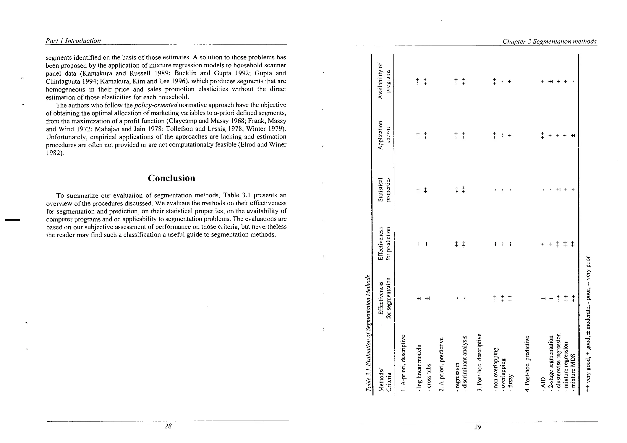
Conclusion 28
4 Tools for Market Segmentation 31
PART 2 — SEGMENTATION METHODOLOGY 37
5 Clustering Methods 39
Example of the Clustering Approach to Market Segmentation 42
Nonoverlapping Hierarchical Methods 43
Similarity Measures 44
A ggiomerative Cluster Algorithms 48
Divisive Cluster Algorithms 50
Ultrametric and Additive Trees 50
Hierarchical Clusterwise Regression 51
Nonoverlapping Nonhierarchical Methods 52
Nonhierarchical Algorithms 53
Determining the number of Clusters 54
Nonhierarchical Clusterwise Regression 55
Miscellaneous Issues in Nonoverlapping Clustering 56
Variable Weighting, Standardization and Selection 56
Outliers and Missing Values 58

Contents
Non-uniqueness and lnversions
Cluster Validation
Cluster Analysis Under Various Sampling Strategies
Stratified samples
Cluster samples
Two-stage samples
Overlapping and Fuzzy Methods
Overlapping Clustering
Overlapping Clusterwise Regression
Fuzzy Clustering
Market Segmentation Applications of Clustering
6 Mixture Models
Mixture Model Examples
Example 1: Purchase Frequency of Candy
Example 2: Adoption oflnnovation
Mixture Distributions (MIX)
Maximum Likelihood Estimation
The EM Algorithm
EM Example
Limitations ofthe EM Algorithm
Local maxima
Standard errors
Identification
Determining the Number of Segments
Some Consequences of Complex Sampling Strategies for the Mixture
Approach
Marketing Applications of Mixtures
Conclusion
7 l‘VIixture Regression Models
Examples of the Mixture Regression Approach
Example 1: Trade Show Performance
Example 2: Nested Logit Analysis of Scanner Data
A Generalized Mixture Regression Model (GLIMMIX)
EM Estimation
EM Example
Standard Errors and Residuals
Identification
Monte’ Carlo Study of the GLIMMIX Algorithm
Study Design
Results
Marketing Applications of Mixture Regression Models
Normal Data
Binary Data
VII]
59
59
60
60
62
63
64
64
65
65
69
75
75
75
76
77
80
84
86
88
88
88
90
91
94
96
99
101
102
102
103
106
108
108
109
109
110
110
112
112
113
113
Multichotomous Choice Data
Count Data
Choice and Count Data
Response-Time Data
Conjoint Analysis
Conclusion
Appendix Al The EM Algorithm for the GLIMMIX Model
The EM Algorithm
The E—Step
The M-Step
Mixture Unfolding Models
Examples of Stochastic Mixture Unfolding Models
Example 1: Television Viewing
Example 2: Mobile Telephone Judgements
A General Family of Stochastic Mixture Unfolding Models
EM Estimation
Some Limitations
__1ssues in Identification
Model Selection
Synthetic Data Analysis
Marketing Applications
Normal Data
Binomial Data
Poisson, Multinomial and Dirichlet Data
Conclusion
Appendix A2 The EM Algorithm for the STUNMIX Model
The E-Step
The M-step
Profiling Segments
Profiling Segments with Demographic Variables
Examples of Concomitant Variable Mixture Models
Example 1: Paired Comparisons of Food Preferences
Example 2: Consumer Choice Behavior with Respect to
Ketchup
The Concomitant Variable Mixture Model
Estimation
Model Selection and Identification
Monte’ Carlo Study
Alternative Mixture Models with Concomitant Variables
Marketing Applications
Conclusions
[X
C ontenls
115
116
116
117
117
119
120
120
121
121
125
127
127
123
131'
133
133
134
134
136
138
138
140
140
140
142
142
142
145
145
146
146
147
150
152
152
152
153
156
156

Fr:
Contents
10
Dynamic Segmentation
Models for Manifest Change
Example 1: The Mixed Markov Model for Brand Switching
Example 2: Mixture Hazard Model for Segment Change
Models for Latent Change
Dynamic Concomitant Variable Mixture Regression Models
Latent Markov Mixture Regression Models
Estimation
Examples ofthe Latent Change Approach
Example 1: The Latent Markov Model for Brand Switching
Example 2: Evolutionary Segmentation of Brand Switching
Example 3: Latent Change in Recurrent Choice
Marketing Applications
Conclusion
Appendix A3 Computer Software for Mixture models
PANMARK
LEM
GLIMMIX
PART 3 — SPECIAL TOPICS IN MARKET
SEGMENTATION
11
12
Joint Segmentation
Joint Segmentation
The Joint Segmentation Model
Synthetic Data Illustration
Banking Services
Conclusion
Market Segmentation with Tailored Interviewing
Tailored Interviewing
Tailored Interviewing for Market Segmentation
Model Calibration
Prior Membership Probabilities
Revising the Segment Membership Probabilities
Item Selection
Stopping Rule
Application to Life-Style Segmentation
Life-Style Segmentation
Data Description
Model Calibration
Profile of the Segments
The Tailored Interviewing Procedure
Characteristics of the Tailored Interview
Quality ofthe Classification
X
159
160
161
162
167
167
168
169
170
170
171
175
176
176
178
178
179
181
187
189
189
189
191
192
194
195
195
198
199
200
201
202
202
203
203
203
203
204
209
209
21 l
14
Conclusion
Model-Based Segmentation Using Structural Equation Models
Introduction to Structural Equation Models
A-Priori Segmentation Approach
Post Hoc Segmentation Approach
Application to Customer Satisfaction
The Mixture of Structural Equations Model
Special Cases ofthe Model
Analysis of Synthetic Data
Conclusion
Segmentation Based on Product Dissimilarity Judgements
Spatial Models
Tree Models
Mixtures ofSpaces and Mixtures of Trees
Mixture of Spaces and Trees
Conclusion
PART 4 — APPLIED MARKET SEGMENTATION
15
16
17
General Observable Bases: Geo-demographics
Applications of Geo—demographic Segmentation
Commercial Geo—demographic Systems
PRIZMTM (Potential Rating Index for ZIP Markets)
ACORNT” (A Classification of Residential Neighborhoods)
The Geo-demographic System of Geo-Marktprofiel
Methodology
Linkages and Datafusion
Conclusion
General Unobservable Bases: Values and Lifestyles
Activities, Interests and Opinions
Values and Lifestyles
Rokeach’s Value Survey
The List of Values (LOV) Scale
The Values and Lifestyles (VALSTM) Survey
Applications of Lifestyle Segmentation
Conclusion
Product—specific observable Bases: Response-based Segmentation
The Information Revolution and Marketing Research
Diffusion of Information Technology
Early Approaches to Heterogeneity
Household-Level Single-Source Data
X]
C amenls
214
217
217
222
223
223
225
226
227
229
231
231
232
235
238
238
239
241
242
244
244
247
248
254
256
257
259
260
261
261
265
266
268
2'76
277
277
277
278
279

Contents
18
Consumer Heterogeneity in Response to Marketing Stimuli
Models with Exogenous Indicators of Preferences
Fixed-Effects Models
Random-Intercepts and Random Coefficients Models
Response-Based Segmentation
Example of Response-Based Segmentation with Single
Source Scanner Data
Extensions
Conclusion
Product—Specific Unobservable Bases: Conjoint Analysis
Conjoint Analysis in Marketing
Choice of the Attributes and Levels
Types of Attributes
Number of Attributes
Attribute Levels
Stimulus Set Construction
Stimulus Presentation
Data Collection and Measurement Scales
Preference Models and Estimation Methods
Choice Simulations
Market Segmentation with Conjoint Analysis
Application of Conjoint Segmentation with Constant Sum
Response Data
Market Segmentation with Metric Conjoint Analysis
A-Priori and Post-Hoc Methods Based on Demographics
Componential Segmentation
Two-Stage Procedures
Hagerty’s Method -
Hierarchical and Non—Hierarchical Clusterwise Regression
Mixture Regression Approach
A Monte Carlo Comparison of Metric Conjoint Segmentation
Approaches
The Monté Carlo Study
Results
Predictive Accuracy
Segmentation for Rank-Order and Choice Data
A-Priori and Post-Hoc Approaches to Segmentation
Two—Stage Procedures
Hierarchical and Non-hierarchical Clusterwise Regression
The Mixture Regression Approach for Rank-Order and
Choice Data
Application of Mixture Logit Regression to Conjoint Segmentation
Results
Conclusion
X1]
282
283
283
284
285
286
288
292
295
295
296
296
297
298
298
299
300
301
302
303
303
305
306
306
306
307
307
308
310
310
312
313
314
315
315
316
316
318
319
320
Contents
PART 5 — CONCLUSIONS AND DIRECTIONS FOR
FUTURE RESEARCH 323
19 Conclusions: Representations of Heterogeneity 325
Continuous Distribution of Heterogeneity versus Market Segments 325
Continuous or Discrete 326 ~
ML or MCMC 327
Managerial relevance 329
Individual Level versus Segment Level Analysis 331
20 Directions for Future Research 335
The Past 335
Segmentation Strategy 336
Agenda for Future Research 341
References 345
Index 371
X111

Table
Table
Table
Table
Table
Table
Table
Table
Table
Table
Table
Table
Table
Table
Table
Table
Table
Table
Table
Table
Table
Table
Table
Table
- Table
Table
Table
Table
Table
2.1:
3.1:
5.1:
5.2:
5.3:
5.4:
5.5:
6.1:
6.2:
6.3:
6.4:
6.5:
7.1:
7.2:
7.3:
7.4:
7.5:
8.1:
8.2:
8.3:
8.4:
9.1:
9.2:
9.3:
9.4:
10.1:
10.2:
10.3:
10.4:
List of Tables and Figures
Evaluation of Segmentation Bases
Evaluation of Segmentation Methods
The Most Important Similarity Coefficients
Definitions of Cluster Distance for several Types of
Hierarchical Algorithms
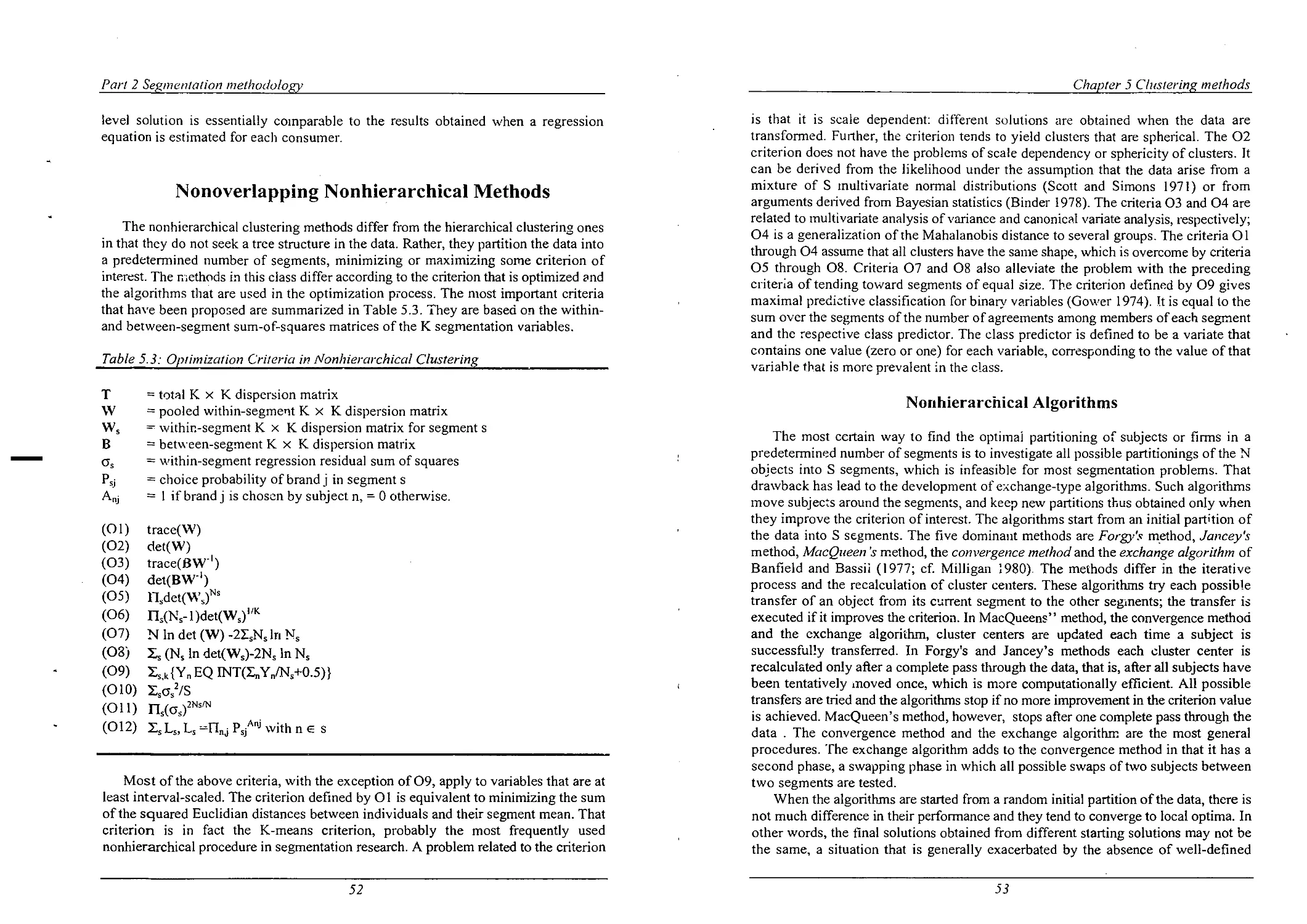
Optimization Criteria in Nonhierarchical Clustering
Fuzzy Clustering Algorithm Estimating Equations
Cluster Analysis Applications to Segmentation
Results of the Green et al. T hree—Segment Model
Some Distributions from the Univariate Exponential Family
Application of the EM Algorithm to Synthetic Mixture
Poisson Data
Mixture Model Applications in Marketing
Special Cases of the Bockenholt (1993) Mixture Model
Family
Aggregate and Segment-Level Results of the Trade Show
Performance Study
Average Price Elasticities within Three Segments
Application of the EM Algorithm to Synthetic Mixture
Regression Data
Results of the'Monté Carlo Study on GLIMMIX Performance
GLIMMIX Applications in Marketing
Numbers of Parameters for STUNMIX Models
Results of STUNMIX Synthetic Data Analyses
ST UNMIX Results for Normal and Log»-Normal Synthetic
Data
STUNMIX Marketing Applications
Concomitant Variable Mixture Model results for Food
Concern Data
Concomitant Variable Mixture Model Results for Ketchup
Choice Data
Estimates from Synthetic Datasets Under Two Conditions
Marketing Applications of Concomitant Variable Models
Mixed Markov Results for MRCA Data
Segment Level S=2 Nonproportional Model Estimates
Latent Markov Results for MRCA Data
Conditional Segment Transition Matrix Between Periods 1
and 2
16
29
46
49
52
70
72
78
82
87
97
98
103
105
111
114
118
135
137
138
141
148
150
157
158
162
165
171
174

Table
Table
Table
Table
Table
Table
Table
Table
Table
Table
Table
Table
Table
Table
Table
Table
Table
Table
Table
Table
Table
Table
Table
Table
Table
Table
Table
Table
Figure
Figure
Figure
Figure
Figure
Figure
10.5:
10.6:
11.1:
11.2:
11.3:
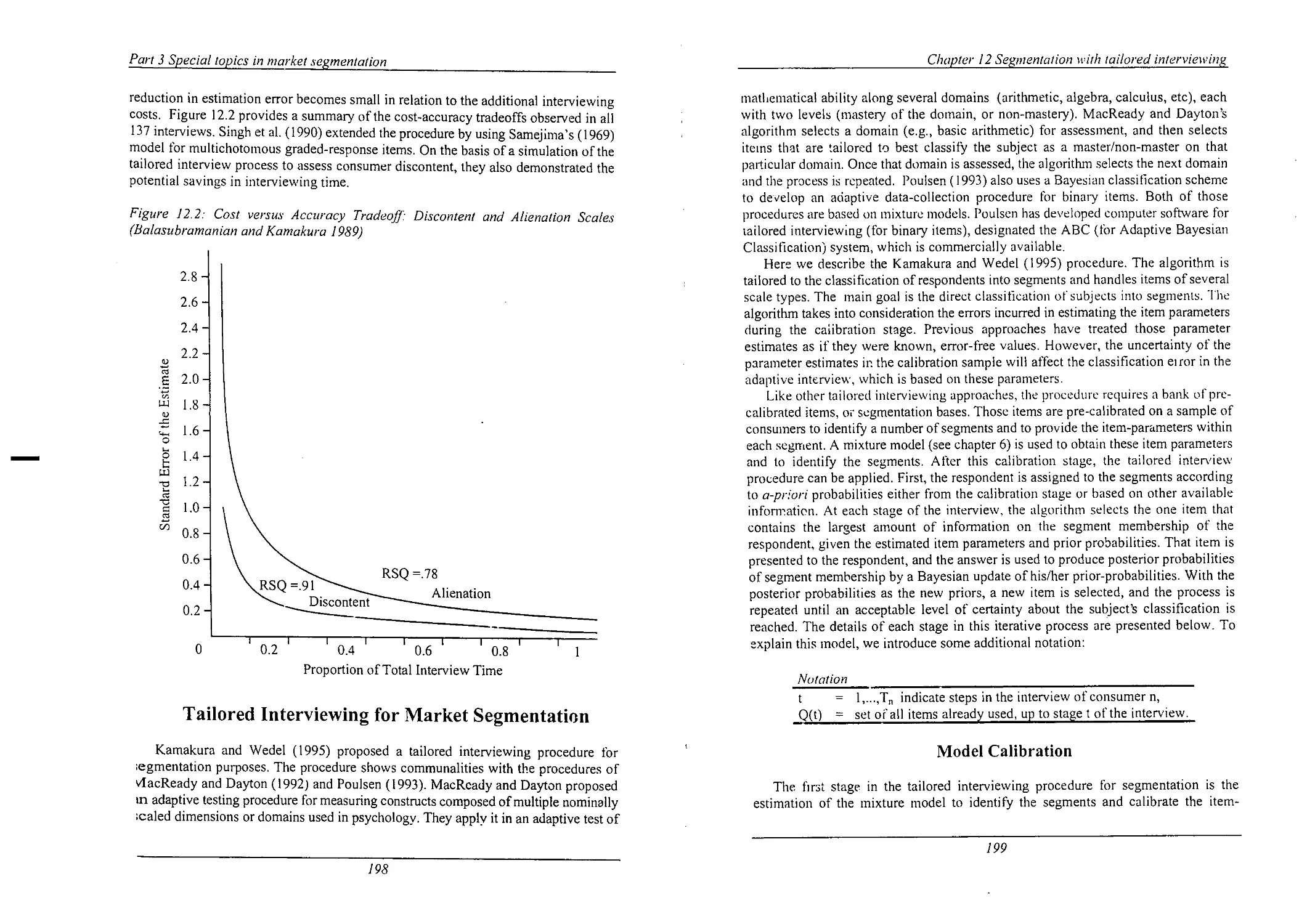
12.1:
12.2:
12.3:
13.1:
13.2:
13.3:
13.4:
13.5:
15.1:
15.2:
15.3:
15.4:
16.1:
16.2:
16.3:
17.1:
18.1:
18.2:
18.3:
18.4:
18.5:
19.1
19.2
2.1:
3.1:
5.1:
5.2:
5.3:
5.4:
Lisr 0/ tables and figures
Preference Structure in Three and Four Switching Segments
in Two Periods
Marketing Applications of Dynamic Segmentation
True and Estimated Joint Segment Probabilities
Segmentation Structure of Binary Joint Segmentation Model
for Banking Services .
Estimated Joint Segment Probabilities for Banking Services
Application
Demographics and Activities by Segment
Activities, Interests and Opinions Toward Fashion by
Segment
Percentage of Cases Correctly Classified
Latent Satisfaction Variables and Their Indicators
Mean Factor Scores in Three Segments
Estimates of Structural Parameters in Three Segments
Performance Measures in First Monte Carlo Study
Performance Measures in Second Monte’ Carlo Study
PRIZM 1" Classification by Broad Social Groups
ACORN" Cluster Classification
Description ofthe Dimensions ofthe GMP System
Media and Marketing Databases Linked to Geo-demographic
Systems
Rokeach’s Terminal and Instrumental Values
Motivational Domains of Rekeach’s Values Scale
Double-Centered Values
Estimated Price Elasticities
Estimated Allocations for Three Profiles in Two Segments
Comparison of Conjoint Segmentation Procedures
Mean Performance Measures of the Nine Conjoint
Segmentation Methods
Mean Performance Measures for Each of the Factors
Parameter Estimates of the Rank-Order Conjoint
Segmentation Model
Comparison of Discrete and Continuous Representations of
Heterogeneity
Comparison of Segment Level and Individual-Level
Approaches
Classification of Segmentation Bases
Classification of Methods Used for Segmentation
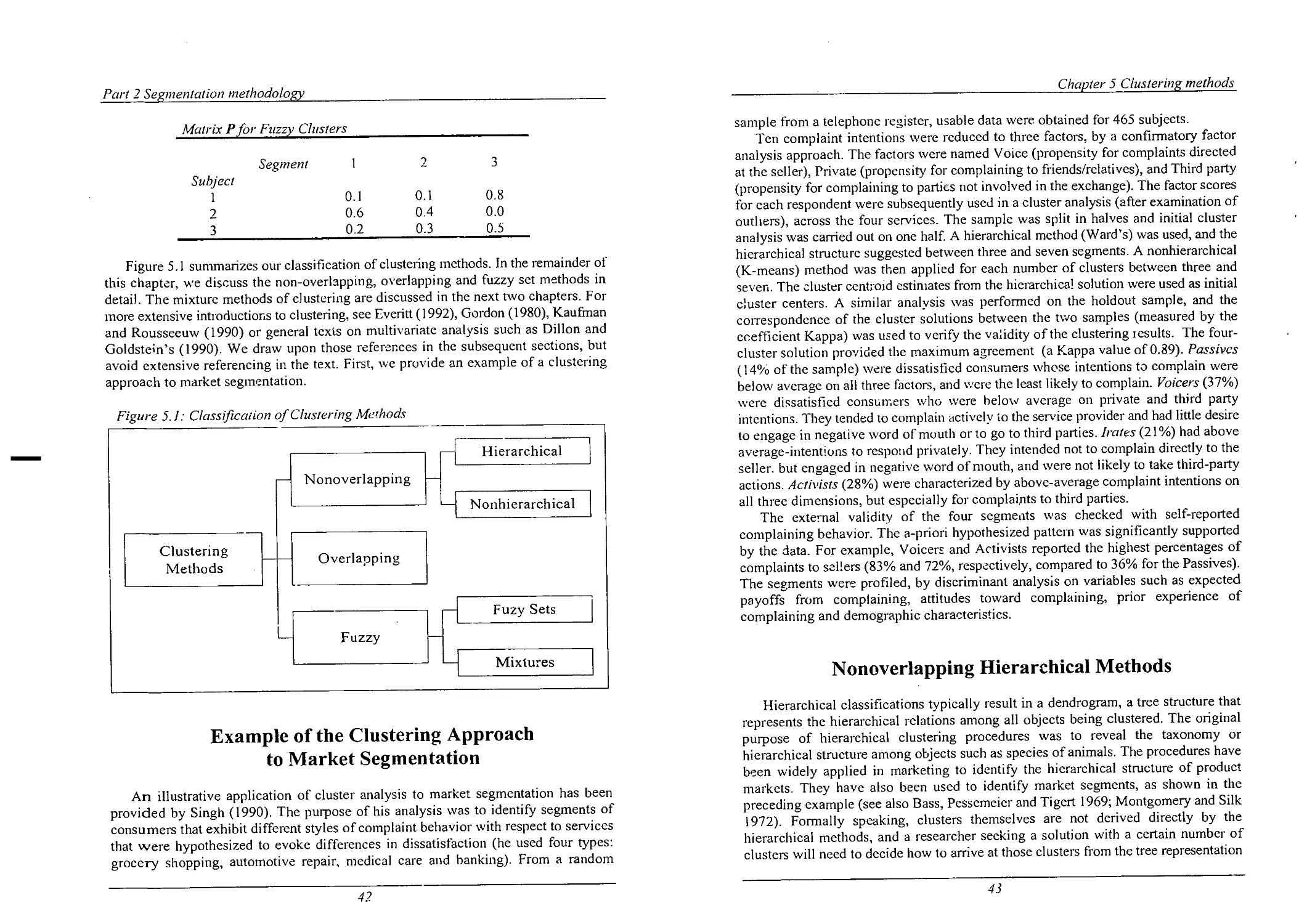
Classification of Clustering Methods
Hypothetical Example of Hierarchical Cluster Analysis
Schematic Representation of Some Linkage Criteria
An Example of Cluster Structures Recovered with the FCV
174
176
191
193
194
205
207
213
218
224
225
228
229
246
250
253
258
263
264
271
289
305
309
313
314
320
328
332
17
42
44
48
XVI
List itables and figures
Figure
Figure
Figure
Figure
Figure
Figure
Figure
Figure
Figure
Figure
Figure
Figure
Figure
Figure
Figure
Figure
Figure
Figure
Figure
Figure
Figure
Figure
Figure
Figure
6.1:
6.2:
8.1:
8.2:
8.3:
9.1:
9.2:
10.1:
10.2:
10.3:
12.1:
12.2:
12.3:
12.4:
12.5:
12.6:
13.1:
14.1:
14.2:
14.3:
16.1:
16.2:
16.3:
16.4:
Family
Empirical and Fitted Distributions of Candy Purchases
Local and Global Maxima
TV-Viewing Solution
Spatial Map ofthe Telephone Brands
Synthetic Data and Results of Their Analyses with
STUNMIX
Directed Graph for the Standard Mixture
Directed Graph for the Concomitant Variable Mixture
Observed and Predicted Shares for the Mixed Markov
Model
Stepwise Hazard Functions in Two Segments
Observed and Predicted Shares for the Latent Markov
Model
Illustration of the Tailored Interview
Cost Versus Accuracy Tradeoff: Discontent and Alienation
Scales
Number of Items Selected in the Tailored Interview until
p>0.99
Number of Items Selccted until p>0.99 with Random Item
Selection
Entropy of Classification at Each Stage of the Interview
Number of Respondents Correctly Classified at Each Stage
Path Diagram for latent Variables in the Satisfaction Study
T=2 dimensional Space for the Schiffman et al. Cola Data
Ultrametric Tree for the Schiffman et al. Cola Data
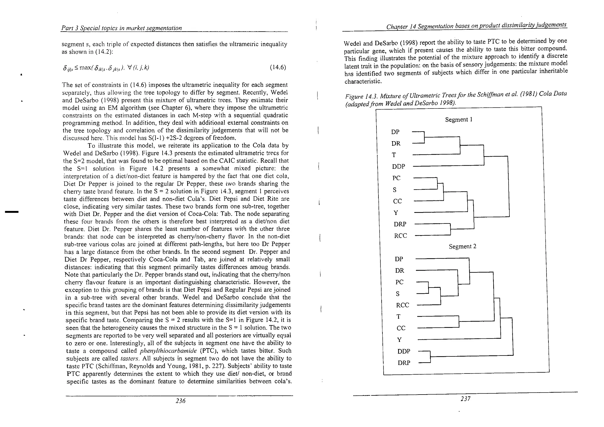
Mixture of Ultrametric Trees for the Schiffman et al. Cola
Data
Values Map: Dimension 2 vs. Dimension 1
Values Map: Dimension 3 vs. Dimension 1
Regional Positions: Dimension 2 vs. Dimension 1
Regional Positions: Dimension 3 vs. Dimension 1
XVII
67
76
89
128
130
139
154
154
163
166
172
197
198
210
210
212
213
219
233
235
237
272
273
274
275

Preface
Market segmentation is an area in which we have been working for nearly a decade.
Although the basic problem of segmentation may appear to be quite simple -the
classification of customers into groups - market segmentation research may be one of
the richest areas in marketing science in terms scientific advancement and development
of methodology. Since the concept emerged in the late 1950s, segmentation has been
one of the most researched topics in the marketing literature. Recently, much of that
literature has evolved around the technology of identifying segments from marketing
data through the development and application of finite mixture models. Although
mixture models have been around for quite some time in the statistical and related
literatures, the substantive problems of market segmentation have motivated the
development of new methods, which in turn have diffused into psychometrics,
sociometrics and econometrics. Moreover, because of their problem—solving potential,
the new mixture methodologies have attracted great interest from applied marketing
researchers and consultants. In fact, we conjecture that in terms of impact on academics
and practitioners, next to conjoint analysis, mixture models will prove to be the most
influential methodological development spawned by marketing problems to date.
However, at this point, further diffusion ofthe mixture methodology is hampered
by the lack of a comprehensive introduction to the field, integrative literature reviews
and computer software. This book aims at filling this gap, but we have attempted to
provide a much broader perspective than merely a methodological one. In addition to
presenting an up-to-date survey of segmentation methodology in parts 2 and 3, we
review the foundations of the market segmentation concept in part 1, providing an
integrative review of the contemporary segmentation literature as well as a historical
overview of its development, reviewing commercial applications in part 4 and
providing a critical perspective and agenda for future research in part 5. In the second
edition, 1.he discussion has been extended and updated.
In part 1, we provide a definition of market segmentation and describe six criteria
for effective segmentation. We then classify and discuss the two dimensions of
segmentation research: segmentation bases and methods. We attempt to anive at a set
of general conclusions both with respect to bases and methods. The discussion of
segmentation methods sets the scene for the remainder of the book.
We start part 2 with a discussion of cluster analysis, historically the most well-
known technique for market segmentation. Although we have decided to discuss cluster
analysis in some detail, our main methodological focus throughout this book is on finite
mixture models. Those models have the main advantage over cluster analysis that they
are model—based and allow for segmentation in a framework in which customer
behavior is described by an appropriate statistical model that includes a mixture
component that allows for market segmentation. In addition, those mixture models have
the advantage of enabling statistical inference.

Preface
We start our treatment of mixture models with classical finite mixtures, as described
in the statistical literature, and applied to market segmentation a number of decades
ago. Those mixtures involve a simple segment-level model of customer behavior,
describing it only by segment-level means of variables. We subsequently move towards
more complicated descriptions of segment level behavior, such as (generalized linear)
response models that explain a dependent variable from a set of independent variables
at the segment level, and scaling models that display the structure of market stimuli in
a spatial manner. In an appendix to part 2 we describe some of the available computer
software for fitting finite mixture models to data, and we include a demonstration of a
flexible WINDOWS program, GLIMMIX, developed by I.E.C. PROGAMMA
(Groningen, Netherlands).
In part 3, we also discuss the simultaneous profiling of segments and models for
dynamic segmentation on the basis of several sets of variables. In the second edition
the discussion on the so called concomitant variable models has been extended to show
some relationships among them. Part 3 contains a descriptions of a variety of special
topics in mixture models for market segmentation, i.e., joint segmentation for several
sets ofsegmentation bases, tailored interviewing for market segmentation, mixtures of
structural equation models (LISREL) and mixture models for paired comparison data,
providing spatial or tree representations of consumer perceptions. Selected topics in
applied market segmentation are contained in part 4, where we discuss selected topics
in four application areas of market segmentation that recently have received quite some
interest: geo-demographic segmentation, life-style segmentation, response based
segmentation, and conjoint analysis. In the final part (5) we step back and try to provide
critical perspective on mixture models, in the light of some of the criticisms it has
received in the literature, recently. We finish our book with an outlook on future
research.
In addition to presenting an up-to-date survey of segmentation methodology in parts
2 and 3, we review the foundations of the market segmentation concept in part 1,
providing an integrative review of the contemporary segmentation literature as well as
a historical overview of its development, and report academic and commercial
applications in part 4. Methodologically, our main focus is on finite mixture models
for segmentation problems, including specific topics such as response based
segmentation, joint segmentation, dynamic segmentation and the profiling of response-
based segments discussed in part 3, but we also provide an overview of the more
classical clustering approach to segmentation in part 2.
When planning this monograph, we decided to target our work to two particular
segments of readers in the hope that, on the one hand, it will enable academic
researchers to advance further in the field and gain a better understanding of the
segmentation concept and, on the other hand, it will help applied marketing researchers
in making better use of available data to support managerial decisions for segmented
markets. Our intention was to produce a review of classic and contemporary research
on market segmentation, oriented toward the graduate student in marketing and
marketing research as well as the marketing researcher and consultant. To graduate
students, this monograph can serve as a reference to the vast literature on market
segmentation concepts (part I), methodology (parts 2 and 3) and applications (part 4).
XX
Preface
To practitioners, it can serve as a guide for the implementation of market segmentation,
from the selection of segmentation bases through the choice of data analysis
methodology to the interpretation of results. In addition, we hope the book may prove
to be a useful source for academics in marketing and related fields who have an interest
in classification problems.
We have attempted to provide a maximum of detail using a minimum of necessary
mathematical formulation, in particular emphasizing marketing applications. Our
standard format for presenting methodology is to start with one or two (previously
published) applications of a specific approach, to give the reader a feel of the problem
and its solution before discussing the specific method in detail. The reason is that we
would like a reader without any prior knowledge ofthe specific concepts and tools to
be able to gain a fairly complete understanding from this monograph. We have tried to
explain most statistical and mathematical concepts required for a proper understanding
of the core material. Rather than including mathematical and statistical appendices, we
have chosen to introduce those concepts loosely in the text where needed. As the text
is not intended to be a statistical text, the more statistically oriented reader may find
some of the explanations short of detail or too course, for which we apologize. Readers
with more background in statistics and/or mixture modeling may want to skip the
descriptions ofthe applications and the introduction ofthe basic statistical concepts.
Interestingly, when reviewing the literature, we observed that at several stages the
further development of the segmentation concept appeared to have been hampered by
the current analytical limitations. In other words, the development of segmentation
theory has been partly contingent on the availability of marketing data and tools to
identify segments on the basis of such data. New methodology has often opened new
ways of using available data and new ways of thinking about the segmentation
problems involved. We therefore do not see this book as an endpoint, but as a
beginning of a new period in segmentation..research. Until fairly recently, the
application of the mixture technology has been monopolized by the developers of the
techniques. We hope this book contributes to the further diffusion of the methodology
among academics, students of marketing and practitioners, thus leading to new
theoretical insights about market segmentation and questions relating to it.
We use the term “mixture models" throughout this book. A brief explanation is in
order. In part of the marketing literature, the models that we are using are called “latent
class models”. This situation has apparently been caused by the first applications of
mixture models in marketing, by Green, Carmone and Wachspress (1976), and Grover
and Srinivasan ( 1987) being applications of a special cases of mixture models formally
called “latent class models”. The term mixture models in general refers to procedures
for dealing with heterogeneity in the parameters of a certain model across the
population by imposing a “mixing distribution” on (part of) the parameters of that
model. For example, in modeling choice behavior, one may assume that the choice
probabilities for the brands in question are heterogeneous across consumers and follow
a certain distribution across the population. This distribution can be assumed to be
either continuous or discrete, an assumption that has important consequences. In the
former case, continuous mixtures arise that are at present regaining popularity in
several substantive fields in marketing. If, on the other hand, a discrete mixing
XXI

Preface
distribution is chosen, “finite mixture models” arise, that enable the identification of
relatively homogeneous market segments. In contrast, a continuous mixing distribution
implies that such groupings of consumers cannot be found in the population. We
contrast the continuous and finite mixtures in the last part of this book and extend that
discussion in the second edition.
In addition, not only the mixing distribution may be continuous or discrete, but also
the distribution describing the vatiables themselves. For example, choices of brands are
typically discrete 0/1 variables, but preference ratings are considered to be measured
on interval scales and often described by a continuous distribution. If all measured
variables are discrete, such as occurs for example in the analysis of contingency tables,
the finite mixture model is called a latent class model. Those latent class models have
been developed and applied in particular in psychology and sociology. In marketing,
however, more often both continuous and discrete variables are measured. Therefore,
we will use the term “finite mixture models”, or loosely “mixture models”, throughout
the book, noting here that latent class models are in fact special cases of the finite
mixture model approach.
Obviously, the mixture approach has not been without its critics. Whereas initially
the advantages created by the methodology were emphasized, more recently critical
questions have been raised and limitations of the techniques have been pointed out. In
our monograph, we attempt not to be uncritical of the mixture approach. We discuss
the potential limitations because we think the methodology can be properly used only
if all of its advantages and disadvantages are fully disclosed. We postpone discussion
of the limitations to the last part (5) of the book in order not to confuse the reader about
the worth of the tools at an early stage. However, writing this book made even more
clear to us the major advantages of the mixture approach and the progress that has been
made by the developments in that field. We believe the current critique may lead to
adaptation and further refinements of the method, but certainly not to its being
discarded in the near future.
Several colieagues provided useful feedback and discussion of drafis of chapters of
this book. We end with a word of thanks to them. First, we thank Julie Kaczynski for
motivating us to write the book. We also benefited greatly from the very useful
comments from Paul E. Green, Frenkel ter Hofstede, Wim Krijnen and Gary Lilien, and
the thoughtful reviews by Ulf Bockcnholt, Venkatramarn Rarnaswamy and Gary J.
Russell. We are grateful to all those readers that provided us with constructive
feedback on the first edition and we are greatly indebted to Bernard van Diepenbeek
and Bertine Markvoort, who worked with great perseverance and accuracy on the
layout of the second edition.
Michel Wedel Wagner A. Kamakura
XXII
PART 1
INTRODUCTION
This introductory part of our book provides a broad review of the past literature on
market segmentation, focusing on a discussion of proposed bases and methods.
Chapter 1 looks at the development of market segmentation as a core concept in
marketing theory and practice, starting from its foundations in the economic theory of
imperfect competition. This first chapter also discusses criteria that must be satisfied
for effective market segmentation. Chapter 2 classifies available segmentation bases
and evaluates them according to those criteria for effective segmentation. In chapter 3,
we present a classification and overview of techniques available for segmentation.
Chapter 4 completes our introduction to market segmentation, with an overview of the
remaining chapters ofthis book.

1
THE HISTORICAL DEVELOPMENT
OF THE
MARKET SEGMENTATION CONCEPT
After briefly introducing the concept and history of market segmentation, we
review the criteria for effective segmentation and introduce the topics to be discussed
in this book.
Market segmentation is an essential element of marketing in industrialized
countries. Goods can no longer be produced and sold without considering customer
needs and recognizing the heterogeneity of those needs. Earlier in this century,
industrial development in various sectors of the economy induced strategies of mass
production and marketing. Those strategies were manufacturing oriented, focusing on
reduction of production costs rather than satisfaction of consumers. But as production
processes became more flexible, and consumer affluence led to the diversification of
demand, firms that identified the specific needs of groups of customers were able to
develop the right ofter for one or more sub-markets and thus obtained a competitive
advantage. As market—oriented thought evolved within firms, the concept of market
segmentation emerged. Since its introduction by Smith (1956), market segmentation
has become a central concept in both marketing theory and practice. Smith recognized
the existence of heterogeneity in the demand of goods and services, based on the
economic theory of imperfect competition (Robinson 1938). He stated: “Market
segmentation involves viewing a heterogeneous market as a number of smaller
homogeneous markets, in response to differing preferences, attributable to the desires
of consumers for more precise satisfaction of their varying wants.”
Many definitions of market segmentation have been proposed since, but in our view
the original definition proposed by Smith has retained its value. Smith recognizes that
segments are directly derived from the heterogeneity of customer wants. He also
emphasizes that market segments arise from managers’ conceptualization of a
structured and partitioned market, rather than the empirical partitioning of the market
on the basis of collected data on consumer characteristics. Smith’s concepts led to
segmentation research that partitioned markets into homogeneous sub-markets in terms
of customer demand (Dickson and Ginter 1987), resulting in the identification of
groups of consumers that respond similarly to the marketing mix. That view of
segmentation reflects a market orientation rather than a product orientation (where
markets are partitioned on the bases of the products being produced, regardless of
consumer needs). Such customer orientation is essential if segmentation is to be used

Part l Introduction
as one ofthe building blocks of effective marketing planning.
The question of whether groups of customers can be identified as segments in real
markets is an empirical one. However, even if a market can be partitioned into
homogeneous segments, market segmentation will be useful only ifthe effectiveness,
efficiency and manageability of marketing activity are influenced substantially by
discerning separate homogeneous groups of customers.
Recent changes in the market environment present new challenges and
opportunities for market segmentation. For example, new developments in infonnation
technology provide marketers with much richer infonnation on customers’ actual
behavior, and with more direct access to individual customers via database marketing
and geo—demographic segmentation. Consequently. marketers are now sharpening their
focus on smaller segments with micro marketing and direct marketing approaches. On
the other hand, the increasing globalization of most product markets (unification of the
EC. WTO, and regional accords such as the MERCOSUR) is leading many multi-
product manufacturers to look at global markets that cut across geographic boundaries.
Those developments have lead to rethinking of the segmentation concept.
Six criteria — identifiability, substantialiry, accessibility. stability, responsiveness
and actionability — have been frequently put forward as determining the effectiveness
and profitability of marketing strategies (e.g., Frank, Massy and Wind 1972; Loudon
and Della Bitta 1984; Baker 1988; Kotler 1988).
Identzfiability is the extent to which managers can recognize distinct groups of
customers in the marketplace by using specific segmentation bases. They should be
able to identify the customers in each segment on the basis of variables that are easily
measured.
The substantiality criterion is satisfied if the targeted segments represent a large
enough portion of the market to ensure the profitability of targeted marketing programs.
Obviously, substantiality is closely connected to the marketing goals and cost structure
of the firm in question. As modern concepts such as micro markets and mass
customization become more prevalent, profitable segments become smaller because of
the lower marginal marketing costs. In the limit, the criterion of substantiality may be
applied to each individual customer; that is the basic philosophy of direct marketing,
where the purpose is to target each individual customer who produces marginal
revenues that are greater than marginal costs for the firm.
Accessibility is the degree to which managers are able to reach the targeted
segments through promotional or distributional efforts. Accessibility depends largely
on the availability and accuracy of secondary data on media profiles and distributional
coverage according to specific variables such as gender, region, socioeconomic status
and so on. Again, with the emergence and increasing sophistication of direct marketing
techniques, individual customers can be targeted in many markets.
If segments respond uniquely to marketing efforts targeted at them, they satisfy the
responsiveness criterion. Responsiveness is critical for the effectiveness of any market
segmentation strategy because differentiated marketing mixes will be effective only if
each segment is homogeneous and unique in its response to them. It is not sufficient
for segments to respond to price changes and advertising campaigns; they should do so
differently from each other, for purposes of price discrimination.
Chaplet‘ l The liistorical development oftlic market segmentation concept
Only segments that are stable in time can provide the underlying basis for the
development of a successful marketing strategy. If the segments to which a certain
marketing effort is targeted change their composition or behavior during its
implementation, the effort is very likely not to succeed. Therefore, stability is
necessary, at least for a period long enough for identification of the segments,
implementation of the segmented marketing strategy, and the strategy to produce
results.
Segments are actionable iftheir identification provides guidance for decisions on
the effective specification of marketing instruments. This criterion differs from the
responsiveness criterion, which states only that segments should react uniquely. Here
the focus is on whether the customers in the segment and the marketing mix necessary
to satisfy their needs are consistent with the goals and core competencies ofthe finn.
Procedures that can be used to evaluate the attractiveness of segments to the managers
of a specific finn involve such methods as standard portfolio analysis, which basically
contrasts summary measures of segment attractiveness with company competitiveness
for each ofthe segments of potential interest (McDonald and Dunbar 1995).
The development of segmented marketing strategies depends on current market
structure as perceived by the firm’s managers (Reynolds 1965; Kotrba 1966). The
perception of market structure is formed on the basis of segmentation research (Johnson
1971). It is important to note that segments need not be physical entities that naturally
occur in the marketplace, but are defined by researchers and managers to improve their
ability to best serve their customers. In other words, market segmentation is a
theoretical marketing concept involving artificial groupings of consumers constructed
to help managers design and target their strategies. Therefore, the identification of
market segments and their elements is highly dependent on the bases (variables or
criteria) and methods used to define them. The selection of appropriate segmentation
bases and methods is crucial with respect to the number and type of segments that are
identified in segmentation research, as well as to their usefulness to the firms The
choice of a segmentation base follows directly from the purpose of the study (e.g., new
product development, media selection, price setting) and the market in question (retail,
business-to-business or consumer markets). The choice of different bases may lead to
different segments being revealed; much the same holds also for the application of
different segmentation methods. Furthenrrore, the choices of methods and bases are not
independent. The segmentation method will need to be chosen on the basis of (1) the
specific purposes of the segmentation study and (2) the properties of the segmentation
bases selected.
The leading reference on market segmentation is the book by Frank, Massy and
Wind (1972). They first distinguished the two major dimensions in segmentation
research, bases and methods, and provided a comprehensive description of the state of
the art at that time. However, the book dates back 25 years. Despite substantial
developments in information technology and data analysis technology, no monograph
encompassing the scientific developments in market segmentation research has
appeared since its publication (we note the recent book by McDonald and Dunbar,
1995, which provides a guide to the implementation of segmentation strategy).
Although Frank, Massy and Wind provide a thorough review of segmentation at that

Part I Introduction
time, important developments have occurred since then in areas such as sample design
for consumer and industrial segmentation studies, measurement of segmentation
criteria, new tools for market segmentation and new substantive fields in which market
segmentation has been or can be applied. Our book attempts to fill that gap.
Frank, Massy and Wind (1972) classified research on market segmentation into two
schools that differ in their theoretical orientation. The first school has its foundation in
microeconomic theory, whereas the second is grounded in the behavioral sciences. The
differences between the two research traditions pertain both to the theoretical underpin-
nings and to the bases and methods used to idcntify segments (Wilkie and Cohen 1977).
We use the Frank, Massy and Wind classification to discuss segmentation bases.
However, new segmentation bases have been identified since, and new insights into the
relative effectiveness of the different bases have led to a fairly clear picture of the
adequacy of each specific base in different situations. From the published literature, it
is now possible to evaluate the segmentation bases according to the six criteria
discussed above generally considered to be essential for effective segmentation.
The recent research in the development of new techniques for segmentation,
especially in the area oflatent class regression procedures, starting with the work of
DeSarbo and Cron (1988) and Kamakura and Russell (1989), suggests the onset ofa
major change in segmentation theory and practice. The full potential of the newly
developed techniques in a large number of areas of segmentation has only begun to be
exploited, and will become known with new user—friendly computer software. In 1978,
Wind called for analytic methods that provide a new conceptualization of the
segmentation problem. The methods that have been developed recently are believed to
meet Wind’s requirement, and should become a valuable adjunct to current market
segmentation approaches in practice. Moreover, the emergence of those new techniques
has led to a reappraisal of the current and more traditional approaches in terms of their
ability to group customers and predict behavioral measures of interest.
In addition to the above developments, segmentation research has recently
expanded to encompass a variety of new application areas in marketing. Examples of
such new applications are segmentation of business markets, segmentation for
optimizing service quality, segmentation on the basis of brand equity, retail
segmentation, segmentation of the arts market, price- and promotion-sensitivity
segmentation, value and lifestyle segmentation, conjoint segmentation, segmentation
for new product development, global market segmentation, segmentation for customer
satisfaction evaluation, micro marketing, direct marketing, geodemographic
segmentation, segmentation using single-source data and so on. A search of the current
marketing literature has revealed more than 1600 references to segmentation,
demonstrating the persistent academic interest in the topic.
This first part of our book reviews segmentation research, focusing on a discussion
of proposed bases and methods. Chapter 2 classifies available segmentation bases and
evaluates them according to the six criteria for effective segmentation mentioned
previously. In chapter 3, we present a classification and overview of techniques
available for segmentation. Chapter 4 is an overview of the subsequent chapters.
2
SEGMENTATION BASES
This chapter classifies segmentation bases into four categories. A literature review
of bases is provided and the available bases are evaluated according to the six criteria
for effective segmentation described in chapter 1. The discussion provides an
introduction to parts 3 and 4 of the book, where some special topics and new
application areas are examined.
A segmentation basis is defined as a set of variables or characteristics used to assign
potential customers to homogeneous groups. Following Frank, Massy and Wind (1972),
we classify segmentation bases into general (independent of products, services or
circumstances) and product-specific (related to both the customer and the product,
service and/or particular circumstances) bases (Frank, Massy and Wind l972; see also
Baker 1988; W ilkie and Cohen 1977). Furthermore, we classify bases into whether they
are observable (i.e., measured directly) or unobservable (i.e., inferred). That typology
holds for the bases used for segmentation of both consumer and industrial markets,
although the intensity with which various bases are used differs across the two types
of markets. Those distinctions lead to the classification of segmentation bases first
proposed by Frank, Massy and Wind (1972), shown in Figure 2.1.
F iflre 2.1: CIQSSIIICIIIIOH of Segmentation Bases
General Product-specific
Observable Cultural, geographic, User status, usage
demographic and socio- frequency, store loyalty
economic variables and patronage, situations
Unobservable Psycographics, values, Psychographics, benefits,
personality and life-style perceptions, elasticities,
attributes, preferences,
intention
This chapter provides an overview of the bases in each of the four resulting classes
(see also Frank, Massy and Wind 1972; Loudon and Della Bitta 1984; Kotler 1988).
Each of the bases is discussed in temis of the six criteria for effective segmentation
(i.e., identifiability, substantiality, accessibility, stability, responsiveness and
actionability).

Part I lnIr0(/m'Ii0n
Observable General Bases
A number of bases widely used, especially in early applications of market
segmentation research are in this category: cultural variables, geographic variables,
neighborhood, geographic mobility, demographic and socio-economic variables, postal
code classifications, household life cycle, household and firm size, standard industrial
classifications and socioeconomic variables. Media usage also is in this class of
segmentation bases. Socioeconomic status is usually derived from sets of measures
involving household income and education ofhousehold members. An example ofa
social classification is the following definition of social classes by Monk (1978, c.f.
McDonald and Dunbar 1995).
A — Upper middle class (head of the household successful business or
professional person, senior civil servant, or with considerable private means)
B —— Middle class (head ofthe household senior, well off, respectable rather
than rich or luxurious)
Cl — Lower middle class (small trades people and white collar workers with
administrative, supervisory and clerical jobs)
C2 — Skilled working class (head of the household mostly has served an
apprenticeship)
D - Semiskilled and unskilled working class (entirely manual workers)
E — Persons at the lowest level of subsistence (old age pensioners, widows,
casual workers, those dependent on social security schemes)
Geodemographic systems aim at neighborhood classifications based on geography,
demography and socioeconomics. There is a wide range of commercially available
geodemographic segmentation systems (examples are PRIZMN and ACORNT").
ACORNN (A Classification Of Residential Neighborhoods) is among the most widely
accepted systems, comprising the following geodemographic segments (Gunter and
Fumham 1992).
— agricultural area’s (villages, famis and small holdings),
— modern family housing, higher incomes (recent and modern private
housing, new detached houses, young families),
— older housing of intennediate status (small town centers and flats above
shops, non-fanning villages, older private houses),
— poor quality older terraced housing (tenement flats lacking amenities,
unimproved older houses and terraces low income, families),
~ better-off council estates, (council estates well-off workers),
C /rapier 2 Segmentation bases
— less well-off council estates (low raise estates in industrial towns,
council houses for the elderly),
- poorest council estates (council estates with overcrowding and worst
poverty, high unemployment),
— multi-racial area's (multi-let housing with Afro-Caribbean’s, multi-
occupied terraces poor Asians),
— high status non-family area's (multi-let big old houses and flats, flats
with single people and/or few children),
e affluent suburban housing (spacious semis big gardens, villages with
wealthy commuters, detached houses in exclusive suburbs),
- better off retirement area's (private houses with well of elderly or single
pensioners).
Household life cycle is commonly defined on the basis of age and employment
status of head(s) ofthe household and the age oftheir children, leading to nine classes
(cf. McDonald and Dunbar 1995).
— bachelor (young, single, not living at home)
~ newly married couples (young, no children)
— full nest I (youngest child under six)
— full nest II (youngest child six or over six)
— full nest Ill (older married couples with dependent children)
- empty nest I (older married couples, no children living with them, head
in labor force)
— empty nest ll (older married couples, no children living with them, head
retired)
- solitary survivor in labor force
- solitary survivor retired
In different countries, slightly different standard industrial classification schemes
are used, but in the United States the following main classification applies (each code
is further partitioned into smaller classes).
000 — agriculture, forestry and fishing
100 -— mining
150 - construction
200 — manufacturing
400 — transportation and communication
500 — wholesale
520 — retail
600 — finance, insurance and real estate
700 — services
900 — public administration

Purl 1 lI1Ii‘odz/(‘Non
These segmentation bases are relatively easy to collect, reliable and generally
stable. Often the variables are available from sampling frames such as municipal and
business registers, so they can be used as stratification variables in stratified and quota
samples. Segments derived from the bases are easy to communicate and resulting
strategies are easy to implement. The corresponding consumer segments are often
readily accessible because ofthe wide availability of media profiles for most of the
bases mentioned. Some differences in purchase behavior and elasticities of marketing
variables have been found among these types of segments, supporting the
responsiveness criterion for effective segmentation, but in many studies the differences
were in general too small to be relevant for practical purposes (e.g., Frank, Massy and
Wind 1972; Frank 1968, 1972; McCann 1974). Although the lack of significant
findings in those studies supports the conclusion that the general observable bases are
not particularly effective, it has not resulted in the demise of such bases. On the
contrary, they continue to play a. role in simple segmentation studies, as well as in more
complex segmentation approaches in which a broad range of segmentation bases are
used. Moreover, they are used to enhance the accessibility of segments derived by other
bases, as media usage profiles are often available according to observable bases.
Observable Product-Specific Base
The bases in this class comprise variables related to buying and consumption
behavior: user status (Boyd and Massy 1972; Frank, Massy and Wind 1972), usage
frequency (Twedt 1967), brand loyalty (Boyd and Massy 1972), store loyalty (Frank,
Massy and Wind 1972; Loudon and Della Bitta 1984), store patronage (Frank, Massy
and Wind 1972), stage of adoption (Frank, Massy and Wind 1972 and usage situation
(Belk 1975; Dickson 1982; Loudon and Della Bitta 1984). Although most of these
variables have been used for consumer markets, they may also apply to business
markets. Many such bases are derived from customer surveys (e.g., Simmons Media
Markets), although nowadays household and store scanner panels and direct mail lists
are a particularly useful sources.
Twedt’s (1967) classification of usage frequency involves two classes: heavy users
and light users. Several operationalizations of loyalty have been proposed. Brand
loyalty may or may not be directly observable; for example, it has been measured
through observable variables such as the last brand purchased (last-purchase loyal) or
as an exponentially weighted average of past purchase history (Guadagni and Little
1983). New operationalizations of brand loyalty are based on event history analysis.
With respect to stage of adoption, commonly the following stages are distinguished
(Rogers 1962).
- innovators (are venturesome and willing to try new ideas at some risk)
- early adopters (are opinion leaders and adopt new ideas early but carefully
- early majority (are deliberate. adopt before the average person but are rarely
leaders)
— late majority (are skeptical, adopt only after the majority)
/0
Chapter 2 Segmentation limes
— laggards (are tradition bound and suspicious of changes, adopt because the
adoption is rooted in tradition)
Accessibility ofthe segments identified from these bases appears to be somewhat
limited in view of the weak associations with general consumer descriptors (Frank
1972; Frank, Massy and Wind 1972). Several researchers (Massy and Frank 1965;
Frank 1967, 1972; Sexton 1974; lvlcCann 1974) found that consumers who belong to
segments with different degrees of brand loyalty do not respond differently to
marketing variables. Loyalty was found to be a stable concept. Weak to moderate
differences in elasticities of marketing mix variables were found among segments
identified by product-specific bases such as usage frequency, store loyalty, etc.,
indicating that those bases are identifiable and substantial. To a lesser extent they are
also stable, accessible and responsive bases for segmentation.
Dickson (1982) provided a general theoretical framework for usage situation as a
segmentation basis. When demand is substantially heterogeneous in different situations,
situational segmentation is theoretically viable. A classification of situational variables
(including purchase and usage situations) has been provided by Belk (1975). He
distinguishes the following characteristics of the situation.
— physical surrounding (place of choice decision, place of consumption)
social surrounding (other persons present)
— temporal perspective (time of day or week)
~ task definition (buy or use)
antecedent states (moods, etc.)
That classification provides a useful framework for the operationalization of usage
situational bases. Situation-based variables are often directly measurable, and the
segments are stable and accessible (Stout et al. 1977; Dickson 1982). The responsive-
ness of usage situational segments was investigated by Belk (1975), Hustad, Mayer and
Whipple (1975), Stout et al. (1977) and Miller and Ginter (1979). Perceptions of
product attributes, their rated importance, buying intentions, purchase frequency and
purchase volume were all found to differ significantly across usage situations
(Srivastava, Alpert and Shocker 1984). Consequently, the explicit consideration of
situational contexts appears to be an effective approach to segmentation.
Unobservable General Bases
The segmentation variables within this class fit into three groups: personality traits,
personal values and lifestyle. These bases are used almost exclusively for consumer
_markets. A comprehensive introduction to this class of segmentation bases is provided
by Gunter and Fumhain (1992). Such psychographic segmentation bases were
developed extensively by marketers in the 1960s in response to the need for a more
lifelike picture of consumers and a better understanding of their motivations. They have
SpLl\V1lCd from the fields of personality and motivation research, which have blended
ll

Part I Introduction
in later years into the psychographics and lifestyle areas. Early landmark papers on
psychographics are those by Lazarfeld (1935) and Dichter (1958).
Edward’s personal preference schedule is probably the most frequently used scale
for measuring general aspects of personality in marketing. Early applications include
those of Evans (1959) and Koponen (1960); later studies include those by Massy, Frank
and Lodahl (1968), Claycamp (1965) and Brody and Cunningham (1968). Other
personality traits used for segmentation include dogmatism, consumerism, locus of
control, religion and cognitive style (cf. Gunter and Furnham 1992).
Values and value systems have been used as a basis for market segmentation by
Kahle, Beatty and Holmer (1986), Novak and MacEvoy (1990) and Kamakura and
Mazzon (1991). The most important instrument for the measurement of human values
and identification of value systems is the Rokeach value survey (Rokeach 1973).
Rokeach postulates that values represent beliefs that certain goals in lite (i.e., tenninal
values) and modes of conduct (instrumental values) are preferable to others. Those
values are prioritized into values systems and used by individuals as guidance when
making decisions in life.
Rokeach’s instrument includes 18 terminal and 18 instrumental values, to be ranked
separately by respondents in order of importance. A shorter and more easily
implemented instrument is the list of values (LOV), suggested by Kahle (1983) on the
basis of Maslow's (1954) hierarchy. The LOV was especially designed for consumer
research. It consists of the following nine items assessing terminal values that are rated
on nine—point important/unimportant scales.
- sense of belonging
— excitement -
- wann relationship with others
- self-fulfillment
- being well-respected
- fun and enjoyment of life
— security
- self-respect
— sense of accomplishment
Another important scale for assessing value systems was developed by Schwartz
and Bilsky (1990) and later modified by Schwartz (1992). It includes 56 values,
representing the following 1 1 motivational types of values.
- self-direction - independent thought and action
— stimulation - need for variety and stimulation
— hedonism - organismic and pleasure-oriented needs
- achievement - personal success
- power - need for dominance and control
— security - safety, stability of society, relationships and self
— conformity - self-restraint
— tradition — respect, commitment and acceptance of customs
/2
Chapter 2 Segmentation bases
— spirituality - inner hamtony, meaning in life
- benevolence - prosocial behaviors and goals
— universalism - concem for the welfare ofall others and nature
The concept oflifestyle was introduced into marketing research by Lazer (1963)
and is based on three components: activities (work, hobbies, social events, vacation,
entertainment, clubs, community, shopping, sports), interests (family, home, job,
community, recreation, fashion, food. media, achievements) and opiniorrs (of oneself,
social issues, politics, business, economics, education, products, future, culture)
(Plummer 1974).
Mitchell (1983) proposed a values and lifestyle typology, which 1S widely known
as the VALSW system. The VALSW typology is hierarchical and defines a basic system
of four categories with nine more detailed segments within them. Drawn originally
from Maslow, the following nine segments were in the original VALSN double
hierarchy.
- need d1'iven (survivors, sustainers)
~ outer directed (belongers, emulators, achievers)
— inner directed (I-am-me, experientials, socially conscious)
- integrated
A new version of the VALSN system has been developed recently. The new
structure (VALS2m) is not hierarchical like the previous one, but defined by two main
dimensions: resomres defined by income, education, self-confidence, health, eagerness
to buy, intelligence, etc. and se/f-orientation (principle—oriented, self-oriented and
status-oriented).
Surveys ofthe literature reveal that general personality measures have a stronger
relationship with patterns of behavior across product classes than with behaviors related
to a single brand (Frank 1972; Frank, Massy and Wind 1972; Wells 1975; Wilkie and
Cohen 1977). General lifestyle segmentation has the same limitations as general
personality scales: it is likely to identify factors that influence general behavioral
patterns rather than any specific behavior toward a single brand (Ziff 1971; Wells 1975;
Dickson 1982). In reviews of the literature, Frank, Massy and Wind (1972) and Wells
(1975) concluded that the predictive validity of lifestyle with respect to purchase
behavior can be substantially better than that of general observable segmentation bases.
As for the validity of the psychographic segmentation bases, a study by Kahle,
Beatty and Holmer (1986) showed that the LOV system of Kahle (1983) better
predicted consumer behavior than Mitchell’s VALSIM system. However, a subsequent
study by Novak and MacEvoy (1990), based on a larger and more representative
sample, found that demographic variables had greater explanatory power than the LOV
variables. Studies by Lastovicka (1982) and Lastovicka, Murray and Joachimsthaler
(1990) also revealed negative evidence for the predictive validity of the original
VALST“ system, but demonstrated the potential validity of lifestyle traits in general.
Earlier studies (Tigert 1969; Bruno and Pessemeier 1972) showed adequate test-retest
reliability for psychographic dimensions.
13

Part I Introduction
Personality, values and lifestyle provide a richer perspective of the market based on
a more lifelike portrait of the consumer and therefore provide actionable bases that are
especially useful for the development of advertising copy. Accessibility, responsiveness
and stability are not unequivocally supported in the literature.
Unobservable Product—Specifrc Bases
This class of bases comprises product-specific psychographics, product-benefit
perceptions and importances, brand attitudes, preferences and behavioral intentions. In
that order, those variables form a hierarchy of effects, as each variable is infiuenced by
those preceding it (Wilkie and Cohen 1977). Although many ofthe variables are used
more often for consumer markets, most can and have been used for segmenting
business markets.
Dhalla and Mahatoo (1976) identified three key areas of product-specific
psychographics: value orientations, role perceptions and buying style. Psychographic
measures that assess personality traits and lifestyle more immediately related to the
choice behavior for the product show a much stronger relationship with that choice
behavior than do general psychographic measures (Wells 1975). Unfortunately, little
is known of the stability of the segments, and few studies have investigated the
reliability and validity ofthe measures (Lastovicka. Murray and Joachimsthaler 1990).
Consumers’ perceptions of brand attributes have been used as a basis for market
segmentation since Yankelovich (1964). Segments identified from perceived product
attributes are identifiable and substantial (Frank, Massy and Wind 1972). In general,
however, purchase behavior toward a product will depend also on the importance
consumers attach to each of those attributes. (Fishbein and Ajzen 1975). Perceptual
segments are actionable in that they provide infonnation on how to communicate to
them. Little research has been done on the stability of perceptual segments, but
cognitive states are found to be much less stable than values (Wilkie and Cohen 1977).
Consequently, perceptual dimensions have low probity as segmentation bases from
both theoretical and strategic points of view (Dhalla and Mahatoo 1976; Wilkie and
Cohen 1977; Howard 1985).
Elasticities are often seen as normative ideal bases for segmentation (Massy and
Frank 1965; Sexton 19'/4; Dhalla and Mahatoo 1976). Elasticity is defined here as the
relative change in demand in response to a relative unit change in a marketing
instrument (mostly price). Claycamp and Massy (1968), however, suggested the
individual responses to marketing variables (i.e., change in demand in response to a
unit change in the marketing variable) as the nomiative ideal. Elasticities cannot be
observed directly, but must be estimated. Most often, linear or logistic regressions are
used for that purpose. A problem in the derivation of individual-level elasticities
(required for segmentation purposes) is that the estimates may be unstable, because of
the often limited amount of data available at the individual level (cf. Wedel and
Kistemaker 1989).
Tollefson and Lessig (1978), Elrod and Winer (1982) and Blozan and Prabhaker
(1984) examined the perfomiance of alternative ideal bases with respect to profit
14
Chapter 2 Segmentation bases
maximization, both theoretically and empirically. Unfortunately, the evidence revealed
by their research is not conclusive in the sense that arguments supporting the use of one
specific measure of demand as a normative ideal basis for the aggregation of consumers
into segments have not yet emerged. However, elasticities have over the years become
the most commonly cited nomrative ideal bases for segmentation. Most studies
evaluating the effectiveness of other segmentation bases have used elasticities as a
benchmark. Note that elasticities capture one of the criteria for effective market
segmentation, the responsiveness criterion. Market segments that differ in elasticities
differ in their response to marketing effort. In other words, the normative ideal has
focused on the responsiveness criterion for segmentation, largely neglecting other
criteria for effective segmentation.
The concept of benefit segmentation was introduced to the marketing literature by
Haley (1968), and has since been applied in both consumer and business markets. Haley
argued that the benefits people seek in products are the basic reasons for the
heterogeneity in their choice behavior, and benefits are thus the most relevant bases for
segmentation. Previously, Yankelovich (1964) and Beldo (1966) had mentioned the
identification of differences in consumer bcnefits as the crucial issue in segmentation
research. Wind (1978) listed benefits as a preferred segmentation basis for general
understanding of a market and for making decisions about positioning, new product
concepts, advertising and distribution because of their actionability. Whereas most
authors have used importance weights (derived either directly or indirectly, using
preference models) as a basis in benefit segmentation (e.g., Hauser and Urban 1977;
Moriarty and Venkatesan 1978; Currirn 1981), a few (Frank, Massy and Wind 1972;
Dickson and Ginter 1987) suggest the use ofideal points obtained directly or inferred
from multidimensional scaling. Benefit segments are potentially identifiable and
substantial as demonstrated in several studies (Beldo 1966; Haley 1968, 1984; Myers
1976; Calantone and Sawyer 1978). Moderate differences among benefit segments in
brand purchase behavior and strong differences in attitudes and buying intentions have
also been demonstrated (Wilkie 1970). In their study on the stability of benefit
segments, Calantone and Sawyer (1978) demonstrated that benefit segments are
consistent across samples within a given time period (of two years). The segments’
benefit importances were stable in time, but segment size. demographics and segment
memberships were not. An effective method for assessing benefits in segmentation
studies is conjoint analysis (Green and Srinivasan 1978; Cattin and Wittink 1982;
Green and Krieger 1991), to be reviewed in a subsequent chapter.
From a theoretical point of view, buying intentions are the strongest correlates of
buying behavior discussed so far (Fishbein and Ajzen 1975). Preferences were used as
a basis for segmentation by Ginter and Pessemeier (1978) and Sewall (1978), among
others. Frank, Massy and Wind (1972) report that preferences and intentions may
result in identifiable, substantial segments. Ginter and Pessemeier (1978) related brand
preference segments to attribute perceptions and AIO measures to make them
accessible and actionable. Responsiveness of the segments is indicated by evidence of
the intention-behavior relationship. Little is known about the stability of segments
based on preferences or intentions but, from a theoretical point of view, they are
expected to be more stable than segments based on purchase behavior itself, in that they
/5

Part I Introduction
are less influenced by the scrambling effects ofthe purchase environment (Wilkie and
Cohen I977). In comparison with psychographics and benefits, preferences and
intentions are less appealing in terms of actionability.
Conclusion
Table 2.1 summarizes our discussion on the various segmentation bases according
to the criteria for effective segmentation reviewed previously. Note, however, that
virtually all ofthe evidence on the effectiveness of alternative bases is derived from
applications to consumer markets, and that a certain segmentation basis may be
preferred depending on the specific requirements ofthe study at hand. In general, the
most effective bases are found in the class of product-specific unobservable bases.
Moreover, in modem market segmentation studies, a variety of bases may be combined,
each according to its own strengths, as depicted in Table 2.1.
Table 2.1: Evaluation ofSt>gmentution Bases
Basesl ldentif- Sustan Acces- Stabi- 2-\ctio— Res~
Criteria iability -tiality sibility lity nabi- ponsiv-
lity eness
1. General, observable ++ ++ ++ ++ - -
2. Specific, observable
Purchase + ++ - + - +
Usage + ++ + + - +
3. General, unobservable
Personality i - i i - -
Life style 1 - i i - -
Psychographics — 1 i ' '
4. Specific, unobservable
Psychographics : + - - ++ i
Perceptions : + - - + -
Benefits + + - + ++ ++
Intentions + + - i - ++
++ very good, + good, : moderate, - poor, -- very poor
/6
3
SEGMENTATION METHODS
This chapter classifies current segmentation methods and techniques into fiour
categories. It provides an overview and evaluation of the methods in each of the fiour
categories. Also, it provides an introduction to part 2 of this book, which describes
cluster analysis. mixture, mixture regression and mixture scaling methods, currently
the most powerful approaches to market segmentation.
Segmentation is essentially a grouping task, for which a large variety of methods
are available and have been used. The methods employed in segmentation research can
be classified in two ways. First, they can be classified into a-priori and post-hoc
approaches (Green 1977; Wind 1978). A segmentation approach is called a priori when
the type and number ofsegments are determined in advance by the researcher and post
hoc when the type and number of segments are detennined on the basis of the results
of data analyses.
The second way of classifying segmentation approaches is according to whether
descriptive or predictive statistical methods are used. Descriptive methods analyze the
associations across a single set of segmentation bases, with no distinction between
dependent or independent variables Predictive methods analyze the association between
two sets of variables, where one set consists of dependent variables to be
explained/predicted by the set of independent variables.
A classification of the methods that have been used for segmentation according to
those two criteria results in the four categories listed in Figure 3.1. Hybrid forms of
segmentation have also been applied, combining both a-priori and post-hoc types of
procedures. They are not included separately in Figure 3.1, but are included in our
discussion.
Fi re 3.]: Classi ication 0 Methods Used or Se entation
A priori Post hoc
Descriptive Contingency tables, Clustering methods:
Log-linear models Nonoverlapping, overlapping,
Fuzzy techniques, ANN,
mixture models
Predictive Cross-tabulation, AID, CART, Clusterwise
Regression, logit and regression, ANN, mixture
Discriminant analysis models
In this chapter we briefly describe segmentation methods in each of the four classes.
Our purpose is to provide an overview, rather than the details of each method. In part
2 of this book we explain in more detail the most important segmentation methods:

Par! 1 lnlrodlrcliun
cluster analysis, mixture regression and scaling. Several methods, such as Q—type
factor analysis (Darden and Perreault 1977), have been used in connection with
segmentation, but were not designed for and are not specifically suited to identifying
or testing groupings of consumers. As we do not consider those methods appropriate
for segmentation purposes, they are not discussed here.
A-Priori Descriptive Methods
In a-priori descriptive segmentation, the type and number of segments are
detennined before data collection. For example, a manager may decide to segment the
market for her fast—food chain by usage situation, into the breakfast, lunch and dinner
sub-markets. Often. multiple segmentation bases are used to form the segments, and the
segments obtained frotn each ofthose criteria are assessed by looking at the associ-
ations between groupings arising from the alternative bases. In the example, the
manager might in addition segment the market by usage situation and location (urban
vs. suburban).
Cross-tabulation appears to have been a popular technique for the evaluation of
bases in the earlier years of segmentation research. A problem in using contingency
tables to measure the association among multiple segmentation bases is that higher
order interactions are difficult to detect and inteipret in the tables. Green, Cannone and
Wachspress (1976) suggested the use of log-linear models for that purpose. The main
objective of cross-tabulation and log-linear analysis in such cases is to test segments
arising from altemative bases, and to predict one segmentation base from other bases.
The methods in this class are suited to quickly obtaining insights about segments and
about the associations among segmentation bases, for example, to compare heavy and
regular users of a brand by lifestyle (e.g., VALSm) segments. Although they are not
very effective, they continue to be used, especially in hybrid segmentation procedures
that combine a-priori and post-hoc methods. Often it is desirable to obtain segments for
two separate strata in a population defined a-priori, such as business and private users,
users and nonusers, national versus international customers, new customers versus
current customers or customer by brand used. In this case a two-step approach is taken.
First, a sample is partitioned a prioti on the basis of the variable(s) in question. Second,
within each of the strata that arise, a post-hoc, mostly clustering-based procedure is
used. The hybrid procedure can be seen as combining the strengths ofthe a-priori and
post-hoc (to be discussed below) approaches, but generally its effectiveness depends
on the post-hoc procedure used in the second step. The a-priori segmentation in the first
step greatly enhances the usefulness of the outcomes for management. For example,
Green ( I977) proposed such a hybrid approach to segmentation. Shapiro and Bonoma
(1984) proposed a hybrid or nested procedure to segment industrial markets. It has been
applied by Maier and Saunders (1990), among others.
18
Chapter 3 Segmentation methods
Post-Hoc Descriptive Methods
In the post-hoc descriptive approach, segments are identified by fonning groups of
consumers that are homogeneous along a set of measured characteristics. In lifestyle
segmentation. for example, consumers are first measured along several demographic
and psychographic characteristics; a clustering procedure is then applied to the data, to
identify groups of consumers that are similar in terms of their values, activities,
interests and opinions. The number of segments and characteristics of each segment
are determined by the data and methodology used. Clustering methods are the most
popular tools for post-hoc descriptive segmentation. Applications of cluster analysis in
marketing research were first reviewed by Punj and Stewart (I983); a more recent
comprehensive review is provided by Arabic and Hubert (1994). Next we briefly
overview the clustering methods to be discussed in more detail in part 2 ofthis book.
A major distinction between clustering methods is in the nature of the clusters
formed: nonover/apping, overlapping or fitzzy (Hruschka I986). In nonoverlapping
clustering each subject belongs to a single segment only. For example, a consumer
belongs to segment A (l) but not to segment B (0) or C (0). In overlapping clustering
a subject may belong to multiple segments; for example, a subject may belong to
segments A (1) and B (I), but not to segment C (0). In fiuzzy clustering the hard
membership or nonmembership of a subject in one (nonoverlapping) or multiple
(overlapping) clusters is replaced by the degree of membership in each segment. For
example, a subject may belong partly to segment A (0.6), segment B (0.3) and segment
C (0.1). Overlapping and fuzzy clustering approaches are consistent with the fact that
consumers may belong to more than one segment, possibly in relation to different
buying and consumption situations (Arabie 1977; Shepard and Arable I979).
Nonoverlapping clustering methods have been the most used in segmentation
research. Two major types of non-overlapping cluster techniques can be distinguished:
the hierarchical (Frank and Green 1968) and the non/1ierarcl1icaI methods.
Hierarchical clustering methods start with single-subject clusters, and link clusters in
successive stages. Two consumers who are placed in the same group at an early stage
of the process will remain in the same segment up to the final clustering solution.
Several different hierarchical methods can be distinguished, such as single linkage,
complete linkage and minimum variance linkage (or Ward’s method). Nonhierarc/1ical
methods start from a (random) initial division of the subjects into a predetennined
number of clusters, and reassign subjects to clusters until a certain criterion is
optimized. Two consumers who are placed in the same group at an early stage may end
up in different segments. A large number of non-hierarchical methods are available;
K-means is the best known and most widely used ofthose procedures (see chapter 3).
Based on a review of the literature, Punj and Stewart’s (1983) main conclusion
about the various cluster analysis techniques was that nonhierarchical methods are
superior to hierarchical methods. They are more robust to outliers and the presence of
irrelevant attributes. A general problem of the nonhierarchical methods is the
detennination of the number of clusters present in the data (Milli gan and Cooper 1985).
Among the nonhierarchical methods, minimum variance linkage is superior.
Punj and Stewart (I983) also review applications of clustering methods to
/9

Part I Introduction
segmentation problems in marketing. Hierarchical methods have been used by Greeno,
Summers and Keman (1973, cf. Punj and Stewart 1983) to identify segments on the
basis of personality characteristics and behavioral patterns, and by Kiel and Layton
(1981, cf. Punj and Stewait 1983) to identify segments of consumers with similar
infonnation-seeking behavior in buying new cars. Other and more recent applications
of hierarchical methods are abundant. Nonhierarchical methods have been used-by
Moriarty and Venkatesan (1978, cf. Punj and Stewart 1983) in a benefit segmentation
study of buying behavior toward marketing information systems.
A major conceptual problem ofthe application of hierarchical clustering methods
to market segmentation problems is that there are hardly any theoretical arguments to
justify the hierarchical relational structure among consumers or fimis. On the other
hand, such hierarchical relations may be assumed present among brands in market
structure studies (cf. DeSarbo, Manrai and Manrai 1994). We therefore conjecture that
the benefits of hierarchical methods primarily arise in market structure analysis, and
much less in market segmentation research. ,
Several extensions have been proposed for both the hierarchical and nonhierarchical
clustering methods. De Soete, DeSarbo and Carroll (1985) proposed a hierarchical
method that clusters objects_and simultaneously derives weights for the variables. The
weights indicate the importance of the variables in clustering. DeSarbo, Carroll and
Clark (1984) extended the K-means algorithm in a similar way. The method also allows
for the analysis of several groups of a—priori weighted variables. The usefulness of the
algorithms to market segmentation lies in exploring the robustness of cluster structure
with respect to alternative sets of variables (such as psychographics and demographics).
Surprisingly, the methods have not yet been used in segmentation research.
The overlapping clustering approach was first suggested by Shepard and Arabic
(1979). Several generalizations have been proposed (INDCLUS by Carroll and Arabic
1983; GENNCLUS by DeSarbo 1982; CONCLUS by DeSarbo and Mahajan 1984).
Those models provide useful approaches to overlapping clustering on the basis of
pairwise similarities. Therefore, for segmentation purposes they must be applied to
(derived) similarities between all pairs of consumers in a sample. Rather than deriving
such similarity measurements from the raw data and applying an overlapping clustering
procedure, one may prefer to cluster the raw data directly (using, e.g., K-means). The
computational requirements for some of the iterative algorithms may be excessive for
real-life segmentation problems with large sample sizes (Arabie et al. 1981), which may
also limit their applicability to segmentation problems. We argue that the potential of
those methods in market segmentation research is therefore limited.
Two types of fuzzy clustering methods can be distinguished. One is based on the
theory of fuzzy sets (Zadeh 1965), which assigns a degree of membership for objects
to a class (Hruschka 1986). The concepts of fuzzy sets and partial set membership were
introduced by Zadeh (1965) as a way of handling imprecision in mathematical
modeling. Dunn (1974) and Bezdek (1974) recognized the applicability of Zadeh’s
concepts to clustering problems and proposed the fuzzy c-means (FCM) algorithm. The
FCM algorithm estimates the cluster centroids of a pre-specified number of clusters,
and the degree of membership for objects to those clusters. A generalization of the
FCM algorithm was developed by Bezdek et al. (l98la,b), called fuzzy c-varieties
20
Chggter 3 Segmentation me!/rods
(FCV), which identifies not only round clusters, but also clusters with a linear
configuration. Hruschka (1986) empirically compared a number of those methods with
a nonoverlapping and an overlapping (ADCLUS) procedure, and demonstrated the
superiority of the fuzzy methods. Hruschka also provided applications of fuzzy
clustering methods to market segmentation. l-le identified fuzzy segments on the basis
of consumerjudgments of the appropriateness of brands to different usage situations.
The second type of clustering algorithm which, yields a seemingly “fuzzy”
assignment of subjects to segments, is based on the assumption that the data arise from
a mixture of (e.g., normal or multinomial) distiibutions (McLachlan and Basford 1988),
and estimates the probabilify that objects belong to each class. Both the fuzzy and the
mixture approaches provide membership values that are between zero and one.
However, the substantive interpretation of the numbers is quite different for the two
methods. In the fuzzy set procedures they provide a consumer’s partial membership
values for the segments, so that s\he actually belongs to more than one segment. In the
case of a mixture model clustering, the underlying assumption is that the consumer
belongs only to one segment, but the information in the data for that subject is
insufficient to determine uniquely his\her actual segment, and probabilities of segment
membership are estimated. A theoretical advantage of the latter assumption is that the
membership values are not actual parameters in the mixture model, which is helpful
from both computational and statistical points of view.
The mixture methodology is the core of the segmentation methodologies described
in chapters 2 and 3 ofthis book. Latent class analysis (LCA) is a generic name given
to a class ofmethods for the analysis of multiway contingency tables (Goodman 1974;
Vennunt 1993). It attempts to explain the observed associations between the factors
that make up the table by introducing unobservable underlying classes (clusters).
Green, Camione and Wachspress (1976) first suggested the application oflatent class
analysis to market segmentation. Grover and Srinivasan (1987) applied the latent class
approach for simultaneous segmentation and market structuring. Their application was
based on the brand-by-brand cross-classification table of two purchase occasions, and
was also generalized to a model that accounts for trends in the segments’ market shares
over time (Grover and Srinivasan 1989). As those approaches provide insight to the
pattems of competition of brands within post-hoc—defined segments, considerable
diagnostic advantages are obtained. In other applications of latent class models in
marketing, Lehman, Moore and Elrod (1982) identified segments on the basis of the
information acquisition process of consumers and used a mixture model to identify two
segments of consumers with limited problem solving and routinized response behavior,
respectively; and Kamakura and Mazzon (1991) developed a latent class model for
identifying of consumer segments with different value systems on the basis of rankings
of the values of Kahle's (1983) LOV instrument. The usefulness of that procedure was
demonstrated by Kamakura and Novak (1992). Those and other latent class approaches
are described in more detail in subsequent chapters of this book.
The post-hoc descriptive procedures are powerful and frequently used tools for
market segmentation. Especially useful are the overlapping and fuzzy methods, which
have conceptual advantages over the nonoverlapping hierarchical approaches.
Unfortunately, computer programs are not yet widely available for the most recent
21

Part I Introduction
techniques, and the methods do not allow for predictions of behavior, attitudes or
preferences from independent measures such as brand attributes or marketing mix
variables.
A-Priori Predictive Methods
A-priori predictive approaches require the definition of a-priori descriptive
segments based on one set of criteria, and the subsequent use of predictive models to
describe the relation between segment membership and a set of independent variables.
Two types of approaches can be distinguished (Wilkie and Cohen 1977). Inforward
approaches, background characteristics such as sociodemographics and psychographics
(see observable and unobservable general segmentation bases in chapter 2) are first
used to form a-priori segments that are then related to product-specific measures of
purchase behavior. For example, the developer ofa new electronic magazine would
tirst identify demographic segments among lntemet users, and then test whether those
segments can predict readership of the various sections of the magazine. In backward
approaches the segments are tirst defined on the basis of product—specific purchase-
related variables (such as brand loyalty). The profiles of those Segments are then
described along a set of general consumer characteristics. For example, the same
electronic magazine developer would identify heavy users of electronic magazines, and
then verify whether demographic characteristics can discriminate between heavy and
regular/light users.
Tabulation appears to be the most popular method in forward segmentation
approaches, where the average values of an at least interval scaled dependent variable
are presented according to one or more predictor or segmentation variables. Bass,
Tigert and Lonsdale (1968) strongly advocated the use of that method. The advantages
are that nonlinear as well as interaction effects can be estimated. A difficulty, however,
is the extension of the technique beyond two variables. The difficulty is overcome by
linear regression, which can estimate the effect of multiple segmentation variables, plus
their partial contributions (Wildt and McCann 1980). However, Bass, Tigert and
Lonsdale (1968) opposed the use of regression analysis in segmentation. They argued
that regression has the individual and not the group (segment) as the unit of analysis.
Initially, that standpoint was confirmed by Morrison’s (1973) analyses, but Wildt
(1976) and Beckwith and Sasieni (1976) produced evidence that supported the use of
regression. Umesh (1987), for example, developed a regression model to explain
consumers’ preferences for transportation to shopping centers. His model was used to
estimate the relation between consumer preference and predictor variables such as
waiting time, traveling time and cost. The regression coefficients represented the
respective importance of the variables in explaining consumer preference. The
regression coefficients were in tum hypothesized to depend on factors such as
geographic location according to a second regression model explaining differences in
attribute importance levels across locations.
A more elaborate forward approach has been proposed and tested by Currim (1981)
combined cluster analysis for post-hoc descriptive segmentation with the subsequent
22
Clypler 3 Segmentation methods
estimation of choice models at the segment-level. Currim tested two segmentation bases
for post-hoc descriptive segmentation: benefits (measured through individual-level
conjoint analysis of urban transportation modes) and usage situation (purpose of the
trip). Once the post-hoc segments were identified from each basis, Currim estimated
a multinomial logit model within each segment, explaining choices among
transportation alternatives as a function of their characteristics. Currim found that the
segment approach provided better fit and predictions than the aggregate one. His
estimation results show no clear advantage of one segmentation basis (benefit or usage
situation) over another. However, he obtained better predictive performance for the
segmentation based on usage situation.
A common method applied in backward approaches for market segmentation is
discriminant analysis. Th method is useful for the description of segments rather than
identifying segments in a market (see, e.g., Frank, Massy and Wind 1972).
Multinomial logit models have also been used to relate segmentation bases to purchase
behavior (Rao and Winter 1978; Gensch 1985). With the growing availability of
scanner panel data, those methods have become more important in forward approaches
to market segmentation. The previous limitation of multinomial probit models, that
they could not be feasibly computed for more than three or four alternatives, has now
been solved by the application of Monte Carlo integration methods, which enhances
their applicability in marketing research (cf. Chintagunta 1993; Elrod and Keane 1995).
In summary, a-priori predictive methods are implemented in two stages. First, a-
priori segments are fonned by using one set of segmentation bases, and then the
identified segments are described by using a set of independent variables. The major
disadvantage of the methods is that they are based on often relatively ineffective a-
priori segmentation bases in the first stage of the process.
Post-Hoe Predictive Methods
Post—hoc predictive methods identify consumer segments on the basis of the
estimated relationship between a dependent variable and a set of predictors. The
segments formed by post-hoc predictive methods are homogeneous in the relationship
between dependent and independent variables. For example, a producer of dairy food
products may want to segment consumers in the European Community on the basis of
the importance they attach to various characteristics of yogurt, such as fat content,
packaging and price. The traditional method for predictive clustering is automatic
interaction detection, AID. That method identifies interactive effects of categorical
segmentation bases on a dependent variable, such as a measure of purchase behavior
(Assael 1970; Assael and Roscoe 1976). It splits a sample into groups that differ
maximally according to a dependent variable, such as purchase behavior, on the basis
of a set of independent variables, often socioeconomic and demographic characteristics.
AID was generalized to cope with multiple dependent variables (MAID, MacLachlan
and Johansson 1981) and with categorical dependent variables (CHAID, Kass 1980).
Martin and Wright (1974) developed an AID-like algorithm, SIMS, to obtain profit-
maximizing segments (a related method, classification and regression trees or CART,
23

Part I Introductioti
Breiinaii et al. 1984. ‘is nonparametric). Doyle and Fenwick (1975) showed, however,
that unless the sample size is very large, trees are often unstable so that cross-validation
results are not satisfactory. Doyle and Hutchinson (1976) provided empirical evidence
that for market segmentation, clustering methods are preferable to AID. At the end of
the 1970s AlD fell into disrepute because it ignores chance capitalization and thus
produces 1o\v cross-validity in holdout predictions. CHIAID (cf. Magdison 1994)
utilizes a Bonfen'oni adjustment to significance tests, whereby the problem of chance
capitalization is largely eliminated. Magdison (1994) extended the CHIAID algorithm
to handle a categorical dependent variable scaled by quantitative scores. Magdison used
CHIAID in the context of the selection of addresses in direct mail and provided
calculations for the profitability ofthe derived segments.
A particularly interesting technique that is increasingly applied to market
segmentation problems is artificial neural network (ANN) analysis. The rationale
behind neural pets is that they attempt to mimic the function of the mammal brain.
Artificial neurons receive input that is transferred to output through some flexible
nonlinear functions. The artificial neurons are organized in layers of three types: the
input layer, the output layer and the hidden layer between the other two. The input
layer in segmentation studies inputs the segmentation bases, which are used to predict
some dependent variable of interest, or segment membership, in the output layer. The
analyst must decide on the number of neurons in each hidden layer and the number of
such layers. ANN provides particularly powerful predictive algorithms, especially in
situations where underlying relations are nonlinear. However, only heuristic procedures
are available to decide on the number of layers and nodes within layers, and the
parameter estimates lack substantive interpretation in most cases and do not have
statistical properties. Moreover studies have demonstrated that ANN may be
outperformed by statistical methods such as partial least squares or K—means cluster
analysis (Balakrishnan et al. 1995). Recent developments in the ANN literature partly
address those problems by estimating the neural networks in a maximum likelihood
framework, which enables the analyst to draw statistical inferences on the parameter
estimates.
Conjoint analysis (discussed in more detail in chapter 3) constitutes an important
area for post-hoc predictive segmentation research. That methodology is particularly
useful for post-hoc predictive segmentation because its more recent developments allow
for the grouping of consumers according to how they respond to product features in
making choice decisions. Componential segmentation (Green 1977; Green and
DeSarbo 1979) involves an extension of conjoint analysis in which both product
profiles and respondent profiles are considered. The respondent profiles are generated
on the basis of predefined (ofien demographic) consumer descriptors. The hypothetical
product profiles are presented to respondents, selected from an available sampling
frame related to the specifications of the respondent profiles. The componential
segmentation model makes possible the prediction of new product preferences for every
segment defined as a combination of the segmentation variables. However, the strength
of the model depends on the particular consumer descriptors (typically observable
segmentation bases) used.
A two-stage procedure is often used for benefit segmentation with conjoint analysis
24
Clltlflllfl‘ 3 Segmentation methods
(e.g., Hauser and Urban 1977; Moriarty and Venkatesan 1978; Currim 1981). At the
first stage, benefit importance values (or part-worths in conjoint analysis) are obtained
at the individual level either by direct rating of product attributes or statistical
estimation. At the second stage, subjects are clustered on the basis of similarity of those
importance values and a prediction equation is detemiined for each segment. Moore
(1980) provided some empirical evidence that the tvvo-stage clustering approach, being
a post-hoc approach, is superior to componential segmentation. The validity of
segments obtained with the two—stage procedure, however, depends on the validity and
reliability ofthe idiosyncratic importance values (Slovic and Lichtenstein 1971; Urban
and Hauser 1980; Brookhouse, Buion and Doherty 1986; Wedel and Kistemaker 1989).
Also, clustering subjects on the basis of importance values does not maximize the
accuracy with which overall product evaluations are predicted (Kaniakura 1988).
Several procedures have been developed that alleviate the disadvantages of the two-
stage procedure. They are reviewed only briefly here because they are discussed in
detail in other parts of the book.
I-lageity (1985) proposed a segmentation method tailored to conjoint analysis that
estimates a set of weights for each subject in such a way that the predictive accuracy
of a conjciiit model is optimized. The optimal scheme for weighting consumer
responses is found by using Q-factor analysis. A problem associated with the optimal
weighting method is the difficulty of interpreting the solution in tenns of segments
(Stewart 1981).
Christal (1968), Bottenberg and Christal (1968), Lutz (1977), Ogawa (1987) and
Kamakura (1988) have presented hierarchical predictive segmentation approaches (the
methods of Ogawa and Kamakura are tailored to conjoint analysis). The procedures
aggregate consumers in such a way that the accuracy with which preferences are
predicted from product attributes or profiles is maximized. A drawback related to the
hierarchical algorithm used in those methods is that misclassifications at earlier stages
of the algorithm may carry on to higher levels. Models that are over-parameterized at
the individual level (i.e., contain more parameters than the number of available
observations per individual) cannot be handled and the methods yield nonoverlapping
partitions.
The disadvantages are overcome in clusterwise regression procedures. Clusterwise
regression is a method for simultaneous prediction and classification, and was
originally proposed by Spath (1979, 1981 and 1982). In a regression context the method
clusters subjects nonhierarchically in such a way that the fit of the regression within
clusters is optimized. Both DeSarbo, Oliver and Rangaswamy (1989) and Wedel and
Kistemaker (1989) recognized the applicability of clusterwise regression to market
segmentation and extended the method to handle more than one observation per
subject. The method of DeSarbo et al. deals with overlapping clusters and multiple
dependent variables. Wedel and Steenkamp (1989) developed a method that also
handles partial membership of consumers in segments. Wedel and Steenkamp (1991)
extended the procedure to allow for a simultaneous grouping of both consumers and
brands into classes, making possible the identification of market segments and market
structures at the same time. The methods are in the class of fuzzy methods as they allow
consumers (and brands) to have certain degrees of membership in several classes.
25

Part I Introduction
Although the fuzzy clusterwise regression procedures are powerful approaches to
segmentation in which classification and prediction are combined, the disadvantages
is that users must subjectively specify fuzzy weight parameters that influence the
degree of separation ofthe clusters and that the statistical properties ofthe estimators
are not established.
The disadvantages are largely alleviated bylatent class (or mixture) regression
methods. Such methods fit into three categories: mixture, mixture regression and
mixture multidimensional scaling models. They are discussed extensively in part 2 of
this book. Mixture regression models simultaneously group subjects into unobserved
segments and estimate a regression model within each segment, relating a dependent
variable to a set of independent variables (cf. Wedei and DeSarb0 1994). A recent
methodological extension is the inclusion of concomitant variables, leading to models
in which latent segments are estimated and simultaneously the segments are profiled
with consumer descriptor variables (Kamakura, Wedel and Agrawal 1994). That
circumvents the necessity of profiling the segments in a second step ofthe analysis.
Mixture multidimensional scaling (MDS) models can be seen as "data unmixing"
procedures, as they simultaneously estimate market segments as well as perceptual or
preference structures of consumers in each segment (i.e., a brand map depicting the
positions of the brands on a set of unobserved dimensions assumed to underlie
perceptual or preference judgments). A review of those procedures is provided by
DeSarbo, Manrai and Manrai (1994).
Mixture, mixture regression and mixture MDS methods currently provide the most
powerful algorithms for market segmentation. They are the core of the methodological
portion of this book, and are described in detail in Parts 2 and 3. A particularly useful
member of this family of models for purposes of market segmentation is the clusterwise
logit model, developed by Kamakura and Russell (1989) for the analysis of consumer
choice behavior. Applied to household scanner data, the clusterwise logit model
identifies consumer segments that are homogeneous in their brand preferences and in
their response to price and sales promotions, thus providing a direct linkage between
actual behavior in the market place and managerially actionable variables of the
marketing mix. The clusterwise logit model has been extended to include the
aforementioned concomitant variables (Gupta and Chintagunta 1994; Kamakura, Wedel
and Agrawal 1994) that simultaneously link segment membership to observable
characteristics of each household, resulting in a model that produces identifiable, _
accessible, actionable and responsive segments. Moreover, the methods confonn to the
nonnative ideal postulated in the early years of market segmentation, and solve a
number of problems that have previously hampered the implementation of that ideal.
Normative Segmentation Methods
In accordance with its orientation in microeconomic theory, the microeconomic
school of segmentation research has suggested that segments should be defined on the
basis of eonsumers’demand functions (Massy and Frank 1965; Claycamp and Massy
1968). Dickson and Ginter (1987) argue that segmentation entails a grouping of
26
("/1a_7ter 3 Se menlarion methods
_l_ &_
demand functions rather than a grouping of consumers. Nonnative segmentation
approaches can be classified according to the types of models used. Typically,
mathematical models are used to describe and explain consumers’purchase behavior.
Naert and Leetlang (1978) classify them as descriptive models that provide predictions
at the (cross—sectional) behavioral level, demand response models that assess
consumers reactions to marketing mix variables, and policy models that entail a profit
function which is maximized to yield an optimal allocation of marketing instruments.
A variety of descriptive normative approaches have been proposed in the
segmentation literature (e.g., Lessig and Tollefson 1971; Frank and Strain 1972; Sexton
1974; Frank 1972; Assuel and Roscoe 1976). A variety of a—priori and post-hoc
methods (automatic interaction detector, clustering and canonical correlation) have
been used to identify segments on the basis of purchase behavior (Blattberg and Sen
1974, 1976; Blattberg et al. 1978; Starr and Rubinson 1978; Blattberg, Buesing and Sen
1980). Essentially those descriptive nonnative ideal approaches are standard
approaches of segmentation applied to bases that can be considered ideal from a
nonnative point ofview.
Demand respon.\'e models relate changes in the number of purchases of a brand
(Wi1dt and McCann 1980), the brand‘s market share (Massy and Frank 1965; Sexton
1974; McCann 1974) or competitive reactions across segments (Plat and Leeflang
1988) to changes in marketing instruments. Elasticities are often seen to be the
normative ideal basis for segmentation (Massy and Frank 1965; Sexton 1974; Dhalla
and Mahatoo 1976; Russell and Kamakura 1994). Elasticity is defined here as the
relative change in demand for a one-unit relative change in a marketing instrument
(mostly price). Claycamp and Massy (1968), however, suggested that individual
marginal responses to marketing variables (i.e., the change in demand for a one-unit
change in the variable) are more appropriate for nonnative segmentation. Because they
are defined in relation to regular demand level, elasticities tend to hide the true
magnitude of the effect. On the other hand, marginal responses make comparisons
more difficult because they depend on the measurement units of the output and inputs.
A prob!em in the derivation of elasticities at the consumer level, which are required
for demand response segmentation purposes, is that estimates may be unstable (cf.
Wedel and Kistemaker 1989) because of limited amounts of data at the individual. level.
That holds especially for elasticities estimated with individual-level logit models, as the
estimates are only asymptotically consistent (which means they converge in probability
to their true value only for large numbers of observations). Because of that limitation,
econometric regression—type methods have been used to estimate the parameters of the
models mostly within segments defined a priori. The potentially powerful approach to
segmentation on the basis of demand response is therefore used mostly in combination
with such rather weak a—priori segmentation designs based on general consumer
descriptors as segmentation bases (Massy and Frank 1965; Frank 1972; McCann 1974;
Plat and Leeflang 1988). An example of post-hoc segmentation using demand response
models is given by Elrod and Winer (1982), who estimated price elasticities for each
of 794 households and applied hierarchical clustering to form homogeneous segments
in their response to price. However, in their approach the individual-level estimates of
elasticities may be unstable because of limited data, and thus negatively affect the
27

Part I Introduction
segments identified on the basis of those estimates. A solution to those problems has
been proposed by the application of mixture regression models to household scanner
panel data (Kamakura and Russell 1989; Bucklin and Gupta 1992; Gupta and
Chirrtagunta 1994; Kamakura, Kim and Lee 1996), which produces segments that are
homogeneous in their price and sales promotion elasticities without the direct
estimation of those elasticities for each household.
The authors who follow the policy-oriented nonnative approach have the objective
of obtaining the optimal allocation of marketing variables to a-priori defined segments,
from the maximization ofa profit function (Claycamp and Massy 1968; Frank, Massy
and Wind 1972; Mahajan and Jain 1978; Tollefson and Lessig 1978; Winter 1979).
Unfortunately, empirical applications of the approaches are lacking and estimation
procedures are often not provided or are not computationally feasible (Elrod and Winer
1982).
Conclusion
To summarize our evaluation of segmentation methods, Table 3.1 presents an
overview of the procedures discussed. We evaluate the methods on their effectiveness
for segmentation and prediction, on their statistical properties, on the availability of
computer programs and on applicability to segmentation problems. The evaluations are
based on our subjective assessment of perfonnance on those criteria, but nevertheless
the reader may find such a classification a useful guide to segmentation methods.
28
Table 3. I .'EvaIuaIion of Segmentation Methods
Application Availability of
Statistical
properties
Effectiveness Effectiveness
Methods/
Criteria
programs
known
for segmentation for prediction
1. A-priori, descriptive
++
++
++
++
+l
- log linear models
++
+1
- cross tabs
2. A-priori, predictive
- regression
++
++
++
++
++
++
++
- discriminant analysis
3. Post-hoc, descriptive
++
++
++
- non overlapping
- overlapping
- fuzzy
Chapter 3 Segmentation met/rods
++
+l-
+l
4. Post-hoe, predictive
++I++-
+
+++++|
--+i++
+++
+"'+++
L:
o
O
o.
E‘
0
>
.
.
5
-+++ 0
+'++++ ‘'3-
of
..
N
La
0.)
'8
E
+|
::
5.9. 1:“
2:3,: 0
.33.; E3
ufiogjm +
ET“Q '0'
mug) o
32...: go
&’o§§§ 3»
Q!U‘{;;¢-t<—I 0
"' ><><
._.:{=3._.._. >
‘CNQEE +
..... +
29

4
TOOLS FOR MARKET SEGMENTATION
In this chapter we reiterate the main conclusions drawn from the two preceding
chapters about segmentation bases and methods, and introduce further developments,
to be presented in the subsequent chapters.
The selection of both segmentation bases and methods is crucial to the effectiveness
of the segmentation study in providing useful input for strategic management decisions.
Normative segmentation has been postulated as the ideal approach, but has hardly been
applied in practice. Elasticities with respect to marketing variables are generally agreed
upon as the nonnative ideal basis for segmentation, even though their use in practice
is not without problems. Normative segmentation has been useful in guiding scientific
thought about segmentation and in evaluating the effectiveness of other segmentation
bases. However, the application of post-hoc approaches for normative segmentation has
traditionally been hampered by difficulties in the estimation of individual demand and
by excessive computational requirements. Given elasticities as the normative ideal
basis, the question remains: How do we obtain segments that approach the normative
ideal from samples of consumers or firms? The mixture logit model proposed by
Kamakura and Russell (1989) has provided a solution by its simultaneous segmentation
and estimation procedure. The procedure reveals segments that differ in their price and
promotion elasticities in a way that maximizes differences in utility among segments,
and therefore represents a feasible implementation of the normative ideal concept, the
more so in View of the wide availability of scanner panel data. A general modeling
framework including that model and several of its extensions is discussed in part 2.
Situational variables have been shown to have potential for segmentation purposes.
However, they are preferably used in addition to, rather than instead of, consumer
segmentation. Domain- or product-specific lifestyle variables and benefits appear to be
the most effective bases currently, as they satisfy several requirements such as stability,
responsiveness, accessibility and actionability. Several chapters in this book pertain to
such approaches to segmentation. Chapter 16 specifically addresses lifestyle
segmentation, whereas chapter 18 covers benefit segmentation using conjoint analysis.
Furthermore, those topics are elaborated upon in several other chapters; for example,
chapter 12 explicitly examines tailored interviewing for lifestyle segmentation.
lowever, other segmentation bases should not be discarded. In modern
segmentation research a variety of different types of bases should be used, each
according to its own strengths. General and observable bases, for example, stand out
in stability and accessibility, and can therefore be used for segment description and in
media selection for consumer markets. In a similar vein, such variables are typically
used as "concomitant variables“ in the concomitant variable mixture models for
segment description discussed in chapter 9. Personality and lifestyle variables provide

Parr 1' Introduction
real-life impressions of consumers within each segment, and hence are well suited for
the development of effective advertising messages. Value segmentation, discussed in
chapter 16 is useful for identifying segments that differ in broad patterns of buying and
consumption behavior, such as food products, and for international market
segmentation. The demands placed on the market research industry for the collection
of data from consumers or finns for segmentation purposes are constantly increasing.
Managers nowadays need insights not only on the buying behavior of segments, but
also on their demographic and socioeconomic profiles, their lifestyle, attitudes and
media exposure. They also want to know how to find and reach those consumers. In
chapter 15 we discuss geodemographic segmentation, which has been widely used to
link various databases at a certain level of aggregation (e.g., ZIP+4 codes).
A topic that appears to be largely overlooked in the segmentation literature is the
optimal sample design for segmentation studies or, more generally, the effects of
sample design on derived segments. For example, in what way should the sample
design be accommodated in segmentation methodology? Do the segments derived from
disproportionally stratified samples reflect the segments in the population from which
the samples were drawn? In what way should surveys or panel studies be conducted to
optimize the ability to draw inferences on segments in the population? We address
those questions in chapters 5 and 6.
Among to segmentation methods, a-priori segmentation procedures are probably the
simplest but least effective. Their most effective use is probably in hybrid procedures,
where they are combined with post-hoc methods. Post-hoc methods, and especially
clustering methods, are relatively powerful and frequently used in practice. Therefore
we discuss clustering methods in more detail in chapter 5. The use of nonoverlapping
clustering seems to be unnecessarily restrictive in many cases, however. Fuzzy
clustering methods allow customers to belong to a number of segments, or attach
probabilities of membership to the subjects or firms being segmented. The development
of such clustering procedures thus affords a better theoretically grounded representation
of markets. From a managerial perspective, directing marketing efforts to fuzzy
segments is not conceptually more difficult than directing them to the traditional
nonoverlapping segments; fuzzy segments can be profiled along general consumer
descriptors, which enables the marketing manager to develop actionable strategies to
target them. In chapter 5, we therefore pay attention to this important class of clustering
methods. A class of clustering methods that has become important in segmentation
research is the clusterwise regression methods, also treated in that chapter. Such
methods simultaneously group customers into segments, and estimate a response
relation within each segment. The discussion of clusterwise regression methods
provides an introduction to the mixture regression methods discussed in chapter 6.
One of the major problems in the application of cluster analysis methods to market
segmentation research is the plethora of methods available to the marketing researcher
and the ad hoc decisions that must be made in their application. The multitude of
techniques has confused marketers and has shifted discussion of research from
methodological developments to issues related to the selection of appropriate methods.
Moreover, it has impeded meta-research directed at integrating findings from market
segmentation research (Punj and Stewart 1983). Our findings support the conclusion
32
Chapter 4 Tools for market segmentation
of Punj and Stewart. Although more than 1600 references on market segmentation were
reviewed, we could not fonn empirical generalizations on the basis of findings for
specific markets or problems because of the enormous variety of segmentation
procedures used and a lack of concise descriptions of the motivation for their use.
Often, cluster analysis has been used as a heuristic technique for data aggregation only,
and theoretical considerations underpinning the application of clustering methods in
segmentation research are limited. In most published research, we find a lack of
specificity about the method of clustering used to arrive at the results and about the
decisions on similarity measures, algorithms, data transformations, missing values and
so on. It may reflect either a lack of concern or a lack of information on the part of
researchers. We believe it is crucial in segmentation research that the selected methods
optimally serve the purpose of the study and the structure of the data collected.
Whereas segmentation research has traditionally been constrained to the application of
available clustering methods to available data, modem research in the area has focused
on the development of segmentation bases and methods that are tailored to specific
segmentation problems, thus producing an optimal match of purpose, method and data.
At the same time, the application of a unifonn methodology, the mixture approach
presented in this book, will contribute to the possibility of empirical generalization in
future segmentation research.
The mixture regression and mixture scaling methodologies discussed in chapters 7
and 8 afford the flexibility currently required by the large number of substantive
marketing applications. The methodologies presented in those chapters are general
enough to subsume most of the mixture segmentation models presented in the
marketing literature to date. They enable the researcher to build models to represent the
market phenomena studied and to segment the population on the basis of the parameters
(or subsets of parameters) of those models. The statistical basis of the methodology
allows for statistical tests that provide answers to questions such as: Are segment
structures similar in different countries? Are the effects of price or advertising
statistically different across segments? What is the number of segments present in the
population? Do segment structures change over time? The statistical approach clearly
is a major step forward in segmentation research.
In part 2 we discuss standard mixture models that can be used for identifying
segments; these models are analogous to standard clustering algorithms, falling in the
category of descriptive segmentation methods, but have the advantages over clustering
algorithms of taking a statistical approach. In part 2 we also discuss mixture regression
models that allow for simultaneous classification and prediction, as well as mixture
unfolding methods that enable one to simultaneously identify segments and latent
variables underlying consumers’ judgments for each of those segments. Both of these
classes of mixture models can be used to translate marketing data into strategic
information, as is illustrated in those chapters by several examples.
We then discuss a class of mixture models that can be used to identify segments and
simultaneously profile them with consumer descriptors: concomitant variable mixtures.
Those models add to the potential to implement segmentation strategies by facilitating
access to segments. The approach is extended to models that allow changes in segment
structure over time in the same chapter. These models conceptually extend market
33

Part I Introductiorv
segmentation to deal with a dynamic marketplace.
In part 3 we describe a number of special topics, in particular, extensions of the
models in part 2. This part illustrates the flexibility ofthe mixture model approach to
describe a wide range of market phenomena. We cover four selected topics. The first
is a model for simultaneously identifying multiple segment structures on the basis of
several segmentation bases. The approach allows one to examine the relationships
among the derived segmentation schemes. Then we discuss a tailored interviewing
approach targeted to life-style segmentation that is based on a mixture model. This
approach yields a substantial reduction in the length of questionnaires where the
purpose is to classify respondents into a number of segments identified in prior
research. We also describe a recently developed mixture segmentation model for
LISREL applications. LISREL is a very flexible model that has gained popularity in the
consumer behavior and services marketing literature. The mixture LISREL model
allows one to build response-based segmentation models in which the variables in
question are described by a LISREL model. Finally, we discuss mixture models for the
analysis of paired comparison data, and in particular mixture of trees and mixture of
spaces.
Among practitioners, there is both an interest in and a need for the next generation
of segmentation models. The mixture model approach enables them to handle a number
of well-known segmentation problems more satisfactorily than traditional clustering-
based segmentation techniques. This holds in particular for geo—demographic
segmentation and for life-style segmentation, application areas that have received
continuing interest. Those application areas are discussed in chapters 15 and 16.
Whereas in those two chapters the focus is on the description of a sample in terms of
underlying segments, the possibilities of mixture models that allow simultaneous
classification and prediction may be of even greater interest to applied market
researchers. The possibility of simultaneous classification and prediction solves long-
standing problems in applied marketing research. Examples arise in direct marketing,
where individuals must be selected from customer lists, based on predictions of their
response to future. mailings, as well as in segmentation on the basis of household level
scanner panel data, where purchases of scanned products are to be predicted and
segments identified simultaneously. Another example occurs i.n conjoint analysis,
where individuals in a sample are grouped into segments and. segment-level part-worths
must be simultaneously estimated so that responses to new product design can be
predicted and simulations perfonned at the segment level. The latter two applications
are discussed in chapters 17 and 18 of the book. A Monte Carlo study is discussed that
shows the advantages of the mixture regression approach to segmentation for conjoint
analysis over an array of alternative procedures that has been proposed in the literature.
In part 5 ofthe book, we draw up conclusions and formulate directions for future
research. We discuss how the identification of market segments relates to the
formulation of segmentation strategy, and the demands that this linkage places on the
further development of mixture model approaches. We address a fundamental
assumption of market segmentation in general and mixture models in particular: that
a limited number of segments in fact exists in the population. We contrast this to the
hierarchical Bayes approach that recently has received considerable attention among
34
Chapter 4 Tools for market segmentation
marketing researchers. The latter approach in contrast assumes a continuous
distribution of heterogeneity; advocates ofthat approach have criticized finite mixture
models for their assumption of discrete underlying heterogeneity. We assess the pro’s
and con‘s of both classes of methods in the final chapter. We conclude that much of the
applicability of the methods depends on the need for individual level versus segment
level analyses, and that the methods have different advantages and disadvantages,
depending on the particular substantive field of application. Our conclusion is that in
spite of these criticisms the mixture model approach will retain its value for market
segmentation, but that there are areas where other approaches, such as the hierarchical
Bayes approach, are more appropriate. We end with fonnulating an agenda for future
research.
A wider implementation of mixture models in market segmentation research has
becn hampered by the lack of user friendly software. The popularity of the clustering
approach, for example, can be ascribed, largely to its availability in the most popular
statistical packages, such as BMDP, GENSTAT, SAS, S-PLUS, SPSS and so on, as
well as in some more specific software packages such as CLUSTAN and PC—MDS.
Mixture model algorithms have not met that level of availability so far. However, a
WINDOWS software package has been recently developed by one of the authors. The
package, called GLIMMIX, includes most ofthe models described in chapters 6 and
7. We describe the program and a few others in this book.
The recent development and application of new approaches to segmentation (i.e.,
mixture models) suggest the onset of a dramatic change in segmentation theory and
practice. The full potential of the newly developed approaches in applied segmentation
research is yet to be exploited and will become known with the new user-friendly
computer sofiware GLIMMIX. In 1978, Wind called for analytic methods that provide
a new conceptualization of the segmentation problem. We believe the methods
presented in this book meet Wind’s requirements, and hope they will become a valuable
tool in market segmentation approaches in marketing academia as well as in marketing
practice. A more unifonn and theoretically sound approach to market segmentation will
contribute to the fonnation of empirical generalizations about market segments in the
future.
35

PART 2
SEGMENTATION METHODOLOGY
This second part contains a more detailed technical discussion of the
segmentation methods reviewed in chapters 3 and 4. Aside from the technical
description of each method, we also review their application in Marketing. We start
(in chapter 5) with a description of the non-overlapping clustering algorithms
traditionally used in market segmentation. Chapter 5 also includes a discussion of
more recent overlapping and fuzzy clustering algorithms.
The subsequent chapters in this second part cover the more recent finite-mixture
models, which are the main methodological focus of our book. Chapter 6
introduces the basic finite-mixture model and methods to fit to observed data.
Chapters 7 and 8 extend the basic finite—mixture model to estimate segment-level
regression coefficients in the regression mixture approach (chapter 7) or map
coordinates and segment—level ideal points in the mixture unfolding models (chapter
8).
The last two chapters in this part present further extensions of the finite-mixture
approach. In chapter 9, a concomitant-variable sub-model is appended to the finite
mixture model, so that segments can be profiled according to other observed
characteristics of their members, at the same time these segments are identified and
their parameters estimated. Chapter 10 presents extensions of the finite-mixture
model that allow for non-stationarity in segment parameters and composition, thus
accounting for the dynamic evolution ofmarket segments.

5
CLUSTERING METHODS
In this chapter, we describe the hierarcitical and nonhierarchical descriptive
clustering methods traditionally used for market segmentation. We also discuss fuzzy
clustering and clusterwise regression methods. The latter two sections also proxtide an
introduction to chapters 6 and 7.
Cluster analysis is a convenient method commonly used in many disciplines to
categorize entities (objects, animals, individuals, etc.) into groups that are
homogeneous along a range of observed characteristics. Once those homogeneous
groups are formed, the researcher can focus attention on a small number of groups
rather than the large number of original entities. Instead of values of variables for a
large number of objects, the researcher works only with the values ofthose variables
for a limited number of homogeneous groups of the same objects. Cluster analysis is
therefore often seen as an exploratory method of data analysis, intended more for
generating hypotheses than for testing them. In marketing research, however, cluster
analysis is used for more than data exploration; clustering methods are commonly used
in marketing for the identification and definition of market segments that become the
focus ofa fim1’s marketing strategy. We established in chapter 3 that cluster analysis
has long been the dominant and preferred method for market segmentation. Part of its
popularity undoubtedly stems from its availability in many standard computer
packages. Cluster analysis is in fact not a single technique, but encompasses a relatively
wide variety of techniques that attempt to fonn clusters, groups with internal cohesion
and external isolation (Gordon 1980).
Cluster analysis originated in the biological sciences, where it was developed to
provide taxonomies of animal and plant species. The use and development of the
technique spread across a large number of scientific disciplines such as medicine, psy-
chology, sociology, food and sensory research, business economics, marketing research
and many others. Cluster analyses has been known in those disciplines under different
names, such as numerical taxonomy, Q-analysis, unsupervised pattern recognition,
clumping and grouping analysis. The problem addressed by those techniques can be
stated as follows (Everitt 1992): Given a collection ofN objects, each of which is
described by a set of K variables, derive a partition into a number of clusters or
segments that are internally homogenous and externally heterogeneous. Both the
number of classes and their properties in tenns ofthe K variables must be determined.
In market segmentation the objects are consumers or fimis and the variables are the
segmentation bases. We define the following basic notation to be used throughout this
chapter.

Part .7 Segmentation methoclolofl .
Notation
Let:
n,m = l,..., N indicate objects (consumers/firms),
k = l,..., K indicate segmentation bases, variables or repeated measures on
the objects,
s,t = l,..., S indicate clusters or segments,
p = l,..., P indicate independent variables,
31",, be the value of the dependent segmentation variable k for consumer/firm n,
x.,kp be the value ofthe pm independent variable for repeated measure k on object
11,
p,.__, be the membership of consumer/firm n in segment s,
Sum be the similarity between objects n and m,
D"... be the distance between objects n and m.
Y = ((ynk)):
P = ((P..s)),
X = (((Xnkp)))-
y = vec(Y).
Two major groups of clustering methods can be distinguished by their use of depen-
dent and independent variables (see chapter 3). Methods that distinguish dependent and
independent variables are called predictive clustering methods, or clusterwise
regression methods. Such methods form clusters that are homogeneous on the estimated
relationship between the two sets of variables. Descriptive or traditional clustering
methods do not make a distinction between dependent and independent variables,
forming clusters that are homogeneous along a set of observed variables. Each of those
two groups of procedures fits into three major categories of cluster analysis that we
distinguish here: nonoverlapping methods, overlapping methods and fuzzy methods.
We distinguish the three major forms of clustering according to the fonn of the
partitioning matrix P they produce. The matrix P has N rows, corresponding to consu-
mers/frrrns, and S columns, corresponding to segments. The entries in the partitioning
matrix P indicate the assignments of consumers to segments. In the case of nonoverlap-
ping clusters a consumer belongs to one and only one segment, and consequently the
matrix P has only one element in each row equal to one, the other elements in that row
being zero. An example of the matrix P for nonoverlapping segments is shown below.
Here subject 1 belongs to segment 1, subject 2 to segment 3, and so on.
40
Chapter 5 Clustering methods
Matrix P tor Nonove/‘lapping Clusters
Segment I 2 3
Subject
I 1 0 0
2 0 0 l
3 0 1 0
4 1 0 0
Two different types of nonoverlapping clustering methods are commonly
distinguished: ltierarcliical and nonnierarcltical methods. Hierarchical methods do not
identify a set ofclusters directly. Rather, they identify hierarchical relations among the
N objects on the basis of some measure of their similarity. Nonhierarchical methods
derive a partitioning ofthe sample into clusters directly from the raw data matrix Y.
Methods providing overlapping and fuzzy partitionings reiax the assumption of
external isolation ofthe clusters. In the situation of overlapping clusters, a consumer
may belong to more than one segment. Therefore one row of the matrix P may contain
several entries equal to one. An example ofthe partitioning matrix P for overlapping
clusters is shown below, where subject 1 belongs to both segments 2 and 3, subject 2
belongs to segments 1 and 2, and so on.
Matrix P /or Over-lappiiig Clusters
Segment 1 2 3
Subject
1 0 l l
2 1 l 0
3 0 I 0
4 l 0 1
In the case of fuzzy clusters, consumers have partial membership in more than one
segment and the matrix P contains nonnegative real numbers that sum to one for each
row. Two types of fuzzy clustering can be distinguished: the procedures based on fuzzy
set theory and the mixture procedures. The mixture and fuzzy procedures are
conceptually different. Mixture procedures assume segments are nonoverlapping but,
because of the limited information contained in the data, subjects are assigned to
segments with uncertainty, reflected in probabilities of membership contained in the
matrix P. The fuzzy set procedures assume consumers actually have partial members-
hips in several segments. Here the partitioning matrix P contains partial membership
values, which also are between zero and one and sum to one for each subject. In the
example of the membership matrix, subject 1 has partial membership of 0.1 in segments
1 and 2 and a partial membership of 0.8 in segment 3; subject 2 has partial
memberships of0.6 and 0.4, respectively, for segments l and 2.
41

Part 2 Segmentation methodology
Matrix P for F 11222 Clusters
Segment 1 2 3
Subject
1 0.1 0.1 0.8
2 0.6 0.4 0.0
3 0.2 0.3 0.5
jj.j
Figure 5.1 summarizes our classification of clustering methods. In the remainder of
this chapter, we discuss the non-overlapping, overlapping and fuzzy set methods in
detail. The mixture methods of clustering are discussed in the next two chapters. For
more extensive introductions to clustering, see Everitt (1992), Gordon (1980), Kaufman
and Rousseeuw (1990) or general texts on multivariate analysis such as Dillon and
Goldstein’s (1990). We draw upon those references in the subsequent sections, but
avoid extensive referencing in the text. First, we provide an example of a clustering
approach to market segmentation.
Figure 5.1: Classification of Clustering Methods
Hierarchical
Nonhierarchical
Nonoverlapping
Clustering
l\/lCtl10dS Overlapplng
Fuzy Sets
Example of the Clustering Approach
to Market Segmentation
An illustrative application of cluster analysis to market segmentation has been
provided by Singh (1990). The purpose of his analysis was to identify segments of
consumers that exhibit different styles of complaint behavior with respect to services
that were hypothesized to evoke differences in dissatisfaction (he used four types:
grocery shopping, automotive repair, medical care and banking). From a random
42
_ Chapter 5 Clustering methods
sample from a telephone register, usable data were obtained for 465 subjects.
Ten complaint intentions were reduced to three factors, by a confirmatory factor
analysis approach. The factors were named Voice (propensity for complaints directed
at the seller), Private (propensity for complaining to friends/relatives), and Third party
(propensity for complaining to parties not involved in the exchange). The factor scores
for each respondent were subsequently used in a cluster analysis (after examination of
outliers), across the four services. The sample was split in halves and initial cluster
analysis was carried out on one half. A hierarchical method (Ward’s) was used, and the
hierarchical structure suggested between three and seven segments. A nonhierarchical
(K-means) method was then applied for each number of clusters between three and
seven. The cluster centroid estimates from the hierarchical solution were used as initial
cluster centers. A similar analysis was performed on the holdout sample, and the
correspondence of the cluster solutions between the two samples (measured by the
ccefficient Kappa) was used to verify the validity ofthe clustering iesults. The four-
cluster solution provided the maximum agreement (a Kappa value of 0.89). Passives
(14% of the sample) were dissatisfied consumers whose intentions to complain were
below average on all three factors, and were the least likely to complain. Voicers (37%)
were dissatisfied consumers who were below average on private and third party
intentions. They tended to complain actively to the service provider and had little desire
to engage in negative word of mouth or to go to third parties. Irates (21%) had above
average-intentions to respond privately. They intended not to complain directly to the
seller. but engaged in negative word of mouth, and were not likely to take third-party
actions. Activists (28%) were characterized by above-average complaint intentions on
all three dimensions, but especially for complaints to third parties.
The external validity of the four segments was checked with self-reported
complaining behavior. The a-priori hypothesized pattem was significantly supported
by the data. For example, Voicers and Activists reported the highest percentages of
complaints to sellers (83% and 72%, respectively, compared to 36% for the Passives).
The segments were profiled, by discriminant analysis on variables such as expected
payoffs from complaining, attitudes toward complaining, prior experience of
complaining and demographic characteristics.
Nonoverlapping Hierarchical Methods
Hierarchical classifications typically result in a dendrogram, a tree structure that
represents the hierarchical relations among all objects being clustered. The original
purpose of hierarchical clustering procedures was to reveal the taxonomy or
hierarchical structure among objects such as species of animals. The procedures have
been widely applied in marketing to identify the hierarchical structure of product
markets. They have also been used to identify market segments, as shown in the
preceding example (see also Bass, Pessemeier and Tigeit 1969; Montgomery and Silk
1972). Formally speaking, clusters themselves are not derived directly by the
hierarchical methods, and a researcher seeking a solution with a certain number of
clusters will need to decide how to arrive at those clusters from the tree representation
43

Part 2 Segmentation m8lh0d0[0£Z')-'
produced. Figure 5.2 is an example ofsuch a hierarchical cluster solution for a market
segmentation problem. The figure shows the derived hierarchical structure, starting
with the single-subject (denoted by A, B, etc.) clusters on the left side. Two possible
segment solutions, for six and two segments at levels of similarity of 10 and 20,
respectively, are also indicated.
Such hierarchical structures can be derived by basically two types of algorithms:
agglomerative and a'i'visi've methods (cf. F.veritt 1992). A gglnmerative methods start
with single-subject clusters, as on the left of Figure 5.2, and proceed by successively
merging those clusters at each stage of the algorithm until one single group is obtained.
Divisive methods start with all subjects in one single group, as on the right of Figure
5.2, and successively separate each group into smaller groups until single-subject
groups are obtained. The latter class of methods has been less popular in applied
segmentation research.
F igi/!'e 5.2: Hypothetical Example of Hierarchical Cluster Analysis
6 segments 2 segments
5 10 15 20
Similarity Measures
Hierarchical cluster algorithms operate on the basis of the relative similarity of the
objects being clustered. A variety of similarity, dissimilarity and distance measures can
44
Cha ter 5 Clusterin methods
be used in hierarchical cluster analysis. Those similarity measures assess the strength
of the relationship between the objects clustered and are derived from the variables
measured on the objects. The type of similarity measure used is at the discretion ofthe
researcher, and will depend on whether the scales of the segmentation bases are metric
or nonmetric and on the type of similarity desired.
Similarity measures are typically non-negative (Sm: 0) and must be symmetric
(S,,,,, = Sm”). Those properties are shared by distance measures, which must also satisfy
the triangle inequality (D,,,,, 5 D,,, + D,,,,), and are sometimes also definite (Dnm = 0 if
n = m). The most important similarity coefficients are stated in Table 5.1.
The siniil.irity/dissimilarity measures in Table 5.1 are symmetric (i.e. S,,,,, = Sm),
and are between zero and one (the correlation is between -1 and 1). Dissimilarity is
defined by 1 - S,,,,,. The similarity measures for binary (0/1) variables are based on the
two-way cross-classification of the two objects, counting the number of times the
objects both have an attribute present (1, l; denoted by “a” in Table 5.1), both have an
attribute absent (0,0; denoted by “d”) or where one has the attribute and the other does
not (l,0: “b”; 0,1: “c”). An extensive overview ofthose measures can be found in the
CLUSTAN manual (Wishan 1987). No definitive rules can be given for the selection
of one of the similarity measures. The most important distinctions are whether or not
(1) negative matches are incorporated into the similarity measure, (2) matched pairs
of variables are \veighted equally to or cany more weight than unmatched pairs and (3)
unmatched pairs carry more weight than matched pairs.
In many market segmentation applications, the absence of a characteristic in
consumers or firms might not reflect similarity among them. However, the simple
matching coefficient, S1, as well as S4, S7, S8 and S9, equate joint absence of a
characteristic to similarity and may therefore be of limited value in segmentation
research. Measures such as the Jaccard coefficient (S2), as well as the measures S3, S5,
S6, S10 and S1 1 do not make that assumption. Note, for example, that the Russell and
Rao coefficient, S6, includes matched absence d in the denominator. The Czesanowski
coefficient (S3) assigns double weight to matched pairs to compensate for the neglect
of unmatched pairs. The measure proposed by Sokal and Sneath (S4) weights both
presence and absence of attributes twice. The phi coefficient (S 12) is based on the well-
known chi-squared statistic for ‘two-way tables. It is the analogue of the correlation
coefficient for binary variables. For categorical data with more than two levels (say Q
levels), an appropriate measure can be obtained by splitting them into Q categories, and
assigning Snmq = 1 if n and m have the same value of Q and zero othenzvise, then
calculating the average of Snmq across all Q levels. Alternatively, as S12 is based on the
chi-squared statistic, it can be extended for this situation.
For ordinal variables, many authors recommend treating the ranks as metric data
and applying some distance metric. When the maximal rank Mk differs among
variables, it is useful to convert-the rank ordered variables to the zero-one range by
dividing each observed rank minus one by Mk - l.
The measures for metric variables reported in Table 5.1 are distance or dissimilarity
measures (except for the correlation coefficient D1). All are based on the differences
ofthe objects with respect to a variable, summed across all variables. The most well
known measure, the Euclidian distance (D2), is not invariant to scale changes in the
45

Part 2 Segmentation metlrodolog
variables Y. That problem is corrected by the standardized measures D2b and D2c.
These measures all assume the variables are uncorrelated. The Mahalanobis distance
(D4) accounts for correlations among the variables and is scale invariant. The
Minkowski metric, for several values of r, includes several other measures as special
cases (e.g., D2 and D3 arise from r= 2 and r = 0, respectively). Dissimilarity measures
can be characterized by whether they account for elevation, scatter and shape of the
variables. Elevation is equivalent to the intercept in a regression of two variables, shape
is equivalent to the direction of the regression line and scatter is equivalent to the
spread of the observations around the line. The measure of angular distance (D6)
accounts for the elevation, scatter and shape of the original variables. The measures D2,
D3 and D4 include scatter and shape, whereas the correlation coefficient (D1) includes
scatter only. The choice among those measures will depend on which of the aspects
(elevation, scatter or shape) is to be included in a measure of similarity.
Some of the coefficients for binary variables and metric variables are related. For
example, using S1 or S2 for binary variables and the standard transformation of
similarity to distance, D,,,,,= (2 - 2S,,..,)'/’, results in the Euclidian distance. For mixed
sets of variables, Gower (1971) has proposed a coefficient that amounts to calculating
a measure for metric variables and for binary variables separately. The similarity Sm,
is obtained by averaging over k (possibly a weighted average can be calculated).
Table 5.1: The most lmeortarzt Similariz Coeflicients
Binary Data
‘1=Zk)’n/Jmk
b=X,,(1-y.,t)y...t
C=Z,,}’n1.(1‘)’mk)
d=2k(1‘ynk)(l*y..,k)
(Sl) Simple matching (a + d)/(a + b + c + d)
(S2) Jaccard a/(a + b + c)
(S3) Czesanowski 2a/(Za + b + c)
(S4) Sokal and Sneath l 2(a + d)/(23 + 2d + b + c)
(S5) Sokal and Sneath 2 a/(a + 2b + 2c)
(S6) Russel and Rao a/(a + b + c + d)
(S7) Hamann (a + d — b — c)/(a + b +c + d)
(S8) Rogers and Tanimoto (a + d)/(a + b + 2c + 2d)
(S9) Yule‘s Q (ad — bc)/(ad + be)
(Sl0) Kulczynski a/(b + c)
(S11) Ochiai a/{(a + b)(a + c)}"‘
(s12) Psi {X2/(a + b + c + d)} '/'1
46
Chapter 5 Clustering met/rods
Table 5.1 — continued
Metric Data
0.2 = variance of measures on object n
H
Rk = range of variable k
tvk = 3 Wfllght
(D1) Correlation coefficient Zk (ynk _ yn )(ymk _ ym ) / 0 "O m
(D2) Euclidian distance Zk Wk (ynk _ ymk )2 )y,
(D2a) Unstandardized wk = 1
(D2b) Pearson distance wk __ 1/07:.
(D22) Range standardized wk = 1 / RE
(D3) City block distance 2 k l ynk _ ymkl
(D4) Mahalanobis distance 0,” _ ym )s2 -1 (yn _ym)
(Zkwk (ynk “ ymk)r)l/r
zkynkymk /(2,,y3ty5.t)y=
zklynk _-ymkl/(ynk +ymk)
(D5) Minkowski distance
(D6) Angular distance
(D7) Canbena distance
Mixed Data
Gower distance 1_ 2k wklynk _ ymkl / K
Metric data: wk ___ 1 /Rk;
nonrnetric data wk = 1
:
In general, the researcher needs to investigate each set of segmentation variables
and theoretical argumenLs—if available—should lead to the selection of the most ap-
propriate similarity measure. Punj and Stewart (1983) reached an important conclusion
about the use of (dis)similarity measures. From their review of the literature, they
concluded that the choice of such a measure does not appear to be critical to recovering
the underlying cluster structure. The choice of the clustering algorithm may be more
important. However, for clustering algorithms that are sensitive to outliers in the data
(see below), they concluded that Pearson correlations may be a preferred choice. A
similar effect can be obtained by standardizing the data before clustering (the issue of
standardization is discussed more extensively below). When dependencies among the
variables are expected, it is useful to select a measure that corrects for such
dependencies, such as the Mahalanobis distance (D4).
47

Part 2 Segmentation methodology
Agglomerative Cluster Algorithms
The similarity S = ((S,,,,,)) or distance D = ((D,,,,,)) matrices among objects constitute
the basic input to hierarchical clustering algorithms. Agglomerative clustering
algorithms produce a series of partitions of the data that arise by fusing groups of
objects at successive stages of the algorithm, starting with single-object clusters.
Several algorithms are available for that purpose. They can be distinguished on the
basis of the way they define the distance between an individual object and a cluster, or
between two clusters, in later stages of the algorithms, as well as in the way the new
cluster center is computed. Table 5.2 lists the definitions of cluster distance for the most
popular hierarchical algorithms.
At each stage of the single linkage cluster algorithm, the distance between two
clusters is defined as the shortest distance between any two members in the two
clusters. Ifthe distance is defined as the longest distance between any two members of
the two clusters, the complete linkage algorithm arises. In average linkage, distance is
defined as the average distance between all pairs of members of the two clusters. The
measure accounts for the complete cluster structure at each stage ofthe algorithm. A
variant of that method is the weighted average linkage algorithm, where the distance
between any pair of members in two clusters is weighted. by the sizes of the respective
clusters. It alleviates the problem of average linkage, that the larger cluster receives
more weight, and the new cluster center is more influenced by the largest of the clusters
merged.
In centroid linkage, the distance between two clusters is defined as the Euclidian
distance between the cluster centers (average of the variables for the members of that
cluster). The method has the same disadvantage as the average linkage method, that the
new cluster is more influenced by the largest of the two clusters being merged. Median
linkage alleviates that problem by calculating the new cluster center not as the average
of the two centroids, but as the middle of the line connecting the two previous cluster
centers. Some of the linkage criteria are represented schematically in Figure 5.3.
Figure 5.3: Schematic Representation of Some Linkage Criteria
Centroid\Median
Linkage
Single Linkage
Complete Linkage
C/1a ter 5 (,'lusterin methods
Ward's method or minimum variance linkage (A6) selects clusters to be linked at
each stage so that their linkage produces the smallest possible increase in the pooled
within-cluster variance. The p-nearest neighbor clustering method is based on the
neighborhood value, which is defined as follows. Suppose subject in is the am nearest
neighbor to subject n, and subject 11 is the b"‘ nearest neighbor of subject m, defined on
the basis of some distance measure. Then their neighborhood value is a + b. Segments
are formed on the basis of neighborhood values exceeding a threshold p. More exten-
sive descriptions of these and other algorithms can be found in several textbooks
(Gordon 1980; Kaufman and Rousseeuw I990; Everitt 1992).
It has been argued that on mathematical grounds, the single linkage algorithm
should be preferred (cf. Everitt 1992, p.70). However, the single linkage criterion has
the often undesirable property of chaining, where the method fails to recover distinct
clusters but links each object successively to the previous ones. Other hierarchical
methods tend to be biased toward finding round or spherical clusters, especially the
centroid (A4) and minimum variance (A6) methods. A disadvantage of the centroid
method is that the centroid of a newly fonned segment will be closer to the centroid of
the largest of the two groups being fused. As stated above, the median method
overcomes that problem but appears to be unsuitable for measures such as correlation
coefficients. In general, no hierarchical method can be universally designated as
superior (see Milligan 1980). Single, centroid and median linkage methods are less -
affected by outliers, but are affected by noise in the data. Complete linkage and
centroid linkage methods are less likely to produce clusters of extremely unequal sizes.
Average linkage performs poorly in the presence of outliers, but is less affected by
noise in the data or clusters of unequal sizes. In addition, median and centroid linkage
algorithms have serious problems of inversion and non-uniqueness, discussed later in
this chapter.
Table 5.2: De mition 0 Cluster Distance or several T es 0 Hierarchical Al orithms.
Algorithm Recurrence relation of distance
(Al) Single linkage Smallest distance between members of two
segments
(A2) Complete linkage Largest distance between members of two
segments
(A3) Average linkage Average distance between members of two
segments
(A3a) Weighted average linkage Weighted average distance between members
of two segments
( A4) Centroid linkage Distance between segment averages of the
variables
(A5) ' Median linkage Distance between segment medians ofthe
variables
(A6) Minimum variance linkage Minimum increase in total sum of squares
(A7) p—Nearest neighbors Mutual neighborhood value
(A8) Clustenzvise regression Minimum increase in total residual sum of
squares of within cluster regressions
49

Part 2 Segmenlatiorl methodology
Minimum variance (Ward’s) clustering is affected negatively by outliers in the data and
is likely to produce clusters of different sizes, but is less affected by random noise in
the data. In general, the method performs well in recovering true clusters. Apparently
average linkage and minimum variance clustering outperform the other methods over
a wide variety of conditions for segmentation purposes (Punj and Stewart 1983),
whereas the p—nearest neighbors procedure seems able to uncover types of cluster
structure that cannot be identified by many of the other hierarchical procedures (Gowda
and Krishna l978).
Divisive Cluster Algorithms
An important divisive hierarchical clustering method mentioned in most textbooks
on clustering is the splinter average a'z'smnce method (Macnaughton-Smith et al. 1964).
That polythetic (i.e., based on several variables) method successively accumulates
"splinter groups" by separating out subjects whose distance to the other individuals in
the main group is larger than that to the splinter group. When no such subject can be
found, the splinter group is further partitioned. Another well-known method, proposed
by Edwards and Cavalli-Sforza (1965), minimizes a least squares criterion as does
Ward's agglomerative method (and the K-means procedure to be discussed later). The
method imposes severe computational burdens, however, because all possible divisions
of a cluster into smaller clusters must be tried. Some proposed extensions alleviate that
problem somewhat.
Monothetic methods (i.e., based on a single variable at each stage) are mostly used
for binary variables. Here, for each cluster the best division of the cluster into two sub-
clusters is found in terms ofpresence or absence ofa binary attribute. One new cluster
contains all objects with the attribute and the other cluster contains the objects without
the attribute. In each step, the attribute is chosen so that the similarity between the two
new clusters, measured over all attributes, is minimized. In principle, any of the above
similarity measures for binary variables can be used for that purpose. Each of the new
clusters is then examined for a new subdivision, and the cluster that divides into the two
most dissimilar sub-clusters is split. The process is continued until a predetermined
number of clusters is reached. The process proceeds from right to left in Figure 5.2,
where potentially different binary variables are used at each node in the hierarchy. The
divisive methods are much less popular that the agglomerative methods, and to our
knowledge have not been used in segmentation research.
Ultrametric and Additive Trees
The hierarchical clustering methods discussed above have some important
limitations: they are detenninistic, do not accommodate the random measurement error
in segmentation variables, do not optimize a certain criterion of interest (with the
exception of Ward’s method) and the choice ofthe similarity measure and the cluster
algorithm is largely subjective. Those limitations are alleviated by procedures that have
been proposed to fit so-called ultrametric and additive tree structures to similarity data.
The ultrametric and additive trees are similar to that in Figure 5.2, but satisfy’ certain
50
Chapter 5 Clustering methods
properties or constraints.
The basic principle of the approaches is to minimize a least-squares function of
observed distances relative to the distances fitted by a prespecified tree structure (Am):
EH4... (D...,, - A,,,,,)2, subject to constraints on the distances, so that they represent the
respective trees. The constraints are respectively the ultrametric inequality,
Dnmg max(D,,.,D,,,g), and the additive inequality, D,,,,,+ DH 5 max(D,,k+ D,,,., D,,. + Dmk).
The choice between the two types of tree models depends on the availability of
substantive arguments motivating either of the two types of constraints or on the
relative fit of the models. We do not discuss these procedures in detail here (see
chapter 14); but an introduction is provided by Corter (1996) and an overview by
DeSarbo, Manrai and Manrai (1993). Moreover, the procedures are suitable to
problems in which a hierarchical structure is assumed to underlie the data, such as in
the derivation of competitive market structure. For segmentation probiems, theoretical
arguments to justify the hierarchical relational structure among consumers or firms
derived by these methods seem to be lacking, except perhaps for business-to-busirress
applications involving a smaller sample of customers logically classified in a
hierarchical (SIC) structure. We therefore conjecture that the benefits of ultrametric
and additive tree models are obtained primarily in market structure analysis and much
less in market segmentation research. Note, however, that much the same argument
applies to the application of hierarchical methods to market segmentation problems.
Hierarchical Clusterwise Regression
Whereas all of the preceding methods are descriptive and do not distinguish
dependent and independent variables, Kamakura (1988) proposed a hierarchical
clustenzvise regression procedure that does allow for predictions within classes (A8).
Originally the method was designed for a specific type of data (conjoint data, see part
3), but it is applicable to a much wider range of problems. The purpose here is to
predict some dependent measure of interest, say preferences obtained from K repeated
measures on n subjects, from a set of P independent variables, such as P characteristics
of the products. At the first stage of the algorithm, a regression equation is estimated
for each subject yielding the regression coefficients of the P independent variables for
each of the N subjects, where [Sn is a (P X 1) vector containing the P regression weights
for subject n. In the second stage, the algorithm tries all possible fusions of two subjects
and re—estimates the regression coefficients for all clusters of two subjects that arise (the
coefficients are estimated across n and k within the clusters). The fusion of subjects that
yields the minimum increase in the total residual sum of squares of the regression
across all clusters is retained, and the two subjects are combined. The agglomerative
process is thus similar to that of Ward’s method. In each successive stage, segments are
linked that provide the smallest possible increase in the pooled within-segment error
variance. Kamakura shows that minimizing the residual sum of squared regression
residuals is equivalent to maximizing the expected predictive accuracy across segments.
Empirical comparisons and applications support the validity of the procedure. However,
replications by Green and Helsen (1989) showed that the predictive fit for the segment-
51

Part 2 Segmentation methodologx
level solution is essentially comparable to the results obtained when a regression
equation is estimated for each consumer.
Nonoverlappingi Nonhierarchical Methods
The nonhierarchical clustering methods differ from the hierarchical clustering ones
in that they do not seek a tree structure in the data. Rather, they partition the data into
a predetermined number of segments, minimizing or maximizing some criterion of
interest. The methods in this class differ according to the criterion that is optimized and
the algorithms that are used in the optimization process. The most important criteria
that have been proposed are summarized in Table 5.3. They are based on the within-
and between-segment sum-of—squares matrices of the K segmentation variables.
Table 5.3: Optimization Criteria in Nonhierarchical Clustering
T = total K X K dispersion matrix
VV = pooled within-segment K X K dispersion matrix
W, = within-segment K x K dispersion matrix for segment s
B = between-segment K x K dispersion matrix
as = within-segment regression residual sum of squares
P,J
A
_ = choice probability of brandj in segment s
nj = 1 if brandj is chosen by subject 11, = 0 otherwise.
(01) trace(W)
(02) det(W)
(03) trace(BW")
(04) det(BW“)
(O5) n,.det(vv,)”‘
Hs(Ns‘1)det(Ws)I/K
(07) N In det (W) -ZZSNS in NS
(03) Z, (N, in det(W,)-2N5 ln N,
(09) 2s.t{Yn EQ INT(2..Y../Ns+0-5)}
(O10) >:,of/s
(O1 1) I-[S(0.S)2NsfN
(012) 2, L5, L, =11, J 1>,,-""1" with n e s
Most of the above criteria, with the exception of O9, apply to variables that are at
least interval-scaled. The criterion defined by 01 is equivalent to minimizing the sum
of the squared Euclidian distances between individuals and their segment mean. That
criterion is in fact the K-means criterion, probably the most frequently used
nonhierarchical procedure in segmentation research. A problem related to the criterion
52
Chapter 5 Clustering methods
is that it is scale dependent: different solutions are obtained when the data are
transformed. Further, the criterion tends to yield clusters that are spherical. The O2
criterion does not have the problems of scale dependency or sphericity of clusters. It
can be derived from the likelihood under the assumption that the data arise from a
mixture of S multivariate normal distributions (Scott and Simons 1971) or from
arguments derived from Bayesian statistics (Binder 1978). The criteria 03 and 04 are
related to multivariate analysis of variance and canonical variate analysis, respectively;
04 is a generalization ofthe Mahalanobis distance to several groups. The criteria 01
through 04 assume that all clusters have the same shape, which is overcome by criteria
05 through 08. Criteria O7 and 08 also alleviate the problem with the preceding
criteria of tending toward segments of equal size. The criterion defined by 09 gives
maximal predictive classification for binary variables (Gower 1974). It is equal to the
sum over the segments of the number of agreements among members of each segment
and the respective class predictor. The class predictor is defined to be a variate that
contains one value (zero or one) for each variable, corresponding to the value ofthat
variable that is more prevalent in the class.
Nonhierarchical Algorithms
The most certain way to find the optimal partitioning of subjects or finns in a
predetennined number of segments is to investigate all possible partitionings ofthe N
objects into S segments, which is infeasible for most segmentation problems. That
drawback has lead to the development of exchange—type algorithms. Such algorithms
move subjects around the segments, and keep new partitions thus obtained only when
they improve the criterion ofinterest. The algorithms start from an initial partition of
the data into S segments. The five dominant methods are Forgy's method, Jancey’s
method, MacQzteen '5 method, the convergence method and the exchange algorithm of
Banfreld and Bassii (1977; cf. Milligan I980). The methods differ in the iterative
process and the recalculation of cluster centers. These algorithms try each possible
transfer of an object from its current segment to the other segments; the transfer is
executed if it improves the criterion. In MacQueens” method, the convergence method
and the exchange algorithm, cluster centers are updated each time a subject is
successfully transferred. In Forgy's and J ancey’s methods each cluster center is
recalculated only afier a complete pass through the data, that is, after all subjects have
been tentatively moved once, which is more computationally efficient. All possible
transfers are tried and the algorithms stop if no more improvement in the criterion value
is achieved. MacQueen’s method, however, stops after one complete pass through the
data . The convergence method and the exchange algorithm are the most general
procedures. The exchange algorithm adds to the convergence method in that it has a
second phase, a swapping phase in which all possible swaps of two subjects between
two segments are tested.
When the algorithms are started from a random initial partition of the data, there is
not much difference in their perfonnance and they tend to converge to local optima. In
other words, the final solutions obtained from different starting solutions may not be
the same, a situation that is generally exacerbated by the absence of well-defined
53

Part 2 Segmentation methodology
clusters in the data, as well as the absence of a good starting partition. The more
advanced procedures tend to be less affected by such convergence to local optima, but
for good starting partitions (e.g., obtained by a hierarchical clustering procedure) their
performance is comparable. Initial partitions can be obtained in several ways: (1) at
random, (2) on the basis of a-priori information, (3) by assignment, given S initial
cluster centers, of each subject to its nearest cluster center and (4) by hierarchical
clustering. Random starting partitions are generally not recommended, unless a large
number of random starts are investigated, to prevent local optima. The use of
hierarchical clustering solutions appears to be a preferred choice for starting points.
Several approaches other than the “hill-climbing” heuristics described above have
been used, including dynamic programming (Jensen 1969), steepest descent numerical
optimization (Gordon and Henderson 1977), branch and bound algorithms (Koontz,
Narenda and Fukunaga 1975), simulated annealing (Klein and Dubes 1989), and
artificial neural networks (Balakrishnan et al. 1995). Especially appealing is the work
in dynamic programming and simulated annealing, as these procedures were designed
to overcome the problem of local optima found with the exchange—type algorithms and
other procedures.
From a review of the iiterature, Purrj and Stewart (1983) concluded that
nonhierarchical models are generally superior to hierarchical models. They are more
robust to outliers and the presence of irrelevant attributes. Among the nonhierarchical
methods, the minimization of det(W) appears to be superior. The performance of
nonhierarchical methods depends, however on the starting partition chosen. In the
absence of any prior infonnation, a hierarchical method such as Ward’s minimum
variance can used to obtain a rational starting partition.
Determining the Number of Clusters
A major issue in nonhierarchical clustering is the determination of the appropriate
number of segments (S). The analyses described above are all conditional on an
assumed number of segments. However, the true number of segments in the data is
unknown in most cases and must be determined. Several methods have been proposed
for determining the number of clusters. The nrost popular approach in practice is to plot
the minimum value of the cluster criterion attained against the number of segments.
Large changes in the value of the criterion fi'om one cluster solution to another with one
less cluster would be suggestive of the true number of segments. That procedure, like
the procedures used to determine the number of segments in hierarchical clustering, is
rather subjective. Moreover, in an extensive simulation study it did not appear to
perfonn well; it recovered the true number of clusters in only about 28% of the times
across a variety of conditions. A more formal procedure, proposed by Calinski and
Habarasz, involves taking the value of S for which (S - l)trace(W)/(N — S)trace(B) is
minimal (cf. Everitt 1992). That procedure generally perfonns best and recovers the
true clusters in more than 90% ofthe cases (Milligan and Cooper 1985).
54
Chapter 5 Clustering methods
Nonhierarchical Clusterwise Regression
The non-hierarchical procedures based on maximizing the criteria 01 through 09
are descriptive clustering methods in the sense that they do not distinguish between
dependent and independent variables. Several authors have proposed nonhierarchical
methods to form clusters that are homogeneous in terms of the relationship between a
dependent variable and a set of independent variables (Spath 1979, 1982; Katahira
1987; Wedel and Kistemaker I989). Those methods optimize the criteria 010, O1 1 or
012 in Table 5.3. The clusterwise regression method proposed by Wedel and
Kistemaker operates as follows:
1. A nonoverlapping starting partition of the sample (random, or derived from
the application of, for example, a K-means clustering to the dependent varia-
ble) is obtained for a given number of segments S. The partitioning results in
a preliminary assignment of the N objects to the sets C,..
2. Within each of the resulting segments, the dependent variable y., = (ynk, n 6
C5, k = l ...K), measured on N subjects (possibly with K repeated
measurements, e.g. for K brands), is regressed on P independent variables X,,=
((x,,kp, n e C,_k = l... K), p = 1...P), according to: y,, = X..Bs + 8".
3. An exchange algorithm, based on that of Banfreld and Bassil (1977), is used
to transfer objects between the segments in such a way that the residual sum
of squared errors within the segments is minimized.
That procedure has an advantage over the hierarchical procedure of Kamakura
(1988), as it can also be applied in situations where the number of observations for each
subject is smaller than the number of explanatory variables (K < P), when the
individual-level models in the hierarchical procedure cannot be estimated. The
procedure shares the general advantages of nonhierarchical over hierarchical
procedures outlined above. Wedel and Kistemaker (1989) show that maximizing the
criterion 010 is identical to maximizing the likelihood under the assumption that the
dependent variable is normally distributed with equal variances within segments,
whereas Oil is obtained if the variances are assumed to differ across segments. Note
that these algorithms are equivalent to nonhierarchical algon't.hms 01 or 02 minimized
with the exchange algorithm. The authors suggest determining the number of segments
on the basis of the plot of the criterion minimized against the number of clusters, but
the Calinski—Habarasz measure calculated on the regression residuals may be better.
After applying the clustenzvise regression procedure to data, the researcher obtains a set
of regression coefficients for each segment, relating the dependent variable to
independent variables, as well as the zero-one segment membership of the objects in
the sample. ,
The procedure proposed by Katahira (1987) is a clusterwise logistic regression
model maximizing 012. Here, the dependent variable is multinomial, for example, the
55

Part 2 Segmentation methodologr
choices among a set of brands. The model is tailored to the analysis of choice behavior,
and the choice probability for brand k in segment s is formulated as:
P,., = exp(Xnk|3,)/)Ikexp(Xnk|3,). That is the ordinary multinomial logit model for
explaining choice probabilities from explanatory variables in segment s. Katahira also
uses an exchange algorithm to maximize the likelihood ofthe multinomial logit model
(012). His procedure estimates the segments and at the same time estimates the
multinomial logit model within each ofthose segments.
A problem with the clusterwise regression procedures is that the usual significance tests
for the regression coefficients are not valid. Wedel and Kistemaker therefore propose
the use of Monte Carlo significance tests. In those tests, the test statistic (e.g., a t-value
for a regression coefficient) is calculated from the data and the model in question, and
compared with the distribution of the t-statistic calculated from a number of data sets,
M (often M = 20), in which the dependent variable is randomized. Ifthe test statistic
from the data exceeds M(l - (1/2) values of the statistic calculated from the random
data, the coefficient is significant at a significance level of (1.
Wedel and Kistemaker use a scree plot of the log-likelihood, whereas Katahira plots
the Akaike information criterion to determine the optimal number of segments. Both
of those procedures are heuristic, however, and the selection of the appropriate number
of segments remains a topic for future research. Monte’ Carlo studies of the
perfonnance of the clusterwise regression models on synthetic data, performed by
Katahira and by Wedel and Kistemaker, supported the validity ofthe methods.
Miscellaneous Issues in Nonoverlapping Clustering
Variable Weighting, Standardization and Selection
Here, we discuss miscellaneous issues in clustering, such as the selection, weighting
and standardization of variables, missing values, outliers and cluster validation. This
section is based largely on the book by Everitt (1992) and the series of articles by
Milligan (1995) in the newsletter of the Classification Society of North America.
In market segmentation research, the choice of variables, or segmentation bases,
should be guided by theory on the substantive domain of application. The choice of
bases is based on the researcher’s judgement of their relevance for the type of segments
being sought and the substantive segmentation problem at hand. Only variables deemed
relevant for the segmentation should be included, as the addition of irrelevant variables
can dramatically interfere with the recovery of the underlying segments (Milligan
1980). Variable selection and variable weighting are two sides of the same coin;
assigning a variable weight of zero is equivalent to not selecting it. However, there are
important pragmatic differences: careful selection of variables results in a reduced data-
collection effort and in clustering models that are more parsimonious and easier to
interpret (Gnanadesikan, Kettenring and Tsao 1995). Whereas techniques for variable
selection are abundant in classical linear models and discriminant analysis, those in
cluster analysis are limited to block clustering algorithms (Duffy and Quiroz 1991) and
56
Chapter 5 Clustering methods
the approach of Fowlkes, Gnanadesikan and Kettenring (1988). The latter is a
computer-intensive procedure that selects variables for complete linkage in a forward-
selection fashion. At the first stage of the procedure, a separate dendrogram is produced
on the basis of Euclidian distances between the objects calculated for each of the K
variables. For each tree, the observations are then partitioned into S clusters. The results
are compared for each variable by using a criterion that assesses the strength of the
clusters. The variable that results in the best separation is selected. In the second stage,
the variable selected is combined with each of the remaining variables, and (K — 1) trees
are produced. Partitions are made and the next variable is selected that exhibits the most
separation between clusters. The procedure continues in that way and stops when
meaningful additions of variables can no longer be found.
Ifthe researcher has prior evidence that some variables may be less relevant to the
clustering than others, a-priori weights can be assigned to those variables, for example,
in calculating the similarity measures. The problem in practice is that it is very difficult
to arrive at such weights (Everitt I992). Procedures have been developed to estimate
optimal variable weights, which may alleviate the problem ofirrelevant variables. De
Soete, DeSarbo and Carroll. (1985) and De Soete (1988) designed a hierarchical proce-
dure that simultaneously derives variable weights to optimally satisfy the ultrametric
inequality. Milligan (1989) showed that DeSoete’s procedure was effective in coping
with irrelevant variables, and that the recovery of the underlying cluster structure was
greatly enhanced when three masking variables were present. DeSarbo, Carroll and
Clark (1984) extended the K-means algorithm in a similar way. Their method also
allows for the analysis of several groups of a-priori weighted variables. Variable
weights are estimated to optimize the clustering results with respect to a measure of fit.
If variables are measured on widely different scales, and the similarity measure
applied is not scale invariant, standardization of variables may be appropriate in
segmentation. Standardization in fact is a specific form of variable weighting. An
important question is how to standardize. The use of the traditional z—score is often not
optimal. Milligan and Cooper (1988) studied eight forms of standardization, and
concluded that standardization by range perfonned consistently well across a wide
variety of conditions. Most commonly, variables are standardized prior to the analysis.
That procedure may not be appropriate, however: if a variable has large variance
because it separates the segments in the data, standardization may reduce differences
between the segments on that variable._ A solution may be to apply a weighted
clustering procedure, as described above, to the standardized data. Another solution
could be to use the within-group standard deviations for standardization. However,
those are not known until after the clustering. A multistage clustering approach could
be used, where in the first stage raw data are subjected to clustering and after the first
stage the data are standardized within segments. Subsequent stages would continue to
refine the within-segment standard error estimates and the segment memberships.
Preliminary work on such an algorithm seems promising (Milligan 1995), but more
work needs to be done. An alternative approach, suggested by Gnanadesikan, Harvey
and Kettenring (1994), is to use the data points with the smallest interpoint distances
to estimate the standard errors of the variables. That approach assumes homogeneity
of within—cluster variances for each variable.
57

Part 2 Segmentation methodolog
Gnanadesikan, Kettenring and Tsao (1995) investigated various forms and
procedures for variable weighting and scaling in cluster analysis. The main conclusions
that can be drawn about variable weighting, scaling and selection are that: (1) scaling
of variables is generally ineffective, but range scaling is superior to variable
standardization, (2) weighting based on estimates of within-cluster variability works
well and dominates various forms of variable scaling, (3) simultaneous estimation of
weights to optimize a hierarchical tree is ineffective (the procedure of De Soete,
DeSarbo and Carroll 1985), (4) optimizing a K-means procedure is more effective
(DeSarbo, Carroll and Clark 1984) but never a top performer, and (5) forward variable
selection is often. but not always, among the best performers (Fowlkes, Gnanadesikan
and Kettering 1988).
At this stage, no definitive conclusions about which procedure perfonns best can
be drawn. However, the procedures of using many variables in standard distance-based
clustering methods and/or scaling the variables before clustering should be discouraged.
Also, the common procedure of using principal components analysis to reduce the
number of variables before clustering cannot be recommended, because PCA discards
relevant distance information and several arbitrary decisions are involved. The tandem
combination of principal components analysis and clustering is not justifiable on
theoretical or empirical grounds (cf. Arabic and 1-lubert 1994).
Outliers and Missing Values
Further potential problems with clustering methods are posed by outliers and
missing values. In cluster analysis, it is not clear a priori what an outlier is. It may be
an entity that is outside the measurement space of its segment. On the other hand, one
or more outliers may represent a unique segment, or ,a very small segment that is
insufficiently covered by the sampling procedure used. Outliers can be identified by
using a clustering procedure such as single linkage. which tends to isolate anomalous
values. Strategies to cope with outliers are to remove them from the data once they are
identified or to use clustering procedures that are less sensitive to the presence of
outliers, such as Ward’s hierarchical method or many of the nonhierarchical procedu-
res. Cheng and Milligan (1996) proposed a way to measure the impact of individual
data points in clustering. The influence of a point on the resulting cluster partition is
related to the extent to which different partitions result with or without that point in the
data set. The authors propose that a modification of the Hubert and Arabie (1985) Rand
index be used for that purpose.
Missing values can likewise be addressed in various ways. First, in hierarchical
cluster analysis, the similarity of each pair of objects can be calculated on the basis of
variables for which values are measured. Second, all entities with one or more missing
values can be eliminated from the data. Third, missing values can be estimated by the
mean of the variable in question, or from regressions on the remaining variables. Here,
segment—specific calculations would be preferable, but again the segments are unknown
a priori. A problem with such imputation procedures is that the statistical properties of
the completed data set are unknown. A solution is to use multiple imputation
procedures (Rubin 1987). However, for the cluster analysis procedures described in this
58
section, a rigorous statistical treatment is lacking. More satisfactory methods for
estimating missing values in cluster analysis are described by Dixon (1979).
Non-uniqueness and Inversions
Non-uniqueness and inversions are two problems that may occur in hierarchical
cluster analysis. Although known for some time, they received relatively little attention
until a recent paper by Morgan and Ray (1995). Non-uniqueness a problem with several
hierarchical methods, is related to the occurrence of ties in the data. When several pairs
of objects have the same level of similarity (to the level of accuracy used in the study),
several sets ofhierarchical cluster structures may be consistent with the data, depending
on which rule is used to break the tics. With single linkage, non~uniqueness, is not a
problem.
Inversion is the problem of two clusters being joined at a certain step of the
algorithm at a level of similarity that is lower than the level of similarity at which
clusters were joined at a preceding step. For example, in Figure 5.2, the clusters AE and
HD are joined at a similarity level of 10.0. In the next step, KB is added with a level
of similarity of 14. Had the similarity ofKB with AEHD been 8.0 (while its similarity
with both AE and HD was > 10.0), an inversion would have occurred, because KB
would be joined to AEHD at a lower level of similarity (8.0) than the similarity of AE
and HD (10.0). Such inversions may occur as the consequence of working with
moving centroids, and consequently the problem arises only with the median and
centroid linkage algorithms.
Morgan and Ray (1995) studied the occurrence of inversions and non-uniqueness
for seven hierarchical methods on 25 datasets. It appeared that the non-uniqueness
problems were worst for complete linkage and less severe for (weighted) average
linkage algorithms. Non—uniqueness certainly did not appear to be a rare event, and the
authors advise researchers to check for non-uniqueness when using standard
hierarchical clustering methods. They suggest the use of clustering criteria to compare
the adequacy of the resulting multiple solutions. Another approach is to construct a
common, pruned tree from the multiple solutions (for this technique, refer to the
Morgan and Ray article).
Inversions occurred frequently with both the median and centroid linkage methods.
Because the resulting trees are useless and no remedies are known, Morgan and Ray
strongly advise against the use of those clustering methods.
Cluster Validation
A final issue is cluster validation, or replication. Strategies for validation may be
based on external, internal and relative criteria. External criteria measure performance
by matching a cluster structure to exogenous information. Internal criteria assess the
fit between the cluster structure and the data, using only the data themselves. Relative
criteria involve the comparison oftwo cluster structures.
Beckenridge (1989) provides evidence that replication analysis may be useful in the
validation of identified segments. Milligan (1994) summarizes the major steps: (1) the
M_j
59
Chagter 5 Clustering methods

Part 2 Seq/nenralion methodo/ogLy
data are split into two random samples, (2) a cluster analysis is applied to the first
sample, (3) the objects in the second sample are assigned to the clusters on the basis of
distances to the cluster centroids, (4) the second sample is cluster analyzed, (5) the
agreement between the two cluster solutions is computed. For that purpose, Hubert and
Ai'abie’s (1985) corrected Rand index is recommended. The level of agreement
between the two classifications of the second (holdout) sample reflects the stability of
the cluster solution across independent samples. Another important criterion is the
iiiterpretability of the cluster structure, that is, its face validity. To be managerially
relevant, the number of clusters must be small enough to allow strategy development.
At the same time, each segment must be large enough to warrant strategic attention
(Arabic and Hubert 1994).
Cluster Analysis Under Various Sampling Strategies
ln this section we address the issue of how to apply market segmentation methods
to data that arise from various complex—sampling strategies. Complex sampling
strategies include, for example, stratified, cluster and multistage sampling. We are
coiicenied with statistical inferences about segments in the population identified on the
basis of a sample obtained with a complex sampling strategy. Good surveys use the
structure of the population and employ sampling designs that incorporate stratification
and different levels of clustering ofthe observations to yield more precise estimates.
Such sampling strategies are commonly used in marketing research. The emphasis in
survey research has traditionally been on description, which still appears to be its
dominant use in applied marketing research. The theory of probability-weighted
estimation for descriptive purposes has been very well established; the book by
Cochran (1957) remains a valuable source almost 20 years after its first publication. We
refer to that book for details on sampling and estimation methods. However, surveys
are being increasingly used for analytic purposes. In traditional inference for
descriptive purposes the complexities in sample design are often intimately connected
to the estimation procedures employed, but many statistical methods for data analysis
do not take the complexity of the sampling strategy into account. Recently, that
problem has been addressed by, for example, Skinner, Holt and Smith (1989).
In applications of clustering-type techniques to survey data, the sampling strategy
used for data collection is mostly ignored. The clustering methodologies described
heretofore all assume that the data come from a simple random sample of the
population. If that is the case, the derived segment structure represents the segments
present in the population. However, when more complex designs are used, that is no
longer the case. The general solution we propose is to employ the segments obtained
from the cluster analysis as a post-stratification factor in the sampling design. We
describe it in detail below for several sampling designs, in particular stratified, cluster
and two-stage samples.’
Stratified samples
Stratified samples arise when the population can be divided into, say, G mutually
60
Chapter 5 Clustering met/rods
exclusive strata (e.g., regions), from which separate random samples are drawn. Thus
the sample ofsize N is stratified into G groups. Now a clustering technique is applied
to the (K x 1) observation vectors y,, of the N subjects. We assume an appropriate
clustering method (e.g., Ward’s) is used to arrive at initial cluster centers, followed by
a iionhierarchical procedure minimizing the det(W) criterion. Assume the Calinski and
Habarasz criterion points to S segments. Under a stratified sampling strategy, the
sample means of the y,, within each cluster are not unbiased estimates of the segment-
level means in the population, and the segment sizes estimated from the sample do not
conform to the sizes ofthe segments in the population. The reason is that the subjects
composing the segments had unequal probabilities of being selected into the sample.
The proper treatment of this problem is based on the fact that the segment structure of
the sample presents a post-stratification on the basis of the unobserved grouping
variable that identifies the segments. Hence, the appropriate estimate of the sample
mean for each variable is a weighted estimate, where each subject is weighted by its
selection probability. That selection probability equals Wg= NE”)/l\l("), where g is the
stratum from which the respondent was drawn (we assume the stratum sizes in the
population are known). Thus, the problem becomes one of estimating the domain mean
for each of the S domains, given the stratification into G other strata. Cross-tabulating
the S segments and the G strata yields estimates ysg. Then the estimate ofthe population
mean vector for segment s (or the vector ofpropoitions ifY is discrete) is:
G T
?5=ZWg ysg- -
g=l
Unfortunately, the variance of an estimate of yk, cannot be computed in the usual
way. The reason is that a clustering procedure is used to minimize the withiii—segment
variance, and the statistical properties of that variance are no longer known. Bootstrap
procedures could be used to obtain correct estimates of the variance.
Given that we calculate the segment sizes within each of the G strata, ‘llsigs the
segment sizes are equal to:
G
22. = Zwg zesig . (5.2)
g=1
By the standard formulas for stratified sampling, the variance of the estimate of 1:, is:
7?:Ig("7?sig)
G
Varm.) = Win - fg) (5.3)
8
Using that formula, we can evaluate the effects of the sampling strategy on the
‘ precision of the estimates of the segment sizes. It is well known that in this case the
61

Par! 2 Segmentation I77(’lh0d()/0&7
gain in precision from stratified random sampling over simple random sampling is
small (< 30%) unless the 7:5,; vary greatly across the G strata and are outside the interval
(0.2, 0.8). In effect what this tells us is that when we expect very small segments to be
present, it would be efficient to employ a stratified sampling strategy, with stratification
variables that are maximally correlated with the (yet unknown) underlying segments
That may in fact be achieved by some of the hybrid segmentation procedures discussed
in chapter 3. Thus, an additional advantage of such hybrid procedures is increased
precision of the estimates. Optimal allocation provides little gain over proportional
allocation. The presumption is that interest focuses on accurately identifying segment
sizes. If we have prior estimates of the segment proportions, we can calculate the
required size ofthe stratified sample. For a proportional allocation, an initial estimate
(assuming the sampling fraction to be negligible) is provided by:
G W 7r (1-21)
N0=§:_s__2___s-
g:1 (d/t )2
where dis the desired error level and t is the value ofthe t-distribution corresponding
to the desired significance level. The corrected value, taking account of the finite
population correction, is obtained as above.
Cluster samples
For cluster samples, population estimates can be obtained if we again consider the
segments arising from the application ofthe clustering algorithms to the sample as a
post-stratification factor. A cluster sample is used when the elements in the population
occur naturally in groups, such as households, neighborhoods or firms, where all
members of the group are included in the sample. The purpose is to provide descriptive
statistics for the population in each of the S clusters. A distinction should be made as
to whether the segments need to be identified at the level of the primary units (i.e.,
sampling clusters) or at the level of the secondary units (i.e., consumer or firm). The
latter situation is most common. If segments across the primary units are sought, the
clustering method should be applied to measures at the primary-unit level, such as the
means or proportions of the variables across the secondary units for each primary unit.
Thus the data are first aggregated for each primary unit before the clustering procedures
are applied. An example of this situation is a cluster sample of firms in which the board
members of each firm are interviewed. If the purpose is to identify segments of firms,
the data of the individual board members are aggregated before clustering. In this case,
ifa simple random sample is applied to sample the clusters of elements, the ordinary
means calculated for each segment provide direct estimates of the population values.
Unfortunately, variances of the estimates cannot be computed because the standard
estimates do not take into account the fact that the data have been subjected to a
clustering routine. Bootstrap procedures can be applied to provide the correct estimates
for the variances ofthe population means.
lf segments are assumed to be present at the level ofthe secondary units (i.e., the ‘
_
62
Chapter 5 Clustering methods
individual members of the board of each firm in the example, denoted by m = l,...,M,,),
a clustering routine is applied to the measurements at the secondary-unit level. To
obtain population estimates, the derived segment structure of the sample is considered
as a post-stratification factor, so the calculation of population estimates for most
sampling procedures is straightforward. The estimates of the population mean of
variable k within segment s, when for example the primary units are of unequal size and
are selected with equal probabilities, are:
n
N M
2 Z ykmns
‘)3/G: (5.4)
Mn
n=l
The estimates of the proportions of the segments in the population can be calculated as
follows. For example, suppose the primary units have unequal sizes Mn, and a sample
of N primary units is drawn with probabilities proportional to size. Now for each
primary unit, an estimate it“, is available, by dividing the total number of secondary
units in segment s by Mn. The estimator for the segment size in the population is:
N
I
— 5.5
N":/r ( )
723 =
An estimate of the variance of the estimated segment proportion can be calculated as:
A = N (72ms'72s)2
Var(;-5:) N(N_1) . (5.6)
The variance estimate in equation 5.6 can be used, for example, in sample size
calculations if initial estimates of the 715 and TE“; are available. An initial estimate of the
sample size (ignoring the finite population correction) is then provided by
N0 = (73 )’ Va»-(is) .
with d and t defined as before.
Two-stage samples
The results for two-stage samples are rather straightforward extensions of the
results for cluster samples, based on the standard results. Two-stage samples arise when
the units in the population occur in groups as above, but the sample of secondary units
(individuals) is drawn from each primary unit (households). Again, we use the segment
63

Parr 2 Segmentation met/iodo/any
______g
structure derived by some clustering procedure as a post-stratification factor. If the
clusters of elements (primary units) in the population have the same size M”’’ and the
N primary units and the M secondary units (population elements) in the sample are
selected by simple random sampling, the population mean is estimated by the sample
average. Note that here a constant fraction M/MW is sampled from each secondary unit
and that the sample is therefore self-weighting.
Ifthc secondary units and primary units are selected by simple random sampling,
there are two types of estimators. In the situation where the sampling fraction within
each secondary unit is constant (Mn/Mn”) = fz), the estimator is self-weighting:
y,,5= %———. (5.7)
N Mn
2 Z yknr.-is
n=1m=I
N
Z A/In
n=l
That estimator is the standard estimator for this sampling strategy, but accounting
for the post-stratification by segments. Variances of the estimator can be derived only
by bootstrapping. Another simple situation occurs when the primary units are selected
with probabilities proportional to size,
NCO)
M2’) / 2 MW.
n=l
and the size of the sub-sample is constant, Mn = M. In this case, the sample is self-
weighting. Cochran provides further extensions for selection without replacement,
estimators for proportions and totals, and other situations.
The estimates of the segment proportions in the population for two-stage sampling
can be calculated as in the case of cluster sampling. As an example, we assume the
primary units have unequal sizes Mn, and a sample of N is drawn with probabilities
proportional to size. The estimator for the population segment size is now simply the
mean of the proportions of the segments across the primary units, as in equation 5.5,
and its variance is provided by 5.6. Estimators for the population mean and variance of
the mean under different sampling strategies follow directly from the results presented
by Cochran (1957).
Overlapping and Fuzzy Methods
Overlapping Clustering
As indicated in part 1, the overlapping clustering model ADCLUS (Shepard and
64
Chapter 5 Clustering met/rods
Arabie 1979) and its generalizations INDCLUS (Carroll and Arabie 1983), GENNCL-
US (DeSarbo 1982) and CONCLUS (DeSarbo and Mahajan 1984) provide useful
approaches to overlapping clustering on the basis of similarities. Overlapping clusters
arise in the models because objects can have zero-one membership in more than one
cluster. To yield overlapping consumer segments, the methods are applied to
similarities between subjects, where the similarities can be calculated according to the
measures summarized in Table 5.1. The computational requirements for some of the
iterative algorithms may be excessive for real-life problems with large sample sizes
(Arabie et al. 1981), which limits the applicability of these methods to segmentation
problems. Moreover, the zero-one measures of overlapping segment membership that
these methods provide, are relatively coarse measures in comparison with the degrees
of membership provided by the fuzzy methods, discussed below. Hruschka (1986)
reported empirical evidence that fuzzy clustering procedures outperform overlapping
procedures such as the ADCLUS algorithm.
Overlapping Clusterwise Regression
Whereas the ADCLUS and related algorithms are descriptive, DeSarbo, Oliver and
Rangaswamy (1989) propose an overlapping clusterwise regression procedure that
allows for the prediction of one or more dependent variables from independent
variables in a regression context. The procedure is similar to that of Wedel and
Kistemaker (1989) described previously in this chapter, but it provides overlapping
clusters. and uses a simulated annealing algorithm for optimization. The simulated
annealing procedure was devised as a method to overcome problems of local optima.
It starts from a random initial partition of the sample, and iteratively specifies steps in
a random direction of the parameter space. The new solution thus obtained is accepted
if it improves the criterion being optimized; if it does not, it is rejected with a
probability proportional to the decrease in the criterion value. The computational effort
is reported to be considerable, which in practical applications also limits the subspace
of the parameters that can be searched. The method uses the more coarse zero - 1
measure of segment membership, which is shown by Wedel and Steenkamp (1989) to
be outperformed by fuzzy clusterwise regression methods.
Fuzzy Clustering
The concepts of fuzzy sets and partial set membership were introduced by Zadeh
(1965) as a way to handle imprecision in mathematical modeling. Dunn (1974) and
Bezdek (1974) recognized the applicability of Zadeh’s concepts to clustering problems,
and developed the fuzzy c—var[eIies (FCV) family of clustering algorithms. In the FCV
clustering methods based on fuzzy-set theory, the traditional assumption that every
object is to be assigned to one and only one cluster is relaxed and replaced with two
assumptions:(l) an object can belong to more than one cluster, where its degree of
membership in a cluster is represented by a number in the interval [0,l], that is,
0 <_u,,5 3 l, and (2) the total membership of an object in a cluster must sum to one
65

Part 2 Segn1enrat1.'on niel/70¢/ologlr
(i.e., 2,. u,,_, = l) for all n. Four major methods of fuzzy clustering have been proposed
(the computational details of the methods are provided in Table 5.4):
1. The fuzzy c-means cluster algorithm, FCM (Bezdek 1974; Dunn 1974), is a
descriptive clustering algorithm, and derives clusters ofa round shape.
2. The fiizzy c-lines algorithm, FCL (Bezdek et al. l98la,b), is also a descriptive
algorithm, and derives clusters ofa linear or planar shape.
3. The fuzzy clusterwise regression algorithm, FCR (Wedel and Steenkamp
1989, 1991), is a predictive algorithm, and derives clusters that differ in their
regression weights. '
4. The fuzzy grade of membership model, GoM, for contingency tables and
discrete data, proposed by Manton, Woodbury and Tolley (1994).
Fuzzy clustering procedures provide a llexible approach to clustering that allows for
the identification of clusters of various shapes. Figure 5.4 provides an example.
The purpose oftlie FCM algorithms proposed by Dunn (1974) and Bezdek (1974)
is to estimate the cluster centroids of a pre-specified number of clusters and the degree
of membership of objects in those clusters. The algorithms arrive at a partitioning of
the data by minimizing a sum of squared errors, analogous to the K-means algorithm
or Ward’s hierarchical method. That function is the same objective function minimized
by the FCM, FCL and FCR algorithms. At the first step, the user provides a starting
partition for the algorithm, which may be obtained by some other method (e.g., Ward’s
minimum variance). Next the algorithm iteratively arrives at a partitioning of the data
by iterating between the two equations provided in Table 5.4 calculating respectively
the memberships of subjects in the segments, pm, and the means of the variables
characterizing eachsegmcnt, yks. In other words, given initial memberships, the cluster
means are computed. Those fuzzy means of all K variables for each of the classes are
computed as simple weighted means, where the fuzzy memberships present the
weights. The distances of subjects to these new cluster means are then calculated, as
well as their degree of membership in the new clusters, which is based on their distance
to the clusters. Some constant r > 1, must be pre-specified by the user, influencing the
degree of separation of the clusters obtained. The iterations proceed until no
improvement occurs (it can be shown that the iterations always converge).
The FCM algorithm can be seen as the fuzzy variant of the K-means
nonhierarchical algorithm. Hruschka (1986) compared FCM empirically with a
traditional nonoverlapping (k—means) and an overlapping (ADCLUS) procedure. The
superiority of FCM was clearly demonstrated.
66
C/1a )ter 5 C/usterin met/rods
Figure 5. 4: An Example of Cluster Structures Recovered with the F C V Family
Cluster 1
0 0
0 0
Cluster 3
A generalization oftlie FCM algorithm developed by Bezdek et al. (l98la,b), called
fuzzy c-lines (FCL), identifies clusters with a linear shape. The algorithm is very
similar to the FCM algorithm, but it differs in how the cluster structure and the
distances between clusters and objects are defined. Here, each cluster is characterized
by a linear cluster structure described by a set ofQ principal components (obtained by
a PCA ofthe weighted within-cluster covariance matrix). A linear cluster structure is
obtained if one principal component is used (Q = 1), a planar cluster structure iftwo
principal components are used for that cluster (Q = 2), and so on. Thus, instead of
calculating the cluster means on the raw data as in the FCM algorithm, the analyst first
performs a principal. components analysis within each cluster. The distance of an object
to a cluster is now defined as the distance of the object to the principal components of
that cluster (Table 5.4). Again, the clustering ofthe data is obtained from an iteration
of the two equations for calculating the cluster principal components and the subject
memberships (provided in the Table 5.5), starting from some initial partition of the
sample. Convergence of the iterations is ensured. However, the maximum obtained
may be a local maximum, and the algorithms may need to be run from different starts
to investigate the seriousness of the local optima problem. The FCL algorithm was
demonstrated to perfonn well in the recovery of linear cluster structures. Disadvantages
ofthe algorithm are that it requires several choices to be made by the researcher: first,
S, the number of segments, must be decided, second, r, the fuzzy weight parameter,
must to be chosen, and third the dimensionality ofthe linear cluster structure, Q, must
be determined. For the third problem, a solution has been provided by Gunderson
(l982), which involves an adaptive estimation algorithm that may yield clusters of
different (round and linear) shapes.
A third member of the FCV family is the fuzzy clusterwise regression (FCR)
algorithm. Contrary to the FCM and FCL methods, this algorithm is an interdependence
67

Part 2 Segmentation methodo/0g_1_1
method that seeks to explain, within each cluster, a dependent variable from a set of
independent variables. Again, the algorithm is based on the estimation equation derived
from minimizing a sum of squared residuals. In the FCR algorithm the clusters are defi-
ned froin regressions of the dependent variables y on a set of P independent variables
X. The distance of an object to a cluster is here defined as the sum ofthe residuals of
the measurements of the object relative to their predicted values for that cluster. The
clustering algorithm is again similar to that of FCM and FCL: it consists of iterating
between calculating the regressions within each cluster (weighted with cluster
membership) and calculating the memberships of subjects in clusters. The solution
consists of a characterization of each of the segments by a set of P regression coef-
ficients describing the relations of the dependent and independent variables within that
cluster, and a set of membership values describing the degrees of membership of the
objects in the clusters. Convergence is guaranteed only to a local optimum. In
applications the user must decide on values ofthe fuzzy weight coefficient r and the
number of segments S. Wedel and Stecnkamp (1989) provide a heuristic procedure to
determine the optimal values of those numbers from plots. A potential problem with the
approach is that the standard errors of the regression estimates, calculated in the usual
way, are not valid. The authors propose a Monte Carlo significance testing procedure
for that purpose. Here, the null hypothesis is to be rejected if the test-criterion from the
observed data (e.g., the t-value of the regression coefficient) is greater (or smaller) than
at least M - M(a/2) values of the same test criterion calculated from M - 1 random
samples (oi is the level of significance and M is an integer, usually M = 20). The
random samples are obtained by randomly pennuting the dependent variable across n
and k. Empirical comparisons with overlapping clusterwise regression procedures and
Monte Carlo studies support the performance of the FCR algorithm. Wedel and
Steenkamp (1991) extend the FCR procedure to a two-mode clustering context; the dis-
cussion ofthat procedure is beyond the purpose ofthis chapter.
A final method for fuzzy set clustering, the grade of membership mode, GoM, was
proposed by Manton, Woodbury and Tolley (1994). Their model is tailored to the
analysis of discrete data, where ynk, is zero or one (here, 1 = 1,...,Lk denotes the
categories of the outcome of variable k). The probability that ynkl = I (denoted by Md,
where 2. X1,“ = l for all n and k) is expressed as a bilinear form, as the product of a
segment-specific probability (ASH) and the grade of membership of subject n in segment
s (pm). The model is estimated from the data by using the method of maximum likeli-
hood. The purpose of likelihood estimation is to find parameters such that the
observations y are more likely to have come from the multinomial distribution descri-
bing the data with that set of parameters than from a multinomial distribution with any
other set of parameters. It is accomplished by maximizing the likelihood function,
which measures the relative likelihood that different sets of parameters have given rise
to the observed vector y. For the GoM model, the likelihood, L, is specified on the basis
of tlie multinomial distribution for the data. The method estimates the grade of mem-
bership of each observation vector for subject n in segment s, and the segment—specific
response probabilities for the categories of the K variables within each segment.
Maximizing the likelihood amounts to alternating between two estimation equations:
one for the segment-specific probabilities of a category 1 of the discrete variable k, and
:
68
Cha Ier 5 Clustering methods
the other for the grade of membership of subject n in each class (the likelihood
expression for the mode and the two estimation equations are provided in Table 5.4).‘
A complete family of models has spawned from the basic GoM model, including
models for longitudinal discrete data and empirical Bayes approaches. Discussion of
those approaches is beyond the purpose of this chapter. Manton, Woodbury and Tolley
(1994) show that some latent class methods, which arise as special cases of mixture
models for categorical data, are in fact special cases of the GoM model. They
demonstrate theoretically and empirically that the GoM model represents individual
differences better because of the grade of membership representation. Mixture and
latent class models are described in more detail in the next chapters.
Market Segmentation Applications of Clustering
The number of applications of clustering methods in marketing is enonnous,
making _it virtually impossible to review all applications to date. In Table 5.5 we
summarize several illustrative applications. The relatively older references, drawn from
the review by Punj and Stewart (1983), are supplemented with some more recent
references. This incomplete listing shows both the wide array of problems addressed
and the large variety of clustering methods used. In many segmentation studies,
however, the authors are not specific about the type of clustering method applied to
their segmentation problem.
I . , _
The authors note that p,,, cannot be estimated consistently. Rather, they show that their
procedure provides consistent estimates of the moments of the distribution of the pm to the order
K (consistency for each p,,, is obtained asymptotically ifK increases much faster than S)
69

C
__._%__%______
par; 2 Se mentation methodolo
fl‘?f
flzagter 5 C /uxte/'ing_ methods
Table 5. 4.‘ Fuzzy Clustering Algorithm Estimating Eguations - continued
. - ' ' E uations _
Table 5.4: Fuzz Clusterzn A1 orzt/1m Estimatzn Distance
Memberships
Criterion
Segment-structure
________________
S
I K _ 2 _ Zlprnrynk
5 N I 125%”? FCM D,,,=];](,V,,;,'y,Q) y,,;= ‘ S_
FCM JFCV = Z] 2] pm Dn: (=2/Dn.r nl * pf”
s= "= .:=/
1 9 K \ _ _ ,
S N puff’ )M,_,) ~ FCL D711‘- kZI(—"nk_~7’<l):)2 si-”2=:,p:;(».-y,)(.v..- y,) =ZxA..z..
. = ‘ P250 2(1),, /Dm "' ‘
FCL Jrcv M [:1 5
FCR D,,5=(y,,-X,,flA.)'(y,,-X,,fl,) ,8Y=(X [>IX)"X’p y
I
S N , pm: 5 2/(rt)
JFCV = Z Z P": D”; ;(Dn5/Dnt) N pin‘;/1.:/J
;=1n—1 I 1
ynk/T——’—*
":1 2 p‘n: /1‘:/rl
_ /1_ GOM - /1 H: _________-E
. M. 5 5 N L * no:
L S P: 1 iiynklsii. ZykZk
N K A Y H ru‘ _ _ '7 +
= ml: ) " y''++ ":1 [=1 ,5/1 5 n= = ‘ ut-
GOM L ,,r=I,,E[,i:[;(;2=Ip H PZIP H I H P ml;/ct
.\‘=1
7]
70

6
MIXTURE MODELS
We now discuss the train statistical approach to clustering and segmentation.‘
mixture models. We examine a general form of such mixtures and describe the EM
estimation algorithm. We consider problems of the model and its estimation that are
related to identification, local optima, standard errors and the number of segments.
Those issues provide the basic foundation for the chapters that follow.
The development of models for mixtures of distributions dates back to the work of
Newcomb (1886) and Pearson (1894). In finite mixture models, the observations in a
sample are assumed to arise from two or more groups that are mixed in unknown
proportions. The purpose is to “unmix” the sample, that is, to identify the groups or
segments, and to estimate the parameters of the density function underlying the
observed data within each group. Mixture models assume a specific density function
for the observations within each ofthe underlying populations. The density function
is used to describe the probabilities of occurrence of the observed values of the variable
in question, conditional on knowing the group from which those values were drawn.
The normal distribution is probably the most frequently used distribution for continuous
variables, whereas the multinomial distribution is commonly used for multichotomous
variables. The unconditional likelihood of the observed data is then defined as a
mixture of the group—level densities, with the mixing weights defining the relative size
of each group. To illustrate the mixture approach, we provide two examples taken from
the literature.
Mixture Model Examples
Example 1: Purchase Frequency of Candy
Dillon and Kumar (1994) provide an illustrative application of mixture models in
marketing. They describe data on the number of packs of a new hard-candy product
purchased by a sample of 456 consumers. Figure 6.1 shows part of the frequency
distribution of the number of packs purchased. The frequency distribution can be
modeled by a Poisson distribution. The Poisson distribution is characterized by a single
parameter: the mean, K, which represents the mean purchase rate for the category. The
(maximum likelihood) estimate of that parameter is simply the average of the
observations, which is 3.99 purchases per week in the example. The figure also shows
the frequencies of purchases predicted by the Poisson distribution with that mean. It is
obvious that the Poisson distribution does not fit the data very well. Dillon and Kumar
attribute the lack of fit to the fact that the data are too heterogeneous, and the Poisson

Part 2 Segmentation bases
distribution cannot account for the heterogeneity. They subsequently assume that the
heterogeneity arises from the presence of a number of segments of consumers in the
sample that purchase the product at different rates. Those segments are unobserved, but
can be recovered from the data by using a mixture Poisson model. Dillon and Kumar
estimate such a model, which assumes that within each unobserved segment, consumers
purchase the product according to a Poisson process with a segment-specific rate. They
estimate the mixture Poisson model on the data and identify six underlying segments.
Two segments consist of relatively light users: segment 1 (15.6%), non-buyers
(average purchase rate of 0.00), and segment 2 (13.4%), consumers purchasing 1.08
packs per week on average. The largest segment. segment 3 (47.4%), purchased 3.21
packs on average, and segment 4 (12.8%), consisting of heavy users, purchased 7.53
packs on average. The remaining two segments, segment 5 (3.0%) and segment 6
(7.9%), are small and are made up of extremely heavy users, purchasing 1 l .1 and 13.6
packs per week, respectively. Dillon and Kumar showed that the siix-segment solution
provided a much better fit to the data (Figure 6.1). The application provides an
example of usage frequeiicy segmentation. enabling managers to identify and target
segments that are light and heavy users to varying degrees.
Figure 6.1." Empirical and F itted Distributions of Candy Purchases (adapted from
Dillon and Kumar 1994)
‘O
.—
Ur
Relative frequency
.0
5
0 1 2 3 4 5 6 7 8 9 10 11‘12 13 14 15
Number of Purchases
- -0- - Empirical -—-I—-Single Poisson -— A— Mixed Poisson
Example 2: Adoption of Innovation
A second example of an application of mixture models to market segmentation has
been provided by Green, Carrnone and Wachpress (1976). It actually represents the
76
Chapter 6 Mixture models
first application ofmixture models in marketing. The authors consider a contingency
table, where 10,524 consumers are classified according to five variables collected in
a mail survey executed for AT&T after the introduction of a new telecommunications
service.
— education: low: high-school graduate or less; high: at least some college
— mobility: non-motile: no change in residence in five years; mobile: one or
more moves
— age: young: < 35, middle: 35-54, older: > 54
— income: low: < $12,500; middle: 3 = $12,500-$20,000; high > $20,000
-- reaction to Innovation: adopters or non-adopters of a new tele-
communications service
The five—way contingency table consists of 72 cells showing various statistically
significant dependencies among the variables. Green and his co-authors assume that the
associations found among the variables result from an unobserved discrete variable,
which is associated with those observed in the contingency table. The unobserved
variable represents the segmentation variable, classifying the respondents into
unobserved segments. Had the segmentation variable been observed, computing the
five-way cross-classification table \vithin each of the segments would have revealed no
association among the five measured variables for each segment. The observed
associations among the five classification variables are assumed to be caused by the
differences across the various levels of the unobserved discrete variable (i.e.,
segments). However, because the discrete variable is unobserved, must to be estimated.
That was accomplished by using latent class analysis, a special type ofmixture model
in which the observed variables have binomial and/or multinomial distributions within
CdCl'1 segment (i.e., a mixture of multinomials). The results indicate that a three-segrnent
solution provides a good fit to the data. The profile ofprobabilities for the categories
within each variable for each segment are used to aid in interpretation of the segments.
The results are reproduced in Table 6.1. Segment 1 (37%) has a high probability of
adopting the new service, 0.25. It is characterized as young, highly educated, mobile
and of relatively low income. Probability of adopting is 0.16 for the sample as a whole.
Segment 2 (34%) also contains a higher than average proportion of adopters. However,
it differs from segment 1 in being less mobile, older and higher in income. Segment 3
(29%) tends to consist of non-adopters. They have lower education and lower mobility,
are older and have lower income than the other two segments. The segmentation
scheme supports differential promotion targeted, for example, at segments 1 and 2.
Mixture Distributions (MIX)
Mixture distributions have been widely used in the field ofcluster analysis. Here,
such mixtures are used as a clustering or segmentation technique. Unlike most ofthe
procedures described in the preceding chapter, which merely present convenient
heuristics for deriving groups or segments in a sample, mixture distributions are a
77

Part 2 Segmentation bases
statistical-model-based approach to clustering. They allow for estimation within the
framework of standard statistical theory. Moreover, the mixture approach to clustering
provides a very flexible class of clustering algorithms that can be tailored to a very
wide range of substantive problems, as demonstrated by the two examples above. Thus,
mixture models enable marketing researchers to cope with heterogeneity in their
samples and to identify segments by using a model-based approach that connects
classical clustering to conventional statistical estimation methods. We demonstrate
those capabilities in this and the subsequent chapters. Here we predominantly use the
books by Everitt and Hand (1981), Titterington, Smith and Makov (1985), McLachlan
and Basford (1988) and Langeheine and Rost (1988) as well as the reviews papers by
Dillon and Kumar (1994) and Wedel and DeSarbo (1994) as the basic sources.
Table 6.1: Results of the Green el al. Three-Seomen! Model (ada ted rom Green et al. 1976)
Variable Segment 1 Segment 2 Segment 3
1. Low education 0-36 0-39 0-76
High education 0.64 0.61 0.24
2. Non-motile 0.13 0.78 0-81
Mobile 0.87 0.22 0.19
3 young age . 0.83 0.07 0.11
Middle age 0.16 0.59 0.29
one, age 0.01 0.34 0.60
3. Low income 0.57 0.05 0.85
Middle income 0.31 0.44 0.14
High income 0.12 0.51 0.01
4, Adopter 0.25 0.18 0.06
Non-adopter 0.75 0.82 0.94
To formulate the finite mixture model, which we call MIX, assume the objects
(consumers or firms) on which the variables y.. = (ynk) are measured arise from a
population that is a mixture of S segments, in proportions 1t.,....,1ts. We do not know in
advance from which segment a particular object arises. The probabilities 7:, are subject
to the following constraints.
78
C/ygter 6 Mixture models
5
E/r,=l, zr, n,20,s=1,...,S. (5.1)
Given that ynk comes from segment s, the conditional distribution fiinction of the vector
y,, is represented by the general form f,(y,,[0,), where 0, denotes the vector of all
unknown parameters associated with the specific form of the density chosen. For
example, in the case that the ynk within each segment are independent normally
distributed, 0, contains the means, irks, and variances, of, of the normal distribution
within each of the S segments. In the two examples above, f,(y,,|8,) represents
respectively the Poisson and the binomial (multinomial) distributions, and 9, the
segment-specific purchase rates or multinomial probabilities. The simple idea behind
the mixture distributions is that if the distributions conditional upon knowing the
segments have been formulated, the unconditional distribution of y,, is obtained as:
S
f(y,|¢)= Z;zsf,(y,,|t9s). (6.2)
s=1
where ¢= (1r,0). That can be seen quite easily from the basic principles of probability
theory: the unconditional probability is equal to the product of the conditional
probability given s times the probability of s and that expression summed over all
values of s.
The conditional density function, f,(y,,k|0,.), can take many forms, including the
normal, Poisson and binomial used above, and other well-known functions such as the
negative binomial, Dirichlet, exponential gamma, and inverse Gaussian distributions.
All of those more commonly used distributions are members of the exponential family
of distributions, a general family that encompasses both discrete and continuous
distributions. The exponential family is a very useful class of distributions, and the
common properties of the distributions in the class allows them to be studied
simultaneously, rather than as a collection of unrelated cases. The distributions are
characterized by their means, pks, and possibly a dispersion parameter, 2,. Those
parameters are assumed to be common to all observations in segment s.
Another useful property of the exponential family is that a conjugate distribution
always exists within the family, so that distributions resulting from compounding are
also members of the family. Examples of such compounding distributions are the beta-
binomial arising from compounding the beta and binomial distributions, the negative
binomial arising from compounding the gamma and Poisson, and the Dirichlet
multinomial arising from compounding the Dirichlet and multinomial distributions.
Such compound distributions will prove to be useful later to account for within-segment
heterogeneity.
Table 6.2 presents several characteristics of some of the most well known univariate
distributions in the exponential family. The univariate distributions are listed in Table
6.2. Other distributions (such as the Bernoulli or Geometric) are special cases of
distributions listed (binomial and negative binomial, respectively). Table 6.2 is not
79

Part 2 S_e_gmcntatz'on bases
exhaustive; for example the beta (a special case ofthe Dirichlet) and inverse Gaussian
distributions are also members of the exponential family. The table gives a short
notation for each distribution, its distribution function as a function ofthe parameters,
the mean or expectation of the distribution, its variance (or variance-covariance matrix)
and the canonical link function, which are discussed more extensively in the next
section. McCul1agh and Nelder (1989) provide more detailed discussions.
If the observations cannot be assumed to be conditionally independent given
knowledge of the segments or mixture components, one of the members of the
multivariate exponential family may be appropriate. The two most important and most
frequently used distributions in the family are the multinomial and the multivariate
normal (shown in Table 6.2). In the latter case, the distribution of y,, takes the well-
known form, where p, is the (K x 1) vector of expectations and 25 is the (K x K)
covariance matrix of the vector yn, for a given mixture component s.
Maximum Likelihood Estimation
The purpose of the analysis of mixture models is to estimate the parameter vector
(1? = (7t,9). That is accomplished by using the method of maximum likelihood, which
provides a statistical framework for assessing the information available in the data
about the parameters in the model. We fomtulate the likelihood for ¢ as:
N
La»; y>=1‘[/(y, 14»). (6.3)
n=l
An estimate of (D can be obtained by maximizing the likelihood equation (6.3) with
respect to (,9 subject to the restrictions in equation 6.1. The purpose of likelihood
estimation is to find a parameter vector (pa such that the observations y are more likely
to have come from f(y|¢°) than from f(y|¢) for any other value of ¢. The estimate (11, thus
maximizes the likelihood of the observed data, given the model. That is accomplished
by maximizing the likelihood function L(_.) above, which measures the likelihood that
the parameter vector 41) could have produced the observed vector y. The likelihood is
simply the product over the densities of the N individual observations (or observation
vectors), as those are assumed to be independent. Hasselblad (1966, 1969) was among
the first to use maximum likelihood estimation for mixtures of two or more distribu-
tions from the exponential family. The likelihood approach for finite normal mixtures
has become increasingly popular (e.g., Day 1969; Wolfe 1970; Fowlkes 1979; Symons
1981; McLachlan 1982; Basford and McLachlan 1985; Wedel and DeSarbo 1995). A
review of maximum likelihood algorithms for mixture models is provided by Bohning
(1995).
The likelihood of finite mixtures can be maximized in basically two ways: by using
standard optimization routines such as the Newton—Raphson method (Mcl-{ugh 1956,
1958) or by using the expectation—maximization (EM) algorithm (Dempster, Laird and
Lubin 1977). Both methods find an approximate solution of the likelihood equations
80
Chapter 6 Mixture models
in an iterative fashion. The Newton—Raphson method requires relatively few iterations
to converge, and provides the asymptotic variances of the parameter estimates as a
byproduct, but convergence is not ensured (McLachlan and Basford 1988). In the EM
algorithm, iterations are computationally attractive, the algorithm can usually be
programmed easily, convergence to a local optimum is ensured, but the algorithm
requires many iterations (Titterington, Smith and Makov 1985; McLachlan and
Basford 1988). Both types of procedures may converge to local optima. As stated in the
preceding chapter, this problem is related to the fact that the likelihood may have
several local optima, and the algorithm may end up in one ofthose optima depending
on the values of the parameters used to start the iterative search process (note that a
similar problem occurs in traditional cluster analysis). The optimum that is reached
from a particular start may not be the global (i.e., the “absolute”) optimum.
It is not yet clear which of the two methods, the EM algorithm or numerical
optimization, is to be preferred in general (cf. Everitt 1984; McLachlan and Basford
1988; Mooijaart and Van der Heijden 1992), but the EM algorithm l1as apparently been
the most popular (Titterington 1990) because of its computational simplicity.
Throughout this book, we use the EM framework for estimating a variety of mixture
models. Although many of the mixture likelihood approaches (beginning with
Newcomb 1886, and later Hasselblad 1966, 1969, and Wolfe 1970) have used iterative
schemes corresponding to particular instances of the EM algorithm, the formal
applicability of the EM algorithm to fmite mixture problems was recognized only after
the developments of Dempster, Laird and Rubin (1977), which were later supplemented
by Boyles (1983) and Wu (1983). (See also Redner and Walker 1984; Titterington
1990.) We show below that the mixture likelihood can be maximized by using an EM
algorithm (Dempster, Laird and Rubin 1977).
Once an estimate of (D has been obtained, estimates of the posterior probability pm
that observation n comes from mixture component s can be calculated for each
observation vector y,, by means of Bayes‘ theorem. The posterior probability is given
by:
71': f; i/yn l9s)l_
TS .
271.5 f:
s=1
NS
(6.4)
The pns estimates provide a probabilistic allocation of the objects to the mixture
components (see chapter 5), and can be used to classify a sample into segments. The
Bayesian updating in equation 6.4 will lead to a more precise allocation of
consumers/firms into the segments when more information is available from each
consumer/firm n. As shown below, the posterior probabilities pm play a crucial role in
the estimation of the parameters for each segment, so that the more information is
available from each consumer/firm n, the more accurate the segment—level estimates
will be.
81

Part 2 Seginentatiori bases . C]7a—E——_.—ji——le" 6 M ixn" '8 models
Table 6.2: Some Distributions from the Uriivariate Exeorieritial Familz Table 6-2 ‘ C0”“i7"9d
gist;-ibution Notation Distribution. Function Distribution Domain Mean Variance Link
DiSCi’@1@ Discrete
K - . .
Binomial B(K.l1) [ yl )’ (1-%)(K-y) E Binomial (0,1) H “(Lu/K) ]n(“/(K_“))
/
_ . 1“ y P '
Poisson P04) 6 :1 01550" (0,oo) p ii 1n(ii)
y.
V »
- - - ~ 1“(v +y) # - - -
Negative Binomial NB(p,v; V ji N°g3“VeB1“Cm1al 2 , -
v+# y!1”(v) v +# / (GPO) In “W A ‘mm/lV+“))
Continuous Continuous
2 l
Nonnal N(].1,6) film exp[‘_(}#l Norma] (-0090) 62
2 C, I4 H
Exponential E(].1) .1_ex -1 -
I“ P ‘u ,i Exponential (090) ‘1 Hz 1/“
1 Y-l
_ , V V
Gamma G(i1,x) y__ ’ eXp|:_ J] Gamma 2
y1'(v) /1 I # (0,°°) l1 ll 1/11
Discrete Discrete
. . K
Multinomial M01) U Iuzk Multinomial (0,!) F ii} (l-pk ), lnmk [No
R-1 Hi: Iii
Continuous Continuous
Multivariate 1 , M _h- - t
MVN ,2 ——-—exp[-1/2(y -ii) >:“(y -ii)] . " “""”‘”
N°”"a'- (" ) (27: )"” |>:1"2 “ " Nonnal_ (—oo,oo [1 2 P
K K 1
17 2 #1:) H yfl‘
D'' 11 ____a*=' "=’ -- - ii (/i-/1)
inc 1 et D01) K Dirichlet (0,1) pk/EM T’; +5 lnulk/FK)
1117 #1:) ‘u ('u’< )
k=l
82 83

Part 2 SegmerItatI'oI1 bases
The EM Algorithm
The basic idea behind the EM algorithm is the following. Rather than applying a
complicated maximization routine to maximize the likelihood across the entire
parameter space, one augments the observed data (y) with additional information that
replaces unobserved data (z), which greatly simplifies the maximization of the
likelihood. In the context of mixture models, this unobserved data constitute the
membership of subjects in segments. That membership is unobserved, but were it
observed, it would facilitate the computation of the segment-level estimates. The
infonnation that is substituted for the missing data is the expected membership of
subjects, given a set of preliminary estimates of the parameters of the model. A detailed
description of the EM algorithm in general is provided, in for example, Tamer (1993).
To derive the EM algorithm for mixture models, we introduce unobserved data, zns,
indicating whether observation n belongs to mixture component s: Zn, = 1 if 11 comes
fi‘om segment s, and z,,, = 0 otherwise. The z,,, are assumed to be independently
multinomially distributed, arising from one draw of the S segments with probabilities
7'[_\-. Further, the observed data yn , given z,,_ are assumed to be independent. With z,,_,
considered as missing data, the log-likelihood fiinction for the complete data X and Z
= (z,,,) can be formed:
S
In L. on =
1["lZ
( Znsln f; (yni6s)+Zns ln 71's
I
5
That complete log-likelihood is maximized by using an iterative EM algorithm. In
the E-step, the expectation of In L, is calculated with respect to the unobserved data Z,
given the observed data y and provisional estimates of 4). It can be easily seen that this
expectation E(ln Lc(d>;y,Z)) is obtained by replacing zn, in the likelihood by their current
expected values, E(z,.5|y, (1)), which can be shown to be identical to the posterior
probability that object n belongs to segment s: p,,,.
In the M-step, the expectation E(ln Lc(¢;y,Z)) is maximized with respect to 1:, under
the constraints on those parameters, producing:
N
,2, = 2 pm / N. (6.6)
n=1
Thus, the estimates of the prior probabilities at each step of the algorithm are simply
the averages of the posterior probabilities in each segment. Maximizing E(ln Lc(¢;y,Z))
with respect to 0 leads to independently solving each of the S expressions:
” 31nf(y .10.)
I3": ‘__"j5=0, (6_7)
365
84
Chapter 6 Mixture models
where the p,,_,. terms are treated as known constants.
The maximum likelihood equations of9, are obtained by weighting the contribution
from each sample unit (i.e., consumer/firm) with the posterior probabilities of segment
membership. Titterington, Smith and Makov (1985) discuss the general fonn of the
equations (6.7) for mixtures of distributions within the exponential family. An attractive
feature of the EM algorithm is that the above equations have a closed form for some
models. For example, iff,.(y,,k|9_,) is the density of the normal or Poisson distributions,
the mixture component means are estimated by pk, = Zn p,,, ynk/2,, pm, which is the
weighted mean of the observations. Similarly, the component variances for the normal
distribution are calculated by using the posterior membership probabilities as weights.
For binomial mixtures a closed-fonn expression for its parameters also exists in the M-
step. In other cases, numerical optimization methods may have to be used in the M-step
to find the solution of equation 6.7. Such numerical methods involve the use of
(conjugate) gradients, Newton-Raphson, quasi-Newton methods and Fisher scoring. A
large literature is available on those techniques for numerical optimization (e.g., Dennis
and Schnabel I983; Scales 1985).
The E- and M-steps are alternated until the improvement in the likelihood function
is possible. Schematically, the EM algorithm consists ofthe following steps:
1. At the first step of the iteration, h = l, initialize the procedure by fixing the
number of segments, S, and generating a starting partition pm“). A random
starting partition can be obtained or a rational start can be used (e.g., using K-
means cluster analysis).
2. Given pnsm, obtain estimates ofn, by using equation 6.6 and of 9, by using
either closed-fonn expressions or a numerical optimization procedure.
3. Convergence test: stop if the change in the log-likelihood from iteration (h -
l) to iteration (h) is sufficiently small.
4. Increment the iteration index, h <~— h + I, and calculate new estimates of the
posterior membership, p,.,("+” by using equation 6.4.
5. Repeat steps 2 through 4.
An attractive feature of the EM algorithm is that it provides monotonically
increasing values of the log-likelihood. Under moderate conditions, the log-likelihood
is bounded from above, thus assuring that the algorithm converges to at least a local
optimum. The EM algorithm provides a general framework for estimating a large
variety of mixture models, including those in the next two chapters. As can be seen in
equation 6.7, the M-step amounts to the maximum-likelihood estimation of the
segment-level model for each segment s, in which the contribution by each
consumer/finn n to the likelihood is weighted by the posterior probabilities pm obtained
in the E-step. The EM algorithm makes the extension of aggregate models to the
segment level quite straightforward, as long as maximum-likelihood estimates can be
obtained for the aggregate model either analytically or through numerical optimization.
The estimation for those models involves only modifications of the likelihood equations
in the M-step, weighting each consumer/firrn by the posterior probabilities computed
in the E-step. The EM algorithm for mixture models is a specific instance ofthe EM
85

Part 2 Segmentation bases Chapter 6 Mixture models
algorithm for mixture regression models (where only constants are included in the
regression equation). The latter algorithm is provided in detail in Appendix Al to the
__ (\l(\lSVr<3'—-—‘®Vr(\l©©'ft©©'f1'f1©©O\ K‘ ‘O
nextchapter. ",5. 88c;'E>8SS8'5888388‘c":’x$883 55 I9 n\
__ 0- c$cSoc>'o'o'c>'o'c>'c>'—3——3c>'—5-——3c>'c>'—-'--—5o‘ O ox" Q
—- O\
EMExample 3: %‘3‘£%3§8$$83%~°88'888e'5‘a388S Q '5 <7:
5- sssgessesss-223°-2°-°=>-° v ~ '
— -— o o o o o O’ _:
We provide a simple example of the EM algorithm in the case of a two—segment
Poisson model. We generated data from a mixture of two Poissons (S = 2), representing
the number of purchases in a product category during a fixed time interval, for 20
hypothetical subjects. We assume one observation per subject, (i.e., K = 1). Subjects ‘I’ C 3‘ 3‘ 3 rr 3 3 3 3 ; 3 3 3 '5 3 3 3 5; 3 3 g 3 -3
- -,. .. -- ,5: °.QC.°°.°.O.°.°.°.°.0.°‘.°.Q°9°‘.°.°‘.°‘ V °‘ 0
1 through 10 were in segment 1 witha purchase rate of ii, — 1.0 and subjects 11 through 0 o o o o o o o (3 o _. _ O _ _. o o —- o 0 :5 o\' g
20 were in segment 2 with a purchase rate of ii; = 10.0. The data generated are ‘ V 00 0° 0‘ O N N O O O O 2
. . . . . e, co co o M o ox m o --« :\ xo 0
displayed in the second column of Table 6.3, The EM-algorithm was applied to this as 3 3 3 3 3 3 3 it 3 3 3 3 '7'
hypothetical small data set to illustrate the procedure. In the estimation we used S = 2, O O O 0 — 0 0 ~ 9 O O O O 0 0 O O O O O 0 --~
according to the true number of segments. The table displays steps 1 to 4 of the
algorithm, as well as the results of the final step, step 1 l.
. . . . . , 4
In step 1 random probabilities were generated representing each subject s V V
membership in thetwo segments as starting values for the ‘EM algorithm. They are § '5: S S ; 5 3 3 5 ; S 3 E g 33 g M
displayed in the third column of Table 6.3. Given those initial posterior values, we 3 O O O O O O O O O 0 0 O O O O O O o O o o ox ‘,2
. . . ("W
computed the segment means in the M-step. The M-step for this model entails only 3 0 3 3 ,\ O‘ IN IN 0‘ IN 0 N N N N N 0 N ,0 0 0° _ W
. . . . . . _=’l "' ,. __ _
closed-fonn expressions; the estimates of the prior probabilities T1: are equal to the mean ‘E 3 8 8 8 O_ 3 8 '8 F—: R °-'
ofthe posteriors for each segment, according to equation (6.6), and the segment means 3, O O O O O O O O O O O O O C’ O O O O O ° ° "
are simple weighted means of the data, where the weights constitute the posterior §
probabilities at step 1: 115 = 2,, pm y,,/Zn pm, (note that the canonical parameter 9, = S
log(u,)). In step 2, new posteriors are calculated from the current estimates of the priors N .,, .n .,, O .,, O O .,, O .,, O ,., O O O O O O O .,, __ O,
. . . = <Y'<Y'Vl't"‘l©O\O\©f"l<Y'("1("1\O("1\O©\OO\\O-1 00 V
and the segment means, according to equation 6.4. In the case of the Poisson ‘/2 g_ N. N N. M. 65 N N N. M, N 00. 0°, "3 09 -5 V: -n_ Ii ~o_ 9 <r, o~_ -n
d. . . L. . . _ . CGGOCOCGCOGOCOCCOGGO C l\ "7
istribution, the kernel 0| log-likelihood takes a simple form and equals y,,ln(p,) - us. 3 N 3
Thus, the posteriors in step 2 are calculated on the basis ofthe segment means and the =; 61 E -_g g 3 5 3 2 2 3 3 3 3 Q 3 g 3 g 3 3 3; 3 3 an
posteriors in column 2. l\Iew segment means are estimated as a weighted average on the v:‘ 5- :5 '3 g :5 '3 '5 ‘:5 3 25 g ‘$5 2 2 '
basis of the new priors in step 2, and so on. E
Note that in the example the structure of the data is already well recovered after a 75
few iterations because the segments are very well separated. The bottom row of the :30
table provides the value of the log-likelihood during the iterations. Observe that it Q -n 0 ex <1‘ so I\ N v (\l o I‘ 00 v o o -n ox so up co m -n
. _ _ -, \ODOl\—<t"1l\©t*'1t*'1\OO\r"il\\O(‘\l©0OO\DO-I oo -—
decreases considerably during the first two steps, but the subsequent decrease is much E ~ "1 ". “. "I "2 "1 °°. “! "1 “. ". °‘. ". ‘"7 ‘O. "3 V. V. "1 -‘ V: M ~
. _ _ _ _ _ L’; D. ®©©©©©©©©©©®©®©©©©©© 9 \O 88
smaller. The EM algonthm converged after 11 iterations; the change in the likelihood \ § -— (#1-
from step 10 to step 11 was less than 0.000l%. The value of the log-likelihood was C; "5 15% F’. ET. 3% E Q ‘£ 8 98 8 8 $3 8 S’, .1’ 3 Z 3 E S ‘.2 £ 9
- - _, _ 0 :2. °°.‘'2~*!<r.<r.~r>.~.I\.~°.°°.r~!'=a<\!~r>.r*=.<r.'n-rt°°°o -0 o '
-21.966 at convergence. At the final step of the iterations, the value of M— ln(i.i.) - E O O O O O O O O O O O O O O O O O O O O O .,,
0.335 (se = 0.269), and ?t2= 2.282 (so = 0.100). The true means appear to be quite well ‘g
recovered despite the small number of observations. -7?‘
I
% >‘, -—-—-—-mot-xic-ic>c-'1--2flI\2:\::~i\‘_:'osoo
3 S is :2 :1
N
§ c ~~~wmo-\ooo~2:.<E2:2~2-:°22~.=,>.
E~.
86 87

Part 2 Segmentation bases
Limitations of the EM Algorithm
In comparison with direct numerical optimization of the likelihood, the convergence
of the EM algorithm may be slow. Sometimes more than 100 iterations may be
necessary because convergence is quadratic in the number of parameters. Several
procedures have been proposed to improve the rate of convergence (e.g., Peters and
Walker 1978; Louis 1982).
Local maxima
Another potential problem associated with the application of the EM algorithm (as
well as direct optimization) to mixture problems is its convergence to local maxima.
The problem is well documented (McLachlan and Basford 1988, p. 16; Titterington,
Smith and Makov 1985, p. 84). It is caused by the likelihood being multimodal, so that
the algorithm becomes sensitive to the starting values used. The convergence to loca.l
optima seems to be exacerbated when the component densities are not well separated,
when the number of parameters estimated is large, and when the information embedded
in each observation is limited, leading to a relatively weak posterior update of the
membership probabilities (pm) in the E-step.
Among the solutions to reduce the occurrence of local optima are to (1) start the
EM algorithm from a wide range of (random) starting values, (2) start the algorithm
from a larger number ofclasses and work down to a smaller number, or (3) use some
clustering procedure such as K-means applied to the dependent variable to obtain an
initial partition of the data (e.g., Banfield and Bassil 1977; McLachlan and Basford
1988). If different starting values yield different optima, the solution with the maximum
value of the likelihood is recommended as the best solution. Figure 6.2. is a
hypothetical illustration of the situation of local maxima of the likelihood.
The choice of a good starting partition is also related to the problem of when to stop
the algorithm. The EM algorithm is stopped when the likelihood hardly changes from
one iteration to the next. However, some researchers have argued that this is a measure
of lack of progress rather than a measure of convergence, and there is evidence that the
algorithm is often stopped too early. The choice of a good starting partition can
positively affect algorithm performance and model identification. Hamilton (1991)
proposed a quasi-Bayesian EM estimation approach for mixtures of normal
distributions, which consistently improves on the maximum likelihood approach and
is less prone to local optima. Another approach, nonparametric maximum likelihood
estimation (NPMLE), treats the number of segments S as a random variable rather than
a fixed number (cf. Dillon and Kumar 1994).
Standard errors
A third problem is that the EM algorithm does not require an information matrix in
the search for the maximum likelihood estimates, and consequently standard errors
88
Chapter 6 Mixture models
Figure 6.2.‘ Local and Global Maxima
LL
Global Optimum
1
Local Optimum
————»o
of the estimates are not known at convergence. Several procedures for computing
standard errors have been proposed, however. Under certain regularity conditions, the
estimators of 95, being maximum likelihood estimators, are asymptotically (i.e., for
large N) normal. The asymptotic covariance matrix of the estimates of 95 can be
calculated from the inverse of the observed Fisher information matrix or from the
expected information matrix (Louis 1982; McLachlan and Basford 1988). From a
frequentist point of view, the observed infonnation matrix, I(¢), is a preferred method
for calculating the standard errors, and it is also easier to obtain as a function of the
gradient (the vector of first derivatives) of the complete log-likelihood. Alternatively,
the covariance matrix of the estimates, can be calculated by using the mispecification-
consistent method proposed by White (1982). The mispecification-consistent method
yields the correct variances and covariances if the model, and in particular the
distribution function, are mispecified. If the model is correctly specified, the estimates
of the asymptotic (co)variances from this method and those based on the infonnation
matrix are the same. The mispecification-consistent covariance matrix is calculated
from the information matrix (I) and the cross-product matrix (H) of the first derivatives:
W) = NK I<¢)"H I<¢ r". (6.8)
The information matrix 1(¢) referred to in equation (6.8) is the observed
information matrix, also denoted as: 10 The complete information matrix is the
information matrix that would be obtained if the segment-memberships of individuals
would be known: IC It is also the infonnation matrix that is produced in the M-step
89

Part 2 Segmentation bases
of the EM algorithm, if a numerical search procedure is used to obtain estimates ofthe
parameters, conditional upon the segment membership probabilities obtained in the
previous E—step. The missing infomration is defined as the difference between the
complete infonnation matrix and the observed infomration matrix:
IM (¢)= IC (¢) — 10 (¢) , (cf. McLachlan and Krishnan 1997, p.101). A consequence of
this is that the standard errors provided by the EM algorithm are approximately correct
ifthe missing information tends to zero. In applications of mixture models, one often
observes that the mixture components are well separated, so that all estimates ofthe
posterior probabilities (equation (6.4)) are very close to either zero or one. This occurs
in particular when the number of observations on an individual, K, is large (Wedel
I999). Then, lM((I3) ——>0 so that IO(é) -—> Ic(¢i). Thus the difference between the
covariance matrices estimated by inverting the complete information matrix IC (qi) , and
the observed infonnation matrix IO(¢i) . disappears as the separation of the classes
becomes more perfect. Therefore, the procedure of computing the covariance matrix
by inverting the complete irrfomration matrix in the final M-step of the EM algorithm
is appropriate when the mixture components are well separated and all posteriors are
close to zero or one. The question arises, however, under which conditions the
complete data information matrix obtained in the M-step of the EM algorithm is an
accurate approximation to the observed data information matrix. Wedel (1999) provides
theoretical and empirical support for the fact that the approximation is reasonably
accurate ifthe entropy ofthe segment memberships (cf. equation 6.1 l) is higher than
0.95.
Identification
Identification of a model refers to the situation in which only one set of parameter
values uniquely maximizes the likelihood. The model is said to be unidentified when
more than one set of values provide a maximum. The interpretation of parameters from
unidentified models is useless because an infinite set of parameters yields the same
solution. Dillon and Kumar (1994) recommend that more attention be paid to
identification issues in the estimation of mixture models in marketing. Throughout the
exposition of the mixture models above, ¢ was assumed to be identifiable. Titterington,
Smith and Makov (1985) provide an extensive overview of the identifiability of
mixtures, including a survey of the literature. Many mixtures involving members of the
exponential family, including the univariate normal, Poisson, exponential and gamma
distributions, are identifiable (see Titterington, Smith and Makov 1985). The lack of
identifiability due to invariance of the likelihood under interchanging of the labels of
the mixture components (Aitkin and Rubin 1985) is of no major concern. An example
of that problem is to the situation in which, a three-segment solution with segments 1,
2 and 3 is exactly the same as a solution that recovers the same segments but in the
order 2, l, 3. We follow the solution of McLachlan and Basford (1988) in reporting
results for only one of the possible arrangements of the segments.
For some more complex models, it is difficult to demonstrate that the parameters
90
Chapter 6 Mixture models
are globally identified (Dillon and Kumar 1994). In such cases, an investigation ofthe
Hessian matrix of second-order partial derivatives can be performed. If the matrix is
positive definite (e.g., all its eigenvalues are positive), the model is said to be locally
identified. Local identification refers to the situation in which a model is identified for
parameter values near the estimated values, but not necessarily for all possible
parameter values.
Determining the Number of Segments
When applying the above models to data, the actual number of segments S is
unknown and must be inferred from the data. The problem of identifying the number
of segments is still without a satisfactory statistical solution. Suppose we want to test
the null hypothesis (Ho) of S segments against the alternative hypothesis (H.) of S + 1
segnrents. Unfortunately, the standard likelihood ratio statistic for this test does not
apply, because it is not asymptotically distributed as chi-square. The likelihood ratio
test statistic is simply the difference ofthe maximized likelihood of the two models.
The statistic follows a chi-square distribution for nested models under the null
hypothesis, given that certain regularity conditions are satisfied. In testing for the
number of components in a mixture model, this asymptotic chi-square distribution is
not valid, because H0 corresponds to a boundary of the parameter space for H., a
situation that violates one of the regularity conditions. A study into the distribution of
the likelihood ratio test for the S = 1 versus the S = 2 model for mixtures of members
of the exponential family has been reported by Bohning, et al. (1994). The main result
of their study, obtained through Monte Carlo simulation, is that the asymptotic
distribution of that LR test appears to be not very well approximated by the
conventional chi-square distribution, and deviates from it in a way that depends on the
actual distribution (e.g. nonnal, Poisson, binomial).
An alternative procedure for determining the number of segments is the Monte
Carlo test procedure (Hope 1968) applied to mixture problems by Aitkin, Anderson and
Hinde (1981), McLachlan (1987) and De Soete and DeSar‘oo (1991). It involves
comparing the likelihood ratio statistic from the real data with a distribution of that
statistic obtained from a number (usually 20) of synthetic datasets generated under the
null hypothesis H0. The procedure is computationally demanding. For example, in
testing for a four-segment versus a three-segment solution, 20 datasets are generated
according to a three-segment solution (using the parameters of the three-segment
solution obtained from the real data). Those datasets are analyzed with the S = 3 and
S = 4 models, and the likelihood-ratio test statistics are computed. The LR test statistic
from the real data is compared with the 20 statistics from the simulated data, and if it
exceeds 19 of the simulated statistics, the 3-segment solution is rejected.
Because of the high computational burden of that procedure, another class of
criteria for investigating the number of segments is frequently used: information
criteria. Those measures are justified by their attempt to balance the increase in fit
obtained against the larger number of parameters estimated for models with more
segments. Basically, such criteria impose a penalty on the likelihood that is related to
91

Par! 2 Segmentation bases
the number of parameters estimated:
C=-2lnL+ Pa’. (6.9)
Here, P is the number of parameters estimated and d is some constant. The constant
imposes a penalty on the likelihood, which weighs the increase in fit (more parameters
yield a higher likelihood) against the additional number of parameters estimated. The
classical Akaike (1974) information criterion, AIC, arises when d = 2. Two criteria that
penalize the likelihood more heavily are the Bayesian information criterion, BIC, and
the consistent Akaike information criterion, CAIC. For those criteria, d = ln(N) and d
= ln(N + 1), respectively. Note that the CAiC penalizes the likelihood even more than
BIC, although the two criteria are quite close. .Both statistics impose an additional
sample size penalty on the likelihood, and are more conservative than the AIC statistic
in that they tend to favor more parsimonious models (i.e., models with fewer segments).
Studies by Bozdogan (1987) indicate that CAIC is preferable in general for mixture
models. Bozdogan also proposed the modified AIC (MAIC) criterion, for which cl = 3.
The major problem with those criteria is that they rely on the same properties as the
likelihood ratio test, and can therefore be used only as indicative for the number of
segments; the number of segments for which the statistics reach a minimum value is
chosen. Bozdogan (l994) used the infomration theoretic measure ICOMP, which is
based on the properties of the estimated infonnation matrix. Here d equals:
d = —n-[i<¢>"1-% detti<¢)"1. (6.10)
where P is the effective number of parameters estimated. That measure tends to
penalize the likelihood more when more parameters are estimated, but also when the
Hessian becomes near—singular because of an increasing number of parameters, in
which case the tenn involving the determinant of the information matrix increases. The
[COMP criterion also penalizes models that produce high variances in the parameter
estimates.
The preceding heuristics account for over-parameterization as large numbers of
segments are derived, but one must also ensure that the segments are sufficiently
separated for the solution that is selected. To assess the separation of the segments, an
entropy statistic can be used to investigate the degree of separation in the estimated
posterior probabilities:
N S
22 pm In pm
E5=1_e_.__ (611)
E5 is a relative measure and is bounded between zero and one. Values close to one
indicate that the derived segments are well separated. A value close to zero, indicating
that all the posteriors are equal for each observation, is of concern as it implies that the
92
Chapter 6 Mixture models
centroids of the segments are not sufficiently well separated.
Recently, Celeux and Soromenho (1996) proposed a nonned entropy criterion,
NEC, for the selection ofthe number of segments in mixture models. It is defined as:
Es
NEC6) = /nL(S) — lr1L(1) '
(6. 12)
Here, lnL(S) is the likelihood for S segments. A Monte Carlo comparison of this
criterion shows favorable results relative to AIC and CAIC, and perfonnance
comparable to that of ICOMP. However, it is computationally more attractive than the
latter A potential problem with the measure is that it is not defined for S = l. A solution
to that problem has been proposed by the authors. However, it applies only to special
cases within the class of mixtures of nonnal distributions, and therefore cannot be
considered as general. Hence, NEC should preferably be applied in conjunction with
one of the other informational criteria in determining the number of segments for S>2.
Another set of diagnostic tools that are useful for mixture models and the selection
of the number of segments has been developed by Lindsay and Roeder (1992), and
applied by Deb and Trivedi (1997) in the context of mixture regression models (see
chapter 7). Lindsay and Roeber establish the properties of the tools for mixtures of
distributions from the exponential family. They propose two diagnostic tools, a residual
function and a gradient function, which are closely related. The residual function
appears to be rather uninformative in practical applications, as the gradient function is
smoother (Deb and Trivedi 1997). We therefore limit our discussion to the gradient
function, defined as:
d(y,s‘)= ’r(’l.(9'e‘9=],)-1 , (6.13)
fl’y|0.S=S)
where, for example, for a Poisson or negative binomial model, f(y l 5, S = 1) is the fitted
probability at support point y for S = l. The graph of 6.13 is used to investigate the
presence of a mixture: the convexity of the graph is interpreted as evidence in favor of
a mixture. However, a convex graph may be observed for more than one value of S‘,
so AIC or other infonnation criteria still need to be used. An additional statistic
suggested by Lindsay and Roeder (1992) is a weighted sum of equation 6.13:
n J
D(s')= 2Zd(y.s‘)f(y). (6.14)
i=1 j=I
with f(y) the sample frequency of y. The statistic should rise above zero if additional
segments are required to fit the data. However, Deb and Trivedi (1997) found this
statistic to be of relatively little use in comparison with the gradient function presented
in equation 6.13.
93

Part 2 Seginentation bases
Some Consequences of Complex Sampling Strategies
for the Mixture Approach
Mixture models are estimated by maximum likelihood. However, a sampling
strategy other than simple random sampling may require the modification of the
likelihood equations provided in the previous chapter. Here, we explain a possible way
to modify the likelihood equations to accommodate the sampling strategy. The
approach to take with complex designs is to introduce for each subject a weight into the
likelihood function that is proportional to the inverse of that subject’s selection
probability under the sampling design. This is called an approximate, or pseudo-
maximum likelihood (PML) estimation approach, and it requires the knowledge of the
inclusion probabilities of each of the units selected in the sample. The discussion of the
PML approach is based on Skinner (1989), its application to the estimation of mixture
models was explored by Wedel, ter Hofstede and Steenkamp (1998). Assume a general
complex sampling that may involve combinations of sampling schemes, for example,
stratified and two-stage sampling. Suppose that under the sampling design a subject 11,
has an inclusion probability of P,,. Complex samples result in different inclusion
probabilities for different n. Mixture models are usually estimated by maximizing the
log likelihood, provided by (6.2) and (6.3). The ML estimator solves the equations:
N N
_ 3111 Z ly Q)_
;t,.<¢) — M -0. (6.15)
This standard fcnnulation ofthe log likelihood applies under simple random sampling,
in which each sampling unit n receives the same weight. The PML approach involves
a modification of the Equations (6.15) to include consistent estimates of the selection
probabilities, P“, yielding the sample estimating equations:
N
a;,Jn(¢) = 0, (6.16)
:1
n=I
in which the weights 0),, are inversely proportional to the P,,: 0),, = N / ( P“ 21/ P"), so
that they sum to N across the sample. Solving equation (6.16) yields an approximate or
pseudo— maximum likelihood estimator (PML) for 4), which is consistent. PML
estimates can be obtained by solving Equation (6.16) using either numerical
optimization or the EM algorithm. The PML estimator, however, is not effieient. The
reason is that introducing as weights the selection probabilities decreases the efficiency
of the estimator. (This points to the advantages of using self-weighting samples.) A
consistent and robust estimator of the asymptotic variance can be obtained, based on
the method proposed by White (1982), see also equation (6.8) and Wedel, ter Hofstede
and Steenkamp (1998). For model selection, Wedel, ter Hofstede and
94
Cfiggter 6 Mixture models
Steenkamp (1998) suggest the use of infomiation statistics based on the log pseudo
likelihood, instead of the likelihood, which involves a modification of equation (6.9).
An advantage of the PML approach is that it provides a unifying framework for
dealing with a large variety of complex sample designs, thus alleviating the problem
of building mixture models that accommodate the specific sample design and the
structure of the observations on a case by case basis. Complex sampling designs for
which all selection probabilities are equal are called self- weighting. For such sampling
designs, the ML and PML estimators coincide. Neglecting the sampling design for
samples that are not self-weighting leads to inconsistent estimators. We provide the
weights for a few common complex sampling designs.
In stratified sampling it is assumed that the population is grouped into g = l,...,G
strata. Within stratum g, Ng subjects are sampled. Let Ngm indicate the corresponding
number of units in stratum g in the population. The sample size is N = X Ng and the
population size is ]V(”’= ENE’). A mixture model is to be applied to the N (Kxl)
observation vectors _v,,. The appropriate PML estimates of the parameters are weighted
estimates obtained from Equation (6.16), in which case the selection probabilities
equal: P,, = N gm) / Ng’()n) , where g(n) is the stratum from which subject it comes. If
the sampled fraction is constant across strata P,, = P, the sample is self-weighting and
the ML and PML estimators coincide.
In cluster sampling a sample of primary units m= l,...,M (often referred to as
clusters) is drawn from a population of M”) units. Within each primary unit
observations on all secondary units n = 1,...,N,,, are obtained, where the sample size is
N = Z N,,. and the size of the population N0’) = 2 NW . Since cluster samples contain
all secondary units in the selected primary units, the inclusion probabilities of the
secondary units equal those of the primary units (PM, = Pm). For example, when a
simple random sample is drawn from primary units, then P,,,,, = M/MU’) . The PML and
ML estimators coincide in this case. If the selection probabilities of the primary units
differ, the sampling design is not self-weighting and should be accommodated in
estimation.
Like in cluster sampling, in two-stage sampling a sample of size M is drawn
from the primary units in the population. However, in two—stage sampling, a sample of
secondary units of size N", is drawn from each primary unit that has been drawn in the
first stage. If, for example, (a) the primary units in the population have the same size,
and (b) the primary and the secondary units are selected by simple random sampling
in a constant fraction, the sample is self-weighting. If the primary and secondary units
are selected by simple random sampling and the sizes of the primary units differ, the
selection probabilities are: P,,,,,= MN," / M0’) NW. Ifthe sampling fraction within
each primary unit is constant, the sampling strategy is again self-weighting.
In an empirical application to values segmentation, Wedel, ter Hofstede and
Steenkamp (1998) showed that not accounting for the sample design may yield
incorrect conclusions on the appropriate numbers of segments, as well as biased
estimates of parameters within segments. Their data were collected within an
international segmentation study. The sample was stratified by country. From each
95

Part 2 Sggiiienration bases C}mQ,e,a 6 Mlxture models
country a sample of approximately the same size was drawn, although the population
sizes in the countries differ substantially. Stratified samples are the rule rather than the
exception in international marketing research. The PML approach was also applied to
international market segmentation using mixture models by ter Hofstede, Steenkamp
D.
M
N
M
M
M
M
DNB, DP,
MNB, MP
and Wede1(1999). 5* 0° 2
Q) Q)
E -5 ,,
'5 2:: so
‘, t- O .‘:‘. ~
Marketing Applications of Mixtures E 0 E g 8 §
.0 cu "‘ --
2 E E § E 8 8
Here, we briefly review applications of mixture models in marketing. Such -3" 5. 5 5 > 3° 3 5 E
. . . . . . in :1 -‘-'-' i O "' o -,:.- -5
applicatioiis have not been very numerous but applications of mixture regression 3- 5 3 :3 3'3) 5 g 3
models and mixture unfolding models, described in the following chapters, have been ' kg 3 g "g 3 E‘ g *2 E ?
abundant. The applications are classified in Table 6.4 according to the distribution 9 3 S, 3’, '3 ;, E E 30 E
. . 'U '-' '-‘ .0
(from the exponential family) assumed for the data. m 5 .2 S E, 2 jg, .2 3,3,3 E, E
The first application, by Green, Carmone and Wachspress (1976), was extensively E '3 E ".5 3 ‘g -.5 E S §
. . . . . . . . . . D. 3,: 1."
described previously in this chapter. It was a reiatively standard application of existing 0 E 0 E 5 Z <° cu -1 °
. . . . '3 -— -E. _‘5 )5 ~ “ -E 8- T’ 0
latent class algorithms to a marketing problem of describing segments of adopters of «.5 g 5 «.5 «.5 5 3 an) «: A 2 «E .2
. . . --- .... O ' L‘ “'
a telecommunication service. Poulsen (1993, cf. Poulsen 1990) was been the first to 3 3 5 59 3 E0 3 <5 3 E .3 3 EL
recognize the applicability of mixture models to choice modeling. He identified E E E E 3 g E E 5
segments of consumers on the basis of stationary and first-order Markov choice go go 3: an 313 § -53,}; 3 § E E‘ . 3
behavior, using binomial and multinomial models of purchase. Grover and Srinivasan «.3 «.3 «fg «.2 «.3 L; «E «I; E E a -E
(1987) used a similar but simpler approach, where segments of coffee brand switchers S 5 8 8 ,1, 5 -5 5 8 -5 5 2 8 3:’ I;
were identified through latent-class decomposition of a two-way contingency table. The ‘E '3 '3 '3 -3 ‘-3 '3 '3 '3 g_ '3 § '3 3 z
. - - - - E3 0 o o o o o 5 ._ o --- 0 cu Q
approach was based on a decomposition of the contingency table of brand switching -T; 5.5 5.3 E 5.; g 5.3 5;. 5.: 5.; O 5; :3 5.; g .3-
on two consecutive purchase occasions. In contrast to Pou1sen’s, the model was based g '5: E 1: :5 -S E E § E g" E D'="_= E E
on the traditional assumption of zero-order switching behavior within each latent class. 3 E in 3 0- 3 E 3 3 -0 3 0 3-'3 f g
Dillon and Kumar (1994) pointed to identification problems with those applications of M z '2
latent-class models. Later, Grover and Srinivasan (1989) extended their approach to § § IE
track choice behavior of segments overtime by modeling repeated cross-classification % :3 :3 S g .0; g 3 5,.‘ g Q 8
tables of brand switching. In a second step of the analysis, they related the choice 3 >. E E 2 2 3.‘ E.‘ 2 E 1‘ 93 ll 3
probabilities over time to marketing mix instruments. .5 :1 E
. . . 51
Another early application of a mixture model was that of Lehman, Moore and Elrod § ‘g E
(1982). Those authors identified segments on the basis of the information acquisition '5, U) 7‘;
process prior to purchase, and identified segments of consumers with limited problem- '7‘: §
solving and routinized response behavior. The Poisson mixture application provided 3- E‘ II -_‘g
by Dillon and Kumar (1994) is described in detail above. Dillon and Kumar also § 8 E
described a mixture model application to the analysis of paired-comparison data, 0 3 E 5 5 5 3 E,
. . . . . . . . E '5 -5 u: an S «I 9 cu
according to the Bradley-Teriy-Luce model. Using a binomial distribution for paired- p 3 5 g g E ,_ E 5 E j
. . . . . . . 2 --< --‘ R!
comparison choices of distinct types of deodorants, they identified four segments with § § «,3 .§ .g _c E g E u
. ' 0
different profiles of preference scale values for those product forms. 3 g E Q Q S :4 :1 3 u ‘E _,?_=
- . cu : 3: E ‘U E "' _ -‘-"
3; E v_ «=* = 2 :3 3 2 E = E -2
. o C ‘“ “’ °’ “’ <“ ‘= ‘= J‘ 0 .-'3 ll
4’ .i: 0 E 3 > > o O 59- A: '3
~g 3 2 g 3 2 2 E ,: .=: 5 .3 E E
E\.4 <1 (3 ,_1 ca. (3 O :4 Q D 54 in Q
96 97

Part 2 Segmentation bases
Kamakura and Mazzon (1991) developed a multinomial mixture model for the
analysis of rank—ordered data to identify groups of consumers sharing the same value
system based on the observed ranking of Rokeach’s (1973) temiinal values. The same
model was applied by Kamakura and Novak (1990) to partial rankings (with ties) of
Kahle’s (1983) list of values; they also obtain a graphical representation of the value
systems using a singular-value decomposition of the parameter estimates in the model.
A very general class of mixture models with compound distributions that characterize
within-segment heterogeneity has been provided by Béickenholt (1993). He developed
a mixture model framework for purchase frequency data. Those data are contained in
an (N X K) subjects by brands purchase-frequency data matrix. Bockenholt assumes
that the overall purchase rate follows a Poisson distribution (conditional on_ the
segments). Further, he assumes that the parameter of the Poisson distribution (the
expected purchase rate) follows a gamma distribution across respondents within each
segment. As a result of compounding those two distributions, the overall purchase
incidence follows a negative binomial distribution. Conditional on the overall purchase
incidence, the brand choice frequencies are assumed to follow a multinomial
distribution. Again, within-segment heterogeneity is accounted for by assuming that the
multinomial purchase probabilities of subjects to follow a Dirichlet distribution. By
compounding the Dirichlet and the multinomial, a Dirichlet-multinomial distribution
of brand purchases is obtained. That model is a very general one accounting for within-
segment heterogeneity in both overall purchase incidence and brand choice. Several
models arise as special cases, specifically by assuming within-segment homogeneity
in the brand selection probabilities and/or in the purchase incidence, or by assuming the
absence of segments (S = 1 solution). Table 6.5 summarizes the special cases of tne
model. Note that the entire class of models presented by Bockenholt is subsumed under
the exponential family of mixtures described in this chapter.
Table 6.5: Special Cases 0! the Bockenholt (19932 Mixture Model Family
Within segment heterogeneity in:
Model Purchase incidence Brand selection
rate probabilities
Dirichlet gamma Garruna Dirichlet
Dirichlet i=oissoii None Dirichlet
multinomial gamma Gamma None
multinomial Poisson None None
;
Analysis of a synthetic data set supported the model. The results suggested that
neglecting to account for within-segment heterogeneity, as for example in the
multinomial-Poisson model, leads to identification of a much larger number of
segments than are identified when within-segment heterogeneity is accounted for, as
in the multinomial-gamma or the Dirichlet-Poisson models. There was substantial
98
Cligfler 6 Mixture models
agreement of the segments identified (in temis of posterior probabilities) with the
different models. The model was applied to a data set on choice frequencies of three
tuna brands. The S = 2 Dirichlet-Poisson and the S = 3 multinomial~Poisson both fit the
data well and give insights to the variations in consumers’ purchase rates among the
three brands.
Conclusion
We have provided a general framework for market segmentation based on mixture
models. The statistical approach to segmentation affords several advantages over the
heuristic clustering-based approach, although several issues related to local optima and
testing for the number of segments remain to be resolved satisfactorily. By
compounding distributions within the exponential family, within-segment heterogeneity
can be accounted for.
One of the main limitations of mixture models, when applied to the analysis of
consumer shopping behavior, is that they ignore the strong influences of price and sales
promotions, which may lead to biased estimates of brand preferences and purchase
rates within each segment. That important limitation is overcome by the mixture
regression models discussed in the next chapter.
99

7
MIXTURE REGRESSION MODELS
We review mixture models that relate a dependent variable to a set of exogenous
or explanatory variables. Also, we describe a generalized linear regression mixture
model that encompasses previously developed models as special cases. The model
allo'.v.cfor a probabilistic classification of observations into segments and simultaneous
estimation of a generalized linear regression model within each segment. Previous
applications of the approach to market segmentation are extensively reviewed.
The preceding chapter described "unconditional" approaches to mixtures.
“Unconditional” refers to the situation in which there are no exogenous Variables
explaining the means and variances of each component in the finite-mixture
distribution. The unconditional mixture models correspond to the descriptive clustering
approaches reviewed in chapter 5, including the K-means and the FCM fuzzy
procedure. In the unconditional mixture of nonnal distributions, for example, the mean
and variance of each underlying segment (or component of the mixture) are estimated
directly. In contrast, "conditional" mixture models allow for the simultaneous
probabilistic classification of observations into underlying segments, and estimation of
regression models explaining the means and Variances of the dependent variable within
each of those segments. The regression models relate a dependent variable, such as
purchase frequencies or brand preferences, to explanatory Variables, such as marketing
mix Variables or product attributes, within latent classes. Hence, the conditional
regression mixtures represent the mixture analog to the clusterwise regression methods
described in the preceding chapter.
In marketing, the fact that it is not very difficult to find reasons for the potential
presence of heterogeneous groups or segments has led to the wide use of clustering and,
more recently, of unconditional mixture procedures for market segmentation. In those
applications, the main objective is mostly descriptive, that is, to form homogeneous
groups of consumers on the basis of several observed characteristics. More recently,
attention has shifted toward fomiing segments that are homogeneous in terms of their
responsiveness to price, sales promotions, product features, etc. Such segments are
fomied on the basis of the inferred relationship between a response variable measuring
behavior (purchase incidence and timing, brand choice, purchase volume, etc.),
intentions, or stated preferences and a set of causal variables (product features, price,
sales promotions, etc.) within each homogeneous group.
The identification of segments and simultaneous estimation of the response
functions within each segment has been accomplished by a variety of mixture

Part .7 Segmentation Methodolog
regression models, including mixtures oflinear regressions (DeSarbo and Cron 1988),
multinomial logits (Kamakura and Russell 1989), rank logits (Kamakura, Wedel and
Agrawal 1994), Poisson regressions (Wedel et al. 1995; Wedel and DeSarbo 1995),
nested logits (Kamakura, Kim and Lee 1996), and so on. Most importantly, these
mixture regression models directly identify segments that are homogeneous in how they
respond to the marketing mix, thus leading to actionable normative segmentation. We
start with two examples ofthis valuable segmentation method.
Examples of the Mixture Regression Approach
Example 1: Trade Show Performance
DeSarbo and Cron (1988) propose a mixture regression model that makes possible
the estimation of separate linear regression functions (and corresponding object
memberships) of several of segments. The model specifies a finite mixture of normal
regression models where the dependent variable is specified as linear functions of a set
of explanatory variables. Thus their model generalizes to more than two classes the
stochastic switching regression models developed previously in econometrics (Quandt
1972; Hosmer 1974; Quandt and Ramsey 1972, 1978).
DeSarbo and Cron used their model to analyze the factors that influence perceptions
of trade show performance. A sample of 129 marketing executives were asked to rate
their finn’s trade show performance on the following eight performance factors, as well
as on overall trade show performance.
Identifying new prospects
Servicing current customers
Introducing new products
Selling at the trade show
Enhancing corporate image
Testing of new products
Enhancing corporate moral
Gathering competitive information
?°.\‘9‘I~":“f-"!":“
An aggregate-level regression analysis of overall performance on the eight
performance factors revealed that “identifying new prospects” and “new product
testing” were related significantly to trade show performance. The results (reported in
Table 7.1) were derived by a standard regression of overall performance ratings on the
ratings of the eight factors. The mixture regression model revealed two segments (on
the basis of AIC), composed of 59 and 70 marketing executives, respectively. The
effects of the performance factors in the two segments are markedly different from
those at the aggregate level, as shown in Table 7.1. Managers in segment A primarily
evaluated trade shows in terms of non-selling factors, including servicing current
customers and enhancing corporate image and moral. Managers in segment B evaluated
/02
Chapter 7 Mixture regression models
trade shows primarily on selling factors, including identifying new prospects,
introducing new products, selling at the shows and new product testing. Neither of the
two segments considered gathering competitive information important.
Whereas the variance explained by the aggregate regression was only 37%, the
variance in overall trade show performance explained in segments A and B was 73%
and 76%, respectively, thus demonstrating the value of the mixture regression model.
The models provide some clear indications for differentially targeting each segment
of marketing executives.
Table 7.1.‘ Aggregate and Segment-Level Results of the Trade Show Performance Study (adapted
from DeSarbo and Cron 19882
Aggregate Segment A Segment B
Intercept 3.03’ 4.093‘ 2.218‘
1. New prospects 0.15’ 0.126 0.242‘
2. New customers -0.02 0.287‘ -0.164‘
3. Product introduction 0.09 -0.157‘ 0.204‘
4. Selling -0.04 0133‘ 0.074‘
5. Enhancing image 0.09 i 0.128‘ 0.072
6. New product testing 018‘ 0.107 0.232’
7. Enhancing morale 0.07 0.155‘ -0.026
8. Competitive information 0.04 -0.124 0.023
Size (%) 1.00 0. 489 0.511
' p< 0.05
Example 2: Nested Logit Analysis of Scanner Data
Many choice models assume that each consumer follows a choice process in which
the choice probability for a given brand is independent from irrelevant alternatives
(HA). That property implies a simple pattem of substitution among all available
altematives for a given consumer or a homogeneous segment. In mixture models based
on such choice models (e.g., Kamakura and Russell 1989), attention is focused on
consumer heterogeneity in preferences, so that segments are defined on the basis of
their similarity in brand preferences. Kamakura, Kim and Lee (1996) argue that
consumers may make choices according to more complex hierarchical processes, and
might in fact differ in the nature of those hierarchical processes. They propose a model
that accounts for both preference and structural heterogeneity in brand choice. They
develop a finite mixture of nested logits that identifies consumer segments that may
differ in their preferences for the available alternatives, in their responses to the
103

par, 2 S(_,g,,,e,7,o,,-on Methodology " Clia ter 7 Mixture re ression models
marketing mix, and perhaps also in the type of choice structure. Some consumers may
be modeled by a simple multinomial logit model with independencefrom irrelevant
alternatives. Others, in the brand-type segments, may follow a hierarchical choice
process, choosing the brand first and then making choices of product forms within the
chosen brand. Still others, of the form type, may also follow a hierarchical choice
process, but first choose the product fomi and then select the brand among the ones
offering that product form. An important implication ofthe model is that it allows for
a more flexible structure of brand competition within each segment, leading to cross-
elasticity structures with nonproportional draw even when computed within a
homogeneous consumer segment. In other words, the mixture of nested logits allows
for a structural pattern ofpriee/promotion competition within a market segment so that
a particular stock keeping unit (SKU) would have more impact on SKUS that are in the
same "branch" ofthe hierarchical choice structure of that segment. This integrated
model gives managers a more realistic portrait of brand preferences, choice process and
price/promotion response within each consumer segment.
Most importantly, the model allows for non-[IA structures, rather than requiring the
elasticities to have any structure defined apriori. That feature is illustrated in Table
7.2, which shows the ::ross—elasticity matrices (i.e., effect of a price change by the
column brand on the market share of the row brand) for three segments of brand-
switching consumers for the leading brands of peanut butter in one metropolitan area
in the United States. The cross-elasticities inform-type segment 1 are larger among
different brands of Peanut Butter in the same product form (crunchy or creamy) than
across product forms. For example, a price discount by creamy Peter Pan would have
more impact on creamy Jif, Skippy and store brand than on their respective crunchy
versions. Therefore. a promotion by any particular SKU (e.g., creamy Peter Pan)
targeted to this segment is likely to draw shares from competitors in the same product
form (e.g., creamy Jif, Skippy or store brand). The second part ofTable 7.2 shows the
typical cross—elasticity pattern in a brand-type segment (segment 2). In that type of
segment, cross-‘elasticities are larger among the various forms of the same brand,
therefore indicating that promotions targeted to such a segment are more likely to
Store
Crunchy
0.0
0.2
0.0
0.2
0.0
0.2
0.0
-6 6
0 3
O 3
0 3
0.3
0 3
0 3
2 5
7 8
0 0
0 0
0 0
0 0
0.0
0 0
0 0
-6.4
Store
Creamy
0 4
0 3
0.4
0 3
0 4
0.3
-6 4
0 3
0.
0.
0
0
0
0
-9
0.9
Sk-ppy Skippy
Creamy Crunchy
0.0
0 0
0 0
0 0
0.0
-10 4
0 0
0.0
l 3
l 3
1.3
l 3
5.5
-10.2
l 3
1.3
l
l
l
l
l
7
Jif
Crunchy
00
02
00
-10.2
00
02
0.0
0.2
3 7
3.7
7.9
-7.8
3 7
3 7
3.7
3 7
Ol
02
01
-9.6
Ol
02
01
02
I if
Creamy
l 4 0.9
l 0 0.6
l 0.9
.0 0.6
4 -9.6
0 0.6
4 0.9
0 0.6
0.l
0.4 0.1
-l4 8 0.l
0.9 0.l
0 4 -15.1
0 4 0.6
0.4 0.1
0 4 0.l
0.l 0.0
O l 0.0
9 0.0
0. 0.0
0. -9.8
0 0 0
0 0 0
0 0 0
cannibalize sales of "sister" brands than to take sales from competitors. For example, 5 E
0 . . 0 .. 9-< o r'1~o_mmw~_.«-qmm <r_<ro~o~o~_o~_o~c~ c-ooqcao-riot;-noq-'3
a 1 Au discount on creamy Peter Pan 1S expected to draw l.58A) ofthe original shmes of 5 E o .7 O N O N O N l\ .7 N N N N N N V, .7 V .,, V llfi V, .,,
crunchy Peter Pan in segment 2, and only 0.81% of the original share of any other 3 (J
SKU. The cross—elasticities for the IIA-gpe segment 3 (bottom part of Table 7.2) show
the proportional draw one would expect from a multinomial logit model. In this case, ) >, A :3
a 1% discount on creamy Peter Pan would produce approximately the same percentage ._ E C E R
. . 3 ci) 5 o_Qi\_o_i\_o_i\_o_ EO_xo_oooooqoooooo -ENr~io~r~Io~N_o«N
loss in share for all SKUS. These results suggest that the benefits from a price £ 5 E :7 -n \D In o -n o m N, g — o o o o o o ., .,,- m M m m m M m
. U I '
promotion would vary across the consumer segments. In the product-fonn segments, 5 g” Q go
a promotion is likely to draw shares from competitors, whereas in brand-type segments E %
it is likely to cannibalize shares from other forms ofthe same brand. I: 2
- [-
E 5- N t: r, g: 5 g-_- N I‘-‘ .1 2: ' :: N I: N 2:
:5 aficaaeag,-, e,,,.2E2a:£ a.,=2E2e
5 l3£UgEUUUU_ndU_u_aEUUUU :n<ooEUUoo
: gushes: ~_- &3‘.x.=:?§%l3E3 n 3‘.&§2%%l3i3
Table 7.2: Average Price Elaslicities within Three Segments (adapted from Km.-iultura et ai. I 996)
104 l05

Part 2 Segmentation Methodology
A Generalized Mixture Regression Model
(GLIMMIX)
Whereas the major thrust of development and application of mixture regression models
has been in marketing and business research, there is potential for substantive
applications in virtually all physical and social sciences. The applications of
generalized linear models, which include as special cases linear regression, logit and
probit models, log-linear and multinomial models, inverse polynomial models, and
some models used for survival data, have been numerous (cf. McCullagh and Nelder
1989). Generalized iiiiear models are regression models, where the dependent variable
is specified to be distributed according to one of the members of the exponential family
(see preceding chapter). Accordingly, those models deal with dependent variables that
can be either continuous with normal, gamma or exponential distributions or discrete
with binomial, multinomial, Poisson or negative binomial distributions. The expectation
ofthe dependent variable is modeled as a function ofa set of explanatory variables, as
in standard multiple regression models (which are a special case of generalized linear
models). The historical development of generalized linear models can be traced to the
pioneering work of Gauss, Legendre, and Fisher (cf. Stigler 1986), but the term
"generalized linear model" was coined by Nelder and Wedderbum (1972). The number
of applications of generalized linear models in marketing research and other social
sciences is vast. However, as argued above and demonstrated in the preceding
examples, the estimation ofa single set of regression coefficients across all observati-
ons may be inadequate and potentially misleading if the observations arise from a
number of unknown groups in which the coefficients differ.
The model detailed in this section, proposed by Wedel and DeSarbo (1995), is a
general extension of the various mixture regressions developed in the past, formulated
within the exponential family. It is called the GLIMMIX model. for Generalized Llnear
Model MIXture. As indicated in the preceding chapter, the exponential family includes
the most commonly used distributions such as the normal, binomial, Poisson, negative
binomial, inverse Gaussian, exponential and gamma, as well as several compound
distributions. Hence, it allows a wide range of marketing data to be analyzed. The
exponential family is a very useful class of distributions and the common properties of
the distributions in the class enable them to be studied simultaneously rather than as a
collection of unrelated cases. The family thus affords a general framework that
encompasses most of the previous developments in this area as special cases.
Assume the vector of observations on object n, y.,, arises from a population that is
a mixture ofS segments in proportions Tl.'1,....,TlI5, where we do not know in advance the
segment from which a particular vector of observations arises. The probabilities 7:, are
positive and sum to one as in equation 5.1. We assume that the distribution of y,,, given
that y,, comes from segment s,f,(y,,k|0s), is one ofthe distributions in the exponential
family or the multivariate exponential family (see Table 6.2 in chapter 6). Conditional
on segment s, the y,, are independent. Ifthe ynk cannot be assumed independent across
k (i.e., repeated measurements on each subject or firm), a distribution within the
106
Chapter 7 Mixture regression models
multivariate exponential family, such as the multivariate normal or the multinomial, is
appropriate. The distribution f5(y,,k|0,) is characterized by parameters Gsk. The means of
the distribution in segment s (or expectations) are denoted by itsk. Some of the
distributions, such as the normal, also have an associated dispersion parameter )\.s that
characterizes the variance ofthe observations within each segment.
The development of the model is very similar to that of the mixture models
described in the preceding chapter. A major difference, however, is that we want to
predict the means of the observations in each segment by using a set of explanatory
variables, as in the clusterwise regression models. To that end, we specify a linear
predictor n,,sk_ which is produced by P explanatory variables X.,...,Xp (Xp = (Xnkp);
p = l,...,P) and parameter vectors [5, = (BSP) in segment 3:
P
nnk5=ZXnkpB;p-
p=l .
The linear predictor is thus a linear combination ofthe explanatory variables, and
a set of coefficients that are to be estimated. The linear predictor is in turn related to the
mean ofthe distribution, llsk, through a link function g(.) such that in segments:
nnsk = g (lurisk) '
Thus, for each segment, a generalized linear model is formulated with a specification
of the distribution of the variable (within the exponential family), a linear predictor nnsk
and a function g(.) that links the linear predictor to the expectation of the distribution.
For each distribution there are preferred links, called canonical links. The canonical
links for the normal, Poisson, binomial, gamma and inverse Gaussian distributions are
the identity, log, logit, inverse and squared inverse functions, respectively (see Table
6.2). For example, for the nomial distribution the identity link involves nnsk = usk, so
that by combining equations 7.1 and 7.2 the standard linear regression model within
segments arises.
The unconditional probability density function of an observation vector y,, can now,
analogous to chapter 6, be expressed in the finite mixture fonn:
S
f(y.i¢)= 22:. 1.6.195). (7.3)
s=l
where the parameter vector (1) = (ns, 6,), 65 = ([3535) . Note that the difference with
equation 6.3 is that here the mean vector ofthe observations (given each segment) is
re-parameterized in terms of regression coefficients relating the means to a set of
107

Part 2 Se menration Merhodolo I
explanatory variables.
EM Estimation
The purpose is to estimate the parameter vector (1). To do so, we maximize the
. . . - ' ' M
likelihood equation with respect to (p. The problem can again be solved using the-E
algorithm as described in the preceding chapter. Estimates of the posterior probability,
. T . b t‘
pus, that observation n comes from segment s can be calculated for each 0 serva ion
vector y,,, as shown in equation 6.4. _ d 1
The EM algorithm is very similar to that describedfor olr_dm3TY nl::l“re(§-3126635;
except for the estimation of the within-class.generalized mear Z1051-{es are
estimate of (1) has been obtained, the posterior membership filo ax lelcltatioprpsofln
calculated in the E-step, as shown in equation 6.4. In Mistep, te ts: Eunher details
L, is maximized with respect to (1) to obtaindnlew PF0‘f‘5‘°‘_‘3Ae5 ‘mg: 'A'l at the end of
about the EM estimation of GLIMMIX mo e s are given in Ppen 1
this chapter.
EM Example
We now provide a simple example of the method discussed in tl'l11S chapterr.eHreers:i\g/I61
demonstrate the EM algorithm in the case of a two-segment nonna mixttinqedatgl There
model For 20 h>130‘h°'~i°al Subjects’ we g‘=“e"‘.‘°“ S .= 2 “figure sezlilesstl 1 through 10
is only one observation for each of the 20 subjects (‘-6- l‘ — 1)-f U 130 St 2 Data were
are members of segment 1 subjects 1 1 through 20 are members 0 s6_g:T1°‘_}he-re ression
generated in each segment with a regression model with one x-vana e. g
. . _ . - h t ' Se ment 2 was
model in segment 1 was yr: -l+*‘n+5nl’ t a m t b S as
_ . ' ‘ ance w
V" = 2 + 2x" +£,,2.The standard erro. of the (normall ,1 distributed) 15 "7
set to 0.2 for the first and 0.3 for the second ‘segr:i1ent._;Thlli: ‘dgtsa :1‘ e1i1:Ptl:)t/$15 ‘£22131
second and third columns of Tablle 7.3.t"Il1'1l:i(x):l1]\/:1ag§23lm' an extelfsive investigation
hypothetical data set to illusttgat: :n.]eSesn:hefic data is presehted in the next Section The
c}::f1\i|h:1l3:::tlct)}:IrIria\l1v(a: ztfatirltfidnvevitlli randolii values for the posterior probabilities-
C
. - ‘ ' le
' th M-ste of the algorithm constitutes a simp
Note that given the posteriors’ e P parameters for each segment
weighted least squares regression in which the regression . I -I [P Y
are obtained from the well-known closed-form 6XPT°55‘°“5 (Le-v B5 = (X Psx) X 5 ’
- ' ' the
I. . - - h th t nors of segment s, p ). The posteriors in
“ “h P5 a diagonal mamx wit 6 P05 e f the estimates of this regression coefficients
btained in step 3 on the basis of the posteriors
second step are calculated on the basis 0
in step 1. New regression estimates are 0
in step 2, and S0 On-
. t d, the structure in the
In this example, because the segments are very well separa e
.::—
108
C hapter 7 ll//ixture r *gressi'on models
data is recovered after only a few iterations. The EM algorithm converged after ll
iterations (the increase in the likelihood was less than 0.000001). The posteiiors in the
final step show that the segment memberships as well as the regression coefficients in
each of the two segments are well recovered. In spite of the small number of
observations, the EM algorithm appears to work very well in this example.
Standard Errors and Residuals
As in the case of unconditional mixtures, the approximate asymptotic covariance
matrix ofthe estimates of I35, conditional on segment s, are calculated from the inverse
of the observed Fisher information matrix, or, if required, calculated according to the
mispecification consistent-formulas provided in the preceding chapter (equation 6.8).
For members ofthe exponential family, several types of residuals are defined that
can be used to explore the adequacy of fit of the model with respect to the choice of the
link function, the specification of the predictor and the presence of anomalous values.
We use the deviance residuals, which can be defined for each segment according to
McCullagh and Nelder (1989, pp. 391-418'). Those authors extensively describe
procedures for model checking that carry over to the models described in this and
subsequent chapters. Their book provides a detailed discussion ofthose procedures.
Identification
Note that the above approach for mixture models is conceptually similar to that for
the unconditional mixture models described in chapter 6. Therefore, the remarks on
identification made in that chapter apply here. However, the mixture regression model
has an additional identification problem: identification related to the condition of the
predictor matrix X. As in linear models, collinearity among predictors may lead to
problems of identification, resulting in unstable estimates of the regression coefficients
and large standard errors. In mixture regression models that situation is compounded
by the fact that there are fewer observations for estimating the regression model within
each segment than there are at the aggregate level. Therefore identification related to
the condition of the X matrix is an important issue in applications of mixture regression
models.
Comments made in the preceding chapter on local maxima and possible remedies
apply here as well, as do the comments about the slow convergence ofthe algorithm.
Close starting estimates for the parameters [is in the M-step of the algorithm are found
by applying the link function to the data ynk, and regressing the transformed dependent
variable on the independent variables.
[09

Part 2 Segmentation Methodology
Monté Carlo Study of the GLIMMIX Algorithm
Study Design
To assess the performance of the EM algorithm for mixture regression models,
Wedel and DeSarbo (1995) conducted an extensive Monte Carlo study. Synthetic
datasets were generated according to the following six factors, which were
hypothesized to affect the performance of the algorithm.
1. Distribution of the dependent variable: normal, Poisson, binomial or gamma
2. Number of segments: S = 2 or S = 4
3. Number of x-variables: P = 2 or P = 5
4. Number of replicated measures per subject: K = 1 or K = 5
5. Cluster separation: low or high
6. Starting values: random or K-means
The factors and their levels were chosen to reflect variation in conditions
representative of practical applications. Synthetic data were generated for 500
hypothetical subjects. The coefficients were generated in the (-2, 2) interval. The
absolute difference of the coefficients between successive segments was set to 0.2 in
the low cluster separation condition and 0.4 in the high cluster separation condition.
The design used in the study was a full factorial in which datasets for all possible
combinations of the levels of the factors were produced (192 synthetic data sets). To
investigate the occurrence of local optima, each data set was analyzed with two
different sets of random starting values, one generated from a uniform distribution in
the interval (0,1) and scaled to satisfy the sum constraint in equation 6.1, and one from
a partition obtained from a K-means clustering of the dependent variable, yielding 0/1
initial values.
Three measures of algorithm performance were calculated, assessing computational
effort, and parameter recovery: the number of iterations required (ITER), the root mean
squared error of the memberships (RMSE(p)), and the root mean squared error of the
segment-specific regression parameters (RMSE([3)).
I10
Cha ter 7 Mixture re ression models
12
pl nl I p2nl I
0 000 1 000
0 000 1 000
0 000 1 000
0 000 1 000
0.000 1 000
0 000 1 000
0 000 1 000
0 000 1 000
0.000 1 000
0.000 1 000
1 000 0 000
1 000 0.000
1 000 0 000
1 000 0 000
1 000 0 000
1 000 0 000
1.000 0 000
1 000 0 000
1 000 0 000
1 000 0 000
0 500 0 500
1 993 0.822
1 986 1.027
9.93
P2113 pln P2114
0.475 0.542 0 458
0.498 0 480 0.520
0468 0.550 O 450
0.475 0 532 0 468
0 779 0 059 0 941
0.729 0 100 0.900
0.534 0.402 0 598
0.769 0 067 0 933
0 495 0 487 0.513
0.529 0.412 0 588
0 477 0 555 0 445
0.399 0 707 0.293
0 497 0 517 0 483
0 478 0 556 0.444
0489 0.527 0 473
0.280 0 878 0.122
0 395 0 715 0.285
0 319 0 832 0.168
0 310 0 844 0 156
0 510 0.488 0 512
0.496 0 505 0.495
1.560 0 046 2 030
1.358 2133 1.118
-26.99
= 2 Mixture Regression Data
3
pln plnz 131113
0 524 0 476 0 525
0 531 0 469 0 502
0.536 0 464 0 532
0 537 0463 0.525
0.340 0.660 0 221
0 383 0 617 0 271
0 512 0 488 0 466
0 348 0 652 0 231
0 531 0469 0.505
0 514 0 486 0 471
0 498 0.502 0 523
0.539 0461 0.601
0 481 0.519 0 503
0 493 0 507 0.522
0 495 0.505 0.511
0 617 0 383 0.720
0 539 0 461 0.605
0589 0 411 0 681
0.592 0.408 0.690
0.475 0 525 0490
0504 0 496 0.504
0.490 1 330 0 310
1 832 1.497 1.957
-31.40 -30 29
plnl p2n|
0.324 0 676
0 759 0 241
0.536 0 464
0 684 0 316
0.342 0 658
0 684 0316
0 583 0417
0.135 0.865
0 718 0282
0.552 0448
0.342 0 658
0 075 0 924
0 930 0 070
0 532 0 468
0.023 0 977
0 561 0439
0 680 0.320
0 431 0 569
0.620 0 380
0.571 0.429
0504 0 496
0.360 1.410
1 795 1.551
-31.72
Xn
0
3
1
2
8
7
4
8
3
4
3
6
2
3
2
9
6
8
8
1
Table 7.3: Application of the EM Algorithm to Synthetic S
Yn
0 76
3 81
1 82
3 03
9 07
7 66
4 85
9 27
4 01
5.03
1 1 7 68
12 3 75
3 6 23
14 7 99
15 5 58
16 19 8
17 13 9
18 17 9
19 18 1
20 4 27
TI
11
Log-likelihood
111

Part 2 Segmentation Methodolofl
Results
The 192 observations for each performance measure were submitted to an analysis
of variance. Table 7.4 gives the means of the four dependent measures according to
type of distribution and each of the five other factors. The conclusions of the study are
that computational performance of the GLIMMIX algorithm improves:
- when the number of parameters estimated (number of x—variables, number of
segments) decreases,
— when more replications are collected per subject, and
- when clusters are well separated
Parameter recovery is better:
- when a smaller number of parameters are estimated,
~ when the clusters are well separated relative to the within—cluster variance
(note that for the binomial, Poisson and gamma distributions, within—cluster
variance increases when cluster separation increases), and
- when a larger number of repeated measures are available per subject (due to
a stronger posterior update in the E-step).
Deterioration of algorithm performance when many parameters are to be estimated
and clusters are not well separated may be largely due to convergence to local optima.
The type of local optimum observed most often was a solution in which classes
occurred more than once. Such solutions are easily recognizable in practical
applications. Local optima of that type occurred in 6% of the analyses for the normal
distribution, 10 % for the binomial distribution, 25% for the Poisson distribution and
31% for the gamma distribution. They also occurred more frequently for five than for
two predictor variables (27% versus 9%) and for four than for two segments (33%
versus 3%). Those findings show the necessity of using several random starts in
applications to identify locally optimum solutions under such conditions. The use of a
rational start using the K-means procedure did not improve algorithm performance. In
fact, results from K-means starting points were sometimes poorer than those from
random starts.
Marketing Applications of
Mixture Regression Models
Here we review applications of mixture regression models to marketing problems.
Table 7.5 is an overview ofthe applications. Most ofthe applications provide special
112
Chapter 7 Mixture regression models
instances of the general model outlined above, but not all. (Note that some of the
distributions used do not provide special instances of the exponential family, and some
models involve extensions that have not been discussed.) The applications can be
classified according to the type of dependent variable used, and more specifically
according to the distribution that is assumed to describe the dependent variable. The
most important ones are within the exponential family: normal data, binomial data,
multinomial data, and count data. A final and important category of applications that
has received much attention is conjoint analysis. The applications are described briefly
below, but are discussed more extensively in chapter 18.
Normal Data
One of the first mixture regression models was proposed by DeSarbo and Cron
(1988), as described above. They assumed a dependent variable that is normally
distributed, so that the M-step in their EM algorithm involves a standard multiple
regression of a dependent on a set of independent variates. A similar model was applied
by Helsen, Jedidi and DeSarbo (1993) to a country segmentation problem in
international marketing. The purpose was to identify segments of countries with similar
patterns of diffusion of durable goods. Ramaswamy, et al. (1993) applied the mixture
regression approach to cross-sectional time-series data. Here the purpose was to pool
the time series for effective estimation of the effects of marketing mix variables on the
market shares of brands. The model assumes a multivariate normal distribution of the
dependent variable (market shares), and allows the time-series data within the pools
(classes) to have an arbitrary covariance structure.
Binary Data
In pick-any experiments, subjects are required to pick any number of objects/brands
from sets of size K. If one assumes that each decision to pick (or not) an object is
independent from all others, the data are binary. The binary decisions are to be
explained from the attributes of the brands. Subjects may be heterogeneous in the
extent to which they consider the attributes important. De Soete and DeSarbo (1991)
developed a mixture of binomial distributions (with a non-canonical probit link) for the
analysis of such data. Using that model, they identified segments in the sample, and
simultaneously estimated the importances of the brand attributes. The model was
applied to explain consumers’ pick-any/K experimental choice data for a set of
communication devices.
113

Part 2 Segmentation Methodology
0
. .. .. .D .3 .D
._ I\ I\ \o I\ O V
Q \o 3 93 N cx \o In o o
O o o_ o o_ o o_ o o_ o_ O
o o o o O O O O O O
s ..
_\ 3 .. .0 . n .. F
3 8 :: 2 3 g 8 e :9 3, I!)
Q n. O. 0. 0. 0. . O. 0. 0. Q 0
.\‘ C G G G ©> C G O O C _‘
o
D .
Q to R F L '50 '30 To ‘So oo \o 3
K V N N V O \o -- In N In
B an o o 0 Q O_ C2 ’:>, Q 0 O, n.
V) A o‘ o‘ o’ o o o o o o o 1;
. A
$ 3 E
xx "’ ~ v “*r ”— L E 3: 3 2 L: §
"1 .
g E z 3 S 8 S o. 0. 0. o. o. 3 t
o o c5 :5 o o o o :> -.5
-\
«g >.
"~" "O 2.. ‘is to :r 3 a L ‘-‘n "’<l‘ T:
§ (3 0 v W °" " 3 3 R N :. 8
W1 '—' 3 "'7 '''‘_ _ . . . . .-
5 :5 o o o :2 o o o o o
D!)
c: es 2.. so '30 L a ‘O no "0 -if ‘E
0 cs I\ —- N \o In <r 0 ch '5
‘I: 9. —~ 0 0. -1 0. —. 0. *1 —. O. =
E c5 o" o o o o 9 o o o 0
..
(E
g‘ —: . a e .o . an 4;‘. in -O E
E '1: S 3 93 -— 3 N o~ <r 00 ':
V C9 Q 0. Q °. °. "1 9. O. O. 0. 3,
Q) 3 o o o o o o o o o o 5
U \/ :2.
‘Ex "’ “co E“. =~ :2». "s 1-. E :2 E E:
E E z o o. 0. ca 0. ca 0. 0. O. O. on
é o’ o o o o o o o o o E
u..
g (E
Q’ .n u u u .-C
Q_ 0 :3 L ‘L “_. ‘-“n To 3
>< ... _. ta N ed In -— In on no I’:
__ ._ no rx —- m -— -- on c.\ Os 3
E 2
E . . .. =3 . £ .9 . . . vi
-. D_ 0. "E 0 CI‘. N. “ °. °‘ N. "C 5
g 9 2 s R. .: 3. 2 a 2 S: -.3
.0
: A '5
3 ,9 7». it Is. “o. "O. ‘L “m 7» ‘v2 %
— C \D -‘I
‘S 3 N 3 2 _. 3 m m 2 in E
..
\
(/3 E
._ ‘. .. . . . .D . 4: . . go
3 9 I\ oq no \o no I\ no I‘ ~<r 03
x —- Z on -n m o o <r o n\ o In II
S In N In m N In In N V V O
i:'
E g 8
‘-2 E :3 .2.’
C o 0 O
E ..= 1: E n.
3 no I: .
O .— 5 :4 ll
g ._ In N In N ~<r ._. ..= n. D‘
\. ._.'‘
\ .2
Q E
Z O
A; 5
..
V3 II
to
cg g :1: Z on
._ ._ LL! (1) O ._*
V l-‘ l"‘ P‘ [1 ‘V
l\' < 75. Z E
2 ca: "4 § r— o
m 2 L4‘ r:
\. -1 < <
--a :3. > O :3. < ll
Q; g . LL! Lu i-I Z
E. X (I) U) U) .
I Chapter 7 Mixture regression models
A similar model was developed by Wedel and DeSarbo (1993). It is a mixture of
binomial distributions with a logit-link (instead of De Soete and DeSat’oo’s probit-link)
function, applied to paired comparisons data. In paired comparisons, subjects are
offered stimuli in all possible pairs and are asked to choose one within each pair. Such
data are also commonly modeled by a binomial distribution. The binary model was
applied to data on risk perceptions in the choice of automobiles, to identify segments
of subjects using different attributes in making their pairwise choices. Dillon and
Kumar (1994) used a similar approach for paired comparisons data.
Multichotomous Choice Data
One of the first mixture regression models applied in marketing was the one
developed by Kamakura and Russell (1989). They proposed a mixture of multinomial
logits to identify market segments that are homogeneous in brand preferences and in
how they respond to price promotions. Their model starts with the same assumptions
of random utility maximization as the multinomial logit model for each consumer.
However, the model allows consumers to differ in their brand preferences and response
to price promotions. One of the major limitations of the multinomial logit model is that
it considers every consumer as a replication of the “typical” consumer, implying not
only that all consumers have the same preferences for the brands available, but also that
they respond equally to the marketing mix, thus leading to a competitive structure in
which a brand’s price promotion has the same impact (i.e., cross-elasticities) on all
competitors. Because of its finite-mixture fonnulation, the Kamakura and Russell
model produces more realistic patterns of brand competition at the market level, in
which each brand draws differentially from every competitor, depending on how
closely they compete at the market-segment level. The model is discussed in more
detail in chapter 17. Bucklin and Gupta (1992) extended the approach by using a
sequential combination of mixture multinomial logi t models within segments, which
allows for heterogeneity in purchase incidence (the probability that the product
category is bought) and brand choice (conditional on a purchase of the category). Gupta
and Chintagunta (1994) extended the Kamakura and Russell approach and
simultaneously estimated the relationship between segment membership probabilities
and consumer characteristics, using a concomitant variables mixture model (Dayton
and MacReady 1988). They also applied their model to scanner panel data,
demonstrating how the concomitant model can be used to determine the profile of each
market segment (discussed in more detail in chapter 9).
Russell and Kamakura (1994) present an approach to link store- (macro-) and
household- (micro-) level scanner data, using a multinomial mixture model estimated
at the micro level and a Dirichlet regression estimated at the macro (market) level. The
macro—level analysis estimates a market response model at the market level that takes
into account the segment preference structure identified at the micro level. In that
analysis certain parameters are replaced by their estimates from the micro—level model.
The resulting model assumes that the coefficients of the marketing mix are constant
across segments, but allows elasticities of the marketing mix to be segment-specific.
I15

Part 2 Segmentation /l/let/7odol0t{y
Count Data
Wedel, et al. (1993) developed a mixture of Poisson distributions (with log link)
that they used to analyze the frequency with which consumers purchase brands in
response to direct mail offerings, The frequency of purchases was assumed to be
described by a Poisson distribution, and the model identified the effects of mailing and
consumer characteristics on response within each segment. The model was applied to
the analysis of a customer database from a direct marketing company. Such customer
lists contain accumulated data on received mailings, orders and payments of the
customers of the company, and are an essential instrument in direct marketing. As an
additional feature. the posterior probabilities of the Poisson mixture model can be used
to select consumers who have optimal probabilities of response for future mailings. A
similar model was applied to scanner panel data by Wedei and DeSarbo (1995) to
investigate heterogeneity in the effects of determinants of the frequency of coupon
usage.
Bucklin, Gupta and Siddarth (1991) used a related approach, but assumed that the
Poisson distribution is truncated at zero. Ramaswamy, Anderson and DeSarbo (1993)
extended these models, and allowed for within-segment heterogeneity. They assumed
that the parameters of the Poisson model within segments follow a gamma distribution
and used the resulting compound mixture of negative binomial distributions (with a log
link) to analyze purchase frequencies derived from scanner data. Deb and Trivedi
(1997) applied a similar model to medical care for the elderly.
Choice and Count Data.
A general framework for the analysis of choice and purchase frequency data has
been proposed by Béckenholt (l993a). The framework is a direct extension of the
mixture framework for brand choice data described in the preceding chapter.
Béckenholt extended that class of models to a mixture regression context. As explained
in chapter 6, he assumed an (NXK) data set of brand choice frequencies. For those data,
a hierarchy of distributional assumptions was used, with a component for the overall
purchase frequency and another for the brand choice probabilities given purchase
frequencies. The most general of his models entails the negative binomial for the
overall purchase frequency, obtained by compounding Poisson frequencies with gamma
heterogeneity, and the Dirichlet-multinomial for the brand choice probabilities,
modeled as a multinomial process with Dirichlet heterogeneity (the DG model, see
Table 6.5). The gamma and Dirichlet distributions account for within-segment
heterogeneity in purchase rates and brand preferences, respectively. The hierarchy of
models is subsumed under the mixture of generalized linear models presented in this
chapter.
Within the general framework, Bdckenholt addresses two types of explanatory
variables, those related to the consumers and those relating brands to consumers. The
116
Chapter 7 A/fixture regression models
first set ofexplanatory variables is included in the linear predictor ofthe means ofthe
negative binomial distributions. The brand-specific variables are included in the linear
predictor of the Dirichlet-multinomial distributions. If within-segment heterogeneity
is ignored, the model reduces to a Poisson and/or multinomial mixture regression for
purchase frequency and choices, respectively. Bockenholt uses a log l_ink for the
purchase frequency models and a logit link for the brand choice models. Using
synthetic data, he shows that in cases of within-segment heterogeneity, a larger number
of segments is needed to represent the data with the simpler homogeneous-segments
fonnulation than is needed for the general heterogeneous model.
This class of models was demonstrated empirically on choices among four brands
of canned tuna for 424 households. The household-specific variables were household
size, college education (yes/ no), and retirement status. Brand-specific variables were
price, display and feature. Starting with the simplest Poisson-multinomial mixture
model, the CAIC statistic revealed an S = 2 segment solution. Both ofthe regression
parts (consumer and brand specific) were tested by likelihood-ratio tests. The
consumer-specific variables appeared not to contribute significantly. Testing the simple
PM model against models that included gamma heterogeneity of purchase intensity and
Dirichlet heterogeneity in brand preferences, Bockenholt concluded that for this
particular data set it was not necessary to address within-segment heterogeneity through
either the gamma or the Dirichlet models, and that the covariates in the mixture
regression model captured within-segment heterogeneity very well.
Response-Time Data
Rosbergen, Pieters and Wedel (1997) developed a mixture of gamma regressions
(with log-link functions) to describe consumers’ gaze duration (registered by eye-
movement devices) when looking at print advertisements. The results revealed three
segments with quite distinct patterns of eye movements, related differentially to
advertising recall.
Conjoint Analysis
An important field of application for GLIMMIX models that has attracted
substantial interest is conjoint analysis. Segmentation research on the basis of conjoint
analysis is treated in more detail in a subsequent chapter; here we present an overview
of applications.
117

Part 2 Segmentation Methodolofl
Table 7.5: GLIMMIX/1pplican'ons in Marketing
Authors Year - Application .Mi.xtur.e a
Dlstrlbutlon
DeSarbo and Cron 1988 Trade sho\v performance N
Ramaswamy et al. 1993 Marketing mix effects N
Helsen, Jedidi and DeSarbo 1993 Country segmentation N
Wedel and DeSarbo 1994 gggjgtuagilysis’ N
Wedel and DeSarbo 1995 Customer satisfaction N
Kamakura and Russell 1989 Brand choice analysis M
Kamakura and Mazzon 1991 Value segmentation M
Bucklm and Gupta 1992 :}l1l(l;:l;lease incidence and brand M
Gupta and Chintagunta 1994 §g:B:Pi::ice and Segment M
Russell and Kamakura l994 {“ei;‘;‘]i‘(;§t;“l°'°' “"d ““‘°’°' M
Kamakura and Russell 1992 Measuring brand equity M
DeSarbo, Wedel et al. 1992 Conjoint analysis M
Kamakura, Wedel and Agrawal 1994 Sgggggoznalysis and Segment M
Kamakura, Kiln and Lee. 1996 Mixture of nested logits NM
De Soete and DeSarbo 1991 Pick-any choices B
Wedel and DeSarbo 1993 Paired comparison choices B
Dillon and Kumar 1994 :I‘::i’:‘:g°n‘:::1"ta§:::‘;i;:‘i‘;i:eS B
Wedel et al. 1993 Direct mail P
van Duyn and Bockenholt 1995 Repeated count data P
Wedel and DeSarbo 1995 Coupon usage P
Deb and Trivedi 1997 Elderly’s health care NB
Bucklin, Gupta and Siddarth 1991 Purchase frequency analysis TP
Ramaswamy et al. 1993 Purchase frequency analysis NB
Rosbergen et al 1997 Eye movements, print ads G
Béickenholt 1993 Brand choice DG’ MG’
DP, MP
8 N = normal, M = multinomial, B = binomial, P = Poisson, G = gamma TP = truncated Poisson,
NB = negative billomial, DM = Dirichlet-multinomial, DG = Dirichlet-gamma, MG = multinomial-gamma,
DP = Dirichlet~Poisson, MP = multinomial Poisson, NM = nested multinomial.
118
Chapter 7 Mixture regression models
Mixture regression models have been applied to both traditional and choice-based
conjoint data. DeSarbo, Wedel et al. (1992) developed a conjoint segmentation model
for metric data. The preference values of a subject were assumed to follow a
multivariate normal distribution, allowing for possible covariances among preference
judgments for the profiles. The authors applied their model to a conjoint experiment on
remote controls for cars, simultaneously identified segments, and estimated the part-
worth and covariance structure within those segments. Similar applications of a mixture
regression model to conjoint experiments are provided by Wedel and DeSarbo (1994,
l995), who analyzed conjoint data on the measurement of service quality and on
cllstomer satisfaction.
A multinomial mixture model for both conjoint choice and rank—order experiments
was developed by Kamakura, Wedel and Agrawal (1994). As an additional feature,
those authors provided a simultaneous profiling of the segments with consumer
descriptor Variables (using a concomitant variables mixture model). The model was
applied to the analysis of a conjoint experiment on banking services. A similar model
for conjoint choice experiments was proposed by DeSarbo, Ramaswamy and Cohen
(1995).
DeSarbo, Ramaswamy and Chatterjee (1995) proposed a model for constant-sum
data collected in conjoint analysis, where consumers are asked to allocate a fixed
nllmber of points across the altemative profiles. They used a mixture of Dirichlet
distributions to describe the data (a log-link function was used). Their model, like the
preceding ones, simultaneously estimates segments and identifies the part-worth of the
conjoint attributes within the segments. It was applied to a conjoint study on industrial
purchasing, where profiles were constructed on the basis of supplier selection criteria.
Conclusion
The mixture regression model has had numerous applications in marketing, where
it has revealed consumer heterogeneity in various markets and various types of
behavior. The approach has been developed predominantly in marketing research,
where interest centers on consumer heterogeneity, as opposed to other disciplines
(microeconomics, econometrics) where unobserved heterogeneity has been considered
mainly a nuisance. The mixtures of generalized linear models presented in this chapter
provide a response-based normative approach to market segmentation that subsumes
most of the work done in that area, including compound models addressing within-
segment heterogeneity.
I19

APPENDIX A1
The EM Algorithm for the GLIMMIX Model
In this appendix we describe the EM algorithm for the generalized linear mixture
model (GLIMMIX), discussed in this chapter. Note that the EM algorithm for the
unconditional mixture model, as described in chapter 6, is a special case of the
algorithm described here with the matrix X consisting ofa set of dummies indicating
each of the K replications.
We explicitly provide the formulation ofthe exponential family here. We assume
that the conditional probability density function of ynk, given that ynk comes from
segment s, is in the exponential family, taking the form:
f; (ynk i fnkj’ A5) = exp [(ynIc ink: _ )/ a(/I15) + c(ynk ’
for specific functions a(-), b(.) and c(.), where conditional on segment s the y,,,,_ are i.i.d.
with canonical parameters énsk and means unsk. The parameter its is called the dispersion
parameter, and is assumed to be constant over observations in segment s, while a(7»s)
> 0. See McCullagh and Nelder (1989) for further details.
The EM Algorithm
To derive the EM algorithm, we introduce unobserved data, zns, indicating whether
observation vector y,, = (ynk) from subject n belongs to segment s: z,,, = 1 if n comes
from segment s and Z,“ = 0 otherwise. The Z“, are assumed to be i.i.d. multinomial:
N
flzm) = Hn§“‘. <A.1.2>
n=l
where the vector 2,, = (z,,1,...,z,,5)’, and we denote the matrix (z.,...,z,,) by Z. With 2“,
considered as missing data, the complete log-likelihood function can be fonned:
N N S
1nLc(¢l.V»Z)=2iZ..:1nf,.1;(yn|/3:;/1s)+ ZZzm1n7ts- (Au)
n=l .r=l n=I :=l
The complete log-likelihood is maximized by using the iterative EM
algorithm. Dempster et a1. (1977) prove that the EM algorithm provides monotone
120
Appendix I The EM Algorithm for the GLIMMIXMOdel
increasing values of In LC. Under moderate conditions, In LC is bounded from above, in
this case by zero, and convergence to at least a local optimum can be established by
using a limiting sums argument (as well as Jensen’s inequality) (cf. Titterington, Smith
and Makov 1985).
The E-Step
In the E-step, the expectation ofln LC is calculated with respect to the conditional
distribution of the unobserved data Z, given the observed data y and provisional
estimates of (1). It can be easily seen that E(ln Lc(¢|y,Z)) is obtained by replacing Zn, in
equation A. 1 .3 by their current expected values, E(z,,,.|y,¢). To obtain that expectation,
we first calculate the conditional distribution of _v,,, given zns, which is:
S
f(y,,I Z. ¢)= Hf.(y.,I ,8.,A. <A.1.4>
s=I
Using Bayes’ rule, we can now derive the conditional distribution of z,.__,. given y,, from
equations A. l .4 and A. l .2, which is in turn used to calculate the required conditional
expectation:
E(z,,.Iy,,¢)= —, (A.1.s)
2 as f.«(y. I flaw)
:'=1
which is easily seen to be equal to the posterior probability pm .
The M-Step
To maximize the expectation of In LC with respect to (p, in the M~step, the
unobserved data Z in equation A.l .3 are replaced by their current expectations:
s N s N
E(ln Lc(¢|yvZ))= P,,,1n f,(y,,| ,3,.2.,)+ P,,,1n7r;- (A-1-5)
s=In=l s=ln=I
As the two terms on the right have zero cross-derivatives, they can be maximized
separately. The maximum of equation A. 1 .6 with respect to 1:, subject to the constraints
on those parameters, is obtained by maximizing the augmented function:
5 N S
ZZp..Inm-M zz.—1). (A.1.7)
s=1
:=l n=l
I21

Part 2 Segmeiitaliori met/iodology
where [.1 is a Lagrangian multiplier. Setting the derivative of equation A. l .7 with respect
to H5 equal to zero and solving for it, yields:
N
72:: 2 13,, I’ N. (A.1.8)
Maximlizing equation A.l.4 with respect to I} and A is equivalent to independently
maximizing each ofthe S expressions:
N
LZ= 2 p,.,1nJ;(y,,|,B_,.,1,). (A.l.9)
ri=l
The. maximization of L; is equivalent to the maximization problem of the
generalized linear model for the complete data, except that each observation y,,
contributes to the log-likelihood for each segments with a known weight pm, which is
obtained in the preceding E—step. The stationary equations are obtained by equating the
first-order partial derivatives of equation A. 1 .9 [0 zero:
8; N 81 3 ‘in 3,}:
L =Zp": n./‘(J )=
0. _ _
amp F, agsp (A i 10)
Introducing the canonical parameter énsk and using the chain rule yields:
(A.1.ll)
where we have assumed independence of the K components of y,,_ McCullagh and
Nelder (1989) show that:
=# d#"5k=d2b(§MSk)=V anHSk__x
dgmk nsk dfmk risk! 8 flsp nkp:
where V“, is the variance function of j’,()2,,|g',L,;,,,L). Therefore:
a]nf:(ynlfi:’15)= rnsk dnrisk
9 fl,,, am) diz,,,,.
(y,,,,—iz,,,,,)x,,,,,,, (A.1.12)
where
122
Agperidix 1 The EM A lgorit/mi for the GLIMMIX Model
d 2
rmkzfi flriskj Vmk.
Substituting equation A.1.l2 in A.l.l l and assuming a(7\S) = 7&5 (McCullagh and Nelder
1989) yields:
—-=fip"”r ( -/1 )x "”~=*=o «<A114>
aflxp n=l ri.r risk yrik ri.rk I1/Wdflmk ' _ ' '
We can see that equation A. l . 14 is the ordinary stationary equation ofthe generalized
linear model fitted across all observations, where observation n contributes to the
estimating equations with fixed weight pns. Therefore, for each segment, L,‘ can be
maximized by the iterative re-weighed least squares procedure, proposed by Nelder and
Wedderbum (1972) for ML estimation of generalized linear models, with each
observation y,, weighted additionally with p,,,.
Given some provisional estimates of Bsp, this procedure involves forming an
adjusted dependent variable for each segments:
a’
flHSk=fiMSk+ (ynk—fln:k)—h’
dp -
risk
where nnsk is the current estimate ofthe linear predictor and ttnsk is the corresponding
fitted value derived from the link function. The derivative of the link function in
character A.l.l5 is evaluated at the current estimate of pm. The adjusted dependent
variable /2,6,, is regressed on xskp (p = 1,...,P), with weight fvmk for each segment s,
to obtain new estimates of Bsp, where:
dn
2
‘am, = [d ” V;,§,, jam. (A.1.16)
risk
The derivative of pm in equation A.l.16 is evaluated at the current estimate of nnsk.
On the basis of those revised estimates of Bsp, new estimates of um and um are
calculated. These values are input for a new weighted regression with the dependent
variable calculated according to equation A.1.15, and weights calculated according to
equation A.l.l6. That procedure is repeated until changes in the log-likelihood are
sufficiently small.
Estimates of K5 are obtained by setting the derivative of equation A. l .9 with respect
to As equal to zero and solving for X5:
123

Part 2 Segmentation methodology
i P” ynk gm - b(§nsk) d a(/1:) + d C(-ynk ' /1-T)
n=l X d /15
atzur’ "d/1.:
(A.l.l7)
]=0.
The iterative weighted least squares procedure maximizes the likelihood equation
(A. l .9) according to Fisher’s scoring method, and is equivalent to a Newton—Raphson
procedure for canonical link functions (McCullagh and Nelder 1989).
124
8
MIXTURE UNFOLDING MODELS
We describe a general mixture unfolding approach that allows simultaneously
for a probabilistic classification of observations into segments (si/m'!ar to the
GLIMMIX models described in tl1e preceding chapter) and the estimation of an internal
unfinlding model within each segment. This multidimensional scaling (MDS) based
methodology is finrmulated in the firamework of the exponential family of distributions,
whereby a wide range of data types can be analyzed. Possible re-pararneterizations of
stimulus coordinates by stimulus characteristics. as well as of probabilities of segment
membership by subject background variables, are permitted. We also review previous
applications of the approach to market segmentation problems.
Multidimensional scaling (MDS) is a class ofstatistical methods developed in the
behavioral sciences to represent subjects’ perceptions of stimuli (brands or products)
as multidimensional spatial structures. For the purposes of MDS analyses, two types
of data can be collected: proximity data (indices defined for each pair of stimuli,
quantifying the degree of similarity/affinity in the pair) or dominance data (indices
defined over sets of stimuli that quantify their relative degrees of superiority). In this
chapter, we focus on dominance data, typically preference or choice data, contained in
a persons-by-brands two-way datamatrix, Y = (ynk) as before. See, for example,
Davison (1983) for a comprehensive introduction to the MDS literature.
The major types of MDS models for dominance data are unfolding and vector
models. In those models, the brands are represented by their coordinates on a number
of dimensions hypothesized to underlie the subjects’ judgments. In unfolding MDS
models, ideal—point coordinates on the underlying dimensions are estimated for each
subject, which specify the ideal combination of brand characteristics for the subject.
According to the simple ideal—point model, a subject’s preference for a stimulus object
decreases as a function of the distance of the object from her/his ideal. An extension
of that model is the weighted ideal—point model, which allows for differential weighting
of the dimensions by each subject. The most general unfolding model allows for
differential weighting and rotation by each subject. Alternatively, a vector model
specifies preference vectors for each subject, indicating the direction in which her/his
liking for the brands increases along the attribute space.
MDS preference/choice maps can be obtained through either internal or external
analyses. Internal analyses estimate the stimulus coordinates, whereas in external
analyses the stimulus coordinates are assumed given or known, for example from
previous analyses. Extemal preference/choice models are usually estimated by using

Part 2 Segn1enmIi0n methodolog
generalized linear models. Therefore, in the presence of assumed heterogeneity, the
external models can be estimated by the GLIMMIX models in the preceding chapter.
Here we focus on internal analysis, conceptually extending the class of models
presented in chapter 6. Note that in internal analyses, brand coordinates can be re-
parameterized later by using information on the stimuli (e.g., features) to help the
interpretation ofthe derived dimensions (this is commonly called property fitting).
A main limitation of several previous unfolding procedures is that they are
deterministic, thus not providing any significance tests for the estimated parameters or
the number of dimensions. Moreover, to account for heterogeneity, an excessive
number of individual-level parameters must be estimated, reducing the degrees of
freedom available for estimation. Major progress has been made in MDS research with
the development of stochastic unfolding (STUN) MDS preference models using either
vector- or ideal-point representations for dominance data. Such models can be used for
statistical inferences (e.g., Béckenholt and Gaul 1986; DeSarbo and Hoffman 1987;
DeSarbo and Cho 1989). Assumptions on the form ofthe statistical distribution of the
dominance data make possible the estimation of STUN models by the method of
maximum likelihood and, consequently, statistical tests identifying the appropriate
models, and the computation of confidence intervals for the estimates. The
development of STUN models has essentially moved MDS preference modeling from
a descriptive tool to an inferential tool.
A common limitation of both deterministic and stochastic MDS preference models
is that they are not suited to provide a joint-space representation for the large samples
of subjects frequently encountered in marketing research. The ability of the models to
portray the structure in such volumes of data is in fact limited. The number of
parameters to be estimated is excessive and the derived joint spaces become saturated
with subjects‘ vectors or ideal points, rendering interpretation very difficult. Often, the
individual-level parameters are clustered in a second step of the analysis to aid
interpretation. The interest then shifis to the derived groups of subjects, or segments.
Those problems have stimulated the development of stochastic unfolding mixture
models (STUNMIX). for which the number of parameters is significantly reduced
relative to the STUN models. STUNMIX models are estimated by the method of
maximum likelihood. This chapter describes a fairly general model that builds on prior
research, integrating previously developed models into a general framework. This
family of models also encompasses a wide range of new options, including different
distributions of the data and a variety of functional forms. The model was recently
developed by Wedel and DeSarbo (1996). Similar to the GLIMMIX model developed
in the preceding chapter, the STUNMIX model is formulated in the framework of the
exponential family of distributions, including the most commonly used distributions
such as the nomial, binomial, Poisson, negative binomial, inverse Gaussian,
exponential and the gamma, as well as several compound disuibutions. It allows for the
spatial representation of a wide range of data, such as ratings, pick-any data, choices,
times and frequencies. In describing the STUNMIX models, we draw from the work
by DeSarbo, Manrai and Manrai (1994) and Wedel and DeSarbo (1996). First, however
we provide examples of STUNMIX applications.
126
Chapter 8 Mixture unfolding Models
Examples of Stochastic
Mixture Unfolding Models
Example 1: Television Viewing
We describe an application ofa stochastic mixture vector model, recently developed
by DeSarbo, Ramaswamy and Lenk (1993). DeSarbo and his co-authors used a sample
of 100 households included in a panel that is used by a large US market research
company to record TV viewing behavior. For each household, the data consist ofthe
proportion of TV-viewing time (in minutes) allocated across five alternatives (ABC,
CBS, NBC, Fox and cable) over a one-year period.
The two-way data were analyzed with a STUNMIX model that simultaneously
derives a spatial map of the five alternatives, as well as the preference vectors of
segments of consumers. As the data take the fonn of proportions that sum to one for
each subject, DeSarbo and colleagues assumed a Dirichlet distribution for them. The
Dirichlet is a multivariate extension of the beta distribution (in the exponential family),
which is suited for the modeling of proportions because it satisfies the sum constraint.
Using the mixture Dirichlet unfolding model, the authors investigated several numbers
of dimensions (T = l to T = 4) and segments (S = l to S = 4), and found that the two-
dimensional, two-segment solution provided the minimum value of the CAIC. That
solution was selected. Figure 8.1 depicts the results. The two segments ofthe solution
were well separated, yielding an entropy value of 0.992. The relative locations ofthe
stimuli in the spatial map suggest a horizontal dimension defining cable versus
traditional broadcast networks and a vertical dimension defining the overall popularity
of the alternatives. The authors name segment 2 (94%) traditional network viewers,
because they devote a substantial amount of time to watching traditional programming,
especially NBC and CBS. Segment 1 (6%) is defined as cable viewers, who watch
more cable TV, presumably for special programs. The relatively new network Fox
appears to have a rather weak position with respect to both segments (note that the
linear projection of a network onto a segment vector provides the relative preference
of that segment for that network). The authors justify the relatively small size of the
cable viewers segment by noting that cable TV had just reached 50% penetration in the
test market and probably lacked the promotional push of the traditional network
services. Socioeconomic and demographic variables did not explain the differences
between the segments very well _in an analysis of the posterior probabilities of segment
membership.
127

Part 2 Segmentation methodology
Figure 8.]: TV— Viewing Solution (adapted from DeSarbo, Ramaswamy
and Lenk 1993)
L_.._
Example 2: Mobile Telephone Judgments
This application was provided by Wedel and DeSarbo (1996). The data for the
application were collected by a major telecommunications firm in the United States.
The study aimed at understanding consumers’ intentions to buy portable telephones. A
sample of 279 respondents were asked to mark, of 12 actual products exhibited, the
ones they would consider buying within the next six months. From those "pick-any/K"
data, the purpose was to uncover the underlying dimensions of portable telephones by
using a binomial distribution to describe the zero-one pick-any data. Seven portable
telephone features were available.
1. Calling options: CALL (1 = send and receive; 0 = receive only)
2. Number of telephone memories: MEMO
3. Speaker phone option: SPEAK (l = yes; 0 = no)
4. PRICE in dollars
128
Chagter 8 Mixture unfolding Models
5. RANGE in feet
6. SETUP (l = stand-up, 0 = lie-down)
7. STYLE (1 = walkie-talkie; 0 = cradle)
The names of the brands were not provided, and the products were identified only
by the letters A through L. Several alternative model specifications were considered,
including a simultaneous re—parameterization of the dimensions with the above seven
product features. On the basis of the ICOMP criterion, the unrestricted S = 4, T = 2
simple ideal-point model appeared to represent the data best. That solution is depicted
in Figure 8.2. Wedel and DeSarbo calculated the 95% confidence regions of the
estimates, which are added to Figure 8.2. The product-feature vectors fitted to the
unrestricted solution by standard procedures also are depicted, as they may be
somewhat useful in interpretation of the dimensions.
The figure shows that the two recovered dimensions separate the choice alternatives
well, because on both dimensions the confidence intervals of the alternatives do not
overlap. The first dimension separates alternatives A, B and H from the others. Pricc,
style, setup and send-receive options load positively on dimension 1. The second
dimension separates the brands E and C from H, I, J, K and L. The brands B, G, F and
D take an intermediate position, where the location ofG differs significantly from that
of the brands in the two aforementioned groups (note that because of identification
restrictions the confidence ellipsoids of K and L were not estimated). Memory,
speakerphone, range and price load negatively on this dimension, and style positively.
The authors labeled the two dimensions quality and function, respectively.
Figure 8.2 also shows that the ideal points of the four segments are very well
separated. The ideal point of segment 2 (20.3% of the sample) is close to the products
A, B and H. The binomial selection probabilities of those alternatives (not shown here)
are much higher than the corresponding probabilities in the other segments. The ideal-
point of Segment 4 (10.5%) is on the opposite end of the first dimension, among the
remaining alternatives C - G, and I — L. The selection probabilities for those alternatives
in segment 4 are much higher than the corresponding probabilities in the other
segments. The ideal points of segment 1 ( 34.6%) and segment 3 (34.7%) take opposite
positions on the second dimension, indicating a preference for brands that load
positively and negatively on that dimension, respectively. Segment 1 has high selection
probabilities for brands I, J and L in comparison with segments 2 and 3, but note that
the probabilities for those brands in segment 4 are higher. Segment 3 has high
probabilities for brands C, E, F and G, in comparison with segments 1 and 2, but
segment 4 has higher probabilities of selecting those brands. Segment 2 appears to
prefer low quality, low price brands, whereas segment 4 prefers higher quality brands.
Segment 1 prefers alternatives with additional options and segment 3 prefers brands
with a walkie-talkie style. Thus, the analysis gives the firm strategic insights on how
to target specific segments with portable telephones with specific sets of features.
129

Part 2 Seglnemation methodology C/1a_p_ter 8 Mixture un&1d;'ngi[0de[s
Figure 8.2: Spatial Map of the Teleplvone Brands (adapted from Wedel and DeSarbo,
1996) A General Family of
Stochastic Mixture Unfolding Models
TI
Here we describe a general stochastic mixture unfolding model that includes
most of the previously published models as special cases. The framework for this
STUNMIX model is similar to that for the GLIMMIX model in the preceding chapter:
the exponential family. The model described in this chapter is from Wedel and DeSarbo
(1996). We add the following notation to that introduced before.
Notation
Let: bk, denote the position of brand k on latent dimension t,
an denote the ideal pointlvector terminus of segment s on latent dimension t,
ws, denote the weight of latent dimension t in segment s, and
An. denote the l—th descriptor variable for subject n.
Assume, as in the preceding two chapters, that the n subjects in the sample come
from a population that is a mixture of S segments in proportions 1E1,....,1[g. The
membership of the subjects in the S segments is not known in advance. "Again we
assume that the probability distribution of ynk, given that ynk comes from segment s, is
a distribution in the exponential family. Conditional on segment 5, the ynk are
independently distributed with means uks. Note that those expectations differ across the
unobserved segments, s, and the brands, k. Again, the parameter 7», is a dispersion
parameter and is assumed to be constant within segment s. We specify a predictor 115k
and a link function g(-) for each unobserved segment s (see the preceding chapter), such
9 that:
n,,,=g(u,,,). ~ (8.1)
Thus, the predictor is a function of the mean of the observations. The specific link
function chosen depends on the specific distribution thought to be appropriate for the
data, for example the identity, log, logit, inverse and squared inverse functions for the
normal, Poisson, binomial, gamma and inverse Gaussian distributions, respectively (see
‘ Table 6.1).
‘ The predictor is assumed to be produced by the locations of the brands On T
// 1 \\ PRICE unobserved dimensions, bk., and by segment-specific preference vectors with termini,
r V /l 215,, according to a vector model:
\
\ \ \ / / / T
—— 77k_g=cI(_g-l-Zbklasll
/=l
or by ideal points, a_,., and (optional) weights (W51):
-1 0 -1
130 131

Part 2 Segmentation methodology
T
nk.=c,.. - Zw.,(b,,, —as,>2. (8.3)
r=l
Thus, conditional on segment s, a nonlinear model is formulated consisting of a
specification of the distribution of the random variable y,,k, as one of the exponential
family, a predictor produced by a vector or ideal-point unfolding model in each
unobserved segment s, and a function g(.) linking the random and systematic
components. Note that the formulation of the STUNMIX model is similar to the
formulation of the GLIMMIX model in the preceding chapter. Here, however, the
predictor is not a linear function of exogenous variables, but a function of latent
variables that must be estimated.
Equations 8.2 and 8.3 present the well-known vector and ideal-point models which,
contrary to standard MDS models, are not formulated directly for the data, but for some
transfcmration of the expectations of the data. Also, the ideal points and vectors are not
specific to individual subjects as in standard MDS models, but are specific to segments,
which are assumed to share a common vector or ideal point. Those segments are to be
identified from the data simultaneously with the segment structure. If the linear
predictors and the segments were observed, one could estimate a vector or unfolding
model directly on that S X K matrix.
The following methodological options are accommodated in the STUNMIX
procedure:
— (M l) Distributions from the exponential family. The y,,k are allowed to be
distributed according to any distribution in the exponential family. As
explained before, that family includes the normal (e.g., for rating scale
measures), the Poisson (e.g., for purchase frequencies), the binomial (e.g., for
choice or pick-any data), and the gamma and inverse Gaussian (e.g., for
duration-type data) distributions.
— (M2) Different types of preference models. Vector, simple and weighted
ideal-point unfolding models are all accommodated. For the ideal-point
model, constraining ws, = 1, for all s and tyields the simple unfolding model.
A weighted unfolding model is obtained by not imposing any constraints on
w,,.
— (M3) Internal versus external analyses. One can estimate bk, and as, from the
data or, ifa configuration bk,‘ of the stimuli is known, one can constrain bk,‘
= bk, and estimate as, only. In fact, this class of models can be estimated by the
GLIMMIX mixture regression models described in the preceding chapter.
— (M4) Constraints on the intercepts. The model that includes all ck, as well »
as the MDS unfolding component is not uniquely identified. One should
impose one of three types of constraints to identify the model. An intercept
can be estimated either for each segment, ck s= cs, or for each brand, cks= ck,
132
Chapter 8 Mixture unfolding Models
or both. Thus, overall differences in the preference or choice measure between
segments or brands can be removed from the scaling model.
— (M5) Simultaneous re-parameterization or property fitting. One can
constrain the bk, to be a linear function of some set of preselected brand
descriptor variables contained in the (N X M) matrix B = ((Bk,,,)):
M
bra: Z Bkm flm, (8.4)
m=l
B is an (M x T) matrix of coefficients (([3,,,,)). The constraints can aid in the
interpretation of the derived dimensions. We formulate the unconditional
distribution as in the preceding chapter (equation 7.3), except for the segment-
specific parameters, which now are defined by 0,.= (a,,b,.,B5, 1,).
EM Estimation
The EM algorithm proceeds as in the preceding mixture models. In the E—step,
posterior segment membership probabilities (p,,,) are computed as shown in equation
6.4. The M-step updates the estimates of the segment sizes (us) as described in
equation 6.6 and of the other parameters within each segment. Details of the EM
estimation for the STUNMIX model are provided in Appendix A2.
Some Limitations
The limitations of the EM algorithm noted in the preceding chapter also apply to
this class of models: its convergence may be rather slow, and convergence to a global
maximum is not ensured. In the case of the STUNMIX models, those problems
reportedly are minimized by having a "close" start at the first step of the algorithm
(Bockenholt and Bockenholt 1991). A close start can obtained by the following
procedure. An unrestricted mixture model is estimated in which an intercept is specified
for each brand. There is no spatial—structure component in the model. That procedure
provides close starting values for the posterior membership probabilities of subjects,
p,,_,. The starting procedure itself should be applied with several sets of random starting
values for p,,,. Close starting values for the vector or ideal-point models are obtained
by computing the segment-by-stimulus matrix of totals of the dependent variable,
transformed by the appropriate link function, g(2,,p,,, y,,k), and performing a singular
value decomposition of that matrix (see Kamakura and Novak 1992 for an example).
Starting values for l3,,,,(°) are obtained from a regression of bk,(°l on B. That procedure
for obtaining starting values has been reported to greatly improve the properties of
numerical algorithms for estimating STUNMIX models. Under typical regularity
conditions, the ML estimates are asymptotically normal, and the standard errors can be
obtained as discussed in the preceding chapter.
133

Par! 2 Segmentation melliodologr C}7aP’e" 8 M[x’“"e “”.Z0ldi”8 Model-9
Issues in Identification
It is important to note the particular indetenninancies involved in the STUNMIX Q Q
models (see Wedel and DeSarbo 1996). Table 8.l is a summary of the effective ? 3
numbers of parameters estimated for the various STUNMIX models and options. The E «~[-_ {— [_'.
unfolding models require the estimation ofS — 1 class size or mixing parameters, S or + “EL 5: [:7 [T {T
J constants, TJ brand coordinate parameters, ST ideal-point coordinates or vector E Q é Q; (/1; E G
termini and possibly ST dimensional weights. The effective number of parameters for 8 + + + + + T
the various models is affected by the respective centering, scaling and rotational '2 E41 EA’ 5 E5 5 g’
invariance to which all MDS models are subject. Essentially, the fact that an MDS E + E“ E“ l: 1-‘
solution can be translated, expanded or rotated without any ef act on the solution 3 :2‘ 3 i 5; ,:
obtained_leads to the indeterminancies. The derived spaces for the weighted unfolding " + + + '4: + :
model are invariant underjoint centering of as, and bk, and scale indeterrninancies exist § § 5/ 2 5 fix, 5
between w,, and (a,.,bk,). Consequently, 2T are subtracted from the number of E ? j 9 j‘ 7-7
parameters estimated. For the simple unfolding model, because the solutions are ‘g :3 Q :3 Q’ :3 Q’
invariant under centering and under rotation through an orthogonal matrix, T(T + l)/2 J, + + + + + +
is subtracted. M U’ "’ U’ "‘ V’ "‘
For the vector model, the solution is invariant under translation of an arbitrary T —
dimensional vector and transformations of a non-singular (T X T) matrix, whereby T(T V, Q N
+ l) is subtracted from the number of parameters estimated. Re-parameterization of the ‘E 2 C 3 2‘
coordinates removes translational indeterminancies in the various models, which + + L + [_ H
alleviates T indetermiriancies and adds T to the number of effective parameters for the § E; E/ [:1 E» 5*.’
object coordinates. The models are identified only for S 2 T. According to the authors’ E 3 [T A ,1‘ A 5; (7)
experience in applications of the models, additional constraints may need to be imposed E E :72‘ if if if S: "_;'
to identify the models. In general, searching for the appropriate identifying restrictions 3 _-3 _: 3 E, 3 2 >3
is not straightforward. § ti’ E: + l: + :‘
I~ E 32 2 1? 2 2‘ 2
U; E : + :1 + 1] +
Model Selection , E Q g 5 g 5 3
3 q‘; T I ' I ' I
When the STUNMIX models are applied to real data, the actual numbers of both § 3 3 (3 3 E 3
dimensions, T, and segments, S, are unknown and must be inferred from the data. #3 2 [2 :2 ,1, (2 1',
Ideally, one would want to test the null hypothesis of S segments against the alternative 3;
hypothesis of S + 1 segments, or the null hypothesis of T dimensions against the 2 no
alternative of T + 1 dimensions. As noted in chapter 6, the standard likelihood ratio E as
statistics for the tests of the number of segments are not asymptotically distributed as § _ ‘-5 E
chi-square, and information criteria such as AIC, CAIC or [COMP must be used to 2 '§ E 5
determine the appropriate number of segments. Much the same holds for the number ._. E E 5 E’ E E
. . . . . . . . . . >, 51 i. '0 Q) '0 H '0
of underlying dimensions T. As the likelihood ratio tests are invalid, information 3 g .3 9 50 g E E) g E) 5
criteria must be used to determine the appropriate value ofT (cf. Anderson 1980), in E § § E 3 5 (2 5 $1 (2 5
deciding between the non-nested vector and simple ideal-point models. To determine
both S and T, we consider a three-step procedure (cf. De Soete and Winsberg 1993).
134 135

Purl .7 Segmentation methodology
1. The appropriate number of segments, S‘, is decided by comparing the AIC,
CAIC and/or ICOMP statistics of saturated models that have different
numbers of segments and maximum dimensionality. Such a saturated model
with maximum dimensionality is identical to a simple mixture model, where
no constraints are imposed on the constants, cks, and where the spatial MDS
structure is absent.
ix)
Once the appropriate number of segments is determined, the appropriate
dimensionality, T‘ (T. S S‘), is identified by comparing the information
statistics of Si»-segment models that have different numbers of dimensions.
3. Given S‘ and T‘, several tests of nested models can be performed. The
appropriateness of constraints on the intercepts (M4) and the stimulus
coordinates (M3, M5) can be tested by using likelihood ratio tests. The
information criteria can be used to decide on the appropriate model fonn
(M2).
The deviance residuals for generalized linear mixture models described in the
preceding chapter can be applied to explore the adequacy ofthe fit STUNMIX models
and the presence of outliers.
Synthetic Data Analysis
Several authors have tested STUNMIX models on synthetic data to investigate their
performance. Here we summarize and extend the results of Wedel and DeSarbo (1996),
who analyzed various synthetic datasets generated from the normal, binomial and
Poisson distributions. To generate the synthetic data, eight stimuli were located on a
3 X 3 equally spaced grid on [-l,l]. The synthetic data were generated for three
segments, where each segment contained eight subjects. Ideal points of the three
segments were located in the interior of the grid (see Figure 8.3). Three datasets,
representing the binomial, Poisson and normal, were constructed by using the simple
ideal-point model.
A second set of three datasets was generated to investigate the robustness of the
models to within-segment heterogeneity of the stimulus coordinates and ideal points.
Here, random numbers were added to the coordinates of the stimuli and ideal points for
each subject to simulate within-segment heterogeneity. Six datasets were generated for
the simple ideal point model. A similar set of six datasets was generated according to
the vector model. The datasets were analyzed by using the STUNMIX model with the
proper distributional assumptions and the appropriate vector model.
The root mean squared error of the true and estimated segment ideal points and
stimulus coordinates, RMSE(b) and RMSE(a), were calculated to evaluate the
solutions. The results are reported in Table 8.2.
For those analyses, the EM algorithm converged quickly to the final solutions. In
136
Chapter 8 Mixture unfolding Moaels
each analysis all subjects were classified correctly into the true segments. The posterior
segment membership probabilities pi, equaled zero or one up to four decimal places.
The small values of RMSE(a) and RMSE(b) show that the actual spatial structure is
recovered very well by the STUNMIX procedure (Table 8.2). Under the conditions of
within-segment heterogeneity, the RMSEs are up to three times as large. (Note that
additional constraints had to be imposed beyond the number indicated in Table 8.1 to
identify vector model 2.)
Table 8.2.‘ Results 0fSTUNM1X Synthetic Data Analyses (adapted from Wedel and DeSarbo
1 996,‘
Ideal-Point Model Vector Model
Distribution RMSE(b) RMSE a RMSE. b) RMSE(a)
Nomial 0.0220 0.0152 0.01_63 0.0344
H normal“ 0.0359 0.0985 0.0553 0.0505
Binomial 0.0707 0.0707 0.1287 0.1 173
H binomial 0.0715 0.0885 0.1097 0.1157
Poisson 0.0336 0.0648 0.0353 0.0378
H Poisson 0.0989 0.0566 0.0470 0.0396
'3 H denotes within-segment heterogeneity.
Figure 8.3 depicts the true configuration and the configurations recovered by the
STUNMIX methodology (after target rotation) for the normal, binomial and Poisson
ideal-point data; the respective solutions for the data with within-segment heterogeneity
have been superimposed. The 95% confidence ellipsoids of the coordinates are
included in each ofthe plots. Figure 8.3 illustrates the previous findings.
Additionally, the authors investigated the robustness of STUNMIX to mispecification
of the distribution. For that purpose they generated, as a benchmark, three datasets with
varying error levels, the error being drawn from the normal distribution with different
standard errors. Second, three additional datasets were generated with the error drawn
from the log-normal distribution, with the same standard deviations. The six datasets
were analyzed with the normal STUNMIX model. The dependent measures are
reported in Table 8.3.
For the normal and log-norrnal data with c = 0.1 and 0 = 1, recovery was relatively
good, as evidenced by the RMSE(a) and RMSE(b) values. All subjects were correctly
classified, with the pi, close to zero or 1 up to four decimal places. Interestingly, the
classification of subjects under mispecification is still relatively good: 23 subjects were
classified into the correct class with a posterior of 0.95 or higher and only one subject
was misclassified. We conclude that the performance ofthe STUNMIX methodology
appears satisfactory. Parameter recovery is good, and the models appear to be relatively
robust to mispecification of the functional and distributional forms.
137

Fart 2 Segmentation methodology
Table 8.3: S TUNA/[IX Results for Normal and Log-Normal Synthetic Data (adapted from Wedel
and DeSarb0 1996)
Distribution RMSE§yg RMSE(x}
Normal, 0 = 0.1 0.0059 0.0059
Log-nonnal, 0 = 0.1“ 0.0058 0.0044
Normal, 6 = 1 0.0302 0.0411
Log-Norrnal, c=l“ 0.1658 0.1025
Normal, 0' = l.25 0.0747 0.0604
Log-Normal, 0 = L25“ 0.6622 0.3606
“ Mispecified model.
Marketing Applications
Several stochastic mixture unfolding models have been developed and applied in
the marketing and psychometrics literature. A review of that literature has been
provided by DeSarbo, Manrai and Manrai (i994). Models for various types of data
(nomial, binomial, Poisson, multinomial and Dirichlet) have been developed. The
DeSarbo, Manrai and Manrai review shows that the literature on mixture unfolding
models consists ofa collection of independent special cases, in which various different
model specifications and estimation procedures have been used. The work by Wedel
and DeSarbo described above integrates the previous developments into a common
framework. Here we discuss the applications by distribution type.
Normal Data
The first published STUNMIX model is that of DeSarbo, Howard and Jedidi
(1990), who developed a STUNMIX vector model for normally distributed data. The
model was applied to consumers’ evaluations of microcomputers. DeSarbo et al. (1991)
extended the model to a weighted ideal-point model, which was applied to the
identification of strategic groups of businesses on the basis of the PIMS data. De Soete
and Winsberg (1993) and De Soete and Heiser (1993) extended the model by
incorporating linear restrictions on the brand coordinates. In those models, the brand
locations were profiled simultaneously with brand characteristics, as in property fitting.
Their applications involved consumers‘ preferences for houses and consumer sympathy
for political parties, among other issues. The derived latent dimensions were described
simultaneously by exogenous variables describing the stimuli.
138
Clgzgter 8 Mixture unfolding Models
Figure 8.3." Synthetic Data and Results of Their Analyses with STUNMIX (adapted flom
Wedel and DeSarbo 1996)
.,v,- — -, estimates and 95% confidence interval, no misspecification
O’? - - - - - -, estimates and 95% confidence interval, misspecification
139

Part 2 Segmentation methodology
Binomial Data
Bockenholt and Bockenholt (1991) applied vector, simple and weighted ideal-point
models to binary data. The models were used to derive simultaneously segments’ ideal
points/vectors and the latent dimensions underlying the preferences of magazines. We
have already described Wedel and DeSarbo’s (1996) application of the binomial
STUNMIX model to the analysis of pick-any data on mobile telephones. A related
binomial STUNMIX model was applied by DeSarbo et al. (1995) to the analysis of
pick-any data on new bundles of car features.
Poisson, Multinomial and Dirichlet Data
Wedel (1995) used a STUNMIX Poisson model to analyze scanner panel data on
consumers’ purchases of soup flavors. He attempted to derive latent sensory dimensions
from consumers‘ purchases of soups over one year, and identified segments with
different preference vectors for the soup flavors. The segments were profiled
simultaneously with consumer characteristics as concomitant variables. A problem
related to such applications is that the data are non-experimental and the model does
not account for the marketing efforts of producers and retailers. DeSarbo, Ramaswamy
and Lenk (1993) developed a vector mixture model for Dirichlet-distributed data. Its
application was presented previously in this chapter.
Another application to scanner panel data was provided by Chintagunta (1994). He
developed a multinomial STUNMIX model that he used to analyze consumers’ choice
behavior for detergents. An important additional feature of his model is that it included
the effect ofmarketing mix variables such as price, display and featuring. The effects
of those marketing variables are taken into account separately, so that the perceptual
map derived is adjusted for them. An extension of that approach was proposed by
W edel et al. (1998). They applied the multinomial STUNMIX model to conjoint choice
experiments. A perceptual map of brands was estimated simultaneously with the ideal
points of segments of consumers. and the part worths of the attributes of the cars were
included in the conjoint design. Simultaneously, they also accounted for the effect of
brand name (un)familiarity. A more thorough discussion of the latter two models is
beyond the scope of this chapter. Table 8.4 summarizes the literature on applications
of STUNMIX models.
Conclusion
This chapter extends the preceding one to mixture unfolding models. In the
STUNMIX methodology described here, latent variables and latent segments
underlying a dependent variable are identified simultaneously. The resulting MDS
model has the same level of generality as the mixture models described in preceding
chapters. Its results may provide useful insights for strategic decision making,
especially for product (re)positioning within targeted market segments. So far, the
I40
C/Egret‘ 8 A/fixture unfolding Models
STUNMIX models have allowed for heterogeneity in preferences (i.e., ideal points or
vectors) across and within segments, but assumed perfect homogeneity in perceptions
(i.e., location of the stimuli). Further research is needed to explore the possible
heterogeneity in perceptions across consumers.
Table 8. 4.‘ STUNMIX Marketing Agelicalions
Authors Year A lication . M” Rb ‘
DeSarbo, Howard and 1990 Microcomputer evaluation V - N
Jedidi
DeSarbo et al. 1991 Identification of strategic groups V - N
Bockenholt and 1991 Magazine preferences l,V -
Bockenholt
De Soete and Heiser 1993 Political party sympathy l N
De Soete and Winsbcrg 1993 1. Housing preferences V C N
2. Student success C N
DeSarbo, Ramaswamy and 1993 TV-channel viewing times V - D
Lenk
Wedel 1995 Soup flavor purchase frequency V P
Wedel and Desarbo 1996 Mobile telephone choices I C B
DeSarbo and Jedidi 1995 Consideration set fonnation B - —
Chintagunta 1994 Detergent choices V X M
DeSarbo et al. 1996 Bandle Composition 1 X B
Wedel et al. 1997 Conjoint choices on cars I X M
“ Model type: 1 = ideal point, V = vector.
” C = restrictions on stimulus coordinates, X = exogenous variables included.
‘ Mixture distributions: N = normal, B = binomial, D = Dirichlet, P = poisson, M = multinomial.
141

APPENDIX A2
The EM Algorithm for the STUNMIX Model
To estimate the parameter vector (1) in the STUNMIX model, we maximize the
likelihood with respect to (1) subject to the restrictions on the priors, similar to the way
that was done in Appendix Al. To derive the EM algorithm, we introduce unobserved
data, 2,15, indicating whether consumer n belongs to segment s: 2", = l ifn comes from
segment s and z,,, = 0 otherwise. With zm considered as missing data, the complete log-
likelihood function is:
S
Mn
N
1nL,<¢1y,z)=Z
n=l
zm(lnf:(y",( [¢)+ln7z'5). (A.2.1)
l
3''
ll
1 3
Note that if, say, R independent repeated measurements are taken for each subject,
the equation for the complete log-likelihood involves an additional summation over r
= l,...,R. We drop that summation for convenience of notation. The distribution fS(y,,k|¢)
is assumed to be one of the exponential family, as defined in equation A.l.l in
Appendix A1.
The E-step
In the E-step the expectation of In LC, equation A.2.l , is calculated with respect to
the conditional distribution of the unobserved data Z = ((z,,5)), given the observed data
y and provisional estimates of q). We can easily see that E(ln Lc(¢iy,Z)) is obtained by
replacing z,,, in equation A.2.l by its current expected value E(z,._S|y, ¢) = pig, as before
(see equation A.1.5), conditional on provisional estimates of the STUNMIX model
parameters within any iteration.
The M-step
To maximize the expectation of In L, with respect to (1), in the M-step, the
unobserved data Z in equation A.2.2 are replaced by their current expectations pig:
S N K
E(ln L.,(¢|y,Z))= Z2 Zf;m(lnfs(y"kl¢)+ln7z,). (A.2.2)
s=ln=lk=l
As the two tenns on the right have zero cross-derivatives, they be maximized
separately. The maximum of equation A.2.2 with respect to 1:5, subject to the constraints
/42
Appendix 2 The EM Alszorit/7m for the S TUNMIX Model
on those parameters, is obtained bypmaximizing the augmented function:
5 1
ZZ13,,,lnm-#(Zm-1). (A23)
where p. is a Lagrangian multiplier. Setting the derivative of equation A.2.3 with respect
to 1:5 equal to zero and solving for Its yields:
IV
72, = Z 13,, / 1. (A24)
n=l
Maximizing equation A.2.2 with respect to C, W, X, or B, Y and L, is equivalent to
maximizing:
. S N K
1. = Z Z Z 13,, In f,(y,,,,|¢)- (A25)
s=ln=lk=I
The stationary equations are obtained by equating the first-order partial derivatives
of equation A.2.5 to zero. Introducing the canonical parameter 2;‘, (see Appendix Al),
using the chain rule and defining Q = cks, ws., as‘, bk, or Bm. yields:
N K s
aalé; =ZZZfi": .LéuflalE_ (A_2_5)
McCullagh and Nelder (1989) show that:
:1 bra) = d up = azbran
, = , A.2.7
Mb flu dag dgi Vlu ( )
where V,“ denotes the variance function of fS(y,,k|¢). We now elaborate on the last tenn
in equation A.2.7 involving the partial derivative of ms with respect to Q. The partial
derivatives with respect to es or cj equal 1. For the vector model, the partial derivatives
with respect to as, and bk. equal bk, and as‘, respectively. For the ideal-point models, the
derivatives with respect to W51, as., bk. and 13m, are:
877,“
8 =0», - an)’. <A.2.s>
lvsl
8 I
87*‘ = - 2 w.,, (a,, - 2;,-.2, <A.2.9>
an
143

Part 2 Segmentation Methodolofl
B
—'’—*‘= 2 Wst(bkt - a.,). <A.2.1o)
B bk:
87]
a flk’; = 2 Wst (bk! ' as!) Bknr
We assume '¢i()\.5) = 1,. Estimates of 1,. are obtained by setting the derivative of
equation A.2.5 with respect to X, equal to zero and solving for 73:
am)’ ' dis 4 1.-
l K '
E: 2 gm Mix! + _‘fl-l’2'<"{3)]= 0, (A_2_12)
n=l k=l K
In each E-step, the estimates are obtained by numerically maximizing expression
A.2.5 with respect to the parameters, using numerical methods such as conjugate
gradients or quasi—Newton methods based on the derivatives in equations A.2.6 through
A.2.l 1. For a discussion ofthose numerical procedures. we refer to standard texts such
as Scales’ (1985).
I44
9
PROFILING SEGMENTS
In this chapter we further expand on the mixture models provided in the preceding
three chapters. We discuss procedures that simultaneously profile segments, Those
procedures, called concomitant variable mixture approaches, apply to any of the MIX,
GLIMMIX and STUNMIX model frameworks described in the preceding chapters. They
allorrfor a simultaneous profiling of the segments derived with external “concomztant
variables” and alleviate some disadvantages of previously used two-step procedures.
Profiling Segments with Demographic Variables
Segments derived by mixture models, whether standard mixture models, mixture
regression models or mixture unfolding models, cannot always be targeted directly with
new products, promotions and so on. Segments must first be profiled with consumer
(finn) descriptors to fulfill the accessibility requirement for effective market
segmentation (see chapter 1). For profiling purposes, demographic and socioeconomic
variables are often used. Although we have shown that those variables are not the most
effective in developing segments, they are used in segmentation studies to profile
segments and thus enhance identifiability and accessibility. In that way, segments can
be targeted, as media profiles and market areas are often described along the
demographic variables. Also, describing the segments with demographic variables
enables the researcher to investigate the face validity of the segments.
Segment profiling is related to the hybrid approaches to segmentation. 1n segment
profiling, segments are described post-hoc with passive (e.g., demographic) variables.
In contrast, hybrid approaches first use demographic and socioeconomic variables to
define a-priori segments. Post-hoc methods (clustering or mixture models) of
segmentation are then used to further segment the sample, given the previously defined
segments.
In mixture models, post-hoc profiling of segments is typically performed by using
the posterior segment membership probabilities (see equation 6.4, Table 6.3). Those
membership probabilities, pn,‘ provide the probability that a particular subject belongs
to each of the derived segments. The segments derived from mixture models have been
profiled by most authors in a second step of the analyses: taking a logit transform of the
probabilities and regressing log(p,,5/(l — p,,5)) on the descriptor variables of interest (see,
e.g., DeSarbo, Ramaswamy and Chatterjee 1995, DeSarbo, Wedel et al.l992).

Part 2 Segmentation met/1od0[0g)_2
However, that procedure has several disadvantages. First, this second step is perfonned
independently from the estimation of the mixture model, and optimizes a different
criterion. Therefore, segments identified in the first step might not have an “optimal”
structure with respect to their demographic profile. Second, the logit model used to
profile the segments in the second step does not take into account the estimation error
of the posterior probabilities. ‘
Several authors in marketing have proposed models that simultaneously profile the
derived segments with descriptor variables (e.g., Dillon, Kumar and Smith de Borrero
l993; Gupta and Chintagunta 1994; Kamakura, Wedel and Agrawal 1994). Their work
was based on the concomitant variable latent class model proposed by Dayton and
MacR~.-ady (1988). They coined the tenninology “concomitant variable” mixture
models, and proposed the term “sub-model” for the model relating the segments to the
concomitant (i.e., profiling) variables. Formann (1992) used the term “linear logistic
latent class analysis” for similar techniques. Before discussing concomitant variable
models and linking them to the mixture, mixture regression and mixture unfolding
models described in the preceding chapters, we report two illustrative applications of
the models.
Examples
of Concomitant Variable Mixture Models
"Example 1: Paired Comparisons of Food Preferences
Dillon, Kumar and Smith de Borrero (1993) analyzed data from 550 women who
were responsible for food shopping. In the survey, respondents were asked to think
about their primary concems in purchasing food products when shown l0 pairs ofthe
following five food-related concems (the stimuli).
l. Nutritional value
2. Convenience of preparation
3. Calories
4. Ingredients
5. Price
For each pair of concerns, respondents were asked to judge which one was more
important when purchasing food products. The model used to analyze the paired
comparisons was based on the Bradley—Terry-Luce (BTL) model. That model re-
parameterizes the probabilities of choosing one of each pair as a function of unobserved
scale values of the concerns included in the pair. The scale values determine the
locations of the stimuli on a unidimensional underlying scale. The authors assumed that
the underlying scale may differ across unobserved consumer segments and extended
the BTL model to a mixture context. Thus, they estimated a set of scale values for each
segment and, moreover, simultaneously estimate the relationships ofthose segments
[46
Chapter 9 Profiling segments
to consumer descriptors. The following three concomitant variables were used.
1. Frequency of exercising per week
2. Number of dependent children living at home
3. Employment status (1 = work outside home, 0 = otherwise)
Monte Carlo testing procedures revealed that a four-segment solution of the
extended BTL model provided an adequate fit to the paired comparison data. The
authors tested various forms of the sub-model (for S=4) and found that a main-effects
sub-model including the three consumer descriptor main effects fitted the data best.
Table 9.1 provides the results.
According to the authors, the four-segment solution provides a fairly clear and
interesting set of segment typologies. Segment 1 (34.6% of the sample) is primarily
concemed with convenience of preparation, and to a lesser extent with price as
evidenced by the high scale values for these concems. Note that the sub-model
coefficients for this segment were not estimated due to identification constraints. As a
result, the profiles of the other segments are presented relative to those of Segment 1.
From the coefficients for the other segments one may conclude that employment
outside the house increases the probability of belonging to this segment, which has a
high concern for convenience of preparation. Segment 2 (21.1%) is concerned with
nutritional value, and to a lesser extent with price. A higher frequency of weekly
exercising, and employment outside the home increases the probability of membership
to this segment, as compared to Segment 1. Segment 3, the smallest segment (1 1.2%),
has rather distinctive concerns, primarily related to ingredients, nutritional value and
calories. A higher frequency of weekly exercise increases the probability of belonging
to this segment, relative to Segment 1, as evidenced by the sub-model coefficients. This
segment appears to be a health-conscious segment. Segment 4 (comprising 33.1% of
the sample), appears to be the most price-sensitive segment. Consistent with this, the
authors found from the sub-model coefficients that the probability of belonging to this
segment increases if the female has no work outside the house, and if the number of
children living at home increases.
Dillon and his co-authors investigated the predictive validity of the sub-model, that
is, its ability. to classify subjects in a holdout sample into the four segments. They found
substantial agreement, with (intra—class) correlation coefficients ranging from 0.76 to
0.89. Note that the application by Dillon and Kumar (1994; see chapter 6) was a
similar application to paired comparison data of product forms, where geographic
location was used as a concomitant variable.
Example 2: Consumer Choice Behavior
with Respect to Ketchup
Gupta and Chintagunta (1994) analyzed A.C. Nielsen scanner panel data on purchases
of ketchup for a sample of 709 households. They used the six largest brand-size
combinations for the analysis: Heinz 28 oz, 32 oz, 40 oz and 64 oz, Hunts 32 oz, and
147

Part 2 Segmemation methodology Chapter 9 Profiling segments
Del Monte 32 oz Those brand-size combinations accounted for 85% of the market. The
authors attempted to assess the impact of price, display and featuring, simultaneously
deriving segments in which the impact of the marketing mix differed. The segments
were simultaneously described by a set of three concomitant variables.
55 1. Income (1 = < $5000; 2 = $5000—$l0,0C0; 3 = $10,000-$15,000, etc.)
§ 2. Household size (number of subjects)
E V G § <3. G S 3. Average age of head of households (years)
3 ~ E 3 § 5 2 ,
: E '3 '3 I; '1; '3, '1; *5 3 '53 The model used by Gupta and Chintagunta is a direct extension ofthe model by
§_ Er“ 3 T.’ S :3 Kamakura and Russell (1989) to include concomitant variables (the latter model is
Q m ' ' ' ' ' ' ' discussed extensively in chapter 16). Gupta and Chintagunta assume a multinomial
é distribution for the observed choices, where the marketing mix variables enter the
g utilities giving rise to the multinomial choice probabilities. They identified three
ER. g‘ A g‘ 3‘ A segments (using the BIC criterion). They used a likelihood ratio test to investigate the
E r3 2', § 3 3 § contribution of the demographic variables, which was significant. Table 9.2 reports the
§ § if ‘K: ‘E 1:’ -5 ‘:1 S as parameter estimates for the S = 3 solution.
Q 59 «'1_ 3 «T5 : m m_ We can see from the brand constants in Table 9.2 that segment l (62.1% of the
§ V1 7 7 “-3 9 0- sample) has the highest preference for Heinz 28 oz (the constant for Del Monte was not
§ 3' estimated in order to identify the model). Segment 1 also appears to be most price and
S: E» i promotion sensitive. The significant negative income coefficient in the sub-model
8 ,; ,3 ,3, ’§:; indicates that lower income results in a higher probability of belonging to segment 1
L: N § § §, 3}, g than to segment 3. That finding supports the face validity ofthe model. Note that the
‘§ E .3’ ‘:3 C .3 .3 . ,5 concomitant-variable coefficients for segment 3 were not estimated because of
T: 3 2 _ L O : .5 3 5 ‘T 3 'dentification constraints and that the coefficients for the other se ments are relative
2 3. 3 E 2 9 2 2; 3 2 ‘ ’ g
; V, -7 O, «*9 0, _g r to segment 3.
§ E Segment 2 (13.5%) prefers Heinz 64 oz, but the preference for Heinz 40 oz is also
E .1 larger than it is for the other segments. This segment is characterized by the lowest
§ A A E levels of price and display coefficients. The coefficient of household size in the sub-
§ _ § § <3 Q Li E model indicates that larger households have a higher probability of belonging to this
3 E .2‘: _$ gr; ?3 _:L 3 ‘ segment than to segment 3. The preference for large packs among larger households
E: E E °._§: ‘Q g-; E makes sense intuitively. Segment 3 (24.4%) appears to have a high preference for
§ 3:‘ O‘ 2 2‘; 2 O‘ . . . . TE. Heinz 28 oz, and is the segment least sensitive to featuring. From the sub-model
E ' ' -; coefficients, we conclude that this segment consists of higher income, smaller
-E 5 35 households. Here, the concomitant variable approach has provided managerially useful
3 § E E and consistent findings. Gupta and Chintagunta note, however, that the improvement
§ 3 § 3 E. in fit obtained from the concomitant variables was very small (an increase of 0.003).
-N. § 0 § m E § ‘_ 0 C '5 They compare the concomitant variable approach to a two-stage procedure which
3:; E :3 5;‘, A5 0 § § .5 _g x c; regression models were used to explain the posterior membership probabilities in a
§ °g "g E g % *5; .3 -g 5 Q E '5 E ‘A second step. They demonstrate the superiority of their approach over the two-step
r~. ‘V: > Z 0 u E n. 0: 0 Lu 0 3 .9‘ .
procedure, which yielded counter intuitive results.
148 I49

Part 2 Segmentation methodolofl
Table 9.2: Concomitant Variable Mixture Model Results for Ketchup Choice Data (adaptedfiom
Guam and CI-tintagunla 1 994
Variable Segment 1 Segment 2 Segment 3
Heinz 64 oz -0.394 6.522‘ 0.759
Heinz 40 oz 1.861‘ 5.830‘ 4.386‘
Heinz 32 oz 2.377‘ 4.558‘ 2.647‘
Heinz 28 oz 2.714‘ 4.924’ 5.363‘
Hunt’s 32 oz 0.957‘ 2.659‘ 2256‘
Price .1899‘ -1043‘ -1231‘
Display 1.068‘ 0.843‘ 1.043“
Feature 1.165‘ 0.607‘ 0.434‘
Sub-model
Constant 0.886 -1.070 -
Income -0168‘ -0.082 —
Household size 0.167 0.356' —
Age 0.014 -0.016 -
' p < 0.05.
The Concomitant Variable Mixture Model
To distinguish the concomitant descriptor variables from the segmentation bases
used in the main part of the mixture model, we need to introduce the following
additional notation.
Notation
l = 1,. . .,L indicate concomitant variables
z,,, = value of the t"‘ concomitant variable for subject n
Z’ = ((Znl))
We start from the basic model formulations provided for standard mixture (MIX),
mixture regression (GLIMMIX) and mixture unfolding (STUNMIX) models provided
in chapters 6, 7 and 8. The data are assumed to be distributed according to some
member of the exponential family (the binomial and multinomial distributions in the
two examples above), conditional on the unobserved segments. We now directly
150
Chapter 9 Profiling segments
formulate the unconditional distribution:
is
f(y.,|¢)= 21 flslz f s( y,,|0s), (9.1)
5:
where 9, denotes the set of parameters to be estimated in the respective model, that is,
the us in the mixture model, the B5 in the mixture regression model and the as, bs, es in
the mixture unfolding model, and the dispersion parameters 1, if applicable. Note that
the prior probabilities ‘Its in the preceding chapter have been replaced by Ttslz. This is the
core of the concomitant variable models: the prior probabilities of segments
membership are re-parameterized in terms of the concomitant variables. For that
purpose, most frequently a logistic formulation is used in the sub—model (although other
formulations are possible; cf. Dayton and MacReady 1988):
L
C7‘-P( 715 Zni)
_ l l
753 [Z _ S L
2 exl-'>(E 7is Znl)
s=l l=l
II
(9.2)
To include an intercept for each segment, Z15 = l is specified for all s. The sub-
model (9.2) relates the prior probabilities to the concomitant variables. The parameter
7., denotes the impact of the l"‘ consumer characteristic on the prior probability for class
5. For reasons of identification, usually “{is= O. The parameters of the logit sub-model
are specific to each descriptor variable and market segment: a positive parameter value
7,, implies that a higher value of variable 1 increases the prior probability that consumer
n belongs to segment s. Note that the posterior probabilities are also affected by the
concomitant variables, as they are calculated by updating the priors according to Bayes’
rule:
am = (93)
élmiz f;(ynl9S) .
Another way of looking at the concomitant variable model is to note that it enables
the prior probabilities, or equivalently the segment sizes, to vary across demographic
and other variables. The concomitant variable model determines the segment sizes on
the basis of a set of descriptors. Thus, in the application of Dillon and his co-authors
above, the latent segment 4 is 34% (e'°'4'2) smaller among working women than
segment 1:
151

Part 2 Segmentation melhodology
Estimation
Although the concomitant variable models can be estimated by a full Newton-type
search over the entire parameter space to maximize the likelihood (cf. Kamakura,
Wedel and Agrawal 1994), here we use the convenient EM algorithm to estimate the
models (cf. Dillon,. Kumar and Smith de Borrero 1993; Wedel and DeSarbo l995). The
EM algorithms for estimating the MIX, GLIMMIX and STUNMIX modelsin chapters
6, 7 and 8, can be easily modified to accommodate concomitant variables. The reason
is that the likelihood can be maximized separately with respect to the parameters of the
main model and the sub-model in the M-step. The EM - algorithm for concomitant
variable models can be shown to consist of one additional estimation step in the M-step
(step 2 of the algorithm provided in chapter 6): here the multinomial model (9.2) is
fitted directly to the estimates of the posterior probabilities, obtained in the previous M-
step. That can be accomplished by gradient—search-type algorithms, such as Newton
and quasi-Newton algorithms (Scales l985).
Model Selection and Identification
For the CV-MIX, CV-GLIMMIX and CV—STUNMlX models the same
identification constraints hold as for the corresponding models without concomitant
variables. In addition, however, in the sub-model the coefficients Yrs for the last
segment S in the sub-model are set to zero for identification.
For model selection, again the information criteria AIC, CAIC, ICOMP etc. can be
used. In addition, because the models with concomitant variables is nested on the
mixture model (by setting all Yrs-= 0, l = 2,..,L), likelihood ratio tests can be performed
to test for the contribution of all (or subsets of) concomitant variables.
Monté Carlo Study
Kamakura, Wedel and Agrawal (1994) performed a small Monte Carlo study on the
performance of a concomitant variable model. They started from a GLIMMIX
multinomial regression model, in which concomitant variables were included. The
model was applied to two synthetic datasets to illustrate its performance in recovering
true model and sub-model parameters. The data generated in the small simulation study
were multinomial choices by subjects in three segments, the prior memberships being
defined by concomitant variables. To create the concomitant variable and choice data,
the researchers used a choice set of four altematives, and two explanatory variables
affecting choice probabilities. The prior probability of membership ofa consumer in
a segment was defined by equation 9.2, where (extreme-value) errors were added to
represent omitted variables. The synthetic data were generated by first specifying true
values for the coefficients Bk, in the main model and for the coefficients 71, in the sub-
model (see Table 9.3). A sample of 500 hypothetical consumers was then created with
values of the explanatory variables X and concomitant variables Z. Each consumer was
[52
Cha ter 9Pr0/ilin se ments
assigned to the segment with the highest probability of membership. Ten choices were
generated for each consumer, based on the coefficients for the segment to which the
consumer was assigned, according to a multinomial model with extreme-value errors.
That procedure was used to generate data for two sets of known true values for the
model and sub-model parameters under two different scenarios.
In the first scenario, segment allocations and discrete choices were generated under
highly noisy conditions; that is, the deterministic components ofthe utility functions
and latent class sub-models were dominated by their stochastic components. The
second scenario reflected a more deterministic choice behavior and a more accurate
definition of prior membership probabilities based on demographics. Table 9.3
compares the true values with the estimates obtained with the ML estimation for each
of the two scenarios.
The results in Table 9.3 clearly show the high degree of randomness in the choice
data under the “high noise" condition. as the R2 equals 4.7%. The log-likelihood ofthe
model is -6128.8. Even under such severe condition, the parameter estimates are
reasonably close to the actual values used to generate the data. One cannot reject the
hypothesis that the estimated parameters equal the actual values used to generate the
data (p < 0.05), and none of the parameters differ significantly from the true values,
although some of the estimates ofthe sub-model for segment 3 are relatively far off.
The R2 under the second scenario is 21.9% and the log-likelihood of the model under
that scenario was -5024.0, reflecting the low noise condition. Once again, one cannot
reject the hypothesis that the estimated parameters equal the actual values used to
generate the data (p < 0.05). The analysis of synthetic data by Kamakura and his co-
authors thus illustrates the ability of the concomitant variable mixture models to recover
true parameters.
Alternative Mixture Models with Concomitant
Variables
An altemative way to accommodate concomitant variables is simply to include
them among the y-variables in the mixture model, see equation (6.2). This approach is
fairly common in latent class modelling and is usually taken if there are no theoretical
reasons to separate the variables into the two types that are used to identify,
respectively discriminate groups (for example, Langeheine and Rost 1988). If
conditional independence of the y and z-variables given s is assumed, the distribution
of the core (y) and concomitant (2) variables can be formulated as:
f()’n=Zn l¢)=27rsfs(v.. t6.)f,(z. 16.). (9.4)
The posterior probabilities of membership are:
153

Part 2 Se mentation methodolo
a __ 7rIfS(ynl0J)fS(Zrzl6S)
"”§UEIfiEfifi’ 9“
The question arises, which of the two formulations, (9.1) versus (9.4) is to be preferred.
Wedel (1999) shows the relations between the concomitant variable (9.1) and standard
(9.4) mixture models, by representing them as directed graphs. Figure 9.1 displays the
directed graph for the standard mixture model. It shows that that applying this model
one assumes conditional independence of the y- and 2- variables given the segments (s).
Figure 9. I .' Directed Graphfor the Standard Mixture
Figure 9.2 contains the directed graph for the concomitant variable mixture model. It
shows that here too the x- and z- variables are conditionally independent, given the
segments, s.
Figure 9.2.‘ Directed Graph for the Concomitant Variable Mixture
From Figures 9.1 and 9.2 it can be seen that the concomitant variable model
specifies the conditional distribution of y given 2, whereas the standard mixture model
fonnulates their joint distribution. Thereby inference for the concomitant variable
model is conditional upon the fixed observed values of z in the sample, which makes
it more relevant to the data at hand. But, the concomitant variable model does not allow
for inference under assumptions of repeated sampling, which does apply to the case of
the standard mixture model (Wedel 1999). To show the relations between the posterior
membership probabilities of the two models, let us start from the posterior for the
standard mixture model provided in (9.5). Dividing numerator and denominator by the
marginal distribution f(zn |¢) one obtains;
I54
C/ut ter 9Pro/ilin se ments
0, :/;(ynI6t)[zzt/;(z,i6,)lr<z.in: 22,/,(z,,i6,)
not I6, I7r.r.fS (2. I6, )1/f(z.. |¢) 2rr,f.,(z. 10,)‘
(9-6)
which equals the posterior probability of membership for the concomitant variable
mixture model, so that (9.3) and (9.5) are the same.
The standard and concomitant variable approaches, however, differ in the
rules they provide for classifying new data. Assume that for a new consumer q data are
available only on the concomitant variables. On the basis of the incomplete data the
new subject needs to be classified into one of the S segments, using the estimates
obtained from fitting the model to previously obtained complete data. Taking a decision
theoretic framework (McLachlan 1992, p.7), allocation rules can be derived by
minimizing the expected risk of misclassification is minimized (assuming 0/1 loss). It
can be shown (Wedel, 1999) that for the standard mixture model classification of a new
consumer. q, is provided by assigning the subject to the segment with the largest
marginal posterior probability:
(9.7)
Q
l
which is the posterior probability in (6.4) computed on the basis of the observed
concomitant variables 2,, only. This rule is identical to the discriminant rule for
classification in supervised pattern recognition (McLachlan, 1992, p. 60). For the
concomitant variable mixture model, the optimal classification of a new observation is
provided by assigning the subject, q, to the segment‘ s. with the largest posterior
probability:
lw 1
A exp 1 [S Zql
7’s|z = a '
zmpmw)
s l ,
which is the prior probability in (9.2), evaluated for the observations on the
concomitant variables, zql. This classification rule is the same as the logistic
discrimination rule in supervised pattern recognition (McLachlan 1992, p. 255). Thus,
the standard mixture model identifies groups and at the same time discriminates them,
using the discriminant rule based on the concomitant variables, while the concomitant
variable mixture discriminates them using logistic discrimination. Wedel (1999) shows
that the information carried by the concomitant variables on group membership is the
same in the standard and concomitant variable mixture models. However, the standard
155

Part 2 Se menlalion mcl/1oa'o/o i"
mixture model may be preferable ifassumptions on the distiibution of the concomitant
variables can be justified; the concomitant variable model is more robust under such
distribution assumptions. The standard mixture model is more appropriate if, on
sub_iects that need to be classified, missing observations occur for both types of
variables, which is more easily accommodated in this model.
Marketing Applications
The marketing applications ofconcomitcint variable mixture models are relatively
limited in number. Most ofthe applications pertain to mixture or mixture regression
models, and are mentioned above or will be discussed in subsequent chapters. The
STUNMIX procedure of Wedel and Dc.-Sarbo (l996) also includes options to re-
parameterize piior mixture probabilities. They do not illustrate that option, but an
illustration is provided by Wedel (1996). For completeness we summarize the
applications in marketing in Table 9.4.
Conclusions
A question that comes to mind when working with concomitant variable models is:
What is the difference in this procedure when the concomitant variables are included
directly in the main part of the model as additional predictor variables? Aside from the
fact that such an approach may be cumbersome for some models (e.g., the mixture
unfolding models), the difference is probably more imponant conceptually than
empirically. The difference is equivalent to the difference between a clustering
approach to segmentation where, for example, both attitudinal and demographic
(concomitant) variables are included as clustering variables, and a hybrid approach
where segments are first delineated on the basis of demographics, and subsequently the
consumers are clustered according to attitudinal data within each demographic group.
It is the underlying theory ofthe substantive application that should drive the choice
of approach.
Despite the limited improvements in fit found in previous empirical applications,
the addition of the concomitant model to the GLIMMIX model produces an integrated
approach that satisfies several of the requirements for effective market segmentation,
because it produces a profile of each segment along the concomitant variables. For
example, when combined with the multinomial GLIMMIX (e.g., Gupta and
Chintagunta 1994; Kamakura, Wedel and Agarwal 1994), it can lead to segments that
are identifiable, accessible, responsive and actionable. Stability of the segments in
composition and profiles is implicitly assumed in all the models discussed so far. The
possibility that segments can shift over time in terms of their underlying characteristics
and composition is discussed in the following chapter. A criticism sometimes raised
about the concomitant variable mixture approach is that when there is voluminous
information on each individual (i.e., a large number of replications per subject), that
156
Cha.7ter 9 Profilin se ments
\
S
.3
Sf 13
:
E E
- _, _‘ (\l
5 1: an M B O‘ V‘
‘Q; 0 $9 llflllfi tam lifia 0.5‘
‘B E do’ 0' ' "'0
m -5 -- .0 0. 0.0.
§ 1:
. o_
§ 3 N
*3 5 T5
: C‘
E 3;, In 90' 0 oo __o
9 5 . ..
'§. 0.5
"S .—l
3 E‘
-? cu
§ E (\l "‘
_ an In "‘
3 0-’ O0 "7"? O. O. O
'0 ~;~.' 6° 0. o. o.
E
Q m
U :
'9 5
I: = S. 2 3 :. 3 8
§ rg mm mm 0.<i- mo "70.
__ .. . O ..
E -E 0.0. 00. 0. 00. 0°
3 5
‘G
‘S Q N
‘G --- 4-0
3 *-' x:
‘S g E (\l N '
tr <r \.D S
Q 8 on V‘ <1‘ on: NV‘ In .3
.2 .. 0-‘ "2"? <\{N_ o--; 0''‘: lnwr U
3 V3 V’ 00 oo o 0 do’ .2
E % II I II E
': E 0
Q .99 E
E I ‘E E
“ii ‘” 2 _ 2
e 5.. F1 oo :3.
§ rg Tqwr ‘‘!‘‘i O O. O o.
E OIOI oo o_ 0' 0' B E
2 u. E
to :1 -3
L34 ._. u 3
.. .: 2 ,_
"1 .2 § 2
o\_ um: = vé
N-\ cu ..
33*. “:3 E 5
3Q\ O 1 .3 5 _n ,9, E‘ 53
(‘N U E >- >— >— . D
/57

Part 2 Se mentation methodolo
information dominates the prior information in the Bayesian update of the prior
membership probabilities, which might reduce the differences in the posteriors across
demographic groups. As experience with the empirical application of concomitant -
variable mixture models accumulates, we will be able to delineate the conditions under
which it affords the greatest advantages.
Table 9.4." Marketin A lications of Concomitant Variable Models
Authors Year Application M0d'3l __
Dillon, Kumar and 1993 Consumer segmentation on the basis Binomial MIX
Smith of paired comparisons ofconcerns in
de Borrero food consumption
Dillon and Kumar 1994 Segmentation of consumers on the Binomial MIX
basis of product-form paired
comparisons
Karnakura, Wedel 1994 Conjoint segmentation for bank Mullinomial
and Agrawal services GUMMIX
Gupta and 1994 Consumer brand choice segmentation Multinomial
chimaguma using scanner data GUMMIX
Wedel 1996 Consumer food choice segmentation Poisson STUNMIX
and perceptual mapping
Wang, Cockbum and 1998 Analysis of relationships of patents Poisson GLIMMIX
Puterman and R&D
I58
10
DYNAMIC SEGMENTATION
In the segmentation methods discussed so far, we make the implicit assumption that
the segments are stationary in structure and characteristics. Segment change is an
important but currently under-researched area. In this chapter we describe
approaches to track segment changes over time. Three types of models are ideiiti/ied
and discussed. Two of the dynamic segmentation approaches build directly on the
concomitant variable methods described in the preceding chapter.
The segmentation methods discussed in the preceding chapters are based on the
assumption that the composition and profile of the uncovered segments are stable over
time or, at the very least, during the sampling period. Aside from the stability and
substantiality requirements for effective segmentation, from a managerial perspective,
violation of the assumption of stability or stationarity may invalidate model estimation
when data collection spans a long time period, such as in tracking studies. For
example, Kamakura, Kim and Lee (1996) considered the possibility that the decision
process and brand preferences could change within the two-year period of their scanner
data. They tested two versions of their mixture of nested - logits. One of the
extensions allowed households to switch among stable (in preferences and decision
process) segments over time; the other version specified segments of stable
composition, but changing brand preferences and responses to marketing variables over
time. In their particular application, Kamakura and his co-authors find that the
stationary model could not be rejected in favor of the non-stationary extensions.
Calantone and Sawyer stated in 1978 that the extent to which segments are stable
over time is a neglected aspect of segmentation studies. If a segment identified at one
point in time changes in terms of desired benefits or size, the marketing effort targeted
at that segment cannot be maintained. Current segment sizes may provide insufficient
justification to warrant a target marketing strategy for specific segments if those
segments appear to be decreasing in size or changing in terms of demographic and
socioeconomic characteristics. Market studies are needed that assess the stability of
segments over relatively long periods of time (Wind 1978). On the basis of the work
by Calantone and Sawyer (1978) and Bockenholt and Langeheine (1996), we formulate
two major sources of segment instability.
l. Manifest change: The segment membership is stable, but changes may occur in the
preference or choice structure of customers (or firms) in a segment over time.

Part 2 Segmentation Methodolofl
2. Latent change: The preference structure of segments is stable, but changes may
occur in segment size and/ or the segment membership of consumers (or firms)
over time.
Accordingly, we can distinguish two types of models that address the. stability criterion
for effective segmentation. One is the mixture model approach for manifest change.
It is an extension of the GLIMMIX approach and includes sU'uctural change in the
regression part of the model (i.e., time series, Markov, hazard and other approaches that
address time — dependence within segments).' The other is the mixture approach for
latent change which addresses changing segment membership and size in basically two
ways: through a simple extension of the concomitant variable approach presented in
chapter 5 or through Markov - type transition probabilities among segments over time.
We provide examples of both approaches, but first introduce the following
additional notation.
Notation
r = 1, , R indicates time periods
u = 1, ..., U indicates segments
Models for Manifest Change
It is difficult to provide a general formulation for models of manifest changes
because ofthe great variety of possible formulations. Nevertheless, the formulations
presented here may contain many others (though certainly not all) as special cases. We
provide two empirical examples to illustrate other possible formulations and
approaches. Models for manifest change extend the GLIMMIX and STUNMIX models
by including structural time change in the linear function. For example, the GLIMMIX
model can be modified to:
P Q
77k5r=2Xnkpfl.rp+ZGq(r)€qs
p=1 q=!
or to
P
T7k5r=2X"kPflspr'
p=l
The STUNMIX equation (8.2) can be modified to:
160
C /1c_zprer 10 D)_2namic segmentation
T Q
77,... = ClcrZbk1q;y+ 20,075,, (10.3)
:=1 q=l
Of 10
T
nI(.rr:CIrJ+ZbkIasIr'
(=1
Here, Gq(r) denote Q different functions oftime (r). For Q = 3, for example, Gl(r) = r,
Gg(r) = r2, and G3(r) = lnr. The aids are parameters capturing time dependence, to be
estimated.
The conceptual difference between formulations 10.3 and 10.4 is that 10.3 includes
a time trend in the mean of the expectation of the dependent variable, whereas 10.4
specifies the preference vector terminus of each segment, aw, to vary over time. Note
that other formulations are possible, for example by specifying lisp, or by constraining
the [3,.,,, = B,,,(r) to be specific functions of time in 10.2 or by constraining as“ to be some
specific function oftime, as” = aS,(r), in 10.3. That can be accomplished through the re-
parameterization option (M5) for STUNMIX models provided in chapter 4. Estimation
of those models proceeds by appropriate modifications of the EM algorithm. We
provide two examples taken from the literature.
Example 1: The Mixed Markov Model for Brand Switching
Poulsen (1990) modeled a data set provided by Aaker from the MRCA panel on a
frequently purchased consumer good. The data represented purchases by the new triers
of a certain brand, and subsequent purchases of that and other brands by those triers in
five subsequent waves. The purpose was to model the sequence of purchases afier the
initial trial of a new brand, for which Poulsen used (among others) a mixed Markov
model. The model postulates that given a segment s, a sequence of buy/‘not buy
decisions follows a first-order Markov process. Suppose there are two possible
outcomes, buy (1) or not buy (0), at two consecutive occasions, indexed by k and 1. The
probability of buying or not buying at the two occasions is denoted by 1;/ms, conditional
on segment s as throughout the preceding chapters. Now, according to the Markov -
model, that probability is written as:
1//kn: = 1//kl: 1//mm , (10-5)
In words, the probability of choosing alternative k at occasion 1 and alternative 1 at
occasion 2, respectively (given segment s), is equal to the probability of choosing k
times the probability of choosing 1 given that k has been chosen before. The former
probabilities are the initial choice probabilities. The latter probabilities form the
161

Part 2 Segmentation Methodology
transition matrix describing the probabilities of switching among the brands. The
unconditional probability can be written in the well-known form as:
S
w,,,=Z;;swk|Sw,|h. (10.6)
s=I ’
The 7:, are the prior segment probabilities.
Fitting that model to the MRCA data, Poulsen recovered the two segments shown
in Table 10.1 apparently segment 1 (19%) has a high initial probability of buying the
brand (68%) and a probability of 50% of switching into the brand at succeeding
purchase occasions. Segment 2 (81%) has a much lower probability of buying the brand
(18%) a.nd a very low probability of switching into it, given that no purchase has been
made yet. Also, when the brand has been bought previously, the probability of a repeat
is much lower in segment 2 than in segment 1. The model fits the data quite well, but
tends to over predict the choice probabilities in a five-wave holdout period (Figure
10.1).
Table 10.]: Mixed Markov Results [or MRCA Data (adaeted tram Poulsen 1990)
Segment s = l s = 2
no buy buy no buy buy
wk‘, 0.32 0.68 0.87 0.13
q/"ks no buy buy no buy buy
no buy 0.50 0.50 no buy 0.94 0.06
buy 0.29 0.71 buy 0.79 0.21
We further illustrate this class of approaches to change in segment preference
structure over time by the mixture hazard model approach developed by Wedel, et al.
(1995).
Example 2: Mixture Hazard Model for Segment Change
Wedel et al. (1995) used the following hypothetical example to set the scene for
their study. A consumer visits a large retail chain once a week. Visiting the supennarket
last week, s/he had noticed that Hunts was reduced in price, but had decided not to buy.
Leaving home for this week’s shopping trip, s/he notices that the 32 oz bottle of Heinz
ketchup purchased four weeks ago is almost empty. S/he purchases two 32 oz bottles
of ketchup of her regular brand (Heinz),'which is under promotion this week. The
162
Chagter 10 D}_2namic segmentation
issues demonstrated by this example are that (1) the timing of purchases can be seen
as a discrete process, being determined by the timing of (weekly) supennarket visits;
(2) as time since the last purchase in one product category increases and inventory
depletes, consumers’sensitivity to the marketing mix may change, and (3) those effects
may vary in magnitude across different segments of consumers. The second point is
of special relevance here, as it pertains to changes in segment structure over time.
Figure 10.1: Observed and Predicted Shares for the Mixed Markov Model (adapted
from Poulsen 1990)
Observation period Prediction period
Wedel and his co-authors present a duration model for the analysis of brand
switching behavior that accommodates the three issues. Duration or hazard models deal
with time-dependent occurrences of events, brand purchases in this case. The model
builds on the previous work of Jain and Vilcassim (1991) in the area of duration
modeling for brand-switching behavior. However, it differs from their approach
because it is fonnulated in discrete-time and it accounts for unobserved heterogeneity
across consumers by using a mixture model fonnulation.
The discrete-time model was applied to the A.C. Nielsen scanner panel data on
163

Part 2 Seflemution Methodology
ketchup purchases. The three major national brands, Heinz, Hunt’s and Del Monte,
were used and the other brands were aggregated into one category. For those four
brands, all brand sizes were included in the analyses, coded as integer-equivalent units
of 14 oz. A random sample of 200 subjects was used. Data were obtained for a period
of 37 weeks. The purchase histories of all households were censored at the final
observation week. The purchase quantities (the dependent variable) and infonnation
on price registered in each week in which a store visit was made by a household were
used in the analyses.
The authors set out to model the hazard of making either a repeat purchase or a
switch between two brands. The hazard is modeled by using a piecewise exponential
distribution firnction for the inter—purchase times, in which the hazard is assumed con-
stant within each week. As a consequence, the inter-purchase time is exponentially dis-
tributed within each week and purchases are assumed to occur randomly within weeks.
(The assumption of random timing of purchases within a week can be justified from
a behavioral point of view, because most consumers plan shopping trips within a week
to buy items from multiple product categories, notjust a single item.) If within-week
purchase times are exponentially distributed, the number of units bought within a week
follows a Poisson distribution. Piecewise exponential models of duration are equivalent
to Poisson regression models ofthe quantity of units purchased within a week. They
are called piecewise exponential because purchases within weeks are exponentially
distributed, whereas the parameter of the exponential distribution is allowed to vary in
a piecewise fashion across weeks.
The model is formulated as a mixture Poisson regression model that includes time-
dependent variables. The log-mean of the dependent variable, the purchase frequency,
is modeled as a linear function of explanatory variables that include price (x, the only
marketing variable included), as well as a variable indicating time since last purchase
(r, in weeks), and log of time since last purchase (ln(r)). The latter two variables allow
for a flexible representation of the time dependence of repeat buying and switching (by
presenting a piecewise approximation to a variety of hazards, such as the exponential,
Weibull and Gompertz). Moreover, the interactive effect of price a.nd time (linear, in
weeks) is included. This interactive effect represents potential non-proportionality, that
is, a change in the effects of price over time. Most previous hazard models in
marketing assumed proportionality, i.e. that the efl°ects of the variables remains constant
over time. The efl°ects of those variables on transitions from brand k to brand 1 on two
consecutive purchase occasions are estimated. In this model, lequaled one if the same
brand (repeat purchase), or zero if another brand (switch) was purchased on the last
occasion. Thus, in effect the model is a relatively simple semi—Markov mixture Poisson
model. The structural part of the Poisson regression model, given segment s, is:
1n(2k1rls)=a2[; + (Ii,-Jr + (If-51n(r) + ,3!“-xnr+}/[Q-xnr" ~
In fitting the model to the ketchup data, the CAIC statistic indicted that the S = 2
model provided an appropriate representation. Several alternative fonns of the brand
switching specification were investigated, but the results reported here provide the most
parsimonious representation of the data.
—_j
164
Chapter 10 Dynamic segmentation
The results of the S = 2 model selected are reported in Table 10_2. The entropy
Statistic, Es = 0.835, indicates that the two segments are well separated. Figure l0.2
shows the estimated hazard functions for repeating and switching for each of the four
brands in both segments. Note that the hazard is a step function, because of the
discrete—time formulation of the model.
$332: 10.2: Segment Level S=2 Nonproportional Model Estimates (adapted from Wedel et al.
______ s = I } ___
Repeat Switch Repeat switch
Week -0.008 -0.065‘ 0.034‘ 0.045‘
Log(week) 1.303‘ 1.457‘ 0.559‘ 0.585‘
Price -0756‘ -1.020‘ -1.163’ -0.921‘
Price*\veek 0.044‘ 0.022 -0.059‘ 0.038‘
Heinz -1.043‘ -1.169‘ -2.322‘ -2.536’
Delmonte -1.452‘ -3.987‘ -2.645‘ -2.999‘
Hunts -4.582‘ -4.220‘ -2.605‘ -3.622‘
Others -6.630‘ -5.177‘ -2.562‘ -3.697‘
- p<0.0l
Segment 1 constitutes 45.6% of the sample. Heinz has a very large market share
(86%), and almost 80% of purchases are repeat purchases. Consequently, this segment
appears to consist of predominantly of loyal Heinz buyers. The average inter-purchase
time is about five weeks. Both repeat purchases and switches are significantly affected
by price, but the effect of price changes on switches is about one-and-a-half times as
great. Apparently, price discounts are less effective in attaining last-brand-loyal
behavior for Heinz than in inducing switching behavior away from Heinz. The repeat
buying hazard shows a positive nonproportional price effect (PRlCE*WEEK), indica-
ting that the effect of a price discount decreases as time since last purchase elapses. In
other words, the longer a consumer resists repeat-purchasing a brand, the less likely
he/she is to repeat purchase in response to a price-promotion. A possible explanation
may be, that as time elapses and stocks deplete, the need for the product rises, and these
loyal consumers buy their favorite brand, whether it is being promoted or not.
Segment 2 constitutes 54.4% of the sample. The average inter-purchase time (seven
weeks) is about 30% longer than among consumers in segment 1. Consequently, there
appears to be considerable heterogeneity with respect to duration dependence across
the two segments. In segment 2, the market share of Heinz is half that in segment 1,
165

Part 2 Segmentation Methodology
whereas the shares of Del Monte, Hunt’s and the other brands are three to four times
as high. Almost 60% of all purchases in segment 2 consist of switches. Segment 2 can
be designated a segment of brand-switchers. It accounts for almost a 20% smaller
purchase volume than segment 1. The hazards of both switching and repeat-buying
increase as a brand offers a price discount (PRICE). Here, the effects of price changes
on switches and repeats are about equal. The repeat-purchase hazard for this segment
shows a significant negative nonproportional effect of price (PRlCE*WEEK), which
indicates that the impact of a price discount on repeat purchases increases as the time
since last purchase elapses. Nonproportional price effects for switches, on the other
hand, are positive, indicating that the impact of price discounts on switches decreases
over time. These consumers apparently wait until their favorite brand is being
promoted, so the effect of price promotions for that brand increases as time since last
purchase elapses and stock deplete.
Figure 10.2: Stepwise Hazard Functions in Two Segments (adapted firom Wedel et al.
I 995 ,‘
repeat segment 1 switch segment 1
0.00 0.02 0.04 0.06 0.08 0.10 0.l2 0.14 0.l6 0.l8 0.20
O.
N
°°.
5:
V.
-
N.
Q
v-
°°.
o
‘D.
e
V.
o
“!
:3
Q
o
D
N
3 4 5 6 7
repeat segment 2 switch segment 2
0.05 U.06
0.04
U
0
0.02 0.0.1
166
Chapter 10 Dynamic segmentation
The authors compare the predictive validity of their model to the hazard model for
brand switching of Vilcassim and Jain (1991) and the mixture multinomial logit model
of choice of Kamakura and Russell (1989) on a hold-out sample. The discrete-time
hazard model predicted choices substantially better than either of those models, and
predicted switch durations more than 20% better than the model of Vilcassim and Jain
(1991).
Models for Latent Change
Here we describe models in which segment sizes and memberships change over
time. There are two main approaches in this class of models, based on different re-
parameterizations of the priors for the mixture components. Therefore, these models
are directly related to the concomitant-variable mixture models described in the
preceding chapter.
Dynamic Concomitant Variable Mixture Regression Models _
This particular model for latent change is a simple extension of the concomitant
variable approach o accommodate changing segment size and membership over time.
We assume the sizes of the segments, 1:, may vary across time intervals. The segment
structure, defined by the parameter vector 0, of the distribution function f,(y,,]0s) is
assumed to remain stable over the entire time horizon considered. Remember that 0,
may represent the [.15 in the mixture model, the B, in the mixture regression model, and
the as, bs, es in the mixture unfolding model, and the dispersion parameters 15 if
applicable (see chapters 6, 7 and 8). Note that this assumption is in line with the
findings of Calantone and Sawyer (1978) for benefit segmentation. They found that
although segment size and membership of a number of benefit segments changed over
a two-year period, segment preferences remained stable.
The above assumptions imply that the prior probabilities or equivalently the
segments sizes change over time intervals. It is further assumed that the prior probabili-
ties may be functions of household descriptor variables, Z, as in the preceding chapter.
This implies that depending on those characteristics, some households have a higher
prior probability of belonging to a given segment than others.
The sub-model for the prior probabilities is formulated as:
L i Q
expllix 7/ls Znl + 2‘ gqs Gq
= q:
7Z'sr|Z= S L
To (10.8)
21 expllil 7/ls Znl + 2! gqs Gq
s= = q=
167

Par! 2 Se_gflenlaIi0n Mellrrrdology
Here, Gq(r) denote Q different functions of time r, for example; for Q = 2: G,(r) = r and
Gg(r) = r2. The parameter y,_,. denotes the impact of the 1"‘ household characteristic on
the prior probability as before, and the 1;, are parameters that capture time dependence.
(For reasons ofidentification, gqs = 0 and Yls = 0.)
' We directly formulate the unconditional distribution:
f(y,,l¢) = W/,<y,,1e,>. (10.9)
N otc that the prior probabilities nsjz of the preceding chapter have been replaced by 1t,,,z,
because they depend on time (r) due to the inclusion of the G(r) functions in equation
10.8. With the formulation above, the segment sizes may change over time. For
example, if only a linear function oftime is included in equation 10.8, and we have a
two-segment model, with &_.. negative and 5,12 positive, the size of segment 1 decreases
over time at the cost of segment 2. Note that the posterior probabilities are also affected
and some consumers may switch segments over time, as they are calculated by updating
the priors according to Bayes rule:
(10.10)
aI1I'.Y =
S
2] 7rsr|Z ./‘S (yn
5:
This dynamic mixture model can be estimated by using the EM algorithm described
in the preceding chapter. To date, no applications of this model in marketing are _
known, other than the simplified version by Kamakura, Kim and Lee (1996), described
at the beginning ofthis chapter.
Latent Markov Mixture Regression Models
For ease of exposition, two time periods indicated by r = 1 and r = 2 are assumed.
The segments at time . = 1 are denoted by s = 1,...,S, and those at time r = 2 by u =
1,...,U. The dependent variable for subject 11 is y,, = ((y,,k,)). The extension to more than
two periods is straightforward.
The expected values of the dependent variable within segments is assumed to be
provided by the mixture, mixture regression or mixture unfolding models described in
chapters 5, 6, and 7. In the latent Markov model, subjects are assigned a simultaneous
prior probability ofbelonging to segments at time r = 1 and to segment u at time r =
2: 7:5“. This simultaneous probability of segments s and u is specified as the product of
the marginal probability of being in segment s at time r, and the conditional probability
of being in segment u at time r = 2, given segment s at time r = 1:
,,,,,=,,_,,,,,,_ (10.11)
Chapter 10 Dynamic segmentation
Equation 10.11 presents the sub-model of the latent Markov mixture regression
model. The unconditional distribution ofthe data is:
fWMFiimflWMmmflWMJ (mm
s=l u=l
The simultaneous posterior probability that subject n is in segment 5 at r = 1 and in
segment u at r = 2 is calculated using Bayes’ rule:
77::7[uls f,(Y,, fa (yn
gémmgxxmnxnm)
pm": (10.13)
The marginal probability of being in s at time r = 1 is obtained by summing pm, across
u, and the marginal probability of being i11 u at r = 2 is obtained by summing pm across
s. In this way, the latent Markov mixture model can be used, for example, to investigate
the effects ofa set ofindependent variables X on a dependent variable y in a number
of unobserved segments, and at the same time the transitions of subjects among those
segments over time.
Estimation
We briefly describe ho\v the EM algorithm provided in appendices Al (chapter 7)
and A2 (chapter 8) can be modified to estimate the latent Markov mixture regression
model. The likelihood (obtained by a product ofthe density in 10.9 over n) can be
maximized separately with respect to the parameters of the main model, 9, and Bu, and
the sub-model (equation 10.1 1) in the M-step. The M step of the EM-algorithm consists
of two independent sub-steps. The first sub-step estimates the parameters 95 and 6., and
the second sub-step fits the model (10.10) to the estimates ofthe posterior probabilities
(10.13) obtained in the E-step, which involves averaging the posteriors in the
appropriate manner. The use of the EM algorithm to estimate latent Markov models has
been described in detail by Van de Pol and De Leeuw (1986). Ramaswamy (1997)
illustrates the performance of the latent Markov approach on synthetic data. His results
illustrate the ability of the latent Markov framework to accommodate and detect
different segment evolution scenarios, to recover the true model parameters, and to
accurately segment the market in two time periods.
Similar identification constraints hold for the latent Markov mixture regression
models as for the mixture regression models, for each of the two sets of prior
probabilities: Eu 7t,,,, = 27:, = Z,):,s7tu5 =1. The same information criteria (i.e., AIC,
CAIC, and ICOMP) can be used for selecting the numbers of segments S and U.
Several restrictions on the model can be tested by using Likelihood ratio tests. See
Ramaswamy (1997), Poulsen (1990) and Bockenholt and Langeheine (1996) for details.
/69

Part 2 Segmentation Methodology
Examples of the Latent Change Approach
Example 1: The Latent Markov Model for Brand Switching
Poulsen (1990) combined the stochastic description of individual choices with
changes in the segment structure of the population. The idea is to define a set models
for the behavior of subjects within a segment. Poulsen used frrst—order (binomial)
choice models for that purpose. The shifts among segments are modeled by using a
stationary transition matrix. The model we describe differs from the Markov model
application by Poulsen (1990) in that here the purpose is to model changes in the latent
segment structure, whereas in the earlier model the purpose was to model changes in
preferences within each segment. i
We assume two purchase occasions, on which the segments are indicated by s and
u. respectively, and the choice options by k and 1. The model postulates that given a
segment s, a purchase sequence of buy/not buy decisions follows a zero— order process.
There are two possible outcomes of the purchase, buy (k,l = 1) or not buy (k,l = 0). The
probability of buying at the two occasions is denoted by xi/H5 and wuu , conditional upon
segment s on occasion r = l and segment u on occasion r = 2, respectively. On the first
occasion the prior probabilities of segment membership are 1:5. Given the segment s on
the first occasion, the prior of segment u on the second occasion is nuts. Now, the
simultaneous probability of choosing brand k and being in segment s on occasion I and
choosing brand l and being in segment u on occasion 2 is:
I/}I:lsu:7rSl/jlrlxrtul-‘I/Jllu
In words, the probability of choosing k on occasion l and alternative 1 on occasion 2,
respectively (given segments 5 and u), is equal to the probability of choosing k given
segment s, times the probability of segment s, times the probability of choosing 1 given
segment u, times the probability of segment u given segment s on the previous
occasion. The unconditional probability can be written:
s u
Wu: 2 Z Wklsu - (10-15)
:=l u=l
Poulsen estimated his latent Markov model on Aaker’s data on triers of a new brand
and their succeeding purchase pattern. He estimated a two-segment model, with
segment sizes of 0.75 and 0.25, respectively (Poulsen restricted S to equal U). The
results of this model are presented in Table l0.3.
Chapter 10 Dynamic segmentation
Table 10.3: Latent Markov Results for MRCA Data (adapted from Poulsen 1990)
Segment _ s = 1 s = 2
7t_,. 0.75 0.25
no buy buy no buy buy
\r/Ms 0.95 0.05 0.23 0.77
u=l I u=2
nut, s = l 0.98 0.02
s = 2 0.19 0 81
The results in Table 10.3 show that the two latent segments differ in their
probability of choosing the new brand. Segment 1 has no or only minor interest in the
brand, whereas segment 2 is characterized by a fairly high choice probability. Initially,
after the first trial purchase, 75% ofthe sample is in segment 1 and 25% is in Segment
2. Then, at the new purchase, the probability of switching out of segment 2 is more than
eight times as large as the probability of switching into that segment. Segment 2
represents a potential market of the new brand, so one concludes that this state of
affairs is adverse to the brand. The proportion of buyers of the brand will decrease over
time as is shown in the path towards the steady state distribution in Figure 10.3. When
Poulsen compared the mixed and latent Markov models, he concluded that both give
a satisfactory fit and that a clear choice between them could not be made.
Example 2: Evolutionary Segmentation of Brand Switching
Ramaswamy (1997) extended the Poulsen (1990) latent Markov model. His model
extracts preference segments in two periods, before and after the introduction of a new
product, and for tracking the evolution among those segments. The model is calibrated
on panel survey data of brand choice. It enables one to test whether the newly
introduced brands have:
1. Penetrated one or more existing segments, without affecting the segment sizes
(the Stability model)
2. increased the size of one or more existing segments in the process of
penetration (the Expansion model),
3. created entirely new segments, while possibly also penetrating existing
segments (the Evolution model). '
171

Part 2 Se mentation Methodolo
Figure 10.3 : Observed and Predicted Shares for the Latent Markov Model (adapted
from Poztlsen 1990)
Observation period Prediction period
0.25
0.20
0.15
0.10
The model fonnulation is conceptually similar to that of Grover and Srinivasan’s
(1987) model, when only one period is considered. The objective is to model the
switching among brands in the two periods. Here we use the following additional
notation.
Notation
i,j = 1, ..., I indicate brands on occasion r = 1
k, 1 — 1,....,K indicate brands on occasion r = 2
Conditional upon segment s in the first time period, the probability of switching
among brands is assumed as a zero-order process, so that:
V/ij.\‘:7r-3"//i|.\‘ '
As in Poulscn’s model, given the segment S on the first occasion, the prior ofsegment
u on the second occasion is 7t,,,_,. Therefore the simultaneous probability of being in u
172
Chapter I 0 Dynamic segmentation
and svv itching from brand k to brand 1 on occasion 2 is (assuming again a zero order
process given segment u):
Wklu =7FuIs'/’k|u '/’11u- (10-17)
Now, the simultaneous probability of switching from i to j at period 1 and from k to l
at period 2 is provided by:
7“ 7714!: Wit: W113 '/’k|u l/’1|u (10-18)
In addition, it is assumed that among the S segments on occasion 1, there are 1 brand-
loyal segments (where i andj indicate the same brand), and (S-1) brand switching
segments. Similarly, at occasion 2 there are K brand-loyal segments (where k and 1
indicate the same brand), and (U—K) brand switching segments. Note that neither S and
U nor 1 and K are assumed to be equal. Ramaswamy discusses several restrictions that
can be placed on the model parameters, yielding the three respective model forms
above.
The model was applied to scanner panel data on heavy-duty laundry detergents to
illustrate the approach. In the period the data encompass, two new brands were
introduced into the particular geographic market: liquid Cheer and liquid Surf. Two
periods of six months before and after introduction were used to calibrate the model.
The data sample consisted of 1450 households, each with two purchases in each of
those two periods before and after introduction. The data pertained to nine national
brands that constituted 80% of the market in the first period.
By a modified AlC criterion (here the value ofd = 3 in equation 6.9), s = 3 and u
= 4 were decided upon. Also, the full first-order evolution model dominated the
stability, and expansion models. Table 10.4 reports the transition probabilities between
the switching segments in the two periods, as well as the marginal (prior) probabilities
of segment membership.
We can see from the table that there is a certain level of segment stability. s=2 in
the first period corresponds to u = 2 in the second period (62%), and s = 3 in the first
period corresponds to u = 4 in the second period (67%). Further, consumers in s = 1
in the first period tend either to switch to u = 4 in the second period after the new
product introduction or to remain in u = 1.
Table 10.5 reports the estimated choice probabilities within segments. These
probabilities are useful in interpreting the choice behavior within segments. For each
period, the Table lists the sizes of the brand loyal segments (e.g., 712;) and the zero-order
choice probabilities in the brand-switching segments (e. g., xv-.5). (Parameter estimates
that equal 0.00 in the table were constrained to that value). Parameters in boldface type
were used to interpret the results.
ln period 1, segment 5 = 1 appears to be a liquid segment, led by Wisk. Segment 5
= 2 is a powder segment, led by Tide. Whereas these first two segments are fonn
I73

Part 2 Se mentation Methodology
primary (powder and liquid), the third segment is a hybrid. Tide powder is the largest
brand, followed by Wisk and Tide liquid.
Table 10.4 Conditional Segment Transition Matrix Between Periods I and 2(adapted
from Ramaswamy 19971
Period2 u=1 u=2 u=3 u=4
Period 1 0.09 0.21 0.07 0.19
s = 1 0.17 0.35 0.10 0.00 0.34
s = 2 0.24 0.04 0.62 0.04 0.00
s = 3 0.17 0.00 0.00 0.07 0.67
Table 10.5 Preference Structure in Three and Four Switching Segments in Two Periods
(adapted trom Ramaswamy 1997i
Period 1 Period 2
Brand Ni \l'n W12 W13 Wk \l/kt W2 11/to Wm
Bold-P 0.05 0.04 0.09 0.02 0.01 0.02 0.05 0.00 0.00
Cheer—P 0.12 0.08 0.25 0.02 0.03 0.04 0.15 0.02 0.01
Oxydol-P 0.11 0.02 0.22 0.05 0.04 0.00 0.26 0.05 0.04
Tide-P 0.24 0.00 0.33 0.29 0.11 0.01 9.36 0.57 0.14
Bold-L 0.15 0.27 0.03 0.25 0.04 0.12 0.06 0.02 0.33
Wisk-L 0.04 0.14 0.00 0.04 0.01 0.16 0.00 0.00 0.01
Era-L 0.11 0.19 0.04 0.11 0.05 0.09 0.04 0.01 0.09
Solo-L 0.07 0.17 0.03 0.00 0.01 0.21 0.00 0.00 0.00
Tide-L 0.11 0.12 0.02 0.23 0.05 0.12 0.01 0.23 0.18
Cheer-L - - - - 0.01 0.09 0.02 0.01 0.08
Surf-L - - — — 0.02 0.13 0.06 0.10 0.1 1
174
g C hagter I0 Dvnamic segmentation
1n period 2. the relative proportions of switchers and loyals are about the same as
in period 1. The largest switching segment is Segment 2. It is a powder segment,
dominated by Tide powder and Oxydol. Segment 4 is also a relatively large liquid
switching segment, led by Wisk and Tide. Segment u = 1 is a small liquid switching
segment, where Bold and Solo dominate. Segment 3 is a brand-primary segment, led
by Tide (powder and liquid) The two new brands, liquid Cheer and liquid Surf, appear
to positioned in both liquid segments, u = 1 and u = 4. However, Surf also seems to
have penetrated the powder segment u = 2, and the Tide primary segment, u = 3. Going
back to Table 10.4, we can see that powder buyers (s = 2) continue to favor the powder
after the new brand introductions (u = 2). However, whereas a portion of the liquid
buyers appears to retain their preference for liquids, a substantial part of the liquid
buyers in period 2 (u = 4) has shifted preference from the hybrid segment in period 1
(s = 3).
The model by Ramaswamy (1997) is related to the model by Ramaswamy,
Chatterjee and Cohen (1996). For a discussion of identification issues ofthese models.
see Walker and Damien (1999) and the reply by Ramaswamy, Chatterjee and Cohen
(1999).
Example 3: Latent Change in Recurrent Choice
The model for latent change described in this chapter was extended by Bockenholt
and Langeheine (1996) to a dynamic model of purchase timing. quantity, and brand
choice. Those authors assume that quantity purchased in a product category by
consumers in a latent class during a fixed time period (e.g., a month) follows a Poisson
process, whereas the multichotomous brand choices in the same product category
follow a multinomial process. With those assumptions, Bockenholt and Langeheine
develop a Poisson-multinomial model for the purchase quantities for each brand. This
product of a Poisson for category volume and a multinomial for brand choices is
conceptually appealing for modeling purchase volume at the brand level because it can
incorporate income effects on the demand for the product category, independently of
price effects on brand preferences.
To account for non—stationarity in purchase rates and brand preferences, those
authors consider several constrained versions of the latent—change model: a) first-order
markov ( nabc = 7:, -,1-4,1,, ncla ), b) random change (nabc = 71,, m, 750 ) and latent symmetry
(nab = mm ), where yum is the prior membership probabilities for classes a, b and c 1.1
the first, second, and third periods, respectively. Their general formulation also allows
the choice probabilities and category buying rate to vary over time. The authors use
purchase incidence data for two brands of tuna from a sample of 5 12 households to test
several constrained versions of their general model. They find that although consumers
switched classes from month to month, the purchase rates, choice probabilities and
segment sizes remained stationary during the three months analyzed.
/75

Part 2 Segmentation Metnodolog
Marketing Applications
The examples presented in this chapter comprise all ofthe applications of dynamic
segmentation that have appeared in the marketing literature to date. For completeness,
we summarize them in Table l0.6. It is clear from the table that the issue of noii-
stationarity in market segmentation has received limited attention. In fact, STUNMIX
models have not yet been tested for dynamic segmentation purposes.
Table 10.6: Marketing Applications ofDvnamic Segmentation
Change Distri- Mixture
Authors Year Application Model‘ butionz Model
Poulsen 1990 Analyses of new brand triers MC B MIX
Poulsen 1990 Analyses of new brand triers LC B MIX
Wedel et al l995 Hazard model of brand MC P GLIMMIX
switching
Ramaswamy 1997 Brand switching after new LC M MIX
brand introduction
Kamakura et al. 1996 Nested logit model of brand MC NM GLIMMIX
choice
Bockenholt and 1996 Purchase quantity and brand LC P-M GLIMMIX
Langeheine choice
' t\/[C mzinifcsi change L.(.' '= latent change
’ B = binomial I’ = Poisson M = inultinomial NM = nested multinomial
Conclusion
Because dynamic segmentation models have been developed only recently,
relatively little is known about their performance. For example, which factors
detennine the choice between models of manifest and latent change? The only
satisfactory answer at this point in time is that primarily substantive arguments should
be used to guide such choices. If one can assume that segment sizes and memberships
are stable, the manifest-change approach may be more appropriate. If not, obviously,
a latent change model is needed. In addition, empirical arguments, such as the relative
lit of the two types of models, may be used. However, limited experience in this field
(Poulsen I990) shows that the two types of approach may yield comparable fit
measures. A third solution may be to include both latent and manifest changes in the
same model, and test for the statistical significance ofthe two components. Several
researchers have attempted that approach. with little success because of problems of
eolliiicarity, identitication. and instability ofthe estimates.
/76
C hagter 10 Dynamic segmentation
With this chapter we conclude our discussion of the market segmentation
methodology currently available to the marketing researcher. We started with a review
of the traditional methodology for marketing segmentation: cluster analysis (chapter 5).
We then followed with descriptions of general formulations of finite-mixture models
for simple latent-class analysis (chapter 6), latent-class regression (chapter 7), and
latent-class unfolding (chapter 8). Those general models form a complete toolbox
for descriptive and predictive market segmentation. The STUNMIX models for latent-
class unfolding are not only useful for segmentation purposes, but may also produce
valuable insights for product p0Slll0!'lll’1g.. The concomitant—variables_ extension
discussed in chapter 9 complement the finite-mixture models by allowing for_the
simultaneous identification and profiling of market segments. The dynamic extensions
discussed in the last chapter relax the common assumptions of sta-tionarity in
composition and/or profiles in the segments. The stationanty assumptions can be
potentially restrictive, especially when the segmentation models are applied to new
product categories where new brands are introduced and preferences are still being
formed. Appendix A3 describes the computer software currently available for
application of these mixture models.
/77

APPENDIX A3
Computer Software for Mixture models
Cluster analysis, both hierarchical and non-hierarchical is im lamented i all
statistical packages, including SPSS, BMDP SAS GENSTAT SYSTEAT and S PLIUS
I . . , I ’ ’ . 3 1 ‘. .
n addition CLUSTAN is a set of dedicated programs that includes a large variety of
clustering procedures. However, most of the standard statistical sofiware packages do
Egtoglcludg programs for mixture ‘models. Many of the mixture models described in this
as GATEIJIISSC grglglrsaptmed in flexible packages that include programming options such
_ , _ AT, GLlM, MATLAB etc. But several dedicated programs are
available that implement part ot the analyses described in chapters 6 through 9
Specifically, mixture models are implemented in the programs MLSSA (Clogg 1977).
LCAG (Hagenaars and Luijkx 1990), PANMARK (Van de Pol Lang-=heine and de
-lgrg§)l99dl)C,n(d?l.YA4.I\l\/;lAN (Bohning, Schlattmann and Lindsay 1992), LEM (Vermunt
an 1 IX. Below, we provide a brief description of the three recent and
general programs: PANMARK, LEM and GLIMMIX. The three programs are
Eiliiarrt-1'3‘lr:n'1entlary to a large extent. PANMARK and DEM subsume most of the analyses
devetl erfirjtented in LCAG and MLSSA. l‘he'tirst two programs are specifically
ope or iscrete data and the analysis of contingency tables. GLIMMIX handles
both discreteand continuous data using the mixture of exponential family framework
as described in part 2 ofthis book.
PANMARK
Authors:
van de Pol, Langeheine and de Jong (1991)
Manual:
Frank van de Pol, RolfLangeheine and Wil de Jong (1991)
PANMARK User’s Manual. Report number 8493-89-M1-2
ot the Netherlands Central Bureau of Statistics, Department
of Statistical Methods, P.O. Box 959, 2270 AZ Voorburg
The Netherlands 5
Netherlands Central Bureau of Statistics, Department of
Statistical Methods, PO. Box 959, 2270 AZ Voorburg. The
Netherlands. 1
Obmiriab/e_/i'()n1:
General description
PANMARK is -tailored to the aiialysisofdiscrete data, that is, frequency data from
a multi way contingency table, classitied by a number of discrete variables. lt
implements the traditional latent class models, that is, mixture models for discrete data
Moreover, it is a program for mixed Markov latent class models as described in Chapter
/78
A 2 iemlix A3 Com ulur so/l\rm"e or m1'.\'rure models
9. The general class ofMixed Markov model includes special cases such as the latent
Markov chain, the mixed Markov model, the mover-stayer model, simultaneous latent
structure analysis in several groups, and the classical latent class model. Applications
such as those by Grover and Srinivasan (1989), Poulsen (1990) and Ramaswamy
(1997) can be implemented with this program.
Some Program Details
The program is written in Turbo Pascal, and implements maximum likelihood
estimation through the EM algorithm. It runs under MS-DOS. A user-friendly
interactive questionnaire specifies the data, the model and several options. Parameters
may be fixed or set equal, standard errors of the parameters may be requested
(approximations are obtained through finite differences), a search of the best ofa set
of random starting values may be performed to avoid local lT1ilXllTla, and identification
tests may be requested.
The program comes in two versions, PM.EXE and PMUNACC.EXE. The former
gives more precise results, whereas the latter runs two times faster on computers
without a coprocessor. At least 300 Kb of memory is required, the maximum number
of non-zero cells in the observed table (the number of observations) is 3119, the
maximum number ofcategories ofa variable is 20, and the maximum number of free
non-boundary parameters is 1 14. The data should be prepared in free format and should
contain only frequencies or "indexed” frequencies (where the indexes of the discrete
variables are included to identify the frequencies). 1n the first case the program
generates the indices for the categorical variables.
The program starts by reading a batch-type setup job from the files SETUP.DAT
and SETUPJOB (other file names can be provided when starting the program). If these
files are not present, PANMARK works interactively using menus (Main, Data-
Definition, Model Definition, and Output, among others). The Data Definition menu
requires one to indicate the number of groups present, the number of indicators for
latent variables, the numbers of categories of indicators and their labels. The Model
Definition menu requires one to choose between classical latent class, latent Markov
chain and latent mixed Markov models. The output options include covariance.
identification tests, restrictions, residuals, posterior probabilities, and others. Estimation
results, standard errors and printer output are produced in separate output files
(respectively NAME.EST, NAME.MAT and NAME.LST).
LEM
Authors: Vermunt (1993)
Oblainablefromz J. l(.Vemiunt, Tilburg University, Methodology
Department, P.O. Box 90153 LE Tilburg, The Netherlands.
Manual: Jeroen K. Vermunt (1993). ALEM: Log-Linear and Event
History Analysis with Missing Data Using the EM
“lgorithm” Working Paper 93.09015/7, Tilburg University,
._.??_—.:_
I79

Parr .7 Seivmenla/ion me/hodologz
Methodology Department, Tilburg, The Netherlands.
General Description
LEM is a program to obtain maximum likelihood estimates ofparameters of log-
linear path models with latent variables and log-linear hazard models. The log-linear
path models are extensions of log-linear models for the analysis of categorical data. The
path models are used to specify log-linear models with latent variables, analogous to
the LISREL approach. As in LISREL, the models combine a measurement pait for the
latent constructs with a structural part specifying the relations between the latent
variables. All variables are categorical. The structural model is a system of
simultaneous logit models, the measurement model consists ofa latent class model in
which relations between the latent constructs and their indicators are specified. The
program also handles non-response, making use of dummy response indicators. LEM
allows the user to specify a variety of linear constraints on the parameters.
LEM can also be used to estimate log linear hazard models (see Chapter 10). It
estimates a general class of hazard models with missing information on the explanatory
variables. Specifically, it handles piecewise exponential survival models with
categorical covariates, time-varying covariates, multiple spells and multiple risks.
Models with misclassified covariates, models with partially observed covariates, and
models with non—parametric unobserved heterogeneity can be estimated.
Some Program Details
LEM implements the EM algorithm for estimation of the model parameters. A
variant of EM, GEM, is used where the likelihood is not maximized, but only increased
in each M-step: the M-step consist ofa single iteration. LEM is written in Turbo Pascal,
uses a co-processor if available and runs under MS—DOS. One starts the program by
typing LEM, specifying the input and output files as parameters, if possible; if not, a
help screen appears. The input is read in free fomiat.
The commands to specify the log-linear path model include the numbers of
response indicators, latent variables, manifest variables and the number of categories
ofthose variables and their labels. Further, the log-linear effects for the structural and
measurement models need to be specified, as well as the marginal tables from which
they are estimated. This is done in the usual log-linear model notation. The commands
to specify the discrete time hazard model include the numbers of response indicators,
latent variables, manifest variables and the number of categories of those variables and
their labels, as before. Further, it requires specification of the number oftime points,
the number of states and the transitions or events to be analyzed, and the huard model,
in the usual log-linear model notation.
Several extra input settings may be specified, including the starting values of the
Jarameters, weights, scale transformations, the number of iterations and the
:onvergence criterion. Outputs that may be requested include the parameter estimates,
:stimated and expected frequencies, residuals, hazard rates and survival probabilities,
he increase in the log-likelihood during iterations, Pearson and LR chi-square
__:____
/80
A endix A3 Com uter so tware or mixture models
measures, and AIC and BIC information criteria. Output can be displayed on the
screen or saved on files specified by the user.
GLIMMIX
Aufhorsf Wedel _
Obtainablefromz PROGAMMA, P.O. Box 841 9700 AV Groningen, e
Netherlands.
Manuak Michel Wedel (1997), GLIMMIX User Manual.
Programina, Groningen, The Netherlands.
General Description
GLIMMIX implements the mixture and mixture regression models described in
chapters 6. and 7. It simultaneously estimates a number of unobserved segments (latent
classes), as well as the regression parameters within each segment. The program allows
both dependent and independent variables to be either discrete or continuous, and
distributed according to a number of members of the exponential family: normal,
binomial, Poisson and gamma. It accommodates a variety of link functions, including
the identity, log, logistic, probit and inverse, leading to nine different combinations of
distributions and link functions. GLIMMIX includes many latent class models and
hazard models for discrete data as special cases. Llnconditional mixtures (Chaplet 5)_C3Tl
be estimated by specifying a regression model with intercepts only. Most applications
listed in Tables 6.5 and 7.5 can be estimated with this program
Some Program Details
GLIMMIX runs under WINDOWS 3.11, 95 and NT. It is installed by double-
clicking the INSTALLEXE file on the floppy disk. After double-clicking the
GLIMMIX ICON, the first screen is activated, showing a tool bar and a power bar.
GLIMMIX operates in five major steps, which are activated from the five buttons on
the toolbar. _ OPEN
The first three buttons on the toolbar are: CLEAR (clears the cuiTent project? Th
FILE (opens a new datafile), and SAVE EILE _(saves the current datafi 6)-STE;
specifications for the analysis are to be provided in five steps. There are five
buttons:
STEP 1: Define the variables in the data set.
STEP 2: Recode the variables in the data set.
STEP 3: Make a selection of cases from the data set.
STEP 4: Provide the specifications for the analysis.
STEP 5: View the results of the analysis.
Each step is activated automatically after the preceding one.
/8]

Part 2 Segmentation methodology
STEP 1: Define
A data file (with the extension .DAT) needs to be opened. You can do this with the
OPEN FILE button, which activates the OPEN FILE dialog box. The STEP 1 button
activates the same dialog box if a file has not yet been opened. The datafile should
contain a variable identifying the observations to be classified (indicated as
“SUBJECTS”), a variable identifying replications for each subject (referred to as
“BRANDS”), a dependent variable and independent variables. These variables may be
in an arbitrary order. The DEFINE DATA dialog box enables you to provide the
details of the variables. If the file has been analyzed previously, a dialog box appears
asking you whether the previous specifications need to be loaded.
The VIEW button enables you to inspect the data set. GLIMMIX automatically
determines the number of variables when reading the file in free format. A fixed format
can be specified, analogous to FORTRAN formats, where for example 2X skips two
positions, F4.0 reads an integer of four positions, 2F6.2 reads two reals with six
positions and two decimals -- 2X,F4.0,3(lX,3F6.2).
To define a variable, choose that variable from the source variable list by clicking
on it. Then click on the EDIT button. You may type a name for the variable and
indicate its order number in the file. For a dependent or independent variable you
should indicate whether it is continuous or discrete. Clicking the USE box forces the
variable to be used in the analysis. The variable names can be saved in a file with the
extension .VAR, which can be loaded in subsequent applications by using the LOAD
button.
182
A endix A3 Com war so rware or mixture models
3‘f:$ubject subject
V Brand brand
Dependent 9
‘Independent x
STEP 2: Recode
STEP 2 allows you to transform variables in the data before analysis. You select a
variable from the variable source list, and the display box shows summary statistics for
that variable.
The MISSING button allows you to indicate which value indicates missing
observations, and whether these observations should be deleted or replacedlwith a
certain value. The TRANSFORM button allows you to indicate whether a variable IS
to be centered, scaled, or multiplied by some constant. For discrete variables a dialog
box is activated that allows you to replace each old value of a level lay a new ones] ”
Through the DUMMIES button and dialog box you can generateKu{r1(IjT1)’ Va_“3 ar:
from a discrete independent variable. For a variable with ls. levels, -_ Umm1§5 _
generated, one for each level ofthe variable that occurs in the data, Wllh €XCeP“0“ "l
the last level. You may use two types of codirlgsi dumm)’ Wdmg» Where 3 dummy
equals 1 for a level ofthe original variable and 0 otherwise, or effects coding, where
the dummy equals 1 for a certain level, -1 for the last level, and 0 otherwise.
183

Part 2 Seqme;1ruIz'on methodolo
$1.32" Reggae
STEP 3: Select
Step 3 : Make Selecliun
l*:Selét:tidh Qf'recotid_s
V " Récordtcoun
TAII I by
(sgandom ‘Vi: ... .\
3-selection.deiaiis¥-§—~—-—§-—l-— ’
i vyartabiezg ‘
T
Qondition:
The MAKE SELECTION dialog box allows you to select a part of the records in the
data for analysis.
This selection may be a random selection of subjects, where you indicate the
percentage selected and the seed for the random number generator. You may also
select on the basis ofsome criterion. Select a variable from the variable source list and
type the selection condition in symbolic notation, i.e,, = 0 or < 3 or <= 3, = 5_ ;= 5_
Manual selections can be made for small tiles by using the editor.
184
Aggendix A3 Computer software [or mixture models
STEP 4: Analyze
In STEP 4 you specify the details for the mixture model analysis.
rv
identity
You may choose a standard mixture model or a regression mixture model. In the
standard mixture model there are no independent variables. For each class, one mean
parameter is estimated for all brands or one for each brand separately. You can choose
between those two options by using the SETTINGS button. The same button allows
you to include or exclude an intercept in the regression equation for each class in the
mixture regression model and to select the independent variables.
The convergence criterion"specifying the minimum change in the log-likelihood
between EM steps can be specified, and the maximum number of MAJOR (EM) and
MINOR (in the M-step) ITERATIONS can be specified. Setting the number of minor
iterations to 1 results in the GEM algorithm, which may be more efficient in terms of
computation. The M step is based on Bunch, Gay and Welsch (1993).
The START-TYPE for the EM algorithm can be chosen to be a RANDOM
.__—::
I85

Part 2 Segmentation methodology
selection of membership probabilities, or some PREFIXED set of starting values can
be read from a file (with the extension .SET). Two spin-boxes allow you to specify the
minimum and maximum numbers of classes for the analysis. The analysis is repeated
for all intermediate numbers of classes.
The DISTRIBUTION box allows you to specify the statistical distribution of the
dependent variable, where the options NORMAL and GAMMA for continuous
variables and BINOMIAL and POISSON for discrete variables are available.
For each distribution, two LINK FUNCTIONS can be chosen. The prefetred
zanonical links are: NORMAL-IDENTITY, POISSON-LOG, BINOMIAL-LOGIT, and
GAMMA-INVERSE. For the BINOMIAL distribution afier pressing the OK button,
you will be prompted to specify the binomial total (if it is the same for all observations)
yr the variable in the file that contains the binomial total for each observation.
STEP 5: Results
in STEP 5 the results are inspected. A file is produced that contains:
— The specifications of the analysis
- For each number of classes:
- The parameter estimates and standard errors.
- The posterior probabilities of membership.
- Selection criteria to select the number of classes, including the log-
likelihood, AIC, CAIC, MAIC, BIC.
- Entropy criterion to detennine the separation of the classes.
- Diagnostic error messages if errors are encountered.
.“his file can be EDITed, SAVEd or PRlNTed. In addition, several graphs are
-roduced:
— The change in the log-likelihood during EM iterations.
— Information statistics against the number of classes.
- Histograms ofthe coefficient values for the classes.
- Plots of residuals and fitted values for each class.
186
PART3
SPECIAL TOPICS IN
MARKET SEGMENTATION
Each chapter in this third section of the book describes an extension of the
finite-mixture models discussed in part 2, developed with a specific purpose in
mind. The joint segmentation model described in chapter ll extends the basic
mixture model (chapter 6) to develop a segmentation solution that simultaneously
considers two or more segmentation bases. This model identifies segments along
each segmentation base and at the same time detennines the relationships among the
Various types ofsegments. ,
The tailored interviewing procedure discussed in chapter 12 uses a previous
segmentation solution obtained from the basic mixture model to classify new
customers into the segments, based only on a subset of the original variables,
leading to substantial reductions in interviewing time. The mixture of structural
equations discussed in chapter 13 estimates a structural equation model within latent
classes of subjects, allowing for distinct structures among observed and latent
variables within each class. This finite-mixture of structural equations allows
researchers to verify whether structures observed cross-sectionally reflect
relationships inferred within homogeneous groups of subjects. In chapter 14 we
discuss mixture model analyses of consumer dissimilarity judgements. We focus on
two important representations of those judgements: spaces and trees, and formulate
mixture model versions of both of them.

1 1
JOINT SEGMENTATION
The mixture models a'iscussea' sojar are applicable for segmentation along a single
dimension or basis, or at most, for segmentation along one criterion while using
another dimension for segment-membership predictions (e.g., concomitant-variable
mL‘xtztre models). In this chapter we describe an extension of the latent-class model for
joint segmentation, which define segments along multiple segmentation bases.
Joint Segmentation
Here we discuss an application of the latent Markov approach (described in chapter
10) to a nondynamic segmentation problem. This application is due to Ramaswamy,
Chatterjee and Cohen (1996), and addresses an important issue in segmentation: How
do we identify segments when distinct types of segmentation bases are present (e.g.,
benefits and product usage)? The joint segmentation model explicitly considers
segments for each type of basis, and the potential interdependence between these two
types of segments. This line of research was initiated by Morwitz and Schmittlein
(1992), who demonstrated the benefit of identifyingjoint segments in the context of
conversion rates from intention to behavior. They demonstrated that demographic
variables moderate the link between intentions and behavior, and their framework
offers an approach for uncovering the relationship between segmentation bases that
may be induced by unobserved consumer variables. In addition, thejoint segmentation
framework capitalizes on the notion that there is not one single best way to segment a
market, but, depending on the purposes of the study and the bases used for
segmentation, several sets ofsegments may be identified in the sample.
The Joint Segmentation Model
The joint segmentation model was originally fonnulated for polychotomous
categorical variables, but here we fonnulate it for two sets of variables of any type. The
distribution of those variables, assumed to be one of the exponential family, is denoted
byfas before. We use the following notation:

Pa/‘I 3 Special topics in market seglnenlation
Notation
k = 1 K indicates variables composing the first set of segmentation bases
1 = 1 L indicates variables composing the second set of bases
s = 1, , S indicates segments on bases of type 1
u = 1 , .-.—., U indicates segments on bases oftype 2
The joint segmentation model is formulated as follows, where the simultaneous
distribution of the variables in the two sets is described from their conditional
distributions as:
S U
f/(1(yk»y1|9xxi)=ZZflxz1_fk|xfykl9.v)f1|uf)’Il9u) (1 1-1)
:=l u=l
In equation 1 1.1, rt,“ denotes the joint probability ofa consumer belonging to segment
s on the first base and to segment u on the second base, where it holds that
S U
2 Z 71,." = /.The sizes of the two types of segments are calculated simply as the
s=Iu=1
marginals of 1:,“ by summing over s or over u, respectively. Equation 1 1.1 states that
the simultaneous distribution ofthe variables k and 1 is described from the conditional
distribution of k given 5, and that ofl given u, times the joint probability of the
segments s and u. Issues of model identification and estimation are not discussed here,
as they are quite similar to those issues as discussed for the latent Markov model above.
The model is estimated by maximizing the likelihood using the EM algorithm. One
of the likelihood-based information criteria, BIC or CAIC, may be used to determine
the optimal numbers of segments, S and U, in both types of bases. Posterior
probabilities of membership to both types of segments are calculated as shown for the
latent Markov approach.
Two alternative approaches to joint segmentation arise as special cases of the model
in equation 1 1.1. In the combined approach no distinction is made between the two
types of bases, and only one set of segment sizes or a-priori probabilities are estimated,
say: TE5. This approach is in fact the simple mixture approach described in chapter 6.,
where all K + L variables are assumed to indicate the same S underlying groups. It
arises as a special case of the joint segmentation model, where the joint probability
matrix is a diagonal matrix (i.e. Tim: 7:, for s = u, and 0 otherwise). The disadvantage
ofthe approach is that the amorphous combination of conceptually distinct bases can
be less meaningful theoretically, and may therefore lead to suboptimal managerial
action. In the example above, the approach would amount to considering segments
formed from benefits and purchases, without distinguishing the two variables, even
though benefits may be a more appropriate base for developing new products, and
product usage may be a more appropriate base for targeting current products.
The second approach is the separate approach, in which both sets of bases are
analyzed separately with a finite mixture model (see chapter 6). It yields two sets of
segments and their prior probabilities 1:, and Ttu. These estimates are identical to those
190
Chapter 11 Joint segmentation
ofthe joint segmentation model under the assumption that the two sets ofsegments are
independent (i.e., 7I_,-.. = 7:, 1t,,). The disadvantage ofthis approach is that because the
two sets of segments are considered to be independent, one cannot assess the
relationship between the segments in developing marketing strategy. In our example,
the approach would amount to considering segments formed from benefits and
segments formed from purchases, without the possibility of relating the two. lfbenefits
are used to develop a new product for particular segments and product usage is used to
target segments with current products, it is appropriate to investigate the relationships
between the two sets ofsegments (e.g., to avoid cannibalization).
Synthetic Data Illustration
We report part of the synthetic data analyses of Ramaswamy, Chatterjee and Cohen
(1996). Synthetic data were generated for 500 hypothetical subjects, with six binary
variables measured in each of two sets (i.e. K = 6 and L = 6). For each ofthe two sets
of variables, three segments were generated, with a certain pattern of association among
them (S = 3, U = 3, the true rt,.,, are shown in Table 1 1.1. in addition, within—segment
heterogeneity was simulated by adding small random numbers to the response
probabilities of the variables within segments.
Table 11.]: True and Eslimated Join! Segment Probabilities (adapted from Ramaswamy el al.
I 996)
.a:j—
Segments s, u u = 1 u = 2 u = 3
s = 1 True 0.22 0.19 0.00
Joint 0.25 0.14 0.00
Separate 0.19 0.12 0.06
s = 2 True 0.00 0.15 _ 0.09
Joint 0.00 0.17 0.11
Separate 0.08 0.1 1 0.07
s = 3 True 0.24 0.00 0.11
Joint 0.23 0.00 0.11
Separate 0.20 0.08 0.09
—j.
Thejoint (binary mixture) segmentation model was estimated for different values
01S and U, and the optimal number was determined on the basis ofthe BIC-criterion.
BIC reached a minimum value for S = 3 and U = 3, indicating the true numbers of
191

’art 3 Special topics in market segmentation
egments on each of the bases. Table 1 1.1 shows the estimated simultaneous
trobabilities and the true probabilities.
The data were also analyzed by the separate approach, where each of the two sets
rfvariables is analyzed with a separate binomial mixture model. In this case, the BIC
riterion points to S = 3 for the first data set, and to U = 3 for the second, correctly
ndicating the number of segments in both cases. For comparison, a-posteriori joint
cgment sizes were calculated by cross classifying the a-posteriori membership values
alculated for the two solutions. The results are shown in Table 11.1. The joint
pproach produces more accurate estimates of the joint segment sizes than the separate
pproach. Moreover, thejoint approach better assigns consumers to their true segments
uased on the a-posteriori probabilities: the hit rate is 76%, whereas that for the separate
nodel is 66%. In addition, the combined model was fitted (S = 6), yielding an even
:>wer hit rate of 58% correct assignment of consumers to their true segments. Further,
t appeared that separate analyses may produce biased estimates of the response
-robabilities within segments when the joint model holds (not shown here).
Banking Services
Here we reiterate the findings of Ramaswamy et al. (1996) in an application ofthe
oint segmentation model to a banking survey. The goal ofthe survey was to segment
ustomers on the ‘oasis of both investment goals (benefits) and banking services used
usages). Customers had to pick their financial investment goals from a list of 13, and
1e banking services they used. also from a list of 13. The final sample comprised 554
ustomers. The binomial mixturejoint segmentation model was applied to the data and,
-n the basis of BIC values, an S = 4, U = 4 solution was selected. Table 1 1.2 reports
re segment-level probabilities for the items from both sets.
From Table 1 1.2, we see that segment s = 1 is characterized by starter goals, such
s buying a first house and saving for a car. Segment s = 2 favors self—nrienIea' goals
uch as preserving assets. minimizing taxes and personal enjoyment. Family oriented
oals appear to be more prevalent for segment s = 3, including saving for education,
-rotection of the family and retirement. The last segment, s=4, is driven by empty nest
‘oals, as they are primarily involved with leaving an estate to their heirs and preserving
ssets.
From the lower panel of Table 1 1.2, we see that segment u = 1 can be characterized
s infrequent investors. They have little or no investment in any financial securities or
-rokerage accounts, and do not seek investment counseling. Segment u = 2 is called
me Simple investors, as they use retirement-related services. Their usage mirrors the
ample average. Segment u = 3 seems to consist of advanced investors. They seek
westment counseling, have brokerage accounts, stocks and bonds, and have a broadly
iversified ponfolio. Segment u = 4 consists of conservative investors, who are likely
3 use the safer financial services, such as certificates ofdeposit.
/92
Cha ter 11 Joint se mentatiorr
Table 1 1.2: Segmentation Structure oz Binafl Joint Segmentation Model for Banking Services
Financial goals - S = 1 S = 2 S = 3 S = 4
(27%) (19%) (14%) (40%)
Save for retirement 0.66 0.78 0-93 0-32
Preserve assets 1 already have 0.14 0.85 0.43 0.59
Safety net for emergencies 0.39 0.63 0.34 0.42
Personal enjoyment 0.53 0.71 0.20 0.27
Save for education 0-24 0-35 0-80 0-11
Minimize taxes 0.05 0.73 0.32 0.20
Leave an estate for my heirs 0.00 0.39 0.22 0-34
Protect my family in case of premature death 0.00 0.46 0.55 0.09
Retire well before 65 0.12 0.37 0.27 0-07
Buy a better house 0.21 0.20 0.24 0.00
Buy my first house 0.23 0.13 0.00 0.00
Save for my automobile 0.13 0.22 0.00 0-00
Care for my aging parents 0.04 0.18 0.00 0.00
Banking services U = 1 U = 2 U‘: 3 11 = 4
(27%) (40%) (17%) (16%)
Savings account 0.81 0.85 0.86 0.88
Individual retirement account 0.21 0.76 0.91 0.58
Money market account at a bank union 0.36 0.58 0.86 0.59
Certificates depcsit 0.28 0.40 0.55 0.83
Safe deposit box 0.25 0.46 0.69 0.55
Mutual funds 0.09 0.44 0.99 0.23
Individual stocks or bonds 0.04 0.44 0.92 0.27
Treasury bills 0.00 0.31 0.77 0.48
Brokerage account 0.00 0.17 0.70 0.07
Keough or 401 (k) accounts 0.00 0.30 0.45 0.00
Tax-exempt securities 0.00 0.13 0.70 0-19
Money market fund obtained through broker 0.00 0.16 0.60 0.00
Investment counseling or planning services 0.00 0.13 0.32 0.06
Table 1 1.3 reports the joint probabilities 7:5“, which reveal considerable dependence
between the two segment types. In particular, the segment with starter goals overlaps
the segments of infrequent and simple investors. Family—oriented and self-oriented
193

Part 3 Special topics in market segmentation
segments both overlap the segments of simple and advanced investors, and the segment
of empty nesters overlaps infrequent and conservative investors. These results appear
:0 be intuitively plausible.
Financial institutions might use this joint segmentation scheme to target some
subsets of the joint segments. The empty nesters seem to be an attractive segment,
which may have been overlooked in the past. Targeting is facilitated by profiling the
segments with demographic variables (not shown here).
The joint segmentation mixture model is a flexible approach to identifying the
nterdependence between different segmentation bases. Even when the purpose of a
;tudy is to segment the market on a single basis, the joint segmentation model may
)rovide a more accurate segmentation by capitalizing on the information about the
)ther set of segmentation bases.
Fable 11.3: Estimated Joint Segment Probabilities for Banking Services Application (adapted
"rain Ramaswamy et al. 1996)
Goal\ investor u = 1 u = 2 u = 3 u = 4
segments Infrequent Simple Advanced Conservative
s = 1 (Starters) 0.15 0.12 0.00 0.00
s = 2 (Self-oriented) 0.00 0.11 0.08 0.00
s = 3 (Family-oriented) 0.00 0.1 1 0.04 0.00
s = 4 (Empty nest) 0.15 0.06 0.04 0.14
Conclusion
Although the latent Markov model was originally developed for dynamic latent-
zlass analysis, it has another valuable application in marketing in defining market
regments based on multiple segmentation bases. Application of this multiple-base
;egmentation approach will produce market segments that afford the advantages of
:ach segmentation base, as discussed in chapter 2, and are more likely to satisfy the
:riteria for effective segmentation listed in chapter 1. A problem that still needs to be
'eso1ved in joint segmentation, as well as other applications oflatent Markov models,
5 that the number of parameters to be estimated explodes with the number of bases
itilized, and the decision on the proper number of segments along each dimension
ie-comes more cumbersome. ldentitiability ofthe joint segmentation was questioned
>y Walker and Damien (1999). However, in response Ramawamy, Chatterjee and
Eohen (1999) showed that while the argument is correct and well known in the mixture
iterature, it does not apply to their specific model.
194
12
MARKET SEGMENTATION WITH
TAILORED INTERVIEWING
In this chapter we introduce the concept of tailored interviewing as a method to
reduce responaent burden and interviewing cost. We then present a tailored adaptive
iltterviewing procethtre designed for market segmentation that is based on a mixture
model approach. An application to life-style segmentation is provided, in which we
demonstrate that the respondent burden is reduced by almost 80%.
Tailored Interviewing
The concept of tailored interviewing is relatively new to marketing researchers.
Tailored interviewing procedures for the measurement of attitudes were introduced by
Balasubramanian and Kamakura (1989) and extended by Singh, Howell and Rhoads
(1990). Tailored interviewing is an approach for measuring one or more underlying
traits ofconsumers, in a way that decreases interviewing costs by using only a fraction
of the number of items in a multi-item measurement scale, while controlling for
measurement accuracy. It attempts to resolve the common dilemma facing survey
researchers: increasing the quantity of information gathered in an interview can
increase costs and decrease the quality of that infonnation. Tailored interviewing
procedures are based on latent trait models for unidimensional scales, rooted in latent
trait theory or item response theory (IRT). ltem response theory uses a probabilistic
approach to modeling the relationship between observable variables and an underlying
construct. lt assumes that items and respondents can be ordered along the same
unidimensionsal trait continuum, and that the probability of responding positively to
the km binary item for respondent n is a function ofthe respondent’s trait level and the
item characteristics:
I
,,.=———j———— 12.1
P A /+ ltexl-)['(Il:(6n 'bk)]/I ( )
where a; is the discrimination parameter indicating the sensitivity of item k, and bi( is
the threshold parameter representing the trait level required for a 50% probability of
agreeing with the k‘“ item. The individual parameter 0,, measures the trait level for
subject n.
The tailored interviewing process operates as follows. All items are first calibrated
on a sample 01‘ respondents by the method 01' maximum likelihood. The estimated

Part 3 Special topics in market segmentation
Jarameters are then used in subsequent tailored interviews. The function that serves as
:he criterion for the selection of items, given a prior estimate ofa subject’s trait level,
s:
Pt./(9,; )2
’*‘9~’;m:mm-
(12.2)
This information function is invcrsely related to the asymptotic variance of the trait
:stimate. The subsequent interviews are tailored to each respondent, in that s/he has to
tnswer only the items that are most informative of his/her trait. In other words, at each
ttage ofthe interviewing process, the most informative item is determined on the basis
if equation 12.2. Thus, savings in interviewing time and cost are obtained. The
mplementation of adaptive interviewing designs requires the following decisions:
1. The quality and size ofthe item bank are critical in the potential payoffs from
adaptive designs. The item bank should allow for reliable measurement of trait
values over the relevant trait range. It has been suggested that the bank should
contain items with sensitivities of at least 0.80, and a wide and even
distribution ofthe thresholds in the [-2.0; 2.0] range.
2. The entry level for the items with which the interview is started. Efficient
tailored interviewing designs usually employ some information about the
sample and purpose of the study to decide which and how many items to use
for starting the interview procedure. For dichotomous items, items with
medium threshold values are recommended to start the interviews. This rule
cannot be applied to graded items, but here separate threshold parameters are
estimated for each of the scale points. One of them, for example, in the middle
category, may be chosen and the above procedure applied.
3 The item selection rule employed. The maximum information approach
outlined above for binary items involves two steps. First, the respondent’s trait
level 9,, is estimated from his or her responses to all preceding questions.
Second, the next item is selected that provides the maximum amount of
information at the estimated value of 9“, according to equation 12.2. This
procedure ensures that different respondents receive different items in
different sequences.
4. The trail estimation procedure. At each stage ofthe interviewing process, an
' estimate of the respondent’s 9,. is to be obtained. In principle this can be
accomplished by either maximum likelihood or Bayesian procedures. In
previous research, the maximum likelihood method has been predominantly
applied.
5 The termination rule. Temiination criteria must be fonnulated to decide when
/96
Chapter 12 Segmentation with tailored interviewing
to stop a particular interview. They include measures of required precision for
the trait estimate or a minimum level of required information for the next item.
In an application to the measurement of consumer alienation and discontent,
Balasubramanian and Kamakura (1989) demonstrated that tailored interviews were
about 70% shoiter than traditional interviews and the increase in measurement error
was minor. Figure 12.1 depicts the results from one tailored interview session
conducted by Balasubramanian and Kamakura. It shows the estimates of the
respondent’s discontent at each stage ofthe interview, as well as their 95% confidence
intervals. The respondent’s discontent measure becomes fairly stable after 20 items, and
the measurement error is not reduced by asking more questions. In other words, after
20 items, little is gained in pursuing the interview further.
Figure 12.] .‘ Illustration of the Tailored Interview {adaptedfiom Balasubramanian and
Kamakura 1989)
3
2
<> <> 0
1 <9<>¢9oo°oooo°ooo°oooo°oo°o<;)oooo
°ooo%c<>°oo:>°«>oWo<>°o>ooooo
Trait Estimate (Theta)
O 10 20 30 40 50 60 70 80
Number ofltems Answered
——Conf. interval 0 Theta
The pattern shown in Figure 12.1 is representative of those for other interviews
measuring consumer discontent and alienation; substantial gains in accuracy are
attained at the beginning of the tailored interview but, after a certain point, the
I97

Part 3 Special topics in market se mentation
reduction in estimation error becomes small in relation to the additional interviewing
costs. Figure 12.2 provides a summary of the cost-accuracy tradeoffs observed in all
137 interviews._Singh et al. (1990) extended the procedure by using Samejima’s (1969)
model tor multichotoinous graded-response items. On the basis ofa simulation ofthe
tailored inter.view.pr_ocess.to assess consumer discontent, they also demonstrated the
potential savings in interviewing time.
Figure 12.2: Cost versus Accuracy Tradeoff Discontent and Alienation Scales
(Baiasubramanian and Kamakura 1989)
2.8
2.6
2.4
2.2
2.0
1.8
1.6
1.4
1.2
1.0
0.8
Standard Error ofthe Estimate
0.6
0 4 RSQ =.78
' Discontent Alienation
0.2 L
0 0.2 0.4 0.6 0.8 1
Proportion of Total Interview Time
Tailored Interviewing for Market Segmentation
Kamakura and Wedel (1995) proposed a tailored interviewing procedure for
iegmentation purposes. The procedure shows communalities with the procedures of
vIacReady and Dayton (1992) and Poulsen (I993). MacRcady and Dayton proposed
in adaptive testing procedure for measuring constructs composed of multiple nominally
:caled dimensions or domains used in psychology. They apply it in an adaptive test of
:j‘m'
198
Chapter 12 Segmentation with tailored interviewing
mathematical ability along several domains (arithmetic, algebra, calculus, etc), each
with two levels (mastery of the domain, or non—mastery). MacReady and Dayton’s
algorithm selects a domain (e.g., basic arithmetic) for assessment, and then selects
items that are tailored to best classify the subject as a master/non—master on that
particular doiriain. Once that domain is assessed, the algorithm selects the next domain
and the process is repeated. Poulsen (1993) also uses a Bayesian classification scheme
to develop an adaptive data-collection procedure for binaiy items. Both of those
procedures are based on mixture models. Poulsen has developed computer software for
tailored interviewing (for binary items), designated the ABC (for Adaptive Bayesian
Classification) system, which is commercially available.
Here we describe the Kamakura and Wedel (1995) procedure. The algorithm is
tailored to the classification of respondents into segments and handles items of several
scale types. The main goal is the direct classification ofsubjects into segments. The
algorithm takes into consideration the errors incurred in estimating the item parameters
during the calibration stage. Previous approaches have treated those parameter
estimates as if they were known, error-free values. However, the uncertainty of the
parameter estimates in the calibration sample will affect the classification eiror in the
adaptive interview, which is based on these parameters.
Like other tailored interviewing approaches, the procedure requires a bank of pre-
calibrated items, or segmentation bases. Those items are pre-calibrated on a sample of
consumers to identify a number of segments and to provide the item-parameters within
each segment. A mixture model (see chapter 6) is used to obtain these item parameters
and to identify the segments. After this calibration stage, the tailored interview
procedure can be applied. First, the respondent is assigned to the segments according
to a-pr."ori probabilities either from the calibration stage or based on other available
information. At each stage of the interview, the algorithm selects the one item that
contains the largest amount of infonnation on the segment membership of the
respondent, given the estimated item parameters and prior probabilities. That item is
presented to the respondent, and the answer is used to produce posterior probabilities
of segment membership by a Bayesian update of his/her prior-probabilities. With the
posterior probabilities as the new priors, a new item is selected, and the process is
repeated until an acceptable level of certainty about the subjects classification is
reached. The details of each stage in this iterative process are presented below. To
explain this model, we introduce some additional notation:
Notation
t = 1,...,T,, indicate steps in the interview of consumer n,
Q(t) = set ofall items already used, up to stage t of the interview.
Model Calibration
The first stage in the tailored interviewing procedure for segmentation is the
estimation of the mixture model to identify the segments and calibrate the item-
199

Part 3 Special topics in market segmentation
Jarameters within each segment. The two most commonly applied types of scale items
are accommodated, ordinal and nominal scales. The response by subject n to item k,
ynk, can assume a value in the set of categories of that scale {I = 1,2,...,Lk}, where L],
.s the highest response category for scale k. Items are scaled either as graded (i.e.,
)rdinal categories) or nominal variables. The conditional probability (given that s/he
)elongs to a segment s) that consumer n answers a graded-response item k with
'esponse category 1 is given by:
LN (eXP(a’k.s-))l_l
Pt , =11 _.;= (12.3;
yk 0”‘ i 2-1,tI+exp(at.)J"’tI+exptat.)JL*"
vhere at, is the item parameter for item k and segment s, reflecting the relative strength
)f that item in segment s. One of the main advantages of formulation 12.3 is that it
rllows for a flexible pattern of responses for the item categories, with a very
)arsimonious, single item—parameter model, while observing the ordinal nature ofthe
'esponse categories. For a nominally scaled item, the response probability is:
P(.y”k ;{lakI_Y'): (124)
ZeXp(akIs)
/=I
where am, reflects the attraction of response category I of item k in segment s, and
vhere for identification cr,\.1,.= (). The unconditional likelihood is obtained by a weighted
um of the conditional likelihoods, with the prior segment sizes (to be estimated) as
veights. Maximum—likelihood estimates ofthese parameters are obtained on the basis
-f the observed responses y,, of a sample ofN consumers. Details of the estimation
-rocedure are pl‘0\‘iLiCti in chapter 6.
The asymptotic distribution of these estimates is multivariate normal. The
ovariance matrix of this multivariate distribution, 2, is given by the inverse ofthe
iisher information matrix (see chapter 6). Once the parameters are estimated,
onsumers in the calibration sample are traditionally assigned in mixture models to the
egnients on the basis of their posterior probabilities p,,, (equation 6.4). A useful
ndicator of the degree of uncertainty about the respondents’ membership in the
egments is the entropy ofclassification, provided in equation 6.1 1. Once the mixture
nodel has been calibrated. the estimates of the item parameters and class-size
-arameters as \vell as the estimate oftheir asymptotic variance-covariance matrix are
he basis for the tailored interviewing process.
Prior Membership Probabilities
To start the actual tailored interviewing process, one must have some prior
ssessment ofthe probability ofmembership in each ot'the life-style segments. We let
me vector of prior probabilities for subject n be denoted by tn" = (t,,,"). Without any
200
Chapter I 2 Segmentation with tailored interviewing
prior information about the respondent, the prior probability of membership in each
segment, computed in the calibration ofthe mixture model, is the best estimate ofthis
prior probability (i.e., 1:,,0 = 1:“). lfa concomitant variable mixture model is calibrated
as described in chapter 9, a respondent’s concomitant variables can be used to obtain
estimates of the prior probabilities. On the basis of the items presented to the
respondent and his/her responses obtained in the successive steps of the tailored
interview, the prior probabilities of segment membership are revised as shown next.
Revising the Segment Membership Probabilities
Every answer obtained from the respondent at subsequent stages ofthe interview
presents new information that is used to revise the prior probability of his/her
membership in each of the segments. The prior membership probabilities are revised
on the basis of the responses obtained up to the current stage of the interview, and the
segment size and item parameters. The item parameters are estimated with error
however, because of random errors in the calibration data, possible model
mispecification, etc. Treating those parameters as values known with certainty may
- lead to an underestimation ofthe uncertainty in the classification obtained at each stage
of the tailored interview, a too-small number of items being used, and an increased
classification error. Therefore, instead of treating the parameter estimates as fixed
values, one should use their asymptotic distribution, thus considering their inaccuracy
and inter-correlations.
Using the asymptotic (posterior) normal distribution of the estimates, we can show
that the posterior membership probability for respondent n, at stage t of the interview
is equal to:
7:; IT P(y,,;. tat‘)
k Qt
z:...= Tm‘ ¢(Q.>2)dQ. (12.5)
2715 n P(,V,,;.iat-s)
s=' keen)
where ¢(.) denotes the multivariate normal density function.
The integration in equation 12.5 does not have a closed form, and cannot be solved
analytically. Therefore, the posterior membership probability needs to be evaluated
numerically by using a simulation of the multivariate normal distribution. Samples
from the distribution (1) (.) are generated, from which equation l2.5 can be calculated
to any required degree of accuracy, depending on the size of the random sample (see
e.g., Casella and George I992). These computations must be performed after every
answer is given by the respondent, but they are fast enough not to affect the pace of the
interview.
20/

Part 3 Special topics in market segmenlarion
ltem Selection
At each stage, the tailored interviewing algorithm selects the item to be asked next,
given the current knowledge about the respondent’s membership in the segments. Here,
the most informative item is selected, which is the item that would lead to the clearest
allocation of the respondent to one ofthe segments. This is accomplished by selecting
the item k that generates the lowest entropy of classification (equation 6.1 1) for that
respondent. However, item k has not yet been presented to the respondent, and
therefore the posterior membership probabilities (which are calculated on the basis of
the response to item k) are not known. The solution is to compute the membership
probabilities from the probabilities that s/he uses each possible response category of
item k. These response probabilities are obtained by using our knowledge of the
segment membership of the respondent at that stage of the interview. The probabilities
are then used to calculate the expected entropy of classification to be obtained with item
k. The item selection strategy amounts to finding that item k, among the ones not yet
used, that has the lowest value ofthe expected classification entropy, defined as:
L S
Ek= i P(_v,,,,=/11$") 2 Tix(}’nk = /)1nn.ry,,, =1), (12.6)
I=l .\'=I
where 1'i"' is the (S X 1) vector ofthe membership probabilities obtained in the previous
stage of the interviewing process (130 = 7:), and 1:,,,(y,,k= 1) are the posterior membership
probabilities given that respondent n answers the new item k with response category
1. The latter quantities are calculated as:
Tin’: P(y,,k:[la/ts)
Tns(y,,k=[)= S
2 TirlsP(ynk =/la/ts)
.t=l
, (12.7)
where P(y,,k = l|1',,“') is the probability that respondent n would answer item k with
category 1, given his/her current membership probabilities:
S
P(yn;.=l|r',.’)= Z TIn[.\' P(y,.r = /1ak.c)- (12-8)
:=l
Stopping Rule
A direct and intuitive criterion for stopping the interview is the degree of
confidence about the respont1ent’s allocation to one ofthe segments. The interview is
stopped when the respondent can be assigned to one ofthe segments with a probability
equal or greater than 99%.
202
Chagter I2 Serzmenta/ion wit/7 tailored interviewing
Application to Life-Style Segmentation
Life-Style Segmentation
Since its introduction by Lazer in 1963, life-style infonnation has become a popular
tool in marketing management decision making. Because life-style characteristics
provide a rich view of the market and a more life-like portrait ofthe consumer, they
meet the demands ofmanagement practice for increasingly sophisticated and actionable
marketing information. Life—sty1e segmentation is discussed in more detail in chapter
14. A disadvantage of life-style questionnaires, however, is that because ofthe broad
domain ot‘AlO’s that need to be covered, they tend to be very long, mostly involving
several hundreds of questions. Often, life-style questions are a part of larger
questionnaires with other objectives besides the identification of life-style segments.
The problem of questionnaire length is increasingly troubling survey researchers. Here
we review the application oftailored interviewing in life style segmentation provided
by Kamakura and Wedel (1995).
Data Description
The data used for the application were collected as part of a large study of brand
preferences, and life-styles directly related to the consumption of fashion in Brazil. The
data were obtained from 800 completed personal interviews among 800 consumers,
chosen through a quota sample specified on the basis of socio-economic class and place
of residence. Ofthe 800 interviews, 700 were randomly selected for calibration of the
latent-class rnodei and the identification of life-style segments. The other 100 were
retained as a holdout sample for the validation of the tailored interview procedure. The
following three types ofitems were used for the application:
a) Demographic items - socio-economic class (upper, middle, lower, based on
the criteria defined by the Brazilian association of marketing researchers-
ABIPEME), gender, age, education, position in the family (head, homemaker,
child or grand-child), marital status, and whether the respondent had children.
b) Interests and opinions - these were assessed using 40 Likert-type items, rated
on 7-point scales.
c) Activities - level of participation in 26 activities was assessed on 4-point
scales.
Model Calibration
The mixture model described in equations 12.3 through 12.4 was applied to the
seven (nominal) demographic items and 66 (ordinal) life-style items, leading to a seven-
segment solution. Tables 12.1 and 12.2 report the parameter estimates (otks) for the 66
life-style items across the seven segments. The results show a clear profile for the
203

Part 3 Sgecial togics in market segmentation
segments. To simplify interpretation of the estimates, statistical tests comparing the
parameters for each segment against the average across all segments were performed
(a conservative test was used: a t-value greater than 3 or smaller than -3 was considered
significant). The results of these tests are highlighted in Tables 12.1 and 12.2 in
different printing fonts. Parameter estimates shown in bold characters indicate that
members of the particular segment are more likely to agree with the item than the
sample on average. Parameter estimates shown in italic indicate that members of the
segment are less likely to agree with the item than the population in general.
Profile of the Segments
The results are discussed next for each segment. From Tables 12.1 and 12.2 it
appears that members of segments 1 and 2 are more concerned than average about
dressing according to their age, less concerned about wearing clothes that appeal to the
opposite sex, and have lower interest in social activities than average. Segment 1 is
more concerned about durability and easy care. Members of this segment are the least
likely to participate in a large part of the activities included in the survey. That finding
is consistent with the demographic protile of this segment: it has a high proportion of
members in the lowest social classes, and its members tend to be older, less educated,
married with children, and more likely to be heads of the household or homemakers.
Segment 2, in contrast, is more concerned about comfort in their clothing. Members
ofthis segment are more likely to read books and newspapers, to attend arts and crafts
shows, and to go on family outings. Those activities are consistent with the
demographic profile of this segment: it has a high proportion of members in the upper
classes and a high proportion of women. Members are more likely to be older, married
with children, and homemakers.
Segment 3 is not markedly different from the sample average in terms of its
activities and socio-demographic profile, but its members are less likely to be
homemakers and more likely to be dependent on parents or grand-parents. This
segment expresses very little interest in fashion, although they are interested in
convenience ofcare and in comfort.
The members of segment 4 tend to respond negatively to many ofthe interest and
opinion items (Table 12.2). These consumers appear to have disinterest in ciothing and
do not care what others think of their clothes. They do have a favorable attitude toward
durability and comfort in wearing. This segment has a higher proportion of men than
the other segments.
Members of segment 5 see fashion as an indicator of social status. They also see
themselves as opinion leaders. They are less concerned with comfort and convenience
than average, and express a strong interest in extravagant and exuberant clothing.
Segment 5 has a higher proportion of members in the lower socio-economic classes,
and of women. They are also more likely to be homemakers, to be married, and to have
children. Their activities are not markedly different from the average.
Segment 6 has no distinguishing demographic characteristics or activities. Its
members show a higher than average probability of agreement with most items, reflec-
ting a_/avorable attitude toward clothing. The answers to the items may be affected to
204
Chagter 12 Segmentation with tailored interviewing
a certain extent by the response-style of these subjects, as this segment appears to
contain "yes-sayers".
Segment 7 expresses little concem about convenience in clothing. These consumers
prefer insinuating clothing with a touch of sensuality that are attractive to the opposite
sex. Members ofthis segment are the most likely to engage in social activities such as
going out with friends, going to bars, and practicing sports. That finding agrees with
the conclusions drawn from the opinion and interest items and the demographic profile.
Segment 7 has a high proportion of members in the upper socio-economic classes and
has a higher formal education. They are more likely to be young, single and dependent
on parents or grandparents.
Table 12.1: Demograehics and Activities bx Segment (adagted from Kamakura and Wedel 1995)
Item VARIABLE Segl Seg2 Seg3 Seg4 Seg5 Seg6Seg7 Total
Segmentsizes 13% 15% 10% 14% 15% 14% 19% 100%
Demographics
1 Socio-Economic
Class — A 3% 21% 9% 13% 13% 14% 23% 14%
Socio-Economic
Class - B 30% 48% 38% 42% 31% 34% 46% 39%
Socio-Economic
Class C&D 67% 31% 53% 45% 57% 52% 31°/o 47%
2 Gender - male 45% 36% 54% 61% 35% 42% 47% 45%
Gender - female 55% 64% 46% 39% 65% 58% 53% 55%
3 Age
(<19/24/29/39/40+) 76% 78% 55% 63% 68% 52% 31% 59%
70 Last school attended 20% 45% 32% 38% 27% 33% 50% 36%
71 Position in the
family-head 34% 29% 26% 3% 25% 21% 3% 23%
Position in the
family-hmkr 48% 51% 19% 29% 51% 32% 9% 34%
Position in the
family -child 18% 20% 56% 39% 25% 47% 88% 43%
72 Marital status-
single 17% 16% 49% 38% 18% 46% 85% 40%
Marital status
-marr/div. 83% 84% 51% 62% 82% 54% 15% 60%
73 Children-yes 78% 80% 47% 58% 77% 49% 12% 56%
Children-no 22% 20% 53% 42% 23% 51% 88% 44%
2()5

PHI’! 3 Sgecial 102568 in "7w’/<¢’/ WQW-"'10’i0’7 C/iagter 12 Segmentation wit/1 ‘tailored interview1'ng
Table 12.1 - continued
Table 12.2: Activities, Interests and Opinions Toward Fashion by Segment (adapted from
Item VARIABLE Seg I Seg 2 Seg 3 Seg 4 Seg 5 Seg 6 Seg 7 Kamakltra and W848’ 1995)
Segment sizes 13% 15% 10% 14% 15% 14% 19% SEGMENTS
Activities ITEM ATTITUDE TOWARDS FASHION 1 2 3 4 5 6 7
50 Read books -0.8 0.4 -0.2 -0.1 -0.5 -0.3 -0.1
53 Read newspapers -0.3 0.4 -0.1 0.1 -0.4 -0.3 0.1 40 Rarely stay home at night -1.2 -1.3 0.2 -0.7 -0.5 0.6 0.5
66 Go 10 ans & crafts ‘ ‘ 42 1 like to have people around 0.5 0.5 0.8 -0.1 0.6 2.0 1.4
68 Sohftwvjith the family 43 1 like parties with music a11d chatting (}.2 0.5 1.4 -0.1 0.7 2.3 2.2
46 Pames or Social 4 1l1(It1l0V\‘lfS0m60ne1S1mp0l'181'11 fromthe -0.1 -0.8 -1.8 -0.6 0.3 0.6 -0.7
functions -1.0 -0.5 -0.3 -0.6 -0.6 -0.1 0.1 ° ° “’”
51 out with friends _()_9 _()_3 02 _()_3 _()_6 ()3 ()_9 9 Others treat me better when I dress-up 0.2 0.5 -0.6 0.2 0.5 1.3 0.3
54 Travel on vacation -0. 7 0.2 -0.1 0.1 -0.3 0.2 0.4 12 Feel more comfortable with others when 0.6 1.2 -().I -0.0 0.9 2.7 1.0
58 Go to the movies -1.8 -0.9 -0.6 -0.8 -1.0 -0.6 -0.1 ldress-up
59 G0 to live music 21 Only those who can’t afford repeat the 1.3 -1.0 -0.6 -0.4 0.4 0.7 -0. 7
shows -2.6 -1.5 -1.2 -1.5 -1.3 -0.7 -0.3 1 same clothes over and over
63 Practice SPOHS ‘I-5 ‘I-2 '06 '0'7l '0-2 28 Know financial status ofa person from -0.7 -0.7 -1.2 -1.0 0.5 0.7 -0.8
64 Go to bars -1. 9 -l. -0.4 -1. -1. — . .. the way Ofdressing
65 Listen to music '04 0'4 0'4 0'2 0'2 0'7 1'2 5 Cannot wear itnytliing not adequate to 0.4 1.0 -2.3 -0.4 -0.0 1.1 0.2
44 Theater -3.3 -1.3 -1.6 -1.9 -1.5 -1.2 -1.2 ‘ my age
47 Read ‘nf"g.“Z‘““S "n6 0'3 '02 0'0 '02. '02 0'3 19 Before buying clothing, 1 verify whether 1.2 1.9 -1.0 -0.1 0.1 3.2 0.6
48 A11 exhibits -3.3 -1.6 -2.0 -1.8 -2.1 -1.5 -1.7 it matches my age
60 Dinning ont ' L3 '05 '06 '07 ‘On 'O'6 '0'} 24 Choose cl the" accordi 1 m a e 1 1 1 1 -1 1 -11 4 -111 2 1 0 4
61 Gardening -0.7 -0.3 -1.0 -0.8 -0.2 -0.8 -1.3 ‘ ‘ 0 “ ng 0 y 3 ‘ ‘ ' ' ' ' '
45 Beach or 6 Extravagant clothes look good on me -2.0 -3.2 -2.0 -1.8 -0.3 -0.5 - I .3
countryside -0.7 -0.4 -0.4 -0.3 -0.4 -0.3 0.0 1 1 Most important is to dress exuberantly -2.5 -4. 7 -2.6 -2.6 -0.3 -0.6 -1.6
49 Watch S0?-Cergames -2-1 -2-1 -1-6 '1-5 '2-0 *1-4 '1-5 22 [dress to be appreciated by the opposite 0.1 0.7 0.5 -0.1 0.6 2.0 1.7
52 Camping -2.4 -2.1 -1.1 -1.6 -2.0 -1.3 -1.2 Sex
55 V35“ relatlves _ '04 0-0 ‘O2 ‘on '0" '02 '03 33 Prefer insinuating clothes -1.9 -2.6 -1.5 -1.7 0.1 -0.2 -0.0
56 Listen to the radio 0.6 1.0 1.2 0.7 1.0 1.5 1.5 _ I _ .
57 Fix things at home _05 _0.3 _0.4 _0_l _0'3 _0'4 _0'8 37 Like c.othes with a touch ofsensuality -0.8 -1.2 -0.6 -1.2 0.6 0.5 0.6
62 watch television 1_() ()_g ()_7 ()_6 0.9 1,1 ()_g 39 Preferclothcs that are attractive to 0.0 -0.1 0.3 -0.7 0.6 1.3 1.3
67 Work on artcrafts -1.0 -0.4 -1.1 -0.7 -0.9 -0.6 -1.0 °PP°5”e 55*
69 Church -0.5 -0.3 -1.1 -0.7 -0.5 -0.5 -0.8 ‘ 7 Friends buy clothes as soon as they see -2.1 -1.7 -3. 7 -1.6 -0.5 0.1 -1.1
‘ ine wearing
10 Others follow me in their way to dress. -2.! -1.9 -2.9 -1.8 -0.1 0.1 -1.2
13 Among my friends 1 know most about -2.0 -1.6 —2.9 -2.0 -0.2 -0.1 -1.1
fashion
207
206

Part 3 S ecial to 7ic.s' in market se mentation
Table 12.2 - continued
SEGMENTS
ITEM ATTITUDE TOWARDS FASHION 1 2 3 4 5 6 7
20 Friends \vait until I wear before adopting -2.0 -3.0 -'4.1 -1.9 -0.4 0.0 -1.6
new fashion
38 Avoid wearing what everyone is using -1.3 -0.6 -2.1 -0.7 -0.2 0.5 -0.7
41 I am always trying new products -1.3 -[.0 -1.] -1.2 -0.2 0.9 0.2
8 Most important is how resistant the 2.2 1.1 1.7 0.6 0. 7 1.9 0. 7
fabric is
17 Cannothave clothes thatrequirespecial 0.5 -0.6 0,5 -0.2 -0.1 0.5 -().4
care
18 Only buy clothes that will last long _ 2.6 0.6 0.5 0.! -0.2 1.4 0.1
26 Only buy clothes that do not require 0.6 -0.3 0.5 -0.6 -0.1 0.6 -0.9
special care
27 Choose clothes that will last long 2.4 0.7 0.8 -0.1 0.2 1.4 0.3
14 I won’t wear anything uncomfortable 1.2 3.8 2.1 1.0 0.5 1.0 1.1
25 Will not wear anything too light 0.5 2.7 1.6 0.9 0.3 1.2 0.8
34 Will not wear uncomfortable clothes 1.0 1.8 1.1 -0.2 0.2 1.5 0.4
even if lo<\kg00(l
16 ln dressing, 1 do not care what others 0.4 1.5 2.9 0.6 0.3 1.3 0.7
think
23 Only go to places where 1 can dress as l 0.4 -0.9 1.3 -0.8 0.3 1.2 ~O.2
wish
36 No matter where 1 go 1 dress the way 1 1.3 -1.0 1.6 -0.3 0.4 0.6 0.1
\\'fll11.
30 Dress to cheer up 1.1 1.9 0.9 0.1 1.1 2.1 1.6
32 Clothes help me feel better with myself 1.4 1.3 0.9 0.2 0.9 2.2 1.3
35 Dress to improve my selfimage 0.8 0.9 0.0 -0.8 0.5 1.4 0.6
29 Like the more classic fashion 0.0 0.8 -1.0 -0.2 0.1 0.4 -0.4
31 Do not feel comfortable with formal 0.7 -0.3 0.3 -0.3 0.1 0.5 -0.2
\\’Ci]l'
15 Think I spend more than 1 should on -1.8 -[.9 --I.6 -1.5 -0.2 0.4 0.1
fashion
208
Chapter 12 Segmentation with tailored interviewing
The Tailored Interviewing Procedure
The tailored interviewing procedure was applied to the holdout sample of 100
respondents to test and validate the procedure. The main purpose of a tailored interview
in market segmentation is the classification of consumers into segments that have been
defined previously (at the calibration stage) by using a set of items that have been
previously calibrated. The procedure is tested on a holdout sample because it allows for
a comparison with alternative (e.g., random) selection rules, while the "true"
classification of respondents (based on all questions) is known. The item pool consists
of the parameters for the 73 socio-demographic and life-style items.
Characteristics of the Tailored Interview
In testing the item—selection strategy, the random selection of items was used as a
benchmark. Application of the stopping rule led to use of 1600 answers from the 100
holdout respondents instead of the 7300 answers that would have been obtained if all
questions for all respondents had been used, an overall reduction of 78% in the total
length of the life-style questionnaire. On average, 16 items were used for each
respondent, whereas an average of 36 items were used when the item selection was
random. Hence, the decrease in the number of items selected was more than two-fold.
Figure 12.3 displays the number of items selected in the tailored interview for each of
the 100 respondents. The number of items selected is rather skewed. On one extreme,
65 respondents were presented 10 or fewer items; on the other extreme, nine
respondents had to go through more than 70 items. This contrasts sharply with the
number of items required when they were chosen at random. Figure 12.4 shows that
with the random item selection procedure, more than 70 items were used for 18 ofthe
interviews, whereas 10 or fewer items were used for only five ofthe interviews.
209

Part 3 S ecial to ics in market se mentation
Figure I 2.3: Number of Items Selected in the Tailored Interview until p>0.99 (Kamakura and
Wedel I995)
70-
60
\
50-
40*
30‘
zoi
1
Frequency (number of respondents)
10-
0“; ‘-V 1.3
V? <!'G‘<1'O\'=l'Ca\
-. =v~.'?'?=.*=r5'.=9:‘7=.’>$§
O o-no-no-no
—- Nmmmflvmmgg
Number ofltems Us ed
Figure 12.4: Number of Items Selected until p>0. 99 with Random Item Selection
(Kamakura and Wedel 1995)
’—fG\
Average = 36 items
Frequency (number of respondents)
0 »— .. .7 -.._- r
’1' O ‘T 9
(‘I (‘I 1"". ('1
3 -3 9 <r ca <r O\ +
V -I‘ -' -1- V in in xo 0 0
A . A . . . . . . . . . .\
\_, In ._, tr, Q in 3 In 3 in Q .n
'* '_' (‘-5 (‘I f"| M ‘T '3' V1 ‘'1 \O ‘O
Number of ltems Used
2/0
Chapter I 2 Segmentation Wlllt tailored interviewing
Quality of the Classification
An important question is whether tailored interviewing leads to an efficient
classification of respondents into life—style segments. We measure the "quality" of
classification as the entropy of the resulting posterior membership probabilities. Here,
all items are used for each respondent. The average entropy ofclassifrcation (computed
across all 100 respondents) obtained for each number ofselected items is displayed ir
Figure 12.4 along with its 95% confidence interval. For comparison, the Entropy for
a random selection ofthe items is also depicted.
As one would expect, Figure 12.5 shows that the degree of uncertainty tends to
decrease as the interview progresses, because information about the respondent is being
gathered with each question. Fluctuations can be attributed to response errors and to
numerical inaccuracies. Figure 12.5 also shows that the selection of the most
informative item is much more efficient than a random selection of items. The tailored
interview procedure approaches the lower-limit of classification uncertainty very early
in the interview (afier about 10 to 15 questions). The uncertainty about the respondents’
classification in the life-style segments is not reduced substantially afier that number
of items. In comparison, random item selection reaches a lower limit of uncertainty
after about 35 to 40 items have been selected in the interview, which is a three- to
fourfold increase relative to the proposed tailored interview procedure.
When the stopping rule is employed, despite the considerable reduction of the
number of items used in the tailored interviews, respondents are assigned to the
segments with a very low degree ofuncertainty. The average entropy of classification
obtained at the end of the tailored interviews across all 100 respondents was equal to
0.01 (representing 1.0% ofthe maximum entropy), on the basisof 16 items on average,
which is close to the minimum attainable. The average entropy of classification attained
with random item selection was 0.03 (3.0% of maximum entropy) on the basis of 36
items on average.
The comparison ofthe entropy of classification at each stage of the interview does
not provide any information about the accuracy of the classification of each respondent
to the life—style segments. Figure 12.6 shows the number of respondents at each stage
ofthe tailored interview that were classified to the same segment as they were on the
basis of all items.
Figure l2.6 clearly shows that the selection ofthe most informative item leads to
a good agreement with the final classification after the 16"‘ item. Afier 16 items, more
than 70% of the respondents are assigned to the same segment as they were on the basis
of all items. When the 99% stopping rule was applied in the tailored interview, the
tailored classification agreed with the one obtained with all items for 73 of the 100
respondents. With random item selection these percentages are a little over 50%, and
only reach the 70% agreement level after use of more than 55 items. One can see,
however that the marginal improvement obtained with the selection of the most
infomtative item decreases as the number of items selected becomes larger.
211

Part 3 Sgecial topics in market segmentation
Figure 12.5." Entropy afC/assi/ication of Each Stage of the Interview (Kamakura and
Wedel 1995)
100
_,.
I
1
1
Random
lnfomiative
Table 12.3 reports the‘ percentage of respondents con'ectly classified (relative to the
full interview) for the tailored interview, the interview with the 24 items chosen by
discriminant analysis to best discriminate across the seven segments, and the random
selections of 16 and 24 items. The results show that, overall, the tailored interviews
produced results closer to those of full interviews than the larger set of 24 items
selected by discriminant analysis or the random selections of 16 and 24 items.
212
Cha ter 12 Se mentation with tailored interviewin
Figure 12.6: Number of Respondents Correctly Classified at Each Stage of the
Interview (Kamakura and Wedel 1995)
100 e
lnfonnative
84 .4.
68 ~-
52
Number of Cases with Agreement
36
1 _T_ ‘ V 7 ._—l —% , , . w —u—— -r 1 1
1 611 162126313641 4651 5661 6671
Number of ltems Used
Table 12.3: Percentage ofCases Correctly Classified
MODEL SEG 1 SEG 2 SEG 3 SEG 4 SEG 5 SEG 6 SEG 7 Total
Tailored 67% 87% 83% 80% 71% 100% 50% 73%
Interview
Discriminant 56% 73% 75% 40% 65% 100% 59% 62%
Analysis
Random 33% 67% 50% 45% 59% 60% 50% 56%
(l6items)
Random 33% 60% 42% 55% 65% 60% 73% 59%
(24items)
213

Part 3 Sgecial Iogics in marker segmentation
One must note that the evaluation of the tailored interviewing process was done in
comparison with the final classification based on all items. That final classification is
also an estimate, subject to the estimation errors of item parameters incurred in the
model calibration. Also, if items are present in the item bank that do not contain any
information about the actual membership in the segments, those items may diminish the
accuracy of the classification based on all items. Moreover, the validation procedure
employed is based on the complete interviews of the holdout subjects. Because tailored
interviewing is expected to lead to less respondent fatigue and boredom, actual tailored
interviews, in which only a fraction of the items are used, are expected to lead to lower
response errors. This again will lead to a lower uncertainty of classification than was
reported in this study. Those factors will have attenuated the reported performance of
the tailored interview procedure.
Conclusion
In traditional life-style segmentation research, a large number of life-style items are
developed and every respondent is subjected to the same battery of questions. The
results of the study of Kamakura and Wedel (1995) demonstrate that tailored
interviewing can lead to substantial savings in interviewing cost and time in this type
of research, with only a limited increase in classification uncertainty. Obviously, the
decreased length of the interviews comes at the cost of a somewhat greater uncertainty
about the respondents’ classification into segments.
The often large volume of questions posed to respondents in traditional life-style
segmentation research necessitates the use of mail or personal interviews, and the
personal interviews are often considered preferable to monitor and control respondent
boredom and fatigue. Apart from the major problems ofboredom and fatigue that may
seriously affect the quality of the data obtained, lengthy life-style questionnaires may
have problems of non-response and partial non-response, as shown in the pilot study
reported above. Non-response affects the representativeness of the sample with respect
:0 particular variables of interest. Partial non-response reduces the number of available
items that might be informative in the allocation of the respondent to the underlying
segments. An important benefit of the tailored interview procedure is therefore not only
the reduction of direct costs, but also the potential improvement in the quality of the
data obtained.
Because of the reduction of questionnaire length, the tailored interviewing approach
lends itselfto computer-assisted telephone interviews CATI), which provide a further
substantial reduction of the costs incurred with data collection compared to traditional
survey methods, as long as a previously calibrated set ofitems is available. With the
growing popularity of CATI systems, the availability of infrastructure no longer
hampers the administration of tailored interviews.
Finally, the tailored segmentation approach discussed in this chapter is applicable
to other forms of segmentation, as long as the segmentation bases have been previously
calibrated. That requirement might restrict the application of the approach, but makes
214
Cha rer 12 Se mentatiori with tailored intervieivin
it well suited for marketing research firms that identify a certain typology of segments
(e.g., values and life-styles) based on a major study, and then use the calibrated
typology in subsequent market segmentation studies for a variety of clients. An
interesting and valuable extension of the approach would involve simultaneous
calibration of the model and tailored interviewing. Currently that is not feasible
because of estimation problems; estimates ofthe mixture model would be inconsistent
at earlier stages ofdata collection, when data would be available only from a limited
sample.
215

13
MODEL-BASED SEGMENTATION USING
STRUCTURAL EQUATION MODELS
We describe a very general approach to response—based segmentation. Market segments
are formed in the context of model structures in which multiple dependent variables are
involved and both dependent and independent variables are potentially measured with error:
structural equation models. The method subsumes several specialized models, such as mixtures
of simultaneous equations and confirmatory factor analysis. We start with a brief introduction
to structural equation models.
Introduction to Structural Equation Models
Many excellent textbooks have been written on structural equation models; see for
example Bollen (1989) or, for a concise introduction, Long (1983). Here, we provide
only an outline of the models to provide a basis for the treatment of the segmentation
approach described later. A chapter on structural equation models is not complete
without mentioning the important work by Jéreskog (1973, 1978), who laid the
foundations of this extremely general form of model and developed the computer
program LISREL, the name of which has become almost synonymous with the models.
Structural equation models are used to test the relationship among latent
(unobservable) and observable variables through the analysis of the covariance among
observed variables. A common application to be discussed in more detail later is the
measurement of customer satisfaction (cf. Jedidi, Jagpal and DeSarbo 1997a). In such
studies, a number of latent satisfaction variables are hypothesized to underlie consumer
satisfaction, which carmot be observed directly. To assess the latent satisfaction factors,
a relatively large number of questions are posed to a sample of customers, who indicate
their potential satisfaction with the product or service (a home shopping club’s services
in the application to be discussed next). Such questions may pertain to satisfaction with
delivery charge, overall price, the product range, brands, and so on, assessed on 10-
point scales. Table 13.1 provides an overview ofthe variables used in the application.
The relationships among the measured variables are characterized by the
covariances among them, and the covariances form the basis for estimating a structural
equation model that describes the relations in question according to some set of
hypotheses. Therefore, working with structural equations requires a reorientation
relative to well-known statistical methods (such as regression analysis) that focus on
individual observations. In the population, the covariances among the variables are
contained in the matrix 2.

“art 3 Special togics in market segmentation
Table 13.1: Latent Satis action Variables ana' Their Indicators Jedidi et al. 1997a
Satisfaction Manifest indicator variables, satisfaction with:
factor
Overall (11,) general satisfaction (yl), closeness to ideal outlet (yg),
conformance (yg), care (y4)
Price (6,1) delivery charge (x.), overall price (X2)
Variety (2:2) product range (X3), brands (x4), fashion (x5), exclusivity (X5)
Catalog (233) overall catalog (x7), picture quality (xg), information (x9), style
(X10)
Promotion (£4) letters (xn), gifts (xlz)
Delivery (£5) availability (xn), shipment (x.4), speed (X15)
Credit (2:6) procedure (x16), reminders (xn)
Quality (2:7) general quality (X13), product guarantees (X19)
The specific structural equation model that is postulated attempts to reproduce the
:ovariances among the observed variables as accurately as possible from a set of
iarameters (collected in the vector 6), so that the fundamental hypothesis is: 2 = 2(6).
The sample covariances among observed variables provide the sufficient statistics for
he model parameters. 2(8) is called the implied covariance matrix. The hypothesized
elations among the variables are depicted in a path diagram. The path diagram for the
atisfaction example is shown in Figure 13.1, where we depict only the relations
netween latent variables in the model.
Two types of observed variables are distinguished: indicators of exogenous and
rndogenous latent variables. Those indicator variables are denoted by x and y,
espectively. An example of an indicator for an endogenous variable in the application
nentioned above is general satisfaction (yr); an example of an exogenous indicator is
.atisfaction with letter (xn).
218
C/1a 2ter I3 Model-basedse rmentatiun ust'ng_structztra1equation models
. - ,- ' ' - ' 1 ' '
Figure 13.1 : Path Diagram for latent Vat tables in the Satisfaction Stud) (Jedzdi et a
199711) -1
Promotion (§,) Satisfaction (Ti)
5553
5%
M
m%
l__a
The structural equation model comprises two sub-models. The first is calbled th:
measurement model and relates the observed indicators (x and Y) K? 3 5?‘ of u“°b5er"'ed
or latent variables. In the example above, satisfaction with vari_6lY 15 not 0 Se”: 1
directly, but is measured by the indicators shown in the table. This_pai_1 of the mo 6
is also called a confirmatory factor model when considered in isolation. The
measurement models for the endogeneous and exogenous mdlcatof Vaflables are
formulated in their general form respectively as:
Y:/\ 0+5 (13.1)
y
and
XZA 5+6. (13.2)
219

°arr 3 Sgecial topics in market segmentation __
iere, 1'] is a (m X 1) vector containing the latent endogenous variables (i.e., the
Iariables that are explained within the model), A, is the (p X n) matrix of factor
oadings, showing which indicator variable loads on which factor, and 5 is a vector of
:nor terms with expectation zero and uncorrelated with the vector of latent \'ariables.
fhc equation for x is similar, with q manifest and n latent variables. In the customer
:atisfaction application, for example, the measurement model for overall satisfaction
s:
y] 8/
l y? 2
I -= J bj+ 8 . (um
1 V3 13/ 53
l_ ya: /1:! 84_l
A similar set of equations determines the measurement model for the X-variates. The
:rror terms in both measurement models may be correlated, with the covariance
natrices of the vectors oferror tenns denoted by G): and (95 respectively. (1) denotes the
:ovariance matrix ofthe latcnt exogenous variables §. (Covariances ofthe endogenous
/ariables are explained by the structural part ofthe model described below). To make
he measurement model identified, the latent variables must be assigned a scale. One
Nay of doing that is to arbitrarily fix one ofthe loadings for each latent variable to one,
;o the latent variable has the same scale as that respective indicator. In equation 13.3
ibove, for example, it. could be set to one. There are several necessary and sufficient
zonditions for (global) identification of the measurement model. An example is the
;ufticient three-indicator rule, which states that there should be one nonzero element
Jer row in the matrix A, three or more indicators per factor, and G) should be diagonal.
We will not elaborate on identification rules here, but refer to the structural equation
nodeling literature for details.
The second part of the model, the structural equation model, specifies the
felationships between exogenous and endogenous (latent) variables:
n=Bn+r§+;. (mm
The (m X m) matrix B specifies the relationships among the m latent endogenous
variables. Its diagonal equals zero (as the endogenous variables cannot affect
themselves). If B is a lower triangular matrix, there are no reciprocal causal effects
(eg, variable in influences variable in but not vice versa), and the structural model is
said to be recursive. The (m X n) matrix F captures the effects of the exogenous
variables on the endogenous variables, and I; is a vector with residuals with expectation
zero and uncorrelated with the endogenous and exogenous latent variables. The error
terms in Q may be correlated and have a covariance matrix denoted by ‘I’. For the
customer satisfaction example, the structural equation is:
220
Chapter 13 Model-based segmentation using structural equation models
9’, it
52 Q
53 C3
l:77l:l=[0:ll:77l:l+[7/II 712 711 714 7/5 715 717i 54 + :4 (135)
«E; C;
56 C6
67 C;
There are several necessary and sufficient conditions for the identification of the
structural part of the model. Examples of sufficient rules are the null-rule, which states
that the matrix B should contain only zeros as in the example above, and the recursive
rule, which states that B can be written as a lower triangular matrix and ‘I’ should be
diagonal. An important rule for identification of the entire structural equation model
is the two—step rule, which states that if the measurement and structural equation models
are identified separately, the whole model is identified. For details we refer to the
literature.
The above form is a very general one, and encompasses a wide variety of specific
models. For example, the confrrrnatory factor analysis model arises if all parameters in
equation 13.4 are set to zero. Likewise, second-order factor models are a special
instance ofthe general model outlined above. Simultaneous equation models arise as
a special case when there are no latent variables, and each manifest variable is set
identical to a corresponding latent variable. Other well-known models that arise as
special cases are panel data models, errors-in-variables models and seemingly unrelated
regression models, among others.
The application of structural equation models in any f01'IT1 requires the use of
efficient numerical methods to estimate all parameters in equations 13.] through 13.5
simultaneously. A major breakthrough has been made by Joreskog, who developed the
flexible LISREL program, that made such estimation routines commonly available.
Parameters can be estimated by optimizing a variety of fitting functions, including
maximum likelihood (ML), which estimate the parameters in such a way that some
“distance” measure between the sample and implied covariance matrices is minimal.
The ML approach requires all variables to be nomially distributed in order for
significance tests of the parameter estimates based on asymptotic standard errors to be
valid. Further, the approach makes likelihood ratio tests of nested models possible. A
variety of criteria are available to judge the goodness of fit of the estimated models,
including the LR-chi-square test for goodness of fit, and goodness-of fit (GFI) and
adjusted goodness of fit (AGFI) indices, which measure the relative amount of the
covariance predicted by the model. In addition, a host of incremental tit indices can be
calculated from the chi-square statistics of the model in question and a baseline model,
and their degrees of freedom. For details we refer to the works cited in the beginning
of this chapter.
221

°art 3 Special topics in market segmentation '
A-Priori Segmentation Approach
Typically, heterogeneity in structural equation models has been addressed by
rssuming that consumers can be assigned to segments a priori, on the basis of, for
:xample, a demographic variable. In the customer satisfaction example above, one may
:xpect that detemiinants ofoverall satisfaction differ according to the usage frequency
)f services: heavy or light user segments may be distinguished. Questions that arise are:
)0 the indicator variables measure the same latent constructs across the two groups?
5\re the mean satisfaction levels the same for heavy and light users? And, are the
leterminants of overall satisfaction the same for these two groups? When the parameter
/alues differ across groups, the aggregate-level model is misspecifred and one runs the
isk of drawing erroneous conclusions. The procedure used to overcome those problems
s called multi group structural equation modeling (Joreskog 1971). Here, the structural
:quation model is specified for S segments, assumed to be known a priori:
Y(S)=v$)+A(yS)’7(S)+e“), 5=1,.~,S (13-6)
x<S>=v€$’+AFf’§‘S’+5<S>, s=1,...,S (13-7)
n(S)=ats)+B(s) n15)+I~(s)§(5)+é’(5), S=1,,,_,g_ (13.3)
Equations 13.6 through 13.8 are the same as equations 13.1 through 13.5, but here they
are specified within each of the S groups separately. In addition, intercepts are
.ncluded; for example, v,"’ is a (p x 1) vector containing the means ofy. Similarly, ml‘)
is a vector of intercepts in the structural part of the model, and E(§ ls’) = 1 ‘S’ is the
zxpectation of the latent exogenous variables. In many applications the means vylsl‘ v_.(‘),
11“) and 1“) are not estimated; the indicator variables are then assumed to be centered.
However, the inclusion of such means may be of interest, especially if segments are to
be compared, because segments may differ in the mean values of the variables.
In the example above s = 1,2 could denote heavy and light users. The covariance
matrices are also indexed by s in this model: 05“) , 0,“) , (Dis) and ‘PG’ . In principle,
models of an entirely different form can be postulated for the S segments. for example,
a model with seven latent satisfaction factors for the heavy users and a model with only
three latent satisfaction factors for the light users. However, in most applications
researchers have assumed that the form of the models is the same across the segments,
while allowing (certain sets of) parameter values to differ across the segments. By
employing a general specification of the model across the segments and testing whether
certain sets of parameter values are equal to zero in either of the segments, models of
different forms may actually be obtained. Any of the above sets of parameters can be
allowed to differ across the segments. A possible hierarchy of hypotheses may be used
to investigate the degree to which the structural equation model differs among
segments: H,, ~ H,,,\— I-1VM,1-—- HVABI-9, — l‘iV/\B[‘(.)\y"‘ HVABr@Iyq;. Here, H, represents
the hypothesis: vxl” = = vxlsl = v, ,and v, “l =. .. = V, ‘S’ = vy and so on. The model
222
Chapter 13 Model-based segmentation using structural equation models
is estimated to the S sample covariance matrices of the segments. Because the hierarchy
of hypotheses presents a series of nested models, the successive hypotheses can be
tested with LR tests.
Post Hoc Segmentation Approach
As already outlined in chapter 3. a limitation of the a-priori approach is that
heterogeneity often is not captured adequately by demographic and psychographic
variables. However, in many situations, substantive theory on the variables causing
heterogeneity is either not available or incomplete. Then, such groups should be
estimated from the data post hoc. Some researchers have used a two—step procedure, in
which the sample is first partitioned into segments by means ofsome cluster algorithm
(e.g., K-means) applied to all variables, and then a structural equation model is brought
to the data within each of the resulting segments. That procedure is sub-optimal in
general because, without a statistical model, clustering methods such as K-means are
not a priori believable to adequately identify the cluster structure in the population. The
problem is compounded when the data contain measurement error, which may seriously
affect cluster solutions, as discussed in chapter 5. Model-based clustering procedures
in the context of simultaneous equation models and structural equation models have
been proposed by Jedidi, et al. (1996), by Jedidi, Jagpal and DeSarbo (l997a,b) and
by Dolan and Van der Maas (1998). These approaches extend the a-priori approach for
addressing heterogeneity discussed above to a post-hoe approach in which the
heterogeneous groups are identified simultaneously with the structural equation model,
using the mixture model framework. Before discussing that approach, we provide the
consumer satisfaction application to illustrate it.
Application to Customer Satisfaction
The data for the application were collected by telephone survey of 1564 customers
for a customer satisfaction study conducted for a home-shopping club in Europe. We
summarize the results presented by Jedidi, Jagpal and DeSarbo (l997a). Overall
satisfaction (11,) was hypothesized to be determined by seven latent predictors, as
shown in Table 13.1 and Figure 13.1.
The approach used was to simultaneously estimate a number of unobserved
segments, and within each of those segments the structural equation model depicted in
Figure 13.1. The method allows one to restrict the measurement model to be identical
across segments. Models with various numbers of segments and with and without the
restriction of identical measurement model parameters were estimated. The CAIC
statistic pointed to an S = 3-segment solution, in which the measurement part of the
model was identical across latent segments. The parameter estimates showed that all
manifest indicators loaded significantly on the respective latent constructs. The
loadings are not reported here, but Table 13.2 shows the mean levels for the satisfaction
223

°art 3 Sgecial togics in market segmentation
:onstructs across segments (the values for segment 1 are not given, as they are
'estricted to zero for reasons of model identification). The results show that segment
1 has the highest and segment 2 the lowest mean satisfaction level across all seven
:onstructs and the mean differences are significant across the segments.
V‘
able 13.2: Mean Factor Scores in Three Segments (adapted from Jedidi et al. 1997a)
Factor Segment 2 Segment 3
Overall satisfaction -0.6 0.85
Price -2.53* 2.77*
Variety —l.27* 1.84*
Catalog -1.56* 1.87*
Promotion —O.76* 0.62*
Delivery -0.86* 1.07*
Credit -0.83* 058*
Quality -297* 3.96*
= p < 0.01.
Table 13.3 gives the structural parameter estimates for the three segments. Delivery,
zredit, and quality satisfaction intluence overall satisfaction in segment 1. in segment
3 those factors also influence overall satisfaction, but catalog and promotion
:atisfaction have significant effects. Finally, in segment 3 only delivery and credit
satisfaction have an effect on overall satisfaction. The results thus show that although
he confirmatory measurement model for overall satisfaction and the satisfaction
:omponents was homogeneous across segments, the structural model was not, and
lifferent segments of customers were present in which overall satisfaction is
lifferentially influenced by satisfaction components. Estimating an aggregate structural
:quation model across all three segments yields incorrect results, as that model
ndicates significant effects ofall satisfaction components, with exception of price (the
'esu1ts are not shown here). The implications of the findings are that managers should
arget the segments differentially to optimize overall satisfaction for all customers.
fargeting the segments would be facilitated by profiling the segments with consumer
aackground variables. However, in the application such variables were not available.
Chagter 13 Model—ba.sed segmentation using structural equation models
Table 13.3: Estimates of Structural Parameters in Three Segments (adapted from Jedidi et al.
1997a)
Segment 1 Segment 2 Segment 3
Factor (43.7%) (39.0%) (17.3%)
0. 0 0.830 -0.17 1
Price 0.093 -0.006 0.011
Variety 0.031 0.051 0.061
Catalog 0.058 0.275* 0.115
Promotion 0.075 0.079* 0.000
Delivery 0.183* 0.188* 0.163*
Credit 0.167* 0.119* 0.163*
Quality 0.33 1* 0.213* 0.099
*p< 0.01.
The Mixture of Structural Equations Model
The post-hoc mixture segmentation approach of Jedidi, Jagpal and DeSarbo
(1997a,b) starts from the existence of S unobserved segments with prior probabilities
7:1 ,...,7rs, as used throughout this book. Conditional upon segment membership, the
model structure as described by equations 13.6 to 13.8 is assumed; that is for each
unobserved segment a structural equation model holds, where the different models have
the same basic form but possibly different parameter values. Consider the general
model defined by the three equations. Then, the mean vector of the observed [(p+q) X
1] vector ofindicator variables (x’,y’)’ conditional upon segments is:
Vt/S) + B(S)-1 (a(S) + 1~(S),z.(§S))
/1. = p . (13.9)
lts [(p + q) X (p + q)] conditional covariance matrix is given by:
:' A(ySIB(S)~1(I-(S)d-)(S)I~(s)'+\y(s)) B(s)_.:A(ys).+ O?) A(ys)B(s)-lI«(s)d.)(s) A53)
:5 = . (13.10)
L A(‘s)¢(.".)I«(s)'B(s)~l'A(yS)' A§(s)¢(s)A§(s)' + OS)

’art 3 Sgecial togics in market segmentation
Fhe model can be estimated by maximum likelihood. It is assumed that conditional
rpon segment s, the vector of observed indicators has a multivariate nonnal
listribution, with mean vector and covariance matrix as shown in equations 13.9 and
310. Then, the likelihood is:
L(y,x1u,2>=fi in./.(y.x11z_..z..>. (13.11)
n=l s=l _
Fhe likelihood needs to be maximized with respect to the free parameters given the data
ind a pre-specified number of segments S. The maximum likelihood estimates of us and
-2, are functions of the postulated measurement and structural model components, as
.hown in equations 13.9 and 13.10. Note that in estimating the model, the determinant
1f 2, needs to be positive for all s, for which a minimum sample size of(p + q)(p + q
- 1)/2 in each segment is needed. The likelihood is maximized by using the EM
rlgorithm, as described in chapters 6 and 7. Here, each M-step comprises a complex
rumerical maximization process. For a description of the M-step we refer to Jedidi,
'agpal and DeSarbo (l997a).
In estimating the mixture of structural equations model, one assumes that it is
dentified. The authors show that it is necessary to assume a specific distribution for the
lata for identification. Suppose the a priori multi groupstructural equation model is
dentifred, then the finite mixture structural equation model is identified provided that
he data within the unknown segments follow a multivariate normal distribution.
nforrnation criteria such as BIC and CAIC can be used to select the appropriate
rumber of segments. Segment separation is investigated by using the entropy statistic
see chapter 6).
Special Cases of the Model
The mixture of structural equations described above is very general and subsumes
1 variety of models as special cases. For example, if the structural model parameters in
:quation 13.8 and the measurement model parameters in equation 13.6 are zero, the
nodel reduces to a mixture of confirmatory factor models. If the model consists of
:quations 13.6 and 13.7, a higher order confirmatory factor model results. The latter
nodel was applied to consumer satisfaction by Jedidi, Jagpal, and DeSarbo (1997a).
fhe results of the application were discussed previously in this chapter. The authors
rlso show that although the three consumer segments vary considerably in terms of
mportances they attach to the various dimensions of satisfaction, an aggregate-level
rnalysis reveals that all satisfaction dimensions are important to all consumers.
If all measures are error-free and the corresponding parameters in equations 13.5
ind 13.6 are set to zero, the system reduces to a mixture of simultaneous equations or
nultivariate regressions. Jedidi et al. (1996) applied the latter model to examine price-
quality relationships, using a sample of 2404 business in the PIMS (Profit Impact of
\/larketing Strategy) database that contains four-year averages of data on business-
narket characteristics and competitive strategies. The endogenous variables in the
226
_ I C/‘rapier I 3 Model-based segmentation using 3lI'Lt(;l‘m‘a[ equation models
model were relative perceived quality and relative price, and the model included several
exogenous variables related to marketing strategy, market structure and internal
structure. In the application an S = 3- segment solution appeared to be optimal. The
results showed that among all three segments, higher quality brands tended to be higher
priced, which implies that price conveys important infonnation about quality. However,
the interdependence between price and quality was much weaker in one ofthe three
segments (15.7% of the tinns). From an analysis of the posterior probabilities it
appeared that businesses in the early stage of the PLC were most likely to belong to this
segment. The segment also tended to consist ofsmaller numbers of competitors, and
businesses that have relatively wide product and consumer scopes. In this application,
the mixture approach was effective in revealing heterogeneity in the sample of
businesses, which invalidates aggregate-level conclusions.
Analysis of Synthetic Data
To investigate the performance of the mixture of structural equations algorithm in
recovering a known structure, Jedidi and co-authors performed two Monte Carlo
studies. In the first study, synthetic data were generated for 1500 subjects according to
a confirmatory one-factor model. Data were generated for S = 2 and S = 4 segments and
p = 3 and p = 6 indicator variables. The loadings were generated randomly from U(0.5,
1.5); for each segment, one loading was set to unity for identification. The means of the
exogenous variables were generated randomly from U(-s, s) for segment s to provide
separation between the segments. Values chosen for the error variances were consistent
with findings in behavioral research. Each dataset was analyzed five times with
different sets of random starting values (each replication was generated with different
sets of random parameter values). In addition, the models were estimated with S =
l,...,5, to investigate the recovery ofthe true number of segments.
The model performance criteria included GFI as a measure of goodness of fit, and
correlations of the actual and estimated segment memberships (CORP) and
measurement model parameters (COR.M). In addition, Jedidi et al. (l997a) report the
proportion of the cases in which the information criteria BIC and CAIC correctly
identified the true number of segments. Table 13.4 replicates some ofthe results.
The results of the model selection criteria indicate that BIC is slightly superior to
CAIC in the case of exactly identified models (the model with p = 3 indicators is
exactly identified). For over identified models (p = 6), both criteria perform very well.
The goodness of fit index (GFI) indicates that the fit of the mixture structural equation
model is excellent. Measurement model recovery, as evidenced by the correlations
between true and estimated parameters, is also very good. Segment membership
recovery is q11ite good, and improves when the model is over identified. The results
were compared with those ofa standard multi group structural equation model in which
segment memberships were known, and were found to be only slightly poorer than the
results of that model (not shown here).
227

’art 3 Special topics in market segmentation
able 13.4: Performance Measures in F irsl Monte’ Carlo Slug (Jedidi ct al. 1997a!
Measures S = 2, S = 2, S = 4, S = 4,
p=3 p=6 p=3 p=6
GFI 0.988 0.995 0.998 0.990
CORM 0.996 0.998 0.995 0.996
CORP 0.890 0.931 0.884 0.903
CAIC 0.90 1.00 0.80 0.90
BIC 0.90 1.00 0.60 1.00
A second experiment was conducted that examined a more complicated
onrecursive model. Here the number of segments (S) was assumed to be known a
riori and the study focused on the robustness of the procedure under violations of the
ssumption of multivariate normality. The correlations between exogenous constructs
vere drawn from U(-0.8, 0.8), the parameters in B and I" were drawn from U(-1,1),
nd the values of variance parameters in the model were generated to conform to
ndings in behavioral research. Again, five replications with different parameter values
Vere generated per treatment. The treatments consisted of different levels of skewness
).0, 0.75 and 1.0) and kurtosis (0.0 and 2.75) and of the number of segments (2 and
). Additional performance measures calculated in the study were the correlation of true
nd estimated structural model parameters (CORS) and the proportion of local optima
-OC) .We summarize the results in Table 13.5.
The GFI seems to be quite stable, independent of violations of distributional
ssumptions and numbers of segments. For S = 2, the recovery of segment membership
ZORP) seems to be rather insensitive to violations of distributional assumptions, but
= 4 models seem to be somewhat more sensitive. The measurement model seems to
e quite robust for both S = 2 and S = 4: the correlation between true and estimated
arameters is almost perfect. The structural part of the model for S = 2 also seems to
e quite robust, but the structural parameters for the S = 4 model seem to be less
ccurate and more sensitive to skewness and kurtosis of the distribution of the data.
roblems with local optima seem to be minor for S = 2, but more severe for S = 4. One
an conclude that parameter recovery is in general satisfactory and that the
iethodology is reasonably robust, except when skewness and kurtosis are severe, but
roblems increase as the number of segments increases.
228
Cha ter 13 Model-based se mentation usin structural e uation models
Table /3.5: Performance Measures in Second Monte Carlo Slug (Jedidi et al. 1997a!
S = 2 S = 4
Skewness\Kurtosis 0/0 1/ 2.75 0/0 1/ 2.75
GFI 0.994 0.994 0.988 0.988
CORM 0.998 0.998 0.997 0.997
CORS 0.976 0.966 0.945 0.883
CORP 0.985 0.988 0.950 0.931
LOC 0.120 0.080 0.360 0.280
Conclusion
The mixtures of structural equations methodology is very general and subsumes a
large number of other models, including mixtures of confirmatory factor models, higher
order confirmatory factor models, simultaneous equations and seemingly unrelated
regressions. We have shown that estimation of this class of models is possible by using
the EM algorithm to maximize the likelihood. The results have strong implications for
users of LISREL and related programs: aggregate analyses performed with these
programs may be seriously misleading when there are significant differences in model
structure across unobserved segments. In addition, two-stage procedures using, for
example, K-means in the first step and a multi group structural equation model in the
second step are not recommended to detect market segments. A potential caveat is that
very large samples are needed to estimate these models. The methodology awaits
further application in marketing research.

14
SEGMENTATION BASED ON PRODUCT
DISSIMILARITY JUDGEMENTS
Dissimilarity judgements have been represented in the marketing and
psychometric literatures as either spaces or trees. The dominant tree
representations have been the ultrametric and the additive trees. We describe an
extension of those approaches to accommodate differential points of view of
consumer segments, by allowing for different segments that have different
perceptions o_/‘the stimuli, represented as mixtures ofspaees, or mixtures of trees, or
mixtures of both.
Spatial Models
Perceptions are frequently studied using graphical representations of
dissimilarity judgments of stimuli that either take the form of trees or spaces. The
assumption underlying the analysis of dissimilarity judgements is that subjects
compare the stimuli on the basis of a number of attributes. These attributes can be
either discrete features or continuous dimensions (Tversky 1977), recovered through
the analysis of dissimilarity judgments with models that represent them as a tree
(Sattath and Tversky 1977) or as a space, respectively (Carroll and Green l997).
The choice between trees and spaces is based on a) prior theory on the attribute-
types discerned by subjects for that particular type of stimuli, b) the basis of the
relative fit ofthe two models, and/or c) diagnostic measures such as the skewness of
the dissirnilarityjudgments (cf. Ghose 1998).
We start with explaining the spatial representation of paired comparison
data. Such a spatial representation relates to the mixture unfolding models described
in Chapter 8. Let i, j, k = l,..-.,I denote stimuli. We_assume a judgement process
based continuous dimensions represented by a spatial MDS model. The data, dun, is
the dissimilarity judgement of stimuli i and j by subject 11. Although many
nonmetric representations have been proposed (e.g. Cox and Cox 1994) we deal
with the stochastic nature of the respondents decision process by making
distributional assumptions, which enables us to adopt the approach of maximum
likelihood estimation. in particular we assume the P = l(l-1)/2 dissimilarity
judgments for subject 11 to follow a normal distribution. Here 6;] is the expected
value olidijn, and 02 its variance.
It is assumed that the dissimilarities are produced by a T-dimensional
spatial model where the location ofstimulus i on dimension t is represented by x;,:

’art 3 Special topics in market segmentation
. T 7
)I]'=/‘[+2[('xiI_xjI)- a (14-1)
,=
/ith tt an intercept term. Note that this representation is homogeneous: it is
ssumed that the parameters apply to the dissimilarity judgements of all subjects n.
iecause of the distribution assumptions on the observed dissimilarities, the model
arameters can be estimated by maximum likelihood. The MDS model has TI
ssociated parameters, but is invariant to centering, scaling and rotation, which
Jbtracts T(T+1)/2 parameters, while there is one variance parameter, so that T]-
'(T+ 1 )/2+2 effective parameters are to be estimated.
We provide an example by analyzing the data published by Schiffman,
.eynolds, and Young (1981, pp. 33-34). We derive the MDS space using maximum
kelihood estimation. In a sensory experiment, 10 subjects (non-smokers, aged 18-
1 years) tasted ten different brands of cola: 1. Diet Pepsi (DP), 2. RC Cola (RCC),
. Yukon (Y), 4. Dr. Pepper (DRP), 5. Shasta (S), 6. Coca-Cola (CC), 7. Diet Dr.
epper (DDP), 8. Tab (T), 9. Pepsi-Cola (PC), 10. Diet Rite (DR). Each subject
rovided 45 dissimilarity judgments by means of paired comparisons on a graphical
nchored line-scale. The judgments were transcribed on a scale from O-100
rpresenting same (near 0), and different (near 100). For the sake ofillustration, we
:strict ourselves to a two-dimensional representation. Figure 14.1 presents the T=2
)atial representation of the ten cola brands. The horizontal dimension seems to
zparate the diet versus the regular brands: On the left hand side of the horizontal
(is one observes Diet Dr. Pepper, Diet Pepsi, Tab, and Diet Rite, on the right hand
de the regular brands Yukon, RC Cola, Pepsi, Shasta and Coca-Cola. Dr. Pepper
:ems to take a somewhat intermediate position. The vertical axis separates the Dr.
epper brands at the top from the other brands, with Yukon taking an intermediate
asition. This is apparently due to the specific cherry-taste ofthis brand. Among the
zgular cola brands on the right hand side of the plot there seems to be fairly little
tstinction, among the diet colas Diet Dr. Pepper stands out. The two dimensions in
ie plot can thus be interpreted as a diet versus regular and a cherry taste dimension,
zspectively. These attributes are however discrete features, rather than continuous
imensions. reason why we tum our attention to a tree-representation of these data.
Tree models
Tree models that have been proposed include traditional hierarchical
ustering, ultrametric trees, and additive trees, as briefly discussed in Chapter 5.
ree models of dissimilarity judgements represent a set of brands as nodes in a
mnected, undirected graph. The proximity between the brands is represented in the
ee by the height distance, or path-length, between the nodes. The two dominant
'pes of tree structures heeded by psychometrieians are ultrametric and additive
ees. Those are characterized respectively by the ultrametric inequality -defined for
1 triples of stimuli and the additive inequality -defined for all quadruples of
imuli, as explained in more detail below. One may interpret ultrametric trees in
232
Cha ter14 Se menratioii bases on rodzictdissimilari 'ud ements
terms of a common features model of dissimilarity, in which the features have a
hierarchical structure, additive trees may be. interpreted in terms of a dist1nctive-
features model (Corter 1996). Extensive reviews have been provided by DeSarbo,
Manrai, and Manrai (1993) and Corter (1996).
O
1 DRP
Q C
DDRP Y
RCC , , s
O 0
PC cc
Figure 14.1: T=2 dimensional Space for the Schzflmari et al. (1981) Cola Data
Assume that the dissimilarity judgements for al subjects are derived from a
single ultrametric tree, so that each triple of expected dissimilarities satisfies the
ultrametric inequality:
5,: m3X(5i'k:5jk)- Wi. 1. k) (14-21
The ultrametric inequality ensures that for any three objects, labeled i, j, and k, for
which (14.2) holds, i andj are less distant from each other than each ofthem is from
k. It can be shown (Corter 1996) that the inequality in (14.2) implies that the largest
two of any three distances are equal. The constraints in (14.2) impose the
ultrametric inequality on the expected distance judgements. Note that agam thts is a
homogeneous representation: a single ultrametric tree is assumed to underlie the
233

Part 3 Special togics in market segmentation _
dissimilarity judgements of all subjects; deviations are assumed to be measurement
error. The so called node-height convention states that for I stimuli there are 1-1
parameters corresponding to the heights of the I-1 nodes in an ultrametric tree
(Corter 1996, p. 16). In addition there is one variance parameter, so that the
effective number of parameters estimated is 1.
If it is assumed that the dissimilarity judgements are derived from an
additive tree, each quadruple of expected dissimilarities satisfies the additive or
four-point inequality:
61,- + 51:13 minla.-t + 5;:-511+ 5,-t) Wz:j,k.I2. (14.3)
It can be shown (Corter 1996) that this inequality is identical to restricting the
largest two of the three sums of distances between the four objects to be equal, or
equivalently, to imposing the ultrametric inequality on pairs of distances. The
constraints in (14.3) impose the additive inequality at the aggregate level: a single
additive tree is assumed to underlie thejudgements of all subjects and deviations are
measurement error. The effective number of parameters for an additive tree is 21-3
(Corter 1996) and there is one variance parameter, which results in 21-2 effective
parameters for this model.
In order to illustrate tree models, we estimate the ultrametric tree for the
cola data. The resulting tree is presented in Figure 14.2. One branch of the tree
contains three diet colas, which have relatively low distances (the distance to their
least common ancestor node): Diet Pepsi, Diet Rite and Tab. Under the feature
matching model, the path-length from the root of the tree to the least common
ancestor node of these tree diet cola’s is a measure of the importance of the features
shared by these stimuli. The interpretation of the common ancestor node of these
three colas as diet/regular feature is hampered somewhat by the fact that the fourth
diet cola in the stimulus set, Diet Dr Pepper isjoined to the regular Dr Pepper, albeit
with a relatively large distance. The common ancestor node of these two brands
seems to be a brand taste feature: Dr Pepper versus other brands, which can be
interpreted as the presence or absence of the characteristic cherry flavor. The sub-
tree in the middle of the ultrametric tree in Figure 14.2 shows a set of nodes that can
be interpreted as representing brand-specific features, distinguishing the five
remaining non-diet brands.
234
Cl1a' (er [4 Se mentatiorz bases on roductclissimilari 'ud emenls
Figure 14.2.‘ Ulrrametric Treefor the Sc/14'/finan er a1. (1981) Cola Dara
.——— -1
DP
DR
T
PC
S
RCC
CC
Y
DDP
DR_P
Mixtures of Spaces and Mixtures of Trees
The above models do not account for heterogeneity. However, using the
mixture model framework, it is relatively straightforward to do so. Assume that the
sample of N subjects is comprised of S unobserved segments in proportions 7:5, as
usual. The observed dissimilarity judgements in different segments are assumed to
be characterized by different spatial or tree representations. Given segment s:
where 8;,-is is the expectation of d,,;,- given segment s, i.e., the expected distance
between stimuli i and j in segment s. Assuming the expected distances in each
segment to conform to (14.1), a mixture of spaces arises:
5rj]s=/-Ix + §.I(.YiIs'-xjls )2 ~
I:
Note that the locations of the brands on the dimensions, x;,_,, differ by segment,
which corresponds to a different set of brand perceptions. Each segment thus has its
own perceptual orientation (cf., De Sarbo, Manrai and Manrai 1994). The number of
parameters is S(Tl-T(T+l)/2)+3S-l. _
Alternatively, one may assume that the unobserved segments have
different ultrametric trees underlying their brand dissimilarity judgements. For
235

Part 3 Special topics in market segmentation
segment s, each triple of expected distances then satisfies the ultrametric inequality
as shown in (14.2):
5,”, S iiiax(5,-,(,_,.5jj.,_,.), V (I, j, k) (14.6)
The set of constraints in (14.6) imposes the ultrametric inequality for each segment
separately, thus allowing, the tree topology to differ by segment. Recently, Wedel
and DeSarbo (1998) present this mixture of ultrametric trees. They estimate their
model using an EM algorithm (see Chapter 6), where they impose the ultrametric
constraints on the estimated distances in each M—step with a sequential quadratic
programming method. In addition, they deal with additional external constraints on
the tree topology and correlation of the dissimilarity judgements that will not be
discussed here. This model has S(I-1) +2S-2 degrees of freedom.
To illustrate this model, we reiterate its application to the Cola data by
Wedel and DeSarbo (1998). Figure 14.3 presents the estimated ultrametric trees for
the S=2 model, that was found to be optimal based on the CAIC statistic. Recall that
the S=l solution in Figure 14.2 presents a somewhat mixed picture: the
interpretation of a diet/non-diet feature is hampered by the fact that one diet cola,
Diet Dr Pepper is joined to the regular Dr Pepper, these ‘two brands sharing the
chem; taste brand feature. In the S = 2 solution in Figure 14.3, segment 1 perceives
taste differences between diet and non-diet Cola’s. Diet Pepsi and Diet Rite are
close, indicating very similar tastes. These two brands fonn one sub-tree, together
with Diet Dr. Pepper and the diet version of Coca-Cola: Tab. The node separating
these four brands from the others is therefore best interpreted as a diet/non diet
feature. Diet Dr. Pepper shares the least number of features with the other three
brands: that node can be interpreted as cherry/non-cherry llavor In the non-diet
sub-tree various colas are joined at different path-lengths, but here too Dr Pepper
has a large distance from the other brands. In the second segment Dr. Pepper and
Diet Dr Pepper, respectively Coca-Cola and Tab, are joined at relatively small
distances: indicating that this segment primarily tastes differences among brands.
Note that particularly the Dr. Pepper brands stand out, indicating that the cherry/non
cherry flavour feature is an important distinguishing characteristic. However, the
exception to this grouping of brands is that Diet Pepsi and Regular Pepsi are joined
in a sub-tree with several other brands. Wedel and DeSarbo conclude that the
specific brand tastes are the dominant features detennining dissimilarity judgements
in this segment, but that Pepsi has not been able to provide its diet version with its
specific brand taste. Comparing the S = 2 results with the S=l in Figure 14.2, it is
seen that the heterogeneity causes the mixed structure in the S = 1 solution. The two
segments are reported to be very well separated and all posteriors are virtually equal
to zero or one. Interestingly, all of the subjects in segment one have the ability to
taste a compound called plienyllhiocarbamide (PTC), which tastes bitter. Such
subjects are called tasters. All subjects in segment two do not have the ability to
taste PTC (Schiffman, Reynolds and Young, 1981, p. 227). Subjects’ ability to taste
PTC apparently detennines the extent to which they use diet/ non-diet, or brand
specific tastes as the dominant feature to determine similarities between cola’s.
236
Cha ter14 Se mentation bases on roducldissimilari 'ud ements
Wedel and DeSarbo (1998) report the ability to taste PTC to be determined by one
particular gene, which if present causes the ability to taste this bitter compound.
This finding illustrates the potential ofthe mixture approach to identify a discrgtq
latent trait in the population: on the basis of sensoiy judgements: the mixture mo e
has identified two segments of subjects which differ in one particular inhentable
characteristic.
Figure 14.3. Mixture ofUltrametrz'c Treesfor the Schiflmarz et al. (1981) Cola Data
(adapted from Wedel and DeSarbo 1998).
Segment 1
DP
DR
T
DDP
PC
S
CC
Y
DRP
RC C
Segment 2
DP
DR
PC
RCC
CC
DDP
DRP
237

Part 3 Special togics in market segmentation
Mixtures of Spaces and Trees
It has been argued that trees and spaces are complements rather than substitutes
(Carroll 1976; Ghose 1998). Therefore, several hybrid models for dissimilarity
judgements have been proposed. Carroll and Pruzansky (Carroll 1976; Carroll and
Pruzansky 1980) developed a hybrid model that combines multiple tree structures
and a single spatial configuration. Carroll and Chaturvedi (1995) proposed a hybrid
model that accommodates individual differences. More recently, Wedel and Bijmolt
(1998) proposed a mixture of ultrametric tree and spatial MDS models for the
analysis of dissimilarity judgements. Their model assumes two segments, where the
distances in segment one are represented by a space, i.,e. for S=l equation (14.5)
with T=2 applies, and for the second segment distances are represented by an
ultrametric tree, i.e. for S=2 equation (14.6) applies. Once the parameters of the
model are estimated, the posterior probabilities,7t,,5, are calculated by means of
Bayes’ Theorem (equation 6.4). These posterior probabilities are important
quantities, since they enable one to assess post hoc whether a subject has used the
tree or the spatial representation, or a mixture of both. Wedel and Bijmolt also
analyse the cola data with this model. They find that the S=2 hybrid model fits
better that the S=2 tree model reported above, but also than the S=2 MDS model.
Different classes of subjects thus seem to have used different strategies to judge the
taste dissimilarity of the colas, based on discrete product features, respectively
continuous dimensions.
Conclusion
Mixtures of spaces, mixture of trees and mixtures of spaces and trees can be
gainfully applied for the analysis of paired comparisons data. Such data seem
currently more frequently collected in sensory research, but we argue that their
collection in marketing research continues to be useful, in particular when combined
with mixture models as described in this chapter, to identify consumer heterogeneity
injudgement.
238
PART 4
APPLIED
MARKET SEGMENTATION
In this part of the book we review four major application fields of market
segmentation that have recently received increasing attention in applied research.
The application areas are in the classes of general observable bases (geo-
demographics, discussed in chapter 15), general unobservable bases (values and
lifestyles, discussed in chapter 16), product-specific observable bases (response-
based segmentation, chapter 17) and product-specific unobservable bases (conjoint
analysis, in chapter 18). -

15
GENERAL OBSERVABLE BASES:
GEO-DEMOGRAPHIC S
In this chapter, we describe an increasingly popular form of market segmentation
that combines multiple segmentation bases: demographics, geography, lifestyle and
consumption behavior. Another distinct characteristic of this type of market
segmentation is that its focus is on neighborhoods rather than individual consumers.
“Birds of a feather flock together. ” That old adage perfectly reflects the essence
of geo-demographic segmentation, which is based on the assumption that people are
similar to their closest neighbors in their sociodemographic characteristics, lifestyles
and consumption behavior (Mitchell 1995). Given that assumption, geo-demographers
identify segments by clustering neighborhoods rather than individual consumers.
Therefore, one can view geo-demographic segmentation as a post hoc segmentation
approach similar to those discussed in chapters 2 and 3, differing mostly in its focus on
small neighborhoods rather than individual consumers. Because geo-demographic
segments are tied directly to geographic location in the form of census block groups,
carriei routes, postal code areas (ZIP, ZIP+4), and so on, the identifiability and
accessibility of segments ( see chapter 1) can be considerably enhanced by classifying
consumers into geo-demographic segments, or by cross-linking the segments obtained
from other bases with those defined geo-demographically.
Geo-demographic segmentation had its origin in the early 1970s, when a marketing
researcher (Jonathan Robbin) had the idea of combining survey data from various
sources with data from the 1970 U.S. Census at the ZIP code level. Rather than
defining market segments by clustering individual consumers or households, he form
ed clusters of small neighborhoods, adopting the principle that individuals of similar
sociodemographic characteristics and lifestyles tend to aggregate in the same
neighborhoods.
In each decennial census, the U.S. Census Bureau collects data from households for
about 150 variables including individual demographics (age, education, income,
occupation, employment, etc.), household information (number and age of children,
marital status, etc), and dwelling characteristics (owner/renter, single/multiple units,
etc.), which are reported only at a certain level of aggregation (i.e., census block group,
as defined later) to protect the privacy of the reporting households. Combined with
additional data on consumer behavior from private sources (e.g., consumer surveys),

Part 4 Applied market segmentation _
these data represent a wealth of useful information to marketers. To identify
homogeneous clusters of neighborhoods in tenns of their socioeconomic and lifestyle
profiles, Robbin first subjected the data to principal component analysis and then used
the uncovered factors as the bases for segmenting neighborhoods. Dozens of cluster
solutions were considered, some with up to 100 clusters, but a 40-cluster solution was
chosen as sufficiently large to represent the distinguishing characteristics of the
neighborhoods and small enough to be meaningful and useful for marketing purposes.
The result from that exercise was PRIZM“ (Potential Rating Index for ZIP Markets).
ZIP codes provided the missing link relating demographic and lifestyle information to
geography. N
As soon as it was launched as a marketing service by Claritas in 1978, PRIZM
was helping magazines such as Time and Newsweek target differentiated versions of
their weekly issues, featuring ads tailored to specific PRIZM” clusters, and helping
advertisers such as GM and American Express pitch their messages to the various
lifestyles in the forty clusters. Geo-demographic segmentation was further popularized
with the publication of an interesting paperback (Weiss 1988) presenting vivid portraits
of the 40 clusters across the United States. On the basis of Weiss’ (1988, pg. xv) own
results, the geo-demographic concept might have received more exposure in the Money
and Brains cluster (where the purchase of books is 54% greater than national average)
than in the Hispanic Mix cluster (with only 56% of the national average in book
purchases). The evidence presented in Weiss’ (I988) book, although annedoctal, is
highly consistent across a variety of lifestyle characteristics and consumption
behaviors, strongly supporting the face and external validity of this form of market
segmentation.
Applications of Geo-demographic Segmentation
Geo-demographic segmentation has many uses in various areas of marketing, some
of which are fairly obvious; marketing problems that require answers to “who are my
customers” (identiflability) or “where are they” (accessibility) are potential applications
of this form of segmentation. Geo-demographic systems will show the type of people
who own a piano and/or a gun, where the dog owners live, and so on. A marketer of
dog foods knows that among affluent Americans, the highest dog ownership is among
PRIZM“ clusters Kids & Cull-de-Sacs and God’s Country, whereas in the middle class
the best bet is the Shotguns & Pickups cluster (Chicago Tribune November 5, 1995).
The popular presentations of geo-demographic data through detailed maps may give
the misleading impression that geo-demography must involve sophisticated
cartography. For most applications it does not. Direct marketers, for example, need only
ZIP or ZIP +4 codes as the link for fusing their mailing lists to a geo-demographic
system for list-segmentation purposes. Because ZIP codes are partially nested within
Census Block Groups (CBGs), the fusion of the two databases can be either done
directly at the ZIP code level,‘ or indirectly through the CBGs (i.e., mailing list ZIP,
CBG, geo-demographic clusters). Once the two databases are fused, the direct marketer
can identify the geo-demographic clusters with the highest concentratiolls of highly
242
Chapter 15 General observable bases: geo-demographics
responsive members of the mailing list, and then select new ZIP codes within those
clusters to be targeted. A direct marketer using a rented list may run a test mailing to
a random sample from the list. Once sales (or enquiry) results are obtained from the test
run, the rented list would be fused to the geo-demographic system to identify clusters
of high response and then select the ZIP codes to be targeted in the final run.
The usefulness of geo-demographic segmentation for marketing purposes is well
demonstrated by the following example, based on actual PRIZM case studies. Home
Pro, a 20- year-old 800—store home improvement chain known for “no-frills good
value,” was facing growing competition from home improvement superstore: and other
retailers catering to “do-it-yourself’ customers. Home Pro used a PRIZM report or
consumers who buy and use home improvement products and services to identify five
target segments. For example, one of the segments, which they named “This Old
Housers,” contained four PRIZM“ cluster groups, made up of college-educated white-
collar professionals with incomes over $75,000, married with children, living in single-
family homes, who like to work on home projects as a pastime. However, the four
clusters differed on the following home-improvement-related lifestyles:
Starter Families: Own dogs, play softball, join a health club, read
“Metropolitan Horne”.
Boomers and Babies: Go jogging, have mortgage, watch MTV, read
“Sunset” and “Personal Computing”
Upward Bound: Visit Seaworld, play tennis, read “Working Mother"
watch “Seinfeld.”
Suburban Sprawl: Enjoy home remodeling, own home gym, read
“Family Handyman" and “Home Mechanics.”
Home Pro conducted focus groups with selected participants from these PRIZM”
clusters to gather more detailed information about their members. On the basis of all
the qualitative and quantitative information, it decided to expand the store assortment,
add in-store consultation services, install interactive computerized help, and offer
remodeling seminars in the evenings. It also focused its promotionaflumessage with (1)
direct mailing of a free instructional video to prospects from PRIZM coded lists in the
trade areas for its stores, (2) print ads in the magazines favored by the target segments,
and (3) newspaper ads in major metropolitan and suburban newspapers selected
through a PRIZM?" link to Scarborough and US Suburban Press databases.
The usefulness of geo-demographic systems is further enhanced by their linkage to
other secondary data sources. For example, by linking geo-demographic information
to media and audience sources (e.g., Arbitron, A.C. Nielsen, CableTrack, Scarborough,
etc.) marketers can target their message more effectively. Using PRIZM s clusters,
Buick decided where to rent billboard space and Isuzu chose lifestyle magazines over
news weeklies (Mitchell 1995). Cable Networks, Inc. uses cluster system maps to help
advertisers find where their best prospects are located within their cable systems
(Mitchell 1995). Cluster systems can also help the media to understand their audience
better. The publishers of Apartment Life, for example, repositioned the magazine to
243

Part 4 A pglied market segmentation _
improve revenues by redirecting subscriptions to an urban, but more affluent
readership. Once the format and content were changed, the magazine was renamed
Metropolitan Home (to reflect the more upscale urban focus) and PRIZI‘/1"‘ was used
to classify the subscribers of Apartment Life and the new subscribers of Metropolitan
Home. The analyses showed that the penetration of Metropolitan Home among the
affluent Blue Blood Estates and Money & Brains clusters was more than three to four
times higher than in the national average, bot only two times higher for Apartment Life.
The reverse was observed in less affluent segments such as Emergent Minorities and
Gray Power, where the penetration of/lpartment Life was more than twice as high as
that for Metropolitan Home (Cuny 1993).
Commercial Geo-demographic Systems
Because of its wide range of marketing applications, geo-demography has evolved
into a significant service within the marketing research industry. Since'the development
of the first system (PRIZMW) in the early 1970s, many others have arisen. A detailed
description of all those services is beyond the scope of this book (we refer to Curry
1993 for a comprehensive discussion of geo-demography and database marketing).
1-Iere, we briefly describe two ofthe major geo-demographic systems in the United
States. Similar systems can be found in other countries, such as the Dutch system
described later in this chapter.
PRIZMTM
(Potential Rating Index for ZIP Markets)
This system. developed and marketed by the U.S. firm Claritas, combines census
data with a wide variety ofprivate information. From a factor analysis of census data,
Claritas identified six main geo-demographic factors: social rank (income, education,
occupation) , household composition (age, marital status, dependents) , mobility (length
of residence, ownership) , ethnicity (race, language, ancestry), urbanization (population
density. urban classification) and housing (owner/renter, home value). Those factors
were combined with data from automobile registrations, magazine subscriptions, credit
applications, consumer product-usage surveys and other sources to identify
homogeneous clusters of census block groups, with the use of traditional clustering
techniques. The system is fine-tuned with annually updated census block and block
group data, in combination with more than a half—billion consumer purchase records
from private sources.
The pioneer of the geo-demography industry, PRIZMN is now in its third
generation; the original typology was first revised after the 1980 census and more
recently with the 1990 census data. The last major revision produced a more complex
typology, increasing from 40 previous clusters to 62 new ones describing a more
ethnically and racially diverse population. Of the 62 new clusters, five are
predominantly Hispanic. Despite the surge of immigration from Asia in the last decade,
244
Cha ter 15 General observable bases: eo-demo ra hics
none of the new clusters are predominantly Asian, but that group shows an above-
average concentration in the most upscale clusters. Another distinction between the
new typology and the older ones is the identification of an extra level of urbanization,
distinguishing between neighborhoods in large cities and small cities. The latter, na.med
“second cities,” also include new cities that emerged on the fringes of large
metropolitan areas. _
In response to clients’ concerns about the Slll)StlIHfl'alTl;‘fy of some of the clusters in
the previous systems, this third generation of the PRIZM system contains clusters of
comparable sizes, each representing no more than 2% of the population of U..S.
households. The 62 PR.1ZM"' clusters are further classified into 15 broader social
groups defined in terms of their degree of urbanization and affluence, as shown in
Table 15.1. Each of the broad social groups contains between two to five clusters
(indicated in parentheses in Table 15.1), also ordered in terms of affluence. Among all
15 groups, Elite Suburbs (S1) contains the most affluent consumers, whereas Urban
Cores (U3) is the group with the lowest income and highest poverty ratios.
Each of the 62 clusters is richly described in Claritas’ literature in terms of its
demographic profile, geographic concentration, lifestyle and other characteristics of
interest to marketers. Below are brief descriptions of a few clusters in some of the
extreme groups ofTable 15.1 (i.e., U1, U3, T1 and T3):
— U1 Urban Uptown: Cluster 06 — “Urban Gold Coast” is the most densely
populated among all 62 clusters, and has the highest per-capita income. This
cluster has the greatest concentration of singles renting in multi-unit high- rise
buildings, the lowest incidence of auto ownership, and the fewest children
among all clusters. The neighborhoods are predominantly white, with a higher
than average concentration of Asians. Half of the cluster lives in New York
City.
— U3 Urban Cores: Cluster 47 - “Inner Cities” is concentrated in large Eastern
cities and among America’s poorest neighborhoods. It has twice the nation’s
level of unemployment, with many residents receiving public assistance. The
majority ofthe households (80%) in this cluster are Afncan-Amencan and
70% of those with children have single parents.
Tl Landed Gentry: Cluster 15 — “God’s Country" consists of neighborhoods
in the exurbs of major metros, the outskirts of second cities and scenic towns,
populated by educated, upscale married executives and professionals with
multiple incomes and large families. Residents are owners of ‘single-unit
homes, and their life centers around the family and outdoor activities.
— T3 Working Towns: Cluster 55 - Mines & Mills is populated by an older,
predominantly white, poor, uneducated and mostly single population living
in old mine or steel towns.
245

Part 4 A lied market se mentatiori
Urbanization
Town 2nd City Suburban Urban
S1 (5)
C1 (3) Elite Suburbs
2nd City
Society
S2 (5)
Aftluentials
U2 (5)
s3 (4) Urban
Inner Suburbs Midscale
U3 (3)
2nd City Blues Urban Cores
Rural
Tl(4)
Country Families
Rl(4)
Country
Families
R2 (2)
Heatlanders
R3 (5)
Rustic Living
lable l 5. l .' l’ltlZM'““ (,'/asstjication by Broad Social Groups
High $
Affluence
Low $
Source: Claritas Promotional material. © l997 Claritas, Inc. PRIZM and Claritas are registered trademarks of Claritas, Inc. The 62 PRIZM
cluster nicknames (“Blue Blood Estimates”, “Starter Families", etc) are trademarks of Claritas, Inc.
246
Chapter 15 General observable bases.‘ geo-demographics
These narrative profiles give managers rich metaphors to use in conceptualizing and
communicating among themselves about their target markets. More concrete,
quantitative details are also available for each cluster in terms of their lifestyle activities
and interests, financial activities, consumption behavior, media exposure and so on.
In addition to the original PRIZMTM, defined at the ZIP code level, Claritas offers
PRlZM+4'“, which works with neighborhoods of fewer than 10 households on average,
defined by ZIP +4 postal codes. It also offers a system (TelePRlZM'“) defined at the
(area code)-prefix combination, which is of special interest to telemarketers.
ACORNTM (A Classification of Residential Neighborhoods)
This geo-demographic system, offered by CACI Marketing Systems in the United
States, classifies 226,000 census block groups into 40 residential clusters (plus three
nonresidential neighborhood segments) based on 61 characteristics from general
(income, age, household type) to very specific (e.g., type of cars owned, home value,
preferred radio fommts, magazine readership). Like other GD systems, ACORN“ goes
beyond simple demography and geography, showing the human beings behind the
numbers: who they are, how they spend their money and where they can be found.
The two-step method of analysis used to develop ACORN"' is similar to the one
described before. First, the most pertinent consumer characteristics were identified by
principal component analysis and graphical methods. Then, in a second independent
stage, market segments were created by cluster analytic techniques. The stability of the
segments was verified and confirmed by replicating the clusters with independent
variables. The validity ofACORNm is constantly verilied by relating the 40 clusters to
external variables not used to generate the clusters, such as recent consumer survey
data, certifying that the 40 clusters are able to distinguish differences in consumer
behavior as expected. This validation process has already been repeated with more than
I40 indicators of consumer choice. Each of the 40 ACORN” segments is richly
described in its User’s Guide in both narrative and table formats, along five main
dimensions: lifestyle (activities and interests), demographic (e.g., age, marital status,
ethnicity), socioeconomic (e.g., disposable income, employment, education), residential
(e.g., renter/owner, single/multiple family units) and location (e.g., degree of
urbanization, geographic location).
Cluster profiles also include a Purchase Potential Index (PPI) for a wide range of
products and activities. PPI measures the potential demand for a product or service in
geographical area in relation to the national average. The index is calculated by linking
ACORN“ segments to survey data such as those of Mediamark Research Inc. or
Simmons Market Research Bureau, leading to a consumption rate for each product and
ACORN segment. On the basis of the ACORN“ composition within a given
geographic area, the demand for the product. in relative to the national average is
computed. With those indices. a marketer can find useful consumption-related
infonnation such as: (1) young, single households and working parents are more likely
than average to buy fast foods, (2) suburban and rural families are more likely to own
pets, and (3) dual eamers and affluent households are more likely to own multiple cars,
247

Par! 4 Applied market .s'eqn1enIati0n
families o\vn minivans, and urbanites are less likely to own cars. Even between the two
most affluent ACORNW clusters one finds clear distinctions in consumption behavior.
Consumers in the Top One Percent cluster, for example, are more likely tojoin country
clubs, whereas those in Wealthy Seaboard Suburbs prefer health clubs.
Table 15.2 lists all ACORNT" segments, organized into eight major residential and
one nonresidential group. The table also includes a few examples of the many
indicators available for each cluster. The socioeconomic ranking is based on a variety
of indicators such as income, education and housing value. Table 15.2 gives the ranking
of the clusters on two of the many PPI indices available for a wide range of products
and services. A comparison of the two indices illustrates ACORNm’s discriminant
validity. Wealthiest Seniors and Successful Suburbanites show the highest demand for
books and are ranked low on demand for lottery tickets; in contrast, the less affluent
Social Security Dependents and Rustbelt Neighborhoods show the highest demand for
lottery tickets.
The Geo-demographic System of Geo-Marktprofiel
Geo-demographic segmentation is being applied in Europe as well as in the United
States. For example, the Dutch finn Geo—Marl<tprofiel has developed a geo-
demographic segmentation system for the Netherlands. The system is based on postal
codes. Each ZIP code in their system refers to 16 households on average, and the
Netherlands is divided into 414,000 ZIP-code areas. For each ZIP code, the databases
contain information from five sources.
1. Street and number information for all 441,000 ZIP code areas in the
Netherlands, containing 16 households per ZIP code area on average.
2. A large number of inhabitant and housing characteristics for each ZIP code
area. This information is obtained and updated through telephone interviews
with two people in each ZIP code area, who are questioned about the type of
housing in that area. Responses of the two subjects are checked for
consistency, and if inconsistent additional interviews are conducted in the same
ZIP code area.
3. Information obtained from the RAI Data Center, the automobile license -plate
register with information on all privately owned cars in the Netherlands.
Characteristics include number of cars, year of make, and current value ofthe
cars.
4. Infonnation on individual consumers obtained from the Response Plus survey.
The survey provides information on more than 150 life-style variables of more
than one million households. Included are characteristics such as purchases
from mail order companies, private or public medical insurance, participation
in lotteries, and magazine readership.
248
Cha ter15 General observable bases." eo-demo ra hics
5. At certain ZIP-code levels, the data are further supplemented with product,
media and interest infonnation obtained from surveys of the market research
agency Interview, among 40.000 respondents.
To make the 414,000 ZIP codes manageable, they are divided into 336 classes,
called Geo-Market Profiles (GMP). A specific GMP is a combination ofthree main
dimensions: socio-economic status (six classes), family lifecycle (seven classes) and
degree of urbanization (eight classes). Table 15.3 describes these three main
dimensions ofthe system.
The 42 main segments that result from cross-classifying socioeconomic and
lifecycle dimensions, show meaningful differences in car ownership, car price, type and
cost of housing, mobility, interest in sports and culture, subscriptions to journals and
magazines, religion and possession of durables. For example, segment 1, labeled
Starters with High Socioeconomic Status, live in houses that are renovated, have central
heating and a bath tub, but less often have a garden. Prices of the houses are above Dfl
200.000. Mobility is high, and these individuals tend to live in the center of large cities.
Their education is high, often at the university level. They are interested in finance,
fitness, running, tennis, skiing, photography, wines, museums, restaurants theater and
concerts, and short holidays. Often, these individuals are either reformed or not
religious. Possession of durables is limited, with exception of surfboards and
Walkmans. Insurance is predominantly private and few donations are given to charity.
Geo-demographic cluster 34 (Retired with Low Socioeconomic Status) contains
older households in the lowest socioeconomic class, many with retired individuals.
Very few have a car, and ifthey own a car it is likely to be more than seven years old.
These individuals live in poorly maintained flats with two or three rooms, commonly
built between 1860 and 1980. Most houses are rented for less than Dfl 500 a month.
This geo-demographic cluster is located in the eastem, northern and southern parts of
the Netherlands, in the center of cities with more than 5,000 inhabitants. Mobility is
very low. Education is often only primary school. Interest focuses on artcrafis such as
needlework. Daily newspapers are seldom read. Members of this cluster are unlikely
to own pets and tend to vote for lefi-wing parties. They pay cash for their groceries, are
publicly insured, and donate above average to charity
249

°art 4 A
."able 15.2: ACORN” Cluster Classification
Ranking by PP1
Lottery
Books Tickets
Cluster Name
1. Affluent Families
1A Top one percent
1B Wealthy Seaboard
Suburbs
1C Upper Income
Empty Nesters
1D Successful
Suburbanites
1E Prosperous Baby
Boomers
1F Semirural Lifestyle
2. Upscale Households
2A Urban Professional
Couples
2B Baby Boomers with
Children
2C Thriving
Immigrants
2D Upscale Urban
Asians
2E Older Settled
Married Couples
3. Up & Coming
Singles
3A High-Rise Renters
3 B Enterprising Young
Singles
4. Retirement Styles
4A Retirement
Communities
4B Active Senior
Singles
4C Prosperous Older
Couples
Socio-
econo-
mic
Rank
10
11
12
13
14
18
15
gglied market segmentation
Median
Hhold.
Income
$1000
95.4
60.6
54.2
68.6
46.6
48.0
40.4
37.1
40.3
37.2
38.5
38.2
31.4
32.5
28.6
35.8
250
Geogra-
phic Area
Suburb
Suburb
Suburb
Suburb
Suburb
Suburb
Urban.
area
Suburb
Central
city
Central
Suburb
Central
city
Urban.
area
Urban
area
Urban
area
Urban
area
Percent
of
1-lholds.
1.1
2.5
2.0
2.0
3.3
4.4
4.2
3.7
1.7
0.7
4.3
2.4
3.7
1.2
3.2
3.4
Read
15
12
34
ll
16
18
21
20
13
23
18
22
17
12
10
33
38
26
24
30
L’:
Table l5..2 - continued
Cha ter 15 General observable buses:
eo-demo ra hlcs
Socio- Median Geogra- Percent Ranking by PPI
econo- Hhold. phic Area of
Cluster Name mic Income Hholds. Read L.°"ery
Rank $1000 Books Tickets
4D Wealthiest Seniors 16 35.2 Town 0.9 1 39
4E Rural Resort 19 24.7 Rural 1.0 24 15
Dwellers
4F Senior Sun Seekers 31 22.2 Town 1.8 9 8
5. Young Male Adults
5A Twenty Somethings 26 19.1 Central 2.0 10 37
city
5B College Campuses 28 15.6 Urban. 0.9 6 36
Area
5C Military Proximity 22 23.6 Urban. 2.1 29 32
area
6. City Dwellers
6A East Coast Immigrants 26.8 Central 2.1 27 16
city
6B Middle-Class Black 29.6 Central 1.1 38 4
Families city
6C Newly Fonned 21 26.6 Urban. 5.3 14 3
Households area
6D Settled Southwestern 35 19.7 Urban. 2.4 35
Hispanics area
6E West Coast Immigrants 22.4 Central 1.2 39 28
city
6F Low income: Young & 16.1 Urban. 2.6 33 25
Old area
7. Factory & Farm
Communities
7A Middle America 20 30.4 Rural 7.6 25 19
7B Young Frequent 24 26.6 Rural 2.8 26 20
Movers
7C Rural lndustrial 33 19.7 Rural 5.3 31 34
Workers
7D Prairie Farmers 25 23.2 Farm 0.9 30 40
7E Small Town Working 27 25.4 Town 1.7 28 27
Families
251

i9d ”7“"/WT Segmentation Chapter /5 General observable bases: geo—demograghi'cs
‘able 15.2 ~ continued
S . M d G Table 15.3: Description of the Dimensions of the GMP System
oc1o- e ian e ra- P t R k" "I b PP1 . _
mono. Hh0id_ phicoi,-ga eI$:fen an m“ y | Class Description Number 1111. Percent
Cluster Name mic Income I-Iholds. Read LFMCW hh.
Rank $1000 Books Tickets _
7F Rustbclt 29 25.1 Town 3.7 19 2 ' S°c'm°"°m'c D""e"s'""
Neighborhoods High Income over two times average, expensive 299,570 4.83
housing
7G H 1‘ d '
30,,,,,°,‘,’,',§,?,',‘,S 32 194 Town 3'7 23 ‘49 Above average Income average to two_ times average, above 1,307,920 21.09
_ average prices ot housing
3. Downtown Residents Average Average income 2,61 1,750 42.1 1
3A Urban HISPHUICS 38 13-5 Cifilgal 1-2 37 21 Low Income below average, cheaper rental houses 1,329,953 21.44
SB Social Security 17 10.3 Urban 1.0 17 1 Minimum Income low or no income, high unemployment 411,348 6.63
Dependents rate
gc Distressed 40 g_6 Central 12 32 H Various Bothhigh and low income, varying prices of 213,735 3.45
Neighborhoods city housing
so Low income Southern 39 11.7 Central 1.7 40 31 Lifecycle Dimension
Blacks city Starters Young singles 11p to 35 years 130,027 2.09
Working 36 215 Cgrsgal 1'8 36 13 Young families Young couples up to 35 years without children 524,365 8.45
9. Non-residential Families with Families with children below 10 years 1,658,303 26.74
Veighborhoods young children
9A Business Districts NA NA NA 0.0 NA NA Families with Families with children above 10 years 2,080,972 33.55
older children
9B Institutional NA NA NA 0.0 t NA NA Older families Couples older than 35 years 1,298,826 20.94
Populations
9C Unpopulated Areas NA NA NA 00 NA NA - Older singles Older singles, mostly retired 388,297 6.26
Ourcez ACORN“. Use“ Guide_ 8 1997 CAC1 Marketing system; Bipolar Both young and older families without children 93,864 1.51
Urbanization Dimension
Large cities 1 ever 500.000 inhabitants: Amsterdam, 581,908 9.38
otterdam
Large cities 2 250.000 to 500.000 inhabitants: The Hague 215,908 3.48
l\/_1i_ddle sized 100.000 to 250.000 inhabitants _ 915,944 14.77
cities
Smaller cities 50.000 to 100.000 inhabitants 1,018,873 16.43
Larger 20.000 to 50.000 inhabitants 1,190,215 19.19
commuter cities
Smaller . _ 10.000 to 20,000 inhabitants 727,678 11.73
commuter cities
Villages 5.000 to 10.000 inhabitants 640,005 10.32
Small villages Less than 5.000 inhabitants 912,011 14.70
__ 253
Ix)
Ln
Ix.)

‘art 4 Agglied market segmentation
Methodology
The starting point for most geo-demographic systems in the United States is the data
upplied by the U.S. Census Bureau from its decennial censuses and periodic revisions.
‘hose data are combined with personal information from credit-card applications,
iarriage licenses, birth registries, auto registrations, survey data and other sources to
dd lifestyle information to demographic data. The merging ofthe public and private
atabases is done at a certain level of geographic aggregation, rather than at the
idividual or household level.
The U.S. Census Bureau defines geographic units on two bases: (1) political -
:presenting the U.S. political system, and (2) statistical, the basis for statistical counts.
"or marketing purposes, the following statistical areas are of most direct relevance.
1. Census blocks- each of these 8.5 million geographic units is roughly
equivalent to a city block. They are usually compact areas bounded by streets
and other prominent physical features (eg, lakes, rivers and railroads), as
well as certain legal/political boundaries. Those in urban areas are grouped
into census block groups.
2. Census block groups (l90,000 units in the U.S.)- These units are the smallest
ones for which complete statistics are available, to ensure privacy. They are
the basic unit of analysis in most geo-demographic systems. Typically, a CBG
comprises about four to six city blocks with about 350 households. Most geo-
demographic systems also include about 60,000 more statistical units in non-
urban areas, where CBGs are not defined.
3. Census tracts (48,200 units)- These county sub-units are locally defined
statistical areas containing collections of census block groups, with generally
stable boundaries. They were originally defined to have relatively
homogeneous demographic profiles and to contain an average of 4,000
residents.
4. Block numbering areas (11,200 units)- Similar to census tracts, these are
defined for the purpose of grouping blocks in counties without census tracts.
5. Counties (3,141 units)- sub-units of the 50 states and the district of Columbia.
Census block groups (containing about 350 households) are the preferred bases for
eo-demographic segmentation, because they closely relate to actual neighborhoods
elineated by natural boundaries such as major streets. Further, they are the smallest
eographic units for which census data are available, thus being a logical common
ases for combining census data with consumer information from private sources.
mother important geographic unit for combining those data is the postal ZIP code area,
/hich defines consumers’ geographic location in most commercial databases. As the
254
_ Clragter 15 General observable bases: geo-demograghics
original ZIP codes contain roughly 2,500 households each on average, the linkage is
not perfect, aside from the fact that CBGs are not necessarily nested within ZIP areas.
With the implementation of ZIP +4 postal codes, the situation improved, but the
relationship between CBGs and postal codes reversed; ZIP +4 areas (containing fewer
than 10 households on average) are contained (but not necessarily nested) within
CBGs. Although constructed at the CBG or ZIP level, the major geo-demographic
systems also relate their segments to other geographic units of direct interest to
marketers, such as Nielsen’s Designated Market Areas (DMA) and Arbitron’s Area of
Dominant Influence (ADI).
Another important factor contributing to the development of geo-demographic
systems and their wide acceptance in marketing was the availability of the TIGER
(topologically integrated geographic encoding and referencing) system for commercial
use. It was the foundation for the automated geographic operations at the U.S.Census
Bureau. This machine- readable mapping database contains information on the
boundaries ofcounties, census tracts, block numbering areas, and county subdivisions,
down to the CBG level. Even though TIGER contains only geographic information
(r.e., individual streets and geographic features digitally coded by latitude and
longitude), it can be easily merged with statistical data to represent geo-demographic
information in graphic form.
The starting point for most of the commercial systems currently available is a large
database at the neighborhood level (CBGs or ZlPs) combining public (e.g., census) and
private data from various sources. In principle, this information could be used to link
with a particular marketer‘s customer database or another secondary source, as long as
those sources have their entries defined at the same level of geographic aggregation.
l-lowever, the databases are likely to be less reliable at the micro-level; whenever
consumers move, change jobs, graduate from college, etc., their entries in the databases
become less accurate. More aggregate clusters of homogeneous geographic units have
relatively more stable profiles. Furthermore, a smaller number of segments (40 to 60)
with distinctive profiles and buying behaviors is more meaningful to marketers than
hundreds of thousands of neighborhoods.
The typical methodology used to uncover geo-demographic clusters is the popular
tandem approach combining principal components analysis with some clustering
algorithm. First, a vast number (hundreds) of variables is reduced to a more manageable
and meaningful set oflatent factors. Then, the CBGs or ZIP areas are grouped into a
smaller number of homogeneous segments through traditional clustering procedures.
l-lowever, this two-stage process has been the subject of recent criticisms (Arabic and
Hubert 1994) for not making full use of all available infonnation. More effective
approaches include the formation of segments by mixture or clustering techniques
applied to all variables, followed by a factor analysis to enhance interpretation of the
clusters or latent classes. Alternatively, one could form the geo-demographic segments
while simultaneously identifying the underlying dimension used to determine their
homogeneity. This can be accomplished with STUNMIX models. As described in
chapter 8, these mixture unfolding models can be used to identify latent segments along
underlying dimensions that are determined at the same time as the segments.
255

’art 4 A gplied market segmentation
idaptations of this general family of models could be used for full-information
iaximum likelihood estimation of latent segments in a geo-demographic context.
Iurrently, a major problem is posed by the computational effort involved in applying
iese methods to real-life geo-demographic databases.
Most geo-demographic segmentation systems form their clusters along multiple
ases, including urbanization, demographics, consumption behavior and other
haracteristics. In fact, one of the major commercial systems (PRIZMIM) uses two main
imensions - degree of urbanization and degree of affluence - to summarize its 62
lusters. With this purpose in mind, one might want to apply the joint segmentation
pproach discussed in chapter 11, which would lead to geo-demographic segments
irectly associated to each of the segmentation bases. The approach would produce
)int segments defined by combinations of basic segments formed along each ofthe
iain underlying bases such as ACORNm’s lifestyle, demographic, socioeconomic,
esidential and location, or PRIZMm‘s urbanization and affluence. Again, more
omputationally efficient algorithms are needed to make such applications feasible at
large scale. .
An additional problem posed by geo-demographic data is its inherent spatial
orrelation structure. Typically, neighboring cluster block groups or ZIP-F4 areas tend
3 be more similar to each other than to areas farther away, thus leading to spatial
orrelation. From research in time-series analysis, it is well known that ignoring such
orrelational patterns across observations can lead to an overestimation of
eterogeiieity. FUl'll1Cl' developments are necessary to incorporate the effects of
nobserved spatial correlation in clustering and mixture models.
Linkages and Datafusion
The first step in using any of the commercially available geo-demographic systems
; to merge the cluster classification database with the firm’s own database or those
rom secondary sources such as other syndicated services or consumer surveys. Once
Jé databases are merged, one can identify which clusters perform below/above average
:1 temis of sales, contribution margin or other measures of performance. Geography
ilays an important role in this merging process; at the most micro level, the dabatases
my be merged on the basis of ZlP+4 codes, comprising no more than 10 households
-n average. Most commonly, customer databases contain ZIP code information. Direct
narketers can use geo-demographic systems and implement their program at the ZIP
rode, carrier route or ZIP+4 level.
The practice of linking geo-demographic systems to other databases is so
videspread that most systems have already been cross-referenced to other syndicated
en/ices and many partnerships have been formed, offering joint services. Once their
ustomer database is merged with a GD system, users can not only relate their sales to
he geo-demographic segments, but also have available all the other infonnation
irovided by the linked syndicated services. A sample of syndicated services linked to
me or more geo-demographic systems is listed in Table 15.4.
Recently, Kamakura and Wedel (1997) proposed a mixture model based
nethodology for datafusion. In practice datasets are often fused with so-called hot-deck
Ix.)
KJI
Ox
Chagter /5 General observable bases: geo-demographics
procedures. These procedures duplicate data based on heuristic rules: when a value is
missing from sample A (the recipient sample), a reported value is taken from sample
B (the donor sample, so that each recipient subject is linked to one (or more) donor
subjects on the basis of common variables, present in both files (often, those are
demographic variables). A major limitation of hot-deck procedures are their heuristical
nature, due to which statistical properties of the fused dataset are unknown. Kamakura
and Wedel (1997) address the situation where a researcher wants to cross—tabulate
discrete variables collected in the two independent samples. The datafusion method
they propose is based on a mixture model and allows for statistical tests of association
based on multiple imputations of the missing information in the files. Here, the data
files are combined multiple times on the basis of the estimated mixture model, which
enables one to assess the variability of the fusion procedure. A comparison revealed
that this method outperfomis the traditional hot-deck procedures for data fusion. An
elaborate description of the approach is beyond the purposes of the present chapter.
Conclusion
Geo—demographic segmentation has been a highly useful and popular tool for
marketers. It is one of the most effective approaches to segmentation based on general
observable bases. In addition, by combining demographic, lifestyle and consumption
information with geographic location, geo-demographic systems address at least two
important criteria for effective market segmentation: ideritzfiability and accessibility.
However, the popularization of geo-demography may overly trivialize GD
segmentation. Fancy names and colorful descriptions can mislead the careless user to
believe that differences across segments and within-segment homogeneity are much
greater than they actually are. The names and narrative descriptions can be useful
metaphors with which managers can communicate with each other about their target
segments, but users are well advised to apply them only after understanding the real,
quantifiable differences between their target segments and the national averages.
One should also be well aware of the fact that most geo-demographic segments are
clusters of neighborhoods, rather than households or consumers. The unit of analysis
is usually the census block group or the ZlP+4 postal region. Therefore, aside from the
usual assumption of homogeneity within clusters, one must also take the aggregate
characteristics of the CBG or ZIP+4 area as representative of each household in that
area. Most commercial geo-demographic systems use a wealth of data from individual
consumers, to supplement the demographic data from the Census Bureau with detailed
life-style information. However, systems that are built from geographic units such as
the census block group must match individual-level data with the more aggregated
units, resulting in clusters of neighborhoods rather than individual households.
Finally, we believe that geo-demography is a fruitful area for the application of
mixture models. The techniques currently used in the development of geo-demographic
systems do not make optimal use of the infomiation contained in the available data. The
257

’art 4 Agglied market segmentation
tffectiveness of geo-demography can be further enhanced by the application of
echniques such as STUNMIX for the simultaneous identification of underlying
limensions and latent classes, and the development of new mixture models to account
'or unobserved spatial correlation within and between census cluster groups. However,
"or such large scale applications to become feasible, more efficient estimation
zlgorithms must be developed. A step in that direction is the Generalized EM algorithm
GEM).
"able 15.4." Media and Marketing Databases Linked to Geo-demographic Systems
Vendor Services
Consumer Research
Information Resources Inc (IRI) Scanner data
MRCA Information Services Diary panels
A.C. Nielsen Scanner and panel data
Gallup Omnibus panel
NPD Group Diary panels
NFO Research Mail panel
SR1 lntemational Values and lifestyles
Survey Sampling Sampling systems
Media Measurement and Planning
Arbitron Radio broadcasting ratings
Interactive Market Systems (IMS) Media research and planning
Mediamark Research Inc (MRI) Media and consumption measurement
Nielsen Media Research TV cable and broadcasting ratings
Scarborough Research Multi-media in local markets
Simmons Market Research Media and market research
Telmar Media research and planning
U.S. Suburban Press Inc. (USSPI) Suburban newspapers
Direct Marketing
ADVO Direct marketing services
Database America Direct marketing services
Donneley Marketing Direct marketing services
Metromail Direct marketing services
Polk Direct Direct marketing services
TRW Target Marketing Direct marketing services
’ndustry Specific Services
DATAMAN Mortgages
EPRI Electric power
Footwear Market Insights Footwear
Inforum Health Care
I-Iooper-I-Iolmes Credit analyses
J .D. Power & Associates Automotive
PNR & Associates Telecommunications
Polk Automotive Vehicle registration database
258
16
GENERAL UNOBSERVABLE BASES:
VALUES AND LIFESTYLES
Li/'e.s'ty/e segmentation has been one of the most popular forms of market
segmentation in the literature. We devote this chapter to a review of psychographics
as it is applied to values and lifestyle segmentation.
Since its inception in the 19603, psychographics and lifestyles have received wide
attention among consumer researchers. The terms “lifestyles” and “psychographics” are
used interchangeably in the marketing literature, although a few authors make a
distinction between the construct (lifestyles) and its operationalization
(psychographics). The main purpose of psychographics is to obtain a better
understanding of the consumer as a person by measuring him/her on multiple
psychological dimensions as well as on the way s/he lives, things in which s/he is
interested, and his/her opinion on a diverse range of current topics. Its popularity as a
basis for market segmentation can be attributed to several factors (see also chapter 2).
First, the quality oftlie motivational insights obtained is useful in understanding the
underlying reasons for observed consumer behavior. Second, the generality of the
consumer profiles obtained through psychographic segmentation makes it applicable
to a wide range of products and services. Third, the conceptual framework is flexible
enough that measurement instruments can be tailored to specific domains of application
(van Raaij and Verhallen 1994). Fourth, the consumer profiles obtained are
implementable, in that they provide guidance for new product development, and the
execution of advertising messages.
Psychographic research has its origin in the confluence of two other schools of
psychological research in marketing: motivational and personality research (Wells
. 1974). Motivational research had its roots in psychoanalysis, making use of projective
techniques and in—depth qualitative analysis ofobservations obtained from very small
samples (Dichter l958). Motivational research produced colorful portraits of
consumers’ needs and desires, but was criticized for its subjectivity and lack of
generalizability. Personality research in marketing had its origins in clinical
psychology, making use of psychometrics, a quantitative approach to the measurement
of individual traits, including personality (Koponen 1960). Personality research
produced objective, quantifiable measures. However, the measurements seldom
correlated with consumer behavior at levels that would be useful for marketing decision
making. Psychographics then arose as an approach to produce a rich and detailed
portrayal of consumers’ motives and reflect various facets of consumers’ lives with
measurements that could be subjected to statistical analysis.

art 4 A pp/red n1m'keIseg_menIaIiorr
Activities, Interests and Opinions
Early lifestyle segmentation studies (starting in the early 1970s) operationalized the
fe-style construct through a large battery of Likert-type statements covering the
>llowing categories (Plummer 1974):
Activities." Reported behavior related to club membership, community,
entertainment hobbies, shopping, social events, sports, vacation
and work.
lnreresm-.' Degree of excitement about and attention to achievement,
community, family, fashion, food, home, job, media and
recreation.
Opim'0ns.' Beliefs about business, culture, economy, education, future,
politics, products, self and social issues.
Aside from the Likert-type items about activities, interests and opinions (AiO’s),
rost AIO studies include demographic variables. The broad range ofareas listed above
commonly used in AIO studies that can be applied to more than one product market.
uch studies may include between 200 to 300 A10 statements. Commonly, a data
rduction technique such as factor analysis is first used to translate the large battery of
ems into a small, more meaningful and interpretable number of underlying
sychographic dimensions (Alpert and Gatty 1969; Darden and Reynolds 1971;
eynolds and Darden 1972; Moschis 1976). For example, in an early study, Wells and
igert (1971) used 300 Likert-type items that were then factor analyzed and reduced
- 22 lifestyle dimensions.
The underlying dimensions are then used in two main types of application. They
.ay be used directly as the basis for post-hoc lifestyle segmentation, as inputs in cluster
' mixture models. The objective here is to use psychographics as a segmentation basis
id create a typology of consumers in terms oftheir lifestyles (Gutman and Mills 1982;
innear and Taylor 1976; Peterson 1972; Ziff 1971). Another common application for
re underlying psychographic dimensions is in describing market segments obtained
y a priori segmentation on a different basis (e.g., buying behavior, demographics,
.c.'). In this second type of application, the objective is to use lifestyles to discriminate
rtong segments obtained from other bases, thus producing a richer profile of their
rembers (Bearden, Teel and Durand 1978; McConkey and Warren 1987; Teel,
earden and Durand 1979).
Rather than using the broad range of AIO’s listed above, some researchers have
;ed more specific items that tap the activities, interests and opinions associated with
;pects of life more directly related to the product or brand under study (Ziff 1971).
-ther researchers combine general AIO items with product-specific items. In a study
>out health care services, for example, Blackwell and Talarzik (1977) included items
rat measured respondents’ opinions about their doctor and about the medical
Chapter 16 General unobservable bases.‘ values and lifestyles
profession in general, among other items. Those authors found significant correlations
between the product-specific items and some of the general AIOs.
The combination of general and product-specific A10 items is likely to produce a
lifestyle typology closely related to consumer behavior in the product category under
study, thus providing more useful insights to the marketing manager. However, it will
also lead to even larger sets of A10 items, with negative consequences for data
collection, especially in view of consumers‘ growing resistance to long surveys. The
length of A10 scales is a major constraint for their inclusion in most surveys. A
common approach is to first develop a typology based on a large battery of items (often
more than 200) and then trim the set to items that best discriminate across the identified
segments. That approach, however, is not necessarily efficient, because it will still
apply a standard questionnaire to every consumer, even if some of the items might
provide little information about a specific person (Kamakura and Wedel 1995). In
chapter 12 we presented a model that allows the researcher to tailor the interview so
that each respondent will be asked only a subset of the general AlO scale that provides
the maximum amount ofinfonnation about his/her lifestyles. For one application, on
average 16 items suffice for accurate classification in lifestyle segments.
Values and Lifestyles
The measurement of activities, interests and opinions is only one of several attempts
to produce general lifestyle typologies that are applicable to a wide spectrum of
consumption behaviors. Some researchers argue that constructs such as activities and
attitudes are immediately affected by the environment, and are therefore neither stable
_ nor generalizable. If the purpose is to create a typology that transcends products and
brands, one must look at the innermost drivers of behavior (Valette-Florence 1986).
The work by Vinson, Scott and Lamont ( 1977) suggested that values, AIO variables
and product attributes (benefits) are ordered hierarchically from most centrally held and
farthest removed from specific behavior to most closely related to actual behaviors.
Similar suggestions have been made by Rokeach (1973) as well as in means-end chain
theory (Reynolds and Gutman 1988), where consequences intervene between values
and product attributes. Researchers in this area argue that values are a useful basis for
psychographic segmentation because values are less numerous, more central and more
closely related to behavior than are personality traits, and more immediately related to
motivations than are attitudes (Valette-Florence 1986). Recently, means and chain
theory was applied to international segmentation by ter Hofstede, Steenkamp and
Wedel (1999).
Rokeach’s Value Survey
Rokeach defines a value as “an enduring belief that a specific mode of conduct or
end-state of existence is personally or socially preferable to an opposite or converse
261

>a,., 4 Agglged market segme,,,a,,'0n Chapter 16 General unobservable bases: values and lizesgles
node of conduct or state of existence” (Rokeach 1973, p. 5). A value is a single central Table 16'1" Rokeach '5 T‘”’"i”"1 “”d1””'“’"e”’"1 Value‘
~elief that transcends any particular Object, in contrast-to an attitude, Wl'11Cl'11S a-belief Terminal Values Instrumental Values
bout a specific object or situation. A value system 1S an enduring organization of
alues along a continuum of relative importance to the individual. Value systems are
Family Security (taking care of loved ones) Honest
sed by individuals as general plans for resolving inner-ccnflicts and for decision _
iaking. Therefore, the identification of value systems and the classification of Happiness (Contentment) L°V'ng
onsumers according to them is likely to result in homogeneous segments in terms of A world et Peeee (free from war and eonfliet) Responsible
1e main motives driving their general behavior. Rokeach was one of the pioneers in I
ie quantitative measurement of values and value systems. He identified two main Selflfespect (se1f.e51eem) Helpful
ypes of values: terminal values, “...beliefs or conceptions about ultimate goals or
esirable end—states of existence...”, and instrumental values, “... beliefs or conceptions True Friendship (C105e eompantonshtp) Cheerful
bout desirable modes of behavior that are instrumental to the attainment of desirable Freedom (iedeeeedenee free eheiee) polite
nd-states” (‘Rokeach 1973, p. 48). Rokeach’s Value Scale (RVS) contains the 18 ’
anninal and 18 instrumental values listed in Table 16.1. mner Hammny (freedom from inner conflict) clean
Given the hierarchical nature of value systems, measures are usually obtained by
sking consumers to rank the 18 values in the terminal and instrumental sets in order Equality (bretnetnooda equal 0pp01'tUntt)/ t‘0T alt) F0FStVtng
f importance. Several researchers have modified the RVS scale to yield interval ‘ , .
neasures of value importance (see Alwin and Krosnick 1985 for a comprehensive A World of Beauty {beam} if nature and the ms) Broadnmmded
eview). Monadic ratings, however, are susceptible to response styles (Alwin and A Comfortable Life (a prosperous life) 1me11ectua1
Lrosnick 1985) and social desirability effects (Rokeach 1973), and reduce respondents’
/illingness to make judgments about the relative importance of the 18 values in each Wisdom (3 mature Understanding Of lite) Sett"e0ntt0“ed
Ct. . . .
The structural relationships among the 36 temiinal and instrumental values in P1eaSUre(8n enjoyable, leisurely life) Independent
Lokeach’s scale were investigated theoretically and empirically by Schwartz and A sense of Accomp1iShmem(1asting contribution) Courageous
lilsky (1987, 1990) in several cross-cultural comparisons of value structures. Those
uthors found that although different cultural groups might show distinct value Mature L0Ve(SeXUa1and Spiritual intimacy) Capable
riorities, they can be mapped into a single universal space composed of only seven Seeiel Reeeeeieee (reeeeet admiration) obedient
iotivational domains, organized according to whether they serve individualistic, ' ' ’
ollectivist/societal or mixed interests, as listed in Table 16.2. National security (protection from attack) Ambitious
Rokeach’s Value Scale has been commonly used to describe the aggregate value
tructure of populations. For example, Rokeach (1973) describes thc value system in An Exciting Life (a Sttmulamlgv active life) 11naStnattVe
rie United States in 1971. Rokeach and Ba1l—Rokeach (1989) compare the aggregate . . . .
'alue system in the U.S. in several years from 1968 to 1981, showing the relative Salmflm (being Saved’ eternal life) Logical
tability of values on the long run. Bond (1988), Penner and Ahn (1977) and Kamakura
nd Mazzon (1991) compare the aggregate value system in the US with those in China,
/ietnam and Brazil, respectively. Although different cultures have been found in these
tudies to differ in their value systems, the universality of human values (i.e., the
Inderlying value dimensions) has been clearly documented (see also Schwartz and
lilsky 1987, 1990).
263
262

’art 4 A 7 lied market se mentation
able 16.2: Motivational Domains ofRokeach ‘s Values Scale
\lature of Interests Motivational Description ofthe Motivational Domain
Domain
Individualistic Enjoyment Values reflecting physiological
gratification translated into socially
acceptable tenns
Self-direction Reliance and gratification from one’s
independent capabilities
Achievement Social recognition and admiration
Collectivistic or Prosocial Values expressing a concern for the
Eocietal welfare of others
Restrictive Values (mostly instrumental)
Conformity emphasizing confomiity to social norms
vlixed Maturity experiencing and coming to terms with
individual & societal) life (Schwartz and Bilsky 1987, p.553)
Security basic needs for safety at the family,
national and global levels.
Rokeach’s Value Scale was also used in the past to explain differences in value
ystems among market segments defined a priori on another basis such as media usage,
rand preferences, and drug and alcohol addiction (Becker and Connor 1981, Pitts and
Voodside 1983, Toler 1975, respectively), among others. In those applications. the
'.VS scale was used to describe segments, rather than as a basis for market
egmentation. A model for the explicit purpose of market segmentation using the RVS
sale was proposed more recently by Kamakura and Mazzon (1991). The purpose of
ieir mixture rank—order logit model (discussed in chapter 13) is to identify groups of
onsumers that are homogeneous in terms of their terminal value priorities, or tenninal
alue systems. Application ofthe model to data obtained from the RVS scale leads to
te identification of multiple value systems within a population. This choice-based
model is also in tune with Rokeach and Ball-Rokeach’s (1989, p. 776) call for
teasuring values “in a manner that will faithfully reflect the phenomenological reality
1' people engaging in value choice behavior”. The model was later extended for the
imultancous identification of value systems defined by both terminal and instrumental
alues (Kamakura et al. l994). There the mixture of rank logits is adapted to consider
.vo sets of value rankings (terminal and instrumental). The two sets of rankings are
acally independent (because each respondent ranks the values within each set in
eparate tasks), but are clearly correlated across the sample because theory predicts a
)gical connection between the desired cnd states in life (terminal values) and modes
f conduct that will lead to those goals (instrumental values). Kamakura et al. (l994)
264
Chapter 16 General unobservable bases.‘ values and litesgles
also identify the value segments based on an incomplete ranking of terminal and
instrumental values. Because of the large number of values in the two sets (a total of
2 H 18 items to be sorted in order of importance), collecting the complete rankings
represents a substantial burden to the respondent, especially because values are only
one of many constructs under study in a typical survey. A desirable feature of the
model is that it is able to measure the relative importances of all tenninal and
instrumental values in each value system, even though each respondent has supplied
only a partial ranking within each set. That is possible because the value system is
identified on the basis of the information (albeit incomplete) provided by all members
of the segment about both terminal and instrumental values. The researchers used a
combined approach (see chapter 1 1), in which each segment is identified on the basis
of both sets of values.
The List of Values (LOV) Scale
Kahle’s (1983) LOV is an abbreviated scale that contains only terminal values.
Moreover. the scale is limited to motivational domains that relate to individualistic or
mixed (individual and societal) interests. The scale is composed of the following nine
values: self-respect, self-fiilfillment, accomplishment, being well respected, fun and
enjoyment, excitement, warm relationships with others, a sense of belonging, and
security. Two of those items are identical to Rokeach’s terminal values. The other
seven either combine several of Rokeach’s items or generalize a specific RVS item.
The nine items cover the three individualistic and the two mixed motivational domains
listed in Table l6.2.
The main distinction between the RVS and LOV scales, from a theoretical point of
view, is that the latter does not include any value related to societal interests. Beatty et
al. (1985) argue that person-oriented (i.e., individualistic) values are of greater
relevance than societal values in a consumer-behavior context. However, their
argument implies that consumption decisions are not influenced by a consumer’s
concern for the welfare of others or conformity to social nonns. An empirical
comparison between the RVS and LOV scales on a convenience sample of 356
residents of a college town (Beatty et al. 1985) showed limited evidence of convergent
validity between the two scales.
An obvious advantage ofthe LOV scale is the simplicity of data collection. A full
ranking of the scale items does not demand as much processing effort from the
respondent as the ranking of the 18 values in the terminal and instrumental sets of
Rokeach’s scale. Moreover, in many applications of the LOV, subjects are placed into
segments on the basis of only the single value chosen as the most important (Beatty et
al 1985; Kahle l983; Kahle et al. 1986, among others), thus requiring just a single
question for classification. However, the classification of consumers into segments on
the basis of a single observation is highly vulnerable to response errors, and is not
consistent with Rokeach’s and Maslow’s hierarchies of values and motivations;
important infomtation about the respondent's value system is lefi out. A recent
comparison between this simple classification and one based on complete value
265

Part 4 Applied market segmentation
systems (Kamakura and Novak 1992) employing the mixture of multinomial logits
showed a substantial advantage of the latter in predicting a wide range of reported
behaviors. Furthermore, the clusterwise rank-logit model can be easily adapted for
value-system segmentation with incomplete and tied rankings, thus requiring only a
partial ranking of Rokeach’s terminal and instrumental values (Kamakura et al. 1994).
The Values and Lifestyles (VALSTM) Survey
Certainly the most widely applied psychographic segmentation instrument is SRl’s
Values and Lifestyles (VALSW). The VALS“ lifestyle typology draws from the same
theoretical concepts used by Rokeach in his value scale. More specifically, the original
VALS typology starts from Maslow's needs hierarchy, defining four major groups:
need-driven, outer-directed, inner-directed and integrated. Need-driven consumers are
at the bottom of the hierarchy and have consumption patterns driven by basic need
rather than preference. At the top ofthe hierarchy are the integrate’s, “self-act'ualizing"
consumers whose value systems combine outer-directed social concerns with inner-
directed personal concerns. VALSm’s complete typology includes a subdivision ofthe
need-driven and inner-directed groups into three hierarchical segments each, as well
as a breakdown of outer-directeds into two hierarchical segments. More details about
this typology are not relevant at this point, because it has been replaced by a new one.
When it was introduced in 1978, the original VALS” system was criticized by
academic consumer researchers, not only for its questionable validity or reliability, but
also for the secrecy of its conceptual development and methodology, which prevented
researchers from testing it. Nevertheless, the VALST“ system was well received in the
popular press for its colorful descriptions of consumers in tenns of their cultural and
societal values. The critics granted that the VALS” typology, given its basis in social
values, was helpful in developing and executing advertising messages tailored to the
intrinsic motivations of the target consumer. However, they complained that its
dependence on general social values led to a typology that did not necessarily apply to
consumers’ behavior toward a specific brand or product category. VALS“ was
criticized for being based solely on criteria (i.e., values) far remote from actual product-
related behavior. When relating actual buying behavior to the VALSYM segments, some
users found that their primary customers were classified into segments with
diametrically opposite VALS“ profiles. Another common complaint was that the nine
segments in the VALS,“ typology differed markedly in sizes, with some segments (e. g.,
experientials) being less than 5% ofthe population.
Using a small convenience sample of students in Oregon, Kahle, Beatty and Homer
(1986) compared the VALS'“ classification with the one obtained with the LOV scale,
coming to the conclusion that the LOV classification predicted consumer behavior
trends more often than the VALS”. system. However, when their study was later
replicated (Novak and MacEvoy 1990) with a large national probability sample,
demographics alone had more predictive power than the LOV scale. Furthermore when
demographics were not included, the VALS“ scoring system produced better
predictions of consumer behavior.
While the criticisms were circulating, a new VALS” typology (VALS2m) was
266
_ Chapter I 6 General unobservable bases: values and lifestyles
under development to address many of the concerns. VALSZW departs from the original
system in two ways. First, in contrast to the original typology based on the hierarchy
of social values, VALSZTM starts from multiple personality constructs. Second, the
typology was developed with explicit consideration of buying behavior. The starting
point for VALS2m was a large survey (400 items) of more than 2,300 consumers,
measuring 65 psychological constructs, including a wide range of personality traits and
interests. In a second survey, the psychological constructs were combined with
respondents’ media behavior and consumption patterns over I70 product categories;
items that did not correlate with behavior were eliminated, leading to a final scale with
four demographic (age, education, income and sex) and 42 psychographic items
measuring intellectual. status and action orientation (Piirto 1991).
The new VALSZW defines lifestyle segments along two constructs: self-orientation
and resources. Even though the new typology started from the measurement of
personality, demographics and interests, its main dimension, self-orientation, refers to
consumers’ three basic motivation: (1) principles or beliefs, (2) status and (3) action.
Principle-oriented consumers try to behave in accordance to their beliefs. Status-
oricnted consumers make consumption decisions to either maintain or improve their
self-perceived social status. Action-oriented consumers seek to affect the social and
physical environment in which they live.
The resources dimension reflects consumers’ ability to act on their motivations.
This second dimension acknowledges financial and psychological constraints that
prevent consumers from acting on their values and motivations. VALS2m defines eight ‘
segments of fairly similar sizes (each representing 8 to 16 % of the population), in
contrast to the original typology of nine highly skewed segments. The two most
extreme segments on the resource dimension are not distinguished in terms of self-
orientation. Actua/izers, who have the most (abundant resources, are able to indulge in
any of the three self-orientations. Strugglers. on the opposite extreme, are poor and
uneducated, and have their lives focused on meeting basic daily needs, thus showing
no clear self-orientation. The remaining six segments are clearly defined on self-
orientation and resources, as shown below:
m.
Principle Oriented Status Oriented Action Oriented
High Resource Fulfilleds Achievers Experiencers
Low Resource Believers Strivers Makers
:?—:_m
As with AIOs and the RVS, the VALS“ typology is often used not to define the
market segments for a brand or product, but to better describe segments formed a priori
on another basis. The purpose generally is to obtain a better understanding of the
segments fonned on another basis. For example, segments may be formed first on the
basis of brand usage, and then described according to the VALS M typology (Piirto
1991). Such classification of heavy/light users by VALS2 typology is reported in
267

Part 4 A 7/iednmrkel se menmtion
Simmons’ Mediamart for a large number of product categories, and for the leading
brands in those categories. W
Aside from the typology ofeight lifestyle segments, VALS2 provides information
about the images and words that most appeal to members of each segmgnt. Therefore,
once the target market fora brand is identified in terms ofthe VALS2‘ typology, its
manager can choose the images and words that best reflect the motivations of the
members of that group in an attempt to produce more effective promotional messages.
Critics of the VALS2” system still argue that only a small portion ofa brand’s target
market will at into a single VALS2“ group (Piirto 1991), leading to multiple (possibly
conflicting) messages for the same target market.
Applications of Lifestyle Segmentation
Here we briefly review a few of the numerous studies applying AIOs for lifestyle
segmentation. For more details, we refer the reader to the comprehensive discussion of
psychographics by Gunter and Fumham (1992). Many ofthe applications of A105 in
market segmentation use activities, interests and opinions not as a basis for
segmentation, but as descriptors of segments defined in terms of product use, media
exposure, shopping behavior, etc. For example, Wells and Beard (1974) use lifestyle
dimensions to produce a psychographic profile of heavy llsers of various products.
McConkey and Warren (1987) use general AIOs to compare the psychographic profiles
of heavy, light and llon-buyers of state lottery tickets, finding significant differences,
especially between heavy and non-buyers.
Several similar descriptive studies using AIO comparisons can be found in the
retailing and advertising literatures. Peterson (1972) compares the psycllographic
profiles of the audiences for newspapers, magazines, TV and radio, whereas Teel et al.
(1979) use AIOs to describe the lifestyle of radio and television audiences defined a
priori by time slots. Potter et al. (1988) identify post hoc segments of VCR owners
based on their reported usage behavior, and then produce a psychographic profile for
each of the behavioral segments based on a small set of 19 A10 items. A more
elaborate approach is used by Bass et al. (1969), who first identify post hoc magazine
readership segments by using cluster analysis, and then discriminate among those
readership segments by using psychographic and demographic variables. In retailing,
AIOs have been used to compare customers and noncustomers of fast food restaurants
and department, discount and convenience stores, as well as to compare shoppers of
different types of stores (Bearden et al. 1978). They have also been used to contrast
local shoppers (those who tend to shop in their trade area) with out-shoppers (those
who make longer shopping trips), defined for various product categories.
The descriptive studies reviewed above highlight an important limitation of general
AIOs (as well as other general bases for lifestyle segmentation): the typologies obtained
from the general bases are useful for marketing decision making only if they are related
to other segments obtained on the basis of product usage, shopping behavior, media
exposure, etc., as shown above. In other words, general lifestylc typologies are rarely
used as market segments per se; they are often used as descriptors of segments obtained
268
Chapter 16 General unobservable bases.‘ values and lizesgles
from other segmentation bases. In these cases, AIOs might be more useful as
multidimensional measures of the various aspects of lifestyle, such as the 22 general
dimensions of lifestyle identified by Wells and Tigert (1971), than as bases for
segmentation.
On the other hand, general AIOs may produce actionable lifestyle segments when
combined with items that are specific to the product/service under study. For example,
Ziff ( 1 97 1) reports a study in which general lifestyle items were combined with items
specific to various product categories. For prescription drugs, Ziff found four segments
with clear health—related lifestyles: (I) realists, who emphasize convenience, do not
worry excessively about their health, and do not see a strong need for prescription
drugs; (2) aut/tority seekers, who are doctor and prescription oriented: (3) skeptics, who
have very low health concerns, and are skeptical about over-the-counter remedies; (4)
hypocliondriacs, who are extremely concemed about their health and heavy users of
over-the-counter drugs. In a similar vein Blackwell and Talarzyk (1977) also combine
general AlOs with items more specifically related to the service under study (health
care services). Lesser and Hughes (1986) combine general AIOs with items more
directly related to consumer shopping behavior. to produce a typology of shopping
lifestyles.
Applications of Rokeach’s Value Survey for market segmentation have been
relatively less common. In most applications, the RVS scale is used to describe
segments formed on another basis. For example, Pitts and Woodside (1983), found that
values were not strongly related to product usage or brand preferences for cars,
deodorants and vacations, but that values were related to the criteria used in making
choice decisions. Becker and Conner (1981) found differences in RVS values across
heavy users of various advertising media. In contrast to those descriptive applications,
Kamakura and Mazzon (1991) use the RVS instrument as the basis for segmentation,
and identify six value segments in a sample of 800 adults in Brazil.
In another application ofthe RVS as a segmentation basis, Kamakura et al. (1994)
constructed a cross-national typology of value systems from a sample of 1573
housewives in three European countries (UK, Italy and West Germany). Their values
segmentation model was applied to the sample irrespective of nationality to identify
value systems that were not necessarily constrained by geopolitical boundaries. That
approach was used to test whether groups of consumers of distinct nationality shared
the same value system. On the basis ofthe CAIC criterion the researchers identified
five segments, described in Table 16.3 in tenns of their latent values, measured as
deviations from the column and row means. The value segments derived with mixture
models often show a dominant ordering of values across all segments, with only subsets
of value systems differing among segments. The authors solved this problem by
double-centering the values, which tends to show the differences among the segments
more clearly. The double-centered values indicate whether a particular tenninal or
instrumental value (marked by bold numbers) is more/less important to a segment than
to tile sample as a whole. The distinctions among those segments can be visualized in
Figures 16.! and 16.2, which show a singular value decomposition ofthe results from
Table 16.3.
269

Part 4 Agglied market segmentation
Contrary to their expectations, Kamakura et al. found a strong country effect in the
value segments. Segments D-and E were clearly Italian, containing the majority (87%)
of them. Segments A and B contained 77% of the Gennans, and more than half (54%)
of the British respondents were members of segment A. Nevertheless, nearly half of the
British, 23% of the Gemians and 13% of the Italians belonged to “cross-national”
segments. The geographic orientation of those segments can be seen in Figures 16.3
and 16.4, which show the centroid position for each of the regions in Italy, Gennany
and the UK, based on the relative size of each segment within those regions among the
1573 respondents. Once again, one can clearly see that the value segments are closely
related to specific nationalities; the regions of the UK mostly contain members of
segment C, all regions in Germany have a even combination of segments A and B, and
the Italian regions contain different combinations of segments C and D.
Several of the published studies on the LOV scale have compared it with other
psychographic instruments (Beatty et al. 1985; Kahle et al.l986; Novak and McEvoy
1990). Early applications ofthe LOV scale defined the lifestyle typology solely on the
basis of the highest ranked value (Kahle I983; Kahle et al. 1986). The empirical results
of Kamakura and Mazzon (1991) illustrate the potential errors in classifying consumers
into value segments solely on that basis; two pairs of segments show the same value as
the most important, but differ substantially on the relative importance ofthe other 17
tenninal values. Predictive tests also show correlations with general activities and
fashion-related beliefs that are of the same order of magnitude as in previous validation
studies. Moreover, arbitrary decisions were previously made to collapse the nine
segments into a smaller number of segments. For example, Kahle (1983) collapsedfun
and enjoyment with life with excitement. Kahle et al. (1986) collapsed those same
segments with being well respected, thus mixing segments that emphasize quite distinct
value domains - enjoyment and achievement (Schwartz and Bilsky 1987). More
recently, LOV users developed a preference for monadic ratings. For example,
Madrigal and Kahle (1994), measured the LOV with a rating scale in a study of
vacation activity preferences. They factor-analyzed the rating scales, reducing the nine
values to four underlying components, and then subjected the factor scores to a cluster
analysis, to produce value segments. They found that one of the four segments had
consistently high scores on all four factors, whereas another segment had consistently
low scores. Those results indicate that the first segment finds all aspects of life very
important and the second finds them unimportant, apparently in contradiction to
Rokeach’s notion of value-systems, i.e., the ordered nature of human values (Rokeach
1973, Rokeach and Ball—Rokeach 1989). Those results may have been brought about
partly by flaws in the segmentation methodology, that is, the use of rating scales to
measure value systems and the application of factor analysis prior to cluster analysis,
which may eliminate part of the variance in the data that could have been useful in
identifying segments (see chapter 5).
270
Chapter 16 General unobservable bases: values and ltfesfis
Table 16.3: Double-Centered Values (adapted from Kamakura et al. 19942
Segments
A B C D E
Rokeach’s Values
Terminal Values
Family security -0.4 1.0 1.4 -0.7 0.1
Happiness 0.4 0.9 1.4 -0.5 -0.8
World peace 0.6 1.1 -0.5 -0.6 0.3
Self-respect 0.1 -0.3 0.2 0.2 0.1
True friendship 0.4 0.2 0.4 -0.4 -0.2
Freedom 0.1 -0.9 -0.1 0.6 0.3
Inner harmony 0.6 0.4 -0.9 0.2 0.0
Equality 0.4 -0.2 -0.7 0.0 0.5
A world of beauty 0.8 0.9 -0.9 -0.2 -0.4
A comfortable life -1.0 -0.3 0.5 0.5 -0.1
Wisdom 0.1 -1.0 -0.1 0.1 0.6
Pleasure -0.8 -0.4 0.8 0.3 -0.4
Accomplishment 0.3 0.4 0.0 -0.1 -0.4
Mature love 0.7 0.5 -0.1 -0.2 -0.5
Social recognition -0.2 -0.3 -0.4 0.5 0.2
National security -0.6 0.3 -0.1 -0.2 0.4
Exciting life -1.1 -1.8 0.5 1.0 -0.8
Salvation -0.4 -0.5 -1.3 -0.5 1.2
Instrumental Values
Honest 0.1 1.4 0.3 -0.9 0.5
Loving 0.5 0.3 0.6 -0.5 -0.1
Responsible 0.7 0.8 0.2 -0.5 -0.4
Helpful 0.8 1.2 -0.1 -0.8 -0.2
Cheerful 0.5 0.3 0.4 -0.2 -0.3
Polite -0.5 0.1 0.4 -0.3 0.4
Clean -1.2 0.1 0.5 -0.2 0.4
Forgiving 0.7 0.4 0.1 -1.0 0.1
Broadminded 1.2 0.2 -0.2 0.1 -0.5
Intellectual 0.7 0.3 -1.7 0.6 -0.2
Self-controlled 0.0 0.3 -0.1 0.0 0.1
Independent -0.2 -0.7 -0.1 0.7 0.2
Courageous -0.4 -1.1 -0.3 0.6 0.6
Capable -0.7 -2.3 0.6 0.6 0.0
Obedient -2.4 0.3 -0.3 -0.2 0.7
Ambitious -1.0 -0.2 0.3 0.7 -0.3
Imaginative 1.0 -0.7 -0.3 0.6 -0.9
Logical 0.1 -0.9 -0.3 0.8 0.0
271

Part 4 Applied market .s'er.{nrcntaIi0n
Full descriptions and discussions of VALSTM applications are not common in the
marketing literature because of its proprietary nature and commercial purposes. A few
attempts have been made to compare the original VALSW with the LOV, as discussed
previously in this chapter. Subscribers of syndicated services such as Simmons and
Mediamark can find cross-tabulations ofthe eight VALSZW lifestyle segments against
a wide range of a priori segments formed on the basis of other observable variables
such as product and brand usage, demographics, media habits, etc. Additional
information about other applications of the VALSZTM typology is mostly anecdotal,
limited to lwiefdescriptions of commercial studies. Piirto (1991) gives an example of
how that typology would be used in a particular product market (analgesic) where users
of leading brands ofpain relievers are described along the eight VALSZN groups. As
‘with the other psychographic approaches, the emphasis in most applications seems to
be on the post-hoe description of populations.
Conclusion
Our review of the various psychographic measurement instruments and their
applications leads to the conclusion that their most valuable contribution is in providing
a richer description of market segments identified from another bases, rather than the
direct formation of homogeneous lifestyle segments. Two critical issues must be
zonsidered in applying those measurement instruments to the identification oflifestyle
segments: stability of the lifestyle typology and its generalizability. Lifestyle segments
aased on value-type instruments (RVS, LOV and VALSm) are likely to be more stable
aver time than those based on activities, interests and opinions. Values are known to
be relatively stable (Rokeach and Ball-Rokeach 1989). AIO’s are more directly affected
by the constraints of everyday life and hence expected to be less stable. Because they
are closer to the core of consumers’ cognitive system, values are likely to be more
generalizable across situations. Because they are more directly affected by the
environment, A105 are less likely to be generalizable across product markets. Future
research in this area should further investigate ways to establish a theoretical link
Jetween values and behavior. Although values are stable, consumers with a specific
aurchase or consumption pattern may fit in different value segments. Means-end chain
'heory, for example, might be used to assess and explain such findings, by showing that
:he same behavior may have different consequences to different individuals, thus
satisfying different value systems. On the methodological side, the application of
mixture models tailored to the analysis oftwo sets of bases (lifestyles and behavior) is
necessary to simultaneously derive lifestyle and behavioral segments and to reveal the
relationship among them (see chapter l l).
276
17
PRODUCT-SPECIFIC OBSERVABLE
BASES: RESPONSE-BASED
SEGMENTATION
The applications of market segmentation discussed in the preceding chapters are
based on the assumption that values, lifestyles and geo-demographic profiles are
associated with consumer behavior. That assumption is crucial if the segments
identified on the basis of those variables are to difler in their response to the marketing
mix. thus enabling managers to target specific marketing strategies to chosen segments.
In this chapter we review applications in which segments are formed directly on the
basis of consumer preferences and their response to price and sales promotions.
The Information Revolution and Marketing Research
Diffusion of Information Technology
In the 1970s laser and computer technology first enabled retailers in the United
States to electronically record purchases made in stores. Since then, the adoption of
scanning has increased rapidly. Although scanning was initially adopted as a means of
saving labor and costs, the accumulation of point- of- sale information in databases has
provided accurate and detailed consumer behavior infonnation to marketers and
marketing researchers. Several years after those developments had taken place in the
United States, scanning was introduced in Europe. In 1990, 18,530 stores were
equipped with scanning devices in the US, and 62% of the commodity volume turnover
was scanned; in Europe 16,230 stores had scanners, and 27% of the commodity volume
was scanned. There are large differences between countries in Europe. For example,
in 1994, only 10% of the volume was registered through scanning in Switzerland,
versus 85% in Sweden (compared to 71% for the US and 50% for Canada in the same
period). In most Westem countries the penetration of scanning is now sufficiently high
to provide reliable infonnation for decision making in the groceries market. Scanning
affords the advantages of greater accuracy and standardization of measurement,
relatively low costs of data collection, short and exact data intervals, higher speed of
reporting and a more detailed infonnation. Scanning data have been used in many fields
of managerial decision making, including brand and category management, the design
and timing of promotional efforts, distribution and shelf space allocation, and efficient
consumer response. Foekens (1995) provides a detailed overview of the development
of scanning in the US and Europe.

’art 4 Agglied market segmentation
With the rapid implementation ofinfonnation technology in the fonn of checkout
canners, large customer databases, and geo-demographic databases, there is a growing
need to coordinate and integrate the accumulating information. The need for integration
5 intensified by the growing complexity of the marketplace, where the increasing
lumber of market segments and the proliferation of products and services are making
I more difficult for managers to decide what to offer, how best to place the offerings
.nd how to communicate with narrower, more specialized market niches. Advertisers
nust now reach a much more diverse consumer population through a broad range of
pecialized media (cable TV, catalogs, specialized magazines, geographically targeted
vrint media, Web pages, E-zines, etc.) to be heard and noticed in a more cluttered
:nvironment. Brand managers must target promotions more effectively in a market
vith multiple targeting options, competing against a larger number of brands for
zonsumer attention and trade acceptance; for example, the average supennarket in the
J S carries more than 20,000 items and a large store carries in excess of 60,000 items.
Traditional sources of marketing data such as diary panels, store audits, advertising
ecall surveys and TV audience panels have provided useful infonnation for marketing
lecision makers on important variables such as advertising exposure, message recall,
.tore environment (shelf facings and position, prices, promotions, displays, etc.) and
iurchase behavior. However, the information was collected in different samples that
vere often not directly related to each other because of differences in samples,
rolumetric definitions, time aggregation, etc. Diary panels provided information about
vho purchased what, but not about why. Store audits provided information on aggregate
lemand and on the store enviromnent, but that information could not be related directly
0 the behavior of consumers at the individual or segment level.
Early Approaches to Heterogeneity
Given the constraints on traditional sources of consumer and retail data, the early
)ehavior-based segmentation models did not consider consumers’ response to
narketing activity. Early consumer choice researchers (Hemiter and Magee l96l,
vlassy 1966) used Markov processes to explain consumers’ brand-switching over time,
ivithout considering causal factors, such as price and sales promotions, that could be
nducing the switching behavior. In the early studies of consumer choice behavior,
'esearchers were concerned with the spurious effects of unobserved heterogeneity. By
rnalyzing the aggregate and individual choice behavior of consumers from a diary
Janel, Massy (1966) demonstrated that the aggregation of zero-order brand switching
natrices across consumers with diverse brand preferences would lead to an aggregate
;witching matrix ofa higher order.
One of the earliest models accounting for unobserved heterogeneity was the bcta-
3emoulli model proposed by Frank (1962), in which the probability ofbuying or not
)uying a brand was modeled as a Bernoulli process at the consumer level, with a beta
iistribution on the purchase probabilities across consumers. Other authors (Massy,
vlontgomery and Morrison 1970, pp. 94-1 12) proposed heterogeneous Markov models
hat allow for individual differences in brand-switching probabilities. For example,
vlorrison (1966) proposed a brand-switching model with two segments, a “stayer.”
278
Chapter 17 Product-specific observable bases.’ resgonse based segmentation
segment that never switches brands and a “mover” segment that switches brands
according to a first-order Markov process. More recently, Grover and Srinivasan (1987;
cf. Poulsen 1993) proposed a model with multiple “stayer” segments and multiple zero-
order switching segments; they applied Clogg’s (1977) MLLSA for a latent-class
analysis (Goodman 1974a) of a brand-switching matrix, identifying the multiple
“stayer” and “mover” segments. Grover and Srinivasan (1989) later extended their
approach to consider the impact of marketing activity on market shares. They first
aggregated household-level choices to produce aggregate brand-switching matrices, and
then applied the latent class analysis of brand switching matrices to identify market
segments. In a third stage, they classified a panel of consumers into the identified
market segments and then applied an MCI logit model (Nakanishi and Cooper 1982)
to relate the segment-level market shares to price and sales promotions. That latent-
class approach for brand switching analysis has been extended by Poulsen (1990), who
proposes a finite-mixture of Markov chains that allows for differences in switching
probabilities across segments, thus allowing for first-order Markov brand-switching
behavior within each segment. These models are described in more detail in chapters
6 and 10 ofthis book.
Household-Level Single—Source Data
The integration of response data (purchase incidence, brand choice) with causal
factors at the store level (store display, feature, discounts) and at the household level
(advertising exposure, coupon use) into single-source databases led to a revolution in
the marketing research industry and in academic research in the field of marketing. An
important step in the development oftechnology has been the collection of household-
level scanner data. Here, individual households identify themselves at the checkout
counter through an identification card, so that purchases made can be traced back to
individual households over time. Such household level scanner data have been
available in the US for some time, but in Europe they are available only on a limited
scale. The combination of store environment data from a store tracking panel with
household-level data on purchase history, demographic and psychographic profile, and
advertising exposure results in powerful single-source databases. The availability of
single-source data, at both store and household levels, created the opportunity for more
accurate and more direct measurement of consumer response to the marketing mix,
especially for the components of the marketing mix with immediate impact on
consumer behavior, such as price and sales promotions. Those integrated sources offer
many benefits over the traditional independent sources, such as:
(1) Measurement of causal factors at the point oftheir effect (e.g., displays and
in-store promotions at the store level; coupon usage and observed exposure
to advertising at the household level).
(2) Non-obtrusive measurements of actual purchase behavior at either the
household or store level and greater reliability of measurement.
279

’art 4 Agglied market segmentation
(3) Timely (typically on a weekly basis) measurements of market response at a
highly disaggregate level (either the household or store level) and high speed
of reporting.
(4) Estimation of consumer and market response to marketing mix by relating
observed behavior with causal factors collected from the same sampling units,
or from directly matched samples.
(5) Convergent volumetric projections at the regional (50 to 66 markets in the US)
and market levels based on both household and store tracking panels.
Despite the richness of information obtained from household scanner panels, it is
cncrally believed that more accurate infomtation about sales volume can be obtained
rom store-tracking panels, because oftheir broader market coverage and higher level
f aggregation over consumers. For example, Leeflang and Olivier (1985) have shown
tat sample survey data from consumer panels and retail store audit data are subject to
ifferent biases, leading to substantial differences in projected sales, while also
iffering from intemal factory shipment data. Those authors have shown that
ubstantial reductions in the biases can be obtained by using coverage factors as
/eights in the analyses. Providers of household panel data attempt to overcome such
roblems through elaborate projection systems that account for the over/under
epresentation of various types of consumers in their samples. The weights necessary
3 project results from the household sample to the population have been largely
gnored in academic research, possibly because these projections systems are
roprietary. The theoretical equivalence between micro-level models of household
urchase behavior and macro-level models of brand shares at the store have been
emonstrated by Russell and Kamakura (1994) for a heterogeneous model of consumer
urchase behavior and by Gupta et al. (1996) for a homogeneous model of brand
hoice. Gupta at al. (1996) also compare own-elasticities obtained from simple IlA
iodels (homogeneous multinomial logit) estimated from household and store-tracking
anels for two product categories, finding statistically significant differences in the
hoice behavior. but only small differences in the estimated own-elasticities. Foekens
1995) presents an overview of problems due to various fomts of aggregation on
canner data. Further research is needed in this area, to isolate the aggregation bias
mplicit in the IIA restriction from the sample biases.
Single-source databases also minimize problems in reconciling definitions of
»roducts, units of measurement, time periods, and market boundaries across data
ourees, and provide richer infomtation for projecting volumes from the household
evel or store level to regions and total market. The highly disaggregated level ofthe
lata (at the SKU, household, store and weekly levels) from integrated sources enables
he analyst to estimate market response to marketing mix variables at the micro-level,
nd to fonn consumer segments on the basis of preferences for brands, sizes, flavors,
tc. and consumer responses to in-store and out-of-store causal factors. The following
nformation is usually available from a single-source database front household and store
»anels in the United States:
280
Chapter I 7 Product-sgecifzc observable bases: resgonse based segmentation
Households: - Household composition (demographic profile of each household
member)
- Dwelling (characteristics of the residence)
- Geographic (ZIP 4+, ADI and other classifications)
- TV viewership (exposure to programming and advertising, by
household member)
- Shopping trip (timing, location and nature of the shopping trip)
- Purchases (UPCs chosen, units and volume purchased, prices paid,
coupon usage)
- Projection weights
Stores: - Store characteristics (store type, ACV by category, market geo-
demographic)
— Shelf stock (UPCs carried each week, shelf facings and location)
- Prices (regular and discounted, by SKU)
— In—store promotions (displays, special packages)
— Weekly store and feature advertising
Currently, the two main providers of single-source databases for packaged goods
in the US and Europe are A.C. Nielsen and Infomtation Resources Inc. (IRI). Nielsen
originally collected sales data through store audits. Nielsen’s store auditing service
evolved into Scantrack, a store tracking panel containing more than 4,800 stores in 50
major metropolitan areas by mid—l990s, reporting weekly sales data directly collected
at the checkout scanners. Nielsen’s Scantrack service started with an in-store ID card
panel of 27,000 households, but moved to an in-home hand-held scanner panel with
40,000 demographically balanced US households that covers purchases in all channels
(food and non-food stores) over 1,147 counties. The household sample is enhanced for
local special studies (e.g., test markets) in 16 major markets. Nielsen ties part of the
household panel to its Monitor Plan TV tracking panel, covering 23 major TV markets.
IRI (founded in 1978) started as a market testing service by equipping all grocery
stores in a market with checkout scanners, building a panel of households that made
purchases at those stores using a scannable ID card, and controlling the exposure of
those households to TV advertising through their cable service. IRI moved from a test
marketing service to a national tracking service (Infoscan) in 1987. By the mid-1990s
IRI provided store-level data from more than 3,000 grocery stores, 550 drug stores and
288 mass merchandisers, combined with household-level behavior data collected from
a sample of 60,000 households through an ID card scanned at the store, and from a
sample of 20,000 household using hand-held scanners at home.
In Europe, for example GFK (previously AGB) has implemented a single-source
data collection system called Dating-2000 based on home scanning. Here, households
scan purchases when they return from a shopping trip by using a hand-held scanning
device, which is downloaded to the computers by telephone. The data are integrated
with demographic, psychographic and media exposure data obtained through
questionnaires.
281

’art 4 Agglied market segmentation
Consumer Heterogeneity
in Response to Marketing Stimuli
Store-level tracking data have been widely used to assess the competitive effects of
-rice and sales promotions at the aggregate (overall market, region or store) level
Blattberg and Wisnewski 1989; Cooper and Nakanishi 1988). Because the sampling
nit is often a store, chain or sales region, these aggregate analyses reflect the actual
ales and shares in the markets under study, leading to more valid results for the
pecific markets. However, the aggregation of consumer behavior at the store or market
:vel may produce results of limited usefulness to managers, because of aggregation
viases. For example, Russell, Bucklin and Srinivasan (1993) report results from
ggregate analyses with a large number of counter-intuitive cross-price elasticities.
/Ioreover, results obtained from stOre—level data can be related to consumer
haracteristics only indirectly, through the profile of the typical shopper at each store.
-tore-tracking data provide limited, if any, insights into brand preferences and response
3 price and sales promotions within consumer segments. A possible exception is the
nfolding logit approach by Zenor and Srivastava (1993).
In contrast, the integration of household scanner panel data and store environment
ata from tracking panels leads to a better understanding of the relationship between
urchasing decisions (timing, incidence, choices), marketing mix variables (e.g., price
rid sales promotions) and consumer characteristics. The availability of actual
ehavioral data from individual households triggered a new wave of academic research
iodeling consumers’ shopping and choice behavior in the packaged-goods industry.
Iowever, because of data limitations (less than a dozen purchase cycles on average
rom each consumer), models have often been estimated by pooling the data across
onsumers. The fact that consumers differ in both brand preferences and response to
ie marketing mix has critical implications for the results of these aggregate models,
3 both marketing researchers and managers. As in the case of the stochastic brand-
witching models mentioned previously in this chapter (Frank 1962, Hemiter and
/[aGee 1961, etc.), the estimation of aggregate models on the basis of individual data
roduces results that misrepresent consumer purchase behavior and the pattem of brand
ompetition in the marketplace. That critical issue was raised by Hausman and Wise
1978), who demonstrated that the behavior of individuals following a simple choice
urocess with Independence from Irrelevant Altematives, when aggregated over
ndividuals, will appear as a more complex process in which similar altematives would
ompete more closely for choice shares than dissimilar ones. Empirical evidence of this
viasing effect was found by Fischer and Nagin (198 1), who compared individual-level
=stimates with those obtained from pooled data across individuals.
Because of the biasing effects of consumer heterogeneity in brand preferences and
esponse to causal factors, several models have been proposed to account for the
inobserved differences across consumers. Those efforts can be grouped into three
riajor categories: (1) models with exogenous indicators of preferences, (2) fixed eflecls
wodels, (3) random-eflects models.
282
Chapter 1 7 Product-specific observable bases: response based segmentation
Models with Exogenous Indicators of Preferences
The biasing effects of unobserved heterogeneity in consumer preferences were a
major concem since the very first attempts to model consumer choice behavior with
single-source databases. In their seminal work on the estimation ofmultinomial logit
models of brand choice with supermarket scanner data, Guadagni and Little (1983)
used two predictors to account for individual differences in preferences for brands and
package sizes. Those “brand loyalty” and “size loyalty” variables were defined as the
exponential smoothing of past choices of brands and package sizes at each choice
occasion, and were used as explanatory variables in the deterministic component of
utility in a multinomial logit model. A similar measure of brand loyalty was used by
Krishnamuithi and Raj (1988), for example, but on the basis ofthe recent choice shares
for each brand; those authors also added income as a predictor to capture variations in
purchase behavior across consumers.
In both cases, the individual-level measures ofbrand and size preferences change
from one choice occasion to the next, depending on the recent purchase history
Therefore, while accounting for differences in preferences across consumers, those
measures of brand and size loyalty impose a serial dependence among consecutive
choice events. On one hand, the measures minimize the problem of spurious state
dependence due to unobserved heterogeneity, but on the other, they imply a choice
process with structural state dependence (l-leckman l98l), for which the traditional
maximum-likelihood estimator for the multinomial logit model no longer applies
because the likelihood function for the observed choice histories can no longer be built
as the product of choice probabilities for independent events. Nevertheless, the
approach of including loyalty measures is widely used to account for spurious state
dependence (as shown later in this chapter), because it is believed to reduce the bias
and improve the consistency of the estimates for the response coefficients in choice
models. However, although accounting for heterogeneity in brand preferences, the
approach still assumes a single response coefficient across all consumers.
Fixed—Effects Models
These models consider differences in brand preferences across consumers by
attempting to estimate certain parameters at the individual level, or to at least account
for the individual-level effects in the estimation. A traditional approach in econometrics
has been to include an intercept for each household or individual in the logit model (cf.
Amemiya 1985 p. 353). Traditionally, heterogeneity has been considered in
econometrics as a nuisance that should be addressed, but that is not the focus of
research. A potential problem with the fixed effects estimator is that the estimates of
the response parameters are not consistent as the sample size N goes to infinity. The
reason is that the regularity conditions of the likelihood equations are violated.
However, if both N and T (the number of time points) go to infinity, the estimators are
consistent. Estimation procedures for fixed effect models include conditional and
283

Part 4 Applied market segmentation
concentrated likelihood methods (cf. Amemiya 1985). Discussion ofthose methods is
beyond the purposes of this chapter. Jones and Landewehr (1988) apply the fixed
effects approach, using Cliamberlain’s (1980) maximum likelihood estimator to
estimate the aggregate choice response to the store environment conditional on
sufficient statistics for the household-specific fixed effects. The price parameter is
assumed to be the same for all households, but is estimated conditional on the potential
differences in brand preferences across consumers. Predictions of consumer response
to the causal factors will be conditional on the unobservable individual effects (i.e.,
brand preferences). A more flexible fixed-effects model is proposed by Rossi and
Allenby (1993). Their two-stage Bayesian approach uses the asymptotic distribution
of the estimates from an aggregate logit model (after a correction for sample size) as
a prior to be updated on the basis ofthe observed data from each household, producing
household-level estimates of the posterior means for both the fixed effects (i.e., brand
intercepts) and the response coefficients at the household level.
Random-Intercepts and Random Coefficients Models
Rather than attempting to obtain estimates for each household as in the fixed-effects
approach or to directly explain differences with the use of exogenous variables,
random-effects models account for unobserved heterogeneity across consumers by
assuming that the parameters of the individual-level model vary across consumers
according to a probability distribution. The so-called random intercepts models are a
special case of this class of models. The random intercepts approach has been
commonly applied in econometrics, where the intercepts in the choice model are
assumed to follow some (usually a normal) distribution (cf. Heckman 1981). The
advantage of assuming such a distribution for the intercepts is that the ML estimators
for all parameters are consistent, as shown by Heckman (1981). Chintagunta, Jain and
Vilcassim (1991) applied several of such models to household-level scanner data.
The random intercepts model is in fact a special case of random coefficients
models, in which all coefficients are allowed to vary across the sample. That approach
is more in line with the interest in response heterogeneity in marketing research. One
of the earliest random coefficients choice models was the random-coefficients probit
model developed by I-lausman and Wise (1978), which assumed a probit choice. model
at the individual level and a multivariate normal distribution of the response
coefficients across individuals. They showed that heterogeneity in “tastes” (i.e.,
multivariate normal distribution of response coefficients) leads to aggregate predictions
that depart from the counterintuitive independence from irrelevant alternatives (IIA),
even in situation where every individual is assumed to follow, an IIA choice process.
Hausman and Wise’s (1978) model was extended to ideal-point preferences by
Kamakura and Srivastava (1986), who show the competitive/cannibalization effects in
product positioning due to preference heterogeneity. That random-ideal-points model
was later extended by Kamakura (1991) in a finite-mixture model that allows for a
more flexible distribution of ideal points in a product-positioning map as a finite
mixture of either multivariate normals or uniform distributions with predefined ranges.
These probit models were previously limited to problems of up to three choice
284
Chapter 1 7 Product-sgecitzc observable bases: resgonse based segmentation
alternatives because of computational problems in evaluating cumulative multivariate
nomials. However, that limitation has been overcome by the estimation of multinomial
probit models with the simulation methods (McFadden 1989). The simulation methods
involve an approximation of the integrals by repeatedly drawing from the distributions
to be integrated, and summing across the draws.
A random-coefficients formulation similar to I-lausman and Wise’s (1978) was
proposed by Gonul and Srinivasan (1993), but they used a multinomial logit model at
the individual level, with a normal mixing distribution for the parameters across
consumers. A different approach was taken by Steckel and VanHonacker (1988) in
their heterogeneous conditional logit model. They assumed a logit model at the
individual level but allowed for differences across consumers in the shape parameter
ofthe extreme-value distribution of random utilities. Therefore, their heterogeneous
logit model accounts for heterogeneity in the variance of the random component of
utility, that is,, the degree of stochasticity in choice behavior.
Other authors (Heckman and Singer 1984) argue that the imposition of a parametric
density function on the random effects might bias the estimates for the aggregate
(common) response coefficients, and therefore advocate the use of nonparametric
formulations. I-leckman and Singer (1984) proposed a non-parametric estimation
method that approximates the probability distribution of the intercepts across
individuals by a point-mass discrete distribution. That approach was used by Gonul and
Srinivasan (1993) to account for preference heterogeneity in a multinomial logit model.
Chintagunta, Jain and Vilcassim (1991) compared the semiparametric with several
parametric specifications of the random intercepts model and found superior fit for the
semi-parametric specification. Similar to some of the models discussed previously, this
“point-mass” nonparametric approach has the drawback of allowing for differences
only in the intercepts, but not in the response coefficients. In fact, the non-parametric
random intercepts approach is a mixture of logits model that fits in the GLIMMIX
framework described in chapter 7 of this book, where only the intercept is allowed to
vary across the mixture components.
Response-Based Segmentation
A full semiparametric random-effects approach was proposed by Kamakura and
Russell (1989). Their finite mixture of multinomial logits assumes that consumers are
grouped into segments that are relatively homogeneous in brand preferences and
response to causal factors. Their article provides one of the benchmark works on
heterogeneity and market segmentation in marketing. Their model, a member of the
GLIMMIX family (chapter 7) of models, allows for consumer heterogeneity in both
brand preferences and response to price and other causal factors. As explained in
chapter 7, estimation of that finite mixture of logits leads to the simultaneous
classification of consumers into market segments and estimation of a multinomial logit
model for each segment. In contrast to the continuous mixtures of multinomial logits
285

Part‘4 Agglied market segmentation
or probits, the semiparametric model affords reasonable flexibility in the distribution
of brand preferences and response coefficients across consumers because it does not
impose any strict functional form or any particular correlation structure among the
segment-level parameters. The model, like many other mixture models in this book,
assumes perfect homogeneity within each segment or mixture component. That
assumption can be verified through the entropy measure (equation 6.1 1); if the derived
segments are not well separated (i.e., the posterior segment membership probabilities
are too “fuzzy”), neither of the segment-level multinomial logit models dominates the
others in explaining each consumer’s observed behavior. The authors propose a
correction to account for within-segment heterogeneity in the computation of price
elasticities. Nevertheless, further research is needed to develop response-seginentation
models that allow for within-segment heterogeneity.
Example of Response—Based Segmentation with Single—Source
Scanner Data
Kamakura and Russel’s model was one of the first GLIMMIX models for response-
based segmentation. They applied their finite mixture of multinomial logits to choice
data obtained from a household scanner panel. The basic assumption of their model is
that consumers differ in their brand preferences and response to the marketing mix, but
can be grouped into relatively homogeneous market segments. Therefore, conditional
on the consumer belonging to a particular (but unobservable) segment, his or her
history ofbrand choices can be modeled by the well—known multinomial logit model.
Before we describe the Kamakura and Russell model in more detail, we define the
following notation.
Notation
n = l,...,N indicate consumers
j = l,...,J indicate brands
t = l,...,T indicate choice occasions
yjm = 1 if brand j was chosen by consumer n at occasion t or zero otherwise
5 = l,...,S indicate segments
Xi,“ = vector of predictors for brand j and consumer n at choice occasion I
[3, = vector of response coefficients for segment s
11:, = relative size ofsegment s
The likelihood of the observed choice history by consumer n, y,,, conditional on
consumer n belonging to segment s is given by,
L(ynlfis)=IIIl_I1I1PJ-(fls)yjm (17'1)
l= j=
where
286
Chapter 17 Producbspecifzc observable bases: response based segmentation
eXp(Xjnt s)
Pjl5s)= (17.2)
The unconditional likelihood is given by
L<y.I ,B;7r) = L(yn|iBs) (mi
The model above can be estimated either by a gradient search or through the EM
algorithm described in Appendix A2, in which the M-step consists of the weighted (by
the posterior class memberships) maximum likelihood estimation of a multinomial logit
model for each segment. Market-level (across segments) cross-elasticities for the
marketing mix variable Xj (for brand j) on the market shares for another brand j’ can be
calculated by
s
77,, = 77:77:: 5,, / S ,- (17.4)
where
,7?! = _ fix SIS X,/_ is the cross-elasticity of variable X} for brand _i on the market
shares of brand j’ within segment 5,
S], is the market share for brandj within segment 5, and
Sj is the aggregate (across all segments) market share for brandj.
An interesting feature of this model is that even though each segment shows a
simple cross-elasticity structure of a simple-effects market share model (Cooper and
Nakanishi 1988), the aggregate (across all segments) cross-elasticities show a more
complex competitive structure with differential effects.
The authors apply their model to 78 weeks of choice data for four brands of a
frequently purchased product by a sample of 585 households. Using Akaike’s
information criterion (AIC), they decided on five segments, one of which did not
respond to price. They also identified four “perfect loyal” segments that purchased
only one brand during the sampling period. The estimated price elasticities for each of
the four price-sensitive segments and for the aggregate (across all segments) market are
shown in the first four columns of Table 17.1. Each of the columns shows the estimated
percentage change in market share for the brand in the row in response to a 1% change
in the price for the brand in the column. The impact ofa brand’s price within each
segment is essentially the same across all competitors, thus showing the well-known
proportional draw implied by the multinomial logit model. Moreover, the brand with
287

’art 4 Applied market segmentation
he largest market share within a segment (e.g., brand A in segment 1, or Brand B in
egment 2) has the highest impact on competitors in that segment. To measure the
)VCT8ii impact a brand has on competitors, Kamakura and Russell (1989) use a
'ariation of the clout index, originally developed by Cooper and Nakanishi (1988),
Clout,-'= Z nf,-v (17.-5)
i=1‘
The extent to which brand j’ is affected by competitors is measured by the vulnerability
ndex,
Vulnerabilityj.= 2 2;}, (17.6)
M‘
The clout index and vulnerability index for each brand are listed in the last columns of
Fable 17.1. They show the strong position of brand A in segment 1, where it has a high
rlout with a minimum vulnerability to competitors. That same brand occupies a weak
)OSl[lO11 in segment 4, however, having the lowest clout and highest vulnerability in
hat segment.
The market-level cross-elasticities show a more complex pattern of brand
zompetition, which depends on how closely the brands compete with each other within
iarticular segments. For example, a price cut by brands B, C or private labels would
rave less market wide impact on brand A than on the other competitors.
Extensions
Despite (and because of) its shortcomings, the model proposed by Kamakura and
{ussell (1989) has been the subject of several extensions. For example, Gupta and
Zhintagunta (1994) combine this model with Dayton and Macready’s (1988)
:oncomitant-variables approach into an integrated model that identifies consumer
;egments on the basis of their similarities in brand preferences and response
:oeffrcients, while simultaneously relating segment membership to consumers’
lemographic profile. This and other concomitant-variables mixture models are
liscussed in detail in chapter 9.
By combining the Kamakura and Russell model with Katahira‘s (l990)joint-space
narl:et response analysis, Chintagunta (1994) develops a model for both market
:egmentation and brand positioning. Instead of estimating a set of brand intercepts for
:ach latent segment, Chintagunta uses Katahira’s factor structure consisting of a joint
rpace where brands are represented as points and the segment-level brand preferences
ire modeled as vectors. That approach is an interesting combination of the models
liscussed in chapters 7 and 8, including the features of a GLIMMIX model for the
'esponse to price and sales promotions and ofa STUNMIX model for the mapping of
)rand preferences.
288
Chapter 17 Producbsgecitzc observable bases.‘ resgonse based segmentation
Table 17.1: Estimated Price Elasticities (adapted from Kamakura and Russell 19891
BrandA BrandB BrandC Private Market Clout Vulnera-
Labe‘ Share bility
Segment 1
Brand A -1.5 0.5 0.4 0.3 79% 90.9 0.5
Brand B 5.7 -5.0 0.3 0.1 9% 0.5 32.0
Brand C 5.2 0.4 -4.6 0.2 7% 0.3 26.9
Private Label 5. 7 0.3 0.3 -4.5 5% 0.1 32.4
Segment 2
Brand A -4.0 2.8 0.3 0.2 22% 3. 7 7.8
BrandB 1.1 -1.5 0.4 0.2 65% 21.9 1.5
Brand C 1.0 2.8 -3.6 0.1 9% 0.4 9.1
Private Label 1.2 2.5 0.3 -3.3 4% 0.1 7. 7
Segment 3
Brand A -8.5 2.1 4.1 0.6 16% 8.4 21.1
Brand B 1.5 -6. 7 4.8 0.4 26% 14.4 26.0
Brand C 1.6 2.5 -4.1 0.5 52% 56.8 9.0
Private Label 1.9 1.9 4.1 -6.9 6% 0. 7 24.3
Segment 4'
Brand A -15.1 3.2 3.6 4. 7 9% 7.5 46.1
Brand B 1.6 -11.3 4.8 4.4 24% 36.9 44.7
BrandC 1.5 4.0 -10.2 4.9 30% 55.4 41.8
Private Label 1.7 3.2 4.4 -8.0 37% 65.5 32.6
Total Market.
Brand A -2.7 0.6 0.7 0.3 35% 4.3 1.1
Brand B 1.1 -3.9 2.1 0.8 26% 8.6 6.1
Brand C 1.3 2.3 -4.5 1.2 25% 10.7 8.4
Private Label 1.2 1. 7 2.4 -4.6 14% 2.3 10.3
Includes four brand loyal and one price-insensitive segments, in addition to segments 1 through
4.
One of the limitations of the finite-mixture of multinomial logits is that it still
assumes independence from irrelevant alternatives within each market segment,
implying a simple cross-elasticity with proportional draw across brands within each
segment. To allow for a more complex competitive structure within a market segment,
Kamakura, Kim and Lee (1996) propose a finite-mixture of nested logit models, based
on an earlier heuristic approach by Kannan and Wright (1991). Their model assumes
a choice process in which choice alternatives are hierarchically organized and. most
importantly, allows the segments to differ in the nature of their hierarchical choice
289

'art 4 Agglied market segmentation
rocesses. The model identifies homogeneous segments in terms of their brand
references and response to causal factors (e.g. price, and sales promotions), as well
s in terms of the type of choice process used by each segment. The authors apply their
1odel to choice data from a household scanner panel and demonstrate that it produces
iore flexible and realistic patterns of brand competition within each segment. They
lso demonstrate that their model subsumes the model by Karnakura and Russell (1989)
s a special case. A more detailed discussion of this model is given in chapter 7.
A different approach for segmentation based on a nested-logit model was proposed
y Bucklin and Gupta (1992) to identify segments on the basis oftheir brand choices
nd purchase incidence. Their integrated model provides valuable insights on how
onsumers respond to price and sales promotions, not only in brand choice but also in
ategory purchase. The authors start with a nested—logit fonnulation in which brand
hoices are nested under the decision to make a purchase in the product category.
lrand choices are modeled by a multinomial logit model, and the purchase incidence
5 modeled by a binary logit model in which the probability of purchase depends on the
xpected value of the maximum utility derived from the choice decision (also called the
vclusive value). The authors use the finite-mixture of multinomial logits (Kamakura
nd Russell 1989) in two stages. First, the mixture of multinomial logits is applied to
he choice data, yielding segments homogeneous in choice behavior. Once the choice
e gments are identified and consumers are assigned to a particular segment, a mixture
-f binary logits is applied to the purchase incidence data of their members, to identify
nd estimate the segment-level purchase incidence models. Although the model might
eem conceptually similar to the finite mixture of nested logits (Kamakura, Kim and
.ee 1996), its estimation is more akin to that of the mixture of multinornial logits,
_pplied in two sequential steps in which the segmentation based on purchase incidence
s conditional on a prior classification based on the results from the choice-based
egmentation. The model formulated by Bucklin and Gupta (1992) combines Guadagni
.nd Litt1e’s (1983) loyalty variables with Kamakura and Russell’s nonparametric
andom-effects treatments for consumer heterogeneity. Bucklin, Gupta and Han (1995)
llSO combine the mixture of multinomial logits with brand “loyalty.”
Because of time-related factors such as inventory depletion, it is reasonable to
zxpect that the propensity to re-purchase in a product category will change as time
zince the last purchase increases (Gupta 1991). However, the changes in purchase
)robability, as well as the impact of marketing variables, are likely to differ across
>rands and consumers. Wedel et al. (1995) propose a finite-mixture of piecewise
:xponential hazards that identifies consumer segments that are homogeneous in how
hey make decisions about when to make a purchase, what brand to choose and how
nany units to buy in response to weekly changes in marketing variables. To apply their
nodel, they assume that (1) the timing of a shopping trip within a given week does not
iepend only on the particular product category under study and that (2) purchase
quantities can be discretized into standardized equivalent units (a common practice in
:he marketing research industry, where volume is defined in standard units, rather than
3y each package size). The first assumption allows use of a discrete piecewise hazard
Function formulation with an exponential hazard within week and varying hazard rates
aetween weeks; the second justifies a Poisson process for purchase volumes.
290
C/1ar_:ter I 7 Product-sgecifzc observable bases: response based segmentation
Wedel rat al. (1995) specify nonproportional piecewise exponential hazards for each
brand-switching pair, with a hazard rate that includes (1) a Box-Cox baseline, (2) cross-
effects of marketing variables for the switching pair, and (3) interactions between the
marketing variables and the duration variables to account for non-proportionality in the
hazard rate. Even though a simple “memory less” exponential hazard is assumed within
a given week, the Box-Cox formulation of the baseline rate across weeks leads to a
flexible hazard rate that allows for inventory effects and for decreasing purchase
propensities, if needed. The nonproportional component of the hazard rate accounts for
the possibility that the impact of marketing variables might change as the time since last
purchase increases. Because of the assumed piecewise exponential hazard, estimation
ofthe model is relatively simple as a finite mixture of Poisson regressions with time-
varying purchase rates. However, because a first-order Markov process is assumed for
brand switches, the model requires a large number of parameters to be estimated for
each segment. A more detailed description of this model and empirical results are given
in chapter 10.
The same problem of segmenting a market on the basis of brand choice and
purchase quantity was tackled by Dillon and Gupta (1996), who used a finite mixture
of Poisson regressions for the category volume and multinomial logits for the brand
purchases given the category volume. Those authors start with the assumption that the
category volume (sum of all brands) purchased by a household follows a Poisson
process. Then they use a multinomial model for brand purchases conditional on the
number of purchases in the product category. Individual differences in the Poisson
purchase rate for the category and choice probabilities given the category volume are
considered through a finite mixture, where the conditional (i.e., segment-level)
likelihood is built as the joint likelihood of the Poisson and multinomial processes. The
model also includes a “stayer/mover” class (Morrison 1966; Colombo and Morrison
1989), an extra latent class of consumers who are not expected ever to switch brands.
Except for this additional mover-strayer class, the Dillon and Gupta model is similar
to the model proposed by Bockenholt (l993b), described in chapter 7. By modeling the
category volume as a Poisson process independent from the multinomial brand choices,
the model assumes that the decision on how many units to purchase does not depend
on brand choices; factors affecting brand choices can have an impact on category
volume only if they are also included in the Poisson model for category volume. In
reality, if a consumer’s favorite brand is offering an unexpected discount in a given
week, he or she is likely to make an unplanned purchase or to buy more than usual, thus
affecting category volume. That effect of brand choice on category volume can be
represented easily by a system of independent Poisson processes for each brand, which
will result into a Poisson process for category volume and in a multinomial process for
brand choices conditional on category volume. Such a model can be viewed as a special
case of the model proposed by Wedel et al. (1995), with zero-order brand switching and
“memory less” proportional hazards.
Despite the richness of information obtained from household scanner panels, more
accurate infonnation about sales volume can be obtained from store-tracking panels
because of their broader market coverage and higher level of aggregation over
29/

’art 4 Applied market segmentation _
onsumers. Even though an un-weighted household panel sample might not produce
esults that match results at the macro level, the richness of information available at the
ousehold level provides a better understanding of consumer behavior and
haracteristics. The possibility that the household sample might not project perfectly
ito market volumes and response to the marketing mix is acknowledged by Russell
nd Kamakura (1994), who start with a model of individual purchase behavior to derive
store-level market-share model that considers consumer heterogeneity in brand
references obtained from a household panel. Their model combines a mixture model
fshare-of-requirements from a sample of households with a constrained Dirichlet
:gression of brand shares at the store level. The mixture model applied to the
ousehold panel identifies segments of consumers on the basis of their brand
references. Those segments and their intrinsic preferences for the available brands are
ten used to constrain the estimation of the Dirichlet regression model at the store level,
ius avoiding the unrealistic patterns of brand competition produced by IIA-constrained
)git models, and the counter intuitive cross-elasticities ofien obtained with
nconstrained market-share models. A drawback of the procedure is that its validity
epends upon the specification of the model in which parameters cannot be different
cross households and upon the way the marketing mix variables are assumed to evolve
ver time according to a stationary time series. The advantage is that the procedure is
alatively simple and can be used with panel data, which does not contain marketing
iix variables.
Conclusion
Because household panels are likely to over/under-represent certain consumer
roups, and because tracking panels do not provide the same richness of information
n how consumers differ in preferences and response to marketing factors, it is
nreasonable to expect aggregate models estimated at the household level to produce
zsults that provide the same managerial insights as those obtained from tracking
anels. To draw substantive conclusions and managerial insights from the models
iscussed here, researchers must concentrate their efforts in two directions: (I) develop
iodels that use information on the characteristics of the sampled households and the
opulation to produce weighted estimates of market response and (2) develop models
tat integrate the rich information on consumer characteristics, brand preferences and
esponsiveness to marketing variables from household panels with the broader
overage and more projectable data collected at the store level.
The response-segmentation models discussed here focus on consumers’ purchase
ehavior in one product category in isolation. However, the actual timing of a purchase
1 most packaged goods categories is determined by the timing of the shopping trip,
/hich depends on many other product categories. By the same token, brand choices are
onstrained by the choice of store; that is particularly true for private labels. The choice
f a store depends on this pricing and promotion strategy over a broad range of brands
1 many product categories. Given the interdependence among product categories, and
etween brand choice and store choice, efforts should be made to develop segmentation
Chapter 17 Pr0duct—sgeci[zc observable bases: resgonse based segmentation
models based on multiple-category shopping behavior. Such models would be useful
to manufacturers, for example in developing and evaluating cross-promotions and in
evaluating brand extensions. They should also be of great value to retailers for
category management and building store loyalty.
Finally, on the technical side, developments should address the integration of
random effect models with mixture models. Note that the mixture model framework
advocated by Btickenholt (l993a,b) is a step in that direction, because within-segment
heterogeneity is accounted for n these models through the use of compounding
distributions that are natural conjugates (i.e. the Poisson and gamma, the binomial and
beta, and the multinomial and the Dirichlet). Bockenholt shows that in general fewer
segments are needed to represent the data accurately when one accounts for within
segment heterogeneity than when it is is neglected. By further integrating mixture and
random coefficient models, the limitations of within-segment homogeneity can be
further alleviated, thus affording a more appropriate description of consumers’ response
behavior and improving the predictive power of mixture models. I-lere, hierarchical
Bayes approaches appear to be a fruitful avenue for research (cf. Allenby and Lenk
1994).
293

18
PRODUCT—SPECIFIC UNOBSERVABLE
BASES: CONJOINT ANALYSIS
We start by providing a brief introduction to conjoint analysis. Conjoint
segmentation is the most common approach in the class of unobservable product-
specific bases. We describe its use for market segmentation, and review the procedures
that have been proposed for metric conjoint segmentation. Then we report the results
of a recently published Monte’ Carlo study that demonstrates the relative strengths of
a variety of proposed segmentation methods for metric conjoint analysis. We conclude
the chapter by discussing segmentation for conjoint choice and rank-order data.
Conjoint Analysis in Marketing
Marketing researchers’ interest in conjoint analysis was spawned by the work of
Luce and Tukey (1964) on conjoint measurement. In marketing research, the
applicability of the approach to the measurement and analysis of multiattribute
preferences is now widely acknowledged and such measurement is now commonly
known as conjoint analysis. Afier its introduction, conjoint analysis received great
attention in academic research (Green and Srinivasan 1990). A definitive
documentation of industry usage of conjoint analysis is contained in the surveys by
Wittink and co-authors (Cattin and Wittink 1982; Wittink and Cattin 1989; and
Wittink, Vriens and Burhenne 1994). Their surveys indicate that as many as 300
conjoint studies may be completed each year in the United States and Europe. The main
applications are in new product evaluation, competitive analysis and market
segmentation. We discuss in detail its use for market segmentation. Before discussing
conjoint segmentation procedures, we review the basic principles of conjoint analysis,
drawing from the recent review papers by Green and Krieger (1991) and Green and
Srinivasan (1990).
Conjoint analysis is a decompositional approach for the measurement of
preferences. Whereas in compositional preference measurement parameters are elicited
directly from the decision maker, in decompositional methods those parameters are
derived from the decision makers’ holistic evaluative responses (in terms of liking,
preference, likelihood of purchasing, stated choices, etc.) to profile descriptions
designed by the researcher. Statistical methods are then applied to estimate the
contribution of the attributes and levels used in the construction of the profiles. The
principal steps in conjoint analysis (Green and Srinivasan 1990), which we discuss in
detail below, involve the selection of:

(Ir! 4 Applied market segnren/atiorr
(1) the attributes and levels,
(2) the stimulus set,
(3) the stimulus presentation method,
(4) the data collection method, and the measurement scale,
(5) the preference model and the estimation method, and
(6) a choice simulator.
Choice of the Attributes and Levels
The choice of the attributes in conjoint studies evolves around the following
iestions: (1) Which attributes should be included? (2) How should the attributes be
zfined? (3) How many attributes should be included? (4) How many levels of each
tribute should be included? and (5) Which levels should be included?
The key determinants of which attributes are to be included in a conjoint study are
tanagement uncertainty about the profitability of current product features, and the
Jtential profitability of new product features, but also the need for information on the
alue of product attributes to consumers and the effects of product attributes of
>mpeting brands. The implication is that attributes not of direct importance to
ranagers for product modification or new product development might be included in
re conjoint design.
Types of Attributes
Attributes included in the conjoint design are often functional or physical attributes.
xamples are the presence of power steering in cars, prices of hotel rooms, and the
.nount of fluoride in toothpaste. Such a design has obvious advantages for R&D
epartments, because it directly links the physical characteristics of products to
Jnsumer preference or choice. On the other hand, physical characteristics may
)metimes be difficult for consumers to use or evaluate. Therefore, the attributes may
ave to be expressed as benefits, or symbolic or hedonic attributes may need to be
icluded. Examples are the use of attributes such as tooth decay prevention in
mthpaste and service standards in hotels. However, such abstract attributes may pose
perationalization problems to R&D for product design and modification.
A solution to that problem is provided by Oppewal, Louviére and Timmerman’s
1993) hierarchical inl‘ormation integration (H11) approach. The H11 approach
ategorizes physical attributes into several non-overlapping sets on the basis of theory,
mpirical evidence or demands of the application, such that the sets represent higher
:vel constructs such as “quality," “status,” or “value for money.” I-III designs and
dministers separate sub-experiments to define the composition of each construct in
:rms of its attributes. The procedure also develops an overall bridging design, which
oncatenates the results from the separate sub-designs and overall design into one
tility model. Oppewal, Louviére and Timmermans (1994) extend the approach by
reating a series ofsub-experiments in which the physical attributes defining a specific
igher level construct are included together with overall indicators of the other higher
svel constructs (thus eliminating the need for the bridging designs in the conventional
296
Chapter /8 product-specific unobservable bases: confoint analysis
1-III approach). The approach is attractive in the sense that it enables one to cope with
large numbers of physical attributes, and includes both physical and abstract attributes‘
in the design of conjoint studies.
Two attributes that warrant special attention in conjoint analysis are brand name
and price. Brand name is an important attribute, likely to show interactive effects with
other attributes. The inclusion of the brand name enables researchers to assess brand
equity from the conjoint results (e.g., Park and Srinivasan 1994). Price poses special
problems because it is environmentally correlated with many other attributes: most of
the attributes included in the conjoint design come at a specific price. Ignoring that fact
may result in unrealistic profiles. Some researchers therefore prefer to include the price
of each attribute in the descriptions of the attributes themselves (i.e., to allow the price
to depend completely on the descriptions of the other attributes). In that case, all non~
price part—worths reflect the presence of price, which cannot be estimated separately.
Number of Attributes
Conjoint analysis in its most common form is restricted to a relatively small number
of attributes. That number is limited by the total number of profiles that can be
evaluated by respondents without undue fatigue and boredom. Typically, the number
is about 30 at maximum, depending on the data collection method. The number of
attributes is also limited by the number of attribute descriptions that need to be
evaluated in each profile. Green and Srinivasan (1978) recommend use of no more than
six attributes in a single profile. The use of fractional factorial designs to construct the
profiles from the attributes increases the number of attributes that can be included, but
the number of attributes needed in industry studies is often very large, e.g., 40 to 50.
That problem has yet not been entirely resolved.
The following options have been considered. First, once the fractional factorial
designs have been used to reduce the number of profiles constructed from the attributes,
blocking designs may be used to group the alternatives into subsets. The subsets are
then presented to different (random) sub-samples. A disadvantage of this approach
arises when the data are to be analyzed at the disaggregate level, because insufficient
information may be present on the importance of certain attributes. A second solution
is provided by bridging procedures (Albaum 1989), which use subsets of attributes in
separate experiments. The separate experiments are “bridged” by at least one common
attribute. The method appears to be somewhat ad hoc, and its statistical properties are
not well understood. A third solution is the use of hybrid conjoint analysis, which uses
both self-explicated and full profile data (Green 1984), or adaptive conjoint analysis
(ACA, Johnson 1987), which uses self-explicated and paired comparisons data. The
self-explicated part of the methods involves eliciting importances on the attributes
directly from respondents (a compositional approach). For example, respondents would
indicate the importance of price, power steering, engine capacity, etc. on five-point
scales. In the hybrid method the utility function is a composite of the data obtained
from the self-explicated and the full-profile evaluation tasks. In ACA, a pair of profiles
that differ on a limited number of attributes (two to five) is selected for each subject on
297

Part 4 Agglied market seggentation
the basis of the self-stated part-worths. After the respondent provides a preference
intensity judgment of the pair, his/her part-worth estimates are updated, and the next
pair is selected on the basis of the updated part—worths. ACA can accommodate larger
numbers of attributes, but the profile design is no longer orthogonal and the method is
partially compositional.
Attribute Levels
Once the attributes are chosen, the researcher needs to determine the levels to be
included in the design. Again, there is a tradeoff between the amount of information
retrieved from the respondents (which increases with the number of levels of the
attributes) and the quality of the responses obtained (which decreases with the number
3f levels, because of respondent fatigue and boredom). Two-level attributes, for
example, reduce the respondents’ burden because the number of profiles to be
evaluated is smaller than it is when three- or four level attributes are used. However,
the use of two levels for an attribute allows the estimation of only linear effects in the
attribute, whereas the use of three levels allows the estimation of quadratic effects, and
so on. A potential problem in conjoint studies is the “number of levels effect.” The
results of conjoint studies are often summarized on the basis of attribute importances,
defined as the differences between the highest and lowest part-worths. The magnitude
of attribute importances, however, is influenced by the number of levels: the addition
of intermediate levels (holding the extreme levels constant) tends to increase the
importance of an attribute in relation to other attributes (Steenkamp and Wittink 1994).
For example, if price ofa hotel room in a conjoint design is specified at two levels, $50
and $150, the importance of price relative to the other attributes is less than when price
is specified at three levels: $50, $100 and $150. It is therefore advisable to use
approximately equal numbers of levels for each of the attributes in conjoint studies.
Another issue in choosing the levels in a conjoint study is the operationalization of the
levels. Physical levels can be used, as in the assessment of hotel service quality for the
attributes check-in time (5 minutes or less/5 to 10 minutes/more than 10 minutes),
message service (yes/no), laundry pickup (twice a day/once a day/not at all), and so on.
Alternatively, perceived levels can be used. In the example of hotel service quality, the
levels of the above three attributes can be operationalized as perfonning “as expected,”
"better than expected” or “worse than expected.” The I-111 approach described above
uses perceived levels of the attributes (four-point scales) in the operationalization of
higher level constructs in conjoint analysis.
Stimulus Set Construction
Orthogonal factorial designs are commonly used to generate all possible
:ombinations ofthe attributes and their levels. If four two-level attributes are used, for
example, a full factorial design will lead to 2“ = 16 profiles. The resulting profiles are
to be used in the evaluation task. An advantage of using full factorial designs is that
interactive effects between the attributes can be estimated. However, the number of
profiles is often too large for reliable evaluation by respondents. In such situations,
298
_ Chapter 18 product-sjtflg/ic unobservable bases.‘ conjolm anal&si'.s'_
orthogonal fractional factorial designs are commonly used (cf. Green and Srinivasan
1990). They allow estimation of the main effects of the attributes, and some of the
designs (compromise designs) allow estimation of a limited set of (e.g., first—order)
interactive effects of the attributes. If, for example, there are five two-level attributes,
a half—replicate of a full factorial design (with 32 profiles) leads to 16 profiles. In such
a design, some main and interaction effects are typically confounded. In some
applications where the number of profiles resulting from these techniques is still too
large, the profiles are grouped into blocks, to create a partially balanced block design.
Different groups of respondents evaluate the different blocks of profiles.
Conjoint choice experiments also make extensive use of blocking designs (Louviere
1988). In those experiments consumers make choices among sets of profiles rather than
rating or evaluating each in isolation. The sets of profiles are constructed using
blocking designs. One can preserve the orthogonality of the design and fix the origin
of the utility scale across the different choice sets by using a common or “base
alternative,” as suggested by Louviere (1988). For example, the 16 profiles from the
half-replicate ofthe 25 design can be blocked in eight sets of two profiles (1 and 2, 3
and 4, 5 and 6. etc.) with the addition ofa base alternative (such as current brand, or
“none”), leading to eight choice sets with three alternatives each.
Problems posed by environmentally correlated attributes can be resolved by
creating “super-attributes.” Environmentally correlated attributes pose problems
because of the occurrence of unrealistic profiles, as explained before for price. The
feasible levels of two (or more) attributes can be combined into the levels of a single
super-attribute (Green and Srinivasan 1990). For example, two levels of engine
capacity (1.5 liters and 2.0 liters) and two levels of fuel consumptions (25 mpg and 30
mpg) can be combined into one two-level attribute (1.5 liters with 30mpg and 2.0 liters
with 25mpg).
Stimulus Presentation
Once the profiles have been designed, one must consider how the profiles are to be
presented to the respondent. The following presentation methods can be considered.
(1) Paragraph descriptions (texts describing the profile in narrative form),
(2) verbal descriptions (profile cards with terse attribute-level
descriptions),
(3) pictorial descriptions (drawings or photographs),
(4) computer aided design (provides pictorial representations of non-
existing products), and
(5) physical products.
299

‘an 4 Applied market segmentation
The use of profile cards with verbal descriptions appears to be by far the most
)0pulEtt‘. Pictorial materials. make the task more interesting to the respondent, however,
md provide an easier and less ambiguous way ofconveying information. Such material
s virtually indispensable in conjoint studies on appearance and ethical attributes, such
IS package design and styling. Computer aided design techniques have the same
tdvantages, but may provide even more realistic descriptions of profiles that are costly
o produce, as in the case of new products. Whenever feasible, for example in the case
)f foods, beverages and fragrances, presenting the physical products provides the
greatest realism in stimulus presentation.
Data Collection and Measurement Scales
Because ofthe complexity of conjoint studies, personal interviews are very well
suited to obtaining high quality conjoint data. Mail and telephone interviews are less
attractive. but peeling-stickers have been used effectively to elicit consumer rank-order
statements in mail interviews. Computer-interactive interviewing is attractive,
especially for ACA, which was designed for that purpose. Alternative methods for
conjoint data collection are:
(l) Thc_/it/l—pro_/I/c approach (respondents evaluate all profiles. based on
combinations ofall attributes, simultaneously).
(2) The tradeoff approach (respondents evaluate combinations of the levels
of two attributes).
(3) The paired’ comparison approach (respondents evaluate pairs of profiles
consisting of combinations of all attributes).
(4) The e.\'perimeI1Ia/ choice approach (respondents choose one profile from
each of a number of choice sets, where each profile is defined on all
attributes).
Current data collection in conjoint analysis tends to emphasize the full-profile
approach over the tradeoff matrix. The reason appears to be the growing interest in
behaviorally oriented constructs such as intentions to buy, likelihood of trying and so
on in stead of traditional liking or preference judgments. Full-profile descriptions are
therefore more relevant because they provide a complete representation of the product
or service. (For similar reasons, the conjoint choice approach is recently gaining
popularity). In both the full-profile and the tradeoff approaches, rating or ranking data
can be collected. Ratings are commonly assessed on seven- or nine- point scales that
have interval—scale properties. However, because of their monadic nature, ratings may
be susceptible to response-style biases. Steenkamp and Wittink (1994) used magnitude
estimation, which results in scales with ratio-scale properties. The paired comparison
approach is used particularly in ACA. In paired comparisons tasks, ratings (graded
paired comparisons), rankings or choice measures can be collected. In conjoint choice
300
Chapter I 8 product-specific unobservable bases: confoint analysis
tasks, multinomial choice data are collected for each choice set offered to the
respondents. Alternatively, respondents may be asked to rank the alternatives in the
choice sets. Computer assisted data collection for conjoint choice experiments enables
one to collect not only choice data, but also response-time data, which provide
additional infonnation on choice-set complexity and Pareto optimality.
Preference Models and Estimation Methods
Four basic models can be used to describe consumers’ multiattribute preference
functions through conjoint analysis: the vector model, the ideal-point model, the part-
worth model and the mixed model. The vector model states that preferences increase
with increasing values of the attribute, the ideal-point model assumes that preferences
are maximal at the ideal and decrease with movement away from it, and the part-worth
model assumes that each level of the attribute has a unique part-utility associated with
it. The mixed model combines the other three models. The part-worth model is the most
general, but also entails more parameters to estimate. It has nevertheless emerged as the
most popular conjoint model. Part—utilities are estimated for each level of each attribute
by specifying a dummy variable for each attribute level in the model. The four models
are specified in the box below.
A variety of techniques can and have been used for the analysis of conjoint data.
The adequacy of the techniques depends on the measurement scale used by consumers
in evaluation ofthe profiles. The three major types of scales in conjoint analysis are:
metric, rank-order, and nominal (choice). Metric data are commonly analyzed by
ordinary least squares regression. The importances of the attribute levels are estimated
by ordinary least squares.
For rank-order preference data, the dominant techniques have been MONANOVA
(Kruskal 1965) and LINMAP (Shocker and Srinivasan 1979). The MONANOVA
algorithm involves an iteration between two steps. In step t, first the importances of the
attribute levels are estimated by ordinary least squares: B‘ = (X’X)"X’Y"' . In the
second step, a monotone transformation is applied to the predicted preferences, such
that the order of these predicted preferences conforms to the order of the observed
preferences: Y‘ ~ M(T"' ) . The monotone transformation M(A) amounts to averaging
those pairs of predicted values for which the order is not the same as the order of the
corresponding pair of data values. The two steps are alternated until convergence (i.e.,
until the badness of fit measure stress is less than some prespecified value). The
MONANOVA algorithm can be applied to both full-profile and tradeoff matrix data.
The LINMAP linear programming method also handles those two types of data. As
shown by Jain et al. (1979), among others, OLS does a very good job in estimating the
part worths, in comparison with the former two non-metric procedures. An alternative
way of analyzing rank- order conjoint data is by using the rank explosion rule, which
expands the rank orders as a series of successive choices. A multinomial logit model
is estimated to the exploded data (Chapman and Staelin 1982; Kamakura, Wedel and
Agrawal 1994; see the example provided at the end of this chapter). However, rank-
301

’art 4 Applied market segmentation
irder (and pairwise choice) data have been analyzed only through choice models based
In the independence of irrelevant alternatives assumption, that is, multinomial logit
nodels.
Conjoint Preterence Models
Notation
l = 1,-..,Lp denote the levels ofattribute p,
xkp is the level of attribute p for profile k,
ynk is the preference judgment of subject n for profile k,
am, is the ideal of subject n for attribute p,
f(.) is an indicator function indicating level l of attribute p.
P
1_ The vector model: ynk = 5,, + Z1 flnpxkp
P:
. . P 2
2_ The ideal-pomt model: ynk = C" + Z flnp (xkp —a,,p)
p=l
P L,
3, The part-worth model: y"k= Z 2 ,B,,, f,(xk,,)
p=1I=l '
4. The mixed model, which involves combinations of models 1 through 3.
An alternative is provided by the multinomial probit model, which allows for
:orrelated errors and is therefore not subject to the independence of irrelevant
tltematives assumption (e.g., Kamakura and Srivastava 1984). The problems of
rstimating probit models when choice sets contain more than three alternatives, arising
iecause four and higher dimensional integrals cannot be solved numerically, have been
esolved by the use of simulation methods to compute the integrals (McFadden 1989).
Choice Simulations
Once conjoint results (i.e., part-worths) have been obtained, choice simulators can
ie used to simulate the effects of new product introductions, product modifications,
:ompetitive entries and product-line extensions. The output of the simulations typically
:onsists of the proportion of choices received by each product (i.e., their market
:hares). The simulations may involve single products, competitive products or product-
)Ll1’1CllE‘.S. The choice rules that can be used include (1) maximum utility, (2) Bradley-
ferry-Luce, (3) logit and (4) alpha. The alpha rule (Green and Krieger 1993) specifies
he choice probability of consumer n for profile k as:
K
pt. = yf. / lglyfi
302
Chapter 18 product-sgecizzc unobservable bases: confoint analysis
If 0. = l the BTL rule is obtained; if 0.—)°°, the maximum utility rule is obtained (the
optimal value of (1 can be found numerically by maximizing the correspondence of
external market shares for a series of current products and those shares as predicted by
the model). One must be aware, however, of the heuristic nature of those rules; the part
worths do not necessarily translate directly into choice probabilities unless they have
been estimated with a probabilistic choice model.
Several procedures are available for post-hoc analyses based on the results of
conjoint analysis to find the optimal products that are on the Pareto frontier, that is, are
not dominated by other products with respect to return and share (Green and Krieger
1993) or to find the optimal products vis a vis competitors by using game-theoretic
procedures (DeSarbo and Choi 1993).
Market Segmentation with Conjoint Analysis
In chapter 2 we saw that the benefits derived from the attributes of a product or
service have proved to be one of the most powerful segmentation bases. Therefore, it
is not surprising that market segmentation is consistently found to be one ofthe primary
purposes of conjoint analysis in commercial applications in the United States as well
as in Europe (Wittink and Cattin 1989; Wittink, Vriens and Burhenne 1994). To
describe conjoint segmentation procedures, we distinguish between metric and non-
metric (rank-order or choice data) conjoint segmentation. We discuss approaches for
the two types of data below. For metric conjoint segmentation we provide the results
ofa recent extensive Monte Carlo study investigating the relative performance of a
large variety of models. First, however, we provide an application of metric conjoint
segmentation to a particular situation in which multiple criteria are assessed for each
ofthe profiles.
Application of Conjoint Segmentation with Constant Sum
Response Data
W e describe the results ofa business-to-business segmentation study performed by
DeSarbo, Ramaswamy and Chatterjee (1995). They analyzed constant sum data
collected for multiple criteria. Constant sum multiple-criteria data may be used in a
variety ofsituations in conjoint analysis, such as for resource allocation decisions, to
investigate the importance of evaluation criteria or to examine the relative likelihood
of different modes of purchase. The authors applied their approach to investigate
industrial buyers‘ tradeoffs between multiple decision criteria and how they are
influenced by the type of product under consideration. We summarize their findings.
The study investigated the criteria used by purchasing managers to select suppliers for
different types ofproducts. Eight product types were generated in a fractional factorial
design, from four two-level attributes:
303

part 4 Applied market segmentation
(1) Customization of the product (standard/customized),
(2) complexity of the product (simple/complex),
(3) novelty of the application (standard/novel),
(4) dollar commitment (low/high).
A customized (as opposed to a standard) product is designed to fulfill the function
:nvisaged for it. A complex product is more difficult to evaluate than a simple one. A
rovel (as opposed to a standard) application is an unfamiliar application of the product.
\ high (as opposed to a low) dollar commitment is an above average dollar outlay
rttributable to volume of purchases per annum or high unit cost.
The eight profiles were offered to a sample of 211 purchasing managers, with
rxamples of products implied by the profiles. For each of the eight profiles, the
nanagers allocated 10 points among four supplier-selection criteria according to
clative perceived importance: economic costs, functional performance, vendor
:ooperation and vendor capability. Economic costs included the price paid to the
.upplier and unanticipated costs. Functional performance consisted of performance
rharacteristics, operating features and product quality, that affected the performance of
he functions for which the product was purchased. Vendor cooperation related to the
ter'cci\/‘ed willingness ofthe supplier to offer s-:rvices. Vendor capability pertained to
he buyer's assessment of the supplier's delivery and production capability. Those
zonstant sum allocations constituted the multiple criterion variables of interest.
The model developed for those data was a mixture Dirichlet regression model. It
vas a special case of the general model described in chapter 7, with the Dirichlet
listribution (Table 6.2) as the distribution of the dependent variable in equation 7.3. On
he basis ofthe CAIC statistic, the authors identified a two-segment solution.
To highlight the differences between the structures of the part-worths for the two
egments, the predicted allocations of points for three specific profiles, A, B and C,
were computed. Profile A was a base profile, comprising a standard product with
imple makeup, standard application and low dollar commitment (scratch pads were
sed as an example). Profile B represented a customized, complex, novel product with
)w dollar commitment (e.g., special video monitors). Profile C represented a
ustomized, complex, novel, product with high dollar commitment. The estimates are
sported in the Table 18.1.
From Table 18.1 we can see that the expected relative importance ofthe supplier
riteria for profile A does not differ much across the two segments. Both segments
tress economic criteria more than non-economic criteria. However, for profile B, in
egment 1 the non-economic criteria have higher salience. For segment 2, on the
ontrary, although the relative salience of functional perfonnance is high, both vendor
ooperation and capability have lower salience. Hence, segment 1 is more concerned
tan segment 2 with reducing risk by trading off economic criteria for non-economic
riteria. For profile C, segment 2 attaches greater importance to vendor capability, at
we expense of functional perfonnance. Those respondents manage financial risk by
ttaching greater importance to vendor capability. 1-lence, even if the procurement
ivolves a customized product with a complex makeup and novel application, if the
ollar commitment is high the perceived ability ofthe supplier to produce and deliver
304
Cha ter 18 roduct-s eci zc unobservable bases: con'oint anal sis
the buyers’ requirement is a critical factor in vendor selection.
The segments were profiled with consumer descriptor variables. The respondents
in segment 1 were found to be more risk-averse and more loyal to current suppliers.
Their greater risk aversion is consistent with their higher emphasis on non-economic
criteria and their loyalty is linked to a risk-handling strategy.
Table 18.]: Estimated Allocations for Three Profiles in Two Segments (adapted from DeSarbo
et al. 1995)
Costs Performance Cooperation Capability
Segment 1
Profile A 4.05 2.13 1.78 2.05
Profile B 1.63 4.16 2.00 ' 2.20
Profile C 1.75 4.16 1.80 2.28
Segment 2
Profile A 4.02 2.11 1.83 2.05
Profile B 1.91 4.92 1.42 1.76
Profile C 1.95 4.94 1.35 2.21
Market Segmentation with Metric Conjoint Analysis
Both in commercial (e.g., Wittink, Vriens and Burhenne 1994) and academic
applications (e.g., Green and Krieger 1991), the segmentation of markets with conjoint
analysis has traditionally involved a two-stage approach in which the identification of
segments and the estimation of conjoint models are performed separately. However,
several alternative techniques have been proposed (i.e., 1-lagerty 1985; Ogawa 1987;
Kamakura 1988; Wedel and Kistemaker 1989; Wedel and Steenkamp 1989; DeSarbo,
Oliver and Rangaswamy 1989; De Soete and DeSarbo 1991; DeSarbo et al. 1992).
Because the estimation and segmentation stages are integrated, we refer to those
approaches as integrated segmentation methods. Note that many of them have already
been discussed in chapter 5 (see also Carroll and Green 1995).
Metric conjoint segmentation methods differ in (1) the type partitioning assumed,
(2) the algorithms and estimation procedures used, and (3) the criterion being
optimized. We discuss those three aspects for each of the proposed conjoint
segmentation methods. A summary is provided in Table 18.2 (based on Vriens, Wedel
and Wilms 1996).
305

Part 4 Agg/ted market segmentation
A-Priori and Post-Hoc Methods Based on Demographics
In a-priori conjoint segmentation (Green and Krieger 1991; Wind 1978) consumers
are assigned to segments designated a--priori on the basis of demographic and
socioeconomic variables. The conjoint model is estimated within each segment.
Alternatively, one can cluster consumers on the basis of demographic and
socioeconomic variables to produce segments post-hoc. Subsequently, a conjoint model
is estimated within each segment. Both a-priori and post-hoc approaches assume that
the bases used in the segmentation stage account for heterogeneity in preferences. For
a discussion ofthe effectiveness of those procedures we refer to chapter 3.
Componential Segmentation
In componential segmentation (Green 1977; Green and DeSarbo 1979), consumer
profiles are generated on the basis of sociodemographic characteristics. Respondents
matching the profiles are sought from an available sampling frame and each of the
selected respondents completes the conjoint task. The componential segmentation
model estimates both main effects of the design variables and interactions between the
design variables and subject profiles. The success of the componential segmentation
method depends on the strength of the associations between consumer background
variables and preferences (chapter 2).
Two—Stage Procedures
In the traditional two-stage conjoint segmentation procedure, estimates of the
individual-level part-worths B" are obtained for each subject by using least squares. At
the second stage, consumers are clustered into segments on the basis of the similarity
of those estimated coefficients (see Green and Krieger 1991). The traditional two-stage
approach has the limitation of depending on possibly unreliable individual-level
estimates. The fractional factorial designs used in conjoint applications generally leave
very few degrees of freedom for estimation at the individual level. The result may be
unreliable part-worth estimates, which may in turn cause misclassification.
Furthermore, it is not possible to estimate models that are over pararneterized at the
individual level. The implication is that conjoint experiments in which blocking designs
are employed cannot be accommodated. A third limitation results from the fact that the
traditional two-stage procedure entails two unrelated steps, in which the procedures
optimize different criteria. In the first step the sum of squared errors of the model is
minimized whereas in the second step the between-to-within-segment ratio of the
variances of the individual part-worths is maximized.
An alternative two-stage procedure has been proposed (Green, Carmone and Wind
1972; Green and Srinivasan 1978). In the first step, individuals are clustered on the
basis of the observed preference ratings of the profiles. In the second step, separate
conjoint models are estimated across consumers and profiles in each segment. The
procedure does not result in possibly unreliable parameter estimates, but models that
306
C/1a )IE.’)' 18 roducl-s Jeci/ic imobservable [;a.s'e.s'.' con ‘aim anal »'.S'i.Y
are over‘-parameterized at the individual level cannot be accommodated. The procedure
also optimizes two distinct criteria in each of the two steps.
Hagerty’s Method
Hagerty (1985) has provided a general formulation ofthe segmentation problem in
conjoint analysis. We let P denote the (N x S) matrix representing a general partitioning
scheme for assigning consumers to segments, B denote a (K x ZLP) matrix of
regression coefficients and E denote the (K x N) matrix of random errors. The general
conjoint segmentation model is fonnulated as:
l’P(P'P)"P' = XB -+- E. (18.1)
Equation 18.1 accommodates individual-level analyses (S = N), segment-level
analyses (1 < S < N) and aggregate-level analyses (S = l). Furthennore, several types
of sample partitioning are handled. The common concept behind conjoint segmentation
procedures is that by weighting similar subjects together (through P), the variance of
the estimates is reduced with respect to individual-level analyses because of the
increase in the number ofobservations available. However, estimating a conjoint model
across subjects that are not exactly identical in their true parameters causes a bias in the
estimates. Clearly, conjoint segmentation involves a tradeoffbetween bias and variance
of the parameter estimates. Four major for-ms ofthe general partitioning matrix P can
be distinguished: (1) a nonoverlapping partitioning, (2) an overlapping partitioning, (3)
a fuzzy partitioning and (4) a factor analytic partitioning (see chapter 5 for the structure
ofthe matrix P in each of these cases).
The particular method proposed by Hagerty (1985) within his general framework
is based on a weighting scheme that optimizes, under a given set of assumptions, the
expected mean squared error of prediction in validation samples (EMSEP). That
weighting scheme represents an optimal overlapping partitioning obtained by a Q-factor
analysis of the between-subjects correlation matrix of preferences and therefore
presents a factor-type partitioning ofthe sample. A possible problem with the method
is the interpretation ofthe factor solution in terms of segments (Stewart 1981). The
number of extracted factors need not be an adequate indicator of the number of
segments and is limited by the number ofindependent observations per subject. The
procedures proposed to identify segments on the basis ofthe factor solution result in
a loss in predictive accuracy.
Hierarchical and Non-hierarchical Clusterwise Regression
Kamakura (1988) proposes a hierarchical clustering method for simultaneous
segmentation and estimation ofconjoint models (see chapter 5). The method is based
on least-squares estimation, and starts from single-subject clusters that are combined
hierarchically to maximize the predictive accuracy index, resulting in nonoverlapping
307

Par! 4 Applied market segmemalion Chapter 18 prot/uci-.rpec[[zc unobservable bases: confoinl analysis
clusters. Its two disadvantages are (1) misclassification at earlier stages in the
hierarchical clustering process will cany on to higher levels in the process and (2)
. . . . . := N 0°
models that are over-parzimeterized at the individual level cannot be estimated. .g 5 S g D_ g n_ '8 '3 3 '3
. . . . . --4 O O
Wedel and Kistemaker (l989) propose a generalization of clusterwise regression ff; 5 ",3: "54 '3: -u :5 3 D: 3 .-E .—E E3 -5.
,_ . . . . . . .1: I: '-‘ '—‘ ... —‘
(Spath l979) for conjoint segmentation. Their method yields nonoverlapping segments E5 “M Q E E E g "3 3
. . . . . . :1, "‘
obtained by a non-hierarchical clustering procedure. The clusterwise regression metho- Q 9‘ 3 ,_,_, "J -‘ -‘
dology proposed by DeSarbo, Oliver and Rangaswamy (l989) is also non-hierarchical
and uses simulated annealing. It allows for overlapping clusters and multiple dependent E E E
. . . . . V1
variables. However, the program is limited to small amounts of data. The fuzzy £3 § §
. . . . “ Q
clusterwise regression (FCR) algorithm of Wedel and Steenkamp (1989) permits .3 E § 33 E g 3.
. . . 3- 5-: U)
consumers to be partial members in a number of segments. However, the fuzzy § § 33 7,
clusterwise regression algorithm depends on the prior specification ofa fuzzy weight :53 2 an E E
parameter that affects the degree of overlap among fuzzy clusters. For a more detailed En _: -3, _: _§ :3 E _-5 2
. . . . ,. rd --- -2-
description of those procedures, refer to chapter 5, where they are discussed 3 E E 55 E) 55 5 .3 .3 g ‘E; .3 _
extensively. 3 E if T,‘ E E E T: 3‘ E E T’ 3 2%
x (:1 -Q ,_ ..... : _~_4 __ .0 U >_‘ .—.
3- 5 -: 5, .33 5 -5 w a 5, 2 go 7, s
. . _. _o *- > i- “ ‘- ‘- *- L’ on .2 3°
Mixture Regression Approach E .45 E g 3 g § g g g 2 5 § «J
E 3 < 5 ca 5 E :2 :2 5 5, ca 2 E
. . . -¥ :2. “
DeSarbo, et ail. (1992) propose a mixture regression methodology for metric g ._
conjoint analysis in which the segments and the conjoint model parameters within those ‘g 3, gr) E" E" E” E’ E” 5 Q E" co E“ Q
. . . . . . . an "" "" "" '-' .... -- -- ,_ -- ._
segments are estimated simultaneously, employing mixtures of multivariate nonnal . §. gg § § § § E. 5 § § -3 E >‘ 7. U»
. . . . . . . _. _. __ _ __ — __ _. rd , E
distributions. In the temiinology of chapter 13, the mixture regression model for metric S; :2 5 5 5 5 5 8 5 5 % E E _o E
. . . . . . . —--‘:1 ~ I— "' NI --,;
conjoint segmentation is a mixture model that assumes a multivariate normal -5, :3, E E E Q E E .3 5 3 § 3 '-'- -8 g
. . . . . . . E-' S I: L.
distribution of the preferences of each subject (Table 6.2). Note that even if no S '§‘‘- g g 2 g g ,_;‘_= g E O 2 2.. 5
. . . ‘'1
segments are estimated (i.e., S = 1), the model is therefore more general than the usual § 73
regression model used to estimate the part-worths, because it addresses correlations of " E 3 3 E 5
. - . . ,. . 5)
the errors on the preferences for different protiles elicited rrom the same subject. The E E: 2 Q 3
model assumes the identity link function and is estimated by maximizing the likelihood 2 .= E’ ’2‘ 5 E 2 g _
. . . . . Q 0 0 -—~ ; :
(equation 7.3), with the EM algorithm described in chapter 7. E ‘.3 ‘g 54 8 8 ; ._<_3
5 E 5 3 5 E?) v v 5 is’
E E E A v -5, 2 "3 g 8 g
(S, U) V) O 8 ‘go ':"‘ 0 8 ‘E
V 5: m
: 1: -0 2 E E - g > o
-:. Q) U, 3 3 3 gf’ . Q .‘L‘ 2 ca. 5 E
.0 3 0 —. cc «'1 .___. :4 _:n ‘g ox U) 3 .0
P .2‘ 3 '° '9 '9 .: >, " -— G‘ :4,’ :1 an
5 g .2 -E E‘ E .2» .o E 2 T 3 Te §
"- N! C " "" ‘D ‘U o—- Os O\ .. E
‘S E E g -S fa 1; E 3 E 2 2: 3° 5 5
Q : 2 E «E U u E g 1:; ,3 3/ V .3. 3 §
'3 -S -E '5 3; so :3 '3 .2 E as 5 *3 3 E .3
° -9 0 <0 E‘. S o on " 0‘ -=4 E °‘ “‘ ‘J
% 5 3 e 8° vs a ~ = 3 3 S ~ 9 3 T8
6 E "° .0 2 ° 9 g 2 °‘ .v= 5 i ‘T '= -=
0 on 2° .2: .2 E 5 ox .20 3 E 3 8 3 E 5
A; <33 7» 3 E E 54> C 2 '£ 5 ">2 :7; 5 E "
. ,__ :1 0.; E _r tn r ,_ ::..
°O 5 __ ‘J I: S ' _ 3 0 O3 O3 ' ll L.-J
N __ ,_ 0 0 o N, >. N, o
o o '2.‘ - }: ¢- -5‘ € —— -—- .0 in V7
flu . ._ '5: 9- --- I‘ g NI 0) Q) L. \ V‘
3 E 5 :7, E 2 § ‘$3 ~: E (E U as “' 2 E
is 8 ° 8 ~ * “' “ 2‘ ‘“ E ~°’ ‘9
l V: v. i— <1 :1: o D 5 Q
. — __ 309
308

’art 4 A lied market se mentation
A Monté Carlo Comparison of
Metric Conjoint Segmentation Approaches
The large number of conjoint segmentation procedures described here may confuse
'esearchers who seek to identify segments in a market on the basis of a conjoint study.
\s a result, a procedure is likely to be selected on the basis of availability, coincidental
icquaintance or subjective preference rather than on the basis of specific strengths and
A/eaknesses of the methods in relation to a specific application. To ‘alleviate the
:onfusion, Vriens, Wedel and Wilms (1996) perfonned a detailed comparison of metric
zonjoint segmentation methods. They performed a Monte Carlo study that assessed the
relative performance of the methods empirically on synthetic data. Their results are
summarized below.
The Monté Carlo Study
To examine the perfonnance of metric conjoint segmentation methods, Vriens and
co-authors designed a Monte Carlo study in which six independent factors (each at two
levels) were considered, reflecting sample size, degrees of freedom, type of partitioning
and error in the data:
— Numbers of subjects: The number of subjects in the sample was varied at
two levels: 100 and 200 subjects.
- Number of profiles: Simulated preferences were generated from a conjoint
design assuming six attributes, each defined on three levels. Given a fixed
number of attributes, the number of profiles was 18 or 25.
- Number of segments: Two-segment and four-segment conditions were
specified. The segments consisted of equal numbers of subjects.
- Error variance: The percentages of error variance used were 5% or 35%.
- Segment homogeneity: Two conditions were specified, representing
"homogeneous“ and "diffuse" segments. In the situation of homogeneous
segments, there is little aggregation bias if the models recover (0/1) segment
memberships exactly.
— Segment similarity.‘ To simulate situations of relatively similar versus
dissimilar segments, the part-worths in the latter condition were multiplied
by two, which results in greater separation of segments.
The study had a full (26) factorial design, with 64 datasets of simulated preferences
for profiles by a sample of subjects. The segments initially generated .were
nonoverlapping. Values drawn from a normal distribution with a standard deviation of
:_
310
Chapter /8 groduct-specific unobservable bases.‘ confoint analysis
either .05 (homogeneous) or .10 (diffuse segments) were added to the part-worths to
simulate within-segment heterogeneity. The “true” preferences calculated for each
subject were based on those coefficients. A random error was added so that the
percentages of error variance in “observed” preferences were 5% (low error condition)
or 35% (high error condition). Holdout preferences on eight profiles were generated.
The 64 datasets were analyzed with nine methods for metric conjoint segmentation.
(1) TTSWA: the Traditional Two-Stage approach, using Ward's hierarchical
clustering procedure
(2) TTSKM: the Traditional Two-Stage approach, using K-Means non-
hierarchical clustering
(3) ATSWA: the Alternative Two-Stage approach, using Ward's clustering
method
(4) ATSKM: the Alternative Two-Stage approach, using K—Means clustering
(5) OW: Optimal Weighting
(6) OWKM: OW, followed by K-Means clustering on the factor scores
(7) CR: the Clusterwise Regression procedure
(8) FCR: the Fuzzy Clusterwise Regression procedure
(9) LCN: the (Latent Class) Normal mixture regression model
Several of the methods have the problem of convergence to local optima (CR, F CR
and LCN). Those methods were applied several times, with different random starts to
overcome that problem. For each of the methods, the number ofestimated segments (or
factors) was set equal to the true number ofsegments.
The following measures, addressing the most important aspects ofthe perfonnance
of the methods (parameter recovery, goodness of fit, and predictive power) were used
to compare their relative performance.
(1) R2: the percentage of variance accounted for by the conjoint models
(2) RMSE(b): the root mean squared error ofthe estimated part-worths
(3) RMSE(P): the root mean squared error of the estimated cluster
memberships
(4) RMSE(Y):the root mean squared error ofthe prcdictcd preferences in the
out-of- sample
The observations on each ofthe dependent performance measures were analyzed
by analysis of variance. The conjoint segmentation method had an overall significant
effect on all performance measures used in the study. The mean performance measures
for each of the methods, averaged over the other factors in the study are presented in
Table 18.3. In Table 18.4 we report the mean performance measures for each ofthe
levels of the data characteristics. Various interaction effects are statistically significant,
the most important being for RMSE(b) and RMSE(P).
31/

’art 4 Atgglied market segmentation
Results
With respect to R2, the two-stage clustering procedures outperform the integrated
iegmentation procedures. Table l8.4 shows that the fit is lower for a larger number of
latapoints, fewer parameters and higher error levels. Optimal weighting and the two-
itage clustering procedures provide the best tit among all methods but, given that they
to less well with respect to parameter recovery, they may be subject to overfitting.
The mixture regression approach, LCN, is clearly superior in coefficient recovery,
is can be seen in Table 18.3. It recovers part-woiths almost three times as well as the
wo-stage clustering procedures. FCR and CR are second best. The optimal weighting
Jrocedures outperform the two-stage clustering procedures, but among the latter no
iignificant differences are found. Table l8.3 indicates that for membership recovery
RMSE(P)), the mixture approach, LCN, perfonns best: it perfonns twice as well as the
iwo-stage procedures. CR and FCR are second best. The two-stage clustering
)l'OC€ClUI‘eS involving Ward's method (TTSWA, ATSWA) outperform those based on
K-means (TTSKM, ATSKM).
Table lS.4l slrmvs that pzii'i1mctei' recovery, as measured by RMSE(b), improves for
.1 larger number of subjects and profiles. An increase in the number of segments results
in the deterioration ofparainetcr recovery as hypothesized, but it is interesting to note
that the effect is much less for the clusterwise and mixture regression methods.
Apparently, the perfonnance of those methods is superior, especially for larger numbers
of segments, whereas FCR and LCN estimates are four times as good as those ofthe
two-stage clustering procedures. An increase in the error level results in a 50% decrease
in the recovery of the parameters, with some minor differences across methods. The
recovery of the parameters is somewhat better for homogeneous segments than for
diffuse segments.
Parameter recovery improves for all methods with an increasing number of
observations (subjects and profiles), and decreases with an increasing number of
parameters estimated and higher error levels. The numbers of subjects and profiles do
not have a significant effect on segment-membership recovery. Membership recovery
deteriorates when the number of segments increases for the two-stage clustering
procedures. With increasing error variance, RMSE(P) deteriorates by about a factor five
on average. Again, the effect is much larger for the two-stage procedures, and it is
smallest for the mixture approach. When segments are homogeneous, dissimilar
segment memberships are recovered better. The relative sensitivity of CR, FCR and
LCN for diffuse and/or similar segments is less than that of the other methods,
however.
From their results, Vriens et al. concluded that LCN, FCR and CR generally
outperfonn the other procedures in coefficient and segment-membership recovery. LCN
performs best. The performance of the optimal weighting procedures was not in
accordance with expectations. In an additional smaller Monte Carlo study, the authors
found that the perfomtance of Kamakura's hierarchical clusterwise regression procedure
was superior to the two-stage clustering procedures but inferior to the other integrated
procedures, LCN, FCR and RMS.
Cha ter 18 r0a’uct—s eci tc unobservable bases: con'0int anal sis
The performance of the two-stage procedures was found to deteriorate faster than
that of the other procedures with increasing numbers of parameters to be estimated, for
higher levels of error variance and for less well separated segments. Among the two-
stage procedures, the application of Ward’s clustering in the second stage tended to
perform best.
Table 18.3: Mean Performance Measures of the Nine Conjoint Segmentation Methods” (adapted
from Vriens et al. 1996)
Performance Measures
Method R2 RMSE(b) RMSE(P) RMSEQ)
l. TTSWA 0.712“-5 0.348 0.212255‘ 1.4685
2. TTSKM 0.7095“ 0.355 0.251‘ 1.4735
3. ATSWA 0.7135-"5 0.352 0.243“ 1.4665
4. ATSKM 0.7093555 0.364 0.284 1.4725
5. ow 0.755 '-2-5-4-5-5-7-"5 0.335“ * 1.571
6. OWKM 0.702‘ 0.253‘-15-“-5 0.208”-“ 1.4875
7. CR 0.70955 0. 1 63 '-5-5~“~5-5 0. 123'-2-5-“~" 1.4705
8. FCR 0.691 0.150‘-2-5'4-5-‘5 0.152‘-5-5~“~5 1.4715
9. LCN 0.695 0. i l 7'-“v“~5-"-75 0.101 ‘~25-“-5-'5 1.4565-5
_
* Not computed for the OW procedure because the factor scores cannot be interpreted as
memberships.
“ Statistically significant differences between means are denoted by superscripts, computed by
the least significant difference (LSD) (p < 0.01).
Predictive Accuracy
Table l8.3 shows that the mixture regression procedure LCN results in the lowest
mean value of RMSE(y). The ATSWA, CR and FCR procedures perform second best
in this respect, although many of the differences are neither significant nor substantial.
A surprising result is that OW performs significantly worse than the other procedures.
Although the effects for predictive accuracy by and large parallel those for coefficient
and segment-membership recovery, differences in predictive accuracy are small and
mostly nonsignificant. The predictive accuracy deteriorates for a larger number of
seggérsent-s, for a higher error level, for diffuse and more dissimilar segments (Table
An explanation for the absence of differences in predictive accuracy between the
methods may be related to the number of segments (and factors) extracted. In the study
the true number of segments was retained in all analyses. A larger number of segments
may have resulted in a better representation ofsimulated within-segment heterogeneity
and a corresponding improvement in the predictive accuracy of the models. That
possibility is confirmed by the predictive accuracy based on individual-level estimates.
Individual-level predictions resulted in the lowest mean RMSE(y) among all methods.
¥.j.
313

’art 4 Agglied market segmentation
‘he explanation is that within-segment heterogeneity was present in all of the datasets.
‘he individual differences within segments apparently affected the performance of all
valuated conjoint segmentation methods negatively, while the fact that there were at
:ast five degrees of freedom in all synthetic datasets may have favored individual-level
vredictions. The results in this respect are consistent with those of previous studies
Green and I-lelsen 1989; Green, Krieger and Schaffer 1993; Montgomery and Wittink
980). Clearly, the topic of the selection of the number segments in relation to
nredictive accuracy warrants further study.
The Monte Carlo study revealed that the mixture regression approach performs best.
lowever, the differences with FCR are small and the predictive performance of the
nethods does not match that of individual level-models. Further, LCN offers the
.dvantage of providing standard errors of the estimated part-worths
"able 18. 4: Mean Performance Measures for Each of the Factors (adapted from Vriens et al.
996)
Performance Measures
Factor R2 RMSE b RMSE P RMSE
Subjects
100 0.713‘ 0.275 0.196 1.484
200 0.708 0.267 0.197 1.479
Profiles
18 0.711‘ 0.274 0.200 1.486
25 0.710 0.268 0.194 1.477
Segments
2 0.694‘ 0.124‘ 0.182‘ 1.297‘
4 0.727 0.418 0.211 1.666
Error variance
5% 0.839‘ 0.220‘ 0.065‘ 0.967‘
35% 0.582 0.322 0.329 1.996
Segment homogeneity
0.05 0.739‘ 0.259‘ 0.167‘ 1.378‘
0.10 0.682 0.283 0.227 1.585
Segment separation
Low 0.610‘ 0.205‘ 0.254‘ 1.195‘
High 0.761 0.336 0.140 1.769
_______________________________
' The difference between the two means is significant (_p < 0.01) as indicated by the LSD rule.
2 The SEDS are 0.0042 (R2), 0.0l l0 (RMSE(b)), 0.0168 (RMSE(l’)), 0.0090 (°/oCORCLS),
0.0169 (RMSE(y), and 0.0058 (°/olstCl-l).
Segmentation for Rank-Order and Choice Data
Rank-order preferences are the second most frequently collected data in commercial
_____________________________—
314
Cha fer 18 rodz.ct—s eci 1c unobservable bases.‘ corfoint anal .s'i.r
conjoint studies (Wittink and Cattin, 1989). As mentioned previously, a major
advantage of ranks is that they are comparative and therefore less affected by the
response—style biases typically found in monadic ratings. Currently, there is much
scientific interest in conjoint choice experiments. Choice data may be preferable for
predicting actual choice behavior a11d choice shares (cf, Elrod, Louviere and Davey
1992). In conjoint choice experiments, the direct link between the model estimation and
choice simulation alleviates the need to make the arbitrary assumptions of choice
simulators. On the other hand, choice models require substantial amounts of data for
estimation, and are thus inadequate for individual-level conjoint analysis. Commonly,
choice-based conjoint analysis is done at either the aggregate level (i.e., assuming
homogeneity of preferences across consumers) or at the segment level. The procedures
that have been developed to identify segments from a sample on the basis of rank-order
or choice data are conceptually (but not methodologically) similar to those for metric
conjoint segmentation. We briefly discuss the procedures below. We describe the
mixture regression approach in more detail.
A-Priori and Post-Hoc Approaches to Segmentation
The segmentation procedures described previously for metric conjoint data may, in
principle, be applied to rank-order data because OLS regression, on which most of the
two-stage and integrated procedures are based, provides good results for rank-order
data as well (cf. Jain et al. 1979). However, OLS estimation is not efficient in the
statistical sense, as it does not provide the minimum variance of the estimates.
Moreover, the OLS estimates are not logically consistent in the sense that predicted
preferences do not have an ordinal scale. Segments can be identified for both conjoint
rank-order preferences and conjoint choices by using the a-priori or post-hoc
approaches to derive segments from demographic, socio-economic data, for example.
The part-worths can then be estimated at the segment level by using non-metric
procedures such as MONANOVA or LINMAP for rank-order data, or the multinomial
logit model for choice data (or rank-order data after rank explosion).
Two-Stage Procedures
Non-metric conjoint data can be grouped into segments by using the traditional and
alternative two-stage procedures described above. For the traditional two-stage
procedure, non-metric methods, such as MONANOVA and LINMAP can be applied
to the data of individual consumers, and the individual-level estimates obtained can
subsequently be grouped by using hierarchical or non-hierarchical clustering. Similarly,
the alternative two-stage procedure would amount to grouping subjects on the basis of
their rank-ordered preferences. Preferably, a hierarchical method employing a similatity
measure tailored to rank-orders should be applied (see chapter 5). For each of the
segments identified, a non-metric procedure can be applied to estimate the segment-
level part-worths. For choice-based conjoint experiments, the traditional two-stage
________________?__%________j
315

‘art 4 Applied market segmentation
rocedures cannot be applied because individual—level estimates obtained with
iultinomial logistic regression are severely biased and unreliable. The altemative t\vo—
:age procedures are applicable. A hierarchical clustering procedure, using a similarity
ieasure tailored to binary data (e.g., Jaccard’s coefficient, S7. in Table 5.3, where each
hoice set represents a variable), can be applied to the individual-level choice data. For
ach ofthe segments, a multinomial logit model can be estimated to obtain the part-
‘orths, as long as the number of observations is substantial.
Hierarchical and Non-hierarchical Clusterwise Regression
An integrated conjoint segmentation method that is tailored to the analysis of rank-
rdered preferences was proposed by Ogawa (1987). A procedure similar to ridge
tgression is proposed for estimating individual—level part-worths by using multinomial
tgit models, and an information theoretic criterion is used to aggregate consumers. The
rocedure starts from single-subject clusters, which are combined hierarchically to
iaximize the log-likelihood. The procedure yields non-overlapping clusters. The
iethod is analogous to Kamakura’s method for metric conjoint. Because the method
mploys individual—lcvel estimates, the limitations documented by (e.g.) Elrotl,
ouviere and Davey (1992) apply, which pertain to instability and bias in the
idividual-level part-worth estimates. The hierarchical clustering process implies that
re method depends in the initial stages on part-worths estimated at the individual level,
iereby creating potential misclassification due to unreliable estimates, which may
any on to higher levels in the hierarchical clustering process. To circumvent the
omputational burden involved in estimating a logit model at each stage of the
lustering algorithm, Ogawa uses OLS to estimate part-worths, which results in
iefficient estimates.
A non-hierarchical clusterwise regression procedure for multinomial choice data
'as proposed by Katahira (1987). That procedure (it is discussed in chapter 5) can be
pplied both to conjoint choice data and conjoint rank-order data (after applying the
ink-explosion rule to the data). The procedure estimates a logistic regression model
)r each segment, and uses an exchange algorithm to allocate consumers into segments
1 such a way that the likelihood is maximized.
The Mixture Regression Approach
for Rank-Order and Choice Data
Kamakura, Wedel and Agrawal (1994) developed a unifying mixture regression
iodel (chapter 7) for segmentation of choice and rank-order data. Their approach
ssumes that rank orders or choices are based on random utility maximization. We
escribe their procedure in more detail. More recently, DeSarbo, Ramaswamy and
fohen (1995) proposed a mixture regression model for conjoint choice data. An
xtension of the mixture regression model, integrating conjoint analysis and
iultidimensional scaling, was provided by Wedel et al. (1998). Some additional
otation is contained in the box below.
316
Chapter 18 product-specific unobservable bases: conjoint analysis
Notation
Choice data:
t
ynki
l,...,T choice sets,
1 if consumer n chooses profile k at choice occasion t,
0 otherwise.
Rank-order preference data:
—o
ll
l,...,T (T = J),
1 if consumer n‘s rank order of profile k is greater or equal to t,
0 otherwise.
ynki
Along the lines of the GLIMMIX family described in chapter 7, the observed
choice variables y,,k., and the rank-ordered preferences are assumed to be independent
multinomial (cf, Luce and Suppes l965), and to arise from a population that is a
mixture ofS unobserved segments. Given segment s, the choice probability for profile
k at (choice replication or rank-order position) t is: Pm, = P(Uk, '5 2 UN, ), where Um,
is the random utility derived from alternative k at t in segments. For the choice model
consumers are assumed to maximize their utility over the entire choice set,
Uq”, — max (unls, rat k ), whereas for the preference rankings it holds:
Uqus = max (U,-us, Uqmls); that is, at each rank consumers choose the profile that has
maximum utility over the remaining set. The latter is equivalent to the rank-explosion
rule derived by Chapman and Staelin (l982), so that the rank orders are modeled as a
set of successive first choices. The random utility is assumed to be a function of the
attributes:
PLp
UkI[s= Z Z flpls xkp[+€kl: '
p=II=1
If the random components, cm, are assumed to be independent and identically
Weibull distributed, the choice and rank probabilities are respectively
Pms_ KeXp(UkI|:) find Pms= _ (133)
2 exp(Uk’l-Y) q§Q eXP(Uq/|s)
/«=1
where Q is the set of alternatives ranked lower than or equal to t. As an additional
feature of the model, the prior probabilities of segment membership are re-
317

’art4A liedmarketse meritation
iarameterized according to a concomitant variables model, as in equation 9.2. The
nodels are estimated by maximizing the likelihood, as explained in chapter 9. Below,
ve reiterate the application to segmenting consumers on the basis of their rank-order
references for banking services.
An extension ofthe procedure was provided by Wedel et al. (1998), who assume
hat the brand intercepts in a conjoint choice model can be decomposed into latent
limensions and segment-specific ideal points along those dimensions. The utility
unction further contains a linear combination of the attribute-level dummies, as in
quation 1 1.2 (here part-worths are specified only at the aggregate level). Their model
ategrates conjoint analysis and multidimensional scaling, which makes it especially
uited for product positioning. The model also incorporates the effect of brand
amiliarity, which moderates the importance of concrete attributes in the conjoint
.esign, and the abstract (latent) dimensions underlying brand equity.
Application of Mixture Logit Regression
to Conjoint Segmentation
l(amakura, Wedel and Agrawal (l994) applied their model to a commercial
0l’1_]Olnt.SIUdy cn consumers’preferences for bank services. Managers of a large bank
/anted information on consumers’ concern about four attributes and about segments
f consumers with different importances for those attributes. The four attributes (with
ieir levels in parentheses) were:
- MTNBAL: minimum balance required to exempt the customer from a
monthly service fee ($0, $500, $1000),
- CHECK: amount charged per check issued by the customer (04, 154, 354),
- FEE: monthly service fee charged ifthe account balance falls below the
minimum ($0, $3, $6), and
- ATM: availability and cost of automatic teller machines in a network of
supermarkets (not available, free ATM, 75c per transaction).
Two equivalent but distinct sets of nine profiles were created from the attributes and
Iere presented to a random sample of 269 of the banks customers in the form of
peeling stickers" in a mail survey. The customers were instructed to peel off their first
hoice and stick it to a designated place, then their second choice and so on, until a full
mking was obtained. The effects of the first three attributes were assumed to be linear
rid modeled with a single dummy variable, whereas the effects of the availability and
0st of automatic teller machines were modeled with using two dummy variables. In
ddition to the conjoint data, the following information for each respondent was
btained from the bank:
318
Chapter 18 groduct-specific unobservable bases: conjoint analysis
- BALANCE: average balance kept in the account during the past six
months, earning 5.5% interest,
- NCHECK: number of checks issued per month in the past six months (at
no charge), and
- NATM: number of ATM transactions per month (all ATM machines).
Those variables represent the actual past banking behavior of each respondent, and
constituted the concomitant variables included in the model to explain segment
membership.
Results
The rank orders of the nine stimuli were analyzed with the concomitant variable
inixture regression model described before .The model was applied to the data for S =
l to 5 segments; the CAIC statistic indicated S = 4 segments. Table 18.5 presents the
estimated coefficients for the four-segment solution. A likelihood ratio test with a chi-
square value of 51.2 with 12 degrees of freedom showed that the contribution ofthe
concomitant variables to fit was statistically significant. (The estimated coefficients Bk,
of the model with and without concomitant variables were quite similar.)
Segment 1 comprised 21.1 % ofthe sample. Customers in this segment were mainly
concerned about the amount charged per check (CHECK) and the monthly service fee
charged (FEE). Relatively little attention was paid to the minimum balance required
(MINBAL) or the availability of automatic teller machines (ATM). The parameters of
the sub-inodel show that customers with high average balance (BALANCE) were more
likely to belong to this segment than to others. Further, those customers issued a
relatively large number of checks per month (NCHECK), which explains their
sensitivity for the amount charged per check.
Consumers in segment 2, 20.9% of the sample, were the most sensitive to the
availability of automatic teller machines in supermarkets (ATM, ATM 754). Members
ofthis segment assigned a high value to free access to ATMs, and would rather pay 754
per ATM transaction than not have access to the machines. That finding is consistent
with the effects of the concomitant variables in the sub-model, from which we can
observe that subjects in segment 2 were heavy users of teller machines. The remaining
attributes, although significant, appear to have less impact than they do in the other
segments.
Customers in segment 3, 26.7% of the sample, were somewhat sensitive to
minimum balance (MINBAL) and ATM availability. Customers with high average
balance (BALANCE) were more likely to belong to this segment than to segments 2
or 4.
Segment 4 consisted of 31.4% of the sample. The coefficient for the minimum
balance (MINBAL) required was nearly four times as large as that in segment 3.
Although the other attributes also had significant coefficients, consumers in this
3/9

“art 4 Agg/iea’ market segmentation
egment were predominantly concerned about the minimum balance required to prevent
l monthly service fee. The coefficients in the sub-model explain this result: consumers
vith low average balance had the highest probability of belonging to this segment.
"able 18.5: Parameter Estimates of the Rank-Ordu/‘ Conjoint Segmentation Model (adapted
ram Kamakura et al. 1994)
Segment 1 Segment 2 Segment 3 Segment 4
_
Attributes
MINBAL -0.320 -1.978‘ -2.633‘ -t0.tt7'
CHECK -7.856‘ -3.984‘ -2.479‘ -4.167‘
FEE -0.336‘ -0.172’ -0.220‘ -0.274‘
ATM 0.5 I 5' 2.414‘ 0.818‘ 0.681‘
ATM 75 -0.025 0.736’ -0.707‘ -0.357‘
Concomitant Variables
BALANC 0.048‘ 0.017 0.028' -0.093‘
NCHECK 0.023’ -0.030 -0.001 0.008
NATM -0.049‘ 0.075‘ -0.00t -0.025
Size 0.211 0.209 0.267 0.314
Statistically significant at p < 0.05.
The results ofthe model have provided information that supports the development
f strategies by the bank’s managers. The viability of differentiated services targeted
t those segments would obviously depend on the marginal revenue generated by each
ustomer and the marginal costs ofthe service features.
Conclusion
Ottr review in this chapter shows that a variety of approaches are now available for
onjoint ztttatlysis and conjoint segmentation. Empirical comparisons and a
omprchensixre Monte Carlo study have not found substantial differences among the
tethods in predicting preference ratings and first choices. However, the clusterwise
nd mixture regression approaches have advantages for market segmentation purposes.
irst, those approaches produce a better recovery ofthe true underlying pan-wotths and
better classiticzttion of subjects into segments. Second, those approaches identify
tgments and estimate their preference functions simultaneously, thus eliminating one
320
Clta ter 18 roditct-s eci ic unobservable bases: con'oint anal sis
step from the traditional two-stage approach. Third, because those approaches do not
estimate part-wotths at the subject level, they can be applied to conjoint experiments
with negative degrees of freedom at the subject level. The mixture regression approach
is well suited for choice-based conjoint segmentation, producing predictions of choice
shares without the arbitrary choice rules used in traditional conjoint analysis. Finally,
with the addition of concomitant variables, the mixture approach results in a hybrid
segmentation model that simultaneously identifies benefit segments, estimates the
preference function within each segment, and relates segment membership to the
background characteristics of each consumer.
321

‘ PART 5
CONCLUSIONS AND DIRECTIONS FOR
FUTURE RESEARCH
In the final part of the book we discuss some of the recent challenges to the
mixture model approach forwarded in the marketing literature and formulate
directions for future research.

19
CONCLUSIONS: REPRESENTATIONS OF
HETEROGENEITY
In this chapter we discuss an issue that has recently received much interest in
marketing: is the discrete distribution of heterogeneity, imposed by the assumption
0] the existence of market segments, adequate?
Continuous Distribution of Heterogeneity
versus Market Segments
Most of our discussion in this book is based on the implicit assumption that
consumers differ from each other, but only to a certain extent, so that they can be
grouped into relatively homogeneous groups or segments. Unobserved
heterogeneity has been widely recognized as a critical issue in modeling choice
behavior, both from a theoretical and substantive standpoint (DeSarbo et al 1997;
Allenby and Rossi 1999). The current state of affairs in both modeling and
estimation presents an opportunity to take stock of the basic ideas behind the
methods involved, and to identify important debates and issues. In doing so, we will
base ourselves on the review in Wedel et al. (1999). Some researchers (Allenby and
Lenk 1994; Allenby and Ginter 1995) argue that tastes, brand preferences and
response to marketing variables are distributed over the population of consumers
according to a continuous (unimodal) distribution rather than assuming a discrete
distribution across homogeneous segments. To those authors, market segmentation
leads to an artificial partition of the continuous distribution into homogeneous
segments that ignores the inherent differences across consumers. Therefore, they
advocate the estimation of consumer preferences and response to the marketing mix
at the consumer'level, applying the recent developments in Bayesian estimation
(Allenby and Lenk 1994; Rossi and Allenby 1993).
The most important ways of representing heterogeneity in marketing models
currently in use are through either a continuous or a discrete mixture distribution of
the parameters. This book has taken the perspective of the discrete mixture
distribution, connected to the concept of market segments. For the purpose of
exposition, we here adopt a Bayesian formulation. The parameters are not fixed
quantities, but random variables. We are interested in the posterior distribution of
the individual-level parameters, given the data. Assume that G is a set of (hyper)
parameters indexing the distribution of individual-level parameters. The posterior
distribution of the individual-level parameters can be written as (Allenby and Rossi
1999):

Par! 5 Conclusions and directions for future research
n(e,e>1y)o=n(y16)vz(61®)n(®). (19.1)
where the three terms after the proportionality sign are the likelihood, the mixing
distribution and the prior for 3, respectively. The mixing distribution is often
taken to be the multivariate normal:
7z(6 |o)= MVN(y,)Z). (19.2)
Frequentist inference, which does not take prior information on the parameters into
account (i.e.1t(®) is omitted), focuses on obtaining point estimates of the (hyper-)
parameters given the observed data (the likelihood does not involve a probability
measure on the parameters, cf. Lindsey 1996, p.76). Equation (19.1) then involves
an integration over the mixing distribution:
rr(e1y)=I2r(y1e)rr(e1®)de. (19.3)
The discussion here focuses on the form of the mixing distribution. Two issues are
pertinent to the discussion of whether a continuous distribution of consumer
parameters or a discrete number of classes is more appropriate to represent
heterogeneity for marketing purposes.
Continuous or Discrete
First, the question is whether consumer heterogeneity is better described by
a continuous or by a discrete distribution. We are of the opinion that to date, no
conclusive evidence has been presented for either of the two arguments. The reason
is that the often limited data available from each individual consumer reduces the
power of any test comparing the two philosophies. Because consumer-level
estimates are often obtained with considerable error, a direct analysis of the
estimates does not provide conclusive evidence to support either assumption.
Some have argued that the underlying assumption of a limited number of
segments of individuals that are perfectly homogeneous within segments in finite
mixture models is overly restrictive (cf. Allenby and Rossi 1999). To those authors,
market segmentation in choice modeling leads to an artificial partition of the
continuous distribution into homogeneous segments. If the underlying distribution is
continuous, then assuming a discrete mixing distribution leads to inconsistent
parameter estimates. Assuming a limited number of segments in which all
consumers are identical seems too restrictive. Critique levied against the discrete
mixture approach to heterogeneity is that its predictive power in hold out samples of
alternatives is limited because individual-level estimates are constrained to lie in the
convex hull ofthe segment-level estimates. Research has shown that the assumption
of within-segment homogeneity may result in a loss of predictive performance.
Because of this, models at the individual-level, or models with continuous
326
_ Chapter 19 Conclusions: regresentation of heterogeneig
heterogeneity distributions have been found to outperform the mixture model
approaches (Vriens, Wedel and Wilms 1996, Lenk, DeSarbo, Green and Young
1996). Several approaches have been developed that allow for within-segment
heterogeneity by compounding the distribution for the dependent variable, for
example a Multinomial distribution for y, with a conjugate heterogeneity
distribution, such as the Dirichlet, giving rise to the Dirichlet-Multinomial, that
effectively captures over-dispersion of the dependent variable within classes (see for
example, Bockenholt 1993).
Assuming a continuous mixing distribution seems to offer several advantages:
they seem to characterize the tails of the heterogeneity distribution better and
predict individual choice behavior more accurately than finite mixture models
(Allenby and Rossi 1999; Allenby, Arora and Ginter 1998). They allow model
specification to closely follow an underlying theory of consumer behavior (see for
example Allenby, Arora and Ginter 1998). Moreover, individual level estimates of
model parameters are easily obtained. But, a continuous distribution of consumer
parameters assumes a specific distributional form, such as the unimodal normal
distribution. Studies have shown that the estimation of response parameters is
sensitive to the specific assumptions made on the form of the heterogeneity
distribution, which may result in a loss of predictive accuracy (Heckman and Singer
1984). On the other hand, a continuous heterogeneity distribution can be
approximated closely by a discrete one by letting the number of support points of
the discrete distribution increase (at the cost of a decrease in the reliability of the
parameters).
Both discrete and continuous representations therefore seem to have some
disadvantages, and under which conditions one of the two is most appropriate
remains an empirical question. As evidence accumulates in the future, empirical
generalizations obtained through meta-analysis of published studies may shed light
on the issue. More recently, combinations of the discrete and continuous
heterogeneity approaches have been developed, that account for both discrete
segments and within segment heterogeneity (Allenby, Arora and Ginter 1998;
Allenby and Rossi 1998; Lenk and DeSarbo 1999). Table 19.1 summarizes several
of the issues discussed above.
ML or MCMC
The two most important ways in which models with heterogeneity have
been estimated is through maximizing a likelihood function, and with Bayesian
approaches. Both discrete and continuous heterogeneity models can in principle be
estimated with either maximum likelihood or Bayesian methods: in fact all models
in Table 19.1 can be estimated with both approaches. However, currently many
published papers in marketing that utilize a continuous distribution of heterogeneity
have relied upon Bayesian methods. The advantage of Bayesian methods lies in
obtaining posterior distributions of individual-level parameters, based on the actual
distribution of the hyper-parameters is used. ML methods approximate the posterior
distribution of hyper-parameters by quadratic approximations to the likelihood
327

Part 5 Conclusions and directions for future research
around the point estimates, and posterior estimates of individual level parameters
can only be obtained by using empirical Bayes estimates, conditioning on the point
estimates ofthe hyper-parameters.
Table 19.]. Comparison of Discrete and Continuous
/zeterogeneig (adapted from Wedel et al. 1999).
representations of
Mixing Discrete Continuous Continuous &
Distribution Discrete
Example Kamakura & Allenby & Lenk Allenby, Arora &
reference Russell (1989) (1995) Ginter (1998)
Typical name Mixture Model Random Mixture Random
Coefficients Coefficients
Model
Estimation ' ML, MCMC SML, MCMC MCMC
Individual-level Constrained in a Influenced by Influenced by
predictions convex hull aggregate component
parameters parameters
Precision of Not available Obtained Obtained
individual — level empirically from empirically from
estimates iterates ofa iterates ofthe
MCMC MCMC
Heterogeneity M for 6 and Arbitrary M and arbitrary
distributions compound for y continuous for 6 continuous for 9
accommodated ‘ e.g. BB, DM e.g. N, G, TN
Nested models Aggregate Aggregate Aggregate,
Discrete and
Continuous
‘ ML = Maximum Likelihood. SML = Simulated ML, MCMC = Markov Chain Monte Carlo
" BB = Beta-Binomial, G = Gamma, DM = Dirichlet-Multinomial, N = Nonnal, M =
Multinomial TN = Truncated Nonnal.
Bayesian estimation methods have gained popularity recently because they
provide a set ot teclmiques that allow for the development and analysis of complex
models. The widely used Monte Carlo Markov Chain (MCMC, e.g. Gelman et al.
1995) methods involve integration over the posterior distribution of the parameters
given the data (see equation 19.1) by drawing samples from that distribution.
Starting from equation (l9.l), this would involve successively drawing samples
from the full conditional distributions of the model parameters (Allenby and Lenk
1994). Many applications in marketing involve the Gibbs-sampler as a special case,
which can be implemented if expressions for the full conditional distributions of all
3 26.‘
Chapter 19 Conclusions: regresentation of heterogeneig
parameters can be obtained. If that is not the case, powerful alternatives such as the
Metropolis—Hastings algorithm are available that, based on a known candidate
distribution, involve a rejection-type of sampling method to approximate those
posterior distributions. Sample statistics such as the mean, mode and other
percentiles, are then computed from the draws to characterize the posterior
distribution. Statistical properties of estimates (e.g. precision) and estimates of
functions of model parameters are thus easily obtained empirically. As marketing
researchers move in the direction of utilizing heterogeneity models to make
decisions, this feature of hierarchical Bayes models becomes an important
advantage. However, a concern with regard to the use of hierarchical Bayes pertains
to the distribution used to characterize heterogeneity, which is determined
subjectively by the researcher. A pragmatic fix is a sensitivity analysis with regard
to the choice of distribution in order to check model robustness (for model-checking
procedures see Allenby and Rossi 1999). From a more dogmatic Bayesian point of
view, the subjective choice of the distribution characterizes the analysts’ uncertain
state of knowledge, which does not need to conform to that of other analysts in this
matter.
Under certain conditions (Lindsey 1996, p. 336) the ML and Bayesian approach
lead to the same results. For example, for large samples the two approaches
converge. In that case the posterior distribution approximates the normal with a
covariance matrix which is equal to the inverse of the Hessian evaluated at the
maximum likelihood estimates. So, the approaches are equivalent for practical
purposes if the database 1S large, thus providing a pragmatic motivation for
continued use of frequentist (ML—based) methods under conditions that occur for
many marketing applications. However, in particular for small samples and certain
parameterizations, the Bayesian approach, involving MCMC estimation, provides
more accurate approximations of the posterior distribution of the parameters.
Managerial relevance
An important issue in the discussion of a continuous versus a discrete
distribution of heterogeneity is managerial relevance. In applying models to
segmentation, one should recognize that every model is at best a workable
approximation of reality. One cannot claim that segments really exist or that the
distributional fonn of unobserved heterogeneity is known. Segmentation is a
marketing concept that is used to approximate the condition of market heterogeneity
by positing diverse homogeneous groups of customers. It has proven to be a very
useful concept to managers, and we conjecture that it will continue to be so for
some time. Models that approximate market heterogeneity by a number of
unobserved segments have great managerial appeal in many applications. Managers
seem comfortable with the idea of market segments, and the models appear to do a
good job of identifying useful groups. In other applications, for example in micro-
marketing or direct marketing applications, a continuous approximation of customer
heterogeneity may be more appropriate, as the purpose is not to find segments but to
target individual customers. Hence, the two fonns of models can be seen as
329

Part 5 Conclusions and directions for tuture research
approaches in which different managerial constraints are implicitly embedded in the
statistical procedures.
On a more philosophical level, one might still question whether the assumption
of a finite set of homogeneous segments is tenable, or whether the distribution of
heterogeneity in populations should be considered continuous and described by
some continuous rather than discrete distributions. A promising direction for future
research is the development of segmentation models that reach a compromise
between the two philosophies, identifying segments but also allowing for a certain
degree of heterogeneity within each one of them. That stream of research has
already been pursued to a certain extent through the development of finite mixtures
of compound distributions, as noted above. Bockenholt (l993a,b) has also shown
that accounting for within-segment heterogeneity decreases the effective number of
segments needed to describe markets, making such approaches more manageable to
marketing managers. A second approach mentioned above is the development of
mixture models where there is a continuous distribution of the response coefficients
within each segment. These studies tend to reach the same conclusion: if within
segment heterogeneity is accounted for, fewer segments are needed to represent the
data. From a managerial perspective this is an important finding, since in some
segmentation studies the number of segments found is too large to enable
development and implementation of efficient and profitable target marketing
strategies. It is important to empirically assess the relative contribution of potential
sources of heterogeneity, through nested model tests and investigation of predictive
validity. Examples are provided by Allenby and Lenk (1994), and Allenby, Arora
and Ginter (i998). Such model tests will ultimately allow for empirical
generalization of heterogeneity findings, A meta-anaiysis of published studies could
shed light on the question of whether accounting for within-segment heterogeneity
through such compound distributions results in a smaller number of segments being
identified by e.g. information criteria.
Further effort should also be made to collect evidence for the empirical
generalization of the market segmentation concept, so that generalizeable
conclusions can be drawn about within-segment heterogeneity and the number of
segments, the form of heterogeneity distributions, separation of segments,
homogeneity in response parameters, segment stability, and so on. Here the mixture
model approach may prove to be a valuable instrument, providing a certain degree
of uniformity in the methodology for identifying and testing segments in future
research and thus facilitating the execution of meta-analyses on segmentation. The
availability of standard user-friendly software is essential to that process. The
GLIMMIX and other software tools described in this book provide an important
step in making the mixture model methodology accessible. Currently, the
GLIMMIX methodology has pervasively made its way into applied marketing
research and may show to be marketing science’s second great hit, after conjoint
analysis.
330
Chapter 19 Conclusions.‘ representation at heterogeneity
Individual Level versus Segment Level Analysis
The possibility of estimating responses to marketing variables at the consumer
level leads to micro—segmentation where, taken to the extreme, each consumer may
represent a segment. An example is list segmentation in direct marketing and
database marketing. Once the response to marketing effort is estimated at the
consumer level, the manager can target efforts to all consumers for whom the
marginal contribution is greater than the marginal cost (Bult and Wansbeek 1995).
Although these concepts call for methods that allow for individual differences to a
much larger extent than mixture models currently do, Poisson regression has been
successfully applied to such problems, not only at the aggregate level (Basu, Basu
and Batra 1995) but also at the segment level by using a mixture model approach
(Wedel et al. 1993). The application of hierarchical Bayes techniques to a customer
database containing each customer’s catalogue-ordering history produces
individual-level estimates. The customer-level estimates can be used by direct
marketers to identify customers with the highest probability of making an order at a
given point in time, or to determine the optimal timing for a catalogue drop for each
customer.
The rapid growth of new technologies in information (computers,
telecommunications), product development (CAD-CAM), production (flexible
manufacturing) and distribution (express delivery) is enabling marketers to
customize their offerings to very small segments, or even to individual buyers,
leading to mass customization (Kotler i989). Such developments as direct
marketing, micro-marketing and mass customization seemingly might make the
mixture approach to market segmentation obsolete in the near future. However,
some authors (Reynolds 1965) contend that much of what appears as individual
differences is the result of consumers making random choices across brands or
reflects changes in tastes over time. The mixture model approach has already
provided some solutions, because customers’ response behavior is explicitly
considered to bc stochastic and, as described in chapter 10, dynamic approaches
have been developed that account for changes over time. A major limitation of most
of those methods (the latent Markov models described in chapter 10) is that they can
be applied only to a limited number of time periods. Extensions of the methods for
application to time series beyond two or three points are therefore needed.
More recently, the practice of segmentation and product differentiation has been
criticized for leading to runaway brand proliferation. Procter & Gamble, a leading
producer of toiletries, has recently come to the conclusion that the world market
does not need its 31 varieties of Head & Shoulders shampoo or 52 varieties of its
popular Crest toothpaste (Businessweek, September 9, 1996). That manufacturer,
along with other leading marketers such as Nabisco and Clorox, decided to
streamline its product line, scaling back its customization of brands to ever smaller
segments. Such events call for more research on the stability of market segments,
and on the dynamic nature of market segmentation, leading to brand evolution
rather than uncontrolled proliferation. In addition, such events support the use of
33]

Part 5 C onclzlsions and directions for future research
market research in identifying a limited number of segments that are as
homogeneous as possible, for example by the mixture approach.
In Table 19.2 we provide a conceptual comparison ofthe segment level (mixture
model) and individual level (hierarchical Bayes) approaches with respect to
technical and managerial issues, summarizing the preceding discussion. It cannot be
concluded that one of the methods is to be universally preferred. Both approaches
still have some unresolved technical problems, and have substantive areas in
marketing where their application best suits the underlying behavioral assumptions
and the managerial issues of primary interest.
Table 19.2: Comparison ofSeg_ment Level and Individual-Level Ageroaches
Issues Segment Level Individual Level
Methodological
Heterogeneity assumption Discrete, all subjects in a Continuous, each subjects
segment are identical has a set of idiosyncratic
parameters
Modeling problems Choosing the number of Computational
segments, requirements,
Model identification, Lack of criteria for
Local optima. convergence,
Lack of software,
Choice of prior
distributions.
Loss in predictive Due to predictions being a Due to parametric
accuracy convex combination of assumptions on the form of
segment level predictions the heterogeneity
distribution
Managerial
Substantive area of Market segmentation Direct- and micro
managerial rclcvance marketing
Supporting developments Continued importance of Trends towards
in marketing practice market segmentation and individualization of
scaling back of runaway consumers and mass
brand proliferation by customization in marketing
marketing management management
The advantage of segment-level models is that the market segments are often
very compelling from a managerial standpoint. Its disadvantage is that they can
Over-simplify and that of limited predictive validity. Segment-level models are more
332
Chapter I 9 Conclusions.‘ representation of heterogeneig
effective in conveying to managers the overall pattern to heterogeneity, but
individual level approaches are more accurate when individual level forecasting is
necessary. However, advantages of the individual level approach accrue in
particular when one wants to obtain posterior distributions of individual-level
parameters. An important consideration is whether one is interested in predicting the
future behavior (such as in direct marketing data for financial products) or in
obtaining results that are representative for the total market or population, based on
a sample of individuals (as household-level scanner data on non—durable goods).
Models with continuous representation of heterogeneity do better than those with
discrete heterogeneity in the former case (especially when estimated with Bayesian
methods that allow for individual level estimates to be obtained). However, the
issue is unresolved if a sample of individuals is analyzed, since individual level
estimates can only be obtained for individuals in the sample and projection to the
population is not possible at the individual level. The approaches cannot be seen as
roughly equivalent ways of representing consumer segments, but are based on quite
different behavioral assumptions, and have different managerial implications.
Importance lies in the association of a unique set of managerial implications for
each type of heterogeneity assumption. An important issue for future research is to
provide theoretical underpinnings of heterogeneity, with the purpose of identifying
variables that need to be included in models and to assist researchers in the
appropriate model specification. Preferably, models should be based on theory-
driven, verifiable assumptions about the underlying process that generates
heterogeneity

20
DIRECTIONS FOR FUTURE RESEARCH
In this final chapter we briefly review the past and dwell upon
segmentation strategy. We provide an agenda for future research.
The Past
Most of our discussion in this monograph has focused on past developments of
bases and methods for market segmentation, and on how they have been applied.
We started with a discussion of the main criteria for evaluating market segments,
and with a review of the most frequently used bases used to group customers into
homogeneous market segments. The review was followed by a detailed discussion
of the many methods that can be used to form those homogeneous groups, starting
with the traditional clustering techniques, and then moving to the more recent
approaches of mixture models, mixture regressions, mixture unfolding and
concomitant variable mixture models. Finally, we reviewed some of the application
areas that have recently attracted much interest.
The emphasis on criteria and methodology reflects the research efforts in the
past, most of which have concentrated on the identification of market segments
(Wilkie and Cohen 1977). Early a-prion’ segmentation approaches started with the
rescarcher’s selection of a single partitioning basis (e.g., heavy vs. light users of the
product or a demographic characteristic), that would directly define segments.
Because it can be very easily applied by managers without the need to collect data,
that approach has been -and continues to be- quite popular. More useful managerial
insights were obtained by the development of post-hoc segmentation, whereby
segments are formed as groups of consumers that are homogeneous along multiple
characteristics. In contrast to earlier descriptive approaches, which formed segments
with homogeneous profiles along observed characteristics, predictive segmentation
methods enabled marketing researchers to form segments homogeneous on the
relationship among observed variables and allowed the prediction of some measure
of market performance, such as consumer preference or choice. The main concerns
in the extensive literature on segmentation research have been related to the
particular variables used to define the segments and the statistical approaches used
to form those segments. Decisions on the number of segments have been based
mostly on statistical fit, and the evaluation of the segments has typically been based
on the face validityof the segment profiles and/or on the ability to predict actual or
intended behavior.

Dart 5 Conclusions and directions or uture research
Segmentation Strategy
The focus on methodology may mislead the reader into believing that
regmentation is essentially a marketing research problem. Quite to the contrary,
narket segmentation strategy (Bass, Tigert and Lonsdale 1968) does not entail a
nere market condition to be investigated and identified (Dickson and Ginter 1987).
Segments are not homogeneous groupings of customers naturally occurring in the
narketplace. Market segments are detennined by the marketing manager’s strategic
/iew of the market. Her/his perspective determines the way homogeneous groups of
)otentia1 customers are to be identified by marketing research. For different
:trategic goals, different segments may need to be identified in the same population.
vloreover, market segments may result from the activities of the marketing
nanager, especially in the process of demand function modification (Dickson and
inter 1987), which is aimed at altering customers’ benefit importance or ideals
rlong certain product dimensions. Segments are groups of customers to whom the
inn may offer a single marketing mix to maximize its long-tenn profit goals. The
:trategic purposes of segmentation detemrine the bases and methods used in market
'esearch; different segments may be identified in the same population of customers
n different segmentation studies with different purposes (e.g., new product
levelopment, pricing or defining direct marketing targets).
_ The strategy of market segmentation has its theoretical basis in early
nrcroeconomic models of price discrimination that showed how a firm selling a
iomogeneous good to a heterogeneous market could maximize profits: by selling at
lifferentiated prices, the firm would extract the maximum surplus from the market,
:harging prices to each group of consumers that optimally match their reservation
irices. Thus, the microeconomic approach has taken the responsiveness criterion for
rffective market segmentation as the starting point. That criterion has played an
mportant role, especially in the first steps of the historical development of the
narket segmentation concept. Nevertheless, even the early days of marketing and
zconomic history, there were other views. Shaw (1912), for example, already
:mphasized the importance of recognizing economic and social market contours and
reating them as separate marketing problems.
However, early economic theory did not account for the finn’s limited
nformation and limited ability to target the segments selectively (The accessibility
zriterion, cf. Claycamp and Massy 1968). Nor did it recognize that to be of
nanagerial use segmentation studies should provide information on how segments
:an be targeted with new products, advertising and the like (the actionability
zriterion), nor that segments may change over time (the stability criterion). Market
zegmentation is one component of a broader strategy of the firm, which Kotler
1989) calls the “four P’s of strategic marketing” (not to be confused with the
wetter-known four P’s of tactical marketing): probing (marketing research),
tartitioning (segmentation), prioritizing (selecting the target segments) and
tositioning (pinpointing the competitive options in each target segment)
Most of the research on market segmentation has focused on the probing and
iartitioning components in isolation, that is, defining segmentation bases and
336
_ Chapter 20 Directions for future research
identifying segments without considering managerial constraints, especially in the
two other phases of the strategic process. Historically, the question of how to find
segments was managers’ first most pressing concem. However, now that
considerable progress has been made in that area, we should begin to address such
issues as how to limit the amount of dissimilarity within a segment only up to the
point at which the segments become “unmanageable.” Because of discontinuities in
the marketing mix due to either environmental constraints (e.g., limited ability to
reach different consumers with different media or distribution channels) or
institutional constraints (e.g., manufacturing limitations in producing multiple
versions of the product), managers’ need to consider segment representations that
are not necessarily the most efficient in the statistical sense. A statistically “less
efficient” segmentation scheme might best fit the environmental and institutional
constraints faced by managers (Mahajan and Jain 1978). Segmentation research
should be conducted within the context of management of efficient consumer
response, whereby the whole chain of production, marketing, distribution logistics
and finance is taken into account. Scanner data have been shown to hold promise in
that respect. The size and number of segments must be determined on the basis of
stability and homogeneity, as well as managerial consideration of the costs of
segmentation in relation to efficient consumer response (Wind 1978). Such an
approach may provide a potential solution to the classical problem of determining
the appropriate number of mixture model segments describing the sample.
Information criteria can only be used as heuristics to determine the number of
segments, as explained in chapter 6, given that certain conditions for their
applicability do not hold in those situations. Promising altemative procedure for
determining the number of mixture components was proposed by Bohning,
Schlattmann and Lindsay (1992) and applied in a marketing context by, for
example, Dillon and Kumar (1994). However, the extension of that procedure to
more general situations appears not to be straightforward. In the context of Bayesian
estimation promise lies in the application of jump-diffusion methods that consider
the number of classes as stochastic unknown parameters to be estimated (Phillips
and Smith 1996). The essential characteristic of this approach is that prior
probabilities are placed on models with different numbers of segments, and that
discrete transitions between those models are allowed in sampling from their
posterior distributions. On the other hand, criteria based on manageability, for
example based on profit maximization, seem to be quite useful to pursue.
The strategic nature of market segmentation has been considered by several
authors in the past (a minority in relation to the extensive research in that area),
starting from the seminal work by Smith (1956), who saw market segmentation as
“a rational and more precise adjustment of product and market effort to consumer or
user requirements.” Whereas Smith saw segmentation as “dis-aggregative in its
effect,” Claycamp and Massy (1968) saw market segmentation as a process of
aggregation in which firms build “to a viable segmentation strategy rather than
tearing a market apart to find one.” Tollefson and Lessig (1978), and many
influential scholars after them, also saw market segmentation as an aggregative
337

Part 5 Conclusions and directions for future research _
process. However, the issue of segmentation being aggregative or disaggrcgative
seems to have been cluttered by the techniques that were available to identify
segments from marketing data: hierarchical and non-hierarchical clustering. As we
argued in chapter 5, although hierarchical clustering may have presented a useful set
of heuristics for identifying market segments, they basically derive hierarchical
relationships among customers that cannot be motivated from any substantive
theory in most markets. Therefore, no theoretical reasons seem to support
aggregative or dis-aggregate views of market segmentation.
Claycamp and Massy (1968) show that even in the idealized condition of no
scale diseconomies in fitting specialized programs to individual consumers, other
constraints will lead firms to market segmentation at a more aggregate level. From
analysis of synthetic data, Tollefson and Lessig (1978) concluded that elasticity
estimates and other response parameters are ineffective criteria for forming
segments. However, in a later study with real data, Elrod and Winer (1982) found
exactly" the opposite: price elasticities outperformed other segmentation criteria in
terms of the profitability of the final segmentation solution. Again, "much of the
discussion seems to have been influenced by the state of the art of market research
at the time. To identify segments on the basis of elasticities, researchers needed first
to obtain elasticity estimates at the individual level. Because of data limitations,
such elasticity estimates were based on relatively few measurements and therefore
were rather unreliable, thus resulting in unstable market segments. Elrod and Winer
were the first to obtain individual level estimates with some adequate level of
reliability. Later, the advent of scanner-data and mixture models made a great
contribution. Elrod and Winer’s results provide support for the scanner data based
mixture approach Kamakura and Russell (1989), which is essentially a dis-
aggregative normative approach in the sense of Smith, as well as for the models
derived from it later.
With a few notable exceptions (such as Elrod and Winer 1982), the normative
segmentation approaches reviewed above have not been implemented and tested.
Moreover, those approaches still focus more on the partitioning aspect of the
problem, with an emphasis on the bases and analytical techniques for identifying
segments rather than on the manager’s problem of designing profitable marketing
mixes. An integration of the four P’s of strategic marketing is necessary to address
the issues that are really relevant to the marketing manager: determining the number
of distinctive marketing mixes to be offered and designing each of those marketing
mixes in the context of efficient consumer response and competitive environment.
Such an integrated approach to market segmentation should go beyond the mere
identification of statistically homogeneous groups of consumers. Rather, it should
help managers to find the most profitable combination of marketing mixes. The
ultimate goal is not to find market segments, but to detennine the most effective
product line, price, promotion mix, distribution strategy, and so on.
Although a model that integrates all aspects of strategic marketing and produces
optimally designed and targeted marketing mixes might be beyond the realm of
possibility, the methods presented in this book can be used to move in that direction.
Response-based segmentation with the application of GLIMMIX (chapter 7) models
338
Chapter 20 Directions or uture research
can be used to detennine the optimal level for the decision variable (e.g., price, sales
promotion) for each segment and the number of segments the manager wants to use,
assuming a cost structure associated with the decision variable. One of the main
obstacles to response—based normative segmentation in the past was the fact that
individual demand functions are not directly observable, which precluded the
application of aggregative clustering techniques. In GLIMMIX models,
segmentation and estimation are done simultaneously, allowing for the estimation of
segment—level response functions even when there are not enough degrees of
freedom for individual-level estimates. By combining the GLIMMIX model with a
concomitant sub-model (see chapter 9) and additional information on the cost
associated with reaching consumers defined by the concomitant variables, the
researcher will also be able to find optimal targeting segments defined along the
concomitant variables. As with the componential segmentation model (Green 1977),
emphasis shifts to predicting which person type will respond to what product
feature; the question of the effectiveness of the segmentation solution shifts from
the methods for identifying segments to the variables that define the person types in
the concomitant sub-model.
The integration of segmentation, targeting and positioning is achieved with the
application of the STUNMIX model (chapter 8). Suppose a sample of consumers
participate in a survey, for example a conjoint choice experiment including brands,
and provides information on their life-style and media exposure along with their
choices. Application of the STUNMIX model to the choice data would produce a
positioning map in which segments of consumers would be placed in the same
space as the underlying brand dimensions, so that the implicit worth of each
dimension for a given segment would be represented by either projections of the
segment onto the attribute vectors (in a vector map) or the distance between the
segment and the attribute location (in an ideal-point map) (Note that the work of
Russell and Kamakura 1994 and Wedel et al. 1998 already has moved conjoint and
choice modeling in that direction). Targeting decisions can be made with the help of
a sub-model in which lifestyle and media exposure serve as concomitant variables.
The integrated model is similar in purposes to the tandem approach proposed by
Green, Krieger and Carroll (1987). Their two-stage approach starts with individual-
level conjoint analyses to estimate part-worths and predict shares of choices. Cluster
analysis and multidimensional scaling are then used in a second stage to portray
conjoint-based results graphically, producing a joint map of attributes, profiles and
consumer segments, for positioning decisions (Wind 1978). At that stage, Green and
his co-authors needed to translate their conceptual ideas of segmentation strategy
into a sequence of steps, which now can be accomplished within a single mixture-
model-based framework.
A second model that makes a step in the direction of integrating several
aspects of strategic marketing is the international market segmentation model
provided by ter 1-lofstede, Steenkamp and Wedel (1999). The authors propose a
methodology to identify cross-national market segments, based on means—end chain
(MEC) theory. It is a step towards integrating theory, measurement and analysis in
339

3dr! 5 C 0I’l(.‘[ll.\‘[0I1.S‘ and directions or future research
narket segmentation. It is based on two pick-any tasks, administered to respondents
n several countries, who are asked to identify idiosyncratic relations between
)l‘0ClLlCl attributes and their benefits, and benefits and values, respectively. The
'esulting pick-any (0/1) data are analyzed with a binomial mixture model (chapter
3), that describes the links between the MEC-concepts in a probabilistic manner.
The model has several distinctive features over the standard binomial mixture
nodel. First, it accounts for the stratified sampling design, often employed in
ntemational market segmentation studies where samples are stratified by country,
ising the procedure described in chapter 6. Second, it deals with differential
'esponse tendencies across subjects and countries, by including a response threshold
:hat is assumed to follow a normal distribution. Finally, it uses a concomitant
variable specification (chapter 9) to allow segment sizes to vary across countries.
The methodology offers the potential for integrating market segmentation, product
ievelopment and communication strategies by linking product characteristics to
:onsumer benefits and at the segment level. As a segmentation bases, MEC
zombines the advantage of product—specific and consumer—specific bases. It
provides segment-specific estimates of strengths of links that tie the consumer to the
product, i.e., that identify cognitive associations between product attributes, benefits
of product use, and consumer values at the segment-level. It supports product
positioning not only at the level of product attributes, but also includes the benefits
derived by segments from those attributes, as well as the values satisfied. This
increases the actionability of the identified segments for targeted strategies of
international product development and communication. The proposed methodology,
integrating intemational segmentation theory, measurement, and analysis in one
framework, provides a step toward a closer fit of marketing research and managerial
objectives in the international marketing domain.
The applications suggested above integrate various aspects of the segmentation
strategy into a single model, but still separate marketing research from marketing
policy. The work presumes an inferential step followed by some form of
optimization or decision making. Segments are identified and described before a
decision is made, either by the manager or by an optimization algorithm, on which
segments should be targeted and how they should be served. An important topic for
future research is the integration of marketing research and marketing strategy
within a single model that combines inference and profit maximization. With such a
model, decisions on the proper number of segments would be based on managerial
criteria (expected profits) rather than goodness of fit; inferences would be made
directly in terms of the optimal marketing effort rather than mere descriptions of the
segments. The mixture models discussed in chapters 6 through 9 are amenable to
such extciisioiis. Suppose cost information is readily available and optimal levels of
the policy variables can be determined on the basis of response parameters
estimated for each segment. Then the optimization algorithm could be implemented
in the estimation algorithm to produce direct estimates of the optimal strategy for
each segment. Such an extension might also lead to a profit-oriented criterion for
the best number of targeted strategies. Admittedly, the details for the integration of
inference and policy must be examined more carefully. Nevertheless, such efforts
??
340
Cha ter 20 Directions for uture research
could lead to approaches for normative segmentation that have important practical
implications. ‘Moreover, they could lead to more objective and managerially
relevant criteria for the optimal number of market segments.
Agenda for Future Research
Market segmentation has been a major research topic in marketing in the 40
years since the concept was introduced by Smith (1956). In a review of the
accomplishments in its first 20 years, Wind (1978) concluded that research efforts
should focus on:
1. Discovery of new bases for segmentation and assessment of their
perfonnance across products, situations and markets.
2. Development of simple and flexible data analysis techniques that combine
discrete and continuous variables, and assessment of the conditions under
which each technique is most appropriate.
3. Development of new research designs and data collection techniques that
place less burden on respondents and better handle incomplete data.
4 Development of normative segmentation approaches that consider the
dynamic allocation of marketing effort in the long run.
5. New conceptualizations of the segmentation problem.
6. Integration of marketing segmentation research with the marketing
infonnation system and with strategic decision making.
7. Extemal validation studies to determine the effectiveness of the methods
and strategies for market segmentation.
Our review of the developments in the 20 years since Wind's (1978) landmark
study leads us to conclude that considerable advances have been made on the issues
related to the methodology of market segmentation (the first four items listed
above).
With respect to segmentation bases (1), we have provided an extensive
evaluation in chapter 3 according to criteria for effective segmentation. Product
benefits appear to be among the most promising bases. An important conclusion is
that several bases need to be used in modem segmentation studies, each according
to its own strength. In part 4 we discussed applications of the most promisingbases
in each ofthe four main types.
With pcct to the segmentation methods (2), the mixture model approach is the
major breakthrough. Mixture models as described in part 2 are a flexible tool for
market segmentation because they provide a statistical model-building approach to
the problem. Their appropriateness can be assessed empirically in each particular
application, by using statistical criteria and tests of nested model specifications are
available.
34]

Part 5 Conclusions and directions for future research
In the development of alternative data collection methods (3), a major
breakthrough is the availability of scanner data (chapters 7 and 17). In addition,
conjoint analysis has proven to be a very powerful tool for benefit segmentation
(chapter 18), and computer-assisted tailored interviewing methods have
substantially reduced respondents’ burden. The means-end chain approach
described above provides a particular actionable segmentation basis that combines
the advantage of product-specific and consumer-specific bases.
The further development of normative segmentation methods (4) remains an
important topic for future research. An important first step in that direction has been
the development of several mixture regression models for scanner data, in which
brand choice is related to marketing instruments at the segment level.
New conceptualizations for market segmentation (5) may be brought about by
strategies that focus on individual customers. However, this has heated the debate
on the most appropriate forms of representation of consumer heterogeneity as either
discrete, continuous or a combination of both.
Much remains to be done in the conceptualization of strategic market
segmentation and in the integration of marketing research and strategy. Therefore,
we feel that the last three issues raised by Wind are still valid. In the future, research
effort should be devoted to those areas, where we think that studies with the
following objectives are of particular interest.
1. The further development of the theoretical underpinning of heterogeneity,
with the purpose of identifying variables to be included in models and of
assisting researchers in appropriate model specification. In particular the
development of normative theories of market segmentation that lead to
feasible and easily—to-implement solutions for the optimal allocation of
marketing effort, require attention. lntemational market segmentation is an
important area to be further explored in that respect.
2. Development of models that integrate measurement, segmentation,
targeting and positioning and avoid sequential stepwise solutions and
decisions. The further integration of measurement, analysis and strategic
decision making will lead to decisions based directly on managerial
objectives rather than statistical fit. Development of techniques for the
efficient estimation of response to the marketing mix at the consumer level
in combination with market segmentation, through integration of
continuous and discrete distributions of heterogeneity. This will permit
empirical validation of the segmentation concept through nested model
testing, will improve the implementation of micro-segmentation and
enhance predictive performance of models.
3. Empirical testing of the predictive validity segment solutions and the study
of the stability of segments over time. Empirical generalizations on
segmentation would need to be formulated, and Monte Carlo empirical
comparisons done to compare the conditions under which models and
342
Cha ter 20 Directions or uture research
estimation methods provide adequate representations of the complex
market conditions facing managers. An understanding of the dynamic
nature of preferences and market segments composition is essential for
strategies focused on the evolution rather than the proliferation of products
and businesses.
343

References
Aitkin, lvI., D. Anderson and J. Hinde, (1981), “Statistical Modeling of Data on
Teaching Styles” (with discussion), Journal of the Royal Statistical Society,
A144, 419-461.
Aitkin, M. and D. B. Rubin (1985), “Estimation and Hypothesis Testing in Finite
Mixture Ddistributions,” Journal of the Royal Statistical Society, B47, 67-75.
Akaike, H. (1974), “A New Look at Statistical Model Identification,” IEEE
Transactions on Automatic Control, AC-19, 716-723.
Albaum, G. (1989), "Bridger (Ver. 1.0) and Simgraf (Ver. 1.0),” Journal of Marketing
Research, 26, 486-488.
Allenby, G. M., N. Arora and J. L. Ginter (1998), “On the Heterogeneity of Demand,”
Journal of Marketing Research, 35, 348-3 89.
Allenby, G. M. and J. L. Ginter (1995), “Using Extremes to Design Products and
Segment Markets,” Journal of Marketing Research, 32, 392-405.
Allenby, G. M. and P. J. Lenk (1994), “Modeling Household Purchase Behavior with
Logistic Normal Regression,” Journal of the American Statistical Association,
89,1218-1231.
Allenby, G. M. and P. E. Rossi (1999), “Marketing Models of Heterogeneity,” Journal
of Econometrics, 89, 57-78.
Alpert, L. and R. Gatty (1969), “Product Positioning by Behavioral Life-Style,”
Journal of Marketing, 4, 65-71.
Alwin, D. F. and J. Krosnick (1985), “The Measurement of Values in Surveys: A
Comparison of Ratings and Rankings,” Public Opinion Quarterly, 49 , 535-
552.
Amemiya, T. (1985), Advanced Econometrics, Cambridge, MA: Harvard University
Press.
Anderson, E. B. (1980), Discrete Statistical Models with Social Science Applications,
New York: North Holland.
Anderson, W. T., .lr., E. P. Cox, III and D. G. Fulcher (1976), “Bank Selection
Decisions and Market Segmentation,” Journal of Marketing, 40, 40-45.
Arabie, P. (1977), "Clustering Representations of Group Overlap," Journal of
Mathematical Sociology,5 1 13-128.
Arabie, P., J. D. Carroll, W. S. DeSarbo and J. Wind (1981), "Overlapping Clustering:
A New Method for Product Positioning," Journal of Marketing Research, 18,
310-317.
Arabie, P. and L. Hubert (1994), “Cluster Analysis in Marketing Research,” in
Advanced Methods of Marketing Research, R.P. Bagozzi (ed.), Cambridge:
Blackwell, 160-189. '
Assael, H. (1970), “Segmenting Markets by Group Purchasing Behavior: An
Application of the AID Technique,” Journal of Marketing Research, 7,

feferences
153-158. -
tssael, H. and A. M. Roscoe, Jr. (1976), "Approaches to Market Segmentation
Analysis," Journal ofMarketing, 40, 67-76.
taker, M. J. (1988), Marketing Strategy and Management, New York: Macmillan
Education.
talakrishnan, P. V., M. C. Cooper, V. S. Jacob and P. A. Lewis (1995), “A Study of
the Classification Capabilities of Neural Net\voks Using Unsupervised
Learning: A Comparison with K-Means Clustering,” Psychometrika, 59, 509-
524.
talasubramanian, S. K. and W. A. Kamakura (1989), “Measuring Consumer Attitudes
Toward the Marketplace with Tailored Interviews,” Journal of Marketing
Research, 26, 311-326.
lanfield, C. F. and L. C. Bassil (1977), “A Transfer Algorithm for Nonhierarchical
Classification,” Applied Statistics, 26, 206-210.
lasford, K. E. and G. J. McLachlan (1985), “The Mixture Method of Clustering
Applied to Three-Way Data,” Journal of Classification, 2, 109-125. '
lass, F. M., E. A. Pessemier and D. J. Tigert (1969), “A Taxonomy of Magazine
Readership Applied to Problems in Marketing Strategy and Media Selection,”
Journal ofBusiness, 42, 337-363.
lass, F. M., D. J. Tigert and R. T. Lonsdale (1968), “Market Segmentation: Group
Versus Individual Behavior,” Journal of Marketing Research, 5, 264-270.
Jasu, A. K., A. Basu and R. Batra (1995), “Modeling the Response Pattern to Direct
Marketing Campaigns,” Journal of_ Marketing Research, 32, 204-212.
Bearden, W., J. E. Teel, Jr. and R. M. Durand (1978), “Media Usage, Psychographics
and Demographic Dimensions of Retail Shoppers,” Journal of Retailing, 54,
65-74.
leatty, S. E., L. R. Khale, P. 1-Iolmer and S. Misra (1985), “Alternative Measurement
Approaches to Consumer Values: The List of Values and the Rokeach Values
Survey," Psychology and Marketing, 2, 181-200.
Seckenridge, J. N. (1989), “Replicating Cluster Analysis: Method, Consistency and
Validity,” Multivariate Behavioral Research, 24‘, 147-161.
Becker, B. W. And P. E. Conner (1981), “Personal Values ofthe Heavy User c" “=5
Media,” Journal of Advertising Research, 21, 37-43.
Beckwith, N. E. and M. W. Sasieni (1976), “Criteria for Market Segmentation Studies,”
Management Sciences, 22, 892-908.
3eldo, L. A. (1966), “Market Segmentation and Food Consumption,” Harvard Business
Review, 184-195.
3elk, R. W. (1975), “Situational Variables and Consumer Behavior,” Journal of
Consumer Research, 2, 157-164.
3ezdek, J. C. (1974), “Numerical Taxonomy with Fuzzy Sets,” Journal of
Mathematical Biology, 1, 57-71.
3ezdek, J. C., C. Coray, R. Gunderson and J. Watson (1981 a), “Detection and
Characterization of Cluster Substructure. 1. Linear Structure: Fuzzy c-Lines,”
SIAM Journal on Applied Mathematics, 40, 339-357.
346
Re erences
ezdek, J. C., C. Coray, R. Gunderson and J. Watson (1981b), “Detection and
Characterization of Cluster Substructure. ll. Fuzzy c-Varieties and Convex
Combinations Thereof,” SIAM Journal on Applied /1/lat/tematics, 40, 358-372.
Binder, D. A. (1978), “Bayesian Cluster Ana1yis,”Biometrica, 65, 31-38.
Blackwell, R. D. and W. W. Talarzyk (1977), “Lifestyle Retailing: Competition
Strategies for the 1980s,” Journal ofRetailing, 59, 7-27.
Blattberg, R. C., T. Buesing, P. Peacock and S. K. Sen (1978), “Identifying the Deal-
Prone Segment,” Journal ofMarketing Research, 15, 369-377.
Blattberg, R. C., T. Buesing and S. K. Sen (1980), “Segmentation Strategies for New
National Brands,” Journal ofMarketing, 44, 59-67.
Blattberg, R. C. and S. K. Sen (1974), “Market Segmentation Using Models of
Multidimensional Purchasing Behavior,” Journal ofMarketing, 38, 17-28.
Blattberg, R. C. and S. K. Sen (1976), “Market Segments and Stochastic Brand Choice
Models,” Journal ofMarketing Research, 13, 34-45.
Blattberg, R. C. and K. J. Wisnewski (1989), “Price-Induced Patterns ofCompetition,”
Marketing Science, 4, 291-309.
Blozan, W. and P. Prabhaker (1984), “Notes on Aggregation Criteria in Market
Segmentation,” Journal of Marketing Research, 21, 332-335.
Bockenholt, U. (1993a), “Estimating Latent Distributions in Recurrent Choice Data,”
Psychometrika, 58, 489-509.
Béickenholt, U. (1993b), “A Latent Class Regression Approach for the Analysis of
Recurrent Choice Data,” British Journal of Mathematical and Statistical
Psychology, 46, 95-1 18.
Béickenholt, U., and 1. Béickenholt (1991), "Constrained Latent Class Analysis:
Simultaneous Classification and Scaling of Discrete Choice Data,"
P.s'ychomeIrika, 56, 699-716.
Bockcnholt, U., and W. Gaul (1986), “Analysis o1‘Choicc Bcliaivior via Probabilistic
Ideal Point and Vector Models,” Applied Stochastic Models and Data
Analysis, 2, 202-226.
Bockcnholt, U. and R. Langeheine (1996), “Latent Change in Recurrent Choice Data,”
Psychometrika 61, 285-302.
Biihning, D. (1995), “A Review of Reliable Maximum Likelihood Algorrithms for
Semiparametric Mixture Models," Journal of Statistical Planning and
Inference, 47, 5-28.
Béihning, D., E. Dietz, R. Schaub, P. Schlatttmann and B.G. Lindsay (1994), “ The
Distribution of the Likelihood Ratio for Mixtures of Densities from the One-
Parameter Exponential Family,” Annals of the Institute of Statistics and
Mathematics, 46, 373-388.
Béihning, D., P. Schlattinann and G. B. Lindsay (1992), “ Computer Assisted Analysis
of Mixtures C.A.MAN: Statistical Algorithms,” Biometrics, 48, 283-303.
Bollen, K. A. (1989), Structural Equations with Latent Variables, New York: John
Wiley & Sons.
Bond, M. H. (1988), “Finding Universal Dimensions oflndividual Variation in Multi-
347

e/erences
cultural Studies of Values: The Rokeach and Chinese Value Surveys,”
Journal ofPer.s'onality and Social Psychology, 55, 1009-1015.
ottenberg, R. A. and R. E. Christal (1968), “Grouping Criteria - A Mcthod Which
Retains Maximum Predictive Efficiency,” Journal of Experimental Education,
36, 28-34.
oyd, H. W. and W. F. Massy (1972), Marketing Management, New York: Harcourt
Brace Jovanovich.
oyles, R. A. (1983), “On the Convergence of the EM Algorithm," Journal of the
Royal Statistical Society,B45, 47-50.
ozdogan, H. (1994), “Mixture Model Cluster Analysis Using Model Selection Criteria
and a New Informational Measure of Complexity,” in Multivariate Statistical
Modelling, 2, H. Bozdogan (ed.), Dordrecht: Kluwer Academic Publishers,
69-1 13.
reiman, L., J. H. Friedman, R. A. Olshen and C. J. Stone (1984), Classification and
Regression Trees, Belmont, CA: Wadsworth lntemational Group.
rody, R. P. and S. M. Cunningham (1968), “Personality Variables and the Consumer
Decision Proccess," Journal of Marketing Research, 5, 50-57.
rookhouse, K. J., R. M. Guion and E. M. Doherty (1986), “Social Desirability
Response Bias as as One Source of the Discrepancy Between Subjective
Weights and Regression Weights," Organizational Behavior and Human
Decision Processes 37, 316-328.
runo, A. V. and E. Pessemeier (1972), “An Empirical Investigation of the Validity of
Selected Attitude and Activity Measures,” Proceedings of the Third Annual
Conference of the Association of Consumer Research, 456-474.
Lucklin, R. and S. Gupta (1992), “Brand Choice, Purchase Incidence and
Segmentation: An Integrated Modeling Approach,” Journal of Marketing
Research, 29, 201-215.
iucklin, R., S. Gupta and S. Han (1995), “A Brand’s Eye View of Response
Segmentation in Consumer Brand Choice Behavior.” Journal of Marketing
Research, 32, 66-74.
Lucklin, R. E., S. Gupta and S. Siddarth (1991), “Segmenting Purchase Quantity
Behavior: A Poisson Regression Mixture Model,” working paper, Graduate
School of Management, University of California, Los Angeles.
tult, J. R. and T. Wansbeek (1995), “Optimal Selection for Direct Mail,” Marketing
Science, 14, 378-394.
lunch, D. S., D. R. Gay and R. E. Welsch (1995), “Algorithm 717, Subroutines for
Maximum Likelihood and Quasi-likelihood Estimation of Parameters in
Nonlinear Regression Models,” ACM Transactions of Mathematical Software.
19, 109-130.
Zalantone, R. J. and A. G. Sawyer (1978), “The Stability of Benefit Segments,”
Journal ofMarketing Research, 15, 395-404.
Zalinski, T. and‘ J . Habarasz (1974), “A Dendrite Method for Cluster Analysis,”
Communications in Statistics, 3, 1-17.
Tarroll, J . (1976). “Spatial, non-spatial and hybrid models for sealing” Psychometrika,
41, 439-463.
348
Re erences
Carroll, J. D. and A. Chaturvedi (1995), “A General Approach to Clustering and
Scaling of Two-way, Three-way or Higer-way Data," in Geometric
Representations of Perceptual Phenomena, R.D. Luce, M. D’Zmura, D.D.
Hoffman, G. lverson and A.K. Romney (eds). Mahwah, N.J. Erlbaum, 295-
318.
Carroll, J. D. and P. Arabie (1983), “INDCLUS: An Individual Differences
Generalization of the ADCLUS Model and the MAPCLUS Algorithm,”
Psychometrika, 48, 157-169.
Carroll, J . D. and P. E. Green (1995). “Psychometric Methods in Marketing Research:
Part 1, Conjoint Analysis,” Journal of Marketing Research, 32, 385-391.
Carroll, J . D. and P. E. Green, (1997), “Psychometric Methods in Marketing Research:
Part II, Multidimensional Scaling,” Journal of Marketing Research, 34, 193-
204.
Carroll, J. D. and S. Pruzansky, (1980), “Discrete and Hybrid Scaling Models,” in
_ Similarity and Choice, E.D. Lanterman and H. Feger (eds), Bern: Hans Huber,
108-139.
Casella, G. and E. 1. George (1992), “Explaining the Gibbs Sampler,” The American
Statistician, 46, 167-174.
Cattin, P. and D. R. Wittink (1982), “Commercial Use of Conjoint Analysis: A
Survey,” Journal of Marketing, 46, 44-53.
Celeux, G. and G. Soromenho (1996), “ An Entropy Based Criterion for Assessing the
Number of Clusters in a Mixture Model,” Journal of Classification, 13, 195-
212.
Chamberlain,'G. (1980), “Analysis of Covariance with Qualitative Data,” Review of
Economic Studies, 47, 225-238.
Chapman, R. G. and R. Staelin (1982), “ Exploiting Rank Ordered Choice Set Data
Within the Stochastic Utility Model,” Journal of Marketing Research, 19,
288-301.
Chaturvedi, A. D., and J . D. Carroll, (1994), “An Alternating Combinatorial
Optimization Approach to Fitting the INDCLUS and Generalized INDCLUS
Models,” Journal of Classification, 1 1, 155-170.
Cheng, R. and G. W. Milligan (1996), “Measuring the Influence of Individual Data
Points in a Cluster Analysis,” Joural of Classification, 13, 315-335.
Chintagunta, P. K. (1993), “Estimating a Multinomial Probit Model of Brand Choice
Using the Method of Simulated Moments,” Marketing Science, 11, 386-407.
Chintagunta, P. K. (1994), “Heterogeneous Logit Implications for Brand Positioning,”
Journal of Marketing Research, 31, 304-31 1.
Chintagunta, P. K., D. C. Jain and N. J. Vilcassim (1991), “Investigating Heterogeneity
in Brand Preferences in Logit Models for Panel Data,” Journal of Marketing
Research, 28, 417-428.
Christal R. E. (1968), “Jan: A Technique for Analyzing Group Judgment,” The Journal
of Experimental Education, 36, 24-27.
Claxton, J. D., J . N. Fry'and B. Portis (1974), “A Taxonomy of Pre-purchase Informa-
349

EZEVEFICES
tion Gathering Patterns,” Jounal of Consumer Research, 1, 35-42.
laycamp, H. J. (1965), “Characteristics of Owners of Thrift Deposits in Commercial
and Savings and Loan Associations,” Journal of Marketing Research, 2,
163-170.
laycamp, H. and W. F. Massy (1968), “A Theory of Market Segmentation,” Journal
of Marketing Research, 5, 388-394.
logg, C. (1977), “Unrestricted and Restricted Maximum Likelihood Latent Structure
Analysis: A Manual for Users,” Working Paper No. 1977-09, Population
Issues Research Office, Pennsylvania State University.
ochran W. G. (1957), Sampling Techniques, New York: John Wiley & Sons.
olombo, R. and D. G. Morrison (1989), “A Brand Switching Model with Implications
for Marketing Strategies,” Marketing Science, 8, 89-99.
'ooper, L. and M. Nakanishi (1988), Market Share Analysis, Boston: Kluwer
Academic Press.
Torter, J. E. (1996), Tree Models of Similarity, London: Sage.
Tox, T. F. and M. A.A. Cox (1994), Multidimensional Scaling, London: Chapman Hall,
London.
Turrim, I. S. (1981), “Using Segmentation Approaches for Better Prediction and
Understanding from Consumer Mode Choice Models,” Journal of Marketing
Research, 18, 301-309.
furry, D. J. (1993), The New Marketing Research Systems, New York: John Wiley &
Sons.
larden, W. R. and W. D. Perreault (1977), “Classification for Market Segmentation:
An Improved Linear Model for Solving Problems of Arbitrary Origin,”
Management Sciewz, 24, 259-271.
)arden, W. and F. Rey. ..;1ds (1971), “Predicting Opinion Leadership for Men’s
Apparel Fashion,” Journal of Marketing Research, 8 , 505-508.
)avison, M. L. (1983), Multidimensional Scaling, New York: John Wiley & Sons.
)ay, N. E. (1969), “Estimating the Components of a Mixture of Two Normal
Distributions,” Biometrika, 56, 463-474.
)ayton, C. M. and G. B. MacReady (1988), “Concomitant Variable Latent Class
Models,” Journal of the American Statistical Association, 83, 173-178.
)e Soete, G. (1988), “OWTRE: A Program for Optimal Variable Weighting for
Ultrametric and Additive Tree Fitting,” Journal of Classification, 5, 101-104.
)e Soete, G. and W. S. DeSarbo (1991), “A Latent Class Probit Model for Analyzing
Pick Any/N Data,” Journal of Classification, 8, 45-63.
)e Soete, G., W. S. DeSarbo and J. D. Carroll (1985), “Optimal Variable Weighting
for Hierarchical Clustering: An Alternating Least-Squares Algorithm,”
Journal ofClasstfication, 2, 173-192.
)e Soete, G. and W. Heiser (1993), “A Latent Class Unfolding Model for Analyzing
Single Stimulus Preference Ratings,” Psychometrika, 58, 545-566.
)e Soete, G. and S. Winsberg (1993), “A Latent Class Vector Model for Preference
Ratings,” Journal of Classification, 10, 195-218.
)eb, P. and P. K. Trivedi (1997), “The Demand for Medical Care by the Elderly: A
Finite Mixture Approach,” Journal of Applied Econometrics, 12, 313-336.
350
References
Dempster, A. P., N. M. Laird and Donald B. Rubin (1977), “Maximum Likelihood
from Incomplete Data via the EM-A1 gorithm,” Journal of the Royal Statistical
Society, Series B39, 1-38.
Dennis, J. E. and R. B. Schnabel (1983), Numerical Methods for Unconstrained
Optimization and Nonlinear Equations, Engelwood Cliffs, NJ: Prentice Hall.
DeSarbo, W. S. (1982), “GENNCLUS: New Models for General Nonhierarchical
Clustering Analysis,” Psychometrika, 47, 449-476.
DeSarbo, W. S., A. Ansari, P. Chintagunta, C. Himmelberg, K. Jedidi, R. Johnson,
W.A. Kamakura, P. Lenk, K. Srinivasan and M. Wedel (1997), “Representing
Heterogeneity in Consumer Response Models,” Marketing Letters, 8, 335-
348.
DeSarbo, W. S., J. D. Carroll and L. A. Clark (1984), “Synthesized Clustering: A
Method for Amalgamating Alternative Clustering Bases with Differential
Weighting of Variables,” Psychometrt'ka, 49, 57-78.
DeSarbo, W. S., and J. Cho (1989), “A Stochastic Multidimensional Scaling Vector
Threshold Model for the Spatial Representation of Pick Any/n Data,”
Psychometrika, 56, 105-310.
DeSarbo, W. S. and S. C. Choi (1993), “Game Theoretic Derovations of Competitive
Srategies in Conjoint Analysis,” Marketing Letters, 4, 337-348.
DeSarbo, W. S. and W. L. Cron (1988), “A Maximum Likelihood Methodology for
Clusterwise Linear Regression," Journal of Classification, 5, 249-282.
DeSarbo, W. S. and D. L. Hoffman (1987), “Constructing MDS Joint Spaces from
Binary Choice Data: A Multidimensional Unfolding Threshold Model for
Marketing Research,” Journal of Marketing Research, 24, 40-54.
DeSarbo, W. S., D. J. Howard and K. Jedidi (1990), “MULTICLUS: A New Method
for Simultaneously Performing Multidimensional Scaling and Cluster
Analysis,” Psychometrika, 56, 121-136.
DeSarbo, W. S. and K. .1edidi (1995), “The Spatial Representation of Homogeneous
Consideration Sets,” Marketing Science, 14, 326-342.
DeSarbo, W. S., K. J. Jedidi, K. Cool and O. Schendel (1991), “Simultaneous
Multidimensional Unfolding and Cluster Analysis: An Investigation of
Strategic Groups," Marketing Letters, 2, 129-146.
De Sarbo, W. S. and V. Mahajan (1984), “Constrained Classification: The Use of A
Priori Information in Cluster Analysis,” Psychometrika, 49, 57-78.
DeSarbo, W. S., A. K. Manrai and L. A. Manrai (1993), “Non-Spatial Tree Models for
the Assessment of Competitive Market Structure: An Integrated Review of the
Marketing and Psychometric Literature,” in Handbooks of Operations
Research and Management Science: Marketing, 5, J . Eliashberg and G.L.
Li1ien(eds.), Amsterdam: North Holland, 193-257.
DeSarbo, W. S., A. K. Manrai and L. A. Manrai (1994), “Latent Class
Multidimensional Scaling: A Review of Recent Developments in the
Marketing and Psychometric Literature,” in Advanced Methods of Marketing
Research, Richard P. Bagozzi (ed.)., Cambridge: Blacwell, 190-222.
DeSarbo, W.S., R. L. Oliver and A. Rangaswamy (1989), “A Simulated Annealing
351

3f&>t'cI7ce.s'
Methodology for Clusterwise Linear Regression,”Psychometrika, 54,
707-736.
eSarbo, W. S. V. Ramaswamy and R. Chatterjee (1995), “Analyzing Constant-Sum
Multiple Criterion Data: A Segment-Level Approach," Journal o_/Marketing
Research, 32, 222-232.
eSarbo, W. S., V. Ramaswamy and S. Cohen (1995), “Market Segmentation with
Choice-based Conjoint Analysis,” Marketing Letters, 6, 137-148.
eSarbo, W. S., V: Ramaswamy and P. Lenk (1993), “A Latent Class Procedure for
the Analysis of Two-Way Compositional Data,” Journal of Classification, 10.
159-194.
eSarbo, W. S., V. Ramaswamy , M. Wedel and T. H. A. Bijmolt (1996), “-A Spatial
Interaction Model for Deriving Joint Space Maps of Bundle Compositions and
Market Segments from Pick-Any/J Data: An Application to New Product
Options, A Marketing Letters,7, 131-145.
eSarbo, W. S., M. Wedel, M. Vriens and V. Ramaswamy (1992), “Latent Class
Metric Conjoint Analysis,” Marketing Letters, 3, 273-288.
halla, N. K. and W. H. Mahatoo (1976). “Expanding the Scope of Segmentation
Research," Journal ofMarketing, 40, 34-41.
ichter, E. (1958), “Typology," Motivational Publications, 3, 3.
ickson, P. R. (1982), “Person-Situation: Segmentation‘s Missing Link,“ Journal of
Marketing. 46, 56-64.
ickson, P. R. and J. L. Ginter (1987), “Market Segmentation, Product Differentiation,
and Marketing Strategy,” Journal ofMarketing, 51, 1-1 1.
illon, V’ _., and M. Goldstein (1990), Multivariate Analysis, New York: John Wiley
6:. Sons.
illon, W. R., and S. Gupta (1996), “A Segment-Level Model of Category Volume and
Brand Choice," Marketing Science, 15, 38-59.
illon, W. R., and A. Kumar (1994), “Latent Structure and Other Mixture Models in
Marketing: An Integrative Survey and Overview,” in Advanced Methods in
Marketing Research, Richard P. Bagozzi (ed.), Cambridge, MA: Blackwell,
295-351.
-illon, W. R., A. Kumar and M. Smith de Borrero (1993), “Capturing Individual
Differences in Paired Comparisons: An Extended BTL Model Incorporating
Descriptor Variables," Journal ofMarketing Research, 30, 42-51.
tixon, J. K. (1979), “Pattem Recognition with Missing Data,” IEE Transactions on
Systems, Man, and Cybernetics, SMC9, 617-621.
lolan, C. V. and H. L. J. van der Maas (1998), “Fitting Multivariate Normal Mixtures
Subject to Structural Equation Modeling," Psychometrika, 63, 227- 254.
toyle, P. and 1. Fenwick (1975), “The Pitfalls ofAID Analysis,” Journal ofMarketing
Research, 12, 408-413.
toyle, P. and P. Hutchinson (1976), “The Identification ofTarget Markets,” Decision
Sciences, 7, 152-161.
Iuffy, D. E. and A. .1. Quiroz (1991), “A Permutation Based Algorithm for
Block-Clustering,” Journal ofClassification, 8, 65-91. ‘
lunn, J. C. (1974), “A Fuzzy Relative of the ISODATA Process and Its Use in
352
Re erences
Detecting Compact Well-Separated Clusters,” Journal of Cybernetics, 3,
32-57.
Edwards, A. W. F. and L. L. Cavali Sforza (1965), “A Method for Cluster Analysis,
Biometrics, 21, 362-375.
Elrod, T. and M. P. Keane (1995), “A Factor-Analytic Probit Model for Representing
the Market Structure in Panel Data,” Journal of Marketing Research, 32, 1- 1 6.
Elrod, T., J. J. Louviere and K. S. Davey (1992), “An Empirical Comparison of
Ratings-Based and Choice-Based Models,” Journal of Marketing Research,
29, 368-377.
Elrod, T. and R. S. Winer (1982), “An Empirical Evaluation of Aggregation
Approaches for Developing Market Segments,” Journal of Marketing, 46, 65-
74.
Evans, F. B. (1959), “Psychological and Objective Factors in Prediction of Brand
Choice,” Journal of Business, 17, 340-369.
Everitt, B. S. (1984), “Maximum Likelihood Estimation of the Parameters in a Mixture
of Two Univariate Nonnal Distributionsz; A Comparison of Different
Algorithms,” The Statistician, 33, 205-215.
Everitt, B. S. (1992), ClusterAnal_vsis, London: Edward Arnold.
Everitt, B. S. and D. J. Hand (1981), Finite Mixture Distributions, London: Chapman
and Hall.
Fischer, G. W. and D. Nagin (1981), “Random Versus Fixed Coefficient Quantal
Choice Models," in Structural Analysis of Discrete Data with Econometric
Application, Charles Masnki and Daniel McFadden (eds.), Cambridge, MA:
The MIT Press.
Fishbein, M. and I. Ajzen (1975), Belief Attitude, Intention, and Behavior: An
Introduction to Theory and Research, New York: Addison-Wesley.
Fisher, R. A. (1935), “The Case of Zero Survivors" (Appendix to C.I.Bliss 1935),
“Annals of Applied Biology, 22, 164-165.
Foekens, W. (1995), Scanner Data Based Marketing Modelling: Empirical
Applications, Capelle a/d IJsse1, The Netherlands: Labyrint.
Formann, A. K. (1992), “Linear Logistic Latent Class Analysis for Polytomous Data,”
Journal ofthe American Statistical Association, 87, 476-486.
Fowlkes, E. B. (1979), “Some Methods for Studying Mixtures of Two Normal
(Lognormal) Distributions," Journal of the American Statistical Association,
74, 561-575.
Fowlkes, E. B., R. Gnanadesikan, and J. Kettenring (1988), “Variable Selection in
Clustering,” Journal of Classification, 5, 205-228.
Frank, R. E. (1962), “Brand Choice as a Probability Process,” Journal of Business, 35,
43-56
Frank, R. E. (1967), “Is Brand Loyalty a Useful Basis for Market Segmentation,”
Journal of Advertising Research, 7, 27-33.
Frank, R. E. (1968), “Market Segmentation Research: Findings and Implications,” in
The Application of the Sciences to Marketing Management, F.M. Bass, C.W.
353

References
King and E.A. Pessemier (eds.), New York: John Wiley & Sons.
Frank R. E. (1972), “Predicting New Product Segments,” Journal of Advertising
Research, 12, 9-13.
Frank, R. E. and P. E. Green (1968), “Numerical Taxonomy in Marketing Analysis: A
Review Article,” Journal of Marketing Research, 5, 83-98.
Frank, R. E., W. F. Massy and Y. Wind (1972), Market Segmentation, Englewood
Cliffs, NJ: Prentice Hall.
Frank, R. E. and C. E. Strain (1972), “A Segmentation Research Design Using
Consumer Panel Data,” Journal of Marketing Research, 9, 285-390.
GAUSS (1991), The GA USS System Version 2.], User’s Manual, Washington: Aptech
Systems Inc.
Gelman, A., J. B. Carlin, H. S. Stern and D. B. Rubin (1995), Bayesian Data Analysis,
London: Chapman Hall.
Gensch, D. H. (1985), “Empirical1y Testing a Disaggregate Choice Model for
Segments,” Journal of Marketing Research, 22, 462-467.
Ghose, S. (1998), “Distance representations of Consumer Perceptions: Evaluating
Appropriateness by Using Diagnostics,” Journal of Marketing Research, 35,
137-153.
Ginter, J. L. and E. A. Pessemeier (1978), “Brand Preference Segments,” Journal of
Business Research, 6, 1 1 1-131.
Gnanadesikan, R. J. W. Harvey and J. Kettenring (1994), “Maha1anobis Metrics for
Cluster Analysis”. Sankhya.
Gnanadesikan, R., J. R. Kettenring and J. L. Tsao (1995), “Weighting and Selection of
Variables for Cluster Analysis,” Journal ofClasstfication, 12, 113-136.
Gonul, F. and K. Srinivasan (1993), “Modelling Multiple Sources of Heterogeneity in
Multinomial Logit Models: Methodological and Managerial lssues,”
Marketing Science, 12, 213-229.
Goodman, L. A. (1974), “Exploratory Latent Structure Analysis Using Both
Identifiable and Unidentifrable Models,” Biometrika, 61, 215-231.
Goodman, L. A. (1974), “The Analysis of Systems of Qualitative Variables When
Some of the Variables are Unobservable,” American Journal ofSociology, 79,
1 179- 1259.
Gordon, A. D. (1980), Classification, London: Chapman and Hall.
Gordon, A. D. and J. T. Henderson (1977), “An Algorithm for Euclidian Sum of
Squares Classification,” Biometrics, 33, 355-362.
Gowda, K. C. and G. Krishna (1978), “Agglomerative Clustering Using the Concept
of Mutual Nearest Neighbourhood,” Pattern Recognition, 10, 105-112.
Gower, J. C. (1971), “A General Coefficient of Similarity and Some of its Properties,”
Biometrics, 27, 857-871.
Gower, J. C. (1974), “Maximal Predictive Classification, Biometrics, 30, 643-654.
Green, P. E. (1977), “A New Approach to Market Segmentation,” Business Horizons,
20, 61-73.
Green, P. J. (1984), “Iteratively Reweighted Least Squares for Maximum Likelihood
Estimation, and Some Robust and Resistant Alternatives,” Journal of the
354
1
Re erences
Royal Statistical Society, B46, 149-192.
Green, P. E. and F. J. Cannone ( 1977), “Segment Congruence Analysis: A Method for
Analyzing Association Among Alternative Bases for Market Segmentation,”
Journal of Consumer Research, 3, 217-222.
Green, P. E., F. J. Cannonc and D. P. Wachspress (1976), “Consumer Segmentation
via Latent Class Analysis,” Journal ofCon.sumer Research, 3, 170-174.
Green, P. E., F. J. Camicne and Y. Wind (1972), “Subjective Evaluation Models and
Conjoint Measurement,” Behavioral Science, 17, 288-299.
Green, P. E. and W. S. DeSarbo (1979), “Componential Segmentation in the Analysis
of Consumer Trade-Offs,” Journal of Marketing, 43, 83-91.
Green, P. E. and K. Helsen (1989), “Cross-Validation Assessment of Alternatives to
Individual-Level Conjoint Analysis: A Case Study,” Journal ofMarketing
Research, 26, 346-350.
Green, P. E. and A. M. Krieger (1991), “Segmenting Markets with Conjoint Analysis,”
Journal ofMarketing, 55, 20-31.
Green, P. E. and A. M. Krieger (1993), “Conjoint Analysis with Product Positioning
Applications,” In: Handbooks of Operations Research and Management
Science, Vol. 5: Marketing, J. Eliashberg and G.J.Lilien (eds.), North Holland,
p.467-516.
Green, P. E., A. M. Krieger and J. D. Carrol (1987), “Conjoint Analysis and
Multidimensional Scaling: A Complementary Approach,” Journal of
Advertising Research, 27, 21-27.
Green, P. E., A. Krieger and C. M. Schaffer (1993), “An Empirical Test of Optimal
Respondent Weighting in Conjoint Analysis,’’, Journal of the Academy of
Marketing Science, 21, 345-351.
Green, P. E. and V. Srinivasan (1978), “Conjoint Analysis in Consumer Research:
Issues and Outlook,” Journal ofConsumer Research, 5, 103-123.
Green, P. E. and V. Srinivasan (1990), “Conjoint Analysis in Marketing: New
Developments with Implications for Research and Practice,” Journal of
Marketing, 54, 3-19.
Greeno, D. W., N. S. Summers and J. B. Keman (1973), “Personality and Implicit
Behavior Patterns,” Journal of Marketing Research, 10, 63-69.
Grover, R. and V. Srinivasan (1987), “A Simultaneous Approach to Market
Segmentation and Market Structuring," Journal of Marketing Research, 24,
139-153.
Grover, R. and V. Srinivasan (1989), “An Approach for Tracking Within-Segment
Shifts in Market Shares,” Journal of Marketing Research, 26, 230-236.
Guadagni, P. and J. Little (1983), “A Logit Model of Brand Choice,” Marketing
Science, 2, 203-238.
Gunderson R. W. (1982), “Choosing the r-Dimension for the FCV Family of Clustering
Algorithms,” BIT, 22, 140-149.
Gunter, B. and A. Fumham (1992), Consumer Profiles: An Introduction to
Psychographics, London: Routledge.
355

Rclerenccs 1
Gupta, S. (1991), “Stochastic Models of Interpurchase Time with Time-Dependent
Covariates," Journal ofMarketing Research, 28, 1-15.
Gupta, S., and P. K. Chintagunta (1994), “On Using Demographic Variables to
Dctennine Segment Membership in Logit Mixture Models,” Journal of
/\/larlceting Rcsearclz, 31, 128-136.
Gupta, S., P. Chintagunta, A. Ka_u1 and D. R.Wittink (1996), “Do Household Scanner
Data Provide Representative lnferences from Brand Choices? A Comparison
with Store Data,” Journal ofMarketing Research, 33, 383-398.
Gutman. J. and M. Mills (1982), “Fashion Life-Style, Self-shopping Orientation, and
Store Patronage: An Integrative Analysis,” Journal ofRetailing, 58, 48-86.
Hagenaars, J. and R. Luijkx (1990), “LCAG: A Program to Estimate Latent Class
Models and Other Loglinear Models with Latent Variables with and without
Missing Data," Working Paper #17, Tilburg University, Netherlands.
Hagerty, M. R. (1985), “Improving the Predictive Power of Conjoint Analysis: The Use
of Factor Analysis and Cluster Analysis," Journal ofMarketing Research, 22,
168-184.
Haley, R. I. (1968), “Benefit Segmentation: A Decision-Oriented Research Tool,”
Journal o_/‘Marketing, 32, 30-35.
Haley, R. I. (1984), “Benefit Segments: Backwards and Forwards,” Journal of
Aa'verti.s‘ing Research, 24, 19-25.
Hamilton, J. D. (1991), “A Quasi-Bayesian Approach to Estimating Parameters for
Mixtures of Nonnal Distributions,” Journal of Busioness and Economic
Statistics, 9, 27-39.
Hasselblad, V. (1966), “Estimation of Parameters for a Mixture of Normal
Distributions,” Technometrics, 8, 431-444.
Hasselblad, V. (1969), “Estimation of Finite Mixtures of Distributions from the
Exponential Family," Journal of the American Statistical_Association, 64,
1459-1471.
Hauser, J. R. and G. L. Urban (1977), “A Nonnative Methodology for Modelling
Consumer Response to Innovation,” Operations Research, 25, 579-617.
Hausman, J. A. and D. A. Wise (1978), “A Conditional Probit Model for Qualitative
Choice: Discrete Decisions Recognizing interdependence and Heterogeneous
Preferences,” Econometrica, 46, 403-426.
I-Ieckman, J. J. (1981), “The Incidental Parameters Problem and the Problem of Initial
Conditions in Estimating a Discrete Time- Discrete Data Stochastic Process,“
in: Structural Analysis of Discrete data with Econometric Applications, C.F.
Manski and D. MacFadden (eds.), Cambridge, MA: MIT-Press, 179-195.
Heckman, J. J. and B. Singer (1984), “A Method for Minimizing the Impact of
Distributional Assumptions in Econometric Models for Duration Data,"
Econometrica, 52, 271-320.
Helsen, K., K. Jedidi and W. S. DeSarbo (1993), “A New Approach to Country
Segmentation using Multinational Diffusion Patterns," Journal of Marketing,
26, 60-71.
Hemiter, J.D. and J. MaGee (1961), “Customer Behavior as a Markov Process,”
356
Re erences
Operations Research, 9, 105-22.
Hofstede, F. ter, J. B. E. M. Steenkamp, and M. Wedel (1999), “International market
' segmentation based on consumer-product relations.” Journal of Marketing
Research, 36, 1-17.
Hope, A. C. A. (1968), “A Simplified Monte Carlo Significance Test Procedure,”
Journal ofthe Royal Statistical Society, B30, 582-558.
Hosmer, D. W. (1974), “Maximum Likelihood Estimates of the Parameters of a
Mixture of Two Regression Lines,” Communications in Statistics, 3,
995-1006.
Howard, J. A. (1985), Consumer Behavior in Marketing Strategy, New York:
Prentice-Hall International.
I-Iruschka, H. (1986), “Market Definition and Segmentation Using Fuzzy Clustering
Methods,” International Journal of Research in Marketing, 3, 1 17-134.
Hubert, L. J. and P. Arabie (1985), “Comparing Partitions,” Journal of Classification,
2, 193-218.
Hustad, T. P., C. S. Mayer and T. W. Whipple (1975), "Consideration of Context
Differences in Product Evaluation and Market Segmentation,”‘ Journal of the
Academy of Marketing Science, 3, 34-37.
Jain, A. K., N. K. Malhotra and V. Mahajan (1979), “A Comparison of Internal
Validity of Alternative Parameter Estimation Methods in Decompositional
Multiattribute Preference Models,” Journal of Marketing Research, 16, 313-
322.
Jain, D. and N. Vilcassim (1991), “Investigating Household Purchase Timing
Decisions: A Conditional Hazard Function Approach,” Marketing Science, 10,
1-23.
Jedidi, K., H. S. Jagpal, W. S. DeSarbo (1997a), “Semi-parametric Structural Equation
Models for Response Based Segmentation,” Journal of Classification, 14, 23-
50.
Jedidi, K., H. S. Jagpal, W. S. DeSarbo (l997b), “Finite Mixture Strucutural Equation
Models for Response Based Segmentation and Unobserved Heterogeneity,”
Marketing Science, 16, 39-59.
Jedidi, K., V. Ramaswamy, W. S. DeSarbo and M. Wedel (1996), “On Estimating
Finite Mixtures of Multivariate Regression and Simultaneous Equation
Models," Journal of Structural Equation Modeling, 3, 266-289.
Jensen, R. E. (1969), “A Dynamic Programming Algorithm for Cluster Analysis,”
Journal of the Operations Research Society of America, 7, 1034-1056.
Johnson, R. M. (1971), “Market Segmentation: A Strategic Management Tool,”
Journal of Marketing Research, 8, 13-8.
Johnson, R. M. (1987), “Adaptive Conjoint Analysis,” in Proceedings of the Sawtooth
Software Conference on Perceptual Mapping, Conjoint Analysis and
Computer Interviewing. Ketchum, ID: Sawtooth Sofiware, Inc., 253-265.
Jones, J. M. and J . T. Landewehr (1988), “Removing Heterogeneity Bias from Logit
model Estimation,” Marketing Science, 7, 41-59.
Joreskog, K. G. (1971), “Simultaneous factor analysis in several populations,”
357

References
Psychometrika, 36, 409-426.
J oreskog, K. G. (1973), “A General Method for Estimating a Linear Structural Equation
System,” in: Structural Equation Models in Mathematical Psychology, 2,
A.S. Goldberger and O.D. Duncan (eds.), New York: Seminar, 85-112.
J oreskog, K. G. (1978), “Statistical Analysis of Covariance and Correlation Matrices,”
Psychometrika, 43, 443-477.
Kahle. L. R., ed. (1983), Social Values and Social Change: Adaptation to life in
America, New York: Praeger.
Kahle, L. R., S. E. Beatty and P. Holmer (1986), “Altemative Measurement
Approaches to Consumer Values: The List of Values (LOV) and Values and
Life Style (VALS),” Journal of Consumer Research, 13, 405-409.
Kamakura, W. A. (1988), “A Least Squares Procedure for Benefit Segmentation with
Conjoint Experiments,” Journal of Marketing Research, 25, 157-167.
Kamakura, W. A. (1991), “Estimating Flexible Distributions of ldeal-Points with
External Analysis of Preference,” Psychometrika, 56, 419-448.
Kamakura, W. A., B. Kim and J. Lee (1996), “Modeling Preference and Structural
Heterogeneity,” Marketing Science, 15, 152-172.
Kamakura, W. A. and J. A. Mazzon (1991), “Value Segmentation: A Model for the
Measurement of Values and Value Systems,” Journal ofConsumer Research,
18, 208-218.
Kamakura, W. A. and T. P. Novak (1992), “Va1ue-System Segmentation: Exploring the
Value of LOV,” Journal of Consumer Research, 19, 119-132.
Kamakura, W. A. and G. J . Russell (1989), “A Probabilistic Choice Model for Market
Segmentation and Elasticity Structure,” Journal of Marketing Research, 26,
379-390.
Kamakura, W. A. and G. J. Russell (1992), “Measuring Brand Value with Scanner
Data,” International Journal of Research in Marketing, 10, 9-22.
Kamakura, W. A. and R. K. Srivastava (1984), “Predicting Choice Shares Under
Conditions of Brand interdependence,” Journal of Marketing Research, 21,
420-434.
Kamakura, W. A. and R. K. Srivastava (1986), “An Ideal-Point Probabilistic Choice
Model for Heterogeneous Preferences,” Marketing Science, 5, 199-217.
Kamakura W. A. and M. Wedel (1995), “Life Style Segmentation with Tailored
Interviewing,” Journal of Marketing Research, 32, 308-317.
Kamakura W. A. and M. Wedel (1997), “Statistical Datafusion for Cross-Tabulation,”
Journal of Marketing Research, 34, 485-498.
Kamakura, W. A., M. Wedel and J. Agrawal (1994), “Concomitant Variable Latent
Class Models for Conjoint Analysis,” International Journal of Research in
Marketing, 1 1, 451-464.
Kannan, P. K. and G. P. Wright (1991), “Modeling and Testing Structured Markets: A
Nested Logit Approach,” Marketing Science, 10, 58-82.
Kass, G. (1980), “An Exploratory Technique for Investigating Large Quantities of
Categorical Data,” Applied Statistics, 29, 119-127.
Katahira, H. (1987), “A Discrete Choice Model and Heterogeneous Preferences” [in
358
Re erences
1
Japanese], Journal of Econometrics (University of Tokyo), 53, 31-45.
Katahira, H. (1990), “Joint Space Market Response Analysis,” Marketing Science, 36,
13-27.
Kaufman, L. and P. J. Rousseeuw (1990), Finding Groups in Data, New York: John
Wiley & Sons.
. Keman, J. B. (1968), “Choice Criteria, Decision Behavior, and Personality,” Journal
of Marketing Research, 5, 155-169.
Kiel, G. C. and R. A. Layton (1981), “Dimensions of Consumer lnfonnation Seeking
Behavior," Journal of Marketing Research, 9, 233-239.
Kinnear, T. and J. Taylor (1976), “Psychographics: Some Additional Findings,"
Journal of Marketing Research, 13, 422-425.
Klein, R W. and R. C. Dubes (1989), “Experiments in Projection and Clustering Using
Simulated Annealing,” Pattern Recognition, 22, 213-220.
Koontz, W. L. G., P. M. Narendra and K. Fukunaga (1975), “A Branch and Bound
Clustering Algorithm,” IEE Transactions on Computers, C-24, 908-915.
Koponen, A. (1960), “Personality Characteristics of Purchasers,” Journal of
Advertising Research, 1, 6-12.
Kotler, P. (1988), Marketing Management, Englewood Cliffs, NJ: Prentice-Hall.
Kotler, P. (1989), “From Mass Marketing to Mass Customization," Planning Review,
(September-October.), 10-47.
Kotrba, R. W. (1966), “The Strategy Selection Chart,” Journal of Marketing, 30, 89-95.
Krishnamurthi, L.and S. P. Raj (1988), “A Model of Brand Choice and Purchase
. Quantity Price Sensitivities,” Marketing Science, 7, 1-20.
Kruskal J. B. (1965). Analysis of Factorial Experiments by Estimating Monotone
Transformations of the Data. Journal of the Royal Statistical Society, B27,
251-263.
Landon, E. L. (1974), “Self Concept, ldeal Self Concept, and Consumer Purchase
1ntentions,” Journal of Consumer Research, 1, 44-51.
Langeheine, R. and J. Rost (1988), Latent Trait and Latent Class Models, New York:
Plenum Press.
Lastovicka, J. L. (1982), “On the Validation of Lifestyle Traits: A Review and
Illustration,” Journal of Marketing Research, 19, 126-138.
Lastovicka, J. L., J. P. Murray and E. A. Joachimsthaler (1990), “Evaluating the
Measurement Validity of Lifestyle Typologies with Qualitative Measures and
Multiplicative Factoring,” Journal of Marketing Research, 27, 1 1-23.
Lazarfeld, P. F. (1935), “The Art of Asking Why,” National Marketing Review, 1,
26-38.
Lazer, W. (1963), “Lifestyle Concepts and Marketing,” in Toward Scientific Marketing,
S. Greyser (ed.), Chicago: American Marketing Association, 130.
Leeflang, P. H. S. and A. J . Olivier (1985), “Bias in Consumer Panel and Store Audit
Data,” International Journal of Research in Marketing, 2, 27-41.
Lehman, D. R., W. L. Moore and T. Elrod (1982), “The Development of Distinct
359

References
Choice Processes Over Time: A Stochastic Modeling Approach,” Journal of
Marketing, 46, 48-59.
-cnk, P. J. and W. S. DeSarbo (1999), “Bayesian Inference for Finite Mixture of
Generalized Linear Models With Random Effects,” Psychometrika,
forthcoming.
_.enk, P. J., W. S. DeSarbo. P. E. Green and M. R. Young (1996), “Hierarchical Bayes
Conjoint Analysis: Recovery of Partworth Heterogeneity from Reduced
Experimental Designs,” Marketing Science, 15, 152-173.
..esser, J. A. and M. A. Hughes (1986), “The Generalizability of Psychographic
Segmentation Across Geographic Locations,” Journal ofMarketing, 50, 18-
27.
_.essig V. P. and J. O. Tollefson (1971), “Market Segmentation Through Numerical
Taxonomy," Journal ofMarketing Research, 8, 480-487.
_indsay, B. J. and K. Roeder(1992), “Residual Diagnostics in the Mixture Model,”
Journal ofthe American Statistical Association, 87, 785-795.
-indsey, J. K. (1996), Parametric Statistical Inference, Oxford: Clarendon Press.
_ong, S. (1983). Covariance Structure Models. An Introduction to LISREL, London:
Sage University Press.
-oudon. D. and A. .1. Della Bitta (1984), Consumer Behavior. Concepts and
Applications, London: McGraw-Hill lmemational Editions.
_ouis, T. A. (1982), “Finding the Observed Information Matrix When Using the EM
Algorithm," Journal ofthe Royal Statistical Society, B44, 226-233.
-ouvierc. J. J.. (1988). Analyzing Decision Making: Metric Conjoint Analysis. Sage
University Papers Series on Quantitative Applications in the Social Sciences,
No 67. Newbury Park, CA: Sage Publications.
-uce, R. D. and P. Suppes (1965), “Preference, Utility and Subjective Probability,” ln:
Handbook of Mathematical Psychology 3, R.D. Luce, R.R. Bush and E.
Galanter (eds.), New York: John Wiley & Sons, 249-410.
-uce R. D. and J. W. Tukey (1964), “Simultaneous Conjoint Measurement: A New
Type of Fundamental Measurement”, Journal of Mathematical Psychology,
1, 1-27.
-utz, J. G. (1977), “The Multivariate Analogue of JAN,” Educational and
Psychological Measurement, 37, 37-45.
v‘lacLachlan, D. L. and .1. K. Johansson (1981), “Market Segmentation with
Multivariate AID”, Journal ofMarketing, 45, 74-84.
vlacnaughton-Smith, P., W. T. Williams, M. B. Dale and L. G. Mockett (1964),
“Dissimilarity Analysis: A New Technique of Hierarchical Subdivision,”
Nature, 202, 1034-1035.
v‘lacReady, G. B. and C. M. Dayton (1992), “The Application of Latent Class Models
in Adaptive Testing," P.s'_vcl1omeIrika, 57, 71-88.
vladrigal, R. and L. R. Kahle (1994), “Predicting Vacation Activity Preferences on the
Basis of Value-System Segmentation," Journal of Travel Research, 22-28
vlagdison, J. (1994), “The CAID Approach to Segmentation Modelling: Chi-squares
Automatic interaction Detection," Advanced Methods of Marketing Research,
R.P. Bagozzi (ed.), Cambridge,MA: Blackwell, 118-119.
360
References
Mahajan, V. and A. K. Jain (1978), “An Approach to Normative Segmentation,”
Journal ofMarketing Research, 15, 338-345.
Maier, J. and J. Saunders (1990), “The lmplementation Process of Segmentation in
Sales Management,” Journal of Personal Selling & Sales Management, 10,
39-48.
Manton, K. G., M. A. Woodbury and H. D. Tolley (1994), Statistical Applications
Using Fuzzy Sets, New York: John Wiley & Sons.
Martin, C. R. and R. L. Wright (1974), Profit-Oriented Data Analysis for Market
Segmentation: An Alternative to AID,” Journal of Marketing Research, 1 1,
237-242.
Maslow, A. H. (1954), Motivation and Personality, New York: Harper.
Massy, W. F. (1966), “Order and Homogeneity of Family Specific Brand-Switching
Processes,” Journal of Marketing Research, 3, 48-53.
Massy, W. F. and R. E. Frank (1965), “Short Tenn Price and Dealing Effects in
Selected Market Segments,” Journal ofMarketing Research, 2, 171-185.
Massy, W. F., R. E. Frank and T. M. Lodahl (1968), Purchasing Behavior and
Personality Attributes, Philadelphia: University of Pennsylvania Press.
Massy, W. F., D. B. Montgomery and D. Morrison (1970), Stochastic Models ofBuying
Behavior, Cambridge, MA:: MIT Press.
McCann, J. M. (1974), “Market Segment Response to the Marketing Decision
Variables,” Journal ofMarketing Research, 1 1, 399-412.
McConkey, C. W. and W. E. Warren (1987), “Psychographic and Demographic
Profiles of State Lottery Ticket Purchasers,” Journal of Consumer Aflairs, 21
314-327.
McCullagh_. P., and J. A. Nelder (1989), Generalized Linear Models, London: Chapman
Hall.
McDonald, M. and I.Dunbar (1995), Market Segmentation: A Step-by-Step Aproach to
Creating Profitable Market Segments, Philadelphia: Transatlantic
Publications.
McFadden, D. (1989), “A Method of Simulated Moments for the Estimation of Discrete
Response Models Without Numerical Integration,” Econometrica, 57, 995-
1026.
McHugh, R. B. (1956), “Efficient Estimation and Local Identification in Latent Class
Analysis,” Psychometrika, 21, 331-347.
Mcllugh, R. B. (1958), “Note on ‘Efficient Estimation and Local Identification in
Latent Class Ana1ysis’,” Psychometrika, 23, 273-274.
McLachlan, G. J. (1982), “The Classification and Mixture Maximum Likelihood
Approaches to Cluster Analysis,” In Handbook of Statistics, 2, P.R.
Krishnaiah and L.N. Kanal (eds.), “Amsterdam: North-Holland, 199-208.
McLachlan, G. J. (1987), “On Bootstrapping the Likelihood Ratio Test Statistic for the
Number of Components in a Normal Mixture," The Journal of the Royal
Statistical Society, C36, 318-324.
McLachlan, G. J. (1992), Discriminant Analysis and Statistical Pattern Recognition,
New York: John Wiley & Sons.
1
361

Re erences
\/IcLach1an, G. J. and K. E. Basford (1988), Mixture Models: Inference and
Applications to Clustering, New York: Marcel Dekker.
.\/IcLachlan, G. J. and T. Krishnan (1997) The EM algorithm and Extensions. New
York: John Wiley & Sons. .
\/Iiller, K. E. and J. L. Ginter (1979), “An Investigation of Situational Variation in
Brand Choice Behavior and Attitude,” Journal ofMarkett'ng Research, 16,
1 1 1-123.
\/Iilligan G. W. (1980), “An Examination of the Effect of Six Types of Error
Perturbation on Fifteen Clustering Algorithms,” Psychometrika, 45, 325-342.
vlilligan, G. W. (1989), “A Validation Study ofa Variable Weighting Algorithm for
Cluster Analysis,” Journal ofClassification, 6, 53-71.
vlilligan, G. W. (1994), “Cluster Validation: Results and Implications for Applied
Analyses,” Clustering and Classification, P.Arabie, L. Hubert and G. DeSoete
(eds.), River Edge, NJ: World Scientific.
vlilligan, G. W. (1995), “Issues in Applied Classification,” CSNA Newsletter, 36-38.
vlilligan, G. W. and M. C. Cooper (1985), “An Examination of Procedures for
Determining the Number of Clusters in a Dataset,” Psychometrika, 50,
159-179.
vlilligan, G. W. and M. C. Cooper (1988), “A Study of Variable Standardization,”
Journal ofClasszfication, 5, 181-204.
vlitchell, A. (1983), The Nine American Life-Styles, New York: Warner.
vlitchell, S. (1995), “Birds of a Feather Flock Together,” American Demographics, 40-
48.
vlonk, D. (1978), “lnterviewers’ Guide on Social Grading,” Social Grading on
National Research Surveys, JICNARS.
vlontgomery, D. B. and A. J. Silk (1972), “Estimating Dynamic Effects ofMarketing
Communications Expenditures,” Management Science, 18, 485-501.
vlontgomery, D. B. and D. R. Wittink (1980), “The Predictive Validity of Tradeoff
Analysis for Alternative Aggregation Schemes,”, in Market Measurement and
Analysis, Proceedings of ORSA/T IMS Special Interest Conference, David B.
Montgomery and Dick R. Wittink (eds.), Marketing Science Insitute,
298-308.
.\/looijaart, A. and P. G. M. van der Heijden (1992), “The EM Algorithm for Latent
Class Analysis with Equality Constraints,” Psychometrika, 57, 261-270.
.\/loore, W. L. (1980), “Levels of Aggregation in Conjoint Analysis: An Empirical
Comparison,” Journal of Marketing Research, 17, 516-523.
.\/lorgan, B. T, and A. P. G. Ray (1995), “Non-uniqueness and Inversion in Cluster
Analysis,” Applied Statistics, 44, 1 17-134.
.\/loriarty, M. and M. Venkatesan (1978), “Concept Evaluation and Market
Segmentation,” Journal ofMarkett'ng, 42, 82-86.
Morrison, D. G. (1966), “Testing Brand Switching Models,” Journal ofMarket1ng
Research, 3, 401-409.
Morrison, D. G. (1973), “Evaluation Market Segmentation Studies: The Properties of
R2,” Management Science, 19, 1213-1221.
Morwitz, V. G. and D. C. Schmittlein (1992), “Using Segmentation to Improve Sales
362
References
Forecasts Based on Purchase Intent: Which Intenders Actually Buy?,” Journal
ofMarketing Research, 29, 391-405.
Moschis, G. (1976), “Shopping Orientations and Consumer Uses of Information,”
Journal ofRetailing, 52, 61-70.
Myers, J. H. (1976). “Benefit Structure Analysis: A New Tool for Product Planning,”
Journal ofMarketing, 40, 23-32.
Myers, .1. G. and F. M Nicosia (1968), “On the Study of Consumer Typologies,"
Journal ofMarketing Assosiation, 107.
Naert, P. and P. Leefang (1978), Building Implementable Marketing Models, Leiden:
Martinus Nijhoff.
Nakanishi, M. and L. G. Cooper (1982), “Simplified Estimation Procedures for MCI
Models,” Marketing Science, 3, 314-322.
Nelder, J. A. and R. W. M. Wedderbum (1972), “Generalized Linear Models,” Jourrml
ofthe Royal Statistical Society, A135, 370-384.
Newcomb, S. (1886), “A Generalized Theory ofthe Combination ofObservations So
As To Obtain the Best Result,” American Journal of Mathematics, 8, 343-366.
Novak, T. P. and B. MacEvoy (1990), “On Comparing Alternative Segmentation
Schemes: The List of Values and Values and Life-Styles,” Journal of
Consumer Research, 17, 105-109.
Ogawa, K. (1987), “An Approach to Simultaneous Estimation and Segmentation in
Conjoint Analysis,” Marketing Science, 6 (1), 66-81.
Oppewal, H., .1. J. Louviére and H. P. Timmermans (1994), “Modeling Hierarchical
Conioint Processes with Integrated Choice Experiments,” Journal of
Marketing Research, 31, 92-105.
Park, C. S. and V. Srinivasan (1994), “A Survey-Based Method for Measuring and
Understanding Brand Equity and Its Extendibility,” Journal of Marketing
Research, 31, 271-288.
Pearson, K. (1894), “Contributions to the Mathematical Theory of Evolution,”
Philosophical Transactions, A185, 71-1 10.
Penner, L. A. and T. Anh (1977), “A Comparison of American and Vietnamese Value
Systems,” Journal ofSocial Psychology, 101, 187-204.
Peters, B. C. and H. F Walker (1978), “An Iterative Procedure for Obtaining Maximum
Likelihood Estimates of the Parameters of a Mixture of Normal
Distributions,” Journal ofApplied Mathematics, 35, 362-378.
Peterson, R. A. (1972), “Psychographics and Media Exposure,” Journal of Advertising
Research, 12, 17-20.
Phillips, D. B. and A. F. M. Smith (1996), “Bayesian Model Comparison Via Jump
Diffusion,” in Markov Chain Monte Carlo in Practice, W.R. Gilks, S.
Richardson and D.J. Spiegelhalter (eds.), London: Chapman & Hall, 215-240.
Piirto, R. (1991), Beyond Mind Games: The Marketing Power of Psychographics,
Ithaca, NY: American Demographics Books.
Pitts, R. E. and A. G. Woodside (1983), “Personal Value Influences on Consumer
Product Class and Brand Preferences,” Journal of Social Psychology, 10, 233-
246.
363

leferences
’1at. F. W. and P. S. H. Leeflang (1988), “Decomposing Sales Elasticitics on
Segmented Markets,” International Journal of Research in Marketing, 5,
303-315.
’lummer, J. T. (1974), “The Concept of Life Style Segmentation,” Journal of
Marketing, 38, 33-37.
‘otter, W. J., E. Forrester, B. Sapolsky and W. Ware (1988), “Segmenting VCR
Owners,“ Journal ofAa’vertising Research, 28, 29-37.
’oulsen, C. S. (1990), “Mixed Markov and Latent Markov Modelling Applied to Brand
Choice Behavior,” International Journal ofResearch in Marketing , 7, 5-19.
’oulsen, C. S. (1993), “Artificial Intelligence Applied to Computer Aided
Interviewing," in Information Based Decision Making in Marketing, Paris:
ESOMAR, 95-108.
‘unj, G. and D. W. Stewart (1983), “Cluster Analysis in Marketing Research: Review
and Suggestions for Application,” Journal of Marketing Research, 20,
134-148.
)uandt, R. E. (1972), “A New Approach to Estimating Switching Regressions,”
Journal ofthe American Statistical Association, 67, 306-310.
)uandt, R. E. and J. B. Ramsey (1972), “A New Approach to Estimating Switching
Regressions,” Journal ofthe Americal Statistical Association, 73. 730-738.
)uandt, R. E. and J. B. Ramsey (1978), “Estimating Mixtures of Normal Distributions
and Switching Regressions,” Journal of the American Statistical Association,
73, 730-738.
Lamaswamy, V. (1997), “Evolutionary Preference Segmentation with Panel Survey
Data: An Application to New Products,” International Journal ofResearch
in Marketing, 14, 57-80.
lamaswamy, V., E. W. Anderson and W. S. DeSarbo (1993), “A Disaggregate
Negative Binomial Regression Procedure for Count Data Analysis,”
Management Science. 40, 405-417.
tamaswamy, V. R. Chatterjee and S. H. Cohen (1996), “Joint Segmentation on
Distinct Interdependent Bases with Categorical Data,” Journal of Marketing
Research, 33, 337-355.
tamaswamy, V., R. Chatterjee and S. H. Cohen (1999), “Reply to: A note on
Ramaswamy, Chatterjee and Cohen’s Latent Joint Segmentation Models,”
Journal ofMarkeIing Researc-I1, 36, 1 15-1 19.
iamaswamy, V., W. S. DeSarbo, D. J. Reibstein and W. T. Robinson (1993), “A
Latent-Pooling Methodology for Regression Analysis with Limited Time-
Series Cross-Sections: A PIMS Data Application,” Marketing Science, 12,
103-124.
1:10. V. R. and F. W. Winter ( 1978), “An Application ofthe Multivariate Probit Model
to Market Segmentation and Product Design,” Journal of Marketing
Research, 15, 361-368.
(edner, R. A. and H. F. Walker (1984), “Mixture Densities, Maximum Likelihood and
the EM Algorithm,” SIAM Review, 26, 195-239.
{eynolds, W. H. (1965), “More Sense About Market Segmentation,” Harvard Business
Review, (September-October) 107-1 14.
364
References J
Reynolds, F. D. and W. R. Darden (1972), “lntennarket Patronage: A Psychographic
Study of Consumer Outshoppers," Journal o_fMarketing, 36, 50-54.
Reynolds T. J. and J. Gutman (1988), “Laddering Theory, Method Analysis and
Interpretation,” Journal of Advertising Research, 1 1-31.
Robinson, J. (1938), The Economics oflmperfect Competition, London: MacMillan.
Rogers, M. (1962), Diflusion oflnnovations, New York: The Free Press.
Rokeach, M. (1973), The Nature ofHuman Values, New York: The Free Press.
Rokeach, M. and S. J. Ball-Rokeach (1989), “Stability and Change in American Value
Priorities 1968-1981," American Psychologist, 44, 775-784.
Rosbergen, E. A., F. G. M. Pieters and M. Wedel (1997), “Visual Attention to
Advertising: A Segment-Level Analysis,” Journal of Consumer Research, 24,
305-314.
Rossi, P. and G. M. Allenby (1993), “A Bayesian Approach to Estimating Household
Parameters,” Journal of Marketing Research, 171-182.
Rubin, D. B. (1987), Multiple Imputations for nonresponse in Surveys, New York: John
Wiley & Sons.
Russell, G. J ., R. E. Bucklin and V. Srinivasan (1993), “Identifying Multiple Preference
Segments from Own- and Cross-Price Elasticities,” Marketing Letters, 4, 5-
18.
Russell, G. J . and W. A. Kamakura (1994), “Understanding Brand Competition Using
Micro and Macro Scanner Data,” Journal of Marketing Research, 31,
289-303.
Samejima, F. (1969), “Estimation of Latent Ability Using A Response Pattern of
Graded Scores,” Psychometrika Monograph Supplement, 34 (Suppl.l7), 1-
100.
Sattath, S., and A. Tversky, (1977), “Additive Similarity Trees,” Psychometrika, 42,
319-345.
Scales, L. E. (1985), Introduction to Numerical Optimization, London: Macmillan
Publishers.
Schaninger, C. M., V. P. Lessig and D. B. Panton (1980), “The Complementary Use
of Multivareate Procedures to Investigate Nonlinear and Interactive
Relationships Between Personality and Product Usage,” Journal of Marketing
Research, 17, 119-124.
Schiffman, S. S., M. L. Reynolds, and F. W. Young, (1981). Introduction to
Multidimensional Scaling. London: Academic Press.
Schwartz, S. H. (1992), “Universals in the Content and Structure of Values: Theoretical
Advances and Empirical Tests in 20 Countries,” in Advances in Experimental
Social Psychology, Mark P. Zanna (ed.), New York: Academic Press.
Schwartz, S. and W. Bilsky (1987), “Towards a Universal Psychological Structure of
Human Values,” Journal of Personality and Social Psychology, 53, 550-562.
Schwartz, S. and W. Bilsky (1990), “Towards a Theory of the Universal Content and
Structure of Values: Extensions and Cross-cultural Replications,” Journal of
Personality and Social Psychology, 58, 878-891.
365

ie erences
Scott, A. J. and M. J. Simons (1971), “Clustering method based on likelihood ratio
criteria,” Biometrics, 27, 387-398.
lethi, S. P. (1971), “Comparative Cluster Analysis for World Markets,” Journal of
Marketing Research, 8, 348-354.
lewall, M. A. (1978), “Market Segmentation Based on Consum.er Ratings of Proposed
Product Designs,” Journal ofMarketing Research, 15, 557-564.
lexton, D. E., Jr. (1974), “A Cluster Analytic Approach to Market Response Function,”
Journal ofMarketing Research, 1 1, 109-1 14.
lhapiro, B. P and T. V. Bonoma (1984), “How to Segment Industrial Markets,”
Harvard Business Review, 62, 104-1 10.
lhaw, Arch W. (1912), “Some Problems in Market Distribution,” Quarterly Journal _
ofEconomi'cs, 703-765.
lhepard, -N..and P. Arabie (1979), “Additive Clustering: Representation of
Similarities as Combinations of Discrete Overlapping Properties,”
Psychological Review, 86, 87-123.
lhocker, A. D. and V. Srinivasan (1979), “Multiattribute Approach for Product
Concept Evaluation and Generation: A Critical Review,” Journal of
Marketing Research, 16, 159-180.
lingh, J. (1990), “A Typology of Consumer Dissatisfaction Response Styles,” Journal
0fRetailing, 66, 57-99.
iingh, J., R.D. Howell and G.K. Rhoads (1990), “Adaptive Designs for Likert-Type
Data: An Approach for Implementing Marketing Surveys,” Journal of
Marketing Research, 27, 304-321.
ikinner, C. J. (1989), “Domain Means Regression and Multivariate Analysis,” in
Analysis of Complex Surveys, C.J. Skinner, D. Holt and T.M.F. Smith (eds),
New York: John Wiley & Sons, 59-87.
lkinner, C. J., D. Holt and T. M. F. Smith (1989), The Analysis ofComplex Surveys,
New York: John Wiley & Sons.
Ilovic, P. and S. Lichtenstein (1971), “Comparison of Bayesian and Regression
Approaches to the Study of Information Processing in Judgment,”
Organizational Behavior and Human Performance, 6, 649-744.
lmith, W. (1956), “Product Differentiation and Market Segmentation as Alternative
Marketing Strategies,” Journal of Marketing, 21, 3-8.
lpath, H. (1979), “Clusterwise Linear Regression,” Computing, 22, 367-373.
ipath, H. (1981), “Clusterwise Linear Regression,” Computing, 26, 275.
Lpath, H. (1982), “A Fast Algorithm for Clusterwise Linear Regression,” Computing,
29, 175-181.
lrivastava, R., M. 1. Alpeit and A. D. Shocker (1984), “A Consumer Oriented
Approach for Determining Market Structure,” Journal of Marketing, 48, 32-
45.
itarr, M. K. and J. R. Rubinson (1978), “A Loyalty Group Segmentation Model for
Brand Purchasing Simulation,” Journal of Marketing Research, 15, 378-383.
iteckel, J. H. and W. R. VanHonacker (1988), “A Heterogeneous Conditional Logit
Model of Choice,” Journal ofBusiness and Economic Statistics, 6, 391-398.
366
Re erences
Steenkamp, J. E. B. M. and M. Wedel (1991), “ Segmenting Retail Markets on Store
linage Using a Consumer-Based Methodology,” Journal of Retailing, 67, 300-
320.
Steenkamp, J. E. B. M. and M. Wedel (1993), “Fuzzy Clusterwise Regression in
Benefit Segmentation: Application and Investigation into its Validity,”
Journal ofBusiness Research, 26, 237-249.
Steenkamp , J. E. B. M. and D. R. Wittink (1994), “The Metric Quality ofFull-Profile
Judgements and the Number of Attribute Levels Effect in Conjoint Analysis,”
International ./ourrtalfor Researh in Marketing, 1 1, 275-286.
Stewart, D. W. (1981), “The Application and Misapplication of Factor Analysis in
Marketing Research,” Journal ofMarketing Research, 18, 51-62.
Stigler, S. M. (1986), The History ofStatistics, Cambridge, MA: Belknap press.
Stout, R. G. et al. (1977), “Usage Incidence as a Basis for Segmentation,” in: Moving
Ahead with Attitude Research, Wind Y. and Greenberg, M. (eds.), Chicago:
American marketing Association, 45-49.
Symons, M. J. (1981), “Clustering Criteria and Multivariate Normal Mixtures,”
Biometrics, 37, 35-43.
Tanner M. A (1993), “Toolsfor Statistical Inference, " New York: Springer-Verlag.
Teel, J. E., W. O. Bearden and R. M. Durand (1979), “Psychographics of radio and
television audiences,” Journal ofAdvertising Research, 19, 53-56.
Teel, J. E., R. H. Williams and W. O. Bearden (1980), “Correlates of Consumer
Susceptibility to Coupons in New Grocery Product Introductions,” Journal of
Advertising, 3, 31-35.
Tigert, D. J. (1969), “A Taxonomy of Magazine Readership Applied to Problems in
Marketing Strategy and Media Selection, Journal ofBusiness, 42, 357-363.
Titterington, D. M. (1990), “Some Recent Research in the Analysis of Mixture
Distributions,” Statistics, 4, 619-641.
Titterington, D. M., A. F. M. Smith and U. E. Makov (1985), “Statistical Analysis of
Finite Mixture Distributions,” New York: John Wiley & Sons.
Toler, C. (1975), “The Personal Values of Alcoholics and Addicts,” Journal of Clinical
Psychology, 31, 554-557.
Tollefson, J. O. and P. Lessig (1978), “Aggregation Criteria in Normative Market
Segmentation Theory,” Journal ofMarketing Research, 15, 364-355.
Tversky, A. (1977), “Features of Similarity,” Psychological Review, 84, 327-352.
Twedt, D. W. (1967). “How Does Awareness-Attitude Affect Marketing Strategy?,”
Journal of Marketing, 31, 64-66.
Umesh, U. N. (1987), “Transferability of Preference Models Across Segments and
Geographic Areas,” Journal ofMarketing, 51, 59-70.
Urban, G. L. and J. R. Hauser (1980), Design and Marketing of New Products,
Englewood Cliffs, NJ: Prentice Hall.
Valette-F. (1986), “Les Démarches de Styles de Vie: Concepts, Champs
d’1nvestigations et Problemes Actuels,” Recherche et Applications en
Marketing, 1, 94-109
van de Pol F. and L. N. de Leeuw (1986), “A Latent-Markov Model to Correct for
367

?u/ererices
Measurement Error," Sociologica.’ Methods and Research, 15, 1 18-141.
ran dc Pol, F., R. Langeheine and W. de Jong (1991), PANMARK User ’s Manual,
Report Number 8493-89-M1-2, Netherlands Central Bureau of Statistics,
Department of Statistical Methods, P.O. Box 959, 2270 AZ Voorburg,
Netherlands.
.;m Duyn, M. A. J. and U. Béickenliolt (1995), “Mixture Models for the Analysis of
Repeated Count Data," Applied Statistics, 44, 473-485.
/km Raaij and T. M. M. Verhallen (1994), “Domain -Specific market segmentation,”
European ./ournal o_/‘Marketing, 28, 49-66.
\/€lTI’1Unt, J. K. (1993), “LEM: Log-Linear and Event History Analysis with Missing
Data Using the EM Algorithm,” Work Paper 93.09015/7, Methodology
Department, Tilburg University, Tilburg, Netherlands.
\/ilcassim, N. and D. C. Jain (1991), “Modeling Purchase Timing and Brand Switching
Behavior Incorporating Explanatory Variables and Unobserved
Heterogeneity,” Journal ofMarketing Research, 28, 29-41.
1/inson, D. E., J. E.Scott and L. M. Lamont (1977), “The Role 0fPersonal Values in
Marketing and Consumer Behavior," Journal ofMarketing, 41, 44-50.
\/riens M, M. Wedel and T. Wilms (1996), “Metric Conjoint Segmentation Methods:
A Monte Carlo Comparison,” Journal ofMarketing Research, 32, 73-85.
Walker, S., and P. Damien (1999), “A note on Ramaswamy, Chatterjee and Cohen’s
Latent Joint Segementation Models,” Journal of Marketing Research, 36, 1 13-
1 14.
Wang. P. I. M., Cockbum and M. L. Puterman (1998), “Analysis ofLatent Data — A
Mixed Poisson Regression Model Approach,” Journal of Business and
Economic Statistics, 16, 27-41.
Ward, J. (1963), “Hierarchical Grouping to Optimize an Objective Function,” Journal
ofthe American Statistical Association, 58, 236-244.
Wedel M. (1995), “Market Segmentation Research: A Review of Bases and Methods
with Special Emphasis on Latent Class Models,” in: Information Based
decision Making in Marketing, Paris: ESOMAR, 191-221.
Wedel, M. (1996), “The identification of Sensory Dimensions of Food Productsfrom
Scanner Data using the STUNMIX Methodology,” in: Agricultural Marketing
and Consumer Behavior in a Changing World, B Wierenga, A. Van Tilburg,
K. Grunert J.E.B.M. Steenkamp and M Wedel (eds.), Dordrecht, Kluwer.
Wedel, M. (1999) “Computing the Standard Errors of Mixture Model Parameter
Estimates with EM,” SOM Working Paper, Faculty of Economics University
of Groningen.
Wedel, M. (1999). Concomitant variables in mixture models. SOM Working paper,
Faculty of Economics, University of Groningen, Netherlands.
Wedel, M. and H. A. Bijmolt (1998), “Mixed Tree and Spatial Representations of
Dissimilarity Judgements.” Center working Paper, Tilburg University,
Netherlands.
Wedel, M. and W. S. DeSarbo (1993), “A Latent Class Binomial Logit Methodology
for the Analysis of Paired Comparison Choice Data: An Application
Reinvestigating the Determinants of Perceived Risk,” Decision Sciences, 24,
368
References
1157-1170.
Wedel, M. and W. S. DeSarbo (1994), “A Review of Latent Class Regression Models
and their Applications,” in Advanced Methods for Marketing Research,
Richard P. Bagozzi (ed.), 353-388.
Wedel, M., and W. S. DeSarbo (1995), “A Mixture Likelihood Approach for
Generalized Linear Models," Journal ofClassification, 12, 1-35.
Wcdel, M. And W. S. DeSarbo (1996), “An Exponential-Family Multidimensional
Scaling Mixture Methodology,” Journal of Business and Economic Statistics,
14, 447-459.
Wedel, M. and W. S. DeSarbo (1998), “Mixtures of Constrained Ultrametric Trees,”
Psychometrika, 63, 419-444.
Wedel, M., W. S. DeSarbo, .1. R.Bult and V. Ramaswamy (1993), “A Latent Class
Poisson Regression Model for Heterogeneous Count Data,” Journal of
Applied Econometrics, 8, 397-41 1.
Wedel, M., W. A. Kamakura, N. Arora, A. Bemmaor, J. Chiang, T. Elrod, R. Johnson,
P. Lenk, S. Neslin, C. Poulsen, (1999), “Discrete and Continuous
Representations of Unobserved Heterogeneity in Choice Modeling,“
Marketing Letters, 10, 217-230.
Wedel M., W. A. Kamakura, W.S. DeSarbo and F. ter Hofstede (1995), “Imp1ications
for Asymmetry, Nonproportionality and Heterogeneity in Brand Switching
from Piece-Wise Exponential Hazard Models,” Journal of Marketing
Research, 32, 457-462.
Wedel, M. and C. Kistemaker (1989), “Consumer Benefit Segmentation using
Clusterwise Linear Regression,” International Journal of Research in
Marketing, 6. 45-49.
Wedel, M., and J. B. E. M. Steenkamp (1989), “Fuzzy Clusterwise Regression
Approach to Benefit Segmentation,” International Journal of Research in
Marketing, 6, 241-258. ‘
Wedel, M. and J. B. Steenkamp (1991), “A Clusterwise Regression Method for
Simultaneous Fuzzy Market Structuring and Benefit Segmentation,” Journal
ofMarketing Research, 28, 385-396.
Wedel, M., F. ter Hofstede and J . E. B. M. Steenkamp (1998), “Mixture model analysis
of complex samples,” Journal of Classification, 15, 225-244.
Wedel, M., M. Vriens, T. H. A. Bijmolt, W. Krijnen and P. S. H. Leeflang (1998),
“Including Abstract Attributes and Brand Familiarity in Conjoint Choice
Experiments,” International Journal of Research in Marketing, 15, 71-78.
Weiss, M. .1. (1988), Clustering ofAmerica, New York: Tilden Press.
Wells, W. D. (1974), Life-style and Psychographics, Chicago: American Marketing
Association.
Wells, W. D. (1975), “Psychographics: A Critical Review,” Journal of Marketing
Research, 12, 196-213.
Wells, W. D. and A. D. Beard (1974), “Personality and Consumer Behavior,” in
Consumer Behavior: Theorectical Sources, S. Ward and T. S. Robertson
369

References
(eds), Englewood Cliffs, NJ: Prentice Hall.
Wells, W. D. and D. Tigert (1971), “Activities, Interests and Opinions,” Journal of
Advertising Research, 1 1, 27-35.
Vhite, H. (1982), “Maximum Likelihood Estimation of Misspecified Models,”
Econometrica, 50, 25.
Vildt, A. R. (1976), “On Evaluating Market Segmentation Studies and the Properties
of R2,” Management Science, 22, 904-908.
Vildt, A. R. and .1. M. McCann (1980), “A Regression Model for Market Segmentation
Studies,” Journal ofMarketing Research, 17, 335-340.
Vilkie, W. L. (1970), “An Empirical Analysis of Alternative Basis for Market
Segmentation,” unpublished doctoral dissertation, Stanford University.
Vilkie, W. L. and J. B. Cohen (1977),"An Overview of Market Segmentation:
Behavioral Concepts and Research Approaches,” Marketing Science Institute
Working Paper.
11/ind, Y. (1978), “Issues and Advances in Segmentation Research,” Journal of
Marketing Research, 15, 317-337.
1V inter, F. W. (1979), “A Cost-Benefit Approach to Market Segmentation,” Journal of
Marketing, 43, 103-111.
Vishart, D. (1987), Clustan User Manual, 4th ed., Computing Laboratory, University
of St. Andrews.
Vittink, D. R. and P. Cattin (1989), “Commercial Use of Conjoint Analysis: An
Update,” Journal ofMarketing, 53, 91-96.
Vittink, D. R., M. Vriens and V. Burhenne (1994), “Commercial Use of Conjoint
Analysis in Europe: Results and Critical Reflections,” International Journal
ofResearc/1 in Marketing ,1 1 , 41-52.
Volfe, J. H. (1970), “Pattem Clustering by Multivariate Mixture Analysis,”
Multivariate Behavioral Research, 5, 329-350.
Vu, C. F. J. (1983), On the Convergence Properties ofthe EM Algorithm, Annals of
Statistics, 11, 95-103.
.’ankelovich, D. (1964), “New Criteria for Market Segmentation,” Harvard Business
Review, 42, 83-90.
Cadeh, L. A. (1965), “Fuzzy sets,” Information and Control, 8, 338-353.
Senor, M. .1. and R. K. Srivastava (1993), “Inferring Market Structure with Aggregate
Data: A Latent-Segment Logit Approach,” Journal of Marketing Research,
30, 369-379.
Ciff, R (1971), “Psychographics for Market Segmentation,” Journal of Advertising
Research, 11, 3-9. '
370
A
ACORN, 247; 248; 250; 252; 256
agglomerative method, 44
Agrawal, 1., 26; 102; 118; 119; 146;
152; 157; 158; 301; 316; 318;
358
AIC, 92; 93; 102; 134; 136 152; 169;
173; 181; 186; 287;
AID, 17; 23; 29; 72;
A10, 15; 260; 261; 268; 272
Aitkin, M., 90; 91; 345
Ajzen, 1., 14; 15; 353
Akaike, H., 56; 92; 345
Akaike information criterion, 56; 92;
Albaum, G., 297; 345
Allenby. G., 284; 293: 325; 326; 327;
328; 329; 330; 345; 365
Alpert, L., 11; 260; 345; 366
Alwin, D.F., 262; 345
Amemiya, T., 283; 345
Anderson, D., 91; 345
Anderson, E.B., 134; 345
Anderson, E.W., 116; 364
Anderson, W., 72; 345
Anh, T., 262; 363
Arabie, P., 19; 20; 58; 60; 65; 255;
345; 349; 357; 366
Arora, 327; 328; 330; 345; 369
Assael, 11., 23; 27; 72; 345; 346
average linkage, 48; 49; 50; 59; 72
B
Baker, M., 4; 7; 346
Balakrishnan, P., 24; 54; 346
Balasubramanian, S., 195; 197; 198;
346
Ball-Rokeach, S., 262; 264; 270;
276; 365
Index
Banf1eld_,C., 53; 55; 88; 346
Basford, K., 21; 78; 80; 81; 88; 89;
90; 346; 362
Bass, F., 22; 43; 72; 268; 336; 346
Bassil, L., 53; 55; 88; 346
Basu, A., 331; 346
Basu, A.K., 331; 346
Batra, R., 331; 346
Bayes’ theorem, 88; 238
Bayesian information criterion, 92
Beard, A., 268; 369
Bearden, W., 260; 268; 346; 367
Beatty, S., 12; 13; 265; 266; 270;
346; 358
Beckenridge,.1., 59; 346
Becker, B., 264; 269; 346
Beckwith, N., 22; 346
Beldo, L., 15; 346
Be1k,R., 10; 11; 346
benefit segmentation, 15; 20; 24; 31;
73; 167; 342
beta-binomial, 79
Bezdek, 1., 20; 65; 66; 67; 346; 347
BIC, 92; 149; 181; 186; 190; 191;
192; 226; 227; 228
Bijmolt, T., 238; 352; 368; 369
Bilsky, W., 12: 262; 264; 270; 365
Binder, D., 53; 347
binomial, 77; 79; 85; 91; 93; 98;
106; 107; 110; 112; 113; 114;
115; 116; 117; 118; 126; 128;
129; 131; 132; 136; 137; 138;
140; 141; 150; 158; 170; 176;
181; 186; 192; 293; 340
Blackwell, R. , 260; 269; 347
Blattberg, R., 27; 282; 347
Blozan, W., 14; 347
Bockenholt, U., XX11; 97; 98; 116;
117; 118; 126; 133; 140; 141;

ndex
159; 169; 175; 176; 291; 293;
327; 330; 347; 368
16ckenholt,1., 133; 140; 141; 347
iohning, D., 80; 91; 178; 337; 347
1ollen, K., 217; 347
10nd, M., 262; 347
1onoma,T., 18; 366
sottenberg, R., 25; 348
Koyd, H., 10; 348
Koyles, R., 81; 348
tozdogan, 1-1., 92; 348
rand loyalty, 10; 11' 22; 283
rand-loyal, 165; 173
ireiman, L., 24; 348
1rody,R., 12; 348
1r00kh0use,K., 25; 348
1runo,A.,13;348
1TL, 97; 146; 147; 148
ii cklin, R., 28; 115; 116; 118; 282;
290; 348.; 365
mesing, T., 27; 347
11111. .I., 331; 348: 369
1unch,D., 185; 348
lurhenne, V., 295, 303, 305; 370
N
IAIC, 92; 93; 117; 127; 134; 136;
152; 164; 169;; 186; 190; 223;
226; 227; 228; 236; 269; 304;
319
falantone, R., 15; 72; 159; 167; 348
Talinski, T., 54; 55; 61; 348
‘nrmone, F., XX1,; 18; 21; 76; 96;
97; 306: 355
iarroll, J., 20; 57; 58; 65; 231; 238;
305; 339; 345; 348; 349; 350;
351; 355
‘ART, 17; 23
fasella, G., 201; 349
Iattin, P., 15; 295; 303; 315; 349;
370
iavali Sforza, L., 50; 353
Ieleux, G., 93; 349
cnsus block groups, 241: 244; 247;
372
254
census blocks, 254
census tracts, 254
centroid linkage, 48; 49; 59
C1-1AID, 23; 73
Chamberlain, G., 284; 349
Chapman, R., 301; 317; 34-9
Chatterjee, R., 145; 189; 191; 194;
303; 352; 364
Chaturvedi, A., 238; 349
Cheng, R., 58; 349
Chintagunta, P., 23; 26; 28; 115; 118;
140; 141; 146; 147; 149; 150;
156; 158; 284; 285; 288; 349;
351; 356
Cho, J., 126; 351
Choi, S., 303; 351
choice-based conjoint, 119; 315; 321;
Christal, R., 25; 348; 349
Clark, L., 20; 58; 351
Claxton, J., 72; 349
Claycamp, H, 12; 14; 26; 27; 28;
336; 338; 350
Clogg, C., 178; 350
clout index, 288
cluster centroid, 43
cluster sample, 62
clusterwise logistic regression, 55
clusterwise logit, 26
clusterwise regression, 25; 29; 32;
39; 40; 51; 55; 56; 65; 66; 67;
68; 101; 107; 307; 308; 309;
311; 312; 316
Cochran, W., 60; 64; 350
Cockbum, 158; 368
Cohen, S., 6; 7; 13; 14; 16; 22; 119;
189; 191; 194; 316; 335; 352;
364; 370
Colombo, R., 291; 350
complete linkage, 19; 48; 49; 57; 59;
72
componential segmentation, 24; 306;
339
concomitant variables, 26; 31; 115;
119; 140; 145; 147; 149; 150;
151; 152; 153; 155; 156; 201;
318; 319; 321
confirmatory factor analysis, 43; 217;
221
conjoint analysis, XIX; XX; 15;
23; 24; 25.; 31; 34; 113; 117;
119; 239; 295; 297; 298; 300;
301; 303; 305; 307; 308; 315;
316; 318; 320; 330; 339; 342
Conner, P., 269; 346
consistent Akaike information
criterion, 9?.
constant-sum, 119
convergence method, 53
Cooper, L., 19; 54; 57; 279; 282;
287; 288; 350; 362; 363
Corter,.1., 51; 233; 234; 350
Cox, E., 72; 345
Cox, M., 231; 350
Cox, T., 231; 350
Cron, W., 6; 102; 103; 113; 118; 351
cross-tabulation, 17; 18
Cunningham, S., 12; 348
Currim, 1., 15; 22; 25; 73; 350
Curry, D., 244; 350
D
Damien, P., 175; 194; 368
Darden, W., 18; 260; 350; 365
datafusion, 256
Davey, K., 315; 316; 353
Davison, M., 125; 350
Day, G., 80; 350
Dayton, C., 115; 146; 151; 198; 288;
350; 360
de Jong, W., 178; 368
de Leeuw, L., 169; 367
De Soete, G., 20; 57; 58; 91; 113;
115; 118; 134; 138; l41;305;
350
Deb, P., 93; 116; 118; 350
Della Bitta, A., 4; 7; 10; 360
Dempster, A., 80; 81; 120; 351
Dennis, J., 85; 351
373
Index
DeSarbo, W., 6; 20; 24; 25; 26; 51;
57; 58; 65; 78; 80; 91; 102; 103;"
106; 110; 113; 114; 115; 116;
118; 119; 126; 127; 128; 129;
130; 131; 134; 136; 137; 138;
139; 140;141;l45;152;156;
217; 223; 225; 226; 233; 235;
236; 237; 303; 305; 306; 309;
316; 325; 327; 345; 350; 351;
352; 355; 356; 357; 360; 364;
368; 369
Dhalla, N., 14; 27; 352
Dichter, E., 12; 259; 352
Dickson, P., 3; 10; 11; 13; 15; 26;
336; 352
Dillon, W., 42; 75; 76; 78; 88; 90;
91; 96; 97; 115; 118; 146; 147;
148; 151; 152;158;291;337;
352
direct marketing, 4; 6; 34; 116; 258;
329; 331; 332; 333
Dirichlet, 79; 80; 82; 83; 97; 98; 115;
116;l17;118; l19;127;138;
140; 141; 292; 293; 304; 327
Dirichlet multinomial, 79; 329
Dirichlet regression, 1 15; 292; 304
discriminant analysis, 23; 29; 43; 56;
212
divisive methods, 44; 50
Dixon, J., 59; 352
Doherty, 13., 25; 348
Dolan, C, 223; 352
Doyle, P., 24; 352
Dubes, R., 54; 359
Duffy, D., 56; 352
Dunbar, 1., 5; 8; 9; 361
Dunn, J., 20; 65; 66; 352
Durand, R., 260; 346; 367
dynamic segmentation, XX; 159;
176
E
Edwards, A., 50; 353
Elrod, T., 14; 21; 23; 27; 28; 96; 97;

'ndex
315; 316; 338; 353; 359; 369
SM, 75; 80; 81; 84; 85; 86 87; 88;
90; 94; 108; 109; 110; 111; 113;
120; 133; 136; 142; 152; 161;
168; 169; 179; 180; 185; 186;
190; 226; 229; 236; 258; 287;
308; 309
:ndogeneous variable, 218
zntropy, 90; 92; 93; 127; 165; 186;
200; 202; 211; 226; 286
rntropy of classification, 200; 202;
211; 212
rntropy statistic, 92; 165; 226
Evans, F., 12; 353
ivertitt, B., 39; 42; 44; 49; 54; 56;
57; 78; 81; 353
txchange algorithm, 53; 55; 56; 316
axpectation-maximization, 80
rxperimental choice approach, 300
=xponentia1 family, 79; 80; 82; 85;
90; 91; 93; 96; 98; 99; 106;
107; 109; 113; 120; 125; 126;
127; 131; 132; 142; 150; 178;
181; 189
-xponential gamma, 79
xtemal analyses, 125; 132
-I-step, 84; 85; 88; 90; 108; 112; 121;
133; 142; 144; 169
1
1
'enwick, 1., 24; 352
inite mixture, XIX; XX; XXI;
XXII; 35; 37; 75; 78; 81; 102;
103; 107; 190; 226; 284; 285;
286; 290; 291; 327; 345
irst-order Markov, 96; 161; 175
'ischer, G., 282; 353
'ishbein, M., 14; 15; 353
'isher, R., 85; 89; 106; 109; 200; 353
oekens, E., 277; 280; 353
'orgy’s method, 53
'onnann, A., 146; 353
'ow1kes, E., 57; 58; 80; 353
ractional factorial design, 303
Frank, R., 4; 5; 6; 7; 10; 11;12; 13;
14; 15; 19; 23; 26; 27; 28; 178;
278; 353; 354; 361
Fry, 1., 72; 349
Fukunaga, K., 54; 359
Fulcher, D., 72; 345
full factorial design, 298
full-profile approach, 300
Fumham, A., 8; 11; 12; 268; 355
fuzzy clustering, 19; 20; 32; 37; 39;
41; 65; 66
fuzzy c-means, 20; 66
fuzzy c-varieties, 20; 65
G
Gatty, R., 260; 345
Gaul, W., 126; 347
Gay, D., 185; 348
Gelman, A., 328; 354
generalized EM, 258
generalized linear model, 106; 107;
108; 122; 123
generalized linear regression, 101
Gensch, D., 23; 354
George, E., 201; 349
geo-demographic segmentation,
XX; 4; 34; 241; 243; 248;
254; 256
Geo-Marktprofiel, 248
Ghose, S., 231; 238; 354
Ginter, J., 3; 11; 15;26; 325; 327;
328; 330; 336; 345; 352; 354;
362
GLIMMIX, XX; 35; 106; 108;
110; 112; 114; 117; 118; 120;
125; 126; 131; 132; 145; 150;
152; 156; 158; 160; 176; 178;
181; 182; 285; 296; 288; 317;
330; 338; 339
Gnanadesikan, R., 56; 57; 58; 353;
354
Goldstein, M., 42; 352
Gonul, F., 285; 354
Goodman, L., 21; 279; 354
374
Gordon, A., 39; 42; 49; 54; 354
Gowda, K., 50; 354
Gower, J., 46; 47; 53; 354
Green, P.E., XXI; XXII; 15; 17; 18;
19; 21; 24; 51; 57; 76; 77; 78;
96; 97; 231; 295; 299; 302;
303; 305; 306; 314; 327; 339;
349; 354; 355; 360
Green, P..1., 297; 354
Greeno, D., 20; 72; 355
Grover, R., XXI; 21; 96; 97; 172;
179; 279; 355
Guadagni, P., 10; 283; 290; 355
Guion, R.. 25; 348 ‘
Gunderson, R., 67; 346; 347; 355
Gunter, B., 8; 11; 12; 268; 355
Gupta, S., 26; 28; 115; 116; 118;
146; 147; 149; 150; 156; 158;
280; 288; 290; 291; 348; 352;
356
Gutman, J., 260; 261; 356; 365
H
Habarasz, J., 54; 55; 61; 348
Hagenaars, J., 178; 356
Hagerty, M., 25; 305; 307; 309; 356
Haley, R., 15; 356
Hamilton, J., 88; 356
Han, S., 290; 348
Hand, D., 78; 353
Harvey, J., 57; 354
Hasselblad, V., 80; 81; 356
Hauser, J., 15; 25; 356; 367
Hausman,.1., 282; 284; 285; 356
hazard model, 162; 163; 164; 167;
180
Heckman, J., 283; 284; 285; 327; 356
1-leiser, W., 138; 141; 350
Helsen, K., 51; 113; 118; 314; 355;
356
Henderson, J., 54; 354
1-lemiter, J., 278; 282; 356
heterogeneous conditional logit, 285
hierarchical clustering, 20; 27; 43;
375
Index
48; 50; 52; 54; 59; 232; 307;
308; 311; 315; 316; 338
Hinde, J., 91; 345
Hoffman, D.,l26; 351
Hofstede, F. ter, XXII; 94; 95; 96;
261; 339; 357; 369
Holmer, P., 12; 13; 346, 358
Holt, D., 60; 366
Hope, A., 91; 357
1-1osmer,D., 102; 357
household panel, 280; 281; 292
1-1oward,J., 14; 138; 141; 351; 357
Howell, R., 195; 366
Hruschka, H., 19; 20; 65; 66; 73; 357
Hubert, L., 19; 58; 60; 255; 345; 357
Hughes, M., 269; 360
Hustad, T., 11; 357
Hutchinson, P., 24; 352
hybrid segmentation, 18; 62; 321
I
ICOMP, 92; 93; 129; 134; 136; 152;
169
ideal-point model, 125; 129; 132;
136; 138; 301; 302
identification, XXI; 3; 5; 12; 15; 25;
34; 39; 66; 75; 88; 90; 91; 96;
98; 101; 109; 129; 134; 138;
141; 147; 149; 151; 152; 168;
169; 175; 176; 177; 179; 190;
200; 203; 220; 221; 224; 226;
227; 245; 258; 262; 264; 276;
279; 305; 345
11A, 101; 104; 105; 280; 284; 292
independence from irrelevant
alternatives, 104
information matrix, 88; 89; 92; 109;
200
instrumental values, 12; 262; 264;
266
internal analyses, 125; 126
inverse Gaussian, 79; 80; 106; 107;
126; 131, 132
inversion, 59

Ln:/ex
iicm response theory. 195
J
1agpal,H., 217;223; 225; 226; 357
1:-1in,A., 28; 301; 315; 337; 357; 361
Jain, D., 163; 167; 284; 285; 349;
357; 368
1ancey’s method, 53
.Icdidi,K., 113; 118; 138; 14l;217;
218; 219; 223; 224; 225; 226;
227; 228; 229; 351; 356; 357
1cnsen,R., 54; 357
10z1chimsthaler,E., 13; 14; 359
1ohansson,1., 23; 360
Johnson, R., 5, 297; 351; 357; 369
joint segmentation, XX; 187; 189;
190; 191; 192; l94;256;
Jones, 1., 284; 357
Jéreskog, K., 217; 221' 222; 357; 358
K
Kah1e,L., 12; 13; 265; 266; 270;
346; 358; 360
Kamakura, W., XXII; 6; 12; 21; 25;
26; 27; 28; 31; 51; 55; 97; 98;
102; 103; 105; 115; 118; 119;
133; 146; 149; 152; 153; 156;
157; 158; 159; 167; 168; 176;
195; 197; 198; 199; 203; 205;
207; 210; 212; 213; 214; 256;
261; 262; 264; 266; 269; 270;
271; 272; 273; 274; 275; 280;
284; 285; 286; 288; 289; 290;
292; 301; 302; 305; 307; 309;
312; 316; 318; 320; 328; 338;
339; 346; 351; 358; 365; 369
Kannan, P., 289; 358
Kass, G., 23; 358
Katahira, 1-1.‘, 55; 56; 316; 358; 359
Kaufman, L., 42; 49; 359
Keane, M., 23; 353
Keman,1., 20; 72; 355; 359
Kettenring, 1., 56; 57; 58; 353; 354
376
Kiel, G., 72; 359
Kim, B., 28; 102; 103; 118; 159: 168;
289; 290; 358
Kinnear, T., 260‘, 359
Kistemaker, C., 14; 25; 27; 55; 56;
65; 305; 308; 309; 369
Klein, R., 54; 359
Koontz, W., 54; 359
Koponen, A., 12; 259; 359
Kotler, P., 4; 7; 331; 336; 359
Kotrba, R., 5; 359
Krieger, A., 15; 295; 302; 303; 305;
306; 314; 355
Krijnen, W., XXII; 369
Krishna, P., 50; 354
Krishnan, T., 90; 362
Krishnamurthi, L., 283; 359
Krosnick, 1., 262; 345
Kruskal, 1., 301; 359
Kumar, V., 75; 7'6; 78; 88; 90; 91;
96; 97; 115; 118; 146; 147; 148;
152; 158; 337; 352
K-means, 19; 20; 24; 43; 50; 52; 55;
57; 58; 66; 72; 72; 85; 88; 101;
110; 112; 114; 223; 229; 312
L
Laird, N., 80; 81; 351
Lamont, L., 261; 368
Landewehr, 1.. 284; 357
Landon, B., 72; 359
Langeheine, R., 78; 169; 175; 176;
178; 347; 359; 368
Lastovicka, 1., 13; 14; 359
latent change, 160; 167; 175; 176
latent Markov, 168; 169; 170; 171;
179; 189; 190; 194; 331
latent trait theoiy, 195
Layton, R., 72; 359
Lazarfeld, P., 12; 359
Lazer, W., 13; 203; 359
Lee, 1., 28; 102; 103; 118, 159; 168;
289; 290; 358
Leet1ang.P., 27; 280; 359; 363; 364;
369
Lehman, D., 21; 96; 97; 359
Lenk, P., 127; 140; 141; 293; 325;
327; 328; 330; 345; 351; 352;
360; 369
Lesser, 1., 269; 360
Lessig, V., 14; 27; 28; 72; 337; 338;
360; 365; 367
Lichtenstein, S., 25; 366
life-style segmentation, XX; 34;
195; 203; 214
likelihood ratio, 91; 92; 134; 136;
149; 152; 169; 221; 319
Lilien, G., XXII
Lindsay, B., 93; 178; 337; 347; 360
Lindsey, 1., 326; 329; 360
link function, 80; 107; 109; 119; 123;
131; 133; 308
LINMAP, 303; 315
LISREL, XX; 34; 180; 217; 221;
229
list segmentation, 331
Little, 1., 10; 14; 15; 283; 290; 355
local optima, 53; 54; 65; 67; 75; 81;
88; 99; 110; 112; 228; 311
Lodahl, T., 12; 361
logit,17;23;26;27;31;56; 104;
106; 107; 115; 117; 131; 145;
151; 167; 176; 180; 186; 264;
266; 279; 280; 282; 283; 285;
286; 287; 289; 290; 292; 301;
302; 315; 316
1og—linear models, 17; 180
Long, S., 217; 360
Lonsdale, T., 22; 336; 346
Loudon, D., 4; 7; 10; 360
Louis, T., 88; 89; 360
Louviére,1., 315; 316; 353; 360; 363
LOV, 12; 13; 21; 97,265; 266; 270;
276
Luce, R., 96; 146; 295; 302; 317; 360
Luijkx, R., 178; 356
Lutz,1., 7.5; 360
377
Index
M
MacEvoy, B., 12; 13; 266; 363
MacLach1an, D., 23; 360
MacNaughton-Smith, P., 50; 360
MacReady,G.,115;146;151;198;
350; 360
Madrigal, R., 270; 360
Magdison, 1., 24; 73; 360
MaGee, 1., 278; 282; 356
Mahajan, V., 20; 28; 65; 337; 351;
357; 361
Mahalanobis distance, 46; 47; 53
Mahatoo, W., 14; 27; 352
Maier,1., 18; 73; 361
Makov, U., 78; 81; 85; 88; 90; 121;
367
manifest change, 159; 160; 176
Manrai, A.K., 20; 26; 51; 126; 138;
233; 235; 351
Manrai, L.A., 20; 26; 51; 126; 138;
233; 235; 351
Manton, K., 66; 68; 69; 361
Martin, C., 23; 361
Maslow, A., 12; 13; 361
mass customization, 4; 331; 332;
Massy, W., 4; 5; 6; 7; 10; 11; 12; 13;
14;15;23;26;27;28;278;336;
338; 348; 350; 354; 361
maximum likelihood, 24; 68; 75; 80;
85; 88; 89; 94; 126; 179; 180;
195; 196; 221; 226; 232; 256;
284; 287; 327
Mayer, C., 11; 357
Mazzon, 1., 12; 21; 97; 98; 118; 262;
264; 269; 270; 358
McCann, 1., 10; 11; 22; 27; 361; 370
McConkey, C., 260; 268; 361
McCu11agh,P., 80; 120; 122; 123;
124; 143; 361
McDonald, M., 5; 8; 9; 361
McFadden, D., 285; 302; 361
McHugh, R., 80; 361
McLachlan, G., 21; 78; 80; 81; 88;
89; 90; 91; 346; 361; 362
measurement model, 180; 219; 220;

Index
223; 224; 226; 227; 228
median linkage, 48; 49
metric conjoint segmentation, 295;
303; 308; 310; 311; 315
micro-marketing, 329; 332
micro-segmentation, 331; 342
Miller, K., 11; 362
Milligan, G., 19; 49; 53; 54; 56; 57;
58; 59; 349; 362
Mills, M., 260; 356
minimum variance linkage, 19; 49
Minkowske metric, 46
missing data, 84; 120; 142; 179;
Mitchell, A., 13; 362
Mitchell, S., 241; 243; 362
mixture MDS, 26; 29
mixture regression, 17; 18; 26; 28;
29; 32; 33; 34; 86; 93; 96; 99;
102; 103; 106; 108; 109; 110;
112; 113; 115; 116; 117; 119;
132; 145; 146; 150; 151; 156;
167; 168; 169; 181; 185; 308;
311; 312; 313; 314; 315; 316;
319; 320; 335; 342
nixture unfolding, 33; 37; 96; 125;
131; 138; 140; 145; 146; 150;
151; 156; 167; 168; 255; 335
nodified AIC, 92; 173
\/Ionk, D., 8; 362
\/IONANOVA, 301; 315
\/lontgomery, D., 43; 72; 278; 314;
361; 362
Vlooijaart, A., 81; 362
.\/Ioore, W., 21; 25; 96; 97; 359; 362
Vlorgan, B., 59; 362
Vloriarty, M., 15; 20; 25; 72; 362
vlorrison, D., 278; 291; 350; 361;
362
vlorwitz, V., 189; 362
Vloschis, G., 260; 363
nultinomial, 21; 23; 55; 56; 68; 75;
77; 79; 80; 82; 83; 96; 97; 98;
102; 104; 106; 107; 113; 115;
116;117;118;119;120;138;
140; 141; 149; 150; 152; 156;
167; 175; 176; 266; 280; 283;
285; 286; 287; 289; 290; 291;
293; 301; 302; 315; 316; 317;
327
multionmial mixture, 98; 117
Murray, J., 13; 14; 359
Myers, J.G., 72; 363
Myers, J.H., 15; 363
M—step, 84; 85; 86; 89; 108; 109;
113; 121; 133; 142; 152; 169;
180; 185; 226; 236; 287
N
Naen, P., 27; 363
Nagin, D., 282; 353
Nakanishi, M., 279; 282; 2.87; 288;
350; 363
Narendra, P., 54; 359
nearest neighbor, 49
negative binomial, 79; 97; 106; 126
Nelder, J., 80; 106; 109; 120; 122;
123; 124; 143; 361; 363
nested logit, 102; 103; 118; 176; 289
neural network, 24
Newcomb, S., 75; 81; 363
Newton-Raphson, 80; 85; 124
Nicosia, F., 72; 363
Nielsen, A.C., 147; 163; 281; 243;
258; 281
nonhierarchical clustering, 20; 52;
54; 338
nonoverlapping clustering, 19; 32;
41; 56
non-response, 214
non-uniqueness, 49; 59
nonnative segmentation, 26; 31; 102;
338; 339; 342
nonned entropy criterion, 93
Novak,T., 12; 13; 21; 97; 98; 133;
266; 270; 358; 363
O
Ogawa, K., 25; 305; 316; 363
378
Index
Oliver, R., 25; 65; 305; 308; 351 pseudo—maximum likelihood, 94
Olivier, A., 280; 359 psychographics, 12; 14; 16; 20; 22;
Oppewal, H., 296; 363 259; 260; 268
overlapping clustering, 19; 20; 37; 64 Punj, G., 19; 32; 47; 50; 54; 69; 364
purchase frequency, 11; 97; 98; 116;
P
paired comparison, 115; 147; 300
Panton, D., 72; 365
Park, C., 297; 363
Pearson, K., 47; 75; 180; 363
Penner, L., 262; 363
Perreau1t,W., 18; 350
Pessemeier, E., 13; 15; 43; 346; 348;
354
Peters, B., 88; 363
Peterson, R., 260; 268; 363
Phillips, D., 337; 363
pick-any data, 126; 128; 132; 140
piecewise exponential hazard, 291
Pieters, P., 117; 365
Piirto, R., 267; 268; 276; 363
Pitts, R., 264; 269; 363
Plat, P., 27; 364
P1ummer,J., 13; 260; 364
Poisson, 75; 79; 82; 83; 85; 86; 87;
90; 91; 93; 96; 98; 102; 106;
10'7; 110; 112; 114; 116', 117;
118; 126; 131; 132; 136; 137;
138; 140; 158; 164; 175; 176;
181; 186; 290; 291; 293
Poisson mixture, 96; 1 16
Poisson regression, 331
Portis, B., 72; 349
post-hoc segmentation, 27; 335
Potter, W., 268; 364
Poulsen, C., 96; 97; 161; 162; 163;
169; 170; 171; 172; 176;179;
198; 279; 364; 369 ,
Prabhaker, P., 14; 347
principal component analysis, 242;
247
PRIZM, 242; 243; 244; 245; 246;
247; 256
Pruzansky, S., 238; 349
379
117; 141; 164
purchase incidence, 98; 101; 1 15;
118; 175; 279; 290
Puterman, M., 158; 368
Q
Quandt, R., 102; 364
Quiroz, A., 56; 352
Q-type factor analysis, 18
R
Raj, S., 283; 359
Ramaswamy, V., XX1l; 113; 116;
118; 119; 127; 140; 141;145;
169; 171; 173; 174; 175; 176;
179; 189; 190; 191; 192; 194;
303; 316; 352; 357; 364; 369
Ramsey, J., 102; 364
Rangaswamy, A., 25; 65; 305; 308;
351
Rao, V., 23; 45; 46; 325; 364
Ray, A., 59; 362
recurrent choice, 175
Redner, R., 81; 364
repeat purchase, 164; 165
response based segmentation, XX
response segmentation, 27
Reynolds, F., 260; 350; 365
Reynolds, M., 232; 365
Reynolds, T..1., 261; 365
Reynolds, W.H., 5; 331; 364
Rhoads, G., 195»; 366
Robinson, J., 3; 365
Roeder, K., 93; 360
Rogers, M., 10; 46; 365
Rokeach, M., 12; 261; 262; 263; 264;
265; 266; 269; 270; 271; 276;
365

-'¢I‘gen,E., 117; 118; 365
R 09, A., 23; 27; 72; 346
R:)\\ 284; 325; 326; 327; 329;
45; 365
1ios:;.. '1, 78; 359
l’.ous.<1y”§Uw, P., 42; 49; 359
Rubin, 15313., 58; 81; 90; 345; 351;
35-41'. 365
Rubinsc>n,.1., 27; 366
Russell, G., XXII; 6; 26; 27; 28; 31;
45 ; 102; 103; 115; 118; 149;
167; 280; 282; 285; 286; 288;
289; 290; 292; 328; 338; 339;
35 8; 365
S
Samejir:r1a,F., 198; 365
Sasieni, M., 22; 346
Sattath, S., 231; 365
Saunders, J., 18; 73; 361
Sawyer, A., 15; 72; 159; 167; 348
Scales, 1., 85; 365
Schaninger, C., 72; 365
Schaffer, C., 314; 355
Schiff‘r*r1an, S., 232; 233; 365
Schlattrnann, P., 337; 347
Schmittlein, D., 189; 362
Schnabel, R., 85; 351
Schwartz, S., 12; 262; 264; 270; 365
Scott, A., 53; 366
Scott, J-, 261; 368
Segment membership, 21; 22; 24; 26;
55;65;85;90;1l5;125; 127;
133; 137; 145; 159'. 160; 170;
173; 199; 201; 202; 225; 227;
228; 286; 288; 317; 319; 321
Stgment profiling, 145
Sen, S., 27;347
Scrhi. S., 72', 366
Sewall , M., 15; 366
Sexton, D., 11; 14; 27; 366
Shapiro, B., 18; 366
Shaw, A., 336; 366
Shepard, R., 19; 20; 64; 366
Shocker, A., 11; 301; 366
Siddanh, S., 116; 118; 348
Silk, A., 43; 72; 362
Simons, M., 53; 366
simple random sample, 60; 62; 95
simulated annealing, 54; 65; 308
Singer, B., 285; 327; 356
Singh, J., 42; 73; 195; 198; 366
single linkage, 19; 48; 49; 58; 59
single-source database, 280
singular-value decomposition, 98
Skinner, C., 60; 94; 366
Slovic, P., 25; 366
Smith, A., 78; 81; 85; 88; 90; 121;
363; 367
Smith, T., 60; 366
Smith, W., 3; 337; 338; 341; 366
Smith de Borrero, M., 146; 148; 152;
158; 352
Soromenho, G., 93; 349
Spath, H., 25; 55; 308; 366
splinter average, 50
spurious state dependence, 283
Srinivasan, V., XXI; 15; 21; 96; 97;
179; 279; 282; 285; 295; 297;
299; 301; 306; 351; 354; 355;
363; 365; 366
Srivastava, R., 11; 282; 284; 302;
358; 366; 370
Staelin, R., 301; 317; 349
Starr, M., 27; 366
stationary equations, 122; 143
Steckel, J., 285; 366
Steenkamp, J., 25; 65; 66; 68; 73; 94;
95; 96; 261; 298; 300; 305; 308;
309; 339; 357; 367; 369
Stewart, D., 19; 25; 32; 47; 50; 54;
69; 307; 364; 367
Stigler, S., 106; 367
stochastic mixture unfolding model,
131
store patronage, 10
Stout, R., 11; 367
Strain, C., 27; 354
stratified sample, 62
-__._
380
structural equation model, 187; 217;
218; 219; 220; 221; 222; 223;
224; 225; 226; 227; 229
structural model, 180; 220; 224; 226;
228
structural state dependence, 283
STUNMIX, 126; 127; 131; 132; 133;
134; 135; 136; 137; 138; 139;
140; 141; 142; 145; 150; 152;
156; 158; 160; 161; 176; 177;
255; 258; 288; 339
Summers, N., 20; 355
Suppes, P., 317; 360
Symons, M., 80; 367
T
tailored interviewing, XX; 31; 34;
195; 196; 198; 199; 200; 202;
203; 209; 211; 214; 215
Talaizyk, W., 269; 347
tandem approach, 255
Tanner, M., 84; 367
Taylor, J., 260; 359
Teel, J., 260; 268; 346; 367
terminal values, 12; 98; 262; 263;
264; 265; 270; 271
Tigert, D., 13; 22; 43; 72; 260; 269;
336; 346; 367; 370
Timmermans, H., 296; 363
Titterington, D., 78; 81; 85; 88; 90;
121; 367
Toler, C., 264; 367
To11efson,.1., 14; 27; 28; 337; 338;
360; 367
Tolley, H., 66; 68; 69; 361
tracking panel, 279; 281
tradeoff approach, 300
Trivedi, P., 93; 116; 118; 350
Tsac, 1., 56; 58; 354
Tukcy, J., 295; 360
Tversky, A., 231; 365; 367
Twedt, D., 10; 367
381
Index
U
Umesh, U., 22; 367
unobserved heterogeneity, 119; 163;
180; 278; 283; 284;
Urban, G., 15; 25; 356; 367
usage situation, 10; 11; 18; 23; 73
V
VALS, 266; 267; 276
Valette-F1orence., 261; 367
value systems, 12; 21; 98; 262; 264;
266; 269; 270; 276
van de Po1,F., 169; 178; 367; 368
van der Heijden, P., 81; 362
van der Maas, H., 223; 352
van Duyn, M., 118; 368
van Raaij, F., 259; 368
VanHonacker, W., 285; 366
vector model, 125; 127; 131; 134;
136; 137; 138; 143; 301; 302
Venkatesan, M., 15; 20; 25; 72; 362
Verha11en,T., 259; 368
Vermunt, J., 21; 178; 179; 368
Vilcassim, N., 163; 167; 284; 285;
349; 357; 368
Vinson, D., 261; 368
Vriens, M., 295; 303; 305; 309; 310;
312; 313; 314; 327; 352; 368;
369; 370
vulnerability index, 288
W
Wachspress, D., XXI; 21; 96; 97; 355
Walker, H., 81; 88; 194; 363
Walker, S. 175; 364; 368
Wang, F., 158; 368
Wansbeek, T., 331; 348
Ward, J., 43; 50; 51; 61; 66; 368
Warren, W., 260; 268; 361
Wedderbum, R., 106; 123; 363
Wedel, M., XXII; 14; 25; 26; 27; 55;
56; 65; 66; 68; 73; 78; 80; 90;
94; 95; 96; 102; 106; 110; 114;

Index
115; 116; 117; 118; 119; 126; Y
128; 129; 130; I31; 134; 136; Yanke1ovich,D.,14;15;370
137; 138; 139; 140; 141; 145; young,F_’232;365
146; 152; 154; 155; 156; 157; young,M_,327;360
158; 162; 163; 165; 176; 181;
198; 199; 203; 205; 207; 210;
212; 213; 214; 236; 237; 238; Z
256; 261; 290; 291; 301; 305; Zadeh’L.’20;65;370
2.3:-; 332089';3:3l9;3339l'63531l§,52)'25; Z°”°r’ M" 282; 370
3571358: 3657 367: 3683369, Ziff’R" 13126012691370
. ’ ’ ’ ’ ’ ZIP+4, 32; 241; 256; 257
Weiss, M., 242; 369
Wells, W., 13; 14; 259; 260; 268;
269; 369; 370
Welsch, R., 185; 348
Whipple, T., 11; 357
White, H., 89; 94; 370
Wildt, A., 22; 27; 370
Wilkie, W., 6; 7; 13; 14; 15; 16; 22;
335; 370
Wilms, T., 305; 310; 327; 368
Wind, Y., 4; 5; 6; 7; 10; 11; 13; 14;
15; 17; 23; 28; 35; 159; 306;
337; 339; 341; 342; 345; 354;
355; 370
Winer, R., 14; 27; 28; 338; 353
Winsberg, S., 134; 138; 141; 350
Winter, F., 23; 28; 364; 370
Wise, D., 282; 284; 285; 356
Wishart, D., 45; 370
Wisnewski, K., 282; 347
within segment heterogeneity, 79; 98;
99; 116; 117; 119; 136; 137;
286; 293; 311; 313; 327; 330
Wittink, D., 15; 295; 298; 300; 303;
305; 314; 315; 349; 356; 362;
367; 370
Wolfe, 1., 80; 81; 370
Woodbury, M., 66; 68; 69; 361
Woodside, A., 264; 269; 363
Wright, G., 289; 358
Wright, R., 23; 361
Wu, C., 81; 370
382