An Introduction to Cluster Analysis
1 »
«
ft
•
*
Leonard Kaufman
Pet J. Rousseeuw

Finding Groups in Data

Finding Groups in Data
An Introduction to Cluster Analysis
LEONARD KAUFMAN
Vrije Universiteit Brussel,
Brussels, Belgium
PETER J. ROUSSEEUW
Universitaire Instelling Antwerpen,
Antwerp, Belgium
iWILEY-
INTERSCIENCE
A JOHN WILEY & SONS, INC., PUBLICATION

Copyright © 1990,2005 by John Wiley & Sons, Inc. All rights reserved.
Published by John Wiley & Sons, Inc., Hoboken, New Jersey.
Published simultaneously in Canada.
No part of this publication may be reproduced, stored in a retrieval system or transmitted
in any form or by any means, electronic, mechanical, photocopying, recording, scanning
or otherwise, except as permitted under Sections 107 or 108 of the 1976 United States
Copyright Act, without either the prior written permission of the Publisher, or
authorization through payment of the appropriate per-copy fee to the Copyright
Clearance Center, 222 Rosewood Drive, Danvers, MA 01923, (978) 750-8400, fax
(978) 750-4470. Requests to the Publisher for permission should be addressed to the
Permissions Department, John Wiley & Sons, Inc., Ill River Street, Hoboken, NJ 07030,
(201) 748-6011, fax (201) 748-6008.
Limit of Liability/Disclaimer of Warranty: While the publisher and author have used their best
efforts in preparing this book, they make no representation or warranties with respect to the accuracy
or completeness of the contents of this book and specifically disclaim any implied warranties of
merchantability or fitness for a particular purpose. No warranty may be created or extended by sales
representatives or written sales materials. The advice and strategies contained herein may not be
suitable for your situation. You should consult with a professional where appropriate. Neither the
publisher nor author shall be liable for any loss of profit or any other commercial damages, including
but not limited to special, incidental, consequential, or other damages.
For general information on our other products and services please contact our Customer Care
Department within the U.S. at 877-762-2974, outside the U.S. at 317-572-3993 or fax 317-572-4002.
Wiley also publishes its books in a variety of electronic formats. Some content that appears in print,
however, may not be available in electronic format.
Library of Congress Cataloging-ln-Publkatlon is available.
ISBN 0-471-73578-7
Printed in the United States of America.
10 987654321

To Our Parents And To Jean Haezendonck

Preface
Cluster analysis is a very practical subject. Some 30 years ago, biologists
and social scientists began to look for systematic ways to find groups in
their data. Because computers were becoming available, the resulting
algorithms could actually be implemented. Nowadays clustering methods are
applied in many domains, including artificial intelligence and pattern
recognition, chemometrics, ecology, economics, the geosciences, marketing,
medical research, political science, psychometrics, and many more. This has
led to a lot of different methods, and articles on clustering have appeared
not only in statistical journals but also in periodicals of all these domains.
Clustering is known under a variety of names, such as numerical taxonomy
and automatic data classification.
Our purpose was to write an applied book for the general user. We
wanted to make cluster analysis available to people who do not necessarily
have a strong mathematical or statistical background. Rather than giving an
extensive survey of clustering methods, leaving the user with a bewildering
multitude of methods to choose from, we preferred to select a few methods
that together can deal with most applications. This selection was based on a
combination of methodological aims (mainly robustness, consistency, and
general applicability) and our own experience in applying clustering to a
variety of disciplines.
The book grew out of several courses on cluster analysis that we taught
in Brussels, Delft, and Fribourg. It was extensively tested as a textbook
with students of mathematics, biology, economics, and political science. It
is one of the few books on cluster analysis containing exercises. The first
chapter introduces the main approaches to clustering and provides guidance
to the choice between the available methods. It also discusses various types
of data (including interval-scaled and binary variables, as well as similarity
data) and explains how these can be transformed prior to the actual
vii

viii
PREFACE
clustering. The other six chapters each deal with a specific clustering
method. These chapters all have the same structure. The first sections give a
short description of the clustering method, explain how to use it, and
discuss a set of examples. These are followed by two sections (marked with
* because they may be skipped without loss of understanding) on the
algorithm and its implementation, and on some related methods in the
literature. The chapters are relatively independent (except for Chapter 3
which builds on Chapter 2), allowing instructors to cover only one chapter
in a statistics course. Another advantage is that researchers can pick out the
method they need for their current application, without having to read
other chapters. (To achieve this structure, some things had to be repeated in
the text.) Occasionally, we handed a single chapter to someone working on
a particular problem.
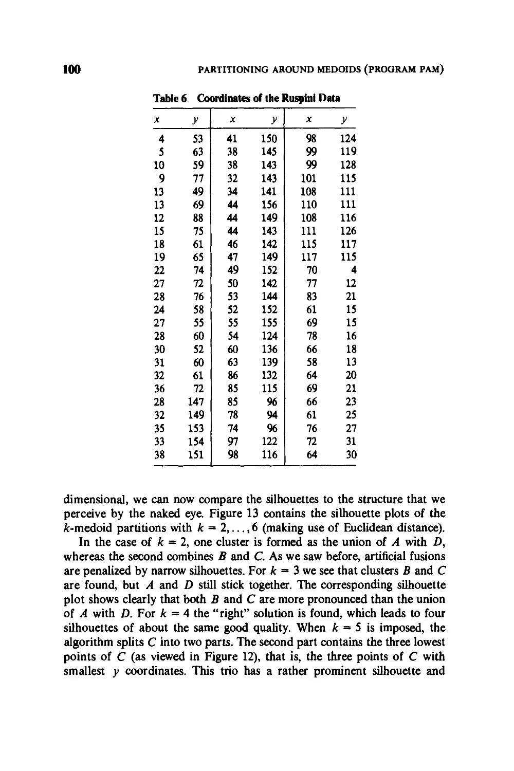
Chapters 2, 3, and 4 are about partitioning methods, whereas Chapters 5,
6, and 7 cover hierarchical techniques. Whenever possible, we constructed
methods that cannot only analyze data consisting of measurements (i.e.,
objects with variables) but also data consisting of dissimilarities between
objects. (This excluded parametric approaches, such as those based on
multivariate mixture distributions.) We also wanted the methods to be
consistent for large data sets. All the selected methods are of the Ll type,
which means that they minimize sums of dissimilarities (rather than sums of
squared dissimilarities, as in the classical nonrobust methods). Some of the
methods are new, such as the approach for partitioning large data sets and
the Lx method for fuzzy clustering. Also, the clusterings are accompanied
by graphical displays (called silhouettes and banners) and corresponding
quality coefficients, which help the user to select the number of clusters and
to see whether the method has found groups that were actually present in
the data.
Current statistical software packages contain only a few clustering
techniques and they are not the more modern methods. This forced us to write
new programs, the use of which is described in the book. Their present
version is for IBM-PC and compatible machines, but the source codes are
very portable and have run on several types of mainframes without
problems. The programs (together with their sources and the data sets used in
the book) are available on floppy disks by writing to the authors. The
programs are also being integrated in the workstation package S-PLUS of
Statistical Sciences, Inc., P.O. Box 85625, Seattle, WA 98145-1625.
We are grateful to Frank Critchley, Jan de Leeuw, Gaetan Libert, Glenn
Milligan, Frank Plastria, Marc Roubens, John Tukey, Bert van Zomeren,
Howard Wainer, Michael Windham, and David Wishart for helpful
suggestions and stimulating discussions on topics covered in this book and to

PREFACE
ix
Etienne Trauwaert for contributing to Section 4 of Chapter 4. Valuable
comments on the manuscript were given by Phil Норке, Doug Martin,
Marie-Paule Derde, and two reviewers. Annie De Schrijver was responsible
for drawing several figures. Finally, we would like to thank our wives,
Jacqueline and Lieve, for their patience and support.
Leonard Kaufman
Peter J. Rousseeuw
Edegem, Belgium
August, 1989

Contents
1. Introduction 1
1. Motivation, 1
2. Types of Data and How to Handle Them, 3
2.1 Interval-Scaled Variables, 4
2.2 Dissimilarities, 16
2.3 Similarities, 20
2.4 Binary Variables, 22
2.5 Nominal, Ordinal, and Ratio Variables, 28
2.6 Mixed Variables, 32
3. Which Clustering Algorithm to Choose, 37
3.1 Partitioning Methods, 38
3.2 Hierarchical Methods, 44
4. A Schematic Overview of Our Programs, 50
5. Computing Dissimilarities with the Program DAISY, 52
Exercises and Problems, 63
2. Partitioning Around Medoids (Program РАМ) 68
1. Short Description of the Method, 68
2. How to Use the Program РАМ, 72
2.1 Interactive Use and Input, 72
2.2 Output, 80
2.3 Missing Values, 88
3. Examples, 92
*4. More on the Algorithm and the Program, 102
4.1 Description of the Algorithm, 102
4.2 Structure of the Program, 104
xi

CONTENTS
*5. Related Methods and References, 108
5.1 The fc-Medoid Method and Optimal Plant Location, 108
5.2 Other Methods Based on the Selection of Representative
Objects, 110
5.3 Methods Based on the Construction of Central Points, 111
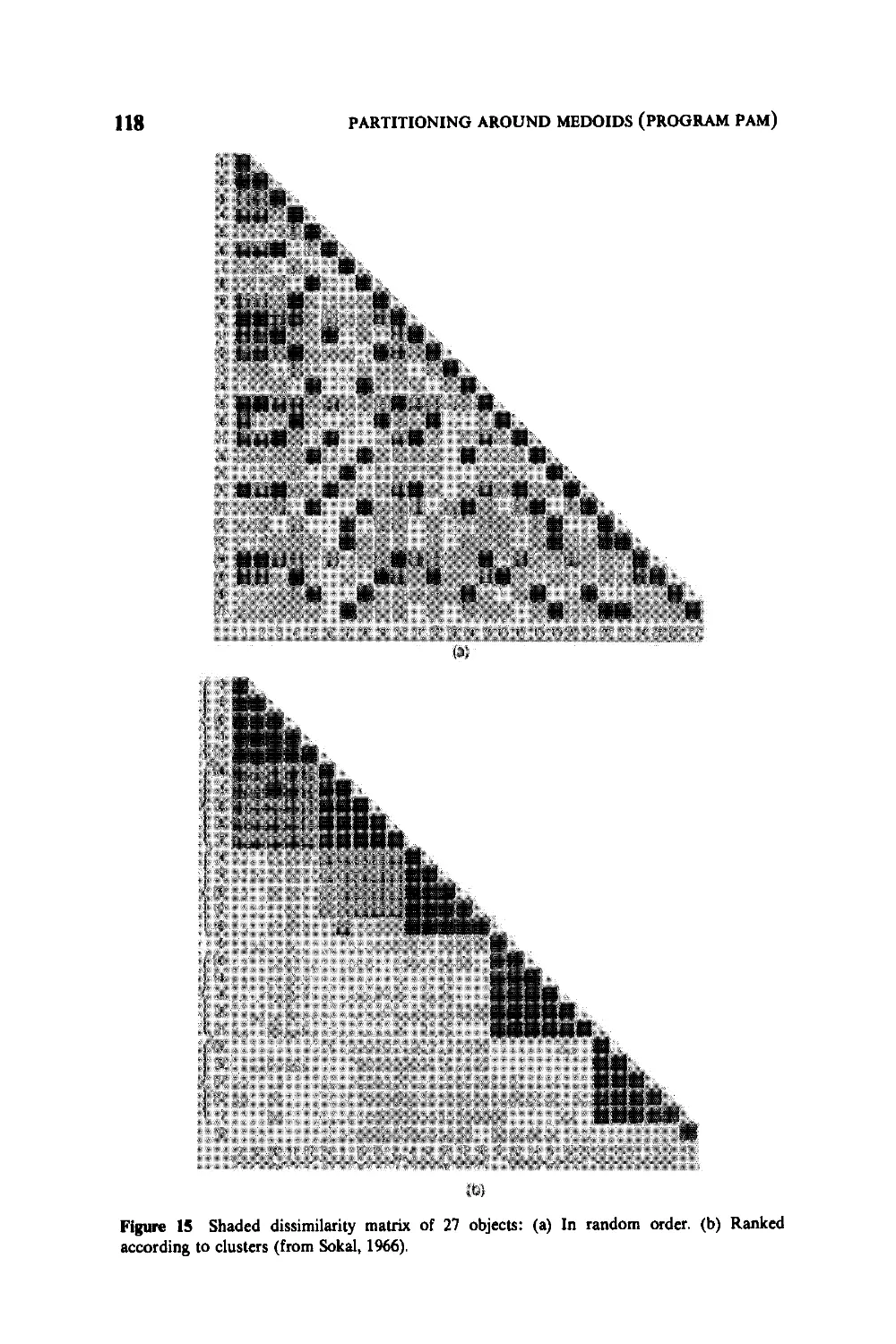
5.4 Some Other Nonhierarchical Methods, 116
5.5 Why Did We Choose the *-Medoid Method?, 117
5.6 Graphical Displays, 119
Exercises and Problems, 123
Clustering Large Applications (Program CLARA) 126
1. Short Description of the Method, 126
2. How to Use the Program CLARA, 127
2.1 Interactive Use and Input, 127
2.2 Output, 130
2.3 Missing Values, 134
3. An Example, 139
*4. More on the Algorithm and the Program, 144
4.1 Description of the Algorithm, 144
4.2 Structure of the Program, 146
4.3 Limitations and Special Messages, 151
4.4 Modifications and Extensions of CLARA, 153
*5. Related Methods and References, 155
5.1 Partitioning Methods for Large Data Sets, 155
5.2 Hierarchical Methods for Large Data Sets, 157
5.3 Implementing CLARA on a Parallel Computer, 160
Exercises and Problems, 162
Fuzzy Analysis (Program FANNY) 164
1. The Purpose of Fuzzy Clustering, 164
2. How to Use the Program FANNY, 166
2.1 Interactive Use and Input, 167
2.2 Output, 170
3. Examples, 175
*4. More on the Algorithm and the Program, 182
4.1 Description of the Algorithm, 182
4.2 Structure of the Program, 188

CONTENTS
*5. Related Methods and References, 189
5.1 Fuzzy fc-Means and the MND2 Method, 189
5.2 Why Did We Choose FANNY?, 191
5.3 Measuring the Amount of Fuzziness, 191
5.4 A Graphical Display of Fuzzy Memberships, 195
Exercises and Problems, 197
5. Agglomerative Nesting (Program AGNES)
1. Short Description of the Method, 199
2. How to Use the Program AGNES, 208
2.1 Interactive Use and Input, 208
2.2 Output, 209
3. Examples, 214
*4. More on the Algorithm and the Program, 221
4.1 Description of the Algorithm, 221
4.2 Structure of the Program, 223
*5. Related Methods and References, 224
5.1 Other Agglomerative Clustering Methods, 224
5.2 Comparing Their Properties, 238
5.3 Graphical Displays, 243
Exercises and Problems, 250
6. Divisive Analysis (Program DIANA)
1. Short Description of the Method, 253
2. How to Use the Program DIANA, 259
3. Examples, 263
*4. More on the Algorithm and the Program, 271
4.1 Description of the Algorithm, 271
4.2 Structure of the Program, 272
*5. Related Methods and References, 273
5.1 Variants of the Selected Method, 273
5.2 Other Divisive Techniques, 275
Exercises and Problems, 277
7. Monothetic Analysis (Program ΜΟΝΑ)
1. Short Description of the Method, 280
2. How to Use the Program ΜΟΝΑ, 283

xiv
CONTENTS
2.1 Interactive Use and Input, 284
2.2 Output, 287
3. Examples, 290
*4. More on the Algorithm and the Program, 298
4.1 Description of the Algorithm, 298
4.2 Structure of the Program, 301
*5. Related Methods and References, 304
5.1 Association Analysis, 304
5.2 Other Monothetic Divisive Algorithms
for Binary Data, 307
5.3 Some Other Divisive Clustering Methods, 308
Exercises and Problems, 310
APPENDIX 312
1. Implementation and Structure of the Programs, 312
2. Running the Programs, 313
3. Adapting the Programs to Your Needs, 316
4. The Program CLUSPLOT, 318
References 320
Author Index 332
Subject Index
335

Finding Groups in Data

Finding Groups in Data: An Introduction to Cluster Analysis
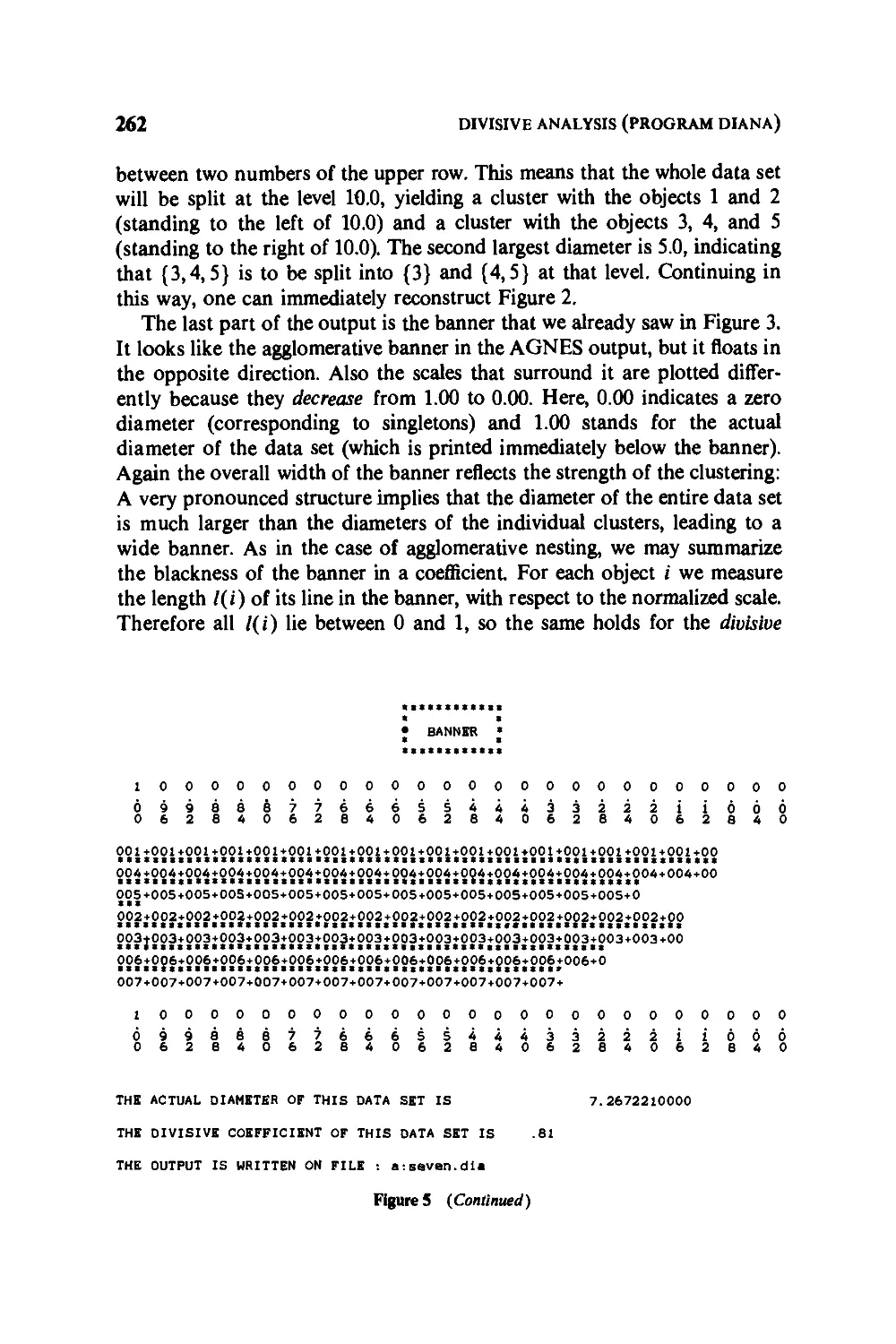
Leonard Kaufman and Peter J. Rousseeuw
Copyright ©1990,2005 by John Wiley & Sons, Inc
CHAPTER 1
Introduction
1 MOTIVATION
Cluster analysis is the art of finding groups in data. To see what is meant by
this, let us look at Figure 1. It is a plot of eight objects, on which two
variables were measured. For instance, the weight of an object might be
displayed on the horizontal axis and its height on the vertical one. Because
this example contains only two variables, we can investigate it by merely
looking at the plot.
In this small data set there are clearly two distinct groups of objects,
namely {TIN, TAL, KIM, ILA} and {LIE, JAC, PET, LEO}. Such groups
are called clusters, and to discover them is the aim of cluster analysis.
Basically, one wants to form groups in such a way that objects in the same
group are similar to each other, whereas objects in different groups are as
dissimilar as possible.
The classification of similar objects into groups is an important human
activity. In everyday life, this is part of the learning process: A child learns
to distinguish between cats and dogs, between tables and chairs, between
men and women, by means of continuously improving subconscious
classification schemes. (This explains why cluster analysis is often considered as a
branch of pattern recognition and artificial intelligence.) Classification has
always played an essential role in science. In the eighteenth century,
Linnaeus and Sauvages provided extensive classifications of animals, plants,
minerals, and diseases (for a recent survey, see Holman, 1985). In
astronomy, Hertzsprung and Russell classified stars in various categories on the
basis of two variables: their light intensity and their surface temperature. In
the social sciences, one frequently classifies people with regard to their
behavior and preferences. In marketing, it is often attempted to identify
market segments, that is, groups of customers with similar needs. Many
more examples could be given in geography (clustering of regions), medicine
1

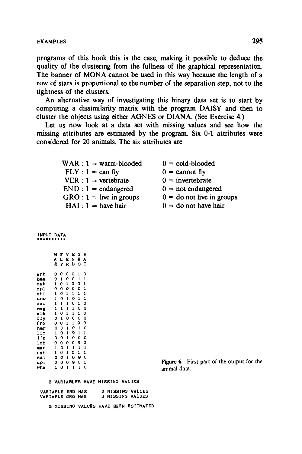
2
INTRODUCTION
,
180
170
160
150
НО
130
120
110
100
9Q
80
HEIGHT (CM)
KIM*»ILA
• TAL
TJN
LIE
PET
•
LEO
10 20 30 40 50 60 70 80
WEIGHT (KG)
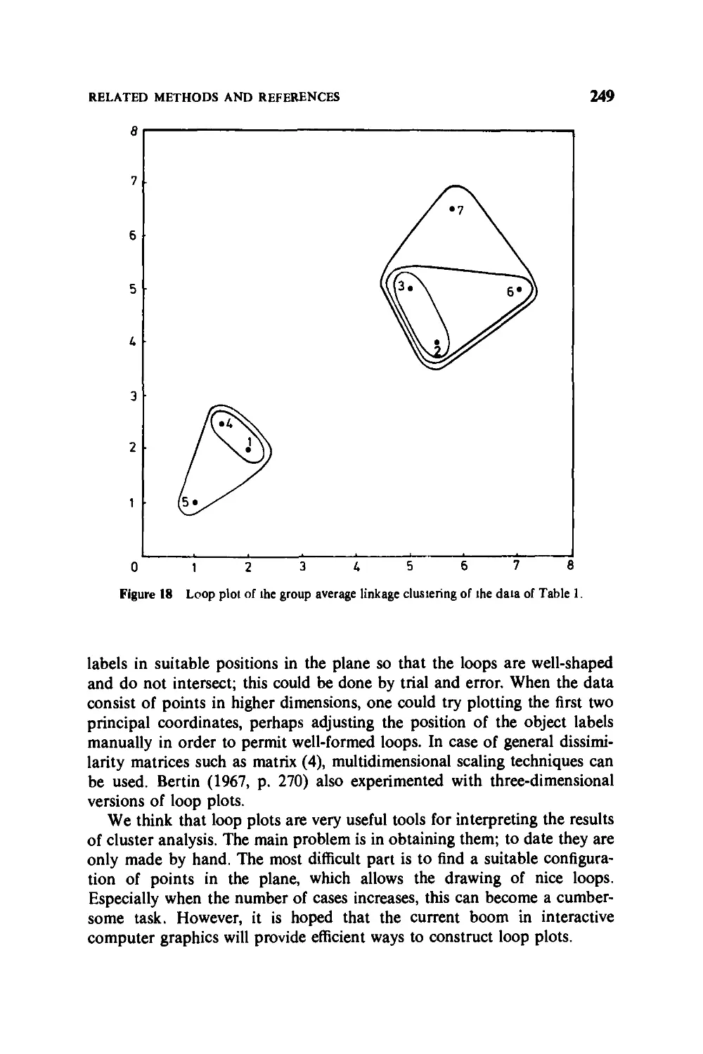
Figure 1 A plot of eight objects.
(incidence of specific types of cancer), chemistry (classification of
compounds), history (grouping of archeological findings), and so on. Moreover,
cluster analysis can be used not only to identify a structure already present
in the data, but also to impose a structure on a more or less homogeneous
data set that has to be split up in a "fair" way, for instance when dividing a
country into telephone areas. Note that cluster analysis is quite different
from discriminant analysis in that it actually establishes the groups, whereas
discriminant analysis assigns objects to groups that were defined in
advance.
In the past, clusterings were usually performed in a subjective way, by
relying on the perception and judgment of the researcher. In the example of
Figure 1, we used the human eye-brain system which is very well suited
(through millenia of evolution) for classification in up to three dimensions.

TYPES OF DATA AND HOW TO HANDLE THEM
3
However, the need to classify cases in more than three dimensions and the
upcoming objectivity standards of modern science have given rise to so-
called automatic classification procedures. Over the last 30 years, a wealth
of algorithms and computer programs has been developed for cluster
analysis. The reasons for this variety of methods are probably twofold. To
begin with, automatic classification is a very young scientific discipline in
vigorous development, as can be seen from the thousands of articles
scattered over many periodicals (mostly journals of statistics, biology,
psychometrics, computer science, and marketing). Nowadays, automatic
classification is establishing itself as an independent scientific discipline, as
witnessed by a full-fledged periodical (the Journal of Classification, first
published in 1984) and the International Federation of Classification
Societies (founded in 1985). The second main reason for the diversity of
algorithms is that there exists no general definition of a cluster, and in fact
there are several kinds of them: spherical clusters, drawn-out clusters, linear
clusters, and so on. Moreover, different applications make use of different
data types, such as continuous variables, discrete variables, similarities, and
dissimilarities. Therefore, one needs different clustering methods in order to
adapt to the kind of application and the type of clusters sought. Cluster
analysis has become known under a variety of names, such as numerical
taxonomy, automatic classification, botryology (Good, 1977), and
typological analysis (Chandon and Pinson, 1981).
In this book, several algorithms are provided for transforming the data,
for performing cluster analysis, and for displaying the results graphically.
Section 2 of this introduction discusses the various types of data and what
to do with them, and Section 3 gives a brief survey of the clustering
methods contained in the book, with some guidelines as to which algorithm
to choose. In particular the crucial distinction between partitioning and
hierarchical methods is considered. In Section 4 a schematic overview is
presented. In Section 5, it is explained how to use the program DAISY to
transform your data.
2 TYPES OF DATA AND HOW TO HANDLE THEM
Our first objective is to study some types of data which typically occur and
to investigate ways of processing the data to make them suitable for cluster
analysis.
Suppose there are η objects to be clustered, which may be persons,
flowers, words, countries, or whatever. Clustering algorithms typically
operate on either of two input structures. The first represents the objects by
means of ρ measurements or attributes, such as height, weight, sex, color,

4
INTRODUCTION
and so on. These measurements can be arranged in an и-by-p matrix, where
the rows correspond to the objects and the columns to the attributes. In
Tucker's (1964) terminology such an objects-by-variables matrix is said to
be two-mode, since the row and column entities are different. The second
structure is a collection of proximities that must be available for all pairs of
objects. These proximities make up an и-Ьу-и table, which is called a
one-mode matrix because the row and column entities are the same set of
objects. We shall consider two types of proximities, namely dissimilarities
(which measure how far away two objects are from each other) and
similarities (which measure how much they resemble each other). Let us
now have a closer look at the types of data used in this book by considering
them one by one.
2.1 Interval-Scaled Variables
In this situation the η objects are characterized by ρ continuous
measurements. These values are positive or negative real numbers, such as height,
weight, temperature, age, cost,..., which follow a linear scale. For
instance, the time interval between 1905 and 1915 was equal in length to that
between 1967 and 1977. Also, it takes the same amount of energy to heat an
object of - 16.4°C to - 12.4°C as to bring it from 35.2°C to 39.2°C. In
general it is required that intervals keep the same importance throughout
the scale.
These measurements can be organized in an п-Ъу-р matrix, where the
rows correspond to the objects (or cases) and the columns correspond to the
variables. When the /th measurement of the ith object is denoted by xif
(where i = 1,..., и and / = 1,..., p) this matrix looks like
и objects
lnl
ρ variables
4/
V
4r
>P
"P
(1)
For instance, consider the following real data set. For eight people, the
weight (in kilograms) and the height (in centimeters) is recorded in Table 1.
In this situation, и = 8 and ρ = 2. One could have recorded many more
variables, like age and blood pressure, but as there are only two variables in
this example it is easy to make a scatterplot, which corresponds to Figure 1

TYPES OF DATA AND HOW TO HANDLE THEM
Table 1 Weight and Height of Eight People, Expressed
in Kilograms and Centimeters
Name
Ilan
Jacqueline
Kim
Lieve
Leon
Peter
Talia
Tina
Weight
(kg)
15
49
13
45
85
66
12
10
Height
(cm)
95
156
95
160
178
176
90
78
given earlier. Note that the units on the vertical axis are drawn to the same
size as those on the horizontal axis, even though they represent different
physical concepts. The plot contains two obvious clusters, which can in this
case be interpreted easily: the one consists of small children and the other
of adults.
Note that other variables might have led to completely different
clusterings. For instance, measuring the concentration of certain natural hormones
might have yielded a clear-cut partition into three male and five female
persons. By choosing still other variables, one might have found blood
types, skin types, or many other classifications.
Let us now consider the effect of changing measurement units. If weight
and height of the subjects had been expressed in pounds and inches, the
results would have looked quite different. A pound equals 0.4536 kg and an
inch is 2.54 cm. Therefore, Table 2 contains larger numbers in the column
of weights and smaller numbers in the column of heights. Figure 2,
although plotting essentially the same data as Figure 1, looks much flatter.
In this figure, the relative importance of the variable "weight" is much
larger than in Figure 1. (Note that Kim is closer to Ilan than to Talia in
Figure 1, but that she is closer to Talia than to Ilan in Figure 2.) As a
consequence, the two clusters are not as nicely separated as in Figure 1
because in this particular example the height of a person gives a better
indication of adulthood than his or her weight. If height had been expressed
in feet (1 ft = 30.48 cm), the plot would become flatter still and the variable
" weight" would be rather dominant.
In some applications, changing the measurement units may even lead
one to see a very different clustering structure. For example, the age (in
years) and height (in centimeters) of four imaginary people are given in

6
INTRODUCTION
Table 2 Weight and Height of the Same Eight People,
But Now Expressed in Pounds and Inches
Name
Ilan
Jacqueline
Kim
Lieve
Leon
Peter
Talia
Tina
Weight
(lb)
33.1
108.0
28.7
99.2
187.4
145.5
26.5
22.0
Height
(in.)
37.4
61.4
37.4
63.0
70.0
69.3
35.4
30.7
Table 3 and plotted in Figure 3. It appears that {A, B) and {C, D) are
two well-separated clusters. On the other hand, when height is expressed in
feet one obtains Table 4 and Figure 4, where the obvious clusters are now
{A,C} and {B, D). This partition is completely different from the first
because each subject has received another companion. (Figure 4 would have
been flattened even more if age had been measured in days.)
To avoid this dependence on the choice of measurement units, one has
the option of standardizing the data. This converts the original
measurements to unitless variables. First one calculates the mean value of variable
1
80
60
40
20
HEIGHT (INCHES)
KIM
TAL.»»ILA
tin·
LIE j'ac
P*ET
LEO
20 40 60 80 100 120 U0 160 180
WEIGHT (POUNDS)
Figure 2 Plot corresponding to Table 2.

TYPES OF DATA AND HOW TO HANDLE THEM
7
Table 3 Age (in years) and Height (in centimeters) of Four People
Person
Age
(yr)
35
40
35
40
Height
(cm)
190
190
160
160
A
В
С
D
190
180
170
160 ·
HEIGHT(CM)
A B
С D
20 30 35 40 50
AGE (YEARS)
Figure 3 Plot of height (in centimeters) versus age for four people.
Table 4 Age (in years) and Height (in feet) of the Same Four People
Person
A
В
С
D
Age
(yr)
35
40
35
40
Height
(ft)
6.2
6.2
5.2
5.2

8
INTRODUCTION
,
9
θ
7
6
5
и
3
2
1
HEIGHT (FEET)
—ih
A.
C·
.в
• D
^
35 36 37 38 39 40 41
AGE (YEARS)
Figure 4 Plot of height (in feet) versus age for the same four people.
/, given by
m/= -(*i/+*2/+ ··· +*■/)
(2)
for each / = 1,..., p. Then one computes a measure of the dispersion or
"spread" of this /th variable. Traditionally, people use the standard
deviation
/ = у ;—[{W " m/)2 + (*2/" m/)2 + · · · + (*«/ - mff)
std
for this purpose. However, this measure is affected very much by the
presence of outlying values. For instance, suppose that one of the xtj has
been wrongly recorded, so that it is much too large. In this case std^ will be
unduly inflated, because xif - mf is squared. Hartigan (1975, p. 299) notes
that one needs a dispersion measure that is not too sensitive to outliers.
Therefore, from now on we will use the mean absolute deviation
1
sf = ~ {l*i/ ~ m/l + 1*2/ ~mf\+ ■■· +]xnf - mf]}
(3)
where the contribution of each measurement xiS is proportional to the
absolute value |x(/ - ntj\. This measure is more robust (see, e.g., Hampel

TYPES OF DATA AND HOW TO HANDLE THEM
9
et al., 1986) in the sense that one outlying observation will not have such a
large influence on sf. (Note that there exist estimates that are much more
robust, but we would like to avoid a digression into the field of robust
statistics.)
Let us assume that Sj is nonzero (otherwise variable / is constant over
all objects and must be removed). Then the standardized measurements are
defined by
za =
c</
- m,
(4)
and sometimes called z-scores. They are unitless because both the
numerator and the denominator are expressed in the same units. By construction,
the ζ у have mean value zero and their mean absolute deviation is equal to
1. When applying standardization, one forgets about the original data (1)
and uses the new data matrix
objects
variables
<*i
Ί/
'»/
Zlp
•P
"P
(5)
in all subsequent computations. The advantage of using sf rather than std/
in the denominator of (4) is that Sj will not be blown up so much in the
case of an outlying x(/, and hence the corresponding zi} will still "stick
out" so the ith object can be recognized as an outlier by the clustering
algorithm, which will typically put it in a separate cluster. [This motivation
differs from that of Milligan and Cooper (1988), who recommended the use
of a nonrobust denominator.]
The preceding description might convey the impression that
standardization would be beneficial in all situations. However, it is merely an option
that may or may not be useful in a given application. Sometimes the
variables have an absolute meaning, and should not be standardized (for
instance, it may happen that several variables are expressed in the same
units, so they should not be divided by different sf). Often standardization
dampens a clustering structure by reducing the large effects because the
variables with a big contribution are divided by a large sf.
For example, let us standardize the data of Table 3. The mean age equals
m, = 37.5 and the mean absolute deviation of the first variable works out
to be s, = {2.5 + 2.5 + 2.5 + 2.5}/4 = 2.5. Therefore, standardization
converts age 40 to +1 and age 35 to -1. Analogously, m2 = 175 cm and

10
INTRODUCTION
Table 5 Standardized Age and Height of the Same Four People
Person
Variable 1
-1.0
1.0
-1.0
1.0
Variable 2
1.0
1.0
-1.0
-1.0
A
В
С
D
s2 = {15 + 15 + 15 + 15}/4 = 15 cm, so 190 cm is standardized to +1
and 160 cm to — 1. The resulting data matrix, which is unitless, is given in
Table 5. Note that the new averages are zero and that the mean deviations
equal 1. Of course, standardizing Table 4 would yield exactly the same
result, so Table 5 is the standardized version of both Tables 3 and 4. Even
when the data are converted to very strange units (such as the proverbial
fortnights and furlongs), standardization will always yield the same
numbers. However, plotting the values of Table 5 in Figure 5 does not give a
very exciting result. Figure 5 looks like an intermediate between Figures 3
and 4 and shows no clustering structure because the four points lie at the
vertices of a square. One could say that there are four clusters, each
HEIGHT(STANDARDIZED)
-1
C*
0 1
AGE(STANDARDIZED)
Figure S Standardized height versus standardized age.

TYPES OF DATA AND HOW TO HANDLE THEM
11
consisting of a single point, or that there is only one big cluster containing
four points.
From a philosophical point of view, standardization does not really solve
the problem. Indeed, the choice of measurement units gives rise to relative
weights of the variables. Expressing a variable in smaller units will lead to a
larger range for that variable, which will then have a large effect on the
resulting structure. On the other hand, by standardizing one attempts to
give all variables an equal weight, in the hope of achieving objectivity. As
such, it may be used by a practitioner who possesses no prior knowledge.
However, it may well be that some variables are intrinsically more
important than others in a particular application, and then the assignment of
weights should be based on subject-matter knowledge (see, e.g., Abra-
hamowicz, 1985). On the other hand, there have been attempts to devise
clustering techniques that are independent of the scale of the variables
(Friedman and Rubin, 1967). The proposal of Hardy and Rasson (1982) is
to search for a partition that minimizes the total volume of the convex hulls
of the clusters. In principle such a method is invariant with respect to linear
transformations of the data, but unfortunately no algorithm exists for its
implementation (except for an approximation that is restricted to two
dimensions). Therefore, the dilemma of standardization appears
unavoidable at present and the programs described in this book leave the choice up
to the user.
Of course, the data offered to the program may already be the result of
some transformation: Often people find it useful to replace some variable
by its inverse or its square, which may be more meaningful in that
particular context. However, we shall assume from now on that such
transformations have been performed prior to the cluster analysis.
The next step is to compute distances between the objects, in order to
quantify their degree of dissimilarity. It is necessary to have a distance for
each pair of objects i and j. The most popular choice is the Euclidean
distance
d{i, j) = /(*л - *;i)2 + (*« - xj2? + ·■■ + (xip ~ Xjpf (6)
(When the data are being standardized, one has to replace all χ by ζ in this
expression.) Formula (6) corresponds to the true geometrical distance
between the points with coordinates (x(1,..., xip) and (xyl,..., xjp). To
illustrate this, let us consider the special case with ρ = 2. Figure 6 shows
two points with coordinates (xn, xa) and (xyl, xJ2). It is clear that the
actual distance between objects i and j is given by the length of the
hypothenuse of the triangle, yielding expression (6) by virtue of Pythagoras'
theorem. For this reason, Gower (1971b) calls (6) the Pythagorean distance.

12
INTRODUCTION
ι
second coordinate
first coordinate
Figure б Illustration of the Euclidean distance formula.
Another well-known metric is the city block or Manhattan distance,
defined by
<*(«', j) = \x,i ~ Xji\ + \xa ~ xji\ + ■■· +\χίρ ~ xjP\ (7)
In Figure 6, this corresponds to the sum of the lengths of the other two
sides of the triangle. The Manhattan distance was used in a cluster analysis
context by Carmichael and Sneath (1969) and owes its peculiar name to the
following reasoning. Suppose you live in a city where the streets are all
north-south or east-west, and hence perpendicular to each other. Let
Figure 6 be part of a street map of such a city, where the streets are
portrayed as vertical and horizontal lines. Then the actual distance you
would have to travel by car to get from location i to location j would total
\xa - Xji\ + \xn - xJ2\, corresponding to (7). This would be the shortest
length among all possible paths from i to / Only a bird could fly straight
from point i to point J, thereby covering the Euclidean distance between
these points. The use of the Manhattan distance is advised in those
situations where for example a difference of 1 in the first variable.and of 3
in the second variable is the same as a difference of 2 in the first variable
and of 2 in the second.

TYPES OF DATA AND HOW TO HANDLE THEM
13
Both the Euclidean metric (6) and the Manhattan metric (7) satisfy the
following mathematical requirements of a distance function:
(Dl) d(i, j) ;> 0
(D2) d(i, 0 = 0
(D3) d(i,j) = d(j,i)
(D4) d(i, j) <Ξ d(i, A) + d(h, j)
for all objects i, j, and A. Condition (Dl) merely states that distances are
nonnegative numbers and (D2) says that the distance of an object to itself is
zero. Axiom (D3) is the symmetry of the distance function. The triangle
inequality (D4) looks a little bit more complicated, but is necessary to allow
a geometrical interpretation. It says essentially that going directly from i to
j is shorter than making a detour over object A.
Note that d(i, j) = 0 does not necessarily imply that ϊ = j, because it
can very well happen that two different objects have the same
measurements for the variables under study. However, the triangle inequality
implies that i and j will then have the same distance to any other object A,
because d(i, A) <, d(i, j) + d(j, A) = d(j, A) and at the same time
d(j, h) £ d(j,i) + d(i, A) = d(i, A), which together imply that d(i, A) =
d(j,
ΜΑ generalization of both the Euclidean and the Manhattan metric is the
Minkowski distance given by
d(i, j) = (|хд " xA\" + \xa ~ Xj2\" + ■■■ +K„ " Xj,\4)U"
where q is any real number larger than or equal to 1. This is also called the
Lq metric, with the Euclidean (q = 2) and the Manhattan (q = 1) as special
cases. Many other distance functions may be constructed (see, e.g., Bock,
1974, Section 3; Hartigan, 1975, Chapter 2; Romesburg, 1984, Chapter 8).
The clustering programs accompanying this book provide a choice between
Euclidean and Manhattan distances.
One sometimes computes weighted Euclidean distances like
d{i, j) = /»ι(χ,ι - *yi)2 + w2(*,2 - XjiY + ■·■ +wp(xip ~ xjPf (8)
where each variable receives a weight according to its perceived importance.
For instance, giving a variable weight 2 is the same thing as using it twice.
However, applying such weighted distances on the raw data is equivalent to
first choosing other measurement units, corresponding to rescaling the
coordinates by the factors y/ivj",..., Jw~p, and then computing ordinary
distances. (Therefore, it was not necessary to provide weighted distances in

14
INTRODUCTION
our programs.) This leads us back to the discussion on standardization. The
essential question remains: Which weights should be assigned to the
variables? If one thinks the measurement units were not particularly well
chosen and one wants to assign equal weights to the variables, it is
preferable to standardize the data first and then to compute ordinary
Euclidean distances (6). But if one wants to keep the data intact, because
the measurement scales are believed to be meaningful, it is best not to
standardize (and hence to use the weights inherent in the raw data).
Furthermore, if one wants to impose certain weights on the variables, due to
prior beliefs or background information, one can either change the
measurement units or apply weighted distances like (8), which boils down to the
same thing.
In all this, it should be noted that a variable not containing any relevant
information (say, the telephone number of each person) is worse than
useless, because it will make the clustering less apparent. The occurrence of
several such "trash variables" will kill the whole clustering because they
yield a lot of random terms in the distances, thereby hiding the useful
information provided by the other variables. Therefore, such noninforma-
tive variables must be given a zero weight in the analysis, which amounts to
deleting them. A recent discussion of variable selection can be found in
Fowlkes et al. (1988). In general, the selection of "good" variables is a
nontrivial task and may involve quite some trial and error (in addition to
subject-matter knowledge and common sense). In this respect, cluster
analysis may be considered an exploratory technique.
It often happens that not all measurements are actually available, so
there are some " holes" in the data matrix (1). Such an absent measurement
is called a missing value and it may have several causes. The value of the
measurement may have been lost or it may not have been recorded at all by
oversight or lack of time. Sometimes the information is simply not
available, as in the example of the birthdate of a foundling, or the patient may
not remember whether he or she ever had the measles, or it may be
impossible to measure the desired quantity due to the malfunctioning of
some instrument. In certain instances the question does not apply (such as
the color of hair of a bald person) or there may be more than one possible
answer (when two experimenters obtain very different results). Because of
all this, missing values are often encountered.
How can we handle a data set with missing values? In the matrix (1) we
indicate the absent measurements by means of some code (like the number
999.99, if it did not already occur), that can then be recognized by the
program. If there exists an object in the data set for which all measurements
are missing, there is really no information on this object so it has to be
deleted. Analogously, a variable consisting exclusively of missing values has
to be removed too.

TYPES OF DATA AND HOW TO HANDLE THEM
15
If the data are standardized, the mean value mf of the /th variable is
calculated by making use of the present values only. The same goes for sj,
so in the denominator of (2) and (3) we must replace и by the number of
nonmissing values for that variable. The z-scores zif can then be computed
as in (4), but of course only when the corresponding xi{ is not missing
itself.
In the computation of distances (based on either the xif or the zif)
similar precautions must be taken. When calculating the distances d(i, j)
given by (6) or (7), only those variables are considered in the sum for which
the measurements for both objects are present; subsequently the sum is
multiplied by ρ and divided by the actual number of terms (in the case of
Euclidean distances this is done before taking the square root). Obviously,
such a procedure only makes sense when the variables are thought of as
having the same weight (for instance, this can be done after
standardization). When computing these distances, one might come across a pair of
objects that do not have any common measured variables, so their distance
cannot be computed by means of the abovementioned approach. Several
remedies are possible: One could remove either object or one could fill in
some average distance value based on the rest of the data. A totally
different approach consists of replacing all missing xif by the mean ntj of
that variable; then all distances can be computed. Applying any of these
methods, one finally possesses a "full" set of distances. From this point on,
many clustering algorithms can be applied, even though the original data
set was not complete.
In any case, we now have a collection of distances (whether based on raw
or standardized data that contained missing values or not) that we want to
store in a systematic way. This can be achieved by arranging them in an
и-Ьу-и matrix. For example, when computing Euclidean distances between
the objects of Table 1 we obtain
ILA
JAC
KIM
LIE
LEO
PET
TAL
TIN
ILA
0
69.8
2.0
71.6
108.6
95.7
5.8
17.7
JAC
69.8
0
70.8
5.7
42.2
26.3
75.7
87.2
KIM
2.0
70.8
0
72.5
109.9
96.8
5.1
17.3
LIE
71.6
5.7
72.5
0
43.9
26.4
77.4
89.2
LEO
108.6
42.2
109.9
43.9
0
19.1
114.3
125.0
PET
95.7
26.3
96.8
26.4
19.1
0
101.6
112.9
TAL
5.8
75.7
5.1
77.4
114.3
101.6
0
12.2
TIN
17.7
87.2
17.3
89.2
125.0
112.9
12.2
0
The distance between object JAC and object LEO can be located at the
intersection of the fifth row and the second column, yielding 42.2. The same

16
INTRODUCTION
number can also be found at the intersection of the second row and the fifth
column, because the distance between JAC and LEO is equal to the
distance between LEO and JAC. This is the symmetry property (D3), which
holds for any pair of objects [formula (6) gives the same result when i and j
are interchanged]. Therefore, a distance matrix is always symmetric.
Moreover, note that the entries on the main diagonal are always zero, because the
distance of an object to itself has to be zero. (The same remarks apply to
the Manhattan or any other distance.) Therefore, it would suffice to write
down only the lower triangular half of the distance matrix, which looks like
ILA JAC KIM LIE LEO PET TAL
JAC 69.8
KIM 2.0 70.8
LIE 71.6 5.7 72.5
LEO 108.6 42.2 109.9 43.9 (10)
PET 95.7 26.3 96.8 26.4 19.1
TAL 5.8 75.7 5.1 77.4 114.3 101.6
TIN 17.7 87.2 17.3 89.2 125.0 112.9 12.2
Note that in the latter form there are only seven rows and seven columns,
because the upper row and the rightmost column of (9) were superfluous.
When the data are represented as in (9) or (10), the cluster structure we
saw so easily in Figure 1 is rather hidden from visual inspection.
Nevertheless, the clustering methods discussed in Chapters 2, 4, 5, and 6 only make
use of this information, without having to return to the original data matrix.
2.2 Dissimilarities
This leads us to our second input data structure, namely an и-Ьу-и matrix
like (9), often presented as in (10). The entries of such a matrix may be
Euclidean or Manhattan distances. However, there are many other
possibilities, so we no longer speak of distances but of dissimilarities (or
dissimilarity coefficients). Basically, dissimilarities are nonnegative numbers d(i, j)
that are small (close to zero) when / and j are "near" to each other and
that become large when / and j are very different. We shall usually assume
that dissimilarities are symmetric and that the dissimilarity of an object to
itself is zero, but in general the triangle inequality does not hold. Indeed, it
is often assumed that dissimilarities satisfy (Dl), (D2), and (D3) (see, e.g.,
Bock, 1974, p. 25), although none of these properties is really essential and
there are clustering methods that do not require any of them. But the main
difference with distances is that (D4) can no longer be relied on.

TYPES OF DATA AND HOW TO HANDLE THEM 17
Table 6 Subjective Dissimilarities between 11 Sciences
Astronomy
Biology
Chemistry
Computer sci.
Economics
Geography
History
Mathematics
Medicine
Physics
Psychology
0.00
7.86
6.50
5.00
8.00
4.29
8.07
3.64
8.21
2.71
9.36
0.00
2.93
6.86
8.14
7.00
8.14
7.14
2.50
5.21
5.57
0.00
6.50
8.21
7.64
8.71
4.43
2.93
4.57
7.29
0.00
4.79
7.71
8.57
1.43
6.36
4.21
7.21
0.00
5.93
5.86
3.57
8.43
8.36
6.86
0.00
3.86
7.07
7.86
7.29
8.29
0.00
9.07
8.43
8.64
7.64
0.00
6.29
2.21
8.71
0.00
5.07
3.79
0.00
8.64 0.00
Dissimilarities can be obtained in several ways. Often they can be
computed from variables that are binary, nominal, ordinal, interval, or a
combination of these (a description of such variables and possible formulas
will be given later in this chapter). Also, dissimilarities can be simple
subjective ratings of how much certain objects differ from each other, from
the point of view of one or more observers. This kind of data is typical in
the social sciences and in marketing.
Let us consider an example of this type. Fourteen postgraduate
economics students (coming from different parts of the world) were asked to
indicate the subjective dissimilarities between 11 scientific disciplines. All of
them had to fill in a matrix like Table 6, where the dissimilarities had to be
given as integer numbers on a scale from 0 (identical) to 10 (very different).
The actual entries of Table 6 are the averages of the values given by the
students. It appears that the smallest dissimilarity is perceived between
mathematics and computer science, whereas the most remote fields were
psychology and astronomy.
Another example of the construction of dissimilarities is to record how
often consonants are misunderstood, because when two consonants are
often confused (like "s " and "z") this indicates that their dissimilarity is
small [see, e.g., Johnson's (1967) analysis of the Miller and Nicely (1955)
data]. Such experiments lead to asymmetric matrices, because "z " may be
more often inadvertently taken for "s " than vice versa. However, in such
situations one can easily symmetrize the data [for instance by averaging
i/(i, j) with d(j, i) for each pair of consonants].
If one wants to perform a cluster analysis on a set of variables that have
been observed in some population, there are other measures of dissimilarity.
For instance, one can compute the (parametric) Pearson product-moment

18
INTRODUCTION
correlation
R(f ) E"-iU/-*/)(** ~w«)
between the variables / and g, or alternatively the (nonparametric)
Spearman correlation. Both coefficients lie between -1 and +1 and do not
depend on the choice of measurement units. The main difference between
them is that the Pearson coefficient looks for a linear relation between the
variables / and g, whereas the Spearman coefficient searches for a
monotone relation. Both coefficients are provided by most statistical packages,
like SPSS, BMDP, or SAS, so they can simply be taken from their routine
output. Correlation coefficients are useful for clustering purposes because
they measure the extent to which two variables are related.
For instance, the Pearson correlation between the variables weight and
height in Table 1 is 0.957. It is very high because there appears to be a
positive relationship between these two variables: The larger somebody's
weight, the larger his or her height is likely to be, as can be seen from the
upward trend in Figure 1. Table 7 also lists some other variables measured
on the same eight people, namely their month and year of birth. We see no
apparent relation between month of birth and weight: There is no obvious
reason why someone born in November (of any year) would be likely to be
heavier than someone born in February. Indeed, the correlation between
month and weight is approximately zero (the actual value in this example is
- 0.036). A third situation occurs when we correlate weight with the year of
birth: The people with a large birth year will typically possess a smaller
weight and vice versa. In such a situation the correlation coefficient be-
Table 7 Data on Eight People. Weight is Expressed in Kilograms and Height
in Centimeters. Also the Month and Year of Birth are Provided
Name
Han
Jacqueline
Kim
Lieve
Leon
Peter
Talia
Tina
Weight
15
49
13
45
85
66
12
10
Height
95
156
95
160
178
176
90
78
Month
1
5
11
7
6
6
12
1
Year
82
55
81
56
48
56
83
84

TYPES OF DATA AND HOW TO HANDLE THEM
19
Table 8 (a) Pearson Correlation Coefficients between the Four Variables
in Table 7, (b) Corresponding Dissimilarities Obtained Through Formula (11),
and (c) Dissimilarities Computed by Means of (12)
Quantity
(a) Correlations
(b) Dissimilarities
According to (11)
(c) Dissimilarities
According to (12)
Weight
Height
Month
Year
Weight
Height
Month
Year
Weight
Height
Month
Year
Weight
1.000
0.957
-0.036
- 0.953
0.000
0.021
0.518
0.977
0.000
0.043
0.964
0.047
Height
1.000
0.021
-0.985
0.000
0.489
0.992
0.000
0.979
0.015
Month
1.000
0.013
0.000
0.493
0.000
0.987
Year
1.000
0.000
0.000
comes strongly negative (in this example it is -0.953, which is close to -1,
because the relation is nearly linear). Continuing like this, we can fill up
Table 8(a).
Correlation coefficients, whether parametric or nonparametric, can be
converted to dissimilarities d(f, g), for instance by setting
d(f,g) = (l-R(f,g))/2
(И)
With this formula, variables with a high positive correlation receive a
dissimilarity coefficient close to zero, whereas variables with a strongly
negative correlation will be considered very dissimilar. In other applications
one might prefer to use
d(f,g) = l-\R(f,g)\
(12)
in which case also variables with a strongly negative correlation will be
assigned a small dissimilarity. Lance and Williams (1979) compared these
formulas by means of real data, and concluded that (11) was unequivocally
the best, whereas (12) still did relatively well. (A third possibility, given by
d(f, g) = 1 - /?(/, g)2, turned out to be uniformly unsatisfactory.) Table
8(b) contains the dissimilarities computed according to (11), in which case
weight and year are perceived to be very different. On the other hand, the

20
INTRODUCTION
use of (12) yields Table 8(c) in which the variable year joins the cluster
formed by weight and height.
Many other ad hoc dissimilarities between variables can be thought of.
For example, in a psychological application (Lecompte et al., 1986) we once
had to cluster nominal variables, some of which possessed two classes and
some three. The resulting contingency tables of pairs of variables led to
chi-squared statistics that could not be compared directly because they
possessed different degrees of freedom. However, the computed significance
level (also called P-value) of these statistics could be used to construct a
dissimilarity measure. The stronger the relationship between two variables,
the smaller their P-value becomes.
In many applications, the input data simply consist of a dissimilarity
matrix, without any measurement values. Indeed, the dissimilarities may
have been computed from attributes that were not published or even have
been lost. It may also be that there never were any variables in the first
place, because the dissimilarities were obtained in another way (from
subjective assessments, confusion data, or whatever). For this reason it is
useful to have clustering algorithms that can operate directly on a
dissimilarity matrix, without having to resort to any measurements. This is the case
for the programs РАМ, FANNY, AGNES, and DIANA, which will be
briefly introduced in Section 3.
2.3 Similarities
Instead of using a dissimilarity coefficient d(i, j) to indicate how remote
two objects ϊ and j are, it is also possible to work with a similarity
coefficient s(i, j). The more objects ϊ and j are alike (or close), the larger
s(/, j) becomes. Such a similarity s(i, j) typically takes on values between
0 and 1, where 0 means that i and j are not similar at all and 1 reflects
maximal similarity. Values in between 0 and 1 indicate various degrees of
resemblance. Often it is assumed that the following conditions hold:
(51) 0 <Ξ s(i, j) <Ξ 1
(52) s(/, 0 = 1
(53) s(ij) = s(j,i)
for all objects ι and j (see Bock, 1974). The numbers s(i, j) can be
arranged in an и-Ьу-и matrix like (9) or (10), which is then called a
similarity matrix. Both similarity and dissimilarity matrices are generally
referred to as proximity matrices, or sometimes as resemblance matrices.

TYPES OF DATA AND HOW TO HANDLE THEM
21
Similarities may arise in several ways. Like dissimilarities, they may be
the results of subjective judgments. Also, there are formulas to compute
similarities between objects characterized by attributes, even when these
variables are of different types, as we shall see in Section 2.6 on mixed
measurements.
In order to define similarities between variables, we can again resort to
the Pearson or the Spearman correlation coefficient. However, neither
correlation measure can be used directly as a similarity coefficient because
they also take on negative values. Some transformation is in order to bring
the coefficients into the zero-one range. There are essentially two ways to do
this, depending on the meaning of the data and the purpose of the
application. If variables with a strong negative correlation are considered to
be very different because they are oriented in the opposite direction (like
mileage and weight of a set of cars), then it is best to take something like
s(/,g) = (l + *(/,g))/2 (13)
which yields s(f, g) = 0 whenever R(f, g) = -1. On the other hand, there
are situations in which variables with a strong negative correlation should
be grouped, because they measure essentially the same thing. (For instance,
this happens if one wants to reduce the number of variables in a regression
data set by selecting one variable from each cluster.) In that case it is better
to use a formula like
s(f,g)-\*(f,g)\ (И
which yields s(f, g) — 1 when R(f, g) = -1.
It must be noted that people have sometimes used correlation coefficients
for assessing similarity between objects by simply interchanging the roles of
objects and variables in the expression of R. This does not make much
sense because it involves such operations as averaging the measurements (in
different units) of the same object. The use of the correlation coefficient
between objects was criticized by Eades (1965), Fleiss and Zubin (1969),
and others, on several grounds.
Suppose the data consist of a similarity matrix but one wants to apply a
clustering algorithm designed for dissimilarities. Then it is necessary to
transform the similarities into dissimilarities. The larger the similarity
s(i, j) between ι and j, the smaller their dissimilarity d(i, j) should be.
Therefore, we need a decreasing transformation, such as
d(i, j) = 1 - s(i, j)
(15)

22
INTRODUCTION
One could also take the square root of 1 - s(i, j), as advocated by Gower
(1966) on the basis of a geometrical argument This makes the differences
between large similarities more important, but on the other hand makes it
more difficult to obtain small dissimilarities. As a consequence, the resulting
dissimilarity matrix might be rather homogeneous and less likely to yield
clear-cut clusterings.
When applying (15) to correlation coefficients, expression (13) leads to
formula (11), which means that negatively correlated variables are
considered far apart. In the opposite case, (14) yields formula (12).
In order to be able to process similarities and correlation coefficients, the
program DAISY executes (11), (12), and (15) as well as some other
calculations. In Section 5 it will be explained how to use this program.
2.4 Binary Variables
Binary variables have only two possible outcomes (or states). For instance,
when clustering people several binary variables may be used: male/female,
smoker/nonsmoker, answered yes/no to a particular question, and so on.
In the data matrix, such variables are often coded as zero or one. When
variable / is binary, the objects ϊ will have either xif - 0 or xif - 1. (It may
be useful to allow a third code for missing values, e.g., to indicate that we
do not know whether that particular person smokes or not.) Often 1 is
taken to mean that a certain attribute is present (e.g., smoking), whereas 0
indicates its absence. Sometimes people treat binary variables just as if they
were interval-scaled, that is, by applying the usual formulas for Euclidean
or Manhattan distance. Although this may sometimes lead to decent results,
it is good to know that there exist approaches designed specifically for
binary data.
To begin with, there are special clustering algorithms for this situation,
such as the monothetic analysis technique described in Chapter 7 and
implemented in the program ΜΟΝΑ. This algorithm operates directly on
the binary data matrix, by dissecting the data according to a well-chosen
variable. For instance, if the variable "smoking" were selected, the data
would first be split into two clusters: the one consisting of smokers and the
other of nonsmokers.
Another possibility is to compute a dissimilarity matrix (or a similarity
matrix) from binary data and then simply to apply one of the clustering
algorithms that operates on such a matrix (such as the methods described in
Chapters 2, 4, 5, and 6). If all binary variables are thought of as having the
same weight, one typically proceeds as follows. When computing a
similarity s(i, j) or a dissimilarity d(i, j) between two objects ϊ and j, one draws

TYPES OF DATA AND HOW TO HANDLE THEM
23
a 2-by-2 contingency table (or association table) such as
object j
1 0
object i
1
0
a b
с d
a + с
b + d
a + b
с + d
Ρ
(16)
Here, a is the number of variables that equal 1 for both objects.
Analogously, b is the number of variables / for which xlf — 1 and χ]{ — 0, and
so on. Obviously a + b + с + d - p, the total number of variables. (When
missing values occur, one has to replace ρ by the number of variables that
are available for both i and j. One could also compute weighted sums: If a
variable is perceived to be very important, it may be given a higher weight
than the other variables. In such a situation, ρ will be replaced by the sum
of all the weights.) The values a, b, c, and d are then combined in a
coefficient describing to what extent objects ι and j agree with regard to
the collection of binary variables.
Table 9 provides an example of binary data. For 8 people, a total of 10
binary variables were considered, such as male/female, blue eyes/brown
eyes, round face/oval face, and so on. The attribute listed first is always the
one coded as 1, for instance blue eyes = 1 and brown eyes = 0. When
comparing Ilan with Talia, we make up a table like (16) which yields a = 1,
6 = 3, с - 1, and d - 5. Note that interchanging Ilan and Talia would
permute b and с (while leaving a and d unchanged), so a good similarity
or dissimilarity coefficient must treat b and с in the same way in order to
satisfy (D3) or (S3).
At this point a crucial remark is in order. Following Gower (1971a,
p. 858) and Bock (1974, Section 4) we can distinguish between two kinds of
binary variables, depending on the particular application.
The binary variable "sex" possesses the possible states "male" and
"female." Both are equally valuable and carry the same weight. There is no
preference which outcome should be coded as 0 and which as 1. Such a
variable is called symmetric. This is the first type of binary variable, which
occurs very frequently. For symmetric variables, it is natural to work with
invariant similarities, that is, the result must not change when some or all of
the binary variables are coded differently. Therefore, a and d should play
the same role. One looks for coefficients that only depend on the number of
agreements (a + d) and the number of disagreements (b + c) between the
objects i and j that are being compared. Table 10 gives the most common

24
INTRODUCTION
Table 9 Binary Variables for Eight People
о
II
II
л
Si
■в
№
О
II
SS
#
Ρ
2
«
1-Η
11
fc
w
3
η
£>
II
0
t-T
II
η
ь
S3
1
о
ел
ear
£
о
II
3
№
73
Й
t-Γ
II
9
№
Τ!
И
о!
s
о
II
я
о
II
3
гН Д
II
ι
■о
I
"8
I
I
Jh
Пап
Jacqueline
Kim
Lieve
Leon
Peter
Talia
Tina
1
0
0
0
1
1
0
0
1
0
1
0
0
0
0
0
0
0
0
0
1
0
1
1
1
0
1
0
0
1
0
0
0
0
0
1
1
1
0
0
0
0
0
1
1
0
0
0
Table 10 Some Invariant Coefficients for Binary Data
Name
·*('> Л
d(t, Л
Simple matching coefficient
(Zubin, 1938; Dumas, 1955;
Sokal and Michener, 1958;
Sneath, 1962; Hill et al., 1965)
Rogers and Tanimoto (1960)
Sokal and Sneath (1963)
(Duran and Odell 1974)
a + d
a+b +c+d
a + d
(a + d) +2(b+c)
2(a + d)
b+ с
a+b+c+d
2(b+c)
(a + d) + 2(b+ c)
b+ с
2(a + d)+(b + c) 2(a + d)+(b+c)

TYPES OF DATA AND HOW TO HANDLE THEM
25
invariant similarities s(i, j), together with the corresponding invariant
dissimilarities d(i, j) = 1 - s(i, j).
The most well known of these is the simple matching coefficient, which
looks for the percentage of matches (i.e., agreements), or equivalently the
percentage of mismatches (i.e., disagreements) between objects ϊ and j. For
the distance between Ilan and Talia it yields d(i, j) = (3 + 1)/(1 + 3 +
1 + 5) = 0.4. Sometimes it is also called M-coefficient or affinity index. If
one treats binary variables as if they were interval-scaled and computes the
Manhattan distance (without first standardizing the measurements), one
obtains d{i, j) = b + с which corresponds to the simple matching
dissimilarity except for a constant factor p. In the same way, the Euclidean
distance between objects i and j corresponds to the square root of the
simple matching dissimilarity. Note that treating binary variables as if they
were interval-scaled implies that they are assumed to be symmetric, because
interchanging the codes 0 and 1 for some or all variables will still yield the
same distance.
The other coefficients in Table 10 are less often used. In the Rogers and
Tanimoto (1960) formulas, the disagreements (b + c) carry twice the weight
of the agreements (a + d). On the other hand, Sokal and Sneath (1963)
doubly weight the agreements. However, there is a simple monotone
relation between all three coefficients, because the Rogers-Tanimoto
dissimilarity can be written as a monotone function of the simple matching
dissimilarity:
lib + c) 2
(17)
(a + d) + 2(b + c) l/((b + c)/(a + b + с + d)) + 1 v '
and the same holds for the dissimilarity coefficient proposed by Sokal and
Sneath:
b + c 1
2(a + d) + (b + c) = 2/((b + c)/(a + b + c + d)) -1 *18'
Therefore, it often makes little difference which of these three coefficients is
used (especially if one applies a clustering algorithm that only depends on
the ranks of the dissimilarities, such as the single linkage method discussed
later). In this book, we prefer to work with the matching coefficient because
it is simple and intuitive. In Section 5 we shall explain how to compute it by
means of the program DAISY.
The situation changes drastically if one works with asymmetric binary
variables, for which the outcomes are not equally important. An example of

26 INTRODUCTION
such a variable is the presence or absence of a relatively rare attribute, such
as bloodtype AB negative. While it can be said that two people with AB
negative have something in common, it is not so clear if the same can be
said of two people who do not have it. In medicine, one may want to study
the incidence of diseases, the presence of which are indicated by 1 and their
absence by 0. For a typical sample of people, the data matrix would contain
many zeroes, and most of the counts of the contingency tables like (16)
would be in d. Applying one of the invariant coefficients of Table 10 would
lead to the conclusion that most people are very similar. Bock (1974,
Section 4) gives an illuminating example concerning the color of flowers:
The binary variable red = 1/not red = 0 is very asymmetric, as the
statement "x,-f = 1 and xjf =1" implies that flowers ϊ and j have the same
color, whereas "xlf = 0 and Xjf = 0" is much weaker and allows the flowers
to have very different colors.
When working with asymmetric binary variables, we need other
proximity coefficients. By convention, we shall always code the most important
outcome (which is typically the rarest one) by 1, and the other by 0. Then
the agreement of two Is (called a positive match or a /-/ match) will be
considered more significant than the agreement of two 0s (called a negative
match or a 0-0 match). Therefore, coefficients will be applied in which a,
the number of positive matches, carries more weight than d, the number of
negative matches. Such coefficients are no longer invariant and the most
common of them, listed in Table 11, do not even count d at all.
The most famous noninvariant coefficient is due to Jaccard (1908) and
looks like the simple matching coefficient except for leaving out d entirely.
It has occasionally been called S-coefficient. The other formulas in Table 11
assign double weight to a or to (b + c), and are monotonically related to
the Jaccard coefficient in a manner analogous to (17) and (18). There are
still other variants, some of which will be listed in Exercise 15. When
Table 11 Some Noninvariant Coefficients for Binary Data
Name s(t, j) d(i, j)
b+ с
a + b + с
b + с
la + b+ с
2(b + c)
a + 2(b + c)
Jaccard coefficient (1908)
(Sneath, 1957; Hill et al„ 1965)
Dice (1945), Sorensen (1948)
Sokal and Sneath (1963)
(Duran and Odell, 1974)
a + b + с
2a
2a+ b+ с
a
a + 2( b + c)

TYPES OF DATA AND HOW TO HANDLE THEM
27
dealing with asymmetric binary variables, we prefer to use the Jaccard
coefficient, which has also been implemented in the program DAISY.
There have been some philosophical debates as to whether or not
negative matches should be counted at all. From a mathematical point of
view, the invariant coefficients are more elegant, whereas in some
applications it may be more appropriate to use a formula of Table 11. In our
opinion there can be no single best coefficient because one should make the
distinction between symmetric and asymmetric variables. Symmetric binary
variables possess two equally important states, so for them the simple
matching coefficient appears to be a logical choice. On the other hand,
asymmetric binary variables are mostly concerned with the presence of a
relatively rare attribute (coded 1), the absence of which (coded 0) is
uneventful. By abuse of the word binary, one might call them monary
variables. In this situation 0-0 matches do not contribute much to the
similarity between two individuals, so the Jaccard coefficient appears to give
a reasonable description. Therefore, DAISY lets the user decide whether the
binary variables are symmetric, in which case simple matching will be
performed, or asymmetric, in which situation the Jaccard coefficient will be
computed.
To illustrate why it is important to make this distinction, let us return to
the example of Table 9. Based on their interpretation, these binary variables
appear to be symmetric. When the simple matching coefficient is used, we
find
i/(JAC, LIE) = 0.3 </(ILA, PET) = 0.5
On the other hand, applying the Jaccard coefficient (which would be rather
inappropriate in this context) would yield
i/(JAC, LIE) = 0.750 i/(ILA, PET) = 0.714
The main point is not that the actual values are different (which was to be
expected), but that the results are not monotone: In the first situation we
find that i/(JAC, LIE) < </(ILA, PET), whereas in the second situation it
turns out that i/(JAC, LIE) > i/(ILA, PET), which could lead to quite
different clusterings. [Applying either of the remaining coefficients of Table
10 would still yield </(JAC, LIE) < i/(ILA, PET) because they have a
monotone relation with the simple matching coefficient, while the measures of
Table 11 all yield </(JAC,LIE) > </(ILA,PET) because they depend in a
monotone way on the Jaccard coefficient.]
When both symmetric and asymmetric binary variables occur in the
same data set, one can apply the "mixed variables" approach described in
Section 2.6.

28
INTRODUCTION
2.5 Nominal, Ordinal, and Ratio Variables
Apart from binary and interval-scaled variables, there exist at least three
other types of data, which are less commonly used. We shall briefly describe
these scales with some discussion as to how to treat them.
a. Nominal Variables
In the previous section we studied binary variables, which can only take on
two states, typically coded as 1 and 0. This generalizes naturally to the
concept of a nominal variable, which may take on more than two states.
For instance, in Table 9 we had the binary variable blue eyes/brown eyes,
which was appropriate for that collection of people. However, in larger
populations one will need at least four states: blue eyes/brown eyes/green
eyes/grey eyes. In general, we denote the number of states by Μ and code
the outcomes as 1,2,..., Μ in the data matrix (sometimes the codes
0,1,..., Μ - 1 are also used). For instance, we could choose 1 =» blue eyes,
2 = brown eyes, 3 = green eyes, and 4 = grey eyes. Note that these states
are not ordered in any way: It is not because grey eyes are given a higher
code number than brown eyes that they would in some sense be better. The
code numbers are only used to facilitate data handling, but one could just
as well code the different outcomes by letters or other symbols. Some
examples of nominal variables are the nationality of people (for which Μ
may be very large) or their marital status (bachelor/married/divorced/
widowed).
Sometimes nominal variables are converted to binary ones. By collapsing
some states until only two remain, a binary variable results. For instance,
one can group green eyes with brown eyes and grey with blue. However,
this clearly amounts to a loss of information. Another strategy would be to
recode the data to a larger number of (asymmetric) binary variables, for
instance by creating a new binary variable for each of the Μ nominal
states, and then to put it equal to 1 if the corresponding state occurs and to
0 otherwise. After that, one could resort to one of the dissimilarity
coefficients of the previous subsection.
By far the most common way of measuring the similarity or dissimilarity
between some objects ί and j that are characterized through nominal
variables is to use the simple matching approach:
s(i, j) = - and d(i, j) = —- (19)
Ρ Ρ
(Sokal and Michener, 1958). Here, и is the number of matches, that is, the
number of variables for which objects i and j happen to be in the same

TYPES OF DATA AND HOW TO HANDLE THEM
29
state. As before, ρ is the total number of variables (or, in a situation with
missing values, the number of variables that are available for both i and j).
Therefore, simple matching has exactly the same meaning as in the
preceding section. For instance, it is invariant with respect to different codings of
the variables because this does not affect the number of matches.
Again it is possible to give a higher weight to w, the number of
agreements, or to ρ - и, the number of disagreements. Such variants were
considered by Rogers and Tanimoto (1960) and Sokal and Sneath (1963),
corresponding to the formulas in Table 10. It must also be noted that
different variables may have different values of M. Therefore, Hyvarinen
(1962) assigns more weight to matches in variables with a large number of
states. Lingoes (1967) extends this by counting, for all variables, the
frequency with which each state actually occurs and by giving a higher
weight to matches corresponding to rare states. (This is reminiscent of the
treatment of asymmetric binary variables.) Some other variants can be
found in Bock (1974, Section 5).
We personally prefer the simple matching approach (19) because of its
intuitive appeal and widespread acceptance. Simple matching dissimilarities
can be computed by means of the program DAISY. It is not necessary to
know the number of states for each variable because the program will itself
produce an inventory with the number of states and the number of missing
values. Also, the codes entered may be arbitrary real numbers, so the
variables do not have to be coded in a discrete way. The main purpose of
DAISY is to deliver a dissimilarity matrix which can be used by some of
the clustering algorithms described in the following chapters.
b. Ordinal Variables
A discrete ordinal variable looks like a nominal variable, only now the Μ
states are ordered in a meaningful sequence. The codes 1,..., Μ are no
longer arbitrary. The distance between two states becomes larger when their
codes are further apart, so the states coded 1 and Μ differ most from each
other.
Ordinal variables are very useful for registering subjective assessments of
qualities that cannot be measured objectively. For example, you may ask
someone to convey his or her appreciation of some paintings in terms of
the following categories: detest = 1/dislike = 2/indifferent = 3/like =
4/admire = 5. This person's taste will then be modelled as an ordinal
variable with Μ = 5 states. Another possibility is to rank 20 paintings in
increasing order of appreciation, yielding an ordinal variable with states
1,2,..., 20 and Μ = 20. (Note that in the latter example each state will
occur exactly once, whereas in the first it may happen that some states
occur very often and others not at all.) One may also obtain ordinal

30
INTRODUCTION
variables from the discretization of interval-scaled quantities, by splitting
up the continuous axis in a finite number of classes. Some examples are
weight categories for boxers and tax brackets.
Sometimes there does exist an underlying interval-scaled variable, but it
has not been measured. For instance, one can construct a ranking of the
hardness of stones by making scratches on one stone with another, without
necessarily being able to measure their hardness in absolute terms. Or one
can organize a race without needing a stopwatch, by merely registering who
came in first, second,..., and so on, as in the ancient Olympics.
Continuous ordinal variables are very similar. They occur when the
measurements are continuous, but one is not certain whether they are in
anything like a linear scale, so the only trustworthy information is in the
ordering of the observations. Indeed, if a scale is transformed by an
exponential, a logarithmic or another nonlinear monotone transformation,
it loses its interval property: A difference of 3.2 on one end of the new scale
may be much more important than a difference of 3.2 on the other end.
Therefore, one replaces the observations by their ranks 1,..., Μ where Μ
is the number of different values taken on by the continuous variable. (Of
course, two equal measurements receive the same rank.) This is also very
useful when the original data were roughly on an interval scale, but
contained some gross errors. By switching to the ranks, such errors will
have a much smaller influence on the result. It is as if we do have the
running times of the race, but we are only interested in the ranking because
we consider the exact time intervals irrelevant (imagine the last runner,
seeing he is going to lose anyway and just walking the final part). Also,
maybe we do not know whether the "right" variable should be the total
running time or the average speed, which is on the inverse scale. In such
situations, it is often useful to reduce the data to the essentials by
converting them to ranks.
Whatever its origin, we are left with a variable with ordered states
1,2,..., M. It would be a waste of information to treat it as if it were
nominal, because the further two states are apart, the larger the resulting
dissimilarity should become. Therefore, most authors advise treating the
ranks as interval-scaled and applying the usual formulas for obtaining
dissimilarities (like the Euclidean or Manhattan distance). As it may
happen that the ordinal variables under study possess different values of M,
it is useful to convert all variables to the 0-1 range in order to achieve equal
weighting of the variables. This can be done by replacing the rank rif of the
ith object in the /th variable by

TYPES OF DATA AND HOW TO HANDLE THEM
31
where M{ is the highest rank for variable /. In this way, all zif will lie
between 0 and 1.
The program DAISY can be applied to a data set with ordinal variables,
whether discrete or continuous. It will first convert each variable / to ranks
1,2,..., Μj in such a way that equal measurements lead to equal ranks and
that each rank occurs at least once. Then it will replace all ranks by zif as in
(20). The final dissimilarity between objects ι and j is then taken to be the
Manhattan distance (7) divided by the number of variables that are non-
missing for both objects.
Note that when the variables are to be clustered one can compute a full
set of nonparametric correlations between them (say, Spearman coefficients)
by means of any standard statistical package and then apply DAISY to
transform these into a dissimilarity matrix by means of (11) or (12).
с Ratio Scale Variables
We have seen that interval-scaled variables are positive or negative numbers
on some kind of linear scale, for instance, the interval between 41 °C and
51°C is equally important as the interval between -28°C and -18°C. By
contrast, ratio-scaled variables are always positive measurements, for which
the distinction between 2 and 20 has the same meaning as the distinction
between 20 and 200. Typical examples are the concentration of a chemical
substance in a certain solvent or the radiation intensity of some radioactive
isotope. Often such ratio-scaled quantities follow exponential laws in time.
For instance, the total amount of microorganisms that evolve in a time / (in
a closed system with abundant nourishment) is approximately given by
Aem (21)
where A and В are positive constants. Formula (21) is usually referred to as
exponential growth and has been a reasonable model for the world
population over certain time periods. Similarly, the concentration of some alien
substances in human blood or the radiation intensity of an isotope can be
modelled by an exponential decay formula
Ae'B' (22)
In both (21) and (22), equal time intervals will lead to equal ratios of the
quantities described, for instance, each year the radioactivity will decrease
by the same percentage when compared to the level of the previous year.
When clustering objects that are characterized by ratio scale variables,
one has at least three options. The first is to simply treat them as if they
were on an interval scale. This is often done by people who only distinguish
between qualitative and quantitative variables, without considering the fine

32
INTRODUCTION
distinction between interval and ratio scales. In general, we would not
recommend this because the scale might become distorted. A second
approach, which is very common in chemistry, is to begin with a logarithmic
transformation of the ratio scale variables χ,γ, at least when they are all
nonzero, that is, one computes
У if = M*//) (23)
and treats these yi{ as interval-scaled. This is quite a sensible procedure,
especially in situations where (21) or (22) apply. A third approach is to treat
the xtj as continuous ordinal data and switch to their ranks. This could also
be done after the logarithmic transformation (23) and would then yield
exactly the same result. The ranks are then treated as interval-scaled data,
in the way already described. This third approach is especially suitable
when there are doubts whether the original data are interval or ratio scaled,
or in case of uncertainty about the quality of the measurements. By only
making use of the ordinal information, the distinction between interval and
ratio disappears. Dissimilarities between objects (according to all three
approaches) can be computed by means of the program DAISY, the use of
which will be explained in Section 5.
2.6 Mixed Variables
In this section we have seen six types of variables:
symmetric binary
asymmetric binary
nominal
ordinal
interval
ratio
and we have discussed methods of dealing with data sets of one of these
types. However, in practical applications it can easily happen that several
kinds of variables occur in the same data set. For example, we could
combine the interval variables of Table 7 with the binary variables of Table
9 because they pertain to the same individuals. A larger example is Table
12, listing certain characteristics of garden flowers. In the first column it is
indicated whether the plant winters, that is, whether it may be left in the
garden when it freezes. The second column shows whether the flower may
stand in the shadow; those for which this is not so should be planted where

TYPES OF DATA AND HOW TO HANDLE THEM
33
Table 12 Characteristics of Some Garden Flowers
о о
II II
о о
Ζ Ζ
υ υ
а
υ
1
.а
I
ΙΛ
II «*>
а и
л та
« 1
J· II ffi
I 17 I
|| |ffi _г
S jjn ι
Ь ^ и ер
£ с5£ 1
1
I
•а
•δ
в
о
Ϊ
3
§
ε
1. Begonia (Bertinii boliviensis)
2. Broom (Cytisus praecox)
3. Camellia (Japonica)
4. Dahlia (Tartini)
5. Forget-me-not (Myosotis sylvatica)
6. Fuchsia (Marinka)
7. Geranium (Rubin)
8. Gladiolus (Flowersong)
9. Heather (Erica earned)
10. Hydrangea (Hortensis)
11. Iris (Versicolor)
12. Lily (Lilium regale)
13. Lily-of-the-valley (Convallaria)
14. Peony (Paeonia lactiflora)
15. Pink Carnation (Dianthus)
16. Red Rose (Rosa rugosa)
17. Scotch Rose (Rosapimpinella)
18. Tulip (Tulipa sylvestris)
1
0
1
0
1
1
0
0
1
1
1
1
1
1
0
0
0
0
1
0
0
1
0
0
0
1
0
0
1
1
0
1
0
0
0
1
4
2
3
4
5
4
4
2
3
5
5
1
1
4
3
4
2
2
15
3
1
16
2
12
13
7
4
14
8
9
6
11
10
18
17
5
25
150
150
125
20
50
40
100
25
100
45
90
20
80
40
200
150
25
15
50
50
50
15
40
20
15
15
60
10
25
10
30
20
60
60
10
they are exposed to direct sunlight. These columns are symmetric binary
variables, with equally important states. The third binary variable is coded
1 for tuberous plants and 0 for plants without tubers. This variable is
asymmetric because two plants with tubers have at least something in
common, whereas plants without tubers may grow in completely different
ways. The next column describes the color of the flowers. This variable is
nominal, with m = 5 states occurring in these data (white = 1, yellow = 2,

34
INTRODUCTION
pink = 3, red = 4, and blue = 5). The fifth column says whether the plant
thrives best in dry (1), normal (2), or humid (3) soil. This is an ordinal
variable, the states being ranked according to increasing moisture. The sixth
column is someone's preference ranking, going from 1 to 18. The code 18
next to the red rose indicates that this flower is best liked, whereas the code
1 is assigned to the plant least liked. This ordinal variable possesses many
states, but each state occurs only once. The last columns list the height of
the plants and the distances that should be left between them, both
expressed in centimeters. Therefore, this data set contains only two
interval-scaled variables out of a total of eight attributes.
Data with mixed variables can be treated in several ways. To begin with,
it is possible not to mix these types at all but to perform a separate cluster
analysis for each kind of variable. When the conclusions of these analyses
more or less agree, all is well. However, when different results are obtained,
it may be difficult to reconcile them.
Therefore, it is more practical to process the data together and then to
perform a single cluster analysis. For instance, one can treat all variables as
if they were interval-scaled. This is quite appropriate for symmetric binary
variables, for the ranks originating from ordinal variables, and for the
logarithms of ratio variables. However, for nominal variables with more
than two states this does not make much sense because some codes may be
further apart than others without reflecting an intrinsic "remoteness" of the
corresponding states. Also, asymmetric binary variables would be treated
symmetrically.
The opposite approach is to reduce everything to binary variables. How
to do this for nominal variables was already discussed. It is also easy to
obtain a binary variable from interval-scaled measurements ylS by cutting
the measurement axis in two, that is, by applying a rule like
if ytj < af, then put xif = 0
if уц ^ df, then put xif — 1
where the threshold af may be chosen by means of subject-matter
information or simply by selecting a value in the center of the data. (It may even be
that the yi{ form two clear clusters in one dimension, in which case af may
be chosen between them.) The same rule can be applied to ordinal and ratio
variables. However, by converting the whole data set to binary attributes
one may lose quite a bit of information, which is often considered a
disadvantage.
In our opinion, the most convenient approach is to combine the different
variables into a single proximity matrix, as was proposed by Ducker et al.

TYPES OF DATA AND HOW TO HANDLE THEM
35
(1965), Rubin (1967), and Colless (1967). The definition of Gower (1971a)
takes care of interval, nominal, and binary data. We shall describe a slight
generalization of this method, also covering ordinal and ratio variables.
Actually, Gower's original definition was a similarity coefficient between 0
and 1, but we shall transform it to a dissimilarity by means of (15).
Conversely, one can always return to similarities by computing s(i, j) =
1 - d(i, j) at the end.
Suppose the data set contains ρ variables of mixed nature. Then the
dissimilarity d(i, j) between objects i and j is defined as
d{L'1)-Jijjtr (24)
The indicator Sj-p is put equal to 1 when both measurements xif and xJf
for the /th variable are nonmissing, and it is put equal to 0 otherwise.
Moreover, Sf-f* is also put equal to 0 when variable / is an asymmetric
binary attribute and objects ϊ and j constitute a 0-0 match. Expression (24)
cannot be computed when all 8$p are zero, in which case d(i, j) must be
assigned a conventional value or object i or j must be removed.
The number d\p is the contribution of the /th variable to the
dissimilarity between ί and j. We may assume that both xtj and xjf are nonmissing:
otherwise d\p does not have to be computed. If variable / is either binary
or nominal, then d\p is defined as
«/,</> -1 tiXtf+Xjf
= 0 ifxif=xjf (25)
If all variables are nominal, expression (24) becomes the number of matches
over the total number of available pairs, so it coincides with the simple
matching coefficient (19). The same holds for symmetric binary variables,
for which the simple matching coefficient of Table 10 is recovered. When
the data consist of asymmetric binary variables, we obtain the Jaccard
coefficient of Table 11 because the 0-0 matches are not counted (because
their δ//) equals zero).
If variable / is interval-scaled, then d\p is given by
dip = ^^ (26)

36
INTRODUCTION
where R/ is the range of variable /, denned as
Λ/= maxjcA/- minjcA/ (27)
A h
where A runs over all nonmissing objects for variable /. Therefore, (26) is
always a number between 0 and 1. Ordinal variables are first replaced by
their ranks, after which (26) is applied. Ratio variables may be treated as
interval variables: They can be converted to ranks or a logarithmic
transformation may be carried out. In either case, (26) is applied to the result.
When all variables are interval-scaled, Gower's formula (24) becomes the
Manhattan distance, assuming that the variables were first divided by their
range [note that this standardization is quite different from (4)]. When all
variables are ordinal, (24) yields the same result as the method described in
Section 2.5. The same is true for ratio variables.
We conclude that the combined method (24) generalizes the
dissimilarities of the homogeneous data discussed earlier. The computations can be
performed with the program DAISY, as described in Section 5. For
instance, it easily deals with Table 12. The same program is used for data
with variables of a single type and for processing similarities and
correlation coefficients. In all cases, it delivers a dissimilarity matrix that can be
used to run four of the clustering programs of this book. Figure 15 of
Section 4 contains a survey of the function of DAISY, among other
information.
Note that we followed Gower in restricting d\0 to the 0-1 range, so each
variable yields a contribution between 0 and 1 to the average dissimilarity
(24). [As a consequence, the resulting dissimilarity d(i, j) also lies between
0 and 1, and can be turned back into Gower's original formula by
computing s(i, j) = 1 - d(i, j).] Why restrict ourselves to this range?
Suppose we were to allow contributions with very different ranges, as done
by Romesburg (1984) in his combined resemblance matrix approach. Then
some interesting anomalies are possible. Take an example with a few
asymmetric binary variables and many interval variables, the latter yielding
contributions d\0 around 3 or 4. Consider an asymmetric binary variable
with x^ - 0 and xjf = 1, which yields a contribution d\j) of 1. Now
change xjS to 0, so we obtain a 0-0 match and the term djf) vanishes both
in the numerator and the denominator. This yields a larger dissimilarity
d( i, j) than before. This effect is, of course, opposite to what was expected.
It appears necessary to have equal ranges if one wants to be able to delete
certain contributions, or else the effects of such deletions may be
unwarranted.

WHICH CLUSTERING ALGORITHM TO CHOOSE
37
As a final remark, it must be noted that it is even possible to cluster
objects that are characterized by a combination of measurements and
proximities. For instance, suppose we have a similarity matrix, a
dissimilarity matrix, and a mixed collection of attributes, all pertaining to the same η
objects. Then DAISY can convert the similarity matrix into a dissimilarity
matrix as in (15), and compute another dissimilarity matrix from the
attributes according to (24). The three resulting dissimilarity matrices can
then be combined into a single one by means of
d(i, j) =
where wlt w2, and w3 are some positive weights that may be chosen in a
subjective way.
This section was devoted to clustering objects that are characterized by
attributes of mixed types. In some situations, however, one might want to
cluster the variables themselves. This was discussed by Lance and Williams
(1979), who compute dissimilarities between variables of mixed types.
3 WHICH CLUSTERING ALGORITHM TO CHOOSE
Let us give an overview of the clustering methods implemented in this
book, together with their most important characteristics and some hints
toward typical applications. The choice of a clustering algorithm depends
both on the type of data available and on the particular purpose.
Sometimes several algorithms are applicable, and a priori arguments may not
suffice to narrow down the choice to a single method. In such a situation it
is probably a good idea to run more than one program and to carefully
analyze and compare the resulting classifications, making use of their
graphical displays. The interpretation of these results must then be based
on insight into the meaning of the original data, together with some
experience with the algorithms used. It is permissible to try several
algorithms on the same data, because cluster analysis is mostly used as a
descriptive or exploratory tool, in contrast with statistical tests which are
carried out for inferential or confirmatory purposes. That is, we do not wish
to prove (or disprove) a preconceived hypothesis; we just want to see what
the data are trying to tell us.
Of course there exist very many clustering algorithms in the literature,
and it would be infeasible to try to review all of them. Bock (1974)

38
INTRODUCTION
undertook the monumental task of compiling an overall survey, which
accurately reflects the state of the art in the early seventies, but the field has
expanded very much since that time. Our own approach has been to select
(and partly construct) six clustering methods, which together are believed to
cover a majority of applications. This selection (which is subjective and
necessarily debatable) has been based on a combination of some theoretical
considerations (such as an attempt to achieve as much logical consistency
and robustness as possible) and our own experience in applying clustering
to a variety of disciplines. To each of these six algorithms we have
dedicated one chapter which develops its background and describes how to
run the corresponding computer program, illustrated with some examples.
3.1 Partitioning Methods
In this book we consider two kinds of clustering algorithms, namely
partitioning and hierarchical methods. In the classification literature, the
vast majority of algorithms is of either type. Therefore we have decided to
provide three partitioning and three hierarchical programs.
A partitioning method constructs к clusters. That is, it classifies the data
into к groups, which together satisfy the requirements of a partition:
Each group must contain at least one object.
Each object must belong to exactly one group.
These conditions imply that there are at most as many groups as there are
objects:
к <,n
The second condition says that two different clusters cannot have any
objects in common and that the к groups together add up to the full data
set. Figure 7 shows an example of a partition of 20 points into three
clusters.
It is important to note that к is given by the user. Indeed, the algorithm
will construct a partition with as many clusters as desired. Of course, not all
values of к lead to "natural" clusterings, so it is advisable to run the
algorithm several times with different values of к and to select that к for
which certain characteristics or graphics look best, or to retain the
clustering that appears to give rise to the most meaningful interpretation. It is also
possible to have this decision made in an automatic way, that is, to let the
computer try out all (or many) possible values of к and to choose the one
which is best relative to some numerical criterion.

WHICH CLUSTERING ALGORITHM TO CHOOSE 39
Figure 7 A partition with η = 20 and к - 3.
Partitioning methods are applied if one wants to classify the objects into
к clusters, where к is fixed (although it may have been selected by the
computer). Some examples are:
You have data on 100 bacteria. Do they form groups?
People give you subjective assessments on 12 countries. Does cluster
analysis provide recognizable groups of states?
Performance criteria have been measured for 800 companies. Can groups
of companies be found that perform in a similar way?
In general, the algorithm tries to find a "good" partition in the sense that
objects of the same cluster should be close or related to each other, whereas
objects of different clusters should be far apart or very different. The aim is
usually to uncover a structure that is already present in the data, but
sometimes the algorithm is used to impose a new structure, for example
when partitioning a country into telephone areas.

40 INTRODUCTION
Figure 8 Illustration of partitioning around medoids for the example of Figure 7.
Partitioning Around Medoids (Chapter 2)
The program РАМ clusters objects that are measured on ρ interval-scaled
variables, and it can also be applied when the input data is a dissimilarity
matrix (possibly set up by the program DAISY).
The idea of this partitioning algorithm is the following. In order to
obtain к clusters, the method selects к objects (which are called
representative objects) in the data set. The corresponding clusters are then found by
assigning each remaining object to the nearest representative object. An
example of such an allocation is shown in Figure 8 for objects characterized
by two interval-scaled measurements (that is, ρ - 2). Of course, not every
selection of к representative objects gives rise to a "good" clustering. The
clue is that the representative objects must be chosen so that they are (in a
certain sense) centrally located in the clusters they define. To be exact, the
average distance (or average dissimilarity) of the representative object to all
the other objects of the same cluster is being minimized. For this reason,
such an optimal representative object we call the medoid of its cluster, and
the method of partitioning around medoids we call the k-medoid technique.
Figure 8 also provides another way of looking at this method. Suppose
the objects are really cities and it is desired to build three household
appliance factories. To reduce transportation costs, the factories should be
constructed in centrally located cities, so that the average distance to the

WHICH CLUSTERING ALGORITHM TO CHOOSE
41
consumers is minimized. Stated in this form, we recognize a problem of
industrial location that belongs to operations research.
On the other hand, people already familiar with cluster analysis will note
a resemblance with the well-known /c-means algorithm, which attempts to
minimize the average squared distance, yielding so-called centroids. We
have decided in favor of the /c-medoid method because it is more robust
with respect to outliers and because this method does not only deal with
interval-scaled measurements but also with general dissimilarity coefficients.
By construction, the /c-medoid method tries to find "spherical" clusters,
that is, clusters that are roughly ball-shaped (as in Figure 8). It is therefore
not suited to discover drawn-out clusters. The program РАМ is especially
recommended if one is also interested in the representative objects
themselves, which may be very useful for data reduction or characterization
purposes. The program also allows a more detailed analysis of the partition
by providing clustering characteristics and a graphical display (a so-called
silhouette plot), and an appropriate choice of к can be made on the basis of
a validity index it computes.
Clustering Large Applications (Chapter 3)
The program CLARA was developed for the express purpose of analyzing
large data sets. Its clustering objective is the same as in the program РАМ:
It also tries to find к representative objects that are centrally located in the
cluster they define. But in РАМ the collection of all pairwise distances
between objects is stored in central memory, thereby consuming 0(n2)
memory space. This means that РАМ cannot be used for large η (a typical
upper bound is η - 100, but this depends on the central memory size).
Therefore, CLARA no longer stores all dissimilarities, but only the actual
measurements. This is paid for by the loss of some other features, the most
important of which is that CLARA does not accept the input of a
dissimilarity matrix (which would be too big anyway).
The program CLARA proceeds as follows. By means of a random
number generator, a sample of objects is drawn from the data and clustered
in the same way as in РАМ. Then each object of the entire data set is
assigned to the nearest medoid of the sample, as illustrated in Figure 9. This
whole procedure is repeated several times and the solution with the best
overall objective function is retained. In this way, the computation time
also remains feasible.
As we are still in the /c-medoid framework, CLARA shares the
robustness of РАМ, and it is also intended for spherical clusters. Also the
majority of clustering characteristics and other tools are still available,
albeit in approximate form.

42
INTRODUCTION
Лг
Figure 9 Illustration of the technique used in the program CLARA. The objects of the
sample are indicated by small squares.
Fuzzy Analysis (Chapter 4)
The program FANNY can be applied to the same data sets as the program
РАМ, but its algorithm is of a different nature. Indeed, it employs the
"fuzziness" principle, which means that FANNY is able to avoid "hard"
decisions. Instead of saying "object a belongs to cluster 1," FANNY can
say that "object a belongs for 90% to cluster 1, for 5% to cluster 2, and for
5% to cluster 3," meaning that a is probably to be assigned to cluster 1 but
that there is still a glimpse of doubt in favor of clusters 2 and 3.
In Figure 10 we see some points that can be classified with a strong
degree of certainty, as well as a few intermediate objects for which it is not
clear to which cluster they should be assigned. In fuzzy analysis, these
different situations can be described by means of so-called membership
coefficients as found in Table 13. They reflect that a belongs mostly to
cluster 1, that b belongs mostly to cluster 2, and that с belongs mostly to
cluster 3. Note that the sum of the membership coefficients in each row
equals 1. Object d is interesting because it is about halfway in between
clusters 2 and 3, yielding a 45% membership in both. At the same time its
membership coefficient in cluster 1 is only 10%, because it lies much further
away from that cluster. The situation of object e is even more ambiguous,
because it lies about equally far away from all three clusters, yielding

WHICH CLUSTERING ALGORITHM TO CHOOSE
43
φ cluster 1
α
"'////
11 ни и/it
.^
\\
\
\
,\
\
\
N
\
\
\
Λ
Xх
\
V
.b.
. .c.
cluster 3
cluster 2
Figure 10 Example with intermediate points, to be classified in a fuzzy way.
membership coefficients of approximately 33%. The ability to describe such
ambiguous situations is an important advantage of the fuzzy approach.
Indeed, a " hard" clustering algorithm would have to assign object e to one
of the clusters, leading to a distorted result.
The actual algorithm to calculate the membership coefficients is very
different from other clustering methods and does not involve any represen-
Table 13 Membership Coefficients Corresponding to Figure 10
Membership Coefficients
Object
Cluster 1
0.90
0.05
0.10
0.10
0.33
Cluster 2
0.05
0.90
0.10
0.45
0.33
Cluster 3
0.05
0.05
0.80
0.45
0.34
a
b
с
d
e

44
INTRODUCTION
tative objects. Unfortunately, the computations are rather complex and
therefore neither transparent nor intuitive.
Another disadvantage is the massive output, because fuzzy analysis
provides an entire п-Ъу-к matrix of membership coefficients, that may be
very hard to interpret because of its mere size. In the end one often resorts
to the corresponding "hard" clustering, obtained by assigning each object
to the cluster in which it has the largest membership coefficient. For this
hard partition, FANNY yields the same kind of graphical display as does
РАМ, so it is possible to compare both outputs.
3.2 Hierarchical Methods
Hierarchical algorithms do not construct a single partition with к clusters,
but they deal with all values of к in the same run. That is, the partition
with к = 1 (all objects are together in the same cluster) is part of the
output, and also the situation with к = η (each object forms a separate
cluster with only a single element). In between, all values of к = 2,3,...,
и - 1 are covered in a kind of gradual transition: The only difference
between к = r and к = r + 1 is that one of the r clusters splits up in order
to obtain r + 1 clusters (or, to put it differently, two of the r + 1 clusters
combine to yield r clusters).
There are two kinds of hierarchical techniques: the agglomerative and
the divisive. They construct their hierarchy in the opposite direction,
possibly yielding quite different results. Figure 11 shows what happens with
a data set with и = 5 objects. Agglomerative methods (indicated by the
upper arrow, pointing to the right) start when all objects are apart (that is,
at step 0 we have и clusters). Then in each step two clusters are merged,
until only one is left. On the other hand, divisive methods start when all
objects are together (that is, at step 0 there is one cluster) and in each
following step a cluster is split up, until there are и of them. In this example
the agglomerative and divisive hierarchies coincide, but usually they are
different.
One might think that now partitioning methods are obsolete, as we
obtain all values of к in a single run. However, this is not true because a
clustering formed "along the way" is not necessarily very good. Indeed, a
partitioning method tries to select the best clustering with к groups, which
is not the goal of a hierarchical method. A hierarchical method suffers from
the defect that it can never repair what was done in previous steps. Indeed,
once an agglomerative algorithm has joined two objects, they cannot be
separated any more. Also, whatever a divisive algorithm has split up cannot
be reunited. This rigidity of hierarchical methods is both the key to their

WHICH CLUSTERING ALGORITHM TO CHOOSE
0 12 3 4
■ ■
0 -/^3)
-^—«— · < ■ ■ divisive
U 3 2 1 0
Figure II Distinction between agglomerative and divisive techniques.
success (because it leads to small computation times) and their main
disadvantage (the inability to correct erroneous decisions).
On the other hand, hierarchical techniques do not really compete with
partitioning methods because they do not pursue the same goal, as they try
to describe the data in a totally different way. The structure in Figure 11
resembles an evolutionary tree, and indeed hierarchical methods have been
found very useful in biological applications, for the classification of animals
and plants (see Figure 12). Biologists have been most instrumental in the
development of hierarchical methods, particularly in the framework of
numerical taxonomy.
Agglomerative Nesting (Chapter 5)
The program AGNES accepts exactly the same data as РАМ and FANNY.
In fact, the interactive input dialogue is almost identical, except of course
that k, the number of clusters, is no longer asked for. The program is
agglomerative, so it executes a complete sequence of fusions as in Figure 11.
In the first step, the two closest objects (that is, with smallest interobject
45
.^agglomerative

—η?—
MESOHIPPUS
BARBOURI
PARAHIPPUSiKi
PRISTINUS ·' 'I
MERYCHIPPUS
SEVERSUS
As.
^U-
MERYCHIPPUS4^^
SECUNDUS ^»
\zn
"ΐΚίί
r* * έ
Φί
I HYPOHIPPUS
OSBORNI
ARCHAEOHIPPUS
BLACKBERGI
NAN N1 PUS
MINOR
\ NEOHIPPARION
' OCCIDENTALE
CALIPPUS
PLACIDUS
1) PLIOHIPPUS
1 MEXICANUS
Figire 12 An example of a taxonomic tree (from Sokal, 1966).

WHICH CLUSTERING ALGORITHM TO CHOOSE
c) R/^#
Figure 13 Representation of some
definitions of intercluster dissimilarity:
(a) Group average, (b) Nearest neighbor,
(c) Furthest neighbor.
dissimilarity) are joined, leaving us with и - 1 clusters, one of which
contains two objects whereas the others still have only a single member.
In all succeeding steps, the two closest clusters are merged. However, this
calls for a definition of the dissimilarity between clusters (based on the
dissimilarities between their objects). There exist many agglomerative
algorithms, which only differ in their definition of between-cluster dissimilarity.
We have selected the unweighted pair-group average method (UPGMA) to
be incorporated in AGNES (this decision was made on several grounds,
which will be explained in Chapter 5). In this method, the dissimilarity
between clusters R and Q is taken to be the average of all dissimilarities
d(i, j), where ι is any object of R and j is any object of Q. In Figure 13a,
d(R,Q) can be thought of as the average length of all lines between objects
of R and objects of Q.
Figure 13 also displays two other well-known agglomerative methods.
The nearest neighbor rule (also called single linkage) defines d(R, Q) as the
smallest dissimilarity between an object of R and an object of Q. On the
other hand, the furthest neighbor rule (also railed complete linkage) uses
the largest dissimilarity between an object of R and an object of Q.
These three agglomerative methods are useful in different types of
applications. The group average technique is aimed at finding roughly
ball-shaped clusters as in Figure 14a. Being relatively robust, this method
can even deal with rather potato-shaped clusters.
The nearest neighbor rule is not always appropriate in such situations:
Whenever both clusters come too close to each other, even when this

48 INTRODUCTION
Figure 14 Some types of clusters: (a) Ball-shaped, (b) Elongated, (c) Compact but not well
separated.
happens at just one point, the clusters immediately stick together (and
remember, they cannot be separated in later steps). This is called the
chaining effect because many objects may be chained together resulting in a
drawn-out cluster, some members of which are very far from each other. On
the other hand, this property can be turned to advantage in applications
where one really wants to find such elongated clusters, as in Figure 14b.
The furthest neighbor rule possesses the opposite property: It tends to
produce very compact clusters, which means that they have a small
diameter. In other words, every member of such a cluster must be close to every
other member of the same cluster and outlying points will not be
incorporated. The resulting clusters are not necessarily well separated, because
clusters will not be joined when they contain at least one pair of too distant
points. (That is, they will only be merged in a much later stage of the
amalgamation.) Therefore, furthest neighbor clustering is suitable for
configurations like Figure 14c.

WHICH CLUSTERING ALGORITHM TO CHOOSE
49
Divisive Analysis (Chapter 6)
The program DIANA analyzes the same data as AGNES and its interactive
input is identical. To the user, the programs AGNES and DIANA appear
to be twins because they can be run in the same way and they yield very
similar output, except of course that they construct their hierarchies in the
opposite direction.
The divisive approach offers a distinct advantage in that most users are
interested in the main structure of their data, consisting of a few large
clusters, rather than in a detailed description of the individual points.
Agglomerative nesting starts with the details and then works its way up to
large clusters, which may however be affected by unfortunate decisions in
the first steps. On the other hand, divisive analysis starts with the main
chunks. In the first step it splits the data into two parts and then goes on by
dividing them further into smaller parts. Because the large clusters are
determined first, they are less likely to suffer from earlier steps. (Moreover,
one might even halt the algorithm at a stage where one is no longer
interested in further splitting.)
On the other hand, divisive analysis poses some computational problems,
at least in principle. Indeed, if the first step of the algorithm involved
consideration of all possible divisions of the data into two subsets, it would
be infeasible due to the large number of combinations. Because of this, the
authors of most books and software packages have restricted their attention
to the agglomerative hierarchical techniques. Therefore, divisive clustering
algorithms are not generally available and rarely have been applied.
However, there does exist a divisive method due to MacNaughton-Smith et al.
(1964) that provides good results within very reasonable amounts of
computation time. By implementing this technique in DIANA, we hope to make
divisive clustering more accessible.
DIANA is suitable for approximately ball-shaped clusters, as is the
group average method implemented in AGNES. Therefore, it is often useful
to compare the output of AGNES with that of DIANA applied to the same
data. Such comparison has been made easy because the results of both
algorithms are displayed in a similar way (in a so-called banner).
Monothetic Analysis (Chapter 7)
The program ΜΟΝΑ differs from the other algorithms in that it is intended
for data consisting exclusively of binary variables. Each of these variables
has only two states: 1 if a certain attribute is present and 0 if it is absent. (If
variables of other types also occur, one should apply the program DAISY
to compute dissimilarities as described in Section S and then run either
РАМ, FANNY, AGNES, or DIANA.)

so
INTRODUCTION
The ΜΟΝΑ algorithm is divisive and takes full advantage of the binary
aspect. Indeed, at each step one of the variables is used to split the data, by
separating the objects for which that variable takes on the value 1 from the
objects for which it is 0. In order to decide which variable to use, one first
computes a measure of the association between variables (for this reason,
the algorithm is often called "association analysis") and then selects the
variable that is most representative in the sense that it is most strongly
associated with the other variables.
In Table 9 above, we have eight people on which 10 binary attributes are
available. In the first step of the algorithm, the variable "married" is found
to be the most representative, and hence the data are split up into the
clusters {Ilan, Kim, Talia, Tina} and (Jacqueline, Leon, Lieve, Peter}
because the people in the second group are married whereas those in the
first are not. In the next step, each cluster is divided in the same way by
means of one of the remaining variables. This illustrates a nice feature of
the method: Not only do we obtain clusters, but we also know which
variables were responsible for them.
Note that the clustering steps are based on one variable at a time.
Therefore, this algorithm is said to be monothetic, whereas the other
methods in this book use all variables simultaneously and hence are called
polythetic. For instance, we can cluster the same data in a polythetic way,
by first applying DAISY and then using the resulting dissimilarities as
input for DIANA, yielding another divisive hierarchy. (Note that in DAISY
we may even make a distinction between symmetric and asymmetric binary
variables, whereas ΜΟΝΑ does not distinguish between them.) Polythetic
methods try to identify a multivariate structure in the p-dimensional space
spanned by all variables, which may not show up in a monothetic analysis
because it only treats the projections on the coordinate axes in a one-
dimensional way. A monothetic analysis is therefore quite primitive, but on
the other hand its simplicity also offers some advantages: The results are
easily interpreted (because we know which variables caused the splits) and
the algorithm is fast and able to deal with large data sets.
4 A SCHEMATIC OVERVIEW OF OUR PROGRAMS
To summarize what has been said in the previous sections, we look at a
kind of flowchart. Figure 15 presents a schematic overview of the programs
and the relations between them.
The second column lists the types of data discussed in Section 2. If you
want to cluster objects that are characterized by some interval-scaled
variables, you may apply РАМ, FANNY, AGNES, and DIANA directly

Data handling
Input data
Clustering programs
Graphics
interval variables
dissimilarity coefficient
similarity coefficients
correlation coefficients
nominal variables
ordinal variables
ratio variables
binary variables
mixed variables
Figure 15 Function of the programs described in this book.
(Л

52
INTRODUCTION
(or CLARA if your data set is very large). Moreover, you can also run
РАМ, FANNY, AGNES, and DIANA if you have a collection of pairwise
dissimilarity coefficients between the objects. Should you have any of the
other data types (that is, similarity coefficients, or correlations between
variables, or objects characterized by attributes that are nominal, ordinal,
ratio, binary, or even mixed) then DAISY will convert them to
dissimilarities too. The purpose of this transformation is to enable you to apply the
same four clustering programs.
When your data consists of interval-scaled measurements (the top entry
in the second column), then you have the choice between two possibilities:
If you want to cluster the objects, then you may directly apply one of the
clustering algorithms (following the arrows to the right), but you may also
cluster the variables by first computing correlation coefficients by means of
DAISY (taking the arrow to the left) in order to convert them to
dissimilarities, after which a clustering program can be run.
There is also a choice when you have objects with a collection of binary
attributes. You may process them with DAISY (as indicated by the arrow
to the left), but they may also be clustered directly by means of ΜΟΝΑ, as
described in Chapter 7. (Note that also variables of other types may be
treated as binary attributes if one is willing to sacrifice a certain amount of
information by grouping measurements.)
In the right half of Figure 15, the separation between hierarchical and
partitioning methods is indicated. The programs AGNES, DIANA, and
ΜΟΝΑ are hierarchical and their results are displayed by means of
banners. The programs CLARA, РАМ, and FANNY are of the partitioning
type and they use silhouettes for their graphical output. It is also possible to
visualize a partition by constructing a faithful two-dimensional
representation of the entities to be clustered (making use of multidimensional scaling)
on which the clusters are portrayed as circles or ellipses. For this purpose,
one may use the program CLUSPLOT described in Section 4 of the
Appendix.
5 COMPUTING DISSIMILARITIES WITH THE PROGRAM DAISY
As already mentioned in the previous sections, it is useful to have a data
handling program to prepare for the actual cluster analysis. This program
has been called DAISY because its main function is to compute DlSsimi-
LAritY coefficients. Like the other programs used in this book, it is written
in Fortran for the IBM PC (including XT and AT) and compatible
microcomputers.

COMPUTING DISSIMILARITIES WITH THE PROGRAM DAISY
53
The program is entirely interactive. One only has to insert the floppy
disk (which contains the file DAISY.EXE) in drive A and type
A: DAISY
(of course, the program may also be put in drive В or on a hard disk C).
The user must then press the enter key (= carriage return), after which the
computer loads the program and starts its execution. Next, questions
appear on the screen, the answers to which have to be keyed in. This
interactive dialogue is quite self-explanatory, so a manual is not really
needed. Whenever the user types an "impossible" answer (like choosing
option 5 when only four are available), DAISY will explain why this is
unacceptable and simply ask the question again. (Some details on these
messages can be found in the Appendix, because they are common to most
of our programs.)
The data set itself can also be keyed in by the user or it may be read
from a file that is already on a floppy or on a hard disk. If the data are
entered with the keyboard, there is an option for storing them in a file, so
that they may be reused in later runs. The output can be sent to the screen
or to the printer or written in a file that is put on a floppy or on the hard
disk.
DAISY starts by listing its four main options, as can be seen in the
upper part of Figure 16. The first option is to compute dissimilarities
between objects, according to formulas (24) to (27) in Section 2.6. The
objects may be characterized by attributes that can be symmetric binary,
asymmetric binary, nominal, ordinal, interval, ratio, or any combination of
these. The flower data in Table 12 provide an example of such "mixed"
measurements, because there are three binary, one nominal, two ordinal,
and two interval variables. Figure 16 shows an entire interactive session,
illustrating how DAISY may be applied to this example. For clarity, the
answers typed by the user are underlined.
Note that DAISY allows to choose variables, so that one does not have
to use all of them. This is often useful, because many applications include
irrelevant variables or some variables may be related to others (in which
case they may not provide any additional information). Sometimes the user
has enough subject-matter knowledge to decide which variable to use or
may only be interested in one particular aspect (say, the data contain both
economic and demographic variables, but one vnshes to obtain a clustering
based on the economic quantities only). Therefore, choosing variables is
possible in all our programs. To illustrate this facility, we only use six out of
eight variables in Figure 16. That is, the whole data set is keyed in, but the

54
INTRODUCTION
«ν******»*·*****************·***
COMPUTING DISSIMILARITIES
*****·***·***·**>**>************
This program has four options :
1. Your data consists of a rectangular matrix of objects
by variables, in which the variables may be of different
types. You wish to cluster the objects. (Please type 1)
2. Your data consists of a rectangular matrix of
objects by variables, but all variables are interval or ratio.
You wish to calculate the Pearson correlation coefficients
for clustering the variables. (Please type 2)
3. Maybe you already have correlation
coefficients between variables (either parametric
or nonparanetric). Your input data consist of a lower
triangular matrix of pairwise correlations. You wiah
to calculate dissimilarities between the variables. (Please type 3)
4. Your data consists of a lower triangular matrix of
similarities between objects (with values between 0 and 1),
which you would like to convert to dissimilarities. (Please type 4)
Please enter your choice : 1
THE PRESENT VERSION OF THE PROGRAM CAN HANDLE UP TO 100 OBJECTS.
(IF MORE ARE TO BE CONSIDERED, THE ARRAYS INSIDE THE PROGRAM MUST BE ADAPTED)
HOW MANY OBJECTS DOES YOUR DATA SET CONTAIN ?
PLEASE GIVE A NUMBER BETWEEN 3 AND
100 : 1§
THE PRESENT VERSION OF THE PROGRAM ALLOWS TO ENTER UP TO 60 VARIABLES,
OF WHICH AT MOST 50 CAN BE USED IN THE ACTUAL COMPUTATIONS.
(IF MORE ARE NEEDED, THE ARRAYS INSIDE THE PROGRAM MUST SE ADAPTED)
WHAT IS THE TOTAL NUMBER OF VARIABLES IN YOUR DATA SET ?
PLEASE GIVE A NUMBER BETWEEN 1 AND
60 : 6
HOW MANY VARIABLES DO YOU WANT TO USE IN THE ANALYSIS ?
(AT MOST
8 )
This option can handle variables of the following types
SYMMETRIC BINARY (please type S)
ASYMMETRIC BINARY (please type A)
NOMINAL (please type N)
ORDINAL (please type O)
INTERVAL (please type I)
RATIO to be treated as ORDINAL (please type O)
RATIO to be treated as INTERVAL (please type I)
RATIO to be logarithmically transforned (please type T)
CAREFUL A VARIABLE FOR WHICH A LOGARITHMIC
TRANSFORMATION IS REQUESTED MAY ONLY
CONTAIN POSITIVE NON-ZERO VALUES
VARIABLES TO BE USED
NUMBER
NUMBER
NUMBER
NUMBER
NUMBER
NUMBER
1
2
3
4
5
6
POSITION
♦ Ш
2
3
4
5
ё
2
LABEL (AT MOST 10 CHARACTERS) TYPE
sbadoy §
lUbSIQUS a
saXaz d
sail a
ErSfsrSDce о
bsi«b$ 1
Figure 16 Interactive session of DAISY with the data of Table 12.

COMPUTING DISSIMILARITIES WITH THE PROGRAM DAISY 55
PLEASE ENTER A TITLE FOR THE OUTPUT (AT MOST 60 CHARACTERS)
cbsrasieri§iis§_fif_gardgD_flfiMsrg
DO YOU WANT TO READ THE DATA IN FREE FORMAT ?
THIS MEANS THAT YOU ONLY HAVE TO INSERT BLANK(S) BETWEEN NUMBERS.
(NOTE: WE ADVISE USERS WITHOUT KNOWLEDGE OF FORTRAN FORMATS TO ANSWER YES.)
MAKE YOUR CHOICE (YES/NO) : Xgfi
PLEASE GIVE THE NAME OF THE FILE CONTAINING THE DATA (e.g.TYPE A:EXAMPLE.DAT)
OR TYPE KEY IF YOU PREFER TO ENTER THE DATA BY KEYBOARD.
WHAT DO YOU CHOOSE ? jce^
DO YOU WANT TO SAVE YOUR DATA ON A FILE ?
PLEASE ANSWER YES OR NO : χ§§
ON WHICH FILE DO YOU WANT TO SAVE YOUR DATA ?
(WARNING : IF THERE ALREADY EXISTS A FILE WITH THE SAME NAME
THEN THE OLD FILE WILL BE OVERWRITTEN.)
TYPE e.g. B:SAVE.DAT : e±ilQHSt±UMS
OUTPUT SECTION
A. On which file do you want to output the dissimilarity matrix ?
(WARNING : IF THERE ALREADY EXISTS A FILE WITH THE SAME NAME
THEN THE OLD FILE WILL BE OVERWRITTEN.)
TYPE e.g. В:EXAMPLE.DIS : SlliSVet^UlM
B. Where do you want the rest of the output ?
TYPE CON IF YOU WANT IT ON THE SCREEN
OR TYPE PRN IF YOU WANT IT ON THE PRINTER
OR TYPE THE NAME OF A FILE (e.g. В:EXAMPLE.OUT)
(WARNING : IF THERE ALREADY EXISTS A FILE WITH THE SAME NAME
THEN THE OLD FILE WILL BE OVERWRITTEN.)
WHAT DO YOU CHOOSE ? : a.iflowgrj.OUt
For the binary variables only the values 0 and 1 are allowed ;
all other values will be treated as missing measurements.
CAN MISSING DATA OCCUR FOR THE OTHER VARIABLES ?
PLEASE ANSWER YES OR NO ■. yes
IS THERE A UNIQUE VALUE WHICH IS TO BE INTERPRETED
AS A MISSING MEASUREMENT VALUE FOR ANY VARIABLE ?
PLEASE ANSWER YES OR NO : yes
PLEASE ENTER THIS VALUE NOW : ??9.,.9.99.
DATA SPECIFICATIONS AND CHOSEN OPTIONS
TITLE : Characteristics of garden flowers
THERE ARE 16 OBJECTS
INPUT OF A MATRIX OF MEASUREMENTS FOR THE CALCULATION
OF DISSIMILARITIES BETWEEN OBJECTS
THERE ARE 8 VARIABLES IN THE DATA SET,
AND 6 OF THEM WILL BE USED IN THE ANALYSIS
MISSING VALUES CAN OCCUR
THE UNIQUE VALUE WHICH REPRESENTS MISSING MEASUREMENTS IS
999.9990000
THE MEASUREMENTS WILL BE READ IN FREE FORMAT
THE DATA WILL BE READ FROM THE KEYBOARD
THE DATA WILL BE SAVED ON FILE -. a.flOwer.dat
THE DISSIMILARITIES WILL BE WRITTEN ON : a:flower.dis
THE OTHER OUTPUT WILL BE WRITTEN ON : a:flower.OUt
ARE ALL THESE PARAMETERS OK ? YES OR NO : y.e.5
Figure 16 (Continued)

56
INTRODUCTION
PLEASE ENTER YOUR DATA FOR EACH OBJECT
THE β MEASUREMENTS FOR OBJECT 1 :
THE β MEASUREMENTS FOR OBJECT 2 ·
THE β MEASUREMENTS FOR OBJECT 3 :
e_l^_3_3_l_l.SQ_5Q
THE β MEASUREMENTS FOR OBJECT 17 :
i_£!_£L2_3_iZ_i5£Le£!
THE β MEASUREMENTS FOR OBJECT 16 :
THE DATA MILL BE SAVED ON FILE : a:flower.dat
This run has been successfully completed
The dissimilarity matrix is on file : a ·, flower .dis
The remaininf output is on file : a:flower.out
Figure 16 (Continued)
distances are computed by means of formula (24) with only the six variables
specified. However, note that all eight variables are being saved on the new
file flower.dat to enable the user to run the analysis again with another
combination of variables. (The user can then simply use flower.dat as input
file for DAISY, without having to key in these numbers again.)
After stating that the program run has been successfully completed,
DAISY also reminds us that we asked to put the dissimilarity matrix of the
18 objects on file ftower.dis. To look at this dissimilarity matrix, we key in
the command
TYPEA:FLOWER.DIS
and obtain Figure 17, which is of the same form as (10) in Section 2.1. The
file ftower.dis can be used as input for the programs РАМ, FANNY,
AGNES, and DIANA.
The other output file (named ftower.out in this example) is given in
Figure 18. It gathers the data specifications and chosen options, including a
list of the variables used, with their position and type. When missing values
have been announced, it provides the number of absent measurements for
each variable. (In this example none actually occurred.) Sometimes there
are so many missing values that certain computations can no longer be
carried out, in which case the output file contains messages about this.

COMPUTING DISSIMILARITIES WITH THE PROGRAM DAISY
.900
.586
.352
.549
.219
.367
.565
.608
.496
.501
.254
.558
.369
.526
.510
.329
. 173
.536
.646
.387
.608
.859
.719
.792
.598
.510
.483
.624
.567
.656
.817
.640
.336
.551
.685
.813
.360
.698
.392
.680
.383
.727
.381
.505
.514
.532
.558
.265
.491
.302
.741
.754
.456
.441
.663
.688
.374
.508
.499
.551
.301
.503
.459
.580
.312
.528
.608
.756
.825
.688
.769
.822
.548
Figure 17
.734
.525
.358
.278
.794
.543
.569
.434
.695
.261
.257
. 196
.471
.556
.256
.690
.366
.634
.450
.516
Dissimilarity
.451
.652
.623
.329
.230
.332
.467
.247
.477
.438
.516
.469
.788
.741
.721
.674
.617
.598
.223
.679
.522
.379
.377
.483
.404
.288
.535
.547
.537
.513
.670
.624
.758
.526
matrix produced by DAISY.
.531
.723
.578
. 554
.669
.605
.473
.335
.337
.472
.469
.405
.592
.480
Therefore, the output file should always be looked at. Finally, an inventory
is produced, in which for each nominal variable the number of (nonmissing)
values is recorded. For each ordinal variable, the different values are ranked
from smallest to largest, so the number of different values is also equal to
the reported maximal rank.
Option 1, although primarily intended for mixed variables, can also be
used if all variables are actually of the same type. For instance, one could
process Table 9, which consists exclusively of symmetric binary variables,
yielding the simple matching dissimilarity described in Section 2.4 (Exercise
20a). If we treat these data as nominal, we find the same result because
symmetric binary attributes are also nominal variables with two states
(Exercise 20b). If we were to consider the variables as asymmetric binary
(1 = presence, 0 = absence), we would obtain the Jaccard dissimilarity
(Exercise 20c). In the same vein we might apply DAISY to ordinal data
sets, which are then processed as described in Section 2.5. We could also
execute the program on the combination of Tables 7 and 9, because for
each person we possess four interval-scaled measurements and 10 binary
attributes (Exercise 21a).
DAISY'S second option computes Pearson correlations between
variables and then transforms these to dissimilarities according to formula (11)
or (12) of Section 2.2. Figure 19 gives an example of the interactive input,
starting from the line where option 2 is chosen (the earlier lines were, of
course, as in Figure 16). In this example the correlations between the four
variables of Table 7 are computed. It is assumed that these data already
exist on a file named families.dat, which consists of eight lines, each
57
.682
.569
.477
.362
.584
.391
.418
.534
.311
.267
. 172
.706

INTRODUCTION
χ*******************************
COMPUTING DISSIMILARITIES
************4********************
TITLE .- Characteristics of garden flowers
DATA SPECIFICATIONS AND CHOSEN OPTIONS
THERE ARE 16 OBJECTS
INPUT OF A MATRIX OF MEASUREMENTS FOR THE CALCULATION
OF DISSIMILARITIES BETWEEN OBJECTS
THERE ARE β VARIABLES IN THE DATA SET,
AND 6 OF THEM MILL BE USED IN THE ANALYSIS
THE LABELS OF THESE VARIABLES ARE :
shadow (POSITION
tuberous (POSITION
color (POSITION
soil (POSITION
preference (POSITION
height (POSITION
MISSING VALUES CAN OCCUR
THE UNIQUE VALUE WHICH REPRESENTS MISSING MEASUREMENTS IS
999.9990000
THE MEASUREMENTS MILL BE READ IN FREE FORMAT
2,
3,
4,
5,
6,
7,
TYPE
TYPE
TYPE
TYPE
TYPE
TYPE
S)
A)
N)
0)
0)
I)
THE DATA MILL BE SAVED ON FILE : a:flower.dat
ANALYSIS OF MISSING DATA
VARIABLE shadow HAS
VARIABLE tuberous HAS
VARIABLE color HAS
VARIABLE soil HAS
VARIABLE preference HAS
VARIABLE height HAS
NO MISSING VALUES
NO MISSING VALUES
NO MISSING VALUES
NO MISSING VALUES
NO MISSING VALUES
NO MISSING VALUES
THE TOTAL NUMBER OF MISSING VALUES IS
SUMMARY OF THE VARIABLES
Variable shadow is symmetric binary.
Variable tuberous is asymmetric binary.
Variable color is nominal. It takes 5 different values.
Variable soil is ordinal. Its maximal rank is 3.
Variable preference is ordinal. Its maximal rank is 16.
Variable height is interval.
The dissimilarity matrix is on file : a:flower.dis
The remaining output is on file : a:flower.out
Figure 18 Output file produced by DAISY.

COMPUTING DISSIMILARITIES WITH THE PROGRAM DAISY
59
Please enter your choice : 2
The correlations can be converted to dissimilarities in two ways :
1. d = ( I - r ) / 2 (Please type 1)
With this formula, variables with a high positive correlation receive
a dissimilarity close to zero, whereas variables with a strongly negative
correlation will be considered very dissimilar.
In other applications one might prefer to use :
2. d = 1 - absolute value of r (Please type 2)
in which case also variables with a strongly negative correlation
will be assigned a small dissimilarity.
Please enter your choice : 1
THE PRESENT VERSION OF THE PROGRAM CAN HANDLE UP TO 100 OBJECTS.
(IF MORE ARE TO BE CONSIDERED. THE ARRAYS INSIDE THE PROGRAM MUST BE ADAPTED)
HOW MANY OBJECTS DOES YOUR DATA SET CONTAIN ?
PLEASE GIVE A NUMBER BETWEEN 3 AND 100 ; 8
THE PRESENT VERSION OF THE PROGRAM ALLOWS TO ENTER UP TO 80 VARIABLES,
OF WHICH AT MOST SO CAN BE USED IN THE ACTUAL COMPUTATIONS.
(IF MORE ARE NEEDED, THE ARRAYS INSIDE THE PROGRAM MUST BE ADAPTED)
WHAT IS THE TOTAL NUMBER OF VARIABLES IN YOUR DATA SET ?
PLEASE GIVE A NUMBER BETWEEN 1 AND 80 : 4
HOW MANY VARIABLES DO YOU WANT TO USE IN THE ANALYSIS ?
(AT MOST i, ) ■ i.
This option can handle variables of the following types
INTERVAL (please type I)
RATIO to be treated as INTERVAL (please type I)
RATIO to be logarithmically transformed (please type T)
CAREFUL A VARIABLE FOR WHICH A LOGARITHMIC
TRANSFORMATION IS REQUESTED MAY ONLY
CONTAIN POSITIVE NON-ZERO VALUES
VARIABLES TO BE USED LABEL (AT MOST 10 CHARACTERS) TYPE
Ш1 llllllllll J~-
NUMBER
NUMBER
NUMBER
NUMBER
1 «eifht
2 belsbi i
3 month I
ь xiac~ ί
PLEASE ENTER A TITLE FOR THE OUTPUT (AT MOST 60 CHARACTERS)
Iiib.t_EeoE!e_and_£out_variables
DO YOU WANT TO READ THE DATA IN FREE FORMAT ?
THIS MEANS THAT YOU ONLY HAVE TO INSERT BLANK(S) BETWEEN NUMBERS.
(NOTE: WE ADVISE USERS WITHOUT KNOWLEDGE OF FORTRAN FORMATS TO ANSWER YES.)
MAKE YOUR CHOICE (YES/NO) : y.es
PLEASE GIVE THE NAME OF THE FILE CONTAINING THE DATA (e.g. TYPE A:EXAMPLE.DAT)
OR TYPE KEY IF YOU PREFER TO ENTER THE DATA BY KEYBOARD.
WHAT DO YOU CHOOSE ? ajjfamiHes^dat
Figure 19 Interactive session for the computation of Pearson correlations and corresponding
dissimilarities, for the variables of Table 7.

INTRODUCTION
OUTPUT SECTION
**************
A. On which file do you want to output the dissimilarity matrix ?
(WARNING : IF THERE ALREADY EXISTS A FILE WITH THE SAME NAME
THEN THE OLD FILE MILL BE OVERWRITTEN.)
TYPE e.g. B:EXAMPLE.DIS : Si.fSffliliSSidiS
B. Where do you want the rest of the output ?
TYPE CON IF YOU WANT IT ON THE SCREEN
OR TYPE PRN IF YOU WANT IT ON THE PRINTER
OR TYPE THE NAME OF A FILE (e.g. В,· EXAMPLE .OUT)
(WARNING : IF THERE ALREADY EXISTS A FILE WITH THE SAME NAME
THEN THE OLD FILE WILL BE OVERWRITTEN.)
WHAT DO YOU CHOOSE ? : £SD
CAN MISSING DATA OCCUR IN THE MEASUREMENTS ?
PLEASE ANSWER YES OR NO : DS
DATA SPECIFICATIONS AND CHOSEN OPTIONS
TITLE : Eight people and four variables
THERE ARE β OBJECTS
INPUT OF A MATRIX OF INTERVAL OR RATIO MEASUREMENTS,
FOR THE CALCULATION OF DISSIMILARITIES BETWEEN VARIABLES
THE CORRELATIONS ARE CONVERTED TO DISSIMILARITIES BY THE FORMULA
d - ( 1 - r ) / 2
THERE ARE 4 VARIABLES IN THE DATA SET,
AND 4 OF THEM WILL BE USED IN THE ANALYSIS
THERE ARE NO MISSING VALUES
THE MEASUREMENTS WILL BE READ IN FREE FORMAT
YOUR DATA RESIDE ON FILE : a:fami 1ies.dat
THE DISSIMILARITIES WILL BE WRITTEN ON : a:fami 1ies.die
THE OTHER OUTPUT WILL BE WRITTEN ON : CON
ARE ALL THESE PARAMETERS OK ? YES OR NO : ygg
CORRELATION MATRIX
******************
.9S7
-.036 .021
-.9S3 -.985 .013
SUMMARY OF THE VARIABLES
Variable weight is interval.
Variable height is interval.
Variable month is interval.
Variable year is interval.
This run has been successfully completed
The dissimilarity matrix is on file : a:families.dis
Figure 19 (Continued)

COMPUTING DISSIMILARITIES WITH THE PROGRAM DAISY
61
containing the four measurements of the corresponding person. This time
the user decides to put the output on the screen, so it is just the bottom part
of Figure 19.
The program prints the lower triangular half of the correlation matrix,
corresponding to the values in Table 8(a) of Section 2.2. The final
dissimilarity matrix (which is being stored on a file families.dis in this example) is
identical to Table 8(b) because the user has chosen the transformation
d{f,g) = (1 - R(f,g))/2. Based on this dissimilarity matrix, one can
then perform a cluster analysis on the four variables.
Option 2 can also be used for another purpose. Indeed, suppose you
have a data set consisting of interval-scaled measurements and you want to
Please enter your choice : 3
The correlations can be converted to dissimilarities in two ways :
1. d * ( 1 - r ) / 2 (Please type 1)
With this formula, variables with a high positive correlation receive
a dissimilarity close to zero, whereas variables with a strongly negative
correlation will be considered very dissimilar.
In other applications one might prefer to use :
2. d - 1 - absolute value of r (Please type 2)
in which case also variables with a strongly negative correlation
will be assigned a small dissimilarity.
Please enter your choice : 2
THE PRESENT VERSION OF THE PROGRAM CAN HANDLE UP TO 50 VARIABLES.
(IF MORE ARE TO BE CONSIDERED, THE ARRAYS INSIDE THE PROGRAM MUST BE ADAPTED)
HOW MANY VARIABLES DOES YOUR DATA SET CONTAIN ?
PLEASE GIVE A NUMBER BETWEEN 3 AND SO : 4
PLEASE ENTER A TITLE FOR THE OUTPUT (AT MOST 60 CHARACTERS)
CocrelatiOQs^betueeQ.touC-Vaciablgs
DO VOU WANT TO READ THE DATA IN FREE FORMAT ?
THIS MEANS THAT YOU ONLY HAVE TO INSERT BLANK(S) BETWEEN NUMBERS.
(NOTE: WE ADVISE USERS WITHOUT KNOWLEDGE OF FORTRAN FORMATS TO ANSWER YES.)
MAKE YOUR CHOICE (YES/NO) : Y.BS
PLEASE GIVE THE NAME OF THE FILE CONTAINING THE DATA (e.g. TYPE A:EXAMPLE.DAT)
OR TYPE KEY IF YOU PREFER TO ENTER THE DATA BY KEYBOARD.
WHAT DO YOU CHOOSE ? key
DO YOU WANT TO SAVE YOUR DATA ON A FILE ?
PLEASE ANSWER YES OR NO : yes
ON WHICH FILE DO YOU WANT TO SAVE YOUR DATA ?
(WARNING : IF THERE ALREADY EXISTS A FILE WITH THE SAME NAME
THEN THE OLD FILE WILL BE OVERWRITTEN.)
TYPE e.g. В:SAVE.DAT : SiyarlSfeiSSI
Figure 20 Interactive session in which a correlation matrix is transformed into a dissimilarity
matrix, as in Table 8(c).

62
INTRODUCTION
cluster the objects by means of РАМ, FANNY, AGNES, or DIANA, which
allow you to specify a subset of variables for the actual computations. In
such a situation it is quite useful to run DAISY'S second option because it
will give you the correlations between the variables, which may help you to
decide which variables to delete: When two variables are strongly
correlated, it makes sense to remove either of them.
OUTPUT SECTION
**************
A. On which file do you umnt to output the dissimilarity matrix ?
(WARNING : IF THERE ALREADy EXISTS A FILE WITH THE SAME NAME
THEN THE OLD FILE MILL BE OVERWRITTEN.)
TYPE e.g. B>EXAMPLE.DIS : Saysriafc^iS
B. Where do you want the reet of the output ?
TYPE CON IF YOU WANT IT ON THE SCREEN
TYPE PRN IF YOU WANT IT ON THE PRINTER
TYPE THE NAME OF A FILE (e.g. В:EXAMPLE.OUT)
(WARNING : IF THERE ALREADY EXISTS A FILE WITH THE SAME NAME
THEN THE OLD FILE WILL BE OVERWRITTEN.)
WHAT DO YOU CHOOSE ? : S^varJab^gyS
DATA SPECIFICATIONS AND CHOSEN OPTIONS
TITLE : Correlations between four variables
THERE ARE A VARIABLES
INPUT OF CORRELATION COEFFICIENTS BETWEEN VARIABLES
THE CORRELATIONS ARE CONVERTED TO DISSIMILARITIES BY THE FORMULA ;
d « 1 - absolute value of r
THE CORRELATIONS WILL BE READ IN FREE FORMAT
THE DATA MILL BE READ FROM THE KEYBOARD
THE DATA MILL BE SAVED ON FILE : a:variab.cor
THE DISSIMILARITIES WILL BE WRITTEN ON ; a:variab.dis
THE OTHER OUTPUT WILL BE WRITTEN ON : a:variab.out
ARE ALL THESE PARAMETERS OK ? YES OR NO : yes
FOR VARIABLE J, ENTER CORRELATIONS WITH VARIABLES 1,2 (J-l)
(CAREFUL .· THE CORRELATIONS MUST BE BETWEEN -1 AND +1)
CORRELATION BETWEEN VARIABLES 2 AND 1 :
£L2S2
THE 2 CORRELATIONS WITH VARIABLE 3
THE 3 CORRELATIONS WITH VARIABLE 4
THE DATA MILL BE SAVED ON FILE : a:varlab.СОГ
This run has been successfully completed
The dissimilarity matrix is on file : aivariab.dis
The remaining output is on file ; aivariab.out
Figure 20 (Continued)

EXERCISES AND PROBLEMS
63
The third option is based on the same formulas (11) and (12), but
assumes that the user already has a full collection of correlation coefficients,
possibly taken from the output of a standard statistical package. These
correlations may be either parametric (Pearson's product-moment
correlation) or nonparametric (Spearman's rank correlation). DAISY verifies
whether these quantities lie between -1 and 1 and then converts them into
dissimilarities, by means of which the variables may be clustered. Figure 20
shows a typical run, where the user enters the correlations between the four
variables of Table 7 (which already appeared in Figure 19). The resulting
dissimilarity matrix is identical to Table 8(c), because now formula (12) has
been chosen.
Option 4 operates in an analogous way, except that now a (lower
triangular) matrix of similarities between objects is converted into a matrix
of dissimilarities. One may again choose between two formulas, namely
d(ij) = 1 - s(i, j) as in (15), and d(i, j) = (1 - s(i, j))l/1 as proposed
by Gower (1966). During input, DAISY checks whether all entered
similarities really lie between 0 and 1. The whole interactive session looks like that
of option 3 in Figure 20.
EXERCISES AND PROBLEMS
Sections 1 and 2
1. Plot the data of Table 1 again with weight expressed in pounds (1
lb = 0.4536 kg) and height expressed in feet (1 ft = 30.48 cm).
Compare the result with Figures 1 and 2.
2. For a data set with 10 objects and an interval-scaled variable / we have
the following measurements xif:
1,2,3,4,5,6,7,8,9,55
containing one outlying value.
(a) Compute the standard deviation std^ and the mean deviation sf of
this variable. Which is more affected by the outlier?
(b) Compute the corresponding z-scores (4) with sf and std^,
respectively. In which case does the outlier stick out most?
3. Suppose that we have a fixed set of и - 1 measurement values of
variable / and an wth measurement that is an outlier equal to x. Prove

64
INTRODUCTION
that
std/ Jn η Jn
lim = ~z 7 β ~r-
x-»oo Sj 2 и - 1 2
showing that std^ is more affected by the outlier than sf.
4. Show that the z-scores (4) always have mean zero and mean deviation
equal to 1.
5. Standardize the variables of Table 4 and compare the result with
Table 5.
6. Compute the Euclidean and Manhattan distances between the objects
А, В, C, and D in Table 3.
7. Show that the Euclidean and Manhattan distances do not always result
in the same ordering of the distances between pairs of objects. That is,
there can be objects A, В, С, and D such that d(A, B) < d(C, D) for
the Euclidean distance whereas d(A, B) > d(C, D) for the Manhattan
distance.
8. Supposing that we have η objects, how many numbers are contained in
a matrix of the type (9)? In (10)?
9. Construct a subjective dissimilarity matrix as in Table 6, but for
another set of objects such as wines, colors, pets,.... Keep these data
for clustering, using one of the methods described in Chapters 2, 4, 5,
or 6.
10. Draw the graphs of the functions given by Eqs. (11) and (12) as well as
of the function
d(/,g) = l-R(f,g)2
Observe that for this last function a small change of R(f,g) in the
region near R(f, g) = 0 results in a much smaller change in d(f, g)
than for the function of (12).
11. Formula (17) writes the Rogers-Tanimoto dissimilarity r as a function
of the simple matching coefficient m. Check that the function / given

EXERCISES AND PROBLEMS
65
by r = f(m) is monotone and plot its graph. Do the same for s = g(m)
where s is the invariant dissimilarity of Sokal and Sneath [formula
(18)]. Is there also a monotone relation between r and s?
12. Write the noninvariant dissimilarity coefficients of Dice and of Sokal
and Sneath (both listed in Table 11) as monotone functions of the
Jaccard dissimilarity.
13. Is it possible to write the Jaccard dissimilarity as a monotone function
of the simple matching dissimilarity?
14. Check that the dissimilarities in Tables 10 and 11 satisfy (Dl), (D2),
and (D3), and that the similarities satisfy (SI), (S2), and (S3).
15. Bock (1974) and Romesburg (1984) consider several coefficients that
were not given in Tables 10 and 11:
s(i,
s(i.
s(i,
s(i,
s(i,
,j)-
,j)·
J)-
J) =
J)-
-[(«M
= [ad-
-[« +
-d/[b
-a/[a
-d)-
■ bc]/\
d]/[(
+ c]
+ b +
(b + c)]/[a + b + с +
[ad+bc] (Yule)
b + c) + 2(a + d))
(Kulczynski)
с + d] (Russell-Rao)
d]
(Hamman)
(a) Check which of these five coefficients are invariant.
(b) None of these coefficients are similarities in the sense of conditions
(SI) to (S3). Which of these conditions are violated?
16. The logarithmic transformation used for ratio-scaled variables cannot
be carried out when a measurement equals zero. Suggest a solution to
this problem based on the precision of the measurements (suppose that
all measurements are nonnegative).
17. Consider the binary data set of Table 9. Calculate the dissimilarities
i/(JAC, LIE) and d(lLA, PET) using the mixed variables approach,
assuming that the first six variables are symmetric and the last four
variables are asymmetric.

66
INTRODUCTION
Section 3
18. Consider Figure 11, which shows the result of applying a hierarchical
clustering algorithm to a set of five objects. From this figure construct
partitionings of the data set into 1, 2, 3, 4, and 5 clusters.
Section 4
19. Which clustering algorithms of this book are applicable to the data sets
in Tables 6, 7, 9, and 12?
Section 5
20. Apply the program DAISY to the data of Table 9, by
(a) treating the variables as symmetric binary,
(b) treating the variables as nominal,
(c) treating the variables as asymmetric binary.
Which dissimilarity coefficients do we obtain? Why are the results of (a)
identical to those of (b)? Explain how you would use this fact when
faced with a data set consisting of symmetric binary variables, with
states not coded as 0 and 1.
21. (a) Combine the data from Tables 7 and 9 and construct a dissimilarity
matrix using the program DAISY. Consider all binary variables to
be symmetric.
(b) Repeat this exercise after combining the two variables month and
year into the variable birth using the formula
birth = year + month/12
22. Table 14 contains data concerning 12 countries. The variables
(registered in 1983) are gross national product in dollars per inhabitant (x),
average calorie intake per day (y), and average life expectancy at birth
(a) Use the program DAISY to calculate the correlation coefficients
and dissimilarities between the variables.
(b) Use DAISY to construct a dissimilarity matrix between the twelve
countries.

EXERCISES AND PROBLEMS
67
Table 14 Three Variables on 12 Countries
Country
Belgium
Brazil
China
Cuba
France
Egypt
India
Israel
USA
USSR
Yugoslavia
Zaire
X
12,180
2,050
290
Missing
11,730
Missing
240
4,500
11,360
Missing
Missing
220
У
3,800
2,498
Missing
2,672
3,412
2,716
1,996
3,145
3,537
3,443
3,510
Missing
2
71.0
59.3
62.6
64.3
73.8
52.7
45.6
73.2
76.5
69.0
67.8
43.5
(c) Combine this dissimilarity matrix with that of Table 5 in Chapter 2,
as described at the end of Section 2.6.
(d) Making use of subsequent chapters, the latter matrix can be used as
input for the programs РАМ, FANNY, AGNES, and DIANA, to
cluster the countries.

Finding Groups in Data: An Introduction to Cluster Analysis
Leonard Kaufman and Peter J. Rousseeuw
Copyright ©1990,2005 by John Wiley & Sons, Inc
CHAPTER 2
Partitioning Around Medoids
(Program РАМ)
1 SHORT DESCRIPTION OF THE METHOD
When partitioning a set of objects into к clusters the main objective is to
find clusters, the objects of which show a high degree of similarity, while
objects belonging to different clusters are as dissimilar as possible. Of
course, many methods exist that try to achieve this aim. The algorithm used
in the program РАМ is based on the search for к representative objects
among the objects of the data set. As evoked by their name, these objects
should represent various aspects of the structure of the data. In the cluster
analysis literature such representative objects are often called centrotypes.
In the РАМ algorithm the representative objects are the so-called medoids
of the clusters (Kaufman and Rousseeuw, 1987). After finding a set of к
representative objects, the к clusters are constructed by assigning each
object of the data set to the nearest representative object.
To illustrate the algorithm used in РАМ (a detailed description is given
in Section 4) let us consider the data set represented in Figure 1. This data
set contains 10 objects (и = 10) each characterized by two variables (ρ = 2),
called χ and y. The χ and у values are given in Table 1.
Suppose the data set must be divided into two subsets or clusters
(k = 2). In the algorithm one first considers possible choices of two
representative objects and then constructs the clusters around these
representative objects. As an example, suppose objects 1 and 5 are the selected
representative objects. In Table 2 the dissimilarities from each of the
objects to the two selected objects are given, as well as the smallest of these
two dissimilarities and the corresponding representative object. (In this
example we have simply used Euclidean distances between the points on
68

SHORT DESCRIPTION OF THE METHOD 69
У
•9
•8 ·10
*7
•1 ·4 ·5 ·6
•3
*2 .
15 10 15 20 25 30 χ
Figure I Two-dimensional example with 10 objects.
Table 1 Coordinates of the Objects of the Example of Figure 1
Number
1
2
3
4
5
6
7
8
9
10
χ Coordinate
1.0
5.0
5.0
5.0
10.0
25.0
25.0
25.0
25.0
29.0
у Coordinate
4.0
1.0
2.0
4.0
4.0
4.0
6.0
7.0
8.0
7.0
the plot.) The average dissimilarity is 9.37. This value measures the
tightness of the clusters and therefore the quality of the clustering.
In Table 3 the assignment is carried out for the case objects 4 and 8 are
selected as representative objects. The clusterings associated with these two
pairs of representative objects are shown in Figure 2.
The average dissimilarity for the case objects 4 and 8 are selected is 2.30,
which is considerably less than the value of 9.37, found when 1 and 5 were
the representative objects. In Section 4 an algorithm will be described,
which for a given к makes it possible to select к representative objects
which yield a very low average dissimilarity, and therefore a "good"
partition. The clustering found with this algorithm is the same one as in
10
8
6
U
2

70 PARTITIONING AROUND MEDOIDS (PROGRAM РАМ)
Table 2 Assignment of Objects to Two Representative Objects
Object
Number
1
2
3
4
5
6
7
8
9
10
Dissimilarity
from Object 1
0.00
5.00
4.47
4.00
9.00
24.00
24.08
24.19
24.33
28.16
Dissimilarity
from Object 5
9.00
5.83
5.39
5.00
0.00
15.00
15.13
15.30
15.52
19.24
Minimal
Dissimilarity
0.00
5.00
4.47
4.00
0.00
15.00
15.13
15.30
15.52
19.24
Average 9.37
Closest
Representative
Object
1
1
1
1
5
5
5
5
5
5
Table 3 Assignment of Objects to Two Other Representative Objects
Object
Number
1
2
3
4
5
6
7
8
9
10
Dissimilarity
from Object 4
4.00
3.00
2.00
0.00
5.00
20.00
20.10
20.22
20.40
24.19
Dissimilarity
from Object 8
24.19
20.88
20.62
20.22
15.30
3.00
1.00
0.00
1.00
4.00
Minimal
Dissimilarity
4.00
3.00
2.00
0.00
5.00
3.00
1.00
0.00
1.00
4.00
Average 2.30
Closest
Representative
Object
4
4
4
4
4
8
8
8
8
8
Table 3, but the two representative objects are 3 and 8 and in this way the
average dissimilarity is 2.19.
There are basically two ways of entering the data in РАМ. The most
common way is by means of a matrix of measurement values. The rows of
this matrix represent the objects and the columns correspond to variables,
which must be on an interval scale. An example of such data is given in
Table 1.

SHORT DESCRIPTION OF THE METHOD 71
Figure 2 Clusterings corresponding to the selections described in Tables 2 and 3.
Alternatively the program can be used by entering a matrix of
dissimilarities between objects. Such dissimilarities can be obtained in several ways.
Often they are computed from variables that are not necessarily on an
interval scale but which may also be binary, ordinal, or nominal. (This can
be done by using the program DAISY of Chapter 1.) It also happens that
dissimilarities are given directly, without resorting to any measurement
values.
In many clustering problems one is particularly interested in a
characterization of the clusters by means of typical or representative objects. These
are objects that represent the various structural aspects of the set of objects
being investigated. There can be many reasons for searching for
representative objects. Not only can these objects provide a characterization of the
clusters, but they can often be used for further work or research, especially
when it is more economical or convenient to use a small set of к objects
instead of the large set one started off with. In the method used in the

72
PARTITIONING AROUND MEDOIDS (PROGRAM РАМ)
program РАМ the representative object of a cluster is its medoid, which we
define as that object of the cluster for which the average dissimilarity to all
the objects of the cluster is minimal. (In fact, the name РАМ comes from
Partitioning /1 round Medoids.) As the objective is to find к such objects,
we call this the k-medoid method (in the literature one also encounters the
name /c-median which to us seems less appropriate, as confusion can arise
with the classical notion of median).
Another typical aspect of РАМ is that it provides a large number of
statistics by which a thorough investigation of the clustering results is made
possible. Particularly worth mentioning are the medoids of the clusters
(with their coordinates), the diameters and separations of the clusters, and
also a graphical representation of the clusters by means of so-called
silhouettes.
2 HOW TO USE THE PROGRAM РАМ
The /c-medoid method can be applied by using the program РАМ. This
program was written in Fortran and runs on an IBM PC, XT, AT, or
compatible computer with at least 256K of internal storage. In Section 4
some details of the program are described and the Appendix discusses the
implementation of the program.
The program РАМ is operated entirely interactively. The data
specifications and options must be entered by keyboard. The data set (consisting of
the measurements or the dissimilarities) can be input by the keyboard or
from a file located on a floppy or hard disk. If they are input from the
keyboard, there is an option for saving them in a file. The output can be
sent either to the screen, to the printer, or to a file which is then written on
floppy or hard disk. In Section 2.1 we will describe how the program is
operated. In Section 2.2 the output of the clustering results will be detailed.
The case of missing measurement values, which is not of interest to all
readers, is discussed in Section 2.3.
2.1 Interactive Use and Input
In order to run the program the first thing to do is to insert the diskette
containing the file PAM.EXE. To load and run the program the user only
has to type A:PAM in case the diskette is in drive A. The user must then
press the key ENTER. (The carriage return or ENTER key, which instructs
the computer to read the information, must follow each answer or input of

HOW TO USE THE PROGRAM РАМ
73
data. It will not be mentioned hereafter.) The program then generates the
following screen:
PARTITIONING AROUND MEDOIDS
DO YOU WANT TO ENTER MEASUREMENTS ? (PLEASE ANSWER M)
OR DO YOU PREFER TO GIVE DISSIMILARITIES ?
(THEN ANSWER D) : m
Note that the user-supplied information (answers or data) is underlined.
The user now must select one of the two types of data to be used for the
clustering algorithm. If he chooses measurements, the program will itself
compute the dissimilarities before performing the clustering. This results in
several additional options concerning the treatment of the measurements.
We will suppose measurements were chosen in order to illustrate these
options.
After the choice of input data type has been made, the following message
appears:
THE PRESENT VERSION OF THE PROGRAM CAN HANDLE UP TO 100
OBJECTS.
(if more are to be clustered, the arrays inside the
program must be adapted)
how many objects are to be clustered ?
please give~a nIJmberYetwIInTandYooT 10
The user then enters the number of cases in his data set. Note that there
are limits on the size of the data set that can be handled. (These are due to
the central memory limitation of the computer.) Also note that if an answer
of less than 3 or more than 100 is given, the program reiterates the question.
The next message concerns the number of clusters:
CLUSTERINGS WILL BE CARRIED OUT IN Kl TO K2 CLUSTERS.
PLEASE ENTER Kl : 2
PLEASE ENTER K2 : 2
If the values K\ and Kl are not satisfactory, special messages are given
and they have to be entered again.
Subsequently, if input of measurements was chosen (see the first
question), specific information related to the measurements must be entered.
The questions and prompts are now discussed. (Note that these do not
appear if input of dissimilarities was chosen.) The user first specifies the

74
PARTITIONING AROUND MEDOIDS (PROGRAM РАМ)
total number of variables in his data set:
THE PRESENT VERSION OF THE PROGRAM ALLOWS TO ENTER UP TO
80 VARIABLES, OF WHICH AT MOST 20 CAN BE USED IN THE ACTUAL
COMPUTATIONS.
(IF MORE ARE NEEDED, THE ARRAYS INSIDE THE PROGRAM MUST BE
ADAPTED.)
WHAT IS THE TOTAL NUMBER OF VARIABLES IN YOUR DATA SET ?
PLEASE GIVE A NUMBER BETWEEN 1 AND 80 : 5
As with the number of objects there are also limits on the number of
variables. If a number is entered outside the range, a message appears and
the question is restated.
In order to make it possible to cluster the same set of objects using
different sets of variables, the program allows the choice of a subset of
variables to be used for the clustering. The choice of variables must be
made by the user:
HOW MANY VARIABLES DO YOU WANT TO USE IN THE ANALYSIS ?
(AT MOST 5): 2
Note that in the text this quantity is denoted by p. When the number of
selected variables equals the total number of variables in the data set, a
table is given in which each variable is to be identified by a label of at most
10 characters. On the other hand, when not all variables are uesd, the
position of the selected variables must also be given. For our example, the
following appears on screen:
VARIABLE TO BE USED: POSITION LABEL (AT MOST 10
CHARACTERS)
uu —milJUll
NUMBER 1 : 2 x-coordina
NUMBER 2: 3 y-coordina
For each variable the position in the measurement matrix (column
number) and its label must be entered on the same line. Note that after the
position has been entered, blanks must be used to reach the area reserved
for the label.

HOW TO USE THE PROGRAM РАМ
75
Also in this table checks on the input are carried out. For example, it is
not allowed to enter the same variable twice. Finally, the user has the
option of standardizing the measurements and a choice is given between
two dissimilarity measures.
DO YOU WANT THE MEASUREMENTS TO BE STANDARDIZED (PLEASE
ANSWER YES) OR NOT? (THEN ANSWER NO) «*
If this option is selected, the data are standardized as follows. First the
mean (mf) and the mean absolute deviation (sf) of the /th variable are
calculated:
1
mf= й^1/+ *2/+ ■"" + *n^
si= "О*·/ ~ mi\ + 1*2/ ~ mf\ + " ·" +\x«/ ~ m/\)
Then, each measurement xif is replaced by the standardized value zif
defined as
sf
which is often called a z-score. The advantages and disadvantages of such
standardization were discussed in Section 2 of Chapter 1.
DO YOU WANT TO USE EUCLIDEAN DISTANCE ? (PLEASE ANSWER E)
OR DO YOU PREFER MANHATTAN DISTANCE ? (THEN ANSWER M) . . f
Let us recollect that the Euclidean distance between two objects ϊ and j is
given by
d(i, j) = /(*л - XjiY + (x,2 ~ Xjif + · · · + (xip ~ XjpY (2)
while their Manhattan distance corresponds to
<*('. j) = 1*л - Xfl\ + 1^.2 - Xfl\ + · · ■ + \xip ~ xJp\ (3)
(For the interpretation of these formulas see Section 2 of Chapter 1.) If a
standardization is carried out, the xlf are replaced by zif in the last two

76 PARTITIONING AROUND MEDOIDS (PROGRAM РАМ)
expressions. The answers to the following questions control the output of
the program.
PLEASE ENTER A TITLE FOR THE OUTPUT (AT MOST 60 CHARACTERS)
Data of Table 1
DO YOU WANT LARGE OUTPUT ? (PLEASE ANSWER YES)
OR IS SMALL OUTPUT SUFFICIENT ? (THEN ANSWER NO)
(IN THE LATTER CASE NO DISSIMILARITIES ARE GIVEN) χ*
DO YOU WANT GRAPHICAL OUTPUT (SILHOUETTES) ? PLEASE
ANSWER YES OR NO χ*
DO YOU WANT TO ENTER LABELS OF OBJECTS ? PLEASE ANSWER YES
OR NO «
If labels of objects are to be entered this is made possible by the
following screen:
EACH LABEL MAY CONSIST OF AT MOST 3 CHARACTERS
OBJECT LABEL
AAA
NUMBER 1
NUMBER 2
NUMBER 3
NUMBER 4
NUMBER 5
BBB
CCC
DDD
EEE
If the labels are not provided by the user, they are constructed by the
program as three-digit integers such as 001,002,... in which the leading
zeroes are maintained. The following questions concern the input of the
data.
DO YOU WANT TO READ THE DATA IN FREE FORMAT ?
THIS MEANS THAT YOU ONLY HAVE TO INSERT BLANK(S) BETWEEN
NUMBERS.
(NOTE : WE ADVISE USERS WITHOUT KNOWLEDGE OF FORTRAN
FORMATS TO ANSWER YES.)
MAKE YOUR CHOICE (YES/ NO): «*
YOUR DESIRED FORTRAN FORMAT IS :
(BETWEEN BRACKETS AND AT MOST 60 CHARACTERS, e.g. (2F3.0.F1.0))
(5F5.1)

HOW TO USE THE PROGRAM РАМ
77
This format is chosen by the user to input the measurements or
dissimilarities. It must be entered between brackets. (For the actual data only
Fortran F formats and Ε formats are allowed because the dissimilarities
are processed as real numbers. For ease of use X and / are also allowed.
Details about formats are described in the Appendix.)
Subsequently, information must be provided concerning the status of
input and output. Several options make it possible to use the keyboard,
screen, printer, and files on disk.
PLEASE GIVE THE NAME OF THE FILE CONTAINING THE DATA (e.g.
TYPE A:EXAMPLE.DAT)
OR TYPE KEY IF YOU PREFER TO ENTER THE DATA BY KEYBOARD.
WHAT DO YOU CHOOSE ? 4%
If the data are to be entered by keyboard, there is an option for saving them
on a file.
DO YOU WANT TO SAVE YOUR DATA ON A FILE ?
PLEASE ANSWER YES OR NO: ^
ON WHICH FILE DO YOU WANT TO SAVE YOUR DATA ?
(WARNING : IF THERE ALREADY EXISTS A FILE WITH THE SAME
NAME THEN THE OLD FILE WILL BE OVERWRITTEN.)
TYPE e.g. B.SAVE.DAT c.botdd
The output can be directed toward the screen, a printer, or a file:
WHERE DO YOU WANT YOUR OUTPUT ?
TYPE CON IF YOU WANT IT ON THE SCREEN
OR TYPE PRN IF YOU WANT IT ON THE PRINTER
OR TYPE THE NAME OF A FILE (e.g. B:EXAMPLE.OUT)
(WARNING : IF THERE ALREADY EXISTS A FILE WITH THE SAME
NAME THEN THE OLD FILE WILL BE OVERWRITTEN.)
WHAT DO YOU CHOOSE ? cM.uo
When measurements are to be entered, РАМ makes provision for the
occurrence of missing values in the data.
CAN MISSING DATA OCCUR IN THE MEASUREMENTS ?
PLEASE ANSWER YES OR NO : no
An affirmative answer to this question results in several prompts which, as
they are not of interest to all users, will be discussed in Section 2.3.

78 PARTITIONING AROUND MEDOIDS (PROGRAM РАМ)
Finally, the data specifications and chosen options are displayed:
DATA SPECIFICATIONS AND CHOSEN OPTIONS
TITLE : Data of Table 1
THERE ARE 10 OBJECTS
LABELS OF OBJECTS ARE NOT READ
INPUT OF MEASUREMENTS
LARGE OUTPUT IS WANTED
GRAPHICAL OUTPUT IS WANTED (SILHOUETTES)
CLUSTERINGS ARE CARRIED OUT IN 2 TO 2 CLUSTERS
THERE ARE 5 VARIABLES IN THE DATA SET,
AND 2 OF THEM WILL BE USED IN THIS ANALYSIS
THE MEASUREMENTS WILL NOT BE STANDARDIZED
EUCLIDEAN DISTANCE WILL BE USED
THERE ARE NO MISSING VALUES
THE INPUT FORMAT FOR THE MEASUREMENTS IS
(5F5.1)
THE DATA WILL BE READ FROM THE KEYBOARD
THE DATA WILL BE SAVED ON FILE : CTEST.DAT
YOUR OUTPUT WILL BE WRITTEN ON : C:TEST.RES
ARE ALL THESE SPECIFICATIONS OK ? YES OR NO : ^
If the user answers no to this question, the program returns to the first line
(concerning the choice of measurements or dissimilarities). Otherwise it
proceeds with the input of the actual data.
Let us first consider the situation of input of measurements. For the
example of Table 1, if the data are entered in the preceding format, (5F5.1),
the following screen will appear:
PLEASE ENTER YOUR DATA FOR EACH OBJECT
THE 5 MEASUREMENTS FOR OBJECT 001 :
1.0 1.0 4.0 24.0 0.6
THE 5 MEASUREMENTS FOR OBJECT 002 :
2.0 5.0 1.0 26.5 -0.3
THE 5 MEASUREMENTS FOR OBJECT 003 :
3.0 5.0 2.0 27.0 0.4
THE 5 MEASUREMENTS FOR OBJECT 004 :
4.0 5.0 4.0 23 5 0.2
THE 5 MEASUREMENTS FOR OBJECT 005 :
5.0 10.0 4.0 24.5 -0.6

HOW TO USE THE PROGRAM РАМ
79
THE 5 MEASUREMENTS FOR OBJECT 006 :
6.0 25.0 4.0 25.5 0.1
THE 5 MEASUREMENTS FOR OBJECT 007 :
7.0 25.0 6.0 26.0 0.3
THE 5 MEASUREMENTS FOR OBJECT 008 :
8.0 25.0 7.0 23.5 -0.2
THE 5 MEASUREMENTS FOR OBJECT 009 :
9.0 25.0 8.0 22.0 0.0
THE 5 MEASUREMENTS FOR OBJECT 010 :
10.0 29.0 7.0 24.5 -0.3
Note that the first variable happens to be the number of the observation
and that only the second and third variables are to be used in this particular
analysis.
Let us now assume that the data consist of a set of dissimilarities. These
are usually listed as in the matrix
a
b
с
d
e
a
0
2
6
10
9
b
2
0
5
9
8
с
6
5
0
4
5
d
10
9
4
0
3
e
9
8
5
3
0
For example, the dissimilarity between objects a and d equals 10.
Observe that the matrix has nonnegative entries, zeroes on the diagonal,
and is symmetric. Therefore, only the lower triangular part of the л-Ьу-л
matrix of dissimilarities is entered.
Be careful to delete the upper triangular part of the matrix, and also the
diagonal, because otherwise wrong values might be read (especially if more
than one line is used per object). We chose to read the lower triangular
matrix instead of the upper one, because this makes it very easy to add
objects to the data set by simply adding lines at the end of the data file.
When entering the dissimilarities by keyboard, the following screen
appears:
FOR OBJECT J, ENTER THE DISSIMILARITIES TO OBJECTS
1,2 (J- 1)
DISSIMILARITY BETWEEN OBJECTS BBB AND AAA :
THE 2 DISSIMILARITIES FOR OBJECT CCC :
6.0 5.0

80
PARTITIONING AROUND MEDOIDS (PROGRAM РАМ)
THE 3 DISSIMILARITIES FOR OBJECT DDD :
10.0 9.0 4.0
THE 4 DISSIMILARITIES FOR OBJECT EEE :
9.0 8.0 5.0 3.0
Conversely, the dissimilarities may also be read from a file which should
then be organized as
2.0
6.0 5.0
10.0 9.0 4.0
9.0 8.0 5.0 3.0
In some applications, similarities are given instead of dissimilarities.
These cannot be used as input to the program but must first be converted to
dissimilarities; this can, for example, be done by means of the program
DAISY described in Chapter 1.
It is important to note that the input file requirements of РАМ are
completely identical to those of FANNY (Chapter 4), AGNES (Chapter 5),
and DIANA (Chapter 6). This means that any input file constructed for
either program will also run on the others. Also, the interactive dialogue is
extremely similar for all four programs.
2.2 Output
In this section the output generated by РАМ is described. Where necessary
it is illustrated with the output of some test data. The output discussed in
this section is obtained from a standard usage of the program, without
missing values. (An example with missing values is given in Section 2.3.
Outputs associated with special situations and error messages are discussed
in the Appendix.)
The output of РАМ is divided into five parts, two of which are not
always obtained (parts с and e):
a. Identification of the Program and the Data Set
The phrase "PARTITIONING AROUND MEDOIDS" shows that the
program РАМ was used to obtain this output. The name of the data set is
then printed as it was provided by the user.
b. Data Specifications and Chosen Options
Number of objects
Options concerning input and output:
• reading labels or not
• input of dissimilarities or measurements

HOW TO USE THE PROGRAM РАМ
81
• large or small output
• graphical output or not
• smallest and largest number of clusters
If measurement values are entered:
• number of variables in the data set
• which variables to be used in the analysis
• standardization or not
• the selected dissimilarity measure
• the absence or presence of missing values
The input format for measurements or dissimilarities.
Options for input and output (choice between keyboard and file for
input and between screen, printer, and file for output).
с Dissimilarities and Standardized Measurements
In case of dissimilarity input and if large output was asked for, the
dissimilarities between objects are given before the clustering results.
In case of input of measurement values which are to be standardized, the
average and mean absolute deviation of each variable are printed. In case of
large output this is followed by the transformed measurements and the
dissimilarities. If the measurements are not standardized and large output
was requested, only the dissimilarities are listed.
In Figure 3, parts a, b, and с of the output are given for the data of
Table 1.
d. Numerical Output Concerning Each Clustering
The number of clusters (number of representative objects).
The average dissimilarity for the solution found in the first part of the
algorithm (called BUILD).
The average dissimilarity for the solution found in the second part of the
algorithm (called SWAP).
(These two values are defined as the average dissimilarity between each
object and its most similar representative object; details are discussed in
Section 4.1.)
For each cluster the following information is printed:
• its medoid (with the label)
• its number of objects (size)

82
PARTITIONING AROUND MEDOIDS (PROGRAM РАМ)
• PARTITIONING AROUND MEDOIDS ■
TITLE : Data of Table 1
DATA SPECIFICATIONS AND CHOSEN OPTIONS
THERE ARE 10 OBJECTS
LABELS OF OBJECTS ARE NOT READ
INPUT OF MEASUREMENTS
LARGE OUTPUT IS WANTED
GRAPHICAL OUTPUT IS WANTED (SILHOUETTES)
CLUSTERINGS ARE CARRIED OUT IN 2 TO 2 CLUSTERS
THERE ARE S VARIABLES IN THE DATA SET,
AND 2 OF THEM MILL BE USED IN THE ANALYSIS
THE LABELS OF THESE VARIABLES ARE :
x-coordlna (POSITION : 2)
y-coordlna (POSITION i 3)
THE MEASUREMENTS WILL NOT BE STANDARDIZED
EUCLIDEAN DISTANCE MILL BE USED
THERE ARE NO MISSING VALUES
THE INPUT FORMAT FOR THE MEASUREMENTS IS
(5F5.1)
THE DATA WILL SE SAVED ON FILE : C:TEST.DAT
DISSIMILARITY MATRIX
001
002
003
004
OOS
006
007
ooe
009
010
5.00
4.47
4.00
9.00
24.00
24.06
24.19
24.33
26.16
4. 12
1.00
3.00
5.83
20.22
20.62
20.88
21. 19
24.74
2.00
5.39
20.10
20.40
20.62
20.88
24.52
5.00
20.00
20. 10
20.22
20.40
24. 19
15.00
15.13
15.30
15.52
19.24
2.00
3.00
4.00
5.00
1.00
2.00
4.12
1.00
4.00
Figure 3 РАМ output, parts a, b, and с
• the labels of its members (if no labels were read in the input,
numbers are generated by the program)
• the coordinates of the medoid: This only occurs when there are
measurements (when standardization is requested, only
standardized coordinates are given)
The clustering vector: The y'th element of this vector is the number of
the cluster to which object j belongs (the clusters are numbered in
such a way that when reading the clustering vector from left to right,
cluster 1 is encountered before cluster 2, cluster 2 before cluster 3, and
so on; therefore cluster 1 is defined as the cluster containing the first
object).
The clustering characteristics:
• whether a cluster is a singleton
• whether a cluster is isolated: Two types of isolated clusters are
considered in the program, L-clusters and L*-clusters. They have

HOW TO USE THE PROGRAM РАМ
83
the following definitions (see Gordon, 1981):
С is an L-cluster if for each object i belonging to C:
m&\d(i, j) < mind(i, h)
jec нес
С is an L*-cluster if:
max d(i, j) < min d(l, h) (5)
i,jeC /eC,A«C
It is clear that L*-clusters are also L-clusters. It should be observed
that the property of being isolated depends both on the internal
structure of a cluster and its position relative to other clusters.
When dividing the data into two clusters, it can happen that one is
isolated and the other is not.
• the diameter and separation of each cluster: the left-hand side of
Eq. (5) is called the diameter of cluster С and the right-hand side its
separation.
• in each cluster, the average dissimilarity of the objects to the medoid
and the maximum dissimilarity of any object to the medoid.
As an illustration, the numerical output of the example of Section 1
concerning the clustering into two clusters (k = 2) is given in Figure 4.
e. Graphical Output Concerning Each Clustering
If this was requested in the interactive part of the program, a graphical
representation of each clustering is provided (except for the boundary cases
к = 1 and к = η) displaying the silhouettes introduced by Rousseeuw
(1987). Each cluster is represented by one silhouette, showing which objects
lie well within the cluster and which objects merely hold an intermediate
position. The entire clustering is displayed by plotting all silhouettes into a
single diagram, allowing the user to compare the quality of the clusters.
Such silhouettes are especially useful when the dissimilarities are on a ratio
scale (as in the case of Euclidean distances) and when one is seeking
compact and widely separated clusters.
Silhouettes are constructed in the following way: For each object i the
value s(i) is defined and then these numbers are combined into a plot. Take
any object i of the data set. In order to define s(/)> first denote by A the
cluster to which it has been assigned and then calculate
a (i) = average dissimilarity of i to all other objects of A

84
PARTITIONING AROUND MEDOIDS (PROGRAM РАМ)
• NUMBER OF REPRESENTATIVE OBJECTS
RESULT OF BUILD
AVERAGE DISSIMILARITY » 3.422
FINAL RESULTS
AVERAGE DISSIMILARITY = 2.186
CLUSTERS
NUMBER MEDOID
1 003
2 008
SIZE
5
5
OBJECTS
001 002 003 004 005
006 007 008 009 010
COORDINATESaOF MEDOIDS
003 5.00 2.00
008 25.00 7.00
CLUSTERING VECTOR
111112 2 2 2 2
CLUSTERING CHARACTERISTICS
CLUSTER 1 IS ISOLATED,
WITH DIAMETER » 9.00 AND SEPARATION - 15.00
THEREFORE IT IS AN L'-CLUSTER.
CLUSTER 2 IS ISOLATED,
WITH DIAMETER · 5.00 AND SEPARATION · 15.00
THEREFORE IT IS AN L'-CLUSTER.
THE NUMBER OF ISOLATED CLUSTERS = 2
DIAMETER OF EACH CLUSTER
9.00 5.00
SEPARATION OF EACH CLUSTER
15.00 15.00
AVERAGE DISSIMILARITY TO EACH MEDOID
2.57 1.80
MAXIMUM DISSIMILARITY TO EACH MEDOID
5.39 4.00
Figure 4 Numerical output for the clustering into two clusters of the example of Table 1.
This can only be done when A contains other objects apart from i, so at
this point we assume that A is not a singleton.
Now consider any cluster С different from A and define
d(i, C) = average dissimilarity of i to all objects of С
After computing d(i, C) for all clusters С Ф A, we select the smallest of
those:
b(i) = mind(i,C)
C + A
The cluster В for which this minimum is attained [that is, d(i, B) = b(i)] is
called the neighbor of object i. This is like the second-best choice for object

HOW TO USE THE PROGRAM РАМ
85
/: If cluster A is discarded, cluster В is closest to i. Therefore, it is very
useful to know the neighbor of each object in the data set. Note that the
construction of b(i) depends on the availability of clusters differing from
A, which explains why silhouettes are not defined for к = 1.
The number s(i) is obtained by combining a(i) and b(i) as follows:
a(i)
5°) = 1~Щ ife(0<*(0
= 0 if a(i) = b(/) (6)
Hi)
= ^ry-l Ua(i)>b(i)
It is possible to write this in one formula:
... b(i)-a(i)
S{1) max{a(i),b(i)}
When cluster A contains only a single object, it is unclear how a(i)
should be defined and then we simply set s(i) = 0. This choice is of course
arbitrary, but a value of zero appears to be most neutral. Indeed, from the
preceding definition we easily see that
-1 <s(i) < 1
for each object /.
Note that s(i) remains invariant when all the original dissimilarities are
multiplied by a positive constant, but that an additive constant is not
allowed. This explains why we explicitly assume that the dissimilarities are
on a ratio scale, which means that a dissimilarity of 6 may be considered
twice as large as a dissimilarity of 3. For instance, Euclidean distances are
on a ratio scale.
To strengthen our intuition about the meaning of s(i), let us look at a
few extreme situations. When s(i) is at its largest (that is, close to 1), this
implies that the "within" dissimilarity a(i) is much smaller than the
smallest "between" dissimilarity b(i). Therefore, we can say that i is "well
classified", as there appears to be little doubt that i has been assigned to an
appropriate cluster: The second-best choice (B) is not nearly as close as the
actual choice (Л).
A different situation occurs when s(i) is about zero. Then a(i) and b(i)
are approximately equal and hence it is not clear at all whether i should

86
PARTITIONING AROUND MEDOIDS (PROGRAM РАМ)
have been assigned to A or to B. Object ϊ lies equally far away from both,
so it can be considered as an "intermediate" case.
The worst situation takes place when s(i) is close to -1. Then a(i) is
much larger than b(i), so i lies on the average much closer to В than to A.
Therefore it would have seemed much more natural to assign object i to
cluster B, so we can almost conclude that object i has been "misclassified".
To conclude, s(i) measures how well object / matches the clustering at
hand (that is, how well it has been classified). In the special case where
there are only two clusters (k = 2), we note that moving object / from one
cluster to the other will convert s(i) to -s(i).
Having computed the quantities s(i) from the dissimilarities, we can
now construct the graphical display. The silhouette of cluster A is a plot of
the s(i), ranked in decreasing order, for all objects i in A. On a line printer,
we represent s(i) by a row of asterisks, the length of which is proportional
to s(i). Therefore, the silhouette shows which objects lie well within their
cluster and which ones are merely somewhere in between clusters. A wide
silhouette indicates large s(i) values and hence a pronounced cluster. The
other dimension of a silhouette is its height, which simply equals the
number of objects in A.
In order to obtain an overview, the silhouettes of the different clusters
are printed below each other. In this way the entire clustering can be
displayed by means of a single plot, which enables us to distinguish
clear-cut clusters from weak ones. Above and below the plot there are scales
going from 0.00 to 1.00 with steps of size 0.04 (to be read vertically). In the
output of РАМ, the following information is given for each object /:
The number of the cluster to which it belongs (under the header CLU).
The number of the neighboring cluster (under NEIG).
The value s(i).
The three-character label of object i.
A line, the length of which is proportional to s(i) (if this value is
positive).
Also the following summary values are added:
The average of the s(i) for all objects i in a cluster, which is called the
average silhouette width of that cluster.
The average of the s(i) for i = 1,2,..., и which is called the average
silhouette width for the entire data set.
This last number, which we will denote by s(k), can be used for the
selection of a "best" value of k, by choosing that к for which s(k) is as

HOW TO USE THE PROGRAM РАМ
87
SILHOUETTES
00000000000000000000000001
CLU NEIG S(I)
.85
.83
.83
.77
.61
.89
.89
.86
.82
.82
0001 122233
0482604826
I +++++++++++++
4445566677888990
0482604826048260
003 +
004 +
002+
001 +
005 +
008+
007 +
009+
006 +
010+
CLUSTER
CLUSTER
00000000000000000000000001
0 0 0
0 4 8
1 1 222334445566677888990
26048260482604826046260
1 HAS AVERAGE SILHOUETTE WIDTH
2 HAS AVERAGE SILHOUETTE WIDTH
.78
.66
.62
FOR THE ENTIRE DATA SET, THE AVERAGE SILHOUETTE WIDTH IS
Figure 5 Graphical output for the clustering into two clusters of the data in Table 1.
high as possible. The choice of к is one of the most difficult problems of
cluster analysis, for which no unique solution exists; for a recent survey of
alternative criteria see Milligan and Cooper (1985).
The silhouettes for к = 2 of the example of Figure 1 are given in Figure
S. Both clusters appear to be quite pronounced because their silhouettes are
relatively wide. We see that the average silhouette width for the entire data
set is s(k) = 0.82 when к = 2. After computing s(k) for all possible к we
find that this value 0.82 is the highest, so we conclude that к = 2 is an
appropriate number of clusters for this data set. It is possible to repeat this
in all applications by computing what we call the silhouette coefficient:
SC = maxs(A:)
к
(7)
where the maximum is taken over all к for which the silhouettes can be
constructed, which means к = 2,3,..., η - 1. On the one hand, this gives
us a selected value of k. On the other, the SC is a useful measure of the
amount of clustering structure that has been discovered by the classification
algorithm. The silhouette coefficient is a dimensionless quantity which is at
most equal to 1 and which does not change when all the original
dissimilarities are multiplied by a constant factor. Experience with the SC has led us

88
PARTITIONING AROUND MEDOIDS (PROGRAM РАМ)
Table 4 Subjective Interpretation of the Silhouette Coefficient (SQ,
Defined as the Maximal Average Silhouette Width for the Entire Data Set
SC Proposed Interpretation
0.71-1.00 A strong structure has been found
0.51-0.70 A reasonable structure has been found
0.26-0.50 The structure is weak and could be
artificial; please try additional methods
on this data set
£ 0.25 No substantial structure has been found
to a rather subjective interpretation, which is summarized in Table 4.
Indeed, an SC close to 1 points to a very clear structure and a low SC
indicates that one might better apply an alternative method of data
analysis.
Because the silhouettes and the SC are not restricted to a particular
partitioning algorithm, Table 4 will also be used in Chapters 3 and 4.
Readers wanting to gather some more experience with silhouettes in order
to obtain a better feeling for their interpretation are referred to the
examples in Section 3 of this chapter.
2.3 Missing Values
In РАМ provision is made for the case that there are missing values in the
input of measurements. As this situation does not interest all users and as it
has a strong impact on both input and output, it is treated in a special
subsection.
If the user answers yes to the question concerning the occurrence of
missing data the following questions must be answered:
IS THERE A UNIQUE VALUE WHICH IS TO BE INTERPRETED
AS A MISSING MEASUREMENT VALUE FOR ANY VARIABLE ?
PLEASE ANSWER YES OR NO : «
If missing values can occur but there is no single code representing a
missing measurement, the following questions are asked:
SHOULD MISSING VALUES BE FORESEEN FOR THE VARIABLE
TEMPERATUR ? PLEASE ANSWER YES OR NO : *>

HOW TO USE THE PROGRAM РАМ
89
SHOULD MISSING VALUES BE FORESEEN FOR THE VARIABLE
WEIGHT ? PLEASE ANSWER YES OR NO : ^
ENTER THE VALUE OF THE VARIABLE WHICH HAS TO BE
INTERPRETED AS THE MISSING VALUE CODE . 9.999
SHOULD MISSING VALUES BE FORESEEN FOR THE VARIABLE
HEIGHT ? PLEASE ANSWER YES OR NO : ^
ENTER THE VALUE OF THE VARIABLE WHICH HAS TO BE
INTERPRETED AS THE MISSING VALUE CODE : 99.99
This means that missing values are only foreseen for the second and third
variables. The actual measurements are introduced in the following
dialogue:
THE 3 MEASUREMENTS FOR OBJECT 001 :
12.3 8.328 38.76
THE 3 MEASUREMENTS FOR OBJECT 002 :
-5.4 9.999 18.12
THE 3 MEASUREMENTS FOR OBJECT 003 :
10.7 9.999 41.71
THE 3 MEASUREMENTS FOR OBJECT 004 :
-4.6 2.981 20.83
THE 3 MEASUREMENTS FOR OBJECT 005 .
-4.8 3.156 99.99
THE 3 MEASUREMENTS FOR OBJECT 006 :
11.0 7.826 40.54
The following adaptations have been incorporated into the program to
take missing data into account. If the data are standardized, the average ntj
and mean absolute deviation sf are calculated using only present values.
When calculating the distances d(i, j), only those variables are considered
in the sum for which the measurements for both objects are present.
Subsequently the sum of terms is multiplied by ρ and divided by the
number of such variables (in the case of Euclidean distances this is done
before taking the square root). If the measurements are standardized, the
transformed values corresponding to missing data are given the value 99.99.
Another consequence of missing values is that in the output of the
program, right after the data specifications, the number of missing values
for each variable and their total number are listed. In Figure 6 the output is
given corresponding to these data.

90
PARTITIONING AROUND MEDOIDS (PROGRAM РАМ)
PARTITIONING AROUND MEDOIDS '
TITLE : DATA WITH MISSINO VALUES
DATA SPECIFICATIONS AND CHOSEN OPTIONS
THERE ARE
LABELS OF OBJECTS ARE
INPUT OF MEASUREMENTS
..._ 6 OBJECTS
LABELS OF OBJECTS ARE NOT READ
LAROE OUTPUT IS WANTED
GRAPHICAL OUTPUT IS WANTED (SILHOUETTES)
CLUSTERINGS ARE CARRIED OUT I"
2 TO
2 CLUSTERS
THERE ARE
3 VARIABLES IN THE DATA SET,
AND 3 OF THEM WILL BE USED IN THE ANALYSIS
THE LABELS OF THESE VARIABLES ARE
TEMPERATUR (POSITION
WEIGHT (POSITION
HEIGHT (POSITION . -.
THE MEASUREMENTS WILL BE STANDARDIZED
MANHATTAN DISTANCE WILL BE USED
MISSINO VALUES CAN OCCUR
THE MEASUREMENTS WILL BE READ IN FREE FORMAT
THE DATA WILL BE SAVED ON FILE : bimiss.dat
' 4
iRDIZEO
VARIABLE WEIGHT
VARIABLE HEIGHT
CONTAINS
CONTAINS
2 MISSINO VALUES
1 MISSINO VALUES
THE TOTAL NUMBER OF MISSINO VALUES IS
VARIABLE TEMPERATUR HAS AVERAOE
VARIABLE WEIGHT HAS AVERAOE
VARIABLE HEIOHT HAS AVERAOE
3.200
5.573
31.992
MEAN DEVIATION
MEAN DEVIATION
MEAN DEVIATION
8. 133
2.504
10.014
STANDARDIZED MEASUREMENTS
( 99.99 DENOTES
001 1.12
002 -1.06
003 .92
004 -.96
005 -.9β
006 .96
A MISSINO
1.10
99.99
99.99
-1.03
-.97
.90
DISSIMILARITY MATRIX
001
002 6.36
003 .74
004 6.00
005 6.25
006 .54
6.50
.55
.22
6.36
VALUE)
.66
-1.39
.97
-1. 11
99.99
.65
5.95
5.72
.23
.14
5.62
5.71
NUMBER OF REPRESENTATIVE OBJECTS
RESULT OF BUILD
AVERAOE DISSIMILARITY ·
FINAL RESULTS
AVERAOE DISSIMILARITY *
CLUSTERS
NUMBER MEDOID SIZE
1 006 3
2 005 3
.189
.169
OBJECTS
001 003 006
002 004 005
Figure 6 Output from the missing data example.

HOW TO USE THE PROGRAM РАМ 91
CTORDINATES^^METOIDS^ySIN^STANDARDIZED^
006 .96 .90 .65
005 -.98 -.97 99.99
CLUSTERING VECTOR
12 12 2 1
CLUSTERING CHARACTERISTICS
CLUSTER 1 IS ISOLATED,
WITH DIAMETER * .74 AND SEPARATION * 5.71
THEREFORE IT IS AN L'-CLUSTER.
CLUSTER 2 IS ISOLATED,
WITH DIAMETER ■ .55 AND SEPARATION * 5.71
THEREFORE IT IS AN L'-CLUSTER.
THE NUMBER OF ISOLATED CLUSTERS * 2
DIAMETER OF EACH CLUSTER
.74 .55
SEPARATION OF EACH CLUSTER
5.71 5.71
AVERAGE DISSIMILARITY TO EACH MEDOID
.26 .12
MAXIMUM DISSIMILARITY TO EACH MEDOID
.54 .22
SILHOUETTES
00000000000000000000000001
όόόί 1222334445566677888990
04626046260462604626046260
CLU NEIG S(I) I ++++++++++++++++++++++++++++++++++++++++++++++++++++
1 2 .94 006+························»··········'·········· +
1 2 .92 003+·············································· +
1 2 .90 001 + ········································"·· +
2 1 .97 005+···································"··········· +
2 1 .94 004+·············································" +
2 1 .94 002+··············································· +
+ +
++++++++++++++++++++++++++++++++++++++++++++++++++++
00000000000000000000000001
Οόόί 1222334445566677888990
04626046260462604626046260
CLUSTER I HAS AVERAGE SILHOUETTE WIDTH .92
CLUSTER 2 HAS AVERAGE SILHOUETTE WIDTH .95
FOR THE ENTIRE DATA SET, THE AVERAGE SILHOUETTE WIDTH IS .93
The output la on file : b:miss.res
Figure 6 (Continued)

92
PARTITIONING AROUND MEDOIDS (PROGRAM РАМ)
3 EXAMPLES
In the previous sections, the algorithm was illustrated with an example
consisting of two-dimensional measurements. In this section we start with
an example in which the basic data consist of a dissimilarity matrix. (The
same example will be used in Chapters 4, 5, and 6.)
The data were obtained by distributing a questionnaire in a political
science class, asking the students to provide subjective dissimilarity
coefficients between 12 countries. This is similar to an experiment of Wish
(1970), with the students' own country (Belgium) included. The countries
selected were (in alphabetical order) Belgium, Brazil, China, Cuba, Egypt,
France, India, Israel, USA, USSR, Yugoslavia, and Zaire. The final
dissimilarity coefficients were obtained by taking the averages of the coefficients
given by the students.
In Table 5 the data are listed and Figure 7 contains the first part of the
output, including the dissimilarity matrix because the option of large output
is selected.
Figure 7 also contains the clustering into a single cluster (selection of one
representative object). An interesting feature is that Belgium is found as
medoid for the entire data set. A possible explanation is that the Belgian
students tend to perceive smaller differences between their own country and
each of the others, than among foreign countries. Further results given are
Table 5 Dissimilarities between 12 Countries, Obtained by Averaging
the Results of a Survey among Political Science Students
Country Dissimilarities to Other Countries
~BEL BRA CHI CUB EGY FRA 1ND ISR USA USS YUG
BRA
CHI
CUB
EGY
FRA
IND
ISR
USA
USS
YUG
ZAI
5.58
7.00
4.83
2.17
6.42
3.42
2.50
6.08
5.25
4.75
6.50
7.00
5.08
5.75
5.00
5.50
4.92
6.67
6.83
3.00
3.83
Θ
6.67
5.58
6.42
6.25
4.25
4.50
6.08
5.83
6.92 4.92
6.00 4.67 6.42
6.42 5.00 3.92 6.17
7.33 4.50 2.25 6.33 2.75
2.67 6.00 6.17 6.17 6.92 6.17
3.75 5.75 5.42 6.08 5.83 6.67 3.67
6.67 5.00 5.58 4.83 6.17 5.67 6.50 6.92

EXAMPLES
93
PARTITIONING AROUND MEDOIDS
TITLE : Dissimilarities betueen 12 countries
DATA SPECIFICATIONS AND CHOSEN OPTIONS
THEREARE 12 OBJECTS
LABELS OF OBJECTS ARE READ
INPUT OF DISSIMILARITIES
LAROE OUTPUT IS WANTED
GRAPHICAL OUTPUT IS WANTED (SILHOUETTES)
CLUSTERINGS ARE CARRIED OUT IN 1 TO 3 CLUSTERS
THE DISSIMILARITIES WILL BE READ IN FREE FORMAT
YOUR DATA RESIDE ON FILE : COUNTRY.DAT
DISSIMILARITY MATRIX
BEL
BRA
CHI
CUB
EGY
FRA
IND
ISR
USA
USS
YUG
ZAI
5.58
7.00
7.08
4.83
2.17
6.42
3.42
2.50
6.08
6.17
5.25
6.67
4.75
S-67
6.50
7.00
5.08
5.75
5.00
5.50
4.92
6.67
6.83
3.67
3.00
6.50
3.83
8.17
6.67
5.58
6.42
6.25
4.25
4.50
6.08
6.92
5.83
6.92
6.00
6.42
7.33
2.67
3.75
6.67
4.92
4.67
5.00
4.50
6.00
5.75
5.00
6.42
3.92
2.25
6.17
5.42
5.58
6.17
6.33
6.17
6.08
4.83
2.75
6.92
5.83
6.17
• NUMBER OF REPRESENTATIVE OBJECTS
FINAL RESULTS
AVERAGE DISSIMILARITY =
CLUSTERS
NUMBER MEDOID SIZE
BEL
12
4.590
OBJECTS
BEL BRA CHI CUB EGY FRA IND ISR USA USS
YUG ZAI
DIAMETER OF EACH CLUSTER
8.17
AVERAGE DISSIMILARITY TO EACH MEDOID
4.59
MAXIMUM DISSIMILARITY TO EACH MEDOID
7.08
Figure 7 First part of the output for the 12 countries example, including the clustering for
к = 1.
the diameter of the cluster and the average and maximum dissimilarity to
the medoid. The respective values of these cluster characteristics are 8.17,
4.59, and 7.08. Two of these values (diameter and maximum dissimilarity)
can be found in Table 5 in which they have been circled. As mentioned in
Section 2, silhouettes do not exist in the situation of a single cluster.
In Figure 8 the output is given for к = 3. The clustering obtained
corresponds rather well to three groups of countries: Western, developing
and Communist. It is remarkable that cluster 3, consisting of Cuba, China,

94
PARTITIONING AROUND MEDOIDS (PROGRAM РАМ)
USSR, and Yugoslavia, is the only isolated cluster. These countries are
perceived as being very similar (within the limited set of countries we
considered). It is also interesting to note that the other values given
(diameter and separation, average dissimilarity, and maximum
dissimilarity) are very close to each other for the three clusters.
Figure 8 also contains the silhouettes of these clusters. The first
silhouette is higher than the others because the first cluster contains more objects
than the remaining two. Our first impression is that the silhouettes are not
very wide, which indicates that the clustering structure is no better than
reasonable. In the first cluster, USA possesses the largest s(i), which means
that it was classified with the least amount of doubt. On the other hand,
Egypt only attains s(i) = 0.02, which means that it lies on the boundary of
the first cluster. Because its neighbor is cluster 2, this means that it has
approximately the same dissimilarity to clusters 1 and 2 [moving Egypt to
cluster 2 would yield s(i) = -0.02]. The second cluster contains the
remaining developing countries and possesses a rather narrow silhouette,
* *
* NUMBER OF REPRESENTATIVE OBJECTS 3 *
• t
RESULT OF BUILD
AVERAGE DISSIMILARITY = 2.583
FINAL RESULTS
AVERAGE DISSIMILARITY - 2.507
CLUSTERS
NUMBER MEDOID SIZE OBJECTS
1 USA 5 BEL EGY FRA ISR USA
2 ZAI 3 BRA IND ZAI
3 CUB 4 CHI CUB USS YUG
CLUSTERING^VECTOR
12331 121 1332
CLUSTERING^CHARACTERISTICS
CLUSTER 3 IS ISOLATED,
WITH DIAMETER = 4.50 AND SEPARATION = 5.2S
THEREFORE IT IS AN L·-CLUSTER.
THE NUMBER OF ISOLATED CLUSTERS = 1
DIAMETER OF EACH CLUSTER
5.00 5.00 4.50
SEPARATION OF EACH CLUSTER
4.67 4.67 5.25
AVERAGE DISSIMILARITY TO EACH MEDOID
2.40 2.61 2.56
MAXIMUM DISSIMILARITY TO EACH MEDOID
4.50 4.63 3.63
Figure 8 Output of the 12 countries example for к = 3.

EXAMPLES
95
SILHOUETTES
00000000000000000000000001
όόόί 1222334445566677888990
04826048260482604826048260
CLU NEIG S(I) I +++++++++++++++++++++++++++++++++++++++++++++++
2 .47 USA+"
2 .44 FRA+'
2 .42 BEL+·
2 .37 ISR+"
2 .02 EGY+·
2 1 .28 ZA1+*
2 1 .25 BRA*"
2 3 .17 IND+
+
3 2 .48 CUB+
3 1 .44 USS*
3 1 .31 YUG+
3 2 .31 CHI+
++++++++++++++++++++++++++++++++++++++++++++++++++++
00000000000000000000000001
ΟΟΟΙ i 22233444S566677B8B990
04826048260482604826048260
CLUSTER 1 HAS AVERAGE SILHOUETTE WIDTH .34
CLUSTER 2 HAS AVERAGE SILHOUETTE WIDTH .24
CLUSTER 3 HAS AVERAGE SILHOUETTE WIDTH .38
FOR THE ENTIRE DATA SET, THE AVERAGE SILHOUETTE WIDTH IS .33
The output is on file : COUNTRY.RES
Figure 8 (Continued)
which means that cluster 2 is not very clearly separated from the other
clusters. It appears that Zaire and Brazil are more inclined toward the
Western countries because their neighbor is cluster 1, whereas India [which
has a smaller value of s(i)] seems to be closer to cluster 3. In the third
cluster there is also a lack of unanimity: USSR and Yugoslavia seem to
have more resemblance to the Western countries, whereas Cuba and China
appear to be closer to the developing ones.
Note that silhouettes only depend on the actual partition of the objects
and not on the clustering algorithm that was used to obtain it. As a
consequence, silhouettes could be used to improve the results of cluster
analysis [for instance, by moving an object with negative s(i) to its
neighbor] or to compare the output of different clustering algorithms
applied to the same data.
However, we think that the main usefulness of silhouettes lies in the
interpretation and validation of cluster analysis results. Often silhouettes
can prevent us from drawing the wrong conclusions. For instance, suppose
the data set consists of some dense clusters that are far away from each

96
PARTITIONING AROUND MEDOIDS (PROGRAM РАМ)
other, but that we have set к too low. In this case, most clustering
algorithms will combine some natural clusters in order to reduce the total
number of groups to the specified value of k. Fortunately, the silhouette
plot will often expose such artificial fusions. Indeed, joining different
clusters will lead to large "within" dissimilarities and hence a large a(i),
resulting in small s(i) values for the objects in such a conglomerate and
yielding a narrow silhouette.
On the other hand, suppose that we have set к too high. Then some
natural clusters have to be divided in an artificial way in order to conform
to the specified number of groups. However, these artificial fragments will
typically also show up through their narrow silhouettes. Indeed, the objects
in such a fragment are on the average very close to the remaining part(s) of
their natural cluster, and hence the "between" dissimilarities b(i) will
become very small, which also results in small s(i) values.
This heuristic reasoning implies that the silhouettes should look best for
a " natural" value of k. Therefore, we want the silhouettes to be as wide (or
as dark) as possible. For each cluster, we have defined the average silhouette
width as the average of the s(i) for all objects i belonging to that cluster.
This allows us to distinguish clear-cut from weak clusters in the same plot:
Clusters with a larger average silhouette width are more pronounced. In
Figure 8, we see that the average silhouette width of the second cluster is
only 0.24, whereas the first and third clusters attain higher values.
We can also consider the overall average silhouette width for the entire
plot, which is simply the average of the s(i) for all objects i in the whole
data set. In Figure 8 this yields 0.33. In general, each value of к will yield
another overall average silhouette width s(k). One way to choose к
appropriately is to select that value of к for which s(k) is as large as
possible. For the 12 countries data, it turns out that the best choice in this
respect is к = 3, hence the so-called silhouette coefficient (SQ equals 0.33.
According to Table 4, this is interpreted as a weak structure, but indeed the
features of this grouping will be confirmed when applying the clustering
algorithms of Chapters 4, 5, and 6.
Let us now look at some rather extreme examples to obtain a better
feeling for the meaning of silhouettes. First suppose we have eight objects
that are divided over some very tight clusters, far away from each other.
For instance, assume that five objects coincide with one geometrical point
and the remaining three coincide with another geometrical point at a large
distance from the first. This is an extremely sharp clustering structure,
which should be recovered by any reasonable clustering algorithm when
к = 2. The resulting silhouette plot in Figure 9 is as wide and as dark as
possible. All s(i) equal 1.00, so the overall average silhouette width attains
its maximal value 1.00 (therefore, к = 2 is the best choice and the SC of

EXAMPLES
97
****************
• SILHOUETTES
****************
CLU NEIG S(I)
1 .00
1 .00
1 .00
1 .00
1 .00
1 1 .00
1 1 .00
1 1 .00
00000000000000000000000001
OOOi i 222334445566677888990
04B2604B2604B2604B2604B260
++++++++++++++++
001+**·
002+***
003+···
00«+***
005+*·'
006+**···"
007+·······
00B+· ···"·
* * *
* * *
* * *
* * *
* * *
******************·*****
************************
************************
************************
***·***********·********
*****·*****************·
********·**************·
************·****··*****
*·********
**********
**********
**********
**********
**********
**·*******
********·*
* * * * +
* * * * +
* * * * +
* * * * +
* * * * +
+
* * * * +
* * * * +
* * * * +
CLUSTER
CLUSTER
00000000000000000000000001
OOOi i 22233444556667788B990
04B2604B2604B2604B2604B260
1 HAS AVERAGE SILHOUETTE WIDTH
2 HAS AVERAGE SILHOUETTE WIDTH
1 .00
1 .00
FOR THE ENTIRE DATA SET, THE AVERAGE SILHOUETTE WIDTH IS 1.00
Figure 9 Silhouettes of an example in which eight objects are divided over two very tight
clusters, for к = 1.
Table 4 equals 1.00). In general, a very large overall average silhouette
width can be taken to mean that the algorithm has discovered a very strong
clustering structure.
However, one must be careful with the interpretation of the last
statement. For instance, a situation where the data set contains one far outlier is
also an example of a strong clustering structure. Indeed, when the outlier is
far enough, the other data look like a tight cluster by comparison. We may
expect our clustering algorithm to provide the following picture for к — 2:
one cluster containing just the outlier and the other cluster consisting of the
bulk of the data. For instance, suppose seven objects have zero
dissimilarities to each other and all have large dissimilarities to the eighth object,
which is an outlier. The resulting silhouette plot is given in Figure 10,
clearly separating object 8 from the rest. Because cluster 2 contains only a
single object, its s(i) was put equal to 0 by convention. In order to mark
such singleton clusters in a more distinctive way, John Tukey (personal
communication) suggested printing the number 1 in the rightmost column
of the plot. The overall average silhouette width equals 0.88, which is very
high (in general, one obtains 1 - l/и where и is the total number of
objects). Therefore, one should never merely accept a high overall average
silhouette width at its face value, but also look at the graphical output itself

PARTITIONING AROUND MEDOIDS (PROGRAM Ρ AM)
***************
SILHOUETTES
***************
CLU NEIG S(I)
1 .00
1 .00
1 .00
1 .00
1 .00
1 .00
1 .00
.00
00000000000000000000000001
6 0 0 i i 22233444SS66677BBB990
04B2604B2604B2604B2604B260
I ++++++++++++++
001 +
002 +
003 +
004+
00S+
006+
007+
****************
****************
****************
****************
****************
****************
****************
I***************
I***************
I***************
I***************
I***************
I***************
I***************
к ***** +
к ***** ч
к ***** ч
к ***** н
к ***** ч
к * * * * *ч
к ***** 4
00В +
CLUSTER
CLUSTER
00000000000000000000000001
О О О i 1 22233444SS66677BBB990
04B2604B2604B2604B2604B26G
1 HAS AVERAGE SILHOUETTE WIDTH
2 HAS AVERAGE SILHOUETTE WIDTH
1 .00
.00
FOR THE ENTIRE DATA SET, THE AVERAGE SILHOUETTE WIDTH IS
Figure 10 Silhouettes of a data set containing a distant outlier, for к - 2.
. bb
to find out what caused the large value. Depending on the subject matter
and the task at hand, one might want to put the outlier aside for further
investigation and run the clustering algorithm again on the remaining data.
When the clustering algorithm does not succeed in finding any "natural"
clustering, the overall average silhouette width tends to become very low.
An extreme case is when all dissimilarities between pairs of objects equal
the same positive constant, so all off-diagonal entries of the dissimilarity
matrix are identical. (In the case of Euclidean distances, this happens with
the и vertices of a regular simplex in и - 1 dimensions.) In such a situation
no clustering is more natural than any other, so there is a total absence of
clustering structure. Whatever the value of к and whatever clustering
algorithm is used, all s(i) will be 0 [as well as the overall average silhouette
width s(k) and the silhouette coefficient SC] and the silhouette plot (see
Figure 11) stays completely empty. In actual applications one sometimes
does encounter cases where even the largest value of s(k) is very small,
pointing to a lack of clustering structure.
Figure 12 shows a plot of the well-known Ruspini data (1970). This data
set consists of 75 points and was originally used by Ruspini in order to
illustrate fuzzy clustering techniques. The actual coordinates, given in Table
6, were communicated to us by G. Libert. The points make up four groups,
А, В, С, and £), as indicated in the plot. Because this example is two-

EXAMPLES
99
CLU NEIG S(I)
.00
*****************
* ·
* SILHOUETTES *
* *
*****************
00000000000000000000000001
000112223344
04B2604B2604
4 S S
В 2 6
6 6 6
о 4 в
7 7 В В
2 6 0 4
В 9 9 О
В 2 6 О
++++++++++++++++++++++++++++++++++
1 2
1 2
1 2
1 2
1 2
1 2
1 2
.00
.00
.00
.00
.00
.00
.00
001
002
003
004
00S
006
007
00В +
000000000000
- + + + + + Н
0 0 0
οοοοοοο
■++++++++
0 0 0 1
000112223344
04В2604В2604
4 S S
В 2 6
6 6 6
0 4В
7 7 В В
2 6 0 4
В 9 9 О
В 2 6 О
CLUSTER
CLUSTER
HAS AVERAGE SILHOUETTE WIDTH
HAS AVERAGE SILHOUETTE WIDTH
.00
.00
FOR THE ENTIRE DATA SET, THE AVERAGE SILHOUETTE WIDTH IS .00
Figure 11 Silhouettes of a data set without any clustering structure, for к = 2.
160
-ι 1 1 1 1 1—"I—1 1 Г
20 40 60 80 100 120
Figure 12 Plot of the two-dimensional data set of Ruspini. The loops are merely drawn to
indicate four groups of points.

100 PARTITIONING AROUND MEDOIDS (PROGRAM РАМ)
Table б Coordinates of the Ruspini Data
X
4
5
10
9
13
13
12
15
18
19
22
27
28
24
27
28
30
31
32
36
28
32
35
33
38
У
53
63
59
77
49
69
88
75
61
65
74
72
76
58
55
60
52
60
61
72
147
149
153
154
151
X
41
38
38
32
34
44
44
44
46
47
49
50
53
52
55
54
60
63
86
85
85
78
74
97
98
У
150
145
143
143
141
156
149
143
142
149
152
142
144
152
155
124
136
139
132
115
96
94
96
122
116
χ
98
99
99
101
108
110
108
111
115
117
70
77
83
61
69
78
66
58
64
69
66
61
76
72
64
У
124
119
128
115
111
111
116
126
117
115
4
12
21
15
15
16
18
13
20
21
23
25
27
31
30
dimensional, we can now compare the silhouettes to the structure that we
perceive by the naked eye. Figure 13 contains the silhouette plots of the
/c-medoid partitions with к = 2,..., 6 (making use of Euclidean distance).
In the case of к = 2, one cluster is formed as the union of A with D,
whereas the second combines В and C. As we saw before, artificial fusions
are penalized by narrow silhouettes. For к = 3 we see that clusters В and С
are found, but A and D still stick together. The corresponding silhouette
plot shows clearly that both В and С are more pronounced than the union
of A with D. For к = 4 the "right" solution is found, which leads to four
silhouettes of about the same good quality. When к = 5 is imposed, the
algorithm splits С into two parts. The second part contains the three lowest
points of С (as viewed in Figure 12), that is, the three points of С with
smallest у coordinates. This trio has a rather prominent silhouette and

EXAMPLES
101
AuD ;;;;;;;!;'
···;;;; aud
II····;;;;; а ΙΙΙΙΙΙΙΙ·;ΙΙΙ;ΙΙΙ;ΙΙ'
k-2
s(k)-0.58
Buc ;l;;l;l;l;·
■;l;l в
k« 1 . .III..·.··. ^ .;:;..*.
.ill!!···. Q IIU ill;
. J..i..·..·. U Itiilittl
Hk)=v0.63 : Sii;·::»?»»·"::;::;
«(k)-0.74
;:;::;:: •% ι;:::;:::::::::;;::·
i ;Ι;·Ι;Ι;ΙΙ; d ;ΙΙ·;;·;ΙΙΙ·Ι;Ι;;;··Ι;;·
I
i
1
<i
|
111 a i
:::·»::::···»:·::
||[b|
!!:Ι!!!ϋ!Ι·ϋ::ϋΙ
|i"iii"|
II
Sea
11
5(k>-
If
<Cr
··:::!;:;■:·;[ В ЖШШ
i(k)-0.60
-<шш
lliiiliiiiiiifi D !!!ilE!IJIIi:
Figure 13 Silhouette plots of the Ruspini data, for к ranging from 2 to 6.

102
PARTITIONING AROUND MEDOIDS (PROGRAM РАМ)
indeed some people consider it as a genuine cluster (see Delattre and
Hansen, 1980). However, the silhouette of the major part of С becomes
somewhat less wide because this cluster is not so well separated from the
three-point one [indeed, one object has an s(i) value of about zero because
it lies rather close to the three-point cluster and therefore holds an
intermediate position]. The last case (k = 6) leads to a more dramatic effect:
Cluster A is being split up in an artificial way and consequently both parts
obtain narrow silhouettes. For к = 7,..., 74 the results are still worse.
In conclusion, the silhouette plots tell us that a partition into к = 4
clusters is probably most natural. Indeed, the overall average silhouette
width s(k) is largest for this value (even if one tries all values of к ranging
from 2 to 74). The second best s(k) is attained for к = 5 and the silhouette
plot shows us the advantages and disadvantages of the corresponding
clustering.
*4 MORE ON THE ALGORITHM AND THE PROGRAM
4.1 Description of the Algorithm
In the description of the /c-medoid method given in Section 1, we minimize
the average dissimilarity of objects to their closest representative object.
However, in the program itself we prefer to minimize the sum of these
dissimilarities, which is mathematically equivalent but gives rise to more
accurate calculations. Therefore, from now on we shall only talk about the
minimization of this sum.
The algorithm we are using in РАМ consists of two.phases. In a first
phase, called BUILD, an initial clustering is obtained by the successive
selection of representative objects until к objects have been found. The first
object is the one for which the sum of the dissimilarities to all other objects
is as small as possible. This object is the most centrally located in the set of
objects. Subsequently, at each step another object is selected. This object is
the one which decreases the objective function as much as possible. To find
this object, the following steps are carried out:
1. Consider an object i which has not yet been selected.
2. Consider a nonselected object j and calculate the difference between
its dissimilarity Dj with the most similar previously selected object,
and its dissimilarity d(j, i) with object i.
3. If this difference is positive, object j will contribute to the decision to
select object i. Therefore we calculate
С,,. = max(D,.-</(;, i),0)

MORE ON THE ALGORITHM AND THE PROGRAM
103
4. Calculate the total gain obtained by selecting object i:
Σ ς,
j
5. Choose the not yet selected object / which
maximizes Σ C^
J
This process is continued until к objects have been found. In the second
phase of the algorithm (called SWAP), it is attempted to improve the set of
representative objects and therefore also to improve the clustering yielded
by this set. This is done by considering all pairs of objects («', A) for which
object i has been selected and object A has not. It is determined what effect is
obtained on the value of the clustering when a swap is carried out, i.e.,
when object ϊ is no longer selected as a representative object but object A
is. Here we should recall that in this subsection, the value of a clustering
determined by к representative objects is defined as the sum of
dissimilarities between each object and the most similar representative object.
To calculate the effect of a swap between i and A on the value of the
clustering, the following calculations are carried out (steps 1 and 2):
1. Consider a nonselected object j and calculate its contribution CJih to
the swap:
a. If j is more distant from both i and A than from one of the other
representative objects, CJih is zero.
b. If j is not further from i than from any other selected
representative object (d(j, i) = Dj), two situations must be considered:
bl. j is closer to A than to the second closest representative object
d{j,h)<Ej
where £■ is the dissimilarity between j and the second most
similar representative object. In this case the contribution of
object j to the swap between objects ϊ and A is
CJih = d(j,h)-d(j,i)
Ы. j is at least as distant from A than from the second closest
representative object
d(j,h)*Ej

104
PARTITIONING AROUND MEDOIDS (PROGRAM РАМ)
In this case the contribution of object j to the swap is
Cm - Ej - Dj
It should be observed that in situation bl the contribution CJih can
be either positive or negative depending on the relative position of
objects J, A, and i. Only if object j is closer to i than to A is the
contribution positive, which indicates that the swap is not
favorable from the point of view of object j. On the other hand, in
situation b2 the contribution is always positive because it cannot
be advantageous to replace i -by an object A further away from j
than from the second closest representative object.
c. j is more distant from object i than from at least one of the other
representative objects but closer to A than to any representative
object. In this case the contribution of j to the swap is
Cflk = d(j,h)-Dj
2. Calculate the total result of a swap by adding the contributions CJih:
To, — l^^jih
j
In the next steps it is decided whether to carry out a swap.
3. Select the pair (i, A) which
minimizes Tih
i, h
4. If the minimum Tih is negative, the swap is carried out and the
algorithm returns to step 1. If the minimum Tih is positive or 0, the
value of the objective cannot be decreased by carrying out a swap and
the algorithm stops.
Note that as all potential swaps are considered, the results of the algorithm
do not depend on the order of the objects in the input file (except in case
some of the distances between objects are tied).
4.2 Structure of the Program
The program РАМ is written in Fortran and consists of approximately 1100
statement lines. Details about portability are given in the Appendix.

MORE ON THE ALGORITHM AND THE PROGRAM
105
The program consists of a main unit, one function, and eight
subroutines. In this section the purpose of each of these units is outlined.
The MAIN unit consists of the following parts:
• dimensions of the arrays
• setting the maximum values of the number of objects, the total
number of variables, and the number of variables which can be used
in a single analysis
• defining the unit for data input (called LUA) and the two units for
output (LUB for the output of results and LUC for storing data
entered by keyboard); in the present version they are given the
values 1, 2, and 3
• call of the subroutine ENTR, which contains the interactive part of
the program
• examination of objects and variables for missing values
• calls of the subroutines STAND (standardization) and DYSTA
(computation of dissimilarities); these subroutines are associated
with the input of measurements. After their input or calculation, the
dissimilarities are stored in an array called DYS. In order to save
memory space only the lower triangular part of the dissimilarity
matrix is stored (an example is given in Figure 14). We chose the
lower half matrix because this makes it possible to add new objects
by simply adding some lines to the input file.
• parts a, b, and с of the output (see Section 2.2)
• a DO loop (DO 140 KK = KBEG.KEND) in which the subroutines
BSWAP, CSTAT, and DARK are called; KK is the variable in
which the number of clusters is stored (the subroutine DARK is
called if graphical output was requested by the user, except if KK
equals one or и)
0
9 ° — lol9hkl3|2|7|-
1 U 0
Figure 14 Illustration of the way dissimilarities are stored in a one-dimensional array. The
first entry of the array is always 0 for convenience.

106
PARTITIONING AROUND MEDOIDS (PROGRAM РАМ)
Subroutine ENTR: This subroutine controls the interactive use of the
program and the input and output of data. It consists of the following
parts:
• input of data specifications and chosen options
• if required by the user, input of labels of objects and information
concerning missing values
• output of special messages
• output of a table with a recapitulation of data specifications and
chosen options
• input of dissimilarities or measurement values
Subroutine QYN: Allows input of the answer to a yes-no question
concerning options of the program (only the first letter of the answer
is read and both upper and lowercase answers are allowed).
Function MEET: When a dissimilarity between objects L and J is
needed, function MEET(L, J) gives the index of DYS where this
dissimilarity is stored:
d(L, J) = DYS(MEET(L, J))
Subroutine NWLAB: This subroutine, which is accessed from the
subroutine ENTR, is only called if no labels are provided. In it labels of
objects are constructed:
001 002 003 ···
They are stored in an integer matrix LAB(L, J) (L = 1,2,3 and
J = 1,2,..., и) using the characters 0,1,2,..., 9 stored in a character
type variable (NUM).
Subroutine STAND: In this subroutine, which is only called if
standardization is requested, new standardized measurements are computed.
Subroutine DYSTA: Computes Euclidean or Manhattan distances (these
are the dissimilarities that will be used in the clustering).
Subroutine BSWAP: Performs the clustering. It consists of two parts in
which the BUILD and SWAP techniques are used.
Subroutine CSTAT: Gives the numerical output concerning each
partition (except for the average dissimilarities, which are already
computed in the subroutine BSWAP).
Subroutine DARK: Gives the graphical output for each partition.
Let us now investigate how the program can be adapted to special
situations. Right after the dimension statements, four variables (MAXNN,

MORE ON THE ALGORITHM AND THE PROGRAM
107
MAXTT, MAXPP, and MAXHH) are given values, which make it possible
to use the program for clustering data sets of different sizes. MAXNN and
MAXTT are the maximum numbers of objects and variables in the data set,
whereas MAXPP is the maximum number of variables that are actually
used in the computations. These values can be freely chosen by the user
taking into account their effect on the storage requirements of the program.
For example when clustering 50 objects measured on 10 variables
(MAXNN = 50, MAXTT = 10, MAXPP = 10) the EXE file occupies
108,644 bytes, whereas for 100 objects and 20 variables (MAXNN = 100,
MAXTT = 20, MAXPP = 20) 136,308 bytes are necessary. Often trial and
error seems to be the easiest way of determining the maximum size of
problems which can be solved on a particular computer.
The fourth variable defined after the dimensions is MAXHH, which
gives the size of the array DYS and must be set equal to
MAXNN(MAXNN - l)/2 + 1.
The four variables MAXNN, MAXTT, MAXPP, and MAXHH are used
as dimensions of arrays (vectors and matrices) in the subroutines. In the
main program the dimensions of the arrays in the first five dimension
statements must be set equal to the values of these four parameters. In
Section 2 the following values were used:
MAXNN = 100
MAXTT = 80
MAXPP = 20
MAXHH = 4951
If the program is used with input of dissimilarities, it is recommended to
give a value of at least 1 to MAXTT and MAXPP.
Another important aspect of using the program on different computers is
the time necessary to solve given problems. As an indication of the speed of
the program, the times (in minutes) on an IBM/XT with an 8087 accelera-
Table 7 Computation Times (in minutes) on an IBM-XT with 8087 Accelerator
for a Set of Randomly Generated Problems of Increasing Sizes
Objects Variables Clusters Time
20 2
40 2
60 2
80 2
100 2
5
5
5
5
5
0.30
1.17
1.87
3.20
6.17

108
PARTITIONING AROUND MEDOIDS (PROGRAM РАМ)
tor for a set of randomly generated problems of increasing sizes are given in
Table 7.
Specific information concerning compilation of the program is given in
the Appendix.
*5 RELATED METHODS AND REFERENCES
5.1 The ft-Medoid Method and Optimal Plant Location
When constructing partitions with a fixed number к of clusters, it is often
assumed that there exists a function which measures the quality of different
clusterings of the same data set. This is also the case for the clustering
method used in the program РАМ. This method is based on a location
model (the /c-median model) with the following general formulation: Given
a finite number of users, whose demands for a given service are known and
must be satisfied, and given a finite set of possible locations among which к
must be chosen for the location of service centers, select the locations in
such a way as to minimize the total distance (or equivalently the average
distance) travelled by the users. In the formulation used in clustering, the
sets of users and of possible locations coincide and both correspond to the
set of objects to be clustered. The location of a center is interpreted as
the selection of an object as a representative object (or centrotype, median,
or medoid) of a cluster. The distance travelled by a user corresponds to the
dissimilarity between an object and the representative object of the cluster
to which it belongs. The idea to use this model for cluster analysis was
introduced by Vinod (1969) and later also discussed by Rao (1971), Church
(1978), and Mulvey and Cowder (1979).
In the mathematical formulation of the /c-medoid model the following
notations are used:
The set of objects is denoted by X\
X = [xl, x2,..·, xn}
The dissimilarity between objects x, and Xj (also called objects i and j)
is denoted by d(i, j).
A solution of the model is determined by two types of decisions:
The selection of objects as representative objects in clusters: yt is denned
as a 0-1 variable, equal to 1 if and only if object i (i = 1,2,..., и) is
selected as a representative object.

RELATED METHODS AND REFERENCES
109
The assignment of each object j to one of the selected representative
objects: ztJ is a 0-1 variable, equal to 1 if and only if object j is
assigned to the cluster of which i is the representative object (and also
the medoid).
The corresponding optimization model, which was first proposed by Vinod
(1969), can then be written as:
л л
minimize £ £ d(i, j)zu (8)
i-iy-i
subject to
£z„ = l, 7 = 1,2 η (9)
ί-1
zu£y„ «,7 = 1,2,..., и (10)
л
Σ yi, = к, к = number of clusters (11)
И,*0.е {0,1}, *,./ = 1,2 и (12)
Constraints (9) express that each object j must be assigned to a single
representative object. They imply [together with constraints (12)] that for a
given j, one of the ztj is equal to 1 and all others are 0. Constraints (10)
ensure that an object j can only be assigned to an object i if this last object
has been selected as a representative object. Indeed, if this is not the case,
then y, is 0 and the constraint [together with constraints (12)] implies that
all ztJ are 0. If i is a representative object, then all the ztJ (for this i) can be
either 0 or 1. Equation (11) expresses that exactly к objects are to be chosen
as representative objects. As the clusters are formed by assigning each
object to the most similar representative object, there will be exactly к
nonempty clusters. (In case of ties the object is assigned to the
representative object which was entered first.) Equation (9) implies that the
dissimilarity between an object j and its representative object is given by
η
Σ d(i, j)zu
i-\
As all objects must be assigned, the total dissimilarity is given by
Σ id(l,j)ztJ (13)
>-i ;-i
which is the function to be minimized in the model.

по
PARTITIONING AROUND MEDOIDS (PROGRAM РАМ)
The algorithm discussed in Section 4 yields a good but not necessarily
optimal solution to model (8) to (12). A branch and bound method which
always yields an optimal solution was discussed in Massart et al. (1983).
Unfortunately this approach is only computationally feasible for relatively
small problems with up to 50 or 60 objects. Another method was used by
Klastorin (1985) in a comparison of several clustering algorithms. It is
based on an algorithm proposed by Erlenkotter (1978) for the simple plant
location problem.
Usually one does not know the number of clusters present in a data set.
Because most partitioning methods provide a fixed number к of clusters,
one must apply them for several values of к in order to find the most
meaningful clustering. A possible way of selecting a value of к is by means
of the silhouette coefficient (see Section 2). Another way is to search for sets
of objects that persistently stay together in the clusterings obtained for
several values of k. This approach has been investigated by Massart et al.
(1983) and Plastria (1986). Another method, based on the bootstrap
technique, was proposed by Moreau and Jain (1987). For one-dimensional
observations, Miiller and Sawitzki (1987) chose к by estimating the number
of modes.
5.2 Other Methods Based on the Selection of Representative Objects
The objective of the /c-medoid method is to minimize the sum of
dissimilarities between the objects and their representative objects. This objective is
suitable if a total value is liable to give a correct description of the structure
being investigated.
One of the possible alternative aims is to try to minimize the largest
distance from any object to the representative object of its cluster. The
maximum dissimilarity between an object and its representative object is
given by
л
max Y.d{Uj)ztJ
and the model of minimizing the maximum dissimilarity can be written as
л
minimize max Σ^Ο'»./)7//
j~l ",-i
subject to constraints (9) to (12). This is called the k-center model and, like
the /c-medoid model, it finds its equivalent in location theory and also in
graph theory. Algorithms for the /c-center model have been proposed by

RELATED METHODS AND REFERENCES
111
Hakimi (1965). A characteristic of the clusterings obtained with the /c-center
model is that they are on average looser, but on the other hand they will
never contain very loose clusters.
Another model using representative objects is the covering model. In this
model the number of clusters is not fixed, but each object must be within
a given distance D of its representative object. The objective is to
minimize the number of representative objects necessary to achieve this aim. As
in the /c-medoid method, once the representative objects have been selected
the clustering is obtained by assigning each object to its most similar
selected representative object. The model can be stated as
η
minimize £ yt (14)
i-l
subject to
Σζ,, = 1, j = 1,2,..., η (15)
/-ι
2и£у„ i, 7 = 1,2,..., и (16)
/I
Ld(i,j)zu^D, j = 1,2,..., η (17)
i-l
yit z„e{0,l}, i,j= 1,2,..., n (18)
Constraints (17) express that each object j must lie within a maximum
dissimilarity D of its representative object.
There are two reasons why the /c-medoid, /c-center, and covering models
have been formulated as 0-1 linear programs such as (8) to (12) and (14) to
(18). The first is that such a formulation can lead to their optimal solution
using methods such as branch and bound. Unfortunately, this approach is
only feasible for small problems. Another reason is that such a formulation
makes it possible to quite easily impose a particular structure on the
clustering being sought. For example, adding a simple constraint can limit
the number of objects in the clusters or can prevent some of the objects
from being selected as representative objects. Integer programming
techniques can then be used to find optimal or good solutions. For a survey of
integer programming see, for example, Garfinkel and Nemhauser (1972).
5.3 Methods Based on the Construction of Central Points
In the methods considered in the previous section each cluster is
characterized by a centrally located object called the representative object. In case
the objects are defined by measurement values, there exists an alternative

112
PARTITIONING AROUND MEDOIDS (PROGRAM РАМ)
way of characterizing a cluster, namely by its centroid. This approach has
been used extensively in the literature as a basis for clustering algorithms.
The centroid of a cluster υ is defined as a point in />-dimensional· space
found by averaging the measurement values along each dimension
(variable). For instance, its /th coordinate is
xf(v) = — Σ x,/
where Cu represents the set of indices of cluster υ (which contains nu
objects). Therefore, the centroid of cluster υ is given by
χ(υ) = (xi(o),X2(«>).···. *,("))
We note two important facts: The centroid does not have to be one of the
objects in the original data set, and it is not defined when the data are
dissimilarities not based on interval-scaled measurement values.
A possible measure for the tightness of a cluster is the error sum of
squares, defined as the sum of squares of (Euclidean) distances between the
objects of a cluster and its centroid:
ESS(Q)= Σ EU/-*»)2 («)
ieCf-l
The error sum of squares of the whole clustering is
к
ESS = Σ ESS(C„) (20)
u=l
Therefore a possible approach to the clustering problem is to look for a
partition into к nonempty subsets that minimize the error sum of squares.
Methods that try to achieve this aim are called variance minimization
techniques. (Observe that a similar objective could be attained in a variant
of the /c-medoid method, by entering the squares of the dissimilarities as
input to РАМ.)
Many variance minimization techniques have been proposed, but we will
limit ourselves to two widely used ones. Let us start with a relatively simple
method suggested by Forgy (1965). This method consists of the following
steps:
1. An initial partition of the objects into к nonempty subsets is
randomly generated. Then go to step 2. The method can also start with a

RELATED METHODS AND REFERENCES
113
set of central points, called seed points, in which case one proceeds
with step 3.
2. Compute seed points as the centroids of the clusters of the current
partition.
3. Assign each object to the cluster with the nearest seed point. The seed
points remain fixed for an entire pass through the set of objects. If
this is the first pass through the objects, go to step 2. In subsequent
passes the clustering is compared to the previous clustering and if no
change in the assignment of objects has occurred, stop. If there has
been a change, go to step 2.
An efficient program for the method can ensure that an object is only
moved if it is strictly closer to a different seed point and therefore the error
sum of squares must decrease. As the number of possible different
clusterings is finite, this ensures that the method converges. However, it cannot be
foreseen how many repetitions of steps 2 and 3 will be required to reach a
(locally) optimal solution. According to Anderberg (1973), five to ten
iterations (passes through steps 2 and 3) are sufficient in most practical
situations. A shortcoming of this method, and of many other variance
minimization techniques, is that during step 3 it is possible that all objects
of a cluster are assigned to other clusters, and at the same time no other
objects are assigned to the centroid of this cluster. In this way the algorithm
sometimes ends up with less than к clusters. (Note that this problem
cannot occur for the /c-medoid method.)
In a variant of this method, proposed by Jancey (1966), the new seed
points of the clusters are found (in step 2) by reflection of the old seed
points with respect to the centroids. In this way the steps taken (by the
seed points) are amplified and a locally optimal solution is usually found in
fewer iterations.
The k-means method of MacQueen (1967) is probably the most widely
applied nonhierarchical clustering technique. It is very similar to Forgy's
method, the only difference being that each time an object changes clusters
the centroids of both its old and new cluster are recalculated. This can be
done quite easily using an update equation for the centroid coordinates. If
object i is moved from cluster υ to cluster w, the coordinates of the new
centroids are given by

114
PARTITIONING AROUND MEDOIDS (PROGRAM РАМ)
and
1 ч
xf(w>) = „ + ι \n»xf(w) + xtf)
where υ' and w' represent the new clusters.
As in Forgy's method, an object is only moved if it is nearer to the new
centroid. Therefore the sum of squares of distances to the centroids must
decrease. Furthermore, in general, the centroids of the newly formed
clusters will not coincide with the old ones. As the centroid is the point
which minimizes the sum of squares of distances, the total sum of squares
will decrease by an even larger quantity. An interesting feature of Mac-
Queen's method is that the number of clusters cannot change. The reason
for this is that if only two objects are left in a cluster and one of these is
removed, the centroid of the new cluster (which is now a singleton)
coincides with its object. This object then cannot be assigned to a different
cluster. Finally, a drawback of this method (as well as those of Forgy and
Jancey) is that the results (sometimes strongly) depend on the order of the
objects in the input file, unlike the algorithm in РАМ.
Many more variance minimization algorithms have been published, such
as the method of Friedman and Rubin (1967) which has frequently been
applied. However, it is not our aim to give a complete enumeration of these
algorithms.
One of the problems with variance minimization methods is the effect of
outliers on the value of the function to be minimized (formula 20). This has
been our principal motivation for selecting the /c-medoid method for РАМ.
Another reason was the possibility of obtaining representative objects in the
clusters, which is very appealing and useful in a wide range of applications.
It should be added that a method was proposed by Cooper (1963) which
makes use of the criterion of the /c-medoid method [Eq. (8)], but in which
the representative objects are replaced by general />-dimensional points.
This method and related ones are discussed by Massart and Kaufman
(1983) and by Spath (1980). In another variant, proposed by Diday (1971,
1974), more general central regions of clusters are considered, which can
consist of one or more objects or />-dimensional points; they are the
so-called kernels.
To conclude the discussion of variance minimization, we will consider a
method that combines the search for a tight clustering (with small error sum
of squares) with the determination of an "optimal" number of clusters.
Almost none of the partitioning methods tackles the problem of finding an
adequate (natural) number of clusters. Ball and Hall (1965) proposed a

RELATED METHODS AND REFERENCES
115
method called ISODATA the main features of which are:
The method starts with a clustering into a given number к of clusters,
according to the method of Forgy.
In a second step, outliers and very small clusters are eliminated; they are
disregarded for the remainder of the method.
Then perform either a lumping (fusion) or splitting of one of the clusters.
This is done according to the following rules:
• perform a lumping if the current number of clusters is more than 2k
• perform a splitting if the current number of clusters is less than k/2
• otherwise alternate between lumping and splitting
• stop if the same clustering is obtained twice.
Return to the first step with the newly obtained number of clusters
(which replaces k), unless the user-specified maximum number of
iterations is reached.
During lumping, clusters are merged with centroids nearer to each other
than the lumping threshold, while during splitting clusters are divided if the
average sum of squares of dissimilarities is greater than the splitting
threshold. If no clusters meet the desired criteria, the algorithm returns to
the first step. ISODATA requires a considerable amount of input from the
user, which implies that the user already has some knowledge of the
structure of the data set. According to Anderberg (1973), who discusses
several versions of ISODATA and gives many references, the method is too
elaborate to be used without periodic human intervention.
The methods of Ball and Hall (1965), Forgy (1965), Jancey (1966), and
MacQueen (1967) are among the numerous methods implemented in the
CLUSTAN package (Wishart, 1978).
The literature also contains some interesting special cases of variance
minimization. Several algorithms have been proposed for the
one-dimensional case in which a much smaller number of partitions has to be
considered. The number of partitions that must be considered when
partitioning a set of objects is a type 2 Stirling number. For и objects and к
clusters it is of the order of kn/k\, for example, 50 objects can be clustered
into five clusters in approximately 7.4 X 1032 different ways. A complete
enumeration of all partitions is clearly impossible except for very small
clustering problems. Fisher (1958) has shown that for one-dimensional data
the optimal clusters for the error sum of squares criterion must be
contiguous; this of course reduces drastically the number of partitions to be

116
PARTITIONING AROUND MEDOIDS (PROGRAM РАМ)
considered. Fisher proposed an algorithm for this case. He also extended
the method to multidimensional data for which there exists a known
complete ordering of the objects. This method is especially useful for the
analysis of time series. Work along the same lines can be found in the paper
by Vinod (1969). Another interesting special case is the clustering into two
subsets (k = 2), which can serve as a basis for a divisive hierarchical
method (see Chapter 6). An extensive discussion of these situations as well
as many other nonhierarchical methods can be found in Bock (1974).
5.4 Some Other Nonhierarchical Methods
In two or three dimensions, an observer can distinguish clusters mainly on
the basis of an impression of the density of objects in different areas. In
particular, a cluster is often denned as a region in which the density of
objects is locally higher than in other regions. Many clustering algorithms
have been proposed which use the density of objects to construct clusters.
Two general approaches have been used for a definition of this concept. In
a first type of method, the density near an object is defined as the number
of objects within a sphere (around this object) with a fixed radius R.
Sometimes the objects are weighted by their dissimilarity to the central
object being considered. In another approach, the density is denned as the
inverse of the dissimilarity to the Tth nearest object or the inverse of the
average dissimilarity to the Τ nearest objects. In both approaches there is
an arbitrary element. In the first it is the radius R of the sphere and in the
second it is the number Τ of objects considered. A too large value of R or
of Τ will lead to a too small number of clusters. The most frequently
applied density seeking method is Wishart's mode analysis (Wishart, 1969a)
which attempts to isolate and remove outliers and to detect dense regions of
space in which clusters of objects can be found. Based on this approach
Wishart proposes two algorithms, one hierarchical and the other
nonhierarchical. Another approach, used by Wolfe (1970) and Coomans and Massart
(1981), is based on the search for к multivariate distributions and the
determination of the most probable population for each object. An
extensive discussion of density seeking methods can be found in the book by
Chandon and Pinson (1981).
The vast majority of clustering methods are designed to classify a set of
objects characterized by measurements of one or more variables. The same
methods can be used to cluster a set of variables using their values on a
given set of objects. In this situation one uses other types of dissimilarity
measures, such as those based on correlation coefficients, but once the
dissimilarities have been calculated the same algorithms can be used.
However, the separate classification of objects (or variables) is sometimes

RELATED METHODS AND REFERENCES
117
inadequate for finding relationships that can exist between groups of
objects and groups of variables. For example, it is quite probable that the
clustering of the objects would be different for different subsets of
variables; this picture might become blurred if all variables are considered
together. In order to discover relationships between subsets of objects and
subsets of variables, methods are required that cluster objects and variables
simultaneously. These are called two-way or block clustering methods.
Hartigan (1972, 1975) and Good (1965) have proposed hierarchical
methods for block clustering, while Kaufman and Plastria (1981) have
introduced a partitioning algorithm. The subject of block clustering is discussed
in some detail by Chandon and Pinson (1981).
5.5 Why Did We Choose the ft-Medoid Method?
As mentioned in Section 5.3, the objective chosen in the /c-medoid method
is appealing because it is more robust than the error sum of squares
employed in most methods. (The maximal dissimilarity used in the /c-center
method is even less robust.) Furthermore it allows a good characterization
of all clusters that are not too elongated and makes it possible to isolate
outliers in most situations.
As will be seen in later chapters, one of the themes of this book is the
preference given to methods based on average dissimilarities instead of
sums of squares of dissimilarities. Indeed, the /c-medoid method minimizes
the average dissimilarity of the objects to the representative objects they are
assigned to. Our preference for average distances is also apparent in the
choice of standardization of the variables, in which the mean absolute
deviation is used and not the more classical standard deviation (see Section
2 of Chapter 1). In many branches of univariate and multivariate statistics
it has been known for a long time that methods based on the minimization
of sums (or averages) of dissimilarities or absolute residuals (the so-called
L, methods) are much more robust than methods based on sums of squares
(which are called L2 methods). The computational simplicity of many of
the latter methods does not make up for the fact that they are extremely
sensitive to the effect of one or more outliers. [The effect of error
perturbation on clustering algorithms was already examined by Milligan (1980), but
his study did not contain the /c-medoid method.]
Also note that the clustering found by РАМ does not depend on the
order in which the objects are presented (except when equivalent solutions
exist, which very rarely occurs in practice). This is not the case for many
other algorithms described in this section. Also, if we ask for к clusters we
do obtain exactly к clusters, and not less.

118
PARTITIONING AROUND MEDOIDS (PROGRAM РАМ)
«β
' ..!.■
пИНг ftflfi HB
jete
ί*&»»β β
■
ц
t-.- si
ti&| К
к*И ■
^&
МШм!Е-:'4 t-i
£j№ Η
ii jdtt Ж
w
m
ш
ш
ί
■
ш
иа
■к'Ж Ш
■
шл
_ 1
■ ш
ш
ш т
ш шш
щ ι , щ
(·)
Μ :'i... к*!:«t!. ' ЯНРРШ
х №лм НнЙ ШХл mtt Я
к
же
ЯНН
гаю 4№и Ям
т
Figure 15 Shaded dissimilarity matrix of 27 objects: (a) In random order, (b) Ranked
according to clusters (from Sokal, 1966).

RELATED METHODS AND REFERENCES
119
The LL method described here is invariant with respect to translations
and orthogonal transformations of the data points, but not with respect to
afflne transformations which change the interobject distances. However, we
wanted to construct a method able to deal with general dissimilarity data,
to which the notion of affine invariance does not apply. In fact, the affine
invariant clustering methods in the literature make use of geometric notions
(like centroids or tolerance ellipsoids) which do not exist for dissimilarity
data. On the other hand, the medoids always exist, even when the data are
only a collection of dissimilarities (see also Kaufman and Rousseeuw,
1987).
5.6 Graphical Displays
Whereas for hierarchical clustering (Chapters 5, 6, and 7) various versions
of the dendrogram have been proposed and widely used to represent
clustering results in a graphical way, for nonhierarchical methods relatively
little has been done in the way of graphics. The main reason is that the
tree-like structure yielded by hierarchical algorithms is suitable for an
appealing graphical representation.
To display a partition, one of the approaches consists of a graphical
representation of the matrix of dissimilarities between objects. The general
idea consists of two phases. In the first phase the dissimilarities are replaced
by symbols that give an impression of their magnitude. For example, black
squares might represent small dissimilarities, white squares large
dissimilarities, and shades of grey intermediate values. In a second phase,
permutations of the objects are carried out (which change the rows and columns of
the matrix) in such a way that the smallest dissimilarities are found close to
the diagonal. Sokal (1966, p. 110) gave an interesting example, which is
reproduced in Figure IS. A display like this can be generated automatically
and drawn with a line printer. Recently, Gale, Halperin, and Costanzo
(1984) proposed a more refined version based on so-called unclassed
cloropleth mapping.
Wainer (1983) gives a survey of methods for displaying multivariate
data, in which each object is represented by an icon (such as a polygon),
made up of parts that vary in size or shape with the measured attributes.
Also some techniques are mentioned for allowing tables to communicate
the data structure in a more efficient way, such as rounding, reordering, and
blocking. Applying the latter to the dissimilarities between 12 countries (of
Table 5) yields Figure 16, given to us by Howard Wainer (personal
communication).
Another approach is to represent a partition using a diagram in which
the groups are displayed as circles. Lines between the groups denote their

120
PARTITIONING AROUND MEDOIDS (PROGRAM РАМ)
в ε f is us
Egypt
France
Israel
USA
Brazil
India
Zaire
China
Cuba
USSR
Yugoslavia
Bit In Ζ
а Си U
6 5 6 6 5
6 5 6 6 6
5 5 6 6 6
7 8 7 6 6
7 6 7 6 7
6 6 6 7 6
5 6 5 6 7
4
4 3
5 4 4
Figure 16 Dissimilarities between 12 countries, with reordered objects and rounded entries,
blocked according to clustering structure.
global dissimilarity. In one of these techniques, proposed by Carmichael
and Sneath (1969) and called the method of taxometric maps, the diameter
of a circle representing a cluster is proportional to the diameter of the
cluster. Clusters with only one object are represented by points. It is
attempted to place the clusters in the map in such a way that the distances
between them are proportional to their actual distance (as defined by the
clustering algorithm). For the pairs of clusters for which this is possible, a
straight full line is drawn. When the distance on the map exceeds the actual
distance, the straight line is divided into a full part of correct length and
dashes for the remainder, and when it is too small a V-shaped line of
correct length is drawn. An example is given in Figure 17. Taxometric maps
are complementary to silhouettes because they depict the relationship
between clusters but not the behavior of the individual objects within those
clusters.
With the silhouettes defined by Rousseeuw (1987) it is possible to obtain
more information on the objects themselves. The height of the silhouette of
a cluster is proportional to the number of objects, while its width gives a
picture of its tightness with respect to the other clusters. Furthermore,
Figure 17 An example of a taxometric map.

RELATED METHODS AND REFERENCES
121
information is immediately perceived concerning the individual objects. For
example, a small (or even negative) value s(i) denotes an object located at
the outskirt of the cluster, whereas a value close to 1 shows the object to be
centrally located. [In this way the s(i) value can be compared with a
correlation coefficient.] By looking at the neighbors one can find the objects
located between two clusters. Additional information is given by the
average silhouette width s(k) over the whole data set. This value can be
used as a criterion to select the optimal number of clusters, but is by no
means the only combination of s(i) that could be computed for this
purpose: One might also use transformations, medians, and so on. Like
most validity coefficients, s could be used as an objective function for the
clustering itself (that is, one might want to find a clustering that maximizes
s). Another idea would be to define s(i) simply by 1 - a(i)/b(i), so s(i)
could become much smaller than -1, thereby penalizing misclassified
points to a larger extent. Several other variants of the definition of s(i) are
possible. For instance, one could replace a(i) and b(i) of Eq. (6) by
medians of dissimilarities (instead of average dissimilarities) in order to
obtain more robustness. Also, when the clustering method is based on the
selection of representative objects or the construction of central points, one
could use the dissimilarities to these privileged entities in order to avoid the
(lengthy) computation of average dissimilarities. However, we prefer the
present definition because it only depends on the partition itself and not on
the method used to construct it.
Silhouettes might be displayed in different ways, for instance, by using
more sophisticated plotting devices instead of a line printer. One could also
plot the negative s(i) [we have not done so in РАМ because very negative
s(i') rarely occur, and we wanted to use the width of the plot to its fullest
advantage].
Recently, Edmonston (1986) proposed a graphical display that is very
similar to the silhouette plot. It is called a clustergram and also contains a
separate panel for each cluster. Each object is again represented by one
printed line, in which two quantities are combined: the object's distance to
the nearest object of another cluster (which is a kind of "neighbor") and the
distance to the object's own cluster centroid.
The distance graph was proposed and used by Chen, Gnanadesikan, and
Kettenring (1974) with further applications and developments by Cohen
et al. (1977), Gnanadesikan, Kettenring, and Landwehr (1977, 1982), and
Chambers and Kleiner (1982). For each cluster centroid, they plot the
distances of every entity from that centroid (the symbol plotted is the
cluster to which the entity was assigned). Figure 18 is an example of a
distance graph. Although such a display gives an indication of the internal
cohesiveness of a cluster, it does not allow the study of individual objects

122
PARTITIONING AROUND MEDOIDS (PROGRAM РАМ)
Figure 18 A distance graph of eight clusters (from Cohen et al., 1977). The centroids are
listed on the horizontal axis. Distances of objects to these centroids are given on the vertical
axis. The plotting symbol (A to H) identifies the cluster to which the object belongs.
because they remain anonymous in each list. Other variants display the
(average) distances between the whole clusters, without further regard to
the objects themselves. For a recent sociological application, see Andes
(1985).
Another development is the introduction of cluster validity profiles
(Bailey and Dubes, 1982). Although their name might suggest otherwise, the
silhouettes proposed in this book are not related to these profiles. The latter
displays are based exclusively on the ranks of the n(n — l)/2 entries of the
triangular dissimilarity matrix. They originate from a method to investigate
the validity of a certain clustering by means of formal testing against some
null hypothesis. The adopted null hypothesis is due to random graph theory
and states that the matrix of ranks of dissimilarities is chosen randomly
from a uniform distribution on all [и(и - l)/2]! possible rank matrices,
supposing that there are no ties. A probability profile for a cluster shows,
for each rank, the probability that an index of clustering is at least as good
as the observed index (under the null hypothesis already specified). The
resulting plots are drawn in function of dissimilarity ranks, whereas silhou-

EXERCISES AND PROBLEMS
123
ettes are drawn in function of the objects of the cluster. Profiles differ from
silhouettes in an essential way because they are used with ordinal
dissimilarities whereas silhouettes are constructed from dissimilarities on a ratio
scale. Also their roots are different: Profiles are based on hypothesis testing
in a mathematical framework, whereas silhouettes are developed as data
analytical tools which are useful mainly because of their simplicity and
intuitive appeal.
Finally Dunn and Landwehr (1976, 1980) proposed graphical
representations for the changes in cluster characteristics when two clusterings are
carried out on the same data set (for example, at two different time periods
or with two sets of variables). Another problem discussed by these authors
is the representation of relationships between clusters and one or several
exogeneous variables (that is, variables not employed in the clustering).
The topic of graphical representation of clustering results has so far
received too little attention in the literature. Some books on clustering do
not even mention the subject. The most comprehensive discussion can be
found in a book by Everitt (1978) on graphical techniques for multivariate
data. Some general methods for the graphical representation of multivariate
data, like Andrews' plots (1972), biplots (Gabriel, 1971), Chernoffs faces
(1973), and Wegman's parallel coordinates (1985), frequently allow
identification of clusters. Our own program CLUSPLOT, displaying the size,
shape, and relative positions of the clusters, is briefly discussed in Section 4
of the Appendix.
EXERCISES AND PROBLEMS
1. Edwards and Cavalli-Sforza (1965) considered the following
dissimilarity matrix between six families of bacteria:
А В С D Ε F
0
5 0
11 10 0
11 6 6 0
14 13 17 13 0
14 15 21 15 6 0
A
В
С
D
Ε
F
Partition these data into two clusters with РАМ and check that both
are L*-clusters. What is the "best" number of clusters according to the
silhouettes? (Try all values of k.)

124
PARTITIONING AROUND MEDOIDS (PROGRAM РАМ)
2. Show that for one-dimensional data the choice of a distance function
(Euclidean or Manhattan) and of the standardization option has no
effect on the clustering found by РАМ.
3. Show that if a /c-medoid clustering contains a doubleton (a cluster
consisting of two objects), either object can be chosen as the medoid of
that cluster.
4. The /c-medoid method allocates objects to the nearest medoid. Give a
geometrical interpretation of this fact when the data are
two-dimensional and к = 2, by drawing the line which forms the boundary
between the regions determined by both medoids. Do the same for
two-dimensional data when к = 3.
5. Consider the countries data of Table 5. Multiply all dissimilarities by a
constant factor (e.g., 5). Then use the program РАМ to partition the
countries into three clusters and compare the results with those
described in Section 3. Repeat the exercise after adding a constant (e.g.,
10) to each of the original dissimilarities.
6. Consider the following data set consisting of 28 two-dimensional points:
(0,1) (0,2) (0,3) (1,0) (1,1) (1,2) (1,3)
(1,4) (1,8) (1,9) (2,1) (2,2) (2,4) (2,7)
(2,9) (3,3) (3,5) (3,7) (3,8) (4,4) (4,6)
(4,7) (5,4) (5,5) (5,6) (6,3) (6,4) (6,5)
(a) Make a plot of these points.
(b) Cluster this data set into two clusters by means of РАМ, with the
options "no standardization" and "Euclidean distance."
(c) Repeat the clustering using only the first variable and then using
only the second variable. Show that both variables are necessary to
retrieve the cluster structure.
7. Cluster the squares of the integers between 0 and 50 (i.e., 0,1,4,9,
16,25,..., 2500) into 2 to 10 clusters by means of РАМ.
8. Consider the dissimilarity matrix (4) in Section 2.
(a) Cluster these data by means of РАМ for к = 2.
(b) If you have access to a program for multidimensional scaling
(MDS), construct a two-dimensional representation of the five

EXERCISES AND PROBLEMS
125
objects characterized by (4). Indicate the clustering obtained by
РАМ on this plot and compare with the information obtained from
the silhouettes.
9. Consider the artificial data set of Figure 1 of Chapter 4 (the actual data
are listed in Section 2.1 of that chapter). Cluster these objects with
РАМ for к = 3, using the options "no standardization" and "Euclidean
distance." What happens with the intermediate objects 6 and 13?
10. Atypical objects usually become singleton clusters. If too few clusters
are requested, these objects are (wrongly) grouped with some other
objects. A particular type of atypical object are the so-called bridges.
These are objects located in between two or more clusters. Suppose too
few clusters have been requested and a bridging object ι has been
assigned to one of the clusters. Can this be recognized from the values
of a(i) and b(i) used to construct the silhouette for this object?
11. Show that for a one-dimensional data set the /c-medoid clustering
consists of contiguous clusters.
12. Show that when two clusters are required, the algorithm used in the
program РАМ always yields the exact minimum of the objective
function.
13. (Research.) Construct a /c-medoid algorithm for the special case of
one-dimensional data, making use of the fact that all clusters must be
contiguous. It is advisable to begin by sorting the observations in
increasing order, because this allows one to exclude many possible
clusters. Another simplification in one dimension is that there is no
longer a need to store all distances between objects in central memory
because the distances can easily be computed along the way. The
program will therefore need little storage space.

Finding Groups in Data: An Introduction to Cluster Analysis
Leonard Kaufman and Peter J. Rousseeuw
Copyright ©1990,2005 by John Wiley & Sons, Inc
CHAPTER 3
Clustering Large Applications
(Program CLARA)
1 SHORT DESCRIPTION OF THE METHOD
The /c-medoid partitioning method described in the previous chapter yields
very satisfactory results in many situations. However, as can be gathered
from the time and memory requirements discussed in Section 4 of that
chapter, the program РАМ is not practical for clustering large data sets.
For this reason a method was constructed especially adapted to large
applications (Kaufman and Rousseeuw, 1986). This method, which is also
based on the /c-medoid approach, has been implemented in the program
CLARA (abbreviated from Clustering LARge Applications) that is the
subject of this chapter.
The clustering of a set of objects with CLARA is carried out in two
steps. First a sample is drawn from the set of objects and clustered into к
subsets using the /c-medoid method, which also gives к representative
objects (this is done with the same algorithm as in РАМ). Then, each object
not belonging to the sample is assigned to the nearest of the к
representative objects. This yields a clustering of the entire data set. A measure of the
quality of this clustering is obtained by computing the average distance
between each object of the data set and its representative object. After five
samples have been drawn and clustered, the one is selected for which the
lowest average distance was obtained.
The resulting clustering of the entire data set is then analyzed further.
For each cluster, CLARA gives its size and its medoid and prints a
complete list of its objects. Also a graphical representation of the clustering
is provided, by means of the silhouettes that have been described in Section
126

HOW TO USE THE PROGRAM CLARA
127
2 of the previous chapter. (This is done for the selected sample, because a
silhouette plot of the entire data set would become too large to be useful
and also consume too much computational effort.)
It turns out that CLARA can deal with much larger data sets than can
РАМ: On an IBM/XT with 8087 coprocessor, we could easily cluster 2000
to 3000 objects.
2 HOW TO USE THE PROGRAM CLARA
The method briefly described in Section 1 can be applied by using the
program CLARA, which is operated in much the same way as the program
РАМ of the previous chapter. The internal structure of CLARA can be
found in Section 4 below. Details about the compilation and the
implementation are given in the Appendix. The use of the program is quite simple:
After evoking the file CLARA.EXE the selected options are entered
interactively by the user. The data set is input by reading a file from a disk. The
output of the program can be directed to the screen, to a printer, or to a
disk. In the next subsection we will show a typical interactive session.
Because the program is very similar to РАМ, only those questions and
options different from that program will be discussed in detail. In Section
2.2 we will look at the interpretation of the output. The treatment of
missing values is explained in Section 2.3.
2.1 Interactive Use and Input
Starting up the program yields the following screen:
CLUSTERING LARGE APPLICATIONS
THE PRESENT VERSION OF CLARA CAN HANDLE DATA SETS WITH AT
LEAST 100 OBJECTS, AND AT MOST 3500 (IF FEWER THAN 100 OBJECTS
ARE TO BE CLUSTERED PLEASE USE THE PROGRAM РАМ)
HOW MANY OBJECTS ARE TO BE CLUSTERED ?
PLEASE GIVE A NUMBER OF AT LEAST 100, AND AT MOST 3500 : 1000
It should be noted here that CLARA stores the measurements in a single
array of 3500 elements. This makes it possible to be flexible concerning the

128
CLUSTERING LARGE APPLICATIONS (PROGRAM CLARA)
size of the problems that the program can deal with. Only the total number
of measurements must be taken into account. For example, one can solve
problems with 100 objects and 35 variables and also problems with 3500
objects and a single variable.
CLARA CAN HANDLE UP TO 30 CLUSTERS.
HOW MANY CLUSTERS ARE WANTED ?
PLEASE ENTER A NUMBER BETWEEN 1 AND 30 : 2
In CLARA only a fixed number of clusters may be requested. If several
clusterings are wanted, repeated runs must be carried out.
IN THE PRESENT VERSION OF THE PROGRAM UP TO 150 VARIABLES
CAN BE ENTERED.
(IF MORE ARE NEEDED, THE ARRAYS INSIDE THE PROGRAM
MUST BE ADAPTED)
WHAT IS THE TOTAL NUMBER OF VARIABLES IN YOUR DATA SET ?
PLEASE GIVE A NUMBER BETWEEN 1 AND 150 : 8
CLARA only allows input of measurements and not of a dissimilarity
matrix. Indeed, one of the problems of clustering large data sets is the size
of the dissimilarity matrix. It was therefore decided not to reserve a large
memory array for the dissimilarities. (The only dissimilarity matrix used in
the program is the one between the elements of each sample, which is much
smaller than the matrix for the entire data set.) Also note that the
measurements are always read from a file, as the data sets are too large to enter
them with the keyboard during an interactive session.
HOW MANY VARIABLES DO YOU WANT TO USE IN THE ANALYSIS ?
(NOTE THAT THE NUMBER OF VARIABLES MAY NOT EXCEED 3
BECAUSE THE PROGRAM CAN STORE AT MOST 3500 MEASUREMENTS)
PLEASE ENTER A NUMBER BETWEEN 1 AND 3 : 3
VARIABLE TO BE USED: POSITION
HH--
NUMBER 1
NUMBER 2
NUMBER 3
1
2
3
LABEL (AT MOST 10
CHARACTERS)
---llllllllll
varl
yar2
var3

HOW TO USE THE PROGRAM CLARA
129
DO YOU WANT THE MEASUREMENTS TO BE STANDARDIZED ? (PLEASE
ANSWER YES) OR NOT ? (THEN ANSWER NO) ^
DO YOU WANT TO USE EUCLIDEAN DISTANCE ?
(PLEASE ANSWER E)
OR DO YOU PREFER MANHATTAN DISTANCE ?
(THEN ANSWER M) t
PLEASE ENTER A TITLE FOR THE OUTPUT (AT MOST 60
CHARACTERS)
DATA SET WITH 1000 OBJECTS AND 8 VARIABLES
HOW MUCH OUTPUT DO YOU WANT ?
SMALL OUTPUT (PLEASE ANSWER 0)
MEDIUM SIZED OUTPUT (PLEASE ANSWER 1):
INCLUDES DETAILS ON CLUSTERING
OR LARGE OUTPUT (PLEASE ANSWER 2):
ALSO INCLUDES DETAILS ON THE DATA 0
DO YOU WANT GRAPHICAL OUTPUT (SILHOUETTES) ? PLEASE
ANSWER YES OR NO : χ*
DO YOU WANT TO READ THE DATA IN FREE FORMAT ?
THIS MEANS THAT YOU ONLY HAVE TO INSERT BLANK(S) BETWEEN
NUMBERS.
(NOTE: WE ADVISE USERS WITHOUT KNOWLEDGE OF FORTRAN
FORMATS TO ANSWER YES.)
MAKE YOUR CHOICE (YES/NO) χ*
PLEASE GIVE THE NAME OF THE FILE CONTAINING THE DATA (e.g.
TYPEA:TEST.DAT) B:EX1000.DAT
WHERE DO YOU WANT YOUR OUTPUT ?
TYPE CON IF YOU WANT IT ON THE SCREEN
OR TYPE PRN IF YOU WANT IT ON THE PRINTER
OR TYPE THE NAME OF A FILE (e.g. B:EXAMPLE.OUT)
(WARNING : IF THERE ALREADY EXISTS A FILE WITH THE SAME
NAME THEN THE OLD FILE WILL BE OVERWRITTEN.)
WHAT DO YOU CHOOSE ? B:EX1000.RES
CAN MISSING DATA OCCUR IN THE MEASUREMENTS ?
PLEASE ANSWER YES OR NO «.

130 CLUSTERING LARGE APPLICATIONS (PROGRAM CLARA)
The situation of missing data is discussed in Section 2.3. It implies
further input with detailed information concerning missing value codes and
also adapted formulas for the computation of standardized measurements
and distances.
DATA SPECIFICATIONS AND CHOSEN OPTIONS
TITLE : DATA SET WITH 1000 OBJECTS AND 8 VARIABLES
THERE ARE 1000 OBJECTS
THE OBJECTS WILL BE CLUSTERED INTO 2 CLUSTERS
SMALL OUTPUT IS WANTED
GRAPHICAL OUTPUT IS WANTED (SILHOUETTES)
THERE ARE 8 VARIABLES IN THE DATA SET,
AND 3 OF THEM WILL BE USED IN THE ANALYSIS
THE MEASUREMENTS WILL BE STANDARDIZED
EUCLIDEAN DISTANCE WILL BE USED
THERE ARE NO MISSING VALUES
THE MEASUREMENTS WILL BE READ IN FREE FORMAT
YOUR DATA RESIDE ON FILE : B:EX1000.DAT
YOUR OUTPUT WILL BE WRITTEN ON : B:EX1000.RES
ARE ALL THESE SPECIFICATIONS OK ? YES OR NO : ^
It should be noted here that the input for CLARA is almost identical to
that of РАМ (and also FANNY, AGNES, and DIANA). The differences
are that in CLARA there are no labels of objects, only measurement input
is allowed, and only a fixed number of clusters may be requested. Also note
that if a data set of measurements is used for РАМ and objects are added
so that РАМ cannot be used any more (because of either memory or
computation time problems), the same input file is suitable for CLARA.
2.2 Output
The output generated by CLARA is divided into the following parts:
a. Identification of the Program and Selected Options
The output starts with the identification "CLUSTERING LARGE
APPLICATIONS" and a list of options that were chosen by the user.
b. Standardized Measurements
If the measurements are standardized and large output is requested, the
transformed measurement values are outputted. They are then accompanied

HOW TO USE THE PROGRAM CLARA
131
*********************************
CLUSTERING LARGE APPLICATIONS
*********************************
DATA SPECIFICATIONS AND CHOSEN OPTIONS
TITLE ; DATA SET WITH 1000 OBJECTS AND β VARIABLES
THERE ARE 1000 OBJECTS
THE OBJECTS MILL BE CLUSTERED INTO 2 CLUSTERS
SMALL OUTPUT IS WANTED
GRAPHICAL OUTPUT IS WANTED (SILHOUETTES)
THERE ARE β VARIABLES IN THE DATA SET.
AND 3 OF THEM WILL BE USED IN THE ANALYSIS
These variables are :
van (POSITION : 1)
var2 (POSITION : 2)
var3 (POSITION : 3)
THE MEASUREMENTS WILL BE STANDARDIZED
EUCLIDEAN DISTANCE WILL BE USED
THERE ARE NO MISSING VALUES
THE MEASUREMENTS WILL BE READ IN FREE FORMAT
YOUR DATA RESIDE ON FILE : b:ex 1000.dat
VARIABLE van HAS AVERAGE 5.267 MEAN DEVIATION 4.977
VARIABLE var2 HAS AVERAGE 5.326 MEAN DEVIATION 4.997
VARIABLE var3 HAS AVERAGE 5.357 MEAN DEVIATION 4.978
Figure 1 CLARA output, parts a and b.
by the mean value and mean deviation of each variable, given by (2) and (3)
of Chapter 1. Note that we chose to compute the mean value and mean
deviation instead of more robust summary values (such as the median and
the median deviation) because the former each need only a single pass
through the objects and no additional arrays are required. This is
particularly important for CLARA, in which the total computation time and
storage are merely linear in the number of measurements. An example of
parts a and b of the output is given in Figure 1.
с Output Concerning Each Sample
This part of the output contains:
A list of objects in the sample (the number of objects in each sample is
40 + 2/c, where к is the number of clusters).
The average distance obtained from BUILD (this is merely an initial
result of our /c-medoid algorithm).
The average distance obtained from SWAP (called the final result for
this sample).
These values are the average distances between each object of the sample
and its most similar representative object.

132
CLUSTERING LARGE APPLICATIONS (PROGRAM CLARA)
tllltltlllttllttlllllllltllllllttltlttltttllt
s
* NUMBER OF REPRESENTATIVE OBJECTS 2
tttllttlllltltlltltltlttlllltllltttltltllttll
RANDOM SAMPLE -
5 25
331 342
463 506
795 601
954 955
93
360
526
803
976
161
362
547
640
992
169
390
613
865
191
400
641
877
206
421
747
661
225
432
760
864
242
«37
777
S91
306
444
785
946
RESULT OF BUILD FOR THIS SAMPLE
AVERAGE DISTANCE « .341
FINAL RESULT FOR THIS SAMPLE
AVERAGE DISTANCE = .317
RESULTS FOR THE ENTIRE DATA SET
TOTAL DISTANCE « 326.923
AVERAGE DISTANCE ■ .329
CLUSTER SIZE MEDOID COORDINATES OF MEDOID (STANDARDIZED MEASUREMENTS)
1 530 640 .92 .69 .96
2 470 161 -1.14 -1.14 -1.04
AVERAGE DISTANCE TO EACH MEDOID
.325 .333
MAXIMUM DISTANCE TO EACH MEDOID
.664 .765
MAXIMUM DISTANCE TO A MEDOID DIVIDED BY MINIMUM
DISTANCE OF THE MEDOID TO ANOTHER MEDOID
.166 .223
Figure 2 CLARA output, part с (concerning one of the samples).
The total and average distance for the entire data set.
For each cluster the following information is given:
• its number of objects (size) in the entire data set
• its medoid
• the coordinates of the medoid (when standardization was requested,
the standardized coordinates are given)
The following clustering characteristics of each cluster:
• the average distance to the medoid
• the maximum distance to the medoid
• the maximum distance to the medoid, divided by the minimum
distance of the medoid to another medoid: This value gives an idea
of the isolation of the cluster.
An example of the output concerning one sample is given in Figure 2.
d. Final Results
The list of objects in the selected sample, and the average distance for
the entire data set are given.

HOW TO USE THE PROGRAM CLARA
133
The clustering vector (for the entire data set): The jth element of this
array is the number of the cluster to which object j belongs (the
clusters are numbered in such a way that when reading the vector
from left to right, the clusters are encountered in ascending order).
If medium sized or large output is requested, a list of objects of each
cluster is given (all objects of the data set are included).
The clustering characteristics of the final partition of the entire data set.
For an example of part d of the output, see Figure 3.
SAMPLE NUMBER S MAS SELECTED, WITH OBJECTS
5 25 93 161
331 342 360 362
463 506 526 547
795 601 603 640
954 955 976 992
169
390
613
665
191
400
641
877
206
421
747
661
225
432
760
664
242
437
777
691
306
444
785
946
AVERAGE DISTANCE FOR THE ENTIRE DATA SET >
.329
1221122121111122121112111
2221222211211121112122221
2221121222112121111121121
121 122222121212221 1222212
1121211212211111212112211
1221211221121111212111121
1211211112212112212111221
2111112111221112221221211
1211111112112212112112221
2212122112112222211111111
1121112221211121112121112
1211222222221212121121112
2111211111121122121112211
2222112112111221221111212
1121221122212111221112121
1222222211122211112112111
2221212221122222112212112
2121211221111111211112221
2222121222212121111222211
1212122221111122121222111
1122212112211111212211211
2112222221121222221112212
222121 12121221 122121 1221 1
1111211212112111221222112
2111221112211121112112222
1122112112121222112111111
2122212111211121122221211
1211211111122221112112211
1112211112221222112222211
2222122112112222122122122
1211221221122212211111212
22212121222221222121 121 12
1211212212212112222121221
2222211221111111122222212
1211212212121112222121111
2121111121121222111112112
1222121221122112221122221
2122211221211222121121211
1211112121221122122111222
2112111221211211111112112
AVERAGE DISTANCE TO EACH MEDOID
.325 .333
MAXIMUM DISTANCE TO EACH MEDOID
.664 .785
MAXIMUM DISTANCE TO A MEDOID DIVIDED BY MINIMUM
DISTANCE OF THE MEDOID TO ANOTHER MEDOID
.168 .223
Figure 3 CLARA output, part d (final results).

134 CLUSTERING LARGE APPLICATIONS (PROGRAM CLARA)
e. Graphical Output Concerning the Selected Sample
If the option of graphical output was chosen, a graphical representation of
the selected sample is provided by means of the silhouettes that are also
used in РАМ (see Section 2.2 of Chapter 2). Only if к = 1 is no graphical
representation given because in this case the silhouettes are not denned. An
example of silhouettes for к = 2 is given in Figure 5 of Chapter 2. The
silhouettes given by CLARA are similar to those of РАМ. The only
difference is that in CLARA only the objects of the selected sample are
included, while in РАМ all the objects of the data set were considered. An
example for CLARA is shown in Figure 4 below.
2.3 Missing Values
In CLARA, provision is made for the case that there are missing
measurement values. If the user says that there are missing data, the following
additional question is asked:
IS THERE A UNIQUE VALUE WHICH IS TO BE INTERPRETED
AS A MISSING MEASUREMENT VALUE FOR ANY VARIABLE ?
PLEASE ANSWER YES OR NO : я?
If this question is answered with a yes, the unique value must then be
entered and the interactive dialogue is terminated. Otherwise, each of the
variables is considered in turn, as in the lines:
SHOULD MISSING VALUES BE FORESEEN FOR THE VARIABLE AAA ?
PLEASE ANSWER YES OR NO : ^
SHOULD MISSING VALUES BE FORESEEN FOR THE VARIABLE BBB ?
PLEASE ANSWER YES OR NO : ^
ENTER THE VALUE OF THIS VARIABLE WHICH HAS TO BE
INTERPRETED AS THE MISSING VALUE CODE : -Л
The provision of missing data has an effect on several computations
carried out in CLARA. If the data are standardized, the averages ntj and
mean deviations sf are calculated using only present values. When
calculating the distance between two objects, only those variables are considered in
the sum for which the measurements for both objects are available;
subsequently the sum of terms is multiplied by ρ and divided by the number of
such variables (in the case of Euclidean distance, the multiplication and
division are carried out before taking the square root).
In the output of CLARA, the provision for missing values yields the
number of missing values for each variable and the total number of missing

AN EXAMPLE
135
***********************************
* *
J CLUSTERING LARGE APPLICATIONS J
a**********************************
3 CLUSTERS
TITLE : Randomly generated data set
DATA SPECIFICATIONS AND CHOSEN OPTIONS
THERe'aRE 200 OBJECTS
THE OBJECTS MILL BE CLUSTERED INTO
MEDIUM SIZED OUTPUT IS WANTED
GRAPHICAL OUTPUT IS WANTED (SILHOUETTES)
THERE ARE 2 VARIABLES IN THE DATA SET.
AND 2 OF THEM WILL BE USED IN THE ANALYSIS
These variables are :
Varl (POSITION : 1)
Var2 (POSITION : 2)
THE MEASUREMENTS WILL NOT BE STANDARDIZED
EUCLIDEAN DISTANCE WILL BE USED
THERE ARE NO MISSING VALUES
THE MEASUREMENTS WILL BE READ IN FREE FORMAT
YOUR DATA RESIDE ON FILE
b:ex200.ran
a*******************·***··**************·***·*
* *
» NUMBER OF REPRESENTATIVE OBJECTS 3 »
* *
χ*******************·**»*»**·*»*******··**·**
5 SAMPLES OF
46 OBJECTS WILL NOW BE DRAWN.
RANDOM SAMPLE =
3 4
43 44
87 107
145 149
176 179
RESULT OF BUILD FOR
AVERAGE DISTANCE
6 12 14
53 55 56
115 120 121
153 154 159
161 163 165
THIS SAMPLE
2.347
FINAL RESULT FOR THIS SAMPLE
AVERAGE DISTANCE = 2.252
RESULTS FOR THE ENTIRE DATA SET
TOTAL DISTANCE = 367.925
AVERAGE DISTANCE = 1.640
CLUSTER SIZE MEDOID
1 120 23
2 60 135
3 20 161
COORDINATES OF
-1 .02
20. 13
10.60
19
56
129
165
199
MEDOID
10.
12
20.
11
.42
27
23
62
130
167
27
63
135
171
33
70
136
173
41
79
139
174
AVERAGE DISTANCE TO EACH MEDOID
2.363 .920 1.456
MAXIMUM DISTANCE TO EACH MEDOID
6.563 1.792 2.645
MAXIMUM DISTANCE TO A MEDOID DIVIDED BY MINIMUM
DISTANCE OF THE MEDOID TO ANOTHER MEDOID
.425 .145 .214
RANDOM SAMPLE
2
37
136
179
RESULT OF BUILD FOR THIS SAMPLE
4
42
97
140
161
7
44
108
145
162
12
56
112
151
164
13
62
122
154
187
19
63
123
161
191
23
65
124
170
26
67
130
173
27
87
134
175
30
95
135
178
Figure 4 Example with 200 objects: Clustering into three clusters using the program CLARA.

136
CLUSTERING LARGE APPLICATIONS (PROGRAM CLARA)
AVERAGE DISTANCE
«
FINAL RESULT FOR THIS
AVERAGE DISTANCE =
RESULTS FOR THE ENTIRE
TOTAL DISTANCE
AVERAGE DISTANCE ·=
CLUSTER SIZE MEDOID
1 120 42
2 60 13S
3 20 187
1.961
SAMPLE
1 .441
DATA SET
343.073
1.715
COORDINATES OF
.01
20. 13
9.66
MEDOI!
9.69
12.42
19.66
AVERAGE DISTANCE TO EACH MEDOID
2.234 .920 .966
MAXIMUM DISTANCE TO EACH MEDOID
5.516 1.792 2.S63
MAXIMUM DISTANCE TO A MEDOID DIVIDED BY MINIMUM
DISTANCE OF THE MEDOID TO ANOTHER MEDOID
.397 .143 .226
RANDOM SAMPLE
2
35
100
126
170
7
42
101
135
173
9
66
104
136
179
12
69
106
140
1B2
13
71
107
145
166
RESULT OF BUILD FOR THIS SAMPLE
AVERAGE DISTANCE =
FINAL RESULT FOR THIS SAMPLE
AVERAGE DISTANCE «
2.067
1.599
RESULTS FOR_THE_ENTIRE DATA SET
14
73
109
146
187
15
61
116
150
27
86
117
152
30
68
119
167
34
91
120
169
3S4.655
1.773
COORDINATES OF MEDOID
TOTAL DISTANCE
AVERAGE DISTANCE
CLUSTER SIZE MEDOID
1 120 42
2 60 138
3 20 182
AVERAGE DISTANCE TO EACH MEDOID
2.234 1.112
MAXIMUM DISTANCE TO EACH MEDOID
5.516 2.284 2.557
MAXIMUM DISTAMCE TO A MEDOID DIVIDED ВУ MINIMUM
DISTANCE OF THE MEDOID TO ANOTHER MEDOID
.406 .169 .169
.01
19.71
9.25
9.89
11.34
19.87
990
RANDOM SAMPLE
1
44
100
152
186
α
3
«5
110
156
187
5
49
122
159
190
16
64
123
161
191
19
67
127
165
196
21
72
129
168
199
36
78
135
170
38
88
145
173
39
89
146
175
42
93
150
177
RESULT OF BUILD FOR THIS SAMPLE
AVERAGE DISTANCE = 2.373
FINAL RESULT FOR THIS SAMPLE
AVERAGE DISTANCE > 1.520
RESULTS FOR THE ENTIRE DATA SET
TOTAL DISTANCE = 346.295
AVERAGE DISTANCE > 1.731
CLUSTER SIZE MEDOID
1 120 100
2 60 127
3 20 1Θ7
COORDINATES OF MEDOID
-.04 9.31
20.07 12.16
9.Θ8 19.66
Figure 4 (Continued)

AN EXAMPLE
AVERAGE DISTANCE TO EACH MEDOID
2.295 .652 .966
MAXIMUM DISTANCE TO EACH MEDOID
5.565 1.705 2.663
MAXIMUM DISTANCE TO A MEDOID DIVIDED BY MINIMUM
DISTANCE OF THE MEDOID TO ANOTHER MEDOID
.366 .135 .226
RANDOM SAMPLE
5
46
65
122
178
s
17
51
87
128
182
30
53
86
135
184
31
62
93
147
186
33
66
102
151
187
35
69
103
157
194
36
74
104
161
RESULT OF BUILD FOR THIS SAMPLE
AVERAGE DISTANCE = 2.151
FINAL RESULT FOR THIS SAMPLE
AVERAGE DISTANCE = 1.609
RESULTS FOR THE ENTIRE DATA SET
343.156
1.716
COORDINATES OF MEDOID
TOTAL DISTANCE
AVERAGE DISTANCE
CLUSTER SIZE MEDOID
1 120 42
2 60 135
3 20 182
AVERAGE DISTANCE TO EACH MEDOID
2.234 .920
MAXIMUM DISTANCE TO EACH MEDOID
5.516 1.792 2.
MAXIMUM DISTANCE TO A MEDOID DIVIDED BY MINIMUM
DISTANCE OF THE MEDOID TO ANOTHER MEDOID
.406 .136 .194
.01
20. 13
9,25
9.89
12.42
19,87
990
557
FINAL RESULTS
*************
SAMPLE NUMBER 2
2 4
37 42
96 97
136 140
179 181
MAS SELECTED,
7 12
44 56
108 112
145 151
162 184
WITH OBJECTS .
13 19
62 63
122 123
154 161
187 191
23
65
124
170
AVERAGE DISTANCE FOR THE ENTIRE DATA SET =
1.7
CLUSTER SIZE MEDOID OBJECTS
120
42
1
11
21
31
41
51
61
71
81
2
12
22
32
42
52
62
72
82
3
13
23
33
43
53
63
73
S3
4
14
24
34
44
54
64
74
84
5
15
25
35
45
55
65
75
85
6
16
26
36
46
56
66
76
86
Figure 4 (Continued)

138
CLUSTERING
LARGE APPLICATIONS (PROGRAM CLARA)
60
20
135
i!i
1
18!
92
122
132
142
152
162
172
162
192
93
103
113
123
133
143
153
163
173
163
193
94
104
114
124
134
144
154
164
174
164
194
95
105
115
125
135
145
155
165
175
165
195
96
106
116
126
136
146
156
166
176
166
196
97
107
Il7
127
137
147
157
167
177
187
197
96
!?i
126
136
146
156
166
178
168
196
99
129
139
149
159
169
179
189
199
100
120
130
140
150
160
170
160
190
200
AVERAGE DISTANCE TO EACH MEDOID
2.234 .920
986
MAXIMUM DISTANCE TO EACH MEDOID
5.516 1.792 2.863
MAXIMUM DISTANCE TO A MEDOID DIVIDED BY MINIMUM
DISTANCE OF THE MEDOID TO ANOTHER MEDOID
.397 .143 .228
************************************
* *
* SILHOUETTES OF SELECTED SAMPLE *
* *
************************************
00000000000000000000000001
OOOi 1222334445566677868990
04626048260462604826046260
CLU
2
2
2
2
2
2
2
2
2
2
2
2
2
2
2
2
2
3
3
3
3
3
NEIG
3
3
3
3
3
3
3
3
3
3
3
3
3
3
3
3
3
3
3
3
3
3
3
3
3
3
3
3
3
3
3
3
3
3
3
3
3
3
3
3
3
2
2
2
2
1
S(I)
.85
.65
.64
.84
.64
.84
.64
.83
.63
.81
.61
.81
.81
.80
.60
.79
.79
.77
.75
.74
.74
.73
.71
.58
.93
.93
.92
.92
.92
.92
.91
.91
.90
.90
.90
.69
.89
.68
.68
.87
.84
.92
.92
.90
.68
.64
I +
42 +
23+
87+
67+
96+
95+
62+
97+
44 +
12+
7+
65+
27+
30 +
58+
2+
108+
37+
4 +
112+
63+
26+
19+
13 +
135+
175+
134 +
154 +
124 +
161 +
122+
178 +
151 +
170+
140+
179+
130 +
145+
173+
123+
136+
187+
162+
191 +
181 +
164 +
tltllt
unit
llllll
Itlttl
s ssss *
s sss * s
sssss s
ssss**
******
******
******
******
******
******
******
******
******
******
******
******
******
******
* ****
ss sss ss
s sss ss s
s ssss s s
s ssss ss
s sssss s
s ssss s s
s ss ss ss
s ssss ss
ss sss ss
s ssss ss
as SSS S a
s ssss s s
ssss ss s
sss ss s s
ssss * ss
ss sss ss
ss sss ss
sssss s a
ssss ss s
s ssss s a
sss sss s
s a sss s a
sss
sss
sss
sss
sss
sss
sss
ss
++++++++++++++++++++++++++++++++++++++++++++++++++++
Figure 4 (Continued)

AN EXAMPLE
139
00000000000000000000000001
OOOi 122233444556 6 677686990
04626046260462604626046260
CLUSTER 1 HAS AVERAGE SILHOUETTE WIDTH .79
CLUSTER 2 HAS AVERAGE SILHOUETTE WIDTH .90
CLUSTER 3 HAS AVERAGE SILHOUETTE WIDTH .89
FOR THE SELECTED SAMPLE. THE AVERAGE SILHOUETTE WIDTH IS .84
Your output Is urltten on file : a:ex200.res
Figure 4 (Continued)
values. If the measurements are standardized, the transformed values
corresponding to missing data are given the value 99.99.
3 AN EXAMPLE
To illustrate CLARA, a set of 200 objects with two variables was randomly
generated. Three groups of objects were constructed. In each group, the
points were generated according to a spherical bivariate normal distribution
with given mean vector μ = (μχ> μγ) and standard deviation σ for both χ
and y:
group 1: 120 objects μχ = 0 μ)Ι = 10 σ = 1.7
group 2: 60 objects μχ = 20 μγ = 12 σ = 0.7
group 3: 20 objects μχ = 10 μν = 20 σ = 1.0
Table l contains the generated data used as input for the program (the
actual input file consisted of 200 lines, one for each object).
In order to test CLARA, the 200 objects were clustered into 2,3,4 10
clusters. Clearly, by the way the data were generated the best results should
be obtained for к = 3. These results are presented in Figure 4.
A careful analysis of the output for к = 3 reveals many things about the
structure of the data. The most important of these results, which can be
used as guidelines for interpreting the output of CLARA, are the following:
All five samples yield the same (correct) clustering. This is of course
expected for such a clear-cut situation. However, the medoids are not
all the same and therefore the average distances for the entire data set
are slightly different. The respective values for the five samples are
1.840, 1.715, 1.773, 1.731, and 1.716, which shows the usefulness of
trying several samples.

140 CLUSTERING LARGE APPLICATIONS (PROGRAM CLARA)
Table 1 Example with 200 Generated Objects
χ,
- 0.44
1.52
-1.85
1.98
-1.43
2.67
0.80
-0.81
1.62
2.68
1.20
0.90
2.67
0.27
-1.10
0.87
2.34
-3.62
- 2.49
0.37
-0.48
-1.39
-1.02
0.60
-1.82
2.34
-2.45
-1.22
-0.89
-1.88
0.79
-2.18
2.71
-1.37
-0.20
-3.60
-1.39
1.74
0.64
0.88
-1.33
0.01
y>
8.76
8.76
9.34
11.04
12.13
6.25
8.35
11.05
8.52
11.47
7.74
8.48
12.68
12.31
9.39
10.16
10.69
9.37
12.75
8.03
8.48
9.28
10.11
8.31
10.32
10.70
9.49
9.98
10.07
11.37
11.35
10.58
10.91
8.66
11.03
12.97
6.79
9.69
8.21
12.39
10.50
9.89
X/
2.21
-0.73
0.02
-1.70
0.50
0.65
-0.18
-2.64
-2.14
0.18
0.79
-0.72
1.34
3.14
0.44
-3.49
-1.43
1.35
-1.53
1.36
-0.20
2.56
-0.16
0.40
-0.60
3.19
-1.94
-0.04
-0.41
-0.42
-0.18
2.28
-2.52
1.78
0.82
-1.95
-0.86
1.19
-2.88
1.04
-2.90
5.52
У·
11.36
11.23
12.75
9.29
4.67
9.20
10.80
10.38
11.85
10.14
12.39
8.62
11.83
10.02
11.17
5.90
9.57
11.25
12.43
8.97
11.38
9.33
12.39
9.58
5.28
11.96
9.52
9.85
8.95
8.04
9.04
9.89
9.30
8.68
11.07
12.57
8.89
9.69
9.86
11.21
12.02
9.59
Xi
-1.74
-1.80
0.81
-0.39
1.67
-2.05
-1.23
-1.46
-0.37
-0.84
-0.92
2.45
2.09
1.92
3.12
-0.22
-1.34
0.33
-2.09
-0.51
20.00
19.84
21.49
19.96
19.99
21.12
20.07
19.41
20.24
19.67
18.81
19.84
20.10
20.70
20.13
18.68
20.30
19.71
20.50
21.04
20.00
19.38
У
11.95
9.55
8.13
8.03
12.55
8.50
10.94
11.76
8.88
14.04
9.02
9.64
6.91
7.66
13.81
12.29
10.62
10.39
8.62
11.74
11.73
12.99
11.25
11.98
11.99
11.83
12.16
11.44
10.96
13.21
11.94
11.76
11.93
12.17
12.42
11.56
11.65
11.34
11.88
11.51
11.66
12.68
χ.
20.87
19.96
18.97
20.27
19.80
20.61
19.30
18.38
20.91
20.21
20.82
20.58
20.44
20.11
19.65
20.55
19.56
20.22
19.56
19.41
20.82
19.76
19.11
19.59
20.58
20.83
19.47
20.30
20.40
20.74
10.60
9.25
10.30
7.96
10.92
9.10
9.88
8.48
8.73
9.12
10.22
9.19
y>
12.96
12.68
13.11
11.82
11.92
12.41
11.82
12.38
11.58
11.91
12.60
11.94
11.67
11.40
13.62
11.93
13.01
10.65
10.93
12.66
12.16
12.56
12.48
13.35
12.21
11.77
11.88
13.16
13.36
12.10
20.27
19.87
19.19
20.19
21.23
19.94
19.66
19.69
20.33
22.42
19.42
18.98

AN EXAMPLE 141
Table 1
Xi
-1.89
-0.93
1.97
-3.05
-0.04
2.53
-1.66
-0.58
Example with 200 Generated Objects
у
7.28
8.23
9.78
7.28
5.70
8.88
8.04
12.36
x,
-0.84
-0.07
0.58
-0.03
-0.52
1.98
-1.27
-0.04
У1
6.64
11.84
9.74
10.62
11.10
9.76
9.17
9.31
*/
19.81
19.25
20.45
19.24
19.36
18.55
19.21
19.89
У1
11.74
12.81
10.95
11.77
12.42
11.65
12.86
11.29
χ·
11.04
9.53
10.26
10.03
9.51
8.92
9.64
9.33
У;
18.50
18.82
19.57
19.52
20.19
19.75
19.27
19.86
Concerning the selected sample, one observes that:
• the final result for the sample is considerably better than the result
of BUILD (1.441 instead of 1.981)
• the average and maximum distances are much larger for the first
cluster than for the two others: This is to be expected because the
first cluster has a larger standard deviation
• the maximum distance to the medoid divided by the minimum
distance of the medoid to another medoid is also much larger in the
first cluster, but still less than 0.5, which indicates a tight cluster (the
values for the other two clusters are 0.143 and 0.228, indicating very
tight clusters).
The silhouettes of the three clusters all have high average widths (0.79,
0.90, and 0.89): A glance at the three silhouettes shows a very good
clustering. Looking at the individual values one observes that even in
the most loose cluster (number 1), the lowest value is as high as 0.58
(for object 13), followed by 0.71 (for object 19). One also sees that
clusters 1 and 2 are positioned more or less on both sides of cluster 3,
because all of their objects have cluster 3 as neighbor, while the
objects of cluster 3 have as neighbors clusters 1 and 2; however, as
seen in the plot of Figure 5 this interpretation is only partially
accurate.
From the silhouettes obtained for к = 4, shown in Figure 6, one can see
that there are two quite weak clusters (1 and 2) and two very tight ones (3
and 4). This is also quite clear when looking at the average silhouette
widths.
The clustering vector given in Figure 6 shows that the 120 objects from
the first group (objects 1 to 120) have been artificially divided into the

142
CLUSTERING LARGE APPLICATIONS (PROGRAM CLARA)
clusters 1 and 2, while the other two generated groups have been left intact.
Another way of obtaining this picture is from the ratio of the maximum
distance to the medoid and the minimum distance of the medoid to another
medoid. For clusters 1 and 2 the values 1.611 and 1.792 are obtained, while
for clusters 3 and 4 the values are 0.137 and 0.245.
Finally, Table 2 contains the average silhouette width and optimal
average distance for the entire data set, for clusterings with к ranging from
2 to 10. This table indicates the usefulness of the average silhouette width
for selecting a "good" number of clusters (see also Section 2.2 of Chapter
2). This selection is based on the maximum average silhouette width, which
is called the silhouette coefficient [see formula (7) of Chapter 2]. In the
example, the value of the silhouette coefficient is 0.84. Looking at Table 4 of
Chapter 2, this corresponds to a strong clustering structure. Additional
information is obtained when comparing the silhouette coefficient with the
second largest average silhouette width: The larger their difference, the
more we are convinced that the selected value of к is distinctly better than
competing values.
26-
24-
22-
20-
18-
16-
U-
12-
10"
8-
6-
4-
2
•
- ι 1
•
3
г ι -■
г
■■ ι ■■ г
0 4 8 12 16 20
Figure 5 Example with 200 objects: Plot of the points of Table 1.

AN EXAMPLE
iWflHIW.YKIW
11122112121122122121111
21111212122121211112112
22211121222122211222222
21111121222121212122222
21112122121211221212333
33333333333333333333333
33333333333333333333333
**********************************
SILHOUETTES OF SELECTED SAMPLE
**********************************
00000000000000000000000001
0 0 0 i i 222334445566677666990
04626046260462604626046260
CLU NEIG S(I)
2
2
2
2
2
2
2
2
2
3
3
3
3
3
3
3
3
3
3
3
3
3
3
3
3
4
4
4
4
4
2
2
2
2
2
2
2
2
2
2
2
2
2
2
2
2
2
2
4
4
4
4
4
4
4
4
4
4
3
2
3
2
2
.65
.64
.64
.62
.62
.61
.61
.56
.56
.56
.54
.49
.46
.43
.42
.38
.31
.26
.26
.22
.21
.16
. 12
.12
.10
.07
-.04
.93
.93
.93
.93
.92
.92
.92
.91
.91
.91
.91
.90
.69
.69
.69
.66
.91
.90
.90
.90
.79
62+
87+ ·
44+»«»««**»
49+·"""·**"*· «««
21 + ·
106+*·**· ·«
1 + «««·«
67+ ·
102+ '*· ·
77i ' """
81 + ·
93+ .·««««
100+ ·«
89+ ··"«
18+ · «««««
39+
78+"""·· ·««··
42+ ·«
not
64+
85+«««· ·
120+ ·««
72+
5+
38+·····
19+"""
86 +
127+
175+ ' ·««««
135+
156+·"·
176+
159+ ·««««
150 + ««
152+
177+
161 + ·
129+
157+··"···
122+ '···
168+· ·"·
123+ ·
173+ · ·"
196+
199+ ' ·
191 + ·««««·««·
182+
190+ ·
************
1С***********
************
1*************************
tc*t**********************
*************************
00000000000000000000000001
0 0 0 i i 222334445566677868990
04826046260482604826048260
CLUSTER 1 HAS AVERAGE SILHOUETTE WIDTH .52
CLUSTER 2 HAS AVERAGE SILHOUETTE WIDTH .13
CLUSTER 3 HAS AVERAGE SILHOUETTE WIDTH .91
CLUSTER 4 HAS AVERAGE SILHOUETTE WIDTH .68
FOR THE SELECTED SAMPLE, THE AVERAGE SILHOUETTE WIDTH IS .62
Figure 6 Example with 200 objects: Clustering vector and silhouettes for к = 4.

144
CLUSTERING LARGE APPLICATIONS (PROGRAM CLARA)
Table 2 Example with 200 Objects: Average Silhouette Width and Average
Distance for the Entire Data Set, for Values of λ between 2 and 10
к
2
3
4
5
6
7
8
9
10
Average Silhouette Width
for the Selected Sample
0.79
0.84
0.62
0.55
0.61
0.58
0.44
0.43
0.45
Average Distance
for the Entire Data Set
2.879
1.715
1.417
1.240
1.162
1.065
1.023
0.971
0.879
*4 MORE ON THE ALGORITHM AND THE PROGRAM
4.1 Description of the Algorithm
In the algorithm used in РАМ, к objects (the medoids) are selected as
being representative or centrally located, and the к clusters are constructed
around these objects. The main computational effort made in the algorithm
of РАМ is a search among a large number of subsets of к objects, for a
subset yielding a satisfactory, locally optimal clustering (there are C„* such
subsets, but the algorithm only examines some of these). With increasing
values of η the number of subsets increases dramatically: For fixed к the
rate of increase is of the order of the /cth power of и. As a consequence, it
is clear that the exact /c-medoid method is only feasible for relatively small
(to medium-sized) numbers of objects because the computation time
becomes enormous otherwise. Another factor with the same effect is the
storage requirement. As discussed in Section 4 of Chapter 2, the number of
memory locations used in РАМ is mainly dependent on the number of
objects, of which it is a quadratic function.
CLARA carries out the actual clustering in conjunction with the search
for a set of representative objects or centrotypes, which should represent the
different aspects of the structure of the data set. The method used in
CLARA, which was first described by Kaufman and Rousseeuw (1986), is
based on the selection of five (or more) random samples of objects. The
random number generator used in the program was constructed by us in
order to make it machine independent. (It should run on most computers
because the largest integer used in it is less than 230.) The period of the
generator is 216, which is good enough for our purposes.

MORE ON THE ALGORITHM AND THE PROGRAM
145
The size of the samples depends on the number of clusters. For a
clustering into к clusters, the size of the samples is given by 40 -t- 2k.
Because the number of clusters must lie between 1 and 30, the samples
contain between 42 and 100 objects. Using a function of the number of
clusters for the sample size is motivated by the objective of having a
reasonable probability of finding objects from all the "existing" clusters in
at least one of the generated samples.
For the construction of the first sample, objects are selected by the
random number generator and ordered by increasing index. Each time an
object is drawn, it is checked against already drawn objects. If it has not yet
been selected, it is inserted at the correct position in the array.
If the sample size is only slightly smaller than the number of objects, it
would often happen that the same object is drawn several times. For this
reason, the random number generator is used to select the objects not
belonging to the sample, whenever the number of objects is smaller than
twice the sample size.
The construction of further samples is initiated by considering the
medoids that have been found in previous samples. At each step of the
algorithm, the current best set of medoids is stored in an array. (This best
set is the one for which the average distance for the entire data set is the
smallest found so far.) A new sample is constructed by adding objects to
this best set, in the same way that objects were accumulated in the first
sample.
After a sample of objects has been drawn, it is partitioned into к clusters
using the same algorithm as in the program РАМ. This algorithm consists
of two parts, called BUILD and SWAP. In BUILD successive
representative objects are selected, with the purpose of obtaining the smallest possible
average distance between the objects (of the sample) and their most similar
representative object. In SWAP it is attempted to decrease the average
distance by replacing representative objects (more details on BUILD and
SWAP are given in Section 4.1 of Chapter 2).
Once к representative objects have been selected, each object of the
entire data set (and not only the sample) is assigned to the nearest
representative object. The average distance obtained for the assignment is
used as a measure of the quality of the clustering. After this calculation has
been done for all five samples, the sample is withheld for which the average
distance is as small as possible.
A further analysis is then carried out on the final partition. The list of
objects of each cluster is given, together with the medoid and size of that
cluster (in the entire data set). The program then lists, for each cluster, the
average and maximum distance to its medoid. Also, the maximum distance
is divided by the minimum distance of the medoid to another medoid. This

146
CLUSTERING LARGE APPLICATIONS (PROGRAM CLARA)
value gives information on the tightness of the cluster. A small value (for
example 0.2) indicates a very tight cluster, while a value exceeding 1
suggests a weak cluster. Finally, a graphical representation of the clustering
is given by means of the silhouette plot, as described in Section 2.2 of
Chapter 2. This is only done for the selected sample because the silhouettes
of the entire data set would become very large and consume a lot of
computation time.
4.2 Structure of the Program
CLARA contains about 1425 statement lines. The program consists of a
main unit, one function, and nine subroutines.
The Main Program Unit
This consists of the following parts:
Dimensions of the arrays.
Setting the maximum value of η Χ p: This maximum value, called
MAXXX in the program, is set equal to 3500. CLARA stores the
measurement values in a one-dimensional array called X. The objects
are stored as they are read and, as shown in Figure 7a, the ρ
measurements for each object are stored contiguously. This approach
uses the storage space much more efficiently than in the case of a
two-dimensional array with bounds on both η and p.
=з> |3|6|2li|o|a|7|3|···
array X
I o 131 η Мз|7[7
array DYS
Figure 7 Storage of (a) measurement values and (b) distances in CLARA.
3 6
2 1
0 β
7 3

MORE ON THE ALGORITHM AND THE PROGRAM
147
Setting the maximum number of variables in the data set to 150 (in the
program this maximum number is denoted by MAXTT).
Defining the units for input of the data set (called LUA) and for output
(LUB). These units are given the values 1 and 2, but these values may
be changed according to the hardware configuration.
Setting NRAN, the number of samples to be drawn, equal to 5 (the user
can change this line if more samples are wanted).
A call to the subroutine ENTR in which the options and parameters are
entered and displayed and the data set is inputted.
Calculation of the number of objects of the samples.
Section in which missing measurements are examined.
If requested by the user, a call to the subroutine STAND (in which the
data are standardized).
Output of the standardized measurements (providing large output was
requested).
Output of the number of clusters and samples.
Do loop over the samples to be drawn (DO 400):
• drawing a sample or its complement: Calls to the subroutine
RANDM. For all samples except the first, the currently best set of
medoids is used to initiate the sample
• output of the objects of the sample
• calculation of the within-sample distances (subroutine DYSTA): If
it was not possible to calculate all distances (due to missing values),
a message is given and the next sample is drawn.
• calculation of the maximum distance S (this value is used for
initialization purposes in the algorithm).
• carrying out the algorithm: subroutine BSWAP
• output of the average distance AZ
• assignment of the objects and calculation of ZB, the total distance
for the entire data set (subroutine SELEC)
β if ZB is better (lower) than all previous values:
a. replace the best value found so far by ZB
b. store the sample number
с store the objects of the sample
d. store the representative objects (medoids)
e. store the maximum distance

148
CLUSTERING LARGE APPLICATIONS (PROGRAM CLARA)
Test if for at least one sample it was possible to calculate all distances. If
not, the program stops.
For the selected sample:
• print the sample number and the average distance
• recalculate the distances in the sample
• carry out the subroutine RESUL: construction of the clustering
vector and (except for small output) a list of clusters
• graphical output showing the selected sample, in the subroutine
BLACK (only if this option was chosen).
A summary of the main unit is shown in Figure 8.
Subroutine ENTR
This subroutine contains the interactive part of the program, in which the
selected options are entered.
Subroutine QYN
Many of the questions asked in the subroutine ENTR have two possible
answers: yes and no. In the subroutine QYN various equivalent answers to
these questions are treated. For example the answers yes, Yes, y, and Υ are
considered equivalent.
Subroutine STAND
In this subroutine standardized measurements are computed. Before the
actual standardization, the average and mean deviation of each variable are
calculated and printed.
Subroutine DYSTA
Computes Euclidean or Manhattan distances between all objects of a
sample (these distances will be used in the /c-medoid algorithm). The
distances are stored in an array called DYS. To save memory space, only
the lower triangular part of the distance matrix is stored (an example is
shown in Figure 7b). Also to save memory space, the same array is used
again to store the distances for the next sample. Because the distances
between objects of the optimal sample are needed for the silhouettes, these
must be computed again when it has been determined which sample is the
optimal one.

MORE ON THE ALGORITHM AND THE PROGRAM 149
Call to subroutine ENTR for entering options and data
Examination of missing data (if necessary)
Loop : DO 400 JRAN = 1,NRAN
(NRAN is the number of samples to be drawn : it is
given the value 5 in the beginning of the program)
- drawing a sample (subroutine RANDM)
- listing the objects of the sample
- calculation of within-sample distances (sub. DYSTA)
- performing the algorithm on the sample (sub. BSWAP)
- assignment of objects of entire data set (sub. SELEC)
For the best sample so far are stored :
- the total value for the entire data set
- the objects of the sample
- the к representative objects
For the best sample :
- recalculation of the distances (subroutine DYSTA)
- construction of the clustering vector and a list of
clusters if requested (subroutine RESUL)
- if requested, graphical output (subroutine BLACK)
Figure 8 Description of the main unit of CLARA.

150
CLUSTERING LARGE APPLICATIONS (PROGRAM CLARA)
Function MEET
When the distance between two objects L and J is needed, the function
MEET(L, J) gives the index of the array DYS where this distance is
stored:
d(L, J) = DYS(MEET(L, J)).
Subroutine RANDM
Generates a pseudorandom number RAN in the interval ]0,1[ each time it
is called. The integer variable NRUN (equal to 216.RAN) is used as initial
value. It is set equal to 0 in the main program, before the first call of the
subroutine RANDM. Although NRUN is not changed in the main
program, it is necessary as one of the arguments of the subroutine to ensure
that a new pseudorandom number is generated at each call. If the program
is run more than once on the same data set (with the same number of
clusters), the same objects are selected in the samples.
Subroutine BSWAP
Performs the clustering. It consists of two parts in which the BUILD and
SWAP techniques are used.
Subroutine SELEC
Consists of the following parts:
Assignment of the objects of the entire data set to their clusters. An
object is assigned to a cluster if its distance to that representative
object is smaller than to all other representative objects (in case of
ties, the smallest numbered cluster is taken). In the situation of
missing values, if an object is encountered for which it is not possible
to calculate the distance to any representative object of the sample,
the program stops (after giving a message).
During the process of assigning objects, the following statistics are
calculated by updating mechanisms:
• average distance to each medoid
• maximum distance to each medoid
• number of objects in each cluster
Permutation of the vectors containing the clustering statistics: The
numbering of the clusters in the output is the same as in the clustering
vector. The permutation is carried out using an array called NEW in
which the new numbering of clusters is stored.
Output of total and average distance for the entire data set.

MORE ON THE ALGORITHM AND THE PROGRAM 151
Output for each cluster:
• size (number of objects)
• medoid
• coordinates of the medoid (if standardization was requested, only
the standardized coordinates are given)
• average distance to the medoid
• maximum distance to the medoid
If there is more than one cluster: Computation of the maximum distance
to a medoid divided by the minimum distance of the medoid to
another medoid (if the minimum distance is zero, a message is
printed).
Subroutine RESUL
The purpose of this subroutine is to provide a description of the clustering
obtained from the optimal sample. It starts with the determination of the
clustering vector. In order to save memory space, the number of the cluster
to which an object belongs is stored in place of the first measurement value
for this object, in the array X. This is done for all objects except the
representative ones (the information lost in this way is not important,
because once a nonrepresentative object has been assigned, its coordinates
are no longer needed in the program). The clustering vector is then
outputted, 30 elements per line (these 30 elements are stored in the array
LYNE).
If at least medium-sized output was requested, another representation is
given of the final clustering. In this case a list of clusters is provided, with,
for each cluster:
The number of objects (size).
The medoid.
A list of its objects, in ascending order.
Subroutine BLA CK
This subroutine constructs the graphical output for the selected sample. It
produces the silhouettes of the clusters, in the same way as in РАМ.
4.3 Limitations and Special Messages
CLARA was intended for clustering large sets of objects. For this reason it
was necessary to build a number of limitations and restrictions into the
program. The first such restriction is that the program only admits input of
measurement values and not of dissimilarity coefficients. Indeed, a major
problem of clustering large data sets is the required memory, because in

152
CLUSTERING LARGE APPLICATIONS (PROGRAM CLARA)
many situations it is impossible to store the n(n - l)/2 dissimilarities
between и objects. Two restrictions that are consequences of the sampling
method concern the minimum number of objects and the maximum number
of clusters. Because it appeared that a reasonable maximum size of the
sample is 100 objects (for reasons of both processing time and memory
requirements), it was decided that the program should only be used with
sets of at least 100 objects. In order to have a reasonable probability of
drawing objects from the different groups, the number of clusters is limited
to 30. The program only performs one clustering at a time because the data
array is reused at the end, and therefore only a single value of к may be
specified (as opposed to РАМ and FANNY, in which all clusterings
between minimum and maximum values of к are carried out in the same
run). To save storage space, CLARA is the only clustering program in this
book that does not allow the input of object labels. Another feature
designed to limit the memory requirements is the method for storing the
measurement values. Instead of a two-dimensional array (as in the other
programs), a one-dimensional vector is used. This feature imposes a
maximum total number of measurements instead of maxima on both the
numbers of objects and variables. In the program, this maximum number is
set equal to 3500. This makes it possible to consider either 3500 objects
characterized by a single variable or, say, 100 objects defined on 35
variables.
As in the other clustering programs of this book, not all variables in the
data set must be used in the clustering. The limitation on the total number
of measurements, that was discussed in the previous paragraph, only
concerns the measurements for the variables actually used. However, the
total number of variables is also limited (to 150).
If missing values have been foreseen, the objects and the variables are
examined for missing values. If an object or variable is encountered for
which all values are missing it is printed, and after all objects and variables
have been examined the program stops. (Actually, all objects are examined,
but only those variables for which missing values have been foreseen.) If an
object causes the program to stop, it should be removed by changing the
input file. In order to delete a variable, a simple remedy is to no longer list
it in the interactive input session.
During the standardization (subroutine STAND) the mean deviation of
each variable is calculated. A special message is given for each variable with
zero mean deviation. If there are any such variables, the program stops
after all variables have been examined. Also here, the problem can be
solved by removing such variables.
The subroutine DYSTA calculates the distances between all objects in
the sample. During its execution all pairs of objects that do not have

MORE ON THE ALGORITHM AND THE PROGRAM 153
common measurements (because there are too many missing data) are
printed. If there are any such pairs, the sample is disregarded and the next
sample is drawn. If such pairs of objects occur in all five samples, the
program stops.
In the subroutine SELEC each object is assigned to one of the
representative objects in the sample. If there is an object that does not have
common measurements with any representative object (and therefore
cannot be assigned), it is printed and the program stops.
4.4 Modifications and Extensions of CLARA
In order to cluster a data set on a particular computer system, one may
have to adapt CLARA slightly. We shall consider some regularly
encountered situations and discuss the possible solutions.
A first requirement for implementing the program concerns the
availability of sufficient storage. The major part of the storage is taken by the vector
X containing the measurement values. The default size of the vector is 3500.
This value is stored in the variable MAXXX. If more than 3500
measurements are to be processed, the value of MAXXX must be increased (this
can be done by adapting the corresponding statement located right after the
dimension statements); also the dimension of the array X in the main
program unit must be increased. (In the subroutines no changes have to be
made because the variable MAXXX is passed on automatically.)
As an indication of the speed of the program, Table 3 gives the times (in
minutes) on an IBM/XT with an 8087 coprocessor, for solving a set of
randomly generated problems. The first data set (with 200 objects) is the
one used in Section 3. All the runs were without standardization, using
Euclidean distances and including large output and silhouettes.
A limitation of the program, which one sometimes wishes to avoid, is
that at most 30 clusters can be determined. Indeed, in many large data sets
there are outliers that should first be removed before looking for the actual
clusters, and even if this is not the case there may be more than 30 groups.
Table 3 Computation Times (in minutes) on an IBM / XT with 8087 Coprocessor
for a Set of Randomly Generated Problems of Increasing Sizes
Number of Objects (Two-Dimensional)
к ~200 400 боб 800 Ϊ000
2
5
10
2.30
5.67
13.75
2.92
7.47
17.52
3.52
6.92
17.88
4.12
8.20
21.65
4.70
9.77
21.98

154 CLUSTERING LARGE APPLICATIONS (PROGRAM CLARA)
A possible solution to this problem is to first cluster into 30 clusters and
then to eliminate outliers or small clusters before running the program
again on a reduced data set. Alternatively, the program could be adapted to
accommodate more than 30 clusters. In this case the following changes
must be made:
In the main program unit, the dimensions of the arrays NR and NRX
must be increased.
In the subroutine ENTR, the test limiting the number of clusters
(statement 170 and format 9040) must be adapted.
In the subroutine SELEC:
• the dimensions of the arrays NEW, NR, NRNEW, NS, NSNEW,
NP, NPNEW, RADUS, RDNEW, TTD, TTNEW, and RATT must
be increased
• the formats 9040, 9050, and 9060 should be adapted
In the subroutine RESUL, the dimension of the array NRX must be
increased.
Here it should be noted that each sample contains 40 + Ik objects. The
data set must contain at least as many objects. This should be taken into
account when more than 30 clusters are wanted.
The probability of finding a large number of small samples is related to
the sampling technique used in the program. For example, when clustering
a set of 1000 objects, the probability of drawing at least one object from a
cluster of 10 objects, in at least one of five samples of 50 objects, is 0.91.
For a cluster of five objects this probability is reduced to 0.69 and for a
singleton it is only 0.21. For larger data sets these probabilities are smaller.
Therefore, it was made easy to increase the number of samples. This is done
by changing the variable NRAN (the statement to be modified is located at
the beginning of the program). No other changes must be made.
One might think of some other extensions to CLARA, such as:
Keeping track of the objective values encountered during execution, and
maybe plotting them in a histogram to see if the selected value was
much better than its competitors.
For each object, computing its minimal distance to any other object of
the entire data set, as done by Kaufman et al. (1985) to identify
outliers in a large data set.
Partitioning extremely large data sets by breaking them up into
contiguous parts that are stored on an external device. Note that this

RELATED METHODS AND REFERENCES
155
extension of CLARA is easy to make because the array X is not
accessed very often during execution, and even then only sequentially.
This modification was proposed by Bert van Zomeren (personal
remark) and could be called CELIA (for Clustering Extremely Large
Industrial Applications). Millions of objects can be clustered in this
way.
*5 RELATED METHODS AND REFERENCES
Few authors of clustering algorithms have paid much attention to the
specific problems encountered when clustering large data sets. The reason
for this might be that these problems mainly concern the implementation of
the methods, which depends on the computer hardware and software being
used.
A first obstacle to solving problems with large sets of objects concerns
the necessity to store and frequently retrieve the n{n - l)/2 dissimilarities
between objects. Some authors have suggested either using an external
storage device for this purpose or calculating the dissimilarities each time
they are needed. Both methods usually result in considerable increases in
computation time. This leads us to the second obstacle to solving large
problems, namely, the substantial number of calculations necessary for the
algorithms, particularly those of the partitioning type. In two subsections,
devoted to partitioning and hierarchical methods, we will discuss the
contributions of several authors to the challenge of clustering large data
sets. In a final subsection, the implementation of CLARA on a parallel
computer will be addressed.
5.1 Partitioning Methods for Large Data Sets
Steinhausen and Langer (1977) have made a suggestion for solving
problems with large sets of objects, using any partitioning algorithm of the
improvement type (such as most methods used for variance minimization;
see Section 5.3 of Chapter 2). This suggestion consists of the following
general steps:
1. Draw a sample from the set of objects and cluster the objects of the
sample.
2. Assign the objects not belonging to the sample to the nearest of the
clusters found during step 1.
3. Use the inflated clusters as the starting point of an iterative
procedure.

156
CLUSTERING LARGE APPLICATIONS (PROGRAM CLARA)
The main difference between this suggestion and the method used in
CLARA is that they only draw one sample whereas CLARA draws several
of them. Also, most iterative procedures that can be used in step 3 are of
order и2, while the whole algorithm in CLARA is of order n. Finally,
CLARA is more robust than most iterative procedures, as it is based on the
minimization of a sum of distances instead of a sum of squares of distances.
Apart from this suggestion of Steinhausen and Langer, partitioning
algorithms for clustering large sets of objects have been proposed by
Hartigan (1975) and Diday (1971, 1975). The first proposal of Hartigan
(1975) is a very simple single pass sequential algorithm, in which the objects
are considered one by one and it is attempted to assign them to one of the
previously generated clusters. If the distances of an object to all existing
clusters exceed a known threshold value, a new cluster is initiated. [Deichsel
(1980) gave a method of determining a threshold value for which the
expected number of clusters is a given value k.] This single pass sequential
algorithm involves very few calculations and is therefore well adapted to
large sets of objects. However, it suffers from several shortcomings:
The results are strongly dependent on the order of the objects in the
input file.
One is not sure of finding exactly к clusters.
The first clusters are usually much larger than the later ones since they
get first chance at each object as it is allocated.
An inherent clustering philosophy (like optimization of a goal function)
appears to be lacking, making it difficult to interpret the results.
Hartigan (1975) also proposed a more refined approach for solving large
clustering problems. The set of objects is first clustered into about 100
clusters using a single pass sequential algorithm (here a guess must be made
of the threshold value which will lead to 100 clusters). The centroids of the
obtained clusters are determined and they themselves are clustered using
the k-means algorithm (in this algorithm the centroids are given weights
equal to the numbers of objects in the corresponding clusters produced by
the sequential algorithm). The clusters of centroids are then used to obtain
a partition of the entire data set into к clusters. This method suffers,
however, from similar problems as the original single pass algorithm.
Diday (1975) proposed a family of so-called sequential dynamic kernel
algorithms, which are closely related to his original dynamic kernel method
(Diday, 1971). The latter is based on two functions:
A function g allowing the representation of a cluster of objects (using
the kernel of the cluster, that can be either a set of points or a subset
of objects): Usually the function g associates a value to the cluster.

RELATED METHODS AND REFERENCES
157
A function / which makes it possible to use the representation given by
g for the purpose of determining a new clustering.
The dynamic kernel method uses / and g alternatively until an equilibrium
is reached (the method of Forgy discussed in Section 5.3 of Chapter 2 is a
special case, because steps 2 and 3 of that method correspond to the use of
some functions g and /). Starting with an initial set of kernels, each object
of the data set is assigned to the "nearest" kernel, defining a first partition,
that is used to yield a new set of kernels. This process is repeated until a
stable clustering is obtained.
The sequential version of this method is based on the same principle but
does not require storing all the data, while the computation times are not
much longer. One starts with a first partition of the set of objects, together
with a set of kernels. One then considers one cluster of the current partition
and assigns each of its objects to the nearest kernel. When all objects of the
cluster have been assigned, a new set of kernels is determined. This is done
in the same way as in the original dynamic kernel method. The next cluster
is then considered and again each of its objects is assigned to the nearest
kernel. This process is continued until a complete pass through the clusters
does not lead to a new assignment of any object. In a sense the method is
intermediate between the method of Forgy (in which new seed points are
determined when all objects are assigned) and the A>means method (in
which each assignment of an object can lead to new seed points). The
contribution of Diday is interesting because it generalizes a whole collection
of clustering methods. Indeed, the kernels can be centroids, medoids, or
even a whole set of points or objects.
5.2 Hierarchical Methods for Large Data Sets
(This subsection can be read most profitably after reading Chapter 5.) In
the area of hierarchical cluster analysis, the techniques proposed for solving
large problems can roughly be divided into two groups. The first group is
concerned with the adaptation of existing algorithms in order to reduce
either the storage or the number of calculations. A second group consists of
new methods that have been specifically designed for clustering large data
sets, although they are often based on concepts used in classical methods.
In the first group of techniques, most work has been done on variants of
the single linkage algorithm that involve fewer calculations but yield the
same results. We will not discuss these methods here because they are
essentially identical with single linkage and suffer from the same problems.
Methods of this type are given by Johnson (1967), Gower and Ross (1969),
Sibson (1973), Jarvis and Patrick (1973), Hartigan (1975), Bentley and
Friedman (1978), and Rohlf (1978). Another technique of the same group,

158
CLUSTERING LARGE APPLICATIONS (PROGRAM CLARA)
similar to single linkage but with a new approach and interesting novelties
for computer implementation, was proposed by Hansen and Lehert (1980).
Their method, called clustering by connected components, consists of linking
all objects i and j for which d(i, j) <, ε, where e is some threshold and d
is the Minkowski distance, of which the Euclidean and Manhattan
distances are special cases (see Section 2.1 of Chapter 1). The basic idea is that
there can be no direct link between / and j as soon as \xif — xyy| > e for
any variable /, so that the actual distance d(i, j) does not have to be
computed for most pairs (/, j). This makes the algorithm very fast, but
the disadvantages of single linkage remain, such as the chaining effect, the
lack of robustness, and the asymptotic inconsistency (see Section 5.2 of
Chapter 5).
Bruynooghe (1978) proposed several agglomerative hierarchical
algorithms adapted to large data sets. These methods all make use of threshold
values as well as the concept of contracting aggregation strategy. He denotes
by d(Q, R) the dissimilarity between two clusters Q and R belonging to a
partition HP (this dissimilarity of course depends on the clustering strategy
being used). For a threshold e the neighborhood of a class Q is then defined
as
N(Q,e) = {R; R(=!?,d(Q, R) Ζ e, R Φ Q)
If N(Q U R, £) с (N(Q, e) U N(R, e)) providing d(Q, R) <, e, the
clustering method is called a contracting aggregation strategy. Bruynooghe showed
that several agglomerative hierarchical methods, including single and
complete linkage, are contracting aggregation strategies, and he uses this
concept to increase the speed of such methods. He does not provide
programs for his methods but states that for up to 1000 objects the
computation time is approximately linear in the number of objects, while
beyond that number it is quadratic.
In the second group of techniques, those specifically designed for
clustering large data sets, Zupan (1982) proposed a method that proceeds by the
construction of a binary tree using an update procedure. The most
significant aspect of the procedure is that objects are inserted into the tree one at
a time, and it can therefore be used effectively for classifying new objects
once a first set of objects has been clustered. The way the hierarchical tree is
built is neither agglomerative nor divisive. The method starts with the
construction of a tree representing two objects (the first two objects in the
data set). Such a tree is depicted in Figure 9.
Subsequently, objects are added to the tree one at a time until all objects
have been incorporated. An object enters an existing tree by its root. The
distance between the new object and each of the two descendants of the
root is calculated and so is the distance between these two descendants. For

RELATED METHODS AND REFERENCES
159
ώ
Figure 9 Initial tree for the method of Zupan (1982).
Figure 10 Adding an object to a tree in Zupan's method: (a) The object cannot be assigned to
either descendant and forms a singleton, (b) The object is assigned to one of the two
descendants.

160
CLUSTERING LARGE APPLICATIONS (PROGRAM CLARA)
these calculations, clusters are represented by their centroids and Euclidean
distances are used. If the new object is further away from both descendants
than the distance between these descendants, the new object forms a
singleton in the tree. This situation is shown in Figure 10a. If this is not the
case, the object is assigned to the closest of the two descendants, as in
Figure 10b. The process is repeated with the descendants of the vertex
(cluster) to which the new object has been assigned. This continues until the
new object itself forms a vertex in the tree. For the example of Figure 10b
the cluster {1,3} is separated into clusters {1} and {3}.
In a book devoted to his method, Zupan (1982) gives a Fortran program
and discusses a chemical application with 500 objects and ISO variables.
The only computation times reported are on a relatively slow PDP 11/34
computer on which it took 40 hours to generate the entire tree. An analysis
of the method shows that it suffers from several problems. The most
important is that the method only yields a binary tree and gives no
information on the strength or cohesion of the clusters (the level of the
clusters). Another is that the results strongly depend on the order of the
objects in the input file. Furthermore, the distance to the centroid of a
cluster lacks robustness, although the method can easily be adapted to
another measure. Finally, an advantage that the method shares with the
algorithm used in CLARA is that it is easy to add objects to a previously
obtained clustering without restarting the entire procedure.
Another hierarchical algorithm intended for large data sets was proposed
by Openshaw (1980). Because this method is a monothetic divisive one, we
postpone its discussion to Chapter 7.
5.3 Implementing CLARA on a Parallel Computer
The method used in CLARA was devised to tackle large clustering
problems efficiently, even on quite small computer systems. However, when one
is confronted with very large problems, with for example tens of thousands
of objects, running CLARA on a small or medium-sized system can
consume considerable computation time.
During the last few years there have been far-reaching innovations in the
computing architecture available for solving scientific problems. The
introduction of parallel systems has offered new software possibilities well
adapted to the solution of many of these. The approach used in CLARA
lends itself well to parallel processing. Each of the processors can be
working independently on a sample, thereby taking maximum advantage of
the parallelism. Communication between the processors, which is often a
bottleneck in parallel systems, can be reduced to a minimum.

RELATED METHODS AND REFERENCES
161
Figure II Structure of the 1CAP 1 system.
In March 1987, an experiment was carried out (together with Phil Норке
of the University of Illinois at Champaign) to investigate the feasibility of
using a parallel system for cluster analysis. The machine used was the 1CAP
1 system at the IBM Research Center in Kingston, NY. This system
consists of a central host processor connected by channels to 10 array
processors, also called slaves. The host processor is an IBM 3081 and the
slaves are Floating Point Systems FPS-164 array processors, connected as in
Figure 11. Both the host and slave processors have bulk memory attached.
There is also shared memory available, but it was not used in our
experiment.
Software running on the 1CAP usually consists of a master Fortran
program running on the host processor, that calls Fortran subroutines to
run on the slaves. In our experiment, all the subroutines were grouped into
a slave program that could be made to run on some or all of the slaves.
The parallelism is controlled by a specific set of instructions that
determine which routines must be executed on each slave and when this is
done. A precompiler is used (on the host computer) to generate the source
code for master and slave programs. More information on the 1CAP system
is given by Clementi and Logan (1985). The precompiler is discussed in
detail by Chin et al. (1985).
When experimenting with the parallelization of CLARA, two strategies
were implemented and compared. In a first approach, each slave processor
is given a sample and the host processor waits until all samples have been
analyzed. After clustering its sample, the slave also assigns each object in
the entire data set to the nearest representative object found in the sample,
and calculates the objective value. The representative objects and the
objective value are then sent back to the host processor. When it has
received this information from each slave, the host determines the best set
of medoids and constructs a new set of samples around this best set. This
strategy is easy to implement and allows a large number of samples to be
analyzed. However, with this strategy there are often idle slave processors,
waiting for samples to be completed on other slaves. The reason for this is

162
CLUSTERING LARGE APPLICATIONS (PROGRAM CLARA)
the substantial variation in time necessary to solve different samples, that is
due to the SWAP algorithm used in CLARA (for a description of this
algorithm see Section 4.1 of Chapter 2).
In a second approach, when the host processor receives a set of medoids
and a total value from a slave, it immediately compares it with the best set
found so far and updates this best set when necessary. A new sample is then
constructed (around the currently best set) and sent back to the idle slave
processor. In this way, there is a very short waiting time for the slave. It
turns out that this second approach makes better use of the parallel system.
Other aspects and strategies may be found in Kaufman et al. (1988). The
same paper also discusses a parallel implementation of least median of
squares regression (see Rousseeuw, 1984).
EXERCISES AND PROBLEMS
1. Consider the data set of Table 1. Cluster the objects into two, three, four,
and five clusters with CLARA, but using the option of standardizing the
data first. Compare the results with those of Section 3.
2. Cluster the data set of Table 1 by means of the program CLARA into
two, three, and four clusters using only variable 1 and then using only
variable 2. Choose the same options as in Section 3 (no standardization
and Euclidean distance). Compare these two clusterings with each other
and with the results in Section 3. Note in particular the relation between
the quality of a clustering and the variability between the results for the
five samples.
3. Consider a set of 500 objects from which random samples of 50 objects
are drawn, with replacement.
(a) Suppose five samples are drawn. Calculate the probability that at
least one of these samples contains a given object.
(b) Calculate the minimum number of samples necessary to have a 90%
probability for at least one of these to include the given object.
4. A single atypical object, disconnected from the other data, can be
considered an outlier. (If at least two such points lie close together,
perhaps they should be called a cluster.) One way to identify an outlier is
to have it show up as a singleton cluster. However, this is not so easy
with CLARA because the probability that the object belongs to one of
the selected samples is rather low, as seen in the preceding exercise. Also,

EXERCISES AND PROBLEMS
163
the number of clusters is limited in CLARA. Therefore, it would be
useful to identify outliers first and then perhaps correct or delete them
before running the CLARA algorithm. This could be done by computing
min d(i, j)
j + i
for each object / in the data set and listing these values in decreasing
order. Indeed, an outlier (in the sense described above) should have an
unusually large value. Write a small program (or CLARA subroutine) to
plot these values.

Finding Groups in Data: An Introduction to Cluster Analysis
Leonard Kaufman and Peter J. Rousseeuw
Copyright ©1990,2005 by John Wiley & Sons, Inc
CHAPTER 4
Fuzzy Analysis (Program FANNY)
1 THE PURPOSE OF FUZZY CLUSTERING
Fuzzy clustering is a generalization of partitioning. In a partition, each
object of the data set is assigned to one and only one cluster. Therefore,
partitioning methods (such as those of Chapters 2 and 3) are sometimes
said to produce a hard clustering, because they make a clear-cut decision
for each object. On the other hand, a fuzzy clustering method allows for
some ambiguity in the data, which often occurs.
Let us consider Figure 1, which contains 22 objects characterized by two
interval-scaled variables. Our eye immediately sees three main clusters, as
well as two intermediate points. Suppose that we run a partitioning method
and ask for three clusters. In that case, the program would have to make a
rather arbitrary choice whether to add object 6 to the cluster {1,2,3,4,5}
or to {7,8,9,10,11,12}, because this object lies at approximately the same
distance from both. Also, it would be very difficult to decide where to put
object 13, which lies between the three main groups.
A fuzzy clustering technique is much better equipped to describe such
situations because each object is "spread out" over the various clusters. For
instance, a fuzzy clustering method is able to say that object 1 belongs for
the most part to the first cluster, whereas object 13 should be divided
almost equally between all three clusters. This degree of belonging is
quantified by means of membership coefficients that range from 0 to 1.
When we apply a fuzzy clustering method to the data of Figure 1, we obtain
a list of membership coefficients as in Table 1.
Table 1 contains 66 membership coefficients. Looking at the first row, we
see that object 1 belongs for 87% to cluster 1, for 6% to cluster 2, and for
7% to cluster 3. Note that the sum of the membership coefficients in each
row equals 1 (or 100%). Also objects 2, 3, 4, and 5 belong mainly to the first
164

THE PURPOSE OF FUZZY CLUSTERING 165
.
■
'
1
•
■
■
■
■
2
•
3
•
i
5
•
К
•
17
•
20
•
• 6
13
•
15
•
18
•
21
•
16
•
19
•
22
•
7
•
8
•
9
•
10
•
11
•
■
12
•
_l
1 2 3 U 5 6 7 8 9 10 11 12 13 U 15
Figure I Data set with two intermediate objects.
cluster. Object 6 is an intermediate case, because it has substantial
memberships (42% and 35%) in clusters 1 and 2, and a lower membership (23%) in
cluster 3. This means that object 6 does not really belong to either cluster,
but that it is still closer to clusters 1 and 2 than to cluster 3. One might say
that object 6 forms a bridge between clusters 1 and 2.
The next objects (numbers 7 to 12) are quite strongly associated with
cluster 2, whereas objects 14 to 22 have their largest memberships in cluster
3. Object 13 is hardest to classify, because it holds an intermediate position
between clusters 1, 2, and 3. The fuzzy clustering does reflect this because
the memberships of object 13 in the three clusters are nearly equal, showing
no definite preference for any of them.
The main advantage of fuzzy clustering over hard clustering is that it
yields much more detailed information on the structure of the data. On the
other hand, this could also be considered a disadvantage, because
the amount of output grows very fast with the number of objects and the
number of clusters, so it may become too much to digest. Some other
disadvantages are the absence of representative objects and the fact that

166 FUZZY ANALYSIS (PROGRAM FANNY)
Table 1 A Fuzzy Clustering of the Data in Figure 1
Object
1
2
3
4
5
6
7
8
9
10
11
12
13
14
15
16
17
18
19
20
21
22
Cluster 1
0.87
0.88
0.93
0.86
0.87
0.42
0.08
0.06
0.06
0.06
0.06
0.07
0.36
0.12
0.08
0.10
0.08
0.04
0.07
0.10
0.07
0.09
Membership
Cluster 2
0.06
0.05
0.03
0.06
0.06
0.35
0.82
0.87
0.86
0.87
0.86
0.84
0.27
0.08
0.07
0.10
0.06
0.04
0.07
0.08
0.06
0.09
Ouster 3
0.07
0.07
0.04
0.08
0.07
0.23
0.10
0.07
0.08
0.07
0.08
0.09
0.37
0.80
0.85
0.80
0.86
0.92
0.86
0.82
0.87
0.82
fuzzy clustering algorithms are usually quite complicated and take
considerable computation time. Nevertheless, we think that the fuzziness principle is
very appealing because it allows a description of some of the uncertainties
that often go with real data. Moreover, in Section 5.4 we will see that the
list of memberships can itself be displayed graphically.
2 HOW TO USE THE PROGRAM FANNY
In order to perform fuzzy cluster analyses, we wrote the program FANNY
which runs in an IBM-PC environment. The program handles data sets that
either consist of interval-scaled measurements or of dissimilarities. As in the
program РАМ of Chapter 2, the actual algorithm only needs a collection of
dissimilarities and does not depend on any measurements. When the data

HOW TO USE THE PROGRAM FANNY
167
do consist of measurements, FANNY starts by computing the interobject
distances and then uses these to construct the fuzzy clustering from.
2.1 Interactive Use and Input
The program FANNY accepts the same data sets as does РАМ and it is
operated in a similar way. To run FANNY, it suffices to type
A: FANNY
which yields the following dialogue:
FUZZY ANALYSIS
DO YOU WANT TO ENTER MEASUREMENTS ?
(PLEASE ANSWER M)
OR DO YOU PREFER TO GIVE DISSIMILARITIES ?
(THEN ANSWER D) : m
THE PRESENT VERSION OF THE PROGRAM CAN HANDLE UP TO 100
OBJECTS.
(IF MORE ARE TO BE CLUSTERED, THE ARRAYS IN THE PROGRAM
MUST BE ADAPTED)
HOW MANY OBJECTS ARE TO BE CLUSTERED ?
PLEASE GIVE A NUMBER BETWEEN 3 AND 100 : 22
CLUSTERINGS WILL BE CARRIED OUT IN Kl TO K2 CLUSTERS.
Kl SHOULD BE AT LEAST 2, AND K2 AT MOST 10.
PLEASE ENTER Kl : 3
PLEASE ENTER K2 : 3
FANNY yields fuzzy clusterings with к clusters, for all values of к between
Kl and K2. Note that it is not allowed to ask for 1 cluster, which would be
meaningless because all membership coefficients would equal 100%. Also,
the maximal number of clusters has to be less than л/2, where η is the
number of objects. There are numerical reasons for this restriction (having
to do with the initialization of the algorithm) but it is also clear that large
values of к would lead to a very extensive table of membership coefficients
that would be hard to interpret.

168
FUZZY ANALYSIS (PROGRAM FANNY)
The rest of the interactive input is identical to that of РАМ:
THE PRESENT VERSION OF THE PROGRAM ALLOWS TO ENTER UP TO
80 VARIABLES, OF WHICH AT MOST 20 CAN BE USED IN THE ACTUAL
COMPUTATIONS.
(IF MORE ARE NEEDED, THE ARRAYS INSIDE THE PROGRAM MUST BE
ADAPTED)
WHAT IS THE TOTAL NUMBER OF VARIABLES IN YOUR DATA SET ?
PLEASE GIVE A NUMBER BETWEEN 1 AND 80 : 2
HOW MANY VARIABLES DO YOU WANT TO USE IN THE ANALYSIS ?
(AT MOST 2) : 2
VARIABLE TO BE USED LABEL (AT MOST 10 CHARACTERS)
llii ШШШ1
NUMBER : 1 x-coordina
NUMBER : 2 y-coordina
DO YOU WANT THE MEASUREMENTS TO BE STANDARDIZED ? (PLEASE
ANSWER YES)
OR NOT ? (THEN ANSWER NO) η
DO YOU WANT TO USE EUCLIDEAN DISTANCE ? (PLEASE ANSWER E)
OR DO YOU PREFER MANHATTAN DISTANCE ?
(THEN ANSWER M) *
PLEASE ENTER A TITLE FOR THE OUTPUT (AT MOST 60 CHARACTERS)
Artificial data set with 22 points
DO YOU WANT LARGE OUTPUT ? (PLEASE ANSWER YES)
OR IS SMALL OUTPUT SUFFICIENT ? (THEN ANSWER NO)
(IN THE LATTER CASE NO DISSIMILARITIES ARE GIVEN) η
DO YOU WANT GRAPHICAL OUTPUT (SILHOUETTES) ? PLEASE
ANSWER YES OR NO t
DO YOU WANT TO ENTER LABELS OF OBJECTS ? PLEASE ANSWER YES
OR NO η
DO YOU WANT TO READ THE DATA IN FREE FORMAT ?
THIS MEANS THAT YOU ONLY HAVE TO INSERT BLANK(S) BETWEEN
NUMBERS.

HOW TO USE THE PROGRAM FANNY
169
(NOTE: WE ADVISE USERS WITHOUT KNOWLEDGE OF FORTRAN
FORMATS TO ANSWER YES)
MAKE YOUR CHOICE (YES/NO) : t
PLEASE TYPE THE NAME OF THE FILE CONTAINING THE DATA (e.g.
A:EXAMPLE.DAT)
OR TYPE KEY IF YOU PREFER TO ENTER THE DATA BY KEYBOARD.
WHAT DO YOU CHOOSE ? a:22.dat
WHERE DO YOU WANT YOUR OUTPUT ?
TYPE CON IF YOU WANT IT ON THE SCREEN
OR TYPE PRN IF YOU WANT IT ON THE PRINTER
OR TYPE THE NAME OF A FILE (e.g. B:EXAMPLE.OUT)
(WARNING : IF THERE ALREADY EXISTS A FILE WITH THE SAME
NAME THEN THE OLD FILE WILL BE OVERWRITTEN.)
WHAT DO YOU CHOOSE ? a:22.fan
CAN MISSING DATA OCCUR IN THE MEASUREMENTS ?
PLEASE ANSWER YES OR NO : л
When there are missing measurements, these are treated in the same way as
in РАМ: The program tries to compute a complete dissimilarity matrix and
then performs the actual clustering algorithm on the latter.
At the end of the interactive session, a summary of the data
specifications and options appears on the screen:
DATA SPECIFICATIONS AND CHOSEN OPTIONS
TITLE : Artificial data set with 22 points
THERE ARE 22 OBJECTS
LABELS OF OBJECTS ARE NOT READ
INPUT OF MEASUREMENTS
SMALL OUTPUT
GRAPHICAL OUTPUT IS WANTED (SILHOUETTES)
CLUSTERINGS ARE CARRIED OUT IN 3 TO 3 CLUSTERS
THERE ARE 2 VARIABLES IN THE DATA SET,
AND 2 OF THEM WILL BE USED IN THE ANALYSIS
THE MEASUREMENTS WILL NOT BE STANDARDIZED
EUCLIDEAN DISTANCE WILL BE USED
THERE ARE NO MISSING VALUES
THE MEASUREMENTS WILL BE READ IN FREE FORMAT

170
FUZZY ANALYSIS (PROGRAM FANNY)
YOUR DATA RESIDE ON FILE : a.22.dat
YOUR OUTPUT WILL BE WRITTEN ON : a:22.fan
ARE ALL THESE SPECIFICATIONS OK ? YES OR NO : ^
In the present run, the data are read from a file called 22.dat, which looks
like
1
2
2
2
3
7
12
13
13
14
14
15
7
6
7
8
6
7
8
6
7
8
9
10
9
8
9
14
9
10
8
10
8
9
7
3
3
3
2
2
2
1
1
1
These are the data of Figure 1. As soon as the program run is completed, a
message appears on the screen and the output can be found in the file
22.fan.
2.2 Output
The output file of the preceding example is displayed in Figure 2. The first
part gives some general information on the type of data and the chosen
options, exactly as in РАМ. Then the results for к - 3 are given, under the
heading NUMBER OF CLUSTERS 3. Note that FANNY does not use
any representative objects. Instead, the algorithm attempts to minimize the

HOW TO USE THE PROGRAM FANNY
171
objective function
^ IT" u2
where uiu stands for the membership of object ϊ in cluster υ. At first sight
this expression looks rather formidable, but we may note a few things.
To begin with, it contains nothing but the dissimilarities d(i, j) and
the membership coefficients that we are trying to find. This explains
why interval-scaled measurements are not required. Second, the sum in the
numerator ranges over all pairs of objects {i, j} (instead of making the
sum of the distances of the objects to some cluster center, which does not
exist here). Each pair {i, j} is encountered twice because {j, i} also occurs,
which is why the sum is divided by 2. The outer sum is over all clusters υ,
so the objective function that we are trying to minimize is really a kind of
total dispersion. More on this may be found in Sections 4 and 5, but for
now it is enough to know that the algorithm is iterative and that it stops
when the objective function converges. In Figure 2 we see that the
algorithm needed five iteration steps and that the final value of the objective
function is 16.0742.
Next, the actual memberships are printed. In this example there are three
columns (because к = 3). Each object is identified by a three-character
label (here the computer has generated the default labels 001,... ,022, but
the user may enter other labels when appropriate). The membership
coefficients of this example were already listed in Table 1 and discussed in
Section 1.
Some fuzzy clusterings are more fuzzy than others. When each object has
equal memberships in all clusters (hence they are all l/k), we have
complete fuzziness. On the other hand, when each object has a membership
of 1 in some cluster (and hence a zero membership in all other clusters), the
clustering is entirely hard (i.e., it is a partition). To measure how hard a
fuzzy clustering is, we compute Dunn's partition coefficient (1976) given by
η к
Fk = Σ Σ и?»/я
i-l u-1
For a completely fuzzy clustering (all uiu - l/k) this takes on its minimal
value l/k, whereas a partition (all uiu - 0 or 1) yields the maximal value
Fk — 1. The normalized version given by
Fk- (l/k) ^kFk-l
k 1 - (l/k) к - 1

FUZZY ANALYSIS (PROGRAM FANNY)
xvccc************·
FUZZV ANALYSIS
*******************
TITLE : Artificial data set with 22 points
DATA SPECIFICATIONS AND CHOSEN OPTIONS
THERE ARE 22 OBJECTS
LABELS OF OBJECTS ARE NOT READ
INPUT OF MEASUREMENTS
SMALL OUTPUT
GRAPHICAL OUTPUT IS WANTED (SILHOUETTES)
CLUSTERINGS ARE CARRIED OUT IN 3 TO 3 CLUSTERS
THERE ARE 2 VARIABLES IN THE DATA SET,
AND 2 OF THEM MILL BE USED IN THE ANALYSIS
THE LABELS OF THESE VARIABLES ARE :
x-coordlna (POSITION : 1)
y-coordina (POSITION : 2)
THE MEASUREMENTS MILL NOT BE STANDARDIZED
EUCLIDEAN DISTANCE MILL BE USED
THERE ARE NO MISSING VALUES
THE MEASUREMENTS MILL BE READ IN FREE FORMAT
YOUR DATA RESIDE ON FILE
a:22.dat
с*****************************
NUMBER OF CLUSTERS
******************************
ITERATION
1
2
3
4
5
FUZZY
OBJECTIVE FUNCTION
CLUSTERING
***********
001
002
003
004
005
006
007
008
009
010
Oil
012
013
014
015
016
017
018
019
020
021
022
1
.8677
8785
.9362
8606
.8741
4205
.0849
0618
.0629
.0596
.0606
.0734
.3553
. 1156
.0787
0972
.0794
0424
.0687
0982
.0696
0873
** * * *
2
.0564
.0551
.0274
,0562
.0549
.3545
.8188
.8718
.8564
.8745
.8614
.8386
.2713
.0853
.0689
.1017
.0617
.0380
.0714
.0796
.0636
.0902
16.8363
16.0871
16.0744
16.0742
16.0742
3
.0759
.0664
.0364
.0832
.0709
.2250
.0963
.0664
.0807
.0659
.0781
.0880
.3734
.7992
.8524
.8012
.8589
.9196
.8599
.8222
.8668
.8226
PARTITION COEFFICIENT OF DUNN =
ITS
NORMALIZED VERSION
.71
.57
CLUSTER NUMBER
1
2
3
SIZE OBJECTS
6 001 002 003 004 005 006
6 007 008 009 010 Oil 012
10 013 014 015 016 017 018 019 020 021 022
Figure 2 FANNY output for the example of Figure 1.

HOW TO USE THE PROGRAM FANNY
173
wifmm.mm
11111122222233333333
3 3
***************
SILHOUETTES
***************
CLU NEIG S(I)
.73
.73
.70
.68
.64
.14
.83
.82
.80
.80
.79
.75
.82
,80
.78
.78
.78
.76
.76
.74
.73
.11
CLUSTER
CLUSTER
CLUSTER
00000000000000000000000001
όάάί 1222334445566677888990
04826048260482604826048260
003*«"
002*""
001*«"
005*««
004*««
006***
010***
008***
Oil***
012*«"
009*«"
007*·»
018*«"
021*·"
019***
015***
017*««
022*"*
020*««
016*««
014*··
013*««
************
************
************
************
************
* * * *
************
************
************
************
************
************
************
************
************
************
************
************
************
************
************
* *
********
********
********
********
********
********
********
********
********
********
********
********
********
********
********
********
********
********
********
********
* * * *
* * *
* * *
* * *
* *
+ + + + + + + + + + + + + + + + + + + + + + + + Ч- + + + + + + + + + + + + + + + + + + + + + + + + + + +
00000000000000000000000001
OOOi 1222334445566677888990
04826048260482604826048260
1 HAS AVERAGE SILHOUETTE WIDTH
2 HAS AVERAGE SILHOUETTE WIDTH
3 HAS AVERAGE SILHOUETTE WIDTH
,60
.80
.71
FOR THE ENTIRE DATA SET. THE AVERAGE SILHOUETTE WIDTH IS
The output Is on file -. a:22,fan
Figure 2 (Continued)
always varies from 0 to 1, whatever value of к was chosen. In Figure 2, we
see that Fk - 0.71 and F{ = 0.57, which lie somewhere between the
extremes.
We are also interested in the partition that is closest to our fuzzy
clustering, especially when the output contains many membership
coefficients. This closest hard clustering is obtained by assigning each object to
the cluster in which it has the largest membership. In our example, objects
1,..., 5 are clearly to be assigned to cluster 1, objects 7,..., 12 to cluster 2,
and objects 14,..., 22 to cluster 3. However, the intermediate objects also
have to be assigned. Object 6 is put in cluster 1 because its membership in
that cluster (0.42) is somewhat larger than that in the second cluster (0.35).

174
FUZZY ANALYSIS (PROGRAM FANNY)
The assignment of object 13 is even more doubtful because its membership
in the third cluster (0.37) is but slightly larger than its other memberships
(0.36 and 0.27). We may conclude that the closest hard clustering does
simplify the situation, but that for some objects quite a bit of information
may be lost. (Another option, not implemented in FANNY, would be to
delete the most fuzzy observations before constructing the hard clustering.)
In the output, the closest hard clustering is listed in the same way as the
partitions obtained from РАМ and CLARA. Each cluster is identified by its
number, followed by its size and the labels of its objects. Also the clustering
vector is printed, in which the different clusters are again encountered in
ascending order, so the user may easily compare the results with the
clusterings obtained from the other programs. (In fact, FANNY first
numbers the hard clusters like this before printing the fuzzy clustering,
where the clusters are ranked in the same way.)
The last part of the output is the silhouette plot of the hard clustering. In
Section 2.2 of Chapter 2 we saw that the silhouettes can be computed for
any partition, regardless of the clustering algorithm used (no representative
objects are needed). The silhouette plot is constructed from the interobject
dissimilarities only. In Figure 2 we see that the first cluster contains five
objects with large s(i) values, whereas for object 6 we find s(i) - 0.14,
which is very low, indicating that this object is not "well-clustered". In the
second column (NEIG) we see that the neighbor of object 6 is cluster 2, so
object 6 is intermediate between its own cluster and cluster 2. The second
cluster is very pronounced because all of its s(i) values are quite large. In
the third cluster we see that nine objects are well inside their cluster,
whereas object 13 has a very low s(i) of 0.11. [Note that object 13 is listed
at the bottom because the s(i) are ranked in decreasing order in each
cluster.]
Below the plot some summary values are given. For each cluster the
average silhouette width is listed [this is just the average of its s(i) values].
They show that cluster 2 is more pronounced than clusters 1 and 3, both of
which are stuck with an outlier. Finally, the average s(i) of the entire data
set is listed. The latter value corresponds to the blackness of the plot and
assesses the overall quality of the partition. The present value (0.70) is quite
high. It is also better than the average silhouette width for other values of
k: If we run FANNY again for к - 2 we find 0.54 and for к = 4,..., 10 we
obtain still lower values. This leads us to assume that к - 3 is a fair choice
for these data. The best average s(i) is called the silhouette coefficient (SC).
If we compare SC = 0.70 to Table 4 of Chapter 2, we may conclude that a
reasonable clustering structure has been found.
If we run РАМ on the same data for к - 3, we happen to find the same
hard clustering and hence the same silhouette plot. Also for к - 2 they turn

EXAMPLES
175
out to coincide, whereas for к - 4, 5, and 6, РАМ and FANNY give
different results (some better, some worse). It is often instructive to run
both programs on the same data sets and to compare the outputs
(preferably across different values of k).
3 EXAMPLES
Our first example is a collection of subjective dissimilarities between 12
countries, listed in Table 5 of Chapter 2. FANNY can be applied to these
data in exactly the same way as РАМ, except that it is no longer allowed to
put к - 1. Figure 3 shows the output for к - 3, for which the algorithm
needed 16 iteration steps. The fuzzy clustering does not immediately appeal
to the intuition, partly because it still lists the countries in their original
(alphabetical) order. None of the membership coefficients is very large, so
there is a considerable amount of fuzziness, as is also reflected by the
normalized partition coefficient which equals 0.11. The closest hard
clustering is easier to interpret because the cluster {BEL, FRA, ISR, USA}
contains the Western countries, (BRA, EGY, IND, ZAI} consists of the
developing countries, and {CHI, CUB, USS, YUG} contains the
Communist countries of this study. In each cluster, the countries are still listed
alphabetically. Note that this hard clustering slightly differs from the
partition found by РАМ (Figure 8 of Chapter 2) in which EGY was added
to the first cluster. Also the silhouettes are not quite the same, because in
the FANNY output EGY now obtains s(i) = -0.02. Without EGY, the
first cluster gets smaller within distances, and so USA, FRA, BEL, and ISR
now obtain better s(i) values than in the РАМ output. The average
silhouette width in the FANNY plot becomes 0.34, a little higher than the
0.33 value yielded by РАМ. In either case, the structure is relatively weak.
In the silhouette plot, the countries are no longer listed in their original
order but ranked according to their s(i). This makes it easy to see that USA
is the "best clustered" object in cluster 1, that ZAI ranks highest in cluster
2, and that CUB ranks highest in cluster 3. This is similar to the original
fuzzy clustering, because USA had the highest membership (0.63) in cluster
1, ZAI had the highest membership (0.53) in cluster 2, and CUB had the
highest membership (0.64) in cluster 3. In the silhouette plot we see that the
"worst clustered" object is EGY, for which s(i) is -0.02. Looking at the
fuzzy clustering, we note that EGY was about evenly distributed over
clusters 1 and 2, with memberships of 0.33 and 0.42.
Let us now try FANNY on the same extreme examples that we
considered in Section 3 of Chapter 2. The first data set contains five objects
coinciding with one geometrical point and three objects coinciding with

******«*«***·
r*****(**fr«********
• NUMBER OF CLUSTERS 3
iiiilitu*iniiiiiiiiniiiii*l>
ITERATION
1
2
3
4
5
6
7
8
9
10
11
12
13
14
15
16
FUZZY
OBJ EC
CLUSTERING
к***********·*·*
BEL
BRA
CHI
CUB
EGY
FRA
!ND
ISR
USA
USS
YUG
ZAI
1
5984
2602
2239
1582
3318
5997
2528
«930
6305
1819
2339
2514
2
. 2400
. 5293
,2823
.2058
.4172
.2313
.4 588
,2931
. 2243
.2170
.2576
, 5345
TIVE FUN(
10,7794
10.0553
9,9468
9.9197
9.9094
9,9045
9.9019
9,9005
9.8998
9,8994
9.8992
9.8991
9,8990
9.8990
9.8990
9.8990
3
. 1616
.2104
4939
,6360
.2509
. 1690
.2884
.2139
. 1452
.6011
5085
.2141
PARTITION COEFFICIENT OF DUNN
ITS NORMALIZED VERSION
.41
. 11
CLOSEST HARD CLUSTERING
CLUSTER NUMBER
1
2
3
SIZE
4
4
4
OBJECTS
BEL FRA ISR USA
BRA EGY IND ZAI
CHI CUB USS YUG
12 3 3
113 3 2
SILHOUETTES
00000000000000000000000001
0 0 0 1 1222334445566677ВВ8990
04826048260482604826048260
LU NEIG S(I) I ++++++++++++++++++++++++++++++++++++++++++++++++++++
1 2 ,53 USA*·«»»»·««««««»·»·»·······«· t
I 2 51 FRA+»»»««««·■»**»«««*·>»***** +
1 2 50 BEL+·*·■»**■·«»«««■«»■«*«·«*· +
1 2 .41 ISR* ·«»···>»¥.««· t
2 1 .23 UIi»"" ♦
2 1 .20 BRA»»«·»»■«»»» ♦
2 3 .19 iNDt»·»···»·» *
2 1 -.02 EGY* ♦
3 2 .46 CUB*·········"·"»·····"··· *
3 ι 44 USS+ inili«»*i«ii»»« +
3 2 .36 cm*···········**···** ♦
3 1 .31 YUG*····»········»· ·
+ +
00000000000000000000000001
όόόί 1222334445566677888990
04826048260462604826048260
CLUSTER 1 HAS AVERAGE SILHOUETTE WIDTH .49
CLUSTER 2 HAS AVERAGE SILHOUETTE WIDTH .15
CLUSTER 3 HAS AVERAGE SILHOUETTE WIDTH .40
FOR THE ENTIRE DATA SET, THE AVERAGE SILHOUETTE WIDTH IS .34
The output is on file : a:country.fan
176
Figure 3 Output of FANNY for the 12 countries data, for к = 3.

EXAMPLES
177
another. Running FANNY with к — 2 yields Figure 4, in which only a
single iteration step was necessary to reduce the objective function to 0. The
fuzzy clustering is already quite hard, because the objects 1,..., 5 have a
membership of approximately 1 in the first cluster and the objects 6, 7, and
8 have a membership of 1 in the second. Therefore Dunn's partition
coefficient becomes 1.00, as well as its normalized version. The closest hard
clustering is what it should be and the silhouette plot is the same as that of
РАМ. The average silhouette width attains its maximal value 1.00, so к = 2
is selected.
The second data set contains seven objects with zero dissimilarities to
each other and one object which is far away from all of them. This kind of
situation occurs when there is a far outlier, which makes all other
dissimilarities look small by comparison. FANNY yields Figure 5, with again only
a single iteration. The membership coefficients are already hard and they
put only object 8 in the second cluster. Dunn's partition coefficient reaches
1.00, as does the normalized version. The clustering vector and silhouette
plot correspond to those of РАМ, so the overall average silhouette width is
again 1 - £ · 0.88.
In the third data set all dissimilarities between objects are equal, so there
is no clustering structure at all. FANNY gives an adequate description of
this by putting all memberships equal to \ (up to numerical accuracy). This
is exactly the situation in which Dunn's partition coefficient takes on its
minimal value l/k — ^, so its normalized version becomes 0. The output in
Figure 6 also contains the closest hard clustering, which is rather arbitrary
because no object shows a definite preference for either cluster. Although
this hard clustering differs from the one found by РАМ, the silhouette plot
is again empty because all s(i) remain 0. Therefore, the average silhouette
width becomes 0, telling the user that no real clusters have been found.
In one of the first papers on fuzzy clustering, Ruspini (1970) used the
data listed in Table 6 of Chapter 2. Their scatterplot (Figure 12 of Chapter
2) clearly contains four groups of points when viewed with the human eye.
Group A equals {1,...,20}, whereas В = {21,...,43}, C= {44,...,60},
and D = {61,..., 75}. If we apply FANNY with к = 2, we obtain the
clusters A U D and В и С that were also found by РАМ, so the average
silhouette width s(k) again equals 0.58. Figure 7 shows the silhouette plots
produced by FANNY for к = 2,..., 6. For к = 3 we find А, В и С, and
D, whereas РАМ yielded A U D, B, and С For к = 4 FANNY yields the
expected clustering into А, В, С, and D. The corresponding average
silhouette width s(k) = 0.74 is the highest across all values of k, so к - 4
is a reasonable choice. Also for к = 5 and к =■ 6 FANNY yields hard
clusterings that differ from those of РАМ: For к - 5 the cluster В is split
in two, whereas for к = 6 the cluster A is bisected. Although FANNY and

178
FUZZY ANALYSIS (PROGRAM FANNY)
DISSIMILARITY MATRIX
001
002
003
004
005
006
007
008
.00
.00
.00
.00
3.60
3.60
3.60
.00
.00
.00
3.60
3.60
3.60
.00
.00
3.60
3.60
3.60
.00
3.60
3.60
3.60
3.60
3.60
3.60
.00
.00
.00
*******************************
*
• NUMBER OF CLUSTERS 2
*
«с*****************************
ITERATION
1
OBJECTIVE FUNCTION
.0000
001
002
003
004
005
006
007
008
.9998
.9999
.9999
.9999
.9999
.0000
.0000
.0000
1
1
1
.0002
0001
.0001
0001
.0001
0000
.0000
0000
PARTITION COEFFICIENT OF DUNN г 1.00
ITS NORMALIZED VERSION ■= 1.00
CLUSTER NUMBER
1
2
SIZE OBJECTS
5 001 002 003 004 005
3 006 007 008
CLUSTERING VECTOR
ж****************
111112 2 2
***************
SILHOUETTES
«с*************
CLU NEIG S(I)
1.00
1.00
1.00
1.00
1.00
00
00
00
00000000000000000000000001
0661 I i J J334H5566S ? ?i N44 ί
04826048260482604826048260
I ++++++++++++++++++++++++++++++++++++++++++++++++++++
+ +
001 ψ**************************************************.*
002+**************************************************+
0Q3+********************cc*c***c***kc*c********c*ccc**+
004+**************************************************+
005+*******************************kc************c****t
+ ♦
006+**************************************************+
007+*********************************************c****+
008+**************************************************+
++++++++
+++++++++++++++++++++++++++++++++++++♦
00000000000000000000000001
00011222334445566677888990
04826048260482604826048260
CLUSTER
CLUSTER
1 HAS AVERAGE SILHOUETTE WIDTH
2 HAS AVERAGE SILHOUETTE WIDTH
00
00
FOR THE ENTIRE DATA SET, THE AVERAGE SILHOUETTE WIDTH IS 1.00
Figure 4 FANNY output for a data set with two tight clusters.

DISSIMILARITY MATRIX
001
002
003
004
005
006
007
008
.00
.00
.00
.00
.00
.00
3.60
.00
.00
.00
.00
.00
3.60
.00
.00
.00
.00
3.60
.00
. 00
.00
3.60
. 00
.00
3.60
.00
3.60
3.60
ft**tt*ftftat*tftftftatt*tft*t«ftft*t*
NUMBER OF CLUSTERS 2
tttlKIIItlllllllttllllllllll
ITERATION
1
08JECTIVE FUNCTION
.0000
001
002
003
004
005
006
007
ooe
.9998
.9999
.9999
.9999
.9999
.0000
.0000
.0000 1
.0002
.0001
.0001
.0001
.0001
.0000
.0000
.0000
PARTITION COEFFICIENT OF DUNN
ITS NORMALIZED VERSION
00
00
CLUSTER NUMBER
1
SIZE 08JECTS
7 001 002 003 004 005 006 007
1 008
SILHOUETTES
a******·******
CLU
00000000000000000000000001
όόόί 1222334445566677888990
04826048260482604826048260
U NEIG
1 2
1 2
1 2
1 2
1 2
1 2
2 1
S(I)
ooooooo
ooooooo
.00
I »♦
001t«
002**
003»·
004t«
OOSt»
006*·
007*'
008*
♦+♦♦+♦+♦+♦♦♦++++♦♦♦♦+♦♦♦♦♦♦♦+♦
++++++*++*+++♦*
1*
+ +
+++♦++++++++++++++++♦+++++++++++++♦♦++++♦+++++++++++
00000000000000000000000001
ΟΟΟΙ 1222334445566677888990
04826048260482604826048260
CLUSTER
CLUSTER
1 HAS AVERAGE SILHOUETTE WIDTH
2 HAS AVERAGE SILHOUETTE WIDTH
1 .00
.00
FOR THE ENTIRE DATA SET. THE AVERAGE SILHOUETTE WIDTH IS .88
Figure 5 FANNY output for a data set with an extreme outlier.

DISSIMILARITY MATRIX
001
002
003
004
005
006
007
008
3.60
3.60
3.60
3.60
3.60
3.60
3.60
3.60
3.60
3.60
3.60
3.60
3.60
3.60
3.60
3.60
3.60
3.60
3.60
3.60
3.60
3.60
3.60
3.60
3.60
3.60
3.60
«««««■a*****·*·*****····*****·
NUMBER OF CLUSTERS 2
«««««««««««•««a***************
ITERATION
1
2
3
4
5
6
7
β
9
10
11
FUZZY
OBJECTIVE FUN
CLUSTERING
«««к************
001
002
003
004
005
006
007
008
1
5001
5000
4997
4992
4999
5000
5002
5006
2
.4999
.5000
.5003
.5008
.5001
.5000
.4998
.4994
6.5880
6.3721
6.3211
6.3064
6.3019
6.3006
6.3002
6.3001
6.3000
6.3000
6.3000
PARTITION COEFFICIENT OF DUNN
ITS NORMALIZED VERSION
.50
.00
CLUSTER NUMBER SIZE OBJECTS
1 4 001 006 007 008
2 4 002 003 004 005
2 2 2 111
***************
SILHOUETTES
***************
CLU NEIG S(I)
.00
.00
.00
.00
.00
.00
.00
.00
00000000000000000000000001
όόόί 1222334445566677888990
04826048260482604826048260
ι +++++++++++++++++++++++++++++++++++++++++++++++++++
OOlI
006* ·
007*
008*
002*
003*
004*
005*
+
++++++++++++++++*++++++++++++++++++++++++++++++++++
00000000000000000000000001
060ί 1222334445566677888990
04826048260482604826048260
CLUSTER
CLUSTER
1 HAS AVERAGE SILHOUETTE WIDTH
2 HAS AVERAGE SILHOUETTE WIDTH
.00
.00
FOR THE ENTIRE DATA SET. THE AVERAGE SILHOUETTE WIDTH IS
180
Figure 6 FANNY output for a data set without clusters.

EXAMPLES
181
Aud ;·····"! ■■·■:··■■■ ;j!!:;:»!:-:::::»!:!;;(:;!-:!:'
. · · . · .·:..·.:... ν:.-■::.·:.·· : ·:······■·::■..::···"··::··:.·::··· .:·:■■·
■'.'■' ·· ■ϋ'^::::::^ϋ:·!·:Ι·:!:" s(k)=0.64 :"""«··..""""""" з(к)
.. ..: · ; ΐ::;;::·::.:::·; ;··:::-: ^\:-;\·]-::;-\·\-::.:
ι #:ρ·":- ■ w
' .' · '·..': · ·■:·: ■■:■■..;;:. ;■
■Ο :·Β:ί':
■''·'' ■ .¥:■"
■ д. .-' «<
:"'■':..: · ^ :
.. : . : . . :■■
<::·;:;!:;!:■;::;;;■;:;;;"■ : ^ ' "· '
!!=:::::::: ! в<^ : ■ ■
.· ·'. '' ·.. ; ι.1!1· ■
• : . :■: ■
• -с.·.·... ι ·: с ··;::::■
: ■ ■ ■ I
D D
Figure 7 Silhouette plots obtained by running FANNY on the Ruspini data, for к ranging
from 2 to 6.

182 FUZZY ANALYSIS (PROGRAM FANNY)
РАМ operate quite differently, they both select the natural clustering with
к = 4 on the basis of the s(k).
*4 MORE ON THE ALGORITHM AND THE PROGRAM
4.1 Description of the Algorithm
The fuzzy clustering technique used in this program aims at the
minimization of the objective function
in which the d(i, j) represent the given distances (or dissimilarities)
between objects i and j, whereas uiu is the unknown membership of object ϊ
to cluster v. Note that each term appears two times in the multiple sum.
The factor 2 in the denominator compensates for this duplicity, while
assuring the coherence with other algorithms (see Section 5.1). The
membership functions are subject to the constraints
w(U^0 fori-1,..., л; u = l,...,/c (2)
£h(U = 1 for i = 1,..., л (3)
υ
expressing that memberships cannot be negative and that each object has a
constant total membership, distributed over the different clusters; by
convention this total membership is normalized to 1.
The remainder of this section is a technical description of the numerical
algorithm used to minimize (1). Readers wishing to skip this material may
continue directly with Section 5.
A characterization of the local optima of (1) can be found from the
Lagrange equation
L - Σ —==-j Στο ΣΧ -l)- Σ li>jv»jo
(4)
in which the γ- and the ψ^„ are known as Lagrange multipliers. Its
derivatives with respect to the membership variables are
dL 2uivLjU%d(i,j) uiuLhLjU)uulud(h, j)
-J— = =—j , 4j Yj - Ψ/„ (5)

MORE ON THE ALGORITHM AND THE PROGRAM 183
Taking into account the objective function and the constraints (2) and (3)
of the original minimization problem, we can write down the corresponding
Kuhn and Tucker conditions:
(6)
(7)
(8)
(9)
2Zju)ud(i,j) LhLjUluu2jud{h, j)
a,u = —ςΓ^ 17~Tv (10)
The function aiu can be either positive, zero, or negative. Considering first
the nonzero cases, one can divide all terms of Eq. (9) by aiu and upon
summation for all values of υ, taking into account Eq. (3), one finds
= ι - Σ„(Ψ/,/0
Replacing this term in (9), one gets
The relations (7) and (5)
in which
Ψίβ
dL
ϊυΨιυ
^0
= 0
= 0
can be combined into
/υ**ΐϋ 11
- Ψ„ = о
Iw(l/a,J aiv aivLw(l/aiw)
Considering the conditions (6), the relations (11) can take one of two forms
for each object i:
1. ψ,„ = 0 for υ — 1,..., к so that
м'« = г и /η \ "г>
K(.l/aiw)
Taking into account constraint (2), this set of solutions is only
possible for each object ϊ if
\/a
;> 0 for» = 1,..., Λ (13)
£„(!/«, J

184
FUZZY ANALYSIS (PROGRAM FANNY)
If this condition is not fulfilled, the preceding solution is not valid
and we have to consider the alternative form:
2. ψ/(, > 0 for at least some v. According to (8) and (11) this solution
implies that
м'«= °= т~гп—г + гтг:—τ (14)
K(l/aiw) αω fl/^J1/a,J
for at least some v. Because Eq. (3) must also be satisfied, it is clear
that this solution is not valid for all υ of one object i. Hence let us
define the partition:
K- = {U;«/U = 0}
V+ - {o; M/u > 0 - ψίβ =■ 0} Φ 0 (15)
If one can exclude the case where \/ai0 — 0, solution (14) implies
In Eq. (16) the right-hand term is independent of υ; hence all ψ,„ are
identical for all υ e V - (but may differ for different i). Solution
(16) can hence be written:
ψ<«=~γ 7Τ"ΖΓΤ for"eK~ (17)
As for υ e V + , (11) becomes
Σ„,(1/α,ν) β,,,Σ,Λΐ/β,*)
Introducing (17) in (18) provides, after some transformation,
«I., =
which is analogous to (12).
(19)

MORE ON THE ALGORITHM AND THE PROGRAM
185
Equations (15), (17), and (19) are, according to Kuhn and Tucker,
necessary conditions for a local minimum, but in general they are not
sufficient conditions. Actually it can be seen that these equations also
describe local maxima and saddle points.
In fact, the local minima will be reached for
and
«,.„ = 0 for υ <= V -
1/β/,
'υ ν (л /л \
for υ <= V +
(20)
(21)
'«.eC+l
у-'^1Ш7)^ (22)
У + - \ °i ν У"/' ι >°) (Μ)
where
and
As for the degenerate case where l/aiu =· 0, it can be seen from (10) that
it corresponds to Σ,«,2„ = 0, meaning that some cluster υ has no
membership at all: Again it can be shown that this solution is not a minimum.
The fact that (13) is not always satisfied implies that aiu can be either
positive or negative. Therefore one must also consider the possibility that
aiu be zero, which invalidates expression (11). However, this particular case
can be solved by regarding it as the limiting solution for aiu being any
positive or negative small value, and it can be seen that both limits render
ulB = 1.
The system of Eqs. (20) and (21) does not provide a straightforward
analytical solution to the problem of minimizing the objective function (1),
because the right-hand term of (21) still contains all the unknowns.
However, it does provide a way to find the solutions iteratively. Indeed, having
some initial values for all ulu, one can compute all aiu according to (10) and
calculate new uiu from (20) and (21), and so on. Hence the iterative
algorithm can take the following form:
Al Initialize the membership functions as
°ы((, for all ϊ = 1,..., η and all υ - 1,..., к

186
FUZZY ANALYSIS (PROGRAM FANNY)
taking into account constraints (2) and (3). Calculate the objective
function °C by (1). (Note that the left superscripts stand for the
number of the iteration step.)
A2 Compute for each i = 1,..., η the following quantities:
A2.1 Compute for each υ = 1,..., к
„, _2(Σ'/-ίΓ44^.7) + Σ;.ιχ^>,7))
^,U^rlujrluld(i, j) + τ<-.\τι.Γ4"<Λί, J)
+r;.£h\\mu]rluld(i, j) + ^.,Σζ.,χχ, </(/, j)
yi-lnl+l 2 , yn m %
A2.2 Compute for each υ = 1,..., к;
1/Ч„
£w(i/mO
A2.2.1 if AvzO=* V- = V- U{u}
A2.2.2 if A„ > 0 =» K+ = V+ U{u}
A2.3 Put for all υ <= Κ -
m+V =0
A2.4 Compute for all υ e V +
-v v1"0^
4 6C+(V a/w)
A2.5 PutK- = K+ = 0and restart from Α2.1 with the next i.
A3 Calculate the new objective function value m+1C by (1). If
(mC/m+lC - 1) < ε, then go to A2; otherwise stop.
The rather cumbersome calculations of A2.1 can be simplified by keeping
track of intermediate results and by limiting the computations to the
updating of the partial sums at each step.
The preceding algorithm has always shown good convergence
performance. However, if ever some convergence problems might arise, it is
still possible to improve on the iteration steps by applying some ade-

MORE ON THE ALGORITHM AND THE PROGRAM
187
quate converging method, such as the steepest descent method, the
Newton-Raphson method, or a similar technique.
Any fuzzy solution found by the preceding algorithm satisfies the general
constraints (2) and (3). The corresponding constraints for a hard solution,
obtained by replacing the uiv by wiv, would require (2) and (3) to be
changed into
w/u = 0orl for i - 1,..., η and υ = 1,..., Λ:
£w(U = l for ϊ = l,...,/i
υ
In a fuzzy clustering the membership coefficients of each object can all be
strictly positive, provided their sum over all clusters is 1. On the contrary, in
a hard cluster solution each object must have one and only one nonzero
membership coefficient, which necessarily takes the value 1.
The hard clustering solutions are hence limiting cases of fuzzy ones. How
far off a fuzzy solution is from a hard clustering can be evaluated by
Dunn's partition coefficient (1976), which is defined as the sum of squares
of all the membership coefficients, divided by the number of objects, i.e.,
Fk(U) = Σ Σ </η (24)
/-1 υ-I
in which U is the matrix of all memberships:
1 ··· к
1 / \
и = : uiB
η \ I
It can be seen that for a partition (utv restricted to Os and Is) Fk(U) gets
the maximum value of 1, whereas it takes on the minimum value of 1/k
when all uiu — 1/k. This coefficient can thus be normalized to vary from 1
(hard clusters) to 0 (entirely fuzzy), independently of the number of
clusters, by the following transformation:
Fk{u)= i-(i/*) = k-\ (25)
This normalized coefficient has sometimes been called "nonfuzziness index"
(Roubens, 1982).

188
FUZZY ANALYSIS (PROGRAM FANNY)
It is often interesting to translate a fuzzy clustering allocation to a hard
one. By definition, the closest hard clustering corresponding to a ftuzy one is
given by putting wlq — 1 for the cluster q with largest w,v In case of ties an
(arbitrary) choice is made.
This transformation can be used to compare fuzzy solutions to hard ones
and for the evaluation of the fuzziness of solutions (see Section 5.3). It
should however be appreciated that the fact that no optimal fuzzy cluster
remains empty does not preclude the preceding fuzzy-to-hard
transformation to produce less than к hard clusters. This occurrence has actually been
observed in some special cases.
4.2 Structure of the Program
The structure of the program FANNY is very similar to that of the former
programs; the main difference is the actual clustering subroutine, which in
the present case is called FUZZY. This subroutine constructs an initial
allocation of the objects to the к clusters and it performs the iterations until
convergence is reached. It calculates and prints Dunn's partition coefficient
(24) as well as its normalized version (25).
The numerical output subroutine is CADDY, which gives both the fuzzy
clustering output and the closest hard clustering. It first renumbers the
clusters as in the other programs.
The optional graphical output is made by the subroutine FYGUR, which
yields the silhouettes (see Chapter 2) that are based on the closest hard
clustering.
All these subroutines are called from the main program, which is
otherwise identical to that of the other programs except for a slightly
different way of storing the dissimilarities in a one-dimensional array.
Table 2 lists some computation times on an IBM/XT with an 8087
accelerator. The same computer and the same data were used as in Table 7
of Chapter 2. It seems that the extra information provided by FANNY (as
Table 2 Computation Times (in minutes) on an IBM / XT with 8087 Accelerator,
for Some Randomly Generated Data
Objects Variables Clusters Time
20
40
60
80
100
2 ί
2 ;
2 ;
2 ;
2 ;
5 1.35
i 6.88
> 11.95
> 34.57
> 27.30

RELATED METHODS AND REFERENCES
189
compared to the hard clustering yielded by РАМ) is obtained at the
expense of a substantial increase of computation time. Note that the
computation time for 100 objects is less than that for 80 objects, because
FANNY needed only 14 iteration steps in the experiment with 100 objects,
whereas 29 iterations were necessary to cluster the smaller data set with 80
objects. In general, the computation time of FANNY is hard to predict
because the number of iteration steps depends on the actual data.
*5 RELATED METHODS AND REFERENCES
5.1 Fuzzy ft-Means and the MND2 Method
One of the first fuzzy clustering techniques was the well known fuzzy
k-means method proposed by Dunn (1974) and Bezdek (1974). This method
is based on the minimization of the objective function
ρ
Σ Σ"?.ιι*ί - тУ = Σ Σ«?„ Σ (*i/- и»/)2 (26)
ί ν i υ f= 1
in which mv is the center of the cluster υ, calculated for each variable / by
and the norm ||дс, - ти\\ is the Euclidean distance between an object xt and
the center of cluster v. Part of the popularity of this approach certainly
rests on the fact that it generalizes the classical /c-means approach of hard
clustering (described in Section 5.3 of Chapter 2).
Implicit in the fuzzy /c-means approach is the assumption that the
different objects are given by means of coordinates in a p-dimensional
space. This is a restrictive condition in comparison with FANNY, for which
no such representation of the objects is needed, because only the distances
or dissimilarities between objects are required.
Note that, when the data do consist of measurements, it is possible to
make a direct comparison between the two methods. In order to do so it is

190
FUZZY ANALYSIS (PROGRAM FANNY)
sufficient to replace mu in (26) by its value from (27). Hence
ΣΣ«?.Σ(*,/- m·/)2
Ъип^\ Xif v „2
-JUJ«XJ/
ΣΣ
ΣΣ
Σ44-2
Zt«fuXifZjU%xjf , (Zj«juXj/Y
Zju%
Σ<4-
&ju%xjf)2
Zju%
LL у 2
~^-^- 2Σ u2 "^ 2Σ u2
(28)
The last expression is exactly the objective function of FANNY, apart from
the fact that the distances are squared, which is a variant of the current Ll
form of our program. This demonstrates the possible equivalence between
FANNY and fuzzy /c-means, for objects described by a set of
measurements. (It would suffice to enter a dissimilarity matrix consisting of squared
Euclidean distances into FANNY, without changing the program.)
The equivalence of the two techniques not only concerns their objective
functions: The algorithms can be so constructed that each iteration
produces the same result with both programs. The only difference is that within
each iteration cycle FANNY performs a loop over all pairs of objects,
whereas fuzzy /c-means loops for each object over the measurement
variables. Because the number of objects is usually larger than twice the
number of variables, the FANNY algorithm will be somewhat slower than
fuzzy /c-means, but with the computation speed of modern computers this
should only be a minor drawback.
Another program that shows some resemblance to FANNY is the
MND2 algorithm of Roubens (1978), with the objective function
ΣΣκ,1«,1«Ό'> j)
(29)
Although (29) looks similar to the FANNY objective (1), it is their
difference that is most important and that explains why FANNY was
preferred to MND2. The importance of this difference, the denominator
Σ^*υ, can best be explained by reference to a hard clustering: In that case,

RELATED METHODS AND REFERENCES
191
with all uju either 0 or 1, this denominator is equal to the number of objects
in each cluster. Hence FANNY minimizes a fuzzy equivalent of a sum of
error functions for each cluster, whereas MND2 does the same with a sum
of products of the number of objects times the error functions. It can be
shown that the MND2 minimization tends to bias the result toward clusters
of more equal number of objects and error functions than does FANNY.
This systematic bias is the main reason for preferring FANNY to MND2.
5.2 Why Did We Choose FANNY?
As seen above, the exponent of the distance term in the objective function
can be 1 or 2. Putting the distance exponent equal to 2 corresponds to fuzzy
/c-means, so the latter is an L2 method. (Already the classical /c-means
approach was of the least squares type because its objective was to
minimize an error sum of squares.) Putting the exponent of the distance
equal to 1 yields FANNY, which is therefore a fuzzy Ll method. It was
shown by Trauwaert (1987) that our fuzzy L, method has some definite
advantages over fuzzy L2: a lower sensitivity to outliers or otherwise
erroneous data and a better recognition of nonspherical clusters.
Not only the exponents of the distances can vary, but also those of the
membership functions uiu and uju. This possibility was already
implemented by Bezdek (1974) in fuzzy /c-means and by Libert and Roubens
(1982) in MNDR. The same potential exists of course for FANNY;
attention must, however, be paid to the fact that the described algorithm
needs membership exponents strictly larger than 1 in order to converge
properly. This is also the case for the other two algorithms. Recent
convergence results for fuzzy /c-means with a general membership exponent
are given by Hathaway and Bezdek (1988).
Changing the exponent of the memberships in FANNY has some
influence on the allocation of the objects in the clustering, although it is not
easy to describe this effect. What is certain is that decreasing the exponent
will yield higher values of the largest membership functions, i.e., the clusters
will appear less fuzzy. However, because the aim of fuzzy clustering is to
use the particular features of fuzziness, one should not go too far in that
direction. Moreover, exponent values near 1 cause the algorithm to
converge more slowly. Therefore, exponents equal to 2 seem to be a reasonable
choice, as is confirmed by actual clustering analyses.
5.3 Measuring the Amount of Fuzziness
It has been seen in Section 4.1 how a fuzzy clustering solution can be
transformed into a hard one, allowing the results to be compared to

192
FUZZY ANALYSIS (PROGRAM FANNY)
partitions obtained by hard clustering methods, such as the technique
described in Chapter 2.
However, by this transformation, a lot of information contained in the
membership functions gets lost. This fuzzy information could be of value in
all sorts of comparisons between fuzzy solutions, such as:
Comparison between different fuzzy algorithms.
Comparison between solutions for various numbers of clusters.
Comparisons between:
• membership function exponents
• distance function exponents
• varying positions of one or a few objects
• varying choices of distances
and so on.
Although the effect of some of these variations could show up in the
hard clusterings, this representation is not as sensitive as the fuzzy one. In
the latter case, with membership values for each object and each cluster, the
problem is rather to summarize the situation. For this purpose, different
coefficients have been proposed by various authors. One of these
coefficients was already defined in Section 4.1. However, considering the к Χ η
elements of matrix U, the reduction to only one value [Fk(U)] is probably
too drastic a condensation to be able to express the most important
features.
Taking into account a second function of U, defined as
fliW-IEk-OV». (30)
one obtains a wider basis for the evaluation of a fuzzy clustering. In this
definition, W is the closest hard representation of the fuzzy U, as derived in
Section 4.1. Hence Dk(U) represents the average squared error of a fuzzy
clustering with respect to the closest hard clustering. It can be shown to
vary between 0 (hard clustering) and 1 - (l/k) (completely fuzzy).
Normalizing this function (in the same way as Dunn's partition
coefficient), we obtain
Dj>(U) = Dk(U)/(l - (l/k)) = kDk(U)/(k - 1) (31)
It is possible to represent each fuzzy clustering as a point in the (Dk, Fk)
system shown in Figure 8 (Trauwaert, 1988). These points have to stay
inside a certain region. The points on the lower boundary correspond to a

RELATED METHODS AND REFERENCES
193
^s2
4/ ^У
Clear two-clusters allocation
ϋ
tf
Clear two-clusters allocation
but with increased mutual
interactions
Figure 8 Representation of some fuzzy clusterings (with η = 10 and к = 2) in a partition
coefficient diagram.

194
FUZZY ANALYSIS (PROGRAM FANNY)
membership matrix of the form
1 ··· k-\
1
/
U =
β
β
к - 1
к- 1
ι-β
with 0 ζβ ζ (к- \)/к
(32)
where each object is primarily attributed to one of the clusters, with a
membership (1 - β), and for all other clusters it has a lower membership of
β/ik - 1). Points on the upper boundary correspond to a membership
matrix of the form
1
U
1 1
υ υ
1
- О
υ
(33)
indicating that each object is uniformly distributed over some clusters and
not at all present in the others.
In terms of the quality of the clustering, a point at or near the upper
boundary indicates that, apart from the well-defined clusters, some objects
are bridges or outliers to a number of clusters. On the other hand, a point at
or near the lower boundary means that all objects show a definite
preference for one cluster, with however some constant membership to all other
clusters. It is as if some background noise is added to an otherwise fairly
well-defined clustering. This background noise could be due to the
algorithm itself.
Moreover, a point near the upper left edge of the diagram corresponds to
a fairly hard clustering, whereas on the lower right edge the clusters are
completely fuzzy.
From this two-dimensional representation one gets a much better image
of a fuzzy clustering than from /**(£/) alone. It appears clearly from this
diagram that the higher values of F^(U) do not necessarily indicate a better
classification.
A variant of the rionfuzziness index (25) was provided by Libert and
Roubens (1982). It is defined as
^^) = (Σ«,/4+ηιΐη«,.,)/2

RELATED METHODS AND REFERENCES
195
with normalized version
L'k(U)-
Lk(U) - (1/A) kLk(U) - 1
1 - (1/jfc) к - 1
in which q is the cluster for which uiu is maximal.
5.4 A Graphical Display of Fuzzy Memberships
The primary output of FANNY is a list of membership coefficients, which
may contain many numbers and therefore becomes difficult to visualize. To
summarize this mass of information, Rousseeuw et al. (1989) proposed
computing the principal components of the membership coefficients. One
merely applies a standard principal components program (as available in
SPSS, BMDP, SAS, etc.) to the memberships, in the same way that it is
usually applied to measurements. The number of nondegenerate principal
components is the number of fuzzy clusters minus 1 (because the sum of
memberships is a constant, for each object). For instance, applying FANNY
with к = 3 to the 12 countries data yielded the fuzzy memberships in
Figure 3. Because there are three fuzzy clusters, we obtain two principal
components, the scores of which are plotted in Figure 9. The vertical
1.4
1.2
ι
0.8
0.6
0.4
0.2
0
-0.2
-0.4
-0.6
-0.8
-1
-1.2
-1.4
-1.6
-1 -0.6 -0.2 0.2 0.6 1 1.4 1.8
Figure 9 Principal components of memberships of 12 countries in three fuzzy clusters.
•usfo 1 '
• •BEL
-FRA
—
—
1 1
—
_ YUG·
~" USS
CUB* | |
1
• ISR
CHI
•
1
1 l 1 1
•EGY
Ι ι Ι ι
! ι
• IND
1 1
I I
—
—
ZAI ~
BRA%~"
—
—
—
—
Ι ι

196
FUZZY ANALYSIS (PROGRAM FANNY)
component can be interpreted as the countries' political orientation, whereas
the horizontal component seems to correspond to the degree of
industrialization. In this plot we clearly see the three clusters (consisting of Capitalist,
developing, and Communist countries) as well as the fact that Egypt holds
an intermediate position.
Because this method is based on the memberships only, the original data
need not consist of measurements (indeed, the 12 countries example was
based on dissimilarities). The idea to compute the principal components of
the memberships did not appear to be in the literature yet.
Let us now look at some special cases. When there are only two fuzzy
clusters, only one nondegenerate component will be left. It is then sufficient
to plot the membership un of each object in the first cluster, because its
membership in the second cluster can then be read from right to left as
«/2 = 1- «n-
When there are three fuzzy clusters, each object has memberships
(w(1, w;2, и/3). The possible combinations fill an equilateral triangle in three-
dimensional space. Principal components recover this triangle (as in Figure
9), but one can also plot the memberships directly by means of barycentric
coordinates (also called trilinear coordinates). For instance, one could plot
1.4
1.2
1
0.8
0.6
0.4
0.2
0
-0.2
-0.4
-0.6
-0.8
-1
-1.2
-1 4
1 1 1 1 I
4l
•
•
··
• ·
/mm
1 1 #l 1 I
• ·
•
•
ι ι ι Ι ι
Ι ι Ι ι
—
_
—
—
• ·*-.*
Ι ι Ι ι ~
-1.2
Figure 10
clusters.
-0.8 -0.4 0 0.4 0.8 1.2 1.6 , 2
First two principal components of memberships of the Ruspini data in four fuzzy

EXERCISES AND PROBLEMS
197
un]/3 /2 versus ua + un/2 for each object, thereby using an equilateral
triangle with vertices (0,0), (1,0), and (1/2, v/3"/2).
When there are more than three fuzzy clusters, there will be more than
two principal components. We then follow the customary practice of
displaying the two components with largest eigenvalues, thereby
"explaining" the largest portion of the variability. An example is given in Figure 10,
displaying the two main components of the memberships of the Ruspini
data in four fuzzy clusters (as given by FANNY). Sometimes one will want
to make a three-dimensional plot or perhaps draw several plots in which
each component is plotted versus every other component.
The plot can also be refined by adding "ideal" objects, corresponding to
the clusters themselves. Indeed, each cluster can be represented by an object
with membership 1 to that cluster and zero membership to all others. By
transforming these "membership coordinates" in the same way as the
actual objects, the plot will be enriched by as many additional points as
there are clusters. In this way the final plot contains both objects and
clusters (in the same way that correspondence analysis yields plots
containing both objects and variables).
EXERCISES AND PROBLEMS
1. Carefully examine the membership coefficients shown in Table 1, in
particular the differences between memberships of objects belonging to
the same cluster. Explain these differences by the positions of the
objects in Figure 1.
2. Run the program FANNY on the data set of Figure 1. Use the same
options as in Section 2.1 but with the number of clusters varying
between 2 and 5. Then select a value of к with the silhouettes.
3. Apply FANNY to the sciences data in Table 6 of Chapter 2. Check
that Dunn's normalized partition coefficient and the silhouettes yield
different choices of k.
4. Apply FANNY to the data in Table 1 of Chapter 2, for к = 2. Which
object is most fuzzy?
5. Apply FANNY with к = 2 to the dissimilarity matrix in Figure 12 of
Chapter 5, concerning nine diseases. What do you think of the cluster-

198
FUZZY ANALYSIS (PROGRAM FANNY)
ing quality of these data based on (a) the memberships, (b) Dunn's
normalized partition coefficient, and (c) the average silhouette width?
6. A possible nonfuzziness index is the average difference between the
largest and the second largest membership for each object. (Observe
that this index can take all values between 0 and 1.) Calculate this
index for the clusterings in Exercises 4 and 5.
7. Consider the bacteria data in Exercise 1 of Chapter 2. Cluster these
data into 2 and 3 clusters using the program FANNY and compare the
results with those obtained from the program РАМ.
8. Show that the exact minimum of the objective function (1) is a
decreasing function of the number of clusters.
9. Compute the fuzzy k-means clustering (with к = 3) of the data of
Figure 1 by entering the matrix of squared Euclidean distances as input
to FANNY. Compare the result with Table 1.
10. Consider the dissimilarities between 12 countries listed in Table 5 of
Chapter 2. Calculate the coefficients Dk(U) and D'k(U) for the FANNY
clustering with к - 3 and draw a plot in which this fuzzy clustering is
represented by the point (Dk, Fk).
11. Compute both principal components of the memberships in Table 1
(this can be done by means of any standard software package).
Compare the resulting bivariate plot with the original data in Figure 1.

Finding Groups in Data: An Introduction to Cluster Analysis
Leonard Kaufman and Peter J. Rousseeuw
Copyright ©1990,2005 by John Wiley & Sons, Inc
CHAPTER 5
Agglomerative Nesting
(Program AGNES)
In the preceding chapters we have seen methods for partitioning a data set
with и objects into a fixed number к of clusters. Whatever the data set is
like, these methods will come up with к clusters, some of which might not
be natural. By varying the number к and studying the resulting clustering
characteristics and graphical representations, one can then often decide on
a " most suitable" value of k.
In the present chapter, as well as in the two subsequent ones, a
completely different approach is adopted. The user does not specify a value of
k, but instead the algorithm constructs a tree-like hierarchy which implicitly
contains all values of k. On the one end of this hierarchy, there are и
clusters each containing a single object, and on the other end there is only
one cluster containing all и objects. There are basically two types of
hierarchical methods. The agglomerative methods, treated in this chapter,
start with и clusters and proceed by successive fusions until a single cluster
is obtained containing all the objects. On the other hand, the divisive
methods of Chapters 6 and 7 proceed by splitting the data set into smaller
and smaller clusters until each object belongs to a separate cluster.
1 SHORT DESCRIPTION OF THE METHOD
The algorithm described in this chapter can be used on exactly the same
data sets as those of Chapters 2, 4, and 6. That is, one has и cases
(sometimes called objects, entities, or individuals) for which either ρ
interval-scaled variables are given, or for which one has a complete set of
dissimilarities between objects. For instance, the interval-scaled variables
199

200
AGGLOMERATIVE NESTING (PROGRAM AGNES)
may be measurements of objective quantities such as height, length, weight,
etc. Dissimilarity coefficients between objects may be obtained from the
computation of distances, such as the Euclidean distance
<*('. J) = /(*а ~ *,i)2 + ■ ■ · + (*,> ~ XjpY (1)
or the Manhattan distance
d{i, j) = ki ~ xA\ + · · · + |x,, - xjp\ (2)
between the objects with measurements xa, xa,..·,χίρ and xJU xJ2,
..., xjp. Dissimilarity coefficients can also arise from a more complicated
computation based on variables of different types (binary, nominal, ordinal,
interval) by means of the program DAISY of Chapter 1. Sometimes people
use similarities s(i, j) taking values between 0 and 1, but in this book it is
always assumed that the user starts by transforming them into
dissimilarities. In cases where one wants to perform cluster analysis on a set of
variables which have been observed on some population, one can use the
(parametric or nonparametric) correlation coefficient R(f,g) of two
variables for determining a dissimilarity coefficient d(f, g) between them.
These transformations are all discussed in Chapter 1 and can be performed
by means of the program DAISY.
When the objects to be clustered are characterized by only two variables,
as in the case of Table 1, it is possible to make a plot of the data as in
Figure 1. Because the data set can be represented in two dimensions, we can
discover its structure visually. In this data set there are clearly two rather
isolated clusters of objects, and we expect any reasonable clustering method
to recover this fact.
Table 1 A Data Set Consisting of Seven Objects
for Which Two Variables Were Measured
Object Variable 1 Variable 2
1 2.00 2.00
2 5.50 4.00
3 5.00 5.00
4 1.50 2.50
5 1.00 1.00
6 7.00 5.00
7 5.75 6.50

SHORT DESCRIPTION OF THE METHOD
201
2 3 4 5 6
Figure 1 Plot of the data of Tabic 1.
It is possible to compute a dissimilarity matrix from these data, for
instance by calculating Euclidean distances between objects [Eq. (1)]. This
yields
1
2
3
4
5
6
7
1
0.0
4.0
4.2
0.7
1.4
5.8
5.9
2
4.0
0.0
1.1
4.3
5.4
1.8
2.5
3
4.2
1.1
0.0
4.3
5.7
2.0
1.7
4
0.7
4.3
4.3
0.0
1.6
6.0
5.8
5
1.4
5.4
5.7
1.6
0.0
7.2
7.3
6
5.8
1.8
2.0
6.0
7.2
0.0
2.0
7
5.9
2.5
1.7
5.8
7.3
2.0
0.0
(3)
The dissimilarity between object 6 and object 2 can be found at the
intersection of row 6 and column 2 of the matrix, yielding 1.8. [Note that

202
AGGLOMERATIVE NESTING (PROGRAM AGNES)
the matrix (3) is symmetric and its diagonal elements are 0, so it would
suffice to give only the lower triangular half.] When the data are represented
in this form, the structure we saw so easily in Figure 1 is rather hidden from
visual inspection.
However, we would like to have a clustering method that only makes use
of the information contained in such a dissimilarity matrix. Indeed, it can
happen that the data simply consist of a dissimilarity matrix that has been
given to us, without any measurement values (perhaps the dissimilarities
have been computed from some unknown number of variables, or there
have never been any variables and the dissimilarities were obtained in some
other way, for example as subjective assessments). For instance, suppose we
have been given the dissimilarity matrix
a
b
с
d
e
a
0.0
2.0
6.0
10.0
9.0
b
2.0
0.0
5.0
9.0
8.0
с
6.0
5.0
0.0
4.0
5.0
d
10.0
9.0
4.0
0.0
3.0
e
9.0
8.0
5.0
3.0
0.0
It is often difficult to spot a structure in a data set by merely looking at its
dissimilarity matrix. Even in this extremely small example, some kind of
clustering algorithm would be useful.
In this chapter we shall apply a method that proceeds by a series of
successive fusions of the objects and which we therefore refer to as
agglomerative nesting. In the beginning (at step 0) all objects are apart, so
we could say that each object forms a small cluster by itself. At the first
step, the two "closest" or "most similar" objects are joined to form a
cluster of two objects (while all other objects remain apart). What we have
to do is to find the smallest entry of the dissimilarity matrix and join the
corresponding objects (when there are several pairs of objects with minimal
dissimilarity, we pick one at random). In matrix (4) the smallest
dissimilarity (not on the diagonal) is 2.0, so objects a and b will be joined to form
cluster {a, b}.
The first step leaves us with four clusters: {a, b}, {c}, {d}, {e}. In the
second step (and in all subsequent steps) we will want to merge the two
closest clusters. But in order to select these, we must first say what we mean
by the dissimilarity between two clusters, because so far we have only used
dissimilarities between objects. This is the crucial point, because there are
many agglomerative algorithms (see Section 5.1) which only differ from
each other in this respect. For several reasons, which will be discussed in
Section 5, we have decided to use the group average method of Sokal and

SHORT DESCRIPTION OF THE METHOD
203
Michener (1958), which is sometimes called "unweighted pair-group
average method" and abbreviated as "UPGMA". Its definition is very simple.
Take two clusters R and Q, and let \R\ and \Q\ denote their number of
objects. Then the dissimilarity d(R,Q) between the clusters R and Q is
defined as the average of all dissimilarities d(i, j), where ί is any object of
R and j is any object of Q. More formally,
'(*-в)-|5ПЙ1?.'('-') (5)
[Actually, Sokal and Michener only used Eq. (5) when one of the clusters
consisted of a single object. The present version of the definition is due to
Lance and Williams (1966b).] As a special case of (5), the dissimilarity
between the clusters [a] and {b} containing only a single object simply
equals d(a, b). In Figure 2, we give an impression of how the group average
rule (5) works for general clusters.
In our example,
d({a,b},{c}) = \[d{a,c) + d(b,c)] = 5.5
d{{a,b),{d}) = \[d{a,d) + d{b,d)\ = 9.5
d{{a,b),{e)) = \[d{a,e) + d(b,e)} =8.5
This means we can now construct a new dissimilarity matrix that gives all
dissimilarities between the four clusters [a, b), [c], {d}, and {e}. [As we
are only interested in the off-diagonal entries, we simply put the diagonal
entries equal to 0, although (5) would not always yield d(R, R) = 0.] We
Figure 2 The straight lines indicate the dissimilarities between the objects of the cluster R
and the objects of the cluster Q. The group average dissimilarity d(R,Q) is defined as the
average of all these dissimilarities.

204
AGGLOMERATIVE NESTING (PROGRAM AGNES)
obtain
{«.*}
{c}
{d}
{e}
{«.*}
0.0
5.5
9.5
8.5
{c}
5.5
0.0
4.0
5.0
id)
9.5
4.0
0.0
3.0
И
8.5
5.0
3.0
0.0
(6)
Of course, the dissimilarities between the clusters [c], {d}, and [e] have
remained unchanged.
In this new matrix (6) the smallest off-diagonal entry is 3.0, which means
that in the second step {d} and {e} will be merged to form the cluster
{d, e). We now need the dissimilarities of {d, e) to the other clusters.
Using the group average rule,
d({d,e),{c)) - ±[d(d,c) + d(e,c)\ =4.5
d(id,e),ia,b}) = \[d(d,a) + d(d,b) + d(e, a) + d(e, b)] = 9.0
This yields the following dissimilarity matrix between the clusters {a, b],
{c}, and {d,e}:
i°,b)
ic}
id,e}
{a,b} {c) {d,e} ^
0.0 5.5 9.0
5.5 0.0 4.5
9.0 4.5 0.0
(7)
The smallest off-diagonal entry of the matrix (7) is 4.5, so the clusters
{с} and {d, e} will be merged in step 3. Using formula (5),
d(ic,d,e},ia,b})
= £Ис, a) + d(c, b) + d(d, a) + d(d, b) + d(e, a) + d(e, b)]
-fa 7.83
Therefore, the final dissimilarity matrix between the two remaining clusters
becomes
ia,b)
ic,d,e)
i^b)
0.00
7.83
ic,d,e]
7.83
0.00
(8)

SHORT DESCRIPTION OF THE METHOD 205
. 1 1 1 1 —·— ».
stepO stepl step 2 step3 stopi step
5 clusters U clusters 3clusters 2clus-ters 1 cluster
Figure 3 Fusions obtained when clustering the data of matrix (4) with the group average
algorithm.
The fourth step simply consists of joining these last two clusters into one
single cluster (a, b, c,d,e) containing all objects.
We have now seen the agglomerative approach in action. In order to
visualize this series of fusions, we need some kind of schematic summary as
in Figure 3. The numbering of the steps (on the horizontal axis) shows the
direction of time. Clearly, objects a and b join in the first step, objects d
and e in the second step, etc.
Figure 3 displays the order in which the objects come together, but does
not give any idea of the relative magnitude of the dissimilarities involved.
For instance, Figure 3 would remain unaltered if the dissimilarity between
objects a and b had been only 0.1 instead of 2.0.
At this point it is worthwhile to note a property of the group average
method: The dissimilarity between merging clusters is monotone. By this
we mean the following. In the example we are looking at, the first fusion
(that of {a} with {b}) joins clusters with dissimilarity 2.0, the second joins
clusters with dissimilarity 3.0, the third with dissimilarity 4.5, and the
fourth with dissimilarity 7.83. The numbers 2.0, 3.0, 4.5, and 7.83 form a
nondecreasing sequence, and it will be seen in Section 4.1 that this is
generally true. This property makes it possible to replace Figure 3 by
another diagram which still shows the order in which the clusters are
merged, but which gives more information. Indeed, Figure 4 actually
displays the critical dissimilarities (which we call levels) on the horizontal
axis.
Two important points should be noted here. First, everything we have
said about the construction of the group average hierarchy and its graphical
representation only makes use of the dissimilarity matrix, and not of any

206
AGGLOMERATIVE NESTING (PROGRAM AGNES)
Figure 4 Display showing the same hierarchy as in Figure 3, but also containing the level of
each fusion.
measurements. Second, making diagrams like Figure 3 or 4 is not as easy as
it looks, because the algorithm often has to change the order of the objects
to avoid crossing lines. This could even be done in different ways, as noted
by Gower (1968, Section 7), Gruvaeus and Wainer (1972), Kraus et al.
(1980), and Critchley and Heiser (1988). At any rate, it is the task of the
clustering program to sort the objects into their appropriate sequence.
Figure 4 is very appealing, but becomes cumbersome when the number
of objects increases to, say, SO. Another disadvantage is that this kind of
display can only be produced automatically by means of good plotting
equipment. At the present time, computer graphics are far from
standardized, so we prefer portable programs that only use an ordinary line printer
(which is usually available).
Therefore, we decided to use another kind of graphical representation,
which is called a banner (Rousseeuw, 1986). Its name stems from the fact
that for many examples it looks like a waving flag. This display is a variant
of the icicle plot of Kruskal and Landwehr (1983). (The connections with
the latter method will be treated in Section 5.3, together with other displays
such as dendrograms.) The banner of Figure 5 contains exactly the same
information as Figure 4.
A banner consists of stars and stripes. The stars indicate linking of
objects and the stripes are repetitions of the labels of these objects. In the
case of agglomerative clustering, the (vertical) flagstaff can be imagined on
the right, whereas in the case of divisive clustering (Chapters 6 and 7) the
flagstaff is on the left. A banner is always read from left to right, just like
Figures 3 and 4.
Let us look at Figure 5. The white space in the left part indicates the
original stage where all the objects are separate entities. Then, at the level

SHORT DESCRIPTION OF THE METHOD
207
AAA+AAA+(« AA+AAA+AAA+AAA* AAA+AAA+AAA+AAA+AAA+AAA+AAA+AAA+ AAA
········« к··*·······»*·* к························*···*·* »··
BBB+BBB+EЭВ+ВВВ+ВВВ+ВВВ+ЭВВ+ВВВ+ВВВ+ВВВ+ВВВ+ВВВ+ВВВ+ВВВ+BBB
»#*
ccc+ccc+ccc+ccc+ccc+ccc+ccc+ccc+ccc
к»·····*··············»*···*·*·*»··
DDD+DDD+DDD+DDD «ODD+DDD+DDD+DDD+DDD+DDD+DDD+DDO (-DD
»·**··*·****··« «ν··*··************************* »##
EEE+EEE+EEE+EEE«ΐΕΕ+EEE+EEE+EEE+EEE+EEE+EEE+EEE+EE
2.0 3.0 45
Figure 5 A banner containing the same information as Figure 4.
2.0, we see the beginning of a strip containing three lines. The first of these
lines reads AAA + AAA + · · · which is simply a repetition of the three-
character label AAA standing for object a, separated by the symbol +.
(Any three-character label could be inserted; when no natural label is
available, one can always take the number of the object, writing 038 for
object number 38.) The label BBB on the third line denotes object b. The
second line is a row of stars ***** indicating that the two objects in
question are joined, starting from level 2.0. Because we are working with an
agglomerative method, objects that have once come together will always
stay together. The next event is the linking of objects d (with label DDD)
and e (with label EEE) at the level 3.0. At the level 4.5, we see that object
с joins this cluster. Finally, at the extreme right, we see that the clusters
{a, b] and {c, d, e) are merged at the level 7.83. If we were to move
further to the right, nothing would change any more, because the five
objects stay together. Therefore, the banner is not drawn any further, but
stops at the highest clustering level 7.83 (at the flagstaff).
A word of caution is necessary here. The white space at the left of the
banner seems to conceal the objects [a], [b], {c}, {d}, and {e}, which
are separated from each other prior to level 2.0. It would have been possible
to draw the lines containing the labels (like AAA + AAA + · · ·) starting
from the left margin, keeping the stars where they are now. This would
seem more logical, the absence of stars indicating the fact that the objects
are not yet linked. However, it turns out that our eye can see the pattern
much more easily when the unlinked labels are deleted, especially when the
data set contains many objects.
The banner allows us to investigate easily the structure of the data set at
a given level. Suppose we want to know what the situation looks like at the
level 6.0: By this we mean the result of the interrupted agglomerative
procedure where all mergers have been executed for which the clusters to be
merged were at most 6.0 apart. To find this out, we draw a vertical line at
the level 6.0 and note immediately that there are two clusters {a, b) and

208
AGGLOMERATIVE NESTING (PROGRAM AGNES)
{c, d, e). It is easy to see this because the object labels are actually in the
display. In order to find the clustering into three groups, we can make a cut
at the level 4.0. This yields the clusters [a, b) and {d, e) and the singleton
{c}, the label of the latter being suppressed in the banner because object с
is still unlinked at this stage.
In order to extract a partitioning from a hierarchy, we have to choose an
appropriate level. For this purpose, Mojena (1977) considers stopping rules
which select a suitable number of clusters based on the distribution of a
clustering criterion.
2 HOW TO USE THE PROGRAM AGNES
The group average clustering algorithm can be applied by using the
program AGNES (this name is abbreviated from AGglomerative NESting),
which runs on IBM-PC and compatible microcomputers. Because the
program AGNES has several parts in common with the program DIANA
discussed in the next chapter, we decided to combine them into a larger
program, called TWINS, in order to save space on floppy disk. This
program accepts the same data types as do РАМ (Chapter 2) and FANNY
(Chapter 4), and the input dialogue is nearly identical. Therefore, it is very
easy to run РАМ, FANNY, AGNES, and DIANA on the same data and
then to compare the results.
2.1 Interactive Use and Input
In order to run AGNES we merely have to put the floppy with the file
TWINS.EXE in drive A and type
A:TWINS
The program then responds with the following screen:
HIERARCHICAL CLUSTERING
DO YOU WANT AGGLOMERATIVE NESTING (AGNES)
OR DIVISIVE ANALYSIS (DIANA) ?
PLEASE ENTER YOUR CHOICE (A OR D) : A

HOW TO USE THE PROGRAM AGNES 209
If we choose agglomerative nesting, we obtain
AGGLOMERATIVE NESTING
DO YOU WANT TO ENTER MEASUREMENTS ? (PLEASE ANSWER M)
OR DO YOU PREFER TO GIVE DISSIMILARITIES ? (THEN ANSWER D) : Μ
and the remainder of the interactive dialogue is the same as in the programs
РАМ or FANNY, except that the number of clusters is no longer asked for.
Also the treatment of missing values is identical.
2.2 Output
The first three parts of the output correspond to the parts a, b, and с of the
output of РАМ, as they were described in Section 2.2 of Chapter 2:
Identification of the program and the data set.
Data specifications and chosen options.
Dissimilarities and standardized measurements.
If we run AGNES on the dissimilarity data (4) we obtain Figure 6, in which
these three parts are immediately recognized. However, the cluster results
and the banner are new.
Cluster Results
This part of the output contains two sequences of numbers: the final
ordering of the и objects and the dissimilarities between clusters. To
understand the importance of these numbers, let us look back to Figure 4.
On the left, there is a vertical ordering of the objects: a, b, c, d, e. When
the objects are listed in this order, the diagram can be drawn without
crossing lines. (In this particular example, the final ordering happens to
coincide with the original ordering of the objects, but this is rarely the case.)
On the horizontal axis of Figure 4, the dissimilarities between joining
clusters are plotted. Looking at Figure 4 from top to bottom, we encounter
the dissimilarities 2.0 (between {a} and {b}), 7.83 (between {a,b} and
[c,d, e}), 4.5 (between {c} and [d, e}), and 3.0 (between {d} and {e}).
Therefore, these numbers 2.0, 7.83, 4.5, and 3.0 are listed in the same order
in Figure 6. (Note that the number of dissimilarities recorded is one less
than the number of objects n, because there are η — 1 fusions.)

210
AGGLOMERATIVE NESTING (PROGRAM AGNES)
• AGGLOMERATIVE NESTING «
TITLE : Dissimilarity matrix of display (4)
DATA SPECIFICATIONS AND CHOSEN OPTIONS
THERE ARE* 5 OBJECTS
LABELS OF OBJECTS ARE READ
INPUT OF DISSIMILARITIES
LARGE OUTPUT IS WANTED
GRAPHICAL OUTPUT IS WANTED (BANNER)
THE DISSIMILARITIES WILL BE READ IN FREE FORMAT
YOUR DATA RESIDE ON FILE
DISSIMILARITY MATRIX
AAA
BBB
CCC
DDD
EEE
2.00
6.00
10.00
9.00
5.00
9.00
6.00
,00
00
a:«xample.dat
3.00
CLUSTER RESULTS
THE FINAL ORDERING OF THE OBJECTS IS
1 2 3
THE DISSIMILARITIES BETWEEN CLUSTERS ARE
2.000 7.833 4.500
* BANNER ·
* *
00000000000000000000000001
00011222334445566677888990
04626046260462604626046260
'5**»*'5*i'5^^i*^^t**A*AA'5tiii *A'5^t*AA','AAA*AAA*AAA','AAA*AAA",'AAA
BBB+BBB+BBB+BBB+BBB+BBB+BBB+BBB+BBB+BBB+BBB+BBBtBBB+BBB+BBB
***
CCC*CC<J*CCC+CCC+CCC+CCC-i-CCC+CCC+CCC
DDD+DDD+DOD+DDD+DDD+DDD+DDD+DDD+DDD+DDD+DDD+DDD+DD
EEEtEEE+EEE+EEE+EEE+EEE+EEE+EEE+EEE+EEE+EEE+EEE+EE
00000000000000000000000001
006ίΪ222334445566677888990
04626046260462604626046260
THE ACTUAL HIGHEST LEVEL IS 7.8333330000
THE AGGLOMERATIVE COEFFICIENT OF THIS DATA SET IS .63
THE OUTPUT IS WRITTEN ON FILE : a:example.agn
Figure 6 Output obtained hy running AGNES on the data of matrix (4).

HOW TO USE THE PROGRAM AGNES
211
On the other hand, we claim that these two sequences of numbers are
sufficient to reconstruct Figure 4 or any equivalent display, such as the
banner or one of the diagrams discussed in Section 5.3 (dendrogram, icicle
plot,...). Indeed, consider the two rows
12 3 4 5
2.0 7.83 4.5 3.0
The upper numbers give us the order in which to list the objects. In the
lower sequence we start by looking up the smallest value, 2.0, which is
directly under the numbers 1 and 2. This means that the objects with
numbers 1 and 2 will be joined first, at the level 2.0. The second smallest
value is 3.0, under the entries 4 and 5, so the objects 4 and 5 will be joined
next. The third value is 4.5 under 3 and 4, but at this point we have to
recollect that 4 was already joined with 5, so this means a merger of {3}
with {4,5}. The largest value is 7.83 under 2 and 3, meaning that {1,2} and
{3,4,5} join in the last step. We conclude that the entire hierarchy can be
described by these two sequences of length η and и — 1.
Banner
Finally, the results of the calculations are summarized in a banner. (The
banner in Figure 6 was already shown and explained in Figure 5.) For
practical reasons, there are fixed scales above and below the banner, going
from 0.00 to 1.00 with steps of size 0.04. Here, 0.00 indicates a dissimilarity
of 0, and 1.00 stands for the largest dissimilarity encountered, that is, the
dissimilarity between the two clusters merged in the last step. This actual
highest level (which equals 7.83 in the present example) is listed below the
banner. The approximate level for a merger can easily be estimated as
follows: Just look above or below the beginning of the string of ····*,
read off the scale at that point, and multiply with the actual highest level.
For instance, {d} and {e} meet at about 0.37 on the scale, so the real level
is approximately 0.37 x 7.83 s 2.90 (indeed, the true value is 3.0).
The overall width of the banner is very important because it gives an
idea of the amount of structure that has been found by the algorithm.
Indeed, when the data possess a clear cluster structure, the between-cluster
dissimilarities (and hence the highest level) will become much larger than
the within-cluster dissimilarities, and as a consequence the black lines in the
banner become longer. For each object i, we look at the line containing its
label and measure its length l(i) on the 0-1 scale above or below the

212
AGGLOMERATIVE NESTING (PROGRAM AGNES)
banner. The agglomerative coefficient (AC) of the data set is then defined as
AC=i£/(i) (9)
The AC is a dimensionless quantity between 0 and 1, because all the /(«') lie
between 0 and 1. It is simply the average width of the banner (or, if you
will, the fraction of "blackness" in the plot) and it does not change when all
the original dissimilarities are multiplied by a constant factor. (This means
that we are assuming that the dissimilarities are on a ratio scale.) In Figure
6, AC = 0.63, which points to a reasonable structure.
In order to obtain some intuition about the meaning of the
agglomerative coefficient, the reader is advised to look at the examples in Section 3.
Generally speaking, the AC describes the strength of the clustering
structure that has been obtained by group average linkage. However, the AC
tends to become larger when η increases, so it should not be used to
compare data sets of very different sizes. For the divisive method of
Chapter 6 there exists a similar divisive coefficient (DC) that typically takes
on slightly larger values when applied to the same data sets. The AC can
also be compared to the silhouette coefficient (SC) of Chapters 2, 3, and 4.
• AGGLOMERATIVE NESTING «
TITLE : Data set of Table 1
DATA SPECIFICATIONS AND CHOSEN OPTIONS
THERE ARE 7~OBJECTS
LABELS OF OBJECTS ARE NOT READ
INPUT OF MEASUREMENTS
LARGE OUTPUT IS WANTED
GRAPHICAL OUTPUT IS WANTED (BANNER)
THERE ARE 2 VARIABLES IN THE DATA SET,
AND 2 OF THEM WILL BE USED IN THE ANALYSIS
THE LABELS OF THESE VARIABLES ARE :
χ
THE MEASUREMENTS WILL NOT BE STANDARDIZED
EUCLIDEAN DISTANCE IS USED
THERE ARE NO MISSING VALUES
THE MEASUREMENTS WILL BE READ IN FREE FORMAT
YOUR DATA RESIDE ON FILE : a:seven.dat
DISSIMILARITY MATRIX
001
002
003
004
005
006
007
4.03
4j_24
5.63
5.66
«>
5.41
1.60
2.51
4.30
5.66
2.00
1.66
1.56
6.04
5.64
7.21
7.27
Figure 7 Output ohtained hy running AGNES on the data of Tahle 1.

HOW TO USE THE PROGRAM AGNES 213
When the AC, DC, or SC are very small, the corresponding method has not
found a natural structure, which can be expressed by saying that no clusters
have been found, or rather that the data consists of one big cluster. On the
other hand, a value of the AC, DC, or SC close to 1 means that a very clear
clustering structure has been identified. We must stress that this does not
necessarily mean that the "right" clustering has been found: For instance,
the AC, DC, and SC all become very large when one bad outlier is added to
any data set. However, the graphical display will clearly expose the outlier
and thereby pinpoint the cause. The use of a quality coefficient like the AC
(or, say, the coefficient of determination in regression analysis) must always
be accompanied by a look at the graphical output (the banner) and an
analysis of the structure that has been obtained.
CLUSTER RESULTS
THE FINAL ORDERING OF THE OBJECTS IS
14 5 2 3
6 7
THE DISSIMILARITIES BETWEEN CLUSTERS ARE
.707 1.498 5.496 1.118 1.901
2.047
« BANNER ·
* *
00000000000000000000000001
8 s a Π i i i И 3 i 8 Ι ι § ί i t I i s % i i δ
005+005+005+005+005+005+005+005+005+005+005+005+005+005+00
003*003*003г003*003*003*003*003;003г003*003*003*003*003*003;003
00$:Stt:SS$:8SS:SSSiSWiSSiiSSSiS«iSSiiSSSiS9iiSW«
007+007+007+007+007+007+007+007+007+007+007*007+007
00000000000000000000000001
δSi 2 Ι ι ι i i i sjβi i *ii ι * ii I it s
THE ACTUAL HIGHEST LEVEL IS 5.4964090000
THE AGGLOMERATIVE COEFFICIENT OF THIS DATA SET IS .76
THE OUTPUT IS WRITTEN ON FILE : a;seven.agn
Figure 7 (Continued)

214
AGGLOMERATIVE NESTING (PROGRAM AGNES)
Let us now consider another example. Figure 7 contains the output for
the data of Table 1. We now also have the specifications concerning
measurements (there are two variables, the measurements will not be
standardized, Euclidean distance is used, there are no missing values).
Labels of objects have not been read, so that the program has produced the
labels 001,002,...,007, which are printed at the left of the dissimilarity
matrix. The final ordering of the objects is now 1,4,5,2,3,6,7: This is how
the object labels are ranked in the banner (looking from top to bottom).
The smallest entry in the dissimilarity matrix is 0.707, indicating that
objects 004 and 001 will be joined first. Indeed, the banner string of
• · · · · extending furthest to the left corresponds to this couple. The
second match is of 002 with 003, at the level 1.118, which can also easily be
detected in the dissimilarity matrix. The other numbers in the
"dissimilarities between clusters" list are the result of applying the group average rule
(5), and can also be traced back in the banner. The agglomerative
coefficient of this data set is 0.76, indicating a more pronounced clustering
structure than in Figure 6. Indeed, the banner consists of two solid strips
which are relatively long, thereby conveying an impression of two tight
clusters that are clearly separated from each other, as was to be expected
from Figure 1.
3 EXAMPLES
In our first example we analyze the 12 countries data given in Table S of
Chapter 2, which were already clustered by means of the program РАМ in
Section 3 of Chapter 2, and with the program FANNY in Section 3 of
Chapter 4.
Figure 8 contains the output obtained by running AGNES on these data.
The first half of the output is almost identical to Figure 7 of Chapter 2,
except for the heading "agglomerative nesting" and the fact that the line
"clusterings are carried out in 1 to 3 clusters" has disappeared. Indeed, the
agglomerative nesting algorithm computes a complete hierarchy, from и
clusters to 1 cluster, so it does not need a prespecified number of clusters.
The lower triangular half of the dissimilarity matrix is reproduced in the
output because the large output option was selected.
The second half of the output contains the final ordering of the objects,
which have been considerably reshuffled (only the first object has remained
where it was, but this is always true for AGNES and DIANA). Then the
critical dissimilarities are listed, the smallest of which is 2.17 between
Belgium and France. Indeed, 2.17 is also the smallest off-diagonal element
of the original dissimilarity matrix (it is the first entry of the fifth line). The

EXAMPLES
215
AGGLOMERATIVE NESTING
TITLE : Subjective dissimilarities between 12 countries
DATA SPECIFICATIONS AND CHOSEN OPTIONS
THERE ARE 12 OBJECTS
LABELS OF OBJECTS ARE READ
INPUT OF DISSIMILARITIES
LARGE OUTPUT IS WANTED
GRAPHICAL OUTPUT IS WANTED (BANNER)
THE DISSIMILARITIES WILL BE READ IN FREE FORMAT
YOUR
DATA RESIDE
ON FILE
DISSIMILARITY MATRIX
BEL
BRA
CHI
CUB
EG Υ
FRA
IND
ISR
USA
USS
YUG
ZAI
5.58
7.00
7.08
4.83
(ΤΠ7>
6.42
3.42
2.50
6.06
6.17
5.25
6.67
4.75
5.67
6.50
7.00
5.08
S.7S
5.00
5.50
4.92
6.67
6.63
3.67
13.851
8158
3.63
8.17
6.67
5.56
6.42
6.25
4.25
4 .50
6.08
6.92
a:country
5.63
6.92
6.00
6.42
[frffi
3.75
6.67
.dat
jl·
Gu
Ύ.
4 .
6
5,
5,
u33.
32
~!ff
50
.00
,75
,00
6.42
3.92
2.25
6.17
5.42
5.58
6
6,
6
6
4
.17
,33
. 17
.06
83
2.
6,
5,
6,
75
,92
83
,17
Figure 8 Output of AGNES for the 12 countries data.
critical dissimilarities of the other three couples, Brazil-Zaire (3.00),
Egypt-India (4.67), and Cuba-USSR (2.67) can also easily be detected in
the original dissimilarity matrix. The other dissimilarities between clusters
have been computed by means of the group average rule.
The banner looks remarkably similar to a mirror image of the silhouettes
for к = 3 obtained from РАМ (Figure 8 of Chapter 2) or from FANNY
(Figure 3 of Chapter 4). We can again easily distinguish three groups of
four countries: Western, developing, and Communist. The first and third
clusters appear to be quite pronounced because their banner sections are
the widest and have only a single top, whereas the developing countries
cluster grows from two different poles: the Brazil-Zaire link and the
Egypt-India link, the latter being formed in a relatively late stage of the
process. These results visualize the combined subjective views of the
students, summarizing some 66 dissimilarity coefficients.
Our overall impression of the banner is that it is merely of medium
width, meaning that the clustering structure is not very strong, and indeed
the agglomerative coefficient equals 0.50. (This confirms the medium
silhouette coefficient of РАМ and FANNY.) On the other hand, some clustering
structure is definitely present, also because many features are confirmed by
the application of РАМ, FANNY, and DIANA.

216
AGGLOMERATIVE NESTING (PROGRAM AGNES)
CLUSTER RESULTS
THE FINAL ORDERING OF THE OBJECTS IS
li
6
5
11
THE DISSIMILARITIES BETWEEN CLUSTERS ARE
2.170
4.977
3.710
2.375
4.670
3.363
6.417
5.532
4.193
3.000
2.670
BANNER
0 0
0 4
112 2
2 6 0 4
3 3
2 6
5 6
6 0
7 7
2 6
9 9
2 6
BEL+BEL+BEL+BELtBEL+BEL+BEL+BEL+BEL+BEL+BEL+BEL+BEL+B
FRA+FRA+FRA+FRA+FRA+FRA+FRA+FRA+FRA+FRA+FRA+FRA+FRA+F
USA+USA»USA+USA+USA+ySA»USA+ySA+USA+USA»USA+ySA+USA
ISR+ISR +ISR+ISR+ISR+ISR+ISR+ISR+ISR+ISR
BRA+BRA+BRA»BRA+BRA+|RA+BRA»BRA»BRA+BRA+BRA
ZAI+ZAI+ZAI+ZAI+ZAI+ZAI+ZAI+ZAI+ZAI+ZAI+ZAI
EGY+EGY+EGY+EGY+EGY+EGY+
CHI+CHI+CHI+CHI+CHI+CHI+CHI+C
CUB+CUB+CUB+CUB+CUB+CUB+CUB+CUB+CUB+CUB+CUB+CUB
0
ό
0
0
ό
4
0
б
β
0
i
2
0
i
6
0
2
0
0
2
4
0
2
β
0
3
2
0
3
6
uss+uss
0 0 0
4 4 4
0 4 6
+uss+uss»uss»uss+uss»uss+uss»uss+uss»uss
0
5
2
YUG + YUG+YUG+YUG+ YUG + YUG+ YUG+ YUG+ YUG
000000000001
566677686990
604626046260
THE ACTUAL HIGHEST LEVEL IS 6.4171660000
THE AGGLOMERATIVE COEFFICIENT OF THIS DATA SET IS .50
THE OUTPUT IS WRITTEN ON FILE : a .-country. agn
Figure 8 (Continued)
Why would the agglomerative coefficient indicate anything? The white
part of the banner begins from the left, at zero dissimilarity, and ends when
the objects get linked, the plotted line of ***** starting at the
corresponding dissimilarity. The dark part of the banner ends at the right (the
flagstaff), at the highest level where all objects come together. The width of
the banner for any given object, measured as the length of its label line

EXAMPLES
217
XYZ + XYZ + XYZ + · · · with respect to the 0-1 scale above and below
the banner, therefore equals the fraction of the total evolution where this
object was linked to another object. The width of the white part equals the
level of first linking divided by the final level, so it corresponds to the
bachelor part of the object's life span. (Because of this formulation, the AC
does not depend on the ordering of the objects and may be defined
independently of the banner itself.)
When the banner is narrow, and therefore the agglomerative coefficient
given by Eq. (9) is low, this means that most objects remain unlinked for a
relatively long time and that therefore the data set does not contain very
natural clusters which would have been formed sooner. Of course, this is
merely a heuristic reasoning. However, let us look at some extreme cases.
On the one hand, suppose we have eight objects for which the off-diagonal
entries of the dissimilarity matrix are all equal to the same positive
constant, say 3.6. (In the case of Euclidean distances, this can happen when
you have at least seven variables: In general one can take the и vertices of a
regular simplex in и - 1 dimensions.) In this case, the objects stay apart
until the very end, when they all join at the level 3.6. The resulting banner is
displayed in Figure 9 and shows that there is indeed no clustering structure
BANNER
00000000000000000000000001
00011222334445566677886990
04626046260462604626046260
001
** *
002
* * *
003
***
004
* * *
005
* * *
006
* * *
007
* * *
006
00000000000000000000000001
00011222334445566677666990
04626046260462604626046260
THE ACTUAL HIGHEST LEVEL IS 3.6000000000
THE AGGLOMERATIVE COEFFICIENT OF THIS DATA SET IS .00
Figure 9 Agglomerative hanner constructed from eight ohjects, with the same dissimilarity
between any two ohjects.

218
AGGLOMERATIVE NESTING (PROGRAM AGNES)
BANNER
00000000000000000000000001
OOOi Ϊ2223344«5566677θέέ990
04826048260482604826048260
ooi+001+001♦ooi+ooi+ooi+ooijooi+ooi+ool+oojjooi+001+001jooi+ooi*goi+ooii951i99
002+002+002+002+002+002+002+002+002+002+002+002+002+002+002+002+002+002+002+00
ООЗ+ООЗ+ООЗ+ООЗ+ООЗ+ООЗ+ООЗ+ООЗ+ООЗ+ООЗ+ООЗ+ООЭ+ООЗ+ООЗ + ООЗ + ООЗ+ООЗ + ОМ+ООЗ+ОО
004+004+004+004+004+004+004+004+004+004+004+004+004+004+004+004+004+004+004+00
005+005+005+005+005+005+005+005+005+005+005+005+005+005+005+005+005+005+005+00
006+006+006+006+006+006+006+006+006+006+006+006+006+006+006+006+006+006+006+00
007+007+007+007+007+007+007+007+007+007+007+007+007+007+007^0p7+007+007+007+00
οοβ+οοβ+οοβ+οοβ+οοβ+οοβ+οοβ+οοβ+οοβ+οοβ+οοβ+οοβ+οοβ+οοβ+οοβ+οοβ+οοβ+οοβ+οοβ+οο
00000000000000000000000001
0 О 0 i 1222334445566677008990
04826048260482604826048260
THE ACTUAL HIGHEST LEVEL IS 3.6000000000
THE AGGLOMERATIVE COEFFICIENT OF THIS DATA SET IS 1.00
Figure 10 Agglomerative hanner constructed from eight ohjects that make up two very tight
clusters.
in the data: No linking is more natural than any other.The agglomerative
coefficient equals 0.00, as well as the divisive coefficient of Chapter 6. [Note
that the silhouettes also have zero width in this case, for any clustering
partition, so the silhouette coefficient (SC) of Chapters 2 and 4 also equals
0.00 for this data set.]
On the other hand, suppose that the objects are divided into some very
tight clusters that are far away from each other. For instance, assume that
five objects coincide with one geometrical point and the other three
coincide with another geometrical point at a distance of, say, 3.6. This is an
extremely sharp clustering structure, and the resulting banner of Figure 10
is as wide as possible. Therefore, the AC attains its maximal value of 1.00,
and the same holds for the divisive coefficient of Chapter 6. (The silhouettes
for к = 2 look exactly like the banner, and therefore the silhouette
coefficient also attains its maximal value 1.00.)
Another extreme example is a tight cluster plus one outlier. For instance,
suppose seven objects have dissimilarities of nearly 0 to each other and all
have large dissimilarities (say, 3.6) to the eighth object, which is an outlier.
The resulting banner then looks like Figure 11, clearly separating object 8
from the rest. The agglomerative coefficient equals 1 - { = 0.875, which is

EXAMPLES
219
BANNER
00000000000000000000000001
8 s s i i i i i i i * i i i i * i I i i δ i I i i s
SSliSSliSiiiSSliSSiiSSiiSSliSiliSSliSSliSiliSSliSSiiSSliSSUSSHSSliSiliSSliM
SS?iSS?iSS?iSS?iSS?iSS?iSS?iSSSi?S5iSS5iSS5i2S5iSS?iSS?iSSiiSSSiSS5iSS5iSS?iSS
SSfiSSfiSSfiS°.fiSSfi°0.fiSSf:0.SfiSSfiSSf:SSf:iSfiSSf:0.Sf:SSfiSSfiSSf:S°.fiSSfiSS
007+007+007+007+007+007+007+007+007+007+007+007+007+007+007+007+007+007+007+00
008
00000000000000000000000001
fiiiiiiiiiiiiiiuiiuitiii
THE ACTUAL HIGHEST LEVEL IS 3.6000000000
THE AGGLOMERATIVE COEFFICIENT OF THIS DATA SET IS .88
Figure II Agglomerative hanner constructed from eight ohjects, one of which is a distant
outlier.
very high. The same value is obtained for the divisive coefficient and the
silhouette coefficient (which is attained at к = 2). In general, when a distant
outlier is present in any data set, all three coefficients will tend to 1 - 1/и
(where и is the sample size) because a distant outlier will make the
remaining data look like a tight cluster. Therefore, one should never merely
accept a high value of either coefficient, but look at the graphical output to
find out what caused it. (Such an outlier usually deserves further
investigation, and sometimes its origin can be traced back. In many applications,
one may delete the outlier and cluster the remaining data again.)
In Figures 10 and 11, the "good" clusters correspond to a long strip of
the banner and only have a very short link to each other near the flagstaff.
When there are more than two natural clusters, usually not all clusters are
at the same dissimilarity from each other, so they have links of varying
length. For instance, in Figure 8 the developing countries have a larger link
with (are closer to) the Western countries than to the Communist ones. The
banner strips corresponding to the three clusters are also shorter, meaning
that the clusters are less tight. In Figures 9, 10, and 11, the banner parts
have very flat left ends because the dissimilarities within each cluster are
very homogeneous. On the other hand, in Figure 8 the left ends are quite

220
AGGLOMERATIVE NESTING (PROGRAM AGNES)
DISSIMILARITY MATRIX
001
002 .99
003 .92
004 1.13
005 .62
006 .94
007 .92
006 1.0S
009 .95
CLUSTER RESULTS
1 .03
1.16
.65
.76
1.17
.69
.66
1 .06
.74
.95
1.04
.62
1 .03
1.26
1.29
.71
.74
.96
.62
1.15
.67
.64
.95
.66
.96
1.22
.67
.90
THE FINAL ORDERING OF THE OBJECTS IS
THE DISSIMILARITIES BETWEEN CLUSTERS ARE
.916
.740
.650
.952
.790
.670
1.004
BANNER
0 0
0 0
4 6
3 3 4
2 6 0
6 6 6
0 4 6
7 7
2 6
θ θ
0 4
6 9 9
6 2 6
002+002+002+002+002+002+002+00
005+005+005+005+005+005+005+00
006+006+006+006+006
***********
003+003+003
*·*
004+004+004+004+004+004
006+006+006+006+006+006
*******
007+007+007+007+007+007+007+
009+009+009+009+009+009+009+
0 0 0
0 4 6
2 2
0 4
2 3 3
6 2 6
4 4
4 6
6 6
4 6
θ θ
0 4
9 9
2 6
THE ACTUAL HIGHEST LEVEL IS 1.0040000000
THE AGGLOMERATIVE COEFFICIENT OF THIS DATA SET IS .25
Figure 12 Agglomerative clustering of nine diseases.

MORE ON THE ALGORITHM AND THE PROGRAM
221
ragged because the dissimilarities within a cluster are far from constant (for
instance, the dissimilarity between USSR and China is 4.25, but between
USSR and Cuba it is only 2.67).
Let us now look at some real data with a very bad clustering quality,
which were provided by Nini Vrijens of the State University of Antwerp.
The occurrence of nine diseases in the female population of 43 Belgian
communities was recorded over several years. Figure 12 shows the
corresponding dissimilarity matrix and the group average linkage results. The
banner is very narrow because there are no clear links, as all dissimilarities
between objects are of the same order of magnitude. The agglomerative
coefficient is only 0.25. The situation resembles that of Figure 9. In
conclusion, we cannot say that we have found any groups in this particular
data set.
*4 MORE ON THE ALGORITHM AND THE PROGRAM
4.1 Description of the Algorithm
In Section 1 we saw the definition of the group average linkage method of
Sokal and Michener (1958), and the algorithm was illustrated step by step
on the data of matrix (4). After each fusion a new dissimilarity matrix was
obtained by applying the group average rule (5) to the newly formed
clusters, leading to matrices (6), (7), and (8). However, we shall see that
these computations can be performed in a more efficient way. Whereas in
the description of Section 1 one always has to return to the original
dissimilarity matrix (4), it is also possible to apply an update mechanism in
order to drastically reduce the number of calculations.
Indeed, assume we have at one step joined the clusters A and В to form
a new cluster R. In the next step we will need the dissimilarity d(R, Q) of
R to any other cluster Q. By formula (5),
■|5Пя,?/(,,л+|«Пй,?.'<',л
j*Q i*Q
Ml
1*1
/
ι
wiei.-r.
Σ d(i.J)
1*1
1*1
/
1
юка,?.'(,"')

222
AGGLOMERATIVE NESTING (PROGRAM AGNES)
Hence
d(R,Q) - ~d(A,Q) + l^d(B,Q) (10)
Note that the dissimilarities d(A, Q) and d(B, Q) are available from the
matrix of the previous step and that the dissimilarities not involving R
remain unaltered. Therefore, it is no longer necessary to go back to matrix
(4); indeed matrix (6) is sufficient to compute matrix (7) and matrix (7) is
sufficient to obtain matrix (8). For instance, in order to construct matrix (8)
it suffices to apply formula (10) as follows:
d({c,d,e},{a,b))-td({c},{a,b}) + id({d,e},{a,b})
= Υ + 2*f = Ш B 7.83
in which we only need the entries of matrix (7). From the point of view of
the computer, this means that only one dissimilarity matrix must be stored
at any given time, and it is possible to devise the program in such a way
that the same memory spaces are being used again in all steps (by
overwriting the altered values over the old ones). But the main advantage of
the update formula (10) lies in its simplicity, because only two
dissimilarities (between A and Q and between В and Q) must be looked up, instead
of all dissimilarities between objects of R and objects of Q (there are
|Л | |β| such dissimilarities, a number which may become very large for
increasing cluster sizes). Therefore, formula (10) reduces the computation
time.
We can also use the update formula (10) for showing that the critical
dissimilarities form a monotone sequence, a fact we already used in Section
1 to represent the hierarchy in Figures 4 and 5. Indeed, suppose we have
merged clusters A and В in the previous step, which means that d(A, B)
was the smallest off-diagonal entry of the dissimilarity matrix at that stage.
Let us denote this critical dissimilarity by d, from which it follows that all
off-diagonal entries of that dissimilarity matrix were larger than or equal to
d. After the merger of A and В into some new cluster called R, we have to
construct the new dissimilarity matrix. All dissimilarities not involving R
remain unaltered and hence are at least equal to d. The dissimilarities that
do involve R can be computed according to (10), and for these it holds that
Ml \в\
d(R,Q)=^d(A,Q)+—d(B,Q)
Ml \в\

MORE ON THE ALGORITHM AND THE PROGRAM
223
Hence they are also at least d. Therefore, all off-diagonal entries of the new
dissimilarity matrix are at least as large as d. The critical dissimilarity of the
next merger equals the smallest off-diagonal entry of this matrix, so it
cannot be smaller than d. Applying this reasoning to the consecutive steps
of the amalgamation process, it follows that the critical dissimilarity is
monotone.
4.2 Structure of the Program
The program TWINS consists of:
a main unit
subroutine ENTR
subroutine QYN
function MEET
subroutine NWLAB
subroutine STAND
subroutine DYSTA
subroutine AVERL
subroutine BANAG
subroutine SPLYT
subroutine SUPCL
subroutine BANDY
The main unit is similar to that of program РАМ, so we refer to Section 4.2
of Chapter 2 for its description, as well as for ENTR, QYN, MEET,
NWLAB, STAND, and DYSTA.
At the end of the main unit, subroutine AVERL is called which actually
performs the AVERage Linkage. This subroutine operates on four arrays,
the first of which is DYS which in the beginning contains the n(n — l)/2
entries of the dissimilarity matrix (as in Figure 14 of Chapter 2). In later
stages of the computation, new dissimilarities are obtained from the group
average recipe (10). These dissimilarities between clusters then replace some
of the original numbers in DYS. To keep track of things, at each step the
number of objects of every cluster is counted and stored in the array
KWAN. The third and fourth arrays are NER, which contains the ordering
of the objects, and BAN, in which the dissimilarities between merging
clusters are stored. The final contents of NER and BAN are printed under
the heading "cluster results" (see Section 2.2). During the computation,
NER is continuously adapted to the merging process. This is done in such a
way as to change the original ordering of the objects as little as possible; as

224
AGGLOMERATIVE NESTING (PROGRAM AGNES)
Table 2 Computation Times (in minutes) on an IBM-XT with
8087 Coprocessor, for a Set of Randomly Generated Problems
of Increasing Sizes Clustered Using the Program AGNES
Objects
20
40
60
80
100
Variables
2
2
2
2
2
Time
0.15
0.35
0.85
1.75
3.50
a consequence, object 1 will always remain the first object in the list. (The
same goal was pursued in DIANA and a very similar approach was
adopted for the numbering of the clusters in РАМ and FANNY, making it
easier to compare the results of these four programs on the same data set.)
At each step, the changes in NER also induce permutations in BAN.
Finally, the two arrays BAN and NER are used by subroutine BANAG to
produce the banner of the agglomerative hierarchy.
The last three subroutines (SPLYT, SUPCL, and BANDY) are not used
at all in the case of agglomerative nesting, but they are needed for the
divisive method described in the next chapter.
As an indication of the speed of agglomerative nesting, Table 2 lists
some computation times for data sets of different sizes. The same computer
and the same data sets were used as for Table 7 of Chapter 2. The times in
the latter table were about twice as large, and they were needed for five
clusters, whereas Table 2 gives the times necessary for obtaining a complete
hierarchy. This means that agglomerative nesting is really much faster than
partitioning into a fixed number к of clusters. [A particularly fast
agglomerative program was constructed by van Zomeren (1985).] On the other hand,
agglomerative procedures suffer from the defect that a "wrong" fusion can
never be repaired in subsequent steps, whereas for a fixed number of
clusters a program like РАМ will try to find a near-optimal solution. The
choice between a hierarchical and a nonhierarchical method depends mainly
on the purpose of the investigation: For instance, in biological applications
one usually wants a hierarchical classification.
*5 RELATED METHODS AND REFERENCES
5.1 Other Agglomerative Clustering Methods
In the last decades, a large number of agglomerative techniques have been
used. We will give a survey of the most popular ones and say something

RELATED METHODS AND REFERENCES
225
about their properties. Other aspects can be found in Anderberg (1973),
Bock (1974), Gordon (1981), Hartigan (1975), and Spath (1980).
a. Single Linkage
The single linkage algorithm, which is the oldest and simplest agglomerative
method, was introduced by Florek et al. (1951) and Sneath (1957b). It
works exactly as the algorithm we described in Section 1, only the
dissimilarity between two clusters is not defined by formula (5) but by
</(Λ,β) = min </(/,» (12)
iGR
This corresponds to a commonly used definition in pure mathematics,
where the distance between two sets is often taken to be the minimum (or,
more generally, the infimum) of all pairwise distances. In this book all
clusters are of course finite, so (12) corresponds to finding a pair of points,
one in R and one in Q, with the smallest possible dissimilarity. Therefore,
single linkage is also often called the nearest neighbor method. As in the
group average method, the single linkage dissimilarity also can be computed
by means of an updating formula. When clusters A and В have joined to
form a new cluster R, all dissimilarities between R and other clusters Q can
be obtained from
d(R,Q) = min{d(A,Q),d(B,Q)}
= \(d(A, Q) + d(B, Q)) ~ \\d(A, Q) - d(B, Q) | (13)
The updating algorithm using the first equation was already applied by
Johnson (1967). The second equation looks slightly artificial, but is used to
fit (13) into a more general framework of equations we shall describe later
on at the end of this subsection. The program AGNES could be turned into
a single linkage program by replacing the seven consecutive lines
ТА = KWAN(LA)
ТВ « KWAN(LB)
FA = TA/(TA + ТВ)
FB -=TB/(TA + ТВ)
NAQ = MEET(LA,LQ)
NBQ = MEET(LB,LQ)
DYS(NAQ) = FA*DYS(NAQ) + FP*DYS(NBQ)
of subroutine AVERL by the following ones:
NAQ = MEET(LA,LQ)
NBQ = MEET(LB, LQ)

226
AGGLOMERATIVE NESTING (PROGRAM AGNES)
DNEW = DYS(NAQ)
IF(DYS(NBQ).LT.DNEW)DNEW = DYS(NBQ)
DYS(NAQ) = DNEW
Similar small modifications could be made to implement the other methods
discussed in this section. For the understanding of these program parts,
note that ТА - \A\, ТВ = \B\, FA = \A\/\R\y FB = \B\/\R\, and
DYS(NBQ) = d(B, Q). The expression DYS(NAQ) first stands for d(A, Q),
but in the end its meaning changes to d(R, Q), as the array DYS is being
overwritten to save memory space. More efficient algorithms, based on
minimum spanning trees, are discussed by Gower and Ross (1969).
When the original dissimilarities between objects are transformed by a
strictly monotone function (such as a square root), the single linkage
hierarchy remains the same (Johnson, 1967; Sibson, 1972). However, the
levels of the fusions will be transformed accordingly, so the banner (and the
agglomerative coefficient) may change a lot.
Formula (12) already shows the main weakness of the single link
algorithm. When two clusters, however large and clearly distinct, come
close to each other at even a single point, the method will not be able to
keep them apart. In other words, a single link between two clusters is
sufficient to connect them. This leads to the notorious chaining effect, by
which poorly separated clusters are chained together. The resulting clusters
can be drawn out or even linear, instead of the usual ball-shaped ones. Of
course, in certain fields drawn out clusters do occur, in which case single
linkage may prove useful. But on the whole, we do not recommend this
method. Baker (1974) shows that single linkage suffers from a lack of
robustness. Also many other authors reject single linkage on the basis of
empirical studies (Milligan and Isaac, 1980). Wishart (1969a) considered a
variant that tries to eliminate the objects in sparsely populated regions
before applying single linkage, in order to inhibit chain building. Jardine
(1969) and van Rijsbergen (1970) propose searching the result of single
linkage for L- and //-clusters (for a definition of L and L*, see Section 2.2
in Chapter 2).
b. Complete Linkage
The complete linkage algorithm is exactly the opposite of single linkage (one
might even say it falls into the other extreme). The dissimilarity between
two clusters is now defined as the largest dissimilarity between an object of
the one cluster and an object of the other. For this reason, complete linkage
is often referred to as the furthest neighbor method. Formally,
d(R,Q) - maxd(i,j) (14)
ieR

RELATED METHODS AND REFERENCES
227
This method was described by McQuitty (I960), Sokal and Sneath (1963)
and Macnaughton-Smith (1965). The updating equation now becomes
d(R,Q) = max{d(A,Q),d(B,Q)}
= \{d(A, Q) + d(B, Q)) + \\d(A, Q) - d(B, Q) | (15)
Like single linkage, complete linkage also yields an invariant hierarchy
under strictly monotone transformations of the original dissimilarities (but
again, the banner may change). Whenever the algorithm joins clusters A
and В to form a new cluster R, the dissimilarity between A and В equals
the diameter of R [this can easily be shown by induction, as in Theorem
39.3 of Bock (1974)].
In order to run complete linkage on the computer, we merely have to
replace the above seven lines of subroutine AVERL by
NAQ = MEET(LA,LQ)
NBQ = MEET(LB,LQ)
DNEW = DYS(NAQ)
IF(DNEW.LT.DYS(NBQ))DNEW = DYS(NBQ)
DYS(NAQ) = DNEW
Defay (1977) and Hansen and Delattre (1978) have constructed some
efficient algorithms for complete linkage.
Whereas single linkage usually leads to too few clusters which are drawn
out, often complete linkage yields the opposite effect: many clusters with
small within-cluster dissimilarities. Indeed, a couple of clusters containing
at least one remote pair of objects will only be joined at a late stage. As a
consequence, relatively similar objects will often stay in different clusters
for a long time (dissection effect), hence complete linkage is sometimes said
to be space dilating. On the other hand, single linkage will often bring
rather dissimilar objects into the same cluster due to the chaining effect,
and is therefore said to be space contracting. The necessity to compromise
between these two extremes has lead to group average linkage and other
methods discussed in this section, which are space conserving.
с Centroid Method
The centroid method (Sokal and Michener, 1958; Lance and Williams,
1966a, b; Gower, 1967) is intended for data consisting of interval-scaled
measurements (in principle without missing values). We denote by xif the
/th measurement of the /th object *,, where ι ranges from 1 to и and /

228
AGGLOMERATIVE NESTING (PROGRAM AGNES)
ranges from 1 to p. The centroid of a cluster R is then the point
i(/l)-(*i(/0.*2(*).···.*,(*))
having for its /th coordinate
'<Я)-Ш.?Л
(16)
ieR
for / = 1,..., p. When all the points making up cluster R have the same
physical mass, the centroid x(R) is simply the center of gravity of R. In
what follows, we shall use the fact that the squared Euclidean distance
between two objects is also the squared norm of their difference:
</2(и,и) = ||и -υ\\2 -(и-о) (и-υ)
= Η·Η-υ·Η-Η·υ + υ·υ = ||«||2 + ||υ||2 - 2κ · υ (17)
where ■ denotes the dot product of vectors
wu = (щ,и2,...,ир) · (υ,,^,.,.,υ,)
= «,«! + h2u2 + ■■■ +upvp
When merging clusters A and В to form cluster R, the centroid of R can
be written as a function of those of A and B:
Ml \B\
x(R) = —x(A) + -гЦВ) (18)
y ' \R\ y ' \R\ K ' v '
where |Л| = \A\ + \B\. The following identity will be useful further on:
\A\\\x(A)-x(R)\\2 + \B\\\x(B)-x(R)\\2
II /Ml i-Bi
= Ml Jc(/i) - —x(A) + —x(B)
ΙΛΙ ΙΛΙ
+ \B\
, Ml 1*1
»\в\ \B\
„1*1
\A\\B\2
\R\>
Ml 1*1
■\\x(A) - x(B)f +
+ \B.
\В\\А\г
\R\2
Ml
ML,
msiB)-m*iA)\
\\x(A) - x(B)f
\R\
\\x(A) - x(B)\\7
(19)

RELATED METHODS AND REFERENCES 229
In the centroid method (also called centroid linkage or centroid sorting), the
dissimilarity between two clusters is defined as the Euclidean distance
between their centroids:
d(R,Q)=\\x(R)-x(Q)\\ (20)
The update equation is more complicated:
Ml \в\ \A\\B\
d\R,Q) = ^ d\A, Q) + j^J d*(B, Q)-1^ *г(Л, В) (21)
Note that this equation contains squares, so the final value of d(R, Q) is
the square root of the right-hand side of (21). By means of identity (19) it is
possible to prove this update equation, starting with the right-hand side:
— \\x{A)-x{Q)\\ + — \\x(B) -x(Q)\\ - —j
+ ]^\\WB)-x(R)) + (x(R)-x(Q))\\2
-[щ\\НА)-^)\\г+1^\\х(В)-х(Я)\\г)
]A] '"x(A) - x(R)\\2 +\\x(R) - x(Q)\\2
1*1
+ 2(x(R) - x(Q)) ■ (x(A) - x(R)) -\\x(A) - x(R) ||2}
+ ||{||ί(β)-ί(Λ)||2+||ί(Λ)-ί(ρ)||2
+ 2(x(R) - HQ)) ■ (HB) - x(R)) -ЫВ) - x(R)\\2}
^1*-<*>-ЗД)Г
+ 2(x(R) - x(Q))
— (x(A) - x(R)) + У (x(B) - x(R))
\R\y v ' x " \R\X v ' x "
-\\x(R) - x(Q)f + 2(x(R) - x(Q)) ■ (*(*) ~ *(*))

230
AGGLOMERATIVE NESTING (PROGRAM AGNES)
The centroid algorithm can be implemented by using the following lines:
ТА = KWAN(LA)
ТВ = KWAN(LB)
FA = ТА /(ТА + ТВ)
FB = TB/(TA + ТВ)
FC FA*FB
NAQ = MEET(LA.LQ)
NBQ = MEET(LB,LQ)
NAB = MEET(LA,LB)
D = FA*DYS(NAQ)*DYS(NAQ) + FB*DYS(NBQ)*DYS(NBQ)
D = D + FC*DYS(NAB)*DYS(NAB)
DYS(NAQ) = SQRT(D)
instead of the original seven lines in subroutine AVERL.
Although this algorithm is intended for Euclidean distances, it is of
course possible to apply the update equation (21) to any kind of
dissimilarity measures, with or without the squares. However, this may lead to
strange results which lack interpretation (Anderberg, 1973; Steinhausen and
Langer, 1977) and is therefore not recommended. This restricts the centroid
method to measurement data. Another problem lies in the fact that the
dissimilarities are no longer monotone, even when Euclidean distances are
used. That is, it may happen that the dissimilarity of a given fusion is
strictly smaller than that of a previous fusion, making it very difficult to
represent the results in a meaningful way (see Anderberg, 1973, Section
6.2.5). For instance, the banner can no longer be used.
<L Want's Method
Like centroid linkage, the method of Ward (1963) is intended for interval-
scaled measurements and makes use of Euclidean distances. The
dissimilarity between two clusters is again based on the Euclidean distance between
their centroids, but now multiplied by a factor:
d^R^ " щштл) ~i(enl (22)
The actual value of d(R, Q) is the square root of (22). The factor 2 in (22)
is necessary to retain the original Euclidean distance between objects, when
both clusters consist of a single object. Definition (22) does not appeal to
the intuition at first, but is the result of a statistical reasoning based on the
idea of least squares, like the variance minimization techniques discussed in

RELATED METHODS AND REFERENCES
231
Section 5.3 of Chapter 2. The error sum of squares of a cluster С is defined
as the sum of squared Euclidean distances between the objects of the cluster
and its centroid:
ess(c) = Σ lk-*(c)|
(23)
/eC
and is used as a measure of the tightness of a cluster.
At each level of the hierarchy we consider the total ESS, which is the
sum of all ESS(C) over all clusters С at this level. With the fusion of two
clusters A and В to form a new cluster R at the next level, their ESS can
only increase (or remain the same in very rare cases). As the ESS of all
other clusters remain unchanged, the increment in total ESS is
AESS = ESS(R) - ESS(/i) - ESS(fl)
= Ек-ЭД!'- Σ Ik-ад II2- Σ Ik-*(Д)II2
/ел
/ел
iefl
- Σ (Ik-*(*)II2-Ik-*(л)II2)
/ел
+ Σ (ik-ад и2-ik-ад и2)
/ей
Making use of ||w||2 - ||υ||2 = (и + υ) · (и — υ) this becomes
Е(*,-ад + *,.-ад)
/ел
Σ (χ, - Η*) + χ, - х(в))
/ей
(ад-ад)
(ад-ад)
Using the fact that Lie/<Jc, = |Л|л:(/1) and identity (19) this yields
= \A\(x(A) - x(R) + x(A) - x(A)) · (x(A) - x(R))
+ \B\(x(B) - x(R) + x(B) - x(B)) ■ (x(B) - x(R))
= иц|ад-ад||2 + |д|||ад-адц2
-Над-ад f
1Д1

232 AGGLOMERATIVE NESTING (PROGRAM AGNES)
Making use of formula (22), we finally conclude that
AESS = \d2(A,B)
(24)
Ward (1963) originally constructed an algorithm by requiring that AESS be
as small as possible at each step. The idea to introduce the dissimilarity
measure (22) in order to establish (24) is due to Wishart (1969b). Because of
this last result, Ward's method simply amounts to merging those clusters A
and В between which the dissimilarity d(A, B) is minimal. Therefore,
Ward's algorithm can be carried out in exactly the same way as the
previously discussed ones. In the computation, we can use the update
equation
d2(R,Q) =
Ml + 161 1*1 + |β|
ι*ι + |βΐ
161
ι*ι + |βΐ
ι*ι + |β|
d\A,B)
(25)
To prove it, use formula (18) to write the left-hand side of (25) as
2|*||β| ι
11 -|ϊ(Λ)-ϊ(β)|2
Ι*Ι + |β|
21*11в111/И-,,ч , 1*1 _, „ν. -(η,
2|*||β| II ΜΙ 1*1
2\R\\Q\ (\A\2 . \Β\2
|*| + |β| 1*1
i*r
+2Щщ№А) ~ *W)' W*) - *&))
and transform the last term using 2« ■ υ = ||и||2 + ||u||2 - ||и - μ||2,

RELATED METHODS AND REFERENCES 233
obtaining
= (|Д| + Ю|)|Д|{'^^) - ^ I!' + №№») - J(fi) II2
+
A\ \B\(\\x(A) - x(Q) f + lx(B) - x(Q) Г ~ l*(A) ~ *(*) Γ)}
\\x(A)-x(Q)\\2
2\Q\\A\ \A\ + \B\U_/^ _, .
l*l + lfll |Λ|
+ \A\
■\\x(B)-x(Q)\\
2\Q\\B\ \B\ + \A\a_t^ _, -
Ι*Ι + |β| |Д|
\x(A)-x(B)\\
|β| 2\Α\\Β\η_ίΛ^ _, -
Ι*Ι + |β| |Λ|
Both factors (|Л| + |Д|)/|Л| vanish and we find the right-hand side of
formula (25).
By means of this update equation, we can easily adapt program AGNES
to Ward's method using the lines
ТА = KWAN(LA)
ТВ = KWAN(LB)
TQ = KWAN(LQ)
FA = (ТА + TQ) / (ТА + ТВ + TQ)
FB = (ТВ + TQ) / (ТА + ТВ + TQ)
FC TQ/(TA + ТВ + TQ)
NAQ = MEET(LA,LQ)
NBQ = MEET(LB, LQ)
NAB = MEET(LA, LB)
D = FA*DYS(NAQ)*DYS(NAQ) + FB*DYS(NBQ)*DYS(NBQ)
D = D + FODYS(NAB)*DYS(NAB)
DYS(NAQ) = SQRT(D)
instead of the original ones.
The methods discussed until now (group average, single linkage,
complete linkage, centroid, Ward) were all based on an inherent definition of
the dissimilarity between any pair of clusters, from which update equations
were derived. The next three methods (weighted average, Gower, flexible
strategy) are of a different type, because they only have update equations.

234
AGGLOMERATIVE NESTING (PROGRAM AGNES)
Hence, the dissimilarity between clusters is defined recursively and can only
be computed among clusters occurring at the same level of the hierarchy.
As we shall see, this may even lead to contradictions. Therefore, we do not
recommend these methods, but merely describe them for the sake of
completeness.
e. Weighted Average Linkage
Weighted average linkage (Sokal and Sneath, 1963) is a variant of the group
average method used in this chapter. One starts with the original
dissimilarities between objects (which need not be Euclidean distances, but may be of
any type) and at each merger of clusters A and B, forming some new
cluster R, the dissimilarities are updated by
d{R,Q) = \d{A,Q) + \d(B,Q) (26)
This recipe is very simple, but does not correspond to any inherent
definition of dissimilarity between clusters. Indeed, in some situations
contradictions will occur. Consider a set of four objects {a,b,c,d} with
the dissimilarity matrix
a
0.0
10.0
10.0
24.0
b
10.0
0.0
15.0
20.0
с
10.0
15.0
0.0
28.0
d
24.0
20.0
28.0
0.0
In the first step, one can choose arbitrarily whether to join a with b or with
с In the second step, the cluster {a, b,c) is formed. However, let us now
consider d({a, b,c), {d}). If a was first joined with b, we find
d({atb,c),{d)) = \d({a,b},{d}) + M{c},{</})
= \[\d{a,d) + !</(*>,</)] + i</(c,i/) =25.0
but if a was first joined with с we obtain
rf({e,b,c},{rf})-W({e.c},{rf}) + irf({*}.{rf})
-i[id(e,d) + id(c,d)] + !</(*>,</) =23.0
These different results also affect the banner, because d([a, b,c),[d}) is
the level of the last step. The same kind of example can even be constructed
using Euclidean distances.

RELATED METHODS AND REFERENCES
235
Implementation of the weighted average linkage method is very simple,
because one only has to insert the lines
NAQ = MEET(LA,LQ)
NBQ- MEET(LB,LQ)
DYS(NAQ) = (DYS(NAQ) + DYS(NBQ)) / 2J0
instead of the original ones.
The name "weighted average linkage" at first sight appears rather
strange, because there are no weights in formula (26). However, imagine a
large cluster A being merged with a small cluster B. In this case, the objects
of В will carry a much larger weight than those of A in the dissimilarity
(26). On the other hand, the group average method assigns to all pairs of
objects the same weight by formula (5) and is therefore sometimes called
unweighted average linkage, notwithstanding the weights in the update
equation (10). This situation has lead to some confusion between the terms
weighted and unweighted, but calling the latter method group average
(Lance and Williams, 1966b) has largely resolved this ambiguity.
/ Gower's Method
The method of Gower (1967) is a variant of the centroid method previously
described and its interpretation is also restricted to measurement data and
Euclidean distances. When clusters A and В join, the centroid x(R) of the
new cluster R is given by formula (18). Thus x(R) lies on the straight line
segment between x(A) and x(B), and it is closer to the centroid of the
cluster containing the largest number of objects. This is part of the
"unweighted" principle, which assigns the same importance to all objects,
making large clusters more influential than small ones. Gower argued that
there are situations in which it is more sensible to attach equal importance
to all clusters, regardless of their number of objects (as in weighted average
linkage). As a consequence, he did not work with the real centroid but with
something we shall call the center c(A) of a cluster. In the case of clusters
containing only a single object, the center equals this object. When joining
clusters A and B, Gower argued that the center of the new cluster should
be the midpoint of the previous centers,
c(R) = \c(A) + \c(B) (28)
instead of (18). Unfortunately, this implies that the center of a cluster is not
always uniquely defined, because it depends on the order in which the
cluster was assembled. The dissimilarity of cluster R to any other cluster Q

236
AGGLOMERATIVE NESTING (PROGRAM AGNES)
is now defined as the Euclidean distance between their centers:
rf(*,e)-llc(/!)-c(e)ii (29)
It turns out that d(R,Q) is measured along the median line passing
through c(Q) of the triangle spanned by (c(A),c(B),c(Q)}, and for this
reason Gower's approach has often been referred to as the median method
(Lance and Williams, 1966b). It is not difficult to obtain the update
equation for the dissimilarity (29) because one only has to note that (28) is
a special case of (18) when \A\ = \B\. Therefore, we can simply repeat the
reasoning leading to (21), substituting |.R| = 2|/l| = 2|lf|inthe latter
equation, which yields
d\R,Q) = \d\A,Q) + \d\B,Q) - \d\A,B) (30)
Gower's algorithm may be applied by means of the lines
NAQ= MEET(LA,LQ)
NBQ = MEET(LB,LQ)
NAB = MEET(LA,LB)
D = (DYS(NAQ)«DYS(NAQ) + DYS(NBQ)*DYS(NBQ))/2jE(
D-D - (DYS(NAB)*DYS(NAB))/4je(
DYS(NAQ) = SQRT(D)
It looks as if (29) provides a solid explicit definition of a dissimilarity
between clusters, but this is not the case because the centers of the clusters
may not be uniquely defined. As in the case of weighted average linkage,
application of the update equation (30) may lead to contradictions [this
happens for the example of (27)].
g. Flexible Strategy
Lance and Williams (1966b) introduced an algorithm depending on a
parameter a which can be specified by the user. They start from an
arbitrary set of dissimilarities between objects (which may be Euclidean
distances, squared Euclidean distances, Manhattan distances, or whatever)
and use the update equation
d(R, Q) = ad(A, Q) + ad(B, Q) + (1 - 2a) d(A, B) (31)
where a is a strictly positive constant. This update equation does not come
from any inherent definition of dissimilarity between clusters, and indeed

RELATED METHODS AND REFERENCES
237
contradictions can occur. [For instance, the matrix (27) provides such an
example for weighted average linkage, Gower's method and the flexible
strategy.] The flexible method can be applied by means of the lines
NAQ = MEET(LA, LQ)
NBQ = MEET(LB, LQ)
NAB = MEET(LA,LB)
D = ALPHA *(DYS(NAQ) + DYS(NBQ))
DYS(NAQ) = D + (1,0-2.0* ALPHA) *DYS(NAB)
provided the user has assigned a value to ALPHA earlier in the subroutine,
for instance by inserting the line
ALPHA = 0.625
The behavior of this clustering algorithm depends strongly on the
specified value of a. For a — \ one obtains weighted average linkage. When
a tends to 0 the method becomes space contracting, leading to long-shaped
clusters. When a grows larger than \ the method becomes space dilating,
yielding a large number of compact clusters in the first stages of the
hierarchy. Lance and Williams themselves proposed taking a value of a
slightly larger than \, so that 1 - 2 a becomes a small negative number.
Lance and Williams (1966b) were the first to consider a unified
framework for the commonly used agglomerative methods. Indeed, all update
equations we have seen in this chapter are of the form
D(R,Q) = aA D(A,Q) + aB D(B,Q) + βD(A, B)
+ y\D(A,Q)-D(B,Q)\ (32)
where D sometimes stands for an arbitrary dissimilarity and sometimes for
squared Euclidean distance. Equation (32) is now generally called the
Lance-Williams formula. The idea is to start from the original
dissimilarities between objects and then to use (32) where the αΛ, αΒ, β, and γ may
be either fixed constants or depend on \A\, \B\, and \Q\. The fact that
Ward's method also falls into this category was proven by Wishart (1969b).
Some mathematical properties of (32) were investigated by DuBien and
Warde (1979).
There exist several agglomerative algorithms that cannot be fitted into
the Lance-Williams framework, such as Delattre and Hansen's (1980)
bicriterion analysis, which compromises between single linkage and com-

238
AGGLOMERATIVE NESTING (PROGRAM AGNES)
plete linkage. However, a discussion of this or other methods falls beyond
the scope of this book. Bock (1974) and Gordon (1981) contain some
references to techniques not covered here.
5.2 Comparing Their Properties
In this chapter we have described eight agglomerative methods: group
average linkage, single linkage, complete linkage, centroid sorting, Ward's
method, weighted average linkage, Gower's method, and the flexible
strategy. These methods are usually considered together because they all fit into
the Lance-Williams formalism (32) and can therefore easily be
implemented with the same computer program. The user of such a program has
to face a perplexing multitude of methods to choose from (also because the
parameter a of the flexible strategy may be selected arbitrarily).
Of course, there is no single "best" clustering procedure, and some
methods will work better for a particular application than others, as was
illustrated by Dubes and Jain (1976). For instance, a user expecting
long-shaped clusters will apply single linkage or the flexible strategy with
small a, but when one searches for compact clusters, of which no two
objects are far apart, one will run complete linkage or the flexible strategy
with large a. Most often people are looking for roughly spherical clusters,
in which case they will use one of the other methods. It is also possible to
compare the results of different algorithms on the same data (Fowlkes and
Mallows, 1983).
A good understanding of the properties of these algorithms is important
because to a certain extent they impose their own structure on the data (this
is especially true for the space-contracting and space-dilating methods).
Jardine and Sibson (1968, 1971) and Sibson (1970, 1971) introduced some
mathematical conditions in an axiomatic framework. For instance, they
required that permutation of the objects or multiplication with a constant
scale factor should not change the clustering in an essential way. Taken
together, their axioms are only satisfied by the single linkage method. The
crucial axiom seems to be the restriction to classifications that are (in a
certain mathematical sense) continuous functions of the data. Several
workers (Cormack 1971, 1980; Gower 1971b) argue that this continuity
condition is too severe. [A similar point was made by Rousseeuw (1983a, Remark
2) showing that the only continuous affine equivariant central point of a
cluster is its centroid, notwithstanding the sensitivity to outliers noted in
Section 5.3 of Chapter 2.] A more versatile approach is due to Fisher and
Van Ness (1971). They made up a list of useful properties one might be
interested in having and then verified which clustering techniques satisfy
these (so-called admissibility) conditions. For instance, the result of a

RELATED METHODS AND REFERENCES
239
clustering technique is image admissible if the data cannot be clustered in
another way (in which each cluster has the same number of objects as in the
original clustering) that is uniformly better (in the sense that within-cluster
dissimilarities are not larger than before and between-cluster dissimilarities
are not smaller, with strict improvement for at least one dissimilarity).
Cluster omission admissibility means that upon omitting a cluster and
restarting the procedure, the remaining clusters will again be found.
Van Ness (1973) extended this work by investigating more clustering
algorithms and adding two admissibility properties. It turns out that single
linkage satisfies the largest number of conditions.
At this point, we feel we should say something about the "optimality" of
single linkage. Because it is the oldest and most simple method, it has
gathered the largest collection of mathematical properties. This situation
resembles the position of the least squares estimator in regression, which
was also the oldest technique and the easiest one to compute. Afterward,
many mathematicians produced nice conditions and optimality criteria
especially tailored to suit the least squares estimator. Some of these
justifications were plainly circular, such as the use of quadratic loss functions or
the argument that least squares is optimal under the Gaussian distribution;
indeed, Gauss himself constructed the distribution carrying his name in
order to fit the least squares estimator (Gauss, 1821). Even now that the
dangers of the least squares estimator are becoming well known, especially
its extreme sensitivity to outliers, many people still hang on to its nice
mathematical properties (although robust methods are available; see
Rousseeuw and Leroy, 1987).
The same kind of self-justification mechanism has been going on for the
single linkage method. Many criteria have been invented to make single
linkage come out best. In our opinion, its most useful property (shared with
complete linkage and some more recent techniques, such as nearest
^-neighbors) is that monotone transformations on the dissimilarities do not
change the clustering, which is important for ordinal dissimilarities.
However, many other criteria have been devised (which do not take the negative
aspects of single linkage into account, such as the chaining effect) in order
to recommend single linkage in all situations. For instance, the axioms of
Jardine and Sibson (1971), taken together, are only satisfied by the single
linkage method. The same thing has been done over and over again for the
least squares estimator, the real advantage of which was its algorithmic
simplicity (the estimate can be obtained explicitly), making it the only
computationally feasible method in the precomputer age. Similarly, the
simplicity of single linkage has made it possible to construct very efficient
algorithms (Sibson, 1973) that can technically run on large data sets.
Ironically, many people have therefore recommended single linkage for

240
AGGLOMERATIVE NESTING (PROGRAM AGNES)
large data sets, when the very nature of the method makes it inappropriate
because the clusters then tend to stick to each other due to the building of
chains connecting them.
To show that the mathematical respectability of a method depends on
who is writing down the criteria, we shall in this subsection consider a set of
three simple conditions leading to the selection of the group average
method among the eight techniques considered, following Rousseeuw (1985).
The first condition is that the dissimilarity between merging clusters be
monotone. We already saw in Section 1 that this condition is necessary for
us to be able to represent the clustering graphically, because we can then
talk about the level of a merger. For group average linkage we saw in
Section 4.1 that this condition is satisfied. We proved this by formula (11)
which followed from the update equation (10). Let us now consider more
general agglomerative procedures defined by the Lance-Williams update
equation (32). It is well known that the resulting dissimilarity D is
monotone whenever aA ^ 0, aB ^ 0, γ = 0, and (aA + aB + β) ^ 1. To see this,
we merely have to repeat the reasoning involving formula (11):
D(R,Q) = aAD(A,Q) + aBD(B,Q) + βΏ(Α,Β)
^aAD + aBD + 0£> = (aA + aB + β) D ^ D
These constraints on aA, aB, β, and γ hold for group average linkage,
Ward's method, weighted average linkage, and the flexible strategy. The
constraint γ = 0 does not hold for single linkage or complete linkage, but
for these methods the monotonicity follows from
d(R,Q) = nun{d(A,Q),d(B,Q)} ^min{d,d) =d
and
d(R, Q) = max{d(A, Q), d(B, Q)} ^ max{</, d) = d
The constraint (αΑ + αΒ + β) ^ 1 does not hold for centroid sorting nor
for Gower's method, and for these cases counterexamples are easily
constructed. Hence, graphical representations of these methods may be very
misleading. [In a dendrogram, exceptions to the monotonicity lead to
so-called reversals discussed by Anderberg (1973).] We conclude that only
centroid sorting and Gower's method do not satisfy the first condition.
For the second condition, we require that the dissimilarities between
clusters be unambiguous. In particular, we do not want contradictions as in
the case of weighted average linkage applied to (27), where two equivalent
choices lead to different dissimilarities between the same clusters. Also

RELATED METHODS AND REFERENCES
241
Gower's method and the flexible strategy suffer from this defect. On the
other hand, there is no problem for the group average rule, single linkage,
and complete linkage, because for them the dissimilarity between two
clusters is defined explicitly in terms of the original interobject
dissimilarities, by (5), (12), and (14). The same can be said about centroid sorting and
Ward's method when the objects are characterized by interval
measurements, that is, when they can be described by points in some Euclidean
space, because then we only have to compute the Euclidean distance
between cluster centroids. Therefore, only weighted average linkage, Gower's
method, and the flexible strategy do not satisfy the second condition.
The third condition imposes that the dissimilarities between clusters be
statistically consistent. In sampling situations, we want the dissimilarity
between groups to be meaningful when the sample becomes larger. For
instance, consider a one-, two-, or multidimensional Euclidean space. Take
two statistical distributions F and G on this space, and sample a large
number of points from both. When the two densities are fairly
well-separated, two clusters will be visible in the resulting data set. What does the
dissimilarity between these samples tend to, when the number of
observations increases? Clearly, there is no point in considering methods that were
already excluded by the second condition. On the other hand, the centroid
method does satisfy the third condition, because the dissimilarity (20) tends
to the Euclidean distance between the means of the underlying
distributions. In mathematical notation, the limit is
yxdF(x)- fydG(y)^
For the group average method the limit is also meaningful because we
obtain
ff\\x-y\\dF(x)dG(y)
(Note that neither limiting formula is a distance in the strict sense. Also
note that the average dissimilarity of points to their medoids, which is the
objective to be minimized in Chapter 2, is statistically consistent as well.
Therefore, average dissimilarities were used again in Chapter 3 for
clustering large data sets.) However, Ward's method runs into trouble because the
factor |Λ| |β|/(|Λ| + |β|) in formula (22) makes the dissimilarity blow up
to infinity. (Indeed, in many real data sets we have noticed that the final
level of Ward's clustering was much larger than the largest dissimilarity
between any two objects.) The dissimilarity (12) of single linkage will tend

242
AGGLOMERATIVE NESTING (PROGRAM AGNES)
to 0: The more points you draw from two strictly positive densities, the
closer will be their nearest neighbors. For any two such densities, their
limiting dissimilarity becomes 0. Complete linkage (14) suffers from the
opposite defect: The more points you draw, the more their furthest
neighbors will be apart. Like Ward's method, complete linkage will also lead to
an infinite limiting dissimilarity. Consequently, only group average linkage
and centroid sorting satisfy the third condition. Probably some people will
say that this condition is too severe. However, we feel that for a statistician
it is perfectly natural to expect that more observations yield more accurate
results, or a sharper image of what is going on, instead of something
completely blurred. In our opinion the third condition is not strong at all,
because it only concerns the dissimilarity between groups known in advance
and does not even ask whether the "right" groups were actually uncovered
by the algorithm. In the case of single linkage, often the " right" groups are
not found because large samples lead to chains of intermediate objects
connecting one cluster to another. The question of consistency of the
clustering itself was addressed by Degens and Federkiel (1978) who found
that complete linkage is not consistent in one dimension.
Combining all three conditions, only the group average method remains.
Of course, we do not claim that group average is the only reasonable
agglomerative clustering method. Nevertheless, we do think that group
average linkage is a good technique which performs well in practice. We
also like it because it is easy to understand and to explain, and can be used
on data that are not restricted to Euclidean distances. This is why we only
implemented the group average method in AGNES. For similar reasons,
average dissimilarities are used in many other parts of this book.
Another way to compare the various clustering methods is by means of
simulation studies. The general idea is to generate data with known
structure and then to see if the clustering techniques can recover it. However,
this leads to a similar problem as in the case of mathematical conditions,
because generating different types of data will make different clustering
methods look best. For instance, when spherical multivariate normal
distributions are used, Ward's method is excellent (Kuiper and Fisher, 1975),
which is only natural because this method is based on a sum of squares
criterion. Similar results were obtained by Blashfield (1976) and Bayne et al.
(1980). However, it must be noted that Ward's method only performs well if
an equal number of objects is drawn from each population and that it has
difficulties with clusters of unequal diameters. Moreover, Everitt (1977)
showed that Ward's method often leads to misclassifications when the
clusters are distinctly ellipsoidal rather than spherical, that is, when the

RELATED METHODS AND REFERENCES
243
variables are correlated within a cluster. On the other hand, Cunningham
and Ogilvie (1972) considered a wide variety of sampling situations and
clustering methods, and found that group average linkage was usually the
most effective technique. Also Sneath (1966) and Milligan and Isaac (1980)
concluded that group average linkage ranked first. It appears that this
method is suitable for many situations and possesses a certain robustness
with respect to slight distortions. Virtually all authors agreed that single
linkage was least successful in their studies.
5.3 Graphical Displays
There are many ways to represent the result of a hierarchical clustering
algorithm graphically. After applying group average linkage to the data of
matrix (4) we first constructed Figure 3, which visualizes the order in which
the clusters are assembled. Because the dissimilarity between merging
clusters turns out to be monotone for this clustering method (a fact we
proved in Section 4.1), it was possible to replace Figure 3 by Figure 4,
which contains all the details of the amalgamation process. In Section 2.2
we explained how all this information can be stored in just two sequences
of numbers, the one containing the final ordering of the objects (array
NER) and the other consisting of the levels at which the clusters are merged
(array BAN). For practical reasons, we decided to use the banner (Figure 5)
instead of Figure 4, because the production of a banner requires no
sophisticated plotting machinery, but merely a line printer, and it can
therefore be implemented in portable programs.
Let us now describe the historical origin of the banner and its relation to
the icicle plot. Basically, there are two roots, the first of them being the
display proposed by Ward (1963). Figure 13 shows a Ward-type display
describing the same hierarchy as in Figures 3, 4, and 5.
Unlike the banner, Figure 13 is to be read from right to left, at least if
one wants to follow the order in which the calculations have taken place.
The number of groups is given from left to right, whereas the number of the
amalgamation step would go from right to left. In Ward's display, the
dotted arrows indicate separation, and white space between objects stands
for linking: Therefore, white space has opposite meanings in this display
and the banner. The labels of the objects are repeated within the display,
even when the object is the only element of a cluster (in which case said
label is suppressed in the banner). The length of the dotted arrows depends
on the number of steps and not on the actual level of the merger, which is
listed at the bottom of the figure. [Actually, Ward himself did not enter the
level but the total error sum of squares ESS given by formula (23), which is

244 AGGLOMERATIVE NESTING (PROGRAM AGNES)
Object
a
b
с
d
e
level
Number of Groups
12 3*»
a a a a
b b b b
с с с с
d d d d
e e e e
7.83 Ц.5 3.0 2.0
5
a
b
с
d
e
0.0
Figure 13 A Ward-type display of the group average linkage clustering of the data of
matrix (4).
basic to the method he was proposing; the dissimilarity between merging
clusters essentially appears as the sequence of first differences Δ ESS given
by (24), which he lists too.]
The second root of both banner and icicle plot is Johnson's (1967)
display, which we have constructed in Figure 14 for the same data.
This display is read from top to bottom. The dissimilarity between
merging clusters is given in the leftmost column, for each computation step.
(In Johnson's application a coefficient of similarity was used, which
decreases from top to bottom.) Again, the scale of the diagram is in terms of
the number of the amalgamation step, in this case going from 0 to 4, and
not in terms of the actual level. The object labels are printed only once, at
the top of the picture. The dots in the main part of the diagram denote
objects that are still unlinked at a certain stage, but as soon as the object
joins at least one other object it is depicted by the letter X. Also the links
Objects
Dissimilarity
a b с d e
0.00
2.00 XXX . . .
3.00 XXX . XXX
4.50 XXX XXXXX
7.83 XXXXXXXXX
Figure 14 A Johnson-lype display of the
group average linkage clustering of the data
of matrix (4).

RELATED METHODS AND REFERENCES
245
А В С D Ε
А В С D Ε
А В С D Ε
4 7.83 А = В = С = D = Ε
3 4.50 A = В С = D = Ε
2 3.00 A = В D-E Figure IS Icicle plot of the group average linkage
1 2.00 & " & clustering of the data of matrix (4).
between clusters are denoted by A"s, whereas white space now separates
clusters. Johnson's display is contained in the output of HICLUS, in the
MDSKX) series of multidimensional scaling programs (Davies and Coxon,
1983). Quite similar displays were also used by Wirth, Estabrook, and
Rogers (1966) and Hartigan (1975, Tables 8.2, 8.6, and 8.7).
The banner is closely related to the icicle plot of Kruskal and Landwehr
(1983), displayed in Figure 15 for the same data set. Its name stems from its
resemblance to a row of icicles hanging from the eaves. This display is to be
read from bottom to top. The leftmost column contains the number of the
amalgamation step and the second column lists the level of each merger.
Again the diagram is scaled by the number of the step and not by the level.
(However, Kruskal and Landwehr also consider a variant that is regularly
spaced in terms of the logarithm of the level.) The object labels can be read
off vertically above the plot as well as in it, where they are separated by the
character "&". The idea to reproduce the labels within the plot stems from
Ward's display, whereas the deletion of labels corresponding to singleton
clusters was inherited from Johnson's diagram. Linking is now denoted
with an equal sign and white space indicates nonlinking.
The resemblance between the icicle plot and the banner is very large. The
different characters for linking clusters (* instead of =) and for separating
labels (+ instead of &) are only a matter of taste. However, there are two
differences. First, the banner lists the objects vertically, whereas the icicle
plot lists them horizontally. Therefore, the banner can always be printed as
a whole, whatever the size of the data set, whereas the icicle plot is limited
by the width of the printing paper. As a consequence, except for small data
sets the icicle plot must be printed in sections, which makes the program
more complicated, and then the user has to tape or paste the parts together.
(It recently came to our attention that the package SPSS-X also provides a
vertical version of the icicle plot.) The second and more essential difference
is the scaling. The banner uses the actual level of each merger, which to us
seems more natural (for instance, imagine what would happen to Figures 9,
10, and 11 if the number of the step were used). This provides a better
impression of relative magnitudes of dissimilarities (at least with a space-

246
AGGLOMERATIVE NESTING (PROGRAM AGNES)
conserving method like group average linkage). As an additional advantage,
the average width of the banner gives a quick impression of the cluster
quality of the data, which can be summarized by the agglomerative
coefficient AC. All this holds for divisive clustering too, only then the banner
floats in the opposite direction.
Most users of agglomerative clustering have been displaying their results
by means of dendrograms. In Figure 16 two types of dendrograms are
illustrated, but many other variants exist. Type (a) is probably most
familiar and descends clearly from the tree diagram in Figure 4. This
dendrogram is read from left to right, and the labels are listed only once in
the column on the left. The horizontal scale is proportional to the actual
level of the mergers. Type (b) is very similar, but the vertical line specifying
each cluster now extends over all its objects: For instance, the vertical line
at level 4.5 extends over c, d, and e (see Kruskal and Landwehr, 1983).
Some people feel that a dendrogram is more aesthetically pleasing than a
О 1
b 1
с 1
d .
• ——
d^
0.0 2.0 3.0 45 7.63
(a)
a . .
b 1
с .
d
β I I
d
~O0 2Ό зЪ ^5 783 *"
(b)
Figure 16 Two lypes of dendrogram, applied to the group average linkage clustering of the
data of matrix (4).

RELATED METHODS AND REFERENCES
247
banner, but we think that the latter display is more practical in actual data
analysis because the labels are within the plot and because—at least to us
—it gives a better overall insight into cluster structure and data quality.
The dendrograms in Figure 16 proceed from left to right, but often the
picture is rotated 90° so it has to be read from bottom to top. In many
cases the axis containing the levels is omitted.
Dendrograms can be prepared in many ways. Figure 16 was made by
hand, but dendrograms very much like these can be produced by automatic
plotting equipment. However, this depends strongly on the computer
system at hand. Therefore, several programs are available which display
dendrograms on a line printer, making them look considerably less
beautiful. Program BMDP2M (Engelman, 1977) prints dendrograms that are to
be read from top to bottom, making use of the characters I, -, and +. This
limits the number of objects by the width of the paper, making it necessary
to print the dendrogram in several sections that must be pasted together.
BMDP2M can also produce a skewed dendrogram if desired. (It also
provides a shaded dissimilarity matrix, as described in Section 5.6 of
Chapter 2). On the other hand, the program of Anderberg (1973) prints
dendrograms in the same direction as Figure 16, only making use of the
characters - and I. Therefore, the dendrograms are always printed as a
whole. Whereas BMDP scales its dendrograms by the number of the
amalgamation step, Anderberg uses the actual level of each merger. Because
a line printer offers only a discrete set of possibilities, Anderberg starts by
segmenting the dissimilarities into 25 equally spaced classes between the
smallest and the largest. (In the banner, we used 75 classes between 0 and
the largest dissimilarity.) The package CLUSTAN (Wishart, 1978) provides
similar horizontal dendrograms which are scaled by the actual level, starting
from 0. Other CLUSTAN options include vertical dendrograms resembling
those of BMDP2M and horizontal tables in which the tree may be sketched
by hand.
Recently, Kent (1984) proposed a display with some characteristics of
both dendrograms and icicle-type diagrams. Figure 17 illustrates this
display for the data of matrix (4). At the left we find the labels and the
numbers of the objects. The diagram is scaled by the number of clusters, as
is Ward's display (Figure 13). To understand the main part of Kent's
display, we must read our previous diagrams in the "wrong" direction, that
is, Figures 3, 4, 5, and 16 from right to left, Figure 13 from left to right,
Figure 14 from bottom to top, and Figure 15 from top to bottom. We first
look at the final stage of the clustering, when all objects have come together.
We call this cluster 1, and write "1" in a vertical line extending over all
objects. The last merger was of clusters {a, b} and {c, d, e}, so Kent calls
{c, d, e} cluster 2 and puts "2" in a vertical line next to CCC, DDD, and

248 AGGLOMERATIVE NESTING (PROGRAM AGNES)
LABEL
AAA
BBB
CCC
UUU
EEE
NO
1
2
3
4
5
2
2
2
2
3
3
3
4
4
5
5
Figure 17 A Keni-iype display of the group average linkage clustering of the data of
matrix (4).
EEE. The merger before that one was of {c} and {d, e}, so Kent calls
{d, e) cluster 3 and writes "3" next to DDD and EEE. Before that, {d}
and {e} came together, so singleton {e} is called cluster 4. In the very first
merger [a] and [b] were joined, so {b} is called cluster 5. Kent's display
allows a backward reconstruction of the clustering. Its main advantage is
that it takes less space than the other displays. However, we think it is
needlessly compressed (a simple printout of the numbers in the arrays NER
and BAN contains even more information in a still smaller space). Kruskal
and Landwehr (1984) pointed out the main weakness of Kent's display:
Because at each divisive step only the lower cluster is numbered, half of the
clusters are not displayed at all and may easily be forgotten by the data
analyst. The vertical lines of digits correspond to some of the vertical lines
of Figure 16(b), but not to all of them: In our example, there is no
counterpart to the vertical line next to cluster {a, b).
All the displays considered until now (Figures 3 to 5 and 13 to 17) can
be constructed from the two arrays NER and BAN in program AGNES.
Indeed, NER lists the final ordering of the objects, which is the same for all
displays, and BAN shows the level of each merger (and hence the order in
which the mergers take place, up to some arbitrariness in the case of equal
levels). Therefore, it is possible to replace the subroutine BANAG by a
different subroutine which plots any of the other displays.
There exists still another type of display, for which more information
about the original data is needed. In Figure 18, the group average linkage
clustering of the data in Table 1 is described by a loop plot. Here the
original data is two-dimensional, so it can easily be plotted as in Figure 1.
The loop plot can then be formed by adding nested loops to this picture
which indicate the clusters that were obtained. The resulting diagram is
pretty and instructive, especially when the loops are smooth. In more
complicated situations, which are no longer two-dimensional, loop plots
may still be used (Shepard, 1974). In general, one has to place the object

RELATED METHODS AND REFERENCES
249
Figure 18 Loop plot of the group average linkage clustering of the data of Table 1.
labels in suitable positions in the plane so that the loops are well-shaped
and do not intersect; this could be done by trial and error. When the data
consist of points in higher dimensions, one could try plotting the first two
principal coordinates, perhaps adjusting the position of the object labels
manually in order to permit well-formed loops. In case of general
dissimilarity matrices such as matrix (4), multidimensional scaling techniques can
be used. Bertin (1967, p. 270) also experimented with three-dimensional
versions of loop plots.
We think that loop plots are very useful tools for interpreting the results
of cluster analysis. The main problem is in obtaining them; to date they are
only made by hand. The most difficult part is to find a suitable
configuration of points in the plane, which allows the drawing of nice loops.
Especially when the number of cases increases, this can become a
cumbersome task. However, it is hoped that the current boom in interactive
computer graphics will provide efficient ways to construct loop plots.

250
AGGLOMERATIVE NESTING (PROGRAM AGNES)
A similar two-dimensional display was proposed by Fowlkes et al.
(1976). Starting from a dendrogram, some important clusters are selected
by means of certain criteria. These clusters are then represented by circles
that are connected by a series of horizontal and vertical lines.
Other people have used agglomerative clustering techniques to construct
general-purpose graphical displays for multivariate data. Kleiner and
Hartigan (1981) apply a hierarchical clustering algorithm to the ρ variables
and then represent each object by a tree or a castle. Kent (1985) uses the
minimum spanning tree (which corresponds to single linkage clustering) to
construct a new coordinate axis against which the objects are plotted.
On the other hand, it is also possible to extend the theory of hierarchical
clustering to allow for overlapping clusters. Diday (1985) introduced so-
called pyramids as a visual representation of such a clustering.
EXERCISES AND PROBLEMS
1. Repeat the group average clustering of (4), but change d(a,b) from 2.0
to 0.1. Check that all subsequent levels remain the same as before and
that Figure 3 is unaltered.
2. Chandon and Pinson (1981) give the following dissimilarity matrix
between four mammals:
Camel
Monkey
Cow
Pig
Camel
0
5.0
5.6
7.2
Monkey
5.0
0
4.6
5.7
Cow
5.6
4.6
0
4.9
Pig
7.2
5.7
4.9
0
Construct an agglomerative hierarchy on this data set by means of the
group average clustering method.
3. Apply the program AGNES to cluster the data concerning the 11
sciences in Table 6 of Chapter 1.
4. Use the data in Table 7 of Chapter 1 to examine the effect of a
noninformative variable on the clustering of objects. First apply AGNES
to all four variables, and then to the same data without the variable
"month."

EXERCISES AND PROBLEMS
251
5. Apply AGNES to the data on 47 stars in Table 1 of Chapter 6, without
standardization and using Euclidean distance. Check whether the
resulting partition with к = 2 separates the giants from the main
sequence stars.
6. (a) Apply AGNES to the bacteria data in Exercise 1 of Chapter 2.
Does the clustering into two clusters correspond to the result of
РАМ?
(b) When a data set consists of two L "-clusters (in the sense of Section
2.2 of Chapter 2) show that AGNES always recovers these groups.
7. The critical dissimilarities of successive mergers can be used to define a
new dissimilarity between objects. This new dissimilarity, denoted by
u(i, j), is the critical dissimilarity encountered when forming the first
cluster containing both objects ι and j.
(a) Show that the u(i, j) possess the ultrametric property
и(/, j) <. тах{и(/, A), u(h, j)} for every i, j, h
(b) Construct the matrix of dissimilarities u(i, j) from the clustering of
the 12 countries data in Section 3.
8. Prove the equalities in (13) and (15):
min{d(A,Q),d(B,Q)} ~\(d(A,Q) + d(B,Q))
-\\d{A,Q)-d{B,Q)\
mM{d(A,Q),d(B,Q)} = \{d{A,Q) + d{B,Q))
+ \\d(AtQ)-d(B,Q)\
9. An alternative to the group average method is to replace (5) by another
dissimilarity between clusters, defined by
d(R,Q) = median d(i, j)
where the median is over all pairs of ι and j, of which there are |Л| \Q\.
The median is defined by sorting the d(i, j) from smallest to largest.
When the number of values is odd, the median is the middle value.

252 AGGLOMERATIVE NESTING (PROGRAM AGNES)
When their number is even, we define the median as the highest of the
two middle values.
(a) Show that the dissimilarity between merging clusters is monotone.
(b) Show that the dissimilarity between clusters is unambiguous and
statistically consistent in the sense of Section 5.2.
(c) Show that monotone transformations on the dissimilarities between
objects do not change the clustering (and, in fact, the levels of the
mergers are transformed in the same way).
10. Another alternative method is based on the dissimilarity
d(R, Q) - max< max min d(i, j) , maxl min d(i, j)\}
[ ieR [jeQ J jeQ Ι ίεί ll
which is again uniquely defined and symmetric in R and Q.
(a) Show that this dissimilarity transforms properly under monotone
transformations of the interobject dissimilarities d(i, j).
(b) As opposed to the group average dissimilarity (5), now the
dissimilarity of a cluster to itself is 0.
(c) Assuming that d(i, j) = 0 implies ι - j, it even follows that
d(R,Q) = 0 implies Λ = β
which is not true for any other method we considered, not even for
single linkage or the centroid method.

Finding Groups in Data: An Introduction to Cluster Analysis
Leonard Kaufman and Peter J. Rousseeuw
Copyright ©1990,2005 by John Wiley & Sons, Inc
CHA PTER 6
Divisive Analysis
(Program DIANA)
1 SHORT DESCRIPTION OF THE METHOD
Divisive clustering techniques are hierarchical in nature. Their main
difference with the agglomerative methods of Chapter 5 is that they proceed in
the inverse order. At each step, a divisive method splits up a cluster into
two smaller ones, until finally all clusters contain only a single element.
This means that the hierarchy is again built in и - 1 steps when the data
set contains и objects.
In the literature, divisive methods have been largely ignored. (In fact,
when people talk about hierarchical clustering, they often mean
agglomerative clustering.) Most books on cluster analysis pay little attention to
divisive techniques, and many software packages do not include divisive
algorithms at all. The main reason for this appears to be the computational
aspect. In the first step of an agglomerative algorithm all possible fusions of
two objects are considered, leading to
combinations. This number grows quadratically with и, so it does become
large, but the computations are still feasible. A divisive algorithm based on
the same principle would start by considering all divisions of the data set
iqto two nonempty subsets, which amounts to
2"'1 - 1 (2)
253
(1)

254
DIVISIVE ANALYSIS (PROGRAM DIANA)
possibilities. The latter number grows exponentially fast and soon exceeds
the current estimate of the number of atoms in the universe. Even for
medium-sized data sets, such a complete enumeration approach is
computationally prohibitive.
Nevertheless, it is possible to construct divisive methods that do not
consider all divisions, most of which would be totally inappropriate
anyway. In this chapter we will use an algorithm based on the proposal of
Macnaughton-Smith et al. (1964). This algorithm can be applied to exactly
the same types of data as in Chapters 2, 4, and 5. All data sets that can be
clustered by means of the agglomerative nesting approach of the preceding
chapter can also be analyzed in a divisive way. In most examples the
computation time is merely increased by a factor of 2, so the algorithm is
still faster than the nonhierarchical methods of Chapters 2 and 4.
To illustrate the divisive analysis algorithm, we cluster the same example
that we used in Section 1 of Chapter 5 to explain the agglomerative
approach. The data consist of a matrix of dissimilarities
a
b
с
d
e
a
0.0
2.0
6.0
10.0
9.0
b
2.0
0.0
5.0
9.0
8.0
с
6.0
5.0
0.0
4.0
5.0
d
10.0
9.0
4.0
0.0
3.0
e
9.0
8.0
5.0
3.0
0.0
between the objects a, b, c, d, and e. Being divisive, the algorithm assumes
that the objects initially form a single cluster {a, b, c, d, e }.
In the first step, the algorithm has to split up the data set into two
clusters. This is not done by considering all possible divisions, but rather by
means of a kind of iterative procedure. The mechanism somewhat
resembles the way a political party might split up due to inner conflicts: First the
most discontented member leaves the party and starts a new one, and then
some others follow him until a kind of equilibrium is attained. So we first
need to know which member disagrees most with the others. Translated
back to the algorithm, we look for the object that is most dissimilar to all
other objects. To make this precise, we have to define the dissimilarity
between an object and a group of objects. As in Chapters 2, 3, and 5, we
use the average dissimilarity for this purpose, so we look for the object for
which the average dissimilarity to all other objects is largest. (When there
are two such objects, we have to pick one at random.) In our example, we

SHORT DESCRIPTION OF THE METHOD
255
obtain
Object Average Dissimilarity to the Other Objects
a (2.0 + 6.0 + 10.0 + 9.0)/4 = 6.75
b (2.0 + 5.0 + 9.0 + 8.0)/4 = 6.00
с (6.0 + 5.0 + 4.0 + 5.0)/4 = 5.00
d (10.0 + 9.0 + 4.0 + 3.0)/4 = 6.50
e (9.0 + 8.0 + 5.0 + 3.0)/4 = 6.25
so object a is chosen to initiate the so-called splinter group. At this stage we
have the groups {a} and {b,c,d,e}, but we don't stop here. For each
object of the larger group we compute the average dissimilarity with the
remaining objects, and compare it to the average dissimilarity with the
objects of the splinter group:
Object
b
с
d
e
Average Dissimilarity
to Remaining Objects
(5.0 + 9.0 + 8.0)/3 - 7.33
(5.0 + 4.0 + 5.0)/3 - 4.67
(9.0 + 4.0 + 3.0)/3 * 5.33
(8.0 + 5.0 + 3.0)/3 - 5.33
Average Dissimilarity
to Objects of
Splinter Group
2.00
6.00
10.00
9.00
Difference
5.33
-1.33
-4.67
-3.67
On the political scene, some party members are secretly asking themselves
whether they disagree more (on average) with the people remaining in the
old party than with the splinter group. The politician for whom this
difference is largest will be the next to move. In our example the difference
is largest for object b, which lies much further from the remaining objects
than from the splinter group. Therefore object b changes sides, so the new
splinter group is {a, b} and the remaining group becomes {c, d, e}. When
we repeat the computations we find
Average Dissimilarity
Average Dissimilarity to Objects of
Object to Remaining Objects Splinter Group Difference
с (4.0 + 5.0)/2 = 4.50 (6.0 + 5.0)/2 = 5.50 -1.00
d (4.0 + 3.0)/2 = 3.50 (10.0 + 9.0)/2 = 9.50 -6.00
e (5.0 + 3.0)/2 = 4.00 (9.0 + 8.0)/2 = 8.50 -4.50

256
DIVISIVE ANALYSIS (PROGRAM DIANA)
At this stage, all the differences have become negative. Returning to our
political analogy, the remaining party members have more quarrels with the
splinter group than with each other. Therefore, no further moves are made.
The process stops and we have completed the first divisive step, which splits
the data into the clusters {a, b} and {c, d, e}.
In the next step we divide the biggest cluster, that is, the cluster with the
largest diameter. (As before, the diameter of a cluster is just the largest
dissimilarity between two of its objects.) The diameter of {a, b) is 2.0, and
for {c, d, e} we find 5.0. Therefore, the above procedure will be applied to
the cluster (c, d, e), with dissimilarity matrix
с d e
с Г 0.0 4.0 5.0 "
d 4.0 0.0 3.0
e L 5.0 3.0 0.0 _
To find the rebel to start the splinter group with, we compute
Average Dissimilarity
Object to the Other Objects
с (4.0 + 5.0)/2 = 4.50
d (4.0 + 3.0)/2 = 3.50
e (5.0 + 3.0)/2 = 4.00
and obtain object c. Afterward, we find
Average Dissimilarity
Average Dissimilarity to Objects of
Object to Remaining Objects Splinter Group Difference
d 3.0 4.00 -1.00
e 3.0 5.00 -2.00
and the process stops because all differences are negative. Therefore, our
second step divides {c, d, e) into {c} and {d, e}, so we are left with the
clusters {a, b], {c}, and {d, e). The cluster {c} is called a singleton
because it contains only one object.
In the third step we must decide which of these clusters to split.
Obviously, the singleton {с} cannot be divided any further (also note that
its diameter is 0). The cluster {a, b} has diameter 2 and that of {d, e} is 3.

SHORT DESCRIPTION OF THE METHOD 257
Therefore, we have to divide the cluster {d, e} with dissimilarity matrix
d e
0.0 3.0
3.0 0.0
To start the splinter group, we calculate very little:
Average Dissimilarity
Object to the Other Objects
d
e
3.00
3.00
Because the average dissimilarities are the same, we may choose either
object to begin the splinter group with. Let us choose object d, so we obtain
{d} and {e}. It is clear that object e, being the last remnant, cannot join
the splinter group. Therefore, step 3 divides {d, e} into the singletons {d}
and {e}. (Note that the same result would be obtained if we had picked
object e to start the splinter group with.) Step 3 leaves us with four clusters:
[a, b),{c),{d), and {e).
In the fourth step we have to split up the cluster {a, b}, because all the
others contain only a single object. As in the third step, {a, b) is divided
into the singletons [a] and [b]. After this fourth step we only have
singleton clusters {a}, {b}, [c], {d}, and {e}, so the algorithm stops.
The resulting hierarchy may be displayed as in Figure 1, in which the
horizontal axis contains the step number. At step 0 there is still a single
stepO stepl step2 step3 stepi step
1 cluster 2elusters 3clusters ^clusters 5clusters
Figure I Graphical display of a divisive hierarchy.

258
DIVISIVE ANALYSIS (PROGRAM DIANA)
ra,b,c,d, ey^
1
1
1
1
1
1
—O-^OcT"
1
1
1 '
1
1
1 '
1 1
1 1—
-\2)
(c)
©
" —©
10.0
50
3.0 2.0
0.0
Figure 2 Diagram showing the same hierarchy as in Figure 1, but also displaying the level of
each division.
cluster with all the objects, while at step 4 all objects are apart (in this
example the objects retain their original ranking, but of course this need not
be true in general).
It is possible to construct a more informative version of this diagram.
Rather than just displaying the order in which the divisions take place, we
could also indicate the diameter of the clusters involved, because we know
that the bigger clusters are divided first. For this purpose, in Figure 2 each
cluster is plotted versus its diameter. This diameter is a monotone function
of the step number, because when a cluster has been split into two
subclusters, neither can have a larger diameter than the original one. Also
note that everything we have done only depends on the dissimilarity matrix,
so the data need not consist of measurements. (When they do consist of
measurements, we begin by computing dissimilarities, as will be illustrated
in some examples.)
Instead of Figure 2, which was drawn by hand, it is possible to construct
a display by means of an ordinary line printer. Figure 3 shows a banner
(Rousseeuw, 1986) that contains the same information as Figure 2. At the
extreme left (where the flagstaff can be imagined) all objects still stick
together and the diameter is 10.0. The first split produces two clusters. The
AAPb AAA+AAA+AAA+AAA t ААА+АЙА+ААА+AAA+AAA-
• H* » » »«
BBE+BBB+BBB+BBB+BBB+BBB+BBB+BBB+BBB+BBB-
С+ССС+ССС+ССС+ССС+ССС+ССС+ССС+ССС+СССЧ
4************************************4
DШl·^DDI>+DDD+DDDИ:)DI)+DDD+DDD+DDD+DDD+DDD^
***********************************i
■i-EEE+EEE+EEE+EEE+EEE+EFE+EEE+EEE+EEF.
4*4
IAA+AAA * AAA+AAfl +ААА+ААЙ
1*************4********
iBB+BBB+BBB+BBB+BtiB+BBE
DDD+DDD+DDD+DDE
***************
ЁЕЕ+ЕЕЕ+ЕЕЕ+ЕЕЕ
10.0 5.0 3.0 2.0
Figure 3 A divisive banner containing the same information as Figure 2.
o.o

HOW TO USE THE PROGRAM DIANA
259
first cluster is {a, b], the objects of which are denoted by the labels AAA
and BBB, and linked by a row of asterisks. The second cluster is {c, d, e}.
Next, {c, d, e} is split (at the level 5.0) into {c} and {d, e}. Note that the
label CCC is no longer continued after that, because {с} is a singleton. The
third step divides [d, e} into {d} and {e} at the level 3.0 and the last step
splits {a, b} at the level 2.0.
Note that the representations in Figures 1, 2, and 3 are very similar to
those of an agglomerative hierarchy, described in Section 1 of Chapter 5.
The main difference is the direction of the algorithm, so the present displays
look like mirror images of the previous ones. Also their interpretations are
alike. For instance, one may again draw a vertical line through the banner
to find the clustering corresponding to a certain level. However, the divisive
algorithm is not the exact counterpart of the agglomerative one, so in
general the resulting hierarchies do not coincide.
2 HOW TO USE THE PROGRAM DIANA
To apply this algorithm we use the program DIANA (from Divisive
ANAlysis), which was combined with the program AGNES described in
Chapter 5. Both programs accept the same data sets. To run DIANA, we
have to insert the floppy with the file TWINS.EXE in drive A and type
A .TWINS
which yields the screen
HIERARCHICAL CLUSTERING
DO YOU WANT AGGLOMERATIVE NESTING (AGNES)
OR DIVISIVE ANALYSIS (DIANA) ?
PLEASE ENTER YOUR CHOICE (A OR D) . D
By typing D we select the divisive algorithm. After that, the remaining
input is exactly the same as for AGNES.
When we apply DIANA to the example treated in Section 1, we obtain
the output shown in Figure 4. The first part is identical to the
corresponding output of AGNES (Figure 6 of Chapter 5), but the cluster results and
the banner are different. The program begins by telling us that in the first
step the five objects are divided into two objects and three objects. This is
useful because the first step of a divisive algorithm is very important.
Indeed, the objects separated in the first step will stay apart throughout the

260
DIVISIVE ANALYSIS (PROGRAM DIANA)
о*********************
* *
J DIVISIVE ANALYSIS J
***********************
TITLE ·' Dissimilarities between five objects
DATA SPECIFICATIONS AND CHOSEN OPTIONS
THERE ARE 5 OBJECTS
LABELS OF OBJECTS ARE READ
INPUT OF DISSIMILARITIES
LARGE OUTPUT IS WANTED
GRAPHICAL OUTPUT IS WANTED (BANNER)
THE DISSIMILARITIES WILL BE READ IN FREE FORMAT
YOUR DATA RESIDE ON FILE
a:example.dat
DISSIMILARITY MATRIX
AAA
BBB
ccc
DDD
EEE
2.00
6.00
10.00
9.00
5.00
9.00
8.00
4.00
5.00
3.00
CLUSTER RESULTS
AT THE FIRST STEP THE 5 OBJECTS ARE DIVIDED INTO
2 OBJECTS AND 3 OBJECTS
THE FINAL ORDERING OF THE OBJECTS IS
1 2 3
THE DIAMETERS OF THE CLUSTERS ARE
2.000 10.000
5.000
3.000
************
1
0
0
0
9
6
0
9
2
0
8
8
0
8
4
0
8
0
0
7
6
0
7
2
0
6
8
0
6
4
* BANNER »
************
0 0 0 0 0
6 S S 4 4
0 6 2 8 4
0
4
0
0
3
6
0
3
2
0
2
8
0
2
4
0
2
0
0
1
6
0
1
2
0
0
8
0
0
4
0
0
0
AAA+AAA+AAA+AAA+AAA+AAA+AAA+AAA+AAA+AAA+AAA+AAA+AAA+AAA+AAA+AAA
χ*************************************************************
BBB+BBBl-BBB+BBB+BBB+BBB+BBB+BBB+BBB+BBB+BBB+BBB+BBB+BBB+BBB+BBB
CCC+CCC1-CCC+CCC+CCC+CCC+CCC + CCC+CCC+CCC +
****************************************
EEE+EEE+EEE+EEE+EEE+EEE+EEE+EEE+EEE+EEE+EEE+EEE+EEE+EEE
0 0
0 0
0 0
9 9 8
6 2 8
8 8
4 0
7 6
2 8
6 6
4 0
3 3
6 2
2 2
8 4
0 0
8 4
THE ACTUAL DIAMETER OF THIS DATA SET IS 10.0000000000
THE DIVISIVE COEFFICIENT OF THIS DATA SET IS .70
THE OUTPUT IS WRITTEN ON FILE : a .-example .die
Figure 4 DIANA output for the example of Section 1.

HOW TO USE THE PROGRAM DIANA
261
hierarchy, in which both clusters are divided further. We can easily identify
the clusters found in the initial step because they consist of the first two and
the last three objects in the "final ordering of the objects" list. The
diameters of the clusters are listed below this ordering.
The final ordering and the diameters were already encountered in Figure
2. In fact, these two sequences of numbers together characterize the whole
hierarchy. In this example, they are
1
3 4 5
2.0 10.0 5.0 3.0
In the bottom row we first look up the largest diameter, 10.0, which stands
«*******>*«««««««««**
DIVISIVE ANALYSIS
*********************
TITLE : Data set of Table 1 of Chapter 5
DATA SPECIFICATIONS AND CHOSEN OPTIONS
THERE ARE 7 OBJECTS
LABELS OF OBJECTS ARE NOT READ
INPUT OF MEASUREMENTS
LARGE OUTPUT IS WANTED
GRAPHICAL OUTPUT IS WANTED (BANNER)
THERE ARE 2 VARIABLES IN THE DATA SET,
AND 2 OF THEM WILL BE USED IN THE ANALYSIS
THE LABELS OF THESE VARIABLES ARE :
χ
THE MEASUREMENTS WILL NOT BE STANDARDIZED
EUCLIDEAN DISTANCE IS USED
THERE ARE NO MISSING VALUES
THE MEASUREMENTS WILL BE READ IN FREE FORMAT
YOUR DATA RESIDE ON FILE
a:seven.dat
DISSIMILARITY MATRIX
001
002
003
004
005
006
007
CLUSTER
4.03
4.24
.71
1 .41
5.83
5.86
RESULTS
1.12
4.27
5.41
1.80
2.51
4.30
5.66
2.00
1 .68
1.58
6.04
5.84
7.21
7.27
AT THE FIRST STEP THE 7 OBJECTS ARE DIVIDED INTO
3 OBJECTS AND 4 OBJECTS
1.95
THE FINAL ORDERING OF THE OBJECTS IS
THE DIAMETERS OF THE CLUSTERS ARE
.707
2.512
1 .581
7.267
1 . 118
Figure S DIANA output for the data in Table 1 of Chapter 5.

262
DIVISIVE ANALYSIS (PROGRAM DIANA)
between two numbers of the upper row. This means that the whole data set
will be split at the level 10.0, yielding a cluster with the objects 1 and 2
(standing to the left of 10.0) and a cluster with the objects 3, 4, and 5
(standing to the right of 10.0). The second largest diameter is 5.0, indicating
that {3,4,5} is to be split into {3} and {4,5} at that level. Continuing in
this way, one can immediately reconstruct Figure 2.
The last part of the output is the banner that we already saw in Figure 3.
It looks like the agglomerative banner in the AGNES output, but it floats in
the opposite direction. Also the scales that surround it are plotted
differently because they decrease from 1.00 to 0.00. Here, 0.00 indicates a zero
diameter (corresponding to singletons) and 1.00 stands for the actual
diameter of the data set (which is printed immediately below the banner).
Again the overall width of the banner reflects the strength of the clustering:
A very pronounced structure implies that the diameter of the entire data set
is much larger than the diameters of the individual clusters, leading to a
wide banner. As in the case of agglomerative nesting, we may summarize
the blackness of the banner in a coefficient. For each object ϊ we measure
the length /(«') of its line in the banner, with respect to the normalized scale.
Therefore all /(«') lie between 0 and 1, so the same holds for the divisive
**********
BANNER
**********
0 0
0 0
о о
0 0 0
9 9
6 2
8 8
β 4
7 7
6 2
6 6 6 5 5
6 4 0 6 2
4 4
4 0
3 2 2
2 6 4
+005+00S+005+005+005+005+005+005+005+005+005+005+005+0
+002+002+002+002+002+002+002+002+002+002+002+002+002+002+00
*************************** I* ******************************
003+003+C
*********
007+007+007+007+007+007+007+007+007+007+007+007+007+
0 0
0 0
0 0
9 9
6 2
8 6
6 4
7 7 6 6 6
6 2 6 4 0
5 5
6 2
3 3 2 2
6 2 6 4
1 1
6 2
0 0 0
6 4 0
THE ACTUAL DIAMETER OF THIS DATA SET IS
THE DIVISIVE COEFFICIENT OF THIS DATA SET IS
THE OUTPUT IS WRITTEN ON FILE -. a:seven.dla
Figure 5 (Continued)
7.2672210000

EXAMPLES
263
coefficient (DC) defined by
DC = - t /(f) (3)
n i-i
The DC can be seen as the average width of the divisive banner, so it is the
counterpart of the agglomerative coefficient (AC) defined in Section 2 of
Chapter 5. Also the DC does not change when all the original dissimilarities
are multiplied by a constant factor, nor does it depend on the ordering of
the objects in the banner [because the /(f) only depend on the actual
hierarchy]. In Figure 4, the DC equals 0.70, which is quite good.
Of course, DIANA can also deal with data consisting of interval-scaled
measurements. To illustrate this, we analyze the data listed in Table 1 of
Chapter 5. When running DIANA, we specify that there are seven objects
and two variables, which we decide not to standardize. We also instruct the
program to compute Euclidean distances. Figure S contains the resulting
output, which again looks very similar to the corresponding AGNES output
in Figure 7 of Chapter 5. In the first (and most important) step, the data are
split up into the clusters {1,4.5} and {2,3,6,7}, as could be anticipated
from the scatterplot (Figure 1 of Chapter 5). The second largest value in the
"diameters of the clusters" list is 2.512, so {2,3,6,7} is divided into
{2,3,6} and {7} in the second step (note that all these diameters are
dissimilarities between two objects, so they can always be traced back in the
dissimilarity matrix). Because the diameter of the entire data set (7.267) is
much larger than those of the clusters, the banner becomes rather wide,
yielding a DC of 0.81. The ordering of the objects in the banner
corresponds to that in Figure 7 of Chapter 5. This is partly due to the particular
implementation of AGNES and DIANA, because in all our programs we
have strived to modify the original ordering as little as possible to enable
the user to compare the results of different methods.
3 EXAMPLES
Let us look at some examples to gain a better insight into the divisive
approach. Applying DIANA to the 12 countries data in Table 5 of Chapter
2 yields Figure 6. (The first part of the output is identical to that produced
by AGNES, so only the second part is shown here.) The first step divides
the 12 objects into the clusters {BEL, FRA, USA, ISR, BRA,
ZAI,EGY,IND} and {CHI,CUB,USS,YUG}, which means that the
Communist countries are split off first. In the second step, the remainder

264
CLUSTER RESULTS
DIVISIVE ANALYSIS (PROGRAM DIANA)
AT THE FIRST STEP THE 12 OBJECTS ARE DIVIDED INTO
β OBJECTS AND 4 OBJECTS
THE FINAL ORDERING OF THE OBJECTS IS
it
6
5
11
2.170
5.080
3.750
2.500
4.670
THE DIAMETERS OF THE CLUSTERS ARE
3.920
8.170
************
* *
» BANNER »
* *
************
6.420
4.500
3.000
2.670
9 9
6 2
0 0
β β
β 4
7 7 6 6
6 2 6 4
5 5
6 2
4 4 4
6 4 0
3 3 2 2
6 2 6 4
1 1
6 2
О О
4 О
.f?..fS..fS..sS..!R+ISR+ISR+ISR+ISR+ISR+IS
fRA.f?A.i?Aii5Aii?A.
ШгКИИНШгт*.
ϊ°ϊίϊ?ϊίϊ°!ίίϊ?ϊίϊ0ϊί
IND+IND+IND+IND+IND+IND+IND+IND+IND
ίϊίίίϊ.ίίϊίίίϊίίίϊ.ίίϊ.ίί
YUG+YUG+YUG+YUG+YUG+YUG+YUG+YUG+YUG+YUG+YUG
9 9
6 2
β β
4 О
7 7
6 2
6 6
β 4
5 5
6 2
4 4 4
6 4 0
3 3 2 2 2 11
6 2 6 4 0 6 2
THE ACTUAL DIAMETER OF THIS DATA SET IS 8.1700000000
THE DIVISIVE COEFFICIENT OF THIS DATA SET IS .60
THE OUTPUT IS WRITTEN ON FILE : a:country.dia
Figure 6 Output of DIANA for the 12 countries data.
is divided into {BEL, FRA, USA, ISR}, the Western countries, and
{BRA, ZAI, EGY, IND}, the developing ones. (This may be seen from the
cluster results or from the banner.) As usual, the most important
information is provided by the first few steps of the divisive algorithm.
This clustering of the 12 countries is very similar to the results we
obtained in previous chapters by means of РАМ, FANNY, and AGNES.

EXAMPLES
265
(a)
(Ь)
(с)
1 0000000000000000000000000
0998aa77666SS44433SSSI 1 0 Π 0
062β<1062β4062β406284062040
οοι
lift»
002
Ο OS
1ЯИ*
006
lilt II
007
кию
οοβ
3
6
Л
2
?
β
?
4
?
0
1
6
Ι
г
0
β
4
0
3
ь
,4
г
:?
Η
■;■
4
ί>
0
1
6
ι
2
Π
β
η
4
0
0
ι 0000000000000000000000000
09эааа77ббб55444ээггг1 ιοοο
0628406284062840628406 ун ΊΟ
ο° 1 Ι % % 8 II % S 8 1 Ι %
001+001+001+001*001*001*001 * 001*001+001+001*001*001 *001*001*001♦001*001+00 Ι♦00
» в tt u η η » it ι» it ιι« » # # » л » » л л it л if» » » # u » »if л if и η η η η и η η w it if it it » « « * if iHi r, it «if if л ι:- it β » и it ι; is '> ;t:; -::it & it ι -κ -ν
003»003·003<003<003»003»003<003ί003<003<003<003<003<003»003·003<003·003»003>00
Ι»««ΙΙΙΙ«««ΙίΙΗΙ«»ΙΙ#Ι»Ι»«Ι»Ι»«»ΙϊΙ»β»Ι»»ββ»Ι»«ββι»Ι»»ι»ΐΜΙβ(|ββιΙ«ΙΙβι»»ι>ΑβΙΚΙβι:ι»ΙΜΙΙΙΙΙ(ΙΙίΙ}^'!ΙΜΜΜΜίΐ;ΐΙΐϊΐ;!Ι
005* 005 + 005+OOS + OOS + OOS+OOS+OOS+OOS +005*005+005*005* 005*005+00S+00b+0QS+00S+ 00
ооа*ооа*оов<ооа<ооа*ооа<ооа<ооа<ооа*оаа*оов>ооа»ооа<оо9<аов*ооаюо9ч'10й»ол!'Оп
10000000000000000000000000
ο° I I i S 8 I I % i 8 I I a
1000000000000000000000 1)
o° 2 ? a8 S 8 11 % S 8 I 1 2 :
001+001*001 + 001+001*001+001+001+001 + 001+001 * 001 * 001*001+001 + 001+001*001*001+00
I» rt If « It tf ft tt It It rt rt rt It * # # « It It rt If If rt f rt If It If » rt Λ # It tf rt It U It It ΙΜΗΗΙ It It If 1} 4 tf U rt It I» « If If « » It It *l· rt it tf If II It - it- .· <■ ■!- № It » Λ ■':
002 * 002 +002+002 + 002 * 002 ♦ 002 * 002 + 002 +002 ♦ 002 * 002+ 002 + 002+ 002+ 002* ΟΠ.?+ Πα:·<4Ίύ.2+00
88^'882,:883,;882;88.3;88?;?8?;882;88?:88?;88?;88^88?;8?^88^?8^88?;,Sl^:8?^;^
88i:88iiS5i:88i:?8i:88i:88i:8?i:88i:85i;88i;88ii88i;8?i:88i;?8ii88i;?s^sSi;ss
89S:88f:885:885:8?5i885i88?:8K:88i:88S:88S:88?;88i:885:88S:885i88?:S?5:S?fi?8
88s:??s:85s:88s:88s:?8Si.08Si88s;85?;88s:88Si58s:85s:8.°s:88f:88s;s8^9??:s9S:s9
007<007<007♦007♦007»007*007<007»007♦007'007*007*007<007*007»007·007»00?-007*00
boa
0998887766655444332221 1000
06284062840628406284062840
Figure 7 Divisive banners of some extreme examples, with (a) no clustering structure, (b) two
very tight clusters, and (c) one distant outlier.
1
6
3
г
?
a
?
4
?
0
I
6
1
2
0
a
0
4
0
0

266 DIVISIVE ANALYSIS (PROGRAM DIANA)
Table 1 Logarithmic Surface Temperature (x) and Logarithmic
Light Intensity (y) of 47 Stars
/'
1
2
3
4
5
6
7
8
9
10
11
12
13
14
15
16
17
18
19
20
21
22
23
24
25
26
27
28
29
30
31
32
33
34
35
36
37
38
39
40
41
42
*.■
4.37
4.56
4.26
4.56
4.30
4.46
3.84
4.57
4.26
4.37
3.49
4.43
4.48
4.01
4.29
4.42
4.23
4.42
4.23
3.49
4.29
4.29
4.42
4.49
4.38
4.42
4.29
4.38
4.22
3.48
4.38
4.56
4.45
3.49
4.23
4.62
4.53
4.45
4.53
4.43
4.38
4.45
У)
5.23
5.74
4.93
5.74
5.19
5.46
4.65
5.27
5.57
5.12
5.73
5.45
5,42
4.05
4.26
4.58
3.94
4.18
4.18
5.89
4.38
4.22
4.42
4.85
5.02
4.66
4.66
4.90
4.39
6.05
4.42
5.10
5.22
6.29
4.34
5.62
5.10
5.22
5.18
5.57
4.62
5.06

EXAMPLES
267
Table 1 (Continued)
43
44
45
46
47
4.50
4.45
4.55
4.45
4.42
5.34
5.34
5.54
4.98
4.50
Source: Rousseeuw and Leroy (1987).
The main features are found in all four analyses. The DC = 0.60, so it is
somewhat larger than the AC, as is often the case.
To illustrate the interpretation of the divisive banner and the DC, we
turn to the same extreme examples that were considered in Section 3 of the
preceding chapter. Figure 7a is the banner of the situation where all
dissimilarities between objects equal the same positive constant. It clearly
tells us that the data have no clustering structure, hence the DC is 0. Figure
7b corresponds to two very tight and well-separated clusters, yielding the
widest possible banner with DC = 1.00. When the data contain an extreme
outlier, we obtain the banner in Figure 7c, with DC = 1 - \/n · 0.88. All
6.0
5.6
5.2-
4.8
4.4
4.0
I.
ι ι ι ι ι ι ι ι ι ι ι ι ι ι ι
46 4.4 42 40 38 3.6 34
Figure 8 Scattcrplot of the data in Table 1.

268
DIVISIVE ANALYSIS (PROGRAM DIANA)
three banners are mirror images of those produced by AGNES, so the
results of both hierarchical methods are consistent with each other.
The data in Table 1 are about the star group denoted by CYG OBI,
which consists of 47 stars in the direction of Cygnus. This set of real data
was given to us by С Doom (personal communication). The variable χ
stands for the logarithm of the star's surface temperature (as measured from
its spectrum) and у is the logarithm of its light intensity. In astronomy it is
common practice to draw the so-called Hertzsprung-Russell diagram
(Figure 8), which is simply a scatterplot of у versus χ (but note that χ is
plotted from right to left).
In Figure 8, our eyes see two rather distinct clusters. Most of the points
lie close to a steep band, whereas four points sit in the upper right corner of
the plot. These regions of the Hertzsprung-Russell diagram are well known:
The 43 stars belong to the so-called main sequence, whereas the four
remaining ones (numbers 11, 20, 30, and 34) are giant stars. Running
DIANA yields the banner of Figure 9, in which the first step does
distinguish the main sequence from the giants. In subsequent steps the
algorithm then splits up both clusters until all points are isolated. Also
when the data are standardized, DIANA finds the "right" clusters in the
first step. By means of AGNES we obtain a similar (though reversed)
picture. Note that this example is not easy, because the first cluster is much
larger and contains many more objects than the second, from which it is
not clearly separated. For this reason, many algorithms have difficulties
with these data. For instance, РАМ yields two other clusters when к - 2,
but it does isolate the giants for к - 3. One may also apply a totally
different approach: Because the largest cluster (the main sequence) is nearly
linear, it may be identified by means of a robust regression technique, as
done by Rousseeuw and Leroy (1987, p. 28) who apply the least median of
squares method of Rousseeuw (1984).
Our last example is the data set of Ruspini (Table 6 of Chapter 2) that
was already analyzed in Chapters 2 and 4. In the scatterplot (Figure 12 of
Chapter 2) four natural groups were indicated, namely A - {1,...,20},
В = {21 43}, С = {44 60}, and D = {61 75}. When we apply
DIANA we obtain the banner of Figure 10. In the first step, the data are
divided into /tuflon the one hand and flUCon the other. In step 2 the
cluster A U D is split into A and D, and in step 3 also BUCis divided
into В and C. In step 4 the trio {46,47,48} is taken out of C, whereas step
5 bisects A (but note that steps 4 and 5 occur at a much lower level, so it
would seem reasonable to stop after step 3). This whole process corresponds
exactly to the partitions obtained by РАМ for 2, 3, 4, 5, and 6 clusters, the
silhouettes of which are shown in Figure 13 of Chapter 2. Apparently the
natural structure is sufficiently clear-cut to be uncovered by very different
clustering algorithms.

1 0000000000000000000000000
0
υ
9
ь
9
2
а
β
а
л
в
0
7
6
7
2
6
В
8 Ι Ι β : о 2 2 § J § 6 2 β° J 8
001♦001♦001 * 001 *001 *001 * 001 * 001 * 001*001*001* 001 *001 *001 *001*001+001 * 001+ 001
» β Η Г li Λ If (HH! » ft tttt tt« If I?» If It * rt »tftf»tt««ttfl-tt«4t««tt«4ttttftttflHt4ttttt«tt» It II tt « « V » IHHt It « « IHHi If iHMf tirt II
5гг:8згггзг;8г1:.огг:гзг:г.э.2:гэг:ггг:гэг:ггг:гзг:5?г:ггг;ггг:ггг:г.эг;ггг:ггг;?
83^82г:8зг;г^:8^;г2г:82г;г2г;г2г;гзг;02г;г2х;82г;8зг;г2^г2г:гзг:82г;г27·0
838;8эгггэ8ггэгггэг:гэгггэг:8ззггэ8г8эг:гзгггзгггэг55эгг8зг:гзг;оэв*оэв*о:1в
8;i:82i:82i:82i:82i:s2i:82i;82i:s2i:92i:?2i:82i;82i:82i;82i:s2i;82i:8gi
?5^;.9?,ё;19?.й^е?^;гзе;55ё:5^ё.гезё;55§;95ё;95^;гзегг?^ле5£;?5&;9зе;53ё;,935гг513
?25:.828;°2β;°2β;°2β:°2!;°2!:°2!;^
2e^,t99?isssisss,t9?s;95f;i?5?;ss5i99s;gsfi99?;59=issi,tes?;?ssie?s:,?ss1t?9e;e??;°?
004+004+004+004+004+004+004+004+004+004+004+004+004+004+004+004+004+004+004+00
(ttt If V (Mt tt^tt tt tttt tt lift *l· tt »»»»»»» *l· » tttt *l· ft ft» » *Ml· » tt tt*l· tt »it tt»1! » ft It »» *l· 4t»t*l· »IMt ttt» » tt» » tt «)?■><;■ (t ft
?35r^2^i?3s;?35:,?i?Si?3s;?35i?i?ei?3j?;,?35;?3ei?3Si?3g,t?35i25?i??^;.?3^.ts??^e?
?35iSi^,;2t;^;?5fi2if;Sif;225i?i5i?5t:22t;22f;?5fiS3S;e3f ;?2f:2i^r,s4S*04S*04
?J2;?J2;0J2:0jf;o;f:o:2;o;2:0j?:?jf;0Jf;o;!:0J2:?i2i?J2:?jf;o;i:sj^?,i?:s,!^a
8J3:si3:s;3iSi3iii3:8J3:8:3:8J3:8j8i?J3:SJ3:8J3iSi3:Si3;8i3i?i3iSi?i8i3:Si3·
?i3i?i3:si3:Si3:si3:8i3:Si3:823:Si3:Si3:9i3:8i3:Si3:?i3:ss3:8i3:?J3:?i3:8J3:
.9ii):?ii;S33;?i5;?3i:235:S3f!;S35t:S33;233;?32i<?3irt?23,:?55;Si3;S3i;?33*044^044*
040<;040*04 0*040*040*040*040*040*040*040*040*04 0·040*040*040*040*040*04 0»
8si;isi:88Hssi:8sH8ir.?S2:ssr.ss2;S82^S2:8S2:ssr.s
8ii;8li;8i«8H:8li:8li:8Ji:8ii:8li:8ii:8ii:8H:8iii8li;8ii;8li;8ii:8i
017+017+017+01?+017+017+017*017+017+017+017+017+017+017+017+017+017+01
μ inMH.'tt *ttt ^ « μ t4i »tt it ft «» tt tfinnt tuttt tt« tt iftt » tt» » » « « » » tt» tt »tut»? » »iMl· tf» w it» « »мми» # *t
8lJ;8is:8i5i8»:8is;8iS:8iS:8i8;8JS:eiS:8i8:8J3:8H;8H:8iS:BiS:8i8;8is:8is:
?:,?;:8ϋ.,18ί,?;?ι?:8ΐ?Η,>8ΐ!;ί?):?;8ΐ?,;8ΐ!;8ΐ?:8ϋ;8,:?;8ΐ8;8ΐ8*01β,0,β,01β<0,β·
8iii8iSi8i6.:8iS:8JS:8is:8is;8i5i?i5:8is:8i5:8is:8is;?J8:8is:8isi8i8;8iSi8iS
Sir.8K:85f;i2J:82.s:sss:82s:82.s;8«:82s:826/.82s:826.:?2s:82s:82s;826.:82s;8SSi
^:8i2:8«:Sir.8i?:Sir.8i?;8ir.8i3i8i?:8i?i8i3:8«;8i3i8«:8i3:8«i8«·0
г2г;85г;?2г:8«:??г;г5?:82?:82г;85г:8к:8к:?2г:85г;?2?:82?:82г:?г*02'
8?ii8ii:82i:8?:i?si;8?i:?si;82i:82l:82l:Ki;82i;8?i:82i:8il:82i:82i:8Sii82i
82.!;8i!;8S8:88!:8s;:82!:82!:82!:828:82!:8;!:82!:8»:828:888:8S!:8i8;82s:82?:
?3!;835t83!:83f:83s:23s;83!:83!:835:83!:8i!:83!i?3f:835:?3f;835i23s;83!403S*
823i8?3r12?3;223i8i3;823r,8?13:8?3;8?3:8?3;223:823i2?,3r!823;8i3i823i8?3i8i3r>?23;
031 * 031*0314031*031*031*031*031*031«031*031«031*031*031*03 К 031·031*031*031»
8iii8Ji:8iii8iJ:8lii8ii:8ili8ii;8ii:8li:8ii:8ii:8ii:8li:8iii8Jli8ii:8Jj:8
020+020+020+020+020+020+020+020+020+020+020+020+020+020+020+020+020+020*0
» tf e- If It It Η If If 4 tf It П tf I»·« ft If If If If It- If » » tt tt tf IHt If ti if If tt If If If If If If If If tf № » It I* It fr I»· If il· If If ίί If If It It
838:838i838:838i838:838:838:838i838*.838:838:838i838:838:838i838i838:83
034*034*034·034·034·034*034*034«034403440344034*0344034*034*034*034*03
098888776665544433222 1 1000
06284062840628406284063840
Figure 9 Divisive banner of the data in Table 1.

8 1 S 1 3 8 2 Ϊ 1 3 8 i 8 i 1 i i i Μ S 1 ! i S 8
00 I.HO I'
OOi.QOi;
003*003;
009 Ό09·
009»009<
0(0*0Ю<
0(4*014·
014.015*
017*017"
ou*oia<
9i?*914!
019.015;
004'004'
004.006-
904.004*1
007*007*1
011.011*1
013.013 И
on.013
030*030;
Οβι'όβι
043*043
044*Οββ
043-043
044-OG*>
044 Ό49
065*0β5;
067*0β?'
049-049;
070Ό70;
07)·07ί|
073.0?»
923;97ii
074*074'
П?б*П?б'
U3T КТЭ) <
оэг*дэЭ;
П73>г>33'
0Э4.0Э4;
ПЭЪ>(1?6<
037 1037;
U36.Ui4'
039·03Β;
оэо.озо
и:в*оэ§;
033*033;
азв-озв;
оэз>6ээ<
034.034
031.031'
036Ό34'
034.039;
0J0O40
0171037'
Oi4.Q3«;
U43*0'7<
0*Э'04Э<
04 I >04»
04вЮ4в<
049.0**'
09 И О·.!"
093.093
060*050'
0941094<
093·092'
04·,. 0951
09ЫС194'
097*0971
о&д>ов«;
040*040'
094109·'
04«·0-1β·
047*047'
0-1ΙΗ01β·
001 >00I
ООЭ'ООЭ
OOJjOOJ
009*009
OOf·00«
oto.gtn
014'
0(Β·
0I7<
014'
■iii!
010
00*.004
004'004
0)3-013
ОЭО'ОЭО'
061.041
'ОвЭ'ОВЭ
044*094
043*043
|064»0β4ι
ОСвιΟββ<
1(345.04^
067>047'
CJ49OU9'
070*0701
,071*071·
:07Э*07Э<
073.073'
074·074ι
0Щ.074
ΟϊΙΧΙΪΙ ι
033*033'
;ОЭз'п?5'
034*034·
оге.оэб.
Τύιϊιν,
030*038'
039*033;
ю
033*033·
035
ОЭЭ>033
034
.OOI'UIH ι
ιΟΟί'ΟΟί.
>003·003·
005'ПО9«
>00*·009'
=010*010'
031
034
039
ОЛ0.040
037
03f
0<13>U43>
0*3.0*3.
04Ь0*1.
044*044·
0*4<0*б!
■«i.Sii!
Пв11Οβ I <
9ЕЗ'°53'
П90Ю90'
05410441
053*04?.
099.091.
(№6 .0961
047.ΟJ7;
090*009.
овв^аси·
044.044-
044Ю4Й1
047*047*
04β·040ι
014*
ΟΙΟ-
°19·
004 <
004·
Q04.
007·
Oil·
013·
01 3*
0301
041'
043'
Οββ ι
043'
064 ^
044.
;065*
0β7·
>??!'
070'
071;
073'
073
074'
074'
031'
033
Ό33
034'
03D'
037'
U3"<
sit;
030
0Я4
озэ;
03S;
033
0Э4<
03i;
030;
,Ηί
UI4'0t9
004>004 ι
004*004'
013·
013-
030*010
,91 il1
ОвЭ'ОвЭ'
Off;Οββ;
ОвЗ'ОЙЗ
αϊ::
1
00»'
доз·
009'
009;
ΟΙΟ'
"sit;
ota<
017;
014'
ii!:
,019
uowooi.ogi'
'003*003*003'
go3*oo3*goj'
009.U09O09-
009«009'00Ч'
10*010'
14*01*'
19*019'
(7·0Ι7<
16<01β'
004
00β>004·004·004
ΟΟβ
1007
010
014'
oia,
on
014
014
οία
004*004*004
дав*оод*оов
1070.070
,073*073'
073*073,
074*074'
074.075
uei.oin
,033*033;
[оэзГпаэ'
034·094ι
034*034'
15!Н5й!
;oae*oae<
039*д391
030*030
I
:й!:
I
■НИ:
043*0C3>043
Ό44>044*04*;
044Ό9β·044
Ό49·045ΐ04β
Όβ7·0β7>αβ7'
Όββ
070
1*033·
0J3·
:93з!
034'
039*034*034*034*0*9
Ж
oae<
!:«3,
|»ОЭв'ОЭв'ОЭв'ОЭв
44*1
070>070'
071*071;
077*073'
V..№
аэо«оэп - -
в
0ii>03i'
03β·03Βι
039.039;
040*010,
040>
037*037*037
Οΐβ;
04 3
||дзв*оэв
|.0*3.013
gjj^Qje^gje'gjf.
033*033*033*033·
0J4;
033
034'
Oil'
034;
039;
040
!°Η;
0481
034^033
033>03t'
;дЭ4*034
031*031*031'
(019*03q*0j9
0*0.040*0*0*0*0
;037*037ι037*037.
03в;0зв.0]0|0зв
0*3Ό*3.043ι043
ooi>οοι·κοΐιοαι·
ojj.gij.
Ο*I.041
0441044'
044*0*4.
uSuii!
04(ι 09 И
№
|'04U04U04UI
992ιΐ·ϊι
003*HOJ.
009>0«βι
004*<I0V
0*0*010'
014*0(4'
S;015;
710171
β'ΟΙβ*
9*019'
0U4HJ04-
00β*004>
004*000'
007*007*
Si';.!'*
013*013;
013Ό11-
оэо>ого*
,06ί.'91Η
'ОвЭ^ОСЗ·
, οββ*Οββ■
043O4J.
04*·0Μ·
Οββ*Οββ·
,(145-045'
,047*067·
049>0C9'
,070*070·
71<071·071·071·
jOOJj
.005*
.009.
ι*010·
*0l4-
Ό(β·
*°.ι'
"ΟΙβ*
,*oia*
ί.οϊ··
ι·004ι
*οοβ*
1;00β·
U007.
•ОН·
!:;!i:
!ί!!3ΐ
Ι·03ΓΙ·
.06)·
°ϊ»ι
Οββ'
06.1·
U64I
06П-
I'OfiJ.
1*070'
i*g«j
1*0731
1*07*'
Η07β·
,:".ϊΐ;
;ϋϊ;
·°»3:
isii!
.034'
037·
0J4'
!?ΐϊ!
030'
•ОЭЭ·
,034'
;03з!
;034J
'5з'!
Ϊ5Η:
9ΪΪΙ
,040'
ΈΙ
,дзв|
043"
1*043
1*04 11
1:044.044.044*1
ι*044ι
ΙΌ4β·
044.
'θ4βι
;5is!5sr:5:s;82s;8ji:9:?,
' Οβ1 * Οβ i105 ί * 09 Ι·05 Ι * 09 Ι
0Ь4*064'
;057*0в7,
049*049-
040*040'
O54.0S0.
ρ9*β1°ΐίΐ
047*047'
двз>
090>
0*£4·
овэ'
.1154 ·
04β>044-041
040*040*040'
054;054.g^4j
093*043*043'
Οξ^όββϊοξξ;
094^094*094·
;0βι·Ό97.097·
0β«·0β«ι09«·
oeo-gaoroeg·
Οββ*054*044'
04β·04β·04βι
047*047*047·
Ό4β·04β·04β<
,933:
040'
044.
053'
55!ί
Οββ·
047'
099.
060·
Οββ·
, ■04β■
lrQ47.
073*073'
07э;073.
,074*074'
074·U76
()?1ι031·
'033^033;
0Э4*дэ4;
030*034'
037*037'
034.034'
isitisii:
,030*030'
|5ί·ξ·03*<
,033*033'
>0je>035;
033*033;
,034.034.
Ό3ΙΌ3Ι,
016'034;
liuluh
(140*0.10.
0J7.037.
03βι039
043*042'
041*043.
04 1.04 1'
044.044.
044.044
's«:SS?!
041*001.
ιΕ"»93ϊΐ
,g^0*U9g'
044·044ι
;0^3·0β3'
054.059.
,дд7*097'
05*-099'
.040^00»;
.044·ϋΓιΟ
04b· [ι lb<
047*.147ι
040 чип
0?3·9?
001*00
00
ggj;0i_i-··
010*0111*
014'U
015'ОТГ.
017*017
016'Πΐι,ι
014.010*11
019ΌΙ943
00* Ό
009Ό0
, ΟΟβ*00
013·01Γ"
0ΐ3·0ι3·
ого
043 4JO.4
Οββ-04b>
043·
044*UU4>
0β4Ό4<1·
,069'U
111·*»*
04" Οϋ V ·
049*0Ь9.
070· 07(11
071*071*
'073
073*07J
074·074
'θ7β*
Oil *0Γ*
ОЭЭ'ОЭГ
,(1J3J0?3;
034*024*
039*034
037*03710
039*030.0
iiilin:
030*030»
03βΐ03β
033*033*
03&·03β»
азз'Озз·
0J4'034.
031J
дз^*дзв*#
03«.дЗО<
040>04
;03J'03V*
034*030*
043.04J
04 3'04 3
lib:
МО
миг:',
I
0 0 0 0
110 0
Figure 10 Divisive banner of the Ruspini data.

MORE ON THE ALGORITHM AND THE PROGRAM
271
*4 MORE ON THE ALGORITHM AND THE PROGRAM
4.1 Description of the Algorithm
A divisive analysis proceeds by a series of successive splits. At step 0
(before starting the algorithm) all objects are together in a single cluster. At
each step a cluster is divided, until at step η - 1 all objects are apart
(forming η clusters, each with a single object).
Each step divides a cluster, let us call it R, into two clusters A and B.
This is done according to the iterative method of Macnaughton-Smith et al.
(1964) that was illustrated in Section 1. Initially, A equals R and В is
empty. In a first stage, we have to move one object from A to B. (Naturally,
it is assumed here that A contains more than one object, or there is nothing
to split.) For each object 11 of A, we compute the average dissimilarity to all
other objects of A:
4A(i))~E^i) (4)
Ml - 1 jeA
j*i
The object Г for which (4) attains its maximal value will be moved, so we
put
Bne„ = BMU{i'} (5)
In the next stages, we look for other points to move from A to B. As long
as A still contains more than one object, we compute
d(i, A\{i})-d(i,в) = —i- Σ d(i. j) - -i- Σ d(i.h) (6)
for each object ϊ of A and we consider the object i" that maximizes this
quantity. When the maximal value of (6) is strictly positive, we move i"
from A to В as in (5) and then look in the new A for another object that
might be moved. On the other hand, when the maximal value of (6) is
negative or 0 we stop the process and the division of R into A and В is
completed.
At each step of the divisive algorithm we also have to decide which
cluster to split. For this purpose we compute the diameter
diam(2) = max d(j, h) (7)

272
DIVISIVE ANALYSIS (PROGRAM DIANA)
for each cluster Q that is available after the previous step, and choose the
cluster for which (7) is largest. This value of (7) is also used as the level for
representing the division of Q in the banner. We can do this because (7) is
monotone:
А с R implies diam(/l) ^ diam(^) (8)
from which it follows that the levels of the successive steps form a
nonincreasing sequence.
4.2 Structure of the Program
A list of subroutines and functions of the program TWINS was already
given in Section 4.2 of Chapter 5. When we ask the program to perform a
divisive analysis, the subroutines AVERL and BANAG (corresponding to
agglomerative nesting) are no longer used, but instead SPLYT, SUPCL,
and BANDY are activated.
The subroutine SPLYT divides a cluster by means of (4) to (6), except
when the cluster has only two objects, because it can then be split without
these computations. At each step the array NER, which contains the
ordering of the objects, is updated in such a way as to disturb the original
ranking as little as possible. (This implies that the splinter group В may
either be listed as the first or as the second subcluster, depending on the
situation.) The diameter (7) of a cluster is computed in subroutine SUPCL
and afterward stored in the array BAN, which is updated accordingly.
When the algorithm is finished, the numbers in NER (" final ordering of the
objects") and BAN ("diameters of the clusters") are printed. Finally,
the subroutine BANDY combines the arrays BAN and NER to draw the
banner of the divisive hierarchy.
Table 2 lists some computation times for various values of n. In order to
compare the speed of DIANA with that of AGNES, we used the same data
Table 2 Computation Times of DIANA (in minutes on an IBM-XT
with 8087 coprocessor) for Increasing Numbers of Objects
Objects Variables Time
20 2 0.20
40 2 0.60
60 2 1.50
80 2 3.45
100 2 6.65

RELATED METHODS AND REFERENCES
273
as in Table 2 of Chapter 5. It turns out that DIANA consumes about twice
as much time as AGNES, which is perfectly feasible. In fact, DIANA is still
faster than the nonhierarchical algorithms of Chapters 2 and 4, because a
single run of DIANA yields partitions for all к - 1,2 п.
*5 RELATED METHODS AND REFERENCES
5.1 Variants of the Selected Method
In their very concise article, Macnaughton-Smith et al. (1964) describe how
a cluster may be split in two by means of (4) to (6). Instead of (4), they also
consider other measures of dissimilarity between clusters, particularly for
binary data. They argue that divisive methods are safer than agglomerative
ones, because "wrong" decisions in the early stages of an agglomerative
analysis cannot be corrected later on, and one is mostly interested in the
large clusters. Also, they note that it is infeasible to consider all possible
divisions, of which there are 2""1 - 1. One could, of course, restrict
attention to monothetic methods, that make each split according to a single
variable, whereas polythetic methods use all variables simultaneously. (Our
own point of view is to give preference to methods that only depend on
interobject distances or dissimilarities, such as the algorithms of Chapters 2,
4, 5, and 6. Such methods are necessarily polythetic.) The method of
Macnaughton-Smith et al. combines the three advantages of being divisive
rather than agglomerative, polythetic rather than monothetic, and
computationally manageable even for large n. To demonstrate the latter property,
Rousseeuw (1983b) implemented this technique on an Apple II
microcomputer in a way to minimize the use of memory. The implementation in
DIANA takes somewhat more memory but less computation time.
Lance and Williams (1966a) investigated the computational complexity
of several hierarchical methods. They found that the number of operations
needed for the first step of the Macnaughton-Smith technique varies with
the evenness of the division it produces. When the data set is divided into
two clusters with ri and η - η' objects, the number of operations was
(л' -t- l)(2/i - 1) - n. In the worst case, when n' - n/2, this is of the order
of л2. In the best case, when n' — 1, it reduces to 3/i - 2. Therefore, the
actual computation time depends on the course of the analysis, as in many
iterative methods (such as our programs РАМ and FANNY). But at any
rate, the worst-case computation time of the Macnaughton-Smith technique
remains feasible.
In order to reduce the amount of computation, Macnaughton-Smith
et al. (1964) also considered the following variant of their procedure.

274
DIVISIVE ANALYSIS (PROGRAM DIANA)
Provided that </(«', A \ {/}) - d(i, B) > 0, they chose the object /'
minimizing d(i, B) instead of maximizing (6). It seems that this version might lead
to a good internal cohesion in the splinter group B, but maybe not in the
remaining cluster A.
Another variant that we might think of would be to start as in (4) and
(5), and at each following stage move the object ϊ that maximizes the group
average dissimilarity
d(A\{i),BV{t)) (9)
A possible stopping rule would be to halt the process as soon as
^(^new> ^new) no longer increases. Note that this procedure is internally
consistent, because (4) is a special case of (9). Unfortunately, it takes
somewhat more computation time than the Macnaughton-Smith method.
Chandon and Pinson (1981, p. 122) go even further when they propose to
divide the data into any clusters A and В maximizing d(A, B). This is a
complete enumeration approach in which all 2"-1 - 1 possible divisions
must be considered, making the method extremely time-consuming
[although much more elegant from a theoretical point of view, because it is
dual to the group average method described in Chapter 5, in which d(A, B)
is minimized at each agglomerative step].
It appears that divisive clustering is only computationally feasible
when performed in some iterative way. However, one aspect of the
Macnaughton-Smith technique one might object to is its asymmetric
treatment of the two clusters A and B, one of which arises as a splinter group
whereas the other may be a rather loose collection of remaining objects.
Therefore, one may prefer to grow the clusters from two kernel objects,
instead of the single object / determined in (4). One proposal (Hubert,
1973, p. 51) would be to start with the objects ί and j with the largest
interobject dissimilarity d(i, j). Afterward one could assign the remaining
objects to i or j, whichever is nearer, or apply an iterative procedure in
which the objects are assigned one at a time, taking into account their
average dissimilarities to the clusters being formed. The main problem with
this method appears to be its lack of robustness, as both ί and j may be
outliers.
A more robust approach would be to begin with two objects i and j that
are centrally located in the clusters they determine. For instance, one might
select г and j so as to maximize d(A, B) where A contains all objects that
are nearer to i than to j and В contains all objects that are nearer to j than
to i. Note that this is similar to the /c-medoid partition (for к = 2)
described in Chapter 2. Indeed, one could also carry out a 2-medoid

RELATED METHODS AND REFERENCES
275
clustering at each step and obtain another divisive hierarchy. However,
these methods would also require more computation time.
Until now, we have only discussed how to split up a cluster. In the
original method of Macnaughton-Smith et al. (1964) this was sufficient
because at each step they split all available clusters. However, in our
concept of a divisive hierarchy we want to split one cluster at a time, so we
also need to know which cluster to split next. Leaving aside trivial solutions
(such as making an arbitrary choice or splitting the cluster with the largest
number of objects) this begs for the definition of a level. For instance, one
may use a dispersion measure of the cluster to be split, or a kind of average
dissimilarity between the two subclusters. Such a level must be meaningful
(in relation to the interobject dissimilarities) and monotone, which means
that neither subcluster may have a larger level than the original one. For
some of the divisive methods sketched above the choice of a level is quite
natural, but for the Macnaughton-Smith technique it is not so simple. We
have tried out many definitions, but most of them were not monotone in all
data sets (sometimes monotonicity could be proved for the splinter group
but not for the remaining subcluster). This left us with the diameter, which
is always monotone by (8) but not very satisfactory otherwise because of its
sensitivity to outliers and its lack of consistency when η goes to infinity.
The program DIANA uses diameters for displaying the divisive
hierarchy (as we did in Figures 2 and 3), which is better than just plotting the
number of the divisive step (as in Figure 1) because it may happen that two
clusters are split at the same level, in which case their step number would be
arbitrary. Moreover, the step number always ranges from 1 to η - 1, so it
does not reflect the particular clustering structure of the data. When a
continuous level is plotted, the user may notice when a data set has been
split into two clusters with much smaller levels than the original one (as in
Figure 7b), leading to a wide banner and thus a large DC, whereas a banner
merely displaying the step number would not have revealed the strength of
the clustering structure.
The graphical displays that were considered in Section 5.3 of Chapter 5,
such as those of Ward and Johnson as well as icicle plots and dendrograms,
may also be used to describe a divisive hierarchy. It suffices to draw these
displays in the inverse direction. Note that the DC does not depend on the
type of display or the ranking of the objects in it.
5.2 Other Divisive Techniques
The methods reviewed in Section 5.1 only needed a matrix of distances or
dissimilarities between the objects. Some other divisive methods are more

276
DIVISIVE ANALYSIS (PROGRAM DIANA)
restrictive, in that they need a matrix of objects by variables. In this
subsection we discuss some polythetic divisive methods, whereas mono-
thetic divisive methods will be treated in Chapter 7.
The most well-known polythetic divisive method is that of Edwards and
Cavalli-Sforza (1965). It assumes that the η objects are characterized by ρ
interval-scaled variables. It is basically a least squares (L2) method, just like
minimum variance partitioning (Section 5.3 of Chapter 2) and Ward's
agglomerative method (Section 5.2 of Chapter 5). Everything is based on
the error sum of squares
ess(r) = Σ lk-*(*)l|2 (ίο)
teR
where x(R) is the centroid of the cluster R, with coordinates
1
X/(R) = TF\ Σ*ι/ for/=l,...,p
\K\ leR
Edwards and Cavalli-Sforza divide the cluster R into two subclusters A and
В in such a way that the objective function
ESS(A) + ESS(B) (11)
is minimized. In Section 5.2 of Chapter 5 [between (23) and (24), in
connection with Ward's method] we proved that
ESS(*) = ESS(A) + ESS(B) + l-^\\HA) - x(B)f
This means that the total sum of squares ESS(Ji) can be written as the
within sum of squares ESS(/1) + ESS(lf) plus the between sum of squares
\A\\B\ ,
ULl\mA) - x(B)\\2 (12)
Therefore, minimizing (11) is equivalent to maximizing (12), and the latter
objective function is somewhat easier to compute. Unfortunately, the
method of Edwards and Cavalli-Sforza still imposes a computational
burden because all possible divisions of R into some clusters A and В must be
tried out. A simplified sequential algorithm was announced, but not
described. Such an approximate algorithm was, however, proposed by Gower
(1967, p. 632). Gower advised against the exhaustive method of Edwards

EXERCISES AND PROBLEMS
277
and Cavalli-Sforza because it is computationally impracticable and because
the centroid is not always a desirable measure of the location of a cluster.
When comparing this method with agglomerative nesting and a monothetic
divisive method, he recommended the agglomerative technique. Also Lance
and Williams (1966a) dismissed the method of Edwards and Cavalli-Sforza
because of the large number of dichotomous choices that would have to be
examined. Steinhausen and Langer (1977, p. 100) decided not to pursue
such divisive methods, because they consume more computation time than
agglomerative methods and at the same time yield less satisfactory results
than partitioning techniques. Roux (1985, pp. 86-87) independently
rediscovered the Edwards and Cavalli-Sforza criterion (12) and proposed
another heuristic algorithm yielding an approximate solution.
Edwards and Cavalli-Sforza split all available clusters at each step.
MacQueen (1967) proposed a variant of this method in which at each step
only the cluster with the largest error sum of squares (10) is divided, so that
there are again л — 1 steps. This algorithm may be considered as a divisive
counterpart to Ward's agglomerative method. Instead of making the splits
by total enumeration, it is also possible to apply the /c-means algorithm
(Section 5.3 of Chapter 2) with к = 2 to find approximate solutions for
some or all steps.
The reasons why we did not select any of these variance minimization
techniques are similar to our objections to /c-means clustering and Ward's
method. First of all, we prefer clustering techniques that only need a
collection of dissimilarities because measurements are not always available,
and second, methods based on sums of squares are generally nonrobust to
the presence of outliers.
EXERCISES AND PROBLEMS
1. Draw a diagram as in Figure 2 for the divisive clustering of the
countries in Section 3.
2. Show that for a three object cluster, the final splinter group consists of
the object for which the average dissimilarity to the other two objects is
maximal.
3. Run DIANA again on the 47 stars in Table 1, but select the option to
standardize the data first.
4. Apply DIANA to the nine diseases in Figure 12 of Chapter 5, and
compare the results with those of AGNES.

278
DIVISIVE ANALYSIS (PROGRAM DIANA)
5. Apply DIANA to cluster the 11 sciences in Table 6 of Chapter 1.
Compare the results with those obtained by running AGNES.
6. Run DIANA to cluster the objects of the artificial data set of Figure 1
in Chapter 4. (The actual data are listed in Section 2.1 of that chapter.)
Do not standardize the measurements, and use Euclidean distance.
What does DIANA do with the intermediate objects 6 and 13?
7. As suggested in Section 5.1, splitting a cluster into two subclusters
could be done with the program РАМ. (Note that for к — 2 the
algorithm in РАМ is exact, so this approach should lead to a tight
clustering.) Apply this method (repeatedly!) to the dissimilarity matrix
in Section 1 and compare the results with those of DIANA.
8. Often agglomerative and divisive algorithms yield similar clustering
results. To show that this is not always the case, consider the following
bivariate data set with 18 points:
(0,0) (0,2) (0,4) (2,0) (2,2) (2,4) (4,0) (4,2) (4,4)
(5,5) (5,7) (5,9) (7,5) (7,7) (7,9) (9,5) (9,7) (9,9)
(a) Make a scatterplot of this data set.
(b) Use both the agglomerative and divisive options of the program
TWINS to cluster the data.
(c) Indicate on the plot the clusterings into two clusters, obtained with
both methods.
9. (a) Apply DIANA to the bacteria data in Exercise 1 of Chapter 2.
Does the clustering into two clusters correspond to the result of
РАМ?
(b) When a data set consists of two //-clusters (in the sense of Section
2.2 of Chapter 2) show that DIANA always recovers these groups.
(Note that AGNES also finds the same groups by Exercise 6 of
Chapter 5.)
10. Show that the number of possible partitions of η objects into two
nonempty subsets is 2"_1 - 1 (either directly, or by means of binomial
coefficients, or as a special case of Stirling's result for a general number
of subsets).

EXERCISES AND PROBLEMS
279
11. At each step of the algorithm, a cluster R is split into two subclusters A
and B. The level of this division is presently defined as the diameter of
R, which is monotone in the sense that the diameters of A and В are
smaller than that of R. One could think of several alternative
definitions of a level, to be used with the same splitting method. Show that
the following variants, although intuitively appealing, are not always
monotone:
(a) average d(i, j)
ι, je R
(b) max average d(i, j)
<e« jeR
J*·
(c) average d(i, j)
ieA

Finding Groups in Data: An Introduction to Cluster Analysis
Leonard Kaufman and Peter J. Rousseeuw
Copyright ©1990,2005 by John Wiley & Sons, Inc
CHAPTER 7
Monothetic Analysis
(Program ΜΟΝΑ)
1 SHORT DESCRIPTION OF THE METHOD
In the social sciences one often encounters binary variables. They take only
two values, 0 and 1, corresponding to the presence or absence of some
attribute. An example of such a data set is shown in Table 1.
There are several ways to cluster such data. Most of the algorithms
described in the previous chapters use a matrix of dissimilarities between
objects. In the case of binary variables, such dissimilarities can be
computed by means of the program DAISY described in Chapter 1. Then one
can apply one of the programs of Chapters 2, 4, 5, or 6 to the resulting
dissimilarity matrix.
In the program ΜΟΝΑ an approach of a quite different nature is
adopted. The basic idea is to select one of the variables and to divide the set
of objects into those objects with and those without the corresponding
attribute. In each of the two subsets, one of the remaining variables is
selected and used in the same way to divide this subset into two smaller
groups. (Note that it is not necessary to use the same second variable in
both subsets.) The process is continued until either the subset contains a
single object (it is then called a singleton) or until the remaining variables
cannot separate the subset any further. This last situation only occurs when
each variable remains constant for all objects of this subset. (For example,
objects CCC and DDD in Table 1 cannot be separated.)
Because the set of objects is divided into subsets and this process is
continued inside each subset, the algorithm is hierarchical. To be more
precise, it is divisive. Furthermore, because each separation is carried out
280

SHORT DESCRIPTION OF THE METHOD 281
Table 1 Example of a Data Set with Binary Variables
Variables
Objects
AAA
BBB
ccc
DDD
EEE
FFF
GGG
HHH
1
1
1
1
1
0
0
0
0
2
1
1
1
1
0
0
0
0
3 i
0
0 (
1 ]
1 ]
0 ]
0 (
1 ]
1 ]
t 5
L 1
) 0
L 1
L 1
L 0
) 0
L 0
L 1
6
0
1
0
0
1
0
1
0
using a single variable, it is called monothetic. Methods such as the divisive
analysis of Chapter 6, which use all variables simultaneously, are called
polythetic.
The most important part of the algorithm is how to choose the variable
to separate a subset. The idea is to select the variable for which the sum of
"similarities" to all the other variables is as large as possible, i.e., the
variable which is the most centrally located. Several measures of association
have been proposed to define the similarity between binary variables, some
of which will be discussed in Section 5.
In ΜΟΝΑ we have opted for a quite simple measure of association
between two variables, which uses the number of objects for each
combination of values that the two variables can take. The product of the number of
objects for which the two variables take on the value 0 and the number for
which they take on the value 1 is calculated. Then the number of objects
for which the first variable is 0 and the second is 1 is multiplied with the
number of objects for which the two variables take on opposite values. The
measure of association (similarity) is defined as the absolute value of the
difference between these two products. As an example, consider the
measurements of Table 1. The variables 1 and 2 are identical and should
therefore show a high association value. The two products are 16 (4 x 4)
and 0 (0 x 0), so the measure of association becomes |16 - 0| = 16. The
variables 1 and 3 are quite different from each other, and indeed their
association value is |(2 X 2) - (2 X 2)| = 0. The measure of association
between two variables can be calculated from a two-by-two contingency
table. In Figure la a general contingency table is shown and Figure lb
corresponds to the variables 1 and 3 of Table 1.

282
MONOTHETIC ANALYSIS (PROGRAM ΜΟΝΑ)
1 0
1
a
с
b
d
(a)
2 2
2 2
(b)
Figure 1 (a) General two-by-two contingency table, (b) Table
for the variables 1 and 3 of Table 1. (c) Table for two variables
with opposing values for all objects.
0 4
4 0
(c)
The measure of association just defined expresses whether two variables
provide similar divisions of the set of objects. The variables 1 and 3 give
quite different information and are therefore not at all similar (their
measure of association is 0). However, if two variables have different values
for all objects of a data set, they give identical information and the measure
of association is very large (see, for example, Figure lc). It should be noted
that the measure of association closely resembles the chi-squared statistic
for the two-by-two table.

HOW TO USE THE PROGRAM ΜΟΝΑ
283
objects
Figure 2 Example of the results of applying the program ΜΟΝΑ.
Because we are searching for the variable that is most similar to all other
variables, we maximize the sum of its associations to all other variables.
Because we are looking at a sum of absolute values, this criterion bears
resemblance to the one used in Chapters 2 and 3 (for finding representative
objects) as well as those of Chapters 5 and 6. It falls in line with one of the
aims of this book, which is to advocate the use of robust criteria in
clustering algorithms.
An example of the results of ΜΟΝΑ is shown in Figure 2. In the
beginning of the algorithm (the left side of the figure), all objects belong to
a single cluster. During the first step, variable S is used to separate this
cluster into two subsets. The separation steps are continued until either a
cluster consists of a single object, or until the remaining variables cannot be
used to split it up. This last situation occurs for the cluster {CCC, DDD).
2 HOW TO USE THE PROGRAM ΜΟΝΑ
Like the techniques of previous chapters, the clustering method described in
Section 1 was programmed in Fortran for an IBM-PC or compatible
computer (with at least 256 К of internal storage). In Section 2.1 we will
describe an interactive session (which is similar to previous chapters), and
in Section 2.2 we will explain the output. In Section 3 some examples will
be examined. In Section 4 some limitations of the program are described,
and the Appendix contains more details on its implementation.

284
MONOTHETIC ANALYSIS (PROGRAM ΜΟΝΑ)
2.1 Interactive Use and Input
In order to run the program, the first thing to do is to insert the diskette
containing the file MONA.EXE and to type ΜΟΝΑ. This starts an
interactive session, an example of which follows.
MONOTHETIC ANALYSIS
THE PRESENT VERSION OF THE PROGRAM CAN HANDLE UP TO 200
OBJECTS.
(IF MORE ARE TO BE CLUSTERED, THE ARRAYS INSIDE THE
PROGRAM MUST BE ADAPTED.)
HOW MANY OBJECTS ARE TO BE CLUSTERED ?
PLEASE GIVE A NUMBER BETWEEN 3 AND 200 : 8
DO YOU WANT TO ENTER LABELS OF OBJECTS ?
PLEASE ANSWER YES OR NO YES
EACH LABEL MAY CONSIST OF AT MOST 3 CHARACTERS
OBJECT LABEL
NUMBER 1 . AAA
NUMBER 2 : BBB
NUMBER 3 : CCC
THE PRESENT VERSION OF THE PROGRAM ALLOWS TO ENTER UP TO
200 VARIABLES, OF WHICH AT MOST 100 CAN BE USED IN THE ACTUAL
COMPUTATIONS.
(IF MORE ARE NEEDED, THE ARRAYS INSIDE THE PROGRAM MUST BE
ADAPTED)
AT LEAST THREE VARIABLES ARE NECESSARY FOR ASSOCIATION
ANALYSIS.
IF LESS ARE AVAILABLE A DIFFERENT CLUSTERING STRATEGY
SHOULD BE USED.
(FOR EXAMPLE, RUN THE PROGRAM DAISY TO COMPUTE A
DISSIMILARITY MATRIX.)
WHAT IS THE TOTAL NUMBER OF VARIABLES IN YOUR DATA SET ?
PLEASE GIVE A NUMBER BETWEEN 3 AND 200 : 6
HOW MANY VARIABLES DO YOU WANT TO USE IN THE ANALYSIS ?
PLEASE GIVE A NUMBER BETWEEN 3 AND 6 : 5
DO YOU WANT TO ENTER LABELS OF VARIABLES ? PLEASE ANSWER
YES OR NO YES

HOW TO USE THE PROGRAM ΜΟΝΑ
285
VARIABLE TO BE USED : POSITION LABEL (AT MOST 3
CHARACTERS)
— — . ν ν X i ^ 4 |
NUMBER 1
NUMBER 2
NUMBER 3
NUMBER 4
NUMBER 5
1 vl
3 v3
4 v4
5 v5
6 v6
PLEASE ENTER A TITLE FOR THE OUTPUT (AT MOST 60 CHARACTERS)
Data of Table 1
DO YOU WANT LARGE OUTPUT ? (PLEASE ANSWER YES)
OR IS SMALL OUTPUT SUFFICIENT ? (THEN ANSWER NO)
(IN THE FORMER CASE MEASUREMENT VALUES AND DETAILED
INFORMATION ON EACH SEPARATION STEP ARE PROVIDED. IF THE
PROGRAM FINDS MISSING VALUES, THE ESTIMATES ARE ALSO
GIVEN.) YES
DO YOU WANT GRAPHICAL OUTPUT (BANNER) ? PLEASE ANSWER YES
OR NO YES
DO YOU WANT TO READ THE DATA IN FREE FORMAT ?
THIS MEANS THAT YOU ONLY HAVE TO INSERT BLANK(S) BETWEEN
MEASUREMENTS.
(NOTE: WE ADVISE USERS WITHOUT KNOWLEDGE OF FORTRAN
FORMATS TO ANSWER YES.)
MAKE YOUR CHOICE (YES / NO) : NO
PLEASE ENTER A FORTRAN FORMAT.
THIS FORMAT MAY CONTAIN AT MOST 60 CHARACTERS AND SHOULD
BE PUT BETWEEN BRACKETS, e.g. (10(2X,F1.0)).
ONLY F AND Ε FORMATS ARE ALLOWED (THIS DOES NOT MEAN
THAT YOUR MEASUREMENTS MUST CONTAIN DECIMAL POINTS, BUT
IT ENABLES YOU TO HANDLE MIXED DATA FILES).
(6(2X,F1.0))
The only measurement values allowed by the program are 0 and 1. All other
values will be treated as missing measurements. (In Section 4.2 it is shown
how the program can be adapted to allow other values.)
PLEASE GIVE THE NAME OF THE FILE CONTAINING THE DATA (e.g.
A:EXAMPLE.DAT) OR TYPE KEY IF YOU PREFER TO ENTER THE DATA
BY KEYBOARD.
WHAT DO YOU CHOOSE ? KEY

286
MONOTHETIC ANALYSIS (PROGRAM ΜΟΝΑ)
DO YOU WANT TO SAVE YOUR DATA ON A FILE ?
PLEASE ANSWER YES OR NO : YES
ON WHICH FILE DO YOU WANT TO SAVE YOUR DATA ?
(WARNING : IF THERE ALREADY EXISTS A FILE WITH THE SAME
NAME THEN THE OLD FILE WILL BE OVERWRITTEN.)
TYPE e.g. B:SAVE.DAT TEST.DAT
WHERE DO YOU WANT YOUR OUTPUT ?
TYPE CON IF YOU WANT IT ON THE SCREEN
OR TYPE PRN IF YOU WANT IT ON THE PRINTER
OR TYPE THE NAME OF A FILE (e.g. B.EXAMPLE.OUT)
(WARNING : IF THERE ALREADY EXISTS A FILE WITH THE SAME
NAME THEN THE OLD FILE WILL BE OVERWRITTEN.)
WHAT DO YOU CHOOSE ? TEST.RES
DATA SPECIFICATIONS AND CHOSEN OPTIONS
TITLE : Data of Table 1
THERE ARE 8 OBJECTS
LABELS OF OBJECTS ARE READ
LABELS OF VARIABLES ARE READ
LARGE OUTPUT IS WANTED
GRAPHICAL OUTPUT IS WANTED (BANNER)
THERE ARE 6 VARIABLES IN THE DATA SET,
AND 5 OF THEM WILL BE USED IN THIS ANALYSIS
THE INPUT FORMAT FOR THE MEASUREMENTS IS
(6(2X,F1.0))
THE DATA WILL BE READ FROM THE KEYBOARD
THE DATA WILL BE SAVED ON FILE : TABLE l.DAT
YOUR OUTPUT WILL BE WRITTEN ON : TABLE l.RES
ARE ALL THESE SPECIFICATIONS OK ? YES OR NO : YES
PLEASE ENTER YOUR DATA FOR EACH OBJECT
THE 6 MEASUREMENTS FOR OBJECT AAA :
110 110
THE 6 MEASUREMENTS FOR OBJECT BBB :
110 0 0 1
THE 6 MEASUREMENTS FOR OBJECT CCC :
111110
THE 6 MEASUREMENTS FOR OBJECT DDD :
111110

HOW TO USE THE PROGRAM ΜΟΝΑ
THE 6 MEASUREMENTS FOR OBJECT EEE .
0 0 0 1 0 1
THE 6 MEASUREMENTS FOR OBJECT FFF :
о о о о о о
THE 6 MEASUREMENTS FOR OBJECT GGG :
0 0 1 1 0 1
THE 6 MEASUREMENTS FOR OBJECT HHH :
0 0 1110
Note that only the variables 1, 3, 4, 5, and 6 are to be used in this particular
analysis.
2.2 Output
In this section the output generated by ΜΟΝΑ is described and illustrated
with the output from the data set of Table 1. This output can be divided
into several parts.
a. Data Specifications and Measurement Values
In Figure 3, an example is given of part a of the output corresponding to
the input described in Section 2.1.
b. Missing Measurements
If there are no missing measurements (all measurement values are 0 or
1), a message is given indicating this.
If there are missing measurements, a message is printed in the following
situations:
• the number of missing measurements for some variable is at least
half the number of objects
• all measured values are identical for some variable
• each variable lacks at least one measurement
If any of these situations arises, the program stops after all variables
have been examined.
Inventory of the variables for which some measurements are lacking, the
number of missing measurements for each of these variables, and the
total number of missing measurements.
After all the missing measurements have been filled in, the revised data
are outputted (only if large output was requested).

288
MONOTHETIC ANALYSIS (PROGRAM ΜΟΝΑ)
MONOTHETIC ANALYSIS
DATA SPECIFICATIONS AND CHOSEN OPTIONS
TITLE : Data of Table 1
THERE ARE β OBJECTS
LABELS OF OBJECTS ARE READ
LABELS OF VARIABLES ARE READ
LARGE OUTPUT IS WANTED
GRAPHICAL OUTPUT IS WANTED (BANNER)
THERE ARE 6 VARIABLES IN THE DATA SET.
AND 5 OF THEM WILL BE USED IN THE ANALYSIS
THESE VARIABLES ARE :
vl
v3
v4
V5
v6
(POSITION
(POSITION
(POSITION
(POSITION
(POSITION
THE INPUT FORMAT FOR THE
(6(2X,F1.0))
YOUR DATA RESIDE ON FILE
INPUT DATA
1)
3)
4)
5)
6)
MEASUREMENTS IS
: TABLE1.DAT
V V V V V
13 4 5 6
AAA 10 110
BBB 10 0 0 1
CCC 11110
DDD 11110
EEE 0 0 10 1
FFF 0 0 0 0 0
GGG 0 110 1
HHH 0 1110
THERE ARE NO MISSING VALUES
Figure 3 Parts a and b of the ΜΟΝΑ output for the example of Section 2.1.
In Section 3 an example is discussed with missing measurements. The
estimation of missing measurements is explained in Section 4.
с Detailed Clustering Information
While the algorithm is being carried out, and if large output was requested,
the following information is provided for each step:
1. The subset to be separated: The objects of the subset are given in the
order obtained after separation.
2. The number of objects in each of the two subsets.
3. The variable used for the separation.

HOW TO USE THE PROGRAM ΜΟΝΑ 289
STEPfNUMBER 1
THE CLUSTER AAA CCC DDD HHH BBB EEE FFF GGG
IS DIVIDED INTO A AND A OBJECTS, USING VARIABLE v5
STEP NUMBER _2
THE CLUSTER AAA CCC DDD HHH
IS DIVIDED INTO 3 AND 1 OBJECTS, USING VARIABLE vl
THE CLUSTER BBB FFF EEE GGG
IS DIVIDED INTO 2 AND 2 OBJECTS, USING VARIABLE vi
STEP>NUMBERj> 3
THE CLUSTER AAA CCC DDD
IS DIVIDED INTO 1 AND 2 OBJECTS. USING VARIABLE v3
THE CLUSTER BBB FFF
IS DIVIDED INTO 1 AND 1 OBJECTS, USING VARIABLE vl
THE CLUSTER EEE GGG
IS DIVIDED INTO 1 AND 1 OBJECTS, USING VARIABLE v3
STEP NUMBER >#4
THE CLUSTER CCC DDD
CANNOT BE SEPARATED ВУ THE REMAINING VARIABLES
FINAL RESULTS
THE FINAL ORDERING OF THE OBJECTS IS
AAA CCC DDD HHH BBB FFF EEE GGG
THE SEPARATION STEP IS
3 0 2 13 2 3
THE VARIABLE USED IS
v3 vl v5 vl v* v3
BANNER
0 12 3
AAA+AAA+AAA+AAA+AAA+AAA+AAA+AAA+AAA+AAA+AAA+AAA+AAA+AAA+AAA+AAA+AAA+AAA+
v3 II i.i тки in in., in II II. II II. II II II I... II imum.iHumiH.mil
CCC+CCC+CCC+CCC+CCC+CCC+CCC+CCC+CCC+CCC+CCC+CCC+CCC+CCC+CCC+CCC+CCC+CCC+
DOD+DDD+DDD+DDO+DDD+DDD+DDD+DDD+DDD+DDD+DDD+DDD+DDD+DDD+DDD+DDD+DOD+DDD+
vl uuiHUHUHiuumuim.uimHHHUum
HHH+HHH+HHH+HHH+HHH+HHH+HHH+HHH+HHH+HHH+HHH+HHH+H
v5 ..........................
BBB+BBB+BBB+BBB+BBB+BBB+BBB+BBB+BBB+BBB+BBB+BBB+BBB+BBB+BBB+BBB+BBB+BBB+
vl ........................................................................
FFF+FFF+FFF+FFF+FFF+FFF+FFF+FFF+FFF+FFF+FFF+FFF+FFF+FFF+FFF+FFF+FFF+FFF+
V4 .................................................
EEE+EEE+EEE+EEE+EEE+EEE+EEE+EEE+EEE+EEE+EEE+EEE+EEE+EEE+EEE+EEE+EEE+EEE+
v3 "Μ·· M..II......MI МИМ.... II..II.I....III..I.IMI.
GGG+GGG+GGG+GGG+GGG+GGG+GGG+GGG+GGG+GGG+GGG+GGG+GGG+GGG+GGG+GGG+GGG+GGG+
0 12 3
The output is on file ; TABLE1.RES
Figure 4 Parts c, d, and e of the ΜΟΝΑ output for the example of Section 2.1.

290
MONOTHETIC ANALYSIS (PROGRAM ΜΟΝΑ)
An example of this output is:
The cluster AAA CCC DDD HHH BBB EEE FFF GGG
is divided into 4 and 4 objects using the variable vS
The two new clusters are {AAA,CCC, DDD, HHH} and {BBB,EEE,
FFF, GGG}.
d. Final Results
The first array in the final results contains the objects, ordered as on the
vertical axis to the right in Figure 2. In the second array the separation
steps are listed: Note, for example, that the 1 in this array appears between
objects HHH and BBB, because at the first step the set of objects starting
with BBB (i.e., objects BBB, FFF, EEE, and GGG) are separated from the
other objects. This separation was carried out using the variable v5, which is
why v5 appears at the same place in the third array. By the way, note that a
0 in the array of separation steps means that the objects above it could not
be separated. This is the case for objects CCC and DDD in the example.
e. Banner
Finally, the results of the algorithm are summarized in a banner, which is
quite similar to the banners used in Chapters 5 and 6. Figure 4 contains the
banner for the data of Table 1.
Each object of the data set corresponds to a horizontal line in the
banner. These horizontal lines are ordered in the same way as in the first
array of the final results. The end of a row of stars ***** indicates a
separation between clusters. (If two or more lines representing objects are
stuck together this means that these objects cannot be divided; see, for
example, the rows of objects CCC and DDD in Figure 4.) The length of a
row of stars is proportional with the step number at which the separation
was carried out. The variable used for the separation is shown to the left of
the row of stars. When the row of an object does not continue to the
right-hand side of the banner, this means that at the corresponding step it
became a singleton cluster. For example, object HHH became a singleton at
step 2.
3 EXAMPLES
The first example is the family data described in Table 9 of Chapter 1. It
consists of 10 binary variables measured on 8 persons (the objects). Only 0s
and Is appear in the data, so that there are no missing measurements.

EXAMPLES
291
The analysis carried out on these data uses all variables. The large output
option and the banner are both selected. The labels of the objects are the
first three letters of each name, and for each variable a three-letter code was
chosen as label.
Figure 5 contains the output of ΜΟΝΑ with these options. This output
was directed to the printer (by entering option PRN for output). Below the
data specifications and chosen options, the input data are shown. The
program then searches for missing data (values different from 0 and 1). As
none are found, this is mentioned and the actual algorithm can be carried
out. In the first step of the calculations the variable MAR was selected as
the most representative, and therefore as the most adequate for dividing the
data set into two clusters. The actual split can be seen in Figure 5 under
"step number 1." In the output, the first object of a cluster is the one which
appears first in the data matrix. Then all objects are given that have the
same value for the separation variable. In the example, the first person
(object) is ILA, who is not married. He is followed by KIM, TAL, and TIN.
After this first cluster, the objects are given that have the opposite value; in
the example they are JAC, LIE, LEO, and PET. Note that in both clusters
the objects appear in the same order as in the data matrix. The algorithm is
constructed so that the final ordering is as close as possible to the original
ranking. This was done in all programs, in order to facilitate comparisons
of outputs for the same data.
It is interesting to observe that in this example the variable used for the
first division is intuitively the most important, because it distinguishes
between the children and the adults.
In the second step, both clusters are separated using one of the
remaining variables. The cluster of children is separated on the basis of the color
of hair, while for the adults the variable SEX is the most centrally located.
In the third step the following clusters are examined: {ILA, KIM},
{TAL, TIN}, {JAC, LIE}, and {LEO, PET}. The first of these clusters can
only be separated using the variables SEX and LFT. (The other variables
take the same value for both children, so they will no longer be considered.)
The similarity between SEX and LFT will be calculated using the following
table:
LFT
1 0
0
1
1
0

MONOTHETIC ANALYSIS (PROGRAM ΜΟΝΑ)
MONOTHETIC ANALYSIS
DATA SPECIFICATIONS AND CHOSEN OPTIONS
TITLE ; Binary family data
THERE ARE β OBJECTS
LABELS OF OBJECTS ARE READ
LABELS OF VARIABLES ARE READ
LARGE OUTPUT IS WANTED
GRAPHICAL OUTPUT IS WANTED (BANNER)
THERE ARE 10 VARIABLES IN THE DATA SET.
AND ALL OF THEM WILL BE USED IN THE ANALYSIS
THESE VARIABLES ARE :
вех
шаг
hai
eye
«la
fac
рев
ev·
one
1ft
(POSITION :
(POSITION :
(POSITION ;
(POSITION :
(POSITION ;
(POSITION ;
(POSITION ;
(POSITION :
(POSITION ;
(POSITION :
1)
2)
3)
4)
5)
6)
7)
6)
9)
10)
THE MEASUREMENTS WILL BE READ IN FREE FORMAT
YOUR DATA RESIDE ON FILE
FAMIMONA.DAT
INPUT
Ila
Jac
Kim
Lie
Leo
Pet
Tal
Tin
DATA
в
e
X
1
0
0
0
1
1
0
0
Ш
a
r
0
1
0
1
1
1
0
0
h
a
i
1
0
1
0
0
0
0
0
e
У
e
1
0
0
0
0
0
1
1
1
1
a
0
1
0
0
1
1
0
0
f
a
с
0
0
0
0
1
0
1
1
Ρ
•
в
1
0
1
0
0
1
0
0
e
ν
e
0
0
0
1
1
1
0
0
о
η
е
0
0
0
1
1
0
0
0
1
f
t
0
0
1
0
0
0
0
0
THERE ARE NO MISSING VALUES
STEP NUMBER
THE CLUSTER Ila Kim Tal Tin Jac Lie Leo Pet
IS DIVIDED INTO 4 AND 4 OBJECTS. USING VARIABLE
Figure S ΜΟΝΑ output for the binary family data.

EXAMPLES
293
STEP NUMBER 2
iiimiiimiiiii
THE CLUSTER Па Kim Tal Tin
IS DIVIDED INTO 2 AND
OBJECTS, USING VARIABLE
THE CLUSTER Jac Lie Leo Pet
IS DIVIDED INTO 2 AND 2 OBJECTS, USING VARIABLE
hai
STEP NUMBER
THE CLUSTER I la Kim
IS DIVIDED INTO 1 AND
1 OBJECTS, USING VARIABLE
THE CLUSTER Tal Tin
CANNOT BE SEPARATED BY THE REMAINING VARIABLES
THE CLUSTER Jac Lie
IS DIVIDED INTO 1 AND
THE CLUSTER Leo Pet
IS DIVIDED INTO 1 AND
1 OBJECTS, USING VARIABLE gla
1 OBJECTS, USING VARIABLE fac
FINAL RESULTS
THE FINAI ORDERING OF THE OBJECTS IS
Па Kim Tal Tin Jac
THE SEPARATION STEP IS
3 2 0 13
THE VARIABLE USED IS
sex hai mar gla
Lie
Pet
fac
ritiiitivv
BANNER '
■ tiiitnni
0 12 3
Ila+Ila+Ila+I)a+Ila+Ila+Ila+Ila+Ila+Ila+Ila+Ila+Ila+Ila+Ila+Ila+Ila+Ila+
Kim+Kim+Kim+Kim+Kim+Kim+Kim+Kim+Kim+Kim+Kim+Kim+Kim+Kim+Kim+Kim+Kim+Kim+
Tal+Tal+Tal+Tal+Tal+Tal+Tal+Tal+Tal+Tal+Tal+Tal+T
Tin+Tin+Tin+Tin+Tin+Tin+Tin+Tin+Tin+Tin+Tin+Tin+T
gla
Jac+Jac+Jac+Jac+Jac+Jac+Jac+Jac+Jac+Jac+Jac+Jac+Jac+Jac+Jac+Jac+Jac+Jac+
Lie+Lie+Lie+Lie+Lie+Lie+Lie+Lie+Lie+Lie+Lie+Lie+Lie+Lie+Lie+Lie+Lie+Lie+
Leo+Leo+Leo+Leo+Leo+Leo+Leo+Leo+Leo+Leo+Leo+Leo+Leo+Leo+Leo+Leo+Leo+Leo+
fac
Pet+Pet+Pet+Pet+Pet+Pet+Pet+Pet+Pet+Pet+Pet+Pet+Pet+Pet+Pet+Pet+Pet+Pet+
0 12 3
Figure 5 (Continued)

294
MONOTHETIC ANALYSIS (PROGRAM ΜΟΝΑ)
The similarity between the two variables equals |0x0-lxl| = l,
which is also the total similarity for each variable. In a situation where
several variables yield the same total similarity, the one that appears first in
the data matrix is chosen for the separation. This is of course an arbitrary
choice. Note that when there are two objects in a cluster, the first variable is
selected which takes different values in them.
The next cluster to be considered in step 3 is {TAL,TIN}. Because all
remaining variables take the same values for these two children, they
cannot be separated. In such a situation this cluster will no longer be
considered in subsequent steps. Observe that the objects of such a cluster
are identical for all variables of the data set, not only for the remaining
ones. Indeed, because they are in the same cluster they are also identical for
the variables used to obtain this cluster.
The remaining clusters {JAC, LIE} and {LEO, PET} are separated by
the variables GLA and FAC, as these are the first variables for which the
objects have different values.
When small output is requested, the detailed clustering information is
not given. In this case the hierarchical structure yielded by the algorithm
can be deduced from the final results. These start with the final ordering
of the objects, which can be different from the original one. (However,
as in the other programs, the first object has remained where it was.) Then,
between each pair of objects the separation step is printed, indicating when
the clusters to which these objects belong were formed. For example, the
number 1 between objects TIN and JAC indicates that the clusters
to which TIN and JAC belong (clusters {ILA, KIM, TAL, TIN} and
{JAC, LEO, LIE, PET}) have been separated during the first step. The
variable used for this separation (MAR) is shown in the third array, right
underneath the number of the step. Sometimes a 0 is given for the
separation step. This means that the adjacent objects (between which the 0
is lying) cannot be separated. In the example this is the case for persons
TAL and TIN.
Finally, the results are summarized in the banner. The first split, using
the variable MAR, divides the data into the clusters {ILA, KIM, TAL, TIN}
and {JAC, LIE, LEO, PET}. In the first of these clusters the variable HAI is
used for the next division, and in the second one it is the variable SEX. The
variables used in the third step are of less importance. However, note that
the cluster {TAL, TIN} cannot be separated, which is why their label lines
were printed right below each other.
In the banner, the end of a row of stars * * * * * indicates a separation.
The shorter the row, the earlier the separation was carried out in the
algorithm. However, the banner does not provide a quantitative measure of
the importance of a separation. In the graphical output of the other

EXAMPLES
295
programs of this book this is the case, making it possible to deduce the
quality of the clustering from the fullness of the graphical representation.
The banner of ΜΟΝΑ cannot be used in this way because the length of a
row of stars is proportional to the number of the separation step, not to the
tightness of the clusters.
An alternative way of investigating this binary data set is to start by
computing a dissimilarity matrix with the program DAISY and then to
cluster the objects using either AGNES or DIANA. (See Exercise 4.)
Let us now look at a data set with missing values and see how the
missing attributes are estimated by the program. Six 0-1 attributes were
considered for 20 animals. The six attributes are
INPUT
ant
bee
cat
cpl
chi
cow
due
eag
• le
fly
fro
her
Ho
liz
lob
man
rab
sal
spi
wha
2
WAR: 1
FLY: 1
VER: 1
END: 1
GRO: 1
HAI : 1
DATA
W F V Ε G Η
A L Ε Ν R A
R Υ R D 0 I
0 0 0 0 10
0 10 0 11
10 10 0 1
0 0 0 0 0 1
10 1111
10 10 11
1110 10
11110 0
10 1110
0 10 0 0 0
0 0 119 0
0 0 10 10
10 19 11
0 0 10 0 0
0 0 0 0 9 0
10 1111
10 10 11
0 0 10 9 0
0 0 0 9 0 1
10 1110
=
=
=
=
=
~
VARIABLES HAVE
VARIABLE END HAS
VARIABLE GRO HAS
warm-blooded
can fly
vertebrate
endangered
live in groups
have hair
MISSING VALUES
2 MISSING VALUES
3 MISSING VALUES
0 = cold-blooded
0 = cannot fly
0 = invertebrate
0 = not endangered
0 = do not live in groups
0 = do not have hair
Figure 6 First part of the ouip
animal data.
5 MISSING VALUES HAVE BEEN ESTIMATED

296
MONOTHETIC ANALYSIS (PROGRAM ΜΟΝΑ)
The following animals were selected (in a rather arbitrary way): ant, bee,
cat, caterpillar, chimpanzee, cow, duck, eagle, elephant, fly, frog, herring,
lion, lizard, lobster, man, rabbit, salmon, spider, and whale. For the
variables WAR, FLY, VER, and HAI information was available for all
animals. But for the variables END and GRO there was some doubt
for, respectively, two and three animals. Therefore we decided to consider
the corresponding measurements as missing. These values were identified
by the program, and in Figure 6 the input data are followed by an
inventory of the missing values for each variable.
After the identification of missing measurements, a procedure is carried
out for estimating their values. In this procedure each variable containing
missing values is considered in turn. Each time the algorithm looks for the
most similar complete variable and then uses the latter for filling in the
missing values. In our example END has two missing values. The
similarities between this variable and the complete variables are given in Figure 7.
The variable WAR has the highest similarity with END and is therefore
the most appropriate for estimating the missing values of END. The two
Figure 7 Similarities between a variable with missing
values (END) and all variables without missing values,
in the animal data set.
variable
1
WAR
0
1
FLY
0
1
VER
0
1
HAI
0
END
1 0
5
1
4
β
END
1 0
1
5
3
9
END
1 0
6
0
7
5
END
1 0
2
4
5
7
similarity
36
6
30
6

EXAMPLES
REVISED
Itltllt
ant
bee
cat
cpl
chi
cow
due
eag
ele
fly
fro
her
lio
Hz
lob
man
rab
sal
spi
wha
W
A
Ft
0
0
1
0
1
1
1
1
1
0
0
0
1
0
0
1
1
0
0
1
DATA
* * 11 *
F
L
Υ
0
1
0
0
0
0
1
1
0
1
0
0
0
0
0
0
0
0
0
0
V
Ε
Ft
0
0
1
0
1
1
1
1
1
0
1
1
1
1
0
1
1
1
0
1
Ε
Ν
D
0
0
0
0
1
0
0
1
1
0
1
0
1
0
0
1
0
0
0
1
α
Ft
О
1
1
0
0
1
1
1
0
1
0
0
1
1
0
0
1
1
0
0
1
Η
А
I
0
1
1
1
1
1
0
0
0
0
0
0
1
0
0
1
1
0
1
0
STEP NUMBER
THE CLUSTER ant be· cpl fly fro her liz lob sal spi cat chi cow
ele lio man rab wha
IS DIVIDED INTO 10 AND 10 OBJECTS, USING VARIABLE MAR
STEP NUMBER
THE CLUSTER ant bee cpl fly lob spi fro her liz sal
IS DIVIDED INTO 6 AND i OBJECTS. USING VARIABLE
THE CLUSTER cat chi cow ele lio man rab wha due eag
IS DIVIDED INTO β AND 2 OBJECTS, USING VARIABLE
STEP NUMBER
THE CLUSTER ant cpl lob spi bee fly
IS DIVIDED INTO 4 AND 2 OBJECTS. USING VARIABLE
FLY
THE CLUSTER fro her liz sal
IS DIVIDED INTO 1 AND 3 OBJECTS, USING VARIABLE
END
THE CLUSTER cat cou rab chi ele lio man wha
IS DIVIDED INTO 3 AND 5 OBJECTS. USING VARIABLE
END
THE CLUSTER due eag
IS DIVIDED INTO 1 AND 1 OBJECTS. USING VARIABLE
END
Figure 8 Some results for the animal data.

298
MONOTHETIC ANALYSIS (PROGRAM ΜΟΝΑ)
animals for which the attribute END is missing (lion and spider) have
values 1 and 0 for WAR. They are given the same value for END, as can be
seen in Figure 8 in the revised data matrix. Figure 8 also contains the first
three steps of the algorithm.
In the first separation step (which is usually the most important) the two
clusters of warm-blooded and cold-blooded species are found. In Figure 8
we can see that after this first separation, different variables are used for
further divisions. In the cold-blooded group the next separation is between
vertebrate and invertebrate animals, while in the warm-blooded cluster the
attribute of being able to fly is the most centrally located. Observe that the
attribute " vertebrate" cannot be used in the warm-blooded cluster because
all animals in this group are vertebrate. Analogously, in the third step, the
cluster {cat, cow, rabbit, chimpanzee, elephant, lion, man, whale} is
separated into {cat, cow, rabbit} and the others. It should be noted that the
separation variables used after step 3 are not very significant because the
total similarities found are often the same for several variables, yielding an
arbitrary choice of the separating variable (in such a case the first variable is
chosen, which implies that another ranking of the variables would result in
a different choice).
Another example can be obtained by applying ΜΟΝΑ to the binary
variables of a mixed data set, such as the flower data in Table 12 of Chapter
1 (see Exercise 6a).
*4 MORE ON THE ALGORITHM AND THE PROGRAM
4.1 Description of the Algorithm
The clustering algorithm used in ΜΟΝΑ assumes that there are no missing
measurements. However, in many situations not all data can be obtained.
Therefore, the program has a provision for filling in missing data. The
program starts by identifying all values different from 0 and 1 as missing.
The actual filling in is done by examining, one at a time, those variables for
which some of the measurements are missing. When investigating such a
variable (with index /), each variable is considered for which all
measurements are available. Let us call g one of these complete variables. Note that
there exists at least one complete variable (because if all variables have
missing measurements, a message is given and the program stops). The
following measure of association is then calculated between / and g:
A/g " Ια/Λ* ~ V/«l
where the values afg, bfg, cfg, and dfg are obtained from the following

MORE ON THE ALGORITHM AND THE PROGRAM
contingency table:
Variable /
Variable g
1 0
af*
ch
bf*
4/.
299
Note that afg + bfg + clg + dlg is the total number of nonmissing values of
the variable /. After calculating Afg for each complete variable g, the
variable t is determined for which the association with the variable / is
maximal:
A {t - max Afg
g
If the same maximal association is found for several complete variables, t is
chosen as the first in the list.
Because the variable t has the largest association with the variable /, it is
used for filling in missing measurements of /. How this is done depends on
the sign of aj,dj, — bflCjr If it is positive, a missing value xi{ of the
variable / is simply replaced by the value xit of the variable t. On the other
hand, if afldfl — bflcft is negative, the variable / is actually most similar to
the complementary variable of t. In this case, a missing value xif is replaced
by 1 - xu.
After a complete data matrix has been obtained, ΜΟΝΑ starts the actual
clustering algorithm. The algorithm used is of the hierarchical divisive type.
At each separation step it selects one of the variables and divides the set of
objects being considered into objects for which the selected variable equals
0 and objects for which it equals 1. The selection of a variable is also based
on the association between variables. For each variable /, the association
measures with all other variables are added, giving the total measure
*"/
The variable t for which this sum is maximal is then determined:
A, — max/ly
Again, if the same maximal value is found for several variables, t is chosen
as the one appearing first.

300
MONOTHETIC ANALYSIS (PROGRAM ΜΟΝΑ)
The association between variables can be considered as a kind of
similarity between them. Indeed, the association between a variable and
itself is usually very large. (The reason for this is that Ъц and cis are both 0.
Note that the association between a variable and itself can be 0 in the
extreme case that either afi or d}} is 0. However, in this case / cannot be
used for separating the set of objects.) On the other hand, if the two
variables provide quite different information (see, for example, the variables
1 and 3 in Table 1), their association is very small. (Strictly speaking, this
association measure is not a real similarity because it may take values
exceeding 1.)
The variable selected for the separation is the one for which the total
association with all other variables is as large as possible. Therefore it can
be argued that the total dissimilarity with other variables is as small as
possible. This variable can thus be considered as a medoid of the variables.
(See Section 1 of Chapter 2 for the definition of a medoid of objects.)
The association measure does not depend on the coding of the variables.
Indeed, if (for example) for variable g all zeroes are replaced by Is and all
Is by 0s, the association measure Aig, is given by
which is equal to the original Afg. This implies that the criterion treats all
binary variables as if they were symmetric. It should be observed that a
variable with many more 0s than Is (or many more Is than 0s) is likely to
yield small association measures. As an illustration, compare the measures
obtained from the two tables in Figure 9.
The association for the contingency table of Figure 9a equals 24. The
table of Figure 9b was obtained by changing three-quarters of the 0s of the
variable / to Is. The association then becomes 6. If only half the 0s had
been changed, a value of 12 would have been obtained. This example
variable t variable t
10 10
12
2
9
1
6
8
6
U
Figure 9 Contingency tables for calculating the measure of association between: (a) a
balanced variable / and a variable /; (b) a strongly unbalanced variable g and the same
variable ι.

MORE ON THE ALGORITHM AND THE PROGRAM
301
Table 2 Example of a Data Set in Which an Arbitrary Choice
is Made for the Selection of a Separation Variable
VI V2 V3
1 1 1
0 0 0
1 1 1
0 0 0
0 1 1
1 0 0
illustrates why strongly unbalanced variables are unlikely to be selected for
separations, because they are located far away from most variables.
After the first separation of the objects into two subsets, the process is
repeated within each of these. Of course the variable used for the first
separation must not be considered any further, because it takes identical
values for all objects of the same subset. Also, the separation of each subset
is carried out independently.
The separation steps are continued until either a subset consists of a
single object or until the remaining variables cannot be used for its
separation (because all of its objects have the same values for these
variables). In the latter situation the subset is kept as a whole.
The separation step relies heavily on the association between remaining
variables. The way in which these associations are calculated implies that
only a limited number of different values can be obtained. This is
particularly the case during the latter stages of the algorithm. As an illustration,
consider Table 2 in which there are six remaining objects and three
variables that can be used for their separation.
For the measurements of Table 2 the following values are obtained:
An = 3, Au = 3, and A13 - 9. Variables 2 and 3 will both yield a total
measure of 12 and an arbitrary choice will be made between them. In most
applications similar situations occur when there are just a few remaining
variables and/or objects. In particular, this happens when there are just
two variables remaining for the separation of a subset. In this case, the
choice is always arbitrary.
4.2 Structure of the Program
The program ΜΟΝΑ is written in Fortran and consists of approximately
800 statement lines. Besides the main unit, the program contains one

302
MONOTHETIC ANALYSIS (PROGRAM ΜΟΝΑ)
MAIN UNIT
dimension statements
file numberE
call ENTR
call DATMT
missing data section
call DATMT
a Igor i thm
call BANMT
interactive input
calls to OYN
cal is to NWLAB
output of data
call FRAME
dranf the banner
call FRAME —
OYN
answers to
yes/no
NWLAB
construct ion
of labels
FRAME
draw the frame
Figure 10 Structure of the program ΜΟΝΑ.
function and six subroutines. The structure of the program is shown in
Figure 10.
The program starts with dimension and character statements. After these
statements, values are given to MAXNN, MAXTT, and MAXPP, making it
possible to cluster data sets of different sizes. MAXNN and MAXTT are
the maximum numbers of objects and variables, and MAXPP is the
maximum number of variables that can be used in the actual computations.
In the compiled version of the program they were given the following

MORE ON THE ALGORITHM AND THE PROGRAM
303
values:
MAXNN = 200
MAXTT = 200
MAXPP = 100
The values of MAXNN, MAXTT, and MAXPP can be changed by the
user who then must also adapt the dimensions of the arrays (both in the
dimension and character statements). These changes only have to be made
in the main program and not in the subroutines. However, it should be
noted that the values cannot be changed arbitrarily because this has an
effect on the size of the EXE file obtained after compilation.
ΜΟΝΑ considers all measurement values different from 0 or 1 as
missing. In order to change the symbols used to denote measurements, two
situations can be considered. If other real values are wanted, instead of 0.0
and 1.0, it is sufficient to adapt the assignment statements situated at the
beginning of the main program (right after the statements for MAXNN,
MAXTT, and MAXPP):
ABSL = -0.001
ABSH = 0.001
PRSL = 0.999
PRSH = 1.001
All values of a measurement between ABSL and ABSH will be
interpreted as the 0 state and all values between PRSL and PRSH as the 1 state.
All other values will be considered as corresponding to a missing
measurement. If the user requires characters instead of reals, he must change the
type of some Fortran variables to characters and also adapt the type of the
array HULP (both in the main program and in the subroutine ENTR).
Another possible adaptation of the program concerns the symbols used
in the banner. The use of other symbols is discussed in the Appendix.
Finally, the user might want to know the value of the objective function A,
for the variable (r) used to separate a cluster. This can easily be achieved by
adding the following statements just before statement 395 NBAN(KM) =
NPASS in the main program:
WRITE (LUB,9097)LAMA
9097 FORMAT('The value of the objective function is ',17)
when the user wishes this information.

304
MONOTHETIC ANALYSIS (PROGRAM ΜΟΝΑ)
*5 RELATED METHODS AND REFERENCES
The monothetic divisive algorithm in ΜΟΝΑ is a variant of a method
called association analysis, which was introduced by Williams and Lambert
(1959). In Section 5.1 association analysis and several other variants are
discussed and compared. These methods are all based on the chi-squared
statistic. The use of other statistics has led to different monothetic divisive
algorithms for binary data (Section 5.2). In Section 5.3 some polythetic
methods for binary data and monothetic divisive methods for continuous
data are described.
5.1 Association Analysis
A well-known result from probability theory is that for a two-by-two
contingency table (as in Figure 1), the statistic
(ad — be) η
K~ (a + b)(a + c)(b + d)(c + d) (1)
has approximately a chi-squared distribution with 1 degree of freedom. This
result is widely used for testing the hypothesis of independence between the
two variables used to construct the table. A corollary is that the value of К
can be used as a measure of the association between the two variables. A
small value of К implies that the two variables are unrelated and in a sense
provide different information on the set of objects. This can be expressed as
a large distance between the two variables. A similar argument shows that a
large value of К implies that the two variables are very related (with either
positive or negative dependence).
The position of a variable / with respect to all other variables can be
measured by calculating the sum of the Kfg for all variables g:
*/-!*,. (2)
**/
A large value of Kf indicates that / is centrally located in the set of
variables.
Association analysis (Williams and Lambert, 1959) is based on the
selection of the variable / that maximizes Kf. The method starts by
dividing the set of objects into those for which xf is 0 and those for which
Xj is 1. After this splitting the same operation is repeated on each of the
two subsets, and subsequently on smaller and smaller subsets. When

RELATED METHODS AND REFERENCES
305
calculating Kf, Williams and Lambert only consider significant Kfg values
(at the 5% level of significance). When for a given subset none of the Kfg
values are significant, this subset is not divided any further. Also, these
authors have suggested two variants of this method. In the first, the Yates
correction is applied to the Kfg values, and in the second the following
objective function is maximized:
Σ/^Α Ο)
Lance and Williams (1965) also consider (3) and justify its use by
observing the following relationship between Klg and the Pearson
correlation coefficient:
This follows from
nLixlixlg- (ΣΛ/)(Σ<*„)
R
where
yjnLtff - (Σ,*,./)2 ]/nLiXft - fax,,)2
i i
Σ**, - Σ·*/* -a + c
i i
Σ *//■*„ = a
Hence
R,.=
na
- (a + b)(a + c)
fS /(n(e + b) - (a + b)2){n(a + c) - (a + c)1)
(a + b + c + d)a - (a + b)(a + c)
/(c + d)(a + b)(b + d)(a + c)
ad — be

306
MONOTHETIC ANALYSIS (PROGRAM ΜΟΝΑ)
so finally
(ad — be) η
nR2f* = (a + b)(c + d)(a + c)(b + d)
This result implies that the original objective (2) is equivalent to
maximizing LgnR2/g or also LgR2/g.
A computer program for association analysis was implemented by
Williams and Lambert (1960). Lance and Williams (1965) also discuss
computer programs for association analysis, as well as for the variants using
the objective functions
Σι*Λι (4)
g
I(a/A*-V/*)2 (5)
g
Il«/A-V/«l (6)
g
They showed that the use of (2) as a basis of splitting approaches the
maximum information split (see the next subsection). However, they also
remark that it has the disadvantage of fragmenting the clustering process by
splitting off outliers at an initial stage of the algorithm. On the other hand,
(4) appears to lead to more even splits and therefore preserves more of the
structure in the data set through the initial part of the analysis. In their
opinion (which to our knowledge is not accompanied by strong empirical or
mathematical evidence), this last criterion provides the best general-purpose
solution.
The program ΜΟΝΑ uses objective (6), which differs from (2) in three
respects:
1. The factor η has been removed because it has no effect on the
clustering.
2. The marginal totals (a + b), (a + c), (b + d\ and (c + d) are not
considered, which has the computational advantage of not having to
worry about any of these values being 0.
3. The absolute value is taken instead of the square of expression
ad — be; this has the general advantage of being a more robust value.
Finally it should be noted that association analysis has been widely
applied in biology and particularly in plant ecology. For more information

RELATED METHODS AND REFERENCES
307
the reader is advised to consult the series of papers by Williams and
Lambert (1959, 1960,1961), by Lambert and Williams (1962,1966), and by
Williams, Lambert, and Lance (1966).
5.2 Other Monothetic Divisive Algorithms for Binary Data
It has been noted by Macnaughton-Smith (1965) that association analysis
yields a near-optimum information split. Lance and Williams (1968) give
the following definition of the information content of a population of η
objects characterized by ρ binary variables.
ρ
I = p/ilog/i - £ ("/loga/+ (n - af)log(n - af))
/-i
where af is the number of objects for which attribute / is present (takes
value 1):
л
If a population X is divided into two groups, A and B, they define the
information fall by:
Ιαβ, χ ~ Ιχ ~ Ιλ ~ Ι в
This coefficient can be considered as a measure for the importance of a
splitting variable. The greater the information fall, the smaller the
information remaining after the splitting. Therefore, the algorithm selects the
variable for which the corresponding division yields a maximal information
fall, and as in association analysis this variable is used to dichotomize the
population. Lance and Williams note that since the information content
falls monotonically (if А с В, then IA <, IB) the hierarchy yielded by the
method can be plotted with the / value as hierarchical level. This is not
possible in association analysis, in which reversals of Kj are frequent.
Crawford and Wishart (1967) describe a rapid clustering method called
group analysis which is based on the potential of a variable for determining
a cluster.
The Clustan package (see Wishart, 1978) contains a general monothetic
algorithm that can be used with a large number of intercluster dissimilarity
coefficients.
In view of constructing a technique particularly suited for clustering
large data sets, Openshaw (1980) has compared 17 methods using 24 data

308
MONOTHETIC ANALYSIS (PROGRAM ΜΟΝΑ)
sets with known cluster structure. Four of these methods are variants of
association analysis, one is group analysis, and the general monothetic
algorithm is considered with 12 intercluster dissimilarity coefficients.
Combining the criteria of quality and computation time, Openshaw concluded
that the error sum dissimilarity coefficient was best suited for clustering
large data sets. The main idea he introduced to improve the performance of
the algorithm is to use a sparse matrix technique to store only the nonzero
measurements. According to Openshaw, his method makes it possible to
cluster data sets of 50,000 to 400,000 objects with 50 variables into 35
groups in times going from 170 to 800 CPU seconds on an IBM 370/168.
Openshaw also proposes a relocation method to improve the resulting
clustering.
5.3 Some Other Divisive Clustering Methods
The methods discussed so far in this chapter are all divisive and
monothetic, and specifically designed for handling binary data. The divisive
methods of Chapter 6 are of the polythetic type and intended for clustering
continuous data. However, those methods can also be used for binary data,
as we will see further on. In this section two additional situations will be
investigated: monothetic methods for quantitative measurement data and
polythetic methods for binary data.
Gower (1967) proposed a variant of association analysis in which the
separation variable is the one that maximizes the multiple correlation
coefficient R2 instead of maximizing the sum of simple correlation
coefficients (see Section 5.1). As in association analysis, each variable is
considered in turn and a multiple linear regression is carried out with the other
ρ — 1 variables as explanatory variables. Normally, this would require a
matrix inversion for each variable. However, Gower also gives a way to
replace all these matrix inversions by a single one, thus considerably
reducing the amount of calculation.
As Gower remarks, his variant is also suited for quantitative data,
provided a rule is added for splitting the set of objects using the selected
variable. Gower suggests using a cutoff point q that maximizes the
difference between the mean values of the selected variable in both subgroups.
The set is then split into objects for which the selected variable is less than
q and objects for which it exceeds q. Another monothetic method for
quantitative measurements is to start by determining cutoff values for all
variables (possibly in the same way as suggested by Gower) and then to
replace all values below the cutoff value by 0 and the values above it by 1.
Subsequently, the clustering can be carried out using ΜΟΝΑ. This
approach can also be used for mixed data sets.

RELATED METHODS AND REFERENCES
309
The projection pursuit algorithm of Friedman and Tukey (1974) is similar
to monothetic clustering because it also uses a single variable for the
splitting at each iteration. (However, because the variable is a linear
combination of the original variables, their algorithm is closer to the
polythetic methods.) The CART approach to discrimination and regression
analysis (Breiman et al., 1984) uses the same kind of tree structure.
When investigating binary data, and if one does not absolutely require a
monothetic classification, a natural approach is to construct a matrix of
dissimilarities between the objects and subsequently to apply one of the
polythetic divisive algorithms. This can be achieved by using DAISY for
the dissimilarity matrix and then running DIANA in which the option of
dissimilarity input is selected. This approach has the additional advantage
of also allowing other clustering methods, such as agglomerative nesting or
partitioning, based on this dissimilarity matrix.
Another algorithm in this category of polythetic methods for binary data
was proposed by Macnaughton-Smith et al. (1964). This much cited method
is a variant of their algorithm for quantitative data. The splitting of a
cluster X proceeds by the construction of a splinter group, to which objects
are assigned one at a time. Suppose the dissimilarity between two clusters A
and В is denoted by d(A, B). Let us denote the splinter group found so far
by X0 and investigate the transfer of an object jc, to the splinter group. One
then calculates the dissimilarity between object x, and the remaining
objects:
</(*\*0\ {*,.},{*,})
and the dissimilarity between jc, and the splinter group:
If the difference between these two dissimilarities
</(*\*o\ {*,},{*,})-</(*<>, {*,-})
is positive, object jc, is a candidate for joining the splinter group. All
objects remaining in X are considered, and the object is transferred for
which the computed difference is maximal. If all the differences are
negative, the separation of this cluster stops. For binary data Macnaughton-
Smith et al. (1964) propose the dissimilarity
ά(Α,Β) = Σ (χα/-χΒ/)2Σχ%
f [ s*f

310
MONOTHETIC ANALYSIS (PROGRAM ΜΟΝΑ)
where xAf and xBf denote the proportions of objects possessing the
attribute / in the clusters A and B. In order to reduce the amount of
calculation, the xjg values are calculated in the cluster X which is to be
divided, and not recalculated in the successive groups (X\X0 and X0)
along the way.
EXERCISES AND PROBLEMS
1. Consider the data set of Table 1. Compute the total similarity between
variable 1 and all other variables. Repeat this computation for variable
2, and so on. Which variable yields the largest total similarity?
2. The animals data were listed in Figure 7 of Section 3. Cluster this data
set with ΜΟΝΑ, after dropping the animals for which not all
measurements are available. Compare the results with those obtained in Section
3. In particular, the order in which the variables are selected should be
considered in both outputs.
3. Extend the animal data set given in Figure 7 by adding data on 10 more
animals. Cluster the entire data set using ΜΟΝΑ. Compare the results
with those obtained for the original data.
4. Consider the family data clustered in Section 3. Compute a
dissimilarity matrix between objects with the program DAISY (considering all
binary variables to be symmetric) and apply DIANA to it. Compare the
resulting hierarchy with the ΜΟΝΑ results in Section 3.
5. Repeat the preceding exercise for the data set of animals in Figure 6,
again considering all binary variables to be symmetric.
6. Consider the mixed data set of flowers listed in Table 12 of Chapter 1.
(a) Apply ΜΟΝΑ to the data set obtained by considering only the
binary variables.
(b) Transform the other variables into binary variables by grouping
values, and then apply ΜΟΝΑ to the entire data set.
7. The program ΜΟΝΑ can also be used to cluster a set of binary
variables. For this purpose the data matrix must first be transposed.
Apply this approach to cluster the variables of the family data
described in Section 3. Check that another clustering may be obtained

EXERCISES AND PROBLEMS
311
when some of the original variables are coded differently (that is, by
interchanging 0 and 1).
8. (a) Which values can be taken by the association measure between a
variable and itself? In which situation is this similarity maximized?
(b) Consider a clustering algorithm, similar to the one used in ΜΟΝΑ,
in which the selection of a variable is based on the sum of
similarities to all variables (including the variable itself). Which
variables will be favored by such an algorithm?
9. Compute upper and lower bounds on the similarity used in ΜΟΝΑ, for
a data set containing η objects. Suggest a way of transforming the
similarity between variables into a dissimilarity. Such a dissimilarity
can then be used as input for РАМ, FANNY, AGNES, and DIANA to
cluster the variables.
10. Construct a divisive monothetic algorithm for binary data, where the
data are split according to the variable with smallest total Manhattan
distance (computed from the transposed data matrix) to all other
variables. Apply this algorithm to the data set of Table 1 and compare
the results with Figure 4.

Finding Groups in Data: An Introduction to Cluster Analysis
Leonard Kaufman and Peter J. Rousseeuw
Copyright ©1990,2005 by John Wiley & Sons, Inc
Appendix
The purpose of this appendix is to provide additional information about the
programs described in this book. Besides giving a better understanding of
the implementation of the various techniques and algorithms, this
information should allow the reader to use the programs efficiently and to adapt
them to his or her particular requirements when needed. Moreover, Section
4 describes a new program called CLUSPLOT, by which a graphical
representation of a partition can be obtained.
1 IMPLEMENTATION AND STRUCTURE OF THE PROGRAMS
The programs of Chapters 1 to 7 were written in Fortran. In an effort to
make the programs as portable as possible we have decided to impose
several restrictions:
Many statements that are not used in the same way by all compilers
or that may make it difficult to modify the programs were excluded,
such as COMMON, DATA, EQUIVALENCE, EXTERNAL, REAL,
INTEGER, and DOUBLE PRECISION.
The only inline functions were ABS and SQRT.
Names of variables and routines were limited to five alphabetical
characters. To avoid confusion, the characters I, O, 1, and 0 were not used.
The first versions of the programs were written for a mainframe
computer. These were extensively tested for portability using the PFORT
verifier (Ryder, 1974) and ran without problems on many different
machines, using either Fortran IV or Fortran 77 compilers. However, when the
IBM-PC standard for personal computers came in general use, we decided
312

RUNNING THE PROGRAMS
313
to switch to the PC and to make all the programs interactively operated.
Although this was done at the expense of some of the portability, this
original aim was withheld whenever possible. Adapting the programs to
various compilers has proven to be very straightforward. Even the
adaptations necessary to run CLARA on a parallel computer system (see Section
5.3 of Chapter 3) were minimal.
The way the logical names of input and output files are assigned in the
programs also serves the purpose of making them portable. The numbers of
the input and output files are given in the main program unit, right after the
dimension statements. In all programs, except DAISY and CLARA, the
following statements are used:
LUA = 1 (input file containing the data set)
LUB = 2 (output file containing the clustering results)
LUC = 3 (file used for saving the data set if it was entered from the keyboard).
The program DAISY may open up to three new files: LUB contains
information on the variables and the missing values, LUC is the file used
for saving the data set if it was entered from the keyboard, and the
dissimilarity matrix computed by the program is sent to LUD. In CLARA,
which can only be used to process large data sets, the data always must be
read from an existing file, so LUC is not used there. In all programs the
actual numbers may of course be adapted to the user's hardware.
The names of all input and output files are entered during the interactive
dialogue at the beginning of each run. The variables used for these names
are FNAMEA, FNAMEB, and FNAMEC. They consist of up to 30
characters and may contain a drive and a path. In all programs except
CLARA the data may also be entered from the keyboard, provided the user
types KEY in answer to the relevant question. This instructs the program to
assign the characters CON to the variable FNAMEA. The name of the
output file can be given as CON (if the output should be shown on screen),
as PRN (if it should be directed to the printer), or the name of a disk file
may be given.
2 RUNNING THE PROGRAMS
The programs described in this book all run on an IBM-PC, XT, AT or any
compatible computer with at least 256 К of storage. A printer is not
mandatory, but if one is available the output can be sent to it. In order to
make this output easy to interpret, it was decided to make all of its lines at
most 80 characters long, so that it fits on any screen or printer. The first
character of any output line is always left blank.

314
APPENDIX
The correspondence between programs, techniques, and chapters is shown
in the following table:
Program
DAISY
РАМ
CLARA
FANNY
TWINS
ΜΟΝΑ
Purpose
Computing dissimilarities
Partitioning by means of the
/c-medoid method
Partitioning large data sets
Fuzzy partitioning
Agglomerative and divisive
clustering (it combines the
programs AGNES and DIANA)
Monothetic analysis of binary data
Chapter
1
2
3
4
5 and 6
7
Each program can be run by simply typing its name and hitting the
return key. This starts an interactive dialogue during which the user may
select certain options by responding to a series of questions. The program
checks each answer to see whether it is a valid option or specification. If
this is not the case, a message is given and the question is reiterated. For
example, when entering the number of objects in РАМ (and in most other
programs), the following dialogue is possible:
THE PRESENT VERSION OF THE PROGRAM CAN HANDLE UP TO 100
OBJECTS.
(IF MORE ARE TO BE CLUSTERED, THE ARRAYS INSIDE THE
PROGRAM MUST BE ADAPTED)
HOW MANY OBJECTS ARE TO BE CLUSTERED ?
PLEASE GIVE A NUMBER BETWEEN 3 AND 100 : 2
AT LEAST 3 OBJECTS ARE NEEDED FOR CLUSTER ANALYSIS,
PLEASE FORESEE MORE OBJECTS
HOW MANY OBJECTS ARE TO BE CLUSTERED ?
PLEASE GIVE A NUMBER BETWEEN 3 AND 100 : 120
NOT ALLOWED ! PLEASE ENTER YOUR CHOICE AGAIN :
HOW MANY OBJECTS ARE TO BE CLUSTERED ?
PLEASE GIVE A NUMBER BETWEEN 3 AND 100 : 12

RUNNING THE PROGRAMS
315
Many options take the form of a yes/no question. Only the first
character of the answer is read. Both у and Υ are interpreted as yes, and
both η and N are taken to mean no. All other characters will cause the
question to be asked again, as in the following excerpt:
DO YOU WANT GRAPHICAL OUTPUT (SILHOUETTES) ?
PLEASE ANSWER YES OR NO : u
NOT ALLOWED ! PLEASE ENTER YOUR CHOICE AGAIN : jr
Because such questions occur very often, a special subroutine was written
for this purpose.
Provisions similar to those for yes/no questions were made for other
situations, such as the choice between measurement input (m) and input of
dissimilarities (d). Sometimes options are numbered, such as 1, 2, 3, and 4
at the beginning of DAISY. In such case all other characters are rejected.
When the name of an input file is entered, the program verifies whether it
exists. If it cannot be found on the disk, the program states this and asks
for the name once again. However, the program does not check whether a
file specified for output already exists. If it does, it will be overwritten by
the new file. For both input and output files, the program does verify the
correctness of the file name syntax. A mistake will be signaled by the
program, which will then ask for another name.
For the input of the data, the programs allow the choice between free
and fixed format. The free format, which is the easiest to use, supposes that
the data all consist of numbers separated by blanks. If some data stick
together or if some of it is not numerical (even if these variables are not
used for the clustering), the user must supply an input format. Because the
Fortran variables used for the data are real, only F and Ε formats are
allowed. The general structure of an F format is Fw.d where w denotes the
total number of characters (including the decimal point) and d is the
number of digits after the decimal point. If the number to be read does not
contain a decimal point, it may occupy all w positions. In this case, the
rightmost d digits are interpreted as following the decimal point. (However,
decimal points that occur at the "wrong" place take precedence over the
format specifications.) Examples of F formats are F15.7 and F8.0. Ε
formats are written as Ew.d. Also here, w is the total number of characters
in the field and d is the number of digits after the decimal point. The
number may also contain an exponent that is either a sign followed by an
integer or an Ε followed by an optional sign followed by an integer. Note
that the data may also contain an exponent when an F format is used. If
the same Ε or F format is appropriate for several variables, it can be
preceded by a repetition factor (as for example in 8F10.2).

316
APPENDIX
D (input of dissimilarities)
12 (number of objects)
1 (initial number of clusters)
3 (final number of clusters)
Country data set (title for output)
N (small output is wanted)
У (graphical output is wanted)
N (no object labels will be entered)
У (data will be read in free format)
COUNTRY.DAT (name of the file containing the data)
COUNTRy.PAM (name of the output file)
У (all entered specifications ara OK)
Figure I Input file to be used with the program РАМ: Its use replaces the interactive
dialogue.
To make it possible to disregard one or more positions on the input line,
an X format may be used. For example, the format 10X ensures that 10
positions are skipped. Such a format is necessary if this field contains
nonnumerical characters. Finally, one or several / make it possible to
employ several input lines for the same object. Each time a / is
encountered, the program moves to the next input line.
Apart from the usual interactive input of options and parameters as
described in each chapter, it is also possible to use an input file containing
all the answers and options that are otherwise entered by keyboard. Figure
1 shows an example of such an input file for РАМ. The meaning of each
line is shown between brackets.
In order to use such an input file (instead of typing the options and
parameters on the keyboard), the input to the program must be redirected.
This is possible by using a "less than" sign in the command. Suppose the
input file depicted in Figure 1 is named OPTIONS.DAT and that it should
be used with РАМ. This is achieved by typing the instruction
РАМ < OPTIONS.DAT
assuming that the file OPTIONS.DAT is on the current disk.
3 ADAPTING THE PROGRAMS TO YOUR NEEDS
In the course of an application it may be necessary or desirable to modify a
program. The most frequent type of modification is due to the size of the
data set to be clustered. All of the programs begin by assigning values to
the maximum dimensions of problems that can be processed. For example,
in РАМ, FANNY, AGNES, and DIANA the following upper limits are

ADAPTING THE PROGRAMS TO YOUR NEEDS
317
set:
MAXNN = 100 (maximum number of objects)
MAXTT = 80 (maximum number of variables in the data set)
MAXPP = 20 (maximum number of variables that
can be used for the clustering)
In order to adapt these values, both the assignment statements and the
DIMENSION and CHARACTER statements located at the beginning of
the main unit must be changed. However, no changes are necessary in
the subroutines because the upper limits are passed on as arguments
in the calling sequences. It should of course be noted that a modification of
the dimensions of the arrays has implications on the compilation of the
programs. The characteristics of the compiler should be considered when
carrying out any changes. For example, if MS Fortran is used it might be
necessary to add a SLARGE metacommand at the beginning of a program
to accommodate large arrays.
Sometimes the user might want to change the algorithm used by the
program. This is most likely to be the case for AGNES (Chapter 5) because
of the popularity of a variety of agglomerative clustering methods. As was
explained in Section 5.1 of Chapter 5, a slight alteration in the subroutine
AVERL makes it possible to replace the group average method by one of
six other agglomerative techniques. In CLARA, the algorithm can be
(slightly) modified by changing either the number or the size of the samples
that are clustered. In the beginning of the main program unit the statements
NRAN = 5
NSAM = 40 + 2*KK
are used to determine the number of samples and their size. Both
statements may be altered.
Finally, the user may also change the appearance of the graphical output
of all the clustering programs by modifying the following assignment
statement that is to be found in the subroutine ENTR:
NUM ='0123456789* + '
Changing the last two characters * and + will alter the graphical output
considerably, because these characters make up the silhouettes and the
banners.

318
APPENDIX
4 THE PROGRAM CLUSPLOT
The graphical output of the partitioning programs (РАМ, CLARA, and
FANNY) consists of the so-called silhouettes. These provide a visual
representation of each cluster, together with some statistics (the average
silhouette width for each cluster and for the entire data set). Apart from
this representation it seemed instructive to have a display containing both
the objects and the clusters. Such a drawing can picture the size and shape
of the clusters and their relative position in space. (Note that this
information is partially provided by the neighbor of each object, as shown in the
silhouette plot.)
CLUSPLOT is a menu driven PASCAL program that uses output from a
partitioning algorithm to visualize the objects and clusters in a
two-dimensional plot. The input data structure can either be a matrix of objects by
measurements or a dissimilarity matrix. The program also requires the
input of a clustering vector, containing the cluster number of each object.
The number of clusters drawn by CLUSPLOT is the number of different
entries found in the clustering vector.
Figure 2 Example of a CLUSPLOT output.

THE PROGRAM CLUSPLOT
319
If a dissimilarity matrix is used as input, CLUSPLOT begins by
converting the data to two-dimensional coordinates by means of multidimensional
scaling. The same technique is used if the data consist of a matrix of
measurements with more than two variables.
In the plot, clusters are indicated by circles or ellipses. The program has
options allowing the rotation and intersection of the clusters, in order to use
the screen area in an optimal way. Further options make it possible to draw
the individual points, number the clusters, plot the coordinate axes, shade
the clusters, and draw lines between them. Also, the plot can be saved in a
file for a quick reproduction on a later occasion.
Figure 2 is a plot showing the results of РАМ, obtained by clustering the
12 countries data set into three clusters. The partition itself was discussed in
Section 3 of Chapter 2.

Finding Groups in Data: An Introduction to Cluster Analysis
Leonard Kaufman and Peter J. Rousseeuw
Copyright ©1990,2005 by John Wiley & Sons, Inc
References
Sections in which a particular reference is cited are given in brackets.
Abrahamowicz, M. (1985), The use of non-numerical a priori information for
measuring dissimilarities, paper presented at the Fourth European Meeting of
the Psychometric Society and the Classification Societies, 2-5 July, Cambridge
(UK). [1.2.1]
Anderberg, M. R. (1973), Cluster Analysis for Applications, Academic, New York.
[2.5.3, 5.5.1, 5.5.2, 5.5.3]
Andes, N. (1985), Application of validity techniques on a hierarchical cluster
solution using U.S. occupations, paper presented at the Fourth European
Meeting of the Psychometric Society and the Classification Societies, 2-5 July,
Cambridge (UK). [2.5.6]
Andrews, D. F. (1972), Plots of high-dimensional data, Biometrics, 28, 125-136.
[2.5.6]
Bailey, Τ. Α., and Dubes, R. (1982), Cluster validity profiles, Pattern Recognition,
15, 61-83. [2.5.6]
Baker, F. B. (1974), Stability of two hierarchical grouping techniques: Case I:
Sensitivity to data errors, /. Amer. Statist. Assoc., 69, 440-445. [5.5.1]
Ball, G. H., and Hall, D. J. (1965), A novel method of data analysis and pattern
classification, Technical Report, Stanford Research Institute, California [2.5.3]
Bayne, С. К., Beauchamp, J. J., Begovich, С L., and Kane, V. E. (1980), Monte
Carlo comparisons of selected clustering procedures, Pattern Recognition, 12,
51-62. [5.5.2]
Bentley, J. L., and Friedman, J. H. (1978), Fast algorithms for constructing minimal
spanning trees in coordinate spaces, IEEE Trans. Computers, C-27, 97-104.
[3.5.2]
Bertin, J. (1967), Semiologie Graphique, Gauthier-Villars, Paris. [5.5.3]
Bezdek, J. С (1974), Cluster validity with fuzzy sets, /. Cybernetics, 3, 58-72. [4.5.1,
4.5.2]
320

REFERENCES
321
Blashfield, R. K. (1976), Mixture model tests of cluster analysis: Accuracy of four
agglomerative hierarchical methods, Psychol. Bull., 83, 377-388. [5.5.2]
Bock, H. H. (1974), Automatische Klassifikation, Studia Mathematica, Vandenhoek
und Ruprecht, Gottingen. [1.2.3,1.2.4, 1.3, l.ex, 2.5.3, 5.5.1]
Breiman, L., Friedman, J. H., Olshen, R. Α., and Stone, С Η. (1984), Classification
and Regression Trees, Wadsworth, Belmont, California [7.5.3]
Bruynooghe, M. (1978), Large data set clustering methods using the concept of
space contraction, COMPSTAT3, Physika Verlag, Vienna, pp. 239-245. [3.5.2]
Carmichael, J. W., and Sneath, P. H. A. (1969), Taxometric maps, Systematic
Zoology, 18, 402-415. [1.2.1, 2.5.6]
Chambers, J. M, and Kleiner, B. (1982), Graphical techniques for multivariate data
and for clustering, in Handbook for Statistics, Volume 2, North-Holland, New
York, pp. 206-244. [2.5.6]
Chandon, J. L., and Pinson, S. (1981), Analyse Typologique: Theories et Applications,
Masson, Paris. [1.1, 2.5.4, 5.ex, 6.5.1]
Chen, H., Gnanadesikan, R., and Kettenring, J. R. (1974), Statistical methods for
grouping corporations, Sankhya Ser. B, 36, 1-28. [2.5.6]
Chernoff, H. (1973), Using faces to represent points in /c-dimensional space
graphically, /. Amer. Statist. Assoc, 68, 361-368. [2.5.6]
Chin, S., Domingo, L., Carnevali, Α., Caltabiano, R., and Detrich, J. (1985), Parallel
computation on the 1CAP computer system: A guide to the precompiler,
Technical Report, IBM Corporation, Data Systems Division, Kingston, New
York. [3.5.3]
Church, R. (1978), Contrasts between facility location approaches and non-
hierarchical cluster analysis, paper presented at ORSA/TIMS Joint National
Meeting, Los Angeles, California, Nov. 1978. [2.5.1]
Clementi, E., and Logan, D. (1985), Parallel processing with the loosely coupled
array of processors system, Technical Report, IBM Corporation, Data Systems
Division, Kingston, New York. [3.5.3]
Cohen, Α., Gnanadesikan, R., Kettenring, J., and Landwehr, J. M. (1977),
Methodological developments in some applications of clustering, in Applications of
Statistics, edited by P. R. Krishnaiah, North-Holland, New York, pp. 141-162.
[2.5.6]
Colless, D. H. (1967), An examination of certain concepts in phenetic taxonomy,
Systematic Zoology, 16, 6-27. [1.2.6]
Coomans, D., and Massart, D. L. (1981), Potential methods in pattern recognition,
Part 2. CLUPOT: An unsupervised pattern recognition technique, Anal. Chim.
Acta, 133, 225-239. [2.5.4]
Cooper, L. (1963), Location-allocation problems, Operat. Res. 11, 331-343. [2.5.3]
Cormack, R. M. (1971), A review of classification (with discussion), /. Roy. Statist.
Soc., Ser. A, 134, 321-367. [5.5.2]

322
REFERENCES
Cormack, R. M. (1980), Classification: An overview, in Analyse de Donnkes et
Informatique, edited by R. Tomassone, I.N.R.I.A., Le Chesnay, 125-147. [5.5.2]
Crawford, R. Μ. Μ, and Wishart, D. (1967), A rapid multivariate method for the
detection and classification of groups of ecologically related species, /.
Ecology, 55, 505-524. [7.5.2]
Critchley, F., and Heiser, W. (1988), Hierarchical trees can be perfectly scaled in
one dimension, /. Classification, 5, 5-20. [5.1]
Cunningham, K. M, and Ogilvie, J. С (1972), Evaluation of hierarchical grouping
techniques: A preliminary study, Computer Journal, 15, 209-213. [5.5.2]
Davies, P.M., and Coxon, A. P. M. (1983), The MDS(X) Series of Multidimensional
Scaling Programs, Program Library Unit, University of Edinburgh
(Inter-University Research Council Series, Report No. 55, January 1983). [5.5.3]
Defay, D. (1977), An efficient algorithm for a complete link method, Computer
Journal, 20, 364-366. [5.5.1]
Degens, P. O., and Federkiel, H. (1978), A Monte Carlo study on agglomerative
large sample clustering, COMPSTAT3, Physika Verlag, Vienna, pp. 246-252.
[5.5.2]
Deichsel, G. (1980), Random walk clustering in large data sets, COMPSTAT 4,
Physika Verlag, Vienna, pp. 454-459. [3.5.1]
Delattre, M., and Hansen, P. (1980), Bicriterion cluster analysis, IEEE Trans.
Pattern Analysis and Machine Intelligence, PAMI-2, 277-291. [2.3, 5.5.1]
Dice, L. R. (1945), Measures of the amount of ecologic association between species,
/. Ecology, 26, 297-302. [1.2.4]
Diday, E. (1971), Une nouvelle methode en classification automatique et
reconnaissance des formes: La methode des nuees dynamiques, Rev. Statist. Appl., 19,
19-33. [2.5.3, 3.5.1]
Diday, E. (1974), Optimization in non-hierarchical clustering, Pattern Recognition,
6, 17-33. [2.5.3]
Diday, E. (1975), Classification automatique sequentielle pour grands tableaux, Rev.
Franqaise Automat. Inform. Recherche Operat., Bl, 29-61. [3.5.1, 3.5.2]
Diday, Ε (1985), An extension of hierarchical clustering: The pyramidal
representation, paper presented at the Fourth European Meeting of the Psychometric
Society and the Classification Societies, 2-5 July, Cambridge (UK). [5.5.3]
Dubes, R., and Jain, A. K. (1976), Clustering techniques: The user's dilemma,
Pattern Recognition, 8, 247-260. [5.5.2]
DuBien, J. L., and Warde, W. D. (1979), A mathematical comparison of the
members of an infinite family of agglomerative clustering algorithms, Canad. J.
Statist., 7, 29-38. [5.5.1]
Ducker, S. C, Williams, W. Т., and Lance, G. N. (1965), Numerical classifications
of the Pacific forms for Chlorodesmis (Chlorophyta), Austral. J. Botany, 13,
489-499. [1.2.6]

REFERENCES
323
Dumas, F. N. (1955), Manifest Structure Analysis, Montana State University Press,
Missoula, Montana. [1.2.4]
Dunn, J. С (1974), A fuzzy relative of the ISODATA process and its use in
detecting compact well-separated clusters, /. Cybernetics, 3, 32-57. [4.5.1]
Dunn, J. C. (1976), Indices of partition fuzziness and the detection of clusters in
large data sets, in Fuzzy Automata and Decision Processes, edited by M. Gupta,
Elsevier, New York. [4.2.2, 4.4.1]
Dunn, D. M., and Landwehr, J. M. (1976), Graphical displays for analyzing
aggregation effects from clustering in two different time periods, ASA Proc.
Stat. Сотр. Section, American Statistical Association, Alexandria, Virginia,
142-147. [2.5.6]
Dunn, D. M., and Landwehr, J. M. (1980), Analyzing clustering effects across time,
/. Amer. Statist. Assoc., 75, 8-15. [2.5.6]
Duran, B. S., and Odell, P. L. (1974), Cluster Analysis, Springer, Berlin. [1.2.4]
Eades, D. С (1965), The inappropriateness of the correlation coefficient as a
measure of taxonomic resemblance, Systematic Zoology, 14, 98-100. [1.2.3]
Edmonston, B. (1986), Clustergram: A new graphical display for cluster partitions,
paper presented at the Annual Meeting of the American Statistical Association,
Chicago, 18-21 August. [2.5.6]
Edwards, A. W. F., and Cavalli-Sforza, L. L. (1965), A method for cluster analysis,
Biometrics, 21, 362-375. [2.ex, 6.5.2]
Engelman, L. (1977), Cluster analysis of cases, in BMDP Biomedical Computer
Programs, edited by W. J. Dixon et al., University of California Press, Berkeley.
[5.5.3]
Erlenkotter, D. (1978), A dual-based procedure for uncapacitated facility location,
Operat. Res., 26, 992-1009. [2.5.1]
Everitt, B. (1977), Cluster Analysis, Heinemann Educational Books, London. [5.5.2]
Everitt, B. (1978), Graphical Techniques for Multivariate Data, Heinemann
Educational Books, London. [2.5.6]
Fisher, L., and Van Ness, J. W. (1971), Admissible clustering procedures, Biometrika,
58, 91-104. [5.5.2]
Fisher, W. D. (1958), On grouping for maximum homogeneity, /. Amer. Statist.
Assoc, 53, 789-798. [2.5.3]
Fleiss, J. L., and Zubin, J. (1969), On the methods and theory of clustering,
Multivariate Behaviour Res., 4, 235-250. [1.2.3]
Florek, K., Lukaszewicz, Perkal, J., Steinhaus, H., and Zubrzycki, S. (1951), Sur la
liaison et la division des points d'un ensemble fini, Colloq. Math., 2, 282-285.
[5.5.1]
Forgy, E. W. (1965), Cluster analysis of multivariate data: Efficiency vs. inter-
pretability of classifications (abstract), Biometrics, 21, 768-769. [2.5.3]
Fowlkes, E. В., Gabbe, J. D, and McRae, J. E. (1976), A graphical technique for
making a two dimensional display of multidimensional clusters, ASA Proceed-

324
REFERENCES
ings of the Business and Economics Statistics Section, American Statistical
Association, Alexandria, Virginia, pp. 308-312. [5.5.2]
Fowlkes, E. В., Gnanadesikan, R., and Kettenring, J. R. (1988), Variable selection
in clustering, /. Classification, 5, 205-228. [1.2.1]
Fowlkes, E. В., and Mallows, С L. (1983), A method for comparing two hierarchical
clusterings (with discussion), /. Amer. Statist. Assoc., 78, 553-584. [5.5.2]
Friedman, H. P., and Rubin, J. (1967), On some invariant criteria for grouping data.
/. Amer. Statist. Assoc, 62,1159-1178. [1.2.1, 2.5.3]
Friedman, J. H., and Tukey, J. W. (1974), A projection pursuit algorithm for
exploratory data analysis, IEEE Trans. Computers, C-23, 881-890. [7.5.3]
Gabriel, K. R. (1971), The biplot graphic display of matrices with application to
principal component analysis, Biometrika, 58, 453-467. [2.5.6]
Gale, N., Halperin, W. C, and Costanzo, С. М. (1984), Unclassed matrix shading
and optimal ordering in hierarchical cluster analysis, /. Classification, 1,75-92.
[2.5.6]
Garfinkel, R. S., and Nemhauser, G L. (1972), Integer Programming, Wiley, New
York. [2.5.2]
Gauss, С F. (1821), Gottingsche gelehrte Anzeigen, pp. 321-327 (reprinted in Werke,
4, 98). [5.5.2]
Gnanadesikan, R., Kettenring, J. R., and Landwehr, J. M. (1977), Interpreting and
assessing the results of cluster analysis, Bull. Int. Statist. Inst., 47, 451-463.
[2.5.6]
Gnanadesikan, R., Kettenring, J. R., and Landwehr, J. M. (1982), Projection plots
for displaying clusters, in Statistics and Probability: Essays in Honor of С R.
Rao, edited by G Kallianpur and J. K. Ghosh, North-Holland, New York,
pp. 269-280. [2.5.6]
Good, I. J. (1965), A categorization of classification, in Mathematics and Computer
Science in Biology and Medicine, Her Majesty's Stationery Office, London,
115-128. [2.5.4]
Good, I. J. (1977), The botryology of botryology, in Classification and Clustering,
edited by J. Van Ryzin, Academic, New York. [1.1]
Gordon, A. D. (1981), Classification: Methods for the Exploratory Analysis of
Multivariate Data, Chapman and Hall, London. [2.2.2, 5.5.1]
Gower, J. С (1966), Some distance properties of latent root and vector methods
used in multivariate analysis, Biometrika, 53, 325-338. [1.2.3]
Gower, J. С (1967), A comparison of some methods of cluster analysis, Biometrics,
23, 623-637. [5.5.1, 6.5.2, 7.5.3]
Gower, J. С (1968), Multivariate analysis and multidimensional geometry, The
Statistician, 17, 13-28. [5.1]
Gower, J. С. (1971а), A general coefficient of similarity and some of its properties,
Biometrics, 27, 857-871. [1.2.4, 1.2.6]

REFERENCES
325
Gower, J. С (1971b), Discussion of a paper by R. M. Cormack, /. Roy. Statist.
Soc, Ser. A, 134, 360-365. [5.5.2]
Gower, J. C, and Ross, G J. S. (1969), Minimum spanning trees and single linkage
cluster analysis, Appl. Statist., 18, 54-64. [3.5.2, 5.5.1]
Gruvaeus, G, and Wainer, H. (1972), Two additions to hierarchical cluster analysis,
Br. J. Math. Statist. Psychol., 25, 200-206. [5.1]
Hakimi, S. L. (1965), Optimum distribution of switching centers in a
communication network and some related graph theoretic problems, Operat. Res., 13,
462-475. [2.5.2]
Hampel, F. R., Ronchetti, E. M., Rousseeuw, P. J., and Stahel, W. A. (1986), Robust
Statistics: The Approach Based on Influence Functions, Wiley, New York. [1.2.1]
Hansen, P., and Delattre, M. (1978), Complete-link cluster analysis by graph
coloring, /. A mer. Statist. Assoc, 73, 397-403. [5.5.1]
Hansen, P., and Lehert, Ph. (1980), Clustering by connected components large data
sets with Minkowsky distances between entities, in Data Analysis and
Informatics, edited by E. Diday, North-Holland, Amsterdam, pp. 561-567. [3.5.2]
Hardy, Α., and Rasson, J. P. (1982), Une nouvelle approche des problemes dc
classification automatique, Statist. Anal. Donnies, 7, 41-56. [1.2.1]
Hartigan, J. (1972), Direct clustering of a data matrix, /. A iner. Statist. Assoc.. 67,
123-129. [2.5.4]
Hartigan, J. (1975), Clustering Algorithms, Wiley-Intcrscience, New York. [1.2.1,
2.5.4, 3.5.1, 3.5.2, 5.5.1, 5.5.3]
Hathaway, R. J., and Bezdek, J. С (1988), Recent convergence results for the fuzzy
c-means clustering algorithms, /. Classification, 5, 237-247. [4.5.1]
Hill, L. R., Silvestri, L. G, lhm, P., Farchi, G, and Lanciani, P. (1965), Automatic
classification of Staphylococci by principal component analysis and a gradient
method, /. Bacteriology, 89,1393-1401. [1.2.4]
Holman, E. W. (1985), Evolutionary and psychological effects in pre-evolutionary
classifications, /. Classification, 2, 29-39. [1.1]
Hubert, L. J. (1973), Monotone invariant clustering procedures, Psychometrika, 38,
47-62. [6.5.1]
Hyvarinen, L. (1962), Classification of qualitative data, Nord. Tidskr. Info. Behand-
ling (BIT), 2, 83-89. [1.2.5]
Jaccard, P. (1908), Nouvelles recherches sur la distribution florale, Bull. Soc. Vaud.
Sci. Nat., 44, 223-270. [1.2.4]
Jancey, R. С (1966), Multidimensional group analysis, Austral. J. Botany, 14,
127-130. [2.5.3]
Jardine, N. (1969), Towards a general theory of clustering (abstract), Biometrics, 25,
609-610. [5.5.1]
Jardine, N., and Sibson, R. (1968), The construction of hierarchic and non-hierarchic
classifications, Computer J., 11, 117-184. [5.5.2]

326
REFERENCES
Jardine, Ν., and Sibson, R. (1971), Mathematical Taxonomy, Wiley, New York.
[5.5.2]
Jarvis, R. Α., and Patrick, E. A. (1973), Clustering using a similarity measure based
on shared near neighbors, IEEE Trans. Computers, C-22, 1025-1034. [3.5.2]
Johnson, S. С (1967), Hierarchical clustering schemes, Psychometrika, 32, 241-254.
[1.2.2, 3.5.2, 5.5.1, 5.5.3]
Kaufman, L., Норке, Ph. K., and Rousseeuw, P. J. (1988), Using a parallel
computer system for statistical resampling methods, Comput. Statist. Quart., 2,
129-141. [3.5.3]
Kaufman, L., and Plastria, F. (1981), Non-hierarchical two-way clustering, working
paper, University of Brussels. [2.5.4]
Kaufman, L., and Rousseeuw, P. J. (1986), Clustering large data sets (with
discussion), in Pattern Recognition in Practice II, edited by E. S. Gelsema and L. N.
Kanal, Elsevier/North-Holland, Amsterdam, pp. 425-437. [3.1, 3.4.1]
Kaufman, L., and Rousseeuw, P. J. (1987), Clustering by means of medoids, in
Statistical Data Analysis based on the L, Norm, edited by Y. Dodge,
Elsevier/North-Holland, Amsterdam, pp. 405-416. [2.1, 2.5.5]
Kaufman, L., Rousseeuw, P. J., Норке, Ph. K„ Massart, D. L., and Derde, M.
(1985), Clustering a large data set containing outliers, ASA Proc. Stat. Сотр.
Section, American Statistical Association, Alexandria, Virginia, pp. 108-112.
[3.4.4]
Kent, Ph. (1984), A comment on icicles, Amer. Statistician, 38,162-163. [5.5.3]
Kent, Ph. (1985), An efficient new way to represent multi-dimensional data,
Computer J., 28,184-190. [5.5.3]
Klastorin, T. D. (1985), The p-median problem for cluster analysis: A comparative
test using the mixture model approach, Management Sci., 31, 84-95. [2.5.1]
Kleiner, В., and Harugan, J. A. (1981), Representing points in many dimensions by
trees and castles (with discussion), /. A mer. Statist. Assoc., 76, 260—276. [5.5,3]
Kraus, W., Kraus, D., and Lesinski, J. A. (1980), A simple method of construction
and rearrangement of dendrograms, COMPSTAT 4, Physika Verlag, Vienna,
pp. 433-439. [5.1]
Kruskal, J. В., and Landwehr, J. M. (1983), Icicle plots: Better displays for
hierarchical clustering, Amer. Statistician, 37,162-168. [5.1, 5.5.3]
Kruskal, J. В., and Landwehr, J. M. (1984), Reply to a note by Ph. Kent, Amer.
Statistician, 38,163. [5.5.3]
Kuiper, F. K., and Fisher, L. (1975), A Monte Carlo comparison of six clustering
procedures, Biometrics, 31, 777-783. [5.5.2]
Lambert, J. M., and Williams, W. T. (1962), Multivariate methods in plant ecology.
IV. Nodal analysis, /. Ecology, 50, 775-802. [7.5.1]
Lambert, J. M., and Williams, W. T. (1966), Multivariate methods in plant ecology.
VI. Comparison of information-analysis and association-analysis, /. Ecology,
54, 635-664. [7.5.1]

REFERENCES
327
Lance, G. N.. and Williams, W. T. (1965), Computer programs for monothetic
classification (association analysis), Computer J., 8, 246-249. [7.5.1]
Lance, G. N.. and Williams, W. T. (1966a), Computer programs for hierarchical
polythetic classification, Computer J., 9, 60-64. [5.5.1, 6.5.1, 6.5.2]
Lance, G. N., and Williams, W. T. (1966b), A general theory of classificatory sorting
strategies: 1. Hierarchical systems, Computer J., 9, 373-380. [5.1, 5.5.1]
Lance, G. N., and Williams, W. T. (1968), Note on a new information-statistic
classificatory program, Computer J., 11,195. [7.5.2]
Lance, G. N.. and Williams, W. T. (1979), INVER: A program for the computation
of distance-measures between attributes of mixed types, Austral. Computer J.,
11, 27-28. [1.2.2,1.2.6]
Lecompte, D., Kaufman, L., and Rousseeuw, P. J. (1986), Hierarchical cluster
analysis of emotional concerns and personality characteristics in a freshman
population, Acta Psychiatrica Belgica, 86, 324-333. [1.2.2]
Libert, G., and Roubens, M. (1982), Non-metric fuzzy clustering algorithms and
their cluster validity, in Approximate Reasoning in Decision Analysis, edited by
M. Gupta and E. Sanchez, North-Holland, Amsterdam. [4.5.2, 4.5.3]
Lingoes, J. С (1967), The multivariate analysis of qualitative data, in Conference on
Cluster Analysis of Multivariate Data, edited by M. Lovi and S. B. Lyerly, U.S.
Department of Commerce, Springfield, Virginia. [1.2.5]
Macnaughton-Smith, P. (1965), Some statistical and other numerical techniques for
classifying individuals, Home Office Research Unit Report No. 6, Her Majesty's
Stationery Office, London. [5.5.1, 7.5.2]
Macnaughton-Smith, P., Williams, W. Т., Dale, M. B. , and Mockett, L. G. (1964),
Dissimilarity analysis: A new technique of hierarchical sub-division, Nature,
202, 1034-1035. [6.1, 6.4.1, 6.5.1, 7.5.3]
MacQueen, J. (1967), Some methods for classification and analysis of multivariate
observations, 5th Berkeley Symp. Math. Statist. Prob., edited by L. Le Cam
and J. Neyman, Volume 1, pp. 281-297. [2.5.3, 6.5.2]
Massart, D. L., and Kaufman, L. (1983), The Interpretation of Analytical Chemical
Data by the Use of Cluster Analysis, Wiley-Interscience, New York. [2.5.3]
Massart, D. L., Plastria, F., and Kaufman, L. (1983), Non-hierarchical clustering
with MASLOC, Pattern Recognition, 16, 507-516. [2.5.1]
McQuitty, L. L. (1960), Hierarchical linkage analysis for the isolation of types,
Ed. Psychol. Measurement, 20, 55-67. [5.5.1]
Miller, G Α., and Nicely, P. E. (1955), An analysis of perceptual confusions among
some English consonants, /. Acoust. Soc. Amer., 27, 338-352. [1.2.2]
Milligan, G W. (1980), An examination of the effect of six types of error
perturbation on fifteen clustering algorithms, Psychometrika, 45, 325-342. [2.5.5]
Milligan, G. W., and Cooper, M. С (1985), An examination of procedures for
determining the number of clusters in a data set, Psychometrika, 50, 159-179.
[2.2.2]

328
REFERENCES
Milligan, G. W., and Cooper, M. С (1988), A study of standardization of variables
in cluster analysis, /. Classification, 5, 181-204. [1.2.1]
Milligan, G. W., and Isaac, P. D. (1980), The validation of four ultrametric
clustering algorithms, Pattern Recognition, 12, 41-50. [5.5.1, 5.5.2]
Mojena, R. (1977), Hierarchical grouping methods and stopping rules: An
evaluation, Computer J., 20, 359-363. [5.1]
Moreau, J. V., and Jain, A. K. (1987), The bootstrap approach to clustering, in
Pattern Recognition: Theory and Applications, edited by P. A. Devijver and
J. Kittler, NATO ASI Series F: Computer and Systems Sciences, Volume 30,
Springer, Berlin, pp. 63-71. [2.5.1]
Muller, D. W., and Sawitzki, G. (1987), Using excess mass estimates to investigate
the modality of a distribution, preprint no. 398, University of Heidelberg,
Germany. [2.5.1]
Mulvey, J., and Cowder, H. (1979), Ouster analysis: An application of Lagrangian
relaxation, Management Sci., 25, 329-340. [2.5.1]
Openshaw, S. (1980), Monothetic divisive algorithms for classifying large data sets,
COMPSTAT4, Physika Verlag, Vienna, pp. 419-425. [3.5.2, 7.5.2]
Plastria, F. (1986), Two hierarchies associated with each clustering scheme, Pattern
Recognition, 19, 193-196. [2.5.1]
Rao, M. R. (1971), Ouster analysis and mathematical programming, /. Amer.
Statist. Assoc., 66, 622-626. [2.5.1]
Rogers, D. J., and Tanimoto, Т. Т. (1960), A computer program for classifying
plants, Science, 132,1115-1118. [1.2.4]
Rohlf, Μ. Ε (1978), A probabilistic minimum spanning tree algorithm, Inform.
Process. Lett., 8, 44-49. [3.5.2]
Romesburg, H. С (1984), Cluster Analysis for Researchers, Lifetime Learning
Publications, Belmont, California. [1.2.6, l.ex]
Roubens, M. (1978), Pattern classification problems and fuzzy sets, Fuzzy Sets and
Systems, 1, 239-253. [4.5.1]
Roubens, M. (1982), Fuzzy clustering algorithms and their cluster validity,
European J. Operat. Res., 10, 294-301. [4.4.1]
Rousseeuw, P. J. (1983a), Multivariate estimation with high breakdown point, paper
presented at the Fourth Pannonian Symposium on Mathematical Statistics,
Bad Tatzmannsdorf, Austria, 4-9 September. Appeared in Mathematical
Statistics and Applications, edited by W. Grossmann, G Pflug, I. Vincze, and
W. Wertz, Reidel, Dordrecht, pp. 283-297 (1985). [5.5.2]
Rousseeuw, P. J. (1983b), Automatic data classification on micro computers, 44th
Meeting of the ISI, Madrid, 12-22 September, Contributed Papers Volume, pp.
75-78. [6.5.1]
Rousseeuw, P. J. (1984), Least median of squares regression, /. Amer. Statist.
Assoc., 79, 871-880. [3.5.3, 6.3]

REFERENCES
329
Rousseeuw, P. J. (1985), Some thoughts on agglomerative cluster analysis,
Centennial Meeting of the ISI, Amsterdam, 12-22 August, contributed papers volume,
pp. 39-40. [5.5.2]
Rousseeuw, P. J. (1986), A visual display for hierarchical classification, in Data
Analysis and Informatics 4, edited by Ε Diday, Y. Escoufier, L. Lebart,
J. Pages, Y. Schektman, and R. Tomassone, North-Holland, Amsterdam,
pp. 743-748. [5.1, 6.1]
Rousseeuw, P. J. (1987), Silhouettes: A graphical aid to the interpretation and
validation of cluster analysis, /. Comput. Appl. Math., 20, 53-65. [2.2.2, 2.5.6]
Rousseeuw, P. J., Derde, M. P., and Kaufman, L. (1989), Principal components of a
fuzzy clustering, Trends in Analytical Chemistry, 8, 249-250. [4.5.4]
Rousseeuw, P. J., and Leroy, A. M. (1987), Robust Regression and Outlier Detection,
Wiley-Interscience, New York. [5.5.2, 6.3]
Roux, M. (1985), Algorithmes de Classification, Masson, Paris. [6.5.2]
Rubin, J. (1967), Optimal classification into groups: An approach for solving the
taxonomy problem, /. Theoret. Biology, 15,103-144. [1.2.6]
Ruspini, Ε Η. (1970), Numerical methods for fuzzy clustering, Inform. Sci., 2,
319-350. [2.3, 4.3]
Ryder, B. G. (1974), The PFORT verifier, Software—Practice and Experience, 4,
359-378. [Appendix. 1]
Shepard, R. N. (1974), Representation of structure in similarity data: Problems and
prospects, Psychometrika, 39, 373-421. [5.5.3]
Sibson, R. (1970), A model for taxonomy II, Math. Biosci., 6, 405-430. [5.5.2]
Sibson, R. (1971), Some observations on a paper by Lance and Williams, Computer
J., 14, 156-157. [5.5.2]
Sibson, R. (1972), Order invariant methods for data analysis (with discussion),
/. Roy. Statist. Soc, Ser. B, 34, 311-349. [5.5.1]
Sibson, R. (1973), SLINK: An optimally efficient algorithm for the single-link
cluster method, Computer J., 16, 30-35. [3.5.2, 5.5.2]
Sneath, P. H. A. (1957a), Some thoughts on bacterial classifications, /. General
Microbiology, 17, 184-200. [1.2.4]
Sneath, P. H. A. (1957b), The application of computers to taxonomy, /. General
Microbiology, 17, 201-226. [5.5.1]
Sneath, P. H. A. (1962), The construction of taxonomic groups, in Microbiological
Classification, edited by G. С Ainsworth and P. H. A. Sneath, Cambridge
University Press, pp. 289-332. [1.2.4]
Sneath, P. H. A. (1966), A comparison of different clustering methods as applied to
randomly-spaced points, Classification Soc. Bull., 1, 2-18. [5.5.2]
Sokal, R. R. (1966), Numerical taxonomy, Scientific American, December, pp.
106-116. [1.3,2.5.6]

330 REFERENCES
Sokal, R. R., and Michener, С D. (1958), A statistical method for evaluating
systematic relationships, Univ. Kansas Sci. Bull., 38, 1409-1438. [1.2.4, 1.2.5,
5.1, 5.4.1, 5.5.1]
Sokal, R. R., and Sneath, P. H. A. (1963), Principles of Numerical Taxonomy,
Freeman, San Francisco. [1.2.4, 5.5.1]
Sorensen, T. (1948), A method of establishing groups of equal amplitude in plant
sociology based on similarity of species content and its application to analysis
of the vegetation of Danish commons, Biol. Skrifter, 5,1-34. [1.2.4]
Spath, H. (1980), Cluster Analysis Algorithms, Ellis Horwood Limited, Chichester.
[2.5.3, 5.5.1]
Steinhausen, D., and Langer, K. (1977), Clusteranalyse: Einfuhrung in Methoden und
Verfahren der automatischen Klassifikation, De Gruyter, Berlin. [3.5.1, 5.5.1,
6.5.2]
Trauwaert, E. (1987), L, in fuzzy clustering, in Statistical Data Analysis Based on
the L, Norm, edited by Y. Dodge, Elsevier/North-Holland, Amsterdam,
pp. 417-426. [4.5.2]
Trauwaert, E. (1988), On the meaning of Dunn's partition coefficient for fuzzy
clusters, Fuzzy Sets and Systems, 25, 217-242. [4.5.3]
Tucker, L. R. (1964), The extension of factor analysis to three-dimensional matrices,
in Contributions to Mathematical Psychology, edited by N. Frederiksen and
H. Gulliksen; Holt, Rinehart and Winston, New York. [1.2]
Van Ness, J. W. (1973), Admissible clustering procedures, Biometrika, d0, 422-424.
[5.5.2]
van Rijsbergen, С J. (1970), A clustering algorithm, Computer J., 13, 113-115.
[5-5.1]
van Zomeren, B. (1985), A fast agglomerative clustering algorithm, Technical
Report No. 85-19, Faculty of Mathematics and Informatics, Delft University of
Technology. [5.4.2]
Vinod, H. (1969), Integer programming and the theory of grouping, /. Amer.
Statist. Assoc., 64, 506-517. [2.5.1]
Wainer, H. (1983), On multivariate display, in Recent Advances in Statistics, edited
by M. H. Rizzi, J. S. Rustagi, and D. Siegmund, Academic, New York, pp.
469-508. [2.5.6]
Ward, J. H. Jr. (1963), Hierarchical grouping to optimize an objective function,
J. Amer. Statist. Assoc., 58, 236-244. [5.5.1, 5.5.3]
Wegman, E. J. (1985), Hyperdimensional data analysis and the estimation of
manifolds, Centennial Meeting of the ISI, Amsterdam, 12-22 August,
contributed papers volume, pp. 205-206. [2.5.6]
Williams, W. Т., and Lambert, J. M. (1959), Multivariate methods in plant ecology.
I. Association-analysis in plant communities, /. Ecology, 47, 83-101. [7.5,
7.5.1]

REFERENCES
331
Williams, W. Т., and Lambert, J. M. (1960), Multivariate methods in plant ecology.
II. The use of an electronic digital computer for association-analysis,
/. Ecology, 48, 689-710. [7.5.1]
Williams, W. Т., and Lambert, J. M. (1961), Multivariate methods in plant ecology.
III. Inverse association-analysis, /. Ecology, 49, 717-729. [7.5.1]
Williams, W. Т., Lambert, J. M., and Lance, G. N. (1966), Multivariate methods in
plant ecology. V. Similarity analyses and information-analysis, /. Ecology, 54,
427-445. [7.5.1]
Wirth, M. G., Estabrook, G. F., and Rogers, D. J. (1966), A graph theory model for
systematic biology, with an example for the Oncidiinae (Orchidaceae),
Systematic Zoology, 15, 59-69. [5.5.3]
Wish, M. (1970), Comparisons among multidimensional structures of nations based
on different measures of subjective similarity, General Systems, 15, 55-65. [2.3]
Wishart, D. (1969a), Mode analysis: A generalization of nearest neighbour which
reduces chaining effects, in Numerical Taxonomy, edited by A. J. Cole,
Academic, London, pp. 282-311. [2.5.4, 5.5.1]
Wishart, D. (1969b), An algorithm for hierarchical classification, Biometrics, 25,
165-170. [5.5.1]
Wishart, D. (1978), CLUSTAN User Manual, 3rd ed., Program Library Unit,
University of Edinburgh, January 1978. [2.5.3, 5.5.3, 7.5.2]
Wolfe, J. H. (1970), Pattern clustering by multivariate mixture analysis, Multivariate
Behavior Res., 5, 329-350. [2.5.4]
Zubin, T. (1938), A technique for measuring like-mindedness, /. Abnorm. Soc.
Psychol., 33, 508-516. [1.2.4]
Zupan, J. (1982), Clustering of Large Data Sets, Research Studies Press, Chichester.
[3.5.2]

Finding Groups in Data: An Introduction to Cluster Analysis
Leonard Kaufman and Peter J. Rousseeuw
Copyright ©1990,2005 by John Wiley & Sons, Inc
Author Index
Abrahamowicz, M., II, 320
Anderberg, M. R., 113, 115, 225, 230, 240,
247
Andes, Ν., Ι22, 320
Andrews, D. F., I23, 320
Bailey, Τ. Α., 122, 320
Baker, F. В., 226, 320
Ball,G. Η., ΙΙ4, N5,320
Bayne, С. К., 242, 320
Beauchamp, J. J., 320
Begovich, С L., 320
Bentley, J. L., 157, 320
Benin, J., 249, 320
Bezdek, J. C, 189, 191, 320, 325
Blashfield, R. K., 242, 321
Bock, H. H., 13, 23, 26, 37-38, 65, 116,
225, 227, 238, 321
Breiman, I.., 309, 321
Bruynooghe, M., 158, 321
Caltabiano, R., 321
Carmichael, J. W., 12, 120, 321
Camevali, Α., 321
Chambers, J. M., 121, 321
Chandon, J. L., 3, 116, 117, 250, 274, 321
Chen, H., 121, 321
Chemoff, H., 123, 321
Chin, S., 161, 321
Church, R., 108, 321
Clementi, E., 161, 321
Cohen, Α., 121, 122, 321
Colless, D. H., 321
Coomans, D., 116, 321
Cooper, L., 9, 87, 114,321
Cooper, M. C, 327, 328
Cormack, R. M., 238, 321
Costanzo, СМ., 119, 324
Cowder, H., 108, 328
Coxon, A. P. M., 245, 322
Crawford, R. Μ. Μ., 307, 322
Critchley, F., 206, 322
Cunningham, К. М., 243, 322
Dale, M. В., 327
Davies, P. M., 245, 322
Defay, D., 227, 322
Degens, P. O., 322
Deichsel, G., 156, 322
Delattre, M., 102, 227, 237, 322, 325
Derde, M., 326
Detrich, J., 321
Dice, L. R., 65, 322
Diday, E., 114, 156-57, 250, 322
Dodge, Y., 326
Domingo, L., 321
Doom, C, 268
Dubes, R., 122, 238, 320, 322
DuBien, J. L., 237, 322
Ducker, S. C. 34-35, 322
Dumas, F. N., 323
Dunn, D. M., 323
Dunn, J. C, 123, 189, 323
Duran, B. S., 323
Eades, D. C, 21, 323
Edmonston, В., 121, 323
Edwards, A. W. F., 123, 276, 277, 323
332

AUTHOR INDEX
333
Engelman, L., 247. 323
Erlenkotter, D., 110, 323
Estabrook, G. F., 331
Everitt, В., 123, 242, 323
Farchi, G., 325
Federkiel, H., 322
Fisher, L., 115, 116, 238, 242, 323, 326
Fisher, W. D., 323
Fleiss, J. L., 21, 323
Florek, K., 225, 323
Forgy, E. W., 112, 113, 115, 157,323
Fowlkes, E. В., 14, 238, 250, 323, 324
Friedman, H. P., II, 114, 157, 309, 324
Friedman, J. H., 320, 321, 324
Gabbe, J. D., 323
Gabriel, K. R., 123, 324
Gale, N.. 119, 324
Garfinkel, R. S., Ill, 324
Gauss, С F., 239, 324
Gelsema, E. S., 326
Gnanadesikan, R., 121, 321, 324
Good, 1. J., 117, 324
Gordon, A. D., 83, 225, 238, 324
Gower, J. C, II, 22, 23, 157, 206, 226, 227,
238, 276, 324
Gruvaeus, G., 206, 325
Hakimi.S. L., Ill, 325
Hall.D. J., 114, 115, 320
Halperin, W. C, 119,324
Hampel, F. R., 325
Hansen, P., 102, 158, 227, 237, 322, 325
Hardy, Α., 325
Hartigan, J., 8, 13, 117, 156, 157, 225, 245,
250, 325
Hartigan, J. Α., 326
Hathaway, R. J., 191.325
Heiser, W., 206, 322
Hill. L. R., 325
Holman. E. W., I, 325
Норке, Phil, 161, 326
Hubert, L. J., 274, 325
Hyvarinen, L., 29, 325
lhm, P., 325
Isaac, P. D., 226, 243, 328
Jaccard, P., 26, 325
Jain, A. K., 110, 238, 322, 328
Jancey, R. C, 113, 114, 115, 325
Jardine, N., 226, 238, 239, 325, 326
Jarvis, R. Α., 157, 326
Johnson, S. C, 157, 225, 226, 275, 326
Kanal, L. N., 326
Kane, V. E., 320
Kent, Ph., 247, 250, 326
Kettenring, J., 321
Kettenring, J. R., 121, 321, 324
Klastorin, T. D., 110, 326
Kleiner, В., 121, 250, 321, 326
Kraus, D., 326
Kraus, W., 206, 326
Kruskal, J. В., 206, 245, 246, 248, 326
Kuiper, F. K., 242, 326
Lambert, J. M., 304, 305, 306, 326, 330,
331
Lance, G. N., 19, 37, 203, 227, 235, 236,
273, 277, 305, 306, 322, 327, 331
Lanciani, P., 325
Landwehr, J. M., 121, 123, 206, 245, 246,
248, 321, 323, 324, 326
Langer, K., 155, 156, 230, 277, 330
Lecompte, D., 327
Lehert, Ph., 158, 325
Lesinski, J. Α., 326
Libert, G., 98, 191, 194, 327
Lingoes, J. С 29, 327
Logan, D., 161, 321
Lukaszewicz, J., 323
MacNaughton-Smith, P., 49, 254, 273, 275,
307, 309, 327
MacQuecn, J., 113, 114, 115, 277, 327
Mallows, С L., 238, 324
Massart, D. L., 110, 114, 116, 321, 326, 327
McQuitty, L. L., 227, 327
McRae, J. E., 323
Michener, С D., 28, 203, 221, 227, 330
Miller, G. Α., 17, 327
Milligan, G. W., 9, 87, 117, 226, 243, 327,
328
Mockett, L. G., 327
Mojena, R., 208, 328
Morcau, J. V., 110, 328
Muller, D. W., 110, 328
Mulvey, J., 108, 328

334
AUTHOR INDEX
Nemhauser, G. L., Ill, 324
Nicely, P. E., 17, 327
Odell, P. L., 323
Ogilvie, J. C, 243, 322
Olshen, R. Α., 321
Openshaw, S., 160, 307-08, 308,
328
Patrick, Ε. Α., 157,326
Perkai, J., 323
Pinson, S., 3, 116, 117, 250,274, 321
Plastria, F., 110, 117, 326, 327, 328
Rao, M. R., 108, 328
Rasson, J. P., II, 325
Rogers, D. J., 25, 29, 245, 328, 331
Rohlf, Μ. Ε., 157, 328
Romesburg, H. C, 13, 36, 65, 328
Ronchetti, Ε. Μ., 325
Ross, G. J. S., 157, 226, 325
Roubens, M., 187, 190, 191, 194, 327,
328
Roux, M., 277, 329
Rubin, J., 11, 114, 324, 329
Ruspini, Ε. Η., 177, 268, 329
Ryder, B. G., 312, 329
Sawitzki, G., 328
Shepard, R. N.. 248, 329
Sibson, R., 157, 226, 238, 239, 325, 326,
329
Silvestri, L. G., 325
Sneath, P. Η. Α., 12, 25, 29, 65, 120, 225,
227,234,243, 321, 329,330
Sokal, R. R., 25, 28, 29, 65, 119, 202-03,
221, 227, 234, 329, 330
Sorensen, Т., 330
Spath, H., 114,225, 330
Stahel, W. Α., 325
Steinhaus, H., 323
Steinhausen, D., 155, 156, 230, 277, 330
Stone, С Н., 321
Trauwaert, E., 191, 192, 330
Tucker, L. R., 330
Tukey, J. W., 97, 309, 324
Van Ness, J. W., 238, 239, 323, 330
Van Rijsbergen, 226, 330
VanZomeren, В., 155,224, 330
Vinod, H., 108, 109, 116, 330
Wainer, H., 119, 206, 325, 330
Ward, J. H. Jr., 232, 237, 243, 275, 330
Warde, W. D., 322
Wegman, E. J., 123, 330
Williams, W. Т., 19, 37, 203, 227, 235, 236,
273, 277, 304, 305, 306, 322, 326, 327,
330, 331
Wirth, M. G., 331
Wish, M., 92, 331
Wishart, D., 115, 116, 226, 232, 237, 247,
307, 322, 331
Wolfe, J. H., 116, 331
Zubin, J., 323
Zubin, Т., 21, 331
Zubrzycki, S., 323
Zupan, J., 158-60, 331

Finding Groups in Data: An Introduction to Cluster Analysis
Leonard Kaufman and Peter J. Rousseeuw
Copyright ©1990,2005 by John Wiley & Sons, Inc
Subject Index
Admissibility conditions, 238-239
Affine equivariant central point, 238
Affine invariant clustering methods, 119
Affine transformations, 119
Affinity index, see Simple matching
coefficient
Agglomerative clustering methods, 199, 206,
224-243
comparison of, 238-243
graphical displays, 243-250
interrupted agglomer.ative procedure,
207-208
Agglomerative coefficient, 212, 215-217,
246, 263
Agglomerative hierarchy, 224
Agglomerative nesting (AGNES), 45-48, 49
adaptation to Ward's method, 233
banner, 262
compact vs. drawn-out clusters, 48
examples, 214-221
final ordering, 209, 2I4, 248
graphical display, 2I3
program structure, 201-208, 223-224
tree-like hierarchy, 199, 205
using the program, 208-214
AGNES, see Agglomerative nesting (AGNES)
Algorithms, see Clustering algorithm
Amalgamation step, 243, 245
Association analysis, 50, 304-307
applications, 306-307
splitting variable, 307
Asymptotic inconsistency, 158
Attributes, 3
Atypical objects, 125
Average dissimilarity, 254, 256
in clustering methods, II7
Average silhouette width, 86, 96, I2I, I4I
CLARA program, 142
fuzzy analysis, 174, 177
Background noise, 194
Banner, 49, 206, 207, 211-2I4, 215, 226
divisive analysis, 258, 262
graphical display, 243
monothetic analysis, 290, 294
relation to icicle plot, 245
width of, 211
Barycentric coordinates, 196
Bicriterion analysis, 237-238
Binary data:
monothetic divisive algorithms, 307
Binary tree clustering method, 158-160
Binary variables, 22-27, 280
asymmetric, 29, 33
converting nominal variables to, 28
finding similarities, 281
invariant coefficients, 24
like-weighted, 22-23
outcomes, 22
reducing data set to, 34
symmetric, 33, 300
Binomial coefficients, 278
Block clustering method, II7
BMDP, 18, 195
dendrograms, 247
Botryology, 3
Branch and bound clustering method,
III
335

336
SUBJECT INDEX
Bridge, 165, 194
BUILD, 14, 102
Centroid, 41, 112, 115
in a ffine in variance methods, 119
clustering, 156, 277
definition, 228
distance graphs, 121, 160
physical mass, 228
Centroid algorithm, 230
Centroid linkage, see Centroid method
Centroid method, 227-230
consisiency of clustering, 242
constraints, 240, 241
variants, 235
Centroid sorting, see Centroid method
Centrotype, 68, 108, 144
Chaining effect, 48, 158, 226, 239
City block, see Manhattan distance
CLARA, see Clustering large applications
(CLARA)
Classification of objects, I
automatic, 3
human eye-brain system, 2
Cloropleth mapping, I 19
Closest hard clustering, 188
CLUSPLOT, 52, 123, 312, 318-319
CLUSTAN, 247, 307
Cluster:
ball-shaped, 49
compact, 48, 238
dense, 95
doubleton, 124
drawn-out, 3, 48
isolated, 94
linear, 3
locating, I
long-shaped, 237, 238
loose, 141
nonspherical, 191
overlapping, 250
quality of, 162
singleton, 124, 208, 262, 290
spherical, 3, 41, 238
tight, 141, 146
types of, 3
weak, |4I, 146
well-defined, 194, 267
Cluster analysis, I, 3
Clustergram, 121
Clustering:
by connected components, 158
clear structure, 211
consistency of, 241-242, 275
hard, FANNY program, 164, 173, 174,
177-181, 190-191
natural structure, 182, 213, 219
sharp structure, 218
Clustering algorithm:
agglomerative, 158
agglutinated nesting, 221-223
CLARA program, 144
divisive analysis, 271-272, 280
fuzzy analysis, 42-44, 182-188
hard, 43
hierarchical methods, 44-50
for large data sets, 41
minimum spanning tree based, 226
РАМ program, 102
partitioning methods, 38-44, 69-70
selection of, 37-50
Clustering extremely large industrial
applications (CELI A), 155
Clustering large applications (CLARA), 41
cluster characteristics, 132
clustering vector, 133, 150
extremely large sets, 154-155
graphical output, 134
hierarchical methods, 157-160
memory required, 151 -152
method, 126-127
missing values, 134
modifications and extensions, 153-155
one-dimensional array, 146, /52
parallelization, 154-155, 160-162
partitioning methods, 155-157
program structure, 146-153
robustness, 156
sample programs, 131-132, 139-143
sampling technique, 154-155
standardized measurements, 130-131
using the program, 127-130
Clustering methods, 50-52
divisive, 308
Clustering vector, 82
CLARA program, 150
FANNY program, 174
Cluster omission admissibility, 239
Cluster validity profile, 122
vs. silhouettes, 123

SUBJECT INDEX
337
Cohesiveness of cluster, 121—122
binary tree method, 160
Columns, 4
Complementary variables, 299
Complete enumeration approach, 254, 274
Complete linkage, 47, 48, 158, 226-227
constraints, 240, 241
furthest neighbors, 242
Computation time:
agglutinated nesting, 224
Bruynooghe method, 158
CLARA program, 131, 153
divisive analysis, 272
fuzzy analysis, 188
РАМ program, 107
worst-case, 273
Computer, parallel:
host and array processors, 161
memory, 161
running CLARA on, 154-155, 160-162,
313
Computer graphics, interactive, 249
Contingency table, 23, 281, 300
asymmetric binary variables, 26
two-by-two, 282
Continuity condition, 238
Continuous measurements, 4
Contracting aggregation strategy, 158
Coordinates, 11
Correlation coefficient, 17-18
AGNES program, 200
clustering variables, 116
converting to dissimilarities, 19
to assess similarity, 21
Correlation matrix, 61
Correspondence analysis, 197
Covering model, 111
Cutoff point, 308
DAISY, 25. See also Divisive analysis
(DIANA)
computing dissimilarities, 29, 52-63
dissimilarity matrix, 36
interactive capabilities, 53
with ordinal variables, 31
Data, types of, 3, 52
Data handling, 51
Data set:
identifying clusters, I
imposing structure, 2
input format, 315-316
missing values in, 14
mixed, 308
Dendrogram, 119, 206, 211, 246, 275
preparation, 247
skewed, 247
Density of objects, 116
Density-seeking clustering method, 116
Diameter of cluster, 93, 256, 271-272
monotone function, 258, 275
DIANA, see Divisive analysis (DIANA)
Discriminant analysis, 2
Dispersion of variables, 7, 8
Dissection effect, 227
Dissimilarities, 3, 16-20. See also Average
dissimilarity
average, 203
between clusters, 214, 240
binary variables, 22-23
computing, II, 17-18, 52-63
converting correlation coefficients to, 19
converting similarities to, 35
critical, 20
intcrcluster, 47
parametric and nonparametric, 17-18
psychological application, 20
subjective, 17
Dissimilarity matrix, 56, 61, 202
shaded, 247
Distance between objects
average, 15
computing, 11
Distance function, 124
mathematical requirements, 13
Distance graph, 121
Divisive analysis (DIANA), 22, 49, 160, 208
examples, 263-270
program structure, 253-259
using the program, 259-263
variant methods, 273-277
Divisive clustering, 253
Divisive coefficient, 262
Divisive methods, 199
Divisive monothetic algorithm, for binary data,
311
Dunn's partition coefficient, 171, 177, 187,
188, 192
Dynamic kernel clustering method, 156-157
Eigenvalues, 197

338
SUBJECT INDEX
Error functions, 191
Error sum dissimilarity coefficient, 308
Error sum of squares, 112, 231, 243, 277
one-dimensional data, 115-116
Euclidean distance, 11, 75, 98
for binary variables, 25
calculating with missing values, 134
computing, 64
dissimilarity matrix, 16
squared, 190, 198, 228
weighted, 13-14
Euclidean metric, 13
Exogeneous variables, 123
Exponential transformation, 30
FANNY, see Fuzzy analysis
Flexible strategy, 236-238
constraints, 240, 241
Fortran, 52, 312
Furthest neighbors, 226-227, 242
Fusion of clusters, 230, 231
1SODATA method, 115
Fuzzy analysis (FANNY), 42
advantages, 164-165
amount of fuzziness, 171, 191-195
examples, 175-182
graphical display, 195
initial allocation of objects, 188
principal components, 195
summary values, 174-175
using the program, 166-170
Gaussian distribution, 23
Geometrical distance, 11
Gower's method, 36, 235-236
constraints, 240, 241
Graphical display, 51
agglomerative clustering methods, 213,
243-250
banner, 243
divisive hierarchy, 257
fuzzy memberships, 195
hierarchical clustering, 243
modifying assignment statements, 317
monothetic analysis, 294-295
multivariate data, I 19, 123, 250
РАМ program, 119-123
permutation of objects, 119
Graph theory, 110
Group analysis, 307
Group average dissimilarity, 274
Group average linkage, 212
consistency of clustering, 242
effectiveness of, 243
icicle plot, 245
Kent-type display, 248
loop plot, 249
Ward-type display, 244
Group average method, 202-204, 214, 221,
223, 234, 235
conditions for selection of, 240-241
constraints, 24
Hertzsprung-Russel diagram, 268
Heuristic reasoning, 96
Hierarchical clustering methods, 273
agglomerative, 259
CLARA program, 157-160
clustering algorithms, 44-50
divisive, 253, 257, 299
graphical displays, 243
Hierarchy, invariant, 227
Histogram, 154
IBM-PC, running programs on, 313-317
Icicle plot, 206, 211, 243, 275
group average linkage, 245
Image admissible, 239
Information fall, 307
Initial clustering, program РАМ, 102
Initial partition, variance minimization
technique, 112-113
Input data, 51
Input structures, 3-4
Integer programming, 111
Interactive dialogue, 313, 314
Intermediate objects, 125, 173-174,
278
Interval-scaled variables, 4-16, 25, 61
computing dissimilarities, 35-36
converting to ordinal, 30
fuzzy clustering, 164-165
treating ratio-scaled variables as, 31
1SODATA, 115
multidimensional data, 116
Iterative procedure, 155, 171,254,273
Jaccard coefficient, 27, 35
Jaccard dissimilarity, 57, 65
Johnson's display, 244, 245

SUBJECT INDEX
339
АГ-ccnter model, 110-111
Kent-type display, 248
Kernels, 114, 274
Af-means method, 113, 191
clustering centroids, 156
fuzzy, 189-190, 191
AT-median model, 108
Af-medoid method, 40, 72, 108-110
average dissimilarity, 102
benefits of, 114, 117-119
doublctons, 124
large applications, 144
minimization, 109, 110
one-dimensional data, 125
optimization model, 109
plant location problem, 110
robustness, 117, 121
Kuhn and Tucker conditions, 183-184
L, clustering methods, 117, 119, 190
fuzzy, 191
L2 clustering methods, 117
fuzzy, 191
Lagrange multipliers, 182
Lance-Williams update equation, 237, 240
L-clusters, 82-83, 123, 226, 250, 278
Least median of squares, 268
Least squares method, 230-231, 239, 276
Level, 275
Limiting formulas, 241
Limiting solution, 18
Linear programs, 111
Linear transformations, 11
Local maximum, 185
Local minimum, 185
Local optima, 182
Location theory, 110
Logarithmic transformation, 30, 65
of ratio scale variables, 32
Loop plot, 248, 249
MacNaughton-Smith method, 271, 274
Manhattan distance, 12, 36, 75-76
for binary variables, 25
computing, 64
dissimilarity matrix, 16
Manhattan metric, 13
Matrix
л by л, 15
л by p, 4
one-mode, 4
similarity, 20
symmetry property, 16, 17
two-mode, 4
Matrix inversion, 308
Maximum distance
CLARA program, 141
threshold value, 156
to medoid, 145-146
Maximum information split, 306
M-coefficient, see Simple matching coefficient
Mean deviation:
absolute, 8, 75, 89, 117
CLARA program, 131
computing, 63
Mean value of variables, 7
Measures of association, 281, 298
total association, 300
Median, 108
Median method, 236
Medoids, 68, 81, 108
best set, 145, 161
CLARA program, 131
of variables, 300
Membership coefficients, 42, 43, 164, 167
fuzzy clustering, 187
Membership functions, fuzzy analysis, 182,
192, 197
Minimum spanning tree, 250
Minkowski distance, 13, 158
Missing values, 14
CLARA program, 134, 152
FANNY program, 169
monothetic analysis, 285, 287-288, 296
Mixed variables, 27, 32-37, 57
converting to dissimilarities, 35-36
treatment of, 34
Monary variables, 27
ΜΟΝΑ, see Monothetic analysis (ΜΟΝΑ)
Monothetic analysis (ΜΟΝΑ), 22, 49-50, 160
examples, 290-298
program structure, 280-283, 301-303
using the program, 283-290
Monothetic clustering methods, 308
Monothetic divisive algorithms, 307-308
Monothetic divisive method, 160, 273
Monothetic variables, 281
Monotone, 272, 275
Monotone relation, 27, 28
Monotone sequence, 222-223

340
SUBJECT INDEX
Monotone transformation, 27, 65, 205, 227,
252
nonlinear, 30
Multidimensional scaling, 319
MDS(X) series, 245
Multiple correlation coefficient, 308
Multiple linear regression, 308
Multivariate data, 117
distribution, 116
graphical display, 119, 123, 250
Nearest neighbors, 225, 239, 242
Negative match, 26, 27
Neighborhood, class Q, 158
Newton-Raphson method, 187
Nominal variables, 28-29, 33
Nonfuzziness index, 187, 194, 198
Nonhierarchical clustering methods,
116-117
Nonincreasing sequence, 272
Noninformative variable, 250
Noninvariant coefficient, 26
Normalized partition coefficient, 175
Null hypothesis, 122
Numerical taxonomy, 3
Objective function, 306
fuzzy clustering, 182
minimization, 125, 171, 183-185
Ρ AM program, 102-103
reducing to zero, 177
Optimal sample, 148
Optimization, 156
Ordinal dissimilarities, 123, 239
Ordinal variables, 29-31
application, 29-30
computing dissimilarities, 36
continuous, 30
converting to 0-1 range, 30-31
discrete, 29
Orthogonal transformations, 119
Outliers, 194
as atypical objects, 162
banner effect, 267
coefficient effect, 213
distant, 219
effect on function, 114
elimination of, 115, 116
identifying, 154
removal of, 153
sensitivity to, 8, 191, 275
splitting off, 306
РАМ, see Partitioning around medoids (РАМ)
Partial sums, 186
Partitioning around medoids (РАМ), 40-41
algorithm, 102-104
cases, 73-74
computing invariants, 85
entering data, 70
examples, 92-102
graphical display, 83-88, 97-98,
119-123
intermediate objects, 125
labels, 74
missing values, 77-78, 88-91
portability, 104
program structure, 104-108
using the program, 72-80
Partitioning methods, 3
PASCAL, 318
Pearson correlation, 17-18, 19, 21, 305
DAISY program, 57
Permutation of objects. 238
graphical display, 119
PFORT, 3|2
Polythetic analysis, 50
Polythetic clustering methods, 308
Polythetic divisive methods, 273
Polythetic variables, 281
Portability of programs, 104, 312-313
Positive match, 26
Probability of locating objects, 145, 162
Projection pursuit, 309
Proximities, 4
Proximity matrix, 20, 34-35
/'-value, 20
Pyramids, 250
Pythagoras' theorem, 11
Pythagorean distance, 11
Quadratic loss function, 239
Random graph theory, 122
Random number generator, 144
Rank matrices, 122
Ratio scale variables:
application, 31
computing dissimilarities, 36
treatment of, 31 -32

SUBJECT INDRX
341
Regression analysis:
CART approach, 309
least squares estimator, 239
Representative objects, 68
CLARA program, 126, 131, 144
clustering, 40
FANNY program, 165-166
РАМ program, 102
replacement by p-dimcnsional points, 114
selection of, 108, 110-111
Resemblance matrix, 20, 36
Reversals, 240
Robustness:
CLARA program, 156
criteria, 283
divisive clustering, 274
/t-medoid method, 117, 121, 274-275
mean absolute deviation, 8
monothetic analysis, 306-307
Robust regression, 268
Rogers-Tanimoto dissimilarity, 64-65
Rows, 4
Ruspini data, 98-101, 196, 268
fuzzy clusters, 197
Saddle points, 185
SAS, 18, 195
Scatterplot, 4-5
S-coefficient, 26
Seed points, 113, 157
Separation variable, 291
Sequential dynamic kernel aglorithms, 156
Silhouette coefficient, 87-88, 96, 142,
212-213
FANNY program, 174
to select к values, 110
Silhouette plot, 41, 72, 97, 318. See also
Average silhouette width
CLARA program, 126-127, 141, 146
FANNY program, 174, 175, 177
fuzzy clustering, 188
РАМ, 83-84
Ruspini data, 101
vs. cluster validity profile, 123
Similarities, 3, 20-22
binary variables, 22-23
converting to dissimilarities, 35
defining, 21
invariant, 23, 24, 25
total, 294
Similarity coefficient, 20
Simple matching, 28-29
Simple matching coefficient, 25
Simulation studies, 242
Single linkage, 25, 47-48, 225-226
admissibility conditions satisfying,
239
consistency of clustering, 242
constraints, 240, 241
large data sets, 157
weakness of algorithm, 226
Single pass sequential algorithm, 156
Space-conserving methods, 227, 245
Space-contracting methods, 227, 237, 238
Space-dilating methods, 227, 237, 238
Spearman correlation, 18, 21, 31, 63
Splinter group, 255, 256, 272, 309
internal cohesion, 274
Splitting of clusters
1SODATA method, 115
SPSS, 18, 195, 245
Standard deviation, 8, 117
computing, 63
Standardizing data, 6-15, 117
benefits of, 11
converting to interval-scaled variables,
35-36
mean value, 15
РАМ program, 89
Star group, 268
Statistical distribution, 241
chi-squared, 304
spherical multivariate normal, 242
Steepest descent method, 87
Stirling number, 115
Stopping rules, 208
Subjective dissimilarity coefficient, 92
Sum of squares, 242
SWAP, 14, 103-104
Taxometric maps, 120
Taxonomic tree, 46
Tolerance ellipsoids, 119
Translation of data points, 119
Tree diagram, 246
Triangle inequality, 13, 18
Trilinear coordinates, 196
TWINS, 208, 223, 259, 272, 278
Two-way clustering method, 117
Typological analysis, 3

342
SUBJECT INDEX
Ultrametric property, 251
Unweighted average linkage, 235
Unweighted pair-group average method, 47,
203
Unweighted principle, 235
Update mechanism, 221, 225, 229, 236
form, 237
UPGMA, see Unweighted pair-group average
method
Validity coefficients, 121
Variables;
association between, 299
continuous, 3
discrete, 3
explanatory, 308
inverse, 11
irrelevant, 53
noninformative, 14
qualitative, 31
quantitative, 3 i
splitting, 307
symmetric, 23
unbalanced, 301
weighted, 13, 29, 156
Variance minimization, 112-114, 230-231,
277
large data sets, 155
Ward's agglomerative method, 230-234, 237,
277
constraints, 240, 241
ellipsoidal clusters, 242-243
furthest neighbors, 242
Ward's display, 243, 245, 247
Weighted average linkage, 234-236, 235,
236, 237
constraints, 240
Yates correction, 305
Z-scores,9, 15, 75
computing, 63