Symbolic Data Analysis and the SODAS Software - Diday Edwin, Noirhomme-Fraiture Monique

Автор: Diday Edwin Noirhomme-Fraiture Monique

Теги: mathematics software data analysis

ISBN: 978-0-470-01883-5

Год: 2008

Похожие

Advanced Deep Learning with Python

Spatial Databases A Tour

Data analysis with python and pyspark

Oracle Database 10g Administration Workshop II by Oracle

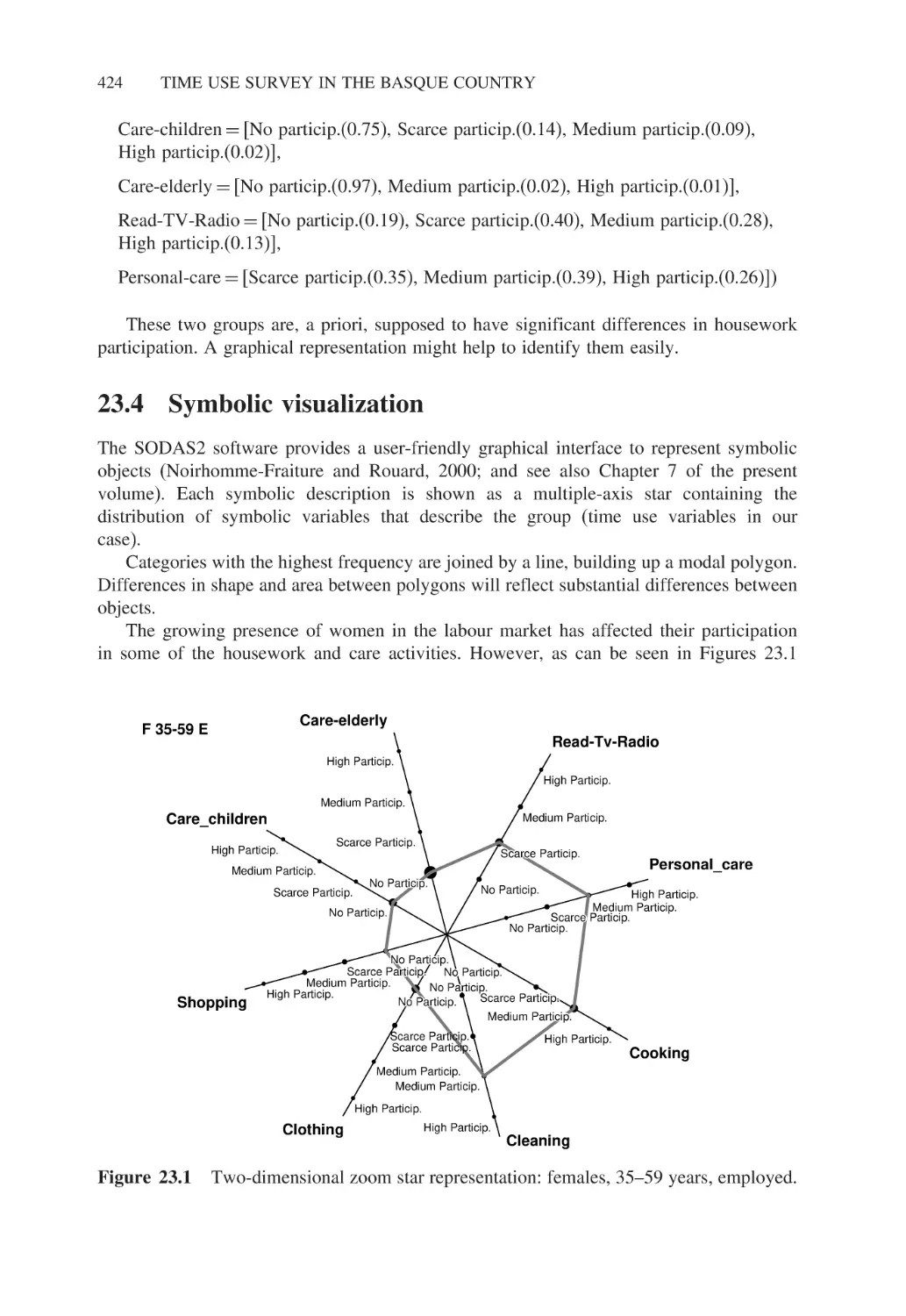
Текст

Symbolic Data Analysis and the
SODAS Software
Edited by

Edwin Diday
Université de Paris IX - Dauphine, France

Monique Noirhomme-Fraiture
University of Namur, Belgium

This page intentionally left blank

Symbolic Data Analysis and the
SODAS Software

This page intentionally left blank

Symbolic Data Analysis and the
SODAS Software
Edited by

Edwin Diday
Université de Paris IX - Dauphine, France

Monique Noirhomme-Fraiture
University of Namur, Belgium

John Wiley & Sons Ltd, The Atrium, Southern Gate, Chichester,
West Sussex PO19 8SQ, England
Telephone +44 1243 779777

Email (for orders and customer service enquiries): cs-books@wiley.co.uk
Visit our Home Page on www.wiley.com
All Rights Reserved. No part of this publication may be reproduced, stored in a retrieval system or transmitted
in any form or by any means, electronic, mechanical, photocopying, recording, scanning or otherwise, except
under the terms of the Copyright, Designs and Patents Act 1988 or under the terms of a licence issued by the
Copyright Licensing Agency Ltd, 90 Tottenham Court Road, London W1T 4LP, UK, without the permission
in writing of the Publisher. Requests to the Publisher should be addressed to the Permissions Department,
John Wiley & Sons Ltd, The Atrium, Southern Gate, Chichester, West Sussex PO19 8SQ, England, or emailed to
permreq@wiley.co.uk, or faxed to (+44) 1243 770620.
This publication is designed to provide accurate and authoritative information in regard to the subject matter
covered. It is sold on the understanding that the Publisher is not engaged in rendering professional services.
If professional advice or other expert assistance is required, the services of a competent professional should be
sought.
Other Wiley Editorial Offices
John Wiley & Sons Inc., 111 River Street, Hoboken, NJ 07030, USA
Jossey-Bass, 989 Market Street, San Francisco, CA 94103-1741, USA
Wiley-VCH Verlag GmbH, Boschstr. 12, D-69469 Weinheim, Germany
John Wiley & Sons Australia Ltd, 42 McDougall Street, Milton, Queensland 4064, Australia
John Wiley & Sons (Asia) Pte Ltd, 2 Clementi Loop #02-01, Jin Xing Distripark, Singapore 129809
John Wiley & Sons Canada Ltd, 6045 Freemont Blvd, Mississauga, ONT, L5R 4J3
Wiley also publishes its books in a variety of electronic formats. Some content that appears in print may
not be available in electronic books.
Library of Congress Cataloging in Publication Data
Symbolic data analysis and the SODAS software / edited by Edwin Diday,
Monique Noirhomme-Fraiture.
p. cm.
Includes bibliographical references and index.
ISBN 978-0-470-01883-5 (cloth)
1. Data mining. I. Diday, E. II. Noirhomme-Fraiture, Monique.
QA76.9.D343S933 2008
005.74—dc22
2007045552
British Library Cataloguing in Publication Data
A catalogue record for this book is available from the British Library
ISBN 978-0-470-01883-5
Typeset in 10/12pt Times by Integra Software Services Pvt. Ltd, Pondicherry, India
Printed and bound in Great Britain by Antony Rowe Ltd, Chippenham, Wiltshire
This book is printed on acid-free paper responsibly manufactured from sustainable forestry
in which at least two trees are planted for each one used for paper production.

Contents

Contributors
Foreword
Preface

Introduction
The state of the art in symbolic data analysis: overview
and future
Edwin Diday

Part I
2

xiii
xv

ASSO Partners

Databases versus Symbolic Objects

Improved generation of symbolic objects from relational
databases
Yves Lechevallier, Aicha El Golli and George Hébrail

xvii

1
3

43
45

Exporting symbolic objects to databases
Donato Malerba, Floriana Esposito and Annalisa Appice

A statistical metadata model for symbolic objects
Haralambos Papageorgiou and Maria Vardaki

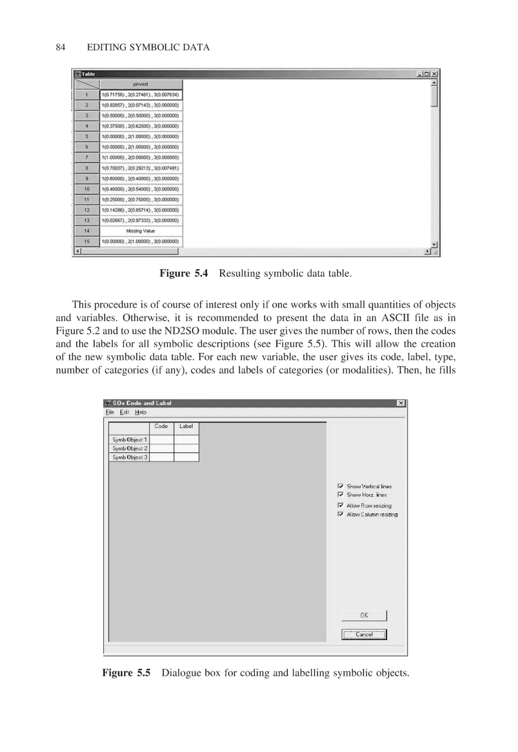
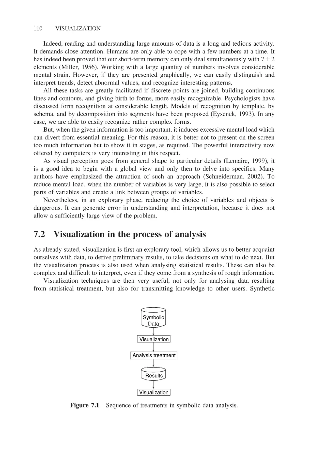
Editing symbolic data
Monique Noirhomme-Fraiture, Paula Brito,
Anne de Baenst-Vandenbroucke and Adolphe Nahimana

The normal symbolic form
Marc Csernel and Francisco de A.T. de Carvalho

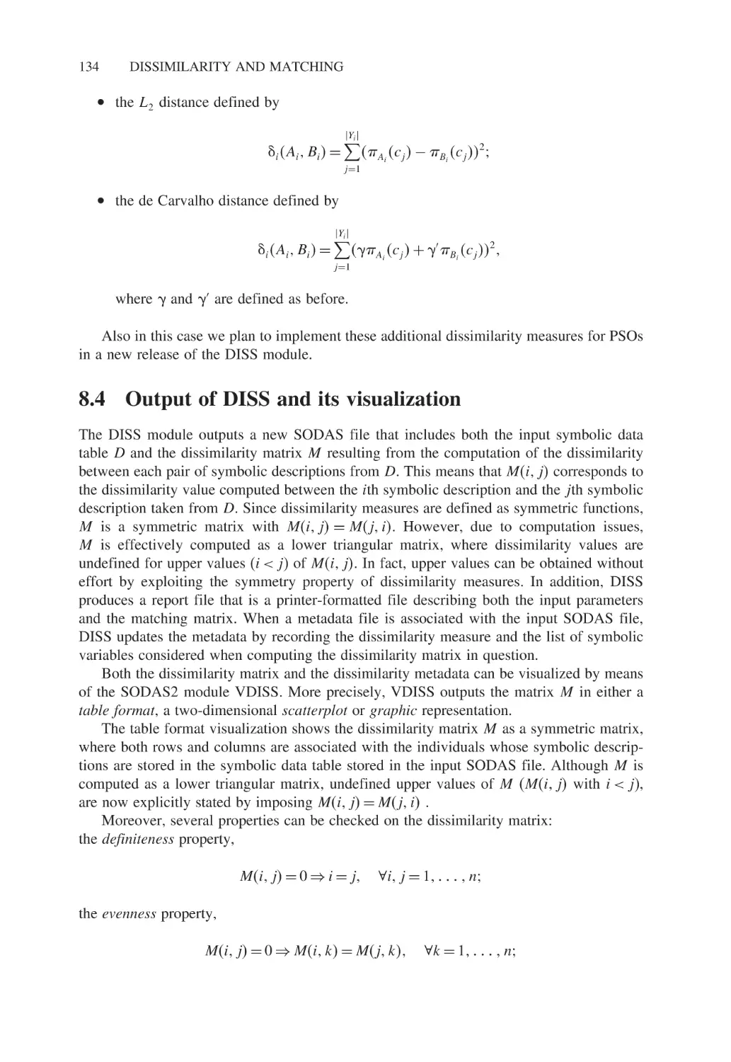
Visualization
Monique Noirhomme-Fraiture and Adolphe Nahimana

109

CONTENTS

Part II

Unsupervised Methods

121

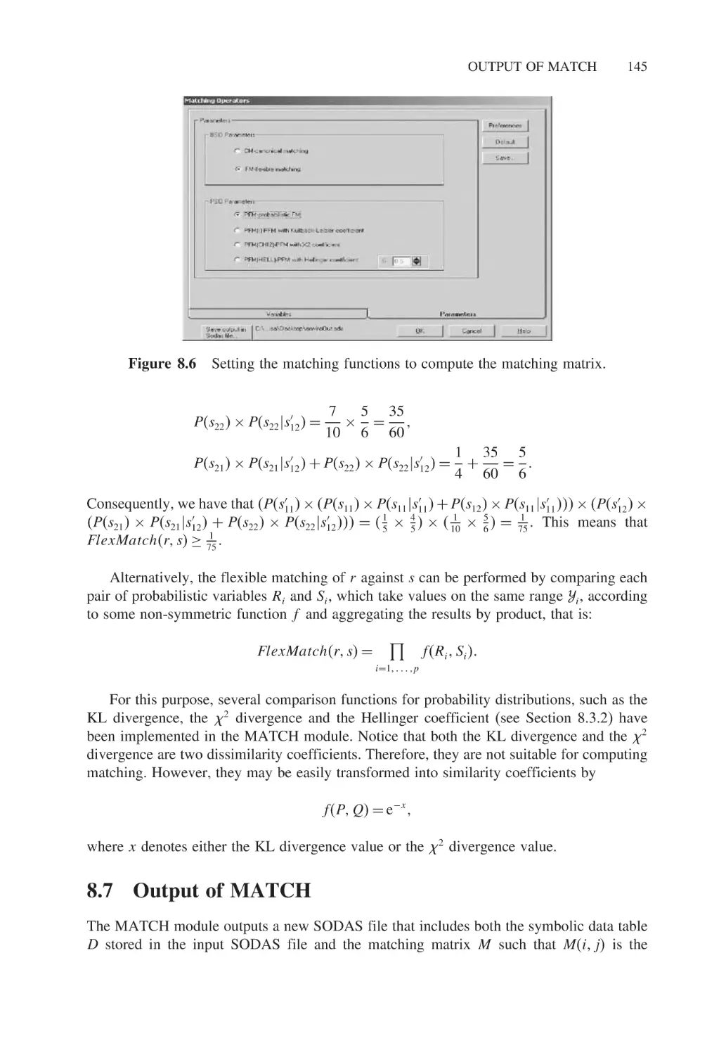
Dissimilarity and matching
Floriana Esposito, Donato Malerba and Annalisa Appice

123

Unsupervised divisive classification
Jean-Paul Rasson, Jean-Yves Pirçon, Pascale Lallemand and
Séverine Adans

149

Hierarchical and pyramidal clustering
Paula Brito and Francisco de A.T. de Carvalho

157

Clustering methods in symbolic data analysis
Francisco de A.T. de Carvalho, Yves Lechevallier and
Rosanna Verde

181

Visualizing symbolic data by Kohonen maps
Hans-Hermann Bock

205

Validation of clustering structure: determination of the
number of clusters
André Hardy

235

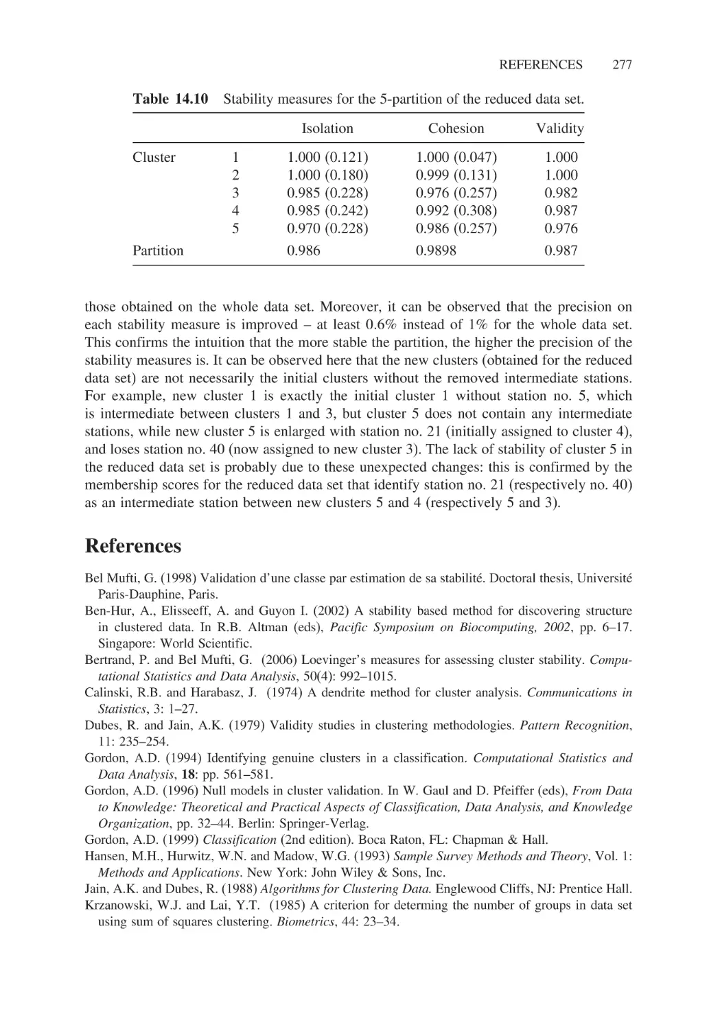
Stability measures for assessing a partition and its clusters:
application to symbolic data sets
Patrice Bertrand and Ghazi Bel Mufti

263

Principal component analysis of symbolic data described by
intervals
N. Carlo Lauro, Rosanna Verde and Antonio Irpino

279

Generalized canonical analysis
N. Carlo Lauro, Rosanna Verde and Antonio Irpino

Part III

Supervised Methods

313

331

Bayesian decision trees
Jean-Paul Rasson, Pascale Lallemand and Séverine Adans

333

Factor discriminant analysis
N. Carlo Lauro, Rosanna Verde and Antonio Irpino

341

Symbolic linear regression methodology
Filipe Afonso, Lynne Billard, Edwin Diday and
Mehdi Limam

359

Multi-layer perceptrons and symbolic data
Fabrice Rossi and Brieuc Conan-Guez

373

CONTENTS

Part IV
21

Applications and the SODAS Software

vii

393

Application to the Finnish, Spanish and Portuguese data of the
European Social Survey
Soile Mustjärvi and Seppo Laaksonen

395

People’s life values and trust components in Europe: symbolic data
analysis for 20–22 countries
Seppo Laaksonen

405

Symbolic analysis of the Time Use Survey in the Basque country
Marta Mas and Haritz Olaeta

421

SODAS2 software: Overview and methodology
Anne de Baenst-Vandenbroucke and Yves Lechevallier

429

Index

445

This page intentionally left blank

Contributors

Séverine Adans, Facultés Universitaires Notre-Dame de la Paix, Déprt. de Mathematique,
Rempart de la Vierge, 8, Namur, Belgium, B-5000
Filipe Afonso, Université Paris IX-Dauphine, LISE-CEREMADE, Place du Maréchal de
Lattre de Tassigny, Paris Cedex 16, France, F-75775
Annalisa Appice, Floriana Esposito Universita degli Studi di Bari, Dipartimento di Informatica, v. Orabona, 4, Bari, Italy, I-70125
Anne de Baenst-Vandenbroucke, Facultés Universitaires Notre-Dame de la Paix, Faculté
d’Informatique, Rue Grandgagnage, 21, Namur, Belgium, B-5000, adb@info.fundp.ac.be
Ghazi Bel Mufti, ESSEC de Tunis, 4 rue Abou Zakaria El Hafsi, Montfleury 1089, Tunis,
Tunisia, belmufti@yahoo.com
Patrice Bertrand, Ceremade, Université Paris IX-Dauphine, Place du Maréchal de Lattre de
Tassigny, Paris Cedex 16, France, F-75775, Patrice.Bertrand@ceremade.dauphine.fr
Lynne Billard, University of Georgia, Athens, USA, GA 30602-1952, lynne@stat.uga.edu
Hans-Hermann Bock, Rheinisch-Westfälische Technische Hochschule Aachen, Institut
für Statistik und Wirtschaftmathematik, Wüllnerstr. 3, Aachen, Germany, D-52056,
bock@stochastik.rwth-aachen.de
Maria Paula de Pinho de Brito, Faculdade de Economia do Porto, LIACC, Rua Dr. Roberto
Frias, Porto, Portugal, P-4200-464, mpbrito@fep.up.pt
Brieuc Conan-Guez, LITA EA3097, Université de Metz, Ile de Saulcy, F-57045, Metz,
France, Brieuc.Conan-Suez@univ-metz.fr
Marc Csernel, INRIA, Unité de Recherche de Roquencourt, Domaine de Voluceau, BP 105,
Le Chesnay Cedex, France, F-78153, Marc.Cesrnel@inria.fr

CONTRIBUTORS

Francisco de A.T. de Carvalho, Universade Federale de Pernambuco, Centro de Informatica, Av. Prof. Luis Freire s/n - Citade Universitaria, Recife-PE, Brasil, 50740-540,
fatc@cin.ufpe.br
Edwin Diday, Université Paris IX-Dauphine, LISE-CEREMADE, Place du Marechal de
Lattre de Tassigny, Paris Cedex 16, France F-75775, diday@ceremade.dauphine.fr
Aicha El Golli, INRIA Paris, Unité de Recherche de Roquencourt, Domaine de Voluceau,
BP 105, Le Chesnay Cedex, France, F-78153, aicha.elgolli@inria.fr
Floriana Esposito, Universita degli Studi di Bari, Dipartimento di Informatica, v. Orabona,
4, Bari, Italy, I-70125, esposito@di.uniba.it
André Hardy, Facultés Universitaires Notre-Dame de la Paix, Départment de Mathématique,
Rempart de la Vièrge, 8, Namur, Belgium, B-5000, andre.hardy@math.fundp.ac.be
Georges Hébrail, Laboratoire LTCI UMR 5141, Ecole Nationale Supériewe des Télécommunications, 46 rue Barrault, 75013 Paris, France, hebrail@enst.fr
Antonio Irpino, Universita Frederico II, Dipartimento di Mathematica e Statistica, Via
Cinthia, Monte Sant’Angelo, Napoli, Italy I-80126, irpino@unina.it
Seppo Laaksonen, Statistics Finland, Box 68, University of Helsinki, Finland, FIN 00014,
Seppo.Laaksonen@Helsinki.Fi
Pascale Lallemand, Facultés Universitaires Notre-Dame de la Paix, Départment de Mathématique, Rempart de la Vièrge, 8, Namur, Belgium, B-5000
Natale Carlo Lauro, Universita Frederico II, Dipartimento di Mathematica e Statistica, Via
Cinthia, Monte Sant’Angelo, Napoli, Italy I-80126, clauro@unina.it
Yves Lechevallier, INRIA, Unité de Recherche de Roquencourt, Domaine de Voluceau,
BP 105, Le Chesnay Cedex, France, F-78153, Yves. Lechevallier@inria.fr
Mehdi Limam, Université Paris IX-Dauphine, LISE-CEREMADE, Place du Maréchal de
Lattre de Tassigny, Paris Cedex 16, France, F-75775
Donato Malerba, Universita degli Studi di Bari, Dipartimento di Informatica, v. Orabona,
4, Bari, Italy, I-70125, malerba@di.uniba.it
Marta Mas, Asistencia Tecnica y Metodológica, Beato Tomás de Zumarraga, 52, 3 -Izda,
Vitoria-Gasteiz, Spain, E-01009, Marta_Mas@terra.es
Soile Mustjärvi, Statistics Finland, Finland, FIN-00022

CONTRIBUTORS

Adolphe Nahimana, Facultés Universitaires Notre-Dame de la Paix, Faculté d’Informatique,
Rue Grandgagnage, 21, Namur, Belgium, B-5000
Monique Noirhomme-Fraiture, Facultés Universitaires Notre-Dame de la Paix, Faculté
d’Informatique, Rue Grandgagnage, 21, Namur, Belgium, B-5000, mno@info.fundp.ac.be
Haritz Olaeta, Euskal Estatistika Erakundea, Area de Metodologia, Donostia, 1, VitoriaGasteiz, Spain, E-010010, haritz.olaeta@uniqual.es
Haralambos Papageorgiou, University of Athens, Department of Mathematics, Panepistemiopolis, Athens, Greece, EL-15784, hpapageo@cc.uoa.gr
Jean-Yves Pirçon, Facultés Universitaires Notre-Dame de la Paix, Déprt. de Mathematique,
Rempart de la Vièrge, 8, Namur, Belgium, B-5000
Jean-Paul Rasson, Facultés Universitaires Notre-Dame de la Paix, Départ. de Mathematique,
Rempart de la Vièrge, 8, Namur, Belgium, B-5000, jpr@math.fundp.ac.be
Fabrice Rossi, Projet AxIS, INRIA, Centre de Rechoche Paris-Roquencourt, Domaine de
Volucean, BP 105, Le Chesney Cedex, France F-78153, Fabrice.Rossi@inria.fr
Maria Vardaki, University of Athens, Department of Mathematics, Panepistemiopolis,
Athens, Greece, EL-15784 mvardaki@cc.uoa.gr
Rosanna Verde, Dipartimento di Studi Europei e Mediterranei, Seconda Universitádegli
Studi di Napoli, Via del Setificio, 15 Complesso Monumentale Belvedere di S. Leucio,
81100 Caserta, Italy

This page intentionally left blank

Foreword

It is a great pleasure for me to preface this imposing work which establishes, with Analysis
of Symbolic Data (Bock and Diday, 2000) and Symbolic Data Analysis (Billard and Diday,
2006), a true bible as well as a practical handbook.
Since the pioneering work of Diday at the end of the 1980s, symbolic data analysis
has spread beyond a restricted circle of researchers to attain a stature attested to by many
publications and conferences. Projects have been supported by Eurostat (the statistical office
of the European Union), and this recognition of symbolic data analysis as a tool for official
statistics was also a crucial step forward.
Symbolic data analysis is part of the great movement of interaction between statistics
and data processing. In the 1960s, under the impetus of J. Tukey and of J.P. Benzécri,
exploratory data analysis was made possible by progress in computation and by the need
to process the data which one stored. During this time, large data sets were tables of a
few thousand units described by a few tens of variables. The goal was to have the data
speak directly without using overly simplified models. With the development of relational
databases and data warehouses, the problem changed dimension, and one might say that it
gave birth on the one hand to data mining and on the other hand to symbolic data analysis.
However, this convenient opposition or distinction is somewhat artificial.
Data mining and machine learning techniques look for patterns (exploratory or unsupervised) and models (supervised) by processing almost all the available data: the statistical
unit remains unchanged and the concept of model takes on a very special meaning. A model
is no longer a parsimonious representation of reality resulting from a physical, biological,
or economic theory being put in the form of a simple relation between variables, but a forecasting algorithm (often a black box) whose quality is measured by its ability to generalize to
new data (which must follow the same distribution). Statistical learning theory provides the
theoretical framework for these methods, but the data remain traditional data, represented
in the form of a rectangular table of variables and individuals where each cell is a value of
a numeric variable or a category of a qualitative variable assumed to be measured without
error.
Symbolic data analysis was often presented as a way to process data of another kind,
taking variability into account: matrix cells do not necessarily contain a single value but an
interval of values, a histogram, a distribution. This vision is exact but reductive, and this book
shows quite well that symbolic data analysis corresponds to the results of database operations
intended to obtain conceptual information (knowledge extraction). In this respect symbolic

xiv

FOREWORD

data analysis can be considered as the statistical theory associated with relational databases.
It is not surprising that symbolic data analysis found an important field of application in
official statistics where it is essential to present data at a high level of aggregation rather
than to reason on individual data. For that, a rigorous mathematical framework has been
developed which is presented in a comprehensive way in the important introductory chapter
of this book.
Once this framework was set, it was necessary to adapt the traditional methods to
this new type of data, and Parts II and III show how to do this both in exploratory
analysis (including very sophisticated methods such as generalized canonical analysis) and
in supervised analysis where the problem is the interrelation and prediction of symbolic
variables. The chapters dedicated to cluster analysis are of great importance. The methods
and developments gathered together in this book are impressive and show well that symbolic
data analysis has reached full maturity.
In an earlier paragraph I spoke of the artificial opposition of data mining and symbolic
data analysis. One will find in this book symbolic generalizations of methods which are
typical of data mining such as association rules, neural networks, Kohonen maps, and
classification trees. The border between the two fields is thus fairly fluid.
What is the use of sound statistical methods if users do not have application software at
their disposal? It is one of the strengths of the team which contributed to this book that they
have also developed the freely available software SODAS2. I strongly advise the reader to
use SODAS2 at the same time as he reads this book. One can only congratulate the editors
and the authors who have brought together in this work such an accumulation of knowledge
in a homogeneous and accessible language. This book will mark a milestone in the history
of data analysis.
Gilbert Saporta

Preface

This book is a result of the European ASSO project (IST-2000-25161) http://www.
assoproject.be on an Analysis System of Symbolic Official data, within the Fifth Framework
Programme. Some 10 research teams, three national institutes for statistics and two private
companies have cooperated in this project. The project began in January 2001 and ended
in December 2003. It was the follow-up to a first SODAS project, also financed by the
European Community.
The aim of the ASSO project was to design methods, methodology and software tools
for extracting knowledge from multidimensional complex data (www.assoproject.be). As a
result of the project, new symbolic data analysis methods were produced and new software,
SODAS2, was designed. In this book, the methods are described, with instructive examples,
making the book a good basis for getting to grips with the methods used in the SODAS2
software, complementing the tutorial and help guide. The software and methods highlight
the crossover between statistics and computer science, with a particular emphasis on data
mining.
The book is aimed at practitioners of symbolic data analysis – statisticians and economists
within the public (e.g. national statistics institutes) and private sectors. It will also be of
interest to postgraduate students and researchers within data mining.

Acknowledgements
The editors are grateful to ASSO partners and external authors for their careful work and
contributions. All authors were asked to review chapters written by colleagues so that we
could benefit from internal cross-validation. In this regard, we wish especially to thank
Paula Brito, who revised most of the chapters. Her help was invaluable. We also thank
Pierre Cazes who offered much substantive advice. Thanks are due to Photis Nanopulos and
Daniel Defays of the European Commission who encouraged us in this project and also to
our project officer, Knut Utwik, for his patience during this creative period.
Edwin Diday
Monique Noirhomme-Fraiture

This page intentionally left blank

ASSO Partners

FUNDP Facultés Universitaires Notre-Dame de la Paix, Institut d’Informatique, Rue
Grandgagnage, 21, Namur, Belgium, B-5000 mno@info.fundp.ac.be (coordinator)
DAUPHINE Université Paris IX-Dauphine, LISE-CEREMADE, Place du Maréchal de
Lattre de Tassigny, Paris Cedex 16, France, F-75775 rossi@ceremade.dauphine.fr
DIB Universita degli Studi di Bari, Dipartimento di Informatica, v. Orabona, 4, Bari, Italy,
I-70125 esposito@di.uniba.it
DMS Dipartimento di Mathematica e Statistica, Via Cinthia, Monte Sant’Angelo, Napoli,
Italy I-80126 clauro@unina.it
EUSTAT Euskal Estatistika Erakundea, Area de Metodologia, Donostia, 1, Vitoria-Gasteiz,
Spain, E-01010 Marina_Ayestaran@eustat.es
FEP Faculdade de Economia do Porto, LIACC, Rua Dr. Roberto Frias, Porto, Portugal,
P-4200-464 mpbrito@fep.up.pt
FUNDPMa Facultés Universitaires Notre-Dame de la Paix, Rempart de la Vierge, 8,
Namur, Belgium, B-5000 jpr@math.fundp.ac.be
INRIA, Unité de Recherche de Roquencourt, Domaine de Voluceau, BP 105, Le Chesnay
Cedex, France, F-78153 Yves.Lechevallier@inria.fr
INS Instituto Nacional de Estatistica, Direcçao Regional de Lisboa e Valo do Tejo, Av.
Antonio José de Almeida, Lisboa, Portugal, P-1000-043 carlos.marcelo@ine.pt
RWTH Rheinisch-westfälische Technische Hochschule Aachen, Institut für Statistik
und Wirtschaftmathematik, Wülnerstr, 3, Aachen, Germany, D-52056 bock@stochastik.
rwth-aachen.de

xviii

ASSO PARTNERS

SPAD Groupe TestAndGO, Rue des petites Ecuries, Paris, France, F-75010
p.pleuvret@decisia.fr
STATFI Statistics Finland, Management Services/R&D Department, Tyoepajakatu, 13,
Statistics Finland, Finland, FIN-00022 Seppo.Laaksonen@Stat.fi
TES Institute ASBL, Rue des Bruyères, 3, Howald, Luxembourg, L-1274
UFPE Universade Federale de Pernambuco, Centro de Informatica-Cin, Citade Universitaria, Recife-PE, Brasil, 50740-540 fatc@cin.ufpe.br
UOA University of Athens, Department of Mathematics, Panepistemiopolis, Athens, Greece,
EL-15784 hpapageo@cc.uoa.gr

INTRODUCTION

This page intentionally left blank

The state of the art in symbolic
data analysis: overview
and future
Edwin Diday

1.1 Introduction
Databases are now ubiquitous in industrial companies and public administrations, and they
often grow to an enormous size. They contain units described by variables that are often
categorical or numerical (the latter can of course be also transformed into categories). It
is then easy to construct categories and their Cartesian product. In symbolic data analysis
these categories are considered to be the new statistical units, and the first step is to get
these higher-level units and to describe them by taking care of their internal variation. What
do we mean by ‘internal variation’? For example, the age of a player in a football team is
32 but the age of the players in the team (considered as a category) varies between 22 and
34; the height of the mushroom that I have in my hand is 9 cm but the height of the species
(considered as a category) varies between 8 and 15 cm.
A more general example is a clustering process applied to a huge database in order to
summarize it. Each cluster obtained can be considered as a category, and therefore each
variable value will vary inside each category. Symbolic data represented by structured
variables, lists, intervals, distributions and the like, store the ‘internal variation’ of categories
better than do standard data, which they generalize. ‘Complex data’ are defined as structured
data, mixtures of images, sounds, text, categorical data, numerical data, etc. Therefore,
symbolic data can be induced from categories of units described by complex data (see
Section 1.4.1) and therefore complex data describing units can be considered as a special
case of symbolic data describing higher-level units.

Symbolic Data Analysis and the SODAS Software Edited by E. Diday and M. Noirhomme-Fraiture
© 2008 John Wiley & Sons, Ltd

THE STATE OF THE ART IN SYMBOLIC DATA ANALYSIS

The aim of symbolic data analysis is to generalize data mining and statistics to higherlevel units described by symbolic data. The SODAS2 software, supported by EUROSTAT, extends the standard tools of statistics and data mining to these higher-level units.
More precisely, symbolic data analysis extends exploratory data analysis (Tukey, 1958;
Benzécri, 1973; Diday et al., 1984; Lebart et al., 1995; Saporta, 2006), and data mining (rule
discovery, clustering, factor analysis, discrimination, decision trees, Kohonen maps, neural
networks, ) from standard data to symbolic data.
Since the first papers announcing the main principles of symbolic data analysis (Diday,
1987a, 1987b, 1989, 1991), much work has been done, up to and including the publication
of the collection edited by Bock and Diday (2000) and the book by Billard and Diday
(2006). Several papers offering a synthesis of the subject can be mentioned, among them
Diday (2000a, 2002a, 2005), Billard and Diday (2003) and Diday and Esposito (2003).
The symbolic data analysis framework extends standard statistics and data mining tools to
higher-level units and symbolic data. For example, standard descriptive statistics (mean,
variance, correlation, distribution, histograms, ) are extended in de Carvalho (1995),
Bertrand and Goupil (2000), Billard and Diday (2003, 2006), Billard (2004) and Gioia
and Lauro (2006a). Standard tools of multidimensional data analysis such as principal
component analysis are extended in Cazes et al. (1997), Lauro et al. (2000), Irpino et al.
(2003), Irpino (2006) and Gioia and Lauro (2006b). Extensions of dissimilarities to symbolic
data can be found in Bock and Diday (2000, Chapter 8), in a series of papers by Esposito
et al. (1991, 1992) and also in Malerba et al. (2002), Diday and Esposito (2003) and Bock
(2005). On clustering, recent work by de Souza and de Carvalho (2004), Bock (2005),
Diday and Murty (2005) and de Carvalho et al. (2006a, 2006b) can be mentioned. The
problem of the determination of the optimum number of clusters in clustering of symbolic
data has been analysed by Hardy and Lallemand (2001, 2002, 2004), Hardy et al. (2002)
and Hardy (2004, 2005). On decision trees, there are papers by Ciampi et al. (2000), Bravo
and García-Santesmases (2000), Limam et al. (2003), Bravo Llatas (2004) and Mballo et al.
(2004). On conceptual Galois lattices, we have Diday and Emilion (2003) and Brito and
Polaillon (2005). On hierarchical and pyramidal clustering, there are Brito (2002) and Diday
(2004). On discrimination and classification, there are papers by Duarte Silva and Brito
(2006), Appice et al. (2006). On symbolic regression, we have Afonso et al. (2004) and de
Carvalho et al. (2004). On mixture decomposition of vectors of distributions, papers include
Diday and Vrac (2005) and Cuvelier and Noirhomme-Fraiture (2005). On rule extraction,
there is the Afonso and Diday (2005) paper. On visualization of symbolic data, we have
Noirhomme-Fraiture (2002) and Irpino et al. (2003). Finally, we might mention Prudêncio
et al. (2004) on time series, Soule et al. (2004) on flow classification, Vrac et al. (2004) on
meteorology, Caruso et al. (2005) on network traffic, Bezera and de Carvalho (2004) on
information filtering, and Da Silva et al. (2006) and Meneses and Rodríguez-Rojas (2006)
on web mining.
This chapter is organized as follows. Section 1.2 examines the transition from a standard
data table to a symbolic data table. This is illustrated by a simple example showing that
single birds can be defined by standard numerical or categorical variables but species of
birds need symbolic descriptions in order to retain their internal variation. Section 1.3 gives
the definitions and properties of basic units such as individuals, categories, classes and
concepts. In order to model a category or the intent of a concept from a set of individuals
belonging to its extent, a generalization process which produces a symbolic description
is used. Explanations are then given of the input of a symbolic data analysis, the five

FROM STANDARD DATA TABLES TO SYMBOLIC DATA TABLES

kinds of variable (numerical, categorical, interval, categorical multi-valued, modal), the
conceptual variables which describe concepts and the background knowledge by means of
taxonomies and rules. Section 1.4 provides some general applications of the symbolic data
analysis paradigm. It is shown that from fuzzy or uncertainty data, symbolic descriptions
are needed in order to describe classes, categories or concepts. Another application concerns
the possibility of fusing data tables with different entries and different variables by using the
same concepts and their symbolic description. Finally, it is shown that much information
is lost if a symbolic description is transformed into a standard classical description by
transforming, for example, an interval into two variables (the maximum and minimum).
In Section 1.5 the main steps and principles of a symbolic data analysis are summarized.
Section 1.6 provides more details on the method of modelling concepts by symbolic objects
based on four spaces (individuals and concepts of the ‘real world’ and their associated
symbolic descriptions and symbolic objects in the ‘modelled world’). The definition, extent
and syntax of symbolic objects are given. This section ends with some advantages of the use
of symbolic objects and how to improve them by means of a learning process. In Section 1.7
it is shown that a generalized kind of conceptual lattice constitutes the underlying structure
of symbolic objects (readers not interested in conceptual lattices can skip this section).
The chapter concludes with an overview of the chapters of the book and of the SODAS2
software.

1.2 From standard data tables to symbolic data tables
Extracting knowledge from large databases is now fundamental to decision-making. In
practice, the aim is often to extract new knowledge from a database by using a standard
data table where the entries are a set of units described by a finite set of categorical or
quantitative variables. The aim of this book is to show that much information is lost if
the units are straitjacketed by such tables and to give a new framework and new tools
(implemented in SODAS2) for the extraction of complementary and useful knowledge
from the same database. In contrast to the standard data table model, several levels of
more or less general units have to be considered as input in any knowledge extraction
process. Suppose we have a standard data table giving the species, flight ability and size
of 600 birds observed on an island (Table 1.1). Now, if the new units are the species
of birds on the island (which are an example of what are called ‘higher-level’ units),
a different answer to the same questions is obtained since, for example, the number of
flying birds can be different from the number of flying species. In order to illustrate
this simple example with some data, Table 1.2 describes the three species of bird on
the island: there are 100 ostriches, 100 penguins and 400 swallows. The frequencies for
the variable ‘flying’ extracted from this table are the reverse of those extracted from
Table 1.1, as shown in Figures 1.1 and 1.2. This means that the ‘micro’ (the birds) and
the ‘macro’ (the species) points of view can give results which are totally different as
the frequency of flying birds in the island is 2/3 but the frequency of the flying species
is 1/3.
Notice that in Table 1.2 the values taken by the variable ‘size’ are no longer numbers
but intervals, which are a first kind of ‘symbolic data’ involving a different kind of variable
from the standard data. New variables can be added in order to characterize the second-level
units such as the variable ‘migration’ which expresses the fact that 90% of the swallows
migrate, all the penguins migrate and the ostriches do not migrate.

THE STATE OF THE ART IN SYMBOLIC DATA ANALYSIS
On an island there are 600 hundred birds:
400 swallows,
100 ostriches,
100 penguins

Figure 1.1
Table 1.1

Three species of 600 birds together.

Description of 600 birds by three variables.

Birds

Species

Flying

599
600

Penguin

Swallow
Ostrich

Yes
No

Size
80

70
125

Table 1.2 Description of the three species of birds plus
the conceptual variable ‘migration’.
Species

Flying

Size

Swallow

{Yes}

[60, 85]

Ostrich

{No}

[85, 160]

Penguin

{No}

[70, 95]

Frequency of birds

Frequency of species

2/3

1/3

1/3
Flying

Figure 1.2

Migration

Not Flying

Flying

Not Flying

Frequencies for birds (individuals) and species (concepts).

As shown in Table 1.3, the need to consider different unit levels can arise in many
domains. For example, one might wish to find which variables distinguish species having
avian influenza from those that do not. In sport, the first-order units may be the players
and the higher-level unit the teams. For example, in football (see Table 1.4), in order to
find which variables best explain the number of goals scored, it may be interesting to study
first-level units in the form of the players in each team, described by different variables
such as their weight, age, height, nationality, place of birth and so on. In this case, the

FROM STANDARD DATA TABLES TO SYMBOLIC DATA TABLES

Table 1.3 Examples of first- and second-order units and requirements on the second-order
units (i.e., the concepts).
First-level units (individuals) Second-level units (concepts) Requirements on concepts
Birds
Players on a team

Species of birds
Teams

Teams

Continent

Patients

Patients’ hospital pathway

Medical records

Insured patients

Books

Publishers

Travellers

Trains

Customers

Shops

Compare species of birds
Which variables explain
the number of goals
scored by teams?
Which variables explain
the winning continent?
Which variables explain
risky pathways?
Which variables explain
patient consumption?
Find clusters of
publishers
Study trains with the
same profit interval
Compare shops

Table 1.4 Initial classical data table describing players by three numerical
and two categorical variables.
Player

Team

Age

Weight

Height

Nationality1

Fernández
Rodríguez
Mballo
Zidane

Spain
Spain
France
France

29
23
25
27

85
90
82
78

184
192
190
185

Spanish
Brazilian
Senegalese
French

Table 1.5 Symbolic data table obtained from Table 1.4 by describing the concepts ‘Spain’
and ‘France’.
Team

AGE

WEIGHT

Spain [23, 29] [85, 90]
France [21, 28] [85, 90]

HEIGHT

Nationality3

FUNDS

[1.84, 1.92] (0.5 Sp , 0.5 Br) 110
[1.84, 1.92] (0.5 Fr, 0.5 Se) 90

Number of goals at
the World Cup 1998
18
24

task is to explain the number of goals scored by a player. If the task is to find an explanation
for the number of goals scored by a team (during the World Cup, for example), then the
teams are the units of interest. The teams constitute higher-level units defined by variables
whose values will no longer be quantitative (age, weight or height) but intervals (say, the
confidence interval or the minimum–maximum interval). For example, Rodríguez is the
youngest player and Fernández the oldest in the Spain team in the symbolic data table
(Table 1.5) where the new units are teams, and the variable ‘age’ becomes an interval-valued

THE STATE OF THE ART IN SYMBOLIC DATA ANALYSIS

variable denoted ‘AGE’ such that AGE(Spain) = 23 29. The categorical variables (such
as the nationality or the place of birth) of Table 1.4 are no longer categorical in the symbolic
data table. They are transformed into new variables whose values are several categories
with weights defined by the frequencies of the nationalities (before naturalization in some
cases), place of birth, etc., in each team. It is also possible to enhance the description of
the higher-level units by adding new variables such as the variable ‘funds’ which concerns
the higher-level units (i.e., the teams) and not the lower-level units (i.e., the players). Even
if the teams are considered in Table 1.5 as higher-level units described by symbolic data,
they can be considered as lower-level units of a higher-level unit which are the continents,
in which case the continents become the units of a higher-level symbolic data table.
The concept of a hospital pathway followed by a given patient hospitalized for a disease
can be defined by the type of healthcare institution at admission, the type of hospital unit
and the chronological order of admission in each unit. When the patients are first-order units
described by their medical variables, the pathways of the patients constitute higher-level
units as several patients can have the same pathway. Many questions can be asked which
concern the pathways and not the patients. For example, to compare the pathways, it may
be interesting to compare their symbolic description based on the variables which describe
the pathways themselves and on the medical symbolic variables describing the patients on
the pathways.
Given the medical records of insured patients for a given period, the first-order units are
the records described by their medical consumption (doctor, drugs, ); the second-order
units are the insured patients described by their own characteristics (age, gender, ) and
by the symbolic variables obtained from the first-order units associated with each patient.
A natural question which concerns the second-order units and not the first is, for example,
what explains the drug consumption of the patients? Three other examples are given in
Table 1.3: when the individuals are books, each publisher is associated with a class of
books; hence, it is possible to construct the symbolic description of each publisher or of the
most successful publishers and compare them; when the individuals are travellers taking
a train, it is possible to obtain the symbolic description of classes of travellers taking the
same train and study, for example, the symbolic description of trains having the same profit
interval. When the individuals are customers of shops, each shop can be associated with the
symbolic description of its customers’ behaviour and compared with the other shops.

1.3 From individuals to categories, classes and concepts
1.3.1 Individuals, categories, classes, concepts
In the following, the first-order units will be called ‘individuals’. The second-level units
can be called ‘classes’, ‘categories’ or ‘concepts’. A second-level unit is a class if it is
associated with a set of individuals (like the set of 100 ostriches); it is a category if it is
associated with a value of a categorical variable (like the category ‘ostrich’ for the variable
‘species’); it is a concept if it is associated with an ‘extent’ and an ‘intent’. An extent is a set
of individuals which satisfy the concept (for the concept ‘ostrich’ in general, for example,
this would be the set of all ostriches which exist, have existed or will exist); an intent is a
way to find the extent of a concept (such as the mapping that we have in our mind which
allows us to recognize that something is an ostrich). In practice, an approximation of the

FROM INDIVIDUALS TO CATEGORIES, CLASSES AND CONCEPTS

intent of a concept is modelled mathematically by a generalization process applied to a set
of individuals considered to belong to the extent of the concept. The following section aims
to explain this process.

1.3.2 The generalization process, symbolic data and symbolic variables
A generalization process is applied to a set of individuals in order to produce a ‘symbolic
description’. For example, the concept ‘swallow’ is described (see Table 1.2) by the description vector d = ({yes}, [60, 85], [90% yes, 10% no]). The generalization process must
take care of the internal variation of the description of the individuals belonging in the set
of individuals that it describes. For example, the 400 swallows on the island vary in size
between 60 and 85. The variable ‘colour’ could also be considered; hence, the colour of the
ostriches can be white or black (which expresses a variation of the colour of the ostriches
on this island between white and black), the colour of the penguins is always black and
white (which does not express any variation but a conjunction valid for all the birds of this
species), and the colour of the swallows is black and white or grey. This variation leads
to a new kind of variable defined on the set of concepts, as the value of such variables
for a concept may be a single numerical or categorical value, but also an interval, a set of
ordinal or categorical values that may or may not be weighted, a distribution, etc. Since
these values are not purely numerical or categorical, they have been called ‘symbolic data’.
The associated variables are called ‘symbolic variables’.
More generally, in order to find a unique description for a concept, the notion of the
‘T-norm of descriptive generalization’ can be used (see, for example, Diday, 2005). The
T-norm operator (Schweizer and Sklar, 2005) is defined from 0 1 × 0 1 to [0, 1]. In
order to get a symbolic description dC of C (i.e., of the concept for which C is an extent),
an extension to descriptions of the usual T-norm can be used; this is called a ‘T-norm of
descriptive generalization’.
Bandemer and Nather (1992) give many examples of T-norms and T-conorms which
can be generalized to T-norms and T-conorms of descriptive generalization. For example,
it is easy to see that the infimum and supremum (denoted inf and sup) are respectively a Tnorm and a T-conorm. They are also a T-norm and T-conorm of descriptive generalization.
Let DC be the set of descriptions of the individuals of C. It follows that the interval
Gy C = infDC supDC constitutes a good generalization of DC , as its extent defined
by the set of descriptions included in the interval contains C in a good and narrow way.
Let C = w1 w2 w3 and DC = yw1 yw2 yw3 = yC. In each of the following
examples, the generalization of C for the variable y is denoted Gy C.
1. Suppose that y is a standard numerical variable such that yw1 = 25 yw2 =
36 yw3 = 71. Let D be the set of values included in the interval [1, 100]. Then
Gy C = 25 71 is the generalization of DC for the variable y.
2. Suppose that y is a modal variable of ordered (e.g., small, medium, large) or not ordered
(e.g., London, Paris, ) categories, such that: yw1 = 11/3 22/3 (where 2(2/3)
means that the frequency of the category 2 is 2/3), yw2 = 11/2 21/2 yw3 =
11/4 23/4. Then, Gy C = 11/4 11/2 21/2 23/4 is the generalization of DC for the variable y.

THE STATE OF THE ART IN SYMBOLIC DATA ANALYSIS

3. Suppose that y is a variable whose values are intervals such that: yw1 =
15 32 yw2 = 36 4 yw3 = 71 84. Then, Gy C = 15 84 is the generalization of DC for the variable y.
Instead of describing a class by its T-norm and T-conorm, many alternatives are possible
by taking account, for instance, of the existence of outliers. A good strategy consists of
reducing the size of the boundaries in order to reduce the number of outliers. This is
done in DB2SO (see Chapter 2) within the SODAS2 software by using the ‘gap test’ (see
Stéphan, 1998). Another choice in DB2SO is to use the frequencies in the case of categorical
variables.
For example, suppose that C = w1 w2 w3 , y is a standard unordered categorical
variable such that yw1 = 2 yw2 = 2 yw3 = 1, D is the set of probabilities on the values
1, 2. Then G yC = 11/3 22/3 is the generalization of DC = yw1 yw2 yw3 =
yC for the variable y.

1.3.3 Inputs of a symbolic data analysis
In this book five main kinds of variables are considered: numerical (e.g.,
height(Tom) = 1.80); interval (e.g., age(Spain) = [23, 29]); categorical single-valued
(e.g., Nationality1 (Mballo) = {Congo}); categorical multi-valued (e.g., Nationality2 (Spain)
= {Spanish, Brazilian, French}); and modal (e.g., Nationality3 (Spain) = {(0.8)Spanish,
(0.1)Brazilian, (0.1)French}, where there are several categories with weights).
‘Conceptual variables’ are variables which are added to the variables which describe
the second-order units, because they are meaningful for the second-order units but not for
the first-order units. For example, the variable ‘funds’ is a conceptual variable as it is
added at the level where the second-order units are the football teams and would have less
meaning at the level of the first-order units (the players). In the SODAS2 software, within
the DB2SO module, the option ADDSINGLE allows conceptual variables to be added (see
Chapter 2).
From lower- to higher-level units missing data diminish in number but may exist. That
is why SODAS2 allows them to be taken into account(see Chapter 24). Nonsense data may
also occur and can be also introduced in SODAS2 by the so-called ‘hierarchically dependent
variables’ or ‘mother–daughter’ variables. For example, the variable ‘flying’ whose answer
is ‘yes’ or ‘no’, has a hierarchical link with the variable ‘speed of flying’. The variable
‘flying’ can be considered as the mother variable and ‘speed of flying’ as the daughter. As
a result, for a flightless bird, the variable ‘speed of flying’ is ‘not applicable’.
In the SODAS2 software it is also possible to add to the input symbolic data table some
background knowledge, such taxonomies and some given or induced rules. For example,
the variable ‘region’ can be given with more or less specificity due, for instance, to confidentiality. This variable describes a set of companies in Table 1.6. The links between its
values are given in Figure 1.3 by a taxonomic tree and represented in Table 1.7 by two
columns, associating each node of the taxonomic tree with its predecessor.
Logical dependencies can also be introduced as input; for example, ‘if age(w) is less
than 2 months, then height(w) is less than 80’. As shown in the next section, these kinds of
rules can be induced from the initial data table and added as background knowledge to the
symbolic data table obtained.

FROM INDIVIDUALS TO CATEGORIES, CLASSES AND CONCEPTS

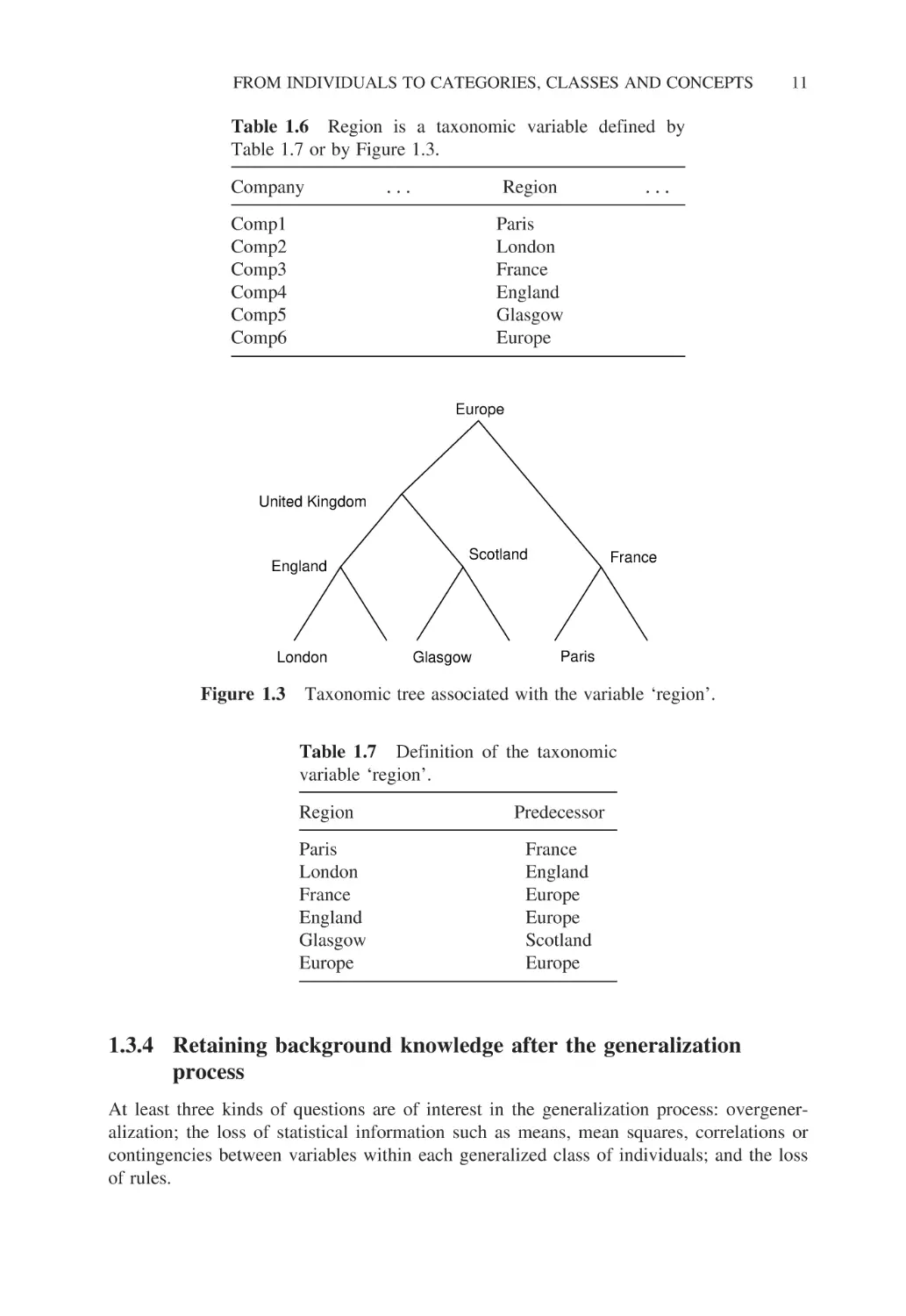
Table 1.6 Region is a taxonomic variable defined by
Table 1.7 or by Figure 1.3.
Company

Region

Comp1
Comp2
Comp3
Comp4
Comp5
Comp6

Paris
London
France
England
Glasgow
Europe

Europe

United Kingdom

England

London

Figure 1.3

Scotland

Glasgow

France

Paris

Taxonomic tree associated with the variable ‘region’.
Table 1.7 Definition of the taxonomic
variable ‘region’.
Region
Paris
London
France
England
Glasgow
Europe

Predecessor
France
England
Europe
Europe
Scotland
Europe

1.3.4 Retaining background knowledge after the generalization
process
At least three kinds of questions are of interest in the generalization process: overgeneralization; the loss of statistical information such as means, mean squares, correlations or
contingencies between variables within each generalized class of individuals; and the loss
of rules.

THE STATE OF THE ART IN SYMBOLIC DATA ANALYSIS

Overgeneralization happens, for example, when a class of individuals described by a
numerical variable is generalized by an interval containing smaller and greater values. For
example, in Table 1.5 the age of the Spain team is described by the interval [23, 29]; this is
one of several possible choices. Problems with choosing [min, max] can arise when these
extreme values are in fact outliers or when the set of individuals to generalize is in fact
composed of subsets of different distributions. These two cases are considered in Chapter 2.
How can correlations lost by generalization be recaptured? It suffices to create new
variables associated with pairs of the initial variables. For example, a new variable called
Cor(yi yj ) can be associated with the variables yi and yj . Then the value of such a variable
for a class of individuals Ck is the correlation between the variables yi and yj on a population
reduced to the individuals of this class. For example, in Table 1.8 the players in the World
Cup are described by their team, age, weight, height, nationality, etc. and by the categorical
variable ‘World Cup’ which takes the value yes or no depending on the fact that they have
played in or have been eliminated from the World Cup. In Table 1.9, the categories defined
by the variable ‘World Cup’ constitute the new unit and the variable Cor(Weight, Height)
has been added and calculated. As a result, the correlation between the weight and the height
is greater for the players who play in the World Cup than for the others. In the same way,
other variables can be added to the set of symbolic variables as variables representing the
mean, the mean square, the median and other percentiles associated with each higher-level
unit.
In the same way, it can be interesting to retain the contingency between two or more
categorical variables describing a concept. This can be done simply by creating new variables
which expresses this contingency. For example, if y1 is a categorical variable with four
categories and y2 is a variable with six categories, a new model variable y3 with 24 categories
which is the Cartesian product of y1 and y2 can be created for each concept. In the case
of numerical variables, it is also possible to retain the number of units inside an interval
or inside a product of intervals describing a concept by adding new variables expressing
the number of individuals that they contain. For example, suppose that the set of birds in
Table 1.1 is described by two numerical variables, ‘size’ and ‘age’, and the species swallow
is described by the cross product of two confidence intervals: Iswallow (size) and Iswallow (age).
The extent of the concept ‘swallow’ described by the cross product Iswallow (size) ×Iswallow
(age) among the birds can be empty or more or less dense. By keeping the contingencies
information among the 600 hundred birds for each concept, a biplot representation of the
Table 1.8

Classical data table describing players by numerical and categorical variables.

Player

Team

Age

Weight

Height

Nationality1

Ferández
Rodríguez
Mballo
Zidane
…
Renie
Olar
Mirce
Rumbum

Spain
Spain
France
France
…
XX
XX
XXX
XXX

29
23
25
27
…
23
29
24
30

85
90
82
78
…
91
84
83
81

1.84
1.92
1.90
1.85
…
1. 75
1.84
1.83
1.81

Spanish
Brazilian
Senegalese
French
…
Spanish
Brazilian
Senegalese
French

World Cup
yes
yes
yes
yes

no
no
no
no

GENERAL APPLICATIONS OF THE SYMBOLIC DATA ANALYSIS APPROACH

Table 1.9 Symbolic data table obtained from Table 1.8 by generalization
for the variables age, weight and height and keeping back the correlations
between weight and height.
World Cup
yes
no

Age

Weight

Height

Cov (Weight, Height)

[21, 26]
[23, 30]

[78, 90]
[81, 92]

[1.85, 1.98]
[1.75, 1.85]

0.85
0.65

Table 1.10 Initial classical data table where individuals
are described by three variables.
Individuals
I1
I2
I3
I4
I5
I6

Concepts

C1
C1
C1
C2
C2
C2

a
b
c
b
b
a

2
1
2
1
3
2

Table 1.11 Symbolic data table induced from Table 1.10
with background knowledge defined by two rules: Y1 =
a ⇒ Y2 = 2 and Y2 = 1 ⇒ Y1 = b.

C1
C2

{a, b, c}
{a, b}

{1, 2}
{1, 2, 3}

species with these two variables will be enhanced by visualizing the density in each obtained
rectangle Ispecies (size) ×Ispecies (age) for each species.
Finally, how can rules lost by generalization be recaptured? Rules can be induced from
the initial standard data table and then added as background knowledge to the symbolic
data table obtained by generalization. For example, from the simple data table in Table 1.10
two rules can be induced: Y1 = a ⇒ Y2 = 2 and Y2 = 1 ⇒ Y1 = b. These rules can be
added as background knowledge to the symbolic data table (Table 1.11) which describes
the concepts C1 and C2 by categorical multi-valued variables.

1.4 Some general applications of the symbolic data analysis
approach
1.4.1 From complex data to symbolic data
Sometimes the term ‘complex data’ refers to complex objects such as images, video, audio
or text documents or any kind of complex object described by standard numerical and/or
categorical data. Sometimes it refers to distributed data or structured data – or, more

THE STATE OF THE ART IN SYMBOLIC DATA ANALYSIS

Table 1.12 Patients described by complex data which can be transformed into classical
numerical or categorical variables.
Patient

Category

X-Ray

Patient1

Patientn

X-Ray1

X-Rayn

Table 1.13
Categories
C1

Radiologist text Doctor text Professional category Age
Rtext1

Rtextn

Dtext1

Dtextn

Worker

Self-employed

Describing categories of patients from Table 1.12 using symbolic data.
X-Ray

Radiologist text

Doctor text

Professional category

Age

{X-Ray}1

{X-Ray}k

{Rtext}1

{Rtext}k

{Dtext}1

{Dtext}k

{worker, unemployed}

{self-employed}

[20, 30]

[35, 55]

specifically, spatial-temporal data or heterogeneous data describing, for example, a medical
patient using a mixture of images, text documents and socio-demographic information. In
practice, complex objects can be modelled by units described by more or less complex data.
Hence, when a description of concepts, classes or categories of such complex objects is
required, symbolic data can be used. Tables 1.12 and 1.13 show how symbolic data are used
to describe categories of patients; the patients are the units of Table 1.12 and the categories
of patients are the (higher-level) units of Table 1.13.
In Table 1.12 patients are described by their category of cancer (level of cancer, for
example), an X-ray image, a radiologist text file, a doctor text file, their professional category
(PC) and age. In Table 1.13, each category of cancer is described by a generalization of
the X-ray image (radiologist text file, doctor text file} denoted {X-Ray} ({Rtext}, {Dtext}).
When the data in Table 1.12 are transformed into standard numerical or categorical data,
the resulting data table, Table 1.13, contains symbolic data obtained by the generalization
process. For example, for a given category of patients, the variable PC is transformed into
a histogram-valued variable by associating the frequencies of each PC category in this
category of patients; the variable age is transformed to an interval variable by associating
with each category the confidence interval of the ages of the patients of this category.

1.4.2 From fuzzy, imprecise, or conjunctive data to symbolic data
The use of ‘fuzzy data’ in data analysis comes from the fact that in many cases users
are more interested in meaningful categorical values such as ‘small’ or ‘average’ than in
actual numerical values. That is to say, they are interested in the membership functions
(Zadeh, 1978; Diday, 1995) associated with these categories. Therefore, they transform their
data into ‘fuzzy data’. Fuzzy data are characterized by fuzzy sets defined by membership
functions. For example, the value 1.60 of the numerical variable ‘height of men’ might be
associated with the value ‘small’ with a weight (i.e. a membership value) of 0.9, ‘average’
with a weight of 0.1, and ‘tall’ with a weight of 0.

GENERAL APPLICATIONS OF THE SYMBOLIC DATA ANALYSIS APPROACH

Table 1.14
Specimen
Mushroom1
Mushroom2
Mushroom3
Mushroom4

Initial data describing mushrooms of different species.
Species

Amanita
Amanita
Amanita
Amanita

muscaria
muscaria
phalloides
phalloides

Stipe
thickness

Stipe
length

15
23
12
20

21
15
10
19

Cap size
24 ± 1
18 ± 1
7 ± 05
15 ± 1

Cap colour
red
red ∧ white
olive green
olive brown

Membership value
Small

Average

Large

0.8

1.6

2.4

1
0.5

1.2 1.5

Stipe thickness

2.0 2.3

Figure 1.4 From numerical data to fuzzy data: if the stipe thickness is 1.2, then it is (0.5)
Small, (0.5) Average, (0) High.

‘Imprecise data’ are obtained when it is not possible to get an exact measure. For
example, it is possible to say that the height of a tree is 10 metres ±1. This means that its
length varies in the interval [9, 11].
‘Conjunctive data’ designate the case where several categories appear simultaneously.
For example, the colour of an apple can be red or green or yellow but it can be also ‘red
and yellow’.
When individuals are described by fuzzy and/or imprecise and/or conjunctive data, their
variation inside a class, category or concept is expressed in term of symbolic data. This is
illustrated in Table 1.14, where the individuals are four mushroom specimens; the concepts
are their associated species (Amanita muscaria, Amanita phalloides). These are described
by their stipe thickness, stipe length, cap size and cap colour. The numerical values of the
variable ‘stipe thickness’ are transformed into a fuzzy variable defined by three fuzzy sets
denoted ‘small’, ‘average’ and ‘high’. The membership functions associated with these fuzzy
sets are given in Figure 1.4: they take three forms with triangular distribution centred on
0.8, 1.6 and 2.4. From Figure 1.4, it can be observed that the stipe thickness of mushroom 1 ,
whose numerical value is 1.5, has a fuzzy measure of 0.2 that it is small, 0.8 that it is
average, and 0 that it is large. The stipe thickness of mushroom2 , whose numerical value is
2.3, has a fuzzy measure of 0 that it is small, 0.1 that it is average. and 0.9 that it is large. In
other words, if the stipe thickness is 2.3, then it is (0)Small, (0.1)Average, (0.9) Large. The
stipe thicknesses for all four individual mushrooms are expressed as fuzzy data as shown
in Table 1.15. For the present purposes, the stipe length is retained as a classical numerical
data. The ‘cap size’ variable values are imprecise and the values of the ‘cap colour’ variable

THE STATE OF THE ART IN SYMBOLIC DATA ANALYSIS

Table 1.15 The numerical data given by the variable ‘stipe thickness’ are transformed
into fuzzy data.
Specimen

Mushroom1
Mushroom2
Mushroom3
Mushroom4

Species

A.
A.
A.
A.

Stipe thickness

muscaria
muscaria
phalloides
phalloides

Table 1.16

Small

Average

Large

0.2
0
0.5
0

0.8
0.1
0.5
0.5

0
0.9
0
0.5

Stipe
length

Cap size

Cap colour

21
15
10
19

24 ± 1
18 ± 1
7 ± 05
15 ± 1

red
red ∧ white
olive green
olive brown

Symbolic data table induced from the fuzzy data of Table 1.15.

Species

Stipe thickness

Stipe length

Cap size

Cap colour

{red, red ∧
white}
{olive
green, olive
brown}

Small

Average

Large

A. muscaria

[0, 0.2]

[0.1, 0.8]

[0, 0.9]

[15, 21]

[17, 25]

A. phalloides

[0, 0.5]

[0.5, 0.5]

[0, 0.5]

[10, 19]

[6.5, 16]

are unique colours or conjunctive colours (i.e., several colours simultaneously, such as ‘red
∧white’).
Suppose that it is desired to describe the two species of Amanita by merging their
associated specimens described in Table 1.15. The extent of the first species (A. muscaria)
is the first two mushrooms (mushroom1 , mushroom2 ). The extent of the second species
(A. phalloides) is the last two mushrooms (mushroom3 , mushroom4 ). The symbolic data
that emerge from a generalization process applied to the fuzzy numerical, imprecise and
conjunctive data of Table 1.15 are as shown in Table 1.16.

1.4.3 Uncertainty, randomness and symbolic data
The meaning of symbolic data, such as intervals, is very important in determining how to
extend statistics, data analysis or data mining to such data. For example, if we considered
the height of a football player without uncertainty we might say that it is 182. But if we
were not sure of his height we could say with some uncertainty that it lies in the interval
I1 = 180 185. That is why, in the following, will say that I1 is an ‘uncertainty height’. If
we now consider the random variable X associated with the height of members of the same
football team, we can associate with X several kinds of symbolic data such as its distribution,
its confidence interval or a sample of heights. If we represent this random variable by its
confidence interval I2 = 180 185, we can see that I1 = I2 but their meanings are completely
different. This comes from the fact that I1 expresses the ‘uncertainty’ given by our own
subjective expectation and I2 expresses the ‘variability’ of the height of the players in the
team. By considering the uncertainty height of all the players of the team we obtain a data
table where the individuals are the players and the variable associates an interval (the height

GENERAL APPLICATIONS OF THE SYMBOLIC DATA ANALYSIS APPROACH

with uncertainty) with each player. We can then calculate the ‘possibility’ (Dubois and
Prade, 1988) that a player has a height in a given interval. For example, the possibility that
a player has a height in the interval I = 175 183 is measured by the higher proportion of
the intervals of height of players which cut the interval I.
By considering the random variable defined by the height of the players of a team in a
competition, we get a random data table where the individuals (of higher level) or concepts
are teams and the variable ‘height’ associates a random variable with each team. We can
then create a symbolic data table which contains in each cell associated with the height and
a given team, a density distribution (or a histogram or confidence interval) induced by the
random variable defined by the height of the players of this team.
Each such density distribution associated with a team expresses the variability of the
height of the players of this team. In symbolic data analysis we are interested by the study of
the variability of these density distributions. For example, we can calculate the probability
that at least one team has a height in the interval I = 175 183. This probability is called
the ‘capacity’ of the teams in the competition to have a height in the interval I = 175 183.
Probabilities, capacities (or ‘belief’) and ‘possibilities’ are compared in Diday (1995). Notice
that in practice such probabilities cannot be calculated from the initial random variables
but from the symbolic data which represent them. For example, in the national institutes of
statistics it is usual to have data where the higher-level units are regions and the symbolic
variables are modal variables which give the frequency distribution of the age of the people
in a region ([0, 5], [5, 10], years old) and, say, the kind of house (farm, house) of
each region. In other words, we have the laws of the random variables but not their initial
values. In SODAS2, the STAT module calculates capacities and provides tools to enable the
study of the variability of distributions. Bertrand and Goupil (2000) and Chapters 3 and 4
of Billard and Diday (2006) provide several tools for the basic statistics of modal variables.

1.4.4 From structured data to symbolic data
There are many kinds of structured data. For example, structured data appear when there
are some taxonomic and/or mother–daughter variables or several linked data tables as in a
relational database. These cases are considered in Chapter 2 of this book. In this section our
aim is to show how several data tables having different individuals and different variables
can be merged into a symbolic data table by using common concepts.
This is illustrated in Tables 1.17 and 1.18. In these data tables the units are different
and only the variable ‘town’ is common. Our aim is to show that by using symbolic data
it is possible to merge these tables into a unique data table where the units are the towns.
In Table 1.17 the individuals are schools, the concepts are towns, and the schools are
described by three variables: the number of pupils, the kind of school (public or private)
and the coded level of the school. The description of the towns by the school variable, after
a generalization process is applied from Table 1.17, is given in Table 1.19. In Table 1.18
the individuals are hospitals, the concepts are towns, and each hospital is described by two
variables: its coded number of beds and its coded specialty. The description of the towns
by the hospital variable, after a generalization process is applied from Table 1.18, is given
in Table 1.20.
Finally, it is easy to merge Tables 1.19 and 1.20 in order to get the symbolic data table
shown in Table 1.21, which unifies the initial Tables 1.17 and 1.18 by using the same
higher-level unit: the concept of town.

THE STATE OF THE ART IN SYMBOLIC DATA ANALYSIS

Classical description of schools.

Table 1.17
School
Jaurès
Condorcet
Chevreul
St Hélène
St Sernin
St Hilaire

Town

No. of pupils

Type

Level

Paris
Paris
Lyon
Lyon
Toulouse
Toulouse

320
450
200
380
290
210

Public
Public
Public
Private
Public
Private

1
3
2
3
1
2

Classical description of hospitals.

Table 1.18
Hospital
Lariboisière
St Louis
Herriot
Besgenettes
Purpan
Marchant

Town

Coded no. of beds

Coded specialty

Paris
Paris
Lyon
Lyon
Toulouse
Toulouse

750
1200
650
720
520
450

5
3
3
2
6
2

Table 1.19 Symbolic description of the towns by the school variable
after a generalization process is applied from Table 1.17.
Town
Paris
Lyon
Toulouse

No. of pupils

Type

Level

[320, 450]
[200, 380]
[210, 290]

(100%)Public
(50%)Public, (50%)Private
(50%)Public, (50%)Private

{1, 3}
{2, 3}
{1, 2}

Table 1.20 Symbolic description of the towns by the hospital variable
after a generalization process is applied from Table 1.18.
Town
Paris
Lyon
Toulouse

Coded no. of beds

Coded specialty

[750, 1200]
[650, 720]
[450, 520]

{3, 5}
{2, 3}
{2, 6}

GENERAL APPLICATIONS OF THE SYMBOLIC DATA ANALYSIS APPROACH

Table 1.21
of towns.

Concatenation of Tables 1.17 and 1.18 by symbolic data versus the concepts

Town

No. of pupils

Paris
Lyon
Toulouse

[320, 450]
[200, 380]
[210, 290]
Table 1.22
analysis.

Type

Level

Coded no.
of beds

Coded
specialty

(100%)Public
(50%)Public, (50%)Private
(50%)Public, (50%)Private

{1, 3}
{2, 3}
{1, 2}

[750, 1200]
[650, 720]
[450, 520]

{3, 5}
{2, 3}
{2, 6}

The four cases of statistical or data mining

Classical data
Symbolic data

Classical analysis

Symbolic analysis

Case 1
Case 3

Case 2
Case 4

1.4.5 The four kinds of statistics and data mining
Four kinds of statistics and data mining (see Table 1.22) can be considered: the classical
analysis of classical data where variables are standard numerical or categorical (case 1); the
symbolic analysis of classical data (case 2); the classical analysis of symbolic data (case
3); and the symbolic analysis of symbolic data (case 4). Case 1 is standard. Case 2 consists
of extracting a symbolic description from a standard data table; for example, symbolic
descriptions are obtained from a decision tree by describing the leaves by the conjunction
of the properties of their associated branches.
In case 3 symbolic data are transformed into standard data in order to apply standard
methods. An example of such a transformation is given in Table 1.23, which is a transformation of Table 1.19. It is easily obtained by transforming an interval-valued variable into
variables for the minimum and maximum values; the modal variables are transformed into
several variables, each one attached to one category. The value of such variables for each
unit is the weight of this category. For example, in Table 1.19, the value of the variable
‘public’ is 50 for Lyon as it is the weight of the category ‘public’ of the variable ‘type’
in Table 1.19. The categorical multi-valued variables are transformed into binary variables
associated with each category. For example, the variable ‘level’ of Table 1.19 is transformed
in Table 1.23 into three variables: Level 1, Level 2, Level 3. Hence, the multi-categorical
Table 1.23
Town

Paris
Lyon
Toulouse

From the symbolic data table given in Table 1.19 to a classical data table.
Min. no.
of pupils

Max.
no. of
pupils

Public

Private

Level 1

Level 2

Level 3

320
200
210

450
380
290

100
50
50

0
50
50

1
0
1

0
1
1

1
1
0

THE STATE OF THE ART IN SYMBOLIC DATA ANALYSIS

value of Lyon in Table 1.19 is {2, 3} and is transformed in Table 1.23 to three values: Level
1 (Lyon) = 0, Level 2 (Lyon) = 1, Level 3 (Lyon) = 1. The advantage of obtaining such a
standard data table is that the standard methods of statistics or data mining can be applied.
The disadvantage is that much information is lost.
Why it is more useful to work on symbolic data than on their standard data table
decompositions? For example, a standard dissimilarity between intervals transformed in a
standard data table, will only take into account the dissimilarity between the two minimum
values and the two maximum values, but not between the maximum and the minimum values,
as done for example by the Hausdorff dissimilarity between intervals (see Chapter 11); a
principal component analysis on the standard data table will produce just points associated
with each concept, but a symbolic principal component analysis (see Chapter 15) will
produce a rectangular (or convex) surface whose size will express the internal variation of the
individuals of the extent of the concept. For example, if the higher-level units are ‘very bad’,
‘bad’, ‘average’, ‘good’, ‘very good’ players, in using the standard data table, each concept
will be represented by a point, but in using the symbolic principal component analysis
the good players will be represented by a small rectangle, showing that they constitute a
homogeneous group. Also a decision tree applied to the standard data table will only select
minimum or maximum variables instead of selecting the symbolic variables themselves (see
Ciampi et al., 2000). Several cases of these examples are illustrated in Billard and Diday
(2006).
Case 4 (symbolic analysis of symbolic data) is developed in several chapters in this
book. For example, in Chapter 11 where clusters are obtained from a symbolic data table
by the SCLUST module, they are associated with prototypes described by symbolic data.

1.5 The main steps and principles of a symbolic data
analysis
1.5.1 Philosophical aspects: the reification process
The aim of a reification process is to transform any subject into an object to be studied. But
as Aristotle (1994) said in the Organon, any object cannot be defined by ‘what it contains
or anything that can be asserted on it’. Therefore, we can only give an approximation of its
definition. In the same book, Aristotle said that there are two kinds of objects: first-level
objects called ‘individuals’ (e.g., a horse or the chair on which I am sitting) and secondlevel objects which we have called ‘concepts’ (e.g., a species of horse or a type of chair).
Following Arnault and Nicole (1965), concepts have intent and extent composed of a set
of individuals which satisfy the intent. Hence, considering that individuals and concepts
are ‘objects’ has four consequences: they are unique; their description is not unique; their
description restricts what they are (what we say on an object is not the object, which is a
consequence of Aristotle); and two individuals (or concepts) having the same description
can remain different. These important properties allow us to extend standard statistics on
standard statistical units to symbolic statistics on concepts.
In statistics, units to be studied (such as households or companies) are reified as ‘statistical units’ described by the variables of a given standard data table. In symbolic data
analysis, these units are reified as first-order objects called ‘individuals’. In SODAS2 these
individuals are approximately defined first by a categorical variable and then by a set of
variables. The categories of the categorical variable are then reified as concepts described

THE MAIN STEPS AND PRINCIPLES OF A SYMBOLIC DATA ANALYSIS

by symbolic variables induced from the one which describes the individuals. In such a case
the intent of the concept is the category and its extent is the extent of the category (i.e., the
set of individuals which satisfy the category). For more details on this reification process
see Section 2.3 in Diday (2005).

1.5.2 Symbolic data analysis in eight steps
This book is based on the eight following steps described in Figure 1.5 (which will be
detailed in Chapter 24). First, a relational database is assumed to be given, composed of
several more or less linked data tables (also called relations).
Second, a set of categories based on the categorical variables values of the database are
chosen by an expert. For example, from the Cartesian product age × gender, with three
levels of age (young if less then 35, age between 35 and 70, old if more than 70), six
categories are obtained.
Third, from a query to the given relational database, a data table is obtained whose
first column represents the individuals (no more than one row for each individual), and
whose second column represents a categorical variable and associates with each individual
its unique category. Each category is associated with its ‘extent’ in the database. This extent

Individuals

Concepts

Relational
database
QUERY

DB2SO

Description of the individuals

Concepts

Concepts description

Columns: symbolic variables

Rows: concepts

Symbolic data table

Figure 1.5

From a relational database to a symbolic data table.

THE STATE OF THE ART IN SYMBOLIC DATA ANALYSIS

is defined by the set of individuals which satisfy the category. For example, a male aged
20 is an individual who satisfies the category (male, young).
Fourth, the class of individuals which defines the extent of a category is considered to
be the extent of the concept which reifies this category.
Fifth, a generalization process is defined, in order to associate a description with any
subset of individuals.
Sixth, the generalization process is applied to the subset of individuals belonging to the
extent of each concept. The description produced by this generalization process is considered
to be a description of each concept. This step is provided in SODAS2 by the DB2SO module
(see Chapter 2). As already noted, the generalization process must take into account the
internal variation of the set of individuals that it describes and leads to symbolic variables
and symbolic data.
Seventh, a symbolic data table, where the units are the concepts and the variables are
the symbolic variables which describe them, is defined. Conceptual variables can be added
at the concept level, as can any required background knowledge (rules and taxonomies).
Eighth, symbolic data analysis tools such as those explained in this book are applied on
this symbolic data table by taking the background knowledge into account.

1.5.3 From data mining to knowledge mining by symbolic data
analysis: main principles
In order to apply the tools of standard data mining (clustering, decision trees, factor analysis,
rule extraction, ) to concepts, these tools must be extended to symbolic data. The main
principles of a symbolic data analysis can be summarized by the following steps:
1. A symbolic data analysis needs two levels of units. The first level is that of individuals,
the second that of concepts.
2. A concept is described by using the symbolic description of a class of individuals
defined by the extent of a category.
3. The description of a concept must take account of the variation of the individuals of
its extent.
4. A concept can be modelled by a symbolic object which can be improved in a learning
process (based on the schema of Figure 1.6 explained in the next section), taking into
account the arrival of new individuals.
5. Symbolic data analysis extends standard exploratory data analysis and data mining to
the case where the units are concepts described by symbolic data.
6. The output of some methods of symbolic data analysis (clustering, symbolic Galois
lattice, decision trees, Kohonen maps, etc.) provides new symbolic objects associated
with new categories (i.e., categories of concepts).
7. The new categories can be used in order to define new concepts such as in step 2,
and so on.

MODELLING CONCEPTS BY SYMBOLIC OBJECTS

1.5.4 Is there a general theory of symbolic data analysis?
As it is not possible to say that there is a general theory of standard statistics, it follows
that we also cannot say that there is a general theory of symbolic data analysis. The aim,
in both cases, is to solve problems arising from the data by using the most appropriate
mathematical theory. However, we can say that in symbolic data analysis, like the units, the
theory increases in generality. For example, if we consider the marks achieved by Tom, Paul
and Paula at each physics and mathematics examination taken during a given year, we are
able to define a standard numerical data table with n rows (the number of exams) and two
columns defined by two numerical random variables XP and XM which associate with each
exam taken by Tom (or Paul or Paula), the marks achieved in physics and mathematics. Thus
XP (exami , Tom) = 15 means that Tom scored 15 in mathematics at the ith examination.
Now, if we consider that Tom, Paul and Paula are three concepts, then we obtain a new
data table with three rows associated with each pupil and two columns associated with two
new variables YP and YM for which the values are the preceding random variables where
the name of the pupil is fixed. For example, YP (Tom) = XP (·, Tom). If we replace, in each
cell of this data table, the random variable that it contains with the confidence interval of its
associated distribution, we obtain an example of symbolic data table where each variable is
interval-valued.

1.6 Modelling concepts by symbolic objects
1.6.1 Modelling description by the joint or by the margins
A natural way to model the intent of a concept (in order to be able to obtain its extent) is
to give a description of a class of individuals of its extent (for example, the penguins of an
island in order to model the concept of ‘penguin’). From a statistical point of view there
are two extreme ways to describe such a class.
The first is to describe it by the joint distribution of all the variables (if the variables
are a mixture of numerical and categorical, it is always possible to transform them so that
they all become categorical). In this case, the problem is that the space tends to become
empty as the number of variables becomes large, which is one of the characteristics of data
mining.
The second is to describe this class of individuals by the margins associated with
all available descriptive variables. In this case, some joint information is lost but easy
interpretable results are obtained, as the variables are transparent instead of being hidden in
a joint distribution.
In practice, between these two extremes, for some variables the joint distribution can
be used, while for others only the marginals can be used. Notice that the use of copulas
(Schweizer and Sklar, 2005) can reduce calculation by getting the joint directly from the
marginal. It is also possible to add new variables, retaining, for example, correlations as
explained in Section 1.3.4. In all these cases, only an approximate description of a concept
is obtained. The following section describes the modelling of concepts based on their intent
description and defined by the so-called ‘symbolic object’.

THE STATE OF THE ART IN SYMBOLIC DATA ANALYSIS

1.6.2 The four basic spaces for modelling concepts by symbolic objects
In Figure 1.6 the ‘set of individuals’ and the ‘set of concepts’ constitute the ‘real world’
set; we might say that the ‘world of objects in the real world: the individuals and concepts’
are considered as lower and higher-level objects. The ‘modelled world’ is composed of the
‘set of descriptions’ which models individuals (or classes of individuals) and the ‘set of
symbolic objects’ which models concepts. In Figure 1.6(a) the starting point is a concept C
whose extent, denoted Ext(C/ ), is known in a sample of individuals. In Figure 1.6(b)
the starting point is a given class of individuals associated with a concept C.
If the concept C is the swallow species, and 30 individual swallows have been captured
among a sample of the swallows of an island, Ext(C/ ) is known to be composed of these
30 swallows (Figure 1.6(a)). Each individual w in the extent of C in is described in the
‘description space’ by using the mapping y such that yw = dw describes the individual w.
Given a class of 30 similar birds obtained, for example, from a clustering process, a
concept called ‘swallow’ is associated with this class (Figure 1.6(b)). Each individual w in
this class is described in the ‘description space’ by using the mapping y such that yw = dw
describes the individual w.
The concept C is modelled in the set of symbolic objects by the following steps described
in Figure 1.6.

REAL WORLD

MODELLED WORLD
L

Space of
individuals

w X

Description
space

Ω′

X
X

X
X
X

X
X

T
X

Ext(SC /Ω)
Ext(C/Ω)
X
C
Concepts
space

X
X

X
X
SC = (aC, RC, dC)
X
X
X
X
X

X
X
X

Symbolic
objects space

(a)

Figure 1.6

(a) Modellization by a symbolic object of a concept known by its extent.

MODELLING CONCEPTS BY SYMBOLIC OBJECTS

MODELLED WORLD

REAL WORLD

L
Description
space

Space of
individuals

y
w X
X

X dw
X

X X
X

X X

X dC

Ext(SC )

Concepts
space
X

X
X
C

SC = (aC, R, dC)

Symbolic
objects space

X
X

(b)

Figure 1.6

(b) Modellization by a concept known by a class of individuals.

First, the set of descriptions of the individuals of Ext(C/ ) in Figure 1.6(a), or of the
class of individuals associated with the concept C in Figure 1.6(b), is generalized with an
operator T in order to produce the description dC (which may be a set of Cartesian products
of intervals and/or distributions or just a unique joint distribution, etc.).
Second, the matching relation R can be chosen in relation to the choice of T . For
instance, if T = ∪, then RC = ‘⊆’; if T = ∩, then R = ‘⊇’ (see Section 1.7). The membership
function is then defined by the mapping aC : → L where L is [0, 1] or {true, false} such that
aC w = yw RC dC which measures the fit or match between the description yw = dw
of the unit w and the description dC of the extent of the concept C in the database. The
symbolic object modelling the concept C by the triple s = aC R dC can then be defined.
In the next section, this definition is considered again and illustrated by several examples.
Sometimes the following question arises: ‘why not reduce the modelling of the concept C
to just the membership function aC as it suffices to know aC in order to obtain the extent?’.
The reason is that in this case we would not know which kind of description dC is associated
with the concept nor which kind of matching relation R is used as several dC or R can
produce the same extent. More intuitively, if I wish to know if the object, w, that I have
in my hand is a pencil, I will get two descriptions – one from my hand, dhand , and another
from my eyes, deyes – and compare them with the concept of pencil dC = dChand , dCeyes
that I have in my head, by two matching relations Rhand and Reyes . Then the membership

THE STATE OF THE ART IN SYMBOLIC DATA ANALYSIS

function a will aggregate both matching results and allow me to say if w is a pencil or not.
This can be summarized by the following kind of formula (detailed in the next section):
aw = dhand Rhand dChand ∧ deyes Reyes dCeyes ∈ {true, false}.
Knowing the extent E1 of a concept in and the extent E2 in of a symbolic object
which models this concept, T , R and a have to be chosen such that E1 and E2 become
as close as possible. Numerous learning processes and their convergence can been defined
depending on the kind of organization or modelling of the concepts. Diday and Emilion
(1997, 2003) showed that as the number of individuals increases, the concepts and their
Galois lattice structure converge. Diday (2002b) and Diday and Vrac (2005) showed that
a partition of concepts modelled by vectors whose entries are distributions converges by
improving a given criteria based on copulas.

1.6.3 Extent of concepts and symbolic objects
By using the description of the extent of a concept, symbolic objects can be used to find
the individuals of this extent.
For example, if the age of two individuals w1 , w2 is given by agew1 = 30, agew2 = 35,
the description of the class C = w1 w2 obtained by a generalization process can be [30, 35].
The extent of this description contains at least w1 and w2 but may contain other individuals.
In this simple case, the symbolic object s is defined by a triple sC = aC RC dC , where
dC = 30 35, RC = ‘∈’ and aC is the mapping: → {true, false} such that aC w is the
true value of ‘agewRC dC ’, written aC w = agew ∈ dC . An individual w is in the extent
of s if and only if aC w = true.
More formally, let be a set of individuals, D a set containing descriptions of individuals
or of classes of individuals, and y a mapping defined from into D which associates with
each w ∈ a description d ∈ D from a given symbolic data table. Let R be a relation defined
on D by a subset E of D × D. If x y ∈ E, then x and y are said to be ‘connected’ by
R, written as xRy. More generally, xRy takes its value in a set L, where L = {true, false}
or L = 0 1. When L = {true, false}, d R d = true means that there is a connection
between d and d . When L = 0 1, d R d = x means that d is more or less connected
to d . In this case, d R d can be interpreted as the ‘true value’ of xRy or the degree to
which d is in relation R with d (see Section 1.5.2 in Bandemer and Nather, 1992, on fuzzy
relations).
For instance, R ∈ = ≡ ⊆ or is an implication, a kind of matching taking account
of missing values, etc. R can also use a logical combination of such operators.
A ‘symbolic object’ is defined by a description d, a relation R for comparing d to
the description of an individual, and a mapping a called the ‘membership function’. More
formally we have the following definition: a symbolic object is a triple s = a R d where
R is a relation between descriptions, d is a description, and a is a mapping defined from
in L depending on R and d.
Symbolic data analysis is usually concerned with classes of symbolic objects where
R is fixed, d varies among a finite set of comparable descriptions, and a is such that
aw = yw R d, which is by definition the result of the comparison of the description of
the individual w to d.
In the case where yw and d are graphs, R is a relation between graphs.

MODELLING CONCEPTS BY SYMBOLIC OBJECTS

More generally, many other cases can be considered. For instance, the mapping a may
take the form aw = he yw hj Rhi d where the mappings he , hj and hi are ‘filters’
(for more details, see Diday, 2000b).
There are two kinds of symbolic objects: if yw R d ∈ L = {true, false} we
have a ‘Boolean symbolic object’, while if yw R d ∈ L = 0 1 we have a ‘modal
symbolic object’, also referred to as a ‘probabilistic symbolic object’. In both cases, yw =
y1 yp , and the yi are as defined in Section 1.3.3.
As an example of a Boolean symbolic object, let aw = yw R d with R: d R d =
∨i=12 di Ri di , where ∨ has the standard logical meaning and Ri =⊆. If yw = (colour(w),
height(w)), d = d1 d2 = ({red, blue, yellow}, [10,15]) and the individual u is such that
colour(u) = {red, yellow}, height(u) = {21}, then au = [colour(u) ⊆ {red, blue, yellow}]
∨ [height(u) ⊆ [10,15]]= true ∨ false = true.
As an example of a modal symbolic object, let au = yuRd where, for instance,
R: d R d = maxi=12 di Ri di . The choice of the maximum is one of many possible
choices related to probabilist, possibilist, belief, and copula theory (see Diday, 1995, 1998,
2000a). For example, in the case of marginal probabilities the likelihood would use the
product. The relation R between two probability distributions can be defined, for example,
for two discrete probability distributions di = r and di = q of k values by r Ri q =

rj −minrj qj
. Chapter 8 discusses the MATCH module of SODAS2 which allows
j=1k rj qj e
an asymmetric comparison between symbolic descriptions.
In the Boolean case, the extent of a symbolic object s, denoted Ext(s), is defined by the
extent of a, which is Extenta = w ∈ aw = true . In the modal case, given a threshold
, it is defined by Ext s= Extent a = w ∈ aw .

1.6.4 Syntax of symbolic objects in the case of assertions and hoards
If the initial data table contains p variables, we denote yw = y1 w yp w D =
D1 Dp , d ∈ D d = d1 dp and R = R1 Rp where Ri is a relation defined
on Di . An ‘assertion’ is a special case of a symbolic object defined by s = a R d where
R is defined by d R d = ∧i=1p di Ri di in which ∧ has the standard logical meaning in the
boolean case and a is defined by aw = ywR d. Notice that, considering the expression
aw = ∧i=1p yi wRi di , we are able to define the symbolic object s = a R d. This
explanatory expression defines a symbolic object called an ‘assertion’.
As an example of an assertion, suppose that aw = [agew ⊆ 12 20 28 ∧ [SPCw ⊆
{employee, worker}]. If the individual u is described in the original symbolic data table
by ageu = 12 20 and SPC(u) = {employee}, then au = 12 20 ⊆ 12 20 28 ∧
[{employee} ⊆ {employee, worker}] = true.
In the modal case, the variables are multi-valued and weighted. An example is
given by au = yu R d with d R d = f yi wRi di i=1p where, for instance,

f yi wRi di i=1p = i=12 di Ri di .
Other kinds of symbolic objects have been introduced such as ‘hoards’ (Diday, 1987a,
1987b), which are used when the variables are not defined on the same units. For example,
in the case of national statistical institutes using regions described by the distribution of age
and type of dwelling, the concept of people aged between 20 and 30 and living on a farm
or smallholding can be written with w = (u,v): aw = [ageu ∈ [20, 30]] ∧ [dwellingv ∈
{farm, smallholding}] where u is a person and v is a dwelling. Gowda and Diday (1992)
develop dissimilarity measures between such hoard objects.

THE STATE OF THE ART IN SYMBOLIC DATA ANALYSIS

1.6.5 Some advantages in the use of symbolic objects and their
learning process
The following are some of the advantages that can be observed in the use of symbolic
objects.
• They model the intent of a concept and provide a way of finding its extent.
• They give a summary of the original symbolic data table in an explanatory way (i.e.,
close to the initial language of the user) by expressing concepts in terms of descriptions
based on properties concerning the initial variables or meaningful variables (such as
indicators obtained by regression or factor axes). This is developed in Chapter 2.
• They can be easily transformed in terms of a database query and so they can be
used in order to propagate concepts between databases (for instance, from one time
to another or from one country to another). This is studied in Chapter 3.
• By being independent of the initial data table, they are able to identify the matching
with any new individual. This is dealt with in Chapter 8.
• In the use of their descriptive part, they are able to give a new higher-level symbolic
data table on which a second-level symbolic data analysis can be applied and so on.
• It is possible to measure their quality, robustness and reliability as explained in the
next section.

1.6.6 Quality, robustness and reliability of symbolic objects
Returning to the scheme of Figure 1.6, it is always possible in the boolean case to choose
an operator T in such a way that the extent of the symbolic object sC contains the extent of
the concept C, but it can also contain individuals which are not in the extent of C. In the
modal case, some individuals belonging to the extent of C may be outside the extent of sC ;
this depends on the choice of the threshold : Ext sC = w aw . Therefore, two
kinds of errors can occur:
(i) individuals who satisfy the concept and are not in the extent of sC ,
(ii) individuals who do not satisfy the concept but are in the extent of sC .
The ‘quality’ and ‘robustness’ of the symbolic objects can then be defined in several ways.
The error percentage in the first and second kind of error are denoted e1 and e2 . In
order to find the best , by varying between 0 and 1, the which minimizes the product
e1 e2 can be retained.
In order to validate the symbolic object sC the following method can be used. Repeat
the following steps n times:
1. Obtain a sample

with replacement from the whole set of given individuals

2. Calculate the symbolic object sC by following the scheme given in Figure 1.6.

UNDERLYING STRUCTURES OF SYMBOLIC OBJECTS

3. Calculate the extent of sC in

4. Calculate the errors of type (i) and (ii).
The quality and robustness of the symbolic object sC is highest when the mean and mean
square of the two histograms of the frequency of errors of type (i) and (ii) are lowest.
In other words, let X1 be the random variable which associates with each sample the
frequency of error of type (i), and X2 be the random variable which associates with each
sample the frequency of error of type (ii). Then, the lower are the mean and mean square
of these two random variables, the higher are the quality and robustness of the symbolic
object sC .
The ‘reliability’ of the membership of an individual w of the extent of sC can be
measured by the mean mw of the membership value aC w when varies . More

precisely, if the ith sample gives the value ai w, then mw = i=1n ai w/n and the

reliability of sC can be defined by WsC = w∈ExtC mw/ ExtC . The higher (i.e. the
closer to 1) WsC is, the better is the reliability of sC . The ‘sensitivity’ of sC can be

measured by W sC = w∈ExtC w/ ExtC , where w2 = i=1n ai w − mw2 /n.
These measures seem natural but their precise study remains to be done in comparison with
other measures of such kind.

1.7 Underlying structures of symbolic objects: a generalized
conceptual lattice
Under some assumptions on the choice of R and T (for instance T ≡ max if R ≡ and
T ≡ min if R ≡≥), it can be shown that the underlying structure of a set of symbolic
objects is a Galois lattice (Diday, 1989, 1991; Brito, 1991, 1994; Diday and Emilion,
1996, 1997, 2003; Polaillon, 1998; Bock and Diday, 2000) where the vertices are closed
sets defined below by ‘complete symbolic objects’. More precisely, the associated Galois
correspondence is defined by two mappings F and G. F is a mapping from P (the
power set of ) into S (the set of symbolic objects) such that FC = s where s = a R d
is defined by d = Tc∈C yc and so aw = ywR Tc∈C yc, for a given R. For example,
if Tc∈C yc = ∪c∈C yc R ≡⊆ yu = {pink, blue}, C = c c , yc = {pink, red} and
yc = {blue, red}, then au = yw R Tc∈C yc = [{pink, blue} ⊆ {pink, red} ∪ {blue,
red}})={pink, red, blue}] = true and u ∈ Ext(s). G is a mapping from S into P such that:
Gs = Exts.
A complete symbolic object s is such that FGs = s (Diday, 1989; Brito, 2002).
Such objects can be selected from the Galois lattice as well as from a partitioning, from a
hierarchical or a pyramidal clustering, from the most influential individuals on a factor axis,
from a decision tree, etc. In the following example we show how all the complete symbolic
objects can be obtained from a Galois lattice.
Figure 1.7 shows a symbolic data table along with the Galois lattice obtained from it
(the theory and algorithm for building such a lattice are given, for instance, in Diday 2000a).
Here, the operator of generalization T ≡ ∪ and R ≡⊆ are chosen. The complete symbolic
objects and their extent, which are the nodes of this lattice, are as follows (the missing
variables come from the fact that in order to simplify, the events yi w ⊆ Oi have been

THE STATE OF THE ART IN SYMBOLIC DATA ANALYSIS

y1
w1 {a, b}
w2 ∅
w3 {c }
w4

∅

{g }

∅
{e, f }

{g, h}

{a, b, c } {e }

s1, {w1, w2, w3, w4}
s2, {w1, w2, w4}

{g, h, i }
{h }

s3, {w2, w3}
s4, { w1, w2}

s5, {w4}

s6, {w1}

s7, {w2}
s8, ∅

Figure 1.7

The conceptual lattice obtained from the symbolic data table.

deleted (except in s1 , as when this event is deleted the extent of si , i = 2 8, does not
change):
s1 a1 w = y1 w ⊆ O1 ∧ y2 w ⊆ O2 ∧ y3 w ⊆ O3 Exts1 = w1 w2 w3 w4
s2 a2 w = y2 w ⊆ e ∧ y3 w ⊆ g h Exts2 = w1 w2 w4
s3 a3 w = y1 w ⊆ c Exts3 = w2 w3
s4 a4 w = y1 w ⊆ a b ∧ y2 w = ∅ ∧ y3 w ⊆ g h Exts4 = w1 w2
s5 a5 w = y2 w ⊆ e ∧ y3 w ⊆ h Exts5 = w4
s6 a6 w = y1 w ⊆ a b ∧ y2 w = ∅ ∧ y3 w ⊆ g Exts6 = w1
s7 a7 w = y1 w = ∅ ∧ y2 w = ∅ ∧ y3 w ⊆ g h Exts7 = w2
s8 a8 w = y1 w = ∅ ∧ y2 w = ∅ ∧ y3 w = ∅ Exts8 = ∅
Observe that s6 Ts7 = s6 ∪ s7 = s4 , by the union of the symbolic descriptions associated with
each value. The extent of s4 is the set of elements w ∈ = w1 w2 w3 w4 such that a4 w
is true. Therefore, Ext(s4 ) = { w1 , w2 }.

1.8 Book overview
The book contains 24 chapters divided into four parts. Part I, consisting of Chapters 2–7,
is concerned with the extraction of symbolic objects from a database and the exportation of symbolic objects to a database. It also includes metadata, editing and visualization
of symbolic objects. Part II consists of Chapters 8–16 and covers dissimilarities between
symbolic descriptions, clustering and factor analysis methods. Part III, which is made up of
Chapters 15–20, is devoted to supervised methods and covers decision trees, factor discrimination, regression and neural networks. Part IV, containing Chapters 21–24, discusses
several applications and the SODAS2 software.
Chapter 2, by Lechevallier, El Golli and Hebrail, is associated with the DB2SO module
of SODAS2. This chapter is devoted to the important question of modelling concepts by
symbolic description obtained from a generalization process. In order to avoid overgeneralization and to make the symbolic descriptions simpler, a refinement process by removing
some atypical individuals is used.
Symbolic descriptions, constructed by the basic generalization process, may be enriched
by metadata, picking up further information from the database: conceptual variables,

BOOK OVERVIEW

taxonomies in variable domains, mother–daughter variables and rules. The process of reification of categories in concepts is illustrated by the possibility of adding ‘conceptual variables’.
For example, starting from a database where the units are players, we can define the teams
as concepts described by the initial variables (age, height, nationality, ) transformed into
symbolic variables; then we can add specific descriptive variables for the teams, such as
the variable ‘funds’.
By adding a membership or matching function to the symbolic description of a concept,
it is possible to export a symbolic object and calculate its extent from one database to
another. This is the aim of Chapter 3, by Malerba, Esposito and Appice. It is associated
with the SO2DB module of SODAS2. SO2DB includes a graphical user interface which
provides the user with facilities for controlling all parameters of the export process and
uses the MATCH module to estimate the matching between each symbolic object and
each individual stored in a relational database table. MATCH implements both canonical
and flexible matching, which are detailed in Chapter 8. Canonical matching compares two
structures (e.g. a symbolic object and a unit of a relational table) just for equality and returns
either 0 (failure) or 1 (success). Flexible matching compares two structures in order to
identify their ‘degree of matching’ rather than their equality. Finally, retrieved individuals
are stored in a table of the input relational database. An application of SO2DB is also
discussed.
Chapter 4, by Papageorgiou and Vardaki, concerns ‘metadata’, or data about data. The
aim is to define a general metadata model for symbolic data. They develop step by step a
statistical metadata model designed specifically for symbolic data in order to capture the
metadata information needed for the symbolic objects, the creation of symbolic data tables
and the successful implementation of the methods of symbolic data analysis. The metadata
model under consideration should hold meta-information for the classical (original) data
(survey variables, statistical units, frame population, etc.) and the symbolic data. More
specifically, it should store meta-information both for the main stages of the processes of
the classical data analysis, and for the symbolic data analysis procedures. It is also desirable
for the model to store the processing history, from the creation of the original variables to
the creation of symbolic data tables and the application of certain statistical methods and/or
the visualization of the final results. The applicability of the model is illustrated using a
data table showing the simultaneous manipulation of both data and metadata, as well as the
improvement of the visualization of symbolic objects.
Chapter 5, by Noirhomme-Fraiture, Brito, de Baenst and Nahimana, concerns the
editing – that is, creation and transformation – of a symbolic data table. The commonest way
to construct a symbolic description is to extract individuals satisfying some criteria on variables (i.e. a query) from a database, as done by DB2SO as described in Chapter 2. Here two
other ways are described: the importation from a ‘native data’ file and interactive creation.
A native data file means that aggregation of individual data has been done with another
statistical package (SAS, SPSS, ). In this case, the file is transformed into an XML one
with SODAS2 software. In the second case, the user has already obtained symbolic objects
from treatments and wishes to record them in a SODAS file, defining variables and objects.
The possible transformations that the SOEDIT module of SODAS2 can carry out are as
follows: modification of a particular cell; selection (or projection) of variables; addition
of variables; modification of the labels of variables or of categories; selection of variables
corresponding to certain rules; selection (or projection) of symbolic objects (considered here
as a unit of a SODAS file); addition of symbolic objects; suppression of symbolic objects;

THE STATE OF THE ART IN SYMBOLIC DATA ANALYSIS

modification of the labels of symbolic objects; and sorting of symbolic objects. It is also
possible to merge two SODAS files having the same objects or the same variables. Finally,
Section 5.4 describes in detail the process of generalization of symbolic descriptions, that
is, the construction of a symbolic description which summarizes (or is more general than)
several others. Different cases of variable types, with different kinds of generalization, are
considered (by union, by intersection, by maximum, by minimum).
Chapter 6, by Csernel and de Carvalho, discusses the ‘normal symbolic form’. Symbolic
descriptions can be constrained by domain knowledge expressed in the form of rules.
However, taking these rules into account in order to analyse symbolic data usually results in
exponential computation time. This chapter shows how their approach, based on a Maxwell–
Boltzmann statistic, leads to a polynomial computation time.
The final chapter in Part I is Chapter 7, by Noirhomme-Fraiture and Nahimana. This
chapter explains the process of visual data mining with the help of cognitive psychology
knowledge. Then it focuses on the case of symbolic data in the symbolic data analysis
framework. The basic options of star representation for symbolic objects are recalled. In the
zoom star representation, each axis corresponds to a variable in a radial graph. In order to
represent a symbolic description it allows variables with intervals, multiple values, weighted
values, logical dependencies and taxonomies to be represented. The superimposition of stars
and their breakdown are described. This is not only a way to visualize a symbolic description,
included in another, but is also a way to construct it interactively. For the purpose of the
method, the meaning of inclusion of symbolic objects and of hierarchies of symbolic objects
is given. Finally, a visual drill-down function is explained, with an example.
Part II is devoted to unsupervised methods. It opens with Chapter 8, by Esposito,
Malerba and Appice, which aims to provide tools for comparing descriptions of individuals
or concepts. Different types of comparisons are required for diverse data analysis tasks. In
this chapter two types of comparison functions are distinguished: resemblance and matching.
The former is defined as a real-valued function that satisfies the symmetric property and can
be further characterized into a similarity or a dissimilarity measure. The latter is a directional
(or asymmetric) comparison where the two symbolic objects play two different roles: the
referent (i.e., intent), which is the symbolic description of a class of individuals, and the
subject, which is an individual. The use of the DISS module of SODAS2 for the computation
of dissimilarity measures for both boolean and modal symbolic objects is illustrated, together
with the VDISS module for the visualization of the dissimilarities by means of bidimensional
scatterplots and line graphs. An explanation of the outputs and the results of the MATCH
module for the computation of the matching functions completes the chapter.
The next chapters of Part II are devoted to clustering methods applied to symbolic
descriptions. Chapter 9, by Rasson, Pirçon, Lallemand and Adans, is devoted to unsupervised
divisive classification and associated with the SCLASS module of SODAS2. By definition
of a divisive clustering method, the algorithm starts with all individuals described by interval
data, in one larger cluster, and successively splits each cluster into (two) smaller ones
until a suitable stopping rule prevents further divisions. The original contribution of this
method lies in the way nodes are split. Indeed, the cut is based only on the assumption
that the distributions of points can be modelled by a non-homogeneous Poisson process,
where the intensity will be estimated by the kernel method. The cut will then be made so
as to maximize the likelihood function. After the tree-growing algorithm and the pruning
procedure, the final clustering tree is obtained. The nodes of the tree represent the binary
questions selected by the algorithm and the k leaves of the tree define the k-partition. Each

BOOK OVERVIEW

cluster is characterized by a rule, that is, the path in the tree which provided it. The clusters
therefore become new symbolic objects defined according to the binary questions leading
from the root to the corresponding leaves. The chapter ends with an application which
illustrates these methods.
Chapter 10, by Brito and de Carvalho, is devoted to hierarchical and pyramidal clustering
of symbolic descriptions. It starts by recalling hierarchical and pyramidal models. It then
describes how these models are adapted to a symbolic clustering method, which allows
for the formation of self-interpreted clusters by a symbolic description. The corresponding
algorithms have an aggregation step where generalization is performed variable-wise and
the procedure, including the computation of generality measures, is detailed for different
types of variables. The problem of symbolic clustering according to these models in the
presence of hierarchical rules, for both categorical and modal data, is also addressed. The
HIPYR module of SODAS2 is presented and its use explained. The chapter ends with an
application which illustrates these methods.
Chapter 11, by de Carvalho, Lechevallier and Verde, is concerned with clustering
methods in symbolic data analysis. It deals with methods for clustering large sets of individuals described by symbolic data into a predefined or optimized (as shown in Chapter 13)
number of homogeneous classes. The proposed partitioning algorithms are based on a
generalization of the classical ‘dynamical clusters method’ (nuées dynamiques). The general
optimized criterion is a measure of the best fit between the partition and the representation
of the classes. The clusters obtained are suitably interpreted and represented by generalized
prototypes. A prototype is a symbolic description model of representation of a class, and it
is an element of the same description space of the individuals to be clustered. The allocation
function for the assignment of an individual to a class depends on the nature of the variables
which defines the symbolic description. This chapter contains two partitioning methods –
symbolic clustering (SCLUST) and clustering on dissimilarity data tables (DCLUST) – and
finally a clustering interpretative aid.
Chapter 12, by Bock, considers a (typically very large) collection of individuals, each
described by a multi-dimensional interval-type data vector. It presents a method for visualizing these data in the form of a landscape (map) where the similarity of individuals with
regard to the recorded data is revealed by their spatial neighbourhood. The mapping obtained
is such that individuals with a similar data-specific behaviour are located in the same region
of the map and their properties can be visualized, for example, by region-specific zoom
stars, or labels. In this way, the user can easily identify groups of similar objects and
identify the internal structure of the data set. The method is a generalization of the classical
construction process for Kohonen maps: the individuals, and thus also the interval data
vectors, are arranged into a number of homogeneous, relatively small-sized clusters which
are represented by cluster prototypes. These cluster prototypes are then suitably assigned to
the vertices of a square grid on the screen (‘neurons’) such that similar clusters are assigned
to neighbouring vertices. By choosing the number of rows and columns of the grid, the
user can control the number of vertices, that is, the number of clusters and thus the degree
of resolution in the picture. Finally, the data-specific properties of the clusters and their
prototypes are visualized by clicking on the corresponding vertex on the screen. This allows
the user to see the properties of the objects and clusters in a selected region of the map in
the form of zoom stars, bar diagrams, etc., and to compare the cluster-specific behaviour of
different clusters and in different regions of the map (e.g., by simultaneously visualizing all

THE STATE OF THE ART IN SYMBOLIC DATA ANALYSIS

zoom stars). Finally, the resulting grouping of objects and the file of cluster prototypes can
be used as input to many other SODAS2 modules for further analysis.
Chapter 13, by Hardy, is devoted to the determination of the number of clusters. Methods
for the determination of the number of clusters are applied to hierarchies produced by four
symbolic hierarchical clustering methods, and to sets of partitions given by the symbolic
clustering procedure SCLUST of Chapter 11. Artificial and real data sets are analysed. Two
hypothesis tests for the number of clusters are considered. These are based on the hypervolumes clustering criterion: the hypervolumes test and the gap test. These statistical methods
are based on the assumption that the observed points are generated by a homogeneous
Poisson process (Karr, 1991) in k disjoint convex sets. The five best stopping rules for the
number of clusters analysed by Milligan and Cooper (1985) are considered. Hardy shows how
these methods can be extended in order to be applied to units described by interval, multivalued and modal variables. Three criteria are used in SODAS2 for the SCLUST module
and five criteria are associated with the four symbolic hierarchical clustering methods.
Chapter 14, by Bertrand and Bel Mufti, is the last of the chapters on clusterings. It is
concerned with stability measures for assessing a partition and its clusters (Bertrand and
Bel Mufti, 2006). These stability measures assess either a cluster or a partition, with respect
to one or both of the following criteria: cluster isolation and cluster cohesion. Informally
speaking, the aim of each of these stability measures is to estimate the reproducibility of
clustering results after removal of a few individuals from the class of individuals to be
partitioned. This motivation is justified because cluster stability is generally intended to
hold if and only if membership of the clusters is not affected by small perturbations of
the data set. In the case of symbolic data, it is often appropriate to identify the individuals
that are intermediate between two or more clusters: a procedure is proposed to this end.
Several recommendations are then given on how to interpret the numerical values taken by
the stability measures. Finally, this approach is illustrated on two symbolic data sets. The
stability criterion is used in the SCLUST module.
In the final two chapters of Part II attention shifts to factor analysis methods extended to
symbolic descriptions. Chapter 15, by Lauro, Verde and Irpino, is concerned with symbolic
principal component analysis, which extends classical principal component analysis to
individuals described by interval variables. Principal component analysis aims to visualize,
synthesize and compare units on factor spaces with a minimum loss of information. Symbolic
principal component analysis aims to look for the best representation of a set of individuals
described by interval variables on a factor plane. On the other hand, symbolic objects
described by interval-valued variables, represented as a hypercube in a multidimensional
space, need to be visualized, synthesized and compared on factor spaces, bearing in mind
not only their location but also their size and shape.
Chapter 16, again by Lauro, Verde and Irpino, is devoted to generalized canonical analysis extended to symbolic data. It looks for the most suitable factor axes in order to study
the relationships between individuals and symbolic variables on a Cartesian plane. The analysis is performed on a coding matrix of the symbolic descriptions where each row identifies the coordinates of the vertices of the hypercube associated with each symbolic description in the original representation space. As for symbolic principal component analysis,
in this analysis a cohesion constraint is considered in order to preserve the uniqueness of
the symbolic descriptions in the analysis. The optimized criterion is an additive criterion
and each component expresses the discriminatory power of each symbolic descriptor. The

BOOK OVERVIEW

generalized canonical analysis of symbolic objects can be considered as a general factor analysis procedure. For instance, it has been used in the intermediate, quantification step of factor
discriminant analysis (see Chapter 18), as well as in a particular case of multiple correspondence analysis when all the individuals are described by categorical multi-valued variables.
Part III moves on to supervised methods. Chapters 17, by Rasson, Lallemand and
Adans, is devoted to the Bayesian decision tree. It is based on a tree-growing algorithm
which explicitly treats interval symbolic variables, and its original contribution lies in
the way nodes are split. Briefly, the Bayesian decision tree, based on density estimation,
aims to classify new objects into one class of a prior partition. Each split is carried out
selecting the best discriminant variable, that is, the one which leads to the purest nodes,
and the classification step is performed in accordance with the Bayesian decision rule using
kernel density estimation. This description requires a class-specific density estimate and an
optimal choice of the corresponding window bandwidths. Suitable prior probabilities are
also computed. The proposed method gives rules in order to classify the new objects. It is
associated with the SBTREE module of SODAS2.
Chapter 18, a third contribution by Lauro, Verde and Irpino, is devoted to factor discriminant analysis. On individuals described by symbolic data, this allows suitable geometrical
classification rules to be defined in order to classify individuals into a priori classes.
The SFDA (symbolic factor discriminant analysis) module of SODAS2 looks for the best
discriminant subspace as a linear combination of the predictors. As a first step, SFDA
performs a selection of the predictors according their discrimination power. Then, because
the predictors of SFDA can be both quantitative and categorical variables, a quantification
step is performed in order to homogenize such variables. Generalized canonical analysis on
symbolic data (SGCA) has been proposed as a quantification procedure for the descriptors
coding in the SFDA. Furthermore, the addictiveness of the optimized criterion in SGCA
makes it possible to get a suitable selection of the best discriminant predictors. Finally,
a classical factor discriminant analysis is carried out on the new factors, obtained by the
quantification process. The SGCA and SFDA modules in SODAS2 accept as input any
kind of variable (single-valued quantitative, interval, single-valued categorical, multi-valued
categorical and modal).
The purpose of Chapter 19, by Afonso, Billard, Diday and Limam, is to propose ways to
adapt classical ideas in regression analysis to enable regression analysis on symbolic data. It is
associated with the SREG module in SODAS2. The present work considers how to implement
regression analysis in the presence of interval, modal, taxonomic and hierarchically dependent
variables. The method is described and tested on a data set simulated from real statistics.
Chapter 20, by Rossi and Conan-Guez, is concerned with multi-layer perceptrons and
symbolic data. In some real-world situations, linear models are not sufficient to accurately
represent complex relations between input variables and output variables of a system of interest.
Multi-layer perceptrons are one of the most successful non-linear regression tools but they
are unfortunately restricted to inputs and outputs that belong to a normalized vector space. In
this chapter, a general recoding method is presented that allows use of symbolic data both as
inputs and outputs to multi-layer perceptrons. The recoding is quite simple to implement and
yet provides a flexible framework that allows the analyst to deal with almost all practical cases.
Part IV presents some applications and closes with an overview of SODAS2. In
Chapter 21, by Mustjärvi and Laaksonen, the data are derived from the European Social
Survey (ESS), a harmonized, academically driven survey carried out in late 2002 and early
2003 in 22 countries. For this application only the Portuguese, Spanish and Finnish data

THE STATE OF THE ART IN SYMBOLIC DATA ANALYSIS

are used. The aim is to compare a selection of political opinions of Finnish, Spanish and
Portuguese citizens. The symbolic data files are created in different ways in order to compare
the impact of these. The categories of the first symbolic data table studied are gender and
residential area (urban versus rural). The maximum number of symbolic objects for the
three countries is 2 × 2 × 3 = 12. The second table also contains three different background
variables – gender, employment status and age group (2 × 3 × 3 = 18) – giving 3 × 18 = 54
symbolic objects. Other alternatives for analysing the data are also discussed. The core
of the chapter includes an application of two symbolic data analysis methods – divisive
classification, and hierarchical and pyramidal clustering. Overall the results show clearly
that Finns differ substantially from the Spanish and Portuguese. It is shown that symbolic
data analysis has several advantages in this kind of analysis.
Chapter 22, by Laaksonen, again uses the ESS data, but now the aim is to study people’s
life values and trust components in 20 of the 22 survey countries. The initial micro-data were
mainly collected by face-to-face questionnaires. Two sets of variables were thus selected.
The first set consists of variables that measure people’s trust in their country’s government
and legal system, and the second concerns Schwartz’s life value factors. The 20 countries are
the ‘concepts’, described by symbolic data after an explained generalization process. Then
several symbolic data analysis methods are conducted on these data. For example, Poland,
Israel, France and Sweden are compared on four symbolic variables, producing interesting,
opposite results. Other interesting results such as a symbolic hierarchical clustering of the
20 countries give a nice overview of the thinking in these countries.
Chapter 23, by Mas and Olaeta, studies a time use survey. This survey provides very
valuable information on what people do with their time, what proportion of time is spent
on economically productive activities, leisure pursuits, personal care or household-related
activities in the Basque country. The study of diverse time use patterns between males and
females, older and younger generations and other different socio-economic groups is important not only for policy development and programmed planning but also for product and
service producers. This chapter focuses on differences in time spent on housework activities and applies symbolic data analysis, and more particularly symbolic visualization and
pyramidal clustering, in order to process, filter and identify subpopulations with significant
differences in housework behaviour.
Chapter 24, by de Baenst and Lechevallier, is an overview of SODAS2. It shows the
facilities of the software: its general human–computer interface, the input and output, with
special attention to the different types of (input and output) data, the types of treatments,
the proposed visualizations for the interpretation of results, how data can be exported, and
the integration of metadata. It then briefly describes the methodological organization of
SODAS2 based on a modular approach offering easy access to software components. The
components, called modules, are of three types: data management, statistical treatment and
visualization. The treatment modules are assembled according to their scientific assessment
in generic methods.

1.9 Conclusion: past, present and future of symbolic data
analysis
Symbolic data analysis is based on three main ideas. First, Aristotle (1994 Vrin edition),
four centuries before the birth of Christ, clearly defined two levels of objects, a first-order
level (‘this man’ or ‘this horse’) and a second-order level (‘man’ in general or the ‘horse’

CONCLUSION

in general). Second, Arnault and Nicole (1662) considered these second-order objects as
‘concepts’ defined by an ‘intent’ and an ‘extent’. The third idea originates from Schweizer
(1984), who says that ‘distributions are the number of the future’.
In this book, from the first idea, our aim is to extend statistics, exploratory data analysis and data mining from first-order objects to second-order objects. From the second
idea, the second-order objects are considered as concepts whose intent and whose extent
calculation method are modelled by ‘symbolic objects’. From the third idea, new variables
whose value for each concept is a random variable defined on the lower-level units can
be defined. These random variables take account of the internal variation among the units
of the extent of each concept. In practice, it is not possible to store the vast amount of
information contained in the random variables but it is feasible to store their distribution,
as is usefully done by the national statistical institutes. Therefore, in a symbolic data
table, a cell can contain a distribution, or interval, or several values, sometimes weighted,
and sometimes linked by taxonomies, logical rules, and copula models in order to reduce
the lost information. The need to extend standard data analysis methods (exploratory,
clustering, factor analysis, discrimination, ) to symbolic data tables is increasing in
order to get more accurate information and to summarize extensive data sets contained in
databases.
In practice, any standard data analysis or standard statistical study can be enhanced by a
complementary symbolic data analysis as it is always possible to find classes, categories or
concepts related to these data (even if all the variables are numerical, it is always possible to
transform them into categories). These classes, categories or concepts considered as ‘atoms’
of knowledge to be studied as higher-level units need new kinds of descriptions based on
‘symbolic data’ for which new tools have to be created. Symbolic data analysis not only
renews the methodology of statistics, multidimensional data analysis, data mining and their
associated computer tools, but also fundamentally modifies our way of thinking about these
domains. In these directions much has already been done, but there remains much to do.
For example, the proceedings of recent conferences of the International Federation of Classification Societies (Kiers et al., 2000; Jajuga et al., 2002; Banks et al., 2004; Batagelj et al.,
2006), published by Springer-Verlag in the ‘Studies in Classification, Data Analysis, and
Knowledge Organization’ series, contain sections with numerous papers on SDA tools and
theory. Recent papers can also be found in the electronic Journal of Symbolic Data Analysis,
edited by R. Verde and Y. Lechevallier, at www.jsda.unina2.it/newjsda/volumes/index.htm.
In the future, from the theoretical point of view, many mathematical results on reducing
the information lost by the generalization process used from the first-level to the secondlevel units (by copula models, rules, taxonomies), the learning of the structure of symbolic
objects (by lattices, non-linear pyramids or hierarchies) and their robustness, quality, validity,
reliability, etc. have to be obtained. Much remains also to be done by extending statistics,
multidimensional data analysis and data mining to symbolic data, for example, in time
series, multidimensional scaling, textual data, sequential and stochastic classification, grid
distributed data mining, spatial classification, rule extraction, etc., extended to symbolic
data.
This book describes the methods and software that have been added to the SODAS2
package since the book prepared by Bock and Diday (2000). A pedagogical volume by
Billard and Diday (2006) describes and illustrates in detail the statistical methodology
of the symbolic data analysis framework. In that sense all three books complement each
other.

THE STATE OF THE ART IN SYMBOLIC DATA ANALYSIS

References
Afonso, F. and Diday, E. (2005) Extension de l’algorithme Apriori et des règles d’association aux
cas des données symboliques diagrammes et intervalles. In Revue RNTI, Extraction et Gestion des
Connaissances (EGC 2005), Vol. 1, pp 205–210, Toulouse: Cépaduès.
Afonso, F., Billard, L. and Diday, E. (2004) Symbolic linear regression with taxonomies. In D. Banks,
L. House, F.R. McMorris, P. Arabie and W. Gaul (eds), Classification, Clustering, and Data Mining
Applications, pp. 429–437. Berlin: Springer-Verlag
Appice, A., D’Amato, C., Esposito, F. and Malerba, D. (2006) Classification of symbolic objects: a
lazy learning approach. Intelligent Data Analysis, 10(4): 301–324.
Aristotle (1994) Organon, Vol. I: Catégories, Vol. II: De l’interprétation. Paris: Vrin.
Arnault, A. and Nicole P. (1965) La Logique ou l’art de penser. Reprinted by Froman, Stuttgart, 1965.
Bandemer, H. and Nather, W. (1992) Fuzzy Data Analysis. Dordrecht: Kluwer.
Banks, D., House, L., McMorris, F.R., Arabie, P. and Gaul, W. (eds) (2004) Classification, Clustering,
and Data Mining Applications. Berlin: Springer-Verlag.
Batagelj, V., Bock, H.-H., Ferligoj, A. and Ziberna, A. (eds) (2006) Data Science and Classification.
Berlin: Springer-Verlag.
Bertrand, P. and Bel Mufti, G. (2006) Loevinger’s measures of rule quality for assessing cluster
stability. Computational Statistics and Data Analysis, 50(4): 992–1015.
Bertrand, P. and Goupil, F. (2000) Descriptive statistics for symbolic data. In H.-H. Bock and E.
Diday (eds), Analysis of Symbolic Data: Exploratory Methods for Extracting Statistical Information
from Complex Data. Berlin: Springer-Verlag.
Benzécri, J.P. (ed.) (1973) L’Analyse de données, Vol. 1: La Taxinomie, Vol. 2: L’Analyse des
correspondances. Paris: Dunod.
Bezerra, B.L.D. and de Carvalho, F.A.T. (2004) A symbolic approach for content-based information
filtering. Information Processing Letters, 92(1): 45–52.
Billard, L. (2004) Dependencies in bivariate interval-valued symbolic data. In D. Banks, L. House, F.R.
McMorris, P. Arabie and W. Gaul (eds), Classification, Clustering, and Data Mining Applications,
pp. 319–354. Berlin: Springer-Verlag.
Billard, L. and Diday, E. (2003) From the statistics of data to the statistics of knowledge: symbolic
data analysis. Journal of the American Statistical Association, 98: 470–487.
Billard, L. and Diday, E. (2006) Symbolic Data Analysis: Conceptual Statistics and Data Mining.
Chichester: Wiley.
Bock, H.-H. (2005) Optimization in symbolic data analysis: dissimilarities, class centers, and clustering. In D. Baier, R. Decker and L. Schmidt-Thieme (eds), Data Analysis and Decision Support,
pp. 3–10. Berlin: Springer-Verlag.
Bock, H.-H. and Diday, E. (2000) Analysis of Symbolic Data: Exploratory Methods for Extracting
Statistical Information from Complex Data. Berlin: Springer-Verlag.
Bravo, M.C. and García-Santesmases, J.M. (2000) Symbolic object description of strata by
segmentation trees. Computational Statistics, 15: 13–24.
Bravo Llatas M.C. (2004) Análisis de segmentación en el análisis de datos simbólicos. Madrid:
Universidad Complutense de Madrid. Servicio de Publicaciones. http://www.ucm.es/BUCM/
tesis/mat/ucm-t25329.pdf (accessed June 2007).
Brito, P. (1991) Analyse des données symboliques. Pyramides d’héritage. Doctoral thesis, Université
Paris IX Dauphine, France.
Brito, P. (1994) Order structure of symbolic assertion objects. IEEE Transactions on Knowledge and
Data Engineering, 6(5), 830–835.
Brito, P. (2002) Hierarchical and pyramidal clustering for symbolic data. Journal of the Japanese
Society of Computational Statistics, 15(2): 231–244.
Brito, P. and Polaillon, G. (2005) Structuring probabilistic data by Galois lattices. Mathématiques et
Sciences Humaines, 169(1): 77–104.

REFERENCES

Caruso, C., Malerba, D. and Papagni, D. (2005) Learning the daily model of network traffic. In M.S.
Hacid, N.V. Murray, Z.W. Ras and S. Tsumoto (eds), Foundations of Intelligent Systems, Lecture
Notes in Artificial Intelligence 3488, pp. 131–141. Berlin: Springer-Verlag.
Cazes, P., Chouakria, A., Diday, E. and Schektman, Y. (1997) Extension de l’analyse en composantes
principales à des données de type intervalle, Revue de Statistique Appliquée, XIV(3): 5–24.
Ciampi, A., Diday, E., Lebbe, J., Perinel, E. and Vignes, R. (2000) Growing a tree classifier with
imprecise data. Pattern Recognition Letters, 21: 787–803.
Cuvelier, E. and Noirhomme-Fraiture, M. (2005) Clayton copula and mixture decomposition. In J.
Janssen and P. Lenca (eds), Applied Stochastic Models and Data Analysis (ASMDA 2005), Brest,
France, 17–20 May, pp. 699–708.
da Silva, A., de Carvalho, F., Lechevallier, Y. and Trousse, B. (2006) Mining web usage data for
discovering navigation clusters. Paper presented at the XIth IEEE Symposium on Computers and
Communications (ISCC 2006), Pula-Cagliari, Italy.
de Carvalho, F.A.T. (1995) Histograms in symbolic data analysis. Annals of Operations Research,
55(2): 229–322.
de Carvalho, F.A.T., Lima Neto, E. de A. and Tenerio, C.P. (2004) A new method to fit a linear
regression model for interval-valued data. In S. Biundo, T. Frühwirth and G. Palm (eds), KI 2004:
Advances in Artificial Intelligence, pp. 295–306. Berlin: Springer-Verlag.
de Carvalho, F.A.T., de Souza, R., Chavent, M. and Lechevallier, Y. (2006a) Adaptive Hausdorff
distances and dynamic clustering of symbolic interval data. Pattern Recognition Letters, 27(3):
167–179.
de Carvalho, F.A.T., Brito, P. and Bock H.-H. (2006b) Dynamic clustering for interval data based on
L2 distance. Computational Statistics, 21(2): 231–250.
de Souza, R.M.C.R. and de Carvalho, F.A.T. (2004) Clustering of interval data based on city-block
distances. Pattern Recognition Letters, 25(3): 353–365.
Diday, E. (1987a) The symbolic approach in clustering and related methods of Data Analysis. In H.-H.
Bock (ed.), Classification and Related Methods of Data Analysis. Amsterdam: North-Holland.
Diday, E. (1987b) Introduction à l’approche symbolique en analyse des données. Première Journées
Symbolique-Numérique. Université Paris IX Dauphine, December.
Diday, E. (1989) Introduction à l’analyse des données symboliques. INRIA Research Report 1074,
August.
Diday, E. (1991) Des objets de l’analyse des données à ceux de l’analyse des connaissances. In
Y. Kodratoff and E. Diday (eds), Induction symbolique et numérique à partir de données. Toulouse:
Cépaduès.
Diday, E. (1995) Probabilist, possibilist and belief objects for knowledge analysis. Annals of Operations
Research, 55: 227–276.
Diday, E. (2000a) L’Analyse des données symboliques: un cadre théorique et des outils pour le data
mining. In E. Diday, Y. Kodratoff, P. Brito and M. Moulet, Induction symbolique numérique à
partir de données. Toulouse: Cépaduès.
Diday, E. (2000b) Symbolic data analysis and the SODAS project: purpose, history, perspective. In
H.-H. Bock and E. Diday (eds), Analysis of Symbolic Data: Exploratory Methods for Extracting
Statistical Information from Complex Data. Berlin: Springer-Verlag.
Diday, E. (2002a) An introduction to symbolic data analysis and the SODAS software. Journal of
Symbolic Data Analysis, 0(0).
Diday, E. (2002b) Mixture decomposition of distributions by copulas. In K. Jajuga, A. Sokolowski and
H.-H. Bock (eds), Classification, Clustering, and Data Analysis: Recent Advances and Applications.
Berlin: Springer-Verlag.
Diday, E. (2004) Spatial pyramidal clustering based on a tessellation. In D. Banks, L. House, F.R.
McMorris, P. Arabie, and W. Gaul (eds), Classification, Clustering, and Data Mining Applications.
Berlin: Springer-Verlag.
Diday, E. (2005) Categorization in symbolic data analysis. In H. Cohen and C. Lefebvre (eds),
Handbook of Categorization in Cognitive Science. Amsterdam: Elsevier.

THE STATE OF THE ART IN SYMBOLIC DATA ANALYSIS

Diday E. and Emilion R. (1996) Lattices and capacities in analysis of probabilist objects. In E. Diday,
Y. Lechevallier and O. Opitz (eds), Ordinal and Symbolic Data Analysis. Berlin: Springer-Verlag.
Diday, E. and Emilion, R. (1997) Treillis de Galois maximaux et capacités de Choquet. Comptes
Rendus de l’Académie des Sciences, Série I, 325: 261–266.
Diday, E. and Emilion, R. (2003) Maximal and stochastic Galois lattices. Journal of Discrete Applied
Mathematics, 127: 271–284.
Diday, E. and Esposito, F. (2003) An introduction to symbolic data analysis and the SODAS software.
Intelligent Data Analysis, 7(6): 583–601.
Diday, E. and Murty, N. (2005) Symbolic data clustering. In J. Wang (ed.), Encyclopedia of Data
Warehousing and Mining. Hershey, PA: Idea Group.
Diday, E. and Vrac, M. (2005) Mixture decomposition of distributions by copulas in the symbolic
data analysis framework. Discrete Applied Mathematics, 147(1): 27–41.
Diday, E., Lemaire, J., Pouget, J. and Testu, G. (1984) Eléments d’analyse des données. Paris: Dunod.
Duarte Silva, A.P. and Brito, P. (2006) Linear discriminant analysis for interval data. Computational
Statistics, 21(2): 289–308.
Dubois, D. and Prade, H. (1988) Possibility Theory. New York: Plenum.
Esposito, F., Malerba, D. and Semeraro, G. (1991) Classification of incomplete structural descriptions
using a probabilist distance measure. In E. Diday and Y. Lechevallier (eds), Symbolic-Numeric
Data Analysis and Learning, pp. 469–482. New York: Nova Science.
Esposito, F., Malerba, D. and Semeraro, G. (1992) Classification in noisy environments using a
distance measure between structural symbolic descriptions. IEEE Transactions on Pattern Analysis
and Machine Intelligence, 14(3): 390–402.
Gioia, F. and Lauro, N.C. (2006a) Dependence and interdependence analysis for interval-valued variables. In V. Batagelj, H.-H. Bock, A. Ferligoj and A. Ziberna (eds) Data Science and Classification.
Berlin: Springer-Verlag.
Gioia, F. and Lauro, N.C. (2006b) Principal component analysis on interval data. Computational
Statistics, 21(2): 343–363.
Gowda, K.C. and Diday, E. (1992) Symbolic clustering using a new similarity measure. IEEE Transactions on Systems, Man and Cybernetics, 22(2): 368–378.
Hardy, A. (2004) Les méthodes de classification et de determination du nombre de classes: du classique
au symbolique, In M. Chavent, O. Dordan, C. Lacomblez, M. Langlais and B. Patouille (eds),
Comptes Rendus des Onzièmes Rencontres de la Société Francophone de Classification, pp. 48–55.
Hardy, A. (2005) Validation in unsupervised symbolic classification. In J. Janssen and P. Lenca
(eds), Applied Stochastic Models and Data Analysis (ASMDA 2005), Brest, France, 17–20 May,
pp. 379–386.
Hardy, A. and Lallemand, P. (2001) Application du test des hypervolumes à des données symboliques
de type intervalle. In Proceedings of EGC 2001 (Extraction et Gestion des Connaissances), Vol. 1,
No. 4, pp. 287–292. Paris: Hermès.
Hardy, A. and Lallemand, P. (2002) Determination of the number of clusters for symbolic objects
described by interval variables. In K. Jajuga, A. Sokolowski and H.-H. Bock (eds), Classification,
Clustering, and Data Analysis: Recent Advances and Applications, pp. 311–318. Berlin: SpringerVerlag.
Hardy, A. and Lallemand, P. (2004) Clustering of symbolic objects described by multi-valued and
modal variables. In D. Banks, L. House, F.R. McMorris, P. Arabie and W. Gaul (eds), Classification,
Clustering, and Data Mining Applications, pp. 325–332. Berlin: Springer-Verlag.
Hardy, A., Lallemand, P. and Lechevallier Y. (2002) La détermination du nombre de classes pour la
méthode de classification symbolique SCLUST. In Actes des Huitièmes Rencontres de la Société
Francophone de Classification, pp. 27–31.
Irpino, A. (2006) Spaghetti PCA analysis: An extension of principal components analysis to time
dependent interval data. Pattern Recognition Letters, 27(5): 504–513.

REFERENCES

Irpino, A., Verde, R. and Lauro, N.C. (2003) Visualizing symbolic data by closed shapes. In M. Shader,
W. Gaul and M. Vichi (eds), Between Data Science and Applied Data Analysis, pp. 244–251.
Berlin: Springer-Verlag.
Jajuga, K., Sokolowski, A. and Bock, H.-H. (eds) (2002) Classification, Clustering, and Data Analysis:
Recent Advances and Applications. Berlin: Springer-Verlag.
Karr, A.F. (1991) Point Processes and Their Statistical Inference. New York: Marcel Dekker.
Kiers, H.A.L., Rasson, J.-P., Groenen, P.J.F. and Schader, M. (eds) (2000) Data Analysis, Classification, and Related Methods. Berlin: Springer-Verlag.
Lauro, N.C., Verde, R. and Palumbo F. (2000) Factorial data analysis on symbolic objects under
cohesion constrains. In H.A.L. Kiers, J.-P. Rasson, P.J.F. Groenen and M. Schader (eds), Data
Analysis, Classification, and Related Methods. Berlin: Springer-Verlag.
Lebart, L., Morineau, A. and Piron M. (1995) Statistique exploratoire multidimensionnelle. Paris:
Dunod.
Limam, M., Diday, E. and Winsberg, S. (2003) Symbolic class description with interval data. Journal
of Symbolic Data Analysis, 1(1).
Malerba, D., Esposito, F. and Monopoli M. (2002) Comparing dissimilarity measures for probabilistic
symbolic objects. In A. Zanasi, C.A. Brebbia, N.F.F. Ebecken and P. Melli (eds), Data Mining III,
Series Management Information Systems, Vol. 6, pp. 31–40. Southampton: WIT Press.
Mballo, C., Asseraf, M. and Diday E. (2004) Binary tree for interval and taxonomic variables. Students,
5(1): 13–28.
Meneses, E. and Rodríguez-Rojas O. (2006) Using symbolic objects to cluster web documents. In
Proceedings of the 15th International Conference on the World Wide Web, pp. 967–968. New York:
ACM Press,
Milligan, G.W. and Cooper, M.C. (1985) An examination of procedures for determining the number
of clusters in a data set. Psychometrika, 50: 159–179.
Noirhomme-Fraiture, M. (2002) Visualization of large data sets: the zoom star solution. Journal of
Symbolic Data Analysis, 0(0).
Pollaillon, G. (1998) Organisation et interprétation par les treillis de Galois de données de type
multivalué, intervalle ou histogramme. Doctoral thesis, Université Paris IX Dauphine, France.
Prudêncio, R.B.C., Ludermir T., de Carvalho F.A.T. (2004) A modal symbolic classifier for selecting
time series models. Pattern Recognition Letters, 25(8): 911–921.
Saporta, G. (2006) Probabilités, analyse des données et statistique. Paris: Editions Technip.
Schweizer, B. (1984) Distributions are the numbers of the future. In A. di Nola and A. Ventre (eds),
Proceedings of the Mathematics of Fuzzy Systems Meeting, pp. 137–149. Naples: University of
Naples.
Schweizer, B. and Sklar, A. (2005) Probabilistic Metric Spaces. Mineola, NY: Dover.
Soule, A., Salamatian, K., Taft, N., Emilion, R. and Papagiannaki, K. (2004) Flow classfication by
histograms: or how to go on safari in the internet. ACM SIGMETRICS Performance Evaluation
Review, 32(1): 49–60.
Stéphan V. (1998) Construction d’objets symboliques par synthèse des résultats de requêtes. Doctoral
thesis, Paris IX Dauphine University.
Tukey, J.W. (1958) Exploratory Data Analysis. Reading, MA: Addison Wesley.
Vrac, M., Diday, E. and Chédin, A. (2004) Décomposition de mélange de distributions et application
à des données climatiques. Revue de Statistique Appliquée, LII (1): 67–96.
Zadeh, L.A. (1978) Fuzzy sets. Information and Control, 8: 338–353.

This page intentionally left blank

Part I
DATABASES VERSUS
SYMBOLIC OBJECTS

This page intentionally left blank

Improved generation of symbolic
objects from relational databases
Yves Lechevallier, Aicha El Golli and George Hébrail

2.1 Introduction
The goal of statistical data analysis is to provide synthesis of large amounts of data or
to use them to make decisions. The classical way of doing so is to process directly the
detailed raw data which are almost always available. Another approach is to proceed in
two steps: a first step transforms the detailed data into summarized descriptions (describing
detailed data at a higher level), and a second step is to analyse the summarized descriptions.
This approach is very interesting because the analyst can concentrate his/her activity on the
core of the analysis, dealing with high-level objects, without being swamped by the large
amounts of detailed data. This approach requires the ability (1) to construct these high-level
summarized objects and (2) to process such high-level objects. The symbolic data analysis
framework (see Bock and Diday, 2000) addresses point (2) by providing a formalism to
describe high-level objects (called ‘assertions’) having the capability to describe groups of
individuals along with their variations within each group. Moreover, standard methods of
statistical data analysis have been extended to treat assertions so that it is possible to use
almost every method of data analysis on high-level objects. As for point (1), Stéphan et al.
(2000) have developed an approach (and a related computer program called DB2SO) which
can extract raw detailed data from relational databases and build high-level summarized
objects using a supervised generalization process.
It is known that generalization is a difficult problem both in the case of supervised
generalization and in the case of unsupervised generalization. The approach developed in
Stéphan et al. (2000) was a supervised generalization approach. The supervised approach
is interesting because at the beginning of the process the end user defines the semantics
associated with the high-level objects. The drawback of this approach is that the available

Symbolic Data Analysis and the SODAS Software Edited by E. Diday and M. Noirhomme-Fraiture
© 2008 John Wiley & Sons, Ltd

SYMBOLIC OBJECTS FROM RELATIONAL DATABASES

detailed data may not be well separated according to the high-level objects. This problem
has been observed on real data sets and a first answer has been given by the application of a
refinement process after the generalization phase. The basic idea of this refinement process
was to determine an optimized small set of atypical observations which were removed from
the input data. Both the generalization and the refinement processes are briefly recalled in
Section 2.2.
In this chapter, we propose another improvement for this generalization process. This
improvement is based on the addition of an unsupervised phase to the supervised generalization process. In the preceding approach (see Stéphan et al., 2000), only one assertion
was generated for each group of individuals defined by the user. In the improved approach,
several assertions may be obtained for each group of individuals by a decomposition process
based on a clustering algorithm locally applied to each group of individuals. This approach
consequently makes it easier to handle heterogeneity within groups of individuals. The
chosen clustering algorithm, a divisive one, is presented in Section 2.3.
Section 2.4 shows how the divisive clustering algorithm can be integrated into the
generalization process, in addition to the refinement process. Applications are given in
Section 2.5 to illustrate the improvement in the generalization process. It is also shown how
the new version of DB2SO software handles this decomposition process.
The concluding Section 2.6 gives some new directions to investigate on the use of
symbolic objects stemming from such a decomposition.

2.2 Construction of symbolic objects by generalization
In this section, we briefly recall the process of constructing symbolic objects (SOs) from
the contents of a relational database. Details can be found in Stéphan et al. (2000). It is
assumed that the relational database stores:
• a set of individuals described by variables, which corresponds to the available detailed
raw data (the variables are assumed to be single-valued but can be numerical or
nominal);
• a set of groups where each group defines one SO;
• the relationship between individuals and groups (an individual belongs to only one
group so that the groups form a partition of the indiduals).
Each generated description SO is the description of one group of individuals by some
variables. The SOs generated are boolean and modal symbolic objects in the framework
of Diday. The variables measuring the variations among the group of individuals are
described by:
• the interval of observed values on individuals in the group for numerical variables;
• the list of observed values on individuals in the group for nominal variables;
• the probability distribution of observed values on individuals in the groups for nominal
variables, when the user asks for a modal SO.

CONSTRUCTION OF SYMBOLIC OBJECTS BY GENERALIZATION

2.2.1 Basic generalization process
The input to the basic process is a database table (or view) containing one row (tuple) for
each individual. Table 2.1 is an example of such a data input. The user has to write an SQL
query which returns such a table with the following expected structure: the first column
gives the individual ID, the second the group ID for the individual, and other columns
represent variables (characteristics) describing individuals.
In our example we use the abalone database (Nash et al., 1994).1 Individuals are abalone.
Their characteristics are their sex, their length/diameter/height, their whole weight, shucked
weight, viscera weight and shell weight, and number of rings (Table 2.1). The first and last
of these characteristics are used to generate groups. For example, the first row of Figure 2.1
shows group F_4-6, female abalone with 4–6 rings.
Figure 2.2 shows the SOs generated from the previous example, of which there are 24.
Symbolic objects are generated using a generalization function to aggregate the individuals
in each group:
• Numerical variables describing individuals lead to interval variables describing groups:
the generalization function is here to generalize a set of values to the interval of values.
• Nominal variables describing individuals lead to either boolean or modal multi-valued
variables describing groups. If the user chooses to generate a boolean multi-valued
variable, the aggregation function simply constructs the list of observed values within
the group. If the user chooses to generate a modal multi-valued variable, the aggregation function constructs the probability distribution of the nominal variable among
individuals of the group.

Table 2.1

Characteristics of abalone and statistics for numeric domains.

Name

Data type

Sex

nominal

Length

continuous

Diameter

continuous

Height
Whole weight
Shucked
weight
Viscera weight

continuous
continuous
continuous

mm
grams
grams

continuous

grams

Shell weight
Ring

continuous
discrete

grams

Mesure

Description
M, F and I
(infant)
Longest shell
measurement
Perpendicular to
length
with meat in shell
whole abalone
weight of meat
gut weight (after
bleeding)
after being dried
Number of rings

Min

Max

Mean

0075

0815

0524

0120

0055

0650

0408

0099

0000
0002
0001

1130
2826
1488

0140
0829
0359

0042
0490
0222

0001

0760

0181

0110

0002
1

1005
29

0239
9934

0139
3224

See the UCI Machine Learning website, http://www.ics.uci.edu/∼mlearn/MLSummary.html

SYMBOLIC OBJECTS FROM RELATIONAL DATABASES

Figure 2.1

Figure 2.2

Descriptions of groups.

Symbolic objects generated by DB2SO.

2.2.2 Symbolic object refinement
The basic generalization functions described in the previous section may lead to group
descriptions of poor quality. Since the generalization process is applied separately to each
variable, one may obtain very similar descriptions for different groups, even if groups
have very different contents. In particular, if groups contain atypical individuals, intervals

CONSTRUCTION OF SYMBOLIC OBJECTS BY GENERALIZATION

Volume before refinement

Atypical individual

Figure 2.3

Volume after refinement

Effect of the refinement process in the case of two interval variables.

describing numerical variables may become large as well as list of values associated with
nominal variables.
The idea of the refinement process is to remove atypical individuals from each group.
Each SO, i.e. each group of individuals, is processed separately. With each SO can be
associated a function which says whether an individual is recognized by an SO or not. In
the case of interval or boolean multi-valued variables, this function says ‘yes’ if individual
values for every variable are in the interval or list of values of the corresponding symbolic
variables. Atypical individuals are removed and simpler SOs are constructed again from
the remaining individuals. Figure 2.3 illustrates this refinement process in the case of two
interval variables.
The choice of atypical individuals to remove is guided by an optimization criterion. The
following optimization constraints are used:
• A minimum threshold is defined on the number of individuals of the group still
recognized by the refined SO (this threshold is specified by the user, typically 80%).
• A volume measure is associated with each SO, representing the amount of subspace
its variable values occupy in the Cartesian product of variable domains. The choice
of atypical individuals to be removed is made to maximize the decrease in volume
associated with the refinement process.
Details of this refinement process and a description of the algorithm can be found
in Stephan (1998). In particular, the refinement process can be applied to individuals
described by several variables which can be either numerical, nominal, or of mixed
type.
Once the refinement process has been run, the user can visualize its effect through a
graphical representation like that shown in Figure 2.4. The result is presented in the form
of a square matrix, in which each cell corresponds to a pair of SOs. Each cell shows:

SYMBOLIC OBJECTS FROM RELATIONAL DATABASES

Figure 2.4

Visualization of the effect of the refinement process.

• a white square with area proportional to the volume of the corresponding row
description SO;
• another white square with area proportional to the volume of the corresponding column
description SO;
• a black square representing the volume of the intersection of the row and column
description SOs (note that the two white squares are laid out so that their intersection
is the black square).
Two dark grey lined squares show the state of this volume matrix before running the
refinement process. This visualization gives an idea of the effect of the process: each
description SO volume is expected to decrease as well the overlap between pairs of SOs.

2.3 Criterion-based divisive clustering algorithm
As mentioned in Section 2.1, the description generated may be of poor quality even after
the refinement process. If the individuals from a group are heterogeneous, the description
may cover much space where there are no individuals observed. Figure 2.5 illustrates this
phenomenon in the case of two interval variables. In this example, the group defined by
the user covers in reality several natural groups of individuals. The solid rectangle shows
the description of the basic generalization process. The solution we propose here to solve
this problem is to perform a clustering of individuals of the group and to describe the group
by several descriptions of SOs, shown in the figure by dotted rectangles. The rest of this
section presents the clustering algorithm we use in this process.
Divisive hierarchical clustering starts with all the objects in one large cluster, successively splitting each cluster into two smaller ones until a suitable stopping rule prevents

CRITERION-BASED DIVISIVE CLUSTERING ALGORITHM

Figure 2.5

Illustration of group heterogeneity.

further divisions. On the other hand, agglomerative clustering reverses the previous process
by starting with n singleton clusters, each consisting of one element of , the set to
be clustered, and successively merging two clusters on the basis of a similarity measure.
Furthermore, the complexity of the two algorithms differs. At the first stage of the agglomerative method, we have to evaluate all the possible aggregations of 2 individuals among
the n, so there are nn − 1/2 possibilities. The divisive method based on the complete
enumeration evaluates all the divisions of n individuals into two not empty subsets, so there
are 2n−1 − 1 possibilities. A lot of strategies have been proposed for the divisive method in
order to reduce this complexity. We propose a divisive clustering method for single-valued
data, quantitative and qualitative, that reduces this complexity to n − 1 and can be integrated
into the process of generating SOs from relational databases.
In this section, we propose a divisive clustering method for single-valued data. A
divisive clustering method for symbolic data (interval, multi-valued, modal) was proposed
in Chavent (2000). The criterion used by Chavent to evaluate the quality of a partition is an
extension of the within-cluster sum-of-squares criterion to the case of a distance matrix. In
our case we work with classical data (numerical, nominal) since the algorithm is applied to
individuals belonging to the groups. We propose to work with the standard within-cluster
criterion based on the centre of gravity.
Let n be the number of individuals in , the set to be clustered. Each individual is
described by p quantitative or qualitative variables. At each stage, the division of a cluster
is carried out according to the within-cluster inertia criterion. This criterion is minimized
among bipartitions induced by a set of binary questions. In fact, we wish to find a bipartition
(C1 C2 ) of C such that the within-cluster inertia is minimized. In the classical approach,
one chooses the optimal bipartition (C1 C2 ) among the 2n−1 − 1 possible bipartitions. It is
clear that the number of computations needed when n is large will be prohibitive. In the
Chavent (2000) approach, to reduce the complexity, C is divided according to a binary
question (Breiman et al., 1984) of the form:
• Yj ≤ c when Yj → R is a real variable and c ∈ R is called the cut point;
• Yj ∈ mi
mk when Yj is a qualitative variable, mi
categories of Yj called the cut subset.

mk is a subset of

SYMBOLIC OBJECTS FROM RELATIONAL DATABASES

The complexity of our algorithm depends on the total number of possible bipartitions
and thus on the type of variable:
• If the variable Yj is quantitative, we evaluate at most n − 1 different bipartitions.
Indeed, whatever the cut point c between two consecutive observations Yj xi may be,
the bipartition induced is the same. In order to ask only n − 1 questions to generate all
these bipartitions, we decide to use the middle point of two consecutive observations
Yj xi ∈ R. If there are p variables, we choose among the pn − 1 corresponding
bipartitions (C1 C2 ), the bipartition having the smallest within-cluster inertia.
• If the variable is ordinal qualitative with m categories, we evaluate at most m − 1
different bipartitions.
• If the variable is nominal qualitative with m categories, we face the problem of
complexity and the number of dichotomies of the domain is equal to 2m−1 − 1.
Each individual is described by a vector xi , and weighted by a real value pi i =
1
n. Usually, the weights are equal to 1 or 1/n. The inertia I of a cluster Ck is a
homogeneity measure equal to
ICk =

2
pi d M
xi gk

(2.1)

xi ∈Ck

where
gk =

1
px
Ck xi ∈Ck i i

in which
Ck =

xi ∈Ck

and pi is the weight of xi ; dM is
• the Euclidean distance in the case of real variables or ordinal qualitative variables, or
• the

distance in the case of nominal qualitative variables;

M is a symmetric positive definite matrix; and gk is the centre of gravity of the cluster Ck .
In the quantitative/ordinal qualitative case,
∀xi ∈ Rp

2
dM
xi gk = xi − gk t Mxi − gk

gk is the centre of gravity of the cluster Ck :
gk =

1
px
Ck xi ∈Ck i i

(2.2)

CRITERION-BASED DIVISIVE CLUSTERING ALGORITHM

In the case where M = I,
d2 xi gk =

xij − gkj 2

j=1

In the nominal qualitative case, the individuals are described by a set of nominal
qualitative variables. A first stage allows recoding of the observed values into a binary
table formed by values in Bm = 0 1 m (i.e. for a variable Yi , Yi xij = 1 when category j is
observed):

2
m

1 fij
j
m
2
xi gk =
− gk
(2.3)
∀xi ∈ B
fi
j=1 fj
where fij = xij /n , fi = ni /n , fj = nj /n , n = np in which n is the total number of
individuals, p the total number of variables, m the total number of categories and xij is the
value for individual i for category j in the B = 0 1 space. In addition,
nj =

xij

i=1

ni =

xij = p

j=1

gkj =

xi ∈Ck

fi fij /fi

xi ∈Ck

xij k

p ∗ nk

where xij k = xi ∈Ck xij and nk is the total number of individuals in cluster Ck . The 2
distance is given by

2
m

np xij
j
2
xi gk =
− gk
ni
j=1 nj

2
m

1 xij
j
= n ∗ p
(2.4)
− gk
p
j=1 nj
So the within-cluster criterion of a cluster Ck in the nominal qualitative case is

fi 2 xi gk
ICk =
xi ∈Ck

Given an Euclidean metric space, according to the Huygens theorem, minimizing the
within-cluster inertia associated with a partition into two clusters (bipartition (C1 C2 )) of a
cluster C is equivalent to maximizing the between-cluster inertia B equal to
BC1 C2 = C1 d2 gC gC1 + C2 d2 gC gC2
In our case we use the between-cluster criterion to evaluate the bipartition. The use of
this criterion allowed a considerable reduction in the complexity of calculation and thus an

SYMBOLIC OBJECTS FROM RELATIONAL DATABASES

efficient implementation of the algorithm. The between-cluster criterion corresponds to the
Ward criterion (Ward, 1963):
BC1 C2 =

C1 ∗ C2 2
d gC1 gC2
C1 + C2

The evaluation criterion of a bipartition in our case corresponds to the simple distance
between the centre of gravity of the two clusters C1 and C2 of C.
The proposed divisive clustering algorithm is as follows:
Initialization:
P1 = ;
k ← 1;
While k < K − 1 do:
1. For each cluster C ∈ Pk
For each variable Yj
For each cut c, calculate the between criterion BC1 C2 of the bipartition C1 C2 of C,
BC1 C2 =

C1 ∗ C2 2
d gC1 gC2
C1 + C2

Among all the bipartitions induced, keep the one which maximizes B
2. Choose the cluster C ∈ Pk that maximizes
C = WPk − WPk+1 = IC − IC1 − IC2
3. Pk+1 = Pk ∪ C1 C2 − C
4. k ← k + 1 ;
End While

The divisions stop after K iterations, where K is the number of clusters specified by the
user.
So, first of all, among all the bipartitions we choose the one that induces the highest
between-cluster inertia. Secondly, we choose to divide the cluster that induces the smallest
within-cluster inertia of the partition into three clusters. These two steps are repeated until
the number K of clusters fixed by the user is reached.
The method can handle missing data, which are very common in real-world applications.
Many approaches have been proposed to solve this problem. Some methods propose to
eliminate the individuals with missing data. Here we use the technique proposed in Jain
(1988). The criterion used to choose which cluster to divide is the inertia. This criterion
requires the calculation at each stage of the centre of gravity of all the induced bipartitions.
The calculation of the centre of gravity is performed on all the non-missing observed
values. Then, each individual having a missing value will be assigned to the cluster of the
induced bipartition with the closest centre of gravity. The technique chosen to calculate

IMPROVING THE GENERALIZATION PROCESS BY DECOMPOSITION

the distance between a vector xi and the centre of gravity gk having missing values, is the
following (Jain, 1988):
The distance dj between two vectors, for a variable j, is defined by

dj =

0
if xij or gkj is missing
xij − gkj otherwise

Then the distance between xi and gk is
d2 xi gk =

p
p
d2
p − d0 j=1 j

with d0 the number of missing values in xi or gk or both. When there are no missing values,
d is the Euclidean distance.

2.4 Improving the generalization process by decomposition
The generalization process described in Section 2.2 is supervised and consequently sensitive
to atypical individuals within each group and to groups containing heterogeneous individuals.
As mentioned in Section 2.2, the problem of atypical individuals can be solved by the
refinement process described in this same section. Heterogeneity of the groups leads to
overgeneralization: the descriptions generated may cover much space which does not correspond to any observed individual. We therefore propose to integrate a decomposition
step, based on the divisive clustering algorithm (presented in the preceding section), that
improves the generalization process while preserving the symbolic formalism. For each
group extracted the decomposition is carried out in order to obtain homogeneous clusters
and to reduce the overgeneralization effect. In fact, the decomposition allows the description of each group to be reduced in an unsupervised way and to obtain homogeneous
subclusters.
To evaluate the contribution of the decomposition in the process of generating symbolic
data, we use the density criterion defined in Stéphan et al. (2000) where details can be
found. In fact, we measure the quality of the description set di of a generalization within
a group Gi , by means of a good trade-off between the homogeneity of the distribution of
individuals within the description set and the covering set of di on Gi . To measure the
parsimony of a generalization, we may use a volume criterion which yields the generality
ip of Gi :
index of a description di = i1 i2
p

voldi =

ij
j=1

where
ij =

cardij
if
maxij − minij if

Yj is nominal
Yj is quantitative or ordinal

SYMBOLIC OBJECTS FROM RELATIONAL DATABASES

We define the density of an assertion si as follows:
Denssi =

extsi Gi

voldi

where extsi Gi is the number of elements of Gi belonging to the assertion si .
The integration of the decomposition step to the generalization process allows the
descriptions of the groups obtained by generalization to be improved and structured. We
illustrate this improvement by a simplified example.

2.5 Applications
2.5.1 Ruspini data
We consider a group formed by 75 individuals described by two quantitative variables Y1
and Y2 (Ruspini, 1970). The generalization process produces the assertion
a = Y1 ∈ 2 131 ∧ Y2 ∈ 17 115
and a problem of overgeneralization (Figure 2.6).
The density of this assertion is approximately 0006. The integration of the decomposition
step based on the proposed divisive method, allows a partition into two, three and four
clusters to be found.
At the first stage, the method induces 275 − 1 = 148 bipartitions (C1 C2 ). We choose
the bipartition with the largest between-cluster inertia; this is induced by the binary question
‘Y1 ≤ 755’. Notice that the number of bipartitions has been reduced from 275 − 1 = 378 ×
1022 to 148.
At the second stage, we have to choose whether we divide C1 or C2 . Here, we choose
C1 and its bipartition (C11 C12 ) because C1 > C2 . The binary question is ‘Y2 ≤ 54’.
120
110
100
90
80
70
Y2

60
50
40
30
20
10
0
0

100

120

140

Figure 2.6

The hypercube obtained after generalization: problem of overgeneralization.

APPLICATIONS

75.5

120
110
C12

100

C22

90
80

75.5

70
Y2

50
40
C21

30
C11

20
10
0
0

100

120

140

Figure 2.7

The four-cluster partition.

At the third stage, we choose the cluster C2 and its bipartition (C21 C22 ). The binary question
is ‘Y2 ≤ 755’. Finally, the divisive algorithm gives the four subgroups in Figure 2.7.
The generalization process produces the following disjunction of assertions:
Y1 ∈ 41 74 ∧ Y2 ∈ 17 46 ∨ Y1 ∈ 2 23 ∧ Y2 ∈ 62 83
∨Y1 ∈ 103 131 ∧ Y2 ∈ 42 72 ∨ Y1 ∈ 77 109 ∧ Y2 ∈ 79 115
The density of this description is approximately 01.

2.5.2 Abalone data
We return to the example of the abalone database (see Section 2.2.1). There are 4177
cases, described by nine attributes (one nominal) and there are no missing attribute values.
Consider the groups generated by sex and number of rings. We have 24 SOs generated
by the generalization process described in Section 2.2.1. The description (assertion) of the
second SO, for example, concerning the female abalone with 7–9 rings is the following:
os “F_7-9”(404) = [ LENGTH ∈ [0.305, 0.745]
∧DIAMETER ∈ [0.225, 0.58]
∧HEIGHT ∈ [0.015, 1.13]
∧WHOLE_WEIGHT ∈ [0.1485, 2.25]
∧SHUCKED_WEIGHT ∈ [0.0585, 1.1565]
∧VISCERA_WEIGHT ∈ [0.026, 0.446]
∧SHELL_WEIGHT ∈ [0.045,0.558]]

After the decomposition step, the generalization process produces the following disjunction of 2 assertions:

SYMBOLIC OBJECTS FROM RELATIONAL DATABASES

os “F_7-9”(404) = [ (Weight = 182)
[LENGTH ∈ [0.305,0.6]
∧[DIAMETER ∈ [0.225,0.485]
∧[HEIGHT ∈ [0.07,1.13]
∧[WHOLE_WEIGHT ∈ [0.1485, 0.8495]
∧[SHUCKED_WEIGHT ∈ [0.0585, 0.4355]
∧[VISCERA_WEIGHT ∈ [0026, 0232]
∧[SHELL_WEIGHT ∈ [0.045, 0.275]]
∨ (Weight = 222)
[LENGTH ∈ [0.485, 0.745]
∧DIAMETER ∈ [0.355, 0.58]
∧HEIGHT ∈ [0.015:0.215]
∧WHOLE_WEIGHT ∈ [0.858, 2.25]
∧SHUCKED_WEIGHT ∈ [0.333, 1.1565]
∧VISCERA_WEIGHT ∈ [0.1255, 0.446]
∧SHELL_WEIGHT ∈ [0.1825, 0.558]] ]

The decomposition step performs a division of assertions, to homogenize the description
of each assertion. The decomposition process decomposes each assertion automatically into
a disjunction of assertions. The user has to specify the number of clusters for each assertion.
In the current version, all assertions are decomposed into the same number of clusters.

2.6 Conclusion
In this chapter we have presented a method to improve the construction of symbolic objects
from detailed raw data stored in relational databases. The basic approach is a supervised
one. Two different improvements have been developed:
• a refinement process which removes atypical individuals in order to reduce the volume
of the symbolic objects generated. In this case each group is still described by only
one assertion.
• a decomposition process which applies a clustering algorithm within each group and
generates one assertion per cluster. In this case each group is described by several
assertions.
It is important to note that the decomposition process adds an unsupervised contribution to the process of generating symbolic objects. This is very useful when detailed raw
data are not compatible with the supervised approach. On the other hand, the decomposition process produces several assertions for each group defined in a supervised way by
the user. Current symbolic data analysis software cannot handle such symbolic objects
structured as disjunctions of assertions. Several directions may be followed to use them
anyway:
• When the number of groups is not too large, the user can interpret the result of the
decomposition process and consider constructing an interpretation for clusters and
then use existing symbolic data analysis software on the clusters.

REFERENCES

• Distances between disjunctions of assertions can be defined (see De Carvalho 1994)
so that standard clustering techniques can be applied. K-nearest-neighbour techniques
can also be applied for classification applications.
• Symbolic data analysis methods can be extended to accept as input objects which are
described by a disjunction of assertions.
This last point can be investigated either by using the hoard structure already introduced
by E. Diday, or by considering assertions of a disjunction describing a group as prototypes
of the group which are richer than standard prototype individuals.

References
Bock, H.-H. and Diday, E. (eds) (2000) Analysis of Symbolic Data: Exploratory Methods for Extracting
Statistical Information from Complex Data. Berlin: Springer-Verlag.
Breiman, L., Friedman, J.H., Olshen, R.A. and Stone, C.J. (1984) Classification and Regression Trees.
Belmont, CA: Wadsworth.
Chavent, M. (2000) Criterion-based divisive clustering for symbolic objects. In H.-H. Bock and
E. Diday (eds), Analysis of Symbolic Data, Exploratory Methods for Extracting Statistical Information from Complex Data, pp. 299–311. Berlin: Springer-Verlag.
De Carvalho, F.A.T. (1994) Proximity coefficients between boolean symbolic objects. In E. Diday,
Y. Lechevallier, M. Schader, P. Bertrand and B. Burtschy (eds), New Approaches in Classification
and Data Analysis, pp. 387–394. Berlin: Springer-Verlag.
Jain, A.K. and Dubes, R.C. (1988) Algorithms for Clustering Data. Englewood Cliffs, NJ: Prentice
Hall.
Nash, W.J., Sellers, T.L., Talbot, S.R., Cawthorn A.J. and Ford, W.B. (1994) The population biology
of abalone (Haliotis species) in Tasmania. I. Blacklip abalone (H. rubra) from the North Coast
and Islands of Bass Strait. Technical Report No. 48, Sea Fisheries Division, Marine Research
Laboratories, Taroona. Department of Primary Industry and Environment.
Ruspini, E.M. (1970) Numerical methods for fuzzy clustering. Information Science, 2, 319–350.
Stéphan, V. (1998) Construction d’objets symboliques par synthèse des résultats de requêtes SQL.
Doctoral thesis, Université Paris IX Dauphine.
Stéphan, V., Hebrail, G. and Lechevallier, Y. (2000) Generation of symbolic objects from relational
databases. In H.-H. Bock and E. Diday (eds), Analysis of Symbolic Data, Exploratory Methods for
Extracting Statistical Information from Complex Data, pp. 78–105. Berlin: Springer-Verlag.
Ward, J.-H. (1963) Hierarchical grouping to optimize an objective function. Journal of the American
Statistical Association, 58, 236–244.

This page intentionally left blank

Exporting symbolic objects to
databases
Donato Malerba, Floriana Esposito and Annalisa Appice

3.1 The method
SO2DB is a SODAS module that exports a set of symbolic objects (SOs) to a relational
database and determines the individuals in a population that are part of the extent of these
SOs. Detailed data (micro-data) on individuals in are stored in a table of a relational
database. Therefore, SO2DB is the counterpart of DB2SO which imports the descriptions
of SOs by generalizing micro-data stored in a relational database.
Recall from Bock and Diday (2000) and Diday and Esposito (2003) that an SO is defined
by a description d, a relation R which compares d to the description dw of an individual,
and a mapping a called the ‘membership function’. Hence, the extent of an SO s, denoted
by Ext(s) in the Boolean case (i.e., yw R d ∈ {true, false}), is defined as the set of all
individuals w from a population with aw = true. It is identical to the extension of a,
denoted by Extension(a). Hence, we have Exts = Extensiona = w ∈ aw = true.
Conversely, in the probabilistic case (i.e., yw R d ∈ 0 1), given a threshold , the
extent of an SO s is defined by Ext s = Extension a = w ∈ aw ≥ .
The extent of an SO that is computed on a population can be used either to manage the
information that is lost during the import process from or to study the evolution of the
retained concept on the same population at a different time. Alternatively, comparing the
extents of the same SO computed on several populations (e.g., populations associated with
different countries) can be used to investigate the behaviour of some phenomenon in different
regions. For instance, let us suppose that the following description associated with an SO s,
gender = F ∧ field = factory ∧ salary = 1 5 2 1
∧ weekly_working_hours = 40 42

Symbolic Data Analysis and the SODAS Software Edited by E. Diday and M. Noirhomme-Fraiture
© 2008 John Wiley & Sons, Ltd

EXPORTING SYMBOLIC OBJECTS TO DATABASES

is obtained by generalizing data collected by the Finnish National Statistics Institute on a
sample of the Finnish female population working in a factory. In this case, the data analyst
may determine the extent of s computed on the populations of other European countries
and perform a comparative analysis of these countries on the basis of working conditions
of women in factories. This operation, supported by SO2DB and known as propagation
on a database, is generally useful for discovering new individuals stored in databases of
individuals different from those used to generate an SO but with similar characteristics.
The SO2DB module is run by choosing Export
from under Sodas file in the SODAS2
menu bar. This module inputs a set of SOs stored in an SODAS file and matches each SO
against the individuals in a population (micro-data) stored in a database table. The correct
association between the names of symbolic variables and the attributes of the database
table is user-defined. The method returns a new database table describing the matching
individuals in . Attributes of the new relational table are denoted with the names of the
input symbolic variables.
Input, matching procedure and output are detailed in the next sections.

3.2 Input data of SO2DB
The input SODAS file contains a symbolic data table, whose columns correspond to symbolic
variables, while rows represent symbolic descriptions d1 . An SO s = d R a corresponding
to a description d1 models the underlying concept and it is assumed to be in the form of
assertion. Individuals of a population are stored in a single table of a relational database.
The current release of SO2DB has been tested on an MS Access database which is accessed
through an ODBC driver.
The association between symbolic variables reported in the input SODAS file and
columns of the database table is interactively established by the user by means of a graphical
user interface (see Figure 3.1). The association may actually involve only a subset of
symbolic variables. The user is allowed to perform a selection in order to link each symbolic
variable to one table column. In any case, both subsets must have the same cardinality and
the user-defined association must be a bijective function. The association of a symbolic
variable with a table column is admissible in the following cases:

Type of symbolic variable

Type of table column

categorical single-valued
categorical multi-valued
quantitative single-valued
interval
modal

string
string
number (integer or real)
number (integer or real)
string

If all selected symbolic variables are either categorical single/multi-valued or quantitative
single-valued or interval then input SOs are handled as Boolean symbolic objects (BSOs)
(see Chapter 8). If all selected symbolic variables are modal then input SOs are handled as
probabilistic symbolic objects (PSOs). As explained in the next section, matching functions

RETRIEVING THE INDIVIDUALS

Figure 3.1 An example of an user-interactive association between the symbolic variables
reported in an SODAS file and columns of a database table in SO2DB.
implemented in SO2DB are defined for either BSOs or PSOs. In the general case of SOs
described by both set-valued and modal variables, a combination of a matching function for
BSOs with a matching function for PSOs is used to compute the extent of input SOs.
Finally, SO2DB allows users to select a subset of rows of the symbolic data table to
match against individuals of the population . In this case, the extent will be computed
only for a subset of input SOs.

3.3 Retrieving the individuals
The exportation of an SO s to a population aims to retrieve the individuals (micro-data) of
which are ‘instances’ of the class description underlying s (i.e., the extent of s computed
on ). Let us consider:
• an SO s whose description is of the form
s Y1 ∈ v1 ∧ Y2 ∈ v2 ∧
where each Yi i = 1

∧ Ym ∈ vm

m is a symbolic variable,

• a population of individuals described by m single-valued (continuous and discrete)
attributes Yi such that there is a correct association between the name of the symbolic
variable Yi and the attribute Yi .
The extent of s is computed by transforming each individual I ∈ in an SO sI that is
underlying the description of I and resorting to a matching judgement to establish whether
the individual I described by sI can be considered as an instance of s.
The matching between SOs is defined in Esposito et al. (2000) as a directional comparison involving a referent and a subject. The referent is an SO representing a class description,
while the subject is an SO that typically corresponds to the description of an individual.

EXPORTING SYMBOLIC OBJECTS TO DATABASES

In SODAS, two kinds of matching are available, namely, canonical matching and flexible
matching. The former checks for an exact match, while the latter computes the degree of
matching that indicates the probability of precisely matching the referent against the subject,
provided that some change is possibly made in the description of the referent.
Canonical matching is defined on the space S of BSOs as follows:
CanonicalMatch S × S → 0 1
This assigns the value 1 or 0 as result of the matching comparison of a referent r against a
subject s. The value is 1 (0) when the individual described by the subject is (not) an instance
of the concept defined by the referent. More precisely, let us consider the following pair:
r Y1 ∈ R1 ∧ Y2 ∈ R2 ∧

∧ Yp ∈ Rp

s Y1 ∈ S1 ∧ Y2 ∈ S2 ∧

∧ Yp ∈ Sp

Then

CanonicalMatchr s =

1
0

if Sj ⊆ Rj ∀j = 1
otherwise

Similarly, flexible matching is defined on S by
FlexMatch S × S → 0 1
such that
FlexMatchr s = max
Pss

s ∈Sr

where Sr = s ∈ SCanonicalMatch r s = 1 and P represents the probability (likelihood) that the observed subject is s when the true subject is s . The reader may refer to
Esposito et al. (2000) for more details on both canonical matching and flexible matching.
Finally, the definition of flexible matching can be extended to the space of PSOs as
described in Chapter 8.
Notice that, in the case of canonical matching comparison, exporting s to retrieves
the individuals I ∈ for which CanonicalMatchs sI = 1, while in the case of flexible
matching comparison, given a user-defined threshold fm-Threshold ∈ 0 1, exporting s to
retrieves the individuals I ∈ such that FlexMatchs sI ≥ fm-Threshold.

3.4 Output of SO2DB
SO2DB outputs a new database table that describes the matching individuals in . This
table includes both attributes denoted with the names of the input symbolic variables and
an additional attribute denoted with ‘SO’. Rows of this table describe the individuals in ,
which have at least one SO matching them.
The matching comparison is performed using either canonical or flexible matching as
specified by the user. In particular, for each individual in , the result of the matching
comparison is stored in the ‘SO’ attribute as either one record for each single matching

AN APPLICATION OF SO2DB

(a)

(b)

Figure 3.2 The result of the SOs exportation to database when the matching comparison
is stored in the ‘SO’ attribute as either (a) one record for each single matching or (b) one
record for multiple matching.
or one record for multiple matching (see Figure 3.2). In the former case, for each SO s
matching an individual I ∈ , a row describing I is inserted in the output database table
and the ‘SO’ attribute contains the identifier (name or label) of s as value. This means that
when several SOs match the same individual I ∈ , the output database table contains one
row for each SO matching I. In the latter case, a single row of the output database table
describes the non-empty list of SOs matching I. In this case, the value assigned to the ‘SO’
attribute is the list of the identifiers of the SOs matching I.

3.5 An application of SO2DB
In this section, we show how SO2DB is used to export 24 SOs stored in the SODAS file
abalone.xml to the abalone database.
The symbolic data involved in this study were generated with DB2SO by generalizing
the micro-data collected in the abalone database.1 In particular, the abalone database contains
4177 cases of marine crustaceans described in terms of nine attributes, namely, sex (discrete),
length (continuous), diameter (continuous), height (continuous), whole weight (continuous),
shucked weight (continuous), viscera weight (continuous), shell weight (continuous), and
number of rings (integer). Symbolic data are then generated by the Cartesian product of
sex (F=female, M=male, I=infant) and the range of values for the number of rings ([4, 6],
[7, 9], [10, 12], [13, 15], [16, 18], [19, 21], [22, 24], [25, 29]) and resulting SOs are described
according to seven interval variables derived from generalizing the continuous attributes
length, diameter, height, whole weight, shucked weight, viscera weight, and shell weight.
The file abalone.xml is opened by selecting File/Open from the menu bar of the SO2DB
graphical user interface. A wizard allows users to select a subset of the symbolic variables
reported in the SODAS file and identify one or more SOs from the SODAS file to be
exported to database.
The database is accessed using the Microsoft ODBC facility. In particular, the wizard
allows users to choose or create an ODBC data source to access the database, select a
table from the list of tables collected in the database and interactively establish a correct
1
The abalone database is available at the UCI Machine Learning Repository (http://www.ics.uci.edu/∼mlearn/
MLRepository.html).

EXPORTING SYMBOLIC OBJECTS TO DATABASES

Figure 3.3

Symbolic descriptions of the SOs stored in abalone.xml.

association between the symbolic variables reported in the input SODAS file and the
columns of this database table.
Finally, users specify the type of matching (canonical or flexible), the name of the output
database table describing the matching individuals and the format of the matching result
(i.e., either one record for each single matching or one record for multiple matching).
In this study, we decided to export the 24 SOs underlying the symbolic descriptions
stored in abalone.xml to the same micro-data processed to generate the symbolic data. All
the symbolic variables associated to the columns of the symbolic data table are selected and
the canonical matching is chosen to determine the abalones that exactly match each SO.
Finally, the extents resulting from exporting abalone SOs to the abalone database are
compared to identify SOs covered by the same individuals. For instance, we may compare
the extents computed on the abalone database of the SO ‘F_10-12’, whose description is
generated by generalizing the abalones with ‘sex = F’ and ‘number of rings ∈ [10, 12]’,
and the SO ‘F_13-15’, whose description is generated by generalizing the abalones with
‘sex = F’ and ‘number of rings ∈ [13, 15]’ (see Figure 3.3). The export of ‘F_10-12’ to the
abalone database retrieves 3650 cases, while the export of ‘F_13-15’ to the abalone database
retrieves 3391 cases. When we compare the extents of ‘F_10-12’ and ‘F_13-15’, we discover
that they share exactly 3379 cases. This may suggest a higher level of aggregation (i.e.,
‘F_10-15’) in generating the SOs.

References
Bock, H.-H. and Diday, E. (2000) Symbolic objects. In H.-H. Bock and E. Diday (eds), Analysis of
Symbolic Data: Exploratory Methods for Extracting Statistical Information from Complex Data,
pp. 54–77. Berlin: Springer-Verlag.
Diday, E. and Esposito, F. (2003) An introduction to symbolic data analysis and the SODAS software.
Intelligent Data Analysis 7(6), 583–602.
Esposito, F., Malerba, D. and Lisi, F.A. (2000) Matching symbolic objects. In H.-H. Bock and E. Diday
(eds), Analysis of Symbolic Data: Exploratory Methods for Extracting Statistical Information from
Complex Data, pp. 186–197. Berlin: Springer-Verlag.

A statistical metadata model for
symbolic objects
Haralambos Papageorgiou and Maria Vardaki

4.1 Introduction
Symbolic data not only serve to summarize large data sets, but also lead to more complex
data tables, thus enabling the manipulation of huge data sets (Billard and Diday, 2003). In
order to handle the underlying concepts, a statistical metadata model is required.
In this section we develop step by step a statistical metadata model designed especially
for the symbolic data environment in order to capture the metainformation needed for the
creation of symbolic objects (SOs) and symbolic data tables (SDTs) and the successful
implementation of symbolic data analysis methods. The metadata model under consideration
should hold metainformation for the classical (original) data (survey variables, statistical
units, frame population, etc.) and the symbolic data. More specifically, it should store
metainformation both for the main stages of the processes of the classical data analysis,
and for the symbolic data analysis procedures. It is also desirable for the model to store
the processing history, from the creation of the original variables to the creation of the
SDT and the application of certain statistical methods and/or the visualization of the final
results.
Finally, the applicability of the model is verified by providing an example based on a
data table recorded in Bock and Diday (2000, p. 58), illustrating the capability of the model
in the simultaneous manipulation of both data and metadata, as well as for the improvement
of the visualization of SOs.

Symbolic Data Analysis and the SODAS Software Edited by E. Diday and M. Noirhomme-Fraiture
© 2008 John Wiley & Sons, Ltd

STATISTICAL METADATA MODEL

4.2 Metadata, templates and statistical metadata models
The general term ‘metadata’ or ‘metainformation’ (used interchangeably in this section) is
used in many different sciences and contexts. It is generally defined as ‘data about data’.
For example, data users may have encountered this term while using a modern database
management system (DBMS) such as Oracle or Microsoft Access. In this case, the term
‘metadata’ simply refers to a set of specific tables also known as the database catalogues
(i.e. a kind of contents table). However, in the case of statistics, the term ‘metadata’
includes much more semantic information (Papageorgiou et al., 1999, 2000a; Sundgren,
1991). The term ‘statistical metadata’ is defined as the body of information required by a
data user to properly understand and use statistical data. They mainly refer to explanations,
definitions and procedures that were followed from the design phase until the publication
of a survey’s results and are generally considered as essential for statistical data processing
concerning primary or secondary data analysis. Examples of metadata are the various
statistical populations, sampling techniques, definitions of nomenclatures, classifications,
and monetary units.

4.2.1 Statistical templates
As is well known, statisticians in national statistical institutes (NSIs) have always captured
and produced statistical metadata. This metainformation was initially stored as series of
free-text sentences (footnotes to tables). However, free-text notes can be ambiguous or
incomplete. Ambiguity in metadata severely jeopardizes data quality, since it creates errors
in the interpretation of final results. Furthermore, incomplete footnotes create the problem
of missing metainformation. This problem forces statisticians to make assumptions that may
later be proved incorrect (Papageorgiou et al., 2000b). Therefore, the use of footnotes is
gradually being abandoned.
To solve the problem of ambiguity and missing metainformation, Sundgren (1991, 1996)
proposed the use of statistical templates for capturing metadata. Templates are actually empty
forms (printed on paper or presented on a computer screen) that a statistician must fill in with
metadata. By providing carefully designed documentation for each field of the template,
the dangers of ambiguity and missing metainformation are greatly reduced. Furthermore,
every piece of metadata captured in a template can easily be stored in a relational DBMS,
thus simplifying the task of long-term storage of metadata. Metainformation captured using
a template-based approach provides the end-user with the necessary documentation to
understand the meaning of his/her data. In addition, this metainformation can subsequently
be used in full-text search engines (such as Excite and Infoseek) and in thesaurus-based
engines to speed up the task of locating statistical information.
However, templates do have a major drawback. They are mainly used for entering
metainformation and not for modelling metainformation. Thus, although they specify
correctly what metainformation is needed and how to store it, they do not specify how to
use it, thus reducing its usefulness. Furthermore, machines fail to understand the meaning
of the captured metadata and treat them as mere strings of characters. That is, as far as
machines are concerned, ‘Euros’ and ‘US Dollars’ are text labels, bearing no other meaning
or relation. Thus, computers cannot provide intelligent assistance to the end-user for the
purpose of statistical data processing. Therefore, in order to enable information systems to

GENERAL REQUIREMENTS FOR THE DEVELOPMENT OF THE METADATA MODEL

use metadata more actively, we need to make machines understand the meaning of the data.
A way of achieving this goal is by using a statistical (meta)data model.

4.2.2 Statistical metadata models
The amount of information processed by NSIs is constantly growing, as the demand for
timely, accurate and high-quality data is increasing. Institutions are trying to extend the
automation of their procedures in order to respond to this challenge. This attempt is influenced by the use of the Internet, as well as by the construction of new metadata-enabled
statistical information systems. One of the most important features of these systems was
the extended use of the metadata concept, as pointed out, for example, in Eurostat (1993),
Froeschl (1997), Grossmann (1999), Grossmann and Papageorgiou (1997) and Sundgren
(1996). However, the huge sets of data and their underlying concepts stored in large databases
by the NSIs cannot be managed easily.
An attempt to tackle this problem has been made by symbolic data analysis in several
fields of activity. Bock and Diday (2000, p. 12) posed the question: ‘How can we obtain
classes and their descriptions?’ A major step was to describe the concepts under consideration
by more complex types of data, which are called ‘symbolic data’ or ‘symbolic objects’,
as they are structured and contain internal variations. This led to the extension of classical
data analysis into symbolic data analysis, and the mathematical design of concepts led to
the introduction of symbolic objects. Symbolic data not only serve to summarize large data
sets (Billard and Diday, 2003), but also lead to more complex data tables, called ‘symbolic
data tables’, where each row is an SO and each column a ‘symbolic variable’. Hence, each
cell contains not just a single value, as in classical data analysis, but several values, which
can be weighted and linked by logical rules and taxonomies (Bock and Diday, 2000, p. 1).
When SDTs are used by advanced systems, their construction and handling will be
automatically accompanied by the appropriate documentation (metadata), which in turn
greatly improves the quality of the tables produced by reducing the dangers of data and
metadata mismatches (Papageorgiou et al., 1999).
In the case of SOs, a prerequisite for enabling new knowledge extraction and the
manipulation of the corresponding SDTs and their underlying concepts is the development
of an appropriate metadata model that can hold additional information for the construction
of an SO and an SDT and their relation to classical data.

4.3 General requirements for the development of the
metadata model
4.3.1 What metadata should be included in the statistical model?
According to the needs of SO and SDT creation, certain categories of metadata should be
considered which not only describe the process of SO and SDT formation, but also store the
history of this process and also allow for further SO manipulations. Two main categories
of metadata are deemed necessary.
4.3.1.1

Metadata for the original data

In this category metadata describing the original data used for the creation of an SO and an
SDT are considered.

STATISTICAL METADATA MODEL

(i) Survey metadata, consisting of metadata describing the way a survey is carried out.
In particular, the statistical population, describing the individuals participating in the
survey, and the sampling method applied, are two examples of survey metadata.
Generally, these metadata refer to all the data collected after the survey has finished
and not to a specific individual or variable. This means that if we store the survey data
in a relational table where each column represents a variable and each row represents
an individual, then survey metadata refer to this table as a whole.
(ii) Metadata: for variables, referring to a specific variable measured in a survey. For
example, if the occupation of individuals is one of the questions required in a survey,
we cannot compare them with relevant surveys in the past or in different countries
unless we know the exact definition of occupation or the classification used to measure
the answers. Hence, these metadata refer to a specific variable of a survey or to a
column in a relational table.
A related, more extended metadata model for classical data has been developed in
Papageorgiou et al. (2001a, 2001b).
4.3.1.2

Symbolic metadata

(i) Metadata for an SO. Metadata should describe the process of SO creation by denoting
the class membership variables, the operator applied to those variables (average, sum,
etc.), the type of condition, the concept with which the SO is associated and the
corresponding values (upper and lower limits, thresholds, etc.). One notable difference
from the classical metadata setting is that metainformation about individuals (now
classes of individuals) is a very important piece of metadata, while in the classical
setting one is mainly interested only in the universe of individuals and the variables,
and not in the individuals themselves. By composing sets (groups) of individuals, the
need to describe them and the process of synthesis provide useful metainformation
both for the interpretation of the results and for the handling of the output for further
processing. Very important pieces of metadata on the SO are the number of individuals
from the sample that form the SO, as well as the equivalent number of individuals
that correspond to the whole population using the sampling weights.
Therefore, metadata considered in the metadata model for the SO are the following:
name, identifier, code, number of individuals participating, condition of aggregation
(type, threshold and restrictions), description, the mapping association, the relation,
the size, the SDT row where this SO is described and the related operations (transformations) that can be used in order to obtain the SO. The related classes should also
be related to the symbolic data methods applied on an SO.
(ii) Metadata for the symbolic variables. The symbolic variables are produced from the
operation of object creation. Each object (class of original individuals) is associated
with a set of values, rather than a single one. An operation on this set forms the
symbolic variable.
Furthermore, metadata should describe how these variables were created from the
original variables. This possibility is deemed necessary when we want to create a new
classification based on the one previously used (see also Vardaki, 2004).
In addition, the symbolic variables should be named, defined and their domain
described by indicating the type of variable among the five possible (Diday,

SELECTION OF MODELLING TECHNIQUE

2000) – (a) single quantitative; (b) single categorical; (c) categorical multi-valued; (d)
interval; (e) modal – and the description of the associated domains, which may be a
set of sets (for cases (c)–(e)).
More specifically, for each type of symbolic variable we should define: the range;
the classification or nomenclature the variable is measured with (i.e for the variable
‘Country’ a list of countries); the superset of the set of values or categories; the superset
of the interval; the number of values and the domain of the associated weights; the
SDT column representing the variable.
Therefore, metadata should describe the symbolic variables, their nature, components and domain.
(iii) Metadata for the symbolic data table. An SDT looks like a (micro)data table in the
sense that it contains rows that correspond to individuals and columns that correspond
to (symbolic) variables. However, in the SDT, the original objects (individuals) can be
changed (aggregated or disaggregated), using the values of one or more of the original
variables such as class membership of a collection of classes of individuals (second
level) and of classes of classes of individuals. Statistical metadata that describe the
universe, the frame and the sample refer to the original objects. These metadata should
be transformed using the metadata that correspond to the class membership variables
into ones describing the new set of objects. This will include documenting the relations
and denoting the operators and the descriptions.

4.3.2 Properties for the metadata items selected to model
The main properties of the metadata items selected are the following:
• Completeness. Data and metadata items should be as complete as possible, meaning
that as many relevant metadata as possible must be held, but avoiding duplication.
• Availability. Data and metadata content should be primarily selected from the information pools for which data providers can guarantee user friendliness.
• Integrability. Data and metadata that will be stored and modelled must comply with
the internationally required information for indicators and standards development and
have a target of comparison with other statistical metadata models developed from
NSIs or other statistical organizations, or through statistical research projects.

4.4 Selection of modelling technique
Having identified the metadata items that will be included in the model, the next step is to
define which modelling technique is most appropriate to be used. The entity–relationship
modelling technique has proved inadequate in the past since it failed to capture the dynamics
of metainformation. Technically, this is due to the fact that there is no way of altering the
definition of an already existing entity–relationship model. That is, after constructing the
model, no additional information can be added, thus the model lacks flexibility.
To solve the above problem, it is recommended that the SO model under consideration
is constructed according to the object-oriented paradigm, because this allows the model to
be adapted in the event that consumers require additional metadata. Therefore, it seems that,

STATISTICAL METADATA MODEL

currently, the best solution for constructing a metadata model is to use a designing tool
which follows the object-oriented paradigm, for example the UML (Universal Modelling
Language).

4.5 Step-by-step development of the model
As described in the previous section, the metadata model necessary for the Symbolic data
creation and manipulation consists of two main parts: the metadata submodel for the original
data (survey, original variables); the metadata submodel for the symbolic data (SO, SDT,
symbolic variables). The transformations that can be applied to a SO and a SDT should also
be considered in order to store the process history of any new SO and SDT creation.
These two submodels provide information about the different stages of the data analysis
and the SO creation and manipulation. However, they are strongly interrelated. The main
link metadata item between these two submodels is the class group which holds information
about the set of individuals – drawn from the sample – that satisfies a specific condition
related to the original variables. Note that in describing the model we use italics to denote
the classes.
A simplified view of the submodels and their link metadata items is given in Figure 4.1.

4.5.1 The metadata submodel for the original data
Figure 4.2 illustrates the parts and the relationships of the submodel under examination
in this section. A survey measures one or more original variables representing certain
characteristics of individuals in the statistical population. An original variable can be either
quantitative or qualitative, depending on the method of measurement used. Its values are
measured in terms of a measure unit, which is probably related with another measure unit
through the equals class. This means that if there is a specified relationship between two

METADATA MODEL

Original data
submodel

Symbolic data submodel
TRANSFORMATIONS
FOR SO AND SDT

INDIVIDUALS FROM
THE SAMPLE

GROUP

CONDITION
DEPENDING ON THE
ORIGINAL VARIABLES

Figure 4.1

Simplified view of the model.

STEP-BY-STEP DEVELOPMENT OF THE MODEL

STATISTICAL POPULATION
definition
population size
1

1..*
+derives of
1..*

+refers to

SURVEY
id
title
description
reference period
legislative framework
type
frequency
geographical coverage

1..*

SAMPLE
INDIVIDUAL
id
id
*
+consists of
method
name
fraction 0..*
description
size
1..*

DEPENDS
kind
rule

1..*

+consists of

+measures
1..*
1..*
ORIGINAL VARIABLE
SET OF ORIGINAL VARIABLES
id
number of variables

id
name
definition
kind : {quantitative, qualitative}
domain

GROUP
id
name
number of members

1..*
+is measured with
0..*
MEASURE UNIT
1..*
formula() 1..*
id
name
1
+is equivalent with

EQUALS
id

Figure 4.2

1+through

The metadata submodel for the original data.

measure units, the one can be transformed into the other and vice versa. For example, yards
are related to metres according to a specific formula (1 yard = 091 metres), thus values
measured in metres can be transformed into new ones measured in yards and vice versa.
The definition of the set of all individuals involved in a survey, and therefore described
by a given set of variables, is the statistical population of the survey. Since it is not
always feasible to examine the entire statistical population, we derive a sample through a
sampling method; therefore, the individuals now considered are the ones included in the
sample.
We can group the individuals according to one or more characteristics (i.e. ‘persons
employed in manufacturing businesses’) and form a group of individuals. The ‘groups of
individuals’ are our key relation of the submodel discussed with the submodel for the
symbolic analysis data that is presented in the following subsection.

4.5.2 The metadata submodel for the symbolic data
Figure 4.3 illustrates the main parts and relationships of a structured metadata schema for
symbolic data (SO, SDT, symbolic variables). We can see how the metadata of individuals are related with the metadata of symbolic objects referring to groups of individuals.

STATISTICAL METADATA MODEL

GROUP
+is described by
id
name
1
number of members 1

1..*

SYMBOLIC OBJECT
id
number of individuals
id_group (of individuals)
type : {boolean, modal}
mapping association (a)
SDT row number
size
label
name
number of generalisations
performed

1..*

apply_mapping()
change_label()

+satisfies

+compose

1..*
1..*

1..*

+has

CONDITION

id
type : {classical, groupby}
description (d)
relation (R)
membership function (α)

SYMBOLIC DATA TABLE

1..*
SYMBOLIC VARIABLE

number of symbolic objects

id
name
description
domain
kind : {interval, multi-valued, modal}
number of components
SDT column number

apply_condition()

0..*
+through

change_name()

inherits from

1..*
inherits from

ORIGINAL VARIABLE

id
name
definition
kind : {quantitative, qualitative}
domain

INTERVAL VARIABLE
begin : real
end : real
step_width

inherts from

MULTI-VALUED VARIABLE

1..*

Figure 4.3

calculate_function()
apply_dissimilarity measure()

+takes

1..*
takes

INTERVAL
begin : real
end : real

MODAL VARIABLE
function (probability, frequency, weight, measure)
dissimilarity measure
matching function

1..*
+takes

1..*

MULTI-COMPONENT

value

MODAL-COMPONENT

value

The submodel of the symbolic data.

In particular, a symbolic object (SO) is defined by a symbolic description (SD), which is
denoted generally by d in our model, an SD relation (denoted generally by R in the model)
plus a membership function (denoted by a). This symbolic description is defined by a set
of conditions satisfied by a group of individuals.
Therefore, for each symbolic object the following attributes are stored: the number of
individuals considered for its creation, its type (according to the type of the related variable),
its symbolic description, the SD relation the mapping association (a), its size, and the SDT
row number where this SO is described.
The conditions on the original variables examined can be either plain value comparisons
or a ‘group-by’ condition meaning that the SOs created are first grouped according to the
common value of these variables. For example, assume that from the set of ‘types of cars’
we wish to create an SO referring to the group ‘limousines produced in Germany’. In this
case, a group-by condition is applied to the original variable ‘Type of car’ (selecting the
value=limousine) and an additional group-by condition on the original variable ‘Country
of production’ selecting ‘Germany’. It should be noted that the two conditions are applied
conjunctively, meaning that the attribute operator of the SO equals the logical AND (ˆ). As a
result, a number of symbolic objects is created having two new symbolic variables: the type
of car, and the regions of production. The rest of the original variables that may be under

STEP-BY-STEP DEVELOPMENT OF THE MODEL

consideration in the initial original data table, e.g. year of production, price, brand, become
symbolic variables without conditions (or with ‘null’ conditions). Consequently, a symbolic
object is related to the group of individuals it stems from and to its variables. Another
important point is that the attribute SDT row number of the symbolic object captures its
position (row) in the symbolic object table, which is useful for further SDT manipulations.
Additionally, for a symbolic variable, its kind is stored as an attribute: it may be either
an interval variable (whose values are intervals of numbers or ordered categorical values),
a multi-valued variable (whose values are sets of values) or a modal variable. The latter is
more complex than the others: its values are sets of pairs, each pair consisting of a value
observed in the specific SO (group of individuals) and its relative function. The relative
function can be calculated using a frequency, probability or weight distribution.
Furthermore, certain operations (transformations) need to be added in case new SOs and
SDTs have to be created by a user, altering the already existing ones. These transformations
can be applied either to a symbolic object or to a symbolic data table.
As illustrated in Figure 4.4, the transformations that a user can apply on an SO are as
follows:
• Addition or removal of one symbolic variable (new SO is created).
• Selection or projection of a set of two or more symbolic variables at the same time
(new SO is created).
• Symbolic analysis methods applied to a SDT.

PROJECT VARIABLES

execute()

ADD VARIABLE

SELECT VARIABLES

execute()

execute()
REMOVE VARIABLE
ADD NEW VARIABLE

execute()
TRANSFORMATION FOR SO

execute()
execute_transformation()
+output

TRANSFORMATIONS FOR SDT

SYMBOLIC OBJECT

+input

id
number of individuals
id_group (of individuals)
type : {boolean, modal}
mapping association (a)
SDT row number
1..* +compose 1..*
size
label
name
number of generalisations performed

PROJECT SOs

execute()

execute_operation()
+output
SYMBOLIC DATA TABLE
number of symbolic objects
1..*

+input

SELECT SOs
ADD SO

execute()

execute()
REMOVE SO

+take as input

apply_mapping()
change_label()

execute()
1..*
1..*

SYMBOLIC ANALYSIS METHODS FOR SDT

+take as input

execute_method()

1..*

SYMBOLIC ANALYSIS METHODS FOR SO

execute_method()

Figure 4.4

Transformations on SO and SDT.

STATISTICAL METADATA MODEL

On an SDT the user can apply the following:
• Addition or removal of one SO (new SDT produced).
• Selection or projection of a set of more than one SO at the same time (new SDT is
produced).
• Sorting of symbolic objects contained in a specific symbolic data table (new SDT is
produced).
• Symbolic analysis methods applied on an SDT.
Such information for the possible transformation should be added in a metadata model
developed for symbolic data, also in order to ensure that the history of the SO and SDT is
stored. All the operations shown in Figure 4.4 are represented by separate classes inheriting
from the class transformations for SO and transformations for SDT accordingly and they
maintain the property of closure, that is, if they are applied on an SDT then the result is a
new SDT. For example, if a user removes a symbolic variable from a symbolic object, then
the new symbolic object will be related with the previous one through an instance of the
class remove variable. Thus, the history of processes is also maintained, as one can trace
back to find out how the final symbolic data table was produced from the previous one.
The maintenance of processing history is regarded essential for symbolic data users as it
assists them in estimating the quality of SOs already defined and supports the execution
of certain transformations in case it is necessary to go back and use the initial microdata
tables.
Furthermore, there are classes for symbolic analysis methods taking as input a symbolic
object or a symbolic data table.

4.6 Metadata representation
In the SDT, metadata should be available for the groups of individuals and the symbolic
variables. With possible mouse-over functionality in the label of the group, the user should be
able to retrieve metainformation on how many individuals formed the group, the condition(s)
for inclusion, and their IDs. Since a group may consist of second- or higher-order objects,
it should be possible to go further and trace the history of group creation by storing the
metainformation for each level.
For the symbolic variables as well, with mouse-over functionality the user should
be able to retrieve information about a variable’s type, definition and domain, and also
have the ability (if applicable) to change its classification using a concordance table. It
is especially useful, for official statistics data, to be able to shift between classifications
especially in the case of modal variables. The example in Figure 4.5 illustrates how metadata
could be presented on an SDT. In the table eight symbolic objects (rows) with three
variables (columns) are represented, describing the educational level according to the ISCED
classification, the occupation and the status of employment of employed individuals.
All SOs have been grouped by sex (taking two values: m for male and f for female) and
age (with values between 15 and 65 aggregated into five categories (intervals)).
In the case of graphical representation of the above SDT in a zoom star, for example
(Noirhomme-Fraiture and Rouard, 1997), the presentation of metadata shown in Figure 4.6
could be considered.

METADATA REPRESENTATION
SYMBOLIC VARIABLE
Name: Status in employment
Type: Modal

SYMBOLIC OBJECT

Definition: The distribution of individuals
based on the economic risk and the
type of authority.

Number of individuals: 100

Variable.ComponentsDescription::
Self employed w/out personnel
Self employed with personnel
Employee
Helper in family business

OriginalVariables.classMembership:Age,Sex
Operator type: Aggregation
Condition type: numerical

Figure 4.5

Metadata representation on a SDT.
SYMBOLIC VARIABLE
Name: Status in employment
Type: Modal
Definition: The distribution of
individuals based on the economic risk
and the type of authority.
Variable.ComponentsDescription:
Self employed w/out personnel
Self employed with personnel
Employee
Helper in family business

45-55/f
Status
self
self
Helpe
emplo

educ
early gradu lower nonun prima unive upper

Clerk
Eleme
Legis
Plant
Profe

occup

SYMBOLIC OBJECT

Servi
Skill
Techn

Number of individuals: 100
OriginalVariables.classMembership:
Age,Sex
Operator type: Aggregation
Condition type: numerical

Labour Force Survey, Greece, 1997

Survey Metadata

Relevant Unit:

Unit of Labour Force survey

Surveys frequency:

quarterly

Geographical coverage:

The whole country (Greece)

International comparability:

NACE REV.1, STEP-92 (ISCO-88),
ISCED-97

Figure 4.6

Metadata representation on a zoom star.

STATISTICAL METADATA MODEL

4.7 Case study
This example is based on Bock and Diday (2000, p. 58, Table 4.3). We consider a classical
table which gives, for six countries (Am, Be, Ci, Do, Fu, Ga), the number of inhabitants,
the main industrial activities (types of industries are indicated as A, Co, C, E, I, En),
the gross national product (GNP in billions of euros) and the political party that won
the elections in 1995. In this table, we have: number of individuals = 308 (in millions),
classical variables = 5 (y1 = country, y2 = number of inhabitants, y3 = main industries,
y4 = political party in the 1995 elections and y5 = GNP), as illustrated in Figure 4.7, where
all related information is stored by the relevant attributes of the classes survey and original
variables.
If we aggregate by the variable y1, a new table (an SDT) is derived with the following
symbolic variables: Y1 = number of individuals, Y2 = GNP, Y3 = main industries, Y4 =
political party, which is aggregated (with a group-by condition) by country.
Suppose that we request the following information: for all countries that are large
(Y1>30), which have a considerable GNP (200<Y2<800 in billions), without a type
of industry (Y3 = {C, Co, E, En, I}), and no consideration of political parties (Y4 not
considered). The procedure, as illustrated in Figure 4.7 (for the sake of simplicity we have
not considered the variable y4), is represented by the model in Figure 4.8. The individuals
are separated into six groups according to the aggregation variable. This grouping has
created the SO and symbolic variables presented in Figure 4.8. We have included only the

Original Variable1
y1
Country
Country Name
categorical multi-valued
{Am, Be, Ci, Do, Fu,Ga}
Survey
S1
countries
large
considerable GNP
without aggriculture
....

Original Variable2
y2
No of Inhabitants
number of inhabitants per country
categorical multi-valued
R+

Original Variable 4
y4
Political Parties
no of political parties in 1995
categorical
{c,d,s,e

Figure 4.7

Original Variable3
y3
Main Industries
Name of main industries
categorical multi-valued
{A, C, Co, E, En, I}

Case study – Original variables’ representation.

CASE STUDY
Group1

Group2

Group3

Group4

Group5

Group6

Inhabitants in Am

Inhabitants in Be

Inhabitants in Ci

Inhabitants in Do

Inhabitants in Fu

Inhabitants in Ga

Symbolic Object
SO1
140
[Yi>30]^[200<Y2<800]^[Y3 = {C, Co, E, En, I}]
1
^

Symbolic Var4

Symbolic Var1

SVar4

SVar1

Main Industries

Country
Name of country

Symbolic Var2

Multi-valued
No of Inhabitants
Number of Inhabitants per country
real
[30, + oo)

Figure 4.8

Main Industies
Multi-valued

SVar3

SVar2

{Ci, Ga}

Symbolic Var3

{C, Co, E, En, I}

GNP
Gross National Product
interval
{[200,250], [300,370]}

Case study – Symbolic variables’ representation.

Original Variable1
Condition1
y1
Country
Country Name
categorical
{Am, Be, Ci, Do, Fu,Ga}

Original Variable2
y2
No of Inhabitants
number of inhabitants per country
categorical multi-valued
R+

Figure 4.9

C1
classificative
'='
18

Condition2

GROUP
G1
Inhabitants in Am
18

C2
GroupBy
'='
Am

Case study – Relation of original variables with group.

SO and the corresponding symbolic variables that are meaningful according to the given
constraints. Note that we have omitted the attributes description and mapping association
from symbolic object class.
We could also illustrate how the original variables are related to each group. Figure 4.9
illustrates this relationship. It should be noted that only Group 1 of Figure 4.8 is provided,
since all others can be developed similarly.

STATISTICAL METADATA MODEL

4.8 Suggestions and conclusions
The metadata model developed in this chapter can be enriched with other metadata items
related to the requirements of each specific data analysis method applied on SOs and SDTs
and to the harmonization of the various classifications used in original and symbolic data
tables. In addition, the original data submodel described has incorporated only the minimum
metadata items that are mandatory for SO and SDT creation. Metadata items concerned
with the ‘quality’ of the entire process, as well as ‘operators’ applied for the original data
table handling, could be also considered.

References
Billard L. and Diday E. (2003), From the statistics of data to the statistics of knowledge: symbolic
data analysis, Journal of the American Statistical Association, 98, 470–487.
Bock, H.-H. and Diday E. (2000) Analysis of Symbolic Data. Springer-Verlag, Berlin.
Diday E. (2000) Symbolic data analysis and the SODAS project: Purpose, history, perspective. In
H.-H. Bock and E. Diday (eds), Analysis of Symbolic Data, pp. 1–22. Springer-Verlag, Berlin.
Eurostat (1993) Statistical Meta Information Systems. Office for Official Publications of the European
Community, Luxembourg.
Froeschl, K.A. (1997) Metadata Management in Statistical Information Processing. Springer-Verlag,
Vienna.
Grossmann, W. (1999) Metadata. In S. Kotz (ed.), Encyclopedia of Statistical Sciences, Vol. 3,
pp. 811–815. John Wiley and Sons, Inc., New York.
Grossmann, W. and Papageorgiou, H. (1997) Data and metadata representation of highly aggregated
economic time-series. In Proceedings of the 51st Session of the International Statistical Institute,
Contributed Papers, Vol. 2, pp. 485–486. ISI, Voorburg.
Noirhomme-Fraiture, M. and Rouard, M. (1997) Zoom Star, a solution to complex statistical object
representation. In S. Howard, J. Hammond and G. Lindgaard (eds), Human–Computer Interaction:
Proceedings of the IFIP TC13 International Conference. London: Chapman & Hall.
Papageorgiou, H. Vardaki, M. and Pentaris, F. (1999) Quality of statistical metadata, Research in
Official Statistics, 2(1), 45–57.
Papageorgiou, H., Vardaki, M. and Pentaris, F. (2000a) Recent advances on metadata, Computational
Statistics, 15(1), 89–97.
Papageorgiou, H., Vardaki, M. and Pentaris, F. (2000b) Data and Metadata Transformations, Research
in Official Statistics, 3(2), 27–43.
Papageorgiou, H., Pentaris, F., Theodorou E., Vardaki M. and Petrakos M. (2001a) Modelling statistical
metadata. In L. Kerschberg and M. Kafatos (eds), Proceedings of the Thirteenth International
Conference on Scientific and Statistical Database Management (SSDBM) Conference, pp. 25–35.
IEEE Computer Society, Los Alamitos, CA.
Papageorgiou, H., Pentaris, F., Theodorou E., Vardaki M. and Petrakos M. (2001b) A statistical metadata model for simultaneous manipulation of data and metadata. Journal of Intelligent Information
Systems, 17(2/3), 169–192.
Sundgren, B. (1991) What metainformation should accompany statistical macrodata? Statistics Sweden
R&D Report.
Sundgren B. (1996) Making statistical data more available. International Statistical Review, 64, 23–38.
Vardaki M. (2004) Metadata for symbolic objects. Journal of Symbilic Data Analysis, 2(1), 1–8.

Editing symbolic data
Monique Noirhomme-Fraiture, Paula Brito, Anne de
Baenst-Vandenbroucke and Adolphe Nahimana

5.1 Introduction
As summarized in Figure 5.1, a symbolic data table can be created by importation from
a database (see Chapter 2) or from native data (data files which have been prepared by
aggregating individual data using standard software). A symbolic data table can also be the
result of an editing process. This chapter is concerned with this editing process, as well as
with the creation of symbolic descriptions.

5.2 Creation of symbolic data
The most common way to construct a symbolic description is to extract statistical units
satisfying some criteria on variables from a file or from a database. For example, we may
want to extract, by querying the database, all the women aged between 25 and 34 years. To
describe this set of units, we transform the initial variables into new ones of more complex
form (interval, categorical multi-valued or modal). These variables are called symbolic
variables. Usually, we construct more than one symbolic description so that all the symbolic
descriptions are presented in a symbolic data table. The SOEDIT module in SODAS2 allows
the visualization and editing of such data tables.
In the software, we use the term symbolic object to refer to an entity described by a
row of the data table and to the description itself. In Section 5.3, to be consistent with the
first chapter, we use the term individual for each entity and symbolic description for the
corresponding description. Stricto sensu, a symbolic object is a more complex mathematical
entity which is presented in Chapter 1.

Symbolic Data Analysis and the SODAS Software Edited by E. Diday and M. Noirhomme-Fraiture
© 2008 John Wiley & Sons, Ltd

EDITING SYMBOLIC DATA

Editing

Database
or
Native Data
+

Importation

Metadata

Symbolic
Data +Table

Symbolic
Analysis

Symbolic
Objects

Metadata

Exportation

Figure 5.1

Visualization

The cycle of symbolic data analysis in the ASSO project.

In this chapter, we will consider variables of the following types: quantitative
single-valued; interval; categorical single-valued; categorical multi-valued; and modal (see
Chapter 1).

5.2.1 Importation from native data file
Most of the standard statistical packages offer a facility for aggregating individual data.
It is possible to select individuals satisfying some conditions on the original variables and
aggregate them into groups or sets. For example, from an environmental survey, it is possible
to group the individuals according to the variables sex and age. For each sex category
crossed with an age category (0–15, 15–20, 20–25, etc.), a group of individuals is built.
For each group, standard software allows the user to compute the minimum and maximum
of quantitative variables and the proportion for categories of qualitative original variables.
The aggregated data are usually stored in an ASCII file and presented in a table.
Figure 5.2 shows such a table for the case of a survey on small industries. In this
example, columns 4, 5 and 6 give the proportion of individuals in the group for categories
pinvest0, pinvest1 and pinvest2 of the variable pinvest, and columns 9 and 10 give the
minimum and maximum for the variable conf.
Obs

SIC92

SIZEBAND

pinvest0

pinvest1

pinvest2

mprod

minconf

maxconf

1
2
3
4
5
6
7
8
9
10
11
12
13
14
15

52111
52111
52111
52111
52111
52111
52111
52119
52119
52119
52119
52119
52119
52119
52119

1
2
3
4
5
6
7
1
2
3
4
5
6
7
8

0.71756
0.92857
0.50000
0.37500
0.00000
0.00000
1.00000
0.70037
0.60000
0.46000
0.25000
0.14286
0.02667
.
0.00000

0.27481
0.07143
0.50000
0.62500
1.00000
1.00000
0.00000
0.29213
0.40000
0.54000
0.75000
0.85714
0.97333
.
1.00000

0.007634
0.000000
0.000000
0.000000
0.000000
0.000000
0.000000
0.007491
0.000000
0.000000
0.000000
0.000000
0.000000
.
0.000000

.
70.616
41.412
56.126
253.273
54.784
.
.
48.232
57.292
62.618
68.911
90.059
48.735
.

.
4
2
4
2
9
.
.
35
20
8
6
62
1
.

.
3.134
28.543
36.157
21.600
35.109
.
.
38.989
36.676
41.793
56.597
73.483
.
.

.
138.097
54.280
76.095
.
74.459
.
.
57.475
77.907
83.443
81.225
106.634
.
.

Figure 5.2

An ASCII file with native data.

CREATION OF SYMBOLIC DATA

The SODAS module ND2SO (from Native Data to Symbolic Objects) is a tool for
transforming an ASCII standard aggregated file into an XML file (which in SODAS2 is
called a SODAS file).
The values of the variables in the input file may be:
• quantitative (for quantitative variables),
• minima or maxima (which will be transformed into an interval variable),
• names or numbers (for categorical variables),
• proportions (which will be transformed into a modal variable).
Only columns with number values 0 or 1 are accepted for creating symbolic multi-valued
categorical variables. The missing values must be represented by the characters‘.’
The software displays the original data in the form of a table. The user selects interactively the appropriate columns in this table and specifies the type and label of the new
variable.
A new table is created and displayed with the symbolic variables as columns and the
same individual labels. The individuals are now modelled by symbolic descriptions and the
new table is a so-called symbolic data table (see Figures 5.3 and 5.4).

5.2.2 Interactive creation of a symbolic data table
In this case, the user has already obtained symbolic descriptions from other treatments
and wishes to record them in a SODAS file. This option has been requested by our user
partners in order to deal with small examples for beginners in symbolic data analysis. But
professionals can also use it when they have obtained symbolic data from other analyses
which are not in a SODAS file. It is offered in the module SOEDIT.

Figure 5.3

Selection of columns and choice of the variable type.

EDITING SYMBOLIC DATA

Figure 5.4

Resulting symbolic data table.

This procedure is of course of interest only if one works with small quantities of objects
and variables. Otherwise, it is recommended to present the data in an ASCII file as in
Figure 5.2 and to use the ND2SO module. The user gives the number of rows, then the codes
and the labels for all symbolic descriptions (see Figure 5.5). This will allow the creation
of the new symbolic data table. For each new variable, the user gives its code, label, type,
number of categories (if any), codes and labels of categories (or modalities). Then, he fills

Figure 5.5

Dialogue box for coding and labelling symbolic objects.

TRANSFORMATION OF SYMBOLIC DATA

in a table with the required values (min, max for interval variables; weights or probabilities
for modal variables). An on-line ‘Help’ file gives all the details of the process, with the
corresponding screens.

5.2.3 Breakdown or drilldown process
This process constructs a new symbolic description, using a database search, through interaction with a visual representation. As this option involves the star visualization, it is
explained in Chapter 7.

5.3 Transformation of symbolic data
5.3.1 Introduction
Starting with a given symbolic data table, the user may want to modify the content of a cell,
add or remove a row or column, or modify the labels. The result of such a transformation
will be a new symbolic data table. In this way, it will be possible to keep track of all
the modifications operated on the data. Of course, all the attributes relating to the original
symbolic data table are maintained or updated.
The SOEDIT module facilitates such a process. The possible transformations included
in SOEDIT are the following:
• modification of a particular cell;
• selection of variables;
• addition of new variables;
• relabelling of variables or categories;
• selection of variables obeying specified rules;
• selection of individuals;
• addition of individuals and their symbolic descriptions;
• modification of the labels of individuals;
• sorting of the individuals.
Moreover, it is possible to combine several symbolic descriptions into a new one. This
transformation is called ‘generalization’ and is explained in Section 5.4. It is also possible
to merge two given symbolic data tables. This process is explained in Section 5.5.

5.3.2 Module transformation
The SOEDIT module has implemented all these transformations in order to allow the user
as much interaction with the table as possible. To modify a cell, the user clicks on the cell
and replaces the content as required, the same way as in Excel (Noirhomme-Fraiture and
Rouard, 2000). If a variable is categorical or modal, the categories are listed in a separate
window. To modify the label of an individual (respectively variable), the user double-clicks

EDITING SYMBOLIC DATA

on the head of the row (or column) and can then proceed with the required modification.
To select rows (i.e. individuals) or columns (i.e. variables), the user clicks on the head of
the row or column. He can also choose Selection from the menu bar and then Symbolic
Objects. The Selection dialogue box appears: choosing the Symbolic Objects tab gives two
lists containing available and selected elements. Objects can then be selected and moved
between boxes as desired.
The selection is saved in a new symbolic file by choosing File from the menu bar
and clicking on Save As. It is possible to select individuals satisfying a given rule on the
values of a particular quantitative variable (single or interval). This rule can be of the form
min ≥ or ≤ and/or max ≥ or ≤ ‘value’. It is also possible to select individuals for which a
categorical variable (single or multiple) has a particular categorical value.
To add a new individual with its symbolic description, the user chooses the Add Symbolic
Object option under File in the menu bar and replaces the value of the newly created
individual by the correct one. This gives a model for the values that he wishes to use.
To add a new symbolic variable, after selecting the respective item and the type of
variable, the user fills in a predefined window with the values describing the symbolic
variable, depending on its type.
To modify the order of symbolic descriptions, individuals can be sorted alphabetically.
They can also be rearranged by the values of a quantitative single variable or of the min
value of an interval variable. The order can also, of course, be modified manually.

5.4 Generalization of symbolic descriptions
5.4.1 Introduction
It is sometimes required to build a symbolic description which is more general than each
symbolic description of a given set. This is done by considering the corresponding symbolic
objects. One symbolic object is more general than another if its extension contains the
extension of this other symbolic object (Diday, 1989).
There are not one but several ways to consider generalization. It depends on the knowledge we have on the initial symbolic objects and on the type of the variables which describe
them.
The basic idea of generalization is to merge the information given by several symbolic
objects into one. For example, given symbolic objects describing geographical statistical
units, we may want to merge these descriptions into one. We will speak of a union
of symbolic descriptions. This can be considered as a description of the set of all the
individuals who are included in the different geographical statistical units. More conceptually, it can also be considered as the description of a concept which generalizes the
other ones.
When several concepts are described, we may also be interested in a concept which is
included in each one of the given concepts. We will speak in this case about generalization
by intersection.
It is not possible to compute the generalization by a union or by an intersection for
modal variables when the individual descriptions are lost. Nevertheless, we will still speak
of generalization, by the maximum or by the minimum, in this case, as explained later.

GENERALIZATION OF SYMBOLIC DESCRIPTIONS

5.4.2 Description of the method
Let si , i = 1 n, be the symbolic objects to be generalized. Generalization of a set of
symbolic objects is performed variablewise. Therefore we must define how a generalization
is performed for different kinds of variables.
5.4.2.1

Interval variables

In the presence of an interval variable y, the assertions associated with the si contain events
of the form ei = y ∈ li ui i = 1 n. Two possibilities arise.
In the case of generalization by union, in the generalized description, the interval
associated with variable y is minli maxui , since this is the smallest interval that
contains all the intervals li ui , i = 1 n.
For example, consider a set of assertions, defined on variables age and salary:
a1 = age ∈ 20 45 ∧ salary ∈ 1000 3000
a2 = age ∈ 35 40 ∧ salary ∈ 1200 3500
a3 = age ∈ 25 45 ∧ salary ∈ 2000 4000
a4 = age ∈ 30 50 ∧ salary ∈ 2000 3200
These correspond to the following group descriptions:
age
Group1
Group2
Group3
Group4

[20,
[35,
[25,
[30,

45]
40]
45]
50]

salary
[1000,
[1200,
[2000,
[2000,

3000]
3500]
4000]
3200]

The generalized assertion is
a = age ∈ 20 50 ∧ salary ∈ 1000 4000
corresponding to the description
20 50 1000 4000
In the case of generalization by intersection, in the generalized description, the interval
associated with variable y is maxli minui , if maxli ≤ minui , otherwise it is the
empty set, ∅, since maxli minui is the largest interval contained in all the intervals
li ui , i = 1 n.
Consider again the data of the previous example. The generalized description in this
case is:
35 40 2000 3000

EDITING SYMBOLIC DATA

5.4.2.2

Categorical single and multi-valued variables

For categorical single or multi-valued variables, the events in the assertions have the form:
ei = y = vi (where y is a categorical single variable) or ei = y ⊆ Vi (y a categorical multivalued variable). For generalization purposes, ei = y = vi is equivalent to ei = y ⊆ vi ,
so both cases can be considered together. Again, two situations may arise.
In the case of generalization by union, generalization is done by performing set union
on the sets associated with the corresponding events; in the generalized description, the set

corresponding to the variable in question will be V = ni=1 Vi , since V is the smallest set
that contains all the Vi , i = 1 n.
For example, consider a set of assertions, each corresponding to a group of people,
defined on variables sex and nationality:
a1 = sex ⊆ M ∧ nationality ⊆ French English
a2 = sex ⊆ M F ∧ nationality ⊆ French German English
a3 = sex ⊆ M F ∧ nationality ⊆ French Belgian
a4 = sex ⊆ M F ∧ nationality ⊆ French Portuguese
The generalized description is:
M F French, Belgian, German, English, Portuguese
In the case of generalization by intersection, generalization is done by performing set
intersection on the sets associated to the corresponding events; in the generalized description,

the set corresponding to the variable in question will be V = ni=1 Vi , since V is the largest
set contained in all the Vi , i = 1 n.
Consider again the data of the previous example. The generalized description is:
M French
5.4.2.3

Modal variables

For modal variables, generalization can be done in three ways, each with a particular
semantics. Let y be a modal variable with underlying domain O = m1 mk (i.e.,
m1 mk are the possible categories of y).
It is easy to carry out generalization when size is known, that is, if we know N1 Nn ,
the number of individuals fitting the description associated with s1 sn .
Let the distribution of variable y for description associated with si be given by
m1 p1i mk pki where p1i pki are the probabilities (or frequencies) of the corresponding categories for the description associated with si . We have
p1i + · · · + pki = 1

∀ i

The generalized description will be defined, as concerns variable y, by
m1 P1

m k Pk

GENERALIZATION OF SYMBOLIC DESCRIPTIONS

where
Pj =

pj1 N1 + pj2 N2 + · · · + pjn Nn
N1 + N2 + · · · + Nn

For example, let x indicate, in each case, the size of the corresponding description and
d1 = 100 administration 30% teaching 70%
d2 = 200 administration 60% teaching 20% secretariat 20%
Then the generalized description D will be defined by
D = x = 300 ∧ y = administration 150/300 teaching 110/300 secretariat 40/300
In the case of generalization by the maximum, generalization of events is performed by
taking, for each category mj , the maximum of its probabilities. The generalization of
e1 = y ≤ m1 p11 mk pk1 en = y ≤ m1 p1n mk pkn
is
e = y ≤ m1 p1 mk pk
where p = maxpi i = 1 n = 1 k. Notice that the generalized event is typically no longer probabilistic, in the sense that the distribution obtained is no longer a
probability distribution, since p1 + · · · + pk > 1 is possible.
The extension of such an elementary event e, as concerns variable y, is the set of modal
objects defined by
Ext e = a

pja pj j = 1 k

and consists of modal objects such that for each category of variable y, the probability/frequency of its presence is at most pj .
For example, the generalization of
y = administration 30% teaching 70% and
y = administration 60% teaching 20% secretariat 20%
is
y ≤ administration 60% teaching 70% secretariat 20%
In the case of generalization by the minimum, generalization of events is performed by
taking, for each category, the minimum of its probabilities. The generalization of
e1 = y ≥ m1 p11 mk pk1 eq = y ≥ m1 p1n mk pkn

EDITING SYMBOLIC DATA

is
e = y ≥ m1 p1 mk pk where p = minpi i = 1 n = 1 k
The generalized event is typically no longer probabilistic since in this case p1 + · · · + pk ≤ 1
is possible.
The extension of such an elementary event e, as concerns variable y, is the set of modal
objects defined by Ext e = a pj pja j = 1 k such that for each category of variable
y, the probability (frequency) of its presence is at least pj .
For example, the generalization of
y = administration 30% teaching 70% and
y = administration 60% teaching 20% secretariat 20%
is
y ≥ administration 30% teaching 20%
5.4.2.4

Taxonomic variables

Let yi
→ Oi , i = 1 p. yi is a taxonomic variable if its underlying domain Oi is
ordered into a tree structure. An example is shown in Figure 5.6. Two different cases may
arise: either the leaves are unordered, or the leaves constitute an ordered set.
Taxonomies may be taken into account in generalizing: first, we proceed as in the case
of multi-valued variables, then a set of values of Oi is replaced by a value placed higher in
the taxonomy. We choose to go up to level h when at least two successors of h are present:
Form = triangle rectangle → Form = polygon
5.4.2.5

Hierarchically dependent variables

Hierarchical rules reduce the dimension of the description space given by the variables, and
a variable yj becomes not-applicable if and only if another one yi takes values within a
given set:
yi takes values in Si

⇐⇒

yj is not applicable

Plane figure

Oval figure

Polygon

Triangle

Rectangle

Figure 5.6

Pentagon

Ellipse

Taxonomy on variable ‘Form’

Circle

MERGING OF SYMBOLIC DATA TABLES

In the case of single dependence, the hierarchical dependence is expressed by the rules
r1 yi ∈ Si ⊆ Oi

=⇒ yj = NA

and
r2 yj = NA

=⇒ yi ∈ Si ⊆ Oi

To perform a generalization in the presence of hierarchical rules, NA is treated as any
other category. However, if in the obtained description, we have for the variable triggering
of the rule, both values for which the rule must be applied and values for which it is not,
then in the generalized description the rule must be included.
Consider, for example, two symbolic objects defined on variables ‘First job’ and ‘Type
of previous job’ associated with the assertions:
FirstJob = no ∧ TPJ = administration teaching
and
FirstJob = yes ∧ TPJ = NA
The assertion corresponding to the generalized symbolic object is:
FirstJob = yes no ∧ TPJ = administration teaching NA ∧ FirstJob ∈ yes
⇐⇒

TPJ = NA

5.4.3 Implementation
The generalization process is implemented in SOEDIT. The user selects individuals in the
table, then chooses the Generalization option under Edit in the menu bar. Finally, he chooses
the type of generalization he wishes to perform.

5.5 Merging of symbolic data tables
It often happens that users want to merge information from several sources. This information
may concern different objects described by the same variables or the same objects described
by different variables. Both types of merging can be done by SOEDIT. We will present
these two cases separately.

5.5.1 Merging for same symbolic variables
Let us describe this functionality with an example. Suppose that symbolic descriptions have
been designed in different European countries using the same variables. It is, for example,
the case for the Labour Force Survey, which has been made uniform by Eurostat. Each
country has the same kind of statistics and can design symbolic descriptions by aggregating
survey data by region crossed with age and gender. The European administration may be
interested in considering all this information together and comparing the different regions,
using analysis methods such as clustering. It is thus very useful to merge the files coming
from the different statistical institutes. This option is of course relevant only if the symbolic
description are described by the same symbolic variables.

EDITING SYMBOLIC DATA

5.5.2 Merging for same individuals
In this case, the same individuals are described by different variables. For example, a first
survey can describe individuals by socio-economic data. When aggregating these data, by
region crossed with gender and age, we obtain individuals described, for example, by level
of education, marital status, and level of income. Or, we can get the results of surveys on
time use, or on ecological attitude, or on mobility. In standard statistics, it is very difficult
to merge these different data if the individuals are not identical in both surveys.
In symbolic data analysis, working at object level, we can merge different sources of
information because the information is given at the level of concepts. Each object (region
× gender × age) will be described by two (or more) kinds of symbolic variables: socioeconomic and answers to surveys. The descriptive variables will be given on the form of
distributions or of intervals (often confidence intervals). After merging the different files, it
is possible to analyse the information globally.

References
Diday, E. (1989) Introduction à l’approche symbolique en analyse des données. RAIRO, 23 (2).
Noirhomme-Fraiture, M. and Rouard, M. (2000) Visualizing and editing symbolic objects. In H.-H.
Bock and E. Diday (eds), Analysis of Symbolic Data. Berlin: Spinger-Verlag.

The normal symbolic form
Marc Csernel and Francisco de A.T. de Carvalho

6.1 Introduction
Symbolic descriptions can be constrained by domain knowledge expressed in the form of
rules. Taking these rules into account in order to analyse the symbolic data usually requires
exponential computation time.
We present an approach called the normal symbolic form (NSF) for managing symbolic
data in the presence of rules within polynomial computation time. The aim of this approach
is to implement a decomposition of a symbolic description in such a way that only coherent
parts of the description (i.e. which do not contradict the rules) are represented. Once this
decomposition is achieved, the computation can be done in polynomial time as described
in Csernel (1998), although in some rare cases it can lead to an increased memory requirement. Nevertheless, we obtain mostly a reduction rather than an increase, as can easily be
demonstrated.
The idea of the normal symbolic form is naturally related to the normal forms as used
in the field of data bases (Codd, 1972), especially the third normal form; see Section 6.2.1
below.
In the following, we first define the kind of rules we are able to deal with and we explain
why the presence of such rules can induce an exponential growth in the computation time.
Then we explain why we transform the data in what we call the normal symbolic form,
we explain what the NSF is, and, after considering the time complexity, the advantages
generated by the NSF. In order to be more concrete in our explanation, we will take an
example of computation which is simple but rather useful, especially, but not only, in the
field of distance computation: the computation of the description potential (i.e. a measure
defined on the coherent part of a symbolic description).

Symbolic Data Analysis and the SODAS Software Edited by E. Diday and M. Noirhomme-Fraiture
© 2008 John Wiley & Sons, Ltd

THE NORMAL SYMBOLIC FORM

We then consider the possible memory growth both locally and globally. We explain
which combination of rules and variables can generate memory growth, and which can
generate a memory reduction.
Before concluding we will look at a real example and see that there is a space reduction
ranging from 55% to 80% instead of a growth.
In this chapter, we mostly focus on categorical multi-valued variables, but the case of
quantitative and interval data is also considered. The extension of the NSF to also manage
modal symbolic data is still a research subject.

6.1.1 Constraints on symbolic descriptions
Symbolic descriptions can be constrained by dependencies between pairs of variables,
expressed by rules. Such rules can be considered as constraints present in the description
space; they produce some ‘holes’ in it because they forbid some points to be considered
as a part of the virtual extension of a symbolic description. We take into account two
kinds of dependencies: hierarchical and logical. A variable associated with the premise (or
conclusion) of each rule will be called a premise (conclusion) variable.
Let y1 and y2 be two categorical multi-valued variables whose domains are respectively
1 and 2 . A hierarchical dependency between y1 and y2 is expressed by the following
kind of rule:
y1 ⊆ D1 =⇒ y2 = NA
where D1 ⊂ 1 and NA stands for ‘not applicable’, hence the variable does not exist. With
this kind of dependency, we sometimes talk about mother–daughter variables. The following
rule is an example of such a rule:
Wings ⊆ absent =⇒ Wings_colour = NA

(r1 )

A logical dependency between the variables y1 and y2 is expressed by the following
kind of rule:
y1 ⊆ D1 =⇒ y2 ⊆ D2
An example of a logical rule is:
Wings_colour ⊆ red =⇒ Thorax_colour ⊆ blue

(r2 )

In this chapter, we will deal mostly with hierarchical rules; further treatment of logical rules
can be found in Csernel and de Carvalho (2002).
Both rules reduce the number of individual descriptions belonging to the extension of
a symbolic description, but the first kind of rule reduces the number of dimensions (i.e.
variables), whereas the second does not. It has been demonstrated in De Carvalho (1998) that
computation using rules leads to exponential computation time depending on the number of
rules. In order to avoid this exponential computation time we introduce the normal symbolic
form.
Remark. Few works have considered the semantics associated with the NA term, but we
can mention the works of N. Lerat (see Lerat and Lipski, 1986) which are mostly in the
field of databases.

COHERENCE WITHIN SYMBOLIC DESCRIPTION

6.2 Coherence within symbolic description
The exponential growth in computation time needed to manage symbolic data constrained
by rules is closely linked to the notion of coherence. Given a symbolic description and
domain knowledge expressed by a set of rules, we say that:
• a symbolic description is fully coherent when it is either not affected by the rules or
if the rules apply to the whole description;
• a symbolic description is coherent when it has a part which is not affected by the
rules.
In any other case a symbolic description is said to be not coherent.
For example, if we have the following rule:
if Wings ⊆ absent then Wings_colour = NA

(r3 )

and the symbolic data table shown in Table 6.1, then:
• d1 is not coherent because when Wings = absent then Wings_colour should be NA,
according to rule r1 , and this is not the case in this description.
• d2 is only coherent because Wings = {absent, present} and Wings_colour has a value.
According to the rule, this value is meaningful only when Wings = present, but not
when Wings = absent.
• d3 is fully coherent because since Wings = {present} and Wings_colour has a value,
the rule does not apply.
• d4 is fully coherent because since Wings = {absent} and Wings_colour has no value
(NA), the rule applies.
Because computations need to be done only on the coherent part of a symbolic description, the computation time has exponential complexity:
• The different algorithms need to compute precisely which part of a symbolic description is coherent in order to carry out computations only using the coherent part of the
description.
• Hence, the idea underlying the NSF is to represent only the fully coherent part of a
symbolic description, in order to avoid the previously mentioned calculus.
Table 6.1
Description
d1
d2
d3
d4

Symbolic data table.
Wings

{absent}
{absent, present}
{present}
{absent}

Wings_colour
{blue, red, yellow}
{blue, red, yellow}
{blue, red, yellow}
{NA}

THE NORMAL SYMBOLIC FORM

If we can achieve such a goal at a reasonable cost, then all the computations will achieve
a linear complexity (as if no rule existed).

6.2.1 Comparison of symbolic description with database relations and
normal forms
Symbolic descriptions in their mathematical presentation are close to relations as they are
used in databases.
The relational model was created by Codd (1972), and at the very beginning it took
into account normalization problems in order to simplify the updating of databases and
reduce redundancy. Of the three normal forms established by Codd, we will focus mostly
on the first, which forbids multiple values as well as composite values, and the third,
which forbids functional dependencies between one non-key field and another. The first is
illustrated by the example shown in Table 6.2. The original relation describes a person, but
the relation does not follow the first normal form: first, because the address (one field) can
be decomposed into four different fields (number, street, city, and postcode); and second,
because the forename is multi-valued.
To follow the first normal form the person relation needs to be decomposed into two
relations. The first one is the person relation, but with a normalized address, the second one
is the forename relation.
An example of Codd’s third normal form can be found in Table 6.3. We see in the car
relation that the owner name and owner address are functionally dependent on the owner ID
(a number): if the owner (ID) changes the owner name and the owner address will change as

Table 6.2

Example of Codd’s first normal form.

p_number

surname

forename

Adress

222
223

Smith
Watson

Peter, Paul, John
John, Hamish
person: original relation

33, Wentworth Street, London E1
221b, Baker Street, London NW1

p_number

surname

s_num

street

city

post-code

222
223

Smith
Watson

33
221b

Wentworth Street
Baker Street

London
London

E1
NW1

person: normalized address
p_number

surname

222
Peter
222
Paul
222
John
223
John
223
Hamish
person: normalized forename

COMPUTATION OF THE DESCRIPTION POTENTIAL

Table 6.3
car_number
222
223

car_number
222
223

brand
Austin
Aston Martin

brand

Example of Codd’s third normal form.
model

owner_id

owner_name

owner_city

Brown
Brown

London
London

Healey
220
DB4
220
car: original relation
model

Austin
Healey
Aston Martin DB4
car: normalized relation

owner_id
220
220

owner_id
220

owner_name
Brown

owner_city
London

owner: new relation

well. But if the owner moves, the owner address of the relation car will have to be changed
in the two tuples. To follow the third normal form, the relation must be decomposed into
two: the car normalized relation and a new relation, owner. The new set of two relations
follows Codd’s third normal form.
The major difference between relations, as they are used in databases, and symbolic
descriptions is the following. All the tuples (rows) of a relational table must be different,
and in most cases all tuples must be identified using a single value (the key) which can be
made up of one or several columns (variables). More precisely:
• All the different symbolic descriptions have a name; this name is independent of their
content. The key notion is absent.
• A set of symbolic descriptions (or knowledge base) can contain as many identical
descriptions as needed. In a relational database all rows must differ, at least in their
key values.
• A knowledge base can contain in each cell a set of values. In a relational database,
this is forbidden by the first normal form.
• Each symbolic description represents an intention, while a relational database contains
only the elements of an extension.
Remark. To facilitate the use of symbolic descriptions, particularly to prevent a user
giving the same name to different concepts, some tools such as DB2SO automatically
generate a different name for each symbolic description. This name has no meaning, it is
not at all a part of the data, and therefore it cannot be considered as a key, even if, because
of its uniqueness, it looks like a key.

6.3 Computation of the description potential
The description potential (de Carvalho, 1998) is a measure frequently used for computation
dealing with symbolic description, especially in the case of distance computation. It is the
measure of the coherent part of the hypervolume generated by a symbolic description, that
is, where all the points respect the rules. Its formal definition is as follows. Let s = a R d

THE NORMAL SYMBOLIC FORM

be a symbolic object, where a = ∧pi= 1 yi ⊆ Di is the assertion associated with s and d =
Dp is the symbolic description also associated with s, Di being a subset of the
D1
domain of definition i of the variable yi . We denote by a the description potential of
a, which is the measure of the coherent part of the Cartesian product R = D1 × · · · × Dp . In
this section we will describe how to compute the description potential.
In the absence of rules, the computation of the description potential is exactly equivalent
to the computation of a volume. If a is the assertion associated to s, then
a =

i=1

where

Di =

cardinal Di
RangeDi

if yi is discrete
if yi is a continuous variable

and RangeDi is the value of the difference between the upper bound and the lower bound
if Di is an interval of R. The complexity of the computation of the description potential is
a linear function of the number of variables.
In the presence of rules, as the ‘holes’ generated in the description space can intersect,
the complexity of the computation of the description potential quickly becomes exponential
in the number of holes which can intersect, i.e. the number of rules. The ‘holes’ induced
by the different rules must be subtracted from the volume, but their pairwise intersections
must be added back, which leads to the formula described below.
p
Let a = ∧i=1 yi ⊆ Di be the assertion associated with a symbolic object s constrained
by a set of rules {r1 rt }, each inducing a dependency among the variables. Then if
rt expresses the value of the description potential of a in the presence of the
ar1
rt ,
rules r1
ar1 · · · rt =

Di −

i=1

j=1

a ∧ ¬rj +

a ∧ ¬rj ∧ ¬rk + · · ·

j<k

+ −1t+1 a ∧ ¬r1 ∧ ¬r2 ∧ · · · ∧ ¬rt
In this case, the complexity is exponential in the number of rules, and linear in the
number of variables. This formula is quite similar to Poincaré’s formula. It can be observed
that the formula applies under any circumstances, even if it is not always the best way to
proceed. The solution we will present below needs some special conditions to be valid, but
if they are fulfilled we have a polynomial complexity in time for the computation of the
description potential.
Example 6.1. Let d = a1 a2 b1 b2 c1 c2 d1 d2 be a symbolic description. In
the absence of rules the description potential computation is quite straightforward:
d = 2 × 2 × 2 × 2 = 16
If we have the following two rules:
if y1 ⊆ a1 then y2 ⊆ b1

(r4 )

if y3 ⊆ c1 then y4 ⊆ d1

(r5 )

NORMAL SYMBOLIC FORM

Table 6.4
No.
1
2
3
4
5
6
7
8

Coherence table.

Description (individual)

Coherent

No.

Description (individual)

Coherent

a 1 b1 c 1 d 1
a1 b1 c1 d2
a1 b1 c2 d1
a 1 b 1 c2 d 2
a1 b 2 c1 d 1
a 1 b 2 c1 d 2
a 1 b 2 c2 d 2
a 1 b 2 c2 d 2

Y
N(r5 )
Y
Y
N (r4 )
Nr4 r5
N(r4 )
N(r4 )

9
10
11
12
13
14
15
16

a 2 b1 c 1 d 1
a 2 b 1 c1 d 2
a 2 b 1 c2 d 1
a2 b1 c2 d2
a 2 b2 c 1 d 1
a 2 b2 c 1 d 2
a 2 b2 c 2 d 1
a2 b2 c2 d2

Y
N(r5 )
Y
Y
Y
N(r5 )
Y
Y

then we must consider one by one the individuals belonging to the virtual extension of d to
verify whether they fit the rules.
In Table 6.4, each row belonging to one half of the array represents an individual
which is numbered. The ‘coherent’ column contains a Y or a N depending on wether the
individual’s description is coherent or not. If the individual is not coherent, the rule by
which the incoherence occurs is indicated in brackets. All rows with an N correspond to the

first terms of the formula − tj=1 a ∧ ¬rj . Row 6, which has N(r4 , r5 ) in the coherence

column, also corresponds to the second term of the formula + j<k a ∧ ¬rj ∧ ¬rk .
Since, in this example, we consider only two rules, the other terms of the formula do not
appear. As there is no additivity among the different elements, we must reduce the volume
according to each rule, and then add back the volume corresponding to their intersection.
The value of the description potential is equal to the number of coherent individuals
described in the previous array, i.e. the number of Y, which is 9.

6.4 Normal symbolic form
In order to provide a better explanation of what the normal symbolic form is, we will consider
the symbolic data table shown in Table 6.5. Here, there are two symbolic descriptions d1 ,
d2 , and three categorical multi-valued variables. The values are constrained by two rules: a
hierarchical one (r6 ) and a logical one (r7 ):
Wings ⊆ absent =⇒ Wings_colour = NA

(r6 )

Wings_colour ⊆ red =⇒ Thorax_colour ⊆ blue

(r7 )

Table 6.5

d1
d2

Original table.

Wings

Wings_colour

Thorax_colour

Thorax_size

{absent, present}
{absent, present}

{red, blue}
{red, green}

{blue, yellow}
{blue, red}

{big, small}
{small}

100

THE NORMAL SYMBOLIC FORM

Table 6.6
wings_T
d1
d2

Decomposition tables.

Thorax_size

{ 1, 3}
{big,small}
{2,4}
{small}
main table

colour_T
1
2
3
4
5

wings_T

Wings

colour_T

1
2

absent
absent

4
5

3
4

Wings_colour
{ red }

present { 1, 2 }
present { 1, 3 }
wings_T table

Thorax_colour
{blue }

{ blue }
{ blue, yellow }
{ green }
{blue, red }
NA
{ blue, yellow }
NA
{ blue, red }
colour_T table

The result of the NSF transformation is presented in Table 6.6. In these tables the upper
left-hand corner contains the table name. A new kind of column appears where the values
are integers referring to a row in another table with the same name as the column.
The first table is called the main table, and refers to the initial table. The other tables
are called secondary tables, and each one of them has a name corresponding to the premise
variable from the rule that induces it.
In each secondary table, a double rule separates the rows where the first variable verifies
the premise from the rows where it does not. The rows in bold face correspond to the
description of d1 .
We observe a growth in the space needed for these two symbolic descriptions. In the
color_T table we need five rows to describe two items. In the original table only two rows
where needed. We will analyse this growth in Section 6.7 and show that it is bounded and
how.
We now have three tables instead of a single one, but only the valid parts of the objects
are represented: the tables now include the rules.

6.5 Computation of description potential with the NSF
The computation of the description potential of a symbolic description under the NSF is
straightforward, because under the NSF only the valid parts of the symbolic descriptions are
represented. So once under the NSF the complexity (in time) of the description potential is
polynomial. We proceed in a recursive way. Each secondary table row describes a coherent
hypervolume, and all the rows contributing to the representation of the same object describe
hypervolumes which do not intersect (by construction). Therefore, one has to sum together
the potentials described by each row of a secondary table.

FORMAL DEFINITION

Table 6.7
Wings
d1
d2

{1,3}
{2,4}

Thorax_size
{big,small}
{small}
main table

colour_T
1
2
3
4
5

101

Potential computation.
pot
10
5

Wings_colour
red
blue
green
NA
NA
colour_T

wings_T

Wings

colour

1
2

absent
absent

4
5

3
4

present {1,2}
present {1,3}
wings_T table

Thorax_colour
{blue }

pot
1

{ blue, yellow }
{blue, red }
{ blue, yellow }
{ blue, red }
table

2
2
2
2

pot
2
2
3
3

In the example in Table 6.7, the description potential of each row of the colour_T table
has to be computed first, then the description potential of the rows of the wings_T table,
and, finally, the description potential of each object described in the main table.
For example, row 3 of the wings_T table refers to the rows 1 and 2 of the colour_T
table. The description potential is the sum of the description potentials described by
these two rows: 1 + 2 = 3. In the same way, the description potential of d1 is obtained
by multiplying the sum of the description potentials of rows 1 and 3 of the wings_T
table (2 + 3) by the description potential due to the variable Thorax_size (2), giving the
result 10. The computation of the description potential is done recursively, following the
table tree.

6.6 Formal definition
In this section we shall give a more formal definition of the NSF. A knowledge base is
under the NSF if it fulfils the following conditions:
• First NSF condition. No dependency exists between variables belonging to the same
table, but between the first variable and the others.
• Second NSF condition. For one symbolic description, all the values of a premise
variable must lead to the same conclusion.
Most of the time, in order to fulfil the NSF conditions, a symbolic data table
needs to be decomposed, as a relation needs to be decomposed to fulfil Codd’s
normal forms.

102

THE NORMAL SYMBOLIC FORM

Concerning the first NSF condition, one can remark that:
• The reference to the first variable is only for convenience, any other place will do, as
long as it is constant.
• The first condition implies that the NSF can be used with maximum efficiency only
when the rules form a tree or a set of trees.
• We have to decompose the original symbolic data table into different tables.
• Because of the table decomposition due to the NSF conditions, we have to introduce
new variables called reference variables.
The second NSF condition has one main consequence – that we have to decompose each individual within a table into two parts: one part where the premise is verified, in which case all the conclusions appearing in the rules do apply; and one part
where the premise is not verified, in which case the values corresponding to the conclusion variables stay unchanged. For case of notation we will denote this consequence
CQ2.
The different tables will form a unique tree according to the dependencies. Each dependency tree between the variables forms one branch of the table tree. The root of the table
tree is called the main table. To refer from one table to another one, we need to introduce
some reference variables, which carry a small space overhead.
All the tables, except the main table, are composed in the following way:
• The first variable is a premise variable, all other variables are conclusion variables.
• In each row the premise variable can lead to a unique conclusion for all conclusion
variables.
• If we want to represent different conclusions within a table, we need, for each object,
as many rows as there are conclusions.
The main advantage of the NSF is that after this transformation we do not have to worry
about rules and there is no longer exponential growth of the computation time necessary
to manage symbolic data. Instead, we have polynomial growth as if there were no rules to
consider.
For example, if we have the following rule:
if Wings_colour ⊆ red then Thorax_colour ⊆ blue
the row
No.
1
becomes

Wings_colour
{red,blue}

Thorax_colour
{blue,yellow}

POSSIBLE MEMORY GROWTH

No.
1
2

Wings_colour
{red}
{blue}

103

Thorax_colour
{blue}
{blue, yellow}

Notice that the union of these two rows implies the initial row.

6.6.1 The reconstruction problem
Having decomposed a given set data in order, for example, to improve computation time, it
is hoped that the result will be the same as if no decomposition had been done. At least we
hope that it will be easy to retrieve the initial data: this process is called reconstruction.
We have not considered this problem until now, but, bearing in mind the initial condition
required for the NSF transformation (dependency between variable forming a tree or a set
of trees), the solution is obvious:
• The new tables contain only the initial variables and the reference variables. If they
are suppressed, only the initial variables remain.
• The first NSF condition implies that the decomposition process follows the dependency
tree between the variables. For the same knowledge base the decomposition, and thus
the tables obtained, will always be identical.
• We have seen that the row decomposition generated by the second NSF condition
produces a set of rows, and that the union of these rows produces the initial rows.
When the dependencies between variables induced by the rules produce a tree or a set of
trees (we only considered that case) the NSF decomposition is unique and the reconstruction
obvious.
Things should be different if we ever consider that a variable can be the conclusion
variable of more that one premise variable. In that case the NSF decomposition could
provide different set of tables according to the order in which the different rules appear,
and the decomposition problem should be tackled with a greater care.

6.7 Possible memory growth
We showed in the previous section that the second NSF condition can induce memory
growth (consequence CQ2). To measure this possible growth, let S be the size of the biggest
secondary table induced by the NSF transformation. For convenience, we will assume here
that all the premise variables have only one set of premise values, and consequently, that
the size of a table can at most double between two nodes of the table tree.
If D is the depth of the dependency tree and N is the number of initial symbolic
descriptions, then S = N × 2D at most. If the tree is well balanced then D = log2 T, T being
the number of premise variables. In this case we have at most S = N × 2log2 T = N × T .
If the tree is not well balanced, in the worst case D = T and S is at most N × 2T . In the
first case we can have polynomial memory growth, in the second case exponential. In the
following, we will study this growth in more detail according to the kind of rules used.

104

THE NORMAL SYMBOLIC FORM

6.7.1 Hierarchical dependency
In this subsection, we will consider the possible memory growth, using only categorical
values and hierarchical dependencies. We will use two indices Sn and Sd : Sn indicates the
maximum possible size of the table due to CQ2, while Sd indicates the maximum possible
size of the table according to the domains of the different variables used. And we always
have S = minSn Sd .
In order to describe the growth more accurately, we will generally distinguish two cases:
the local case, where the comparison is done by comparing a mother table to one of its
daughters; and the global case, where the comparison is done by comparing the original
table with a leaf table.
6.7.1.1

When all the conclusions are determined by the same set of premise values

Locally In this case we have one premise variable y and m conclusion variables x1

xm . Each conclusion variable xj is defined on the domain Xj .
Let the domain of the variable y be divided into two parts: A and A. A is the set of
values which makes the conclusion variables inapplicable. Let Nm be the number of rows
in the mother table.
According to CQ2, the size Nd of the daughter table is at most Nd = 2 × Nm . According
to the domain of the variables, the size Nd is at most:

Nd ≤ Sd = 2A − 1 + 2A − 1

2Xj − 1

(6.1)

j=1

where A is the cardinality of the set A.
Equation (6.1) has two terms, each of which represents the maximum number of possible
rows within the table, the first one when the premise is true, and the second one when the
premise is false.
The first term represents the number of all possible combinations of values of the premise
variable when the premise is true. This term is not a product because all the conclusions
variables have a unique value, NA.
The second term of the equation is a product; the last factor of this product represents
the number of all possible combinations of values of the different conclusion variables. The
first factor represents all the possible combinations of values of the premise variable when
the premise is false.
We define the local growth factor Fl as the ratio between the number of rows Nd of a
daughter table and the number of rows of its mother table Nm : Fl = Nd /Nm . Its upper bound
is given by
Fl =

Nd minSn Sd
=
≤ 2
Nm
Nm

(6.2)

Globally If the set of rules forms a tree, the question arises whether there is an increase
in size depending on the depth of the tree. This idea is natural because, if for a single level
the number of rows doubles, one may suppose that for two levels the number of rows will
quadruple.

APPLICATION

105

In fact, this is not the case. If the number of rows doubles, half of these rows (in fact all
the newly introduced rows) are filled with NA values. These rows, because of the semantics
of the NA term, cannot refer to any row of another table, so, only some of the Nm initial
rows will lead to values in the second table.
We define the global growth factor Fg as the ratio between the number of rows of a
leaf table and the number of rows of the initial table. Its upper bound is given by
Fg =
6.7.1.2

Nd minSn Sd
=
≤ 2
N
N

(6.3)

When all the conclusions are determined by different sets of values

Locally First we will consider the case where we have y, the premise variable, and two
xm and z1
zt . The domain of xj and zk is
sets of conclusion variables: x1
respectively Xj and Zk .
Let the domain of y be partitioned into three sets A1 , A2 and A3 . A1 is the set of values
that make xj inapplicable, A2 the set of values that make zk inapplicable, and A3 = A1 ∪ A2 .
According to CQ2 the size Nd of the daughter table is at most Nn = 3 × Nm . According
to the domain of the variables the size Nd is at most
Nd ≤ Sd = 2A1 − 1

2Zj − 1 + 2A2 − 1

j=1

+ 2A3 − 1

2Xk − 1

k=1
m

k=1

2Xk − 1

2Zj − 1

(6.4)

j=1

So, Nd is at most minSn Sd and the upper bound of Fl is
Fl =

Nd minSn Sd
=
≤ 3
Nm
Nm

(6.5)

More generally, if the domain of the variable y is partitioned into n parts, then Fl ≤ n.
Globally When the premise value is partitioned into three sets, we observe the same kind
of phenomenon. Each table is divided into three parts, in the first part all the xj have a
value and all zk are NA. In the third part all xj have the same value as in the first part. So,
if xj is a mother variable, it will reference the same row of the daughter table in the first
and in the third part, so we have Fg ≤ 3. More generally, if the domain of the variable y is
partitioned into n parts, then Fg ≤ n.

6.8 Application
The biological knowledge base describes the male phlebotomine sand flies from French
Guiana (see Vignes, 1991). There are 73 species (each corresponding to a Boolean symbolic
description) described by 53 categorical variables. There are five hierarchical dependencies
corresponding to five rules. These rules are represented by three different connected graphs
involving eight variables. These variables are categorical multi-valued.

106

THE NORMAL SYMBOLIC FORM

The three secondary tables had 32, 18 and 16 rows. In this particular example the local
and global growth factors are identical for each secondary table, because there is only one
mother table, the main table. The values of the different growth factors are 32/73, 18/73
and 16/73. As expected, there is a reduction in memory requirement.
The computation time taken to obtain a dissimilarity matrix for the 73 symbolic descriptions, which was around 15 minutes without the use of the NSF, is now down to less than
3 seconds.

6.9 Conclusion
Hitherto we have just indicated how the growth of memory requirement is bounded, using
categorical variables and hierarchical rules. But in real applications, we have observed a
reduction rather than a growth. This reduction concerns the secondary tables and is due to
the fact that with a limited number of variables (as in the secondary tables) some different
symbolic descriptions can have the same description which will appear only once in the
table. The greater the number of symbolic descriptions, the greater the chance of obtaining
a factorization.
In the case of logical dependency a major change occurs. If the local growth factor is
exactly the same, the global one is different, because the limitation due to the semantics
of the NA term will not appear. The size of each secondary table can grow according
to its position within the table tree. However, if the tree is deep and the number
of variables within a table is small, then Sd is smaller than Sn and the growth will
be bounded.
In the case of continuous variables, the number of rows in a secondary table cannot
be bounded by Sd because the domain of each continuous variable is infinite. As a consequence, factorization is less likely to occur. Nevertheless, there is little chance of having
continuous variables as premise when using hierarchical rules, but they can just induce a
local growth.
To conclude, it appears that we can say that in every case the NSF reduces the computation time necessary to manage symbolic data from exponential to polynomial. If the
variables are categorical and there are only hierarchical rules, the possible memory growth
is bounded by a small constant factor, and in most cases a memory reduction is obtained.
If the rules are logical, the memory growth is usually linear depending on the number of
rules, but in the worst cases the memory growth can be exponential but still bounded by
Sd . In both cases a factorization may occur and reduce the memory growth. If continuous
variables are used there are no longer any bounds to the possible growth, and very little
chance of obtaining a factorization. However, they may still be used without introducing an
exponential growth in the memory requirement.
Nowadays no method in SODAS2 software uses the NSF, and research concerning the
integration of rules in most of the method is not yet fully completed. This integration will
need some modifications, for example all methods using the description potential (mostly
methods related to distance computation) will need to call a different subprogram. The
integration of the NSF (and the related program) in the ASSO library is nearly completed.
But to taking constraints into account via the NSF is a task which is as yet beyond most of
the methods. However, in the case of distance computation, the reasearch phase seems to
be complete, but not the implementation.

REFERENCES

107

6.10 References
Codd, E.F. (1972) Further normalization of the data relational model. In R. Rustin (ed.), Data Base
Systems, pp. 33–64. Prentice Hall, Englewood Cliffs, NJ.
Csernel, M. (1998) On the complexity of computation with symbolic objects using domain knowledge.
In A. Rizzi, M. Vichi and H.-H. Bock (eds), New Advances in Data Science and Classification,
pp. 403–408. Springer-Verlag, Berlin.
Csernel, M. and de Carvalho, F.A.T. (2002) On memory requirement with normal symbolic form. In
M. Schwaiger and O. Opitz (eds), Exploratory Data Analysis in Empirical Research, pp. 22–30.
Springer-Verlag, Berlin.
De Carvalho, F.A.T. (1998) Extension based proximities between constrained Boolean symbolic
objects. In C. Hayashi, K. Yajima, H.-H. Bock, N. Ohsumi, Y. Tanaka and Y. Baba (eds), Data
Science, Classification, and Related Methods, pp. 370–378. Springer-Verlag, Tokyo.
Lerat, N. and Lipski, W. (1986) Nonapplicable nulls. Theoretical Computer Science, 46, 67–82.
Vignes, R. (1991) Caractérisation automatique de groupes biologiques. Doctoral thesis, Université
Paris VI, Paris.

This page intentionally left blank

Visualization
Monique Noirhomme-Fraiture and Adolphe Nahimana

7.1 Visualization: from cognitive psychology to data mining
Visual perception is, for humans, a highly developed tool for recognizing complex
information. Humans can distinguish huge amounts of detail, interpret complex shapes,
and mentally reconstruct hidden details and fuzzy images. This ability is vital for data
exploration and is used in a method now called ‘visual data mining’.
It is generally recognized that, in the first weeks after birth, a child begins to notice
contours and discontinuities. These soon begin to be organized into objects and become
meaningful (Harris, 1999). An adult sees objects directly, because his long training and
experience help him to recognize them, but the primitive starting points are still contours,
discontinuities and contrasts. He can easily compare complex shapes, or recognize a form,
as soon as he has memorized it.
In fact, the perception process is only the first step in visualization. A human perceptor
model (Norman and Draper, 1986; Eysenck, 1993) presents the process as a series of
steps, relying on memory. In response to a visual stimulus, a perceptive subsystem stores
the image in an entry buffer. This is followed by consciousness, comprehension, analysis,
decision-making and action.
These successive stages are supported by different kinds of memory: perceptive memory,
short-term memory and long-term memory (Eysenck, 1993). Let us examine the importance
of short-term memory in data mining.
Data analysis and especially data mining are focused on a knowledge acquisition process;
they are concerned with the building up of knowledge from numerous and complex data. In
this interpretative process, visualization can play an important part. Relying on the power
of visual treatment, data exploration and the results of analysis can be exploited to improve
understanding.

Symbolic Data Analysis and the SODAS Software Edited by E. Diday and M. Noirhomme-Fraiture
© 2008 John Wiley & Sons, Ltd

110

VISUALIZATION

Indeed, reading and understanding large amounts of data is a long and tedious activity.
It demands close attention. Humans are only able to cope with a few numbers at a time. It
has indeed been proved that our short-term memory can only deal simultaneously with 7 ± 2
elements (Miller, 1956). Working with a large quantity of numbers involves considerable
mental strain. However, if they are presented graphically, we can easily distinguish and
interpret trends, detect abnormal values, and recognize interesting patterns.
All these tasks are greatly facilitated if discrete points are joined, building continuous
lines and contours, and giving birth to forms, more easily recognizable. Psychologists have
discussed form recognition at considerable length. Models of recognition by template, by
schema, and by decomposition into segments have been proposed (Eysenck, 1993). In any
case, we are able to easily recognize rather complex forms.
But, when the given information is too important, it induces excessive mental load which
can divert from essential meaning. For this reason, it is better not to present on the screen
too much information but to show it in stages, as required. The powerful interactivity now
offered by computers is very interesting in this respect.
As visual perception goes from general shape to particular details (Lemaire, 1999), it
is a good idea to begin with a global view and only then to delve into specifics. Many
authors have emphasized the attraction of such an approach (Schneiderman, 2002). To
reduce mental load, when the number of variables is very large, it is also possible to select
parts of variables and create a link between groups of variables.
Nevertheless, in an explorary phase, reducing the choice of variables and objects is
dangerous. It can generate error in understanding and interpretation, because it does not
allow a sufficiently large view of the problem.

7.2 Visualization in the process of analysis
As already stated, visualization is first an explorary tool, which allows us to better acquaint
ourselves with data, to derive preliminary results, to take decisions on what to do next. But
the visualization process is also used when analysing statistical results. These can also be
complex and difficult to interpret, even if they come from a synthesis of rough information.
Visualization techniques are then very useful, not only for analysing data resulting
from statistical treatment, but also for transmitting knowledge to other users. Synthetic

Symbolic
Data
Visualization
Analysis treatment

Results
Visualization

Figure 7.1

Sequence of treatments in symbolic data analysis.

CHOICE OF SYMBOLIC DATA REPRESENTATION

Exploration

Analysis

Figure 7.2

111

V
i
s
u
a
l
i
z
a
t
i
o
n

New sequence of treatments in data mining process.

visualization of results is much more easily understood than lengthy (verbal) descriptions. It
facilitates mental representations of difficult concepts using images. We need good images
and metaphors to ground our reasoning (Kuhn, 1996).
The sequence of steps in the data mining process is illustrated in the classical schema of
Figure 7.1. This leads to the new schema of Figure 7.2 where visualization is the frame in
which different treatments evolve: exploration or analysis. Such an architecture of the data
mining process has also been suggested by Ankerst et al. (2003a, 2003b).

7.3 Choice of symbolic data representation
It is one thing to be convinced of the advantages visualization, but quite another to find a
good visual representation. Once we tackle the question of the choice of representation, we
have to specify what we want to represent and for what purpose.
In the exploratory phase, we want to visualize complex, multidimensional data. Symbolic
data are multidimensional because, by definition, they involve many variables. They are
complex because each variable may be given not only in the form of a single value, but
also in the form of an interval or histogram. Chronological features can also be considered
for some kinds of problems. Hierarchies of values can exist, as well as logical relations
between variables.
The goal of the exploratory phase is first to better understand the data and generally to
compare symbolic data in order to distinguish interesting patterns. Based on this preliminary
analysis, a decision can be made on subsequent treatments. An exploratory analysis can also
give some indication on relevant variables; the choice of variables will have some bearing
on the choice of the following methods.
Before comparing objects, inspecting them one by one gives a better understanding
of them as concepts, a better perception of their identity. Aberrant values can sometimes
immediately be detected and appropriate action taken.
Once we have identified the data to be visualized and the goals, we can more easily
specify the representation required. Nevertheless, as the problem is generally complex,
there exists not one good representation but several. Each one highlights some aspect
of the problem. The complementarity of representations gives rise to understanding and
knowledge. It is important to make simple links between different views, using the interactive

112

VISUALIZATION

facilities provided by computers. In this way one can concentrate on mental tasks such as
understanding and not on data manipulation or transformation tasks.
Several visualization methods have been suggested for representing multidimensional
data, among them scatterplot matrices (Cleveland, 1993), parallel coordinates (Inselberg,
1985), icon-based techniques (Chernoff faces, stick figures, shape coding), pixel-oriented
techniques, and worlds within worlds. Some interesting methods allow representation of
numerous chronological data, for example pixel representation or calendar representation
(Keim and Kriegel, 1994; Ankerst et al., 2003a).
Few solutions exist for symbolic data, in particular because symbolic data analysis is
still relatively new. We have been able to contribute to the domain thanks to the SODAS
(Bock and Diday, 2000) and ISO-3D (Noirhomme-Fraiture, 2002) projects. We will develop
our solution in the next section.

7.4 Visualisation with stars
We have already described the zoom star visualization in Noirhomme-Fraiture and Rouard
(2000) and Noirhomme-Fraiture (2002). In this section, we will just recall the basic options
of our symbolic object representation. As stated in the preceding section, we want to
represent complex, multidimensional data in order to compare and understand symbolic
objects. The variables can be of different types: quantitative, categorical, interval or modal.
To take into account as many variables as possible, we represent one object by means of
one graph, and not several objects in a space with a limited number of dimensions. In fact
standard multidimensional representation enables visualization in two or three dimensions,
sometimes more, but seldom more than five. Some solutions exist for representing distinct
individuals with multiple variables: the iconic representation, parallel coordinates and radial
coordinates. The iconic representation (auto-glyph, stick figure, colour icon) does not allow
many variables to be taken into account: 5 to 10 would seem to be the maximum. Moreover,
the variables must be categorical, or at least discrete. Parallel and radial coordinates are
equivalent means in the sense that they dedicate one axis to one variable and allow us
to represent as many variables as we want. The size and definition of the display is the
only limitation, at least a priori, but of course human perception and mental load will
impose natural limits on the number of axes. Instead of the now very well-known parallel
coordinates (Inselberg, 1985), we have preferred a radial representation because it allows
the early perception of a closed shape.
As stated in Section 7.1, humans construct visual objects mentally and are particularly
adept at object recognition. A parallel coordinate representation (Inselberg, 1985) is not as
easily identifiable as a circular representation, because the latter has a shape (Figure 7.3).
Moreover, it optimizes the space occupied on the screen, at least on a PC.
To summarize our 2D zoom star representation, each variable is represented on a
radial axis. For quantitative variables, values or interval limits are represented on standard
graduated axes. Categorical or modal variables are equally distant dots, the size of which
is proportional to the weight associated with the category. The limits of intervals and the
dots of larger size are joined and the internal surface is coloured. If, in the description of
the symbolic object, categorical or modal variables are in the majority, users usually prefer
a 3D version where bar charts are directly visible on the axes. In this case, the form is lost
but interactivity is greater because users can select the best viewing angle. They can also
change the scale of the histograms (Figure 7.4).

VISUALISATION WITH STARS

Figure 7.3

Two-dimensional zoom star with dependency.

Figure 7.4

Three-dimensional zoom star.

113

114

VISUALIZATION

Figure 7.5

Superimposition of two symbolic objects.

7.5 Superimposition of stars
As explained in Noirhomme-Fraiture and Rouard (2002), it is possible to compare several
objects when visualizing stars displayed side by side (tile mode), although the size of
the screen may impose limits on the analysis. Another very helpful representation is the
superimposition of figures (Figure 7.5). It is then much easier to detect differences between
shapes. Fine-grained analysis of the detailed structure of the objects is provided. Of course,
the number of objects is once again rather limited.
For superimposition, we prefer to use transparency for the surfaces, as in Figure 7.5.
Unfortunately, the C++ library used in the SODAS software does not provide such a
facility. We have thus used hatched surfaces. Otherwise, if we use the standard zoom star
representation, one prominent object will hide the rest and prevent comparison between
them.

7.6 Breakdown option
The breakdown option (Figure 7.6) is a way to build new symbolic objects or to retrieve
existing ones. Thus this option could have been described in Chapter 5, on editing. But
since, in SODAS2, breakdown is linked to object visualization, we have chosen to describe
it here.
As explained in Chapter 1, a symbolic object may represent a concept but it can
also be specified when aggregating a set of individuals. This is called its description in
extension.

BREAKDOWN OPTION

Individual
Data

Symbolic
Data

115

Visualization

Visual breakdown.

Figure 7.6

7.6.1 Inclusion
Before describing the breakdown option, we have to make precise the notion of inclusion.
When can we say that one symbolic object is included in another? Inclusion means that
a concept described by a symbolic object is included in another, more general, described
by another symbolic object. When both objects are described in extension, the problem is
simpler because it concerns membership of individuals in a set.
Let S1 and S2 be two symbolic objects which respectively model two concepts C1 and
C2 . The inclusion between concepts or between symbolic objects will be denoted C1 ⊂ C2
or S1 ⊂ S2 and defined in two ways:
• Definition by extension.
extension, we can say

Let w be an individual. If both objects are known by
S1 ⊂ S2

if and only if
w ∈ ExtE S1

=⇒

w ∈ ExtE S2

• Definition by intension. This is much more complex because it depends on the type
of variables describing the symbolic objects: if
S1 = y1 = V11 ∧ y2 = V12 ∧ · · · ∧ yp = V1p
S2 = y1 = V21 ∧ y2 = V22 ∧ · · · ∧ yp = V2p
then S1 ⊂ S2 if and only if inclusion exists on all the variables. This means that
V1j ⊂ V2j

for all j = 1 p

Let us see what this means for the various types of variables. (We shall suppress the
index j in what follows.)
For a quantitative single variable, the only description is of type constant:
y = V = y = C
Thus we must have
V1 = V2

116

VISUALIZATION

For an interval variable, y = V can be written y = a b.
Thus if, for S1 y = a1 b1 , and, for S2 y = a2 b2 , then we must have
a1 b1 ⊂ a2 b2
For a categorical single variable, y = V can be written y = vi . We must have the same
membership of a category for both objects:
V1 = V2 = y = vi
For modal variables, let us first note that a categorical multiple variable can be considered
as a modal one where weights are equal to 1 or 0. For a more general modal variable, we
have
V = m1 p1 m2 p2 mk pk
where m1 mk are the categories and p1 pk the related probabilities or weights. It
is not possible here to say that one histogram is included in another. For inclusion, we need,
in this case, an additional notion which is the weight of S1 relative to S2 . Let us suppose that
basic individuals belonging to S1 and S2 are known. Let n1 be the number of individuals
in S1 , n∗1 the number of individuals in the complement S1∗ of S1 relative to S2 , and n2 the
number of individuals in S2 . We have
n2 = n1 + n∗1
The relative weight of S1 and S2 is
W=

n1
·
n2

We have the relation
p2i =

∗
p1i n1 + p1i
n∗1
∗
n1 + n1

∗
where p1i
denotes the probability of category i in S1∗ , and thus

p1i

n1
≤ p2i
n2

or
p1i W ≤ p2i
If the relation holds for all i, then we can say that S1 ⊂ S2 .

BREAKDOWN OPTION

117

7.6.2 Hierarchies of symbolic objects
In practice, symbolic objects are often obtained by crossing factors in the basic data. We
call the resulting objects natural symbolic objects. This operation leads in fact to hierarchies
of symbolic objects.
For example, let us suppose that for each individual in the basic database, we know
Gender, Age (three categories) and Educational level (two categories). At the first level, we
can consider the object ‘women’ and the object ‘men’. At the second level, crossing Age
with Gender, we obtain the objects: (Women × Age 1), (Women × Age 2), (Women ×
Age 3), (Men × Age 1), (Men × Age 2), (Men × Age 3). At the third level, we can cross
Gender × Age with Educational level, and so on. We obtain the hierarchy of objects shown
in Figure 7.7. We summarize this hierarchy by writing
F1 → F1 × F2 → F1 × F2 × F3
At each level of the hierarchy, the objects are split into smaller ones.
Let xi denote the category of F1 , yj that of F2 , and zk that of F3 , with 1 ≤ i ≤ 2, 1 ≤ j ≤ 3,
1 ≤ k ≤ 2. An object of the hierarchy can be designated by xi yj zk which means that, if
it is the set of individuals with F1 = xi , F2 = yj and F3 = zk , we have
xi yj zk ⊂ xi yj ⊂ xi
But, inverting the order of factors, we could have
F2 −→ F2 × F3 −→ F2 × F3 × F1
yj zk xi ⊂ yj zk ⊂ yj
We also have
xi yj ⊂ xi

and

xi yj ⊂ yj

so that the hierarchy can exist in the hypercube F1 × F2 × F3 .

F1 × F2

F1 × F2 × F3

1,1

1,1,1

1,2

1,1,2

1,2,1

1,3

1,2,2

1,3,1

2,1

1,3,2

2,1,1

2,2

2,1,2

2,2,1

2,3

2,2,2

F1 : Gender
F1 × F2 : Gender × Age
F1 × F2 × F3 : Gender × Age × Education

Figure 7.7

Sequence of treatments in symbolic data analysis.

2,3,1

2,3,2

118

VISUALIZATION

7.6.3 Breakdown
When working with a collection of symbolic objects stored in a file, it is sometimes necessary
to go to the lower level. For example, we work on level F1 × F2 and want to go to level
F1 × F2 × F3 . Two cases can occur:
1. The lower level in the hierarchy already exists, which means that the crossing has
been done in the basic database and that the objects of this operation have been stored
in a file. It is then only necessary to retrieve this file. If we want to work at the same
time on objects of different levels ( F1 × F2 and F1 × F2 × F3 ), we will first have to
merge the two levels before being able to deal with the objects (see Chapter 5).
2. The lower level has not been aggregated, which implies that we have to go back to the
basic database (if available) and carry out the task of symbolic object construction.
This can be tedious if we have started a task of visualization or of other treatment.

7.6.4 Visual breakdown or drilldown
In SODAS2, we offer a facility for interactively constructing lower-level objects, in selecting
the appropriate category on the display.
Breakdown or drilldown is a new interactive way to create a symbolic object inside a
given class. When selecting a category on an axis of a zoom star, a search in the individuals

Figure 7.8

Original objects for breakdown.

REFERENCES

Figure 7.9

119

Breakdown superimposition of the new and the old objects.

database is generated and the corresponding object is automatically created. This represents
the set of individuals who match the selected characteristic. For example, if we import data
on sociological investigation, we can interactively create the objects corresponding to gender
(women or men), see Figure 7.8, or the class of individuals corresponding to status (single
person, widower, cohabitation, divorced). The two symbolic objects will be displayed on
the same graph (with superimposition). Figure 7.9 shows the initial object (‘Méditerranée’)
and the set of men inside it.

7.7 References
Ankerst, M., Elsen, C., Ester, M. and Kriegel, H.P. (2003a) Perception-based classification. Informatica, An International Journal of Computing and Informatics, 23(4), 493–499.
Ankerst, M., Jones, D., Kao, A. and Wang, C. (2003b) Data Jewel: Tightly integrating visualization
with temporal data mining. In S. Simoff, M. Noirhomme, M. Böhlen and M. Ankerst (eds), Third
International Workshop on Visual Data Mining, Third IEEE International Conference on Data
Mining, 19–22 Nov. 2003, Melbourne, Florida.
Bock, H.-H. and Diday, E. (eds) (2000) Analysis of Symbolic Data. Springer-Verlag, Berlin.
Cleveland, W.S. (1993) Visualizing Data, AT&T Bell Laboratories, Murray Hill, NJ. Hobart Press,
Summit, NJ.
Eysenck, M.W. (1993) Principles of Cognitive Psychology, Lawrence Erlbraum Associates, Hove.
Harris, N.G.E. (1999) Noticing. Theory and Psychology, 9(2), 147–164.
Inselberg, A. (1985) The plane with parallel coordinates. The Visual Computer, 1(4), 69–91.
Keim, D.A. and Kriegel, H.-P. (1994) VisDB: Database exploration using multidimensional visualization, Computer Graphics & Applications, September, 40–49.

120

VISUALIZATION

Kuhn, T.S. (1996) The Structure of Scientific Revolutions, 3rd edn. University of Chicago Press,
Chicago.
Lemaire, P. (1999) Psychologie cognitive. De Boeck, Brussels.
Miller, G.A. (1956) The magic number seven, plus or minus two: Some limits on our capacity for
processing information. Psychological Review, 63, 81–93.
Noirhomme-Fraiture, M. (2002) Visualizing of large data sets: the zoom star solution, E-Journal of
Symbolic Data Analysis, No. 0. http://www.jsda.unina2.it/newjsda/volumes/vol0/noirho.pdf
Noirhomme-Fraiture, M. and Rouard, M. (2000) Visualizing and editing symbolic objects. In H.-H.
Bock and E. Diday (eds), Analysis of Symbolic Data, pp. 125–138. Springer-Verlag, Berlin.
Norman, D.A. and Draper, S.W. (1986) User Centered System Design – New Perspectives on Human–
Computer Interaction. Lawrence Erlbaum Associates, Hillsdale, NJ.
Schneiderman, B. (2002) Inventing discovery tools: Combining information visualization with data
mining. Information Visualization, 1(1), 5–12.

Part II
UNSUPERVISED METHODS

This page intentionally left blank

Dissimilarity and matching
Floriana Esposito, Donato Malerba and Annalisa Appice

8.1 Introduction
The aim of symbolic data analysis (SDA) is to investigate new theoretically sound techniques
by generalizing some standard statistical data mining methods to the case of second-order
objects, that is, generalizations of groups of individuals or classes, rather than single individuals (first-order objects).
In SDA, generalizations are typically represented by means of set-valued and modal
variables (Bock and Diday, 2000). A variable Y is termed set-valued with domain if it
takes its values in P = U U ⊆ , that is, the power set of . When Xk is finite
for each k, then Y is called multi-valued, while when an order relation ≺ is defined on ,
then the value returned by a set-valued variable is expressed by an interval [, ] and Y
is termed an interval variable. A modal variable Y is a multi-valued variable with weights,
such that Yk describes both multi-valued data Uk and associated weights k.
Generalizations of different groups of individuals from the same population are described
by the same set of symbolic variables. This leads to data tables, named symbolic data tables,
which are more complex than those typically used in classical statistics. Indeed, the columns
of a symbolic data table are called symbolic variables, while the rows correspond to distinct
generalizations (or symbolic descriptions) describing a class of individuals that are in turn
the partial or complete extent of a given concept.
Starting with a symbolic description, a symbolic object (SO) models the underlying
concepts and provides a way to find at least the individuals of this class. In Bock and Diday
(2000) and Diday and Esposito (2003), an SO is formally defined as a triple s = a R d,
where R is a relation between descriptions (e.g., R ∈ = ≡ ≤ ⊆ or R is an implication,
a kind of matching), d is a description and a is a membership function defined by a set of

Symbolic Data Analysis and the SODAS Software Edited by E. Diday and M. Noirhomme-Fraiture
© 2008 John Wiley & Sons, Ltd

124

DISSIMILARITY AND MATCHING

individuals
in a set L (e.g., L = true false or L = 0 1 ), such that a depends on R
and d.
Many techniques for both the construction of SOs from records of individuals and the
analysis of SOs are actually implemented in the ASSO Workbench. They deal with special
classes of SOs, called assertions, where R is defined as d Rd = ∧j=1 p dj Rj dj , with
∧ as the standard logical conjunction operator and a is defined as aw = ywRd , with
yp w being the vector of variables describing w.
yw = y1 w
Dissimilarity and matching constitute one of the methods available in the ASSO Workbench. Several dissimilarity measures (DISS module) and matching functions (MATCH
module) are implemented, enabling the user to compare symbolic data in a symbolic data
table.
The DISS module implements the dissimilarity measures presented in Malerba et al.
(2001, 2002). Henceforth, the dissimilarity measure d on a set of individuals E refers to
a real-valued function on E × E, such that da∗ = da a ≤ da b = db a < for all a,
b ∈ E. In contrast, a similarity measure s on a set of objects E is a real-valued function
on E × E such that sa∗ = sa a ≥ sa b = sb a ≥ 0 for all a, b ∈ E. Generally, da∗ = d∗
and sa∗ = s∗ for each object a in E, and more specifically, d∗ = 1 when s∗ = 0 (Batagelj and
Bren, 1995).
Since the similarity comparison can be derived by transforming a dissimilarity measure
into a similarity one,1 only dissimilarity measures are actually implemented in the DISS
module.
The MATCH module performs a directional (or asymmetric) comparison between the
SOs underlying symbolic descriptions stored in a symbolic data table, in order to discover
their linkedness or differences. Notice that, while the dissimilarity measures are defined
for symbolic descriptions and do not consider how the extent of corresponding SOs is
effectively computed according to R, the matching comparison is performed at the level of
SOs by interpreting R as a matching operator.
This matching comparison has a referent and a subject (Patterson, 1990). The former
represents either a prototype or a description of a class of individuals, while the latter is
either a variant of the prototype or an instance (individual) of a class of objects. In its
simplest form, matching compares referent and subject only for equality, returning false
when they fail in at least one aspect, and true otherwise. In more complex cases, the matching
process performs the comparison between the description of a class C (subject of matching)
and the description of some unit u (referent of matching) in order to establish whether the
individual can be considered an instance of the class (inclusion requirement). However,
this requirement of equality (canonical matching), even in terms of inclusion requirement,
is restrictive in real-world problems because of the presence of noise, the imprecision of
measuring instruments or the variability of the phenomenon described by the referent of
matching. This makes it necessary to rely on a relaxed definition of matching that aims to
compare two SOs in order to identify their similarities rather than to establish whether they
are equal. The result is a flexible matching function with a range in the interval [0,1] that
indicates the probability of precisely matching the subject with the referent, provided that
some change is possibly made in the description of the referent. It is interesting to note
1

This transformation is made possible by preserving properties defined with the induced quasi-ordering and
imposing d = s and s = d, respectively, where · and · are strictly decreasing functions with boundary
conditions (e.g. 0 = 1 and 1 = 0, or 0 = 1 and = 0).

DISSIMILARITY MEASURES

125

that even flexible matching is not a dissimilarity measure, due to the non-symmetry of the
matching function.
Both DISS and MATCH input a symbolic data table stored in a SODAS file and output
a new SODAS file that includes the same input data, in addition to the matrix of the results
of dissimilarity (or matching) computation.
More precisely, the dissimilarity (or matching) value computed between the ith symbolic
description (SO) and the jth symbolic description (SO) taken from the input symbolic data
table is written in the (i, j)th cell (entry) of the output dissimilarity (matching) matrix. The
main difference is that the dissimilarity matrix is stored as a lower triangular matrix, since the
upper values (i < j) can be derived from the symmetry property of dissimilarity. Conversely,
the matching matrix is stored as a sparse square matrix, due to the non-symmetry of the
matching function.
Finally, the ASSO Workbench supports users in choosing the list of symbolic variables
forming the symbolic descriptions (SOs) to be compared, the dissimilarity measure or
matching function to be computed as well as some related parameters.
In this chapter, the use of DISS for the computation of dissimilarity measures is illustrated
together with the VDISS module for the visualization of the dissimilarities by means of
two-dimensional scatterplots and line graphs. The explanation of the outputs and the results
of MATCH for the computation of the matching functions are given at the end of the
chapter.

8.2 Input data
The main input of the dissimilarity and matching method is a SODAS file describing a
symbolic data table, whose columns correspond to either set-valued or probabilistic symbolic
variables. Each row represents the symbolic description d of an individual of E. The ASSO
Workbench allows users to select one or more symbolic variables associated with the
columns of the symbolic data table stored in the input SODAS file.
Statistical metadata concerning the source agencies of symbolic data, collection information, statistical populations, original variables and standards, symbolic descriptions and
symbolic variables, logistical metadata and symbolic analysis previously performed on the
data may be available in the metadata file, meta<SODAS file name>.xml, stored in the
same directory as the input SODAS file. Notice that metadata information is not manipulated
by the dissimilarity and matching method, but it is simply updated by recording the last
dissimilarity measure or matching function computed on such data and the list of symbolic
variables involved in the comparison.

8.3 Dissimilarity measures
Several methods have been reported in the literature for computing the dissimilarity between
two symbolic descriptions da and db (Malerba et al., 2001, 2002). In the following, we
briefly describe the dissimilarity measures implemented in the DISS module for two kinds
of symbolic descriptions, named Boolean and probabilistic. The former are described by
set-valued variables, while the latter are described by probabilistic variables, that is, modal
variables describing frequency distributions. SOs underlying Boolean and probabilistic
symbolic descriptions are referred to as Boolean symbolic objects (BSOs) and Probabilistic
symbolic objects (PSOs), respectively.

126

DISSIMILARITY AND MATCHING

Mixed symbolic descriptions, that is, symbolic descriptions described by both setvalued and probabilistic variables, are treated by first separating the Boolean part from
the probabilistic part and then computing dissimilarity values separately for these parts.
Dissimilarity values obtained by comparing the Boolean and probabilistic parts respectively
are then combined by sum or product.

8.3.1 Dissimilarity measures for Boolean symbolic descriptions
Let da and db be two symbolic descriptions described by m set-valued variables Yi with
domain i . Let Ai Bi be the set of values (subset of Yi ) taken from Yi in da (db ). A class
of dissimilarity measures between da and db is defined by aggregating dissimilarity values
computed independently at the level of single variables Yi (componentwise dissimilarities).
A classical aggregation function is the Minkowski metric (or Lq distance) defined on Rm .
Another class of dissimilarity measures is based on the notion of description potential
da of a symbolic description da , which corresponds to the volume of the Cartesian
product A1 × A2 × · · · × Ap . For this class of measures no componentwise decomposition is
necessary, so that no function is required to aggregate dissimilarities computed independently
for each variable.
Dissimilarity measures implemented in DISS are reported in Table 8.1 together with
their short identifier used in the ASSO Workbench. They are:
• Gowda and Diday’s dissimilarity measure (U_1: Gowda and Diday, 1991);
• Ichino and Yaguchi’s first formulation of a dissimilarity measure (U_2: Ichino and
Yaguchi, 1994);
• Ichino and Yaguchi’s normalized dissimilarity measure (U_3: Ichino and Yaguchi,
1994);
• Ichino and Yaguchi’s normalized and weighted dissimilarity measure (U_4: Ichino
and Yaguchi, 1994);
• de Carvalho’s normalized dissimilarity measure for constrained2 Boolean descriptions
(C_1: de Carvalho, 1998);
• de Carvalho’s dissimilarity measure (SO_1: de Carvalho, 1994);
• de Carvalho’s extension of Ichino and Yaguchi’s dissimilarity (SO_2: de Carvalho,
1994);
• de Carvalho’s first dissimilarity measure based on description potential (SO_3: de
Carvalho, 1998);
• de Carvalho’s second dissimilarity measure based on description potential (SO_4: de
Carvalho, 1998);
2
The term constrained Boolean descriptions refers to the fact that some dependencies are defined between two
symbolic variables Xi and Xj , namely hierarchical dependencies which establish conditions for some variables
which are not measurable (not-applicable values), or logical dependencies which establish the set of possible
values for a variable Xi conditioned by the set of values taken by the variable Xj . An investigation of the effect of
constraints on the computation of dissimilarity measures is outside the scope of this paper, nevertheless it is always
possible to apply the measures defined for constrained Boolean descriptions to unconstrained Boolean descriptions.

DISSIMILARITY MEASURES

127

• de Carvalho’s normalized dissimilarity measure based on description potential (SO_5:
de Carvalho, 1998);
• a dissimilarity measure based on flexible matching between BSOs (SO_6).
The last measure (SO_6) differs from the others, since its definition is based on the notion
of flexible matching (Esposito et al., 2000), which is an asymmetric comparison. The
dissimilarity measure is obtained by means of a symmetrization method that is common to
measures defined for probabilistic symbolic descriptions.
The list of dissimilarity measures actually implemented in DISS cannot be considered complete. For instance, some clustering modules of the ASSO Workbench (e.g.,
NBCLUST and SCLUST; see Chapter 14) estimate the dissimilarity value between two
boolean symbolic descriptions da and db as follows:
dda db =

1/2
2i Ai Bi

i=1

where i denotes a dissimilarity index computed on each pair (Ai , Bi ). In particular, if Yi
is an interval variable, we have that Ai = ai inf ai sup and Bi = bi inf bi sup . In this case,
i Ai Bi is computed in terms of:
• the Hausdorff distance defined by
bi inf bi sup = maxai inf − bi inf ai sup − bi sup

i ai inf ai sup

• the L1 distance defined by
i ai inf ai sup

bi inf bi sup = ai inf − bi inf + ai sup − bi sup

• the L2 distance defined by
i ai inf ai sup

bi inf bi sup = ai inf − bi inf 2 + ai sup − bi sup 2

On the other hand, if Yi is a multi-valued variable that takes its values in the power set
of Yi (i.e., Pi = U U ⊆ i ), the dissimilarity index i is computed by estimating the
difference in the frequencies of each category value taken by Yi .
Denoting by pi the number of categories in Yi (pi = Ui , with Ui the range of Yi ), the
, pi ) of the variable
frequency value qi Ui cs associated with the category value cs (s = 1,
Yi = Ui cs ∈ Ui is given by

qi Ui cs =

1
Ui

if cs ∈ Ui
otherwise

Therefore, the symbolic descriptions da and db can be transformed as follows:
da = q1 A1 c1

q1 A1 cp1

qm Am c1

qm Am cpm

db = q1 B1 c1

q1 B1 cp1

qm Bm c1

qm Bm cpm

Table 8.1

Dissimilarity measures defined for Boolean symbolic descriptions.

Name

Componentwise dissimilarity measure

U_1

Di Ai Bi = D Ai Bi +
Ds Ai Bi + Dc Ai Bi where
D Aj Bj is due to position,
Ds Aj Bj to spanning and
Dc Aj Bj to content.

U_2

U_3
U_4
C_1

Ai Bi = Ai ⊕ Bi − Ai ⊗ Bi +
2Ai ⊗ Bi − Ai − Bi with
meet (⊗) and join (⊕) Cartesian
operators.
Ai Bi
Ai Bi =
Xi
Ai Bi =

Ai Bi
Xi

D1 Ai Bi = 1 − / + +
D2 Ai Bi = 1 − 2/2 + +
D3 Ai Bi = 1 − /
+ 2 + 2

+ +
D4 Ai Bi = 1 − 21 +
D5 Ai Bi =
1 − / + +
with = cAi ∩ Bi
= Ai ∩ Bi = Ai ∩ cBi

Objectwise dissimilarity measure
m

Di Ai Bi

i=1

Ai Bi

i=1

q
i=1

wi Ai Bi

i=1
m

i=1

wi Dr Ai Bi
m

,
i

i=1

where i is the indicator function

For each subset
Vj ⊆ Yi Vj = Vj if Yj is
integer, nominal or ordinal and
Vj = a − b if Yj is continuous
and Vj = a − b . cVj denotes the
complementary set of Vj in the
domain Yi .
SO_1

wi Dr Ai Bi

i=1

SO_2

Ai Bi
Ai Bi =
Ai ⊕ Bi

i=1

1
m

Ai Bi

da ⊕ db − da ⊗ db
+2da ⊗ db − a − b
where meet (⊗) and join (⊕) are Cartesian operators defined
on BSOs.

SO_3

none

SO_4

none

da ⊕ db − da ⊗ db + 2da ⊗ db − da − db
daE

SO_5

none

da ⊕ db − da ⊗ db + 2da ⊗ db − da − db
da ⊕ db

SO_6

none

1 – [FlexMatcha b + FlexMatchb a]/2
where FlexMatch denotes the flexible matching function,
while a and b are the BSOs in the form of assertions
underlying the descriptions da and db , respectively.

130

DISSIMILARITY AND MATCHING

mi
mi
such that j=1
qi Ai cj = 1 and j=1
qi Bi cj = 1, for all i ∈ 1
ilarity index i Ai Bi is computed in terms of:

m. Hence the dissim-

• the L1 distance defined by
i Ai Bi =

qi Ai cj − qi Bi cj

j=1

• the L2 distance defined by
i Ai Bi =

qi Ai cj − qi Bi cj 2

j=1

• the de Carvalho distance defined by
i Ai Bi =

qi Ai cj + qi Bi cj 2

j=1

where

1
0

if cj ∈ Ai ∧ cj Bi
otherwise

if cj Ai ∧ cj ∈ Bi
otherwise

These dissimilarity measures will be implemented in an extended version of the DISS
module.

8.3.2 Dissimilarity measures for probabilistic symbolic descriptions
Let da and db be two probabilistic symbolic descriptions and Y a multi-valued modal
variable describing them. The sets of probabilistically weighted values taken by Y in da
and db define two discrete probability distributions P and Q whose comparison allows
us to assess the dissimilarity between da and db on the basis of Y only. For instance,
we may have: P = (red:03̄, white:03̄, black:03̄) and Q = (red:0.1, white:0.2, black:0.7)
when the domain of is = {red, white, black}. Therefore, the dissimilarity between two
probabilistic symbolic descriptions described by p symbolic probabilistic variables can be
obtained by aggregating the dissimilarities defined on as many pairs of discrete probability
distributions (componentwise dissimilarities). Before explaining how to aggregate them,
some comparison functions m(P Q) for probability distributions are introduced.
Most of the comparison functions for probability distributions belong to the large family
of ‘convex likelihood-ratio expectations’ introduced by both Csiszár (1967) and Ali and
Silvey (1996). Some well-known members of this family are as follows:

DISSIMILARITY MEASURES

131

• The Kullback–Leibler (KL) divergence, which is a measure of the difference between
two probability distributions (Kullback and Leibler, 1951). This is defined as
mKL P Q = x∈X qx logqx/px and measures to what extent the distribution
P is an approximation of the distribution Q. It is asymmetric, that is, mKL P Q =
mKL Q P in general, and it is not defined when px = 0. The KL divergence is
generally greater than zero, and it is zero only when the two probability distributions
are equal.
• The 2 divergence, defined as m 2 P Q = x∈X px − qx2 /px, is strictly topologically stronger than the KL divergence, since the inequality mKL P Q ≤ m 2 P Q
holds, i.e. the convergence in 2 divergence implies convergence in the KL divergence,
but the converse is not true (Beirlant et al., 2001). Similarly to the KL divergence, it
is asymmetric and is not defined when px = 0.
• The Hellinger coefficient is a similarity-like measure given by
ms P Q = x∈X q s xp1−s x
where s is a positive exponent with 0 < s < 1. From this similarity-like measure
Chernoff’s distance of order s is derived as follows:
s

mC P Q = − log ms P Q
This distance diverges only when the two distributions have zero overlap, that is, the
intersection of their support is empty (Kang and Sompolinsky, 2001).
• Rényi’s divergence (or information gain) of order s between two probability distributions P and Q is given by mR s P Q = − log ms P Q/s − 1. It is noteworthy
that, as s → 1, Rényi’s divergence approaches the KL divergence (Rached et al.,
2001).
• The variation distance, given by m1 P Q = x∈X px − qx, is also known as
the Manhattan distance for the probability functions px and qx and coincides
with the Hamming distance when all features are binary. Similarly, it is possible to
use Minkowski L2 (or Euclidean) distance given by m2 P Q = x∈X px − qx2
and, more generally, the Minkowski Lp distance with p ∈ 1 2 3
. All measures
mp P Q satisfy the metric properties and in particular the symmetry property.
The main difference between m1 and mp , p > 1, is that the former does not amplify the
effect of single large differences (outliers). This property can be important when the
distributions P and Q are estimated from noisy data.
• The Kullback divergence is given by mK P Q = x∈X qx logqx/1/2px +
1/2qx (Lin, 1991), which is an asymmetric measure. It has been proved that the
Kullback divergence is upper bounded by the variation distance m1 P Q mK P Q ≤
m1 P Q ≤ 2.
Some of the divergence coefficients defined above do not obey all the fundamental
axioms that dissimilarities must satisfy. For instance, the KL divergence does not satisfy

132

DISSIMILARITY AND MATCHING

the symmetric property. Nevertheless, a symmetrized version, termed the J -coefficient (or
J -divergence), can be defined as follows:
JP Q = mKL P Q + mKL Q P
Alternatively, many authors have defined the J -divergence as the average rather than
the sum JP Q = mKL P Q + mKL Q P/2. Generally speaking, for any (possible)
non-symmetric divergence coefficient m there exists a symmetrized version mP Q =
mQ P + mP Q which fulfils all axioms for a dissimilarity measure, but typically not the
triangle inequality. Obviously, in the case of Minkowski’s Lp coefficient, which satisfies the
properties of a dissimilarity measure and, more precisely, of a metric (triangular inequality),
no symmetrization is required.
Given these componentwise dissimilarity measures, we can define the dissimilarity
measure between two probabilistic symbolic descriptions da and db by aggregation through
the generalized and weighted Minkowski metric:

dp da db = p
ci m Ai Bi p
i=1

where ∀k ∈ 1
m ck > 0 are weights with k=1 m ck = 1 and mAi Bi is either
the Minkowski Lp distance (LP) or a symmetrized version of the J -coefficient (J), 2
divergence (CHI2), Rényi’s distance (REN), or Chernoff’s distance (CHER). These are
all variants of the dissimilarity measure denoted by P_1 in the ASSO Workbench. Notice
that the Minkowski Lp distance, the J -coefficient, the 2 divergence, Rényi’s distance and
Chernoff’s distance require no category of a probabilistic symbolic variable in a probabilistic
symbolic description to be associated with a zero probability. To overcome these limitations,
symbolic descriptions may be generated by using the KT estimate when estimating the
probability distribution, in order to prevent the assignments of a zero probability to a
category. This estimate is based on the idea that no category of a modal symbolic variable
in a PSO can be associated with a zero probability. The KT estimate is computed as:
px =

No. of times x occurs in R1
M + K/2

RM + 1/2

RM are sets of aggregated
where x is the category of the modal symbolic variable, R1
individuals, M is the number of individuals in the class, and K is the number of categories
of the modal symbolic variable (Krichevsky and Trofimov, 1981).
The dissimilarity coefficients can also be aggregated through the product. Therefore, by
adopting appropriate precautions and considering only Minkowski’s Lp distance, we obtain
the following normalized dissimilarity measure between probabilistic symbolic descriptions:

m √
p
p
m √
2 − p pxi − qxi
p
i=1
2 − p Lp
yi
i=1

√ m
√ m
=1−
dp da db = 1 −
p
p
2
2
where each xi corresponds to a value of the ith variable domain.

DISSIMILARITY MEASURES

Table 8.2
Name

P_1

133

Dissimilarity measures defined for probabilistic symbolic descriptions.
Componentwise
dissimilarity measure

Objectwise dissimilarity measure
m

Either mp P Q or a
symmetrized version of
mKL P Q m2 P Q,
s
s
mC P Q, mR P Q

P_2

mp P Q

P_3

none

ci m Ai Bi

i=1

2 − p mp Ai Bi
√ m
1 − i=1
p
2
1 − FlexMatcha b +
FlexMatchb a /2,
where FlexMatch denotes the flexible
matching function, while a and b are the
PSOs in the form of assertions representing
the descriptions da and db , respectively.
m √

Note that this dissimilarity measure, denoted as P_2 in the ASSO Workbench, is
symmetric and normalized in [0,1]. Obviously dp da db = 0 if da and db are identical and
dp da db = 1 if the two symbolic descriptions are completely different.
Alternatively, the dissimilarity measure between two probabilistic dissimilarity descriptions da and db can be computed by estimating both the matching degree between the
corresponding PSOs a and b and vice versa. The measure denoted as P_3 in the ASSO
Workbench extends the SO_6 measure defined for BSOs. A summary of the three dissimilarity measures, defined on probabilistic symbolic descriptions, is reported in Table 8.2.
As already observed for the Boolean case, the list of dissimilarity measures implemented
in DISS for PSOs is not exhaustive. Some clustering modules of the ASSO Workbench (e.g.,
NBCLUST and SCLUST; see Chapter 14) implement a further dissimilarity measure that
estimates the dissimilarity between two probabilistic symbolic descriptions by composing
the values of dissimilarity indices i as follows:
dda db =

1/2
2i Ai

Ai Bi Bi

i=1

In this case, the dissimilarity index i Ai Ai Bi Bi is computed in terms of:
• the L1 distance defined by
i Ai Ai Bi Bi =

j=1

Ai cj − Bi cj

134

DISSIMILARITY AND MATCHING

• the L2 distance defined by
i Ai Bi =

Ai cj − Bi cj 2

j=1

• the de Carvalho distance defined by
i Ai Bi =

Ai cj + Bi cj 2

j=1

where and are defined as before.
Also in this case we plan to implement these additional dissimilarity measures for PSOs
in a new release of the DISS module.

8.4 Output of DISS and its visualization
The DISS module outputs a new SODAS file that includes both the input symbolic data
table D and the dissimilarity matrix M resulting from the computation of the dissimilarity
between each pair of symbolic descriptions from D. This means that Mi j corresponds to
the dissimilarity value computed between the ith symbolic description and the jth symbolic
description taken from D. Since dissimilarity measures are defined as symmetric functions,
M is a symmetric matrix with Mi j = Mj i. However, due to computation issues,
M is effectively computed as a lower triangular matrix, where dissimilarity values are
undefined for upper values (i < j) of Mi j. In fact, upper values can be obtained without
effort by exploiting the symmetry property of dissimilarity measures. In addition, DISS
produces a report file that is a printer-formatted file describing both the input parameters
and the matching matrix. When a metadata file is associated with the input SODAS file,
DISS updates the metadata by recording the dissimilarity measure and the list of symbolic
variables considered when computing the dissimilarity matrix in question.
Both the dissimilarity matrix and the dissimilarity metadata can be visualized by means
of the SODAS2 module VDISS. More precisely, VDISS outputs the matrix M in either a
table format, a two-dimensional scatterplot or graphic representation.
The table format visualization shows the dissimilarity matrix M as a symmetric matrix,
where both rows and columns are associated with the individuals whose symbolic descriptions are stored in the symbolic data table stored in the input SODAS file. Although M is
computed as a lower triangular matrix, undefined upper values of M (Mi j with i < j),
are now explicitly stated by imposing Mi j = Mj i .
Moreover, several properties can be checked on the dissimilarity matrix:
the definiteness property,
Mi j = 0 ⇒ i = j

∀i j = 1

the evenness property,
Mi j = 0 ⇒ Mi k = Mj k

∀k = 1

OUTPUT OF DISS AND ITS VISUALIZATION

135

the pseudo-metric or semi-distance,
Mi j ≤ Mi k + Mk j

∀i j k = 1

the Robinsonian property, by which, for each k = 1
Mk k ≤ Mk k + 1 ≤
≤ Mk k − 1 ≤
Mk k ≤ Mk + 1 k ≤
≤ Mk − 1 k ≤

n, we have that

≤ Mk n − 1 ≤ Mk n ∧ Mk k
≤ Mk 2 ≤ Mk 1
≤ Mn − 1 k ≤ Mn k ∧ Mk k
≤ M2 k ≤ M1 k

Buneman’s inequality,
Mi j + Mh k ≤ maxMi h + Mj k Mi k + Mj h ∀i j h k = 1

and, finally, the ultrametric property,
Mi j ≤ maxMi k Mk j

∀i j k = 1

The two-dimensional scatterplot visualization is based on the non-linear mapping of
symbolic descriptions stored in the input SODAS file and points of a two-dimensional
space. This non-linear mapping is based on an extension of Sammon’s algorithm (Sammon,
1969) that takes as input the dissimilarity matrix M and returns a collection of points in the
two-dimensional space (visualization area), such that their Euclidean distances preserve the
‘structure’ of the original dissimilarity matrix.
Scatterplot visualization supports both scrolling operations (left, right, up or down) as
well as zooming operations over the scatterplot area. For each point in the scatterplot area,
the user can also display the (X Y ) coordinates as well as the name (or label) of the
individual represented by the point.
The dissimilarity matrix M can also be output graphically in the form of a partial or
total line, bar and pie chart. In line chart based output, dissimilarity values are reported
along the vertical axis, while individual identifiers (labels or names) are reported on the
horizontal axis. For each column j of M, a different line is drawn by connecting the set of
points Pi j associated with the Mi j value. In particular, the (X Y ) coordinates of the
point Pi j represent the individual on the ith row of M and the dissimilarity value stored
in the Mi j cell, respectively. The main difference between a partial line chart and a total
line chart is that the former treats M as a lower triangular matrix and draws a line for each
column j of M by ignoring points whose ordinate value is undefined in M (i.e. i < j), while
the latter treats M as a symmetric matrix and derives undefined values by exploiting the
symmetry property of the dissimilarity measures.
Both partial and total line charts can be visualized in a two- or three-dimensional space.
Dissimilarity values described with total line charts can also be output as bar or pie charts.
Finally, a report including the list of variables and the dissimilarity measures adopted
when computing M can be output in a text box.

136

DISSIMILARITY AND MATCHING

8.5 An Application of DISS
In this section, we show the use of both the DISS module for the computation of a
dissimilarity matrix from a symbolic data table stored in an input SODAS file and the VDISS
module for the visualization of dissimilarities by means of two-dimensional scatterplots
and line graphs. For this purpose, we present a case study of the analysis of the symbolic
data table stored in the SODAS file enviro.xml that contains symbolic descriptions of 14
individuals generated by DB2SO.
Symbolic data are extracted by generalizing the data derived from a survey conducted by
Statistics Finland. The population under analysis is a sample of 2500 Finnish residents aged
between 15 and 74 in December 2000. Data are collected by interview and missing values are
imputed by logistic regression. The survey contains 46 questions, but only 17 questions representing both continuous and categorical variables are selected as independent variables for
symbolic data generation. Symbolic data are constructed by Cartesian product among three
categorical variables (grouping variables): gender (M, F), age ([15–24], [25–44], [45–64],
[65–74]) and urbanicity (very urban and quite urban).3 Statistical metadata concerning information about the sample Finnish population analysed for the survey, the original variables,
the symbolic descriptions and the symbolic variables are stored in metaenviro.xml.
Starting from the enviro symbolic data, a new ASSO chain named enviro is created
by selecting Chaining from the main (top-level) menu bar and clicking on New chaining
or typing Ctrl-N. The base node is associated with the SODAS file enviro.xml and a new
empty block is added to the running chain by right-clicking on the Base block and choosing
Insert method from the pop-up menu. The DISS module is selected from Dissimilarity and
Matching in the Methods drop-down list and dragged onto the empty block (see Figure 8.1).

Figure 8.1
3

An example of the ASSO chain.

The enviro.xml SODAS file contains the symbolic descriptions of only 14 individuals instead of 16. This is due
to the fact that no enviro micro-data fall in two of the grouping sets obtained by DB2SO when aggregating enviro
micro-data with respect to the ‘gender–age–urbanicity’ attributes.

AN APPLICATION OF DISS
(a)

137

(b)

Figure 8.2 (a) List of variables and (b) dissimilarity measures selected when computing
the dissimilarity matrix from the symbolic descriptions stored in the enviro SODAS file.

This chain is now able to compute and output the dissimilarity matrix representing
dissimilarity values between each pair of symbolic descriptions stored in the enviro symbolic
data table.
Before computing the dissimilarity matrix, users must choose the list of symbolic variables to be involved in computing dissimilarities, the dissimilarity measure(s) to be used,
the name of the output SODAS file, and so on. Both the list of symbolic variables and
the dissimilarity measures are chosen by selecting Parameters
from the pop-up menu
associated with the DISS block in the chain. The list of symbolic variables taken from
the input symbolic data table is shown in a list box and users choose the variables to be
considered when computing dissimilarity (see Figure 8.2(a)).
For each symbolic variable some statistics can be output, namely, the minimum and
maximum for continuous (single-valued or interval) variables and the frequency distribution
of values for categorical (single-valued or multi-valued) variables.
By default, all the symbolic variables are available for selection without any restriction
on the type. However, users may decide to output only a subset of the variables taken from
the input symbolic data by filtering on the basis of the variable type. Whenever users select
only set-valued (probabilistic) variables, symbolic descriptions to be compared are treated
as Boolean (probabilistic) data. Conversely, when users select probabilistic variables in
addition to set-valued variables, symbolic descriptions to be compared are treated as mixed
data.
In this application, let us select all the symbolic variables (13 interval variables and
four probabilistic variables) from the enviro data. This means that symbolic descriptions
considered for dissimilarity computation are mixed data, where it is possible to separate the
Boolean part from the probabilistic part. Users have to choose a dissimilarity measure for
the Boolean part and a dissimilarity measure for the probabilistic part and to combine the
result of computation by either sum or product (see Figure 8.2(b)).
In this example, we choose the dissimilarity measures SO_2 to compare the Boolean parts
and P_1(LP) to compare the probabilistic parts of the enviro symbolic descriptions. Equal
weights are associated with the set-valued variables, while dissimilarity values obtained by
comparing Boolean parts and probabilistic parts are combined in an additive form.
When all these parameters are set, the dissimilarity matrix can be computed by choosing
Run method from the pop-up menu associated with the DISS block in the running chain.
DISS produces as output a new SODAS file that is stored in the user-defined path and

138

DISSIMILARITY AND MATCHING

Figure 8.3 The table format output of the dissimilarity matrix and the dissimilarity metadata output of DISS on symbolic descriptions stored in the enviro.xml SODAS file.

includes both the symbolic data table stored in the input SODAS file and the dissimilarity
matrix computed by DISS.
The metadata file is updated with information concerning the dissimilarity measures and
the symbolic variables involved in the dissimilarity computation.
When the dissimilarity matrix is correctly constructed, the dissimilarity matrix is stored
in the output SODAS file, in addition to the input symbolic data table. Moreover, the running
chain is automatically extended with a yellow block (report block) that is directly connected
to the DISS block. The report block allows users to output a report that describes the
symbolic variables and the dissimilarity measures selected for the dissimilarity computation,
as well as the lower triangular dissimilarity matrix computed by DISS. A pop-up menu
associated with the report block allows users to either output this report as a printer-formatted
file by selecting Open
and then View Result Report
or remove the results of the
DISS computation from the running chain by selecting Delete results
from the menu in
question.
Moreover, a red block connected to the yellow one is introduced in the running chaining.
This block is automatically associated with the VDISS module and allows users to output
both the dissimilarity matrix and the dissimilarity metadata (see Figure 8.3).
Table format output is shown by selecting Open
from the pop-up menu associated
with the VDISS block of the running chain.
VDISS allows users to plot the symbolic descriptions taken from the enviro SODAS
file as points on a two-dimensional scatterplot such that the Euclidean distance between the
points preserves the dissimilarity values computed by DISS.
Notice that opting for a scatterplot highlights the existence of three clusters of similar
symbolic descriptions (see Figure 8.4). In particular, symbolic descriptions labelled with
AA00 and AA08 appear tightly close in the scatterplot area. This result is confirmed

THE MATCHING FUNCTIONS

AA08

139

AA00

Figure 8.4 Scatterplot output of the symbolic descriptions stored in the enviro SODAS
file, such that the Euclidean distance between the points preserves the dissimilarity values
computed by the DISS module.

Figure 8.5 Line chart output of the dissimilarity matrix computed on the mixed symbolic
data stored in the enviro SODAS file.

when visualizing line charts of the dissimilarity matrix in question (see Figure 8.5). This
result suggests that the SOs underlying the symbolic descriptions AA00 and AA08 have
a small dissimilarity (i.e., large similarity), that is, they identify ‘homogeneous’ classes of
objects.

8.6 The matching functions
Matching comparison is a directional judgement involving a referent and a subject. In SDA,
the referent is an SO representing a class description, while the subject is an SO that typically
corresponds to the description of an individual.

140

DISSIMILARITY AND MATCHING

The matching problem consists of establishing whether the individual described by the
subject can be considered an instance of the referent. For instance, the SO
r = colour = black white ∧ height = 170 200
describes a group of individuals either black or white, whose height is in the interval [170,
200], while the SO
s1 = colour = black ∧ height = 180
corresponds to an individual in the extent of rs1 ∈ Ext E r, since it fulfils the requirements
stated in r. Conversely, the SO
s2 = colour = black ∧ height = 160
does not correspond to an individual in the extent of rs2 ExtE r, since 160 170 200 .
Thus, we can say that r matches s1 but not s2 .
More formally, given two SOs, r and s, the former describes a class of individuals
(referent of matching), the latter an individual (subject of matching) and matching checks
whether s is an individual in the class described by r. Canonical matching returns either 0
(failure) or 1 (success).
The occurrence of noise as well as the imprecision of measuring instruments makes
canonical matching too restrictive in many real-world applications. This makes it necessary
to rely on a flexible definition of matching that aims at comparing two descriptions and
identifying their similarities rather than the equalities.
The result is a flexible matching function with ranges in the interval [0,1] that indicates
the probability of a precisely matching the subject against a referent, provided that some
change is possibly made in the description of the referent. Notice that both canonical
matching and flexible matching are not a resemblance measure, due to the non-symmetry
of the matching function.
In the following, we briefly describe the matching operators implemented in the MATCH
module for BSOs and PSOs. In the case of mixed SOs, matching values obtained by
comparing the Boolean parts and the probabilistic parts are combined by product.

8.6.1 Matching functions for boolean symbolic objects
Let S be the space of BSOs in the form of assertions. The canonical matching between
BSOs is defined as the function,
CanonicalMatch S × S → 0 1
that assigns the value 1 or 0 to the matching of a referent r ∈ S against a subject s ∈ S, where
r = Y1 ∈ w1 ∧ Y2 ∈ w2 ∧

∧ Yp ∈ wp

s = Y1 ∈ v1 ∧ Y2 ∈ v2 ∧

∧ Yp ∈ vp

THE MATCHING FUNCTIONS

141

More precisely, the canonical matching value is determined as follows:

p
1
if vj ⊆ wj ∀j = 1
CanonicalMatchr s =
0
otherwise
Conversely, the flexible matching between two BSOs is defined by
FlexMatch S × S → 0 1
such that:

FlexMatchr s =

if CanonicalMatchr s = 1
otherwise

1
∈ 0 1

Notice that the flexible matching yields 1 for an exact match.
In Esposito et al. (2000), the definition of flexible matching is based on probability
theory in order to deal with chance and uncertainty. In this way, the result of flexible
matching can be interpreted as the probability of r matching s, provided that a change is
made in s.
More precisely, let
Sr = s ∈ SCanonicalMatchr s = 1
be the set of BSOs matched by r. Then the probabilistic view of flexible matching defines
FlexMatch as the maximum conditional probability in Sr, that is,
Pss
FlexMatchr s = max

s ∈Sr

∀r s ∈ S

where ss is the conjunction of simple BSOs (i.e., elementary events), that is,
s1
sp s1
sp such that each si si is in the form Yi = vi Yi = vi . Then, under
the assumption of conditional independence of the variables Yj , the probability P(ss ) can
be factorized as
Pss =

i=1

Psi s =
p

i=1

Psi s1 ∧

∧ sp

where P(si s ) denotes the probability of observing the event si given s .
Suppose that si is an event in the form [Yi = vi ], that is, s describes an individual. If s
contains the event [Yi = vi ], Psi s is the probability that while we observed vi , the true
value was vi . By assuming that si depends exclusively on si , we can write Psi s = Psi si .
This probability is interpreted as the similarity between the events [Yi = vi ] and [Yi = vi ], in
the sense that the more similar they are, the higher the probability:
Psi si = P Yi = vi Yi = vi
We denote by P the probability distribution of a random variable Y on the domain i
and I a distance function such that I i × i → R. We obtain that
Psi si = P Yi = vi Yi = vi = PI vj Y ≥ I vj vj

142

DISSIMILARITY AND MATCHING

Henceforth, we make some tacit assumptions on the distance I as well as on the
probability distribution P when they are not specified (Esposito et al., 1991). In particular,
we assume that the distance function I for continuous-valued variables is the L1 norm,
I v w = v − w
for nominal variables it is the binary distance,

v w =

if v = w
otherwise

0
1

while for ordinal variables it is
I v w = ordv − ordw
where ord(v) denotes the ordinal number assigned to the value v.
The probability distribution of Yi on the domain i is assumed to be the uniform
distribution.
Example 8.1. We assume a nominal variable Yi with a set i of categories and a uniform
distribution of Y on the domain i . If we use the binary distance, then
P Yi = vi Yi = vi =

i − 1
i

where i denotes the cardinality of i .
The definition of flexible matching can be generalized to the case of comparing any pair
of BSOs and not necessarily comparing a BSO describing a class with a BSO describing
an individual. In this case, we have that:
FlexMatchr s = max

s ∈Sr

i=1

p j=1

1
Psij si
q
q

when q is the number of categories for the variable j in the symbolic object s.
Example 8.2. (Flexible matching between BSOs). Let us consider a pair of BSOs r
(referent of matching) and s (subject of matching) in the form of assertions, such that:
r = R1 ∈ yellow green white ∧ R2 ∈ Ford Fiat Mercedes
s = S1 ∈ yellow black ∧ S2 ∈ Fiat Audi
such that 1 = {yellow, red, green, white, black} is the domain of both R1 and S1 while 1
is the cardinality of 1 with 1 = 5. Similarly 2 = {Ford, Fiat, Mercedes, Audi, Peugeot,

THE MATCHING FUNCTIONS

143

Renault} is the domain of both R2 and S2 and 2 is the cardinality of 2 with 2 = 6. We
build the set Sr as follows:
Sr = s ∈ SCanonicalMatch r s = 1 =
s1 = S1 = yellow ∧ S2 = Ford
s2 = S1 = yellow ∧ S2 = Fiat
s3 = S1 = yellow ∧ S2 = Mercedes
s4 = S1 = green ∧ S2 = Ford
s5 = S1 = green ∧ S2 = Fiat
s6 = S1 = green ∧ S2 = Mercedes
s7 = S1 = white ∧ S2 = Ford
s8 = S1 = white ∧ S2 = Fiat
s9 = S1 = white ∧ S2 = Mercedes
When s = s1 , we obtain that:

Ps11 s11
= PS1 = yellowS1 = yellow = 1

Ps12 s11
= PS1 = blackS1 = yellow =

1 − 1 4
=
i
5

9
10
− 1 5

= PS2 = FiatS2 = Ford = 2
Ps21 s12
=
2
6

Ps1 s1 = 05Ps11 s11
+ Ps12 s11
=

= PS2 = AudiS2 = Ford =
Ps22 s12

2 − 1 5
=
2
6

Ps2 s1 = 05Ps21 s12
+ Ps22 s12
=
6

Consequently, we have that Ps1 s1 × Ps2 s1 = 43 . This means that FlexMatchr s ≥ 075.

8.6.2 Matching functions for probabilistic symbolic objects
The definition of the flexible matching function given for BSOs can be extended to the case
of PSOs. If rand s are two PSOs, the flexible matching of r (referent of matching) against
s (subject of matching) can be computed as follows:
FlexMatchr s = max

s ∈Sr

i=1

Psi
p

j=1

Psij Psij si
q

144

DISSIMILARITY AND MATCHING

Example 8.3. (Flexible matching between PSOs). Let us consider a pair of PSOs r and s,
such that:
r = R1 ∈ yellow02 green05 white03
∧ R2 ∈ Ford01 Fiat05 Mercedes04
s = S1 ∈ white06 green04 ∧ S2 ∈ Fiat03 Audi07
such that 1 = {yellow, red, green, white, black} is the domain of both R1 and S1 , while
2 = {Ford, Fiat, Mercedes, Audi, Peugeot, Renault} is the domain of both R2 and S2 . We
build the set Sr as follows:
Sr = s ∈ SCanonicalMatchr s = 1 =
s1 = S1 = yellow ∧ S2 = Ford
s2 = S1 = yellow ∧ S2 = Fiat
s3 = S1 = yellow ∧ S2 = Mercedes
s4 = S1 = green ∧ S2 = Ford
s5 = S1 = green ∧ S2 = Fiat
s6 = S1 = green ∧ S2 = Mercedes
s7 = S1 = white ∧ S2 = Ford
s8 = S1 = white ∧ S2 = Fiat
s9 = S1 = white ∧ S2 = Mercedes
When s = s1 , we obtain that:

Ps11 s11
= PS1 = whiteS1 = yellow =

Ps11 × Ps11 s11
=

4
5

3 4 12
× =
5 5 25

Ps12 b11
= PS1 = greenS1 = yellow =

Ps12 × Ps11 s11
=

2 4
8
× =
5 5 25

Ps11 × Ps11 s11
+ Ps12 × Ps11 s11
=

= PS2 = FiatS2 = Ford =
Ps21 s12

=
Ps21 × Ps21 s12

4
5

5
6

5 1
3
× =
10 6 4

Ps22 s12
= PS1 = AudiS2 = Ford =

5
6

12
8
4
+
=
25 25 5

OUTPUT OF MATCH

Figure 8.6

145

Setting the matching functions to compute the matching matrix.

=
Ps22 × Ps22 s12

7
5 35
× =
10 6 60

Ps21 × Ps21 s12
+ Ps22 × Ps22 s12
=

1 35 5
+
=
4 60 6

× Ps11 × Ps11 s11
+ Ps12 × Ps11 s11
× Ps12
×
Consequently, we have that Ps11
1
4
1
5
1

Ps21 × Ps21 s12 + Ps22 × Ps22 s12 = 5 × 5 × 10 × 6 = 75 . This means that
FlexMatchr s ≥ 751 .

Alternatively, the flexible matching of r against s can be performed by comparing each
pair of probabilistic variables Ri and Si , which take values on the same range i , according
to some non-symmetric function f and aggregating the results by product, that is:
FlexMatchr s =

i=1

fRi Si
p

For this purpose, several comparison functions for probability distributions, such as the
KL divergence, the 2 divergence and the Hellinger coefficient (see Section 8.3.2) have
been implemented in the MATCH module. Notice that both the KL divergence and the 2
divergence are two dissimilarity coefficients. Therefore, they are not suitable for computing
matching. However, they may be easily transformed into similarity coefficients by
fP Q = e−x
where x denotes either the KL divergence value or the 2 divergence value.

8.7 Output of MATCH
The MATCH module outputs a new SODAS file that includes both the symbolic data table
D stored in the input SODAS file and the matching matrix M such that Mi j is the

146

DISSIMILARITY AND MATCHING

(canonical or flexible) matching value of the ith SO (referent) against the jth SO (subject)
taken from the input data table. Matching values are computed for each pair of SOs whose
descriptions are stored in the input SODAS file.
In addition, a report file is generated that is a printer-formatted file describing the input
parameters and the matching matrix.
Finally, if a metadata file is associated with the input SODAS file, MATCH updates
metadata by recording both the matching functions and the list of symbolic variables
involved in the computation of the matching function.

8.8 An Application of the MATCH Module
In this section, we describe a case study involving the computation of the matching matrix
from the SOs underlying as assertions the symbolic descriptions stored in enviro.xml. To
this end, we create a new ASSO chain that includes a base block associated to the enviro.xml
file. The running chain is then extended with a new block that is assigned to the MATCH
module.
Before computing the matching matrix, users choose the list of symbolic variables to be
involved in computing matching values, the matching functions to be computed, the name
of the output SODAS file, and so on. Notice that in the current version of MATCH, users
are not able to select a subset of SOs to be involved in matching computation. Conversely,
all the SOs whose symbolic descriptions are stored in input SODAS file are processed to
compute the matching matrix.
Both the list of variables and the matching functions are set by selecting Parameters
from the pop-up menu associated with the MATCH block in the running chain. The list
of symbolic variables taken from the symbolic data table stored in the input SODAS file
is shown in a list box and some statistics (e.g. minimum and maximum or frequency
distribution) can be output for each variable.
Users choose symbolic variables to be considered when computing the matching matrix
of the SOs taken from the enviro data. By default, all variables can be selected by users
without any restriction on the type. However, users may decide to output only a subset of
these variables (e.g. interval variables or probabilistic variables).
In this application, we decide to select all the symbolic variables (13 interval variables
and four probabilistic variables) from the enviro data. This means that the SOs considered
for matching computation are mixed SOs, where the Boolean part is separated from the
probabilistic part. The matching values computed when comparing both the Boolean and
probabilistic parts are then combined by product (see Figure 8.6).
When all the parameters are set, the matching matrix is built by choosing Run method
from the pop-up menu associated with the MATCH block in the running chain.
If the matching matrix is correctly constructed, then MATCH produces as output a new
SODAS file (e.g. enviroMatch.sds) that is associated with the current chain and is stored
in the user-defined path and includes both the input symbolic data table and the matching
matrix computed by MATCH.
A report file describing the input parameters (e.g. matching functions or symbolic variables) and the matching matrix is associated with a new block that is automatically introduced
into the running chain and directly connected to the MATCH block (see Figure 8.7(a)).

AN APPLICATION OF THE MATCH MODULE
(a)

147

(b)

Figure 8.7 (a) Example of the ASSO chain including the Report block generated by
MATCH and (b) the output of the report on the matching computation performed by
MATCH.

Figure 8.8

Matching matrix computed from the MATCH module on enviro data.

This report can be output as a printer-formatted file by selecting Open
and then View
Result Report
from the pop-up menu associated with the report block (see Figure 8.7(b)).
Alternatively, the report block can be removed from the running chain by selecting Delete
Results
from the pop-up menu.
The matching matrix is stored in the output SODAS file that is associated with the
current chain. Both the enviro symbolic data table and matching matrix are stored in XML
format (see Figure 8.8). Such matching values are involved in the directional comparison
of the SOs extracted from the enviro data in order to identify the set of SOs matched (i.e.,
covered) from each fixed SO.
Finally, the metadata file is updated by recording matching measures and symbolic
variables involved in the matching comparison.

148

DISSIMILARITY AND MATCHING

References
Ali, S.M. and Silvey, S.D. (1966) A general class of coefficient of divergence of one distribution from
another. Journal of the Royal Statistical Society B, 2, 131–142.
Batagelj, V. and Bren, M. (1995) Comparing resemblance measures. Journal of Classification, 12,
73–90.
Beirlant, K. J., Devroye, L., Györfi, L. and Vajda, I. (2001) Large deviations of divergence measures
on partitions. Journal of Statistical Planning and Inference, 93, 1–16.
Bock, H.-H. and Diday, E. (2000) Symbolic objects. In H.-H. Bock and E. Diday (eds), Analysis of
Symbolic Data: Exploratory Methods for Extracting Statistical Information from Complex Data,
pp. 54–77. Berlin: Springer-Verlag.
Csiszár, I. (1967) Information-type measures of difference of probability distributions and indirect
observations. Studia Scientiarum Mathematicarum Hungarica, 2, 299–318.
de Carvalho, F.A.T. (1994) Proximity coefficients between Boolean symbolic objects. In E. Diday,
Y. Lechevallier, M. Schader, P. Bertrand and B. Burtschy (eds), New Approaches in Classification
and Data Analysis, pp. 387–394. Berlin: Springer-Verlag.
de Carvalho, F.A.T. (1998) Extension based proximity coefficients between constrained Boolean
symbolic objects. In C. Hayashi, K. Yajima, H.-H. Bock, N. Ohsumi, Y. Tanaka and Y. Baba (eds),
Data Science, Classification, and Related Methods, pp. 370–378. Tokyo: Springer-Verlag.
Diday, E. and Esposito F. (2003) An introduction to symbolic data analysis and the SODAS software.
Intelligent Data Analysis, 7, 583–602.
Esposito, F., Malerba, D., Semeraro, G. (1991) Flexible matching for noisy structural descriptions. In
J. Mylopoulos and R. Reiter (eds), Proceedings of the Twelfth International Joint Conference on
Artificial Intelligence, pp. 658–664. San Mateo, CA: Morgan Kaufmann.
Esposito, F., Malerba, D. and Lisi, F.A. (2000) Matching Symbolic Objects. In H.-H. Bock and
E. Diday (eds), Analysis of Symbolic Data: Exploratory Methods for Extracting Statistical Information from Complex Data, pp. 186–197. Berlin: Springer-Verlag.
Gowda, K.C. and Diday, E. (1991) Symbolic clustering using a new dissimilarity measure. Pattern
Recognition, 24, 567–578.
Ichino, M. and Yaguchi, H. (1994) Generalized Minkowski metrics for mixed feature-type data
analysis. IEEE Transactions on Systems, Man, and Cybernetics, 24, 698–707.
Kang, K. and Sompolinsky, H. (2001) Mutual information of population codes and distance measures
in probability space. Physical Review Letters, 86, 4958–4961.
Krichevsky R.E. and Trofimov V.K. (1981) The performance of universal encoding. IEEE Transaction
Information Theory, IT-27, 199–207.
Kullback, S. and Leibler, R.A. (1951) On information and sufficiency. Annals of Mathematical
Statistics, 22, 76–86.
Lin, J. (1991) Divergence measures based on the Shannon entropy. IEEE Transactions on Information
Theory, 37, 145–151.
Malerba, D., Esposito, F., Gioviale, V. and Tamma, V. (2001) Comparing dissimilarity measures for
symbolic data analysis. In Proceedings of Techniques and Technologies for Statistics – Exchange
of Technology and Know-How, Crete, 1, pp. 473–481. http://www.csc.liv.ac.uk/∼valli/Papers/
ntts-asso.pdf (accessed May 2007).
Malerba, D., Esposito, F. and Monopoli, M. (2002) Comparing dissimilarity measures for Probabilistic
Symbolic Objects. In A. Zanasi, C.A. Brebbia, N.F.F. Ebecken and P. Melli (eds), Data Mining III,
Vol. 6: Series Management Information Systems, pp. 31–40. Southampton: WIT Press.
Patterson, D.W. (1990) Introduction to Artificial Intelligence and Expert Systems. London: Prentice
Hall.
Rached, Z., Alajaji, F. and Campbell, L.L. (2001) Rényi’s divergence and entropy rates for finite
alphabet Markov sources. IEEE Transactions on Information Theory, 47, 1553–1561.
Sammon, J.J.W. (1969) A nonlinear mapping for data structure analysis. IEEE Transactions on
Computers C, 18, 401–409.

Unsupervised divisive
classification
Jean-Paul Rasson, Jean-Yves Pirçon, Pascale Lallemand
and Séverine Adans

9.1 Introduction
One of the most common tasks in data analysis is the detection and construction of homogeneous groups C1 C2 of objects in a population such that objects from the same group
show a high similarity whereas objects from different groups are typically more dissimilar.
Such groups are usually called clusters and must be constructed on the basis of the data
which were recorded for the objects. This is commonly called the clustering problem.
The method discussed in this chapter is a divisive clustering method for a symbolic
n × p data array X. By the definition of a divisive clustering method, the algorithm starts
with all objects in one cluster, and successively splits each cluster into (two) smaller ones
until a suitable stopping rule prevents further divisions.
This algorithm proceeds in a monothetic way (Chavent, 1998). In other words, the
algorithm assumes as input n data vectors and proceeds such that each split is carried out
by using only a single variable (which is selected optimally).
The resulting classification structure is a k-partition = C1 Ck such that:
• the created clusters are disjoint,
Ci ∩ Cj = ∅

∀i j ∈ 1 k i = j

• each cluster is non-empty,
Ci = ∅

∀i = 1 k

Symbolic Data Analysis and the SODAS Software Edited by E. Diday and M. Noirhomme-Fraiture
© 2008 John Wiley & Sons, Ltd

150

UNSUPERVISED DIVISIVE CLASSIFICATION

• the union of all classes is the whole set of objects,
∪ki=1 Ci = E
where E is the initial set of objects.

9.2 Input data: interval data
This algorithm studies the case where n symbolic objects are described by p interval variables
y1 yp . The interval-valued variable yj j = 1 p is measured for each element
of the basic set E = 1 n . For each element x ∈ , we denote the interval yj x by
yjx ȳjx , thus yjx (ȳjx ) is the lower (upper) bound of the interval yj x ⊆ R.
A small example is given by Table 9.1. Here the fourth item is described by the fourth
row of the table; i.e. the vector of intervals
⎛
⎞
90 110
x4 = ⎝ 109 125 ⎠
71 81

9.3 The clustering tree method
We propose a recursive algorithm for organizing a given population of symbolic objects into
classes. According to the clustering tree method, nodes are split recursively by choosing the
best interval variable.
The original contribution of this method lies in the way a node is split. Indeed, the cut
will be based on the sole assumption that the distribution of points can be modelled by
a non-homogeneous Poisson process, where the intensity will be estimated by the kernel
method. The cut will then be made so as to maximize the likelihood function.

9.3.1 Homogeneous and non-homogeneous Poisson process
A Poisson process is a natural point process which can be used on randomly and independently distributed data. This process is characterized by two elements: the variables counting
Table 9.1
x\j
1
2
3
4
5
6
7
8

A symbolic interval data table.

y1
[8.5,
[6.3,
[7.9,
[9.0,
[6.3,
[7.1,
[7.5,
[6.6,

10]
9.1]
11.8]
11.0]
7.2]
7.9]
9.4]
7.8]

y2
[13.0,
[14.1,
[11.6,
[10.9,
[12.9,
[11.5,
[13.2,
[12.4,

15.2]
16.0]
13.5]
12.5]
15.0]
12.9]
15.0]
13.2]

y3
[5.0,
[6.3,
[4.9,
[7.1,
[6.2,
[4.8,
[6.6,
[5.7,

8.2]
7.2]
6.5]
8.1]
7.4]
5.7]
8.1]
7.2]

THE CLUSTERING TREE METHOD

151

the number of points into disjoint intervals are independent; the average number of points
in every area A of the space is proportional to the Lebesgue measure mA of this area.
In particular, consider a process N such that, ∀A ⊂ , NA is a variable representing
the cardinality of A. A process of n points is a Poisson process of rate on ⊂ Rp , where
p ∈ N, if
1. ∀A1 Ak ⊂ E, ∀i = j ∈ 1 k , Ai ∩ Aj = ∅
NAi ⊥⊥NAj
i.e. the variables are independent.
2. ∀A ⊂ , and k ∈ N, k ≥ 0,
PNA = k = e−mA

mAk

where mA is the Lebesgue measure of A.

If the rate is constant, the Poisson process is a homogeneous Poisson process. If the
rate is dependent on the points, it will be denoted a non-homogeneous Poisson process.

9.3.2 General hypothesis: non-homogeneous Poisson process
We consider a clustering problem where the observed points are independent and identically
distributed. In particular, the observed points are generated by a non-homogeneous Poisson
process with intensity q and are observed in E, where E ⊂ is the union of k disjoint
convex fields.
The likelihood function, for the observations x = x1 x2 xn with xi ∈ Rp i =
1 n, is
fE x =

1
1l x qxi
En i=1 E i

where E = E qxdx is the integrated intensity and q is the process intensity (qx >
0 ∀x).
Consequently, if the intensity of the process is known, the maximum likelihood solution
will correspond to k disjoint convex fields containing all the points for which the sum of
the integrated intensities is minimal. When the intensity is unknown, it will be estimated.

9.3.3 Kernel method
To estimate the intensity of a non-homogeneous Poisson process, we will use a nonparametric method, the kernel method. Because this algorithm proceeds in a monothetic
way, we do not need to extend formulae beyond one dimension.

152

UNSUPERVISED DIVISIVE CLASSIFICATION

The kernel estimator, which is a sum of ‘bumps’, each of which is placed on an
observation, is defined by
q̂x =

n
x − Xi
1
1
K
n i=1 h
h

where h is the window width, also called the smoothing parameter, which determines the
width of the bumps, and K is the kernel with the following properties:
1. It is symetric.
2. It is continuous.

3. Kxdx = 1.
4. K ≥ 0.
5. It determines the shape of the bumps.

The choice of smoothing parameter will be important. If it is too small, the estimator
degenerates into a succession of peaks located at each point of the sample. If it is too large,
the estimation approaches a uniform law and then we will have a loss of information. So,
the question is how to determine this parameter.

9.3.4 Bumps and multi-modalities
Within the clustering context, Silverman (1981, 1986) has clearly distinguished the concept
of mode from the concept of bump: a mode in a density f will be a local maximum, while
a bump will be characterized by an interval in such way that the density is concave on this
interval but not on a larger interval.
In the framework of density estimation by the kernel method, the number of modes will
be determined by the smoothing parameter: for very large values of h, the density estimation
will be unimodal; for h decreasing, the number of modes will increase. In Silverman’s
words: ‘the number of modes is a decreasing function of the smoothing parameter h’.
This has been shown at least for the normal kernel. Consequently, to estimate the
intensity of the non-homogeneous Poisson process, we will use the kernel method with this
normal kernel, defined by
1
2
K t = √ e−t /2
2
Since we use the normal kernel, there is a critical value hcrit of the smoothing parameter
for which the estimation changes from unimodality to multi-modality. Our split criterion
will look for this value.

9.3.5 Splitting criteria
For each variable, by a dichotomizing process, we find the greatest value of the parameter
h, giving a number of modes of the associated intensities strictly larger than one. Once

THE CLUSTERING TREE METHOD

153

this h has been determined, we cut E into two convex disjoint fields E1 and E2 , such that
E = E1 ∪ E2 , for which the likelihood function
fE1 E2 x =

1
1l
q̂xi
E1 + E2 n i=1 E1 ∪E2

is maximum, i.e. for which the integrated density
E1 + E2
is smallest. Since we are proceeding variable by variable, we will be able to select the
best one, i.e. the one which generates the greatest likelihood function. This procedure is
recursively performed until some stopping rule is satisfied: the number of points in a node
must be below a cut-off value.
9.3.5.1

Set of binary questions for interval data

In the framework of the divisive clustering method, a node C is split on the basis of a single
variable (suitably chosen) and answers (Chavent, 1992) to a specific binary question of the
form ‘Is Yj ≤ c?’, where c is called the cut value.
An object x ∈ C answers this question ‘yes’ or ‘no’ according to a binary function
qc E → true false . The partition (C1 C2 ) of C induced by the binary question is as
follows:
C1 = x ∈ C qc x = true

C2 = x ∈ C qc x = false

Consider the case of interval variables. Let Yj x = ; the midpoint of is
mx = + /2.
1. The binary question is: Is mx ≤ c?
2. The function qc is defined by
qc x = true if mx ≤ c

qc x = false if mx > c

3. The partition (C1 C2 ) of C induced by the binary question is
C1 = x ∈ C qc x = true

C2 = x ∈ C qc x = false

9.3.6 Pruning method
At the end of the splitting process, we obtain a huge tree. The best subtree is then selected.
Indeed, we have developed, under the hypothesis of a non-homogeneous Poisson process,
a tree pruning method that takes the form of a classical hypothesis test, the gap test
(Kubushishi, 1996; Rasson and Kubushishi, 1994).

154

UNSUPERVISED DIVISIVE CLASSIFICATION

Actually, we are testing each cut, i.e. we want to know if each cut is a good (gap test
satisfied) or bad one (gap test not satisfied). In the case of two classes, D1 and D2 , with
D1 ∪ D2 = D, the hypotheses are
H0 there are n = n1 + n2 points in D1 ∪ D2
versus
H1 there are n1 points in D1 and n2 points in D2 with D1 ∩ D2 = ∅
This pruning method crosses the tree branch by branch, from its root to its leaves, in order
to index the good cuts and the bad cuts. The leaves for which there are only bad cuts are
pruned.

9.3.7 Application to interval data
The current problem is to apply this new method to symbolic data of interval type (Bock
and Diday, 2000; Chavent and Lechevallier, 2002). Define the interval space
I = ai bi i = 1 n ai ≤ bi
We decide to represent each interval by its coordinates (midpoint, half-length), on the space
M L ⊆ R × R+ .
As we use a divisive method, separations must respect the order of the classes centres,
and thus we are led to consider, in the half-plane R × R+ , only partitions invariant in relation
to M.
We must minimize, in the most general case of a non-homogeneous Poisson process,
the integrated intensity,
Mi+1
Mi

1 mdm +

maxLi Li+1
minLi Li+1

2 ldl

(9.1)

and choose as our partition the one generated by any point being located inside the interval
which maximizes (9.1).

9.3.8 Output data and results
After the tree-growing algorithm and the pruning procedure, we obtain the final clustering
tree. The nodes of the tree represent the binary questions selected by the algorithm and the
k leaves of the tree define the k-partition. Each cluster is characterized by a rule, that is,
the path in the tree which provided it. The clusters therefore become new symbolic objects
defined according to the binary questions leading from the root to the corresponding leaves.

9.4 Example
The above clustering method has been tested with Ichino’s (1988) well-known oils data
set. The data set is composed of eight oils described in terms of four interval variables,
(Table 9.2). Our divisive algorithm yields the three-cluster partition shown in Figure 9.1.

EXAMPLE

Table 9.2
Sample
linseed oil
perilla oil
cottonseed oil
sesame oil
camellia oil
olive oil
beef tallow
hog fat

155

Table of oils and fats.

Specific gravity

Freezing
point

Iodine
value

Saponification value

[0.930, 0.935]
[0.930, 0.937]
[0.916, 0.918]
[0.920, 0.926]
[0.916, 0.917]
[0.914, 0.919]
[0.860, 0.870]
[0.858, 0.864]

[−27−18]
[−5− 4]
[−6−1]
[−6− 4]
[−21−15]
[0, 6]
[30, 38]
[22, 32]

[170, 204]
[192, 208]
[99, 113]
[104, 116]
[80, 82]
[79, 90]
[40, 48]
[53, 77]

[118, 196]
[188, 197]
[189, 198]
[187, 193]
[189, 193]
[187, 196]
[190, 199]
[190, 202]

Number of SO:
8
Cut Variable: specific
0.890750
Cut Value:

Number of SO:
“beef”
“hog”

Number of SO: 6
Cut Variable: Iodine
Cut Value:
148.500000

Number of SO:
“cottonseed”
“sesam”
“camelia”
“olive”

Figure 9.1
cluster).

Number of SO:
“linseed”
“perilla”

Classification of oils into three clusters (each terminal node corresponds to a

Two binary questions correspond to two binary functions E → true false , given by
q1 = SpecGravx ≤ 089075

q2 = IodValx ≤ 1485

Each cluster corresponds to a symbolic object, e.g. a query assertion:
C1 = Spec Gravx ≤ 089075
C2 = Spec Gravx > 089075 ∧ Iod Valx ≤ 1485
C3 = Iod Valx > 1485
Then the resulting three-cluster partition is:
C1 = beef hog

156

UNSUPERVISED DIVISIVE CLASSIFICATION

C2 = cottonseed sesam camelia olive
C3 = linseed perilla
For instance, the object ‘linseed’ will be in the cluster C3 because
• Spec.Grav.(linseed) = [0.930, 0.935] and 0930 + 0935/2 > 0890 75,
• Iod.Val.(linseed) = [170, 204] and 170 + 204/2 > 1485.

References
Bock, H.-H. and Diday, E. (2000) Analysis of Symbolic Data: Exploratory Methods for Extracting
Statistical Information from Complex Data. Berlin: Springer-Verlag.
Chavent, M. (1992) Analyse des données symboliques: Une méthode divisive de classification.
Doctoral thesis, Université Paris IX-Dauphine.
Chavent, M. (1998) A montothetic clustering method. Pattern Recognition Letters, 19: 989–996.
Chavent, M. and Lechevallier, Y. (2002) Dynamical clustering of interval data: Optimization of an
adequacy criterion based on Hausdorff distance. In K. Jajuga, A. Sokolowski and H.-H. Bock (eds),
Classification, Clustering, and Data Analysis, pp. 53–60. Berlin: Springer-Verlag.
Ichino, M. (1988) General metrics for mixed features – the cartesian space theory for pattern recognition. In Proceedings of the 1988 IEEE International Conference on Systems, Man and Cybernetics,
Volume 1, pp. 494–497. Beijing: International Academic Publishers.
Kubushishi, T. (1996) On some applications of the point process theory in cluster analysis and pattern
recognition. Doctoral thesis, Facultés Universitaires Notre-Dame de la Paix.
Rasson, J.P. and Kubushishi, T. (1994) The gap test: an optimal method for determining the number
of natural classes in cluster analysis. In E. Diday, Y. Lechevallier, M. Schader, P. Bertrand and
B. Burtschy (eds), New Approaches in Classification and Data Analysis, pp. 186–193. Berlin:
Springer-Verlag.
Silverman, B. (1981) Using kernel density estimates to investigate multimodality. Journal of Royal
Statistic Society B, 43: 97–99.
Silverman, B. (1986) Density Estimation for Statistics and Data Analysis. London: Chapman & Hall.

Hierarchical and pyramidal
clustering
Paula Brito and Francisco de A.T. de Carvalho

10.1 Introduction
This chapter addresses the problem of clustering symbolic data, using the hierarchical and
the pyramidal models. Pyramids (Diday, 1984, 1986; Bertrand and Diday, 1985) extend the
hierarchical clustering model by allowing overlapping clusters which are not nested, but
they impose a linear order on the set of individuals to be clustered, and all clusters formed
are intervals of this order. Pyramidal clustering produces a structure that is richer than a
hierarchy, in that it allows for the formation of a larger number of clusters and provides a
seriation of the given data set.
A symbolic clustering method has been proposed (Brito and Diday, 1990; Brito, 1991,
1994), using the hierarchical and pyramidal models and allowing the clustering of multivalued data. This method was further developed in order to allow for categorical variables
for which a frequency or probability distribution is given (modal variables) (Brito, 1998),
defining appropriate operators for clustering modal symbolic data. Later, Brito and de
Carvalho extended this work so as to allow for the existence of hierarchical rules between
multi-valued categorical variables (Brito and de carvalho, 1999) and between modal variables (Brito and de carvalho 2002), by suitably defining the generalization operators and the
generality measures for this case. The consideration of hierarchical rules in symbolic data
analysis has also been widely studied by Vignes (1991), de Carvalho (1994) and Csernel and
de Carvalho (1999). The general clustering method falls within the framework of conceptual
clustering, since each cluster formed is associated with a conjunction of properties in the
input variables, which constitutes a necessary and sufficient condition for cluster membership. Clusters are thus ‘concepts’, described both extensionally, by the set of their members,
and intentionally, by a symbolic object expressing their properties.

Symbolic Data Analysis and the SODAS Software Edited by E. Diday and M. Noirhomme-Fraiture
© 2008 John Wiley & Sons, Ltd

158

HIERARCHICAL AND PYRAMIDAL CLUSTERING

Many other hierarchical clustering methods have since been proposed for symbolic data,
which differ in the type of symbolic variables they work on and/or the criteria considered. An
agglomerative approach has been introduced which forms composite symbolic objects using
a join operator whenever mutual pairs of symbolic objects are selected for agglomeration
based on minimum dissimilarity (Gowda and Diday, 1999) or maximum similarity (Gowda
and Diday 1992). Ichino and Yaguchi (1994) define generalized Minkowski metrics for
mixed feature variables and present dendrograms obtained from the application of standard
linkage methods for data sets containing numeric and symbolic feature values. Gowda and
Ravi (1995a, 1995b) have presented divisive and agglomerative algorithms for symbolic
data based on the combined usage of similarity and dissimilarity measures. Chavent (1998)
has proposed a divisive clustering method for symbolic data which simultaneously provides
a hierarchy for the symbolic data set and a characterization of each cluster in the hierarchy
by necessary and sufficient descriptions. El-Sonbaty and Ismail (1998) have introduced
an on-line agglomerative hierarchical technique based on the concept of a single-linkage
method for clustering both symbolic and numerical data. Gowda and Ravi (1999) have
presented a hierarchical clustering algorithm for symbolic objects based on the gravitational
approach, which is inspired by the movement of particles in space due to their mutual
gravitational attraction.
In Section 10.2, we describe the general symbolic hierarchical and pyramidal clustering method, starting by recalling the hierarchical and pyramidal clustering models, and
then detailing the generalization procedure and the computation of generality measures
for the different types of variables, and the clustering algorithm. Section 10.3 addresses
the problem of symbolic clustering in the presence of hierarchical rules, both for categorical and for modal data. In Section 10.5, the HIPYR module of the SODAS software
is presented and its use explained. Finally, in Section 10.6 an application illustrates the
method.

10.2 Symbolic hierarchical and pyramidal clustering: the
basic method
10.2.1 Hierarchical and pyramidal models
The general aim of a clustering method is to aggregate the elements of a set E into
homogeneous clusters. In the case of hierarchical or pyramidal clustering, the clusters formed
are organized in a tree-like structure. In a bottom-up approach, the most similar objects are
merged together, then similar clusters are merged, until a unique cluster, containing all the
elements in E, is formed. In the case of a hierarchy, each level corresponds to a partition; in
the case of a pyramid we get, at each level, a family of overlapping clusters, but all clusters
are intervals of a total linear order on E.
Formally, a hierarchy on a set E is a family H of non-empty subsets h h of E,
such that:
• ∀w ∈ E w ∈ H,
• E ∈ H,
• ∀h h ∈ H h ∩ h = ∅ or h ⊆ h or h ⊆ h.

SYMBOLIC HIERARCHICAL AND PYRAMIDAL CLUSTERING

159

Often, a non-negative real value is associated with each cluster, characterizing its heterogeneity. An indexed hierarchy or dendrogram is a pair H f, where H is a hierarchy and
f a mapping f H → R+ such that:
• fh = 0 ⇔ cardh = 1 (where cardh stands for the cardinality of h),
• h ⊂ h ⇒ fh ≤ fh .
A cluster h ∈ H is said to be a successor of a cluster h ∈ H if h ⊆ h and there does not exist
a cluster h ∈ H h = h h = h , such that h ⊂ h ⊂ h ; h is then said to be a predecessor
of h. In a hierarchy, each cluster has at most one predecessor.
The pyramidal model (Diday, 1984, 1986, Bertrand and Diday, 1985) generalizes hierarchies by allowing non-disjoint classes at each level, but it imposes the existence of a linear
order on E such that all classes are intervals of this order. Figure 10.1 shows a hierarchy
and a pyramid on a five-element set.
Formally, a pyramid is defined as a family P of non-empty subsets p p of E,
such that:
• ∀w ∈ E w ∈ P,
• E ∈ P,
• ∀p p ∈ P p ∩ p = ∅ or p ∩ p ∈ P,
• there exists an order

on E such that each element of P is an interval of .

A pyramid indexed in the broad sense is a pair P f, where P is a pyramid and f a
mapping f P → R+ such that
• fp = 0 ⇔ cardp = 1,
• p ⊂ p ⇒ fp ≤ fp ,
• fp = fp with p ⊂ p and p = p ⇒ ∃p1 = p p2 = p such that p = p1 ∩ p2 .
The notions of successor and predecessor, defined for hierarchies, also apply to the case of
pyramids. It is easy to prove that in a pyramid each cluster admits up to two predecessors.
Hence, a pyramid provides both a clustering and a seriation on the data. The pyramidal
model, leading to a system of clusters which is richer than that produced by hierarchical

(a)

x3
(b)

Figure 10.1

(a) Hierarchy, (b) pyramid.

160

HIERARCHICAL AND PYRAMIDAL CLUSTERING

clustering, allows for the identification of clusters that the hierarchical model would not
identify; the existence of a compatible order on the objects leads, however, to a structure
which is much simpler than lattices.
Pyramidal clustering algorithms have been developed by suitably adapting the ascending
hierarchical clustering algorithm (Bertrand & Diday 1985; Rodríguez et al., 2001).

10.2.2 Clustering criterion: complete objects
The symbolic hierarchical/pyramidal clustering method (Brito and Diday, 1990; Brito,1991,
1994) takes as its input a symbolic data set, where each element is described by possibly
mixed kinds of symbolic variables, yj → Oj j = 1 p, being the population under
study. Let O = O1 × · · · × Op be the observation space. Let E = w1 wn be the set of
units we wish to cluster, and si = ai Ri ywi where
ai =

yj Rj yj wi

j=1

is the assertion associated with wi i = 1 n.

Recall that the extent of a symbolic object s = a R yw, where a = pj=1 yj Rj dj ,
in E is defined as ExtE s = w ∈ E yj wRj dj j = 1 p. The virtual extent of s is
defined as Ext O s = d1 × · · · × dp ⊆ O.
A symbolic object s is said to be more general than a symbolic object s if Ext O s ⊆
Ext O s. In this case, s is said to be more specific than s.
The intent of a set C ⊆ E, denoted intC, is the most specific symbolic object s such
that ∀w ∈ C w ∈ ExtE s.
A symbolic object s is said to be complete if the intent of its extent is the object itself:
s complete ⇒ intExtE s = s. That is, s is complete if it is the most specific object that
exhaustively describes its extent. A concept is a pair C s, where C is a subset of E
and s a complete symbolic object, such that s is the intent of C and C is the extent of s:
intC = s Ext E s = C.
The initial set of concepts is w1 s1 wn sn : it is assumed that all
wi si i = 1 n, are concepts.
The criterion that guides cluster formation is the intent–extent duality: each cluster of
the hierarchy or pyramid should correspond to a concept, that is, each cluster, which is a part
of E, is represented by a complete symbolic object whose extent is the cluster itself. This
means that each cluster is by construction associated with a symbolic object that generalizes
its members, and that no element outside the cluster meets the description given by this
symbolic object.
Clusters, and the corresponding concepts, are formed recursively: at each step a new
concept C s is formed by merging suitable and previously constructed concepts C s
and C s , with C = C ∪ C , and providing that s, the generalization of s and s , is
such that s = s ∪ s = intC. The generalization procedure for the different variable types
is detailed below.
An additional criterion must then be considered for choosing among the possible aggregations. The principle is that clusters associated with less general symbolic objects should
be formed first. Since the generality relation between symbolic objects is just a partial order
relation, a numerical criterion has been defined that allows the generality of a symbolic
object to be evaluated: this is the ‘generality degree’, which is detailed in Section 10.2.3.

SYMBOLIC HIERARCHICAL AND PYRAMIDAL CLUSTERING

161

The generalization procedure
When forming a new concept by merging previously formed concepts, it is necessary to
determine its intent, in the form of a symbolic object. The symbolic object to be formed
should generalize the symbolic objects associated with the concepts that are merged.
Generalizing two symbolic objects s and s means determining a symbolic object s
such that s is more general than both s and s , and is the least general symbolic object
fulfilling this condition. Generalization is performed variable-wise and the procedure differs
according to the variable type. Let s1 sq be a set of symbolic objects we wish to
generalize.
Interval-valued variables In the presence of an interval-valued variable y, the symbolic
objects sh h = 1 q, with sh = ah Rh dh , use events of the form eh = y ⊆ Ih , with
Ih = lh uh h = 1 q. In the generalized object, the event corresponding to this variable
will be
e = y ⊆ minlh maxuh
since this is the smallest interval that contains all the intervals Ih = lh uh h = 1 q.
Example
Consider the symbolic objects sAlfa and sPorsche defined on variables Price and Engine
Capacity, describing the car models Alfa 145 and Porsche, respectively, associated with the
following assertions:
aAlfa = Price ⊆ 27 806 33 596 ∧ Engine Capacity ⊆ 1000 3000
aPorsche = Price ⊆ 147 704 246 412 ∧ Engine Capacity ⊆ 3387 3600
The generalized object is associated with the assertion:
a = Price ⊆ 27 806 246 412 ∧ Engine Capacity ⊆ 1000 3600
Categorical single and categorical multi-valued variables For a categorical single- or
multi-valued variable y with domain O = m1 mk , the events in the symbolic objects
s1 sq take the form eh = y = vh with vh ∈ O (if y is a classical categorical single-valued
variable), or eh = y ⊆ Vh with Vh ⊆ O (if y is a multi-valued variable). For generalization
purposes, eh = y = vh is equivalent to eh = y ⊆ vh , so both cases can be considered
together. Then, generalization is made by applying the union operator to the sets associated
with the corresponding events; in the generalized
object, the event corresponding to the
variable in question will be e = y ⊆ V , with V = qh=1 Vh since V is the smallest set that
contains all the Vh h = 1 q.
Example
Consider the symbolic objects zAlfa and zPorsche , defined on variables Fuel and Category,
describing car models Alfa 145 and Porsche, respectively, associated with the assertions:
bAlfa = Fuel ⊆ Petrol Diesel ∧ Category ⊆ Utilitarian
bPorsche = Fuel ⊆ Petrol ∧ Category ⊆ Sporting

162

HIERARCHICAL AND PYRAMIDAL CLUSTERING

The generalized object is associated with the assertion:
b = Fuel ⊆ Petrol Diesel ∧ Category ⊆ Sporting Utilitarian
Modal Variables For a modal variable y, with underlying domain Oy = m1 mk ,
we have yw = m1 p1w mk pkw . We shall consider events of the form
ywRm1 p1 mk pk , with the following relations:
‘=’such that yw = m1 p1 mk pk is true iffpw = p = 1 k
‘≤’such that yw ≤ m1 p1 mk pk is true iffpw ≤ p = 1 k
‘≥’such that yw ≥ m1 p1 mk pk is true iff pw ≥ p = 1 k
Generalization can then be defined in two ways – by the maximum and by the minimum –
each with a particular semantics.
Generalization of events by the maximum is done by taking, for each category m , the maximum of its probabilities/frequencies. The generalization of e1 =
yRm1 p11 mk pk1 eq = yRm1 p1q mk pkq with R ∈ = ≤ is e =
y ≤ m1 p1 mk pk where p = maxph h = 1 q = 1 k. Notice that
the generalized event is typically not probabilistic, in the sense that the obtained distribution
is not a probability distribution, since p1 + · · · + pk > 1 is possible.
Example
Consider events eAlfa and ePorsche describing the colour distribution of the car models Alfa
145 and Porsche, respectively. Let
eAlfa = Colour = red30% black70%
ePorsche = Colour = red60% black20% white20%
The generalized event is:
e = Colour ≤ red60% black70% white20%
Generalization of events by the minimum is done by taking, for each category, the minimum of its probabilities/frequencies. The generalization of e1 =
yRm1 p11 mk pk1 eq = yRm1 p1q mk pkq with R ∈ = ≥ is e =
y ≥ m1 p1 mk pk where p = minph h = 1 q = 1 k. The generalized event is typically not probabilistic, since, in this case, p1 + · · · + pk < 1 is possible.
Example
Define eAlfa and ePorsche as in the previous example. The generalized event is now:
e = Colour ≥ red30% black20%

SYMBOLIC HIERARCHICAL AND PYRAMIDAL CLUSTERING

163

Ordinal variables Let y −→ O i = 1 p. y is an ordinal variable if its observation
space is an ordered set O ≤. Let O = m1 ≤ m2 ≤ · · · ≤ mk . An interval of O is a set I ⊆ O
such that if mi mj ∈ I then m ∈ I ∀m such that mi ≤ m ≤ mj . An interval of an ordinal
variable will be denoted I = minI maxI . The principle as concerns ordinal variables
is that the descriptions should only admit intervals, that is, an event corresponding to an
ordinal variable is of the form e = y ⊆ I with I an interval of O.
In the presence of an ordinal variable y, the assertions ah associated with symbolic
objects sh = ah Rh dh h = 1 q, contain events of the form eh = y ⊆ Ih , with Ih =
lh uh h = 1 q. As in the case of interval-valued variables, in the generalized object,
the event corresponding to this variable will be e = y ⊆ minlh maxuh , since this is
the smallest interval that contains all the intervals Ih = lh uh h = 1 q.
Taxonomic variables Let y −→ O i = 1 p. y is a taxonomic variable if O, the
observation space of y, is ordered into a tree structure. Taxonomies may be taken into
account in generalizing: first, we proceed as in the case of categorical multi-valued variables,
then each set of values of O is replaced by the lowest value in the taxonomy covering all
the values of the given set. We choose to go up to level h when at least two successors of
h are present:
Form = triangle rectangle −→ Form = polygon

10.2.3 The generality degree
The generality degree allows us to express the generality of a symbolic object, and hence to
choose among the possible aggregations. For interval and categorical multi-valued variables,
it expresses the proportion of the underlying domain that is covered by the assertion
associated with a symbolic object; for modal variables, it expresses how much the given
distributions are close to uniform distributions. Let s = a R d be the symbolic object

associated with the assertion a = pj=1 yj ∈ Vj Vj ⊆ Oj . We allow Oj to be bounded,
1 ≤ j ≤ p. Then, the generality degree of s is
Gs =

p
p

cVj
= Gej
j=1 cOj
j=1

0 < Gs ≤ 1

(10.1)

The generality degree is computed variable-wise; for each variable yj , corresponding to
event ej , a factor Gej ∈ 0 1 is computed, and these factors are then combined to get a
measure of the variability of the symbolic object. The definition of the operator c· depends
on the type of variables; it is a measure of the size of the underlying sets, and it should be
increasing with respect to set inclusion and hence with respect to generality (the larger the
extent of ej , the larger the value of cVj ).
For interval-valued variables, c· is defined as the length of the interval; for categorical
single, categorical multi-valued and ordinal variables, c· is defined as the cardinality.
For modal variables with k categories, m1 mk , on which we have a
probability/frequency distribution p1 pk , and e = yRm1 p1 mk pk , with R ∈
= ≤ ≥, two measures have been proposed, according to the generalization operator used:

164

HIERARCHICAL AND PYRAMIDAL CLUSTERING

• If R ∈ = ≤ and generalization is performed by the maximum of the probability/frequency values,

k √
k
pj

1
j=1

(10.2)
pj × =
G1 e =
√
k
k
j=1
• If R ∈ = ≥ and generalization is performed by the minimum of the probability/frequency values,
G2 e =

j=1

1
1 − pj ×
=
kk − 1

k
j=1

1 − pj

kk − 1

(10.3)

These expressions evaluate, in each case, the similarity between the given distribution
and the uniform distribution. G1 e is the affinity coefficient (Matusita, 1951) between
p1 pk and the uniform distribution; it is maximum when the given distribution is
uniform: pj = 1/k j = 1 k. G2 e is the affinity coefficient between 1 − p1 1 −
pk and k−1 k − 1−1 k−1 k − 1−1 ; again, if p1 + · · · + pk = 1 for the modal variable
Y , G2 e is maximum, and G2 e = 1 when the given distribution is uniform. Thus, the
more similar the corresponding distributions are to uniform distributions, the more general
we consider an object.
Table 10.1 summarizes the generalization procedures and the corresponding operators
to compute the generality degree, for the different variable types.

10.2.4 Algorithm
Let E = w1 wn be the set of units we wish to cluster, and si the symbolic object
associated with wi i = 1 n. The initial set of concepts is w1 s1 wn sn :
it is assumed that all wi si i = 1 n, are concepts. Let Gs be the generality degree
of a symbolic object s. Let C s and C s be candidates for merging, C = C ∪ C
and s = s ∪ s . To be merged, the concepts C s and C s should fulfil the following
conditions:
(a) C and C can be merged together according to the desired clustering structure.
(b) ExtE s = C, i.e., no element of E outside C belongs to the extent of s (i.e. fulfils the
conditions expressed by s).
(c) A numerical criterion is minimum. This criterion may be the generality degree of the
resulting symbolic object s, Gs or the increase in the generality degree.
Table 10.1

Generalization operators and corresponding measures.

Variables
Interval
categorical single and multi-valued
modal (prob./freq. distr.)
modal (prob./freq. distr.)

Generalization

c·

covering interval
set union
maximum
minimum

interval length
cardinal
G1
G2

SYMBOLIC CLUSTERING IN THE PRESENCE OF RULES

165

Then the concept corresponding to the new cluster is C s. If no pair of concepts C s ,
C s fulfils conditions (a) and (b), the algorithm proceeds by trying to merge more
than two concepts at a time (with suitable adaptation of the merging conditions). By using
the minimum generality degree criterion to choose among the pairs of concepts C s ,
C s , fulfilling conditions (a) and (b), the algorithm forms clusters first which are
associated with less general symbolic objects.
The new cluster C is indexed by fC = Gs, the value of the generality degree
of s. Notice that fC = Gs is monotone increasing as regards cluster inclusion; that is,
given two concepts C s , C s , if C ⊆ C then Gs ≤ Gs . This ensures the
non-existence of inversions in the graphical representation.
The algorithm stops when the cluster E is formed which corresponds to a concept E s,
for a suitable s.
The following algorithm constructs an indexed hierarchy or a pyramid indexed in the
broad sense, such that each cluster formed corresponds to a concept. Let Pt denote the
set of clusters formed after step t, Qt the corresponding set of concepts, and St ⊆ Pt × Pt
the set of pairs of elements of Pt that may be merged at step t + 1, according to the
chosen model. For the sake of simplicity of presentation, we shall assume that St = ∅ in all
steps.
Initialization: P0 = E, Q0 = w1 s1 wn sn , S0 = P0 × P0 , Ci = wi , fCi = 0
i = 1 n· Aggregation/generalization:
After step t: Pt = Ch h = 1 m, Qt = Ch sh h = 1 m,
St = Ch Ch ⊆ Pt × Pt Ch may be merged with Ch
While E Pt :
1
Let Gs ∪ s = minGsh ∪ sh forCh Ch ∈ St
If ExtE s ∪ s = C ∪ C
Then
Cm+1 = C ∪ C
sm+1 = s ∪ s
fCm+1 = Gs ∪ s
Pt+1 = Pt ∪ Cm+1
Qt+1 = Qt ∪ Cm+1 sm+1
Else
St = St \ C C
Go to 1

10.3 Symbolic clustering in the presence of rules
The symbolic clustering method presented in the previous section may also be applied in the
case where the data present some dependence rules between variables. The general algorithm
remains the same, provided that suitable adaptations are introduced in the generalization
procedure and in the computation of the generality degree.
We shall start by clearly defining hierarchical dependence, which is the type of dependence that is allowed for, and then detail the adaptations to be introduced in the generalization
procedure and in the computation of the generality degree, both in the case of rules between
categorical single- or categorical multi-valued variables, and in the case of rules between
modal variables.

166

HIERARCHICAL AND PYRAMIDAL CLUSTERING

10.3.1 Hierarchical dependence
A variable z is said to be dependent on another variable y if the range of values for z
depends on the value recorded for y (Bock and Diday, 2000). A variable z is said to be
hierarchically dependent on a variable y if z makes no sense for some categories of y, and
hence becomes ‘non-applicable’.
Let Oy be the range of y and Oz the range of z, and Oy ⊆ Oy the set of values for
which z makes no sense. Then the hierarchical dependence may be expressed by the rule
(de Carvalho, 1998):
y takes values in Oy ⇐⇒ z is not applicable
When such a dependence exists, the special code NA (non-applicable) is used to express
the fact that no value can be recorded for z. This corresponds to considering an enlarged
domain which contains NA as a category, Oz = Oz ∪ NA.
Example
Let y = gender, Oy = male female and z = number of pregnancies, Oz = 0 1 2 3 .
Clearly, the applicability of z depends on the value of y: if yw = male for some w then Z
is not applicable for w, zw = NA.

10.3.2 Rules between non-modal variables
In this section we will only consider hierarchical dependence between categorical singleor categorical multi-valued variables.
The generalization procedure
As concerns generalization, in the case of existence of hierarchical rules, NA is treated like
any other category of a categorical single- or categorical multi-valued variable. Suppose z is
hierarchically dependent on y. Then if a1 = y ∈ V1 ∧ z ∈ W1 and a2 = y ∈ V2 ∧ z ∈ W2 ,
we have
a1 ∪ a2 = y ∈ V1 ∪ V2 ∧ z ∈ W1 ∪ W2
where NA may belong to either W1 or W2 (or both).
The generality degree
In the presence of hierarchical rules r1 , , rt , the generality degree must be adjusted by
subtracting the cardinal corresponding to the non-coherent descriptions.
Consider again a variable z hierarchically dependent on a variable y:
y takes values in Oy ⇔ z is not applicable
and Oz = Oz ∪ NA. Let s = a R d where a = y ∈ Oy ∪ Oy ∧ z ∈ Oz ∪ NA , where
Oy ⊆ Oy \ Oy and Oz ⊆ Oz . Then
Gs r =

cOy ∪ Oy × cOz ∪ NA − cOy × cOz − cOy × cNA
(10.4)
cOy × cOz − cOy × cOz − cOy \ Oy × cNA

SYMBOLIC CLUSTERING IN THE PRESENCE OF RULES

167

Example
As in the previous example, let y = gender, Oy = {male, female} and z = number of
pregnancies. We have
Oz = 0 1 2 3 4 more NA yw = male ⇒ zw = NA
Consider a symbolic object s defined by the assertion
a = y ∈ male female ∧ z ∈ 0 1 2 NA
Then
Gs =

2 × 4 − 1 × 3 + 1 × 1 4
= = 06667
2 × 6 − 1 × 5 + 1 × 1 6

10.3.3 Rules between modal variables
When we are in the presence of hierarchically dependent variables, for which probability/frequency distributions are known, we say that we have constrained probabilistic
data. In such cases, the distributions possess some special features, which follow from the
imposition of coherence of the descriptions.
Example
Again let y = gender and z = number of pregnancies. An example of an assertion associated
with a probabilistic constrained object is:
y = female07 male03 ∧ z = 003 103 201 NA03
Notice that the frequency of NA for the dependent variable z must equal the frequency
of the category ‘male’ for variable y, which triggered off the rule. In fact, if in a sample
there are 30% of males then, of course, for 30% of the individuals the variable z is not
applicable.
In general, if yw ∈ Oy implies that z is not applicable, then the frequency of the NA
category must equal the sum of the frequencies of all categories in Oy . Another alternative
would be to use conditional probabilities in the description of the dependent variable z.
In this work, taking into account the generalization operators used and the corresponding
interpretation, we shall use absolute probabilities.
The generalization procedure
For modal variables, two possibilities have been presented:
Generalization by the maximum In this case, we take for each category the maximum
of its frequencies. If there are hierarchical rules of the form
yw ∈ Oy ⊂ Oy ⇒ zw = NA
the maximum is computed for all categories
except NA and then the weight of NA in the

generalized object is given by min1 mi ∈Oy pi .

168

HIERARCHICAL AND PYRAMIDAL CLUSTERING

Example
Let y = Education, with Oy = {basic, secondary, superior} and z = University diploma, with
Oz = {BSc, MSc, PhD}. Clearly, if yw = basic or yw = secondary, for some w, then z is
not applicable for w zw = NA.
Let us consider a town whose education profile may be described by the assertion
a1 = y = basic03 secondary05 superior02
∧ z = BSc01 MSc01 PhD00 NA08
and another town with education profile given by
a2 = y = basic01 secondary08 superior01
∧ z = BSc00 MSc005 PhD005 NA09
The generalized profile is described by the assertion
a1 ∪ a2 = y ≤ basic03 secondary08 superior02
∧ z ≤ BSc01 MSc01 PhD005 NA10
The extent of the corresponding symbolic object is composed by towns with at most 30%
people with basic education, at most 80% people with secondary education, at most 20%
people with superior education, etc., and so z may be non-applicable in up to 100% of the
cases.
Generalization by the minimum In this case, we generalize by taking for each category
the minimum of its frequencies. In the presence of hierarchical rules, the minimum is
computed for all categories except NA and then the weight of NA in the generalized object

is given by mi ∈Oy pi .
Example
Consider again the previous example. The generalized profile is now described by the
assertion
a1 ∪ a2 = y ≥ basic01 secondary05 superior01
∧ z ≥ BSc00 MSc005 PhD00 NA06
The extent of the corresponding symbolic object is composed by towns with at least 10%
people with basic education, at least 50% people with secondary education, at least 10%
people with superior education, etc., and so z is non-applicable in at least 60% of the cases.
The generality degree
For modal variables with dependence rules, generality measures G1 and G2 , described
in Section 10.2.3, are used. However, in the presence of hierarchical rules r1 , , rt ,
the generality degree has to be adjusted by subtracting the generality of the non-coherent

POSTPROCESSING

169

descriptions to the value of generality computed without taking rules into account. Let
Gs r1 ∧ ∧ rt be the generality of a symbolic object taking into account rules r1 , ,
rt . Then
Gs r1 ∧ ∧ rt = Gs − Gs ¬r1 ∧ ∧ rt

(10.5)

Example
Let us again consider the town whose education profile is described by s = a R d
associated with the assertion
a = y = basic03 secondary05 superior02
∧ z = BSc01 MSc01 PhD00 NA08
In this example, the hierarchical dependence between Education and University diploma
is expressed by the rule r yw ∈ basic secondary ⇐⇒ zw = NA. The non-coherent
descriptions are those for which there is a contradiction with the rule r, that is, those for
which yw = basic or secondary and zw = BSc, MSc or PhD, or yw = superior and
zw = NA. Then,
√
√
√
√
√
√
√
03 + 05 + 02
01 + 01 + 0 + 08
= 075
G1 s =
√
√
3
4
√
√
√
√
√
√
√
03 + 05
01 + 01 + 0
02
08
G1 s ¬r =
+ √
= 034
√
√
√
3
4
3
4
is the generality corresponding to the non-coherent descriptions ({basic, secondary}, {BSc,
MSc, PhD}) and ({superior}, NA). Therefore,
G1 s r = G1 s − G1 s ¬r = 041

10.4 Postprocessing
10.4.1 Pruning
Pruning a hierarchy or pyramid involves suppressing clusters with the aim of obtaining a
structure which is easier to interpret, without important loss of information. Let C be a
cluster with a single predecessor C (recall that in the case of pyramids a cluster may have
up to two predecessors). Let f be the index function. Suppose that fC − fC < , where
> 0 is a fixed threshold. We can then suppress C from the structure, with no great loss (see
Figure 10.2). The choice of depends on the degree of simplification we wish to achieve:
too small an will scarcely change the structure, while a large will considerably simplify
it, and remove a lot of clusters; usually will be a suitable percentage of the maximum
height. Once the graphical representation is displayed, the user may ask for a simplification
of the structure, choosing the pruning parameter .

170

HIERARCHICAL AND PYRAMIDAL CLUSTERING
C′

Figure 10.2

Pruning a pyramid.

10.4.2 Rule generation
If the hierarchy/pyramid is built from a symbolic data table, we obtain an inheritance structure, in the sense that each cluster inherits the properties associated with its
predecessors. This fact allows us to generate rules between clusters. Two methods are
considered:
• Fusion method (pyramids only). Let p1 s1 , p2 s2 be two concepts in the pyramid,
and p s be another concept such that p = p1 ∩ p2 (see Figure 10.3). We can then
write the rule:
s1 ∧ s2 ⇒ s
• Splitting method (hierarchies and pyramids). Let p s be a concept obtained by
merging p1 s1 with p2 s2 , that is, p = p1 ∪ p2 , s = s1 ∪ s2 (see Figure 10.4). Then,
s ⇒ s1 ∨ s2

(p1, s1)

(p2, s2)

(p, s)

Figure 10.3

Fusion rule.
(p, s)

(p1, s1)

(p2, s2)

Figure 10.4

Fission rule.

HIERARCHICAL AND PYRAMIDAL CLUSTERING WITH SODAS SOFTWARE

171

10.5 Hierarchical and pyramidal clustering with the
SODAS software
10.5.1 Objectives
The HIPYR module allows a hierarchy or a pyramid to be constructedon a set of symbolic
data. HIPYR assumes that you have a set of entities, hereafter called ‘individuals’ (persons,
institutions, cities, objects, etc.), that you wish to organize in a nested clustering structure.
Individuals, associated with symbolic objects, are described by quantitative single, interval,
categorical single, categorical multi-valued and/or modal variables; mixed types are allowed.
If a dissimilarity matrix is available, it may be used for numerical clustering. Taxonomies
and hierarchical dependencies defined on variables may be taken into account.
HIPYR constructs the cluster structure based either on the individual-variable data set
or on dissimilarity values between the elements of the data set. In the former case, the
symbolic hiearchical/pyramidal clustering method described in Sections 10.2 and 10.3 is
applied. The description of each cluster is then given by the associated symbolic object and
each cluster is defined by the set of its members together with its description (as a complete
symbolic object that generalizes its members).
If the clustering is based on a dissimilarity matrix between the elements of E, then
dissimilarites must previously be computed by the DISS module and the input of HIPYR is
a file containing a triangular dissimilarity matrix. Then, a classical hierarchical or pyramidal
clustering algorithm is applied. The most similar clusters are aggregated at each step and
aggregation measures, which express the dissimilarity between clusters, are used. In HIPYR
the following aggregation measures may be used: complete linkage, single linkage, average
linkage and diameter. In this case, the clusters are not automatically associated with a
discriminant description, only dissimilarity values are available, so no description is given
for the clusters.
Once the structure has been completed, a comparison measure between individuals may
be obtained. This is an induced dissimilarity measure: for any two individuals, the induced
dissimilarity is equal to the height of the cluster where they first appear together when
exploring the structure bottom-up. This induced dissimilarity may then be compared with
the dissimilarity or generality degree values directly obtained from the data.
Let do be the initial comparison measure (dissimilarity or generality) and dI the induced
measure. The evaluation value ev is defined as
2
n−1 n
i=1
j=i+1 do wi wj − dI wi wj
ev =

(10.6)
n−1 n
i=1
j=i+1 do wi wj
The program also allows for an automatic selection of ‘interesting’ clusters. Here, a
cluster is considered to be ‘interesting’ if its index value (i.e., its height) differs significantly
from the height of its predecessors.
The program starts by computing the differences between the index values of the clusters
and those of their predecessors. Let DC be the value of this difference for cluster C.
Then, the mean D̄ and the standard deviation SDD of those differences are computed, and
standardized values D C are computed for all clusters:
D C =

DC − D̄

SDD

(10.7)

172

HIERARCHICAL AND PYRAMIDAL CLUSTERING

Clusters C for which D C > 2 are selected.
Visualization of the hierarchy or pyramid is performed by VPYR. Pruning may be
performed from the graphical representation.

10.5.2 Options and parameters
HIPYR provides several different choices for clustering data; therefore, the user must specify
the values of a variety of parameters which characterize special options. On the other hand,
it is also possible to run HIPYR in a semi-automatic way, i.e., without worrying about the
correct choice of all parameters, since HIPYR provides default (standard) values for all
parameters. Figure 10.5 shows the options dialogue box for the HIPYR module. The options
are explained below in the same order as they appear in the dialogue box.
• Hierarchy/pyramid. The user must choose to form either a hierarchy or a pyramid and
click on the corresponding button. By default, a hierarchy is formed.
• Data source. Here, the user must choose whether the clustering is to be done on the
basis of a dissimilarity matrix (numerical clustering) or using the symbolic objects
(symbolic clustering).
• Aggregation function. The user must select the aggregation function to be used by
the clustering algorithm. For numerical clustering (data source: dissimilarity matrix)
the following options are available: maximum (complete linkage), minimum (single
linkage), average linkage and diameter. For symbolic clustering (data source: symbolic
objects) there are two options: generality degree and increment of the generality
degree. By default, the maximum is selected for numerical clustering and the generality
degree for symbolic clustering.

Figure 10.5

HIPYR module options dialogue box.

HIERARCHICAL AND PYRAMIDAL CLUSTERING WITH SODAS SOFTWARE

173

• Select order variable. If the user wants the objects of the data array to be ordered in
a given way (thus fixing the basis of the pyramid), this button must be checked. Then
the user must indicate the variable which contains this order. Only quantitative single
or ordinal variables are displayed. By default, no order variable is selected.
• Modal variables generalization type. If modal variables are present, the user may
choose whether to perform generalization (in symbolic clustering) by the maximum or
by the minimum. Only one of these options may be chosen; by default, generalization
is performed by the maximum.
• Taxonomy. If taxonomies are defined for some variables, HIPYR allows the user
to use them in the generalization process (symbolic clustering). If this option is
checked, taxonomies are used, otherwise they are not. By default, taxonomies are not
used.
• Selection. If this option is checked, the program will automatically produce a set of
‘interesting’ formed clusters. By default, the selection is not made.
• Text file identification. Here the user must choose whether to use names or
labels in the text output file. A ‘best fit’ option is also available, which chooses
the best solution depending on the length of the labels. By default, names are
used.
• Write induced matrix. Here the user must indicate whether he wants the induced
dissimilarity matrix to be written in the output listing. This is an n × n triangular
matrix. By default, it is not written in the listing.
• Save output file. Here the user must indicate the name of the output file. This file
contains the initial data array – top left n × p array – and the description of the
clusters formed in the basis of the initial variables (one row for each cluster). Some
columns are added to the initial variables: index value, a quantitative single variable
that indicates the height of the cluster (equals 0 for all single individuals); list of
cluster members, a categorical multi-valued variable.

10.5.3 Output results
Listing
The HIPYR algorithm produces as output a SODAS file containing both the input data and
a new set of symbolic objects corresponding to the clusters of the hierarchy or pyramid.
Supplementary results are provided in a text file:
• File and options used.
• List of clusters, and, for each cluster, the clusters merged to form the present cluster,
membership list, index value, and symbolic object – if the hierarchy or pyramid was
constructed by a symbolic clustering method, then this symbolic description constitutes
a necessary and sufficient condition for cluster membership.
• Evaluation value: this gives the fit between the obtained structure and the original
data – the lower its value the better the fit.

174

HIERARCHICAL AND PYRAMIDAL CLUSTERING

Figure 10.6

Graphical representation of a hierarchy.

• List of the selected ‘interesting’ clusters, if requested.
• The induced dissimilarity matrix, if requested.

Graphical representation
A graphical output is provided by VPYR (see Figure 10.6). Several options are then available
to explore the structure (hierarchy or pyramid):

Figure 10.7

Interpretation tools on the graphical representation.

EXAMPLE: CULTURAL SURVEY DATA

175

• A cluster is selected by clicking on it. Then the user may get the description of
the cluster in terms of a list of chosen variables or its representation by a zoom
star (Figure 10.7); see Noirhomme-Fraiture and Rouard (2000), and Chapter 7 of the
present volume.
• The user can prune the hierarchy or pyramid using the aggregation heights as a
criterion. First, the rate of simplification must be selected, then the user must click
on the simplification button in the menu; this launches a new graphic window with a
simplified graphic.
• If the hierarchy/pyramid is built from a symbolic data table, rules may be generated
and saved in a specified file.
• Should the user be interested in a particular cluster, he may obtain a window with the
structure restricted to this cluster and its successors.

10.6 Example: cultural survey data
This data set was obtained from a survey, carried out in five Portuguese towns in 1997, on
participation in cultural and leisure activities. The 1409 individuals in the survey database
were aggregated according to gender, age group and qualifications, leading to a data set of
35 symbolic objects describing the distribution of each variable in each group. Among the
large number of variables in the database, we have chosen those indicated in Table 10.2,
with the corresponding categories.
We performed symbolic hierarchical and pyramidal clusterings on these data. Figure
10.8 shows the symbolic hierarchy obtained, when generalization is done by the maximum
and using the generality degree as criterion for cluster formation. Figure 10.9 shows the
zoom star comparing the descriptions of clusters 32 and 33. Figure 10.10 shows the symbolic
pyramid obtained on these data, for the same parameters, and where the automatically
selected clusters are indicated. Figure 10.11 shows the same pyramid after pruning at a
20% rate.
Table 10.2 Variables used
cultural survey application.
Variables
Frequency
watching TV

Radio
Art museum
Books
Cinema
Football
Daily newspapers
Weekly newspapers

the

Categories
everyday
from time to time
almost never
never
yes, no
yes, no
yes, no
yes, no
yes, no
yes, no
yes, no

176

HIERARCHICAL AND PYRAMIDAL CLUSTERING

Figure 10.8

Figure 10.9
survey data.

Symbolic hierarchy for the cultural survey data.

Zoom star for clusters 32 and 33 of the symbolic hierarchy for the cultural

Figure 10.10

Symbolic pyramid for the cultural survey data.

REFERENCES

Figure 10.11

177

Pyramid pruned at a 20% rate.

For instance, cluster 181 of the pyramid, composed of fem._25_34 years _ superior, fem._45_64 years_superior, masc._45_64 years_superior, masc._25_34 years_superior,
masc._35_44years_superior, masc._35_44 years_secondary, is associated with the
following assertion:
freq_TV = everyday ≤ 0916667 almost never ≤ 00681818 from time to time
≤ 02 no_answer ≤ 0030303
∧ radio = yes ≤ 0873239 no ≤ 05 no_ans ≤ 008
∧ art_museum = yes ≤ 0666667 no ≤ 0757576 no_ans ≤ 00333333
∧ books = yes ≤ 0583333 no ≤ 0787879 no_ans ≤ 004
∧ cinema = no ≤ 0757576 yes ≤ 0605634
∧ football = no ≤ 1 yes ≤ 0484848 no_ans ≤ 00333333
∧ daily_news = yes ≤ 0939394 no ≤ 025
∧ weekly_news = no ≤ 0454545 yes ≤ 0746479
We can see that this group of people who have superior education or are men between 35
and 44 years old and have secondary education is characterized by high values of the ‘yes’
category for most cultural activities and not so high a value for attending football matches.
Pruning the pyramid at a 20% rate allowed for a much more simplified clustering
structure, where the most important clusters are kept and intermediate clusters are pruned.

References
Bertrand, P. and Diday, E. (1985) A visual representation of the compatibility between an order and
a dissimilarity index: The pyramids. Computational Statistics Quarterly, 2(1), 31–42.
Bock, H.-H. and Diday, E. (eds) (2000) Analysis of Symbolic Data: Exploratory Methods for
Extracting Statistical Information from Complex Data. Berlin: Springer-Verlag.

178

HIERARCHICAL AND PYRAMIDAL CLUSTERING

Brito, P. (1991) Analyse de données symboliques. Pyramides d’héritage. Doctoral thesis, Univ. Paris
IX Dauphine.
Brito, P. (1994) Use of pyramids in symbolic data analysis. In E. Diday, Y. Lechevallier, M. Schader,
P. Bertrand and B. Burtschy (eds), New Approaches in Classification and Data Analysis,
pp. 378–386. Berlin: Springer-Verlag.
Brito, P. (1995) Symbolic objects: Order structure and pyramidal clustering. Annals of Operations
Research, 55, 277–297.
Brito, P. (1998) Symbolic clustering of probabilistic data. In A. Rizzi, M. Vichi and H.-H. Bock (eds),
Advances in Data Science and Classification. Berlin: Springer-Verlag.
Brito, P. (2000) Hierarchical and pyramidal clustering with complete symbolic objects. In H.-H. Bock
and E. Diday (eds) Analysis of Symbolic Data: Exploratory Methods for Extracting Statistical
Information from Complex Data, pp. 312–324. Berlin: Springer-Verlag.
Brito, P. and de Carvalho, F.A.T. (1999) Symbolic clustering in the presence of hierarchical rules. In
Studies and Research, Proceedings of the Conference on Knowledge Extraction and Symbolic Data
Analysis (KESDA’98), pp. 119–128. Luxembourg: Office for Official Publications of the European
Communities.
Brito, P. and de Carvalho, F.A.T. (2002) Symbolic clustering of constrained probabilistic data. In
M. Schwaiger and O. Opitz (eds), Exploratory Data Analysis in Empirical Research, pp. 12–21.
Berlin: Springer-Verlag.
Brito, P. and Diday, E. (1990) Pyramidal representation of symbolic objects. In M. Schader and
W. Gaul (eds),Knowledge, Data and Computer-Assisted Decisions. Berlin: Springer-Verlag.
Chavent, M. (1998) A monothetic clustering method. Pattern Recognition Letters, 19, 989–996.
Csernel, M. and de Carvalho, F.A.T. (1999) Usual operations with symbolic data under normal
symbolic form. Applied Stochastic Models in Business and Industry, 15, 241–257.
de Carvalho, F.A.T. (1994) Proximity coefficients between Boolean symbolic objects. In E. Diday,
Y. Lechevallier, M. Schader, P. Bertrand and B. Burtschy (eds), New Approaches in Classification
and Data Analysis, pp. 387–394. Berlin: Springer-Verlag.
de Carvalho, F.A.T. (1998) Extension based proximity coefficients between constrained Boolean
symbolic objects. In C. Hayashi, K. Yajima, H.-H. Bock, N. Ohsumi, Y. Tanaka and Y. Baba (eds),
Data Science, Classification, and Related Methods, pp. 370–378. Tokyo: Springer-Verlag.
Diday, E. (1984) Une représentation visuelle des classes empiétantes: Les pyramides. Research Report
291. INRIA, Rocquencourt, Le Chesnay, France.
Diday, E. (1986) Orders and overlapping clusters by pyramids. In J. de Leeuw, J. Heiser, J. Meulman
and F. Critchley (eds), Multidimensional Data Analysis, pp. 201–234. Leiden: DSWO Press.
El-Sonbaty, Y. and Ismail, M.A. (1998) On-line hierarchical clustering. Pattern Recognition Letters,
19, 1285–1291.
Gowda, K.C. and Diday, E. (1991) Symbolic clustering using a new dissimilarity measure. Pattern
Recognition, 24(6), 567–578.
Gowda, K.C. and Diday, E. (1992) Symbolic clustering using a new similarity measure. IEEE Transactions on Systems, Man and Cybernetics, 22, 368–378.
Gowda, K.C. and Ravi, T.R. (1995a) Divisive clustering of symbolic objects using the concepts of
both similarity and dissimilarity. Pattern Recognition, 28(8), 1277–1282.
Gowda, K.C. and Ravi, T.R. (1995b) Agglomerative clustering of symbolic objects using the concepts
of both similarity and dissimilarity. Pattern Recognition Letters, 16, 647–652.
Gowda, K.C. and Ravi, T.R. (1999) Clustering of symbolic objects using gravitational approach. IEEE
Transactions on Systems, Man and Cybernetics, 29(6), 888–894.
Ichino, M. and Yaguchi, H. (1994) Generalized Minkowski metrics for mixed feature type data
analysis. IEEE Transactions on Systems, Man and Cybernetics, 24(4), 698–708.
Matusita, K. (1951) Decision rules based on distance for problems of fit, two samples and estimation.
Annals of Mathematical Statistics, 3, 1–30.

REFERENCES

179

Noirhomme-Fraiture, M. and Rouard, M. (2000) Visualising and editing symbolic objects. In H.-H.
Bock and E. Diday (eds), Analysis of Symbolic Data: Exploratory Methods for Extracting Statistical
Information from Complex Data, pp. 125–138. Berlin: Springer-Verlag.
Rodríguez, O., Brito, P. and Diday, E. (2001) Algoritmos para la classificación piramidal simbólica.
Revista de Matemática: Teoría y Aplicaciones, 7(1–2), 23–42.
Vignes, R. (1991) Caractérisation automatique de groupes biologiques. Doctoral thesis, Université
Paris VI.

This page intentionally left blank

Clustering methods in symbolic
data analysis
Francisco de A.T. de Carvalho, Yves Lechevallier
and Rosanna Verde

11.1 Introduction
This chapter deals with methods for clustering concepts modelled by symbolic objects (SOs)
into a predefined number of homogeneous classes. The classes are suitably interpreted
and represented by class prototypes. The proposed partitioning algorithms are based on a
generalization of the classical dynamic clustering method. The general optimization criterion
is a measure of the best fit between the partition and the representation of the classes. The
prototype is a model of a class, and its representation may be an element of the same space
of representation of the concepts to be clustered which generalizes the characteristics of
the elements belonging to the class. Therefore, the prototype is a concept itself and is also
modelled as an SO.
We can extend the algorithm to cluster a set of individuals E having a symbolic
description. In this context, the prototypes are symbolic descriptions of the classes of
individuals.
The allocation function for the assignment of the elements to the classes depends on the
nature of the variables which describe the SOs. The choice of the allocation function must
be related to the particular type of prototype taken as the representation model of the a class.
Finally, we distinguish between two main approaches to dynamic clustering: the
symbolic clustering algorithm (SCLUST) and the symbolic clustering algorithm on distance
tables (DCLUST). The former method has as input a set of concepts modelled by SOs, while
the latter has as input a distance matrix. The distances between the SOs are computed using
suitable functions which measure the proximity between SOs according to their descriptions.

Symbolic Data Analysis and the SODAS Software Edited by E. Diday and M. Noirhomme-Fraiture
© 2008 John Wiley & Sons, Ltd

182

CLUSTERING METHODS

Moreover, the choice of these measures must be consistent with the type of prototypes that
represent the classes of the partition.
What distinguishes the symbolic clustering method is the interpretation of the classes as
concepts. Modelling the concepts by prototypes, defined as SOs, makes it possible to give
a symbolic meaning to the elements of the partition at each step of the algorithm and not
only at the end of the procedure.
Tools for the interpretation of clusters and for the evaluation of the quality of the partition
are presented in Section 11.5. Two applications on artificial and on real data, illustrated in
Section 11.6, serve to corroborate the procedure.

11.1.1 Generality of the dynamic clustering method
Let F be a set of elements to be clustered. The aim of the dynamic clustering algorithm
(Diday, 1971; Diday and Simon, 1976; Celeux et al., 1989) is to divide a set of elements x ∈ F
into k homogeneous clusters. The general idea is to construct a suitable representation for each
cluster by means of a description of the elements of F belonging to this cluster in order to allocate
new elements to the clusters obtained. The algorithm is based on the following principles:
• the number k of classes must be fixed, but a different number of classes can be
requested in order to look for the best partition into k classes. This can be done by
moving k between two and a selected maximum number of classes.
• the algorithm is performed in two steps. The representation step describes the
k classes P1 Pi Pk of the partition P of the set F by a vector L =
G1 Gi Gk of k prototypes. The allocation step assigns the elements of F
to the classes, according to their proximity to the prototypes. This proximity is a value
given by an allocation function defined on F × , where is a set of prototypes,
such that Gi ∈ and L ∈ k .
The algorithm looks for the partition P ∈ k of F into k classes, among all the possible
partitions Pk , and the vector L ∈ k of k prototypes representing the classes in P, such that
a criterion is minimized:
P ∗ L∗ = min P LP ∈ k ∈ k
Moreover, the algorithm can be reinitialized in order to improve the final partition and the
value of the optimization criterion.
The convergence of the algorithm to a stationary value of the criterion function is
guaranteed by the optimal fit between the type of representation of the classes by prototypes
and the allocation function ·.

11.1.2 Existence and uniqueness conditions in the dynamic clustering
process
Usually, the criterion P L is defined as
P L =

i=1 x∈Pi

x Gi

SYMBOLIC DYNAMIC CLUSTERING APPROACHES

183

This criterion being additive, convergence can be guaranteed by the existence and uniqueness of a Gi ∈ . Given a predefined and arbitrary index on the vector L = G1 Gk ,
we define the argmin function on L by i = argmin x Gl /l = 1 k , for x ∈ F ,
as the index of the element Gi of the vector L which satisfies the following two
properties: x Gi = min x Gl /l = 1 k and the index of Gi is minimal.
The definition of the argmin function guarantees the decreasing of the criterion during
the allocation step, whereas the decreasing of the criterion during the representation step
is guaranteed by the existence and the uniqueness of Gi ∈ for all the k classes Pi of the
partition P, i.e.,

x Gi <
x G
∀P ∀Pi ∈ P ∃Gi ∈
x∈Pi

x∈Pi

where G ∈ and G = Gi .

11.2 Symbolic dynamic clustering approaches
The proposed dynamic clustering method generalizes the standard clustering method in order
to partition a set of individuals E, modelled by symbolic descriptions, or a set of concepts
C, modelled by SOs, into k classes. The algorithm is based on the choice of prototypes for
representing the classes, and the choice of a proximity function to allocate the concepts to
classes at each step. The clustering criterion to be optimized is a measure of best fit between
the partition of the set of concepts and the prototype descriptions.

11.2.1 The input data
Like other symbolic data analysis (SDA) techniques, the clustering methods proposed here
run on a symbolic data table, denoted X (Bock and Diday, 2000, Chapter 3). In the SODAS
software, this matrix is furnished in .sds or .xml format. The columns of the input data table are
associated with symbolic variables y1 yj yp and the rows contain the descriptions
dc = dc1 dcp ∈ D of the concepts c of C, which are modelled by SOs sc = ac R dc ,
where R is a binary or fuzzy relation between descriptions, and ac is the mapping from a
set of individuals to the interval [0,1] or to the set {0,1} (Bock and Diday, 2000, Chapter 1).
The prototype gi of a class Pi ∈ P is modelled as an SO gi = agi R Gi . We denote by
the space of the prototypes g ∈ and by the space of their descriptions.
If the space D of descriptions of the elements of C is the same as the space of the
descriptions of the prototypes gi then we have c gi = Ryc ygi = dc RGi .
The symbolic dynamic clustering algorithm can be applied to symbolic data described
by any type of symbolic variable – interval, categorical multi-valued and modal. It considers
the classical quantitative and categorical single-valued variables as a particular case of,
respectively, interval-valued and categorical multi-valued symbolic variables.
According to the nature of the symbolic variables which describe the SOs and the
prototypes, different proximity measures or distances are proposed to allocate the SOs
associated with the elements of C to classes. Classical L2 and 2 distances are used when
the SOs are described by real-valued or categorical variables, while the Hausdroff distance,
based on the L1 -norm, is used to compute the proximity between SOs described by interval
variables, and a context-dependent proximity, or alternatively a 2 function, is proposed
when the SOs are described by categorical multi-valued or modal variables.

184

CLUSTERING METHODS

Generally the proximity measures are computed on the symbolic descriptions of the SOs
associated with the concepts or on the symbolic descriptions of the individuals. Nevertheless,
we remark how, in this context, rules, taxonomies and metadata, that moreover characterize
SOs, can be taken into account in the computation of the dissimilarity between concepts.
Finally, tools for evaluating the partition obtained are proposed in Section 11.4.

11.2.2 Symbolic interpretation
The following tools give a measure of the quality of the partition as well as of the classes
generalizing the inertia criterion to symbolic data contained in the symbolic data table X.
The classical decomposition of the total sum of squares (TSS) into the within sum of
squares (WSS) and the between sum of squares (BSS) is given by
n

h=1

2 xh G =

TSS

i=1 h∈Pi

2 xh Gi +

WSS

i=1

ni 2 Gi G

(11.1)

BSS

where xh (for h = 1 n) is the hth row of X which contains the description dh . Furthermore, 2 is the Euclidean distance, G is the mean of the n points xh ∈ Rp, Gi is the mean
of the points xh associated with the elements of the class Pi , and ni = cardPi .
As is well known, the mean of a cluster Pi is the point Gi ∈ Rp which minimizes the
adequacy criterion
2
xh Gi
fPi Gi =
h∈Pi

In the clustering methods proposed in this chapter, we have generalized the concept of
the mean of a cluster Pi by a prototype gi which minimizes the adequacy criterion:

c gi
fPi gi =
c∈Pi

The allocation function measures the degree of proximity between a concept c and the
SOs gi . We remark that when the set of elements to be clustered are elements of E or C, the
function measures the degree of proximity between an individual and a suitable symbolic
description of the class.
TSS (the total inertia) and WSS (the within-cluster inertia) can be generalized by
using the previously defined prototypes and comparison functions. Specifically, the generalization of WSS is the criterion P L with P = P1 Pk and L = G1 Gk
performed by the dynamic cluster algorithm; and the generalization of TSS is the adequacy
criterion fC GC , where GC is the prototype of the whole set of n concepts in C.
Of course, equation (11.1) no longer holds after generalization to symbolic data.

11.3 Symbolic dynamic clustering algorithm (SCLUST)
The symbolic dynamic clustering method is an generalization of the standard dynamic
clustering method to cluster a set of concepts c ∈ C into k homogeneous classes. The
procedure is based on the same principles as the classical one:

SYMBOLIC DYNAMIC CLUSTERING ALGORITHM (SCLUST)

185

• fixing the number k of classes;
• a representation step, describing the k classes P1 Pi Pk of the partition P
of the set C by a vector of prototypes g = g1 gi gk g ∈ ;
• an allocation step, defining an allocation function to assign the elements of C to the
classes of the partition P.
The criterion minimized by the algorithm is assumed additive and is based on the
function Therefore, the convergence of the algorithm to an optimum value of the
function is guaranteed by the consistency between the representation of the classes by
prototypes and the allocation function .

11.3.1 The general scheme of the symbolic dynamical clustering
algorithm
• Initialization. Let P 0 = P10
classes.

• Representation step t. For i = 1
the class Pi ∈ P t .

k, compute a prototype gi as the SO representing

be the initial random partition of C in k
t

• Allocation step t. Any concept c ∈ C is assigned to the class Pi if and only if c gi
is a minimum:
t+1

= c ∈ C i = argmin c gl /l = 1 k

• Stopping rule or stability. If P t+1 = P t then stop, else go to the representation step.
Notice that the algorithm can be initialized by a random set of k concepts of C. The
0
0
SOs associated to these concepts are assumed as the starting prototypes g1 gk . Then
the initial partition is obtained by the allocation step.
The criterion P L optimized by the dynamic clustering algorithm is additive with
respect to the data descriptors. We propose to define the criterion P L as the sum of the
allocation function c gi for each concept c belonging to a class Pi ∈ P and the prototype
gi ∈ :
P L =

c gi

i=1 c∈Pi

An alternative general scheme, based on the optimization of the criterion P L, is a
k-means-like one (MacQueen, 1967). This approach performs the allocation step before the
representation step:
• Initialization. Let g 0 = (g10 gk0 ) be the initial prototypes. These prototypes are
obtained by random symbolic objects associated of the concepts of C.
• Step t. For all c ∈ C:

186

CLUSTERING METHODS

Allocation step t. An object c is assigned to the class Pit , if and only if c git is
minimum.
Representation step t. The prototype git+1 is updated by including the last allocated
element.
• Stopping rule or stability. If P t+1 = P t then stop, else go to previous step.
In the first algorithm, the description Gi of each prototype gi changes when all the
objects have been assigned to the class. In the second, it is modified after the assignment
of each object to a new class Pi of the partition.
Partitioning of classical data
Whenever input data are described by classical variables yj (j = 1 p), even of different
types, that is, quantitative and categorical single-valued, the prototypes of the classes can
be described by both classical and symbolic variables. Different kinds of proximity or
dissimilarity measures can be proposed as allocation functions (see Table 11.1). All distances
used in this chapter are described in Chapter 8 of Bock and Diday (2000).
Partitioning of Boolean symbolic data
The partitioning method, illustrated here, is performed on symbolic data, described by
symbolic variables of two types: categorical multi-valued and interval variables. This method
allows a partition of symbolic objects to be constructed using dissimilarity or distance
measures defined for both types of variables (Table 11.2). The class prototypes are also
described by symbolic variables.
We can distinguish two main ways of representing a class: a prototype expressed by a
single element of the class (e.g., the element at the minimum average distance from all the
elements of the class as well as by the element which minimizes the criterion function); or a
prototype chosen as a summarizing function of the elements of the class. In the latter case,
Table 11.1
SO descriptors
quantitative
nominal
quantitative
nominal
nominal
Table 11.2
SO descriptors
interval
categorical multi-valued

Default parameters for classical input data.
Gi

j xh Gi

quantitative (real-valued)
nominal (categories)
interval
categorical multi-valued
modal (frequency distr.)

L2
2
Hausdorff distance
de Carvalho
de Carvalho

Definitions for Boolean symbolic input data.
Gi described by

j xh Gi

interval
modal

Hausdorff distance
de Carvalho

SYMBOLIC DYNAMIC CLUSTERING ALGORITHM (SCLUST)

187

the prototype can be suitably modelled by a modal SO (Bock and Diday, 2000, Chapter 3).
The description of a modal SO is given by frequency (or probability) distributions associated
with the categories of the p categorical descriptors.
In the representation step, depending on the nature of the descriptors of the set C of
SOs we distinguish different cases:
(i) all the SO descriptors are intervals;
(ii) all the SO descriptors are multi-valued categorical variables.
In the first case, Chavent (1997), Chavent and Lechevallies (2002) and Chavent et al.
(2003) demonstrated that is possible to represent a class by an interval chosen as the
one at minimum average distance from all the other intervals, elements of the class. The
optimal solution was found analytically, assuming as distance a suitable measure defined
on intervals: the Hausdorff distance.
The second case can be considered according to two different approaches:
(i) the prototype is expressed by the most representative element of the class (or by a
virtual element vb ) according to the allocation function;
(ii) the prototype is a high-order SO, described by the distribution function associated
with the multinominal variables domains.
In particular, in the first approach the prototype is selected as the neighbour of
all the elements of the class. Given a suitable allocation function ch gi the prototype gi of the class Pi is chosen as the SO associated with the concept ch , where h =

argmin h ∈Pi ch ch ch ∈ Pi . Similarly, a prototype g of Pi can be constructed
considering all the descriptions of the SOs ch ∈ Pi and associating with them a set of
descriptions corresponding to the most representatives among the elements of Pi , such

that h∈Pi ch g = min
h∈Pi ch g g ∈ . A similar criterion has been used by
Chavent and Lechavallies (2002) and Chavent et al. (2003) in the choice of the description
of the prototypes as interval data, according to the Hausdorff distance.
Nevertheless, we observe that if the virtual prototype g is not an SO associated with a
concept of C, its description may be inconsistent with the conceptual meaning of a symbolic
object. Thus, instead of taking g to represent the class Pi , it is more appropriate to choose
the nearest SO of ch ∈ Pi , according to the allocation function value.
This choice is a generalization of the nearest-neighbour algorithm criterion in the
dynamic clustering. However, it respects the numerical criterion of the minimum dissimilarity measure and guarantees coherence with the allocation function.
In the second approach, we can also assume a uniform distribution associated with
multi-categorical variables to transform SO descriptors into modal ones. The prototype gi ,
representing the cluster Pi , is described by the minimum generalization of the descriptions
of the elements belonging to the class Pi , for all the categorical multi-valued variables
(de Carvalho et al., 1999).
In the allocation step the coherence between the prototype and the allocation function
guarantees the convergence of the partitioning algorithm. Thus, we distinguish two different
situations: (i) the description space of SOs associated with ch ∈ C and prototypes is the
same; (ii) the prototypes are represented as modal SOs.

188

CLUSTERING METHODS

The first case corresponds to the situation where the prototypes and SOs are modelled
by vectors of intervals for interval variables, as well as by sets of categories for categorical
multi-valued variables. Finally, they are also in the same space of representation whenever
both are described by modal variables.
The second case corresponds to the situation where the prototypes are modelled by
modal variables, while the SOs are described by interval and/or categorical multi-valued
variables.
Hausdorff distance for interval data As noted above, Chavent (1997) proposed the Hausdorff distance in the SO clustering procedure. The Hausdorff distance is usually proposed
as a distance between two sets A and B and is defined as follows:
H A B = max sup inf a b sup inf a b
b∈B a∈A

a∈A b∈B

where H A B is a distance between two elements a and b. When A and B are two
intervals, a a, b b ⊂ R, the Hausdroff distance is
H A B = max a − b a − b
which is a L -distance.
It is known that the Hausdorff distance A B between two intervals can be decomposed
as the sum of the distances between the middle points, A and B , and between the radii
A and B (semi-length) of A and B:
H A B = A − B + A − B
Chavent and Lechevallier (2002) and Chavent et al. (2003) found the best representation
of clusters of interval-valued data, which is obtained by minimizing the Hausdorff average
distance between all the intervals describing the objects of the class and the more suitable
interval representing the class. Because the Hausdorff distance is additive, the criterion
function (for all classes Pi , i = 1 k) is
fGh =

xh Gi =

h∈Pi

xhj Gji

h∈Pi j=1

where J is the number of interval variables. Thus, the ‘best’ interval can be found for each
interval variable yj (j = 1 J ) by minimizing
fGji =

h∈Pi

xhj Gji = max

j − ajh j − ajh

h∈Pi

A dissimilarity function to compare multinominal data Among the dissimilarity functions proposed in the SDA context to compare SOs, we can assume as an allocation function
in the clustering algorithm the most general dissimilarity function (Gower, 1966; Ichino and
Yaguchi, 1994; Gordon, 1999) when the SOs of C are all described by interval data or by
categorical multi-valued variables. In the case of interval descriptions, this measure is an
alternative to the Hausdorff distance.

SYMBOLIC DYNAMIC CLUSTERING ALGORITHM (SCLUST)

189

Ichino and Yaguchi proposed this measure as a suitable comparison function between
pairs of objects. In our context of analysis, this is the measure consistent with the fitting
criterion of the algorithm when the representation prototype is in the same space of representation of the elements of the class.
To define this dissimilarity we need to introduce the description potential function ,
proposed by de Carvalho and Souza (1999):
• djh is the length of the interval djh if yj is an interval variable;
• djh is the cardinality of the set of values included in djh if yj is multi-categorical.
Given two concepts ch , ch ∈ C, the Ichino–Yaguchi measure is expressed by the
following formula:
j xh xh = djh ⊕ djh − djh ∩ djh + 2djh ∩ djh − djh − djh
where is between 0 and 0.5 and ⊕ is the Cartesian join which is defined as:
djh ⊕ djh =

min djh djh max djh djh
djh ∪ djh

if yj is a quantitative or a ordinal variable
if yj is a nominal variable

When is set to 0.5, the Ichino–Yaguchi function becomes
j xh xh = djh ⊕ djh −

djh + djh
2

Starting from this measure, different kinds of normalization of can be considered: by
the description potential Dj of the domain Dj (Ichino and Yaguchi, 1994) of yj or by the
description potential of the combination set of the two symbolic descriptions, djh ⊕ djh
(de Carvalho and Souza, 1999). Further values for the parameter in [0, 0.5] were also
considered. Then, the aggregation function is usually chosen according to a Minkowski
metric (with parameter r):
xh xh = p−1

1/r

j xh xh r

r ≥ 1

j=1

The prototypes of the classes, described by interval data, are chosen as the neighbouring
elements from all the other ones, according to the dissimilarity measure selected. This means
that the prototype of the class is the SO belonging to this class such that the sum of the
dissimilarities between this so and all the other SO belonging to this class is the smallest
one. In this context, the virtual intervals, equal to the median intervals of the elements of
each class, are consistent for the Hausdorff distance but are not consistent with respect to
this different type of dissimilarity measure.
Two-component distance as allocation matching function When the SO concept and
prototype are in two different description spaces D and , we consider a suitable contextdependent proximity function (de Carvalho and Souza, 1999), as a matching function, to
compare the objects to prototypes.

190

CLUSTERING METHODS

In this case the description space of the concepts ch to be clustered and the description
space are not homogeneous because the symbolic object of ch is described by categorical
multi-valued or interval variables, and the prototypes are described by modal ones. To
retrieve the two configurations of data in the same description space, we consider the
transformation on the SO description by a uniform distribution (de Carvalho and Souza,
1999) and we estimate the empirical distribution of the prototypes. Note that the distributions
can be assumed non-uniform on the basis of external information on the SO descriptions.
Therefore, the allocation function can be considered as a suitable comparison function which measures the degree of matching between the concept ch and the prototype gi ,
according to their description Gi and dh . The particular allocation function that we consider is
based on a function of two additive components (de Carvalho et al., 1999; Verde et al., 2000).
Partitioning for modal symbolic data
When the set of elements to be clustered are modal objects and D = , suitable dissimilarity
measures can be proposed as allocation function.
When both concepts and prototypes are modelled by distributions, a classical 2 distance
can be proposed as allocation function (see Table 11.3). As noted above, modal data can be
derived by imposing a system of weights (pseudo-frequencies, probabilities, beliefs) on the
domain of categorical multi-valued or interval descriptors. These transformations of the SO
description space are requested wherever prototypes have been chosen as modal SOs.
In this way, concepts ch ∈ C are allocated to the classes according to their minimum
distance from the prototype. Because 2 is also an additive measure, the distance of xh to
Gi can be expressed as
Lj
J

1 h
i 2
xh Gi =
qvj − qvj

q
j=1 v=1 v·
2

where v = 1 Lj is the set of the Lj categories constituting the domain of a categorical
multi-valued variable yj or a set of elementary intervals of an interval variable yj (Chavent
i
is obtained as the average profile of the distribution qjh =
et al., 2003, 2006). The qvj
h
h
q1j qLj j associated with ch ∈ Pi for the modal variable yj . Thus, simple Euclidean
distances between profiles can also be used.
Partitioning for mixed symbolic data
All the proposed distance functions for p variables are determined by sums of dissimilarities
corresponding to the univariate symbolic component descriptors yj . The most appropriate
dissimilarity functions are listed in the tables above according to the type of variables.
In practice, however, symbolic data to be clustered are typically described by different
types of variables. In order to compute an overall dissimilarity measure two approaches are
proposed here:
Table 11.3

Definitions for symbolic modal input data.

SO descriptors
modal

j xh Gi

modal

CLUSTERING ALGORITHM ON DISTANCE TABLES (DCLUST)

191

1. Weighted linear combination of dissimilarity measures. If the SO associated with c is
described by a different type of variable the overall dissimilarity between c and gi is
obtained by a linear combination of the proximity measures computed with respect to
the different (classical or symbolic) variables:
c gi =

k=1

j k xhj Gji

(11.2)

j∈Vk

where Vk is the set of variables of a priori type k (k = 1 for quantitative, k = 2 for
categorical, k = 3 for interval, and k = 4 for modal), k is a normalizing factor for the
set of variables of type k, and j is a normalizing factor for the jth variable yj .
2. Categorization (discretization, segmentation, ). In this case, all the variables yj
are transformed to the same type.

11.3.2 Output of SCLUST in SODAS software
The result of SCLUST is a new set of concepts gi modelled by SOs. The SODAS software
produces as output a file in .sds or .xml format containing a description of this set of
symbolic objects. At the symbolic input data table X, the program adds a categorical variable
in order to classify the SO according to the clusters given by SCLUST.
The following supplementary output is furnished by SODAS in a text file:
• a list of classes (membership list, binary membership vector, class summary);
• a description vector associated with the prototypes;
• the relation for each variable,
• the extension mapping.
The visualization of the prototypes is performed by the VSTAR and VPLOT modules.
Tools for interpreting the clusters of the partition obtained are also available (see
Section 11.6).

11.4 Clustering algorithm on distance tables (DCLUST)
The aim of the clustering method on distance tables (DCLUST) is to partition a set C
into a (fixed) number k of homogeneous classes on the basis of the proximities between
pairs of concepts or individuals of C. The criterion which is optimized by DCLUST is
based on the sum of the dissimilarities (or the sum of squares of the distances) between
elements belonging to the same cluster. In the SODAS software the proximity table is
provided by the DISS module (or by DI or DIM). Alternatively, it can be given directly
by proximity functions which are able to take into account dependencies (hierarchical
and logical) between variables. Therefore, the use of proximity functions allows logical
dependencies and hierarchical dependencies to be taken into account. Thus, input proximity
between two elements is obtained by context-free proximity functions or by a dissimilarity
table.

192

CLUSTERING METHODS

11.4.1 Generality of the method
The clustering process aims to group the objects of a set C into k homogeneous clusters on
the basis of a dissimilarity table. The proposed approach is an application of the dynamical
clustering algorithm applied to a dissimilarity table (Lechevallier, 1974). The algorithm
follows the main principles of the method.
The number k of classes must be fixed, but a different number of classes can be requested
in order to look for the best partition in k classes. This can be done by moving k between
2 classes and a selected maximum number of classes.
Moreover, the algorithm can be reinitialized in order to improve the final partition and
the value of the optimization criterion.
The DCLUST algorithm is as follows:
• Initialization. The initial vector of prototypes, q0 = g10
concepts or elements of C.

contains random

• Allocation step t. An object ch is assigned to the class Pit if and only if i =
t−1
argmin c gl /l = 1 k .
• Representation step t. For i = 1 k, the prototype git representing class Pit ∈ P t
is the SO of the concept where the index is equal to
⎧
⎫
⎨
⎬
h = argmin
cl sm /m = 1 C
⎩ t
⎭
cl ∈Pi

Then the prototype gi is equal to the SO sh of the concept ch .
• Stopping rule or stability. If P t = P t−1 then stop, else go to the allocation step.

11.4.2 Input data
DCLUST can be used on dissimilarity matrices on a set of concepts or a set of individuals.
If DCLUST is used on a set of individuals, the prototypes are only defined by the symbolic
descriptions of the elements of E.
With the SODAS software the dissimilarity table must be given by a file in .sds or .xml
format containing the data table between the individuals. This data table is obtained by one
of the following strategies: a SODAS file (e.g., using the procedure DISS in the new version
of the SODAS software or DI or DIM in the old version); or using functions (taking into
account hierarchical and logical dependencies).

11.4.3 Output data and results
SODAS produces as output a file in .sds or .xml format containing an informatics representation of the set of concepts or individuals associated with the classes. If the input is
just a dissimilarity table, only the alternative algorithm DCLUST can be used. A symbolic
description of the classes is not available.
If the input consists of both a symbolic data table and a proximity table, the basic
DCLUST algorithm produces as output a .sds or .xml file containing a new set of symbolic

CLUSTER INTERPRETATIVE AIDS

193

objects: the clusters of the final partition, described by a vector of the description of the
prototypes. In the DCLUST algorithm, an indicator variable is added to the original symbolic
data table containing the index of the classes of the final partition.
Supplementary results are furnished in a text file as described in Section 11.3.2
If the input is just a given dissimilarity table it is not possible to construct a symbolic
description of the classes.
If the symbolic data table is furnished and the basic algorithm is applied, the visualization
of the prototypes will be performed by VSTAR.

11.5 Cluster interpretative aids
This section deals with several indices to measure and interpret the quality of the partition or
the quality of the clusters of the partition. The classical interpretative aids are usually based
on the inertia criterion. In our approach we propose to generalize this criterion to symbolic
data, where the centre of gravity is replaced by the symbolic description of the prototypes.
Our interpretative aids are only based on the symbolic description of the prototypes; the
relation R and the set of the mapping functions are not used.
As in the classical method (Celeux et al., 1989), the proposed indices to describe a
partition are based on the decomposition of the total sum of squares (TSS) into the withincluster (WSS) and between-clusters (BSS) sum of squares.
In order to simplify our presentation we assume that all the elements of C have the
same weight equal to 1.
The gain in inertia obtained by replacing the description prototype G of C by the k
description prototypes G1 Gk of the partition P is no longer the between-cluster
inertia (BSS in (11.1)).
Considering that by construction of the prototypes we have
k

i=1

fCi Gi ≤

i=1

fCi GC

(11.3)

fC GC

we define the gain in homogeneity obtained by replacing the n objects by the k prototypes,
as the difference between fC GC and P L. In other words, the gain can be interpreted
as the ‘difference’ between the null hypothesis ‘no structure = partition in one cluster’
and the k-cluster partition obtained by minimization of the adequacy criterion . Thus, the
indices used to interpret a partition, as well as its clusters, are:
• fCi Gi , which is a measure of homogeneity of the cluster Ci ;
• P L, which is a measure of within-cluster homogeneity of the partition P;
• fC GC , which is a measure of total homogeneity of the set of concepts C.
We consider as homogeneity measures fCi Gi the allocation function used in the clustering
approach.

194

CLUSTERING METHODS

11.5.1 Interpretation of the partition
The quality index QP of a partition P can be interpreted as the gain between the null
hypothesis ‘no structure = partition into one cluster’ and the partition into k clusters obtained
by optimizing the fitting criterion between the partition P and the corresponding vector of
prototypes, normalized by the total homogeneity fC GC :
QP = 1 −

P L
fC GC

(11.4)

This index takes values between 0 and 1. It is equal to 1 when all the clusters are reduced
to a single object or to identical objects. It is equal to 0 for the one-cluster partition of C.
Because this criterion decreases with the number of clusters it can only be used to compare
two partitions having the same number of clusters. Because one k-cluster partition is better
than another if the criterion P L is smaller, this partition will be better if QP is larger.
For classical quantitative data,
QP =

WSS
BSS
=1−
TSS
TSS

is that part of the inertia of C explained by P. In our context QP measures, in the same
way, the part of the homogeneity of C explained by P.
For each variable j, we similarly define the quality of the partition on the variable j:
k
Qj P = 1 −

j
i=1 f̃Ci Gi
fC GjC

(11.5)

which is the part of the homogeneity of the classes Ci of P due by the variable j. This
criterion measures the power of discrimination of the variable j on the partition P. Moreover,
because the quality of QP is a weighted average of the values Qj P,
QP =

fC GjC
j=1

fC GC

Qj P

(11.6)

this index measures even the importance of the variable j in the building of the partition.
Finally, a relative index Qj P is obtained by normalizing it by QP.

11.5.2 Interpretation of the clusters
The quality of a cluster Ci is defined by:
QCi = 1 −

fCi Gi
fCi GC

(11.7)

If the value of QCi is near 1 then the elements of the clusters are very different from the
general prototype GC .
A contribution measure is given as the ratio between the homogeneity value computed
for each cluster (or variable) and the global homogeneity criterion of the partition P G.

APPLICATIONS

195

The sum of all the contributions is equal to 1. We can measure the contribution of the
cluster Ci to the global variability by
KCi =

fCi Gi
P L

(11.8)

The sum of the k contributions is obviously 1.
A final criterion useful in interpreting a cluster according to a variable j is:
Qj Ci = 1 −

fCi Gji
fCi GjC

(11.9)

If this value is near to 1 then the description prototype of the cluster Ci is very far
from GC . In other words, this criterion helps to find the variables which characterize the
cluster Ci . Because the quality of the cluster, QCi , is a weighted average of the values
Qj Ci ,
QCi =

f̃Ci GjC
j=1

fCi GC

Qj Ci

(11.10)

the values of the criterion Qj Ci have to be interpreted by comparison with the value
QCi . In other words, we will consider that a variable j characterizes the cluster Ci
if Qj Ci > QCi .

11.6 Applications
11.6.1 Application to micro-organism data
This simple example is designed to show the main differences between dynamical clustering for symbolic objects and numerical clustering methods. The data set is a recoding
set proposed by Michalski et al. (1981) in a conceptual classification context. The components of the problem are: the set of objects (micro-organisms) to be clustered (see
Figure 11.1); the set of categorical variables selected for describing micro-organisms shown
in Table 11.4.
A dynamic classification has been carried out on this data set. The ten symbolic objects
are classified into k = 3 classes according to their characteristics by using as allocation
function the context-dependent proximity measure. The set of descriptors consists of four
categorical multi-valued variables with the following categories:
body spots = {top, bottom, right, left}
body part = {triangle, rectangle, circle}
tail type = {top, bottom, right, nobody}
texture = {black, white}

196

CLUSTERING METHODS

Figure 11.1

Table 11.4
Micro-organism
a
b
c
d
e
f
g
h
i
j

a
b
c
d
e
f
g
h
i
j

Micro-organisms.

Categorical descriptions of micro-organisms.

Body parts

Body spots

Texture

1
1
1
2
2
many
many
many
many
many

one
one
many
one
many
many
one
many
one
many

blank
blank
striped
blank
striped
striped
blank
striped
blank
crosshatched

Table 11.5
Micro-organism

Tail type
single
none
multiple
multiple
single
none
multiple
multiple
none
multiple

Symbolic descriptions of micro-organisms.

Body spots

Body part

bottom
triangle
bottom
circle
top
rectangle, circle
top
rectangle, circle
bottom, right, left
circle
top, right, left
nobody
top
circle
top, bottom, right, left triangle, rectangle
bottom
rectangle, circle
top, bottom, right, left rectangle, circle

Tail type
top
nobody
bottom
top, bottom
top
striped
right
bottom
bottom, right
bottom, right

Texture
white
white
black,
white
black,
black,
black
black,
white
black,

white
white
white
white
white

APPLICATIONS

Table 11.6
Prototypes
G1

Step 1: symbolic descriptions of prototypes.

Body spots

Body part

Tail type

Texture

top(1/4),
bottom(31/60)
right(7/30), left(7/30)

triangle(1/5),
rectangle(1/5)
circle(3/5)

top(2/5),
bottom(3/10)
right(1/10),
nobody(1/5)

black(3/10)

top(3/4), bottom(1/12)

top(1/6),
bottom(1/2)
right(1/3)

black(1/6)

right(1/12), left(1/12)

triangle(1/6),
rectangle(1/3)
circle(1/2)

top(1/6), bottom(1/2)
right(1/6), left(1/6)

rectangle(1/4)
circle(3/4)

nobody(1)

Table 11.7
Prototypes
a
b
c
d
e
f
g
h
i
j

197

white(7/10)

white(5/6)
black(1/4)
white(3/4)

Step 1: distance between objects and prototypes.
· G1

· G2

· G3

Partition

2 18
1 98
1 65
1 55
1 25
1 72
2 35
13
1 78
08

2 75
3 58
0 92
0 92
2 08
2 58
1 58
10
3 25
0 33

4 75
10
2 83
3 08
2 42
0 75
3 33
3 25
0 75
20

C1
C3
C2
C2
C1
C3
C2
C2
C3
C2

Table 11.5 shows the symbolic description of the micro-organisms.
Denoting the 10 SOs by a b j the algorithm initializes by clustering the objects as
C1 = a b c e j C2 = d g h and C3 = f i and representing the classes by prototypes
shown in Table 11.6.
The allocation function of each object to a class is given by Table 11.7, the final column
of which shows the assigned class of the object.
According to the minimum value of the allocation function between the object x and the
set of prototypes Gi , we obtain the following partition P 1 of the set C C1 = a e C2 =
c d g h j and C3 = b f i . This differs from the previous one for the elements b c j
that move from C1 to C2 and C3 .
1
The partial criteria computing with respect to each cluster are respectively 1 =
1
1
1
3 43 2 = 4 75 3 = 2 5. Thus, the global criterion is equal to 10.68. The representation by prototype Gi of the new clusters Ci , at step 2, is shown in Table 11.8.
The partition P 2 of the set C obtained at step 2, C1 = a e C2 = c d g h j and
C3 = b f i (see Table 11.9), is coincident with that obtained at the previous step. The
2
2
2
partial criterion values according to this partition are 1 = 2 0 2 = 4 7 3 = 1 58 and
1
the global criterion value is equal to 8.28, less than .

198

CLUSTERING METHODS

Table 11.8
Prototypes

Step 2: symbolic descriptions of prototypes.

Body spots

Body part

Tail type

Texture

bottom(4/6)
right(1/6), left(1/6)

triangle(1/2)
circle(1/2)

top(1)

black(3/4)
white(1/4)

top(7/10),
bottom(1/10)
right(1/10), left(1/10)

triangle(1/10),
rectangle(2/5)
circle(1/2)

top(1/10),
bottom(3/5)
right(3/10)

black(3/10)

top(1/9), bottom(4/6)
right(1/9), left(1/9)

rectangle(1/6)
circle(5/6)

nobody(1)

Table 11.9
Prototypes
a
b
c
d
e
f
g
h
i
j

· G1

· G2

· G3

Partition

1 08
3 08
5
3 75
05
35
4 75
3 25
3 59
3 25

3
37
08
10
21
26
18
09
33
02

45
0 67
2 89
3 05
2 28
0 83
3 22
3 33
05
2

C1
C3
C2
C2
C1
C3
C2
C2
C3
C2

Class 2

black(1/6)
white(5/6)

Step 2: distance between objects and prototypes.

Class 1

white(7/10)

Class 3

Figure 11.2

Partition.

APPLICATIONS

199

The algorithm is stopped at this best partition P 2 of the set C whose clusters are
optimally represented by the prototype Gi (Figure 11.2).
The partition we have obtained with our algorithm coincides with the best partition
given by PAF in Michalski et al. (1981) on the same objects but described by classical
nominal variables. Such partition correspond well to the human solution (Michalski et al.
(1981, p. 52).

11.6.2 Application to 60 meteorological stations in China
In this subsection we partition a set of data from the Long-Term Instrumental Climatic Data
Base of the People’s Republic of China (http://dss.ucar.edu/datasets/ds578,5/data).
This set of data contains the monthly (maximum and minimum) temperatures observed
in 60 meteorological stations in China. For our example we have considered the temperatures
of the year 1988 and we have constructed a table of dimension 60 rows × 12 columns,
corresponding to the number of stations and the number of months of the year (see Table
11.10). The different quality and contribution indices have been computed on an example
of partition into five clusters obtained by a dynamical clustering algorithm on symbolic
data described by interval variables. For instance, the ChangSha station is described by the
12 intervals of the monthly temperatures which is the symbolic description used by our
method:
January = 2 7 7 4 ∧ February = 3 1 7 7
∧ March = 6 5 12 6 ∧ April = 12 9 22 9
∧ May = 19 2 26 8 ∧ June = 21 9 31
∧ July = 25 7 34 8 ∧ August = 24 4 32
∧ September = 20 27 ∧ October = 15 3 22 8
∧ November = 7 6 19 6 ∧ December = 4 1 13 3
The symbolic data table contains the descriptions of the 60 meteorological stations.

Table 11.10
stations.

Minima and maxima monthly temperatures recorded by the 60 meteorological

Meteorological station
AnQing
BaoDing
BeiJing

ChangChun
ChangSha
ZhiJiang

January

February

December

[1.8, 7.1]
[−7 1, 1.7]
[−7 2, 2.1]

[−16 9, −6 7]
[2.7, 7.4]
[2.7, 8.2]

[5.2, 11.2]
[−5 3, 4.8]
[−5 3, 4.8]

[−17 6, −6 8]
[3.1, 7.7]
[2.7, 8.7]

[4.3, 11.8]
[−3 9, 5.2]
[−4 4, 4.7]

[−15 9, −7 2]
[4.1, 13.3]
[5.1, 13.3]

200

CLUSTERING METHODS

Classe 2

Classe 4

Classe 3
.

.
.

Classe 5

Classe 1
Classe 2
Classe 3
Classe 4
Classe 5 .

Classe 1

Figure 11.3

The five clusters of the partition of the 60 meteorological stations.

Fixing the number of clusters to 5, the algorithm is reiterated 50 times and the best
solution is found for the minimum value of the criterion equal to D = 3848 97. It is worth
noting that the obtained partition of the 60 elements conforms to follows the geographical
contiguity of the stations (see Figure 11.3).

Table 11.11 Quality and contribution measures (×100) of the intervals of
temperatures observed in the 12 months to the partition of the stations into five
clusters.
Variable
January
February
March
April
May
June
July
August
September
October
November
December

Quality

Contribution with P

Contribution with E

69.50
66.18
64.52
64.36
61.68
53.36
46.31
47.19
61.10
70.41
70.63
71.33

13.76
12.63
9.30
6.74
6.15
4.56
4.05
3.73
6.05
8.97
10.79
13.26

12.74
12.28
9.27
6.73
6.42
5.50
5.63
5.08
6.37
8.19
9.83
11.96

APPLICATIONS

201

According to the kind of representation of the clusters by intervals proposed in the
partitioning algorithm on interval data, the prototype of each cluster is the interval which
minimizes the Hausdorff distances from all the elements belonging to the cluster.
In Table 11.11 we have indicated the values of the different indices of quality and
contribution proposed here. We can observe that the winter months are more discriminant
of the cluster (high value of the quality index and contribution index) than the summer ones.
In Figure 11.4 the prototypes of the clusters computed on the interval values of January
and December are much more separated than the ones in Figure 11.5 corresponding to
the prototype of temperatures of June and September. For the months January, February,
November and December the values of the quality and the contribution are similar, while
for the months April and October, even if the quality measure assumes quite the same value
of the winter months, the contribution value is lower, which means the discriminant power
of these months is weaker.

January
Set
Cluster_5
Cluster_4
Cluster_3
Cluster_2
Cluster_1
–22.3

–14.27

–6.24

1.79

9.82

December
Set
Cluster_5
Cluster_4
Cluster_3
Cluster_2
Cluster_1
–20.25

–12.09

–3.93

4.23

12.39

20.55

Figure 11.4 Representation of the prototypes of the clusters for the months December
and January.

202

CLUSTERING METHODS

June
Set
Cluster_5
Cluster_4
Cluster_3
Cluster_2
Cluster_1
14

17.76

21.52

25.28

29.04

32.8

21.71

25.98

30.25

September
Set
Cluster_5
Cluster_4
Cluster_3
Cluster_2
Cluster_1
8.9

Figure 11.5
September.

13.17

17.44

Representation of the prototypes of the clusters for the months June and

References
Bock, H.-H. and Diday, E. (eds), (2000) Analysis of Symbolic Data. Springer Verlag. Berlin.
Celeux, G., Diday, E., Govaert, G., Lechevallier, Y. and Ralambondrainy, H. (1988) Classification
Automatique des Données. Bordas, Paris.
Chavent, M. (1997) Analyse des données symboliques. Une méthode divisive de classification. Thesis,
Université Paris IX Dauphine.
Chavent, M. and Lechevallier, Y. (2002) Dynamical clustering algorithm of interval data: optimization
of an adequacy criterion based on Hausdorff distance. In A. Sokolowski and H.-H. Bock (eds),
Classification, Clustering and Data Analysis, pp. 53–59. Springer-Verlag, Berlin.
Chavent, M., de Carvalho, F.A.T., Lechevallier, Y. and Verde, R. (2003) Trois nouvelles méthodes
de classification automatique des données symboliques de type intervalle. Revue de Statistique
Appliquée, 51(4), 5–29.
Chavent, M., de Carvalho, F.A.T., Lechevallier, Y. and Verde, R. (2006) New clustering methods for
interval data. Computational Statistics, 21, 211–230.

REFERENCES

203

de Carvalho, F.A.T. (1992) Méthodes descriptives en analyse des données symboliques. Doctoral
thesis, Université Paris IX Dauphine.
de Carvalho, F.A.T. (1994) Proximity coefficients between Boolean symbolic objects. In E. Diday,
Y. Lechevallier, M. Schader, P. Bertrand and B. Bustschy (eds), New Approaches in Classification
and Data Analysis, pp. 387–394. Springer-Verlag, Berlin.
de Carvalho, F.A.T. and Souza, R.M.C. (1998) Statistical proximity functions of Boolean symbolic
objects based on histograms. In A. Rizzi, M. Vichi and H.-H. Bock (eds), Advances in Data Science
and Classification, pp. 391–396. Springer-Verlag, Berlin.
de Carvalho, F.A.T. and Souza, R.M.C. (1999) New metrics for constrained Boolean symbolic objects.
In Studies and Research: Proceedings of the Conference on Knowledge Extraction and Symbolic
Data Analysis (KESDA’98). pp. 175–187. Office for Official Publications of the European Communities, Luxembourg.
de Carvalho, F.A.T, Verde, R. and Lechevallier, Y. (1999) A dynamical clustering of symbolic objects
based on a context dependent proximity measure. In H. Bacelar-Nicolau, F.C. Nicolau and J. Janssen
(eds), Proc. IX International Symposium – ASMDA’99, pp. 237–242. LEAD, University of Lisbon.
Diday, E. (1971) La méthode des nuées dynamiques Revue de Statistique Appliquée, 19(2), 19–34.
Gordon, A.D. (1999) Classification. Chapman and Hall/CRC, Boca Raton, FL.
Gower, J.C. (1966) Some distance properties of latent root and vector methods using multivariate
analysis. Biometrika, 53, 325–338.
Ichino, M. and Yaguchi, H. (1994). Generalized Minkowski metrics for mixed feature type data
analysis. IEEE Transactions on Systems, Man and Cybernetics, 24, 698–708.
Lechevallier, Y. (1974) Optimisation de quelques critères en classification automatique et application à l’étude des modifications des protéines sériques en pathologie clinique. Thesis, Université
Paris VI.
MacQueen, J. (1967) Some methods for classification and analysis of multivariate observations.
Proceedings of the Fifth Berkeley Symposium on Mathematical Statistics and Probability, Vol. 1,
pp. 281–297. University of California Press, Berkeley.
Michalski, R.S., Stepp, R.E. and Diday, E. (1981) A recent advance in data analysis: Clustering
objects into classes characterized by conjunctive concepts. In L.N. Kanal and A. Rosenfeld A. (eds),
Progress in Pattern Recognition, pp. 33–56. North-Holland, Amsterdam.
Verde, R., de Carvalho, F.A.T. and Lechevallier, Y. (2000) A dynamical clustering algorithm for
multi-nominal data. In H.A.L. Kiers, J.-P. Rasson, P.J.F. Groenen and M. Schader (eds), Data
Analysis, Classification, and Related Methods, pp. 387–394. Springer-Verlag, Berlin.

This page intentionally left blank

Visualizing symbolic data by
Kohonen maps
Hans-Hermann Bock

12.1 Introduction
Visualizing data in the form of illustrative diagrams and searching such diagrams for
structures, clusters, trends, dependencies or anomalies (e.g., outliers) is one of the main
motives and strategies in exploratory statistics, data analysis and data mining. In the case of
symbolic data, powerful methods are provided by suitable ‘symbolic’ adaptations of classical
methods such as symbolic principal component analysis (SPCA) and symbolic generalized
canonical (or factor) analysis (SGCA) that produce, for example, two-dimensional displays
in the space of the first and second ‘factors’.
An alternative visualization of symbolic data is obtained by constructing a Kohonen
map: instead of displaying the individual items k = 1 n (data points, data rectangles,
etc.) as n points or rectangles in a two-dimensional ‘factor space’ as in SPCA, the n items
are first clustered into a (smaller) number m of ‘mini-clusters’ (this is essentially a data
reduction step), and these mini-clusters are then assigned to (and represented by) the vertices
of a fixed, prespecified rectangular lattice of points (or cells) in the plane such that
‘similar’ clusters (in the original data space) are represented by neighbouring vertices in
(see Figures 12.2, 12.4 and 12.12).
In SODAS such a map is constructed by the SYKSOM module, which provides several
options for the clustering process. In order to visualize the properties of the clusters,
SYKSOM determines, during the cluster construction process, suitable cluster representatives or prototypes. These prototypes are visualized, in a third step, by clicking on the
corresponding vertex of the screen, or by displaying all cluster prototypes simultaneously,
as illustrated by Figures 12.4–12.7. Such a display is called a Kohonen map. It reveals the
properties of the data units and clusters in a ‘landscape’ (a map, a factor space) where

Symbolic Data Analysis and the SODAS Software Edited by E. Diday and M. Noirhomme-Fraiture
© 2008 John Wiley & Sons, Ltd

206

KOHONEN MAPS

the multidimensional structure of the data is unfolded in two dimensions and ‘similar’ data
items are located in the same region of the landscape.
SYKSOM assumes a data table for n items or individuals (rows) that are described by p
interval-type variables (columns; see Table 12.1). The visualization of clusters is obtained
by the VMAP, VIEW and VPLOT modules (accessible directly from the output screen),
and by other SODAS modules for displaying the properties of clusters (including also, for
example, additional categorical variables).
Why and when should Kohonen maps be used for analysing data? Three arguments
must be considered in this context. First, the implicit dimension reduction process (from p
to 2 dimensions) operates here in a non-linear way and therefore also works for data (data
rectangles) that are located along complex, non-linear, and possibly even bent manifolds
in Rp (in contrast, for example, to SPCA; see Figure 12.2). Second, the Kohonen strategy
is well suited to the analysis of a large number n of items since the implicitly underlying
clustering process reduces the n items to a relatively small number m of clusters (or vertices)
whose properties can be more easily visualized than those of the original n data (where
SPCA or SGCA might yield unwieldy displays). Third, we will see that in the Kohonen
approach both clustering and class prototype construction are conducted in a simultaneous
process where the data are entered sequentially and current results (clusters, prototypes) are
progressively updated by considering further data points.1 It is this sequential approach that
enables the analysis of thousands of data items, in contrast to other clustering or visualization
methods that operate bulkwise, that is, simultaneously with all data, and can therefore run
into computational difficulties.
This chapter is organized as follows: In Section 12.2 we describe the basic ideas
that underlie the Kohonen and SYKSOM approach, in particular the sequential cluster
construction process and the subsequent visualization methods. We mention three versions
of the SYKSOM approach whose details will be explained later on. Section 12.3 specifies
various notations and concepts not explained in Section 12.2 – dissimilarity measures,
cluster prototypes, kernel functions, etc. – and describes various optional steps (initialization,
learning, cooling). Finally, in Section 12.4, we detail the three variants of the SYKSOM
approach – the StochApprox, MacQueen1, and MacQueen2 algorithms.

12.2 Kohonen maps
12.2.1 The linear projection paradigm in PCA and SPCA
A classical data visualization method is provided by principal component analysis (PCA).
We are given n p-dimensional data vectors x1 xn ∈ Rp which describe the properties
of n objects k = 1 n (individuals, items, ) in terms of p real-valued variables
(components). As illustrated in Figure 12.1, in order to visualize the (often high-dimensional)
data, PCA selects an appropriate (linear!) hyperplane H of a given low dimension s in the
Euclidean space Rp (typically s = 2) and projects the data points x1 xn onto H. The
resulting configuration of projected points y1 yn ∈ H is then displayed on the screen
and can reveal interesting features of the data set, for example, clustering tendencies and
1
This ‘self-organizing’ structure explains the acronym SYKSOM that combines the SYmbolic context with the
classical terminology ‘Kohonen’s Self-Organizing Map’.

KOHONEN MAPS

207

xk
H

yk
H

Figure 12.1

PCA of n data points xk ∈ R3 , with two-dimensional on-screen display.

trends. A suitable generalization to symbolic interval-type data is described in Chapter 9 of
Bock and Diday (2000) and implemented by the SPCA module in the SODAS software.
From their construction principles, both PCA and SPCA are oriented towards a situation where the data x1 xn are essentially concentrated in the neighbourhood of an
s-dimensional linear manifold of Rp . Unfortunately, this linearity assumption is rarely
fulfilled in practice since the cloud of data points is often concentrated near a non-linear
manifold F of Rp which may be bent down or back (see Figure 12.2). Then PCA (and
SPCA) may return an erroneous, artificial, or non-interpretable configuration, or even a
methodological artefact.

12.2.2 The Kohonen approach for visualizing symbolic data
In order to overcome this difficulty, Kohonen (1982, 1995) proposed an alternative visual
representation which does not use a linear hyperplane H in Rp (that is displayed on the
screen), but represents the data (specifically, m data clusters) by the vertices P1 Pm
of a rectangular lattice with b rows and a columns, such that each vertex Pi of this
lattice represents a homogeneous cluster Ci of objects, and also a prototype zi describing the
overall properties of this cluster (Figure 12.2). The construction of clusters and prototypes is
conducted in a way such that, in verbal terms, the neigbourhood structure of the vertices Pi in
approximates the neighbourhood structure of the corresponding clusters Ci or prototypes
zi in Rp and thus of a non-linear manifold F on which the data may be located (topological
correctness).
While the classical Kohonen approach is designed for data points xk = xk1 xkp ∈
p
R , the SYKSOM module provides a generalization to the case of symbolic interval-type
data, that is, n vectors of intervals x1 xn ⊂ Rp with
⎛

⎞
ak1 bk1
⎜
⎟

xk = ⎝
⎠

akp bkp

208

KOHONEN MAPS

Table 12.1 A data table for n = 8 items (cities,
k = 1 8) and p = 3 interval-type variables (price ranges
for three brands of whisky, j = 1 2 3).
k\j
1
2
3
4
5
6
7
8

Var. 1
[8.5,
[6.3,
[7.9,
[9.0,
[6.3,
[7.1,
[7.5,
[6.6,

for example

Var. 2

10.0]
9.1]
11.8]
11.0]
7.2]
7.9]
9.4]
7.8]

[13.0,
[14.1,
[11.6,
[10.9,
[12.9,
[11.5,
[13.2,
[12.4,

Var. 3

15.2]
16.0]
13.5]
12.5]
15.0]
12.9]
15.0]
13.2]

[5.0,
[6.3,
[4.9,
[7.1,
[6.2,
[4.8,
[6.6,
[5.7,

⎞
90 110
x4 = ⎝109 125⎠
71 81

8.2]
7.2]
6.5]
8.1]
7.4]
5.7]
8.1]
7.2]

⎛

(12.1)

where xk describes the properties of the kth item and may, equivalently, be interpreted as a
rectangle (hypercube)
bk

Qk = ak bk ⊂ Rp

Qk
ak

in the p-dimensional space R with component-specific sides akj bkj for j = 1 p.
Here
⎛ ⎞
⎛ ⎞
ak1
bk1
⎜ ⎟
⎜ ⎟
ak = ⎝ ⎠
and
bk = ⎝ ⎠
(12.2)
p

akp

bkp

are the ‘left lower vertex’ and the ‘right upper vertex’ of Qk . We will often identify the
interval-type data vector xk with the corresponding hypercube Qk ∈ Rp .
Table 12.1 provides an example of an interval-type data matrix for n = 8 items with
p = 3 interval-type variables, where xk is given by the kth row, and Figure 12.2 illustrates
a case where the data hypercubes Q1 Qn are concentrated near a bent hypersurface F
(such that SPCA would be an inappropriate tool).
The symbolic Kohonen approach, implemented by the SODAS module SYKSOM,
essentially combines the following steps (see also Bock, 1997, 2003, 2004):
1. The n data hypercubes are clustered into m non-overlapping clusters C1 Cm ⊂
1 n of (items with) ‘similarly located’ hypercubes (where m = b · a is the
number of vertices of the selected b × a lattice ). This is essentially a data aggregation
step where the size of the constructed clusters is typically small in relation to the total
number n of individuals. We will refer to these clusters as ‘mini-clusters’.

KOHONEN MAPS

209

2. Each mini-cluster Ci is characterized by a prototype hypercube zi in Rp (as a class
representative).
3. Each mini-cluster Ci , and thus each prototype zi , is assigned to a vertex P i of the
lattice (with i ∈ 1 n for all i).
4. This assignment process is conducted in a way such that any two prototypes zi ,
zj (clusters Ci and Cj ) which are neighbouring in Rp (i.e., which have a small
dissimilarity to or distance from each other) are typically assigned to two vertices P i ,
P j of which are neighbouring in (i.e., such that the ‘path distance’ between the
vertices P i and P j along the edges of is small).2
y

F
Cj

Pj
Pk
Pi

Figure 12.2 A set of hypercubes Qk in R3 concentrated near a non-linear manifold F with
clusters Ci to be displayed by the m = b · a = 7 · 11 = 77 vertices Pi in the rectangular lattice
in a topologically correct form.
2
In the following, we use a labelling of clusters and vertices such that Ci and zi are assigned to the vertex Pi (i.e.,
with i ≡ i).

210

KOHONEN MAPS

After a series of iterative steps, the SYKSOM algorithm yields a final partition
C1 Cm of objects and describes each mini-cluster Ci by a ‘typical’ hypercube zi ⊂ Rp
that is called the ‘prototype’ of Ci .
It is expected that, in the end, the lattice together with the m mini-clusters and
cluster prototypes provides an illustrative ‘flat representation’ of the (unknown) bent and
twisted surface F which is visualized by the Kohonen map on the screen (see Figure 12.4)
and may be interpreted by using the graphical modules VMAP, VPLOT, VIEW, etc. (see
Figures 12.5–12.8).
The SYKSOM approach comprises three different but similar methods for building
the mini-clusters and their cluster representatives from n interval-type data x1 xn :
StochApprox, MacQueen1 and MacQueen2. All three follow the same lines, described in
the next subsection.

12.2.3 The basic steps of the SYKSOM algorithms
Kohonen map approaches are often considered in the context of neural networks and sequential learning. This is due to the fact that the underlying algorithms (and also SYKSOM)
enter the data in their sequential order x1 x2 x3 (e.g., time order), and not simultaneously as a bulk x1 xn of n data vectors. Here we briefly describe the basic steps
of this sequential process. A detailed presentation is deferred to Section 12.4, after various
concepts and definitions have been explained in Section 12.3.
The SYKSOM approach proceeds in a series of steps t = 0 1 2 . At stage t we
have included the first t data hypercubes x1 xt and obtained, as a preliminary result, m
t
mini-clusters C1 Cmt which form a partition of the set 1 t of the first t items
(these classes are assigned to the vertices P1 Pm of ) and also m class prototypes
t
p
z1 zt
m (hypercubes in R ). Then, at the next step t + 1, we include the t + 1th data
rectangle xt+1 and update the previous clusters and prototypes in some suitable way. This
is iterated until a stopping criterion is fulfilled.
A basic version of the algorithm proceeds as follows.
12.2.3.1

Initialization
0

When starting at t = 0 we define an initial set of m = b · a empty classes C1 = ∅ Cm0 = ∅
0
p
of items and m cluster prototypes z1 z0
m , that is, hypercubes in R (various options
0
exist; see Section 12.3.1). For all i = 1 m, the class Ci is assigned to the vertex Pi of
the lattice.
12.2.3.2

Iteration step

At the end of step t, we have processed the first t data hypercubes x1 = a1 b1 xt =
at bt and obtained
• an m-partition t = C1t Cmt of the set 1 t of the first t objects;
t
t
t
t
• a system t = zt
1 zm of m interval-type prototypes where zi = ui vi is a
t
t
p
hypercube in R with lower-left vertex ui and upper-right vertex vi (i = 1 m).

KOHONEN MAPS

211

In the next step t + 1, the algorithm considers the next data vector xt+1 = at+1 bt+1
(a hypercube Qt+1 in Rp ) and proceeds as follows.
Minimum-distance assignment First, it determines, from the m currently available class
t
t
prototypes z1 zt
m , the prototype zi∗ which is closest to xt+1 in the following sense:
t

dxt+1 zi∗ = min

j=1 m

dxt+1 zj

(12.3)

Here d· · is a dissimilarity measure between the data hypercube xt+1 = at+1 bt+1 and
t
t
t
the prototype zj = uj vj . This measure has to be specified by the user. In the case of
the StochApprox algorithm, SYKSOM provides three options:
• vertex-type distance;
• Hausdorff-type L1 -distance;
• Hausdorff-type L2 -distance.
For details, see Section 12.3.2. For the MacQueen1 algorithm, see ii∗ in Section 12.4.2.2
(vertex-type distance); and for MacQueen2, see the specifications in (12.50) and (12.51) of
Section 12.4.2.4.
t
The new object t + 1 is then assigned to the class Ci∗ ,
t+1

Ci ∗

= Ci∗ ∪ t + 1

(12.4)

whereas all other classes remain unchanged:
t+1

= Ci

for all i with i = i∗
t

Updating the class prototypes Having included the t + 1th item in the class Ci∗ , all m
t
t
t
t
t
t
cluster prototypes z1 zj are updated (not only zi∗ !). Each prototype zj = uj vj
t
is shifted towards xt+1 , but the amount of shifting zj depends on the distance Pj Pi∗
between those vertices Pj and Pi∗ in the lattice which correspond to the classes Cj and
Ci∗ , respectively. In fact, it is this ‘weighting’ scheme which finally guarantees that the
topological ordering of the vertices P1 Pm in the lattice resembles the geometrical
t
p
configuration of the obtained classes or prototypes z1 zt
m in R .
Shifting rectangles is described by two update formulae for the lower-left and the
t+1
t+1
t+1
= uj vj as follows:
upper-right vertices of the hypercube zj
t+1

= uj + t+1 · Ki∗ j · at+1 − uj

t+1

= vj + t+1 · Ki∗ j · bt+1 − vj

uj
vj

j = 1 m t = 0 1 . In this formula:

(12.5)

212

KOHONEN MAPS
K (δ)

K (δ)

K (δ)
(b)

(a)

(c)

Figure 12.3 Three common kernel functions: (a) threshold kernel, K = 1 and 0 if ≤
2
and > , respectively (with a threshold > 0); (b) Gaussian kernel, K = e− /2 ; and
−
for > 0.
(c) exponential kernel, K = e
• 1 2 denotes a decreasing sequence of ‘learning factors’ t > 0. In the case
of StochApprox they are to be specified by the user (see Sections 12.3.4 and 12.4.1).
In the case of the MacQueen algorithms these factors depend on the data and are
automatically calculated by the algorithm (see (12.43) and (12.54) below).
• The ‘weights’ Ki∗ j are defined as functions of the path distance Pi∗ Pj :
Ki∗ j = K Pi∗ Pj = Kji∗

(12.6)

where K is, for ≥ 0, a typically decreasing ‘weighting’ or ‘kernel’ function (see
Figure 12.3). This kernel must be selected by the user (see Sections 12.3.5, 12.3.6,
and 12.4.1).

12.2.3.3

Three different construction schemes for a Kohonen map

SYKSOM provides three different versions of the update formulae (12.5), yielding essentially three different, but related algorithms:
• Stochastic approximation (StochApprox), which is a direct generalization of
Kohonen’s original self-organizing map method for classical data vectors and uses a
prespecified sequence t of learning factors (see Section 12.4.1).
• Two generalized clustering schemes due to MacQueen, MacQueen1 and MacQueen2,
which use, for each class, its ‘optimal’ class prototype – as in the classical clustering
method of MacQueen (1967) – with the consequence that the ‘learning factors’ are
automatically determined by the data (see Section 12.4.2).
12.2.3.4

Iteration cycles and stopping

The previous steps are iterated for t = 1 2 n such that all n available data rectangles
n
x1 xn are processed. This first cycle results in an m-partition n = C1 Cmn
n
n
n
of 1 n and a system = z1 zm of m class prototypes.
After this first cycle ( = 1) the algorithm repeats, in a series of further cycles ( =
2 3 ), the same procedure for the same n data in the same order. The cluster prototypes
obtained at the end of the th cycle are used as the initial cluster prototypes for the ( + 1)th

KOHONEN MAPS

213

cycle. Cycling stops after a prespecified number c of cycles, or if the class prototypes have
attained a stationary state. A detailed formulation is as follows.
Stopping rule The algorithm is stopped after the first full cycle = 1 2 (i.e., after t = · n
·n
updates) for which either ≥ c or the difference between the current prototypes zi and the
−1·n
at the end of the previous cycle − 1 is sufficiently small in the sense that
prototypes zi
m
l·n
l−1·n 2
z − zi
<
(12.7)
l = i=1mi
l·n 2
i=1 zi
where is a prespecified accuracy threshold. Otherwise a new cycle + 1 with n updates
is performed. The initial configuration 0 of this new cycle is given either
·n

(a) by the prototype system ·n = z1
(default; ‘no centre replacement’),

z·n
m obtained in the end of the th cycle

·n
(b) or by the system ˜ 0 of the most typical prototypes for the classes C1 Cm·n ⊂
1 n in the sense of the option which has been selected from Section 12.3.3
below (‘centre replacement’).

In both cases, the algorithm starts the new cycle with m empty classes and proceeds as
described in Section 12.2.3.2.
Remark 12.1. The SYKSOM module conducts always at least 20 cycles even if c is fixed
below 20 or if the selected accuracy level is attained before.
Remark 12.2. When the algorithm finally stops we obtain an m-partition =
C1 Cm of the set 1 n of all n items with clusters C1 Cm , together with
m cluster prototypes (hypercubes) z1 zm in Rp which can be saved by the options
Save partition in SODAS file and Save prototypes in SODAS file in the Parameters
dialogue box of SYKSOM.

12.2.4 Visualizing the SYKSOM output by means of Kohonen maps
Neither the (mini-)clusters C1 Cm nor the class prototypes z1 zm constructed by
SYKSOM can be directly seen in the lattice . The usefulness of the Kohonen approach lies
in the fact that there exist various tools for visualizing the mini-clusters, their properties and
similarities, and thus the data. The SODAS software provides, in particular, the following
three modules:
• VMAP, a module for displaying the lattice with icons, zoom stars, and diagrams
describing the properties of the classes in a (topologically ordered) map;
• VIEW, a module for displaying the class prototypes, for example, by zoom stars;
• VPLOT, a module for displaying the (projection of the) class prototypes in the twodimensional Euclidean space spanned by two variables which can be selected by the
user.
In the following we will briefly illustrate these options.

214

12.2.4.1

KOHONEN MAPS

The VMAP module

The VMAP module displays the Kohonen map in the form of Figure 12.4. Each cell (vertex
of ) corresponds to a mini-cluster Ci and contains two icons, a circle and a square. The
circle indicates the size Ci of a cluster Ci (with area proportional to Ci ). The square
displays essentially the volume of the corresponding prototype hypercube zi = ui vi :
its area is proportional to the geometric mean pj=1 vij − uij 1/p of the p side lengths
vij − uij (j = 1 p) of the rectangle zi . Up to the exponent 1/p, this is the volume of zi
(standardization is such that the maximum volume is 1).
Left-clicking on a cell yields the member list of the corresponding class. Right-clicking
on a cell gives a detailed description of the corresponding class prototype either in the
form of a zoom star (Polaire) or a bar diagram (Parallèle). The latter displays, for the
selected mini-cluster Ci , the p sides uij vij of the corresponding prototype rectangle
zi = ui vi = ui1 vi1 uip vip dependent on the variables coded by j = 1 p
(see Figure 12.5).
The Proximité option provides a (smoothed) version of the map where the dissimilarities
between all classes and a selected class are displayed by the grey level. The Toutes option
displays all three displays.
The user can also generate these displays for two or several clusters simultaneously.
This option makes it easy to compare the properties of clusters.
12.2.4.2

VIEW: visualizing the class prototypes

While the VMAP module provides a class description for one or more mini-clusters Ci ,
the user can also display the properties of all m classes simultaneously just by saving the

u=1

u=b=5
v=1

v=a=5

Figure 12.4 Display of a 5 × 5 lattice (the 25 cells of the display correspond to the 25
vertices of ). Circles represent the cluster size Ci , squares the geometric mean of the p
side lengths of the prototype hypercubes.

KOHONEN MAPS

215

Figure 12.5 A Kohonen map of size 4 × 3 with the bar diagram of the mini-cluster C2
represented by the vertex P2 =
ˆ 1 × 2.
prototypes z1 zm in a ‘prototype file’ (by choosing some parameter in a SYKSOM
window) and utilizing the VIEW module.
This is illustrated by Figures 12.6 and 12.7, where p = 12 interval-type variables (monthly
temperatures) were considered with a lattice of size 3 × 4 and 4 × 4, respectively. The
first uses bar diagrams to display the class properties, while the second uses zoom stars.

Figure 12.6 Bar diagram of the sides of the class-specific prototype rectangles zi in the
case of p = 12 interval-type variables (monthly temperatures), simultaneously for all m = 12
mini-clusters C1 C12 .

216

KOHONEN MAPS

Figure 12.7 Zoom star diagrams of class-specific prototype rectangles zi in the case of
p = 12 interval-type variables, simultaneously for all m = 16 mini-clusters C1 C16 .

In principle, it is to be expected that zoom stars in the same region of the map are
similar to each other, whereas distant vertices should show marked differences in the
display.
12.2.4.3

The VPLOT display

The VPLOT module provides a geometrical display of the mini-clusters in the space of two
arbitrarily selected interval-type variables j j ∈ 1 p : it displays the projection of
the class prototypes z1 zm onto the two-dimensional Euclidean space spanned by the
selected variables j and j (see Figure 12.8). This provides some idea of how clusters are
distributed in this two-dimensional space and (by trying several different pairs of variables
j, j ) even in the whole space Rp . Such displays can also reveal the amount of overlap and
separation that may exist among the cluster prototypes.
12.2.4.4

Other visualization methods provided by SODAS

A further approach considers the partition C1 Cm of the original set 1 n of
items as a new (categorical) variable and stores for each item its class membership as a
p + 1th variable (the SYKSOM module provides such an option). To these p + 1 variables
we may also add other (quantitative, qualitative, or modal) variables which are available for
the n items and thereby obtain an enlarged data table X̃ of size n × p + 1 + q, say, which
includes the original n × p table X of interval-type data that was used for the construction of
the mini-clusters. Describing the m mini-clusters now by the m corresponding symbolic class
descriptions (symbolic objects), we may analyse and visualize this class-specific behaviour
of all recorded variables in X̃ by using other modules in the SODAS software.

TECHNICAL DEFINITIONS AND METHODOLOGICAL OPTIONS

217

Figure 12.8 Projection of the class prototype rectangles z1 zm (here m = 7 · 5 = 35)
onto the space of two selected variables j = 1 and j = 2 (the underlying sample consists of
10 000 randomly simulated rectangles in a square of R5 ).

12.3 Technical definitions and methodological options
In this section we define a range of theoretical concepts that are used in the iterative cluster
construction process and thus specify options that are provided by the SYKSOM approach.

12.3.1 Initial configuration of class prototypes
As described above, the SYKSOM algorithm starts from an initial configuration 0 =
0
p
z1 z0
m of m class prototypes in the form of m hypercubes in R . SYKSOM provides
0
two standard options for defining .

218

12.3.1.1

KOHONEN MAPS

Random single-point prototypes

For a given number n of data rectangles xk = ak bk , let
aminj = min akj k = 1 n
bmaxj = max bkj k = 1 n
be the minimum and maximum boundary of n intervals for the jth variable (j = 1 p).
Let Z = Z1 Zp be a random vector of independent real-valued variables where
each Zj has a uniform distribution in the interval [aminj , bmaxj ] such that Z has
a uniform distribution in the p-dimensional hypercube Qmax = amin1 bmax1 × · · · ×
aminp bmaxp .
The initial configuration 0 is constructed by simulating m independent realizations
z1 zm ∈ Rp of Z and defining the m class prototypes by
0

= z1 z1 z0
m = zm zm

that is, as single-point hypercubes.
In the course of the subsequent map construction process, these single-point prototypes
0
zi = zi zi of volume 0 will be blown up into ‘regular’ rectangles, that is, with a positive
volume.
12.3.1.2

First-data method

This classical initialization method uses the first m data hypercubes x1 xm as the m
initial prototypes:
0

= x1 z0
m = xm

This method may be used whenever it is plausible that the first m data rectangles
are a ‘random’ choice over all n rectangles. This does not necessarily hold for all
applications.
Remark 12.3. Under this option, the recursive update process has to start with
xm+1 xm+2 . Therefore the update formulae below necessitate, in principle, a shift by m
in the indices of the data xk .

12.3.2 Metrics and distances for hypercubes
SYKSOM provides three distance measures dQ Q for measuring the dissimilarity
between two p-dimensional rectangles Q = a b Q = a b in Rp with ‘lower left’ and
‘upper right’ vertices a = a1 ap and b = b1 bp , respectively, and similarly for
a b ∈ IRp with a ≤ b and a ≤ b (componentwise).

TECHNICAL DEFINITIONS AND METHODOLOGICAL OPTIONS

12.3.2.1

219

The vertex-type distance

Here dQ Q is defined as the sum of the squared Euclidean distances between the 2p
vertices v = a + · b − a and v = a + · b − a of the hypercubes Q and Q , where
= 1 p ∈ 0 1 p is a p-vector of zeros and ones, and · u = 1 u1 p up
denotes, for any vector u ∈ Rp , the vector of componentwise products (see Figure 12.9(a)).
The corresponding formula
dQ Q =

v − v
∈ 01

p
p

a − a + · b − b − a + a

=
∈ 01

1 − j aj − aj + j bj − bj 2

j=1

= 2p−1 · a − a

a
a
−
b
b

+ b − b 2 = 2p−1

(12.8)

shows that dQ Q is, up to the factor 2p−1 (which will be neglected in all subsequent
formulae), identical to
• either the sum of squared (p-dimensional) Euclidean distances a − a 2 and b − b
of the lower and upper vertices of Q and Q , respectively (see Figure 12.9(a)),

• or, equivalently, the squared (2p-dimensional) Euclidean distance of the vectors
Q=
ˆ

Q =
ˆ

a
b

(12.9)

in R2p which represent the two hypercubes Q and Q .
12.3.2.2

Hausdorff-type distance measures

The Hausdorff distance between two sets Q and Q of Rp is defined by
dQ Q = max max min − max min −
∈Q

∈Q

= max 1 − 1 2 − 2
Q

(12.10)
α1

β1

b´

d (Q, Q´ )
a

α2
Q´

(a)

(b)
a´

Figure 12.9

a´

(a) Vertex-type distance; (b) Hausdorff distance.

β2

220

KOHONEN MAPS

(see Figure 12.9(b)). For the one-dimensional case p = 1 where − = −
is the absolute difference between ∈ IR1 (L1 -distance), we obtain for two intervals
Q = a b Q = a b in IR1 the Hausdorff distance formula
dQ Q = d1 a b a b = max a − a b − b

(12.11)

In the p-dimensional case the determination of the Hausdorff distance (12.10) is computationally more demanding (an algorithm is provided in Bock, 2005). For this case, SYKSOM
uses the following modification:
1/2

dQ Q = dp a b a b =

d1 aj bj aj bj 2

j=1

1/2

aj − aj

max

bj − bj

(12.12)

j=1

which is called a Hausdorff-type L2 -distance here. It combines the p one-dimensional,
coordinatewise Hausdorff distances d1 aj bj aj bj in a way which is similar to the
definition of Euclidean (L2 ) distance in Rp .
A Hausdorff-type L1 -distance results in the alternative definition
d̃Q Q =

d1 aj bj aj bj =

j=1

max aj − aj bj − bj

(12.13)

j=1

which is analoguous to the L1 -distance in Rp .
Remark 12.4. Various other dissimilarity measures for interval data have been proposed.
They introduce suitable weights for the variables j = 1 p, or they use the range of those
variables (in the data set) and the length of the overlap between the intervals aj bj and
aj bj in order to find an empirically attractive relative weighting for the distances in the
jth coordinate (see Sections 8.3 and 11.2.2 in Bock and Diday, 2000).

12.3.3 Cluster prototypes
In the case of interval-type data x1 x2 (p-dimensional hypercubes), the prototype of
a class C ⊂ 1 n of items will be assumed to be a suitable p-dimensional rectangle
G = GC = u v, with two vertices u v ∈ Rp where u ≤ v. Since ‘suitability’ can be defined
in various ways, SYKSOM proposes three different options for choosing a class prototype
GC. For ease of presentation, we denote this class by C = 1 n with n interval-type
data vectors x1 xn where xk corresponds to the hypercube Qk = ak bk ⊂ Rp .
12.3.3.1

The envelope-type prototype

A first choice for the prototype G = GC = u v is the smallest rectangle which includes
all rectangles Qk from C (Figure 12.10(a)). The lower and upper vertices u = u1 up
v = v1 vp of G are then given by
uj = min akj
k∈C

vj = max bkj
k∈C

j = 1 m

(12.14)

TECHNICAL DEFINITIONS AND METHODOLOGICAL OPTIONS
G(C )

221

G(C )

~
G(C )

(a)

(b)

(c)

Figure 12.10 Prototype of a class C of rectangles in R2 : (a) envelope-type; (b) truncation
process; (c) -truncated envelope-type G̃C, here with = 2/3.
In the terminology
of Ichino and Yaguchi (1994), G is the join of all Qk from C and denoted

by G = k∈C Qk (see also Section 8.3 in Bock and Diday, 2000).
12.3.3.2

The -truncated envelope-type prototype

The envelope rectangle G = u v from Section 12.3.3.1 is obviously sensitive to outliers in
C. Therefore it may be preferable to truncate G in some way and to use a smaller rectangle
G̃ = G̃C = ũ ṽ in G = u v as the class prototype for C. We postulate that:
(i) G̃ should be homothetic to the envelope-type rectangle G = u v from
Section 12.3.3.1;
(ii) G̃ has the same midpoint u + v/2 as G;
(iii) G̃ should contain at least a given percentage (with 0.7 ≤ < 1, say) of rectangles
Qk from C.
Such a rectangle G̃ is given by the lower and upper vertices defined by
ũ = 05 − v + 05 + u
ṽ = 05 + v + 05 − u
where 0 < < 1/2 is a suitable (class-specific) scaling factor which guarantees the -overlap
condition (iii) for the class C (see Figures 12.10(b) and 12.10(c)).
12.3.3.3

The most typical rectangle of a cluster

A general approach for defining a prototype G ⊂ Rp for a given cluster C proceeds by first
defining, for a given rectangle G, a measure of typicality with respect to the n hypercubes in
C, and then choosing a rectangle with maximum typicality (see Bock, 1974, pp. 100–103).
A suitable measure of typicality is provided by the sum of all dissimilarities dQk G
between G and the hypercubes Qk from C which has to be minimized with respect to G.
Then G = GC is the rectangle with ‘minimum average deviation’ in the sense
gC G =

dQk G
k∈C

−→ min
G

(12.15)

222

KOHONEN MAPS

For a general distance measure d the solution of this optimization problem may be computationally difficult or even prohibitive. However, for the vertex-type distance and the
Hausdorff-type L1 -distance we obtain neat and explicit formulae (see also Bock, 2005).
Average rectangle for vertex-type distance If in (12.15) we use the vertex-type distance
dQk G = ak − u 2 + bk − v 2 between Qk = ak bk and G = u v, this criterion is
minimized by the rectangle G = u v with the ‘average’ lower left and upper right vertices
given by:
1
a
·
C k∈C k

u = aC =

v = bC =

1
b
·
C k∈C k

(12.16)

In fact, here the optimization problem (12.15) is equivalent to the classical sum-of-squares
minimization problem in R2p :
gC G =

dQk G =
k∈C

=
k∈C

ak − u

k∈C

bk − v

k∈C

ak
u
−
v
bk

−→ min
uv∈R2p

(12.17)

whose solution u = u v = v automatically satisfies the condition u ≤ v as required.
Remark 12.5. If one more element n + 1 is added to the class C = 1 n with a data
C = C + n + 1 = 1 n n + 1 has the
vector xn+1 = an+1 bn+1 , the resulting class
=
u
v
prototype Q
u
v = aC bC . It appears that its lower left and upper right vertices
can be calculated from Q = aC bC by a simple recursion:
1

u = aC =
C +1
1

v = bC =
C +1

ak + an+1
k∈C

aC +

1
bC +
b − bC
C + 1 n+1

bk + bn+1
k∈C

1
a − aC
C + 1 n+1

(12.18)

Median prototype for Hausdorff-type L1 -distance If we use for d the Hausdorfftype L1 -distance d̃Qk G between the rectangles Qk and G in Rp , see (12.13), then
the criterion (12.15) is minimized by a rectangle G = ũ ṽ which is obtained from the
medians of the centres and of the lengths of the n coordinatewise intervals kj bkj R1 ,
k = 1 n for each j = 1 p.
More specifically, let
mkj =

akj + bkj

kj =

bkj − akj
2

(12.19)

TECHNICAL DEFINITIONS AND METHODOLOGICAL OPTIONS

223

be the midpoint and the half-length of the interval akj bkj = mkj − kj mkj + kj that is
the jth coordinate in Qk (or xk ). We write a prototype G in the analogous form
G = u v = − +
where = 1 p = v + u/2 is the midpoint of G and the vector =
1 p = v − u/2 comprises the half-lengths 1 p of the coordinatewise
intervals u1 v1 up vp of G. Then the most typical rectangle for C in the sense of
(12.15) is obtained from the coordinatewise medians (Chavent and Lechevallier, 2002): the
centre of G is given by

˜ j = median m1j mnj

j = 1 p

and the half side-lengths of G are given by
˜ j = median 1j nj

j = 1 p

We call this optimum rectangle G = GC the median prototype. Formally, it is given by
⎛
⎞

˜ 1 − ˜ 1
˜ 1 + ˜ 1
⎜
⎟

GC = ũ ṽ = ⎝
(12.20)
⎠

˜ p − ˜ p
˜ p + ˜ p

12.3.4 The learning factors
In the update formulae (12.5) the learning factors 1 2 determine the amount by
which the prototypes are changed in the steps t = 1 2 of the SYKSOM algorithm.
Whereas these factors are automatically calculated by the MacQueen1 and MacQueen2
methods (see (12.43) and (12.54) with (12.49) below), they must be chosen by the user in
the case of the StochApprox algorithm. In order to attain convergence, the general theory
of stochastic approximation suggests the use of a sequence t with

t = and

t=1

2t <

(12.21)

t=1

SYKSOM provides two alternatives:
• Classical. The fixed standard choice for these learning factors is the arithmetic
sequence
1
t =
t

for

t = 1 2 n n + 1 n + 2

(12.22)

• Cyclic repetition. The first n elements of the previous sequence are repeated at the
begining of each cycle of n data rectangles, that is,
t =

1
t mod n

for

t = 1 2

(12.23)

224

KOHONEN MAPS

which yields the series 1/1 1/2 1/n 1/1 1/2 1/n 1/1 . The latter
alternative makes sense only for a large number n of objects.

12.3.5 The weighting kernel function
t

As shown by the updating formulae (12.5), the amount by which a class prototype zj is
t
shifted ‘towards the new data xt+1 ’ in step t is different for different classes Cj , due to
the factor Ki∗ j = K Pi∗ Pj which depends on the path distance Pi∗ Pj between the
t
vertices Pi∗ Pj in the lattice (recall that i∗ denotes the class prototype zi∗ which is closest
p
to xt+1 in R ; see (12.3)).
It is a major trick of Kohonen approaches to arrange the shifting process such that
t
a prototype zj is shifted by a larger amount if Pj is close to Pi∗ in (e.g., is in an
-neighbourhood of Pi∗ in terms of the path distance ) than in the case where Pj is far
away from Pi∗ in .
This shifting idea is modelled by the formula
Kij = K Pi Pj

i j = 1 m

(12.24)

where K ≥ 0 is a non-increasing kernel function of the path distance ≥ 0, typically with
K0 = 1. Often K is identical (or proportional) to a common probability distribution density.
SYKSOM uses three alternative options for the kernel function K· (see Figures 12.3 and
12.11):
(i) The threshold kernel which defines the -neighbourhood of a vertex Pi in :

K = K =

1
0

for 0 ≤ ≤
for < <

(12.25)

(see Figure 12.3(a)). Adopting this kernel, no centre zj with a distance Pi∗ Pj >
is shifted in the updating step t.

Pi = (v,u)

Pj = (v´,u´ )

(a)

Figure 12.11
of Pi .

(b)

(c)

(a), (b) -neighbourhood of Pi for = 1 and = 2 (c) 8-point neighbourhood

TECHNICAL DEFINITIONS AND METHODOLOGICAL OPTIONS

225

Remark 12.6. SYKSOM provides the alternatives = 0 1 2 3 and 4 (with = 1 as
default). For = 1 and = 2 the corresponding neighbourhoods (in terms of the path
distance = Pi Pj are illustrated in Figure 12.11.
(ii) The Gaussian distribution kernel with
K = e−

2 /2

for

≥0

(12.26)

(see Figure 12.3(b)).
(iii) The exponential distribution kernel with
K = e−

for

≥0

(12.27)

(see Figure 12.3(c)).
Note that in order to limit computation time, SYKSOM sets Kij = 0 whenever
Pi Pj > 4. This corresponds to replacing the original weighting scheme (12.24) by
Kij = K Pi Pj · K4 Pi Pj

(12.28)

Since the weight values computed from (12.24) will typically be negligible for the
truncated pairs Pi Pj , there is no much difference between the truncated and nontruncated versions.
(iv) A fourth option uses the Euclidean distance Pi Pj = v − v 2 + u − u 2 1/2 of
the lattice points Pi =v
ˆ
u and Pj =v
ˆ u which are here described by their Cartesian
2
coordinates in IR (see Figure 12.12). For this option the weights are specified by
Kij = K Pi Pj

(12.29)

SYKSOM uses only the value = 15 which corresponds to the eight-point neighbourhood displayed in Figure 12.11(c)
P1 = (1,1)
1

Pa = (1,a)
P2a = (2,a)
Pi = (v,u)

P
k

Pm = Pba = (b,a)
1

Figure 12.12 Coordinates in a rectangular lattice with b = 6 rows, a = 8 columns and
m = b · a = 6 · 8 = 48 vertices corresponding to 48 mini-clusters.

226

KOHONEN MAPS

12.3.6 Cooling and the cooling parameter Tt
Practical as well as theoretical considerations lead to the idea of shrinking the ‘effective
neighbourhood’ of a lattice point Pi more and more during the sequential updating process
such that finally only those class prototypes are updated that are very close to the ‘winning’
prototype zi∗ in (12.3). For example, start with a large -neighbourhood and decrease
after each cycle of size n, and simultaneously strengthen those weights Kij in (12.24) that
correspond to very close pairs of vertices Pi Pj ∈ , whereas these weights are more and
more reduced if Pi Pj are far away from each other in .
Technically this idea is formalized by introducing a positive factor T = Tt which is
usually called the ‘temperature’ and depends on the step t of the algorithm, and by replacing
the transformation formula (12.24) by
Kij = K Tt Pi Pj

(12.30)

where K T denotes the rescaled kernel
KT = K

≥ 0

(12.31)

In fact, if K is the distribution density of a random variable X, K /T/T provides the
density of the rescaled variable X̃ = T · X (for any fixed temperature T > 0). For t = 1 2
the function T = Tt is decreasing from a value Tmax to a value Tmin .
SYKSOM adopts three specifications for Tt: no cooling, single-step linear cooling,
and batchwise linear cooling. Recall that the algorithm starts with the data x1 xn in
the first cycle, then uses the same data (now denoted by xn+1 x2n ) in the second
cycle and so on, until we stop after (maximally) c cycles, say. Thus we have the steps
t = 0 1 2 cn − 1 where in step t the observation xt+1 is observed.
1. No cooling. Here Tt = 1 for all t. This option will automatically be used with
the threshold kernel (12.25) and the 8-point neighbourhood kernel (see (iv) in
Section 12.3.5 and Fig. 12.11(c)). For the Gaussian and exponential kernels, it is the
default option in SYKSOM.
2. Single-step linear cooling. Tt is linearly decreasing from Tmax to a smaller value
Tmin for t = 0 1 nc − 1. This leads to the formula
Tt = Tmax −

Tmax − Tmin
· T
nc − 1

t = 0 1 nc − 1

(12.32)

3. Batchwise linear cooling. Here Tt is constant in each cycle and decreases linearly
from cycle 1 to cycle c. Since the rth cycle comprises the steps t = r − 1n rn–1,
this amounts to
Tt = Tmax −

Tmax − Tmin
· r
c

for t = r − 1n rn − 1 r = 1 c
(12.33)

The parameters 0 < Tmin < Tmax are automatically fixed by SYKSOM as described in the
following remark.

THE STOCHAPPROX AND MACQUEEN ALGORITHMS

227

Table 12.2 Weights Kij = K T Pi Pj for various values of =
Pi Pj in the case of the Gaussian and the exponential kernel (for ˜ = 4).
Gaussian kernel
Tmax = 0466˜
= 1864
0
1
2
3
4

1000
0750
0325
0075
0010

Exponential kernel

Tmin = 0915
1000
0303
0008
0000
0000

Tmax = 0434˜
= 1737
1000
0562
0316
0178
0100

Tmin = 0558
1000
0167
0028
0005
0001

Remark 12.7. In the case of the Gaussian and the exponential kernel, (12.26) and (12.27)
respectively, SYKSOM determines Tmax and Tmin from a distance threshold ˜ which determines the maximum neighbourhood from a vertex to be considered in the cooling method
(note that ˜ has a different meaning here than when defining a threshold kernel (i) in
Section 12.3.5). The user must specify some value ˜ = 1 2 3 4. The default value is ˜ = 4.
• The initial value T0 = Tmax is determined from the condition K T0 0/K T0 ˜ =
k1 = 10. This means that the centre Pj = Pi of an ˜ -neighbourhood of Pi gets a
weight K T0 0 = K T0 Pi Pi 10 times as large as a vertex Pj with path distance
Pi Pj = ˜ from Pi , that is, on the boundary of this neighbourhood.
• The final value Tmin is determined from the condition K T 1/K T 2 = k2 = 6. This
means that in the ˜ -neighbourhood of Pi all points with path distance = 1 have a
weight 6 times as large as those with path distance = 2.
These rules lead, in case of the Gaussian kernel, to the specifications

˜ 2
3
T0 = Tmax =

Tmin =

2 ln k1
2 ln k2

(12.34)

and for the exponential kernel to
T0 = Tmax =

ln k1

Tmin =

ln k2

(12.35)

In order to get some idea about the range of absolute weight values, we display in Table 12.2
the weights obtained for the threshold parameter ˜ = 4.

12.4 The StochApprox and MacQueen algorithms
SYKSOM provides essentially two recursive algorithms for building a Kohonen map:
StochApprox and MacQueen. There are two versions, MacQueen1 and MacQueen2, of the
latter. For all these algorithms, the basic skeleton is the same and has been described in
Section 12.2.3.

228

KOHONEN MAPS

In the following we motivate and summarize these procedures as far as this has not
yet been done in Sections 12.2.3 and 12.3. Essentially, we have only to specify the update
formula (12.5), but we also include, as remarks, some guidelines for running the SYKSOM
module.

12.4.1 Generalized stochastic approximation
The StochApprox option provides a direct generalization of Kohonen’s classical selforganizing algorithm for constructing a topologically ordered map of data in a lattice in
IR2 . Essentially, it is based on classical methods for stochastic approximation (see Bock,
1998, 1999).
Before running the StochApprox algorithm the user must make some choices:
1. Open the data file and select p interval-type variables for construction.
2. Select the size of the lattice , i.e., the numbers b and a of rows and columns,
respectively.
3. Select a dissimilarity measure dQ Q for comparing two rectangles Q Q in Rp
(see Section 12.3.2).
4. Specify the initial system of class prototypes (see Section 12.3.1).
5. Select the type of cluster prototypes (see Section 12.3.3).
6. Choose the weights Kij by selecting
(a) the kernel K (see Section 12.3.5),
(b) the neighbourhood size ∈ 1 2 3 4 (in case of the threshold kernel (12.26)),
and
(c) the cooling method (no cooling, single-step or batchwise linear cooling).
7. Select the maximum number c of cycles and the precision threshold
Section 12.2.3.4).

(see

After these preparatory specifications, the StochApprox algorithm proceeds as described
in Section 12.2.3 by including sequentially all data hypercubes x1 xn in Rp .
t
Formulae (12.5) for adapting the m current class prototypes (hypercubes) z1 =
t
t
t
t
t
p
u1 v1 zm = um vm in R to the new data hypercube xt+1 = at+1 bt+1 (assigned
t+1
to cluster Ci∗ ) are in this case as follows:
t+1

= uj + t+1 Ki∗ j · at+1 − uj

t+1

= vj + t+1 Ki∗ j · bt+1 − vj

uj
vj

(12.36)

for j = 1 m, with weights Ki∗ j = K Tt Pi∗ Pj which depend on the path distance
Pi∗ Pj between the vertices Pi∗ Pj in the lattice .

THE STOCHAPPROX AND MACQUEEN ALGORITHMS

229

12.4.2 The MacQueen1 and MacQueen2 algorithms
In this subsection we first describe the sequential clustering method of MacQueen designed
for classical data points and then generalize it to the case of data hypercubes and the
construction of Kohonen maps.
12.4.2.1

MacQueen’s classical clustering method for data points

For the case of single-valued data points x1 x2 ∈ Rp , MacQueen (1967) proposed a
sequential clustering method that proceeds with steps t = 0 1 2 and is based on the
following principles (see also Bock, 1974, pp. 279–297):
(i) At the end of step t we have incorporated the data points x1 xt and obtained a
t
partition t = C1 Cmt of the set 1 t of the first t items and a system
t
t
p
of class centroids z1 zt
m (points in R ). In the next step t + 1, a new data
point xt+1 is observed.
t

(ii) The data point xt+1 (i.e., the item t + 1) is assigned to the cluster Ci∗ which is closest
to xt+1 in the sense that
t

t 2

dxt+1 zi∗ = xt+1 − zi∗
t+1

such that Ci∗
(12.4)).

t+1

j=1 m

= Ci∗ ∪ t + 1 and Ci

(iii) The prototype of each cluster Ci
zi

= min

= xC t+1 =
i

= Ci

t 2

xt+1 − zj

(12.37)

for all i = i∗ (see also (12.3) and

is defined as the cluster centroid

1
t+1
Ci
t+1
k∈Ci
t+n

that is, the most typical point of Ci

for i = 1 m

(12.38)

in Rp in the classical sum-of-squares sense.

(iv) Steps (i) to (iii) are iterated until a stopping criterion is fulfilled.
Remark 12.8. In the previously described step t + 1, only the i∗ th class and its centroid
are changed whereas all other classes and prototypes are maintained. As a matter of fact,
t+1
and with a view to the update formulas below, the new prototype zi∗
can be calculated
by a simple recursion formula instead of using the definition formula (12.38) that involves
t+1
all data points in Ci∗ . This recursion formula is given by
t+1

zi∗

= xC t+1
= zi ∗ +
∗
i

1
t
Ci ∗

xt+1 − zi∗

(12.39)

= zi for all i = i∗ . This formula resembles (12.5), but involves a learning
while zi
t
factor t+1 = 1/ Ci∗ + 1 which is dependent on class size and the data.
t+1

230

KOHONEN MAPS

12.4.2.2

A symbolic version of MacQueen’s clustering method for interval data

In the case of interval-type data with hypercubes xk = ak bk (instead of data points)
in Rp , we can easily formulate a ‘symbolic’ version of MacQueen’s algorithm just by
applying the previous update formula to the vertices of a prototype rectangle. This yields the
following symbolic sequential clustering approach (where we have italized the modifications
to MacQueen’s original method (i) to (iv)):
(i*) At the end of step t we have incorporated the data hypercubes x1 xt and
t
obtained a partition t = C1 Cmt of the set 1 t of the first t items
t
t
t
t
t
and a system t of class prototypes z1 = u1 v1 zt
m = um vm (i.e., hyperp
cubes in R ). In the next step t + 1, a new data hypercube xt+1 = at+1 bt+1 is
observed.
t

(ii*) The data hypercube xt+1 (i.e., the item t + 1) is assigned to the cluster Ci∗ which has
t
the closest prototype zi when using the vertex-type distance (12.8), i.e., with
t

t 2

dxt+1 zi∗ = at+1 − ui∗
= min

t 2

+ bt+1 − vi∗
t 2

j=1 m

t 2

at+1 − uj

+ bt+1 − vj
t+1

whereas all other classes remain unchanged: Ci∗
for all i = i∗ .

(12.40)
t+1

= Ci∗ ∪ t + 1 and Ci

= Ci

t+1

(iii*) The prototype of each cluster Ci
is defined as the most typical hypercube in Rp in
the sense of (12.17) with the average rectangles from (12.16):
t+1

t+1

= ui

t+1

= aC t+1 bC t+1
i

t+1

Thus all class prototypes except for zi∗

(12.41)

remain unchanged.

(iv*) Steps (i*) to (iii*) are iterated until a stopping criterion is fulfilled.
Remark 12.9. Similarly as in Remark 12.8, there exists a recursion formula for the lower
t+1
t+1
t+1
and upper boundaries (averages) of the prototype zi
= ui vi of the new class
t+1
Ci∗ :
t+1

ui∗

t+1

vi∗
12.4.2.3

= ui ∗ +
t

= vi ∗ +

1
t
Ci ∗

1
t

Ci ∗ + 1

at+1 − ui∗
t

bt+1 − vi∗

(12.42)

MacQueen1

In the SODAS framework, the previously described symbolic MacQueen method is generalized so as to produce a Kohonen map such that the neighbourhood topology of the class
t
p
prototypes z1 zt
m in R is finally approximated by the neighbourhood topology of the
vertices P1 Pm in the rectangular lattice as formulated in Sections 12.1 and 12.2.

THE STOCHAPPROX AND MACQUEEN ALGORITHMS

231

This new method, MacQueen1, is obtained (a) by using the update formula (12.42) for all
t+1
t+1
(and not only for the new class Ci∗ ) and (b) by introducing the
m class prototypes zj
weights Ki∗ j = K Pi∗ Pj defined in Section 12.2.3.2 in order to differentiate among the
classes.
This new symbolic MacQueen-type construction of a Kohonen map proceeds as
described in the previous section with (i∗ ), (ii∗ ) and (iv∗ ), but the update formula (iii∗ ) is
replaced by the following:
t+1

Ki ∗ j

= uj +

t+1

t
Cj

Ki ∗ j

= vj +

t
Cj

at+1 − uj
t

bt+1 − vj

(12.43)

for j = 1 m, where the index i∗ characterizes the class Ci∗ which has the smallest
t
vertex-type distance dxt+1 zi from xt+1 (see (12.40)).
t

12.4.2.4

MacQueen2

The alternative method, MacQueen2, provides another way to define class prototypes and is
based on an optimality criterion (K-criterion) formulated by Bock (1999) and Anouar et al.
(1997) in order to optimize Kohonen maps in the case of n data points x1 xn ∈ Rp . A
discrete version of this criterion is given by

gn =

Kij xk − zj
i=1 k∈Ci

−→ min

j=1

(12.44)

and must be minimized with respect to all systems = z1 zm of m class centres
(points) in Rp and all m-partitions = C1 Cm of the given items 1 n . Note that
the inner sum can be interpreted as a dissimilarity between the class Ci and the hypercube
xk .
Considering here only the set 1 t of the first t items, it can be shown that for
t
a fixed m-partition = t = C1 Cmt of these items the optimum centre system
t
t = z1 zt
m is given by
m
t

wij xC t
j

j=1

i = 1 m

(12.45)

with the class centroids xC t (see also (12.38)) and non-negative weights
j

wij

· Kij /wi

i j = 1 m

(12.46)

with class-specific norming factors
m
t

Cj
j=1

· Kij

(12.47)

232

KOHONEN MAPS

t
such that m
j=1 wij = 1 for all i. Before generalizing this method to the case of interval-type
data, the following remark, is in order.
Remark 12.10. If (only) one of the classes of t is modified by adding a new element
t+1
t
t+1
t
= Ci for all i = i∗ , the new weights
xt+1 , for example, Ci∗ = Ci∗ ∪ t + 1 while Ci
and the optimum centres can be obtained by a recursion: since (12.47) implies
t+1

= wi + Kii∗

i = 1 m

we obtain the recursion formula
m
t+1

t+1

wij
t

i = 1 m

xC t+1
j

j=1
t

= zi + i xt+1 − zi

(12.48)

where the coefficients i are defined by
t

Kii∗
t+1
wi

Kii∗
t
wi

+ Kii∗

(12.49)

The MacQueen2 method generalizes the previous approach to the case of interval-type
data with data hypercubes xk = ak bk in Rp (k = 1 n), essentially by considering
the hypercubes as 2p-dimensional data points x̃k = ak bk in IR2p and then introducing
the update formulae from Remark 12.10 into the algorithmic steps (i*) to (iv*) of the
MacQueen1 algorithm instead of (12.43). The resulting algorithm is as follows:
(i**) At the end of step t we have incorporated the data hypercubes x1 xt and
t
obtained a partition t = C1 Cmt of the set 1 t of the first t items and
t
t
t
t
t
a system t of class prototypes z1 = u1 v1 zt
m = um vm (i.e., hyperp
cubes in R ). In the next step t + 1, a new data hypercube xt+1 = at+1 bt+1
is observed.
(ii**) The data hypercube xt+1 = at+1 bt+1 (i.e., the item t + 1) is assigned to the
t
t
cluster Ci∗ which has the closest prototype zi (minimum-distance assignment, see
(12.3)). But in contrast to MacQueen1, MacQueen2 provides two alternatives for
measuring dissimilarity: in addition to
• Option 1: Vertex-type (as in MacQueen1, see (iii*) or (12.17)):
t

t 2

dxt+1 zi = at+1 − ui

t 2

+ bt+1 − vi

−→ min

(12.50)

MacQueen2 also includes
• Option 2: Average-type (default) (based on criterion (12.44)):

m
t

dxt+1 zi =

Kij

t 2

at+1 − uj

t 2

+ bt+1 − vj

−→ min (12.51)
i

j=1
t+1

All other classes remain unchanged: Ci∗
all i = i∗ .

t+1

= Ci∗ + t + 1 and Ci

= Ci for

REFERENCES

233

t+1

(iii**) For both options, the new prototype system t+1 = z1 zt+1
is defined to
m
be the solution of (12.44) (with the fixed partition = t+1 ) and is given by the
t+1
t+1
t+1
= ui vi with
hypercubes zi
m
t+1

t+1

wij
j=1

uC t+1

(12.52)

vC t+1

(12.53)

m
t+1

t+1

wij
j=1

for i = 1 m. By analogy with (12.48), this yields the update formulae
t+1

ui + i at+1 − ui

t+1

vi + i bt+1 − vi

ui
vi

(12.54)

with coefficients i as before.
(iv**) The steps (i∗∗ ) to (iii∗∗ ) are iterated until the stopping criterion is fulfilled (see
Section 12.2.3.4).
Comparing the StochApprox method with MacQueen1 and MacQueen2, it is evident
that all proceed in a very similar way, but that with StochApprox the learning factors t
must be specified (somewhat arbitrarily), whereas MacQueen derives them from a general
‘most typical cluster prototype’ definition, dependent on the data (and without additional
cooling). It should be noted, however, that the clusters and centres produced by Option 2
of MacQueen2 do not in general share the classical properties and do not typically have a
spherical, ellipsoidal or at least a convex form. Thus the clusters obtained with Option 2
must always be checked for interpretability (even if they are derived by a general optimality
criterion).
Remark 12.11. The alert reader may wonder why Option 1 of MacQueen2 (identical to
(ii*) of MacQueen1) is combined with the update formula (12.54) and not with the former
update (12.43) of MacQueen1. In fact, this is the same inconsistency as in Kohonen’s
original self-organizing map method (Kohonen, 1982). For details, see Bock (1999).

References
Anouar, F., Badran, F. and Thiria, S. (1997) Cartes topologiques et nuées dynamiques. In S. Thiria,
Y. Lechevallier, O. Gascuel and S. Canu (eds), Statistique et méthodes neuronales, pp. 190–206.
Dunod, Paris.
Bock, H.-H. (1974) Automatische Klassifikation. Theoretische und praktische Methoden zur Strukturierung von Daten (Clusteranalyse). Vandenhoeck & Ruprecht, Göttingen.
Bock, H.-H. (1997) Simultaneous visualization and clustering methods as an alternative to Kohonen
maps. In G. Della Riccia, H.-J. Lenz and R. Kruse (eds), Learning, Networks and Statistics,
pp. 67–85. Springer-Verlag, Vienna.
Bock, H.-H. (1998) Clustering and neural networks. In A. Rizzi, M. Vichi and H.-H. Bock (eds),
Advances in Data Science and Classification, pp. 265–277. Springer-Verlag, Berlin.

234

KOHONEN MAPS

Bock, H.-H. (1999) Clustering and neural network approaches. In W. Gaul and H. Locarek-Junge
(eds), Classification in the Information Age, pp. 42–57. Springer-Verlag, Berlin.
Bock, H.-H. (2003) Clustering algorithms and Kohonen maps for symbolic data. Journal of the
Japanese Society of Computational Statistics, 15, 217–229.
Bock, H.-H. (2004) Visualizing symbolic data tables by Kohonen maps: The SODAS module
SYKSOM. In User Manual for SODAS2 Software, public deliverable D3.4b of ASSO project
(IST-2000-25161). http://www.assoproject.be/sodaslink/.
Bock, H.-H. (2005) Optimization in symbolic data analysis: dissimilarities, class centers, and clustering. In D. Baier, R. Decker, L. Schmidt-Thieme (eds), Data Analysis and Decision Support,
pp. 3–10. Springer-Verlag, Berlin.
Bock, H.-H. and Diday, E. (eds) (2000) Analysis of Symbolic Data. Exploratory Methods for Extracting
Statistical Information from Complex Data. Springer-Verlag, Berlin.
Chavent, M. and Lechevallier, Y. (2002) Dynamic clustering of interval data. In K. Jajuga,
A. Sokolowski and H.-H. Bock (eds), Classification, Clustering, and Data Analysis – Recent
Advances and Applications, pp. 53–60. Springer-Verlag, Berlin.
Ichino, M. and Yaguchi, H. (1994) Generalized Minkowski metrics for mixed feature type data
analysis. IEEE Transactions on Systems, Man and Cybernetics, 24(4), 698–708.
Kohonen, T. (1982) Self-organized formation of topologically correct feature maps. Biological Cybernetics, 43, 59–69.
Kohonen, T. (1995) Self-Organizing Maps. Springer-Verlag, New York.
MacQueen, J. (1967) Some methods for classification and analysis of multivariate observations. In
L. LeCam and J. Neyman (eds), Proceedings of the Fifth Berkeley Symposium on Mathematical
Statistics and Probability, vol. 1, pp. 281–297. University of California Press, Berkeley.

Validation of clustering structure:
determination of the number of
clusters
André Hardy

13.1 Introduction
The aim of cluster analysis is to identify structure within a data set. When hierarchical
algorithms are used, an important problem is then to choose one solution in the nested
sequence of partitions of the hierarchy. On the other hand, optimization methods for cluster
analysis usually demand the a priori specification of the number of groups. So most clustering
procedures require the user to fix the number of clusters, or to determine it in the final
solution.
Some studies have been proposed to compare procedures for the determination of the
number of clusters. For example, Milligan and Cooper, (1985) conducted a Monte Carlo
evaluation of 30 indices for determining the number of clusters. Hardy (1996) compared
three methods based on the hypervolumes clustering criterion with four other methods
available in the Clustan software. Gordon (1998) modified the five stopping rules whose
performance was best in the Milligan and Cooper study in order to detect when several
different, widely separated values of c, the number of clusters, would be appropriate, that
is, when a structure is detectable at several different scales.
In this chapter we consider two hypothesis tests for the number of clusters based
on the hypervolumes clustering criterion: the hypervolumes test and the gap test. These
statistical methods are based on the assumption that the points we observe are generated
by a homogeneous Poisson process (Karr, 1991) in k disjoint convex sets. We consider the
five criteria for the number of clusters analysed by Milligan and Cooper (1985). We show

Symbolic Data Analysis and the SODAS Software Edited by E. Diday and M. Noirhomme-Fraiture
© 2008 John Wiley & Sons, Ltd

236

VALIDATION OF CLUSTERING STRUCTURE

how these methods can be extended in order to be applied to symbolic objects described by
interval-valued, multi-valued and modal variables (Bock and Diday, 2000).
In this chapter, then, we are interested in what is usually considered as the central
problem of cluster validation: the determination of the number of clusters for symbolic
objects described by interval-valued, multi-valued and modal variables.

13.2 The clustering problem
The clustering problem we are interested in is the following. Let E = w1 w2 wn be a
set of units. On each of the n units we measure the value of p variables y1 y2 yp . The
objective is to find a ‘natural’ partition P = C1 C2 Ck of the set E into k clusters.

13.3 Classical criteria for the number of clusters
Many different methods for the determination of the number of clusters have been published
in the scientific literature. The most detailed and complete comparative study was undertaken
by Milligan and Cooper. They analysed and classified 30 indices for the determination of
the number of clusters, and investigated the extent to which these indices were able to
detect the correct number of clusters in a series of simulated data sets containing a known
structure. The five best rules investigated in this study are defined below in the case of
classical quantitative data, in the order in which they were ranked in Milligan and Cooper’s
investigation (see also Hardy and André, 1998). In Section 13.9 we extend these methods
to symbolic objects described by interval-valued, multi-valued and modal variables.

13.3.1 The Calinski and Harabasz method
The Calinski and Harabasz (1974) index is given by
CH =

B/c − 1
W/n − c

where n is the total number of units, and c the number of clusters in the partition. B and
W denote, the total between-clusters sum of squared distances (about the centroids) and
the total within-cluster sum of squared distances, respectively. The maximum value of the
index is used to indicate the true number of clusters in the data set.

13.3.2 The J -index
Duda and Hart (1973) proposed a hypothesis test for deciding whether a cluster should
be subdivided into two sub-clusters. The test statistic is based on the comparison between
W1 , the within-cluster sum of squared distances, and W2 , the sum of within-cluster sums
of squared distances when the cluster is optimally partitioned into two clusters. The null
hypothesis of a single cluster is rejected if

2
W
J = − 2 +1−
W1
p

21 − 8/ 2 p
np

−1/2
> z1−

CLASSICAL CRITERIA FOR THE NUMBER OF CLUSTERS

237

where p denotes the dimensionality of the data, n the number of objects in the cluster being
investigated, and z1− a standard normal deviate specifying the significance level of the test.
Several values for the standard score were tested by Milligan and Cooper (1985), Gordon
(1998) and Hardy and André (1998). The best results were obtained when the value was set
to 3.20 (Milligan and Cooper) or 4 (Gordon; Hardy and André).

13.3.3 The C-index
This index requires the computation of V , the sum of the within-cluster pairwise dissimilarities. If the partition has r such dissimilarities, we denote by Vmin (Vmax ) the sum of the
r smallest (largest) pairwise dissimilarities. The C-index (Hubert and Levin, 1976) is then
defined by
C=

V − Vmin
Vmax − Vmin

The minimum value of the index across the partitions into clusters ( = 1 K) is used
to indicate the optimal number of clusters where K is a reasonably large integer fixed by
the user. The best minimal value is 0. This absolute minimum is attained when a partition
is such that the largest within-cluster dissimilarity is less than the smallest between-clusters
dissimilarity.

13.3.4 The -index
Here comparisons are made between all within-cluster pairwise dissimilarities and all
between-clusters pairwise dissimilarities. A comparison is defined as consistent (inconsistent) if a within-cluster dissimilarity is strictly smaller (greater) than a between-clusters
dissimilarity. The -index (Baker and Hubert, 1975) is computed as
=

−
++
+

−
−

where + ( − ) represents the number of consistent (inconsistent) comparisons. The maximum
value of the -index indicates the correct number of clusters. We observe that the absolute
maximum value of the index is 1.

13.3.5 The Beale test
Beale (1969) proposed a hypothesis test in order to decide the existence of k2 versus k1
clusters in the data (k2 > k1 ). The test statistic is based on the increase in the mean square
deviation from the cluster centroids as one moves from k2 to k1 clusters against the mean
square deviation when k2 clusters were present. The test is applied at each level of a
hierarchy, in order to test whether a cluster should be divided into two clusters. In this
chapter, k1 = 1 and k2 = 2.
The test involves the statistic
W1 − W2 /W2
n − 1n − 2−1 22/p − 1

238

VALIDATION OF CLUSTERING STRUCTURE

Under the null hypothesis that the cluster should not be subdivided, this statistic has an F
distribution with p and n − 2p degrees of freedom, where p is the number of variables
and n is the sample size. Milligan and Cooper (1985) found that the 0.005 significance level
gave the best results for the data they analysed.

13.4 Symbolic variables
Symbolic data analysis is concerned with the extension of classical data analysis and
statistical methods to more complex data called symbolic data. Here we are interested in
symbolic objects described by interval-valued, multi-valued and modal variables. Consider
the classical situation with a set of units E = w1 wn and a series of p variables
y1 yp . This chapter is based on the following definitions (Bock and Diday, 2000).

13.4.1 Multi-valued and interval-valued variables
A variable y is termed set-valued with the domain Y , if, for all wk ∈ E,
y E→D
wk −→ ywk
where the description set D is defined by D = Y = U = ∅ U ⊆ Y.
A set-valued variable y is called multi-valued if its description set Dc is the set of all
finite subsets of the underlying domain Y ; so ywk < , for all units wk ∈ E.
A set-valued variable y is called categorical multi-valued if it has a finite range Y of
categories and quantitative multi-valued if the values ywk are finite sets of real numbers.
A set-valued variable y is called interval-valued if its description set DI is the set of
intervals of R.

13.4.2 Modal variables
A modal variable y on a set E = w1 wn of objects with domain Y is a mapping
ywk = Uwk k

for all wk ∈ E

where k is a measure or a (frequency, probability or weight) distribution on the domain
Y of possible observation values (completed by a suitable -field), and Uwk ⊆ Y is the
support of k in the domain Y . The description set of a modal variable is denoted by Dm .

13.5 Dissimilarity measures for symbolic objects
Clustering algorithms and methods for the determination of the number of clusters usually
require a dissimilarity matrix which reflects the similarity structure of the n units. In this
section we present distance measures on the set E = w1 wn in order to determine an
n × n distance matrix on E.

DISSIMILARITY MEASURES FOR SYMBOLIC OBJECTS

239

13.5.1 Interval-valued variables
Let E = w1 wn be a set of n units described by p interval-valued variables y1 yp .
p dissimilarity indices 1 , , p defined on the description sets DI j are used to form a
global dissimilarity measure on E,
j DI j × DI j → R+
wkj w j −→ j wkj w j
If wkj = kj kj and w j =
ables: the Hausdorff distance,

j j ,

three distances are defined for interval-valued vari-

j wkj w j = max

j wkj w j =

−

kj − j

the L1 distance,
kj

+ kj − j

and the L2 distance,
j wkj w j =

−

+ kj − j 2

The p dissimilarity indices 1 p defined on the description sets DI j are combined to
form a global dissimilarity measure on E,
d E × E −→ R+
wk w −→ dwk w =

1/2
2j wkj w j

j=1

where j is one of the dissimilarity measures defined above.

13.5.2 Multi-valued variables
Let E = w1 wn be a set of n units described by p multi-valued variables y1 yp
with domains Y1 Yp respectively. Let mj denote the number of categories of yj . The
frequency value qjwk cs associated with the category cs s = 1 mj of the variable yj
is given by
1

if cs ∈ yj wk
qjwk cs = yj wk
0
otherwise
The symbolic description of the unit wk ∈ E is an (m1 + · · · + mp )-dimensional vector given
by
wk = q1wk c1 q1wk cm1 qpwk c1 qpwk cmp
So the original data matrix X= yj wk is transformed into a frequency matrix X̃

240

VALIDATION OF CLUSTERING STRUCTURE

···

q1w1 c1

···

q1w1 cm1

···

qpw1 c1

···

qpw1 cmp

q1wk c1

···

q1wk cm1

···

qpwk c1

···

qpwk cmp

q1wn c1

···

q1wn cm1

···

qpwn c1

···

qpwn cmp

where, for all wk ∈ E and for all j ∈ 1 p,
Let j be a distance function defined on Dcj :

i=1 qjwk ci = 1.

j Dcj × Dcj → R+
wkj w j −→ j wkj w j
The L1 and L2 distances on Dcj are respectively defined by
j wkj w j =

qjwk ci − qjw ci

and

j wkj w j =

i=1

qjwk ci − qjw ci 2

i=1

and the de Carvalho distance by
j wkj w j =

qjwk ci + qjw ci

i=1

where

1
0

if ci ∈ yj wk and ci ∈ yj w
otherwise

1
0

if ci ∈ yj wk and ci ∈ yj w
otherwise

The p dissimilarity indices 1 , , p defined on the sets Dcj are combined to form a global
dissimilarity measure on E,
d E × E −→ R+
wk w −→ dwk w =

1/2
2j wkj w j

j=1

where j is one of the dissimilarity measures defined above.

13.5.3 Modal variables
The case of modal variables is similar to that of multi-valued variables. The frequencies
qjwk cs are simply replaced by the values of the distribution jk associated with the
categories of yj wk .

SYMBOLIC CLUSTERING PROCEDURES

241

13.6 Symbolic clustering procedures
13.6.1 Introduction
In order to generate partitions, several symbolic clustering methods are considered. SCLUST
(Verde et al., 2000), see also Chapter 11, is a partitioning clustering method; it is a
symbolic extension of the well-known dynamical clustering method (Diday, 1972; Diday
and Simon, 1976). DIV (Chavent, 1998) is a symbolic hierarchical monothetic divisive
clustering procedure based on the extension of the within-class sum-of-squares criterion.
SCLASS (Pirçon, 2004), see also Chapter 9, is a symbolic hierarchical monothetic divisive
method based on the generalized hypervolumes clustering criterion (Section 13.8.2).
The hierarchical part of HIPYR (Brito, 2000, 2002), see also Chapter 10, is a module
including the symbolic extensions of four hierarchical clustering methods: the single linkage,
the complete linkage, the average linkage and the diameter. The corresponding aggregation
measures are based on a dissimilarity matrix computed by the DISS module of the SODAS2
software (Chapter 8).
Hardy (2004) has developped a module called SHICLUST containing the symbolic
extensions of four well-known classic hierarchical clustering methods: the single linkage,
complete linkage, centroid and Ward methods.
These agglomerative methods execute a complete sequence of fusions. In the first step,
the two closest objects are joined, leaving n − 1 clusters, one of which contains two objects
while the rest have only one. In each successive step, the two closest clusters are merged.
The aggregation measures used are defined below.

13.6.2 Aggregation indices
Let E be the set of all subsets of E. An aggregation index between groups of objects h
and h is a mapping
d

E × E

−→

such that, for all h h ∈ E, dh h ≥ 0 (positivity) and dh h = dh h (symmetry).

13.6.3 Four classic hierarchical methods
The single linkage method
Groups initialy consisting of single individuals are fused according to the distance between
their nearest members, the groups with the smallest distance being fused. The aggregation
measure is defined by
d1 h h = min x y
x∈h
y∈h

where is any dissimilarity measure between objects x and y.

242

VALIDATION OF CLUSTERING STRUCTURE

The complete linkage method
This method is the opposite of the single linkage method. The distance between groups is
now defined as the distance between their most remote pair of individuals. The complete
linkage method is based on
d2 h h = max x y
x∈h
y∈h

where is any dissimilarity measure between objects x and y.
The centroid method
The distance between groups is defined as the distance between the group centroids. The
procedure fuses groups according to the distance between their centroids, the groups with
the smallest distance being fused first. Thus,
d3 h h = g h g h
where is any dissimilarity measure between objects x and y and g h the centroid of
group h.
The centroid of group h is a p-dimensional vector
h

g h = g1 gph
where p is the number of variables, h the number of objects in h and

x∈h xj
h

j = 1 p
gj =
h
In the case of interval-valued variables, we have
Yj E → j xi → Yj xi = xij =

ij ij ⊂ R

j = 1 p

The centroid of group h is the hyperrectangle of gravity of h defined by

1
1
1
1
g h =

nh xi ∈h i1 nh xi ∈h i1
nh xi ∈h ip nh xi ∈h ip
where nh is the number of objects in class h.
In the case of multi-valued variables, we have
Yj E → j xi → Yj xi = xij = c1 cmj

j = 1 p

The frequency qjxi cs associated with category cs s = 1 mj of Yj xi is given by

qjxi cs =

Yj xi

if cs ∈ Yj xi
otherwise

DETERMINATION OF THE NUMBER OF CLUSTERS FOR SYMBOLIC OBJECTS

243

The centroid of group h is defined by
g h =

1
q c q1xi cm1 qpxi c1 qpxi cmp
nh xi ∈h 1xi 1

The case of modal variables is similar to the case of multi-valued variables. The frequencies qjxi cs are simply replaced by the values of the distribution ji associated with the
categories of yj xi .
The Ward method
The aggregation measure is based on the computation of the total sum of squared deviations
of every point from the mean of the cluster to which it belongs. At each step of the procedure,
the union of every possible pair of clusters is considered and the two clusters whose fusion
results in the minimum increase in the error sum of squares are combined. The method is
thus based on
d4 h h = Ih ∪ h − Ih − Ih
where Ih is the inter-cluster inertia of cluster h, defined by
Ih =

2 x g h

x∈h

in which is any dissimilarity measure between objects x and y and g h is the centroid of
group h.

13.6.4 Symbolic extensions of the four classic hierarchical methods:
SHICLUST
All these aggregation indices are based on a dissimilarity measure between the elements of
E. In this chapter we use the L1 , L2 , Hausdorff and de Carvalho dissimilarity measures. The
corresponding methods are included in the SHICLUST module. But we can also consider
the dissimilarity measures included in the DISS module of SODAS2 (Chapter 8). Thanks
to these aggregation indices and dissimilarity measures, we are able to classify symbolic
objects described by interval-valued, multi-valued and modal variables.

13.7 Determination of the number of clusters for symbolic
objects
The five best methods for the determination of the number of clusters from the Milligan
and Cooper (1985) study are based on a dissimilarity matrix. Such a dissimilarity matrix
can be computed for symbolic objects described by interval-valued, multi-valued and modal
variables. Consequently, these five methods can be used in order to determine the structure
of symbolic data. They have been included in a module called NBCLUST (Hardy et al.,
2002; Hardy and Lallemand, 2004), integrated in the SODAS2 software. The five methods
of NBCLUST are computed at each level of the four hierarchies of SHICLUST.

244

VALIDATION OF CLUSTERING STRUCTURE

Concerning SCLUST, we select the best partition into clusters, for each value of
( = 1 K, where K is a reasonably large integer fixed by the user), and we compute the
three indices available for non-hierarchical classification (Calinski–Harabasz, the C-index
and the -index). The analysis of these indices should provide the “best” number of clusters.

13.8 Statistical models based on the Poisson processes
13.8.1 The hypervolumes clustering method
13.8.1.1

Definition: homogeneous (or stationary) Poisson process

N is a Poisson process with intensity q (q ∈ R) on a set D ⊂ Rp 0 < mD <
following hold (Cox and Isham, 1980):

if the

• For all A1 Ak ⊂ D, for all i = j ∈ 1 k with Ai ∩ Aj = ∅,
NAi ⊥⊥ NAj
The random variables NAi and NAj that count the number of points in disjoint
regions of the space are independent.
• For all A ⊂ D, for all k > 0,
PNA = k =

q mAk −q mA
e
k!

The random variable NA has a Poisson distribution with mean mA where m· is
the multidimensional Lebesgue measure.
13.8.1.2

Conditional uniformity property for the homogeneous Poisson process

If ND = n is finite, then the n points are independently and uniformly distributed on D.
This conditional uniformity property allows us to write the density function associated with
the homogeneous Poisson process
fx =

1
I x
mD D

and thus, if x = x1 xn , the likelihood function LD takes the form
LD x =

1
mDn

ID xi
i=1

where ID denotes the indicator function of the set D.
13.8.1.3

Starting problem: the estimation of a convex set

The starting point of this approach is the following problem: given a realization of a
homogeneous Poisson process N with an unknown intensity q over a convex compact
domain D, find D (using inferential statistical methods).

STATISTICAL MODELS BASED ON THE POISSON PROCESSES

245

The convex hull of the points belonging to D is both a sufficient statistic and the
maximum likelihood estimate of the domain D. An unbiaised estimator can be obtained
by taking a dilation of the convex hull of the points from its centroid (Ripley and Rasson,
1977; Moore, 1984).
13.8.1.4

The hypervolumes clustering criterion

The hypervolumes clustering method (Hardy and Rasson, 1982; Hardy, 1983) assumes that
the n p-dimensional observation points x1 xn are a random sample of a homogeneous
Poisson process N in a set D included in the Euclidean space Rp (with 0 < mD < ) . The
set D is supposed to be the union of k disjoint convex compact domains D1 D2 Dk .
The problem is then to estimate the unknown domains Di in which the points were generated.
We denote by Ci ⊂ x1 xn the subset of the points belonging to Di 1 ≤ i ≤ k.
The likelihood function LD takes the form given in Section 13.8.1.2. The maximization of
LD is equivalent to the minimization of the hypervolumes clustering criterion (Hardy, 1983)
max LD x

D1 Dk

⇐⇒

min

P∈k

mHCi

i = 1

where k is the set of all the partitions of C into k clusters. The maximum likelihood
estimates of the k unknown domains D1 D2 Dk are the k convex hulls HCi of the
k subgroups of points Ci such that the sum of the Lebesgue measures of the disjoint convex
hulls HCi is minimal.
The hypervolumes clustering criterion is defined by
Wk =

mHCi =

i = 1

mdx

i = 1 HCi

where HCi is the convex hull of the points belonging to Ci and mHCi is the multidimensional Lebesgue measure of that convex hull. This clustering criterion has to be
minimized over the set of all the partitions of the observed sample into k clusters. In the
context of a clustering problem, we try to find the partition P ∗ such that
P ∗ = arg min

Pk ∈k

mdx

i = 1 HCi

13.8.2 The generalized hypervolumes clustering method
13.8.2.1

Definition: non-homogeneous (or non-stationary) Poisson process

The non-homogeneous Poisson process N with intensity q· on the domain D ⊂ Rp 0 <
mD < is characterized by the two following properties:
• For all A ⊂ D NA has a Poisson distribution with mean

qx mdx.

• Conditional property: if NA = n, then the n points are independently distributed in
A, with a density function proportional to qx.

246

13.8.2.2

VALIDATION OF CLUSTERING STRUCTURE

The generalized hypervolumes clustering criterion

The generalized hypervolumes clustering method (Kubushishi, 1996; Rasson and
Granville, 1996) assumes that the n p-dimensional points x1 xn are generated by a
non-homogeneous Poisson process N with intensity q· in a set D ⊂ Rp 0 < mD <
where D is the union of k disjoint convex domains D1 Dk . The problem is then to
estimate the unknown domains Di in which the points were generated.
Thanks to the conditional property for the non-homogeneous Poisson process, we can
write the density of the process as
fx =

qx ID x
qx ID x
=
D
qt mdt
D

where D = D qt mdt is called the integrated intensity of the process on D.
The likelihood function can be written as (x = x1 xn )
n

LD x =

fX xi =
i=1

1
Dn

ID xi qxi
i=1

The generalized hypervolumes clustering criterion is deduced from this statistical model
using maximum likelihood estimation.
Let k be the set of all the partitions of C into k clusters. If the intensity q· of the
non-homogeneous Poisson process is known, the maximization of the likelihood function
LD is equivalent to the minimization of the generalized hypervolumes criterion Wk∗ :
max LD x

D1 Dk

⇐⇒

min

P∈k

HCi ⇐⇒

i = 1

min Wk∗

P∈k

The generalized hypervolumes criterion is defined by
Wk∗ =

HCi =

i = 1

qxmdx

i = 1 HCi

where q· is the intensity of the nonhomogeneous Poisson process and HCi is the convex
hull of the points belonging to Ci . In the context of a clustering problem, we try to find the
partition P ∗ such that
P ∗ = arg min

Pk ∈k

qx mdx

i = 1 HCi

If q· is not known, it must be estimated.
13.8.2.3

Estimation of the intensity of the non-homogeneous Poisson process

In order to estimate q, we use a non-parametric method: the kernel method. The kernel
estimate q̂ of q is defined by
q̂x =

n
1 x − xi
1
K
n i=1 h
h

STATISTICAL TESTS FOR THE NUMBER OF CLUSTERS

247

where the kernel K has the following properties:
• K is symmetric and continuous;
• K ≥ 0;
•

Kx dx = 1.

The parameter h is the window width also called the ‘smoothing parameter’. The kernel
estimate is a sum of ‘bumps’ around the observations xi . The kernel function K determines
the shapes of the bumps while the window width h determines their width. In order to
estimate h, we distinguish the notions of ‘bump’ and ‘mode’. A mode of a density q is a
local maximum of that density. A bump is characterized by an interval such that the density
is concave on that interval, but not on a larger interval.
Due to its properties, we use a normal kernel defined by
1
2
e−x /2
KN x = √
2
Silverman (1981, 1986) proved that the number of modes for a normal kernel is a decreasing
function of the smoothing parameter h. So for practical purposes we estimate h by choosing
the largest value of h such that q̂ remains multimodal.

13.9 Statistical tests for the number of clusters based on the
homogeneous Poisson point process
13.9.1 The hypervolumes test
The statistical model based on the homogeneous Poisson process allows us to define
a likelihood ratio test for the number of clusters (Hardy, 1996). Let us denote by
clusters and B =
C = C1 C2 C the optimal partition of the sample into
B1 B2 B −1 the optimal partition into − 1 clusters. We test the hypothesis H0 : t =
against the alternative H1 : t = − 1, where t represents the number of ‘natural’ clusters
( ≥ 2). The test statistic is defined by
Sx =

W
W −1

where Wi is the value of the hypervolumes clustering criterion associated with the best
partition into i clusters.
Unfortunately the sampling distribution of S is not known. But Sx belongs to 0 1.
Consequently, for practical purposes, we can use the following decision rule: reject H0 if S
is close to 1. We apply the test in a sequential way: if 0 is the smallest value of ≥ 2 for
which we reject H0 we choose 0 − 1 as the best number of ‘natural’ clusters.

13.9.2 The gap test
The gap test (Kubushishi, 1996; Rasson and Kubushishi, 1994) is based on the same
statistical model (homogeneous Poisson process). We test H0 : the n = n1 + n2 observed

248

VALIDATION OF CLUSTERING STRUCTURE

points are a realization of a Poisson process in D against H1 : n1 points are a realization of
a homogeneous Poisson process in D1 and n2 points in D2 where D1 ∩ D2 = ∅. The sets
D D1 D2 are unknown. Let us denote by C (C1 , C2 ) the set of points belonging to D (D1 ,
D2 ). The test statistic is given by

Qx =

1−

m
mHC

where HC is the convex hull of the points belonging to C, = HC \ HC1 ∪ HC2
is the ‘gap space’ between the clusters and m is the multidimensional Lebesgue measure.
The test statistic is the Lebesgue measure of the gap space between the clusters.
The decision rule is the following (Kubushishi, 1996). We reject H0 , at level , if (the
asymptotic distribution)
nm
− log n − p − 1 log log n ≥ − log− log1 −
mHC

13.9.3 From the homogeneous Poisson process to the
non-homogeneous Poisson process
By a change of variables (Cox and Isham, 1980) it is possible to transform a nonhomogeneous Poisson process into a homogeneous Poisson process. Let x1 xn be a
realization of a non-homogeneous Poisson process with intensity qx.
We use the following change of variables:
x =

x
0

qt mdt on Rp

We obtain new data 1 n , where i = xi ∈ Rp i = 1 n. These data are
distributed according to a homogeneous Poisson process.
The hypervolumes test and the gap test were initially developed with the homogeneous
Poisson process. Thanks to this transformation, they can be used with the non-homogeneous
Poisson process.

13.9.4 Application to interval-valued data
The hypervolumes test and the gap test are not based on the existence of a dissimilarity
matrix. They require the computation of convex hulls of points. In order to extend these tests
to interval-valued data, we proceed as follows. An interval is summarized by two numbers:
its centre and its length (C L modelling). Each object can thus be represented as a point
in a 2p-dimensional space where p is the number of interval-valued variables measured on
each object.
For practical purposes, the hypervolumes test and the gap test are applied to the points
obtained from C L modelling, in the two-dimensional spaces associated with each of the
p interval-valued variables.
When the hypervolumes test is applied to the hierarchies of partitions generated by each
of the four hierarchical methods included in SHICLUST, it computes, in each of the p C L
representations, the areas of the convex hulls corresponding to the partitions generated, at

STATISTICAL TESTS FOR THE NUMBER OF CLUSTERS

249

the corresponding level of the hierarchy. Consequently, the number of clusters obtained
with one interval-valued variable may be different from the number of clusters obtained
with another interval-valued variable.
In order to solve this problem we select from the set of all the variables the most
discriminant one and we apply the hypervolumes test and the gap test in the two-dimensional
C L space associated with that variable.
The total inertia (Celeux et al., 1989) of the set E of objects is defined by
T=

xi − g xi − g

i=1

It is possible to compute the contribution of the class C or of the jth variable to the total
inertia T :
T=

xi − g xi − g =

p
k

j=1 Tj .

p
k

=1 j=1 xi ∈C

i=1

where T =

xij − gj 2 =

Tj =

=1 j=1

We also have

xi − g xi − g =

p
k

xij − gj 2 =

=1 j=1 xi ∈C

i=1

p
k

Tj =

=1 j=1

j=1

where Tj = k=1 Tj . So T is the contribution of class C to the total inertia T . Tj is the
contribution of variable j to the total inertia T .
We have a similar decomposition for the inter-class inertia B:
B=

n g − g g − g =

p
k

where B =
B=

p
k

=1 j=1

j=1 Bj .

n gj − gj 2 =

Bj =

=1 j=1

We also have

n g − g g − g =

p
k

n gj − gj 2 =

=1 j=1

p
k

=1 j=1

Bj =

j=1

where Bj = k=1 Bj . So B is the contribution of class C to the inter-class inertia B and
Bj is the contribution of the jth variable to the inter-class inertia B.
Thanks to these decompositions, we can determine the most discriminant variable by
the following indices:
corj = 100

ctrj = 100

Bj
B

We proceed as follows. The symbolic clustering method SCLUST is applied to the
original interval-valued data. We consider the successive partitions of E into clusters
( = 1 K, where K is a reasonably large integer fixed by the user). We transform the
symbolic objects into classical data using C L modelling. We apply the hypervolumes

250

VALIDATION OF CLUSTERING STRUCTURE

test and the gap test in the two-dimensional space associated with the most discriminant
interval-valued variable.
When cor and ctr do not produce the same choice of the best variable, we recommend
analysing the best partitions given by each in order to validate one of them.

13.10 Examples
13.10.1 Symbolic artificial data set
The artificial data set in Table 13.1 consists of 30 objects described by two interval-valued
variables. Thus each object can be represented by a rectangle in the two-dimensional space

Table 13.1
Objects
1
2
3
4
5
6
7
8
9
10
11
12
13
14
15
16
17
18
19
20
21
22
23
24
25
26
27
28
29
30

Artificial data.

Variable 1

Variable 2

[3.37, 6.28]
[0.81, 3.17]
[2.19, 4.69]
[1.06, 3.59]
[2.33, 5.31]
[0.63, 2.64]
[0.43, 2.59]
[2.10, 5.08]
[1.38, 5.13]
[1.05, 3.42]
[13.21, 16.12]
[10.07, 12.43]
[10.46, 12.96]
[11.05, 13.58]
[10.66, 13.64]
[13.79, 15.81]
[10.60, 12.77]
[11.63, 14.62]
[11.77, 13.93]
[9.02, 11.39]
[13.27, 16.18]
[10.64, 13.00]
[19.68, 22.07]
[21.39, 23.84]
[20.14, 22.99]
[19.64, 22.07]
[19.01, 21.44]
[23.21, 26.17]
[19.48, 22.32]
[19.90, 22.37]

[0.35, 1.10]
[3.35, 5.11]
[1.57, 1.72]
[1.92, 3.55]
[2.72, 3.95]
[1.21, 3.04]
[2.96, 4.28]
[−0 63 1 01]
[−0 04 1 53]
[1.91, 3.37]
[2.63, 3.78]
[3.66, 5.58]
[0.58, 1.66]
[1.93, 3.87]
[3.64, 5.35]
[−0 30 0 87]
[2.78, 4.04]
[0.95, 2.00]
[−0 44 1 14]
[1.00, 2.68]
[0.64, 2.03]
[3.13, 4.50]
[4.30, 5.59]
[0.63, 1.68]
[1.71, 3.30]
[3.81, 5.07]
[2.32, 4.12]
[0.43, 2.38]
[0.24, 1.99]
[1.80, 3.37]

EXAMPLES

251

Visualization of the interval-valued data of Table 13.1.

Figure 13.1

R2 . The data were generated in order to present a well-defined structure into three clusters
(Figure 13.1). The three rectangles printed in bold in Figure 13.1 are the prototypes of the
three clusters, that is, the hyper-rectangles of gravity of the three natural clusters.
13.10.1.1

SHICLUST

NBCLUST is applied to the hierarchies of partitions given by the four hierarchical methods
included in SHICLUST. The five criteria for the number of classes give the correct number
of natural clusters. For example, Table 13.2 presents the values of the indices given by
NBCLUST applied to the hierarchy of partitions given by the centroid clustering method.
The maximum value of the indices for the Calinski and Harabasz method and the -index
is obtained for k = 3. The minimum value of the C-index is also obtained for k = 3. If we
choose the best levels for the statistical tests proposed by Milligan and Cooper (1985), the
J -index and the Beale test also detect the existence of the same three natural clusters in
the data.
13.10.1.2

SCLUST

The SCLUST procedure is applied to the original interval-valued data. We consider the
best partitions into
clusters ( = 1 K). The three number-of-clusters criteria of
NBCLUST available for non-hierarchical clustering methods are then implemented. The
results are presented in Table 13.3. We conclude that the natural structure contains three
clusters.
For the hypervolumes test and the gap test, we determine the most discriminant variable
using corj and ctrj from Section 13.9.4. The values of these indices are presented in
Table 13.4, showing that the first variable is the most discriminant one.
Table 13.2
Centroid
k=8
k=7
k=6
k=5
k=4
k=3
k=2
k=1

Centroid and NBCLUST.

Calinski and Harabasz

J -index

C-index

-index

Beale test

147 46524
147 36367
151 08969
142 02988
138 96187
189.95941
67 04706
—

0 93037
0 61831
0 75366
1 29472
0 99391
0.41215
2 93795
2 74934

0 00214
0 00287
0 00355
0 00409
0 00168
0.00002
0 05495
—

0 96108
0 95356
0 95240
0 95895
0 99245
0.99990
0 81996
—

1 04810
0 70219
0 83174
1 38609
0 97659
0.56737
4 24084
2 23490

252

VALIDATION OF CLUSTERING STRUCTURE

Table 13.3
SCLUST

SCLUST and NBCLUST.

Calinski and Harabasz

C-index

-index

156 35205
165 37531
189.95941
67 04706
—

0 00574
0 00527
0.00002
0 05495
—

0 95018
0 96158
0.99990
0 81996
—

k=5
k=4
k=3
k=2
k=1

Table 13.4 Selection of the most
discriminant variable.
Variable
1
2

cor

ctr

96 98
2 29

99 91
0 09

The hypervolumes test and the gap test are applied to the hierarchies of partitions
generated by SHICLUST in the two-dimensional space associated with the first variable. The analysis of the indices leads to the conclusion that there are three clusters in
the data.
For example, Table 13.5 presents the values of the statistics S associated with the
hypervolumes test for the centroid clustering method. From Table 13.5, the first value of k
that can be considered as close to 1 is k0 = 4. So we conclude that the best partition contains
4 − 1 = 3 clusters.
Finally, when the hypervolumes test and the gap test are applied to the partitions
generated by SCLUST, we conclude also that the natural partition contains three clusters.
The indices associated with the test statistic S for the hypervolumes test are presented in
Table 13.6.

Table 13.5 SHICLUST
and the hypervolumes test.
Centroid

Var.1

k=1
k=2
k=3
k=4
k=5
k=6
k=7
k=8

—
0 578
0 526
0 874
0 947
0 955
0 891
0 617

EXAMPLES

253

Table 13.6 SCLUST
and hypervolumes.
sclust

Var.1

k=1
k=2
k=3
k=4
k=5
k=6
k=7

—
0 578
0 526
0 954
0 961
0 815
0 847

Table 13.7
Sample

Specific gravity

Linseed oil
Perilla oil
Cottonseed oil
Sesame oil
Camellia oil
Olive oil
Beef tallow
Hog fat

[0.930
[0.930
[0.916
[0.92
[0.916
[0.914
[0.86
[0.858

:
:
:
:
:
:
:
:

0.935]
0.937]
0.918]
0.926]
0.917]
0.919]
0.87]
0.864]

Table of oil and fats.

Freezing point
[−27
[−5
[−6
[−6
[−21
[0
[30
[22

:
:
:
:
:
:
:
:

−18]
−4]
−1]
−4]
−15]
6]
38]
32]

Iodine value
[170
[192
[99
[104
[80
[79
[40
[53

:
:
:
:
:
:
:
:

204]
208]
113]
116]
82]
90]
48]
77]

Saponification value
[118
[188
[189
[187
[189
[187
[190
[190

:
:
:
:
:
:
:
:

196]
197]
198]
193]
193]
196]
199]
202]

13.10.2 Real interval-valued data: oils and fats
Ichino’s (1988) data are displayed in Table 13.7. This data set is made up of eight oils,
described in terms of four interval-valued variables: specific gravity (y1 ), freezing point
(y2 ), iodine value (y3 ) and saponification value (y4 ).
13.10.2.1

SCLUST

SCLUST and NBCLUST are applied to the oils and fats data, with the Hausdorff distance.
The indices of the three number-of-clusters criteria are given in Table 13.8. The maximum
value of the Calinski and Harabasz index is obtained for k = 3. The C-index is close to 0
when k = 3. The maximum value of the -index is 0.63636; it corresponds to three clusters.
SCLUST and NBCLUST agree on the following three-cluster partition: C1 = {beef, hog},
C2 = {cottonseed, sesame, camellia, olive}, C3 = {linseed, perilla}.
13.10.2.2

SHICLUST

We consider SHICLUST, NBCLUST (with the Hausdorff distance) and the hypervolumes
test. The results are given in Table 13.9. The other distances (L1 and L2 ) give similar
results. The best four-cluster partition given by the hypervolumes test is C1 = {beef, hog},
C2 = {camellia, olive, cottonseed, sesame}, C3 = {linseed}, C4 = {perilla}. The best threecluster partition is the same as the one given by SCLUST and NBCLUST.

254

VALIDATION OF CLUSTERING STRUCTURE

Table 13.8
SCLUST
7
6
5
4
3
2
1

Table 13.9
SHICLUST

SCLUST and NBCLUST.

Calinski and Harabasz

C-index

-index

0 34849
2 22292
2 54987
3 61575
13.46313
3 16596
—

0 08378
0 15840
0 19063
0 19063
0.03633
0 42138
—

0 57333
0 51304
0 50877
0 50877
0.63636
0 25000
—

SHICLUST, NBCLUST and the hypervolumes test: Ichino’s data.
Hypervolumes Calinski
test
and
Harabasz

Single linkage
Complete linkage
Centroid
Ward

4
4
4
4

4
3
3
3

J -index

C-index

2
4
3
4

4
2
4
2

-index

4
3
3
3

Beale test

2
3
3
3

Size: 8
Cut variable: specific
Cut value: 0.890750
y1 ≤ 0.890750

y1 > 0.890750
Size: 6
Cut variable: iodine
Cut value: 148.5

Size: 2
beef; hog

y3 ≤ 148.500000

Size: 4
cottonseed; sesame; camellia; olive

Figure 13.2
13.10.2.3

y3 > 148.500000

Size: 2
linseed; perilla

SCLASS decision tree.

SCLASS

The output of SCLASS is a decision tree (Figure 13.2). This has advantage of allowing the
clusters to be interpreted in terms of the original variables. The three-cluster partition given
by SCLASS is C1 = {beef, hog}, C2 = {cottonseed, sesame, camellia, olive}, C3 = {linseed,
perilla}. A symbolic object of the assertion type (Bock and Diday, 2000) is associated with
each of the clusters:

EXAMPLES

255

Size: 8
Cut variable: specific
Cut value: 0.890750
y1 ≤ 0.89075

y1 > 0.89075
Size: 6
Cut variable: saponification
Cut value: 173.5

Size: 2
beef; hog
y4 ≤ 173.5

Size: 1
linseed
y3 ≤ 155

y4 > 173.5

Size: 5
Cut variable: iodine
Cut value: 155
camellia, olive, cotton, sesame, perilla
y3 > 155

Size: 1
camellia

Figure 13.3

Size: 4
olive, cotton, sesame, perilla

DIV decision tree.

C1 a1 = y1 ≤ 0 890750
C2 a2 = y1 > 0 890750 ∧ y3 ≤ 148 5
C3 a3 = y1 > 0 890750 ∧ y3 > 148 5
The extensions of the symbolic objects in E correspond to the three clusters of the
partition:
ExtE a1 = beef hog
ExtE a2 = cottonseed sesame camellia olive
ExtE a3 = linseed perilla
For example, the object ‘linseed’ is classified in C3 because
y1 linseed = 0 930 0 935 and 0 930 + 0 935/2 > 0 89075
y3 linseed = 170 204 and 170 + 204/2 > 148 5

13.10.2.4

DIV

The application of DIV to Ichino’s data leads to the decision tree in Figure 13.3. The best
partition into three clusters is different from the one given by the other clustering methods.
The best partition into four clusters is the same for all methods. We remark that the decision

256

VALIDATION OF CLUSTERING STRUCTURE

Table 13.10

Merovingian buckles: six categorical multi-valued variables.

Variables
Fixation
Damascening
Contours
Background
Inlaying
Plate

Categories
iron nail; bronze bump; none
bichromate; predominant veneer; dominant inlaid;
silver monochrome
undulations; repeating motives; geometric frieze
silver plate; hatching; geometric frame
filiform; hatching banner; dotted banner; wide ribbon
arabesque; large size; squared back; animal pictures;
plait; circular

trees associated with the two monothetic divisive methods DIV and SCLASS are different.
This can be explained by the fact that the two methods use different cutting criteria.

13.10.3 Real multi-valued data: Merovingian buckles
This set of symbolic data is constituted by 58 Merovingian buckles described by
six multi-valued symbolic variables. These variables and the corresponding categories
are presented in Table 13.10 (the complete data set is available at http://wwwrocq.inria.fr/sodas/WP6/data/data.html). The 58 buckles were examined by archaeologists,
who identified two natural clusters. SCLUST and SHICLUST have been applied to the data
set, with the three previously defined distances (L1 , L2 and de Carvalho).
13.10.3.1

SCLUST

Table 13.11 presents the values of three stopping rules obtained with SCLUST and the de
Carvalho dissimilarity measure. The table shows the number of clusters in each partition,
and the indices given by the three methods for the determination of the number of clusters
available for non-hierarchical procedures.
The ‘optimal’ number of clusters is the value of k corresponding to the maximum value
of the indices for the Calinski and Harabasz method and the C-index, and the minimum

Table 13.11
SCLUST
8
7
6
5
4
3
2
1

SCLUST and NBCLUST.

Calinski and Harabasz

C-index

-index

28 52599
30 37194
23 36924
31 03050
32 66536
41 24019
51.13007
—

0 03049
0 04221
0 05127
0 04869
0 05707
0 03788
0.01201
—

0 95382
0 95325
0 92168
0 93004
0 95822
0 96124
0.99917
—

EXAMPLES

Table 13.12
Complete
linkage
8
7
6
5
4
3
2
1

257

SHICLUST and NBCLUST.

Calinski and Harabasz

J -index

C-index

-index

31 07487
33 83576
34 66279
28 87829
34 53483
29 45371
51.47556
—

2 39966
2 35439
2 28551
3 56668
1 48947
2 91271
1.53622
5 27061

0 00790
0 00860
0 01338
0 03270
0 03986
0 02761
0.00932
—

0 99238
0 99117
0 98565
0 94615
0 93230
0 95592
0.99010
—

Beale test
3 72846
0 00000
2.34051
3 59244
1 20779
1 88482
1.24133
3 20213

value for the -index. The three methods agree on two clusters of buckles. Furthermore,
these two clusters are exactly the ones identified by the archaeologists.
SHICLUST
The five best rules from the Milligan and Cooper (1985) study are applied at each level of
the four hierarchies. The results for the complete linkage clustering method associated with
the L2 dissimilarity measure are presented in Table 13.12.
The Calinski and Harabasz method, the C-index and the -index indicate that there are
two clusters in the data set. For the Duda and Hart method and the Beale test, standard
scores have to be fixed. Adopting the recommended values (Milligan and Cooper, 1985),
these methods detect respectively two clusters for the J -index, and two or six clusters for
the Beale test. The partition into six clusters given by the Beale test is close to another
classification of the buckles into seven clusters given by the same archeologists.
Equivalent results are found with the complete linkage algorithm associated with the
two other distances (L1 and de Carvalho), and by the other clustering procedures (single
linkage, centroid and Ward) with the L1 , L2 and de Carvalho distances.

13.10.4 Real modal data: e-Fashion stores
This data set (available at http://www.ceremade.dauphine.fr/∼touati/exemples.htm)
describes the sales for 1999, 2000 and 2001 in a group of stores (items of clothing and
accessories) located in six different countries. The 13 objects are the stores (Paris 6, Lyon,
Rome, Barcelona, Toulouse, Aix-Marseille, Madrid, Berlin, Milan, Brussels, Paris 15, Paris
8, London). Eight modal variables (Table 13.13) are recorded on each of the 13 objects,
describing the items sold in these stores. For example, the variable ‘family product’ has 13
categories (dress, sweater, T-shirt, ). The proportion of sales in each store is associated
with all these categories. On the other hand, the variable ‘month’ describes the proportion
of sales for each month of the year.
We apply SCLUST and NBCLUST with the three distances (L1 , L2 , de Carvalho). The
resulting partitions are analysed by the methods for the determination of the number of
clusters. The results are given in Tables 13.14 and 13.15 (de Carvalho distance), 13.16 and
13.17 (L1 distance) and 13.18 and 13.19 (L2 distance).

258

VALIDATION OF CLUSTERING STRUCTURE

The eight modal variables in the e-Fashion

Table 13.13
data set.

Modal variables
1
2
3
4
5
6
7
8

Number of categories

item tag
category
family product
colour tag
range of colours
month
level of sale
number

SCLUST and NBCLUST – de Carvalho

Table 13.14
distance.

Calinski and Harabasz

C-index

SCLUST

Table 13.15

-index
1

SHICLUST and NBCLUST – de Carvalho distance.

Calinski and Harabasz

J -index

C-index

2
2
2
2

Single linkage
Complete linkage
Centroid
Ward

Calinski and Harabasz

C-index

SCLUST

Table 13.17

-index
2
2
2
2

Beale test
2
2
2
2

SCLUST and NBCLUST – L1 distance.

Table 13.16

Single linkage
Complete linkage
Centroid
Ward

153
31
12
160
17
12
5
5

-index
2

SHICLUST and NBCLUST – L1 distance.

Calinski and Harabasz

J -index

C-index

3
4
4
4

3
3
3
3

2
2
2
2

-index
2
2
2
2

Beale test
3
3
3
3

EXAMPLES

SCLUST and NBCLUST – L2 distance.

Table 13.18

Calinski and Harabasz

C-index

SCLUST
Table 13.19

Single linkage
Complete linkage
Centroid
Ward

259

-index
2

SHICLUST and NBCLUST – L2 distance.

Calinski and Harabasz

J -index

C-index

2
2
2
2

-index
2
2
2
2

Beale test
2
2
2
2

The analysis of these tables and of the corresponding partitions leads to the following
comments:
• The partition into two clusters is interesting. In almost all cases (except for SCLUST
associated with the de Carvalho distance) the partition into two clusters is the same.
The first cluster contains the London store, while all the other stores belong to
the second cluster. If we analyse the results and examine the (zoom star) graphical
representations (Noirhomme-Fraiture and Rouard, 2000; see also Chapter 7 of the
present volume) associated with each of the symbolic variables (Figures 13.4–13.7),
London distinguishes itself from the other stores by two variables: the type of ‘sales
promotion’ (number) and the number of ‘accessories’ sold (family product).
• When a classification into more than two clusters is considered, in all cases a class is
obtained with only two objects: Madrid and Rome. This can mainly be explained by
the fact that these two stores sell mainly accessories (family product), and that these
sales are equally distributed during the year (month).

Figure 13.4

Zoom star for London.

260

VALIDATION OF CLUSTERING STRUCTURE

Figure 13.5

Zoom star for Madrid.

Figure 13.6

Zoom star for Rome.

Figure 13.7

Zoom star for Paris.

REFERENCES

261

13.11 Conclusion
In this chapter we have been concerned with the determination of the number of clusters
for symbolic objects described by interval-valued, multi-valued and modal variables. In
order to generate partitions we have chosen four symbolic clustering modules: SHICLUST,
SCLUST, DIV and SCLASS. The determination of the best number of natural clusters
has been undertaken, by proposing and using a symbolic extension of two hypothesis tests
based on the homogeneous Poisson process and five classic number-of-clusters criteria well
known in the scientific literature. These symbolic clustering procedures and methods for
the determination of the number of clusters were applied to artificial and real data sets.
The methods for the determination of the number of clusters do not always detect the
same structure. We therefore recommend using several methods or tests, carefully comparing
and analysing the results obtained, in order to reach a conclusion as to the true structure of
the data.

References
Baker, F.B. and Hubert, L.J. (1975) Measuring the power of hierarchical cluster analysis. Journal of
the American Statistical Association, 70, 31–38.
Beale, E.M.L. (1969) Euclidean cluster analysis. Bulletin of the International Statistical Institute, 43,
92–94.
Bock, H.-H. and Diday, E. (2000) Analysis of Symbolic Data. Berlin: Springer-Verlag.
Brito, P. (2000) Hierarchical and pyramidal clustering with complete symbolic objects. In H.-H. Bock
and E. Diday (eds), Analysis of Symbolic Data Analysis, pp. 312–323. Berlin: Springer-Verlag.
Brito, P. (2002) Hierarchical and pyramidal clustering for symbolic data. Journal of the Japanese
Society of Computational Statistics, 231–244.
Calinski, T. and Harabasz, J. (1974) A dendrite method for cluster analysis. Communications in
Statistics, 3, 1–27.
Celeux, G., Diday, E., Govaert, G., Lechevallier, Y. and Ralambondrainy, H. (1989) Classification
automatique des données. Paris: Bordas.
Chavent, M. (1998) A monothetic clustering method. Pattern Recognition Letters, 19, 989–996.
Cox, D.R. and Isham, V. (1980) Point Processes. London: Chapman & Hall.
Diday, E. (1972) Nouveaux concepts et nouvelles méthodes en classification automatique. Thesis,
Université Paris VI.
Diday, E. and J. Simon. (1976) Clustering analysis. In K.S. Fu (ed), Digital Pattern Recognition,
pp. 47–94. Springer-Verlag, Berlin.
Duda, R.O. and Hart, P.E. (1973) Pattern Classification and Scene Analysis. Wiley, New York.
Gordon, A.D. (1998) How many clusters? An investigation of five procedures for detecting nested
cluster structure. In C. Hayashi, N. Ohsumi, K. Yajima, Y. Tanaka, H.-H. Bock, and Y. Baba (eds),
Data Science, Classification, and Related Methods, pp. 109–116. Springer-Verlag, Tokyo.
Hardy, A. (1983) Statistique et classification automatique – un modèle. un nouveau critère, des
algorithmes, des applications. Doctoral thesis, University of Namur, Belgium.
Hardy, A. (1996) On the number of clusters. Computational Statistics and Data Analysis, 83–96.
Hardy, A. (2004) Les méthodes de classification et de détermination du nombre de classes: du classique
au symbolique. In M. Chavent, O. Dordan, C. Lacomblez, M. Langlais, and B. Patouille (eds),
Comptes rendus des Onzièmes Rencontres de la Société Francophone de Classification, pp. 48–55.
Hardy, A. and André, P. (1998) An investigation of nine procedures for detecting the structure in a
data set. In A. Rizzi, M. Vichi and H.-H. Bock (eds), Advances in Data Science and Classification,
pp. 29–36. Springer-Verlag, Berlin.

262

VALIDATION OF CLUSTERING STRUCTURE

Hardy, A. and Lallemand, P. (2004) Clustering of symbolic objects described by multi-valued and
modal variables. In D. Banks, L. House, F.R. McMorris, P. Arabie and W. Gaul (eds), Classification,
Clustering, and Data Mining Applications, pp. 325–332. Springer-Verlag, Berlin.
Hardy, A. and Rasson, J.P. (1982) Une nouvelle approche des problèmes de classification automatique.
Statistique et Analyse des Données, 7(2), 41–56.
Hardy, A., Lallemand, P. and Lechevallier, Y. (2002) La détermination du nombre de classes pour la
méthode de classification symbolique SCLUST. In Actes des Huitièmes Rencontres de la Société
Francophone de Classification, pp. 27–31.
Hubert, L.J. and Levin, J.R. (1976) A general statistical framework for assessing categorical clustering
in free recall. Psychological Bulletin, 83, 1073–1080.
Ichino, M. (1988) General metrics for mixed features – the cartesian space theory for pattern
recognition. In Proceedings of the 1988 IEEE International Conference on Systems, Man and
Cybernetics, Volume 1, pp. 494–497. International Academic Publishers, Beijing.
Karr, A.F. (1991) Point Processes and Their Statistical Inference. Marcel Dekker, New York.
Kubushishi, T. (1996) On some applications of the point process theory in cluster analysis and pattern
recognition. Doctoral thesis, University of Namur, Belgium.
Milligan, G.W. and Cooper, M.C. (1985) An examination of procedures for determining the number
of clusters in a data set. Psychometrika, 50, 159–179.
Moore, M. (1984) On the estimation of a convex set. Annals of Statistics, 12(3), 1090–1099.
Noirhomme-Fraiture, M. and Rouard, M. (2000) Visualising and Editing Symbolic Objects. In H.-H.
Bock, and E. Diday, (eds), Analysis of Symbolic Data Analysis, pp. 125–138. Springer-Verlag,
Berlin.
Pirçon, J.Y. (2004) Le clustering et les processus de Poisson pour de nouvelles méthodes monothétiques. Doctoral thesis, University of Namur, Belgium.
Rasson, J.P. and Granville, V. (1996) Geometrical tools in classification. Computational Statistics and
Data Analysis, 23, 105–123.
Rasson, J.P. and Kubushishi, T. (1994) The gap test: an optimal method for determining the number
of natural classes in cluster analysis. In E. Diday, Y. Lechevallier, M. Schader, P. Bertrand, and
B. Butschy (eds), New Approaches in Classification and Data Analysis, pp. 186–193. SpringerVerlag, Berlin.
Ripley, B.D. and Rasson, J.P. (1977) Finding the edge of a Poisson forest. Journal of Applied
Probability, 14, 483–491.
Silverman, B.W. (1981) Using kernel density estimates to investigate multimodality. Journal of the
Royal Statistical Society B, 43, 97–99.
Silverman, B.W. (1986) Density Estimation for Statistics and Data Analysis. Chapman & Hall, London.
Verde, R., de Carvalho, F. and Lechevallier, Y. (2000) A dynamical clustering algorithm for
multi-nominal data. In H. Kiers, J.P. Rasson, P. Groenen and M. Schader, (eds), Data Analysis,
Classification, and Related Methods, pp. 387–393. Springer-Verlag, Berlin.

Stability measures for assessing
a partition and its clusters:
application to symbolic data sets
Patrice Bertrand and Ghazi Bel Mufti

14.1 Introduction
Cluster validation can be carried out on the basis of the degree of accordance between the data
set and the collection of clusters examined. This type of approach leads to the (sometimes
implicit) assumption of a hypothesis on the characteristics of the clusters being examined.
For example, the validation indices of Calinski and Harabasz (1974) and Krzanowski and
Lai (1985) are both based on the adequacy criterion of minimal cluster inertia, so that they
both tend to favour spherical clusters. For an overview of the validation methods that are
based on the accordance between the data set and its partitioning, we refer the reader to
Dubes and Jain (1979), Jain and Dubes (1988) and the introductory section in Milligan
(1996). A different approach validates clusters on the basis of their stability after the impact
of removing a few objects from the data set: see, for example, Levine and Domany (2001),
Ben-Hur et al., (2002), Tibshirani and Walther (2005) and Bertrand and Bel Mufti (2006).
Stability-based methods of cluster validation that come within this approach, generally make
it unnecessary to resort to any criteria of accordance between the data and the set of clusters.
With the aim of assessing clusters and partitions obtained on symbolic data sets, we propose
in this text an improvement of the stability-based method of validation that was introduced
by Bertrand and Bel Mufti (2006).
In Section 14.2 we recall the definitions and some properties of the stability measures
that were introduced by Bertrand and Bel Mufti (2006) for assessing partitions of classical
numeric data sets. Then, in Section 14.3, we consider the discrimination between the case of

Symbolic Data Analysis and the SODAS Software Edited by E. Diday and M. Noirhomme-Fraiture
© 2008 John Wiley & Sons, Ltd

264

STABILITY MEASURES

a data set that is structured into clusters that are well separated and whose cohesions are
high, and the case of an homogeneous data set. One approach is to perform Monte Carlo tests
that assess how likely the values taken by the stability indices are under a null model that
specifies the absence of cluster structure. However, Monte Carlo simulations are frequently
computationally expensive, particularly in the case of symbolic data sets. For this reason,
we will introduce a different approach that aims to identify the objects that are intermediate
between two or more clusters. In Section 14.4 several recommendations are given on how
to interpret the numerical values taken by the stability measures. Finally, in Section 14.5,
we illustrate our approach on two symbolic data sets introduced in previous chapters of this
book: the first includes 59 Merovingian buckles described by multi-valued variables (see
Chapter 13), and the second includes 60 meteorological stations in China that are described
by interval-valued variables (see Chapter 11).

14.2 Stability measures
In this section we recall the definitions of the stability measures that were introduced and
investigated in detail by Bertrand and Bel Mufti (2006) for the case of classical numerical
data sets.1 These stability measures assess either a cluster or a partition, with respect to either
or both of the following criteria: cluster isolation and cluster cohesion. Informally speaking,
the aim of each of these stability measures is to estimate the reproducibility of clustering
results after removal of a few objects from the collection of (symbolic or numeric) objects
to be partitioned. This motivation is justified because cluster stability is generally intended
to hold if and only if membership of the clusters is not affected by small perturbations of
the data set.
We also recall some structural properties, such as the property that each stability measure
of a partition is a linear combination of the stability measures of its clusters. The proofs of
these properties were established in Bertrand and Bel Mufti (2006).
We denote by E the collection of objects to be partitioned and by a partition of E
into k clusters that was obtained by applying some partitioning method to E. We do
not make any assumption either about the type of partitioning method or about the type
of description available for the objects in E, which therefore may be either numerical or
symbolic.

14.2.1 Sampling the data set and partitioning the obtained samples
First, a large number N of samples, denoted by E 1 E N , are randomly selected from
E, the value of N being selected a posteriori. More precisely, N is defined as the smallest
value such that each stability measure is computed with a desired precision (the detailed
description of the determination of N is delayed to the end of Section 14.2.2 in the case of
cluster stability defined with the isolation criterion).
Since our aim is to measure cluster stability, the cluster structure of the samples E j
(j = 1 N ) should not depart significantly from the cluster structure of E. This
constraint leads us to draw each sample E j of E according to the so-called proportionate
sampling scheme (see, for example, Hansen et al., 1993):
1

See also Bel Mufti (1998) for a preliminary version of some of these definitions.

STABILITY MEASURES

265

1. Choose a sampling ratio, say p. Here the value of p must be large, since our aim is to
estimate the stability of clusters after removal of only a few objects from the whole
data set.
2. Select randomly, and without replacement, p Ci objects2 from each cluster Ci of
, for i = 1 k. Therefore, the sizes of the samples E 1 E N are identical.

Denoting this common size by n , it is clear that n = ki=1 p Ci , and thus n is
approximately equal to pn.
Each sample E j (j = 1 N ) is then partitioned into k clusters by applying the
method . We will denote by 1 N the k-partitions on samples E 1 E N
thus obtained. These partitions 1 N are referred to as reference partitions.

14.2.2 Measuring the stability of a cluster with respect to the criterion
of isolation
Consider an arbitrary cluster of partition , say C, and any reference partition, say j .
Let us first observe that j must contain some information about the stability of C, since
j is obtained by applying on the subset E j that is a type of perturbation of the initial
data set E as previously noticed. Based on this remark, the following logical rule, denoted
by (), expresses the fact that cluster C is isolated from the rest of the data.
Rule (): isolation of cluster C. Consider a sample E j together with its associated
reference partition j . If one, and only one, of two sampled objects belongs to C, then
these two objects are not clustered together by the reference partition.
The reader may refer to Vaillant et al. (2004) for an exhaustive comparison of most
of the indices proposed in the literature for assessing the quality of a (logical) rule. Based
on this comparison, Loevinger’s index H (see Loevinger, 1947) is a suitable choice for
measuring the extent to which logical rule () is satisfied. Given any logical rule, say
a → b, where a and b denote two events, Loevinger’s index H for assessing rule a → b
is defined by Ha → b = 1 − Pra ∩ ¬b/PraPr¬b. Loevinger’s index for rule () is
denoted hereafter by tis C j. It is easily proved that
tis C j = 1 −

n n − 1mj CC
2nC n − nC mj

(14.1)

where n is the common size of the samples E j with j = 1 N (see Section 14.2.1),
mj is the number of pairs of objects that are clustered together by j , and mj CC is the
number of pairs of sampled objects that are in the same cluster of j and for which exactly
one of the two objects belongs to C. The extent to which rule () is satisfied is finally
measured by the average value of all values tis C j for j = 1 N , and is denoted by
is
tN C.
Let us define the random variable T is C as Loevinger’s index of rule () when this
rule is computed for a random sample, say E R , instead of the (observed) sample E j that
2

We denote by x the integer part of any real number x.

266

STABILITY MEASURES
is

was considered when defining tis C j. Using the central limit theorem, tN C provides
an (unbiased) estimation of the expected value of variable T is C, and a standard 95%
confidence interval for ET is C. The parameter N is then chosen large enough so that the
length of this confidence interval is less than some desired threshold value. In any case,
the value of N must be chosen greater than or equal to 100 in order to obtain a faithful
estimation of the standard deviation of the statistic T is C that is computed.

14.2.3 Measuring the stability of a cluster with respect to the criterion
of cohesion
The stability measure of cluster C, with respect to the criterion of cohesion, is defined using
the same approach as for the previous case concerning the criterion of cluster isolation.
Based on the information contained in an arbitrary reference partition, we then consider the
following logical rule, denoted by ( ), that asserts that cluster cohesion of C is high.
Rule (): cohesion of cluster C. Consider a sample E j together with its associated
reference partition j . If two (sampled) objects belong to cluster C, then these two objects
are clustered together in partition j .
Loevinger’s index of rule ( ), denoted by tco C j, can be expressed as
tco C j = 1 −

n n − 1mj
nC nC

C C

− 1mj

(14.2)

where mj is the number of pairs of objects that are not clustered together by j , and
mj C C is the number of pairs of sampled objects that are not clustered together by j
and belong to C. The extent to which rule ( ) is satisfied is finally measured by the average
co
value of all values tco C j for j = 1 N , and is denoted hereafter by tN C.
The choice of N is made following the procedure of determination of N that was
described in the case of the stability measure based on the criterion of isolation. Let
us define the random variable T co C as Loevinger’s index of rule ( ) when this rule
is computed for a random sample, say E R , instead of the (observed) sample E j that
was considered when defining tco C j. Based on the central limit theorem, the unbiaised
co
estimation tN C of ET co C provides a standard 95% confidence interval of ET co C.
As for the case of cluster stability based on the criterion of isolation, the value of N is
again chosen large enough so that this confidence interval has a length smaller than some
desired threshold. If stability measures based on the criteria of isolation and cohesion are
both computed, then N is defined as the smallest number of samples such that the length
of each confidence interval of the two (expected) stability measures is less than the given
desired threshold.

14.2.4 Measuring the stability of a cluster with respect to the criterion
of global validity
When assessing the global validity of an individual cluster C, it is required that the stability
measure evaluates the joint quality of the two rules () and ( ), in order to assess the effects
of sampling on both the isolation and the cohesion of cluster C. With this aim in mind, an

STABILITY MEASURES

267

extension of Loevinger’s index was introduced in order to measure the overall degree of
validity of the two rules () and ( ); see Bertrand and Bel Mufti (2006) for more details.
The extension of Loevinger’s index for these two rules leads to the following definition
of the overall stability measure of cluster C, denoted hereafter by tva C j:
tva C j =

2 n − nC mj tis C j + nC − 1 mj tco C j
2 n − nC mj + nC − 1 mj

(14.3)

The measure of cluster validity of C is then defined as the average of values tva C j,
va
j = 1 N . This average is denoted by tN C. Unfortunately, the overall stability measure
of a cluster cannot be expressed as some weighted mean of its two stability measures
according to the criteria of isolation and cohesion. This is because of the well-known fact
that the properties of isolation and cohesion are mutually dependent.

14.2.5 Stability measures of a partition
Two stability measures of a partition are defined using the same approach as in the previous
definitions of the stability measures of an individual cluster, that is, by assessing a logical
rule that expresses some property concerning either cluster isolation or cluster cohesion.
For example, the stability measure of partition , with respect to the criterion of isolation,
is defined by assessing the following rule:
Rule (): isolation of partition . Given any arbitrary reference partition j , if two
sampled objects are not clustered together by , then they are not clustered together in
partition j .
We denote by tis j Loevinger’s index as computed for assessing rule ( ) on the
basis of the information provided only by the reference partition j . It can be proved that
tis j =

nC n − nC is
t C j
2m
C∈

(14.4)

Therefore, the estimation of the cluster isolation of partition is defined as the average of
is
the tis j, for j = 1 N . This average, denoted by tN , can be expressed as
is

tN =

nC n − nC is
tN C
2m
C∈

(14.5)

Concerning the criterion of cohesion, we follow the same type of approach. Denoting by
co
tN the estimation of the overall cluster cohesion of partition , it has been proved that
co

tN =
is

nC nC − 1 co
tN C
2 m
C∈

(14.6)

Therefore, tN and tN can be seen as linear combinations of all the estimations
of (single) cluster stability measures based on the criteria of isolation and cohesion,
respectively.

268

STABILITY MEASURES
va

Denoting by tN j the estimation of the cluster validity of partition , estimated on
the basis of the information provided only by the partition j , it has been proved that
tva j =

mj m tis j + mj m tco j
mj m + mj m

(14.7)

Finally, the overall cluster validity of partition is estimated by the average, denoted by
va
tN , of all the tva j, j = 1 N .

14.3 The case of a homogeneous data set
In the case of homogeneous data sets, the values taken by cluster stability measures can be
arbitrarily high or low. For example, assume that 4-partitions are obtained by running the
K-means algorithm on the following two types of data set:
(i) the objects of the data set are drawn uniformly inside a square in the Euclidean plane;
(ii) the objects of the data set are drawn uniformly inside a circle in the Euclidean plane.
It is clear that the stability measures obtained for the 4-partitions are much more stable in
case (i) than they are in case (ii); see Bertrand and Bel Mufti (2006), where stability measures
for case (i) were computed. In fact, for data sets in case (ii), each diameter of the circle
defines a symmetry axis, which induces instability, whereas in case (i) two perpendicular
axes define four square regions, each containing a corner of the square, so that the four
square regions form ‘natural’ clusters that are stable when running the K-means algorithm.
In order to identify the case of a homogeneous data set, one can perform Monte Carlo
tests that assess how likely the values taken by the stability indices are under a null model
that specifies the absence of cluster structure. The level of statistical significance (with
respect to the null hypothesis specified by the null model) of each previously defined
stability measure can be determined, both for any cluster C and for the partition , by
following the general three-step procedure:
1. Randomly generate data sets according to a data null model specifying that the data
set is homogeneous.
2. Compute the distribution of the values of the stability index for clusters that are
obtained by applying the partitioning method to simulated data sets generated in
step 1.
3. Compute the level of statistical significance of the observed value of the stability
index, on the basis of the previous empirical distribution. If the level of significance
is low, say less than 5%, then the hypothesis of a homogeneous data set is rejected.
It should be noted that the above procedure, for the determination of the levels of
significance, is very similar to the cluster validation test proposed by Gordon (1994). In
particular, the choice of an appropriate null model for data requires careful attention (see
Gordon, 1996). The symbolic data null model used by our approach involves randomly and
uniformly selecting symbolic objects within the convex hull of the examined symbolic data

THE CASE OF A HOMOGENEOUS DATA SET

269

set E. The computation of the convex hull of a symbolic data set is not straightforward: it
requires coding the symbolic objects examined as points in a Euclidean space. When the
variables are classical quantitative variables, such a coding is clearly not needed. When the
variables are interval-valued, a simple coding involves representing each interval as a point
x y where x is the centre of the interval and y its length. The other types of symbolic
variables are not taken into account by our approach.
When the number of variables is too large (here, ‘large’ means greater than 10),
an alternative of interest in order to avoid the exponential increase in computation due
to the determination of convex hulls is to use the ellipsoidal model. The ellipsoidal
null model involves randomly selecting the symbolic objects from a multivariate normal
distribution whose variance–covariance matrix is the data set variance–covariance matrix.
The model still requires the symbolic objects to be coded as points in a Euclidean
space.
A rather different alternative for identifying the homogeneity of a data set is to determine
the objects that are intermediate between two or several clusters. Compared with the two
previous approaches, this alternative can be very useful particularly in explaining the degrees
of stability of the clusters. The identification of homogeneous data sets should be less
precise, though it should facilitate the detection of homogeneous subsets of the data set. Let
us define more precisely this alternative approach. Denoting by w and w two objects in E,
and by a partition of E, we introduce the following notation:
Jw = j ∈ 1 N w ∈ E j
Jw w = j ∈ 1 N w w ∈ E j
w = w ∈ E \ w w and w belong to the same cluster of
We now borrow the notion of partial membership from the theory of soft classification
(fuzzy clustering), though we endow it with a different meaning. For the object w, we
define partial membership (or just membership) of the cluster C as the probability that,
in a random sample of E, an object distinct from w and clustered with w belongs to
C \ w; we denote this probability by Mw C. Intuitively, this probability measures
the membership score of cluster C for the object w as the theoretical frequency with
which w is clustered with an object of C, when considering the partition of some random
sample of E.
Following Qiu and Joe (2005), we will say that an object is vague if none of its
membership scores in a cluster is 1 (and 0 in the other clusters). A vague point will be said
to be intermediate between clusters, say C1 Cr , if its membership score in each of these
r clusters is different from 0 and is 0 in each other cluster.
Each membership score Mw C can be estimated by its corresponding empirical

frequency, Mw
C, defined by

Mw
C =

j w ∩ C
1
Jw j ∈ Jw j w

(14.8)

Clearly, for any arbitrary object in E, the sum of its (theoretical or estimated) membership
scores in all the clusters of is 1.
We also introduce the membership resemblance R defined as follows. The membership
resemblance between two objects w and w , denoted by Rw w , is the probability that w

270

STABILITY MEASURES

and w are clustered together by the partition obtained on a random sample of E, assuming
this random sample contains w and w . Rw w is estimated by the empirical probability

Rw w , in other words, by the observed frequency of random samples for which w and
w are clustered together:

Rw w =

j ∈ Jw w j w = j w
Jw w

(14.9)

Both the estimated score Mw
C and the estimated resemblance
Rw w should be

computed for values of Jw and Jw w sufficiently large to ensure that the lengths of
the standard 95% confidence intervals for the expected values, Mw C and Rw w , are
less than some desired threshold.
Once the membership scores of each cluster are computed for each object, the vague
points are identified, together with the pairs of clusters for which there exist intermediate
objects. The membership resemblance index may then be computed for any two objects
that are intermediate between two given clusters, say C1 and C2 . The hypothesis that the
subset C1 ∪ C2 of the data set is homogeneous can be dismissed when there are only a
few intermediate points between the two clusters C1 and C2 , and/or when the membership
resemblance of the intermediate points is high: see Section 14.5 for an illustration of this case.

14.4 The interpretation of the stability measures
In this section we will consider different ways of interpreting the stability measures of a
partition. The stability measures estimate the inherent stability in each of the characteristics
of isolation, cohesion and validity, for both the examined partition and all its clusters.
Recall first that each stability measure evaluates some logical rule, say A ⇒ B, using
Loevinger’s index. This means that each stability measure can attain a maximum value of
1, and that it is not bounded below so that it can take, in theory, an arbitrary negative value.
Otherwise, if A ⇒ B denotes the logical rule that is assessed by some stability measure,
then this stability measure takes the value 0 if and only if there is a perfect independence
between the premise A and the conclusion B. However, this independence seldom occurs
because the clusters are not chosen randomly, but obtained by using the same partitioning
method either for the partition examined or for the reference partitions generated on the
samples. Since Loevinger’s index increases with the degree to which the assessed rule is
satisfied, the stability measures are very rarely negative.
It should be noted that the values of stability measures are relative measures. In
particular, any value taken by a stability measure (different from 0 and 1) may indicate
quite different degrees of stability depending on the values taken by different parameters
concerning the data set or the partitioning method , such as the number n of objects, the
dimension of the space that includes the data set, or the number k of clusters determined
by the method . In other words, the numerical values taken by a stability measure only
allow comparison of the degrees of stability of clusters having approximatively the same
size and which were obtained by the same partitioning method applied to the same data
set. Otherwise these values do not indicate which of the two clusters (or partitions) can
be viewed as more stable: in this case, a real difference between two stability measures
could occur without the presence of a real difference in the stability of the two clusters (or
partitions) examined.

APPLICATION TO REAL DATA SETS

271

A second way to interpret the stability measures takes into account the levels of statistical
significance (p-values) of the stability measures. The p-values are a by-product of the test of
the null hypothesis of a homogeneous data set, and their definition was briefly given in the
previous section. The reader may refer to Section 3.2 in Bertrand and Bel Mufti (2006) for
a detailed description of the procedure of the test, in particular for the choice of the number
of data sets to be simulated under the null model. The p-values are more intrinsic stability
measures than the (raw) stability measures. They provide a kind of normalized measure of
the departure from the case of a set of objects uniformly distributed in the convex hull of
the data set examined. It may occur that the order between two values of a (raw) stability
measure is reversed when considering the order between the two associated p-values. This
case might happen when one stability measure is high only because of the specific shape of
the data set: for example, if the shape of a homogeneous data set is a square, then a partition
into four clusters will tend to be highly stable when running the method of K-means, but
the associated p-value will not be significant for all that.
Note that the (raw) stability measures do not take account of the form of the input
data required by the symbolic partitioning method , whereas computing the p-values
requires, in practice, that the input data be a pattern matrix where each variable is either an
interval-valued variable or a classical numerical variable. This restriction on the type of data
results from the fact that computing the levels of significance requires use of a null data
model based on an approximation of the minimal convex hull (or, failing that, the minimal
ellipsoid) containing the data set, in order to provide a faithful and ‘data-influenced’ null
data model.
Alternatively, we propose here a third way that is based on the computation of the
membership scores between clusters. This approach does not require that the input data be
of any specific type, and by analysing the impact of intermediate objects on the stability of
clusters, the membership scores enable us to detect the case where two or more clusters are
not well separated. This way of interpreting the values taken by stability measures will be
discussed and illustrated in the rest of this chapter.

14.5 Application to real data sets
In this section we apply our approach in order to assess two partitions that are considered elsewhere in this book. First, we examine the 2-partition of the data set including
59 Merovingian buckles that are described by six multi-valued symbolic variables (see
Chapter 13). Then we will assess the 5-partition of the meteorological stations data set
characterized by 12 interval-valued variables (Chapter 11). Each partition was obtained by
running the clustering method SCLUST introduced in Chapter 11. In accordance with our
previous experience and previous reports on stability-based methods of cluster validation
(Levine and Domany, 2001; Ben-Hur et al., 2002), the value of the sampling ratio p should
belong in the interval 0 7 0 9. In what follows, the stability measures for the partitions
will be computed using the sampling ratio p = 0 8.

14.5.1 The Merovingian buckles data set
The symbolic data set which is investigated here includes 59 Merovingian buckles, that are
described by six multi-valued symbolic variables (Table 14.1; see also Chapter 13). For
example, the symbolic description of buckle no. 55 is:

272

STABILITY MEASURES

s55 = Fixation = bronze bump
∧ Damascening = dominant inlaid silver monochrome
∧ Contours = NULL ∧ Background = geometric frame
∧ Inlaying = NULL ∧ Plate = squared back; plait
According to the NBCLUST validation method presented in Chapter 13, the number of
clusters in a partition obtained by running the SCLUST method on these data is estimated
to be 2. Here, our aim is then to determine the stability of such a 2-partition after sampling
the data set. Table 14.2 indicates the number of sampled buckles that are drawn from each
cluster, according to the procedure of proportionate sampling (with p = 0 8).
Recall that the number of sampled objects that are drawn from each cluster does not
depend on the sample being considered: here, each sample contains 16 buckles from cluster
1 and 32 buckles from cluster 2.
Table 14.3 presents the stability measures for the 2-partition: each was computed by
running SCLUST on 500 samples drawn according to the proportionate sampling procedure.
When the criterion examined is either the isolation or the cohesion, the stability measure
of the 2-partition can be viewed as a weighted average of the stability measures of the two
individual clusters (see Section 14.2.5). The weights of this weighted average are indicated
in parentheses in the corresponding two columns of Table 14.3. All the stability measures
were computed with a precision3 of at least 0.5%.
The 2-partition is clearly seen to be stable: cluster 2 is characterized by high stability
values both in its isolation (0.990) and its cohesion (0.978), and consequently has a high
global stability measure (0.985), while cluster 1 is even more stable than cluster 2, since its
Table 14.1

Symbolic descriptors of the Merovingian buckles.

Variables
Fixation
Damascening
Contours
Background
Inlaying
Plate

Descriptors
iron nail; bronze bump; none
bichromate; predominant veneer; dominant inlaid; silver monochrome
undulations; repeating motives; geometric frieze
silver plate; hatching; geometric frame
filiform; hatching banner; dotted banner; wide ribbon
arabesque; large size; squared back; animal pictures; plait; circular
Table 14.2 Number of sampled buckles in
each assessed cluster.
Cluster
1
2

Size

Number of sampled buckles

20
39

16
32

3
The precision of a stability measure (or any statistical estimation) is half of the length of the (standard) approximate
95% confidence interval computed for the expected value of the stability measure.

APPLICATION TO REAL DATA SETS

Table 14.3

Cluster

1
2

Partition

Table 14.4
Buckle (w)

no. 20

273

Stability measures for the 2-partition.
Isolation

Cohesion

Validity

0.990 (0.500)
0.990 (0.500)
0.990

1 (0.195)
0.978 (0.805)
0.982

0.992
0.985
0.986

Membership scores for buckle no. 20.
Cluster

Membership scores
in clusters

420

0.22

0.78

global stability is estimated at level 0.992, and its stability measure with respect to cohesion
is 1. In addition to the fact that cluster 1 is characterized by a maximal stability measure with
respect to cohesion, these stability values suggest that for some samples, a few elements of
cluster 2 should be clustered together with all elements of cluster 1. Since the input space is
not naturally embedded in some Euclidean space, the p-values of stability measures cannot
be computed. However, membership scores enable us to gain more insight into the lack
of cluster isolation. Indeed, it appears that there is only one buckle that is vague, namely
buckle no. 20 which belongs to cluster 2. Table 14.4 presents the membership scores of
buckle no. 20 in the two clusters (with a precision of at least 5%).
These scores confirm the suggestion mentioned above in order to explain the slight lack
of isolation between the two clusters. Additionally, we removed buckle no. 20 and redid
both the 2-partitioning of the data set and its assessment on the basis of stability measures.
All stability values are then equal to 1. Therefore the only reason for the slight lack of
isolation between the two clusters is the existence of the intermediate buckle no. 20.

14.5.2 The meteorological stations data set
The meteorological stations data set consists of the monthly temperatures observed in 60
meteorological stations in China during the year 1988. Each observation is coded in a table
as the interval of the minima and maxima for each month. These observations were taken
from the Long-Term Instrumental Climatic Data Base of the People’s Republic of China.
Here is the description of one of these 60 meteorological stations:
ChangSha_1988 = January = 2 7 7 4 ∧ February = 3 1 7 7
∧ March = 6 5 12 6 ∧ April = 12 9 22 9
∧ May = 19 2 26 8 ∧ June = 21 9 31
∧ July = 25 7 34 8 ∧ August = 24 4 32

274

STABILITY MEASURES

∧ September = 20 27 ∧ October = 15 3 22 8
∧ November = 7 6 19 6 ∧ December = 4 1 13 3
In Chapter 11, this data set was clustered into five clusters in order to illustrate the
SCLUST partitioning method. This 5-partition is in fact not the most valid according to both
NBCLUST (see Chapter 13) and the stability measures indicated in Table 14.5. However,
we will assess the 5-partition and each of its clusters, since this partition is quite appropriate
for illustrating various possibilities of interpretation provided by stability measures. Stability
measures will be computed on the basis of co-membership defined by running SCLUST on
500 samples of the data set. The common structure of these 500 samples is described by
Table 14.6, which gives the numbers of sampled stations that are drawn in each (initial)
cluster.
The stability measures for the 5-partition are given in Table 14.7. With the exception of
cluster 1, for which the stability measures were computed with a precision of at least 1.7%,
all the stability measures concerning this partition and its clusters were computed with a
precision of at least 1%.
It turns out that cluster 5 is characterized by high stability values both in its isolation and
its cohesion (0.999). The stability measure of the validity of cluster 2 is also high (0.977),
Table 14.5
k
Stability measure of
partition validity
Table 14.6

Stability measures of the k-partitions when k ∈ 2 10.
2

0.99

0.91

0.90

0.96

0.95

0.99

0.78

0.97

0.82

Number of sampled stations in all (assessed) clusters.

Cluster
1
2
3
4
5
Table 14.7

Size

Number of sampled stations

7
10
13
17
13

6
8
11
14
11

Stability measures for the 5-partition.
Isolation

Cluster

Partition

1
2
3
4
5

0.899
0.969
0.937
0.979
0.999
0.962

(0.135)
(0.171)
(0.219)
(0.257)
(0.219)

Cohesion
0.859
1.000
0.939
0.955
0.999
0.961

(0.061)
(0.115)
(0.225)
(0.373)
(0.225)

Validity
0.892
0.977
0.937
0.969
0.999
0.961

APPLICATION TO REAL DATA SETS

275

and this cluster is characterized by a perfect stability in its cohesion. Even if clusters 3 and
4 are less stable, since their stability values for the criterion of validity are 0.937 and 0.969,
respectively, these two clusters can be deemed as stable. Cluster 1 is assessed by a quite
low stability value, namely 0.892. The stability measures are higher than 0.96 both for the
isolation and the cohesion of the 5-partition. Moreover, when considering the criterion of
validity, the stability measure is equal to 0.961. Thus, the partition can be deemed to be
stable.
Since the stations are described by 12 interval-valued variables, the computation of
the p-values of the stability measures would require us to compute a convex hull in a
24-dimensional space in order to use the data-influenced null model. To avoid computations
of such complexity, we will decide whether two or several clusters form a homogeneous
subset of the data on the basis of the number of intermediate stations between these clusters.
According to the membership scores of all the clusters computed for each station, it appears
that there are 45 stations that are vague. Table 14.8 shows the distribution of the vague
points by cluster. However, only 5 of these 45 vague stations have at least one membership
score for which the (standard) 95% confidence interval has lower bound less than 0 95.
In what follows, we will consider that these five stations are the only significant vague
stations. They are stations no. 5, no. 13, no. 26, no. 44 and no. 48. Table 14.9 presents their
membership scores in each cluster. The scores in this table were computed with a precision
of at least 1% for stations no. 13 and no. 26, and with a precision of at least 8% for the other
three stations no. 5, no. 44 and no. 48.
Notice that the memberships of cluster 1 for stations no. 5 and 44, are 0.53 and 0.33
respectively, while the memberships of cluster 3 for the same two stations are 0.46 and
Table 14.8 Number of vague
stations in each cluster.
Cluster

Number of
vague stations

1
2
3
4
5
Table 14.9

7
10
13
2
13

Membership scores for significant vague stations.
Membership scores in clusters

Station (w)
5
13
26
44
48

Cluster

|J(w)|

1
1
1
3
4

405
425
442
436
450

0.53
0.95
0.95
0.33
0

0
0
0
0
0.28

0.47
0.05
0.05
0.67
0

0
0
0
0
0.72

0
0
0
0
0

276

STABILITY MEASURES

0.67, respectively. Thus both stations are intermediate between the two clusters 1 and 3.
Moreover, the membership resemblance between these two stations is 0.77, which means
that they were clustered together in the partitions obtained for 77% of the samples containing
both station no. 5 and station no. 44. Stations no. 13 and no. 26 are also intermediate
between cluster 1 and cluster 3, but they are of less interest because their membership scores
in cluster 1 are both equal to 0.95 with a precision of at least 1%. These results confirm
the lack of isolation and cohesion of cluster no. 1. It might also be emphasized that the
presence of two intermediate stations between the two clusters 1 and 3, especially station
no. 5, damages cluster 1 more than it does cluster 3. Nevertheless this does not mean that
the union of clusters 1 and 3 forms a homogeneous subset of the data set, since the number
of intermediate stations, namely 2, is not large enough when compared with the sizes of the
two clusters, namely 7 and 13.
Station no. 48’s membership scores in clusters 2 and 4 are 0.28 and 0.72, respectively.
Therefore, station no. 48 can be considered as intermediate between clusters 2 and 4. The
lack of isolation of cluster 2 can thus be explained by the presence of this intermediate
station, taking into account that the size of cluster 2 is rather small. We may also notice
that there is no (significant) intermediate station belonging to cluster 5, which confirms the
high stability of this cluster.
Finally, the above detailed examination of the stability measures, together with the
membership scores for all the stations, leads to the following conclusions:
• Cluster 5 is clearly stable.
• Cluster 2 has perfect cohesion, but its isolation is not perfect probably because of the
intermediate station no. 48 that belongs to cluster 4.
• Cluster 4 is rather stable but both its isolation and its cohesion are perturbed by one
of its stations (48) that is significantly intermediate between clusters 4 and 2.
• Clusters 3 and 1, especially cluster 1, are not very stable. This is mainly due to the
presence of the two stations, no. 5 and no. 44, that are intermediate between the two
clusters. In particular, station no. 5, which belongs to cluster 1, has membership scores
close to 0.5 in the two clusters and this is likely to seriously damage the stability of
cluster 1 both in its isolation and its cohesion.
• The 5-partition as a whole can be deemed to be rather stable. This assertion is
confirmed by the values of the weights of the clusters in the decomposition of the
partition stability, in particular by the two small weights of cluster 1, which is the
least stable cluster.
• Due to the fact that there are only three stations that are really vague, it can be asserted
that the data set is not homogeneous.
In order to reinforce the above conclusions, we redid both the partitioning of the data
set into five clusters and its assessment by computing the stability measures, after removing
the three intermediate stations no. 5, no. 44 and no. 48. Table 14.10 contains the stability
measures related to the 5-partition obtained on the reduced data set.
The stability measures were computed after applying SCLUST to 500 samples of the
reduced data set. With the exception of cluster 5 whose global validity is assessed 0 976,
instead of 0 999 for the whole data set, all the stability measures are markedly larger than

REFERENCES

Table 14.10

Stability measures for the 5-partition of the reduced data set.
Isolation

Cluster

Partition

277

1
2
3
4
5

1.000
1.000
0.985
0.985
0.970
0.986

(0.121)
(0.180)
(0.228)
(0.242)
(0.228)

Cohesion

Validity

1.000 (0.047)
0.999 (0.131)
0.976 (0.257)
0.992 (0.308)
0.986 (0.257)
0.9898

1.000
1.000
0.982
0.987
0.976
0.987

those obtained on the whole data set. Moreover, it can be observed that the precision on
each stability measure is improved – at least 0 6% instead of 1% for the whole data set.
This confirms the intuition that the more stable the partition, the higher the precision of the
stability measures is. It can be observed here that the new clusters (obtained for the reduced
data set) are not necessarily the initial clusters without the removed intermediate stations.
For example, new cluster 1 is exactly the initial cluster 1 without station no. 5, which
is intermediate between clusters 1 and 3, but cluster 5 does not contain any intermediate
stations, while new cluster 5 is enlarged with station no. 21 (initially assigned to cluster 4),
and loses station no. 40 (now assigned to new cluster 3). The lack of stability of cluster 5 in
the reduced data set is probably due to these unexpected changes: this is confirmed by the
membership scores for the reduced data set that identify station no. 21 (respectively no. 40)
as an intermediate station between new clusters 5 and 4 (respectively 5 and 3).

References
Bel Mufti, G. (1998) Validation d’une classe par estimation de sa stabilité. Doctoral thesis, Université
Paris-Dauphine, Paris.
Ben-Hur, A., Elisseeff, A. and Guyon I. (2002) A stability based method for discovering structure
in clustered data. In R.B. Altman (eds), Pacific Symposium on Biocomputing, 2002, pp. 6–17.
Singapore: World Scientific.
Bertrand, P. and Bel Mufti, G. (2006) Loevinger’s measures for assessing cluster stability. Computational Statistics and Data Analysis, 50(4): 992–1015.
Calinski, R.B. and Harabasz, J. (1974) A dendrite method for cluster analysis. Communications in
Statistics, 3: 1–27.
Dubes, R. and Jain, A.K. (1979) Validity studies in clustering methodologies. Pattern Recognition,
11: 235–254.
Gordon, A.D. (1994) Identifying genuine clusters in a classification. Computational Statistics and
Data Analysis, 18: pp. 561–581.
Gordon, A.D. (1996) Null models in cluster validation. In W. Gaul and D. Pfeiffer (eds), From Data
to Knowledge: Theoretical and Practical Aspects of Classification, Data Analysis, and Knowledge
Organization, pp. 32–44. Berlin: Springer-Verlag.
Gordon, A.D. (1999) Classification (2nd edition). Boca Raton, FL: Chapman & Hall.
Hansen, M.H., Hurwitz, W.N. and Madow, W.G. (1993) Sample Survey Methods and Theory, Vol. 1:
Methods and Applications. New York: John Wiley & Sons, Inc.
Jain, A.K. and Dubes, R. (1988) Algorithms for Clustering Data. Englewood Cliffs, NJ: Prentice Hall.
Krzanowski, W.J. and Lai, Y.T. (1985) A criterion for determing the number of groups in data set
using sum of squares clustering. Biometrics, 44: 23–34.

278

STABILITY MEASURES

Levine, E. and Domany, E. (2001) Resampling method for unsupervised estimation of cluster validity.
Neural Computation, 13(11): 2573–2593.
Loevinger, J. (1947) A systemic approach to the construction and evaluation of tests of ability.
Psychological Monographs, 61(4).
Milligan, G.W. (1996) Clustering validation: results and implications for applied analyses. In P. Arabie,
L.J. Hubert, and G. De Soete (eds.), Clustering and Classification, pp. 341–375 River Edge, NJ:
World Scientific.
Qiu, W. and Joe, H. (2006) Separation index and partial membership for clustering. Computational
Statistics and Data Analysis, 50(3): 585–603.
Tibshirani, R. and Walther, G. (2005) Cluster validation by prediction strength. Journal of Computational & Graphical Statistics, 14(3): 511–528.
Vaillant, B., Lenca, P. and Lallich S. (2004) A clustering of interestingness measures. In E. Suzuki,
and S. Arikawa, (eds), Discovery Science, pp. 290–297. Berlin: Springer-Verlag.

Principal component analysis of
symbolic data described by
intervals
N. Carlo Lauro, Rosanna Verde and Antonio Irpino

15.1 Introduction
Principal component analysis (PCA) aims to visualize, synthesize and compare units on
factor spaces with the minimum loss of information (e.g. minimum distortion of the distance
between original data). When such units are represented by points, all that is of interest is
their position in space. However, when they are represented by boxes in a multidimensional
space, as is the case with symbolic objects described by interval-valued variables, it is
necessary to take into account not only their location but also their size and shape. That
is to say, two points can only be differentiated by their location in space, but two boxes
can also be differentiated by their size (the volume of the box) and shape (one box can
be narrow or wide in one or more dimensions compared to another). Several approaches
have been developed to take these three aspects into consideration when defining the similarity between boxes. These approaches start with different theoretical and methodological
assumptions.
According to the symbolic data analysis (SDA) paradigm, considering the input, the
technique of analysis and the output, we may have two families of analysis: symbolic (input)–
classical (treatment)–symbolic (output) and symbolic–symbolic–symbolic. The former

Symbolic Data Analysis and the SODAS Software Edited by E. Diday and M. Noirhomme-Fraiture
© 2008 John Wiley & Sons, Ltd

280

PRINCIPAL COMPONENT ANALYSIS

family came first historically and is based on a symbolic input table, a suitable
numerical coding of data, a treatment with some classical data analysis technique,
and a suitable transformation of classical results into a symbolic description. To
this family belong PCA on vertices (VPCA), center (CPCA) and symbolic objects
(SPCA).
VPCA and CPCA (Cazes et al., 1997; Chouakria et al., 1998) involve a two-step
analysis based first on the numerical coding of the vertices of a box or their centre and then
performing a classical PCA on these coded data.
SPCA (Lauro and Palumbo, 2000), implemented in the SODAS software, stresses the
fact that a box is a cohesive set of vertices that depends also on its size and shape, introducing
a more consistent way to treat units as a complex data representation by introducing suitable
constraints for the vertices belonging to the same object. This approach overcomes the
drawback of the previous approach, where vertices are treated as single independent units
described by points. Both approaches represent boxes on factor planes as rectangles of
minimum area enclosing the projections of vertices for each box. Such rectangles are also
interpreted as symbolic objects.
In order to avoid loss of information due to the data transformation, more recently, the
interval algebra introduced by Moore (1966) is considered for a different approach to the
PCA on boxes.
Among the interval algebra theorems for the computation of interval data functions, one
has been emphasized for the treatment of such kinds of data: ‘If a system of equations has
a symmetric coefficient matrix, then the midpoints of the interval solutions are equal to the
solution of the interval midpoints’ (Lawson and Hanson, 1974). This theorem permitted the
development of new analysis methods not based merely on the representation of intervals
by means of their extreme points (the vertices of the boxes), but based on coding the
intervals by their centres or midpoints and radii. In this direction, an intermediate family
of analyses have been developed. These take a symbolic table as input, classical techniques
are extended to take into account some interval algebra theorems or definitions, and the
output is reconstructed symbolic data according to the same theorems of interval algebra.
This family can be considered as a hybrid approach as the treatement step is neither fully
classical nor fully based on interval algebra.
We refer in particular to the methods called midpoints radii principal component analysis (MRPCA: Palumbo and Lauro, 2003), where classic linear algebra techniques are
used to treat intervals coded as a pair (midpoint, radius). This is a hybrid approach in
the sense that it takes into consideration some theorems of interval algebra but uses a
classic linear algebra algorithm to analyse data by simply reconstructing boxes ex post on
the factor planes. Within this approach is a new method called ‘spaghetti’ PCA (Irpino,
2006). This technique starts from a global representation of a box by means of its main
diagonal, expressed as a function, and then performs a PCA of the associated correlation
matrix.
In order to accomplish the symbolic–symbolic–symbolic paradigm of analysis Gioia and
Lauro proposed an approach developed using interval linear algebra called IPCA (Gioia and
Lauro, 2006). This approach is fully consistent with the interval nature of the descriptors of
boxes, and performs a PCA of an interval correlation matrix allowing interval eigenvalues
and eigenvectors with interval components.
The aim of this chapter is to review these different results, with particular reference to
those methods implemented in SODAS.

PRINCIPAL COMPONENT ANALYSIS OF INTERVAL DATA MATRICES

281

15.2 Principal component analysis of interval data
matrices: the input
In the SDA framework, various authors have proposed approaches designed to extend
factorial data analysis techniques so as to study the relationships between symbolic objects
(SOs) in a reduced subspace.
Statistical units described by interval variables can be considered as special cases of
symbolic data, in which only numerical (interval and single-value) variables are considered.
Moreover, the SDA approach to interval data treatment offers many useful tools that can be
helpful in interpreting the results. For these reasons our approach to interval data representation is presented by adopting the notation and definitions of SDA. Let be a set of SOs
i (1 ≤ i ≤ n) described by p variables or descriptors Y = y1 y2 yp with domain in
(D1 D2 Dp ).
Nowadays, SDA is based either on numerical treatments of suitably coded SOs followed
by symbolic interpretations of results, or on symbolic methods that directly process the
symbolic descriptors. In the following we use the first framework to analyse SOs described
only by quantitative interval variables. Henceforth, an observed value of a variable yj no
longer represents a single measure, as in the classic data analysis, but refers to the lower yj
and the upper yj bounds of an interval.
To process, by numerical methods, SOs described by interval variables, they are recoded
by combining min and max values into the so-called vertices data matrix. In the simple case
of p = 2, the description of the generic SO i is associated with the ith row of the interval
data matrix Y:
⎤
⎡
⎤ ⎡

⎥ ⎢

⎥
⎢
⎥ = ⎢ yi1 yi1
y
y
y

yi2 ⎥
(15.1)
Y=⎢
i1
i2
i2
⎦
⎣
⎦ ⎣

The related vertices coordinates with respect to the new variables z1 and z2 – having the
same domains as y1 and y2 , respectively – correspond to the rows of the matrix Zi :
z1 z2
⎤
yi1
yi2
yi2 ⎥
Zi = ⎢
⎢ yi1
⎥
⎣ yi1
yi2 ⎦
yi1
yi2
⎡

(15.2)

In a geometric view (Figure 15.1) the generic SO i is represented by a rectangle, having
22 = 4 vertices corresponding to all possible (min, max) combinations.
In the general case of p variables, each coding matrix Zi is constituted by 2p rows and
p columns. The coding matrix Z is obtained by stacking the n coding matrices Zi (with
1 ≤ i ≤ n). Z has N = n × 2p rows and p columns, and represents the numerical coding of
the n SOs. Without loss of generality, we can assume that the zj are standardized.
Other methods start from a different codification of the interval data matrix. The interval
data matrix is transformed into two matrices containing the centres and the radii of intervals.

282

PRINCIPAL COMPONENT ANALYSIS
z2
max, max

ωi
min, min
z1

Figure 15.1

SO graphical representation in two dimensions.

Considering a generic interval yij ≡ yij yij , it is possible to rewrite it as an ordered
couple yij ≡ mij rij where mij = yij + yij /2 represents its midpoint and rij = yij − yij /2
represents its half-length or radius:
Y ≡ M R ≡ mij rij

for i = 1 n and j = 1 p

(15.3)

In the following we list the most interesting approaches considering also the decomposition
criterion underlying the single PCA.

15.3 Symbolic–numerical–symbolic PCAs
15.3.1 The first approaches to the PCA of interval data: VPCA and
CPCA
Cazes et al. (1997) and Chouakria et al. (1998) developed an extension of PCA to SOs
described by interval variables. They named their method vertices principal component
analysis (VPCA). Specifically, this approach, based on a geometric representation of the
SOs as hypercubes, is a classical PCA on a suitable numerical coding of their vertices
considered as statistical units. VPCA looks for the best representation of the SOs on a factor
plane, by optimizing the total variance of all the vertices of the hypercubes.
The technique works by decomposing the correlation matrix associated with the vertices
of hyper-rectangles expressed in terms of lower and upper bounds. Let p be the interval
variables and n the number of observations. The analysis is performed on the matrix coding
the vertices that has 2pn rows and p columns.
In the original proposal, VPCA consists of performing a classic PCA on the standardized
Z matrix. In this way, vertices are elements of the subspace Rp , whereas the p quantitative
descriptors are elements of RN . VPCA looks for a suitable subspace to represent SOs and,
from a dual point of view, to represent the p variables. As in classical PCA the optimal
subspace is here spanned by the axes vm (with 1 ≤ m ≤ p , maximizing the sum of squares
of projected vertex coordinates m = Zvm :
m m = v m Z Zvm

(15.4)

SYMBOLIC–NUMERICAL–SYMBOLIC PCAs

283

where vm vm = 0 for m = m and vm vm = 1 for m = m . Therefore, the characteristic equation
of VPCA in RN is given by:
1
Z Zvm =
N

1 ≤ m ≤ p

m vm

(15.5)

where vm and m are the generic eigenvector and the generic eigenvalue, respectively,
associated with the matrix N −1 Z Z.
Performing the analysis in Rp , we define the equation
1
ZZ wm =
N

1 ≤ m ≤ p

m wm

(15.6)

which has the same non-zero eigenvalues as (15.2), but different eigenvectors, obeying the
relation vm = −1/2
Z wm . In VPCA, the principal axes can be interpreted in terms of the
m
variables zj having maximal contributions (Lebart et al., 1995).
CPCA decomposes the correlation matrix of the centres of intervals and then projects
on the factor axes the vertices as supplementary points. Let p be the number of interval
variables and n the number of observations. The analysis is performed on the matrix coding
the centres that has n rows and p columns.
The characteristic equation of CPCA in Rn is given by
1
M̃ M̃vm = m vm
n

1 ≤ m ≤ p

(15.7)

where vm and m are the generic eigenvector and the generic eigenvalue, respectively,
associated with the matrix M̃ M̃ where M̃ is the matrix M standardized by the standard
deviation of the centres.

15.3.2 SPCA
In VPCA vertices are treated as independent statistical units. In this case several pieces of
information about boxes, such as their size and shape, are lost. In order to overcome this
drawback, Lauro and Palumbo (2000) proposed a new version of PCA on vertices. They first
introduced a cohesion constraint in the codification of boxes by their vertices, emphasizing
the membership of vertices belonging to the boxes. The technique they developed allows
the maximization of the inter-object variance being, in this sense, similar to CPCA.
The method is based on the maximization of the between (SOs) variance matrix:
1
Z A A A
N

−1

A Z

(15.8)

where A is a Boolean matrix (N × n) describing the membership of the N vertices in the
n SO representations. If all SOs have the same number of vertices, for example N n,
A A = N/n In . If SO descriptions are constrained by hierarchical or logical dependencies,
or when some interval descriptions are thin, A A is a diagonal matrix with the ith generic
element of the main diagonal equal to the number of vertices of the ith SO.
The axes of maximum inertia are obtained in RN as solutions to the following characteristic equation:
1
Z A A A
N

−1

A Z ṽm =

1
Z PA Z = ˜ m ṽm
N

(15.9)

284

PRINCIPAL COMPONENT ANALYSIS

where ˜ m are the eigenvalues of the matrix Z PA Z and Vm are the associated eigenvectors
(for m = 1 M; with M the maximum number of non-null eigenvalues), defined under
the orthonormality constraints already expressed in (15.1). Since
PA = A A A

−1

(15.10)

is an orthogonal projector matrix, this approach can be seen as a particular case of the
so-called PCA with respect to a reference subspace (D’Ambra and Lauro, 1982). We recall
that this consists of a PCA of variables projected onto a subspace, here spanned by the
columns of A.
The vertex coordinates, of the generic hypercube associated with an SO i , on the axis
˜ im = Zi ṽm .
m, are given by the vector
p
The analysis in R consists of solving the characteristic equation
A A

−1/2

A ZZ A A A

−1/2

w̃m = ˜ m w̃m

(15.11)

where w̃m = A A −1/2 A Zṽm except for a constant 1/N .
The contributions of the variables are defined as in VPCA, whereas it has been proposed
to evaluate the representation of SOs considering all the vertices of each SO and representing
only SOs having high values of relative contribution (computed as the mean of the relative
contributions of the vertices belonging to the SO).
The SO images – as in VPCA – are made by maximum covering area rectangles. Nevertheless, in the proposed approach, the constraint on the vertices allows,
according to the optimized criterion, the area of the SOs representation to be
reduced.
The previous treatment of interval data is an extension of the so-called multiple PCA
(Escofier and Pagès, 1988) where the data in the input are points (the vertices or centres).
Alternatively, the partial PCA can be used to better stress the differences among SOs.
Later, a partial PCA where hypercube vertices are centred with respect to their min value
is shown.
Comparing the SPCA with the CPCA proposed by Cazes et al. (1997), where a PCA is
performed only on the centres of the interval descriptions standardized by the correlation
matrix of the centres of variables, several minor improvements have been introduced.1
In order to take into consideration only the sizes and the shapes of the boxes associated
with a multi-valued interval data description, Lauro and Palumbo (2000) proposed a PCA
on the range transformation of data (RTPCA).
In the classical PCA, each statistical unit is represented by a point, while in SDA we
have to cope with SOs’ shape and size. In
order to consider the latter structural elements,
we use the range transformation Vji = yij − yij , which reveals useful information for
studying size and shape. In SDA an important role is played by the description potential
(DP) measure, which is the hypervolume associated with an SO, computed as the Cartesian
1
First of all, data are standardized by the standard deviation of the vertices which are all considered to be active
units for the analysis, while in PCA on centres they are considered as supplementary units. More generally, it can
be considered to be an improvement of CPCA as it can also be performed when data descriptions are constrained
by logical or hierarchical rules.

SYMBOLIC–NUMERICAL–SYMBOLIC PCAs

285

product V1i × · · · × Vji × · · · × Vpi of the p descriptors associated with the SO i 1 ≤ i ≤ N
(de Carvalho, 1992, 1997).
When interval descriptors need to be normalized, the DP of a SO ai is formally defined as:
ai =

(15.12)

j=1
i

where V j is the normalized range with respect to the domain Dj = V̄ji of the interval
descriptor yj : Oj . As the DP measure tends to zero if at least one V̄j is close to zero,
we prefer to use the following alternative measure, called the linear description potential
(LDP). The LDP of i is defined by de Carvalho (1997) as
ai =

V̄ji

(15.13)

j=1

Let 1 n be a set of SOs
described by p interval descriptors, and X the (n × p)
i
matrix with generic term xij = V̄ j .
n The method proposed in this section performs a factor decomposition of the quantity
i=1 ai allowing a graphical representation which, differently from VPCA, shows the
descriptors’ influence on the total LDP.
From a geometric point of view, the range transformation implies an affine translation
of each object, so that the vertices min = yi1 yij yip are reported in the origin
(see Figure 15.2). It is easy to see that, given the orthogonality relationship between pairs
of sides of each hypercube, the search for a suitable subspace in order to visualize the
size and shape of each SO can be simply realized on the n max vertices as a PCA with
respect to the origin (non-centred PCA): yi1 yij yip .2 We refer to this approach as
principal component analysis on the range transformation (RTPCA) of interval variables.
The cohesion of vertices is respected, and the hypercube can be easily visualized by
projecting all the other vertices, that have not concurred in the analysis, as supplementary
points.
V2
ωi

Figure 15.2
2

SO transposition to the origin.

Notice that, in this way the curse of dimensionality, which affects both VPCA and SPCA, can be overcome. The
total number of points is reduced from n × 2p to n.

286

PRINCIPAL COMPONENT ANALYSIS

The PCA performed on the matrix X decomposes the LDP criterion,

tr X X = tr X X =

(15.14)

according to the following characteristic equation:
X Xtm = m tm

1 ≤ m ≤ p

(15.15)

or equivalently
XX um = m um

1 ≤ m ≤ p

(15.16)

where m is the mth eigenvalue
and um and tm are the associated eigenm m =
i ai
vectors in Rp and Rn respectively. Both analyses are defined under the usual orthonormality
constraints.
The SO i representation in the optimal subspace m∗ < p can be obtained by the matrix
, whose elements are obtained as the juxtaposition of the first m∗ (1 ≤ m∗ ≤ p axes:
= 1 · · · m · · · m∗

(15.17)

with m = Xtm .
In RTPCA the amount of information contribution associated with each axis is given
by the corresponding eigenvalue m . The ratio between the squared coordinate and the
eigenvector, both with respect to the axis m,
CTAim =

2im

(15.18)

is a measure of the contribution of the SO i to principal axis m. The relative contribution,
giving the quality of the SO representation, is measured as
2

CTRim = i im
2
j xij

with m = 1 m∗

Because the matrix X has all positive entries, the eigenvector u1 and the factor t1
also have all positive values. Thus the first axis is easily interpreted in terms of SO size
factors, while the following ones discriminate SOs according to their shape features. Their
interpretation depends on the contribution (squared coordinates) of the original variables to
2
the axis: CTAjm = tjm
.
It is worth noting that in RTPCA, SOs can be more simply represented by single points
(max vertex coordinates). Therefore, close points refer to SOs whose LDPs are mainly
influenced by the same variables. In other words, the closeness means that hypercubes,
which represent SOs, are quite similar for shape and size.3
3

A similar approach to the analysis of the length of intervals was proposed by Cazes (2002).

SYMBOLIC–NUMERICAL–SYMBOLIC PCAs

287

VPCA (Lauro and Palumbo, 2000) allows the evaluation of SOs with respect to their
positioning in the space of the recoded descriptors. On the other hand, RTPCA analyses
interval data emphasizing SOs size and shape. Lauro and Palumbo (2000) presented a mixed
strategy aiming to combine VPCA and RTPCA to improve SOs representation when their
differences in terms of scale and structural (size and shape) are taken into account, defining
the so-called principal components analysis on symbolic objects (SPCA). They outlined the
following three-step approach:
1. Perform the RTPCA of Y in order to extract the principal axes that better represent
the size and shape of SOs.
2. Transform Z into Ẑ = PA Z, allowing SO vertex cohesion to be taken into account.
3. Perform a PCA of the projections of the rows of Ẑ on by the projection matrix
−1
P = , in order to stress the size and shape information.
This approach is based on the solution of the characteristic equation
Ẑ P Ẑ = Z A A A

−1/2

P A A

−1/2

A Zsm = m sm

(15.19)

where the diagonal matrix A A −1 has been decomposed into A A −1/2 A A −1/2 in order to
ensure symmetry, and sm and m are the mth eigenvector and eigenvalue. The m = 1 M

sm = 0 (m = m ) and
eigenvectors are calculated under the orthonormality constraints sm

sm sm = 1.
The interpretation of results depends on the choice of P . In fact, considering P as a
weighting system related to the size and the shape of the SOs, the projection matrix allows
different aspects of the set of SOs to be emphasized. The generic diagonal term of P is
equal to the quantity in (15.16):
2
m im

−1

(15.20)
i i i i =
m
In order to show the size of SOs we shall include the first principal component 1 in the
definition of P ; alternatively, the shape aspects could be emphasized by dropping the first
principal component.

z 1i

z 2i
PΦ = Φ(Φ′Φ)1 Φ′

Figure 15.3

Vertex projection on the structure subspace.

288

PRINCIPAL COMPONENT ANALYSIS

Figure 15.3 shows an intuitive schematic of the procedure. The top of the figure represents vertices in RZ space, and the two ellipses refer to two different SOs. By means of P ,
these vertices are projected into RT , and then VPCA is performed.

15.4 Interval algebra based methods
15.4.1 The hybrid approach
Moore’s (1966) interval algebra, based on the theory of hybrid numbers, defines a set
of operations that can be performed on intervals (sum, difference, multiplication, etc.) on
the basis of the following theorem (Moore, 1966): if f(x) is a continuous function where
each variable xi i = 1 n, is present no more than once, then f x 1 x n =
f x1 xn xi ∈ x i .
This theorem allowed several new techniques to treat interval-valued data especially
in numerical computing fields. The use of this theorem and of the interval algebra in a
statistical perspective is currently the subject of great debate in the scientific community.
While much work has already been done towards the solution of linear systems of equation
of interval data, a lot of work has to be done in order to achieve significant results in
the treatment of non-linear problems such as the treatment of quadratic forms. In order
to introduce some concepts related to the algebra of intervals into the PCA treatment, the
definition of a suitable codification of the boxes must be clarified.
Recall the result due to Lawson and Hanson (1974) quoted in Section 15.1. This statement
has sparked a new way of seeing the analysis of interval data. It means that coding intervals
as pairs of midpoints and radii may be more fruitful than coding them as pairs of minima
and maxima.
The first way to deal with PCA in an interval algebra framework has been deepened by
Gioia and Lauro (2006). This approach, called IPCA (PCA based on interval algebra), will
be discussed in Section 15.4.2.
15.4.1.1

MRPCA

Let us consider a quadratic extension of the distance proposed by Neumaier (1990):

(15.21)
d yij yi j = mij − mi j + rij − ri j
(the distance is better known as the Hausdorff distance in R between two intervals). If
represents the mean interval of a I , b I and c I , the following is true:
aI−

+ bI−

+ cI−

= 0

(15.22)

I can also be expressed in terms of radii and midpoints:
I = m r

(15.23)

Taking into account the definition of distance between intervals, we have the following
measure of variability:

2
2
2 i mij − mj · rij − r j
i mij − mj
i rij − r j
var j =
+
+

(15.24)
n
n
n

INTERVAL ALGEBRA BASED METHODS

289

Given a generic interval variable Yj , the ‘variance’ is defined as the sum of three components: the variance between midpoints; the variance between radii; and twice a measure of
congruence between midpoints and radii.
PCA is generalized to interval variables, described by midpoints and radii, by maximizing
the projections of distances between any interval and the mean interval.
The generic term of the data matrix is given by the standardized interval

mij − mj + rij − r j
d y I ij I j
d̃ij =

(15.25)
=

var j · n
var j · n
The full matrix of the correlations is

M −1 M + R −1 R + M −1 R + R −1 M

(15.26)

The distance formulation allows calculation of principal components (PCs) in three steps:
(i) a PCA of the matrix of midpoints,
m
M−1 ukm = m
k uk

(15.27)

where ukm and m
k (1 ≤ k ≤ p) are defined under the usual orthonormality constraints;
(ii) a PCA of the matrix of radii,
R−1 ukr = rk ukr

(15.28)

with the same orthonormality constraints on ukr and rk (1 ≤ k ≤ p);
(iii) and an interval reconstruction step by the projection of suitably rotated ranges into
the midpoints space spanned by the eigenvectors associated with the PCA of the
midpoints matrix.
A radius rotation matrix is obtained by maximizing the Tucker congruence coefficient
between midpoints and radii:
fT =

tl Ml r
t M Mt 1/ 2 r r 1/ 2
l

(15.29)

l l

under the constraint T T = I.
An alternative approach to MRPCA has been proposed by D’Urso and Giordani (2004).
The technique is based on the assumption that the midpoints and the radii are modelled
by means of the same components. It follows that the MRPCA model can be seen as a
special case of simultaneous component analysis with invariant pattern (SCAP). SCA is
a generalization of PCA proposed by Kiers and ten Berge (1989) when observations on
the same variables have been observed in more than one population. Instead of analysing
the observations separately, MRPCA finds components that explain as much variance as
possible in all populations simultaneously, based on a matrix that is the vertical juxtaposition
of the matrix of midpoints and radii. It is based on the decomposition of a distance between
multidimensional boxes computed as the sum of the Euclidean distances between all the
vertices of a box and all the vertices.

290

PRINCIPAL COMPONENT ANALYSIS

15.4.1.2

Spaghetti PCA

A further hybrid approach to the PCA of multidimensional interval data was proposed
by Irpino (2006).4 The so-called spaghetti PCA decomposes the correlation matrix of
the main diagonals of the hyper-rectangles representing multidimensional interval data.
The multidimensional boxes are represented by their main diagonals (mdi ), considered as
segments of uniform points described in the following way:
⎧
⎨

Midpoint–radius notation

Vertex notation

⎧

⎨
mdi t = yij + t ȳij − yij = mij + rij
⎩
⎩

2t − 1

j = 1 p 0 ≤ t ≤ 1

(15.30)

The technique decomposes the correlation matrix of the descriptors of such segments
according to the following formulae for the computation of the mean, standard deviation,
covariance and correlation, respectively:
j =
!
"
"
"1
j = #
n i

1
n i

mij + rij 2t − 1 dt =
0

mij + rij 2t − 1

dt − 2j =

cov Yj Yk =

1
n i

1
m
n i ij

1 2
c + 1/3rij2 − 2j
n i ij

(15.31)

(15.32)

mij + rij 2t − 1

mik + rik 2t − 1 dt − j k

1
=
mij mik + 1/3rij rik − j k
n i
corr Yj Yk =

cov Yj Yk

j k

(15.33)
(15.34)

Considering the standardized main diagonals as
Midpoint–radius notation

Vertex notation

⎧

⎪
⎪
mdi t − ⎨ yij + t yij − yij
ỹi t =
=
⎪

j
⎪
⎩

⎧

⎪
⎪
⎪
⎪
⎨ mij + rij 2t − 1 − j
− j

=
j
⎪
⎪
⎪

⎪
⎩
j = 1 p 0 ≤ t ≤ 1

(15.35)

the method decomposes the correlation matrix of the main diagonals:
1 ˜
Ỹ Yum = m um
n
4

1 ≤ m ≤ p

(15.36)

Originally the method was developed to treat oriented interval data but can be used without loss of generality
on classical interval data.

INTERVAL ALGEBRA BASED METHODS

291

under the usual orthonomality constraint on the um .
The principal innovation introduced by spaghetti PCA is that the main diagonals represent, at the same time, the information related to the position (by means of centres), the size
(by means of the lengths) and the shape (by means of the slopes) of a box in a multidimensional space. It allows the discovery of how much of the total inertia of data is related to
the inertia of centres and how much to the internal variability of the boxes.

15.4.2 IPCA
Starting from Moore’s algebra of intervals, Gioia and Lauro (2006) propose a PCA of
interval data according to the linear algebra developed for this kind of data. Indeed, starting
from the novel approach for treating interval-valued variables (Gioia and Lauro, 2005), the
methodology consists of using both the interval algebra and the optimization theory for
the decomposition of the interval correlation matrix of a set of multidimensional interval
data. This is the first extension of PCA to interval data consistent with interval computation
theory.
An n × n interval matrix is the set
&
'
YI = Y Y = Y Y ≤ Y ≤ Y
(15.37)
where Y and Y are n × n matrices which satisfy
Y ≤ Y

(15.38)

and whose elements are standardized according to the interval standard deviation computed
using formulae presented in the Appendix to this chapter. The aim is to use, if possible, the
interval algebra instruments to adapt the mathematical models, on the basis of the classical
PCA, to the case in which an interval data matrix is given. Let us suppose that the intervalvalued variables have been previously standardized according to the method proposed by
Gioia and Lauro (2005).
It is known that the classical PCA on a real matrix Y, in the space spanned by the
variables, solves the problem of determining m ≤ p axes u = 1 m, such that the
sum of the squared projections of the point units on u is maximum:
u Y Yu = max
under the constraints

(
u u

0
1

1 ≤ ≤ m

for =
for =

(15.39)

(15.40)

The above optimization problem may be reduced to the eigenvalue problem:
Y Yu = u

1 ≤ ≤ m

(15.41)

When the data are of interval type, YI may be substituted into (39) and the interval algebra
may be used for the products; equation (15.39) becomes an interval eigenvalue problem of
the form
YI

YI uI = I uI

(15.42)

292

PRINCIPAL COMPONENT ANALYSIS

which has the interval solutions
Z Z ∈ Y I T Y I

u Z Z ∈ YI T YI

= 1 p

(15.43)

that is, the set of th eigenvalues of any matrix Z contained in the interval product YI T YI ,
and the set of the corresponding eigenvectors respectively.
Using the interval algebra for solving problem (42), the interval solutions will be
computed but, generally, these intervals are oversized with respect to the intervals of
solutions that we are searching for. This will be discussed in more detail below.
For the sake of simplicity, let us consider the case p = 2, where two interval-valued
variables

Y1I = Yi1 = yi1 yi1

i = 1 n

Y2I = Yi2 = yi2 yi2

i = 1 n
(15.44)

have been observed on the n units considered. Y1I and Y2I assume an interval of values
on each statistical unit: we do not know the exact value of the components yi1 or yi2 for
i = 1 n, only the range in which this value falls. In the proposed approach the task is to
contemplate all possible values of
the components xi1 , xi2 , each of which in its own interval
of values Yi1 = yi1 yi1 ,Yi2 = yi2 yi2 for i = 1 n. Furthermore, for each different

set of values y11 y21 yn1 and y12 y22 yn2 where yij ∈ yij yij i = 1 n j =
1 2, a different cloud of points in the plane is uniquely by determined and the PCA on that
set of points must be computed. Thus, with interval PCA (IPCA) we mean to determine
the set of solutions of the classical PCA on each set of point units, set which is univocally
determined for any different choice of the point units each of which is in its own box of
variation.
Therefore, the interval of solutions which we are looking for are the set of the th axes,
each of which maximizes the sum of square projections of a set of points in the plane, and the
set of the variances of those sets of points respectively. This is equivalent to solving the optimization problem (15.41), and thus the eigenvalue problem (15.42) for each matrix Y ∈ YI .
In light of the above considerations, the background to approaching directly the interval
eigenvalue problem (15.38), comes out by observing that the following inclusion holds:
&
' &
'
YI T YI = YX Y ∈ YT I X ∈ YI ⊃ YT Y Y ∈ YI
(15.45)
This means that the interval matrix YI T YI also contains matrices which are not of the
form YT Y. Thus the interval eigenvalues and the interval eigenvectors of (15.42) will
be oversized and, in particular, will include the set of all eigenvalues and the set of the
corresponding eigenvectors of any matrix of the form YT Y contained in YI T YI .
This drawback may be solved by computing an interval eigenvalue problem considering,
in place of the product
&
'
Y I YI = YX Y ∈ Y I X ∈ YI
(15.46)
the set of matrices
&
I = Y Y

'
Y ∈ YI

(15.47)

VISUALIZING PCA RESULTS ON FACTOR PLANES

293

i.e., the set of all matrices given by the product of a matrix multiplied by its transpose.
For computing the th eigenvalue and the corresponding eigenvector of , still denoted by
I uI , some results of the interval linear algebra presented by Gioia and Lauro (2006)
may be used.
The correlation interval matrix will be indicated by I = corrIij where corrIij
is the interval of correlations between YiI YjI (Gioia and Lauro, 2005), computed
using the formula in the Appendix. Notice that while the ijth component of I
is the interval of correlations between YiI YjI , the ijth component of Y I YI is
an interval which includes that interval of correlations and also contains redundant
elements.
The interval eigen-equation decomposed by IPCA is then
I uI = I uI

(15.48)

It is important to remark that I ⊂ I ; then the eigenvalues/eigenvectors of I will also be
oversized with respect to those of I .
The th interval axis or interval factor will be the th interval eigenvector associated
with the th interval eigenvalue in decreasing order.5
The orthonormality between couples of interval axes must be interpreted according to:
∀u ∈ uI such that u u = 1 ∃ u ∈ uI with = such that u u = 1

u u = 0

Thus two interval axes are orthonormal to one another if, given a unitary vector in the first
interval axis, there exists a unitary vector in the second one so that their scalar product is
zero.

15.5 Visualizing PCA results on factor planes
PCAs developed for interval-valued data allow the representation of projected boxes in
three different ways: enclosing the projected vertices by means of minimum covering area
rectangles (MCARs) for VPCA, CPCA and SPCA; using reconstruction formulae using
midpoint and radius rotation operators for MRPCA; or using the inner product interval
operator for IPCA. On the other hand, in PCA it is also possible to represent the projection
of the original variables on the so-called circle of correlation. Indeed, for each type of PCA
the projection of results (boxes and variables) on factor spaces is done according to the
following formulae.
• VPCA. The matrix of vertices Z N ×p is multiplied by the mth eigenvector in order to
calculate the coordinates of the vertices on the mth factorial axis:
m = Zvm

(15.49)

Considering that the ath eigenvalue of is computed by perturbing the ath eigenvalue of Yc Yc , the ordering
on the interval eigenvalues is given by the natural ordering of the corresponding scalar eigenvalues of Yc Yc .

294

PRINCIPAL COMPONENT ANALYSIS

Considering the ith SO, having in general 2p vertices, im = min jm max jm ,
if the jth vertex belongs to the ith SO, is the interval coordinate of the ith SO for the
mth axis. The correlations plot is plotted according to (15.6):
= Z w m

(15.50)

• CPCA. The matrix of vertices Z∗N ×p (considered as supplementary units) is multiplied
by the mth eigenvector of the correlation matrix of centres in order to calculate the
coordinates of the vertices on the mth factorial axis:
m = Z∗ vm

(15.51)

Considering the ith SO, having in general 2p vertices, im = min jm max jm ,
where the jth vertex belongs to the ith SO, is the interval coordinate of the ith
SO for the mth axis. The correlations plot is plotted according to the calculation of
correlations between the variables and the new PCs. Given the generic jth original
variable and the mth PC, the correlation is equal to
jm = corr Mj M̃j vm

(15.52)

• SPCA. The matrix of cohesive vertices, Ẑ = PA Z, is premultiplied by the P projection
operator on the subspace spanned by the decomposition of radii and then they are
finally multiplied by the mth eigenvector in order to calculate the coordinates of the
vertices on the mth factorial axis:
m = P Ẑsm

(15.53)

(15.54)

The visualization of SOs on factor planes by MCARs, proposed in symbolic factorial
data analysis, even if it is the easiest way to represent and describe projected SOs, seems
not to be the most satisfactory shape for representing the projections of the boxes associated with them. MCARs allow simple descriptions of the SOs by means of symbolic
interval descriptions given by the interval coordinates on the factor variables, but also
provide an overgeneralization in the descriptions of the projected SOs (Lauro et al.,
2000). The same problem has been faced by the interval computation research group
that referred to the MCAR as an interval hull and the overgeneralization problem as a
wrapping effect.
An alternative visualization can be furnished by convex hulls (Verde and De Angelis,
1997; Porzio et al., 1998), constructed on the projected box vertices. Nevertheless, even
if it seems, from a geometrical point of view, the most capable visualization of the boxes

VISUALIZING PCA RESULTS ON FACTOR PLANES

295

images, the symbolic description of SOs is hard to achieve. Indeed, a description of the SOs
with respect to the factor axes cannot be expressed in terms of symbolic interval values.
The description of the convex hull is given by the simplex generated by edges obtained as
linear bounded combinations of the new factor variables.
Another important aspect of the representation by means of convex hulls is that they
require considerable computing resources. Irpino et al. (2003) have developed a fast algorithm for the generation of a 2D convex hull. Given p interval variables, the hypercube
which describes an SO has n = 2p vertices. From a computational point of view the number
of projected points (hypercube vertices), on which the convex hull has been computed,
increases exponentially when the number of variables increases (for example, 10 intervals generate 1024 vertices). If no structure on data is defined, the best algorithm for
the generation of a 2D convex hull needs at least n log n = 2p log 2p comparisons. Irpino
et al. (2003) introduced a faster algorithm that has a lower number of comparison operations due to the geometrical properties of the boxes and to the linearity of the projection
operators.
The algorithm (2DPP-CH, 2D Projected Parallelogram Convex Hull) is based on the
following principles:
1. In the original space, a box is a geometrical shape symmetric with respect the centre
of gravity.
2. It is possible to prove that the edges of the 2D convex hull drawn on the factorial plane correspond to the projections of the sides of the box in the original
space.
3. As the projection operator is a linear combination of the original variables, the
vertices projected onto a factor plane are symmetric to the projection of the hypercube
barycentre. Thus, given p interval variables the maximum number of extreme points
of the 2D convex hull is 2p. Once we have calculated p consecutive extreme points,
the other p are given by the property of the symmetry to the centre of gravity of the
shape. It is easy to prove that from a point (a projected vertex of the original box) it
is possible to go only in p different directions.
Given p interval variables the number of comparisons is equal to
p

i=1

p−i =

p2 + p
2

2p log 2p

The convex hull (Figure 15.4) allows better visualization of the projection of the hypercube describing an SO. However, its description in terms of symbolic assertion is not so
easy. In fact, the convex hull is a polygon that can be described by the simplex of the half
planes starting from its edges.
In the same paper, Irpino et al. (2003) propose a novel graphical representation of the
projected box called a PECS (Parallel Edges Connected Shape) which is a compromise
between the great interpretability of MCARs and the non-overgeneralized description of
convex hulls.
• MRPCA. In order to represent the boxes on the kth factor axes MRPCA considers a
m
reconstruction formula based on the following quantities: m
k = M̃uk as the coordinates

296

PRINCIPAL COMPONENT ANALYSIS
v2

a = [v1 ⊆ [ν1a; ν1a]]^

SOMCAR

Overfitting

^ [v2 ⊆ [v2a; v2a]]
a = [h ≤ (αv1 + β v2) ≤ k] ^

Factor plane 1–2

Figure 15.4

SOCH

^[l ≤ (δ v1 + ε v2) ≤ m] ^

^[r ≤ (γ v1 + η v2) ≤ s]

) MCAR and CH SO
) CH .
Representing and describing SO using MCAR SO

of the projected standardized midpoints M̃ on the kth factor axis; rk = R̃uk as the
∗
coordinates of the projected standardized radii R̃ on the kth factor axis; kr = T R̃u rk
as the coordinates of the projected standardized rotated radii T R̃ on the kth factor
axis. Then the coordinate interval of the ith SO for the kth axis is calculated as:
∗

∗

ik = ikm − ikr ikm + ikr

(15.55)

Two circles of correlations are plotted: one for the components of centres and one for
the radius components. Given the generic jth original variable and the kth PC, the
two correlations are computed:
m
= corr M̃j m
jk
k
r
jk

= corr

R̃j rk

(15.56)

(15.57)

• Spaghetti PCA. The representation of the main diagonal of the ith box is the projection
of all the points belonging to the diagonal on the factor axes:
t

m̃ij + r̃ij 2t − 1 ujk

0 ≤ t ≤ 1

(15.58)

j=1

The circle of correlations is plotted according to the calculation of correlations between
the variables and the new PCs. Given the generic jth original variable and the kth PC,
the correlation is computed using (15.34):
jk = corr Ỹj t

(15.59)

• IPCA. This technique uses the dot product developed for intervals. In this case the
coordinate interval of the ith box on the kth factor axis is obtained as for classical PCA,
but in this case the elements of the vectors and matrices involved in the calculation
are intervals:
Ik = YI uk

(15.60)

A COMPARATIVE EXAMPLE

297

The circle of correlations is plotted according to the calculation of correlations between
the variables and the new PCs. Given the generic jth original variable and the kth PC
the correlation interval is computed as
I
jk
= corr ỸjI Ik

(15.61)

15.6 A comparative example
In this section, we present the main results of the application of the PCAs described above
to the Ichino (1988) oil data set. The data set (Table 15.1) describes eight different classes
of oils characterized by four quantitative interval-valued variables.
We start by showing the main results of the VPCA where a PCA on the standardized
vertices is performed. The standardization of vertices is done using the standard deviation
of each variable computed by taking into consideration all the vertices of the boxes. The
correlation matrix to decompose is described in Table 15.2. The total inertia of vertices
is decomposed and provides the eigenvalues in Table 15.3. The main graphical results are
Table 15.1
Name

Symbolic data table: Ichino oils data set.

Specific gravity

Linseed
Perilla
Cottonseed
Sesame
Camellia
Olive
Beef tallow
Hog fat

[0.93,
[0.93,
[0.92,
[0.92,
[0.92,
[0.91,
[0.86,
[0.86,

0.94]
0.94]
0.92]
0.93]
0.92]
0.92]
0.87]
0.86]

GRA

Eigenvalues
E1
E2
E3
E4

FRE

10000
−08982
07470
−02900
Table 15.3

−27 −18
−5 −4
−6 −1
−6 −4
−21 −15
[0, 6]
[30, 38]
[22, 32]

[170, 204]
[192, 208]
[99, 113]
[104, 116]
[80, 82]
[79, 90]
[40, 48]
[53, 77]

[118,
[188,
[189,
[187,
[189,
[187,
[190,
[190,

196]
197]
198]
193]
193]
196]
199]
202]

VPCA: correlation matrix of vertices.

Table 15.2

GRA
FRE
IOD
SAP

Freezing point Iodine value Saponification

IOD

10000
−06399
03679

10000
−03741

SAP

10000

VPCA: eigenvalues and explained inertia.

Explained inertia

% of total inertia

Cumulative

2732
0809
0380
0079

6829%
2023%
950%
198%

6829%
8852%
9802%
10000%

298

PRINCIPAL COMPONENT ANALYSIS

PC2 (20.23)
L

0.75

S Ca

Co
O

–0.75
–1.50
–2.25
–3.00
–3.0

–1.5

Figure 15.5

1.5

PC1 (68.29)

VPCA: SOs representation on the first factor plane.

1
0.8
SAP

0.6
0.4
GRA
0.2
0

IOD

–0.2

FRE

–0.4
–0.6
–0.8
–1
–1

Figure 15.6

–0.5

0.5

VPCA: Circle of correlation on the first factor plane.

shown in Figures 15.5 and 15.6 for the first factor plane, which explains the 88.52% of
the total inertia. The representation of the boxes (Figure 15.5) has been performed using
the MCARs of the vertices projected onto the factor plane for each box. The correlation
circle (Figure 15.6) represents the correlation between original variables and the first two
factor axes (Table 15.4) as in classical PCA.
CPCA performs a principal component analysis only of the centres of the boxes. Each
box is then represented only by its centre. The matrix to decompose (Table 15.5) is then the
correlation matrix of the standardized centres. The standardization is performed according

A COMPARATIVE EXAMPLE

299

Table 15.4 VPCA: correlations between original variables and
principal components.

GRA
FRE
IOD
SAP
Table 15.5

PC1

PC2

PC3

PC4

−0934
0915
−0857
0536

0265
−0163
0062
0842

−0113
0325
0508
0061

0210
0174
−0061
−0028

CPCA: correlation matrix of the centres of boxes.
GRA

GRA
FRE
IOD
SAP

10000
−09213
07652
−04581
Table 15.6

Eigenvalues
E1
E2
E3
E4

FRE

IOD

SAP

10000
−06591
05842

10000
−05933

10000

CPCA: eigenvalues and explained inertia.

Explained inertia

% of total inertia

Cumulative

30094
06037
03483
00386

7524%
1509%
871%
096%

7524%
9033%
9904%
10000%

to the standard deviation of centres. The eigendecomposition allows the eigenvalues listed
in Table 15.6.
It is worth noting that even if the first factor plane explains 90.33% of the total inertia,
this inertia is related only to the centres, losing, in this case, the inertia internal to the boxes.
Indeed, in order to obtain the projection of boxes on the first factor plane (Figure 15.7) by
means of the MCARs, the vertices are projected as supplementary units according after their
standardization using the standard deviation of centres. Figure 15.8 reports the correlation
between the original variables and the first two factorial axes (Table 15.7).
SPCA allows the inertia of vertices to be taken into consideration according to a cohesion
constraint. The vertices are then projected in the space of transformed radii and a PCA is
performed. The covariance matrix of the standardized and projected (in the transformed radii
space) vertices is described in Table 15.8. The decomposition produces the first two eigenvalues as described in Table 15.9. Axes–variables correlations are shown in Table 15.10.
The first factor plane is capable of synthesizing 98.40% of the inertia. The MCARs
associated with the vertices of each box are shown in Figure 15.9. In this plot, objects are
more separated than in VPCA and or CPCA. Figure 15.10 shows the correlation circle that
represents the correlation between the original variables and the first two factor axes.
Turning to MRPCA, we first consider partial analysis based on the matrix of centre
(or midpoint) values standardized according to (15.25). In Tables 15.11, 15.12 and 15.13

300

PRINCIPAL COMPONENT ANALYSIS

PC2 (15.09%)
2

LIN

CAM

PER

COT
OLI

SES
BEE

HOG

–1

–2

–3

–4

–5
–5

–4

–3

Figure 15.7

–2

–1

3
4
PC1 (75.24%)

CPCA: SOs representation on the first factor plane.

1
0.8
0.6
SAP
0.4

GRA

0.2
0
IOD
–0.2
FRE

–0.4
–0.6
–0.8
–1
–1

Figure 15.8

–0.5

0.5

CPCA: circle of correlation on the first factor plane.

A COMPARATIVE EXAMPLE

301

Table 15.7 VPCA: correlations between original variables and principal
components.

GRA
FRE
IOD
SAP

PC1

PC2

PC3

PC4

−09236
09237
−08722
07366

03544
−02020
−00312
06606

00454
−03017
−04855
−01395

−01393
−01223
00516
00398

Table 15.8 SPCA: covariance matrix of the projected vertices onto
the subspace spanned by RTPCs.

GRA
FRE
IOD
SAP

GRA

FRE

IOD

SAP

039660
−032074
054456
−030035

036770
−044184
036602

081726
−040215

039581

Trace = 199737

Table 15.9
Eigenvalues
E1
E2

SPCA: eigenvalues and explained inertia.

Explained inertia

% of total inertia

Cumulative

174248
020337

8812%
1028%

8812%
9840%

Axis 2(10.285%)
P
0.75
Co
0
S
o
–0.75

–1.50

–2.25
–3.0

–1.5

1.5
Axis 1(88.122%)

Figure 15.9

SPCA: SOs representation on the first factor plane.

302

PRINCIPAL COMPONENT ANALYSIS
Axis 2

0.8

0.4

GRA
FRE

–0.4

SAP

IOD

–0.8

–0.4

0.4

0.8
Axis 1

Figure 15.10

SPCA: Circle of correlation on the first factor plane.

Table 15.10 SPCA: correlations between original variables
and principal components.

GRA
FRE
IOD
SAP
Table 15.11
(M −1 M).

GRA
FRE
IOD
SAP

PC1

PC2

−092679
090282
−090781
070057

−009624
−022163
−03432
−049518

MRPCA: covariance matrix of the standardized midpoints
GRA

FRE

IOD

SAP

08704
−08128
06688
−02186

08943
−05839
02826

08775
−02842

02616

Trace = 2.9038 (72.59%)

are respectively reported the standardized covariance matrices of midpoints, radii and the
midpoints vs. radii. The sum of the three matrices is reported in Table 15.14. This is a
classical PCA on the interval midpoints whose solutions are given by the eigensystem in
(15.27).

A COMPARATIVE EXAMPLE

Table 15.12

GRA
FRE
IOD
SAP

303

MRPCA: covariance matrix of the standardized radii (R −1 R).
GRA

FRE

IOD

SAP

00066
−00018
00010
00116

00057
00025
00163

00069
00336

02457

Trace= 02649 (6.62%)

Table 15.13 MRPCA: covariance matrix of the standardized midpoints and
radii (M −1 R).

GRA
FRE
IOD
SAP

GRA

FRE

IOD

SAP

00615
00611
00543
00245

00611
00500
00578
00239

00555
00683
00578
00368

02515
03075
03253
02464

Trace= 04157 (10.39%)

Table 15.14 MRPCA: sum of the covariance matrices (M −1 M + R −1 R +
M −1 R + R −1 M).

GRA
FRE
IOD
SAP

GRA

FRE

IOD

SAP

10000
−06924
07796
00690

10000
−04553
06303

10000
01115

10000

Trace = 4 (100%)

Similarly to the PCA on midpoints, a PCA on radii (also standardized according to
(15.25)) is performed solving (15.28); see Table 15.15. Both midpoints and radii PCAs admit

r
an independent representation. The quantity k m
k + k ≤ p but it does not include the
entire variability because the residual inertia, given by the midpoints–radii interconnection,
has not yet been taken into account.
The interval bounds over the PCs are derived from the midpoints and radii coordinates,
if PCs of radii are superimposed on the PCs of midpoints. This can be achieved if radii are
rotated proportionally to their connections with midpoints.
Palumbo and Lauro (2003) proposed, as orthogonal congruence rotation criterion, to
maximize the congruence coefficient proposed by Tucker between midpoints and radii.
As in single-valued PCA, it is also possible in interval-valued variables PCA to define
some indicators that are related to interval contribution.
Measures of explanatory power are defined with respect to the partial analyses (midpoints
and radii) as well as with respect to the global analysis. The authors observed that the

304

PRINCIPAL COMPONENT ANALYSIS

variability associated with each dimension is expressed by its eigenvalue. For example, the
proportion of variability associated with the first dimension is given by
r
m
1 + 1
−1

tr M M + R −1 R

Table 15.15 MRPCA: eigenvalues of the matrices of the covariance of the midpoints and
of the covariance of the radii.
Eigenvalues Midpoints
inertia

E1
E2
E3
E4
Total

23593
03316
01823
00306
29038

Radii
inertia

Midipoints
plus radii
inertia

8125%
1142%
628%
105%

0252
0008
00027
00021
02648

9517%
302%
102%
079%

26113
03396
0185
00327
31686

8241%
1072%
584%
103%

% with respect
the the trace of
the matrix in
Table 15.4
6528%
849%
463%
082%
7922%

Rotated radii
1.5

Perilla

0.5

Hog
Beef
0
Linseed
Cotton

–0.5

Sesame Olive

–1
Camellia

–1.5
–4

Figure 15.11
of radii.

–3

–2

–1

MRPCA: representation of SOs on the first factor plane after the rotation

A COMPARATIVE EXAMPLE

305

r
where m
1 and 1 represent the first eigenvalues related to the midpoints and radii, respectively. They express a partial information; indeed, there is a residual variability that depends
on the midpoints and radii connection that cannot be explicitly taken into account.
The MCARs associated with each box are represented in Figure 15.11. In this plot,
objects are more separated than in VPCA, CPCA or SPCA. In different cases, if the
correlation of midpoints with radii has a stronger impact on the total inertia, MRCA achieves
a better separation of the projected boxes. Figure 15.12 shows the correlation circle that
represents the correlation between the original variables and the first two factorial axes for
the midpoints (Table 15.16) and for the radii (Table 15.17).
‘Spaghetti’ PCA performs a PCA of the main diagonals of the boxes associated with
a multidimensional interval description of SOs. The interval bounds and their midpoints

Correlations (Midpoints)

0.5

Correlation (Radii)

0.08

Iodine

Gravity

0.4

0.06
FrezPoint

0.3

0.04

0.2

0.02

0.1

–0.02

Saponif.

Iodine

–0.1

–0.04

Saponif.

FrezPoint

Gravity

–0.2
–1 –0.8 –0.6 –0.4 –0.2

Figure 15.12

0.2

0.4

0.6

0.8

–0.06
–0.5 –0.45 –0.4 –0.35 –0.3 –0.25 –0.2 –0.15 –0.1 –0.05 0

MRPCA: correlation plot of midpoints and of radii on the first factor plane.

Table 15.16 MRPCA: correlations between original variables and
principal components for the midpoints.

GRA
FRE
IOD
SAP

PC1

PC2

PC3

PC4

−09618
09363
−08710
06321

−01724
03138
04799
−02442

−01727
−01157
−00940
−07226

−01241
−01073
00480
01365

Table 15.17 MRPCA: correlations between original variables and
principal components for the radii.

GRA
FRE
IOD
SAP

PC1

PC2

PC3

PC4

−02906
−04391
−08248
−09999

08762
−07143
−01121
00031

03539
05336
−01964
−00037

−01502
−01107
−05182
00143

306

PRINCIPAL COMPONENT ANALYSIS

Spaghetti PCA: matrix of correlation.

Table 15.18

GRA
FRE
IOD
SAP

Table 15.19

GRA

FRE

IOD

SAP

10000
−09083
07648
−03466

10000
−06441
05172

10000
−04379

10000

Spaghetti PCA: eigenvalues and decomposition of inertia.

Eigen
values

Explained
inertia

% of
total
inertia

Cumulative

Expl.
inertia by
midpoints

% of inertia
due to
midpoints

Expl.
inertia
by radii

E1
E2
E3
E4
Total

28532
07235
03772
00461
40000

7133%
1809%
943%
115%

7133%
8942%
9885%
10000%

281782
042954
036207
003923
364867

7045%
1074%
905%
098%
9122%

003538
029396
001513
000687
035133

% of
inertia
due to
radii
088%
735%
038%
017%
978%

and radii are standardized according to (15.35). The elements of the correlation matrix
(Table 15.18) to be decomposed are computed according to (15.36).
The PCA presented is capable of treating simultaneously the inertia due to the midpoints
and radii. Irpino (2006) shows their additive properties allowing the computation of the
inertia related to the radii and to the midpoints. The main results of the eigendecomposition
are shown in Table 15.19. The inertia due to the internal variability of the boxes (the radii
component) is 9.78% of the total inertia.
Figure 15.3 shows the main diagonals projected on the first factor plane that
explains 89.42% of the total inertia. The MCAR built according the main diagonals
allows a comparison with the other methods. In this case, ‘Spaghetti’ PCA seems
to discriminate the projected boxes better than the other PCAs. Figure 15.14 shows
the circle of the correlations between the original variables and the first two factorial
axes (Tab. 15.20).6
IPCA firstly uses interval algebra and optimization theory to solve the PCA problem
when data are described by intervals. IPCA extends to the interval numeric data the
classic PCA. Using an extension of the classic basic statistics to interval data, Gioia and
Lauro (2006) propose to apply an eigendecomposition of the interval correlation matrix
(Table 15.21) of interval data standardized according the interval standard deviation developed by the same authors (Gioia and Lauro, 2005). The eigendecomposition, according to
suitable optimization techniques, produces the interval eigenvalues described in Table 15.22.
6

The greyed parts on the graph represent the intersection between the unit circle and the rectangle defined by
the interval correlation. Indeed, all the values external to the circle are not consistent with the measure of the
correlation (that belongs to the interval [−1 1]).

A COMPARATIVE EXAMPLE

307

0.5
PER
CAM SES COT

OLI
HOG

–0.5

BEE

–1
LIN
–1.5
–1.5

–1

Figure 15.13

–0.5

Spaghetti PCA: representation of SOs on the first factor plane.

1
0.8
SAP

0.6
0.4

GRA

0.2
0

IOD
FRE

–0.2
–0.4
–0.6
–0.8
–1
–1

Figure 15.14

–0.5

0.5

Spaghetti PCA: circle of correlation on the first factor plane.

308

PRINCIPAL COMPONENT ANALYSIS

Table 15.20 Spaghetti PCA: correlations between original variables
and principal components.

GRA
FRE
IOD
SAP

PC1

PC2

PC3

PC4

−09264
09283
−08549
06344

−03211
00881
−01292
−07720

01213
−03356
−04998
−00052

−01545
−01338
00520
00403

Table 15.21

GRA
FRE
IOD
SAP

IPCA: matrix of correlation intervals.

GRA

FRE

IOD

SAP

[1.00,1.00]
−097 −080
[0.62,0.88]
−064 −016

[1.00,1.00]
−077 −052
[0.30,0.75]

[1.00,1.00]
−077 −034

[1.00,1.00]

Table 15.22 IPCA: eigenvalue intervals and decomposition of the inertia.
Eigenvalues

Explained
inertia

% of total
inertia

E1
E2
E3
E4

[2.45,3.40]
[0.68,1.11]
[0.22,0.33]
[0.00,0.08]

[61%,86%]
[15%,32%]
[4%,9%]
[0%,2%]

Table 15.23 IPCA: correlation intervals between original
variables and the first two principal caomponents.

GRA
FRE
IOD
SAP

PC1

PC2

−099 −034
[0.37,0.99]
−099 −020
[−025,0.99]

[−099,0.99]
[−099,0.99]
[−099,0.99]
[−099,0.99]

The main graphical results are reported in Figure 15.5 which shows the box representation on the first factor plane and circle of interval correlations between the original variable
and the first two principal components (Table 15.23). In this case data are less separated
than in the other methods. This is due to the well-known wrapping effect of interval operations, especially when linear transformations of data are taken into consideration or when
computing non-linear functions of interval data.

CONCLUSION AND PERSPECTIVES
8

1.5

Camellia

Perilla

Beef

Olive

0.5

–2

–0.5

–4

Linseed

–8
–8

–6

–4

Figure 15.15
tion circle.

–1

Hog

–2

Freezing Point

Cotton

Sesame

–6

Specific gravity

309

–1.5
0

–2
–2 –1.5 –1 –0.5

0.5

1.5

IPCA: representation of SOs on the first factor plane and the correla-

15.7 Conclusion and perspectives
The present chapter has described the history of the PCAs developed for the analysis of SOs
described by interval data, observing how, from a symbolic–numerical–symbolic treatment
of the former PCAs, first a symbolic–hybrid–symbolic treatment was developed that allowed
new PCAs to be defined, emphasizing the role of the size and of the shape of the boxes
into the analysis, leading eventually to a symbolic–symbolic–symbolic PCA where data are
intervals and the computations are based on interval algebra methods. In all other methods,
intervals are coded into bounds, midpoints, radii, etc. and then treated with the usual data
analysis techniques based on classical algebra (this means ‘by construction’). In the case of
ICPA data are ‘naturally’ treated using ‘interval algebra’.
Whereas VPCA and CPCA work on some boxes representative points considered as
independent of each other, IPCA was the first attempt to treat boxes, with the great
advantage of using well established methods (like classical PCA) which are easy to
interpret.
SPCA allowed the cohesiveness of vertices and the size and shape to come into play,
but continued to work separately on some boxes’ representative points.
MRPCA introduced some interval algebra results in the treatment of interval data, but
suffers, for example, from the subjective choice of the rotation operator and continues to
treat separately the space spanned by the midpoints and the space spanned by the radii of
boxes.
‘Spaghetti’ PCA, even if it unifies the treatment of midpoints and radii, continued to be
a method based on classical numerical treatment.
IPCA, despite being the first fully consistent method for the PCA of interval data
(data as well as methods are well defined by the interval algebra theory), suffers from
drawbacks deriving from the wrapping effect of the interval operations. In this direction, it
is useful to refine the IPCA in order to reduce the wrapping effect using also some paving
techniques for the representation of results and for the computation of more consistent
eigenpairs.

310

PRINCIPAL COMPONENT ANALYSIS

Appendix.
Correlation matrix computation and the standardization of data for IPCA
Given two single-valued variables: Xr = xir Xs = xis i = 1 n, it is known that
the correlation between Xr and Xs is given by
corr Xr Xs = h x1r xnr x1s xns =

cov Xr Xs

var Xr var Xs

(15.62)

Let us consider now the following interval-valued variables:
XrI = Xir = xir xir

XsI = Xis = xis xis

i = 1 n

The interval correlation is computed as follows (Gioia and Lauro 2005):
corr XrI XsI = min h x1r xnr x1s xns max h x1r xnr x1s xns
(15.63)

where h x1r xnr x1s xns is the function in (15.62).
Analogously, given the single-valued variable Xr , the standardized Sj = sir i , of Xr is
given by
x − x̄r
sir = √ir

n · r2

i = 1 n

(15.64)

where xr and r2 are the mean and the variance of Xr , respectively.
Given an interval-valued variable XrI , following the approach of Gioia and Lauro (2005),
the component sir in (15.64) for each i = 1 n, transforms into the following function:
x − x̄r
sir xir xnr = √ir
n · r2

(15.65)

as xir varies in xir xir , i = 1 n. The standardized interval component sirI of XrI may
be computed by minimizing/maximizing function (15.64), i.e. calculating the following set:
sirI = min sir xir xnr max sir xir xnr

(15.66)

This is the interval of the standardized component sir that may be computed when each
component xir ranges in its interval of values. For computing the interval standardized
matrix S I of an n × p matrix XI , interval (15.66) may be computed for each i = 1 n
and each r = 1 p. Given a real matrix X and denoting by S the standardized version
of X, we define the product matrix SS = ssij . Given an interval matrix XI , the product
of SI by its transpose will not be computed by the interval matrix product S I SI but by
minimizing/maximizing each component of SS’ when xij varies in its interval of values.
The interval matrix is

ssij I = min ssij xij xnj max ssij xij xnj
(15.67)

REFERENCES

311

References
Cazes, P. (2002) Analyse factorielle d’un tableau de lois de probabilité. Revue de Statistique Appliquée,
L (3), 5–24.
Cazes, P., Chouakria, A., Diday, E. and Schektman, Y. (1997) Extension de l’analyse en composantes
principales à des données de type intervalle. Revue de Statistique Appliquée, XIV(3), 5–24.
Chouakria, A., Diday, E. and Cazes, P. (1998) An improved factorial representation of symbolic
objects. In Studies and Research, Proceedings of the Conference on Knowledge Extraction and
Symbolic Data Analysis (KESDA’98), pp. 276–289. Luxembourg: Office for Official Publications
of the European Communities.
D’Ambra, L. and Lauro, C. N. (1982) Analisi in componenti principali in rapporto a un sottospazio
di riferimento. Rivista di Statistica Applicata 15(1), 51–67.
de Carvalho, F.A.T. (1992) Méthodes descriptives en analyse de données symboliques. Doctoral thesis
Université Paris IX Dauphine, Paris.
de Carvalho, F.A.T. (1997) Clustering of constrained symbolic objects based on dissimilarity functions.
Indo-French Workshop on Symbolic Data Analysis and its Applications, University of Paris IX.
D’Urso, P. and Giordani, P. (2004) A least squares approach to principal component analysis for
interval valued data. Chemometrics and Intelligent Laboratory Systems, 70(2), 179–192.
Escofier, B. and Pagès, J. (1988), Analyse factorielles multiples. Dunod, Paris.
Gioia, F. and Lauro, N.C. (2005) Basic statistical methods for interval data. Statistica applicata, 1.
Gioia, F. and Lauro, N.C. (2006) Principal component analysis on interval data. Computational
Statistics, 21(2), 343–363.
Ichino, M. (1988) General metrics for mixed features – the cartesian space theory for pattern recognition. In Proceedings of the 1988 IEEE International Conference on Systems, Man and Cybernetics,
Vol. 1, pp. 494–497. International Academic Publishers, Beijing.
Irpino, A. (2006) ‘Spaghetti’ PCA analysis: An extension of principal components analysis to time
dependent interval data. Pattern Recognition Letters, 27(5), 504–513.
Irpino, A., Verde, R. and Lauro N. C. (2003) Visualizing symbolic data by closed shapes. In M. Shader,
W. Gaul and M. Vichi (eds), Between Data Science and Applied Data Analysis, pp. 244–251.
Springer-Verlag, Berlin.
Kiers, H.A.L. and ten Berge J.M.F. (1989) Alternating least squares algorithms for simultaneous
components analysis with equal component weight matrices for all populations. Psychometrika, 54,
467–473
Lauro, N.C. and Palumbo, F. (2000) Principal components analysis of interval data: a symbolic data
analysis approach. Computational Statistics, 15(1), 73–87.
Lauro, N.C., Verde, R. and Palumbo, F. (2000) Factorial data analysis on symbolic objects under
cohesion constrains. In H.A.L Kiers, J.-P. Rasson, P.J.F. Groenen and M. Schader (eds), Data
Analysis, Classification, and Related Methods, Springer-Verlag, Berlin.
Lawson, C. L. and Hanson, R. J. (1974) Solving Least Squares Problems. Prentice Hall, Englewood
Cliffs, NJ.
Lebart L. Morineau, A. and Piron, M. (1995) Statistique exploratorie multidimensionelle. Dunod,
Paris.
Moore, R.E. (1966) Interval Analysis. Prentice Hall, Englewood Cliffs, NJ.
Neumaier, A. (1990) Interval Methods for Systems of Equations, Cambridge University Press,
Cambridge.
Palumbo, F. and Lauro, N.C. (2003) A PCA for interval valued data based on midpoints and radii.
In H. Yanai, A. Okada, K. Shigemasu, Y. Kano, and J.J. Meulman (eds), New Developments in
Psychometrics. Springer-Verlag, Tokyo.
Porzio, G., Ragozini, G. and Verde, R. (1998) Generalization of symbolic objects by convex hulls. In
Actes des XXXèmes Journées de Stabistique, Rennes, pp. 458–460.
Verde, R. and De Angelis, P. (1997) Symbolic objects recognition on a factorial plan. In NGUS’97,
Bilbao, Spain.

This page intentionally left blank

Generalized canonical analysis
N. Carlo Lauro, Rosanna Verde and Antonio Irpino

16.1 Introduction
The aim of generalized canonical analysis of symbolic objects (SGCA) is to analyse the
relationships between symbolic object (SO) descriptors and SOs on a factor plane. In the
symbolic data analysis (SDA) framework this technique allows the treatment of SOs whose
descriptors are of different types (interval, categorical multi-valued, modal).
The SGCA of symbolic data (Verde 1997, 1999) is based on an extension of classic
generalized canonical analysis (Volle, 1985). The decomposition criterion in the analysis is
the squared multiple correlation index computed on coded symbolic variables. The analysis
is performed on a coding matrix of the SO descriptions where each row identifies the
coordinates of the vertices of the hypercubes associated with each SO in the representation
space.
Similarly to the other factor methods (principal component analysis, factor discriminant
analysis) employed in SDA, SGCA is a multi-step symbolic–numerical–symbolic procedure.
This means it is based on an intermediate coding phase in order to homogenize different kinds
of descriptors using, for instance, a fuzzy or a crisp (complete disjunctive) coding system.
Therefore, the symbolic nature of the input data is retrieved in a symbolic interpretation of
the output.
As with SPCA, in the analysis we consider a cohesion constraint in order to preserve
the unity of the SO in the analysis. The optimized criterion is additive and each component
is an expression of the power of each descriptor to discriminate between SOs. According
to the classic SO representation, the SOs are geometrically visualized by hypercubes, in
the original coding or factor space. The coordinates of the vertices of the hypercubes, after
the data coding process, are the values of the row vectors of the table obtained from the
numerical transformation of the symbolic data.

314

GENERALIZED CANONICAL ANALYSIS

SGCA looks for factor axes, as a linear combination of the coded symbolic descriptors,
in order to analyse, on the reduced subspace (factor plane), both relationships among SOs
and associations between the categories of the symbolic variables. Such geometrical results
allow SOs to be compared with respect to shape, size and location of their images on the
factor plane, and the associations between descriptors to be analysed graphically.
SGCA can also be performed when logical rules and taxonomies are considered in the
SO descriptions, which reduce the representation space and introduce a hierarchy on the
categories of categorical multi-valued variables.
In order to consider such supplementary information, the original SO description space
has to be decomposed into a consistent subspace according to the spatial constraints deriving
from conditions defined by the logical rules. A taxonomy on the categories of a categorical
multi-valued variable allows the data to be represented with respect to different levels of
the hierarchy by going up or down in the tree structure.
As SGCA is usually considered as a general factor analysis procedure, it can be implemented to homogenize and quantify the symbolic predictors that in factor discriminant
analysis on SOs can be of different type (see Chapter 18). Moreover, when all SOs are
described by categorical multi-valued variables, SGCA leads to multiple correspondence
analysis on symbolic data (SMCA).

16.2 SGCA input data
Let E be a set of SOs described by p symbolic variables Y1 Yp of different types
(categorical multi-valued, interval, modal) with domain in Dj j = 1 p (Bock and Diday,
Chapter 3, 2000). Symbolic data are collected in a symbolic data table X. The rows contain
the symbolic descriptions of the SOs and the columns the symbolic descriptors. Each cell of
the table contains different types of data: a set of categories for the categorical multi-valued
variable, an interval of values for the interval variables and a frequency, probability or
belief distribution for modal variables. SGCA can take into account logical dependence
rules, taxonomies and missing values present in the SOs description.

16.3 Strategy
Like most factor techniques, SGCA is a symbolic–numerical–symbolic technique (Diday,
1987) and consists of the following steps:
(i) symbolic data coding process;
(ii) extension of the classical GCA to the transformed symbolic data;
(iii) Symbolic interpretation of the results according to the nature of the original symbolic
data.

16.3.1 Coding of the symbolic descriptors
GCA is based on the optimization of a numerical criterion. In order to extend this technique to
symbolic data analysis, both numerical and categorical descriptors have to be homogenized.
Therefore, the first phase of the proposed approach involves the numerical coding of the
descriptors Yj j = 1 p of each SO in a table Zij .

STRATEGY

315

For instance, the symbolic description
si = incomei = 10 35 ∧ professioni = employer worker ∧ sexi
= M055 F045
contains the interval description of income, the categorical multi-valued description of
profession and the modal description of sex.
The system of coding used differs according to the type of descriptor. In particular, if Yj
is a categorical multi-valued variable, the coding table Zij , associated with the ith SO and the
jth variable, is a binary matrix of 0/1 values. The ith SO is coded with respect to kij rows of
Zij , kij being the categories that it presents for the descriptor Yj ; in the above example, taking
the domain of the profession variable as the set of categories employer worker manager ,
the coded description of the profession is done in two rows as follows:
⎡

⎤
employer worker manager
⎢ − − −− − − −− − − −− ⎥
⎣
⎦
1
0
0
0
1
0
If Yj is a modal variable, the ith SO is coded in the table Zij according to the frequency
or probability values that it assumes for the categories of Yj . In the above example, taking
the domain of the sex variable as the set of couples (category, weight) M M F F ,
where the weights are relative frequencies, the coded description of the profession is done
in one row as follows:

M
F
− − − −−
055 045
If Yj is an interval variable, it is categorized and codified according to a fuzzy coding
system (e.g. using basic spline functions which allow the numerical information of the
original numerical variables to be preserved). Usually, linear functions are used to code
a numerical variable, with values in [0,1], with respect to a certain number of categories
(e.g. low, medium and high). Thus, the two bounds of the interval of values, assumed by
the ith SO, are coded in two different rows of the coding matrix Zij . However, we have
observed that a fuzzy coding of the only interval bounds with respect to three categories
(low, medium, high) does not allow us to retrieve all the points of the interval according to
the usual reconstruction formulae of the B-splines (De Boor, 1978). In order to overcome
this numerical drawback, the coding of each interval must be performed not only for the
two bounds but also for an intermediate value coincident with the medium point of the
coding. In this way, the interval is split into two consecutive intervals [lower bound, medium
value], [medium value, upper bound] and they are coded according to the fuzzy system (e.g.
semilinear) in four rows.
In order to code the interval description of income for the description presented above,
we need to categorize the interval variable and then, using a semilinear B-spline, to code
the interval in a fuzzy way. Let us assume that 0 represents the low level of income, 2 the
medium level and 4 the high level. Figure 16.1 shows a scheme for the fuzzy coding of the
interval description.

316

GENERALIZED CANONICAL ANALYSIS

low

medium

high

0.95

0.50
0.05

1.9 2

Scheme for the B-spline fuzzy coding of an interval description.

Figure 16.1

To be consistent with the coding system and the topological spaces involved, the fuzzy
coding of the interval description is done as follows:
⎡

⎤
Income
⎢ low medium high ⎥
⎢ − − − − − −− − − − ⎥
⎢
⎥
10 ⇒ ⎣ 05
05
0 ⎦
10 19 ⇒
19 ⇒
005 095
0
The complete coding of the symbolic description associated with the ith SO, as reported in
the above example, is then the following:
⎡

⎤
Income
Profession
Sex
⎢ low medium high
employer worker manager
M
F ⎥
⎢ − − − − − −− − − − − − − − − − − − − − − − − − − − − − − ⎥
⎢
⎥
⎢
05
0
1
0
0
055 045 ⎥
Zi = Zi1 Zi2 Zi3 = ⎢ 05
⎥
⎢ 005
095
0
1
0
0
055 045 ⎥
⎢
⎥
⎣ 05
05
0
0
1
0
055 045 ⎦
005
095
0
0
1
0
055 045

This represents a large increase in the number of the rows of the matrix Zij with consequent
effect on the computational cost of the procedure.
In the space of the coding descriptors, the geometrical representation of the generic
ith SO, in terms of hypercubes, is obtained by the Cartesian product of the Zij rows
(j = 1 p) and is denoted Zij . By a vertical concatenation of all the matrices Zij (for all
the SOs: i = 1 n) we obtain p matrices Zj j = 1 p, of dimension N × kj , where
kj is the number of categories of Yj when it is a categorical multi-valued or modal variable.
If Yj is numerical (quantitative single-valued or interval) then kj is the number of categories
(usually kj = 2 or 3) into which the variable has been categorized and coded according to a
fuzzy system.
Finally, the number N of rows depends on the number of variables of different type
which influence, in several ways, the number of coding rows of each Zij .
Let q be the number of categorical multi-valued variables and g the number of interval
descriptors. Then the number of rows of each Zij is Ni = 2g+fi × qj=1 kij (where fi is the
number of intervals in the ith SO description that contain the medium values of the interval
variable domains with respect to which the fuzzy coding is done). The number of rows of
the matrices Zij j = 1 p is N = ni=1 Ni .

STRATEGY

317

Finally, the global coding matrix, denoted by ZN ×K , containing all the coordinates of the
hypercube vertices representing the n SOs, can be also seen as formed by the juxtaposition
of the p binary or fuzzy coding matrices:
ZN ×K = Z1 Zj Zp

(16.1)

where N is the number of rows of the upgraded coding matrices Zj (for j = 1 p).
The total number K of categories of all the Yj transformed variables is equal to K =
h × g + qj=1 kj , where h is the number of categories associated with interval or numerical
variables coded in a fuzzy way (usually h = 3) and kj is the number of categories for each
of the q categorical or modal variables Yj .
Moreover, in the coding phase, logical relations among the descriptors, as well as
taxonomies, can be taken into account as will be shown in Sections 16.3.2 and 16.3.3.

16.3.2 Logical rules in the SO description space
Logical conditions reduce the SO description space, according to logical coherence
constraints expressed by relationships between symbolic variables, as
if Yk ∈ Sk then Yj = NA or

if Yk ∈ Sk then Yj = Sj

In the first case, we have a hierarchical dependence (HD) rule which restricts the domains
of a descriptor Yk if another descriptor Yj assumes a subset of values Sj of its domain Dj .
This means that if Yk assumes values in Sk ⊆ Dk then Yj becomes non-applicable. In the
second case, we have a logical dependence (LD) rule which provides a restriction of the
domain of a descriptor Yj to a subset Sj ⊆ Dj if another descriptor Yk assumes a subset of
values Sk ⊆ Dk .
We describe a redefinition of SOs in the presence of a sequence of logical inductions
between their descriptors. SOs are geometrically represented by hypercubes, where each
dimension corresponds to the values taken by a descriptor. Of course, the original SO
description space is reduced whenever dependence rules are introduced. Thus, the real
dimension of the hypercubes associated with the SOs goes down. In fact, induction allows
us to identify a subset of the space of the description that is not admissible.
Therefore, we aim to look for a subset of disjoint symbolic sub-objects consistently with
restrictions given by the rules. A possible solution was proposed by Csernel and de Carvalho
(1998) using the normal symbolic form algorithm when the dependence rules are structured
into a tree of dependence graphs. Alternatively, we can redefine the logical rules in terms
of implication (LD) and equivalence (HD) relations between variables, typical of first-order
logic, and consider their properties in order to search for a coherent decomposition of the
SOs, independently of the order of the multiple rules (for more details, see Irpino and Verde,
2004).
Briefly, the SO decomposition scheme, here proposed, can be synthesized as follows.
Let Yj ⊆ Sj → Yk ⊆ Sk be a dependence rule between two descriptors Yj and Yk j = k,
and Pjk = Dj × Dk the Cartesian product of the description space of the two descriptors.
Denoting the premise as a = Yj ⊆ Sj × Dk and the consequence as b = Yk ⊆ Sk × Dj , we
may write the rule r as a → b, and in logic form, ā ∨ b, where ā is the complement of a. A
dependence rule allows us to identify a subset of Pjk that is not admissible in the description

318

GENERALIZED CANONICAL ANALYSIS
Yk

a → b ⇔ a– ∨ b

–
a

Non-admissible
space
Yj

Figure 16.2

Decomposition of the Pjk space.

space. In particular, this subset is given by the expression a ∧ b that is the complement of
ā ∨ b.
For instance, if Yj ≥ lj → Yk ≥ lk the space of admissibility (and the complementary
space of non-admissibility) is graphically represented in Figure 16.2.
Given the ith SO, an element of the set E which takes values dij and dik for Yj and Yk ,
the assertion si = Yj = dij ∧ Yk = dik is decomposed into two sub-objects with descriptions
that are consistent with the condition expressed by the logical rule:

si ∧ ā si1 = Yj = dij ∩ S̄j ∧ Yk = dik
si ∧ b si2 = Yj = dij ∧ Yk = dik ∩ Sk
These descriptions give the graphical representations of the SOs shown in Figure 16.3. As
we can observe, the two descriptions overlap. This means that a redundancy in the SO
representation space has been generated by this decomposition. To solve this problem, we
introduce the third excluded rule: ā ∨ a. Applied to the rule, it allows a partition of the
admissible space instead of an overlapping of the admissible space (Figure 16.4). In such a

Si1

Overlapping description space

Sk
Non-admissible
space
Si2
Sj

Figure 16.3

Representations of the two symbolic sub-objects.

STRATEGY
Yk

319

(a → b) ∧ (a– ∨ a) ⇔ a– ∨ (a ∧ b)
a∧b

Sk
a–

Non-admissible
space
Sj

Decomposition of the Pjk space into non-overlapping.

Figure 16.4

way, since dik ∩ Sk = ∅, the object si can be now decomposed into the two sub-objects si1
and si2 having the following ‘no-overlap’ descriptions:

si ∧ ā si1 = Yj = dij ∩ S̄j ∧ Yk = dik

si ∧ a ∧ b si2 = Yj = dij ∩ Sj ∧ Yk = dik ∩ Sk
The graphical representation of the two descriptions of the symbolic sub-objects is shown
in Figure 16.5.
Because of the splitting of the initial SOs due to the rules into sub-objects, the number
of SOs to be considered in the analysis increases. Indeed, the analysis in the presence
of rules is performed using the sub-objects instead of the initial SOs. For simplicity, we
leave denoted by n the total number of SOs, considering the initial ones, when no split is
performed, otherwise n denotes the number of the whole set of sub-objects.
The sub-objects are coded according to the same system of coding of the original SOs.
An indicator variable G is also introduced in order to keep the information about the
membership of the coded sub-objects in the same original SO. The binary matrix associated
with the variable G is then denoted G. Its dimensions are N and n.
N represents the number of rows in which the vertices of the objects or sub-objects have
been coded (N increases considerably depending on to the number of splits of the SOs into
sub-objects) and n is the number of elements of the set E of SOs.
Further, on the basis of the rules, some objects can be split into several sub-objects,
while others remain undivided. In order to avoid the split SOs playing a greater role in the

Si 2
Si 1
Non-admissible
space

Figure 16.5

Representations of the two symbolic sub-object descriptions with no overlap.

320

GENERALIZED CANONICAL ANALYSIS

analysis than undivided ones, because of an increase in the number of rows Ni associated
with their descriptions in the matrix Z, a suitable weight system has to be considered.
Thus, assigning weights proportional to the inverse of the number of symbolic sub-objects
generated by the decomposition procedure, all the new (split and undivided) SOs of E
will play the same role in the analysis. The weights can be easily gathered in a diagonal
matrix , of dimension n × n with elements the inverse of the number of sub-objects
into which each SO has been decomposed. For example, if there are only two SOs, if the
first SO has been split into four sub-objects and the last SO is undivided, we have n = 5.
The first four sub-objects have a 0.25 weight (1/4) while for the last one (the undivided)
the weight is equal to 1. For simplicity, we can also consider the matrix G̃ = G where
the ith column is equal to zero except for those elements indicating the membership of
the vertices to the ith SO (undivided object or sub-object) that are equal to the weights
in .

16.3.3 Taxonomical structure on the categories of the symbolic
categorical multi-valued descriptors
The SGCA is the only factorial technique in SDA which allows categorical multi-valued
variables to be analysed. In particular, when all the SO descriptors are categorical multivalued, SGCA is to be considered as a multiple correspondence analysis on SOs.
Taxonomies related to hierarchical relations between the categories of categorical singleand multi-valued variables can cause different effects in the analysis of symbolic data related
to the different degrees of generality of the categories (e.g. we have different results if SOs
are described by the variable ‘eye colour’ categorized as {black, brown, green, blue} instead
of {dark, pale}). Therefore, to consider relationships among categories in SO descriptions,
we suggest relating a suitable coding of symbolic data to each level of the hierarchical
structure.
A sequence of levels of a hierarchy can be defined for a categorical multi-valued variable
Yj as follows. Starting with the root node r (level 0), the first level is constituted by the
direct descendant nodes (both terminals or internals) of r, e.g. L1 r; the second level is
formed by the direct descendant nodes (both terminals or internals) of the nodes in L1 r,
e.g. L2 a, L2 b , with a b ∈ L1 r ; the hth level contains as elements all the
nodes descending from all the nodes f (terminals or internals) belonging to the level h − 1;
the last level contains all the terminal nodes of the tree structure.
In order to take into account the different level of generalization on the categories,
we propose to weight the categories assumed by the SOs associated with the nodes at
each level of the hierarchical structure of the categorical multi-valued variable Yj . Let
a b ∈ Lr; at level 1, we propose to associate weights proportionally to the path distance:
a = b = 1/#L1 r = 05 (where #L1 r is the number of nodes at first level). The weights
taken by the elements x y ∈ Lh g s t ∈ Lh k (with g k ∈ Lh−1 f, for
all f at level h–1) at the level h are x = g · 1/#Lh g, and so on. Thus, the system of
coding results is normalized to 1 at each level.
In SDA techniques, taxonomies on the SO description induce a reduction in the number
of categories in the description space. However, the proposed system of coding, based on
fuzzy transformation, allows us to keep the structure information on the SOs.
In accordance with the SGCA aim of representing the relationships between the categories of multi-valued variables, we analyse the data, considering as categories all the

STRATEGY

321

terminal leaves. In order to display the intermediate nodes (more general categories) of the
hierarchical structure, we project the centre of gravity of the coordinates of their represented
sons’ leaves. For example, we analyse data considering the variable ‘eye colour’ categorized
as {black, brown, green, blue}. In order to display the categories {dark, pale} we respectively
compute the centre of gravity of {black, brown} and of {green, blue} and then we project
them.

16.3.4 GCA on the matrix Z under cohesion constraint
The procedure is carried out on the global coding matrix ZN ×K that can also be considered
as constituted by the juxtaposition of the p fuzzy and/or disjunctive coding matrices, Z =
Z1 Zj Zp . If a previous decomposition of the SOs into sub-objects by logical
rules has been provided, the matrix Z is replaced by the matrix Z̃ = G̃ Z. This takes into
account the membership of the sub-objects in the same SOs and the appropriate system
of weights to grant the same importance to all the SOs in the analysis. For simplicity, we
continue to denote by Z the matrix of coded data.
In order to keep the cohesion among the vertices of the hypercube associated with each
SO, we introduce a cohesion constraint on the rows of the matrix Z. Therefore, AN ×n is
an indicator matrix that identifies the membership of the N vertices in the different n SOs.
Moreover, to preserve the unity of the decomposed SO, consistently with the conditions
expressed by logical rules, they will be assigned with the same code to their original SO in
the indicator matrix A.
The maximized criterion expresses the explanatory power of the coded descriptors with
respect to the set of hypercube vertices that geometrically represent each SO. The factor
axes are obtained as the solution of the following characteristic equation:
1
−1
˜ m ˜ m
A Z Z Am =
N

(16.2)

under the orthonormality constraints ˜ m ˜ m = 1 and ˜ m ˜ m = 0 (for m = m ), where is a
block diagonal matrix of dimension K × K as follows:
⎡

Z1 Z1
⎢ 0
⎢
=⎢
⎣
0

0
Z2 Z2

···
···

0
0

···

Z p Zp

⎤
⎥
⎥
⎥
⎦

The maximum number of non-trivial eigenvalues is K−p + 1 (provided that the total number
of all categories K = pj=1 kj is less than N ).
If the matrix A is assumed centred, the trace of the matrix decomposed in the analysis
corresponds, up to a constant, to the sum of the Goodman–Kruskal indices (Goodman and
Kruskal, 1954), computed for each categorized descriptor (binary or fuzzy coded):
p

−1
tr A Z Z A = Zj
j=1

(16.3)

322

GENERALIZED CANONICAL ANALYSIS

The eigenvectors of dual space are given by
1
˜ m = −1 Z Am

˜m
The vector of the coordinates of the vertices belonging to the ith SO for the mth factor axis is:

˜ im = Zi 1/2 ˜ m

m = 1 K − p + 1

In the GCA the amount of information contribution associated with each axis is given
by the corresponding eigenvalue
˜ m . The ratio between the squared coordinate and the
eigenvector norm, both with respect to the axis m,
CTAim =

˜ m im im

is a global measure of the contribution of the ith SO to mth axis. It is expressed as the sum
of the CTA values of all the vertices belonging to it. The relative contribution, giving the
quality of the SO representation, is given by
CTRim =

j=1 M ij

−1

im
im

where M ≤ K − p + 1 is the number of the non-trivial eigenvectors. The contributions of
the categories are computed according to their correlation with respect to the new axes.

16.4 Example
Example 16.1. In the following example, vertices SGCA is performed on the file car.xml,
which describes 11 characteristics of 33 car models. Once SGCA is executed, textual and
graphical outputs are available. The input symbolic data table is shown in Table 16.1. The
inertia explained by the first six factors is 95%, as shown in Table 16.2.
Considering the first three factor axes, the coordinate intervals of the 33 car models are
presented in Table 16.3. The positions of the 33 car models on the first factor plane are
shown in Figure 16.6.
It is also possible to consider the coordinates of the categories on the first three factor
axes (Table 16.4) and their graphical representation (Figure 16.7).
In order to interpret the axes in terms of the original categories it is possible to obtain
the axis description table (Table 16.5), based on the absolute contribution of each of the
categories to the axes (the column sum is equal to 1). For each of the first three axes, the
categories are ordered by their absolute contribution and by the sign of the coordinates of
the categories; not all the categories are displayed, only those one that have a contribution
greater than the mean contribution of all categories to the axis. The sign (− or +) represents
the axis orientation, and when a category contributes with a + (−) sign it is used to explain
the positive (negative) half of the axis.
In this example, the first factor axis separates those cars having high values for Length,
Height, Width, and Axes distance on the right (luxury cars: Audi A8, Audi A7, Lancia K,
BMW 7, Mercedes S), from those having low Width, medium Height, high Acceleration

Table 16.1
Model

Alfa 145
Alfa 156
Alfa 166
Aston Martin
Audi A3
Audi A6
Audi A8
BMW 3 series
BMW 5 series
BMW 7 series
Ferrari
Punto
Fiesta
Focus
Honda NSK
Lamborghini
Lancia Y
Lancia K

Price

Cubic
capacity

[27.8,33.5]
[41.5,62.2]
[64.4,88.7]
[260.5,460]
[40.2,68.8]
[68.2,140.2]
[123.8,171.4]
[45.4,76.3]
[70.2,198.7]
[104.8,276.7]
[240.2,391.6]
[19.2,30.8]
[19.2,24.7]
[27.4,34]
[205.2,215.2]
[413,423]
[19.8,29]
[58.8,81.3]

[1370,1910]
[1598,2492]
[1970,2959]
[5935,5935]
[1595,1781]
[1781,4172]
[2771,4172]
[1796,2979]
[2171,4398]
[2793,5397]
[3586,5474]
[1242,1910]
[1242,1753]
[1596,1753]
[2977,3179]
[5992,5992]
[1242,1242]
[1998,2959]

Symbolic data table.

Fuel
Traction
P = Petrol, F = front,
D = diesel R = rear
I = 4WD
P
P
P
P
P
P
P
P
P
P
P
P
P
P
P
P
P
P

,D
,D
,D

F
F
F
R
F, I
F, I
I
R,I
R
R
R
F
F
F
R
I
F
F

Max
speed

[185,211]
[200,227]
[204,211]
[298,306]
[189,238]
[216,250]
[232,250]
[201,247]
[226,250]
[228,240]
[295,298]
[155,170]
[167,167]
[185,193]
[260,270]
[335,335]
[158,174]
[212,220]

Acceleration

[8.3,11.2]
[8.5,10.5]
[9.8,9.9]
[4.7,5]
[6.8,10.9]
[6.7,9.7]
[5.4,10.1]
[6.6,10.9]
[6.7,9.1]
[7,8.6]
[4.5,5.2]
[12.2,14.3]
[13.1,13.9]
[10.8,11]
[5.7,6.5]
[3.9,3.9]
[11.2,14.1]
[8.9,9.2]

Axes
distance

Length

Width

Height

[254,254]
[260,260]
[270,270]
[259,269]
[250,251]
[276,276]
[289,289]
[273,273]
[283,283]
[293,307]
[260,260]
[246,246]
[245,245]
[262,262]
[253,253]
[265,265]
[238,238]
[270,270]

[406,406]
[443,443]
[472,472]
[465,467]
[415,415]
[480,480]
[503,503]
[447,447]
[478,478]
[498,512]
[476,476]
[380,384]
[383,383]
[415,415]
[414,414]
[447,447]
[372,372]
[469,469]

[171,171]
[175,175]
[182,182]
[183,192]
[174,174]
[181,181]
[188,188]
[174,174]
[180,180]
[186,186]
[192,192]
[166,166]
[163,163]
[170,170]
[175,175]
[204,204]
[169,169]
[183,183]

[143,143]
[142,142]
[142,142]
[124,132]
[142,142]
[145,145]
[144,144]
[142,142]
[144,144]
[143,143]
[130,130]
[148,148]
[132,132]
[143,143]
[129,129]
[111,111]
[144,144]
[146,146]

Table 16.1
Model

Maserati GT
Mercedes SL
Mercedes C
Mercedes E
Mercedes S
Nissan Micra
Corsa
Vectra
Porsche
Twingo
Rover 25
Rover 75
Skoda Fabia
Skoda Octavia
Passat

Price

Cubic
capacity

[155,159.5]
[132.8,262.5]
[55.9,115.2]
[69.2,389.4]
[128.2,394.3]
[18.4,24.1]
[19.2,30.6]
[36.4,49.0]
[147.7,246.4]
[16.9,23.4]
[21.4,33.0]
[50.4,65.3]
[19.5,32.6]
[27.4,48.6]
[39.6,63.4]

[3217,3217]
[2799,5987]
[1998,3199]
[1998,5439]
[3199,5786]
[998,1348]
[973,1796]
[1598,2171]
[3387,3600]
[1149,1149]
[1119,1994]
[1796,2497]
[1397,1896]
[1585,1896]
[1595,2496]

Fuel
Traction
P = Petrol, F = front,
D = diesel R = rear
I = 4WD
P
P
P
P
P
P
P
P
P
P
P
P
P
P
P

,D
,D
,D
,D

R
R
R
R
R
F
F
F
R,I
F
F
F
F
F
F,I

(continued).
Max
speed

[280,290]
[232,250]
[210,250]
[222,250]
[210,240]
[150,164]
[155,202]
[193,207]
[280,305]
[151,168]
[160,185]
[195,210]
[157,183]
[190,191]
[192,220]

Acceleration

[5.1,5.7]
[6.1,9.7]
[5.2,11]
[5.7,9.7]
[7.2,8.4]
[12.5,15.5]
[9,17]
[10.5,12.5]
[4.2,5.2]
[11.7,13.4]
[10.7,15]
[10.2,11.6]
[11.5,16.5]
[11.1,11.8]
[9.6,12.7]

Axes
distance

Length

Width

Height

[266,266]
[252,252]
[272,272]
[283,283]
[297,309]
[236,236]
[249,249]
[264,264]
[235,235]
[235,235]
[251,251]
[275,275]
[246,246]
[251,251]
[270,270]

[451,451]
[447,447]
[453,453]
[482,482]
[504,516]
[375,375]
[382,382]
[450,450]
[443,444]
[343,343]
[399,399]
[475,475]
[396,396]
[452,452]
[470,470]

[182,182]
[181,181]
[173,173]
[180,180]
[186,186]
[160,160]
[165,165]
[171,171]
[177,183]
[163,163]
[169,169]
[178,178]
[165,165]
[173,173]
[175,175]

[131,131]
[129,129]
[143,143]
[144,144]
[144,144]
[144,144]
[144,144]
[143,143]
[130,131]
[142,142]
[142,142]
[143,143]
[145,145]
[143,143]
[146,146]

EXAMPLE

Table 16.2
Eigenvalues

Inertia

1
2
3
4
5
6

000088
000041
000021
000010
000007
000005

Model
Alfa 145
Alfa 156
Alfa 166
Aston Martin
Audi A3
Audi A6
Audi A8
BMW 3 series
BMW 5 series
BMW 7 series
Ferrari
Punto
Fiesta
Focus
Honda NSK
Lamborghini
Lancia Y
Lancia K
Maserati GT
Mercedes SL
Mercedes C
Mercedes E
Mercedes S
Nissan Micra
Corsa
Vectra
Porsche
Twingo

SGCA eigenvalues.

Percentage
of explained
inertia

Cumulative
% of inertia

48483
22669
11725
5240
3944
2937

48483
71152
82877
88117
92061
94998

Table 16.3

325

Histogram
0− − −50%− − −100%
∗∗∗∗∗∗∗∗∗∗∗∗
∗ ∗ ∗ ∗∗
∗∗
∗
∗

Coordinate intervals of car models.

Factor 1

Factor 2

Factor 3

−00102 −00009
−00015 00061
[ 0.0085, 0.0146]
−00057 00008
−00048 00063
[ 0.0125, 0.0265]
[ 0.0247, 0.0287]
−00083 00125
[ 0.0047, 0.0139]
[ 0.0103, 0.0185]
−00019 00024
−00127 −00029
−00205 −00140
−00090 −00030
−00019 −00010
[ 0.0058, 0.0060]
−00126 −00084
[ 0.0124, 0.0183]
[ 0.0009, 0.0016]
−00025 00036
−00047 00080
[ 0.0041, 0.0148]
[ 0.0097, 0.0199]
−00181 −00135
−00153 −00033
−00065 00029
−00067 00081
−00173 −00141

−00080 00009
00027 00086
[ 0.0036, 0.0080]
[ 0.0124, 0.0167]
−00010 00105
[ 0.0015, 0.0150]
[ 0.0096, 0.0127]
[ 0.0103, 0.0238]
[ 0.0173, 0.0224]
[ 0.0141, 0.0206]
[ 0.0140, 0.0181]
−00174 −00080
−00139 −00070
−00055 00004
[ 0.0204, 0.0211]
[ 0.0042, 0.0043]
−00121 −00098
[ 0.0024, 0.0066]
[ 0.0223, 0.0226]
[ 0.0172, 0.0234]
[ 0.0181, 0.0246]
[ 0.0150, 0.0223]
[ 0.0116, 0.0192]
−00154 −00120
−00124 −00035
−00041 00045
[ 0.0095, 0.0192]
−00149 −00129

−00124 −00090
−00109 −00088
−00084 −00068
[ 0.0104, 0.0123]
−00108 −00067
−00093 −00029
−00049 −00008
−00108 00034
[ 0.0016, 0.0071]
[ 0.0053, 0.0102]
[ 0.0094, 0.0117]
−00114 −00082
−00092 −00069
−00123 −00100
[ 0.0061, 0.0070]
[ 0.0039, 0.0039]
−00087 −00075
−00094 −00077
[ 0.0071, 0.0077]
[ 0.0035, 0.0087]
−00002 00059
[ 0.0013, 0.0089]
[ 0.0060, 0.0106]
−00077 −00065
−00102 −00072
−00122 −00091
−00014 00106
−00074 −00065

326

GENERALIZED CANONICAL ANALYSIS

Table 16.3
Model
Rover 25
Rover 75
Skoda Fabia
Skoda Octavia
Passat

(continued).

Factor 1

Factor 2

Factor 3

−00179 −00055
[ 0.0061, 0.0122]
−00170 −00051
−00083 −00002
[ 0.0012, 0.0178]

−00127 −00014
[ 0.0009, 0.0057]
−00152 −00050
−00062 00007
−00062 00124

−00115 −00076
−00090 −00076
−00111 −00073
−00116 −00088
−00132 −00084

Axis 2 (22.67%)
Mercedes Classe C
Mercedes SL
Masct alt CT
Honda NSK

0.0225

Porsche
Ferran
Aston Martin

Mercedes Classe E
Bmw serie 7
Mercedes Classe S

Audi A6

0.0150

Audi A8

Passat
Audi A3
Alfa 150

0.0075

Alfa 166
Rover 75
Lamborghini

Vectra

Lancia K

FSkoda Octavia

Rover 25
Corsa
Skoda Fabia
Fiesta
Punto

–0.0075
Lancia Y
Nissan Miora
Twingo

–0.0150
–0.02

–0.01

0.01

0.02
Axis 1 (48.48%)

Figure 16.6

Representation of objects on the first factor plane.
Table 16.4

Coordinates of categories.

Variable–Category

Factor 1

Factor 2

Factor 3

Price–LOWetc
Price–MED
Price–HI
Cub.Cap.–LOW
Cub.Cap.–MED
Cub.Cap.–HI
Fuel–Pet
Fuel–Die
Traction–Fro
Traction–Rea
Traction–4wd
Top_Speed–LOW

−000105
000075
−000078
−000075
000024
000019
000006
−000062
000013
−000057
000055
−000133

−000024
000020
−000051
−000057
000027
−000036
000005
−000050
−000035
000042
000000
−000071

−000017
000004
000067
−000012
−000002
000042
000001
−000014
−000010
000028
−000021
000004

EXAMPLE

Top_Speed–MED
Top_Speed–HI
Accelerati–LOW
Accelerati–MED
Accelerati–HI
Axes_dist.–LOW
Axes_dist.–MED
Axes_dist.–HI
Length–LOW
Length–MED
Length–HI
Width–LOW
Width–MED
Width–HI
Height–LOW
Height–MED
Height–HI

000028
−000056
−000027
000025
−000166
−000109
−000026
000147
−000053
−000103
000234
−000193
000013
000180
000071
−000183
000207

327

−000008
000066
000032
−000006
−000001
000022
−000021
000056
000011
−000011
000020
000020
−000014
000083
000070
000006
−000012

000015
−000029
000004
000008
−000076
−000084
000017
−000005
−000152
000054
−000072
−000054
000028
−000145
−000139
000068
−000068

Axis 2 (22.67%)
Heig-MED
Leng-MED
Trac-Rear

0.0025

Widt-MED MED
Pric-MED
Axes-MED
Max_-MED
Fuel-P Acce-MED
Acce-LOW
Trac-Integral

0
Pric-LOW

Max_-HI

Axes-HI

Trac-Front
Cubi-Hi

–0.0025

Pric-F Fuel-Diesel

Widt-LOW
Acce-HI

Cubi-LOW
Heig-HI

Max_-LOW

Leng-HI

Axes-LOW

–0.0050

–0.0075

Heig-LOW
Widt-HI
Leng-LOW

–0.010

Figure 16.7

–0.005

0.005

0.010
Axis 1 (48.48%)

Representation of descriptor categories on the first factor plane.

time, low Max speed, and Axes distance on the left (city cars: Fiesta, Twingo, Nissan Micra,
Lancia Y, Punto, Skoda Fabia, Corsa).
The second factor axis separates those cars having low values for Length, Height, Axes
distance, Max speed, high Width, Acceleration time, Length, and Height on the bottom, and
medium Height on the top.
The quality of representation of the car models and of the categories is presented in
Tables 16.6 and 16.7 (the row sum, considering all the factors, is equal to 1).

Table 16.5
Axis 1
Category

Contribution

Width–LOWetc
01079
Height–MED
00975
Accelerati–HI
00798
Top_Speed–LOW
00515
Axes_dist.–LOW
00347
Central zone
Axes_dist.–HI
00629
Width–HI
00947
Height–HI
01248
Length–HI
01598

Description of first three axes.
Axis 2

Direction
−
−
−
−
−
+
+
+
+

Category

Contribution

Central zone
Cub.Cap.–HI
00581
Axes_dist.–HI
01008
Top_Speed–HI
01412
Price–HI
01448
Height–LOW
01568
Width–HI
02229

Direction
+
+
+
+
+
+

EXAMPLE

Table 16.6

329

Quality of representation of categories.

Variable–Category

Factor 1

Factor 2

Factor 3

Price–LOWetc
Price–MED
Price–HI
Cub.Cap.–LOW
Cub.Cap.–MED
Cub.Cap.–HI
Fuel–Pet
Fuel–Die
Traction–Fro
Traction–Rea
Traction–4WD
Top_Speed–LOW
Top_Speed–MED
Top_Speed–HI
Accelerati–LOW
Accelerati–MED
Accelerati–HI
Axes_dist.–LOW
Axes_dist.–MED
Axes_dist.–HI
Length–LOW
Length–MED
Length–HI
Width–LOW
Width–MED
Width–HI
Height–LOW
Height–MED
Height–HI

071944
071352
015122
038572
024418
002879
022441
022441
004413
027653
037901
057612
047484
010131
011247
054873
053317
029710
010503
038561
004466
057489
078253
065856
004444
026017
004743
067289
070631

008015
011282
013977
047638
061856
021594
031252
031252
068502
032394
000000
035095
028717
005979
000492
012673
023920
037424
009433
000108
077098
034042
015866
011123
046997
035773
038445
019727
016405

007777
000976
046465
004181
000817
056622
004685
004685
011846
027766
021978
000257
017189
058390
064491
014287
000002
005071
029486
023025
000770
002628
002343
002886
022792
022807
018735
000253
000922

Table 16.7

Quality of representation of car models.

Model of cars

Factor 1

Factor 2

Factor 3

Alfa 145
Alfa 156
Alfa 166
Aston Martin
Audi A3
Audi A6
Audi A8
BMW series 3
BMW series 5

072332
050905
033844
004958
077424
099525
088858
026553
056972

017920
016755
015235
003065
000332
000053
001859
066887
020938

009055
026814
022672
072973
013272
000383
006114
004796
018998

330

GENERALIZED CANONICAL ANALYSIS

Table 16.7

(continued).

Model of cars

Factor 1

Factor 2

Factor 3

BMW series 7
Ferrari
Punto
Fiesta
Focus
Honda NSK
Lamborghini
Lancia Y
Lancia K
Maserati GT
Mercedes SL
Mercedes C
Mercedes E
Mercedes S
Nissan Micra
Corsa
Vectra
Porsche
Twingo
Rover 25
Rover 75
Skoda Fabia
Skoda Octavia
Passat

062047
001150
028041
069028
076081
048561
001307
048736
088462
013512
023857
005818
058373
057947
053961
056231
073794
032859
052722
075608
008267
054782
076716
016776

000001
003381
066108
029979
010337
007372
026489
047477
001309
025314
012816
090112
011597
001873
042488
039840
002634
000008
042221
021591
002772
041526
011807
013973

031757
078588
001245
000000
011268
032892
046007
000237
005806
043605
045581
000556
025734
034119
000012
001030
018221
043790
000044
002007
067780
000928
010323
049262

References
Bock, H.-H. (2000) Symbolic data. In H.-H. Book and E. Diday (eds), Analysis of Symbolic Data,
Chapter 3. Springer-Verlag, Berlin.
Csernel, M. and de Carvalho, F.A.T. (1998) Towards a normal symbolic form. In C. Hayashi,
K. Yajima, H.-H. Bock, N. Ohsumi, Y. Tanaka and Y. Baba (eds), Data Science, Classification
and Related Methods, pp. 379–386. Springer-Verlag, Tokyo,
De Boor, C. (1978) A Practical Guide to Splines. Springer-Verlag, New York.
Diday, E. (1987) Introduction à l’approche symbolique en analyse des données. Journées SymboliqueNumérique, Université Paris Dauphine.
Goodman, L.A. and Kruskal, W.H. (1954) Measures of association for cross-classifications. Journal
of the American Statistical Association, 49, 732–764.
Irpino A. and Verde R. (2004) Analysis of symbolic data under constraints. Atti della XLII Riunione
Scientifica della SIS, Bari, Italy.
Verde, R. (1997) Symbolic object decomposition by factorial techniques. Indo-French Meeting, LISECEREMADE, Université Paris IX Dauphine.
Verde, R. (1999) Generalised canonical analysis on symbolic objects. In M. Vichi and O. Opitz (eds),
Classification and Data Analysis: Theory and Application, pp. 195–202. Springer-Verlag, Berlin.
Volle, M. (1985) L’Analyse des données. Economica, Paris.

Part III
SUPERVISED METHODS

This page intentionally left blank

Bayesian decision trees
Jean-Paul Rasson, Pascale Lallemand and Séverine Adans

17.1 Introduction
The Bayesian decision tree provides a discriminant decision procedure that solves the
following discriminant analysis problem (Bardos, 2001). Let = x1 xn be a set of
n individuals described by p explanatory variables yi i = 1 p and a class variable
C, with values in 1 m where m is the number of classes. Discriminant analysis tries
to predict the unknown C for an individual x̃ on the basis of its p characteristics yi x̃
(i = 1 p) and a training set. The steps of this symbolic discrimination procedure are:
to represent the given partition in the form of a Bayesian decision tree; to create a rule that
is able to assign a new individual to one class of a prior partition.

17.2 The underlying population and variables
We consider a population = x1 xn where each individual is described by two
categories of variables:
• p predictors y1 yp (interval-valued variables);
• the class variable C (a categorical single-valued variable).
The variable yj is an interval-valued variable if, for all xk ∈ yj xk is a closed and bounded
interval in IR: yj xk = xkj x̄kj . The class variable C specifies the class of an individual
xk in the training set in the form of a unique value Cxk = ck ∈ 1 m and should be
determined for each individual x̃ to be classified. The data table in Table 17.1 summarizes
the above specifications.

334

BAYESIAN DECISION TREES

Table 17.1

A symbolic data table and new data for x̃.

y1 x1

yj x1

yp x1

y1 xj

yj xj

yp xj

xn
x̃

y1 xn
y1 x̃

yj xn
yj x̃

yp xn
yp x̃

cn
?

The case of interval data is explained in detail in Chapter 9 – see Section 9.3.7.
Briefly, let us consider an interval a b . Instead of using the lower and upper bounds (a
and b) of this interval, we will use its centre, M = a + b/2, and its half-length, L = b − a/2
(Bock and Diday, 2000).

17.3 Creation of the decision tree
We have chosen to create a binary tree following our experience with the system used by
credit companies. These companies work in a monothetic fashion, that is, if they have a set
of individuals to be classified:
• they take the variables one by one;
• they choose a ‘cut value’;
• they decide which individual has a value of the variable greater than (or less than)
this cut value.
In this section we explain this procedure.

17.3.1 What is a binary tree?
The binary tree construction process is as follows. We begin with a first node, called the
root. By using a ‘cut rule’ (explained later), the individuals of this node are separated into
a left node and a right node. If the node can no longer be split, it is called terminal. The
process continues until we have only terminal nodes (see Figure 17.1).
The entire construction of the tree, then, has to follow three steps:
• the selection of the splits;
• the decision to declare a node terminal or to continue splitting;
• the assignment of each terminal node to a class.

CREATION OF THE DECISION TREE

335

root
Cut 1

node
Cut 2

terminal node

Example of a binary tree.

Figure 17.1

17.3.2 Set of binary questions
In the framework of the recursive algorithm, each node division step is performed on the
basis of a single variable (suitably chosen) and yes/no answers to specific binary questions.
The set of binary questions that will be useful for the recursive partition procedure is based
on the Bayesian rule (Bertholet, 2003; Breiman et al., 1984).
17.3.2.1

Bayesian rule

Suppose that for the population , the data vector x is distributed with density functions
fk xk = 1 m. Suppose also that the prior probabilities pk (k = 1 m) are known.
By definition, the Bayesian rule assigns x to the population with the largest value of pk fk x.
Thus, the acceptance region for the class k is
Pi = xpi fi x ≥ pj fj x∀j = 1 m
17.3.2.2

i = 1 k

(17.1)

Determining the prior probabilities

The maximum likelihood rule or the Bayesian rule is the splitting criterion if the density
function and the prior probabilities of belonging to the classes are known.
If the prior probabilities are unknown, two choices are available to determine them. We
can use:
• the uniform prior probabilities based on the number of classes (then (17.1) is the
maximum likelihood rule),
p̂k =

for k = 1 m

• the prior probabilities based on the proportions observed in the training set,
p̂k =

for k = 1 m

336

BAYESIAN DECISION TREES

where nk is the number of data in class k and n the total number of data in the training
set.
17.3.2.3

Kernel method

To estimate the intensity of a non-homogeneous Poisson process, we use a non-parametric
method, the kernel method (Silverman, 1981; 1986). The kernel estimator, in fact a sum of
‘bumps’ placed around the observations, is defined by

nl
x − Xi
1
1
K

x ∈ IR l = 1 m
f̂l x =
nl i=1 h
h

where K is called the kernel (which is symmetric, continuous, and is such that Kxdx = 1,
K ≥ 0) and determines the shape of the bumps, and h > 0 is a parameter determining the
width of the bumps, called the smoothing parameter.
The most important point is the determination of a suitable value h; this is further
detailed in Section 9.3.4.
17.3.2.4

Construction of questions

To a binary question, an individual answers ‘yes’ or ‘no’ according to a binary function. In
the case of the Bayesian decision tree,
• the binary question is ‘Is p1 f1 x > p2 f2 x?
• the binary function is defined by

true
x
qB =
false

if p1 f1 x > p2 f2 x
if p1 f1 x ≤ p2 f2 x

• the bipartition (B1 B2 ) of B induced by the binary question is
B1 = x ∈ B qB x = true
B2 = x ∈ B qB x = false
By convention, when building a dichotomous hierarchy of classes with a ‘left’ and
‘right’ subclass (node) for any class, we will assume that membership of the left node results
from the property [p1 f1 x > p2 f2 x], while membership of the right node is based on the
property [p1 f1 x ≤ p2 f2 x].

17.3.3 Cut variable
As already stated, our method works with a single variable at each split. This variable must
therefore be the most discriminant one, that is, the one which leads to the ‘purest’ nodes.
The purity of a node is actually the number of individuals which are correctly classified
in it (by leave-one-out and/or bootstrap methods), where the classification is verified in
relation to the class variable C. This number can be obtained by the Bayesian rule computed
for each variable. The choice of the most discriminant variable, at one step, will result in
selecting the variable which minimizes some impurity measure, the number of misclassified
individuals, at this step.

EXAMPLE

337

17.3.4 Splitting criteria
For each variable, by a dichotomic process, we find the largest value of the parameter h,
giving a specified number of nodes of the associated intensities, strictly larger than one.
Once this h determined, we divide the set of individuals in the node into two groups, for
which the impurity measure is minimum. Proceeding variable by variable, we will be able
to select the one which generates the purest nodes. This procedure is recursively performed
until some stopping rules are fulfilled:
• the number of points in a node is less then a predefined value;
• there is only one class in a node.

17.3.5 Pruning method
At the end of the splitting process, we obtain a huge tree. The best subtree is selected. Indeed,
we have developed, under the hypothesis of a non-homogeneous Poisson process, a treepruning method that takes the form of a classical hypothesis test, the gap test (Kubushishi,
1996; Rasson and Kubushishi, 1994). This method is detailed in Section 9.3.6.

17.4 Decision rule and discriminant analysis
To each terminal node an individual is allocated. This individual, described by the path in
the tree that provides it, defines a decision rule which is able to classify new individuals
into one of the two classes.
The cut variable and its associated cut value will form the cut rule, used later for
discriminant analysis. Subsequently, using the cut value given by the Bayesian rule, we
can compute the value of the variable concerned, in order to properly classify the new
individual.

17.5 Example
We have applied our discriminant analysis method to an artificial data set (Table 17.2). This
data set consists of 20 individuals, described by two interval variables and a categorical
single-valued variable. The latter represents the class of the individual, and takes value 1 or
2, or is set to 99 for new individuals to be classified. The data set is shown graphically in
Figure 17.2, in which the dark rectangles represent the individuals to be classified.
As already described, the first step is the determination of the cut rule. The graphical
representation in Figure 17.3 illustrates this.
The binary question used for the cut rule is
q = Variable 1 ≤ 8 31
Then we have:
class 1

Variable 1 ≤ 8 31

class 2

Variable 1 > 8 31

338

BAYESIAN DECISION TREES

Table 17.2

Artificial data set.

Sample

Variable 1

Variable 2

Class

artif
artif
artif
artif
artif
artif
artif
artif
artif
artif
artif
artif
artif
artif
artif
artif
artif
artif
artif
artif

[2, 4]
[5, 7]
[1.5, 2.5]
[1, 3]
[5, 6]
[3.5, 6]
[1, 2.5]
[9.5, 11.5]
[11, 13]
[12, 13]
[11.5, 13.5]
[9.5, 13.5]
[8.5, 10.5]
[12.5, 13.5]
[9.5, 10.5]
[9.5, 12]
[4, 5.5]
[8.5, 9]
[3, 4]
[12, 14]

[4, 5.5]
[6.5, 8]
[6, 7.5]
[2.5, 3.5]
[3.5, 4.5]
[1.5, 3]
[0.5, 2]
[5, 6]
[6.5, 8]
[4, 6]
[2, 3.5]
[0.5, 1.5]
[2.5, 4]
[8.5, 9.5]
[6.5, 8.5]
[9, 10]
[9, 10.5]
[0.5, 1.5]
[7.5, 8.5]
[10.5, 11]

1
1
1
1
1
1
1
2
2
2
2
2
2
2
2
2
99
99
99
99

1
2
3
4
5
6
7
8
9
10
11
12
13
14
15
16
17
18
19
20

1
0

Figure 17.2

Graphical representation of the artificial data set.

REFERENCES

339

Number of SO:
16
Cut Variable:
variable_1
Cut Value:
8.312500

Number of SO:
“artif_1”
“artif_2”
“artif_3”
“artif_4”
“artif_5”
“artif_6”
“artif_7”

Figure 17.3

Number of SO:
“artif_8”
“artif_9”
“artif_10”
“artif_1”
“artif_12”
“artif_13”
“artif_14”
“artif_15”
“artif_16”

Tree representing the classification of the first 16 objects.

This leads to the following result:
CLASSIFICATION:
---------INDIVIDUAL CLASS 1
16
1
17
0
18
1
19
0

CLASS 2
0
1
0
1

It is easy to see that the results are correct. For example, if we consider individual no.
17, the centre of the interval for the first variable is equal to 4.75 (< 8 31), so it is assigned
to the first class.

References
Bardos, M. (2001) Analyse discriminante: Application au risque et scoring financier. Paris: Dunod.
Bertholet, V. (2003) Apports de l’estimation de densité aux arbres de discrimination:
Applications réelles. Doctoral thesis. Namur: Facultés Universitaires Notre-Dame de la
Paix.
Bock, H.-H. and Diday E. (2000) Analysis of Symbolic Data: Exploratory Methods for Extracting
Statistical Information from Complex Data. Berlin: Springer-Verlag.
Breiman, L., Friedman J., Olshen, R. and Stone, C.(1984) Classification and Regression Trees.
Belmont, CA: Wadsworth.
Kubushishi T. (1996) On some applications of the point process theory in cluster analysis and
pattern recognition. Doctoral thesis. Namur: Facultés Universitaires Notre-Dame de la Paix, Namur,
Belgium.
Rasson, J.P. and Kubushishi T. (1994) The gap test: an optimal method for determining the number
of natural classes in cluster analysis. In E. Diday, Y. Lechevallier, M. Schader, P. Bertrand and

340

BAYESIAN DECISION TREES

B. Burtschy, (eds), New Approaches in Classification and Data Analysis, pp. 186–193. Berlin:
Springer-Verlag.
Silverman, B. (1981) Using kernel density estimates to investigate multimodality. Journal of the Royal
Statistical Society, B, 43: 97–99.
Silverman, B. (1986) Density Estimation for Statistics and Data Analysis. London: Chapman & Hall.

Factor discriminant analysis
N. Carlo Lauro, Rosanna Verde and Antonio Irpino

18.1 Introduction
The aim of discrimination techniques is to predict the membership of statistical units in r a
priori classes based on the values that they take for p predictive variables (predictors), usually
assumed to be numerical. In general, discrimination techniques look for a classification rule,
as a function of the predictors. This may be a linear, quadratic or logistic function or an
expression for an underlying probability density function.
Factor discriminant analysis on symbolic objects (SFDA) (Lauro et al., 2000) is
concerned with defining suitable geometrical classification rules to classify SOs into a priori
classes. It looks for the best discriminant subspace as a linear combination of the predictors.
It begins by selecting the predictors according to their discriminant power. Then, because
the predictors can be both quantitative and categorical variables, a quantification step is
performed in order homogenize such variables. Generalized canonical analysis on symbolic
data (SGCA; see Chapter 16) has been proposed as a quantification procedure for coding
the descriptors in the SFDA. Further, the additivity of the optimized criterion in the SGCA
can enable a suitable selection of the best discriminant predictors. Finally, a classical FDA
is carried out on the new factors, obtained by the quantification process.
Different geometrical classification rules are proposed on the images of SOs and classes
in the factor plane. Different assignment criteria have been proposed based on the concepts
of classes of SOs (i.e., the class is the set of member SOs) and SO classes (i.e., the class is a
new SO summarizing the set of member SOs). In the first case the assignment of a new SO
to a class is governed by the distance from the nearest, furthest or by the centre of gravity
of all the elements of the class (simple, average or complete linkage). We observe that the
distance is a suitable measure, defined between intervals in terms of the coordinates of the
SOs on the factor axes.

342

FACTOR DISCRIMINANT ANALYSIS

In the second case, an SO is classified using as criterion the minimum generalization of
the characteristics of a class in order to include the new SO.

18.2 Principles of the method
SFDA is performed on a set E of SOs, belonging to r a priori classes, and described by p
predictors, which can be of any of the five types described in Chapter 1. SOs are represented
by hypercubes, with each side corresponding to the value taken by an interval descriptor;
while the values assumed for categorical variables identify more hypercubes, one for each
category, in a non-metric space (see SGCA).
SFDA can also take into account some other external information on the structure of the
predictors in the form of logical or hierarchical rules and taxonomies defined on categorical
descriptors. Like the other factor methods, SFDA is based on a symbolic (input)–numerical
(treatment)–symbolic (output) approach (Diday, 1987).
SFDA is performed in the following main steps:
(i) quantification of the SO descriptors;
(ii) FDA on the transformed predictors;
(iii) definition of the classification geometrical rules;
(iv) symbolic interpretation of the results (factor discriminant axes and classification rules)
according to the original data.

18.2.1 Quantification of class predictors
The first phase of the SFDA procedure involves the quantification of predictors, which
corresponds to quantification of the descriptive variables of the SOs belonging to the a
priori classes.
As SO descriptors are of several types, SGCA (see Chapter 16) is used to code and
select them as well as to transform these variables into a new set of numerical predictors.
We briefly recall the process of homogenization of the SO descriptors (Section 16.3.1).
Depending on the nature of the variables, the SOs are coded in p tables Zj (for j = 1 p),
where Zj is:
• a binary coding matrix of 0/1 values if yj is a categorical multi-valued variable with
kj different categories;
• a fuzzy coding matrix of values in [0,1] if yj is a modal variable and the values are
the relative frequencies or probabilities that each SO assumes for the categories of the
variable;
• a fuzzy coding matrix if yj is a quantitative single-valued or interval variable, categorized and codified according to a fuzzy system of coding (e.g. using basic spline
functions), to preserve the numerical information of the original numerical variables.
In this context, linear functions are usually used to code the numerical variables with
respect to three categories (e.g. low, medium and high). The two bounds of each
interval are coded in two different rows of the coding matrix Zj .

PRINCIPLES OF THE METHOD

343

The global coding matrix Z is obtained by the Cartesian product of the rows, corresponding
to the same SO, of the various Zj .
From the solution of the characteristic equation of SGCA, we obtain the eigenvalues
and eigenvectors denoted by
˜ m ˜ m and, in the dual space, ˜ m . Using ˜ m , it is possible to
compute the coordinates of the vertices of the hypercubes associated with the description of
the SOs, denoted by
˜ im (Section 16.3.4). These vectors of coordinates are then assumed in
SFDA as the quantified predictors, according to the classical FDA on qualitative variables
(Celeux and Nakache, 1994)

18.2.2 Selection of variables
A critical point of SFDA is the selection of the symbolic predictors to better discriminate
the a priori classes, especially when the SFDA is performed with a confirmative aim.
There are several reasons why the selection of variables is important in discriminant
analysis:
• The reduction of the number of variables involves a remarkable reduction of computation time and cost caused by the reduction in the amount of data that need to be
dealt with.
• By reducing the number of variables, redundancy is reduced. It is worth considering
variables which cannot improve the accuracy of the analysis.
• The effect of the previous point is the so-called curse of dimensionality: there is a
point beyond which each variable introduced in the analysis involves a decrease in
the correct classification ratio (CCR). In fact, a higher correct classification rate can
be often achieved by using fewer variables in the analysis.
Excluding a variable with a lower discriminant power can provide an improvement in
the performance of the analysis in terms of higher CCR. In the same way, it can involve a
remarkable reduction of the dimensions of the matrix X and a consequent decrease in the
computational time and cost.
The criterion defined for selecting symbolic variables is based on a generalization of
the Goodman–Kruskal capability index Y Xj (Goodman and Kruskal, 1954), for binary and
fuzzy coded variables, which is consistent with the criterion optimized in the quantification
phase for symbolic categorical predictors.
The trace of the matrix in the SFDA quantification step is decomposed, up to a constant,
in terms of the generalized Goodman–Kruskal index Y Xj , computed for each categorized
variable Xj :

p
1

X
G
−
11
G
=
G X−1
G
x
N
N

Y Xj

j=1

The quantification of categorical variables is based on an additive approach that allows
the capability index to be used to select predictors according to their discriminant power.
Therefore, the selection procedure involves the following steps:

344

FACTOR DISCRIMINANT ANALYSIS

1. Compute the Y Xj indices for the response variable Y and each explicative variable Xj .
2. Sort the Y Xj indices in ascending order and compute the cumulative percentage Y Xj .
3. Evaluate the decrease in the multiple tau index Y X1 Xj by dropping the variables
with the lower Y Xj with respect to the aggregate multiple Y X1 Xp with all p
variables:

Y X1 + · · · + Y Xj − Y X1 + · · · + Y Xj−1
Y X1 Xj − Y X1 Xj−1
=
Y X1 X2 Xp
Y X1 X2 Xp
=

Y Xj
Y X1 X2 Xp

4. Remove as many variables Xj as necessary to get a cumulate percentage of the sum of
the Y Xj indices larger than a predefined percentage (in general, greater than 75%).

18.3 The analysis on the transformed predictors
The second phase assumes as new predictors the SO coordinate
variables
on the SGCA

˜ = ˜ 1 ˜ M . Then, denoting by
factor axes ˜ j ∀j = 1 M, collected in a matrix
CN ×r the indicator matrix of the membership of the object vertices in r a prori classes, the
factor discriminant axes are obtained as solutions of the following characteristic equation:

˜ H
˜ −1
˜ HCC HC−1 C H
˜

(18.1)
m = m m
˜ are centred, while the columns of the matrix C are not
where the column vectors of
centred; H is the diagonal matrix of the weights of the hypercube vertices, with generic
term hii equal to Ns /N (i = 1 N , s = 1 n, and Ns is the set of vertices associated
with the sth object), according to the number of vertices of the SOs in each class. Moreover,
m and m are the mth eigenvalue and eigenvector of the matrix in (18.1).
The number of axes to be retained in the FDA analysis is chosen in the usual way – the
percentage of variance explained by the first q axes (with q ≤ minN M − 1).
The coordinates of the bounds
of the mth (1 ≤ m ≤ q) interval associated with the sth SO

are given by s̃sm ≡ im im , where im = mini∈N im , im = max im , and im = ˜ im m
s

i∈Ns

is the coordinate of the generic ith vertex belonging to the sth SO and Ns is its number of
vertices. The projected object in the reduced subspace is then described as:
ss ≡

i1 i1 im im iq iq

In particular, each SO and class is described by an assertion containing the interval coordinates for each factor axis.

18.3.1 Symbolic interpretations of the factor analysis results
Further aspects, related to the factor analyses on SOs, concern the quality, the interpretation
of the results on factor planes, and the stability of the factorial configuration.

THE ANALYSIS ON THE TRANSFORMED PREDICTORS

345

As in classic factor discriminant analysis, the quality of the representation of the set of
SOs on factor planes is directly related to the percentage of total variability explained by
the factor axes used for the definition of the factor plane.
The most immediate interpretation of factor axes is done with respect to the contributions
of the original variables. The measures of descriptors’ contribution to the axes are expressed,
as in the classical PCA, as the squared correlation variable/factor (see Lebart et al., 1995). In
particular, it is possible to compute the contribution of each predictor using its contribution
to the GCA quantification phase for each new predictor ˜ j ∀j = 1 M. In SFDA it is
possible to compute the contribution of each ˜ j ∀j = 1 M, to the factor discriminant
axes. We may then compute the contribution of each original predictor to the FDA factor
axes by multiplying the contribution to GCA factor axes (or to the new predictors ˜ j ∀j =
1 M) and the contribution of each ˜ j ∀j = 1 M, to the factor discriminant axes.

18.3.2 Definition of the classification rule
The last phase is represented by the definition of alternative geometrical classification rules.
We suppose that both SOs and classes are represented on factor planes by rectangles. The
classification of a generic SO in a class Ci is defined according to two events:
(i) If an SO image is included in the representation of Ci (of the training set) it is assigned
to this class Ci .
(ii) If an SO is partially or completely outside all the represented classes or it is in an
overlapping area between two or more classes, we need to consider a suitable measure
of similarities to assign it to a single class Ci .
To define a geometric classification rule, we propose three approaches, two based on
the description potential (.), defined by de Carvalho (1992) as the volume obtained by
the Cartesian product of the SO descriptor values, and one based on the Hausdorff distance
between polygons:
1. Ichino–de Carvalho dissimilarity index. This is based on the following measure
between projected objects represented as hypercubes:
d s̃j s̃s =

p s̃j s̃s

where s̃j and s̃s are the factor representation of two SOs, j and s, p is the th
eigenvalue, m is the metric, and
s̃j s̃s =

s̃s ⊕ s̃j − s̃s ∩ s̃j + 2 s̃s ∩ s̃j − s̃s − s̃j
s̃s ⊕ s̃j

where s̃j is the length of the coordinate interval of object j on the th axis,
s̃s ⊕ s̃j is the length of the coordinate interval of the conjunction of the two
coordinate intervals of the objects j and s on the th axis, and s̃s ∩ s̃j is the
length of the intersection of the coordinate intervals of the two objects on the th

346

FACTOR DISCRIMINANT ANALYSIS

axis. Computation of the dissimilarity between two objects requires the choice of a
suitable metric (1 = city block, 2 = Euclidean, ), and a bound ∈]0,1[ that allows
the intersection between objects to be emphasized.
2. Descriptor potential increase (dpi) index. This measure is based on the concept of
descriptor potential increase. It involves computing how much a class image has to be
enlarged in order to contain the image of the object to be affected. The dpi is given
by the following formula:
m
dpi s̃j s̃s =

s̃s ⊕ s̃j −
s̃j
=1
m
=1 s̃j

where s̃j represents the jth class, s̃s the sth object to be affected, s̃j is the interval
coordinate length of the jth ‘object class’ on the th axis, and s̃s ⊕ s̃j of the
conjunction of the two intervals.
3. Hausdorff distance. This is based on the Hausdorff distance between two objects
computed on the interval coordinates on the factorial axes. This measure requires only
the choice of the metric (1 = city block, 2 = Euclidean, ). The Hausdorff distance
is the maximum distance from one set to the nearest element of another set. More
formally, the Hausdorff distance from set A to set B is a maximin function, defined as

(18.2)
hA B = max minda b
a∈A

b∈B

where a and b are the points of the sets A and B respectively, and da b is a metric
between points.
Generally, the Hausdorff distance is oriented (we could also say asymmetric), which
means that most of the time hA B = hB A. This asymmetry is a property of maximin
functions, while a minimin function is symmetric.
A more general definition of Hausdorff distance is given by
HA B = max hA B hB A

(18.3)

The two distances hA B and hB A are sometimes termed the forward and backward
Hausdorff distances from A to B. Although the terminology is not universally accepted
among authors, (18.3) is what is usually meant when talking about Hausdorff distance.
Henceforth, we will refer to (18.3) as Hausdorff distance.
First of all, let us show how to compute a Hausdorff distance between two symbolic
data described by interval variables. This type of data is a particular case of symbolic data,
collected in a symbolic table, where each cell contains an interval of real values.
Given two symbolic data A and B, described by p interval variables, they can be
represented by the following vectors of intervals:

A = y1A y2A yiA ypA = y1A y1A y2A y2A yiA yiA ypA ypA

B = y1B y2B yiB ypB = y1B y1B y2B y2B yiB yiB ypB ypB

EXAMPLE

347

A and B are visualized by two parallelepipeds in Rp . The Hausdorff distance between the
observed intervals on A and B with respect to the variable i can be computed as follows:

hi A B =

⎧
⎪
⎪
⎪
⎨

⎤

min yiA − yiB yiA − yiB
⎪

⎦
⎣

max
⎪
⎪

⎩
min yiA − yiB yiA − yiB
⎡

if yiA yiA ⊆ yiB yiB
(18.4)
otherwise

Hi A B = max hi A B hi B A

(18.5)

Choosing a suitable Lr norm, the Hausdorff distance between the two vectors of intervals
is equal to

1/r
1/r

p
p

r
r
hA B = hi A B hB A = hi B A
i=1

i=1

(18.6)

HA B = max hA B hB A
If the distance between a new SO s and a class is evaluated for all the SOs belonging to
such class (in (1) and (3)), the classification criterion can be the single, average or complete
linkage, as in classical clustering techniques.
In SFDA, we compute the Hausdorff distance H s̃j s̃s , where s̃j is the representation
of the jth class and s̃s is the representation of the sth object to be affected, once a metric
and a linkage criterion are chosen.

18.4 Example
The following example involves a set of 12 concepts (sex–age typology of people in
Portugal) described by 37 interval variables and one categorical single-valued variable that
identifies the membership of the SOs in three classes (partition into three clusters; see
Table 18.1). The 37 predictors describe the interval of proportion observed for each of them
in the 12 typologies of people observed. If all the predictors have been chosen, they are
quantified via GCA and we have the eigenvalues for the FDA phase shown in Table 18.2.
The analysis on the whole set of predictor variables allows the representation of objects and
classes of objects on the first factor plane shown in Figure 18.1.
It is easy to see that the three classes are overlapping and, in particular, that class 2 is
included in class 3. Table 18.3 shows what predictor has contributed to defining the first
two factor axes, ordered on the basis of their contribution, from the negative to the positive
half of the axis (the category on the top has the highest contribution and a negative sign for
its coordinate, while the category on the bottom has the highest contribution and a positive
sign for its coordinate). We recall that each numerical variable is fuzzy-coded (see GCA)
into a categorical variable with three levels (high, medium and low). In our case we have
the contribution of each category to the factor axes. The number of categories (see GCA) in
our case is equal to 111. The categories represented are those having a contribution greater
than 1/111 = 0 009 = 0 9%.

Table 18.1
Typology of
people (sex–age)

Full-time

Part-time

Primary
studies or
less

Secondary
studies –
professional

University
studies

The symbolic data table.

Without
studies

Employee

Family
worker

Other
professional
status

Self-employed
with employees

Self-employed
without
employees

Agriculture,
cattle, hunting,
forestry and
fishing

Construction

Men 15–24

[94.5,96.5]

[3.5,5.5]

[54.4,59]

[36.5,41]

[1.4,2.7]

[1.8,3.2] [86.8,89.8]

[4,6.1]

[0.2,0.8]

[0.9,2]

[3.8,5.8]

[4.1,6.2]

[23.9,28]

Men 25–34

[96.3,97.6]

[2.4,3.7]

[57.5,61.1]

[27.6,31]

[6.8,8.8]

[2.9,4.3] [80.2,83.1]

[0.9,1.8]

[0.3,0.9]

[4.3,6]

[10.1,12.4]

[4.4,6]

[21.7,24.8]

Men 35–44

[97.9,98.8]

[1.2,2.1]

[60.7,64.2]

[23.9,27]

[6.7,8.6]

[3.7,5.2] [71.3,74.5]

[0.1,0.4]

[0.3,0.9]

[9.2,11.3]

[14.7,17.3]

[5.4,7.1]

[19.4,22.3]

Men 45–54

[96.6,97.9]

[2.1,3.4]

[67.1,70.7]

[16.5,19.5]

[6.8,8.9]

[4.3,6.1] [65.5,69.2]

[0.1,0.6]

[0.2,0.8]

[11.3,13.8]

[17.7,20.7]

[8.4,10.6]

[12.8,15.5]

Men 55–64

[87.2,90.1]

[9.9,12.8]

[63.3,67.7]

[7.1,9.7]

[4.4,6.5] [18.8,22.6] [47.8,52.5]

[0.7,1.7]

[0.4,1.3]

[11.3,14.4]

[32.7,37.1]

[24,28.1]

[8.9,11.8]

Men 65 +
Women 15–24
Women 25–34
Women 35–44
Women 45–54
Women 55–64
Women 65 +

[53.2,59.8] [40.2,46.8]
[89.1,92.3] [7.7,10.9]
[88.2,90.7] [9.3,11.8]
[87.4,89.9] [10.1,12.6]
[80,83.4]
[16.6,20]
[61.6,67]
[33,38.4]
[35.3,43.3] [56.7,64.7]

[45.1,51.7]
[46.4,51.9]
[49.1,53.2]
[56.9,60.8]
[61.6,65.8]
[43.6,49.1]
[22.2,29.3]

[4.2,7.3]
[39.5,44.9]
[29.3,33]
[22.1,25.4]
[12.1,15.1]
[2.9,5.1]
[0.8,3]

[2.9,5.6] [38.3,44.8] [12.6,17.3]
[5.5,8.3]
[1,2.4] [88.9,92.1]
[14.6,17.6]
[1.1,2.1] [82.9,85.9]
[12.1,14.8]
[3.1,4.7] [74.6,77.9]
[9,11.7] [10.9,13.8] [65.3,69.4]
[4.6,7.2]
[41,46.5] [41.1,46.6]
[1.3,3.8] [66.1,73.6] [12.7,18.6]

[3.6,6.4]
[3.4,5.7]
[1.5,2.7]
[1.2,2.2]
[2.6,4.1]
[3.1,5.3]
[4,7.9]

[1.3,3.2]
[0.1,0.8]
[0.8,1.7]
[0.7,1.5]
[0.5,1.3]
[1,2.4]
[1.7,4.4]

[6.1,9.7]
[0.1,0.9]
[1.8,3.1]
[3.8,5.4]
[4.3,6.3]
[3.5,5.9]
[1.5,4.2]

[66.9,72.9]
[2.9,5.1]
[8.6,11]
[14.9,17.8]
[21.3,25]
[42.9,48.4]
[68.9,76.1]

[65.6,71.7]
[3.1,5.4]
[5.7,7.7]
[8.9,11.2]
[14.6,17.9]
[34.4,39.8]
[66.7,74.1]

[1.1,3]
[0.5,1.7]
[0.7,1.6]
[0.6,1.4]
[0.4,1.2]
[0,0.6]
[0,0.6]

Table 18.1
Typology

Electricity,
Financial
gas and
intermediation
water

Hotels
Manufacturing Mining
and
and
restaurants
quarrying

Other
services

(continued).

Public
administration

Real state,
Transport,
renting and
storage and
business
communication
activities

Wholesale
and
retail trade,
repairs

Armed
forces

Clerks

Craft and
Elementary
related trades occupations
workers

M.15–24

[0.2,0.8]

[0.8,1.9]

[4.2,6.3]

[29.2,33.5]

[0,0.5]

[2.2,3.8]

[3.5,5.4]

[2.8,4.5]

[2.5,4.1]

[14.1,17.5]

[1.5,2.8]

[5.7,8]

[39.7,44.3]

M.25-34

[0.6,1.3]

[2,3.2]

[3.3,4.8]

[24.8,28.1]

[0.3,0.9]

[5.6,7.4]

[5,6.8]

[3.3,4.8]

[4.1,5.7]

[14.1,16.8]

[1.3,2.2]

[6.4,8.4]

[34.1,37.6]

[7.2,9.2]

M.35–44

[1.1,2]

[1.6,2.6]

[3.2,4.6]

[21.8,24.8]

[0.3,0.9]

[6.3,8.2]

[8.2,10.3]

[3.1,4.4]

[5.3,7.1]

[13.6,16.1]

[0.8,1.6]

[6.1,7.9]

[31.5,34.9]

[6.1,7.9]

M.45–54

[0.8,1.6]

[1.9,3.1]

[3.4,5]

[24.3,27.7]

[0.4,1.1]

[7.2,9.4]

[7.5,9.7]

[2.3,3.6]

[6.7,8.8]

[12.8,15.5]

[0.5,1.2]

[6.7,8.8]

[26.2,29.7]

[5.9,7.8]

M.55–64

[0.6,1.6]

[1.1,2.3]

[2.5,4.2]

[18.6,22.4]

[0.3,1.1]

[5.2,7.5]

[4.8,7.1]

[1.7,3.1]

[4.7,6.9]

[14,17.4]

[0,0.4]

[3.7,5.7]

[19.6,23.5]

[7.9,10.6]

[0,0]

[6.1,9.7]

M.65+

[12.3,15.5]

[0,0.7]

[0,0.6]

[0.6,2.2]

[3.7,6.6]

[0,0]

[3.5,6.4]

[1.5,3.5]

[1.4,3.4]

[1,2.8]

[8.4,12.4]

[0.7,2.3]

[4.4,7.6]

W.15–24

[0,0]

[0.5,1.7]

[8.1,11.3]

[35.7,41]

[0,0.1]

[15.7,19.9]

[1.3,2.8]

[4.8,7.4]

[0.7,2]

[16.1,20.4]

[0,0.6] [11.9,15.8]

[20.9,25.6]

[9.5,13]

W.25–34

[0,0.3]

[1.1,2.2]

[5.6,7.6]

[27.7,31.3]

[0,0.3]

[28,31.7]

[3.2,4.7]

[4.4,6.2]

[1.6,2.7]

[11.4,14.2]

[0,0.1] [12.9,15.7]

[15.6,18.7]

[13.2,16.1]

W.35–44

[0.1,0.6]

[1.6,2.7]

[5.6,7.5]

[21.8,25.1]

[0,0.2]

[31.8,35.5]

[5.7,7.7]

[2.8,4.3]

[1.1,2.1]

[9.6,12.1]

[0,0.1] [11.2,13.8]

[12,14.7]

[17.7,20.8]

W.45–54

[0.1,0.5]

[1,2]

[6.9,9.3]

[15,18.2]

[0,0.2]

[31.2,35.4]

[5.8,8.1]

[2.4,4]

[1.1,2.3]

[9.8,12.6]

[0,0] [10.3,13.1]

[7.4,9.8]

[20.5,24.2]

W.55–64

[0,0.2]

[0.4,1.4]

[4.1,6.6]

[8.1,11.4]

[0,0]

[25.1,30.1]

[2.5,4.6]

[0.9,2.3]

[0.3,1.3]

[11.1,14.8]

[0,0]

[2.2,4.1]

[5.4,8.2]

[25.3,30.3]

[0,0]

[0,0.9]

[0.3,2]

[3.2,6.7]

[0,0]

[9.2,14.5]

[0.3,2]

[0,1.2]

[0,0.6]

[6.8,11.5]

[0,0.2]

[0.3,2.1]

[1.8,4.6]

[11,16.6]

W.65+

Table 18.1
Typology

Legislators,
senior
officials and
managers

Plant and
machine
operators and
assemblers

Professionals

Service
workers and
shop and
market sales
workers

Skilled
agricultural
and fishery
workers

(continued).
Technicians
and
associate
professionals

Divorced or
separated

Married

Single

Widow(er)

Class

M.15–24

[1,2.2]

[10.2,13.2]

[0.9,2]

[9.3,12.2]

[3.3,5.1]

[4.4,6.5]

[0,0.6]

[12.7,15.9]

[83.8,87]

[0,0]

Class 1

M.25–34

[4.1,5.8]

[12.1,14.6]

[5.3,7.1]

[9.5,11.8]

[3.1,4.5]

[6.8,8.8]

[1.3,2.2]

[62.4,66]

[32.3,35.8]

[0,0]

Class 1

M.35–44

[9.4,11.6]

[10.8,13.1]

[5.3,7]

[9,11.1]

[4.1,5.6]

[7.1,9.1]

[1.3,2.3]

[88.7,90.8]

[7.2,9.2]

[0.1,0.4]

Class 3

M.45–54

[12.2,14.8]

[12.8,15.5]

[4.8,6.6]

[6.6,8.7]

[6,8]

[7.5,9.7]

[1.7,2.8]

[93,94.9]

[2.4,3.7]

[0.4,1.1]

Class 3

M.55–64

[12.5,15.8]

[10,13]

[2.8,4.6]

[5.5,7.9]

[21.1,25.1]

[4,6.1]

[0.7,1.7]

[93.5,95.6]

[1.4,2.7]

[1.5,2.9]

Class 3
Class 2

M.65+

[7,10.7]

[0.9,2.7]

[2.1,4.4]

[2.9,5.6]

[61.5,67.8]

[1,2.8]

[0.2,1.3]

[84.1,88.7]

[1.4,3.4]

[8.4,12.5]

W.15–24

[0.8,2.2]

[7.4,10.5]

[2.6,4.6]

[25.4,30.3]

[2,3.8]

[5.1,7.8]

[0.3,1.4]

[25.7,30.7]

[68.4,73.4]

[0,0.1]

Class 1

W.25–34

[2.3,3.6]

[5.2,7.1]

[10.2,12.8]

[18.1,21.3]

[4.2,6]

[7.4,9.7]

[2.2,3.5]

[71,74.7]

[21.9,25.4]

[0.3,1]

Class 1

W.35–44

[5.4,7.3]

[3.4,5]

[7.6,9.8]

[15.7,18.7]

[7.3,9.5]

[8.8,11.2]

[5.1,7]

[82.9,85.8]

[7.1,9.2]

[1,1.9]

Class 1

W.45–54

[6.8,9.2]

[2.2,3.7]

[5.2,7.3]

[15.3,18.7]

[12.7,15.8]

[7.7,10.2]

[5.3,7.5]

[80.3,83.7]

[4.7,6.8]

[4.8,6.9]

Class 3

W.55–64

[6.1,9.1]

[0.3,1.3]

[2.1,4.1]

[11.1,14.9]

[30.2,35.4]

[3.8,6.2]

[3.3,5.6]

[70,75]

[5.1,7.8]

[14.5,18.7]

Class 2

W.65+

[3.9,7.7]

[0,0]

[1,3.4]

[3.4,7]

[63,70.7]

[0.6,2.7]

[0.9,3.1]

[51.4,59.5]

[7.2,12]

[29.1,36.7]

Class 2

EXAMPLE

Table 18.2
Eigenvalues

1
2
3

351

SFDA eigenvalues.

Inertia

Percentage of
explained inertia

Cumulative %
of inertia

0 00583
0 00105
0 00029

81 247
14 669
4 084

81 247
95 916
100 000

Histogram
0− − −−
50%− − −
100%
∗∗∗∗∗∗∗∗∗∗∗∗∗∗∗
∗∗
∗

Figure 18.1 Classes and objects represented on the first factorial plane, without the automatic selection of the predictors.
The first factor, which explains 81.25% of the total inertia, differentiates those objects
(on the negative half) with a higher percentage (with respect to the average percentage)
of workers in service sectors and as clerks from those (on the positive half) with a higher
percentage (with respect to the average percentage) of workers in manufacturing or as family
workers.
The second factor, which explains 14.67% of the total inertia, differentiates those objects
(on the negative half) with a higher percentage of workers in industrial sectors (electricity,
transport) and with secondary and professional studies from those (on the positive half) with
a higher percentage of people with university studies, low level of secondary and primary
studies and manufacturers and craft and related trades workers.

352

FACTOR DISCRIMINANT ANALYSIS

Table 18.3

Contribution of predictors to axes.

Axis 1

Axis 2

Variable–Category

Contribution (%)

Half

Variable–Category

Contribution (%)

Service_wo–HI
Wholesale_–LOW
Primary_st–LOW
Elementary–HI
Clerks–HI
Transport–LOW
Without_st–MED
Hotels_and–HI
Plant_and_–LOW
Agricultur–MED
Skilled_ag–MED
Technician–HI
Public_adm–HI
Self-emplo–MED
Manufactur–LOW
Widow/Wido–MED
Primary_st–HI
Employee–MED
Divorced_o–HI
Other_serv–MED
Craft_and_–LOW
Other_prof–HI
Full-time–MED
Part-time–MED
University–HI
Self-emplo–MED
Secondary_–LOW
Legislator–MED
Married–MED
Other_serv–HI
Armed_forc–LOW
Constructi–LOW
Real_state–LOW

8 080
5 024
4 900
3 872
3 145
3 089
3 075
3 060
3 007
2 919
2 860
2 795
2 558
1 869
1 719
1 616
1 579
1 505
1 464
1 414
1 409
1 262
1 178
1 178
1 159
1 134
1 109
1 104
1 098
1 079
1 026
1 012
0 979

–
–
–
–
–
–
–
–
–
–
–
–
–
–
–
–
–
–
–
–
–
–
–
–
–
–
–
–
–
–
–
–
–

Electricit–HI
Legislator–HI
Other_serv–MED
Self-emplo–HI
Transport–HI
Constructi–MED
Family_wor–LOW
Elementary–LOW
Financial_–HI
Service_wo–LOW
Mining_and–HI
Craft_and_–MED
Part-time–HI
Full-time–LOW
Widow/Wido–HI
Married–HI
Without_st–HI
Divorced_o–MED
Skilled_ag–HI
Public_adm–HI
Agricultur–HI

6 244
5 579
5 464
5 448
4 629
4 306
3 986
3 794
3 146
2 932
2 581
2 469
2 124
2 124
2 115
1 845
1 599
1 598
1 417
1 285
1 154

Central zone
Family_wor–HI
Manufactur–HI

1 118
1 700

Half
–
–
–
–
–
–
–
–
–
–
–
–
–
–
–
–
–
–
–
–
–

Central zone
+
+

Other_serv–HI
Divorced_o–HI
Hotels_and–HI
Married_–MED
Secondary_–LOW
University–HI
Wholesale_–LOW
Manufactur–LOW
Primary_st–LOW
Craft_and_–LOW

HI = High level for the variable, MED = medium level and LOW = low level.

0 980
1 133
1 162
1 430
1 589
1 900
1 947
2 318
2 491
2 965

+
+
+
+
+
+
+
+
+
+

EXAMPLE

353

If we use the automatic selection procedure based on the capability index Y Xj ,
Table 18.4 shows the ranking for the predictors and which were selected for the FDA
phase. In this case only the following 22 out of 37 predictors are chosen as active in the
analysis:

Table 18.4

Ranking of the descriptors on the basis of their predictivity power.

Selection

Predictor

Y Xj

Cum.

% of Y Xj

Cum% Y Xj

Refused
Refused
Refused
Refused
Refused
Refused
Refused
Refused
Refused
Refused
Refused
Refused
Refused
Refused
Refused

Real_estate
Financial_intermedia
Mining_and_quarrying
Electricity
Other_professional_s
Service_workers_and_
Hotels_and_restauran
Clerks
Wholesale_and_retail
Family_worker
Plant_and_machine_op
Full-time
Part-time
Technicians_and_asso
Transport

0 087
0 120
0 128
0 155
0 161
0 191
0 254
0 278
0 402
0 426
0 460
0 473
0 473
0 525
0 536

0 09
0 21
0 34
0 49
0 65
0 84
1 10
1 37
1 78
2 20
2 66
3 14
3 61
4 13
4 67

0 42
0 57
0 62
0 74
0 78
0 92
1 22
1 33
1 93
2 04
2 21
2 27
2 27
2 52
2 57

0 42
0 99
1 61
2 35
3 13
4 04
5 26
6 60
8 53
10 60
12 80
15 10
17 30
19 80
22 40

Accepted
Accepted
Accepted
Accepted
Accepted
Accepted
Accepted
Accepted
Accepted
Accepted
Accepted
Accepted
Accepted
Accepted
Accepted
Accepted
Accepted
Accepted
Accepted
Accepted
Accepted
Accepted

Armed_forces
Other_services
Public_administratio
Craft_and_related_tr
Widow/Widower
Skilled_agricultural
Manufacturing
Construction
Divorced_or_Separated
Elementary_occupatio
University_studies
Agriculture
Professionals
Without_studies
Primary_studies_or_l
Self-employed_with_e
Legislators
Married
Secondary_studies_-_
Single
Self-employed_withou
Employee

0 552
0 566
0 571
0 664
0 667
0 676
0 677
0 679
0 708
0 713
0 722
0 733
0 738
0 740
0 746
0 787
0 831
0 832
0 855
0 870
0 910
0 924

5 22
5 79
6 36
7 02
7 69
8 36
9 04
9 72
10 40
11 10
11 90
12 60
13 30
14 10
14 80
15 60
16 40
17 30
18 10
19 00
19 90
20 80

2 65
2 72
2 74
3 19
3 20
3 25
3 25
3 26
3 40
3 42
3 47
3 52
3 54
3 55
3 58
3 78
3 99
3 99
4 11
4 17
4 37
4 44

25 10
27 80
30 50
33 70
36 90
40 20
43 40
46 70
50 10
53 50
57 00
60 50
64 00
67 60
71 20
74 90
78 90
82 90
87 00
91 20
95 60
100 00

354

FACTOR DISCRIMINANT ANALYSIS

1. Primary studies or less
2. Secondary studies and professional
3. University studies
4. Without studies
5. Employee
6. Self-employed with employees
7. Self-employed without employees
8. Agriculture, cattle, hunting, forestry and fishing
9. Construction
10. Manufacturing
11. Other services
12. Public administration
13. Armed forces
14. Craft and related trades workers
15. Elementary occupations
16. Legislators, senior officials and managers
17. Professionals
18. Skilled agricultural and fishery workers
19. Divorced or separated
20. Married
21. Single
22. Widow/widower
The SFDA eigenvalues associated with the selection of 22 predictors are shown in
Table 18.5.
The main result is that the inertia explained is greater in FDA (the total inertia is
0.011 23) with the variable selection based on the index Y Xj than on the full selection of
Table 18.5
Eigenvalues

1
2
3

SFDA eigenvalues.

Inertia

Percentage of
explained
inertia

Cumulative
% of inertia

0 00901
0 00171
0 00051

80 227
15 259
4 513

80 227
95 487
100 000

Histogram
0− − − − −
50%− − −100%
∗∗∗∗∗∗∗∗∗∗∗∗∗
∗∗
∗

EXAMPLE

355

Figure 18.2 Classes and objects represented on the first factorial plane, using the automatic selection of the predictors.

predictors (the total inertia is 0.007 17). This is quite evident from the first factor plane
(Figure 18.2).
In this case we observe that classes are more separated and in particular the first axis
separates class 2 from classes 3 and 1, while the second axis separates class 1 and class 3.
Table 18.6 shows what predictor has best contributed to the definition of the first two factor
axes ordered on the basis of their contribution from the negative to the positive half of the
axis. Recall that each numerical variable is fuzzy-coded (see GCA) into a categorical variable
with three levels (high, medium and low). In our case we have the contribution of each category to the factor axes. The number of categories (see GCA) in our case is equal to 66. The
categories represented are those having a contribution greater than 1/66 = 0 015 = 1 5%.
The first factor, which explains 80.23% of the total inertia, differentiates those objects
which are more characterized, with a higher percentage (with respect to the average
percentage), by workers in positions of responsibility such as self-employed with employees
and managers, from those (on the positive half) more characterized by older people who have
a higher percentage (with respect to the average percentage) of people with secondary and
professional studies, a higher percentage (with respect to the average percentage) of workers
that are self-employed without employees, but also a higher percentage (with respect to the
average percentage) of people without studies and of widowers.
The second factor, which explains 15.26% of the total inertia, differentiates those objects
(on the negative half) with a higher percentage (with respect to the average percentage) of
single people, working as manufacturers and with secondary and professional studies from
those (on the positive one) with a higher percentage (with respect to the average percentage)
of widowers, without studies and low level of primary studies completed.

356

FACTOR DISCRIMINANT ANALYSIS

Table 18.6

Contribution of predictors to axes.

Axis 1

Axis 2

Variable–category

%contr

Half

Variable–category

%contr

Half

Constructi–MED
Public_adm–HI
Legislator–HI
Primary_st–HI
Self-emplo–HI
Self-emplo–MED
Employee–MED
Secondary_–MED
Married–HI
Elementary–LOW

3.274
3.048
2.966
2.543
2.535
2.075
1.984
1.951
1.692
1.576

−
−
−
−
−
−
−
−
−
−

Manufactur–HI
Single–HI
Secondary_–HI
Married–LOW
Legislator–LOW
Armed_forc–HI
Constructi–HI
Employee–HI
Self-emplo–LOW
Craft_and_–HI

3.664
3.337
3.042
2.909
2.518
2.442
2.331
2.176
2.164
2.051

−
−
−
−
−
−
−
−
−
−

Central zone
Self-emplo–LOW
Legislator–LOW
Armed_forc–HI
University–LOW
Single–HI
Secondary_–LOW
Employee–HI
Profession–LOW
Married–LOW
Public_adm–LOW
Craft_and_–LOW
Manufactur–HI
Manufactur–LOW
Skilled_ag–HI
Agricultur–HI
Employee–LOW
Primary_st–LOW
Secondary_–HI
Self-emplo–HI
Without_st–HI
Widow/Wido–HI

1.568
1.606
1.738
1.771
1.811
1.854
1.893
1.894
1.931
2.086
2.197
2.488
2.996
3.039
3.077
3.111
3.366
3.420
3.447
3.705
3.990

Central zone
+
+
+
+
+
+
+
+
+
+
+
+
+
+
+
+
+
+
+
+
+

Skilled_ag–MED
Agricultur–MED
Elementary–HI
Secondary_–LOW
Craft_and_–LOW
Agricultur–HI
Skilled_ag–HI
Employee–LOW
Self-emplo–HI
Manufactur–LOW
Without_st–HI
Widow/Wido–HI
Primary_st–LOW

1.545
1.611
2.436
2.768
2.943
2.979
3.016
3.144
3.190
3.374
3.556
3.957
4.879

+
+
+
+
+
+
+
+
+
+
+
+
+

Axes description contribution, direction (+ positive, − negative)
HI = High level for the variable, MED = medium level and LOW = Low level.

18.4.1 Comparison of dissimilarities used for classification step
To compare and choose the best dissimilarity (Hausdorff distance, Ichino–de Carvalho, pdi)
and criteria of classification (single, average and complete linkage) to use, we present a
comparison of the possible rules that can be chosen, both when all predictors are chosen and

REFERENCES

Table 18.7
criteria.

Misclassification rate using different dissimilarity measure and linkage

Linkage

Single
Average
Complete

Table 18.8
criteria.

Misclassification rate
Hausdorff distance
Euclidean metric

Ichino–de Carvalho
dissimilarity = 0 5 and
Euclidean metric

50.00%
33.34%
50.00%

75.00%
59.33%
50.00%

Potential description
increase index

50.00%

Misclassification rate using different dissimilarity measure and linkage

Linkage

Single
Average
Complete

357

Misclassification rate
Hausdorff distance
Euclidean metric

Ichino–de Carvalho
dissimilarity = 0 5 and
Euclidean metric

16.66%
16.66%
8.33%

50.00%
16.66%
8.33%

Potential description
increase index

33.34%

when automatic selection based on the Goodman–Kruskal has been used. To calculate the
misclassification index we have performed the following procedure: for each object, we omit
it from the data set, we identify classes and we use the dissimilarity and the classification
criteria in order to reassign it.
Table 18.7 compares the misclassification rates using the three dissimilarity or distance
measures and linkages, for complete selection of predictors. On the basis of our example,
we note that the Hausdorff distance is generally the best choice of assignment rule, with
misclassification rates not greater than the other measures using the three linkages. In
particular, the best rule to use is Hausdorff distance and average linkage.
Table 18.8 compares the misclassification rates using the three dissimilarity or distance
measures and linkages, in the case of automatic selection based on the Goodman–Kruskal
predictivity index (22 variables on 37). On the basis of our example, we may observe that
the Hausdorff distance is generally the best choice of assignment rule, with misclassification
rates not greater than the other measures using the three linkages. In particular, the best rule
to use is the Hausdorff distance or Ichino–de Carvalho dissimilarity and complete linkage.

References
Celeux, G. and Nakache, J.P. (1994) Analyse discriminante sur variables qualitatives, Polytechnica.
de Carvalho, F.A.T. (1992) Méthodes descriptives en analyse de données symboliques. Doctoral thesis,
Université Paris IX Dauphine.

358

FACTOR DISCRIMINANT ANALYSIS

Diday, E. (1987) Introduction à l’approche symbolique en analyse des données, Journées SymboliqueNumerique, Université Paris IX Dauphine.
Goodman, L.A. and Kruskal, W.H. (1954). Measures of association for cross-classifications. Journal
of the American Statistical Association, 49, 732–764.
Lauro, C., Verde, R. and Palumbo, F. (2000) Factorial discriminant analysis on symbolic objects. In
H.-H. Bock and E. Diday (eds), Analysis of Symbolic Data. Springer-Verlag, Berlin.
Lebart, L., Morineau, A. and Piron, M. (1995) Statistique exploratorie multidimensionelle. Dunod,
Paris.

Symbolic linear regression
methodology
Filipe Afonso, Lynne Billard, Edwin Diday and Mehdi
Limam

19.1 Introduction
Symbolic data can occur naturally in their own right on any sized data set. They can occur
as a result of aggregation of a (usually, but not necessarily) large or extremely large data set
into one of a smaller size so as to make it more manageable for subsequent analysis, with
specific aggregation designed to answer some particular scientific question. A symbolic data
set can also be the result after organizing a (classical or symbolic) data set, via the assertion
mechanism, to enable appropriate statistical analyses to assist in answering fundamental
scientific question(s) behind the assertion(s). A review of what constitutes symbolic data
and how such data contrast with classical data can be found in Billard and Diday (2003) and
Bock and Diday (2000). A key distinction is that a classical observation is a single point
in the space Rp , whereas a symbolic observation is a hypercube in Rp . A review of how
an initial data set is transformed into a symbolic data set is provided in Chapter 5 and also
in Bock and Diday (2000). The purpose of the present chapter is to propose ways to adapt
classical ideas in regression analysis to enable regression analysis on quantitative symbolic
data. Billard and Diday introduced regression for interval-valued symbolic data (2000) and
histogram-valued symbolic data (2002). Other approaches have been considered in, for
example, de Carvalho et al. (2004) and Lima Neto et al. (2005). This chapter considers how
to implement regression analysis in the presence of taxonomical and hierarchical dependent
variables. The method is described and tested on a data set simulated from real statistics.
Finally, we present an example of symbolic linear regression in order to study concepts.

360

SYMBOLIC LINEAR REGRESSION METHODOLOGY

19.2 State of the art
19.2.1 Linear regression
In a linear regression model on classical data, we wish to explain a dependent variable Y
in terms of a linear function of explanatory variables Xj , j = 1 k
Y = 0 + 1 X1 + · · · + k Xk + = X +

(19.1)

where X = 1 X1 Xk is the vector of regressor or predictor variables, = 0 k
is the vector of regression parameters, and is the residual error vector with zero mean
and standard deviation I. In order to find the best vector , we minimize the sum of the
squared residual errors. We obtain
∗ = X X

−1

X Y

(19.2)

where ∗ = ∗0 ∗k is the vector of estimated regression parameters. In the special case
where p = 1, (19.2) reduces to
∗1 =

Xi − X̄ Yi − Ȳ /

i=1

Xi − X̄

(19.3)

i=1

and
∗0 = Ȳ − ∗1 X̄

(19.4)

where X̄ and Ȳ are the sample means of the observed X and Y values.

19.2.2 Linear regression with interval-valued data1
1

For interval-valued data, denote
Yi = ai bi

and

Xi = ci1 di1 cik dik

Then the elements of the variance–covariance matrix V = covXj1 Xj2 , j1 j2 = 1 k,
are, for j1 = j2 ,
covXj1 Xj2 =

n
1
c + dij1 cij2 + dij2
4n i=1 ij1

n
n

1
c + dij1
cij2 + dij2
− 2
4n i=1 ij1
i=1

(19.5)

and, for j1 = j2 (Betrand and Goupil, 2000),
varXj1

n
1
=
c + dij1
4n i=1 ij1

This section is based on Billard and Diday (2000, 2002).

2
n
1
− 2
c + dij1

4n i=1 ij1

(19.6)

STATE OF THE ART

361

Likewise (Bertrand and Goupil, 2000) the variance of Y , Y2 , is found from (19.6) replacing
cij and dij everywhere by ai and bi , respectively. Also, the symbolic means of the intervalvalued X and Y are
Ȳ =

n
1
a + bi
2n i=1 i

X̄j =

n
1
c + dij
2n i=1 ij

j = 1 k

(19.7)

The j + 1 th element of the k + 1 × 1 vector X Y becomes
xj yj =

m
1
c + dij ai + bi
2 i=1 ij

j = 1 k

(19.8)

The symbolic regression model fitted to these interval-valued observations is found from
(19.2) using the symbolic statistics of (19.5)–(19.8).

19.2.3 Linear regression with histograms2
For histogram-valued observations, let us write the dependent observations as
Yi = pi1 ai1 bi1 pisi aisi bisi
where pisi is the relative frequency for the subinterval aisq bisq , sq = 1 si , i = 1 n;
that is, for observation i, the observed histogram takes values on si subintervals. Note that
in general si1 = si2 , i1 , i2 = 1 n. Similarly, the predictor variables Xj , when histogramvalued, are denoted by, for observation i,
Xij = pij1 cij1 dij1 pijsij cijsij dijsij
where pijsq q is the relative frequency for the subinterval cijsq q dijsq q , sqi qj = 1 sij ,
i j
i j
i j
i = 1 n, j = 1 k; that is, for the observation i, the observed histogram on the Xj
variable takes values on sij subintervals. In general, si1 j1 = si2 j2 for i1 = i2 and/or j1 = j2 .
However, for the special case where a given histogram-valued observation Yi (say) is
interval-valued, then si = 1; likewise for any Xij that is interval-valued, sij = 1.
The histogram-valued counterparts of the interval-valued terms in (19.5)–(19.8) used in
(19.2) to fit a regression model are defined as follows. From Billard and Diday (2002),
⎫
⎧
sij1
sij2
⎬
n ⎨

1
pij1 sq qj pij2 sq q cij1 sij + dij1 sij cij2 sij + dij2 sij
covXj1 Xj2 =
i 1
i j2
1
1
2
2 ⎭
4n i=1 ⎩s
s
qi qj =1 qi qj =1
1
2

⎡
⎤⎡
⎤
sij1
sij2
n
n

1 ⎣
−
p
c
+ dij1 sij ⎦ ⎣
pij2 sij cij2 sij + dij2 sij ⎦
1
2
2
2
4n i=1 sq q =1 ij1 sij1 ij1 sij2
i=1 sq q =1
i j1

i j2

(19.9)

This section is based on Billard and Diday (2002).

362

SYMBOLIC LINEAR REGRESSION METHODOLOGY

Again from Billard and Diday (2002),
varXj =

sij
n

1
p
c
+ dijsq q
i j
4n i=1 sq q =1 ijsqi qj ijsqi qj

i j

⎡

⎤2
sij
n

1 ⎣
− 2
p
c
+ dijsq q ⎦
i j
4n i=1 sq q =1 ijsqi qj ijsqi qj

(19.10)

i j

Ȳ =
X̄j =

si
n
1
p a + bisq
n i=1 sq =1 isq isq

(19.11)

sij
n
1
p
c
+ dijsq j
i
n i=1 sq j=1 ijsqi j ijsqi j

j = 1 k

(19.12)

Finally, we have the j + 1 th element of X Y, for j = 1 k, given by
⎡
⎤

sij
si
n

1
⎣
xj yj =
p
c
+ dijsq q ⎦
pisq aisq + bisq
i j
2 i=1 sq q =1 ijsqi qj ijsqi qj
sq =1

(19.13)

i j

19.3 Taxonomic and hierarchical dependent variables
Taxonomic variables are variables organized in a tree in order to express several levels of
generality. Taxonomies are, for example, useful for classifying flora and fauna, or geographical zones (towns, regions, countries). We will study an example with two taxonomic
variables, ‘zone’ and ‘age’ (Figure 19.1).
Hierarchical dependent variables (or mother–daughter variables) are those organized in
a hierarchy. Some variables, the daughters, exist only when another variable, the mother,
takes a restricted set of values. There can be several levels (as when X has a daughter Y
who in turn has a daughter Z, and so on). For example, in Figure 19.2, ‘radius’ (‘side’) is
only meaningful if the mother variable, ‘form’, takes the value {circle} ({square}).

Zone
levels:
country1

country2

Age

levels:
1

2
Reg1

Reg2

Reg3

<50

Reg4

>50

3
town1

town2 town3

town4 town5 town6

Figure 19.1

town7

town8

2
<25

Two taxonomic variables.

(25, 50)

(50, 80)

>80

LINEAR REGRESSION FOR TAXONOMIC VARIABLES

363

Variable << form >>
form = {square}

Variable <<side>>

Figure 19.2

form = {circle}

Variable <<radius>>

Hierarchically dependent variables.

19.4 Linear regression for taxonomic variables
19.4.1 Input data
In general, suppose there are t taxonomical variables, with the jth such variable having
tj levels, j = 1 t. To illustrate the methodology, suppose there are two taxonomic
variables, ‘zone’ and ‘age’ (as in Figure 19.1). Suppose the taxonomic variable ‘age’ divides
into young (as in age < 50) and old (age ≥ 50) age ranges (at level v = 1, X1 = age range,
say) with these in turn dividing into ages ≤ 25 and 25 50 , and 50 80 and ≥ 80 years,
respectively (at level v = 2, X2 = age, say). Here, t1 = 2. Suppose that ‘zone’ consists of
two possible countries each of which has two possible regions with the regions in turn
comprising two towns. There are three levels, at level v = 3, Z3 = town, at level v = 2,
Z2 = region, and at level v = 1, Z1 = country, with t2 = 3.
Then, assume the data are as in Table 19.1 where ‘zone’ and ‘age’ are the explanatory
variables and Y = income is the quantitative dependent variable. The problem is that we
are dealing with values at different levels of generality. Indeed, for individuals 5, 9, 11 and
15 we know the age range X2 but not the age X1 . For individuals 4, 5, 6, 8 and 18, we
know the country or the region but not the town. In this example, ‘age’ and ‘zone’ are the
taxonomical explanatory variables and ‘income’ is the quantitative dependent variable.

19.4.2 Method of regression
In this method, t∗ = maxj tj regressions are performed, one at each level. Thus, for each
level, we increase the generality of the values at lower levels and decrease the generality of
Table 19.1
Individual

Age

Zone

1
2
3
4
5
6
7
8
9
10

[25, 50)
< 25
≥ 80
< 25
< 50
[25, 50)
≥ 80
[50, 80)
≥ 50
[25, 50)

town1
town3
town3
region2
region1
country1
town5
region3
town5
town7

Data matrix with taxonomies.
Income

Individual

3000
2100
2400
2000
1900
2500
3000
2500
3200
2600

11
12
13
14
15
16
17
18
19
20

Age

Zone

< 50
[50, 80)
[50, 80)
[25, 50)
< 50
[25, 50)
≥ 80
[50, 80)
[50, 80)
< 25

town8
town7
town7
town6
town4
town1
town1
country1
town7
town4

Income
3000
2800
3800
2300
2800
3100
3300
3100
3400
1500

364

SYMBOLIC LINEAR REGRESSION METHODOLOGY

the values at higher levels to the relevant level. For example, at the level t = 3, we perform
a regression at the level of the towns Z3 and of the age X2 . Thus, if the zone variable is
known only to be of region Z2 = region1, with no information about the value of the town
Z3 variable, then a weight of 1/2 1/2 is given to the possible values (town1, town2).
Moreover, if the zone variable is known only to be of country Z1 = country1 (say) with no
information about the value of the town Z3 variable, then a weight of 1/4 1/4 1/4 1/4 is
given to the possible values (town1, town2, town3, town4) in country1. At the level t = 2, a
regression is fitted across the regions Z2 and the age range X1 . Thus, the towns are aggregated
up to their regions (e.g., town3 is replaced by region2) and if the zone variable is known only
to be of country Z1 = country1 (country2) with no information about the value of the region
Z2 variable, then a weight of 1/2 1/2 is given to the possible values, here region1 and
region2 (region3 and region4). At the level t = 1, we perform a regression at the level of the
countries Z1 and of the age range X1 . Therefore, the towns and regions are aggregated up to
their countries (town1 is replaced by country1, region3 is replaced by country2, ). Thus,
the data of the first ten observations in Table 19.1 under this method assume the form of
Table 19.2. In this weighting scheme, it is assumed all possible values of Xj , Zj are equally
likely.
Thus the regression equations at the levels t = 3, 2, 1, respectively, are:
1

Y = 34320 − 8229U1 − 410U2 + 3949U3 − 2713V1 − 18199V2
1

− 7389V3 − 6229V4 − 5336V5 − 12968V6 − 5679V7
1

where Ui , i = 1 4, represent the binary variables associated with the four ages, and
1
Vj , j = 1 8, are the corresponding variables for the eight towns;
2

Y = 33376 − 5440U1 − 724V1 − 7166V2 − 4516V3

Table 19.2

Weight matrix at (a) level t = 3 = max3 2 ; (b) level 2; (c) level 1.
(a)
Age

i
1
2
3
4
5
6
7
8
9
10

Zone

< 25 [25, 50) [50, 80) ≥ 80 town1 town2 town3 town4 town5 town6 town7 town8
0
1
0
1
05
0
0
0
0
0

1
0
0
0
05
1
0
0
0
1

0
0
0
0
0
0
0
1
05
0

0
0
1
0
0
0
1
0
05
0

1
0
0
0
05
025
0
0
0
0

0
0
0
0
05
025
0
0
0
0

0
1
1
05
0
025
0
0
0
0

0
0
0
05
0
025
0
0
0
0

0
0
0
0
0
0
1
05
1
0

0
0
0
0
0
0
0
05
0
0

0
0
0
0
0
0
0
0
0
1

0
0
0
0
0
0
0
0
0
0

LINEAR REGRESSION FOR TAXONOMIC VARIABLES

Table 19.2

(Continued)

(b)

(c)

Age
i
1
2
3
4
5
6
7
8
9
10

Zone

Age

< 50 ≥ 50 region1 region2 region3 region4
1
1
0
1
1
1
0
0
0
1

0
0
1
0
0
0
1
1
1
0

1
0
0
0
1
05
0
0
0
0

365

0
1
1
1
0
05
0
0
0
0

0
0
0
0
0
0
1
1
1
0

0
0
0
0
0
0
0
0
0
1

Zone

i < 50 ≥ 50 country1 country2
1
2
3
4
5
6
7
8
9
10

1
1
0
1
1
1
0
0
0
1

0
0
1
0
0
0
1
1
1
0

1
1
1
1
1
1
0
0
0
0

0
0
0
0
0
0
1
1
1
1

where Ui , i = 1 2, are the indicator variables for the two age ranges and Vj , j = 1 4
are the indicator variables for the four regions; and
3

Y = 31319 − 5290U1 − 2290V1
3

where Ui , i = 1 2, and Vj , j = 1 2, are the indicator variables for age range and country,
respectively.
Note that when using the predictor variables in an indicator variable format, we have to
delete one of the possible values (at level t = 2, ≥ 80 for age, and at level t = 3, town8 for
zone) in order to be able to invert the X X matrix in (19.2).
An advantage of this method is that all observations are used. A disadvantage is that the
weights used to apportion missing values at lower levels may not be faithful to the real data
set. Other weights can be used. For example, weights corresponding to the proportion or
cardinality of those possible values that do occur could be used. Alternatively, these values
could be estimated with linear regression using the taxonomic variable as the dependent
variable and then the regression can be fitted to the ‘completed’ data set at level 1.

19.4.3 Example
We illustrate the method with a data set simulated from real statistics. Since there are both
taxonomic and non-taxonomic variables, we first demonstrate the methodology when all
the explanatory variables are taxonomic (Test 1, say), and then demonstrate it by adding
non-taxonomic variables (Test 2).
For Test 1 the data set consists of 10 000 individuals with dependent variable Y as
income. The predictor variables are two taxonomical variables, work characteristics X and
zone Z. The work variable has two levels, t1 = 2. Thus, at the first level representing the
type of work X1 , individuals either work full-time X1 = 1, part-time X1 = 2, or do not work

366

SYMBOLIC LINEAR REGRESSION METHODOLOGY

X1 = 3. At the second level, the variable X2 is weeks worked and takes four possible values
where each of X1 = 1 and X1 = 2 has three branches corresponding to number of weeks
worked with values 50 weeks or more X2 = 1 , 27 to 49 weeks X2 = 2 and 26 weeks
or less X2 = 3 . The fourth level value is X2 = 4 which is the only branch pertaining to
X1 = 3.
The zone variable Z has four levels, t2 = 4. At the top of the tree, Z1 represents
the division variable with Z1 = 1 2 3 4 being the NorthEast, MidWest, South and West,
respectively. Each division has branches at the second level v = 2 corresponding to the
region variable Z2 with two regions in each division, except for the South which has
three regions. Each region has two branches at the third v = 3 level corresponding to
Z3 = 1, 2, if the observation is from a metro or non-metro area, respectively. Finally, at
level v = 4, Z4 takes values 1 (2) if the metro area is a central city with fewer (more)
than 1 million inhabitants, respectively, Z4 = 3 4 if the metro area is a non-central city
with fewer (more) than 1 million inhabitants and Z4 = 5 if it is a non-metro area. For
Test 2, in addition to the taxonomic variables X and Z described in Test 1, the data set
contains values for non-taxonomic quantitative variables, namely, W1 (age), W2 (glucose),
W3 (cholesterol), W4 (haemoglobin), W5 (haematocrit), W6 (red blood count), W7 (white
blood count) and non-taxonomic qualitative variables W8 (race = 1, 2 for white, black),
W9 (age group, W9 = 1 7 for age groups 15–24, 25–34, 35–44, 45–54, 55–64, 65–74,
and over 74) and W10 (diabetes, with W10 = 0, 1, 2 for no diabetes, mild diabetes and yes,
respectively).
Since a data set will typically contain some observations with missing values on (some)
lower branches, what happens in these situations is of interest. To study this, three different
sets of missing data are generated by random selection. Thus, in the first case all the
data are used (see Table 19.3, column (a)), in the second scenario only a few values are
missing (12% of the fourth level of the taxonomy, 6% of level 3 and 3% of level 2,
column (b)) while in the third scenario there is a large percentage of lower-level values
missing (40%, 20%, 10% at levels 4, 3, 2, respectively, column (c)). In order to capture
the impact of the missing values on the measure, we use the usual correlation coefficient R. The R values of Test 1 and Test 2 for each of the cases (a)–(c) are shown in
Table 19.3.
The quality of the regression persists with the replacement of taxonomic values at the
lower levels of the tree by their corresponding values at higher levels. However, if we
look at the R values, we observe that level 4 is clearly the best level, as expected, when
there are only a few missing values (from column (a), R = 086 at level 4 and R = 072 at
level 3, for Test 2). However, in the presence of a lot of missing values at the first level,
Table 19.3

R values of Test 1 and Test 2.

Test 1
Level v
4
3
2
1

Test 2

(a)

(b)

(c)

(a)

(b)

(c)

033
016
005
003

031
016
005
003

025
014
005
003

086
072
059
056

084
072
059
056

078
070
059
056

LINEAR REGRESSION FOR HIERARCHICAL VARIABLES

367

the difference between level 4 and level 3 is relatively less important (from column (c),
R = 078 at level 4 and R = 070 at level 3, for Test 2). As would be expected, fits at level
2 and 1 are not as good. Indeed, for Test 1 with no missing values the correlations are
R = 005 003 at level 2 (1). Consequently, it seems that this method retains the inherent
structure of the taxonomy tree, as a taxonomic variable could explain a variable at level
t = k but not at level t = k − 1. In contrast, when there are many missing values at the kth
level, a regression at the k − 1 th level may be interesting.

19.5 Linear regression for hierarchical variables
19.5.1 Input data
Let us consider the regression methodology for mother–daughter variables organized in a
hierarchical tree. We describe the methodology through the following example. Suppose
there are five predictor variables Xj , j = 1 5, organized into the hierarchy as given in
Figure 19.3 with a dependent quantitative variable Y . Thus, the variable X1 takes possible
values a, b or c. Then, if for individual i (or symbolic object i) the mother variable
X1 i = a, the daughter variable X2 is considered; while if X1 i = b, then the daughter
variable X5 is considered. Suppose the data are as given in Table 19.4. Notice that if
X1 i = a, then the variable X5 i is non-applicable (written X5 i = NS).

19.5.2 Methodology
The regression algorithm proceeds by fitting predictor variables at the top of the hierarchical
tree and then moving progressively down the tree, as follows:
1. Fit a (classical or symbolic) regression model to the predictor variable at the top of the
tree (here X1 ) and the dependent variable Y (along with the other non-mother–daughter
variables).
2. Calculate the residuals Y − Y ∗ , where Y ∗ is the predicted Y value based on the
regression model of step 1.
3. Fit a regression model to the daughter predictor variable (of the previous mother
predictor variable) on the residuals obtained from that previous regression. The
X1 {a,b,c }
If X1(W ) = {a}

If X1(W ) = {b}
X5 quantitative

X2 {a1, a2}
If X2(W ) = {a1}

X3 {a11, a12}

Figure 19.3

If X2(W ) = {a2}

X4 quantitative

Hierarchically dependent variables Xi , i = 1 5.

368

SYMBOLIC LINEAR REGRESSION METHODOLOGY

Table 19.4
i
1
2
3
4
5
6
7
8
9
10
11
12
13
14
15

Data matrix hierarchical variables.

4100
3500
3200
2600
2500
2000
2400
1800
1700
1500
1400
1200
300
400
500

a
a
a
a
a
a
a
b
b
b
b
b
c
c
c

a1
a1
a1
a2
a2
a2
a2
NS
NS
NS
NS
NS
NS
NS
NS

a11
a11
a12
NS
NS
NS
NS
NS
NS
NS
NS
NS
NS
NS
NS

NS
NS
NS
10
12
20
15
NS
NS
NS
NS
NS
NS
NS
NS

NS
NS
NS
NS
NS
NS
NS
40
50
60
70
80
NS
NS
NS

daughter variables selected are those with the largest number of relevant individuals
(i.e., those individuals with NS values removed).
4. The regression equation from step 3 is ‘added’ to that from the previous regression
fit.
5. Return to step 2, and continue until the base of the hierarchical tree is reached.

19.5.3 Example
Take the data of Table 19.4. At step 1, the fit of Y on X1 , using all observations, gives
Y = 400 + 2500a + 1120b
Then, the residuals Y − Y ∗ are as shown in Table 19.5.
The daughter variables of X1 are X2 and X5 , of which X2 has the most observations
(seven). Hence, at step 3, we first fit a regression model to X2 on the residuals R1 = Y − Y ∗
using the observations i = 1 7. This gives the equation
R1 = Y − Y ∗ = −525 + 1225a1
where X2 = a1 a2 .
Then, we repeat step 3 using the daughter variable which has the second most observations, in this case X5 . Thus, we fit a regression model to X5 on the residuals R1 = Y − Y ∗
using the observations i = 8 12. This gives the equation
R1 = Y − Y ∗ = 900 − 15X5

LINEAR REGRESSION FOR HIERARCHICAL VARIABLES

Hierarchical variables regression fits.

Table 19.5
Fit of X1
Y
4100
3500
3200
2600
2500
2000
2400
1800
1700
1500
1400
1200
300
400
500

Fit of X2 X5

Y∗

R1 = Y − Y ∗

2900
2900
2900
2900
2900
2900
2900
1520
1520
1520
1520
1520
400
400
400

1200
600
300
−300
−400
−900
−500
280
180
−20
−120
−320
−100
0
100

369

Y∗

700
700
700
−525
−525
−525
−525
300
150
0
−150
−300
400
400
400

Fit of X3 X4

R2 = R1 − Y1∗
500
−100
−400
225
125
−375
25
−20
30
−20
30
−20
−100
0
100

Final fit

Y∗

R3 = R2 − Y ∗

Y∗

R4 = Y − Y ∗

200
200
−400
2528
1338
−3420
−446
300
150
0
−150
−300
400
400
400

300
−300
0
−278
−88
−330
696
−20
30
−20
30
−20
−100
0
100

3800
3800
3200
26275
25085
20325
2330
1820
1670
1520
1370
1220
400
400
400

300
−300
0
−275
−85
−325
70
−20
30
−20
30
−20
−100
0
100

There being no other daughter variables of X1 , we proceed to step 4. Thus, we ‘add’ the
two previous equations to the first one to give:
Y = 400 + 2500a + 1120b + 1a −525 + 1225a1 + 1b 900 − 15X5
where ij = 1 0 if i = j i = j . The (new) Y ∗ can be calculated from the new equation
and hence the residuals R2 = Y − Y ∗ can be found, as given in Table 19.5.
We now do step 5, that is, we return to step 2 and repeat this process at the next level of
the tree. Here there are two variables X3 and X4 . Since X4 has more observations (four) than
X3 (three), we fit a regression of X4 to the residuals R2 using the observations i = 4 7.
This gives
R2 = 8475 − 595X4
Fitting R2 to the three observations i = 1 2 3 on X4 gives
R2 = −400 + 600X3
We proceed to step 4 to ‘add’ the two previous equations to the first one. The fitted
predictions Y ∗ residuals R3 = Y − Y ∗ are displayed in Table 19.5. The resulting regression
equation is:
Y = 400 + 2500a + 1120b + 1a −525 + 1225a1
+ 1b 900 − 15X5 + 1a1 −400 + 600a11
+ 1a2 8475 − 595X4

370

SYMBOLIC LINEAR REGRESSION METHODOLOGY

There being no more variables, the algorithm stops. Fitting this whole regression gives the
predicted values Y ∗ and the corresponding residuals R4 , as shown in Table 19.5.
In effect, the methodology starts with a regression analysis on the data at the top of
the hierarchical tree (on the X1 predictor variable), and then adds regressions calculated
on the resulting residuals at each lower branch of the tree corresponding to the daughters.
Each daughter variable improves the regression calculated on its mother variable only.
This improvement is reflected by the increasing value of the squared correlation coefficient
values. In the above example, it can also be shown that performing the regression with the
variable at the top of the hierarchy X1 gives R = 086 while performing the regression with
all the daughter variables gives R = 098.
This methodology remains efficient even for those hierarchies with several mother–
daughter variables since those variables at the bottom of the tree have less importance
than those at the top. We note that we cannot apply the standard-type regression analysis
of variance to the whole regression. However, it is possible to do this at each daughter
regression level. Thus, the F -test values for each of these sub-regressions can guide us as
to when the algorithm should be stopped.

19.6 SREG module
These different methods have been implemented in the SODAS2 software. The SREG
module provides methods and tests for multiple linear regression on symbolic data that
are in the form of intervals, histograms, taxonomic variables, mother–daughter variables,
multinominal variables and qualitative histograms.

19.7 Applications of symbolic linear regression
While the methodology was illustrated above on data sets of individuals i = 1 n,
where each variable takes a single (classical) value, the methods developed apply equally to
symbolic data. In this case, we wish to study concepts. For example, we may be interested
in the regression relation between variables for the concept defined by an age × race (or age
× race × gender, or age × region, etc.) descriptor. Here, the particular choices of concepts
will depend on the fundamental questions or interest, and therefore there can be many such
choices. In other situations, the data can describe predefined concepts. For example, we
may have a data set where each individual is a football team player but we do not wish to
study the players but rather the teams composed of players.
To illustrate, in the work–demographic–medical data set studied in Section 19.4.3,
suppose we are interested in concepts defined by a cholesterol-group × work descriptor
where cholesterol-group is the qualitative variable constructed from the 28 intervals
57 999 100 1099 110 1199 120 1299 130 1349
135 1399 230 2349 235 2449 245 2599 260 281
and where work is the taxonomic variable defined in Section 19.4.3. Therefore, we have
28 × 7 = 196 concepts. Hence, we may be interested in the relation between cholesterol as the quantitative dependent variable with the variables haematocrit (quantitative), haemogroup (categories are 10 intervals of haemoglobin [10,11], [11.1,11.4], ,

CONCLUSIONS AND PERSPECTIVES

i
1
2
3
4
5

Concepts
150 1549
150 1549
150 1549
180 1849
180 1849

Table 19.6

Initial classical data matrix.

Cholesterol

X = work

Haematocrit

Haemogroup

151
153
154
180
184

1
1
1
1
1

1
1
1
2
2

11
11
11
12
12

35
32
31
43
46

[13.9, 14.2]
[13.9, 14.2]
[13.5, 13.8]
[11.0, 11.4]
[11.5, 11.8]

× 11
× 11
× 11
× 12
× 12

Table 19.7
Concepts
150 1549 × 11
180 1849 × 12

Table 19.8

371

Concepts built from Table 19.6.

Cholesterol

Work

Haematocrit

Haemogroup

[151, 154]
[180, 184]

11
12

[31, 35]
[43, 46]

1/3[13.5, 13.8],2/3[13.9, 14.2]
[11.0, 11.4], [11.5, 11.8]

Symbolic regression diagnostics dependent variable = cholesterol.

Explanatory variables
Haematocrit
Haemogroup
Work (level 1)
Multiple regression

Fisher test F

Quantile f095

345
323
005
171

417
417
242
331

042
040
001
043

[13.9,14.2], [14.3,15.2]), and work (see Table 19.6). After the creation of the concepts, the
quantitative variables haematocrit and cholesterol become interval-valued variables (with
the DB2SO module of SODAS). Moreover, the haemogroup variable becomes a quantitative histogram-valued variable because the categories are intervals. Finally, as the work
variable is a part of the definition of concepts, work remains a taxonomic variable (see
Table 19.7).
We present the results (Fisher test F and coefficient of determination R) of the simple
symbolic linear regressions and the multiple linear regression with all the explanatory
variables in Table 19.8. We can conclude that haematocrit and haemogroup seem to be
quite good predictors (F > f095 and Rhaematocrit = 042 and Rhaemogroup = 040 whereas the
taxonomic variable work is rejected by the F -test.

19.8 Conclusions and perspectives
This work first developed the methodology to fit regression models to data which internally
contain taxonomic and hierarchical dependent variables. Other methods of regression have
been discussed and tested in Afonso et al. (2003, 2004). This symbolic linear regression

372

SYMBOLIC LINEAR REGRESSION METHODOLOGY

is useful when we wish to study concepts instead of individuals. The need to develop
mathematical rigour for these new linear regression methods remains an open problem.
Future work with regard to non-linear regression is also of interest.

References
Afonso, F., Billard, L. and Diday, E. (2003) Extension des méthodes de régression linéaire aux cas des
variables symboliques taxonomiques et hiérarchiques. In Actes des XXXV Journées de Statistique,
SFDS Lyon 2003, Vol. 1, pp. 89–92.
Afonso, F., Billard, L. and Diday, E. (2004) Symbolic linear regression with taxonomies. In D. Banks,
L. House, F.R. McMorris, P. Arabie and W. Gaul (eds), Classification, Clustering, and Data Mining
Applications, pp. 429–437. Berlin: Springer-Verlag.
Bertrand, P. and Goupil, F. (2000) Descriptive statistics for symbolic data. In H.-H. Bock and E.
Diday (eds), Analysis of Symbolic Data: Exploratory Methods for Extracting Statistical Information
from Complex Data, pp. 103–124. Berlin: Springer-Verlag.
Billard, L. and Diday, E. (2000) Regression analysis for interval-valued data. In H.A.L. Kiers, J.-P.
Rasson, P.J.F. Groenen and M. Schader (eds), Data Analysis, Classification, and Related Methods,
pp. 369–374. Berlin: Springer-Verlag.
Billard, L. and Diday, E. (2002) Symbolic regression analysis. In K. Jajuga, A. Sokolowski and H.H. Bock (eds), Classification, Clustering, and Data Analysis: Recent Advances and Applications,
pp. 281–288. Berlin: Springer-Verlag.
Billard, L. and Diday, E. (2003) From the statistics of data to the statistics of knowledge: symbolic
data analysis. Journal of the American Statistical Association, 98: 470–487.
Bisdorff, R. and Diday, E. (2000) Symbolic data analysis and the SODAS software in official statistics.
In H.A.L. Kiers, J.-P. Rasson, P.J.F. Groenen and M. Schader (eds), Data Analysis, Classification,
and Related Methods, pp. 401–407. Berlin: Springer-Verlag.
Bock, H.H. and Diday, E. (eds) (2000) Similarity and dissimilarity. In H.-H. Bock and E. Diday
(eds), Analysis of Symbolic Data: Exploratory Methods for Extracting Statistical Information from
Complex Data, Chapter 8. Berlin: Springer-Verlag.
de Carvalho, F.A.T., Lima Neto, E. de A. and Tenerio, C.P. (2004) A new method to fit a linear
regression model for interval-valued data. In S. Biundo, T. Frühwirth and G. Palm (eds), KI 2004:
Advances in Artificial Intelligence, pp. 295–306. Berlin: Springer-Verlag.
Lima Neto, E. de A., de Carvalho, F.A.T. and Freire, E.S. (2005) Applying constrained linear
regression models to predict interval-valued data. In U. Furbach (ed), KI 2005: Advances in Artificial
Intelligence, Lecture Notes on Artificial Intelligence 3698, pp. 92–106. Berlin: Springer-Verlag.

Multi-layer perceptrons and
symbolic data
Fabrice Rossi and Brieuc Conan-Guez

20.1 Introduction
Multi-layer perceptrons (MLPs) are a powerful non-linear regression tool (Bishop, 1995).
They are used to model non-linear relationship between quantitative inputs and quantitative
outputs. Discrimination is considered as a special case of regression in which the output
predicted by the MLP approximates the probability of the input belonging to a given class.
Unfortunately, MLPs are restricted to inputs and outputs that belong to a normed vector
space such as Rn or a functional space (Rossi and Conan-Guez, 2005; Rossi et al., 2005).
In this chapter, we propose a solution that allows use of MLPs for symbolic data both as
inputs and as outputs.

20.2 Background
We briefly recall in this section some basic definitions and facts about MLPs. We refer the
reader to Bishop (1995) for a much more detailed presentation of neural networks.

20.2.1 The multi-layer perceptron
The MLP is a flexible and powerful statistical modelling tool based on the combination of
simple units called neurons. A neuron with n real-valued inputs is a parametric regression

model with n + 1 real parameters given by EY X = NX = T0 + nj=1 j Xj . In this
equation, Y is the target variable in R, X is the explanatory variable in Rn (Xj is the jth
coordinate of X), is the parameter vector in Rn+1 and T is a fixed non-linear function

374

MULTI-LAYER PERCEPTRONS

called the activation function of the neuron. In this very basic regression model, is the
only unknown information.
An MLP is obtained by combining neurons into layers and then by connecting layers.
A layer simply consists in using several neurons in parallel, in general with the same
activation function for all neurons. In this way we construct a multivariate regression
model given by EY X = HX 1 p . In this model, Y is now a target variable
p
with values
n in R . Each coordinate of Y is modelled by a simple neuron, i.e. EYi X =
Ti0 + j=1 ij Xj .
We then combine layers by a simple composition rule. Assume, for instance, that we
want to build a multivariate regression model of Y (with values in Rp ) on X (with values
in Rn ). A possible model is obtained with a two-layer MLP using q neurons in its first
layer and
p neurons in its second layer. In this situation, the model is given by EYi X =
T2 i0 + qk=1 ik Z
k , where the q intermediate variables Z1 Zq are themselves given
by Zk = T1 k0 + nj=1 kj Xj . In fact, the Zk variables are obtained as outputs from the
first layer and used as inputs for the second layer. Obviously, more than two layers can be
used.
In this regression model, the activation functions T1 and T2 as well as the number of
neurons q are known parameters, whereas the vectors and have to be estimated using
the available data.

20.2.2 Training and model selection
Given a sample of size N , Y i X i 1≤i≤N , distributed as Y X, our goal is to construct a
model that explains Y given X, i.e., we want to approximate EY X. Theoretically, this
can be done with an MLP (see White, 1990).
Let us first consider a fixed architecture, that is, a fixed number of layers, with a fixed
number of neurons in each layer and with a given activation function for each layer. In
this situation, we just have to estimate the numerical parameters of the model. Let us
denote by w the vector of all numerical parameters of the chosen MLP (parameters are also
called weights). The regression model is EY X = HX w. As EY X can be distributed
differently from HX w, it is possible that for all w, HX w is distinct from EY X;
therefore, we have to choose w so as to minimize the differences between HX w and
EY X. This is done indirectly by choosing an error measure in the target space (Rp ),
denoted by d, and by searching for the value of w that minimizes w = EdY HX w.
In practice, this is done by minimizing the empirical error defined by
N
1
N w =
dY i HX i w
N i=1

This minimization is performed by a gradient descent algorithm, for instance the Broyden–
Fletcher–Goldfarb–Shanno method, or a conjugate gradient method (see Press et al., 1992;
Bishop, 1995).
In practice, d is taken to be either the quadratic distance or the cross-entropy, depending
on the setting: the rationale is to obtain a maximum likelihood estimate in cases where there
is actually a w such that EY X = HX w. See Section 20.3.3 for practical examples of
the choice of the error distance in the case of symbolic data.
Unfortunately, even if w is optimal and minimizes N w, the model might be limited
because the architecture of the MLP was badly chosen. We therefore have to perform a

A NUMERICAL CODING APPROACH

375

model selection to choose the number of neurons, and possibly the number of layers and the
activation functions. Traditional model selection techniques can be used to perform this task.
We can, for instance, compare different models using an estimation of w constructed
thanks to k-fold cross-validation, bootstrap, etc. (see Bishop, 1995).

20.3 A numerical coding approach
As stated in the introduction, MLPs are restricted to real-valued inputs and outputs. Some
extensions allow functional inputs (see Rossi and Conan-Guez, 2005; Rossi et al., 2005).
Older works have also proposed the use of interval-valued inputs (see Šíma, 1995; Simoff,
1996; Beheshti et al., 1998; see also Rossi and Conan-Guez, 2002, and Section 20.3.4
below) but there is currently no simple way to deal with symbolic data. In this chapter we
propose a numerical coding approach that allows MLPs to be used on almost any symbolic
data.

20.3.1 Recoding one symbolic variable
In this section, we present a numerical coding scheme for each type of variable. First,
single-valued variables are considered (quantitative and categorical variables), then we focus
on symbolic variables:
• Quantitative single-valued. Obviously, we do not have to do any recoding for a
quantitative single-valued variable as this is a standard numerical variable.
• Categorical single-valued. The values of a categorical single-valued variable are
categories (also called modalities). Let A1 Am be the list of those categories.
A categorical single-valued variable is recoded thanks to the traditional disjunctive
coding, as follows:
A1
A2

is recoded as 1 0 0 0
is recoded as 0 1 0 0

is recoded as 0 0 0 1

Therefore, we replace the categorical single-valued variable of interest by m numerical variables. It should be noted that if the categories are ordered (if we have
A1 < A2 < · · · < Am ), then the disjunctive coding scheme is not well adapted to the
problem nature. In such a case, a standard numerical coding, where each category is
replaced by its rank (Ai → i), should be considered. This gives rise to a numerical
variable.
• Interval. An interval variable is described by a pair of extreme values, a b . We
replace one interval variable by two quantitative single-valued variables, = a + b/2
(the mean of the interval) and = b − a, the length of the interval (we refer to this
as mean and length coding). From a statistical point of view, it is better to use log
rather than directly, but some symbolic data include zero-length intervals and it
is therefore not always possible to use the logarithmic representation (see Section

376

MULTI-LAYER PERCEPTRONS

20.3.3). Another possibility is to recode a b as a and b, considered as quantitative
single-valued variable (bound-based coding).
• Categorical multi-valued. Categorical multi-valued variables are generalizations of
categorical single-valued variables for which the value of the variable is no longer a
category but a subset of the set of categories. We use exactly the same coding strategy
as above (m numerical variables), but we allow several 1 for a given variable, one
in each column corresponding to a category in the subset. For instance, A1 A3 is
recoded as 1 0 1 0 0.
• Modal. Modal variables are generalizations of categorical multi-valued variables for
which each category has a weight. We again use the m-variable coding but we use
the weights of the categories rather than 0 and 1.

20.3.2 Recoding the inputs
Input data are recoded as explained in the previous section, but additional care is needed. It
is indeed well known that MLP inputs must be centred and scaled before being considered
for training in order to avoid numerical problems in the training phase (when we minimize
N w). Moreover, this preprocessing must be compatible with the initialization strategy
used by the minimizing algorithm. Indeed, all gradient descent algorithms are iterative: we
start from a randomly chosen candidate solution w0 and improve its quality iteratively. In
general, w0 uses small initial values and it is important to be sure that the MLP inputs will
belong to the same approximate range of values. It is therefore important to apply centring
and scaling to the recoded inputs before the training.
Moreover, it is very common in practice to use regularization in order to improve the
quality of the modelling performed by the MLP (and to avoid over-fitting, see Bishop,
N w rather than the standard
1995). This is done by minimizing a new error function
error N w. The rationale of this new error is to penalize complex models. This can be
done, for instance, using the following error function:
N w = N w +

j wj2

(20.1)

j=1

In this equation, j is a penalty factor for weight j and is called the weight decay parameter
for weight j. Its practical effect is to restrict the permitted variation for this weight: when j
N w
is small, the actual value of wj has almost no effect on the penalty term included in
and therefore this weight can take arbitrary values. On the other hand, when j is big, wj
must remain small.
In general we use only one value and j = for all j, but in some situations we use one
penalty term per layer (the optimal value of the weight decay parameters is determined by the
model selection algorithm). In our situation, the recoding scheme introduces some problems.
Indeed, a categorical variable with a lot of categories is translated into a lot of variables.
This means that the corresponding numerical parameters will be heavily constrained by
the weight decays. Therefore, the recoding method introduces arbitrary differences between
variables when we consider them from a regularization point of view. In order to avoid this
problem, we normalize the decay parameter.

A NUMERICAL CODING APPROACH

377

Let us consider a categorical single-valued variable with five categories translated into
five variables X1 X5 . For each neuron in the first layer, we have five corresponding
weights, w11 w15 for the first neuron, w21 w25 for the second neuron, etc. The
N w, is normally q 5 w2 if there are q neurons in the
corresponding penalty,
k=1
i=1 ki
first layer and if we use only weight decay for the whole layer. We propose to replace

2
this penalty by 15 qk=1 5i=1 wki
, that is, we divide the weight decay parameter used for
each variable corresponding to the recoding of a categorical single-valued variable by the
category number of this variable.
We use the same approach for extension of the categorical type, that is, the categorical
multi-valued and the modal types. We do not modify the weight decay for interval variables
as they really are comparable to two variables: for instance, modifying one and not the other
is meaningful, which is not the case for categorical and modal variables.

20.3.3 Recoding the outputs
Output data are recoded as explained in Section 20.3.1, but additional care is again needed.
First of all, a noise model has to be chosen in order to justify the use of an error measure d.
More precisely, while any error measure with derivatives can be used, it is very important
to model the way Y behaves around EY X so as to obtain sensible estimation of w, the
weight vector. Given a model of Y (for instance Gaussian with known variance and mean
given by EY X, i.e., the output of the MLP), we can choose an error measure that leads
to a maximum likelihood estimate for w: in the case of numerical output, using a quadratic
error corresponds to assuming that the noise is Gaussian, which is sensible. Second of all,
some constraints must be enforced on the outputs of the MLP so as to obtain valid symbolic
values: the length of an interval must be positive, the sum of values obtained for a modal
variable must be one, etc.
For non-numerical variables, the situation is quite complex. Let us review the different
cases.

20.3.3.1

Interval variable

We have here both a noise problem and a consistency problem. Indeed, while the mean of an
interval can be arbitrary, this is not the case for its length, which must be positive. Therefore,
the output neuron that models the length variable obtained by recoding an interval must use
an activation function that produces only positive values. Moreover, while it is sensible to
assume that the noise is Gaussian for the mean of the target interval, leading to a quadratic
error measure for the corresponding output, this assumption is not valid for the length.
A simple solution can be applied to symbolic data in which there is no zero-length
interval. In this situation, rather than recoding a b into two variables = a + b/2 and
= b − a, we replace by l = log . With this transformation, we can use a regular activation
function and model the noise as Gaussian on l. Therefore, the error measure can be the
quadratic distance.
Unfortunately, this recoding is not possible for degenerate intervals a a which might
be encountered. In this kind of situation, we have to use an adapted activation function and
choose a model for the variability of . A possibility is to use a gamma distribution (or one

378

MULTI-LAYER PERCEPTRONS

of its particular cases such as an exponential distribution or chi-square distribution). This
implies the use of a specific error measure.
The case of bound-based recoding is similar. If we recode a b into two variables a
and b, we have to ensure that b ≥ a. There is no direct solution to this problem and we have
to rely on specific activation functions. It is therefore simpler to use the mean and length
recoding for output variables.
20.3.3.2

Categorical single-valued variable

This case has been already studied by the neural community because it corresponds to
a supervised classification problem. Indeed, when we want to classify inputs into classes
A1 Am , we construct a prediction function that maps an input into a label chosen in
the set A1 Am . This can be considered similar to the construction of a regression for
a categorical single-valued target variable with values in A1 Am .
In order to train an MLP, we must be able to calculate the gradient of N w, and
therefore the activation functions must be differentiable. As a consequence, an MLP cannot
directly output labels. Of course, we will use the disjunctive coding proposed in Section
20.3.1, but the MLP will seldom output exact 0 and 1. Therefore, we will interpret outputs
as probabilities.
Specifically, let us assume that the target variable Y is categorical single-valued, with
values in A1 Am . It is therefore translated into m variables Y1 Ym with values

in 0 1 and such that m
i=1 Yi = 1. Then the last layer of the MLP must have m neurons.
Let us call T1 Tm the outputs of the last layer. Using a softmax activation function
(described below and in Bishop, 1995), we can ensure that Ti ∈ 0 1 for all i and that
m
i=1 Ti = 1. The natural interpretation for those outputs is probabilistic: Ti approximates
PY = Ai X.

The model for the recoded variable is normally EYi X = Ti = Ti0 + qk=1 ik Zk ,
where Z1 Zq are outputs from the previous layer. In order to construct the softmax

activation function, we introduce Ui = i0 + qk=1 ik Zk and define
expUi
T i = m

j=1 expUj

This activation function implies that Ti ∈ 0 1 and that m
i=1 Ti = 1. Using the probabilistic
interpretation, it is easy to construct the likelihood of T1 Tm given the observation
Y1 Ym . It is obviously
m

Ti i

i=1

The maximum likelihood principle leads to the minimization of the quantity
dY T = −

Yi ln Ti

i=1

The corresponding distance is the cross-entropy, which should therefore be used for nominal
output.

A NUMERICAL CODING APPROACH

379

To summarize, when we have a categorical single-valued output variable with m
categories:
• we use disjunctive coding to represent this variable as m numerical variables;
• we use a softmax activation function for the corresponding m output neurons;
• we use the cross-entropy distance to compare the values produced to the desired
outputs;
• the actual output of the MLP can be either considered directly as a model variable, or transformed into a categorical single-valued variable by using a probabilistic
interpretation of the outputs to translate numerical values into the most likely label.
20.3.3.3

Categorical multi-valued variable

The case of the categorical multi-valued variable is a bit more complex because such a
variable does not contain a lot of information about the underlying data it is summarizing.
Indeed, if we have, for instance, a value of A1 A3 , it does not mean that A1 and A3
are equally likely. Therefore, we use a basic probabilistic interpretation: we assume that
categories are conditionally independent given X.
That said, the practical implementation is very close to that for categorical singlevalued variables. Let us consider a categorical multi-valued target variable Y , with values
in A1
Am . It is translated into m variables Y1 Ym with values in 0 1 (the
constraint m
i=1 Yi = 1 is no longer valid). As for a nominal variable, we denote by T1 Tm
the outputs of the last layer of the MLP. We use an activation function such that Ti ∈ 0 1 ,
for instance the logistic activation function
Tx =

1 + exp−x

Then Ti is interpreted as the probability of category Ai appearing in Y . Given that categories
are assumed independent, the likelihood of T1 Tm given the observation Y1 Ym
is again
m

Ti i

i=1

As for a categorical single-valued variable, the maximum likelihood estimation is obtained
by using the cross-entropy error distance.
To summarize, when we have a categorical multi-valued output variable with m
categories:
• we use the 0/1 coding to represent this variable as m numerical variables;
• we use an activation function with values in 0 1 for the corresponding m output
neurons;
• we use the cross-entropy distance to compare produced values to desired outputs;
• we use a probabilistic interpretation of the outputs – we consider that category Ai
belongs to the categorical multi-valued output if and only if Ti > 05.

380

20.3.3.4

MULTI-LAYER PERCEPTRONS

Modal variable

The modal variable case can be handled in almost exactly the same way as the categorical single-valued variable case. Let us consider a modal variable with support =
A1 Am . This is described by a vector p1 pm ∈ Rm , with the following additional
constraints:
• pi ∈ 0 1 , for all i;
m
•
i=1 pi = 1.
A modal variable must be interpreted as a probability distribution on . It is recoded by the
vector p1 pm . Unfortunately, we do not know exactly how the probability distribution
has been constructed. As symbolic descriptions are often summaries, we will assume here
that l micro-observations with values in were used to construct the estimated probabilities
p1 pm . This implies that lpi out of l observations correspond to the category Ai .
Exactly as for a categorical single-valued variable, we use m output neurons with a
softmax activation function. We again denote by T1 Tm the corresponding outputs.
With the proposed interpretation of the variable, the likelihood of T1 Tm given the
observation p1 pm is (by construction lpi are integers)
l!
lp
lp
T 1 T 2 Tmlpm
lp1 ! lpm ! 1 2
The maximum likelihood principle leads to the minimization of the quantity
dY T = −l

pi ln Ti

i=1

Of course, l might be removed from this cross-entropy-like distance, but only if each
considered value of the modal variable Y comes from l micro-observations. When the
number of micro-observations depends on the value of the variable, we must keep this
weighting in the error distance. Unfortunately, this value is not always available. When the
information is missing, we can use the cross-entropy error distance unweighted.
To summarize, when we have a modal output variable with m categories:
• we use the probabilities associated with the categories to translate the variable into m
real-valued variables;
• we use a softmax activation function for the corresponding m output neurons;
• we use the cross-entropy distance to compare the values produced to the desired
outputs;
• when the information is available, we use the size of the micro-observations set that
has been used to produce the modal description as a weight in the cross-entropy
distance;
• thanks to the softmax activation function, the output of the m neurons are probabilities
and can therefore be directly translated into a modal variable.

OPEN PROBLEMS

381

20.3.4 Alternative solutions
Alternative solutions for interval-valued inputs have been proposed by Šíma (1995), Simoff
(1996) and Beheshti et al. (1998). The basic idea of these works is to use interval arithmetic,
an extension of standard arithmetic to interval values (see Moore, 1966). The main advantage
of interval arithmetic is that it allows uncertainty to be taken into account: rather than
working on numerical values, we work on intervals centred on the considered numerical
values.
Unfortunately, these approaches are not really suited to symbolic data. Rossi and ConanGuez (2002) showed that a recoding approach provides better results than an interval
arithmetic approach. The main reason is that extreme values in an interval do not always
correspond to uncertainty. In meteorological analysis, for instance, we cannot differentiate
broad classes of climate simply by using the mean temperature: extreme values give valuable
information, as continental weather is characterized in general by important yearly variation
around the mean, while oceanic weather is characterized by smaller yearly variation (see
also Section 20.5).

20.4 Open problems
20.4.1 High number of categories
It is unfortunately common to deal with categorical or modal variables with many categories.
The proposed recoding method introduces a lot of variables. The practical consequence is
a slow training phase for the MLP. In some situations, when the number of categories is
really high (100, say), this might even prevent the training from succeeding.
One way around this is to use a lossy encoding in which several categories are merged,
for instance based on their frequencies in the data set. Unfortunately, it is very difficult to
carry out this kind of simplification while taking target variables into account. Indeed, an
optimal unsupervised lossy encoding might lose small details that are needed for a good
prediction of target variables.

20.4.2 Multiple outputs
We have shown in Section 20.3.3 how to deal with symbolic outputs. While we can handle
almost any type of symbolic data, we have to be extremely careful when mixing symbolic
outputs of different types. For instance, it is well known (see Bishop, 1995) that using
the quadratic error distance for vector output corresponds to assuming that the noise is
Gaussian, with a fixed variance and independent on each output. Departure from this model
(for instance, a different variance for each output) is possible but implies the modification
of the error measure.
The problem is even more crucial when we mix different types of symbolic data. If
we have, for instance, a numerical variable and a categorical single-valued variable, simply
using the sum of a quadratic distance and a cross-entropy distance will seldom result in a
maximum likelihood estimation of the parameters of the MLP. One at least has to take into
account the variance of the noise of the numerical variable. Moreover, the basic solution
will be to assume that the outputs are conditionally independent given the input, but this
might be a very naive approach.

382

MULTI-LAYER PERCEPTRONS

We do not believe that there is an automatic general solution for this problem and we
emphasize the importance of choosing a probabilistic model for the outputs in order to
obtain meaningful results.

20.4.3 Other types of symbolic data
Our solution does not deal with additional structure in symbolic data. For instance, we do
not take into account taxonomies or rules. One way to deal with taxonomies is to use a
hierarchical recoding: the deepest level of the hierarchy is considered as a set of categories
for a categorical single-valued variable which leads to a disjunctive coding. Values from
higher levels of the hierarchy are coded as categorical multi-valued values, that is, by setting
to 1 all categories that are descendants of the considered value.
Another limitation comes from the fact that we cannot deal with missing data: if a
symbolic description is not complete for one individual (for instance, one interval variable is
missing for this individual), treatment of that individual by the MLP model is not possible.
One solution to overcome this limitation is to apply classical imputation methods on recoded
variables, that is, to replace missing data by ‘guessed’ values. Of course, some care has to
be taken to respect the semantics of imputed variables. A naive method involves replacing
missing values by means of corresponding variables. A more sophisticated method relies on
the k-nearest-neighbour algorithm: given a vector in which some coordinates are missing,
we calculate its k nearest neighbours among vectors that do not lack these coordinates, and
we replace missing values by averages of coordinates of the k nearest neighbours. Usually
the meta-parameter k is determined by cross-validation. It is also possible to use this kind
of imputation method directly at the symbolic level, that is, before the recoding phase, if
some generalized mean operator is available for the data considered (for examples of such
operators, see Bock and Diday, 2000).

20.5 Experiments
20.5.1 Introduction
In this section, we use a semi-synthetic example to show how in practice neural net models,
and specifically MLPs, can process symbolic objects. Only the specific case of interval
variables will be considered in these experiments (categorical multi-valued variables and
modal variables will not be addressed here and require additional experiments). Results
obtained in this specific example will allow us to tackle three important issues relative to
treatment of data involving symbolic objects:
• Benefits of symbolic objects over standard approaches. Symbolic approaches allow
richer and more complex descriptions of data than standard approaches (for instance,
the mean approach where data are simply averaged). We saw at the beginning of
this chapter that these complex descriptions imply some specific adaptations of neural
net models (adaptation of the activation function, careful use of the weight decay
technique, etc.). Moreover, in some cases, the model complexity (which is related
to the number of weights) can be higher for symbolic approaches than for standard
approaches: indeed, a categorical single-valued variable with a large number of categories implies a high-dimensional input, and therefore a large number of weights. As a

EXPERIMENTS

383

direct consequence, estimation of neural net models can be more difficult when dealing
with symbolic objects. It is therefore legitimate to wonder if symbolic approaches
are worthwhile. In the proposed example, we show that they are indeed very helpful:
model performances are improved thanks to symbolic objects.
• Difficult choice of coding method. In many real-world problems, the practitioner has
at his disposal the raw data, that is, primary data on which no preprocessing stages
have been applied. He is therefore free to choose the best coding method to recode
such data into symbolic objects: for instance, he can recode the raw data into modal
variables, or into intervals in accordance with the nature of the problem. For each of
these recoding methods, some meta-parameters have to be set up: for instance, in the
case of modal variables, it is up to the practitioner to choose the number of categories.
For an interval variable, he has to decide whether bound-based coding or mean and
length coding is more appropriate. As we will see in the proposed experiments, such
choices have a noticeable impact on model performance.
• Low-quality data and robustness of models. Finally, it is not uncommon in many
real-world problems to have to deal with low-quality raw data, that is, data with
missing values or with noisy measurements. It is therefore tempting to wonder if
symbolic approaches can cope successfully with such data. Once again, the proposed
experiments will allow us to address this problem: symbolic approaches perform better
when dealing with low-quality data than standard approaches.

20.5.2 Data presentation
In order to address the different issues described above, we have chosen a synthetic example
based on real-world data: we consider climatic data from China published by the Institute of
Atmospheric Physic of Chinese Academy of Sciences, Beijing (see Shiyan et al., 1997). This
application concerns mean monthly temperatures, and total monthly precipitations observed
in 260 meteorological stations spread over the Chinese territory. In these experiments, we
restrict ourselves to the year 1988: each station is therefore described by a single vector
(12 temperatures and 12 precipitations). Moreover, we have the coordinates of all the stations
(longitude and latitude).
As the goal of this chapter is to show how in practice we can process symbolic objects
with neural net models, we represent meteorological information related to each station
using symbolic objects (only interval variables are considered in this application). The goal
of these experiments is then to infer from the meteorological description of each station
(which may be symbolic or not), its location in China (longitude and latitude). This problem
is not a real practical application, but it has two interesting characteristics.
First, inference of station location is quite a difficult task, as it is obviously an illposed problem. Indeed, we try to use an MLP to model the inverse of the function which
maps station location to meteorological description. As this function is not a one-to-one
mapping (two stations located far away one from each other in China can have very similar
meteorological descriptions), the inverse function is therefore a set-valued function, which is
very difficult to model with standard techniques. We will see that MLPs based on symbolic
objects perform better in this case than standard approaches.
Secondly, the data are not native symbolic data and we have access to underlying raw
data. This allows us to study the effect of the coding on model performance. Moreover, as

384

MULTI-LAYER PERCEPTRONS

we are interested in the robustness of symbolic approaches when dealing with low-quality
data, we can intentionally degrade the original data, and then study the effects on model
performance (we remove from the original data some chosen values). Experiments will
show that, using symbolic approaches, models estimated on high-quality data (data with no
missing values) perform correctly on low-quality data.

20.5.3 Recoding methods and experimental protocol
We consider four different experiments corresponding to standard and symbolic approaches
(the first two can be considered as standard approaches, whereas the last two are symbolic
approaches):
1. We simply process the raw data. Therefore, the input of the MLP model is a vector
of 24 coordinates (the 12 temperatures and the 12 precipitations associated with a
given station over one year). It is worth noticing that in this experiment the model
complexity is quite high, as the number of weights is directly linked to the input
dimension (24 in this case).
2. We aggregate temperature and precipitation data using a simple average. Therefore, in this case, each station is described by a two-dimensional vector,
tempmean precipmean .
3. Temperature data as well as precipitation data are recoded into intervals. In this case,
each station is described by its extrema, tempmin tempmax precipmin precipmax .
The input dimension of the MLP model is 4, as each pair of intervals is submitted as
a four-dimensional vector.
4. In order to explore different coding methods, we input into the MLP model the
mean and the standard deviation of each variable. This corresponds to a robust
interval coding in which the length is estimated using the standard deviation
rather than using the actual extreme values. Each station is therefore described by
tempmean tempsd precipmean precipsd . The input dimension of each MLP is 4.
In all the experiments, we use two distinct MLPs: one for the longitude inference, and
one for the latitude inference. Of course, it would have been possible to infer the location
(longitude and latitude) as a whole with a unique MLP. As we will see in the experiments,
such an approach is not well adapted to the nature of the problem: indeed, latitude inference
is much easier than longitude inference. Therefore, in order not to penalize one problem
over the other, we decided to keep the problems separated.
All the MLPs in this application have a single hidden layer. We test different sizes for
the hidden layer: 3, 5, 7, 10, 15, 20, 30 and 40 neurons. In order to estimate models and
to compute a good estimate of their real performance, the whole data set is split into three
parts. The training set contains 140 stations. This set is used to estimate model parameters
using a standard minimization algorithm (a conjugate gradient method). The error criterion
is the quadratic error. The second part of the data set is the validation set (60 stations) which
is used to avoid over-fitting: the minimization algorithm is stopped when the quadratic error
on this validation set is minimized. For each experiment, the minimization is carried out 10
times: the starting point is randomly chosen at each time. The best architecture (the number
of hidden neurons and the values of the weights) is chosen according to the quadratic error

EXPERIMENTS

Table 20.1

385

Mean absolute error in degrees and architecture complexity.

Inputs
Full data (24)
Mean
Mean and std. dev.
Min. and max.

Longitude

Latitude

Number of weights

4073
73130
49120
47325

12730
25117
13425
15640

860
190
272
392

on the validation set. Finally, as the error on the validation set is not a good estimate of
model real performance, we compute the mean absolute error in degrees on the test set (60
stations).
Table 20.1 summarizes the results obtained in the different experiments. These clearly
show that longitude inference is a more difficult task than latitude inference: indeed, in the
latter, model accuracy is close to 1 degree, whereas in the former the accuracy is at best
4 degrees. On the whole data set, the range for longitude is 56 degrees and the range for
latitude is 34.23 degrees. This means that the best relative error for latitude is less than 4%,
whereas it is more than 7% for longitude.
This difference can be partly explained by taking a closer look at the characteristics
of the Chinese climate: due to its large surface, there is a large diversity of climates in
China (from cold and dry to hot and wet). If we focus on temperature and precipitation,
some geographical inferences can be made. Mean yearly temperature is of course highly
indicative of station latitude (south is hot, north is cooler). However, the coldest region of
China is Tibet (south-west), which is not located in the north of China. The total yearly
precipitation is informative on the Xinjiang–Guangzhou (NW–SE) axis: the Xinjiang region
is very dry, whereas Guangzhou city has a very wet climate (monsoon). Therefore we can
see that both variables contribute quite obviously to the inference of the latitude. For the
longitude case, accuracy is not as good, as both variables contribute less information on this
east–west axis.
If we now study the performance of the different approaches, we can see that the full
data approach does best. Symbolic approaches ((min, max) and (mean, sd)) do quite well
too, with a performance very close to that of the full data approach. Finally, the mean
approach gives the worst results. This leads to the following remarks:
• First, only approaches which are able to model the variability of the meteorological
phenomenon over one year can achieve good performance. Indeed, if two distant
stations have similar mean temperature and mean precipitation, then the mean approach
cannot accurately infer their locations. This is the case, for example, for the cities of
Urumqi and Harbin. Urumqi is located in the north-west of China, and Harbin is located
in the north-east of China. Urumqi has a continental climate with very hot summer
and very cold winter, whereas Harbin has an oceanic climate with cool summer and
chilly winter. However, both cities have quite similar mean temperature and mean
precipitation over one year. In the case of the other approaches (full data approach and
symbolic approaches), the variability of the meteorological phenomenon is preserved
in the description (for instance, as explained before, for the temperature description,
interval length is greater for continental climates than for oceanic climates), which
leads to better performances.

386

MULTI-LAYER PERCEPTRONS

• Even if the full data approach leads to some slight performance improvements over
symbolic approaches, the latter should be preferred over the former in practical situations. Indeed, in the case of the full data approach, input dimension is quite high
(24), which implies a large number of parameters for the model (860 weights).
In the case of symbolic approaches, important information available in the original data, such as variability, has been summarized thanks to a compact description.
We can see that this data reduction does not impair performance too much. Moreover, model complexity is lower than for the full data approach (272 for the (mean,
sd) coding and 392 for the (min, max) coding), which leads to a faster estimation
phase.
• Finally, there is little to choose between the two symbolic representations. The (min,
max) coding and (mean, sd) coding give quite similar results. We will see nevertheless
in the next section, that both coding are not strictly equivalent.
In order to illustrate the behaviour of the different approaches, Figures 20.1–20.4 show,
for each approach, model inferences versus true station locations. Triangles represent the
location of the 60 stations which belong to the test set. Line segments represent the location
inferred by the model. In each figure, we can see that line segments tend to be horizontal, which corroborates the fact that longitude inference is more difficult than latitude
inference.

20.5.4 Low-quality data
We have seen that the full data approach and symbolic approaches perform quite similarly
on the Chinese data example. The only advantage at this point of symbolic approaches is
60
stations
55
50
45
40
35
30
25
20
15
70

Figure 20.1

100

110

120

130

Model inferences versus true station locations: full data.

140

EXPERIMENTS

387

60
stations
55
50
45
40
35
30
25
20
15
70

Figure 20.2

100

110

120

130

140

Model inferences versus true station locations: mean approach.

stations

55
50
45
40
35
30
25
20
15
70

Figure 20.3

100

110

120

130

140

Model inferences versus true station locations: minimum and maximum.

that the model complexity (number of weights) is lower. The goal now is to show that
models based on symbolic objects are much more robust to low-quality data than those
based on the full data approach. Specifically, for each approach (standard and symbolic),
we consider the MLP model estimated in the previous section: this estimation was carried

388

MULTI-LAYER PERCEPTRONS
60
stations

55
50
45
40
35
30
25
20
15
70

Figure 20.4

100

110

120

130

140

Model inferences versus true station locations: mean and standard deviation.

out with high-quality data (no missing values). Our goal is to study the performance of this
model when unseen data with missing values (low-quality data) are submitted.
In order to investigate the robustness of the different approaches, we intentionally
degrade the Chinese data which belong to the test set (the training set and the validation set
are not considered in this section, as we use the models which have been estimated in the
previous section). Data degradation is done three times: the first degradation leads to data
of medium quality (half the values are missing); the second degradation leads to low-quality
data (two-thirds are missing); and the third degradation leads to very low-quality data
(three-quarters are missing). Data degradation is done according to the following protocol:
we consider for each meteorological station the temperature vector (12 coordinates) and the
precipitation vector (12 coordinates). For the first degradation, we remove one coordinate
in two for each vector (coordinates 2, 4, 6, 8, 10, 12 are missing values). Therefore the
temperature vector is now a six-dimensional vector, just like the precipitation vector. For
the second degradation, we remove two coordinates out of three from the original data, and
the dimension of each vector is 4 (coordinates 2, 3, 5, 6, 8, 9, 11, 12 are missing values).
Finally, in the third experiment we remove three coordinates out of four, and the dimension
of each vector is 3 (coordinates 2, 3, 4, 6, 7, 8, 10, 11, 12 are missing values).
Models based on mean, minimum and maximum, or mean and standard deviation
calculation can be applied directly to these new data. All we have to do is to recompute each
of these quantities with the remaining values. For the full data approach, direct treatment is
not so simple, as MLP models have an input dimension of 24, which is incompatible with
the data dimension (12 for the first degradation, 8 for the second degradation and 6 for the
third degradation). Therefore, in order to submit these data to the full data model, we must
replace each missing value by an estimate. Many well-known missing-value techniques can
be applied in order to compute these estimates. In order not to penalize the full data approach,

EXPERIMENTS

389

we choose to replace missing values by new values computed by linear interpolation. For
the sake of clarity, we denote by ci the ith coordinate. For the first degradation, coordinates
c2 , c4 , c6 , c8 , c10 , c12 are missing. Coordinate c2 is replaced by c1 + c3 /2. We proceed
in the same way for coordinates c4 , c6 , c8 , c10 . For coordinate c12 , we make use of the
periodic aspect of the climate: coordinate c12 is replaced by c1 + c11 /2 (December is
computed from November and January of the same year). For the second degradation, we
have c2 = 2c1 + c4 /3 and c3 = c1 + 2c4 /3, and so on for coordinates c5 , c6 , c8 , c9 , c11 ,
c12 . Finally, for the third degradation, we have c2 = 3c1 + c5 /4, c3 = c1 + c5 /2 and
c4 = c1 + 3c5 /4, and so on for coordinates c6 , c7 , c8 , c10 , c11 , c12 .
For each of the models estimated in the first experiments, we compute the mean absolute
error on the modified test set. Figure 20.5 summarizes the performance of the different
approaches for the inference of station latitude with respect to the data degradation level.
Figure 20.6 does the same for longitude. The results lead to the following remarks:
• The full data approach is very sensitive to data quality compared to the other
approaches. Indeed, data degradation strongly impairs performance (error increases
from 4.07 degrees to 12.4 degrees for the longitude when half the values are missing,
while increasing from 1.27 degrees to 4.1 degrees for the latitude). Other approaches
are not impacted in these proportions for the same degradation. We can see the
outcome of using complex models, that is, models with a large number of weights: if
the submitted data are close to the training data, the model performs well. However,
if the submitted data differ too much from the training data, performance suffers.
• The performance of the mean approach is quite uniform with respect to data degradation. Nevertheless, symbolic approaches outperform the mean approach in almost all
cases. Once again, descriptions obtained by means of a simple average are too poor,
which prevents MLP models from making accurate inferences.

1.0

1.5

2.0

2.5

3.0

3.5

4.0

full inputs (24)
mean
min & max
mean & sd

full

1 out of 2

Figure 20.5

2 out of 3

Data quality reduction: latitude.

3 out of 4

MULTI-LAYER PERCEPTRONS
20

390

full inputs (24)
mean
min & max
mean & sd

full

Figure 20.6

1 out of 2

2 out of 3

3 out of 4

Data quality reduction: longitude.

• The symbolic approach based on (mean, sd) estimation is more robust than that based
on (min, max) estimation. We can explain this result by the fact that (min, max)
estimation is more sensitive to outliers (months with unusual temperature, for instance)
than (mean, sd) estimation. This dependency has noticeable consequences for model
inferences. We can conclude that (mean, sd) estimation should be preferred in all cases.

20.6 Conclusion
We have proposed in this chapter a simple recoding solution that allows us to use arbitrary
symbolic inputs and outputs for multi-layer perceptrons. We have shown that traditional
techniques, such as weight decay regularization, can be easily transposed to the symbolic
framework. Moreover, the proposed approach does not necessitate specific implementation:
the standard neural net toolbox can be used to process symbolic data. Experiments on
semi-synthetic data have shown that neural processing of intervals gives satisfactory results.
In future work, we plan to extend these experiments to categorical multi-valued variables
and modal variables in order to validate all the recoding solutions. Finally, we plan also
to study more precisely the adaptation of standard imputation methods (mean approach
and k-nearest-neighbour approach) to the symbolic framework, especially by comparing
imputation on recoded variables and imputation on symbolic variables using symbolic mean
operators.

References
Beheshti, M., Berrached, A., de Korvin, A., Hu, C. and Sirisaengtaksin, O. (1998) On interval weighted
three-layer neural networks. In Proceedings of the 31st Annual Simulation Symposium, pp. 188–194.
Los Alamitos, CA: IEEE Computer Society Press.

REFERENCES

391

Bishop, C. (1995) Neural Networks for Pattern Recognition. Oxford: Oxford University Press.
Bock, H.-H. and Diday, E. (2000) Analysis of Symbolic Data: Exploratory Methods for Extracting
Statistical Information from Complex Data. Berlin: Springer-Verlag.
Moore, R. (1966) Interval Analysis. Englewood Cliffs, NJ: Prentice Hall.
Press, W.H., Teukolsky, S.A., Vetterling, W.T. and Flannery, B.P. (1992) Numerical Recipes in C, 2nd
edn. Cambridge: Cambridge University Press.
Rossi, F. and Conan-Guez, B. (2002) Multilayer perceptron on interval data. In A.S.K. Jajuga,
A. Sokolowski and H.-H. Bock (eds), Classification, Clustering, and Data Analysis, pp. 427–434.
Berlin: Springer-Verlag.
Rossi, F. and Conan-Guez, B. (2005) Functional multi-layer perceptron: a nonlinear tool for functional
data analysis. Neural Networks, 18(1): 45–60.
Rossi, F., Delannay, N., Conan-Guez, B. and Verleysen, M. (2005) Representation of functional data
in neural networks. Neurocomputing, 64: 183–210.
Shiyan, T., Congbin, F., Zhaomei, Z. and Qingyun, Z. (1997) Two long-term instrumental climatic data
bases of the people’s republic of China. Technical Report 4699, Institute of Atmospheric Physics
Chinese Academy of Sciences, Beijing, September. ftp://cdiac.ornl.gov/pub/ndp039/ (accessed May
2007).
Šíma, J. (1995) Neural expert systems. Neural Networks, 8(2): 261–271.
Simoff, S.J. (1996) Handling uncertainty in neural networks: An interval approach. In IEEE International Conference on Neural Networks, pp. 606–610. New York: IEEE.
White, H. (1990) Connectionist nonparametric regression: mutilayer feedforward networks can learn
arbitrary mappings. Neural Networks, 3: 535–549.

This page intentionally left blank

Part IV
APPLICATIONS AND THE
SODAS SOFTWARE

This page intentionally left blank

Application to the Finnish,
Spanish and Portuguese data of
the European Social Survey
Soile Mustjärvi and Seppo Laaksonen

21.1 The initial database
The European Social Survey (ESS) is designed to chart and explain the attitudes, beliefs
and behaviour patterns of Europe’s diverse populations (Jowell et al., 2003). The survey
is funded by the European Commission, the European Science Foundation, and academic
funding bodies in each participating country. The data for the first round of the survey were
collected in 2002 and 2003. These data cover 21 nations throughout Europe.
Among the main requirements imposed on the survey were full coverage of the target
population, high response rate (70%), no substitutions, the same minimum effective sample
size in the participating countries (neff = 1500, or 800 where population is smaller than
2 million), and a minimum net sample size of nnet = 2000. The ESS represents all persons
aged 15 or over and resident within private households in each country, regardless of their
nationality, citizenship, language or legal status (Häder et al., 2003).
The samples were selected by strict random probability methods at each stage and the
respondents were interviewed face-to-face (60 minutes average duration). There were also
self-administered questionnaires (20 minutes average duration) which were sent to selected
people by post. Around half of the interview questionnaire comprised ‘core’ items and the
other half ‘rotating’ items. The self-administered questionnaires contained items designed
specifically to help evaluate the reliability and validity of other items. The target response
rate for the self-administered questionnaires was 90%.

396

EUROPEAN SOCIAL SURVEY

More detailed information on the sampling and on the data from the survey is available
on the website of the ESS at http://www.europeansocialsurvey.com.

21.2 Variables of interest for this study
We used six variables as background variables in this survey. These are age, gender, country,
employment status and residential area (Table 21.1). We use the data from three countries –
Finland, Spain and Portugal. The age variable has three different groups: young, middle
age and old. Employment status has three categories: the first comprises employed and
self-employed persons, the second persons not gainfully employed, and the third category
contains all those who did not answer this question.
We carried out our experiments using two kinds of symbolic variables, interval-valued
and modal. Modal variables were categorical (or ordinal-scaled) and divided into three or
four groups. These variables are placement on left–right scale (rightleft), ‘politicians generally care about the opinions of people like the respondents’ (pocare), ‘discusses politics’
(podisc), ‘member of political party’ (party), ‘voted in latest national election’ (voting),
‘could take an active role in a group involved with political issues’ (poact), ‘politics too
complicated to understand’ (pocompl) and degree of interest in politics (pointr). Table 21.2
shows how these variables are constructed.
The interval-valued symbolic variables used in this study were formed by summing the
values of two or three different variables together and dividing these sums by the number of
the summed values. Therefore, these variables are average-based indicators of each interest
area. Since the initial scale of these variables was from 0 to 10, the scale of these variables
remains the same. The new symbolic variables are trust in a European organ of government
(trust_eur), trust in own country’s organ of government (trust_own), satisfaction in own
country’s economical and democratic state (satisfy_own), satisfaction in current system
(satisfy_sys), political following (pol_ follow), trust in other people (trust_other), own voice
(own_voice) and political activity (pol_activ).
All these interval-valued symbolic variables were prepared by Winsorizing so that 1%
of the smallest part and 1% of the largest part, respectively, were removed to these limits.

Table 21.1 Background
symbolic objects.

variables

for

creating

Country
F = Finland
E = Spain
P = Portugal

Gender
1 = Male
2 = Female

Age group
1 = 15-30
2 = 31 - 60
3 = 61+

Employment status
1 = Employed
2 = Not gainfully employed
3 = No answer

Residential area
1 = Urban
2 = Rural

SYMBOLIC OBJECTS

Table 21.2

397

Modal variables.

Rightleft (placement on left–right scale)
1 = Left
2 = Middle
3 = Right

Pocare (Politicians generally
care about the opinions of
people like the respondents)
1 = Hardly
2 = Some
3 = Many
4 = No answer
Podisc (Discusses politics)
Party (Member of political
1 = Often
party)
2 = Once a week to once a month
1 = Yes
2 = No
3 = Less often than once a month
3 = No answer
Voting (Voted in latest national election) Poact (Could take an active
1 = Yes
role in a group involved with
2 = No
political issues)
3 = No answer
1 = No
2 = Probably
3 = Yes
4 = No answer

The purpose was to make the minimum/maximum values more robust. Secondly, we tested
quartile range intervals which naturally are shorter and obviously more robust than the
previous ones. Thirdly, we applied the same information to modal variables so that the
initial values are categorized into four or five subgroups so that each includes an as equal
as possible number of frequencies. The latter approach loses a very small amount of the
information.
The initial data set also included the sampling weights that were constructed based on the
sampling design only, not taking into account non-response and frame errors. These design
weights vary in such countries where unequal inclusion probabilities and/or clustering are
used, but for Finland all the weights are equal due to simple random sampling design. For
the analysis, the weights are further transformed so that the average of all weights in each
country is equal to 1. This means that when using these weights, each country will be taken
into account with the same weight.

21.3 Symbolic objects
The data were distributed into two different symbolic data tables for each of the three
countries. In one example the data for the three countries are combined. All the data tables
include two or three different background variables within each country. The symbolic
objects are constructed from these background variables and the maximum number of
objects depended on the symbolic data table and on the background variables.
The background variables of the first table are gender and residential area (urban
vs. rural). The maximum number of symbolic objects is 2 × 2 × 3 = 12 due to the three
countries. The second table also contains three different background variables which are

398

EUROPEAN SOCIAL SURVEY

gender, employment status and age group (2 × 3 × 3 = 18), leading to 3 × 18 = 54 symbolic
objects. This full number was used for hierarchical and pyramidal clustering. Due to the fact
that the oldest age group for Portugal and Finland was not well represented in the sample,
we excluded this group from the analysis of divisive clustering in order to get fair results.
Hence, this combined symbolic data set includes 42 objects. Most results are based on the
second approach, but some descriptive analyses are given using the first approach.

21.4 Targets
Our symbolic data from the ESS were analysed with the help of various methods of the
SODAS2 software, including symbolic principal component analysis, generalized canonical
analysis and symbolic Kohonen maps, but in this chapter we only concentrate on the two
clustering methods, that is, divisive classification and hierarchical and pyramidal clustering.
Naturally, several graphical tools of the software were also used.
The main research problem was to compare some political opinions of the Finnish,
Spanish and Portuguese citizens. We carried out this analysis using different approaches:
(i) each country data table was handled separately; (ii) one combined data table based
on the background variables was created and analysed; (iii) all independent country data
SODAS files were pooled together and analysed as such. We consider all approaches to be
interesting and to give a partially different picture to the phenomenon, but we concentrate
in this chapter on the last approach which is perhaps most illustrative.

21.5 Some technicalities on the data creation
As is known, a SODAS file may be created directly using the module of the native data
(module ND2SO; see Chapter 5 of this volume). In this case, we used a more traditional
method as described below. The initial micro-data set was an SAS file. Using SAS, we
created the appropriate background variables for constructing symbolic objects. Correspondingly, we performed the necessary operations (categories, quantiles, Winsorization) within
SAS in order to later create the symbolic variables.
The SAS file was exported to Microsoft Access in which the file was converted to the
format required in SODAS (for example, with unique identity code in position 1, symbolic
object in position 2, sampling weight in the last position, and correct coding format).
SODAS2 fairly straightforwardly creates a correct SODAS file from an Access file via
module DB2SO, and this was naturally exploited in our analyses.

21.6 Symbolic data analysis strategy
Our strategy for handling the pooled ESS data is quite standard, so we start with descriptive
analysis, and especially looking at the data using SODAS graphics. This step is also
important for checking the data quality and analysing whether this kind of file could be
useful for multivariate analysis. In some cases we rejected our file and created a new one.
Core data analysis is always related to the topic of interest. In this case, we tested, as
mentioned earlier, several SODAS modules such as principal component analysis. Some
interesting outcomes were found, but we excluded these results from this core analysis,
because the clustering modules seemed to be of greater interest.

SOME RESULTS

399

21.7 Some results
21.7.1 Graphics
Figures 21.1, 21.2 and 21.3 show four symbolic objects and four variables for the Finnish,
Spanish and Portuguese data, represented using star visualization (see Chapter 7). The axes
represent the variables, with three categories, and the bars represent the distributions. The
bars have different colours according to the four different objects. The notation of these
classes and objects is explained in Tables 21.1 and 21.2.
From Figure 21.1 we can see that most Finnish people voted in the last national election
and most of them felt that their placement on the left–right scale was on the right or in
the middle. When it came to degree of interest in politics, the commonest answer was
‘quite interested’. The Finnish people also thought that politics was seldom or regularly too
complicated to understand. There were no major differences between the objects.

22
12
21
11

RightLeft
Voting
3

3
2

2
1

1
2

PoCompl

Pointr

Figure 21.1 Zoom star superimposition for Finnish data when symbolic objects were
formed by using gender (first position) and residential area.

21
11
12
22

RightLeft
Voting

3
3

2
2

1
2
PoCompl

1
2
3
Pointr

Figure 21.2 Zoom star superimposition for Spanish data when symbolic objects were
formed by using gender (first position) and residential area.

400

EUROPEAN SOCIAL SURVEY

22
12
11
21

RightLeft
Voting
3

3
2

2
1

1
2
PoCompl

1
2

Pointr

Figure 21.3 Zoom star superimposition for Portuguese data when symbolic objects were
formed by using gender (first position) and residential area.
Most Spanish people voted in the last national election. They felt that their placement
on the left–right scale was in the middle or on the left. Spanish people thought that politics
was quite or not at all interesting and they also felt that politics was seldom or regularly too
complicated to understand.
In Portugal, most people also voted in the last national election, but there was also quite
a large population who did not vote. The distribution on the left–right scale is quite even
between different placements, but the biggest bars are in middle of the scale. Portuguese
people felt that politics was quite or not at all interesting and they also thought that politics
was seldom or regularly too complicated to understand

21.7.2 Divisive classification for modal variables
The SODAS divisive classification (DIV) module was thus applied to the pooled Finnish,
Spanish and Portuguese data for the ESS ‘trust’ and ‘satisfaction’ variables; see Section 21.2.
This method performs an indexed hierarchy of symbolic objects based in this example on
continuous and modal ordinal variables. The output of DIV, hierarchy of partitions, is a
decision tree.
We tested several approaches to DIV. Three of them are presented in Table 21.3.
A general observation of the table leads us to the hypothesis that the clusters are rather
country-specific, but some mixed-country clusters are also found. However, there is no
cluster with all three nationalities. Most mixed-country clusters are Spanish–Portuguese. This
being the case, we can conclude that Finns differ substantially from the other nationalities,
especially using the first and second data sets in which all Finnish groups belong to their own
cluster without any other nationalities. In the second data set, Finns are divided into the two
subgroups, clusters 4 and 7. The latter consists only of Finns, while cluster 4 includes Spanish
non-working young women as well as several Finnish groups. We continued the clustering
using the first data set, in an attempt to divide the Finns. This was successful and increased
the number of clusters to eight, including the female Finnish cluster (F223,F212,F222,F213)
without any other nationalities.
Some subgroups are so different that they constitute a cluster in themselves. It is interesting that Spanish middle-aged men not working constitute such a cluster in all applications.

SOME RESULTS

401

Table 21.3 Clusters using DIV, and based on the three different data specifications. The
variables are concerned with trust and satisfaction; see Section 21.2.
Cluster

Symbolic objects (Notation for code ABCD, A=country (S=Finland,
E=Spain, P=Portugal), B=gender, C=age group, D=employment status)
Modal

Interval (1%, 99%)

Interval (25%, 75%)

S223 S113 S112 S111
S221 S123 S212 S122
S222 S211 S121 S213
all Finns
E123 Spanish middle
age men not working

E111 E131 E211 E122
E121 E231 P213 P121

P212 P213 P323 P111 P112
P222 P121 P221 P211 P122
P113

E112 E133 E232 E212
E233 E132 E222

E112 E111 E133 E131
E232 E212 E233 E132
E211 E122 E222 E121
E113 P111 P121
E231 E213 P212 P123
P112 P221 P211 P113

E223 E213 E221

S223 S113 S112 S111 S221
S123 S212 S122 S222 S211
S121 S213
all Finns
E123 Spanish middle age
men not working

E221 P213 P223 P222

E223

P122

Explained 69.0
inertia

P223

S223 S113 S112 S111
S123 S212 S122 S222
E113
E123 Spanish middle
age men not working
P212 P123 P111 P112
P223 P222 P221 P211
P122 P113
S221 S211 S121 S213

E112 E111 E133 E131 E231
E232 E212 E233 E132 E211
E122 E222 E121 E221 E113
E223

75.6

99.3

E213

Some other one-group clusters were not found across applications. This thus means that
the results based on different databases from the same micro data vary to some extent, but
not dramatically. Note that we excluded the basic interval solution from our examples, thus
the data without any robustness. Moreover, the first and third results seem to be closer to
each other. This is a good thing as we lose less information than in the second example.
What else can we learn about these results? At least, that a user has to carefully consider
how to construct the SODAS variables, so that they are not too sensitive, and so that the
information loss is as minor as possible.
We can continue the interpretation of the results taking into account which background
variables were behind these clusters. In this chapter we use a low profile and exclude a
comprehensive subject-matter (politological) interpretation of the results. We hope that the
reader will continue from our brief interpretation in the rest of the chapter, starting from
the Table 21.4 that is based on the first application, being a formulation from the SODAS
output.

402

EUROPEAN SOCIAL SURVEY

Table 21.4
group 4.

Some further analyses based on modal variables. Note that we cut this to
Group 1:
All Finns

High
satisfaction
with public
services in the
country

Yes ↑
No ↓

High
satisfaction
with politics
and economics
of the country

Group 2:
Spanish
non-working
men over 60 years
Yes ↑
No ↓

High trust to
politicians and
institutions of the
country

Group 3:
Spanish and
Portuguese men
under 30 years,
working or not,
men, and 30–60,
not working
Yes ↑
No ↓
Group 4:
Spanish and
Portuguese
non-working
women under
30 years, and
working women
over 60 years

21.7.3 Hierarchical and pyramidal clustering
This application is constructed from the same database as the application for the divisive
clustering already discussed. In addition, the three modal variables (pointr, poact, pocare)
are included. We can compare these results with those from the divisive clustering, but not
completely. Figure 21.4 gives our main results. In order to make some summaries from the
full clustering, we have divided all symbolic objects into five groups (Ryhmä 1, Ryhmä 2,
etc.), marked in the figure.
The first group includes citizens from all countries. All the Finns and Spaniards are over
30 years old but the Portuguese are from all age groups. Spanish women in this group are
not working and 30–60 years old. Political opinions vary in this group, but a majority are
not very interested in politics. Their left–right position is rather central. Nevertheless, most
of them voted in the last election.

SOME RESULTS

403

Ryhmä 3

Ryhmä 1

Ryhmä 2
Ryhmä 4

E
1
3
3

E
2
3
2

P
2
1
2

P
1
3
3

P
1
1
1

S
1
3
2

S
2
3
2

E
1
2
2

E
1
3
2

E
1
1
2

S
2
3
3

S
1
3
3

S
1
1
2

S
2
1
2

Figure 21.4

S
1
3
1

S
2
3
1

S
2
1
1

E
1
2
3

E
2
1
1

E
1
2
1

P
1
1
3

E
1
1
3

S
1
2
1

S
1
1
1

S
1
2
2

S
1
2
3

S
2
2
2

S
2
2
3

S
1
1
3

S
2
1
3

S
2
2
1

E
2
2
3

E
2
2
1

P
1
2
1

E
2
1
3

P
2
1
3

P
2
2
1

P
2
2
2

P
2
2
3

E
2
2
2

E
2
1
2

P
2
1
1

P
1
2
2

P
2
3
2

P
1
3
2

P
1
2
3

P
2
3
1

P
1
3
1

P
1
1
2

Ryhmä 5

E
1
1
1

E
1
3
1

E
2
3
1

P
2
3
3

E
2
3
3

Pyramids and groups formed from the symbolic objects.

The second group is much smaller than the first. It includes only Finnish and Spanish
people. All Finns are under 30 years old, and men are not working. Spanish women in this
group are working and under 30 years old, but Spanish men not working and over 60 years
old. This group was less politically active than the first.
There are in the third group citizens from all three countries. Politically they were not
active but more active than the previous groups. The fourth group includes only Portuguese
and Spaniards, and their political activity was lower than average but they were willing to
discuss items of this kind. The fifth group was small and consisted also only of Portuguese
(over 30 years) and Spanish (under 30 and over 60) females. Their political interest was
lowest, as was their voting activity, although most of them did vote.

21.7.4 Conclusions from the results
The results differ considerably between divisive clustering, and hierarchical and pyramidal
clustering, although common features are found. For example, these results also show well
that Finns differ from Portuguese and Spanish substantially, although there are even the
two groups with symbolic objects from each country (in contrast to the two examples
with divisive clustering). From both results we also see that Finns are most satisfied and
Portuguese least, Spaniards being in the middle but in the same direction as Portuguese. In
some sense, divisive clustering was easier to use and interpret.

404

EUROPEAN SOCIAL SURVEY

References
Bock, H.-H. and Diday, E. (2000) Analysis of Symbolic Data: Exploratory Methods for Extracting
Statistical Information from Complex Data. Berlin: Springer-Verlag.
Diday, E. (2001) An introduction to symbolic data analysis and the SODAS software. In The Yearbook
of the Finnish Statistical Society, pp. 36–67. Helsinki: Finnish Statistical Society.
Diday, E. (2004) From data-mining to knowledge mining: Symbolic data analysis and the SODAS
software. Paper presented to the Workshop on Symbolic Data Analysis, Lisbon, 26 January.
http://www.info.fundp.ac.be/asso/dissemlink.htm.
Häder, S., Gabler, S., Laaksonen, S. and Lynn, P. (2003). Sampling for the European Social Survey –
Round I. http://www.europeansocialsurvey.org/
Jowell, R. and the Central Co-ordinating Team (2003) European Social Survey 2002/2003:
Technical Report. London: Centre for Comparative Social Surveys, City University.
http://www.europeansocialsurvey.org/ (accessed November 2003).

People’s life values and trust
components in Europe: symbolic
data analysis for 20–22 countries
Seppo Laaksonen

22.1 Introduction and the data
The first round of the European Social Survey (ESS) was carried out during 2002 and
2003 in 22 countries: Austria (AT), Belgium (BE), Switzerland (CH), Czech Republic (CZ),
Germany (DE), Denmark (DK), Spain (ES), Finland (FI), France (FR), United Kingdom
(GB), Greece (GR), Hungary (HU), Ireland (IE), Israel (IL), Italy (IT), Luxembourg (LU),
Netherlands (NL), Norway (NO), Poland (PL), Portugal (PT), Sweden (SE) and Slovenia
(SI); for more details, see http://www.europeansocialsurvey.org and Chapter 21 in this
volume. The initial microdata were mainly collected in face-to-face interviews, but selfadministered questionnaires were used for some questions. This latter part included life-value
factors (based on those formulated by Shalom Schwartz), among other things. Unfortunately,
this was not carried out in Italy and Luxembourg, and hence we have used two types of
data here: (i) 22 countries as symbolic objects with the four initial variables (converted from
about 40 000 individuals), and (ii) 20 countries as symbolic objects with the eight initial
variables (converted from about 36 000 individuals).
The initial variables are described in more detail in Table 22.1. Two sets of variables were
thus selected. The first set consists of variables that measure people’s trust in their country’s
government and legal system, and in general. These are available for all 22 countries. By
contrast, we have Schwartz’s life-value factors for only 20 of the countries. These are
labelled here in our way, not in full compliance with social-psychological terminology, since
this is a methodological study. The factor scores are automatically scaled so that their mean

406

LIFE VALUES AND TRUST IN EUROPE

Table 22.1

Creation of the basis of symbolic variables.

First group: ‘Trust variables’
TRUSTLEG

TRUSTGOV

PEOPLETRUST
PEOPLEFAIR

The average of two questions scaled from 0 to 10
relating to trust in the police and legal systems in
the country of residence. A smaller value means
lower trust. This was then standardized so that the
mean = 0 and the standard deviation = 1.
The average of three questions as above relating to
trust in government and other administrations in the
country of residence. Standardized as above.
One question measuring trust in other people, scale
as above. Standardized as above.
One question measuring people’s fairness, scale as
above. Standardized as above.

Second group: ‘Life-value variables’
TRADITION

EQUALITY

SUCCESS

ENJOY

This is the first factor of the 21 life-value variables
in the questionnaire. It is rescaled so that a higher
value means a higher belief in these values, e.g.
importance of following traditions, behaving
properly.
The second factor as above, e.g. importance of
people being treated equally and having equal
opportunities, understand different people.
The third factor relates to the following values:
importance in life of being rich and successful,
demonstrating abilities and being admired, and
being recognized for achievements.
The fourth factor: importance of having a good
time, seeking fun and things that give pleasure.

is equal to zero and the standard deviation is equal to one. We do not change this scaling
but we still have a scaling problem with other variables that are initially measured within a
closed interval [0, 10]. Our question is: does it matter how these are scaled? We tested this
with some symbolic methods and observed that it does matter. Since we desired that each
variable in a certain symbolic analysis should have the same influence in some sense, we
rescaled these variables similarly to factors as far as the symbolic interval variables were
concerned.
Our main emphasis is on the data for the 20 countries that give us the opportunity to use
all eight variables together. Nevertheless, it is not at all clear how the symbolic variables
should be created, even though they have all been scaled in the same way (this is not the
only way to make scaling consistent, either). We tested several specifications, both interval
and modal-based, the most important ones being the following:

DESCRIPTIVE METHODS

407

(a) Averages that correspond to the strategy of classical analysis.
(b) Interval variables based on 95% confidence intervals (CIs) that do not differ essentially
from specification (a) because these CIs are not very large in this case due to a
well-harmonized survey and fairly large sample sizes. Hence, we do not present any
of these results.
(c) Minimum vs. maximum values as intervals: this is not of interest in this case because
the variation between the countries and their associated symbolic descriptions almost
disappears.
(d) Intervals based on 90% vs. 10% quantiles. The variation between the countries
(symbolic objects) is too small in this case, too, and consequently this analysis is not
of great importance.
(e) Intervals based 75% vs. 25% quantiles (quartile ranges). This distinguishes the countries quite well and hence the majority of our experiments are based on this approach.
(f) Modal variables based on several categories created from continuous variables. We
tested seven categories and thus calculated a relative frequency for each category.
This strategy was not very useful, since these symbolic methods do not take into
account the fact that categories are ordered. Hence, for example, the method based on
this kind of modal variable clusters together countries using categories which are not
connected. This, consequently, makes interpretation more difficult.
(g) Modal variables based on two categories, in which case such problems as in (f) will
not occur. Our main experiments are based on the categories of below vs. above mean,
but we did some tests so that the cut value was either −03 or +03, in which cases
the countries far from the mean would receive more attention.
In the following sections we present a selection of results based on different SODAS
modules. We start from descriptive statistics and continue towards such methods that are
workable for our symbolic variables.

22.2 Descriptive methods
First, we give an illustration of the difference between a classical variable and a symbolic
one in Figure 22.1. As we recall, the initial variables are normally distributed and ideally
it would be good if the distribution of the symbolic ones did not differ much from this.
This would mean that the information loss due to aggregation was small. As observed, the
symbolic solution is much nicer than the classical average-based solution from this point of
view. These two interval variables are not exceptional, for the results for all the others are
quite similar.
In Figures 22.2 and 22.3 we present some examples of the use of zoom stars. Figure 22.2
is for four modal variables and Figure 22.3 for eight quartile-based interval variables.
We have chosen the four examples of the 20 countries for Figure 22.2 so that extremes
in a certain sense are included. Naturally, the value may be still quite close to the cut value
and thus not substantial. However, some general principles of life values are nicely visible.
For Israel, all these values are more important than the average for the other countries,
whereas for Sweden all are less important. For French people EQUALITY and ENJOY

408
0.24

LIFE VALUES AND TRUST IN EUROPE
mtradition

0.4

menjoy

0.16
0.2
0.08

–0.25

0.24

0.25

–0.30

tradition

0.24

0.16

0.08

–1.0

1.0

0.30

1.0

enjoy

–1.0

Figure 22.1 Distributions for the variables TRADITION and ENJOY. The upper figures
are for averages (case (a)) and the lower ones for quartiles (case (e)). Both analyses were
done by SODAS.

ENJOYC

ENJOYC
TRADITIONC

TRADITIONC

SUCCESSC

SUCCESSC
EQUALITYC

EQUALITYC
ENJOYC

ENJOYC

TRADITIONC

SUCCESSC

SUCCESSC
EQUALITYC

EQUALITYC

Figure 22.2 Simple graphics for modal-based factors in case (g) so that the cut value is
the mean of each variable.

DESCRIPTIVE METHODS

409

(a)

(b)

Figure 22.3 Superimposition examples for the eight interval variables including (a) France
and Greece and (b) Spain, Finland and Portugal.
are relatively important but TRADITION and SUCCESS are not. Poland is a ‘complete
opposite’ to France.
Figure 22.3(a) shows well how much Greece and France differ from each other, ENJOY
being the only variable that is at the same level. The majority of Greek people trust their
government and legal system much more than the French people do theirs. However, the
minimum interval value is equal for TRUSTGOV, which indicates that this trust varies
relatively much among people.
Figure 22.3(b) shows clearly that trust in these four aspects is much higher in Finland
than in Spain and Portugal. In these four factors Portugal and Finland are fairly close to
each other but in Spain traditions, equality and success are more important than in Portugal
and Finland. The difference between the countries is minor for ENJOY.

410

LIFE VALUES AND TRUST IN EUROPE

These descriptive statistics are just examples but still illustrate the fact that the people
in these European countries are not similar in their opinions, attitudes and life values. Next,
we present various clustering and other techniques using the SODAS software. These give
some explanations for these differences between the countries.

22.3 Divisive classification (DIV) vs. unsupervised
classification tree (SCLASS)
Two SODAS modules, DIV (see Bock and Diday, 2000) and SCLASS, yield a tree based
on interval variables. SCLASS does this automatically in the sense that it ‘decides’ the
number of clusters of symbolic objects but the user must give a maximum number of
symbolic objects for each cluster. So, if the desire is to compare results, the user has
to decide how many clusters to produce. We made this decision after constructing an
SCLASS tree in which we used the default value of 3. For DIV we used the Hausdorff
distance and set the number of clusters equal to 11 since this number was obtained via
SCLASS. In this analysis, we also wanted to see how the full number of variables worked,
thus including the question of which types of variables play the most important role in
clustering.
A priori, it is not clear how similar or different the trees will be, even though the number
of clusters is fixed to be the same. This is due to their different approaches, although both
modules have many similarities, giving an explanatory tree and thus ‘monothetic’ clusters,
that is, described by conjunctive expressions on the values taken by the variables. Both our
trees are presented in Figure 22.4 (ellipses are nodes which will be split further into other
nodes and finally into terminal nodes, represented by boxes).
The trees cannot be completely similar due to the different approaches of the methods,
although many common features are found. The clusters they have in common are Greece
(GR), the Czech Republic plus Poland (CZ, PL) and Denmark plus Finland (DK, FI)
although Norway and Sweden (NO, SE) are in the same clusters in both cases, too. Much
depends on the order in which the symbolic variables are chosen for the tree construction.
It is interesting that both trees start with a ‘trust’ variable, although the first choice is
different.
The values below the ‘tree’ variable are cut values. The countries below this value are
selected to the left and the countries above the cut value to the right side of the tree. So,
for example, SCLASS first uses the variable TRUSTLEG and immediately distinguishes
Denmark and Finland as countries where trust in the legal system is highest. Second, the
method chooses the same variable again and finds Greece where this trust is fairly high. In
the next step the SCLASS module exploits TRUSTGOV on the one hand and SUCCESS
on the other, and creates new terminal nodes (clusters). The method does not need all eight
variables: PEOPLEFAIR, TRADITION and EQUALITY are missing. This is due to the
method trying to take advantage of the most important variables (TRUSTLEG is here the
most significant variable).
The general principle of the DIV tree is similar to that of SCLASS tree but the criteria
for the choice of variables are different. Hence the trees naturally differ to some extent.
DIV shows more clearly the similarity of the Nordic countries. This is largely because this
clustering is based on ‘trust’ variables, in which sense the Nordic countries are more similar
than in the case of life-value variables. It should be noted that if we do not want as many

CLUSTERING BY SCLASS, DIV, SCLUST, SYKSOM AND HIPYR

411

DIV
TRUSTGOV
0.221
PEOPLETRUST

PEOPLETRUST

–0.305

0.498

TRUSTLEG
– 0.042
ENJOY
– 0.229

SUCCESS
0.209
TRUSTLEG
–0.262

HU
PT
SI

CZ
PL

TRUSTLEG
0.178

BE
ES

AT
IL

TRUSTLEG
0.562

PEOPLETRUST

NO
SE

–0.004

DE
FR

DK
FI

GB
IE

SCLASS
TRUSTLEG
0.562
TRUSTLEG
0.397
TRUSTGOV
– 0.184

DK
FI

GR
SUCCESS
–0.153

ENJOY
– 0.229

CZ
PL

TRADITION
– 0.156

PEOPLETRUST

ENJOY
0.063

– 0.205

PT
SI

TRUSTGOV
0.059

GB
IL
FR

BE
NL

CH
SE
NO

ENJOY
– 0.160

AT
DE
ES

Figure 22.4 VTREE using DIV and SCLASS using the eight variables for the 20 countries.
Each node gives the name of the explanatory variable and the cut value.
terminal nodes as this, we can easily go up the tree and merge the clusters within each node
together (ellipse levels).

22.4 Clustering by SCLASS, DIV, SCLUST, SYKSOM and
HIPYR for ‘trust’ variable in 22 countries
This analysis is based on the four ‘trust’ interval variables. We compare the four methods,
although they have different approaches. SCLUST and SYKSOM produce prototypes as
cluster representatives. Some of these prototypes have no exact interpretation but some

412

LIFE VALUES AND TRUST IN EUROPE

are well related to the symbolic objects, that is, the 22 countries. HIPYR constructs a
hierarchy or pyramid on a set of symbolic data, with the cluster structure based either
on the individual-variable data set or on dissimilarity values between the elements of the
data set. In the first case, the symbolic hiearchical/pyramidal clustering method described
in Chapter 10 is applied. The description of each cluster is then given by the associated
symbolic object, and each cluster is defined by the set of its members together with its
description (as a complete SO that generalizes its members).
We first present the clusters given by each method in Table 22.2 and then illustrate the
results of HIPYR in Figure 22.5. Finally, we give some examples of prototypes relating to
these ‘trust’ variables.
This analysis illustrates how different the results can be, depending on the choice of
clustering method. In fact, they discover interesting and complementary symbolic objects
and prototypes by using different points of view on the data due to the different criteria they
use. Naturally, there are, and should be, different strategies for approaching this question
and hence, although these are two different approaches, they produce similar results in terms
of general tendency. It is interesting that the clusters are very stable for some countries
but not for some others. This means that they simultaneously satisfy different criteria. In
particular, Greece is almost always in its own cluster, as are Denmark and Finland, although
Table 22.2 Clustering of 22 countries based on SCLASS, DIV, SCLUST, SYKSOM and
HIPYR so that the number of clusters is nine, except for HIPYR in which case this cannot
be done exactly in the same way.
Country

Other countries, if any, clustered together with the reference country
SCLASS

AT
BE
CH
CZ
DE
DK
ES
FI
FR
GB
GR
HU
IE
IL
IT
LU
NL
NO
PL
PT
SE
SI

ES LU
DE NL
IE NO SE
PT
BE NL
FI
AT LU
DK
HU IT
IL
—
FR IT
CH NO SE
GB
FR HU
AT ES
BE DE
CH IE SE
SI
CZ
CH IE NO
PL

DIV
DE FR GB IE IL
ES
LU SE
PT
AT FR GB IE IL
FI NO
BE
DK NO
AT DE GB IE IL
AT DE FR IE IL
—
PL SI
AT DE FR GB IL
AT DE FR GB IE
—
CH SE
—
DK FI
HU SI
CZ
CH LU
HU PL

SCLUST
ES GB IL IT
DE FR
IE LU SE
—
BE FR
FI NO
AT GB IL IT
DK NO
BE DE
AT ES IL IT
—
PL SI
CH LU SE
AT ES GB IT
AT ES GB IL
CH IE SE
—
DK FI
HU SI
—
CH IE LU
HU PL

SYKSOM
BE CZ DE ES FR IL
AT CZ DE ES FR IL
—
AT BE DE ES FR IL
AT BE CZ ES FR IL
FI NO SE
AT BE CZ DE FR IL
DK NO SE
AT BE CZ ES DE IL
IE
—
PL PT SI
GB
AT BE CZ DE ES FR
—
—
—
DK FI SE
HU PT SI
HU PL SI
DK FI NO
HU PL PT

HIPYR
IE GB
DE NL
LU
SI FR PT
BE NL
NO FI SE
—
DK NO SE
PT CZ SI
AT IE
IT
PL
AT GB
—
GR
CH
DE BE
DK FI SE
HU
FR CZ SI
NO DK FI
CZ FR PT

CLUSTERING BY SCLASS, DIV, SCLUST, SYKSOM AND HIPYR

413

6 3

2 1

4
PT

CZ
SI
PL
HU
FI

DK
NO

LU
CH
IT
R
G
B
G

AT
IE
NL

BE
IL
ES

Figure 22.5 Hierarchy obtained by HIPYR based on ‘trust’ variables using the symbolic
objects, with generality degree as criterion.
sometimes these countries have one or two companions (Norway, Sweden and Switzerland).
The Netherlands also has a unique nature in three cases and in the rest of the methods it
is close to Belgium and/or Germany or Sweden. The companions of some countries, for
example, France and Italy, vary surprisingly. These differences could be explained quite
well if the focus were on a subject-matter analysis (thus considering how people’s trust, in
its four senses, is related to each country) but since this chapter is a technical one we will
not pursue such an evaluation.
The HIPYR graph extends the analysis illustratively. It shows well the order in which
countries are clustered together. Finland and Denmark are cluster 1. This is mainly due to
their high values on all the trust variables, while the interval is rather narrow. Norway is
close to these countries and Sweden as well, although the trust values are lower for the
latter country. Cluster 3 consists of the Netherlands and Germany. The trust values in these
countries are quite similar on all four variables and slightly above the average country, while
the interval is narrow. Belgium is quite close to these. On the right-hand side of the graph are
first found Portugal, France, Czech Republic and Slovenia and then Poland and Hungary. In
all these countries the trust variables are below the average, except for PEOPLEFAIR which
is at average level. The uniqueness of Israel is due to a big interval, thus some people have
a high level of trust, while others have very little. Spain is not much different from Israel,
but TRUSTLEG is lower there. It is a little surprising that Greece and Italy are as close
to each other as they are. In these countries, the values for TRUSTPEOPLE are very low
(lowest overall for Greece), quite low for PEOPLEFAIR, but are close to the average for
TRUSTLEG and TRUSTGOV. Ireland, Austria and United Kingdom are roughly average
countries on all variables.
Both methods, SCLUST and SYKSOM, give the opportunity to produce prototypes. We
present here an example from SYKSOM in Figure 22.6. In this graph we can see how ‘trust
in other people’ is related to ‘trust in government and other administration’ by the opinions
of the people in these country clusters.
The relationship between these two symbolic variables is not very close, although ‘trust
in people’ often means ‘trust in administration’ as well. This holds well for the Nordic
cluster 3 × 5 in which both are fairly high and for the eastern European cluster 1 × 2 in
which both are rather low. However, the Greek cluster 3 × 3 is not in line with this: ‘trust
in people’ is rather low in Greece but they have more trust in administration, in contrast to
the general tendency in the ESS countries.

414

LIFE VALUES AND TRUST IN EUROPE
Class Prototypes
trustgov

Cluster_3 × 5
Cluster_3 × 3
Cluster_1 × 3

0.8

Cluster_1 × 2

Cluster_1 × 4

0.4
0
–0.4
–0.8
–1.0

–0.5

0.5

1.0
peopletrust

Figure 22.6 A prototype example from SYKSOM when using the same model as
presented in Table 22.2. Clusters have the following interpretation: 1 × 2 = HU, PL, PT, SI;
1 × 3 = IT, 3 × 5 = DK, FI, NO, SE; 1 × 4 = AT, BE, CZ, DE, ES, FR, IL, 3 × 3 = GR.

22.5 DIV for life-value variables using modal and interval
variables
It is useful to compare results using both categorical and interval variables from the same
database. For this purpose there are not many methods available in the SODAS, but DIV is
workable for both types of variables. Hence we tested it and at the same time we were able
to get results from the clustering of the 20 ESS countries by life values, that is, initially
based on the four main factors.
The trees in Figure 22.7 are similar in the sense that the first clustering variable is
the same, TRADITION. Later, the modal tree exploits the three other variables but the
interval tree does not need the variable EQUALITY. For this reason and due to the different
handling of the cut value, the results differ quite substantially. The modal tree is easier to
interpret although it loses more information. The number of countries in each cluster also
differs.
There are three single-country clusters in the modal tree (Belgium, the Czech Republic
and Austria), but only one similar case in the interval tree (Greece). This country is clustered
with Israel, Hungary and Slovenia in the second graph. The first graph is preferable,
however. It shows that the Nordic countries of Norway and Sweden are close to each other
in people’s life values, but Denmark is closer to Switzerland and France, and Finland to
Austria, Germany and the United Kingdom. The majority of people in Belgium and the
Netherlands are also quite similar to each other, as well as people in the Czech Republic,
Ireland, Poland and Portugal. The results were not easy to see in advance but they look
quite believable when taking into account the religions and the histories of the countries,

DIV FOR LIFE-VALUE VARIABLES

415

DIV 4 interval variables, 20 countries
TRADITION
0.057
ENJOY
0.035

ENJOY
–0.054

EQUALITY
–0.162

NO
SE

CZ
IE
PL
PT

TRADITION
–0.156

AT
DE
FI
GB

CH
DK
FR

TRADITION
0.576

ES
HU
IL
SI

BE
NL

Left = below cut value
Right = above cut value

DIV 4 binary variables, 20 countries
TRADITION
0
1

ENJOY

SUCCESS
0
1

EQUALITY
0
1

1
SUCCESS
0
1

GR
HU
IL
SI

SUCCESS
0
1

ES
IE
PL

CH DE
DK FI
FR

GB NL
NO PT
SE

0 = Majority below average
1 = Majority above average

Figure 22.7 DIV tree using both interval and modal (binary) variables for life values for
20 countries.

among other things. Perhaps surprisingly, Israel is not in its own single cluster, but together
with the Catholic countries of Spain, Hungary and Slovenia.
We carried out some further modal variable tests by categorizing each variable as
explained in (g) in Section 22.1. When this was done so that the higher value was the cut
point, a fairly big cluster was obtained (AT, BE, CH, DE, ES, GB, GR, HU, IE, IL, NL,
PT, SI) due to the small variation between these countries. Consequently, the other clusters
were quite small: Denmark, Sweden and Norway in their own cluster, the Czech Republic

416

LIFE VALUES AND TRUST IN EUROPE

and Poland in one cluster, and France and Finland together in yet another cluster. The latter
was formed as fairly large proportions of people in these countries appreciate success in
their life but not so much traditions.
When more consideration is given to low appreciation in the categorization the biggest
cluster consists of Germany, Finland, United Kingdom, Ireland, Netherlands, Norway,
Portugal, Sweden and Slovenia. This was the result when all four variables were utilized in
this order: SUCCESS (0 = less), TRADITION (1 = more), EQUALITY (0) and ENJOY (1).
Denmark and Belgium were included in the same node until the third step and Switzerland
and France until the second step. The rest of the countries divided into two main clusters:
the Czech Republic, Spain and Hungary, on the one hand, and Greece, Poland, Austria and
Israel, on the other.

22.6 Dissimilarity module DISS
This module gives the opportunity for a general description of differences or similarities
between the symbolic objects. The basic output is a dissimilarity matrix between variables.
We present here some results based on our eight interval variables. The dissimilarities thus
show how much the whole pattern of these variables differs from one country to another.
Naturally, the dissimilarity is zero in the diagonal of the matrix and in all other cases more
or less positive unless all variable values are equal in the countries compared.
Our analysis thus includes both the ‘trust’ and ‘life-value’ variables and should be
interpreted accordingly. Thus this does not prove anything about how good or bad the
countries with a small or large dissimilarity are.
Figures 22.8 and 22.9 illustrate the two basic graphical representations of DISS. These
are useful for getting a general idea of differences. For example, we see from Figure 22.8
that a specially marked country, Greece, receives quite high dissimilarity values, on average.
Figure 22.9 shows this same feature since the Greek pie is fairly large, implying that this
country deviates considerably from the others, on average. By contrast, the sizes of the pies
for the United Kingdom and Ireland and also for France are fairly small, implying that these
are quite ‘average’ countries.
In most cases, the user will not confine his/her analysis to the graphic representations of
DISS. He/she will, of course, look at the numerical details of the matrix and, for example,
can rank the symbolic objects and get some useful ideas, and maybe go to the other SODAS
modules to deepen his/her study. Naturally, the matrix may be taken as input to other
analyses. The SODAS software offers various facilities for this purpose, but the DISS matrix
may also be used in classical analyses.
We carried out an analysis using the classical factor analysis so that all 20 countries
were both statistical objects and variables, and the variable values were dissimilarities. This
kind of analysis yields distance dimensions of which the first one could be interpreted as
the general distance (or is, at least, the most important); see Figure 22.10.
This ranking gives quite a traditional picture of these European countries. For example,
the Nordic countries constitute their own group, and next come Switzerland and Germany.
Both eastern European (Slovenia, Poland, Hungary, Greece, Czech Republic) and southwestern European countries (Portugal and Spain) locate on the right-hand side. France,
United Kingdom, Belgium, Ireland, Austria, Netherlands as well as Israel are in the middle
and do not differ much from each other.

DISSIMILARITY MODULE DISS

417

Figure 22.8 Line representation of the dissimilarity matrix. The data are from 20 countries
and all eight interval variables are used. Greece (GR) is specially marked.

Figure 22.9 Pie representation of the dissimilarity matrix. The data are from 20 countries
and all eight interval variables are used.

418

LIFE VALUES AND TRUST IN EUROPE
2
1.5
1
0.5
SI

–0.5

–1
–1.5
–2

Figure 22.10
the text.

The 20 countries sorted by the first distance dimension. For details, see

22.7 Further analysis and concluding remarks
We carried out further analysis with our data using other SODAS modules, but will only
present partial results before drawing conclusions. Both the analyses presented are based on
the data for the 20 countries, hence the larger number of variables.
The principal component analysis (SPCA; see Chapter 15) illustrates, for example, that
this set of variables could be classified into three groups: the ‘life-value’ variables behave
quite similarly from one country to another, but the ‘trust’ variables differ depending on
whether one is concerned with trust in people (PEOPLETRUST and PEOPLEFAIR) or trust
in government and legal system (TRUSTGOV and TRUSTLEG). This latter point can be
observed via the classical analysis with microdata as well. It is also interesting that the ‘trust
in people’ variables are on opposite sides of the same axis when compared especially to
the variables SUCCESS, TRADITION and ENJOY. The classical microdata analysis gives
almost the same result, but SUCCESS is of a more unique nature. People who appreciate
success are not very much related to the other dimensions.
The regression analysis (SREG) can be run in SODAS analogously to the classical
approach. We explained the variable TRUSTGOV with the following explanatory variables:
PEOPLETRUST, PEOPLEFAIR, TRADITION, EQUALITY, SUCCESS and ENJOY. We
did not include TRUSTLEG since it is presumed to be highly correlated with the dependent
variable. Two significant explanatory variables were found, both with a positive regression
coefficient: ENJOY and PEOPLETRUST. These were also positively significant in the
classical microdata analysis in which all the other variables also had a significant effect,
which is natural due to the large sample sizes. We can thus say that if people appreciate
enjoyable, creative or other similar types of things and they have trust in other people, their
trust in government and other administration will be high. Thus, these two characteristics
are important at both individual and country level.
The above two examples concerning comparison between the microdata analysis and the
aggregated symbolic analysis are presented here to illustrate the point that, in some cases,
even if the results are not the same, which can be understood because they present micro
and macro points of view, it seems evident that they cannot be totally different. This is

REFERENCES

419

particularly useful if the symbolic analysis is carried out because microdata are not available
for confidentiality or budgetary reasons, among other things. Hence, if this is the case it is
important to create symbolic data in order for this to succeed reasonably well.
On the other hand, aggregation of microdata is by no means the only reason to use
symbolic data. Symbolic data with interesting symbolic units (aggregates), such as the
ESS countries here, are often needed for further analysis by multivariate techniques. The
multivariate analysis, of course, can be based on classical techniques but in most cases this
would be too limited due to poor construction of symbolic variables. For example, the use
of averages in the classical analysis leads to too simple an analysis. Naturally, the classical
analysis could be tried with several simple variables (such as inclusion of medians and
other quantiles, and variances) but would lead to confusion in interpretations. The symbolic
approach is in such cases more capable of creating variables whose values can be intervals
or frequencies but the analysis and interpretation would be simpler. Our examples in this
chapter show some uses (and advantages) of the symbolic analysis. It should be noted that
each symbolic analysis requires careful consideration of how the symbolic variables should
be created. Our solutions for this analysis are fairly correct.
Even if the methods and SODAS software are helpful, much work remains to be
done such as taking into account ordinal variables or variables expressed as a continuous
distribution. Another big problem is that this ‘symbolic world’ is not well known, but it has
made a promising start.

References
Bock, H.-H. and Diday, E. (eds) (2000) Analysis of Symbolic Data. Exploratory Methods for Extracting
Statistical Information from Complex Data. Berlin: Springer-Verlag.

This page intentionally left blank

Symbolic analysis of the Time Use
Survey in the Basque country
Marta Mas and Haritz Olaeta

23.1 Introduction
Time use surveys provide valuable information on what people do with their time, what
proportion of time is spent on economically productive activities, leisure pursuits, personal
care or household-related activities. Diversity in time use patterns between male and females,
older and younger generations and any other different socio-economic groups is important
not only for policy development and programme planning but also for product and service
provision.
The amount of data collected by statistical institutes has increased enormously in recent
decades for a number of different reasons. Difficulties in understanding, processing and
filtering this information have emerged accordingly. Symbolic data analysis – see, for
instance, Bock and Diday (2000) and references therein – allows one to work with complex
structured data or symbolic objects within a coherent framework. The Institute of Statistics
of the Basque country (EUSTAT) has tested the SODAS2 software for symbolic data
analysis that will be used in this work.
Symbolic analysis techniques will be briefly introduced and applied to the Time Use
Survey of 1998 (EUSTAT, 1999) in the Basque Country in order to process, filter and
identify subpopulations with significant differences in time use behaviour.

23.2 Data description
Data refer to the Time Use Survey performed in the Basque country in 1998 (EUSTAT, 1999).
The microfile consists of 5040 statistical units (Basque people over 16 years old) and 47

422

TIME USE SURVEY IN THE BASQUE COUNTRY

Table 23.1

Time use survey: microdata structure.

Socio-demographic var.
Id

Day

Sex

Age

Time use var.

Cleaning

Clothing

Sleep

Weight

variables. These variables constitute a list of all activities carried out by individuals during
the day. These activities are divided into various areas: physiological needs, work and
studies, housework, family care, social life, active leisure and sports, passive leisure, and
travelling. Each week is divided into working days, Fridays, and weekends. This ensures
that all activities are included in the survey. Finally, data are collected in two steps, half
in the spring and the rest in the autumn, in order to capture the seasonal nature of some
activities.
Each statistical unit is described by socio-demographic and time use variables, the day
of the week the information refers to, and the sampling weight (Table 23.1). The sociodemographic variables used in this work are categorical and can be described as follows:
• Sex: male, female.
• Age: < 35 years old, 35–59 years old, > 59 years old.
• Relation to labour force: inactive, employed, unemployed.
Time use variables can be considered in two different ways (Calvo, 2000):
• As quantitative – each variable represents time in minutes for each activity.
• As categorical variables with four categories – each category indicates the frequency
in performing the activity: 1 = no participation, 2 = scarce participation, 3 = medium
participation, 4 = high participation.
Of course, the first modality indicates no participation at all in the considered activity,
which means zero values in the quantitative version. The remaining categories divide the
population in groups of the same weight preserving the marginal distribution of time in each
activity. That is, for example, less than 8 hours of sleep is considered scarce participation,
while more than 30 minutes and less than an hour of personal care is classified as medium
participation. Thus, each time variable keeps its own properties and can be compared with
the others in a homogeneous way (Iraola et al., 1997).
Variables which are quantitative in character are not included in the study, and we
concentrate on the second approach in the following sections.

23.3 Symbolic approach
The general philosophy of symbolic analysis relies on the construction and study of a set
of individuals derived from the original statistical units. These new second-order units,
defined by group attributes (in our case, the socio-demographic variables) and described by

SYMBOLIC APPROACH

423

symbolic variables (in this work, time use variables), will be treated as new statistical units.
Therefore, all the classical statistical analysis techniques can be performed on them (Bock
and Diday, 2000).
The maximum number of symbolic descriptions that can be constructed from the sociodemographic variables described above is the Cartesian product of their numbers of categories (2 × 3 × 3 = 18). Time use variables will describe each socio-demographic group by
means of a probabilistic distribution computed taking into account the frequency of each
category in the group, and the sampling weights. In the symbolic notation, these kinds of
variables are known as modal variables.
The symbolic descriptions of two of these individuals are given below (with the relative
frequencies of each category in parentheses):

w = “Male 35–59 years old employed”
dw = Sleep = [Scarce particip.(0.60), Medium particip.(0.30),
High particip.(0.10)]
Cooking = [No particip.(0.74), Scarce particip.(0.19), Medium particip.(0.06),
High particip.(0.01)],
Cleaning = [No particip.(0.92), Scarce particip.(0.04), Medium particip.(0.02),
High particip.(0.02)],
Clothing = [No particip.(0.96), Scarce particip.(0.03), Medium particip.(0.01)],
Shopping = [No particip.(0.81), Scarce particip.(0.09), Medium particip.(0.05),
High particip.(0.05)],
Care-children = [No particip.(0.90), Scarce particip.(0.05), Medium particip.(0.03),
High particip.(0.01)],
Care-elderly = [No particip.(0.99), High particip.(0.01)],
Read-TV-Radio = [No particip.(0.11), Scarce particip.(0.40), Medium particip.(0.31),
High particip.(0.17)],
Personal-care = [Scarce particip.(0.36), Medium particip.(0.48), High particip.(0.16)])
w = “Female 35–59 years old employed”
dw = Sleep = [Scarce particip.(0.71), Medium particip.(0.24), High particip.(0.06)],
Cooking = [No particip.(0.09), Scarce particip.(0.36), Medium particip.(0.41),
High particip.(0.15),
Cleaning = [No particip.(0.26), Scarce particip.(0.28), Medium particip.(0.32),
High particip.(0.14)],
Clothing = [No particip.(0.46), Scarce particip.(0.24), Medium particip.(0.19),
High particip.(0.11)],
Shopping = [No particip.(0.35), Scarce particip.(0.24), Medium particip.(0.25),
High particip.(0.17)],

424

TIME USE SURVEY IN THE BASQUE COUNTRY

Care-children = [No particip.(0.75), Scarce particip.(0.14), Medium particip.(0.09),
High particip.(0.02)],
Care-elderly = [No particip.(0.97), Medium particip.(0.02), High particip.(0.01)],
Read-TV-Radio = [No particip.(0.19), Scarce particip.(0.40), Medium particip.(0.28),
High particip.(0.13)],
Personal-care = [Scarce particip.(0.35), Medium particip.(0.39), High particip.(0.26)])
These two groups are, a priori, supposed to have significant differences in housework
participation. A graphical representation might help to identify them easily.

23.4 Symbolic visualization
The SODAS2 software provides a user-friendly graphical interface to represent symbolic
objects (Noirhomme-Fraiture and Rouard, 2000; and see also Chapter 7 of the present
volume). Each symbolic description is shown as a multiple-axis star containing the
distribution of symbolic variables that describe the group (time use variables in our
case).
Categories with the highest frequency are joined by a line, building up a modal polygon.
Differences in shape and area between polygons will reflect substantial differences between
objects.
The growing presence of women in the labour market has affected their participation
in some of the housework and care activities. However, as can be seen in Figures 23.1

Care-elderly

F 35-59 E

Read-Tv-Radio
High Particip.
High Particip.
Medium Particip.

Care_children

Medium Particip.
Scarce Particip.

High Particip.

Scarce Particip.

Medium Particip.
Scarce Particip.

No Particip.

High Particip.
Medium Particip.
Scarce Particip.
No Particip.

No Particip.

Shopping

Personal_care

No Particip.

No Particip.
Scarce Particip.
No Particip.
Medium Particip.
No Particip.
High Particip.
Scarce Particip.
No Particip.
Medium Particip.
Scarce Particip.
Scarce Particip.

High Particip.

Cooking

Medium Particip.
Medium Particip.
High Particip.

Clothing

Figure 23.1

High Particip.

Cleaning

Two-dimensional zoom star representation: females, 35–59 years, employed.

SYMBOLIC VISUALIZATION

No Particip.

0.35

Scarce Particip.

0.24

Medium Particip.

0.25

High Particip.

Figure 23.2

425

0.17

Univariate distribution for shopping: females, 35–59 years, employed.

Care-elderly

M 35-59 E

Read-Tv-Radio

High Particip.
High Particip.
Medium Particip.

Care_children

Medium Particip.

High Particip.

Scarce Particip.

Medium Particip.
Scarce Particip.

No Particip.

Shopping

Personal_care

No Particip.

High Particip.
Medium Particip.
Scarce Particip.
No Particip.

No Particip.
Scarce Particip. No Particip.
Medium Particip.
No Particip. Scarce Particip.
High Particip.
No Particip.
Medium Particip.
Scarce Particip.
High Particip.
Scarce Particip.

Cooking

Medium Particip.
Medium Particip.

Clothing

Figure 23.3

High Particip.
High Particip.

Cleaning

Two-dimensional zoom star representation: males, 35–59 years, employed.

and 23.3, women still spend much more time on housekeeping (cleaning, cooking, ) than
men with the same socio-economical characteristics.
In addition, the highest concentration of men in the ‘no participation’ category, mainly
in housework and care activities, contrasts with a more heterogeneous distribution of
women within all the modalities in variables such as clothing or shopping (see Figures 23.2
and 23.4).

426

TIME USE SURVEY IN THE BASQUE COUNTRY

No Particip.

Scarce Particip.

Figure 23.4

0.81

0.09

Medium Particip.

0.05

High Particip.

0.05

Univariate distribution for shopping: males, 35–59 years, employed.

23.5 Pyramidal clustering
A clustering analysis has been done using the HIPYR module in SODAS2 (see Chapter 11 in
this book). We have focused again on housework activities. Subpopulations with significant
differences in housework behaviour will be identified and classified by a pyramid. The
pyramidal clustering generalizes hierarchies by forming non-disjoint classes instead of a

M < 35 U
M 35–59 U
M > 59 I

males

M 35–59 I
M < 35 I
M > 59 E
M 35–59 E
M < 35 E
F < 35 I
F < 35 E
F < 35 U
F 35–59 E

females

F > 59 E
F > 59 I
F 35–59 U
F 35–59 I

Figure 23.5

Pyramidal representation of symbolic objects.

PYRAMIDAL CLUSTERING

427

partition. Clusters are formed by considering variation on the values taken by the variables
that describe the groups. In particular, symbolic objects are joined following the ‘generality
degree’ criterion (Brito, 1991, 2004).
Three socio-demographic variables (sex, age, and relation to labour force) have been
used to construct 18 symbolic objects defined by nine time use variables (i.e. sleep, personal
care, read-TV-radio, care elderly, care of children, shopping, clothing, cleaning, cooking).
For this analysis only data referring to working days have been considered.
The symbolic objects described above constitute the input data for the method and,
therefore, a symbolic pyramid is constructed. However, a numerical (classical) pyramid
using previously computed distance or dissimilarity matrices could have been used as an
input.
The graphical output (Figure 23.5) clearly shows two gender clusters and also a natural
order, given by the method, which determines the ‘closest’ symbolic objects. Employed
men between 16 and 59 years old are joined in a first step (class 1), while the first ‘female
cluster’ (class 18) consists of women under 35 either employed or inactive. Age groups in
women have more effect on housework activity behaviour than the economic situation.
Each node in the pyramid has its own symbolic description. An intermediate node that
contains the closest male–female objects is described as follows:
THE CLASS EXTENSION (SYMBOLIC OBJECTS)
[Males < 35 Employed, Females < 35 Inactive]
LONG SYMBOLIC OBJECT DESCRIBING THE CLASS
[Sleep = (Scarce particip.(0.64), Medium particip.(0.30), High particip.(0.11))]
∧ [Cooking = (No particip.(0.66), Scarce particip.(0.24), Medium particip.(0.20), High
particip.(0.28))]
∧ [Cleaning = (No particip.(0.90), Scarce particip.(0.22), Medium particip.(0.18), High
particip.(0.18))]
∧ [Clothing = (No particip.(0.92), Scarce particip.(0.15), Medium particip.(0.17), High
particip.(0.09))]
∧ [Shopping = (No particip.(0.80), Scarce particip.(0.15), Medium particip.(0.18),
High particip.(0.13))]
∧ [Care_children = (No particip.(0.80), Scarce particip.(0.10), Medium particip.(0.09),
High particip.(0.25))]
∧ [Care-elderly = (No particip.(1), Scarce particip.(0.002))]
∧ [Read-TV-Radio = (No particip.(0.13), Scarce particip.(0.55), Medium particip.
(0.30), High particip.(0.13))]
∧ [Personal_care = (Scarce particip.(0.36), Medium particip.(0.37), High
particip.(0.36))]

428

TIME USE SURVEY IN THE BASQUE COUNTRY

In general, male objects are ‘closer’ than female ones (see differences in pyramid
volumes in Figure 23.5). This reveals a quite homogeneous behaviour of men in relation to
housework activities but a changeable situation in the case of women.
Notice that frequencies in symbolic variables do not form a probabilistic distribution
but an accumulative distribution. Values in the modalities reflect the ‘at most’ proportion
of the population that presents this modality.

23.6 Conclusions
We have shown an approach that is able to deal with large amounts of data and uses
software (SODAS2) that is both user-friendly and easy to interpret. A descriptive analysis
and a clustering division have been performed to point out the gender differences in time
use, especially in housework activities.

References
Bock. H. and Diday E. (2000) Analysis of Symbolic Data. Springer-Verlang, Berlin.
Brito, P. (1991) Analyse de données symboliques. Pyramides d’héritage. Doctoral thesis, Université
de Paris IX Dauphine.
Brito, P. (2004) Hierarchical and pyramidal clustering. In User Manual for SODAS2 Software, public
deliverable D3.4b of ASSO project (IST-2000-25161). http://www.assoproject.be/sodaslink/.
Calvo, P. (2000), Applications of symbolic objects in official statistics. Technical report, Eustat.
Iraola, J., Iztueta, A. and Pérez, Y. (1997) Análisis de tipologías de Jornadas Laborales Eustat,
Vitoria-Gasteiz, Spain.
EUSTAT (1999) Encuesta de presupuestos de tiempo 98. Instituto Vasco de Estadística, VitoriaGasteiz, Spain.
Noirhomme-Fraiture, M. and Rouard, M. (2000) Visualising and editing symbolic objects. In
H.-H. Bock and E. Diday (eds), Analysis of Symbolic Data. Springer-Verlag, Berlin.

SODAS2 software: Overview
and methodology
Anne de Baenst-Vandenbroucke and Yves Lechevallier

24.1 Introduction
The SODAS2 software1 is the outcome of the ‘ASSO: Analysis System of Symbolic Official
Data’ project (IST-2000-25161). It is the tool dedicated to the symbolic data analysis
framework described in the previous chapters of this book. It is the new and extended
version of the prototype called SODAS.2
SODAS2 provides a wide selection of innovative statistical methods to carry out analysis
on symbolic data tables and symbolic objects. It also implements data management, including
metadata support. Moreover, it offers a set of tools for graphical visualization of results.
In SODAS2, a symbolic data analysis is graphically represented as a chain of icons. The
top icon represents the symbolic data file or ‘SODAS file’. The rest of the chain gathers
the set of symbolic statistical methods applied to this file. The successive methods are
executed in the order in which they appear in the chain, and subsequent methods can use
the results created by the preceding one. In all cases, consistency checks are carried out
if the method needs previous results. After execution, icons representing result reports and
graphical visualization tools are added to the right of the method icons.
The SODAS2 software is based on a modular architecture managed by a workbench
structure that links, organizes and controls the computation. It is developed mainly in C++
and runs on Microsoft Windows NT4, 2000 or XP platforms.
1

The SODAS2 software may be downloaded from the ASSO project website (http://www.assoproject.be).
SODAS was the result of the SODAS project belonging to the DOSIS programme (1996–99). It may be obtained
from the web page of this project (http://www.ceremade.dauphine.fr/∼touati/sodas-pagegarde.htm).
2

430

SODAS2 SOFTWARE OVERVIEW

24.2 Features
The purpose of the SODAS2 software is to extend the standard tools of statistics and data
mining to concepts modelled by symbolic objects and to generalize knowledge discovery,
data mining and statistics to higher-level units described by symbolic data. Here is only a
sketchy list of features offered by the software.
SODAS2 is an appropriate software environment for manipulating, joining, visualizing,
comparing, analysing and explaining complex statistical data.
SODAS2 allows the construction of symbolic data from a relational database or directly
through editing. It offers the possibility of retrieving new symbolic data and propagating
results on the initial database. Moreover, it permits the introduction of structured statistical
metadata, ensuring better quality of statistical results.
SODAS2 provides outstanding tools for the study of quality, stability and robustness
of symbolic data analysis methods and offers user-friendly dissemination of statistical data
by means of symbolic data. It uses, creates, propagates and designs statistical concepts by
means of symbolic objects. It proposes new measures of dissimilarity between symbolic
objects and new symbolic data analysis methods of supervised classification of symbolic
objects.
SODAS2 includes various tools for visualizing symbolic objects and/or the results of
symbolic data analysis.

24.3 Overview
24.3.1 Main windows in SODAS2
On launching SODAS2, the main graphical user interface consists of three components as
shown in the screenshot of Figure 24.1. First, the main toolbar is the heart of SODAS2,
containing the highest-level menu. Second, the Methods window offers the various symbolic
data analysis methods in the form of drag and drop icons. For the sake of simplicity, the
methods are grouped in the following way: Descriptive Statistics (2 methods), Dissimilarity
and Matching (2 methods), Clustering (7 methods), Factorial (2 methods), Discrimination
& Regression (8 methods). Third, the chaining window is the SODAS2 workspace where
the list of operations of a symbolic data analysis is represented visually with a chaining of

Figure 24.1

The initial SODAS2 graphical user interface.

OVERVIEW

431

icons representing the various elements. All the window functionalities can be reached from
the window top menu but also using drag and drop facilities and the right mouse button.

24.3.2 Starting with SODAS2
24.3.2.1

Data management

The SODAS2 software works on symbolic data files or SODAS files that contain symbolic
objects, variables and, possibly, metadata. The entire data management procedure is done
through the SODAS file option in the main toolbar menu (Figure 24.2). It allows the user
to create and edit a SODAS file (with SOEDIT), to import it from a native ASCII file
(with ND2SO) or from a relational database (with DB2SO), as well as to export symbolic
information back to the original database (with SO2DB).
24.3.2.2

Preparing an analysis

The actual symbolic data analysis is performed through a chaining window that opens or
is created via the Chaining option in the main toolbar menu. It is possible to work with
several chaining windows at the same time.
When a new chaining window is opened, it shows an empty BASE icon that represents
the main SODAS file containing the SODAS database on which the analyses will be done
(see Figure 24.1). The first step is to choose the SODAS file using the Chaining option
from the top menu of the chaining window or by clicking on the BASE icon with the left
or right mouse button.
The next step is to add the desired methods using the Method option from the chaining
menu or directly by drag and drop from the Methods window. Each method icon is associated
with a treatment module and the chaining of the method icons represents the desired
procedure to be run on the main SODAS file.
In a chaining, visual links between method icons indicate the order of execution of the
methods. This does not mean that the computation of a method requires the results of the
preceding one. If this is the case, the software manages it. A method may need one or more

Figure 24.2

The SODAS file menu in the main toolbar.

432

SODAS2 SOFTWARE OVERVIEW

Figure 24.3

Dialogue window for defining parameters for the SPCA method.

result files from the preceding one. If files are explicit, the software asks for their names as
parameters of both methods. If these files are implicit, the user has nothing to manage. In
both cases, the software checks that the chaining of the two methods is allowed. A method
may also need two SODAS files as input, one at the top of the chaining and another one.
Moreover, a method may create a new SODAS file. The name of the additional file will also
be requested from the user as a parameter. Only one SODAS file is visible in the chaining
window, and it is the main one at the top of the chaining.
The manipulation on a chaining is handled by the menu bar options in the chaining
window or by using the right mouse button. When a method is inserted, the method icon
is in grey colour. The parameters then have to be defined. This involves selecting the
variables and symbolic objects to be considered in the treatment and, if necessary, defining
the additional parameters that characterize the method. The names and the location of the
additional SODAS files are also defined. When all the parameters corresponding to a method
are defined, the method icon in the chaining window turns red.
Figure 24.3 shows an example of the dialogue used for the definition of the variables,
symbolic objects and additional in the case of the SPCA method.
24.3.2.3

Execution of analysis

It is only when all the method icons are highlighted in red that the Chaining representing
the symbolic data analysis may be executed by selecting Run chaining from Chaining in
the chaining menu bar (or pressing F5). If the execution is successful, the results report
and the access to the relevant visualization tools are added to the chaining as icons inserted
horizontally to the right of the corresponding method icon.

METHODOLOGY

Figure 24.4

433

A chaining before and after a successful execution in SODAS2.

Figure 24.4 shows a chaining before (when all the parameters have been defined) and
after a successful execution. All the result icons on the right of the method icons are
clickable. The yellow report icons open a window containing the results report in text format.
The other icons are visualization icons and give access to the corresponding visualization
tools.

24.4 Methodology
24.4.1 SODAS2 structure
As already mentioned in Chapter 5, SODAS2 is based on the modular architecture illustrated
in Figure 24.5. The core of the system is the symbolic analysis part, which consists of a set of
21 modules associated with the treatment methods allowing symbolic objects and symbolic
data tables to be manipulated. The other parts encompass modules connected with data
(and metadata) management (importation, exportation, editing) and graphical visualization
of results.
The symbolic analysis modules are classified into five groups depending on the type of
statistical method implemented in each module, namely descriptive statistics and visialization

Editing

Database
or
Native Data

Importation

Symbolic
Data Table
+
Metadata

+
Metadata

Exportation

Figure 24.5

Symbolic
Analysis

Visualization

The SODAS2 architecture.

Symbolic
Objects

434

SODAS2 SOFTWARE OVERVIEW

(2 modules), dissimilarity and matching (2 modules), clustering (7 modules), factorial (2
modules) and discrimination and regression (8 modules).

24.4.2 Data types
The symbolic data table is the main input of a symbolic data analysis. In the input data
table, the columns correspond to the symbolic variables that are used to describe a set of
units called individuals, and the rows provide the description of the symbolic objects. Each
cell of the symbolic data table contains the data.
The data in SODAS2 may be one of the five following types:3
(a) quantitative single-valued (for instance, if ‘height’ is a variable and w an individual,
heightw = 35);
(b) interval (for instance, heightw = 3 5, which means that the height of w varies in
the interval [3, 5] );
(c) categorical single-valued (for instance, heightw = tall);
(d) categorical multi-valued (for instance, in the quantitative case heightw =
35 21 5 , which means that the height of w can be either 3.5 or 2.1 or 5);
(e) modal or multi-valued with weights or probabilities (for instance, a histogram or a
membership function).
In addition to the five basic types of symbolic variables, SODAS2 uses other types of
data, namely missing values (NUL or ∗ ), basic dependence between variables (logical or
hierarchical (NA)), data structures for relationships between objects (dissimilarity matrix,
matching matrix, or tree structure, and data structures for relationship between variables),
correlation matrix and order between variables.4
Figure 24.6 shows how the symbolic variables are selected in SODAS2 in the case of
the VIEW module.

24.4.3 SODAS file format
The standard used in SODAS2 for the SODAS file is XML, although it is still possible to
use as input the SODAS file in the proprietary ‘sds’ standard defined previously.
The top of a SODAS file shows the XML declaration. It also indicates the used XML
style sheet (.xsl) and schema (.xsd) files used. The information elements are nested between
the start tag <assofile> and the end tag </assofile>. A first section contains information
about the file (title, creation method and date, number of symbolic objects and number of
symbolic variables by type). Then follows the definition of the symbolic objects named
‘individus’ (between the tags <individus> and </individus>), of the variables (between the
tags <variables> and </variables>) and of the values for all the data table cells enumerated
3
More information about data types may be found in Chapter 1. For an extensive study, see the first four chapters
of Bock and Diday (2000).
4
These other data types are described in more detail in the previous chapters as well as in the help files of the
SODAS2 modules.

METHODOLOGY

435

Figure 24.6 Example of the type selection for the variables in the parameters window for
the VIEW module.

line by line (between the tags <indiv_mat> and </indiv_mat>). If there exist non-basic
variables, they are enumerated here with the appropriate start and end tags.
The following listing excerpt, taken from the SODAS file abalone.xml provided with
the SODAS2 release, illustrates this XML structure and content:
<?xml version="1.0" encoding="UTF-8"?> <?xml-stylesheet
type="text/xsl" href="asso2.2.xsl"?>
<assofile xmlns:xsi="http://www.w3.org/2000/10/XMLSchemainstance" xsi:noNamespaceSchemaLocation ="asso.xsd">
<contains FILES="YES" HEADER="YES" INDIVIDUALS="YES"
VARIABLES="YES" RULES="NO" RECTANGLE_MATRIX="YES"
DIST_MATRIX="NO" MATCH_MATRIX="NO"
HIERARCHIE="NO" />
<filed>
<Procedure>db2so</Procedure>
<date_creat>Wed Jun 11 09:11:39 2003</date_creat>
</filed>
<header title = "abalone" sub_title = "abalone"
indiv_nb = "24" var_nb = "7" rules_nb = "0"
nb_var_nom = "0" nb_var_cont = "0"
nb_var_text = "0" nb_var_cont_symb = "7"
nb_var_nom_symb = "0" nb_var_nom_mod = "0"
nb_na = "0" nb_hierarchies = "0" nb_nu = "0" />

436

SODAS2 SOFTWARE OVERVIEW

<individus>
<stindiv>
<num>0</num>
<name>AA00</name>
<label>F_4-6</label>
</stindiv>
...
...
</individus>
<variables>
<stvar>
<ident>
<num>1</num>
<name>AB00</name>
<label>LENGTH</label>
</ident>
<inter-cont>
<continue-desc nbna = "0" nbnu= "0" min= "0.075"
max= "0.815"/>
</inter-cont>
</stvar>
...
...
</variables>
<indiv_mat>
<ligmat>
<valmat>
<val_interv>
<pmin>0.275</pmin>
<pmax>0.66</pmax>
</val_interv>
</valmat>
...
</ligmat>
...
</indiv_mat>
</assofile>

Figure 24.7 shows how the information about the file is visualized in SODAS2. In
this file, there are 24 symbolic objects and 7 variables. All the variables are of interval
type.

METHODOLOGY

Figure 24.7

437

Base SODAS Parameters window for abalone.xml.

Figure 24.8 shows how the information defining the symbolic data table is visualized
with the help of the SOEDIT module. The listing excerpt focuses on the first cell of the
table. It concerns the symbolic object with name AA00 and label F_4-6 (first line in the
table) for the variable with name AB00 and label LENGTH of type interval with no missing
values and values bounded by 0.075 as minimum and 0.815 as maximum. The value of this
first cell is bounded by 0.28 as minimum and 0.66 as maximum (visualized in SOEDIT as
[0.28:0.66]).

Figure 24.8

Visualization of the symbolic data table of abalone.xml in SOEDIT.

438

SODAS2 SOFTWARE OVERVIEW

24.4.4 Metadata
Metadata are generally defined as data about data.5 The metadata kept in SODAS2 give
metainformation for the classical original data such as survey variables, statistical units,
frame population, etc. (between the tags <OrigInfo> and </OrigInfo>) as well as for the
symbolic data analysis procedure (between the tags <MetaMat> and </MetaMat>). These
metadata refer to symbolic data tables, to symbolic objects and to symbolic variables. For
the sake of simplicity, metadata other than those occurring in the header of the SODAS file
are defined in a separate file with the same name preceded with ‘meta’. This file is also
defined using a XML format based on an appropriate XML schema.
Here are excerpts from the XML code taken from the SODAS metadata file
metaabalone.xml also provided as an example in the SODAS2 release:
<?xml version="1.0" encoding="ISO-8859-1"?>
<?xml-stylesheet type="text/xsl" href="Metasso2.2.xsl"?>
<MetaAsso xmlns:xsi=" http://www.w3.org/2000/10/XMLSchemainstance"
xsi:noNamespaceSchemaLocation ="./Metasso5.xsd">
<OrigInfo>
<NbOrigVar>7</NbOrigVar>
<NbOrigMat>1</NbOrigMat>
...
<ListeVarOrig>
<OrigVar>
...
</OrigVar>
<OrigVar>
<Num>3</Num>
<Name>Abalone_OS </Name>
<Label>HEIGHT</Label>
<Source>C:\...\SODAS version 2.0\bases\Abalone</Source>
<Computed>select * from Abalone_OS</Computed>
<DataType>continue</DataType>
</OrigVar>
...
</ListeVarOrig>
...
</OrigInfo>
<MetaMat>
<Author>unknown</Author>
<MetaHistory>
<SqlQuery>select * from Abalone_OS</SqlQuery>
<OdbcSource>C:\...\bases\Abalone</OdbcSource>
<History>
<PrevFile>none</PrevFile>
5

See Chapter 4 for a detailed theoretical approach to a statistical metadata model for symbolic objects.

SODAS2 MODULES

439

<PrevTreatment>none</PrevTreatment>
</History>
</MetaHistory>
<Comment>NU</Comment>
<NbMetaVar>7</NbMetaVar>
<NbMetaInd>24</NbMetaInd>
...
<MetaVarLis>
<MetaVar>
<Num>1</Num>
<Name>AB00</Name>
<VarOrig>LENGTH</VarOrig>
<VarOrigLis>
<Vo>1</Vo>
</VarOrigLis>
<Label>LENGTH</Label>
...
<Operator>aggregated</Operator>
</MetaVar>
...
</MetaVarLis>
</MetaMat>
</MetaAsso>

24.5 SODAS2 modules
SODAS2 modules are classified according to their purpose in the software: there are modules
for data management; for operational symbolic data analysis, called treatment modules;
and for the graphical representation of the output results, called visualization modules.
Figure 24.9 gives a schematic overview of the SODAS2 software showing all the modules
and their purposes, and the rest of this section gives a brief sketch. An extended technical
description of the modules may be found in ASSO (2004a, 2004b).

24.5.1 Data management modules
The data management modules are those modules dedicated to the import, export and editing
of symbolic data. They are opened by selecting SODAS file option from the main toolbar
menu as shown in Figure 24.2. The modules are as follows:
ND2SO: From Native Data to Symbolic Objects (FUNDP). This manages the import of
external data into symbolic objects. It allows native data to be imported directly from
an ASCII file into a SODAS file (see Chapter 5).
DB2SO: From DataBase to Symbolic Objects (INRIA). This also manages the import
of external data into symbolic objects. It allows a SODAS file to be constructed from
data stored in any relational database (see Chapter 2).

440

SODAS2 SOFTWARE OVERVIEW

ASCII

Database
+
Metadata

Import

ND2SO

Export

DB2SO

SO2DB

Data Table
Edit & New

Symbolic
Data Table
+

SOEDIT

Metadata

Symb. Object
Visualisation

Symbolic Analysis
Descriptive Statistics
DSTAT
VIEW/VSTAR
Dissimilarity and Matching
DISS
MATCH
Clustering
DIV
DCLUST
SCLUST SYKSOM
HIPYR
SCLASS
CLINT
Factorial
SPCA
SGCA
Discrimination and Regression
SFDA
SREG
SBTREE
TREE
SMLP
SDD
Visualisation Tools
SFDR
SDT
VSTAT
VDISS
VPLOT
VPYR
VMAP
VTREE

Symbolic
Objects

Figure 24.9

A SODAS2 software overview.

SODAS2 MODULES

441

SO2DB: From Symbolic Objects to DataBase (DIB). This makes it possible to export
additional data into the initial relational database if it exists (see Chapter 3).
SOEDIT: Symbolic Objects Editing (FUNDP). This allows the user to edit a SODAS file
in a symbolic data table. It also offers various interactive editing facilities enabling work
on the data table such as addition, selection or suppression of symbolic objects and/or
variables, cells modification, symbolic object generalization and merging of data files.
It also allows a SODAS file to be created interactively from scratch (see Chapter 5).

24.5.2 Treatment modules
The treatment modules are the core modules of SODAS2. They offer a set of 21 methods6
for performing analysis on symbolic data. They are managed using the Method option in
the top menu in the Chaining window or by drag and drop from the Methods window.
For the user’s convenience, the treatment methods have been split into the five categories
mentioned in Section 24.4.1.
24.5.2.1

Descriptive statistics

The descriptive statistics modules are devoted to methods affording basic analysis tools for
symbolic data analysis:
DSTAT: Descriptive Statistics (DAUPHINE). This extends to symbolic objects several
elementary statistics methods (see Bertrand and Goupil, 2000).
VIEW: Symbolic Objects Viewer (FUNDP). This is a launcher allowing the visualization
module VSTAR to be used as a treatment method (see Chapter 7).
24.5.2.2

Dissimilarity and matching

The aim of the dissimilarity and matching modules is to compare symbolic objects in
order to quantify the existing correlations, to cluster or to discriminate between them. The
results of this class of methods help to explicitly understand, measure and identify groups
of symbolic objects. The modules are as follows:
DISS: Dissimilarity Measures (DIB). This compares boolean or probabilistic symbolic
objects specified in a SODAS file in order to evaluate their dissimilarity (see Chapter 8).
MATCH: Matching Operators (DIB). This implements two forms of matching: the
canonical matching that checks for an exact matching and the flexible matching that
computes a degree of matching (see Chapter 8).
24.5.2.3

Clustering

The clustering modules are for clustering large sets of symbolic objects into a reduced
number of homogeneous classes also expressed as symbolic objects, and/or visualizing them
6

The modules DIV, TREE and SDT are added just as they were developed in the SODAS prototype. They have
only been adapted to the SODAS2 standards and they do not take advantage of the graphical visualization tools
resulting from the ASSO project.

442

SODAS2 SOFTWARE OVERVIEW

geometrically in order to obtain synthetic and effective descriptions of such objects. The
modules encompass three approaches that appropriately extend some classical multivariate
data analysis methods to the case of symbolic objects, namely hierarchical and pyramidal
clustering, partitional clustering, and divisive clustering of symbolic objects. The modules
are as follows:
DIV: Divisive Classification (INRIA). This offers a hierarchical divisive clustering
method adapted to symbolic objects (see Chavent, 2000).
DCLUST: Clustering Algorithm based on Distance Tables (UFPE). This interactively
clusters a large set of symbolic objects into a reduced (fixed) number of homogeneous
classes on the basis of a proximity (dissimilarity) table (see Chapter 11).
SCLUST: Symbolic Dynamic Clustering (INRIA). This provides several options for
partitioning a set of symbolic objects into a defined number of homogeneous clusters
where each class has a prototype in the form of a symbolic object. The optimality
criterion used for the partition is based on the sum of the proximities between the
individuals and the prototypes of the clusters (see Chapter 11).
SYKSOM: Kohonen Self-Organizing Map for Symbolic Data (RWTH). This constructs
a Kohonen map that assumes a data set with a defined number of items or individuals
being described by symbolic variables of interval type (see Chapter 12).
HIPYR: Hierarchical and Pyramidal Clustering (FEP). This performs a hierarchical or
pyramidal clustering on a set of symbolic objects based either on a set of symbolic data
type (symbolic clustering) or on a dissimilarity matrix computed by the dissimilarity
module DISS (dissimilarity matrix clustering) (see Chapter 10).
SCLASS: Symbolic Unsupervised Classification Tree (FUNDPMa). This reduces the
symbolic objects and/or variables in a symbolic data table by keeping the most discriminant symbolic variables and the most representative sample (see Chapter 9).
CLINT: Interpretation of Clusters (FEP). This allows the user to obtain an interpretation
of classes or subsets of the data set, taking into account the roles of the symbolic
variables.
24.5.2.4

Factorial

The factorial modules extend the classical factorial techniques to symbolic data analysis.
They aim to visualize in a reduced dimension space symbolic objects represented in forms
of hypercubes with images pointing out differences and similarities according to their
descriptors. The modules are as follows:
SPCA: Symbolic Objects Principal Component Analysis (DMS). This looks for the best
representation of a set of symbolic data described by symbolic variables of interval type
on a factorial plane through three principal component analysis approaches extended
to symbolic objects (see Chapter 15).
SGCA: Symbolic Objects Generalized Canonical Analysis (DMS). This offers an extension to symbolic objects of the generalized canonical analysis for all types of variables
(see Chapter 16).

SODAS2 MODULES

24.5.2.5

443

Discrimination and regression

The discrimination and regression modules cope with data that are structured according to
information. They model the relationship between a target variable and other variables in
order to explain the relationship and to predict the target value when it is missing. The
modules are as follows:
SFDA: Symbolic Objects Factorial Discriminant Analysis (DMS). This defines the factorial subspace that best discriminates the a priori classes defined in the training set
descriptions of the symbolic objects (see Chapter 18).
SREG: Symbolic Regression (DAUPHINE). This implements methods for linear regression with symbolic data (see Chapter 19).
SBTREE: Symbolic Bayesian Decision Tree (FUNDPMa). This offers a tree-growing
algorithm merging approaches of density estimation and decision tree (see Chapter 17).
TREE: Decision Tree (INRIA). This offers a tree-growing algorithm applied to explicitly
imprecise data (see Brito, 2000).
SMLP: Symbolic Multi-Layer Perceptron (DAUPHINE). This constructs a multi-layer
perceptron neural network from a set of objects described by variables (see Chapter 20).
SDD: Symbolic Discriminant Description towards Interpretation (DAUPHINE). This
proposes a procedure for marking and generalization by symbolic objects that can be
used for the building of a new symbolic data table summarising an initial given one
for interpretation aid in a clustering or factorial method.
SFDR: Symbolic Objects Factorial Discriminant Rule (DMS). This aims to use the
geometrical rule achieved by the SFDA module to affect the new set of symbolic
objects to the classes (see Chapter 18).
SDT: Strata Decision Tree (UCM Madrid). This extends binary segmentation techniques
to the symbolic data analysis framework (see Polaillon, 2000).

24.5.3 Visualization modules
In order to visualize the results of the treatment modules, seven tools, the visualization
modules, have been developed:
VSTAR: Zoom Star Visualization (FUNDP). This displays the symbolic data table of a
SODAS file and visualizes the symbolic objects in 2D and 3D using a radial star shape,
the zoom star, individually or superposed on a common window (see Chapter 7).
VSTAT: Descriptive Statistics Visualization (DAUPHINE). This gives many graphical
representations of statistical indices and histograms on symbolic variables.
VDISS: Matrix Visualization (DIB). This gives a graphical visualization of the output
dissimilarity matrix computed by the treatment module DISS, also showing information
stored in the metadata file associated to the current running chain (see Chapter 8).
VPLOT: Biplot Visualization (DAUPHINE). This displays rectangular or circular biplot
type graphs for interval variables.

444

SODAS2 SOFTWARE OVERVIEW

VPYR: Hierarchy or Pyramid Visualization (FEP). This provides a graphical interactive
display of a hierarchy or a pyramid (see Chapter 10).
VMAP: Symbolic Kohonen Map Visualization (INRIA). This displays the selforganization map and the prototypes associated with a neural network node (see
Chapter 10).
VTREE: Tree Visualization (FUNDPMa) This outputs a Bayesian decision tree corresponding to a discriminant analysis rule (see Chapter 17).

References
ASSO (2004a) Help Guide for SOSAS2 Software. Public deliverable D3.4a of ASSO project (IST2000-25161), April. http://www.assoproject.be/sodaslink/.
ASSO (2004b) User Manual for SODAS2 Software. Public deliverable D3.4b of ASSO project (IST2000-25161), April. http://www.assoproject.be/sodaslink/.
Bertrand, P. and Goupil, F. (2000) Descriptive statistics for symbolic data. In H.-H. Bock and
E. Diday (eds), Analysis of Symbolic Data: Exploratory Methods for Extracting Statistical Information from Complex Data, pp. 103–124. Springer-Verlag, Berlin.
Bock, H.-H. and Diday, E.(eds) (2000) Analysis of Symbolic Data: Exploratory Methods for Extracting
Statistical Information from Complex Data, pp. 1–77. Springer-Verlag, Berlin.
Brito, P. (2000) Hierarchical and pyramidal clustering with complete symbolic objects. In H.-H. Bock
and E. Diday (eds), Analysis of Symbolic Data: Exploratory Methods for Extracting Statistical
Information from Complex Data, pp. 312–324. Springer-Verlag, Berlin.
Chavent, M. (2000) Criterion based divisive clustering for symbolic data. In H.-H. Bock and E. Diday
(eds), Analysis of Symbolic Data: Exploratory Methods for Extracting Statistical Information from
Complex Data, pp. 299–311. Springer-Verlag, Berlin.
Polaillon, G. (2000) Pyramidal classification for interval data using Galois lattice reduction. In H.-H.
Bock and E. Diday (eds), Analysis of Symbolic Data: Exploratory Methods for Extracting Statistical
Information from Complex Data, pp. 324–341. Springer-Verlag, Berlin.

Index

Note: Figures and Tables are indicated by italic page numbers, footnotes by suffix ‘n’
Abalone database 47, 57–8, 65–6
Abalone.xml file 65, 66, 435–6
Agglomerative clustering 51
Aggregation functions 126
Aggregation index/measure 241
Argmin function 183
Aristotle, definition of objects 22, 36
Artificial data sets 250, 338
discriminant analysis 337–9
number-of-clusters determination 250–3
Assertions 27, 45, 124
ASSO files 62, 125, 146
abalone.xml 65, 66, 435–6
enviro.xml 136, 147
see also Data sets; SODAS2 files
ASSO project 82, 429
ASSO Workbench 124, 125, 429
see also SODAS2 Software
Association rules 320
Average rectangle for vertex-type
distance 222
Background knowledge, retaining after
generalization process 11–13
Bar diagrams 215
Basque country, time use survey 36,
421–8
Bayesian decision trees 35, 333–40
Bayesian rule 335
Beale test 237–8
in examples 251, 254, 257, 258, 259
Binary tree, construction process 334, 335
Boolean symbolic data, partitioning of 186–90

Boolean symbolic descriptions 125
dissimilarity measures for 126–30
Boolean symbolic objects (BSOs) 27, 46,
62, 125
matching functions for 140–3
Bound-based coding 376
Breakdown process 85, 114–19
Bumps (in kernel method) 152, 247, 336
Buneman’s inequality 135
C-index 237
in examples 251, 252, 254, 256, 257,
258, 259
Calinski–Harabasz index 236
in examples 251, 252, 254, 256, 257,
258, 259
Canonical matching 31, 64, 124
between boolean symbolic objects
140–1
‘Capacities’ 17
Car models data set 323–4
SGCA applied to 322–30
Categorical multi-valued variables
factorial analysis of 320
generalization of 88, 161–2, 166, 376
recoding of 376, 377, 379
Categorical single-valued variables
generalization of 88, 161–2, 166, 376
recoding of 375, 377, 378–9
Categorical variables 3, 7, 238
dissimilarity measures for 127, 239–40
generality degree for 163
under hierarchical dependence rules
166–7

446

INDEX

Categorical variables (Continued)
generalization of 88, 161–2
under hierarchical dependence rules 166
inclusion and 116
number-of-clusters determination, examples
256–7
rules between 166–7
in time use survey 422
with high numbers of categories 381
Categories 3, 8
Center principal component analysis (CPCA)
280, 283, 309
compared with SPCA 284
example (oils and fats data set) 298–9,
300
visualization of results on factor planes 294
Chernoff’s distance 131, 132
2 divergence 131, 132, 145, 183
China
climatic variations 385
meteorological stations data set 199–202,
273–7, 383
Circle of correlation, see Correlation circles
Class prototypes
initial configuration of 217–18
visualizing 214–16, 413, 414
Classes 8
Classical data
classical analysis of 19
partitioning by dynamic clustering 186
symbolic analysis of 19
Classification rules 341, 345–7
CLINT module (in SODAS2) 442
Cluster analysis 235
Cluster cohesion 34
Cluster isolation 34
Cluster prototypes 220–3
Cluster stability 263–78
measuring w.r.t. cohesion criterion 266
measuring w.r.t. global validity criterion
266–7
measuring w.r.t. isolation criterion 265–6
Cluster validation 235–78
Clustering 3
agglomerative 51
dynamic 33, 182–202
hierarchical 33, 50–1, 157–79
pyramidal 33, 157–79
Clustering algorithm on dissimilarity data
tables 33
see also DCLUST algorithm
Clustering algorithm on distance tables
181, 191–3
see also DCLUST algorithm
Clustering criterion 160–3
Clustering interpretative aids 33, 193–5

Clustering methods
aims 149, 158
divisive classification 32, 149–56
hierarchical clustering 33, 50–1, 157–79
pyramidal clustering 33, 157–79
see also Divisive classification/clustering,
algorithm; Hierarchical clustering;
Pyramidal clustering
Clustering modules (in SODAS2) 441–2
Clustering problem 149
Clustering tree method 150–4
application to interval data 154
bumps and multi-modalities 152
example 154–6
gap test 153
non-homogeneous Poisson process 150–1
kernel method used to estimate intensity
151–2
output data 154
pruning method 153–4
splitting criteria 152–3
stopping rule 153
Clusters
meaning of term 149
number of 235–62
Cognitive psychology, visual data mining
explained using 32, 109
Cohesion criterion, cluster stability measured
w.r.t. 266
Complete symbolic object 29–30
Complex data 3, 13–14
mining of 45–59
Componentwise dissimilarities 126
Computer methodologies 429–44
see also SODAS2 software
Concepts 8–9, 20, 37, 160
extent of 8–9, 26
modelling by symbolic description 23–9
Conceptual clustering 157
Conceptual lattice 29–30
Conceptual variables 10, 31
Conjunctive data 15
Constrained boolean symbolic descriptions
126n2
dissimilarity measures for 126
Contingencies, retention after generalization
12–13
Contribution measure 194–5
listed in worked example 200
Convex hulls, visualization of PCA results as
294–5
Cooling parameter, in SYKSOM algorithms
226–7
Correlation circles 293, 296
in example PCAs 297, 300, 302, 307, 309

INDEX
Correlation interval matrix 293
computation of 310
Correlations, recapture after generalization 12
CPCA, see Centres principal component
analysis (CPCA)
Criterion-based divisive clustering algorithm
50–5
Cross-country comparisons 35–6, 405–19
Cross-entropy distance 378, 379, 380
Cut rule (for binary trees) 334, 336
Cut rule(s) for decision trees 154, 334,
336, 337
examples 155, 255, 339
Data management modules (in) 439, 441
Data mining 19–20
extension to second-order objects
4, 22, 37
visualization used in 109–10, 322
Data sets
abalone 47, 57–8, 65–6
artificial 250, 338
car models 323–4
e-Fashion stores data set 257–60
Merovingian buckles data set 256, 271–2
meteorological stations in China 199–202,
273–7
micro-organisms 195–9
oils and fats 155, 253, 297
Portuguese people gender/age/employment
348–50
work/demographic/medical 365–6, 370–1
Database catalogues 68
Database management system (DBMS) 68
Database relations 96–7
compared with symbolic descriptions 97
Databases
extracting knowledge from 5, 45–59
symbolic objects exported to 61–6
see also Relational databases
DB2SO module (in SODAS2) 10, 22, 30, 45,
48, 97, 136, 439
DCLUST algorithm 192–3
DCLUST module (in SODAS2) 33, 181,
191–3, 442
generality of method 192
input data 192
output data 192–3
De Carvalho distance 130, 240
in examples 258
Decision trees 4, 20, 35
binary questions at each node division step
153, 335–6
construction process 334, 335
Definiteness property (of dissimilarity
matrix) 134

447

Description potential 97–8,
284–5, 345
computation of 98–9
under normal symbolic form 100–1
dissimilarity measures based on 126–7, 190
linear 285
Description space 24
Descriptive statistics modules
(in SODAS2) 441
Descriptor potential increase (dpi)
index 346
compared with other dissimilarity
measures 345–7
in example 355–7
Dimensionality, curse of 343
Discrimination analysis
by Bayesian decision tree 333–40
SODAS modules implementing 443
DISS module (in SODAS2) 32, 124, 125,
126, 127, 441
applications 136–9, 416, 417
input data 125
output 134, 171, 191, 243
Dissimilarity data tables, clustering on 33
Dissimilarity matrix 134
properties 134–5
representation/visualization of 134–5,
138–9, 416, 417
Dissimilarity measures 124, 125–34,
238–40
for boolean symbolic descriptions
126–30, 188
comparison of 127, 183, 239, 345–7,
356–7
for probabilistic symbolic descriptions
130–4
SODAS2 module implementing 441
for symbolic objects 238–40
DIV module (in SODAS2) 241, 442
application in examples 255–6, 400–1,
410–11, 411, 412, 414–16
compared with SCLASS 410–11, 412
Divergence coefficients 131–2
Divisive classification/clustering 149–56
algorithm 32, 50–5, 149
application to interval data 154, 400
clustering tree method 150–4
input data 150
output data 154
pruning method 153–4
splitting criteria for 152–3
stopping rule for 153
examples 154–6, 400–2, 410–11, 412,
414–16
Drilldown 85, 118–19
DSTAT module 441

448

INDEX

Duda–Hart number-of-clusters test 236–7
Dynamic clustering method 33, 181–204
allocation step 182
existence and uniqueness conditions 182–3
generality 182
representation step 182

between probabilistic symbolic objects
143–5
Form recognition 110
Fusion rule (for pyramids) 170
Fuzzy coding 315–16, 342, 347, 355
Fuzzy data 14

E-Fashion stores data set
modal variables 258
number-of-clusters determination 257–60
Editing of symbolic data 31, 81–92
Eight-point neighbourhood 224, 225
Ellipsoidal null model 269
Entity–relationship model 71
Envelope-type prototype 220–1
Euclidean distance 131, 184
European Social Survey (ESS) 35–6, 395–6
background variables 396
Finnish/Spanish/Portuguese data 396
divisive classification 400–2
hierarchical and pyramidal clustering
402–3
zoom star visualization 399–400
‘political’ variables 396, 397
‘trust’ variables 396, 405, 406
Eurostat 4
Evenness property (of dissimilarity
matrix) 134
Exploratory data analysis, extension to
second-order objects 4, 37
Exponential distribution kernel 212, 225, 227
Extent, meaning of term 8, 21–2, 61, 160

Galois lattice 29
Gap test 34, 153–4, 247–8
application to interval-valued data 248–50
in examples 251–2
Gaussian distribution kernel 212, 225, 227
Generality degree criterion 160, 163–4, 427
for categorical variables 163
under hierarchical dependence
rules 166–7
for modal variables 163–4
under hierarchical dependence
rules 168–9
Generalization by intersection 87, 88
Generalization by maximum (for modal
variables) 89
Generalization by minimum (for modal
variables) 89–90
Generalization process 9–10, 47, 86–91,
161–3
background knowledge retained
after 11–13
for categorical variables 88, 161–2
under hierarchical dependence rules 166
improvement by decomposition 55–6
for interval variables 87, 161
for modal variables 88–90, 162, 163–4
under hierarchical dependence rules
167–8
for ordinal variables 163
supervised approach 45–6
for taxonomic variables 90, 163
Generalization by union 87, 88
Generalization when size is known (for modal
variables) 88–9
Generalized canonical analysis 34, 35, 313,
314
of symbolic objects 313–30
Generalized hypervolumes clustering
criterion 246
Generalized hypervolumes clustering method
245–7
Global growth factor 105
Global validity criterion, cluster stability
measured w.r.t 266–7
Goodman–Kruskal index/indices 321, 343
Graphical representation
symbolic hierarchy 174, 176
symbolic pyramid 176–7

Factor analysis methods
extension to symbolic objects 34, 279–330,
341–357
see also Generalized canonical analysis;
Principal component analysis (PCA)
Factor discriminant analysis 35, 341
on symbolic objects 341–357
see also SFDA module
Factorial techniques SODAS2 modules
implementing 442
Finnish people
compared with Portuguese and Spanish
‘life-value’ variables 409
political opinions 35–6, 399–403
‘trust’ variables 409
First-level objects 20, 36
First-order units 8
examples 5, 6, 7, 8
Fission rule (for hierarchies and pyramids) 170
Flexible matching 31, 64, 124–5
between Boolean symbolic objects 141,
142–3

INDEX
Hamming distance 131
Hausdorff distance 20, 187, 188, 219–20, 288,
346–7, 410
compared with other dissimilarity measures
127, 183, 239, 345–7
in example 355–7
Hausdorff-type distance, in SYKSOM
algorithm 220
Hausdorff-type L1 -distance 220
median prototype for 222–3
Hellinger coefficient 131, 145
Hierarchical clustering 33, 50–1, 157–79
algorithm 164–5
classical methods 241–3
centroid method 242–3
complete linkage method 242
single linkage method 241
symbolic extensions 243
Ward method 243
examples 175–7, 402–3
pruning 169
SODAS software used 171–5
see also HIPYR algorithm
Hierarchical dependence
between categorical variables 166–7
between modal variables 167–9
Hierarchical dependence (HD) rule 317
Hierarchical dependencies 94, 126n2
memory growth under 104–5
Hierarchically dependent variables 10, 90–1,
94, 166, 362, 363
generalization of 91
linear regression for 367–70
example 368–70
input data 367
methodology 367–8
Hierarchies of symbolic objects 117
Hierarchy
definition 117, 158–9, 159
graphical representation of 174–5, 174
rule generation for 170
Hierarchy tree 174, 176, 363
pruning of 169
Higher-level units 3
examples 5, 6, 7, 8
HIPYR algorithm 173
HIPYR module (in SODAS2) 33,
171–5, 442
applications 412, 413, 426–7
objectives 171–2
options and parameters 172–3
output
graphical representation 174–5, 413
as listing 173–4
Histogram-valued observations, linear
regression of 361–2

449

Hoards 27, 59
Homogeneous data set, cluster stability
measures for 268–70
Homogeneous groups 149
Homogeneous Poisson process 151, 244
conditional uniformity property 244
Hybrid numbers theory 288
Hypervolumes clustering criterion 34, 245
Hypervolumes clustering method 244–5
Hypervolumes test 34, 247
application to interval-valued data
248–50
in examples 251–2, 253, 254
Ichino–de Carvalho dissimilarity
index 345–6
compared with other dissimilarity measures
345–7
in example 355–7
Icon-based representation/visualization
methods 112
Imprecise data 15
Inclusion between concepts or symbolic
objects 115–16
definition by extension 115
definition by intension 115
Individuals
meaning of term 8, 20, 81
retrieving 63–4
Inertia criterion 54
Inputs of symbolic data analysis 10–11
Intent–extent duality 160
Intent, meaning of term 8, 160
Inter-country comparisons 35–6, 405–19
Internal variation 3
Interpretative aids, clustering 193–5
Interval algebra 280, 288
Interval algebra based methods 288–93
hybrid approach 288–91
IPCA 291–3
MRPCA 288–9
spaghetti PCA 290–1
Interval arithmetic 381
Interval correlation, computation of 310
Interval principal component analysis (IPCA)
280, 288, 291–3, 309
example (oils and fats data set) 306–8,
308–9
standardization of data for 310
visualization of results on factor planes
296–7
Interval-valued data
dissimilarity measures for 188, 239
linear regression of 360–1
principal component analysis extended to
281–2, 291–3

450

INDEX
Linear regression 360
with histograms 361–2
with interval-valued data 360–1
Local growth factor 104
Loevinger’s index 265, 266, 267, 270
Logical dependence (LD) rule 317
Logical dependencies 10, 94, 126n2
Logistic activation function 379
Low-quality data, in multi-layer perceptron
methods 386–90

Interval variables 7, 123, 238
divisive clustering algorithm used
150, 154
in European Social Survey 396, 407
fuzzy coding of 315
generalization of 87, 161
inclusion and 116
number-of-clusters determination,
examples 250–6
recoding of 375–6, 377–8
IPCA, see Interval principal component
analysis (IPCA)
J-coefficient (J-divergence) 132
J -index 236–7
in examples 251, 254, 257, 258, 259
Joint distribution, modelling description by
K-criterion 231
K-nearest-neighbour algorithm 382
Kernel functions 212, 225
Kernel method, estimation of intensity of
non-homogeneous Poisson process using
151–2, 246–7, 336
Kernel, properties 152, 247, 336
Knowledge base 97
Knowledge discovery 45–59
Knowledge mining 22
Kohonen maps 33, 205–33
meaning of term 206
reason for use in data analysis 206, 213
visualizing SYKSOM output by means of
213–16
see also SYKSOM algorithms
KT estimate 132
Kullback divergence 131
Kullback–Leibler (KL) divergence 131, 145
L1 distance 127, 130, 239
in example 258
L2 distance 127, 130, 183, 239
in example 259
Lattice 207
Cartesian coordinates 225
Lattice structure of symbolic
objects 29–30
see also Conceptual lattice
Learning factors 223–4
Lebesgue measure 151, 248
‘Life-value’ variables 406
divisive clustering 414–16
inter-country comparisons 407–9, 414–16
Line representation, of dissimilarity matrix
416, 417
Linear description potential (LDP) 285
Linear projection 206–7

MacQueen algorithms 212, 230–3
compared with StochApprox algorithm 233
MacQueen’s clustering method for data
points 229
MacQueen’s clustering method for interval
data, symbolic version 230
Manhattan distance 131
Margins, modelling description by 23
MATCH module (in SODAS2) 27, 31, 32,
124, 125, 140, 145, 441
application 146–7
input data 125
output 145–6
Matching functions 31, 32, 124–5, 139–45
for Boolean symbolic objects 140–3
for probabilistic symbolic objects 143–5
Matching operators SODAS2 module
implementing 441
Maximum covering area rectangles 284
Maximum likelihood estimation 379
principle 378, 380
rule 335
Mean and length coding 375
Median prototype 223
Membership functions 15, 26, 31, 61
resemblance index 269–70
scores 269
Memory growth, under normal symbolic form
transformation 103–5
Merging of symbolic data tables 32, 91–2
Merovingian buckles data set 256, 272
cluster validation 271–3
number-of-clusters determination 256–7
Metadata 31, 68, 438
in SODAS2 438–9
for symbolic data table 71, 125
symbolic descriptions enriched by 30–1
for symbolic object 70
for symbolic variables 70–1
for variables 70
Metadata representation 76, 77
Metainformation, see Metadata
Meteorological analysis 381, 383–90
Meteorological stations data set 199–202,
273–7

INDEX
Micro-data 62
see also Individuals
Micro-organism data set 196
dynamic clustering application 195–9
Midpoints radii principal component analysis
(MRPCA) 280, 288–9, 309
example (oils and fats data set) 302–5
visualization of results on factor planes
295–6
Mini-clusters 208
Minimal cluster inertia 263
Minimum covering area rectangles (MCARs)
293, 294
in example (oils and fats data set) 297, 299,
301, 304, 307, 309
Minkowski Lp distance 131, 132
Minkowski metric 126, 132, 189
Missing data, ways of handling 54, 382
Mixed symbolic data 314, 347, 381
partitioning of 190–1
Mixed symbolic descriptions, dissimilarity
measures for 126
Modal symbolic data, partitioning of 190
Modal symbolic objects 27, 46
Modal variables 123, 238
generality degree for 163–4
under hierarchical dependence rules
168–9
generalization of 88–90, 162
under hierarchical dependence rules
167–8
inclusion and 116
number-of-clusters determination, examples
257–60
in political opinions survey 396, 397
recoding of 376, 377, 380
rules between 167–9
with high numbers of categories 381
Mode, distinguished from ‘bump’ 152, 247
Monte Carlo simulations 264, 268
Mother–daughter variables 10, 94, 362
see also Hierarchically dependent variables
MRPCA, see Midpoints radii principal
component analysis (MRPCA)
Multi-layer perceptrons (MLPs) 35, 373–91
construction of 374
effect of low-quality data 386–90
examples 382–90
model selection for 374–5
numerical coding approach 375–82
in example 384
recoding a symbolic variable 375–6
recoding the inputs 376–7
recoding the outputs 377–80
problems
high number of categories 381

451

missing data 382
multiple outputs 381–2
taxonomies 382
symbolic approaches 35, 375–81
benefits compared with standard
approaches 382–3, 386–7, 389–90
training 374
factors affecting 381
Multi-valued variables 238
dissimilarity measures for 127, 239–40
generalization of 88, 161–2
number-of-clusters determination, examples
256–7
Multidimensional data, visualization methods
for representing 111, 112
Multiple correspondence analysis on symbolic
data (SMCA) 314
Multivariate analysis 419
Native data file 31, 82
importation from 82–3, 398
Natural symbolic objects 117
NBCLUST module (in SODAS2) 127,
133, 243
application in examples 251, 253, 254, 256,
257, 258, 259, 272, 274
ND2SO module (in SODAS2) 83, 398, 439
Neural net models 373–4, 382
see also Multi-layer perceptrons (MLPs)
Neurons 33, 373
Non-applicable values (nulls) 94,
126n2, 166
Non-homogeneous Poisson process 151, 245
estimation of intensity 151–2, 246–7
transformation to homogeneous Poisson
process 248
Non-linear operation of Kohonen approach
206
Non-linear regression, see Multi-layer
perceptrons (MLPs)
Normal kernel 152, 247
Normal symbolic form (NSF) 32, 93–107
advantages 102
applications 105–6, 317
computation of description potential under
100–1
computation time reduction using 106
definition 101–3
meaning of term 99–100
Number of clusters
criteria for 236–8
determination of 235–62
examples 250–60
statistical tests 247–50
in partition 272

452

INDEX

Numerical recoding approach for multi-layer
perceptrons 375–81
choice in real-world examples 383,
384, 390
Object-oriented paradigm 71–2
Objects
first-level 20, 36
second-level 20, 36–7
Oils and fats data set 155, 253, 297
divisive clustering 154–6, 255–6
number-of-clusters determination 253–6
principal component analysis 297–309
CPCA 298–9, 299–300
IPCA 306–8, 308–9
MRPCA 302–5
‘spaghetti’ PCA 305–6, 307–8
SPCA 299, 301–2
VPCA 297–8, 298–9
Ordinal variables, generalization of 163
Overgeneralization 12, 56, 294
avoidance of 30, 56–7
Parallel coordinate representation/visualization
methods 112
Parallel Edges Connected Shape (PECS) 295
Partial membership 269
Partition, stability measures of 267–8
Perceptor model 109
Pie chart representation, of dissimilarity matrix
416, 417
Poisson process 151, 244
see also Homogeneous Poisson process;
Non-homogeneous Poisson process
Political opinions, inter-country comparison
(Finland/Portugal/Spain) 35–6, 399–403
Portuguese people
compared with Finnish and Spanish
‘life-value’ variables 409
political opinions 35–6, 399–403
‘trust’ variables 409
cultural survey data 175–7
gender/age/employment data set 348–50
factor discriminant analysis 347–57
‘Possibility’ 17
Power of discrimination 194
Premise (conclusion) variable 94
Principal component analysis (PCA) 4, 20,
34, 206, 279–311
extension to interval data 291–3
extension to symbolic data 207, 283–8
applications 299–302, 418
visualization of results on factor planes
293–7, 298, 300, 301, 304, 307, 309
see also SPCA module

Principal component analysis w.r.t. reference
subspace (PCAR) 284
Prior probabilities 335–6
Probabilistic symbolic descriptions 125
dissimilarity measures for 130–5
Probabilistic symbolic objects (PSOs)
27, 62, 125
matching functions for 143–5
Probability distributions, comparison
functions for 130–2, 145
Propagation on database 62
Proportionate sampling 264–5, 272
Proximit initial configuration 217–18
Pruning
in clustering tree method 153–4
decision trees 337
in hierarchical or pyramidal clustering
169, 177
Pseudo-metric (of dissimilarity matrix) 135
Pyramid
definition 159
graphical representations 174–5, 176–7,
403, 426
pruning of 169
rule generation for 170
Pyramidal clustering 33, 157–79
algorithm 164–5
examples 175–7, 402–3, 426–8
pruning 169
SODAS software used 171–5
see also HIPYR algorithm
Quality index
of cluster 194
listed in worked example 200
of partition 194
Quality, metadata model 80
Quantitative variables, inclusion and
Quartile range intervals 397

115

Radial coordinate representation/visualization
methods 112
Radius rotation matrix 289
Random data table 17
Range transformation, principal component
analysis (RTPCA) 284–6
combined with VPCA 287–8
compared with VPCA 287
Reconstruction process 103
Reference partitions 265
Reference variables 102
Regression analysis
SODAS module implementing 443
on symbolic data 35, 359–72
applications 370–1, 418

INDEX
see also Linear regression; Multi-layer
perceptrons (MLPs); SREG module
Reification process 20–1, 31
Relational databases 21, 46
construction of symbolic objects from
21–2, 46–50
Relations in databases 96–7
compared with symbolic descriptions 97
Rényi’s divergence 131, 132
Resemblance measure 32, 140
Retrieving individuals 63–4
Robinsonian property (of dissimilarity
matrix) 135
Root (of binary tree) 334
RTPCA, see Range transformation, principal
component analysis (RTPCA)
Rule discovery 13
Rule generation, in hierarchical or pyramidal
clustering 170
Rules, recapture after generalization 13
SBTREE module (in SODAS2) 35, 443
SCLASS module (in SODAS2) 32,
241, 442
application in examples 254–5, 410,
411, 412
compared with DIV 410–11, 412
SCLUST module (in SODAS2) 20, 33,
34, 127, 133, 181, 191, 241, 244,
249, 442
application in examples 251, 252, 253, 253,
254, 256–7, 258, 259, 272, 274, 411,
412, 413
SDD module (in SODAS2) 443
SDT module 443
Second-level objects 20, 36–7
Second-order units 8
examples 5, 7, 8
Semi-distance (of dissimilarity
matrix) 135
Set-valued variables 123, 238
SFDA module (in SODAS2) 35, 443
SFDR module (in SODAS2) 443
SGCA, see Symbolic generalized canonical
analysis (SGCA)
SGCA module (in SODAS2) 35, 442
SHICLUST module (in SODAS2) 241,
243, 248
application in examples 251, 252, 254, 257,
258, 259
Short-term memory, in data mining 109–10
Simultaneous component analysis with
invariant pattern (SCAP) 289
SMCA, see Multiple correspondence analysis
on symbolic data (SMCA)
SMLP module (in SODAS2) 443

453

Smoothing parameter 152, 247, 336
SO2DB module (in SODAS2) 31, 61–6,
441
application 65–6
input data 62–3
output 64–5
SODAS2 software 4, 429–44
architecture/structure 82, 433–4
chaining window 430–1, 431, 433
CLINT module 442
clustering modules (listed) 441–2
data management modules (listed)
439, 441
data management procedure 431
data types used 434
DB2SO module 10, 22, 30, 45, 48, 97, 136,
431, 439
DCLUST module 33, 181, 191–3, 442
definitions used 20
descriptive statistics modules (listed) 441
discrimination and regression modules
(listed) 443
DISS module 32, 124, 125, 126, 127, 441
applications 136–9, 416, 417
input data 125
output 134, 171, 191, 243
DIV module 241, 442
application in examples 255–6, 400–1,
410–11, 411, 412, 414–16
compared with SCLASS 410–11, 412
DSTAT module 441
execution of analysis 432–3
factorial modules (listed) 442
features 430
file format 434–7
graphical user interface 430
HIPYR module 33, 170–5, 442
applications 412, 413, 426–7
objectives 171–2
options and parameters 172–3
output 173–5
main windows 430–1
MATCH module 27, 31, 32, 124, 125,
140, 145, 441
application 146–7
input data 125
output 145–6
metadata 438–9
methodology 433–9
modules 433–4, 439–44
data management modules 439, 441
treatment modules 441–3
visualization modules 443–4
NBCLUST module 127, 133, 243
application in examples 251, 253, 254,
256, 257, 258, 259, 272, 274

454

INDEX

SODAS2 software (Continued)
ND2SO module 83, 398, 431, 439
overview 36, 430–3, 440
Parameters windows for data file 437
preparing an analysis 431–2
SBTREE module 35, 443
SCLASS module (in SODAS2) 32,
241, 442
application in examples 254–5, 410,
411, 412
compared with DIV 410–11, 412
SCLUST module 20, 33, 34, 127, 133, 181,
191, 241, 244, 249
application in examples 251, 252, 253,
253, 254, 256–7, 258, 259, 272, 274
SDD module 443
SDT module 443
SFDA module 35, 443
SFDR module 443
SGCA module 35, 322, 442
SHICLUST module 241, 243, 248
application in examples 251, 252, 254,
257, 258, 259
SMLP module 443
SO2DB module 31, 61–6, 431, 441
application 65–6
input 62–3
output 64–5
SOEDIT module 31, 81, 85–6, 91,
431, 437, 441
SPCA module 280, 418, 442
dialog box for defining parameters 432
SREG module 35, 370, 418, 443
starting 431–3
STAT module 17
SYKSOM module 205–6, 210–13, 442
basic steps 210–13
example (European Social Survey) 411,
412, 413, 414
MacQueen algorithms 229–33
StochApprox algorithm 227, 228, 233
technical definitions and methodological
options 217–27
treatment modules (listed) 441–3
TREE module 443
VDISS module 32, 125, 134, 443
VIEW module 213, 214–16, 441
visualization modules (listed) 443–4
VMAP module 213, 214, 444
VPLOT module 191, 213, 216, 443
VPYR module 174, 444
VSTAR module 191, 193, 443
VSTAT module 443
VTREE module 411, 444
Softmax activation function 378, 380
Software 171, 191, 393, 429

SOML files 83
‘Spaghetti’ principal component analysis 280,
290–1, 309
example (oils and fats data set) 305–6,
307–8
visualization of results on factor
planes 296
Spanish people
compared with Finnish and Portuguese
‘life-value’ variables 409
political opinions 35–6, 399–403
‘trust’ variables 409
SPCA, see Symbolic principal component
analysis (SPCA)
SPCA module 280, 418, 442
dialog box for defining parameters 432
Splitting criteria, in tree growing
152–3, 337
SREG module 35, 370, 418, 443
Stability-based validation method 263–78
applications
Chinese meteorological data set 273–7
Merovingian buckles data set 271–3
Stability measures 264–8
of clusters 264–7
interpretation of 270–1
of partitions 267–8
Standard data tables, extraction into symbolic
data tables 4, 5–8
Star representation, see Zoom star
representation/visualization
Statistical metadata 68
Statistical metadata model(s) 31, 67–80
background to 69
case study 78–9
general requirements for development of
69–71
metadata to be included 69–71
properties for metadata items selected to be
modelled 71
selection of modelling technique 71–2
step-by-step development of 72–6
metadata submodel for original data
72–3
metadata submodel for symbolic data
73–6
Statistical templates 68–9
StochApprox algorithm 212, 227, 228
compared with MacQueen algorithms 233
Stochastic approximation (for Kohonen maps)
212, 228
Stopping rule(s)
divisive clustering algorithm 153
SYKSOM algorithms 213
symbolic dynamic clustering algorithm 185,
186, 199

INDEX
Structured data 17
Superimposition of symbolic objects 114,
114, 119
Supervised methods 35, 331–91
Survey metadata 70
SYKSOM algorithms 205–6, 210–13,
442
basic steps 210–13
construction of Kohonen map 212
initialization 210
iteration cycles 212–13
iteration step 210–12
stopping rule 213
distance measures 218–20
example (European Social Survey) 411,
412, 413, 414
MacQueen algorithms 212, 230–3
StochApprox algorithm 227, 228
technical definitions and methodological
options 217–27
cluster prototypes 220–3, 413
cooling 226–7
initial configuration of class prototypes
217–18
kernel function 224–5
learning factors 223–4
metrics and distances for hypercubes
218–20
visualizing output by means of Kohonen
maps 213–17
see also Kohonen maps
Symbolic clustering 33, 157–79
basic method 158–65
example 175–7
postprocessing 169–70
in presence of rules 165–9
SODAS software used 171–5, 241
Symbolic clustering procedures 241–3
Symbolic data 9, 359
classical analysis of 19–20
creation of 81–5
editing of 31, 81–92
representation/visualization methods
111–12
symbolic analysis of 20
visualization by Kohonen approach
207–10
implementation by SYKSOM algorithms
210–33
Symbolic data analysis
basis 22, 36–7
early papers 4
future developments 37
general applications 13–20
general theory 23
inputs 10–11

455

literature survey for 4
philosophical aspects 20–1
Symbolic data analysis (SDA)
aims 4, 123
principles 22
steps 21–2
Symbolic data tables (SDTs) 69, 123
creation of 4, 5–8, 31, 67, 83–5
extraction from standard data tables 4,
5–8
interactive creation of 83–5
merging of 32, 91–2
metadata for 71
metadata representation on 76, 77
transformations for 76, 85–6
Symbolic descriptions 9, 74, 81, 123
coherence within 95–7
constraints on 94
enrichment of 30–1
generalization of 86–91
production of 9, 86–91
in time use survey 423
Symbolic dynamic clustering algorithm
184–91
allocation step 185, 186, 187, 197
applications
meteorological stations in China
199–202
micro-organism data 195–9
initialization 185, 197
partitioning of Boolean symbolic data
186–90
partitioning of classical data 186
partitioning of mixed symbolic data
190–1
partitioning of modal symbolic data 190
representation step 185, 186, 187, 197
stopping rule 185, 186, 199
see also SCLUST module
Symbolic dynamic clustering method 183–4
input data 183–4
symbolic interpretation 184
Symbolic factor discriminant analysis (SFDA)
35, 341–58
example (gender/age/employment data set of
people in Portugal) 347–57
principles 342
steps
analysis on transformed predictors 344
coding of symbolic descriptors 342
definition of classification rule 345–7
quantification of class predictors 342–3
selection of variables 343–4
symbolic interpretation of results 344–5
see also SFDA module

456

INDEX

Symbolic generalized canonical analysis
(SGCA) 34, 35, 205
example (car models data set) 322–30
input data 314
strategy 314–22
coding of symbolic descriptors 314–17
GCA on matrix Z under cohesion
constraint 321–2
logical rules in symbolic object description
space 317–20
taxonomical structure on categories of
symbolic categorical multi-valued
descriptors 320–1
see also SGCA
Symbolic linear regression methodology
359–72
applications 370–1
see also SREG module
Symbolic–numerical–symbolic techniques
factor discriminant analysis (SFDA) 341–58
generalized canonical analysis (SGCA)
313–30
principal component analysis (SPCA)
282–8
Symbolic objects
advantages 28
attributes 74
definition 26, 61, 74, 81, 123–4
exporting to databases 61–6
extent of 21–2, 61
factor discriminant analysis on 341–58
generalized canonical analysis on 313–30
generation from relational databases 45–59
hierarchies 117
kinds 27
metadata for 70
modelling concepts by 23–9
basic spaces for 24–6
principal component analysis on 34, 205,
206, 280, 283–8, 309
quality 28–9
refinement of 30, 48–50
visualization of effect 49–50
reliability 29
robustness 28–9
star representation 32
superimposition of, in zoom star
representation 114, 114, 119
syntax in case of assertions and hoards 27
zoom star representation 32
Symbolic principal component analysis (SPCA)
34, 205, 206, 280, 283–8, 309
compared with CPCA 284
example (oils and fats data set) 299, 301–2
visualization of results on factor planes 294
see also SPCA

Symbolic sequential clustering approach
Symbolic variables 9, 69, 81
definitions 123, 238
metadata for 70–1

230

T-conorms 9
T-norms 9
Taxonomic variables 362
generalization of 90, 163
linear regression for 363–7
example 365–7
input data 363
method of regression 363–5
Taxonomies 314, 320–1, 362
Taxonomy tree 10, 11, 90, 362
Terminal nodes (of binary tree) 334
Threshold kernel 212, 225, 227
Time use survey(s) 421
Basque country 36, 421–8
socio-demographic variables 422
time-use variables 422
Topological correctness 207
Transformations
symbolic data table 76, 85–6
symbolic object 75
Treatment modules (in SODAS2) 441–3
Tree-growing algorithms
Bayesian decision trees 35, 334, 335
clustering tree method 150
TREE module (in SODAS2) 443
‘Trust’ variables 396, 406
inter-country comparisons 409
Tucker congruence coefficient 289, 303
Two-dimensional projected parallelogram
convex hull (2DPP-CH) 295
Typicality measure 221–2
Ultrametric property (of dissimilarity matrix)
135
Uncertainty, and symbolic data 16–17
Unsupervised divisive classification 149–56
Unsupervised methods 32–5, 121–330
Vague point 269
Validation of clustering structure 235–62
Variation distance 131
VDISS module (in SODAS2) 32, 125, 134,
443
Vertex-type distance 219
average rectangle for 222
Vertices data matrix 281
Vertices principal component analysis (VPCA)
280, 282–3, 309
compared with RTPCA 287
combined with RTPCA 287–8

INDEX
example (oils and fats data set) 297–8,
298–9
visualization of results on factor planes
293–4
VIEW module ( in SODAS2) 213, 214–16,
434, 435, 441
Visual breakdown 115, 118–19
Visual data mining 32, 109
Visual perception 109
Visualization 32, 109–20
applications 259–60, 399–400, 408, 409,
417, 424–6
in data analysis 110–11
of dissimilarity matrix 134–5, 138–9,
416, 417
as exploratory tool 110
multidimensional data 112
SODAS modules (listed) 443–4
VMAP display 213, 214, 444
VPCA, see Vertices principal component
analysis (VPCA)
VPLOT display 191, 213, 216, 443
VPYR module (in SODAS2) 174,
444
VSTAR module (in SODAS2) 191,
193, 443

457

VSTAT module (in SODAS2) 443
VTREE module (in SODAS2) 411, 444
Ward criterion 54
Weight decay parameter 376
Winsorization 396–7
Work/demographic/medical data set
370–1
Wrapping effect 294, 308, 309
XML files

365–6,

65, 66, 136, 147, 435–6

Zoom star representation/visualization 32,
112–13, 215–16
applications 259–60, 399–400, 408, 409,
424–5
metadata 76, 77
superimposition of 114, 409
symbolic hierarchy 176
three-dimensional plots 112, 113, 176,
259–60, 399–400
-index 237
in examples 251, 252, 254, 256, 257,
258, 259