Big Data
Computing

This page intentionally left blank

Big Data
Computing

Edited by

Rajendra Akerkar
Western Norway Research Institute
Sogndal, Norway

CRC Press
Taylor & Francis Group
6000 Broken Sound Parkway NW, Suite 300
Boca Raton, FL 33487-2742
© 2014 by Taylor & Francis Group, LLC
CRC Press is an imprint of Taylor & Francis Group, an Informa business
No claim to original U.S. Government works
Version Date: 20131028
International Standard Book Number-13: 978-1-4665-7838-8 (eBook - PDF)
This book contains information obtained from authentic and highly regarded sources. Reasonable efforts
have been made to publish reliable data and information, but the author and publisher cannot assume
responsibility for the validity of all materials or the consequences of their use. The authors and publishers
have attempted to trace the copyright holders of all material reproduced in this publication and apologize to
copyright holders if permission to publish in this form has not been obtained. If any copyright material has
not been acknowledged please write and let us know so we may rectify in any future reprint.
Except as permitted under U.S. Copyright Law, no part of this book may be reprinted, reproduced, transmitted, or utilized in any form by any electronic, mechanical, or other means, now known or hereafter invented,
including photocopying, microfilming, and recording, or in any information storage or retrieval system,
without written permission from the publishers.
For permission to photocopy or use material electronically from this work, please access www.copyright.
com (http://www.copyright.com/) or contact the Copyright Clearance Center, Inc. (CCC), 222 Rosewood
Drive, Danvers, MA 01923, 978-750-8400. CCC is a not-for-profit organization that provides licenses and
registration for a variety of users. For organizations that have been granted a photocopy license by the CCC,
a separate system of payment has been arranged.
Trademark Notice: Product or corporate names may be trademarks or registered trademarks, and are used
only for identification and explanation without intent to infringe.
Visit the Taylor & Francis Web site at
http://www.taylorandfrancis.com
and the CRC Press Web site at
http://www.crcpress.com

To
All the visionary minds who have helped create a modern data science profession

This page intentionally left blank

Contents
Preface.......................................................................................................................ix
Editor.................................................................................................................... xvii
Contributors.......................................................................................................... xix

Section I

Introduction

1. Toward Evolving Knowledge Ecosystems
for Big Data Understanding..........................................................................3
Vadim Ermolayev, Rajendra Akerkar, Vagan Terziyan, and Michael Cochez
2. Tassonomy and Review of Big Data Solutions Navigation.................. 57
Pierfrancesco Bellini, Mariano di Claudio, Paolo Nesi, and Nadia Rauch
3. Big Data: Challenges and Opportunities............................................... 103
Roberto V. Zicari

Section II

Semantic Technologies and Big Data

4. Management of Big Semantic Data......................................................... 131
Javier D. Fernández, Mario Arias, Miguel A. Martínez-Prieto,
and Claudio Gutiérrez
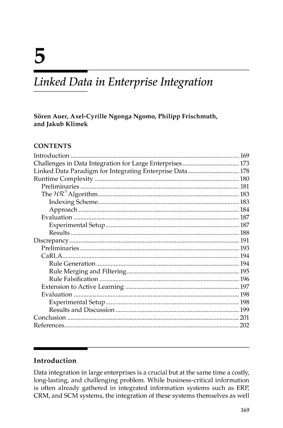
5. Linked Data in Enterprise Integration.................................................... 169
Sören Auer, Axel-Cyrille Ngonga Ngomo, Philipp Frischmuth,
and Jakub Klimek
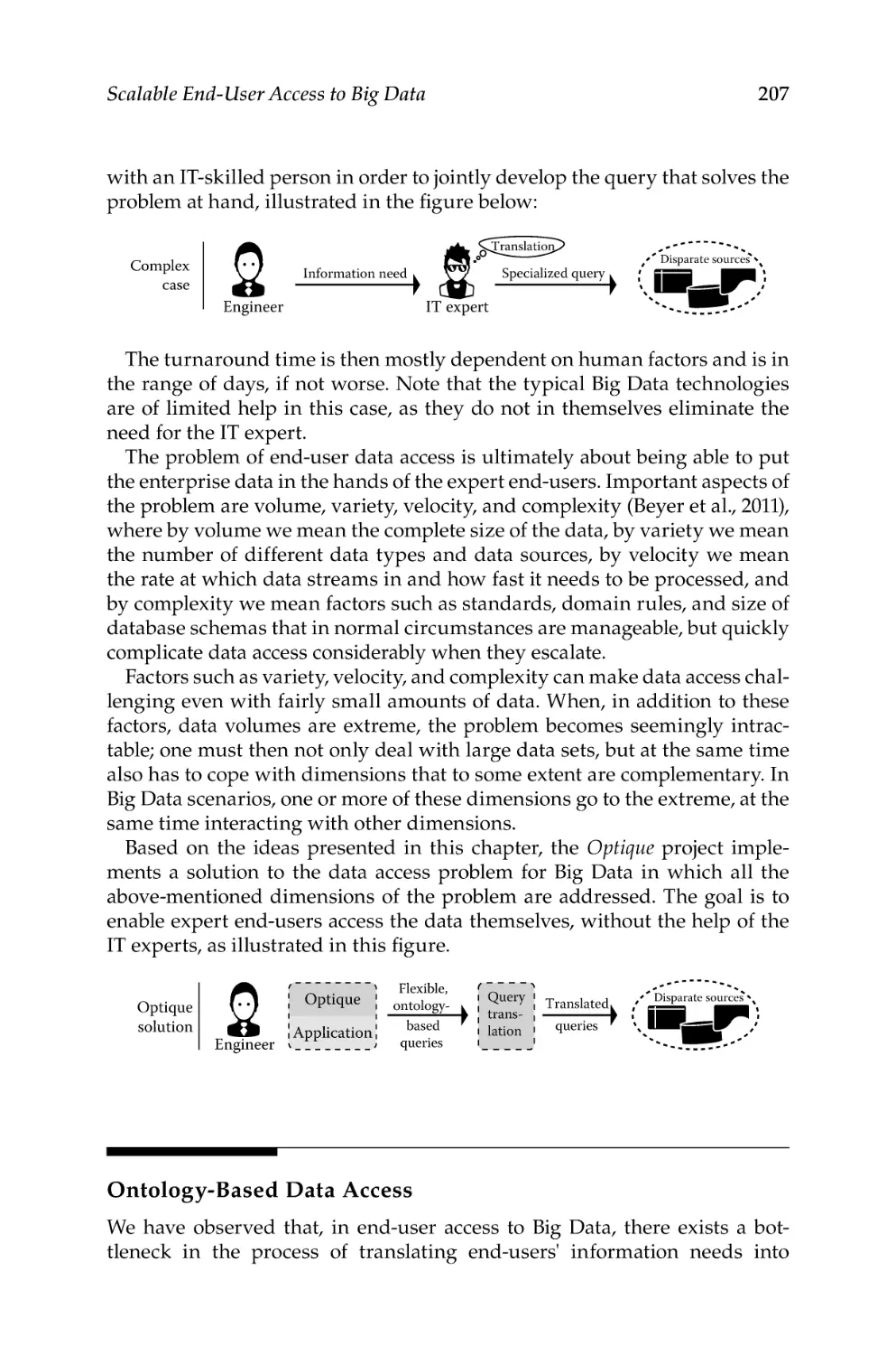
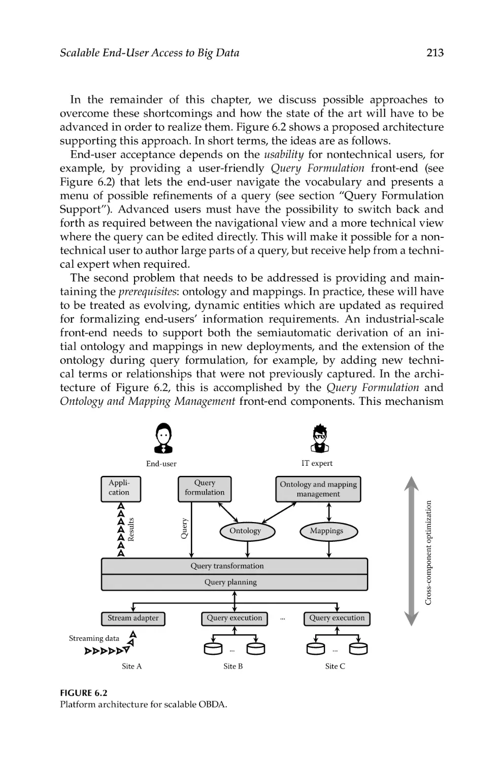
6. Scalable End-User Access to Big Data..................................................... 205
Martin Giese, Diego Calvanese, Peter Haase, Ian Horrocks,
Yannis Ioannidis, Herald Kllapi, Manolis Koubarakis, Maurizio Lenzerini,
Ralf Möller, Mariano Rodriguez Muro, Özgür Özçep, Riccardo Rosati,
Rudolf Schlatte, Michael Schmidt, Ahmet Soylu, and Arild Waaler
7. Semantic Data Interoperability: The Key Problem of Big Data........ 245
Hele-Mai Haav and Peep Küngas

vii

viii

Section III

Contents

Big Data Processing

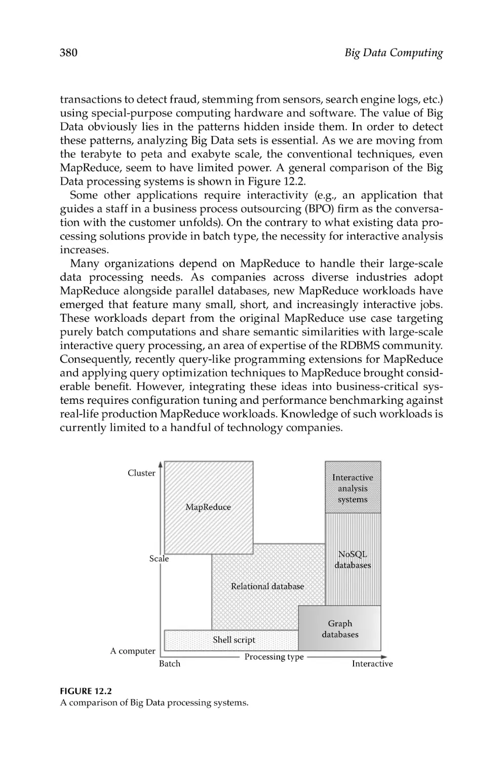
8. Big Data Exploration................................................................................... 273
Stratos Idreos
9. Big Data Processing with MapReduce.................................................... 295
Jordà Polo
10. Efficient Processing of Stream Data over Persistent Data................... 315
M. Asif Naeem, Gillian Dobbie, and Gerald Weber

Section IV

Big Data and Business

11. Economics of Big Data: A Value Perspective on State of the Art
and Future Trends.......................................................................................343
Tassilo Pellegrin
12. Advanced Data Analytics for Business................................................... 373
Rajendra Akerkar

Section V

Big Data Applications

13. Big Social Data Analysis............................................................................ 401
Erik Cambria, Dheeraj Rajagopal, Daniel Olsher, and Dipankar Das
14. Real-Time Big Data Processing for Domain Experts: An
Application to Smart Buildings................................................................ 415
Dario Bonino, Fulvio Corno, and Luigi De Russis
15. Big Data Application: Analyzing Real-Time Electric Meter Data..... 449
Mikhail Simonov, Giuseppe Caragnano, Lorenzo Mossucca, Pietro Ruiu,
and Olivier Terzo
16. Scaling of Geographic Space from the Perspective of City and
Field Blocks and Using Volunteered Geographic Information.........483
Bin Jiang and Xintao Liu
17. Big Textual Data Analytics and Knowledge Management................. 501
Marcus Spies and Monika Jungemann-Dorner
Index...................................................................................................................... 539

Preface
In the international marketplace, businesses, suppliers, and customers create
and consume vast amounts of information. Gartner* predicts that enterprise
data in all forms will grow up to 650% over the next five years. According
to IDC,† the world’s volume of data doubles every 18 months. Digital information is doubling every 1.5 years and will exceed 1000 exabytes next year
according to the MIT Centre for Digital Research. In 2011, medical centers
held almost 1 billion terabytes of data. That is almost 2000 billion file cabinets’
worth of information. This deluge of data, often referred to as Big Data, obviously creates a challenge to the business community and data scientists.
The term Big Data refers to data sets the size of which is beyond the capabilities of current database technology. It is an emerging field where innovative technology offers alternatives in resolving the inherent problems that
appear when working with massive data, offering new ways to reuse and
extract value from information.
Businesses and government agencies aggregate data from numerous private and/or public data sources. Private data is information that any organization exclusively stores that is available only to that organization, such
as employee data, customer data, and machine data (e.g., user transactions
and customer behavior). Public data is information that is available to the
public for a fee or at no charge, such as credit ratings, social media content
(e.g., LinkedIn, Facebook, and Twitter). Big Data has now reached every
sector in the world economy. It is transforming competitive opportunities
in every industry sector including banking, healthcare, insurance, manufacturing, retail, wholesale, transportation, communications, construction,
education, and utilities. It also plays key roles in trade operations such as
marketing, operations, supply chain, and new business models. It is becoming rather evident that enterprises that fail to use their data efficiently are at a
large competitive disadvantage from those that can analyze and act on their
data. The possibilities of Big Data continue to evolve swiftly, driven by innovation in the underlying technologies, platforms, and analytical capabilities
for handling data, as well as the evolution of behavior among its users as
increasingly humans live digital lives.
It is interesting to know that Big Data is different from the conventional
data models (e.g., relational databases and data models, or conventional governance models). Thus, it is triggering organizations’ concern as they try to
separate information nuggets from the data heap. The conventional models
of structured, engineered data do not adequately reveal the realities of Big
*
†

http://www.gartner.com/it/content/1258400/1258425/january_6_techtrends_rpaquet.pdf
http://www.idc.com/

ix

x

Preface

Data. The key to leveraging Big Data is to realize these differences before
expediting its use. The most noteworthy difference is that data are typically
governed in a centralized manner, but Big Data is self-governing. Big Data
is created either by a rapidly expanding universe of machines or by users of
highly varying expertise. As a result, the composition of traditional data will
naturally vary considerably from Big Data. The composition of data serves
a specific purpose and must be more durable and structured, whereas Big
Data will cover many topics, but not all topics will yield useful information
for the business, and thus they will be sparse in relevancy and structure.
The technology required for Big Data computing is developing at a satisfactory rate due to market forces and technological evolution. The evergrowing enormous amount of data, along with advanced tools of exploratory
data analysis, data mining/machine learning, and data visualization, offers
a whole new way of understanding the world.
Another interesting fact about Big Data is that not everything that is considered “Big Data” is in fact Big Data. One needs to explore deep into the
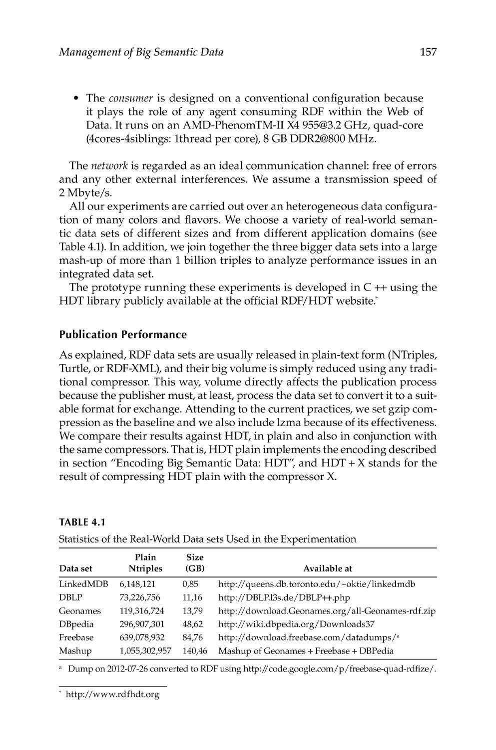
scientific aspects, such as analyzing, processing, and storing huge volumes
of data. That is the only way of using tools effectively. Data developers/
scientists need to know about analytical processes, statistics, and machine
learning. They also need to know how to use specific data to program algorithms. The core is the analytical side, but they also need the scientific background and in-depth technical knowledge of the tools they work with in
order to gain control of huge volumes of data. There is no one tool that offers
this per se.
As a result, the main challenge for Big Data computing is to find a novel
solution, keeping in mind the fact that data sizes are always growing. This
solution should be applicable for a long period of time. This means that the
key condition a solution has to satisfy is scalability. Scalability is the ability of
a system to accept increased input volume without impacting the profits; that
is, the gains from the input increment should be proportional to the increment itself. For a system to be totally scalable, the size of its input should not
be a design parameter. Pushing the system designer to consider all possible
deployment sizes to cope with different input sizes leads to a scalable architecture without primary bottlenecks. Yet, apart from scalability, there are
other requisites for a Big Data–intensive computing system.
Although Big Data is an emerging field in data science, there are very few
books available in the market. This book provides authoritative insights and
highlights valuable lessons learnt by authors—with experience.
Some universities in North America and Europe are doing their part to
feed the need for analytics skills in this era of Big Data. In recent years,
they have introduced master of science degrees in Big Data analytics,
data science, and business analytics. Some contributing authors have been
involved in developing a course curriculum in their respective institution
and ­country. The number of courses on “Big Data” will increase worldwide
because it is becoming a key basis of competition, underpinning new waves

Preface

xi

of productivity growth, innovation, and consumer surplus, according to a
research by MGI and McKinsey’s Business Technology Office.*
The main features of this book can be summarized as
1. It describes the contemporary state of the art in a new field of Big
Data computing.
2. It presents the latest developments, services, and main players in
this explosive field.
3. Contributors to the book are prominent researchers from academia
and practitioners from industry.

Organization
This book comprises five sections, each of which covers one aspect of Big Data
computing. Section I focuses on what Big Data is, why it is important, and
how it can be used. Section II focuses on semantic technologies and Big Data.
Section III focuses on Big Data processing—tools, technologies, and methods
essential to analyze Big Data efficiently. Section IV deals with business and
economic perspectives. Finally, Section V focuses on various stimulating Big
Data applications. Below is a brief outline with more details on what each
chapter is about.

Section I: Introduction
Chapter 1 provides an approach to address the problem of “understanding”
Big Data in an effective and efficient way. The idea is to make adequately
grained and expressive knowledge representations and fact collections that
evolve naturally, triggered by new tokens of relevant data coming along.
The chapter also presents primary considerations on assessing fitness in an
evolving knowledge ecosystem.
Chapter 2 then gives an overview of the main features that can characterize architectures for solving a Big Data problem, depending on the source of
data, on the type of processing required, and on the application context in
which it should be operated.

*

http://www.mckinsey.com/Insights/MGI/Research/Technology_and_Innovation/Big_
data_The_next_frontier_for_innovation

xii

Preface

Chapter 3 discusses Big Data from three different standpoints: the business, the technological, and the social. This chapter lists some relevant initiatives and selected thoughts on Big Data.

Section II: Semantic Technologies and Big Data
Chapter 4 presents foundations of Big Semantic Data management. The
chapter sketches a route from the current data deluge, the concept of Big
Data, and the need of machine-processable semantics on the Web. Further,
this chapter justifies different management problems arising in Big Semantic
Data by characterizing their main stakeholders by role and nature.
A number of challenges arising in the context of Linked Data in Enterprise
Integration are covered in Chapter 5. A key prerequisite for addressing these
challenges is the establishment of efficient and effective link discovery and
data integration techniques, which scale to large-scale data scenarios found
in the enterprise. This chapter also presents the transformation step of
Linked Data Integration by two algorithms.
Chapter 6 proposes steps toward the solution of the data access problem that end-users usually face when dealing with Big Data. The chapter
discusses the state of the art in ontology-based data access (OBDA) and
explains why OBDA is the superior approach to the data access challenge
posed by Big Data. It also explains why the field of OBDA is currently not
yet sufficiently complete to deal satisfactorily with these problems, and it
finally presents thoughts on escalating OBDA to a level where it can be well
deployed to Big Data.
Chapter 7 addresses large-scale semantic interoperability problems of
data in the domain of public sector administration and proposes practical
solutions to these problems by using semantic technologies in the context
of Web services and open data. This chapter also presents a case of the
Estonian semantic interoperability framework of state information systems
and related data interoperability solutions.

Section III: Big Data Processing
Chapter 8 presents a new way of query processing for Big Data where data
exploration becomes a first-class citizen. Data exploration is desirable when
new big chunks of data arrive speedily and one needs to react quickly. This
chapter focuses on database systems technology, which for several years has
been the prime data-processing tool.

Preface

xiii

Chapter 9 explores the MapReduce model, a programming model used to
develop largely parallel applications that process and generate large amounts
of data. This chapter also discusses how MapReduce is implemented in
Hadoop and provides an overview of its architecture.
A particular class of stream-based joins, namely, a join of a single stream
with a traditional relational table, is discussed in Chapter 10. Two available
stream-based join algorithms are investigated in this chapter.

Section IV: Big Data and Business
Chapter 11 provides the economic value of Big Data from a macro- and a
microeconomic perspective. The chapter illustrates how technology and
new skills can nurture opportunities to derive benefits from large, constantly
growing, dispersed data sets and how semantic interoperability and new
licensing strategies will contribute to the uptake of Big Data as a business
enabler and a source of value creation.
Nowadays businesses are enhancing their business intelligence practices to include predictive analytics and data mining. This combines the
best of strategic reporting and basic forecasting with advanced operational
intelligence and decision-making functions. Chapter 12 discusses how Big
Data technologies, advanced analytics, and business intelligence (BI) are
interrelated. This chapter also presents various areas of advanced analytic
technologies.

Section V: Big Data Applications
The final section of the book covers application topics, starting in Chapter 13
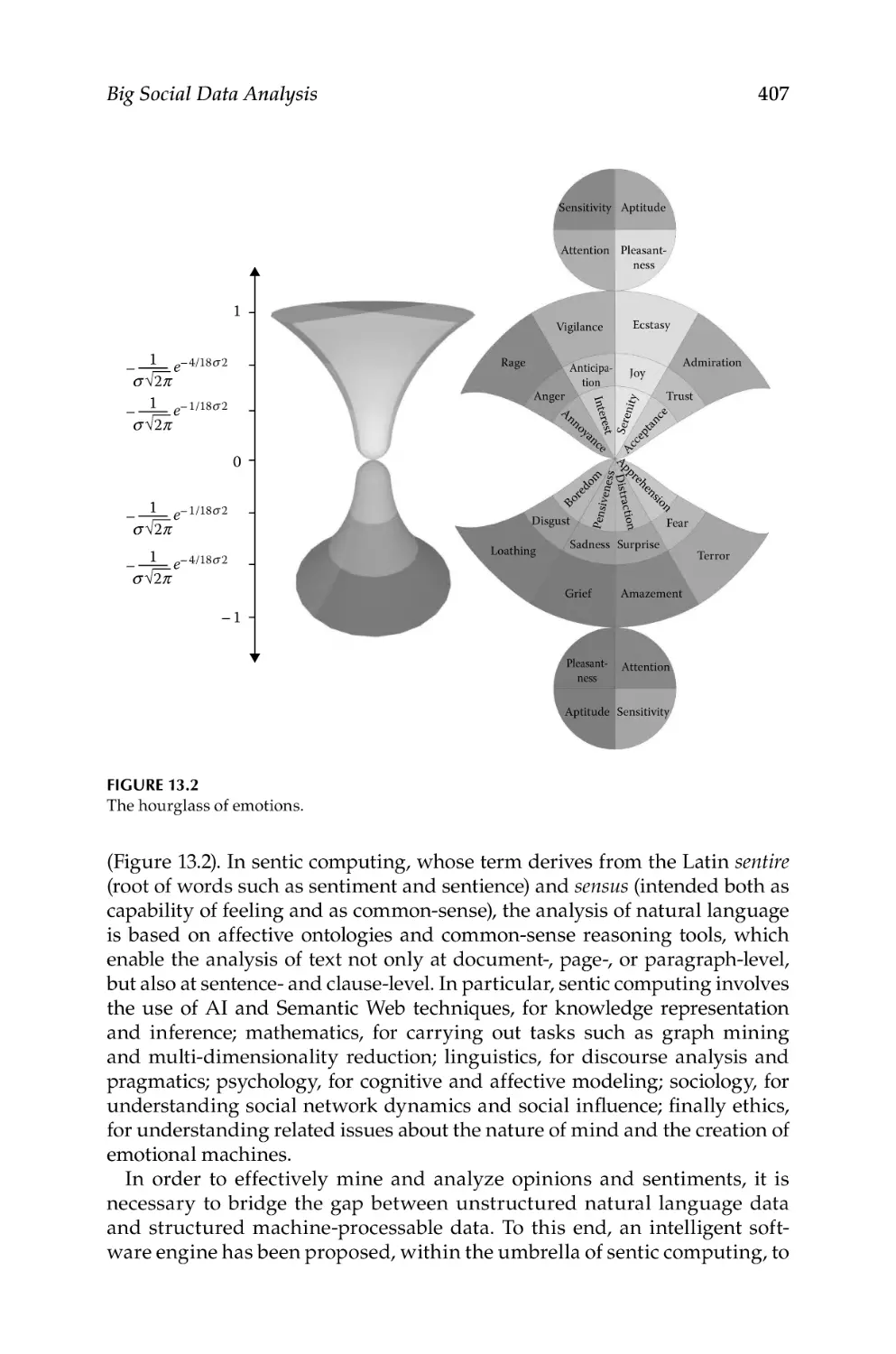
with novel concept-level approaches to opinion mining and sentiment analysis that allow a more efficient passage from (unstructured) textual information to (structured) machine-processable data, in potentially any domain.
Chapter 14 introduces the spChains framework, a modular approach to support mastering of complex event processing (CEP) queries in an abridged,
but effective, manner based on stream processing block composition. The
approach aims at unleashing the power of CEP systems for teams having
reduced insights into CEP systems.
Real-time electricity metering operated at subsecond data rates in a grid
with 20 million nodes originates more than 5 petabytes daily. The requested
decision-making timeframe in SCADA systems operating load shedding
might be lower than 100 milliseconds. Chapter 15 discusses the real-life

xiv

Preface

optimization task and the data management approach permitting a solution
to the issue.
Chapter 16 presents an innovative outlook to the scaling of geographical space using large street networks involving both cities and countryside.
Given a street network of an entire country, the chapter proposes to decompose the street network into individual blocks, each of which forms a minimum ring or cycle such as city blocks and field blocks. The chapter further
elaborates the power of the block perspective in reflecting the patterns of
geographical space.
Chapter 17 presents the influence of recent advances in natural language
processing on business knowledge life cycles and processes of knowledge
management. The chapter also sketches envisaged developments and market impacts related to the integration of semantic technology and knowledge
management.

Intended Audience
The aim of this book is to be accessible to researchers, graduate students,
and to application-driven practitioners who work in data science and related
fields. This edited book requires no previous exposure to large-scale data
analysis or NoSQL tools. Acquaintance with traditional databases is an
added advantage.
This book provides the reader with a broad range of Big Data concepts,
tools, and techniques. A wide range of research in Big Data is covered, and
comparisons between state-of-the-art approaches are provided. This book
can thus help researchers from related fields (such as databases, data science, data mining, machine learning, knowledge engineering, information
retrieval, information systems), as well as students who are interested in
entering this field of research, to become familiar with recent research developments and identify open research challenges on Big Data. This book can
help practitioners to better understand the current state of the art in Big Data
techniques, concepts, and applications.
The technical level of this book also makes it accessible to students taking
advanced undergraduate level courses on Big Data or Data Science. Although
such courses are currently rare, with the ongoing challenges that the areas
of intelligent information/data management pose in many organizations in
both the public and private sectors, there is a demand worldwide for graduates with skills and expertise in these areas. It is hoped that this book helps
address this demand.
In addition, the goal is to help policy-makers, developers and engineers,
data scientists, as well as individuals, navigate the new Big Data landscape.
I believe it can trigger some new ideas for practical Big Data applications.

Preface

xv

Acknowledgments
The organization and the contents of this edited book have benefited from our
outstanding contributors. I am very proud and happy that these researchers
agreed to join this project and prepare a chapter for this book. I am also very
pleased to see this materialize in the way I originally envisioned. I hope this
book will be a source of inspiration to the readers. I especially wish to express
my sincere gratitude to all the authors for their contribution to this project.
I thank the anonymous reviewers who provided valuable feedback and
helpful suggestions.
I also thank Aastha Sharma, David Fausel, Rachel Holt, and the staff at
CRC Press (Taylor & Francis Group), who supported this book project right
from the start.
Last, but not least, a very big thanks to my colleagues at Western Norway
Research Institute (Vestlandsforsking, Norway) for their constant encouragement and understanding.
I wish all readers a fruitful time reading this book, and hope that they experience the same excitement as I did—and still do—when dealing with Data.
Rajendra Akerkar

This page intentionally left blank

Editor
Rajendra Akerkar is professor and senior researcher at Western Norway
Research Institute (Vestlandsforsking), Norway, where his main domain
of research is semantic technologies with the aim of combining theoretical
results with high-impact real-world solutions. He also holds visiting academic assignments in India and abroad. In 1997, he founded and chaired the
Technomathematics Research Foundation (TMRF) in India.
His research and teaching experience spans over 23 years in academia
including different universities in Asia, Europe, and North America. His
research interests include ontologies, semantic technologies, knowledge systems, large-scale data mining, and intelligent systems.
He received DAAD fellowship in 1990 and is also a recipient of the prestigious BOYSCASTS Young Scientist award of the Department of Science
and Technology, Government of India, in 1997. From 1998 to 2001, he was a
UNESCO-TWAS associate member at the Hanoi Institute of Mathematics,
Vietnam. He was also a DAAD visiting professor at Universität des Saarlandes and University of Bonn, Germany, in 2000 and 2007, respectively.
Dr. Akerkar serves as editor-in-chief of the International Journal of Computer
Science & Applications (IJCSA) and as an associate editor of the International
Journal of Metadata, Semantics, and Ontologies (IJMSO). He is co-organizer
of several workshops and program chair of the international conferences
ISACA, ISAI, ICAAI, and WIMS. He has co-authored 13 books, approximately 100 research papers, co-edited 2 e-books, and edited 5 volumes of
international conferences. He is also actively involved in several international ICT initiatives and research & development projects and has been for
more than 16 years.

xvii

This page intentionally left blank

Contributors
Rajendra Akerkar
Western Norway Research Institute
Sogndal, Norway
Mario Arias
Digital Enterprise Research Institute
National University of Ireland
Galway, Ireland
Sören Auer
Enterprise Information Systems
Department
Institute of Computer Science III
Rheinische Friedrich-WilhelmsUniversität Bonn
Bonn, Germany
Pierfrancesco Bellini
Distributed Systems and Internet
Technology
Department of Systems and
Informatics
University of Florence
Firenze, Italy
Dario Bonino
Department of Control and
Computer Engineering
Polytechnic University of Turin
Turin, Italy

Giuseppe Caragnano
Advanced Computing and
Electromagnetic Unit
Istituto Superiore Mario Boella
Torino, Italy
Michael Cochez
Faculty of Information
Technology
University of Jyväskylä
Jyväskylä, Finland
Fulvio Corno
Department of Control and
Computer Engineering
Polytechnic University of Turin
Turin, Italy
Dipankar Das
Department of Computer
Science
National University of Singapore
Singapore
Luigi De Russis
Department of Control and
Computer Engineering
Polytechnic University of Turin
Turin, Italy

Diego Calvanese
Department of Computer Science
Free University of Bozen-Bolzano
Bolzano, Italy

Mariano di Claudio
Department of Systems
and Informatics
University of Florence
Firenze, Italy

Erik Cambria
Department of Computer Science
National University of Singapore
Singapore

Gillian Dobbie
Department of Computer Science
The University of Auckland
Auckland, New Zealand
xix

xx

Vadim Ermolayev
Zaporozhye National University
Zaporozhye, Ukraine
Javier D. Fernández
Department of Computer Science
University of Valladolid
Valladolid, Spain
Philipp Frischmuth
Department of Computer Science
University of Leipzig
Leipzig, Germany
Martin Giese
Department of Computer Science
University of Oslo
Oslo, Norway
Claudio Gutiérrez
Department of Computer
Science
University of Chile
Santiago, Chile
Peter Haase
Fluid Operations AG
Walldorf, Germany
Hele-Mai Haav
Institute of Cybernetics
Tallinn University of
Technology
Tallinn, Estonia
Ian Horrocks
Department of Computer Science
Oxford University
Oxford, United Kingdom
Stratos Idreos
Dutch National Research Center
for Mathematics and Computer
Science (CWI)
Amsterdam, the Netherlands

Contributors

Yannis Ioannidis
Department of Computer Science
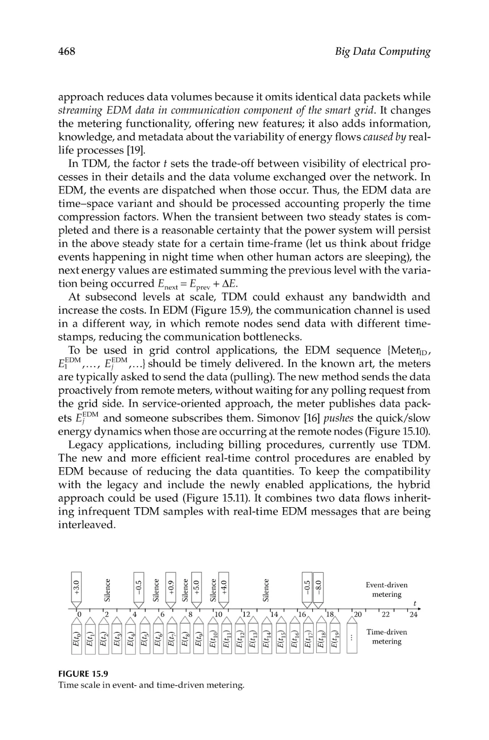
National and Kapodistrian
University of Athens
Athens, Greece
Bin Jiang
Department of Technology
and Built Environment
University of Gävle
Gävle, Sweden
Monika Jungemann-Dorner
Senior International Project
Manager
Verband der Verein
Creditreform eV
Neuss, Germany
Jakub Klimek
Department of Computer
Science
University of Leipzig
Leipzig, Germany
Herald Kllapi
Department of Computer Science
National and Kapodistrian
University of Athens
Athens, Greece
Manolis Koubarakis
Department of Computer
Science
National and Kapodistrian
University of Athens
Athens, Greece
Peep Küngas
Institute of Computer Science
University of Tartu
Tartu, Estonia

xxi

Contributors

Maurizio Lenzerini
Department of Computer
Science
Sapienza University of Rome
Rome, Italy
Xintao Liu
Department of Technology
and Built Environment
University of Gävle
Gävle, Sweden
Miguel A. Martínez-Prieto
Department of Computer
Science
University of Valladolid
Valladolid, Spain
Ralf Möller
Department of Computer
Science
TU Hamburg-Harburg
Hamburg, Germany
Lorenzo Mossucca
Istituto Superiore Mario Boella
Torino, Italy
Mariano Rodriguez Muro
Department of Computer Science
Free University of Bozen-Bolzano
Bolzano, Italy
M. Asif Naeem
Department of Computer Science
The University of Auckland
Auckland, New Zealand
Paolo Nesi
Department of Systems
and Informatics
Distributed Systems and Internet
Technology
University of Florence
Firenze, Italy

Axel-Cyrille Ngonga Ngomo
Department of Computer Science
University of Leipzig
Leipzig, Germany
Daniel Olsher
Department of Computer Science
National University of Singapore
Singapore
Özgür Özçep
Department of Computer Science
TU Hamburg-Harburg
Hamburg, Germany
Tassilo Pellegrin
Semantic Web Company
Vienna, Austria
Jordà Polo
Barcelona Supercomputing Center
(BSC)
Technical University of Catalonia
(UPC)
Barcelona, Spain
Dheeraj Rajagopal
Department of Computer Science
National University of Singapore
Singapore
Nadia Rauch
Department of Systems
and Informatics
University of Florence
Firenze, Italy
Riccardo Rosati
Department of Computer Science
Sapienza University of Rome
Rome, Italy
Pietro Ruiu
Istituto Superiore Mario Boella
Torino, Italy

xxii

Contributors

Rudolf Schlatte
Department of Computer
Science
University of Oslo
Oslo, Norway

Vagan Terziyan
Department of Mathematical
Information Technology
University of Jyväskylä
Jyväskylä, Finland

Michael Schmidt
Fluid Operations AG
Walldorf, Germany

Olivier Terzo
Advanced Computing and
Electromagnetics Unit
Istituto Superiore Mario Boella
Torino, Italy

Mikhail Simonov
Advanced Computing and
Electromagnetics Unit
Istituto Superiore Mario Boella
Torino, Italy
Ahmet Soylu
Department of Computer
Science
University of Oslo
Oslo, Norway
Marcus Spies
Ludwig-Maximilians University
Munich, Germany

Arild Waaler
Department of Computer Science
University of Oslo
Oslo, Norway
Gerald Weber
Department of Computer Science
The University of Auckland
Auckland, New Zealand
Roberto V. Zicari
Department of Computer Science
Goethe University
Frankfurt, Germany

Section I

Introduction

This page intentionally left blank

1
Toward Evolving Knowledge Ecosystems for
Big Data Understanding
Vadim Ermolayev, Rajendra Akerkar, Vagan Terziyan,
and Michael Cochez
Contents
Introduction..............................................................................................................4
Motivation and Unsolved Issues...........................................................................6
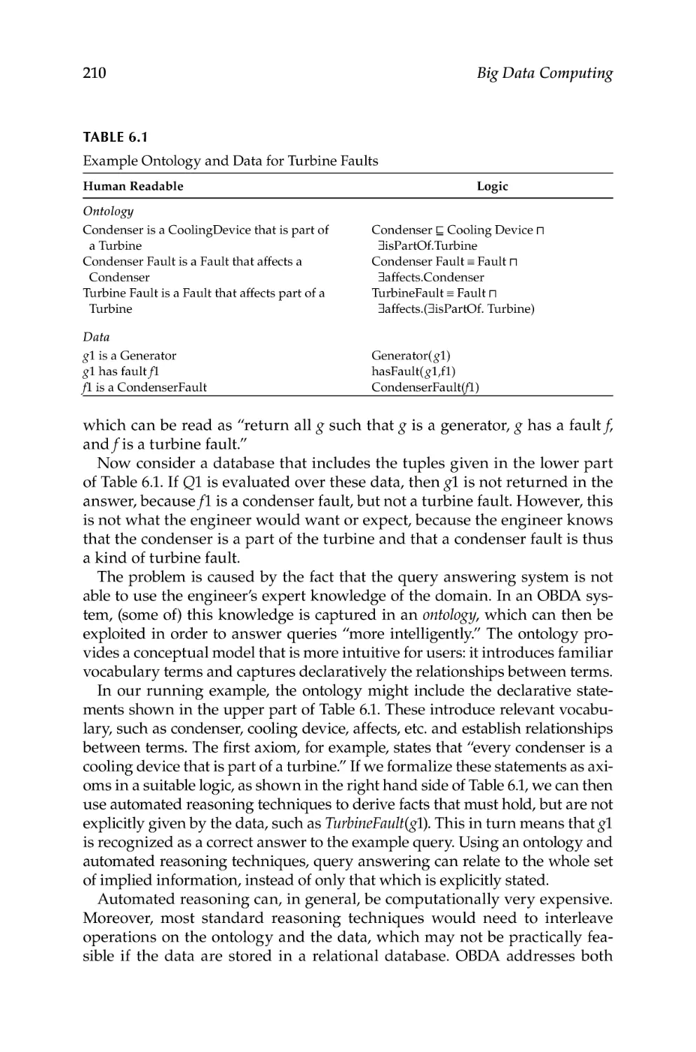
Illustrative Example............................................................................................7
Demand in Industry............................................................................................9
Problems in Industry..........................................................................................9
Major Issues....................................................................................................... 11
State of Technology, Research, and Development in Big Data Computing... 12
Big Data Processing—Technology Stack and Dimensions.......................... 13
Big Data in European Research....................................................................... 14
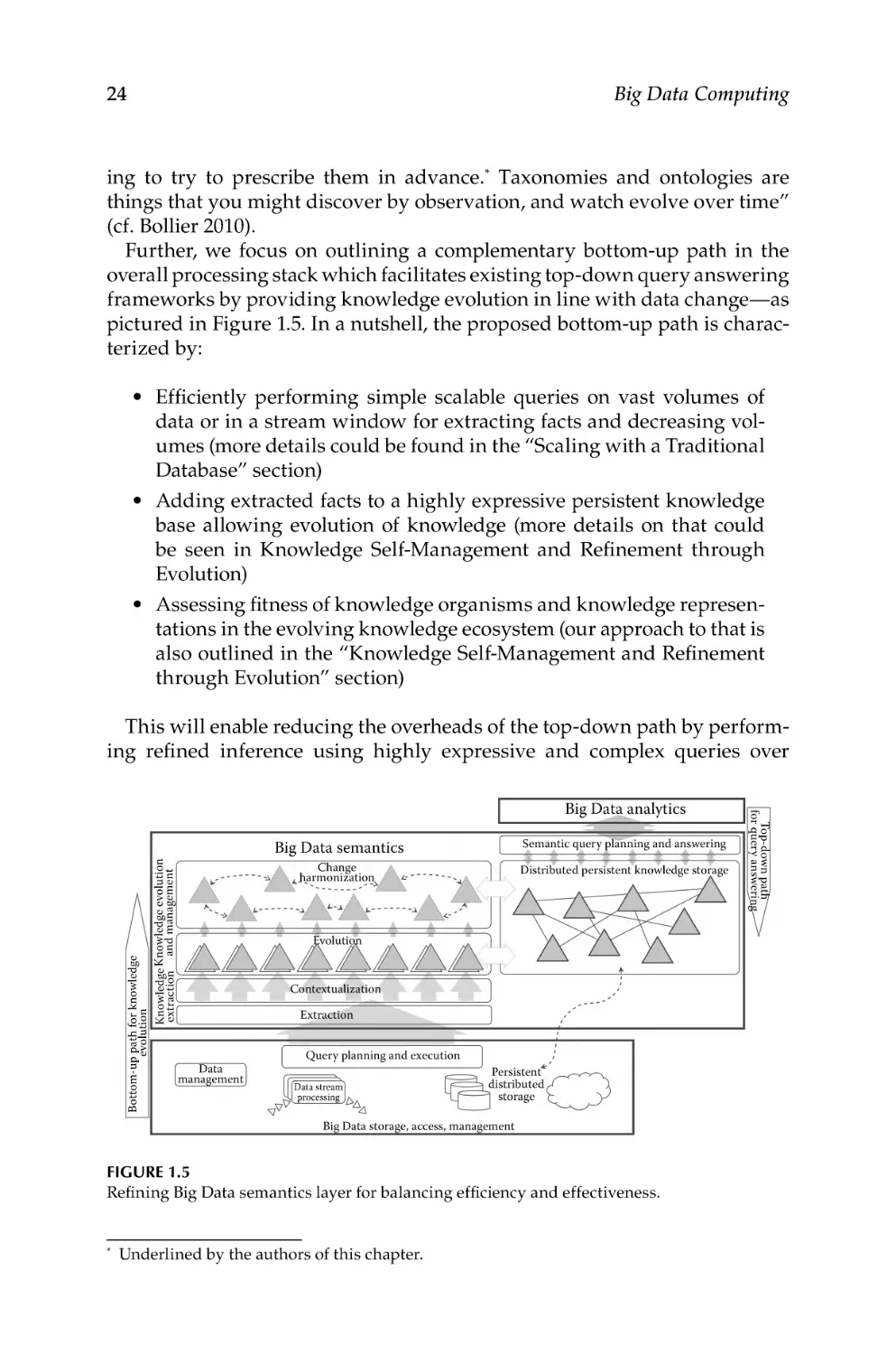
Complications and Overheads in Understanding Big Data....................... 20
Refining Big Data Semantics Layer for Balancing Efficiency
Effectiveness....................................................................................................... 23
Focusing......................................................................................................... 25
Filtering.......................................................................................................... 26
Forgetting....................................................................................................... 27
Contextualizing............................................................................................. 27
Compressing................................................................................................. 29
Connecting..................................................................................................... 29
Autonomic Big Data Computing....................................................................30
Scaling with a Traditional Database.................................................................... 32
Large Scale Data Processing Workflows........................................................ 33
Knowledge Self-Management and Refinement through Evolution...............34
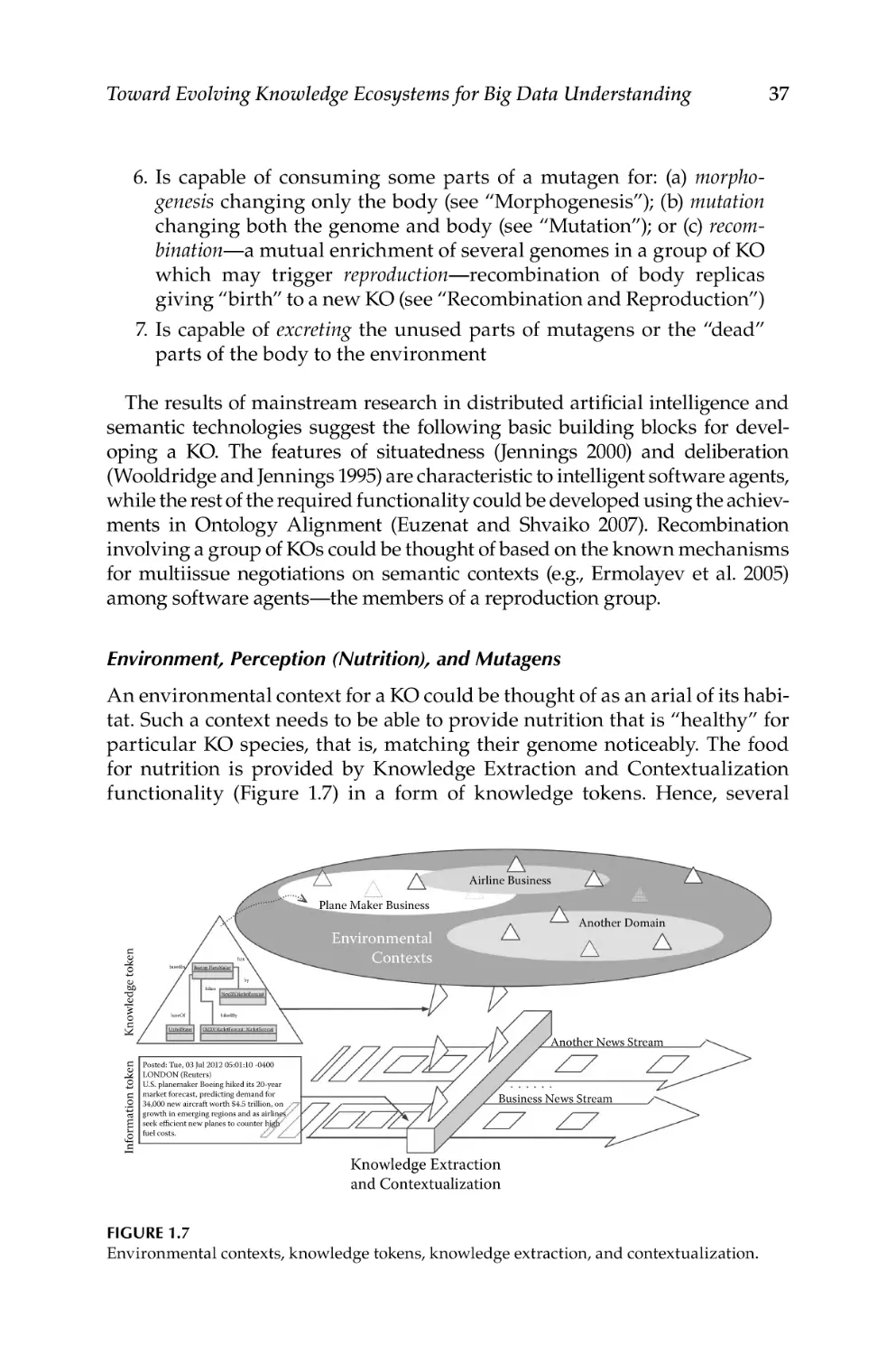
Knowledge Organisms, their Environments, and Features........................ 36
Environment, Perception (Nutrition), and Mutagens............................. 37
Knowledge Genome and Knowledge Body............................................. 39
Morphogenesis............................................................................................. 41
Mutation........................................................................................................42
Recombination and Reproduction.............................................................44
Populations of Knowledge Organisms.......................................................... 45
Fitness of Knowledge Organisms and Related Ontologies......................... 46
3

4

Big Data Computing

Some Conclusions.................................................................................................. 48
Acknowledgments................................................................................................. 50
References................................................................................................................ 50

Introduction
Big Data is a phenomenon that leaves a rare information professional negligent these days. Remarkably, application demands and developments in the
context of related disciplines resulted in technologies that boosted data generation and storage at unprecedented scales in terms of volumes and rates. To
mention just a few facts reported by Manyika et al. (2011): a disk drive capable
of storing all the world’s music could be purchased for about US $600; 30 billion of content pieces are shared monthly only at Facebook (facebook.com).
Exponential growth of data volumes is accelerated by a dramatic increase in
social networking applications that allow nonspecialist users create a huge
amount of content easily and freely. Equipped with rapidly evolving mobile
devices, a user is becoming a nomadic gateway boosting the generation of
additional real-time sensor data. The emerging Internet of Things makes
every thing a data or content, adding billions of additional artificial and
autonomic sources of data to the overall picture. Smart spaces, where people,
devices, and their infrastructure are all loosely connected, also generate data
of unprecedented volumes and with velocities rarely observed before. An
expectation is that valuable information will be extracted out of all these data
to help improve the quality of life and make our world a better place.
Society is, however, left bewildered about how to use all these data efficiently and effectively. For example, a topical estimate for the number of a
need for data-savvy managers to take full advantage of Big Data in the United
States is 1.5 million (Manyika et al. 2011). A major challenge would be finding
a balance between the two evident facets of the whole Big Data adventure: (a)
the more data we have, the more potentially useful patterns it may include
and (b) the more data we have, the less the hope is that any machine-learning algorithm is capable of discovering these patterns in an acceptable time
frame. Perhaps because of this intrinsic conflict, many experts consider that
this Big Data not only brings one of the biggest challenges, but also a most
exciting opportunity in the recent 10 years (cf. Fan et al. 2012b)
The avalanche of Big Data causes a conceptual divide in minds and opinions. Enthusiasts claim that, faced with massive data, a scientific approach “. . .
hypothesize, model, test—is becoming obsolete. . . . Petabytes allow us to say:
‘Correlation is enough.’ We can stop looking for models. We can analyze the
data without hypotheses about what it might show. We can throw the numbers
into the biggest computing clusters the world has ever seen and let statistical
algorithms find patterns . . .” (Anderson 2008). Pessimists, however, point out

Toward Evolving Knowledge Ecosystems for Big Data Understanding

5

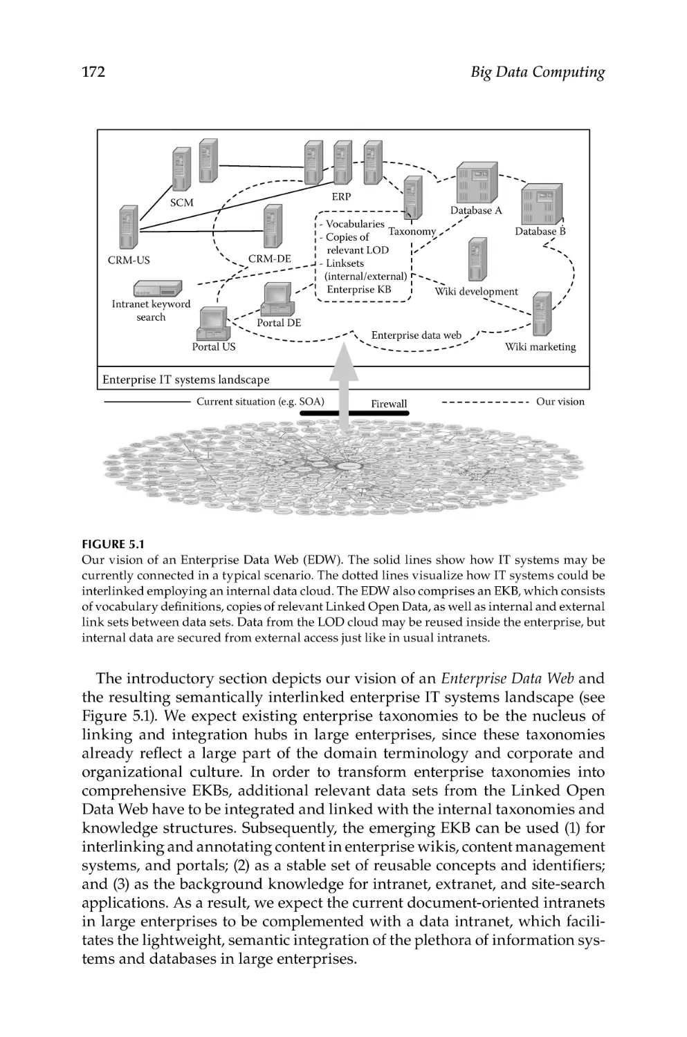
that Big Data provides “. . . destabilising amounts of knowledge and information that lack the regulating force of philosophy” (Berry 2011). Indeed, being
abnormally big does not yet mean being healthy and wealthy and should be
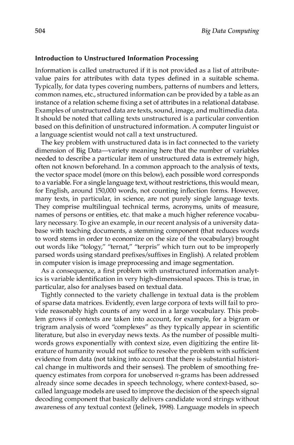
treated appropriately (Figure 1.1): a diet, exercise, medication, or even surgery
(philosophy). Those data sets, for which systematic health treatment is ignored
in favor of correlations, will die sooner—as useless. There is a hope, however,
that holistic integration of evolving algorithms, machines, and people reinforced by research effort across many domains will guarantee required fitness
of Big Data, assuring proper quality at right time (Joseph 2012).
Mined correlations, though very useful, may hint about an answer to a
“what,” but not “why” kind of questions. For example, if Big Data about
Royal guards and their habits had been collected in the 1700s’ France, one
could mine today that all musketeers who used to have red Burgundy regularly for dinners have not survived till now. Pity, red Burgundy was only one
of many and a very minor problem. A scientific approach is needed to infer
real reasons—the work currently done predominantly by human analysts.
Effectiveness and efficiency are the evident keys in Big Data analysis.
Cradling the gems of knowledge extracted out of Big Data would only be
effective if: (i) not a single important fact is left in the burden—which means
completeness and (ii) these facts are faceted adequately for further inference—which means expressiveness and granularity. Efficiency may be interpreted as the ratio of spent effort to the utility of result. In Big Data analytics,
it could be straightforwardly mapped to timeliness. If a result is not timely,
its utility (Ermolayev et al. 2004) may go down to zero or even far below in
seconds to milliseconds for some important industrial applications such as
technological process or air traffic control.
Notably, increasing effectiveness means increasing the effort or making the
analysis computationally more complex, which negatively affects efficiency.

Figure 1.1
Evolution of data collections—dimensions (see also Figure 1.3) have to be treated with care.
(Courtesy of Vladimir Ermolayev.)

6

Big Data Computing

Finding a balanced solution with a sufficient degree of automation is the
challenge that is not yet fully addressed by the research community.
One derivative problem concerns knowledge extracted out of Big Data as
the result of some analytical processing. In many cases, it may be expected
that the knowledge mechanistically extracted out of Big Data will also be
big. Therefore, taking care of Big Knowledge (which has more value than
the source data) would be at least of the same importance as resolving challenges associated with Big Data processing. Uplifting the problem to the
level of knowledge is inevitable and brings additional complications such as
resolving contradictory and changing opinions of everyone on everything.
Here, an adequate approach in managing the authority and reputation of
“experts” will play an important role (Weinberger 2012).
This chapter offers a possible approach in addressing the problem of
“understanding” Big Data in an effective and efficient way. The idea is making adequately grained and expressive knowledge representations and fact
collections evolve naturally, triggered by new tokens of relevant data coming
along. Pursuing this way would also imply conceptual changes in the Big Data
Processing stack. A refined semantic layer has to be added to it for providing adequate interfaces to interlink horizontal layers and enable knowledgerelated functionality coordinated in top-down and bottom-up directions.
The remainder of the chapter is structured as follows. The “Motivation
and Unsolved Issues” section offers an illustrative example and the analysis of the demand for understanding Big Data. The “State of Technology,
Research, and Development in Big Data Computing” section reviews the
relevant research on using semantic and related technologies for Big Data
processing and outlines our approach to refine the processing stack. The
“Scaling with a Traditional Database” section focuses on how the basic
data storage and management layer could be refined in terms of scalability,
which is necessary for improving efficiency/effectiveness. The “Knowledge
Self-Management and Refinement through Evolution” section presents our
approach, inspired by the mechanisms of natural evolution studied in evolutionary biology. We focus on a means of arranging the evolution of knowledge, using knowledge organisms, their species, and populations with the
aim of balancing efficiency and effectiveness of processing Big Data and its
semantics. We also provide our preliminary considerations on assessing fitness in an evolving knowledge ecosystem. Our conclusions are drawn in the
“Some Conclusions” section.

Motivation and Unsolved Issues
Practitioners, including systems engineers, Information Technology architects, Chief Information and Technology Officers, and data scientists, use

Toward Evolving Knowledge Ecosystems for Big Data Understanding

7

the phenomenon of Big Data in their dialog over means of improving sensemaking. The phenomenon remains a constructive way of introducing others,
including nontechnologists, to new approaches such as the Apache Hadoop
(hadoop.apache.org) framework. Apparently, Big Data is collected to be analyzed. “Fundamentally, big data analytics is a workflow that distills terabytes
of low-value data down to, in some cases, a single bit of high-value data. . . .
The goal is to see the big picture from the minutia of our digital lives” (cf.
Fisher et al. 2012). Evidently, “seeing the big picture” in its entirety is the key
and requires making Big Data healthy and understandable in terms of effectiveness and efficiency for analytics.
In this section, the motivation for understanding the Big Data that improves
the performance of analytics is presented and analyzed. It begins with presenting a simple example which is further used throughout the chapter. It
continues with the analysis of industrial demand for Big Data analytics. In
this context, the major problems as perceived by industries are analyzed and
informally mapped to unsolved technological issues.
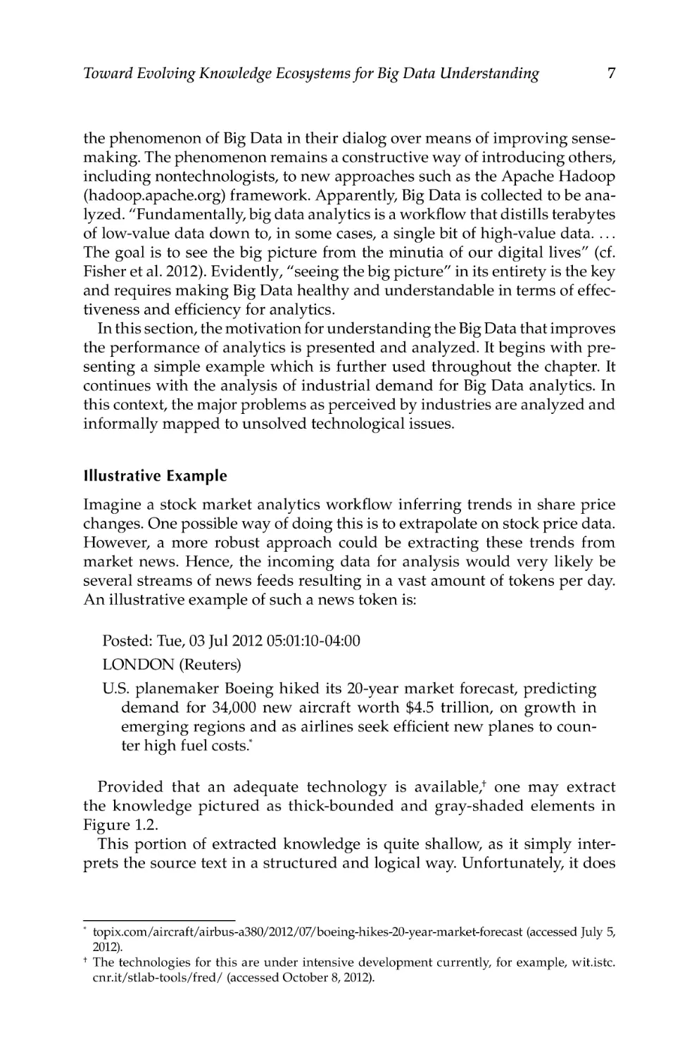
Illustrative Example
Imagine a stock market analytics workflow inferring trends in share price
changes. One possible way of doing this is to extrapolate on stock price data.
However, a more robust approach could be extracting these trends from
market news. Hence, the incoming data for analysis would very likely be
several streams of news feeds resulting in a vast amount of tokens per day.
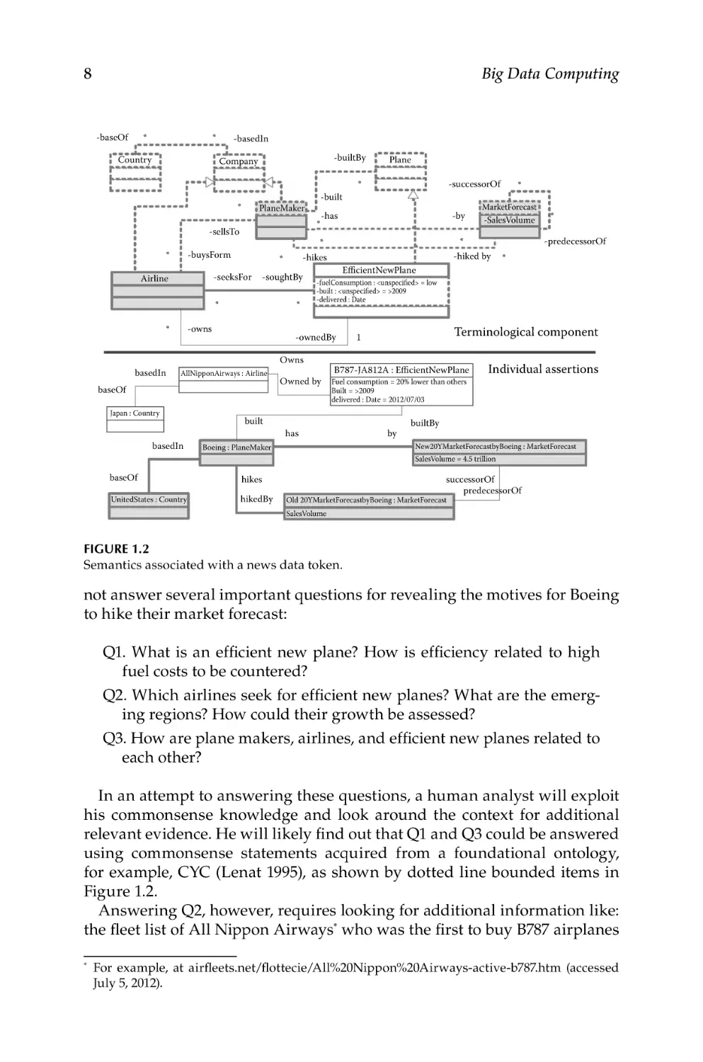
An illustrative example of such a news token is:
Posted: Tue, 03 Jul 2012 05:01:10-04:00
LONDON (Reuters)
U.S. planemaker Boeing hiked its 20-year market forecast, predicting
demand for 34,000 new aircraft worth $4.5 trillion, on growth in
emerging regions and as airlines seek efficient new planes to counter high fuel costs.*
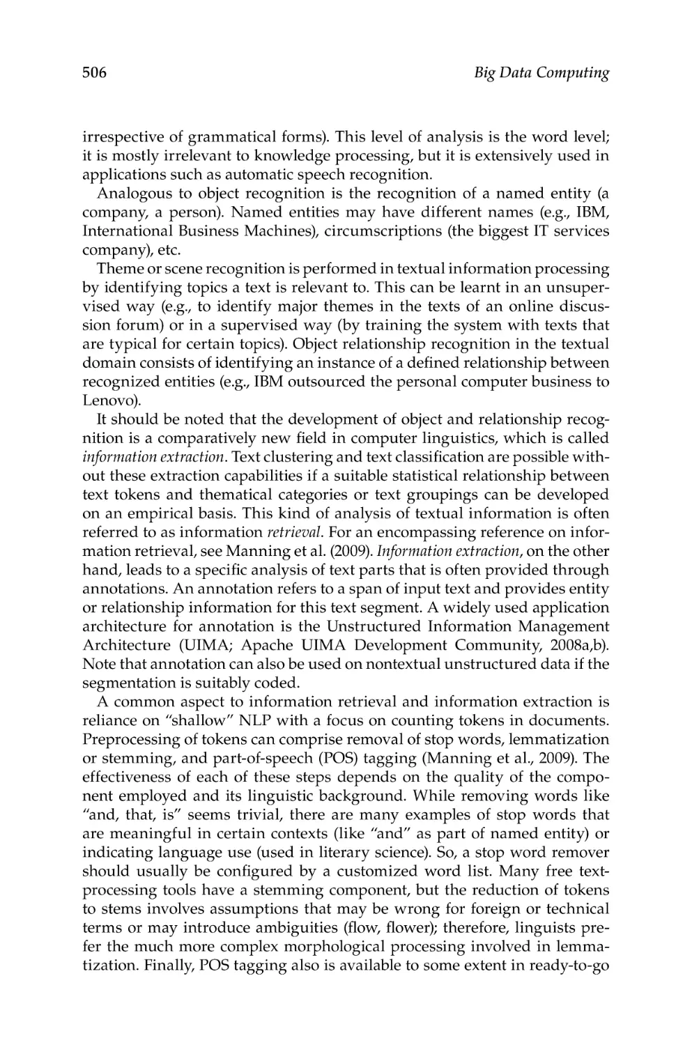
Provided that an adequate technology is available,† one may extract
the knowledge pictured as thick-bounded and gray-shaded elements in
Figure 1.2.
This portion of extracted knowledge is quite shallow, as it simply interprets the source text in a structured and logical way. Unfortunately, it does

*

†

topix.com/aircraft/airbus-a380/2012/07/boeing-hikes-20-year-market-forecast (accessed July 5,
2012).
The technologies for this are under intensive development currently, for example, wit.istc.
cnr.it/stlab-tools/fred/ (accessed October 8, 2012).

8

Big Data Computing

-baseOf

*

*

Country

-basedIn
-builtBy

Company

*

PlaneMaker
*

-sellsTo

-soughtBy

*

basedIn

*

-owns

*

baseOf
built

hikes

UnitedStates : Country

hikedBy

-SalesVolume

-hiked by

EfficientNewPlane

*
-predecessorOf

*

Owned by

*

Terminological component

1

B787-JA812A : EfficientNewPlane

Fuel consumption = 20% lower than others
Built = >2009
delivered : Date = 2012/07/03

has

Boeing : PlaneMaker

baseOf

*

MarketForecast

-fuelConsumption : <unspecified> = low
-built : <unspecified> = >2009
-delivered : Date

Owns

basedIn

-by

-ownedBy

AllNipponAirways : Airline

Japan : Country

-successorOf

-has

-hikes

*

-seeksFor

Airline

*

*

-buysForm

*

-built

Plane

by

Individual assertions

builtBy
New20YMarketForecastbyBoeing : MarketForecast
SalesVolume = 4.5 trillion

successorOf
predecessorOf

Old 20YMarketForecastbyBoeing : MarketForecast
SalesVolume

Figure 1.2
​Semantics associated with a news data token.

not answer several important questions for revealing the motives for Boeing
to hike their market forecast:
Q1. What is an efficient new plane? How is efficiency related to high
fuel costs to be countered?
Q2. Which airlines seek for efficient new planes? What are the emerging regions? How could their growth be assessed?
Q3. How are plane makers, airlines, and efficient new planes related to
each other?
In an attempt to answering these questions, a human analyst will exploit
his commonsense knowledge and look around the context for additional
relevant evidence. He will likely find out that Q1 and Q3 could be answered
using commonsense statements acquired from a foundational ontology,
for example, CYC (Lenat 1995), as shown by dotted line bounded items in
Figure 1.2.
Answering Q2, however, requires looking for additional information like:
the fleet list of All Nippon Airways* who was the first to buy B787 airplanes
*

For example, at airfleets.net/flottecie/All%20Nippon%20Airways-active-b787.htm (accessed
July 5, 2012).

Toward Evolving Knowledge Ecosystems for Big Data Understanding

9

from Boeing (the rest of Figure 1.2); and a relevant list of emerging regions
and growth factors (not shown in Figure 1.2). The challenge for a human
analyst in performing the task is low speed of data analysis. The available
time slot for providing his recommendation is too small, given the effort to
be spent per one news token for deep knowledge extraction. This is one good
reason for growing demand for industrial strength technologies to assist in
analytical work on Big Data, increase quality, and reduce related efforts.
Demand in Industry
Turning available Big Data assets into action and performance is considered
a deciding factor by today’s business analytics. For example, the report by
Capgemini (2012) concludes, based on a survey of the interviews with more
than 600 business executives, that Big Data use is highly demanded in industries. Interviewees firmly believe that their companies’ competitiveness and
performance strongly depend on the effective and efficient use of Big Data.
In particular, on average,
• Big Data is already used for decision support 58% of the time, and
29% of the time for decision automation
• It is believed that the use of Big Data will improve organizational
performance by 41% over the next three years
The report by Capgemini (2012) also summarizes that the following are the
perceived benefits of harnessing Big Data for decision-making:
• More complete understanding of market conditions and evolving
business trends
• Better business investment decisions
• More accurate and precise responses to customer needs
• Consistency of decision-making and greater group participation in
shared decisions
• Focusing resources more efficiently for optimal returns
• Faster business growth
• Competitive advantage (new data-driven services)
• Common basis for evaluation (one true starting point)
• Better risk management
Problems in Industry
Though the majority of business executives firmly believe in the utility
of Big Data and analytics, doubts still persist about its proper use and the
availability of appropriate technologies. As a consequence, “We no longer

10

Big Data Computing

speak of the Knowledge Economy or the Information Society. It’s all data
now: Data Economy and Data Society. This is a confession that we are no
longer in control of the knowledge contained in the data our systems collect” (Greller 2012).
Capgemini (2012) outlines the following problems reported by their
interviewees:
• Unstructured data are hard to process at scale. Forty-two percent of
respondents state that unstructured content is too difficult to interpret. Forty percent of respondents believe that they have too much
unstructured data to support decision-making.
• Fragmentation is a substantial obstacle. Fifty-six percent of respondents
across all sectors consider organizational silos the biggest impediment to effective decision-making using Big Data.
• Effectiveness needs to be balanced with efficiency in “cooking” Big Data.
Eighty-five percent of respondents say the major problem is the lack
of effective ability to analyze and act on data in real time.
The last conclusion by Capgemini is also supported by Bowker (2005, pp.
183–184) who suggests that “raw data is both an oxymoron and a bad idea;
to the contrary, data should be cooked with care.” This argument is further
detailed by Bollier (2010, p. 13) who stresses that Big Data is a huge “mass of
raw information.” It needs to be added that this “huge mass” may change in
time with varying velocity, is also noisy, and cannot be considered as selfexplanatory. Hence, an answer to the question whether Big Data indeed represent a “ground truth” becomes very important—opening pathways to all
sorts of philosophical and pragmatic discussions. One aspect of particular
importance is interpretation that defines the ways of cleaning Big Data. Those
ways are straightforwardly biased because any interpretation is subjective.
As observed, old problems of data processing that are well known for
decades in industry are made even sharper when data becomes Big. Boyd
and Crawford (2012) point out several aspects to pay attention to while
“cooking” Big Data, hinting that industrial strength technologies for that are
not yet in place:
• Big Data changes the way knowledge is acquired and even defined. As
already mentioned above (cf. Anderson 2008), correlations mined
from Big Data may hint about model changes and knowledge representation updates and refinements. This may require conceptually
novel solutions for evolving knowledge representation, reasoning,
and management.
• Having Big Data does not yet imply objectivity, or accuracy, on time. Here,
the clinch between efficiency and effectiveness of Big Data interpretation and processing is one of the important factors. Selecting

Toward Evolving Knowledge Ecosystems for Big Data Understanding

11

a sample of an appropriate size for being effective may bring bias,
harm correctness, and accuracy. Otherwise, analyzing Big Data in
source volumes will definitely distort timeliness.
• Therefore, Big Data is not always the best option. A question that requires
research effort in this context is about the appropriate sample, size,
and granularity to best answer the question of a data analyst.
• Consequently, taken off-context Big Data is meaningless in interpretation. Indeed, choosing an appropriate sample and granularity may
be seen as contextualization—circumscribing (Ermolayev et al.
2010) the part of data which is potentially the best-fitted sample for
the analytical query. Managing context and contextualization for
Big Data at scale is a typical problem and is perceived as one of the
research and development challenges.
One more aspect having indirect relevance to technology, but important
in terms of socio-psychological perceptions and impact on industries, is ethics and Big Data divide. Ethics is concerned with legal regulations and constraints of allowing a Big Data collector interpreting personal or company
information without informing the subjects about it. Ethical issues become
sharper when used for competition and lead to the emergence of and separation to Big Data rich and poor implied by accessibility to data sources at
required scale.
Major Issues
Applying Big Data analytics faces different issues related with the characteristics of data, analysis process, and also social concerns. Privacy is a very
sensitive issue and has conceptual, legal, and technological implications.
This concern increases its importance in the context of big data. Privacy
is defined by the International Telecommunications Union as the “right of
individuals to control or influence what information related to them may
be disclosed” (Gordon 2005). Personal records of individuals are increasingly being collected by several government and corporate organizations.
These records usually used for the purpose of data analytics. To facilitate
data analytics, such organizations publish “appropriately private” views
over the collected data. However, privacy is a double-edged sword—there
should be enough privacy to ensure that sensitive information about the
individuals is not disclosed and at the same time there should be enough
data to perform the data analysis. Thus, privacy is a primary concern that
has widespread implications for someone desiring to explore the use of Big
Data for development in terms of data acquisition, storage, preservation,
presentation, and use.
Another concern is the access and sharing of information. Usually private
organizations and other institutions are reluctant to share data about their

12

Big Data Computing

clients and users, as well as about their own operations. Barriers may include
legal considerations, a need to protect their competitiveness, a culture of confidentiality, and, largely, the lack of the right incentive and information structures. There are also institutional and technical issues, when data are stored
in places and ways that make them difficult to be accessed and transferred.
One significant issue is to rethink security for information sharing in Big
Data use cases. Several online services allow us to share private information (i.e., facebook.com, geni.com, linkedin.com, etc.), but outside record-level
access control we do not comprehend what it means to share data and how
the shared data can be linked.
Managing large and rapidly increasing volumes of data has been a challenging issue. Earlier, this issue was mitigated by processors getting faster,
which provide us with the resources needed to cope with increasing volumes of data. However, there is a fundamental shift underway considering
that data volume is scaling faster than computer resources. Consequently,
extracting sense of data at required scale is far beyond human capability.
So, we, the humans, increasingly “. . . require the help of automated systems
to make sense of the data produced by other (automated) systems” (Greller
2012). These instruments produce new data at comparable scale—kick-starting a new iteration in this endless cycle.
In general, given a large data set, it is often necessary to find elements
in it that meet a certain criterion which likely occurs repeatedly. Scanning
the entire data set to find suitable elements is obviously impractical. Instead,
index structures are created in advance to permit finding the qualifying elements quickly.
Moreover, dealing with new data sources brings a significant number of
analytical issues. The relevance of these issues will vary depending on the
type of analysis being conducted and on the type of decisions that the data
might ultimately inform. The big core issue is to analyze what the data are
really telling us in an entirely transparent manner.

State of Technology, Research, and Development in Big Data
Computing
After giving an overview of the influence of Big Data on industries and
society as a phenomenon and outlining the problems in Big Data computing
context as perceived by technology consumers, we now proceed with the
analysis of the state of development of those technologies. We begin with
presenting the overall Big Data Processing technology stack and point out
how different dimensions of Big Data affect the requirements to technologies, having understanding—in particular, semantics-based processing—
as a primary focus. We continue with presenting a selection of Big Data

Toward Evolving Knowledge Ecosystems for Big Data Understanding

13

research and development projects and focus on what they do in advancing the state-of-the-art in semantic technologies for Big Data processing.
Further, we summarize the analysis by pointing out the observed complications and overheads in processing Big Data semantics. Finally, we outline a
high-level proposal for the refinement of the Big Data semantics layer in the
technology stack.
Big Data Processing—Technology Stack and Dimensions
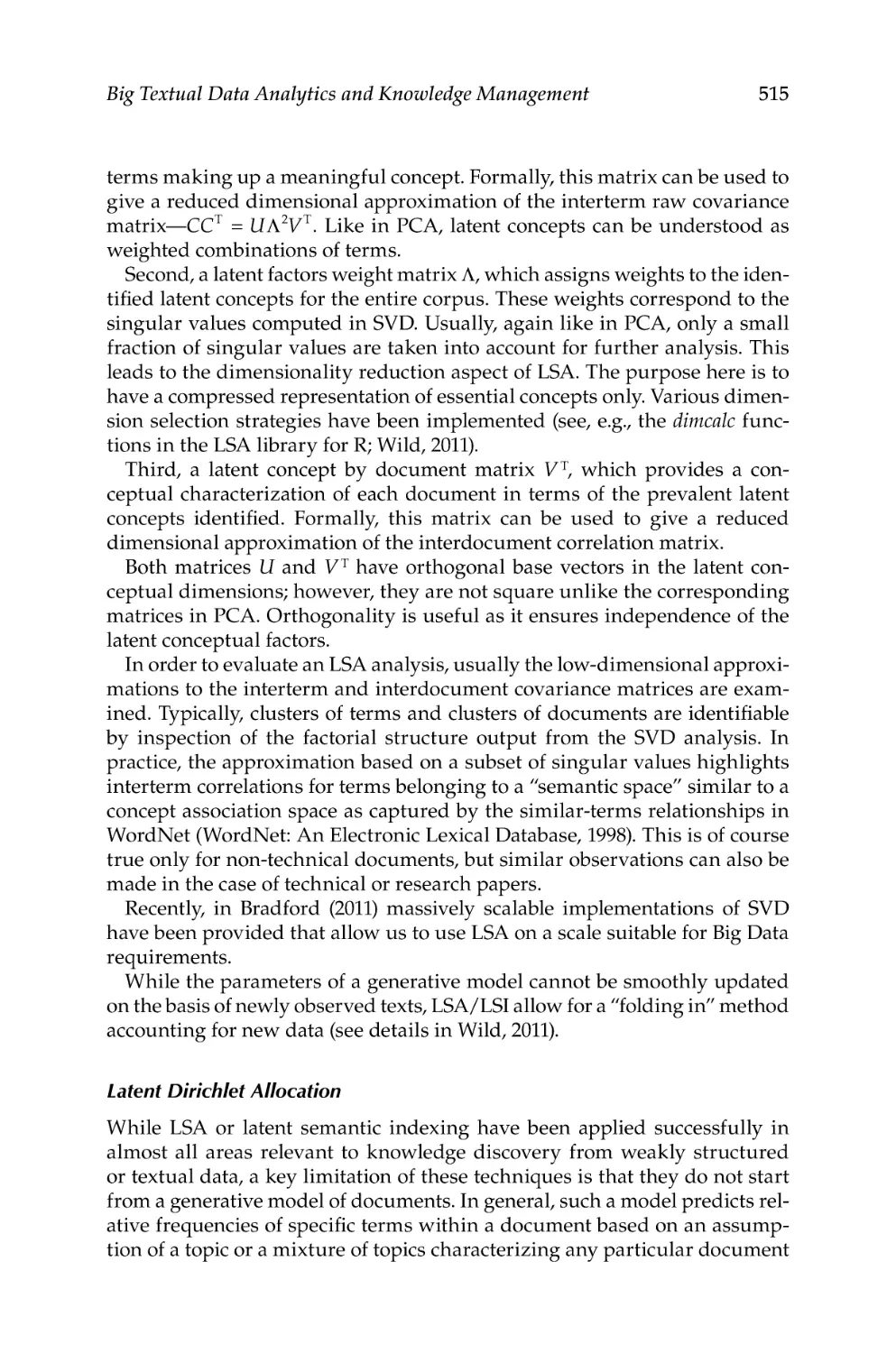
At a high level of detail, Driscoll (2011) describes the Big Data processing
technology stack comprising three major layers: foundational, analytics, and
applications (upper part of Figure 1.3).
The foundational layer provides the infrastructure for storage, access, and
management of Big Data. Depending on the nature of data, stream processing solutions (Abadi et al. 2003; Golab and Tamer Ozsu 2003; Salehi 2010),
distributed persistent storage (Chang et al. 2008; Roy et al. 2009; Shvachko
et al. 2010), cloud infrastructures (Rimal et al. 2009; Tsangaris et al. 2009;
Cusumano 2010), or a reasonable combination of these (Gu and Grossman
2009; He et al. 2010; Sakr et al. 2011) may be used for storing and accessing
data in response to the upper-layer requests and requirements.

Focused services

Volume

Variety

Velocity

Big Data analytics
Efficiency...
...Effectiveness

Complexity

Big Data storage, access, management infrastructure
Velocity

Data
management
Storage

Data stream
processing
Velocity

Efficiency

Volume

Query planning
and exceution

Volume

Big Data

Variety

Effectiveness

Complexity

Figure 1.3
Processing stack, based on Driscoll (2011), and the four dimensions of Big Data, based on Beyer
et al. (2011), influencing efficiency and effectiveness of analytics.

14

Big Data Computing

The middle layer of the stack is responsible for analytics. Here data warehousing technologies (e.g., Nemani and Konda 2009; Ponniah 2010; Thusoo
et al. 2010) are currently exploited for extracting correlations and features
(e.g., Ishai et al. 2009) from data and feeding classification and prediction
algorithms (e.g., Mills 2011).
Focused applications or services are at the top of the stack. Their functionality is based on the use of more generic lower-layer technologies and
exposed to end users as Big Data products.
Example of a startup offering focused services is BillGuard (billguard.
com). It monitors customers’ credit card statements for dubious charges and
even leverages the collective behavior of users to improve its fraud predictions. Another company called Klout (klout.com/home) provides a genuine
data service that uses social media activity to measure online influence.
LinkedIn’s People you may know feature is also a kind of focused service. This
service is presumably based on graph theory, starting exploration of the
graph of your relations from your node and filtering those relations according to what is called “homophily.” The greater the homophily between two
nodes, the more likely two nodes will be connected.
According to its purpose, the foundational layer is concerned about being
capable of processing as much as possible data (volume) and as soon as possible. In particular, if streaming data are used, the faster the stream is (velocity), the more difficult it is to process the data in a stream window. Currently
available technologies and tools for the foundational level are not equally
well coping with volume and velocity dimensions which are, so to say, anticorrelated due to their nature. Therefore, hybrid infrastructures are in use
for balancing processing efficiency aspects (Figure 1.3)—comprising solutions focused on taking care of volumes, and, separately, of velocity. Some
examples are given in “Big Data in European Research” section.
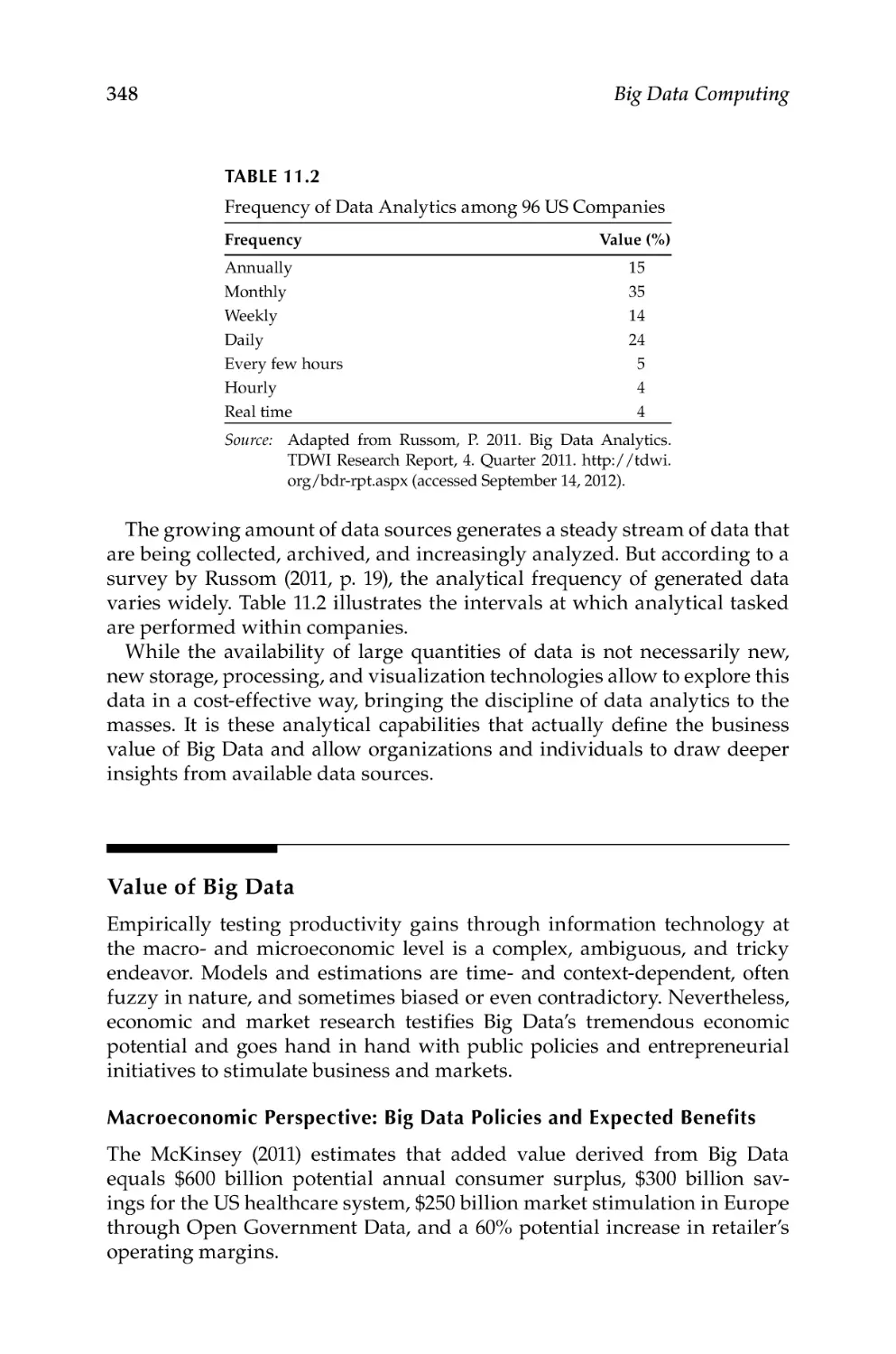
For the analytics layer (Figure 1.3), volume and velocity dimensions (Beyer
et al. 2011) are also important and constitute the facet of efficiency—big volumes of data which may change swiftly have to be processed in a timely
fashion. However, two more dimensions of Big Data become important—
complexity and variety—which form the facet of effectiveness. Complexity
is clearly about the adequacy of data representations and descriptions for
analysis. Variety describes a degree of syntactic and semantic heterogeneity
in distributed modules of data that need to be integrated or harmonized for
analysis. A major conceptual complication for analytics is that efficiency is
anticorrelated to effectiveness.
Big Data in European Research
Due to its huge demand, Big Data Computing is currently on the hype as a
field of research and development, producing a vast domain of work. To keep
the size of this review observable for a reader, we focus on the batch of the
running 7th Framework Programme (FP7) Information and Communication

Toward Evolving Knowledge Ecosystems for Big Data Understanding

15

Technology (ICT; cordis.europa.eu/fp7/ict/) projects within this vibrant
field. Big Data processing, including semantics, is addressed by the strategic objective of Intelligent Information Management (IIM; cordis.europa.eu/
fp7/ict/content-knowledge/projects_en.html). IIM projects funded in frame
of FP7 ICT Call 5 are listed in Table 1.1 and further analyzed below.
SmartVortex [Integrating Project (IP); smartvortex.eu] develops a technological infrastructure—a comprehensive suite of interoperable tools, services, and methods—for intelligent management and analysis of massive
data streams. The goal is to achieving better collaboration and decisionmaking in large-scale collaborative projects concerning industrial innovation engineering.
Legend: AEP, action extraction and prediction; DLi, data linking; DM, data
mining; DS, diversity in semantics; DV, domain vocabulary; FCA, formal
concept analysis; IE, information extraction; Int, integration; KD, knowledge
discovery; M-LS, multi-lingual search; MT, machine translation; O, ontology;
OM, opinion mining; QL, query language; R, reasoning; SBI, business intelligence over semantic data; SDW, semantic data warehouse (triple store); SUM,
summarization.
LOD2 (IP; lod2.eu) claims delivering: industrial strength tools and methodologies for exposing and managing very large amounts of structured
information; a bootstrap network of multidomain and multilingual ontologies from sources such as Wikipedia (wikipedia.org) and OpenStreetMap
(openstreetmap.org); machine learning algorithms for enriching, repairing,
interlinking, and fusing data from Web resources; standards and methods for
tracking provenance, ensuring privacy and data security, assessing information quality; adaptive tools for searching, browsing, and authoring Linked
Data.
Tridec (IP; tridec-online.eu) develops a service platform accompanied with
the next-generation work environments supporting human experts in decision processes for managing and mitigating emergency situations triggered
by the earth (observation) system in complex and time-critical settings. The
platform enables “smart” management of collected sensor data and facts
inferred from these data with respect to crisis situations.
First [Small Targeted Research Project (STREP); project-first.eu] develops
an information extraction, integration, and decision-making infrastructure
for financial domain with extremely large, dynamic, and heterogeneous
sources of information.
iProd (STREP; iprod-project.eu) investigates approaches of reducing product development costs by efficient use of large amounts of data comprising
the development of a software framework to support complex information
management. Key aspects addressed by the project are handling heterogeneous information and semantic diversity using semantic technologies
including knowledge bases and reasoning.
Teleios (STREP; earthobservatory.eu) focuses on elaborating a data
model and query language for Earth Observation (EO) images. Based on

Online Content,
Interactive and
Social Media

X

X

X

First

iProd

Teleios

X
X

X

X

Reasoning and
Information
Exploitation

Tridec

SmartVortex
LOD2

Acronym

Knowledge
Discovery and
Management

X

X

X

X

X
X

Industrial innovation engineering
Media and publishing, corporate data
intranets, eGovernment
Crisis/emergency response, government,
oil and gas
Market surveillance, investment
management, online retail banking and
brokerage
Manufacturing: aerospace, automotive,
and home appliances
Civil defense, environmental agencies.
Use cases: a virtual observatory for
TerraSAR-X data; real-time fire
monitoring

Domain(s)/Industry(ies)

Volume
X

X

X

X

X
X

Velocity
X

X

X

X

X

X

Variety

IIM Clustera

X

X

X

X

Complexity

Contribution to
Big Data
Processing Stack
Layersc

X

X

X

X

X
X

i. Fast Access
to/Management
of Data at Scale

Contribution
to Coping
with Big
Data
dimensionsb

X

X

X

X
X

ii. Fast
Analytics of
Data at Scale

FP7 ICT Call 5 Projects and their Contributions to Big Data Processing and Understanding

iii. Focused
Services

Table 1.1

DM, QL, KD

R, Int

IE

R

O, ML

Contribution
to Big Data
Understanding

16
Big Data Computing

X
X
X

Digital.me
Fish4Knowledge
Render

c

b

a

X

X
X
X
X

X
X
X

X

X

X
X

Medical imaging in healthcare,
biomedicine
Online communities (internet, extranet
and intranet) addressing: customer
support; knowledge sharing; hosting
services
Personal sphere
Marine sciences, environment
Information management (wiki), news
aggregation (search engine), customer
relationship management
(telecommunications)
Cross-domain
Government
Logistics
Market intelligence, computational
biology, control centre operations
Cross-domain
Clinico-genomic research, healthcare,
marketing
X

X

X
X

X

X

X

X

X

X

X
X

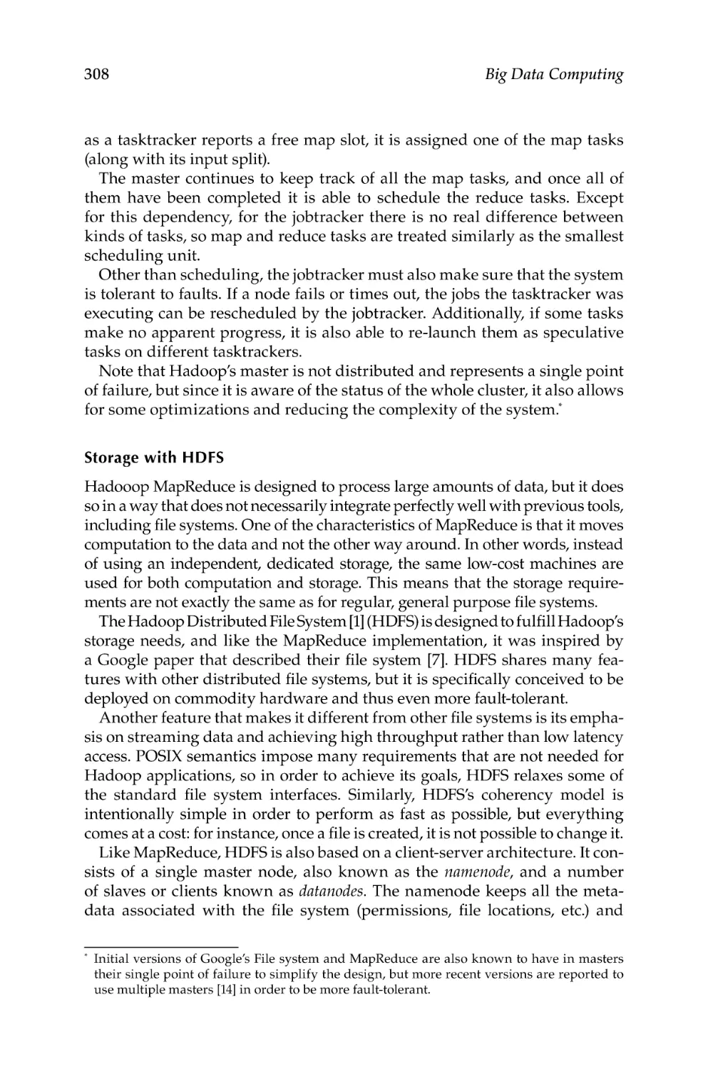
X

X

X
X

X

X
X

X
X
X

X
X
X

X

X

X
X

X
X

X

X

X

X

DM, OM

SDW, SBI, FCA

DV (fish), SUM
DS

IE, DLi, M-LS,
MT
AEP

IIM clustering information has been taken from the Commission’s source cordis.europa.eu/fp7/ict/content-knowledge/projects_en.html.
As per the Gartner report on extreme information management (Gartner 2011).
The contributions of the projects to the developments in the Big Data Stack layers have been assessed based on their public deliverables.

Promise
Dicode

PlanetData
LATC
Advance
Cubist

X

Robust

Khresmoi

Toward Evolving Knowledge Ecosystems for Big Data Understanding
17

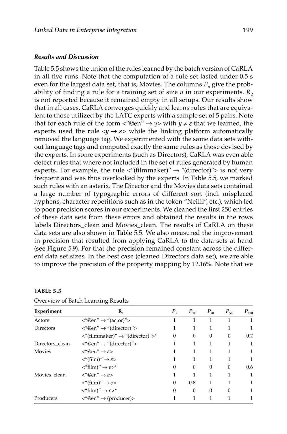
18

Big Data Computing

these, a scalable and adaptive environment for knowledge discovery from
EO images and geospatial data sets, and a query processing and optimization technique for queries over multidimensional arrays and EO image
annotations are developed and implemented on top of the MonetDB (monetdb.org) system.
Khresmoi (IP; khresmoi.eu) develops an advanced multilingual and multimodal search and access system for biomedical information and documents.
The advancements of the Khresmoi comprise: an automated information
extraction from biomedical documents reinforced by using crowd sourcing,
active learning, automated estimation of trust level, and target user expertise; automated analysis and indexing for 2-, 3-, 4D medical images; linking information extracted from unstructured or semistructured biomedical
texts and images to structured information in knowledge bases; multilingual search including multiple languages in queries and machine-translated
pertinent excerpts; visual user interfaces to assist in formulating queries and
displaying search results.
Robust (IP; robust-project.eu) investigates models and methods for describing, understanding, and managing the users, groups, behaviors, and needs
of online communities. The project develops a scalable cloud and streambased data management infrastructure for handling the real-time analysis of
large volumes of community data. Understanding and prediction of actions
is envisioned using simulation and visualization services. All the developed
tools are combined under the umbrella of the risk management framework,
resulting in the methodology for the detection, tracking, and management of
opportunities and threats to online community prosperity.
Digital.me (STREP; dime-project.eu) integrates all personal data in a personal sphere at a single user-controlled point of access—a user-controlled
personal service for intelligent personal information management. The software is targeted on integrating social web systems and communities and
implements decentralized communication to avoid external data storage and
undesired data disclosure.
Fish4Knowledge (STREP; homepages.inf.ed.ac.uk/rbf/Fish4Knowledge/)
develops methods for information abstraction and storage that reduce the
amount of video data at a rate of 10 × 1015 pixels to 10 × 1012 units of information. The project also develops machine- and human-accessible vocabularies
for describing fish. The framework also comprises flexible data-processing
architecture and a specialized query system tailored to the domain. To
achieve these, the project exploits a combination of computer vision, video
summarization, database storage, scientific workflow, and human–computer
interaction methods.
Render (STREP; render-project.eu) is focused on investigating the aspect
of diversity of Big Data semantics. It investigates methods and techniques,
develops software, and collects data sets that will leverage diversity as
a source of innovation and creativity. The project also claims providing
enhanced support for feasibly managing data on a very large scale and for

Toward Evolving Knowledge Ecosystems for Big Data Understanding

19

designing novel algorithms that reflect diversity in the ways information is
selected, ranked, aggregated, presented, and used.
PlanetData [Network of Excellence (NoE); planet-data.eu] works toward
establishing a sustainable European community of researchers that supports
organizations in exposing their data in new and useful ways and develops
technologies that are able to handle data purposefully at scale. The network
also facilitates researchers’ exchange, training, and mentoring, and event
organization based substantially on an open partnership scheme.
LATC (Support Action; latc-project.eu) creates an in-depth test-bed for dataintensive applications by publishing data sets produced by the European
Commission, the European Parliament, and other European institutions as
Linked Data on the Web and by interlinking them with other governmental
data.
Advance (STREP; advance-logistics.eu) develops a decision support platform for improving strategies in logistics operations. The platform is based
on the refinement of predictive analysis techniques to process massive data
sets for long-term planning and cope with huge amounts of new data in real
time.
Cubist (STREP; cubist-project.eu) elaborates methodologies and implements a platform that brings together several essential features of Semantic
Technologies and Business Intelligence (BI): support for the federation of
data coming from unstructured and structured sources; a BI-enabled triple
store as a data persistency layer; data volume reduction and preprocessing
using data semantics; enabling BI operations over semantic data; a semantic
data warehouse implementing FCA; applying visual analytics for rendering,
navigating, and querying data.
Promise (NoE; promise-noe.eu) establishes a virtual laboratory for conducting participative research and experimentation to carry out, advance, and
bring automation into the evaluation and benchmarking of multilingual and
multimedia information systems. The project offers the infrastructure for
access, curation, preservation, re-use, analysis, visualization, and mining of
the collected experimental data.
Dicode (STREP; dicode-project.eu) develops a workbench of interoperable
services, in particular, for: (i) scalable text and opinion mining; (ii) collaboration support; and (iii) decision-making support. The workbench is designed
to reduce data intensiveness and complexity overload at critical decision
points to a manageable level. It is envisioned that the use of the workbench
will help stakeholders to be more productive and concentrate on creative
activities.
In summary, the contributions to Big Data understanding of all the projects mentioned above result in the provision of different functionality for a
semantic layer—an interface between the Data and Analytics layers of the
Big Data processing stack—as pictured in Figure 1.4.
However, these advancements remain somewhat insufficient in terms of
reaching a desired balance between efficiency and effectiveness, as outlined

20

Big Data Computing

Focused services
MT

SBI

Big data analytics

Query formulation/ QL,
transformation
ML-S
Extraction/ AE, DE, IE,
elicitation KD, FCA, SUM

Query planning
and execution
Data stream
processing

Reasoning Integration: DLi, Int
R, AP,
Representation: O, DV
OM
DS

Storage: SDW
Big data semantics
Data
management
Storage

Big data storage, access, management
Figure 1.4
Contribution of the selection of FP7 ICT projects to technologies for Big Data understanding.
Abbreviations are explained in the legend to Table 1.1.

in the introduction of this chapter. Analysis of Table 1.1 reveals that no one
of the reviewed projects addresses all four dimensions of Big Data in a balanced manner. In particular, only two projects—Trydec and First—claim
contributions addressing Big Data velocity and variety-complexity. This fact
points out that the clinch between efficiency and effectiveness in Big Data
processing still remains a challenge.
Complications and Overheads in Understanding Big Data
As observed, the mankind collects and stores data through generations,
without a clear account of the utility of these data. Out of data at hand,
each generation extracts a relatively small proportion of knowledge for
their everyday needs. The knowledge is produced by a generation for their
needs—to an extent they have to satisfy their “nutrition” requirement for
supporting decision-making. Hence, knowledge is “food” for data analytics. An optimistic assumption usually made here is that the next generation
will succeed in advancing tools for data mining, knowledge discovery, and
extraction. So the data which the current generation cannot process effectively and efficiently is left as a legacy for the next generation in a hope that
the ancestors cope better. The truth, however, is that the developments of
data and knowledge-processing tools fail to keep pace with the explosive
growth of data in all four dimensions mentioned above. Suspending understanding Big Data until an advanced next-generation capability is at hand is
therefore an illusion of a solution.

Toward Evolving Knowledge Ecosystems for Big Data Understanding

21

Do today’s state-of-the-art technologies allow us to understand Big Data
with an attempt to balance effectiveness and efficiency?—probably not.
Our brief analysis reveals that Big Data computing is currently developed
toward more effective versus efficient use of semantics. It is done by adding the semantics layer to the processing stack (cf. Figures 1.3 and 1.4) with
an objective of processing all the available data and using all the generated
knowledge. Perhaps, the major issue is the attempt to eat all we have on the
table. Following the metaphor of “nutrition,” it has to be noted that the “food”
needs to be “healthy” in terms of all the discussed dimensions of Big Data.
Our perceptions of the consequences of being not selective with respect to
consuming data for understanding are as follows.
The major problem is the introduction of a new interface per se and in an
improper way. The advent of semantic technologies aimed at breaking down
data silos and simultaneously enabling efficient knowledge management at
scale. Assuming that databases describe data using multiple heterogeneous
labels, one might expect that annotating these labels using ontology elements as semantic tags enables virtual integration and provides immediate benefits for search, retrieval, reasoning, etc. without a need to modify
existing code, or data. Unfortunately, as noticed by Smith (2012), it is now
too easy to create “ontologies.” As a consequence, myriads of them are being
created in ad hoc ways and with no respect to compatibility, which implies
the creation of new semantic silos and, further bringing something like a
“Big Ontology” challenge to the agenda. According to Smith (2012), the big
reason is the lack of a rational (monetary) incentive for investing in reuse.
Therefore, it is often accepted that a new “ontology” is developed for a new
project. Harmonization is left for someone else’s work—in the next generation. Therefore, the more semantic technology simplifying ontology creation
is successful, the more we fail to achieve our goals for interoperability and
integration (Smith 2012).
It is worth noting here that there is still a way to start doing things correctly which, according to Smith (2012), would be “to create an incremental,
evolutionary process, where what is good survives, and what is bad fails;
create a scenario in which people will find it profitable to reuse ontologies,
terminologies and coding systems which have been tried and tested; silo
effects will be avoided and results of investment in Semantic Technology
will cumulate effectively.”
A good example of a collaborative effort going in this correct direction
is the approach used by the Gene Ontology initiative (geneontology.org)
which follows the principles of the OBO Foundry (obofoundry.org). The
Gene Ontology project is a major bioinformatics initiative with the aim of
standardizing the representation of gene and gene product attributes across
species and databases. The project provides a controlled vocabulary of terms
for describing gene product characteristics and gene product annotation
data, as well as tools to access and process this data. The mission of OBO
Foundry is to support community members in developing and publishing

22

Big Data Computing

fully interoperable ontologies in the biomedical domain following common
evolving design philosophy and implementation and ensuring a gradual
improvement of the quality of ontologies.
Furthermore, adding a data semantics layer facilitates increasing effectiveness in understanding Big Data, but also substantially increases the
computational overhead for processing the representations of knowledge—decreasing efficiency. A solution is needed that harmonically and
rationally balances between the increase in the adequacy and the completeness of Big Data semantics, on the one hand, and the increase in computational complexity, on the other hand. A straightforward approach is
using scalable infrastructures for processing knowledge representations.
A vast body of related work focuses on elaborating this approach (e.g.,
Broekstra et al. 2002; Wielemaker et al. 2003; Cai and Frank 2004; DeCandia
et al. 2007).
The reasons to qualifying this approach only as a mechanistic solution are
• Using distributed scalable infrastructures, such as clouds or
grids, implies new implementation problems and computational
overheads.
• Typical tasks for processing knowledge representations, such as
reasoning, alignment, query formulation and transformation, etc.,
scale hardly (e.g., Oren et al. 2009; Urbani et al. 2009; Hogan et al.
2011)—more expressiveness implies harder problems in decoupling
the fragments for distribution. Nontrivial optimization, approximation, or load-balancing techniques are required.
Another effective approach to balance complexity and timeliness is maintaining history or learning from the past. A simple but topical example in
data processing is the use of previously acquired information for saving
approximately 50% of comparison operations in sorting by selection (Knuth
1998, p. 141). In Distributed Artificial Intelligence software, agent architectures maintaining their states or history for more efficient and effective
deliberation have also been developed (cf. Dickinson and Wooldridge 2003).
In Knowledge Representation and Reasoning, maintaining history is often
implemented as inference or query result materialization (cf. Kontchakov
et al. 2010; McGlothlin and Khan 2010), which also do not scale well up to the
volumes characterizing real Big Data.
Yet another way to find a proper balance is exploiting incomplete or
approximate methods. These methods yield results of acceptable quality
much faster than approaches aiming at building fully complete or exact, that
is, ideal results. Good examples of technologies for incomplete or partial reasoning and approximate query answering (Fensel et al. 2008) are elaborated
in the FP7 LarKC project (larkc.eu). Remarkably, some of the approximate
querying techniques, for example, Guéret et al. (2008), are based on evolutionary computing.

Toward Evolving Knowledge Ecosystems for Big Data Understanding

23

Refining Big Data Semantics Layer for Balancing Efficiency Effectiveness
As one may notice, the developments in the Big Data semantics layer are
mainly focused on posing and appropriately transforming the semantics of
queries all the way down to the available data, using networked ontologies.
At least two shortcomings of this, in fact, unidirectional* approach need to
be identified:
1. Scalability overhead implies insufficient efficiency. Indeed, executing
queries at the data layer implies processing volumes at the scale of
stored data. Additional overhead is caused by the query transformation, distribution, and planning interfaces. Lifting up the stack and
fusing the results of these queries also imply similar computational
overheads. A possible solution for this problem may be sought following a supposition that the volume of knowledge describing data
adequately for further analyses is substantially smaller than the volume of this data. Hence, down-lifting queries for execution need to
be stopped at the layer of knowledge storage for better efficiency.
However, the knowledge should be consistent enough with the data
so that it can fulfill completeness and correctness requirements
specified in the contract of the query engine.
2. Having ontologies inconsistent with data implies effectiveness problems.
Indeed, in the vast majority of cases, the ontologies containing
knowledge about data are not updated consistently with the changes
in data. At best, these knowledge representations are revised in a
sequence of discrete versions. So, they are not consistent with the
data at an arbitrary point in time. This shortcoming may be overcome only if ontologies in a knowledge repository evolve continuously in response to data change. Ontology evolution will have a
substantially lower overhead because the volume of changes is
always significantly lower than the volume of data, though depends
on data velocity (Figure 1.3).
To sum up, relaxing the consequences of the two outlined shortcomings
and, hence, balancing efficiency and effectiveness may be achievable if a
bidirectional processing approach is followed. Top-down query answering
has to be complemented by a bottom-up ontology evolution process, which
meet at the knowledge representation layer. In addition to a balance between
efficiency and effectiveness, such an approach of processing huge data sets
may help us “. . . find and see dynamically changing ontologies without hav-

*

Technologies for information and knowledge extraction are also developed and need to be
regarded as bottom-up. However, these technologies are designed to work off-line for updating the existing ontologies in a discrete manner. Their execution is not coordinated with the
top-down query processing and data changes. So, the shortcomings outlined below persist.

24

Big Data Computing

ing to try to prescribe them in advance.* Taxonomies and ontologies are
things that you might discover by observation, and watch evolve over time”
(cf. Bollier 2010).
Further, we focus on outlining a complementary bottom-up path in the
overall processing stack which facilitates existing top-down query answering
frameworks by providing knowledge evolution in line with data change—as
pictured in Figure 1.5. In a nutshell, the proposed bottom-up path is characterized by:
• Efficiently performing simple scalable queries on vast volumes of
data or in a stream window for extracting facts and decreasing volumes (more details could be found in the “Scaling with a Traditional
Database” section)
• Adding extracted facts to a highly expressive persistent knowledge
base allowing evolution of knowledge (more details on that could
be seen in Knowledge Self-Management and Refinement through
Evolution)
• Assessing fitness of knowledge organisms and knowledge representations in the evolving knowledge ecosystem (our approach to that is
also outlined in the “Knowledge Self-Management and Refinement
through Evolution” section)
This will enable reducing the overheads of the top-down path by performing refined inference using highly expressive and complex queries over

Bottom-up path for knowledge
evolution
Knowledge Knowledge evolution
extraction and management

Data
management

Semantic query planning and answering

Big Data semantics
Change
harmonization

Distributed persistent knowledge storage

Evolution
Contextualization
Extraction
Query planning and execution
Data stream
processing

Persistent
distributed
storage

Big Data storage, access, management

Figure 1.5
Refining Big Data semantics layer for balancing efficiency and effectiveness.

*

Underlined by the authors of this chapter.

Top-down path
for query answering

Big Data analytics

Toward Evolving Knowledge Ecosystems for Big Data Understanding

25

evolving (i.e., consistent with data) and linked (i.e., harmonized), but reasonably small fragments of knowledge. Query results may also be materialized
for further decreasing computational effort.
After outlining the abstract architecture and the bottom-up approach, we
will now explain at a high level how Big Data needs to be treated along the
way. A condensed formula for this high-level approach is “3F + 3Co” which
is unfolded as
3F: Focusing-Filtering-Forgetting
3Co: Contextualizing-Compressing-Connecting
Notably, both 3F and 3Co are not novel and used in parts extensively in
many domains and in different interpretations. For example, an interesting
interpretation of 3F is offered by Dean and Webb (2011) who suggest this formula as a “treatment” for senior executives (CEOs) to deal with information
overload and multitasking. Executives are offered to cope with the problem
by focusing (doing one thing at a time), filtering (delegating so that they do
not take on too many tasks or too much information), and forgetting (taking
breaks and clearing their minds).
Focusing
Following our Boeing example, let us imagine a data analyst extracting
knowledge tokens from a business news stream and putting these tokens
as missing bits in the mosaic of his mental picture of the world. A tricky
part of his work, guided by intuition or experience in practice, is choosing
the order in which the facts are picked up from the token. Order of focusing
is very important as it influences the formation and saturation of different
fragments in the overall canvas. Even if the same input tokens are given, different curves of focusing may result in different knowledge representations
and analysis outcomes.
A similar aspect of proper focusing is of importance also for automated
processing of Big Data or its semantics. One could speculate whether a processing engine should select data tokens or assertions in the order of their
appearance, in a reversed order, or anyhow else. If data or assertions are processed in a stream window and in real time, the order of focusing is of lesser
relevance. However, if all the data or knowledge tokens are in a persistent
storage, having some intelligence for optimal focusing may improve processing efficiency substantially. With smart focusing at hand, a useful token can
be found or a hidden pattern extracted much faster and without making a
complete scan of the source data. A complication for smart focusing is that
the nodes on the focusing curve have to be decided upon on-the-fly because
generally the locations of important tokens cannot be known in advance.
Therefore, the processing of a current focal point should not only yield what

26

Big Data Computing

is intended directly of this portion of data, but also hint about the next point
on the curve.
A weak point in such a “problem-solving” approach is that some potentially
valid alternatives are inevitably lost after each choice made on the decision
path. So, only a suboptimal solution is practically achievable. The evolutionary approach detailed further in section “Knowledge Self-Management and
Refinement through Evolution” follows, in fact, a similar approach of smart
focusing, but uses a population of autonomous problem-solvers operating
concurrently. Hence, it leaves a much smaller part of a solution space without
attention, reduces the bias of each choice, and likely provides better results.
Filtering
A data analyst who receives dozens of news posts at once has to focus on the
most valuable of them and filter out the rest which, according to his informed
guess, do not bring anything important additionally to those in his focus.
Moreover, it might also be very helpful to filter out noise, that is, irrelevant
tokens, irrelevant dimensions of data, or those bits of data that are unreadable or corrupted in any other sense. In fact, an answer to the question about
what to trash and what to process needs to be sought based on the understanding of the objective (e.g., was the reason for Boeing to hike their market
forecast valid?) and the choice of the proper context (e.g., should we look into
the airline fleets or the economic situation in developing countries?).
A reasonable selection of features for processing or otherwise a rational
choice of the features that may be filtered out may essentially reduce the
volume as well as the variety/complexity of data which result in higher efficiency balanced with effectiveness.
Quite similar to focusing, a complication here is that for big heterogeneous
data it is not feasible to expect a one-size-fits-all filter in advance. Even more,
for deciding about an appropriate filtering technique and the structure of a
filter to be applied, a focused prescan of data may be required, which implies
a decrease in efficiency. The major concern is again how to filter in a smart
way and so as to balance the intentions to reduce processing effort (efficiency)
and keep the quality of results within acceptable bounds (effectiveness).
Our evolutionary approach presented in the section “Knowledge SelfManagement and Refinement through Evolution” uses a system of environmental contexts for smart filtering. These contexts are not fixed but may be
adjusted by several independent evolutionary mechanisms. For example, a
context may become more or less “popular” among the knowledge organisms that harvest knowledge tokens in them because these organisms
may migrate freely between contexts in search for better, more appropriate, healthier knowledge to collect. Another useful property we propose
for knowledge organisms is their resistance to sporadic mutagenic factors,
which may be helpful for filtering out noise.

Toward Evolving Knowledge Ecosystems for Big Data Understanding

27

Forgetting
A professional data analyst always keeps a record of data he used in his work
and the knowledge he created in his previous analyses. The storage for all
these gems of expertise is, however, limited, so it has to be cleaned periodically. Such a cleaning implies trashing potentially valuable things, though
never or very rarely used, but causing doubts and further regrets about the
lost. Similar thing happens when Big Data storage is overflown—some parts
of it have to be trashed and so “forgotten.” A question in this respect is about
which part of a potentially useful collection may be sacrificed. Is forgetting
the oldest records reasonable?—perhaps not. Shall we forget the features that
have been previously filtered out?—negative again. There is always a chance
that an unusual task for analysis pops up and requires the features never
exploited before. Are the records with minimal potential utility the best candidates for trashing?—could be a rational way to go, but how would their
potential value be assessed?
Practices in Big Data management confirm that forgetting following
straightforward policies like fixed lifetime for keeping records causes regret
almost inevitably. For example, the Climate Research Unit (one of the leading
institutions that study natural and anthropogenic climate change and collect
climate data) admits that they threw away the key data to be used in global
warming calculations (Joseph 2012).
A better policy for forgetting might be to extract as much as possible knowledge out of data before deleting these data. It cannot be guaranteed, however,
that future knowledge mining and extraction algorithms will not be capable of
discovering more knowledge to preserve. Another potentially viable approach
could be “forgetting before storing,” that is, there should be a pragmatic reason
to store anything. The approach we suggest in the section “Knowledge SelfManagement and Refinement through Evolution” follows exactly this way.
Though knowledge tokens are extracted from all the incoming data tokens, not
all of them are consumed by knowledge organisms, but only those assertions
that match to their knowledge genome to a sufficient extent. This similarity is
considered a good reason for remembering a fact. The rest remains in the environment and dies out naturally after the lifetime comes to end as explained in
“Knowledge Self-Management and Refinement through Evolution”.
Contextualizing
Our reflection of the world is often polysemic, so a pragmatic choice of a
context is often needed for proper understanding. For example, “taking a
mountain hike” or “hiking a market forecast” are different actions though
the same lexical root is used in the words. An indication of a context: recreation or business in this example would be necessary for making the statement explicit. To put it even broader, not only the sense of statements, but

28

Big Data Computing

also judgments, assessments, attitudes, and sentiments about the same data
or knowledge token may well differ in different contexts. When it goes about
data, it might be useful to know:
1. The “context of origin”—the information about the source; who organized and performed the action; what were the objects; what features
have been measured; what were the reasons or motives for collecting
these data (transparent or hidden); when and where the data were
collected; who were the owners; what were the license, price, etc.
2. The “context of processing”—formats, encryption keys, used preprocessing tools, predicted performance of various data mining algorithms, etc.; and
3. The “context of use”—potential domains, potential or known applications, which may use the data or the knowledge extracted from it,
potential customers, markets, etc.
Having circumscribed these three different facets of context, we may say
now that data contextualization is a transformation process which decontextualizes the data from the context of origin and recontextualizes it into the
context of use (Thomason 1998), if the latter is known. This transformation is
performed via smart management of the context of processing.
Known data mining methods are capable of automatically separating
the so-called “predictive” and “contextual” features of data instances (e.g.,
Terziyan 2007). A predictive feature stands for a feature that directly influences the result of applying to data a knowledge extraction instrument—
knowledge discovery, prediction, classification, diagnostics, recognition, etc.
RESULT = INSTRUMENT(Predictive Features).
Contextual features could be regarded as arguments to a meta-function
that influences the choice of appropriate (based on predicted quality/performance) instrument to be applied to a particular fragment of data:
INSTRUMENT = CONTEXTUALIZATION(Contextual Features).
Hence, a correct way to process each data token and benefit of contextualization would be: (i) decide, based on contextual features, which would
be an appropriate instrument to process the token; and then (ii) process it
using the chosen instrument that takes the predictive features as an input.
This approach to contextualization is not novel and is known in data mining
and knowledge discovery as a “dynamic” integration, classification, selection, etc. Puuronen et al. (1999) and Terziyan (2001) proved that the use of
dynamic contextualization in knowledge discovery yields essential quality
improvement compared to “static” approaches.

Toward Evolving Knowledge Ecosystems for Big Data Understanding

29

Compressing
In the context of Big Data, having data in a compact form is very important for
saving storage space or reducing communication overheads. Compressing is
a process of data transformation toward making data more compact in terms
of required storage space, but still preserving either fully (lossless compression) or partly (lossy compression) the essential features of these data—those
potentially required for further processing or use.
Compression, in general, and Big Data compression, in particular, are
effectively possible due to a high probability of the presence of repetitive,
periodical, or quasi-periodical data fractions or visible trends within data.
Similar to contextualization, it is reasonable to select an appropriate data
compression technique individually for different data fragments (clusters),
also in a dynamic manner and using contextualization. Lossy compression
may be applied if it is known how data will be used, at least potentially.
So that some data fractions may be sacrificed without losing the facets of
semantics and the overall quality of data required for known ways of its use.
A relevant example of a lossy compression technique for data having quasiperiodical features and based on a kind of “meta-statistics” was reported by
Terziyan et al. (1998).
Connecting
It is known that nutrition is healthy and balanced if it provides all the necessary components that are further used as building blocks in a human body.
These components become parts of a body and are tightly connected to the
rest of it. Big Data could evidently be regarded as nutrition for knowledge
economy as discussed in “Motivation and Unsolved Issues”. A challenge is
to make this nutrition healthy and balanced for building an adequate mental
representation of the world, which is Big Data understanding. Following the
allusion of human body morphogenesis, understanding could be simplistically interpreted as connecting or linking new portions of data to the data
that is already stored and understood. This immediately brings us about the
concept of linked data (Bizer et al. 2009), where “linked” is interpreted as a
sublimate of “understood.” We have written “a sublimate” because having
data linked is not yet sufficient, though necessary for further, more intelligent phase of building knowledge out of data. After data have been linked,
data and knowledge mining, knowledge discovery, pattern recognition,
diagnostics, prediction, etc. could be done more effectively and efficiently.
For example, Terziyan and Kaykova (2012) demonstrated that executing business intelligence services on top of linked data is noticeably more efficient
than without using linked data. Consequently, knowledge generated out of
linked data could also be linked using the same approach, resulting in the
linked knowledge. It is clear from the Linking Open Data Cloud Diagram
by Richard Cyganiak and Anja Jentzsch (lod-cloud.net) that knowledge

30

Big Data Computing

(e.g., RDF or OWL modules) represented as a linked data can be relatively
easily linked to different public data sets, which creates a cloud of linked
open semantic data.
Mitchell and Wilson (2012) argue that the key to extract value from Big
Data lies in exploiting the concept of linked. They believe that linked data
potentially creates ample opportunities from numerous data sources. For
example, using links between data as a “broker” brings more possibilities
of extracting new data from the old, creating insights that were previously
unachievable, and facilitating exciting new scenarios for data processing.
For developing an appropriate connection technology, the results are relevant from numerous research and development efforts, for example, Linking
Open Data (LOD; w3.org/wiki/SweoIG/TaskForces/CommunityProjects/
LinkingOpenData) project, DBpedia (dbpedia.org), OpenCyc (opencyc.org),
FOAF (foaf-project.org), CKAN (ckan.org), Freebase (freebase.com), Factual
(factual.com), and INSEMTIVES (insemtives.eu/index.php). These projects
create structured and interlinked semantic content, in fact, mashing up the
features from Social and Semantic Web (Ankolekar et al. 2007). One strength
of their approach is that collaborative content development effort is propagated up the level of the data-processing stack which allows creating semantic representations collaboratively and in an evolutionary manner.
Autonomic Big Data Computing
The treatment offered in the “Refining Big Data Semantics Layer for
Balancing Efficiency-Effectiveness” section requires a paradigm shift in Big
Data computing. In seeking for a suitable approach to building processing
infrastructures, a look into Autonomic Computing might be helpful. Started
by International Business Machines (IBM) in 2001, Autonomic Computing
refers to the characteristics of complex computing systems allowing them
to manage themselves without direct human intervention. A human, in
fact, defines only general policies that constrain self-management process.
According to IBM,* the four major functional areas of autonomic computing
are: (i) self-configuration—automatic configuration of system components; (ii)
self-optimization—automatic monitoring and ensuring the optimal functioning of the system within defined requirements; (iii) self-protection—automatic
identification and protection from security threats; and (iv) self-healing—
automatic fault discovery and correction. Other important capabilities of
autonomic systems are: self-identity in a sense of being capable of knowing
itself, its parts, and resources; situatedness and self-adaptation—sensing the
influences from its environment and acting accordingly to what happens
in the observed environment and a particular context; being non-proprietary
in a sense of not constraining itself to a closed world but being capable of
functioning in a heterogeneous word of open standards; and anticipatory in
*

research.ibm.com/autonomic/overview/elements.html (accessed October 10, 2012).

Toward Evolving Knowledge Ecosystems for Big Data Understanding

31

a sense of being able to automatically anticipate needed resources and seamlessly bridging user tasks to their technological implementations hiding
complexity.
However, having an autonomic system for processing Big Data semantics might not be sufficient. Indeed, even such a sophisticated entity system
may once face circumstances which it would not be capable of reacting to
by reconfiguration. So, the design objectives will not be met by such a system and it should qualify itself as not useful for further exploitation and die.
A next-generation software system will then be designed and implemented
(by humans) which may inherit some valid features from the ancestor system
but shall also have some principally new features. Therefore, it needs to be
admitted that it is not always possible for even an autonomic system to adapt
itself to a change within its lifetime. Consequently, self-management capability may not be sufficient for the system to survive autonomously—humans
are required for giving birth to ancestors. Hence, we are coming to the necessity of a self-improvement feature which is very close to evolution. In that we
may seek for inspiration in bio-social systems. Nature offers an automatic
tool for adapting biological species across generations named genetic evolution. An evolutionary process could be denoted as the process of proactive
change of the features in the populations of (natural or artificial) life forms
over successive generations providing diversity at every level of life organization. Darwin (1859) put the following principles in the core of his theory:
• Principle of variation (variations of configuration and behavioral
features);
• Principle of heredity (a child inherits some features from its parents);
• Principle of natural selection (some features make some individuals more competitive than others in getting needed for survival
resources).
These principles may remain valid for evolving software systems, in particular, for Big Data computing. Processing knowledge originating from Big
Data may, however, imply more complexity due to its intrinsic social features.
Knowledge is a product that needs to be shared within a group so that
survivability and quality of life of the group members will be higher than
those of any individual alone. Sharing knowledge facilitates collaboration
and improves individual and group performance. Knowledge is actively
consumed and also left as a major inheritance for future generations, for
example, in the form of ontologies. As a collaborative and social substance,
knowledge and cognition evolve in a more complex way for which additional
facets have to be taken into account such as social or group focus of attention,
bias, interpretation, explicitation, expressiveness, inconsistency, etc.
In summary, it may be admitted that Big Data is collected and supervised by different communities following different cultures, standards,

32

Big Data Computing

objectives, etc. Big Data semantics is processed using naturally different
ontologies. All these loosely coupled data and knowledge fractions in fact
“live their own lives” based on very complex processes, that is, evolve following the evolution of these cultures, their cognition mechanisms, standards,
objectives, ontologies, etc. An infrastructure for managing and understanding such data straightforwardly needs to be regarded as an ecosystem of
evolving processing entities. Below we propose treating ontologies (a key
for understanding Big Data) as genomes and bodies of those knowledge
processing entities. For this, basic principles by Darwin are applied to their
evolution aiming to get optimal or quasi-optimal (according to evolving definition of the quality) populations of knowledge species. These populations
represent the evolving understanding of the respective islands of Big Data
in their dynamics. This approach to knowledge evolution will require interpretation and implementation of concepts like “birth,” “death,” “morphogenesis,” “mutation,” “reproduction,” etc., applied to knowledge organisms,
their groups, and environments.

Scaling with a Traditional Database
In some sense, “Big data” is a term that is increasingly being used to describe
very large volumes of unstructured and structured content—usually in
amounts measured in terabytes or petabytes—that enterprises want to harness and analyze.
Traditional relational database management technologies, which use indexing for speedy data retrieval and complex query support, have been hard
pressed to keep up with the data insertion speeds required for big data analytics. Once a database gets bigger than about half a terabyte, some database
products’ ability to rapidly accept new data start [start is to database products] to decrease.
There are two kinds of scalability, namely vertical and horizontal. Vertical
scaling is just adding more capacity to a single machine. Fundamentally,
every database product is vertically scalable to the extent that they can make
good use of more central processing unit cores, random access memory, and
disk space. With a horizontally scalable system, it is possible to add capacity
by adding more machines. Beyond doubt, most database products are not
horizontally scalable.
When an application needs more write capacity than they can get out of a
single machine, they are required to shard (partition) their data across multiple database servers. This is how companies like Facebook (facebook.com)
or Twitter (twitter.com) have scaled their MySQL installations to massive
proportions. This is the closest to what one can get into horizontal scalability
with database products.

Toward Evolving Knowledge Ecosystems for Big Data Understanding

33

Sharding is a client-side affair, that is, the database server does not do it
for user. In this kind of environment, when someone accesses data, the data
access layer uses consistent hashing to determine which machine in the cluster a precise data should be written to (or read from). Enhancing capacity to
a sharded system is a process of manually rebalancing the data across the
cluster. The database system itself takes care of rebalancing the data and
guaranteeing that it is adequately replicated across the cluster. This is what
it means for a database to be horizontally scalable.
In many cases, constructing Big Data systems on premise provides better
data flow performance, but requires a greater capital investment. Moreover,
one has to consider the growth of the data. While many model linear growth
curves, interestingly the patterns of data growth within Big Data systems
are more exponential. Therefore, model both technology and costs to match
up with sensible growth of the database so that the growth of the data flows.
Structured data transformation is the traditional approach of changing the
structure of the data found within the source system to the structure of the
target system, for instance, a Big Data system. The advantage of most Big Data
systems is that deep structure is not a requirement; without doubt, structure
can typically be layered in after the data arrive at the goal. However, it is a
best practice to form the data within the goal. It should be a good abstraction of the source operational databases in a structure that allows those who
analyze the data within the Big Data system to effectively and efficiently find
the data required. The issue to consider with scaling is the amount of latency
that transformations cause as data moves from the source(s) to the goal, and
the data are changed in both structure and content. However, one should
avoid complex transformations as data migrations for operational sources
to the analytical goals. Once the data are contained within a Big Data system, the distributed nature of the architecture allows for the gathering of the
proper result set. So, transformations that cause less latency are more suitable within Big Data domain.
Large Scale Data Processing Workflows
Overall infrastructure for many Internet companies can be represented as
a pipeline with three layers: Ingestion, Storage & Processing, and Serving.
The most vital among the three is the Storage & Processing layer. This layer
can be represented as a multisub-layer stack with a scalable file system such
as Google File System (Ghemawat et al. 2003) at the bottom, a framework
for distributed sorting and hashing, for example, Map-Reduce (Dean and
Ghemawat 2008) over the file system layer, a dataflow programming framework over the map-reduce layer, and a workflow manager at the top.
Debugging large-scale data, in the Internet firms, is crucial because
data passes through many subsystems, each having different query interface, different metadata representation, different underlying models (some
have files, some have records, some have workflows), etc. Thus, it is hard

34

Big Data Computing

to maintain consistency and it is essential to factor out the debugging from
the subsystems. There should be a self-governing system that takes care of
all the metadata management. All data-processing subsystems can dispatch
their metadata to such system which absorbs all the metadata, integrates
them, and exposes a query interface for all metadata queries. This can provide a uniform view to users, factors out the metadata management code,
and decouples metadata lifetime from data/subsystem lifetime.
Another stimulating problem is to deal with different data and process
granularity. Data granularity can vary from a web page, to a table, to a row,
to a cell. Process granularity can vary from a workflow, to a map-reduce program, to a map-reduce task. It is very hard to make an inference when the
given relationship is in one granularity and the query is in other granularity and therefore it is vital to capture provenance data across the workflow.
While there is no one-size-fits-all solution, a good methodology could be
to use the best granularity at all levels. However, this may cause a lot of
overhead and thus some smart domain-specific techniques need to be implemented (Lin and Dyer 2010; Olston 2012).

Knowledge Self-Management and Refinement through
Evolution
World changes—so do the beliefs and reflections about it. Those beliefs
and reflections are the knowledge humans have about their environments.
However, the nature of those changes is different. The world just changes in
events. Observation or sensing (Ermolayev et al. 2008) of events invokes generation of data—often in huge volumes and with high velocities. Humans
evolve—adapt themselves to become better fitted to the habitat.
Knowledge is definitely a product of some processes carried out by conscious living beings (for example, humans). Following Darwin’s (1859)
approach and terminology to some extent, it may be stated that knowledge,
both in terms of scope and quality, makes some individuals more competitive than others in getting vital resources or at least for improving their quality of life. The major role of knowledge as a required feature for survival is
decision-making support. Humans differ in fortune and fate because they
make different choices in similar situations, which is largely due to their possession of different knowledge. So, the evolution of conscious beings noticeably depends on the knowledge they possess. On the other hand, making a
choice in turn triggers the production of knowledge by a human. Therefore,
it is natural to assume that knowledge evolves triggered by the evolution of
conscious beings, their decision-making needs and taken decisions, quality
standards, etc. To put both halves in one whole, knowledge evolves in support of and to support the proactive needs of the owners more effectively, for

Toward Evolving Knowledge Ecosystems for Big Data Understanding

35

example, to better interpret or explain the data generated when observing
events, corresponding to the diversity and complexity of these data. This
observation leads us to a hypothesis about the way knowledge evolves:
The mechanisms of knowledge evolution are very similar to the mechanisms of biological evolution. Hence, the methods and mechanisms for
the evolution of knowledge could be spotted from the ones enabling the
evolution of living beings.

In particular, investigating the analogies and developing the mechanisms
for the evolution of formal knowledge representations—specified as ontologies—is of interest for the Big Data semantics layer (Figure 1.5). The triggers
for ontology evolution in the networked and interlinked environments could
be external influences coming bottom-up from external and heterogeneous
information streams.
Recently, the role of ontologies as formal and consensual knowledge representations has become established in different domains where the use
of knowledge representations and reasoning is an essential requirement.
Examples of these domains range from heterogeneous sensor network data
processing through the Web of Things to Linked Open Data management
and use. In all these domains, distributed information artifacts change sporadically and intensively in reflection of the changes in the world. However,
the descriptions of the knowledge about these artifacts do not evolve in line
with these changes.
Typically, ontologies are changed semiautomatically or even manually and
are available in a sequence of discrete revisions. This fact points out a serious disadvantage of ontologies built using state-of-the-art knowledge engineering and management frameworks and methodologies: expanding and
amplified distortion between the world and its reflection in knowledge. It is
also one of the major obstacles for a wider acceptance of semantic technologies in industries (see also Hepp 2007; Tatarintseva et al. 2011).
The diversity of domain ontologies is an additional complication for proper
and efficient use of dynamically changing knowledge and information artifacts for processing Big Data semantics. Currently, the selection of the best
suiting one for a given set of requirements is carried out by a knowledge
engineer using his/her subjective preferences. A more natural evolutionary
approach for selecting the best-fitting knowledge representations promises
enhancing robustness and transparency, and seems to be more technologically attractive.
Further, we elaborate a vision of a knowledge evolution ecosystem where
agent-based software entities carry their knowledge genomes in the form of
ontology schemas and evolve in response to the influences percieved from
their environments. These influences are thought of as the tokens of Big Data
(like news tokens in the “Illustrative Example” section) coming into the species’ environments. Evolution implies natural changes in the ontologies which

36

Big Data Computing

reflect the change in the world snap-shotted by Big Data tokens. Inspiration
and analogies are taken from evolutionary biology.
Knowledge Organisms, their Environments, and Features
Evolving software entities are further referred to as individual Knowledge
Organisms (KO). It is envisioned (Figure 1.6) that a KO:
1. Is situated in its environment as described in “Environment, Perception
(Nutrition), and Mutagens”
2. Carries its individual knowledge genome represented as a schema or
Terminological Box (TBox; Nardi and Brachman 2007) of the respective ontology (see “Knowledge Genome and Knowledge Body”)
3. Has its individual knowledge body represented as an assertional component (ABox; Nardi and Brachman 2007) of the respective ontology
(see “Knowledge Genome and Knowledge Body”)
4. Is capable of perceiving the influences from the environment in the
form of knowledge tokens (see “Environment, Perception (Nutrition),
and Mutagens”) that may cause the changes in the genome (see
“Mutation”) and body (see “Morphogenesis”)—the mutagens
5. Is capable of deliberating about the affected parts of its genome and
body (see “Morphogenesis” and “Mutation”)

Mutagen

Communication

Perception

Sensor input

(ABox)

KO

KO

(TBox)

Deliberation
Morphogenesis
Mutation
Recombination

Genome
(TBox)
Body
(ABox)
Reproduction

Action output

Excretion

KO

Environment

Figure 1.6
A Knowledge Organism: functionality and environment. Small triangles of different transparency represent knowledge tokens in the environment—consumed and produced by KOs.
These knowledge tokens may also referred to as mutagens as they may trigger mutations.

Toward Evolving Knowledge Ecosystems for Big Data Understanding

37

6. Is capable of consuming some parts of a mutagen for: (a) morphogenesis changing only the body (see “Morphogenesis”); (b) mutation
changing both the genome and body (see “Mutation”); or (c) recombination—a mutual enrichment of several genomes in a group of KO
which may trigger reproduction—recombination of body replicas
giving “birth” to a new KO (see “Recombination and Reproduction”)
7. Is capable of excreting the unused parts of mutagens or the “dead”
parts of the body to the environment
The results of mainstream research in distributed artificial intelligence and
semantic technologies suggest the following basic building blocks for developing a KO. The features of situatedness (Jennings 2000) and deliberation
(Wooldridge and Jennings 1995) are characteristic to intelligent software agents,
while the rest of the required functionality could be developed using the achievments in Ontology Alignment (Euzenat and Shvaiko 2007). Recombination
involving a group of KOs could be thought of based on the known mechanisms
for multiissue negotiations on semantic contexts (e.g., Ermolayev et al. 2005)
among software agents—the members of a reproduction group.
Environment, Perception (Nutrition), and Mutagens
An environmental context for a KO could be thought of as an arial of its habitat. Such a context needs to be able to provide nutrition that is “healthy” for
particular KO species, that is, matching their genome noticeably. The food
for nutrition is provided by Knowledge Extraction and Contextualization
functionality (Figure 1.7) in a form of knowledge tokens. Hence, several

Airline Business

Information token

Knowledge token

Plane Maker Business

has
basedIn

Boeing: PlaneMaker

Another Domain

Environmental
Contexts

by
hikes

baseOf
UnitedStates

New20YMarketForecast

hikedBy
Old20YMarketForecast : MarketForecast

Another News Stream
Posted: Tue, 03 Jul 2012 05:01:10 -0400
LONDON (Reuters)
U.S. planemaker Boeing hiked its 20-year
market forecast, predicting demand for
34,000 new aircraft worth $4.5 trillion, on
growth in emerging regions and as airlines
seek efficient new planes to counter high
fuel costs.

Business News Stream

Knowledge Extraction
and Contextualization

Figure 1.7
Environmental contexts, knowledge tokens, knowledge extraction, and contextualization.

38

Big Data Computing

and possibly overlapping environmental contexts need to be regarded in
a ­hierarchy which corresponds to several subject domains of intetrest and
a foundational knowledge layer. By saying this, we subsume that there is a
single domain or foundational ontology module schema per environmental
context. Different environmental contexts corresponding to different subject
domais of interest are pictured as ellipses in Figure 1.7.
Environmental contexts are sowed with knowledge tokens that correspond to their subject domains. It might be useful to limit the lifetime of a
knowledge token in an environment—those which are not consumed dissolve finally when their lifetime ends. Fresh and older knowledge tokens are
pictured with different transparency in Figure 1.7.
KOs inhabit one or several overlapping environmental contexts based
on the nutritional healthiness of knowledge tokens sowed there, that is,
the degree to which these knowledge tokens match to the genome of a
particular KO. KOs use their perceptive ability to find and consume
knowledge tokens for nutrition. A KO may decide to migrate from one
environment to another based on the availability of healthy food there.
Knowledge tokens that only partially match KOs’ genome may cause both
KO body and genome changes and are thought of as mutagens. Mutagens,
in fact, deliver the information about the changes in the world to the environments of KOs.
Knowledge tokens are extracted from the information tokens either in
a stream window or from the updates of the persistent data storage and
further sawn in the appropriate environmental context. The context for
placing a newly coming KO is chosen by the contextualization functionality (Figure 1.7) based on the match ratio to the ontology schema characterizing the context in the environment. Those knowledge tokens that are not
mapped well to any of the ontology schemas are sown in the environment
without attributing them to any particular context.
For this, existing shallow knowledge extraction techniques could be
exploited, for example, Fan et al. (2012a). The choice of appropriate techniques depends on the nature and modality of data. Such a technique
would extract several interrelated assertions from an information token
and provide these as a knowledge token coded in a knowledge representation language of an appropriate expressiveness, for example, in a tractable
subset of the Web Ontology Language (OWL) 2.0 (W3C 2009). Information
and knowledge* tokens for the news item of our Boeing example are pictured in Figure 1.7.

*

Unified Modeling Language (UML) notation is used for picturing the knowledge token in
Figure 1.7 because it is more illustrative. Though not shown in Figure 1.7, it can be straightforwardly coded in OWL, following, for example, Kendall et al. (2009).

39

Toward Evolving Knowledge Ecosystems for Big Data Understanding

Knowledge Genome and Knowledge Body
Two important aspects in contextualized knowledge representation for an
outlined knowledge evolution ecosystem have to be considered with care
(Figure 1.8):
• A knowledge genome etalon for a population of KOs belonging to
one species
• An individual knowledge genome and body for a particular KO
A knowledge genome etalon may be regarded as the schema (TBox) of
a distinct ontology module which represents an outstanding context in a
subject domain. In our proposal, the etalon genome is carried by a dedicated
Etalon KO (EKO; Figure 1.8) to enable alignments with individual genomes
and other etalons in a uniform way. The individual assertions (ABox) of this
ontology module are spread over the individual KOs belonging to the corresponding species—forming their individual bodies.
The individual genomes of those KOs are the recombined genomes of the
KOs who gave birth to this particular KO. At the beginning of times, the
individual genomes may be replicas of the etalon genome. Anyhow, they
evolve independently in mutations or because of morphogenesis of an individual KO, or because of recombinations in reproductive groups.
EKO
C1

Species
Genome
Etalon

∅
KOa

KOb

C1

C1

Genome

Genome
∅

Body

Environmental

∅

Body

Contexts

Figure 1.8
Knowledge genomes and bodies. Different groups of assertions in a KO body are attributed to
different elements of its genome, as shown by dashed arrows. The more assertions relate to a
genome element, the more dominant this element is as shown by shades of gray.

40

Big Data Computing

Different elements (concepts, properties, axioms) in a knowledge genome
may possess different strengths, that is, be dominant or recessive. For example (Figure 1.8) concept C1 in the genome of KOa is quite strong because it
is reinforced by a significant number of individual assertions attributed to
this concept, that is, dominant. On the contrary, C1 in the genome of KOb is
very weak—that is, recessive—as it is not supported by individual assertions in the body of KOb. Recessivness or dominance values may be set
and altered using techniques like spreading activation (Quillian 1967, 1969;
Collins and Loftus 1975) which also appropriately affect the structural contexts (Ermolayev et al. 2005, 2010) of the elements in focus.
Recessive elements may be kept in the genome as parts of the genetic memory, but until they do not contradict any dominant elements. For example, if
a dominant property of the PlaneMaker concept in a particular period of time
is PlaneMaker–hikes–MarketForecast, then a recessive property PlaneMaker–
lessens–MarketForecast may die out soon with high probability, as contradictory to the corresponding dominant property.
The etalone genome of a species evolves in line with the evolution of the individual genomes. The difference, however, is that EKO has no direct relationship (situatedness) to any environmental context. So, all evolution influences
are provided to EKO by the individual KOs belonging to the corresponding
species via communication. If an EKO and KOs are implemented as agentbased software entities, the techniques like agent-based ontology alignment
are of relevance for evolving etalon genomes. In particular, the alignment
settings are similar to a Structural Dynamic Uni-directional Distributed
(SDUD) ontology alignment problem (Ermolayev and Davidovsky 2012).
The problem could be solved using multiissue negotiations on semantic
contexts, for example, following the approach of Ermolayev et al. (2005) and
Davidovsky et al. (2012). For assuring the consistency in the updated ontology modules after alignment, several approaches are applicable: incremental
updates for atomic decompositions of ontology modules (Klinov et al. 2012);
checking correctness of ontology contexts using ontology design patterns
approach (Gangemi and Presutti 2009); evaluating formal correctness using
formal (meta-) properties (Guarino and Welty 2001).
An interesting case would be if an individual genome of a particular KO
evolves very differently to the rest of KOs in the species. This may happen
if such a KO is situated in an environmental context substantially different
from the context where the majority of the KOs of this species are collecting
knowledge tokens. For example, the dominancy and recessiveness values in
the genome of KOb (Figure 1.8) differ noticeably from those of the genomes
of the KOs similar to KOa. A good reason for this may be: KOb is situated in
an environmental context different to the context of KOa —so the knowledge
tokens KOb may consume are different to the food collected by KOa. Hence,
the changes to the individual genome of KOb will be noticeably different to
those of KOa after some period of time. Such a genetic drift may cause that the
structural difference in individual genomes goes beyond a threshold within

Toward Evolving Knowledge Ecosystems for Big Data Understanding

41

which recombination gives ontologically viable posterity. A new knowledge
genome etalon may, therefore, emerge if the group of the KOs with genomes
drifted in a similar direction reaches a critical mass—giving birth to a new
species.
The following are the features required to extend an ontology representation language for to cope with the mentioned evolutionary mechanisms:
• A temporal extension that allows representing and reasoning about
the lifetime and temporal intervals of validity of the elements in
knowledge genomes and bodies. One relevant extension and reasoning technique is OWL-MET (Keberle 2009).
• An extension that allows assigning meta-properties to ontological
elements for verifying formal correctness or adherence to relevant
design patterns. Relevant formalisms may be sought following
Guarino and Welty (2001) or Gangemi and Presutti (2009).
Morphogenesis
Morphogenesis in a KO could be seen as a process of developing the shape
of a KO body. In fact, such a development is done by adding new assertions
to the body and attributing them to the correct parts of the genome. This
process could be implemented using ontology instance migration technique
(Davidovsky et al. 2011); however, the objective of morphogenesis differs from
that of ontology instance migration. The task of the latter is to ensure correctness and completeness, that is, that, ideally, all the assertions are properly
aligned with and added to the target ontology ABox. Morphogenesis requires
that only the assertions that fit well to the TBox of the target ontology are
consumed for shaping it out. Those below the fitness threshold are excreted.
If, for example, a mutagen perceived by a KO is the one of our Boeing example
presented in Figures 1.2 or 1.7, then the set of individual assertions will be*
{AllNipponAirways:Airline, B787-JA812A:EfficientNewPlane,
Japan:Country, Boeing:PlaneMaker, New20YMarketForecastbyBoeing:Mark
etForecast, United States:Country, Old20YMarketForecastbyBoeing:MarketF
orecast}.
(1.1)
Let us now assume that the genome (TBox) of the KO contains only the concepts represented in Figure 1.2 as grey-shaded classes—{Airline, PlaneMaker,
MarketForecast} and thick-line relationships—{seeksFor–soughtBy}. Then
only the bolded assertions from (1.1) could be consumed for morphogenesis by this KO and the rest have to be excreted back to the environment.
Interestingly, the ratio of mutagen ABox consumption may be used as a good
*

The syntax for representing individual assertions is similar to the syntax in UML for compatibility with Figure 1.2: 〈assertion-name〉:〈concept-name〉.

42

Big Data Computing

metric for a KO in deliberations about: its resistance to mutations; desire to
migrate to a different environmental context, or to start seeking for reproduction partners.
Another important case in a morphogenesis process is detecting a contradiction between a newly coming mutagenic assertion and the assertion that is in the body of the KO. For example, let us assume that the
body already comprises the property SalesVolume of the assertion named
New20YMarketForecastbyBoeing with the value of 2.1 million. The value of the
same property coming with the mutagen equals to 4.5 million. So, the KO
has to resolve this contradiction by: either (i) deciding to reshape its body
by accepting the new assertion and excreting the old one; or (ii) resisting
and declining the change. Another possible behavior would be collecting
and keeping at hand the incoming assertions until their dominance is not
proved by the quantity. Dominance may be assessed using different metrics.
For example, a relevant technique is offered by the Strength Value-Based
Argumentation Framework (Isaac et al. 2008).
Mutation
Mutation of a KO could be understood as the change of its genome caused
by the environmental influences (mutagenic factors) coming with the consumed knowledge tokens. Similar to the biological evolution, a KO and its
genome are resistent to mutagenic factors and do not change at once because
of any incoming influence, but only because of those which could not be
ignored because of their strength. Different genome elements may be differently resistant. Let us illustrate different aspects of mutation and resistance using our Boeing example. As depicted in Figure 1.9, the change of the
AirPlaneMaker concept name (to PlaneMaker) in the genome did not happen
though a new assertion had been added to the body as a result of morphogenesis (Boeing: (PlaneMaker) AirPlaneMaker*). The reason AirPlaneMaker concept resisted this mutation was that the assertions attributed to the concept
of PlaneMaker were in the minority—so, the mutagenic factor has not yet
been strong enough. This mutation will have a better chance to occur if similar mutagenic factors continue to come in and the old assertions in the body
of the KO die out because their lifetime periods come to end. More generally,
the more individual assertions are attributed to a genome element at a given
point in time—the more strong this genome element is to mutations.
In contrast to the AirPlaneMaker case, the mutations brought by hikes—
hikedBy and successorOf—predecessorOf object properties did happen
(Figure 1.9) because the KO did not possess any (strong) argument to resist
*

UML syntax is used as basic. The name of the class from the knowledge token is added in
brackets before the name of the class to which the assertion is attributed in the KO body. This
is done for keeping the information about the occurrences of a different name in the incoming knowledge tokens. This historical data may further be used for evaluating the strength
of the mutagenic factor.

Toward Evolving Knowledge Ecosystems for Big Data Understanding

43

them. Indeed, there were no contradictory properties both in the genome
and the body of the KO before it accepted the grey-shaded assertions as a
result of morphogenesis.
Not all the elements of an incoming knowledge token could be consumed
by a KO. In our example (Figure 1.9), some of the structural elements (AirLine,
EfficientNewPlane, seeks—soughtBy) were
• Too different to the genome of this particular KO, so the similarity
factor was too low and the KO did not find any match to its TBox.
Hence, the KO was not able to generate any replacement hypotheses
also called propositional substitutions (Ermolayev et al. 2005).
• Too isolated from the elements of the genome—having no properties
relating them to the genome elements. Hence, the KO was not able to
generate any merge hypotheses.
These unused elements are excreted (Figure 1.9) back to the environment
as a knowledge token. This token may further be consumed by another
*

hikes

- mutations

-basedIn

hikedBy

AirPlaneMaker

-has

*

*

Boeing : AirPlaneMaker
Boeing (PlaneMaker) : AirPlaneMaker
Boeing : AirPlaneMaker
Boe Boeing (PlaneMaker) : AirPlaneMaker

- irrelevant
and excreted
elements

AirBus: AirPlaneMaker
AirBus: AirPlaneMaker
AirBus: AirPlaneMaker
AirBus: AirPlaneMaker

Consumed
knowledge
token

PlaneMaker

Airline

*
basedIn
baseOf
UnitedStates : Country

hikes
hikedBy

hikedby

New20YMarketForecastbyBoeing : MarketForecast
Old20YMarketForecastbyBoeing : MarketForecast

Canada : Country

Excretion

Brasil : Country

MarkerForecast
-SalesVolume

Airline

*

has by

*

successorOf

Body

UnitedStates : Country

EfficientNewPlane

-soughtBy

Genome

5YMarketForcastbyBoeing2010 : MarketForecast

-fuelConsumption : <unspecified> = low
-built : <unspecified> = >2009
-delivered : Date

-seeksFor

Boeing : PlaneMaker

*

predecessorOf

*
*

-has -by

*

successorOf
predecessorOf

MarketForecast
-SalesVolume

hikes

*

Perception

-by

*

*

- morphogeneses

Mutating KO

Country

-baseOf

Genome
Body

*

*

-seeksFor
-soughtBy

EfficientNewPlane

-fuelConsumption : <unspecified> = low
-built : <unspecified> = >2009
-delivered : Date

New20YMarketForecastbyBoeing : MarketForecast
SalesVolume = 4.5 trillion

successorOf
Old20YMarketForecastbyboeing : MarketForecast
SalesVolume

Excreted
knowledge
token

predecessorOf

Figure 1.9
Mutation in an individual KO illustrated by our Boeing example.

Genome

44

Big Data Computing

KO with different genome comprising matching elements. Such a KO may
migrate from a different environmental context (e.g., Airlines Business).
Similar to morphogenesis, mutation may be regarded as a subproblem of
ontology alignment. The focus is, however, a little bit different. In contrast
to morphogenesis which was interpreted as a specific ontology instance
migration problem, mutation affects the TBox and is therefore structural
ontology alignment (Ermolayev and Davidovsky 2012). There is a solid body
of related work in structural ontology alignment. Agent-based approaches
relevant to our context are surveyed, for example, in Ermolayev and
Davidovsky (2012).
In addition to the requirements already mentioned above, the following
features extending an ontology representation language are essential for
coping with the mechanisms of mutation:
• The information of the attribution of a consumed assertion to a particular structural element in the knowledge token needs to be preserved for future use in possible mutations. An example is given
in Figure 1.8—Boeing: (PlaneMaker) AirPlaneMaker. The name of the
concept in the knowledge token (PlaneMaker) is preserved and the
assertion is attributed to the AirPlaneMaker concept in the genome.
Recombination and Reproduction
As mutation, recombination is a mechanism of adapting KOs to environmental changes. Recombination involves a group of KOs belonging to one
or several similar species with partially matching genomes. In contrast to
mutation, recombination is triggered and performed differently. Mutation
is invoked by external influences coming from the environment in the form
of mutagens. Recombination is triggered by a conscious intention of a KO
to make its genome more resistant and therefore better adapted to the environment in its current state. Conscious in this context means that a KO first
analyzes the strength and adaptation of its genome, detects weak elements,
and then reasons about the necessity of acquiring external reinforcements
for these weak elements. Weaknesses may be detected by:
• Looking at the proportion of consumed and excreted parts in the
perceived knowledge tokens—reasoning about how healthy is the
food in its current environmental context. If not, then new elements
extending the genome for increasing consumption and decreasing
excretion may be desired to be acquired.
• Looking at the resistance of the elements in the genome to mutations. If weaknesses are detected, then it may be concluded that the
assertions required for making these structural elements stronger
are either nonexistent in the environmental context or are not consumed. In the latter case, a structural reinforcement by acquiring

Toward Evolving Knowledge Ecosystems for Big Data Understanding

45

new genome elements through recombination may be useful. In the
former case (nonexistence), the KO may decide to move to a different
environmental context.
Recombination of KOs as a mechanism may be implemented using several available technologies. Firstly, a KO needs to reason about the strengths
and weaknesses of the elements in its genome. For this, in addition to the
extra knowledge representation language features mentioned above, it needs
a simple reasoning functionality (pictured in Figure 1.6 as Deliberation).
Secondly, a KO requires a means for getting in contact with the other KOs
and checking if they have similar intentions to recombine their genomes. For
this, the available mechanisms for communication (e.g., Labrou et al. 1999;
Labrou 2006), meaning negotiation (e.g., Davidovsky et al. 2012), and coalition formation (e.g., Rahwan 2007) could be relevant.
Reproduction is based on recombination mechanism and results and goes
further by combining the replicas of the bodies of those KOs who take part
in the recombination group resulting in the production of a new KO. A KO
may intend to reproduce itself because his lifetime period comes to an end or
because of the other individual or group stimuli that have to be researched.
Populations of Knowledge Organisms
KOs may belong to different species—the groups of KOs that have similar
genomes based on the same etalon carried by the EKO. KOs that share the
same areal of habitat (environmental context) form the population which may
comprise the representatives of several species. Environmental contexts may
also overlap. So, the KOs of different species have possibilities to interact.
With respect to species and populations, the mechanisms of (i) migration, (ii)
genetic drift, (iii) speciation, and (iv) breeding for evolving knowledge representations are of interest.
Migration is the movement of KOs from one environmental context to
another context because of different reasons mentioned in the “Knowledge
Organisms, their Environments, and Features” section. Genetic drift is the
change of genomes to a degree beyond the species tolerance (similarity)
threshold caused by cumulative efffect of a series of mutations as explained
in the “Knowledge Genome and Knowledge Body” section. Speciation effect
occurs if genetic drift results in a distinct group of KOs capable of reproducing themselves with their recombined genomes.
If knowledge evolves in a way similar to biological evolution, the outcome of this process would best-fit KOs desires of environmental mimicry,
but perhaps not the requirements of ontology users. Therefore, for ensuring
human stakeholders’ commitment to the ontology, it might be useful to keep
the evolution process under control. For this, constraints, or restrictions in
another form, may be introduced for relevant environmental contexts and
fitness measurement functions so as to guide the evolution toward a desired

46

Big Data Computing

goal. This artificial way of control over the natural evolutionary order of
things may be regarded as breeding—a controlled process of sequencing
desired mutations that causes the emergence of a species with the required
genome features.
Fitness of Knowledge Organisms and Related Ontologies
It has been repeatedly stated in the discussion of the features of KOs in
“Knowledge Organisms, their Environments, and Features” that they exhibit
proactive behavior. One topical case is that a KO would rather migrate away
from the current environmental context instead of continuing consuming
knowledge tokens which are not healthy for it in terms of structural similarity to its genome. It has also been mentioned that a KO may cooperate
with other KOs to fulfill its evolutionary intentions. For instance, KOs may
form cooperative groups for recombination or reproduction. They also
interact with their EKOs for improving the etalon genome of the species.
Another valid case, though not mentioned in “Knowledge Organisms, their
Environments, and Features”, would be if a certain knowledge token is available in the environment and two or more KOs approach it concurrently with
an intention to consume. If those KOs are cooperative, the token will be consumed by the one which needs it most—so that the overall “strength” of the
species is increased. Otherwise, if the KOs are competitive, as it often happens in nature, the strongest KO will get the token. All these cases require
a quantification of the strength, or fitness, of KOs and knowledge tokens.
Fitness is, in fact, a complex metric having several important facets.
Firstly, we summarize what fitness of a KO means. We outline that their fitness is inseparable from (in fact, symmetric to) the fitness of the knowledge
tokens that KOs consume from and excrete back to their environmental contexts. Then, we describe several factors which contribute to fitness. Finally,
we discuss how several dimensions of fitness could be used to compare different KOs.
To start our deliberations about fitness, we have to map the high-level
understanding of this metric to the requirements of Big Data processing as
presented in the “Motivation and Unsolved Issues” and “State of Technology,
Research, and Development in Big Data Computing” sections in the form
of the processing stack (Figures 1.3 through 1.5). The grand objective of a
Big Data computing system or infrastructure is providing a capability for
data analysis with balanced effectiveness and efficiency. In particular, this
capability subsumes facilitating decision-making and classification, providing adequate inputs to software applications, etc. An evolving knowledge
ecosystem, comprising environmental contexts populated with Kos, is introduced in the semantics processing layer of the overall processing stack. The
aim of introducing the ecosystem is to ensure seamless and balanced connection between a user who operates the system at the upper layers and the
lower layers that provide data.

Toward Evolving Knowledge Ecosystems for Big Data Understanding

47

Ontologies are the “blood and flesh” of the KOs and the whole ecosystem as they are both the code registering a desired evolutionary change and
the result of this evolution. From the data-processing viewpoint, the ontologies are consensual knowledge representations that facilitate improving
data integration, transformation, and interoperability between the processing nodes in the infrastructure. A seamless connection through the layers
of the processing stack is facilitated by the way ontologies are created and
changed. As already mentioned above in the introduction of the “Knowledge
Self-Management and Refinement through Evolution” section, ontologies
are traditionally designed beforehand and further populated by assertions
taken from the source data. In our evolving ecosystem, ontologies evolve in
parallel to data processing. Moreover, the changes in ontologies are caused
by the mutagens brought by the incoming data. Knowledge extraction subsystem (Figure 1.7) transforms units of data to knowledge tokens. These in
turn are sown in a corresponding environmental context by a contextualization subsystem and further consumed by KOs. KOs may change their body
or even mutate due to the changes brought by consumed mutagenic knowledge tokens. The changes in the KOs are in fact the changes in the ontologies
they carry. So, ontologies change seamlessly and naturally in a way to best
suite the substance brought in by data. For assessing this change, the judgments about the value and appropriateness of ontologies in time are important. Those should, however, be formulated accounting for the fact that an
ontology is able to self-evolve.
A degree to which an ontology is reused is one more important characteristic to be taken into account. Reuse means that data in multiple places refers
to this ontology and when combined with interoperability it implies that
data about similar things is described using the same ontological fragments.
When looking at an evolving KO, having a perfect ontology would mean that
if new knowledge tokens appear in the environmental contexts of an organism, the organism can integrate all assertions in the tokens, that is, without
a need to excrete some parts of the consumed knowledge tokens back to
the environment. That is to say, the ontology which was internal to the KO
before the token was consumed was already prepared for the integration of
the new token. Now, one could turn the viewpoint by saying that the information described in the token was already described in the ontology which
the KO had and thus that the ontology was reused in one more place. This
increases the value, that is, the fitness of the ontology maintained by the KO.
Using similar argumentation, we can conclude that if a KO needs to excrete
a consumed knowledge token, the ontology fits worse to describing the fragment of data to which the excreted token is attributed. Thus, in conclusion,
we could say that the fitness of a KO is directly dependent on the proportion between the parts of knowledge tokens which it: (a) is able to consume
for morphogenesis and possibly mutation; versus (b) needs to excrete back
to the environment. Additionally, the age of the assertions which build up
the current knowledge body of a KO influences its quality. If the proportion

48

Big Data Computing

of very young assertions in the body is high, the KO might be not resistant
to stochastic changes, which is not healthy. Otherwise, if only long-living
assertions form the body, it means that the KO is either in a wrong context
or too resistant to mutagens. Both are bad as no new information is added,
the KO ignores changes, and hence the ontology it carries may become irrelevant. Therefore, a good mix of young and old assertions in the body of
a KO indicates high fitness—KO’s knowledge is overall valid and evolves
appropriately.
Of course stating that fitness depends only on the numbers of used and
excreted assertions is an oversimplification. Indeed, incoming knowledge
tokens that carry assertions may be very different. For instance, the knowledge token in our Boeing example contains several concepts and properties
in its TBox: a Plane, a PlaneMaker, a MarketForecast, an Airline, a Country,
SalesVolume, seeksFor—soughtBy, etc. Also, some individuals attributed to these TBox elements are given in the ABox: UnitedStates, Boeing,
New20YMarketForecastByBoeing, 4.5 trillion, etc. One can imagine a less
complex knowledge token which contains less information. In addition to
size and complexity, a token has also other properties which are important to
consider. One is the source where the token originates from. A token can be
produced by knowledge extraction from a given channel or can be excreted
by a KO. When the token is extracted from a channel, its value depends on
the quality of the channel, relative to the quality of other channels in the
system (see also the context of origin in the “Contextualizing” section). The
quality of knowledge extraction is important as well, though random errors
could be mitigated by statistical means. Further, a token could be attributed
to a number of environmental contexts. A context is important, that is, adds
more value to a token in the context if there are a lot of knowledge tokens in
that context or more precisely there have appeared many tokens in the context recently. Consequently, a token becomes less valuable along its lifetime
in the environment.
Till now, we have been looking at different fitness, value, and quality factors in insulation. The problem is, however, that there is no straightforward
way to integrate these different factors. For this, an approach to address the
problem of assessing the quality of an ontology as a dynamic optimization
problem (Cochez and Terziyan 2012) may be relevant.

Some Conclusions
For all those who use or process Big Data a good mental picture of the world,
dissolved in data tokens, may be worth of petabytes of raw information
and save weeks of analytic work. Data emerge reflecting a change in the
world. Hence, Big Data is a fine-grained reflection of the changes around

Toward Evolving Knowledge Ecosystems for Big Data Understanding

49

us. Knowledge extracted from these data in an appropriate and timely way
is an essence of adequate understanding of the change in the world. In this
chapter, we provided the evidence that numerous challenges stand on the
way of understanding the sense, the trends dissolved in the petabytes of
Big Data—extracting its semantics for further use in analytics. Among those
challenges, we have chosen the problem of balancing between effectiveness
and efficiency in understanding Big Data as our focus. For better explaining
our motivation and giving a reader the key that helps follow how our premises are transformed into conclusions, we offered a simple walkthrough
example of a news token.
We began the analysis of Big Data Computing by looking at how the
phenomenon influences and changes industrial landscapes. This overview
helped us figure out that the demand in industries for effective and efficient
use of Big Data, if properly understood, is enormous. However, this demand
is not yet fully satisfied by the state-of-the-art technologies and methodologies. We then looked at current trends in research and development in order
to narrow the gaps between the actual demand and the state of the art. The
analysis of the current state of research activities resulted in pointing out the
shortcomings and offering an approach that may help understand Big Data
in a way that balances effectiveness and efficiency.
The major recommendations we elaborated for achieving the balance are: (i)
devise approaches that intelligently combine top-down and bottom-up processing of data semantics by exploiting “3F + 3Co” in dynamics, at run time;
(ii) use a natural incremental and evolutionary way of processing Big Data
and its semantics instead of following a mechanistic approach to scalability.
Inspired by the harmony and beauty of biological evolution, we further
presented our vision of how these high-level recommendations may be
approached. The “Scaling with a Traditional Database” section offered a
review of possible ways to solve scalability problem at data processing level.
The “Knowledge Self-Management and Refinement through Evolution” section presented a conceptual level framework for building an evolving ecosystem of environmental contexts with knowledge tokens and different species
of KOs that populate environmental contexts and collect knowledge tokens
for nutrition. The genomes and bodies of these KOs are ontologies describing
corresponding environmental contexts. These ontologies evolve in line with
the evolution of KOs. Hence they reflect the evolution of our understanding
of Big Data by collecting the refinements of our mental picture of the change
in the world. Finally, we found out that such an evolutionary approach to
building knowledge representations will naturally allow assuring fitness of
knowledge representations—as the fitness of the corresponding KOs to the
environmental contexts they inhabit.
We also found out that the major technological components for building
such evolving knowledge ecosystems are already in place and could be effectively used, if refined and combined as outlined in the “Knowledge SelfManagement and Refinement through Evolution” section.

50

Big Data Computing

Acknowledgments
This work was supported in part by the “Cloud Software Program” managed by TiViT Oy and the Finnish Funding Agency for Technology and
Innovation (TEKES).

References
Abadi, D. J., D. Carney, U. Cetintemel, M. Cherniack, C. Convey, S. Lee, M. Stonebraker,
N. Tatbul, and S. Zdonik. 2003. Aurora: A new model and architecture for data
stream management. VLDB Journal 12(2): 120–139.
Anderson, C. 2008. The end of theory: The data deluge makes the scientific method
obsolete. Wired Magazine 16:07 (June 23). http://www.wired.com/science/
discoveries/magazine/16–07/pb_theory.
Ankolekar, A., M. Krotzsch, T. Tran, and D. Vrandecic. 2007. The two cultures:
Mashing up Web 2.0 and the Semantic Web. In Proc Sixteenth Int Conf on World
Wide Web (WWW’07), 825–834. New York: ACM.
Berry, D. 2011. The computational turn: Thinking about the digital humanities. Culture
Machine 12 (July 11). http://www.culturemachine.net/index.php/cm/article/
view/440/470.
Beyer, M. A., A. Lapkin, N. Gall, D. Feinberg, and V. T. Sribar. 2011. ‘Big Data’ is only
the beginning of extreme information management. Gartner Inc. (April). http://
www.gartner.com/id=1622715 (accessed August 30, 2012).
Bizer, C., T. Heath, and T. Berners-Lee. 2009. Linked data—The story so far. International
Journal on Semantic Web and Information Systems 5(3): 1–22.
Bollier, D. 2010. The promise and peril of big data. Report, Eighteenth Annual
Aspen Institute Roundtable on Information Technology, the Aspen Institute.
http://www.aspeninstitute.org/sites/default/files/content/docs/pubs/The_
Promise_and_Peril_of_Big_Data.pdf (accessed August 30, 2012).
Bowker, G. C. 2005. Memory Practices in the Sciences. Cambridge, MA: MIT Press.
Boyd, D. and K. Crawford. 2012. Critical questions for big data. Information, Communication
& Society 15(5): 662–679.
Broekstra, J., A. Kampman, and F. van Harmelen. 2002. Sesame: A generic architecture
for storing and querying RDF and RDF schema. In The Semantic Web—ISWC
2002, eds. I. Horrocks and J. Hendler, 54–68. Berlin, Heidelberg: Springer-Verlag,
LNCS 2342.
Cai, M. and M. Frank. 2004. RDFPeers: A scalable distributed RDF repository based
on a structured peer-to-peer network. In Proc Thirteenth Int Conf World Wide
Web (WWW’04), 650–657. New York: ACM.
Capgemini. 2012. The deciding factor: Big data & decision making. Report. http://
www.capgemini.com/services-and-solutions/technology/business-information-management/the-deciding-factor/ (accessed August 30, 2012).
Chang, F., J. Dean, S. Ghemawat, W. C. Hsieh, D. A. Wallach, M. Burrows,
T. Chandra, A. Fikes, and R. E. Gruber. 2008. Bigtable: A distributed storage

Toward Evolving Knowledge Ecosystems for Big Data Understanding

51

system for structured data. ACM Transactions on Computer Systems 26(2):
a­ rticle 4.
Cochez, M. and V. Terziyan. 2012. Quality of an ontology as a dynamic optimisation
problem. In Proc Eighth Int Conf ICTERI 2012, eds. V. Ermolayev et al., 249–256.
CEUR-WS vol. 848. http://ceur-ws.org/Vol-848/ICTERI-2012-CEUR-WS-DEISpaper-1-p-249-256.pdf.
Collins, A. M. and E. F. Loftus. 1975. A spreading-activation theory of semantic processing. Psychological Review 82(6): 407–428.
Cusumano, M. 2010. Cloud computing and SaaS as new computing platforms.
Communications of the ACM 53(4): 27–29.
Darwin, C. 1859. On the Origin of Species by Means of Natural Selection, or the Preservation
of Favoured Races in the Struggle for Life. London: John Murrey.
Davidovsky, M., V. Ermolayev, and V. Tolok. 2011. Instance migration between ontologies having structural differences. International Journal on Artificial Intelligence
Tools 20(6): 1127–1156.
Davidovsky, M., V. Ermolayev, and V. Tolok. 2012. Agent-based implementation for
the discovery of structural difference in OWL DL ontologies. In Proc. Fourth Int
United Information Systems Conf (UNISCON 2012), eds. H. C. Mayr, A. Ginige,
and S. Liddle, Berlin, Heidelberg: Springer-Verlag, LNBIP 137.
Dean, J. and S. Ghemawat. 2008. MapReduce: Simplified data processing on large
clusters. Communications of the ACM 51(1): 107–113.
Dean, D. and C. Webb. 2011. Recovering from information overload. McKinsey
Quarterly. http://www.mckinseyquarterly.com/Recovering_from_information_
overload_2735 (accessed October 8, 2012).
DeCandia, G., D. Hastorun, M. Jampani, G. Kakulapati, A. Lakshman, A. Pilchin,
S. Sivasubramanian, P. Vosshall, and W. Vogels. 2007. Dynamo: Amazon’s
highly available key-value store. In 21st ACM Symposium on Operating Systems
Principles, eds. T. C. Bressoud and M. Frans Kaashoek, 205–220. New York: ACM.
Dickinson, I. and M. Wooldridge. 2003. Towards practical reasoning agents for the
semantic web. In Proc. of the Second International Joint Conference on Autonomous
Agents and Multiagent Systems, 827–834. New York: ACM.
Driscoll, M. 2011. Building data startups: Fast, big, and focused. O’Reilly Radar
(9). http://radar.oreilly.com/2011/08/building-data-startups.html (accessed
October 8, 2012).
Ermolayev, V. and M. Davidovsky. 2012. Agent-based ontology alignment: Basics,
applications, theoretical foundations, and demonstration. In Proc. Int Conf on
Web Intelligence, Mining and Semantics (WIMS 2012), eds. D. Dan Burdescu, R.
Akerkar, and C. Badica, 11–22. New York: ACM.
Ermolayev, V., N. Keberle, O. Kononenko, S. Plaksin, and V. Terziyan. 2004. Towards
a framework for agent-enabled semantic web service composition. International
Journal of Web Services Research 1(3): 63–87.
Ermolayev, V., N. Keberle, W.-E. Matzke, and V. Vladimirov. 2005. A strategy for automated meaning negotiation in distributed information retrieval. In Proc 4th Int
Semantic Web Conference (ISWC’05), eds. Y. Gil et al., 201–215. Berlin, Heidelberg:
Springer-Verlag, LNCS 3729.
Ermolayev, V., N. Keberle, and W.-E. Matzke. 2008. An ontology of environments,
events, and happenings, computer software and applications, 2008. COMPSAC
'08. 32nd Annual IEEE International, pp. 539, 546, July 28, 2008–Aug. 1, 2008.
doi: 10.1109/COMPSAC.2008.141

52

Big Data Computing

Ermolayev, V., C. Ruiz, M. Tilly, E. Jentzsch, J.-M. Gomez-Perez, and W.-E. Matzke.
2010. A context model for knowledge workers. In Proc Second Workshop on
Content, Information, and Ontologies (CIAO 2010), eds. V. Ermolayev, J.-M.
Gomez-Perez, P. Haase, and P. Warren, CEUR-WS, vol. 626. http://ceur-ws.
org/Vol-626/regular2.pdf (online).
Euzenat, J. and P. Shvaiko. 2007. Ontology Matching. Berlin, Heidelberg: Springer-Verlag.
Fan, W., A. Bifet, Q. Yang, and P. Yu. 2012a. Foreword. In Proc First Int Workshop on Big
Data, Streams, and Heterogeneous Source Mining: Algorithms, Systems, Programming
Models and Applications, eds. W. Fan, A. Bifet, Q. Yang, and P. Yu, New York: ACM.
Fan, J., A. Kalyanpur, D. C. Gondek, and D. A. Ferrucci. 2012b. Automatic knowledge
extraction from documents. IBM Journal of Research and Development 56(3.4):
5:1–5:10.
Fensel, D., F. van Harmelen, B. Andersson, P. Brennan, H. Cunningham, E. Della
Valle, F. Fischer et al. 2008. Towards LarKC: A platform for web-scale reasoning, Semantic Computing, 2008 IEEE International Conference on, pp. 524, 529,
4–7 Aug. 2008. doi: 10.1109/ICSC.2008.41.
Fisher, D., R. DeLine, M. Czerwinski, and S. Drucker. 2012. Interactions with big data
analytics. Interactions 19(3):50–59.
Gangemi, A. and V. Presutti. 2009. Ontology design patterns. In Handbook on
Ontologies, eds. S. Staab and R. Studer, 221–243. Berlin, Heidelberg: SpringerVerlag, International Handbooks on Information Systems.
Ghemawat, S., H. Gobioff, and S.-T. Leung. 2003. The Google file system. In Proc
Nineteenth ACM Symposium on Operating Systems Principles (SOSP’03), 29–43.
New York: ACM.
Golab, L. and M. Tamer Ozsu. 2003. Issues in data stream management. SIGMOD
Record 32(2): 5–14.
Gordon, A. 2005. Privacy and ubiquitous network societies. In Workshop on ITU
Ubiquitous Network Societies, 6–15.
Greller, W. 2012. Reflections on the knowledge society. http://wgreller.­wordpress.
com/2010/11/03/big-data-isnt-big-knowledge-its-big-business/ (accessed
August 20, 2012).
Gu, Y. and R. L. Grossman. 2009. Sector and sphere: The design and implementation
of a high-performance data cloud. Philosophical Transactions of the Royal Society
367(1897): 2429–2445.
Guarino, N. and C. Welty. 2001. Supporting ontological analysis of taxonomic relationships. Data and Knowledge Engineering 39(1): 51–74.
Guéret, C., E. Oren, S. Schlobach, and M. Schut. 2008. An evolutionary perspective
on approximate RDF query answering. In Proc Int Conf on Scalable Uncertainty
Management, eds. S. Greco and T. Lukasiewicz, 215–228. Berlin, Heidelberg:
Springer-Verlag, LNAI 5291.
He, B., M. Yang, Z. Guo, R. Chen, B. Su, W. Lin, and L. Zhou. 2010. Comet: Batched
stream processing for data intensive distributed computing, In Proc First ACM
symposium on Cloud Computing (SoCC’10), 63–74. New York: ACM.
Hepp, M. 2007. Possible ontologies: How reality constrains the development of relevant ontologies. IEEE Internet Computing 11(1): 90–96.
Hogan, A., J. Z. Pan, A. Polleres, and Y. Ren. 2011. Scalable OWL 2 reasoning for linked
data. In Lecture Notes for the Reasoning Web Summer School, Galway, Ireland
(August). http://aidanhogan.com/docs/rw_2011.pdf (accessed October 18,
2012).

Toward Evolving Knowledge Ecosystems for Big Data Understanding

53

Isaac, A., C. Trojahn, S. Wang, and P. Quaresma. 2008. Using quantitative aspects
of alignment generation for argumentation on mappings. In Proc ISWC’08
Workshop on Ontology Matching, ed. P. Shvaiko, J. Euzenat, F. Giunchiglia, and
H. Stuckenschmidt, CEUR-WS Vol-431. http://ceur-ws.org/Vol-431/om2008_
Tpaper5.pdf (online).
Ishai, Y., E. Kushilevitz, R. Ostrovsky, and A. Sahai. 2009. Extracting correlations,
Foundations of Computer Science, 2009. FOCS '09. 50th Annual IEEE Symposium
on, pp. 261, 270, 25–27 Oct. 2009. doi: 10.1109/FOCS.2009.56.
Joseph, A. 2012. A Berkeley view of big data. Closing keynote of Eduserv Symposium
2012: Big Data, Big Deal? http://www.eduserv.org.uk/newsandevents/
events/2012/symposium/closing-keynote (accessed October 8, 2012).
Keberle, N. 2009. Temporal classes and OWL. In Proc Sixth Int Workshop on OWL:
Experiences and Directions (OWLED 2009), eds. R. Hoekstra and P. F. PatelSchneider, CEUR-WS, vol 529. http://ceur-ws.org/Vol-529/owled2009_submission_27.pdf (online).
Kendall, E., R. Bell, R. Burkhart, M. Dutra, and E. Wallace. 2009. Towards a graphical
notation for OWL 2. In Proc Sixth Int Workshop on OWL: Experiences and Directions
(OWLED 2009), eds. R. Hoekstra and P. F. Patel-Schneider, CEUR-WS, vol 529.
http://ceur-ws.org/Vol-529/owled2009_submission_47.pdf (online).
Klinov, P., C. del Vescovo, and T. Schneider. 2012. Incrementally updateable and
persistent decomposition of OWL ontologies. In Proc OWL: Experiences and
Directions Workshop, ed. P. Klinov and M. Horridge, CEUR-WS, vol 849. http://
ceur-ws.org/Vol-849/paper_7.pdf (online).
Kontchakov, R., C. Lutz, D. Toman, F. Wolter, and M. Zakharyaschev. 2010. The combined approach to query answering in DL-Lite. In Proc Twelfth Int Conf on the
Principles of Knowledge Representation and Reasoning (KR 2010), eds. F. Lin and U.
Sattler, 247–257. North America: AAAI.
Knuth, D. E. 1998. The Art of Computer Programming. Volume 3: Sorting and Searching.
Second Edition, Reading, MA: Addison-Wesley.
Labrou, Y. 2006. Standardizing agent communication. In Multi-Agent Systems and
Applications, eds. M. Luck, V. Marik, O. Stepankova, and R. Trappl, 74–97. Berlin,
Heidelberg: Springer-Verlag, LNCS 2086.
Labrou, Y., T. Finin, and Y. Peng. 1999. Agent communication languages: The current
landscape. IEEE Intelligent Systems 14(2): 45–52.
Lenat, D. B. 1995. CYC: A large-scale investment in knowledge infrastructure.
Communications of the ACM 38(11): 33–38.
Lin, J. and C. Dyer. 2010. Data-Intensive Text Processing with MapReduce. Morgan &
Claypool Synthesis Lectures on Human Language Technologies. http://lintool.
github.com/MapReduceAlgorithms/MapReduce-book-final.pdf.
Manyika, J., M. Chui, B. Brown, J. Bughin, R. Dobbs, C. Roxburgh, and A. Hung Byers.
2011. Big data: The next frontier for innovation, competition, and productivity.
McKinsey Global Institute (May). http://www.mckinsey.com/insights/mgi/
research/technology_and_innovation/big_data_the_next_frontier_for_innovation (accessed October 8, 2012).
McGlothlin, J. P. and L. Khan. 2010. Materializing inferred and uncertain knowledge
in RDF datasets. In Proc Twenty-Fourth AAAI Conference on Artificial Intelligence
(AAAI-10), 1951–1952. North America: AAAI.
Mills, P. 2011. Efficient statistical classification of satellite measurements. International
Journal of Remote Sensing 32(21): 6109–6132.

54

Big Data Computing

Mitchell, I. and M. Wilson. 2012. Linked Data. Connecting and Exploiting Big Data.
Fujitsu White Paper (March). http://www.fujitsu.com/uk/Images/Linkeddata-connecting-and-exploiting-big-data-(v1.0).pdf.
Nardi, D. and R. J. Brachman. 2007. An introduction to description logics. In
The Description Logic Handbook, eds. F. Baader, D. Calvanese, D. L. McGuinness,
D. Nardi, and P. F. Patel-Schneider. New York: Cambridge University Press.
Nemani, R. R. and R. Konda. 2009. A framework for data quality in data warehousing.
In Information Systems: Modeling, Development, and Integration, eds. J. Yang, A.
Ginige, H. C. Mayr, and R.-D. Kutsche, 292–297. Berlin, Heidelberg: SpringerVerlag, LNBIP 20.
Olston, C. 2012. Programming and debugging large scale data processing workflows.
In First Int Workshop on Hot Topics in Cloud Data Processing (HotCDP’12),
Switzerland.
Oren, E., S. Kotoulas, G. Anadiotis, R. Siebes, A. ten Teije, and F. van Harmelen. 2009.
Marvin: Distributed reasoning over large-scale Semantic Web data. Journal of
Web Semantics 7(4): 305–316.
Ponniah, P. 2010. Data Warehousing Fundamentals for IT Professionals. Hoboken, NJ:
John Wiley & Sons.
Puuronen, S., V. Terziyan, and A. Tsymbal. 1999. A dynamic integration algorithm
for an ensemble of classifiers. In Foundations of Intelligent Systems: Eleventh Int
Symposium ISMIS’99, eds. Z.W. Ras and A. Skowron, 592–600. Berlin, Heidelberg:
Springer-Verlag, LNAI 1609.
Quillian, M. R. 1967. Word concepts: A theory and simulation of some basic semantic
capabilities. Behavioral Science 12(5): 410–430.
Quillian, M. R. 1969. The teachable language comprehender: A simulation program
and theory of language. Communications of the ACM 12(8): 459–476.
Rahwan, T. 2007. Algorithms for coalition formation in multi-agent systems. PhD
diss., University of Southampton. http://users.ecs.soton.ac.uk/nrj/downloadfiles/lesser-award/rahwan-thesis.pdf (accessed October 8, 2012).
Rimal, B. P., C. Eunmi, and I. Lumb. 2009. A taxonomy and survey of cloud computing systems. In Proc Fifth Int Joint Conf on INC, IMS and IDC, 44–51. Washington,
DC: IEEE CS Press.
Roy, G., L. Hyunyoung, J. L. Welch, Z. Yuan, V. Pandey, and D. Thurston. 2009. A
distributed pool architecture for genetic algorithms, Evolutionary Computation,
2009. CEC '09. IEEE Congress on, pp. 1177, 1184, 18–21 May 2009. doi: 10.1109/
CEC.2009.4983079
Sakr, S., A. Liu, D.M. Batista, and M. Alomari. 2011. A survey of large scale data
management approaches in cloud environments. IEEE Communications Society
Surveys & Tutorials 13(3): 311–336.
Salehi, A. 2010. Low Latency, High Performance Data Stream Processing: Systems
Architecture. Algorithms and Implementation. Saarbrücken: VDM Verlag.
Shvachko, K., K. Hairong, S. Radia, R. Chansler. 2010. The Hadoop distributed file
system, Mass Storage Systems and Technologies (MSST), 2010 IEEE 26th Symposium
on, pp.1,10, 3–7 May 2010. doi: 10.1109/MSST.2010.5496972.
Smith, B. 2012. Big data that might benefit from ontology technology, but why this
usually fails. In Ontology Summit 2012, Track 3 Challenge: Ontology and Big
Data. http://ontolog.cim3.net/file/work/OntologySummit2012/2012-02-09_
BigDataChallenge-I-II/Ontology-for-Big-Data—BarrySmith_20120209.pdf
(accessed October 8, 2012).

Toward Evolving Knowledge Ecosystems for Big Data Understanding

55

Tatarintseva, O., V. Ermolayev, and A. Fensel. 2011. Is your Ontology a burden or a
Gem?—Towards Xtreme Ontology engineering. In Proc Seventh Int Conf ICTERI
2011, eds. V. Ermolayev et al., 65–81. CEUR-WS, vol. 716. http://ceur-ws.org/
Vol-716/ICTERI-2011-CEUR-WS-paper-4-p-65–81.pdf (online).
Terziyan, V. 2001. Dynamic integration of virtual predictors. In Proc Int ICSC Congress
on Computational Intelligence: Methods and Applications (CIMA’2001), eds. L. I.
Kuncheva et al., 463–469. Canada: ICSC Academic Press.
Terziyan, V. 2007. Predictive and contextual feature separation for Bayesian metanetworks. In Proc KES-2007/WIRN-2007, ed. B. Apolloni et al., 634–644. Berlin,
Heidelberg: Springer-Verlag, LNAI 4694.
Terziyan, V. and O. Kaykova. 2012. From linked data and business intelligence to
executable reality. International Journal on Advances in Intelligent Systems 5(1–2):
194–208.
Terziyan, V., A. Tsymbal, and S. Puuronen. 1998. The decision support system for telemedicine based on multiple expertise. International Journal of Medical Informatics
49(2): 217–229.
Thomason, R. H. 1998. Representing and reasoning with context. In Proc Int Conf on
Artificial Intelligence and Symbolic Computation (AISC 1998), eds. J. Calmet and J.
Plaza, 29–41. Berlin, Heidelberg: Springer-Verlag, LNAI 1476.
Thusoo, A., Z. Shao, S. Anthony, D. Borthakur, N. Jain, J. S. Sarma, R. Murthy, and
H. Liu. 2010. Data warehousing and analytics infrastructure at Facebook. In
Proc 2010 ACM SIGMOD Int Conf on Management of Data, 1013–1020. New York:
ACM.
Tsangaris, M. M., G. Kakaletris, H. Kllapi, G. Papanikos, F. Pentaris, P. Polydoras, E.
Sitaridi, V. Stoumpos, and Y. E. Ioannidis. 2009. Dataflow processing and optimization on grid and cloud infrastructures. IEEE Data Engineering Bulletin 32(1):
67–74.
Urbani, J., S. Kotoulas, E. Oren, and F. van Harmelen. 2009. Scalable distributed reasoning using MapReduce. In Proc Eighth Int Semantic Web Conf (ISWC’09),
eds. A. Bernstein, D. R. Karger, T. Heath, L. Feigenbaum, D. Maynard, E. Motta,
and K. Thirunarayan, 634–649. Berlin, Heidelberg: Springer-Verlag.
W3C. 2009. OWL 2 web ontology language profiles. W3C Recommendation (October).
http://www.w3.org/TR/owl2-profiles/.
Weinberger, D. 2012. Too Big to know. Rethinking Knowledge now that the Facts aren’t the
Facts, Experts are Everywhere, and the Smartest Person in the Room is the Room. First
Edition. New York, NY: Basic Books.
Wielemaker, J., G. Schreiber, and B. Wielinga. 2003. Prolog-based infrastructure
for RDF: Scalability and performance. In The Semantic Web—ISWC 2003, eds.
D. Fensel, K. Sycara, and J. Mylopoulos, 644–658. Berlin, Heidelberg: SpringerVerlag, LNCS 2870.
Wooldridge, M. and N. R. Jennings. 1995. Intelligent agents: Theory and practice. The
Knowledge Engineering Review 10(2): 115–152.

This page intentionally left blank

2
Tassonomy and Review of Big Data
Solutions Navigation
Pierfrancesco Bellini, Mariano di Claudio, Paolo Nesi, and Nadia Rauch
Contents
Introduction............................................................................................................ 58
Main Requirements and Features of Big Data Solutions..................................65
Infrastructral and Architectural Aspects........................................................65
Scalability.......................................................................................................65
High Availability.......................................................................................... 67
Computational Process Management........................................................ 68
Workflow Automation................................................................................. 68
Cloud Computing........................................................................................ 69
Self-Healing................................................................................................... 70
Data Management Aspects.............................................................................. 70
Database Size................................................................................................ 71
Data Model.................................................................................................... 71
Resources....................................................................................................... 72
Data Organization........................................................................................ 73
Data Access for Rendering.......................................................................... 74
Data Security and Privacy........................................................................... 74
Data Analytics Aspects..................................................................................... 75
Data Mining/Ingestion................................................................................ 76
Data Access for Computing........................................................................77
Overview of Big Data Solutions........................................................................... 78
Couchbase...................................................................................................... 79
eXist................................................................................................................ 82
Google Map-Reduce..................................................................................... 82
Hadoop..........................................................................................................83
Hbase..............................................................................................................83
Hive................................................................................................................84
MonetDB........................................................................................................84
MongoDB.......................................................................................................85
Objectivity.....................................................................................................85
OpenQM........................................................................................................ 86
RDF-3X........................................................................................................... 86
57

58

Big Data Computing

Comparison and Analysis of Architectural Features........................................ 87
Application Domains Comparison...................................................................... 87
Conclusions............................................................................................................. 96
References................................................................................................................ 97

Introduction
Although the management of huge and growing volumes of data is a challenge for the past many years, no long-term solutions have been found so far.
The term “Big Data” initially referred to huge volumes of data that have the
size beyond the capabilities of current database technologies, consequently
for “Big Data” problems one referred to the problems that present a combination of large volume of data to be treated in short time. When one establishes
that data have to be collected and stored at an impressive rate, it is clear
that the biggest challenge is not only about the storage and management,
their analysis, and the extraction of meaningful values, but also deductions
and actions in reality is the main challenge. Big Data problems were mostly
related to the presence of unstructured data, that is, information that either
do not have a default schema/template or that do not adapt well to relational
tables; it is therefore necessary to turn to analysis techniques for unstructured data, to address these problems.
Recently, the Big Data problems are characterized by a combination of the
so-called 3Vs: volume, velocity, and variety; and then a fourth V too has been
added: variability. In essence, every day a large volume of information is produced and these data need a sustainable access, process, and preservation
according to the velocity of their arrival, and therefore, the management of
large volume of data is not the only problem. Moreover, the variety of data,
metadata, access rights and associating computing, formats, semantics, and
software tools for visualization, and the variability in structure and data
models significantly increase the level of complexity of these problems. The
first V, volume, describes the large amount of data generated by individuals,
groups, and organizations. The volume of data being stored today is exploding. For example, in the year 2000 about 800,000 petabytes of data in the world
were generated and stored (Eaton et al., 2012) and experts estimated that in
the year 2020, about 35 zettabyte of data will be produced. The second V,
velocity, refers to speed at which Big Data are collected, processed, and elaborated, may handle a constant flow of massive data, which are impossible to
be processed with traditional solutions. For this reason, it is not only important to consider “where” the data are stored, but also “how” they are stored.
The third V, variety, is concerned with the proliferation of data types from
social, mobile sources, machine-to-machine, and traditional data that are
part of it. With the explosion of social networks, smart devices, and sensors,

Tassonomy and Review of Big Data Solutions Navigation

59

data have become complex, because they include raw, semistructured, and
unstructured data from log files, web pages, search indexes, cross media,
emails, documents, forums, and so on. Variety represents all types of data
and usually the enterprises must be able to analyze all of them, if they want
to gain advantage. Finally, variability, the last V, refers to data unpredictability and to how these may change in the years, following the implementation
of the architecture. Moreover, the concept of variability can be attributed to
assigning a variable interpretation to the data and to the confusions created
in Big Data analysis, referring, for example, to different meanings in Natural
Language that some data may have. These four properties can be considered
orthogonal aspects of data storage, processing, and analysis and it is also
interesting that increasing variety and variability also increases the attractiveness of data and their potentiality in providing hidden and unexpected
information/meanings.
Especially in science, the need of new “infrastructures for global research
data” that can achieve interoperability to overcome the limitations related to
language, methodology, and guidelines (policy) would be needed in short
time. To cope with these types of complexities, several different techniques
and tools may be needed, they have to be composed and new specific algorithms and solutions may also have to be defined and implemented. The
wide range of problems and the specifics needs make almost impossible to
identify unique architectures and solutions adaptable to all possible applicative areas. Moreover, not only the number of application areas so different
from each other, but also the different channels through which data are daily
collected increases the difficulties of companies and developers to identify
which is the right way to achieve relevant results from the accessible data.
Therefore, this chapter can be a useful tool for supporting the researchers
and technicians in making decisions about setting up some Big Data infrastructure and solutions. To this end, it is very helpful to have an overview
about Big Data techniques; it can be used as a sort of guidelines to better
understand possible differences and relevant best features among the many
needed and proposed by the product as the key aspects of Big Data solutions.
These can be regarded as requirements and needs according to which the
different solutions can be compared and assessed, in accordance with the
case study and/or application domain.
To this end, and to better understand the impact of Big Data science and
solutions, in the following, a number of examples describing major applicative domains taking advantage from the Big Data technologies and solutions are reported: education and training, cultural heritage, social media
and social networking, health care, research on brain, financial and business,
marketing and social marketing, security, smart cities and mobility, etc.
Big Data technologies have the potential to revolutionize education.
Educational data such as students’ performance, mechanics of learning, and
answers to different pedagogical strategies can provide an improved understanding of students’ knowledge and accurate assessments of their progress.

60

Big Data Computing

These data can also help identify clusters of students with similar learning style or difficulties, thus defining a new form of customized education
based on sharing resources and supported by computational models. The
proposed new models of teaching in Woolf et al. (2010) are trying to take into
account student profile and performance, pedagogical and psychological
and learning mechanisms, to define personalized instruction courses and
activities that meet the different needs of different individual students and/
or groups. In fact, in the educational sector, the approach to collect, mine,
and analyze large data sets has been consolidated, in order to provide new
tools and information to the key stakeholders. This data analysis can provide
an increasing understanding of students’ knowledge, improve the assessments of their progress, and help focus questions in education and psychology, such as the method of learning or how different students respond to
different pedagogical strategies. The collected data can also be used to define
models to understand what students actually know and understand how
to enrich this knowledge, and assess which of the adopted techniques can
be effective in whose cases, and finally produce a case-by-case action plan.
In terms of Big Data, a large variety and variability of data is presented to
take into account all events in the students’ career; the data volume is also
an additional factor. Another sector of interest, in this field, is the e-learning domain, where two main kinds of users are defined: the learners and
the learning providers (Hanna, 2004). All personal details of learners and
the online learning providers’ information are stored in specific database,
so applying data mining with e-learning can enable one to realize teaching programs targeted to particular interests and needs through an efficient
decision making.
For the management of large amounts of cultural heritage information data,
Europeana has been created with over 20 millions of content indexed that can
be retrieved in real time. Earlier, each of them was modeled with a simple
metadata model, ESE, while a new and more complete models called EDM
(Europeana Data Model) with a set of semantic relationships is going to be
adopted in the 2013 [Europeana]. A number of projects and activities are connected to Europeana network to aggregate content and tools. Among them
ECLAP is a best practice network that collected not only content metadata for
Europeana, but also real content files from over 35 different institutions having different metadata sets and over 500 file formats. A total of more than 1
million of cross media items is going to be collected with an average of some
hundreds of metadata each, thus resulting in billions of information elements
and multiple relationships among them to be queried, navigated, and accessed
in real time by a large community of users [ECLAP] (Bellini et al., 2012a).
The volume of data generated by social network is huge and with a high
variability in the data flow over time and space, due to human factor; for
example, Facebook receives 3 billion uploads per month, which corresponds
to approximately 3600 TB/year. Search engine companies such as Google
and Yahoo! collect every day trillions of bytes of data, around which real new

Tassonomy and Review of Big Data Solutions Navigation

61

business is developed, offering useful services to its users and companies in
real time (Mislove et al., 2006). From these large amounts of data collected
through social networks (e.g., Facebook, Twitter, MySpace), social media and
Big Data solutions may estimate the user-collective profiles and behavior,
analyze product acceptance, evaluate the market trend, keep trace of user
movements, extract unexpected correlations, evaluate the models of influence, and perform different kinds of predictions (Domingos, 2005). Social
media data can be exploited by considering geo-referenced information and
Natural Language Processing for analyzing and interpreting urban living:
massive folk movements, activities of the different communities in the city,
movements due to large public events, assessment of the city infrastructures,
etc. (Iaconesi and Persico, 2012). In a broader sense, by this information it
is possible to extract knowledge and data relationships, by improving the
activity of query answering.
For example, in Healthcare/Medical field large amount of information about
patients’ medical histories, symptomatology, diagnoses, and responses to
treatments and therapies is collected. Data mining techniques might be
implemented to derive knowledge from this data in order to either identify new interesting patterns in infection control data or to examine reporting practices (Obenshain, 2004). Moreover, predictive models can be used
as detection tools exploiting Electronic Patient Record (EPR) accumulated for
each person of the area, and taking into account the statistical data. Similar
solutions can be adopted as decision support for specific triage and diagnosis
or to produce effective plans for chronic disease management, enhancing the
quality of healthcare and lowering its cost. This activity may allow detecting
the inception of critical conditions for the observed people over the whole
population. In Mans et al. (2009), techniques to the fast access and extraction of information from event’s log from medical processes, to produce easily interpretable models, using partitioning, clustering, and preprocessing
techniques have been investigated. In medical field, especially hospital, run
time data are used to support the analysis of existing processes. Moreover,
taking into account genomic aspects and EPR for millions of patients leads to
cope with Big Data problems. For genome sequencing activities (HTS, highthroughput sequencing) that produce several hundreds of millions of small
sequences, a new data structure for indexing called Gkarrays (Rivals et al.,
2012) has been proposed, with the aim of improving classical indexing system
such as hash table. The adoption of sparse hash tables is not enough to index
huge collections of k-mer (subword of a given length k in a DNA sequence,
which represents the minimum unit accessed). Therefore, new data structure
has been proposed based on three arrays: the first for storing the start position of each k-mer, the second as an inverted array allows finding any k-mer
from a position in a read, and the last records the interval of position of each
distinct k-mer, in sorted order. This structure allowed obtaining in constant
time, the number of reads that contain a k-mer. A project of the University of
Salzburg with the National Institute of sick of Salzburg studies how to apply

62

Big Data Computing

machine learning techniques to the evaluation of large amounts of tomographic images generated by computer (Zinterhof, 2012). The idea is to apply
proven techniques of machine learning for image segmentation, in the field
of computer tomography.
In several areas of science and research such as astronomy (automated sky
survey), sociology (web log analysis of behavioral data), and neuroscience
(genetic and neuroimaging data analysis), the aim of Big Data analysis
is to extract meaning from data and determine what actions take. To cope
with the large amount of experimental data produced by research experiments, the University Montpellier started the ZENITH project [Zenith] that
adopts a hybrid architecture p2p/cloud (Valduriez and Pacitti, 2005). The
idea of Zenith is to exploit p2p to facilitate the collaborative nature of scientific data, centralized control, and use the potentialities of computing, storage, and network resources in the Cloud model, to manage and analyze this
large amount of data. The storage infrastructure used in De Witt et al. (2012)
is called CASTOR and allows for the management of metadata related to
scientific files of experiments at CERN. For example, the database of RAL
(Rutherford Appleton Laboratory) uses a single table for storing 20 GB (which
reproduces the hierarchical structure of the file) that runs about 500 transactions per second on 6 clusters. With the increasing number of digital scientific
data, one of the most important challenges is the digital preservation and for
this purpose is in progress the SCAPE (SCAlable Preservation Environment)
project [SCAPE Project]. The platform provides an extensible infrastructure
to achieve the conservation of workflow information of large volume of data.
The AzureBrain project (Antoniu et al., 2010) aims to explore cloud computing techniques for the analysis of data from genetic and neuroimaging
domains, both characterized by a large number of variables. The Projectome
project, connected with the Human Brain Project, HBP, aims to set up a highperformance infrastructure for processing and visualizing neuroanatomical
information obtained by using confocal ultramicroscopy techniques (Silvestri
et al., 2012), the solution is connected with the modeling of knowledge of and
information related to rat brains. Here, the single image scan of a mouse is
more than 1 Tbyte and it is 1000 times smaller than a human brain.
The task of finding patterns in business data is not new; nowadays it is getting a larger relevance because enterprises are collecting and producing a
huge amount of data including massive contextual information, thus taking into account a larger number of variables. Using data to understand and
improve business operations, profitability, and growth is a great opportunity
and a challenge in evolving. The continuous collection of large amounts of
data (business transaction, sales transaction, user behavior), widespread use
of networking technologies and computers, and design of Big Data warehouse
and data mart have created enormously valuable assets. An interesting possibility to extract meaningful information from these data could be the use
of machine learning techniques in the context of mining business data (Bose
and Mahapatra, 2001), or also to use an alternative approach of structured

Tassonomy and Review of Big Data Solutions Navigation

63

data mining to model classes of customers in client databases using fuzzy
clustering and fuzzy decision making (Setnes et al., 2001). These data can be
analyzed in order to define prediction about the behavior of users, to identify
buying pattern of individual/group customers, and to provide new custom
services (Bose and Mahapatra, 2001). Moreover, in recent years, the major market analysts conduct their business investigations with data that are not stored
within the classic RDBMS (Relational DataBase Management System), due to
the increase of various and new types of information. Analysis of web users’
behavior, customer loyalty programs, the technology of remote sensors, comments into blogs, and opinions shared on the network are contributing to create a new business model called social media marketing and the companies must
properly manage these information, with the corresponding potential for
new understanding, to maximize the business value of the data (Domingos,
2005). In financial field, instead, investment and business plans may be created
thanks to predictive models derived using techniques of reasoning and used
to discover meaningful and interesting patterns in business data.
Big Data technologies have been adopted to find solutions to logistic and
mobility management and optimization of multimodal transport networks in
the context of Smart Cities. A data-centric approach can also help for enhancing the efficiency and the dependability of a transportation system. In fact,
through the analysis and visualization of detailed road network data and
the use of a predictive model, it is possible to achieve an intelligent transportation environment. Furthermore, through the merging of high-fidelity
geographical stored data and real-time sensor networks scattered data, it
can be made an efficient urban planning system that mix public and private transportation, offering people more flexible solutions. This new way
of traveling has interesting implications for energy and environment. The
analysis of the huge amount of data collected from the metropolitan multimodal transportation infrastructure, augmented with data coming from
sensors, GPS positions, etc., can be used to facilitate the movements of people
via local public transportation solutions and private vehicles (Liu et al., 2009).
The idea is to provide intelligent real-time information to improve traveler
experience and operational efficiencies (see, for example, the solutions for the
cities of Amsterdam, Berlin, Copenhagen, and Ghent). In this way, in fact, it
is possible in order to use the Big Data both as historical and real-time data
for the applications of machine learning algorithms aimed to traffic state
­estimation/planning and also to detect unpredicted phenomena in a sufficiently accurate way to support near real-time decisions.
In security field, Intelligence, Surveillance, and Reconnaissance (ISR) define
topics that are well suited for data-centric computational analyses. Using
analysis tools for video and image retrieval, it is possible to establish alert for
activity and event of interest. Moreover, intelligence services can use these
data to detect and combine special patterns and trends, in order to recognize threats and to assess the capabilities and vulnerabilities with the aim to
increase the security level of a nation (Bryant et al., 2010).

64

Big Data Computing

In the field of energy resources optimization and environmental monitoring,
the data related to the consumption of electricity are very important. The
analysis of a set of load profiles and geo-referenced information, with appropriate data mining techniques (Figueireido et al., 2005), and the construction
of predictive models from that data, could define intelligent distribution strategies in order to lower costs and improve the quality of life in this field, and
another possible solution is an approach that provides for the adoption of
a conceptual model for a smart grid data management based on the main
features of a cloud computing platform, such as collection and real-time management of distributed data, parallel processing for research and interpretation of information, multiple and ubiquitous access (Rusitschka et al., 2010).
In the above overview about some of the application domains for Big Data
technologies, it is evident that to cope with those problems several different
kinds of solutions and specific products have been developed. Moreover, the
complexity and the variability of the problems have been addressed with a
combination of different open source or proprietary solutions, since presently
there is not an ultimate solution to the Big Data problem that includes in an
integrated manner data gathering, mining, analysis, processing, accessing,
publication, and rendering. It would therefore be extremely useful if a “map”
of the hot spots to be taken into account, during the design process and the
creation of these architectures, which helps the technical staff to orient themselves in the wide range of products accessible on the Internet and/or offered
by the market. To this aim, we have tried to identify the main features that
can characterize architectures for solving a Big Data problem, depending on
the source of data, on the type of processing required, and on the application
context in which should be to operate.
The paper is organized as follows. In the “Main Requirements and Features
of Big Data Solutions” section, the main requirements and features for Big
Data solutions are presented by taking into account infrastructural and
architectural aspects, data management, and data analytics aspects. Section
“Overview of Big Data Solutions” reports a brief overview of existing solutions for Big Data and their main application fields. In the “Comparison and
Analysis of Architectural Features” section, a comparison and analysis of
the architectural features is presented. The analysis has permitted to put in
evidence the most relevant features and different among the different solution. Section “Application Domains Comparison” is characterized by the
description of the main application domains of the Big Data technologies and
includes our assessment of these applicative domains in terms of the identified
features reported in the “Overview of Big Data Solutions” section. Therefore,
this section can be very useful to identify which are the major challenges of
each domain and the most important aspects to be taken into account for each
domain. This analysis allowed us to perform some comparison and consideration about the most commonly adopted tools in the different domains. Also in
the same session, the identified application domains are crossed with the solutions analyzed in “Overview of Big Data Solutions” section, thus providing a

Tassonomy and Review of Big Data Solutions Navigation

65

shortcut to determine whose products have already been applied to a specific
field of application, that is, a hint for the development of future applications.
Finally, in the “Conclusions” section, conclusions are drawn.

Main Requirements and Features of Big Data Solutions
In this section, according to the above-reported short overview of Big Data
problems, we have identified a small number of main aspects that should
be addressed by architectures for management of Big Data problems. These
aspects can be regarded as a collection of major requirements to cope with
most of the issues related to the Big Data problems. We have divided the
identified main aspects in three main categories which, respectively, concern
with the infrastructure and the architecture of the systems that should cope
with Big Data; with the management of the large amount of data and characteristics related to the type of physical storage; and with the accesses to data
and techniques of data analytics, such as ingestion, log analysis, and everything else is pertinent to post-production phase of data processing. In some
cases, the features are provided and/or inherited by the operating system or
by the cloud/virtual infrastructure. Therefore, the specific Big Data solutions
and techniques have to be capable of taking advantage from the underlining
operating system and the infrastructure.
Infrastructral and Architectural Aspects
The typical Big Data solutions are deployed on cloud exploiting the flexibility
of the infrastructure. As a result, some of the features of Big Data solutions
may depend on the architecture and infrastructure facilities from which the
solution inherits/exploits the capabilities. Moreover, specific tool for data
gathering, processing, rendering, etc. may be capable or incapable of exploiting a different range of cloud-based architectural aspects. For example, not
all databases can be distributed on multiple servers, not all algorithms can be
profitable remapped on a parallel architecture, not all data access or rendering solutions may exploit multilayered caches, etc. To this end, in the following paragraphs, a set of main features are discussed, among them are the:
scalability, multitiered memory, availability, parallel and distributed process
management, workflow, self-healing, and data security, and privacy. A summary map is reported in the “Overview of Big Data Solutions” section.
Scalability
This feature may impact on the several aspects of the Big Data solution (e.g.,
data storage, data processing, rendering, computation, connection, etc.) and

66

Big Data Computing

has to cope with the capability of maintaining acceptable performances coping from small-to-large problems. In most cases, the scalability is obtained
by using distributed and/or parallel architectures, which may be allocated
on cloud. Both computing and storage resources can be located over a network to create a distribute system where managing also the distribution of
workload.
As regards the computational scalability, processing a very huge data set
is important to optimize the workload, for example, with a parallel architecture, as proposed in Zenith project [Zenith], which may perform several
operations simultaneously (on an appropriate number of tasks), or providing a dynamic allocation of computation resources (i.e., a process releases
a resource as soon as it is no more needed, and thus it can be assigned to
another process) technique used in the ConPaas platform (Pierre et al., 2011).
Usually, the traditional computational algorithms are not scalable and thus
specific restructuring of the algorithms have to be defined and adopted.
On the other hand, not all the algorithms can take advantage by parallel
and/or distributed architectures for computing; specific algorithms have to
be defined, provided that an efficient parallel and/or distributed solution
exists. The evolution to distributed and parallel processing is just the first
step, since processes have to be allocated and managed in some parallel
architecture, which can be developed ad hoc or generally setup. Semantic
grid and parallel architectures can be used to the problem (Bellini et al.,
2012b) [BlueGene].
Each system for Big Data may provide a scalable storage solution. In fact,
the main problem could be to understand in which measure a storage solution has to be scalable to satisfy the worst operative cases or the most common cases (and, in general, the most expensive cases). Moreover, for large
experiments, the data collection and processing may be not predictable with
high precision in the long term, for example, for the storage size and cost.
For example, it is not clear how much storage would be needed to collect
genomic information and EHR (Electronic Healthcare Records) for a unified
European health system in 5 or 10 years. In any case because EHR contains
a large amount of data, an interesting approach for their management could
be the use of a solution based on HBase that builds a system distributed,
fault-tolerant, and scalable database on clouds, built on top of the HDFS, with
random real-time read/write access to big data, overcoming the design limits of traditional RDBMS (Yang et al., 2011). Furthermore, to focus on this
problem, a predictive model to understand how will increase the need for
storage space should be made, while complexities and costs of this model are
high. In most cases, it is preferable to have a pragmatic approach, first guess
and work with the present problems by using cheap hardware and if necessary, increase the storage on demand. This approach obviously cannot be
considered completely scalable, scalability is not just about the storage size,
and then remains the need to associate the solution presented, with a system
capable of scaling operationally (Snell, 2011).

Tassonomy and Review of Big Data Solutions Navigation

67

A good solution to optimize the reaction time and to obtain a scalable solution at limited costs is the adoption of a multitiered storage system, including
cache levels, where data pass from one level to another along the hierarchy of storage media having different response times and costs. In fact, a
multitier approach to storage, utilizing arrays of disks for all backup with
a primary storage and the adoption of an efficient file systems, allows us to
both provide backups and restores to online storage in a timely manner, as
well as to scale up the storage when primary storage grows. Obviously, each
specific solution does not have to implement all layers of the memory hierarchy because their needs depend on the single specific case, together with
the amount of information to be accessed per second, the deepness of the
cache memories, binning in classes of different types of data based on their
availability and recoverability, or the choice to use a middleware to connect
separate layers. The structure of the multitiered storage can be designed on
the basis of a compromise from access velocity to general storage cost. The
multiple storages create as counterpart a large amount of maintenance costs.
Scalability may take advantage from the recent cloud solutions that implements techniques for dynamic and bursting on cloud storage and processes
from private to public clouds and among the latter. Private cloud computing
has recently gained much traction from both commercial and open-source
interests (Microsoft, 2012). For example, tools such as OpenStack [OpenStack
Project] can simplify the process of managing virtual machine resources. In
most cases, for small-to-medium enterprises, there is a trend to migrate multitier applications into public cloud infrastructures (e.g., Amazon), which are
delegated to cope with scalability via elastic cloud solutions. A deep discussion on cloud is out of the scope of this chapter.
High Availability
The high availability of a service (e.g., it may be referred to general service,
to storage, process, and network) is a key requirement in an architecture that
can affect the simultaneous use of a large number of users and/or computational nodes located in different geographical locations (Cao et al., 2009).
Availability refers to the ability of the community of users to access a system
exploiting its services. A high availability leads to increased difficulties in
guarantee data updates, preservations, and consistency in real time, and it is
fundamental that a user perceives, during his session, the actual and proper
reactivity of the system. To cope with these features, the design should be
fault-tolerant, as in redundant solution for data and computational capabilities to make them highly available despite the failure of some hardware and
software elements of the infrastructure. The availability of a system is usually expressed as a percentage of time (the nines method) that a system is up
over a given period of time, usually a year. In cloud systems, for instance,
the level of 5 nines (99.999% of time means HA, high availability) is typically
related to the service at hardware level, and it indicates a downtime per year

68

Big Data Computing

of approximately 5 min, but it is important to note that time does not always
have the same value but it depends on the organization referred to by the
critical system. The present solutions obtain the HA score by using a range
of techniques of cloud architectures as fault-tolerant capabilities for virtual
machines, redundant storage for distributed database and balancing for the
front end, and the dynamic move of virtual machines.
Computational Process Management
The computational activities on Big Data may take a long time and may be
distributed on multiple computational computers/nodes on some parallel
architecture, in connection with some networking systems. Therefore, one
of the main characteristics of most of the Big Data solutions has to cope with
the needs of controlling computational processes by means of: allocating them
on a distributed system, putting them in execution on demand or periodically, killing them, recovering processing from failure, returning eventual
errors, scheduling them over time, etc. Sometimes, the infrastructure that
allows to put in execution parallel computational processes can work as a
service, thus it has to be accessible for multiple users and/or other multitier
architecture and servers. This means that sophisticated solutions for parallel
processing and scheduling are needed, including the definition of Service
Level Agreement (SLA) and in classical grid solutions. Example of solutions to cope with these aspects are solutions for computational grid, media
grid, semantic computing, distributed processing such as AXCP media grid
(Bellini et al., 2012c) and general grid (Foster et al., 2002). The solution for
parallel data processing has to be capable of dynamically exploiting the
computational power of the underlining infrastructure, since most of the
Big Data problems may be computationally intensive for limited time slots.
Cloud solutions may help one to cope with the concepts of elastic cloud for
implementing dynamic computational solutions.
Workflow Automation
Big Data processes are typically formalized in the form of process workflows from data acquisition to results production. In some cases, the workflow is programed by using simple XML (Extensible Markup Language)
formalization or effective programing languages, for example, in Java,
JavaScript, etc. Related data may strongly vary in terms of dimensions and
data flow (i.e., variability): an architecture that handles well with both limited and large volumes of data, must be able to full support creation, organization, and transfer of these workflows, in single cast or broadcast mode. To
implement this type of architectures, sophisticated automation systems are
used. These systems work on different layers of the architecture through
applications, APIs (Application Program Interface), visual process design
environment, etc. Traditional Workflow Management Systems (WfMS) may

Tassonomy and Review of Big Data Solutions Navigation

69

not be suitable for processing a huge amount of data in real time, formalizing the stream processing, etc. In some Big Data applications, the high
data flow and timing requirements (soft real time) have made inadequate
the traditional paradigm “store-then-process,” so that the complex event processing (CEP) paradigms are proposed (Gulisano et al., 2012): a system that
processes a continuous stream of data (event) on the fly, without any storage. In fact, the CEP can be regarded as an event-driven architecture (EDA),
dealing with the detection and production of reaction to events, that specifically has the task of filtering, match and aggregate low-level events in
high-level events. Furthermore, creating a parallel-distributed CEP, where
data are partitioned across processing nodes, it is possible to realize an
elastic system capable of adapting the processing resources to the actual
workload reaching the high performance of parallel solutions and overcoming the limits of scalability.
An interesting application example is the Large Hadron Collider (LHC),
the most powerful particle accelerator in the world, that is estimated to produce 15 million gigabytes of data every year [LHC], then made available to
physicists around the world thanks to the infrastructure support “worldwide
LHC computing grid” (WLCG). The WLCG connects more than 140 computing
centers in 34 countries with the main objective to support the collection and
storage of data and processing tools, simulation, and visualization. The idea
behind the operation requires that the LHC experimental data are recorded
on tape at CERN before being distributed to 11 large computer centers (centers called “Tier 1”) in Canada, France, Germany, Italy, the Netherlands,
Scandinavia, Spain, Taiwan, the UK, and the USA. From these sites, the data
are made available to more than 120 “Tier-2” centers, where you can conduct
specific analyses. Individual researchers can then access the information
using computer clusters or even their own personal computer.
Cloud Computing
The cloud capability allows one to obtain seemingly unlimited storage space
and computing power that it is the reason for which cloud paradigm is
considered a very desirable feature in each Big Data solution (Bryant et al.,
2008). It is a new business where companies and users can rent by using
the “as a service” paradigm infrastructure, software, product, processes,
etc., Amazon [Amazon AWS], Microsoft [Microsoft Azure], Google [Google
Drive]. Unfortunately, these public systems are not enough to extensive
computations on large volumes of data, due to the low bandwidth; ideally a
cloud computing system for Big Data should be geographically dispersed, in
order to reduce its vulnerability in the case of natural disasters, but should
also have a high level of interoperability and data mobility. In fact, there are
systems that are moving in this direction, such as the OpenCirrus project
[Opencirrus Project], an international test bed that allows experiments on
interlinked cluster systems.

70

Big Data Computing

Self-Healing
This feature refers to the capability of a system to autonomously solve the failure problems, for example, in the computational process, in the database and
storage, and in the architecture. For example, when a server or a node fails, it
is important to have the capability of automatically solve the problem to avoid
repercussions on the entire architecture. Thus, an automated recovery from
failure solution that may be implemented by means of fault-tolerant solutions,
balancing, hot spare, etc., and some intelligence is needed. Therefore, it is
an important feature for Big Data architectures, which should be capable of
autonomously bypassing the problem. Then, once informed about the problems and the performed action to solve it, the administrator may perform an
intervention. This is possible, for example, through techniques that automatically redirected to other resources, the work that was planned to be carried out
by failed machine, which has to be automatically put offline. To this end, there
are commercial products which allow setting up distributed and balanced
architecture where data are replicated and stored in clusters geographically
dispersed, and when a node/storage fails, the cluster can self-heal by recreating the missing data from the damage node, in its free space, thus reconstructing the full capability of recovering from the next problem. On the contrary,
the breakdown results and capacity may decrease in the degraded conditions
until the storage, processor, resource is replaced (Ghosh et al., 2007).
Data Management Aspects
In the context of data management, a number of aspects characterize the Big
Data solutions, among them: the maximum size of the database, the data
models, the capability of setting up distributed and clustered data management solutions, the sustainable rate for the data flow, the capability of
partitioning the data storage to make it more robust and increase performance, the query model adopted, the structure of the database (relational,
RDF (resource description framework), reticular, etc.), etc. Considering data
structures for Big Data, there is a trend to find a solution using the so-called
NoSQL databases (NoSQL, Simple Query Language), even if there are good
solutions that still use relational database (Dykstra, 2012). In the market and
from open source solutions, there are several different types of NoSQL databases and rational reasons to use them in different situations, for different
kinds of data. There are many methods and techniques for dealing with Big
Data, and in order to be capable of identifying the best choice in each case,
a number of aspects have to be taken into account in terms of architecture
and hardware solutions, because different choices can also greatly affect the
performance of the overall system to be built. Related to the database performance and data size, there is the so-called CAP Theorem that plays a
relevant role (Brewer, 2001, 2012). The CAP theorem states that any distributed storage system for sharing data can provide only two of the three main

Tassonomy and Review of Big Data Solutions Navigation

71

features: consistency, availability, and partition tolerance (Fox and Brewer, 1999).
Property of consistency states that a data model after an operation is still in
a consistent state providing the same data to all its clients. The property of
availability means that the solution is robust with respect to some internal
failure, that is, the service is still available. Partition tolerance means that
the system is going to continue to provide service even when it is divided in
disconnected subsets, for example, a part of the storage cannot be reached.
To cope with CAP theorem, Big Data solutions try to find a trade-off between
continuing to issue the service despite of problems of partitioning and at
the same time attempting to reduce the inconsistencies, thus supporting the
­so-called eventual consistency.
Furthermore, in the context of relational database, the ACID (Atomicity,
Consistency, Isolation and Durability) properties describe the reliability of
database transactions. This paradigm does not apply to NoSQL database
where, in contrast to ACID definition, the data state provides the so-called
BASE property: Basic Available, Soft state, and Eventual consistent. Therefore,
it is typically hard to guaranteed an architecture for Big Data management
in a fault-tolerant BASE way, since, as the Brewer’s CAP theorem says, there
is no other choice to make a compromise if you want to scale up. In the following, some of the above aspects are discussed and better explained.
Database Size
In Big Data problems, the database size may easily reach magnitudes like
hundreds of Tera Byte (TB), Peta Byte (PB), or Exa Byte (EB). The evolution
of Big Data solutions has seen an increment of the amounts of data that can
be managed. In order to exploit these huge volumes of data and to improve
the productivity of scientific, new technologies, new techniques are needed.
The real challenge of database size are related to the indexing and to access
at the data. These aspects are treated in the following.
Data Model
To cope with huge data sets, a number of different data models are available
such as Relational Model, Object DB, XML DB, or Multidimensional Array
model that extend database functionality as described in Baumann et al.
(1998). Systems like Db4o (Norrie et al., 2008) or RDF 3X (Schramm, 2012)
propose different solutions for data storage can handle structured information or less and the relationships among them. The data model represents
the main factor that influences the performance of the data management. In
fact, the performance of indexing represents in most cases the bottleneck of
the elaboration. Alternatives may be solutions that belong to the so-called
category of NoSQL databases, such as ArrayDBMS (Cattel, 2010), MongoDB
[mongoDB], CouchDB [Couchbase], and HBase [Apache HBase], which provide higher speeds with respect to traditional RDBMS (relational database

72

Big Data Computing

management systems). Within the broad category of NoSQL database, large
NoSQL families can be identified, which differ from each other for storage
and indexing strategy:
• Key-value stores: high scalable solution, which allows one to obtain
good speed in the presence of large lists of elements, such as stock
quotes; examples are Amazon Dynamo [Amazon Dynamo] and
Oracle Berkeley [Oracle Berkeley].
• Wide column stores (big tables): are databases in which the columns
are grouped, where keys and values can be composed (as HBase
[Apache HBase], Cassandra [Apache Cassandra]). Very effective to
cope with time series and with data coming from multiple sources,
sensors, device, and website, needing high speed. Consequently,
they provide good performance in reading and writing operations,
while are less suitable for data sets where the data have the same
importance of the data relationships.
• Document stores: are aligned with the object-oriented programing,
from clustering to data access, and have the same behavior of keyvalue stores, where the value is the document content. They are
useful when data are hardly representable with a relational model
due to high complexity; therefore, are used with medical records
or to cope with data coming from social networks. Examples are
MongoDB [mongoDB] and CouchDB [Couchbase].
• Graph databases: they are suitable to model relationships among
data. The access model is typically transactional and therefore suitable for applications that need transactions. They are used in fields
such as geospatial, bioinformatics, network analysis, and recommendation engines. The execution of traditional SQL queries is not
simple. Examples are: Neo4J [Neo4j], GraphBase [GraphBase], and
AllegroGraph [AllegroGraph].
Other NoSQL database categories are: object databases, XML databases,
multivalue databases, multimodel databases, multidimensional database,
etc. [NoSQL DB].
It is therefore important to choose the right NoSQL storage type during
the design phase of the architecture to be implemented, considering the different features that characterize the different databases. In other words, it is
very important to use the right tool for each specific project, because each
storage type has its own weaknesses and strengths.
Resources
The main performance bottlenecks for NoSQL data stores correspond to
main computer resources: network, disk and memory performance, and the

Tassonomy and Review of Big Data Solutions Navigation

73

computational capabilities of the associated CPUs. Typically, the Big Data
stores are based on clustering solutions in which the whole data set is partitioned in clusters comprising a number of nodes, cluster size. The number
of nodes in each cluster affects the completion times of each job, because
a greater number of nodes in a cluster corresponds to a lower completion
time of the job. In this sense, also the memory size and the computational
capabilities of each node influence the node performance (De Witt et al., 2008).
Most of the NoSQL databases use persistent socket connections; while disk
is always the slowest component for the inherent latency of non-volatile
storages. Thus, any high-performance database needs to have some form of
memory caching or memory-based storage to optimize the memory performance. Another key point is related to the memory size and usage of the solution selected. Some solutions, such as HBase [Apache HBase], are considered
memory-intensive, and in these cases a sufficient amount of memory on each
server/node has to be guaranteed to cover the needs of the cluster that are
located in its region of interest. When the amount of memory is insufficient,
the overall performance of the system would drastically decrease (Jacobs,
2009). The network capability is an important factor that affects the final performance of the entire Big Data management. In fact, network connections
among clusters make extensive use during read and write operations, but
there are also algorithms like Map-Reduce, that in shuffle step make up a
high-level network usage. It is therefore important to have a highly available
and resiliency network, which is also able to provide the necessary redundancy and that could scale well, that is, it allows the growth of the number
of clusters.
Data Organization
The data organization impacts on storage, access, and indexing performance of data (Jagadish et al., 1997). In most cases, a great part of data
accumulated are not relevant for estimating results and thus they could be
filtered out and/or stored in compressed size, as well as moved into slower
memory along the multitier architecture. To this end, a challenge is to define
rules for arranging and filtering data in order to avoid/reduce the loss of useful information preserving performances and saving costs (Olston et al.,
2003). The distribution of data in different remote tables may be the cause
of inconsistencies when connection is lost and the storage is partitioned for
some fault. In general, it is not always possible to ensure locally available data
on the node that would process them. It is evident that if this condition is
generally achieved, the best performance would be obtained. Otherwise, it
would be needed to retrieve the missed data blocks, to transfer them and
process them in order to produce the results with a high consumption of
resources on the node requested them and on the node that owns them,
and thus on the entire network; therefore, the time of completion would be
significantly higher.

74

Big Data Computing

Data Access for Rendering
The activity of data rendering is related to the access of data for representing them to the users, and in some cases by performing some prerendering processing. The presentation of original or produced data results may
be a relevant challenge when the data size is so huge that their processing
for producing a representation can be highly computational-intensive, and
most of the single data would not be relevant for the final presentation to
the user. For example, representing at a glance the distribution of 1 billion
of economical transactions on a single image would be in any way limited
to some thousands of points; the presentation of the distribution of people
flows in the large city would be based on the analysis of several hundreds
of millions of movements, while their representation would be limited on
presenting a map on an image of some Mbytes. A query on a huge data set
may produce enormous set of results. Therefore, it is important to know in
advance their size and to be capable of analyzing Big Data results with scalable display tools that should be capable of producing a clear vision in a
range of cases, from small-to-huge set of results. For example, the node-link
representation of the RDF graph does not provide a clear view of the overall
RDF structure: one possible solution to this problem is the use of a 3D adjacency matrix as an alternate visualization method for RDF (Gallego et al.,
2011). Thanks to some graph display tools, it is possible to highlight specific
data aspects. Furthermore, it should be possible to guarantee efficient access,
perhaps with the definition of standard interfaces especially in business and
medical applications on multichannel and multidevice delivering of results
without decreasing data availability. An additional interesting feature for
data access can be the save of user experience in data access and navigation (parameters and steps for accessing and filtering them). The adoption
of semantic queries in RDF databases is essential for many applications that
need to produce heterogeneous results and thus in those cases the data rendering is very important for presenting them and their relationships. Other
solutions for data access are based on the production of specific indexes, such
as Solr [Apache Solr] or in NoSQL databases. An example are the production
of faceted results, in which the query results are divided into multiple categories on which the user can further restrict the search results, by composing
by using “and”/“or” different facets/filters. This important feature is present
in solutions such as RDF-HDT Library, eXist project (Meier, 2003).
Data Security and Privacy
The problem of data security is very relevant in the case of Big Data solutions. The data to be processed may contain sensitive information such as
EPR, bank data, general personal information as profiles, and content under
IPR (intellectual property rights) and thus under some licensing model.
Therefore, sensitive data cannot be transmitted, stored, or processed in clear,

Tassonomy and Review of Big Data Solutions Navigation

75

and thus have to be managed in some coded protected format, for example, with some encryption. Solutions based on conditional access, channel
protection, and authentication may still have sensible data stored in clear
into the storage. They are called Conditional Access Systems (CAS) and are
used to manage and control the user access to services and data (normal
users, administrator, etc.) without protecting each single data element via
encryption. Most Big Data installations are based on web services models,
with few facilities for countering web threats, whereas it is essential that
data are protected from theft and unauthorized accesses. While, most of the
present Big Data solutions present only conditional access methods based on
credentials only for accessing the data information and not to protect them
with encrypted packages. On the other hand, content protection technologies are sometimes supported by Digital Rights Management (DRM), solutions that allow to define and execute licenses that formalize the rights that
can be exploited on a given content element, who can exploit that rights and
at which condition (e.g., time, location, number of times, etc.). The control
of the user access rights is per se a Big Data problem (Bellini et al., 2013).
The DRM solutions use authorization, authentication, and encryption technologies to manage and enable the exploitation of rights at different types
of users; logical control of some users with respect to each single pieces of
the huge quantities of data. The same technology can be used to provide
contribution to safeguard the data privacy allowing keeping the encrypted
data until they are effectively used by authorized and authenticated tools
and users. Therefore, the access to data outside permitted rights and content would be forbidden. Data security is a key aspect of architecture for the
management of such big quantities of data and is excellent to define who can
access to what. This is a fundamental feature in some areas such as health/
medicine, banking, media distribution, and e-commerce. In order to enforce
data protection, some frameworks are available to implement DRM and/
or CAS solutions exploiting different encryption and technical protection
techniques (e.g., MPEG-21 [MPEG-21], AXMEDIS (Bellini et al., 2007), ODRL
(Iannella, 2002)). In the specific case of EPR, several millions of patients with
hundreds of elements have to be managed; where for each of them some tens
of rights should to be controlled, thus resulting in billions of accesses and
thus of authentications per day.
Data Analytics Aspects
Data analysis aspects have to do with a large range of different algorithms
for data processing. The analysis and review of the different data analytic
algorithms for Big Data processing is not in the focus of this chapter that
aims at analyzing the architectural differences and the most important features of Big Data solutions. On the other hand, the data analytic algorithms
may range on data: ingestion, crawling, verification, validation, mining, processing, transcoding, rendering, distribution, compression, etc., and also for

76

Big Data Computing

the estimation of relevant results such as the detection of unexpected correlations, detection of patterns and trends (for example, of events), estimation
of collective intelligence, estimation of the inception of new trends, prediction of new events and trends, analysis of the crowd sourcing data for sentiment/affective computing with respects to market products or personalities,
identification of people and folk trajectories, estimation of similarities for
producing suggestion and recommendations, etc. In most of these cases, the
data analytic algorithms have to take into account of user profiles, content
descriptors, contextual data, collective profiles, etc.
The major problems of Big Data are related to how their “meanings” are
discovered; usually this research occurs through complex modeling and analytics processes: hypotheses are formulated, statistical, visual, and semantic
models are implemented to validate them, and then new hypotheses are formulated again to take deductions, find unexpected correlations, and produce
optimizations. Also, in several of these cases, the specific data analytic algorithms are based on statistical data analysis; semantic modeling, reasoning,
and queries; traditional queries; stream and signal processing; optimization
algorithms; pattern recognition; natural language processing; data clustering; similarity estimation; etc.
In the following, key aspects are discussed and better explained.
Data Mining/Ingestion
Aspects are two key features in the field of Big Data solutions; in fact, in
most cases there is a trade-off between the speed of data ingestion, the ability to answer queries quickly, and the quality of the data in terms of update,
coherence, and consistency. This compromise impacts the design of the storage system (i.e., OLTP vs OLAP, On-Line Transaction Processing vs On-Line
Analytical Processing), that has to be capable of storing and index the new
data at the same rate at which they reach the system, also taking into account
that a part of the received data could not be relevant for the production of
requested results. Moreover, some storage and file systems are optimized to
read and others for writing; while workloads generally involve a mix of both
these operations. An interesting solution is GATE, a framework and graphical
development environment to develop applications and engineering components for language processing tasks, especially for data mining and information extraction (Cunningham et al., 2002). Furthermore, the data mining
process can be strengthened and completed by the usage of crawling techniques,
now consolidated in the extraction of meaningful data from web pages richer
information, also including complex structures and tags. The processing of a
large amount of data can be very expensive in terms of resources used and
computation time. For these reasons, it may be helpful to use a distributed
approach of crawlers (with additional functionality) who works as distributed system under, with a central control unit which manages the allocation
of tasks between the active computers in the network (Thelwall, 2001).

Tassonomy and Review of Big Data Solutions Navigation

77

Another important feature is the ability to get advanced faceted results
from queries on the large volumes of available data: this type of queries
allows the user to access the information in the store, along multiple explicit
dimensions, and after the application of multiple filters. This interaction
paradigm is used in mining applications and allows to analyze and browse
data across multiple dimensions; the faceted queries are especially useful in
e-commerce websites (Ben-Yitzhak et al., 2008). In addition to the features
already seen, it is important to take into account the ability to process data
in real time: today, in fact, especially in business, we are in a phase of rapid
transition; there is also the need to faster reactions, to be able to detect patterns and trends in a short time, in order to reduce the response time to
customer requests. This increases the need to evaluate information as soon
as an event occurs, that is, the company must be able to answer questions on
the fly according to real-time data.
Data Access for Computing
The most important enabling technologies are related to the data modeling and to the data indexing. Both these aspects should be focused on fast
access/retrieve data in a suitable format to guarantee high performance
in the execution of the computational algorithms to be used for producing results. The type of indexing may influence the speed of data retrieval
operations at only cost of an increased storage space. Couchbase [Couchbase]
offers an incremental indexing system that allows an efficient access to data
at multiple points. Another interesting method is the use of Hfile (Aiyer
et al., 2012) and the already mentioned Bloom filters (Borthakur et al., 2011).
It consists of an index-organized data file created periodically and stored
on disk. However, in Big Data context, there is the need to manage often
irregular data, with a heterogeneous structure and do not follow any predefined schema. For these reasons could be interesting the application of
an alternative indexing technique suitable for semistructured or unstructured data as proposed in McHugh et al. (1998). On the other hand, where
data come from different sources, to establish relationships among datasets,
allows data integration and can lead to determine additional knowledge and
deductions. Therefore, the modeling and management of data relationships
may become more important than the data, especially where relationships
play a very strong role (social networks, customer management). This is the
case of new data types for social media that are formalized as highly interrelated content for which the management of multi-dimensional relationships
in real time is needed. A possible solution is to store relationships in specific
data structures that ensure good ability to access and extraction in order
to adequately support predictive analytics tools. In most cases, in order to
guarantee the demanded performance in the rendering and production of
data results, a set of precomputed partial results and/or indexes can be estimated. These precomputed partial results should be stored into high-speed

78

Big Data Computing

caches stores, as temporary data. Some kinds of data analytic algorithms create
enormous amounts of temporary data that must be opportunely managed
to avoid memory problems and to save time for the successive computations. In other cases, however, in order to make some statistics on the information that is accessed more frequently, it is possible to use techniques to
create well-defined cache system or temporary files to optimize the computational process. With the same aim, some incremental and/or hierarchical
algorithms are adopted in combination of the above-mentioned techniques,
for example, the hierarchical clustering k-means and k-medoid for recommendation (Everitt et al., 2001; Xui and Wunsch, 2009; Bellini et al., 2012c).
A key element of Big Data access for data analysis is the presence of metadata
as data descriptors, that is, additional information associated with the main
data, which help to recover and understand their meaning with the context.
In the financial sector, for example, metadata are used to better understand
customers, date, competitors, and to identify impactful market trends; it is
therefore easy to understand that having an architecture that allows the storage of metadata also represents a benefit for the following operations of data
analysis. Structured metadata and organized information help to create a
system with more easily identifiable and accessible information, and also
facilitate the knowledge identification process, through the analysis of available data and metadata. A variety of attributes can be applied to the data,
which may thus acquire greater relevance for users. For example, keyword,
temporal, and geospatial information, pricing, contact details, and anything
else that improves the quality of the information that has been requested. In
most cases, the production of suitable data descriptors could be the way to
save time in recovering the real full data, since the matching and the further
computational algorithms are based on those descriptors rather than on the
original data. For example, the identification duplicated documents could be
performed by comparing the document descriptors, the production of user
recommendations can be performed on the basis of collective user descriptors or on the basis of the descriptors representing the centre of the clusters.

Overview of Big Data Solutions
In this section, a selection of representative products for the implementation
of different Big Data systems and architectures has been analyzed and organized in a comparative table on the basis of the main features identified in
the previous sections. To this end, the following paragraphs provide a brief
overview of these considered solutions as reported in Table 2.1, described in
the next section.
The ArrayDBMS extends database services with query support and a
multi-dimensional array modeling, because Big Data queries often involve

Tassonomy and Review of Big Data Solutions Navigation

79

a high number of operations, each of which is applied to a large number
of elements in the array. In these conditions, the execution time with traditional database would be unacceptable. In the literature, and from the
real applications, a large number of examples are available that use various
types of ArrayDBMS, and among them, we can recall a solution that is based
on ArrayDBMS Rasdaman (Baumann et al., 1998): different from the other
types, Rasdaman ArrayDBMS provides support for domain-independent
arrays of arbitrary size and it uses a general-purpose declarative query language, that is also associated with an optimized internal execution, transfer,
and storage. The conceptual model consists of arrays of any size, measures,
and types of cells, which are stored in tables named collections that contain an OID (object ID) column and an array column. The RaSQL language
offers expressions in terms of multi-dimensional arrays of content objects.
Following the standard paradigm Select-from-where, firstly the query process
gathers collections inspected, then the “where” clause filters the array corresponding to the predicate, and finally, the “Select” prepares the matrices
derived from initial query. Internally, Rasdaman decomposes each object
array in “tiles” that form the memory access units, the querying units and the
processing units. These parts are stored as BLOBs (Binary Large Object) in a
relational database. The formal model of algebra for Rasdaman arrays offers
a high potential for query optimization. In many cases, where phenomena
are sampled or simulated, the results are data that can be stored, searched,
and submitted as an array. Typically, the data arrays are outlined by metadata that describe them; for example, geographically referenced images may
contain their position and the reference system in which they are expressed.
Couchbase
[Couchbase] is designed for real-time applications and does not support SQL
queries. Its incremental indexing system is realized to be native to JSON
(JavaScript Object Notation) storage format. Thus, JavaScript code can be
used to verify the document and select which data are used as index key.
Couchbase Server is an elastic and open-source NoSQL database that automatically distributes data across commodity servers or virtual machines
and can easily accommodate changing data management requirements,
thanks to the absence of a schema to manage. Couchbase is also based on
Memcached which is responsible for the optimization of network protocols and hardware, and allows obtaining good performance at the network
level. Memcached [Memcached] is an open-source distributed caching system based on main memory, which is specially used in high trafficked websites and high-performance demand web applications. Moreover, thanks
to Memcached, CouchBase can improve its online users experience maintaining low latency and good ability to scale up to a large number of users.
CouchBase Server allows managing in a simple way system updates, which
can be performed without sending offline the entire system. It also allows

80

Big Data Computing

Table 2.1
Main Features of Reviewed Big Data Solutions
ArrayDBMS

CouchBase

Db4o

eXist

Google
MapReduce

Hadoop

Infrastructural and Architectural Aspects
Distributed

Y

Y

Y

A

Y

Y

High availability

A

Y

Y

Y

Y

Y

Process
management

Computationinsensitive

Auto distribution

NA

So high for update
of entire files

Configurable

Configurable

Cloud

A

Y

A

Y/A

Y

Y

Parallelism

Y

Y

Transactional

Y

Y

Y

Data Management Aspects
Data dimension

100 PB

PB

254 GB

231doc.

10 PB

10 PB

Traditional/not
traditional

NoSQL

NoSQL

NoSQL

NoSQL

NoSQL

NoSQL

SQL
interoperability

Good

SQL-like language

A

A

A

Low

Data organization

Blob

Blob 20 MB

Blob

NA

Blob

Chunk

Data model

Multidim. array

1 document/concept
(document store)

object DB + B-tree for
index

XML-DB + index
tree

Big table (CF,
KV, OBJ,
DOC)

Big table
(column
family)

Memory footprint

Reduces

Documents +
bidimensional index

Objects + index

Documents +
index

NA

NA

Users access type

Web interface

Multiple point

Remote user interface

Web interface,
REST interface

Many types of
interface

API, common
line interface
or HDFS-UI
web app

Data access
performance

Much higher if
metadata are
stored in DBMS

Speed up access to a
document by
automatically
caching

Various techniques for
optimal data access
performance

NA

NA

NA

Data Analitycs Aspects
Type of indexing

Multimensional
index

Y (incremental)

B-Tree field indexes

B+-tree (XISS)

Distributed
multilevel
tree indexing

HDFS

Data relationships

Y

NA

Y

Y

Y

A

Visual rendering
and
visualization

Y (rView)

NA

Y

NA

P

A

Faceted query

NA

A

P

Y

A (Lucene)

A (Lucene)

Statistical analysis
tools

Y

Y/A

A (optional library)

A (JMXClient)

A

Y

Log analysis

NA

Y

NA

NA

Y

Y

Semantic query

P

A (elastic search)

P

A

A

P (index for
semantic
search)

Indexing speed

More than
RDBMS

Non-optimal
performance

5–10 times more than SQL

High speed with
B+Tree

Y/A

A

Real-time
processing

NA

Indexing + creating
view on the fly

More suitable for
real-time processing of
events

NA

A

A
(streambased,
Hstreaming)

Note: Y, supported; N, no info; P, partially supported; A, available but supported by means a plug-in or external extension; NA, not available.

81

Tassonomy and Review of Big Data Solutions Navigation

HBase

Hive

MonetDB

MongoDB

Objectivity

RdfHdt
Library

OpenQM

RDF 3X

Y

Y

Y

Y

Y

NA

A

Y

Y

Y

P

Y

Y

Y

A

A

Writeintensive

Read-dominated (or Read-dominated More Possibility
rapidly change)

Divided among NA
more processes

Optimized

Y

Y

A

Y

Y

NA

A

A

Y

Y

Y

Y

Y

NA

NA

Y

PB

PB

TB

PB

TB

16 TB

100 mil Triples (TB) 50 mil Triples

NoSQL

NoSQL

SQL

NoSQL

XML/SQL++

NoSQL

NoSQL

NoSQL

A

Y

Y

JOIN not support Y (SQL++)

NA

Y

Y

A

Bucket

Blob

Chunk 16 MB

Chunk 32 KB

NA

Blob

Big table
(column
family)

Table—
partitions—
Bucket (column
family)

BAT (Ext SQL)

1 Table for each
Classic Table in
collection
which define +
(document DB)
models
(GraphDB)

1 file/table (data 3 structures, RDF
1 Table +
+ dictionary)
graph for Header permutations
(MultivalueDB) (RDF store)
(RDF store)

Optimized use NA

Efficient use

Document +
Metadata

Like RDBMS

No compression

Jython or scala HiveQL queries
interface,
rest or thrift
gateway

Full SQL interfaces

Command Line,
Web Interface

Multiple access
Console or web
from different
application
query application,
AMS

Access on demand Web interface
(SPARQL)

Blob

−50% data set

Less than data
set

NA

Accelerate queries Fast data access
Over 50 GB, 10
with bitmap
(MonetDB/
times faster
indices
XQuery is among
than MySQL
the fastest and
mostscalable)

Not provide any
NA
optimization for
accessing replicas

NA

NA

h-files

Bitmap indexing

Hash index

Index RDBMS
like

Y (function e
B-tree based
objectivity/
SQL++ interfaces)

RDF-graph

Y (efficient
triple
indexes)

Y

NA

Y

Y

Y

Y

Y

Y

NA

NA

NA

A

A (PerSay)

Y

Y

P

A (filter)

NA

NA

NA

Y (Objectivity PQE) NA

Y

NA

Y

y

A (SciQL)

Y (network
traffic)

Y

A

A

Y

P

Y

NA

A

Y

NA

Y

Y

Y

NA

NA

NA

NA

NA

Y

Y

Y

NA

More than RDBMS

High speed if DB High speed
dimension
doesnot exceed
memory

Increased speed
with alternate
key

15 times faster than Aerodynamic
RDF

Y

NA

NA

A (HBaseHUT A (Flume + Hive NA
library)
indexes our data
and can be
queried in
real-time)

Y (release 8)

NA

82

Big Data Computing

realizing a reliable and highly available storage architecture, thanks to the
multiple copies of the data stored within each cluster.
The db4o is an object-based database (Norrie et al., 2008) which provides
a support to make application objects persistent. It also supports various
forms of querying over these objects such as query expression trees and iterator query methods, query-by-example mechanisms to retrieve objects. Its
advantages are the simplicity, speed, and small memory footprint.
eXist
eXist (Meier, 2003) is grounded on an open-source project to develop a native
XML database system that can be integrated into a variety of possible applications and scenarios, ranging from web-based applications to documentation systems. The eXist database is completely written in Java and maybe
deployed in different ways, either running inside a servlet-engine as a standalone server process, or directly embedded into an application. eXist provides schema-less storage of XML documents in hierarchical collections. It
is possible to query a distinct part of collection hierarchy, using an extended
XPath syntax, or the documents contained in the database. The eXist’s query
engine implements efficient, index-based query processing. According to
path join algorithms, a large range of queries are processed using index information. This database is an available solution for applications that deal with
both large and small collections of XML documents and frequent updates of
them. eXist also provides a set of extensions that allow to search by keyword,
by proximity to the search terms, and by regular expressions.
Google Map-Reduce
Google Map-Reduce (Yang et al., 2007) is the programing model for processing Big Data used by Google. Users specify the computation in terms of a map
and a reduction function. The underlying system parallelizes the computation across large-scale clusters of machines and is also responsible for the failures, to maintain effective communication and the problem of performance.
The Map function in the master node takes the inputs, partitioning them into
smaller subproblems, and distributes them to operational nodes. Each operational node could perform this again, creating a multilevel tree structure. The
operational node processes the smaller problems and returns the response to
its parent node. In the Reduce function, the root node takes the answers from
the subproblems and combine them to produce the answer at the global problem is trying to solve. The advantage of Map-Reduce consists in the fact that it
is intrinsically parallel and thus it allows to distribute processes of mapping
operations and reduction. The operations of Map are independent of each
other, and can be performed in parallel (with limitations given from the data
source and/or the number of CPU/cores near to that data); in the same way,
a series of Reduce can perform the reduction step. This results in running

Tassonomy and Review of Big Data Solutions Navigation

83

queries or other highly distributable algorithms potentially in real time, that
is a very important feature in some work environments.
Hadoop
[Hadoop Apache Project] is a framework that allows managing distributed
processing of Big Data across clusters of computers using simple programing models. It is designed to scale up from single servers to thousands of
machines, each of them offering local computation and storage. The Hadoop
library is designed to detect and handle failures at the application layer, so
delivering a highly available service on top of a cluster of computers, each of
which may be prone to failures. Hadoop was inspired from Google’s MapReduce and Google File System, GFS, and in practice it has been realized to
be adopted in a wide range of cases. Hadoop is designed to scan large data
set to produce results through a distributed and highly scalable batch processing systems. It is composed of the Hadoop Distribute File System (HDFS)
and of the programing paradigm Map-Reduce (Karloff et al., 2010); thus, it is
capable of exploiting the redundancy built into the environment. The programing model is capable of detecting failures and solving them automatically by running specific programs on various servers in the cluster. In fact,
redundancy provides fault tolerance and capability to self-healing of the
Hadoop Cluster. HDFS allows applications to be run across multiple servers,
which have usually a set of inexpensive internal disk drives; the possibility
of the usage of common hardware is another advantage of Hadoop. A similar
and interesting solution is HadoopDB, proposed by a group of researchers
at Yale. HadoopDB was conceived with the idea of creating a hybrid system
that combines the main features of two technological solutions: parallel databases in performance and efficiency, and Map-Reduce-based system for scalability, fault tolerance, and flexibility. The basic idea behind HadoopDB is to
use Map-Reduce as the communication layer above multiple nodes running
single-node DBMS instances. Queries are expressed in SQL and then translated into Map-Reduce. In particular, the solution implemented involves the
use of PostgreSQL as database layer, Hadoop as a communication layer, and
Hive as the translation layer (Abouzeid et al., 2009).
Hbase
Hbase (Aiyer et al., 2012) is a large-scale distributed database build on top of
the HDFS, mentioned above. It is a nonrelational database developed by means
of an open source project. Many traditional RDBMSs use a single mutating
B-tree for each index stored on disk. On the other hand, Hbase uses a Log
Structured Merge Tree approach: first collects all updates into a special data
structure on memory and then, periodically, flush this memory on disk, creating
a new index-organized data file, the called also Hfile. These indices are immutable over time, while the several indices created on the disk are periodically

84

Big Data Computing

merged. Therefore, by using this approach, the writing to the disk is sequentially performed. HBase’s performance is satisfactory in most cases and may
be further improved by using Bloom filters (Borthakur et al., 2011). Both HBase
and HDFS systems have been developed by considering elasticity as fundamental principle, and the use of low cost disks has been one of the main goals
of HBase. Therefore, to scale the system results is easy and cheap, even if it has
to maintain a certain fault tolerance capability in the individual nodes.
Hive
[Apache Hive] is an open-source data warehousing solution based on top of
Hadoop. Hive has been designed with the aim of analyzing large amounts
of data more productively, improving the query capabilities of Hadoop. Hive
supports queries expressed in an SQL-like declarative language—HiveQL—
to extract data from sources such as HDFS or HBase. The architecture is
divided into: Map-Reduce paradigm for computation (with the ability for
users to enrich the queries with custom Map-Reduce scripts), metadata
information for a data storage, and a processing part that receives a query
from user or applications for execution. The core in/out libraries can be
expanded to analyze customized data formats. Hive is also characterized
by the presence of a system catalog (Metastore) containing schemas and statistics, which is useful in operations such as data exploration, query optimization, and query compilation. In Facebook, the Hive warehouse contains
tens of thousands of tables and stores over 700 TB of data and is being used
extensively for both reporting and ad-hoc analyses by more than 200 users
per month (Thusoo et al., 2010).
MonetDB
MonetDB (Zhang et al., 2012) is an open-source DBMS for data mining applications. It has been designed for applications with large databases and queries, in the field of Business Intelligence and Decision Support. MonetDB has
been built around the concept of bulk processing: simple operations applied
to large volumes of data by using efficient hardware, for large-scale data processing. At present, two versions of MonetDB are available and are working
with different types of databases: MonetDB/SQL with relational database,
and MonetDB/XML with an XML database. In addition, a third version is
under development to introduce RDF and SPARQL (SPARQL Protocol and
RDF Query Language) supports. MonetDB provides a full SQL interface and
does not allow a high-volume transaction processing with its multilevel ACID
properties. The MonetDB allows performance improvement in terms of speed
for both relational and XML databases thanks to innovations introduced at
DBMS level, a storage model based on vertical fragmentation, run-time query
optimization, and on modular software architecture. MonetDB is designed
to take advantage of the large amount of main memory and implements new

Tassonomy and Review of Big Data Solutions Navigation

85

techniques for an efficient support of workloads. MonetDB represents relational tables using the vertical fragmentation (column-stores), storing each
column in a separate table, called BAT (Binary Association Table). The left
column, usually the OID (object-id), is called the head and the right column,
which usually contains the actual attribute values, is called the tail.
MongoDB
[MongoDB] is a document-oriented database that memorizes document data
in BSON, a binary JSON format. Its basic idea consists in the usage of a more
flexible model, like the “document,” to replace the classic concept of a “row.” In
fact, with the document-oriented approach, it is possible to represent complex
hierarchical relationships with a single record, thanks to embedded documents and arrays. MongoDB is open-source and it is schema-free—that is,
there is no fixed or predefined document’s keys—and allows defining indices
based on specific fields of the documents. In order to retrieve data, ad-hoc queries based on these indices can be used. Queries are created as BSON objects
to make them more efficient and are similar to SQL queries. MongoDB supports MapReduce queries and atomic operations on individual fields within
the document. It allows realizing redundant and fault-tolerant systems that
can easily horizontally scaled, thanks to the sharing based on the document
keys and the support of asynchronous and master–slave replications. A relevant advantage of MongoDB are the opportunities of creating data structures
to easily store polymorphic data, and the possibility of making elastic cloud
systems given its scale-out design, which increases ease of use and developer
flexibility. Moreover, server costs are significantly low because MongoDB
deployment can use commodity and inexpensive hardware, and their horizontal scale-out architecture can also reduce storage costs.
Objectivity
[Objectivity Platform] is a distributed OODBMS (Object-Oriented Database
Management System) for applications that require complex data models.
It supports a large number of simultaneous queries and transactions and
provides high-performance access to large volumes of physically distributed data. Objectivity manages data in a transparent way and uses a distributed database architecture that allows good performance and scalability.
The main reasons for using a database of this type include the presence of
complex relationships that suggest tree structures or graphs, and the presence of complex data, that is, when there are components of variable length
and in particular multi-dimensional arrays. Other reasons are related to the
presence of a database that must be geographically distributed, and which
is accessed via a processor grid, or the use of more than one language or
platform, and the use of workplace objects. Objectivity has an architecture
consisting of a single distributed database, a choice that allows achieving

86

Big Data Computing

high performance in relation to the amount of data stored and the number of
users. This architecture distributes tasks for computation and data storage in
a transparent way through the different machines and it is also scalable and
has a great availability.
OpenQM
[OpenQM Database] is a DBMS that allows developing and run applications
that includes a wide range of tools and advanced features for complex applications. Its database model belongs to the family of Multivalue and therefore
has many aspects in common with databases Pick-descended and is transactional. The development of applications Multivalue is often faster than
using other types of database and this therefore implies lower development
costs and easier maintenance. This instrument has a high degree of compatibility with other types of systems with database Multivalue as UniVerse
[UniVerse], PI/open, D3, and others.
The RDF-HDT (Header-Dictionary-Triples) [RDF-HDT Library] is a new
representation format that modularizes data and uses structures of large
RDF graphs to get a big storage space and is based on three main components: Header, Dictionary, and a set of triples. Header includes logical and
physical data that describes the RDF data set, and it is the entry point to the
data set. The Dictionary organizes all the identifiers in an RDF graph and
provides a catalog of the amount of information in RDF graph with a high
level of compression. The set of Triples, finally, includes the pure structure of
the underlying RDF graph and avoids the noise produced by long labels and
repetitions. This design gains in modularity and compactness, and addresses
other important characteristics: allows access addressed on-demand to the
RDF graph and is used to design specific compression techniques RDF (HDTcompress) able to outperform universal compressors. RDF-HDT introduces
several advantages like compactness and compression of stored data, using
small amount of memory space, communication bandwidth, and time. RDFHDT uses a low storage space, thanks to the asymmetric structure of large
RDF graph and its representation format consists of two primary modules,
Dictionary and Triple. Dictionary contains mapping between elements and
unique IDs, without repetition, thanks to which achieves a high compression rate and speed in searches. Triple corresponds to the initial RDF graph
in a compacted form where elements are replaced with corresponding IDs.
Thanks to the two processes, HDT can be also generated from RDF (HDT
encoder) and can manage separate logins to run queries, to access full RDF
or to carry out management operations (HDT decoder)
RDF-3X
RDF-3X (Schramm, 2012) is an RDF store that implements SPARQL [SPARQL]
that achieves excellent performance making an RISC (Reduced Instruction

Tassonomy and Review of Big Data Solutions Navigation

87

Set Computer) architecture with efficient indexing and query processing.
The design of RDF-3X solution completely eliminates the process of tuning indices thanks to an exhaustive index of all permutations of subject–­
predicate–object triples and their projections unary and binary, resulting in
highly compressed indices and in a query processor that can provide data
results with excellent performance. The query optimizer can choose the
optimal join orders also for complex queries and a cost model that includes
statistical synopses for entire join paths. RDF-3X is able to provide good support for efficient online updates, thanks to an architecture staging.

Comparison and Analysis of Architectural Features
A large number of products and solutions have been reviewed for analyzing the most interested products for the readers and for the market, while
a selection of solutions and products has been proposed in this paper with
the aim of representing all of them. The analysis performed has been very
complex since a multidisciplinary team has been involved in assessing the
several aspects in multiple solutions including correlated issues in the case of
tools depending on other solutions (as reported in Table 2.1). This is due to the
fact that features of Big Data solutions are strongly intercorrelated and thus it
was impossible to identify orthogonal aspects to provide a simple and easy to
read taxonomical representation. Table 2.1 can be used to compare different
solutions in terms of: infrastructure and the architecture of the systems that
should cope with Big Data; data management aspects; and of data analytics
aspects, such as ingestion, log analysis, and everything else is pertinent to
post-production phase of data processing. Some of the information related
to specific features of products and tools have not been clearly identified. In
those cases, we preferred to report that the information was not available.

Application Domains Comparison
Nowadays, as reported in the introduction, Big Data solutions and technologies are currently used in many application domains with remarkable results
and excellent future prospects to fully deal with the main challenges like data
modeling, organization, retrieval, and data analytics. A major investment in Big
Data solutions can lay the foundations for the next generations of advances in
medicine, science, research, education, and e-learning, business and financial,
healthcare, smart city, security, info mobility, social media, and networking.
In order to assess different fields and solutions, a number of factors
have been identified. In Table 2.2, the relevance of the main features of Big

H

H

High availability

Internal
parallelism
(related to
velocity)

Data access
performance

H

M

H

H

Data variety

Data variability

Data Access Aspects

M

H

M

Data relationships

SQL
interoperability

L

H

H

M

Blob

H

Chuncks, Blob

Data replication

M

H

M

M

M

Data organization

Data dimension
(data volume)

Data Management Aspects

H

Distributed
management

L

M

M

L

L

Cluster, Blob

M

M

H

H

H

Educational
and
Cultural
Energy/
Heritage
Transportation

Infrastructural and Architectural Aspects

Data Analysis
Scientific
Research
(biomedical)

M

H

M

H

H

Cluster,
Chuncks

H

H

M

H

H

Financial/
Business

H

H

M

H

H

Blob, Chuncks

H

M

H

H

H

Healthcare

L

H

H

L

M

Blob

H

H+

H

H

H

Security

H

H

H

H

H

Blob

H

H+

H

H

M

Smart Cities
and mobility

M

H+

M

H

H

Social Network
Internet
Service Web
Data

L

H

H

H

H

H

H

H

M

H

Chuncks (16 MB), Chunks, Bucket
Blob

H

H+

M

M

H

Social Media
Marketing

Relevance of the Main Features of Big Data Solutions with Respect to the Most Interesting Applicative Domains

Table 2.2

88
Big Data Computing

L

Graph
relationships
navigation

H

H

Statistical analysis
tools in queries

L

L

M

Streaming
processing

L

L

M

CEP (active query) H

Log analysis

M

L

H

Indexing speed

Ontologies,
index
RDBMS
like,

Array
multidimensional,
hash index

Semantic query

Type of indexing

Data Analytics Aspects

H

L

Faceted Query
results

M

M

AQL (SQL
Standard
array version), interfaces,
full SQL
remote
interfaces,
user
specific API
interfaces

Visual rendering
H
and visualization

Data access type

M

L

M

H

M

L

Key index
distributed,
B-tree field
indexes

M

L

M

Remote user
interface, get
API, multiple
access query

H

H

H

H

M

H

HDFS, index,
RDBMS like,
B-tree index

H

H

H

L

L

L

M

M

H

H

H

H

H

H

H

M

L

L

H

H

H

M

L

H

Hash index,
HDFS,
RDF-graph

H

L

H

Remote user
Interfaces for
interfaces,
on-demand
multiple access access,
from different
ad-hoc SQL
query
interfaces
application

MultiDistributed
dimensional
multi-level
index, HDFS, tree indexing,
index,
HDFS, index,
RDBMS like
RDBMS like

M

H

H

HDFS-UI web API, common
app, API,
line
common line interfaces,
interfaces,
concurrency
AMS
access

M

H

L

H

M

M

Distributed
index, RDBMS
like

H

H

M

API and
customized
interfaces,
command Line,
web interfaces,
AMS

H (network
monitoring)

H

H

H

H

H

Inverted index,
MinHash,
B+-tree, HDFS,
RDF graph

H

H

M

Open ad-hoc
SQL access (es.
HiveQL), Web
interfaces,
REST
interfaces

Tassonomy and Review of Big Data Solutions Navigation
89

90

Big Data Computing

Data solutions with respect to the most interesting applicative domains is
reported. When possible, each feature has been expressed for that applicative domain in terms of relevance by expressing: high, medium, and low
­relevance/impact. For some features, the assessment of the grading was not
possible, and thus a comment including commonly adopted specific solutions and/or technologies has been provided.
The main features are strongly similar to those adopted in Table 2.1 (the
features those not presented relevant differences in the different domains
have been removed to make the table more readable). Table 2.2 could be
considered a key lecture to compare Big Data solutions on the basis of the
relevant differences. The assessment has been performed according to the
state-of-the-art analysis of several Big Data applications in the domains and
corresponding solutions proposed. The application domains should be considered as macro-areas rather than specific scenarios. Despite the fact that
the state of the art of this matter is in continuous evolution, the authors
think that the work presented in this chapter can be used as the first step
to understand which are the key factors for the identification of the suitable
solutions to cope with a specific new domain. This means that the considerations have to be taken as examples and generalization of the analyzed
cases.
Table 2.2 can be read line by line. For example, considering the infrastructural aspect of supporting distributed architectures “Distributed management,” at the first glance, one could state that this feature is relevant for all
the applicative domains. On the other hand, a lower degree of relevance has
been notified for the educational domain. For example, the student profile
analysis for the purpose of the personalized courses are typically locally
based and are accumulating a lower number of information with respect to
global market analysis, security, social media, etc. The latter cases are typically deployed as multisite geographical distributed databases at the worldwide level, while educational applications are usually confined at regional
and local levels. For instance, in high educational domains, a moderate number of information is available and their use is often confined at local level
for the students of the institute. This makes the advantage of geographically
distributed services less important and interesting. While social networking
applications typically needs highly distributed architectures since also their
users are geographically distributed. Similar considerations can be applied
for the demand of database consistency and may be about the high availability that could be less relevant for educational and social media with respect
to the demands of safety critical situations of energy management and of
transportation. Moreover, the internal parallelism of the solution can be an
interesting feature that can be fully exploited only in specific cases depending on the data analytic algorithms adopted and when the problems can take
advantage from a parallel implementation of the algorithm. This feature is
strongly related to the reaction time, for example, in most of the social media
solution, the estimation of suggestions and thus of clustering user profiles

Tassonomy and Review of Big Data Solutions Navigation

91

and content is something that is performed offline updating values periodically but not in real time.
As regards the data management aspects, the amount of data involved
is considerably huge in almost all the application domains (in the order of
several petabytes and exabyte). On the other hand, this is not always true
for the size of individual files (with the exception of satellite images, medical images, or other multimedia files that can also be several gigabytes in
size). The two aspects (number of elements to be indexed and accessed, and
typical data size) are quite different and, in general, the former (number of
elements) creates major problems, for processing and accessing them. For
this reason, security, social media, and smart cities have been considered the
applicative domains with higher demand of Big Data solutions in terms of
volume. Moreover, in many cases, the main problem is not their size, rather
the management and the preservation of the relationships among the various elements; they represent the effective semantic value of data set (the data
model of Table 2.1 may help in comparing the solutions). For example, for the
user profile (human relationships), traffic localization (service relationships,
time relationships), patients’ medical records (events and data relationships),
etc. Data relationships, often stored in dedicated structures, and making
specific queries and reasoning can be very important for some applications
such as social media and networking. Therefore, for this aspect, the most
challenging domains are again smart cities, social networks, and health care.
In this regard, in these last two application domains, the use of graph relationship navigation constitutes a particularly useful support to improve the
representation, research, and understanding of information and meanings
explicitly not evident in the data itself.
In almost all domains, the usage and the interoperability of both SQL and
NoSQL database are very relevant, and some differences can be detected in the
data organization. In particular, the interoperability with former SQL is a very
important feature in application contexts such as healthcare, social media marketing, business, and smart cities, to the widespread use of traditional RDBMS,
rather than in application domains such as research scientific, social networks,
and web data, security, and energy, mainly characterized by unstructured or
semistructured data. Some of the applicative domains intrinsically present a
large variety and variability of data, while others present more standardized
and regular information. A few of these domains present both variety and
variability of data such as the scientific research, security, and social media
which may involve content-based analysis, video processing, etc.
Furthermore, the problems of data access is of particular importance
in terms of performances and for the provided features related to the
­rendering, representation, and/or navigation of produced results as visual
­rendering tools, presentation of results by using faceted facilities, etc. Most
of the domains are characterized by the needs of different custom interfaces
for the data rendering (built ad hoc on the main features) that provide safe
and consistent data access. For example, in health and scientific research, it is

92

Big Data Computing

important to take account of issues related to the concurrent access and thus
data consistency, while in social media and smart cities it is important to
provide on-demand and multidevice access to information, graphs, real-time
conditions, etc. A flexible visual rendering (distributions, pies, histograms,
trends, etc.) may be a strongly desirable features to be provided, for many
scientific and research applications, as well as for financial data and health
care (e.g., for reconstruction, trend analysis, etc.). Faceted query results can
be very interesting for navigating in mainly text-based Big Data as for educational and cultural heritage application domains. Graph navigation among
resulted relationships can be an avoidable solution to represent the resulted
data in smart cities and social media, and for presenting related implications
and facts in financial and business applications. Moreover, in certain specific
contexts, the data rendering has to be compliant with standards, for example,
in the health care.
In terms of data analytic aspects, several different features could be of
interest in the different domains. The most relevant feature in this area is
the type of indexing, which in turn characterizes the indexing performance.
The indexing performance are very relevant in the domains in which a huge
amount of small data have to be collected and need to be accessed and elaborated in the short time, such as in finance, health care, security, and mobility. Otherwise, if the aim of the Big Data solution is mainly on the access
and data processing, then fast indexing can be less relevant. For example,
the use of HDFS may be suitable in contexts requiring complex and deep
data processing, such as the evaluation on the evolution of a particular disease in the medical field, or the definition of a specific business models.
This approach, in fact, runs the process function on a reduced data set, thus
achieving scalability and availability required for processing Big Data. In
education, instead, the usage of ontologies and thus of RDF databases and
graphs provides a rich semantic structure better than any other method of
knowledge representation, improving the precision of search and access for
educational contents, including the possibility of enforcing inference in the
semantic data structure.
The possibility of supporting statistical and logical analyses on data via
specific queries and reasoning can be very important for some applications
such as social media and networking. If this feature is structurally supported, it is possible to realize direct operations on the data, or define and
store specific queries to perform direct and fast statistical analysis: for example, for estimating recommendations, firing conditions, etc.
In other contexts, however, it is very important to the continuous processing of data streams, for example, to respond quickly to requests for information and services by the citizens of a “smart city,” real-time monitoring of
the performance of financial stocks, or report to medical staff unexpected
changes in health status of patients under observation. As can be seen from
the table, in these contexts, a particularly significant feature is the use of
the approach CEP (complex event processing), based on active query, which

93

Tassonomy and Review of Big Data Solutions Navigation

Table 2.3

X
X

X
X

X
X
X

X
X
X

X

Objectivity

OpenQM

RdfHdt Library

RDF 3X

X
X

MongoDB

X

MonetDB

X

Hive

X

HBase

X

Hadoop

Google MapReduce

X
X

eXist

X

Db4o

Data analysis scientific research
(biomedical)
Education and cultural heritage
Energy/transportation
Financial/business
Healthcare
Security
Smart mobility, smart cities
Social marketing
Social media

CouchBase

ArrayDBMS

Relevance of the Main Features of Big Data Solutions with Respect to the Most
Interesting Applicative Domains

X

X

X

X

X

X

X

X

X
X

X
X

X

X
X

X
X

X
X
X
X

X
X
X
X

X
X

X
X
X

X
X
X

X
X
X
X
X

X
Y
X
X

X
X

Note: Y = frequently adopted.

improves the user experience with a considerable increase in the speed of
analysis; on the contrary, in the field of education, scientific research and
transport speed of analysis is not a feature of primary importance, since
in these contexts, the most important thing is the storage of data to keep
track of the results of experiments or phenomena or situations occurred in
a specific time interval, then the analysis is a passage that can be realized
at a later time.
Lastly, it is possible to observe Table 2.3 in which the considered application domains are shown in relation to the products examined in the previous
session and to the reviewed scenarios. Among all the products reviewed,
MonetDB and MongoDB are among the most flexible and adaptable to different situations and contexts of applications. It is also interesting to note that
RDF-based solutions have been used mainly on social media and networking applications.
Shown below are the most effective features of each product analyzed and the main application domains in which their use is commonly
suggested.
HBase over HDFS provides an elastic and fault-tolerant storage solution
and provides a strong consistency. Both HBase and HDFS are grounded on
the fundamental design principle of elasticity. Facebook messages (Aiyer
et al., 2012) exploit the potential of HBase to combine services such as messages, emails, and chat in a real-time conversation, which leads to manage

94

Big Data Computing

approximately 14 TB of messages and 11 TB of chats, each month. For these
reasons, it is successfully used in the field of social media Internet services
as well as on social media marketing.
RDF-3X is considered as one of the fastest RDF representations and it provides an advantage with handling of the small data. The physical design of
RDF-3X completely eliminates the need for index tuning, thanks to highly
compressed indices for all permutations of triples and their binary and
unary projections. Moreover, RDF-3X is optimized for queries and provides a suitable support for efficient online updates by means of a staging
architecture.
MonetDB achieves a significant speed improvement for both relational/
SQL and XML/XQuery databases over other open-source systems; it introduces innovations at all layers of a DBMS: a storage model based on vertical
fragmentation (column store), a modern CPU-tuned query execution architecture, automatic, and self-tuning indexes, a run-time query optimization,
and a modular software architecture. MonetDB is primarily used for the
management of the large amount of images, for example, in astronomy, seismology, and earth observations. These relevant features collocate MonetDB
as on the best tools in the field of scientific research and scientific data analysis, thus defining an interesting technology on which to develop scientific
applications and create interdisciplinary platform for the exchange of data
in the world community of researchers.
HDT has been proved by experiments to be a good tool for compacting
data set. It allows to be compacted more than 15 times with respect to standard RDF representations; thus, improving parsing and processing, while
maintaining a consistent publication scheme. Thus, RDF-HDT allows to
improve compactness and compression, using much less space, thus saving
storing space and communication bandwidth. For these reasons, this solution is especially suited to share data on the web, but also in those contexts
that require operations such as data analysis and visualization of results,
thanks to the support of 3D visualization of the RDF Adjacency matrix of the
RDF Graph.
eXist’s query engine implements efficient index structure to collect data for
scientific and academic research, educational assessments, and for consumption in the energy sector, and its index-based query processing is needed
to efficiently perform queries on large document collections. Experiments
have, moreover, demonstrated the linear scalability of eXist’s indexing, storage, and querying architecture. In general, the search expressions using full
text index perform better with eXist, than that with the corresponding queries based on XPath.
In scientific/technical applications, ArrayDBMS is often used in combination with complex queries, and therefore, the optimization results are
fundamental. ArrayDBMS may be used with both hardware and software
parallelisms, which make possible the realization of efficient systems in many
fields, such as geology, oceanography, atmospheric sciences, gene data, etc.

Tassonomy and Review of Big Data Solutions Navigation

95

Objectivity/DB guarantees a complete support for ACID and can be replicated to multiple locations. Objectivity/DB is highly reliable and thanks to the
possibility of schema evolution, it provides advantages over other technologies that had a difficult time with change/update a field. Thus, it has been
typically used for making data-insensitive systems or real-time applications,
which manipulate the large volumes of complex data. Precisely because of
these features, the main application fields are the healthcare and financial services, respectively, for the real-time management of electronic health records
and for the analysis of products with higher consumption, with also the monitoring of sensitive information to support intelligence services.
OpenQM enables the system development with reliability and also provides efficiency and stability. The choice of using OpenQM is usually related
to the need for speed, security, and reliability and also related to the ability
of easily built excellent GUI interfaces into the database.
Couchbase is a high-performance and scalable data solution supporting
high availability, fault tolerance, and data security. Couchbase may provide extremely fast response time. It is particularly suggested for applications developed to support the citizens in the new model of smart urban
cities (smart mobility, energy consumption, etc.). Thanks to its low latency,
Couchbase is mainly used in the development of gaming online, and, in
applications where obtaining a significant performance improvements is
very important, or where the extraction of meaningful information from the
large amount of data constantly exchanged is mandatory. For example, in
social networks such as Twitter, Facebook, Flickr, etc.
The main advantage of Hadoop is its ability to analyze huge data sets
to quickly spot trends. In fact, most customers use Hadoop together with
other types of software such as HDFS. The adoption of Google MapReduce
provides several benefits: the indexing code is simpler, smaller, and easier
to understand, and it guarantees fault tolerance and parallelization. Both
Hadoop and Google MapReduce are preferably used in applications requiring large distributed computation. The New York Times, for example, uses
Hadoop to process row images and turn them into a pdf format in an acceptable time (about 24 h each 4 TB of images). Other big companies exploit the
potential of these products: Ebay, Amazon, Twitter, and Google itself that
uses MapReduce to regenerate the Google’s Index, to update indices and to
run various types of analyses. Furthermore, this technology can be used in
medical fields to perform large-scale data analysis with the aim of improving treatments and prevention of disease.
Hive significantly reduces the effort required for a migration to Hadoop,
which makes it perfect for data warehousing and also it has the ability to create ad-hoc queries, using a jargon similar to SQL. These features make Hive
excellent for the analysis of large data sets especially in social media marketing and web application business.
MongoDB provides relevant flexibility and simplicity, which may reduce
development and data modeling time. It is typically used in applications

96

Big Data Computing

requiring insertion and updating in real time, in addition to real-time query
processing. It allows one to define the consistency level that is directly
related to the achievable performance. If high performance is not a necessity,
it is possible to obtain maximum consistency, waiting until the new element
has been replicated to all nodes. MongoDB uses internal memory to store the
working set, thus allowing faster access of data. Thanks to its characteristics,
MongoDB is easily usable in business and in social marketing fields and, it
is actually successfully used in Gaming environment, thanks to its high performance for small operations of read/write. As many other Big Data solutions, it is well suited for applications that handled high volumes of data
where traditional DBMS might be too expensive.
Db4o does not need a mapping function between the representation
in memory and what actually is stored on disk, because the application
schema corresponds with the data schema. This advantage allows one to
obtain better performance and good user experience. Db4o also permits one
to database access by using simple programing language (Java, .NET, etc.),
and thanks to its type safety, it does not need to hold in check query against
code injection. Db4o supports the paradigm CEP (see Table 2.2) and is therefore very suitable for medical applications, scientific research, analysis of
financial and real-time data streams, in which the demand for this feature
is very high.

Conclusions
We have entered an era of Big Data. There is the potential for making faster
advances in many scientific disciplines through better analysis of these large
volumes of data and also for improving the profitability of many enterprises.
The need for these new-generation data management tools is being driven
by the explosion of Big Data and by the rapidly growing volumes and variety of data that are collecting today from alternative sources such as social
networks like Twitter and Facebook.
NoSQL Database Management Systems represents a possible solution to
these problems; unfortunately they are not a definitive solutions: these tools
have a wide range of features that can be further developed to create new
products more adaptable to this huge stream of data constantly growing and
to its open challenge such as error handling, privacy, unexpected correlation
detection, trend analysis and prediction, timeliness analysis, and visualization. Considering this latter challenge, it is clear that, in a fast-growing market for maps, charts, and other ways to visually sort using data, these larger
volumes of data and analytical capabilities become the new coveted features;
today, in fact in the “Big Data world,” static bar charts and pie charts just
do not make more sense, and more and more companies are demanding

Tassonomy and Review of Big Data Solutions Navigation

97

more dynamic, interactive tools, and methods for line-of-business managers
and information workers for viewing, understanding, and operating on the
analysis of big data.
Each product compared in this review presents different features that may
be needed in different situations with which we are dealing. In fact, there is
still no definitive ultimate solution for the management of Big Data. The best
way to determine on which product to base the development of your system may consist in analyzing the available data sets carefully and determine
what are the requirements to which you cannot give up. Then, an analysis
of the existing products is needed to determine the pros and cons, also considering other nonfunctional features such as the programing language, the
integration aspects, the legacy constraints, etc.

References
Abouzeid A., Bajda-Pawlikowski C., Abadi D., Silberschatz A., Rasin A., HadoopDB:
An architectural hybrid of MapReduce and DBMS technologies for analytical
workloads. Proceedings of the VLDB Endowment, 2(1), 922–933, 2009.
Aiyer A., Bautin M., Jerry Chen G., Damania P., Khemani P., Muthukkaruppan K.,
Ranganathan K., Spiegelberg N., Tang L., Vaidya M., Storage infrastructure
behind Facebook messages using HBase at scale. Bulletin of the IEEE Computer
Society Technical Committee on Data Engineering, 35(2), 4–13, 2012.
AllegroGraph, http://www.franz.com/agraph/allegrograph/
Amazon AWS, http://aws.amazon.com/
Amazon Dynamo, http://aws.amazon.com/dynamodb/
Antoniu G., Bougè L., Thirion B., Poline J.B., AzureBrain: Large-scale Joint Genetic
and Neuroimaging Data Analysis on Azure Clouds, Microsoft Research Inria Joint
Centre, Palaiseau, France, September 2010. http://www.irisa.fr/kerdata/lib/
exe/fetch.php?media=pdf:inria-microsoft.pdf
Apache Cassandra, http://cassandra.apache.org/
Apache HBase, http://hbase.apache.org/
Apache Hive, http://hive.apache.org/
Apache Solr, http://lucene.apache.org/solr/
Baumann P., Dehmel A., Furtado P., Ritsch R., The multidimensional database system RasDaMan. SIGMOD’98 Proceedings of the 1998 ACM SIGMOD International
Conference on Management of Data, Seattle, Washington, pp. 575–577, 1998,
ISBN: 0-89791-995-5.
Bellini P., Cenni D., Nesi P., On the effectiveness and optimization of information
retrieval for cross media content, Proceedings of the KDIR 2012 is Part of IC3K 2012,
International Joint Conference on Knowledge Discovery, Knowledge Engineering
and Knowledge Management, Barcelona, Spain, 2012a.
Bellini P., Bruno, I., Cenni, D., Fuzier, A., Nesi, P., Paolucci, M., Mobile medicine:
Semantic computing management for health care applications on desktop and
mobile devices. Multimedia Tools and Applications, Springer, 58(1), 41–79, 2012b.

98

Big Data Computing

DOI 10.1007/s11042-010-0684-y. http://link.springer.com/article/10.1007/
s11042-010-0684-y
Bellini P., Bruno I., Cenni D., Nesi P., Micro grids for scalable media computing and
intelligence in distributed scenarios. IEEE MultiMedia, 19(2), 69–79, 2012c.
Bellini P., Bruno I., Nesi P., Rogai D., Architectural solution for interoperable content
and DRM on multichannel distribution, Proc. of the International Conference on
Distributed Multimedia Systems, DMS 2007, Organised by Knowledge Systems
Institute, San Francisco Bay, USA, 2007.
Bellini P., Nesi P., Pazzaglia F., Exploiting P2P scalability for grant authorization digital rights management solutions, Multimedia Tools and Applications, Multimedia
Tools and Applications Journal, Springer, April 2013.
Ben-Yitzhak O., Golbandi N., Har’El N., Lempel R., Neumann A., Ofek-Koifman S.,
Sheinwald D., Shekita E., Sznajder B., Yogev S., Beyond basic faceted search,
Proc. of the 2008 International Conference on Web Search and Data Mining, pp.
33–44, 2008.
BlueGene IBM project, http://www.research.ibm.com/bluegene/index.html
Borthakur D., Muthukkaruppan K., Ranganathan K., Rash S., SenSarma J.,
Spielberg N., Molkov D. et al., Apache Hadoop goes realtime at Facebook,
Proceedings of the 2011 International Conference on Management of Data, Athens,
Greece, 2011.
Bose I., Mahapatra R.K., Business data mining—a machine learning perspective.
Information & Management, 39(3), 211–225, 2001.
Brewer E., CAP twelve years later: How the rules have changed. IEEE Computer, 45(2),
23–29, 2012.
Brewer E., Lesson from giant-scale services. IEEE Internet Computing, 5(4), 46–55,
2001.
Bryant R., Katz R.H., Lazowska E.D., Big-data computing: Creating revolutionary breakthroughs in commerce, science and society, In Computing Research
Initiatives for the 21st Century, Computing Research Association, Ver.8, 2008. http://
www.cra.org/ccc/files/docs/init/Big_Data.pdf
Bryant R.E., Carbonell J.G., Mitchell T., From data to knowledge to action: Enabling
advanced intelligence and decision-making for America’s security, Computing
Community Consortium, Version 6, July 28, 2010.
Cao L., Wang Y., Xiong J., Building highly available cluster file system based on
replication, International Conference on Parallel and Distributed Computing,
Applications and Technologies, Higashi Hiroshima, Japan, pp. 94–101, December
2009.
Cattel R., Scalable SQL and NoSQL data stores. ACM SIGMOND Record, 39(4), 12–27,
2010.
Couchbase, http://www.couchbase.com/
Cunningham H., Maynard D., Bontcheva K., Tablan V., GATE: A framework and
graphical development environment for robust NLP tools and applications,
Proceedings of the 40th Anniversary Meeting of the Association for Computational
Linguistics, Philadelphia, July 2002.
De Witt D.J., Paulson E., Robinson E., Naugton J., Royalty J., Shankar S., Krioukov A.,
Clustera: an integrated computation and data management system. Proceedings
of the VLDB Endowment, 1(1), 28–41, 2008.
De Witt S., Sinclair R., Sansum A., Wilson M., Managing large data volumes from
scientific facilities. ERCIM News 89, 15, 2012.

Tassonomy and Review of Big Data Solutions Navigation

99

Domingos P., Mining social networks for viral marketing. IEEE Intelligent Systems,
20(1), 80–82, 2005.
Dykstra D., Comparison of the frontier distributed database caching system to NoSQL
databases, Computing in High Energy and Nuclear Physics (CHEP) Conference,
New York, May 2012.
Eaton C., Deroos D., Deutsch T., Lapis G., Understanding Big Data: Analytics for
Enterprise Class Hadoop and Streaming Data, McGraw Hill Professional, McGraw
Hill, New York, 2012, ISBN: 978-0071790536.
ECLAP, http://www.eclap.eu
Europeana Portal, http://www.europeana.eu/portal/
Everitt B., Landau S., Leese M., Cluster Analysis, 4th edition, Arnold, London, 2001.
Figueireido V., Rodrigues F., Vale Z., An electric energy consumer characterization framework based on data mining techniques. IEEE Transactions on Power
Systems, 20(2), 596–602, 2005.
Foster I., Jeffrey M., and Tuecke S. Grid services for distributed system integration,
IEEE Computer, 5(6), 37–46, 2002.
Fox A., Brewer E.A., Harvest, yield, and scalable tolerant systems, Proceedings of the
Seventh Workshop on Hot Topics in Operating Systems, Rio Rico, Arizona, pp. 174–
178, 1999.
Gallego M.A., Fernandez J.D., Martinez-Prieto M.A., De La Fuente P., RDF visualization using a three-dimensional adjacency matrix, 4th International Semantic
Search Workshop (SemSearch), Hyderabad, India, 2011.
Ghosh D., Sharman R., Rao H.R., Upadhyaya S., Self-healing systems—Survey and
synthesis, Decision Support Systems, 42(4), 2164–2185, 2007.
Google Drive, http://drive.google.com
GraphBase, http://graphbase.net/
Gulisano V., Jimenez-Peris R., Patino-Martinez M., Soriente C., Valduriez P., A big
data platform for large scale event processing, ERCIM News, 89, 32–33, 2012.
Hadoop Apache Project, http://hadoop.apache.org/
Hanna M., Data mining in the e-learning domain. Campus-Wide Information Systems,
21(1), 29–34, 2004.
Iaconesi S., Persico O., The co-creation of the city, re-programming cities using
real-time user generated content, 1st Conference on Information Technologies for
Performing Arts, Media Access and Entertainment, Florence, Italy, 2012.
Iannella R., Open digital rights language (ODRL), Version 1.1 W3C Note, 2002,
http://www.w3.org/TR/odrl
Jacobs A., The pathologies of big data. Communications of the ACM—A Blind Person’s
Interaction with Technology, 52(8), 36–44, 2009.
Jagadish H.V., Narayan P.P.S., Seshadri S., Kanneganti R., Sudarshan S., Incremental
organization for data recording and warehousing, Proceedings of the 23rd
International Conference on Very Large Data Bases, Athens, Greece, pp. 16–25,
1997.
Karloff H., Suri S., Vassilvitskii S., A model of computation for MapReduce. Proceedings
of the Twenty-First Annual ACM-SIAM Symposium on Discrete Algorithms, pp.
938–948, 2010.
LHC, http://public.web.cern.ch/public/en/LHC/LHC-en.html
Liu L., Biderman A., Ratti C., Urban mobility landscape: Real time monitoring of urban
mobility patterns, Proceedings of the 11th International Conference on Computers in
Urban Planning and Urban Management, Hong Kong, June 2009.

100

Big Data Computing

Mans R.S., Schonenberg M.H., Song M., Van der Aalst W.M.P., Bakker P.J.M.,
Application of process mining in healthcare—A case study in a Dutch hospital.
Biomedical Engineering Systems and Technologies, Communications in Computer and
Information Science, 25(4), 425–438, 2009.
McHugh J., Widom J., Abiteboul S., Luo Q., Rajaraman A., Indexing semistructured
data, Technical report, Stanford University, California, 1998.
Meier W., eXist: An open source native XML database. Web, Web-Services, and Database
Systems—Lecture Notes in Computer Science, 2593, 169–183, 2003.
Memcached, http://memcached.org/
Microsoft Azure, http://www.windowsazure.com/it-it/
Microsoft, Microsoft private cloud. Tech. rep., 2012.
Mislove A., Gummandi K.P., Druschel P., Exploiting social networks for Internet
search, Record of the Fifth Workshop on Hot Topics in Networks: HotNets V, Irvine,
CA, pp. 79–84, November 2006.
MongoDB, http://www.mongodb.org/
MPEG-21, http://mpeg.chiariglione.org/standards/mpeg-21/mpeg-21.htm
Neo4J, http://neo4j.org/
Norrie M.C., Grossniklaus M., Decurins C., Semantic data management for db4o,
Proceedings of 1st International Conference on Object Databases (ICOODB 2008),
Frankfurt/Main, Germany, pp. 21–38, 2008.
NoSQL DB, http://nosql-database.org/
Obenshain M.K., Application of data mining techniques to healthcare data, Infection
Control and Hospital Epidemiology, 25(8), 690–695, 2004.
Objectivity Platform, http://www.objectivity.com
Olston C., Jiang J., Widom J., Adaptive filters for continuous queries over distributed
data streams, Proceedings of the 2003 ACM SIGMOD International Conference on
Management of Data, pp. 563–574, 2003.
OpenCirrus Project, https://opencirrus.org/
OpenQM Database, http://www.openqm.org/docs/
OpenStack Project, http://www.openstack.org
Oracle Berkeley, http://www.oracle.com/technetwork/products/berkeleydb/
Pierre G., El Helw I., Stratan C., Oprescu A., Kielmann T., Schuett T., Stender J.,
Artac M., Cernivec A., ConPaaS: An integrated runtime environment for elastic
cloud applications, ACM/IFIP/USENIX 12th International Middleware Conference,
Lisboa, Portugal, December 2011.
RDF-HDT Library, http://www.rdfhdt.org
Rivals E., Philippe N., Salson M., Léonard M., Commes T., Lecroq T., A scalable
indexing solution to mine huge genomic sequence collections. ERCIM News,
89, 20–21, 2012.
Rusitschka S., Eger K., Gerdes C., Smart grid data cloud: A model for utilizing cloud
computing in the smart grid domain, 1st IEEE International Conference of Smart
Grid Communications, Gaithersburg, MD, 2010.
Setnes M., Kaymak U., Fuzzy modeling of client preference from large data sets: An
application to target selection in direct marketing. IEEE Transactions on Fuzzy
Systems, 9(1), February 2001.
SCAPE Project, http://scape-project.eu/
Schramm M., Performance of RDF representations, 16th TSConIT, 2012.
Silvestri Ludovico (LENS), Alessandro Bria (UCBM), Leonardo Sacconi (LENS), Anna
Letizia Allegra Mascaro (LENS), Maria Chiara Pettenati (ICON), SanzioBassini

Tassonomy and Review of Big Data Solutions Navigation

101

(CINECA), Carlo Cavazzoni (CINECA), Giovanni Erbacci (CINECA), Roberta
Turra (CINECA), Giuseppe Fiameni (CINECA), Valeria Ruggiero (UNIFE),
Paolo Frasconi (DSI-UNIFI), Simone Marinai (DSI-UNIFI), Marco Gori (DiSIUNISI), Paolo Nesi (DSI-UNIFI), Renato Corradetti (Neuroscience-UNIFI),
GiulioIannello (UCBM), Francesco SaverioPavone (ICON, LENS), Projectome:
Set up and testing of a high performance computational infrastructure for processing and visualizing neuro-anatomical information obtained using confocal
ultra-microscopy techniques, Neuroinformatics 2012 5th INCF Congress, Munich,
Germany, September 2012.
Snell A., Solving big data problems with private cloud storage, White paper, October
2011.
SPARQL at W3C, http://www.w3.org/TR/rdf-sparql-query/
Thelwall M., A web crawler design for data mining. Journal of Information Science,
27(1), 319–325, 2001.
Thusoo A., Sarma J.S., Jain N., Zheng Shao, Chakka P., Ning Zhang, Antony S., Hao
Liu, Murthy R., Hive—A petabyte scale data warehouse using Hadoop, IEEE
26th International Conference on Data Engineering (ICDE), pp. 996–1005, Long
Beach, CA, March 2010.
UniVerse, http://u2.rocketsoftware.com/products/u2-universe
Valduriez P., Pacitti E., Data management in large-scale P2P systems. High
Performance Computing for Computational Science Vecpar 2004—Lecture Notes
in Computer Science, 3402, 104–118, 2005.
Woolf B.P., Baker R., Gianchandani E.P., From Data to Knowledge to Action: Enabling
Personalized Education. Computing Community Consortium, Version 9,
Computing Research Association, Washington DC, 2 September 2010. http://
www.cra.org/ccc/files/docs/init/Enabling_Personalized_Education.pdf
Xui R., Wunsch D.C. II, Clustering, John Wiley and Sons, USA, 2009.
Yang H., Dasdan A., Hsiao R.L., Parker D.S., Map-reduce-merge: simplified relational
data processing on large clusters, SIGMOD’07 Proceedings of the 2007 ACM
SIGMOD International Conference on Management of Data, Beijing, China, pp.
1029–1040, June 2007, ISBN: 978-1-59593-686-8.
Yang J., Tang D., Zhou Y., A distributed storage model for EHR based on HBase,
International Conference on Information Management, Innovation Management and
Industrial Engineering, Shenzhen, China, 2011.
Zenith, http://www-sop.inria.fr/teams/zenith/
Zhang Y., Kersten M., Ivanova M., Pirk H., Manegold S., An implementation of adhoc array queries on top of MonetDB, TELEIOS FP7-257662 Deliverable D5.1,
February 2012.
Zinterhof P., Computer-aided diagnostics. ERCIM News, 89, 46, 2012.

This page intentionally left blank

3
Big Data: Challenges and Opportunities
Roberto V. Zicari
Contents
Introduction.......................................................................................................... 104
The Story as it is Told from the Business Perspective..................................... 104
The Story as it is Told from the Technology Perspective................................ 107
Data Challenges............................................................................................... 107
Volume......................................................................................................... 107
Variety, Combining Multiple Data Sets................................................... 108
Velocity......................................................................................................... 108
Veracity, Data Quality, Data Availability................................................. 109
Data Discovery............................................................................................ 109
Quality and Relevance............................................................................... 109
Data Comprehensiveness.......................................................................... 109
Personally Identifiable Information......................................................... 109
Data Dogmatism......................................................................................... 110
Scalability..................................................................................................... 110
Process Challenges.......................................................................................... 110
Management Challenges................................................................................ 110
Big Data Platforms Technology: Current State of the Art......................... 111
Take the Analysis to the Data!.................................................................. 111
What Is Apache Hadoop?.......................................................................... 111
Who Are the Hadoop Users?.................................................................... 112
An Example of an Advanced User: Amazon.......................................... 113
Big Data in Data Warehouse or in Hadoop?........................................... 113
Big Data in the Database World (Early 1980s Till Now)....................... 113
Big Data in the Systems World (Late 1990s Till Now)........................... 113
Enterprise Search........................................................................................ 115
Big Data “Dichotomy”............................................................................... 115
Hadoop and the Cloud.............................................................................. 116
Hadoop Pros................................................................................................ 116
Hadoop Cons.............................................................................................. 116
Technological Solutions for Big Data Analytics.......................................... 118
Scalability and Performance at eBay....................................................... 122
Unstructured Data...................................................................................... 123
Cloud Computing and Open Source....................................................... 123
103

104

Big Data Computing

Big Data Myth.................................................................................................. 123
Main Research Challenges and Business Challenges................................ 123
Big Data for the Common Good........................................................................ 124
World Economic Forum, the United Nations Global Pulse Initiative..... 124
What Are the Main Difficulties, Barriers Hindering Our
Community to Work on Social Capital Projects?........................................ 125
What Could We Do to Help Supporting Initiatives for Big Data
for Good?.......................................................................................................... 126
Conclusions: The Search for Meaning Behind Our Activities....................... 127
Acknowledgments............................................................................................... 128
References.............................................................................................................. 128

Introduction
“Big Data is the new gold” (Open Data Initiative)

Every day, 2.5 quintillion bytes of data are created. These data come from
digital pictures, videos, posts to social media sites, intelligent sensors, purchase transaction records, cell phone GPS signals, to name a few. This is
known as Big Data.
There is no doubt that Big Data and especially what we do with it has the
potential to become a driving force for innovation and value creation. In
this chapter, we will look at Big Data from three different perspectives: the
business perspective, the technological perspective, and the social good
perspective.

The Story as it is Told from the Business Perspective
Now let us define the term Big Data. I have selected a definition, given by
McKinsey Global Institute (MGI) [1]:
“Big Data” refers to datasets whose size is beyond the ability of typical
database software tools to capture, store, manage and analyze.

This definition is quite general and open ended, and well captures the rapid
growth of available data, and also shows the need of technology to “catch up”
with it. This definition is not defined in terms of data size; in fact, data sets
will increase in the future! It also obviously varies by sectors, ranging from a
few dozen terabytes to multiple petabytes (1 petabyte is 1000 terabytes).

Big Data

105

(Big) Data is in every industry and business function and is an important
factor for production. MGI estimated that 7 exabytes of new data enterprises
globally were stored in 2010. Interestingly, more than 50% of IP traffic is nonhuman, and M2M will become increasingly important. So what is Big Data
supposed to create? Value. But what “value” exactly? Big Data per se does not
produce any value.
David Gorbet of MarkLogic explains [2]: “the increase in data complexity
is the biggest challenge that every IT department and CIO must address.
Businesses across industries have to not only store the data but also be able
to leverage it quickly and effectively to derive business value.”
Value comes only from what we infer from it. That is why we need Big Data
Analytics.
Werner Vogels, CTO of Amazon.com, describes Big Data Analytics as follows [3]: “in the old world of data analysis you knew exactly which questions
you wanted to asked, which drove a very predictable collection and storage
model. In the new world of data analysis your questions are going to evolve
and changeover time and as such you need to be able to collect, store and
analyze data without being constrained by resources.”
According to MGI, the “value” that can be derived by analyzing Big Data
can be spelled out as follows:
•
•
•
•

Creating transparencies;
Discovering needs, exposing variability, and improving performance;
Segmenting customers; and
Replacing/supporting human decision-making with automated algorithms—Innovating new business models, products, and services.

“The most impactful Big Data Applications will be industry- or even
­ rganization-specific, leveraging the data that the organization consumes
o
and generates in the course of doing business. There is no single set formula for extracting value from this data; it will depend on the application”
explains David Gorbet.
“There are many applications where simply being able to comb through
large volumes of complex data from multiple sources via interactive queries can give organizations new insights about their products, customers,
services, etc. Being able to combine these interactive data explorations with
some analytics and visualization can produce new insights that would otherwise be hidden. We call this Big Data Search” says David Gorbet.
Gorbet’s concept of “Big Data Search” implies the following:
• There is no single set formula for extracting value from Big Data; it
will depend on the application.
• There are many applications where simply being able to comb
through large volumes of complex data from multiple sources via

106

Big Data Computing

interactive queries can give organizations new insights about their
products, customers, services, etc.
• Being able to combine these interactive data explorations with some
analytics and visualization can produce new insights that would
otherwise be hidden.
Gorbet gives an example of the result of such Big Data Search: “it was analysis of social media that revealed that Gatorade is closely associated with flu
and fever, and our ability to drill seamlessly from high-level aggregate data
into the actual source social media posts shows that many people actually
take Gatorade to treat flu symptoms. Geographic visualization shows that
this phenomenon may be regional. Our ability to sift through all this data
in real time, using fresh data gathered from multiple sources, both internal
and external to the organization helps our customers identify new actionable
insights.”
Where Big Data will be used? According to MGI, Big Data can generate financial value across sectors. They identified the following key sectors:
• Health care (this is a very sensitive area, since patient records and, in
general, information related to health are very critical)
• Public sector administration (e.g., in Europe, the Open Data
Initiative—a European Commission initiative which aims at opening up Public Sector Information)
• Global personal location data (this is very relevant given the rise of
mobile devices)
• Retail (this is the most obvious, since the existence of large Web
retail shops such as eBay and Amazon)
• Manufacturing
I would add to the list two additional areas
• Social personal/professional data (e.g., Facebook, Twitter, and the
like)
What are examples of Big Data Use Cases? The following is a sample list:
•
•
•
•
•

Log analytics
Fraud detection
Social media and sentiment analysis
Risk modeling and management
Energy sector

Big Data

107

Currently, the key limitations in exploiting Big Data, according to MGI, are
• Shortage of talent necessary for organizations to take advantage of
Big Data
• Shortage of knowledge in statistics, machine learning, and data
mining
Both limitations reflect the fact that the current underlying technology is
quite difficult to use and understand. As every new technology, Big Data
Analytics technology will take time before it will reach a level of maturity
and easiness to use for the enterprises at large. All the above-mentioned
examples of values generated by analyzing Big Data, however, do not take
into account the possibility that such derived “values” are negative.
In fact, the analysis of Big Data if improperly used poses also issues, specifically in the following areas:
•
•
•
•

Access to data
Data policies
Industry structure
Technology and techniques

This is outside the scope of this chapter, but it is for sure one of the most
important nontechnical challenges that Big Data poses.

The Story as it is Told from the Technology Perspective
The above are the business “promises” about Big Data. But what is the reality
today? Big data problems have several characteristics that make them technically challenging.
We can group the challenges when dealing with Big Data in three dimensions: data, process, and management. Let us look at each of them in some detail:
Data Challenges
Volume
The volume of data, especially machine-generated data, is exploding,
how fast that data is growing every year, with new sources of data
that are emerging. For example, in the year 2000, 800,000 petabytes
(PB) of data were stored in the world, and it is expected to reach 35
zettabytes (ZB) by 2020 (according to IBM).

108

Big Data Computing

Social media plays a key role: Twitter generates 7+ terabytes (TB) of
data every day. Facebook, 10 TB. Mobile devices play a key role as
well, as there were estimated 6 billion mobile phones in 2011.
The challenge is how to deal with the size of Big Data.
Variety, Combining Multiple Data Sets
More than 80% of today’s information is unstructured and it is typically too
big to manage effectively. What does it mean?
David Gorbet explains [2]:
It used to be the case that all the data an organization needed to run
its operations effectively was structured data that was generated
within the organization. Things like customer transaction data,
ERP data, etc. Today, companies are looking to leverage a lot more
data from a wider variety of sources both inside and outside the
organization. Things like documents, contracts, machine data, sensor data, social media, health records, emails, etc. The list is endless
really.
A lot of this data is unstructured, or has a complex structure that’s
hard to represent in rows and columns. And organizations want to
be able to combine all this data and analyze it together in new ways.
For example, we have more than one customer in different industries
whose applications combine geospatial vessel location data with
weather and news data to make real-time mission-critical decisions.
Data come from sensors, smart devices, and social collaboration technologies. Data are not only structured, but raw, semistructured,
unstructured data from web pages, web log files (click stream data),
search indexes, e-mails, documents, sensor data, etc.
Semistructured Web data such as A/B testing, sessionization, bot
detection, and pathing analysis all require powerful analytics on
many petabytes of semistructured Web data.
The challenge is how to handle multiplicity of types, sources, and formats.
Velocity
Shilpa Lawande of Vertica defines this challenge nicely [4]: “as businesses get more value out of analytics, it creates a success problem—
they want the data available faster, or in other words, want real-time
analytics.
And they want more people to have access to it, or in other words, high
user volumes.”

Big Data

109

One of the key challenges is how to react to the flood of information in the
time required by the application.
Veracity, Data Quality, Data Availability
Who told you that the data you analyzed is good or complete? Paul Miller
[5] mentions that “a good process will, typically, make bad decisions if based
upon bad data. E.g. what are the implications in, for example, a Tsunami that
affects several Pacific Rim countries? If data is of high quality in one country,
and poorer in another, does the Aid response skew ‘unfairly’ toward the
well-surveyed country or toward the educated guesses being made for the
poorly surveyed one?”
There are several challenges:
How can we cope with uncertainty, imprecision, missing values, misstatements or untruths?
How good is the data? How broad is the coverage?
How fine is the sampling resolution? How timely are the readings?
How well understood are the sampling biases?
Is there data available, at all?
Data Discovery
This is a huge challenge: how to find high-quality data from the vast collections of data that are out there on the Web.
Quality and Relevance
The challenge is determining the quality of data sets and relevance to particular issues (i.e., the data set making some underlying assumption that renders it biased or not informative for a particular question).
Data Comprehensiveness
Are there areas without coverage? What are the implications?
Personally Identifiable Information
Much of this information is about people. Partly, this calls for effective industrial practices. “Partly, it calls for effective oversight by Government. Partly—
perhaps mostly—it requires a realistic reconsideration of what privacy really
means”. (Paul Miller [5])
Can we extract enough information to help people without extracting so
much as to compromise their privacy?

110

Big Data Computing

Data Dogmatism
Analysis of Big Data can offer quite remarkable insights, but we must be
wary of becoming too beholden to the numbers. Domain experts—and common sense—must continue to play a role.
For example, “It would be worrying if the healthcare sector only responded
to flu outbreaks when Google Flu Trends told them to.” (Paul Miller [5])
Scalability
Shilpa Lawande explains [4]: “techniques like social graph analysis, for
instance leveraging the influencers in a social network to create better
user experience are hard problems to solve at scale. All of these problems
combined create a perfect storm of challenges and opportunities to create
faster, cheaper and better solutions for Big Data analytics than traditional
approaches can solve.”
Process Challenges
“It can take significant exploration to find the right model for analysis, and
the ability to iterate very quickly and ‘fail fast’ through many (possible throw
away) models—at scale—is critical.” (Shilpa Lawande)
According to Laura Haas (IBM Research), process challenges with deriving insights include [5]:
• Capturing data
• Aligning data from different sources (e.g., resolving when two
objects are the same)
• Transforming the data into a form suitable for analysis
• Modeling it, whether mathematically, or through some form of
simulation
• Understanding the output, visualizing and sharing the results,
think for a second how to display complex analytics on a iPhone or
a mobile device
Management Challenges
“Many data warehouses contain sensitive data such as personal data. There
are legal and ethical concerns with accessing such data.
So the data must be secured and access controlled as well as logged for
audits.” (Michael Blaha)
The main management challenges are
• Data privacy
• Security

Big Data

111

• Governance
• Ethical
The challenges are: Ensuring that data are used correctly (abiding by its
intended uses and relevant laws), tracking how the data are used, transformed, derived, etc., and managing its lifecycle.
Big Data Platforms Technology: Current State of the Art
The industry is still in an immature state, experiencing an explosion of different technological solutions. Many of the technologies are far from robust
or enterprise ready, often requiring significant technical skills to support
the software even before analysis is attempted. At the same time, there is
a clear shortage of analytical experience to take advantage of the new data.
Nevertheless, the potential value is becoming increasingly clear.
In the past years, the motto was “rethinking the architecture”: scale and
performance requirements strain conventional databases.
“The problems are a matter of the underlying architecture. If not built
for scale from the ground-up a database will ultimately hit the wall—
this is what makes it so difficult for the established vendors to play in
this space because you cannot simply retrofit a 20+year-old architecture
to become a distributed MPP database over night,” says Florian Waas of
EMC/Greenplum [6].
“In the Big Data era the old paradigm of shipping data to the application isn’t working any more. Rather, the application logic must ‘come’ to
the data or else things will break: this is counter to conventional wisdom
and the established notion of strata within the database stack. With terabytes, things are actually pretty simple—most conventional databases
scale to terabytes these days. However, try to scale to petabytes and it’s a
whole different ball game.” (Florian Waas)

This confirms Gray’s Laws of Data Engineering, adapted here to Big Data:
Take the Analysis to the Data!
In order to analyze Big Data, the current state of the art is a parallel database
or NoSQL data store, with a Hadoop connector. Hadoop is used for processing the unstructured Big Data. Hadoop is becoming the standard platform for
doing large-scale processing of data in the enterprise. Its rate of growth far
exceeds any other “Big Data” processing platform.
What Is Apache Hadoop?
Hadoop provides a new open source platform to analyze and process Big
Data. It was inspired by Google’s MapReduce and Google File System (GFS)
papers. It is really an ecosystems of projects, including:

112

Big Data Computing

Higher-level declarative languages for writing queries and data analysis
pipelines, such as:
• Pig (Yahoo!)—relational-like algebra—(used in ca. 60% of Yahoo!
MapReduce use cases)
• PigLatin
• Hive (used by Facebook) also inspired by SQL—(used in ca. 90% of
Facebook MapReduce use cases)
• Jaql (IBM)
• Several other modules that include Load, Transform, Dump and
store, Flume Zookeeper Hbase Oozie Lucene Avro, etc.
Who Are the Hadoop Users?
A simple classification:
• Advanced users of Hadoop.
They are often PhDs from top universities with high expertise in
analytics, databases, and data mining. They are looking to go
beyond batch uses of Hadoop to support real-time streaming
of content. Product recommendations, ad placements, customer
churn, patient outcome predictions, fraud detection, and sentiment analysis are just a few examples that improve with realtime information.
How many of such advanced users currently exist?
“There are only a few Facebook-sized IT organizations that can
have 60 Stanford PhDs on staff to run their Hadoop infrastructure. The others need it to be easier to develop Hadoop applications, deploy them and run them in a production environment.”
(JohnSchroeder [7])
So, not that many apparently.
• New users of Hadoop
They need Hadoop to become easier. Need it to be easier to develop
Hadoop applications, deploy them, and run them in a production environment.
Organizations are also looking to expand Hadoop use cases to
include business critical, secure applications that easily integrate
with file-based applications and products.
With mainstream adoption comes, the need for tools that do not
require specialized skills and programers. New Hadoop developments must be simple for users to operate and to get data in

Big Data

113

and out. This includes direct access with standard protocols
using existing tools and applications.
Is there a real need for it? See also Big Data Myth later.
An Example of an Advanced User: Amazon
“We chose Hadoop for several reasons. First, it is the only available framework that could scale to process 100s or even 1000s of terabytes of data and
scale to installations of up to 4000 nodes. Second, Hadoop is open source and
we can innovate on top of the framework and inside it to help our customers
develop more performant applications quicker.
Third, we recognized that Hadoop was gaining substantial popularity
in the industry with multiple customers using Hadoop and many vendors
innovating on top of Hadoop. Three years later we believe we made the right
choice. We also see that existing BI vendors such as Microstrategy are willing
to work with us and integrate their solutions on top of Elastic. MapReduce.”
(Werner Vogels, VP and CTO Amazon [3])
Big Data in Data Warehouse or in Hadoop?
Roughly speaking we have:
• Data warehouse: structured data, data “trusted”
• Hadoop: semistructured and unstructured data. Data “not trusted”
An interesting historical perspective of the development of Big Data comes
from Michael J. Carey [8]. He distinguishes between:
Big Data in the Database World (Early 1980s Till Now)
• Parallel Databases. Shared-nothing architecture, declarative set-­
oriented nature of relational queries, divide and conquer parallelism
(e.g., Teradata). Later phase re-implementation of relational databases (e.g., HP/Vertica, IBM/Netezza, Teradata/Aster Data, EMC/
Greenplum, Hadapt)
and
Big Data in the Systems World (Late 1990s Till Now)
• Apache Hadoop (inspired by Google GFS, MapReduce), contributed
by large Web companies. For example, Yahoo!, Facebook, Google
BigTable, Amazon Dynamo

114

Big Data Computing

The Parallel database software stack (Michael J. Carey) comprises
• SQL → SQL Compiler
• Relational Dataflow Layer (runs the query plans, orchestrate the local
storage managers, deliver partitioned, shared-nothing storage services for large relational tables)
• Row/Column Storage Manager (record-oriented: made up of a set of
row-oriented or column-oriented storage managers per machine in a
cluster)
Note: no open-source parallel database exists! SQL is the only way into the
system architecture. Systems are monolithic: Cannot safely cut into them to
access inner functionalities.
The Hadoop software stack comprises (Michael J. Carey):
• HiveQL. PigLatin, Jaql script → HiveQL/Pig/Jaql (High-level
languages)
• Hadoop M/R job → Hadoop MapReduce Dataflow Layer/
• (for batch analytics, applies Map ops to the data in partitions of an
HDFS file, sorts, and redistributes the results based on key values in
the output data, then performs reduce on the groups of output data
items with matching keys from the map phase of the job).
• Get/Put ops → Hbase Key-value Store (accessed directly by client
app or via Hadoop for analytics needs)
• Hadoop Distributed File System (byte oriented file abstraction—
files appears as a very large contiguous and randomly addressable
sequence of bytes
Note: all tools are open-source! No SQL. Systems are not monolithic: Can
safely cut into them to access inner functionalities.
A key requirement when handling Big Data is scalability.
Scalability has three aspects
• data volume
• hardware size
• concurrency
What is the trade-off between scaling out and scaling up? What does it mean
in practice for an application domain?
Chris Anderson of Couchdb explains [11]: “scaling up is easier from a software perspective. It’s essentially the Moore’s Law approach to scaling—buy
a bigger box. Well, eventually you run out of bigger boxes to buy, and then
you’ve run off the edge of a cliff. You’ve got to pray Moore keeps up.

Big Data

115

Scaling out means being able to add independent nodes to a system. This
is the real business case for NoSQL. Instead of being hostage to Moore’s Law,
you can grow as fast as your data. Another advantage to adding independent
nodes is you have more options when it comes to matching your workload.
You have more flexibility when you are running on commodity hardware—
you can run on SSDs or high-compute instances, in the cloud, or inside your
firewall.”
Enterprise Search
Enterprise Search implies being able to search multiple types of data generated by an enterprise. There are two alternatives: Apache Solr or implementing a proprietary full-text search engine.
There is an ecosystem of open source tools that build on Apache Solr.
Big Data “Dichotomy”
The prevalent architecture that people use to analyze structured and
unstructured data is a two-system configuration, where Hadoop is used for
processing the unstructured data and a relational database system or an
NoSQL data store is used for the structured data as a front end.
NoSQL data stores were born when Developers of very large-scale userfacing Web sites implemented key-value stores:
•
•
•
•

Google Big Table
Amazon Dynamo
Apache Hbase (open source BigTable clone)
Apache Cassandra, Riak (open source Dynamo clones), etc.

There are concerns about performance issues that arise along with the
transfer of large amounts of data between the two systems. The use of connectors could introduce delays and data silos, and increase Total Cost of
Ownership (TCO).
Daniel Abadi of Hadapt says [10]: “this is a highly undesirable architecture,
since now you have two systems to maintain, two systems where data may be
stored, and if you want to do analysis involving data in both systems, you end
up having to send data over the network which can be a major bottleneck.”
Big Data is not (only) Hadoop.
“Some people even think that ‘Hadoop’ and ‘Big Data’ are synonymous
(though this is an over-characterization). Unfortunately, Hadoop was
designed based on a paper by Google in 2004 which was focused on use
cases involving unstructured data (e.g., extracting words and phrases from
Web pages in order to create Google’s Web index). Since it was not originally designed to leverage the structure in relational data in order to take

116

Big Data Computing

short-cuts in query processing, its performance for processing relational data
is therefore suboptimal” says Daniel Abadi of Hadapt.
Duncan Ross of Teradata confirms this: “the biggest technical challenge is
actually the separation of the technology from the business use! Too often
people are making the assumption that Big Data is synonymous with Hadoop,
and any time that technology leads business things become difficult. Part of
this is the difficulty of use that comes with this.
It’s reminiscent of the command line technologies of the 70s—it wasn’t
until the GUI became popular that computing could take off.”
Hadoop and the Cloud
Amazon has a significant web-services business around Hadoop.
But in general, people are concerned with the protection and security of
their data. What about traditional enterprises?
Here is an attempt to list the pros and cons of Hadoop.
Hadoop Pros
• Open source.
• Nonmonolithic support for access to file-based external data.
• Support for automatic and incremental forward-recovery of jobs
with failed task.
• Ability to schedule very large jobs in smaller chunks.
• Automatic data placement and rebalancing as data grows and
machines come and go.
• Support for replication and machine fail-over without operation
intervention.
• The combination of scale, ability to process unstructured data along
with the availability of machine learning algorithms, and recommendation engines create the opportunity to build new game changing applications.
• Does not require a schema first.
• Provides a great tool for exploratory analysis of the data, as long as
you have the software development expertise to write MapReduce
programs.
Hadoop Cons
• Hadoop is difficult to use.
• Can give powerful analysis, but it is fundamentally a batch-oriented
paradigm. The missing piece of the Hadoop puzzle is accounting for
real-time changes.

Big Data

117

• Hadoop file system (HDS) has a centralized metadata store
(NameNode), which represents a single point of failure without
availability. When the NameNode is recovered, it can take a long
time to get the Hadoop cluster running again.
• Hadoop assumes that the workload it runs will belong running, so
it makes heavy use of checkpointing at intermediate stages. This
means parts of a job can fail, be restarted, and eventually complete
successfully—there are no transactional guarantees.
Current Hadoop distributions challenges
• Getting data in and out of Hadoop. Some Hadoop distributions are
limited by the append-only nature of the Hadoop Distributed File
System (HDFS) that requires programs to batch load and unload data
into a cluster.
• The lack of reliability of current Hadoop software platforms is a
major impediment for expansion.
• Protecting data against application and user errors.
• Hadoop has no backup and restore capabilities. Users have to contend with data loss or resort to very expensive solutions that reside
outside the actual Hadoop cluster.
There is work in progress to fix this from vendors of commercial Hadoop
distributions (e.g., MapR, etc.) by reimplementing Hadoop components.
It would be desirable to have seamless integration.
“Instead of stand-alone products for ETL,BI/reporting and analytics we
have to think about seamless integration: in what ways can we open up
a data processing platform to enable applications to get closer? What language interfaces, but also what resource management facilities can we
offer? And so on.” (Florian Waas)

Daniel Abadi: “A lot of people are using Hadoop as a sort of data refinery.
Data starts off unstructured, and Hadoop jobs are run to clean, transform,
and structure the data. Once the data is structured, it is shipped to SQL
databases where it can be subsequently analyzed. This leads to the raw data
being left in Hadoop and the refined data in the SQL databases. But it’s basically the same data—one is just a cleaned (and potentially aggregated) version of the other. Having multiple copies of the data can lead to all kinds of
problems. For example, let’s say you want to update the data in one of the
two locations—it does not get automatically propagated to the copy in the
other silo. Furthermore, let’s say you are doing some analysis in the SQL
database and you see something interesting and want to drill down to the
raw data—if the raw data is located on a different system, such a drill down

118

Big Data Computing

becomes highly nontrivial. Furthermore, data provenance is a total nightmare. It’s just a really ugly architecture to have these two systems with a
connector between them.”
Michael J. Carey adds that is:
• Questionable to layer a record-oriented data abstraction on top of a
giant globally sequenced byte-stream file abstraction.
(E.g., HDFS is unaware of record boundaries. “Broken records” instead of
fixed-length file splits, i.e., a record with some of its bytes in one split and
some in the next)
• Questionable building a parallel data runtime on top of a unary
operator model (map, reduce, combine). E.g., performing joins with
MapReduce.
• Questionable building a key-value store layer with a remote query
access at the next layer. Pushing queries down to data is likely to
outperform pulling data up to queries.
• Lack of schema information, today is flexible, but a recipe for future
difficulties. E.g., future maintainers of applications will likely have
problems in fixing bugs related to changes or assumptions about the
structure of data files in HDFS. (This was one of the very early lessons in the DB world).
• Not addressed single system performance, focusing solely on
scale-out.
Technological Solutions for Big Data Analytics
There are several technological solutions available in the market for Big Data
Analytics. Here are some examples:
An NoSQL Data Store (CouchBase, Riak, Cassandra, MongoDB, etc.) Connected to
Hadoop
With this solution, an NoSQL data store is used as a front end to process
selected data in real time data, and having Hadoop in the back end processing Big Data in batch mode.
“In my opinion the primary interface will be via the real time store,
and the Hadoop layer will become a commodity. That is why there is
so much competition for the NoSQL brass ring right now” says J. Chris
Anderson of Couchbase (an NoSQL datastore).

In some applications, for example, Couchbase (NoSQL) is used to enhance
the batch-based Hadoop analysis with real-time information, giving the
effect of a continuous process. Hot data live in Couchbase in RAM.

Big Data

119

The process consists of essentially moving the data out of Couchbase
into Hadoop when it cools off. CouchDB supplies a connector to Apache
Sqoop (a Top-Level Apache project since March of 2012), a tool designed
for efficiently transferring bulk data between Hadoop and relational
databases.
An NewSQL Data Store for Analytics (HP/Vertica) Instead of Hadoop
Another approach is to use a NewSQL data store designed for Big Data
Analytics, such as HP/Vertica. Quoting Shilpa Lawande [4] “Vertica was
designed from the ground up for analytics.” Vertica is a columnar database
engine including sorted columnar storage, a query optimizer, and an execution engine, providing standard ACID transaction semantics on loads and
queries.
With sorted columnar storage, there are two methods that drastically
reduce the I/O bandwidth requirements for such Big Data analytics workloads. The first is that Vertica only reads the columns that queries need.
Second, Vertica compresses the data significantly better than anyone else.
Vertica’s execution engine is optimized for modern multicore processors
and we ensure that data stays compressed as much as possible through
the query execution, thereby reducing the CPU cycles to process the query.
Additionally, we have a scale-out MPP architecture, which means you can
add more nodes to Vertica.
All of these elements are extremely critical to handle the data volume challenge. With Vertica, customers can load several terabytes of data quickly (per
hour in fact) and query their data within minutes of it being loaded—that is
real-time analytics on Big Data for you.
There is a myth that columnar databases are slow to load. This may have
been true with older generation column stores, but in Vertica, we have a
hybrid in-memory/disk load architecture that rapidly ingests incoming data
into a write-optimized row store and then converts that to read-optimized
sorted columnar storage in the background. This is entirely transparent to
the user because queries can access data in both locations seamlessly. We
have a very lightweight transaction implementation with snapshot isolation
queries can always run without any locks.
And we have no auxiliary data structures, like indices or materialized views, which need to be maintained postload. Last, but not least, we
designed the system for “always on,” with built-in high availability features.
Operations that translate into downtime in traditional databases are online
in Vertica, including adding or upgrading nodes, adding or modifying database objects, etc. With Vertica, we have removed many of the barriers to monetizing Big Data and hope to continue to do so.
“Vertica and Hadoop are both systems that can store and analyze large
amounts of data on commodity hardware. The main differences are how the
data get in and out, how fast the system can perform, and what transaction

120

Big Data Computing

guarantees are provided. Also, from the standpoint of data access, Vertica’s
interface is SQL and data must be designed and loaded into an SQL schema
for analysis. With Hadoop, data is loaded AS IS into a distributed file system and accessed programmatically by writing Map-Reduce programs.”
(Shilpa Lawande [4])
A NewSQL Data Store for OLTP (VoltDB) Connected with Hadoop or a Data
Warehouse
With this solution, a fast NewSQL data store designed for OLTP (VoltDB) is
connected to either a conventional data warehouse or Hadoop.
“We identified 4 sources of significant OLTP overhead (concurrency control, write-ahead logging, latching and buffer pool management).
Unless you make a big dent in ALL FOUR of these sources, you will not
run dramatically faster than current disk-based RDBMSs. To the best of my
knowledge, VoltDB is the only system that eliminates or drastically reduces
all four of these overhead components. For example, TimesTen uses conventional record level locking, an Aries-style write ahead log and conventional
multi-threading, leading to substantial need for latching. Hence, they eliminate only one of the four sources.
VoltDB is not focused on analytics. We believe they should be run on a
companion data warehouse. Most of the warehouse customers I talk to want
to keep increasing large amounts of increasingly diverse history to run their
analytics over. The major data warehouse players are routinely being asked
to manage petabyte-sized data warehouses. VoltDB is intended for the OLTP
portion, and some customers wish to run Hadoop as a data warehouse platform. To facilitate this architecture, VoltDB offers a Hadoop connector.
VoltDB supports standard SQL. Complex joins should be run on a companion data warehouse. After all, the only way to interleave ‘big reads’
with ‘small writes’ in a legacy RDBMS is to use snapshot isolation or run
with a reduced level of consistency. You either get an out-of-date, but consistent answer or an up-to-date, but inconsistent answer. Directing big
reads to a companion DW, gives you the same result as snapshot isolation.
Hence, I do not see any disadvantage to doing big reads on a companion
system.
Concerning larger amounts of data, our experience is that OLTP problems
with more than a few Tbyte of data are quite rare. Hence, these can easily fit
in main memory, using a VoltDB architecture.
In addition, we are planning extensions of the VoltDB architecture to handle larger-than-main-memory data sets.” (Mike Stonebraker [13])
A NewSQL for Analytics (Hadapt) Complementing Hadoop
An alternative solution is to use a NewSQL designed for analytics (Hadapt)
which complements Hadoop.

Big Data

121

Daniel Abadi explains “at Hadapt, we’re bringing 3 decades of relational
database research to Hadoop. We have added features like indexing, copartitioned joins, broadcast joins, and SQL access (with interactive query
response times) to Hadoop, in order to both accelerate its performance for
queries over relational data and also provide an interface that third party
data processing and business intelligence tools are familiar with.
Therefore, we have taken Hadoop, which used to be just a tool for supersmart data scientists, and brought it to the mainstream by providing a high
performance SQL interface that business analysts and data analysis tools
already know how to use. However, we’ve gone a step further and made it
possible to include both relational data and non-relational data in the same
query; so what we’ve got now is a platform that people can use to do really
new and innovative types of analytics involving both unstructured data like
tweets or blog posts and structured data such as traditional transactional
data that usually sits in relational databases.
What is special about the Hadapt architecture is that we are bringing database technology to Hadoop, so that Hadapt customers only need to deploy a
single cluster—a normal Hadoop cluster—that is optimized for both structured and unstructured data, and is capable of pushing the envelope on the
type of analytics that can be run over Big Data.” [10]
A Combinations of Data Stores: A Parallel Database (Teradata) and Hadoop
An example of this solution is the architecture for Complex Analytics at eBay
(Tom Fastner [12])
The use of analytics at Ebay is rapidly changing, and analytics is driv­
ing many key initiatives like buyer experience, search optimization, buyer
protection, or mobile commerce. EBay is investing heavily in new technologies and approaches to leverage new data sources to drive innovation.
EBay uses three different platforms for analytics:
1. “EDW”: dual systems for transactional (structured data); Teradata
6690 with 9.5 PB spinning disk and 588 TB SSD
• The largest mixed storage Teradata system worldwide; with
spool, some dictionary tables and user data automatically
managed by access frequency to stay on SSD.10+ years experience; very high concurrency; good accessibility; hundreds of
applications.
2. “Singularity”: deep Teradata system for semistructured data; 36 PB
spinning disk;
• Lower concurrency that EDW, but can store more data; biggest
use case is User Behavior Analysis; largest table is 1.2 PB with
~3 Trillion rows.

122

Big Data Computing

3. Hadoop: for unstructured/complex data; ~40 PB spinning disk;
• Text analytics, machine learning, has the user behavior data and
selected EDW tables; lower concurrency and utilization.
The main technical challenges for Big Data analytics at eBay are
• I/O bandwidth: limited due to configuration of the nodes.
• Concurrency/workload management: Workload management tools usually manage the limited resource. For many years, EDW systems
bottleneck on the CPU; big systems are configured with ample CPU
making I/O the bottleneck. Vendors are starting to put mechanisms
in place to manage I/O, but it will take sometime to get to the same
level of sophistication.
• Data movement (loads, initial loads, backup/restores): As new platforms
are emerging you need to make data available on more systems challenging networks, movement tools, and support to ensure scalable
operations that maintain data consistency.
Scalability and Performance at eBay
• EDW: models for the unknown (close to third NF) to provide a solid
physical data model suitable for many applications, which limits
the number of physical copies needed to satisfy specific application
requirements.
A lot of scalability and performance is built into the database, but as any
shared resource it does require an excellent operations team to fully leverage
the capabilities of the platform
• Singularity: The platform is identical to EDW, the only exception
are limitations in the workload management due to configuration
choices.
But since they are leveraging the latest database release, they are exploring
ways to adopt new storage and processing patterns. Some new data sources
are stored in a denormalized form significantly simplifying data modeling and ETL. On top they developed functions to support the analysis of
the semistructured data. It also enables more sophisticated algorithms that
would be very hard, inefficient, or impossible to implement with pure SQL.
One example is the pathing of user sessions. However, the size of the data
requires them to focus more on best practices (develop on small subsets, use
1% sample; process by day).
• Hadoop: The emphasis on Hadoop is on optimizing for access. There
usability of data structures (besides “raw” data) is very low

Big Data

123

Unstructured Data
Unstructured data are handled on Hadoop only. The data are copied from
the source systems into HDFS for further processing. They do not store any
of that on the Singularity (Teradata) system.
Use of Data management technologies:
•
•
•
•
•
•
•

ETL: AbInitio, home-grown parallel Ingest system
Scheduling: UC4
Repositories: Teradata EDW; Teradata Deep system; Hadoop
BI: Microstrategy, SAS, Tableau, Excel
Data Modeling: Power Designer
Ad hoc: Teradata SQL Assistant; Hadoop Pig and Hive
Content Management: Joomla-based

Cloud Computing and Open Source
“We do leverage internal cloud functions for Hadoop; no cloud for Teradata.
Open source: committers for Hadoop and Joomla; strong commitment to
improve those technologies.” (Tom Fastner, Principal Architect at eBay)
Big Data Myth
It is interesting to report here what Marc Geall, a research analyst at
Deutsche Bank AG/in London, writes about the “Big Data Myth,” and predicts [9]:
“We believe that in-memory/NewSQL is likely to be the prevalent database model rather than NoSQL due to three key reasons:
1. The limited need of petabyte-scale data today even among the
NoSQL deployment base,
2. Very low proportion of databases in corporate deployment which
requires more than tens of TB of data to be handles,
3. Lack of availability and high cost of highly skilled operators (often
post-doctoral) to operate highly scalable NoSQL clusters.”
Time will tell us whether this prediction is accurate or not.
Main Research Challenges and Business Challenges
We conclude this part of the chapter by looking at three elements: data, platform, and analysis with two quotes:
Werner Vogels: “I think that sharing is another important aspect to the
mix. Collaborating during the whole process of collecting data, storing

124

Big Data Computing

it, organizing it and analyzing it is essential. Whether it’s scientists in a
research field or doctors at different hospitals collaborating on drug trials, they can use the cloud to easily share results and work on common
datasets.”
Daniel Abadi: “Here are a few that I think are interesting:
1. Scalability of non-SQL analytics. How do you parallelize clustering,
classification, statistical, and algebraic functions that are not ‘embarrassingly parallel’ (that have traditionally been performed on a single server in main memory) over a large cluster of shared-nothing
servers.
2. Reducing the cognitive complexity of ‘Big Data’ so that it can fit in
the working set of the brain of a single analyst who is wrangling
with the data.
3. Incorporating graph data sets and graph algorithms into database
management systems.
4. Enabling platform support for probabilistic data and probabilistic
query processing.’’

Big Data for the Common Good
“As more data become less costly and technology breaks barrier to acquisition and analysis, the opportunity to deliver actionable information for civic
purposed grow. This might be termed the ‘common good’ challenge for Big
Data.” (Jake Porway, DataKind)
Very few people seem to look at how Big Data can be used for solving
social problems. Most of the work in fact is not in this direction.
Why this? What can be done in the international research/development
community to make sure that some of the most brilliant ideas do have an
impact also for social issues?
In the following, I will list some relevant initiatives and selected thoughts
for Big Data for the Common Good.
World Economic Forum, the United Nations Global Pulse Initiative
The United Nations Global Pulse initiative is one example. Earlier this year
at the 2012 Annual Meeting in Davos, the World Economic Forum published a white paper entitled “Big Data, Big Impact: New Possibilities for
International Development.” The WEF paper lays out several of the ideas
which fundamentally drive the Global Pulse initiative and presents in concrete terms the opportunity presented by the explosion of data in our world

Big Data

125

today, and how researchers and policy-makers are beginning to realize the
potential for leveraging Big Data to extract insights that can be used for
Good, in particular, for the benefit of low-income populations.
“A flood of data is created every day by the interactions of billions of people using computers, GPS devices, cell phones, and medical devices. Many
of these interactions occur through the use of mobile devices being used by
people in the developing world, people whose needs and habits have been
poorly understood until now.
Researchers and policymakers are beginning to realize the potential for
channeling these torrents of data into actionable information that can be
used to identify needs, provide services, and predict and prevent crises for
the benefit of low-income populations. Concerted action is needed by governments, development organizations, and companies to ensure that this
data helps the individuals and communities who create it.”
Three examples are cited in WEF paper:
• UN Global Pulse: an innovation initiative of the UN Secretary General,
harnessing today’s new world of digital data and real-time analytics to gain better understanding of changes in human well-being
(www.unglobalpulse.orgGlobal).
• Viral Forecasting: a not-for-profit whose mission is to promote understanding, exploration, and stewardship of the microbial world
(www.gvfi.orgUshadi).
• SwiftRiver Platform: a non-profit tech company that specializes in
developing free and open source software for information collection, visualization, and interactive mapping (http://ushahidi.com).
What Are the Main Difficulties, Barriers Hindering Our Community
to Work on Social Capital Projects?
I have listed below some extracts from [5]:
• Alon Havely (Google Research): “I don’t think there are particular
barriers from a technical perspective. Perhaps the main barrier is
ideas of how to actually take this technology and make social impact.
These ideas typically don’t come from the technical community, so
we need more inspiration from activists.”
• Laura Haas: (IBM Research): “Funding and availability of data are
two big issues here. Much funding for social capital projects comes
from governments—and as we know, are but a small fraction of
the overall budget. Further, the market for new tools and so on
that might be created in these spaces is relatively limited, so it is
not always attractive to private companies to invest. While there is a
lot of publicly available data today, often key pieces are missing, or

126

Big Data Computing

privately held, or cannot be obtained for legal reasons, such as the
privacy of individuals, or a country’s national interests. While this is
clearly an issue for most medical investigations, it crops up as well
even with such apparently innocent topics as disaster management
(some data about, e.g., coastal structures, may be classified as part of
the national defense).”
• Paul Miller (Consultant): “Perceived lack of easy access to data that’s
unencumbered by legal and privacy issues? The large-scale and long
term nature of most of the problems? It’s not as ‘cool’ as something
else? A perception (whether real or otherwise) that academic funding opportunities push researchers in other directions? Honestly,
I’m not sure that there are significant insurmountable difficulties or
barriers, if people want to do it enough. As Tim O’Reilly said in 2009
(and many times since), developers should ‘Work on stuff that matters.’ The same is true of researchers.”
• Roger Barga (Microsot Research): “The greatest barrier may be social.
Such projects require community awareness to bring people to take
action and often a champion to frame the technical challenges in
a way that is approachable by the community. These projects will
likely require close collaboration between the technical community
and those familiar with the problem.”

What Could We Do to Help Supporting Initiatives for Big Data
for Good?
I have listed below some extracts from [5]:
• Alon Havely (Google Research): “Building a collection of high quality data that is widely available and can serve as the backbone for
many specific data projects. For example, datasets that include
boundaries of countries/counties and other administrative regions,
data sets with up-to-date demographic data. It’s very common that
when a particular data story arises, these data sets serve to enrich it.”
• Laura Haas (IBM Research): “Increasingly, we see consortiums of
institutions banding together to work on some of these problems.
These Centers may provide data and platforms for data-intensive
work, alleviating some of the challenges mentioned above by acquiring and managing data, setting up an environment and tools, bringing in expertise in a given topic, or in data, or in analytics, providing
tools for governance, etc.
		  My own group is creating just such a platform, with the goal of
facilitating such collaborative ventures. Of course, lobbying our governments for support of such initiatives wouldn’t hurt!”

127

Big Data

• Paul Miller (Consultant): “Match domains with a need to researchers/companies with a skill/product. Activities such as the recent Big
Data Week Hackathons might be one route to follow—encourage the
organisers (and companies like Kaggle, which do this every day) to
run Hackathons and competitions that are explicitly targeted at a
‘social’ problem of some sort. Continue to encourage the Open Data
release of key public data sets. Talk to the agencies that are working
in areas of interest, and understand the problems that they face. Find
ways to help them do what they already want to do, and build trust
and rapport that way.”
• Roger Barga (Microsot Research): “Provide tools and resources to
empower the long tail of research. Today, only a fraction of scientists and engineers enjoy regular access to high performance and
data-intensive computing resources to process and analyze massive
amounts of data and run models and simulations quickly. The reality for most of the scientific community is that’s peed to discovery
is often hampered as they have to either queue up for access to limited resources or pare down the scope of research to accommodate
available processing power. This problem is particularly acute at the
smaller research institutes which represent the long tail of the research
community. Tier 1 and some tier 2 universities have sufficient funding
and infrastructure to secure and support computing resources while
the smaller research programs struggle. Our funding agencies and
corporations must provide resources to support researchers, in particular those who do not have access to sufficient resources.”

Conclusions: The Search for Meaning Behind Our Activities
I would like to conclude this chapter with this quote below which I find
inspiring.
“All our activities in our lives can be looked at from different perspectives and within various contexts: our individual view, the view of our
families and friends, the view of our company and finally the view of
society—the view of the world. Which perspective means what to us
is not always clear, and it can also change over the course of time. This
might be one of the reasons why our life sometimes seems unbalanced.
We often talk about work-life balance, but maybe it is rather an imbalance between the amount of energy we invest into different elements of
our life and their meaning to us.”
—Eran Davidson, CEO Hasso Plattner Ventures

128

Big Data Computing

Acknowledgments
I would like to thank Michael Blaha, Rick Cattell, Michael Carey, Akmal
Chaudhri, Tom Fastner, Laura Haas, Alon Halevy, Volker Markl, Dave
Thomas, Duncan Ross, Cindy Saracco, Justin Sheehy, Mike OSullivan, Martin
Verlage, and Steve Vinoski for their feedback on an earlier draft of this chapter.
But all errors and missing information are mine.

References
1. McKinsey Global Institute (MGI), Big Data: The next frontier for innovation,
competition, and productivity, Report, June, 2012.
2. Managing Big Data. An interview with David Gorbet ODBMS Industry Watch,
July 2, 2012. http://www.odbms.org/blog/2012/07/managing-big-data-an		 interview-with-david-gorbet/
3. On Big Data: Interview with Dr. Werner Vogels, CTO and VP of Amazon.
com. ODBMS Industry Watch, November 2, 2011. http://www.odbms.org/
blog/2011/11/on-big-data-interview-with-dr-werner-vogels-cto-and-vp-ofamazon-com/
4. On Big Data: Interview with Shilpa Lawande, VP of Engineering at Vertica.
ODBMs Industry Watch, November 16, 2011.
5. “Big Data for Good”, Roger Barca, Laura Haas, Alon Halevy, Paul Miller,
Roberto V. Zicari. ODBMS Industry Watch, June 5, 2012.
6. On Big Data Analytics: Interview with Florian Waas, EMC/Greenplum. ODBMS
Industry Watch, February 1, 2012.
7. Next generation Hadoop—interview with John Schroeder. ODBMS Industry
Watch, September 7, 2012.
8. Michael J. Carey, EDBT keynote 2012, Berlin.
9. Marc Geall, “Big Data Myth”, Deutsche Bank Report 2012.
10. On Big Data, Analytics and Hadoop. Interview with Daniel Abadi. ODBMS
Industry Watch, December 5, 2012.
11. Hadoop and NoSQL: Interview with J. Chris Anderson. ODBMS Industry Watch,
September 19, 2012.
12. Analytics at eBay. An interview with Tom Fastner. ODBMS Industry Watch,
October 6, 2011.
13. Interview with Mike Stonebraker. ODBMS Industry Watch, May 2, 2012.

Links:
ODBMS.org www.odbms.org
ODBMS Industry Watch, www.odbms.org/blog

Section II

Semantic Technologies
and Big Data

This page intentionally left blank

4
Management of Big Semantic Data
Javier D. Fernández, Mario Arias, Miguel A. Martínez-Prieto,
and Claudio Gutiérrez
Contents
Big Data................................................................................................................. 133
What Is Semantic Data?....................................................................................... 135
Describing Semantic Data.............................................................................. 135
Querying Semantic Data................................................................................ 136
Web of (Linked) Data........................................................................................... 137
Linked Data...................................................................................................... 138
Linked Open Data........................................................................................... 139
Stakeholders and Processes in Big Semantic Data.......................................... 140
Participants and Witnesses............................................................................ 141
Workflow of Publication-Exchange-Consumption.................................... 144
State of the Art for Publication-Exchange-Consumption.......................... 146
An Integrated Solution for Managing Big Semantic Data............................. 148
Encoding Big Semantic Data: HDT............................................................... 149
Querying HDT-Encoded Data Sets: HDT-FoQ........................................... 154
Experimental Results........................................................................................... 156
Publication Performance................................................................................ 157
Exchange Performance................................................................................... 159
Consumption Performance............................................................................ 159
Conclusions and Next Steps............................................................................... 162
Acknowledgments............................................................................................... 163
References.............................................................................................................. 164

In 2007, Jim Gray preached about the effects of the Data deluge in the sciences
(Hey et al. 2009). While experimental and theoretical paradigms originally
led science, some natural phenomena were not easily addressed by analytical models. In this scenario, computational simulation arose as a new paradigm enabling scientists to deal with these complex phenomena. Simulation
produced increasing amounts of data, particularly from the use of advanced
exploration instruments (large-scale telescopes, particle colliders, etc.) In this
scenario, scientists were no longer interacting directly with the phenomena,
131

132

Big Data Computing

but used powerful computational configurations to analyze the data gathered from simulations or captured by instruments. Sky maps built from the
Sloan Digital Sky Survey observations, or the evidences found about the
Higgs Boson are just two successful stories of just another paradigm, what
Gray called the fourth paradigm: the eScience.
eScience sets the basis for scientific data exploration and identifies the common problems that arise when dealing with data at large scale. It deals with
the complexities of the whole scientific data workflow, from the data creation and capture, through the organization and sharing of these data with
other scientists, to the final processing and analysis of such data. Gray linked
these problems to the way in which data are encoded “because the only way
that scientists are going to be able to understand that information is if their
software can understand the information.” In this way, data representation
emerges as one of the key factors in the process of storing, organizing, filtering, analyzing, and visualizing data at large scale, but also for sharing and
exchanging them in the distributed scientific environment.
Despite its origins in science, the data deluge effects apply to many other
fields. It is easy to find real cases of massive data sources, many of them are
part of our everyday lives. Common activities, such as adding new friends
on social networks, sharing photographs, buying something electronically,
or clicking in any result returned from a search engine, are continuously
recorded in increasingly large data sets. Data is the new “raw material of
business”.
Although business is one of the major contributors to the data deluge, there
are many other players that should not go unnoticed. The Open Government
movement, around the world, is also converting public administrations in
massive data generators. In recent years, they have released large data sets
containing educational, political, economic, criminal, census information,
among many others. Besides, we are surrounded by multitude of sensors
which continuously report information about temperature, pollution, energy
consumption, the state of the traffic, the presence or absence of a fire, etc.
Any information anywhere and in anytime is recorded in big and constantly
evolving heterogeneous data sets that take part in the data deluge. If we add
the scientific contributions, the data sets released by traditional and digital
libraries, geographical data or collections from mass media, we can see that
the data deluge is definitely an ubiquitous revolution.
From the original eScience has evolved what has been called data science
(Loukides 2012), a discipline that cope with this ubiquity, and basically refers
to the science of transforming data in knowledge. The acquisition of this
knowledge strongly depends on the existence of an effective data linkage,
which enables computers for integrating data from heterogeneous data sets.
We bump again with the question of how information is encoded for different kinds of automatic processing.
Definitively, data and information standards are at the ground of this revolution, and due to its size, semiautomatic processing of them is essential.

Management of Big Semantic Data

133

An algorithmic (and standardized) data encoding is crucial to enable computer exchange and understanding; for instance, this data representation
must allow computers to resolve what a gene is or what a galaxy is, or
what a temperature measurement is (Hey et al. 2009). Nowadays, the use of
graph-oriented representations and rich semantic vocabularies are gaining
momentum. On the one hand, graphs are flexible models for integrating
data not only with different degrees of structure, but also enable these heterogeneous data to be linked in a uniform way. On the other hand, vocabularies describe what data mean. The most practical trend, in this line,
suggests the use of the Resource Description Framework: RDF (Manola
and Miller 2004), a standard model for data encoding and semantic technologies for publication, exchange, and consumption of this Big Semantic
Data at universal scale.
This chapter takes a guided tour to the challenges of Big Semantic Data
management and the role that it plays in the emergent Web of Data. Section
“Big Data” provides a brief overview of Big Data and its dimensions. Section
“What is Semantic Data?” summarizes the semantic web foundations and
introduces the main technologies used for describing and querying semantic data. These basics set the minimal background for understanding the
notion of web of data. It is presented in section “The Web of (Linked) Data”
along with the Linked Data project and its open realization within the
Linked Open Data movement. Section “Stakeholders and Processes in Big
Semantic Data” characterizes the stakeholders and the main data flows performed in this web of Data: publication, exchange, and consumption, defines
them and delves not only into their potential for data interoperability, but
also in the scalability drawbacks arising when Big Semantic Data must be
processed and queried. Innovative compression techniques are introduced
in section “An Integrated Solution for Managing Big Semantic Data,” showing how the three Big Data dimensions (volume, velocity, and variety) can
be successfully addressed through an integrated solution, called HDT
(Header-Dictionary-Triples). Section “Experimental Results” comprises our
experimental results, showing that HDT allows scalability improvements to
be achieved for storage, exchange, and query answering of such emerging
data. Finally, section “Conclusions and Next Steps” concludes and devises
the potential of HDT for its progressive adoption in Big Semantic Data
management.

Big Data
Much has been said and written these days about Big Data. News in relevant magazines (Cukier 2010; Dumbill 2012b; Lohr 2012), technical reports
(Selg 2012) and white papers from leading enterprises (Dijcks 2012), some

134

Big Data Computing

emergent research works in newly established conferences,* disclosure
books (Dumbill 2012a), and more applied ones (Marz and Warren 2013) are
flooding us with numerous definitions, problems, and solutions related to
Big Data. It is, obviously, a trending topic in technological scenarios, but it
also is producing political, economical, and scientific impact.
We will adopt in this article a simple Big Data characterization. We refer
to Big Data as “the data that exceed the processing capacity of conventional
database systems” (Dumbill 2012b). Thus, any of these huge data sets generated in the data deluge may be considered Big Data. It is clear that they are
too big, they move too fast, and they do not fit, generally, the relational model
strictures (Dumbill 2012b). Under these considerations, Big Data result in the
convergence of the following three V’s:
Volume is the most obvious dimension because of a large amount of
data continuously gathered and stored in massive data sets exposed
for different uses and purposes. Scalability is the main challenge
related to Big Data volume by considering that effective storage
mechanisms are the first requirement in this scenario. It is worth
noting that storage decisions influence data retrieval, the ultimate
goal for the user, that expects it to be performed as fast as possible,
especially in real-time systems.
Velocity describes how data flow, at high rates, in an increasingly distributed scenario. Nowadays, velocity increases in a similar way
than volume. Streaming data processing is the main challenge related
to this dimension because selective storage is mandatory for practical volume management, but also for real-time response.
Variety refers to various degrees of structure (or lack thereof) within
the source data (Halfon 2012). This is mainly due to Big Data may
come from multiple origins (e.g., sciences, politics, economy, social
networks, or web server logs, among others) and each one describes
its own semantics, hence data follow a specific structural modeling.
The main challenge of Big Data variety is to achieve an effective
mechanism for linking diverse classes of data differing in the inner
structure.
While volume and velocity address physical concerns, variety refers to a
logical question mainly related to the way in which data are modeled for
enabling effective integration. It is worth noting that the more data are integrated, the more interesting knowledge may be generated, increasing the
resulting data set value. Under these considerations, one of the main objectives in Big Data processing is to increase data value as much as possible by
directly addressing the Big Data variety. As mentioned, the use of semantic
*

Big Data conferences: http://lanyrd.com/topics/big-data/

Management of Big Semantic Data

135

technologies seems to be ahead in this scenario, leading to the publication of
big semantic data sets.

What Is Semantic Data?
Semantic data have been traditionally related to the concept of Semantic Web.
The Semantic Web enhances the current WWW by incorporating machineprocessable semantics to their information objects (pages, services, data
sources, etc.). Its goals are summarized as follows:
1. To give semantics to information on the WWW. The difference between
the approach of information retrieval techniques (that currently
dominate WWW information processing) and database ones is that
in the latter data are structured via schemas that are essentially
metadata. Metadata gives the meaning (the semantics) to data, allowing structured query, that is, querying data with logical meaning
and precision.
2. To make semantic data on the WWW machine-processable. Currently,
on the WWW the semantics of the data is given by humans (either
directly during manual browsing and searching, or indirectly via
information retrieval algorithms which use human feedback entered
via static links or logs of interactions). Although it is currently successful, this process has known limitations (Quesada 2008). For Big
Data, it is crucial to automatize the process of “understanding”
(giving meaning to) data on the WWW. This amounts to develop
machine-processable semantics.
To fulfill these goals, the Semantic Web community and the World Wide
Consortium (W3C)* have developed (i) models and languages for representing the semantics and (ii) protocols and languages for querying it. We will
briefly describe them in the next items.
Describing Semantic Data
Two families of languages sufficiently flexible, distributively extensible, and
machine-processable have been developed for describing semantic data.
1. The Resource Description Framework (RDF) (Manola and Miller 2004).
It was designed to have a simple data model, with a formal semantics, with an extensible URI-based vocabulary, and which allows
*

http://www.w3.org

136

Big Data Computing

anyone to distributedly make statements about any resource on the
Web. In this regard, an RDF description turns out to be a set of URI
triples, with the standard intended meaning. It follows the ideas of
semantic networks and graph data specifications, based on universal identifiers. It gives basic tools for linking data, plus a lightweight
machinery for coding basic meanings. It has two levels:
a. Plain RDF is the basic data model for resources and relations
between them. It is based on a basic vocabulary: a set of properties, technically binary predicates. Formally, it consists of triples of the form (s,p,o) (subject–predicate–object), where s,p,o are
URIs that use distributed vocabularies. Descriptions are statements in the subject–predicate–object structure, where predicate
and object are resources or strings. Both subject and object can
be anonymous entities (blank nodes). Essentially, RDF builds
graphs labeled with meaning.
b. RDFS adds over RDF a built-in vocabulary with a normative
semantics, the RDF Schema (Brickley 2004). This vocabulary
deals with inheritance of classes and properties, as well as typing, among other features. It can be thought of as a lightweight
ontology.
2. The Web Ontology Language (OWL) (McGuinness and van Harmelen
2004). It is a version of logic languages adapted to cope with the Web
requirements, composed of basic logic operators plus a mechanism
for defining meaning in a distributed fashion.
From a metadata point of view, OWL can be considered a rich vocabulary
with high expressive power (classes, properties, relations, cardinality, equality, constraints, etc.). It comes in many flavors, but this gain in expressive
power is at the cost of scalability (complexity of evaluation and processing).
In fact, using the semantics of OWL amounts to introduce logical reasoning
among pieces of data, thus exploiting in complexity terms.
Querying Semantic Data
If one has scalability in mind, due to complexity arguments, the expressive
power of the semantics should stay at a basic level of metadata, that is, plain
RDF. This follows from the W3C design principles of interoperability, extensibility, evolution, and decentralization.
As stated, RDF can be seen as a graph labeled with meaning, in which each
triple (s,p,o) is represented as a direct edge-labeled graph s p
→ o . The data
model RDF has a corresponding query language, called SPARQL. SPARQL
(Prud’hommeaux and Seaborne 2008) is the W3C standard for querying
RDF. It is essentially a graph-pattern matching query language, composed
of three parts:

Management of Big Semantic Data

137

a. The pattern matching part, which includes the most basic features of
graph pattern matching, such as optional parts, union of patterns,
nesting, filtering values of possible matchings, and the possibility of
choosing the data source to be matched by a pattern.
b. The solution modifiers which, once the output of the pattern has been
computed (in the form of a table of values of variables), allow to
modify these values applying standard classical operators such as
projection, distinct, order, and limit.
c. Finally, the output of an SPARQL query comes in tree forms. (1) May
be: yes/no queries (ASK queries); (2) selections of values of the variables matching the patterns (SELECT queries), and (3) construction
of new RDF data from these values, and descriptions of resources
(CONSTRUCT queries).
An SPARQL query Q comprises head and body. The body is a complex
RDF graph pattern expression comprising triple patterns (e.g., RDF triples in
which each subject, predicate, or object may be a variable) with conjunctions,
disjunctions, optional parts, and constraints over the values of the variables.
The head is an expression that indicates how to construct the answer for Q.
The evaluation of Q against an RDF graph G is done in two steps: (i) the body
of Q is matched against G to obtain a set of bindings for the variables in the
body and then (ii) using the information on the head, these bindings are
processed applying classical relational operators (projection, distinct, etc.) to
produce the answer Q.

Web of (Linked) Data
The WWW has enabled the creation of a global space comprising linked documents (Heath and Bizer 2011) that express information in a human-readable
way. All agree that the WWW has revolutionized the way we consume information, but its document-oriented model prevents machines and automatic
agents for directly accessing to the raw data underlying to any web page content. The main reason is that documents are the atoms in the WWW model
and data lack of an identity within them. This is not a new story: an “universal database,” in which all data can be identified at world scale, is a cherished
dream in Computer Science.
The Web of Data (Bizer et al. 2009) emerges under all previous considerations in order to convert raw data into first class citizens of the WWW.
It materializes the Semantic Web foundations and enables raw data, from
diverse fields, to be interconnected within a cloud of data-to-data hyperlinks. It achieves a ubiquitous and seamless data integration to the lowest

138

Big Data Computing

level of granularity over the WWW infrastructure. It is worth noting that
this idea does not break with the WWW as we know. It only enhances the
WWW with additional standards that enable data and documents to coexist
in a common space. The Web of Data grows progressively according to the
Linked Data principles.
Linked Data
The Linked Data project* originated in leveraging the practice of linking data
to the semantic level, following the ideas of Berners-Lee (2006). Its authors
state that:
Linked Data is about using the WWW to connect related data that wasn’t
previously linked, or using the WWW to lower the barriers to linking
data currently linked using other methods. More specifically, Wikipedia
defines Linked Data as “a term used to describe a recommended best
practice for exposing, sharing, and connecting pieces of data, information, and knowledge on the Semantic Web using URIs (Uniform
Resource Identifiers) and RDF.”

The idea is to leverage the WWW infrastructure to produce, publish, and
consume data (not only documents in the form of web pages). These processes are done by different stakeholders, with different goals, in different
forms and formats, in different places. One of the main challenges is the
meaningful interlinking of this universe of data (Hausenblas and Karnstedt
2010). It relies on the following four rules:
1. Use URIs as names for things. This rule enables each possible realworld entity or its relationships to be unequivocally identified at
universal scale. This simple decision guarantees that any raw data
has its own identity in the global space of the Web of Data.
2. Use HTTP URIs so that people can look up those names. This decision
leverages HTTP to retrieve all data related to a given URI.
3. When someone looks up a URI, provide useful information, using standards. It standardizes processes in the Web of Data and pacts the
languages spoken by stakeholders. RDF and SPARQL, together with
semantic technologies described in the previous section, defines the
standards mainly used in the Web of Data.
4. Include links to other URIs. It materializes the aim of data integration
by simply adding new RDF triples which link data from two different data sets. This inter-data set linkage enables the automatic
browsing.
*

http://www.linkeddata.org

Management of Big Semantic Data

139

These four rules provide the basics for publishing and integrating Big
Semantic Data into the global space of the Web of Data. They enable raw data
to be simply encoded by combining the RDF model and URI-based identification, both for entities and for their relationships adequately labeled over
rich semantic vocabularies. Berners-Lee (2002) expresses the Linked Data
relevance as follows:
Linked Data allows different things in different data sets of all kinds to be connected. The added value of putting data on the WWW is given by the way it
can be queried in combination with other data you might not even be aware
of. People will be connecting scientific data, community data, social web
data, enterprise data, and government data from other agencies and organizations, and other countries, to ask questions not asked before.
Linked data is decentralized. Each agency can source its own data without a big
cumbersome centralized system. The data can be stitched together at the edges,
more as one builds a quilt than the way one builds a nuclear power station.
A virtuous circle. There are many organizations and companies which will
be motivated by the presence of the data to provide all kinds of human access
to this data, for specific communities, to answer specific questions, often in
connection with data from different sites.
The project and further information about linked data can be found in
Bizer et al. (2009) and Heath and Bizer (2011).
Linked Open Data
Although Linked Data do not prevent its application in closed environments (private institutional networks on any class of intranet), the most visible example of adoption and application of its principles runs openly. The
Linked Open Data (LOD) movement set semantic data to be released under
open licenses which do not impede data reuse for free. Tim Berners-Lee also
devised a “five-star” test to measure how these Open Data implements the
Linked Data principles:
1. Make your stuff available on the web (whatever format).
2. Make it available as structured data (e.g., excel instead of image scan
of a table).
3. Use nonproprietary format (e.g., CSV instead of excel).
4. Use URLs to identify things, so that people can point at your stuff.
5. Link your data to other people’s data to provide context.
The LOD cloud has grown significantly since its origins in May 2007.* The first
report pointed that 12 data sets were part of this cloud, 45 were acknowledged
in September 2008, 95 data sets in 2009, 203 in 2010, and 295 different data sets
*

http://richard.cyganiak.de/2007/10/lod/

140

Big Data Computing

in the last estimation (September 2011). These last statistics* point out that more
than 31 billion triples are currently published and more than 500 million links
establish cross-relations between data sets. Government data are predominant
in LOD, but other fields such as geography, life sciences, media, or publications
are also strongly represented. It is worth emphasizing the existence of many
cross-domain data sets comprising data from some diverse fields. These tend
to be hubs because providing data that may be linked from and to the vast
majority of specific data sets. DBpedia† is considered the nucleus for the LOD
cloud (Auer et al. 2007). In short, DBpedia gathers raw data underlying to the
Wikipedia web pages and exposes the resulting representation following the
Linked Data rules. It is an interesting example of Big Semantic Data, and its
management is considered within our experiments.

Stakeholders and Processes in Big Semantic Data
Although we identify data scientists as one of the main actors in the management of Big Semantic Data, we also unveil potential “traditional” users
when moving from a Web of documents to a Web of data, or, in this context,
to a Web of Big Semantic Data. The scalability problems arising for data
experts and general users cannot be the same, as these are supposed to manage the information under different perspectives. A data scientist can make
strong efforts to create novel semantic data or to analyze huge volumes of
data created by third parties. She can make use of data-intensive computing,
distributed machines, and algorithms, to spend several hours performing a
closure of a graph is perfectly accepted. In contrast, a common user retrieving, for instance, all the movies shot in New York in a given year, expects
not an immediate answer, but a reasonable response time. Although one
could establish a strong frontier between data (and their problems) of these
worlds, we cannot forget that establishing and discovering links between
diverse data is beneficial for all parties. For instance, in life sciences it is
important to have links between the bibliographic data of publications and
the concrete genes studied in each publication, thus another researcher can
look up previous findings of the genes they are currently studying.
The concern here is to address specific management problems while
remaining in a general open representation and publication infrastructure
in order to leverage the full potential of Big Semantic Data. Under this premise, a first characterization of the involved roles and processes would allow
researchers and practitioners to clearly focus their efforts on a particular
area. This section provides an approach toward this characterization. We
*
†

http://www4.wiwiss.fu-berlin.de/lodcloud/state/
http://dbpedia.org

Management of Big Semantic Data

141

first establish a simple set of stakeholders in Big Semantic Data, from where
we define a common data workflow in order to better understand the main
processes performed in the Web of Data.
Participants and Witnesses
One of the main breakthroughs after the creation of the Web was the consideration of the common citizen as the main stakeholder, that is, a part
involved not only in the consumption, but also in the creation of content. To
emphasize this fact, the notion of Web 2.0 was coined, and its implications
such as blogging, tagging, or social networking became one of the roots of
our current sociability.
The Web of Data can be considered as a complementary dimension to this
successful idea, which addresses the data set problems of the Web. It focused
on representing knowledge through machine-readable descriptions (i.e.,
RDF), using specific languages and rules for knowledge extraction and reasoning. How this could be achieved by the general audience, and exploited
for the general market, will determine its chances to success beyond the scientific community.
To date, neither the creation of self-described semantic content nor the
linkage to other sources is a simple task for a common user. There exist several initiatives to bring semantic data creation to a wider audience, being the
most feasible use of RDFa (Adida et al. 2012). Vocabulary and link discovery
can also be mitigated through searching and recommendation tools (Volz
et al. 2009; Hogan et al. 2011). However, in general terms, one could argue
that the creation of semantic data is still almost as narrow as the original
content creation in Web 1.0. In the LOD statistics, previously reported, only
0.42% of the total data is user generated. It means that public organizations
(governments, universities, digital libraries, etc.), researchers, and innovative
enterprises are the main creators, whereas citizens are, at this point, just witnesses of a hidden increasingly reality.
This reality shows that these few creators are able to produce huge volumes of RDF data, yet we will argue, in the next section, about the quality
of these publication schemes (in agreement with empirical surveys; Hogan
et al. 2012). In what follows, we characterize a minimum set of stakeholders interacting with this huge graph of knowledge with such an enormous
potential. Figure 4.1 illustrates the main identified stakeholders within Big
Semantic Data. Three main roles are present: creators, publishers, and consumers, with an internal subdivision by creation method or intended use. In parallel, we distinguish between automatic stakeholders, supervised processes, and
human stakeholders. We define below each stakeholder, assuming that (i) this
classification may not be complete as it is intended to cover the minimum
foundations to understand the managing processes in Big Semantic Data
and (ii) categories are not disjoint; an actor could participate with several
roles in a real-world scenario.

142

Big Data Computing

Automatic
stakeholders

Creator

Publisher

Supervised
processes

Human
stakeholders

• From scratch
• Conversion from other data format
• Data integration from existing content

• Linked data compliant

• Direct consumption
• Intensive consumer processing
Consumer • Composition of data

Figure 4.1
Stakeholder classification in Big Semantic Data management.

Creator: one that generates a new RDF data set by, at least, one of these
processes:
• Creation from scratch: the novel data set is not based on a previous
model. Even if the data exist beforehand, the data modeling process
is unbiased from the previous data format. RDF authoring tools* are
traditionally used.
• Conversion from other data format: the creation phase is highly determined by the conversion of the original data source; potential mappings between source and target data could be used; for example, from
relational databases (Arenas et al. 2012), as well as ­(semi-)automatic
conversion tools.†
• Data integration from existing content: the focus moves to an efficient
integration of vocabularies and the validation of shared entities
(Knoblock et al. 2012).
Several tasks are shared among all three processes. Some examples of this
commonalities are the identification of the entities to be modeled (but this
*
†

A list of RDF authoring tools can be found at http://www.w3.org/wiki/AuthoringToolsForRDF
A list of RDF converters can be found at http://www.w3.org/wiki/ConverterToRdf

Management of Big Semantic Data

143

task is more important in the creation from scratch, as no prior ­identification
has been done) or the vocabulary reuse (crucial in data integration in which
different ontologies could be aligned). A complete description of the creation
process is out of the scope of this work (the reader can find a guide for Linked
Data creation in Heath and Bizer 2011).
Publisher: one that makes RDF data publicly available for different purposes and users. From now on, let us suppose that the publisher follows the
Linked Data principles. We distinguish creators from publishers as, in many
cases, the roles can strongly differ. Publishers do not have to create RDF content but they are responsible of the published information, the availability of
the offered services (such as querying), and the correct adaptation to Linked
Data principles. For instance, a creator could be a set of sensors giving the
temperature in a given area in RDF (Atemezing et al. 2013), while the publisher is an entity who publish this information and provide entry points to
this information.
Consumer: one that makes use of published RDF data:
• Direct consumption: a process whose computation task mainly
involves the publisher, without intensive processing at the consumer.
Downloads of the total data set (or subparts), online querying, information retrieval, visualization, or summarization are simple examples in which the computation is focused on the publisher.
• Intensive consumer processing: processes with a nonnegligible consumer computation, such as offline analysis, data mining, or reasoning over the full data set or a subpart (live views; Tummarello et al.
2010).
• Composition of data: those processes integrating different data sources
or services, such as federated services over the Web of Data (Schwarte
et al. 2011; Taheriyan et al. 2012) and RDF snippets in search engines
(Haas et al. 2011).
As stated, we make an orthogonal classification of the stakeholders attending the nature of creators, publishers, and consumers. For instance, a sensor
could directly create RDF data, but it could also consume RDF data.
Automatic stakeholders, such as sensors, Web processes (crawlers, search
engines, recommender systems), RFID labels, smart phones, etc. Automatic
RDF streaming, for instance, would become a hot topic, especially within the
development of smart cities (De et al. 2012). Note that, although each piece of
information could be particularly small, the whole system can be seen also
as a big semantic data set.
Supervised processes, that is, processes with human supervision, as semantic
tagging and folksonomies within social networks (García-Silva et al. 2012).
Human stakeholders, who perform most of the task for creating, publishing,
or consuming RDF data.

144

Big Data Computing

The following running example provides a practical review of this
c­ lassification. Nowadays, an RFID tag could document a user context through
RDF metadata descriptions (Foulonneau 2011). We devise a system in which
RFID tags provide data about temperature and position. Thus, we have thousands of sensors providing RDF excerpts modeling the temperature in distinct parts of a city. Users can visualize and query online this information,
establishing some relationships, for example, with special events (such as a
live concert or sport matches). In addition, the RDF can be consumed by a
monitoring system, for example, to alert the population in case of extreme
temperatures.
Following the classification, each sensor is an automatic creator, conforming altogether a potentially huge volume of RDF data. While a sensor should
be designed to take care of RDF description (e.g., to follow a set of vocabularies and description rules and to minimize the size of descriptions), it
cannot address publishing facilities (query endpoints, services to user, etc.).
Alternatively, intermediate hubs would collect the data and the authoritative organization will be responsible of its publication, and applications and
services over these data. This publication authority would be considered as
a supervised process solving scalability issues of huge RDF data streams
for collecting the information, filtering it (e.g., eliminating redundancy), and
finally complying with Linked Data standards. Although these processes
could be automatic, let us suppose that human intervention is needed to
define links between data, for instance, linking positions to information
about city events. Note also that intermediate hubs could be seen as supervised consumers of the sensors, yet the information coming from the sensors
is not openly published but streamed to the appropriate hub. Finally, the
consumers are humans, in the case of the online users (concerned of query
resolution, visualization, summarization, etc.) or an automatic (or semiautomatic) process, in the case of monitoring (doing potential complex inference
or reasoning).
Workflow of Publication-Exchange-Consumption
The previous RFID network example shows the enormous diversity of processes and different concerns for each type of stakeholder. In what follows,
we will consider the creation step out of the scope of this work, because our
approach relies on the existence of big RDF data sets (without belittling those
ones which can be created hereinafter). We focus on tasks involving large-scale
management; for instance, scalability issues of visual authoring a big RDF data
set are comparable to RDF visualization by consumers, or the performance of
RDF data integration from existing content depends on efficient access to the
data and thus existing indexes, a crucial issue also for query response.
Management processes for publishers and consumers are diverse and
complex to generalize. However, it is worth characterizing a common workflow present in almost every application in the Web of Data in order to place

145

Management of Big Semantic Data

l i s h e rs

3. Con

P

ub

1. Publication
APP

RDF dump
SPARQL endpoints/
APIs

Q/P

on

I

Reasoning/integration
Quality/Provenance
Indexing

o

C

Sensor

Dereferenceable URls

ge
chan
2. Ex

sumpti

R/I

ns

APP

u m e rs

Figure 4.2
Publication-Exchange-Consumption workflow in the Web of Data.

scalability issues in context. Figure 4.2 illustrates the identified workflow of
Publication-Exchange-Consumption.
Publication refers to the process of making RDF data publicly available for
diverse purposes and users, following the Linked Data principles. Strictly,
the only obligatory “service” in these principles is to provide dereferenceable URIs, that is, related information of an entity. In practice, publishers
complete this basic functionality exposing their data through public APIs,
mainly via SPARQL endpoints, a service which interprets the SPARQL query
language. They also provide RDF dumps, files to fully or partly download
the RDF data set.
Exchange is the process of information exchange between publishers and
consumers. Although the information is represented in RDF, note that consumers could obtain different “views” and hence formats, and some of
them not necessarily in RDF. For instance, the result of an SPARQL query
could be provided in a CSV file or the consumer would request a summary
with statistics of the data set in an XML file. As we are issuing management of semantic data sets, we restrict exchange to RDF interchange. Thus,
we rephrase exchange as the process of RDF exchange between publishers
and consumers after an RDF dump request, an SPARQL query resolution or
another request or service provided by the publisher.
Consumption can involve, as stated, a wide range of processes, from direct
consumption to intensive processing and composition of data sources. Let us
simply define the consumption as the use of potentially large RDF data for
diverse purposes.
A final remark must be done. The workflow definition seems to restrict
the management to large RDF data sets. However, we would like to open
scalability issues to a wider range of publishers and consumers with more
limited resources. For instance, similar scalability problems arise when
managing RDF in mobile devices; although the amount of information could
be potentially smaller, these devices have more restrictive requirements for
transmission costs/latency, and for postprocessing due to their inherent
memory and CPU constraints (Le-Phuoc et al. 2010). In the following, whenever we provide approaches for managing these processes in large RDF data
sets, we ask the lecture to take into consideration this appreciation.

146

Big Data Computing

State of the Art for Publication-Exchange-Consumption
This section summarizes some of the current trends to address publication,
exchange, and consumption at large scale.
Publication schemes: the straightforward publication, following Linked
Data principles, presents several problems in large data sets (Fernández et al.
2010); a previous analysis of published RDF data sets reveals several undesirable features; the provenance and metadata about contents are barely present, and their information is neither complete nor systematic. Furthermore,
the RDF dump files have neither internal structure nor a summary of their
content. A massive empirical study of Linked Open Data sets in Hogan
et al. (2012) draws similar conclusions; few providers attach human readable
metadata to their resources or licensing information. Same features can be
applied to SPARQL endpoints, in which a consumer knows almost nothing
about the content she is going to query beforehand. In general terms, except
for the general Linked Data recommendations (Heath and Bizer 2011), few
works address the publication of RDF at large scale.
The Vocabulary of Interlinked Data sets: VoiD (Alexander et al. 2009) is
the nearest approximation to the discovery problem, providing a bridge
between publishers and consumers. Publishers make use of a specific vocabulary to add metadata to their data sets, for example, to point to the associated SPARQL endpoint and RDF dump, to describe the total number of
triples, and to connect to linked data sets. Thus, consumers can look up this
metadata to discover data sets or to reduce the set of interesting data sets in
federated queries over the Web of Data (Akar et al. 2012). Semantic Sitemaps
(Cyganiak et al. 2008) extend the traditional Sitemap Protocol for describing RDF data. They include new XML tags so that crawling tools (such as
Sindice*) can discover and consume the data sets.
As a last remark, note that deferenceable URIs can be done in a straightforward way, publishing one document per URI or set of URIs. However, the
publisher commonly materializes the output by querying the data set at URI
resolution time. This moves the problem to the underneath RDF store, which
has also to deal with scalability problems (see “Efficient RDF Consumption”
below). The empirical study in Hogan et al. (2012) also confirmed that publishers often do not provide locally known inlinks in the dereferenced
response, which must be taken into account by consumers.
RDF Serialization Formats: as we previously stated, we focus on exchanging
large-scale RDF data (or smaller volumes in limited resources stakeholders).
Under this consideration, the RDF serialization format directly determines
the transmission costs and latency for consumption. Unfortunately, data
sets are currently serialized in plain and verbose formats such as RDF/XML
(Beckett 2004) or Notation3: N3 (Berners-Lee 1998), a more compact and readable alternative. Turtle (Beckett and Berners-Lee 2008) inherits N3 compact
*

http://sindice.com/

Management of Big Semantic Data

147

ability adding interesting extra features, for example, abbreviated RDF data
sets. RDF/JSON (Alexander 2008) has the advantage of being coded in a language easier to parse and more widely accepted in the programing world.
Although all these formats present features to “abbreviate” constructions,
they are still dominated by a document-centric and human-readable view
which adds an unnecessary overhead to the final data set representation.
In order to reduce exchange costs and delays on the network, universal
compressors (e.g., gzip) are commonly used over these plain formats. In
addition, specific interchange oriented representations may also be used. For
instance, the Efficient XML Interchange Format: EXI (Schneider and Kamiya
2011) may be used for representing any valid RDF/XML data set.
Efficient RDF Consumption: the aforementioned variety of consumer tasks
hinders to achieve a one-size-fits-all technique. However, some general concerns can be outlined. In most scenarios, the performance is influenced by
(i) the serialization format, due to the overall data exchange time, and (ii) the
RDF indexing/querying structure. In the first case, if a compressed RDF has
been exchanged, a previous decompression must be done. In this sense, the
serialization format affects the consumption through the transmission cost,
but also with the easiness of parsing. The latter factor affects the consumption process in different ways:
• For SPARQL endpoints and dereferenceable URIs materialization,
the response time depends on the efficiency of the underlying RDF
indexes at the publisher.
• Once the consumer has the data set, the most likely scenario is
indexing it in order to operate with the RDF graph, for example, for
intensive operation of inference, integration, etc.
Although the indexing at consumption could be performed once, the
amount of resources required for it may be prohibitive for many potential
consumers (especially for mobile devices comprising a limited computational configuration). In both cases, for publishers and consumers, an RDF
store indexing the data sets is the main actor for efficient consumption.
Diverse techniques provide efficient RDF indexing, but there are still workloads for scalable indexing and querying optimization (Sidirourgos et al.
2008; Schmidt et al. 2010). On the one hand, some RDF stores are built over
relational databases and perform SPARQL queries through SQL, for example,
Virtuoso.* The most successful relational-based approach performs a vertical
partitioning, grouping triples by predicates, and storing them in independent 2-column tables (S,O) (Sidirourgos et al. 2008; Abadi et al. 2009). On the
other hand, some stores: Hexastore (Weiss et al. 2008) or RDF-3X (Neumann
and Weikum 2010) build indices for all possible combinations of elements
in RDF (SPO, SOP, PSO, POS, OPS, OSP), allowing (i) all triple patterns to
*

http://www.openlinksw.com/dataspace/dav/wiki/Main/VOSRDF

148

Big Data Computing

be directly resolved in the corresponding index and (ii) the first join step
to be resolved through fast merge-join. Although it achieves a global competitive performance, the index replication largely increases spatial requirements. Other solutions take advantage of structural properties of the data
model (Tran et al. 2012), introduce specific graph compression techniques
(Atre et al. 2010; Álvarez-García et al. 2011), or use distributed nodes within a
MapReduce infrastructure (Urbani et al. 2010).

An Integrated Solution for Managing Big Semantic Data
When dealing with Big Semantic Data, each step in the workflow must be
designed to address the three Big Data dimensions. While variety is managed through semantic technologies, this decision determines the way volume and velocity are addressed. As previously discussed, data serialization
has a big impact on the workflow, as traditional RDF serialization formats
are designed to be human readable instead of machine processable. They
may fit smaller scenarios in which volume or velocity are not an issue, but
under the presented premises, it clearly becomes a bottleneck of the whole
process. We present, in the following, the main requirements for an RDF
serialization format of Big Semantic Data.
• It must be generated efficiently from another RDF input format. For
instance, a data creator having the data set in a semantic database
must be able to dump it efficiently into an optimized exchange
format.
• It must be space efficient. The generated dump should be as small as
possible, introducing compression for space savings. Bear in mind
that big semantic data sets are shared on the Web of Data and they
may be transferred through the network infrastructure to hundreds
or even thousands of clients. Reducing size will not only minimize
the bandwidth costs of the server, but also the waiting time of consumers who are retrieving the data set for any class of consumption.
• It must be ready to post process. A typical case is performing a sequential triple-to-triple scanning for any post-processing task. This can
seem trivial, but is clearly time-consuming when Big Semantic Data
is postprocessed by the consumer. As shown in our experiments,
just parsing a data set of 640 million triples, serialized in NTriples
and gzip-compressed, wastes more than 40 min on a modern computational configuration.
• It must be easy to convert to other representations. The most usual scenario at consumption involves loading the data set into an RDF

Management of Big Semantic Data

149

Store. Most of the solutions reviewed in the previous section use
disk-resident variants of B-Trees, which keep a subset of the pages in
the main memory. For instance, if data are already sorted, this process is more efficient than doing it on unsorted elements. Therefore,
having the data pre-sorted can be a step ahead in these cases. Also,
many stores keep several indices for the different triples orderings
(SPO, OPS, PSO, etc.). If the serialization format enables data traversing to be performed in different orders, the multi-index generation
process can be completed more efficiently.
• It should be able to locate pieces of data within the whole data set. It is
desirable to avoid a full scan over the data set just to locate a particular piece of data. Note that this scan is a highly time-consuming
process in Big Semantic Data. Thus, the serialization format must
retain all possible clues, enabling direct access to any piece of data
in the data set. As explained in the SPARQL query language, a basic
way of specifying which triples to fetch is specifying a triple pattern
where each component is either a constant or a variable. A desirable
format should be ready to solve most of the combinations of triple
patterns (possible combinations of constants or variables in subject,
predicates, and objects). For instance, a typical triple pattern is to
provide a subject, leaving the predicate and object as variables (and
therefore the expected result). In such cases, we pretend to locate
all the triples that talk about a specific subject. In other words, this
requirement contains a succinct intention; data must be encoded in
such a way that “the data are the index.”
Encoding Big Semantic Data: HDT
Our approach, HDT: Header–Dictionary–Triples (Fernández et al. 2010), considers all of the previous requirements, addressing a machine-processable RDF
serialization format which enables Big Semantic Data to be efficiently managed within the common workflows of the Web of Data. The format formalizes
a compact binary serialization optimized for storage or transmission over a
network. It is worth noting that HDT is described and proposed for standardization as W3C Member Submission (Fernández et al. 2011). In addition, a succinct data structure has been proposed (Martínez-Prieto et al. 2012a) to browse
HDT-encoded data sets. This structure holds the compactness of such representation and provides direct access to any piece of data as described below.
HDT organizes Big Semantic Data in three logical components (Header,
Dictionary, and Triples) carefully described to address not only RDF peculiarities, but also considering how these data are actually used in the PublicationExchange-Consumption workflow.
Header. The Header holds, in plain RDF format, metadata describing a big
semantic data set encoded in HDT. It acts as an entry point for a consumer,
who can peek on certain key properties of the data set to have an idea of

150

Big Data Computing

its content, even before retrieving the whole data set. It enhances the VoID
Vocabulary (Alexander et al. 2009) to provide a standardized binary data set
description in which some additional HDT-specific properties are ­appended.*
The Header component comprises four distinct sections:
• Publication Metadata provides information about the publication act,
for instance, when was the data set generated, when was it made
public, who is the publisher, where is the associated SPARQL endpoint, etc. Many properties of this type are described using the popular Dublin Core Vocabulary.†
• Statistical Metadata provides statistical information about the data
set, such as the number of triples, the number of different subjects,
predicates, objects, or even histograms. For instance, this class of
metadata is very valuable or visualization software or federated
query evaluation engines.
• Format Metadata describes how Dictionary and Triples components
are encoded. This allows one to have different implementations or
representations of the same data in different ways. For instance, one
could prefer to have the triples in SPO order, whereas other applications might need it in OPS. Also the dictionary could apply a very
aggressive compression technique to minimize the size as much as
possible, whereas other implementation could be focused on query
speed and even include a full-text index to accelerate text searches.
These metadata enable the consumer for checking how an HDTencoded data set can be accessed in the data structure.
• Additional Metadata. Since the Header contains plain RDF, the publisher can enhance it using any vocabulary. It allows specific data
set/application metadata to be described. For instance, in life sciences a publisher might want to describe, in the Header, that the
data set describes a specific class of proteins.
Since RDF enables data integration at any level, the Header component
ensures that HDT-encoded data sets are not isolated and can be interconnected. For instance, it is a great tool for query syndication. A syndicated
query engine could maintain a catalog composed by the Headers of different
HDT-encoded data sets from many publishers and use it to know where to
find more data about a specific subject. Then, at query time, the syndicated
query engine can either use the remote SPARQL endpoint to query directly
the third-party server or even download the whole data set and save it in a
local cache. Thanks to the compact size of HDT-encoded data sets, both the
transmission and storage costs are highly reduced.
*
†

http://www.w3.org/Submission/2011/SUBM-HDT-Extending-VoID-20110330/
http://dublincore.org/

151

Management of Big Semantic Data

Dictionary. The Dictionary is a catalog comprising all the different terms
used in the data set, such as URIs, literals, and blank nodes. A unique identifier (ID) is assigned to each term, enabling triples to be represented as tuples
of three IDs which, respectively, reference the corresponding terms in the
dictionary. This is the first step toward compression, since it avoids long
terms to be repeatedly represented. This way, each term occurrence is now
replaced by its corresponding ID, whose encoding requires less bits in the
vast majority of the cases. Furthermore, the catalog of terms within the dictionary may be encoded in many advanced ways focused on boosting querying or reducing size. A typical example is to use any kind of differential
compression for encoding terms sharing long prefixes, for example, URIs.
The dictionary is divided into sections depending on whether the term
plays subject, predicate, or object roles. Nevertheless, in semantic data, it
is quite common that a URI appears both as a subject in one triple and as
object on another. To avoid repeating those terms twice in the subjects and
in the objects sections, we can extract them into a fourth section called shared
Subject-Object.
Figure 4.3 depicts the 4-section dictionary organization and how IDs are
assigned to the corresponding terms. Each section is sorted lexicographically
and then correlative IDs are assigned to each term from 1 to n. It is worth noting that, for subjects and objects, the shared Subject–Object section uses the
lower range of IDs; for example, if there are m terms playing interchangeably
as subject and object, all x IDs such that x < m belong to this shared section.
HDT allows one to use different techniques of dictionary representation.
Each one can handle its catalog of terms in different ways, but must always
implement these basic operations
• Locate (term): finds the term and returns its ID
• Extract (id): extracts the term associated to the ID
• NumElements (): returns the number of elements of the section
More advanced techniques might also provide these optional operations
• Prefix (p): finds all terms starting with the prefix p
• Suffix (s): finds all terms ending with the suffix s
1
|sh|
|S|

Shared
Subjects

1
|sh|

Objects
|O|

Figure 4.3
HDT dictionary organization into four sections.

Predicates

1
|P|

152

Big Data Computing

• Substring (s): finds all the terms containing the substring s
• Regex (e): finds all strings matching the specified regular expression e
For instance, these advanced operations are very convenient when serving query suggestions to the user, or when evaluating SPARQL queries that
include REGEX filters.
We suggest a Front-Coding (Witten et al. 1999) based representation as the
most simple way of dictionary encoding. It has been successfully used in
many WWW-based applications involving URL management. It is a very simple yet effective technique based on differential compression. This technique
applies to lexicographically sorted dictionaries by dividing them into buckets
of b terms. By tweaking this bucket size, different space/time trade-offs can
be achieved. The first term in the bucket is explicitly stored and the remaining b − 1 ones are encoded with respect to their precedent: the common prefix
length is first encoded and the remaining suffix is appended. More technical
details about these dictionaries are available in Brisaboa et al. (2011).
The work of Martínez-Prieto et al. (2012b) surveys the problem of encoding
compact RDF dictionaries. It reports that Front-Coding achieves a good performance for a general scenario, but more advanced techniques can achieve better compression ratios and/or handle directly complex operations. In any case,
HDT is flexible enough to support any of these techniques, allowing stakeholders to decide which configuration is better for their specific purposes.
Triples. As stated, the Dictionary component allows spatial savings to be
achieved, but it also enables RDF triples to be compactly encoded, representing tuples of three IDs referring the corresponding terms in the Dictionary.
Thus, our original RDF graph is now transformed into a graph of IDs which
encoding can be carried out in a more optimized way.
We devise a Triples encoding that organizes internally the information
in a way that exploits graph redundancy to keep data compact. Moreover,
this encoding can be easily mapped into a data structure that allows basic
retrieval operations to be performed efficiently.
Triple patterns are the SPARQL query atoms for basic RDF retrieval. That
is, all triples matching a template (s, p, o) (where s, p, and o may be variables)
must be directly retrieved from the Triples encoding. For instance, in the
geographic data set Geonames,* the triple pattern below searches all the subjects whose feature code (the predicate) is “P” (the object), a shortcode for
“country.” In other words, it asks about all the URIs representing countries:
? <http://www.geonames.org/ontology#featureCode>
   <http://www.geonames.org/ontology#P>

Thus, the Triples component must be able to retrieve the subject of all those
triples matching this pair of predicate and object.
*

http://www.geonames.org

153

Management of Big Semantic Data

HDT proposes a Triples encoding named BitmapTriples (BT). This technique needs the triples to be previously sorted in a specific order, such as
subject–predicate–object (SPO). BT is able to handle all possible triple orderings, but we only describe the intuitive SPO order for explanation purposes.
Basically, BT transforms the graph into a forest containing as many trees as
different subjects are used in the data set, and these trees are then ordered by
subject ID. This way, the first tree represents all triples rooted by the subject
identified as 1, the second tree represents all triples rooted by the subject
identified as 2, and so on. Each tree comprises three levels: the root represents the subject, the second level lists all predicates related to the subject,
and finally the leaves organize all objects for each pair (subject, predicate).
Predicate and object levels are also sorted.
• All predicates related to the subject are sorted in an increasing way.
As Figure 4.4 shows predicates are sorted as {5, 6, 7} for the second
subject.
• Objects follow an increasing order for each path in the tree. That
is, objects are internally ordered for each pair (subject, predicate). As
Figure 4.4 shows the object 5 is listed first (because it is related to the
pair (2, 5)), then 1,3 (by considering that these are related to the pair
(2, 6)), and 4 is the last object because of its relation to (2, 7).
Each triple in the data set is now represented as a full path root-to-leave in
the corresponding tree. This simple reorganization reveals many interesting
features.
• The subject can be implicitly encoded given that the trees are sorted
by subject and we know the total number of trees. Thus, BT does not
perform a triples encoding, but it represents pairs (predicate, object).
This is an obvious spatial saving.
• Predicates are sorted within each tree. This is very similar to a wellknown problem: posting list encoding for Information Retrieval
(Witten et al. 1999; Baeza-Yates and Ribeiro-Neto 2011). This allows
applying many existing and optimized techniques to our problem.
ID-triples
1
1
2
2
2
2

7
8
5
6
6
7

2
4
4
1
3
4

Subjects:

1

Predicates:

7

8

5

Objects:

2

4

4

Figure 4.4
Description of Bitmap Triples.

Bitmap Triples

2
6
1

7
3 4

1

2

Predicates:

BP
SP

1 0 1 0

0

7 8 5

7

Objects:

Bo
So

1 1 1 1 0 1

6

2 4 4 1 3 4

154

Big Data Computing

Besides, efficient search within predicate lists is enabled by assuming that the elements follow a known ordering.
• Objects are sorted within each path in the tree, so (i) these can be
effectively encoded and (ii) these can also be efficiently searched.
BT encodes the Triples component level by level. That is, predicate and
object levels are encoded in isolation. Two structures are used for predicates:
(i) an ID sequence (Sp) concatenates predicate lists following the tree ordering; (ii) a bitsequence (Bp) uses one bit per element in Sp: 1 bits mean that
this predicate is the first one for a given tree, whereas 0 bits are used for
the remaining predicates. Object encoding is performed in a similar way:
So concatenates object lists, and Bo tags each position in such way that 1 bits
represent the first object in a path, and 0 bits the remaining ones. The right
part of Figure 4.4 illustrates all these sequences for the given example.
Querying HDT-Encoded Data Sets: HDT-FoQ
An HDT-encode data set can be directly accessed once its components are
loaded into the memory hierarchy of any computational system. Nevertheless,
this can be tuned carefully by considering the volume of the data sets and
the retrieval velocity needed by specific applications. Thus, we require a data
structure that keeps the compactness of the encoding to load data at the higher
levels of the memory hierarchy. Data in faster memory always means faster
retrieval operations. We call this solution HDT-FoQ: HDT Focused on Querying.
Dictionary. The dictionary component must be able to be directly mapped
from the encoding to the computer because it must embed enough information to resolve the basic operations previously described. Thus, this component follows the idea of “the data are the index.” We invite interested readers
to review the paper of Brisaboa et al. (2011) for a more detailed description on
how dictionaries provide indexing capabilities.
Triples. The previously described BitmapTriples approach is easy to map
due to the simplicity of its encoding. Sequences Sp and So are loaded into two
integer arrays using, respectively, log(|P|) and log(|O|) bits per element. Bit
sequences can also be mapped directly, but in this case they are enhanced
with an additional small structure (González et al. 2005) that ensures constant time resolution for some basic bit operations.
This simple idea enables efficient traversal of the Triples component. All
these algorithms are described in Martínez-Prieto et al. (2012a), but we
review them in practice over the example in Figure 4.4. Let us suppose that
we ask for the existence of the triple (2, 6, 1). It implies that the retrieval
operation is performed over the second tree:
1. We retrieve the corresponding predicate list. It is the 2nd one in Sp
and it is found by simply locating where is the second 1 bit in Bp. In
this case P2 = 3, so the predicate list comprises all elements from Sp[2]

Management of Big Semantic Data

155

until the end (because no more this is the last 1 bit in Bp). Thus, the
predicate list is {5, 6, 7}.
2. The predicate 6 is searched in the list. We binary search it and
find that it is the second element in the list. Thus, it is at position
P2 + 2 − 1 = 3 + 2 − 1 = 4 in Sp so we are traversing the 4th path of the
forest.
3. We retrieve the corresponding object list. It is the 4th one in So. We
obtain it as before: firstly locate the fourth 1 bit in Bo:O4 = 4 and then
retrieve all objects until the next 1 bit. That is, the list comprises the
objects {1, 3}.
4. Finally, the object list is binary searched and locates the object 3 in
its first position. Thus, we are sure that the triple (2, 6, 1) exists in the
data set.
All triple patterns providing the subjects are efficiently resolved on variants of this process. Thus, the data structure directly mapped from the
encoding provides fast subject-based retrieval, but makes difficult accessing by predicate and object. Both can easily be accomplished with a limited
overhead on the space used by the original encoding. All fine-grain details
about the following decisions are also explained in Martínez-Prieto et al.
(2012a).
Enabling access by predicate. This retrieval operation demands direct access
to the second level of the tree, so it means efficient access to the sequence Sp .
However, the elements of Sp are sorted by subject, so locating all predicate
occurrences demands a full scanning of this sequence and this result in a
poor response time.
Although accesses by predicate are uncommon in general (Arias et al.
2011), some applications could require them (e.g., extracting all the information described with a set of given predicates). Thus, we must address it by
considering the need of another data structure for mapping Sp. It must enable
efficient predicate locating but without degrading basic access because it is
used in all operations by subject. We choose a structure called wavelet tree.
The wavelet tree (Grossi et al. 2003) is a succinct structure which reorganizes a
sequence of integers, in a range [1, n], to provide some access operations to the
data in logarithmic time. Thus, the original Sp is now loaded as a wavelet tree,
not as an array. It means a limited additional cost (in space) which holds HDT
scalability for managing Big Semantic Data. In return, we can locate all predicate occurrences in logarithmic time with the number of different predicates
used for modeling in the data set. In practice, this number is small and it means
efficient occurrence location within our access operations. It is worth noting
that to access to any position in the wavelet tree has also now a logarithmic cost.
Therefore, access by predicate is implemented by firstly performing an
occurrence-to-occurrence location, and for each one traversing the tree by
following comparable steps to than explained in the previous example.

156

Big Data Computing

Enabling access by object. The data structure designed for loading HDTencoded data sets, considering a subject-based order, is not suitable for doing
accesses by object. All the occurrence of an object are scattered throughout
the sequence So and we are not able to locate them unless we do sequential
scan. Furthermore, in this case a structure like the Wavelet Tree becomes
inefficient; RDF data sets usually have few predicates, but they contain many
different objects and logarithmic costs result in very expensive operation.
We enhance HDT-FoQ with an additional index (called O-Index), that is
responsible for solving accesses by object. This index basically gathers the
positions in where each object appears in the original So. Please note that
each leave is associated to a different triple, so given the index of an element
in the lower level, we can guess the predicate and subject associated by traversing the tree upwards processing the bit sequences in a similar way than
that used for subject-based access.
In relative terms, this O-Index has a significant impact in the final HDTFoQ requirements because it takes considerable space in comparison to the
other data structures used for modeling the Triples component. However, in
absolute terms, the total size required by HDT-FoQ is very small in comparison to that required by the other competitive solutions in the state of the art.
All these results are analyzed in the next section.
Joining Basic Triple Patterns. All this infrastructure enables basic triple patterns to be resolved, in compressed space, at higher levels of the hierarchy of
memory. As we show below, it guarantees efficient triple pattern resolution.
Although this kind of queries are massively used in practice (Arias et al.
2011), the SPARQL core is defined around the concept of Basic Graph Pattern
(BGP) and its semantics to build conjunctions, disjunctions, and optional parts
involving more than a single triple pattern. Thus, HDT-FoQ must provide more
advanced query resolution to reach a full SPARQL coverage. At this moment, it
is able to resolve conjunctive queries by using specific implementations of the
well-known merge and index join algorithms (Ramakrishnan and Gehrke 2000).

Experimental Results
This section analyzes the impact of HDT for encoding Big Semantic Data
within the Publication-Exchange-Consumption workflow described in the
Web of Data. We characterize the publisher and consumer stakeholders of
our experiments as follows:
• The publisher is devised as an efficient agent implementing a
powerful computational configuration. It runs on an Intel Xeon
E5645@2.4 GHz, hexa-core (6cores-12siblings: 2 thread per core),
96 GB DDR3@1066 Mhz.

157

Management of Big Semantic Data

• The consumer is designed on a conventional configuration because
it plays the role of any agent consuming RDF within the Web of
Data. It runs on an AMD-PhenomTM-II X4 955@3.2 GHz, quad-core
(4cores-4siblings: 1thread per core), 8 GB DDR2@800 MHz.
The network is regarded as an ideal communication channel: free of errors
and any other external interferences. We assume a transmission speed of
2 Mbyte/s.
All our experiments are carried out over an heterogeneous data configuration of many colors and flavors. We choose a variety of real-world semantic data sets of different sizes and from different application domains (see
Table 4.1). In addition, we join together the three bigger data sets into a large
mash-up of more than 1 billion triples to analyze performance issues in an
integrated data set.
The prototype running these experiments is developed in C ++ using the
HDT library publicly available at the official RDF/HDT website.*
Publication Performance
As explained, RDF data sets are usually released in plain-text form (NTriples,
Turtle, or RDF-XML), and their big volume is simply reduced using any traditional compressor. This way, volume directly affects the publication process
because the publisher must, at least, process the data set to convert it to a suitable format for exchange. Attending to the current practices, we set gzip compression as the baseline and we also include lzma because of its effectiveness.
We compare their results against HDT, in plain and also in conjunction with
the same compressors. That is, HDT plain implements the encoding described
in section “Encoding Big Semantic Data: HDT”, and HDT + X stands for the
result of compressing HDT plain with the compressor X.

Table 4.1
Statistics of the Real-World Data sets Used in the Experimentation
Data set
LinkedMDB
DBLP
Geonames
DBpedia
Freebase
Mashup
a

*

Plain
Ntriples

Size
(GB)

Available at

6,148,121
73,226,756
119,316,724
296,907,301
639,078,932
1,055,302,957

0,85
11,16
13,79
48,62
84,76
140,46

http://queens.db.toronto.edu/~oktie/linkedmdb
http://DBLP.l3s.de/DBLP++.php
http://download.Geonames.org/all-Geonames-rdf.zip
http://wiki.dbpedia.org/Downloads37
http://download.freebase.com/datadumps/a
Mashup of Geonames + Freebase + DBPedia

Dump on 2012-07-26 converted to RDF using http://code.google.com/p/freebase-quad-rdfize/.
http://www.rdfhdt.org

158

Big Data Computing

Figure 4.5 shows compression ratios for all the considered techniques.
In general, HDT plain requires more space than traditional compressors.
It is an expected result because both Dictionary and Triples use very basic
approaches. Advanced techniques for each component enable significant improvements in space. For instance, our preliminary results using
the technique proposed in Martínez-Prieto et al. (2012b) for dictionary
encoding show a significant improvement in space. Nevertheless, if we
apply traditional compression over the HDT-encoded data sets, the spatial requirements are largely diminished. As shown in Figure 4.5, the comparison changes when the HDT-encoded data sets are compressed with
gzip and lzma. These results show that HDT + lzma achieves the most
compressed representations, largely improving the effectiveness reported
by traditional approaches. For instance, HDT + lzma only uses 2.56% of
the original mash-up size, whereas compressors require 5.23% (lzma) and
7.92% (gzip).
Thus, encoding the original Big Semantic Data with HDT and then applying compression reports the best numbers for publication. It means that
publishers using our approach require 2−3 times less storage space and
bandwidth than using traditional compression. These savings are achieved
at the price of spending some time to obtain the corresponding representations. Note that traditional compression basically requires compressing the
data set, whereas our approach firstly transforms the data set into its HDT
encoding and then compresses it. These publication times (in minutes) are
depicted in Table 4.2.

0.00
LinkedMDB
DBLP
Geonames

Compression ratio
4.00
6.00

2.00

1.43
1.81
2.20
1.56
2.01

1.68

4.46

2.87

Freebase

HDT + gz
NT + Izma

2.63

2.56

Mashup

12.00

HDT + LZMA

6.68

4.97
3.34

2.06

10.00

6.34

4.10

2.16
2.47

DBPedia

8.00

4.32

6.67

4.40
3.32

HDT

9.73

6.65
6.24
5.23

NT + gz

8.33

7.92

8.70

Figure 4.5
Dataset compression (expressed as percent of the original size in NTriples).

11.25

159

Management of Big Semantic Data

Table 4.2
Publication Times (Minutes)
HDT+
Data set
LinkedMDB
DBLP
Geonames
DBPedia
Freebase
Mash-up

gzip
0.19
2.72
3.28
18.90
24.08
47.23

lzma

gzip

lzma

14.71
103.53
244.72
664.54
1154.02
2081.07

1.09
13.48
26.42
84.61
235.83
861.87

1.52
21.99
38.96
174.12
315.34
1033.0

Note: Bold values emphasize the best compression
times.

As can be seen, direct publication, based on gzip compression, is up to 20
times faster than HDT + gzip. The difference is slightly higher compared to
HDT + lzma, but this choice largely outperforms direct lzma compression.
However, this comparison must be carefully analyzed because publication is
a batch process and it is performed only once per data set, whereas exchange
and postprocessing costs are paid each time that any consumer retrieves the
data set. Thus, in practical terms, publishers will prioritize compression versus publication time because: (i) storage and bandwidth savings and (ii) the
overall time that consumers wait when they retrieve the data set.
Exchange Performance
In the ideal network regarded in our experiments, exchange performance is
uniquely determined by the data size. Thus, our approach also appears as
the most efficient because of its excellent compression ratios. Table 4.3 organizes processing times for all data sets and each task involved in the workflow. Column exchange lists exchanging times required when lzma (in the
baseline) and HDT + lzma are used for encoding.
For instance, the mash-up exchange takes roughly half an hour for
HDT + lzma and slightly more than 1 h for lzma. Thus, our approach reduces
by the half exchange time and also saves bandwidth in the same proportion
for the mash-up.
Consumption Performance
In the current evaluation, consumption performance is analyzed from two complementary perspectives. First, we consider a postprocessing stage in which the
consumer decompresses the downloaded data set and then indexes it for local
consumption. Every consumption task directly relies on efficient query resolution, and thus, our second evaluation focuses on query evaluation performance.

160

Big Data Computing

Table 4.3
Overall Client Times (Seconds)
Data set

Config.

Exchange

Decomp.

LinkedMDB

Baseline
HDT
Baseline
HDT
Baseline
HDT
Baseline
HDT
Baseline
HDT
Baseline
HDT

9.61
6.25
164.09
89.35
174.46
118.29
1659.95
832.35
1910.86
891.90
3757.92
1839.61

5.11
1.05
70.86
14.82
87.51
19.91
553.43
197.62
681.12
227.47
1238.36
424.32

DBLP
Geonames
DBPedia
Freebase
Mashup

Index
111.08
1.91
1387.29
16.79
2691.66
44.98
7904.73
129.46
58080.09
286.25
>24 h
473.64

Total
125.80
9.21
1622.24
120.96
2953.63
183.18
10118.11
1159.43
60672.07
1405.62
>24 h
2737.57

Note: Bold values highlight the best times for each activity in the workflow. Baseline means
that the file is downloaded in NTriples format, compressed using lzma, and indexed
using RDF-3X. HDT means that the file is downloaded in HDT, compressed with lzma,
and indexed using HDT-FoQ.

Both postprocessing and querying tasks require an RDF store enabling
indexing and efficient SPARQL resolution. We choose three well-known
stores for fair comparison with respect to HDT-FoQ:
• RDF3X* was recently reported as the fastest RDF store (Huang et al.
2011).
• Virtuoso† is a popular store performing on relational infrastructure.
• Hexastore‡ is a well-known memory-resident store.
Postprocessing. As stated, this task involves decompression and indexing
in order to make queryable the compressed data set retrieved from the publisher. Table 4.3 also organizes post-processing times for all data sets. It is
worth noting that we compare our HDT + lzma against a baseline comprising lzma decompression and RDF3X indexing because it reports the best
numbers. Cells containing “ >24 h” mean that the process was not finished
after 24 h. Thus, indexing the mash-up in our consumer is a very heavy task
requiring a lot of computational resources and also wasting a lot of time.
HDT-based postprocessing largely outperforms RDF3X for all original
data sets in our setup. HDT performs decompression and indexing from ≈ 25
(DBPedia) to 114 (Freebase) times faster than RDF3X. This situation is due to
*
†
‡

RDF3X is available at http://www.mpi-inf.mpg.de/~neumann/rdf3x/
Virtuoso is available at http://www.openlinksw.com/
Hexastore has been kindly provided by the authors.

Management of Big Semantic Data

161

two main reasons. On the one hand, HDT-encoded data sets are smaller than
its counterparts in NTriples and it improves decompression performance.
On the other hand, HDT-FoQ generates its additional indexing structures
(see section “Querying HDT-Encoded Data sets: HDT-FoQ”) over the original HDT encoding, whereas RDF3X first needs parsing the data set and then
building their specific indices from scratch. Both features share an important
fact: the most expensive processing was already done in the server side and
HDT-encoded data sets are clearly better for machine consumption.
Exchange and post-processing times can be analyzed together and because
of it the total time than a consumer must wait until the data is able to be
efficiently used in any application. Our integrated approach, around HDT
encoding and data structures, completes all the tasks 8−43 times faster than
the traditional combination of compression and RDF indexing. It means,
for instance, that the configured consumer retrieves and makes queryable
Freebase in roughly 23 min using HDT, but it needs almost 17 h to complete
the same process over the baseline. In addition, we can see that indexing is
clearly the heavier task in the baseline, whereas exchange is the longer task
for us. However, in any case, we always complete exchange faster due to our
achievements in space.
Querying. Once the consumer has made the downloaded data queryable,
the infrastructure is ready to build on-top applications issuing SPARQL queries. The data volume emerges again as a key factor because it restricts the
ways indices and query optimizers are designed and managed.
On the one hand, RDF3X and Virtuoso rely on disk-based indexes which
are selectively loaded into main memory. Although both are efficiently tuned
for this purpose, these I/O transfers result in very expensive operations that
hinder the final querying performance. On the other hand, Hexastore and
HDT-FoQ always hold their indices in memory, avoiding these slow accesses
to disk. Whereas HDT-FoQ enables all data sets in the setup to be managed
in the consumer configuration, Hexastore is only able to index the smaller
one, showing its scalability problems when managing Big Semantic Data.
We obtain two different sets of SPARQL queries to compare HDT-FoQ
against the indexing solutions within the state of the art. On the one hand,
5000 queries are randomly generated for each triple pattern. On the other
hand, we also generate 350 queries of each type of two-way join, subdivided
into two groups depending on whether they have a small or big amount of
intermediate results. All these queries are run over Geonames in order to
include both Virtuoso and RDF3X in the experiments. Note that, both classes
of queries are resolved without the need of query planning, hence the results
are clear evidence of how the different indexing techniques perform.
Figure 4.6 summarizes these querying experiments. The X-axis lists all
different queries: the left subgroup lists the triple patterns, and the right ones
represent all different join classes. The Y-axis means the number of times that
HDT-FoQ is faster than its competitors. For instance, in the pattern (S, V, V)
(equivalent to dereference the subject S), HDT-FoQ is more than 3 times

Times HDT is better

162

Big Data Computing

16
15
14
13
12
11
10
9
8
7
6
5
4
3
2
1
0

Query evaluation time

RDF-3x
Virtuoso

spV

sVo

sVV

Vpo

VpV

VVo

SSbig

SSsmall

SObig SOsmall OObig OOsmall

Type of query (triple patterns and joins)
Figure 4.6
Comparison on querying performance on Geonames.

faster than RDF3X and more than 11 times faster than Virtuoso. In general,
HDT-FoQ always outperforms Virtuoso, whereas RDF3X is slightly faster for
(V, P, V), and some join classes. Nevertheless, we remain competitive in all
theses cases and our join algorithms are still open for optimization.

Conclusions and Next Steps
This chapter presents basic foundations of Big Semantic Data management.
First, we trace a route from the current data deluge, the concept of Big Data,
and the need of machine-processable semantics on the WWW. The Resource
Description Framework (RDF) and the Web of (Linked) Data naturally
emerge in this well-grounded scenario. The former, RDF, is the natural codification language for semantic data, combining the flexibility of semantic
networks with a graph data structure that makes it an excellent choice for
describing metadata at Web Scale. The latter, the Web of (Linked) Data, provides a set of rules to publish and link Big Semantic Data.
We justify the different and various management problems arising in Big
Semantic Data by characterizing their main stakeholders by role (Creators/
Publishers/Consumers) and nature (Automatic/Supervised/Human). Then,
we define a common workflow Publication-Exchange-Consumption, existing in most applications in the Web of Data. The scalability problems arising
to the current state-of-the-art management solutions within this scenario set
the basis of our integrated proposal HDT, based on the W3C standard RDF.

Management of Big Semantic Data

163

HDT is designed as a binary RDF format to fulfill the requirements of
portability (from and to other formats), compact ability, parsing efficiency
(readiness for postprocessing), and direct access to any piece of data in the
data set. We detail the design of HDT and we argue that HDT-encoded data
sets can be directly consumed within the presented workflow. We show that
lightweight indices can be created once the different components are loaded
into the memory hierarchy at the consumer, allowing for more complex operations such as joining basic SPARQL Triple Patterns. Finally, this compact
infrastructure, called HDT-FoQ (HDT Focused on Querying) is evaluated
toward a traditional combination of universal compression (for exchanging)
and RDF indexing (for consumption).
Our experiments show how HDT excels at almost every stage of the
publish-exchange-consumption workflow. The publisher spends a bit more
time to encode the Big Semantic data set, but in return, the consumer is
able to retrieve it twice as fast, and the indexing time is largely reduced to
just a few minutes for huge data sets. Therefore, the time since a machine
or human client discovers the data set until she is ready to start querying
its content is reduced up to 16 times by using HDT instead of the traditional approaches. Furthermore, the query performance is very competitive compared to state-of-the art RDF stores, thanks to the size reduction
the machine can keep a vast amount of triples in main memory, avoiding
slow I/O transferences.
There are several areas where HDT can be further exploited. We foresee
a huge potential of HDT to support many aspects of the workflow PublishExchange-Consume. HDT-based technologies can emerge to provide supporting tools for both publishers and consumers. For instance, a very useful
tool for a publisher is setting up an SPARQL endpoint on top of an HDT file.
As the experiments show, HDT-FoQ is very competitive on queries, but there
is still plenty of room for SPARQL optimization, by leveraging efficient resolution of triple patterns, joins, and query planning. Another useful tool for
publishers is configuring a dereferenceable URI materialization from a given
HDT. Here the experiments also show that performance will be very high
because HDT-FoQ is really fast on queries with a fixed RDF subject.

Acknowledgments
This work was partially funded by MICINN (TIN2009-14009-C02-02); Science
Foundation Ireland: Grant No. ~ SFI/08/CE/I1380, Lion-II; Fondecyt 1110287
and Fondecyt 1-110066. The first author is granted by Erasmus Mundus, the
Regional Government of Castilla y León (Spain) and the European Social
Fund. The third author is granted by the University of Valladolid: programme of Mobility Grants for Researchers (2012).

164

Big Data Computing

References
Abadi, D., A. Marcus, S. Madden, and K. Hollenbach. 2009. SW-Store: A vertically
partitioned DBMS for Semantic Web data management. The VLDB Journal 18,
385–406.
Adida, B., I. Herman, M. Sporny, and M. Birbeck (Eds.). 2012. RDFa 1.1 Primer. W3C
Working Group Note. http://www.w3.org/TR/xhtml-rdfa-primer/.
Akar, Z., T. G. Hala, E. E. Ekinci, and O. Dikenelli. 2012. Querying the Web of
Interlinked Datasets using VOID Descriptions. In Proc. of the Linked Data on the
Web Workshop (LDOW), Lyon, France, Paper 6.
Alexander, K. 2008. RDF in JSON: A Specification for serialising RDF in JSON. In
Proc. of the 4th Workshop on Scripting for the Semantic Web (SFSW), Tenerife,
Spain.
Alexander, K., R. Cyganiak, M. Hausenblas, and J. Zhao. 2009. Describing linked
datasets-on the design and usage of voiD, the “vocabulary of interlinked datasets”. In Proc. of the Linked Data on the Web Workshop (LDOW), Madrid, Spain,
Paper 20.
Álvarez-García, S., N. Brisaboa, J. Fernández, and M. Martínez-Prieto. 2011.
Compressed k2-triples for full-in-memory RDF engines. In Proc. 17th Americas
Conference on Information Systems (AMCIS), Detroit, Mich, Paper 350.
Arenas, M., A. Bertails, E. Prud’hommeaux, and J. Sequeda (Eds.). 2012. A Direct
Mapping of Relational Data to RDF. W3C Recommendation. http://www.
w3.org/TR/rdb-direct-mapping/.
Arias, M., J. D. Fernández, and M. A. Martínez-Prieto. 2011. An empirical study of
real-world SPARQL queries. In Proc. of 1st Workshop on Usage Analyss and the Web
of Data (USEWOD), Hyderabad, India. http://arxiv.org/abs/1103.5043.
Atemezing, G., O. Corcho, D. Garijo, J. Mora, M. Poveda-Villalón, P. Rozas, D. VilaSuero, and B. Villazón-Terrazas. 2013. Transforming meteorological data into
linked data. Semantic Web Journal 4(3), 285–290.
Atre, M., V. Chaoji, M. Zaki, and J. Hendler. 2010. Matrix “Bit” loaded: A scalable
lightweight join query processor for RDF data. In Proc. of the 19th World Wide
Web Conference (WWW), Raleigh, NC, pp. 41–50.
Auer, S., C. Bizer, G. Kobilarov, J. Lehmann, and Z. Ives. 2007. Dbpedia: A nucleus
for a web of open data. In Proc. of the 6th International Semantic Web Conference
(ISWC), Busan, Korea, pp. 11–15.
Baeza-Yates, R. and B. A. Ribeiro-Neto. 2011. Modern Information Retrieval—the
Concepts and Technology Behind Search (2nd edn.). Pearson Education Ltd.
Beckett, D. (Ed.) 2004. RDF/XML Syntax Specification (Revised). W3C Recommendation.
http://www.w3.org/TR/rdf-syntax-grammar/.
Beckett, D. and T. Berners-Lee. 2008. Turtle—Terse RDF Triple Language. W3C Team
Submission. http://www.w3.org/TeamSubmission/turtle/.
Berners-Lee, T. 1998. Notation3. W3C Design Issues. http://www.w3.org/
DesignIssues/Notation3.
Berners-Lee, T. 2002. Linked Open Data. What is the idea? http://www.thenationaldialogue.org/ideas/linked-open-data (accessed October 8, 2012).
Berners-Lee, T. 2006. Linked Data: Design Issues. http://www.w3.org/DesignIssues/
LinkedData.html (accessed October 8, 2012).

Management of Big Semantic Data

165

Bizer, C., T. Heath, and T. Berners-Lee. 2009. Linked data—the story so far. International
Journal on Semantic Web and Information Systems 5, 1–22.
Brickley, D. 2004. RDF Vocabulary Description Language 1.0: RDF Schema. W3C
Recommendation. http://www.w3.org/TR/rdf-schema/.
Brisaboa, N., R. Cánovas, F. Claude, M. Martínez-Prieto, and G. Navarro. 2011.
Compressed string dictionaries. In Proc. of 10th International Symposium on
Experimental Algorithms (SEA), Chania, Greece, pp. 136–147.
Cukier, K. 2010. Data, data everywhere. The Economist (February, 25). http://www.
economist.com/opinion/displaystory.cfm?story_id=15557443 (accessed October
8, 2012).
Cyganiak, R., H. Stenzhorn, R. Delbru, S. Decker, and G. Tummarello. 2008. Semantic
sitemaps: Efficient and flexible access to datasets on the semantic web. In Proc.
of the 5th European Semantic Web Conference (ESWC), Tenerife, Spain, pp. 690–704.
De, S., T. Elsaleh, P. M. Barnaghi, and S. Meissner. 2012. An internet of things platform
for real-world and digital objects. Scalable Computing: Practice and Experience
13(1), 45–57.
Dijcks, J.-P. 2012. Big Data for the Enterprise. Oracle (white paper) (January). http://
www.oracle.com/us/products/database/big-data-for-enterprise-519135.pdf
(accessed October 8, 2012).
Dumbill, E. 2012a. Planning for Big Data. O’Reilly Media, Sebastopol, CA.
Dumbill, E. 2012b. What is big data? Strata (January, 11). http://strata.oreilly.
com/2012/01/what-is-big-data.html (accessed October 8, 2012).
Fernández, J. D., M. A. Martínez-Prieto, and C. Gutiérrez. 2010. Compact representation of large RDF data sets for publishing and exchange. In Proc. of the 9th
International Semantic Web Conference (ISWC), Shangai, China, pp. 193–208.
Fernández, J. D., M. A. Martínez-Prieto, C. Gutiérrez, and A. Polleres. 2011. Binary RDF
Representation for Publication and Exchange (HDT). W3C Member Submission.
http://www.w3.org/Submission/2011/03/.
Foulonneau, M. 2011. Smart semantic content for the future internet. In Metadata and
Semantic Research, Volume 240 of Communications in Computer and Information
Science, pp. 145–154. Springer, Berlin, Heidelberg.
García-Silva, A., O. Corcho, H. Alani, and A. Gómez-Pérez. 2012. Review of the state
of the art: Discovering and associating semantics to tags in folksonomies. The
Knowledge Engineering Review 27(01), 57–85.
González, R., S. Grabowski, V. Mäkinen, and G. Navarro. 2005. Practical implementation of rank and select queries. In Proc. of 4th International Workshop Experimental
and Efficient Algorithms (WEA), Santorini Island, Greece, pp. 27–38.
Grossi, R., A. Gupta, and J. Vitter. 2003. High-order entropy-compressed text indexes.
In Proc. of 9th Annual ACM-SIAM Symposium on Discrete Algorithms (SODA),
Baltimore, MD, pp. 841–850.
Haas, K., P. Mika, P. Tarjan, and R. Blanco. 2011. Enhanced results for web search. In
Proc. of the 34th International Conference on Research and Development in Information
Retrieval (SIGIR), Beijing, China, pp. 725–734.
Halfon, A. 2012. Handling big data variety. http://www.finextra.com/community/
fullblog. aspx?blogid = 6129 (accessed October 8, 2012).
Hausenblas, M. and M. Karnstedt. 2010. Understanding linked open data as a webscale database. In Proc. of the 1st International Conference on Advances in Databases
(DBKDA), 56–61.

166

Big Data Computing

Heath, T. and C. Bizer. 2011. Linked Data: Evolving the Web into a Global Data Space.
Synthesis Lectures on the Semantic Web: Theory and Technology, Morgan &
Claypool.
Hey, T., S. Tansley, and K. M. Tolle. 2009. Jim Gray on eScience: A transformed scientific method. In The Fourth Paradigm. Microsoft Research.
Hogan, A., A. Harth, J. Umbrich, S. Kinsella, A. Polleres, and S. Decker. 2011. Searching
and browsing linked data with SWSE: The semantic web search engine. Journal
of Web Semantics 9(4), 365–401.
Hogan, A., J. Umbrich, A. Harth, R. Cyganiak, A. Polleres, and S. Decker. 2012. An
empirical survey of linked data conformance. Web Semantics: Science, Services
and Agents on the World Wide Web 14(0), 14–44.
Huang, J., D. Abadi, and K. Ren. 2011. Scalable SPARQL querying of large RDF
graphs. Proceedings of the VLDB Endowment 4(11), 1123–1134.
Knoblock, C. A., P. Szekely, J. L. Ambite, S. Gupta, A. Goel, M. Muslea, K. Lerman,
and P. Mallick. 2012. Semi-Automatically Mapping Structured Sources into
the Semantic Web. In Proc. of the 9th Extended Semantic Web Conference (ESWC),
Heraklion, Greece, pp. 375–390.
Le-Phuoc, D., J. X. Parreira, V. Reynolds, and M. Hauswirth. 2010. RDF On the Go:
An RDF Storage and Query Processor for Mobile Devices. In Proc. of the 9th
International Semantic Web Conference (ISWC), Shangai, China. http://ceur-ws.
org/Vol-658/paper503.pdf.
Lohr, S. 2012. The age of big data. The New York Times (February, 11). http://www.
nytimes.com/2012/02/12/sunday-review/big-datas-impact-in-the-worl
d.html (accessed October 8, 2012).
Loukides, M. 2012. What is Data Science? O’Reilly Media.
Manola, F. and E. Miller (Eds.). 2004. RDF Primer. W3C Recommendation. www.
w3.org/TR/rdf-primer/.
Martínez-Prieto, M., M. Arias, and J. Fernández. 2012a. Exchange and consumption
of huge RDF data. In Proc. of the 9th Extended Semantic Web Conference (ESWC),
Heraklion, Greece, pp. 437–452.
Martínez-Prieto, M., J. Fernández, and R. Cánovas. 2012b. Querying RDF dictionaries in compressed space. ACM SIGAPP Applied Computing Reviews 12(2), 64–77.
Marz, N. and J. Warren. 2013. Big Data: Principles and Best Practices of Scalable Realtime
Data Systems. Manning Publications.
McGuinness, D. L. and F. van Harmelen (Eds.). 2004. OWL Web Ontology Language
Overview. W3C Recommendation. http://www.w3.org/TR/owl-features/.
Neumann, T. and G. Weikum. 2010. The RDF-3X engine for scalable management of
RDF data. The VLDB Journal 19(1), 91–113.
Prud’hommeaux, E. and A. Seaborne (Eds.). 2008. SPARQL Query Language for RDF.
http://www.w3.org/TR/rdf-sparql-query/. W3C Recommendation.
Quesada, J. 2008. Human similarity theories for the semantic web. In Proceedings of
the First International Workshop on Nature Inspired Reasoning for the Semantic Web,
Karlsruhe, Germany.
Ramakrishnan, R. and J. Gehrke. 2000. Database Management Systems. Osborne/
McGraw-Hill.
Schmidt, M., M. Meier, and G. Lausen. 2010. Foundations of SPARQL query optimization. In Proc. of the 13th International Conference on Database Theory (ICDT),
Lausanne, Switzerland, pp. 4–33.

Management of Big Semantic Data

167

Schneider, J. and T. Kamiya (Eds.). 2011. Efficient XML Interchange (EXI) Format 1.0.
W3C Recommendation. http://www.w3.org/TR/exi/.
Schwarte, A., P. Haase, K. Hose, R. Schenkel, and M. Schmidt. 2011. FedX: Optimization
techniques for federated query processing on linked data. In Proc. of the 10th
International Conference on the Semantic Web (ISWC), Bonn, Germany, pp. 601–616.
Selg, E. 2012. The next Big Step—Big Data. GFT Technologies AG (technical report).
http://www.gft.com/etc/medialib/2009/downloads/techreports/2012.
Par.0001.File. tmp/gft_techreport_big_data.pdf (accessed October 8, 2012).
Sidirourgos, L., R. Goncalves, M. Kersten, N. Nes, and S. Manegold. 2008. Columnstore Support for RDF Data Management: not All Swans are White. Proc. of the
VLDB Endowment 1(2), 1553–1563.
Taheriyan, M., C. A. Knoblock, P. Szekely, and J. L. Ambite. 2012. Rapidly integrating
services into the linked data cloud. In Proc. of the 11th International Semantic Web
Conference (ISWC), Boston, MA, pp. 559–574.
Tran, T., G. Ladwig, and S. Rudolph. 2012. Rdf data partitioning and query processing
using structure indexes. IEEE Transactions on Knowledge and Data Engineering 99.
Doi: ieeecomputersociety.org/10.1109/TKDE.2012.134
Tummarello, G., R. Cyganiak, M. Catasta, S. Danielczyk, R. Delbru, and S. Decker.
2010. Sig.ma: Live views on the web of data. Web Semantics: Science, Services and
Agents on the World Wide Web 8(4), 355–364.
Urbani, J., J. Maassen, and H. Bal. 2010. Massive semantic web data compression with
MapReduce. In Proc. of the 19th International Symposium on High Performance
Distributed Computing (HPDC) 2010, Chicago, IL, pp. 795–802.
Volz, J., C. Bizer, M. Gaedke, and G. Kobilarov. 2009. Discovering and maintaining
links on the web of data. In Proc. of the 9th International Semantic Web Conference
(ISWC), Shanghai, China, pp. 650–665.
Weiss, C., P. Karras, and A. Bernstein. 2008. Hexastore: Sextuple indexing for semantic
web data management. Proc. of the VLDB Endowment 1(1), 1008–1019.
Witten, I. H., A. Moffat, and T. C. Bell. 1999. Managing Gigabytes: Compressing and
Indexing Documents and Images. San Francisco, CA, Morgan Kaufmann.

This page intentionally left blank

5
Linked Data in Enterprise Integration
Sören Auer, Axel-Cyrille Ngonga Ngomo, Philipp Frischmuth,
and Jakub Klimek
Contents
Introduction.......................................................................................................... 169
Challenges in Data Integration for Large Enterprises.................................... 173
Linked Data Paradigm for Integrating Enterprise Data................................. 178
Runtime Complexity........................................................................................... 180
Preliminaries.................................................................................................... 181
3
The HR Algorithm......................................................................................... 183
Indexing Scheme......................................................................................... 183
Approach..................................................................................................... 184
Evaluation........................................................................................................ 187
Experimental Setup.................................................................................... 187
Results.......................................................................................................... 188
Discrepancy........................................................................................................... 191
Preliminaries.................................................................................................... 193
CaRLA............................................................................................................... 194
Rule Generation.......................................................................................... 194
Rule Merging and Filtering....................................................................... 195
Rule Falsification........................................................................................ 196
Extension to Active Learning........................................................................ 197
Evaluation........................................................................................................ 198
Experimental Setup.................................................................................... 198
Results and Discussion.............................................................................. 199
Conclusion............................................................................................................ 201
References.............................................................................................................. 202

Introduction
Data integration in large enterprises is a crucial but at the same time a costly,
long-lasting, and challenging problem. While business-critical information
is often already gathered in integrated information systems such as ERP,
CRM, and SCM systems, the integration of these systems themselves as well
169

170

Big Data Computing

as the integration with the abundance of other information sources is still
a major challenge. Large companies often operate hundreds or even thousands of different information systems and databases. This is especially true
for large OEMs. For example, it is estimated that at Volkswagen there are
approximately 5000 different information systems deployed. At Daimler—
even after a decade of consolidation efforts—the number of independent IT
systems still reaches 3000.
After the arrival and proliferation of IT in large enterprises, various
approaches, techniques, and methods have been introduced in order to solve
the data integration challenge. In the last decade, the prevalent data integration approaches were primarily based on XML, Web Services, and ServiceOriented Architectures (SOA) [9]. XML defines a standard syntax for data
representation, Web Services provide data exchange protocols, and SOA is a
holistic approach for distributed systems architecture and communication.
However, we become increasingly aware that these technologies are not sufficient to ultimately solve the data integration challenge in large enterprises.
In particular, the overheads associated with SOA are still too high for rapid
and flexible data integration, which are a prerequisite in the dynamic world
of today’s large enterprises.
We argue that classic SOA architectures are well suited for transaction processing, but more efficient technologies are available that can be deployed for
solving the data integration challenge. Recent approaches, for example, consider ontology-based data integration, where ontologies are used to describe
data, queries, and mappings between them [33]. The problems of ontologybased data integration are the required skills to develop the ontologies and
the difficulty to model and capture the dynamics of the enterprise. A related,
but slightly different approach is the use of the Linked Data paradigm for
integrating enterprise data. Similarly, as the data web emerged complementing the document web, data intranets can complement the intranets and SOA
landscapes currently found in large enterprises.
The acquisition of Freebase by Google and Powerset by Microsoft are
the first indicators that large enterprises will not only use the Linked Data
paradigm for the integration of their thousands of distributed information
systems, but they will also aim at establishing Enterprise Knowledge Bases
(EKB; similar to what Freebase now is for Google) as hubs and crystallization
points for the vast amounts of structured data and knowledge distributed in
their data intranets.
Examples of public LOD data sources being highly relevant for large
enterprises are OpenCorporates* (a knowledge base containing information
about more than 50,000 corporations worldwide), LinkedGeoData [1] (a spatial knowledge base derived from OpenStreetMap containing precise information about all kinds of spatial features and entities) or Product Ontology†
*
†

http://opencorporates.com/
http://www.productontology.org/

Linked Data in Enterprise Integration

171

(which comprises detailed classifications and information about more
than 1 million products). For enterprises, tapping this vast, crowd-sourced
knowledge that is freely available on the web is an amazing opportunity.
However, it is crucial to assess the quality of such freely available knowledge, to complement and contrast it with additional nonpublic information
being available to the enterprise (e.g., enterprise taxonomies, domain databases, etc.) and to actively manage the life cycle of both—the public and
private data—being integrated and made available in an Enterprises data
intranet.
In order to make large enterprises ready for the service economy, their
IT infrastructure landscapes have to be made dramatically more flexible.
Information and data have to be integrated with substantially reduced costs
and in extremely short-time intervals. Mergers and acquisitions further
accelerate the need for making IT systems more interoperable, adaptive, and
flexible. Employing the Linked Data approach for establishing enterprise
data intranets and knowledge bases will facilitate the digital innovation
capabilities of large enterprises.
In this chapter, we explore the challenges large enterprises are still facing with regard to data integration. These include, but are not limited to,
the development, management, and interlinking of enterprise taxonomies, domain databases, wikis, and other enterprise information sources
(cf. “Challenges in Data Integration for Large Enterprises”). Employing
the Linked Data paradigm to address these challenges might result in the
emergence of enterprise Big Data intranets, where thousands of databases
and information systems are connected and interlinked. Only a small part
of the data sources in such an emerging Big Data intranet will actually be
the Big Data itself. Many of them are rather small- or medium-sized data
and knowledge bases. However, due to the large number of such sources,
they will jointly reach a critical mass (volume). Also, we will observe on
a data intranet a large semantic heterogeneity involving various schemas,
vocabularies, ontologies, and taxonomies (variety). Finally, since Linked
Data means directly publishing RDF from the original data representations,
changes in source databases and information systems will be immediately
visible on the data intranet and thus result in a constant evolution (velocity).
Of particular importance in such a Big Data intranet setting is the creation
of links between distributed data and knowledge bases within an enterprise’s Big Data intranet. Consequently, we also discuss the requirements
for linking and transforming enterprise data in depth (cf. “Linked Data
Paradigm for Integrating Enterprise Data”). Owing to the number of linking targets to be considered and their size, the time efficiency of linking
is a key issue in Big Data intranets. We thus present and study the complexity of the first reduction-ratio-optimal algorithm for link discovery (cf.
“Runtime Complexity”). Moreover, we present an approach for reducing the
discrepancy (i.e., improving the coherence) of data across knowledge bases
(cf. “Discrepancy”).

172

Big Data Computing

ERP

SCM

CRM-DE

CRM-US

Intranet keyword
search

Database A
- Vocabularies
Taxonomy
Database B
- Copies of
relevant LOD
- Linksets
(internal/external)
Enterprise KB
Wiki development

Portal DE
Portal US

Enterprise data web

Wiki marketing

Enterprise IT systems landscape
Current situation (e.g. SOA)

Firewall

Our vision

Figure 5.1
​Our vision of an Enterprise Data Web (EDW). The solid lines show how IT systems may be
currently connected in a typical scenario. The dotted lines visualize how IT systems could be
interlinked employing an internal data cloud. The EDW also comprises an EKB, which consists
of vocabulary definitions, copies of relevant Linked Open Data, as well as internal and external
link sets between data sets. Data from the LOD cloud may be reused inside the enterprise, but
internal data are secured from external access just like in usual intranets.

The introductory section depicts our vision of an Enterprise Data Web and
the resulting semantically interlinked enterprise IT systems landscape (see
Figure 5.1). We expect existing enterprise taxonomies to be the nucleus of
linking and integration hubs in large enterprises, since these taxonomies
already reflect a large part of the domain terminology and corporate and
organizational culture. In order to transform enterprise taxonomies into
comprehensive EKBs, additional relevant data sets from the Linked Open
Data Web have to be integrated and linked with the internal taxonomies and
knowledge structures. Subsequently, the emerging EKB can be used (1) for
interlinking and annotating content in enterprise wikis, content management
systems, and portals; (2) as a stable set of reusable concepts and identifiers;
and (3) as the background knowledge for intranet, extranet, and site-search
applications. As a result, we expect the current document-oriented intranets
in large enterprises to be complemented with a data intranet, which facilitates the lightweight, semantic integration of the plethora of information systems and databases in large enterprises.

173

Linked Data in Enterprise Integration

Challenges in Data Integration for Large Enterprises
We identified six crucial areas (Table 5.1) where data integration challenges
arise in large enterprises. Figure 5.2 shows the Linked Data life cycle in conjunction with the aforementioned challenges. Each challenge may be related
to a ­single or to multiple steps in the Linked Data life cycle.
Enterprise Taxonomies. Nowadays, almost every large enterprise uses taxonomies to provide a shared linguistic model aiming at structuring the large
quantities of documents, emails, product descriptions, enterprise directives,
etc. which are produced on a daily basis. Currently, terminology in large
enterprises is managed in a centralized manner mostly by a dedicated and
independently acting department (often referred to as Corporate Language
Management (CLM)). CLM is in charge of standardizing all corporate terms
both for internal and external uses. As a result, they create multiple dictionaries for different scopes that are not interconnected. An employee who aims
at looking up a certain term needs to know which dictionary to use in that
very context, as well as where to retrieve the currently approved version of
it. The latter may not always be the case, especially for new employees. The
former applies to all employees, since it might be unclear, which dictionary
should be used, resulting in a complicated look-up procedure or worse the
Table 5.1
Overview of Data Integration Challenges Occurring in Large Enterprises
Information
Integration Domain
Enterprise
Taxonomies

XML Schema
Governance

Current State

Linked Data Benefit

Proprietary, centralized, no
relationships between
terms, multiple independent
terminologies (dictionaries)
Multitude of XML schemas,
no integrated
documentation

Open standards (e.g., SKOS),
distributed, hierarchical,
multilingual, reusable in other
scenarios
Relationships between entities from
different schemas, tracking/
documentation of XML schema
evolution
Reuse of (structured) information via
data wikis (by other applications),
interlinking with other data sources,
for example, taxonomies
Sophisticated search mechanisms
employing implicit knowledge from
different data sources
Lightweight data integration through
RDF layer
No passwords, more sophisticated
access control mechanisms (arbitrary
metadata attached to identities)

Wikis

Text-based wikis for teams or
internal-use encyclopedias

Web Portal and
Intranet Search

Keyword search over textual
content

Database Integration

Data warehouses, schema
mediation, query federation
Consolidated user
credentials, centralized SSO

Enterprise Single
Sign-On

174

Big Data Computing

Inter-linking/
fusing
Manual/
revision/
authoring

Classification/
enrichment
Enterprise single sign-on

Wikis and
portals

Enterprise
taxonomies

Storage/
querying

Quality analysis
Web portal
and intranet
search

XML schema
governance

Database integration
Evolution/
repair

Extraction
Search/
browsing
exploration

Figure 5.2
​Linked data life cycle supports four crucial data integration challenges arising in enterprise
environments. Each of the challenges can relate to more than one lifecycle stage.

abandonment of a search at all. As a result, the main challenge in the area of
enterprise taxonomies is defragmentation of term definitions without centralization of taxonomy management. We propose to represent enterprise
taxonomies in RDF employing the standardized and widely used SKOS
[17] vocabulary as well as publishing term definitions via the Linked Data
principles.
XML Schema Governance. The majority of enterprises to date use XML for
message exchange, data integration, publishing, and storage, often in a form
of Web Services and XML databases. To be able to process XML documents
efficiently, it need to be known what kind of data can be expected to find
them. For this purpose, XML schemas should be presented for each XML
format used. XML schemas describe the allowed structure of an XML document. Currently, there are four widespread languages for describing XML

Linked Data in Enterprise Integration

175

schemas: the oldest and the simplest DTD [3], the popular XML Schema
[31], the increasingly used Relax NG [4], and the rule-based Schematron
[12]. In a typical enterprise, there are hundreds or even thousands of XML
schemas in use, each possibly written in a different XML schema language.
Moreover, as the enterprise and its surrounding environment evolve, the
schemas need to adapt. Therefore, new versions of schemas are created,
resulting in a proliferation of XML schemas. XML schema governance now
is the process of bringing order into the large number of XML schemas
being generated and used within large organizations. The sheer number
of IT systems deployed in large enterprises that make use of the XML technology bear a challenge in bootstrapping and maintaining an XML schema
repository. In order to create such a repository, a bridge between XML schemata and RDF needs to be established. This requires in the first place the
identification of XML schema resources and the respective entities that are
defined by them. Some useful information can be extracted automatically
from XML schema definitions that are available in a machine-readable format, such as XML schemas and DTDs. While this is probably given for
systems that employ XML for information exchange, it may not always be
the case in proprietary software systems that employ XML only for data
storage. In the latter case as well as for maintaining additional metadata
(such as responsible department, deployed IT systems, etc.), a substantial
amount of manual work is required. In a second step, the identified schema
metadata needs to be represented in RDF on a fine-grained level. The challenge here is the development of an ontology, which not only allows for the
annotation of XML schemas, but also enables domain experts to establish
semantic relationships between schemas. Another important challenge is to
develop methods for capturing and describing the evolution of XML schemata, since IT systems change over time and those revisions need to be
aligned with the remaining schemas.
Wikis. These have become increasingly common through the last years
reaching from small personal wikis to the largest Internet encyclopedia
Wikipedia. The same applies for the use of wikis in enterprises [16] too. In
addition to traditional wikis, there is another category of wikis, which are
called semantic wikis. These can again be divided into two categories: semantic text wikis and semantic data wikis. Wikis of this kind are not yet commonly used in enterprises, but crucial for enterprise data integration since
they make (at least some of) the information contained in a wiki machineaccessible. Text-based semantic wikis are conventional wikis (where text is
still the main content type), which allow users to add some semantic annotations to the texts (e.g., typed links). The semantically enriched content can
then be used within the wiki itself (e.g., for dynamically created wiki pages)
or can be queried, when the structured data are stored in a separate data
store. An example is Semantic MediaWiki [14] and its enterprise counterpart
SMW+ [25]. Since wikis in large enterprises are still a quite new phenomenon, the deployment of data wikis instead of or in addition to text wikis will

176

Big Data Computing

relatively be easy to tackle. A challenge, however, is to train the users of such
wikis to actually create semantically enriched information. For example, the
value of a fact can either be represented as a plain literal or as a relation to
another information resource. In the latter case, the target of the relation can
be identified either by a newly generated URI or one that was introduced
before (eventually already attached with some metadata). The more the users
are urged to reuse information wherever appropriate, the more all the participants can benefit from the data. It should be part of the design of the
wiki application (especially the user interface), to make it easy for users to
build quality knowledge bases (e.g., through autosuggestion of URIs within
authoring widgets). Data in RDF are represented in the form of simple statements, information that naturally is intended to be stored in conjunction
(e.g., geographical coordinates) is not visible as such per se. The same applies
for information which users are accustomed to edit in a certain order (e.g.,
address data). A nonrational editing workflow, where the end-users are
confronted with a random list of property values, may result in invalid or
incomplete information. The challenge here is to develop a choreography of
authoring widgets in order to provide users with a more logical editing workflow. Another defiance to tackle is to make the deployed wiki systems available to as many stakeholders as possible (i.e., cross department boundaries)
to allow for an improved information reuse. Once Linked Data resources
and potentially attached information are reused (e.g., by importing such
data), it becomes crucial to keep them in synchronization with the original
source. Therefore, mechanisms for syndication (i.e., propagation of changes)
and synchronization need to be developed, both for intra- and extranet semantic wiki resources. Finally, it is also necessary to consider access control in
this context. Semantic representations contain implicit information, which
can be revealed by inferencing and reasoning. A challenge is to develop and
deploy scalable access control mechanisms, which are aligned with existing
access control policies in the enterprise and which are safe with regard to the
hijacking of ontologies [10].
Web Portal and Intranet Search. The biggest problem with enterprise
intranets today is the huge difference in user experience when compared
to the Internet [18]. When using the Internet, the user is spoiled by modern technologies from, for example, Google or Facebook, which provide
very comfortable environments, precise search results, auto-complete text
boxes, etc. These technologies are made possible through large amounts of
resources invested in providing comfort for the millions of users, customers, beta testers, and by their large development team and also by the huge
number of documents available, which increases the chances that a user will
find what he is looking for. In contrast, in most enterprises, the intranet experience is often poor because the intranet uses technologies from the previous millennium. In order to implement search systems that are based on a
Linked Data approach and that provide a substantial benefit in comparison
with traditional search applications, the challenge of bootstrapping an initial

Linked Data in Enterprise Integration

177

set of high-quality RDF datasources needs to be tackled first. For example, as a
prerequisite for linking documents to terms a hierarchical taxonomy should
be created (see “Challenges in Data Integration for Large Enterprises”).
Mechanisms then need to be established to automatically create high-quality
links between documents and an initial set of terms (e.g., by crawling), since
it is not feasible to manually link the massive amount of available documents.
Furthermore, the process of semi-automatic linking of (a) terms that occur in
documents but are not part of the taxonomy yet (as well as their placement in
the taxonomy) and (b) terms that do not occur in documents but are related
and thus useful in a search needs to be investigated and suitable tools should
be developed to support responsible employees. To provide results beyond
those that can be obtained from text-based documents directly, other data
sets need to be transformed to RDF and queried. Finally, although a search
engine that queries RDF data directly works, it results in suboptimal performance. The challenge here is to develop methods for improving performance to match traditional search engines, while keeping the advantages of
using SPARQL directly. In an enterprise there exist at least two distinct areas
where search technology needs to be applied. On the one hand, there is corporate internal search, which enables employees to find relevant information
required for their work. On the other hand, all large enterprises need at least
simple search capabilities on their public web portal(s), since otherwise the
huge amounts of information provided may not be reachable for potential
customers. Some dedicated companies (e.g., automotive companies) would
actually have a need for more sophisticated query capabilities, since the complexity of offered products is very high. Nevertheless, in reality, search, both
internal and external, is often solely based on keyword matching. We argue
that by employing the Linked Data paradigm in enterprises the classical keyword-based search can be enhanced. Additionally, more sophisticated search
mechanisms can be easily realized since more information is available in a
uniform and machine-processable format.
Database Integration. Relational Database Management Systems (RDBMS)
are the predominant mode of data storage in the enterprise context. RDBMS
are used practically everywhere in the enterprise, serving, for example, in
computer-aided manufacturing, enterprise resource planning, supply chain
management, and content management systems. We, therefore, deem the integration of relation data into Linked Data a crucial Enterprise Data Integration
technique. A primary concern when integrating relational data is the scalability
and query performance. With our R2RML-based tool SparqlMap,* we show that
an efficient query translation is possible, thus avoiding the higher deployment
costs associated with the data duplication inherent in ETL approaches. The
challenge of closing the gap between triple stores and relational databases is
also present in SPARQL-to-SQL mappers and drives research. A second challenge for mapping relational data into RDF is a current lack of best practices
* http://aksw.org/Projects/SparqlMap

178

Big Data Computing

and tool support for mapping creation. The standardization of the RDB to RDF
Mapping Language (R2RML) by the W3C RDB2RDF Working Group establishes
a common ground for an interoperable ecosystem of tools. However, there is
a lack of mature tools for the creation and application of R2RML mappings.
The challenge lies in the creation of user-friendly interfaces and in the establishment of best practices for creating, integrating, and maintaining those
mappings. Finally, for a read–write integration updates on the mapped data
need to be propagated back into the underlying RDBMS. An initial solution
is presented in [5]. In the context of enterprise data, an integration with granular access control mechanisms is of vital importance. Consequently, semantic
wikis, query federation tools, and interlinking tools can work with the data of
relation databases. The usage of SPARQL 1.1 query federation [26] allows relational databases to be integrated into query federation systems with queries
spanning over multiple databases. This federation allows, for example, portals,
which in combination with an EKB provide an integrated view on enterprise
data.
Enterprise Single Sign-On. As a result of the large number of deployed software applications in large enterprises, which are increasingly web-based,
single sign-on (SSO) solutions are of crucial importance. A Linked Data-based
approach aimed at tackling the SSO problem is WebID [30]. In order to deploy
a WebID-based SSO solution in large enterprises, a first challenge is to transfer
user identities to the Enterprise Data Web. Those Linked Data identities need to
be enriched and interlinked with further background knowledge, while maintaining privacy. Thus, mechanisms need to be developed to assure that only
such information is publicly (i.e., public inside the corporation) available, that
is required for the authentication protocol. Another challenge that arises is
related to user management. With WebID a distributed management of identities is feasible (e.g., on department level), while those identities could still be
used throughout the company. Though this reduces the likeliness of a single
point of failure, it would require the introduction of mechanisms to ensure
that company-wide policies are enforced. Distributed group management and
authorization is already a research topic (e.g., dgFOAF [27]) in the area of social
networks. However, requirements that are gathered from distributed social
network use-cases differ from those captured from enterprise use-cases. Thus,
social network solutions need a critical inspection in the enterprise context.

Linked Data Paradigm for Integrating Enterprise Data
Addressing the challenges from the previous section leads to the creation
of a number of knowledge bases that populate a data intranet. Still, for this
intranet to abide by the vision of Linked Data while serving the purpose of
companies, we need to increase its coherence and establish links between
the data sets. Complex applications that rely on several sources of knowledge

Linked Data in Enterprise Integration

179

usually integrate them into a unified view by the means of the extract-transform-load (ETL) paradigm [13]. For example, IBM’s DeepQA framework [8]
combines knowledge from DBpedia,* Freebase,† and several other knowledge
bases to determine the answer to questions with a speed superior to that of
human champions. A similar view to data integration can be taken within
the Linked Data paradigm with the main difference that the load step can
be discarded when the knowledge bases are not meant to be fused, which
is mostly the case. While the extraction was addressed above, the transformation remains a complex challenge and has currently not yet been much
addressed in the enterprise context. The specification of this integration processes for Linked Data is rendered tedious by several factors, including
1. A great number of knowledge bases (scalability) as well as
2. The Schema mismatches and heterogeneous conventions for property values across knowledge bases (discrepancy)
Similar issues are found in the Linked Open Data (LOD) Cloud, which consists of more than 30 billion triples‡ distributed across more than 250 knowledge bases. In the following, we will use the Linked Open Data Cloud as
reference implementation of the Linked Data principles and present semiautomatic means that aim to ensure high-quality Linked Data Integration.
The scalability of Linked Data Integration has been addressed in manifold
previous works on link discovery. Especially, Link Discovery frameworks such
as LIMES [21–23] as well as time-efficient algorithms such as PPJoin+ [34] have
been designed to address this challenge. Yet, none of these manifold approaches
provides theoretical guarantees with respect to their performance. Thus, so far,
it was impossible to predict how Link Discovery frameworks would perform
with respect to time or space requirements. Consequently, the deployment of
techniques such as customized memory management [2] or time-optimization
strategies [32] (e.g., automated scaling for cloud computing when provided with
very complex linking tasks) was rendered very demanding if not impossible.
A novel approach that addresses these drawbacks is the HR 3 algorithm [20].
Similar to the HYPPO algorithm [22] (on whose formalism it is based), HR 3
assumes that the property values that are to be compared are expressed in an
affine space with a Minkowski distance. Consequently, it can be most naturally
used to process the portion of link specifications that compare numeric values
(e.g., temperatures, elevations, populations, etc.). HR 3 goes beyond the state of
the art by being able to carry out Link Discovery tasks with any achievable reduction ratio [6]. This theoretical guarantee is of practical importance, as it does
not only allow our approach to be more time-efficient than the state of the art

* http://dbpedia.org
† http://www.freebase.com
‡ http://www4.wiwiss.fu-berlin.de/lodcloud/state/

180

Big Data Computing

but also lays the foundation for the implementation of customized memory
management and time-optimization strategies for Link Discovery.
The difficulties behind the integration of Linked Data are not only caused
by the mere growth of the data sets in the Linked Data Web, but also by large
number of discrepancies across these data sets. In particular, ontology mismatches [7] affect mostly the extraction step of the ETL process. They occur
when different classes or properties are used in the source knowledge bases to
express equivalent knowledge (with respect to the extraction process at hand).
For example, while Sider* uses the class sider:side_effects to represent
diseases that can occur as a side effect of the intake of certain medication, the
more generic knowledge base DBpedia uses dbpedia:Disease. Such a mismatch can lead to a knowledge base that integrates DBpedia and Sider containing duplicate classes. The same type of mismatch also occurs at the property
level. For example, while Eunis† uses the property eunis:binomialName
to represent the labels of species, DBpedia uses rdfs:label. Thus, even
if the extraction problem was resolved at class level, integrating Eunis and
DBpedia would still lead to the undesirable constellation of an integrated
knowledge base where instances of species would have two properties that
serve as labels. The second category of common mismatches mostly affects
the transformation step of ETL and lies in the different conventions used for
equivalent property values. For example, the labels of films in DBpedia differ
from the labels of films in LinkedMDB‡ in three ways: First, they contain a
language tag. Second, the extension “(film)” if another entity with the same
label exists. Third, if another film with the same label exists, the production
year of the film is added. Consequently, the film Liberty from 1929 has the
label “Liberty (1929 film)@en” in DBpedia, while the same film bears the label
“Liberty” in LinkedMDB. A similar discrepancy in naming persons holds for
film directors (e.g., John Frankenheimer (DBpedia: John Frankenheimer@
en, LinkedMDB: John Frankenheimer (Director)) and John Ford (DBpedia:
John Ford@en, LinkedMDB: John Ford (Director))) and actors. Finding a
conform representation of the labels of movies that maps the LinkedMDB
representation would require knowing the rules replace(“@en”, ε) and
replace(“(*film)”, ε), where ε stands for the empty string.

Runtime Complexity
The development of scalable algorithms for link discovery is of crucial
importance to address for the Big Data problems that enterprises are increasingly faced with. While the variety of the data is addressed by the extraction
* http://sideeffects.embl.de/
† http://eunis.eea.europa.eu/
‡ http://linkedmdb.org/

181

Linked Data in Enterprise Integration

processes presented in the sections above, the mere volume of the data makes
it necessary to have single linking tasks carried out as efficiently as possible.
Moreover, the velocity of the data requires that link discovery is carried out
on a regular basis. These requirements were the basis for the development
of HR 3 [20], the first reduction-ratio-optimal link discovery algorithm. In the
following, we present and evaluate this approach.
Preliminaries
In this section, we present the preliminaries necessary to understand the
subsequent parts of this section. In particular, we define the problem of
Link Discovery, the reduction ratio, and the relative reduction ratio formally as well as give an overview of space tiling for Link Discovery. The
subsequent description of HR 3 relies partly on the notation presented in
this section.
Link Discovery. The goal of Link Discovery is to compute the set of pair of
instances (s, t) ∈ S × T that are related by a relation R, where S and T are two
not necessarily distinct sets of instances. One way of automating this discovery is to compare s ∈ S and t ∈ T based on their properties using a distance
measure. Two entities are then considered to be linked via R if their distance
is less or equal to a threshold θ [23].
Definition 1: Link Discovery on Distances
Given two sets S and T of instances, a distance measure δ over the properties of
s ∈ S and t ∈ T and a distance threshold θ ∈ [0, ∞ [, the goal of Link Discovery is to
compute the set M = {(s, t, δ(s, t)): s ∈ S ∧ t ∈ T ∧ δ(s, t) ≤ θ}
Note that in this paper, we are only interested in lossless solutions, that is,
solutions that are able to find all pairs that abide by the definition given above.
Reduction Ratio. A brute-force approach to Link Discovery would execute
a Link Discovery task on S and T by carrying out |S||T| comparisons. One
of the key ideas behind time-efficient Link Discovery algorithms A is to
reduce the number of comparisons that are effectively carried out to a number C(A) < |S||T| [29]. The reduction ratio RR of an algorithm A is given by
RR(A ) = 1 −

C( A )
.
| S  T|

(5.1)

RR(A) captures how much of the Cartesian product |S||T| was not explored
before the output of A was reached. It is obvious that even an optimal lossless solution which performs only the necessary comparisons cannot achieve
an RR of 1. Let Cmin be the minimal number of comparisons necessary to
complete the Link Discovery task without losing recall, that is, Cmin = |M
|. We define the relative reduction ratio RRR(A) as the proportion of the

182

Big Data Computing

minimal number of comparisons that was carried out by the algorithm A
before it terminated. Formally,
RRR(A ) =

1 − (Cmin /| S  T |)
| S  T | −Cmin
=
.
1 − (C(A )/| S  T |) | S  T | −C(A )

(5.2)

RRR(A) indicates how close A is to the optimal solution with respect to the
number of candidates it tests. Given that C(A) ≥ Cmin, RRR(A) ≥ 1. Note that
the larger the value of RRR(A), the poorer the performance of A with respect
to the task at hand.
The main observation that led to this work is that while most algorithms
aim to optimize their RR (and consequently their RRR), current approaches to
Link Discovery do not provide any guarantee with respect to the RR (and consequently the RRR) that they can achieve. In this work, we present an approach
to Link Discovery in metric spaces whose RRR is guaranteed to converge to 1.
Space Tiling for Link Discovery. Our approach, HR 3, builds upon the same
formalism on which the HYPPO algorithm relies, that is, space tiling. HYPPO
addresses the problem of efficiently mapping instance pairs (s, t) ∈ S × T
described by using exclusively numeric values in an n-dimensional metric
space and has been shown to outperform the state of the art in the previous work [22]. The observation behind space tiling is that in spaces (Ω, δ )
with orthogonal (i.e., uncorrelated) dimensions,* common metrics for
Link Discovery can be decomposed into the combination of functions
ϕi,i∈{1. . .n}, which operate on exactly one dimension of Ω: δ = f(ϕ1,. . .,ϕn). For
Minkowski distances of order p, ϕi(x, ω) = |xi − ωi| for all values of i and
δ ( x , ω) =

p

∑

n

i =1

φ ip ( x , ω )p .

A direct consequence of this observation is the inequality ϕi (x,ω) ≤ δ
(x, ω). The basic insight into this observation is that the hypersphere H(ω,
θ) = {x ∈ Ω:δ (x, ω) ≤θ} is a subset of the hypercube V defined as V(ω,
θ) = {x ∈ Ω: ∀i ∈ {1. . .n}, ϕi (xi, ωi) ≤ θ. Consequently, one can reduce the number of comparisons necessary to detect all elements of H(ω, θ ) by discarding
all elements that are not in V (ω, θ) as nonmatches. Let Δ = θ/α, where α ∈ℕ
is the granularity parameter that controls how fine-grained the space tiling
should be (see Figure 5.3 for an example). We first tile Ω into the adjacent
hypercubes (short: cubes) C that contain all the points ω such that
∀ i ∈ {1...n}, ci ∆ ≤ ω i < (ci + 1)∆ with (c1 ,..., cn ) ∈  n .

(5.3)

We call the vector (c1, . . ., cn) the coordinates of the cube C. Each point
ω ∈ Ω lies in the cube C(ω) with coordinates ( ω i/∆ )i=1...n . Given such a space
*

Note that in all cases, a space transformation exists that can map a space with correlated
dimensions to a space with uncorrelated dimensions.

183

Linked Data in Enterprise Integration

(a)

(c)

(b)

θ

θ

θ

Figure 5.3
Space tiling for different values of α. The colored squares show the set of elements that must be
compared with the instance located at the black dot. The points within the circle lie within the
distance θ of the black dot. Note that higher values of α lead to a better approximation of the
hypersphere but also to more hypercubes.

tiling, it is obvious that V(ω,θ ) consists of the union of the cubes such that
∀ i ∈ {1,… , n} :|ci − c(ω )i |≤ α .
Like most of the current algorithms for Link Discovery, space tiling does
not provide optimal performance guarantees. The main goal of this paper is
to build upon the tiling idea so as to develop an algorithm that can achieve
any possible RR. In the following, we present such an algorithm, HR 3.
3

The HR Algorithm
The goal of the HR 3 algorithm is to efficiently map instance pairs (s, t) ∈ S × T
that are described by using exclusively numeric values in an n-dimensional
metric space where the distances are measured by using any Minkowski
distance of order p ≥ 2. To achieve this goal, HR 3 relies on a novel indexing
scheme that allows achieving any RRR greater than or equal to than 1. In
the following, we first present our new indexing scheme and show that we
can discard more hypercubes than simple space tiling for all granularities
α such that n(α − 1)p > α p. We then prove that by these means, our approach
can achieve any RRR greater than 1, therewith proving the optimality of our
indexing scheme with respect to RRR.
Indexing Scheme
Let ω ∈ Ω = S ∪ T be an arbitrary reference point. Furthermore, let δ be the
Minkowski distance of order p. We define the index function as follows:
0
 n
index(C , ω ) = 
(|ci − c(ω )i |−1)p

 i =1

∑



if ∃i :|ci − c(ω )i |≤ 1 with i ∈ {1,..., n},
else,
(5.4)

184

Big Data Computing

where C is a hypercube resulting from a space tiling and ω ∈ Ω. Figure 5.4
shows an example of such indices for p = 2 with α = 2 (Figure 5.4a) and α = 4
(Figure 5.4b).
Note that the highlighted square with index 0 contains the reference point
ω. Also note that our indexing scheme is symmetric with respect to C(ω).
Thus, it is sufficient to prove the subsequent lemmas for hypercubes C such
that ci > c(ω)i. In Figure 5.4, it is the upper right portion of the indexed space
with the gray background. Finally, note that the maximal index that a hypercube can achieve is n(α − 1)p as max|ci − ci(ω)| = α per construction of H(ω, θ).
The indexing scheme proposed above guarantees the following:
Lemma 1
Index(C , ω ) = x → ∀s ∈ C(ω ), ∀t ∈ C , δ p (s, t) > x∆ p .
Proof
This lemma is a direct implication of the construction of the index.
Index(C,ω) = x implies that
n

∑ (c − c(ω ) − 1)
i

i

p

= x.

i =1

Now given the definition of the coordinates of a cube (Equation (5.3)), the
following holds:
∀s ∈ C(ω ), ∀t ∈ C , |si − ti |≥ (|ci − c(ω )i |−1)∆.
Consequently,
n

∀s ∈ C(ω ), ∀t ∈ C ,

∑

|si − ti |p ≥

i =1

n

∑ (|c − c(ω ) |−1) ∆ .
i

i

p

p

i =1

By applying the definition of the Minkowski distance of the index function, we finally obtained ∀s ∈ C(ω ), ∀t ∈ C , δ p (s, t) > x∆ p
Note that given that ω ∈ C(ω), the following also holds:
index(C , ω ) = x → ∀t ∈ C : δ p (ω , t) > x∆ p .

(5.5)

Approach
The main insight behind HR 3 is that in spaces with Minkowski distances,
the indexing scheme proposed above allows one to safely (i.e., without

185

Linked Data in Enterprise Integration

(a)

(b)

2

1

1
0

1

2

1

0

0

0

1

1
0

0

0

0

1
0

1

0

0

0

1

2

1

1
0

1

2

25

18

13

10

9

0

9

10

13

18

20

13

8

5

4

0

4

5

8

13

17

10

5

2

1

0

1

2

5

10

16

9

4

1

0

0

0

1

4

9

0

0

0

0

0

0

0

0

0

0

16

9

4

1

0

0

0

1

4

9

17

10

5

2

1

0

1

2

5

10

20

13

8

5

4

0

4

5

8

13

25

18

13

10

9

0

9

10

13

18

32

25

20

17

16

0

16

17

20

25

Figure 5.4
​Space tiling and resulting index for a two-dimensional example. Note that the index in both
subfigures was generated for exactly the same portion of space. The black dot stands for the
position of ω.

186

Big Data Computing

dismissing correct matches) discard more hypercubes than when using simple space tiling. More specifically,
Lemma 2
∀s ∈ S : index(C , s) > α p implies that all t ∈ C are nonmatches.
Proof
This lemma follows directly from Lemma 1 as
index(C , s) > α p → ∀t ∈ C , δ p (s, t) > ∆ pα p = θ p .

(5.6)

For the purpose of illustration, let us consider the example of α = 4 and p = 2
in the two-dimensional case displayed in Figure 5.4b. Lemma 2 implies that
any point contained in a hypercube C18 with index 18 cannot contain any element t such that δ(s, t) ≤ θ. While space tiling would discard all black cubes in
Figure 5.4b but include the elements of C18 as candidates, HR 3 discards them
and still computes exactly the same results, yet with a better (i.e., smaller) RRR.
One of the direct consequences of Lemma 2 is that n(α − 1)p > α p is a necessary and sufficient condition for HR 3 to achieve a better RRR than simple
space tiling. This is simply due to the fact that the largest index that can be
n
assigned to a hypercube is ∑ i=1(α − 1)p = n(α − 1)p. Now, if n(α − 1)p > α p, then
this cube can be discarded. For p = 2 and n = 2, for example, this condition is
n
satisfied for α ≥ 4. Knowing this inequality is of great importance when decidi =1
ing on when to use HR 3 as discussed
in the “Evaluation” section.
Let H(α , ω ) = {C : index(C , ω ) ≤ α p }. H(α, ω) is the approximation of the
hypersphere H(ω) = {ω′:δ (ω,ω′) ≤ θ} generated by HR 3. We define the volume
of H(α, ω) as

∑

V (H(α , ω )) =|H(α , ω )|∆ p .

(5.7)

To show that given any r > 1, the approximation H(α, ω) can always achieve
an RRR(HR 3) ≤ r, we need to show the following.
Lemma 3
lim RRR(HR 3, α ) = 1.

α →∞

Proof
The cubes that are not discarded by HR 3 (α) are those for which (|ci − ci(ω)| − 1)
p ≤ α p. When α → ∞, Δ becomes infinitesimally small, leading to the cubes

187

Linked Data in Enterprise Integration

being single points. Each cube C thus contains a single point x with coordinates xi = ciΔ. Especially, ci(ω) = ω. Consequently,
n

∑

n

(|ci − ci (ω )| −1)p ≤ α p ↔

i =1

∑
i =1

p

|xi − ω i| − ∆ 
p

 ≤ α .
∆

(5.8)

Given that θ = Δα, we obtain
n

∑
i =1

p

|xi − ω i| − ∆ 
p

 ≤ α ↔
∆

n

∑ (|x − ω | − ∆)

≤ θ p.

(5.9)

∑|x − ω | ≤ θ .

(5.10)

i

i

p

i =1

Finally, Δ → 0 when α → ∞ leads to
n

n

∑

(|xi − ω i| − ∆ )p ≤ θ p ∧ α → ∞ →

i =1

i

i

p

p

i =1

This is exactly the condition for linking specified in Definition 1 applied
to Minkowski distances of order p. Consequently, H(ω,∞) is exactly H(ω, θ)
for any θ. Thus, the number of comparisons carried out by HR 3 (α) when α
→ ∞ is exactly Cmin, which leads to the conclusion limα →∞ RRR(HR 3, α ) = 1.
Our conclusion is illustrated in Figure 5.5, which shows the approximations computed by HR 3 for different values of α with p = 2 and n = 2. The
higher the α, the closer the approximation is to a circle. Note that these
results allow one to conclude that for any RRR-value r larger than 1, there
is a setting of HR 3 that can compute links with a RRR smaller or equal to r.
Evaluation
In this section, we present the data and hardware we used to evaluate our
approach. Thereafter, we present and discuss our results.
Experimental Setup
We carried out four experiments to compare HR 3 with LIMES 0.5’s HYPPO
and SILK 2.5.1. In the first and second experiments, we aimed to deduplicate
DBpedia places by comparing their names (rdfs:label), minimum elevation,
elevation, and maximum elevation. We retrieved 2988 entities that possessed
all four properties. We use the Euclidean metric on the last three values with
the thresholds 49 and 99 m for the first and second experiments, respectively.
The third and fourth experiments aimed to discover links between Geonames
and LinkedGeoData. Here, we compared the labels (rdfs:label), longitude,

188

Big Data Computing

Figure 5.5
​Approximation generated by HR 3 for different values of α. The white squares are selected,
whilst the colored ones are discarded. (a) α = 4, (b) α = 8, (c) α = 10, (d) α = 25, (e) α = 50, and
(f) α = 100.

and latitude of the instances. This experiment was of considerably larger scale
than the first one, as we compared 74,458 entities in Geonames with 50,031
entities from LinkedGeoData. Again, we measured the runtime necessary to
compare the numeric values when comparing them by using the Euclidean
metric. We set the distance thresholds to 1 and 9° in experiments 3 and 4,
respectively. We ran all experiments on the same Windows 7 Enterprise 64-bit
computer with a 2.8 GHz i7 processor with 8 GB RAM. The JVM was allocated
7 GB RAM to ensure that the runtimes were not influenced by swapping. Only
one of the kernels of the processors was used. Furthermore, we ran each of the
experiments three times and report the best runtimes in the following.
Results
We first measured the number of comparisons required by HYPPO and
HR 3 to complete the tasks at hand (see Figure 5.6). Note that we could not
carry out this section of evaluation for SILK 2.5.1 as it would have required
altering the code of the framework. In the experiments 1, 3, and 4, HR 3 can
reduce the overhead in comparisons (i.e., the number of unnecessary comparisons divided by the number of necessary comparisons) from approximately
24% for HYPPO to approximately 6% (granularity = 32). In experiment 2, the
overhead is reduced from 4.1 to 2%. This difference in overhead reduction
is mainly due to the data clustering around certain values and the clusters

Linked Data in Enterprise Integration

189

having a radius between 49 and 99 m. Thus, running the algorithms with
a threshold of 99 m led to only a small a priori overhead and HYPPO performing remarkably well. Still, even on such data distributions, HR 3 was
able to discard even more data and to reduce the number of unnecessary
computations by more than 50% relative. In the best case (experiment 4,
α = 32, see Figure 5.6d), HR 3 required approximately 4.13 × 106 less comparisons than HYPPO for α = 32. Even for the smallest setting (experiment 1, see
Figure 5.6a), HR 3 still required 0.64 × 106 less comparisons.
We also measured the runtimes of SILK, HYPPO, and HR 3. The best runtimes of the three algorithms for each of the tasks is reported in Figure 5.7.
Note that SILK’s runtimes were measured without the indexing time, as the
data fetching and indexing are merged to one process in SILK. Also note
that in the second experiment, SILK did not terminate due to higher memory
requirements. We approximated SILK’s runtime by extrapolating approximately 11 min it required for 8.6% of the computation before the RAM was
filled. Again, we did not consider the indexing time.
Because of the considerable difference in runtime (approximately two
orders of magnitude) between HYPPO and SILK, we report solely HYPPO
and HR 3‘s runtimes in the detailed runtimes Figures 5.8a,b. Overall, HR
3 outperformed the other two approaches in all experiments, especially for
α = 4. It is important to note that the improvement in runtime increases with
the complexity of the experiment. For example, while HR 3 outperforms
HYPPO by 3% in the second experiment, the difference grows to more than
7% in the fourth experiment. In addition, the improvement in runtime augments with the threshold. This can be seen in the third and fourth experiments. While HR 3 is less than 2% faster in the third experiment, it is more
than 7% faster when θ = 4 in the fourth experiment. As expected, HR 3 is
slower than HYPPO for α < 4 as it carries out exactly the same comparisons
but still has the overhead of computing the index. Yet, given that we know that
HR 3 is only better when n(α − 1)p > α p, our implementation only carries out
the indexing when this inequality holds. By these means, we can ensure that
HR 3 is only used when it is able to discard hypercubes that HYPPO would
not discard, therewith reaching superior runtimes both with small and large
values α. Note that the difference between the improvement of the number
of comparisons necessitated by HR 3 and the improvement in runtime over
all experiments is due to the supplementary indexing step required by HR 3.
Finally, we measured the RRR of both HR 3 and HYPPO (see Figures 5.8c
and d). In the two-dimensional experiments 3 and 4, HYPPO achieves an RRR
close to 1. Yet, it is still outperformed by HR 3 as expected. A larger difference
between the RRR of HR 3 and HYPPO can be seen in the three-dimensional
experiments, where the RRR of both algorithms diverge significantly. Note
that the RRR difference grows not only with the number of dimensions, but
also with the size of the problem. The difference in RRR between HYPPO
and HR 3 does not always reflect the difference in runtime due to the indexing overhead of HR 3. Still, for α = 4, HR 3 generates a sufficient balance of

6 × 106
5 × 106
5 × 106
4 × 106
4 × 106
3 × 106

(c)

0

106

2

2

4

4

8
Granularity

8
Granularity

16

16

Figure 5.6
Number of comparisons for HR 3 and HYPPO.

2

× 106

3 × 106

4 × 106

5 × 106

3 × 106
2 × 106
2 × 106
106
500 × 103
0

Number of comparisons

Number of comparisons

32

32

HYPPO
HR3
Minimum

HYPPO
HR3
Minimum

(b)

(d)

Number of comparisons
Number of comparisons

(a)

0

5 × 106

10 × 106

15 × 106

20 × 106

25 × 106

30 × 106

35 × 106

40 × 106

6 × 106

7 × 106

7 × 106

8 × 106

8 × 106

2

2

4

4

8
Granularity

8
Granularity

16

16

32

32

HYPPO
HR3
Minimum

HYPPO
HR3
Minimum

190
Big Data Computing

191

Linked Data in Enterprise Integration

104

Runtime (s)

103

HR3

102

HYPPO
SILK

101

100

Exp. 1

Exp. 2

Exp. 3

Exp. 4

Figure 5.7
Comparison of the runtimes of HR 3, HYPPO, and SILK 2.5.1.

indexing runtime and comparison runtime (i.e., RRR) to outperform HYPPO
in all experiments.

Discrepancy
In this section, we address the lack of coherence that comes about when
integrating data from several knowledge data and using them within one
application. Here, we present CaRLA, the Canonical Representation Learning
Algorithm [19]. This approach addresses the discrepancy problem by learning canonical (also called conform) representation of data-type property
values. To achieve this goal, CaRLA implements a simple, time-efficient,
and accurate learning approach. We present two versions of CaRLA: a batch
learning and an active learning version. The batch learning approach relies
on a training data set to derive rules that can be used to generate conform
representations of property values. The active version of CaRLA (aCarLa)
extends CaRLA by computing unsure rules and retrieving highly informative candidates for annotation that allow one to validate or negate these candidates. One of the main advantages of CaRLA is that it can be configured
to learn transformations at character, n-gram, or even word level. By these
means, it can be used to improve integration and link discovery processes
based on string similarity/distance measures ranging from character-based
(edit distance) and n-gram-based (q-grams) to word-based (Jaccard similarity) approaches.

(c)

2

2

4

4

8
Granularity

8
Granularity

16

16

32

32

HYPPO (Exp. 1)
HR3 (Exp. 1)
HYPPO (Exp. 2)
HR3 (Exp. 2)

HYPPO (Exp. 1)
HR3 (Exp. 1)
HYPPO (Exp. 2)
HR3 (Exp. 2)

1

1,001

1,002

1,003

1,004

(d) 1,005

0

20

40

60

80

100

120

2

2

4

4

8
Granularity

8
Granularity

16

16

32

32

HYPPO (Exp. 3)
HR3 (Exp. 3)
HYPPO (Exp. 4)
HR3 (Exp. 4)

HYPPO (Exp. 3)
HR3 (Exp. 3)
HYPPO (Exp. 4)
HR3 (Exp. 4)

Figure 5.8
​Comparison of runtimes and RRR of HR 3 and HYPPO. (a) Runtimes for experiments 1 and 2, (b) runtimes for experiments 3 and 4, (c) RRR for experiments 1 and 2, and (d) RRR for experiments 3 and 4.

1

1,1

1,2

1,3

1,4

1,5

1,6

1,7

1,8

0

20

40

60

80

100

120

140

160

140

(b) 180

160

RRR

Runtime (s)
RRR

Runtime (s)

(a) 180

192
Big Data Computing

Linked Data in Enterprise Integration

193

Preliminaries
In the following, we define terms and notation necessary to formalize the
approach implemented by CaRLA. Let s ∈ Σ* be a string from an alphabet Σ.
We define a tokenization function as follows:
Definition 2: Tokenization Function
Given an alphabet A of tokens, a tokenization function token: Σ* → 2A maps any
string s ∈ Σ* to a subset of the token alphabet A.
Note that string similarity and distance measures rely on a large number
of different tokenization approaches. For example, the Levenshtein similarity [15] relies on a tokenization at character level, while the Jaccard similarity
[11] relies on a tokenization at word level.
Definition 3: Transformation Rule
A transformation rule is a function r: A → A that maps a token from the alphabet A
to another token of A.
In the following, we will denote transform rules by using an arrow notation. For example, the mapping of the token “Alan” to “A.” will be denoted
by <“Alan” → “A.” >. For any rule r = <x → y > , we call x the premise and y the
consequence of r. We call a transformation rule trivial when it is of the form
<x → x> with x ∈ A. We call two transformation rules r and r′ inverse to each
other when r = <x → y > and r′ = <y → x>. Throughout this work, we will
assume that the characters that make up the tokens of A belong to Σ ∪ {ε},
where ε stands for the empty character. Note that we will consequently
denote deletions by rules of the form <x → ε > , where x ∈ A.
Definition 4: Weighted Transformation Rule
Let Γ be the set of all rules. Given a weight function w:Γ → ℝ , a weighted transformation rule is the pair (r,w(r)), where r ∈ Γ is a transformation rule.
Definition 5: Transformation Function
Given a set R of (weighted) transformation rules and a string s, we call the function
φR:Σ* → Σ* ∪ {ε} a transformation function when it maps s to a string φR(s) by
applying all rules ri ∈ R to every token of token(s) in an arbitrary order.
For example, the set R = {<“Alan” → “A.”>} of transformation rules would
lead to φR (“James Alan Hetfield”) = “James A. Hetfield”.

194

Big Data Computing

CaRLA
The goal of CaRLA is two-fold: First, it aims to compute rules that allow
to derive conform representations of property values. As entities can have
several values for the same property, CaRLA also aims to detect a condition
under which two property values should be merged during the integration
process. In the following, we will assume that two source knowledge bases
are to be integrated to one. Note that our approach can be used for any number of source knowledge bases.
Formally, CaRLA addresses the problem of finding the required transformation rules by computing an equivalence relation e between pairs of property values (p1, p2), that is, such that e(p1, p2) holds when p1 and p2 should be
mapped to the same canonical representation p. CaRLA computes e by generating two sets of weighted transformation function rules R1 and R 2 such that
for a given similarity function σ ε ( p1 , p2 ) → σ (ϕ R1 ( p1 ), ϕ R2 ( p2 )) ≥ θ , where θ is
a similarity threshold. The canonical representation p is then set to ϕ R1 ( p1 ).
The similarity condition σ (ϕ R1 ( pR1 ), ϕ R2 ( p2 )) ≥ θ is used to distinguish
between the pairs of properties values that should be merged.
To detect R1 and R2, CaRLA assumes two training data sets P and N,
of which N can be empty. The set P of positive training examples is composed of pairs of property value pairs (p1, p2) such that e(p1, p2) holds. The
set N of negative training examples consists of pairs (p1,p2) such that e(p1, p2)
does not hold. In addition, CaRLA assumes being given a similarity function σ and a corresponding tokenization function token. Given this input,
CaRLA implements a simple three-step approach: It begins by computing
the two sets R1 and R 2 of plausible transformation rules based on the positive examples at hand (Step 1). Then it merges inverse rules across R1 and R2
and discards rules with a low weight during the rule merging and filtering
step. From the resulting set of rules, CaRLA derives the similarity condition
ε ( p1 , p2 ) → σ (ϕ R1 ( p1 ), ϕ R2 ( p2 )) ≥ θ . It then applies these rules to the negative
examples in N and tests whether the similarity condition also holds for the
negative examples. If this is the case, then it discards rules until it reaches a
local minimum of its error function. The retrieved set of rules and the novel
value of θ constitute the output of CaRLA and can be used to generate the
canonical representation of the properties in the source knowledge bases.
In the following, we explain each of the three steps in more detail.
Throughout the explanation, we use the toy example shown in Table 5.2. In
addition, we will assume a word-level tokenization function and the Jaccard
similarity.
Rule Generation
The goal of the rule generation set is to compute two sets of rules R1 and R2
that will underlie the transformation ϕ R1 and ϕ R2, respectively. We begin by
tokenizing all positive property values pi and pj such that (pi, pj) ∈ P. We call T1

195

Linked Data in Enterprise Integration

Table 5.2
​Toy Example Data Set
Type
⊕
⊕
⊕
⊕
⊖

Property Value 1

Property Value 2

“Jean van Damne”
“Thomas T. van Nguyen”
“Alain Delon”
“Alain Delon Jr.”
“Claude T. Francois”

“Jean Van Damne (actor)”
“Thomas Van Nguyen (actor)”
“Alain Delon (actor)”
“Alain Delon Jr. (actor)”
“Claude Francois (actor)”

Note: The positive examples are of type ⊕ and the negative of type ⊖.

the set of all tokens pi such that (pi, pj) ∈ P, while T2 stands for the set of all pj. We
begin the computation of R1 by extending the set of tokens of each pj ∈ T2 by
adding ε to it. Thereafter, we compute the following rule score function score:
score(< x → y >) =|{( pi , p j ) ∈ P : x ∈ token( pi ) ∧ y ∈ token( p j )}|.

(5.11)

score computes the number of co-occurrences of the tokens x and y across P.
All tokens, x ∈ T1, always have a maximal co-occurrence with ε as it occurs
in all tokens of T2. To ensure that we do not compute only deletions, we
decrease the score of rules <x → ε > by a factor κ ∈ [0, 1]. Moreover, in the
case of a tie, we assume the rule <x → y> to be more natural than <x → y′> if
σ(x, y) > σ(x, y′). Given that σ is bound between 0 and 1, it is sufficient to add a
fraction of σ(x, y) to each rule <x → y> to ensure that the better rule is chosen.
Our final score function is thus given by
score(< x → y >) + σ ( x , y )/2,
score final (< x → y >) = 
κ × score(< x → y >)

if y ≠ ε ,
else.

(5.12)

Finally, for each token x ∈ T1, we add the rule r = < x → y> to R1 iff x ≠ y
(i.e., r is not trivial) and y = argmax y ′∈T2 score final (< x → y ′>). To compute R2,
we simply swap T1 and T2, invert P (i.e., compute the set {(pj, pi): (pi, pj) ∈ P})
and run through the procedure described above.
For the set P in our example, we obtain the following sets of rules:
R1 = {(<“van” → “Van”>, 2.08), (<“T.” → ε >, 2)} and R2 = {(<“Van” → “van”>,
2.08), (<“(actor)” → ε >, 2)}.
Rule Merging and Filtering
The computation of R1 and R2 can lead to a large number of inverse or improbable rules. In our example, R1 contains the rule <“van” → “Van”> while R2
contains <“Van” → “van” >. Applying these rules to the data would consequently not improve the convergence of their representations. To ensure that

196

Big Data Computing

the transformation rules lead to similar canonical forms, the rule merging step
first discards all rules <x → y > ∈ R2 such that <y → x > ∈ R1 (i.e., rules in R2
that are inverse to rules in R1). Then, low-weight rules are discarded. The idea
here is that if there is not enough evidence for a rule, it might just be a random
event. The initial similarity threshold θ for the similarity condition is finally
set to
θ = min σ (ϕ R1 ( p1 ), ϕ R2 ( p2 )).

(5.13)

( p1 , p2 )∈P

In our example, CaRLA would discard <“van” → “Van”> from R 2. When
assuming a threshold of 10% of P’s size (i.e., 0.4), no rule would be filtered
out. The output of this step would consequently be R1 = {(<“van” → “Van”>,
2.08), (<“T.” → ε >, 2)} and R2 = {(<“(actor)” → ε >, 2)}.
Rule Falsification
The aim of the rule falsification step is to detect a set of transformations that
lead to a minimal number of elements of N having a similarity superior to θ
via σ. To achieve this goal, we follow a greedy approach that aims to minimize the magnitude of the set

{

}

E = ( p1 , p2 ) ∈ N : σ (ϕ R1 ( p1 ), ϕ R2 ( p2 )) ≥ θ = min σ (ϕ R1 ( p1 ), ϕ R2 ( p2 )) . (5.14)
( p1 , p2 )∈P

Our approach simply tries to discard all rules that apply to elements of E
by ascending score. If E is empty, then the approach terminates. If E does
not get smaller, then the change is rolled back and the next rule is tried.
Else, the rule is discarded from the set of final rules. Note that discarding a
rule can alter the value of θ and thus E. Once the set E has been computed,
CaRLA concludes its computation by generating a final value of the threshold θ.
In our example, two rules apply to the element of N. After discarding the
rule <”T.” → ε >, the set E becomes empty, leading to the termination of the
rule falsification step. The final set of rules are thus R1 = {<“van” → “Van”>}
and R 2 = {<“(actor)” → ε >}. The value of θ is computed to be 0.75. Table 5.3
shows the canonical property values for our toy example. Note that this
threshold allows to discard the elements of N as being equivalent property
values.
It is noteworthy that by learning transformation rules, we also found an
initial threshold θ for determining the similarity of property values using
σ as similarity function. In combination with the canonical forms computed by CaRLA, the configuration (σ, θ) can be used as an initial configuration for Link Discovery frameworks such as LIMES. For example, the

197

Linked Data in Enterprise Integration

Table 5.3
Canonical Property Values for Our Example Data Set
Property Value 1
“Jean van Damne”
“Thomas T. van Nguyen”
“Alain Delon”
“Alain Delon Jr.”
“Claude T. Francois”

Property Value 2

Canonical Value

“Jean Van Damne (actor)”
“Thomas Van Nguyen (actor)”
“Alain Delon (actor)”
“Alain Delon Jr. (actor)”

“Jean Van Damne”
“Thomas T. Van Nguyen”
“Alain Delon”
“Alain Delon Jr.”
“Claude T. Francois”
“Claude Francois”

“Claude Francois (actor)”

smallest Jaccard similarity for the pair of property values for our example lies by 1/3, leading to a precision of 0.71 for a recall of 1 (F-measure:
0.83). Yet, after the computation of the transformation rules, we reach an
F-measure of 1 with a threshold of 1. Consequently, the pair (σ, θ ) can
be used for determining an initial classifier for approaches such as the
RAVEN algorithm [24].
Extension to Active Learning
One of the drawbacks of batch learning approaches is that they often require
a large number of examples to generate good models. As our evaluation
shows (see the “Evaluation” section), this drawback also holds for the batch
version of CaRLA, as it can easily detect very common rules but sometimes
fails to detect rules that apply to less pairs of property values. In the following, we present how this problem can be addressed by extending CaRLA to
aCARLA using active learning [28].
The basic idea here is to begin with small training sets P0 and N0. In each
iteration, all the available training data are used by the batch version of
CaRLA to update the set of rules. The algorithm then tries to refute or validate rules with a score below the score threshold smin (i.e., unsure rules). For
this purpose, it picks the most unsure rule r that has not been shown to be
erroneous in a previous iteration (i.e., that is not an element of the set of
banned rules B). It then fetches a set Ex of property values that map the left
side (i.e., the premise) of r. Should there be no unsure rule, then Ex is set to
the q property values that are most dissimilar to the already known property values. Annotations consisting of the corresponding values for the elements of Ex in the other source knowledge bases are requested by the user
and written in the set P. Property values with no corresponding values are
written in N. Finally, the sets of positive and negative examples are updated
and the triple (R1, R 2, θ ) is learned anew until a stopping condition such as
a maximal number of questions is reached. As our evaluation shows, this
simple extension of the CaRLA algorithm allows it to detect efficiently the
pairs of annotations that might lead to a larger set of high-quality rules.

198

Big Data Computing

Evaluation
Experimental Setup
In the experiments reported in this section, we evaluated CaRLA by two
means: First, we aimed to measure how well CaRLA could compute transformations created by experts. To achieve this goal, we retrieved transformation rules from four link specifications defined manually by experts within
the LATC project.* An overview of these specifications is given in Table 5.4.
Each link specification aimed to compute owl:sameAs links between entities across two knowledge bases by first transforming their property values
and by then computing the similarity of the entities based on the similarity of their property values. For example, the computation of links between
films in DBpedia and LinkedMDB was carried out by first applying the set of
R1 = {<(film) → ε >} to the labels of films in DBpedia and R 2 = {<(director) → ε >}
to the labels of their directors. We ran both CaRLA and aCaRLA on the property values of the interlinked entities and measured how fast CaRLA was
able to reconstruct the set of rules that were used during the Link Discovery
process.
In addition, we quantified the quality of the rules learned by
CaRLA. In each experiment, we computed the boost in the precision
of the mapping of property pairs with and without the rules derived
by CaRLA. The initial precision was computed as |P|/|M|, where
M = {( pi , p j ) : σ ( pi , p j ) ≥ min( p1 , p2 )∈P σ ( p1 , p2 )}. The precision after applying CaRLA’s results was computed as |P|/|M′|, where M′ = {(pi,pj):
σ (ϕ R1 ( pi ), ϕ R2 ( p j )) ≥ min( p1 , p2 )∈P σ (ϕ R1 ( p1 ), ϕ R2 ( p2 ))}. Note that in both cases,
the recall was 1 given that ∀( pi , p j ) ∈ P : σ ( pi , p j ) ≥ min( p1 , p2 )∈P σ ( p1 , p2 ). In all
experiments, we used the Jaccard similarity metric and a word tokenizer
with κ = 0.8. All runs were carried on a notebook running Windows 7
Enterprise with 3 GB RAM and an Intel Dual Core 2.2 GHz processor. Each
of the algorithms was ran five times. We report the rules that were discovered by the algorithms and the number of experiments within which they
were found.

Table 5.4
Overview of the Data Sets
Experiment
Actors
Directors
Movies
Producers

*

Source

Target

Source Property

Target Property

Size

DBpedia
DBpedia
DBpedia
DBpedia

LinkedMDB
LinkedMDB
LinkedMDB
LinkedMDB

rdfs:label
rdfs:label
rdfs:label
rdfs:label

rdfs:label
rdfs:label
rdfs:label
rdfs:label

1172
7353
9859
1540

http://latc-project.eu

199

Linked Data in Enterprise Integration

Results and Discussion
Table 5.5 shows the union of the rules learned by the batch version of CaRLA
in all five runs. Note that the computation of a rule set lasted under 0.5 s
even for the largest data set, that is, Movies. The columns Pn give the probability of finding a rule for a training set of size n in our experiments. R 2
is not reported because it remained empty in all setups. Our results show
that in all cases, CaRLA converges quickly and learns rules that are equivalent to those utilized by the LATC experts with a sample set of 5 pairs. Note
that for each rule of the form <“@en” → y> with y ≠ ε that we learned, the
experts used the rule <y → ε > while the linking platform automatically
removed the language tag. We experimented with the same data sets without language tags and computed exactly the same rules as those devised by
the experts. In some experiments (such as Directors), CaRLA was even able
detect rules that where not included in the set of rules generated by human
experts. For example, the rule <“(filmmaker)” → “(director)”> is not very
frequent and was thus overlooked by the experts. In Table 5.5, we marked
such rules with an asterix. The Director and the Movies data sets contained
a large number of typographic errors of different sort (incl. misplaced
hyphens, character repetitions such as in the token “Neilll”, etc.), which led
to poor precision scores in our experiments. We cleaned the first 250 entries
of these data sets from these errors and obtained the results in the rows
labels Directors_clean and Movies_clean. The results of CaRLA on these
data sets are also shown in Table 5.5. We also measured the improvement
in precision that resulted from applying CaRLA to the data sets at hand
(see Figure 5.9). For that the precision remained constant across the different data set sizes. In the best case (cleaned Directors data set), we are able
to improve the precision of the property mapping by 12.16%. Note that we

Table 5.5
Overview of Batch Learning Results
Experiment
Actors
Directors
Directors_clean
Movies

Movies_clean

Producers

R1
<“@en” → “(actor)”>
<“@en” → “(director)”>
<“(filmmaker)” → “(director)”>*
<“@en” → “(director)”>
<“@en” → ε >
<“(film)” → ε >
<“film)” → ε >*
<“@en” → ε >
<“(film)” → ε >
<“film)” → ε >*
<“@en” → (producer)>

P5

P10

P20

P50

P100

1
1
0
1
1
1
0
1
0
0
1

1
1
0
1
1
1
0
1
0.8
0
1

1
1
0
1
1
1
0
1
1
0
1

1
1
0
1
1
1
0
1
1
0
1

1
1
0.2
1
1
1
0.6
1
1
1
1

200

(a)

Big Data Computing

100%

Precision

80%

60%
Baseline
CaRLA

40%

20%

0%
(b)

Actors

Directors Directors_clean Movies

Movies_clean Producers

100%

Threshold

80%

60%
Baseline
CaRLA

40%

20%

0%

Actors

Directors Directors_clean Movies

Movies_clean Producers

Figure 5.9
Comparison of the precision and thresholds with and without CaRLA. (a) Comparison of the
precision with and without CaRLA. (b) Comparison of the thresholds with and without CaRLA.

can improve the precision of the mapping of property values even on the
noisy data sets.
Interestingly, when used on the Movies data set with a training data
set size of 100, our framework learned low-confidence rules such as
<“(1999” → ε >, which were yet discarded due to a too low score. These are
the cases where aCaRLA displayed its superiority. Thanks to its ability to
ask for annotation when faced with unsure rules, aCaRLA is able to validate or negate unsure rules. As the results on the Movies example show,

201

Linked Data in Enterprise Integration

Table 5.6
Overview of Active Learning Results
Experiment
Actors
Directors
Directors_clean
Movies

Movies_clean

Producers

R1
<“@en” → “(actor)”>
<“@en” → “(director)”>
<“(actor)” → “(director)”>*
<“@en” → “(director)”>
<“@en” → ε >
<“(film)” → ε >
<“film)” → ε >*
<“(2006” → ε >*
<“(199” → ε >*
<“@en” → ε >
<“(film)” → ε >
<“film)” → ε >*
<“@en” → (producer)>

P5

P10

P20

P50

P100

1
1
0
1
1
1
0
0
0
1
0
0
1

1
1
0
1
1
1
0
0
0
1
1
0
1

1
1
0
1
1
1
0
0
0
1
1
0
1

1
1
0
1
1
1
0
0
0
1
1
0
1

1
1
1
1
1
1
1
1
1
1
1
1
1

aCaRLA is able to detect several supplementary rules that were overlooked
by human experts. Especially, it clearly shows that deleting the year of creation of a movie can improve the conformation process. aCaRLA is also able
to generate a significantly larger number of candidate rules for the user’s
convenience. For example, it detects a large set of low-confidence rules
such as <“(actress)” → “(director)”>, <“(actor)” → “(director)”> and <“(actor/
director)” → “(director)”> on the Directors data set. Note that in one case
aCARLA misses the rule <“(filmmaker)” → “(director)” > that is discovered
by CaRLA with a low probability. This is due to the active learning process being less random. The results achieved by aCaRLA on the same data
sets are shown in Table 5.6. Note that the runtime of aCaRLA lied between
50 ms per iteration (cleaned data sets) and 30 s per iteration (largest data set,
Movies). The most time-expensive operation was the search for the property values that were least similar to the already known ones.

Conclusion
In this chapter, we introduced a number of challenges arising in the context
of Linked Data in Enterprise Integration. A crucial prerequisite for addressing these challenges is to establish efficient and effective link discovery and
data integration techniques, which scale to large-scale data scenarios found
in the enterprise. We addressed the transformation and linking steps of the
Linked Data Integration by presenting two algorithms, HR 3 and CaRLA. We
proved that HR 3 is optimal with respect to its reduction ratio by showing

202

Big Data Computing

that its RRR converges toward 1 when α converges toward ∞. HR 3 aims to be
the first of a novel type of Link Discovery approaches, that is, approaches that
can guarantee theoretical optimality, while also being empirically usable. In
the future work, more such approaches will enable superior memory and
space management. CaRLA uses batch and active learning approach to discover a large number of transformation rules efficiently and was shown to
increase the precision of property mapping by up to 12% when the recall is
set to 1. In addition, CaRLA was shown to be able to detect rules that escaped
experts while devising specifications for link discovery.

References
1. S. Auer, J. Lehmann, and S. Hellmann. LinkedGeoData: Adding a spatial
dimension to the Web of Data. The Semantic Web-ISWC 2009, pp. 731–746,
2009.
2. F. C. Botelho and N. Ziviani. External perfect hashing for very large key sets. In
CIKM, pp. 653–662, 2007.
3. T. Bray, J. Paoli, C. M. Sperberg-McQueen, E. Maler, and F. Yergeau. Extensible
Markup Language (XML) 1.0 (Fifth Edition). W3C, 2008.
4. J. Clark and M. Makoto. RELAX NG Specification. Oasis, December 2001. http://
www.oasis-open.org/committees/relax-ng/spec-20011203.html.
5. V. Eisenberg and Y. Kanza. D2RQ/update: Updating relational data via virtual
RDF. In WWW (Companion Volume), pp. 497–498, 2012.
6. M. G. Elfeky, A. K. Elmagarmid, and V. S. Verykios. Tailor: A record linkage tool
box. In ICDE, pp. 17–28, 2002.
7. J. Euzenat and P. Shvaiko. Ontology Matching. Springer-Verlag, Heidelberg,
2007.
8. D. A. Ferrucci, E. W. Brown, J. Chu-Carroll, J. Fan, D. Gondek, A. Kalyanpur,
A. Lally et al. Building Watson: An overview of the deepQA project. AI Magazine,
31(3):59–79, 2010.
9. A. Halevy, A. Rajaraman, and J. Ordille. Data integration: The teenage years. In
Proceedings of the 32nd International Conference on Very Large Data Bases (VLDB’06),
pp. 9–16. VLDB Endowment, 2006.
10. A. Hogan, A. Harth, and A. Polleres. Scalable authoritative OWL reasoning for
the web. International Journal on Semantic Web and Information Systems (IJSWIS),
5(2):49–90, 2009.
11. P. Jaccard. Étude comparative de la distribution florale dans une portion des
Alpes et des Jura. Bulletin del la Société Vaudoise des Sciences Naturelles, 37:547–
579, 1901.
12. R. Jelliffe. The Schematron—An XML Structure Validation Language using Patterns
in Trees. ISO/IEC 19757, 2001.
13. R. Kimball and J. Caserta. The Data Warehouse ETL Toolkit: Practical Techniques for
Extracting, Cleaning, Conforming, and Delivering Data. Wiley, Hoboken, NJ, 2004.
14. M. Krötzsch, D. Vrandečić, and M. Völkel. Semantic Media Wiki. The Semantic
Web-ISWC 2006, pp. 935–942, 2006.

Linked Data in Enterprise Integration

203

15. V. I. Levenshtein. Binary codes capable of correcting deletions, insertions, and
reversals. Technical Report 8, 1966.
16. A. Majchrzak, C. Wagner, and D. Yates. Corporate wiki users: Results of a
­survey. In WikiSym’06: Proceedings of the 2006 International Symposium on Wikis,
Odense, Denmark. ACM, August 2006.
17. A. Miles and S. Bechhofer. SKOS Simple Knowledge Organization
System Reference. W3C Recommendation, 2008. http://www.w3.org/TR/
skos-reference/.
18. R. Mukherjee and J. Mao. Enterprise search: Tough stuff. Queue, 2(2):36, 2004.
19. A.-C. Ngonga Ngomo. Learning conformation rules for linked data integration.
In International Workshop on Ontology Matching, Boston, USA, 2012.
20. A.-C. Ngonga Ngomo. Link discovery with guaranteed reduction ratio in affine
spaces with Minkowski measures. In International Semantic Web Conference (1),
Boston, USA, pp. 378–393, 2012.
21. A.-C. Ngonga Ngomo. On link discovery using a hybrid approach. J. Data
Semantics, 1(4):203–217, 2012.
22. A.-C. Ngonga Ngomo. A time-efficient hybrid approach to link discovery. In
Sixth International Ontology Matching Workshop, Bonn, Germany, 2011.
23. A.-C. Ngonga Ngomo and S. Auer. LIMES—A time-efficient approach for
large-scale link discovery on the web of data. In Proceedings of IJCAI, Barcelona,
Catalonia, Spain, 2011.
24. A.-C. Ngonga Ngomo, J. Lehmann, S. Auer, and K. Höffner. RAVEN—Active
learning of link specifications. In Proceedings of OM@ISWC, Bonn, Germany,
2011.
25. ontoprise. SMW + —Semantic Enterprise Wiki, 2012. http://www.smwplus.
com.
26. E. Prud’hommeaux. SPARQL 1.1 Federation Extensions, November 2011.
http://www.w3.org/TR/sparql11-federated-query/.
27. F. Schwagereit, A. Scherp, and S. Staab. Representing distributed groups with
dgFOAF. The Semantic Web: Research and Applications, pp. 181–195, 2010.
28. B. Settles. Active learning literature survey. Technical Report 1648, University of
Wisconsin-Madison, 2009.
29. D. Song and J. Heflin. Automatically generating data linkages using a domainindependent candidate selection approach. In ISWC, Boston, USA, pp. 649–664,
2011.
30. M. Sporny, T. Inkster, H. Story, B. Harbulot, and R. Bachmann-Gmür. WebID 1.0:
Web identification and Discovery. W3C Editors Draft, December 2011. http://
www.w3.org/2005/Incubator/webid/spec/.
31. H. S. Thompson, D. Beech, M. Maloney, and N. Mendelsohn. XML Schema Part
1: Structures (Second Edition). W3C, 2004.
32. L. M. Vaquero, L. Rodero-Merino, and R. Buyya. Dynamically scaling applications in the cloud. SIGCOMM Comput. Commun. Rev., 41:45–52.
33. H. Wache, T. Voegele, U. Visser, H. Stuckenschmidt, G. Schuster, H. Neumann,
and S. Hübner. Ontology-based integration of information—A survey of existing approaches. IJCAI-01 Workshop: Ontologies and Information Sharing, 2001:108–
117, 2001.
34. C. Xiao, W. Wang, X. Lin, and J. X. Yu. Efficient similarity joins for near duplicate
detection. In WWW, Beijing, China, pp. 131–140, 2008.

This page intentionally left blank

6
Scalable End-User Access to Big Data
Martin Giese, Diego Calvanese, Peter Haase, Ian Horrocks,
Yannis Ioannidis, Herald Kllapi, Manolis Koubarakis, Maurizio Lenzerini,
Ralf Möller, Mariano Rodriguez Muro, Özgür Özçep, Riccardo Rosati,
Rudolf Schlatte, Michael Schmidt, Ahmet Soylu, and Arild Waaler
Contents
Data Access Problem of Big Data....................................................................... 206
Ontology-Based Data Access.............................................................................. 207
Example............................................................................................................ 209
Limitations of the State of the Art in OBDA................................................ 212
Query Formulation Support............................................................................... 215
Ontology and Mapping Management.............................................................. 219
Query Transformation.........................................................................................222
Time and Streams.................................................................................................225
Distributed Query Execution............................................................................. 231
Conclusion............................................................................................................ 235
References.............................................................................................................. 236

This chapter proposes steps toward the solution to the data access problem that
end-users typically face when dealing with Big Data:
• They need to pose ad-hoc queries to a collection of data sources, possibly including streaming sources.
• They are unable to query these sources on their own, but are dependent on assistance from IT experts.
• The turnaround time for information requests is in the range of
days, possibly weeks, due to the involvement of the IT personnel.
• The volume, complexity, variety, and velocity of the underlying data
sources put very high demands on the scalability of the solution.
We propose to approach this problem using ontology-based data access
(OBDA), the idea being to capture end-user conceptualizations in an ontology and use declarative mappings to connect the ontology to the underlying
205

206

Big Data Computing

data sources. End-user queries posed are in terms of concepts of ontology
and are then rewritten as queries against the sources.
The chapter is structured as follows. First, in the “The Data Access Problem
of Big Data” section, we situate the problem within the more general discussion about Big Data. Then, in section “Ontology-Based Data Access,”
we review the state of the art in OBDA, explain why we believe OBDA is a
superior approach to the data access challenge posed by Big Data, and also
explain why the field of OBDA is currently not yet sufficiently mature to deal
satisfactory with these problems. The rest of the chapter contains concepts
for raising OBDA to a level where it can be successfully deployed to Big Data.
The ideas proposed in this chapter are investigated and implemented
in the FP7 Integrated Project Optique—Scalable End-user Access to Big Data,
which runs until the end of year 2016. The Optique solutions are evaluated on
two comprehensive use cases from the energy sector with a variety of data
access challenges related to Big Data.*

Data Access Problem of Big Data
The situation in knowledge- and data-intensive enterprises is typically as follows. Massive amounts of data, accumulated in real time and over decades,
are spread over a wide variety of formats and sources. End-users operate
on these collections of data using specialized applications, the operation
of which requires expert skills and domain knowledge. Relevant data are
extracted from the data sources using predefined queries that are built into
the applications. Moreover, these queries typically access just some specific
sources with identical structure. The situation can be illustrated like this:
Simple
case

Application

Predefined queries

Uniform sources

Engineer

In these situations, the turnaround time, by which we mean the time from
when the end-user delivers an information need until the data are there, will
typically be in the range of minutes, maybe even seconds, and Big Data technologies can be deployed to dramatically reduce the execution time for queries.
Situations where users need to explore the data using ad hoc queries are
considerably more challenging, since accessing relevant parts of the data
typically requires in-depth knowledge of the domain and of the organization of data repositories. It is very rare that the end-users possess such skills
themselves. The situation is rather that the end-user needs to collaborate
*

See http://www.optique-project.eu/

207

Scalable End-User Access to Big Data

with an IT-skilled person in order to jointly develop the query that solves the
problem at hand, illustrated in the figure below:
Complex
case

Translation

Specialized query

Information need

Engineer

Disparate sources

IT expert

The turnaround time is then mostly dependent on human factors and is in
the range of days, if not worse. Note that the typical Big Data technologies
are of limited help in this case, as they do not in themselves eliminate the
need for the IT expert.
The problem of end-user data access is ultimately about being able to put
the enterprise data in the hands of the expert end-users. Important aspects of
the problem are volume, variety, velocity, and complexity (Beyer et al., 2011),
where by volume we mean the complete size of the data, by variety we mean
the number of different data types and data sources, by velocity we mean
the rate at which data streams in and how fast it needs to be processed, and
by complexity we mean factors such as standards, domain rules, and size of
database schemas that in normal circumstances are manageable, but quickly
complicate data access considerably when they escalate.
Factors such as variety, velocity, and complexity can make data access challenging even with fairly small amounts of data. When, in addition to these
factors, data volumes are extreme, the problem becomes seemingly intractable; one must then not only deal with large data sets, but at the same time
also has to cope with dimensions that to some extent are complementary. In
Big Data scenarios, one or more of these dimensions go to the extreme, at the
same time interacting with other dimensions.
Based on the ideas presented in this chapter, the Optique project implements a solution to the data access problem for Big Data in which all the
above-mentioned dimensions of the problem are addressed. The goal is to
enable expert end-users access the data themselves, without the help of the
IT experts, as illustrated in this figure.
Optique
solution

Optique
Engineer

Application

Flexible,
ontologybased
queries

Query
translation

Translated

Disparate sources

queries

Ontology-Based Data Access
We have observed that, in end-user access to Big Data, there exists a bottleneck in the process of translating end-users' information needs into

208

Big Data Computing

IT expert

End-user

Query

Results

Application
Ontology

Mappings

Query answering

Figure 6.1
The basic setup for OBDA.

executable and optimized queries over data sources. An approach known
as “ontology-based data access” (OBDA) has the potential to avoid this bottleneck by automating this query translation process. Figure 6.1 shows the
essential components in an OBDA setup.
The main idea is to use an ontology, or domain model, that is a formalization of the vocabulary employed by the end-users to talk about the problem
domain. This ontology is constructed entirely independent of how the data
are actually stored. End-users can formulate queries using the terms defined
by the ontology, using some formal query language. In other words, queries
are formulated according to the end-users’ view of the problem domain.
To execute such queries, a set of mappings is maintained which describe the
relationship between the terms in the ontology and their representation(s) in
the data sources. This set of mappings is typically produced by the IT expert,
who previously translated end-users’ queries manually.
It is now possible to give an algorithm that takes an end-user query, the
ontology, and a set of mappings as inputs, and computes a query that can be
executed over the data sources, which produces the set of results expected
for the end-user query. As Figure 6.1 illustrates, the result set can then be
fed into some existing domain-specific visualization or browsing application
which presents it to the end-user.
In the next section, we will see an example of such a query translation process, which illustrates the point that including additional information about
the problem domain in the ontology can be very useful for end-users. In general, this process of query translation becomes much more complex than just
substituting pieces of queries using the mappings. The generated query can

Scalable End-User Access to Big Data

209

also, in some cases, become dramatically larger than the original ontologybased query formulated by the end-user.
The theoretical foundations of OBDA have been thoroughly investigated
in recent years (Möller et al., 2006; Calvanese et al., 2007a,b; Poggi et al.,
2008). There is a very good understanding of the basic mechanisms for
query rewriting, and the extent to which expressivity of ontologies can be
increased, while maintaining the same theoretical complexity as is exhibited
by standard relational database systems.
Also, prototypical implementations exist (Acciarri et al., 2005; Calvanese
et al., 2011), which have been applied to minor industrial case studies (e.g.,
Amoroso et al., 2008). They have demonstrated the conceptual viability of the
OBDA approach for industrial purposes.
There are several features of a successful OBDA implementation that lead
us to believe that it is the right basic approach to the challenges of end-user
access to Big Data:
• It is declarative, that is, there is no need for end-users, nor for IT
experts, to write special-purpose program code.
• Data can be left in existing relational databases. In many cases, moving large and complex data sets is impractical, even if the data owners
were to allow it. Moreover, for scalability it is essential to exploit existing optimized data structures (tables), and to avoid increasing query
complexity by fragmenting data. This is in contrast to, for example,
data warehousing approaches that copy data: OBDA is more flexible
and offers an infrastructure which is simpler to set up and maintain.
• It provides a flexible query language that corresponds to the enduser conceptualization of the data.
• The ontology can be used to hide details and introduce abstractions.
This is significant in cases where there is a source schema which is
too complex for the end-user.
• The relationship between the ontology concepts and the relational
data is made explicit in the mappings. This provides a means for the
DB experts to make their knowledge available to the end-user independent of specific queries.
Example
We will now present a (highly) simplified example that illustrates some of the
benefits of OBDA and explains how the technique works. Imagine that an engineer working in the power generation industry wants to retrieve data about
generators that have a turbine fault. The engineer is able to formalize this information need, possibly with the aid of a suitable tool, as a query of the form:
Q1(g) ← Generator(g)∧hasFault(g,f)∧TurbineFault(f)

210

Big Data Computing

Table 6.1
Example Ontology and Data for Turbine Faults
Human Readable

Logic

Ontology
Condenser is a CoolingDevice that is part of
a Turbine
Condenser Fault is a Fault that affects a
Condenser
Turbine Fault is a Fault that affects part of a
Turbine

Condenser ⊑ Cooling Device ⊓
∃isPartOf.Turbine
Condenser Fault ≡ Fault ⊓
∃affects.Condenser
TurbineFault ≡ Fault ⊓
∃affects.(∃isPartOf. Turbine)

Data
g1 is a Generator
g1 has fault f1
f1 is a CondenserFault

Generator( g1)
hasFault( g1,f1)
CondenserFault(f1)

which can be read as “return all g such that g is a generator, g has a fault f,
and f is a turbine fault.”
Now consider a database that includes the tuples given in the lower part
of Table 6.1. If Q1 is evaluated over these data, then g1 is not returned in the
answer, because f1 is a condenser fault, but not a turbine fault. However, this
is not what the engineer would want or expect, because the engineer knows
that the condenser is a part of the turbine and that a condenser fault is thus
a kind of turbine fault.
The problem is caused by the fact that the query answering system is not
able to use the engineer’s expert knowledge of the domain. In an OBDA system, (some of) this knowledge is captured in an ontology, which can then be
exploited in order to answer queries “more intelligently.” The ontology provides a conceptual model that is more intuitive for users: it introduces familiar
vocabulary terms and captures declaratively the relationships between terms.
In our running example, the ontology might include the declarative statements shown in the upper part of Table 6.1. These introduce relevant vocabulary, such as condenser, cooling device, affects, etc. and establish relationships
between terms. The first axiom, for example, states that “every condenser is a
cooling device that is part of a turbine.” If we formalize these statements as axioms in a suitable logic, as shown in the right hand side of Table 6.1, we can then
use automated reasoning techniques to derive facts that must hold, but are not
explicitly given by the data, such as TurbineFault(g1). This in turn means that g1
is recognized as a correct answer to the example query. Using an ontology and
automated reasoning techniques, query answering can relate to the whole set
of implied information, instead of only that which is explicitly stated.
Automated reasoning can, in general, be computationally very expensive.
Moreover, most standard reasoning techniques would need to interleave
operations on the ontology and the data, which may not be practically feasible if the data are stored in a relational database. OBDA addresses both

Scalable End-User Access to Big Data

211

these issues by answering queries using a two-stage process, first using the
ontology to rewrite the query and then evaluating the rewritten query over
the data (without any reference to the ontology). The rewriting step generates
additional queries, each of which can produce extra answers that follow from
a combination of existing data and statements in the ontology. Ensuring that
this is possible for all possible combinations of data, and ontology statements
require some restrictions on the kinds of statement that can be included in
the ontology. The OWL 2 QL ontology language profile has been designed as
a maximal subset of OWL 2 that enjoys this property.
Coming back to our example, we can easily derive from the ontology that
a condenser fault is a kind of turbine fault, and we can use this to rewrite the
query as
Q2(g) ← Generator(g)∧hasFault(g,f)∧CondenserFault(f)
Note that there are many other possible rewritings, including, for example,
Q3(g) ← Generator(g)∧hasFault(g,f)∧Fault(f)∧affects(f,c)∧Condenser(c)
all of which need to be considered if we want to guarantee that the answer to
the query will be complete for any data set, and this can result in the rewritten query becoming very large (in the worst case, exponential in the size of
the input ontology and query).
One final issue that needs to be considered is how these queries will be
evaluated if the data are stored in a data store such as a relational database.
So far, we have assumed that the data are just a set of ground tuples that use
the same vocabulary as the ontology. In practice, however, we want to access
data in some kind of data store, typically a relational database management
system (RDBMS), and typically one whose schema vocabulary does not correspond with the ontology vocabulary. In OBDA, we use mappings to declaratively capture the relationships between ontology vocabulary and database
queries. A mapping typically takes the form of a single ontology vocabulary
term (e.g., Generator) and a query over the data sources that retrieves the
instances of this term (e.g., “SELECT id FROM Generator”). Technically, this
kind of mapping is known as global as view (GAV).
In our example, the data might be stored in an RDBMS using tables for generators and faults, and using a hasFault table to capture the one-to-many relationship between generators and faults, as shown in Table 6.2. Mappings from
the ontology vocabulary to RDBMS queries can then be defined as follows:
Generator

↦

SELECT id FROM Generator

CondenserFault

↦

SELECT id FROM Fault WHERE type = ‘C’

TurbineFault

↦

SELECT id FROM Fault WHERE type = ‘T’

↦

SELECT g-id,f-id FROM hasFault

hasFault

212

Big Data Computing

Table 6.2
Database Tables
Generator

Fault

hasFault

id

Serial

id

Type

g-id

f-id

g1
g2
⋮

1234
5678
⋮

f1
f2
⋮

C
T
⋮

g1
g2
⋮

f1
f2
⋮

When combined with Q2, these mappings produce the following query
over the RDBMS:
SELECT Generator.id FROM Generator, Fault, hasFault
WHERE Generator.id = g-id AND f-id = Fault.id AND
type = ‘C’

The answer to this query will include g1. However, in order to ensure that
all valid answers are returned, we also need to include the results of Q1
(the original query) and all other possible rewritings. In an SQL setting, this
leads to a UNION query of the form:
SELECT Generator.id FROM
WHERE Generator.id = g-id
type = ‘T’
UNION
SELECT Generator.id FROM
	
WHERE Generator.id = g-id
type = ‘C’
UNION
…

Generator, Fault, hasFault
AND f-id = Fault.id AND
Generator, Fault, hasFault
AND f-id = Fault.id AND

Limitations of the State of the Art in OBDA
As mentioned above, OBDA has been successfully applied to first industrial case studies. Still, realistic applications, where nontechnical end-users
require access to large corporate data stores, lie beyond the reach of current
technology in several respects:
1. The usability is hampered by the need to use a formal query language that makes it difficult for end-users to formulate queries, even
if the vocabulary is familiar.
2. The prerequisites of OBDA, namely ontology and mappings, are in
practice expensive to obtain.
3 The scope of existing systems is too narrow: they lack many features
that are vital for applications.
4. The efficiency of both the translation process and the execution of the
resulting queries is too low.

213

Scalable End-User Access to Big Data

In the remainder of this chapter, we discuss possible approaches to
overcome these shortcomings and how the state of the art will have to be
advanced in order to realize them. Figure 6.2 shows a proposed architecture
supporting this approach. In short terms, the ideas are as follows.
End-user acceptance depends on the usability for nontechnical users, for
example, by providing a user-friendly Query Formulation front-end (see
Figure 6.2) that lets the end-user navigate the vocabulary and presents a
menu of possible refinements of a query (see section “Query Formulation
Support”). Advanced users must have the possibility to switch back and
forth as required between the navigational view and a more technical view
where the query can be edited directly. This will make it possible for a nontechnical user to author large parts of a query, but receive help from a technical expert when required.
The second problem that needs to be addressed is providing and maintaining the prerequisites: ontology and mappings. In practice, these will have
to be treated as evolving, dynamic entities which are updated as required
for formalizing end-users’ information requirements. An industrial-scale
front-end needs to support both the semiautomatic derivation of an initial ontology and mappings in new deployments, and the extension of the
ontology during query formulation, for example, by adding new technical terms or relationships that were not previously captured. In the architecture of Figure 6.2, this is accomplished by the Query Formulation and
Ontology and Mapping Management front-end components. This mechanism

Query
formulation
Query

Results

Application

Ontology and mapping
management

Ontology

Mappings

Query transformation
Query planning

Stream adapter

Query execution

···

Query execution

Streaming data
Site A

···

···

Site B

Site C

Figure 6.2
Platform architecture for scalable OBDA.

Cross-component optimization

IT expert

End-user

214

Big Data Computing

of bootstrapping and query-driven ontology construction can enable the creation of an ontology that fits the end-users’ needs at a moderate cost. The
same Ontology and Mapping Management component can then also support
the IT expert in maintaining a set of mappings that is consistent with the
evolving ontology. The sections on “Query Formulation” (see section “Query
Formulation Support”) and “Ontology and Mapping Management” (see section “Ontology and Mapping Management”) expand on the requirements
for such a management component.
Providing a robust answer to the scope problem is difficult, because there is
a trade-off between expressivity and efficiency: very expressive mechanisms
in the ontology and mapping languages, which would guarantee applicability to virtually any problem that might occur in industrial applications, are
known to preclude efficient query rewriting and execution (Brachman and
Levesque, 1984; Artale et al., 2009; Calvanese et al., 2012). To ensure efficiency,
a restricted set of features must be carefully chosen for ontology and mapping languages, with the aim of covering as many potential applications as
possible.
Still, concrete applications will come with their own specific difficulties
that cannot be covered by a general-purpose tool. This expressivity problem needs to be resolved by plugging application-specific modules into the
query answering engine. These domain-specific plug-ins must take care of
query translation and optimization in those cases where a generic declarative mechanism is not powerful enough for an application. A wide range
of special-purpose vocabulary and reasoning could be covered by such
domain-specific modules, such as, to name just a few,
• Geological vocabulary in a petroleum industry application
• Protein interactions and pathways in molecular biology
• Elementary particle interactions for particle physics
On the other hand, important features that occur in many applications need to be built into the core of any OBDA system. Notably, temporal aspects and the possibility of progressively processing data as it is
generated (stream processing) are vital to many industrial applications.
Fortunately, existing research on temporal databases, as well as time and
streams in semantic technologies can be integrated into a unified OBDA
framework (see section “Time and Streams”). Another important domain
that occurs in many applications is that of geospatial information, spatial
proximity, containment, etc. Again, we expect that existing research about
geospatial data storage, querying, and semantics can be integrated into the
OBDA framework.
Other examples are aggregation (summation, averaging, etc.) and epistemic negation (questions about missing data) that have received little theoretical or practical attention, but which are important in many practical
applications.

Scalable End-User Access to Big Data

215

To address efficiency, we propose to decompose the “Query Answering”
component into several layers, as shown in Figure 6.2:
1. Query Transformation using the ontology and mappings
2. Query Planning to distribute queries to individual servers
3. Query Execution using existing scalable data stores, or a massively
parallelized (cloud) architecture
The implementation of the query transformation layer can take recent
theoretical advances in query rewriting into account, which can lead to significantly improved performance (see section “Query Transformation”). The
same holds for query execution, which can take advantage of research on
massive parallelization of query execution, with the possibility of scaling
orders of magnitude beyond a conventional RDBMS architecture (see section
“Distributed Query Execution”).
We surmise, however, that to gain a real impact on efficiency, a holistic, crosscomponent view on query answering is needed: current OBDA implementations leave query planning and execution to off-the-shelf database products,
often leading to suboptimal performance on the kinds of queries produced
by a rewriting component. The complete query answering stack needs to
be optimized as a whole, so that the rewritten queries can capitalize on the
strengths of the query execution machinery, and the query execution machinery is optimized for the queries produced by the rewriting component.
In the following sections, we give a detailed discussion of the state of the
art in the mentioned aspects, and the necessary expansions for an industrialscale OBDA tool.

Query Formulation Support
Traditional database query languages, such as SQL, require some technical skills and knowledge about language syntax and domain schema. More
precisely, they require users to recall relevant domain concepts and syntax
elements and communicate their information need in a programmatic way.
Such an approach makes information systems almost, if not completely,
inaccessible to the end-users. Direct manipulation (Schneiderman, 1983) languages, which employ recognition (rather than recall) and direct manipulation objects (rather than a command language syntax), have emerged as
a response to provide easy to use and intuitive interactive systems. In the
database domain, Visual Query Systems (Catarci et al., 1997) follow the direct
manipulation approach in which the domain of interest and the information
need are represented by visual elements. Various interaction mechanisms

216

Big Data Computing

and visualization paradigms—such as diagrams, forms, etc.—have been
employed (Epstein, 1991; Catarci et al., 1997) to enable end-users to easily
formulate and construct their query requests. However, early approaches
mostly missed a key notion, that is, usability (Catarci, 2000), whose concern
is the quality of the interaction between the user and the software system
rather than the functionality or the technology of the software product.
Increasing awareness of the usability in database domain is visible through a
growing amount of research addressing end-user database access (e.g., Uren
et al., 2007; Barzdins et al., 2008; Popov et al., 2011).
One of the key points for the success of a system, from the usability perspective, is its ability to clearly communicate the provided affordances for user
interaction and the domain information that the user is expected to operate on.
This concerns the representation and interaction paradigm employed by the
system and the organization of the underlying domain knowledge. Concerning
the former, researchers mostly try to identify the correlation between task (e.g.,
simple, complex, etc.) and user type (e.g., novice, expert, etc.) and the visual
representation and interaction paradigm used (Catarci et al., 1997; Catarci,
2000; Popov et al., 2011). Regarding the latter, ontologies are considered a key
paradigm for capturing and communicating domain knowledge with the endusers (Uren et al., 2007; Barzdins et al., 2008; Tran et al., 2011).
A key feature of any OBDA system is that the ontology needs to provide
a user-oriented conceptual model of the domain against which queries can
be posed. This allows the user to formulate “natural” queries using familiar
terms and without having to understand the structure of the underlying data
sources. However, in order to provide the necessary power and flexibility,
the underlying query language will inevitably be rather complex. It would
be unrealistic to expect all domain experts to formulate queries directly in
such a query language, and even expert users may benefit from tool support
that exploits the ontology in order to help them to formulate coherent queries. Moreover, the ontology may not include all the vocabulary expected or
needed by a given user. Ideally, it should be possible for users with differing
levels of expertise to cooperate on the same query, by allowing them to switch
between more or less technical representations as required, and to extend
the ontology on the fly as needed for the query being formulated.
Many existing applications today use navigation of simple taxonomic
ontologies in order to search for information; a user of eBay, for example, can
navigate from “electronics” to “cameras & photography” to “camcorders”
in order to find items of interest. In some cases, additional attributes may
also be specified; in the above example, attributes such as “brand,” “model,”
and “price” can also be specified. This is sometimes called faceted search
(Schneiderman, 1983; Suominen et al., 2007; Lim et al., 2009; Tunkelang, 2009),
but the structure of the ontology is very simple, as is the form of the query—
effectively just retrieving the instances of a given concept/class. The faceted
search is based on series of orthogonal categories that can be applied in combination to filter the information space. Facets are derived from the properties

Scalable End-User Access to Big Data

217

of the information elements. In an ontology-based system, identification of
these properties is straightforward. An important benefit of faceted search
is that it frees users from the burden of dealing with complex form-based
interfaces and from the possibility of reaching empty result sets. This faceted
search approach, however, in its most common form breaks down as soon
as a “join” between information about several objects is required. Consider,
for example, searching for camcorders available from sellers who also have a
digital camera with ≥12 MP resolution on offer.
Similarly, ontology development tools such as Protégé may allow for the
formulation of query concepts using terms from the ontology, but the query
is again restricted to a single concept term. Specialized applications have
sometimes used GUIs or form-based interfaces for concept formulation, for
example, the Pen & Pad data entry tool developed in the GALEN project
(Nowlan et al., 1990), but if used for querying this would again provide only
for concept/class instance retrieval queries.
An essential part of any practically usable system must be an interface
that supports technically less advanced users by some kind of “query by
navigation” interface, where the user gradually refines the query by selecting more specific concepts and adding relationships to other concepts,
with the ontology being used to suggest relevant refinements and relationships (Nowlan et al., 1990; Catarci et al., 2004). Work on ontology-supported
faceted search (Suominen et al., 2007; Lim et al., 2009) is also relevant in
this context. Owing to the rising familiarity of users with faceted search
interfaces, a promising direction seems to be to extend faceted search with,
among others,
• The ability to select several pieces of information for output (querying instead of search)
• A possibility for adding restrictions on several objects connected
through roles, in order to allow joins
• A possibility to specify aggregation, like summation or averaging
• A possibility to specify the absence of information (e.g., that a vendor has no negative reviews)
The amalgamation of faceted search and navigational search, so-called query
by navigation (ter Hofstede et al., 1996), is of significance for the realization of
the aforementioned objectives. The navigational approach exploits the graphbased organization of the information to allow users to browse the information
space by iteratively narrowing the scope. Stratified hypermedia (Bruza and van
der Weide, 1992), a well-known example of the navigational approach, is an
architecture in which information is organized via several layers of abstraction.
The base layer contains the actual information, while other layers contain the
abstraction of this information and enable access to the base layer. In a document
retrieval system, the abstraction layer is composed of hierarchically organized

218

Big Data Computing

keywords. An indexing process is required to characterize the documents and
to construct the abstraction layer. However, the characterization of information
instances in an ontology-based system is simple and provided by the reference
ontology (ter Hofstede et al., 1996). The query by navigation approach is particularly supportive at the exploration phase of the query formulation (Marchionini
and White, 2007). Recent applications of query by navigation are available in
the Semantic Web domain in the form of textual semantic data browsers (e.g.,
Popov et al., 2011; Soylu et al., 2012).
A particular approach that combines faceted search and a diagrammatic
form of query by navigation is presented in Heim and Ziegler (2011). The
approach is based on the hierarchical organization of facets, and hence allows
joins between several information collections. The main problem with such
diagrammatic approaches and with textual data browsers is that they do not
support dealing with large complex ontologies and schemata well, mainly
lacking balance between overview and focus. For instance, a diagrammatic
approach is good at providing an overview of the domain; however, it has its
limits in terms of information visualization and users’ cognitive bandwidths.
A textual navigation approach is good at splitting the task into several steps;
however, it can easily cause users to lose the overview. Therefore, it is not
enough to provide navigation along the taxonomy and relations captured in
the ontology. In many cases, it turns out that accessing data is difficult even
for end-users who are very knowledgeable in their domain, for two reasons:
(a) not only because of the complexity of the data model—which can be hidden using an ontology and mappings, but also (b) because of the complexity
of an accurate description of the domain. Often an ontology that accurately
describes all relevant details of the domain will be more complicated than
even experienced domain experts usually think about it in their daily work.
This means that they approach the task of query construction without having complete knowledge of all the details of the domain model. It is therefore necessary to develop novel techniques to support users in formulating
coherent queries that correctly capture their requirements. In addition to
navigation, a query formulation tool should allow searching by name for
properties and concepts the expert knows must be available in the ontology.
The system should help users understand the ontology by showing how the
concepts and properties relevant for a query are interconnected.
For instance, assume that the user would like to list all digital cameras with
≥12 MP resolution. This sounds like a reasonable question that should have a
unique interpretation. But the ontology might not actually assign a “resolution” to a camera. Rather, it might say that a camera has at least one image sensor, possibly several,* each of which has an effective and a total resolution. The
­camera also may or may not support a variety of video resolutions, independent
of sensor’s resolution. The system should let the users search for “resolution,”
*

For instance, front-facing and rear-facing on a mobile phone, two sensors in a 3D camcorder,
etc.

Scalable End-User Access to Big Data

219

help them find chains of properties from “Camera” to the different notions of
“Resolution,” and help them find out whether all sensors need to have ≥12 MP,
or at least one of them, etc., and which kind of resolution is meant.
For complex queries, any intuitive user interface for nontechnical users
will eventually reach its limits. It is therefore important to also provide a textual query interface for technically versed users, which allows direct editing
of a query using a formal syntax such as the W3C SPARQL language. Ideally,
both interfaces provide views on an underlying partially constructed query,
and users can switch between views at will. Even in the textual interface,
there should be more support than present-day interfaces provide, in the
form of context-sensitive completion (taking account of the ontology), navigation support, etc. (as is done, e.g., in the input fields of the Protégé ontology
editor; Knublauch et al., 2005).
Finally, no ontology can be expected to cover a domain’s vocabulary completely. The vocabulary is to a certain extent specific to individuals, projects,
departments, etc. and subject to change. To adapt to changing vocabularies,
cater for omissions in the ontology, and to allow a light-weight process for
ontology development, the query formulation component should also support “on the fly” extension of the ontology during query formulation. This
can be achieved by adapting techniques from ontology learning (Cimiano
et al., 2005; Cimiano, 2006) in order to identify relevant concepts and relations, and adapting techniques from ontology alignment (aka matching) in
order to relate this new vocabulary to existing ontology terms. In case such
on-the-fly extensions are insufficient, users should also have access to the
range of advanced tools and methodologies discussed in the “Ontology and
Mapping Management” section, although they may require assistance from
an IT expert in order to use such tools.

Ontology and Mapping Management
The OBDA architecture proposed in this chapter depends crucially on the
existence of suitable ontologies and mappings. In this context, the ontology
provides a user-oriented conceptual model of the domain that makes it easier for users to formulate queries and understand answers. At the same time,
the ontology acts as a “global schema” onto which the schemas of various
data sources can be mapped.
Developing suitable ontologies from scratch is likely to be expensive.
A more cost-effective approach is to develop tools and methodologies for
semiautomatically “bootstrapping” the system with a suitable initial ontology and for extending the ontology “on the fly” as needed by a given application. This means that in this scenario, ontologies are dynamic entities that
evolve (i) to incorporate new vocabulary required in user queries and (ii) to

220

Big Data Computing

accommodate new data sources. In both cases, some way is needed to ensure
that vocabulary and axioms are added to the ontology in a coherent way.
Regarding the ontology/data-source mappings, many of these will, like
the ontology, be generated automatically from either database schemata and
other available metadata or formal installation models. However, these initial mappings are unlikely to be sufficient in all cases, and they will certainly
need to evolve along with the ontology. Moreover, new data sources may be
added, and this again requires extension and adjustment of the mappings.
The management of large, evolving sets of mappings must be seen as an
engineering problem on the same level as that of ontology management.
Apart from an initial translation from structured sources like, for example,
a relational database schema, present-day ontology management amounts to
using interactive ontology editors like Protégé, NeOn, or TopBraid Composer.*
These tools support the construction and maintenance of complex ontologies,
but they offer little support for the kind of ontology evolution described above.
The issue of representing and reasoning about schema mappings has been
widely investigated in recent years. In particular, a large body of work has
been devoted to studying operators on schema mappings relevant to model
management, notably, composition, merge, and inverse (Madhavan and
Halevy, 2003; Fagin et al., 2005c, 2008b, 2009b; Kolaitis, 2005; Bernstein and
Ho, 2007; Fagin, 2007; Arenas et al., 2009, 2010a,b; Arocena et al., 2010). In
Fagin et al. (2005a,b), Arenas et al. (2004), Fuxman et al. (2005), and Libkin
and Sirangelo (2008), the emphasis is on providing foundations for data
interoperability systems based on schema mappings. Other works deal with
answering queries posed to the target schema on the basis of both the data at
the sources, and a set of source-to-target mapping assertions (e.g., Abiteboul
and Duschka, 1998; Arenas et al., 2004; Calì et al., 2004) and the surveys (e.g.,
Ullman, 1997; Halevy, 2001; Halevy et al., 2006).
Another active area of research is principles and tools for comparing both
schema mapping languages, and schema mappings expressed in a certain language. Comparing schema mapping languages aim at characterizing such languages in terms of both expressive power and complexity of
­mapping-based computational tasks (ten Cate and Kolaitis, 2009; Alexe et al.,
2010). In particular, ten Cate and Kolaitis (2009) studied various relational
schema mapping languages with the goal of characterizing them in terms of
structural properties possessed by the schema mappings specified in these
languages. Methods for comparing schema mappings have been proposed in
Fagin et al. (2008a, 2009b), Gottlob et al. (2009), and Arenas et al. (2010a), especially in the light of the need of a theory of schema mapping optimization. In
Fagin et al. (2009b) and Arenas et al. (2010a), schema mappings are compared
with respect to their ability to transfer source data and avoid redundancy
in the target databases, as well as their ability to cover target data. In Fagin
et al. (2008a), three notions of equivalence are introduced. The first one is the
*

http://protege.stanford.edu/, http://neon-toolkit.org/, and http://www.topbraidcomposer.com/
   

Scalable End-User Access to Big Data

221

usual notion based on logic: two schema mappings are logically equivalent
if they are indistinguishable by the semantics, that is, if they are satisfied by
the same set of database pairs. The other two notions, called data exchange
and conjunctive query equivalence, respectively, are relaxations of logical
equivalence, capturing indistinguishability for different purposes.
Most of the research mentioned above aim at methods and techniques for
analyzing schema mappings. However, mapping management is a broader
area, which includes methods for supporting the development of schema
mappings, debugging such mappings, or maintaining schema mappings
when some part of the specification (e.g., one of the schemas) changes.
Although some tools are already available (e.g., CLIO; Fagin et al., 2009a),
and some recent papers propose interesting approaches (e.g., Glavic et al.,
2010), this problem is largely unexplored, especially in the realm of OBDA.
Specifically, the following problems are so far unsolved in the area, but are
crucial in dealing with complex scenarios:
1. Once a set of mappings has been defined, the designer often needs
to analyze them, in order to verify interesting properties (e.g.,
minimality).
2. Mappings in OBDA systems relate the elements of the ontology to
the data structures of the underlying sources. When the ontology
changes, some of the mappings may become obsolete. Similarly,
when the sources change, either because new sources are added, or
because they undergo modifications of various types, the mappings
may become obsolete.
3. Different types of mappings (LAV, GAV, etc.) have been studied in
the literature. It is well known that the different types have different
properties from the point of view of expressive power of the mapping language and computational complexity of mapping-based
tasks. The ideal situation would be to use rich mapping languages
during the design phase and then transforming the mappings in
such a way that efficient query answering is possible with them.
This kind of transformation is called mapping simplification. Given a
set of mappings M, the goal of simplification is to come up with a set
of mappings that are expressed in a tractable class C, and approximate at best M, that is, such that no set M′ of mappings in C exists
which is “closer” to M than M′.
Regarding ontologies, the required management and evolution described
above could be reached by a combination of different techniques, including
ontology alignment (Shvaiko and Euzenat, 2005; Jiménez-Ruiz et al., 2009) and
ontology approximation (Brandt et al., 2001; Pan and Thomas, 2007). Both the
addition of user-defined vocabulary from a query formulation process and
the incorporation of the domain model for a new data source are instances of
an ontology alignment problem. The results of aligning new user-requested

222

Big Data Computing

vocabulary or new knowledge coming from new data sources, with the
existing ontology do not necessarily fall within the constrained fragments
required for efficient OBDA (such as OWL 2 QL; Calvanese et al., 2007b). This
problem can be dealt with by an approximation approach, that is, transforming the ontology into one that is as expressive as possible while still falling
within the required profile. In general, finding an optimal approximation
may be costly or even undecidable, but effective techniques are known for
producing good approximations (Brandt et al., 2001; Pan and Thomas, 2007).
Concerning mapping management, in order to be able to freely analyze
schema mappings, one possibility is to define a specific language for querying schema mappings. The goal of the language is to support queries of the
following types: return all mappings that map concepts that are subsets of
concept C; or, return all mappings that access table T in the data source S. The
basic step is to define a formal meta-model for mapping specification, so that
queries over schema mappings will be expressions over this meta-model.
A query language can thus be defined over such a meta-model: the general
idea is to design the language in such a way that important properties (e.g.,
scalability of query answering) will be satisfied.
Based on this meta-model, reasoning techniques could be designed that
support the evolution of schema mappings. The meta-model could also be
used in order to address the issue of monitoring changes and reacting to
them. Indeed, every change to the elements involved in the schema mappings may be represented as specific updates on the instance level of the
meta-level. The goal of such a reasoning system is to specify the actions to
perform, or the actions to suggest to the designer, when these update operations change the instances of the meta-model.

Query Transformation
The OBDA architecture proposed in this chapter relies heavily on query
rewriting techniques. The motivation for this is the ability of such techniques
to separate ontology reasoning from data reasoning, which can be very costly
in the presence of Big Data. However, although these techniques have been
studied for several years, applying this technology to Big Data introduces
performance requirements that go far beyond what can be obtained with
simple approaches. In particular, emphasis must be put both on the performance of the rewriting process and on the performance of the evaluation of
the queries generated by it. At the same time, meeting these performance
requirements can be achieved by building on top of the experiences in the
area of OBDA optimization which we now briefly mention.
In the context of query rewriting with respect to the ontology only (i.e.,
mappings and query execution aside), recent results (Rosati and Almatelli,

Scalable End-User Access to Big Data

223

2010; Kikot et al., 2011) have shown that performing query rewriting by means
of succinct query expressions, for example, nonrecursive Datalog programs,
can be orders of magnitude faster than the approaches that produce UCQs
(unions of conjunctive queries) a priori (Calvanese et al., 2007b; Pérez-Urbina
et al., 2008; Calì et al., 2009; Chortaras et al., 2011). Moreover, these succinct
query representations are, in general, cheaper to deal with during optimization, since the structure that needs to be optimized is smaller. Complementary
to these results are optimization results for OBDA systems in which the data
are in control of the query answering engine, where dramatic improvements
can be achieved when load-time precomputation of inferences is allowed. In
particular, it has been shown in Rodríguez-Muro and Calvanese (2011) that
full materialization of inferences is not always necessary to obtain these benefits, that it is possible to capture most of the semantics of DL-Lite ontologies
by means of simple and inexpensive indexing structures in the data-storage
layer of the query answering system. These precomputations allow one to further optimize the rewriting process and the queries returned by this process.
In the context of query rewriting in the presence of mappings and where
the data sources cannot be modified by the query answering system, a
point of departure are recent approaches that focus on the analysis of the
data sources and the mappings of the OBDA system (Rodríguez-Muro,
2010). Existing approaches (Rodríguez-Muro and Calvanese, 2011) focus
on detecting the state of completeness of the sources with respect to the
semantics of the ontology. The result of this analysis can be used for at
least two types of optimization, namely: (i) optimization of the ontology
and mappings used during query rewriting (offline optimization) and (ii)
optimization of the rewritten queries (online optimization). For the former, initial work can be found in the semantic preserving transformations
explored in Rodríguez-Muro and Calvanese (2011). For the latter, early
experiences (Pérez-Urbina et al., 2008; Rodríguez-Muro, 2010; Calvanese
et al., 2011; Rodríguez-Muro and Calvanese, 2012) suggest that traditional
theory of Semantic Query Optimization (SQO; Grant et al., 1997) can be
applied in the OBDA context as long as the chosen rewriting techniques
generate queries that are cheap to optimize using SQO techniques (e.g.,
Rosati and Almatelli, 2010; Kikot et al., 2011). Complementarily, a firstorder logics-based approach to SQO in the context of semantic data formats
and reasoning has been proposed in Schmidt et al. (2010). Finally, previous experiences also suggest that in the context of query rewriting into
SQL, obtaining high performance is not guaranteed by using an optimized
DBMS system; instead, it has been shown (Rodríguez-Muro, 2010) that the
form of the SQL query (e.g., use of subqueries, views, nested expressions,
etc.) plays a critical role and that even in commercial DBMS engines, care
must be taken to guarantee that the SQL queries are in a form that the
DBMS can plan and execute efficiently.
Regarding systems, a lot of experience has been accumulated in the
past years and can be used to build the next-generation OBDA systems.

224

Big Data Computing

In particular, most of the aforementioned rewriting techniques, as well as
optimization techniques, have been accompanied by prototypes that were
used to benchmark and study the applicability of these techniques empirically. The first example of these systems is QuOnto (Acciarri et al., 2005), a
system that implements the core algorithms presented in Calvanese et al.
(2007b) and that seeded the idea of query answering through query rewriting in the context of Description Logic (DL) ontologies. QuOnto has also
served as a platform for the implementation of the epistemic-query answering techniques proposed in Calvanese et al. (2007a) and served as a basis
for the Mastro system (Calvanese et al., 2011), which implements OBDAspecific functionality. While these systems allowed for query answering
over actual databases, initially they put little attention to the performance
issue. Because of this, following prototypes focused strongly on the performance of the query rewriting algorithms; examples are Requiem (PérezUrbina et al., 2010), which implemented the resolution-based query rewriting
techniques from Pérez-Urbina et al. (2008), and Presto (Rosati and Almatelli,
2010), which implemented a succinct query translation based on nonrecursive Datalog programs. Finally, the latest generation OBDA systems such as
Quest (Rodríguez-Muro and Calvanese, 2012) and Prexto (Rosati, 2012) have
focused on the exploitation of efficient rewriting techniques, SQO optimization, as well as the generation of efficient SQL queries.
At the same time, while these initial steps toward performance are promising, there are many challenges that arise in the context of industrial applications and Big Data that are not covered by current techniques. For example,
optimizations of query rewriting techniques have only been studied in the
context of rather inexpressive ontology and query languages such as OWL
2 QL/DL-Lite and UCQs; however, empirical evidence indicates that none
of these languages is enough to satisfy industrial needs. Also, current proposals for optimization using constraints have considered only the use of
few classes of constraints, in particular, only simple inclusion dependencies,
and little attention has been given to the use of functional dependencies and
other forms of constraints that allow one to represent important features of
the sources and that are relevant for query answering optimization.
Likewise, optimization of OBDA systems has so far only been considered
either in a pure “on-the-fly” query rewriting context, in which sources are
out of the scope of the query answering system, or in a context in which the
data has been removed from the original source and transformed into an
ABox. However, the experience that has been obtained experimenting with
the current technology indicates, that in practice, a middle ground could
give rise to a higher degree of optimization of the query answering process.
It also appears that in the context of Big Data and the complex analytical queries that are often used in this context, good performance cannot be achieved
otherwise and these hybrid approaches might be the only viable alternative.
It has also become clear that declarative OBDA might not be the best choice
to handle all tasks over Big Data. In some cases, domain-specific procedures

225

Scalable End-User Access to Big Data

Ontology

Query/results

Mappings

Query transformation
Query answering plugins

Configuration plugins

Query rewriting

Ontology/mapping optimization

Query planning
Stream adapter

Query execution

Query execution

···

···

Site A

Site B

Site C

Aux. source

Figure 6.3
Fine structure of the query transformation component.

can be more efficient, and hence an OBDA system should provide the means
to define such procedures (e.g., by means of domain-specific plug-ins).
To conclude, an optimal system for query answering through query
rewriting in the context of Big Data must be approached in an integral way,
including modules that handle and optimize each of the aspects of the query
answering process, while trying to maximize the benefits that are obtained
by separating reasoning with respect to the ontology vs. reasoning with
respect to the data. The resulting architecture of such a system may look
like the one proposed in this chapter and is depicted in Figure 6.3, where all
optimization techniques previously mentioned are combined into a single
framework that is expressive enough to capture industrial requirements, can
understand the data sources (in the formal sense), and is able to identify the
best way to achieve performance, being able to go from pure on-the-fly query
answering to (partially) materialized query answering as needed.

Time and Streams
Time plays an important role in many industrial applications. Hence, OBDAbased solutions for such applications have to provide means for efficiently
storing and querying timed-stamped data. If we recast these user requirements to technical ones on the OBDA components involved in the life cycle

226

Big Data Computing

of a query, we come to the conclusion that, first, the user query language
should allow the reference to time (instances, intervals) and allow for adequate combinations with concepts of the ontology; that, second, the mapping
language should allow the handling of time; and that, third, the back-end
database should provide means for efficiently storing and retrieving temporal data, in particular, it should provide a temporal query language into
which the user query will be transformed. One might also want to add a
requirement for the ontology language such that it becomes possible to build
temporal-thematic concepts in the user ontology; but regarding well-known
unfeasibility results on temporal description logics (Artale et al., 2010), we
will refrain from discussing any aspect concerning temporal constructors
for ontology languages and rather focus on temporal query languages and
temporal DBs.
While SQL provides built-in data types for times and dates, which can be
used, for instance, for representing birthday data, representing validity of
facts using, say, two attributes Start and End imposes severe problems for
formulating queries in SQL. For instance, in a Big Data scenario involving
possibly mobile sensors of one or more power plants, measurement values
might be stored in a table Sensor with schema
Sensor(ID,Location,Value,Start,End),
and it might happen that the location changes while the value remains the
same.
ID

Location

Value

Start

End

...
S_42
S_42
S_42
S_42
...

...
Loc_1
Loc_1
Loc_2
Loc_2
...

...
16
17
17
18
...

...
15
20
25
30
...

...
20
25
30
35
...

Now, querying for the (maximum) duration of a measurement with a particular value 17 (and neglecting the location of the sensor) should return a
relation
{(S_42,17,20,30)}.
Although in principle one could specify an SQL query that maximizes the
interval length to be specified in result tuples (see, e.g., Zaniolo et al. 1997
for pointers to the original literature in which solutions were developed),
the query is very complex (Zaniolo et al., 1997, p. 104) and will hardly be

Scalable End-User Access to Big Data

227

optimized appropriately by standard SQL query engines. Even worse, if
only (irregular) time points are stored for measurements, one has to find the
next measurement of a particular sensor and time point by a minimization
query, and the problem of maximizing validity intervals in output relations
as described above remains. In addition, an attribute Timepoint might also
refer to the insertion time (transaction time) of the tuple rather than to the
valid time as we have assumed in the discussion above.
In order to support users in formulating simpler queries for accessing temporal information appropriately, extensions to relational database
technology and query languages such as SQL have been developed (e.g.,
TSQL2; see Zaniolo et al., 1997 for an overview). The time ontology usually is defined by a linear time structure, a discrete representation of the
real-time line, and proposals for language standards as well as implementations provide data types for intervals or timestamps. A useful distinction
adapted from ­constraint databases (Kuper et al., 2000) is the one between
abstract and concrete temporal databases (Chomicki and Toman, 2005). The
representation-­independent definitions of temporal databases relying on the
infinite structures of the time ontology are called abstract temporal databases; these are the objects relevant for describing the intended semantics for
query answering. Finite representations of abstract temporal databases are
termed concrete temporal databases (Chomicki and Toman, 2005); these rely
on compact representations by (time) intervals.
Temporal databases provide for means of distinguishing between valid
time and transaction time. Valid time captures the idea of denoting the time
period during which a fact is considered to be true (or to hold with respect
to the real world). With transaction time, the time point (or time period) during which a fact is stored in the database is denoted. It might be the case that
valid time is to be derived from transaction time (due to a sampling interval). In the case of a transaction time point often valid time is to be derived
by retrieving the “next” entry, assuming an assertion is valid until the next
one appears. It might also be the case that both types of time aspects are
stored in the database leading to the so-called bitemporal databases (Jensen
et al., 1993). Using a temporal database, a query for checking which values
the sensors indicate between time units should be as easy as in the following
example:
SELECT ID, Value FROM Sensor WHERE Start >= 23 and End <= 27;

with the intended result being a single tuple
{(S_42,17)}.
The reason for expecting this result can be explained by the abstract vs.
concrete distinction. The table with the mobile sensor from the beginning
of this section is considered to be part of a concrete temporal database that

228

Big Data Computing

represents an abstract temporal database. The abstract temporal database
holds relations of the form
Sensor(ID,Location,Value,T)
meaning that sensor ID, located in Location, has a value Value measured/
valid in time T for all T such that there is an entry in the concrete temporal
database with Start and End values in between which T lies.
Note that the resulting answer to the last query above is the empty set if
the mobile sensor data are understood as being part of a pure (nontemporal)
SQL DB.
One could extend the simple SQL query from above to a temporal SQL
query that also retrieves the locations of the sensors.
SELECT ID, Location, Value FROM Sensor WHERE Start >= 20 and
End <= 27;

The expected result with respect to the semantics of abstract temporal
databases is
{(S_42,Loc_1,17),(S_42,Loc_2,17)}.
Again note that the resulting answer set would have been different for
nontemporal SQL, namely
{(S_42,Loc_1,17)}.
A third example of querying a temporal database is given by the following
query, which retrieves start and end times of sensor readings. For the query
SELECT ID, Value, Start, End FROM Sensor WHERE Start <= 23 and
End >= 27;

the expected result is
{(S_42,17,20,30)}.
Index structures for supporting these kinds of queries have been developed, and add-ons to commercial products offering secondary-memory
query answering services such as those sketched above are on the market.
Despite the fact that standards have been proposed (e.g., ATSQL), no agreement has been achieved yet, however. Open source implementations for
mapping ATSQL to SQL have been provided as well (e.g., TimeDB; Steiner,
1997; Tang et al., 2003).

Scalable End-User Access to Big Data

229

For many application scenarios, however, only small “windows” of data
are required, and thus, storing temporal data in a database (and in external memory) as shown above might cause a lot of unnecessary overhead
in some application scenarios. This insight gave rise to the idea of streambased query answering. In addition to window-based temporal data access,
stream-based query answering adopts the view that multiple queries are
registered and assumed to be answered “continuously.” For this kind of continuous query answering, appropriate index structures and join algorithms
have been developed in the database community (see, e.g., Cammert et al.
2003, 2005 for an overview). Data might be supplied incrementally by multiple sources. Combining these sources defines a fused stream of data over
which a set of registered queries is continuously answered. In stream-based
query answering scenarios, an algebraically specified query (over multiple
combined streams set up for a specific application) might be implemented by
several query plans that are optimized with respect to all registered queries.
An expressive software library for setting up stream-based processing scenarios is described in Cammert et al. (2003).
Rather than by accessing the whole stream, continuous queries refer to
only a subset of all assertions, which is defined by a sliding time window.
Interestingly, the semantics of sliding windows for continuous queries over
data streams is not easily defined appropriately, and multiple proposals exist
in the literature (e.g., Zhang et al., 2001; Krämer and Seeger, 2009).
For event recognition, temporal aggregation operators are useful extensions to query languages, and range predicates have to be supported in a
special way to compute temporal aggregates (Zhang et al., 2001). In addition, expectation on trajectories helps one to answer continuous queries in
a faster way (Schmiegelt and Seeger, 2010). Moreover, it is apparent that the
“best” query plan might depend on the data rates of various sources, and
dynamic replanning might be required to achieve best performance over
time (Krämer et al., 2006; Heinz et al., 2008).
While temporal query answering and stream-based processing have been
discussed for a long time in the database community (e.g., Law et al., 2004),
recently NOSQL data representation formats and query answering languages have become more and more popular. Besides XML, for example,
the Resource Description Format (RDF) has been investigated in temporal
or stream-based application contexts. Various extensions to the RDF query
language SPARQL have been proposed for stream-based access scenarios in
the RDF context (Bolles et al., 2008; Barbieri et al., 2010b; Calbimonte et al.,
2010). With the advent of SPARQL 1.1, aggregate functions are investigated in
this context as well.
Streaming SPARQL (Bolles et al., 2008) was one of the first approaches
based on a specific algebra for streaming data. However, data must be provided “manually” in RDF in this approach. On the other hand, mappings for
relating source data to RDF ontologies in an automated way have been investigated in stream-based query answering scenarios as well (e.g., Calbimonte

230

Big Data Computing

et al., 2010). In contrast to OBDA methods, nowadays these approaches require
the materialization of structures at the ontology level (RDF) in order to provide the input data for stream-based query systems. For instance, C-SPARQL
queries are compiled to SPARQL queries over RDF data that was produced
with specific mappings. C-SPARQL deals with entailments for RDFS or OWL
2 RL by relying on incremental materialization (Barbieri et al., 2010a). See
also Ren and Pan (2011) for an approach based on EL++.
SPARQLstream (Calbimonte et al., 2010) provides for mappings to ontology
notions and translates to stream-based queries to SNEEQL (Brenninkmeijer
et al., 2008), which is the query language for SNEE, a query processor for
wireless sensor networks. Stream-based continuous query answering is
often used in monitoring applications for detecting events, possibly in real
time. EP-SPARQL (Anicic et al., 2011a), which is tailored for complex event
processing, is translated to ETALIS (Event TrAnsaction Logic Inference
System; Anicic et al., 2011b), a Prolog-based real-time event recognition system based on logical inferences.
While translation to SQL, SPARQL, or other languages is attractive with
respect to reusing existing components in a black box approach, some information might be lost, and the best query execution plan might not be found.
Therefore, direct implementations of stream-based query languages based
on RDF are also investigated in the literature. CQELS (Phuoc et al., 2011) is a
much faster “native” implementation (and does not rely on transformation
to underlying non-stream-based query languages). In addition, in the latter
stream-based querying approach, queries can also refer to static RDF data
(e.g., linked open data). In addition, a direct implementation of temporal and
static reasoning with ontologies has been investigated for media data interpretation in Möller and Neumann (2008) and Peraldi et al. (2011). Event recognition with respect to expressive ontologies has been investigated recently
(Wessel et al., 2007, 2009; Luther et al., 2008; Baader et al., 2009).
As we have seen, it is important to distinguish between temporal queries and window-based continuous queries for streams. Often the latter
are executed in main memory before data are stored in a database, and
much work has been carried out for RDF. However, temporal queries are
still important in the RDF context as well. T-SPARQL (Grandi, 2010) applies
techniques from temporal DBs (TSQL2, SQL/Temporal, TimeDB) to RDF
querying (possibly also with mappings to plain SQL) to define a query
language for temporal RDF. For data represented using the W3C standard
RDF, an approach for temporal query answering has been developed in an
industrial project (Motik, 2010). It is shown that ontology-based answering
of queries with specific temporal operators can indeed be realized using a
translation to SQL.
In summary, it can be concluded that there is no unique semantics for the
kind of queries discussed above, that is, neither for temporal nor for streambased queries. A combination of stream-based (or window-based), temporal (history-based), and static querying is useful in applications, but is not

Scalable End-User Access to Big Data

231

provided at a time by most approaches. Early work on deductive event recognition (Neumann, 1985; Neumann and Novak, 1983, 1986; André et al., 1988;
Kockskämper et al., 1994) already contains many ideas of recently published
efforts, and in principle a semantically well-founded combination of quantitative temporal reasoning with respect to valid time has been developed.
However, scalability was not the design goal of these works.
While database-based temporal querying approaches or RDF-based temporal and stream-querying approaches as discussed above offer fast performance for large data and massive streams with high data rates, query
answering with respect to (weakly expressive) ontologies is supported only
with brute-force approaches such as materialization. It is very unlikely that
this approach results in scalable query answering for large real-world ontologies of the future due to the enormous blowup (be the materialization managed incrementally or not). Furthermore, reasoning support is quite limited,
that is, the expressivity of the ontology languages that queries can refer to
is quite limited. Fortunately, it has been shown that brute-force approaches
involving materialization for ontology-based query answering are not
required for efficiently accessing large amounts of data if recently developed
OBDA techniques are applied.
A promising idea for scalable stream-based answering of continuous queries is to apply the idea of query transformation with respect to ontologies
also for queries with temporal semantics. Using an ontology and mapping
rules to the nomenclature used in particular relational database schemas,
query formulation is much easier. Scalability can, for example, be achieved
by a translation to an SQL engine with temporal extensions and native index
structures and processing algorithms (e.g., as offered by Oracle).
As opposed to what current systems offer, stream-based processing of data
usually does not give rise to the instantiation of events with absolute certainty. Rather, data acquired (observations) can be seen as cues that have to
be aggregated or accumulated in order to be able to safely infer that a certain event has occurred. These events might be made explicit in order to be
able to refer to them directly in subsequent queries (rather than recomputing
them from scratch all the time). The central idea of Gries et al. (2010) is to
use aggregation operators for data interpretation. Note that interpretation
is more than mere materialization of the deductive closure: with interpretation, new and relevant data are generated to better focus temporal and
stream-based query answering algorithms.

Distributed Query Execution
In the past, OBDA approaches simply assumed centralized query execution
using a well-known relational database system, for example, PostgreSQL

232

Big Data Computing

(Savo et al., 2010). However, this assumption does not usually hold in the
real world where data are distributed over many autonomous, heterogeneous sources. In addition, existing relational database systems, such as
PostgreSQL, cannot scale when faced with TBs of data and the kinds of complex queries to be generated by a typical OBDA query translation component
(Savo et al., 2010).
Relevant research in this area includes previous work on query processing in parallel, distributed, and federated database systems, which has been
studied for a long time by the database community (Sheth, 1991; DeWitt and
Gray, 1992; Özsu and Valduriez, 1999; Kossmann, 2000). Based on principles
established in these pioneering works, recently also a variety of approaches
for federated query processing in the context of semantic data processing
have been proposed (see Görlitz and Staab, 2011 for a recent survey). Falling
into this category, our own work on FedX (Schwarte et al., 2011) presents a
federated query processing engine operating on top of autonomous semantic databases. The FedX engine enables the virtual integration of heterogeneous sources and implements efficient query evaluation strategies, driven
by novel join processing and grouping techniques to minimize the number
of requests sent to the federation members. These techniques are based on
innovative source selection strategies, pursuing the goal to identify minimal sets of federation members that can contribute answers to the respective
subqueries. Coming with all these features, FedX can easily be leveraged
to OBDA scenarios whenever the source systems scale with the amounts of
data and queries to be processed in the concrete ODBA scenario.
For truly large scale, heterogeneous data stores, efficient evaluation of
queries produced by the query translation component discussed in section
“Query Transformation” requires massively parallel and distributed query
execution. To cover such scenarios, cloud computing has attracted much
attention in the research community and software industry. Thanks to virtualization, cloud computing has evolved over the years from a paradigm of
basic IT infrastructures used for a specific purpose (clusters), to grid computing, and recently to several paradigms of resource provisioning services:
depending on the particular needs, infrastructures (IaaS—Infrastructure as
a Service), platforms (PaaS—Platform as a Service), and software (SaaS—
Software as a Service) can be provided as services (Gonzalez et al., 2009). One
of the important advantages of these newest incarnations of cloud computing is the cost model of resources. Clusters represent a fixed capital investment made up-front and a relatively small operational cost paid over time.
In contrast, IaaS, PaaS, and SaaS clouds are characterized by elasticity (Kllapi
et al., 2011), and offer their users the ability to lease resources only for as long
as needed, based on a per quantum pricing scheme, for example, one hour
on Amazon EC2.* Together with the lack of any up-front cost, this represents
a major benefit of clouds over earlier approaches.
*

http://aws.amazon.com/ec2

233

Scalable End-User Access to Big Data

The ability to use computational resources that are available on demand
challenges the way that algorithms, systems, and applications are implemented. Thus, new computing paradigms that fit closely the elastic computation model of cloud computing were proposed. The most popular of these
paradigms today is MapReduce (Dean and Ghemawat, 2008). The intuitive
appeal of MapReduce, and the availability of platforms such as Hadoop
(Apache, 2011), has recently fueled the development of Big Data platforms
that aim to support the query language SQL on top of MapReduce (e.g., Hive;
Thusoo et al. 2010 and HadoopDB; Bajda-Pawlikowski et al. 2011).
Our own work on massively parallel, elastic query execution for Big Data
takes place in the framework of the Athena Distributed Processing (ADP) system (Tsangaris et al., 2009; Kllapi et al., 2011). Massively parallel query execution is the ability to run queries with the maximum amount of parallelism at
each stage of execution. Elasticity means that query execution is flexible; the
same query can be executed with more or less resources, given the availability of resources for this query and the execution time goals. Making sure that
these two properties are satisfied is a very hard problem in a federated data
sources environment such as those discussed in this chapter. The current
version of ADP, and its extensions planned for the near future, provides a
framework with the right high-level abstractions and an efficient implementation for offering these two properties.
ADP utilizes state-of-the-art database techniques: (i) a declarative query
language based on data flows, (ii) the use of sophisticated optimization techniques for executing queries efficiently, (iii) operator extensibility to bring
domain-specific computations into the database processing, and (iv) execution platform independence to insulate applications from the idiosynchracies of execution environments such as local clusters, private clouds, or
public clouds.
Figure 6.4 shows the current architecture of ADP. The queries are
expressed in a data flow language allowing complex graphs with operators
as nodes and with edges representing producer–consumer relationships.
Query

Optimizer

Registry

Execution
plan

ART

ARM

Container

Figure 6.4
The architecture of the ADP system.

Cloud

234

Big Data Computing

Queries are optimized and transformed into execution plans that are executed in ART, the ADP Run Time. The resources needed to execute the
queries (machines, network, etc.) are reserved or allocated by ARM, the
ADP Resource Mediator. Those resources are wrapped into containers.
Containers are used to abstract from the details of a physical machine in a
cluster or a virtual machine in a cloud. The information about the operators
and the state of the system is stored in the Registry. ADP uses state-of-theart technology and well-proven solutions inspired by years of research in
parallel and distributed databases (e.g., parallelism, partitioning, various
optimizations, recovery).
Several services that are useful to the OBDA paradigm discussed in
this chapter have already been developed on top of ADP: an SQL engine
(AdpDB), a MapReduce engine (AdpMR), and a data mining library
(AdpDM). Some core research problems have also been studied in depth.
For example, in Kllapi et al. (2011), we have studied the problem of scheduling data flows that involve arbitrary data-processing operators in the
context of three different optimization problems: (1) minimize completion
time given a fixed budget, (2) minimize monetary cost given a deadline,
and (3) find trade-offs between completion time and monetary cost without
any a priori constraints. We formulated these problems and presented an
approximate optimization framework to address them that uses resource
elasticity in the cloud. To investigate the effectiveness of our approach,
we incorporate the devised framework into ADP and instantiate it with
several greedy, probabilistic, and exhaustive search algorithms. Finally,
through several experiments that we conducted with the prototype elastic
optimizer on numerous scientific and synthetic data flows, we identified
several interesting general characteristics of the space of alternative schedules as well as the advantages and disadvantages of the various search
algorithms. The overall results are very promising and show the effectiveness of our approach.
To maximize the impact of ADP to the OBDA Big Data paradigm discussed
in this chapter, ADP will be extended as follows:
• Tight integration with query transformation modules: We will develop
query planning and execution techniques for queries produced by
query translators such as the ones of section “Query Transformation”
by integrating the ADP system tightly with Quest (Rodríguez-Muro
and Calvanese, 2012). The integration will start by interfacing with
SQL using the AdpDB service and continue using lower level dataflow languages and providing hints (e.g., the degree of parallelism)
to the ADP engine in order to increase its scalability.
• Federation: Building on the input of the query transformation modules, federation will be supported in ADP by scheduling the operators of the query to the different sites so that appropriate cost metrics
are minimized. Among others, the techniques include scheduling

Scalable End-User Access to Big Data

235

of operators close to the appropriate data sources and moving data
(when possible) to sites with more compute power.
• Continuous and temporal query support: Continuous queries such as
the ones discussed in section “Time and Streams” will be supported
natively by data streaming operators. Similarly, temporal queries
will be supported by special operators that can handle temporal
semantics.

Conclusion
Giving end-users with limited IT expertise flexible access to large corporate
data stores is a major bottleneck in data-intensive industries. Typically, standard domain-specific tools only allow users to access data using a predefined
set of queries. Any information need that goes beyond these predefined queries will require the help of a highly skilled IT expert, who knows the data
storage intimately and who knows the application domain sufficiently well
to communicate with the end-users.
This is costly, not only because such IT experts are a scarce resource, but
also because the time of the expert end-users are not free for core tasks. We
have argued how OBDA can provide a solution: by capturing the end-users’
vocabulary in a formal model (ontology) and maintaining a set of mappings
from this vocabulary to the data sources, we can automate the translation
work previously done by the IT experts.
OBDA has, in recent years, received a large amount of theoretical attention, and there are also several prototypical implementations. But in order to
apply the idea to actual industry data, a number of limitations still need to
be overcome. In the “Limitations of the State of the Art in OBDA” section, we
have identified the specific problems of usability, prerequisites, scope, and
efficiency.
We have argued that these problems can be overcome by a novel combination of techniques, encompassing an end-user oriented query interface,
query-driven ontology construction, new ideas for scalable query rewriting,
temporal and streaming data processing, and query execution on elastic
clouds.
The ideas proposed in this chapter are now investigated and implemented in the FP7 Integrating Project Optique—Scalable End-user Access to
Big Data.*

*

See http://www.optique-project.eu/

236

Big Data Computing

References
Abiteboul, S. and O. Duschka. 1998, Complexity of answering queries using materialized views. In Proc. of the 17th ACM SIGACT SIGMOD SIGART Symp. on
Principles of Database Systems (PODS’98), Seattle, WA, 254–265.
Acciarri, A., D. Calvanese, G. De Giacomo, D. Lembo, M. Lenzerini, M. Palmieri, and
R. Rosati. 2005, QuOnto: Querying ontologies. In Proc. of the 20th Nat. Conf. on
Artificial Intelligence (AAAI 2005), Pittsburgh, PA, 1670–1671.
Alexe, B., P. Kolaitis, and W.-C. Tan. 2010, Characterizing schema mappings via data
examples. In Proc. of the 29th ACM SIGACT SIGMOD SIGART Symp. on Principles
of Database Systems (PODS 2010), Indianapolis, IA, 261–271.
Amoroso, A., G. Esposito, D. Lembo, P. Urbano, and R. Vertucci. 2008, Ontologybased data integration with Mastro-i for configuration and data management at
SELEX Sistemi Integrati. In Proc. of the 16th Ital. Conf. on Database Systems (SEBD
2008), Mondello (PA), Italy, 81–92.
André, E., G. Herzog, and T. Rist 1988, On the simultaneous interpretation of real
world image sequences and their natural language description: The system
Soccer. In Proc. of the European Conference on Artificial Intelligence (ECAI 1988),
Munich, Germany, 449–454.
Anicic, D., P. Fodor, S. Rudolph, and N. Stojanovic. 2011a, EP-SPARQL: A unified language for event processing and stream reasoning. In Proc. of the 20th Int. World
Wide Web Conference (WWW 2011), Hyderabad, India.
Anicic, D., P. Fodor, S. Rudolph, R. Stühmer, N. Stojanovic, and R. Studer. 2011b, ETALIS:
Rule-based reasoning in event processing. In Reasoning in Event-Based Distributed
Systems (Sven Helmer, Alex Poulovassilis, and Fatos Xhafa, eds.), volume 347 of
Studies in Computational Intelligence, 99–124, Springer, Berlin/Heidelberg.
Apache. 2011, Apache Hadoop, http://hadoop.apache.org/.
Arenas, M., P. Barcelo, R. Fagin, and L. Libkin. 2004, Locally consistent transformations and query answering in data exchange. In Proc. of the 23rd ACM SIGACT
SIGMOD SIGART Symp. on Principles of Database Systems (PODS 2004), Paris,
France, 229–240.
Arenas, M., R. Fagin, and A. Nash. 2010a, Composition with target constraints. In Proc. of
the 13th Int. Conf. on Database Theory (ICDT 2010), Lausanne, Switzerland, 129–142.
Arenas, M., J. Pérez, J. L. Reutter, and C. Riveros. 2010b, Foundations of schema mapping management. In Proc. of the 29th ACM SIGACT SIGMOD SIGART Symp. on
Principles of Database Systems (PODS 2010), Indianapolis, IA, 227–238.
Arenas, M., J. Pérez, and C. Riveros 2009, The recovery of a schema mapping: Bringing
exchanged data back. ACM Trans. on Database Systems, 34, 22:1–22:48.
Arocena, P. C., A. Fuxman, and R. J. Miller. 2010, Composing local-as-view mappings:
Closure and applications. In Proc. of the 13th Int. Conf. on Database Theory (ICDT
2010), Lausanne, Switzerland, 209–218.
Artale, A., D. Calvanese, R. Kontchakov, and M. Zakharyaschev. 2009, The DL-Lite
family and relatives. Journal of Artificial Intelligence Research, 36, 1–69.
Artale, A., R. Kontchakov, V. Ryzhikov, and M. Zakharyaschev. 2010, Past and future
of DL-Lite. In AAAI Conference on Artificial Intelligence, Atlanta, GA.
Baader, F., A. Bauer, P. Baumgartner, A. Cregan, A. Gabaldon, K. Ji, K. Lee, D.
Rajaratnam, and R. Schwitter. 2009, A novel architecture for situation awareness

Scalable End-User Access to Big Data

237

systems. In Proc. of the 18th Int. Conf. on Automated Reasoning with Analytic
Tableaux and Related Methods (Tableaux 2009), Oslo, Norway, volume 5607 of
Lecture Notes in Computer Science, 77–92, Springer-Verlag.
Bajda-Pawlikowski, K., D. J. Abadi, A. Silberschatz, and E. Paulson. 2011, Efficient
processing of data warehousing queries in a split execution environment. In
Proc. of SIGMOD, Athens, Greece.
Barbieri, D. F., D. Braga, S. Ceri, E. D. Valle, and M. Grossniklaus. 2010a, Incremental
reasoning on streams and rich background knowledge. In Proc. of the 7th Extended
Semantic Web Conference (ESWC 2010), Heraklion, Greece, volume 1, 1–15.
Barbieri, D. F., D. Braga, S. Ceri, E. D. Valle, and M. Grossniklaus. 2010b, Querying
RDF streams with C-SPARQL. SIGMOD Record, 39, 20–26.
Barzdins, G., E. Liepins, M. Veilande, and M. Zviedris. 2008, Ontology enabled graphical database query tool for end-users. In Databases and Information Systems V—
Selected Papers from the Eighth International Baltic Conference, DB&IS 2008, June
2–5, 2008, Tallinn, Estonia (Hele-Mai Haav and Ahto Kalja, eds.), volume 187 of
Frontiers in Artificial Intelligence and Applications, 105–116, IOS Press, Netherlands.
Bernstein, P. A. and H. Ho. 2007, Model management and schema mappings: Theory
and practice. In Proc. of the 33rd Int. Conf. on Very Large Data Bases (VLDB 2007),
Vienna, Austria, 1439–1440.
Beyer, M. A., A. Lapkin, N. Gall, D. Feinberg, and V. T. Sribar. 2011, ‘Big Data’ is only
the beginning of extreme information management. Gartner report G00211490.
Bolles, A., M. Grawunder, and J. Jacobi. 2008, Streaming SPARQL—Extending SPARQL
to process data streams. In Proc. of the 5th European Semantic Web Conference
(ESWC 2008), Tenerife, Canary Islands, Spain, 448–462. http://data.semanticweb.org/conference/eswc/2008/paper/3.
Brachman, R. J. and H. J. Levesque. 1984, The tractability of subsumption in framebased description languages. In AAAI, 34–37, Austin, TX.
Brandt, S., R. Küsters, and A-Y. Turhan. 2001, Approximation in description logics. LTCS-Report 01-06, LuFG Theoretical Computer Science, RWTH Aachen,
Germany. Available at http://www-lti.informatik.rwth-aachen.de/Forschung/
Reports.html.
Brenninkmeijer, C., I. Galpin, A. Fernandes, and N. Paton. 2008, A semantics for a
query language over sensors, streams and relations. In Sharing Data, Information
and Knowledge, 25th British National Conference on Databases (BNCOD 25), Cardiff,
UK (Alex Gray, Keith Jeffery, and Jianhua Shao, eds.), volume 5071 of Lecture
Notes in Computer Science, 87–99, Springer, Berlin/Heidelberg.
Bruza, P. D. and T. P. van der Weide. 1992, Stratified hypermedia structures for information disclosure. Computer Journal, 35, 208–220.
Calbimonte, J.-P., Ó. Corcho, and A. J. G. Gray. 2010, Enabling ontology-based access to
streaming data sources. In Proc. of the 9th Int. Semantic Web Conf. (ISWC 2010), Bonn,
Germany, 96–111.
Calì, A., D. Calvanese, G. De Giacomo, and M. Lenzerini. 2004, Data integration
under integrity constraints. Information Systems, 29, 147–163.
Calì, A., G. Gottlob, and T. Lukasiewicz. 2009, A general datalog-based framework for
tractable query answering over ontologies. In Proc. of the 28th ACM Symposium
on Principles of Database Systems (PODS 2009), Providence, RI, 77–86.
Calvanese, D., G. De Giacomo, D. Lembo, M. Lenzerini, A. Poggi, M. RodríguezMuro, R. Rosati, M. Ruzzi, and D. F. Savo. 2011, The MASTRO system for ontology-based data access. Semantic Web Journal, 2, 43–53.

238

Big Data Computing

Calvanese, D., G. De Giacomo, D. Lembo, M. Lenzerini, and R. Rosati. 2007a, EQL-Lite:
Effective first-order query processing in description logics. In Proc. of the 20th Int.
Joint Conf. on Artificial Intelligence (IJCAI 2007), Hyderabad, India, 274–279.
Calvanese, D., G. De Giacomo, D. Lembo, M. Lenzerini, and R. Rosati. 2007b, Tractable
reasoning and efficient query answering in description logics: The DL-Lite family. Journal of Automated Reasoning, 39, 385–429.
Calvanese, D., G. De Giacomo, D. Lembo, M. Lenzerini, and R. Rosati. 2012, Data
complexity of query answering in description logics. Artificial Intelligence, 195,
335–360.
Cammert, M., C. Heinz, J. Krämer, M. Schneider, and B. Seeger. 2003, A status report
on XXL—a software infrastructure for efficient query processing. IEEE Data
Eng. Bull., 26, 12–18.
Cammert, M., C. Heinz, J. Krämer, and B. Seeger. 2005, Sortierbasierte Joins über
Datenströmen. In BTW 2005, volume 65 of LNI, Karlsruhe, Germany, 365–384,
GI, http://dblp.uni-trier.de/db/conf/btw/btw2005.html#CammertHKS05.
Catarci, T. 2000, What happened when database researchers met usability. Information
Systems, 25, 177–212. http://www.sciencedirect.com/science/article/pii/
S03064379000 00156.
Catarci, T., M. F. Costabile, S. Levialdi, and C. Batini. 1997, Visual query systems for
databases: A survey. Journal of Visual Languages & Computing, 8, 215–260. http://
www.sciencedirect.com/science/article/pii/S1045926X979 00379.
Catarci, T., P. Dongilli, T. Di Mascio, E. Franconi, G. Santucci, and S. Tessaris. 2004,
An ontology based visual tool for query formulation support. In Proc. of the 16th
Eur. Conf. on Artificial Intelligence (ECAI 2004), Valencia, Spain (Ramon López de
Mántaras and Lorenza Saitta, eds.), 308–312, IOS Press, Netherlands.
Chomicki, J. and D. Toman. 2005, Temporal databases. In Handbook of Temporal
Reasoning in Artificial Intelligence (Michael Fisher, Dov M. Gabbay, and Lluis
Vila, eds.), volume 1, 429–467, Elsevier B.V., Amsterdam, The Netherlands.
Chortaras, A., D. Trivela, and G. B. Stamou. 2011, Optimized query rewriting for OWL
2 QL. In Proc. of the 23st Int. Conf. on Automated Deduction (CADE 2011), Wroclaw,
Poland, 192–206.
Cimiano, P. 2006, Ontology Learning and Population from Text: Algorithms, Evaluation and
Applications. Springer, USA.
Cimiano, P., A. Hotho, and S. Staab. 2005, Learning concept hierarchies from text corpora using formal concept analysis. Journal of Artificial Intelligence Research, 24,
305–339.
Dean, J. and S. Ghemawat. 2008, MapReduce: simplified data processing on large
clusters. Communications of the ACM, 51, 107–113. http://doi.acm.org/10.1145/
1327452.1327492.
DeWitt, D. J. and J. Gray. 1992, Parallel database systems: The future of high performance database systems. Communications of the ACM, 35, 85–98.
Tunkelang, D. 2009, Faceted Search. Morgan and Claypool.
Epstein, R. G. 1991, The tabletalk query language. Journal of Visual Languages &
Computing, 2, 115–141. http://www.sciencedirect.com/science/article/pii/
S1045926X058 00266.
Fagin, R. 2007, Inverting schema mappings. ACM Transactions on Database Systems,
32, 25:1–25:53.
Fagin, R., L. M. Haas, M. A. Hernández, R. J. Miller, L. Popa, and Y. Velegrakis.
2009a, Clio: Schema mapping creation and data exchange. In Conceptual

Scalable End-User Access to Big Data

239

Modeling: Foundations and Applications—Essays in Honor of John Mylopoulos
(A. T. Borgida, V. K. Chaudhri, P. Giorgini, and E. S. Yu), 198–236, Springer,
Berlin/Heidelberg.
Fagin, R., P. G. Kolaitis, R. J. Miller, and L. Popa. 2005a, Data exchange: Semantics and
query answering. Theoretical Computer Science, 336, 89–124.
Fagin, R., P. G. Kolaitis, A. Nash, and L. Popa. 2008a, Towards a theory of schemamapping optimization. In Proc. of the 27th ACM SIGACT SIGMOD SIGART
Symp. on Principles of Database Systems (PODS 2008), Vancouver, Canada, 33–42.
Fagin, R., P. G. Kolaitis, and L. Popa. 2005b, Data exchange: Getting to the core. ACM
Transactions on Database Systems, 30, 174–210.
Fagin, R., P. G. Kolaitis, L. Popa, and W.-C. Tan. 2005c, Composing schema mappings:
Second-order dependencies to the rescue. ACM Transactions on Database Systems,
30, 994–1055.
Fagin, R., P. G. Kolaitis, L. Popa, and W.-C. Tan. 2008b, Quasi-inverses of schema mappings. ACM Transactions on Database Systems, 33, 1–52.
Fagin, R., P. G. Kolaitis, L. Popa, and W.-C. Tan. 2009b, Reverse data exchange:
Coping with nulls. In Proc. of the 28th ACM SIGACT SIGMOD SIGART Symp. on
Principles of Database Systems (PODS 2009), Providence, RI, 23–32.
Fuxman, A., P. G. Kolaitis, R. Miller, and W.-C. Tan. 2005, Peer data exchange. In
Proc. of the 24rd ACM SIGACT SIGMOD SIGART Symp. on Principles of Database
Systems (PODS 2005), Baltimore, MD, 160–171.
Glavic, B., G. Alonso, R. J. Miller, and L. M. Haas. 2010, TRAMP: Understanding
the behavior of schema mappings through provenance. PVLDB, 3, Singapore,
1314–1325.
Gonzalez, L. M. V., L. Rodero-Merino, J. Caceres, and M. A. Lindner. 2009, A break
in the clouds: Towards a cloud definition. Computer Communication Review, 39,
50–55.
Görlitz, O. and S. Staab. 2011, Federated data management and query optimization
for linked open data. In New Directions in Web Data Management (A. Vakali and
L. C. Jain), 1, 109–137, Springer-Verlag, Berlin/Heidelberg.
Gottlob, G., R. Pichler, and V. Savenkov. 2009, Normalization and optimization
of schema mappings. Proceedings of the VLDB Endowment, Lyon, France, 2,
1102–1113.
Grandi, F. 2010, T-SPARQL: A TSQL2-like temporal query language for RDF. In Proc. of the
ADBIS 2010 Int. Workshop on Querying Graph Structured Data (GraphQ 2010), Novi
Sad, Serbia, 21–30.
Grant, J., J. Gryz, J. Minker, and L. Raschid. 1997, Semantic query optimization for
object databases. In Proc. of the 13th IEEE Int. Conf. on Data Engineering (ICDE’97),
Birmingham, UK, 444–453.
Gries, O., R. Möller, A. Nafissi, M. Rosenfeld, K. Sokolski, and M. Wessel. 2010, A probabilistic abduction engine for media interpretation based on ontologies. In Proc.
of the 4th Int. Conf. on Web Reasoning and Rule Systems (RR 2010), Bressanone/
Brixen, Italy (J. Alferes, P. Hitzler, and Th. Lukasiewicz, eds.) Springer, Berlin/
Heidelberg.
Halevy, A. Y. 2001, Answering queries using views: A survey. Very Large Database
Journal, 10, 270–294.
Halevy, A. Y., A. Rajaraman, and J. Ordille. 2006, Data integration: The teenage years.
In Proc. of the 32nd Int. Conf. on Very Large Data Bases (VLDB 2006), VLDB 2006,
Seoul, Korea, 9–16.

240

Big Data Computing

Heim, P. and J. Ziegler. 2011, Faceted visual exploration of semantic data. In
Proceedings of the Second IFIP WG 13.7 Conference on Human-Computer Interaction
and Visualization, HCIV 2009, co-located with INTERACT 2009, Uppsala,
Sweden, 58–75, Springer-Verlag, Berlin, Heidelberg. http://dl.acm.org/citation.cfm?id=1987029.1987035.
Heinz, C., J. Krämer, T. Riemenschneider, and B. Seeger. 2008, Toward simulationbased optimization in data stream management systems. In Proc. of the 24th Int.
Conf. on Data Engineering (ICDE 2008), Cancun, Mexico, 1580–1583.
Jensen, C. S., M. D. Soo, and R. T. Snodgrass. 1993, Unification of temporal data models. In Proceedings of IEEE International Conference on Data Engineering, (ICDE
1993), Vienna, Austria, 262–271.
Jiménez-Ruiz, E., B. C. Grau, I. Horrocks, and R. B. Llavori. 2009, Logic-based ontology
integration using ContentMap. In Proc. of XIV Jornadas de Ingeniería del Software y
Bases de Datos (JISBD 2009), San Sebastián, Spain (Antonio Vallecillo and Goiuria
Sagardui, eds.), 316–319, Los autores. download/2009/JCHB09c.pdf.
Kikot, S., R. Kontchakov, and M. Zakharyaschev. 2011, On (in)tractability of OBDA
with OWL 2 QL. In Proc. of the 24th Int. Workshop on Description Logic (DL 2011),
Barcelona, Spain.
Kllapi, H., E. Sitaridi, M. M. Tsangaris, and Y. E. Ioannidis. 2011, Schedule optimization for data processing flows on the cloud. In Proc. of SIGMOD (SIGMOD 2011),
Athens, Greece, 289–300.
Knublauch, H., M. Horridge, M. A. Musen, A. L. Rector, R. Stevens, N. Drummond,
P. W. Lord, N. F. Noy, J. Seidenberg, and H. Wang. 2005, The Protégé OWL experience. In Proc. of the OWL: Experience and Directions Workshop (OWLED 2005),
Galway, Ireland, volume 188 of CEUR (http://ceur-ws.org/).
Kockskämper, S., B. Neumann, and M. Schick. 1994, Extending process monitoring by
event recognition. In Proc. of the 2nd Int. Conf. on Intelligent System Engineering
(ISE’94), Hamburg-Harburg, Germany, 455–460.
Kolaitis, P. G. 2005, Schema mappings, data exchange, and metadata management. In
Proc. of the 24rd ACM SIGACT SIGMOD SIGART Symp. on Principles of Database
Systems (PODS 2005), Baltimore, MD, 61–75.
Kossmann, D. 2000, The state of the art in distributed query processing. ACM
Computing Surveys, 32, 422–469.
Krämer, J. and B. Seeger. 2009, Semantics and implementation of continuous sliding window queries over data streams. ACM Transactions on Database Systems, 34, 4:1–4:49.
Krämer, J., Y. Yang, M. Cammert, B. Seeger, and D. Papadias. 2006, Dynamic
plan migration for snapshot-equivalent continuous queries in data stream
systems. In Proc. of EDBT 2006 Workshops (EDBT 2006), Munich, Germany,
volume 4254 of Lecture Notes in Computer Science, 497–516, Springer, Berlin/
Heidelberg.
Kuper, G. M., L. Libkin, and J. Paredaens, eds. 2000, Constraint Databases. Springer,
Berlin Heidelberg.
Law, Y.-N., H. Wang, and C. Zaniolo. 2004, Query languages and data models for
database sequences and data streams. In Proc. of the 30th Int. Conf. on Very
Large Data Bases (VLDB 2004), Toronto, Canada, 492–503, VLDB Endowment.
http://dl.acm.org/citation.cfm?id=1316689.1316733.
Libkin, L. and C. Sirangelo. 2008, Data exchange and schema mappings in open and
closed worlds. In Proc. of the 27th ACM SIGACT SIGMOD SIGART Symp. on
Principles of Database Systems (PODS 2008), Vancouver, Canada, 139–148.

Scalable End-User Access to Big Data

241

Lim, S. C. J., Y. Liu, and W. B. Lee. 2009, Faceted search and retrieval based on semantically annotated product family ontology. In Proc. of the WSDM 2009 Workshop on
Exploiting Semantic Annotations in Information Retrieval (ESAIR 2009), Barcelona,
Spain, 15–24. http://doi.acm.org/10.1145/1506250.1506254.
Luther, M., Y. Fukazawa, M. Wagner, and S. Kurakake. 2008, Situational reasoning for
task-oriented mobile service recommendation. Knowledge Engineering Review,
23, 7–19. http://dl.acm.org/citation.cfm?id=1362078.1362080.
Madhavan, J. and A. Y. Halevy. 2003, Composing mappings among data sources. In Proc.
of the 29th Int. Conf. on Very Large Data Bases (VLDB 2003), Berlin, Germany, 572–583.
Marchionini, G. and R. White. 2007, Find what you need, understand what you find.
International Journal of Human-Computer Interaction, 23, 205–237.
Möller, R. and B. Neumann. 2008, Ontology-based reasoning techniques for multimedia interpretation and retrieval. In Semantic Multimedia and Ontologies: Theory
and Applications (Yiannis Kompatsiaris and Paola Hobson, eds.), SpringerVerlag, London.
Möller, R., V. Haarslev, and M. Wessel. 2006, On the scalability of description logic
instance retrieval. In 29. Deutsche Jahrestagung für Künstliche Intelligenz (C.
Freksa and M. Kohlhase, eds.), Bremen, Germany, Lecture Notes in Artificial
Intelligence. Springer, Netherlands.
Motik, B. 2010, Representing and querying validity time in RDF and OWL: A logicbased approach. In Proc. of the 9th Int. Semantic Web Conf. (ISWC 2010), Bonn,
Germany, volume 1, 550–565.
Neumann, B. 1985, Retrieving events from geometrical descriptions of time-varying
scenes. In Foundations of Knowledge Base Management—Contributions from Logic,
Databases, and Artificial Intelligence (J. W. Schmidt and Costantino Thanos, eds.),
443, Springer Verlag, Berling/Heidelberg.
Neumann, B. and H.-J. Novak. 1986, NAOS: Ein System zur natürlichsprachlichen
Beschreibung zeitveränderlicher Szenen. Informatik Forschung und Entwicklung,
1, 83–92.
Neumann, B. and H.-J. Novak. 1983, Event models for recognition and natural language description of events in real-world image sequences. In Proc. of the 8th Int.
Joint Conference on Artificial Intelligence (IJCAI’83), Karlsruhe, Germany, 724–726.
Nowlan, W. A., A. L. Rector, S. Kay, C. A. Goble, B. Horan, T. J. Howkins, and A.
Wilson. 1990, PEN&PAD: A doctors’ workstation with intelligent data entry and
summaries. In Proceedings of the 14th Annual Symposium on Computer Applications
in Medical Care (SCAMC’90), Washington, DC (R. A. Miller, ed.), 941–942. IEEE
Computer Society Press, Los Alamitos, California.
Özsu, M. T. and P. Valduriez. 1999, Principles of Distributed Database Systems, 2nd edition. Prentice-Hall.
Pan, J. Z. and E. Thomas. 2007, Approximating OWL-DL ontologies. In Proc. of the
22nd Nat. Conf. on Artificial Intelligence (AAAI-07), Vancouver, British Columbia,
Canada, 1434–1439.
Peraldi, I. S. E., A. Kaya, and R. Möller 2011, Logical formalization of multimedia
interpretation. In Knowledge-Driven Multimedia Information Extraction and
Ontology Evolution, volume 6050 of Lecture Notes in Computer Science, 110–133,
Springer, Berlin/Heidelberg.
Pérez-Urbina, H., B. Motik, and I. Horrocks. 2008, Rewriting conjunctive queries
over description logic knowledge bases. In Revised Selected Papers of the 3rd Int.
Workshop on Semantics in Data and Knowledge Bases (SDKB 2008), Nantes, France,

242

Big Data Computing

(K.-D. Schewe and B. Thalheim, eds.), volume 4925 of Lecture Notes in Computer
Science, 199–214, Springer, Berlin/Heidelberg.
Pérez-Urbina, H., B. Motik, and I. Horrocks. 2010, Tractable query answering
and rewriting under description logic constraints. Journal of Applied Logic, 8,
186–209.
Phuoc, D. L., M. Dao-Tran, J. X. Parreira, and M. Hauswirth. 2011, A native and adaptive approach for unified processing of linked streams and linked data. In Proc.
of the 10th Int. Semantic Web Conf. (ISWC 2011), Boston, MA, 1, 370–388.
Poggi, A., D. Lembo, D. Calvanese, G. De Giacomo, M. Lenzerini, and R. Rosati. 2008,
Linking data to ontologies. Journal on Data Semantics, X, 133–173.
Popov, I. O., M. C. Schraefel, W. Hall, and N. Shadbolt. 2011, Connecting the
dots: a multi-pivot approach to data exploration. In Proceedings of the 10th
International Conference on The Semantic web—Volume Part I, ISWC’11, Boston,
MA, 553–568. Springer-Verlag, Berlin, Heidelberg. http://dl.acm.org/citation.
cfm?id=2063016.2063052.
Ren, Y. and J. Z. Pan 2011, Optimising ontology stream reasoning with truth maintenance system. In Proc. of the ACM Conference on Information and Knowledge
Management (CIKM 2011), Glasgow, Scotland.
Rodríguez-Muro, M. 2010, Tools and Techniques for Ontology Based Data Access
in Lightweight Description Logics. Ph.D. thesis, KRDB Research Centre for
Knowledge and Data, Free University of Bozen-Bolzano.
Rodríguez-Muro, M. and D. Calvanese. 2011, Dependencies to optimize ontology
based data access. In Proc. of the 24th Int. Workshop on Description Logic (DL 2011),
Barcelona, Spain, volume 745 of CEUR (http://ceur-ws.org/).
Rodríguez-Muro, M. and D. Calvanese 2012, Quest, an owl 2 ql reasoner for ontology-based data access. In Proc. of the 9th Int. Workshop on OWL: Experiences and
Directions (OWLED 2012), Heraklion, Crete, volume 849 of CEUR Electronic
Workshop Proceedings. http://ceur-ws.org/.
Rosati, R. 2012, Prexto: Query rewriting under extensional constraints in dl-lite. In
Proc. of the 9th Extended Semantic Web Conference (ESWC 2012), Heraklion, Crete,
volume 7295 of LNCS, 360–374, Springer, Berlin/Heidelberg.
Rosati, R. and A. Almatelli. 2010, Improving query answering over DL-Lite ontologies. In Proc. of the 12th Int. Conf. on the Principles of Knowledge Representation and
Reasoning (KR 2010), Toronto, Canada, 290–300.
Savo, D. F., D. Lembo, M. Lenzerini, A. Poggi, M. Rodríguez-Muro, V. Romagnoli, M.
Ruzzi, and G. Stella. 2010, Mastro at work: Experiences on ontology-based data
access. In Proc. of the 23rd Int. Workshop on Description Logic (DL 2010), Waterloo,
Canada, volume 573 of CEUR (http://ceur-ws.org/), 20–31.
Schmidt, M., M. Meier, and G. Lausen. 2010, Foundations of sparql query optimization. In ICDT 2010, Lausanne, Switzerland, 4–33.
Schmiegelt, P. and B. Seeger. 2010, Querying the future of spatio-temporal
objects. In Proc. of the 18th SIGSPATIAL Int. Conf. on Advances in Geographic
Information Systems (GIS 2010), San Jose, CA, 486–489, ACM. http://doi.acm.
org/10.1145/1869790.1869868.
Schneiderman, B. 1983, Direct manipulation: A step beyond programming languages.
Computer, 16, 57–69.
Schwarte, A., P. Haase, K. Hose, R. Schenkel, and M. Schmidt. 2011, Fedx: Optimization
techniques for federated query processing on linked data. In International
Semantic Web Conference (ISWC 2011), Boston, MA, 601–616.

Scalable End-User Access to Big Data

243

Sheth, A. P. 1991, Federated database systems for managing distributed, heterogeneous, and autonomous databases. In VLDB, Barcelona, Spain, 489.
Shvaiko, P. and J. Euzenat. 2005, A survey of schema-based matching approaches.
Journal on Data Semantics, IV, 146–171.
Soylu, A., F. Modritscher, and P. De Causmaecker. 2012, Ubiquitous web navigation
through harvesting embedded semantic data: A mobile scenario. Integrated
Computer-Aided Engineering, 19, 93–109.
Steiner, A. 1997, A Generalisation Approach to Temporal Data Models and their
Implementations. Ph.D. thesis, Departement Informatik, ETH Zurich,
Switzerland.
Suominen, O., K. Viljanen, and E. Hyvänen. 2007, User-centric faceted search for
semantic portals. In Proc. of the 4th European Semantic Web Conf. (ESWC 2007),
Innsbruck, Austria, 356–370. http://dx.doi.org/10.1007/978-3-540-72667-8_26.
Tang, Y., L. Liang, R. Huang, and Y. Yu. 2003, Bitemporal extensions to non-temporal
RDBMS in distributed environment. In Proc. of the 8th Int. Conf. on Computer
Supported Cooperative Work in Design, Xiamen, China, 370-374. DOI: 10.1109/
CACWD.2004.1349216.
ten Cate, B. and P. G. Kolaitis. 2009, Structural characterizations of schema-mapping
languages. In Proc. of the 12th Int. Conf. on Database Theory (ICDT 2009), SaintPetersburg, Russia, 63–72.
ter Hofstede, A. H. M., H. A. Proper, and Th. P. van der Weide. 1996, Query formulation as an information retrieval problem. The Computer Journal, 39, 255–274.
http://comjnl.oxfordjournals.org/content/39/4/255.abstract.
Thusoo, A., J. Sen Sarma, N. Jain, Z. Shao, P. Chakka, N. Zhang, S. Anthony, H. Liu,
and R. Murthy. 2010, Hive—a petabyte scale data warehouse using Hadoop. In
Proc. of the 26th IEEE Int. Conf. on Data Engineering (ICDE 2010), Long Beach, CA,
996–1005.
Tran, T., D. M. Herzig, and G. Ladwig. 2011, Semsearchpro—using semantics throughout the search process. Web Semantics: Science, Services and Agents on the World
Wide Web, 9, 349–364. http://www.sciencedirect.com/science/article/pii/
S15708268110 00758. JWS special issue on Semantic Search.
Tsangaris, M. M., G. Kakaletris, H. Kllapi, G. Papanikos, F. Pentaris, P. Polydoras,
E. Sitaridi, V. Stoumpos, and Y. E. Ioannidis. 2009, Dataflow processing
and optimization on grid and cloud infrastructures. IEEE Data Eng. Bull., 32,
67–74.
Ullman, J. D. 1997, Information integration using logical views. In Proc. of the 6th Int.
Conf. on Database Theory (ICDT’97), volume 1186 of Lecture Notes in Computer
Science, Delphi, Greece, 19–40. Springer, London.
Uren, V., Y. Lei, V. Lopez, H. Liu, E. Motta, and M. Giordanino. 2007, The usability
of semantic search tools: A review. Knowl. Eng. Rev., 22, 361–377. http://dx.doi.
org/10.1017/S0269888907001233.
Wessel, M., M. Luther, and R. Möller. 2009, What happened to Bob? Semantic data
mining of context histories. In Proc. of the 2009 Int. Workshop on Description Logics
(DL 2009), Oxford, UK. CEUR Workshop Proceedings, Vol. 477.
Wessel, M., M. Luther, and M. Wagner. 2007, The difference a day makes—
Recognizing important events in daily context logs. In Proc. of the Int.
Workshop on Contexts and Ontologies: Representation and Reasoning C&O:RR
2007, collocated with CONTEXT 2007, Roskilde, Denmark. CEUR Workshop
Proceedings, Vol. 298.

244

Big Data Computing

Zaniolo, C., S. Ceri, Chr. Faloutsos, R. T. Snodgrass, V. S. Subrahmanian, and R. Zicari.
1997, Advanced Database Systems, chapter Overview of Temporal Databases.
Morgan Kaufmann, USA.
Zhang, D., A. Markowetz, V. J. Tsotras, D. Gunopulos, and B. Seeger. 2001, Efficient
computation of temporal aggregates with range predicates. In Proceedings of the
Twentieth ACM SIGACT-SIGMOD-SIGART Symposium on Principles of Database
Systems (PODS 2001) (Peter Buneman, ed.), May 21–23, 2001, Santa Barbara, CA.
ACM 2001, ISBN 1-58113-361-8.

7
Semantic Data Interoperability:
The Key Problem of Big Data
Hele-Mai Haav and Peep Küngas
Contents
Introduction.......................................................................................................... 245
Data Interoperability Framework for Estonian e-Government..................... 247
Semantic Data Interoperability Architecture for Estonian e-Government..... 250
Ontology Development....................................................................................... 251
Ontology Network...................................................................................... 251
Domain Expert Centric Ontology Development Methodology........... 252
Overview.......................................................................................... 252
Ontology Development Process................................................... 253
Evaluation........................................................................................ 255
Semantic Enrichment of Data and Services...................................................... 255
Semantic Descriptions in SAWSDL.......................................................... 256
Annotation Patterns for Semantic Enrichment of Schemas.................. 258
Pattern 1—URIdtp.......................................................................... 258
Pattern 2—URIc URIdtp................................................................ 259
Pattern 3—URIop URIc URIdtp.................................................... 259
Pattern 4—URIc URIop URIc URIdtp.......................................... 260
Common Faults in Semantic Annotation......................................................... 260
Applications of Semantics.................................................................................. 261
Semantic Data Analysis: Redundancy Detection................................... 261
Data Interoperability with Semantic Data Services............................... 262
Linked Open Government Data............................................................... 264
Conclusion and Future Work............................................................................. 266
Acknowledgments............................................................................................... 267
References.............................................................................................................. 267

Introduction
Data-intensive applications (social media sites, e-commerce, e-government,
e-health, e-science, etc.) are common in our society. They utilize and generate huge volumes of data of different kinds. For example, according to the
245

246

Big Data Computing

recent report on Big Data by McKinsey Global Institute, enterprises worldwide stored more than 7 exabytes and consumers stored more than 6 exabytes of new data in 2010 (Manyika et al. 2011). The report also refers to the
fact that volume of data created globally is expected to grow exponentially in
forthcoming years. As a consequence, the “Big Data” problem has emerged.
Currently, the term “Big Data” does not have a well-defined and commonly accepted meaning. Therefore, many researchers and practitioners use
the term rather freely. However, there is a common understanding regarding
the three characteristics of Big Data, which are as follows: volume, velocity, and variety (Gartner 2012). Volume usually indicates large volumes (e.g.,
petabytes or more) of data of different types. Taking into account the complexity of data, volumes of data may be smaller for highly complex data sets
compared to the simple ones. For example, taking into account the complexity dimension of data, 30 billion of RDF* triples can be viewed as Big Data.
Volume is also dependent on what sizes of data sets are common in a particular field. It is difficult to draw a certain boundary over what all data sets
can be considered as Big Data. Velocity characterizes time sensitiveness of
data for applications like fraud or trade event detection, where near real-time
analysis of large volumes of data is needed. Variety refers to different types
of data that need to be integrated and analyzed together. As a rule, these
data are originated from various data sources (e.g., SQL/NoSQL databases,
textual and XML† documents, web sites, audio/video streams, etc.). In many
cases, volumes of data are not that big issue as meaningful interoperability
of relevant data extracted from disparate sources.
Data interoperability as a term might be confused with notions of data
integration and data exchange well known from database management field.
In this chapter, we define semantic data interoperability as the ability of systems to automatically and accurately interpret meaning of the exchanged
data. Semantic interoperability in its broad sense covers data and process
interoperability. Data interoperability is a precondition for process interoperability. In this chapter, we consider only semantic data interoperability
(see also Stuckenschmidt 2012). For achieving semantic data interoperability,
systems need not only to exchange their data, but also exchange or agree to
explicit models of these data (Harmelen 2008). These shared explicit models
are known as ontologies that formally represent knowledge used to interpret
the data to be exchanged. Using stronger ontology representation languages
increases the semantic interoperability among systems. For example, RDF
enables less semantic interoperability than OWL DL‡ as it is less expressive
knowledge representation language.
In the context of Big Data, achieving meaningful (semantic) interoperability of data from heterogeneous sources is a challenging problem. This
*
†
‡

RDF; http://www.w3.org/RDF/
XML; http://www.w3.org/XML/
OWL DL; www.w3.org/TR/owl-guide

Semantic Data Interoperability

247

mainly addresses the variety of characteristic of Big Data. Practical solutions
to this problem are important for enterprises and public sector.
There is not a single technology that could solve the data heterogeneity
issue of Big Data, but combining different technologies may provide a solution. One possible way is to consider semantic data interoperability problem
of Big Data as a semantic data interoperability problem of large-scale distributed systems providing data or data analytics services. According to this
approach, semantic technologies are combined with Web services technologies that are used to handle the complexity of networking systems. Semantic
technologies allow adding meaning (semantics) to data and linking data
provisioning services. The meaning is provided to data through semantic
enrichment of data. This means linking each data element to a shared ontology component. Ontologies are used in this context to give a common interpretation of terminology of different data sources. They are represented in a
formal language (e.g., OWL DL), enabling machine readability and automatic
reasoning. OWL DL representations of different modular ontologies can be
linked together and when a set of linked ontologies grows, it can by itself
become complex Big Data.
One advantage of this approach is that such semantic enrichment of data
provides meta-data that is machine-interpretable and linked to the data
independent of any system that uses the data. This is in contrast to current
Hadoop/MapReduce Big Data solutions that mostly embed meta-data into
the code (Marshall 2012) and thus render data integration more complex.
In this chapter, we consider semantic enrichment of data combined with
linked data and web services technology in order to build infrastructure for
semantic data interoperability of Big Data. We show how large-scale semantic data interoperability problems can be solved in the domain of public
sector administration by using a combination of SQL database technology,
linked data, semantic technology, and Web services. In this book, we discuss
several semantic data interoperability issues and share our personal experience derived from design and implementation of the Estonian semantic
interoperability framework of state information systems and related data
interoperability solutions.

Data Interoperability Framework for Estonian e-Government
We base our discussion in this chapter on the real case study from the field
of information systems of public administration that covers different emerging semantic data interoperability issues. The case study is about long-term
development of Estonian e-government infrastructure and efforts to cope
with data interchange between wide varieties of disparate data sources
being independently designed and managed by different governmental

248

Big Data Computing

agencies. The case study presents Big Data challenges as a network of distributed heterogeneous state information systems data sources (about 600
data sources including more than 20,000 different data fields) by showing a
need for semantic data interoperability.
Before providing infrastructure for data sharing, the Estonian government
faced common problems of disparity of data sources that could be characterized as follows: wide variety in data types and semantics; varying access
and security policies; low degree of interoperability and reuse of information; unclear ownership of data. In order to overcome these problems, the
Estonian government decided to build a distributed secure data exchange
framework based on Web services approach that allows implementation of
platform neutral data services to be accessed via standard Internet protocols.
Since Web services can be used as wrappers around existing state information systems (mostly legacy systems), it is possible to connect distributed disparate information systems to the network while hiding its complexity. In
2001, the first version of the middleware platform X-Road (Kalja 2009) started
to provide secure data transfer between governmental IS data sources and
between individuals and governmental institutions.
Nowadays, X-road platform is based on SOAP* standard for data transfer,
its data service descriptions are presented in WSDL† language and registered
in UDDI‡ register (X-road 2011). X-road services differ from ordinary Web
services in that data are transferred through standardized security gateways (servers) and service providers need to implement a custom component called adapter server in order to connect to X-road. The role of adapter
servers is to convert an X-road query to the query acceptable by data server
of a particular information system (e.g., based on SQL, SOAP, etc. protocols)
and transform the results back into services responses. In order to guarantee
secure data transfer, all complex security processes (e.g., authenticity, integrity, confidentiality of the exchanged data, etc.) are performed by security
gateways that are needed for each of the information systems connected to
X-road (X-road 5.0. 2011).
Currently, about 1500 e-government data services are registered and run on
X-road. Data sources of more than about 600 organizations are connected via
X-road middleware (X-road 2011, X-road 5.0. 2011). X-road services are operable 24/7 and some of them are accessible via dedicated e-government portals by any Estonian citizen. According to the statistics provided regularly by
the Administration System for the State Information System (RIHA 2009), the
estimated number of requests was 226 million in 2010 and 240 million in 2011.
In X-road approach, data interoperability between disparate data sources
is achieved by data services that reduce effort needed for custom-coding. In
this case, provided secure data services form an abstract layer between data
*
†
‡

SOAP; http//www.w3.org/TR/soap12-part1/#intro
WSDL; http://www.w3.org/TR/wsdl
UDDI; http://uddi.xml.org/

249

Semantic Data Interoperability

sources of state information systems and consumers of that data as shown
in Figure 7.1. Services layer hides complexity of accessing data sources and
reduces a need for knowledge about the underlying data structures.
For example, population register has published among others the most
widely used data service that given national ID code of a citizen, returns
detailed data about the citizen like first name, last name, date of birth, etc.
This service in turn is used by other more complex data services that run
queries over different heterogeneous databases by combining different data
services. For example, one can have an application that provides an opportunity to ask a national ID code of the owner of a car given a vehicle’s registration number. In this case, data services provided by population register
and vehicle registration database are combined into one service. This web
service composition is custom-coded by application/service providers and
published in the X-road service register for further use. However, as we see
in the following sections, there are attempts to automate service composition
process by using semantic technologies.
Although X-road approach provides means for data interoperability, it does
not solve semantic data interoperability problems. Data semantics is hard
coded into data services (i.e., X-road services). Currently, state information
systems provide data services and corresponding WSDL descriptions that do
not contain or refer to the meaning of data used. It is sufficient for a person if
a data object has, besides a label, a textual description in a natural language
they can understand, but a software agent (e.g., a web service, a search engine,
a service matchmaker, etc.) requires some formal description of data object
to interpret its label. For both humans and software agents to interpret the
meaning of data objects in the same way, descriptions of data objects must be
enriched with semantic descriptions, that is, references to the concepts used
in a given ontology. The X-road data services use data objects as input–output
parameters of services. Enriching descriptions of X-road data services with

Data consumers

Secure data services

Data sources of state IS
Figure 7.1
Data interoperability approach used by X-road middleware.

250

Big Data Computing

semantic references to the components of the ontology of the relevant domain
makes it possible to use software agents for maintaining X-road data services
and facilitating semantic data and service interoperability.

Semantic Data Interoperability Architecture for Estonian
e-Government
X-road middleware does not support semantic data interoperability.
Therefore, the strategic document on semantic interoperability of state information technology (RISO 2007, Vallner 2006) was issued by Estonian Ministry
of Economic Affairs in 2005. Following this visionary document, the semantic interoperability architecture for Estonian state information systems was
proposed by Haav et al. (2009). It is designed as the semantic layer on top of
X-road infrastructure providing general principles for semantically describing objects of state information systems. Central components of this architecture are domain ontologies related to state information systems databases.
OWL DL was chosen as an ontology description language. It is W3C recommendation and a commonly used standard. The architecture concentrates on
two types of objects; data objects and input/output parameters of operations
of data services that are to be semantically described by using domain ontologies. Semantic descriptions are seen as semantic enrichments of descriptions
of data by providing a link to the meaning of the data elements in domain
ontology. Currently, data services of state information systems are described
in WSDL and data structures of state databases are presented among other
formats by their XMI* data model descriptions. SAWSDL† has been chosen
for semantic enrichment of these descriptions, as it provides mechanisms for
semantic annotations of WSDL and XMI descriptions.
As a repository of domain ontologies and semantic descriptions of data
services (semantic data services), the Administration System for the State
Information System (called RIHA in Estonian) is used. As explained by
Parmakson and Vegmann (2009), RIHA is a secure web-based database that
stores systematic and reliable meta-data, including semantic meta-data,
about public information systems. It provides a user-friendly web interface
for searching and browsing all the collected meta-data.
In addition, the semantic interoperability architecture suggests that ontology creation, as well as semantic enrichment, is supported by corresponding
policies, guidelines, tools, educational, and promotional activities.
The architecture was set up by a related legislation in Estonia in
2009 demanding from holders of state information systems creation of
*
†

XMI; http://www.omg.org/spec/XMI/
SAWSDL; http://www.w3.org/TR/sawsdl/

Semantic Data Interoperability

251

corresponding domain ontologies in OWL and semantic annotations of Web
services in SAWSDL (RIHA 2009).
After that, the process of collecting semantic descriptions of domain ontologies and data services to RIHA has started. However, in 2012, only 13 domain
ontologies were published in RIHA. There are several reasons for that. First
of all, there is a lack of knowledge about semantic technologies and ontology
engineering in Estonia. Therefore, a number of training courses were provided to approximately 200 domain experts responsible for ontology creation
in their respective domains. In 2010–2011, special hands-on training courses
were offered to smaller groups of domain experts in order to develop ontology descriptions of their respective domain. This activity resulted in 22 new
ontologies. The main problem was that not all ontologies were completed after
the courses and were not published in RIHA repository. Some of them did not
meet quality requirements set to ontologies to be stored in RIHA and needed
redesign. However, it was decided at the beginning of the ontology development that four critical ontologies that captured semantics of 80% of data elements used by governmental data services will have high priority. These are
ontologies of population, business, and address registers as well as Estonian
topographic database. By now, three of these ontologies have been completed
and the population register ontology is under development. These four basic
ontologies can be and are reused by many other domain ontologies making
further ontology development processes easier and faster. However, still a lot
of ontology engineering work is to be done in order to support full semantic
enrichment of data elements of state information systems data sources.
On the other hand, feedback from training courses has shown that general existing ontology engineering methodologies like METHONTOLOGY
(Gómez-Pérez et al. 2004) are too technically demanding for domain experts
creating a need for more practical and domain-expert centric approaches.
In reality, public administration agencies do not have a large number of
ontology engineers or knowledge engineers available for converting domain
knowledge to a formal ontology. In view of this situation, a practical methodology for developing domain ontologies was created by Haav (2010a, 2011)
and guidelines for semantic enrichment of data services with domain ontologies were developed by Küngas (2010). We introduce these in the following
sections of this chapter.

Ontology Development
Ontology Network
Domain ontologies of state information systems are not isolated ontologies,
but they form a network of interlinked ontologies. Modular ontologies are
easier to develop, reuse, and maintain. As we planned that domain experts

252

Big Data Computing

do ontology engineering of their respective fields, then creation of modular
and simple ontologies was our intention from the very beginning. Each of
the domain ontologies is not large and of high complexity. As a rule, state
information systems domain ontologies contain only descriptions of primitive classes. These are classes that do not have any sets of necessary and sufficient conditions; they only may have necessary conditions (Horrige 2011).
A typical description of state information systems domain ontology includes
about 60 descriptions of classes, 25 object properties, and 100 data-type properties. Its Description Logics (DL) complexity is ALCQ(D) (Baader et al. 2003).
As mentioned above, state information systems in Estonia have over
20,000 data entity attributes that should be semantically enriched using corresponding ontology components (i.e., data-type properties). Consequently,
the ontology network should contain in the worst case approximately the
same number of data-type properties in addition to the number of concepts
and object properties. By now, we are in the initial stage of development of
ontology network of state information systems in Estonia.
Besides domain ontologies, the semantic interoperability framework has
foreseen creation of Estonian Top Ontology. This ontology is a linguistic
ontology that has been developed by converting EuroWordNet Estonian
(EuroWordNet Estonian 1999) to the corresponding machine readable
OWL representation. Estonian Top Ontology is available (not publicly) and
it can be used for linking domain ontology concepts to corresponding linguistic concepts.
Domain Expert Centric Ontology Development Methodology
Overview
One of the main reasons why domain ontologies and semantic data services
are not developed and completed in time is the complexity of ontology development and the process of semantic enrichment. Generally, most of wellknown ontology development methodologies (Staab et al. 2001, Gómez-Pérez
et al. 2004, Haase et al. 2006) are technically demanding and are not easy
to learn by employees of governmental agencies. They are domain experts
rather than knowledge engineers. Therefore, it was important to reduce the
complexity of ontology development by providing an easy to learn domain
expert centric ontology development methodology. The idea was to disable
the roles of mediators (i.e., knowledge and ontology engineers) from the
chain of ontology engineering provided by most of current ontology development methodologies (Gómez-Pérez et al. 2004, Haase et al. 2006, Lavbiĉ
and Krisper 2010) and delegate activities of these roles to a domain expert
as an actual knowledge holder. A new ontology engineering methodology
was provided and presented by Haav (2011) aimed at development of lightweight domain ontologies in OWL by domain experts without any profound
knowledge of semantic technologies. The main goal of the methodology is

Semantic Data Interoperability

253

to make ontology development process easier for domain experts by providing processes and guidelines that they could learn and use. Ontologies
to be developed according to the methodology are intended to be used
for semantic enrichment of data and data services of the state information
systems. In meta-level, the methodology takes into account some of the
proposals of widely accepted ontology development methodologies like
METHONTOLOGY (Gómez-Pérez et al. 2004) and NeOn (Haase et al. 2006).
The domain expert centric ontology development methodology defines
ontology development process as a sequence of ontology development activities, their inputs, and outputs. In more detail, the methodology is presented
by Haav (2011). However, in this chapter, we briefly discuss some of its practical aspects and show its novel features.
As an input to the ontology development process, different reuseable
knowledge resources including ontological and nonontological resources
that are available in governmental agencies are used. Reuse of these
resources speeds up ontology development process. For example, nonontological resources are conceptual schemas of databases, vocabularies, thesauri, regulatory documents of a state information systems, databases, data
service descriptions, etc. Ontological resources are primarily domain ontologies of state information systems collected to RIHA repository, but may also
be ontologies available in other repositories.
The methodology defines main activities of ontology development process
for specification, conceptualization, and implementation phases of ontology.
Management and support activities are defined as in METHONTOLOGY
methodology.
For a lifecycle model, two levels of ontology development are identified
and the corresponding lifecycle model was developed as follows:
• Domain ontology level. An iterative lifecycle model is used for creation
of ontology modules corresponding to domain ontologies of state
information systems. During each of the iterations, domain ontologies are improved until all the requirements are met.
• Ontology network level. A method of evolutionary prototyping is proposed for development of entire ontology network. In the beginning,
a partial network of state information systems domain ontologies
meeting already known requirements is developed as a prototype.
This is assessed by different applications and after that the requirements are refined based on feedback from the application developers.

Ontology Development Process
Ontology development process of the proposed methodology was made
as simple as possible for domain experts. This was achieved by merging together ontology conceptualization and implementation phases and

254

Big Data Computing

Specification

Early implementation

Final implementation

Conceptualization Implementation

Figure 7.2
Main activities of ontology development process.

applying iterative lifecycle model to this merged process called early implementation as shown in Figure 7.2. Early implementation phase is composed
of the following steps:
• Conceptualization. The middle out conceptualization strategy is chosen as the most appropriate for domain experts. They can easily
identify central concepts of a domain and move from there toward
more general or more specific concepts, if necessary. In contrast,
top-down approach (from legislation terminology to data fields) creates too many concept hierarchy levels of ontology and bottom-up
method (from data fields to domain concepts) makes generalization hard as differentiation of concepts and attributes is not easy.
Conceptualization activity starts with identification of 7–10 central
concepts (classes) of a domain and generalization and specification
of these concepts one level up or down in concept hierarchy. After
that, main relationships (object properties) between these central
concepts are defined.
• Implementation. At the first iteration, conceptualization in the scope
of basic (central) domain concepts is implemented as ontology represented in OWL. During each of the next iterations, new concepts and
relationships are added and implemented.
Early implementation enables one to detect logical errors of ontology
description at early stage of its implementation as well as to evaluate how
well it meets the requirements.
Attributes of individuals of concepts are added in the final implementation stage. After that ontology is evaluated according to the requirements,
for example, are all input/output parameters of Web services covered by
corresponding components of respective domain ontology? Or are all data
objects covered by data type properties? If not, then missing components are
added. Ontology editing tool Protégé* was used for ontology implementation
process. This tool enables usage of DL reasoners (e.g., Pellet,† Fact++,‡ etc.) in
*
†
‡

Protégé; http://protege.stanford.edu
Pellet; http://www.clarkparsia.com/pellet
Fact++; http://owl.man.ac.uk/factplusplus

Semantic Data Interoperability

255

order to automatically find inconsistencies in ontology description presented
in OWL. This activity was highly recommended to ontology developers as a
part of ontology implementation process.
During the process of implementation, ontologies are commented in
Estonian and English languages in order to provide also human understandable ontology descriptions.
Evaluation
The provided methodology has been iteratively developed and evaluated
during 2010–2011. The methodology was widely used in numerous training courses on ontology engineering provided for domain experts of state
information systems. By now, the methodology is accepted as the ontology
development methodology of creation of domain ontologies of state information systems in Estonia and made publicly available in RIHA (Haav 2010a).
In addition, guidelines and requirements for creation of domain ontologies
of state information systems have been developed by Haav (2010b) in order to
assure quality of ontology descriptions loaded to RIHA repository.
However, applying the methodology shows that its implementation activity is sometimes still too complex for domain experts even if using simple
ontology editors. Therefore, in the future this ontology development methodology will be improved by introducing simple intermediate representations of domain conceptualizations that could be automatically translated
to corresponding OWL ontology. In this case, implementation activity of the
methodology may be automatic or at least semiautomatic.

Semantic Enrichment of Data and Services
Although ontologies facilitate explicit description of domain knowledge,
which can be effectively used in applications, in order to exploit the knowledge automatically, a binding must be created between the application, data,
and ontology elements. Depending on the application and its architecture,
such bindings may include application-specific details, which aim to simplify the usage of ontologies in particular applications. In the case of Estonian
semantic interoperability framework, the complete set of applications has
not been finally determined since involved parties have low expectations
with respect to semantic technologies. Anyway, the initial applications are
artifact indexing and discovery, automated Web service composition, linking open data, and redundancy detection in Web services.
In fact, it has been indicated (Ventrone and Heiler 1994) that about 80% of
data are redundant in large information systems leading to high maintenance
costs from both technical and organization perspectives. Systematic indexing

256

Big Data Computing

of software artifacts, that is, descriptions of Web services and database schemata in XML form, leverages the exploration of dependencies between them
through which they can be optimized. Service composition is relevant in the
Estonian context since the state information system is based on individual
services and the overall intuition is that new value-added services can be
formed by skillfully combining the existing ones. Finally, integration of heterogeneous data is recognized as an issue since many decisions are currently
made based on data collected by individual organizations solely for their own
purposes. This, however, has limited the quality of decision-making, since a
lot of decisions are based on partial or insufficient data.
Finally, it is important to note that the choice for linking meta-data to
artifacts themselves is preferred to make the sources as self-explanatory as
possible.
On the basis of these applications, we have set the following requirements
to annotations:
• Minimal effort should be required to annotate artifacts.
• The annotation schemata should facilitate specification of the semantics as specifically as possible.
• The annotations should facilitate matching the artifacts and exposing dependencies between them explicit.
• Annotations should allow namespaces and it should be possible
to attach to them additional descriptions (i.e., links to the Web
resources).
We scoped annotation to Web services descriptions and realization-level data
models and used the cost-effective schema annotation methodology described
by Küngas and Dumas (2009) and inspired by UPON (Nicola et al. 2009).
Semantic Descriptions in SAWSDL
There are several languages for describing semantic Web services like
OWL-S,* WSMO† and SAWSDL. In the context of the Estonian e-government
case study, the semantics of Web services are presented in SAWSDL since
it provides mechanisms for embedding semantic annotations to existing
WSDL and XSD descriptions of services. For expressing the semantics of
schema elements, SAWSDL defines an extension to XSD and WSDL in terms
of three attributes: modelReference, liftingSchemaMapping, and loweringSchemaMapping. Model reference attributes are used mainly for linking schema
elements with any meta-model (in our case, an ontology), while schema
mapping attributes are to support schema transformations.
*
†

OWL-S; http://www.w3.org/Submission/OWL-S/
WSMO; http://www.wsmo.org/

Semantic Data Interoperability

257

However, SAWSDL itself is far from being perfect for schema annotations.
Namely, SAWSDL is very general and too flexible concerning style and meaning of semantic annotations as well as the type of concepts that are used
for annotations. These issues are also recognized in the works devoted to
SAWSDL-based semantic service matchmaking (Klusch et al. 2009, Schulte
et al. 2010). Therefore, for the Estonian e-government case study, the following constraints have been imposed on the usage of SAWSDL:
• It is required that the semantic concepts are to be formally defined in
OWL DL ontology language—the SAWSDL specification, in general,
allows heterogeneity in ontologies and ontology languages. The only
constraint of the SAWSDL specification is that the resources (in our
case, ontology elements), semantically describing WSDL elements,
should be identifiable via URI references. In general, this may create
a problem with respect to automatic interpretation of these concepts.
• References to multiple ontologies to describe the semantics of the
same WSDL element are allowed but their usage is strictly regulated—­
elements from different ontologies are allowed in two cases. First, if
alternative semantics are described due to the usage of the semantics
in a specific context. And second, when an annotation is refined by following the RDF graph of an ontology, which imports other ontologies.
• Bottom-level annotations are recommended—the SAWSDL specification does not set any restrictions to the style of annotations: both
top- and bottom-level annotations are supported. The top-level
annotation means that a complex type or element definition of a
message parameter is described by a model reference as a whole.
A bottom-level annotation enhances the parts of the definition of a
complex type or element. In the Estonian semantic interoperability
framework, a set of bottom-level annotation rules for the SAWSDL
service descriptions is provided by Küngas (2010) and applied. These
rules specify that only leaf nodes of data structures of message parts
of service operations are annotated and give bottom-level schemas
(patterns) for annotation of different XSD types.
An example of bottom-level annotations, where WSDL elements “county”
and “street” are enriched with data-type properties countyName and streetName from the land ontology using SAWSDL model reference statements is
presented as follows:
<wsdl:types >
...
<complexType name = “aadress1” >
<sequence >
<element name = “county” type = “xsd:string” sawsdl:model
    Reference = “http://www.riik.ee/onto/land/countyName”/ >

258

Big Data Computing

<element name = “street” type = “xsd:string” sawsdl:model
    Reference = “http://www.riik.ee/onto/land/streetName”/ >
...
</sequence >
</complexType >
...
</wsdl:types >
Annotation Patterns for Semantic Enrichment of Schemas
We do not distinguish services and data definitions from annotation point
of view. In fact, our main concern in services is their data semantics. This
allows us to use the same annotation approach to both data and services.
We have defined four reification patterns for presenting semantics of data
attributes. In general, the patterns define a path in the RDF graph, which
encodes the semantics of a particular data attribute. In the following, we
write URIdtp, URIop, and URIc, respectively, to denote URI-s of OWL datatype properties, object properties, and classes. The four basic patterns are
usually sufficient for describing the semantics of well-structured data structures. Other constructs might be needed mostly in cases where data structures are either too generic, originate from legacy systems, or their usage
has changed in time. Since such cases mostly originate from ignorance with
respect to best practices in data model design, we assume that the data models will be aligned with the best practices before annotation.
Pattern 1—URIdtp
In case a schema element is used to encode a data attribute for a wide range
of settings, that is, its domain is not restricted, a reference to data-type property in an ontology would be sufficient for annotation. In the following
example, a data-type property nationalIdCode, defined in namespace http://
ws.soatrader.com/ontology/BaseOntology.owl, is used to refer to an attribute, which can encode a national code of citizens from any country:
<element xmlns:sawsdl = “http://www.w3.org/ns/sawsdl” sawsdl:model
Reference = “http://www.soatrader.com/ontology/Base Ontology.owl/
nationalIdCode” name = “national_idcode” type = “string”/ >
While writing such one-element annotations, one should bear in mind that
the subject of a particular attribute should comply with the domain of the
data-type property. For instance, if, in the preceding example, the national
identification code attribute is used only for presenting the national identification codes of notaries in a data set and the domain of the national identification code is not the notary, then this pattern is not applicable. In this case,
pattern 2 is needed for semantic annotations.

Semantic Data Interoperability

259

To summarize, this pattern should only be applied in cases where there is
no need to distinguish classes in ontologies—either the semantics of a data
type is general enough or the attribute, to be annotated, is domain-specific
and appears only in very specific data sets and contexts.
Pattern 2—URIc URIdtp
In order to explicitly state semantics of data entity attributes more precisely,
one should combine the elements of developed ontologies. For instance, in
ontology http://www.soatrader.com/ontology/BaseOntology.owl, we have
class Notary to encode the concept of a notary and a datatype property for
referring to the semantics of any national identification code (nationalIdCode).
By applying pattern “URIc URIdtp,” we can represent the semantics for a
national identification code of a notary given that class Notary is allowed
to be used as a domain of the datatype property. The preceding is demonstrated in the following annotation:
<element xmlns:sawsdl = “http://www.w3.org/ns/sawsdl” sawsdl:model
Reference = “http://www.soatrader.com/ontology/BaseOntology.owl/
Notary http://www.soatrader.com/ontology/BaseOntology.owl/nationalId
Code” name = “notary_idcode” type = “string”/>
By applying this pattern, we are able to semantically describe majority of
data attributes when the number of ontologies for the state information system is relatively small and their modularity is low.
Pattern 3—URIop URIc URIdtp
In the case of ontologies of higher degree of modularity, such as the ones
where property clumps (an ontology design anomaly) are resolved under
specific classes, there is a need for richer patterns than the previously introduced ones. In the following example, we show how to specify semantics
of an e-mail address of an arbitrary person after resolution of property
clumps has been applied. In ontology, http://www.soatrader.com/ontology/BaseOntology.owl, we have defined a class for representing contact
information (ContactInfo). This class is a domain for data-type properties
encoding the semantics of contact info attributes such as e-mail addresses,
street names, postal codes, etc. In the current case, there is a data-type
property e-mailAddress for encoding the semantics of an e-mail address
of an arbitrary entity. In order to bind the contact information to a specific subject, the ontology contains object property hasContactInfo, which
encodes the semantics of having contact information. By applying pattern
“URIop URIc URIdtp” to these three ontology elements, we can express
the semantics of an e-mail address belonging to contact information of an
arbitrary subject.

260

Big Data Computing

<element xmlns:sawsdl = “http://www.w3.org/ns/sawsdl”
sawsdl:modelReference = “http://www.soatrader.com/ontology/
BaseOntology.owl/hasContactInfo http://www.soatrader.com/ontology/
BaseOntology.owl/ContactInfo http://www.soatrader.com/ontology/
BaseOntology.owl/e-mailAddress” name = “e-mail” type = “string”/ >
Since such semantic description pattern does not state explicitly the subject (of contact info in particular case) it suits for annotating data attributes,
which are not scoped to a particular subject type.
Pattern 4—URIc URIop URIc URIdtp
In the case of ontologies with higher degree of modularity, there is a need to
describe relations between subjects and relevant data objects. In such case, it
is not enough to apply pattern 3. In the following example, we exemplify the
usage of pattern 4 in conjunction with expressing explicitly subject–object
relation within an annotation.
In ontology, http://www.soatrader.com/ontology/BaseOntology.owl, we
have defined classes Notary and ContactInfo. Class ContactInfo is a domain for
data-type properties encoding semantics of contact information details of organizations and individuals. One of such properties is e-mailAddress for representing semantics of any e-mail address. In order to bind the contact information
to a specific subject, the ontology contains object property hasContactInfo, which
encodes the semantics of having contact information. By applying pattern 4 to
these ontology elements, we are able to express in the following example the
semantics of an e-mail address within notary contact information.
<element xmlns:sawsdl = “http://www.w3.org/ns/sawsdl”
sawsdl:modelReference = “http://www.soatrader.com/ontology/
BaseOntology.owl/Notary http://www.soatrader.com/ontology/
BaseOntology.owl/hasContactInfo
http://www.soatrader.com/ontology/BaseOntology.owl/ContactInfo
http://www.soatrader.com/ontology/BaseOntology.owl/e-mailAddress”
name = “notary_e-mail” type = “string”/ >

Common Faults in Semantic Annotation
Throughout our case study, we have experienced common faults, which
appear in annotations. Here, we list the most prevalent ones as follows:
1. Precision of semantic annotation—people tend to think in terms of
their own field and do not often see relations to other fields. Thus,

Semantic Data Interoperability

261

they often provide annotations by considering its applicability
within a particular application of their own domain. In practice, it
means that mostly pattern 1 is used in annotations. In such cases,
in addition to incomplete semantic descriptions, there is also a risk
that, even if an ontology is initially constructed for a single domain,
in time it gets linked to others and this implies that the semantic
scope of annotations will change, if not explicitly constrained.
2. Class vs Data-type property in semantic annotations—people without proper training in knowledge engineering tend to mix the meanings/intentions of datatype properties and classes in ontologies.
3. Encoding vs meaning—people tend to get confused by the representation of data and often extend domain ontologies with encoding
details. Therefore, we encourage them to design the data models and
interfaces in such a way that the semantic descriptions will be kept
simple.

Applications of Semantics
We have built several applications that use semantically enriched data and
services. In this section, we introduce applications that exploit semantic
annotations for semantic data analysis as well as for interoperability of data
and services.
Semantic Data Analysis: Redundancy Detection
We have used the developed annotations for analyzing redundancy (Küngas
and Dumas 2010) in WSDL descriptions of information system interfaces (services). The intuition here is that redundancy in interfaces leads to redundancy
in data management. However, since developers use different naming conventions and structuring styles in interface descriptions, we used semantic
annotations first to identify links between the interfaces and then applied the
developed metrics for redundancy detection. In Figure 7.3, cluster map layout is
used for visualizing an overlap in entity attributes (i.e., leaf nodes of data structures) from different information systems. The dots represent entity attributes
with specific semantics, while the clusters visualize the information systems.
An entity attribute appears in a cluster if it appears in interface descriptions of
the corresponding information system. One can see that there is a significant
overlap in entity attributes of different information systems.
In the Estonian state information systems case study, we were able to automatically detect the redundancy with relatively high precision and recall
(Küngas and Dumas 2010). Furthermore, the proposed framework allowed

262

Big Data Computing

Health insurance inform.... (40)

Land information system (83)

Business rigistry (new) (71)

Figure 7.3
Cluster map representation of redundant entity attributes.

identification of the primary location (an individual information system in
the federated information system) of redundant attributes. This finding suggests that in future while developing new information systems we have the
capability of suggesting in which information systems new types of data
should be managed and how to rearrange the data models and services of
existing systems with respect to new ones.
This case study unveiled that, although individual information systems
might not have a lot of data redundancy, there can be considerable redundancy in federated state information system as a whole. More specifically,
we found that 79% of data items are redundant, which is consistent with
findings of Ventrone and Heiler (1994), who point to several cases where data
model overlap in large federated information systems was up to 80%.
Data Interoperability with Semantic Data Services
One of the most studied applications of semantics of Web services is matchmaking of services (Klusch et al. 2009, Küngas and Dumas 2009, Schulte
et al. 2010) and their (automated) composition (Rao et al. 2006, Maigre et al.
2013). Although there are tools available for facilitating automated composition, they are mostly exploited in scientific environments (Stevens et al. 2003,
Wassermann and Emmerich 2006, Villegas et al. 2010) where new workflows

263

Semantic Data Interoperability

for scientific computation can be composed from existing Web services.
There are some approaches (Haav et al. 2007, Maigre et al. 2013) to automate
semantic web service composition taking into account the requirements
of the Estonian e-government case study. However, these methods are not
implemented within some practical service composition tools.
Major benefits of using automated Web services composition include the
following: (1) complex components can be managed by different organizations and still used collectively allowing to share the IT management costs
and (2) data-intensive computations can be performed close to the data reducing the network bottlenecks and increasing performance of computations.
Such benefits are not well recognized in the context of the Estonian state
information systems, where public sector service providers do not timely
enrich their data services with semantic annotations.
Therefore, in order to demonstrate the capabilities of semantic annotations
of services, we developed a prototype solution, which, instead of public sector services, uses the services publicly available in the Web. Furthermore,
one of the aims of building the prototype solution was to demonstrate how
the semantics of services can be used for automated service composition in
end-user applications. Therefore, one of the objectives was to hide the complexities related to composition and semantic annotations from the user.
As a result, we developed a framework, where we fused natural language
processing, ontology reasoning, service annotation, discovery, composition
and execution, Web technologies, Web widgets, and on-the-fly semantic
data aggregation into a deep web search engine. Flowchart of the framework platform is illustrated in Figure 7.4. The idea of the prototype was
simple—after a user has entered a search query, a simple Web application
Web application synthesis

Visual widget selection

Composition query construction

Application execution

Language processing

Figure 7.4
The flowchart illustrating the prototype implementation.

Automated composition

User search query

264

Big Data Computing

Figure 7.5
An instance of a synthesized Web application.

is synthesized, which will answer user’s query, when executed. For doing
this, language technology is used to process the query and transform it to
semantic service composition task. This task is used to initiate composition
and services selection. After the set of relevant services has been identified, suitable visual widgets with matching interfaces are selected. Finally,
the Web application will be synthesized from discovered components
and named entities in the original search query are used to initialize and
execute the application. The latter will visualize search results to the user.
A sample application synthesized for a company background check query
is presented in Figure 7.5.
Linked Open Government Data
Open data initiatives have been expected to positively impact the economy,
increase openness of societies, accelerate democracy, and other aspects,
which are important from political point of view and are of concern to decision-makers. Here, Estonia is no exception and a thread of the open data initiative is managed at the national level. There are no guidelines yet on which
level the openly provided governmental data should comply with respect to
the five star scale proposed by Tim Berners-Lee at his Bag of Chips talk at
the Gov 2.0 Expo in 2010 (Berners-Lee 2010). In this scale, one star means that

Semantic Data Interoperability

265

data are available in any format and five stars means that data are available
in RDF format and are linked with other data sets.
To understand the benefits, in 2011 a competition was launched in Estonia
where four private sector service providers were granted funding for developing demonstrators for exposing and using open data. One of the demonstrators, which is currently under development took the linked data
approach. The main motivators for this choice were scalability and reduction in the number of technologies for using the data set with other data sets.
While model-based data integration, which can be bound easily to linked
data, provides scalability from data integration point of view, simplified
reuse is leveraged through reduced number of different technologies to be
used for data processing when it comes to its usage.
Although ontologies are not a prerequisite for linked data, they provide extended possibilities for querying data sets with languages such as
SPARQL* or SERQL† Ontologies in such case provide a sort of view of the
data and impose the domain-specific constraints and rules for automated
inference. The latter simplifies usage of linked data in the sense that you do
not need to encode extensive domain knowledge into your applications.
The linked data demonstrator uses data provisioning services from the
Estonian Register of Buildings to first download the records of all buildings (database consists of about 900 k records). Then these data are linked
to the data from Address Data System to bind addresses to the buildings.
The addresses of companies are then linked to the data set as well to facilitate linking buildings with companies. Finally, the data set in a structural
database is transformed into RDF triples (about 200M triples are expected
for this dataset) and stored into an RDF data store where it can be either
downloaded or queried directly. More specifically, OpenLink Virtuoso Open
Source Edition is used to store and expose the linked data from the Register
of Buildings through its SPARQL endpoint. Besides RDF, JSON‡ and other
data formats are also supported by the platform.
For updating the data set, an existing data service is regularly invoked
to retrieve and store the updates. This approach has set additional requirements to services engineering—for such an open linked data creation and
update mechanism, we need two kinds of services—services for retrieving
changes or identifiers of changed records and services for retrieving complete data records or changes. Furthermore, there is a need for a specific service for retrieving data records, which exposes only public data. Currently,
the majority of services return both confidential and public data since the
main service consumers have been traditionally public sector authorities and
organizations.

*
†
‡

SPARQL; http://www.w3.org/TR/rdf-sparql-query/
SERQL; http://www.w3.org/2001/sw/wiki/SeRQL
JSON; http://www.json.org/

266

Big Data Computing

Although for this solution mappings from structured data to RDF format
are provided currently manually, we see great potential in using the semantic annotations of data provisioning services in construction of such mappings automatically.

Conclusion and Future Work
We have discussed some practical semantic interoperability problems of data
in the domain of public sector administration on the basis of the Estonian case
study. We have provided e-government solutions that benefit from semantic
technologies used together with Web services and open data technologies.
According to our experience, meta-data creation and semantic enrichment
of data and services are hard problems to solve before successful semantic
data interoperability solutions can be developed and deployed. For existing
legacy systems as in the Estonian case study, it is very hard. For new information systems, it can be included to the system development life cycle as a
part of system analysis and implementation activities.
In order to make semantic technologies practically applicable, we have created the domain expert centric agile method for ontology development and
the set of rules for semantic enrichment of data and services using OWL
ontologies.
We have considered application of semantics in detection of data redundancy of information systems, in achieving semantic data interoperability
with semantic data services using automatic service composition and in
linking open government data. Although the case of the Estonian Register of
Buildings, with an estimated number of 200M RDF triples, does not classify
yet as a Big Data case, further activities in the context of the open data initiative are expected to grow this linked data set to the reasonable size in the
following few years. Furthermore, we have learned that enhancing linked
data by ontological structures makes data integration easier and provides
benefits to (open) data publishing.
We are working on improving our ontology development methodology.
We intend to provide (semi)automatic generation of machine readable metadata (e.g., domain ontologies).
We continue our work on automatic composition of data provisioning services based on semantic annotations of service parameters. We also foresee that the semantic annotations of data provisioning services can be used
for automatically constructing mappings from structured data to RDF to be
used in the context of linked data.
According to our experience, manual creation of domain ontologies and
semantic enrichment of data and data services is too resource-consuming
to be widely used for solving semantic data interoperability problems of Big

Semantic Data Interoperability

267

Data (possible coming from distributed heterogeneous sources). By considering our experience with linked data and services, we suggest that some
of the future challenges of large-scale semantic data interoperability are
related to (semi)automatic generation of machine readable meta-data, ontology matching and (semi)automatic semantic enrichment of data and data
services. Solutions in these fields will facilitate building an infrastructure for
meaningful interoperability of heterogeneous data sources and on-demand
flexible integration of data.

Acknowledgments
This research was supported by the target-financed theme no. SF0140007s12
of the Estonian Ministry of Education and Research, and by the European
Regional Development Fund (ERDF) through the project no 3.2.1201.13-0026
and EXCS.

References
Baader, F., D. Calvanese, D. McGuiness, D. Nardi, and P. Patel-Schneider. 2003. The
Description Logic Handbook: Theory, Implementation and Applications. Cambridge
University Press, Cambridge, UK.
Berners-Lee, T. 2010. Open, Linked Data for a Global Community. http://www.youtube.com/watch?v = ga1aSJXCFe0 (accessed January 17, 2013).
EuroWordNet Estonian. 1999. OLAC record of EuroWordNet Estonian. http://
		 www.language-archives.org/item/oai:catalogue.elra.info:ELRA-M0022
(accessed October 1, 2012).
Gartner. 2012. Gartner Says Solving ‘Big Data’ Challenge Involves More Than Just
Managing Volumes of Data. http://www.gartner.com/it/page.jsp?id = 1731916
(accessed October 1, 2012).
Gómez-Pérez, A., M. Fernández-López, and O. Corcho. 2004. Ontological Engineering
with Examples from the Areas of Knowledge Management, e-Commerce and the
Semantic Web. Springer, Heidelberg.
Haase, P., S. Rudolph, Y. Wang et al. 2006. NeOn Deliverable D1.1.1: Networked
Ontology Model. http://www.neon-project.org (accessed March 12, 2012).
Haav, H.-M. 2010a. Nõuded RIHA ontoloogiatele. http://www.ria.ee/public/RIHA/
nouded_riha_ontoloogiatele_r26.PDF (accessed October 3, 2012) (in Estonian).
Haav, H.-M. 2010b. Ontoloogiate loomise metoodika. http://www.ria.ee/public/
RIHA/ontoloogiate_loomise_metoodika_v4.PDF (accessed October 3, 2012) (in
Estonian).
Haav, H.-M. 2011. A practical methodology for development of a network of e-government domain ontologies. In Building the e-World Ecosystem: 11th IFIP WG 6.11

268

Big Data Computing

Conference on e-Business, e-Services, and e-Society, I3E 2011, Revised Selected Papers,
eds. T. Skersys, R. Butleris, L. Nemuraite, and R. Suomi, pp. 1–13, Springer,
Heidelberg.
Haav, H.-M., T. Tammet, V. Kadarpik, K. Kindel et al. 2007. A semantic-based web
service composition framework. In Advances in Information Systems Development:
New Methods and Practice for the Networked Society [Proc. of 15th Int. Conf. on
Information Systems Development, ISD 2006 (Budapest, Aug./Sept. 2006)], eds. G.
Magyar et al., (1), pp. 379–391, Springer, New York.
Haav, H.-M., A. Kalja, P. Küngas, and M. Luts. 2009. Ensuring large-scale semantic interoperability: The Estonian public sector’s case study. In Databases and
Information Systems V, eds. H.-M. Haav and A. Kalja, pp. 117–129, IOS Press,
Amsterdam, the Netherlands.
Harmelen, F. van. 2008. Semantic web technologies as the foundation for the information infrastructure. In Creating Spatial Information Infrastructures, ed. P. van
Ooster, Wiley, New York.
Horrige, M. 2011. A Practical Guide to Building OWL Ontologies Using Protégé 4 and
CO-ODE Tools. http://owl.cs.manchester.ac.uk/tutorials/protegeowltutorial
(accessed January 9, 2013).
Kalja, A. 2009. New version of the x-road. In Information Society Yearbook 2009. Ministry
of Economic Affairs and Communications of Estonia, Department of State
Information Systems (RISO). http://www.riso.ee/en/pub/2009it/#p = 2-1-4
(accessed August 3, 2012).
Klusch, M., P. Kapahnke, and I. Zinnikus. 2009. SAWSDL-MX2: A machine-learning approach for integrating semantic web service matchmaking variants. In
Proceedings of the 2009 IEEE International Conference on Web Services (ICWS), Los
Angeles, CA, pp. 335–342, IEEE Computer Society.
Küngas, P. 2010. Semantilise kirjeldamise juhis v0.4. http://ftp.ria.ee/pub/
riha/Semantilise_kirjeldamise_juhis_v04.pdf (accessed October 1, 2012) (in
Estonian).
Küngas, P. and M. Dumas. 2009. Cost-effective semantic annotation of XML schemas
and web service interfaces. In Proceedings of the IEEE International Conference on
Services Computing (SCC 2009), Bangalore, India, pp. 372–379, IEEE Computer
Society Press.
Küngas, P. and M. Dumas. 2010. Redundancy detection in service-oriented systems.
In Proceedings of the 19th International Conference on World Wide Web (WWW’10),
eds. M. Rappa, P. Jones, J. Freire, and S. Chakrabarti, pp. 581–590, ACM, New
York.
Lavbiĉ, D. and M. Krisper. 2010. Rapid ontology development, In Proceedings of the
19th Conference on Information Modelling and Knowledge Bases XXI, Maribor,
Slovenia, eds. T. Welzer Družovec, H. Jaakkola, Y. Kiyoki, T. Tokuda, and N.
Yoshida, pp. 283–290, IOS Press.
Maigre, R., P. Grigorenko, H.-M. Haav, and A. Kalja. 2013. A semantic method of automatic composition of e-government services. In Databases and Information Systems
VII: Selected Papers from 10th Int. Baltic Conf. on Databases and Information Systems,
Baltic DB&IS 2012, Frontiers of Artificial Intelligence and Applications, eds. A.
Caplinskas, G. Dzemyda, A. Lupeikene, and O. Vasilecas, (249):204–217, IOS Press,
Amsterdam, the Netherlands.
Manyika, J., M. Chui, B. Brown, et al. 2011. Big data: The next frontier for innovation, competition, and productivity. McKinsey Global Institute. http://www.

Semantic Data Interoperability

269

mckinsey.com/insights/mgi/research/technology_and_innovation/big_data_
the_next_frontier_for_innovation (accessed September 15, 2012).
Marshall, P. 2012. What you need to know about big data. Government Computer
News, February 7. http://gcn.com/articles/2012/02/06/feature-1-future-ofbig-data.aspx (accessed October 1, 2012).
Nicola, A., M. Missikoff, and R. Navigli. 2009. A software engineering approach to
ontology building. Information Systems 34(2):258–275.
Parmakson, P. and E. Vegmann. 2009. The administration system of the state information system (RIHA). In Information Society Yearbook 2009. Ministry of Economic
Affairs and Communications of Estonia, Department of State Information
Systems (RISO). http://www.riso.ee/en/pub/2009it/#p = 2-1-6 (accessed
August 3, 2012).
Rao, J., P. Küngas, and M. Matskin. 2006. Composition of semantic web services using
linear logic theorem proving. Information Systems 31(4–5):340–360.
RIHA. 2009. Riigi infosüsteemi haldussüsteem. https://www.riigiteataja.ee/
akt/12933746?leiaKehtiv (accessed October 3, 2012) (in Estonian).
RISO. 2007. Riigi infosüsteemide semantilise koosvõime raamistik. http://www.riso.
ee/et/files/RISsemantikaV07-loplik.pdf. Versioon 0.7 (01.08.2007) (accessed
October 1, 2012) (in Estonian).
Schulte, S., U. Lampe, J. Eckert, and R. Steinmetz. 2010. LOG4SWS.KOM: Selfadapting semantic web service discovery for SAWSDL. In Proceedings of the 2010
IEEE 6th World Congress on Services (SERVICES-1), Miami, FL, pp. 511–518, IEEE
Computer Society.
Staab, S., H.P. Schnurr, R. Studer, and Y. Sure. 2001. Knowledge processes and ontologies. IEEE Intelligent Systems 16(1):26–34.
Stevens, R.D., A.J. Robinson, and C.A. Goble. 2003. MyGrid: Personalised bioinformatics on the information grid. Bioinformatics 19:i302–i304.
Stuckenschmidt, H. 2012. Data semantics on the web. Journal of Data Semantics 1:1–9.
Vallner, U. 2006. Nationwide components of Estonia’s state information system. Baltic
IT&T Review 3(42):34–38.
Ventrone, V. and S. Heiler. 1994. Some advice for dealing with semantic heterogeneity in federated database systems. In Proceedings of the Database Colloquium, San
Diego, CA, August 1994, Armed Forces Communications and Electronics Assc
(AFCEA).
Villegas, M., N. Bel, S. Bel, and V. Rodríguez. 2010. A case study on interoperability
for language resources and applications. In Proceedings of the Seventh conference
on International Language Resources and Evaluation (LREC’10), ed. N. Calzolari
et al., pp. 3512–3519, European Language Resources Association (ELRA), Paris,
France.
Wassermann, B. and W. Emmerich. 2006. Reliable scientific service compositions.
In Proceedings of the 4th International Conference on Service-oriented Computing
(ICSOC’06), eds. D. Georgakopoulos, N. Ritter, B. Benatallah et al., 14–25,
Springer-Verlag, Berlin, Heidelberg.
X-road 5.0. 2011. Turvaserveri kasutusjuhend. Redaktsioon 5.05 (29.04.2011). http://
ee.x-rd.net/docs/est/turvaserveri_kasutusjuhend.pdf (accessed October 1,
2012) (in Estonian).
X-road. 2011. Nõuded infosüsteemidele ja adapterserveritele. Versioon 8.0 (04.05.2011).
http://ee.x-rd.net/docs/est/nouded_infosusteemidele_ja_adapterserveritele.
pdf (accessed October 1, 2012) (in Estonian).

This page intentionally left blank

Section III

Big Data Processing

This page intentionally left blank

8
Big Data Exploration
Stratos Idreos
Contents
Introduction.......................................................................................................... 274
The Big Data Era.............................................................................................. 274
In Need for Big Data Query Processing............................................................ 275
Big Data in Businesses.................................................................................... 275
Big Data in Sciences........................................................................................ 275
Big Data Challenges for Query Processing...................................................... 276
Existing Technology........................................................................................ 276
Big Data Challenges........................................................................................ 276
Because More is Different.............................................................................. 277
Data Exploration.................................................................................................. 277
Key Goals: Fast, Interactive, and Adaptive................................................. 278
Metaphor Example.......................................................................................... 278
Data Exploration Techniques......................................................................... 279
Adaptive Indexing............................................................................................... 279
Indexing............................................................................................................ 279
Offline Indexing............................................................................................... 280
Big Data Indexing Problems.......................................................................... 280
Database Cracking.......................................................................................... 280
Column Stores.................................................................................................. 280
Selection Cracking Example.......................................................................... 281
Data Structures................................................................................................ 281
Continuous Adaptation.................................................................................. 281
Performance Examples................................................................................... 282
Sideways Cracking.......................................................................................... 282
Partial Cracking............................................................................................... 283
Updates.............................................................................................................284
Adaptive Merging...........................................................................................284
Hybrids............................................................................................................. 285
Robustness........................................................................................................ 286
Concurrency Control...................................................................................... 286
Summary.......................................................................................................... 287
Adaptive Loading................................................................................................ 287
The Loading Bottleneck.................................................................................. 287
273

274

Big Data Computing

External Files.................................................................................................... 288
Adaptive Loading........................................................................................... 288
Selective Parsing.............................................................................................. 288
Indexing............................................................................................................ 289
Caching............................................................................................................. 289
Statistics............................................................................................................ 289
Splitting Files................................................................................................... 290
Data Vaults....................................................................................................... 290
Summary.......................................................................................................... 290
Sampling-Based Query Processing.................................................................... 291
Sciborg............................................................................................................... 291
Blink.................................................................................................................. 291
One-Minute DB Kernels................................................................................. 292
dbTouch............................................................................................................ 292
Summary.......................................................................................................... 293
References.............................................................................................................. 293

Introduction
The Big Data Era
We are now entering the era of data deluge, where the amount of data outgrows the capabilities of query processing technology. Many emerging applications, from social networks to scientific experiments, are representative
examples of this deluge, where the rate at which data are produced exceeds
any past experience. For example, scientific analysis such as astronomy is
soon expected to collect multiple terabytes of data on a daily basis, while
already web-based businesses such as social networks or web log analysis
are confronted with a growing stream of large data inputs. Therefore, there
is a clear need for efficient Big Data query processing to enable the evolution
of businesses and sciences to the new era of data deluge.
In this chapter, we focus on a new direction of query processing for Big
Data where data exploration becomes a first-class citizen. Data exploration is
necessary when new big chunks of data arrive rapidly and we want to react
quickly, that is, with little time to spare for tuning and set-up. In particular,
our discussion focuses on database systems technology, which for several
decades has been the predominant data processing tool.
In this chapter, we introduce the concept of data exploration and discuss
a series of early techniques from the database community toward the direction of building database systems which are tailored for Big Data exploration, that is, adaptive indexing, adaptive loading, and sampling-based
query processing. These directions focus on reconsidering fundamental

Big Data Exploration

275

assumptions and on designing next-generation database architectures for
the Big Data era.

In Need for Big Data Query Processing
Let us first discuss the need for efficient query processing techniques over
Big Data. We briefly discuss the impact of Big Data both in businesses and
in sciences.
Big Data in Businesses
For businesses, fast Big Data analysis translates to better customer satisfaction, better services, and in turn it may happen to be the catalyst in creating and maintaining a successful business. Examples of businesses in need
for analyzing Big Data include any kind of web- and data-based IT business, ranging from social networks to e-commerce, news, emerging mobile
data businesses, etc. The most typical example in this case is the need to
quickly understand user behavior and data trends; this is necessary in order
to dynamically adapt services to the user needs.
Businesses continuously monitor and collect data with regard to the way
users interact with their systems, for example, in an e-commerce web site,
in a social network, or in a GPS navigation system, etc. and these data need
to be analyzed quickly in order to discover interesting trends. Speed here is
of essence as these businesses get multiple terabytes of data on a daily basis
and the kinds of trends observed might change from day to day or from
hour to hour. For example, social networks and mobile data applications
observe rapid changes on user interests, for example, every single minute
there are 700,000 status updates on Facebook and 700,000 queries on Google.
This results in staggering amounts of data that businesses need to analyze as
soon as possible and while it is still relevant.
Big Data in Sciences
For sciences, fast Big Data analysis can push scientific discovery forward. All
sciences nowadays struggle with data management, for example, astronomy,
biology, etc. At the same time, the expectation is that in the near future sciences will increase their ability to collect data even more. For example, the
Large Synoptic Survey Telescope project in the USA expects a daily collection of 20 terabytes, while the Large Hadron Collider in CERN in Europe
already creates an even bigger amount of data. With multiple terabytes of
data on a daily basis, data exploration becomes essential in order to allow

276

Big Data Computing

scientists to quickly focus on data parts where there is a good probability of
finding interesting observations.

Big Data Challenges for Query Processing
We continue the discussion by focusing on the challenges that Big Data bring
for state-of-the-art data management systems.
Existing Technology
Data management technology has a tremendous and important history of
achievements and numerous tools and algorithms to deal with scalable data
processing. Notable recent examples include column-store database systems
(Boncz et al. 2005; Stonebraker et al. 2005) and MapReduce systems (Dean
and Ghemawat 2004) as well as recent hybrids that take advantage of both
the structured database technology and the massively scalable MapReduce
technology (Abouzeid et al. 2009; Hadapt 2012; Platfora 2012). All small and
major organizations rely on data management technology to store and analyze their data. Sciences, on the other hand, rely on a mix of data management technologies and proprietary tools that accommodate the specialized
query processing needs in a scientific environment.
Big Data Challenges
Regardless of the kind of technology used, the fundamental problem nowadays is that we cannot consume and make sense of all these data fast enough.
This is a direct side effect of some of the assumptions that are inherent in
modern data management systems.
First, state-of-the-art database systems assume that there is always enough
workload knowledge and idle time to tune the system with the proper
indices, with the proper statistics, and with any other data structure that
is expected to speed up data access. With Big Data arriving quickly, unpredictably, and with the need to react fast, we do not have the luxury to spend
considerable amounts of time in tuning anymore. Second, database systems
are designed with the main assumption that we should always consume all
data in an effort to provide a correct and complete answer. As the data grow
bigger, this becomes a significantly more expensive task.
Overall, before being able to use a database system for posing queries, we
first need to go through a complex and time-consuming installation process
to (a) load data inside the database system and (b) to tune the system. These
steps require not only a significant amount of time (i.e., in the order of several hours for a decent database size), but also expert knowledge as well as

Big Data Exploration

277

workload knowledge. In other words, we need to know exactly what kind
of queries we are going to pose so that we can tune the system accordingly.
However, when we are in need to explore a Big Data pile, then we do not
necessarily know exactly what kind of queries we would like to pose before
the exploration process actually progresses; the answer to one query leads to
the formulation of the next query.
Attempts to “throw more silicon” to the problem, that is, with Big Data
clusters, can allow for more scalability (until the data grow even bigger), but
at the expense of wasted resources when consuming data that is not really
necessary for the exploration path. This brings yet another critical side effect
of Big Data into the picture, that is, energy consumption. Overall, high-performance computing and exploitation of large clusters are complementary
to the approaches described in this chapter; to deal with Big Data, we need
innovations at all fronts.
Because More is Different
We cannot use past solutions to solve radically new problems. The main
observation is that with more data, the query-processing paradigm also
has to change. Processing all data is not possible; in fact, often it is not even
necessary. For example, a scientist in the astronomy domain is interested in
studying parts of the sky at a time searching for interesting patterns, maybe
even looking for specific properties at a time. This means that the numerous terabytes of data brought every few hours by modern telescopes are not
relevant all the time. Why should a scientist spend several hours loading all
data in a database? Why should they spend several hours indexing all the
data? Which data parts are of importance becomes apparent only after going
over parts of the data and at least after partially understudying the trends.
To make things worse, in a few hours, several more terabytes of data will
arrive, that is, before we make sense of the previous batch of data.
Similarly, in a business analytics setting, changing the processing paradigm can be of critical importance. As it stands, now analysts or tools need to
scan all data in search of interesting patterns. Yet in many emerging applications, there is no slack time to waste; answers are needed fast, for example,
when trying to figure out user behavior or news trends, when observing
traffic behavior or network monitoring for fraud detection.

Data Exploration
With such overwhelming amounts of data, data exploration is becoming a
new and necessary paradigm of query processing, that is, when we are in
search for interesting patterns often not knowing a priori exactly what we

278

Big Data Computing

are looking for. For example, an astronomer wants to browse parts of the
sky to look for interesting effects, while a data analyst of an IT business
browses daily data of monitoring streams to figure out user behavior patterns. What both cases have in common is a daily stream of Big Data, that
is, in the order of multiple terabytes and the need to observe “something
interesting and useful.”
Next-generation database systems should interpret queries by their intent,
rather than as a contract carved in stone for complete and correct answers.
The result in a user query should aid the user in understanding the database’s content and provides guidance to continue the data exploration journey. Data analysts should be able to stepwise explore deeper and deeper the
database, and stop when the result content and quality reaches their satisfaction point. At the same time, response times should be close to instant such
that they allow users to interact with the system and explore the data in a
contextualized way as soon as data become available.
With systems that support data exploration, we can immediately discard the
main bottleneck that stops us from consuming Big Data today; instead of considering a Big Data set in one go with a slow process, exploration-based systems can incrementally and adaptively guide users toward the path that their
queries and the result lead. This helps us avoid major inherent costs, which
are directly affected by the amount of data input and thus are showstoppers
nowadays. These costs include numerous procedures, steps, and algorithms
spread throughout the whole design of modern data management systems.
Key Goals: Fast, Interactive, and Adaptive
For efficient data exploration to work, there are few essential goals.
First, the system should be fast to the degree that it feels interactive, that
is, the user poses a question and a few seconds later an answer appears.
Any data that we load do not have to be complete. Any data structure that
we build does not have to represent all data or all value ranges. The answer
itself does not have to represent a correct and complete result but rather a
hint of how the data look like and how to proceed further, that is, what the
next query should be. This is essential in order to engage data analysts in a
seamless way; the system is not the bottleneck anymore.
Second, the system and the whole query-processing procedure should be
adaptive in the sense that it adapts to the user requests; it proceeds with
actions that speed up the search toward eventually getting the full answer
the user is looking for. This is crucial in order to be able to finally satisfy the
user needs after having sufficiently explored the data.
Metaphor Example
The observations to be made about the data in this case resemble an initially empty picture; the user sees one pixel at a time with every query

Big Data Exploration

279

they pose to the system. The system makes sure it remembers all pixels
in order to guide the user toward areas of the picture where interesting
shapes start to appear. Not all the pictures have to be completed for interesting effects to be seen from a high-level point of view, while again not
all the pictures are needed for certain areas to be completed and seen in
more detail.
Data Exploration Techniques
In the rest of this chapter, we discuss a string of novel data exploration techniques that aim to rethink database architectures with Big Data in mind.
We discuss (a) adaptive indexing to build indices on-the-fly as opposed to
a priori, (b) adaptive loading to allow for direct access on raw data without
a priori loading steps, and (c) database architectures for approximate query
processing to work over dynamic samples of data.

Adaptive Indexing
In this section, we present adaptive indexing. We discuss the motivation for
adaptive indexing in dynamic Big Data environments as well as the main
bottlenecks of traditional indexing approaches. This section gives a broad
description of the state of the art in adaptive indexing, including topics such
as updates, concurrency control, and robustness.
Indexing
Good performance in state-of-the-art database systems relies largely on
proper tuning and physical design, that is, creating the proper accelerator
structures, called indices. Indices are exploited at query-processing time to
provide fast data access. Choosing the proper indices is a major performance
parameter in database systems; a query may be several orders of magnitude
faster if the proper index is available and is used properly. The main problem is that the set of potential indices is too large to be covered by default.
As such, we need to choose a subset of the possible indices and implement
only those.
In the past, the choice of the proper index collection was assigned to database administrators (DBAs). However, as applications became more and
more complex, index selection too became complex for human administration alone. Today, all modern database systems ship with tuning advisor
tools. Essentially, these tools provide suggestions regarding which indices
should be created. A human DBA is then responsible of making and implementing the final choices.

280

Big Data Computing

Offline Indexing
The predominant approach is offline indexing. With offline indexing, all
tuning choices happen up front, assuming sufficient workload knowledge
and idle time. Workload knowledge is necessary in order to determine the
appropriate tuning actions, that is, to decide which indices should be created, while idle time is required in order to actually perform those actions.
In other words, we need to know what kind of queries we are going to ask
and we need to have enough time to prepare the system for those queries.
Big Data Indexing Problems
However, in dynamic environments with Big Data, workload knowledge
and idle time are scarce resources. For example, in scientific databases, new
data arrive on a daily or even hourly basis, while query patterns follow an
exploratory path as the scientists try to interpret the data and understand the
patterns observed; there is no time and knowledge to analyze and prepare a
different physical design every hour or even every day; even a single index
may take several hours to create.
Traditional indexing presents three fundamental weaknesses in such
cases: (a) the workload may have changed by the time we finish tuning; (b)
there may be no time to finish tuning properly; and (c) there is no indexing
support during tuning.
Database Cracking
Recently, a new approach, called database cracking, was introduced to the
physical design problem. Cracking introduces the notion of continuous,
incremental, partial, and on-demand adaptive indexing. Thereby, indices
are incrementally built and refined during query processing. The net effect
is that there is no need for any upfront tuning steps. In turn, there is no
need for any workload knowledge and idle time to set up the database system. Instead, the system autonomously builds indices during query processing, adjusting fully to the needs of the users. For example, as scientists start
exploring a Big Data set, query after query, the system follows the exploration path of the scientist, incrementally building and refining indices only
for the data areas that seem interesting for the exploration path. After a few
queries, performance adaptively improves to the level of a fully tuned system. From a technical point of view, cracking relies on continuously physically reorganizing data as users pose more and more queries.
Every query is treated as a hint on how data should be stored.
Column Stores
Before we discuss cracking in more detail, we give a short introduction
to column-store databases. Database cracking was primarily designed for

Big Data Exploration

281

modern column stores and thus it relies on a number of modern ­column-store
­characteristics. Column-stores store data one column at a time in fixed-width
dense arrays. This representation is the same both for disk and for main
memory. The net effect compared to traditional row stores is that during
query processing, a column store may access only the referenced data/columns. Similarly, column stores rely on bulk and vector-wised processing.
Thus, a select operator typically processes a single column in one go or in
a few steps, instead of consuming full tuples one at a time. Specifically for
database cracking, the column-store design allows for efficient physical reorganization of arrays. In effect, cracking performs all physical reorganization
actions efficiently in one go over a single column; it does not have to touch
other columns.
Selection Cracking Example
We now briefly recap the first adaptive indexing technique, selection cracking, as it was introduced in Idreos et al. (2007a). The main innovation is that
the physical data store is continuously changing with each incoming query
q, using q as a hint on how data should be stored. Assume an attribute A
stored as a fixed-width dense array in a column store. Say a query requests
all values where A < 10. In response, a cracking DBMS clusters all tuples of
A with A < 10 at the beginning of the respective column C, while pushing
all tuples with A ≥ 10 to the end. In other words, it partitions on-the-fly and
in-place column C using the predicate of the query as a pivot. A subsequent
query requesting A ≥ v1, where v1 ≥ 10, has to search and crack only the last
part of C, where values A ≥ 10 reside. Likewise, a query that requests A < v2,
where v2 < 10, searches and cracks only the first part of C. All crack actions
happen as part of the query operators, requiring no external administration.
The terminology “cracking” reflects the fact that the database is partitioned (cracked) into smaller and manageable pieces.
Data Structures
The cracked data for each attribute of a relational table are stored in a normal
column (array). The very first query on a column copies the base column to
an auxiliary column where all cracking happens. This step is used such that
we can always retrieve the base data in its original form and order. In addition, cracking uses an AVL-tree to maintain partitioning information such as
which pieces have been created, which values have been used as pivots, etc.
Continuous Adaptation
The cracking actions continue with every query. In this way, the system
reacts to every single query, trying to adjust the physical storage, continuously reorganizing columns to fit the workload patterns. As we process more

282

Big Data Computing

queries, the more performance improves. In essence, more queries introduce
more partitioning, while pieces become smaller and smaller. Every range
query or more precisely every range select operator needs to touch at most
two pieces of a column, that is, those pieces that appear at the boundaries of
the needed value range. With smaller pieces, future queries need less effort
to perform the cracking steps and as such performance gradually improves.
To avoid the extreme status where a column is completely sorted, cracking poses a threshold where it stops cracking a column for pieces which
are smaller than L1 cache. There are two reasons for this choice. First, the
AVL-tree, which maintains the partitioning information, grows significantly,
and causes random access when searching. Secondly, the benefit brought by
cracking pieces that are already rather small is minimal. As such, if during
a query, a piece smaller than L1 is indicated for cracking, the system completely sorts this piece with an in-memory quick sort. The fact that this piece
is sorted is marked in the AVL-tree. This way, if a future query needs to
search within a piece p which happens to be fully sorted, then it simply performs a binary search on this piece as opposed to physically reorganizing it.
Performance Examples
In experiments with the Skyserver real query and data logs, a database system with cracking enabled, finished answering 160,000 queries, while a traditional system was still half way creating the proper indices and without
having answered a single query (Halim et al. 2012). Similarly, in experiments
with the business standard TPC-H benchmark, perfectly preparing a system
with all the proper indices took ~3 h, while a cracking database system could
answer all queries in a matter of a few seconds with zero preparation, while
still reaching optimal performance, similar to that of the fully indexed system (Idreos et al. 2009).
Being able to provide this instant access to data, that is, without any tuning,
while at the same time being able to quickly, adaptively, and incrementally
approach optimal performance levels in terms of response times, is exactly
the property that creates a promising path for data exploration. The rest of
the chapter discusses several database architecture challenges that arise
when trying to design database kernels where adaptive indexing becomes
a first-class citizen.
Sideways Cracking
Column-store systems access one column at a time. They rely on the fact that
all columns of the same table are aligned. This means that for each column,
the value in the first position belongs in the first tuple, the one in the second position belongs to the second tuple, and so on. This allows for efficient
query processing for queries that request multiple columns of the same table,
that is, for efficient tuple reconstruction.

Big Data Exploration

283

When cracking physically reorganizes one column, the rest of the columns
of the same table remain intact; they are separate physical arrays. As a result,
with cracking, columns of the same table are not aligned anymore. Thus,
when a future query needs to touch more than one columns of the same
table, then the system is forced to perform random access in order to reconstruct tuples on-the-fly. For example, assume a selection on a column A, followed by a projection on another column B of the same table. If column A
has been cracked in the past, then the tuple IDs, which is the intermediate
result out of the select operator on A, are in a random order and lead to an
expensive access to fetch the qualifying values from column B.
One approach could be that every time we crack one column, we also crack
in the same way all columns of the same table. However, this defeats the
purpose of exploiting column stores; it would mean that every single query
would have to touch all attributes of the referenced table as opposed to only
touching the attributes which are truly necessary for the current query.
Sideways cracking solves this problem by working on pairs of columns
at a time (Idreos et al. 2009) and by adaptively forwarding cracking actions
across the columns of the same table. That is for a pair of columns A and B,
during the cracking steps on A, the B values follow this reorganization. The
values of A and B are stored together in a binary column format, making
the physical reorganization efficient. Attribute A is the head of this column
pair, while attribute B is the tail. When more than two columns are used in a
query, sideways cracking uses bit vectors to filter intermediate results, while
working across multiple column-pairs of the same head. For example, in
order to do a selection on attribute A and two aggregations, one on attribute
B and one attribute C, sideways cracking uses pairs AB and AC. Once both
pairs are cracked in the same way using the predicates on A, then they are
fully aligned and they can be used in the same plans without tuple reconstruction actions.
Essentially, sideways cracking performs tuple reconstructions via incremental cracking and alignment actions as opposed to joins. For each pair, there is a
log to maintain the cracking actions that have taken place in this pair as well as
in other pairs that use the same head attribute. Two column-pairs of the same
head are aligned when they have exactly the same history, that is, they have
been cracked for the same bounds and exactly in the same order.
Partial Cracking
The pairs of columns created by sideways cracking can result in a large set of
auxiliary cracking data. With Big Data, this is an important concern. Cracking
creates those column pairs dynamically, that is, only what is needed is created and only when it is needed. Still though, the storage overhead may be
significant. Partial cracking solves this problem by introducing partial cracking columns (Idreos et al. 2009). With partial cracking, we do not need to
materialize complete columns; only the values needed by the current hot

284

Big Data Computing

workload set are materialized in cracking columns. If missing values are
requested by future queries, then the missing values are fetched from the
base columns the first time they are requested.
With partial cracking, a single cracking column becomes a logical view of
numerous smaller physical columns. In turn, each one of the small columns
is cracked and accessed in the same way as described for the original database cracking technique, that is, it is continuously physically reorganized as
we pose queries.
Users may pose a storage budget and cracking makes sure it will stay
within the budget by continuously monitoring the access patterns of the various materialized cracking columns. Each small physical column of a single
logical column is completely independent and can be thrown away and recreated at any time. For each column, cracking knows how many times it has
been accessed by queries and it uses an LRU policy to throw away columns
when space for a new one is needed.
Updates
Updates pose a challenge since they cause physical changes to the data
which in combination with the physical changes caused by cracking may
lead to significant complexity. The solution proposed in Idreos et al. (2007b)
deals with updates by deferring update actions for when relevant queries
arrive. In the same spirit as with the rest of the cracking techniques, cracking updates do not do any work until it is unavoidable, that is, until a query,
which is affected by a pending update, arrives. In this way, when an update
comes, it is simply put aside. For each column, there is an auxiliary delete
column where all pending deletes are placed and an auxiliary insertions column where all pending inserts are placed. Actual updates are a combination
of a delete and then an insert action.
Each query needs to check the pending deletes and inserts for pending
actions that may affect it. If there are any, then those qualifying pending
insertions and deletions are merged with the cracking columns on-the-fly.
The algorithm for merging pending updates into cracking columns takes
advantage of the fact that there is no strict order within a cracking column. For example, each piece in a cracking column contains values within
a given value range but once we know that a new insertion, for example,
should go within this piece, then we can place it in any position of the
piece; within each cracking piece, there is no strict requirement for maintaining any order.
Adaptive Merging
Cracking can be seen as an incremental quicksort where the pivots are
defined by the query predicates. Adaptive merging was introduced as a
complementary technique, which can be seen as an incremental merge sort

Big Data Exploration

285

where the merging actions are defined by the query predicates (Graefe and
Kuno 2010). The motivation is mainly toward disk-based environments and
toward providing fast convergence to optimal performance.
The main design point of adaptive merging is that data are horizontally
partitioned into runs. Each run is sorted in memory with a quicksort action.
This preparation step is done with the first query and results in an initial
column that contains the various runs. From there on, as more queries arrive
data are moved from the initial column to a results column where the final
index is shaped. Every query merges into the results column only data that
are defined by its selection predicates and those that are missing from the
results column. If a query is covered fully by the results column, then it does
not need touch the initial runs. Data that are merged are immediately sorted
in place in the results column; once all data are merged, the results column
is actually a fully sorted column. With data pieces being sorted both in the
initial column and in the results column, queries can exploit binary search
both during merging and accessing only the results column.
Hybrids
Adaptive merging improves over plain cracking when it comes to convergence speed, that is, the number of queries needed to reach performance
levels similar to that of a full index is significantly reduced. This behavior
is mainly due to the aggressive sorting actions during the initial phase of
adaptive merging; it allows future queries to access data faster. However,
these sorting actions put a sizeable overhead on the initial phase of a
workload, causing the very first query to be significantly slower. Cracking,
on the other hand, has a much more smooth behavior, making it more
lightweight to individual queries. However, cracking takes much longer
to reach the optimal index status (unless there is significant skew in the
workload).
The study in Idreos et al. (2011a,b) presents these issues and proposes a
series of techniques that blend the best properties of adaptive merging with
the best properties of database cracking. A series of hybrid algorithms are
proposed where one can tune how much initialization overhead and how
much convergence speed is needed. For example, the crack–crack hybrid
(HCC) uses the same overall architecture as adaptive merging, that is,
using an initial column and a results column where data are merged based
on query predicates. However, the initial runs are now not sorted; instead,
they are cracked based on query predicates. As a result, the first query is not
penalized as with adaptive merging. At the same time, the data placed in the
results column are not sorted in place. Several combinations are proposed
where one can crack, sort, or radix cluster the initial column and the result
column. The crack–sort hybrid, which cracks the initial column, while it
sorts the pieces in the result column, brings the best overall balance between
initialization and converge costs (Idreos et al. 2011a,b).

286

Big Data Computing

Robustness
Since cracking reacts to queries, its adaptation speed and patterns depend
on the kind of queries that arrive. In fact, cracking performance crucially
depends on the arrival order of queries. That is, we may run exactly the set
of queries twice in slightly different order and the result may be significantly different in terms of response times even though exactly the same
cracking index will be created. To make this point more clear, consider
the following example. Assume a column of 100 unique integers in [0, 99].
Assume a first query that asks for all values v where v < 1. As a result,
cracking partitions the column into two pieces. In piece P1, we have all
values in [0, 1) and in piece P2 we have all values in [1, 99]. The net effect is
that the second piece still contains 99 values, meaning that the partitioning achieved by the first query is not so useful; any query falling within
the second piece still has to analyze almost all values of the column. Now
assume that the second query requests all values v, where v < 2. Then, the
third query requests all values v, where v < 3, and so on. This sequence
results in cracking having to continuously analyze large portions of the column as it always leaves back big pieces. The net effect is that convergence
speed is too slow and in the worst case cracking degrades to a performance
similar to that of a plain scan for several queries, resulting in a performance which is not robust (Halim et al. 2012).
To solve the above problem, Halim et al. (2012) propose stochastic cracking.
The main intuition is that stochastic cracking plugs in stochastic cracking
actions during the normal cracking actions that happen during processing.
For example, when cracking a piece of a column for a pivot X, stochastic
cracking adds an additional cracking step where this piece is also cracked for
a pivot which is randomly chosen. As a result, the chances of leaving back
big uncracked pieces become significantly smaller.
Concurrency Control
Cracking is based on continuous physical reorganization of the data. Every
single query might have side effects. This is in strong contrast with what
normally happens in database systems where plain queries do not have side
effects on the data. Not having any side effects means that read queries may
be scheduled to run in parallel. Database systems heavily rely on this parallelism to provide good performance when multiple users access the system
simultaneously. On the other hand, with cracking, every query might change
the way data are organized and as a result it is not safe to have multiple queries working and changing the same data in parallel.
However, we would like to have both the adaptive behavior of database
cracking, while still allowing multiple users to query Big Data simultaneously. The main trick to achieve this is to allow concurrent access on the various pieces of each cracking column; two different queries may be physically

Big Data Exploration

287

reorganizing the same column as long as they do not touch the exact same
piece simultaneously (Graefe et al. 2012). In this way, each query may lock
a single piece of a cracking column at a time, while other queries may be
working on the other pieces. As we create more and more pieces, there are
more opportunities to increase the ability for multiple queries to work in parallel. This bonds well with the adaptive behavior of database cracking; if a
data area becomes hot, then more queries will arrive to crack it into multiple
pieces and subsequently more queries will be able to run in parallel because
more pieces exist.
Contrary to concurrency control for typical database updates, with adaptive indexing during read queries, we change only the data organization; the
data contents remain intact. For this reason, all concurrency mechanisms for
adaptive indexing may rely on latching as opposed to full-fledged database
locks, resulting in a very lightweight design (Graefe et al. 2012).
Summary
Overall, database cracking opens an exciting path towards database systems
that inherently support adaptive indexing. As we do not require any workload knowledge and any tuning steps, we can significantly reduce the time it
takes to query newly arrived data, assisting data exploration.

Adaptive Loading
The previous section described the idea of building database kernels that
inherently provide adaptive indexing capabilities. Indexing is one of the
major bottlenecks when setting up a database system, but it is not the only
one. In this section, we focus on another crucial bottleneck, that is, data loading. We discuss the novel direction of adaptive loading to enable database
systems to bypass the loading overhead and immediately be able to query
data before even being loaded in a database.
The Loading Bottleneck
Data loading is a necessary step when setting up a database system.
Essentially, data loading copies all data inside the database system. From
this point on, the database fully controls the data; it stores data in its own format and uses its own algorithms to update and access the data. Users cannot
control the data anymore directly, but only through the database system. The
reason to perform the loading step is to enable good performance during
query processing; by having full control on the data, the database system can
optimize and prepare for future data accesses. However, the cost of copying

288

Big Data Computing

and transforming all data are significant; it may take several hours to load a
decent data size even with parallel loading.
As a result, in order to use the sophisticated features of a database system,
users have to wait until their data are loaded (and then tuned). However,
with Big Data arriving at high rates, it is not feasible anymore to reserve several hours for data loading as it creates a big gap between data creation and
data exploitation.
External Files
One feature that almost all open source and commercial database products
provide is external tables. External files are typically in the form of raw textbased files in CSV format (comma-separated values). With the external tables
functionality, one can simply attach a raw file to a database without loading the
respective data. When a query arrives for this file, the database system automatically goes back to the raw file to access and fetch the data on-the-fly. This
is a useful feature in order to delay data loading actions but unfortunately it is
not a functionality that can be used for query processing. The reason is that it
is too expensive to query raw files; there are several additional costs involved.
In particular, parsing and tokenizing costs dominate the total query processing
costs. Parsing and tokenizing are necessary in order to distinguish the attribute
values inside raw files and to transform them into binary form. For this reason,
the external tables functionality is not being used for query processing.
Adaptive Loading
The NoDB project recently proposed the adaptive loading direction (Alagiannis
et al. 2012; Idreos et al. 2011a,b); the main idea is that loading actions happen
adaptively and incrementally during query processing and driven by the
actual query needs. Initially, no loading actions take place; this means that
there is no loading cost and that users can immediately query their data. With
every query, the system adaptively fetches any needed data from the raw data
files. At any given time, only data needed by the queries are loaded. The main
challenge of the adaptive loading direction is to minimize the cost to touch
the raw data files during query processing, that is, to eliminate the reason that
makes the external tables fuctionality unusable for querying.
The main idea is that as we process more and more queries, NoDB can collect knowledge about the raw files and significantly reduce the data access
costs. For example, it learns about how data reside on raw files in order to
better look for it, if needed, in the future.
Selective Parsing
NoDB pushes selections down to the raw files in order to minimize the parsing
costs. Assume a query that needs to have several filtering conditions checked

Big Data Exploration

289

for every single row of a data file. In a typical external files process, the system
tokenizes and parses all attributes in each row of the file. Then, it feeds the
data to the typical data flow inside the database system to process the query.
This incurs a maximum parsing and tokenizing cost. NoDB removes this overhead by performing parsing and tokenizing selectively on a row-by-row basis,
while applying the filtering predicates directly on the raw file. The net benefit
is that as soon as any of the filtering predicates fails, then NoDB can abandon
the current row and continue with the next one, effectively avoiding significant parsing and tokenizing costs. To achieve all these steps, NoDB overloads
the scan operator with the ability to access raw file in addition to loaded data.
Indexing
In addition, during parsing, NoDB creates and maintains an index to mark
positions on top of the raw file. This index is called positional map and its
functionality is to provide future queries with direct access to a location of
the file that is close to what they need. For example, if for a given row we
know the position of the fifth attribute and the current query needs to analyze the seventh attribute, then the query only needs to start parsing as of
the attribute on the fifth position of the file. Of course, given that we cannot realistically assume fixed length attributes, the positional map needs to
maintain information on a row-by-row basis. Still though, the cost is kept
low, as only a small portion of a raw file needs to be indexed. For example,
experiments in Alagiannis et al. (2012) indicate that once 15% of a raw file is
indexed, then performance reaches optimal levels.
Caching
The data fetched from the raw file are adaptively cached and reused if similar queries arrive in the future. This allows the hot workload set to always be
cached and the need to fetch raw data appears only during workload shifts.
The policy used for cache replacement is LRU in combination with adaptive
loading specific parameters. For example, integer attributes have a priority
over string attributes in the cache; fetching string attributes back from the
raw file during future queries is significantly less expensive than fetching
integer attributes. This is because the parsing costs for string attributes are
very low compared to those for integer values.
Statistics
In addition, NoDB creates statistics on-the-fly during parsing. Without
proper statistics, optimizers cannot make good choices about query plans.
With adaptive loading, the system is initiated without statistics as no data
is loaded up front. To avoid bad plans and to guarantee robustness, NoDB
immediately calculates statistics the very first time an attribute of a given

290

Big Data Computing

raw file is requested by a query. This puts a small overhead at query time, but
it allows us to avoid bad optimization choices.
Splitting Files
When accessing raw files, we are limited in exploiting the format of the
raw files. Typically, data are stored in CSV files where each row represents
an entry in a relational table and each file represents all data in a single
relational table. As a result, every single query that needs to fetch data from
raw files has to touch all data. Even with selective parsing and indexing, at
the low level the system still needs to touch almost all the raw file. If the
data were a priori loaded and stored in a column-store format, then a query
would need to touch only the data columns it really needs. NoDB proposed
the idea of text cracking, where during parsing the raw file is separated into
multiple files and each file may contain one or more of the attributes of the
original raw file (Idreos et al. 2011a,b). This process works recursively and as
a result future queries on the raw file, can significantly reduce the amount of
data they need to touch by having to work only on smaller raw files.
Data Vaults
One area where adaptive loading can have a major impact is sciences. In
the case of scientific data management, several specialized formats already
exist and are in use for several decades. These formats store data in a binary
form and often provide indexing information, for example, in the form of
clustering data based on the date of creation. In order to exploit database systems for scientific data management, we would need to transform data from
the scientific format into the database format, incurring a significant cost.
The data vaults project provides a two-level architecture that allows exploiting the metadata in scientific data formats for adaptive loading operations
(Ivanova et al. 2012). Given that the scientific data are already in a binary
format, there are no considerations regarding parsing and tokenizing costs.
During the initialization phase, data vaults load only the metadata information, resulting in a minimal set-up cost. During query processing time,
the system uses the metadata to guide the queries to the proper files and to
transform only the needed data on-the-fly. This way, without performing
any a priori transformation of the scientific data, we can pose queries through
the database system directly and selectively.
Summary
Loading represents a significant bottleneck; it raises a wall between users
and Big Data. Adaptive loading directions provide a promising research
path towards systems that can be usable immediately as soon as data arrive
by removing loading costs.

Big Data Exploration

291

Sampling-Based Query Processing
Loading and indexing are the two essential bottlenecks when setting up a
database system. However, even after all installation steps are performed,
there are more bottlenecks to deal with; this time bottlenecks appear during
query processing. In particular, the requirements for correctness and completeness raise a significant overhead; every single query is treated by a database system as a request to find all possible and correct answers.
This inherent requirement for correctness and completeness has its roots
in the early applications of database systems, that is, mainly in critical sectors such as in banking and financial applications where errors cannot be
tolerated. However, with modern Big Data applications and with the need
to explore data, we can afford to sacrifice correctness and completeness in
favor of improved response times. A query session that may consist of several exploratory queries can lead to exactly the same result, regardless of
whether the full answer is returned every time; in an exploratory session,
users are mainly looking for hints on what the next query should be and a
partial answer may already be informative enough.
In this section, we discuss a number of recent approaches to create database systems that are tailored for querying with partial answers, sacrificing
correctness, and completeness for improved response times.
Sciborg
Sciborg proposed the idea of working over data that is organized in a hierarchy of samples (Sidirourgos et al. 2011). The main idea is that queries can
be performed over a sample of the data providing a quick response time.
Subsequently, the user may choose to ask for more detail and to query more
samples. Essentially, this is a promising research path to enable interactive
query processing. The main innovation in Sciborg is that samples of data
are not simply random samples; instead, Sciborg creates weighted samples
driven by past query-processing actions and based on the properties of the
data. In this way, it can better follow the needs of the users by collecting relevant data together such as users can infer interesting patterns using only a
small number of samples.
Blink
Another recent project, Blink, proposes a system where data are also organized in multiple samples (Agarwal et al. 2012). The characteristic of Blink is
its seamless integration with cloud technology, being able to scale to massive
amounts of data and processing nodes.
Both the Blink and the Sciborg projects represent a vision to create database kernels where the system inherently supports query processing over

292

Big Data Computing

samples. For example, the user does not have to create a sample explicitly and
then query it, followed by the creation of a different sample, while repeating
this process multiple times. In a database architecture that supports samples
at its core, this whole process is transparent to the user and has the potential
to be much more effective. For example, with tailored database kernels (a) the
samples are created with minimal storage overhead, (b) they adapt continuously, and (c) query results over multiple samples can be merged dynamically by the system.
One-Minute DB Kernels
Another vision in the direction of exploration-based database kernels is the
one-minute database kernels idea (Kersten et al. 2011). Similar to Sciborg and
Blink, the main notion is that correctness and completeness are sacrificed in
favor of performance; however, contrary to past approaches, this happens at
a very low level, that is, at the level of database operators. Every decision in
the design of database algorithms can be reconsidered to avoid expensive
actions by sacrificing correctness. For example, a join operator may choose
to drop data from the inner join input as soon as the size of the hash table
exceeds the size of the main memory or even the size of CPU cache. A smaller
hash table is much faster to create and it is also much faster to probe, avoiding cache misses. Similar decisions can be made across the whole design of
database kernels.
Essentially, the one-minute database kernels approach is equivalent to the
sample-based ideas. The difference is that it pushes the problem at a much
lower level where possibly we may have better control of parameters that
affect performance. One of the main challenges is to be able to provide quality guarantees for the query results.
dbTouch
One significant bottleneck when querying database systems is the need to
be an expert user; one needs to be aware of the database schema and needs
to be fluent in SQL. When it comes to Big Data exploration, we would like to
render data accessible to more people and to make the whole process of discovering interesting patterns as easy as possible. dbTouch extends the vision
of sample-based processing with the notion of creating database kernels
which are tailored for touch-based exploration (Idreos and Liarou 2013). Data
appear in a touch device in a visual form, while users can simply touch the
data to query. For example, a relational table may be represented as a table
shape and a user may slide a finger over the table to run a number of aggregations. dbTouch is not about formulating queries; instead, it proposes a new
database kernel design which reacts instantly to touch. Users do not pose
queries as in normal systems; in dbTouch, users point to interesting data and
the system continuously reacts to every touch. Every touch corresponds to

Big Data Exploration

293

analyzing a single tuple (or at most a few tuples), while a slide gesture can be
seen as multiple single touches and can be used to explore a given data area.
As such, only a sample of the data is processed every time, while now the user
has full control regarding which data are processed and when; by changing
the direction or the speed of a slide gesture, users can control the exploration
process, while observing running results as they are visualized by dbTouch.
The main challenge with dbTouch is in designing database kernels that
can react instantly to every touch and to provide quick response times even
though the database does not control anymore the order and the kind of data
processed for every query session.
Summary
Overall, correctness and completeness pose a significant bottleneck during query time; with Big Data, this problem becomes a major showstopper
as it becomes extremely expensive to consume big piles of data. The novel
research directions described in this chapter make a first step towards
a new era of database kernels where performance becomes more important than correctness and where exploration is the main query-processing
paradigm.
In the presence of Big Data, query processing is facing significant new
challenges. A particular aspect of those challenges has to do with the fact
that there is not enough time and workload knowledge to properly prepare
and tune database management systems. In addition, producing correct and
complete answers by consuming all data within reasonable time bounds
is becoming harder and harder. In this chapter, we discussed the research
direction of data exploration where adaptive and incremental processing
become first-class citizens in database architectures.
Adaptive indexing, adaptive loading, and sampling-based database kernels provide a promising path towards creating dedicated exploration systems. It represents a widely open research area as we need to reconsider
every single aspect of database design established in the past.

References
Abouzeid, A., K. Bajda-Pawlikowski, D. J. Abadi, A. Rasin, and A. Silberschatz.
HadoopDB: An architectural hybrid of MapReduce and DBMS technologies for
analytical workloads. Proceedings of the Very Large Databases Endowment (PVLDB)
2(1), 2009: 922–933.
Agarwal, S., A. Panda, B. Mozafari, A. P. Iyer, S. Madden, and I. Stoica. Blink and
it’s done: Interactive queries on very large data. Proceedings of the Very Large
Databases Endowment (PVLDB) 5(6), 2012: 1902–1905.

294

Big Data Computing

Alagiannis, I., R. Borovica, M. Branco, S. Idreos, and A. Ailamaki. NoDB: Efficient
query execution on raw data files. ACM SIGMOD International Conference on
Management of Data, Scottsdale, AZ, 2012.
Boncz, P. A., M. Zukowski, and N. Nes. MonetDB/X100: Hyper-pipelining query execution. Biennial Conference on Innovative Data Systems Research (CIDR), Asilomar,
CA, 2005. pp. 225–237.
Dean, J. and S. Ghemawat. MapReduce: Simplified data processing on large clusters. USENIX Symposium on Operating Systems Design and Implementation (OSDI),
San Francisco, CA, 2004. pp. 137–150.
Graefe, G., F. Halim, S. Idreos, S. Manegold, and H. A. Kuno. Concurrency control for
adaptive indexing. Proceedings of the Very Large Databases Endowment (PVLDB)
5(7), 2012: 656–667.
Graefe, G. and H. A. Kuno. Self-selecting, self-tuning, incrementally optimized
indexes. International Conference on Extending Database Technology (EDBT),
Lausanne, Switzerland, 2010.
Hadapt. 2012. http://www.hadapt.com/
Halim, F., S. Idreos, P. Karras, and R. H. C. Yap. Stochastic database cracking: Towards
robust adaptive indexing in main-memory column-stores. Proceedings of the Very
Large Databases Endowment (PVLDB) 5(6), 2012: 502–513.
Idreos, S., and E. Liarou. dbTouch: Analytics at your Fingetips. International Conference
on Innovative Data Systems Research (CIDR), Asilomar, CA, 2013.
Idreos, S., I. Alagiannis, R. Johnson, and A. Ailamaki. Here are my Data Files. Here are
my Queries. Where are my results? International Conference on Innovative Data
Systems Research (CIDR), Asilomar, CA, 2011a.
Idreos, S., M. Kersten, and S. Manegold. Database cracking. International Conference on
Innovative Data Systems Research (CIDR), Asilomar, CA, 2007a.
Idreos, S., M. Kersten, and S. Manegold. Self-organizing tuple reconstruction in
­column-stores. ACM SIGMOD International Conference on Management of Data,
Providence, RI, 2009.
Idreos, S., M. Kersten, and S. Manegold. Updating a cracked database. ACM SIGMOD
International Conference on Management of Data, Beijing, China, 2007b.
Idreos, S., S. Manegold, H. Kuno, and G. Graefe. Merging what’s cracked, cracking
what’s merged: Adaptive indexing in main-memory column-stores. Proceedings
of the Very Large Databases Endowment (PVLDB) 4(9), 2011b: 585–597.
Ivanova, M., M. L. Kersten, and S. Manegold. Data vaults: A symbiosis between
database technology and scientific file repositories. International Conference on
Scientific and Statistical Database Management (SSDBM), Chania, Crete, Greece,
2012.
Kersten, M., S. Idreos, S. Manegold, and E. Liarou. The researcher’s guide to the data
deluge: Querying a scientific database in just a few seconds. Proceedings of the
Very Large Databases Endowment (PVLDB) 4(12), 2011: 174–177.
Platfora. 2012. http://www.platfora.com/
Sidirourgos, L., M. L. Kersten, and P. A. Boncz. SciBORQ: Scientific data management
with bounds on runtime and quality. International Conference on Innovative Data
systems Research (CIDR), Asilomar, CA, 2011.
Stonebraker, M. et al. C-Store: A column-oriented DBMS. International Conference on
Very Large Databases (VLDB), Trondheim, Norway, 2005, pp. 553–564.

9
Big Data Processing with MapReduce
Jordà Polo
Contents
Introduction.......................................................................................................... 295
MapReduce Model............................................................................................... 297
Comparison with Other Systems.................................................................. 298
RDBMS......................................................................................................... 298
Distributed Key-Value and Column-Oriented DBMS.......................... 299
Grid Computing......................................................................................... 299
Shared-Memory Parallel Programming.................................................. 299
Examples and Uses of MapReduce..............................................................300
Word Count: MapReduce’s “Hello World!”...........................................300
Use Cases..................................................................................................... 302
MapReduce Implementations.......................................................................304
Google MapReduce....................................................................................304
Hadoop........................................................................................................304
Disco.............................................................................................................305
Skynet...........................................................................................................305
Dryad............................................................................................................305
Open-Source Implementation: Hadoop............................................................306
Project and Subprojects..................................................................................306
Cluster Overview............................................................................................ 307
Storage with HDFS..........................................................................................308
Dataflow...........................................................................................................309
Summary............................................................................................................... 312
References.............................................................................................................. 313

Introduction
Current trends in computer science drive users toward more service-­
oriented architectures such as the so-called cloud platforms. The cloud
allows provisioning of computing and storage, converting physical centralized resources into virtual shared resources. The ideas behind it are not
that different from previous efforts such as utility or grid computing, but
295

296

Big Data Computing

thanks to the development of technologies, it is becoming much more efficient: cost-, maintenance-, and energy-wise.
At the same time, more business are becoming aware of the relevance of
the data they are able to gather: from social websites to log files, there is a
lot of hidden information ready to be processed and mined. Not so long ago,
it was relatively difficult to work with large amounts of data, and so most
of it was usually discarded. The problem was not with hard drive capacity,
which has increased a lot over the years, but that with access speed, which is
improving only at a much lower pace. However, new tools, most of which are
originally designed and built around web-related technologies, are making
things easier. Developers are finally getting used to the idea of dealing with
large data sets.
Both of these changes are not coincidental and respond to certain needs.
On the one hand, nowadays it is much easier for companies to become global,
target a larger number of clients, and consequently deal with more data. On
the other hand, there is a limit to the initial expenses that they are willing
to spend. Another issue that these new trends help one to address is that
benefits may only arrive when dealing with sufficiently large data, but the
upfront cost and the maintenance of the large clusters required to process
such data sets is usually a hindrance compared to the benefits.
Despite the availability of new tools and the shift to service-oriented computing, there is still room for improvement, especially with regard to the
integration of the two sides of cloud computing: the applications that provide services and the systems that run these applications.
Developers still need to think about the requirements of the applications
in terms of resources (CPU, memory, etc.) and will inevitably end up either
under- or over-provisioning. In a cloud environment, it is easier to update
the provisioning as needed, but for many applications this process is still
manual and requires human intervention.
Moving away from the old style of managing resources is one of the major
challenges of cloud computing. In a way, it can be thought of as the equivalent of the revolution that the introduction of time-sharing supposed in the
era of batch processing. Time-sharing allowed everyone to interact with
computers as if they were the owners of the system. Likewise, freeing users
from thinking about provisioning is the definite step in creating the illusion
of the cloud as an unlimited source of computing resources.
The main obstacle, though, is that the cloud is not actually an infinite and
free source of computing: maintaining it is not trivial, resources are limited,
and providers need some way to prioritize services. If users are freed of the
task of provisioning, then there must be some other mechanism to make
both, sharing and accounting, possible.
On the other hand, some parts of these systems seem to be ready for this
shift, especially the lower level components and the middleware. But the
applications that run the services on top of cloud platforms seem to be lagging behind. The cloud is still a relatively young development platform, so

Big Data Processing with MapReduce

297

it is to be expected that not all applications are fully integrated. But it seems
clear that these applications represent the next and most obvious target in
order to consolidate cloud platforms. One example of this kind of application
is the MapReduce programming framework. The MapReduce model allows
developers to write massively parallel applications without much effort
and is becoming an essential tool in the software stack of many companies
that need to deal with large data sets. MapReduce fits well with the idea of
dynamic provisioning, as it may run on a large number of machines and is
already widely used in cloud environments.

MapReduce Model
MapReduce [5] is a programming model used to develop massively parallel applications that process and generate large amounts of data. It was first
introduced by Google in 2004 and has since become an important tool for
distributed computing. It is especially suited to operate on large data sets on
clusters of computers, as it is designed to tolerate machine failures.
Essentially, MapReduce divides the work into small computations in two
major steps, map and reduce, which are inspired by similar primitives that
can be found in LISP and other functional programming languages. The
input is formed by a set of key-value pairs, which are processed using the
user-defined map function to generate a second set of intermediate keyvalue pairs. Intermediate results are then processed by the reduce function,
which merges values by key.
While MapReduce is not something entirely new nor a revolutionary concept, it has helped us to standardize parallel applications. And even though
its interface is simple, it has proved to be powerful enough to solve a widerange of real-world problems: from web indexing to image analysis to clustering algorithms.
MapReduce provides high scalability and reliability, thanks to the division
of the work into smaller units. Jobs are submitted to a master node, which
is in charge of managing the execution of applications in the cluster. After
submitting a job, the master initializes the desired number of smaller tasks
or units of work and puts them to run on worker nodes. First, during the map
phase, nodes read and apply the map function to a subset of the input data.
The map’s partial output is stored locally on each node and served to worker
nodes executing the reduce function.
Input and output files are usually stored in a distributed file system, but in
order to ensure scalability, the master tries to assign local work, meaning the
input data are available locally. On the other hand, if a worker node fails to
deliver the unit of work it has been assigned to complete, the master node is
always able to send the work to some other node.

298

Big Data Computing

Comparison with Other Systems
Analyzing and performing computations on massive data sets is not something new, but it is not easy to compare MapReduce to other systems since it
is often used to do things in a way that simply was not possible before using
standardized tools. But besides creating a new market, MapReduce is also
drawing the attention of developers, who use it for a wide range of purposes.
The following comparison describes some of the technologies that share
some kind of functionality with MapReduce.
RDBMS
Relational Database Management Systems are the dominant choice for
transactional and analytical applications, and they have traditionally been
a well-balanced and good enough solution for most applications. Yet its
design has some limitations that make it difficult to keep the compatibility
and provide optimized solution when some aspects such as scalability are
the top priority.
There is only a partial overlap of functionality between RDBMSs
and MapReduce: relational databases are suited to do things for which
MapReduce will never be the optimal solution, and vice versa. For instance,
MapReduce tends to involve processing most of the data set, or at least a
large part of it, while RDBMS queries may be more fine-grained. On the
other hand, MapReduce works fine with semistructured data since it is interpreted while it is being processed, unlike RDBMSs, where well-structured
and normalized data are the key to ensure integrity and improve performance. Finally, traditional RDBMSs are more suitable for interactive access,
but MapReduce is able to scale linearly and handle larger data sets. If the
data are large enough, doubling the size of the cluster will also make running jobs twice as fast, something that is not necessarily true of relational
databases.
Another factor that is also driving the move toward other kind of storage solutions are disks. Improvements in hard drives seem to be relegated
to capacity and transfer rate only. But data access in an RDBMS is usually
dominated by seek times, which have not changed significantly for some
years. Solid-state drives may prove to be a good solution in the medium to
long term [10], but they are still far from affordable compared to HDD, and
besides, databases still need to be optimized for them.
MapReduce has been criticized by some RDBMS proponents due to its lowlevel abstraction and lack of structure. But taking into account the different
features and goals of relational databases and MapReduce, they can be seen
as complementary rather than opposite models. So the most valid criticism is
probably not related to the technical merits of MapReduce, but with the hype
generated around it, which is pushing its use to solve problems for which it
may not be the best solution.

Big Data Processing with MapReduce

299

Distributed Key-Value and Column-Oriented DBMS
Alternative database models such as Distributed Key-Value and Columnoriented DBMS are becoming more widely used for similar reasons as
MapReduce. These two different approaches are largely inspired by Amazon’s
Dynamo [6] and Google’s BigTable [3]. Key-value storage systems have properties of databases and distributed hash tables, while column-oriented databases
serialize data by column, making it more suitable for analytical processing.
Both models depart from the idea of a fixed schema-based structure and
try to combine the best of both worlds: distribution and scalability of systems like MapReduce with a higher and more database-oriented level of
abstraction. In fact, some of the most popular data stores actually use or
implement some sort of MapReduce. Google’s BigTable, for instance, uses
Google MapReduce to process data stored in the system, and other column-oriented DBMS such as CouchDB use their own implementations of
MapReduce internally.
This kind of databases also mark a new trend and make it clear that the
differences between traditional databases and MapReduce systems are blurring as developers try to get the best of both worlds.
Grid Computing
Like MapReduce, Grid computing services are also focused on performing
computations to solve a single problem by distributing the work across several computers. But these kinds of platforms often built on a cluster with a
shared file system, which are good for CPU-bound jobs, but not good enough
for data-intensive jobs. And that is precisely one of the key differences
between these kind of systems: Grid computing does not emphasize as much
as MapReduce on data, especially on doing the computation near the data.
Another distinction between MapReduce and Grid computing is the interface it provides to the programmer. In MapReduce, the programmer is able to
focus on the problem that needs to be solved since only the map and reduce
functions need to be implemented, and the framework takes care of the distribution, communication, fault-tolerance, etc. In contrast, in Grid computing
the programmer has to deal with lower-level mechanisms to control the data
flow, checkpoint, etc. which makes it more powerful, but also more errorprone and difficult to write.
Shared-Memory Parallel Programming
Traditionally, many large-scale parallel applications have been programmed
in shared-memory environments such as OpenMP. Compared to MapReduce,
this kind of programming interfaces are much more generic and provide
solutions for a wider variety of problems. One of the typical use cases of
these systems is parallel applications that require some kind of synchronization (e.g., critical sections).

300

Big Data Computing

However, this comes at a cost: they may be more flexible, but the interfaces
are also significantly more low level and difficult to understand. Another
difference between MapReduce and this model is the hardware for which
each of these platforms has been designed. MapReduce is supposed to work
on commodity hardware, while interfaces such as OpenMP are only efficient
in shared-memory multiprocessor platforms.
Examples and Uses of MapReduce
MapReduce is currently being used for many different kinds of applications, from very simple helper tools that are part of a larger environment, to
more complete and complex programs that may involve multiple, chained
MapReduce executions.
This section includes a description of a typical MapReduce application,
and what needs to be done to make it work, following the steps from the
input to the final result. After the initial description, you will find a list of
some of the problems MapReduce is able to solve, briefly explained. And
finally, a more detailed study of how it is currently being used in production.
Word Count: MapReduce’s “Hello World!”
The goal of a word count application is to get the frequency of words in a
very large collection of documents. Word count was the problem that exemplified MapReduce in the original paper [5] and has since become the canonical example to introduce how MapReduce works.
To compute the frequency of words, a sequential program would be needed
to read all the documents, keeping a list of 〈word, count〉 pairs, incrementing
the appropriate count value every time a word is found.
As you will see below, MapReduce’s approach is slightly different. First of
all, the problem is divided into two stages known as map and reduce, named
after the functions that are applied while they are in progress. The map()
function is applied to every single element of the input, and since there is
no need to do so in any particular order, it effectively makes it possible to
parallelize all the work. For each element, map() emits key-value pairs to be
worked on later during the reduce stage. The generated key-value pairs are
grouped and processed by keys, so for every key there will be a list of values.
The reduce() function is applied to these lists of values produced during the
map stage and provides the final result.
Listings 9.1 and 9.2 show how these functions are implemented in an application such as word count. The map() is simple: it takes a line of the input,
splits it into words, and for each word emits a 〈word, count〉 key-value pair,
where count is the partial count and thus always 1. Note that in this example
the input is split into lines, but it could have been split into some other identifiable unit (e.g., paragraphs, documents, etc.).

Big Data Processing with MapReduce

301

Listing 9.1: Word count: map() function
//i: ignored in this example
//line: line contents
void map(string i, string line):
	  for word in line:

print word, 1
The reduce function takes 〈key, list(values)〉 pairs and goes through all the
values to get the aggregated result for that particular key.
Listing 9.2: Word count: reduce() function
//word: the key
//partial_counts: a list of partial count values
void reduce(string word, list partial_counts):
total = 0
for c in partial_counts:

total + = c
print word, total
A good exercise to understand how data are processed by MapReduce is
to follow step by step how a small input evolves into the final output. For
instance, imagine that the input of the word count program is as follows:
Hello World
Hello MapReduce
Since, in this example, the map() function is applied to every line and the
input has two lines, it is possible to run two map() functions simultaneously.
Each function will produce a different output, but the format will be similar:
〈word, 1〉 pairs for each word. For instance, the map() reading the first line
will emit the following partial output:
Hello, 1
World, 1
During the reduce stage, the intermediate output is merged grouping outputs by keys. This results in new pairs formed by key and lists of values:
〈Hello, (1, 1)〉, 〈World, (1)〉, and 〈MapReduce, (1)〉. These pairs are then processed by the reduce() function, which aggregates the lists and produces
the final output:
Hello, 2
World, 1
MapReduce, 1

302

Big Data Computing

Word count is an interesting example because it is simple, and the logic
behind the map() and reduce() functions is easy to understand. As can
be seen in the following examples, MapReduce is able to compute a lot
more than a simple word count, but even though it is possible to make
these functions more complex, it is recommended to keep them as simple
as possible to help distribute the computation. If need be, it is always possible to chain multiple executions, using the output of one application as
the input of the next one.
On the other hand, MapReduce may seem a bit overkill for a problem like
word counting. For one thing, it generates huge amounts of intermediate keyvalue pairs, so it may not be entirely efficient for small inputs. But it is designed
with scalability in mind, so it begins to make sense as soon as the input is
large enough. Besides, most MapReduce programs also require some level
of tweaking on both the application itself and on the server side (block size,
memory, etc.). Some of these refinements are not always obvious, and it is usually after a few iterations that applications are ready to be run on production.
It should also be noted that this example is focused on the MapReduce
­computation, and some steps such as input distribution, splitting, and reduce
partitioning are intentionally omitted, but will be described in more detail later.
Use Cases
MapReduce is especially well suited to solve embarrassingly parallel problems,
that is, problems with no dependencies or communication requirements in
which it is easy to achieve a speedup proportional to the size of the problem
when it is parallelized.
Below is the description of some of the main problems (not necessarily
embarrassingly parallel) and areas where MapReduce is currently used.
Distributed Search and Sort
Besides the aforementioned word frequency counting application, searching and sorting are some of the most commonly used examples to describe
the MapReduce model. All these problems also share the fact that they are
helper tools, thought to be integrated into larger environments with other
applications, very much like their pipeline-based UNIX-like equivalent tools:
wc, grep, sort, etc. Moreover, knowing how these problems are implemented in MapReduce can be of great help to understand it, as they use different techniques.
A distributed version of grep is especially straightforward to implement
using MapReduce. Reading line by line, maps only emit the current line if
it matches the given pattern. And since the map’s intermediate output can
be used as the final output, there is no need to implement the reduce()
function.
Sorting is different from searching in that the map stage only reads the input
and emits everything (identity map). If there is more than one reducer and the

Big Data Processing with MapReduce

303

output is supposed to be sorted globally, the important part is how to get the
appropriate key and partition the input so that all keys for a particular reducer
N come before all the keys for the next reducer N + 1. This way the output of
the reducers can be numbered and concatenated after they are all finished.
Inverted Indexing and Search Engines
When Google’s original MapReduce implementation was completed, it was
used to regenerate the index of their search engine. Keeping indices up to
date is one of the top priorities of Internet search engines, but web pages are
created and updated every day, so a scalable solution is a must.
Inverted indices are one of the typical data structures used for information
retrieval. Basically, an inverted index contains a list of references to documents for each word. To implement an inverted index with MapReduce, the
map reads the input and for each words emits the document ID. MapReduce
then reads it and outputs words along with the list of documents in which
they appear.
Other than Google, other major search engines such as Yahoo! are also
based on MapReduce. The need to improve the scalability of the Free, opensource software search engine Nutch also promoted the foundation of
Hadoop, one of the most widely used MapReduce implementations to date.
Log Analysis
Nowadays service providers generate large amounts of logs from all kinds of
services, and the benefits of analyzing them are to be found when processing
them en masse. For instance, if a provider is interested in tracking the behavior of a client during long periods of time, reconstructing user sessions, it is
much more convenient to operate over all the logs.
Logs are a perfect fit for MapReduce for other reasons too. First, logs usually follow a certain pattern, but they are not entirely structured, so it is not
trivial to use an RDBMS to handle them and may require changes to the
structure of the database to compute something new. Secondly, logs represent a use case where scalability not only matters, but is also a key to keep
the system sustainable. As services grow, so does the amount of logs and the
need of getting something out of them.
Companies such as Facebook and Rackspace [8] use MapReduce to examine log files on a daily basis and generate statistics and on-demand analysis.
Graph Problems
MapReduce is not perfectly fit for all graph problems, as some of them
require walking through the vertices, which will not be possible if the mappers receive only a part of the graph, and it is not practical to receive the
whole graph as it would be way too big to handle and require a lot of bandwidth to transfer. But there are ways to work around these issues [4] such
as using multiple maps and reduce iterations, along with custom optimized
graph representations such as sparse adjacency matrices.

304

Big Data Computing

A good example of an Internet-scale graph problem solved using
MapReduce is PageRank, an algorithm that ranks interlinked elements.
PageRank can be implemented as a chained MapReduce application that at
each step iterates over all the elements calculating its PageRank value until
converging.
MapReduce Implementations
Google MapReduce
MapReduce is both, the name of the programming model and the original
framework, designed and implemented by Jeff Dean and Sanjay Ghemawat
at Google [5]. Even though it is only used internally at Google and its code
is not freely available, it is known to be written in C + +, with interfaces in
Python and Java.
Google MapReduce is used in some of the largest MapReduce clusters to
date. According to an interview with Jeff Dean, “The MapReduce software
is increasing use within Google. It ran 29,000 jobs in August 2004 and 2.2
million in September 2007. Over that period, the average time to complete
a job has dropped from 634 seconds to 395 seconds, while the output of
MapReduce tasks has risen from 193 terabytes to 14,018 terabytes. On any
given day, Google runs about 100,000 MapReduce jobs; each occupies about
400 servers and takes about 5 to 10 minutes to finish.”
In November 2008, Google reported that their MapReduce implementation
was able to sort 1 TB of data on 1000 computers in 68 seconds, breaking the
previous record of 209 seconds on 910 computers.
Hadoop
Hadoop is a popular and widely used open source MapReduce implementation. It has a large community base and is also backed and used by companies such as Yahoo!, IBM, Amazon, Facebook, etc.
Hadoop was originally developed by Doug Cutting to support distribution
for the Nutch search engine. The first working version was available by the
end of 2005, and soon after that, in early 2006, Doug Cutting joined Yahoo! to
work on it full-time with a dedicated team of developers. In February 2008,
Yahoo! announced that they were using a 10,000-core Hadoop cluster in production to generate their search index.
In April 2008, Hadoop was able to sort a terabyte of data on a 910-node
cluster in 209 seconds [12]. That same year in November, Google managed
to break that record by a wide margin with a time of 68 seconds on a 1000node cluster. But in May 2009, Yahoo! reclaimed the record with a time of 62
seconds on a cluster with 1460 nodes running Hadoop [13].
Hadoop is now a top-level Apache project and hosts a number of subprojects such as HDFS, Pig, HBase, ZooKeeper, etc. For a more detailed descrip-

Big Data Processing with MapReduce

305

tion of how the Hadoop project is organized, see section “Open-Source
Implementation: Hadoop.”
Disco
Disco is another open source implementation of the MapReduce programming model, developed at Nokia Research Center as a lightweight framework for rapid scripting of distributed data processing.
The Disco core is written in Erlang, a functional language that is designed
for building robust fault-tolerant distributed applications. MapReduce
programs are typically written in Python, though, which lowers the entry
barrier and makes it possible to write data-processing code in only a few
lines of code.
Unlike Hadoop, Disco is only a minimal MapReduce implementation, and
does not include a customized file system. Instead, Disco supports POSIXcompatible distributed file systems such as GlusterFS.
Skynet
Skynet is an open source implementation of the MapReduce framework created at Geni. It is written in Ruby, and MapReduce programs are also written
in the same language. It has gained some popularity, especially in the Ruby
community, since it can be easily integrated into web development frameworks such as Rails.
As expected, Skynet claims to be fault-tolerant, but unlike other implementations, its administration is fully distributed and does not have a single point of failure such as the master servers that can be found in Google
MapReduce and Hadoop. It uses a peer recovery system in which workers
watch out for each other. If a node dies or fails for any reason, another worker
will notice and pick up that task.
Dryad
Dryad is an ongoing research project and Microsoft’s response to MapReduce.
Dryad intends to be a more general-purpose environment to execute data
parallel applications [9]. It is not exactly a new MapReduce implementation, but it subsumes other computation frameworks, including MapReduce.
Instead of simply dividing applications into map and reduce, Dryad programs are expressed as directed acyclic graphs in which vertices are computations and edges are communication channels.
Dryad has been deployed at Microsoft since 2006, where it runs on various
clusters of more than 3000 nodes and is used by more than 100 developers
to process 10 PB of data on a daily basis. The current implementation is written in C++, but there are interfaces that make it possible to use higher-level
languages.

306

Big Data Computing

Open-Source Implementation: Hadoop
Since its first releases, Hadoop has been the standard Free software
MapReduce implementation.* Even though there are other open source
MapReduce implementations, they are not as complete and usually lack
some component of the full platform (e.g., a storage solution). It is more difficult to compare to proprietary solutions, as most of them are not freely available, but judging from the results of the Terasort benchmark [12,13], Hadoop
is able to compete even with the original Google MapReduce.
This section describes how MapReduce is implemented in Hadoop and
provides an overview of its architecture.
Project and Subprojects
Hadoop is currently a top-level project of the Apache Software Foundation,
a nonprofit corporation that supports a number of other well-known projects
such as the Apache HTTP Server.
Hadoop is mostly known for its MapReduce implementation, which is in
fact a Hadoop subproject, but there are also other subprojects that provide
the required infrastructure or additional components. The core of Hadoop
upon which most of the other components are built is formed by the following subprojects:
Common The common utilities and interfaces that support the other
Hadoop subprojects (configuration, serialization, RPC, etc.).
MapReduce Software framework for distributed processing of large
data sets on compute clusters of commodity hardware.
HDFS Distributed file system that runs on large clusters and provides
high throughput access to application data.
The remaining subprojects are simply additional components that are
usually used on top of the core subprojects to provide additional
features. Some of the most noteworthy are:
Pig High-level data-flow language and execution framework for parallel computation [11]. Programs written in the high-level language are
translated into sequences of MapReduce programs.
HBase Distributed, column-oriented database modeled after Bigtable
[3] that supports structured data storage for large tables. It is built on
top of HDFS and supports MapReduce computations.

*

Hadoop is licensed under the Apache License 2.0, a free software license that allows developers to modify the code and redistribute it. It is not a copyleft license, though, so distribution
of modified versions is not required.

307

Big Data Processing with MapReduce

Hive Data warehouse infrastructure that provides data summarization
and ad-hoc querying and analysis of large files. It uses a language
similar to SQL, which is automatically converted to MapReduce
jobs.
Chukwa Data collection and monitoring system for managing large distributed systems [2]. It stores system metrics as well as log files into
HDFS, and uses MapReduce to generate reports.
Cluster Overview
A typical Hadoop MapReduce cluster is formed by a single master, also
known as the jobtracker, and a number of slave nodes, also known as tasktrackers. The jobtracker is in charge of processing the user’s requests, and
distributing and scheduling the work on the tasktrackers, which are in turn
supposed to execute the work they have been handed and regularly send
status reports back to the jobtracker.
In the MapReduce context, a job is the unit of work that users submit to
the jobtracker (Figure 9.1) and involves the input data as well as the map()
and reduce() functions and its configuration. Jobs are divided into two different kinds of tasks, map tasks and reduce tasks, depending on the operation
they execute. Tasktrackers control the execution environment of tasks and
are configured to run up to a certain amount of slots of each kind. It defaults
to two slots for map tasks and two slots for reduce tasks, but it can vary significantly depending on the hardware and the kind of jobs that are run in
the cluster.
Before assigning the first map tasks to the tasktrackers, the jobtracker
divides the input data depending on its format, creating a number of virtual
splits. The jobtracker then prepares as many map tasks as splits, and as soon
Tasktracker 0

Jobtracker

User 0

User U

Submit job
Submit job
Submit job

Queue

Initialize

Running

Job 0

Task 0

Job 1

Task 1

...

...

Job J

Task T

Assign
Assign

Assign

Task slot
Task slot
Tasktracker T
Task slot
Task slot

Figure 9.1
Job submission.

308

Big Data Computing

as a tasktracker reports a free map slot, it is assigned one of the map tasks
(along with its input split).
The master continues to keep track of all the map tasks, and once all of
them have been completed it is able to schedule the reduce tasks. Except
for this dependency, for the jobtracker there is no real difference between
kinds of tasks, so map and reduce tasks are treated similarly as the smallest
scheduling unit.
Other than scheduling, the jobtracker must also make sure that the system
is tolerant to faults. If a node fails or times out, the jobs the tasktracker was
executing can be rescheduled by the jobtracker. Additionally, if some tasks
make no apparent progress, it is also able to re-launch them as speculative
tasks on different tasktrackers.
Note that Hadoop’s master is not distributed and represents a single point
of failure, but since it is aware of the status of the whole cluster, it also allows
for some optimizations and reducing the complexity of the system.*
Storage with HDFS
Hadooop MapReduce is designed to process large amounts of data, but it does
so in a way that does not necessarily integrate perfectly well with previous tools,
including file systems. One of the characteristics of MapReduce is that it moves
computation to the data and not the other way around. In other words, instead
of using an independent, dedicated storage, the same low-cost machines are
used for both computation and storage. This means that the storage requirements are not exactly the same as for regular, general purpose file systems.
The Hadoop Distributed File System [1] (HDFS) is designed to fulfill Hadoop’s
storage needs, and like the MapReduce implementation, it was inspired by
a Google paper that described their file system [7]. HDFS shares many features with other distributed file systems, but it is specifically conceived to be
deployed on commodity hardware and thus even more fault-tolerant.
Another feature that makes it different from other file systems is its emphasis on streaming data and achieving high throughput rather than low latency
access. POSIX semantics impose many requirements that are not needed for
Hadoop applications, so in order to achieve its goals, HDFS relaxes some of
the standard file system interfaces. Similarly, HDFS’s coherency model is
intentionally simple in order to perform as fast as possible, but everything
comes at a cost: for instance, once a file is created, it is not possible to change it.
Like MapReduce, HDFS is also based on a client-server architecture. It consists of a single master node, also known as the namenode, and a number
of slaves or clients known as datanodes. The namenode keeps all the metadata associated with the file system (permissions, file locations, etc.) and
*

Initial versions of Google’s File system and MapReduce are also known to have in masters
their single point of failure to simplify the design, but more recent versions are reported to
use multiple masters [14] in order to be more fault-tolerant.

309

Big Data Processing with MapReduce

1. Create file
User

2. Write block

Namenode
Datanode

Datanode
Block

Block

3. Replicate

Block

Block

Figure 9.2
HDFS file creation.

coordinates operations such as opening, closing, or renaming. Datanodes
are spread throughout the cluster and are responsible of storing the data,
allowing read and write requests.
As in other general-purpose file systems, files in HDFS are split into one
or more blocks, which is the minimum unit used to store files on datanodes
and to carry out internal operations. Note that just like HDFS is designed to
read and write very large files, its block size is likewise larger than the block
size of other file systems, defaulting to 64 MB. Also, to ensure fault tolerance,
files have a replication factor, which is used to enforce the number of copies
of each block available in the cluster.
In order to create a new file, the client first requests it to the namenode, but
upon approval it writes directly to the datanodes (Figure 9.2). This process
is handled by the client and is transparent for the user. Similarly, replication
is coordinated by the namenode, but data are directly transferred between
datanodes. If a datanode fails or times out, the namenode goes through all
the blocks that were stored in that datanode, issuing replication requests for
all the blocks that have fallen behind the desired replication ratio.
Dataflow
The previous sections introduced how MapReduce and the file system work,
but one of the keys to understanding Hadoop is to know how both systems
are combined and how data flow from the initial input to the processing and
final output.
Note that although the MapReduce model assumes that data are available in
a distributed fashion, it does not directly deal with pushing and maintaining
files across the cluster, which is the file system’s job. A direct advantage of this
distinction is that Hadoop’s MapReduce supports a number of file systems with
different features. In this description, though, as well as in the remaining chapters of this document, the cluster is assumed to be running HDFS (described
in section “Storage with HDFS”), which is the most widely used file system.

310

Big Data Computing

Slave
Datanode

Tasktracker

(HDFS)

(MapReduce)

Split

Map task

Split

Map task

Split

Slave
Tasktracker

Datanode
Split

Map task

Map task

Figure 9.3
Local and remote reads from HDFS to MapReduce.

MapReduce is able to start running jobs as soon as the required data are
available in the file system. First of all, jobs are initialized by creating a series
of map and reduce tasks. The number of map tasks is usually determined
by the number of splits into which the input data are divided. Splitting the
input is what makes it possible to parallelize the map phase and can have a
great impact on the performance, so splits can also be thought of as the first
level of granularity of the system, and it also shows how the file system and
MapReduce are integrated. For instance, if the input consists of a single 6.25
GB file in an HDFS file system, using a block size (dfs.block.size) of 64
MB and the default input format, the job will be divided into 1000 map tasks,
one for each split.
Map tasks read its share of the input directly from the distributed file
system, meaning they can read either locally if the data are available, or
remotely from another host if they are not (Figure 9.3). While reading and
processing the input, the partial output is continuously written to a circular memory buffer. As can be observed in Figure 9.4, as soon as the buffer reaches a certain threshold (defined by io.sort.spill.percent,

Figure 9.4
Hadoop dataflow.

Map M

Map 0

Buffer

Buffer

Sort + flush

Sort + flush 0

Sort + flush p
...

R

0 1
...

Local
R

Local Part 0
1 ... R

0

Local Part P

Map phase

Merge

Merge
0

Copy

Copy

1 ...

Local
R
Copy

Copy
R

...
M

0 0

...

M

Local & buffers

R

Local & buffers
Sort

Sort

Buffer

Buffer

Reduce phase

Reduce 0

Reduce R

Big Data Processing with MapReduce
311

312

Big Data Computing

defaults to 80%), its contents are sorted and flushed to a temporary file in
the local disk. After reading the input, if there is more than one temporary
file, the map task will merge them and write the merged result again to
disk. Optionally, if the number of spills is large enough, Hadoop will also
perform the combined operation at this point in order to make the output
smaller and reduce bandwidth usage.
Note that in the end it is always necessary to write the map’s result to disk
even if the buffer is not completely filled: map tasks run on its own JVM
instance and are supposed to finish as soon as possible and not wait indefinitely for the reducers. So after writing to disk, the map’s partial output is
ready to be served to other nodes via HTTP.
The number of reduce tasks is determined by the user and the job’s needs.
For example, if a job requires global sorting, a single reducer may be ­needed.*
Otherwise, any number of reduces may be used: using a larger number of
reducers increases the overhead of the framework, but can also help it to
improve the load balancing of the cluster.
Reduce tasks are comprised of three phases: copy, sort, and reduce. Even
though reduce tasks cannot be completed until all map tasks are, it is possible to run the first phase of reduce tasks at the same time as map tasks.
During the copy phase (also known as shuffle), reduce tasks request their
partitions of data to the nodes where map tasks have already been executed,
via HTTP. As soon as data are copied and sorted in each reducer, they are
passed to the reduce() function, and its output is directly written to the
distributed file system.

Summary
This chapter presented the MapReduce model and how it is currently used to
process massive amounts of data. The simplicity of this model, which splits
the work into two smaller steps, map and reduce, has become a standard
for parallel data processing. MapReduce makes data processing easier for
developers, but it is still powerful enough to solve a wide range of problems,
from indexing to log analysis. At the same time, its scalability and reliability
ensure its affinity with the goals of Big Data.
While there are a number of MapReduce implementations, this chapter
focused on the architecture of Hadoop, a free and open source software version that has become one of the most widely used MapReduce frameworks
and is now a basic component of the Big Data toolset.

*

For some kind of problems, there may be more efficient options such as chaining multiple
jobs, using the output of one job as the input for the next one.

Big Data Processing with MapReduce

313

References
1. HDFS Architecture, 2009. http://hadoop.apache.org/core/docs/current/
hdfs_design.html
2. J. Boulon, A. Konwinski, R. Qi, A. Rabkin, E. Yang, and M. Y. Chukwa. A largescale monitoring system. In Cloud Computing and Its Applications (CCA 08), pp.
1–5, Chicago, IL, 10/2008 2008.
3. F. Chang, J. Dean, S. Ghemawat, W. C. Hsieh, D. A. Wallach, M. Burrows, T.
Chandra, A. Fikes, and R. E. Gruber. Bigtable: A distributed storage system
for structured data. In OSDI’06: Proceedings of the 7th USENIX Symposium on
Operating Systems Design and Implementation, p. 15, Berkeley, CA, USA, USENIX
Association, 2006.
4. J. Cohen. Graph twiddling in a MapReduce world. Computing in Science and
Engineering, 11(4):29–41, 2009.
5. J. Dean and S. Ghemawat. MapReduce: Simplified data processing on large clusters. In OSDI’04: Sixth Symposium on Operating System Design and Implementation,
pp. 137–150, San Francisco, CA, December 2004.
6. G. DeCandia, D. Hastorun, M. Jampani, G. Kakulapati, A. Lakshman, A. Pilchin,
S. Sivasubramanian, P. Vosshall, and W. Vogels. Dynamo: Amazon’s highly
available key-value store. SIGOPS Oper. Syst. Rev., 41(6):205–220, 2007.
7. S. Ghemawat, H. Gobioff, and S.-T. Leung. The Google file system. SIGOPS
Oper. Syst. Rev., 37(5):29–43, 2003.
8. S. Hood: MapReduce at Rackspace, January 23, 2008. http://blog.racklabs.
com/?p=66 15.
9. M. Isard, M. Budiu, Y. Yu, A. Birrell, and D. Fetterly. Dryad: distributed dataparallel programs from sequential building blocks. SIGOPS Oper. Syst. Rev.,
41(3):59–72, 2007.
10. S.-W. Lee, B. Moon, C. Park, J.-M. Kim, and S.-W. Kim. A case for flash memory
SSD in enterprise database applications. In SIGMOD’08: Proceedings of the 2008
ACM SIGMOD International Conference on Management of Data, pp. 1075–1086,
New York, NY, USA, ACM, 2008.
11. C. Olston, B. Reed, U. Srivastava, R. Kumar, and A. Tomkins. Pig latin: A notso-foreign language for data processing. In SIGMOD’08: Proceedings of the 2008
ACM SIGMOD International Conference on Management of Data, pp. 1099–1110,
New York, NY, USA, ACM, 2008.
12. O. O’Malley. Terabyte sort on Apache Hadoop, 2008. http://sortbenchmark.
org/YahooHadoop.pdf.
13. O. O’Malley, and A. Murthy. Winning a 60 second dash with a yellow elephant,
2009.
14. S. Quinlan and M. K. McKusick, GFS: Evolution on fast-forward. Queue, 7(7):10–
20, 2009.
15. T. White. Hadoop: The Definitive Guide. 2nd edition, O’Reilly and Yahoo! Press,
New York, 2009.

This page intentionally left blank

10
Efficient Processing of Stream Data over
Persistent Data
M. Asif Naeem, Gillian Dobbie, and Gerald Weber
Contents
Introduction.......................................................................................................... 316
Data Stream Processing.............................................................................. 316
Stream-Based Joins..................................................................................... 316
Application Scenario.................................................................................. 317
Existing Approaches and Problem Definition................................................. 318
Proposed Solution................................................................................................ 321
Execution Architecture............................................................................... 321
Algorithm..................................................................................................... 323
Asymptotic Runtime Analysis.................................................................. 324
Cost Model................................................................................................... 325
Memory Cost................................................................................... 325
Processing Cost............................................................................... 326
Analysis of w with Respect to its Related Components....................... 327
Effect of the Size of the Master Data on w.................................. 328
Effect of the Hash Table Size on w............................................... 328
Effect of the Disk Buffer Size on w............................................... 329
Tuning........................................................................................................... 329
Tests with Locality of Disk Access..................................................................... 330
Experiments.......................................................................................................... 333
Experimental Arrangement.......................................................................334
Hardware Specifications................................................................334
Data Specifications..........................................................................334
Measurement Strategy...................................................................334
Experimental Results..................................................................................334
Performance Comparison.............................................................. 335
Cost Validation................................................................................ 338
Summary............................................................................................................... 338
References.............................................................................................................. 338

315

316

Big Data Computing

Introduction
A data stream is a continuous sequence of items produced in real time. A stream
can be considered to be a relational table of infinite size [1]. It is therefore considered impossible to maintain an order of the items in the stream with respect
to an arbitrary attribute. Likewise, it is impossible to store the entire stream in
memory. However, results of operations are expected to be produced as soon
as possible. As a consequence, standard relational query processing cannot be
straightforwardly applied, and online stream processing has become a new
field of research in the area of data management. A number of common examples where online stream processing is important are network traffic monitoring [2–6], sensor data [7], web log analysis [8,9], online auctions [10], inventory
and supply-chain analysis [11–13], as well as real-time data integration [14,15].
Data Stream Processing
Conventional Database Management Systems (DBMSs) are designed using
the concept of persistent and interrelated data sets. These DBMSs are stored
in reliable repositories, which are updated and queried frequently. But there
are some modern application domains where data are generated in the form
of a stream, and Data Stream Management Systems (DSMSs) are required to
process the stream data continuously. A variety of stream processing engines
have been described in the literature [1,16].
The basic difference between a traditional DBMS and a DSMS is the nature
of query execution. In DBMSs, data are stored on disk and queries are performed over persistent data [17,18]. In DSMSs, in contrast, data items arrive
online and stay in the memory for short intervals of time. DSMSs need to
work in nonblocking mode while executing a sequence of operations over
the data stream [16,19–21]. The eight important requirements for processing
real-time stream data are described by Stonebraker et al. [22]. To accommodate the execution of a sequence of operations, DSMSs often use the concept
of a window. A window is basically a snapshot taken at a certain point in
time and it contains a finite set of data items. When there are multiple operators, each operator executes and stores its output in a buffer, which is further
used as an input for some other operator. Each operator needs to manage the
contents of the buffer before it is overwritten.
Common operations performed by most DSMSs are filtering, aggregation,
enrichment, and information processing. A stream-based join is required to
perform these operations.
Stream-Based Joins
A stream-based join is an operation that combines information coming from
multiple data sources. These sources may be in the form of streams or they

Efficient Processing of Stream Data over Persistent Data

317

may be disk-based. Stream-based joins are important components in modern
system architectures, where just-in-time delivery of data is expected. There
are a number of important examples that can be interpreted as stream joins,
even if they might often be implemented with different methods. For example, in the field of networking, two streams of data packets can be joined
using their packet ids to synchronize the flow of packets through routers [6].
Another example is an online auction system which generates two streams,
one stream for opening an auction, while the other stream consists of bids
on that auction [23,24]. A stream-based join can relate the bids with the corresponding opened auction in a single operation.
In this chapter, we consider a particular class of stream-based joins, namely
a join of a single stream with a traditional relational table. This table is given
in advance and considered to be so slowly changing, that it can be considered constant for the discussion of the algorithm. The application scenario
most widely considered in the literature is near-real-time data warehousing
[14,15,25–28], as outlined in the following.
Application Scenario
In traditional data warehousing, the update tuples are buffered and joined
when resources become available [29,30]. In contrast to this, in real-time data
warehousing, these update tuples are joined when they are generated in the
data sources.
In this application, the slowly changing table is typically a master data table.
Incoming real-time sales data may comprise the stream. The stream-based
join can be used, for example, to enrich the stream data with master data. The
most natural type of join in this scenario would be an equijoin, performed,
for example, on a foreign key in the stream data. In near-real-time data warehousing, stream-based joins can be used in the ETL (extract-transform-load)
layer. Typical applications would be the detection of duplicate tuples, identification of newly inserted tuples, and the enriching of some new attribute
values from master data. One common transformation is the key transformation. The key used in the data source may be different from that in the data
warehouse and therefore needs to be transformed into the required value for
the warehouse key. This transformation can be obtained by implementing
a join operation between the update tuples and a lookup table. The lookup
table contains the mapping between the source keys and the warehouse keys.
Figure 10.1 shows a graphical interpretation of such a transformation. In the
figure, the attributes with column name id in both data sources DS1 and DS2
contain the source data keys and the attribute with name warehouse key in the
lookup table contains the warehouse key value corresponding to these data
source keys. Before loading each transaction into the data warehouse, each
source key is replaced by the warehouse key with the help of a join operator.
One important factor related to the join is that both inputs of the join come
from different sources with different arrival rates. The input from the data

318

Big Data Computing

DS1

Id

Name

KBD_01

Keyboard

M_02

Mouse
DS2

Id

Stream-based
join operator

Name

KBD_01

Keyboard

CPU_03

CPU

Fact table
Id

Name

101

Keyboard

102

Mouse

103

CPU

Data warehouse

Data sources
Look-up table
Id

Name

Warehouse key

KBD_01
M_02
CPU_03

Keyboard
Mouse
CPU

101
102
103

Master data
Figure 10.1
An example of stream-based join.

sources is in the form of an update stream which is fast, while the access rate
of the lookup table is comparatively slow due to disk I/O cost. This creates
a bottleneck in the join execution and the research challenge is to minimize
this bottleneck by amortizing the disk I/O cost on the fast update stream.

Existing Approaches and Problem Definition
A novel stream-based equijoin algorithm, MESHJOIN (Mesh Join) [14,15],
was described by Polyzotis et al. in 2008. MESHJOIN was designed to support streaming updates over persistent data in the field of real-time data
warehousing. The MESHJOIN algorithm is in principle a hash join, where
the stream serves as the build input and the disk-based relation serves as the
probe input. The main contribution is a staggered execution of the hash table
build and an optimization of the disk buffer for the disk-based relation. The
algorithm reads the disk-based relation sequentially in segments. Once the
last segment is read, it again starts from the first segment. The algorithm contains a buffer, called the disk buffer, to store each segment in memory one
at a time, and has a number of memory partitions, equal in size, to store the
stream tuples. These memory partitions behave like a queue and are differentiated with respect to the loading time. The number of partitions is equal

Efficient Processing of Stream Data over Persistent Data

319

to the number of segments on the disk, while the size of each ­segment on the
disk is equal to the size of the disk buffer. In each iteration, the algorithm
reads one disk segment into the disk buffer and loads a chunk of stream
tuples into the memory partition. After loading the disk segment into memory, it joins each tuple from that segment with all stream tuples available in
different partitions. Before the next iteration, the oldest stream tuples are
expired from the join memory and all chunks of the stream are advanced
by one step. In the next iteration, the algorithm replaces the current disk
segment with the next one, loads a chunk of stream tuples into the memory partition, and repeats the above procedure. An overview of MESHJOIN
is presented in Figure 10.2, where we consider only three partitions in the
queue, with the same number of pages on disk. For simplicity, we do not
consider the hash table at this point and assume that the join is performed
directly with the queue.
The crux of the algorithm is that the total number of partitions in the
stream queue must be equal to the total number of partitions on the disk and
that number can be determined by dividing the size of the disk-based relation R by the size of disk buffer b (i.e., k = NR/b). This constraint ensures that
a stream tuple that enters into the queue is matched against the entire disk
relation before it expires.
As shown in the figure, for each iteration, the algorithm reads a partition
of stream tuples, wi, into the queue and one disk page pj into the disk buffer. At any time t, for example, when the page p3 is in memory the status of
the stream tuples in the queue can be explained. The w1 tuples have already
joined with the disk pages p1 and p2 and therefore after joining with the page
p3 they will be expired. The w2 tuples have joined only with the page p2 and

w3
Input
stream

Stream
buffer
Disk buffer

Disk-based
Relation

Queue
p1
p2
p2
w2 w1

Hash
function
p3
p1
p2
p3

Figure 10.2
Interpretation of MESHJOIN when disk page p3 is in memory.

Hash table

320

Big Data Computing

therefore, after joining with page p3 they will advance one step in the queue.
Finally, the tuples w3 have not joined with any disk pages and they will also
advance by one step in the queue after joining with page p3. Once the algorithm completes the cycle of R, it again starts loading sequentially from the
first page.
The MESHJOIN algorithm successfully amortizes the fast arrival rate of
the incoming stream by executing the join of disk pages with a large number
of stream tuples. However, there are still some further issues that exist in the
algorithm. Firstly, due to the sequential access of R, the algorithm reads the
unused or less used pages of R into memory with equal frequency, which
increases the processing time for every stream tuple in the queue due to extra
disk I/O(s). Processing time is the time that every stream tuple spends in the
join window from loading to matching without including any delay due to
the low arrival rate of the stream. The average processing time in the case of
MESHJOIN can be estimated using the given formula.
1
Average processing time (s ) = (seek time + access time) for the whole of R
2
To determine the access rate of disk pages of R, we performed an experiment using a benchmark that is based on real market economics. The detail
is available in the “Tests with Locality of Disk Access” section. In this experiment, we assumed that R is sorted in an ascending order with respect to the
join attribute value and we measure the rate of use for the same size of segments (each segment contains 20 pages) at different locations of R. From the
results shown in Figure 10.3, it is observed that the rate of page use decreases
towards the end of R. The MESHJOIN algorithm does not consider this factor
and reads all disk pages with the same frequency.
Secondly, MESHJOIN cannot deal with bursty input streams effectively.
In MESHJOIN, a disk invocation occurs when the number of tuples in the
stream buffer is equal to or greater than the stream input size w. In the case
of intermittent or low arrival rate (λ) of the input stream, the tuples already
in the queue need to wait longer due to a disk invocation delay. This waiting
time negatively affects the performance. The average waiting time can be calculated using the given formula
Average waiting time (s) =

w
λ

Index nested loop join (INLJ) is another join operator that can be used to
join an input stream S with the disk-based relation R, using an index on
the join attribute. In INLJ for each iteration, the algorithm reads one tuple
from S and accesses R randomly with the help of the index. Although in this
approach both of the issues presented in MESHJOIN can be handled, the

321

Efficient Processing of Stream Data over Persistent Data

2500

Rate of usability

2000

1939

1500

1336
910

1000

630
500

0
s
age
p
0 000
2
1
st
La t of
ou

471

s
age
0 p ,000
2
6
st
La t of 1
ou
Segments of pages at different locations in R

s
age
0 p 000
2
2
st
La t of
ou

s
s
age
age
0 p 000
0 p 000
2
2
8
4
st
st
La t of
La t of
ou
ou

Figure 10.3
​Measured rate of page use at different locations of R while the size of total R is 16,000 pages.

access of R for each tuple of S makes the disk I/O cost dominant. This factor affects the ability of the algorithm to cope with the fast arrival stream of
updates and eventually decreases the performance significantly.
In summary, the problems that we consider in this chapter are: (a) the
minimization of the processing time and waiting time for the stream tuples
by accessing the disk-based relation efficiently and (b) dealing with the true
nature of skewed and bursty stream data.

Proposed Solution
In the previous section, we explained our observations related to the
MESHJOIN and INLJ algorithms. As a solution to the stated problems, we propose a robust stream-based join algorithm called Hybrid Join (HYBRIDJOIN).
In this section, we describe the architecture, pseudo-code, and run-time analysis of our proposed algorithm. We also present the cost model that is used
for estimating the cost of our algorithm and for tuning the algorithm.
Execution Architecture
The schematic execution architecture for HYBRIDJOIN is shown in Figure
10.4. The key components of HYBRIDJOIN are the disk buffer, hash table,
queue, and stream buffer. The disk-based relation R and stream S are the

322

Big Data Computing

Queue
... .
Hash table
Stream
S
Stream buffer

Join
output

Hash
function

………..
………..
………..
Disk buffer

Join window
Disk-based
relation
R
Figure 10.4
​Architecture of HYBRIDJOIN.

inputs. In our algorithm, we assume that R is sorted and has an index on the
join attribute. The disk page of size vP from relation R is loaded into the disk
buffer in memory. The component queue, based on a double linked list, is
used to store the values for join attributes, and each node in the queue also
contains the addresses of its one-step neighbor nodes. Contrary to the queue
in MESHJOIN, we implement an extra feature of random deletion in our
HYBRIDJOIN queue. The hash table is an important component that stores
the stream tuples and the addresses of the nodes in the queue corresponding to the tuples. The key benefit of this is when the disk page is loaded into
memory using the join attribute value from the queue as an index, instead
of only matching one tuple as in INLJ, the algorithm matches the disk page
with all the matching tuples in the queue. This helps one to amortize the fast
arrival stream. In the case where there is a match, the algorithm generates
that tuple as an output and deletes it from the hash table along with the corresponding node from the queue, while the unmatched tuples in the queue
are dealt with in a similar way to the MESHJOIN strategy. The role of the
stream buffer is to hold the fast stream if necessary. To deal with the intermittencies in the stream, for each iteration, the algorithm loads a disk page
into memory and checks the status of the stream buffer. In the case where no
stream tuples are available in the stream buffer, the algorithm will not stop
but continues its working until the hash table becomes empty. However, the
queue keeps on shrinking continuously and will become empty when all
tuples in the hash table are joined. On the other hand, when tuples arrive
from the stream, the queue again starts growing.

Efficient Processing of Stream Data over Persistent Data

323

In MESHJOIN, every disk input is bound to the stream input, while in
HYBRIDJOIN we remove this constraint by making each disk invocation
independent of the stream input.
Algorithm
Once the memory has been distributed among the join components,
HYBRIDJOIN starts its execution, according to the procedure defined in
Algorithm 1. Initially since the hash table is empty, hS is assigned to stream
input size w where hS is the total number of slots in the hash table H (line 1).
The algorithm consists of two loops: one is called the outer loop, while the
other is called the inner loop. The outer loop, which is an endless loop, is
used to build the stream input in the hash table (line 2), while the inner
loop is used to probe the disk tuples in the hash table (line 9). In each outer
loop iteration, the algorithm examines the availability of stream input in the
stream buffer. If stream input is available, the algorithm reads w tuples of
the stream and loads them into the hash table while also placing their join
attribute values in the queue. Once the stream input is read, the algorithm
resets the value of w to zero (lines 3–6). The algorithm then reads the oldest
value of a join attribute from the queue and loads a disk partition into the
disk buffer, using that join attribute value as an index (lines 7 and 8). After
the disk partition has been loaded into memory, the inner loop starts and
for each iteration of the inner loop the algorithm reads one disk tuple from
the disk buffer and probes it into the hash table. In the case of a match, the
algorithm generates the join output. Since the hash table is a multi-hash-map,
there may be more than one match against one disk tuple. After generating
the join output, the algorithm deletes all matched tuples from the hash table,
along with the corresponding nodes from the queue. Finally, the algorithm
increases w with the number of vacated slots in the hash table (lines 9–15).
Algorithm 1: HYBRIDJOIN
Input: A master data R with an index on join attribute and a stream of
updates S
Output: S ⋈ R
Parameters: w tuples of S and a partition of R
Method:
1: w ← hS
2: while (true) do
3: if (stream available) then
4:   READ w tuples from the stream buffer and load them into hash table,
H, while enqueuing their join attribute values in queue, Q
5:     w ← 0

324

Big Data Computing

6: end if
7: READ the oldest join attribute value from Q
8:  READ a partition of R into disk buffer using that join attribute value as
an index
9: for each tuple r in the chosen partition do
10:    if r ∈ H then
11:     OUTPUT r ⋈ H
12:     DELETE all matched tuples from H along with the related nodes
from Q
13:     w ← w+ number of matching tuples found in H
14:    end if
15: end for
16: end while
Asymptotic Runtime Analysis
We compare the asymptotic runtime of HYBRIDJOIN with that of MESHJOIN
and INLJ as throughput, that is, the time needed to process a stream section.
The throughput is the inverse of the service rate. Consider the time for a concrete stream prefix s. We denote the time needed to process stream prefix s
as MEJ(s) for MESHJOIN, as INLJ(s) for INLJ, and as HYJ(s) for HYBRIDJOIN.
Every stream prefix represents a binary sequence, and by viewing this binary
sequence as a natural number, we can apply asymptotic complexity classes
to the functions above. Note therefore that the following theorems do not use
functions on input lengths, but on concrete inputs. The resulting theorems
imply analogous asymptotic behavior on input length, but are stronger than
statements on input length. We assume that the setup for HYBRIDJOIN and
for MESHJOIN is such that they have the same number hs of stream tuples in
the hash table—and in the queue accordingly.
Comparison with MESHJOIN: Theorem 1: HYJ(s) = O(MEJ(s))
Proof
To prove the theorem, we have to prove that HYBRIDJOIN performs no
worse than MESHJOIN. The cost of MESHJOIN is dominated by the number
of accesses to R. For asymptotic runtime, random access of disk pages is as
fast as sequential access (seek time is only a constant factor). For MESHJOIN
with its cyclic access pattern for R, every page of R is accessed exactly once
after every hs stream tuples. We have to show that for HYBRIDJOIN no page
is accessed more frequently. For that we look at an arbitrary page p of R at
the time it is accessed by HYBRIDJOIN. The stream tuple at the front of the
queue has some position i in the stream. There are hs stream tuples currently
in the hash table, and the first tuple of the stream that is not yet read into the
hash table has position i + hs in the stream. All stream tuples in the hash table

Efficient Processing of Stream Data over Persistent Data

325

are joined against the disk-based master data tuples on p, and all matching
tuples are removed from the queue. We now have to determine the earliest
time that p could be loaded again by HYBRIDJOIN. For p to be loaded again,
a stream tuple must be at the front of the queue and has to match a master
data tuple on p. The first stream tuple that can do so is the aforementioned
stream tuple with position i + hs, because all earlier stream tuples that match
data on p have been deleted from the queue. This proves the theorem.
Comparison with INLJ: Theorem 2: HYJ(s) = O(INLJ(s))
Proof
INLJ performs a constant number of disk accesses per stream tuple. For the
theorem, it suffices to prove that HYBRIDJOIN performs no more than a constant number of disk accesses per stream tuple as well. We consider first
those stream tuples that remain in the queue until they reach the front of the
queue. For each of these tuples, HYBRIDJOIN loads a part of R and hence
makes a constant number of disk accesses. For all other stream tuples, no
separate disk access is made. This proves the theorem.
Cost Model
In this section, we derive the general formulas to calculate the cost for our
proposed HYBRIDJOIN. We generally calculate the cost in terms of memory and processing time. Equation 10.1 describes the total memory used to
implement the algorithm (except the stream buffer). Equation 10.3 calculates
the processing cost for w tuples, while the average size for w can be calculated using Equation 10.2. Once the processing cost for w tuples is measured,
the service rate μ can be calculated using Equation 10.4. The symbols used to
measure the cost are specified in Table 10.1.
Memory Cost
In HYBRIDJOIN, the maximum portion of the total memory is used for the
hash table H, while a comparatively smaller amount is used for the disk buffer and the queue. We can easily calculate the size for each of them separately.
Memory reserved for the disk buffer (bytes) = vP
Memory reserved for the hash table (bytes) = α (M − vP)
Memory reserved for the queue (bytes) = (1 − α)(M − vP)
The total memory used by HYBRIDJOIN can be determined by aggregating all the above.
M = vP + α ( M − vP ) + (1 − α )( M − vP ).

(10.1)

326

Big Data Computing

Table 10.1
​Notations Used in Cost Estimation of HYBRIDJOIN
Parameter Name

Symbol

Total allocated memory (bytes)
Stream arrival rate (tuples/s)
Service rate (processed tuples/s)
Average stream input size (tuples)
Stream tuple size (bytes)
Size of disk buffer (bytes) = size of disk page
Size of disk tuple (bytes)
Size of disk buffer (tuples)

M
λ
μ
w
vS
vP
vR

Memory weight for hash table
Memory weight for queue
Size of hash table (tuples)
Size of disk-based relation R (tuples)
Exponent value for benchmark
Cost to read one disk page into disk buffer (ns)
Cost of removing one tuple from the hash table
and queue (ns)
Cost of reading one stream tuple into the stream
buffer (ns)
Cost of appending one tuple into the hash table
and queue (ns)
Cost of probing one tuple into the hash table (ns)
Cost to generate the output for one tuple (ns)
Total cost for one loop iteration of HYBRIDJOIN (s)

α
(1 − α)
hs
Rt
e
cI/O(vP)
cE

d=

vP
vR

cS
cA
cH
cO
cloop

Currently, we are not including the memory reserved for the stream buffer
due to its small size (0.05 MB was sufficient in all our experiments).
Processing Cost
In this section, we calculate the processing cost for HYBRIDJOIN. To calculate the processing cost, it is necessary to calculate the average stream input
size w first.
Calculate average stream input size w: In HYBRIDJOIN the average stream
input size w depends on the following four parameters.
•
•
•
•

Size of the hash table, hS (in tuples)
Size of the disk buffer, d (in tuples)
Size of the master data, Rt (in tuples)
The exponent value for the benchmark, e

Efficient Processing of Stream Data over Persistent Data

327

In our experiments, w is directly proportional to hS and d (where dvP/vR)
and inversely proportional to Rt. Further details about these relationships
can be found in the “Analysis of w with respect to its Related Components”
section. The fourth parameter represents the exponent value for the stream
data distribution as explained in section “ Tests with Locality of Disk Access,”
and using an exponent value equal to 1 the 80/20 Rule [31] can be formulated
approximately for market sales. Therefore, the formula for w is:
w∝

hS · d
,
Rt

h ·d
w=k S ,
Rt

(10.2)

where k is a constant influenced by system parameters. The value of k has
been obtained from measurements. In this setup, it is 1.36.
On the basis of w, the processing cost can be calculated for one loop iteration. In order to calculate the cost for one loop iteration, the major components are:
Cost to read one disk partition = cI/O(vP)
Cost to probe one disk partition into the hash table=(vP/vR)cH
Cost to generate the output for w matching tuples = w ⋅ cO
Cost to delete w tuples from the hash table and the queue = w ⋅ cE
Cost to read w tuples from the stream S = w ⋅ cS
Cost to append w tuples into the hash table and the queue = w ⋅ cA
By aggregation, the total cost for one loop iteration is:
v


cloop = 10 −9 cI/O (vP ) + P cH + w ⋅ cO + w ⋅ cE + w ⋅ cS + w ⋅ cA  .
vR



(10.3)

Since the algorithm processes w tuples of the stream S in cloop seconds, the
service rate μ can be calculated by dividing w by the cost for one loop iteration:
µ=

w
cloop

(10.4)

Analysis of w with Respect to its Related Components
This section presents details of the experiments that have been conducted to
observe the individual effects of each component on w.

328

Big Data Computing

Effect of the Size of the Master Data on w
An experiment has been conducted to observe the effect of the size of the
master data, denoted by Rt, on w. In this experiment, the value of Rt has been
increased exponentially while keeping the values for other parameters, hS
and d, fixed. The results of this experiment are shown in Figure 10.5a. It is
clear that the increase in Rt affects w negatively. This can be explained as follows: increasing Rt decreases the probability of matching the stream tuples
for the disk buffer. Therefore, the relationship of Rt with w is inversely proportional, represented mathematically as w ∝ 1/Rt.
Effect of the Hash Table Size on w
This experiment has been conducted to examine the effect of hash table size
hs on w. In order for us to observe the individual effect of hs on w, the values
for other parameters, Rt and d, have been assumed to be fixed. The value of hs
(b)

103

w (tuples)

w (tuples)

(a)

102

101
0.5

1

2

4

8

104

103

102
0.32

w (tuples)

(c)

0.64

1.28

2.56

5.12

Size of hash table (million tuples)
(on log−log scale)

Size of R (million tuples)
on log−log scale
103

102

101
250

500

1000

2000

4000

Size of disk buffer (tuples)
(on log−log scale)
Figure 10.5
Analysis of w while varying the size of necessary components. (a) Effect of size of R on w; (b)
effect of size of hash table on w; (c) effect of size of disk buffer on w.

Efficient Processing of Stream Data over Persistent Data

329

has been increased exponentially and w has been measured for each setting.
The results of the experiment are shown in Figure 10.5b. It can be observed
that w increases at an equal rate while increasing hs. The reason for this
is that with an increase in hs more stream tuples can be accommodated in
memory. Therefore, the matching probability for the tuples in the disk buffer
with the stream tuples increases and that causes w to increase. Hence, w is
directly proportional to hs which can be described mathematically as w∝ hs.
Effect of the Disk Buffer Size on w
Another experiment has been conducted to analyze the effect of the disk buffer size d on w. Again the effect of only d on w can be observed, and the values
for other parameters, Rt and hs, have been considered to be fixed. The size of
the disk buffer has been increased exponentially and w has been measured
against each setting. Figure 10.5c presents the results of this experiment. It is
clear that increasing d results in w increasing at the same rate. The reason for
this behavior is that, when d increases, more disk tuples can be loaded into
the disk buffer. This increases the probability of matching for stream tuples
with the tuples in the disk buffer and eventually w increases. The relationship of w with d is directly proportional, that is, w ∝ d.
Tuning
Tuning of the join components is important to make efficient use of available resources. In HYBRIDJOIN, the disk buffer is the key component to
tune to amortize the disk I/O cost on fast input data streams. From Equation
(10.4), the service rate depends on w and the cost cloop, required to process
these w tuples. In HYBRIDJOIN for a particular setting (M = 50 MB) assuming the size of R and the exponent value are fixed (Rt = 2 million tuples and
e = 1), from Equation (10.2) w then depends on the size of hash table and the
size of disk buffer. Furthermore, the size of the hash table is also dependent
on the size of the disk buffer as shown in Equation (10.1). Therefore, using
Equations (10.2)–(10.4), the service rate μ can be specified as a function of vP
and the value for vP at which the service rate is maximum can be determined
by applying standard calculus rules.
In order to explain it experimentally, Figure 10.6 shows the relationship
between the I/O cost and service rate. From the figure, it can be observed that
in the beginning, for a small disk buffer size, the service rate is also small
because there are fewer matching tuples in the queue. In other words, we can
say w is also small. However, the service rate increases with an increase in
the size of the disk buffer due to more matching tuples in the queue. After
reaching a particular value of the disk buffer size, the trend changes and
performance decreases with further increments in the size of the disk buffer.
The plausible reason behind this decrease is the rapid increment in the disk
I/O cost.

330

Big Data Computing

250
200

Service rate (102 tuples/s)
I/O cost (ms)

150
100
50
0
30

60

120

240

480

960

Disk buffer size (KB)
on log scale
Figure 10.6
Tuning of the disk buffer.

Tests with Locality of Disk Access
A crucial factor for the performance of HYBRIDJOIN is the distribution of
master data foreign keys in the stream. If the distribution is uniform, then
HYBRIDJOIN may perform worse than MESHJOIN, but by a constant factor, in line with the theoretical analysis. Note, however, that HYBRIDJOIN
still has the advantage of being efficient for intermittent streams, while the
original MESHJOIN would pause in intermittent streams, and leave tuples
unprocessed for an open-ended period.
It is also obvious that HYBRIDJOIN has advantages if R contains unused
data, for example, if there are old product records that are currently accessed
very rarely, that are clustered in R. HYBRIDJOIN would not access these
areas of R, while MESHJOIN accesses the whole of R.
More interesting, however, is whether HYBRIDJOIN can also benefit from
more general locality. Therefore, the question arises whether we can demonstrate a natural distribution where HYBRIDJOIN measurably improves over
a uniform distribution, because of locality.
The popular types of distributions are Zipfian distributions, which exhibit a
power law similar to Zipf’s law. Zipfian distributions are discussed as at least
plausible models for sales [31], where some products are sold frequently while
most are sold rarely. This kind of distribution can be modeled using Zipf’s law.
A generator for synthetic data has been designed that models a Zipfian distribution, and it has been used to demonstrate that HYBRIDJOIN performance
increases through locality and that HYBRIDJOIN outperforms MESHJOIN.
In order to simplify the model, it has been assumed that the product
keys are sorted in the master data table according to their frequency in the
stream. This is a simplifying assumption that would not automatically hold

Efficient Processing of Stream Data over Persistent Data

331

in typical warehouse catalogues, but it provides a plausible locality behavior
and makes the degree of locality very transparent.
Finally, in order to demonstrate the behavior of the algorithm under intermittence, a stream generator has been implemented that produces stream
tuples with a timing that is self-similar.
This bursty generation of tuples models a flow of sales transactions
which depends upon fluctuations over several time periods, such as market hours, weekly rhythms, and seasons. The pseudo-code for the generation of the benchmark used here is shown in Algorithm 2. In the figure,
STREAMGENERATOR is the main procedure, while GETDISTRIBUTION VALUE and
SWAPSTATUS are the subprocedures that are called from the main procedure.
According to the main procedure, a number of virtual stream objects (in
this case 10), each representing the same distribution value obtained from
the GETDISTRIBUTION VALUE procedure, are inserted into a priority queue,
which always keeps sorting these objects into ascending order (lines 5–7).
Once all the virtual stream objects have been inserted into the priority
queue, the top most stream object is taken out (line 8). A loop is executed
to generate an infinite stream (lines 9–18). In each iteration of the loop,
the algorithm waits for a while (which depends upon the value of variable oneStep) and then checks whether the current time is more than the
time when that particular object was inserted. If the condition is true, the
algorithm dequeues the next object from the priority queue and calls the
SWAPSTATUS procedure (lines 11–14). The SWAPSTATUS procedure enqueues the
current dequeued stream object by updating its time interval and bandwidth (lines 19–27). Once the value of the variable totalCurrentBandwidth
has been updated, the main procedure generates the final stream tuple
values as an output, using the procedure GETDISTRIBUTION VALUE (lines 15–17).
For each call of the procedure GETDISTRIBUTION VALUE, it returns a value based
on Zipf’s law (lines 28–31).
Algorithm 2: STREAMGENERATOR
1: totalCurrentBandwidth ← 0
2: timeInChosenUnit ← 0
3: on ← false
4: d ← GETDISTRIBUTIONVALUE()
5: for i ← 1 to N do
6:   PriorityQueue.enqueue(d; bandwidth ← Math.power(2,i), timeInChosen​
Unit ← currentTime())
7: end for
8: current ← PriorityQueue.dequeue()
9: while (true) do
10:   wait(oneStep)
11: if (currentTime() > current:timeInChosenUnit) then

332

Big Data Computing

12:     current ← PriorityQueue.dequeue()
13:     SWAPSTATUS(current)
14: end if
15: for j ← 1 to totalCurrentBandwidth do
16:    OUTPUT GETDISTRIBUTIONVALUE()
17: end for
18: end while
procedure SWAPSTATUS(current)
19: timeInChosenUnit ← (current:timeInChosenUnit + getNextRandom()
× oneStep × currentBandwidth)
20: if on then
21:    totalCurrentBandwidth ← totalCurrentBandwidth - current:bandwidth
22:    on ← false
23: else
24:    totalCurrentBandwidth ← totalCurrentBandwidth + current.bandwidth
25:    on ← true
26: end if
27: PriorityQueue.enqueue(current)
end procedure
procedure GETDISTRIBUTIONVALUE()
1
1
dx at x = max −
dx at x = min
28: sumOfFrequency ←
x
x
29: random ← getNextRandom()
30: distributionValue ← inverseIntegralOf (random × sumOfFrequency +
1
dx at x = min)
x
31: RETURN [distributionValue]
end procedure

∫

∫

∫

The experimental representation of the benchmark is shown in Figures
10.7 and 10.8, while the environment in which the experiments have been
conducted is described in the “Experimental Arrangement” section. As
described previously in this section, the benchmark is based on two characteristics: one is the frequency of sales of each product, while the other is the
flow of these sales transactions. Figure 10.7 validates the first characteristic,
that is, Zipfian distribution for market sales. In the figure, the x-axis represents the variety of products, while the y-axis represents the sales. It can be
observed that only a limited number of products (20%) are sold frequently,
while the rest of the products are sold rarely.
The HYBRIDJOIN algorithm is adapted to these kinds of benchmarks in
which only a small portion of R is accessed again and again, while the rest
of R is accessed rarely.
Figure 10.8 represents the flow of transactions, which is the second characteristic of the benchmark. It is clear that the flow of transactions varies with
time and the stream is bursty rather than input appearing at a regular rate.

333

Efficient Processing of Stream Data over Persistent Data

(b)

5

80,000

4

60,000

3

Sale

Sale

(a)

40,000

2

20,000

1

0

0
0

00

0,0

50

00

0,0

0
1,0

00

0,0

0
1,5

Products rank

00

0

0,0

0
2,0

1

2

3

4

5

6

Products rank

Figure 10.7
​A long tail distribution using Zipf’s law that implements 80/20 Rule. (a) On plain scale; (b) on
log-log scale.
1200

Input stream of updates

1000
800
600
400

0

1
1061
2121
3181
4241
5301
6361
7421
8481
9541
10,601
11,661
12,721
13,781
14,841
15,901
16,961
18,021
19,081
20,141
21,201
22,261
23,321
24,381
25,441
26,501
27,561
28,621
29,681
30,741

200

Time (ns)
Figure 10.8
An input stream having bursty and self-similarity type of characteristics.

Experiments
We performed an extensive experimental evaluation of HYBRIDJOIN, proposed in the “Proposed Solution” section, on the basis of synthetic data sets.
In this section, we describe the environment of our experiments and analyze
the results that we obtained using different scenarios.

334

Big Data Computing

Experimental Arrangement
In order to implement the prototypes of existing MESHJOIN, INLJ, and our
proposed HYBRIDJOIN algorithms, we used the following hardware and
data specifications.
Hardware Specifications
We carried out our experimentation on a Pentium—IV 2 × 2.13 GHz machine
with 4 GB main memory. We implemented the experiments in Java using
the Eclipse IDE. We also used built-in plugins, provided by Apache, and nanoTime(), provided by the Java API, to measure the memory and processing
time, respectively.
Data Specifications
We analyzed the performance of each of the algorithms using synthetic data.
The relation R is stored on disk using a MySQL database, while the bursty
type of stream data is generated at run time using our own benchmark
algorithm.
In transformation, a join is normally performed between the primary key
(key in lookup table) and the foreign key (key in stream tuple) and therefore our HYBRIDJOIN supports join for both one-to-one and one-to-many
relationships. In order to implement the join for one-to-many relationships,
it needs to store multiple values in the hash table against one key value.
However, the hash table provided by the Java API does not support this feature and therefore we used Multi-Hash-Map, provided by Apache, as the hash
table in our experiments. The detailed specification of the data set that we
used for analysis is shown in Table 10.2.
Measurement Strategy
The performance or service rate of the join is measured by calculating
the number of tuples processed in a unit second. In each experiment,
the algorithm runs for 1 h and we start our measurements after 20 min
and continue it for 20 min. For more accuracy, we calculate confidence
intervals for every result by considering 95% accuracy. Moreover, during
the execution of the algorithm, no other application is assumed to run in
parallel.
Experimental Results
We conducted our experiments in two dimensions. In the first dimension, we
compare the performance of all three approaches and in the second dimension we validate the cost by comparing it with the predicted cost.

335

Efficient Processing of Stream Data over Persistent Data

Table 10.2
Data Specification
Parameter

Value

Disk-Based Data
Size of disk-based relation R
Size of each tuple

0.5 million to 08 millions tuples
120 bytes

Stream Data
Size of each tuple
Size of each node in queue
Stream arrival rate, λ

20 bytes
12 bytes
125–2000 tuples/s

Performance Comparison
As the source for MESHJOIN is not openly available, we implemented
the MESHJOIN algorithm ourselves. In our experiments, we compare the
performance in two different ways. First, we compare HYBRIDJOIN with
MESHJOIN with respect to the time, both processing time and waiting time.
Second, we compare the performance in terms of service rate with the other
two algorithms.
Performance Comparisons with Respect to Time
In order to test the performance with respect to time, two different types of
experiments have been conducted. The experiment, shown in Figure 10.9a,
presents the comparisons with respect to the processing time, while Figure
10.9b depicts the comparisons with respect to waiting time. The terms processing time and waiting time have already been defined in the “Proposed
Solution” section. According to Figure 10.9a, the processing time in the case
of HYBRIDJOIN is significantly smaller than that of MESHJOIN. The reason behind this is that in HYBRIDJOIN a different strategy has been used
to access R. The MESHJOIN algorithm accesses all disk partitions with the
same frequency without considering the rate of use of each partition on the
disk. In HYBRIDJOIN, an index-based approach that never reads unused
disk partitions has been implemented to access R. The experiment has not
reflected the processing time for INLJ because it was constant even when the
size of R changes.
In the experiment shown in Figure 10.9b, the time that each algorithm waits
has been compared. In the case of INLJ, since the algorithm works at tuple
level, the algorithm does not need to wait, but this delay then appears in the
form of a stream backlog that occurs due to a faster incoming stream rate
than the processing rate. The amount of this delay increases further when the
stream arrival rate increases. Turning to the other two approaches, from the
figure the ratio of waiting time in MESHJOIN is greater than in HYBRIDJOIN.

336

Big Data Computing

(b)
101

104

HYBRIDJOIN
MESHJOIN

Waiting time (ms)
on log scale

Average processing time for
each tuple (min) on log scale

(a)

100

10−1
0.5

1

2

4

103
102
101
125

8

(d)

×104

HYBRIDJOIN
MESHJOIN
INLJ

2.5
2

Service rate (tuples/s)

Service rate (tuples/s)

3

1.5
1
0.5
0
0.5

1

2

4

3

×104

2.5

Service rate (tuples/s)

0.9
0.8
0.7
0.6
0.5
0.4
0.3
0.2
0.1
0

500

1000

2000

2

1
0.5
0
50

8

HYBRIDJOIN
MESHJOIN
INLJ

1.5

Size of R (million tuples) on log scale

(e)

250

Stream arrival rate (tuples/s)
on log scale

Size of R (tuples in millions)
on log scale

(c)

HYBRIDJOIN
MESHJOIN
INLJ

100
150
200
Total memory (MB)

250

×104
HYBRIDJOIN
MESHJOIN
INLJ

0

0.25

0.5

0.75

1

Zipfian exponent value

Figure 10.9
Experimental results. (a) Processing time; (b) waiting time; (c) performance comparison: R varies; (d) performance comparison: M varies; (e) performance comparison: e varies.

In HYBRIDJOIN, since there is no constraint to match each stream tuple with
the whole of R, each disk invocation is not synchronized with the stream
input. However, for stream arrival rates of less than 150 tuples/s, the waiting
time in HYBRIDJOIN is greater than that in INLJ. A plausible reason for this
is the greater I/O cost in the case of HYBRIDJOIN when the size of the input
stream has been assumed to be equal in both algorithms.

337

Efficient Processing of Stream Data over Persistent Data

Performance Comparisons with Respect to Service Rate
In this category of experiments, the performance of HYBRIDJOIN has been
compared with that of the other two join algorithms in terms of the service
rate by varying both the total memory budget and the size of R with a bursty
stream. In the experiment shown in Figure 10.9c, the total allocated memory
for the join is assumed fixed (50 MB), while the size of R varies exponentially.
It can be observed that for all sizes of R, the performance of HYBRIDJOIN is
significantly better than the other join approaches.
In the second experiment of this category, the performance of HYBRIDJOIN
has been analyzed using different memory budgets, while the size of R is
fixed (2 million tuples). Figure 10.9d depicts the comparisons of all three
approaches. From the figure, it is clear that for all memory budgets the performance of HYBRIDJOIN is better than the other two algorithms.
Finally, the performance of HYBRIDJOIN has been evaluated by varying
the skew in the input stream S. The value of the Zipfian exponent e is varied
in order to vary the skew. In these experiments, it was allowed to range from
0 to 1. At 0 the input stream S is uniform and the skew increases as e increases.
Figure 10.9e presents the results of the experiment. It is clear from Figure
10.9e that under all values of e except 0, HYBRIDJOIN performs considerably

0.02
0.019
0.018
0.017
0.016
0.015
0.014
0.013
0.012
50

(b)
Measured
Calculated

100

Processing cost (s)

Processing cost (s)

(a)

150

200

250

0.22
0.2
0.18
0.16
0.14
0.12
0.1
0.08
0.06
50

Processing cost (s)

300
290
280
270
260
250
240
230
220
210
200
50

100

Measured
Calculated

100

150

200

Total memory (MB)

Total memory (MB)
(c)

Measured
Calculated

150

200

Total memory (MB)
Figure 10.10
Cost validation. (a) HYBRIDJOIN; (b) MESHJOIN; (c) INLJ.

250

250

338

Big Data Computing

better than MESHJOIN and INLJ. Also this improvement increases with an
increase in e. The plausible reason for this better performance in the case
of HYBRIDJOIN is that the algorithm does not read unused parts of R into
memory and this saves unnecessary I/O cost. Moreover, when the value of
e increases the input stream S becomes more skewed and, consequently, the
I/O cost decreases due to an increase in the size of the unused part of R.
However, in a particular scenario, when e is equal to 0, HYBRIDJOIN performs worse than MESHJOIN but worse only by a constant factor.
Cost Validation
In this experiment, we validate the cost model for all three approaches by
comparing the predicted cost with the measured cost. Figure 10.10 presents
the comparisons of both costs. In the figure, it is demonstrated that the predicted cost closely resembles the measured cost in every approach which
also reassures us that the implementations are accurate.

Summary
In the context of real-time data warehousing, a join operator is required to
perform a continuous join between the fast stream and the disk-based relation within limited resources. In this chapter, we investigated two available stream-based join algorithms and presented a robust join algorithm,
HYBRIDJOIN. Our main objectives in HYBRIDJOIN are: (a) to minimize the
stay of every stream tuple in the join window by improving the efficiency of
the access to the disk-based relation and (b) to deal with the nonuniform nature
of update streams. We developed a cost model and tuning methodology in
order to achieve the maximum performance within the limited resources.
We designed our own benchmark to test the approaches according to current
market economics. To validate our arguments, we implemented a prototype
of HYBRIDJOIN that demonstrates a significant improvement in service rate
under limited memory. We also validate the cost model for our algorithm.

References
1. D. J. Abadi, D. Carney, U. Çetintemel, M. Cherniack, C. Convey, S. Lee, M.
Stonebraker, N. Tatbul, S. Zdonik, Aurora: A new model and architecture for
data stream management, The VLDB Journal, 12(2), 120–139, 2003.
2. A. Arasu, M. Cherniack, E. Galvez, D. Maier, A. S. Maskey, E. Ryvkina, M.
Stonebraker, R. Tibbetts, Linear road: A stream data management benchmark,

Efficient Processing of Stream Data over Persistent Data

3.

4.
5.
6.
7.
8.

9.

10.
11.

12.
13.
14.

15.
16.
17.

339

Proceedings of the Thirtieth International Conference on Very Large Data Bases,
Toronto, Canada, 30, 480–491, 2004.
C. Cranor, Y. Gao, T. Johnson, V. Shkapenyuk, O. Spatscheck, Gigascope: High
performance network monitoring with an SQL interface, Proceedings of the 2002
ACM SIGMOD International Conference on Management of Data, Wisconsin, pp.
623–623, 2002.
A. C. Gilbert, Y. Kotidis, S. Muthukrishnan, M. J. Strauss, QuickSAND: Quick
summary and analysis of network data, Technical Report 2001-43, DIMA CS, 2001.
S. Madden, M. J. Franklin, Fjording the stream: An architecture for queries over
streaming sensor data, Proceedings of 18th IEEE International Conference on Data
Engineering, San Jose, CA, pp. 555–566, 2002.
M. Sullivan, A. Heybey, Tribeca: A system for managing large databases of network traffic, Proceedings of the Annual Technical Conference on USENIX, Louisiana,
pp. 2–2, 1998.
P. Bonnet, J. Gehrke, P. Seshadri, Towards sensor database systems, Proceedings
of the Second International Conference on Mobile Data Management, Hong Kong, pp.
3–14, 2001.
C. Cortes, K. Fisher, D. Pregibon, A. Rogers, F. Smith, Hancock: A language for
extracting signatures from data streams, Proceedings of the Sixth ACM SIGKDD
International Conference on Knowledge Discovery and Data Mining, Boston, MA, pp.
9–17, 2000.
A. C. Gilbert, Y. Kotidis, S. Muthukrishnan, M. Strauss, Surfing wavelets on
streams: One-pass summaries for approximate aggregate queries, Proceedings of
the 27th International Conference on Very Large Data Bases, Rome, Italy, pp. 79–88,
2001.
A. Arasu, S. Babu, J. Widom, An abstract semantics and concrete language for
continuous queries over streams and relations, Stanford Info Lab, 2002.
M. J. Franklin, S. R. Jeffery, S. Krishnamurthy, F. Reiss, S. Rizvi, E. Wu, O.
Cooper, A. Edakkunni, W. Hong, Design considerations for high fan-in systems:
The HiFi approach, Proceedings of Second Biennial Conference on Innovative Data
Systems Research (CIDR’05), California, pp. 290–304, 2005.
H. Gonzalez, J. Han, X. Li, D. Klabjan, Warehousing and analyzing massive
RFID data sets, Proceedings of the 22nd IEEE International Conference on Data
Engineering, Georgia, pp. 83–83, 2006.
E. Wu, Y. Diao, S. Rizvi, High-performance complex event processing over
streams, Proceedings of the 2006 ACM SIGMOD International Conference on
Management of Data, Illinois, pp. 407–418, 2006.
N. Polyzotis, S. Skiadopoulos, P. Vassiliadis, A. Simitsis, N. E. Frantzell,
Supporting streaming updates in an active data warehouse, ICDE 2007:
Proceedings of the 23rd International Conference on Data Engineering, Washington,
DC, pp. 476–485, 2007.
N. Polyzotis, S. Skiadopoulos, P. Vassiliadis, A. Simitsis, N. E. Frantzell,
Meshing streaming updates with persistent data in an active data warehouse,
IEEE Transactions on Knowledge and Data Engineering, 20(7), 976–991, 2008.
A. Arasu, B. Babcock, S. Babu, J. Cieslewicz, M. Datar, K. Ito, R. Motwani, U.
Srivastava, J. Widom, STREAM: The Stanford data stream management system,
Concrete, 2004.
P. A. Bernstein, D. W. Chiu, Using semi-joins to solve relational queries, Journal
of transactions of the ACM, 28(1), 25–40, 1981.

340

Big Data Computing

18. A. Gupta, I. S. Mumick, Maintenance of materialized views: Problems, techniques, and applications, IEEE Data Engineering Bulletin, 18, 3–18, 1995.
19. A. Arasu, J. Widom, Resource sharing in continuous sliding-window aggregates, Proceedings of the Thirtieth international conference on Very Large Data Bases,
Toronto, Canada, pp. 336–347, 2004.
20. S. Babu, J. Widom, Continuous queries over data streams, SIGMOD Rec., 30(3),
109–120, 2001.
21. L. Golab, M. T. Özsu, Issues in data stream management, SIGMOD Rec., 32(2),
5–14, 2003.
22. M. Stonebraker, U. Çetintemel, S. Zdonik, The 8 requirements of real-time
stream processing, SIGMOD Rec., 34(4), 42–47, 2005.
23. P. A. Tucker, D. Maier, T. Sheard, Applying punctuation schemes to queries over
continuous data streams, IEEE Data Eng. Bull., 26(1), 33–40, 2003.
24. Y. Ya-xin, Y. Xing-hua, Y. Ge, W. Shan-shan, An indexed non-equijoin algorithm
based on sliding windows over data streams, Wuhan University Journal of Natural
Sciences, 11(1), 2006.
25. F. Araque, Real-time data warehousing with temporal requirements, CAiSE
Workshops, Austria, pp 293–297, 2003.
26. L. Golab, T. Johnson, J. S. Seidel, V. Shkapenyuk, Stream warehousing with Data
Depot, SIGMOD’09: Proceedings of the 35th SIGMOD International Conference on
Management of Data, Providence, RI, pp. 847–854, 2009.
27. A. Karakasidis, P. Vassiliadis, E. Pitoura, ETL queues for active data warehousing, IQIS’05: Proceedings of the 2nd International Workshop on Information Quality
in Information Systems, Baltimore, MD, pp. 28–39, 2005.
28. M. A. Naeem, G. Dobbie, G. Weber, An event-based near real-time data integration architecture, EDOCW’08: Proceedings of the 2008 12th Enterprise Distributed
Object Computing Conference Workshops, Munich, Germany, pp. 401–404, 2008.
29. A. N. Wilschut, P. M. G. Apers, Dataflow query execution in a parallel mainmemory environment, PDIS’91: Proceedings of the First International Conference on
Parallel and Distributed Information Systems, Florida, pp. 68–77, 1991.
30. L. D. Shapiro, Join processing in database systems with large main memories,
ACM Transactions of Database Systems, 11(3), 239–264, 1986.
31. C. Anderson, The Long Tail: Why the Future of Business is Selling Less of More,
2006, Hyperion, pp. 125, ISBN: 1401302378.

Section IV

Big Data and Business

This page intentionally left blank

11
Economics of Big Data: A Value Perspective
on State of the Art and Future Trends
Tassilo Pellegrin
Contents
Introduction..........................................................................................................344
Defining “Big Data”.............................................................................................345
Volume..............................................................................................................345
Variety...............................................................................................................346
Velocity..............................................................................................................346
Value of Big Data..................................................................................................348
Macroeconomic Perspective: Big Data Policies and Expected
Benefits......................................................................................................... 348
Microeconomic Perspective: Big Data and the Value Chain..................... 350
Technology Development......................................................................... 351
Excursion: The Costs of Cloud Computing............................................ 352
Firm Infrastructure..................................................................................... 353
Human Resource Management................................................................354
Procurement................................................................................................ 355
Why Linking Big Data?: The Added Value of Semantic Interoperability
in the Primary Activities of the Value Chain.................................................... 356
Metadata as an Economic Asset.................................................................... 356
Semantic Interoperability and the Benefits of Linked Data...................... 357
Added Value of Linked Data in the Content Value Chain........................ 359
Content Acquisition................................................................................... 359
Content Editing........................................................................................... 360
Content Bundling....................................................................................... 361
Content Distribution.................................................................................. 362
Content Consumption............................................................................... 363
Licensing Big Data...............................................................................................364
Traditional IPR Instruments..........................................................................364
Commons-Based Approaches....................................................................... 365
Conclusion............................................................................................................ 367
References.............................................................................................................. 367

343

344

Big Data Computing

Introduction
Big Data has emerged as one of the most hyped IT terms of the last few years.
It has been heralded as “a game-changing asset” (The Economist 2011) bringing the global economy “to a cusp of a new wave of growth and productivity” (McKinsey 2011, p. 15).
But what is actually the substance behind this relatively fuzzy concept?
And what indicators exist that might prove the disruptive business potential
of Big Data?
Big Data refers to the notion that with increasing availability of large amounts
of data and networked computing facilities, new business opportunities arise
from advanced analytics and corresponding knowledge discovery purposes.
This will be scrutinized by discussing three issues in the utilization of Big
Data: (1) the underlying infrastructure as supportive layer to harness Big Data,
(2) the role of semantic interoperability in the exploitation of Big Data, and (3)
the need for diversified licensing models to nurture business around Big Data.
Complementary trends such as cloud computing, social computing, and
mobile computing contribute to the cost-sensitive domestication of Big Data
beyond the scope of large corporations, opening up new opportunities for
small and medium enterprises that would normally lack the financial resources
and skills to engage in this business area. In this respect, Big Data is closely
related to concepts such as virtualization and cloud computing, which lay the
basis for service orientation and contribute to the cost-efficient utilization of
Big Data for business purposes—be it within open or closed environments.
An additional aspect associated with the emergence of Big Data refers to
the changing nature of the Internet as a universal distribution platform for
information and communication. Because as the Internet becomes increasingly content-centric (Cisco 2012) providing massive amounts of unstructured data from text and multimedia, data will be stored in various formats
and separate locations, generated, owned, and shared by a multitude of organizations and individuals across the globe for the most diverse purposes.
Hence, new approaches for integration of heterogeneous data from multiple
sources are needed to pave new ways for exploiting existing and continuously generated data with higher accuracy, thus contributing to value creation within organizational settings. Here the concept of Linked Data comes
into play, a technological paradigm originating from and incorporating the
basic principles of the Semantic Web, which acts as a design catalyst to draw
added value from data by making it a networked resource.
And finally new licensing strategies are needed that better suit the attributes of data in highly networked environments. According to a recent
report from the World Economic Forum (2012), a diversification of licensing
strategies for Big Data is a necessary condition to foster cross-sectoral cooperation and new forms of value creation within collaborative environments.

Economics of Big Data

345

Defining “Big Data”
“Big Data” is a poorly defined concept. Despite numerous market studies,
business surveys, technology white papers, and management briefings on
the topic, the concept itself remains fuzzy and hard to grasp. Oracle (2012,
p. 4) refers to Big Data as “datasets that are challenging to store, search, share,
visualize and analyze.” The consulting firm Price Waterhouse Coopers
describes Big Data as “data sets that are growing exponentially and that are
too large, too raw, or too unstructured for analysis using relational database
techniques” (Gruman 2010, p. 6). And McKinsey (2011, p. 1) refers to Big Data
as “datasets whose size is beyond the ability of typical database software
tools to capture, store, manage and analyze.”
Existing definitions are at best epistemic, oscillating between a technology
buzz word for marketing purposes—in bringing data technologies and analytics to the masses—and the attempt to frame incremental path dependencies that derive from the massive digitization of society.
So how can we gain a better understanding of what Big Data actually is?
An often referenced approach defines “Big Data” by the attributes of volume,
variety, and velocity (Russom 2011).
Volume
The attribute volume refers to the quantitative characteristics of “Big Data”
especially for analytical purposes. Since the massive adoption of digital
technologies in the 1980s, the emergence of the World Wide Web in the mid1990s, and the increasing appropriation of mobile and sensor technologies
in recent years, the available amount of data has exploded and is doubling
every 18 months (Cisco 2012). This “data deluge” varies across regions (see
Figure 11.1) and is often dramatically illustrated by astronomic numbers and
pictorial metaphors.
According to Mitchell and Wilson (2012) by 2015 the globally available
amount of digital information will reach 8 zettabytes with an annual growth
rate of 6–10. Metaphorically speaking, in the 1920s the available amount of
data would have covered the size of Madagascar and in 2020 it will take up
to 1700 globes to represent all the data that have been generated till then
(Mitchell and Wilson 2012, p. 3), which equals the amount of information
stored in 60,000 US Libraries of Congress (McKinsey 2011, p. 15).
At the enterprise level, “Big Data” is usually defined from the perspective of data capacities (from terabytes to petabytes), temporal characteristics,
or formats. From this perspective, Big Data can be quantified by measuring
bytes, counting records, transactions or files, taking time series into account
(i.e., a fiscal period of seven years), or counting the organizational units that
generate and share data (Russom 2011).

346

Big Data Computing

North
America
>3500
Latin
America
> 50

Europe
>2000
Africa and
Middle East
> 200

China
> 250
India
> 50

Japan
> 400

Rest of
APAC
> 300

Figure 11.1
New data stored by region in 2010 (in petabytes). (Adapted from McKinsey 2011. Big data:
The next frontier for innovation, competition and productivity. Research Report. http://www.
mckinsey.com/insights/mgi/research/technology_and_innovation/big_data_the_next_frontier_for_innovation (accessed September 14, 2012).)

Variety
The attribute of variety takes account of the fact that Big Data is fuelled
by various sources such as data warehouses, document stores, logs, clickstreams, social media, sensors, mobile phones, and many more. These data
vary in structure, volume, and format and due to their heterogeneity pose
serious challenges to storage, integration, and analytics. Just about 5% of
the information that is created everyday is “structured,” which means that
it comes in a standardized, machine-readable format (The Economist 2010,
p. 3). The rest is available as unstructured or semistructured information
such as images, videos, or text as a result of the increasing amount of content
being transferred electronically.
Taking a more systematic approach, Big Data can be distinguished in
terms of structure, volume, and purpose. Table 11.1 gives an overview of
relevant data types.
Velocity
A third attribute of Big Data is velocity which circumscribes the speed at
which data are generated, circulated, and delivered for analytical purposes.
To illustrate this in 2010, an average of 294 billion emails has been sent,
approximately 750 million Facebook users generated an average of 90 pieces
of content every month, and the retail giant Wal-Mart has fed more than
one million transactions every hour into databases comprising more than 2.5
petabytes of data (The Economist 2011, p. 6).

Medium–high

High

Structured

Structured

Unstructured

Structured,
semistructured,
unstructured

Metadata

Analytical data

Documents and
content
Big data

Medium–high

Low

Low–medium

Description

Business transactions that are captured
during business operations and processes
Internally managed or externally
sourced facts to support an
organization’s ability to effectively
process transactions, manage master
data, and provide decision support
capabilities
Defined as “data about the data.” Used
as an abstraction layer for standardized
descriptions and operations, for
example, integration, intelligence,
services
Derivations of the business operation
and transaction data used to satisfy
reporting and analytical needs
Documents, digital images, geospatial
data, and multimedia files
Large data sets that are challenging to
store, search, share, visualize, and
analyze

Enterprise-level data entities that are of
strategic value to an organization.
Typically nonvolatile and
nontransactional in nature

Examples

Data that reside in data warehouses, data
marts, and other decision support
applications
Claim forms, medical images, maps, video
files
User and machine-generated content through
social media, web and software logs,
cameras, information-sensing mobile devices,
aerial sensory technologies, and genomics

Data name, data dimensions, units or
relations, properties, definition of a data
entity, or a calculation formula of metrics

Geodata, market data, dictionaries,
terminologies, encyclopedic data

Purchase records, enquiries, and payments

Customer, product, supplier, and location/
site

Source: Adapted from Oracle 2012. Oracle Information Architecture: An Architect’s Guide to Big Data. White Paper. http://www.oracle.com/technetwork/topics/entarch/articles/oea-big-data-guide-1522052.pdf (accessed September 10, 2012).

Reference data

Medium–high

Structured and
semistructured
Structured and
semistructured

Volume

Low

Transaction data

Structure

Structured

Master data

Data Realm

Data Realms Definitions According to Oracle Information Architecture Framework

Table 11.1

Economics of Big Data
347

348

Big Data Computing

Table 11.2
​Frequency of Data Analytics among 96 US Companies
Frequency
Annually
Monthly
Weekly
Daily
Every few hours
Hourly
Real time

Value (%)
15
35
14
24
5
4
4

Source: Adapted from Russom, P. 2011. Big Data Analytics.
TDWI Research Report, 4. Quarter 2011. http://tdwi.
org/bdr-rpt.aspx (accessed September 14, 2012).

The growing amount of data sources generates a steady stream of data that
are being collected, archived, and increasingly analyzed. But according to a
survey by Russom (2011, p. 19), the analytical frequency of generated data
varies widely. Table 11.2 illustrates the intervals at which analytical tasked
are performed within companies.
While the availability of large quantities of data is not necessarily new,
new storage, processing, and visualization technologies allow to explore this
data in a cost-effective way, bringing the discipline of data analytics to the
masses. It is these analytical capabilities that actually define the business
value of Big Data and allow organizations and individuals to draw deeper
insights from available data sources.

Value of Big Data
Empirically testing productivity gains through information technology at
the macro- and microeconomic level is a complex, ambiguous, and tricky
endeavor. Models and estimations are time- and context-dependent, often
fuzzy in nature, and sometimes biased or even contradictory. Nevertheless,
economic and market research testifies Big Data’s tremendous economic
potential and goes hand in hand with public policies and entrepreneurial
initiatives to stimulate business and markets.
Macroeconomic Perspective: Big Data Policies and Expected Benefits
The McKinsey (2011) estimates that added value derived from Big Data
equals $600 billion potential annual consumer surplus, $300 billion savings for the US healthcare system, $250 billion market stimulation in Europe
through Open Government Data, and a 60% potential increase in retailer’s
operating margins.

Economics of Big Data

349

These numbers are impressive but also highly volatile and subject to negotiation. Nevertheless, the potential impact of Big Data can be estimated by
looking at the institutional framework in which Big Data is about to unfold.
In this respect, at the macroeconomic level, Big Data has less to do with
technology than policy. Policies are deliberate social actions to create certain conditions that benefit certain groups or foster desired societal arrangements. A well-documented example for a policy-driven action to stimulate
market growth is Open Government Data. This policy originated in the
United States with the Obama Administration in 2009 and has swept over to
the European Union and parts of Asia in the following years (Kundra 2012).
Especially in the European Union, where due to historical reasons disclosure
policies have been handled more restrictive than in the US Open Government
Data has become one of the pillars of the Digital Agenda for Europe to foster
the creation of a single European market for digital products and services.*
In December 2011, Nellie Kroes, Vice President of the European Commission,
publicly announced that Open Data available as public sector information
already generates €32 billion of economic activity each year, which would
at least double with the prospected release of new data as envisioned with
running and future activities† and reach a level of up to €300 billion till 2020
(McKinsey 2011, p. 61).
A recent macroeconomic survey from the British Centre for Economics and
Business Research (Cebr 2012) provides interesting insights into the effects
of Big Data on the expected UK gross domestic product in 2017. Within their
simulation, the added value is derived from increased business efficiency in
the areas customer intelligence, supply chain management, quality management, risk management, performance management, and fraud detection.
While in 2011, the gross equity generated by the utilization of Big Data
equaled £25 billion, this value will increase to £216 billion in the period from
2012 to 2017. Table 11.3 illustrates the absolute growth in economic equity
generated by Big Data according to the economic stimulators activated by
Big Data.
Herein, the operational benefits derived from the utilization of Big Data
draw from cost savings and increased revenue opportunities leading to
an average growth of 2.2% for the UK economy as a whole till 2017. These
findings correlate with research results from Brynjolfsson et al. (2011), who
predict a growth effect of 5–6% due to the adoption of data-driven decision
support systems.
It is open to debate whether these numbers will be reached in the years to
come. But it illustrates the high expectations attached to the Big Data hype.
A look at the microeconomic effects of Big Data will point to the business
drivers behind the appropriation of Big Data at the enterprise level.
*

†

See http://ec.europa.eu/digital-agenda/en/our-targets/pillar-i-digital-single-market (accessed
October 4, 2012).
See http://europa.eu/rapid/press-release_SPEECH-11-872_en.htm (accessed October 4, 2012).

350

Big Data Computing

Table 11.3
​Estimated Economic Benefit by Economic Stimulators in £ Million
Economic Benefits
Business efficiency
Business innovation
Business creation
Total

Data Equity by 2011
17,379
2865
4843
25,087

Data Equity by 2017
149,471
24,062
42,430
215,964

Source: Adapted from Cebr 1012. Data Equity. Unlocking the Value of Big Data.
Research Report. http://www.sas.com/offices/europe/uk/downloads/
data-equity-cebr.pdf (accessed September 12, 2012).

Microeconomic Perspective: Big Data and the Value Chain
From a microeconomic perspective, the economic value of Big Data derives
from efficiency gains it generates in the process of value creation. The concept
of the value chain is rooted in competition theory, where it is used to provide
an analytical framework for business management processes and competition strategies. According to this notion, a company’s value chain comprises
its value activities (as primary and supportive activities) together with the
profit margin (as the difference between return on investment and operating
costs). The concept of the value chain was first introduced by Porter (1985)
and since then been adopted in a variety of ways to describe the structure of
sector-specific value creation mechanisms and sequential production logics.*
As communication within electronic networks has become increasingly
content-centric (Cisco 2012)—in terms of the growing amount of unstructured information that is produced and transmitted electronically†—the concept of the value chain has gained popularity in the discipline of information
and media economics where it has been used to distinguish the production
logic of informational subsectors such as print, broadcasting, telecommunications, software, and online media from each other and illustrate their specificities with respect to information assets and revenue models (Zerdick et al.
1999). Figure 11.2 depicts an adopted version of Porter’s model under special
consideration of a generic value creation process in the production of content.
The following section will discuss how Big Data contributes to value creation in the support activities of the value chain. The added value derived
from Big Data in the primary activities will be discussed in the following
section under special consideration of semantic interoperability as a central
*

†

Although often criticized for its rigid and reductionist abstraction level that does not
reflect the dynamic and intertwined nature of contemporary production practices, newer
approaches prefer to talk about value or connectivity networks (i.e., Winter 2006). Although
these newer approaches are better suited to capture the real-world circumstances of value
creation, they also increase the analytical complexity and therefore are difficult to operationalize, which is why the author sticks to the metaphor of the value chain.
Cisco (2012) reports for the time period from 2011 to 2016 an increase of 90% of video content,
76% of gaming content, 36% VoIP, 36% file sharing being transmitted electronically.

351

Economics of Big Data

Support
activities

Technology development
Firm infrastructure
Human resource management
Procurement

Primary
activities

Inbound
logistics

(content
acquisition)

Operations
(content
editing)

Sales and
marketing
(content
bundling)

Outbound
logistics

(content
distribution)

Customer
service

Profit

(content
consumption)

Figure 11.2
Porter’s model of the value chain. (Adapted from Porter, M. 1985. Competitive Advantage. New
York, Free Press.)

attribute of next generation Big Data. Although a quantification of economic
benefits is difficult to achieve due to structural dependencies and specificities of the various industry sectors, anecdotal evidence shall be applied to
carve out the promises and pitfalls of Big Data as an enabler of business
opportunities and market growth.
Technology Development
Productivity gains through Big Data highly correlate with the underlying
infrastructure necessary to improve existing business processes and leverage savings and new business opportunities. In this respect, the emergence
of Big Data coincides with the increasing popularity of cloud computing
as cost-effective alternative to conventional IT architectures. Grounding
technologies such as Hadoop,* MapReduce,† related applications such as
Cloudera‡ or Hive§ and their adoption through large vendors such as IBM,
Oracle, or SAS strongly contributed to the rise of Big Data and the broad
reception within a wider public.
The cloud computing paradigm¶ builds on the premise that computational capacity can be consumed on-demand, thus reducing the costs at
*
†
‡
§
¶

See http://hadoop.apache.org (accessed October 1, 2012).
See http://research.google.com/archive/mapreduce.html (accessed October 1, 2012).
See http://www.cloudera.com (accessed October 1, 2012).
See http://hive.apache.org (accessed October 1, 2012).
According to the National Institute of Standards and Technology (NIST), cloud computing
can be defined as a model for enabling convenient, on-demand network access to a shared
pool of configurable computing resources (e.g., networks, servers, storage, applications, and
services) that can be rapidly provisioned and released with minimal management effort
or service provider interaction. See http://csrc.nist.gov/publications/drafts/800-146/DraftNIST-SP800-146.pdf (accessed September 5, 2012).

352

Big Data Computing

the demand side while improving the utilization of resources at the supply
side. According to Biocic et al. (2011), virtualization via cloud computing can
increase the utilization of computing infrastructures from an average of 15%
up to 90% compared to traditional IT environments, thus leading to significant productivity gains over the long run. The expected benefits draw from
flexible management of capacities to perform computational tasks without
investing in new infrastructure, training of personnel, or licensing of software. This is especially relevant in the area of Big Data where the increasing
availability of heterogeneous data requires large amounts of storage capacities and compute-intensive analytics to derive business value from this new
kind of resource.
Case studies from market research and business literature suggest that Big
Data storage systems based on the principle of cloud computing coincide
with massive savings in IT infrastructure and operation. Numbers exist, that
is, for Walt Disney, who had set up a Hadoop cluster with annual operating
costs of $300,000 to $500,000, roughly a tenth of the amount necessary if the
same functional requirements would have been solved with conventional
technologies.* With this technological approach, Walt Disney lowered the
company’s IT expense growth from 27 to 3%, while increasing its annual
processing growth from 17 to 45% (Gruman 2010, p. 6f).
This anecdotal evidence is further illustrated by a model calculation from
AMD (2010) as discussed in the following section.
Excursion: The Costs of Cloud Computing†
Consider a hypothetical application designed to retrieve and catalog all of
the images on the Internet. As part of the process, the application will convert each image to a 100 × 100 thumbnail, compute an MD5 hash on each
image, extract EXIF data and store when available, and then push the generated catalog to a central location.
Let us estimate the cost per billion images to create an image catalog of all
images on the net. For the purposes of this exercise, we will assume that the
technologies used include:
•
•
•
•

*
†

Nutch (an apache open-source search engine based on Hadoop)
Hadoop
Amazon EC2
Amazon Elastic Block Store (a web service for storage but with better
performance characteristics than S3)

Similar findings are also reported from Savitz (2012).
The following section was adopted from an AMD white paper on the business effects of
cloud computing (AMD 2010).

Economics of Big Data

353

We will use the following cost estimate methodology. We will randomly
select approximately 70,000 domain names, crawl the home page of each,
and extract all images from the crawled pages. Next, we will randomly select
100,000 images from the gathered set. Then, we will retrieve and process
selected images as described above. From the costs determined in this exercise, we can extrapolate the cost per billion.
First, let us look at numbers associated with computing and bandwidth
capacity. Low-end EC2 instances can successfully retrieve and process about
100,000 images per hour. Once processed, the resulting image data within
the catalog averages to approximately 2 k bytes compressed. Further, we find
that it takes about 10,000 h of computing time to retrieve 1 billion images,
with a storage requirement of about 2 TB of data per billion.
We therefore find that the server cost per billion images is $850. This is
because low-end EC2 instances sell for $0.085 per hour. We also find that the
storage cost is $0. This is because the data will not be stored by Amazon.com,
but will be pushed to a site owned by the developer.
Next, bandwidth costs inbound are $0, since inbound bandwidth on
Amazon.com is currently free. However, we can assume $750 per billion
images in the future at current bandwidth prices. Bandwidth outbound costs
are about $300 per billion, noting the cost of $15 per GB with 1 billion images
yielding 2 TB of data. The resulting total cost, then, is about $1200 per billion
images, rising to as much as $2000 per billion if Amazon.com starts charging
for inbound bandwidth.
Some additional considerations are that data acquisition at a rate of 1 billion images per month requires about 15 servers. Low-end EC2 instances can
push about 30 mbps of bandwidth, which, multiplied by 15 servers, puts us
at about 450 mbps of bandwidth consumed to retrieve 1 billion images per
month.
What if we had performed this same exercise in 2000? To begin, there was
no cloud-computing option, so we would have had to actually purchase and
provision 15 rack mounted servers at a cost of about $75,000. Costs associated with a data center infrastructure to support the servers, such as racks,
routers, and switches, would have been, conservatively, $250,000. The cost of
450 mbps of bandwidth per month would have run about $300,000.
In short, the costs would have been not only $325,000 up front capital investment, but also some $300,000 per month in ongoing bandwidth
costs. This puts the cost at about $500,000 just to retrieve 1 billion images
processed.
Firm Infrastructure
Numerous authors have discussed the key advantages of cloud computing
compared to conventional architectures (i.e., Zheng and Chen 2010; Rafique
et al. 2011) and provided cost models that quantify the effective savings
from the application of cloud services (i.e., Niyato et al. 2009; Wu and Gan

354

Big Data Computing

2011; Chaisiri et al. 2012; Martens et al. 2012). Summing up the literature,
the following cost incentives drive the adoption of Big Data for analytical
purposes:
• Economies of scale: The shared provision of infrastructures allows
savings at the supply side, the demand side, and multitenancy
efficiency due to dynamic provision/consumption of infrastructure, lower cost of electricity consumption, infrastructure labor
cost distribution, security, and reliability and buying power for
negotiations.
• Reduced upfront costs: The utilization of existing resources shifts the
fixed costs of market entrance to operative costs depending on the
size of demand and production (Pay-As-You-Go-Principle). Thus,
necessary hardware is immediately available when required and it
can be flexibly configured to serve individual purposes either for
standard tasks or completely new classes of applications.
• Lower management and operational costs: The reduced complexity of
IT management due to the layered architecture and APIs coincides
with less labor costs in running and maintaining an operational
infrastructure.
Human Resource Management
Big Data adoption will incrementally grow as long as existing technologies
advance in conjunction with the necessary skills for the utilization of Big
Data technologies to solve complex tasks.
In other words, it is not primarily the technology that creates a bottleneck
to economic growth but the analytical competence in terms of data-savvy
personnel needed to derive effective value from it. Hence, inadequate staffing or skills for Big Data analytics is perceived as one of the major bottlenecks
in the adoption of Big Data technologies (Russom 2011, p. 12; The Economist
2011, p. 19; Evans 2012). As Bollier (2010) points out, the sheer volume of data
might be completely senseless without the necessary scientific and statistical understanding to derive valid and reliable subsets from Big Data sets
for analytical purposes. It is this kind of expertise that will prevent analysts
confusing correlations of causalities and vice versa that often lead to faulty
decisions despite an abundance of data.
According to McKinsey (2011, p. 105), the US market will demand 4 million
experts in the area of Big Data analytics by 2018 from which just 2.5 million
can be covered by new graduates. The rest has to be filled by retraining existing workforce and importing talent from abroad. The unserved demand will
in turn generate a new area of business and job opportunities. The British
Centre for Economics and Business Research (Cebr 2012) expects a crosssectoral leverage effect of 36,000 new start ups and 60,000 new jobs in the

355

Economics of Big Data

area of Big Data analytics in the UK till 2017 increasing the adoption rate of
Big Data analytics among the UK industry from an average of 34% by the
year 2011 to an estimated 54% by 2017.*
Procurement
Procurement—in the widest sense—will be one of those economic areas
where Big Data analytics will play an important role. This coincides with the
increasing role of Business Intelligence applications in areas such as enterprise resource planning, R&D, and marketing to leverage operational efficiency, competitive advantages, and risk reduction. This is especially relevant
to the retail area where better consumer targeting, faster fraud detection,
more accurate predictions, and customer segmentation play an important
role. These are also the areas where most of the added value from Big Data
analytics is to be expected (i.e., Russom 2011, p. 11; The Economist 2011, p. 11).
McKinsey (2011, p. 67) provides a heuristic overview of relevant retail
levers associated with Big Data (Table 11.4).
Table 11.4
Big Data Levers in the Retail Industry
Function

Big Data Lever

Marketing

Cross-selling
Location-based marketing
In-store behavior analysis
Customer microsegmentation
Sentiment analysis
Enhancing the multichannel consumer experience
Assortment optimization
Pricing optimization
Placement and design optimization
Performance transparency
Labor inputs optimization
Inventory management
Distribution and logistics optimization
Informing supplier negotiations
Price comparison services
Web-based markets

Merchandising

Operations
Supply chain

New business models

Source: Adapted from McKinsey 2011. Big Data. The next frontier for innovation, competition and productivity. Research Report. http://www.
mckinsey.com/insights/mgi/research/technology_and_innovation/big_data_the_next_frontier_for_innovation (accessed September
14, 2012).)
*

This adoption rate coincides with results from an independent survey conducted by Russom
(2011, p. 10) who report that approximately 34% of the respondents utilize Big Data analytics
within their organization.

356

Big Data Computing

Why Linking Big Data?: The Added Value of Semantic
Interoperability in the Primary Activities of the Value Chain
Enabling and managing interoperability at the data and the service level is
probably one of the strategic key issues in networked environments and a
growing issue in the effective management of Big Data (Mitchell and Wilson
2012). Without interoperability, silos of data and systems are being created
that prohibit the ecosystem to nurture network effects and positive feedback
loops around its assets. This is especially relevant for data-driven businesses
that rely on fast and flexible data analytics from federated sources to generate content for decision support purposes. Here, interoperability is a precondition to enable the cost-effective transaction and integration of data and
provide adequate tools for its consumption (Cranford 2009).
The following sections will focus on the added value of semantic interoperability in the primary activities of the value chain as enabled by the socalled Linked Data principles for the effective integration and reutilization
of data on top of semantic metadata.
Metadata as an Economic Asset
A key concept in the creation of interoperability for Big Data is metadata.
Metadata has become a key enabler in the creation of controllable and exploitable information ecosystems under highly networked circumstances (The
Economist 2010). This coincides with findings from Saumure and Shiri (2008)
who revealed that with the emergence of the World Wide Web as a universal platform for the creation and distribution of information the nature and
importance of metadata has changed significantly. To illustrate this, they conducted a survey on research topics in the Library and Information Sciences
by analyzing publications from the LISTA Database (Library, Information
Science, and Technology Abstracts)* with the year 1993 as a demarcation line
of a pre-web and a post-web era. Table 11.5 shows their research results.
The survey illustrates three trends: (1) the spectrum of research areas
has broadened significantly from originally complex and labor-intensive
methodologies to more light-weight, application-oriented approaches; (2)
while certain areas have kept their status over the years (i.e., Cataloging
and Classification or Machine Assisted Knowledge Organization), new
areas of research have gained importance (i.e., Metadata Applications and
Uses, Classifying Web Information, Interoperability Issues), and others have
declined or dissolved into other areas; and (3) metadata issues have significantly increased in popularity in terms of the quantity of papers that is
explicitly and implicitly dealing with corresponding issues.
*

See http://www.ebscohost.com/academic/library-information-science-technology-abstracts-​
lista, as of April 4, 2012.

357

Economics of Big Data

Table 11.5
Research Areas in Library and Information Science
Research Area
Metadata applications/uses
Cataloging/classification
Classifying web information
Interoperability
Machine-assisted knowledge organization
Education
Digital preservation/libraries
Thesauri initiatives
Indexing/abstracting
Organizing corporate or business information
Librarians as knowledge organizers of the web
Cognitive models

Pre-Web (%)

Post-Web (%)

—
14
—
—
14
7
—
7
29
—
—
29

16
15
14
13
12
7
7
5
4
4
2
1

Source: Adapted from Saumure, K., Shiri, A. 2008. Journal of Information Science,
34/5, 651–666.

These findings coincide with results from an econometric survey of various information growth patterns by Haase (2004), who points to the fact
that from a certain point in time the economic value of metadata is rising
faster than the actual instance data that is being managed by it. In other
words, a sustainable metadata strategy is a necessary means to preserve and
leverage the value of data for purposes such as aggregation, processing, and
consumption of information. And the retail giant Wal-Mart illustrated that
these theoretical assumptions have a real economic impact. They recently
announced that improved semantic interoperability in their e-commerce
system has increased sales up to 15% since its deployment in 2012.*
Semantic Interoperability and the Benefits of Linked Data
From the large amount of information produced every day, just about 5% is
“structured” (The Economist 2010, p. 3). But 92% of all analytical activities
are exercised on top of structured data (Russom 2011, p. 18). The remaining data are currently hardly utilized or discarded as a whole. Hence, new
approaches are being developed to improve the machine-processability of
available data ideally by not just creating more structured data but also by
applying structural principles that support interoperability. One of these
approaches is called Linked Data.
Since 2009, the Linked Data paradigm has emerged as a light-weight
approach to improve data portability among systems. According to this
*

See http://www.computerworld.com/s/article/9230801/Walmart_rolls_out_semantic_search_​
engine_sees_business_boost (accessed September 10, 2012).

358

Big Data Computing

approach, the web is being perceived as “an immense database that can
be mined to link to data, rather than document-based resources” (Mitchell
and Wilson 2012, p. 11). This is especially relevant in environments that
are characterized by heterogeneous data formats and sources that are
spread among various locations and time zones. By building on Semantic
Web standards, the Linked Data approach offers significant benefits compared to conventional data integration approaches. These are according to
Auer (2011):
• De-referencability. IRIs are not just used for identifying entities, but
since they can be used in the same way as URLs, they also enable
locating and retrieving resources describing and representing these
entities on the Web.
• Coherence. When an RDF triple contains IRIs from different
namespaces in subject and object position, this triple basically
establishes a link between the entity identified by the subject (and
described in the source dataset using namespace A) with the entity
identified by the object (described in the target data set using
namespace B). Through these typed RDF links, data items are effectively interlinked.
• Integrability. Since all Linked Data sources share the RDF data model,
which is based on a single mechanism for representing information,
it is very easy to attain a syntactic and simple semantic integration
of different Linked Data sets. A higher-level semantic integration
can be achieved by employing schema and instance matching techniques and expressing found matches again as alignments of RDF
vocabularies and ontologies in terms of additional triple facts.
• Timeliness. Publishing and updating Linked Data is relatively simple, thus facilitating a timely availability. In addition, once a Linked
Data source is updated, it is straightforward to access and use the
updated data source, as this is time-consuming and error-prone
extraction, transformation, and loading are not required.
On top of these technological principles, Linked Data promises to lower
the costs of data integration (Cranford 2009), thereby improving the reusability and richness of information (in terms of depth and broadness).
According to Mitchell and Wilson (2012, p. 14), Linked Data provides an
efficient means for “brokering, mapping, interconnecting, indexing and
feeding real-time information from a variety of sources. [It allows to]
infer relationships from big data analysis that might otherwise have been
discarded.”
Along this line of argument, the following section will elaborate on how
these characteristics contribute to the primary activities of the content value
chain.

359

Economics of Big Data

Added Value of Linked Data in the Content Value Chain
With reference to Zerdick et al. (1999), we now refer to a modified view of the
value chain that takes account of the specificities of content creation. Herein
the content production process consists of five sequential steps: (1) content
acquisition, (2) content editing, (3) content bundling, (4) content distribution,
and (5) content consumption. As illustrated in Figure 11.3, Linked Data can
contribute to each step by supporting the associated intrinsic production
function. The following sections will discuss achievements and challenges
in the application of Linked Data to the management of unstructured and
semistructured content.
Content Acquisition
Content acquisition is mainly concerned with the collection, storage, and
integration of relevant information necessary to produce a content item. In
the course of this process, information is being pooled from internal or external sources for further processing.
At the time of writing, limited attention is being paid to issues of data
pooling for business purposes from a content-perspective. While “immature
integration capabilities” have already been subject to criticism several years
ago (i.e., Goth 2006), modest approaches do exist that address the topic of
data acquisition from a general perspective (i.e., Hausenblas 2009; Graube
et al. 2011; Heino et al. 2011) and multimedia content (i.e., Kobilarov et al.
2009; Messina et al. 2011; Schandl et al. 2011).

Content

Content

Content

Content

Content

acquisition

editing

bundling

distribution

consumption

Harvesting, storage
and integration of
internal or external
data sources for
purposes like
Content pooling

Semantic analysis,
adaptation and
linking of data for
purposes
like Content
enrichment

Contextualization and Provision of
personalization of

machine-readable and navigability and

information products semantically
for purposes like
Landing pages,
dossiers, or
customized

Improved findability,

interoperable data
and metadata via
APIs or
endpoints

visualization on top
of semantic metadata
via Semantic search
and recommendation
engines

delivery

Figure 11.3
Linked Data in the content value chain. (Adapted from Pellegrini, T. 2012. Proceeding of the 16th
International Academic MindTrek Conference 2012. ACM SIGMM, pp. 125–133.)

360

Big Data Computing

Most work dealing with syndication, acquisition, and integration issues of
Linked Data concentrates on the technological feasibility, but none of them
addresses aspects of data quality such as provenance, reliability, validity,
or completeness of data sources. But data quality as well as the explorative
and narrative value of data sources within the triangle of “objectivity vs.
selectivity vs. validity” are crucial factors in the content production process
and should be targeted carefully when integration issues for analytical purposes are concerned. Hence, more research is needed to develop machine-­
readable quality metrics for linked data sets with respect to their syntactic
and semantic attributes.
Content Editing
The editing process entails all necessary steps that deal with the semantic
adaptation, interlinking, and enrichment of data. Adaptation can be understood as a process in which acquired data are provided in a way that it can
be reused within editorial processes. Interlinking and enrichment are often
performed via processes such as annotation and/or referencing to enrich
documents either by disambiguating existing concepts or by providing
background knowledge for deeper insights.
Especially, the enrichment of documents in the editorial workflow has
been subject to numerous works and is probably the most elaborated area
in the utilization of semantic metadata. Earlier work (i.e., Kosch et al. 2005;
Ohtsuki et al. 2006; Smith and Schirling 2006) provides design principles
for a metadata lifecycle management and demonstrates the value of well-­
structured metadata for indexing and compiling unstructured content across
various modalities such as text, speech, and video. Hu et al. (2009) present
an ontology-based reasoning system that supports the automated analysis
and aggregation of content items from very large corpora. Their system is
capable of extracting names, terms, temporals (i.e., time stamps and durations), and locations incorporating metadata from third party sources (such
as OpenCyc* and IPTC†) and reason over these elements to detect semantic
similarities between content items. Kim et al. (2008) discuss the benefits of
domain ontologies as integration layers for tagging purposes in collaborative
environments. They demonstrate that shared knowledge models can help one
to improve the reuse of descriptors from various systems and increase flexibility in the editorial process without disrupting it. Yu et al. (2010) describe
a system that uses a two-stage SOA-based approach for semantically annotating and brokering TV-related services in Electronic Program Guides. By
utilizing the light-weight semantics available from Linked Data, they were
*
†

See http://www.opencyc.org/doc (accessed October 10, 2012).
The IPTC (International Press & Telecommunications Codes) NewsCodes consist of the
following subsets: EventsML-G2, NewsML-G2, SportsML-G2, rNews, IIM, NewsML 1, IPTC
7901, NITF. See: http://www.iptc.org/site/Home/ (accessed April 4, 2012).

Economics of Big Data

361

able to significantly lower the integration complexity of external data and
improve the maintenance of the system for developers. And Mannens et al.
(2009) propose a system for automated metadata enrichment and indexing to
improve customized delivery of news items based on the IPTC NewsML-G2
standard. They enrich the IPTC news model with extracted entities from
DBpedia* and generate facets that help the user to fuzzily browse a knowledge base thus improving content discovery.
As content editing is a highly time- and cost-intensive task, the work
discussed in this section is of high importance in editorial processes.
Unfortunately, most research is not taking account of the technological preconditions (infrastructure, skills) in organizations and structural constraints
in editorial workflows (i.e., time constraints, underdeveloped metadata
culture). The work discussed above builds on the premise that a sufficient
amount of quality approved metadata is already available. As this is rarely
the case, further research is necessary on the (semi-)automatic generation
of high-quality metadata, on the one hand, and its reuse for the semantic
adaptation, interlinking, and enrichment of documents, on the other hand.
Content Bundling
The bundling process is mainly concerned with the contextualization and
personalization of information products. It can be used to provide customized access to information and services, that is, by using metadata for the
device-sensitive delivery of content or to compile thematically relevant material into Landing Pages or Dossiers thus improving the navigability, findability, and reuse of information.
In the area of content bundling, we find a large amount of work that is
dealing with the role of semantic metadata in the development of new products and delivery services. In 2001, Jokela et al. (2001) have proposed a system
called “SmartPush” that adapts to personal preferences of users by linking
user feedback to the well-structured set of metadata used to annotate news
items. They applied a Mixed-Initiative-Approach, which has outperformed
purely algorithmic recommendation services but suffers from a cold-start
problem. A similar approach has been proposed by Bomhardt (2004), Zhou
et al. (2007), and Gao et al. (2009) who utilize behavioral data (i.e., browsing
history) to match personal reading preferences with structural similarities
between content items. And Knauf et al. (2011) present a system that uses a
rich set of metadata derived from manual and automated video annotations
to discover semantic links and similarities between multimedia files and use
this for personalized delivery especially on mobile devices.
But excessive collection and reuse of behavioral data poses threats to user
­privacy and can cause adverse effects among the targeted users (McKinsey
2011; Cebr 2012). As an alternative to approaches that match content items to
*

See http://dbpedia.org/About (accessed September 20, 2012).

362

Big Data Computing

user profiles, Liu et al. (2007), Bouras and Tsogkas (2009), and Schouten et al.
(2010) illustrate how the extraction of metadata from documents can be used to
calculate similarities between files and thus improve the relevance of automated
content selection and recommendation services. They achieve this by combining rule-based natural language processing techniques with domain ontologies, thus providing fuzzy-search mechanisms to explore document stores.
This approach is also followed by Ijntema et al. (2010) who propose a framework
to build content personalization services by combining domain ontologies with
text analytics from GATE and WordNet. This work is extended by Goosen et al.
(2011) who use a Concept Frequency—Inverse Document Frequency algorithm
for personalized content services on top of the same framework.
What the latter approaches have in common is that they utilize domain
ontologies to organize metadata and pull reasonable information from linked
vocabularies. This allows new forms of knowledge discovery and delivery
services that go beyond the established search and retrieval paradigms and
provide the users with a richer interaction experience without necessarily
intruding their privacy. But the availability and costs of qualitatively sufficient ontologies are a significant barrier to the deployment of Linked Data
techniques in this area. In addition, the quality of recommendations is difficult to evaluate and can be accompanied by reactance effects on the user side.
Content Distribution
In a Linked Data environment, the process of content distribution mainly
deals with the provision of machine-readable and semantically interoperable (meta)data via Application Programming Interfaces (APIs) or SPARQL
Endpoints (Zimmermann 2011). These can be designed either to serve internal purposes so that data can be reused within controlled environments (i.e.,
within or between organizational units) or for external purposes so that data
can be shared between anonymous users (i.e., as open SPARQL Endpoints
on the Web).
Over the past years, we have seen several examples where (mainly media)
companies have started to offer news-relevant data as Linked Data. Since
2009, BBC is offering public SPARQL Endpoints for their program, music,
and sports data (i.e., Kobilarov et al. 2009; Smethurst 2009; Rayfield 2012) and
in the same year the New York Times has started to offer large amounts
of subjects headings as SKOS* via their Article Search API† (Larson and
Sandhaus 2009). The Reuters Open Calais API‡ supports SOAP, REST, and
*

†
‡

SKOS (Simple Knowledge Organization System) is a set of specifications and standards to
support the use of knowledge organization systems (KOS) such as thesauri, classification
schemes, subject heading systems, and taxonomies within the framework of the Semantic
Web. See http://www.w3.org/2004/02/skos/ (accessed October 3, 2012).
See http://developer.nytimes.com/docs (accessed September 20, 2012).
See http://www.opencalais.com/documentation/calais-web-service-api (accessed September
20, 2012).

Economics of Big Data

363

HTTP requests providing data in RDF. And The Guardian is offering an
MP Data SPARQL Editor* from which data about British politicians can be
retrieved in RDF.
Despite these encouraging examples, companies have not yet embraced
the logic and culture of open publishing, especially when data assets are concerned. Here, we face a typical chicken-and-egg-problem where the willingness of opening up data sources heavily depends on the quantifiable added
value that can be derived from such a strategy. Economic gains derived from
an open data strategy heavily vary by industry sector and structural factors
such as revenue portfolio, licensing constraints, and competition strategy.
Nevertheless—as the following section on Big Data Licensing will argue—a
diversification of the licensing strategy might also foster new business and
revenue opportunities within networked environments.
Content Consumption
The last step in the content value chain is dealing with content consumption.
This entails any means that enable a human user to search for and interact with
content items in a pleasant und purposeful way. So according to this view, this
step mainly deals with end-user applications that make use of Linked Data to
provide access to content items (i.e., via search or recommendation engines)
and generate deeper insights (i.e., by providing reasonable visualizations).
While most of the methodologies for contextualization and personalization and corresponding applications such as search and recommendation
services described in the previous section (Content Bundling) serve the purpose of content consumption, increasing attention has also been paid to visualization and interaction issues associated with Linked Data although most
of it is still in an experimental phase. A comprehensive overview is given
by Paulheim (2011) who developed a tool called Semantic Data Explorer.
And Freitas et al. (2012) discuss recent challenges, approaches, and trends
in querying and visualizing heterogeneous data sets on the Linked Data
web. Böhm et al. (2010) present a tool called GovWild that integrates and
cleanses open government data at a large scale, thus providing easy access
to linked government data via a simple search interface. A similar approach
is followed by Hoxha et al. (2011) who provide a research tool to visualize
Albanian Government Data using the Google Visualization API to process
RDF data retrieved via an easy to use SPARQL endpoint.
Research on the improvement of interface design for the handling of semantic data services will be one of the crucial success factors in the broad adaptation of Linked Data for Big Data analytics. Tools and functionalities need to
be designed to meet the requirements and skills of technology laypersons.
Technology should be harbored from them as good as possible, but accessible, documented, and transparent for personal scrutiny. This is important
*

See http://api.talis.com/stores/guardian (accessed September 20, 2012).

364

Big Data Computing

as filtering mechanisms deprive users of their informational autonomy and
consumers of sovereignty. Hence, the “tyranny of the algorithms” and the
“technological unconscious” might outweigh expected benefits due to reactance as an effect of insufficient functional and editorial transparency.

Licensing Big Data
New technology has never been a sufficient precondition for the transformation of business practices but has always been accompanied and influenced
by nontechnological modes of cultural change (Ghosch 2005). In the case of
Big Data, one of these nontechnological modes is the changing notion of ownership in digital products and the corresponding emergence of alternative
legal instruments (i.e., commons-based approaches) and licensing practices.
These allow the owner of intellectual property rights to design ownership
models that better suite the attributes and specificities of the digital asset
in networked products and services. According to a recent report from the
World Economic Forum (2012), a diversification of licensing strategies for Big
Data is a necessary condition to foster cross-sectoral cooperation and new
forms of value creation within collaborative environments.
Traditional IPR Instruments
Semantic metadata is a fairly new kind of intellectual asset that is still subject
to debate concerning the adequate protection instruments (Sonntag 2006).
Table 11.6 gives an overview over the applicability of various IPR instruments to various asset types.
Table 11.6
​IPR Instruments for Semantic Metadata
Documents
Base data
Description
Identifier
Name space
Vocabulary
Classification
Ontology
Rules

Copyright

Database Right

Unfair Practice

YES
NO
YES
NO
YES
PARTLY
PARTLY
PARTLY
PARTLY

YES
NO
NO
YES
YES
YES
PARTLY
YES
YES

YES
PARTLY
YES
NO
YES
YES
PARTLY
YES
YES

Patents
NO
NO
NO
NO
NO
NO
NO
PARTLY
PARTLY

Source: Adapted from Pellegrini, T. 2012. Proceeding of the 16th International Academic MindTrek
Conference 2012. ACM SIGMM, pp. 125–133.

Economics of Big Data

365

• Copyright basically protects the creative and original nature of a literary work and gives its holder the exclusive legal right to reproduce,
publish, sell, or distribute the matter and form of the work. Hence,
any literary work that can claim a sufficient degree of originality can
be protected by copyright.
• Database Right protects a collection of independent works, data, or
other materials which are arranged in a systematic or methodological way and are individually accessible by electronic or other means.
Databases are also protected as literary works and need to have a
sufficient degree of originality that requires a substantial amount of
investment.
• An Unfair Practices Act protects rights holders against certain trade
practices, which are considered unfair in terms of misappropriation,
advertising, sales pricing, or damages to reputation. Especially, the
first aspect is relevant to semantic metadata, which actually occurs,
when data are being reused without appropriate compensation, that
is, in terms of attribution or financial return.
• Patenting does not directly impact the protection of semantic metadata as—at least in Europe—patents can just be acquired for hardware-related inventions. But as soon as semantic metadata becomes
indispensable subject of a methodology that generates physical
effects, has a sufficient level of inventiveness, and can be exploited
commercially, these components can be protected under Patent Law.
Table 11.6 illustrates the complex nature of semantic metadata as intellectual property. Various instruments can be applied to various assets, while
copyright, database right, and competition right are the most relevant ones.
But traditional IPR approaches pose the problem of “over-protection,”
which means that inadequate rights management stifles economic and
cultural development, especially under collaborative working conditions.
Hence, complementary approaches have emerged over the past few years
that allow complementary and flexible alternatives to traditional licensing
regimes.
Commons-Based Approaches
The open and nonproprietary nature of Linked Data design principles
allow one to easily share and reuse these data for collaborative purposes.
This also offers new opportunities to content publishers to diversify their
assets and nurture new forms of value creation (i.e., by extending the production environment to open or closed collaborative settings) or unlock
new revenue channels (i.e., by establishing highly customizable data syndication services on top of fine granular accounting services based on
SPARQL).

366

Big Data Computing

To meet these requirements, commons-based licensing approaches such as
Creative Commons* or Open Data Commons† have gained popularity over
the last years, allowing a high degree of reusability while at the same time
providing a legal framework for protection against unfair usage practices
and rights infringements. Nevertheless to meet the requirements of the various asset types a Linked Data licensing strategy should make a deliberate
distinction between the database and the content stored in it. This is necessary as content and databases are distinct subjects of protection in intellectual property law and therefore require different treatment and protection
instruments. An appropriate commons-based protection strategy for a data
provider could look as follows:
• The contents of a linked data set, which are comprised of the
terms, definitions, and its ontological structure, are protected by a
CC-License,‡ which allows the commercial and/or noncommercial
reuse of any published artifact.
• The underlying database, which comprises all independent elements
and works that are arranged in a systematic or methodological way
and are accessible by electronic or other means, are protected by a
ODC-License,§ which also allows for the commercial and/or noncommercial reuse of any published artifact.
• In addition to these two aspects, the licensing strategy should
also incorporate a Linking Policy Community Norm, which explicitly
defines the expectations of the rights holder towards good conduct
when links are made to the various artifacts provided in the dataset.¶
This norm should provide administrative information (i.e., creator,
publisher, license, and rights), structural information about the data
set (i.e., version number, quantity of attributes, types of relations),
and recommendations for interlinking (i.e., preferred vocabulary to
secure semantic consistency).
All in all, the three elements of a commons-based licensing policy—the
CC-License, the ODC-License, and the Community Norm—provide a secure
and resilient judicial framework to protect against the unfair appropriation
of open data sets. In combination with traditional IPR instruments as part
of a dual licensing strategy, the defined framework can be the basis for new
business models and revenue streams.
*
†
‡
§
¶

See http://creativecommons.org/ (accessed September 22, 2012).
See http://opendatacommons.org/ (accessed September 22, 2012).
See http://creativecommons.org/licenses/, (accessed September 22, 2012).
See http://opendatacommons.org/ (accessed September 22, 2012).
See, for example, the community norm provided by the Leibniz Information Center for
Economics: http://zbw.eu/stw/versions/8.08/mapping/gnd/ (accessed September 22, 2012).

Economics of Big Data

367

Conclusion
This chapter discussed the economic value of Big Data from macro- and
a microeconomic perspectives. It illustrated how technology and new
skills can nurture opportunities to derive benefits from large, constantly
growing, dispersed data sets and how semantic interoperability and new
licensing strategies will contribute to the uptake of Big Data as a business
enabler and source of value creation. There is no doubt that Big Data is
a possible lever for economic growth and well being, but it also touches
upon societal issues such as copyright, security, and privacy go beyond the
simplistic desire for competitive advantage and profit. A detailed discussion of the ethical implications of Big Data would have gone beyond the
scope of this paper, but it is obvious that the massive availability of data
and the increasing desire to link it for gaining better analytical insights
might be accompanied by deep cultural disruptions. Balancing the promises and perils of Big Data will therefore be one of many critical factors to
its success.
Nevertheless, the business adoption of Big Data is still in its infancy. Time
will tell whether the concept of Big Data is here to stay.

References
AMD 2010. Big Data. The Software and Compelling Economics of Big Data Computing.
White Paper. http://sites.amd.com/us/Documents/Big_Data_Whitepaper.pdf
(accessed October 3, 2012).
Auer, S. 2011. Creating knowledge out of interlinked data. In: Proceedings of WIMS’11,
May 25–27, 2011, New York: ACM, pp. 1–8.
Biocic, B., Tomic, D., Ogrizovic, D. 2011. Economics of cloud computing. In: Proceedings
of MIPRO 2011, Opatija, Croatia, May 23–27, pp. 1438–1442.
Böhm, C., Naumann, F., Freitag, M. 2010. Linking open government data: What journalists wish they had known. In: Proceedings of the 6th International Conference on
Semantic Systems, Graz, Austria, ACM, pp. 1–4.
Bollier, D. 2010. The Promise and Peril of Big Data. Research Report by The Aspen
Institute, Washington. http://www.thinkbiganalytics.com/uploads/AspenBig_Data.pdf (accessed October 10, 2012).
Bomhardt, C. 2004. NewsRec, a SVM-driven personal recommendation system for
news websites. In: IEEE/WIC/ACM International Conference on Web Intelligence,
20–24 Sept. 2004, pp. 545–548.
Bouras, C., Tsogkas, V. 2009. Personalization mechanism for delivering news articles
on the user’s desktop. In: Fourth International Conference on Internet and Web
Applications and Services, Venice, Italy, 24–28 May 2009, pp. 157–162.
Brynjolfsson, E., Hitt, L. M., Kim, H. H. 2011. Strength in Numbers: How Does DataDriven Decisionmaking Affect Firm Performance? In: SSRN, Working Paper,

368

Big Data Computing

April 2011. http://papers.ssrn.com/sol3/papers.cfm?abstract_id=1819486
(accessed September 25, 2012).
Cebr 1012. Data Equity. Unlocking the Value of Big Data. Research Report. http://
www.sas.com/offices/europe/uk/downloads/data-equity-cebr.pdf (accessed
September 12, 2012).
Chaisiri, S., Lee, B.-S., Niyato, D. 2012. Optimization of resource provisioning cost on
cloud computing. IEEE Transactions on Services Computing, 5/2, 164–177.
Cisco 2012. Cisco Visual Networking Index: Forecast and Methodology, 2011–2016,
http://www.cisco.com/en/US/solutions/collateral/ns341/ns525/ns537/
ns705/ns827/white_paper_c11–481360_ns827_Networking_Solutions_White_
Paper.html (accessed September 30, 2012).
Cranford, S. 2009. Spinning a data web. In: Price Waterhouse Coopers (Ed.). Technology
Forecast,
Spring.
http://www.pwc.com/us/en/technology-forecast/
spring2009/index.jhtml (accessed September 20, 2012).
Evans, B. 2012. The Deadly Cost of Ignoring Big Data: $71.2 Million per Year. Forbes,
September 20, 2012. https://blogs.oracle.com/TheInnovationAdvantage/
entry/the_deadly_cost_of_ignoring (accessed October 10, 2012).
Freitas, A., Curry, E., Oliveira, J. G., O’Riain, S. 2012. Querying heterogeneous datasets on the linked data web. Challenges, approaches, and trends. IEEE Internet
Computing, 16/1, 24–33.
Gao, F., Yuhong L., Li, H., Jian, M. 2009. InfoSlim: An ontology-content based personalized mobile news recommendation system. In: 5th International Conference
on Wireless Communications, Networking and Mobile Computing, New York, USA,
24–26 Sept. 2009, pp. 1–4.
Ghosch, R. A. 2005. CODE. Collaborative Ownership in the Digital Economy. Cambridge:
MIT Press.
Goosen, F., Ijntema, W., Frasincar, F., Hogenboom, F., Kaymak, U. 2011. News personalization using the CF-IDF semantic recommender. In: Proceedings of WIMS’11,
New York, USA, May 25–27, 2011, pp. 1–12.
Goth, G. 2006. Data-driven enterprise. Slouching toward the semantic web. IEEE
Distributed Systems Online, 7/3, 1–5.
Graube, M., Pfeffer, J., Ziegler, J., Urbas, L. 2011. Linked data as integrating technology
for industrial data. In: 2011 International Conference on Network-Based Information
Systems, Tirana, Albania, 7–9 Sept. 2011, pp. 162–167.
Gruman, G. 2010. Tapping into the power of Big Data. In: Price Waterhouse Coopers
Technology Forecast. Making Sense of Big Data. 3/2010, pp. 4–13. http://www.pwc.
com/us/en/technology-forecast/2010/issue3/index.jhtml (accessed September
14, 2012).
Haase, K. 2004. Context for Semantic Metadata. In: MM’04, October 10–16, 2004, New
York, USA: ACM.
Hausenblas, M. 2009. Exploiting linked data to build web applications. IEEE Internet
Computing, 13/4, 68–73.
Heino, N., Tramp, S., Auer, S. 2011. Managing Web Content using Linked Data
Principles—Combining semantic structure with dynamic content syndication.
In: 35th IEEE Annual Computer Software and Applications Conference, Munich,
Germany, 18–22 July 2011, pp. 245–250.
Hoxha, J., Brahaj, A., Vrandecic, D. 2011. open.data.al—Increasing the utilization of
government data in Albania. In: Proceedings of the 7th International Conference on
Semantic Systems, Graz, Austria, ACM, pp. 237–240.

Economics of Big Data

369

Hu, B., Wang, J., Zhou, Y. 2009. Ontology Design for Online News Analysis. In: WRI
Global Congress on Intelligent Systems, Xiamen, China, 19–21 May 2009, pp.
202–206.
Ijntema, W., Goossen, F., Frasincar, F., Hogenboom, F. 2010. Ontology-based news
­recommendation. In: EDBT’10 Proceedings of the 2010 EDBT/ICDT Workshops,
New York, USA, 22–26 March 2010, pp. 1–6.
Jokela, S., Turpeinen, M., Kurki, T., Savia, E., Sulonen, R. 2001. The role of structured
content in a personalized news service. In: System Sciences, 2001. Proceedings of
the 34th Annual Hawaii International Conference, Hawaii, USA. pp. 1–10.
Kim, H. L., Passant, A., Breslin, J. G., Scerri, S., Decker, S. 2008. Review and alignment
of tag ontologies for semantically-linked data in collaborative tagging spaces.
In: IEEE International Conference on Semantic Computing, Santa Clara, USA, 4–7
Aug. 2008, pp. 315–322.
Knauf, R., Kürsten, J., Kurze, A., Ritter, M., Berger, A., Heinich, S., Eibl, M. 2011.
Produce. annotate. archive. repurpose: Accelerating the composition and metadata accumulation of tv content. In: Proceedings of the 2011 ACM International
Workshop on Automated Media Analysis and Production for Novel TV Services, New
York, USA, 1 December 2011, pp. 31–36.
Kobilarov, G., Scott, T., Raimond, Y., Oliver, S., Sizemore, C., Smethurst, M., Bizer,
C., Lee, R. 2009. Media meets Semantic Web—How the BBC uses DBpedia and
Linked Data to make Connections. In: Proceedings of ESWC 2009, the 6th European
Semantic Web Conference. New York: Springer LNCS, pp. 723–747.
Kosch, H., Boszormenyi, L., Doller, M., Libsie, M., Schojer, P., Kofler, A. 2005. The life
cycle of multimedia metadata. Multimedia, IEEE, 12(1), 80–86.
Kundra, V. 2012. Digital Fuel of the 21st Century: Innovation through Open Data and
the Network Effect. Harvard: Joan Shorenstein Center on the Press, Politics and
Public Policy. Discussion Paper.
Larson, R., Sandhaus, E. 2009. NYT to release thesaurus and enter linked data cloud.
http://open.blogs.nytimes.com/2009/06/26/nyt-to-release-thesaurus-andenter-linked-data-cloud/ (last accessed April 20, 2012).
Liu, Y., Wang, Q. X., Guo, L., Yao, Q., Lv, N., Wang, Q. 2007. The optimization in news
search engine using formal concept analysis. In: 4th International Conference on
Fuzzy Systems and Knowledge Discovery, Haikou, China, 24–27 Aug. 2007, pp. 45–49.
Martens, B., Walterbusch, M., Teuteberg, F. 2012. Costing of cloud computing services: A total cost of ownership approach. In: Proceedings of the 45th Hawaii
International Conference on System Sciences, Hawaii, USA, pp. 1563–1572.
Mannens, E., Troncy, R., Braeckman, K., Van Deursen, D., Van Lancker, W., De Sutter,
R., Van de Walle, R. 2009. Automatic metadata enrichment in news production.
In: 10th Workshop on Image Analysis for Multimedia Interactive Services, London,
England, 6–8 May 2009, pp. 61–64.
McKinsey 2011. Big data: The next frontier for innovation, competition and productivity. Research Report. http://www.mckinsey.com/insights/mgi/research/technology_and_innovation/big_data_the_next_frontier_for_innovation (accessed
September 14, 2012).
Messina, A., Montagnuolo, M., Di Massa, R., Elia, A. 2011. The hyper media news
system for multimodal and personalised fruition of informative content. In:
Proceedings of ICMR’11, New York, USA, April 17–20, 2011, pp. 1–2.
Mitchell, I., Wilson, M., 2012. Linked Data. Connecting and exploiting big data.
Fujitsu White Paper, March 2012. http://www.fujitsu.com/uk/Images/

370

Big Data Computing

Linked-data-connecting-and-exploiting-big-data-%28v1.0%29.pdf
(accessed
September 12, 2012).
Niyato, D., Chaisiri, S., Lee, B.-S. 2009. Economic analysis of resource market in
cloud computing environment. In: Proceedings of 2009 IEEE Asia-Pacific Services
Computing Conference, Singapore, pp. 156–162.
Ohtsuki, K., Katsuji, B., Yoshihiro, M., Shoichi, M., Yoshihiko, H. 2006. Automatic
multimedia indexing: combining audio, speech, and visual information to
index broadcast news. Signal Processing Magazine, IEEE, 23(2), 69–78.
Oracle 2012. Oracle Information Architecture: An Architect’s Guide to Big Data.
White Paper. http://www.oracle.com/technetwork/topics/entarch/articles/
oea-big-data-guide-1522052.pdf (accessed September 10, 2012).
Paulheim, H. 2011. Improving the usability of integrated applications by using interactive visualizations of linked data. In: Proceedings of the International Conference
on Web Intelligence, Mining and Semantics WIMS’11, New York, USA, ACM, pp.
1–12.
Pellegrini, T. 2012. Semantic metadata in the news production process. Achievements
and challenges. In: Lugmayr, A., Franssila, H., Paavilainen, J., Kärkkäinen, H.
(Eds). Proceeding of the 16th International Academic MindTrek Conference 2012,
Tampere, Finland. ACM SIGMM, pp. 125–133.
Porter, M. 1985. Competitive Advantage. New York: Free Press.
Rafique, K., Tareen, A. W., Saeed, M., Wu, J., Qureshi, S. S. 2011. Cloud computing
­economics—Opportunities and challenges. In: Proceedings of IEEE IC-BNMT2011,
Shenzhen, China, pp. 401–406.
Rayfield, J. 2012. Sports refresh: Dynamic semantic publishing. In: http://www.bbc.
co.uk/blogs/bbcinternet/2012/04/sports_dynamic_semantic.html (last accessed
April 20, 2012).
Russom, P. 2011. Big Data Analytics. TDWI Research Report, 4. Quarter 2011. http://
tdwi.org/bdr-rpt.aspx (accessed September 14, 2012).
Saumure, K., Shiri, A. 2008. Knowledge organization trends in library and information studies: A preliminary comparison of pre- and post-web eras. Journal of
Information Science, 34/5, 651–666.
Savitz, E. 2012. The Big Cost of Big Data. Forbes, April 16, 2012. http://www.forbes.
com/sites/ciocentral/2012/04/16/the-big-cost-of-big-data/ (accessed October
10, 2012).
Schandl, B., Haslhofer, B., Bürger, T., Langegger, A., Halb, W. 2011. Linked Data and
multimedia: The state of affairs. In: Multimedia Tools and Applications, Online
First, pp. 1–34.
Schouten, K., Ruijgrok, P., Borsje, J., Frasincar, F., Levering, L., Hogenboom, F. 2010.
A semantic web-based approach for personalizing news. In: SAC’10 Proceedings
of the 2010 ACM Symposium on Applied Computing, Sierre, Switzerland, 22–26
March 2010, pp. 854–861.
Smethurst, M. 2009. BBC Backstage SPARQL endpoint for programmes and music.
http://www.bbc.co.uk/blogs/radiolabs/2009/06/bbc_backstage_sparql_endpoint.shtml (accessed April 20, 2012).
Smith, J. R., Schirling, P. 2006. Metadata standards roundup. IEEE Multimedia, 13/2,
84–88.
Sonntag, M. 2006. Rechtsschutz für ontologien. In: Schweighofer, E., Liebwald, D.,
Drachsler, M., Geist, A. (Eds.). e-Staat und e-Wirtschaft aus Rechtlicher Sicht.
Stuttgart: Richard Boorberg Verlag, pp. 418–425.

Economics of Big Data

371

The Economist 2010. Data, data everywhere. A special report on managing information. http://www.emc.com/collateral/analyst-reports/ar-the-economist-datadata-everywhere.pdf (accessed September 30, 2012).
The Economist 2011. Big Data. Harnessing a game-changing asset. A report by the
Economist Intelligence Unit. http://lp.pervasive.com/rs/pervasive/images/
Big-Data-Strategy-EconomistReport.pdf (accessed September 18, 2012).
Winter, C. 2006. TIME-Konvergenz als Herausforderung für Management und
Medienentwicklung. In: Karmasin, M. Winter, C. (Eds.). Konvergenzmanagement
und Medienwirtschaft. Munich: Wilhelm Fink Verlag, pp. 13–54.
World Economic Forum 2012. Big Data, Big Impact: New Possibilities for International
Development. White Paper. http://www.weforum.org/reports/big-data-bigimpact-new-possibilities-international-development (accessed October 5, 2012).
Wu, Z., Gan, A. 2011. Qualitative and quantitative analysis of the value of cloud
computing. In: Proceedings of the 2011 International Conference on Information
Management, Innovation Management and Industrial Engineering, Shenzhen,
China, pp. 518–521.
Yu, H. Q., Benn, N., Dietze, S., Pedrinaci, C., Liu, D., Domingue, J., Siebes, R. 2010.
Two-staged approach for semantically annotating and brokering TV-related services. In: IEEE International Conference on Web Services, Miami, Florida, 5–10 July
2010, pp. 497–503.
Zerdick, A., Picot, A., Schrape, K., Artope, A., Golhammer, K., Lange, U., Vierkant,
E., Lopez-Escobar, E., Silverstone, R. 1999. E-Conomics. Strategies for the Digital
Market Place. New York: Springer.
Zheng, J.-W., Chen, L. 2010. The evolution process and economic analysis of cloud
computing. In: Proceedings of the 2010 International Conference on Challenges in
Environmental Science and Computer Engineering, Wuhan, China, pp. 361–364.
Zhou, Y.-Q., Hu, Y.-F., He, H.-C. 2007. Learning user profile in the personalization
news service. In: International Conference on Natural Language Processing and
Knowledge Engineering, 2007, Beijing, China, pp. 485–490.
Zimmermann, A. 2011. Leveraging the linked data principles for electronic communications. In: IEEE/WIC/ACM International Conferences on Web Intelligence and
Intelligent Agent Technology, Lyon, France, 22–27 Aug. 2011, pp. 385–388.

This page intentionally left blank

12
Advanced Data Analytics for Business
Rajendra Akerkar
Contents
Introduction.......................................................................................................... 374
Classification of Analytics Landscape............................................................... 375
Application Areas............................................................................................ 376
Degree of Complexity..................................................................................... 376
Descriptive Analytics................................................................................. 377
Predictive Analytics................................................................................... 378
Prescriptive Analytics................................................................................ 379
Scale and Interactive Analysis....................................................................... 379
Big Data Analytics................................................................................................ 381
Big Data Management Technologies............................................................ 382
Approaches to Big Data Analysis................................................................. 383
MapReduce.................................................................................................. 383
Parallel DBMSs...........................................................................................384
Learning from Data.............................................................................................. 385
Decision Trees.................................................................................................. 387
Rule Induction................................................................................................. 388
Clustering......................................................................................................... 388
Logistic Regression......................................................................................... 389
Optimization and Control.............................................................................. 391
Feature Construction and Data Reduction.................................................. 392
Examples of Analytic Technologies................................................................... 392
Smart Cities...................................................................................................... 392
Analysis of Structured and Unstructured Data to Generate Business
Insights.............................................................................................................. 393
Extracting Actionable Insights in Real Time from Massive Amounts
of Data............................................................................................................... 394
Social Media Analytics................................................................................... 395
Recommendation Engine............................................................................... 396
Conclusion............................................................................................................ 396
References.............................................................................................................. 396

373

374

Big Data Computing

Introduction
Every individual on amazon.com undergoes a personalized experience,
based on the actions they venture on the site. For decades, credit card firms
have been analyzing our purchasing patterns to sense hazardous behavior
or illegal use. These examples reflect the growing power of data analytics in
how we purchase, sell, serve—and occasionally even design or refine what
we offer. The next wave of innovation promises us to have an even more
pervasive impact on our life. It also holds better opportunities for enterprises
to create differentiating value for those they serve. Primarily business data
analytics tap information within the closed system in which a company operates. Amazon, for example, captures an increasingly rich profile of each site
visitor and customer’s habits by studying their data trails while on the site.
Many businesses enlarge their understanding of customers by buying that
data from each other. They more efficiently connect with their customers’
needs by tracking purchasing histories, demographics, and how customers
engage with them.
Yet they are limited by the restricted data drawn from the closed or proprietary mechanisms they use. The data are considerable yet they are not
social. They lack a broader context about the relationships and behaviors of
the people creating them. That context can be gathered from what is stored
and shared openly on the Internet, or can be captured via mobile and tablet usage. Smart companies are observing and analyzing our social choices,
especially from what can be observed in social interactions, such as co-creating, sharing, liking, and following. These behaviors are often more accurate
than surveys, for instance, that ask consumers, what they believe, want and
will do.
Even without the social capacity, this data deluge has enabled firms to
predict prices, reconfigure supply chains, and shape consumer behavior.
This Big Data flood of information refers to the digital wave of emails,
voicemails, images, video files, and many more. This enormous information is being crunched to reveal patterns and to predict individual and
collective behavior. The rapidly growing volume of such electronic data
is staggering.
Nowadays, the exceptional value of Big Data is driving creation of new
tools and systems to facilitate intelligence in consumer behavior, economic
forecasting, and capital markets. Market domination may be driven by
which companies absorb and use the best data fastest. Understanding the
social context of individuals’ and organizations’ actions means a company
can track, not just what their customers do, but get much closer to learning
why they do what they do.
The chapter is divided into five sections. Section “Classification of Analytics
Landscape” presents an overall classification of analytics landscape. Next,

Advanced Data Analytics for Business

375

section “Big Data Analytics” describes Big Data management technologies
and approaches to data analytics. Section “Learning from Data” deals with
concept of learning and machine learning techniques. Various cases of analytic technologies are presented in the “Examples of Analytic Technologies”
section. Finally, conclusion is given in the “Conclusion” section.

Classification of Analytics Landscape
Business intelligence (BI) is not a new concept. Davenport and Harris (2007)
define BI as “a set of technologies and processes that use data to understand
and analyze business performance.” They also define analytics as “the extensive use of data, statistical and quantitative analysis, explanatory and predictive models, and fact-based management to drive decisions and actions.”
Nowadays, a tremendous amount of data is available in the form of structured data (from sensors) and unstructured data (from cameras, social
media, and sentiment from the social network). The main factor behind the
growth of business analytics is the availability of enormous amounts of data.
Business analytics is being used within the information technology
industry to refer to the use of computing to gain insights from data. The
data may be obtained from a company’s internal sources, such as its enterprise resource planning application, data warehouses/marts, from a thirdparty data provider, or from public sources. Enterprises seek to leverage
the digitized data from transaction systems and automated business processes to support “fact-based” decision-making. Thus, business analytics
is a category of computing rather than a specific method, application, or
product.
In today’s challenging economic world, “acceptable” is no longer satisfactory. For instance, in any scam analysis knowing what happened yesterday
and stopping the same thing from happening in the future is only the first
step. By using advanced analytics, organizations now have the capability of
identifying fraud before they write a check, refund money, or settle a claim.
Organizations with good enterprise data management practices, processes,
and infrastructures that were built for old-fashioned BI reporting are not
always positioned to successfully address the complex requirements and
unpredictable workloads of operational analytics. However, the question
often asked is how to use current production platforms and maintain predictable performance without restricting the ability of analysts to explore,
transform, and develop data and models in an off-the-cuff way. No doubt,
advanced analytics requires a demand-driven, forward-looking, flexible,
exploratory process. Any attempt to limit these dimensions will inhibit the
effectiveness of the analyst.

376

Big Data Computing

Application Areas
Numerous functions within a business can benefit from analytics. The most
common functional categories include:
1. Customer analytics: This category includes applications to marketing
(customer profiling, segmentation, social network analysis, brand
reputation analysis, marketing mix optimization) and customer
experience.
2. Supply chain analytics (SCA): This includes demand forecasting and
optimization of inventory, pricing, scheduling, transportation, and
storage, while mitigating and risk. A branch of SCA, human capital
analytics aka workforce analytics, relates to service industries where
human resources are the foremost means of production.
3. Analytics in public domain: Driven by natural resource constraints,
governments are using analytics for tasks such as detecting water
leakages in distribution systems, making energy grids and traffic
systems smarter, and improving public safety.
4. Fraud and risk analytics: This includes assessment of various types of
risk (market, operational, credit) mostly in the financial sector.
Degree of Complexity
Complexity of analytics can be broken down into three layers: descriptive analytics, predictive analytics, and prescriptive analytics. To be specific, business
analytics center around five key themes of customer needs, as given below:
• Information access: This fragment is foundational to business analytics. It is all about fostering informed or collaborative decision-­making
across the organization—safeguarding that decision-makers can
understand how their area of the business is performing, so they
can make informed decisions.
• Insight: Gaining a deeper understanding of why things are happening, for instance, gaining a thorough view of your customer (transaction history, segmentation, sentiment and opinion, etc.) to make
better decisions and enable profitable growth.
• Foresight: Leveraging the past to predict potential future outcomes so
that actions and decisions are computed in order to meet the objectives and requirements of the organization.
• Business agility: Driving real-time decision optimization in both people-centric process and automated-centric processes.
• Strategic alignment: This fragment of the market is about tactically
aligning everyone in the organization—from strategy to execution.
It deals with recording the preferences, priorities, objectives, and
requirements that drive decision-making.

377

Advanced Data Analytics for Business

Organizations that undertake a voyage into the applications of business
analytics must begin with an information management agenda that treats
data and information as a strategic asset. Once information is treated as
an asset, then descriptive, predictive, and prescriptive analytics can be
applied. Every organization begins this voyage by examining the data generated from its automation systems: enterprise resource planning, customer
relationship management, time and attendance, e-commerce, warranty
management, and the like. Data warehouses, data mining, and database
technologies have existed in various forms for years. Big Data as a term
might be new, but many IT professionals have worked with large amounts
of data in various industries for years. However, now Big Data is not just
about large amounts of data. Digging and analyzing semistructured and
unstructured data is new. A decade ago, we did not analyze email messages, PDF files, or videos. The Internet was just a new trend; distributed
computing was not created yesterday, but being able to distribute and scale
out a system in a flash is new. Similarly, wanting to predict the future is
not a new concept, but being able to access and store all the data that are
created is new.
Many enterprises have multiple databases and multiple database vendors,
with terabytes or even petabytes of data. Some of these systems accumulated
data over several years. Many enterprises build entire data warehouse and
analytic platforms off this old data. For data to be useful to users, they must
integrate customers with finance and sales data, with product data, with
marketing data, with social media, with demographic data, with competitors’ data, and more.
After decades of channelizing data collection, structures, storage, access,
and retrieval, a value chain has emerged. The value chain connects Big Data
and Analytics through the convergence of complexity and diversity shown
in Figure 12.1.
Descriptive Analytics
Several businesses start with descriptive analytics to analyze business
performance. Descriptive analytics analyze historical data and identifies

Big Data

Processing

Access to structured or unstructured data
Moving from data to insight

Figure 12.1
​The analytics value chain.

Reporting

Analytics

Insight driving processes
Automatically prescribe and take actions to impact results

378

Big Data Computing

patterns from samples for reporting of trends. Techniques such as data
modeling, visualization, and regression analysis are most common in this
analytics.
Descriptive analytics can be classified into following tasks:
• Usual reporting and dashboards: What took place? How does it relate
to our blueprint?
• Ad hoc reporting: How many? Where?
• Analysis/query: What exactly is the challenge? Why is this happening?
Descriptive analytics are the commonly used and well-understood type of
analytics. It basically categorizes, characterizes, consolidates, and classifies
data. Tools for descriptive analytics may provide mechanisms for interfacing to enterprise data sources. They contain report generation, distribution
capability, and data visualization facilities. Descriptive analytic techniques
are mostly applied to structured data, although there have been attempts to
extend to unstructured data, through the creation of structured metadata
and indices. Descriptive analytics help us provide an understanding of the
past as well as events occurring in real-time.
In general, organizations that effectively use descriptive analytics typically have a single view of the past and can focus their attention on the present, rather than on reconciling different views of the past.
Predictive Analytics
Predictive analytics use data to find out what could happen in the future. It
is a more refined and higher level usage of analytics. It predicts future probabilities and trends and finds relationships in data not instantly apparent
with traditional analysis. Data mining and predictive modeling tools and
techniques are being used in this kind of analytics.
Predictive analytics are applied both in real-time to affect the operational
process or in batch. The predictions are made by examining data about the
past, detecting patterns, or relationships in these data, and then inferring
these relationships forward in time.
Predictive analytics can be classified into six tasks:
• Data mining: What data are correlated with other data?
• Forecasting: What revenue will we close our annual balance sheet
with?
• Root cause analysis: Why did it occur?
• Pattern recognition: When should we alter a process?
• Monte-Carlo simulation: What could emerge?
• Predictive modeling: What will happen then?

Advanced Data Analytics for Business

379

As descriptive analytics reach the stage where they support anticipatory
action, a threshold is passed into the domain of predictive analytics. Predictive
analysis applies sophisticated techniques to investigate scenarios and helps
one to detect hidden patterns in large quantities of data in order to project
forthcoming events. It uses techniques that segment and group data into comprehensible sets in order to predict behavior and detect trends. It utilizes clustering, rules, decision trees, and even neural network tools and techniques.
From a broader perspective, data are pooled from descriptive data (attributes,
demographics), behavior data (orders, transaction), interaction data (e-mail,
Web click-streams), and attitudinal data (opinions, preferences). At this juncture, customers can achieve superior performance and significant outcomes.
Beyond acquiring the data, accessing trusted and social data inside and
outside of the organization, and modeling and applying predictive algorithms, deployment of the model is just as crucial in order to maximize the
impact of analytics in real-time operations.
Prescriptive Analytics
Once the past is understood and predictions can be made about what might
happen in the future, one need to know what the best action will be, given the
limited resources of the enterprise. This is the area of prescriptive analytics.
Prescriptive analytics use data to propose the best course of action to increase
the chances of realizing the finest outcome. Optimization and simulation
techniques are being used for this kind of analytics. Prescriptive analytics are
based on the concept of optimization, which can be divided into two areas:
• Optimization: How can we achieve the best results?
• Stochastic optimization: How can we achieve the best result and tackle
improbability in the data to make better decisions?
A perfect example of prescriptive analytics is the use of product recommendation engines such as Amazon and NetFlix. Usually, internal workflow
of such engine is fully automated, for instance: data are collected, models are
built and updated, and their final recommendations are pushed back to their
users. While data scientists monitor high-level model results, no one is in
charge for ensuring that your recommendations are updated on the website.
The analytic results, associated content, and delivery of said content are all
controlled through an automated workflow.
Big Data, combined with Prescriptive Analytics, is how we would make
the Big Data trend productive.
Scale and Interactive Analysis
Some business applications need to process huge amounts of data on a realtime streaming basis (e.g., analysis of stock market, mining of financial

380

Big Data Computing

transactions to detect fraud, stemming from sensors, search engine logs, etc.)
using special-purpose computing hardware and software. The value of Big
Data obviously lies in the patterns hidden inside them. In order to detect
these patterns, analyzing Big Data sets is essential. As we are moving from
the terabyte to peta and exabyte scale, the conventional techniques, even
MapReduce, seem to have limited power. A general comparison of the Big
Data processing systems is shown in Figure 12.2.
Some other applications require interactivity (e.g., an application that
guides a staff in a business process outsourcing (BPO) firm as the conversation with the customer unfolds). On the contrary to what existing data processing solutions provide in batch type, the necessity for interactive analysis
increases.
Many organizations depend on MapReduce to handle their large-scale
data processing needs. As companies across diverse industries adopt
MapReduce alongside parallel databases, new MapReduce workloads have
emerged that feature many small, short, and increasingly interactive jobs.
These workloads depart from the original MapReduce use case targeting
purely batch computations and share semantic similarities with large-scale
interactive query processing, an area of expertise of the RDBMS community.
Consequently, recently query-like programming extensions for MapReduce
and applying query optimization techniques to MapReduce brought considerable benefit. However, integrating these ideas into business-critical systems requires configuration tuning and performance benchmarking against
real-life production MapReduce workloads. Knowledge of such workloads is
currently limited to a handful of technology companies.

Cluster

Interactive
analysis
systems

MapReduce

NoSQL
databases

Scale
Relational database

A computer

Shell script
Batch

Processing type

Figure 12.2
​A comparison of Big Data processing systems.

Graph
databases
Interactive

Advanced Data Analytics for Business

381

Big Data Analytics
Data analytics refer to the business intelligent technologies that are grounded
mostly in data mining and statistical analysis. Most of these techniques rely
on the mature commercial technologies of relational DBMS, data warehousing, ETL, OLAP, and BPM. Since the late 1980s, various data mining algorithms have been developed by researchers from the artificial intelligence,
algorithm, and database communities (Akerkar and Lingras, 2007). There
are many data mining algorithms covering classification, clustering, regression, association analysis, and network analysis—such as C4.5, k-means,
SVM (support vector machine), Apriori, EM (expectation maximization),
PageRank, AdaBoost, k-NN (k-nearest neighbors), Naive Bayes, and CART.
Most of these popular data mining algorithms have been incorporated in
commercial and open source data mining systems (Witten et al., 2011). Other
advances such as neural networks for classification/prediction and clustering and genetic algorithms for optimization and machine learning have all
contributed to the success of data mining in different applications.
Two other data analytic approaches commonly taught in business school
are also critical for business analytics. Grounded in statistical theories and
models, multivariate statistical analysis covers analytical techniques such as
regression, factor analysis, clustering, and discriminant analysis that have
been used successfully in various business applications. Developed in the
management science community, optimization techniques, and heuristic
search are also suitable for selected business analytic problems such as database feature selection and web crawling.
Owing to the success achieved collectively by the data mining and statistical analysis community, data analytics continue to be an active area of
research. Statistical machine learning often based on well-grounded mathematical models and powerful algorithms; techniques such as Bayesian
networks, Hidden Markov models, support vector machine, reinforcement
learning, and ensemble models have been applied to data, text, and web analytic applications. Other new data analytic techniques explore and leverage
unique data characteristics, from sequential/temporal mining and spatial
mining, to data mining for high-speed data streams and sensor data.
There are obviously several privacy issues in e-commerce, e-­government,
and healthcare applications and thus privacy preserving data mining has
become an emerging area of Research. Many of these methods are datadriven, relying on various anonymization techniques, while others are
process-driven, defining how data can be accessed and used (Gelfand,
2011/2012). Over the past decade, process mining has also emerged as a
new research field that focuses on the analysis of processes using event data.
Process mining has become possible due to the availability of event logs in
various businesses (e.g., healthcare, supply chains) and new process discovery and conformance checking techniques (van der Aalst, 2012).

382

Big Data Computing

In addition to active academic research on data analytics, business research
and development has also generated much interest, notably with respect to
Big Data analytics for semistructured content. Unlike the structured data
that can be handled repeatedly through a RDBMS, semistructured data may
call for ad hoc and one-time extraction, parsing, processing, indexing, and
analytics in a scalable and distributed MapReduce or Hadoop environment.
MapReduce has been hailed as a revolutionary new platform for large-scale,
massively parallel data access (Patterson, 2008).
Inspired in part by MapReduce, Hadoop provides a Java-based software
framework for distributed processing of data-intensive transformation and
analytics. The open source Apache Hadoop has also gained significant traction for business analytics, including Chukwa for data collection, HBase for
distributed data storage, Hive for data summarization and ad hoc querying,
and Mahout for data mining (Henschen, 2011). Stonebraker et al. (2012)
compared MapReduce with the parallel DBMS. The commercial parallel
DBMS showed clear advantages in efficient query processing and highlevel query language and interface, whereas MapReduce excelled in ETL
and analytics for “read only” semistructured data sets (Chaudhuri et al.,
2011). New Hadoop- and MapReduce-based systems have become another
viable option for Big Data analytics in addition to the commercial systems
developed for RDBMS, column-based DBMS, in-memory DBMS, and parallel DBMS.
Big Data Management Technologies
Big Data represents data management and analytic solutions that could not
previously be supported because of technology performance limitations, the
high costs involved, or limited information. Big Data solutions allow organizations to build optimized systems that improve performance, reduce costs,
and allow new types of data to be captured for analysis. Big Data involves
two important data management technologies:
• Analytic relational systems that are optimized for supporting complex
analytic processing against both structured and multistructured data.
These systems are evolving to support not only relational data, but
also other types of data structures. These systems may be offered as
software-only solutions or as custom hardware/software appliances.
• Non-relational systems that are well suited to the processing of large
amounts of multistructured data. There are many different types of
nonrelational systems, including distributed file systems, document
management systems, and database and analytic systems for handling complex data such as graph data.
When combined, these Big Data technologies can support the management
and analysis of the many types of electronic data that exist in organizations,

Advanced Data Analytics for Business

383

regardless of volume, variety, or volatility. They are used in concurrence
with four advances in business analytics:
1. Latest and improved analytic techniques and algorithms that
increase the sophistication of existing analytic models and results
and allow the creation of new types of analytic applications.
2. Value-added data visualization techniques that make large volumes
of data easier to explore and understand.
3. Analytics-powered business processes that enhance the pace of
decision-making and enable close to real-time business agility.
4. Stream processing systems that filter and analyze data in action as it
flows through IT systems and across IT networks.
These developments in business analytics enable users to make more precise and speedy decisions and also answer questions that were not earlier
possible for economical or technology reasons. They also empower data scientists to investigate Big Data to look for new data patterns and identify new
business opportunities. This investigation work is done using an independent investigative computing platform. The results from exploratory computing may lead to novel and enhanced analytic models and analyses, or
innovative built-for-purpose analytic applications and systems.
Approaches to Big Data Analysis
MapReduce
MapReduce is a distributed computing engine inspired by concepts of functional languages and has become a ubiquitous tool for massive data processing. The MapReduce program consists only of two functions, called
Map and Reduce that are written by a user to process key/value data pairs.
The input data set is stored in a collection of partitions in a distributed file
system deployed on each node in the cluster. The program is then injected
into a distributed processing framework and executed in a manner to be
described. The Map function reads a set of “records” from an input file, does
any desired filtering or transformations, and then outputs a set of intermediate records in the form of new key/value pairs. As the Map function produces these output records, a “split” function partitions the records into R
disjoint buckets by applying a function to the key of each output record. This
split function is typically a hash function, though any deterministic function
will suffice. Each map bucket is written to the processing node’s local disk.
The Map function terminates having produced R output files, one for each
bucket. In general, there are multiple instances of the Map function running
on different nodes of a compute cluster. We use the term instance to mean a
unique running invocation of either the Map or Reduce function. Each Map
instance is assigned a distinct portion of the input file by the MapReduce

384

Big Data Computing

scheduler to process. If there are M such distinct portions of the input file,
then there are R files on disk storage for each of the M Map tasks, for a total
of M × R files; Fij, 1 ≤ i ≤ M, 1 ≤ j ≤ R.
The key observation is that all Map instances use the same hash function;
thus, all output records with the same hash value are stored in the same
output file. The second phase of a MapReduce program executes R instances
of the Reduce program, where R is typically the number of nodes. The input
for each Reduce instance Rj consists of the files Fij, 1 ≤ i ≤ M. These files are
transferred over the network from the Map nodes’ local disks. At this point,
all output records from the Map phase with the same hash value are consumed by the same Reduce instance, regardless of which Map instance produced the data. Each Reduce processes or combines the records assigned to
it in some way, and then writes records to an output file (in the distributed
file system), which forms part of the computation’s final output. The input
data set exists as a collection of one or more partitions in the distributed file
system. It is the job of the MapReduce scheduler to decide how many Map
instances to run and how to allocate them to available nodes. Likewise, the
scheduler must also decide on the number and location of nodes running
Reduce instances. The MapReduce main controller is responsible for coordinating the system activities on each node. A MapReduce program finishes
execution once the final result is written as new files in the distributed file
system.
The typical MapReduce implementation of PageRank is quite popular. The
graph is serialized as adjacency lists for each vertex, along with the current
PageRank value. Mappers process all the vertices in parallel. For each vertex
on the adjacency list, the mapper releases a transitional key–value pair with
the destination vertex as the key and the partial PageRank contribution as
the value. The shuffle stage performs a large “group by,” gathering all key–
value pairs with the same destination vertex, and each reducer sums up the
partial PageRank contributions. Each iteration of PageRank corresponds to
a MapReduce task. Running PageRank to convergence requires lots of iterations. This is handled by a control program that sets up the MapReduce task,
waits for it to complete, and then checks for convergence by reading in the
updated PageRank vector, and comparing it with the previous. The cycle
repeats until convergence. Interestingly, the primitive structure of this algorithm can be applied to a large class of “message-passing” graph algorithms.
The key advantages of MapReduce are: the ability to horizontally scale to
petabytes of data on thousands of servers, unfussy programming semantics,
and a high degree of fault tolerance.
Parallel DBMSs
Database systems support standard relational tables and SQL, and thus the
fact that the data are stored on multiple machines is transparent to the enduser. The two crucial aspects that enable parallel execution are that most

Advanced Data Analytics for Business

385

tables are partitioned over the nodes in a cluster and that the system uses
an optimizer that translates SQL commands into a query plan whose execution is divided among multiple nodes. Because programmers only need to
specify their goal in a high-level language, they are not burdened by the
underlying storage details, such as indexing options and join strategies.
Let us consider a SQL command to filter the records in a table T1 based on a
predicate, along with a join to a second table T2 with an aggregate computed
on the result of the join. A primary idea of how this command is processed in
a parallel DBMS contains three stages. Since the database will have already
stored T1 on some collection of the nodes partitioned on some attribute, the
filter subquery is first performed in parallel at these sites similar to the filtering performed in a Map function. Following this step, one of the two common parallel join algorithms is employed based on the size of data tables.
Suppose, if the number of records in T2 is small, then the DBMS could replicate it on all nodes when the data are first loaded. This allows the join to
execute in parallel at all nodes. So, each node then computes the aggregate
using its portion of the answer to the join. A final step is required to compute
the final answer from these partial aggregates.
If the size of the data in T2 is large, then T2’s contents will be distributed
across multiple nodes. If these tables are partitioned on different attributes
than those used in the join, the system will have to hash both T2 and the filtered version of T1 on the join attribute using a common hash function. The
redistribution of both T2 and the filtered version of T1 to the nodes is similar
to the processing that occurs between the Map and the Reduce functions.
Once each node has the necessary data, it then performs a hash join and
calculates the preliminary aggregate function. Again, a roll-up computation
must be performed as a last step to produce the final answer.
Many complex analytical problems require the capabilities provided by
both systems. This requirement motivates the need for interfaces between
MapReduce systems and DBMSs that allow each system to do what it is good
at. The result is a much more efficient overall system than if one tries to do
the entire application in either system.

Learning from Data
The concept of learning can be termed as “to gain knowledge, or understanding, by study, instruction, or experience.” Trying to understand how humans
learn, researchers attempt to develop methods for accomplishing the acquisition and application of knowledge algorithmically, naming this machine
learning. According to Mitchell’s definition, “machine learning is concerned
with the question how to construct computer program that automatically
improve with experience” (Mitchell, 1995).

386

Big Data Computing

Learning can be divided into four types: rote learning (that is memorization by repetition), learning by being told, learning from examples, and
learning by analogy. Learning by examples is employing inductive inference,
in the sense that general concepts are resulting from particular examples.
Inductive inference is used as a common mechanism in knowledge discovery, data mining, machine learning, statistics, etc., namely in disciplines that
concern learning from data. These disciplines are not mutually exclusive, as
emerges from the following well-known definitions.
Learning from data is the nontrivial process of identifying valid, novel,
potentially useful, and ultimately understandable patterns in data. It can
be viewed as a multidisciplinary activity that exploits artificial intelligence
(machine learning, pattern recognition, knowledge-based systems, knowledge acquisition) and mathematics disciplines (statistics, theory of information, and uncertainty processing).
The verification of the user’s hypothesis and the discovery of the new patterns are two goals of the learning from data process. The Discovery goal
can further be divided into Prediction, where new patterns are found for the
purpose of predicting the future behavior of some entities and Description,
where patterns can be found for the purpose of presenting them to a user in
an understandable form.
In the paradigm of learning from examples, one possible representation is a
vector of attributes (features, variables) describing examples (instances, objects).
One of the basic machine learning tasks is classification: to map examples into
predefined groups or classes. This task is often referred to as supervised learning, because the classes are determined before examining the data. Given a
training set of data and correct classes, the computational model successively
applies each entry in the training set. Based on its ability to handle each of
these entries correctly, the model is changed to ensure that it works better
with this entry if it were applied again. Given enough input values, the model
will learn the correct behavior for any potential entry. Machine learning algorithms such as decision trees, neural networks, and genetic algorithms are
examples of supervised learning algorithms (Akerkar and Sajja, 2012).
In the unsupervised learning approach, models are built from data without
predefined classes. The goal is to organize or to reduce dimensionality of
the unlabelled data to obtain insights about internal data structure. Data
instances are grouped together using a certain similarity metric. With the
help of some evaluation methods, a decision can be made about the meaning
of the formed clusters. Examples of unsupervised learning algorithms are
k-means clustering and self-organizing maps.
Machine learning can also accomplish tasks that would be difficult to program explicitly due to data complexity and difficult-to-enumerate processing procedures. Big Data can come from sensors and sources of almost any
and all types, from text to video, raw or organized, and many challenges
associated with mining such complex aggregations of data are well suited
to machine learning. The kinds of undirected association and classification

Advanced Data Analytics for Business

387

tasks we want to perform to extract knowledge and meaning from the flood
of Big Data are strengths of machine learning algorithms.
Decision Trees
Decision tree learning is one of the most used methods for inductive inference. It is a classification method that approximates a discrete-valued target
function (Akerkar and Lingras, 2007).
Decision trees are constructed using only those attributes best able to differentiate the concepts to be learned. The selection of the attribute to be used
for splitting is determined by measures as information gain or gain ratio. They
measure how well a given attribute separates the training examples according
to the target classification. A decision tree is built by initially selecting a subset
of instances from a training set. This subset is then used by the algorithm to
construct a decision tree. The remaining training set instances test the accuracy of the constructed tree. If the decision tree classifies the instances correctly,
the procedure terminates. If an instance is incorrectly classified, the instance is
added to the selected subset of training instances and a new tree is constructed.
This process continues until a tree that correctly classifies all nonselected
instances is created or the decision tree is built from the entire training set.
To improve the readability, the learned trees can be converted into sets of
if-then rules. ID3 and C4.5 are among the most well-known decision-tree
algorithms. The improved version of ID3, C4.5 (and its commercial version
C5.0) includes methods for dealing with numeric attributes, missing values,
noisy data, and generating rules from trees.
Recently, Revolution R* Enterprise 6.1 software includes “rxDTree” function, an approximate decision tree algorithm with horizontal data parallelism, that is a powerful tool for fitting classification and regression trees,
which are among the most frequently used algorithms for data analysis
and data mining. The implementation provided in Revolution Analytics’
RevoScaleR package is parallelized, scalable, and designed with Big Data
in mind. The Big Data decision trees are parallelized in different ways to
enable large-scale learning. Data parallelism partitions the data either horizontally or vertically so that different processors see different observations
or variables and task parallelism builds different tree nodes on different processors. With this function, one can control the balance between time complexity and prediction accuracy by specifying the maximum number of bins
for the histogram. The algorithm builds the histogram with roughly equal
number of observations in each bin and takes the boundaries of the bins as
the candidate splits for the terminal tree nodes. Since only a limited number
of split locations are examined, it is possible that a suboptimal split point is
chosen causing the entire tree to be different from the one constructed by a
classical algorithm.
*

http://www.revolutionanalytics.com

388

Big Data Computing

Rule Induction
If-then rules are human readable representations of induced models. They may
sometimes be preferable to decision trees, which can result in very complex
and difficult trees. One way to obtain a more readable representation is first
to learn a decision tree and second to translate the tree into a set of rules (e.g.,
C4.5 rules). Another alternative is to employ algorithms that directly learn sets
of rules. One approach for rule induction is the covering approach, which at
each stage identifies a rule that “covers” some of the instances. The covering
approach considers each class and seeks a way of covering all instances in it, at
the same time excluding instances not in the class. Algorithms for rule induction provide rules in propositional representation, or allow for more expressive
rules, for example, learn rule-sets of first-order rules that contain variables.
Clustering
Clustering is considered as a method of unsupervised learning. Unlike
classification, the groups are not predefined. The grouping is performed
by finding similarities between data. A basic issue in clustering is to define
the similarity metric for the considered data. Subsequently, clusters can be
defined as follows:
• Set of alike elements. Elements from different clusters are not alike.
• The distance between points in a cluster is smaller than the distance
between a point in the cluster and any point outside it.
k-means is a core algorithm for many clustering strategies that operates by calculating the Euclidean distance (in multidimensional “feature
space”) from every instance to each of k cluster centroids and associating the
instances with the centroid to which they are nearest. Initially, the number
of clusters to be sought (k) is chosen by the user (or sometimes algorithmically, when k-means is part of a more complex organizing algorithm) and the
initial placement of the k centroids in feature space is chosen at random. In
every iteration, after associating all instances to the closest centroid, k-means
calculates a new position for the centroid based on the mean “location” of the
associated instances in feature space. In due course, cluster membership and
the locations of the centroids stabilize, and the iteration is complete. k-means
is sensitive to initial choices of “seed” locations of the centroids and can easily settle into local minima. Finding universally optimal clusters may be very
difficult. To increase the odds of success, it is common to run the algorithm
multiple times with different seeds and choose the results with the least total
squared distance of the instances to the centroids. Used skillfully, k-means is
a powerful mechanism for exposing order in unlabelled data sets.
Figure 12.3 shows an example of k-means clustering on an artificial twodimensional data set. The data come from two different normal distributions,
one centered at (0, 0) and the other at (1, 1).

389

Advanced Data Analytics for Business

2.5
2.0
1.5

y

1.0
0.5
0.0
–0.5
–1.0
–1

0

1
x

2

3

Figure 12.3
​k-means clustering iterations.

Clustering algorithms can be categorized as hierarchical or partitional. In
hierarchical clustering, a nested set of clusters is created and the number of
clusters is not fixed beforehand. Hierarchical algorithms can be further categorized as agglomerative, that is, clusters are created in a bottom-up fashion, and
divisive algorithms work in a top-down fashion. Hierarchical algorithms differ
in the way they compute the distance between items. Well-known hierarchical
algorithms are single link, complete link, and average link. Partitional clustering results into just one set of clusters, containing a fixed number of clusters.
While using k-means on Big Data, one has to run the algorithm several times.
The RevoScaleR* package inversion4.3 has a k-means function called, rxKmeans, implemented as an external memory algorithm that works on a portion
of data at a time. Since the k-means algorithm is absurdly parallel, rxKmeans
reads portions of data at a time and iterates the algorithm on each portion (in
parallel if multiple processors are available). Once all of the portions have been
processed, the means are updated one last time to produce the final result.
Logistic Regression
Logistic regression was invented in the late 1930s by statisticians Ronald
Fisher and Frank Yates. Binomial (or binary) logistic regression is a form
of regression which is used when the dependent is a dichotomy and the
*

http://www.revolutionanalytics.com/products/revolution-enterprise.php

390

Big Data Computing

independents are of any type. Logistic regression is a discriminative
probabilistic classification model that operates over real-valued vector
inputs. The dimensions of the input vectors being classified are called
“features” and there is no constraint against them being correlated.
Logistic regression is a popular probabilistic classifier, measured in both
log loss and first-best classification accuracy across a number of tasks.
Logistic regression models provide multicategory classification in cases
where the categories are exhaustive and mutually exclusive. Inputs are
coded as real-valued vectors of a fixed dimensionality. The dimensions
are called features. There is no prerequisite that they are independent,
and with regularization, they may be linearly correlated. The model comprises of parameter vectors for categories of the dimensionality of inputs.
The last category does not get a parameter vector; or equivalently, it gets
a constant 0 parameter vector.
If the inputs are of dimension d and there are k categories, the model
consists of k − 1 vectors β[0], ..., β[k − 2]. Then for a given input vector x of
dimensionality k, the conditional probability of a category given the input is
defined to be:
p(0 | x) ∝ exp(β[0]*x)
p(1 | x) ∝ exp(β[1]*x)
...
p(k - 2 | x) exp(β[k - 2]*x)
p(k - 1 | x) exp(0*x)
Generated the probability estimates:
p(0 | x) = exp(β[0]*x)/(exp(β[0]*x) + … + exp(β[k - 2]*x) + exp(0*x))
p(1 | x) = exp(β[1]*x)/(exp(β[0]*x) + … + exp(β[k - 2]*x) + exp(0*x))
...
p(k - 2 | x) = exp(β[k - 2]*x)/(exp(β[0]*x) + … + exp(β[k - 2]*x) + exp(0*x))
p(k - 1 | x) = exp(0*x)/(exp(β[0]*x) + … + exp(β[k - 2]*x) + exp(0*x))
Thus, for c < k - 1:
p(c | x) = exp(β[c]*x)/(1 + Σi < k - 1 exp(β[i]*x))

Advanced Data Analytics for Business

391

and for c = k - 1:
p(k - 1 | x) = 1/(1 + Σi < k - 1 exp(β[i]*x))
Logistic regression has many analogies to the linear regression; however, it
does not assume linearity of relationship between the independent variables
and the dependent, does not require normally distributed variables, does not
assume homoscedasticity, and in general has less stringent requirements.
The success of the logistic regression can be assessed by looking at the classification table, showing correct and incorrect classifications of the dependent variable. Also, goodness-of-fit tests are available as indicators of model
appropriateness to test the significance of individual independent variables.
Optimization and Control
A set of methods based on constructing an optimal training set (Settles,
2011). The methods are mostly trained on an initial training set, evaluated on
the unlabelled set, resulting instances with high model uncertainty are then
labeled by humans, and the process is restarted. When learning feedback
operators for social media, the active learner selects the set of control inputs
with high model uncertainty. The controller then manipulates the inputs to
the system and additional input/output data is gathered. The problem of
modeling dynamic systems for learning and optimizing feedback operators
for social media involves two basic design choices: choosing how to represent dynamic processes and designing experiments to estimate them. This
may encompass nonlinear dynamics, delayed effects, and making decisions
under uncertainty. These settings present a challenge for classical control
theory that is concerned with the existence of solutions and their characteristics under specific assumptions that may not be general enough. Recently,
some alternative machine learning approaches have been proposed. Some of
the most prominent state-of-the-art approaches are discussed below.
Reinforcement learning is an area of machine learning that focuses on
agents making actions in order to maximize cumulative reward. The methodology naturally lends itself to learning the feedback operators: the exploration corresponds to testing different feedback operators and studying their
effects and exploitation corresponds to selecting optimal actions that satisfy
the given constraints.
There are three important areas of study of any control system: stability, system identification, and optimal control. Stability is the study of the behavior of a
system under a control scheme, to ensure it remains well-behaved. Delays in
the control systems usually make a system less stable, an extensively studied
area of research. System identification relates to understanding the effect that
inputs have on the output and therefore serves as a guide to how a controller
should behave in order to achieve a desired state. Gaussian processes present
a rich and flexible family of stochastic processes capable of modeling highly

392

Big Data Computing

nonlinear dynamics. Using the Bayesian optimal control framework, the processes also model uncertainty. Uncertainty estimates facilitate a principled
way of designing experiments (e.g., selecting which feedback operators to
apply). The methodology presents a new research direction in social engineering mainly in selecting sensible model priors for the problem domain.
However, there is a need to enhance available methods by modeling a nonlinear control system for analyzing and influencing social and mainstream
media, incorporating delayed feedback into the system, and proposing and
developing a learning framework (e.g., based on constrained reinforcement
learning) with delays.
Feature Construction and Data Reduction
The role of representation has been recognized as a crucial issue in artificial intelligence and machine learning. In the paradigm of learning from
examples and attribute-value representation of input data, the original representation is a vector of attributes (features, variables) describing examples
(instances, objects). The transformation process of input attributes, used in
feature construction, can be formulated as follows: given the original vector
of features and the training set, construct a derived representation that is
better given some criteria (i.e., predictive accuracy, size of representation).
The new transformed attributes either replace the original attributes or can
be added to the description of the examples. Examples of attribute transformations are counting, grouping, interval construction/discretization,
scaling, flattening, normalization (of numerical values), clustering, principal
component analysis, etc. Many transformations are possible, by applying all
kinds of mathematical formulas, but in practice, only a limited number of
transformations are really effective.
Machine learning is a powerful and essential class of tools for understanding Big Data: discovery of relationships and patterns in the data, predicting
new outcomes based on dynamic analysis of time-series records, classifying information and inferring when a set of patterns constitutes a particular
opportunity, situation, or diagnosis, adaptively learning from a “warehousefree” real-time stream of data to almost instantly forecast future trends and
detect anomalies, and more.

Examples of Analytic Technologies
Smart Cities
Cities of today are confronting massive urbanization challenges that can
threaten long-term sustainability. These challenges can affect the city’s

Advanced Data Analytics for Business

393

economy, businesses, and people and can encompass core infrastructures
such as traffic, water, energy, and communication. A “smart city” makes optimal use of all interconnected information available today to better understand and control its operations and optimize the use of limited resources.
At this point, we highlight some key domains that play an important role in
a city.
The basic conflict between population increase and availability of fresh
water leads to increasing concerns over water quality, failing water infrastructures, and overall water management complexity. IT and analytics can
help deliver solutions to numerous water-related issues that are currently
handled inadequately by inefficient and often manual processes. For example, noninvasive leakage detection is possible using optimization algorithms
at the network level, by detecting anomalies between modeled performance
and actual sensor readings.
The idea here is to achieve desired levels of citizen protection in an urbanizing world that is becoming more interconnected, fast paced, and unpredictable. There needs to be a fundamental shift from responding to events to
anticipating and preventing them when possible. These technology advances
include autonomic sense and respond capabilities, analytics, visualization,
and computational modeling. Data warehouses can stitch together millions
of criminal complaints and national crime records along with billions of public records. Information can be visualized quickly and acted upon by those
people who need it.
Congested transportation systems deter economic activity, waste energy,
and emit significant amounts of carbon into the atmosphere. Traditional
approaches that increase the size of the underlying infrastructure are beginning to hit a wall because it is economically and environmentally unsustainable. Smarter traffic systems take advantage of technology and collect
physical data about urban traffic and mobility patterns. These data can help
traffic management centers analyze and make better decisions regarding
road network management, toll road practices, and public transit services.
Smart cities and Big Data are the important themes, but the insinuations of
how the city is being connected, how it is generating new data, how this data
might force new theories and models relevant to our understanding, how
we might use our strategic models and intelligence to plan the city, building
on this new understanding these are all crucial questions to be explored. For
sure, Big Data is not just a passing craze or marketing hype, but it is definitely a phenomenon that has a direct impact on the quality of life for those
of us that choose to live in a town or city.
Analysis of Structured and Unstructured Data to Generate Business
Insights
Market demand for analytics software and integration/consulting solutions
is rapidly growing. There is a strong need to handle unstructured data in

394

Big Data Computing

segments such as Operational/Service Analytics and Marketing/Customer
Analytics in domains such as Customer Relationship Management—Business
Process Outsourcing (CRM BPO). Customer analytics is an analytics service
to capture data from a wide variety of data sources in the enterprise, structured as well as unstructured (such as call logs and conversation transcripts).
It enables business analysts to find actionable business insights in a comprehensive and time-efficient manner. The analyst analyzes various heterogeneous data sources enabled by advanced analytical capabilities such as data
linking, text clustering, text annotation, sentiment mining, and predictive
modeling, to come up with actionable insights regarding customer churn,
first call resolution, key customer satisfaction, and dissatisfaction drivers.
The main research challenge addressed in customer analytics involves
assisting the analyst in discovering and tracking various concepts and
issues mentioned in the text, and detecting which concepts are key drivers of customer sentiments. For concept discovery, customer analytics provide the analyst with sophisticated text clustering algorithms that perform
both word and document clustering so that no important concepts are
overlooked, and a Synonym-Finder tool that helps in concept expansion by
automatically suggesting synonyms from the data, making it robust with
respect to noise. An ontology of concepts is maintained for future reuse and
bootstrapping new analytics engagements. Concept discovery is backed up
by a SentimentMiner tool that automatically segregates the discovered concepts according to sentiment, and a CorrelationMiner tool that efficiently
searches the large space of textual concepts and structured dimensions to
discover hidden patterns with critical business dimensions. The important
concepts so identified are then used by the analyst for predictive modeling/reporting purposes. Usage of unstructured data adds significant value
to business insights due to the richness of information available in such
sources. The customer analytics tool minimizes the effort required by the
human data miner by maximizing the quality of the data analytics workflow output.
Extracting Actionable Insights in Real Time from Massive Amounts
of Data
Digital data in enterprises is growing at an unprecedented rate. Most of
these data include operational cues (for instance, customer behavior, market
trends, etc.) that can be a source of valuable insights for running the business more effectively and efficiently. The challenge most enterprises face is in
managing and extracting such insights in a timely manner from the massive
amount of accumulated historical data, coupled with the deluge of new data
arriving at a high rate.
This massive scale is beyond what most database systems can handle,
which has led to the development of a new breed of products that can
efficiently handle high volumes of data, both at rest and in motion. IBM

Advanced Data Analytics for Business

395

Infosphere BigInsights relies on Apache Hadoop for scalability and provides a programming language and a suite of enterprise grade libraries for
processing semistructured and unstructured (text) data. IBM Infosphere
Streams processes data in motion, enabling sophisticated real-time analytics
of the streaming data through a highly expressive programming language.
Significant value can be achieved by deploying such systems at tandem—
for instance, the telecommunications company can use BigInsights to analyze the historical data to learn predictive models on user behavior, which
can be used to generate promotions in real time by Streams as it analyzes the
streaming call records.
Even with the availability of such sophisticated analytics platforms, several challenges remain. For instance, building analytic solutions remains
notoriously hard, requiring expertise in machine learning, data management, graph theory, algorithms, systems and parallel processing (for parallel/multicore deployment), which IT staff in most organizations lack. To
enable adoption, rapid experimentation, and innovation, there is a need to
significantly reduce the entry barrier for creating analytics applications. A
promising line of future research, therefore, would be to develop declarative platforms that provide prepackaged high-level primitives that can be
assembled together easily.
Social Media Analytics
Many enterprises anxious about managing their public image find that
social media are these days a strong force, however one where they are
no longer in control of their marketing message. Carrying out reputation
management requires Big Data scales of in-depth analysis over heterogeneous streams of social media content and correlated news media, as well
as real-time support with deciding upon the extremely suitable course of
action and executing it within economic, resource, scheduling, and capability constraints. In order to accomplish reputation management in the social
media space, strategic decisions need to be made on a real time: which social
media channels are relevant to achieve a given desired effect; which comments have influence based on social network, and when should a response
be made; how to customize content toward a specific social media channel;
when should a new message be released to best effect and when to initiate public engagement within social media. These decisions depend on the
availability of analytic insights over very large amounts of content—such as
blogs, microblogs, social networks, newsgroups, discussion forums, media
sharing platforms, and product review sites—that is produced and consumed at speed, in heterogeneous formats and across different sites, uses
different natural languages, and is of varying quality. To offer truly valuable decision support in questions of marketing and reputation social media
management solutions need to turn this complex information space into
knowledge.

396

Big Data Computing

Recommendation Engine
Machine learning algorithms are at the heart of recommendation engines for
online or mobile application companies. These companies use ratings and
history of viewed items by a subscriber to learn their tastes and make recommendations. For example, by offering new movies (i.e., new means not earlier viewed by this user) that were highly rated by other users with similar
tastes, the application improves the likelihood a recommended video will
entertain the user. Part of the recommendation is a prediction of the rating
the user will give the movie, should they choose to watch it. Usually 70–75%
of the videos watched by an average user are chosen from the recommendations produced and presented by such engine. This is no doubt a strong
indicator of its effectiveness.
Foursquare,* the mobile location-sharing app has an exceptional recommendation system. Based on your latest check-ins, places your friends found
popular, and even the time of day, Foursquare will recommend a best place
for eating tikka masala, or the best place to buy sofa.
Interestingly, the real test is to see whether the recommendations produced
by new solution are better than those of the legacy system.

Conclusion
Integrating BI and Big Data analytics is no easy task. The goal for any data or
analytical system is to make the data useful and available to as many users
as possible. In order to do so, we need too powerful platforms providing both
highly scalable and low cost data storage tightly integrated with scalable
processing. So that businesses will be able to tackle increasingly complex
problems by unlocking the power of their data. The capability to understand
and act upon their data will open the door to a richer and more robust Big
Data ecosystem. This requires time, patience, and innovation.

References
Akerkar, R. and Lingras, P. 2007. Building an Intelligent Web: Theory and Practice, Jones
& Bartlett Publishers, Sudbury.
Akerkar, R. and Sajja, P. 2012. Intelligent Technologies for Web Applications, Taylor &
Francis, USA.

*

https://foursquare.com/

Advanced Data Analytics for Business

397

Chaudhuri, S., Dayal, U., and Narasayya, V. 2011. An overview of business intelligence technology, Communications of the ACM (54:8), 88–98.
Davenport, T. H. and Harris, J. G. 2007, Competing on Analytics: The New Science of
Winning, Harvard Business School, Boston, MA.
Gelfand, A. 2011/2012. Privacy and biomedical research: Building a trust
­infrastructure—an exploration of data-driven and process-driven approaches
to data privacy, Biomedical Computation Review, Winter, 23–28.
Henschen, D. 2011. “Why All the Hadoopla?” Information Week, November 14, pp.
19–26.
Mitchell, T. M. 1995. Machine Learning. McGraw-Hill, New York.
Patterson, D. A. 2008. Technical perspective: The data center is the computer,
Communications of the ACM (51:1), 105.
Settles, B. 2011. Algorithms for active learning. In B. Krishnapuram, S. Yu, and R.B.
Rao (Eds.), Cost-Sensitive Machine Learning. Chapman & Hall, Boca Raton, FL.
Stonebraker, M., Abadi, D., DeWitt, D. J., Madden, S., Pavlo, A., and Rasin, A. 2012.
MapReduce and parallel DBMSs: Friends or foes, Communications of the ACM
(53:1), 64–71.
van der Aalst, W. 2012. Process mining: Overview and opportunities, ACM Transactions
on Management Information Systems (3:2), 7:1–7:17.
Witten, I. H., Frank, E., and Hall, M. 2011. Data Mining: Practical Machine Learning Tools
and Techniques, 3rd ed., Morgan Kaufmann, San Francisco, CA.

This page intentionally left blank

Section V

Big Data Applications

This page intentionally left blank

13
Big Social Data Analysis
Erik Cambria, Dheeraj Rajagopal, Daniel Olsher, and Dipankar Das
Contents
From Small to Big Social Data Analysis............................................................ 401
Large-Scale Sentiment Analysis and Tracking................................................. 403
Toward the Concept-Level Analysis of Big Sentiment Data.......................... 406
Conclusion............................................................................................................ 412
References.............................................................................................................. 412

From Small to Big Social Data Analysis
As the Web rapidly evolves, Web users too are evolving with it. In an era of
social connectedness, people are becoming increasingly enthusiastic about
interacting, sharing, and collaborating through social networks, online
communities, blogs, Wikis, and other online collaborative media. In recent
years, this collective intelligence has spread to many different areas, with
particular focus on fields related to everyday life such as commerce, tourism, education, and health, causing the size of the social Web to expand
exponentially. The distillation of knowledge from such a large amount of
unstructured information, however, is an extremely difficult task, as the
contents of today’s Web are perfectly suitable for human consumption,
but remain hardly accessible to machines. Big social data analysis grows
out of this need and it includes disciplines such as social network analysis, multimedia management, social media analytics, trend discovery, and
opinion mining. The opportunity to capture the opinions of the general
public about social events, political movements, company strategies, marketing campaigns, and product preferences, in particular, has raised growing interest both within the scientific community, leading to many exciting
open challenges, as well as in the business world, due to the remarkable
benefits to be had from marketing and financial market prediction. This
has led to the emerging fields of opinion mining and sentiment analysis,
which deal with information retrieval and knowledge discovery from text
using data mining and natural language processing (NLP) techniques to
distill knowledge and opinions from the huge amount of information on
401

402

Big Data Computing

the World Wide Web. Opinion mining and sentiment analysis are branches
of the broad field of text data mining [21] and refer generally to the process of extracting interesting and nontrivial patterns or knowledge from
unstructured text documents. They can be viewed as an extension of data
mining or knowledge discovery from (structured) databases [12,36]. As the
most natural form of storing information is text, opinion mining is believed
to have a commercial potential higher than that of data mining. Opinion
mining, however, is also a much more complex task, as it involves dealing
with text data that are inherently big, unstructured, and fuzzy.
Most of the existing approaches to opinion mining rely on the extraction of
a vector representing the most salient and important text features, which is
later used for classification purposes. Some of the most commonly used features are term frequency [42] and presence [33]. The latter is a binary-valued
feature vectors in which the entries merely indicate whether a term occurs
(value 1) or not (value 0) formed a more effective basis for reviewing polarity
classification. This is indicative of an interesting difference between typical
topic-based text categorization and polarity classification. While a topic is
more likely to be emphasized by frequent occurrences of certain keywords,
overall sentiment may not usually be highlighted through repeated use of
the same terms. Other term-based features are often added to the features
vector. Position is one of these, in consideration of how the position of a token
in a text unit can affect the way in which the token affects the sentiment of
the text. Also presence of n-grams, typically bi-grams and tri-grams, is often
taken into account as useful features.
Some methods also rely on the distance between terms. Part of speech
(POS) information (nouns, adjectives, adverbs, verbs, etc.) are also commonly exploited in general textual analysis as a basic form of word sense
disambiguation [41]. Certain adjectives, in particular, have been proved to
be good indicators of sentiment and sometimes have been used to guide
feature selection for sentiment classification. In other works, eventually, the
detection of sentiments was performed through selected phrases, which
were chosen via a number of prespecified POS patterns, most including
an adjective or an adverb [39]. All such approaches mainly rely on parts
of text in which opinions and sentiments are explicitly expressed, for
example, polarity terms, affect words, and their co-occurrence frequencies.
Opinions and sentiments, however, are often conveyed implicitly through
context- and domain-dependent concepts, which make purely syntactical
approaches ineffective. To this end, novel approaches that go beyond mere
word-level sentiment analysis are needed. Such approaches should employ
new techniques capable of better grasping the conceptual rules that govern sentiment and the clues that can convey these concepts from realization to verbalization in the human mind. Next-generation opinion mining
systems need broader and deeper common-sense knowledge bases and
more cognitive and affective inspired reasoning methods, in order to better understand natural language opinions and sentiments and, hence, more

Big Social Data Analysis

403

efficiently bridge the gap between (unstructured) textual information and
(structured) machine-processable data.

Large-Scale Sentiment Analysis and Tracking
Sentiment analysis research at large scale has mainly been performed
through syntactical approaches. Godbole et al. [16] proposed a system for
large-scale analysis of news and blogs built on Lydia [32]. Their approach
involves the identification of sentiments and the subsequent assignment
of orientation to them. Seven sentiment dimensions were chosen, namely
general, health, crime, sports, business, politics, and media. An initial seed of
sentiments is expanded using the synonym and antonym queries in two
steps. During the first iteration, a preliminary score for each word is calculated using a WordNet-based depth function. During the second iteration,
the number of flips, or apparent alternations, of words is calculated. The
words that qualify above the 5-hop threshold are classified as valid sentiment words. The extracted sentiments were assigned both a polarity and a
subjectivity score, which were exploited for the classification of news and
blogs.
Kucuktunc et al. [24] showed that human factors affect sentiments extracted
from big data. They analyzed the Yahoo! Answers Corpus, a large-scale
online question and answering system, where people ask questions and
the community provides relevant answers. Users can choose a category for
the question and vote on answers. Corpus contained 412 M sentences with
about 34 M questions and 132 M answers. Several features that affected the
sentiment of answers were analyzed: textual features, for example, question
length (a general observation was that negative sentiments were dominant in
the longer questions), punctuation (after 3–4 question marks, the attitude and
sentimentality of the sentence shows a decreasing trend), and starting words;
topical and temporal features; demographical features, for example, gender
(women show a general positive attitude in their answers, whereas men are
mostly neutral), age (a general trend is that the sentimentality decreases with
increasing age), and education level (an increased sentimentality level is
observed with increasing education level).
A large-scale distributed system for Twitter sentiment analysis was built
by Khuc et al. [23]. Twitter is a huge source of text data but the character limit
of 140 makes it difficult to mine the sentiment data effectively. Twitter data,
in fact, do not comply well with the existing NLP engines because of the
increased use of nonlexical words and smileys to indicate sentiments. The
primary advantage of Khuc et al.’s system is the identification of sentiments
of nontrivial sentiment words such as abbreviations and extended words, for
example, lol and veeerrryyy goooodddd, and emoticons. After a lexicon builder

404

Big Data Computing

normalizes the incoming tweets, a co-occurrence matrix is created through
bi-gram phrases using the MapReduce framework. The cosine similarity
between words is then computed and the edges with low cosine score are
removed. Finally, a sentiment score propagation algorithm is implemented
and the sentiment scores are calculated. Brew et al. [2] use a crowdsourced
approach to label sentiments. They ask volunteers to manually annotate RSS
feeds and use these for training on a daily basis, in order to create a sentiment tag cloud. Although the approach presents very good accuracy, the
scope of the work is very narrow.
The major issue with using machine-learning techniques is that a model
that works well for sentiments in one domain might not work well for
another. To overcome such an issue, Glorot et al. [14] proposed a deep learning approach that trains a classifier in one domain and successfully applies
it to another. This method is called domain adaptation. The intuition behind
using the intermediate concepts is that these better guide the semantic and
affective transfer among domains. The approach works at two levels. Firstly,
an unsupervised classifier learns higher-level features from Amazon reviews
in all available domains. Secondly, a linear SVM with squared hinge loss is
used for the training phase on the labeled data from the source domain and
tested on the target domain.
A task that immediately derives from large-scale sentiment analysis is big
sentiment data tracking, that is, the aggregation of all the scattered emotional information related to a specific topic through the delivery of an at-aglance presentation of the main sentiment topics or a graphical visualization
of how sentiment changes from time to time over multiple events. To this
end, related sentiment components need to be gathered and associated in a
structured way, so that the affective information is tractable with respect to
user, topic/event, sentiment, and time. In many applications, analysts and
other users are interested in tracking changes in sentiment about a product,
political candidate, company, or other issues, over time.
Early work proposed to detect and track events from text archives [40].
Such events were extracted from different newspaper texts, stories, and other
important documents, where occurrence time of events, temporal location,
and ordering of the events were specified. The event–sentiment association
highlights the fact that, though events and sentiments are closely coupled
with each other from social, psychological, and commercial perspectives,
there has been very little attention regarding their detection. The identification of the temporal relations between two events by taking the sentiment
feature into account is also crucial in analyzing and tracking human sentiments. This is also important in a wide range of other NLP applications that
include temporal question answering, document summarization, current
information retrieval systems, etc.
Later studies focused on temporal sentiment identification from social
events. Fukuhara et al. [13] analyzed the temporal trends of sentiments and
topics from a text archive that provided timestamps in weblogs and news

405

Big Social Data Analysis

(a)

Anger
Panicky
Attentive

1
0.6
0.4
0

Annoyed

–0.2
–0.4

Joy

Ecstatic
Disagreeable Enthusiastic
Disgust
Fear Initial
Amused
position
Hopeful

0.8

0.2

(b)
Proceed

Absence of input
information

Neutral Serene
Final
position

–1.5 –1 –0.5 0 0.5

0.6
0.4
0.2
0

Proceed

Joy

Ecstatic
Disagreeable Enthusiastic
Initial
Disgust
Fear position Amused

0.8

Hopeful
Annoyed

–0.2

Satisfied

Sadness

Anger
Panicky
Attentive

1

–0.4

Neutral Serene

Final
position
Satisfied

Sadness

1 1.5

2 2.5

–1.5 –1 –0.5 0 0.5 1 1.5 2 2.5

Figure 13.1
​Ensemble sentiment streams obtained when fusing natural language data and facial expressions, without (a) and with (b) Kalman filtering.

articles. The system produces two kinds of graphs: topic graph, which shows
the temporal change of topics associated with a sentiment, and sentiment
graph, which shows temporal change of sentiments associated with a topic.
Mishne and de Rijke [28] proposed MoodViews, a system for the analysis
of sentiment temporal changes based on LiveJournal mood tags. Similarly,
Havre et al. [20] proposed ThemeRiver, a tool for visualizing thematic flows
along with a timeline.
In the context of multimodal sentiment analysis, finally, Cambria et al. [3]
proposed a scalable methodology for fusing multiple cognitive and affective
recognition modules in real time. Such a methodology is able to fuse any
number of unimodal categorical modules, with very different time-scales
and output labels. This is possible thanks to the use of a multidimensional
vector space that provides the system with mathematical capabilities to deal
with temporal issues. The proposed methodology outputs a continuous
multidimensional stream that represents the user’s cognitive and affective
progress over time in a novel and efficient way (Figure 13.1). A Kalman filtering technique controls the ensemble stream in real time to ensure temporal
consistency and robustness. In particular, the methodology has been shown
effective to fuse two different modalities: natural language data and facial
expressions. In general, evaluation issues are largely solved for categorical
recognition approaches. Unimodal categorical modules can be exhaustively
evaluated, thanks to the use of large well-annotated databases and wellknown measures and methodologies (such as percentage of correctly classified instances, cross-validation, etc.). The evaluation of the performance of
dimensional approaches is, however, an open and difficult issue to be solved.
To this end, future works are expected to focus in depth on evaluation issues
applicable to dimensional approaches and multimodality.

406

Big Data Computing

Toward the Concept-Level Analysis of Big Sentiment Data
Standard approaches to opinion mining can be classified into three main categories: keyword spotting, lexical affinity, and statistical methods. All such
approaches mainly rely on specific affect words that need to be explicitly
used in the opinionated text. Hence, when emotions are conveyed implicitly,
standard approaches are unable to correctly mine opinions and sentiments.
More recent approaches to sentiment analysis, for example, the energy-based
knowledge representation formalism [30] and sentic computing [4], in turn,
work at concept-level in which they exploit semantic networks that allow
one to take into account the conceptual and affective information implicitly
conveyed by natural language concepts.
Although scientific research in the area of emotion stretches back to the
nineteenth century when Charles Darwin and William James proposed theories of emotion that continue to influence thinking today [8,22], the injection
of affect into computer technologies is much more recent. During most of
the last century, research on emotions was conducted by philosophers and
psychologists, whose work was based on a small set of emotion theories that
continue to underpin research in this area. The first researchers to try linking text to emotions were actually social psychologists and anthropologists
who tried to find similarities on how people from different cultures communicate [31]. This research was also triggered by dissatisfaction with the dominant cognitive view centered around humans as ‘information processors’
[26]. Later on, in the 1980s, researchers such as Turkle [38] began to speculate
about how computers might be used to study emotions. Systematic research
programs in this front began to emerge in the early 1990s. For example,
Scherer [35] implemented a computational model of emotion as an expert
system. A few years later, Picard’s landmark book affective computing [34]
prompted a wave of interest among computer scientists and engineers looking for ways to improve human–computer interfaces by coordinating emotions and cognition with task constraints and demands.
Affect detection is critical because an affect-sensitive interface can never
respond to users’ affective states if it cannot sense their affective states.
Affect detection need not be perfect but must be approximately on target.
Affect detection is, however, a very challenging problem because emotions
are constructs (i.e., conceptual quantities that cannot be directly measured)
with fuzzy boundaries and with substantial individual difference variations
in expression and experience. To overcome such an issue, sentic computing*
builds upon a brain-inspired and psychologically motivated affective categorization model [5] that can potentially describe the full range of emotional
experiences in terms of four independent but concomitant dimensions, whose
different levels of activation make up the total emotional state of the mind
*

http://sentic.net/sentics

407

Big Social Data Analysis

Sensitivity Aptitude
Attention Pleasantness

1
Rage

Anticipation

ya

1 e– 1/18σ 2
–
σ √2π
1 e– 4/18σ 2
–
σ √2π

re
Bo

Disgust
Loathing

nc

e

m
do

Ap
p

re

ction
Distra

0

Trust

Ac Sereni
ty
ce
pt
an
ce

no

Pensiv
eness

Anger
An

Admiration

Joy

est
Inter

1 e– 4/18σ 2
–
σ √2π
1 e– 1/18σ 2
–
σ √2π

Ecstasy

Vigilance

he

ns

io

n
Fear

Sadness Surprise

Grief

Amazement

Pleasantness

Attention

Terror

–1

Aptitude Sensitivity

Figure 13.2
The hourglass of emotions.

(Figure 13.2). In sentic computing, whose term derives from the Latin sentire
(root of words such as sentiment and sentience) and sensus (intended both as
capability of feeling and as common-sense), the analysis of natural language
is based on affective ontologies and common-sense reasoning tools, which
enable the analysis of text not only at document-, page-, or paragraph-level,
but also at sentence- and clause-level. In particular, sentic computing involves
the use of AI and Semantic Web techniques, for knowledge representation
and inference; mathematics, for carrying out tasks such as graph mining
and multi-dimensionality reduction; linguistics, for discourse analysis and
pragmatics; psychology, for cognitive and affective modeling; sociology, for
understanding social network dynamics and social influence; finally ethics,
for understanding related issues about the nature of mind and the creation of
emotional machines.
In order to effectively mine and analyze opinions and sentiments, it is
necessary to bridge the gap between unstructured natural language data
and structured machine-processable data. To this end, an intelligent software engine has been proposed, within the umbrella of sentic computing, to

408

Big Data Computing

Training corpus

CF-IOF

Spectral
association
Concept n-grams

IsaCore

SBoCs
Concept n-grams
Semantics

Pre-processing
Text

lemmas

Sentic parser

AffectNet
Truncated SVD

Sentics

Hourglass model

Affective valence indicators

SBoCs

AffectiveSpace

Sentic medoids

Figure 13.3
Opinion mining engine block diagram. After performing a first skim of the input text, the
engine extracts concepts from it and, hence, infers related semantics and sentics.

extract the semantics and sentics (i.e., the conceptual and affective information) associated with natural language text, in a way that the opinions and
sentiments in it contained can be more easily aggregated and interpreted.
The engine exploits graph mining and multi-dimensionality reduction techniques on IsaCore [7] and AffectNet [4], respectively (Figure 13.3). Several
other affect recognition and sentiment analysis systems [1,9–11,25,27,37]
are based on different emotion categorization models, which generally
comprise a relatively small set of categories (Table 13.1). The Hourglass of
Emotions, in turn, allows the opinion-mining engine to classify affective
information both in a categorical way (according to a wider number of emotion categories) and in a dimensional format (which facilitates comparison
and aggregation).
The opinion-mining engine consists of four main components: a preprocessing module, which performs a first skim of the opinion; the sentic parser,
whose aim is to extract concepts from the opinionated text; the IsaCore
module, for inferring the semantics associated with the given concepts; the
AffectiveSpace module, for the extraction of sentics.
The pre-processing module first exploits linguistic dictionaries to interpret all the affective valence indicators usually contained in opinionated
text, for example, special punctuation, complete upper-case words, cross-linguistic onomatopoeias, exclamation words, degree adverbs, and emoticons.
Second, the module detects negation and spreads it in such a way that it can
be accordingly associated to concepts during the parsing phase. Handling

409

Big Social Data Analysis

Table 13.1
​An Overview of Recent Model-Based Sentiment Analysis Systems
Study
[25]
[10]
[11]
[9]
[37]
[27]
[1]
[15]
[6]
[7]

Techniques

Model

Corpora

NB, SVM
2 categories Political articles
LSA, MLP, NB, KNN 3 categories Dialog turns
Cohesion indices
4 categories Dialog logs
VSM, NB, SVM
5 categories ISEAR
WN presence, LSA
6 categories News stories
WN presence
6 categories Chat logs
Winnow linear, C4.5 7 categories Children stories
VSM, k-means
24 categories YouTube, LiveJournal
VSM, neural
24 categories PatientOpinion
networks
VSM, k-medoids,
24 categories Twitter, LiveJournal,
LDA
PatientOpinion

Knowledge Base
None
ITS interaction
ITS interaction
ConceptNet
WNA
WNA
None
ConceptNet, WNA, HEO
ConceptNet, WNA
ConceptNet, Probase

Note: Studies are divided by techniques applied, number of categories of the model adopted,
corpora, and knowledge base used.

negation is an important concern in opinion- and sentiment-related analysis,
as it can reverse the meaning of a statement. Such task, however, is not trivial
as not all appearances of explicit negation terms reverse the polarity of the
enclosing sentence and that negation can often be expressed in rather subtle
ways, for example, sarcasm and irony, which are quite difficult to detect.
Lastly, the module converts text to lower-case and, after lemmatizing it,
splits the opinion into single clauses according to grammatical conjunctions
and punctuation.
For parsing text, a modified version of COGPARSE [29] is exploited for
quickly identifying meaningful stretches of text without requiring timeconsuming phrase structure analysis. The use of constructions, defined as
“stored pairings of form and function” [17], makes it possible to link distributed linguistic components to one another, easing extraction of semantics from linguistic structures. Constructions are composed of fixed lexical
items and category-based slots, or “spaces” that are filled in by lexical
items during text processing. An interesting example from the relevant literature would be the construction [<ACTION> <OBJECT> <DIRECTION>
<OBJECT>], instances of which include “sneeze the napkin across the table”
or “hit the ball over the fence.” Constructions help us understand not only
how various lexical items work together to create overall meanings, but
also give the parser a sense of what categories of words are used together
and thus which words to expect where. The sentic parser uses this knowledge to determine which constructions are matched by which lexical items
and how good each match is. Each sentic parser’s construction contributes
its own unique semantics and carries a unique name. The sentic parser uses

410

Big Data Computing

knowledge about the lexical items found in text to choose the best possible construction for each span of text. Specifically, the parser looks each
lexical item up in AffectNet and IsaCore, obtaining information about the
basic category membership of that word. It then efficiently compares these
potential memberships with the categories specified for each construction
in the Corpus, finding the best matches so that, for example, the parser can
extract a concept such as “buy christmas present” from a sentence such
as “today I bought a lot of very nice Christmas bells.” Constructions are
typically nested within one another: the sentic parser is capable of finding
only those construction overlaps that are semantically sensible based on
the overall semantics of constructions and construction slot categories, thus
greatly reducing the time taken to process large numbers of texts. In the Big
Data environment, a key benefit of construction-based parsing is that only
small regions of correct text are required in order to extract meaning; word
category information, and the generally small size of constructions mean
that use can still be made of error-filled or otherwise normally unparseable
texts. Texts do not have to have correct sentence-wide phrase structure in
order to be parsed.
Additionally, the sentic parser provides, for each retrieved concept, its relative frequency, valence, and status, that is, the concept’s occurrence in the
text, its positive or negative connotation, and the degree of intensity with
which the concept is expressed, respectively. For each clause, the module
outputs a small bag of concepts (SBoC), which is later on analyzed separately by the IsaCore and AffectiveSpace modules to infer the conceptual
and affective information associated with the input text, respectively. In
case any of the detected concepts is found more than once in the vector
space (i.e., any of the concepts has multiple senses), all the SBoC concepts
are exploited for a context-dependent coarse sense disambiguation. In particular, to represent the expected semantic value of the clause as a whole,
the vectors corresponding to all concepts in the clause (in their ambiguous
form) can be averaged together. The resulting vector does not represent a
single meaning but the “ad hoc category” of meanings that are similar to the
various possible meanings of concepts in the clause [19]. Then, to assign the
correct sense to the ambiguous concept, the concept sense with the highest dot product (and thus the strongest similarity) with the clause vector is
searched.
Once natural language text is deconstructed into concepts, these are given
as input to both the Isacore and the AffectiveSpace modules. While the former exploits the graph representation of the common and common-sense
knowledge base to detect semantics, the latter exploits the vector space
representation of AffectNet to infer sentics. In particular, the IsaCore module applies spectral association for assigning activation to key nodes of the
semantic network, which are used as seeds or centroids for classification.
Such seeds can simply be the concepts corresponding to the class labels
of interest plus their available synonyms and antonyms, if any. Seeds can

Big Social Data Analysis

411

also be found by applying CF-IOF [4] on a training corpus (when available),
in order to perform a classification that is more relevant to the data under
analysis. After seed concepts are identified, the module spreads their values
across the IsaCore graph. This operation, an approximation of many steps
of spreading activation, transfers the most activation to concepts that are
connected to the seed concepts by short paths or many different paths in
affective common-sense knowledge. Therefore, the concepts of each SBoC
provided by the sentic parser are projected on the matrix resulting from
spectral association in order to calculate their semantic relatedness to each
seed concept and, hence, their degree of belonging to each different class.
Such classification measure is directly proportional to the degree of connectivity between the nodes representing the retrieved concepts and the seed
concepts in the IsaCore graph.
The concepts retrieved by the sentic parser are also given as input to the
AffectiveSpace module, which, in turn, exploits dimensionality reduction
techniques to infer the affective information associated with them. To this end,
the concepts of each SBoC are projected into AffectiveSpace and, according
to their position in the vector space representation of affective common-sense
knowledge, they are assigned to an affective class defined through the sentic medoids technique [3]. As well as in the IsaCore module, the categorization does not consist in simply labeling each concept, but also in assigning a
confidence score to each emotional label, which is directly proportional to the
degree of belonging to a specific affective cluster (dot product between the
given concept and the relative sentic medoid). Such affective information can
also be exploited to calculate a polarity value associated with each SBoC provided by the sentic parser, as well as to detect the overall polarity associated
with the opinionated text.
In order for the engine to perform fast real-time opinion mining, the
sentic vector associated with each AffectNet concept can be calculated a
priori and saved in an SQL database. At runtime, then, the sentic vectors
relative to each of the concepts composing the SBoC can be retrieved from
such a database and aggregated to compute the overall affective information associated with the specific SBoC. This allows the sentic extraction
process to be faster than directly applying the AffectiveSpace process.
Similarly, spectral association can be computed a priori on IsaCore and the
semantic classification of each concept (i.e., a set of different topic labels
and the confidence associated with these) can be stored in an SQL database. On average, in fact, while the processing of a 100-word opinion is in
the order of tens of seconds when directly applying the AffectiveSpace and
IsaCore processes, the extraction of semantics and sentics is in the order
of seconds when using the corresponding SQL databases. Both resources
are in the order of hundreds of megabytes and, hence, easily exportable
and embeddable into bigger systems for the development of applications
in fields such as social media marketing, human–computer interaction,
and e-health [4].

412

Big Data Computing

Conclusion
As society evolves at the same pace of the Web, online social data are
becoming increasingly important for both individuals and businesses.
The Web 2.0, however, has unleashed an era of online participation that
is causing user-generated contents to grow exponentially and, hence, to
become continuously larger and more complex. In order to reduce such
complexity, we need to adopt a multidisciplinary approach to big social
data analysis, which combines different perspectives by means of social
media analytics, trend discovery, multimedia management, social network
analysis, opinion mining, and more. Specifically, in order to translate mere
collected intelligence into true collective intelligence [18], we need to aim
for a concept-level analysis of online social data that can enable the aggregation of the semantics and sentics associated with text. Next-generation
opinion mining systems, thus, need broader and deeper affective commonsense knowledge bases, coupled with more brain-inspired and psychologically motivated reasoning models, in order to better understand natural
language opinions through more efficiently bridging the gap between
(unstructured) human-processable information and (structured) machineprocessable data.

References
1. C. Alm, D. Roth, and R. Sproat. Emotions from text: Machine learning for textbased emotion prediction. In HLT/EMNLP, pp. 347–354, Vancouver, 2005.
2. A. Brew, D. Greene, and P. Cunningham. Using crowdsourcing and active
learning to track sentiment in online media. In ECAI, pp. 145–150, Lisbon, 2010.
3. E. Cambria, N. Howard, J. Hsu, and A. Hussain. Sentic blending: Scalable multimodal fusion for the continuous interpretation of semantics and sentics. In IEEE
SSCI, pp. 108–117, Singapore, 2013.
4. E. Cambria and A. Hussain. Sentic Computing: Techniques, Tools, and Applications.
Springer, Dordrecht, the Netherlands, 2012.
5. E. Cambria, A. Livingstone, and A. Hussain. The hourglass of emotions. In A.
Esposito, A. Vinciarelli, R. Hoffmann, and V. Muller, editors, Cognitive Behavioral
Systems, volume 7403 of Lecture Notes in Computer Science, pp. 144–157. Springer,
Berlin, 2012.
6. E. Cambria, T. Mazzocco, and A. Hussain. Application of multi-dimensional
scaling and artificial neural networks for biologically inspired opinion mining.
Biologically Inspired Cognitive Architectures, 4:41–53, 2013
7. E. Cambria, Y. Song, H. Wang, and N. Howard. Semantic multi-dimensional
scaling for open-domain sentiment analysis. IEEE Intelligent Systems, DOI
10.1109/MIS.2012.118, 2013.

Big Social Data Analysis

413

8. C. Darwin. The Expression of the Emotions in Man and Animals. John Murray,
London, 1872.
9. T. Danisman and A. Alpkocak. Feeler: Emotion classification of text using vector
space model. In AISB, Aberdeen, 2008.
10. S. D’Mello, S. Craig, J. Sullins, and A. Graesser. Predicting affective states
expressed through an emote-aloud procedure from autotutor’s mixed-initiative dialogue. International Journal of Artificial Intelligence in Education, 16:3–28,
2006.
11. S. D’Mello, N. Dowell, and A. Graesser. Cohesion relationships in tutorial dialogue as predictors of affective states. In Conf. Artificial Intelligence in Education,
pp. 9–16, Brighton, 2009.
12. U. Fayyad, G. Piatetsky, and P. Smyth. From data mining to knowledge discovery: An overview. In Advances in Knowledge Discovery and Data Mining, U.
Fayyad, G. Piatetsky-Shapiro, P. Smyth, and R. Uthurusamy, eds. pp. 1–36. MIT
Press, Cambridge, 1996.
13. T. Fukuhara, H. Nakagawa, and T. Nishida. Understanding sentiment of people
from news articles: Temporal sentiment analysis of social events. In ICWSM,
Boulder, 2007.
14. X. Glorot, A. Bordes, and Y. Bengio. Domain adaptation for large-scale sentiment classification: A deep learning approach. In ICML, Bellevue, 2011.
15. M. Grassi, E. Cambria, A. Hussain, and F. Piazza. Sentic web: A new paradigm for managing social media affective information. Cognitive Computation,
3(3):480–489, 2011.
16. N. Godbole, M. Srinivasaiah, and S. Skiena. Large-scale sentiment analysis for
news and blogs. In ICWSM, Boulder, 2007.
17. A. Goldberg. Constructions: A new theoretical approach to language. Trends in
Cognitive Sciences, 7(5):219–224, 2003.
18. T. Gruber. Collective knowledge systems: Where the social web meets the
semantic web. Web Semantics: Science, Services and Agents on the World Wide Web,
6(1):4–13, 2007.
19. C. Havasi, R. Speer, and J. Pustejovsky. Coarse word-sense disambiguation
using common sense. In AAAI CSK, Arlington, 2010.
20. S. Havre, E. Hetzler, P. Whitney, and L. Nowell. Themeriver: Visualizing thematic changes in large document collections. IEEE Transactions on Visualization
and Computer Graphics, 8(1):9–20, 2002.
21. M. Hearst. Text data mining: Issues, techniques, and the relationship to information access. In UW/MS Workshop on Data Mining, Berkeley, 1997.
22. W. James. What is an emotion? Mind, 34:188–205, 1884.
23. V. Khuc, C. Shivade, R. Ramnath, and J. Ramanathan. Towards building largescale distributed systems for twitter sentiment analysis. In ACM Symposium on
Applied Computing, pp. 459–464, Riva del Garda, 2012.
24. O. Kucuktunc, B. Cambazoglu, I. Weber, and H. Ferhatosmanoglu. A large-scale
sentiment analysis for Yahoo! answers. In ACM International Conference on Web
Search and Data Mining, pp. 633–642, Seattle, 2012.
25. W. Lin, T. Wilson, J. Wiebe, and A. Hauptmann. Which side are you on?
Identifying perspectives at the document and sentence levels. In Conference on
Natural Language Learning, pp. 109–116, Boston, 2006.
26. C. Lutz and G. White. The anthropology of emotions. Annual Review of
Anthropology, 15:405–436, 1986.

414

Big Data Computing

27. C. Ma, A. Osherenko, H. Prendinger, and M. Ishizuka. A chat system based
on emotion estimation from text and embodied conversational messengers. In
International Conference on Active Media Technology, pp. 546–548, Kagawa, 2005.
28. G. Mishne and M. de Rijke. Capturing global mood levels using blog posts. In
AAAI, pp. 145–152, Boston, 2006.
29. D. Olsher. COGPARSE: Brain-inspired knowledge-driven full semantics parsing. In Advances in Brain Inspired Cognitive Systems, Volume of 7366 Lecture Notes
in Computer Science, pp. 1–11, 2012.
30. D. Olsher. Full spectrum opinion mining: Integrating domain, syntactic and
lexical knowledge. In ICDM, Brussels, 2012.
31. C. Osgood, W. May, and M. Miron. Cross-Cultural Universals of Affective Meaning.
University of Illinois Press, Brussels, pp. 693–700, 1975.
32. B. Pang and L. Lee. Opinion mining and sentiment analysis. Foundations and
Trends in Information Retrieval, 2:1–135, 2008.
33. B. Pang, L. Lee, and S. Vaithyanathan. Thumbs up? Sentiment classification
using machine learning techniques. In EMNLP, pp. 79–86, Philadelphia, 2002.
34. R. Picard. Affective Computing. The MIT Press, Boston, 1997.
35. K. Scherer. Studying the emotion-antecedent appraisal process: An expert system approach. Cognition and Emotion, 7:325–355, 1993.
36. E. Simoudis. Reality check for data mining. IEEE Expert, 11(5), 1996.
37. C. Strapparava and R. Mihalcea. Learning to identify emotions in text. In ACM
Symp. Applied Computing, pp. 1556–1560, Fortaleza, 2008.
38. S. Turkle. The Second Self: Computers and the Human Spirit. Simon & Schuster,
New York, 1984.
39. P. Turney. Thumbs up or thumbs down? Semantic orientation applied to unsupervised classification of reviews. In ACL, pp. 417–424, Philadelphia, 2002.
40. C. Wayne. Multilingual topic detection and tracking: Successful research
enabled by corpora and evaluation. In LREC, pp. 1487–1494, Athens, 2000.
41. Y. Wilks and M. Stevenson. The grammar of sense: Using part-of-speech tags as
a first step in semantic disambiguation. Journal of Natural Language Engineering,
4(2):135–143, 1998.
42. H. Wu, R. Luk, K. Wong, and K. Kwok. Interpreting TF-IDF term weights as
making relevance decisions. ACM Transactions on Information Systems, 26(3),
Article 13, 2008.

14
Real-Time Big Data Processing for Domain
Experts: An Application to Smart Buildings
Dario Bonino, Fulvio Corno, and Luigi De Russis
Contents
Basic Principles and Terminology..................................................................... 417
Pipes-and-Filters Pattern................................................................................ 417
Complex Event Processing............................................................................ 418
Events, Queries, and Time Windows....................................................... 418
Moving Window......................................................................................... 420
Batch Window............................................................................................. 421
Block-Based Stream Processing..........................................................................422
Stream Processing Blocks...............................................................................423
Chains, Drains, and Sources..........................................................................425
spXML...............................................................................................................425
Architecture..........................................................................................................430
spChains...........................................................................................................430
Configuration Handling............................................................................430
Runtime Stream Processing...................................................................... 435
Implementation.................................................................................................... 436
Experimental Results........................................................................................... 437
Performance Characterization....................................................................... 439
Real-World Deployment.................................................................................443
Related Works.......................................................................................................443
Conclusions...........................................................................................................445
References..............................................................................................................446

After nearly 10 years of Ambient Intelligence research (see [8] for an overview), smart environments, and, in particular, smart buildings are slowly
becoming a reality, with installations starting to spread all around the world.
Smart offices, smart factories, and smart housing, especially social housing,
are nowadays giving a new impulse to AmI research, with new needs and
issues to tackle. Among the several problematics stemming from such a wide
deployment of these technologies, Big Data issues are currently gaining a
415

416

Big Data Computing

new momentum: while installations grow and start covering large-scale
­settings with hundreds or thousands of installed sensors and actuators, data
granularity, frequency, scalability, and cardinality issues are increasingly
attracting research efforts. In prototypical environments, these issues were
usually neglected or tackled with custom data sampling and representation.
In real-world large settings, instead, standard, fast, and effective solutions
shall be designed, enabling modularity, reusability, and easy adaptation to
the different installation features.
Big Data research is already facing similar issues, aiming at effectively
handling, processing, and delivering high-cardinality and/or high-throughput streams of data stemming from several sources, be they blogs, tweets,
Internet sensors, or measures extracted from a smart building. Smart buildings, in effect, are a highly demanding test environment for Big Data technologies as almost all of the most important issues are present. In a smart
building, say a smart factory, data are typically delivered at high rates, with
single event delivery at intervals often much lower than a second. Data granularity is diverse, as sensors on the field operate on different time frames, for
example, process control sensors work on milliseconds time scales, whereas
energy metering usually operates on a minute or hour scale. On the one
hand, such diversity shall be preserved, as fine-grained events are needed
to identify anomalous situations or to perform short-term adaptation and/or
forecasting. On the other hand, this great amount of data is seldom of interest for the high-level processes driving smart-building operations, and effective data aggregation and summarization shall be performed, accounting for
the inherently temporal nature of involved events. Finally, data cardinality is
usually high as building, office, or factory-level automation (or “smartness”)
involves hundreds or thousands of sensors deployed in possibly different
locations, ranging from multiple buildings to distributed factories.
These issues can actually be addressed by exploiting some of the current
Big Data solutions, in particular, by exploiting the so-called complex event
processing (CEP) theory [1,10,12,15] and the related solutions. Initially studied
and developed in the context of Business Process Management and Operations
Research [14,23], CEP offers reliable, fast, and cost-effective solutions for
handling high-throughput and high-granularity data streams. Nowadays
engines [9,17], in fact, can effectively handle data at rates ranging from 1000 to
over 100,000 events per second, by relying on a number of techniques involving event-pattern detection, event abstraction, event hierarchies, etc.
CEP application in the smart-building domain, however, is still confined
to a niche of stream-processing experts as quite in-depth knowledge of the
inner processing mechanisms and engines (see [13,22] to get a glimpse of
required skills) is required to effectively set-up usable monitoring and processing functions.
While easily responding to data elaboration issues, at multiple granularity levels (single event and aggregation), current CEP engines are difficult
to adopt in smart buildings, as AmI designers, process engineers, asset, and

Real-Time Big Data Processing for Domain Experts

417

energy managers, the technical staff who continuously monitor and tune-up
the environment performance, are usually not able to directly use CEP syntaxes for defining data aggregation and delivery. Moreover, direct writing of
customized CEP queries (e.g., in STREAM [12]) is seldom suited for industrial or large-scale settings where the ability to reuse validated processes is a
key factor to cost reduction.
This chapter summarizes and contextualizes around 1 year of research
activities [3,4] in this field, by introducing the spChains Big Data elaboration
framework and by discussing its applicability and effectiveness in the smartbuilding application domain. spChains is specifically designed to tackle two
main data-processing issues emerging from the smart-building domain: (a)
decoupling low-level CEP query writing from high-level definition of monitoring processes, which shall be accessible to teams having reduced knowledge of CEP systems; (b) providing a modular approach to query definition,
reducing the efforts needed to write common, often reused, processing functions while maintaining almost unchanged the event processing performance typical of direct CEP operation.
To satisfy these apparently contrasting goals, spChains represents monitoring (and alerting) tasks in form of reusable and modular processing chains
built atop of a set of standard, and extensible, stream processing blocks. Each
block encapsulates a single (parametrized and optimized) stream query, for
example, windowed average or threshold checking, and can be cascaded to
other blocks to obtain complex elaboration chains, using a pipes-and-filter [11]
composition pattern. Stream processing blocks are defined in an extensible
library and designed to be application-independent; the library components
cover a relevant set of elaborations emerging from typical smart-building
applications, with a particular focus on energy monitoring. They can readily
be reused in almost any processing task. On the converse, chains (i.e., Direct
Acyclic Graphs of processing blocks) must be designed according to the specific monitoring needs, composing the available blocks, and extending the
base block library when needed.

Basic Principles and Terminology
For the sake of clarity, we report a short overview of basic principles and
domain-specific terminology used throughout the chapter. Experienced
readers may directly refer to section “Block-Based Stream Processing” for
gaining insights into the framework approach to Big Data issues.
Pipes-and-Filters Pattern
Pipes and filters is a widely adopted design pattern involving the application
of a set of transformations to a stream of data. Firstly described in [6], it divides

418

Big Data Computing

Filter 1

Filter 2

Source

Filter n
Sink

Figure 14.1
The pipes-and-filter design pattern.

a large processing task into a sequence of smaller, independent processing
steps (filters) connected by channels (pipes). Each filter exposes a very simple
interface: it receives messages on the inbound pipes, processes the message,
and publishes the results to the outbound pipes (Figure 14.1). The pipe connects two filters sending messages from one filter output to the next filter
input. Because all filters use the same external interface, they can be composed
into different solutions by connecting the filter components to different pipes.
A well-known implementation of this pattern is the Unix operating system’s
support for the pipe operator “|” which connects processes that read data from
the standard input stream and write results to the standard output stream.
Complex Event Processing
According to Luckham [15], CEP is a set of tools and techniques for analyzing and controlling the complex series of interrelated events that drive modern distributed information systems. CEP consists of a mix of old and new
techniques: rule-based systems, tracking causal histories of events in large
distributed computer systems, use of patterns of events, and event relationships, to recognize the presence of complex events from hundreds or thousands of simpler events.
Events, Queries, and Time Windows
CEP typically deals with event stream processing. An event stream is a possibly infinite temporal sequence of discrete events. Events can be raw measures or complex objects carrying contextual information identifying the
data origin, its unit of measure, and other information useful to discriminate
and further process the event data. In the spChains framework, events are
defined as data structures (objects) carrying a simple numeric payload, either
a real number with a unit of measure expressed according to the “Unified
Code for Units of Measure” (UCUM) [20], or a Boolean value, and they are
marked with a time stamp value reporting the time instant during which
they have been generated (Figure 14.2).
The CEP system applies complex computations, for example, event-pattern
matching, time-dependent operators, etc., on the live feed of events and produces new event streams, usually by aggregating low-level data into more
meaningful/usable information. CEP operators, that is, queries (Figure 14.3),
can either involve single events, by applying numerical transformations

419

Real-Time Big Data Processing for Domain Experts

Generic
event
Object: payload
Date: timestamp

Real
event

Boolean
event

Double: payload

Boolean: payload

Date: timestamp

Date: timestamp

Figure 14.2
Basic structure of the spChains events.

(e.g., scaling or thresholding), or multiple events gathered in the so-called
time windows.
Each time window is an interval that starts with the occurrence of an
event that satisfies some predicates and terminates with an occurrence of
another event that satisfies a predicate, or when a given period has elapsed
[10]. Following paragraphs better detail the two most important variants of
time windows: sliding or moving windows and batch windows.

Figure 14.3
A sample CEP query (in EPL).

420

Big Data Computing

Moving Window
A moving window (or sliding window) is a time period that stretches back
in time from the present. For instance, a moving window of two minutes
includes any events that have occurred in the past two minutes. Moving
windows enable to limit the number of events considered by a processing
block, usually with the purpose of aggregating event information or detecting specific event patterns. Figure 14.4 illustrates the typical behavior of a
moving window.
The diagram starts at a given time t and displays the contents of the window at t + 4 and t + 5 s and so on. The activity as illustrated by the diagram
is as follows:
1.
2.
3.
4.

At time t + 4 s, an event W1 arrives and enters the moving window.
At time t + 5 s, an event W2 arrives and enters the moving window.
At time t + 6.5 s, an event W3 arrives and enters the moving window.
At time t + 8 s, the event W1 leaves the time window.
Incoming events
t

t+4

t+5

t + 6.5

t+8

W1

W1

W1

W2

W2

W2

W3

W3

Out

t+1
t+2
t+3
W1

W2

t+4
t+5
t+6

W3
t+7

t+8
Figure 14.4
Sliding window.

W1

W2

W3

421

Real-Time Big Data Processing for Domain Experts

Batch Window
The batch window buffers events and releases them every specified time interval in one update. Batch windows are opened at regular intervals. These
windows are not tied to a particular time of the day; instead, each window
is opened at a specified time after its predecessor. Each window has a fixed
size, specified either as a time interval or a count of event instances [10].
Figure 14.5 illustrates the typical behavior of a batch window.
The diagram starts at a given time t and displays the contents of the time
window at t + 3 and t + 4 s and onwards. The activity as illustrated by the
diagram is as follows:
1.
2.
3.
4.
5.

At time t + 1 s, an event W1 arrives and enters the batch.
At time t + 3 s, an event W2 arrives and enters the batch.
At time t + 4 s, the batch window ends and a new batch is started.
At time t + 6.5 s, an event W3 arrives and enters the batch.
At time t + 8 s, the batch window ends and a new batch is started.
Incoming events
t
W1

t+1

W1

t+3

t+4

W1

W1

W2

W2

t + 6.5

t+8

Out

t+2
W2
Window
expiration

t+3
t+4

W1 and W2

t+5
t+6
W3

Window
expiration

Figure 14.5
Batch window.

W3
t+7
t+8

W3

422

Big Data Computing

Block-Based Stream Processing
Typical CEP queries manipulate information packed into event streams: whatever operator is applied, be it simple aggregation (e.g., a temporal average),
pattern matching (e.g., selecting all the events that are preceded by a sequence
of three events with ascending values), or complex stream join, input and
output are both represented as streams. When queries involve more than
one CEP operator, many intermediate streams might be generated, as such
queries are usually organized into subqueries, each applying a partial elaboration on the original stream data (or on partially elaborated streams) and
generating a new event stream processed by subsequent subqueries. Figures
14.6 through 14.8 report the Source Monitoring Query defined in the ATLaS
example pages* (adopted to check the 10-min exponentially decaying average of the number of packets from a set of source hosts, on a per-minute
basis), respectively, using the ATLaS, CQL, and EPL query languages, and
highlights the different subqueries using a double-dash (–) notation.
In all the previous cases (Figures 14.6 through 14.8), subquery organization of complex CEP processing is evident, and it actually results in a shared
feature between most of the currently available stream processing engines
and languages. This supports the hypothesis of using subquery organization
as a suitable base for abstracting the CEP query-writing process. Moreover,
each involved subquery clearly reminds a block in the pipes-and-filters pattern: it is, in fact, a small, independent processing step connected to the other
process subqueries by means of event streams (channel or pipe).
spChains exploits this query structure, to decouple low-level CEP query
writing from high-level definition of processing tasks, using a block

Figure 14.6
Sample query in ATLaS.
*

http://wis.cs.ucla.edu/wis/atlas/examples/netmon.html

Real-Time Big Data Processing for Domain Experts

423

Figure 14.7
Sample query in CQL.

Figure 14.8
Sample query in EPL.

composition approach, in some aspects very similar to well-known blockbased programming paradigms such as in Scratch [16] or in well-established
processing tools, for example, LabView,* Simulink,† etc. In such a way, complex CEP query writing is mapped to simpler block interconnection (see
Figure 14.9), while keeping the processing efficiency almost unchanged.
Stream Processing Blocks
We define a stream processing block as a (software) component taking one or
more event streams in input and generating one or more event streams as
output. The output and input streams are correlated by means of a processing function (i.e., a CEP query), which, in general, is not linear (e.g., threshold) and/or with memory (e.g., a moving average). A block is
• Transparent if the block filters out a subset of its entering events, only,
depending on some block parameter. On the contrary, it is called
opaque if it computes/generates new event values.
*
†

http://www.ni.com/labview/i/
http://www.mathworks.it/products/simulink/

424

Big Data Computing

-- sub-query 1
Q1: Select
From

Rstream(srcIP, Count(*) as num)
Packets [Range 1 Minute
Slide 1 Minute]
Group By srcIP

range = 1 minute

Q1 => Count

slide = 1 minute

-- sub-query 2
Q2: Select
From

Rstream(srcIP, ExpDecAvg(num))
Q1 [Range 10 Minute
Slide 1 Minute]
Group By srcIP

range = 10 minute

Q2 => ExpDecAvg
slide = 1 minute

Direct CEP query

Processing chain
(spChains)

Figure 14.9
Direct CEP query mapped on processing blocks.

• Linear if the processing function only applies linear operators to the
input stream, while it is nonlinear otherwise.
• With memory if the computation made for generating the output
stream depends on past events, while it is without memory if the processing function only depends on the last event.
Figure 14.10 shows the general structure of a stream processing block.
A stream processing block has a set of input ports, and a set of output ports,
identified by unique port identifiers. Every port can only handle a specific
type of event, that is, it has an associated data type, either real-valued or
Boolean, that shall match the type of events received (generated) in input
(output). A set of constant parameters can be defined to affect/tune the
inner block functionality (i.e., the generated CEP query), for example, values,
window lengths, operating modes (see the example given in Figure 14.11).
Temporal computations performed by blocks can be based on moving or

port 1

Output
port 1

Input
Stream processing
block

port n

port n
Parameters

Figure 14.10
Generic stream processing block.

425

Real-Time Big Data Processing for Domain Experts

Out
M1

Average

1 h Batch

Threshold

Alarm

1 kW Rising

Figure 14.11
A sample chain (hourly average).

batch windows. The base library is composed of 14 blocks whose functionalities and features are briefly summarized in Table 14.1. More complex blocks
can be easily designed and integrated.
Blocks are instantiated by data-centric applications through a simple XMLbased notation, called spXML (see the example given in Figure 14.12).
Chains, Drains, and Sources
spChains elaboration pipelines (i.e., CEP queries), or chains, are composed
by connecting together several block instances, depending on the specific
application need. Interblock connection rules permit only to connect blocks
with compatible input/output ports (e.g., Boolean event streams cannot
be connected with real-valued inputs) and prevent cycles in connections:
a chain is therefore a directed acyclic graph of stream processing blocks
(Figure 14.11).
Real-valued events are automatically handled as physical quantities, that
is, as numbers with a unit of measure (defined according to the UCUM standard) and computations involving different units and scales are automatically handled performing the needed conversions. Every chain consumes
data from one or more event sources and produces data for one or more event
drains. Drains and sources are simple interfaces defining a standard way of
pushing/extracting events in/from the spChains framework.
spXML
According to the design goal of decoupling CEP query writing from processing task definition, spChains blocks and chains are defined using a language
neutral (with respect to the adopted CEP engine) representation based on
an XML notation: spXML. This allows, on the one hand, to widen the accessibility of the representation to all stakeholders somewhat exposed to the
XML syntax and rules. On the other hand, it provides an intermediate representation easy to exploit by user-level graphic applications, thus enabling in
the long-term support for fully fledged CEP development environments for
domain experts, for example, for energy managers, with specific libraries of
processing blocks.

Opaque, nonlinear,
with memory

Opaque, nonlinear

Opaque, nonlinear,
with memory

Hysteresis
threshold

Time Guard

Range

Threshold

Sum

Opaque, nonlinear,
with memory
Opaque, linear,
with memory
Opaque, nonlinear,
with memory

Average

Type

Transparent, linear,
with memory

Last

Block Name

The spChains Stream Processing Blocks

Table 14.1
Description

Given the time window w, whenever w expires, this block provides as output the last
received event within the window. Every time a filtering window expires, events in
the window are dropped and a new batch filtering is started
It computes the average of all (real-valued) events received in a given time window
w. It can either operate in batch or moving mode
The Sum block is an opaque block computing the sum of all events received in a
given time window w. It can either operate in batch or moving mode
Generates a stream of Boolean events by monitoring one real-valued event stream for
specific threshold passing. The threshold block can work in 3 different threshold
checking modes
The Hysteresis threshold block acts almost like the threshold block except for the
threshold traversal detection, which exploits a tunable hysteresis parameter to
smooth frequent near-threshold triggers that might make the output signal too
unstable
Generates a Boolean event stream by monitoring a stream of Boolean or real-valued
events for time limit/frequency compliance. It has two operating modes: missing
and present
The Range block is an opaque, nonlinear block that checks real-valued input events
against a range of accepted values (either in-range or out-range checking is
supported)

1/1/4

1/1/3

1/1/3

1/1/2

1/2/2

1/2/2

1/2/1

#I/#O/#P

426
Big Data Computing

Opaque, nonlinear,
without memory

Transparent, linear,
without memory

Opaque, linear,
with memory

Opaque, linear,
without memory
Opaque, nonlinear,
without memory
Opaque, linear,
without memory

And

Join

Delta

Scale

Difference

Abs

Transparent, linear

Time Filter

The Time Filter is a linear, transparent block which acts as a time-based switch,
allowing incoming events to pass through depending on the current time
The And block is a nonlinear and opaque block which acts as a multiport time guard.
Given a time window tw, usually short (around few seconds or less) the block
provides one output event (Boolean) iff all input ports have received at least one
event in tw
The Join block is a linear, transparent block that multiplexes input events on different
channels into a single output channel. It works with an event-based paradigm:
whenever an event arrives on any input port, it is automatically forwarded to the
output port
The Delta block is a linear, opaque block that computes the difference between pairs
of consecutive events arriving on the block real-valued input port. Events
participating in the difference are discarded one at time, that is, the block works
with a moving sampling window having a width of 2 samples
The Scale block is a linear, opaque block that scales the value of input events by a
given multiplying factor s defined as block parameter
The Abs block is an opaque block that provides as output (real-valued, positive) the
absolute value of incoming real-valued events
The Difference block is an opaque block that provides as output (real-valued) the
difference of last real-valued events arriving on the 2 input ports in the given tw
(usually very short)
2/1/1

1/1/1

1/1/1

1/1/0

n/1/0

n/1/1

1/1/1

Real-Time Big Data Processing for Domain Experts
427

428

Big Data Computing

Figure 14.12
A processing task in spXML.

An spXML representation of a set of stream processing tasks is organized
in three main sections (Figure 14.12): the first defines the chain instances
needed to perform a specific set of computations (at least one chain must be
specified); the second identifies the available sources of events and the registered drains (consumers) of processed events; and finally, the third defines
the connections between sources and chains, and between chains and drains.

Real-Time Big Data Processing for Domain Experts

429

Every elaboration chain is defined in a chain section (Figure 14.13) and
is assigned a unique id, possibly mnemonic, to recall the actual goal of the
chain itself. It may be composed by a variable number of processing blocks
(minimum cardinality 1) connected to form a direct acyclic graph.
Similar to the overall spXML file structure, the chain section also is organized into three main parts: (a) block instance definition, (b) description of
block interconnections, and (c) identification of the chain inputs and outputs
(i.e., of the chain boundary blocks).
Blocks are identified by a unique id (mnemonic) and by a function attribute assuming a value between those defined in the adopted spChains block
library (the base library allows for 14 different function values corresponding to the 14 available blocks). Depending on the block function, zero or more
parameters can be specified for tuning the block functionality to the desired
behavior, that is, to set the free parameters of the precompiled CEP query
represented by the stream processing block. Each parameter can either be a
pure number or a real-valued measure for which a unit must be specified.

Figure 14.13
Chain definition in spXML.

430

Big Data Computing

Interconnection between blocks is obtained by specifying the block port
(block id + port id) from which the connection starts and by selecting the
specific block port in which the connection ends. The input and output ports
of a chain are assigned a unique id (mnemonic) and mapped to the input and
output ports of selected blocks, identified by their ids.

Architecture
The spChains logic architecture is deployed along three main tiers (see Figure
14.14): (a) the field-data sources, for example, energy meters, item counters,
pressure, position sensors, etc.; (b) the spChains processing framework; and
(c) the data-centric applications exploiting higher-level data streams generated by spChains.
Field data sources generate high-throughput and/or high-cardinality
event streams with different temporal behaviors. Events can be delivered
either periodically (constant data sampling) or in a sporadic manner (e.g., for
wireless sensor networks), and delivery rates vary from few events per minute to hundreds of events per second, depending on the application context.
The number of streams to monitor (and elaborate) is rather variable, ranging
from few event streams in small deployments (e.g., small offices or small
enterprises) to hundreds or thousands of streams for deployment in large
companies, possibly extending across multiple sites.
Applications, on the other side of the three-tiered architecture, consume
high-level event streams generated by spChains at a much lower rate (in the
order of few events per second, as they are typically delivered to people such
as asset or energy managers) and instruct spChains to perform the elaborations required to transform low-level data into meaningful information,
for example, into asset-related information in enterprise resource planning
(ERP) systems.
spChains
spChains is the middle tier, providing single-event granularity, high-throughput, aggregation, and computation capabilities for monitoring and alerting.
It is organized into two main parts dealing with configuration handling (i.e.,
query generation) and with runtime processing (see Figure 14.15).
Configuration Handling
Given a processing task specification, in spXML, the configuration subsystem generates one (or more) instance(s) of stream processor to be employed
in runtime elaboration of data streams. Generation is independent of actual

Figure 14.14
The spChains framework logic architecture.

Field-level sensors/data sources

Field
data streams
Stream
processing
chains

Stream
processing
block

spChains

Chain definition

Aggregate/computed
measures

Pattern match/alerts

Data-centric
application
(e.g., E.R.P.)

Industrial
stakeholders
(e.g., management)

Real-Time Big Data Processing for Domain Experts
431

Event drains

Event sources

Figure 14.15
The inner spChains architecture.

Base
blocks

Runtime
discovery

Block library

Configuration

spChains

Extension
blocks

Block classes

Block factory

getChains
Generate
a stream
processor
instance

Read the spXML
definition

Stream
processor
factory

spXML process task
definition

<spXML:blocks>
<spXML:block id="Avg1"
function="AVERAGE">
<spXML:param name="window"
value="1"
unitOfMeasure="h" />
<spXML:param name="mode"
value="batch" />
</spXML:block>
<spXML:block id="Th1"
function="THRESHOLD">
<spXML:param
name="threshold"

Create Block
instances

getBlockInstances

Chain factory

Create sources
and drains

Actual
event
source
Actual
event
source

Stream
processing
engine

Actual event
drain
(e.g., report
generator)

Output layer

Actual event
drain
(e.g., web service)

Stream processing
output events

Stream processing
output events mapped
to spXML
event drains

Stream
processor
instance

Events
(actual sources
mapped to
spXML sources)

Events

Actual
event
source

Collection layer

Actual
event
source

Actual event
drain
(e.g., chart widget)

Runtime

Actual
event
source

Actual
event
source

432
Big Data Computing

Real-Time Big Data Processing for Domain Experts

433

block implementations and exploits runtime discovery of available block
libraries to locate and correctly instantiate the processing elements defined
in the spXML specification.
It is deployed along three main stages: block discovery and instantiation,
chain creation, and source/drain definition and connection (see Figure 14.16).
In the first stage (Figure 14.17), for each block used by the chains defined
in the spXML specification, a suitable block class is dynamically discovered,
be it part of the core library or of any additional library of blocks accessible
to the configuration subsystem (this is accomplished by adopting the Java
services pattern [19]).
If a block implementation is found, the processing block is instantiated
(resulting in one distinct instance of block for each occurrence in the spXML
description) and the corresponding CEP query is customized using the block
parameters defined in spXML. Every block encapsulates a manually tuned,
precompiled CEP query and therefore no translation process is actually
carried and the parameter customization only acts on the free parameters
defined in the precompiled query (Figure 14.18).
This design choice supports development-time query optimization while
staged composition of queries, typical of CEP, grants a nearly global optimization of processing chains, as they simply compose the needed subqueries
together (see “Section Block-Based Stream Processing”).
Block discovery and instantiation is followed by the chain instantiation
process (Figure 14.19), which basically deals with block connection, that is,
with query composition. Block-generated subqueries are composed together
by matching the corresponding event streams, following the typical CEP
query composition pattern. Moreover, streams are generated, at the CEP
engine level, to host the chain input (source) and output (drain) events.

Figure 14.16
Stream processor instantiation and configuration, in pseudo-code.

434

Big Data Computing

Figure 14.17
Block instantiation and configuration, in pseudo-code.

Finally, the third stage generates stubs to: (a) convey external events to the
corresponding spXML sources (event consumers) and (b) deliver process
results to the actual event consumers associated with spXML drains (event
publishers). This stage provides as final result a runnable instance of stream
processor, implementing the spXML-defined processing tasks, ready to be
executed at runtime.

Figure 14.18
A sample precompiled query extracted from the Esper-based difference block (core library).

Real-Time Big Data Processing for Domain Experts

435

Figure 14.19
Chain instantiation and configuration, in pseudo-code.

Runtime Stream Processing
At runtime, that is, immediately after the configuration phase, the processing tasks defined in spXML are encoded into a suitable stream processor
instance, ready to perform the needed computations. In such a phase, on-line
processing can start provided that actual event producers and consumers
have been “connected” to the processor sources and drains. This is typically
done through a collection (on the input side) and an output layer, dealing
with event capture/delivery logic. Depending on the application domain, the
collection layer can either be a web service client, a complete sampling system or an interface to a smart building management system. In a similar way,
the actual output layer implementation depends on the application scope, for
example, it can be a web service client, a GUI, etc. Both layers are not part
of the spChains framework, decoupling the framework from the application
domain, for example, ERP versus energy management.
On-line processing starts with the so-called plug operation, which triggers the injection of queries into the underlying stream processing engine.
Different block and chain implementations can rely on different engines,
thus decoupling the framework from the engine implementation, for example, STREAM, Esper, etc. Mixed use of different processing engines or even
of custom-built (hardcoded) blocks is allowed, at the cost of a lower performance. Once plugged, the stream processor starts processing incoming
events and generating output events.
At any time, the stream processor instance can be unplugged, that is, disconnected from input and output events. Such an operation actually removes
the corresponding queries from the underlying processing engine, safely
supporting changes in the processor configuration.

436

Big Data Computing

11: Unplug

7: Update spXML

Application

1: Get StreamProcessor
from spXML
6a: Push
events
(in)

Configuration
subsystem

2: Create stream
processor instance
8: Unplug
9: Update processor instance
10: Plug

5: Plug

3: Map input events
to event sources
6b: Push
(collection layer)
events
4: Map output events
(out)
to event drains
(output layer)

Stream processor
instance
CEP engine

Figure 14.20
spChains runtime interactions.

Plugging and unplugging can also work at the single chain level, thus
enabling runtime modification of single processing queries. The current
implementation of spChains (see “Implementation” section) uses this feature
to support automatic detection of changes in the spXML task definition and
to trigger the corresponding chain updates with virtually no downtimes
(except for the updated chains); Figure 14.20 shows the runtime interaction
diagram.

Implementation
The spChains framework is implemented as an open-source Java library,
distributed under the Apache v2.0 license.* It provides an abstract implementation of the logical modules of the architecture (Figure 14.21 reports the
corresponding class diagram) together with all the utilities needed to automatically verify and establish block connections as well as source-to-chain
and chain-to-drain communications.
It is currently composed of 80 Java classes organized in several packages,
each dealing with a specific aspect of the spChain architecture. In particular, the abstract implementations for modules shown in Figure 14.21, and
discussed in the “Architecture” section, are grouped in the so-called core
package. The core is then extended to support specific block implementation,
*

http://elite.polito.it/spchains

437

Real-Time Big Data Processing for Domain Experts

Event source

Port

1
connectedTo
Input

subclassOf

1..*

InputPort
hasInputPort
1

1

1..*

1..*

hasOutputPort

1..*
1

1

t

hasBlocks

subclassOf

Event drain
1..*
1

OutputPort

connectedTo
Drain

1..*

or
utP
Inp
ha s

StreamProcessing
Block

1..*

con
n
1 o ecte
utp dTo
ut
1..*

hasOutputPort
1

Stream processing
chain
Figure 14.21
The abstract spChains modules.

based on well-defined CEP engines. Currently, a complete implementation of
the base block library (14 blocks) is provided, by exploiting a state-of-the-art
CEP engine called Esper [17].
The framework distribution also includes a set of test tools enabling easier development of new blocks, either based on Esper or on other processing engines. A sample visual tool shows how to integrate the framework into
existing applications, with advanced features such as dynamic detection of
configuration changes and runtime update of processing chains. Figure 14.22
reports a screenshot of such a tool where two sources are feeding events, at
25 Hz frequency to 29 different processing chains (small displays on the right).

Experimental Results
The spChains framework underwent a two-level testing process aimed at
assessing its applicability in possibly large real-world scenarios. To perform this assessment, two separate test phases have been deployed: a first
in-­laboratory performance test aimed at assessing the performance of each
block, in terms of achieved throughput and memory occupation, and a second real-world deployment of the spChains framework in three applications
developed by third parties in the smart-building domain and focused on
energy monitoring.

Figure 14.22
The spChains test tool showing 2 sources and 29 drains (i.e., processing chains).

438
Big Data Computing

439

Real-Time Big Data Processing for Domain Experts

Performance Characterization
The first test aimed at characterizing the achievable throughput and memory
occupation of each block given an event stream with increasing event delivery frequency. The test set-up involves two distinct components, running
on the same machine: a random event generator and spChains. The event
generator uses a fast generation algorithm, which overcomes the current
Java virtual machine timing limit of around 1 ms, and reaches an open-loop
performance of nearly 700 k events per second on a desktop PC equipped
with an Intel Core i5 processor at 2.67 GHz and 4 GB of memory (see Table
14.2). This performance depends on the current machine load and, in the
presented tests, degrades to 170 k/200 k events/s due to the concurrent
execution of the spChains framework (Figure 14.23). Alternative test settings
involving more machines connected via a local area network, which might
appear more suited for performance profiling, shall be carefully designed as
the event delivery rates are near, or over, the capacity of typical 100 MBit/s
Ethernet connections.
The 14 blocks composing the spChains base library have been tested, with
a particular focus on the Abs, And, Avg, Delta, Join, Last, Scale, Max, and
Difference blocks. Every block has been connected with the random event
generator with an event delivery rate increasing from 100 events per second up to the maximum achievable rate (≈170 k events/s), with an increase
factor of 2 (i.e., doubling the event generation rate at each step). Adopted
metrics include the achieved throughput (in healthy work conditions, i.e.,
without losing events in output), compared to the theoretical one, and the
corresponding memory occupation. Both have been averaged over 10 trials,
for each of the adopted generation rates.
Three different block groups have been identified, on the basis of the
above-defined metrics, and analyzed separately: aggregation blocks, blocks
without memory, and pattern-based blocks.
Aggregation blocks, for example, avg, max, show a typically constant throughput (much lower than the corresponding input throughput) and are characterized in terms of memory occupation. Figure 14.24 reports the performance
analysis of the Avg, Max, Last, and Sum blocks, configured to operate on a 1-s
batch time window. As expected, the output rate is almost constant and equal
Table 14.2
Event Generation Performance (Averaged on 10 runs)
Events/s
(k)
38.6
748
648
736
432

Processor(s)

Clock
(GHz)

RAM
(GB)

Description

Intel Atom N330 (4 cores)
Intel Core i5-750 (4 cores)
Intel Core i5-2410M (4 cores)
Intel Core i7 (4 cores)
Intel Xeon X5450 (8 cores)

1.6
2.67
2.3
3.4
3.0

2
4
6
8
8

Atom-based mini-ITX fanless nettop
Core I5 consumer desktop PC
Acer TimelineX laptop
Core I7 high-end desktop PC
HP workstation

440

Big Data Computing

Event generation profiling

1e+006

Achieved event frequency (Hz)

100,000

10,000

1000

100

10
100

Atom N330 (4 cores @ 1.6 GHz, 2 GB RAM)
Core i5-750 (4 cores @ 2.67 GHz, 4 GB RAM)
Core i5-2410M (4 cores @ 2.3 GHz, 6 GB RAM)
HP workstation (8 cores @ 3.0 GHz, 8 GB RAM)
Core i7 (4 cores @ 3.4 GHz, 8 GB RAM)

1000

10,000

100,000

1e+006

1e+007

Required event frequency (Hz)

1e+008

1e+009

Figure 14.23
Event generation performance profiling results.

Aggregation blocks (1s batch window) event handling performance

450

Used RAM (Max)
Used RAM(Avg)
Used RAM(Last)
Used RAM(Sum)

400
350

Memory (MB)

300
250
200
150
100
50
0

0

50,000

100,000

Figure 14.24
Aggregation block performance analysis.

150,000

Input rate (1/s)

200,000

250,000

Real-Time Big Data Processing for Domain Experts

441

to the time window, with a constant delay of 0.05 s due to the chain latency.
As can easily be noticed, memory occupation grows almost linearly with
respect to the rate of input events. This reflects the fact that, given a fixed size
window, an increase in the input delivery rate corresponds to an increase in
the amount of events included in the time window. Limit conditions can be
detected when the occupied memory stops growing linearly, as in the Last
case, highlighting a critical condition of the spChains framework. Whether
such a condition depends on the spChains implementation or on the underlying Esper library remains to be investigated. Overall, memory occupation is
reasonable, with an average of 1.6 KB per event (in the worst case shown by
the Avg block). It must be noticed that such an average figure accounts for the
memory load due to the block instantiation, connection, and messaging infrastructure as well as for the Esper engine memory occupation. This evidence,
together with the results reported in the following paragraphs, suggests one
to use spChains aggregation blocks as first, highly efficient, elaboration layer
able to decimate huge data streams for further elaboration.
Blocks without memory: they typically involve single event operations such
as Abs or Scale, without event pattern matching. They are analyzed in terms
of achieved output throughput with respect to the theoretical output rate
expected for the blocks, in terms of memory occupation and in terms of
maximum achieved throughput (Figure 14.25). Since these blocks operate
on single events, they are more sensitive to the computation performance of
the implemented CEP queries. In particular, as reported in Figure 14.25, all
Pattern-based blocks—event handling performance

200,000

Abs
Scale
Join

180,000
160,000

Output rate (1/s)

140,000
120,000
100,000
80,000
60,000
40,000
Maximum throughput (~42k)

20,000
0

0

20,000

40,000

60,000

80,000 100,000 120,000 140,000 160,000 180,000 200,000

Input rate (1/s)
Figure 14.25
Single-event block performance analysis.

442

Big Data Computing

the tested blocks, that is, Abs, Scale, and Join, show a maximum throughput
point of around 40 k events per second, after which the achieved throughput
degrades, and input events start to be discarded. Memory occupation, on
the other hand, is almost constant (around 32 MB, 64 MB for the Join block)
as the number of handled events is fixed and typically equal to 1 (2 in Join).
Although the achieved performance is lower than the one achieved
by aggregation blocks, it still permits one to effectively handle huge data
streams in input. In typical industrial settings, for example, event delivery
rates seldom exceed 1 event per second; however, data stream cardinality
(i.e., the number of monitored sensors) can be relevant. In such a typical case,
a maximum throughput of 40 k events per second permits handling of up
to 40 k sensors, much farther than typical amount of installed sensors: the
Politecnico di Torino monitoring network, for example, employs around 300
sensors distributed over three different sites.
Pattern-based blocks: they implement computations based on pattern matching, for example, the And, Delta, and Difference blocks. As reported in Figure
14.26, they offer the worst performance of the 3 block groups, achieving a
maximum throughput of only 6 k events per second. While being acceptable
in most industrial settings, these blocks require further analysis to investigate whether the performance gap with respect to single-event blocks is due
to the pattern matching process or if it originates from a poor query optimization, possibly requiring improvements to the current block implementations.
Pattern-based blocks—event handling performance
And
Delta
Theoretical output rate (And)
Theoretical output rate (Delta)
Used RAM (And)
Used RAM (Delta)

35,000

Output rate (1/s)

30,000

250

200

25,000

150

20,000
100

15,000
10,000

50

5000
Maximum throughput (~6k)
0

0

10,000

20,000

30,000

40,000

50,000

Input rate (1/s)

Figure 14.26
Pattern-based block performance analysis.

60,000

70,000

0
80,000

Memory (MB)

40,000

Real-Time Big Data Processing for Domain Experts

443

Real-World Deployment
spChains has been tested for real-world applicability in two technology transfer projects involving Italian companies*,† located in Turin and Milan, respectively. In both cases, spChains has been integrated into energy monitoring
applications for smart buildings: an Enterprise Resource Planning‡ software
in the former case (one installed instance) and energy managers’ dashboards
in the latter (two installed instances). Events generated by field sensors, 38 in
the first case and 47 in the second installation, have been monitored 24/7
with a sampling period of one event per second (per sensor) and with a typical chain delivery time of 15 min (aggregated measures use 15-min windows, typically). A formal assessment of spChains reliability has not yet been
devised; however, preliminary, qualitative feedback has been gathered from
the two companies and shows a rather high rating of the system in terms of
performance and up-time. Results are summarized in Table 14.3 and they
represent the system status at the time of writing: up-time and failures are
subject to change as these systems are real-world commercial installations
currently deployed at customers’ sites.
According to both companies, chain definition by energy managers is simple, even if a visual editing framework is considered a must, especially for
large settings, with hundreds of sensors involved in the processing. In both
cases, the learning process has been fast and effective as the support requests
for chain definition were very few (totally 3) and the adopted processing
chains mostly involved blocks for which no sample instantiations were provided (we just provided the block functionality descriptions).

Related Works
Effective data handling and management is attracting an increasing interest
due to the constantly growing amount of distributed sensors and devices
contributing to production processes or participating in pervasive environments. As the order of magnitude of involved data streams grows, new and
more effective data-processing techniques are required to off-load low-level
data handling from applications to dedicated middleware [5,21], having the
required computational capabilities.
The Solar system [7] provides a data-centric infrastructure to support
context-aware applications, exploiting the previously cited filter-and-pipe
patterns [11]. Similar to the proposed spChains, Solar treats sensors as data
stream publishers and applications as data stream consumers. Application
*
†
‡

Proxima Centauri s.r.l., http://http://www.proxima-centauri.it
Eudata, http://www.eudata.biz/
http://www.oratio-project.org/

Company

Proxima
Centauri

Eudata

Customer
of Eudata

Location

Turin, Italy

Milan, Italy

Northern Italy

8 months/0 failures

8 months/0 failures

7 months/0 failures

Up-Time/#Failures

28

19

38

#Sensors

Qualitative Assessment of spChains Deployment

Table 14.3
Sampling

1 event/s

1 event/s

1 event/s

30

9

38

#Chains

Smart Building Size

Small enterprise
(office), data center
Medium enterprise
(unknown)

Small enterprise
(office), data center

Feedback
Very positive feedback, no relevant
issues were reported, the base library
was sufficient to support all required
computationsitive feedback
Very positive feedback, 3 custom blocks
were developed by the company
Very positive feedback

444
Big Data Computing

Real-Time Big Data Processing for Domain Experts

445

developers explicitly compose desired sensor streams and transform
­low-level data into more meaningful context using operators (comparable to
the spChains Stream Processing Blocks). Solar defines operators as customdeveloped solutions ranging from simple logic AND to complex supervised
machine learning, whereas spChains exploits highly efficient stream processing engines, such as Esper, while also permitting nonstream solutions as
the ones envisioned in Solar. Moreover, while Solar defines the infrastructure, leaving developers free to design and implement the needed processing operators, spChains aims at providing a standard, yet extensible, set of
basic processing blocks ensuring reusability of the approach across different
application domains.
Obweger et al., in their “CEP off the Shelf” paper [18], tackle this issue
by proposing solution templates based on the SARI event-processing framework. Solution templates offer well-proven, standardized event-processing
logic for common business needs with an underlying rationale pretty similar to the spChains motivations. Similar to spChains, solution templates can
be assembled from predefined, easy-to-use building blocks, in a way that
abstracts from the underlying complexity. However, compared with spChains,
templates are defined in terms of if-then-else rules, somewhat less expressive
than the block composition offered by spChains.
In the Jeffery et al. [13] approach, CEP techniques are exploited for building sensor data cleaning infrastructures for pervasive applications. In the
extensible sensor stream processing (ESP) framework, they propose, sensor
data are cleaned by means of a pipeline defined through declarative mechanisms based on spatial and temporal data features. Two main differences
and shortcomings can be identified with respect to spChains. First, processing components are defined as CQL [2] queries (supported by the STREAM
[12] processing engine), which are difficult to compose and deploy for people
without a deep knowledge of stream-processing languages and that are difficult to reuse by being optimized for specific purposes, only. Second, the
domain of application is much more restricted than the one targeted by
spChains: while ESP is focused on data cleaning, spChains defines a general
framework and a set of standard blocks that can be easily reused and composed into application-specific processing chains.

Conclusions
This chapter introduced the spChains framework, a modular approach to
support mastering of CEP queries in a simplified, yet effective, manner based
on stream processing block composition. The approach aims at unleashing
the power of CEP systems for teams having reduced insights into CEP systems. In this context, the spChains provides a small, but easy to extend, set of

446

Big Data Computing

processing block that can be composed, in a “Lego-like” approach enabling
effective data-centric processing of huge data flows.
While trading off global query optimization with modular composition,
the spChains framework is able to handle high-cardinality/high-throughput
data flows, with peak processing performance at around 170 k events per
second. Performance analysis suggest a general strategy of first instantiating
aggregation blocks, as such an operation allows to reach very high elaboration throughputs, of over 100 k events per second, while blocks based on
single-event elaboration or on pattern detection are more suited for processing streams at lower rates.
Exploitation in real-world smart buildings is sustainable, as shown by
the two commercial applications (in three different installations) reported
in the “Experimental Results” section. Currently, we are collaborating with
the energy managers of the Politecnico di Torino to deploy a university-wise
monitoring network comprising over 300 sensors. Future work will involve
further optimization/integration of the base block library, the development
of chain definition interfaces (standalone and web-based), and integration of
chain/block hot-plugging functionalities, to better support the data processing life cycle in industrial environments.

References
1. D. J. Abadi, D. Carney, U. Çetintemel, M. Cherniack, C. Convey, S. Lee, M.
Stonebraker, N. Tatbul, and S. Zdonik. Aurora: A new model and architecture
for data stream management. The VLDB Journal, 12:120–139, 2003.
2. A. Arasu, S. Babu, and J. Widom. Cql: A language for continuous queries over
streams and relations. In G. Lausen and D. Suciu, editors, Database Programming
Languages, volume 2921 of Lecture Notes in Computer Science, pp 123–124.
Springer, Berlin, Heidelberg, 2004.
3. D. Bonino and F. Corno. spchains: A declarative framework for data stream processing in pervasive applications. Procedia Computer Science, 10(0):316–323, 2012.
4. D. Bonino and L. De Russis. Mastering real-time big data with stream processing chains. XRDS, 19(1):83–86, 2012.
5. B. Bony, M. Harnischfeger, and F. Jammes. Convergence of OPC UA and DPWS
with a cross-domain data model. In 2011 9th IEEE International Conference on
Industrial Informatics (INDIN), 26–29 July, Caparica, Lisbon, pp. 187–192, 2011.
6. F. Buschmann, R. Meunier, H. Rohnert, P. Sommerlad, and M. Stal. Patterns
Oriented Software Architecture. John Wiley & Sons, Chichester, UK, 1996.
7. G. Chen, M. Li, and D. Kotz. Data-centric middleware for context-aware pervasive computing. Pervasive and Mobile Computing, 4(2008):216–253, 2007.
8. D. J. Cook, J. C. Augusto, and V. R. Jakkula. Review: Ambient intelligence:
Technologies, applications, and opportunities. Pervasive and Mobile Computing,
5(4):277–298, 2009.

Real-Time Big Data Processing for Domain Experts

447

9. N. Dindar, B. Güç, P. Lau, A. Ozal, M. Soner, and N. Tatbul. Dejavu: Declarative
pattern matching over live and archived streams of events. In Proceedings of the
35th SIGMOD international conference on Management of data (SIGMOD’09), pp.
1023–1026, ACM, New York, USA, 2009.
10. O. Etzion and P. Niblett. Event Processing in Action. Manning Publications and
Co., Stamford, CT, 2010.
11. D. Garlan and M. Shaw. An Introduction to Software Architectures. Technical
Report CMU-CS-94-166, Carnegie Mellon University, January 1994.
12. The STREAM Group. STREAM: The Stanford Stream Data Manager. Technical
Report 2003-21, Stanford InfoLab, 2003.
13. S. R. Jeffery, G. Alonso, M. J. Franklin, W. Hong, and J. Widom. Declarative support for sensor data cleaning. In Proceedings of the 4th International Conference
on Pervasive Computing (PERVASIVE’06), pp. 83–100, Springer-Verlag, Berlin,
Heidelberg, 2006.
14. I. Kellner and L. Fiege. Viewpoints in complex event processing: Industrial
experience report. In Proceedings of the Third ACM International Conference on
Distributed Event-Based Systems (DEBS’09), pp. 9:1–9:8, ACM, New York, USA,
2009.
15. D. C. Luckham. The Power of Events: An Introduction to Complex Event Processing
in Distributed Enterprise Systems. Addison-Wesley Longman Publishing Co., Inc.,
Boston, MA, USA, 2001.
16. J. Maloney, M. Resnick, N. Rusk, B. Silverman, and E. Eastmond. The scratch
programming language and environment. ACM Transactions on Computing
Education, 10(4):16:1–16:15, 2010.
17. S. Oberoi. Esper complex event processing engine. Embedded System Engineering,
16(2):28–29, 2011.
18. H. Obweger, J. Schiefer, M. Suntinger, F. Breier, and R. Thullner. Complex event
processing off the shelf—rapid development of event-driven applications with
solution templates. In 2011 19th Mediterranean Conference on Control Automation
(MED), 20–23 June, Aquis Corfu Holiday Palace, Corfu, pp. 631–638, 2011.
19. J. O’Conner. Creating Extensible Applications With the Java Platform. Technical
report, Oracle, Java, 2007.
20. G. Schadow and C. J. McDonald. The unified code for units of measure. Technical
report, Regenstrief Institute, Inc. and the UCUM Organization, 2009.
21. H. Schweppe, A. Zimmermann, and D. Grill. Flexible on-board stream processing for automotive sensor data. IEEE Transactions on Industrial Informatics,
6(1):81–92, 2010.
22. W. Wang, J. Sung, and D. Kim. Complex event processing in EPC sensor network
middleware for both RFID and WSN. In 2008 11th IEEE International Symposium
on Object Oriented Real-Time Distributed Computing (ISORC), 5–7 May, Orlando,
FL, pp. 165–169, 2008.
23. C. Zang and Y. Fan. Complex event processing in enterprise information systems based on RFID. Enterprise Information Systems, 1(1):3–23, 2007.

This page intentionally left blank

15
Big Data Application: Analyzing Real-Time
Electric Meter Data
Mikhail Simonov, Giuseppe Caragnano, Lorenzo Mossucca, Pietro Ruiu,
and Olivier Terzo
Contents
Introduction.......................................................................................................... 449
Data Sources................................................................................................ 450
Methodologies............................................................................................. 451
Big Data Issues...................................................................................................... 452
Data Transfer Bottleneck............................................................................ 453
Big Database................................................................................................ 453
Big Data Tools.............................................................................................. 455
Clouds of Big Data...................................................................................... 456
Renewable Energy Sources................................................................................. 458
Photovoltaic Systems Monitoring............................................................ 459
Wind Systems Monitoring......................................................................... 460
Metering................................................................................................................ 461
Data Volumes and Rates by Metering...............................................................463
Operating with Metering Data................................................................. 465
Event-Driven Metering.............................................................................. 466
Using Event-Driven Metering............................................................................ 469
Cooperative Approach............................................................................... 470
Use of Explicit Knowledge................................................................................. 471
Noncooperative Optimization of PV Plants..................................................... 473
Cooperative Optimization using EDM............................................................. 476
Conclusion............................................................................................................ 479
References..............................................................................................................480

Introduction
New electricity metering devices operating within the distribution networks
originate data flows. Metering data are created at remote locations and processed somewhere else. The term “Data” denotes a substance, almost all useful
449

450

Big Data Computing

data are “given” to us either by nature, as a reward for careful observation of
physical processes, or by other people, usually inadvertently. By the term “Big
Data,” we mean the enormous volume, velocity, and type of data that come
from different application fields and have the potential to be turned into business value. More and more companies store great amounts of data and its volume is expanding at a terrifying rate in today’s hyperconnected world where
people and businesses are creating more and more data every day. For example, very frequent metering—up to subsecond sampling—depicts the true picture about the energy dynamics in power system. Big Data issue concerns:
(a) complexity within the data set; (b) amount of value that can be derived from
optimized and not analysis techniques; and (c) support data for the analysis.
One could describe “big” in terms of the number of useful permutations of
sources making useful querying difficult (such as the sensors in an aircraft)
and complex interrelationships making cleaning data difficult. We can consider two primary attributes. However, the term “Big” refers to big complexity
rather than big volume. Usually relevant and complex data sets of this sort
tend to grow rapidly and so Big Data quickly becomes truly astronomical.
Data Sources
According to the known art [1], we can imagine the volume of digital content
in the world will grow to 2.7 zettabytes in 2012, up 48% from 2011, and will
reach 8 ZB by 2015.
Big Data challenges to understand the origins of the data and extract it into
useful information that human brains can use. Not only can the data come
from corporate databases, from Internet (web pages, blogs), social networking messages (Facebook, Twitter, MySpace), but also there are many digital
sensors worldwide in industrial equipment, electric cars, electricity meters,
and so on. They measure and communicate not only location, movement, quantities (vibration, temperature, humidity, voltages, currents, power, energy),
but also changes/variations. Cars, trains, planes, and power stations have
increasing numbers of sensors constantly collecting masses of data. It is common to talk of having hundreds of thousands or even millions of sensors that
collect information about simulation, performance, and activities of a machine
or a system along the time. Let us think about one hour of flight monitored
through a hundred thousand sensors covering everything from the speed of
air over every part of the air frame through to the amount of carbon dioxide
in each section of the cabin. Each sensor could act as an independent device or
part of a system. The real interest is usually in combinations of sensor readings.
Also, there are an increasing number of systems that generate very large
quantities of very simple data. For instance, media streaming is generating very large volumes with increasing amounts of structured metadata.
Similarly, telecommunication companies have to track vast volumes of calls,
internet connections, and mobile devices. Let us think about one electricity
grid with 20–30 millions of nodes being observed by digital meters supplying

Big Data Application

451

readings in real time. Even if these two activities are combined, and petabytes of data are produced, the content is extremely structured. With so
many sensors, the combinations are incredibly complex and vary with the
error tolerance and characteristics of individual devices. The difficulty is not
only storage, but also processing that in some cases becomes very costly both
in terms of cost and computation.
Methodologies
There are many techniques that draw on fields such as bioinformatics, simulation, and computer science that can be used to analyze data sets. One of
the main challenges of working with Big Data is to collect it, assemble it,
prepare it for analysis, and store it. Different systems store data in different
formats, even within the same company. In this domain, a central challenge
is to assemble, to standardize, and to clean data without scrubbing it from
the information that makes it valuable. Report [1] states that several kinds
of techniques are applicable to Big Data across a range of fields, such as the
following.
Data fusion and data integration. A set of techniques to integrate and analyze
data from multiple sources in order to develop insights into ways that are
more efficient and potentially more accurate than if they were developed by
analyzing a single source of data. One application example is IoT sensor data
being combined to develop an integrated perspective on the performance of
a complex distributed system such as an oil refinery.
Data mining. Means to extract patterns from large data sets by combining
methods from statistics and machine learning with database management.
They include association rule learning, cluster analysis, classification, and
regression. Applications include mining customer data to define segments
most likely to respond to an offer, mining human resources data to identify
characteristics of most successful employees, or market basket analysis to
model the purchase behavior of customers.
Genetic algorithms. Optimization tools inspired by the process of natural
evolution or “survival of the fittest.” For instance, potential solutions are
encoded as “chromosomes” that can combine and mutate. These individual
chromosomes are selected for survival within a modeled “environment”
that determines the fitness or performance of each individual in the population. Often described as a type of “evolutionary algorithm,” these algorithms
are well suited for solving nonlinear problems.
Neural networks. Computational models, inspired by the structure and
workings of biological neural networks, which find patterns in data. Neural
networks are well suited for finding nonlinear patterns. They can be used
for pattern recognition and optimization. Some neural network applications
involve supervised learning and others involve unsupervised learning.
Network analysis. Toolkit adopted to characterize relationships among discrete nodes in a graph or a network. In social network analysis, connections

452

Big Data Computing

between individuals in a community are analyzed, for example, how information travels, or who has the most influence over whom.
Signal processing. Methods coming from electrical engineering and applied
mathematics originally developed to analyze discrete and continuous signals,
that is, representations of analog physical quantities such as radio signals,
sounds, and images. This category includes techniques from signal detection
theory, which quantifies the ability to discern between signal and noise.
Spatial analysis. A set of techniques, some applied from statistics, which analyze the topological, geometric, or geographical properties encoded in a data
set. Often the data for spatial analysis come from Geographic Information
Systems that capture data including location information, for example,
addresses or latitude/longitude coordinates.
Statistics. The science of the collection, organization, and interpretation of
data, including the design of surveys and experiments. Statistical techniques
make judgments about what relationships between variables could have
occurred by chance (the “null hypothesis”), and what relationships between
variables likely result from some kind of underlying causal links.
Simulation. Modeling the behavior of complex systems for forecasting, predicting, and scenario planning. For example, Monte Carlo simulations rely
on repeated random sampling, that is, running thousands of simulations,
each based on different assumptions.

Big Data Issues
The existence of many data in a distributed manner raises the problem of the
network. The data on geographically distributed servers require a strong and
efficient network infrastructure. When it comes to Big Data, you think only
the issues related to storage of information, and network-related aspects are
considered unimportant. The transfer can occur between data center or from
a data center to a peripheral location. The existing network infrastructures,
especially in Europe, are promising a significant technological improvement
in a short time. This means that it will take a lot of work to plan important
investments that will create networks able to allow for the exchange of large
amounts of data from one location to another. There is also an improvement
of applications for cloud computing, virtualized networks that use software
to optimize the flow of information in order to have the potential to reach
speeds up to 250 times faster than today’s Internet. Many US cities participate in the program with dozens of new applications in strategic sectors
such as health care, clean energy production, and transportation [2]. With
an infrastructure of high-capacity network, stakeholders can perform remote
diagnostics, big-crunch data, predict the next hurricane and move people to
safety faster, and so on.

Big Data Application

453

Data Transfer Bottleneck
There are several reasons why the Big Data issue can be addressed with
the cloud technology. The aim is to make it attractive to keep data in the
cloud, for once data is in the cloud for any reason, it may no longer be a
bottleneck and may enable new services that could drive the purchase of
Cloud Computing cycles. Amazon recently began hosting large public data
sets for free on S3; since there is no charge to transfer data between S3 and
EC2, these data sets might “attract” EC2 cycles. Another example considers
backup services. Since cloud hosting companies send much more data than
they receive, the cost of ingress bandwidth could be much less. Therefore, for
example, if weekly full backups are moved by compressed daily incremental
backups are sent over the network, Cloud Computing might be able to offer
an affordable off-premise backup service. Once archived data are conveyed
in the cloud, new services become possible. More Cloud Computing cycles
could be sold, such as creating searchable indices of all your archival data or
performing image analysis on all your archived data to group them according
to a specific model. There is also the opportunity to reduce the cost of WAN
bandwidth more quickly. Researchers are exploring simpler routers built
from commodity components with centralized control as a low-cost alternative to the high-end distributed routers [3]. If such technology were adopted,
WAN costs could drop more quickly than they have historically. Therefore,
intra-cloud networking technology may be a performance bottleneck as well.
Today inside the data center, typically 20–80 processing nodes within a rack
are connected via a top-of-rack switch to a second-level aggregation switch.
These in turn are connected via routers to storage area networks and widearea connectivity, such as the Internet or inter-data center WANs. Low-cost 1
Gigabit Ethernet (1GbE) is deployed at the lower levels of aggregation. This
bandwidth is considered as a bottleneck for inter-node processing. Another
set of batch applications that need higher bandwidth is high-performance
computing applications; lack of bandwidth is one reason few scientists using
Cloud Computing. It is currently too expensive to deploy a 10 GB Ethernet.
However, as the cost per 10 GbE server connections is expected to drop to
less than $200 in next years, it will gain widespread deployment inside the
cloud since it has the effect of reducing network contention and data transfer latencies. It enables more cores and virtual machines per physical server
node by scaling up the network.
Big Database
When you are dealing with activities concerning the management of large
amounts of data, one of the preliminary activities that are done at the design
stage is the definition of a database, its property, and its features. But “Big
data” is defined as data sets whose size is beyond the ability of typical database software tools to capture, store, manage, and analyze [1]. According to

454

Big Data Computing

this definition, Big Data is not denied in terms of being larger than a certain
number of terabytes, but as technology advances over time, the size of data
sets that qualify as Big Data will also increase.
There are several solutions to both commercial and noncommercial
release of various forms of open source license. Despite being a highly professional, very common in industry, it has difficulty in analyzing the stored
data, not in storing it. The database can easily manage billion records; presumably there would have been no difficulty storing the entire billionsrow, 10-column table. The big truth about Big Data in traditional databases
is that it is easier to get the data in than out. Most DBMSs are designed
for an efficient transaction processing: adding, updating, searching for,
and retrieving small amounts of information in a large database. Data are
typically acquired in a transactional fashion: imagine a user logging into a
retail web site (account data are retrieved; session information is added to
a log), searching for products (product data are searched for and retrieved;
more session information is acquired), and making a purchase (details are
inserted in an order database; user information is updated). A fair amount
of data has been added effortlessly to a database that, if it is a large site that
has been in operation for a while, probably already constitutes “Big Data.”
In recent years, the context in which decision-makers are working within
companies has become increasingly complex. The market environment in
which companies are working to change speeds that were unthinkable a
few years ago, requiring an increasing amount of information in ever more
stringent. At the same time, an increase in count of the number and complexity of systems management at the farms, that if one side makes more
information available, the other lengthens the time required to extract
and create a potential multiplicity of definitions, resulting overloaded IT
departments.
The data warehouse is a solution (a) turning data into information, (b) giving information at the right time to the right people, (c) integrating heterogeneous data sources, (d) offering in-depth historical and independence from
source systems, (e) cleansing and certifying data at all levels, and (f) doing
business process management by exception.
Today, the prevailing database model is the relational database, and this
model explicitly ignores the ordering of rows in tables. Database implementations that follow this model, eschewing the idea of an inherent order on
tables, will inevitably end up retrieving data in a nonsequential fashion once
it grows large enough that it no longer fits in memory. As the total amount
of data stored in the database grows, the problem becomes more significant.
To achieve acceptable performance for highly order-dependent queries on
truly large data, one must be willing to consider abandoning the purely relational database model for one that recognizes the concept of inherent ordering of data down to the implementation level. Not only in databases, but
also in application programming, in general, Big Data greatly magnifies the
performance impact of suboptimal access patterns. As data set sizes grow,

Big Data Application

455

it becomes increasingly important to choose algorithms that exploit the efficiency of sequential access as much as possible at all stages of processing.
Actual trends enable data storage management and analysis in ways that
were not possible before with more costly traditional technologies, such as
traditional RDBMS. Relational databases were not designed to handle and to
work well with “big data” applications. Most of the Internet companies (e.g.,
Google, Yahoo, Facebook) do not rely on RDBMS technology for this reason. An increasingly important part of Big Data trends is NoSQL. Contrary
to misconceptions caused by its name, NoSQL does not prohibit structured
query language (SQL). While it is true that some NoSQL systems are entirely
nonrelational, others simply avoid selected relational functionality. It can be
not only an SQL-based or simply not an SQL-based relational database management system. NoSQL databases form a broad class of nonrelational database management systems that are evolving rapidly, and several solutions
are emerging with highly variable feature sets and few standards.
Big Data Tools
Companies and technologies are emerging to solve the Big Data challenges
in order to satisfy the increasing demand of novel methods related to discovering, storage, elaboration, and aggregation data to make it manageable.
MapReduce [4] is a programming model for processing large data sets
implemented by Google. Usually, MapReduce is used in distributed computing on clusters of computers. The model is inspired by the “map and reduce”
functions commonly used in functional programming. Computational processing can occur on data stored either in unstructured file system or in
a structure database (also distributed DB). Algorithm is composed of two
steps: the first step is Map that consists of dividing tasks into smaller subproblems and distributes them to worker nodes. A worker node may do
this again in turn, leading to a multilevel tree structure. The worker node
processes the smaller problems and passes the answer back to its master
node. Reduce step: consists of collecting the answers to all the subproblems
received from worker nodes and combines them in some way to make the
output. MapReduce allows for distributed processing of the map and reduction operations. Main features are that each mapping operation must be
independent of the others, so all maps can run in parallel way.
Hadoop is an open-source software framework derived from Google’s Map
Reduce and Google File System (GFS) for reliable, scalable, distributed computing of huge data amounts. It is designed to scale up from single servers to
thousands of machines, each offering local computation and storage. Rather
than relying on hardware to deliver high-availability, the library itself is
designed to detect and handle failures at the application layer, so delivering
a highly available service on top of a cluster of computers, each of which may
be prone to failures. Hadoop allows splitting them into smaller subtasks,
before reducing the results into one master calculation. This technique is

456

Big Data Computing

not new, it was born with the grid computing that has a new life in the age
of cloud computing. Hadoop has been very successful and had seen widespread adoption in both industry and academia alike.
Apache Cassandra is a free open-source, distributed storage system designed
to manage large amounts of structured data. It differs from traditional relational database management systems in some significant ways. Cassandra
allows scaling to a very large size across many commodity servers, with no
single point of failure, and provides a simple schema-optional data model
designed to allow maximum power and performance at scale. It was originally developed at Facebook and is now managed as a project of the Apache
Software foundation.
HBase is a free open-source, distributed, nonrelational, Hadoop database
modeled on Google’s Big Table. It is conceived as a distributed, scalable,
and Big Data store. HBase is a type of “NoSQL” database. “NoSQL” is a
general term meaning that the database is not an RDBMS which supports
SQL as its primary access language, but there are many types of NoSQL
databases (BerkeleyDB). HBase is more a “Data Store” than “Data Base”
because it lacks many of the RDBMS features, such as typed columns, secondary indices, triggers, and advanced query languages. HBase has many
features which supports both linear and modular scaling. RDBMS can
scale well, but only up to a point—specifically, the size of a single database
server—and for the best performance requires specialized hardware and
storage devices [5].
Hadoop Distributed File System (HDFS) is designed to store very large data
sets reliably and to stream those data sets at high bandwidth to user applications. In a large cluster, thousands of servers both host directly attached to
storage and execute user application tasks. By distributing storage and computation across many servers, the resources can grow with demand while
remaining economical at every size [6].
R is a free open-source programming language and an integrated environment with software facilities for data manipulation, calculation, and
graphical display. The R language has become a de facto standard among
statisticians for developing statistical software and is widely used for data
analysis. It provides a wide variety of statistical (linear and nonlinear modeling, classical statistical tests, time-series analysis, classification, clustering)
and graphical techniques, and is highly extensible. One of R’s strengths is the
ease with which well-designed publication-quality plots can be produced,
including mathematical symbols and formulae where needed.
Clouds of Big Data
As cloud computing is a technological growing trend and more and more
enterprises are shifting their information systems into the cloud, it can be
assumed that also the migration of Big Data service will be a constant for
next years. This shift [7] is also explained by the dropping cost of storage,

457

Big Data Application

Network

Apple, 14 M$/Tb
Barracuda, 70 $/Tb
1980

No. of hosts

$/Tb

Storage

2010

Arpanet
1st node

Bandwidth

IBM 1620, 1.1 M$
AMD radeon 0.59$
2009

$/Mbps

$/Gflops

hosts
Today

1969

CPU

1961

1 Billion

1998

1200 $/Mbps
5 $/Mbps
Today

Figure 15.1
​Cost factors.

CPU, and bandwidth and the exponential increasing of network access over
the past decades (see Figure 15.1).
Thus, classes of data that were previously economically unviable to store
and mine now can be processed at low cost with cloud services and represent prospects for profit. Cloud and Big Data are not linked only by economic aspects: a strong relationship from the computing point of view can
be pointed out. Big data needs performing computing infrastructures for
processing huge amount of information and cloud computing is the best and
modern way to provide resources in an efficient and dynamic way. Cloud
computing in its Infrastructure as a Service (IaaS) model provides computing
resources that can be consumed in a pay-per-use way. Typically, it is necessary to build your system manually, to rent virtualized servers and to install
your own software. Major providers are Rackspace Cloud, Amazon EC2,
Google compute, and Microsoft Azure. It can also be possible to create a Big
Data infrastructure in its own data center. In this case should be installed a
cloud platform to easily manage computational resources. Some open-source
examples are Open Nebula, Open Stack, and Eucalyptus. These platforms
exhibit APIs that support also public cloud interaction allowing building
hybrid infrastructures. In both cases (public or private cloud), the deployment of clusters for Big Data processing must not be handled manually, but
by solutions for automated management of resources and installation of software stacks. Recently, more and more cloud providers offer ready to use Big
Data services. Cloud-based Big Data services offer considerable advantages
in removing the overhead of configuring and tuning your own clusters, and
in ensuring you pay only for what you use. Data locality remains the main
issue as it is slow and expensive to transfer data into the cloud, and therefore
attention must be given to those solutions where the data are also collected

458

Big Data Computing

in the cloud. However, cloud services and Big Data are still at an early stage,
and in the near future there will be a rapid grow of these technologies, thanks
to increasing standardization and innovation.

Renewable Energy Sources
Industrial processes of energy production and distribution occur in nationwide grid infrastructures. They supply huge quantities of electrical measurements and other data related to the above processes being controlled by
Supervisory Control and Data Acquisition (SCADA) systems. To do so, SCADA
takes high-frequency measurements and process them in real time. The only
small part of the observational data could be treated by existing automation
algorithms, which are becoming obsolete. Therefore, the true challenge is
represented by Big Data management techniques being applied to smart grid
and its management. Higher penetration levels of renewable energy sources
(RES) in actual energy grid determines the need to manage the unpredictability of the aforementioned RES in real time. Consequently, the Intelligent
Distributed Data Processing (IDDP) becomes a new frontier and one valid
challenge to solve the above issues by applying the Big Data management. An
example is a continuous growing energy production coming from photovoltaic (PV) and other renewable sources that operate independently. In current
scenario (Figure 15.2), the cooperative behavior of PV plants is still limited
to the simultaneous injection of the energy flows in the grid, mainly because the
sophisticated optimization techniques would operate with enormous data
P1(t0), P1(t1), …, P1(tk–1), P1(tk), P1(tk+1), …, P1(tm),
Production
side
Solar
panel(s)
P1p(t), P2p(t), …, Pjp(t)

Demand
side

P1c(t), P2c(t), …, Pjc(t)

Figure 15.2
Abstraction of the power system with photovoltaic and wind electricity plants.

Big Data Application

459

sets from within the very short time frame. Their commitment in generation
terms is expressed in a time scale that comes from hours to several days to
enable operators to change system parameters to follow the load.
The huge amount of real-time information available from various sensors in the grid is one of the challenges to address with a modernization
effort known as the smart grid. Growing data rates in electricity domain
is a known fact, so the industry slowly makes the transition toward smart
grid, but there is one peculiarity: an increase in data is of multiple orders
of magnitude, not simply a doubling or tripling of the amount of data they
will be getting.
Installing smart meters at energy production and consumption sites and
upgrading utility networks, it provides far more information than the existing processing facilities can elaborate. Once intelligent data-processing systems have fine-grained information about power use, both the supply of
power and the demand for it can be managed more efficiently. However, the
utilities need to prepare for an onslaught of data before extending them on
widespread basis.
Photovoltaic Systems Monitoring
To operate reliably and offer maximum yield, any photovoltaic electric plant
requires monitoring and control functions. Most importantly, inverter and
grid-related parameter values, for example, PV array voltage VDC (V), grid
voltage VAC (V), PV array current IDC (A), grid current IAC (A), PV array power
PDC (W), AC grid power PAC (W), and some others are usually available
locally being typically stored in an inverter’s memory or external data logger for certain time (obviously depending on the data rate) for monitoring
purposes. The above items are data logged locally. The simplest monitoring
can be performed by reading the aforementioned values of almost each gridconnected inverter. The local control might be wired (RS232, RS485), wireless
(Bluetooth and Wi-Fi), and powerline interconnecting inverters. The easiest
monitoring scheme starts at local PC connected to an inverter (control unit).
On a small topology up to 1 km2, the neighborhood of PV plants can be monitored at the same time. Remote control and communication between a chain
of several dozens of inverters can be realized through an RS485 interface,
with a Bluetooth or Wi-Fi wireless connection, or via a powerline grid connection. Wider topologies are typically served by Ethernet, Internet, GSM,
UMTS, 4G, and other networking means to reach network-wide control
centers. To balance energy production and demand, the gathered and transmitted data have to be analyzed in real time to take control decisions and
actuate them timely. From electric viewpoint, photovoltaic production unit
has hierarchical structure containing a number of small PV cells assembled
in PV modules, PV panels, and PV strings. A number of PV strings originate the electricity production (flow). Since PV production is poorly predictable because it is affected by weather variabilities and many other factors,

460

Big Data Computing

Data flow (t)

PV
plant

System message flow (t)
Energy flow (t)

Figure 15.3
Abstraction of photovoltaic electricity plant.

more sophisticated monitoring and control schemes require environmental
data such as module temperature TMOD (°C), ambient temperature TAMB (°C),
global solar irradiance G (W/m2), global solar radiation H (J/m2), wind speed
v (m/s), and so on. From ICT viewpoint, photovoltaic energy plant operating
from within smart grid context can be abstracted as data provider D(t), physical and digitized energy provider E(t) and E′(t), respectively (Figure 15.3).
Alerts and triggers are elaborated by artificial cognitive systems embodied in software originating system message flow M(t). A growing number of
PV plants tending to become ubiquitous/pervasive and very frequent data
sampling bring the digital flows accompanying the physical electricity into
Big Data problem area. PV plants could store some energy in battery banks.
Since continuous overcharging of the batteries would boil their electrolytes,
a charge controller is used. Charge controllers used in PV plants monitor
the battery voltage. When the battery reaches the full charge, it shorts the
PV panel leads. This way some power being generated will be lost, but the
operation is harmless for PV panels.
In the context of smart power system, PV plant is an entity originating data
volumes going to flow into the grid. Depending on the number of monitored
parameters and the frequency of data sampling, the data volumes might
vary significantly.
Wind Systems Monitoring
Wind power plants use wind turbines to produce optimized power output
corresponding to the most probable wind speeds. Since wind turbines cannot
operate at improbable wind speeds, the power output in high wind conditions
should be limited to avoid failures of overloaded electrical generators. The
yaw position control is used to orient wind turbine rotor perpendicular to the
wind stream. Therefore, any wind electric plant requires specific monitoring
and control functions. The power control protects the integrity of wind turbine
stopping it when the extreme conditions occur. Larger wind turbines (more
than 1 kW) could be equipped with active power controls using the combined
stall-pitch regulation. Depending on wind speeds, the pitch angle is adjusted

Big Data Application

461

continuously to maintain the maximum power specified. In smaller wind
(1 kW or less), the whole rotor mechanism could be rotated out of the wind
to decrease its rotational speed and power output. Sometimes small wind
power plants use the storage. When the wind flow is too low, the wind plant
releases the power stored in the batteries. Similarly, the overcharging of the
battery bank is managed by charge controllers, but those used in PV plants are
unsuitable for wind power applications. Shorting the wind generator output
at high-speed spinning, it generates harmful large current spikes. Detaching
the generator from the battery with no load on it, it leads to over-speed with
a risk of self-destruction. An optimal wind power application charges the battery bank until fully charged and switch to an alternate load then. To do so,
the controller constantly monitors the battery charge. When the battery voltage being monitored falls below a given threshold, for example, 0.5 V below
the float voltage, the dump load goes offline and the battery charging process
starts again. The stored energy is better predictable and it complements the
wind production. In this scenario, an intelligent demand-side application can
use the additional energy quantities for any useful purpose, such as heating
and cooling or anything else, but it calls for real-time energy management
schemes. To enable DSM functionalities, system messages could release to the
network the status of the batteries being charging.
Wind plant is also an entity originating certain data volumes and data traffic, depending on the data sampling in the way identical to PV plants.

Metering
Electric energy production from any source originates a physical energy
flow. The energy is flowing across the distribution grid until it reaches the
consumers. Observing physical flows, the electric energy digitization process occurs inside electronic meters capable of supplying the instantaneous
and cumulative values. Electricity metering is a process that measures the
amount of electric energy produced or consumed during a certain timeline,
supplying the relevant information about the behavior of the power system
in the recent past. In a typical electricity meter, a processor sequentially
and endless processes digitized samples coming from the voltage and current inputs performing calculations to measure the power components. The
output comes to the peripheral devices for further information processing
and knowledge elicitation. The elaborated data are then injected into the
powerline communication network. Thus, a digital electricity meter takes
the instantaneous electric values (analogic voltages and currents), finding their products to give instantaneous powers first. It integrates them in
time dimension to obtain the energy quantities (kW h) and then supplies
them to the relevant stakeholders. The collection of daily metering data is

462

Big Data Computing

frequently displayed as load shape and used in analytics. Automatic meter
reading and management (AMM/AMR) is a process automatically collecting
and exchanging series of digital data between metering devices and other
grid’s stakeholders, interpreting the above data and undertaking controlling
actions, if any. It originates data volumes and data traffic (rates) at a smart grid
level. In the digital world, AMR is a producer of time (data) series.
Time-driven electricity metering (TDM) is a process that measures the
amount of electric energy produced or consumed during a certain period
of time, supplying the relevant information about the behavior of the power
system in the recent past. AMM automates and makes less expensive operations in smart grids. Operating frequent TDM, near real-time consumption
data might replace the estimated/forecasted values. Timely information,
broadband connectivity channels (wired/wireless, mobile/handheld, powerline and similar), and automated analytic tools make substantial difference
between the Legacy and smart grids providing better process control.
Non-intrusive load monitoring (NILM) is a process for analyzing changes
in the electrical quantities such as voltages and/or currents deducing what
electric appliances are used in the households and attempting to approximate their individual energy consumption [8]. It detects behavioral patterns of appliances: it models them as finite state machines. Meters with
NILM might be used to survey specific uses of electric power in different
settings. Although NILM presents privacy concerns [9], it is considered a
cheap alternative to intelligent plugs and individual monitors attached on
each appliance.
Phasor measurement is a real-time process obtaining representations of
the magnitude and phase angle of the electrical waves [10]. The above wave’s
attributes help one to assess multiple remote points of the electricity grid in
stability terms using a common synchronized time source. The increased
power quality, prevention of power outages, and demand response automation rely on the use of phasors. The necessary equipment—PMU/PDC
units—is rather expensive. This process requires significant data volumes
being exchanged in real-time.
The consumption and production are constantly balanced in time
dimen­sion. The aim of load management is to ensure the optimum
Consumption(t) ≈ Production(t) for any t. To manage the production and
consumption flows, the electrical quantities should be measured in real time
at remote nodes and exchanged at the grid level with grid operators and/
or other stakeholders. The electricity metering at remote nodes is the main
source of the electricity web data. Small-scale PV plants are usually equipped
by time-driven meters characterizing the energy flows several times per day
(Figure 15.4) at regular intervals and providing the above information to the
grid stakeholders. Using TDM, a posteriori analysis detects one power drop
occurred between 9.30 and 10.00. The above information supports billing,
but it is not timely for controlling purposes because it describes only what
had happened in the past.

463

Big Data Application

PV energy production

0.6

WR30-005A

0.5
kW h

0.4
0.3
0.2
0.1

.0
0
11 .00
.4
5
12 .00
.3
0
13 .00
.1
5
14 .00
.0
0
14 .00
.4
5
15 .00
.3
0
16 .00
.1
5
17 .00
.0
0
17 .00
.4
5
18 .00
.3
0
19 .00
.1
5.
00

0

00

11

10

.1

5.

0

9.

30

.0

0

8.

45

.0

0

.0

8.

00

.0

15

7.

6.

30

.0

0

0

Figure 15.4
Energy production on 10 kW h PV plant measured at 15 min time interval daily.

3500
3000
2500
2000
1500
1000
500
0

(P1, t1)

(P2, t2)

(Pj, tj)

(P3, t3) (P4, t4)

(Pk, tk)

Ironing

Other processes

(Po, tk)

46 13 37 03 25 49 13 37 01 25 49 13 37 01 25 49 13 37 01 25 49 13 37 01 25 49 13 37 01 25
8. 9. 9. 0. 0. 0. 1. 1. 2. 2. 2. 3. 3. 4. 4. 4. 5. 5. 6. 6. 6. 7. 7. 8. 8. 8. 9. 9. 0. 0.
.2 6.2 6.2 6.3 6.3 6.3 6.3 6.3 6.3 6.3 6.3 6.3 6.3 6.3 6.3 6.3 6.3 6.3 6.3 6.3 6.3 6.3 6.3 6.3 6.3 6.3 6.3 6.3 6.4 6.4
6
1 1 1 1 1 1 1 1 1 1 1 1 1 1 1 1 1 1 1 1 1 1 1 1 1 1 1 1 1 1

Figure 15.5
Very frequent time-driven metering scheme shows ironing process.

To support demand side management (DSM) operations, the variations of
the electricity flow should be captured while occurring. To do so, the sampling
frequency should be dramatically increased up to subsecond levels. Operating
at high temporal resolution, the processes become visible. In the example
(Figure 15.5), the consumption dynamics caused by ironing process becomes
visible. Similarly, the example (Figure 15.6) shows the variability of photovoltaic production caused by different meteorological conditions (clouds).

Data Volumes and Rates by Metering
In electricity domain, the automated control applications are common and
widely used. Meters communicate electricity quantities at regular time

464

Big Data Computing

Cloud index 0

Cloud index 4

Cloud index 8

1200
1000
800
kW; W/m2

600

E2

E1

42.8 kW h

E3

33.1 kW h

37.2 kW h

400
200
0

1 13 25 37 49 61 73 85 97 109 121 133 145 157 169 181 193 205 217 229 241 253 265 277
PV power
Hours
Irradiation
–400
PV dynamics
–600
–200

Figure 15.6
​Frequent measurements of solar radiation (W/m 2) and produced power PPV (kW) in 1.6 MW
plant shows dynamics in different meteorological conditions.

intervals sending the data to the energy utility company. In the smart grid,
the broadband communication channel is fully available, but it is used at
certain time intervals only. For instance, having been supplied metering
data every 15 min, the communication channel is used 96 times per day
to exchange data samples/packets. Table 15.1 compares the information
exchange between meters occurring hourly, every minute, or less. At certain
sampling rate, the real-life events become tractable, and specifically those
causing energy consumption dynamics in smart homes [11].
In general, metering data packets contain attributes describing the power
(active and reactive) and/or the energy, the identification of remote nodes, the
timestamps, and any further information. In theory, the metering data might
be exchanged in raw format. In practice, the industrial protocols add security,
interoperability, and other features increasing the payload. Operating subsecond sampling, TDM originates too many data. In the current state of the
art of the networking technologies, the grid cannot scale the same increase in
Table 15.1
Scalability, Data Volumes Expressed in Tbytes Generated at Different Rates

Nodes
30,000,000
30,000,000
30,000,000
30,000,000
30,000,000
30,000,000

Period

Samples/
Day

Packets

Hourly
15 min
1 min
1s
0.2 s
0.02 s

24
96
1440
86,400
432,000
4,320,000

720,000
2,880,000
43,200,000
2,592,000,000
12,960,000,000
129,600,000,000

Data
Size
(raw, Tb)

Data Size
(packets,
Tb)

Data Rate
(Tbps)

0.01
0.03
0.43
25.92
129.60
1296.00

0.74
2.95
44.24
2,654.21
13,271.04
132,710.40

0.01
0.03
0.51
30.72
153.60
1536.00

Big Data Application

465

the sampling rate. In electricity distribution grid with 30 millions of nodes,
the data streaming process supplying measurements every 1 s or so will
likely produce more than 2 petabytes of data grid-wide (Table 15.1). In saturated grids alimented by significant portion of poorly predictable renewable
energies, the real-time load management and control would require higher
frequency of data, giving the data volumes expressed in petabytes, and data
rates requiring the bandwidth expressed in Pbps, which is unmanageable in
the known art. Indeed, metering events traveling every 20 ms grid-wide over
30 million of nodes would become a crowd. Similar to metering operating
with power quantities, the control applications observing the remote nodes
of the grid operate with Big Data sets. Considering the scalability limits of
existing ICT systems, the solution of this Big Data issue would be relevant.
Operating with Metering Data
Smart metering plays an important role in real-time load balancing of power
systems using RES. This task uses observational data acquired from within the
grid [12]. The algorithms operate both demand’s and supply’s time series at
the grid level. In the context of traditional energy plants, legacy energy plants
ensure the stable levels of the energy production. The poor predictability of
the photovoltaic and wind energy production—both depending on variable/
changing weather conditions—brings an additional difficulty in load balancing. To decide about the appropriate grid control actions, the algorithms
operate in time dimension checking constantly and endless the match/missmatch between the energy production and consumption. The non-real-time
assessment of load profiles is explained in [13], while the real-time case giving
the precise picture of what is happening in the system is discussed in [14]. The
Energy Web relies on the cooperation [15] enabled by metering.
Compared with the equipment used in Phasor measurements, the meters
are less expensive. Several and different data management techniques could
be applied to the data originated by electricity meters in the smart grid. One
intuitive option is the use in the control schemes of smart devices calculating
locally the indicators replacing the measurement data to reduce data volumes.
Another option derives from the consideration of the hierarchical structure of
the electricity grid, accounting for the specificity of the distribution processes.
The multilayered approach balances the nodes in isolated partitions first and
upgrading the broadcast schemes then could be a further option. The third
valuable option could be the exploration of knowledge sharing. Finally, the
anticipatory process knowledge about the natural processes being translating
between the nodes could give another key to solve Big Data issues.
Making observable low voltage (LV) segments of the smart grid at reasonable cost and keeping the information flow under the flooding thresholds
have industrial value. Let us analyze the aforementioned techniques and
compare the possible benefits in optimization terms (data volumes and data
rates) they could offer.

466

Big Data Computing

Event-Driven Metering
t

The energy delivered into a load is an integral E(t) = ∫0 V (t)I (t)dt calculated using voltages V(t) and currents I(t). In discrete time–space, the sum
Et = ΣV (ti )I (ti )∆t for i = [0, t] gives steadily growing metering components Et
based on sampled V(ti) and I(ti) instead of E(t). Each Et corresponds to time interval [0, t]. The TDM scheme supplies Et—each Et ≈ E(t) approximately—in discrete
time–space with Δti = const. TDM meter simply delivers computed electrical values
without any reasoning over time series. For these reasons, very frequent TDM
data items supply several repetitive values ETDM(tk) ≈ ETDM(tj) (Figure 15.7).
Calculating energy integrals numerically for short time frames Δti = [ti, ti−1],
one gets another endless rapid sequences of values Ei,i−1 = E(ti) − E(ti−1).
Because of the relationship E(ti) = E(ti−1) + Ei,i−1, the energy variations Ei,i−1
might be used to filter identical values and to estimate the next expected
value. Thus, the event-driven metering (EDM) proposed by Simonov [16]
reduces dramatically the data volumes that are being exchanged. The new
method eliminates the repetitive/same data being broadcasted in the current
metering schemes concentrating on the energy variations only. It sends the
data as frequently as the energy dynamics occur.
Since energy flows are not constant with time, E′(t) ≠ 0 for many t. The factor
t (ti in discrete time–space) sets the trade-off between visibility of electrical
processes in their details and the data volume exchanged over the network.
The author uses instant tk in which E′(tk ) ≠ 0 to modify the dialog between the
AMM counterparts obtaining one new metering method. Defining an event
as a change in the state of one of the metering process elements that influences the AMM/AMR outcomes, the smart meter becomes an event source
supplying events. Energy utility becomes one of event recipients. Thus, eventdriven approach offering several advantages [17] could be used for metering

kW
10
8
6
Power (profile)

4
2
0

E3

E2

E1
2

4

Ei

…
6

8

ETDM
kW h Energy/load shape E(t)
Figure 15.7
​Time-driven metering.

Ei+1
10

Ei+2
12

Ei+3
14

Ei+4
16

Ei+5
18

Ek
20

22

Time
24

Enext = unknown

467

Big Data Application

in smart grids. It changes the way of doing business [18]. The author calculates E1,0, . . . ,Ei,i−1. Until the energy flow is almost constant with time, the author
omits grid-wide broadcast of almost identical Et,t−1 = Et−1,t−2. Instead, the
author sends events when |E(t)′| exceeds certain δE value. The plurality of
differently programmed smart meters cooperating with intelligent server(s)
relates to a novel method of managing electric energy consumption and/or
production dynamics and a device therefore described in [16].
Although energy variations are visible in the instant samples of voltage V(t),
current I(t), and powers, the method described in [16] operates with integral
sums Ej,j−k adopting irregular time slicing to match the energy cycles caused
by real-life processes. To compare adjacent integrals of E(t), it calculates cyclically the speed of variations Ei′ = Ei , i −1/∆t = (Ei − Ei −1 )/∆t . To detect relevant
events, it looks at any (a) big variation occurring quickly Ei′ > δE and (b) series
of small variations (Ei′ + Ei′−1 + ) > δE , but for all ΔEi < δE: those accumulating one meaningful change slowly. The first condition is similar to event
detection in NILM (variation could be accompanied by semantic labels). The
second condition is essential to make observable the grid in stability terms:
too many small events could have destabilizing impact on the whole. When
the condition (a) or (b) occurs, the meter sends events to the network using
communication channel. Typically, meters limit the maximal energy using
static thresholds. Depending on the contractual conditions of residential/
SOHO users, it could be 3–6 or 20–50 kW h, respectively. For example, δE
could be set using 10% of the said threshold.
EDM supplies data series with different timing (Figure 15.8). It originates
data when energy variations occur. The server side computers perform
intelligent event processing then. The new timing puts online transitions
between the stable energy levels. Compared with frequent TDM, the EDM

kW

ETDM(t0) = EEDM(t0)

10

4
2

Power
(profile)

E7 = ETDM(t24)
E6 – 8.0
Time

…
16

18

EDM: –8

14

EDM: –0.5

12

EDM: silence

10

EDM: +4

8

EDM: +5

Figure 15.8
​Load shape with events.

6

EDM: +0.9

4

EDM: –0.5

2

EDM: silence

0

EDM: +3.0

EEDM
kW h

E2 =
E3 = E4 =
E1 – 0.5 E2 + 0.9 E3 + 0.0

E1

TDM: silence

6

TDM: silence

TDM: silence

8

20

22

24

Enext = Eprev + ΔE
Energy/load shape
E(t)

468

Big Data Computing

–0.5
–8.0

Silence

Figure 15.9
​Time scale in event- and time-driven metering.

E(t19)

18
E(t18)

E(t17)

16
E(t16)

E(t15)

14
E(t14)

E(t13)

12
E(t12)

Silence
+4.0
E(t11)

E(t9)

10
E(t10)

Silence
+5.0

+0.9
E(t7)

E(t6)

E(t5)

E(t4)

E(t3)

8
E(t8)

Silence

–0.5

Silence

6

4

Event-driven
metering
20
…

E(t2)

2
E(t1)

0
E(t0)

+3.0

approach reduces data volumes because it omits identical data packets while
streaming EDM data in communication component of the smart grid. It changes
the metering functionality, offering new features; it also adds information,
knowledge, and metadata about the variability of energy flows caused by reallife processes [19].
In TDM, the factor t sets the trade-off between visibility of electrical processes in their details and the data volume exchanged over the network. In
EDM, the events are dispatched when those occur. Thus, the EDM data are
time–space variant and should be processed accounting properly the time
compression factors. When the transient between two steady states is completed and there is a reasonable certainty that the power system will persist
in the above steady state for a certain time-frame (let us think about fridge
events happening in night time when other human actors are sleeping), the
next energy values are estimated summing the previous level with the variation being occurred Enext = Eprev + ΔE.
At subsecond levels at scale, TDM could exhaust any bandwidth and
increase the costs. In EDM (Figure 15.9), the communication channel is used
in a different way, in which remote nodes send data with different timestamps, reducing the communication bottlenecks.
To be used in grid control applications, the EDM sequence {MeterID ,
E1EDM , … , EEDM
, …} should be timely delivered. In the known art, the meters
j
are typically asked to send the data (pulling). The new method sends the data
proactively from remote meters, without waiting for any polling request from
the grid side. In service-oriented approach, the meter publishes data packand someone subscribes them. Simonov [16] pushes the quick/slow
ets EEDM
j
energy dynamics when those are occurring at the remote nodes (Figure 15.10).
Legacy applications, including billing procedures, currently use TDM.
The new and more efficient real-time control procedures are enabled by
EDM because of reducing the data quantities. To keep the compatibility
with the legacy and include the newly enabled applications, the hybrid
approach could be used (Figure 15.11). It combines two data flows inheriting infrequent TDM samples with real-time EDM messages that are being
interleaved.

22
Time-driven
metering

t
24

469

Big Data Application

Meter
j
Time-driven

Polling
Pj(t1)
AMI
Response
Pj(t1) at t2

Listener

Push data
Pi(t1) at t1

Meter
i

Event-driven
Pk(t1)
Data

Meter
k

Event-driven

Event-driven component

Listener

Time-driven meter (AMR)

Cognitive component

AMM component (actuator)

AMM/SCADA controller

Time-driven
AMR data packet

AMI server

DEj
Idj, ΔPj, ΔQj, ΔSj, tj

AMI (remote node)

Time-driven
AMR data packet

Figure 15.10
Grid-side operator pulling remote meters.

00 s

∀tj

9000 s

Figure 15.11
​Time scale in hybrid metering with both events and time-driven components.

Using Event-Driven Metering

07
.3
2.
2
16 2
.3
3.
1
16 6
.3
4.
1
16 6
.3
5.
0
16 4
.3
5.
5
16 8
.3
6.
4
16 6
.3
7.
5
16 2
.3
9.
5
16 2
.4
0.
4
16 6
.4
1.
4
16 3
.4
2.
5
16 5
.4
5.
00

1.

16

.3

0.

16

.3

9.

16

.2
16

00

Combining metering schemes
400
337
Energy process 320
350
300
Time-driven samples (900 s.)
250
200
Event-driven samples (variable)
150
100
13
30
15
17
12
13
13 12 13 15 12
14
10
50
8 9
10
8
9
10
10
10 9 10 10
8
9 10
0
43

Wh

Let us compare TDM and EDM series acquired during the same time-frame.
Limiting zooming to 900 s (Figure 15.12), the infrequent TDM operated at
15 min time interval in one residential house that supplies values of 337 and
320 W h at 16:30 and 16:45, respectively.

Time
Figure 15.12
​Hybrid metering scheme with both TDM and EDM components.

470

Big Data Computing

The overall energy consumption between 16:30 and 16:45 measured by
both TDM and EDM schemes is the same (ca. 320 W h). Using the above values and their timestamps, the calculation of the superposed (complex) processes in energy terms in new way becomes possible: event-driven approach
gives analytically energy values for all the subperiods characterized by stable levels and supplied the exact durations of each cycle. Thus, EDM supplies
additional information about how energy processes occur in time dimension.
The EDM has the time-wrapping/compression property. The EDM data set has
the variable time-scale, so it might be analyzed from different perspectives.
The main advantage of EDM is the reduced information flow compared
with TDM at frequent sampling. In the example, frequent TDM at 1-s sampling
gave 900 values, while EDM sequence counts 25 events only. During the
same time-frame, 25 EDM samples describe how the energy variations are
occurred in time dimension. Thus, the new method exchanged fewer events
but gave more information about the processes.
Electronic meters are relatively cheap, widely available, and installed at
the customer’s premises. A good overview of the communication standards
used in the commercial metering systems is reported in [20]. Compared with
Phasor Measurement Units and Power Quality Analyzers, the above devices
represent a low-cost opportunity to trace the footprint of the real-life processes
in energy terms. Therefore, the extension of the low-cost device used only
for billing purposes to the DSM functionalities appears valuable. The new
communication scheme makes unnecessary frequent sampling in metering. It
sends metering data for billing purposes at the same time intervals at the same
cost as before. The event-driven data exchange brings some additional data
and costs, but the additional data traffic is limited to a relatively small number
of energy variations occurring at the remote nodes. In turn, it gives the possibility to assess the power system in stability terms and set up the real-time
controlling policy over a plurality of the remote nodes equipped by the above
devices. The compression ratio offered by EDM could be tuned varying the
fuzzy thresholds δE. Because the sensibility of the extended metering system
distinguishing between the “meaningful” and “irrelevant” energy dynamics depends on δE, the number of EDM samples being exchanged depends
directly on IFfuzzy (ΔPj > δP) THEN Send_DE_Message().
Cooperative Approach
In the smart grid there are many meters. These might be reprogrammed to
supply EDM data in real time (Figure 15.13) telling about the processes and
energy dynamics.
Cooperative metering schemes require the presence of one listener receiving messages from the network and processing them (Figure 15.14).
Summing the variations occurring in subtopology during the same time
frames, some negative dynamics could be compensated by positives ones,
giving a chance to obtain new control schemes based on the aforementioned

471

Big Data Application

8 10 10 12 10

…

Other nodes
This node

(Ej, tj)

16.38.43

16.38.16

16.37.49

16.37.22

16.36.55

16.36.28

16.36.01

16.35.34

16.35.07

16.34.40

16.34.13

16.33.46

16.33.19

16.32.52

16.32.25

16.31.58

16.31.31

16.31.04

16.30.37

16.30.10

16.29.43

16.29.16

16.28.46

16.40.04

Ironing

Wh

3500
(8,,t6) (10,,t8)
(10,,t2)
(10,,t4)
3000
C D
2500
2000
1500
F
A
B E
1000
(10, t6)
(17, t5)
(14, t3)
500 (15, t1)
0

…
…… …
15
10

16.39.37

17

16.39.10

…
…… …
15
10 14 10

Time

Figure 15.13
Visualization of elementary components in hybrid metering.

Id1 :
Id2 :
Idk :

…

DE1(t1)

DE2(t1)
DEk(t1)

DE1(t2)

DE1(t3)

DE1(t4)

DE1(t5)

DEk(t2)

DEk(t3)

DEk(t4)

DEk(t5)

DE2(t2)

DE2(t3)

DE2(t4)

DE2(t5)

DE1(tj)
DE2(tj)
DEk(tj)

…

Idn :

DEn(t1)

DEn(t2)

DEn(t3)

DEn(t4)

DEn(t5)

DEn(tj)

Sum:

S(t1)

S(t2)

S(t3)

S(t4)

S(t5)

S(tj)

[t0,t1]

[t1,t2]

[t2,t3]

[t3,t4]

[t4,t5]

[tj-1,tj]

Time

Figure 15.14
Server-side aggregation of the energy dynamics.

information. This approach draws from Phasor techniques [10] inheriting
their time windowing. For control purposes at the node level, the Ej(tk) values
could be used. In addition, the grid (segments) could be controlled using S(tk).
The grid partitioning could be assessed using Ej(tk) and S(tk) series altogether.
The described method enables capturing events. It reduces data volumes
and rates.

Use of Explicit Knowledge
Business actors tend to maximize independently and individually their objectives in energy and economic efficiency terms with no other cooperation
forms. They estimate energy quantities using local information related to

472

Big Data Computing

local conditions and local production dynamics without any knowledge
about neighborhood. Several PV plants operating in the same neighborhood
are typically affected by the same natural phenomena/process slowly migrating over. Once the translation of their effects in time–space becomes tractable,
its anticipatory control potential could be used to optimize the energy flows.
The almost immediate electronic communication between PV plants lets us
share the real-time facts about their energy dynamics. Another method to
reduce data volumes relies on the use of process knowledge.
Hyman operate energy flows in time dimension. Energy dynamics are
caused by some known agents. The processes showing repetitive time series
of data are called cyclic or nomothetic. In nomothetic processes, the time
series of data are repetitive. Having detected certain patterns or their parts,
these could be translated in time–space and reappear again. The simplest
example comes from photovoltaic generation cyclically varying in the time–
space because depending on daily Sun path (Figure 15.15). In addition, it is also
affected by moving clouds (Figure 15.6) introducing another type of variability being superposed.
The PV energy production originates time series of metering data. Remote
nodes in the neighborhood supply daily data sets making large collection of similar load shapes. Using formalized knowledge about ideal PV production shapes
and the topology, the dependencies between series might be found and expressed
by formulae. Considering the annual Sun path, the calculation of PV production
for the next day in the ideal weather conditions becomes possible based on the
following functions (Figure 15.16). It gives another key to reduce data.
PV energy production is affected by the rotation of Earth. Consequently,
pairs of load shapes from different plants staying in one relatively small
neighborhood are dependant (Figure 15.15) in time dimension. Sunrise occurring in two—eastern and western—places, but not simultaneous. Therefore,
knowing the ideal daily Sun path occurring in one place “A,” it becomes
Fspace

Sunset

Fturin(x,y,t)

16.50.04
16.57.18

t)
,y,

et (x
ns

t)
,y,

n (x
no
o

Time

su

F

su
nr

ise (

Date

F

x,y
,

t)

01/01/2012

8.03.14
8.07.46

200

F

Noontime

400

12.26.39
12.32.32

600

Fmilan(x,y,t)

Sunrise

F

tim
e

PV production
kW h
800

Figure 15.15
Cyclic process of photovoltaic generation shows spatial and temporal translations.

473

0.00.00
21.36.00
19.12.00
16.48.00
14.24.00
12.00.00
9.36.00
7.12.00
4.48.00
2.24.00
0.00.00

Sunrise
Noontime
Sunset

Fsunset(x,y,t)
Fsunrise(x,y,t)

Date

1
18
35
52
69
86
10
3
12
0
13
7
15
4
17
1
18
8
20
5
22
2
23
9
25
6
27
3
29
0
30
7
32
4
34
1
35
8

Time (hh:mm:ss)

Big Data Application

Figure 15.16
Annual Sun path. Discontinuity comes from the light-saving time.

possible to calculate the Sun path going to occur in another place “B” nearby
“A.” The functional link EA(tk) = f(EB(tk−dt)) is a method to calculate EA(t) values
when the value of EB(t) is known. Using this, repetitive sequences coming from
different locations could be reduced. Compared with the speed of electronic
communication, the Earth’s rotation is much slower. The example is oversimplified to depict the idea, but metering data volumes might be reduced
furthermore using the knowledge about time translation of effects.
Let us consider two different PV plants j and k supplying load shapes
Fj(t) and Fk(t) from the same neighborhood. Because of the Sun path, two
observers staying nearby PVj and PVk, respectively, will register their sunrise, noon, and sunset events occurring at different time. The energy variation
EA(tk) − EA(tk−1) occurring in one place is useful in calculating the expectation
of the next EB(tk+1) in the neighborhood. In the experimental setup (Figure
15.17), observers 1 and 5 register power dropouts caused by moving clouds
at different time tj and tk. The time difference |tj − tk| comes from the fraction
between spatial distance |PVj, PVk| and constant Earth rotation’s speed. The
spatial distance |PV1, PV2| determines the 1-s time difference between E1(t)
and E2(t). Assuming the same PV production capacity installed at both sites,
the EB(tk+1) = EB(tk) + (EA(tk) − EA(tk−1)).
Knowing the propagation speed of the phenomenon (Earth’s rotation, cloud
mobility, etc.) over local topology, the effects caused by the same agent could
be calculated in terms of corresponding energy dynamics. In the example
(Figure 15.15), the time difference dt between sunset in Milan and Turin—
Fk(t) and Fj(t + dt), respectively, on January 1, 2012, is 4 min 32 s, whereas the
time difference between the nodes PV4 and PV3 depicted in Figure 15.17 is 1 s.

Noncooperative Optimization of PV Plants
The state-of-the-art energy grids use the electronic meters communicating over the ICT networks with central legacy/ERP systems [21]. From the

474

Big Data Computing

PV2
+

PV3
+
PV4
+

PV5
+
PV6
+

Figure 15.17
​Experimental setup used to acquire data in the neighborhood.

ICT viewpoint, the smart grid is an intelligent combination of several roles
(e.g., consumer, producer, etc.) operating in real-time with the abstractions
of energy flows (data sets). Having been simultaneously exchanged, both
energy and information quantities travel across the common grid topology
ℜ hosting several PV plants PVi, i ∈ [1, n], with generation capacities PPVi(t)
expressed in kW h. Let us denote values metered in discrete time–space as
Ei(tk). Electronic meters generate and exchange in the network ℜ data series,
indicating the amounts of electric energy that have been produced/consumed during given past periods of time {(E1,t1), (E2,t2),..., (Ej,tj),...}.
The renewable energy Ei(t) in ℜ depends on several factors, such as
geographical coordinates, meteorological effects, installation parameters,
age and conditions of PV panels, etc. Predictability is important because
the addition of variable PV generation source reduces system stability.
Forecasts of expected PV output—let us denote the said believe/expectation by Pi*(t)—and the degree of uncertainty to predict particular volatile periods are required for days ahead down to hours ahead. Different
methods do exist to forecast solar resources at differing time scales (e.g.
[22]). Knowledge about the future production of solar plants Pi*(t) allows
for enhanced planning and management of energy reserve, which leads,
as example, to the avoidance of a forced shedding of power supply from
renewable energy plants, with a corresponding saving of energy reserve
correlated costs [23].
Output of PV plants is considerably variable because of the pluriannual Sun intensity variations, annual Sun path, the degradation of the PV

Big Data Application

475

elements, and meteorological events and clouds. Until the forecast is elaborated in advance for each t using any state-of-the-art technique, pairs Pi *(t)
and Pj *(t) remain independent. A single distribution feeder with independent
small-scale plants limits the massive RES generation. Operating independent
forecasts, the influence of different time dimensions cannot be captured.
Modeling at the same time influence of large- and small-scale distributed
PV plants in electric terms of grid voltages and frequencies disturbance is a
complex task. Difference between PiPV (t) and Pi * (t) might become critical in
saturated grids where all reserves PiPV (t) − Pi * (t) are already utilized by the
existing loads for certain time periods.
PV energy production curve (Figure 15.6) shows power generation profiles
of three days with different meteorological conditions: totally sunny day,
partial cloud coverage, and rapidly changing cloud coverage. The data set
shows that integral sums E1 > E2 > E3. E2 is lower than E1 because of the power
drops caused by clouds. The forecast could estimate the expected drop as
13% compared with E1 because of the Sun index, but the known art states
nothing about when the power drops occur during the day.
To operate with comparable categories, Simonov et al. [22] use the cloud
index concept partitioning the conservative Event Space in numbered similarity clusters from totally sunny to totally cloudy. The corresponding cloud
index values shown in Figure 15.6 are 0, 4, and 8, for totally sunny, partial
cloudy, and totally cloudy, respectively, which are in agreement with the values given in [22]. The major forecast errors are mainly concentrated during
the days with cloud index in the interval 3–7 because the irradiance profile
changes sharply due to clouds and their relative movement. Any reduction
of negative effect on power quality contributes in better PV integration.
Simonov [16] observes the relationships between power drops (events)
attempting to calculate the relevant timing. In a massive PV energy distribution, clouds cause diverse changes and ramps in PV output in different parts of the same plant or among different plants in the same area.
The degree of diversity among points/plants can be characterized by the
degree of correlation of simultaneous changes in the output. The known algorithms remain efficient until PjPV = f (PiPV ) refers to the same tk. Using EDM
scheme, the proposed method captures energy variations. Comparing for
a given PV plant j its actual Ej(tk) with the expected Ej *(tk) value supplied
by forecast procedures, one data packet should be sent into the network
only if |Ej(tk) − Ej *(tk)| exceeds the ΔE threshold. Using this approach, the
system populated by a number of independent agents remains silent in all the
remaining cases, which reduces the data volumes and data rates. Setting
ΔE = 10% of the nominal power, in the example (Figure 15.6), the number of
messages telling about unexpected significant power dropouts was 40 and
35 (cloud index 4 and 8, respectively). The ideal load shape (cloud index 0)
acquired by TDM gives 96 messages. Because the method filters all expected
values and supplies the only unexpected energy dynamics, it reduces data
volumes and rates.

476

Big Data Computing

Cooperative Optimization using EDM
Increasing substantially the number of PV sources, system complexity
becomes a factor to cope with. Because clouds could cause diverse changes
and ramps in PV output among different plants in the same area, the calculation of effects caused by clouds locally at one site is statistically relevant
to the neighbors because some of them are going to experience effects of the
same cause being translating. Thus, the elaboration of real-time metering data
originates a mutual knowledge to share, exchange, and elaborate using cooperative approach. When the differences between energy dynamics occurring
at multiple PV sites are not simultaneous, in several cases the time translation
between similar energy dynamics PVi and PVj for different tk and tl (Figure
15.18) exists. It could be observed and captured by EDM supplying time series
containing certain patterns. Pattern-matching techniques could be used to
discover repetitive patterns in time series coming form different nodes then.
In one small neighborhood hosting PV plants, meteorological information
about the area can help one to forecast approaching clouds and predict the
impact the atmospheric disturbance will cause on PV output. The time it
takes for a passing cloud to shade a PV system depends on the PV plant
size, cloud speed, and other factors that can be predicted with some accuracy
[22]. However, the independent load forecast becomes inefficient in saturated
grids with distributed PV generation because it does not consider properly
the intraday events.
Simonov [16] uses new EDM method in limited 4D areas of conservative Event Space to trace and handle the sequence of energy dynamics in
real time. One observer—denoted as Oi —takes Ei(tk) data at each tk when
energy variation happens: |ΔEi(t)| > δE. Using EDM and sharing the data,
one timely acquires the awareness about sequences of events occurring in
10

Plant 5A

0.1
0.01

5
18
.0
0
18
.4
5
19
.3
0

0

.1

17

16

15

.3

0
.4
5

5

15

.0

0

14

.1

5

13

.3

0

.4

12

.0

0

.1

.3

10

11

45

00

9.

15

9.

30

8.

45

7.

5

PV production (kW h)

0.001
6.

Plant 5C

Event at tk: production drop at the plant 5A

Pattern A

12

Wh

Event at tj: production drop at the plant 5C

Pattern C

1

Time
Figure 15.18
​Two neighbors having different nominal power are linked by one relationship translating
effects in time.

Big Data Application

477

different places. Oj has the simultaneous information about all effects occurred
so far, but Oi knows also what should happen next according to the model
and/or formal rules. Thus, one can form the belief based on Oi observations
and continue waiting until it will be validated positively or negatively at the
right future time.
The author uses belief/expectation expressed by an observer as set of formal rules, expressions, or formulae describing the expected or calculated
effect going to mature in a certain place at a certain time because of certain
process(es) occurring in 4D are being modeled. The belief could be written
symbolically as Bj (Pi , tkA , tkB+ dt ) = {R1 , R2 , … , because of Pi } , where j characterizes the observer Oj, tA is the time in the place A, tB is the time in the place
B, Pi is a process originating the effects. In electricity observation by EDM,
the belief relates E(tkA ) → E(tkB+ dt ) in the time earlier than tkB+dt . The conditional
probability P(Bj|Pi) expressed by belief tends to 1 because the relationship during short finite time [tk, tk+dt] remains continuous. Unlike the traditional IF
SomeCondition(tk) THEN DoSomething(tk) clauses calculated at the same tk,
belief anticipates the effect E(tkB+dt ) because of Pi, which will become verifiable by IF E(tkB+dt ) later on. The anticipatory discrete systems computing
present states as a function of prediction of the model relies on the incursion x(tk + 1 ) = f [… , x(tk −1 ), x(tk ), x(tk + 1 ), …], where the value of a variable x(tk+1)
at time tk+1 is a function of this variable at past, present, and future times [24].
Operations with the instances of such processes require deeper consideration of time dimension.
This approach enables the calculation of the next expected values at one
node (k) for which the time–space dependence is given explicitly by one
functional, by knowing the observation of energy dynamics occurring at
another node (j). The author calculates the expected EB~(tk+1) = EB(tk) + (EA
(tk) − EA(tk−1)). Until EB(tk) and EB~(tk) remain identical along the time, there is
no need to stream repetitive data grid-wide. In such cases, the knowledge
about the function linking EB(t) and EA(t) is sufficient to eliminate redundant
static samples coming from the second data source. When temporal relationships exist and those could be described explicitly, the new formal knowledge enables anticipatory control schemes. In effect, cause C1 acting in place
A and giving an effect C1 measured at t1 is the knowledge anticipating the
effect E2 going to occur—but not yet occurred—in the place B because of the
same C1 in translation from A to B.
The method is valid because daily patterns {Ej(tk),Ej(tk+1), …} show effects of
the repetitive daily processes and events (sunrise, noon, sunset). Occurring in
the different points of 4D, the spatial and temporal distances could be calculated
depending on the Earth’s rotation. Mostly eastern observer detects an effect,
gains the anticipatory knowledge earlier than the western observers. Using
these observations, any observer builds his own belief/expectation and remains
waiting until the materialization or rejection of said hypothesis. The above calculated shape permits one filtering the unnecessary metering values. In effect,
the only unexpected values need to be broadcasted. Because of the temporal

478

Big Data Computing

distance but instant messaging, the result of the aforementioned computation
might be supplied to neighboring observers earlier than the effect of (Pj at PVj)
will occur. Any agent, specifically the eastern ones, can decide appropriate control actions based on the most complete knowledge about the ongoing Pj, effects
of Pj occurred elsewhere, and expected effects Pj will have at given premises.
In this cooperative way, an anticipatory discrete system with hyper-incursion
gains the ability to compute the future attributes of electric quantities.
Simonov [16] takes the geographical coordinates of PV plants, calculates
the respective spatial distances between nodes d(PVi, PVj) = ||xij, yij||, and
stores the resulting scalar values in the database. The temporal distances
dtP(PVi, PVj) between the PV nodes are process-dependant, with the Earth’s
rotation denoted as P. In northern Italy, the EW component of daily Sun path
P
= 0.0041deg/s ) makes dtP ≈ 333 linear meters per second. The result is
(vang
a function of time–space, but it could be precalculated and represented as a
set. In Europe, the morning and afternoon Sun path components are asymmetric. In the example, the d(PV3, PV4) = 609 m, while the dtSun path(t, PV34)
gives 1–3 s on the 1st of June. In Figure 15.17, from 2 to 5 s could be available
to anticipate the control of PV1 based on the observation of PV5. This time is
sufficient to control proactively cyclic processes occurring at the said nodes
based on the dynamics occurring at neighboring ones.
Similarly, the effects of moving clouds could be calculated. The daily
events for each PVi come from EDM observation. The plants in neighborhood could have different nominal production values, for example,
Max(PjPV (t)) = kij * Max(PiPV (t)). Using coefficients kij stored in the database, the
author makes comparable load shapes Ei(t) and Ej(t) applying Ei′(t) = Ej (t)/kij
and takes the corresponding forecast P′, which is produced in advance. Now,
the endless EDM flow observation starts. The trigger monitors the difference
between the expected and real values. Thus, the formulae δEi(t) = Ei(t) − Ei *(t)
quantifies the difference between the actual and expected values. Since the
sequences δEi and δEj were made comparable, those might contain patterns
being translated in time–space. Pattern matching attempts the detection of
the energy dynamics caused by the same agent acting while moving in 4D. It
could make explicit the relationships between some pairs of Ei and Ej, those
existing during some time frames. The newly elicited relationship RP(Ei,Ej,t)
linking neighboring nodes can be described in mathematical or logical terms.
The same cause moving in space translates effects along the time. Effects of the
same causes depend on kij. If nodes PVi and PVj are related by any R, the identical effect occurs when kij = 1. It will be amplified if kij > 1 or reduced if kij < 1.
In the experimental settings (Figure 15.6), two small-scale PV neighbors 5A
and 5C have produced load shapes (Figure 15.18) showing the time dependencies between effects: several terms Ei(tk) and Ej(tm) were linked by cause–
effect relationship. Although absolute PV energy dynamics dEi(tk) and dEj(tl)
occurring at the above plants are not yet directly comparable because of kij
(Figure 15.19a), the time-shift becomes visible (Figure 15.19b) operating comparable series.

479

Big Data Application

(a) 1.20

kW h

0.70

Energy dynamics (kW h)
EC(tj)
EC(tj+1)
EC(tj+2)

Observer C

0.20
EA(tk)
EA(tk+1)
EA(tk+2)

–0.30

Observer A

6.

30
7.
15
8.
00
8.
45
9.
30
10
.1
5
11
.0
0
11
.4
5
12
.3
0
13
.1
5
14
.0
0
14
.4
5
15
.3
0
16
.1
5
17
.0
0
17
.4
5
18
.3
0
19
.1
5
20
.0
0

–0.80

Plant 5A
Plant 5C

(b) 0.50
0.40
kW h

0.30

Observer C

Pattern C′

Observer A

Pattern A

E′C(tk+j+Δt)
EA(tk+2)

EA(tk+j)

7.
00
7. .00
15
7. .00
30
7. .00
45
8. .00
00
8. .00
15
8. .00
30
8. .00
45
9. .00
00
9. .00
15
9. .00
30
9. .00
4
10 5.0
.0 0
10 0.0
.1 0
10 5.0
.3 0
10 0.0
.4 0
11 5.0
.0 0
11 0.0
.1 0
11 5.0
.3 0
11 0.0
.4 0
12 5.0
.0 0
12 0.0
.1 0
12 5.0
.3 0
12 0.0
.4 0
13 5.0
.0 0
0.
00

0.00

EA(tk)

Plant 5A
Plant 5C

E′C(tk+2+Δt)

E′C(tk+Δt)

0.20
0.10

Δt

–0.10

Figure 15.19
​Energy dynamics on two plants with different nominal power.

Contrary to Sun path dynamics keeping the same time constraints at all
nodes, the cloud variability is always limited in time dimension. Once the
first pattern match is detected giving R P(Ei, Ej, t), the validity of R P needs to
be controlled. Using EDM, the author relates at least three subsequent patterns to conclude about repetitiveness. The inference on relations is possible because of the transitivity A(tk,tk+dt) → B(tl,tl+dt) and C(tm,tm+dt) → D(tn,tn+dt)
saying that (A → C) is (B → D) until (tk − tm) and (tl − tn) remain the same.
Using this approach, the system populated by a number of cooperative agents
reduces the data volumes and data rates: the only deviations from the corresponding ideal beliefs originate system messages. The system sends no data
when actual values are in line with the forecast made for neighbors.

Conclusion
The described methods are useful to reduce data volumes and data rates originated by metering in smart grids. The EDM method captures energy dynamics in real time making unnecessary very frequent time-driven observations.

480

Big Data Computing

Proactive control actions on a very short time horizon rely on shared real-time
knowledge about energy dynamics going to diverge from the forecasted
and/or computed values at any location. Supplying the time series for one
plant and the formula to calculate the expected events, the communication
of the only unexpected ones reduce data volumes.
Mutual knowledge produced by EDM and quickly exchanged with the
neighbors anticipates effects of natural phenomena being translated slowly.
The relationships between pairs of nodes—even if limited in time—are useful to calculate the time series for neighbors. It reduces the redundant data
collections and gives a tool to simplify massive incorporation of RES in saturated grid conditions. Example shows how the new computational method
masters real-time cooperation between PV plants during the days with variable cloudiness (cloud index stays in the range 3–7) impacting proportionally on all PV plants in the neighborhood but at different times. When the
only predictive model to reduce uncertainty becomes insufficient, the local
cooperative approach brings both the collective optimization and anticipatory control. The real-life achievable impact still depends on the capacity to
operate efficient decision-making within the relatively short timeframes. The
author exploited the information available locally at the grid level transforming the implicit knowledge into benefits in a collective global optimization
perspective.

References
1. J. Manyika, M. Chui, B. Brown, J. Bughin, R. Dobbs, C. Roxburgh, A. Hung
Byers, Big data: The next frontier for innovation, competition, and productivity,
Report. McKinsey Global Institute, USA.
2. Next-generation Internet applications, http://us-ignite.org (accessed January
2013).
3. N. Mckeown, T. Anderson, H. Balakrishnan, G. ParuklarL, L. Peterson, J.
Rexford, S. Shenker, J. Turner, OpenFlow: Enabling innovation in campus networks. ACM SIGCOMM Computer Communication Review 38, 2 (April 2008).
4. J. Dean, S. Ghemawat, MapReduce: Simplified data processing on large clusters,
Communications of the ACM—50th anniversary issue: 1958, 51(1), 107–113, 2008.
5. HBASE, http://hbase.apache.org/ (accessed January 2013).
6. HADOOP, hadoop.apache.org/ (accessed January 2013).
7. M. Driscoll, Tutorial: Building Data Startups, Strata On Line Conference, May
2011, http://strataconf.com/strata-may2011/public/schedule/detail/20623
8. G. Hart, E. Kern, F. Schweppe, U.S. Patent 4858141, 1989.
9. T. Nicol, T. Overbye, Toward technological defenses against Load Monitoring
techniques, North American Power Symposium, NAPS 2010, Arlington, TX, pp.
1–5, 26–28 Sept. 2010.
10. A.G. Phadke, J.S. Thorp, Synchronized Phasor Measurements and Their Applications,
Springer, New York, 2008.

Big Data Application

481

11. A. Ricci, B. Vinerba, E. Smargiassi, I. De Munari, V. Aisa, P. Ciampolini, PowerGrid Load Balancing by Using Smart Home Appliances, Consumer Electronics,
2008. ICCE 2008, Hoi An City, Vietnam. Digest of Technical Papers. Int. Conf.,
pp. 1–2, 9–13 Jan. 2008.
12. S. Bruno, S. Lamonaca, S.M. La Scala, G. Rotondo, U. Stecchi, Load control through smart-metering on distribution networks, PowerTech, 2009 IEEE
Bucharest, pp. 1–8, June 28, 2009–July 2, 2009.
13. D. Gerbec, F. Gubina, Z. Toros, Actual load profiles of consumers without realtime metering, Power Engineering Society General Meeting, 2005. IEEE, 3,
2578–2582, 2005.
14. M. Dondo, M. El-Hawary, An approach to implement electricity metering in
real-time using artificial neural networks, IEEE Transactions on Power Delivery,
18(2), 383–386, 2003.
15. D. Tuan, The Energy Web: Concept and challenges to overcome to make large
scale renewable and distributed energy resources a true reality, Industrial
Informatics, 2009. INDIN 2009, Cardiff, UK. 7th IEEE Int. Conf., pp. 384–389,
2009.
16. M. Simonov, ISMB Patent application PCT/IB2011/055991, 2011.
17. S. Sucic, B. Bony, L. Guise, Standards-compliant event-driven SOA for semanticenabled smart grid automation: Evaluating IEC 61850 and DPWS integration, 2012
IEEE International Conference on Industrial Technology (ICIT-2012), Athens, Greece,
pp. 403–408, 2012.
18. C. Edwards, Working the event horizon [Systems Event-Driven SOA],
Information Professional, 4(6), 30–34, 2007.
19. M. Simonov, R. Zich, M. Mussetta, Information processing in smart grids
and consumption dynamics, In A. Soro, E. Vargiu, G. Armano and G. Paddeu
(eds), Information Retrieval and Mining in Distributed Environments, Studies in
Computational Intelligence, 2011, Vol. 324/2011, pp. 267–286, DOI: 10.1007/9783-642-16089-9_15, Springer, Heidelberg, 2011.
20. K. De Cramer, G. Deconick, Analysis of state-of-the-art smart metering communication standards, Proc. of YRS-2010 Conf, Leuven, 2010.
21. J. Fan, S. Borlase, The evolution of distribution, IEEE Power and Energy Magazine,
7(2), 63–68, 2009.
22. M. Simonov, M. Mussetta, F. Grimaccia, S. Leva, R. Zich, Artificial Intelligence
forecast of PV plant production for integration in smart energy systems,
International Review of Electrical Engineering (IREE), 7(1), 3454–3460, 2012.
23. E. Collino, C. Dainese, D. Ronzio, Application of solar radiation forecast for the
management of a mixed PV-biomass power plant: A preliminary evaluation,
EMS Annual Meeting Abstracts, Vol. 8, EMS2011-530-1, 2011, 11th EMS/10th
ECAM, September 2011.
24. D. Dubois, Computing Anticipatory Systems with Incursion and Hyperin­
cursion, 1st Int.l Conf. on Computing Anticipatory Systems: CASYS, The American
Institute of Physics, AIP Conference Proceedings, Vol. 437, pp. 3–29, USA, 1998.

This page intentionally left blank

16
Scaling of Geographic Space from the
Perspective of City and Field Blocks and
Using Volunteered Geographic Information*
Bin Jiang and Xintao Liu
Contents
Introduction..........................................................................................................483
Data and Data Processing................................................................................... 485
Data Pre-Processing for Building Up Topological Relationships............. 486
Extraction of City and Field Blocks.............................................................. 486
Log-Normal Distribution of Block Sizes and Head/Tail Division Rule...... 488
Delineating Urban Boundaries or Defining Natural Cities Based on
Head/Tail Division Rule..................................................................................... 490
Mapping the Image of the Country Using the Border Number.................... 491
Discussions on the Study.................................................................................... 495
Conclusion............................................................................................................ 496
Acknowledgments............................................................................................... 497
References.............................................................................................................. 497
Appendix: Algorithmic Functions and Flow Chart for Computing
Individual Blocks and the Border Numbers.................................................... 499

Introduction
Scaling of geographic space refers to the fact that for a large geographic area,
the small constituents or units are far more common than the large ones
(Jiang 2010). For example, there are far more short streets than long ones
(Jiang 2007, Kalapala et al. 2006); far more small city blocks than large ones
(Lämmer et al. 2006); far more small cities than large ones, a phenomenon
referred to as Zipf’s law (1949); far more short axial lines than long ones (Jiang
* This chapter is a reprint, with permission of the publisher, of the original paper: Jiang B. and
Liu X. 2012, Scaling of geographic space from the perspective of city and field blocks and
using volunteered geographic information. International Journal of Geographical Information
Science, 26(2), 215–229.

483

484

Big Data Computing

and Liu 2010). This notion of far more small things than large ones is a de
facto heavy-tailed distribution that includes power law, exponential, log-normal, stretched exponential, and power law with a cutoff (Clauset et al. 2009).
The heavy-tailed distributions have been well studied to characterize many
natural and societal phenomena and have received a revival of interest in the
Internet age; interested readers can refer to Clauset et al. (2009) and references
therein for more details. The heavy-tailed distributions differ fundamentally
from a normal distribution. For things that follow a normal distribution, the
sizes of the things would not vary much but be centered around a typical
value—a mean or an average. In this respect, the standard deviation is used
to measure the overall variation between the individual values and the mean.
The scaling of geographic space is closely related to, yet fundamentally different from, the conventional concept of spatial heterogeneity, which is usually
characterized by a normal distribution (Anselin 2006, Goodchild 2004).
This paper is motivated by the belief that geographic space essentially exhibits a heavy-tailed distribution rather than a normal distribution. We attempt
to investigate the scaling of geographic space from the perspective of city and
field blocks using street networks involving both cities and countryside of
the three largest European countries: France, Germany, and the UK. We take
the three-street networks and decompose them into individual blocks, each
of which forms a minimum ring or cycle such as city blocks and field blocks.
The sizes of the blocks in each country exhibit a log-normal distribution, that
is, far more small blocks than large ones. We further find that the mean of
the blocks make a clear-cut distinction between small and large blocks and
that the blocks with a size below the mean tend to belong to city blocks, while
those above the mean belong to field blocks. In contrast to city blocks, field
blocks are surrounded by a minimum ring of road segments in countryside.
Based on this interesting finding and using the concept of spatial autocorrelation, we develop an approach to defining and identifying cities or city boundaries for countries. We define the border number as the topological distance
of blocks far from the outmost borders extracted from the street networks;
refer to the “Data and Data Processing” section for more details. We map the
border number for individual blocks to identify true center(s) of the countries.
This paper is further motivated by another intriguing issue, that is, how
to delineate city boundaries. Delineating city boundaries objectively is
essential for many urban studies and urban administrations (Rozenfeld
et al. 2008). Researchers and practitioners alike usually rely on the boundaries provided by census or statistical bureaus. These imposed boundaries
are considered to be subjective or even arbitrary. Advanced geospatial technologies such as geographic information system (GIS) and remote sensing
provide updated data sources for extracting urban boundaries. However,
to the best of our knowledge, existing solutions are established on a raster
format. For example, detecting urban areas from satellite imagery, in particular, using nightlight imagery (Sutton 2003) and creating city boundaries
from density surface of street junctions based on kernel density estimation

Scaling of Geographic Space from the Perspective of City and Field Blocks

485

(Borruso 2003, Thurstain-Goodwin and Unwin 2000). Jiang and Jia (2011)
adopted an approach that clusters street nodes (including intersections and
ends) first and then imposes a grid to delineate city boundaries, thus being
raster-based in essence. The raster-based solutions, due to the resolution
choice, inevitably suffer from the modified areal unit problem—the sizes of
map units affect the results of statistical hypothesis tests (Openshaw 1984).
Following scaling analysis of city and field block sizes, this paper suggests
a vector-based approach to delineating city boundaries. This approach is
considered to be a by-product of the scaling analysis, a nice application of
the head/tail division derived (cf. section “Lognormal Distribution of Block
Sizes and Head/Tail Division Rule” for more details).
The contribution of this paper is three-fold: (1) we find that the mean of
block sizes can divide all blocks into city blocks and field blocks; (2) based
on this finding, we develop a novel approach to delineating city boundaries
from large street networks; and (3) we define border number from a topological perspective to map the centers of a large geographic space. Besides, we
provide a set of procedures or algorithms to extract city and field blocks from
large street networks using data-intensive geospatial computing.
The remainder of this paper is structured as follows. Section “Data and
Data Processing” introduces in a detailed manner data and data processing to extract individual city and field blocks from the large street networks
of the three European countries. Section “Lognormal Distribution of Block
Sizes and Head/Tail Division Rule” illustrates the log-normal distribution
of block sizes, based on which we derive the head/tail division rule to characterize the inbuilt imbalance between a minority of blocks in the head and
a majority of those in the tail. Based on the head/tail division rule, in the
“Delineating Urban Boundaries or Defining Natural Cities Based on Head/
Tail Division Rule” section, we develop an approach to delineating urban
boundaries that are naturally defined, termed by natural cities. The sizes
of the natural cities follow a power law-like distribution, P(x) ~ x−α, one of
the heavy-tailed distributions. Section “Mapping the Image of the Country
Using the Border Number” adopts the concept of border number to map the
center(s) of countries or cities. Before drawing a conclusion to this paper, we
elaborate on the implications of the study in the “Discussions on the Study”
section, in particular, on how a country, a city, or geographic space, in general, can be compared to a complex organism in terms of the imbalanced
structure and the self-organization processes.

Data and Data Processing
Data and data processing constitute a very important part of the research.
The data are taken from OpenStreetMap (OSM; www.openstreetmap.org), a

486

Big Data Computing

wiki-like collaboration or grass roots movement, which aims to create a free
editable map of the world using free sources such as GPS traces and digital
imagery (Bennett 2010, Haklay and Weber 2008). The OSM data are one of
many successful examples of volunteered geographic information contributed by individuals and supported by the Web 2.0 technologies (Goodchild
2007). The quantity and quality of OSM data can be compared to that of data
collected by national mapping agencies or commercial companies.
Data Pre-Processing for Building Up Topological Relationships
We adopt the street networks of three largest European countries (France,
Germany, and the UK) for computation and experiments. Before the extraction of individual blocks for scaling analysis, we need to build up topological
relationships. This is because the original OSM data are without topology,
much like digitizing lines without generating coverage—a topology-based
vector data format. Through this pre-processing, all line segments will be
assigned a direction and become arcs that meet at nodes and have left and
right polygons. The original OSM data are too large to load into any existing GIS package for the preprocessing. To solve this problem, we parceled
them into several pieces, processed them separately, and merged them again
afterward. To have some idea of the data sizes, the numbers of arcs for the
individual countries are listed in Table 16.1. As one can see, there are several million arcs for each of the three networks, up to 8 million arcs for the
Germany street network. It took several hours for a 64-bit machine (4 cores
CPU, 48 GB memory, and 1 TB hard disk) to finish the preprocessing of creating the topological relationships for each of the three networks.
Extraction of City and Field Blocks
Based on the preprocessing, we compute the arc-based networks to extract
individual blocks in order to investigate some scaling properties. To introduce the computation, we adopt a fictive street network shown in Figure
16.1, which includes 40 blocks and several dangling arcs that do not constitute any part of the blocks. To extract the individual blocks, we first need to
set a minimum bounding box for the network in order to select an outmost

Table 16.1
The Number of Arcs, Blocks, and the Maximum
Border Number for the Three Street Networks
Arcs
Blocks
MaxBorder#

France

Germany

UK

2,323,980
569,739
79

8,176,518
2,095,388
125

2,970,534
586,809
73

Scaling of Geographic Space from the Perspective of City and Field Blocks

1
1
1

1

1

2

2

1

Bounding box
1-4: Border number

3
4
4
3

3
3
3
3

2

1

2

2

2
2

1
2

3
3
3
3

3
4
4
3

2
2
2

2

1

487

1
1
1

Cycle/block
Dangling arc

Figure 16.1
Illustration of the minimum cycles (or blocks) and the maximum cycle.

arc to start traversal processes. There are two kinds of traversal processes:
left traversal process and right traversal process. The left traversal process
means that when it comes to a node with two or more arcs, it always chooses
the most left arc. On the other hand, it always chooses the most right arc for
the right traversal process. Once the traversal process (starting from the outmost arc) is over, it ends up with one cycle: either a minimum cycle (which
is a block) or a maximum cycle that is the outmost border. If the maximum
cycle is not generated, then the program chooses a reverse direction for the
traversal process until the maximum cycle is detected, and the corresponding arcs are marked with the traversal direction (left or right).
The next step is to choose an arc on the border and begin the traversal
process along the opposite direction as previously marked, until all arcs on
the border are processed. This way all the blocks on the border are detected
and are assigned to border number 1. This process goes recursively for the
blocks that are adjacent to the blocks with border number 1. We will get all
the blocks with border number 2. The above process continues until all the
blocks are exhausted and are assigned to an appropriate border number; refer
to Appendix and Figure A.1 for details on the algorithmic procedures. As
a note on computation, it takes many hours for the server-like machine to
have the process done: France and the UK each about 5 h, and Germany 63 h.
Eventually, those dangling arcs are dropped out in the process of extracting
the blocks. The border number is a de facto topological distance of a block far
from the outmost border. (Note: the border is not necessarily a country border.) Every block has a border number, showing how far it is from the outmost

488

Big Data Computing

border. The higher the border number, the farther the block is from the border,
or reversely the lower the border number, the closer the block is to the border.
We apply the above computing process to the three networks and obtain
large numbers of blocks as shown in Table 16.1. We can note that Germany
has far more blocks than France and the UK, almost four times as many. Each
individual block is assigned a border number to show how far it is to the
outmost border. Interestingly, the maximum border number for the farthest
block from the border varies from one country to another. Both France and
the UK have very similar maximum border numbers at around 70–80, while
Germany has the largest maximum border number of 125. We will illustrate
that the blocks with the maximum border number tend to be in the deep
center of the countries. By center, we mean topological centers rather than
geometric ones. This point will be clearer later on when we visualize all the
blocks according to their border numbers.

Log-Normal Distribution of Block Sizes and Head/Tail
Division Rule
We conduct detailed analysis of the extracted blocks and find that there
are far more small blocks than large ones. For example, 90% of blocks are
small ones, while 10% are large ones in the UK. This observation is applicable to the other two networks, although the percentages may slightly
vary from one to another (Table 16.2). The block sizes for the individual
countries ­follow a log-normal distribution (Figure 16.2), rather than a
power-law distribution as claimed in a previous study by Lämmer et al.
(2006) that focuses only on city blocks. This finding is very interesting.
Even more interesting is the fact that the mean of block sizes can make a
clear-cut distinction between small blocks and large blocks. For example,
0.4 km 2 is the mean to distinguish the small blocks and the large blocks
for the UK network. This mean varies slightly from one country to another
(Table 16.2). Overall, there is a very high percentage of small blocks and a

Table 16.2
The Numbers of Blocks in Head and Tail for the Three Networks
Number of blocks (all)
Mean value of block sizes (km2)
Number of blocks (<mean)
Tail (<mean)%
Head (>mean)%

France

Germany

UK

569,739
0.9
534,800
94
6

2,095,388
0.2
1,802,924
86
14

586,809
0.4
526,302
90
10

Scaling of Geographic Space from the Perspective of City and Field Blocks

18%

France
Gaussian fit
Germany
Gaussian fit
UK
Gaussian fit

16%
14%
12%
Pr(Log(x))

489

10%
8%
6%
4%
2%
0
−5

0

5

10
Log(x)

15

20

25

Figure 16.2
Log-normal distribution of the block sizes for the three street networks.

very low percentage of large blocks. Put more generally, given a variable X,
if its values x follow a heavy-tailed distribution, then the mean (m) of the values
can divide all the values into two parts: a high percentage in the tail, and a low
percentage in the head. For the sake of convenience, we call this regularity
the head/tail division rule.
We apply the head/tail division rule into the three networks and find
some very interesting results related to the 80/20 principle or the principle of least effort (Zipf 1949). As seen from Table 16.2, about 10% of blocks
are larger blocks constituting rural areas, and 90% of blocks are smaller
blocks forming urban areas. On the other hand, the 10% of blocks enclose
about 90% of the land, and the 90% of the blocks enclose only 10% of the
land, which is located in cities. In contrast, the 10% of the land owns 90%
of the blocks (which are in cities), and the 90% of the land owns only 10%
of the blocks (which are in the countryside). This inbuilt imbalance between
the minority (in the head) and the majority (in the tail) is exactly what the
80/20 principle or the principle of least effort illustrates. A further investigation on the areas of the blocks indeed illustrates the above facts as shown
in Table 16.3, where all the blocks are divided into the head and the tail in
terms of the areas of the blocks rather than the number of blocks. The head/
tail division rule constitutes a foundation for delineating cities which is the
topic of the next section.

490

Big Data Computing

Table 16.3
The Areas (km2) of Blocks in the Head and the Tail for the Three Networks
Area of blocks (all)
Mean of block sizes
Area of blocks (< mean)
Head (< mean)%
Tail (> mean)%

France

Germany

UK

528,706
0.9
27,687
5
95

353,706
0.2
42,669
12
88

209,062
0.4
16,186
8
92

Delineating Urban Boundaries or Defining Natural Cities
Based on Head/Tail Division Rule
Because all blocks in one country exhibit a heavy-tailed distribution, we
can use the mean to divide all the blocks into smaller ones (smaller than
the mean) and larger ones (larger than the mean). We then cluster the
smaller blocks into individual groups. This clustering process goes like this.
Starting from any smaller block whose neighboring blocks are also smaller
ones, we design a program to traverse its adjacent blocks, and cluster those
smaller blocks whose adjacent blocks are also smaller ones. This processing
continues recursively until all the smaller ones are exhausted. We find that
the sizes of the clustered groups demonstrate a heavy-tailed distribution.
Because of this, we then rely on the head/tail division rule to divide the
groups into smaller ones (smaller than the mean) and larger ones (larger
than the mean). The larger groups are de facto cities or natural cities as
shown in Figure 16.3.

Figure 16.3
All natural cities in red identified for the three networks of (a) France, (b) Germany, and (c) the
UK. (Note: the gray background shows the extracted blocks.)

Scaling of Geographic Space from the Perspective of City and Field Blocks

491

The natural cities in this paper are defined as agglomerated smaller blocks
(smaller than the mean), whose adjacent blocks are also smaller ones. In
the above clustering process, we in fact consider the spatial autocorrelation
effect, which helps us to exclude smaller blocks, whose adjacent blocks are
larger ones. The spatial autocorrelation can be expressed equivalently by the
first law of geography, which reads “everything is related to everything else,
but near things are more related than distant things” (Tobler 1970). These
smaller blocks, whose adjacent blocks are larger ones, are unlikely to be part
of cities. Following this rule has one potential side effect, that is, the smaller
blocks that initially form a part of a city edge are mistakenly categorized
into the countryside category. However, this side effect is very trivial. This
is because the blocks that are mistakenly categorized into countryside are at
the city edge, so they are relatively large according to spatial autocorrelation.
So categorizing them as countryside is still a reasonable decision given their
relatively large sizes.
The above process of delineating city boundaries is quite straightforward.
It is mainly the selection based on the head/tail division rule and a clustering
process of smaller blocks by considering spatial autocorrelation. The entire
process can be summarized as this: all blocks  >  smaller blocks  >  clustered
groups  >  cities, where > denotes the processes of the selection or clustering.
It is worth noting that only the head part of the clustered groups is considered to be cities, that is, we filtered out smaller groups in the tail. These cities
are what we call natural cities, as the boundaries are naturally or automatically obtained. The sizes of the natural cities follow power-law distributions
as shown in Figure 16.4. This power-law detection is strictly based on the
method suggested by Clauset et al. (2009), but only France and Germany pass
the goodness-of-fit test. The reason why the UK did not pass the statistical test
is a matter of research. However, we suspect that it may be due to the fact that
it is an island country, and the urban growth is constrained by the coastline.

Mapping the Image of the Country Using the Border Number
In this section, we will examine how the defined border number in section
“Data and Data Processing” can be used to map the image of the country, a
notion with a similar meaning as in The Image of the City (Lynch 1960). That is
how those distinguished cities (being landmarks) shape the mental image of
the country by filtering out the vast majority of redundant or trivial human
settlements in the heavy or fat tail. As we have learned, all those blocks on
the border has border number 1, those blocks adjacent to the border number
1 have border number 2, and so on. Every block has a unique border number;
the more central a block, the higher the border number. The blocks with the
highest numbers are within the deep centers of the megacities in the countries.

492

Big Data Computing

(a)

100

Pr(X ≥ x)

10−1

10−2

10−3

10−4
101
(b)

France
Power law fit
Germany
Power law fit
United Kingdom
Power law fit

102

α = 1.79
α = 1.94

α = 2.08

103
x

104

105

100

Pr(X ≥ x)

10−1

10−2

France

α = 1.96

Power law fit
Germany

10−3

α = 1.90

Power law fit
United Kingdom

α = 2.14

Power law fit
10−4
104

105

106

x

107

108

109

Figure 16.4
Power-law distribution of city sizes for the three networks in terms of (a) the number of city
blocks and (b) the area or physical extent (m2).

Using a spectral color legend, we map the blocks according to their border
numbers (Figure 16.5). The patterns shown in Figure 16.5 reflect the true structure of the countries, for example, the red spots or patches are the true centers of the countries. The sizes of the spots or patches vary from one country
to another. This reflects another interesting structure which deserves some
further elaboration. We learn from the mapping that the red spots or patches

Scaling of Geographic Space from the Perspective of City and Field Blocks

493

Figure 16.5
Mapping the border number using a spectral color legend. (Note: the higher the border number, the warmer the color; red and blue represent, respectively, the highest and lowest border
numbers. (a) France, (b) Germany, and (c) UK.)

represent the largest cities (in terms of both the number of blocks and physical extent) in the countries. Owing to the use of Jenks’ natural breaks (Jenks
1967), which minimize intraclasses variation and maximize interclasses one,
it implies that in France there is no other cities in the same group as Paris—
the largest city in the country. This is indeed true that Paris has 62,242 city
blocks, more than five times bigger than the second largest city. In the case of
Germany, this is another extreme that all biggest cities are very similar in size
around 20,000–30,000 blocks. This can also be seen from Figure 16.3.
The patterns shown in Figure 16.5 are illustrated from a topological perspective, which is very different from a geometric one. For example, given
any country border or shape, we can partition the shape into equal-sized
rectangular cells (at a very fine scale, e.g., 1000 × 1000) and then compute the
border number for the individual cells. Eventually, we obtain the patterns
shown in Figure 16.6. As we can see, the centers of the countries are geometric or gravity centers that are equal distances to the corresponding edges of
the borders. Essentially, the country forms or shapes are viewed symmetrically. This is a distorted image of the countries, since the geometric centers
are not true centers that the human minds perceive. This geometric view is
the fundamental idea behind the concept of medial axis (Blum 1967), which
has found a variety of applications in the real world in describing the shape
of virtually all kinds of objects from the infinitely large to the infinitely small
including biological entities (Leymarie and Kimia 2008). While medial axis
is powerful enough in capturing a symmetric structure of a shape, it presents a distorted image of a shape as seen from Figure 16.6. This distortion is
particularly true for France, since the true center Paris is far from the geometric or gravity center. We should stress that the point here is not so much
about how Figure 16.5 captures the mental image of the country for different
people, but rather how the topological perspective (the border number and
block perspective) is superior to the geometric view as shown in Figure 16.6,

494

Big Data Computing

Figure 16.6
Distorted images of the country based on the geometric distance far from the outmost
boundaries. (a) France, (b) Germany, (c) the UK.

which gives a distorted image. This is the message we want to convey about
the image of the country.
The above scaling analysis and insights into the structure can be extended
to individual cities to illustrate their internal structure and patterns. Taking
London, for example, those blocks with the highest border numbers reflect
a true center of the city (Figure 16.7a). We found that the city block sizes
of London follow a log-normal distribution as well, one of the heavy-tailed
distributions. To some extent, it is consistent with an early study that claims
a power-law distribution of city block sizes (Lämmer et al. 2006), since both
log-normal and power law are heavy-tailed distributions. The fact that the
block sizes follow a log-normal distribution gives us a possibility to distinguish the blocks above the mean and below the mean. Those blocks above
the mean constitute individual city core or cores, which match pretty well to
the city center (Figure 16.7b).

Figure 16.7
Scaling patterns illustrated with the case of London (a) city border number, and (b) city cores.
(Note: the border is relative to the London city rather than the UK country border.)

Scaling of Geographic Space from the Perspective of City and Field Blocks

495

Discussions on the Study
This study provides an example of uncovering new knowledge from massive
geographic information using ever increasing computing power of personal
computers. The increasingly available volunteered geographic information such as the OSM data, GPS traces, and geotagged photos provides an
unprecedented data source for the kind of scaling analysis without any particular constraints (Crandall et al. 2009). Nowadays researchers can take the
street networks of virtually the entire world for computing and analysis. The
computation at the massive data scale can lead to some in-depth insights into
structure or patterns of large geographic space. For example, it is surprise
to us that the head/tail division rule can be used to delineate city boundaries in such a simple manner. The ever increasing computing power of personal computers makes the data-intensive computing involved in this kind
of study possible. As a by-product of the study, we generate two valuable
data sets that can be of use for various urban studies: one about blocks and
another about natural cities for the three counties. We will release soon the
data up to 2 GB for research uses.
The head/tail division rule we derived from the study has some implications to other natural and socioeconomic phenomena that exhibit a powerlaw distribution or a heavy-tail distribution, in general. For example, the
distinction between rich and poor may clearly be defined by the mean of
all individuals’ wealth in a country or society. This of course warrants a
further study for verification. In a previous study (Jiang 2007), we divided
streets around the mean connectivity (which is 4) into two categories:
well-connected and less connected. In addition, these extremely well connected or extremely few tend to shape part of mental maps about geographic space or cities. Those most connected streets in a city tend to stay
in the human mind, just as most people tend to remember those richest
people in the world.
We believe that the perspective of city and field blocks has a certain implication to understanding morphology of organism as well. This perspective of city and field blocks is in fact a topological perspective rather than a
geometric one. This can be seen from the difference of pattern or structure
illustrated by Figures 16.5 and 16.6: the former being the topological perspective, while the latter being the geometric one. Given a biological entity like
a human body, the medial axis can indeed help one to derive bone structure or skeleton which is symmetric in essence, just like the one illustrated
in Figure 16.6. However, it is hard or impossible for medial axis to derive
true centers of human bodies: the brains and the hearts. Consequently, we
believe that the idea of the border number can be extended to some complex
organisms. We know that cells are the basic constituents of biological organisms. For example, human beings have about 100 trillion or 1014 cells, and the
cell sizes range from 4 to 135 µm. We believe, based on the high ratio of the

496

Big Data Computing

biggest cell to the smallest cell 135/4, that the human body’s cell sizes follow
a heavy-tailed distribution. Also the highly complex organisms such as the
brains and the hearts tend to have smaller cells. This is much like the smaller
city blocks in a capital city or other megacities in a country. Thus, mapping
the border number for all the human body cells that make up the solid tissues including muscle and skeletal cells would illustrate true centers of the
human body, that is, two red spots representing the heart and the mind as
one can imagine following the patterns shown in Figures 16.5 and 16.7. Note
that the cells we discussed and compared here could be unknown units,
which are equivalent to the blocks in geographic space. This speculation is
not yet supported by scientific references. We also believe that for the cells or
the unknown units of the brains and hearts, they have similar heavy-tailed
distributions of sizes as the cells in the human bodies.
Following the analog between geographic space and complex organisms,
we tend to believe that geographic spaces or cities, in particular, are selforganized. There has been an increasing awareness that a city needs to be
better understood as a biological entity in terms of its form and how it functions. For example, theoretical physicist Geoffrey West and his co-workers
(1999) have studied a set of scaling laws originated in biology and found
that the laws hold true remarkably precise for cities. The scaling laws state
a nonlinear relationship, for example, the bigger the city, the less infrastructure per capital. This economy of scale indicates that various infrastructures
such as utilities networks, street networks, and buildings needed to sustain
a big city are far less than the amount one would expect. This is much along
the line of research on allometry—the study on the growth of part of an
organism in relation to that of the entire organism. Some studies on how
cities can be compared to organisms have been carried out (Batty et al. 2008,
Samaniego and Moses 2008, Steadman 2006). We can foresee more studies
coming up in the near future due to the availability of massive geographic
information.

Conclusion
Geographic space is essentially very large and very complex. There is no
average place that can represent any other places. The scaling of geographic
space can characterize this inherent “spatial heterogeneity” by a heavytailed distribution. In this paper, we examined the scaling of geographic
space from the perspective of city and field blocks. We found that block
sizes at both country and city levels exhibit a log-normal distribution and
that the mean size can divide all the blocks into a low percentage at the head
and a high percentage in the tail. This head/tail division rule has been used
to differentiate urban and rural areas. Thus, we developed a simple solution

Scaling of Geographic Space from the Perspective of City and Field Blocks

497

to delineating urban boundaries from large street networks. The perspective of blocks is unique in the sense that it can capture underlying structure
and patterns of geographic space. In this regard, the defined border number
is particularly of use in detecting the centers of a country or a city.
This study further adds some implications to understanding the morphology of organisms. The city and field blocks can be compared to the cells
of complex organisms. We believe that this kind of scaling analysis of geographic space can be applied to complex organisms and we consequently
conjecture that a similar scaling structure is appeared in complex organisms
such as human bodies or human brains. This would reinforce our belief that
cities, or geographic space, in general, can be compared to a biological entity
in terms of their structure and their self-organized nature in their evolution.
Our future work will concentrate on the further verification of the findings
and applications of the head/tail division rule.

Acknowledgments
We thank the OSM community for providing the impressive data of street
networks. We also thank Tao Jia for his assistance in creating Figure 16.2, and
Marc Barthelemy for his insightful comments on the head/tail division rule.
All source codes and produced data are put online for free access at http://
fromto.hig.se/~bjg/scalingdata/.

References
Anselin L. 2006, Spatial heterogeneity, In: Warff B. (ed.), Encyclopedia of Human
Geography, Sage Publications: Thousand Oaks, CA, 452–453.
Batty M., Carvalho R., Hudson-Smith A., Milton R., Smith D. and Steadman P. 2008,
Scaling and allometry in the building geometries of Greater London, European
Physical Journal B, 63, 303–318.
Bennett J. 2010, OpenStreetMap: Be Your Own Cartographer, PCKT: Birmingham, UK.
Blum H. 1967, A transformation for extracting new descriptors of form, In: WhatenDunn W. (ed.), Models for the Perception of Speech and Visual Form, MIT Press:
Cambridge, MA, 362–380.
Borruso G. 2003, Network density and the delimitation of urban areas, Transactions in
GIS, 7(2), 177–191.
Clauset A., Shalizi C. R., and Newman M. E. J. 2009, Power-law distributions in
empirical data, SIAM Review, 51, 661–703.
Crandall D., Backstrom L., Huttenlocher D., and Kleinberg J. 2009, Mapping the
world’s photos, 18th International World Wide Web Conference, Madrid, April
20–24, 2009.

498

Big Data Computing

Goodchild M. F. 2004, The validity and usefulness of laws in geographic information
science and geography, Annals of the Association of American Geographers, 94(2),
300–303.
Goodchild M. F. 2007, Citizens as sensors: The world of volunteered geography,
GeoJournal, 69(4), 211–221.
Haklay M. and Weber P. 2008, OpenStreetMap: User-generated street maps, IEEE
Pervasive Computing, 7(4), 12–18.
Jenks G. F. 1967, The data model concept in statistical mapping, International Yearbook
of Cartography, 7, 186–190.
Jiang B. 2007, A topological pattern of urban street networks: Universality and peculiarity, Physica A: Statistical Mechanics and Its Applications, 384, 647–655.
Jiang B. 2010, Scaling of geographic space and its implications, A position paper presented at Las Navas 20th Anniversary Meeting on Cognitive and Linguistic Aspects of
Geographic Space, Las Navas del Marques, Avila, Spain, July 5–9, 2010.
Jiang B. and Jia T. 2011, Zipf’s law for all the natural cities in the United States: A
geospatial perspective, International Journal of Geographical Information Science,
25(8), 1269–1281.
Jiang, B. and Liu X. 2010, Automatic generation of the axial lines of urban environments to capture what we perceive. International Journal of Geographical
Information Science, 24(4), 545–558.
Kalapala V., Sanwalani V., Clauset A., and Moore C. 2006, Scale invariance in road
networks, Physical Review E, 73, 026130.
Lämmer S., Gehlsen B., and Helbing D. 2006, Scaling laws in the spatial structure of
urban road networks, Physica A, 363(1), 89–95.
Leymarie F. F. and Kimia B. B. 2008, From the infinitely large to the infinitely small:
Applications of medial symmetry representations of shape, In: Siddiqi K. and
Pizer S. M. (eds), Medial Representations: Mathematics, Algorithms and Applications,
Springer: Berlin.
Lynch K. 1960, The Image of the City, The MIT Press: Cambridge, MA.
Openshaw S. 1984, The Modifiable Areal Unit Problem, Norwich: Geo Books.
Rozenfeld H. D., Rybski D., Andrade J. S. Jr., Batty M., Stanley H. E., and Makse H. A.
2008, Laws of population growth, Proceedings of the National Academy of Sciences,
105, 18702–18707.
Samaniego H. and Moses M. E. 2008, Cities as organisms: Allometric scaling of urban
road networks, Journal of Transport and Land Use, 1:1, 21–39.
Steadman P. 2006, Allometry and built form: Revisiting Ranko Bon’s work with
the Harvard philomorphs, Construction Management and Economics, 24,
755–765.
Sutton P. 2003, A scale-adjusted measure of urban sprawl using nighttime satellite
imagery, Remote Sensing of Environment, 86, 370–384.
Thurstain-Goodwin M. and Unwin D. 2000, Defining and delineating the central
areas of towns for statistical monitoring using continuous surface representations, Transactions in GIS, 4(4), 305–317.
Tobler W. R. 1970, A computer movie simulating urban growth in the Detroit region,
Economic Geography, 46, 234–240.
West G. B., Brown J. H. and Enquist B. J. 1999, The fourth dimension of life: Fractal
geometry and the allometric scaling of organisms, Science, 284, 1677–1679.
Zipf G. K. 1949, Human Behaviour and the Principles of Least Effort, Addison Wesley:
Cambridge, MA.

Scaling of Geographic Space from the Perspective of City and Field Blocks

499

Appendix: Algorithmic Functions and Flow Chart for
Computing Individual Blocks and the Border Numbers
This appendix is to supplement the description of the data processing introduced in the “Data and Data Processing” section. The algorithmic functions
and flow chart (Figure A.1) provide a very detailed description about the
computational processes. Interested readers are encouraged to contact us for
access of the source codes.
Input: a set of arcs with calculated deflection angles
Output: block set

Function BlockDetection ()

Select the rightmost (leftmost, uppermost or downmost) one in arcs as the start arc
Let maximum block = MaximumBlock (start arc)
Let border number of maximum block = 0
Let new block list = null

For each arc in maximum block

Let current block = BlockTracking (current arc, the traversal strategy)
Let border number of current block = 1
Add current block to new block list

While (the number of blocks in new block list > 0)

Let base block = the first block in new block list
Add base block to block set
For each arc in base block

Let current block = BlockTracking (current arc, the opposite traversal strategy)
Let border number of current block = border number of base block + 1
Add current bock to new block list

Remove the first block in new block list

Return block set

Function MaximumBlock (start arc)

Let left block = BlockTracking (start arc, left)

Let right block = BlockTracking (start arc, right)
Let maximum block = null

If (left block contains more of the arcs)
Let maximum block = left block

Let traversal strategy of maximum block = left

If (right block contains more of the arcs)
Let maximum block = right block

Let traversal strategy of maximum block = right

Return maximum block

Function BlockTracking (start arc, traversal strategy)
Let next arc = null

Let current arc = start arc

While (next arc != start arc)

If (traversal strategy is right)

Select rightmost connected one in arcs connected with current arc as next arc

Else

Select leftmost connected one in arcs connected with current arc as next arc
Add current arc to current block
Let current arc = next arc

Return current block

500

Big Data Computing

Building up topology

Add to current
minimum cycle list

Arc-based graph

Border number + = 1
For each untraversed arc in each
minimum cycle as initial arc

Choose any outmost arc as
current arc, and set left or right
traverse strategy

Check links of current arc
Check links of current arc

No

Get the most left or right one,
and set it as current arc

Get the most right or left one,
and set it as current arc
No

Current arc = initial arc?
Yes

Current arc = selected
outmost arc?

Add to new minimum
cycle list

Yes
Maximum cycle

No

Yes

Remove current minimum cycle

Set border number = 1
Current minimum cycle
list = NULL?

For each arc in maximum cycle as
initial arc

Yes

Check links of current arc

No

Get the most left or right one,
and set it as current arc

Current arc = initial arc?

New minimum cycle list =
NULL?
Yes

No
Set current minimum cycle list =
new minimum cycle list

End

Figure a.1
Flow chart of the data processing for computing individual blocks and their border numbers.

17
Big Textual Data Analytics and
Knowledge Management
Marcus Spies and Monika Jungemann-Dorner
Contents
Big Data Analytics from Texts............................................................................ 501
Knowledge Life Cycles and the Processing of Unstructured
Information........................................................................................................... 503
Introduction to Unstructured Information Processing..............................504
Unstructured Information Processing on Text Data..................................505
Processing Information and Knowledge from Texts: An Overview........508
Topic Modeling................................................................................................ 512
Document Vector Models.......................................................................... 512
Latent Semantic Analysis.......................................................................... 514
Latent Dirichlet Allocation........................................................................ 515
Extended Topic Modeling.............................................................................. 519
Infinitely Many (Possible) Topics............................................................. 520
Correlated Topic Models........................................................................... 522
Hierarchical Topic Modeling.................................................................... 523
Practical Considerations............................................................................ 523
Latent Factor-Based versus Probabilistic Topic Models............................ 524
Knowledge Life Cycles................................................................................... 525
Impact of Unstructured Information Processing on Knowledge
Management.................................................................................................... 527
Enterprise Monitoring: A Case Study............................................................... 528
Conclusion............................................................................................................ 533
Acknowledgments...............................................................................................534
References..............................................................................................................534

Big Data Analytics from Texts
According to a recent publication on challenges and approaches to Big Data
(Zikopoulos et al., 2013), it is not sufficient to consider this just a buzzword
for the undoubted increase in the size of data in the public, private, and any
501

502

Big Data Computing

combined domains. Instead, there are four key dimensions characterizing
“Big Data”—volume, velocity, variety/variability, and veracity. On all these
dimensions, textual data appearing in the world wide web have significant
scores:
1. The volume of textual data can be estimated, for example, from the
year 2012 figure of 30+ PB of user data managed by the Facebook
social network.
2. The velocity (rate of change over time) of textual data, given the
“social web” with its massive posting, chatting, and commenting
capabilities, is immense also. For example, the estimated frequency
of textual posts on Twitter can be estimated from the current (as of
late 2012) 12 TB/day to be roughly 1 million per second. The velocity
dimension makes document-based trend analysis a new and important realm within content management.
3. The variety of textual data is rooted in the variety of topics discussed
on the web. We also observe a variety of text types being used (like
research papers, short reports, blogs); however, the possible text
types are much fewer than the dynamic and, to some degree, even
unpredictable variety of topics (considering also topics coming up
in the context of events in politics, weather, scientific discovery, etc.).
While variety and variability are sometimes confused in discussions on Big Data, for textual data variability is quite different from
variety. Variability of textual data comes from multilinguality and
specific vocabularies (in technology, for instance). Variability is one
of the key causes why semantic modeling of complex domains is so
difficult. Combining velocity and variety leads to another interesting category of content visualizations, namely dynamically created
topic landscapes (not identical to the ISO topic map standard, see
below).
4. Veracity. A key problem with the content of textual data is the degree
to which it is reliable, based on sound analysis, appropriate data, etc.
There are many examples of purposeful misinformation, fraudulent,
or manipulating content in textual data. A key task of Big Data analytics regarding veracity is to discern reliable from unreliable sources
and even to automatically detect fraudulent or manipulating content.
To sum up, even without taking into account a wider range of online
resources comprising multimedia, textual data by itself present all the problems which research on Big Data is addressing. Regarding this research, this
paper focuses on an approach using knowledge life cycles. Knowledge life
cycles allow us to focus on the added value provided by Big Data technologies for enterprises or public purposes. The approach is described in the section “Knowledge Life Cycles” below.

Big Textual Data Analytics and Knowledge Management

503

As an example of research on Big Data analytics, we refer to the EU project FIRST. To account for the volume and velocity dimensions, FIRST has
developed a data acquisition pipeline building on current no-SQL technology with open source components (Gsell et al., 2012). Regarding the velocity dimension, Twitter posts are scanned with sentiment analysis tools and
then visualized (Grcar et al., 2010). This works in the financial domain, but
the FIRST team recently showcased the capabilities of real-time sentiment
analysis in a preelection TV discussion between presidential candidates by
monitoring tweets during the public broadcast in the national TV.
The dimension of variety is taken up in FIRST by providing innovative
real-time visualizations of millions of texts on the basis of extracted information on topics. Topic spaces are quite common already in innovation and patent research, where they are used to build a low-dimensional representation
of a topic-neighborhood space computed from textual data by sophisticated
similarity analysis and the self-organizing map technology (Kohonen et al.,
2000). FIRST research has a new approach to computing topic landscapes
(see Grcar et al., 2012). We will discuss other recent approaches in the “Topic
Modeling” section.
Regarding veracity, many fraud-detection applications can be significantly
enhanced if massive amount of textual material can be integrated into the
analysis. Well-known examples comprise predictions of political unrest or
even terrorist activities from written or spoken text monitoring.
As we will argue, all these research results have immediate benefits as drivers of knowledge life cycles. In fact, one of the reasons of the high awareness
for Big Data in the industry is not so much the challenging aspect to database
and data management technologies, but rather the business challenges.
In the technology and application parts of the present paper, we elaborate
on the variety dimension of Big Data. In the present chapter, we elaborate on
the question of how topic structures can be identified from big textual data.
More specifically, we discuss technologies for automated detection of key
concepts or topics from large sets of documents. Then, using a sample application based on information extraction, we examine their impact of technologies addressing big textual data on some knowledge life cycles in financial
decision-making.

Knowledge Life Cycles and the Processing of Unstructured
Information
In this section, we discuss the relationship between knowledge management and processing of unstructured information. We will argue that recent
advances in unstructured information processing enable a more effective
management of knowledge life cycles.

504

Big Data Computing

Introduction to Unstructured Information Processing
Information is called unstructured if it is not provided as a list of attributevalue pairs for attributes with data types defined in a suitable schema.
Typically, for data types covering numbers, patterns of numbers and letters,
common names, etc., structured information can be provided by a table as an
instance of a relation scheme fixing a set of attributes in a relational database.
Examples of unstructured data are texts, sound, image, and multimedia data.
It should be noted that calling texts unstructured is a particular convention
based on this definition of unstructured information. A computer linguist or
a language scientist would not call a text unstructured.
The key problem with unstructured data is in fact connected to the variety
dimension of Big Data—variety meaning here that the number of variables
needed to describe a particular item of unstructured data is extremely high,
often not known beforehand. In a common approach to the analysis of texts,
the vector space model (more on this below), each possible word corresponds
to a variable. For a single language text, without restrictions, this would mean,
for English, around 150,000 words, not counting inflection forms. However,
many texts, in particular, in science, are not purely single language texts.
They comprise multilingual technical terms, acronyms, units of measure,
names of persons or entities, etc. that make a much higher reference vocabulary necessary. To give an example, in our recent analysis of a university database with teaching documents, a stemming component (that reduces words
to word stems in order to economize on the size of the vocabulary) brought
out words like “tology,” “ternat,” “terpris” which turn out to be improperly
parsed words using standard prefixes/suffixes in English). A related problem
in computer vision is image preprocessing and image segmentation.
As a consequence, a first problem with unstructured information analytics is variable identification in very high-dimensional spaces. This is true, in
particular, also for analyses based on textual data.
Tightly connected to the variety challenge in textual data is the problem
of sparse data matrices. Evidently, even large corpora of texts will fail to provide reasonably high counts of any word in a large vocabulary. This problem grows if contexts are taken into account, for example, for a bigram or
trigram analysis of word “complexes” as they typically appear in scientific
literature, but also in everyday news texts. As the number of possible multiwords grows exponentially with context size, even digitizing the entire literature of humanity would not suffice to resolve the problem with sufficient
evidence from data (not taking into account that there is substantial historical change in multiwords and their senses). The problem of smoothing frequency estimates from corpora for unobserved n-grams has been addressed
already since some decades in speech technology, where context-based, socalled language models are used to improve the decision of the speech signal
decoding component that basically delivers candidate word strings without
awareness of any textual context (Jelinek, 1998). Language models in speech

Big Textual Data Analytics and Knowledge Management

505

recognition typically use smoothing algorithms to give estimates of word
sequence probabilities from text corpora also for unseen word sequences.
Consequently, a second issue with analytics based on textual data is
parameter smoothing given limited evidence.
The general setting of unstructured information processing from texts can
readily be described by comparison to image processing as developed in the
field of computer vision.
1. In image processing, one important step is image segmentation—
decomposition of an image into parts (e.g., a street and buildings),
which is followed by object recognition (e.g., a house).
2. In the next step, relationships between objects can be recognized
and output symbolically.
3. A more holistic analysis consists of the discovery of typical object
configurations, typical scenes in images. Technically, this is done
through cluster analysis applied to results of segmentation or object
recognition steps. It is, as we will see in detail below, related to topic
analysis from texts.
Segmentation and object recognition are used in two ways. A theme of
a segment is recognized (e.g., a landscape, a beach) or specific objects are
recognized (e.g., a tree, a shell). Note that segmentation is a prerequisite to
further image-processing steps. A special case of object detection is novelty
detection (e.g., find an object that does not belong to the theme or scene in
question). Novelty detection is of high practical importance in all areas of
unstructured information processing.
Object relationships can be of spatial nature only (e.g., a tree on the top of
a hill) or they include intentional information (e.g., the hand grasps a cup of
coffee).
Image analysis may proceed by single images; it may compare pairs or
sequences of images for changes occurring with specific objects or relationships (e.g., in traffic scene analysis).
Both standard machine learning methodology groups, classification (based
on supervised learning) and clustering (based on unsupervised learning),
can be applied to these processing steps on different levels.
Unstructured Information Processing on Text Data
We now compare equivalent or at least similar methodologies to those
explained in the previous section for processing unstructured information
in textual documents. We use the common acronym NLP for natural language processing.
Analogous to image segmentation is the decomposition of texts into
grammatical units (sentences, etc.) down to specific tokens (words, often

506

Big Data Computing

irrespective of grammatical forms). This level of analysis is the word level;
it is mostly irrelevant to knowledge processing, but it is extensively used in
applications such as automatic speech recognition.
Analogous to object recognition is the recognition of a named entity (a
company, a person). Named entities may have different names (e.g., IBM,
International Business Machines), circumscriptions (the biggest IT services
company), etc.
Theme or scene recognition is performed in textual information processing
by identifying topics a text is relevant to. This can be learnt in an unsupervised way (e.g., to identify major themes in the texts of an online discussion forum) or in a supervised way (by training the system with texts that
are typical for certain topics). Object relationship recognition in the textual
domain consists of identifying an instance of a defined relationship between
recognized entities (e.g., IBM outsourced the personal computer business to
Lenovo).
It should be noted that the development of object and relationship recognition is a comparatively new field in computer linguistics, which is called
information extraction. Text clustering and text classification are possible without these extraction capabilities if a suitable statistical relationship between
text tokens and thematical categories or text groupings can be developed
on an empirical basis. This kind of analysis of textual information is often
referred to as information retrieval. For an encompassing reference on information retrieval, see Manning et al. (2009). Information extraction, on the other
hand, leads to a specific analysis of text parts that is often provided through
annotations. An annotation refers to a span of input text and provides entity
or relationship information for this text segment. A widely used application
architecture for annotation is the Unstructured Information Management
Architecture (UIMA; Apache UIMA Development Community, 2008a,b).
Note that annotation can also be used on nontextual unstructured data if the
segmentation is suitably coded.
A common aspect to information retrieval and information extraction is
reliance on “shallow” NLP with a focus on counting tokens in documents.
Preprocessing of tokens can comprise removal of stop words, lemmatization
or stemming, and part-of-speech (POS) tagging (Manning et al., 2009). The
effectiveness of each of these steps depends on the quality of the component employed and its linguistic background. While removing words like
“and, that, is” seems trivial, there are many examples of stop words that
are meaningful in certain contexts (like “and” as part of named entity) or
indicating language use (used in literary science). So, a stop word remover
should usually be configured by a customized word list. Many free textprocessing tools have a stemming component, but the reduction of tokens
to stems involves assumptions that may be wrong for foreign or technical
terms or may introduce ambiguities (flow, flower); therefore, linguists prefer the much more complex morphological processing involved in lemmatization. Finally, POS tagging also is available to some extent in ready-to-go

Big Textual Data Analytics and Knowledge Management

507

tools, but a professional POS-tagger takes specific grammars and statistical
models, for example, the Stanford POS-tagger (Toutanova et al., 2003).
Deep NLP, on the other hand, involves syntactic analysis of the texts being
processed and systematically uses lexica for analyzing or identifying features
of terms. Deep NLP constructs syntax trees, which has often been considered
as impractical for the purposes involved in processing large document corpora for document classification or clustering. For some decades, deep NLP
has been mainly used for machine translation and related applications (like
multilingual virtual tourist kiosks), but recent research has demonstrated the
value of deep NLP for knowledge extraction and knowledge-based question
answering. The most prominent result of this research is the IBM Watson*
system for question answering in Jeopardy!† games (see Fan et al., 2012; Lally
et al., 2012; McCord et al., 2012; Wang et al., 2012). For some time, this system
was called DeepQA to stress the reference to deep NLP. Related systems and
resources from computer linguistics are presented in Fan et al. (2012).
A key component in Deep NLP systems is a syntactic parser. For the purposes of knowledge extraction or knowledge-based analysis, parsing is performed with a slot grammar (McCord et al., 2012). The slot grammar used
in the IBM Watson system builds on a feature-rich lexicon representation of
terms (which correspond to terminal symbols in the parse tree) with different syntactic contexts for different senses of the term. Thereby, deep parsing (as it is called in McCord et al., 2012) leads to an analysis of the input
text in terms of syntactic structures together with semantic markers. This
structure can be transformed to a logical structure involving predicates and
arguments (predicate–argument structure, PAS; McCord et al., 2012). This
structure can be used by a rule engine downstream the UIMA analysis pipeline for extracting or further processing the knowledge implied in the sentences being analyzed. In the case of DeepQA system, a Prolog engine is
used (Lally et al., 2012).
Deep NLP with a focus on knowledge extraction can be used to build
“machine readers,” components that process large corpora of texts and
extract factual knowledge (involving individuals) as well as rule-like knowledge (Fan et al., 2012). One of the key challenges for this analysis is domain
independence. In the aforementioned IBM Watson system, a large and extensible type system is used in order to accommodate for the domain independence of the questions to be answered.
One of the key challenges in machine reading is to map the knowledge
extracted from texts to common or cultural knowledge. In fact, many linguistic expressions exist even in one language for an entity or a predicate of common knowledge (a usual example for predicates is creation or production of
*

†

This is a trademark or service mark of International Business Machines Corporation in the
United States, or other countries, or both.
This is a trademark or service mark of Jeopardy Productions, Inc., Trustees of Princeton
University, or Wikimedia Foundation in the United States, or other countries, or both.

508

Big Data Computing

artwork, where terms such as “write,” “author,” “produce,” etc. could appear
in a text in verbal, nominalized forms, etc.). Therefore, an additional step for
entity or predicate disambiguation is needed. In order to refer to a common
type system, relation extraction is needed for appropriate uses of machine
reading. Wang et al. (2012) propose a procedure that starts from structured
web sources like DBPedia plus machine reading with type matching using
public ontologies like Freebase or YAGO (see http://www.mpi-inf.mpg.de/
yago-naga/yago/) to generate training data. These data are used to generate
a relational topic model, basic mechanisms to do that will be described in
the “Latent Dirichlet Allocation” section. This topic model, together with the
other training data, is used to train a support vector machine (see, e.g., Hastie
et al., 2009) for later document classification. The entire procedure enables
relation detection—identifying extracted relations in a given document.
It should be noted that there is another stream of current research addressing machine reading that builds on statistical relational learning (for an
overview, see Spies, 2013).
Processing Information and Knowledge from Texts: An Overview
To sum up, we can distinguish knowledge discovery analyses on textual
data along several dimensions.
First, with respect to the scope of the analysis, we distinguish between document scope (e.g., delivering annotations in the field of information extraction), including inter-document comparisons (e.g., for novelty detection), and
corpus scope (descriptor definition and parameter inference for large bodies
of textual data). As most text processing involves corpora in the setup phase,
the criterion for distinguishing these two scopes is rather the analysis output than the reference to descriptors or parameters that are definable on the
corpus level.
Second, with respect to the modeling level of the analysis, we distinguish
between information retrieval, information extraction, and knowledge
extraction. At least for knowledge extraction, deep NLP is needed, while
usually the two preceding levels are based on shallow NLP.
For each modeling level, a subdivision of the modeling focus makes sense. For
information retrieval, we distinguish term from topics focus. The distinction
implies that there can be a term-based analysis without explicitly addressing
topics. In an analogous way, for the information extraction modeling level,
we distinguish entity focus and relationship focus. While named entity recognition has become very common in recent years (e.g., see the ThomsonReuters powered opencalais service), relationship extraction and recognition
are still rather emerging technologies. Finally, for the knowledge extraction
field, we have an analogous distinction between fact-based analysis (e.g.,
find what a text says about the position of Mr X in company Y) and schema
or rule focused analysis (like used in the relation extraction component in
DeepQA; see above).

Big Textual Data Analytics and Knowledge Management

509

Third, with respect to the machine learning method approach to the analysis,
we distinguish between classification (based on supervised learning) and
clustering (unsupervised learning). In practice, the two approaches are often
combined in an exploratory phase using clustering for class identification
and a detailed modeling phase based on training a classifier on the classes.
It is also true that distinction is not sharp—especially in text processing we
find methods which would be more appropriately termed semisupervised.
In this paper, they are considered to be unsupervised by stipulation.
Table 17.1 summarizes the knowledge discovery procedures possible along
these dimensions.
Analysis on a single document scope is used on the information retrieval
level with supervised methods either for document classification or for
extracting information from a given document (e.g., finding out what
company a document is referring to). Document classification can focus
on a specific conceptual area of interest. A common usage of document
classification is for subject identification. A prominent example of this is
found in electronic patent filing (use case European Patent Agency, Inxight
2006, Knowtech Conference Munich, unpublished). Here, documents and
reviewers are described according to common taxonomies. Document
classification (actually multilabeling) helps assigning reviewers to patent
applications based on specific thematic areas covered. The granularity of
the assigned labels is much finer than the keywords provided by patent
authors, thereby permits near to 80% automatic assignments of reviewers to
patent applications.
Document-based information extraction allows us to uncover specific
items of information according to a predefined information structure, typically referred to as an information type (and usually modeled by model
elements of an XML schema, in some applications also by domain ontologies using the web ontology language OWL; Motik et al., 2006). A common example of information extraction is named entity recognition (NER),
whereby an entity like a company can be recognized from different names
in different documents, and additional information about the entity is recognized using a type-system-based conceptual structure (for a statistical
approach, see Bunescu and Mooney, 2007; for an ontology-based approach,
see Cunningham et al., 2008).
Document classification can also be based on information extraction. This
is exploited, for example, in opinion or sentiment mining. Here, for small
documents or single sentences, a degree or graduation of a concept or set
of concepts related to opinions are examined using NER and a simple form
of relationship recognition. A form of relationship detection is to identify
which sentiment a document is expressing on a given entity.
Knowledge extraction applied to a document would enable us to detect
statements (like source A says James Watt discovered the steaming engine)
or fact schemes corresponding to identified relations (like source A contains information on engineers and their inventions). In practice, supervised

Corpus

Document

Corpus

For details, see text.

Unsupervised
methods

Supervised
methods

Scope
Document

Modeling Level

Term
Document
classification
Controlled
vocabulary
Document
similarity
LSA-Space
analytics

Topic
Topic relevance
scoring
Subject
classification
Document
profiling
Topic modeling

Information Retrieval

Knowledge Discovery from Texts—Overview

Table 17.1

Entity class
mining

Relationship
mining

Relationship
Relation
detection
Relation
extraction
—

Information Extraction
Entity
Annotation,
type detection
Named entity
recognition
—

Fact type
detection
Lexical type
grouping
Fact schema
extraction

Rule
Fact schema
detection
Rule schema
detection
Fact type
grouping
Rule schema
extraction

Knowledge Extraction
Fact
Fact detection

510
Big Data Computing

Big Textual Data Analytics and Knowledge Management

511

methods of knowledge extraction are used to populate ontologies on the
basis of given fact schemes from documents. The main distinction of such
approaches against information extraction is that shifts in the ontology
should be accounted for by the extraction methods without a full reprogramming of entity or relationship patterns.
Analysis on a single document scope with unsupervised methods is used
on the information retrieval level either for document term profile generation (document vector representation in a term space, as detailed below in
section “Document Vector Models”) or for a representation of a document
in topic space.
Unsupervised methods for information extraction consist of mining corpora for possible entities or relationships. While this kind of analysis underlies some of the extraction technologies on the knowledge level, it does not
seem to have an application on the document scope. Most of the setup analyses in machine reading as discussed above for the DeepQA technology consists of partially unsupervised knowledge extraction methods.
Passing from single document scope to multidocument scope on the
information retrieval level, we have document similarity analysis, which is
commonly based on the cosine similarity measure applied to a vector space
representation of documents. Document similarity analysis, in the first
place, allows us to cluster documents according to prototypical profiles and
thus to identify groups of specific thematic areas in the domain of discourse.
Moreover, this kind of analysis allows us to associate individual documents
with clusters of documents as identified beforehand. This can be used for
practical applications such as collaborative filtering.
A second application area of multidocument analysis is related to the comparison of different levels of an attribute or a property as they occur across
a time series of documents of related content or from one homogeneous corpus. An example of this kind of analysis is given by extending opinion mining for a set of entities as described above to a corpus of newspaper articles
within a given time span.
On the modeling level of information extraction, the document is not
considered just as a bag of words, but as a collection of mentions of entities
and their possible relationships to other entities. Such entities can be named
entities like companies or products, or humans. Their relationships can be
simple ones like those of belonging to or having, or more complex ones
reflecting, for example, business relationships. In recent work, information
extraction is combined with conceptual analysis on the formal logical level
using ontology-based text annotation technology. In this approach, information extraction entities and relationships are classes or associations from an
ontology and are defined in an ontology such that individual information
entities or relationships correspond to individual statements conforming to
the theory implicit in the underlying ontology. Extracted statements can be
used to draw inferences which allow more meaningful conclusions from the
results of unstructured information processing.

512

Big Data Computing

Finally, applying unsupervised methods for knowledge extraction on the
corpus level, we have the important areas related to ontology learning, that
is, the inference of plausible ontology concepts and predicates using knowledge discovery from texts. As a general remark, ontology population vs ontology learning are distinguished like facts vs rules focus in the corresponding
knowledge extraction technologies.
Topic Modeling
This section focuses on topic modeling, as this is currently one of the fastest
expanding technologies for Big Data. Interestingly, topic modeling originates
from information retrieval, but it has recently been found to be an important
preprocessing step in knowledge extraction as well (Wang et al., 2012).
According to the topic-oriented view of a document, topics constitute a
holistic level of conceptual theme(s) underlying a document. The ISO standard for topic maps captures this intuition (for an introduction, see Pepper,
2006). According to this standard, the topic is characterized by a few key relationships. The first is that a topic may specialize or generalize another topic.
Second, a topic may have associations to another topic, such that documents
covering one of these topics will probably cover at least a subset of these
associated topics. Finally, a topic is characterized by words that are probable
occurrences of this topic in a document. It should be mentioned that words
appearing as occurrences of a topic do not constitute a semantic analysis
of the topic. Rather, occurrences may be words of quite different kinds and
quite different provenience, when a certain topic is being addressed in a document. In statistical terminology, occurrences of words can be seen as indicators of a topic, with each word frequency constituting an indicator variable
of the latent topic variable.
Document Vector Models
Frequency-based word profiles for documents have become popular in information retrieval for document management and document indexing during
the 1990s. According to the vector space model for documents, a document
can be considered as a “bag of words” (BOW, as often found in computer
linguistic texts), that is, a multiset containing one or more occurrences of elements drawn from a set of words. In computer linguists’ parlance, documents
are actually composed of occurrences of terms, called tokens. So, according
to linguistic terminology, we model a document as a “bag of tokens,” which
can be understood as a frequency distribution given by the occurrences of
terms in the document’s tokens.
Considered as being a mere bag of tokens, a document can be described
by the frequency profile of its terms. In information retrieval research, it
was found out that, instead of raw term frequencies, a combined measure
composed of term frequencies and inverted document frequencies should

Big Textual Data Analytics and Knowledge Management

513

be used, which captures the characteristics of the text both with regard to
terms it contains frequently and specifically compared to other texts. So,
usually, an entry (i,j) in a term-document matrix is defined is defined from
two ­corpus data components as follows:
1. A number monotonically increasing with the local frequency of term
ti in document dj. This number is computed from the raw frequency
fij by applying a local weight, which is often referred to as term frequency (TF). A common choice for computing TF is log (fij + 1).
2. A number monotonically decreasing with the overall or global commonality of term ti across the entire corpus. One common choice is
the inverse of Σ j f ij 2 . Note this is equivalent to the inverse of the
Euclidean norm of the raw frequency vector over all documents
considered as dimensions. Therefore, this choice of the communality
component is often referred to as normalization. Another common
choice (even combinable with normalization) is the inverted document frequency (IDF). The document frequency (DF) dfi of a term ti is
the number of documents in which ti appears. For a corpus of size N
(meaning it contains N documents), the IDF value is then log(N/dfi + 1).
3. The two components TF and IDF are combined by multiplication to
yield the final entry (i, j) in the term-document matrix.
For a discussion of choices for TF and IDF, see Manning et al. (2009). In
practice, different weight functions and nonlinear transformations for TF/
IDF are in use. In literary science, the use of IDF weights is rather uncommon, since the overall goal of the analysis here is not a terminology with
which to characterize each document but rather an account of words in a
“discourse” that exists on the corpus level. A very interesting choice for the
TF component reported in a Blog on digital humanities (see http://tedunderwood.com/tech-notes/) is a correction of observed TF by expected term frequency (ETF). By ETF, we mean the expectation of fij based on a uniform
distribution of ti occurrences among all documents in the corpus, that is,

E( f ij ) =

∑
∑

k

k ,m

f kj
f km

∑f

im

.

m

This corresponds to the observed frequency of ti in the corpus, multiplied
by the quotient of document length (number of tokens) for dj, and the overall
length (number of tokens) of the corpus. Note that, compared to IDF, the
document boundaries are not relevant here, as the observed frequencies are
summed over documents. This is in line with the scientific focus of literary science and related approaches in the humanities, where a universe of

514

Big Data Computing

discourse is relevant rather than a collection of specific documents from
which a user might wish to retrieve single elements. The final (possibly negative) TF score proposed by Underwood is the difference fij - E(fij).
Latent Semantic Analysis
The key drawback of frequency-based document profiles is the strong connection to the physically used terminology in a document or a set of documents. To some degree, this can be alleviated by linguistic preprocessing
in order to eliminate stop words from a document and focus the analysis
on word stems instead of full words. Interestingly, latent semantic analysis (LSA) resolves, to some extent, the classical problems of homonymy
(multiple words with one meaning) and synonymy (multiple meanings
of one word) automatically. Evaluations (Landauer and Dumais, 1997)
have shown that LSA identifies word meanings in feature vectors without human intervention at approximately the quality of a foreign student
passing a TOEFL exam.
Therefore, LSA allows us to describe documents in a compact way by terms
representing (at least common sense) word meanings instead of raw words.
Analysis on the topics levels is most often oriented towards either individual document classification, or cross-documents topics comparisons, or
document versus corpus representativeness descriptions. Individual document classification aims at identifying one or several topics characteristic for
an individual document.
Frequency-based document vector profiles can be used beyond the specific
method employed in LSA with unsupervised learning for identifying thematic clusters of documents and with supervised learning for training set
guided document classification.
We briefly introduce different approaches to document topic analysis,
namely LSA or latent semantic indexing, and latent Dirichlet allocation
(LDA), abbreviated, respectively, to LSA, LSI, and LDA. All these approaches
are based on an analysis of the term by documents matrix. The entries of this
matrix are TF-IDF numbers or related frequency weights. In LSA or latent
semantic indexing, a term by documents C matrix is decomposed into three
different matrices using the singular value decomposition (SVD) technique
that basically generalizes principal components analysis (PCA) to nonsquare
matrices (see, e.g., Manning et al., 2009):
C = U ΛVT
First, the term by latent factors matrix U, which relates the raw words
found in the document to hypothetical latent concepts. These concepts can
be understood like factors in PCA explaining the term covariance across
documents. In particular, latent concepts can represent aggregates of raw

Big Textual Data Analytics and Knowledge Management

515

terms making up a meaningful concept. Formally, this matrix can be used to
give a reduced dimensional approximation of the interterm raw covariance
matrix—CC T = U Λ 2V T . Like in PCA, latent concepts can be understood as
weighted combinations of terms.
Second, a latent factors weight matrix Λ, which assigns weights to the identified latent concepts for the entire corpus. These weights correspond to the
singular values computed in SVD. Usually, again like in PCA, only a small
fraction of singular values are taken into account for further analysis. This
leads to the dimensionality reduction aspect of LSA. The purpose here is to
have a compressed representation of essential concepts only. Various dimension selection strategies have been implemented (see, e.g., the dimcalc functions in the LSA library for R; Wild, 2011).
Third, a latent concept by document matrix V T, which provides a conceptual characterization of each document in terms of the prevalent latent
concepts identified. Formally, this matrix can be used to give a reduced
dimensional approximation of the interdocument correlation matrix.
Both matrices U and V T have orthogonal base vectors in the latent conceptual dimensions; however, they are not square unlike the corresponding
matrices in PCA. Orthogonality is useful as it ensures independence of the
latent conceptual factors.
In order to evaluate an LSA analysis, usually the low-dimensional approximations to the interterm and interdocument covariance matrices are examined. Typically, clusters of terms and clusters of documents are identifiable
by inspection of the factorial structure output from the SVD analysis. In
practice, the approximation based on a subset of singular values highlights
interterm correlations for terms belonging to a “semantic space” similar to a
concept association space as captured by the similar-terms relationships in
WordNet (WordNet: An Electronic Lexical Database, 1998). This is of course
true only for non-technical documents, but similar observations can also be
made in the case of technical or research papers.
Recently, in Bradford (2011) massively scalable implementations of SVD
have been provided that allow us to use LSA on a scale suitable for Big Data
requirements.
While the parameters of a generative model cannot be smoothly updated
on the basis of newly observed texts, LSA/LSI allow for a “folding in” method
accounting for new data (see details in Wild, 2011).
Latent Dirichlet Allocation
While LSA or latent semantic indexing have been applied successfully in
almost all areas relevant to knowledge discovery from weakly structured
or textual data, a key limitation of these techniques is that they do not start
from a generative model of documents. In general, such a model predicts relative frequencies of specific terms within a document based on an assumption of a topic or a mixture of topics characterizing any particular document

516

Big Data Computing

in the entire corpus under consideration. The key assumptions of generative
approaches to topic modeling are
1. A topic is a probability distribution over terms. Terms can appear
in several topics. (Unique terms to a given topic are referred to as
anchor terms.)
2. A topic model on the document level is a probability distribution
over topics. Thus, a document is essentially modeled as a specific
mixture of topics.
An approach based on these considerations is latent Dirichlet analysis
(LDA), which has been implemented in several open source software distributions (Blei et al., 2003b; Heinrich, 2008). The merit of LDA is to integrate a topic-based document generation model with Bayesian inference.
Specifically, in its original version, LDA makes use of the Bayesian learning
relationship between empirical multinomial distributions and Dirichlet distributions as conjugate priors.
LDA specifies the assumed probability distributions as follows:
1. Each topic distribution is multinomial over the set of terms. These
distributions are parameterized on the corpus level.
2. A document topic distribution is locally multinomial over the set
of topics. The selection of a locally multinomial topic distribution
is based on a corpus level prior distribution (the Dirichlet distribution acting as conjugate prior of a multinomial). This implies that the
overall number of topics for a given LDA analysis is fixed and must
be specified in advance.
In order to set up an LDA analysis for a given corpus of N documents,
we continue letting dj a document from the corpus, and ti a term from the
vocabulary. Now, the following choices are assumed to be made on the corpus level:
1. An overall number m of topics is chosen. Let k ∈ {1, . . ., m}.
2. A base vocabulary of n terms is selected. Let i ∈ {1, . . ., n}.
3. A Dirichlet prior distribution with hyperparameter vector
α = (α0,...,αm) for generating the document-topic multinomial with
parameter vector θj for each document dj.
4. A Dirichlet prior distribution with hyperparameter vector
β = (β0,...,βn) for generating the corpus level topic-term multinomials
with parameter vector φi for each term ti.
5. A set of topic-term multinomials φi drawn from β for all terms ti in
the vocabulary, i ∈ {1, . . ., n}.

Big Textual Data Analytics and Knowledge Management

517

6. A set of document-topic multinomials θj drawn from α for all documents dj in the corpus, j ∈ {1, . . ., N}.
		  Next, the generative model describes the generation of a document
as a combination of a stochastic sampling from these distributions
(it should be remarked that “generative” here has a quite different
meaning from “generative” in the context of formal grammars, as
this generation process by sampling has no implications regarding
the sequence of tokens!). Essentially, we have a two-step sampling
procedure explaining the generation of each token w (for which we
do not introduce an extra index variable here for simplicity) in a
given document dj:
7. A topic tw is sampled according to the document dj ’s topic distribution θj. (To illustrate, imagine sampling with replacement from an
urn with balls of m different colors with frequencies in proportion to
the components of θj.)
8. A term “explaining” w is sampled from the topic-term multinomial
ϕ tw (i.e., the topic-term distribution selected in accordance with topic
tw sampled in the preceding step).
These assumed sampling procedures pave the way for data-driven estimation of all model parameters (Blei et al., 2003b; Heinrich, 2008). In theory,
statistical inference proceeds by inverting the above sequence of sampling
steps on the basis of a tokenized document corpus and adapting the parameters and hyperparameters according to Bayes’ rule. In practice, either Gibbs
sampling or variational inference methods are used for selecting and aggregating counts efficiently. The interested reader will find the details in Blei
et al. (2003b). A graphical illustration of the Gibbs sampling learning process
for LDA can be found in Steyvers and Griffiths (2006). The R topic modeling
package supports several algorithms (Grün and Hornik, 2011).
The results of LDA can be evaluated in a multitude of ways. By way of a
standard approach, a perplexity calculation like in other probability learning models can be reported on the basis of a held-out set from the training
corpus. Usually, perplexity is plotted against the number of topics assumed.
A sample from an LDA analysis of an e-learning corpus at the university of
the first author is given in Figure 17.1.
A second key to evaluate LDA from a domain perspective is the examination of the word lists by topic and the topic lists by document.
1. Words-by-topic distributions often indicate thematic coherence from
a domain-specific point of view. While there is no commonly agreed
measure of thematic coherence, domain experts usually can judge
by inspection whether a topic analysis is overly mixing concepts or
overly separating them among topics. This is a useful indication for
the selection of appropriate numbers of topics to use.

t07

t07
37%

t14
1%

t06
5%

1735

t05
1%

t00
17%

t15
1%

t02
20%

t01
3%

t03
t04 2%
3%

agreement, compliance

perfection

being based on
development, further development
approaches

surpass, go beyond
exception

quality requirements

quality management

adequate

performance indicators

quality assurance
transformation

university
fitness for purpose

fulfil, comply with

flawlessness
education sector

quality
standard

Topic 07 - Quality

Figure 17.1
Example of an LDA analysis taken from e-learning materials at LMU (Trautmann and Suleiman, 2012). The upper diagram shows a scaled likelihood of
a given topic (numbered t07) in a set of pdf documents generated from slides of lectures on quality management for the social sciences. This diagram
represents the use case of searching documents on a topic basis, such a search would return slide 1735 with high confidence score. The pie diagram
illustrates the specific topic distribution on this slide, with 37% going to t07. The topic-term distribution of t07 is visualized as a word list (in two columns, from left to right) in the order of decreasing probability. The topic is named by a human expert. The other highly likely topics on this slide refer
to organization theory and organizational learning.

t10
2% t09
1%
t08
2%

t13
t12 1%
2%

1692
1692
1692
1732
1732
1732
1732
1732
1732
1732
1732
1735
1735
1763
1813
1813
1813
1817
1817
1817
1817
1851
1851
1851
1851
1851
1851
1875
1875
1875
1900
1900
1900
1900
2240
2240
2240
2240
2426
2426
2426
2426
2613
2613
2613
2613
2715
2715
2715
2715
2715

t11
2%

1
0.9
0.8
0.7
0.6
0.5
0.4
0.3
0.2
0.1
0

518
Big Data Computing

Big Textual Data Analytics and Knowledge Management

519

2. Topic-by-document distributions are the basis for classifying documents in thematic search applications. Interestingly, LDA covers
multilabel classification by construction, as classes are assigned to
documents only up to posterior probabilities, and these distributions can be actually flat over several applicable classes for a given
document.
Several successful applications of LDA have been published in Blei (2011,
2012).
In an yet unpublished work at our group at LMU, LDA was applied to
scripts and slides from university lectures as presented on an internal online
platform to LMU students of different faculties. We could confirm the essential capabilities of LDA to uncover scientific topics “hidden” in the documents. The specific benefit of the analysis from a university point of view
is the perspective of a knowledge network comprising learning resources
from multiple disciplines integrated by a common topic model viewpoint.
It would not be feasible to construct such a network by handcrafted multidomain ontologies.
Extended Topic Modeling
While LDA in its standard version is sufficient for finding topics in corpora of
substantial size, some of the basic assumptions have been replaced either for
more generic approaches or for specific modeling requirements. We begin
with an overview:
1. The assumption of a fixed number of topics, in practice, leads to
explorative approaches in using LDA. As an alternative, an infinite
collection of topics from which document-topic distributions are
sampled has been proposed.
2. The property of neutrality implicit in the Dirichlet prior both for
topic-term and for document-topic distributions is questionable as
neutrality prevents correlations between terms viz. topics to be adequately modeled. The correlated topic model (CTM) is an approach
to account for these correlations.
3. As a combination of the preceding extensions (flexible number of
topics, explicit topic correlations estimated by the model), recently,
a new approach based on discrete infinite logistic normal (DILN)
distributions has been proposed.
4. An important requirement in topic analysis is hierarchy—in most
fields, topics have a hierarchical structure that a statistical analysis
should uncover. This requirement has led to several approaches,
among which hLDA, the original Pachinko allocation model (PAM),
and the more recent hPAM.

520

Big Data Computing

The introduction of a flexible number of topics was found to make sense
only if new documents can bring in new topics. So, by comparison to clustering methods allowing for an adaptable number of clusters, the specific challenge here is that there is no meaningful distinction of a “training sample”
of documents that would provide all the structural information needed for
topic analysis. Essentially, topic analysis should always be an open-loop process that allows for new topics coming in at any time. This can be seen from
everyday experience, where unexpected political or scientific developments
lead to new terms in our vocabulary and new topics (e.g., from recent years
include millennium bug, swine flu, high-speed trading, etc.).
Infinitely Many (Possible) Topics
The requirement to account for possibly new topics entering the analysis
with each additional document led researchers to extend the LDA approach
in a much more general sense than one would need just to have an integrated
approach for analyzing, say, a range of possible topics instead of a fixed number. If new topics must be allowed to become introduced with any new document, there is no choice but to allow for a principally infinite number of
topics; the issue of infinity also occurs in transformational grammars for natural language (Chomsky, 2006). A countably infinite number of topics correspond, in statistical theory, to a stochastic process with a countable index set.
Now, independent of topic modeling research, Bayesian statisticians have
defined a stochastic process that exhibits the particular property that any
finite partition of the sample space has a Dirichlet distribution (Ferguson,
1973). This so-called Dirichlet process is important as a major approach in
nonparametric Bayesian statistics.
As a consequence, a Dirichlet process allows one to define a prior distribution over an infinite set of possible topics, from which a corpus of documents selects a finite subset, corresponding to some partition of the topic
space. A technical problem with applying this approach is that several
instances of such a process have zero probability of sharing a given topic.
So our documents would be lost in a space of infinitely fine-grained topics, as we do not have a neighborhood structure on this space. Therefore,
in practice, the Dirichlet process (DP) is used only to model the choice of
topics within one document. Then, a generating process is defined on top
of this document-specific process that describes how a multitude of documents in a corpus can share topics. This generating process turns out to
be another DP. Therefore, the overall construction is named hierarchical
Dirichlet process (HDP). A highly attractive feature of HDP is that it readily generalizes to arbitrary many levels. This can be used for modeling
topics across several corpora.
It is outside the scope of the present paper to give a full account of HDP, in
particular, regarding the learning algorithm (see Teh et al., 2006). However,
as we did before for LDA, let us briefly work through the essential steps of

Big Textual Data Analytics and Knowledge Management

521

document generation. We need extra notation here for the universe of all
possible topic-term distributions. Recall that this is actually the universe of
all possible topics. For a finite set of m topics, this universe corresponds to a
simplex in m + 1 space. As the HDP approach can account for infinitely many
topics, let us denote the corresponding universe by T.
It is also easier to understand HDP, if we first look at the implied topic modeling within a given document and then generalize to a hierarchical model.
So, first, on the level of one document dj, a DP can be used as follows:
1. On the corpus level, select a prior probability distribution G0 on the
set of topic-term distributions for a given vocabulary. This is usually
a “flat” Dirichlet distribution with all parameters equal. Note that
each topic-term distribution actually is a definition of a topic in the
sense of Bayesian topic modeling.
2. For a given document dj, sample Gdj from G 0. The result is a distribution of topic-term distributions local to document dj. Now we
introduce a sequential scheme for introducing and reusing topics
within dj. For this, we need a document topic counter cdj , which initially equals zero. Later, this scheme will be used for inferring the
topic distribution in dj from term occurrence wti in dj. We also need
an updatable version of Gdj , gn. For the nth term occurrence, starting
with n = 1, g1 = Gdj , do:
a. With probability gn-1(T)/(n + gn - 1 (T)), select an unused topic
according to Gdj . Increment cdj by 1.
b. With probability n/(n + g n −1(T )), select a topic that was already
used, and set g n = g n −1 + δ ϕ cd j , as explained below.
c. Go to the next term occurrence.
3. For each term occurrence wti in dj, we sample a topic-term distribution ϕ cd j from a normalized version of gn as constructed in the preceding step.
Note that, if n = 1, in step 2 alternative (a) applies with certainty. In the subroutine under step 2, we essentially generalize the fixed-size document-topic
distribution per document in conventional LDA. Each of δ ϕ cd j , a so-called
Dirac distribution, gives full probability mass to one out of infinitely many
topic-term distributions ϕ cd j . Adding δ ϕ cd j to gn-1 implies that gn is not normalized for n > 1, and this is used to gradually decrease the chance of introducing additional topics as we work through a given document (in step 2(b)).
Second, to this per-document procedure, we now need to add steps for
additional documents. It should be stressed that this is a challenge as the
stochastic process represented by the sequence of the gn, n = 1,... is built
from a countable sequence of atomic distributions δ ϕ cd j which have common elements with probability equal to 0. This implies that without an

522

Big Data Computing

extra mechanism, documents would never share topics (even if the analysis
might identify topics with very similar distributions in several documents).
The key to solving this problem is the introduction of a higher-level DP
from which the a priori per-document topic distributions are sampled. This
means that, while an infinite variety of such distributions is possible, with
increasing number of documents a reuse of some distributions becomes
more likely (as a reuse of topics becomes more likely when sampling repeatedly from the per-document DP). More formally, instead of sampling Gdj
from G0, we take a higher-level DP (G, α0) from which Gdj is sampled (and
then extended in the document generation process according to the description given above).
Simulations have shown that HDP-based topic modeling actually eliminates the need to find out adequate numbers of topics for LDA analyses by
experience or examination of the perplexity plot. Another attractive feature
of the HDP approach is that it can be extended to multiple corpora. This is
particularly interesting if topics across different publication media are to be
traced. Recently, a study on the temporal development of topics across multiple corpora has demonstrated the capabilities of this approach in view of
the Big Data phenomenon (Zhang et al., 2010).
Correlated Topic Models
CTMs extend LDA by allowing for an explicit representation of topic correlations. Topic correlations are a valuable source of information as different
corpora may exhibit different correlation patterns on similar topics. As an
example, in the bioinformatics literature, classification and sequence analysis might be highly correlated, while in generic machine learning papers,
sequence analysis might be one among several example topics and thus
only mildly correlating with classification analysis. Another advantage of a
correlation-based approach is that the resulting parameter estimates include
correlations which can be interpreted as topic similarities and used for easier
generation of tag clouds and navigation interfaces for topic-based end user
search applications.
The Dirichlet distribution, since it uses per-topic counts for updating the
prior on document-topic distributions, has no parameters for topic correlations. Therefore, a differently constructed prior needs to be used, which
implies different learning and inferencing procedures. The most common
approach used for CTM builds on a multivariate log-normal prior distribution which has mean vector and covariance matrix like a multivariate
Gaussian (Blei and Lafferty, 2007).
Since a transformed multivariate Gaussian still has fixed dimensionality, a
challenge to the CTM approach is to extend it to a potentially unlimited number of topics, much like HDP-topic models extend LDA. Recent research has
just tackled this problem, by using the DILN approach (Paisley et al., 2012a).

Big Textual Data Analytics and Knowledge Management

523

Hierarchical Topic Modeling
Another extension/modification to probabilistic modeling based on LDA
is hierarchical topic modeling. Basically, hierarchical topic modeling constructs a tree of topics with more generic topics closer to the root, and more
detailed topics closer to the leaves. The challenge is to be able to account for
flexible tree structure—the entire hierarchical structure should be inferred
using Bayesian statistical inference.
As a side remark, we note that hierarchical topic modeling in the sense discussed in this subsection should not be confused with a hierarchical modeling approach. While hierarchical topic modeling constructs end-user visible
topic hierarchies, a hierarchical modeling approach is concerned with a multilevel hierarchic generation process of documents. This can also be seen from
the application of HDP analyses to multiple corpora.
In one approach (hLDA) (Blei et al., 2003a), hierarchies of topics are built for
a fixed tree depth with variable tree structure. The topic composition of each
document is modeled as a traversal of a possibly infinite branching structure
up to the given depth limit. Using a fixed tree depth implies thus a fixed
number of topics per document, where topics closer to the root are shared
by more documents (all those sharing the particular path from the root to
the given node representing one particular topic). All documents share the
root node. Therefore, this node usually has a term distribution emphasizing
highly common words in a corpus, for example, units of measure, names of
institutions hosting document authors, etc.
A related approach is hPAM building on the Pachinko allocation model
PAM. PAM was defined from the beginning to account for topic dependencies by a highly flexible structure which does not enforce a fixed hierarchy
depth. The original version of PAM (Li and McCallum, 2006) infers a directed
acyclic graph (DAG) of topic-like entities; however, only the leaf elements
of this DAG are topic-term distributions. So, while PAM generates plausible
graphs even for multihierarchical topic structures, the interpretation of nonleaf nodes from an end-user point of view is somewhat difficult. This difficulty has been addressed in an extended model hPAM (Mimno et al., 2007)
that estimates topic-term distributions across the entire DAG.
Recently, the hierarchical modeling approach has been combined with
hierarchical topic modeling in Paisley et al. (2012b). This paper reports simulations on a very large data set (over 1 million documents).
Practical Considerations
Several tools for building probabilistic topic models are available mainly
as standalone code or tool boxes (e.g., for LDA, the original C code on the
home page of David Blei, or TMT, the topic modeling toolbox available
from U Stanford’ NLP web pages), and packaged in libraries for the statistical analysis language/development environment R (Grün and Hornik,

524

Big Data Computing

2011). Another integrated modeling toolkit is Mallet (MAchine Learning for
LanguagE Toolkit, available on the Computer Science Department home­
page of University of Massachusetts).
Regarding LSA, given the fact that it builds on a standard technique from
linear algebra, a dedicated tool mainly needs to provide efficient algorithms
for processing SVD on sparse matrices. Moreover, it will usually provide
utilities for document preprocessing. A commonly used library is the R LSA
package (Wild, 2011) which integrates procedures for generating documentterm matrices. This nicely integrates with other R tools for text mining, package tm (Feinerer, 2012).
Regarding the volume/velocity dimensions of Big Data, scalability of all
topic modeling approaches needs further research. While progress has been
reported for LSA for millions of documents and for DILN-extended LDA for
over 200 K documents, neither the fast adaptability nor the best method for
parameter sharing and updating given a high-speed inflow of documents
are clear from the theory. There is also research needed on how to exploit
Big-Data specific architectures like Hadoop or Stratosphere and related computational models in statistical inference with large data and parameter sets
(Alexandrov et al., 2011).
Latent Factor-Based versus Probabilistic Topic Models
The different approaches underlying LSI/LSA and LDA plus its extensions
have been discussed in several perspectives.
A key advantage of LDA over LSA is the two-level model of a text distinguishing a topic mixture layer from a word selection layer. This allows for
the same terms appearing with different senses in different topics (e.g., the
term “deposit” may occur in the word distribution of both a financial topic
and an oil-drilling topic according to the two senses of the word). In LSA,
terms as well as documents are represented in a spatial model as points.
One space (corresponding to the U matrix) represents topic-like structures
as linear combinations of term weights derived from the orthogonalization
implicit in SVD. The other space (corresponding to the VT matrix) represents documents in a low-dimensional orthogonal space computed again
from the orthogonalization in SVD. However, these spaces do not share
dimensions, and therefore the topics characterizing a document can only
be inferred by inspecting the position of the document’s term vector in the
U-space.
In LDA, on the contrary, the topic mixture composing a document from the
generative perspective is an explicit result of the Bayesian learning process.
From the perspective of text analysis in the humanities and literary sciences, there are also advantages of LSA. This is due to the fact that in these
sciences, the overall objective is not so much classification of additional texts
using the posterior distributions computed by LDA Bayesian parameter
learning. Rather, research on inherent conceptual structures in historical

Big Textual Data Analytics and Knowledge Management

525

corpora can base analyses on document spaces, for example, for following historical trends, while analyses on the term spaces can uncover shifts
in terminology. A separation between topic shift and terminology shift is
impossible in LDA, and thus, LDA cannot even identify topics across several
analyses—which is readily possible with LSA.
Knowledge Life Cycles
In order to examine the impact of unstructured information processing on
knowledge management, we introduce the key concepts of a specific approach
to knowledge management by Firestone (2003). While many approaches are
available, Firestone’s work is most closely related to enterprise architecture and enterprise information systems infrastructure. According to this
approach, knowledge management is management of enterprise knowledge life cycles. These knowledge life cycles are composed of two essential
phases, namely knowledge production and knowledge dissemination. An
overview of Firestone’s model according to the Object Management Groupy
system modeling language (Object Management Group, 2006) is given in
Figure 17.2.
Knowledge production comprises all activities related to knowledge generation on an individual, team, or organizational scale. Knowledge production
is a problem-solving activity that implies learning or information acquisition
activities. Information acquisition consists of integrating information from
various sources and applying the results of this research to a specific problem at hand in the daily work of a knowledge worker. A convenient example

Figure 17.2
A SysML model of enterprise knowledge life cycles. For details, see text.

526

Big Data Computing

of information acquisition is the application of business intelligence methods to data of relevance to the problem to be solved, for example, market
basket data for a decision prioritization problem related to product lifecycle
management. Learning, in this framework, is a procedure for generating and
testing hypotheses relevant to the problem to be solved. Learning comprises
dedicated empirical and even foundational research. Knowledge production
by learning is closely related to innovation.
The key task of knowledge production in the overall knowledge life cycle
is producing codified knowledge claims. A knowledge claim is not just a
hypothesis, whereas it is a specific approach consisting of elements of knowledge supposed to solve the problem that kicked off a particular knowledge
lifecycle instance. As an example of a knowledge claim resulting from business intelligence, take a set of association rules derived from mining suitable
customer data that suggest a way to address emerging demands with a new
product. Codified knowledge claims are passed to a validation process that
leads either to the adoption or to the rejection of the claim. An adoption is
not merely a confirmation of a hypothesis, but rather means that the knowledge produced is going to be activated in the business transaction space of
the organization in question. It means that the validated knowledge claim is
now a knowledge asset or part of the organization’s intellectual capital.
Activation of a knowledge asset presumes a set of processes that allows
one to integrate the related knowledge elements into specific business activities across an organization. These processes are referred to by Firestone
as knowledge integration. Knowledge integration comprises all activities
related to maintaining and fostering the usage of knowledge that a company
or an organization has acquired through knowledge production.
Joseph Firestone distinguishes four key processes of knowledge integration, namely broadcasting, searching or retrieving, teaching, and knowledge
sharing. The distinctive feature of knowledge sharing compared to broadcasting is that it addresses a limited set of recipients (e.g., a community of
practice), while broadcasting is unaware of the number and composition of
recipients.
Broadcasting and knowledge sharing can be subsumed under the concept
of knowledge dissemination. Teaching, in this framework, is knowledge
sharing with a control loop in which the degree of success of knowledge
transfer is monitored and used for adapting the content and even the method
of sharing elements of a knowledge domain. Searching and retrieving cover
knowledge integration from the demand point of view. These processes are
closely related to intelligent search engines building on information retrieval
technologies. Searching and retrieving address elements of knowledge that
are available without having been supplied without reference to a specific knowledge integration process, for example, government documents,
reports, and public domain research reports. Searching and retrieving are
also keys to leveraging knowledge captured in organizational document and
content repositories.

Big Textual Data Analytics and Knowledge Management

527

All knowledge integration activities are focused on, but not confined to
the knowledge elements from validated knowledge claims. As an example,
consider the adoption of a new go-to market strategy for a product as a result
of a knowledge production process. Implementing the new strategy usually
affects several existing processes, might require adaptations of roles, etc. The
knowledge needed for these implementation specifics is accessed and combined with the newly validated knowledge in knowledge integration.
It should be noted that since the rapid increase of social web functionalities
including massive content posting and social bookmarking, knowledge broadcasting has become a widespread everyday activity, even if sometimes on a
rather superficial level, contrary to the knowledge management discussions in
the 1990s that focused on incentives for fostering knowledge sharing within
companies. In addition, Wikipedia and related information resources have
considerably reshaped the teaching and the searching/retrieving processes
related to knowledge integration. Nevertheless, all four knowledge integration
subprocesses take a specific shape when used in a business context of problem
solving in the knowledge life cycle. Quality, effectiveness, and reliability of
these processes are keys, while the social web realizations of these processes
are characterized by spontaneity and large degrees of error tolerance.
Impact of Unstructured Information Processing on Knowledge
Management
How can unstructured information processing contribute to knowledge lifecycle processes and their specific implementations?
Considering first the essential phase of the knowledge life cycle, knowledge production, contributions to information acquisition, and even learning processes are possible by either information extraction on the relational
level or text clustering in order to identify topics or subjects of interest and
estimating their proximity and interrelationships. Information extraction on
the relational level is equivalent to formulating meaningful sentences in a
given domain related to a specific problem. From a logical point of view,
these sentences are individual statements (e.g., “IBM has developed a new
software for credit card fraud detection”). Collections of individual statements support accumulation of evidence in favor or against a given hypothesis. Text clustering is a means of identifying topics of interest for knowledge
claims. Proximity relationships as revealed by clustering can help formulating specific hypotheses relevant to the knowledge lifecycle instance at hand.
As an example, consider the problem to prevent high losses due to system
failures at an IT-managed operations provider. Typically, the provider has
document collections describing system failures and customer claims data.
Through clustering, it is possible to derive significant groupings of system
log entries and failure descriptions, on the one hand, and significant groupings of customer claims, on the other hand. Through data merging, it is further possible to use the results from both cluster analyses to derive plausible

528

Big Data Computing

causation hypotheses for a customer claim given a system failure. A related
method of knowledge production has been used in the EU MUSING project
for the IT operational risk analysis in the private customers division of a
major Italian financial services provider.
Regarding the second essential phase of the knowledge life cycle, knowledge integration, the assignment of unstructured information to distinct
information categories by text classification or entity recognition are major
supporting technologies for searching and retrieving processes since they
allow the integration of much more comprehensive sets of knowledge
resources than it would be possible by fixed index terms and predefined
document categories. In fact, the first generation of knowledge document
repositories in the 1990s was entirely based on author or editor provided
document classification terms and search terms under which important facets of documents often went unnoticed. This led to the often described underutilization of such repositories and, finally, to their abandonment in favor of
more dynamic socially supported Wikis, etc.
Processing unstructured information is becoming of key importance to
further knowledge integration processes as distinguished by Firestone. For
teaching, the most promising aspects of applications of unstructured information processing lie in the capabilities of content syndication. Content syndication summarizes the capability to dynamically reorganize textual material
with respect to the needs of specific interests of specific user communities or
enterprise teams. Finally, with respect to knowledge dissemination, most of
the functionalities as supplied by unstructured information processing can
provide significant enhancements to today’s knowledge-sharing facilities.
As an example, in recent years, keyword spotting has become part of many
blogsphere platforms, often visualized by word clouds (e.g., see worldle.net).
Sophisticated algorithms for information extraction will allow to combine
information from different sources in a still more efficient way for information consumers and later information producers.

Enterprise Monitoring: A Case Study
In this part, we describe a pilot application exploiting information extraction
from web pages to improve knowledge life cycles for credit information providers and other information service providers regarding business relevant
information about companies.
Credit information providers are offering a large variety of services that
focus on the sector of company information, such as international company
profiles, annual accounts/balance sheets, address data, data of commercial
register, etc. The readiness to take a chance and thus fast decision-making
are important qualities for successful companies in the fast-moving world

Big Textual Data Analytics and Knowledge Management

529

of the twenty-first century. Make the right decision and take advantage of
Creditreform’s reliable business and consumer information. The Creditreform
company profiles provide customers with general business information.
These profiles help customers to get a short and inexpensive overview of a
companies’ situation and to add or update the data stored in the own database.
With a monitoring service, customers can even watch single customers or
complete customer portfolios in order to notice changes in the address, the
financial or corporate structure of a business partners as early as possible.
Updates of information about a company are necessary in the case of
change events, which are detected from analyzing the content of web pages
or news articles, as soon as a company under monitoring appears in current
data sources registered to the application. The underlying events are usually
caused by a change of business information, for example, a change in capital,
business rating, or address. The list of possible causes that trigger change
events has been classified as “a trigger to be monitored by a research analyst.”
The monitoring service is based on a MUSING information extraction service that builds the monitoring information by applying natural language
processing to the unstructured information resources (web pages, etc.). The
overall information flow of the pilot application is depicted in Figure 17.3.
The Creditreform enterprise monitoring service allows users to take into
account huge amounts of public data which will speed up the workflow to
get the estimation of a company’s correct address or the financial situation
they can rely on. The interest of customers aims at a high level of transparency of company information and at the collection of details supporting the
evaluation of the business conduct of a company.
MUSING
Changes in
company
profiles

Data
maintenance
(case worker)
Validation

Database
company
information

Updating

Figure 17.3
Enterprise monitoring: overview of the information flow.

530

Big Data Computing

The goal of this innovative application is the development of a versatile
information extraction service, which is able to aggregate enterprise information from a variety of data sources and is capable of converting it into a
predefined format for further processing. Converting the extracted data into
a predefined data format is supposed to facilitate a comfortable integration
into existing databases of Creditreform in order to have updated information of high quality. Therefore, a final manual checking of the information
extracted will be performed by human experts before committing the data
to the Creditreform Firmenwissen database.
The application combines thus information extraction and monitoring
services and provides the basis for an innovative data maintenance service,
which shows the high potential of market relevance in other sectors, for
example, address and competitors monitoring.
The use case will start with a researcher of a local branch of Creditreform
who needs to update the available information on a company in the central
database. Each company information is monitored for a period of time—
updates are registered as monitoring events (triggered by a change of
business information, e.g., a change in personal, capital or address). These
triggers of events have been classified as “reasons to forward a supplement
to previously provided information.”
In the case of changes of a company website, notifications by e-mail are
delivered to the Creditreform analysts and business research experts.
The notifications also identify outdated data in the internal company
information database. These alerts facilitate more efficient and time-saving
enquiries with respect to company information, for Creditreform’s information researchers. Furthermore, they will decide whether the information
attached in the Enterprise Monitoring service is of value for customers and
should be inserted in the central database.
In the sequel, we explain the processing steps of the enterprise monitoring
pilot application as developed in the EU MUSING project (see Figure 17.4).
The starting point is a set of URLs of the company websites, which shall
be monitored by the service. Every URL is attributed with a Creditreform
unique identifier (UID) which is used by Creditreform to identify data sets
of specific companies and to encode additional meta-information. Assigning
the UID to each company URL is a first step towards simplifying the integration process. Each extract from a company website can easily be attributed
with the UID and therefore be easily associated with the corresponding company profile in the database. This is crucial, since in the further process, comparisons between the extract and the company profile need to be conducted
in regular intervals. Furthermore, the UID is important for the automatic
distribution of notifications/alerts to the responsible Creditreform branch.
The IE tool analyzes the links on company websites, which can easily be
identified by the html tags (〈a href = “URL”〉description〈/a〉). The links, which
include strings that indicate they are directed at an imprint page, are then
being selected by the IE tool. The administrator will be informed, in the case

531

Big Textual Data Analytics and Knowledge Management

Merging
Tool

Extracted
information

Company URL
Unique ID

Wikipedia
extraction

DBpedia
extraction

Imprint
extraction

MUSING

Ontology
update

1

2

Each company URL
has a uniqur ID

IE Tools extract and
merge data for
companies

Notification
service
3

Update ontology if
data has changed

4
Notify users about
detected changes

Figure 17.4
Enterprise monitoring pilot in MUSING: application workflow.

the imprint page could not be found, so that the imprint URL can be inserted
manually if necessary.
After an imprint page has been identified, the extraction process can be
executed. The extracted information is aligned with the company profiles by
directly mapping it to the FirmenWissen—XML schema. Subsequently, the
XML document will be time-stamped automatically in order to keep the time
of the extraction stored for later comparisons. This value is important for the
monitoring component, because a new extract will always be compared with
the last extract to determine whether the provided company information
was altered and needs to be analyzed or no further processing is necessary.
There is the eventuality of extracting ballast information while processing
the imprint data. Web design agencies often include their contact information on sites they developed for an enterprise. The system must be able to differentiate between that information and the information of the enterprise. By
operating on segregated text segments, the IE System is able to avoid these
kinds of problems. The system is mainly based on handwritten extraction
rules for recognizing patterns. Subsequent to applying the extraction rules,
the HTML code of an imprint page is converted into an intermediate format
called “WebText.” The extraction rules then work with text items, whereby
confusions can be minimized. Currently, the manually crafted extraction
patterns are being analyzed and utilized to advance in the development of
the machine-learning-based IE System.

532

Big Data Computing

The link between the online portal of FirmenWissen enterprise profiles
and the monitoring component is the FirmenWissen XML Gateway. The
comparisons of enterprise profiles and the extracted information, which
need to be conducted to identify changes in company information, are realized by the monitoring tool. The monitoring component pulls the company
profiles via the XML gateway from the FirmenWissen database. The selection process is based on the given UID.
The normalized extracts can then be compared with the corresponding
company profile. The IE Tool extracts information regularly and passes them
on to the monitoring component. If the information on the imprint page has
changed, an alert will be created. In this case, a monitoring alert is sent to the
responsible researcher in the Creditreform Office.
As quality assurance is of high value to Creditreform, the extracted information needs to be checked by a human expert. Information on an imprint
page can be obsolete or incorrect, even though it is classified as an administrative offence in countries such as Germany and Austria.
The use case has a large variety of deployment potential as the impact
of the enterprise monitoring service may characterize so far. The value of
information is high if relevant, true and reliable, and provides impetus for
progress in key areas.
The value added of this use case is in enhancing the quality of knowledge
work in terms of production efficiency, improvement of performance, and
the value of current products and services by allowing the information provider to focus human efforts on more demanding analysis and development
phases and generating growth by unearthing revenue opportunities.
A series of validation studies have been carried out on successive versions
of a pilot application, implementing the enterprise monitoring service in the
framework of the MUSING project. The last validation study (2010) could
be performed in direct cooperation with six selected Creditreform branch
offices. In the validation phase, 1605 e-mails were generated on the basis of
925 company websites. The functionality of the currently being developed
enterprise monitoring service has been validated with regard to the following major items:
• What is the quality of the results delivered by the prototype? This
includes questions about the usefulness, completeness, and proper
allocation of the extracted information.
• Can the potential time and cost savings as well as the expected
improvements in quality, actuality, and degree of filling by using
such a monitoring service be estimated?
• Another focus was on the scalability of the prototype at this status.
As a result out of validation, it came out that 84% of the delivered information by the enterprise monitoring application has been useful or partly

Big Textual Data Analytics and Knowledge Management

533

useful. There was no problem with the scalability of the service. All validators confirmed the usefulness of this service as there will be a growing need
for optimized continuous knowledge working instruments on a daily basis.
The classical work of a knowledge worker will change in the upcoming
years. Information must be acquired and processed in a short and efficient
way. However, the goal should be to create automated data synchronization
as a service. The reasons are obvious for that: The monitoring of the whole
or parts of the data is carried out using too much time and person load.
A timely forwarding supporting the current work process would be more
effective. If the application can be effectively adjusted to this requirement,
then this would be a major benefit.
An improvement of the quality of the knowledge or research worker is
achieved by this application. The processing of the internet information base
is part of the daily work. The researcher in the local office receives valuable
input and advice and has not to “pick in the fog.” The enterprise monitoring
is an innovative instrument toward intelligent engineering of information.
These results also indicated that the key improvement from knowledge
workers’ point of view is not time saving, but rather quality enhancement in
terms of reliability and timeliness of information updates about enterprises.
The value added is in enhancing the quality of reports and reliable
addresses and therefore protecting enterprises from unforeseen risk and
ensuring revenue opportunities.

Conclusion
In the context of knowledge-driven business information gathering, processing, and scoring, MUSING* supports the development in this domain aiming
at enhancing the use of semantic technologies in specific industrial sectors.
With the aid of the semantic technology, information providers or knowledge-driven companies can generate added value through implementation
of business intelligence software. On the other hand, it is clear that knowledge-driven products often purchased based on pressure for modernization
or to higher expectations of the management.
Knowledge life cycles are, in most cases, depending on semi- or unstructured information. From production log sheets that are annotated manually
even in completely automated car manufacturing plants over analyst opinions to customer satisfaction reports—textual information that can initiate
or support knowledge life cycles is abundant. As is well confirmed, the relative amount of unstructured over structured information is increasing fast.
In a standard presentation of its InfoSphere business intelligence suite, IBM
*

MUlti-industry, Semantic-based next-generation business INtelliGence.

534

Big Data Computing

reports an expected four times faster increase in unstructured over structured information in the forthcoming decade (2010 onwards). Many of the
texts being produced are not aimed at supporting a given knowledge life
cycle; they come from different business contexts. In order to exploit the
information residing in these sources, information retrieval and extraction
methods are of prime importance.
As our case study has shown, analysis of semistructured (web pages) and
unstructured (texts) information for tracing entity descriptions and registering their changes over time is a feasible application of semantic technology. These registered changes can support a knowledge production life
cycle quite directly since they amount to codified knowledge claims about
an enterprise. They can also deliver back-up arguments for the assessment,
rating, or valuation of a company.
On the knowledge integration side, the production of structured information by information extraction methods offers tangible benefits especially for
knowledge broadcasting—distributing knowledge to subscribers participating potentially in many different knowledge-related activities. Combined with
content syndication mechanisms like RSS or specific publish/subscribe solutions, this step in our case study has enabled a deployment of a research prototype to the desks of many knowledge workers and led to high usability ratings.
The authors of the present paper expect the integration of natural language-processing technologies, notably information extraction, with knowledge lifecycle optimization and knowledge management to continue and to
enable a new generation of broadly usable organizational knowledge management support tools.

Acknowledgments
The sections on knowledge life cycles and on enterprise monitoring in the
present work have been supported by the European Commission under the
umbrella of the MUSING (multi-industry semantics based next generation
business intelligence) project, contract number 027097, 2006–2010. The authors
wish to thank the editor of the present volume for his continued support.

References
Alexandrov, A., Ewen, S., Heimel, M., Hueske, F., Kao, O., Markl, V., . . ., Warneke, D.
2011. MapReduce and PACT—Comparing Data Parallel Programming Models.
Proceedings of the 14th Conference on Database Systems for Business, Technology, and
Web (BTW) (pp. 25–44). Kaiserslautern, Germany: GI.

Big Textual Data Analytics and Knowledge Management

535

Apache UIMA Development Community. 2008a. UIMA Overview and SDK Setup
(A. S. Foundation, Trans.) (Version 2.2.2 ed.): International Business Machines.
Apache UIMA Development Community. 2008b. UIMA References (A. S. Foundation,
Trans.) (Version 2.2.2 ed.): International Business Machines.
Blei, D. M. 2011. Introduction to Probabilistic Topic Models. Princeton: Princeton University.
Blei, D. M. 2012. Probabilistic Topic Models. Communications of the ACM, 55(4), 77–84.
Blei, D. M. and Lafferty, J. D. 2007. A correlated topic model of Science. Annals of
Applied Statistics, 1(1), 17–35.
Blei, D. M., Griffiths, T., Jordan, M., and Tenenbaum, J. 2003a. Hierarchical topic models and the nested Chinese restaurant process, Presented at the Neural Information
Processing Systems (NIPS) 2003, Vancouver, Canada.
Blei, D. M., Ng, A. Y., and Jordan, M. I. 2003b. Latent Dirichlet allocation. Journal of
Machine Learning Research, 3, 993–1022.
Bradford, R. B. 2011. Implementation techniques for large-scale latent semantic
indexing applications. Proceedings of the 20th ACM International Conference on
Information and Knowledge Management (pp. 339–344). Glasgow, Scotland, UK:
ACM.
Bunescu, R. and Mooney, R. 2007. Statistical relational learning for natural language information extraction. In L. Getoor and B. Taskar (Eds.), Introduction to
Statistical Relational Learning (535-552), Cambridge, MA: MIT Press.
Chomsky, N. 2006. Language and Mind, 3rd ed. Cambridge: Cambridge University
Press.
Cunningham, H., Maynard, D., Bontcheva, K., Tablan, V., Aswani, N., Roberts, I.,
Gorrell, G. et al. 2008. Developing Language Processing Components with GATE
(General Architecture for Text Engineering) Version 5—A User Guide. Sheffield:
University of Sheffield.
Fan, J., Kalyanpur, A., Gondek, D. C., and Ferrucci, D. A. 2012. Automatic knowledge
extraction from documents. IBM Journal of Research and Development, 56(3.4),
5:1–5:10.
Feinerer, I. An introduction to text mining in R. R News, 8(2):19–22, October 2008.
R News, now R Journal, is online only.
Ferguson, T. 1973. A Bayesian analysis of some nonparametric problems. The Annals
of Statistics, 1(2), 209–230.
Firestone, J. M. 2003. Enterprise Information Portals and Knowledge Management.
Amsterdam, Boston: Butterworth Heinemann.
Grcar, M., Podpecan, V., Jursic, M., and Lavrac, N. 2010. Efficient visualization of
document streams. Lecture Notes in Computer Science, vol. 6332, 174–188. Berlin:
Springer.
Grcar, M., Kralj, P., Smailovic, J., and Rutar, S. 2012. Interactive visualization of textual streams In F. E. p. n. 257928 (Ed.), Large Scale Information Extraction and
Integration Infrastructure for Supporting Financial Decision Making.
Grün, B. and Hornik, K . 2011. Topicmodels: An R package for fitting topic models.
Journal of Statistical Software, 40(13), 1–30.
Gsell, M., Razimski, M., Häusser, T., Gredel, L., and Grcar, M. 2012. Specification of
the information-integration model. In FIRST EU project no. 257928 (Ed.), Large
Scale Information Extraction and Integration Infrastructure for Supporting Financial
Decision Making. First EU project no. 257928. http://project-first.eu/
Hastie, T., Tibshirani, R., and Friedman, J. 2009. The Elements of Statistical Learning.
Berlin: Springer.

536

Big Data Computing

Heinrich, G. 2008. Parameter Estimation for Text Analysis. Leipzig: University of Leipzig.
Jelinek, F. 1998. Statistical Methods for Speech Recognition. Cambridge, MA: MIT Press.
Kohonen, T., Kaski, S., Lagus, C., Salojärvi, J., Honkela, J., Paatero, V., and Saarela, A.
2000. Self organization of a massive document collection. IEEE Transactions on
Neural Networks, 11(3), 574–585. doi: 10.1109/72.846729.
Lally, A., Prager, J. M., McCord, M. C., Boguraev, B. K., Patwardhan, S., Fan, J., Fodor,
P., and Chu-Carroll, J. 2012. Question analysis: How Watson reads a clue. IBM
Journal of Research and Development, 56(3.4), 2:1–2:14.
Landauer, T. K. and Dumais, S. T. 1997. A solution to Plato’s problem: The latent
semantic analysis theory of acquisition, induction, and representation of knowledge. Psychological Review, 104, 211–240.
Li, W. and McCallum, A. 2006. Pachinko allocation: DAG-structured mixture models
of topic correlations ICML.
Manning, C. D., Raghavan, P., and Schu¨tze, H. 2009. An Introduction to Information
Retrieval. Retrieved from http://www.informationretrieval.org/.
McCord, M. C., Murdock, J. W., and Boguraev, B. K. 2012. Deep parsing in Watson.
IBM Journal of Research and Development, 56(3.4), 3:1–3:15.
Mimno, D., Li, W., and McCallum, A. 2007. Mixtures of hierarchical topics with
Pachinko allocation. ICML.
Motik, B., Patel-Schneider, P., and Horrocks, I. 2006. OWL 1.1 Web Ontology Language
Structural Specification and Functional-Style Syntax.
Object Management Group. 2006. OMG Systems Modeling Language (OMG SysML)
Specification (Vol. ptc/06-05-04): Object Management Group.
Paisley, J., Wang, C., and Blei, D. M. 2012a. The Discrete Infinite Logistic Normal
Distribution. arxiv.org.
Paisley, J., Wang, C., Blei, D. M., and Jordan, M. I. 2012b. Nested Hierarchical Dirichlet
Processes. arxiv.org.
Pepper, S. 2006. The TAO of Topic Maps—Finding the Way in the Age of Infoglut. Oslo:
Ontopia.
Spies, M. 2013. Knowledge discovery from constrained relational data—A tutorial
on Markov logic networks. In E. Zimanyi and M.-A. Aufaure (Eds.), Business
Intelligence Second European Summer School, eBISS 2102. Berlin: Springer.
Steyvers, M. and Griffiths, T. 2006. Probabilistic topic models. In T. Landauer, D. S.
McNamara, S. Dennis, and W. Kintsch, (Eds.), Latent Semantic Analysis: A Road
to Meaning, Hillsdale, NJ: Laurence Erlbaum, 1–15.
Teh, Y. W., Jordan, M. I., Beal, M. J., and Blei, D. M. 2006. Hierarchical Dirichlet processes. Journal of the American Statistical Association, 101(476), 1566–1581.
Toutanova, K., Klein, D., Manning, C. D., and Singer, Y. 2003. Feature-rich partof-speech tagging with a cyclic dependency network. Paper presented at the
Proceedings of the 2003 Conference of the North American Chapter of the Association for
Computational Linguistics on Human Language Technology - Volume 1, Edmonton,
Canada.
Trautmann, D. and Suleiman, F. 2012. Topic Analyse auf Grundlage des LDA–
Modells. In M. Spies (Ed.), Knowledge Management Working Papers. Munich:
LMU—University of Munich.
Wang, C., Kalyanpur, A., Fan, J., Boguraev, B. K., and Gondek, D. C. 2012. Relation
extraction and scoring in DeepQA. IBM Journal of Research and Development,
56(3.4), 9:1–9:12.
Wild, F. 2011. Latent Semantic Analysis—Package lsa. CRAN Repository.

Big Textual Data Analytics and Knowledge Management

537

WordNet: An Electronic Lexical Database. 1998. Cambridge, MA: MIT Press.
Zhang, J., Song, Y., Zhang, C., and Liu, S. 2010. Evolutionary hierarchical Dirichlet
processes for multiple correlated time-varying corpora, Paper presented at the
KDD, July 25–28, 2010, Washington, DC.
Zikopoulos, P. C., deRoos, D., Parasuraman, K., Deutsch, T., Corrigan, D., and Giles,
J. 2013. Harness the Power of Big Data: The IBM Big Data Platform. New York:
McGraw-Hill.

This page intentionally left blank