MANNING
Jonathan Rioux

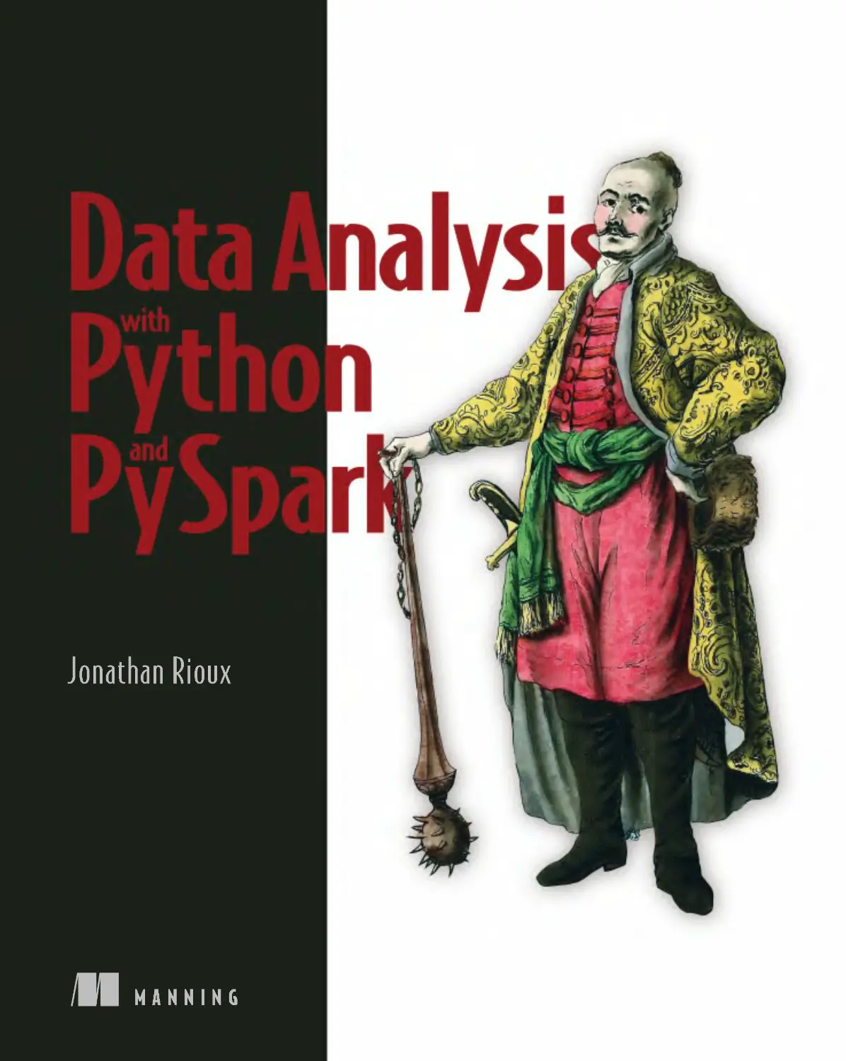
An RDD versus a data frame. In the RDD, we think of each record as an independent entity.
With the data frame, we mostly interact with columns, performing functions on them. We still
can access the rows of a data frame, via RDD, if necessary.
Resilient distributed data set (RDD)
Record/Object 1
Record/Object 2
Record/Object 3
Record/Object 4
Record/Object 5
Record/Object 6
...
Record/Object N
Data frame (DF)
Col 1
Col 2
Col N
...
(1, 1)
(2, 1)
(3, 1)
(4, 1)
(5, 1)
(6, 1)
...
(N, )
1
(1, )
2
(2, )
2
(3, )
2
(4, )
2
(5, )
2
(6, )
2
...
(N, )
2
(1, )
N
(2, )
N
(3, )
N
(4, )
N
(5, )
N
(6, )
N
...
(N, )
N
In an RDD, we think of each record as
being an independent object on which
we perform functions to transform them.
Think “collection,” not “structure.”
A data frame organizes the records in columns.
We perform transformations either directly on
those columns or on the data frame as a whole;
we typically don’t access records horizontally
(record by record) as we do with the RDD.

Data Analysis with
Python and PySpark
JONATHAN RIOUX
MANNING
SHELTER ISLAND

For online information and ordering of this and other Manning books, please visit
www.manning.com. The publisher offers discounts on this book when ordered in quantity.
For more information, please contact
Special Sales Department
Manning Publications Co.
20 Baldwin Road
PO Box 761
Shelter Island, NY 11964
Email: orders@manning.com
©2022 by Manning Publications Co. All rights reserved.
No part of this publication may be reproduced, stored in a retrieval system, or transmitted, in
any form or by means electronic, mechanical, photocopying, or otherwise, without prior written
permission of the publisher.
Many of the designations used by manufacturers and sellers to distinguish their products are
claimed as trademarks. Where those designations appear in the book, and Manning Publications
was aware of a trademark claim, the designations have been printed in initial caps or all caps.
Recognizing the importance of preserving what has been written, it is Manning’s policy to have
the books we publish printed on acid-free paper, and we exert our best efforts to that end.
Recognizing also our responsibility to conserve the resources of our planet, Manning books
are printed on paper that is at least 15 percent recycled and processed without the use of
elemental chlorine.
The author and publisher have made every effort to ensure that the information in this book
was correct at press time. The author and publisher do not assume and hereby disclaim any
liability to any party for any loss, damage, or disruption caused by errors or omissions, whether
such errors or omissions result from negligence, accident, or any other cause, or from any usage
of the information herein.
Manning Publications Co.
Development editor: Marina Michaels
20 Baldwin Road
Technical development editor: Arthur Zubarev
PO Box 761
Review editor: Aleksander Dragosavljević
Shelter Island, NY 11964
Production editor: Keri Hales
Copy editor: Michele Mitchell
Proofreader: Melody Dolab
Technical proofreader: Alex Ott
Typesetter: Dennis Dalinnik
Cover designer: Marija Tudor
ISBN: 9781617297205
Printed in the United States of America

iii
contents
preface xi
acknowledgments xiii
about this book xv
about the author xviii
about the cover illustration xix
1 Introduction 1
1.1 What is PySpark? 2
Taking it from the start: What is Spark? 2 ■ PySpark = Spark +
Python 3 ■ Why PySpark? 4
1.2 Your very own factory: How PySpark works 6
Some physical planning with the cluster manager 7 ■ A factory
made efficient through a lazy leader 10
1.3 What will you learn in this book? 13
1.4 What do I need to get started? 14
PART 1 GET ACQUAINTED: FIRST STEPS IN PYSPARK .......15
2 Your first data program in PySpark 17
2.1 Setting up the PySpark shell 18
The SparkSession entry point 20 ■ Configuring how chatty spark
is: The log level 22

CONTENTS
iv
2.2 Mapping our program 23
2.3 Ingest and explore: Setting the stage for data
transformation 24
Reading data into a data frame with spark.read 25 ■ From
structure to content: Exploring our data frame with show() 28
2.4 Simple column transformations: Moving from a sentence
to a list of words 31
Selecting specific columns using select() 32 ■ Transforming
columns: Splitting a string into a list of words 33 ■ Renaming
columns: alias and withColumnRenamed 35 ■ Reshaping your
data: Exploding a list into rows 36 ■ Working with words:
Changing case and removing punctuation 37
2.5 Filtering rows 40
3 Submitting and scaling your first PySpark program 45
3.1 Grouping records: Counting word frequencies 46
3.2 Ordering the results on the screen using orderBy 48
3.3 Writing data from a data frame 50
3.4 Putting it all together: Counting 52
Simplifying your dependencies with PySpark’s import conventions 53
Simplifying our program via method chaining 54
3.5 Using spark-submit to launch your program
in batch mode 56
3.6 What didn’t happen in this chapter 58
3.7 Scaling up our word frequency program 58
4 Analyzing tabular data with pyspark.sql 62
4.1 What is tabular data? 63
How does PySpark represent tabular data? 64
4.2 PySpark for analyzing and processing tabular data 65
4.3 Reading and assessing delimited data in PySpark 67
A first pass at the SparkReader specialized for CSV files 67
Customizing the SparkReader object to read CSV data files 69
Exploring the shape of our data universe 72
4.4 The basics of data manipulation: Selecting, dropping,
renaming, ordering, diagnosing 73
Knowing what we want: Selecting columns 73 ■ Keeping what we
need: Deleting columns 76 ■ Creating what’s not there: New

CONTENTS
v
columns with withColumn() 78 ■ Tidying our data frame:
Renaming and reordering columns 81 ■ Diagnosing a data
frame with describe() and summary() 83
5 Data frame gymnastics: Joining and grouping 87
5.1 From many to one: Joining data 88
What’s what in the world of joins 88 ■ Knowing our left from
our right 89 ■ The rules to a successful join: The predicates 90
How do you do it: The join method 92 ■ Naming conventions in
the joining world 96
5.2 Summarizing the data via groupby and
GroupedData 100
A simple groupby blueprint 101 ■ A column is a column: Using
agg() with custom column definitions 105
5.3 Taking care of null values: Drop and fill 106
Dropping it like it’s hot: Using dropna() to remove records with null
values 107 ■ Filling values to our heart’s content using fillna() 108
5.4 What was our question again? Our end-to-end
program 109
PART 2GET PROFICIENT: TRANSLATE YOUR IDEAS
INTO CODE ..................................................... 115
6 Multidimensional data frames: Using PySpark
with JSON data 117
6.1 Reading JSON data: Getting ready for the
schemapocalypse 118
Starting small: JSON data as a limited Python dictionary 119
Going bigger: Reading JSON data in PySpark 121
6.2 Breaking the second dimension with complex
data types 123
When you have more than one value: The array 125 ■ The map
type: Keys and values within a column 129
6.3 The struct: Nesting columns within columns 131
Navigating structs as if they were nested columns 132
6.4 Building and using the data frame schema 135
Using Spark types as the base blocks of a schema 135 ■ Reading a
JSON document with a strict schema in place 138 ■ Going full
circle: Specifying your schemas in JSON 141

CONTENTS
vi
6.5 Putting it all together: Reducing duplicate data
with complex data types 144
Getting to the “just right” data frame: Explode and collect 146
Building your own hierarchies: Struct as a function 148
7 Bilingual PySpark: Blending Python and SQL code 151
7.1 Banking on what we know: pyspark.sql vs. plain SQL 152
7.2 Preparing a data frame for SQL 154
Promoting a data frame to a Spark table 154 ■ Using the Spark
catalog 156
7.3 SQL and PySpark 157
7.4 Using SQL-like syntax within data frame methods 159
Get the rows and columns you want: select and where 159
Grouping similar records together: group by and order by 160
Filtering after grouping using having 161 ■ Creating new tables/
views using the CREATE keyword 163 ■ Adding data to our table
using UNION and JOIN 164 ■ Organizing your SQL code better
through subqueries and common table expressions 166 ■ A quick
summary of PySpark vs. SQL syntax 168
7.5 Simplifying our code: Blending SQL and Python 169
Using Python to increase the resiliency and simplifying the data
reading stage 169 ■ Using SQL-style expressions in
PySpark 170
7.6 Conclusion 172
8 Extending PySpark with Python: RDD and UDFs 175
8.1 PySpark, freestyle: The RDD 176
Manipulating data the RDD way: map(), filter(), and
reduce() 177
8.2 Using Python to extend PySpark via UDFs 185
It all starts with plain Python: Using typed Python functions 186
From Python function to UDFs using udf() 188
9 Big data is just a lot of small data: Using pandas UDFs 192
9.1 Column transformations with pandas: Using Series
UDF 194
Connecting Spark to Google’s BigQuery 194 ■ Series to Series UDF:
Column functions, but with pandas 199 ■ Scalar UDF + cold start
= Iterator of Series UDF 202

CONTENTS
vii
9.2 UDFs on grouped data: Aggregate and apply 205
Group aggregate UDFs 207 ■ Group map UDF 208
9.3 What to use, when 210
10 Your data under a different lens: Window functions 215
10.1 Growing and using a simple window function 216
Identifying the coldest day of each year, the long way 217
Creating and using a simple window function to
get the coldest days 219 ■ Comparing both
approaches 223
10.2 Beyond summarizing: Using ranking and analytical
functions 224
Ranking functions: Quick, who’s first? 225 ■ Analytic
functions: Looking back and ahead 230
10.3 Flex those windows! Using row and range
boundaries 232
Counting, window style: Static, growing, unbounded 233
What you are vs. where you are: Range vs. rows 235
10.4 Going full circle: Using UDFs within windows 239
10.5 Look in the window: The main steps to a successful
window function 240
11 Faster PySpark: Understanding Spark’s query
planning 244
11.1 Open sesame: Navigating the Spark UI to understand
the environment 245
Reviewing the configuration: The environment tab 247
Greater than the sum of its parts: The Executors tab and resource
management 249 ■ Look at what you’ve done: Diagnosing
a completed job via the Spark UI 254 ■ Mapping the
operations via Spark query plans: The SQL tab 257
The core of Spark: The parsed, analyzed, optimized,
and physical plans 260
11.2 Thinking about performance: Operations and
memory 263
Narrow vs. wide operations 264 ■ Caching a data frame:
Powerful, but often deadly (for perf) 269

CONTENTS
viii
PART 3G
ET CONFIDENT: USING MACHINE LEARNING
WITH PYSPARK ................................................ 275
12 Setting the stage: Preparing features for machine
learning 277
12.1 Reading, exploring, and preparing our machine
learning data set 278
Standardizing column names using toDF() 279 ■ Exploring our
data and getting our first feature columns 281 ■ Addressing data
mishaps and building our first feature set 283 ■ Weeding out
useless records and imputing binary features 286 ■ Taking care of
extreme values: Cleaning continuous columns 287 ■ Weeding out
the rare binary occurrence columns 290
12.2 Feature creation and refinement 291
Creating custom features 292 ■ Removing highly correlated
features 293
12.3 Feature preparation with transformers and
estimators 296
Imputing continuous features using the Imputer estimator 298
Scaling our features using the MinMaxScaler estimator 300
13 Robust machine learning with ML Pipelines 303
13.1 Transformers and estimators: The building blocks
of ML in Spark 304
Data comes in, data comes out: The Transformer 305
Data comes in, transformer comes out: The Estimator 310
13.2 Building a (complete) machine learning pipeline 312
Assembling the final data set with the vector column type 314
Training an ML model using a LogisticRegression
classifier 316
13.3 Evaluating and optimizing our model 319
Assessing model accuracy: Confusion matrix and evaluator
object 320 ■ True positives vs. false positives: The ROC
curve 323 ■ Optimizing hyperparameters with cross-
validation 325
13.4 Getting the biggest drivers from our model:
Extracting the coefficients 328

CONTENTS
ix
14 Building custom ML transformers and estimators 331
14.1 Creating your own transformer 332
Designing a transformer: Thinking in terms of Params and
transformation 333 ■ Creating the Params of a transformer 335
Getters and setters: Being a nice PySpark citizen 337 ■ Creating a
custom transformer’s initialization function 340 ■ Creating our
transformation function 341 ■ Using our transformer 343
14.2 Creating your own estimator 344
Designing our estimator: From model to params 345
Implementing the companion model: Creating our own Mixin 347
Creating the ExtremeValueCapper estimator 350 ■ Trying out our
custom estimator 352
14.3 Using our transformer and estimator in an ML
pipeline 353
Dealing with multiple inputCols 353 ■ In practice: Inserting
custom components into an ML pipeline 356
appendix A Solutions to the exercises 361
appendix B Installing PySpark 389
appendix C Some useful Python concepts 408
index 423

xi
preface
While computers have been getting more powerful and more capable of chewing
though larger data sets, our appetite for consuming data grows much faster. Conse-
quently, we built new tools to scale big data jobs across multiple machines. This does
not come for free, and early tools were complicated by requiring users to manage not
only the data program, but also the health and performance of the cluster of
machines themselves. I recall trying to scale my own programs, only to be faced with
the advice to “just sample your data set and get on with your day.”
PySpark changes the game. Starting with the popular Python programming lan-
guage, it provides a clear and readable API to manipulate very large data sets. Still,
while in the driver’s seat, you write code as if you were dealing with a single machine.
PySpark sits at the intersection of powerful, expressive, and versatile. Through a pow-
erful multidimensional data model, you can build your data programs with a clear
path to scalability, regardless of the data size.
I fell in love with PySpark while working as a data scientist for building credit risk
models. On the cusp of migrating our models to a new big data environment, we
needed to devise a plan to intelligently convert our data products while “keeping the
lights on.” As the self-appointed Python guy, I got tasked to help the team become
familiar with PySpark and help accelerate the transition. This love grew exponentially
as I got the chance to work with a myriad of clients on different use cases. The com-
mon thread? Big data and big problems, all solvable through a powerful data model.
One caveat: most of the material available for learning Spark focused on Scala and
Java, with Python developers left transliterating the code to their favorite programming

PREFACE
xii
language. I started writing this book to promote PySpark as a great tool for data ana-
lysts. In a fortunate turn of events, the Spark project really promoted Python as a
first-class citizen. Now, more than ever, you have a powerful tool for scaling your
data programs.
And big data, once tamed, really feels powerful.

xiii
acknowledgments
Although my name is on the cover, this book has been a tremendous team effort, and
I want to take the time to thank those who helped me along the way.
First and foremost, I want to thank my family. Writing a book is a lot of work, and
with this work comes a lot of complaining. Simon, Catherine, Véronique, Jean, merci
du fond du coeur pour votre soutien. Je vous aime énormément.
Regina, in a way, you’ve were my very first PySpark student. Through your leader-
ship, you literally changed everything for me career-wise. I will forever cherish the
time we worked together, and I feel lucky our paths crossed when they did.
I want to thank Renata Pompas, who allowed me to use a color palette made under
her supervision for the diagrams in my book. I am color-blind, and finding a set of
safe colors to use that would please me and be consistent was helpful during book
development. If the figures look good to you, thank her (and the fine Manning
graphic designers). If they look bad, blame it on me.
Thank you to my team at EPAM, with a special shout-out to Zac, James, Nasim,
Vahid, Dmitrii, Yuriy, Val, Robert, Aliaksandra, Ihor, Pooyan, Artem, Volha, Ekaterina,
Sergey, Sergei, Siarhei, Kseniya, Artemii, Anatoly, Yuliya, Nadzeya, Artsiom, Denis,
Yevhen, Sofiia, Roman, Mykola, Lisa, Gaurav, Megan, and so many more. From the day
I announced that I was writing a book to when I wrote these words, I felt supported
and encouraged. Thank you to the Laivly team, Jeff, Rod, Craig, Jordan, Abu, Brendan,
Daniel, Guy, and Reid, for the opportunity to continue the adventure. I promise you
that the future is bright.

ACKNOWLEDGMENTS
xiv
A warm thank you to those who believed in my “use PySpark, you’ll be grateful
you did” mantra. There are too many folks to be exhaustive here, but I want to give
a shout out to Mark Derry, Uma Gopinath, Tom Everett, Dhrun Lauwers, Milena
Kumurdjieva, Shahid Amlani, Sam Diab, Chris Wagner, JV Eng, Chris Purtill, Naveen
Pothayath, Vish Tipirneni, and Patrick Kurkiewicz.
During the writing of the book, I had the joy to geek out on PySpark with some
fine podcast producers: Brian at Test and Code (https://testandcode.com/), Lior and
Michael at WHAT the Data?! (https://podcast.whatthedatapodcast.com/), and Ben at
Profitable Python (https://anchor.fm/profitablepythonfm). I am so humbled and grate-
ful that you invited me to exchange with you. Thank you Alexey Grigorev for having
me in your Book of the Week club on Slack—what an awesome community you’ve
built!
I want to thank readers who provided comments on the manuscript during devel-
opment, as well as the reviewers who provided excellent feedback: Alex Lucas, David
Cronkite, Dianshuang Wu, Gary Bake, Geoff Clark, Gustavo Patino, Igor Vieira, Javier
Collado Cabeza, Jeremy Loscheider, Josh Cohen, Kay Engelhardt, Kim Falk, Michael
Kareev, Mike Jensen, Patrick A. Mol, Paul Fornia, Peter Hampton, Philippe Van Ber-
gen, Rambabu Posa, Raushan Jha, Sergio Govoni, Sriram Macharla, Stephen Oates,
and Werner Nindl.
Finally, and most importantly, I want to thank the dream team at Manning that par-
ticipated in making this book a reality. There are many folks who made this experi-
ence incredible: Marjan Bace, Michael Stephens, Rebecca Rinehart, Bert Bates,
Candace Gillhoolley, Radmila Ercegovac, Aleks Dragosavljević, Matko Hrvatin, Chris-
topher Kaufmann, Ana Romac, Branko Latincic, Lucas Weber, Stjepan Jureković,
Goran Ore, Keri Hales, Michele Mitchell, Melody Dolab, and the rest of the Manning
production team.
Speaking of Manning, I want to thank the authors of two specific books: Noel Rap-
pin and Robin Dunn from wxPython in Action (Manning, 2016; https://www.manning
. com/books/wxpython-in-action), as well as Michael Fogus and Chris Houser from
The Joy of Clojure (Manning, 2014; https://www.manning.com/books/the-joy-of-clojure
-s e cond-edition). These books triggered something in my brain and made me plunge
headfirst into programming (and then data science). In a way, they were the initial
spark (bad pun intended) that resulted in this book.
Finally, I want to highlight the team at Manning that helped me stay accountable
on a day-to-day basis and made this book something I am proud of. Arthur Zubarev, I
can’t believe we live in the same city and couldn’t meet! Thank you for your excellent
feedback and answering my many questions. Alex Ott, I don’t think I could have
wished for a better technical advisor. Databricks is incredibly lucky to have you. Last,
but certainly not least, I want to thank Marina Michaels for supporting me from the
moment I had the idea of writing this book. Writing a book is a lot more difficult than
I originally thought, but you made the whole experience enjoyable, formative, and rel-
evant. Thank you from the bottom of my heart.

xv
about this book
Data Analysis with Python and PySpark teaches you how to use PySpark to conduct your
own big data analysis programs. It takes a practical stance on teaching both the how
and why of PySpark. You’ll learn about how to effectively ingest, process, and work
with data at scale as well as how to reason about your own data transformation code.
After reading this book, you should feel comfortable using PySpark to write your own
data programs and analyses.
Who should read this book
This book is structured around increasingly complicated use cases, moving from sim-
ple data transformation to machine learning pipelines. We cover the whole cycle,
from data ingestion to results consumption, adding more elements with regard to
data source consumption and transformation possibilities.
This book caters mostly to data analysts, scientists, and engineers who want to scale
their Python code to larger data sets. Ideally, you should have written a few data pro-
grams, either through your work or while learning to program. You’ll get more out of
this book if you already are comfortable using the Python programming language and
ecosystem.
Spark (and PySpark, naturally) borrows a lot from object-oriented and functional
programming. I do not think it’s reasonable to expect complete knowledge of both pro-
gramming paradigms just to use big data efficiently. If you understand Python classes,
decorators, and higher-order functions, you’ll have a blast using some of the more
advanced constructions in the book to bend PySpark to your will. Should those concepts

ABOUT THIS BOOK
xvi
be foreign to you, I cover them in the context of PySpark throughout the book (when
appropriate) and in the appendixes.
How this book is organized: A road map
The book is divided into three parts. Part 1, “Get Acquainted,” introduces PySpark
and its computation model. It also covers building and submitting a simple data pro-
gram, focusing on the core operations that you certainly will use in every PySpark pro-
gram you create, such as selecting, filtering, joining, and grouping data in a data
frame.
Part 2, “Get Proficient,” goes further into data transformation by introducing hier-
archical data, a key element of scalable data programs in PySpark. We also make our
programs more expressive, flexible, and performant through the judicious introduc-
tion of SQL code, an exploration of resilient distributed datasets/user-defined func-
tions, efficient usage of pandas within PySpark, and window functions. We also explore
Spark’s reporting capabilities and resource management to pinpoint potential perfor-
mance problems.
Finally, Part 3, “Get Confident,” builds on parts 1 and 2 and covers how to build a
machine learning program in PySpark. We use our data transformation tool kit to cre-
ate and select features before building and evaluating a machine learning pipeline.
We finish this part with creating our own machine learning pipeline components,
ensuring maximum usability and readability for our ML programs.
Parts 1 and 2 have exercises throughout the chapters, as well as at the end of the
chapters. Exercises at the end of a section don’t require you to code; you should be
able to answer the questions with what you learned.
The book was written with the idea of being read cover to cover, using the appen-
dixes as needed. Should you want to dig directly into a topic, I still recommend covering
part 1 before delving into a specific chapter. Here are the hard and soft dependencies
to help you navigate the book more efficiently:
 Chapter 3 is a direct continuation of chapter 2.
 Chapter 5 is a direct continuation of chapter 4.
 Chapter 9 uses some concepts taught in chapter 8, but advanced readers can
read it on its own.
 Chapters 12, 13, and 14 are best read one after the other.
About the code
This book works best with Spark version 3.1 or 3.2: Spark introduced many new func-
tionalities in version 3, and most commercial offerings are now defaulting to this ver-
sion. When appropriate, I provide backward-compatible instructions for Spark version
2.3/2.4. I do not recommend Spark 2.2 or below. I also recommend using Python ver-
sion 3.6 and above (I used Python 3.8.8 for the book). Installation instructions are
available in appendix A.

ABOUT THIS BOOK
xvii
You can find the companion repository for the book, with data and code, at https://
github.com/jonesberg/DataAnalysisWithPythonAndPySpark. When appropriate, it also
contains runnable versions of the programs developed throughout the book, as well as
a few optional exercises. In addition, you can get executable snippets of code from the
liveBook (online) version of this book at https://livebook.manning.com/book/data-
analysis-with-python-and-pyspark.
This book contains many examples of source code both in numbered listings and
in line with normal text. In both cases, source code is formatted in a fixed-width
font like this to separate it from ordinary text. Sometimes code is also in bold to
highlight code that has changed from previous steps in the chapter, such as when a
new feature adds to an existing line of code.
In many cases, the original source code has been reformatted; we’ve added line
breaks and reworked indentation to accommodate the available page space in the
book. In rare cases, even this was not enough, and listings include line-continuation
markers (➥). Additionally, comments in the source code have often been removed
from the listings when the code is described in the text. Code annotations accompany
many of the listings and highlight important concepts.
liveBook discussion forum
Purchase of Data Analysis with Python and PySpark includes free access to liveBook,
Manning’s online reading platform. Using liveBook’s exclusive discussion features,
you can attach comments to the book globally or to specific sections or paragraphs.
It’s a snap to make notes for yourself, ask and answer technical questions, and receive
help from the author and other users. To access the forum, go to https://livebook
. manning.com/book/data-analysis-with-python-and-pyspark/discussion. You can also
learn more about Manning’s forums and the rules of conduct at https://livebook
. manning.com/#!/discussion.
Manning’s commitment to our readers is to provide a venue where a meaningful
dialogue between individual readers and between readers and the author can take
place. It is not a commitment to any specific amount of participation on the part of
the author, whose contribution to the forum remains voluntary (and unpaid). We sug-
gest you try asking the author some challenging questions lest his interest stray! The
forum and the archives of previous discussions will be accessible from the publisher’s
website as long as the book is in print.

xviii
about the author
JONATHAN RIOUX uses PySpark inside and out on a daily basis.
He also teaches large-scale data analysis to data scientists, engi-
neers, and data-savvy business analysts.
Jonathan spent a decade in various analytical positions in
the insurance industry before venturing into the consulting
industry as a machine learning and data analysis expert. He
currently works as the director of machine learning for Laivly,
a company that equips friendly humans with intelligent auto-
mations and machine learning to create the best customer
experiences on the planet.

xix
about the cover illustration
The figure on the cover of Data Analysis with Python and PySpark is “Russien,” or Rus-
sian man, taken from a book by Jacques Grasset de Saint-Sauveur, published in 1788.
Each illustration is finely drawn and colored by hand.
In those days, it was easy to identify where people lived and what their trade or
station in life was just by their dress. Manning celebrates the inventiveness and ini-
tiative of today’s computer business with book covers based on the rich diversity of
regional culture centuries ago, brought back to life by pictures from collections such
as this one.

1
Introduction
According to pretty much every news outlet, data is everything, everywhere. It’s the
new oil, the new electricity, the new gold, plutonium, even bacon! We call it power-
ful, intangible, precious, dangerous. At the same time, data itself is not enough: it is
what you do with it that matters. After all, for a computer, any piece of data is a col-
lection of zeroes and ones, and it is our responsibility, as users, to make sense of
how it translates to something useful.
Just like oil, electricity, gold, plutonium, and bacon (especially bacon!), our
appetite for data is growing. So much, in fact, that computers aren’t following. Data
is growing in size and in complexity, yet consumer hardware has been stalling a lit-
tle. RAM is hovering for most laptops at around 8 to 16 GB, and SSDs are getting
prohibitively expensive past a few terabytes. Is the solution for the burgeoning data
analyst to triple-mortgage their life to afford top-of-the-line hardware to tackle big
data problems?
This chapter covers
 What PySpark is
 Why PySpark is a useful tool for analytics
 The versatility of the Spark platform and its
limitations
 PySpark’s way of processing data

2
CHAPTER 1 Introduction
Here is where Apache Spark (which I’ll call Spark throughout the book) and its com-
panion PySpark are introduced. They take a few pages of the supercomputer playbook—
powerful, but manageable compute units meshed in a network of machines—and bring
them to the masses. Add on top a powerful set of data structures ready for any work you’re
willing to throw at them, and you have a tool that will grow (pun intended) with you.
A goal for this book is to provide you with the tools to analyze data using PySpark,
whether you need to answer a quick data-driven question or build an ML model. It
covers just enough theory to get you comfortable while giving you enough opportuni-
ties to practice. Most chapters contain a few exercises to anchor what you just learned.
The exercises are all solved and explained in appendix A.
1.1 What is PySpark?
What’s in a name? Actually, quite a lot. Just by separating PySpark in two, you can
already deduce that this will be related to Spark and Python. And you would be right!
At its core, PySpark can be summarized as being the Python API to Spark. While
this is an accurate definition, it doesn’t give much unless you know the meaning of
Python and Spark. Still, let’s break down the summary definition by first answering
“What is Spark?” With that under our belt, we then will look at why Spark becomes
especially powerful when combined with Python and its incredible array of analytical
(and machine learning) libraries.
1.1.1 Taking it from the start: What is Spark?
According to the authors of the software, Apache SparkTM, which I’ll call Spark
throughout this book, is a “unified analytics engine for large-scale data processing”
(see https://spark.apache.org/). This is a very accurate, if a little dry, definition. As a
mental image, we can compare Spark to an analytics factory. The raw material—here,
data—comes in, and data, insights, visualizations, models, you name it, comes out.
Just like a factory will often gain more capacity by increasing its footprint, Spark
can process an increasingly vast amount of data by scaling out (across multiple smaller
machines) instead of scaling up (adding more resources, such as CPU, RAM, and disk
space, to a single machine). RAM, unlike most things in this world, gets more expensive
the more you buy (e.g., one stick of 128 GB is more than the price of two sticks of 64
GB). This means that, instead of buying thousands of dollars of RAM to accommodate
your data set, you’ll rely on multiple computers, splitting the job between them. In a
world where two modest computers are less costly than one large one, scaling out is
less expensive than scaling up, which keeps more money in your pockets.
Cloud cost and RAM
In the cloud, prices will often be more consequential. For instance, as of January
2022, a 16-Core/128-GB RAM machine can be about twice the cost of an 8 Core/64
GB of RAM machine. As the data size grows, Spark can help control costs by scaling
the number of workers and executors for a given job. As an example, if you have a

3
What is PySpark?
A single computer can crash or behave unpredictably at times. If instead of one you
have one hundred, the chance that at least one of them goes down is now much
higher.1 Spark therefore has a lot of hoops to manage, scale, and babysit so that you
can focus on what you want, which is to work with data.
This is, in fact, one of the key things about Spark: it’s a good tool because of what you
can do with it, but especially because of what you don’t have to do with it. Spark provides a
powerful API (application programming interface, the set of functions, classes, and variables
provided for you to interact with) that makes it look like you’re working with a cohesive
source of data while also working hard in the background to optimize your program to use
all the power available. You don’t have to be an expert in the arcane art of distributed com-
puting; you just need to be familiar with the language you’ll use to build your program.
1.1.2 PySpark = Spark + Python
PySpark provides an entry point to Python in the computational model of Spark.
Spark itself is coded in Scala.2 The authors did a great job of providing a coherent
interface between languages while preserving the idiosyncrasies of each language
where appropriate. It will, therefore, be quite easy for a Scala/Spark programmer to
read your PySpark program, as well as for a fellow Python programmer who hasn’t
jumped into the deep end (yet).
Python is a dynamic, general-purpose language, available on many platforms and
for a variety of tasks. Its versatility and expressiveness make it an especially good fit for
PySpark. The language is one of the most popular for a variety of domains, and cur-
rently it is a major force in data analysis and science. The syntax is easy to learn and
read, and the number of libraries available means that you’ll often find one (or
more!) that’s just the right fit for your problem.
PySpark provides access not only to the core Spark API but also to a set of bespoke
functionality to scale out regular Python code, as well as pandas transformations. In
Python’s data analysis ecosystem, pandas is the de facto data frame library for memory-
bound data frames (the entire data frame needs to reside on a single machine’s
memory). It’s not a matter of PySpark or pandas now, but PySpark and pandas.
Chapters 8 and 9 are dedicated to combining Python, pandas, and PySpark in one
data transformation job on a modest data set (a few TB), you can limit yourself to a
lower number—say, five—machines, scaling up to 60 when you want to do machine
learning. Some vendors, such as Databricks (see appendix B), offer auto-scaling,
meaning that they increase and decrease the number of machines during a job
depending on the pressure on the cluster. The implementation of auto-scaling/cost
controlling is 100% vendor-dependent. (Check out chapter 11 for an introduction to
the resources making up a Spark cluster, as well as their purpose.)
1 It can be a fun probability exercise to compute, but I will try to keep the math to a minimum.
2 Databricks, the company behind Spark, has a project called Photon, which is a rewrite of the Spark execution
engine in C++.

4
CHAPTER 1 Introduction
happy program. For those really committed to the pandas syntax (or if you have a large
pandas program you want to scale to PySpark), Koalas (now called pyspark.pandas and
part of Spark as of version 3.2 .0; https://koalas.readthedocs.io/) provides a pandas-
like porcelain on top of PySpark. If you are starting a new Spark program in Python, I
recommend using the PySpark syntax—covered thoroughly in this book—reserving
Koalas for when you want to ease the transition from pandas to PySpark. Your pro-
gram will work faster and, in my opinion, will read better.
1.1.3 Why PySpark?
There is no shortage of libraries and frameworks to work with data. Why should one
spend their time learning PySpark specifically?
PySpark has a lot of advantages for modern data workloads. It sits at the intersec-
tion of fast, expressive, and versatile. This section covers the many advantages of
PySpark, why its value proposition goes beyond just “Spark, with Python,” and when it
is better to reach for another tool.
PYSPARK IS FAST
If you search for “big data” in a search engine, there is a very good chance that Hadoop
will come up within the first few results. There is a good reason for this: Hadoop popu-
larized the famous MapReduce framework that Google pioneered in 2004 and inspired
how data is processed at scale (we touch on MapReduce in chapter 8, when talking
about PySpark’s low-level data structure, the resilient distributed data set).
Spark was created a few years later, sitting on Hadoop’s incredible legacy. With an
aggressive query optimizer, a judicious usage of RAM (reducing disk I/O; see chap-
ter 11), and some other improvements we’ll touch on in the next chapters, Spark can
run up to 100 times faster than plain Hadoop. Because of the integration between the
two frameworks, you can easily switch your Hadoop workflow to Spark and gain some
performance boost without changing your hardware.3
PYSPARK IS EXPRESSIVE
Beyond Python being one of the most popular and easy-to-learn languages, PySpark’s
API has been designed from the ground up to be easy to understand. PySpark borrows
and extends the vocabulary for data manipulation from SQL. It does so in a fluent man-
ner: each operation on a data frame returns a “new” data frame, so you can chain oper-
ations one after the other. Although we are just in the early stages of learning PySpark,
listing 1.1 shows how readable, well-crafted PySpark looks. Even with no prior knowl-
edge, the vocabulary choices and the consistency of the syntax makes it read like prose.
We read a CSV file, create a new column that contains a value conditional to an old col-
umn, filter (using where), group by the values of the column, generate the count for each
group, and finally write the results back to a CSV file. All these methods are covered
throughout part 1 of the book, but we can already deduce what this code is doing.
3
As always, the standard disclaimer applies: not every Hadoop job will get faster in Spark. Your mileage may
vary. Always test your job before making large architectural changes.

5
What is PySpark?
(
spark.read.csv("./data/list_of_numbers/sample.csv", header=True)
.withColumn(
"new_column", F.when(F.col("old_column") > 10, 10).otherwise(0)
)
.where("old_column > 8")
.groupby("new_column")
.count()
.write.csv("updated_frequencies.csv", mode="overwrite")
)
Under the hood, Spark optimizes these operations so that we don’t get an intermedi-
ate data frame after each method. Because of this, we can program our data transfor-
mation code in a very succinct and self-describing way, relying on Spark to optimize
the end results—a programmer’s comfort at its finest.
You will see many (more complex!) examples throughout this book. As I was writ-
ing the examples, I was pleased about how close to my initial (pen-and-paper) reason-
ing the code ended up looking. After understanding the fundamentals of the
framework, I’m confident you’ll be in the same situation.
PYSPARK IS VERSATILE
A key advantage of PySpark is its versatility: you learn one tool and use it in a variety of
settings. There are two components to this versatility. First, there is the availability of
the framework. Second, there is the diversified ecosystem surrounding Spark.
PySpark is everywhere. All three major cloud providers (Amazon Web Services
[AWS], Google Cloud Platform [GCP], Microsoft Azure) have a managed Spark
cluster as part of their offerings, which means you have a fully provisioned cluster at
the click of a few buttons. You can also easily install Spark on your computer to nail
down your program before scaling on a more powerful cluster. Appendix B covers
how to get your local Spark running and succinctly walks you through the current
main cloud offerings.
PySpark is open source. Unlike other analytical software, you aren’t tied to a single
company. You can inspect the source code if you’re curious and even contribute if you
have an idea for new functionality or find a bug. It also gives a low barrier to adoption:
download, learn, profit!
Finally, Spark’s ecosystem doesn’t stop at PySpark. There is also an API for Scala,
Java, and R, as well as a state-of-the-art SQL layer. This makes it easy to write a polyglot
program in Spark. A Java software engineer can tackle the data transformation pipe-
line in Spark using Java, while a data scientist can build a model using PySpark.
WHERE PYSPARK FALLS SHORT
It would be awesome if PySpark was the answer to every data problem. Unfortunately,
there are some caveats. None of them are deal breakers, but they are to be considered
when you’re selecting a tool for your next project.
Listing 1.1 Simple ETL pipeline showing expressiveness of PySpark

6
CHAPTER 1 Introduction
PySpark isn’t the right choice if you’re dealing with rapid processing of (very)
small data sets. Executing a program on multiple machines requires a level of coordi-
nation between the nodes, which comes with some overhead. If you’re just using a sin-
gle node, you’re paying the price but aren’t using the benefits. As an example, a
PySpark shell will take a few seconds to launch; this is often more than enough time to
process data that fits within your RAM. As new PySpark versions get released, though,
this small data set performance gap gets narrower and narrower.
PySpark also has a small disadvantage compared to the Java and Scala API. Since
Spark is at the core of a Scala program, pure Python code has to be translated to and
from JVM (Java Virtual Machine, the runtime that powers Java and Scala code) instruc-
tions. Since the DataFrame API is available with PySpark, the differences between lan-
guages have been narrowed significantly: data frame operations are mapped to highly
efficient Spark operations that work at the same speed, whether your program is writ-
ten in Scala, Java, or Python. You will still witness slower operations when you’re using
the resilient distributed data set (RDD) data structure or when you define your
Python user-defined functions. This does not mean that we will avoid them: I cover
both topics in chapter 8.
Finally, while programming PySpark can feel straightforward, managing a cluster
can be a little arcane. Spark is a pretty complicated piece of software; while the code
base matured remarkably over the past few years, we are not yet to the point that we
can manage a 100-machine cluster as easily as a single node. Understanding how
Spark is configured and tuning for performance is introduced in chapter 11, and
cloud options are making it easier than ever (see appendix B). For hairier problems,
do what I do: befriend your operations team.
This section provided the why of PySpark, but also some why not, as knowing where
and when to use PySpark is key to having a great development experience and process-
ing performance. In the next section, we delve a little deeper into how Spark processes
data and makes distributed data processing look like you’re controlling a single factory.
1.2 Your very own factory: How PySpark works
In this section, we cover how Spark processes a program. It can be a little odd to pres-
ent the workings and underpinnings of a system that we claimed, a few paragraphs
ago, hides that complexity. Still, it is important to have a working knowledge of how
Spark is set up, how it manages data, and how it optimizes queries. With this, you will
be able to reason with the system, improve your code, and figure out quickly when it
doesn’t perform the way you want.
If we keep the factory analogy, we can imagine that the cluster of computers Spark
is sitting on is the building. If we look at figure 1.1, we can see two different ways to
interpret a data factory. On the left, we see how it looks from the outside: a cohesive
unit where projects come in and results come out. This is how it will appear to you most
of the time. Under the hood, it looks more like what’s on the right: you have some work-
benches that some workers are assigned to. The workbenches are like the computers

7
Your very own factory: How PySpark works
in our Spark cluster: there is a fixed amount of them. Some modern Spark implemen-
tations, such as Databricks (see appendix B), allow for auto-scaling the number of
machines at runtime. Some require more planning, especially if you run on the prem-
ises and own your hardware. The workers are called executors in Spark’s literature: they
perform the actual work on the machines/nodes.
One of the little workers looks spiffier than the other. That top hat definitely
makes him stand out from the crowd. In our data factory, he’s the manager of the
work floor. In Spark terms, we call this the master.
4
The master here sits on one of the
workbenches/machines, but it can also sit on a distinct machine (or even your com-
puter!) depending on the cluster manager and deployment mode. The role of the
master is crucial to the efficient execution of your program, so section 1.2 .2 is dedi-
cated to this.
TIP In the cloud, you can have a high-availability cluster, meaning that your
master will be replicated on more than one machine.
1.2.1 Some physical planning with the cluster manager
Upon reception of the task, which is called a driver program in the Spark world, the fac-
tory starts running. This doesn’t mean that we get straight to processing. Before that,
the cluster needs to plan the capacity it will allocate for your program. The entity or
program taking care of this is aptly called the cluster manager. In our factory, this cluster
manager will look at the workbenches with available space and secure as many as nec-
essary, and then start hiring workers to fill the capacity. In Spark, it will look at the
machines with available computing resources and secure what’s necessary before
launching the required number of executors across them.
4 The term master is getting phased out. The replacement has not been decided, but you can follow the conver-
sation here: https://issues.apache.org/jira/browse/SPARK-32333.
Spark
Factory
Figure 1.1 A totally relatable data factory, outside and in. Ninety percent of the time we
care about the whole factory, but knowing how it’s laid out helps when reflecting on our code
performance.

8
CHAPTER 1 Introduction
NOTE Spark provides its own cluster manager, called Standalone, but can
also play well with other ones when working in conjunction with Hadoop or
another big data platform. If you read about YARN, Mesos, or Kubernetes in
the wild, know that they are used (as far as Spark is concerned) as cluster
managers.
Any directions about capacity (machines and executors) are encoded in a Spark-
Context representing the connection to our Spark cluster. If our instructions don’t
mention any specific capacity, the cluster manager will allocate the default capacity
prescribed by our Spark installation.
As an example, let’s try the following operation. Using the same sample.csv file in
listing 1.1 (available in the book’s repository), let’s compute a simplified version of the
program: return the arithmetic average of the values of old_column. Let’s assume that
our Spark instance has four executors, each working on its own worker node. The
data processing will be approximately split between the four executors: each will have
a small portion of the data frame that it will work with.
less data/list_of_numbers/sample.csv
old_column
1
4
4
5
7
7
7
10
14
1
4
8
Figure 1.2 depicts one way that PySpark could process the average of our old_column
in our small data frame. I chose the average because it is not trivially distributable,
unlike the sum or the count, where you sum the intermediate values from each
worker. In the case of computing the average, each worker independently computes
the sum of the values and their counts before moving the result—not all the data!—
over to a single worker (or the master directly, when the intermediate result is really
small) that will process the aggregation into a single number, the average.
For a simple example like this, mapping the thought process of PySpark is an easy
and fun exercise. The size of our data and the complexity of our programs will grow and
will get more complicated, and we will not be able to easily map our code to exact physi-
cal steps performed by our Spark instance. Chapter 11 covers the mechanism Spark uses
to give us visibility into the work performed as well as the health of our factory.
Listing 1.2 Content of the sample.csv` file

9
Your very own factory: How PySpark works
This section took a simple example—computing the average of a data frame of num-
bers—and we mapped a blueprint of the physical steps performed by Spark to give us
the right answer. In the next section, we get to one of Spark’s best, and most misun-
derstood, features: laziness. In the case of big data analysis, hard work pays off, but
smart work is better!
Some language convention: Data frame vs. DataFrame
Since this book will talk about data frames more than anything else, I prefer using
the noncapitalized nomenclature (i.e., “data frame”). I find this more readable than
using capital letters or even “dataframe” without a space.
When referring to the PySpark object directly, I’ll use DataFrame but with a fixed-width
font. This will help differentiate between “data frame” the concept and DataFrame
the object.
old_column
1
4
4
old_column
5
7
7
old_column
7
10
14
old_column
1
4
8
Worker 1
Worker 2
Worker 3
Worker 4
Instructions
(9, 3)
(19, 3)
(31, 3)
(13, 3)
(sum, count)
(72, 12)
6
Each worker has a sample of the
data and performs an intermediate
step to get the sum and the count of
each chunk (or partition) of the data
frame.
The intermediate data, much
smaller than the original
data frame, is then sent to a
single worker for further
reduction.
We finally get our desired
answer. Spark effectively hides
the complexity of efficiently
distributing the computation
across nodes. We get our
average, no fuss.
Figure 1.2 Computing the average of our small data frame, PySpark style: each worker works on a distinct
piece of data. As necessary, the data gets moved/shuffled around to complete the instructions.

10
CHAPTER 1 Introduction
1.2.2 A factory made efficient through a lazy leader
This section introduces one of the most fundamental aspects of Spark: its lazy evalua-
tion capabilities. In my time teaching PySpark and troubleshooting data scientists’
programs, I would say that laziness is the concept in Spark that creates the most confu-
sion. It’s a real shame because laziness is (in part) how Spark achieves its incredible
processing speed. By understanding at a high level how Spark makes laziness work,
you will be able to explain a lot of its behavior and better tune for performance.
Just like in a large-scale factory, you don’t go to each employee and give them a
list of tasks. No, here, the master/manager is responsible for the workers. The driver
is where the action happens. Think of a driver as a floor lead: you provide them your
list of steps and let them deal with it. In Spark, the driver/floor lead takes your
instructions (carefully written in Python code), translates them into Spark steps, and
then processes them across the worker. The driver also manages which worker/table
has which slice of the data, and makes sure you don’t lose some bits in the process.
The executor/factory worker sits atop the workers/tables and performs the actual
work on the data.
As a summary:
 The master is like the factory owner, allocating resources as needed to complete
the jobs.
 The driver is responsible for completing a given job. It requests resources from
the master as needed.
 A worker is a set of computing/memory resources, like a workbench in our factory.
 Executors sit atop a worker and perform the work sent by the driver, like
employees at a workbench.
We’ll review the terminology in practice in chapter 11.
Taking the example of listing 1.1 and breaking each instruction one by one,
PySpark won’t start performing the work until the write instruction. If you use regu-
lar Python or a pandas data frame, which are not lazy (we call this eager evaluation),
each instruction is performed one by one as it’s being read.
Your floor lead/driver has all the qualities a good manager has: it’s smart, cautious,
and lazy. Wait, what? You read me right. Laziness in a programming context—and, one
could argue, in the real world too—can be a very good thing. Every instruction you’re
providing in Spark can be classified into two categories: transformations and actions.
Actions are what many programming languages would consider I/O. The most typical
actions are the following:
 Printing information on the screen
 Writing data to a hard drive or cloud bucket
 Counting the number of records
In Spark, we’ll see those instructions most often via the show(), write(), and count()
methods on a data frame.

11
Your very own factory: How PySpark works
Transformations are pretty much everything else. Some examples of transformations
are as follows:
 Adding a column to a table
 Performing an aggregation according to certain keys
 Computing summary statistics
 Training a machine learning model
Why the distinction, you might ask? When thinking about computation over data, you,
as the developer, are only concerned about the computation leading to an action.
You’ll always interact with the results of an action because this is something you can
see. Spark, with its lazy computation model, will take this to the extreme and avoid
performing data work until an action triggers the computation chain. Before that, the
driver will store your instructions. This way of dealing with computation has many
benefits when dealing with large-scale data.
NOTE As we see in chapter 5, count() is a transformation when applied as an
aggregation function (where it counts the number of records of each group)
but an action when applied on a data frame (where it counts the number of
records in a data frame).
First, storing instructions in memory takes much less space than storing intermediate
data results. If you are performing many operations on a data set and are materializ-
ing the data each step of the way, you’ll blow your storage much faster, although you
don’t need the intermediate results. We can all agree that less waste is better.
Second, by having the full list of tasks to be performed available, the driver can
optimize the work between executors much more efficiently. It can use the information
available at run time, such as the node where specific parts of the data are located. It
can also reorder, eliminate useless transformations, combine multiple operations, and
rewrite some portion of the program more effectively, if necessary.
spark.read.csv
withColumn
where
groupby
count
write.csv
PySpark does not evaluate all data
transformations (including reading
data). A variable containing a series
of data frame transformations will
return almost immediately, as no
data work is being performed.
write.csv explicitly writes data to
disk. An operation where PySpark
actually writes or shows data is
called an
and triggers the
action
actual data work. No action, no
visible result, no work. That’s laziness!
Figure 1.3 Breaking down the data frame instructions
as a series of transformations and one action. Each
“job” Spark will perform consists of zero or more
transformations and one action.

12
CHAPTER 1 Introduction
Third, should one node fail during processing—computers fail!—Spark will be able to
recreate the missing chunks of data since it has the instructions cached. It’ll read the
relevant chunk of data and process it up to where you are without the need for you to
do anything. With this, you can focus on the data-processing aspect of your code, off-
loading the disaster and recovery part to Spark. Check out chapter 11 for more infor-
mation about compute and memory resources, and how to monitor for failures.
Finally, during interactive development, you don’t have to submit a huge block of
commands and wait for the computation to happen. Instead, you can iteratively build
your chain of transformation, one at a time, and when you’re ready to launch the
computation, you can add an action and let Spark work its magic.
Lazy computation is a fundamental aspect of Spark’s operating model and part of
the reason it’s so fast. Most programming languages, including Python, R, and Java,
are eagerly evaluated. This means that they process instructions as soon as they
receive them. With PySpark, you get to use an eager language—Python—with a lazy
framework—Spark. This can look a little foreign and intimidating, but you don’t need
to worry. The best way to learn is by doing, and this book provides explicit examples of
laziness when relevant. You’ll be a lazy pro in no time!
One aspect to remember is that Spark will not preserve the results of actions (or
the intermediate data frames) for subsequent computations. If you submit the same
program twice, PySpark will process the data twice. We use caching to change this
behavior and optimize certain hot spots in our code (most noticeably when training
an ML model), and chapter 11 provides you with how and when to cache (spoiler: not
as often as you’d think).
NOTE Reading data, although being I/O, is considered a transformation by
Spark. In most cases, reading data doesn’t perform any visible work for the
user. You, therefore, won’t read data until you need to perform some work on
it (writing, reading, inferring schema; see chapter 6 for more information).
withColumn
where
groupby
count
Eager
evaluation
read
withColumn
where
groupby
count
Lazy
evaluation
Figure 1.4 Eager versus lazy evaluation: storing (and computing on the fly) transformation
saves memory by reducing the need for intermediate data frames. It also makes it easier
to recreate the data frame if one of the nodes fails.

13
What will you learn in this book?
What’s a manager without competent employees? Once the task, with its action, has
been received, the driver starts allocating data to what Spark calls executors. Executors
are processes that run computations and store data for the application. Those execu-
tors sit on what’s called a worker node, which is the actual computer. In our factory anal-
ogy, an executor is an employee performing the work, while the worker node is a
workbench where many employees/executors can work.
That concludes our factory tour. Let’s summarize our typical PySpark program:
 We first encode our instructions in Python code, forming a driver program.
 When submitting our program (or launching a PySpark shell), the cluster man-
ager allocates resources for us to use. Those will mostly stay constant (with the
exception of auto-scaling) for the duration of the program.
 The driver ingests your code and translates it into Spark instructions. Those
instructions are either transformations or actions.
 Once the driver reaches an action, it optimizes the whole computation chain
and splits the work between executors. Executors are processes performing the
actual data work, and they reside on machines labeled worker nodes.
That’s it! As we can see, the overall process is quite simple, but it’s obvious that Spark
hides a lot of the complexity that arises from efficient distributed processing. For a
developer, this means shorter and clearer code, and a faster development cycle.
1.3 What will you learn in this book?
This book will use PySpark to solve a variety of tasks that a data analyst, engineer, or
scientist will encounter during their day-to-day life. We will therefore
 Read and write data from (and to) a variety of sources and formats
 Deal with messy data with PySpark’s data manipulation functionality
 Discover new data sets and perform exploratory data analysis
 Build data pipelines that transform, summarize, and get insights from data in
an automated fashion
 Troubleshoot common PySpark errors and how to recover from them and avoid
them in the first place
After covering those fundamentals, we’ll also tackle different tasks that aren’t as frequent
but are interesting and excellent ways to showcase the power and versatility of PySpark:
 We’ll build machine learning models, from simple throwaway experiments to
robust ML pipelines.
 We’ll work with multiple data formats, from text to tabular to JSON.
 We’ll seamlessly blend Python, pandas, and PySpark code, leveraging the strengths
of each, and most importantly will scale pandas code to new territories.
We are trying to cater to many potential readers but are focusing on people with little to
no exposure to Spark and/or PySpark. More seasoned practitioners might find useful
analogies for when they need to explain difficult concepts and maybe learn a thing or two!

14
CHAPTER 1 Introduction
1.4 What do I need to get started?
The book focuses on Spark version 3.2, which is the most recent. The data frame
made its appearance in Spark 1.3, so some code will work on Spark versions as old as
this one. For this book, to avoid any headaches, I recommend you use Spark version
3.0 or later; if impossible, aim for the most recent version available to you.
We’re assuming some basic Python knowledge; some useful concepts are outlined
in appendix C. If you want a more in-depth introduction to Python, I recommend The
Quick Python Book, by Naomi Ceder (Manning, 2018; https://www.manning.com/books/
the-quick-python-book-third-edition), or Python Workout, by Reuven M. Lerner (Man-
ning, 2020; https://www.manning.com/books/python-workout).
To get started, the only thing required is a working installation of Spark. It can
either be on your computer or on a cloud provider (see appendix B). Most examples
in the book are doable using a local installation of Spark, but some may require more
horsepower and will be identified as such.
A code editor will also be very useful for writing, reading, and editing scripts as you
go through the examples and craft your programs. A Python-aware editor, such as
PyCharm, VS Code, or even Emacs/Vim, is nice to have but is in no way necessary. All
the examples will work with Jupyter as well; check out appendix B to set up your note-
book environment.
The book’s code examples are available on GitHub (http://mng.bz/6ZOR), so Git
will be a useful piece of software to have. If you don’t know Git or don’t have it handy,
GitHub provides a way to download all the book’s code in a zip file. Make sure you
check regularly for updates!
Finally, I recommend that you have an analog way of drafting your code and
schema. I am a compulsive notetaker and doodler, and even if my drawings are very
basic and crude, I find that working through a new piece of software via drawings
helps in clarifying my thoughts. This means rewriting less code and a happier pro-
grammer! Nothing spiffy is required: some scrap paper and a pencil will do wonders.
Summary
 PySpark is the Python API for Spark, a distributed framework for large-scale
data analysis. It provides the expressiveness and dynamism of the Python pro-
gramming language to Spark.
 Spark is fast: it owes its speed to a judicious usage of the RAM available and an
aggressive and lazy query optimizer.
 You can use Spark in Python, Scala, Java, R, and more. You can also use SQL for
data manipulation.
 Spark uses a driver that processes the instructions and orchestrates the work.
The executors receive the instructions from the master and perform the work.
 All instructions in PySpark are either transformations or actions. Because Spark
is lazy, only actions will trigger the computation of a chain of instructions.

Part 1
Get acquainted:
First steps in PySpark
When working with a new technology, the best way to get familiar with it is
to jump right in, building our intuition along the way. This first part succinctly
introduces PySpark before going over two distinct use cases.
Chapter 1 introduces the technology and the computing model that power
Spark.
Then, in chapters 2 and 3, we build a simple end-to-end program and learn
how to structure PySpark code in a readable and intuitive fashion. We go from
the data ingestion of text data to processing, to the presentation of the results,
and, finally, to submitting the program in a noninteractive fashion.
Chapters 4 and 5 look at working with tabular data, the most frequently used
type of data. We build on the foundation from the previous chapters (already!)
to manipulate structured data to our will. At the end of part 1, you should feel
comfortable about writing your own simple programs from start to finish!

17
Your first data
program in PySpark
Data-driven applications, no matter how complex, all boil down to what we can
think of as three meta steps, which are easy to distinguish in a program:
1 We start by loading or reading the data we wish to work with.
2 We transform the data, either via a few simple instructions or a very complex
machine learning model.
3 We then export (or sink) the resulting data, either into a file or by summariz-
ing our findings into a visualization.
This chapter covers
 Launching and using the pyspark shell for
interactive development
 Reading and ingesting data into a data frame
 Exploring data using the DataFrame structure
 Selecting columns using the select() method
 Reshaping single-nested data into distinct
records using explode()
 Applying simple functions to your columns to
modify the data they contain
 Filtering columns using the where() method

18
CHAPTER 2 Your first data program in PySpark
The next two chapters will introduce a basic workflow with PySpark via the creation of
a simple ETL (extract, transform, and load, which is a more business-speak way of saying
ingest, transform, and export). You will find these three simple steps repeated in every
program we build in this book, from a simple summary to the most complex ML
model. We will spend most of our time in the pyspark shell, interactively building our
program one step at a time. Just like normal Python development, using the shell or
REPL (I’ll use the terms interchangeably) provides rapid feedback and quick progres-
sion. Once we are comfortable with the results, we will wrap our program so we can
submit it in batch mode.
NOTE REPL stands for read, evaluate, print, and loop. In the case of Python, it
represents the interactive prompt in which we input commands and read
results.
Data manipulation is the most basic and important aspect of any data-driven pro-
gram, and PySpark puts a lot of focus on this. It serves as the foundation of any
reporting, machine learning, or data science exercise we wish to perform. This sec-
tion gives you the tools to not only use PySpark to manipulate data at scale but also
to think in terms of data transformation. We obviously can’t cover every function
provided in PySpark, but I provide a good explanation of the ones we use. I also
introduce how to use the shell as a friendly reminder for those cases when you for-
get how something works.
Since this is your first end-to-end program in PySpark, we get our feet wet with a
simple problem to solve: What are the most popular words used in the English lan-
guage? Since collecting all the material ever produced in the English language would
be a massive undertaking, we start with a very small sample: Pride and Prejudice, by Jane
Austen. We first make our program work with this small sample and then scale it to
ingest a larger corpus of text. I use this principle—starting with a sample of the data
locally to get the structure and concepts right—when building a new program; when
working in a cloud environment, this means less cost when exploring. Once I am con-
fident about the flow of my program, I go all nodes blazing on the full data set.
Since this is our first program, and I need to introduce many new concepts, this
chapter will focus on the data manipulation part of the program. Chapter 3 will cover
the final computation, as well as wrapping our program and then scaling it.
TIP The book repository contains the code and data used for the examples
and exercises. It is available online at http://mng.bz/6ZOR.
2.1 Setting up the PySpark shell
Python provides a REPL for interactive development. Since PySpark is a Python
library, it also uses the same environment. It speeds up your development process by
giving instantaneous feedback the moment you submit an instruction instead of forc-
ing you to compile your program and submit it as one big monolithic block. I’ll even
say that using a REPL is even more useful in PySpark, since every operation can take a

19
Setting up the PySpark shell
fair amount of time. Having a program crash midway is always frustrating, but it’s even
worse when you’ve been running a data-intensive job for a few hours.
For this chapter (and the rest of the book), I assume that you have access to a
working installation of Spark, either locally or in the cloud. If you want to perform the
installation yourself, appendix B contains step-by-step instructions for Linux, macOS,
and Windows. If you can’t install it on your computer, or prefer not to, the same
appendix also provides a few cloud-powered options.
Once everything is set up, the easiest way to ensure that everything is running is by
launching the PySpark shell by inputting pyspark into your terminal. You should see
an ASCII-art version of the Spark logo, as well as some useful information. Listing 2.1
shows what happens on my local machine. In section 2.1 .1, you’ll find a less magical
alternative to running pyspark as a command that will help you with integrating PyS-
park into an existing Python REPL.
$ pyspark
Python 3.8 .8 | packaged by conda-forge | (default, Feb 20 2021, 15:50:57)
[Clang 11.0.1 ] on darwin
Type "help", "copyright", "credits" or "license" for more information.
21/08/23 07:28:16 WARN Utils: Your hostname, gyarados-2.local resolves to a
loopback address: 127.0 .0.1; using 192.168.2 .101 instead (on interface en0)
21/08/23 07:28:16 WARN Utils: Set SPARK_LOCAL_IP if you need to bind to another
address
21/08/23 07:28:17 WARN NativeCodeLoader: Unable to load native-hadoop library
for your platform... using builtin-java classes where applicable
Using Spark's default log4j profile: org/apache/spark/log4j-defaults.properties
Setting default log level to "WARN".
To adjust logging level use sc.setLogLevel(newLevel). For SparkR, use
setLogLevel(newLevel).
Welcome to
_ ___
__
/__/__
___
_____/
/__
_\
\/_\/
_
`/ __/
'_/
/__ /
. __/ \_, _/_/ /_/\_\
version 3.2 .0
/_/
Using Python version 3.8.8 (default, Feb 20 2021 15:50:57)
Spark context Web UI available at http:/ /192.168.2.101:4040
Spark context available as 'sc' (master = local[*], app id = local-
1629718098205).
SparkSession available as 'spark'.
+In [1]:
Listing 2.1 Launching pyspark on a local machine
When using PySpark locally, you most often won’t have a full Hadoop
cluster preconfigured. For learning purposes, this is perfectly fine.
Spark is indicating the level of details
it’ll provide to you. We will see how
to configure this in section 2.1 .2.
We are
using Spark
version
3.2.0.
PySpark is using the Python available on your path. This will
display the Python version on the master node. Since we are
working locally, this is the Python installed on my machine.
The Spark UI is available at this
address (check chapter 11 on
how to use it efficiently).
The pyspark shell provides an
entry point for you through
the variables spark and sc.
More on this insection 2.1 .1 .
The REPL is now ready
for your input!

20
CHAPTER 2 Your first data program in PySpark
The pyspark program provides quick and easy access to a Python REPL with PySpark
preconfigured: in the last two lines of listing 2.1, we see that the variables spark and
sc are preconfigured. When using my favorite code editor, I usually prefer to start
with a regular python/IPython shell and add a Spark instance from said shell, like in
appendix B. In the next section, we explore spark and sc as the entry points of a
PySpark program by defining and instantiating them.
2.1.1 The SparkSession entry point
This section covers the SparkSession object and its role as the entry point to PySpark’s
functionality within a program. Knowing how it gets created and used removes some
of the magic of getting PySpark set up. I also explain how to connect PySpark within
an existing REPL, simplifying integration with Python IDEs and tooling.
If you have a pyspark shell already launched, exit() (or Ctrl-D) will get you back
to your regular terminal. Launch a python (or better yet, an ipython) shell and input
the code in listing 2.2; we create the spark object by hand. This makes it very explicit
that PySpark is used as a Python library and not as a separate tool. It becomes easy to
mix and blend Python libraries with PySpark when you start with a Python REPL.
Chapter 8 and 9 are focused on integrating Python and pandas code within PySpark’s
data frame.
PySpark uses a builder pattern through the SparkSession.builder object. For
those familiar with object-oriented programming, a builder pattern provides a set of
methods to create a highly configurable object without having multiple constructors.
In this chapter, we will only look at the happiest case, but the SparkSession builder
pattern will become increasingly useful in parts 2 and 3 as we look into cluster config-
uration and adding dependencies to our jobs.
No IPython? No problem!
I highly recommend you use IPython when using PySpark in interactive mode. IPython
is a better frontend to the Python shell, with many useful functionalities, such as
friendlier copy-and-paste and syntax highlighting. The installation instructions in
appendix B include configuring PySpark to use the IPython shell.
If you don’t use the IPython REPL, you will see something like this:
Using Python version 3.9.4 (default, Apr 5 2021 01:47:16)
Spark context Web UI available at http://192.168.0.12:4040
Spark context available as 'sc' (master = local[*], app id = local-
1619348090080).
SparkSession available as 'spark'.
>>>
Appendix B also provides instructions for how to use PySpark with a Jupyter notebook
interface if you prefer this user experience. In the cloud—for instance, when using
Databricks—you’ll most often be provided with the option to use a notebook by
default.

21
Setting up the PySpark shell
In listing 2.2, we start the builder pattern and then chain a configuration parame-
ter that defined the application name. This isn’t necessary, but when monitoring your
jobs (see chapter 11), having a unique and well-thought-out job name will make it eas-
ier to know what’s what. We finish the builder pattern with the .getOrCreate() method
to materialize and instantiate our SparkSession.
from pyspark.sql import SparkSession
spark = (SparkSession
.builder
.appName("Analyzing the vocabulary of Pride and Prejudice.")
.getOrCreate())
NOTE By using the getOrCreate() method, your program will work in both
interactive and batch mode by avoiding the creation of a new SparkSession if
one already exists. Note that if a session already exists, you won’t be able to
change certain configuration settings (mostly related to JVM options). If you
need to change the configuration of your SparkSession, kill everything and
start from scratch to avoid any confusion.
In chapter 1, we spoke briefly about the Spark entry point called SparkContext, which
is the liaison between your Python REPL and the Spark cluster. SparkSession is a
superset of that. It wraps the SparkContext and provides functionality for interacting
with the Spark SQL API, which includes the data frame structure we’ll use in most of
our programs. Just to prove our point, see how easy it is to get to the SparkContext
from our SparkSession object—just call the sparkContext attribute from spark:
$ spark.sparkContext
# <SparkContext master=local[*] appName=Analyzing the vocabulary of [...]>
The SparkSession object is a more recent addition to the PySpark API, making its way
in version 2.0. This is due to the API evolving in a way that makes more room for the
faster, more versatile data frame as the main data structure over the lower-level RDD.
Before that time, you had to use another object (called the SQLContext) to use the
data frame. It’s much easier to have everything under a single umbrella.
This book will focus mostly on the data frame as our main data structure. I’ll dis-
cuss the RDD in chapter 8 when we discuss lower-level PySpark programming and how
to embed our Python functions in our programs. In the next section, I explain how we
can use Spark to provide more (or less!) information about its underpinning via the
log level.
Listing 2.2 Creating a SparkSession entry point from scratch
The SparkSession entry point is located in
the pyspark.sql package, providing the
functionality for data transformation.
PySpark provides a builder pattern abstraction for
constructing a SparkSession, where we chain the
methods to configure the entry point.
Providing a relevant appName
helps in identifying which
programs run on your Spark
cluster (see chapter 11).

22
CHAPTER 2 Your first data program in PySpark
2.1.2 Configuring how chatty spark is: The log level
This section covers the log level, probably the most overlooked (and annoying) ele-
ment of a PySpark program. Monitoring your PySpark jobs is an important part of
developing a robust program. PySpark provides many levels of logging, from nothing
at all to a full description of everything happening on the cluster. The pyspark shell
defaults on WARN, which can be a little chatty when we’re learning. More importantly, a
non-interactive PySpark program (which is how you’ll run your scripts for the most
part) defaults to the oversharing INFO level. Fortunately, we can change the settings
for your session by using the code in the next listing.
spark.sparkContext.setLogLevel("KEYWORD")
Table 2.1 lists the available keywords you can pass to setLogLevel (as strings). Each
subsequent keyword contains all the previous ones, with the obvious exception of OFF,
which doesn’t show anything.
Reading older PySpark code
While this book shows modern PySpark programming, we are not living in a vacuum.
Online you might face older PySpark code that uses the former SparkContext/sql-
Context combo. You’ll also see the sc variable mapped to the SparkContext entry
point. With what we know about SparkSession and SparkContext, we can reason
about old PySpark code by using the following variable assignments:
sc = spark.sparkContext
sqlContext = spark
You’ll see traces of SQLContext in the API documentation for backward compatibility.
I recommend avoiding using this, as the new SparkSession approach is cleaner,
simpler, and more future-proof.
If you are running pyspark from the command line, all of this is defined for you, as
seen in listing 2.1 .
Listing 2.3 Deciding how chatty you want PySpark to be
Table 2.1 Log-level keywords
Keyword
Signification
OFF
No logging at all (not recommended).
FATAL
Only fatal errors. A fatal error will crash your Spark cluster.
ERROR
Will show FATAL, as well as other recoverable errors.
WARN
Add warnings (and there are quite a lot of them).
INFO
Will give you runtime information, such as repartitioning and data recovery (see chapter 1).

23
Mapping our program
NOTE When using the pyspark shell, anything chattier than WARN might
appear when you’re typing a command, which makes it quite hard to input
commands into the shell. You’re welcome to play with the log levels as you
please, but we won’t show any output unless it’s valuable for the task at hand.
Setting the log level to ALL is a very good way to annoy oblivious coworkers if
they don’t lock their computers. You didn’t hear this from me.
You now have the REPL fired up and ready for your input. This is enough housekeep-
ing for now. Let’s start planning our program and get coding!
2.2 Mapping our program
This section maps the blueprint of our simple program. Taking the time to design our
data analysis beforehand pays dividends since we can construct our code knowing
what’s coming. This will eventually speed up our coding and improve the reliability
and modularity of our code. Think of it like reading the recipe when cooking: you
never want to realize you’re missing a cup of flour when mixing the dough!
In this chapter’s introduction, we introduced our problem statement: “What are
the most popular words used in the English language?” Before we can even hammer
out code in the REPL, we have to start by mapping the major steps our program will
need to perform:
1 Read —Read the input data (we’re assuming a plain text file).
2 Token —Tokenize each word.
3 Clean —Remove any punctuation and/or tokens that aren’t words. Lowercase
each word.
4 Count —Count the frequency of each word present in the text.
5 Answer —Return the top 10 (or 20, 50, 100).
Visually, a simplified flow of our program would look like figure 2.1 .
Our goal is quite lofty: the English language has produced, throughout history, an
unfathomable amount of written material. Since we are learning, we’ll start with a rel-
atively small source, get our program working, and then scale it to accommodate a
larger body of text. For this, I chose to use Jane Austen’s Pride and Prejudice, since it’s
already in plain text and freely available. In the next section, we ingest and explore
our data to start building our program.
DEBUG
Will provide debug information on your jobs.
TRACE
Will trace your jobs (more verbose debug logs). Can be quite informative but very annoying.
ALL
Everything that PySpark can spit, it will spit. As useful as OFF .
Table 2.1 Log-level keywords (continued)
Keyword
Signification

24
CHAPTER 2 Your first data program in PySpark
2.3 Ingest and explore: Setting the stage
for data transformation
This section covers the three operations every PySpark program will encounter,
regardless of the nature of your program: ingesting data into a structure, printing the
structure (or schema) to see how the data is organized, and finally showing a sample of
the data for review. Those operations are fundamental to any data analysis, whether it
is text (this chapter and chapter 3), tabular (most chapters, but especially chapter 4
and 5), or even binary or hierarchical data (chapter 6); the general blueprint and
methods will apply everywhere in your PySpark journey.
Data analysis and Pareto’s principle
Pareto’s principle, also known as the 80/20 rule, is often summarized as “20% of
the efforts will yield 80% of the results.” In data analysis, we can consider that 20%
to be analysis, visualization, or machine learning models, anything that provides tan-
gible value to the recipient.
The remainder is what I call invisible work: ingesting the data, cleaning it, figuring out
its meaning, and shaping it into a usable form. If you look at your simple steps,
steps 1 to 3 can be considered invisible work: we’re ingesting data and getting it
ready for the counting process. Steps 4 and 5 are the visible ones that are answering
our question (one could argue that only step 5 is performing visible work, but let’s
not split hairs here). Steps 1 to 3 are there because the data requires processing for
it to be usable for our problem. The steps aren’t core to our problem, but we can’t do
without them.
When building your project, this will be the part that will be the most time-consuming,
and you might be tempted (or pressured!) to skimp on it. Always keep in mind that
the data you ingest and process is the raw material of your programs, and that feed-
ing it garbage will yield, well, garbage.
This
is
a
very,
very
simple
sentence.
Read
Token
Clean
Count
Answer (top 1)
this
is
a
very
very
simple
sentence
this: 1
is: 1
a:1
very: 2
simple: 1
sentence: 1
very: 2
This is a very, very simple sentence.
Figure 2.1 A simplified flow of our program, illustrating the five steps

25
Ingest and explore: Setting the stage for data transformation
2.3.1 Reading data into a data frame with spark.read
The first step of our program is to ingest the data in a structure we can perform work
in. This section introduces the basic functionality PySpark provides for reading data
and how it is specialized for plain text.
Before ingesting any data, we need to choose where it’s going to go. PySpark pro-
vides two main structures for storing data when performing manipulations:
 The RDD
 The data frame
The RDD was the only structure for a long time. It looks like a distributed collection
of objects (or rows). I visualize this as a bag that you give orders to. You pass orders to
the RDD through regular Python functions over the items in the bag.
The data frame is a stricter version of the RDD. Conceptually, you can think of it
like a table, where each cell can contain one value. The data frame makes heavy usage
of the concept of columns, where you operate on columns instead of on records, like
in the RDD. Figure 2.2 provides a visual summary of the two structures. The data
frame is now the dominant data structure, and we will almost exclusively use it in this
book; chapter 8 covers the RDD (a more general and flexible structure, from which
the data frame inherits) for cases that need record-by-record flexibility.
If you’ve used SQL in the past, you’ll find that the data frame implementation takes
a lot of inspiration from SQL. The module name for data organization and manipula-
tion is even named pyspark.sql! Furthermore, chapter 7 teaches how to mix PySpark
and SQL code within the same program.
Resilient distributed data set (RDD)
Record/Object 1
Record/Object 2
Record/Object 3
Record/Object 4
Record/Object 5
Record/Object 6
...
Record/Object N
Data frame (DF)
Col 1
Col 2
Col N
...
(1, 1)
(2, 1)
(3, 1)
(4, 1)
(5, 1)
(6, 1)
...
(N, )
1
(1, )
2
(2, )
2
(3, )
2
(4, )
2
(5, )
2
(6, )
2
...
(N, )
2
(1, )
N
(2, )
N
(3, )
N
(4, )
N
(5, )
N
(6, )
N
...
(N, )
N
In an RDD, we think of each record as
being an independent object on which
we perform functions to transform them.
Think “collection,” not “structure.”
A data frame organizes the records in columns.
We perform transformations either directly on
those columns or on the data frame as a whole;
we typically don’t access records horizontally
(record by record) as we do with the RDD.
Figure 2.2 An RDD versus a data frame. In the RDD, we think of each record as an independent
entity. With the data frame, we mostly interact with columns, performing functions on them. We
still can access the rows of a data frame via RDD if necessary.

26
CHAPTER 2 Your first data program in PySpark
Reading data into a data frame is done through the DataFrameReader object, which
we can access through spark.read. The code in listing 2.4 displays the object, as well
as the methods it exposes. We recognize a few file formats: CSV stands for comma-
separated values (which we’ll use as early as chapter 4), JSON for JavaScript Object
Notation (a popular data exchange format), and text is, well, just plain text.
In [3]: spark.read
Out[3]: <pyspark.sql.readwriter.DataFrameReader at 0x115be1b00>
In [4]: dir(spark.read)
Out[4]: [<some content removed>, _spark', 'csv', 'format', 'jdbc', 'json',
'load', 'option', 'options', 'orc', 'parquet', 'schema', 'table', 'text']
Let’s read our data file in listing 2.5 . I am assuming you launched PySpark at the root
of this book’s repository. Depending on your case, you might need to change the path
where the file is located. The code is all available on the book’s companion repository
on GitHub (http://mng.bz/6ZOR).
book = spark.read.text("./data/gutenberg_books/1342-0.txt")
book
# DataFrame[value: string]
We get a data frame, as expected! If you input your data frame, conveniently named
book, into the shell, you see that PySpark doesn’t output any data to the screen. Instead,
it prints the schema, which is the name of the columns and their type. In PySpark’s
world, each column has a type: it represents how the value is represented by Spark’s
Listing 2.4 The DataFrameReader object
PySpark reads your data
PySpark can accommodate the different ways you can process data. Under the hood,
spark.read.csv() will map to spark.read.format('csv').load(), and you may
encounter this form in the wild. I usually prefer using the direct csv method as it pro-
vides a handy reminder of the different parameters the reader can take.
orc and parquet are also data formats that are especially well suited for big data
processing. ORC (which stands for “optimized row columnar”) and Parquet are com-
peting data formats that pretty much serve the same purpose. Both are open sourced
and now part of the Apache project, just like Spark.
PySpark defaults to using Parquet when reading and writing files, and we’ll use this
format to store our results throughout the book. I’ll provide a longer discussion about
the usage, advantages, and trade-offs of using Parquet or ORC as a data format in
chapter 6.
Listing 2.5
“Reading” our Jane Austen novel in record time

27
Ingest and explore: Setting the stage for data transformation
engine. By having the type attached to each column,
you can instantly know what operations you can do on
the data. With this information, you won’t inadver-
tently try to add an integer to a string: PySpark won’t
let you add 1 to “blue.” Here, we have one column,
named value, composed of a string. A quick graphical
representation of our data frame would look like figure
2.3: each line of text (separated by a newline character)
is a record. Besides being a helpful reminder of the
content of the data frame, types are integral to how
Spark processes data quickly and accurately. We will
explore the subject extensively in chapter 6.
When working with data frames, we will most
often worry about the logical schema, which is the
organization of the data as if the data were on a single
node. We use schemas to understand the data and its
type (integer, string, date, etc.) for a given data frame.
Spark displays the logical schema when we input the
variable in the REPL: columns and types. In practice,
your data frame will be distributed across multiple nodes, each one having a segment
of the records. When performing data transformation and analysis, it is more conve-
nient to work with the logical schema. Chapter 11 provides a deeper look into the log-
ical versus physical world through query planning, which gives us insight into how
Spark moves from high-level instruction to optimized machine instructions.
When working with a larger data frame (think hundreds or even thousands of col-
umns), you may want to see the schema displayed more clearly. PySpark provides
printSchema() to display the schema in a tree form. I use this method probably more
than any other one as it gives you direct information on the structure of the data
frame. Since printSchema() directly prints to the REPL with no other option, should
you want to filter the schema, you can use the dtypes attributes of the data frame,
which gives you a list of tuples (column_name, column_type). You can also access the
schema programmatically (as a data structure) using the schema attribute (see chapter
6 for more information).
book.printSchema()
# root
# |-- value: string (nullable = true)
print(book.dtypes)
# [('value', 'string')]
Listing 2.6 Printing the schema of our data frame
Each data frame tree starts with
a root, which the columns are
attached to.
We have one column
value, containing
strings that can be
null (or None in
Python terms).
The same information is
stored as a list of tuples
under the data frame’s
dtypes attribute.
book
value: string
The
This book...
Chapter 1
Once upon a...
...
The end
Figure 2.3 A high-level logical
schema of our book data frame,
containing a value string column.
We can see the name of the
column, its type, and a small
snippet of the data.

28
CHAPTER 2 Your first data program in PySpark
In this section, we ingested our textual data into a data frame. This data frame
inferred a simple columnar structure that we can explore through the variable name
in the REPL, the printSchema() method, or the dtypes attribute. In the next section,
we go beyond the structure to peek at the data inside.
# you can use `print(spark.__doc__)` if you don't have iPython.
In [292]: spark?
Type:
SparkSession
String form: <pyspark.sql.session.SparkSession object at 0x11231eb80>
File:
~/miniforge3/envs/pyspark/lib/python3.8/site-
packages/pyspark/sql/session.py
Docstring:
The entry point to programming Spark with the Dataset and DataFrame API.
A SparkSession can be used create :class:`DataFrame`, register
:class:`DataFrame` as
tables, execute SQL over tables, cache tables, and read parquet files.
To create a SparkSession, use the following builder pattern:
..
autoattribute:: builder
:annotation:
[... more content, examples]
2.3.2 From structure to content: Exploring our data frame with show()
One of the key advantages of using the REPL for interactive development is that you
can peek at your work as you’re performing it. Now that our data is loaded into a data
frame, we can start looking at how PySpark structured our text. This section covers the
most important method for looking at the data contained in a data frame, show().
In section 2.3 .1, we saw that the default behavior of inputting a data frame in the
shell is to provide the schema or column information of the object. While very useful,
sometimes we want to take a peek at the data.
Enter the show() method, which displays a few rows of the data back to you—noth-
ing more, nothing less. With printSchema(), this method will become one of your
best friends when performing data exploration and validation. By default, it will show
20 rows and truncate long values. The code in listing 2.8 shows the default behavior of
Speeding up your learning by using the shell
Using the shell doesn’t just apply to PySpark, but using its functionality can often
save a lot of searching in the documentation. I am a big fan of using dir() on an
object when I don’t remember the exact method I want to apply, as I did in listing 2.4 .
PySpark’s source code is very well documented. If you’re unsure about the proper
usage of a function, class, or method, you can print the __doc__ attribute or, for
those using IPython, use a trailing question mark (or two, if you want more details).
Listing 2.7 Using PySpark’s documentation directly in the REPL

29
Ingest and explore: Setting the stage for data transformation
the method applied to our book data frame. For text data, the length limitation is lim-
iting (pun intended). Fortunately, show() provides some options to display just what
you need.
book.show()
# +--------------------+
#|
value|
# +--------------------+
# |The Project Guten...|
#|
|
# |This eBook is for...|
# |almost no restric...|
# |re-use it under t...|
# |with this eBook o...|
#|
|
#|
|
# |Title: Pride and ...|
#|
|
# | [... more records] |
# |Character set enc...|
#|
|
# +--------------------+
# only showing top 20 rows
The show() method takes three optional parameters:
 n can be set to any positive integer and will display that number of rows.
 truncate, if set to true, will truncate the columns to display only 20 characters.
Set to False, it will display the whole length, or any positive integer to truncate
to a specific number of characters.
 vertical takes a Boolean value and, when set to True, will display each record
as a small table. If you need to check records in detail, this is a very useful
option.
The code in the next listing shows a more useful view of the book data frame, show-
ing only 10 records but truncating them at 50 characters. We can see more of the
text now!
book.show(10, truncate=50)
# +--------------------------------------------------+
#|
value|
# +--------------------------------------------------+
# |The Project Gutenberg EBook of Pride and Prejud...|
#|
|
# |This eBook is for the use of anyone anywhere at...|
Listing 2.8 Showing a little data using the .show() method
Listing 2.9 Showing less length, more width with the show() method
Spark displays the data from the
data frame in an ASCII art-like table,
limiting the length of each cell to
20 characters. If the contents spill
over the limit, an ellipsis is added
at the end.

30
CHAPTER 2 Your first data program in PySpark
# |almost no restrictions whatsoever. You may cop...|
# |re-use it under the terms of the Project Gutenb...|
#|
with this eBook or online at www.gutenberg.org|
#|
|
#|
|
#|
Title: Pride and Prejudice|
#|
|
# +--------------------------------------------------+
# only showing top 10 rows
Together, show() and printSchema() give you a complete overview of the structure
and the content of the data frame. It’s no surprise that those will be the methods you
will reach for most often when building a data analysis at the REPL.
We can now start the real work: performing transformations on the data frame to
accomplish our goal. Let’s take some time to review the five steps we outlined at the
beginning of the chapter:
1 [DONE]Read —Read the input data (we’re assuming a plain text file).
2 Token —Tokenize each word.
3 Clean —Remove any punctuation and/or tokens that aren’t words. Lowercase
each word.
4 Count —Count the frequency of each word present in the text.
5 Answer —Return the top 10 (or 20, 50, 100).
In the next section, we start performing some simple column transformations to toke-
nize and clean the data. Our data frame will start changing right before our eyes!
Optional topic: Nonlazy Spark?
If you are coming from another data frame implementation, such as pandas or R
data.frame, you might find it odd to see the structure of the data frame instead of
a summary of the data when calling the variable. The show() method might be a nui-
sance to you.
If we take a step back and think about PySpark’s use cases, it makes a lot of sense.
show() is an action, since it performs the visible work of printing data on the screen.
As savvy PySpark programmers, we want to avoid accidentally triggering the chain of
computations, so the Spark developers made show() explicit. When building a com-
plicated chain of transformations, triggering its execution is a lot more annoying and
time-consuming than having to type the show() method when you’re ready. This
transformation-versus-action distinction also leads to more opportunities for the
Spark optimizer to generate a more efficient program (see chapter 11).
That being said, there are some moments, especially when learning, when you want
your data frames to be evaluated after each transformation (which we call eager eval-
uation). Since Spark 2.4 .0, you can configure the SparkSession object to support
printing to screen. We will cover how to create a SparkSession object in greater
detail in chapter 3, but if you want to use eager evaluation in the shell, you can paste
the following code in your shell:

31
Simple column transformations: Moving from a sentence to a list of words
2.4 Simple column transformations: Moving
from a sentence to a list of words
When ingesting our selected text into a data frame, PySpark created one record for each
line of text and provided a value column of type String. To tokenize each word, we
need to split each string into a list of distinct words. This section covers simple transfor-
mations using select(). We will split our lines of text into words so we can count them.
Because PySpark’s code can be pretty self-explanatory, I start by providing the code
in one fell swoop, and then we’ll break down each step one at a time. You can see it in
all its glory in the next listing.
from pyspark.sql.functions import split
lines = book.select(split(book.value, " ").alias("line"))
lines.show(5)
# +--------------------+
#|
line|
# +--------------------+
# |[The, Project, Gu...|
#|
[]|
# |[This, eBook, is,...|
# |[almost, no, rest...|
# |[re-use, it, unde...|
# +--------------------+
# only showing top 5 rows
In a single line of code (I don’t count the import or the show(), which is only being
used to display the result), we’ve done quite a lot. The remainder of this section will
introduce basic column operations and explain how we can build our tokenization
step as a one-liner. More specifically, we learn about the following:
 The select() method and its canonical usage, which is selecting data
 The alias() method to rename transformed columns
 Importing column functions from pyspark.sql.functions and using them
from pyspark.sql import SparkSession
spark = (SparkSession.builder
.config("spark.sql.repl.eagerEval.enabled", "True")
.getOrCreate())
All the examples in the book assume that the data frames are evaluated lazily, but
this option can be useful if you’re demonstrating Spark. Use it as you see fit, but
remember that Spark owes a lot of its performance to its lazy evaluation. You’ll be
leaving some extra horsepower on the table!
Listing 2.10 Splitting our lines of text into arrays or words

32
CHAPTER 2 Your first data program in PySpark
Although our example looks very specific (moving from a string to a list of words), the
blueprint for using PySpark’s transformation functions is very consistent: you’ll see
and use this pattern very frequently when transforming data frames.
2.4.1 Selecting specific columns using select()
This section will introduce the most basic functionality of select(), which is to select
one or more columns from your data frame. It’s a conceptually very simple method
but provides the foundation for many additional operations on your data.
In PySpark’s world, a data frame is made out of Column objects, and you perform
transformations on them. The most basic transformation is the identity, where you
return exactly what was provided to you. If you’ve used SQL in the past, you might
think that this sounds like a SELECT statement, and you’d be right! You also get a free
pass: the method name is also conveniently named select().
We’ll go over a quick example: selecting the only column of our book data frame.
Since we already know the expected output, we can focus on the gymnastics for the
select() method. The next listing provides the code for that very useful task.
book.select(book.value)
PySpark provides for each column in its data frame a dot notation that refers to the
column. This is the simplest way to select a column, as long as the name doesn’t con-
tain any funny characters: PySpark will accept $!@# as a column name, but you won’t
be able to use the dot notation for this column.
PySpark provides more than one way to select columns. I display the four most
common in the next listing.
from pyspark.sql.functions import col
book.select(book.value)
book.select(book["value"])
book.select(col("value"))
book.select("value")
The first way to select a column is the trusty dot notation we got acquainted with a few
paragraphs ago. The second one uses brackets instead of the dot to name the column.
It addresses the $!@# problem since you pass the name of the column as a string.
The third one uses the col function from the pyspark.sql.functions module.
The main difference here is that you don’t specify that the column comes from the
book data frame. This will become very useful when working with more complex data
pipelines in part 2 of the book. I’ll use the col object as much as I can since I consider
its usage more idiomatic and it’ll prepare us for more complex use cases, such as per-
forming column transformation (see chapter 4 and 5).
Listing 2.11 The simplest select statement ever
Listing 2.12 Selecting the value column from the book data frame

33
Simple column transformations: Moving from a sentence to a list of words
Finally, the fourth one only uses the name of the column as a string. PySpark is
smart enough to infer that we mean a column here. For simple select statements (and
other methods that I’ll cover later), using the name of the column directly can be a
viable option. That being said, it’s not as flexible as the other options, and the
moment your code requires column transformations, like in section 2.4.2, you’ll have
to use another option.
Now that we’ve selected our column, let’s start working PySpark out. Up next is
splitting the lines of text.
2.4.2 Transforming columns: Splitting a string into a list of words
We just saw a very simple way to select a column in PySpark. In this section, we build
on this foundation by selecting a transformation of a column instead. This provides a
powerful and flexible way to express our transformations, and as you’ll see, this pat-
tern will be frequently used when manipulating data.
PySpark provides a split() function in the pyspark.sql.functions module for
splitting a longer string into a list of shorter strings. The most popular use case for this
function is to split a sentence into words. The split() function takes two or three
parameters:
 A column object containing strings
 A Java regular expression delimiter to split the strings against
 An optional integer about how many times we apply the delimiter (not used here)
Since we want to split words, we won’t overcomplicate our regular expression and will
use the space character to split. The next listing shows the results of our code.
from pyspark.sql.functions import col, split
lines = book.select(split(col("value"), " "))
lines
# DataFrame[split(value, , -1): array<string>]
lines.printSchema()
# root
# |-- split(value, , -1): array (nullable = true)
#|
|-- element: string (containsNull = true)
lines.show(5)
# +--------------------+
# | split(value, , -1)|
# +--------------------+
# |[The, Project, Gu...|
#|
[]|
# |[This, eBook, is,...|
Listing 2.13 Splitting our lines of text into lists of words

34
CHAPTER 2 Your first data program in PySpark
# |[almost, no, rest...|
# |[re-use, it, unde...|
# +--------------------+
# only showing top 5 rows
The split functions transformed our string column into an array column, contain-
ing one or more string elements. This is what we were expecting: even before look-
ing at the data, seeing that the structure behaves according to plan is a good way to
sanity-check our code.
Looking at the five rows we’ve printed, we can see that our values are now sepa-
rated by a comma and wrapped in square brackets, which is how PySpark visually rep-
resents an array. The second record is empty, so we just see [], an empty array.
PySpark’s built-in functions for data manipulations are extremely useful, and you
should spend a little bit of time going over the API documentation (http://spark
.apache.org/docs/latest/api/python/) to see what’s available at core functionality. If
you don’t find exactly what you’re after, chapter 6 covers how you can create your
function over Column objects, and gives a deeper look into PySpark’s complex data
types like the array. Built-in PySpark functions are as performant as plain Spark (in
Java and Scala), as they map directly to a JVM function. (See the following sidebar for
more information.)
With our lines of text now tokenized into words, there is a little annoyance present:
Spark gave a very unintuitive name (split(value, , -1)) to our column. The next
Advanced topic: PySpark’s architecture and the JVM heritage
If you’re like me, you might be interested to see how PySpark builds its core pyspark
.sql.functions functions. If you look at the source code for split() (from the API
documentation; see http://mng.bz/oa4D), you might be in for a disappointment:
def split(str, pattern, limit=-1):
""" [... elided ] """
sc = SparkContext._active_spark_context
return Column(sc._jvm.functions.split(_to_java_column(str), pattern,
limit))
It effectively refers to the split function of the sc._jvm.functions object. This has
to do with how the data frame was built. PySpark uses a translation layer to call JVM
functions for its core functions. This makes PySpark faster since you’re not trans-
forming your Python code into a JVM one all the time; it’s already done for you. It also
makes porting PySpark to another platform a little easier: if you can call the JVM func-
tions directly, you don’t have to re-implement everything.
This is one of the trade-offs of standing on the shoulders of the Spark giant. This also
explains why PySpark uses JVM-base regular expressions instead of the Python ones
in its built-in functions. Part 3 will expand on this subject greatly, but in the meantime,
explore PySpark’s source code!

35
Simple column transformations: Moving from a sentence to a list of words
section addresses how we can rename transformed columns to our liking so we can
explicitly control our columns’ naming schema.
2.4.3 Renaming columns: alias and withColumnRenamed
When performing a transformation on your columns, PySpark will give a default name
to the resulting column. In our case, we were blessed by the split(value, , -1) name
after splitting our value column, using a space as the delimiter. While accurate, it’s not
programmer-friendly. This section provides a blueprint to rename columns, both
newly created and existing, using alias() and withColumnRenamed().
There is an implicit assumption that you’ll want to rename the resulting column
yourself, using the alias() method. Its usage isn’t very complicated: when applied to
a column, it takes a single parameter and returns the column it was applied to, with
the new name. A simple demonstration is provided in the next listing.
book.select(split(col("value"), " ")).printSchema()
# root
# |-- split(value, , -1): array (nullable = true)
#|
|-- element: string (containsNull = true)
book.select(split(col("value"), " ").alias("line")).printSchema()
# root
# |-- line: array (nullable = true)
#|
|-- element: string (containsNull = true)
alias() provides a clean and explicit way to name your columns after you’ve per-
formed work on it. On the other hand, it’s not the only renaming player in town.
Another equally valid way to do so is by using the .withColumnRenamed() method on
the data frame. It takes two parameters: the current name of the column and the
wanted name of the column. Since we’re already performing work on the column
with split, chaining alias makes a lot more sense than using another method. List-
ing 2.15 shows you the two different approaches.
When writing your code, choosing between those two options is pretty easy:
 When you’re using a method where you’re specifying which columns you want
to appear, like the select() method, use alias().
 If you just want to rename a column without changing the rest of the data
frame, use .withColumnRenamed. Note that, should the column not exist, PySpark
will treat this method as a no-op and not perform anything.
# This looks a lot cleaner
lines = book.select(split(book.value, " ").alias("line"))
Listing 2.14 Our data frame before and after the aliasing
Listing 2.15 Renaming a column, two ways
Our new column is called
split(value, , -1), which
isn’t really pretty.
We aliased our column to
the name line. Much better!

36
CHAPTER 2 Your first data program in PySpark
# This is messier, and you have to remember the name PySpark assigns
automatically
lines = book.select(split(book.value, " "))
lines = lines.withColumnRenamed("split(value, , -1)", "line")
This section introduced a new set of PySpark fundamentals: we learned how to select
not only plain columns but also column transformations. We also learned how to
explicitly name the resulting columns, avoiding PySpark’s predictable but jarring
naming convention. Now we can move forward with the remainder of the operations.
If we look at our five steps, we’re halfway done with step 2. We have a list of words, but
we need each token or word to be its own record:
1 [DONE]Read —Read the input data (we’re assuming a plain text file).
2 [IN PROGRESS]Token —Tokenize each word.
3 Clean —Remove any punctuation and/or tokens that aren’t words. Lowercase
each word.
4 Count —Count the frequency of each word present in the text.
5 Answer —Return the top 10 (or 20, 50, 100).
2.4.4 Reshaping your data: Exploding a list into rows
When working with data, a key element in data preparation is making sure that it “fits
the mold”; this means making sure that the structure containing the data is logical
and appropriate for the work at hand. At the moment, each record of our data frame
contains multiple words into an array of strings. It would be better to have one record
for each word.
Enter the explode() function. When applied to a column containing a container-
like data structure (such as an array), it’ll take each element and give it its own row.
This is much easier explained visually rather than using words, and figure 2.4 explains
the process.
Each row is an array containing a
number of cells.
Exploding the array column creates
a record for each element of each array.
This
is
in
a
also
list
This
is
This
is
in
a
list
also
This
is
Figure 2.4 Exploding a data frame of array[String] into a data frame of String. Each element
of each array becomes its own record.

37
Simple column transformations: Moving from a sentence to a list of words
The code follows the same structure as split(), and you can see the results in the
next listing. We now have a data frame containing, at most, one word per row. We are
almost there!
from pyspark.sql.functions import explode, col
words = lines.select(explode(col("line")).alias("word"))
words.show(15)
# +----------+
#|
word|
# +----------+
#|
The|
# | Project|
# | Gutenberg|
#|
EBook|
#|
of|
#|
Pride|
#|
and|
# |Prejudice,|
#|
by|
#|
Jane|
#|
Austen|
#|
|
#|
This|
#|
eBook|
#|
is|
# +----------+
# only showing top 15 rows
Before continuing our data-processing journey, we can take a step back and look at a
sample of the data. Just by looking at the 15 rows returned, we can see that Prejudice,
has a comma and that the cell between Austen and This contains the empty string.
That gives us a good blueprint of the next steps that need to be performed before we
start analyzing word frequency.
Looking back at our five steps, we can now conclude step 2, and our words are toke-
nized. Let’s attack the third one, where we’ll clean our words to simplify the counting:
1 [DONE]Read —Read the input data (we’re assuming a plain text file).
2 [DONE]Token —Tokenize each word.
3 Clean —Remove any punctuation and/or tokens that aren’t words. Lowercase
each word.
4 Count —Count the frequency of each word present in the text.
5 Answer —Return the top 10 (or 20, 50, 100).
2.4.5 Working with words: Changing case and removing punctuation
So far, with split() and explode() our pattern has been the following: find the rele-
vant function in pyspark.sql.functions, apply it, profit! This section will use the
Listing 2.16 Exploding a column of arrays into rows of elements

38
CHAPTER 2 Your first data program in PySpark
same winning formula to normalize the case of our words and remove punctuation, so
I’ll focus on the functions’ behavior rather than on how to apply them. This section
takes care of lowering the case (using the lower() function) and removing punctua-
tion through the usage of a regular expression.
Let’s get right to it. Listing 2.17 contains the source code to lower the case of all
the words in the data frame. The code should look very familiar: we select a column
transformed by lower, a PySpark function lowering the case of the data inside the col-
umn passed as a parameter. We then alias the resulting column to word_lower to
avoid PySpark’s default nomenclature.
from pyspark.sql.functions import lower
words_lower = words.select(lower(col("word")).alias("word_lower"))
words_lower.show()
# +-----------+
# | word_lower|
# +-----------+
#|
the|
#|
project|
# | gutenberg|
#|
ebook|
#|
of|
#|
pride|
#|
and|
# | prejudice,|
#|
by|
#|
jane|
#|
austen|
#|
|
#|
this|
#|
ebook|
#|
is|
#|
for|
#|
the|
#|
use|
#|
of|
#|
anyone|
# +-----------+
# only showing top 20 rows
Next, we want to clean our words of any punctuation and other non-useful characters;
in this case, we’ll keep only the letters using a regular expression (see the end of the
section for a reference on regular expressions [or regex]). This can be a little trickier:
we won’t improvise a full NLP (Natural Language Processing) library here, and
instead rely on the functionality PySpark provides in its data manipulation toolbox. In
the spirit of keeping this exercise simple, we’ll keep the first contiguous group of let-
ters as the word, and remove the rest. It will effectively remove punctuation, quotation
Listing 2.17 Lower the case of the words in the data frame

39
Simple column transformations: Moving from a sentence to a list of words
marks, and other symbols, at the expense of being less robust with more exotic word
construction. The next listing shows the code in all its splendor.
from pyspark.sql.functions import regexp_extract
words_clean = words_lower.select(
regexp_extract(col("word_lower"), "[a-z]+", 0).alias("word")
)
words_clean.show()
# +---------+
#|
word|
# +---------+
#|
the|
# | project|
# |gutenberg|
#|
ebook|
#|
of|
#|
pride|
#|
and|
# |prejudice|
#|
by|
#|
jane|
# | austen|
#|
|
#|
this|
#|
ebook|
#|
is|
#|
for|
#|
the|
#|
use|
#|
of|
# | anyone|
# +---------+
# only showing top 20 rows
Our data frame of words looks pretty regular by now, except for the empty cell
between austen and this. In the next section, we cover the filtering operation by
removing any empty records.
Listing 2.18 Using regexp_extract to keep what looks like a word
Regular expressions for the rest of us
PySpark uses regular expressions in two functions we have used so far: regexp_
extract() and split(). You do not have to be a regexp expert to work with PySpark
(I certainly am not). Throughout the book, each time I use a nontrivial regular expres-
sion, I’ll provide a plain English definition so you can follow along.
If you are interested in building your own, the RegExr (https://regexr.com/) website
is really useful, as well as the Regular Expression Cookbook by Steven Levithan and
Jan Goyvaerts (O’Reilly, 2012).
We only match for multiple lowercase
characters (between a and z). The
plus sign (+) will match for one
or more occurrences.

40
CHAPTER 2 Your first data program in PySpark
2.5 Filtering rows
An important data manipulation operation is filtering records according to a certain
predicate. In our case, blank cells shouldn’t be considered—they’re not words! This
section covers how to filter records from a data frame. After select()-ing records, fil-
tering is probably the most frequent and easiest operation to perform on your data;
PySpark provides a simple process to do so.
Conceptually, we should be able to provide a test to perform on each record. If it
returns true, we keep the record. False? You’re out! PySpark provides not one, but two
identical methods to perform this task. You can use either .filter() or its alias
.where(). This duplication is to ease the transition for users coming from other data-
processing engines or libraries; some use one, some the other. PySpark provides both,
so no arguments are possible! I prefer filter(), because w maps to more data frame
methods (withColumn() in chapter 4 or withColumnRenamed() in chapter 3). If we
look at the next listing, we can see that columns can be compared to values using the
usual Python comparison operators. In this case, we’re using “not equal,” or !=.
words_nonull = words_clean.filter(col("word") != "")
words_nonull.show()
# +---------+
#|
word|
# +---------+
#|
the|
# | project|
# |gutenberg|
#|
ebook|
#|
of|
#|
pride|
#|
and|
Exercise 2.1
Given the following exo_2_1 _df data frame, how many records will the solution_
2_1 _df data frame contain? (Note: No need to write code to solve this problem.)
exo_2_1_df.show()
# +-------------------+
#|
numbers|
# +-------------------+
#|
[1,2,3,4,5]|
#|[5,6,7,8,9,10]|
# +-------------------+
solution_2_1_df = exo_2_1_df.select(explode(col("numbers")))
Listing 2.19 Filtering rows in your data frame using where or filter

41
Filtering rows
# |prejudice|
#|
by|
#|
jane|
# | austen|
#|
this|
#|
ebook|
#|
is|
#|
for|
#|
the|
#|
use|
#|
of|
# | anyone|
# | anywhere|
# +---------+
# only showing top 20 rows
TIP If you want to negate a whole expression in a filter() method, PySpark
provides the ~ operator. We could theoretically use filter(~(col("word")
== "")). Look at the exercises at the end of the chapter to see them in an
application. You can also use SQL-style expression; check out chapter 7 for an
alternative syntax.
We could have tried to filter earlier in our program. It’s a trade-off to consider: if we
filtered too early, our filtering clause would have been comically complex for no good
reason. Since PySpark caches all the transformations until an action is triggered, we
can focus on the readability of our code and let Spark optimize our intent, like we saw
in chapter 1. We’ll see in chapter 3 how you can transform PySpark code so it almost
reads like a series of written instructions and take advantage of the lazy evaluation.
This seems like a good time to take a break and reflect on what we have accom-
plished so far. If we look at our five steps, we’re 60% of the way there. Our cleaning
step took care of nonletter characters and filtered the empty records. We’re ready for
counting and displaying the results of our analysis:
1 [DONE]Read —Read the input data (we’re assuming a plain text file).
2 [DONE]Token —Tokenize each word.
3 [DONE]Clean —Remove any punctuation and/or tokens that aren’t words.
Lowercase each word.
4 Count —Count the frequency of each word present in the text.
5 Answer —Return the top 10 (or 20, 50, 100).
In terms of PySpark operations, we covered a huge amount of ground in the data
manipulation space. You can now select not only columns but transformations of col-
umns, renaming them as you please after the fact. We learned how to break nested
structures, such as arrays, into single records. Finally, we learned how to filter records
using simple conditions.
We can now rest. The next chapter will cover the end of our program. We will also
be looking at bringing our code into one single file, moving away from the REPL into
The blank
cell is gone!

42
CHAPTER 2 Your first data program in PySpark
batch mode. We’ll explore options to simplify and increase the readability of our pro-
gram and then finish by scaling it to a larger corpus of texts.
Summary
 Almost all PySpark programs will revolve around three major steps: reading,
transforming, and exporting data.
 PySpark provides a REPL (read, evaluate, print, loop) via the pyspark shell
where you can experiment interactively with data.
 PySpark data frames are a collection of columns. You operate on the structure
using chained transformations. PySpark will optimize the transformations and
perform the work only when you submit an action, such as show(). This is one
of the pillars of PySpark’s performance.
 PySpark’s repertoire of functions that operate on columns is located in pyspark
.sql.functions.
 You can select columns or transformed columns via the select() method.
 You can filter columns using the where() or filter() methods and by provid-
ing a test that will return True or False; only the records returning True will
be kept.
 PySpark can have columns of nested values, like arrays of elements. In order
to extract the elements into distinct records, you need to use the explode()
method.
Additional exercises
For all exercises, assume the following:
from pyspark.sql import SparkSession
spark = SparkSession.builder.getOrCreate()
Exercise 2.2
Given the following data frame, programmatically count the number of columns that
aren’t strings (answer = only one column isn’t a string).
createDataFrame() allows you to create a data frame from a variety of sources,
such as a pandas data frame or (in this case) a list of lists.
exo2_2_df = spark.createDataFrame(
[["test", "more test", 10_000_000_000]], ["one", "two", "three"]
)
exo2_2_df.printSchema()
# root
# |-- one: string (nullable = true)
# |-- two: string (nullable = true)
# |-- three: long (nullable = true)

43
Additional exercises
Exercise 2.3
Rewrite the following code snippet, removing the withColumnRenamed method. Which
version is clearer and easier to read?
from pyspark.sql.functions import col, length
# The `length` function returns the number of characters in a string column.
exo2_3_df = (
spark.read.text("./data/gutenberg_books/1342-0.txt")
.select(length(col("value")))
.withColumnRenamed("length(value)", "number_of_char")
)
Exercise 2.4
Assume a data frame exo2_4 _df . The following code block gives an error. What is the
problem, and how can you solve it?
from pyspark.sql.functions import col, greatest
exo2_4_df = spark.createDataFrame(
[["key", 10_000, 20_000]], ["key", "value1", "value2"]
)
exo2_4_df.printSchema()
# root
# |-- key: string (containsNull = true)
# |-- value1: long (containsNull = true)
# |-- value2: long (containsNull = true)
# `greatest` will return the greatest value of the list of column names,
# skipping null value
# The following statement will return an error
from pyspark.sql.utils import AnalysisException
try:
exo2_4_mod = exo2_4_df.select(
greatest(col("value1"), col("value2")).alias("maximum_value")
).select("key", "max_value")
except AnalysisException as err:
print(err)
Exercise 2.5
Let’s take our words_nonull data frame, available in the next listing. You can use the
code from the repository (code/Ch02/end_of_chapter.py) in your REPL to get the
data frame loaded.
from pyspark.sql import SparkSession
from pyspark.sql.functions import col, split, explode, lower, regexp_extract
Listing 2.20 The words_nonull for the exercise

44
CHAPTER 2 Your first data program in PySpark
spark = SparkSession.builder.getOrCreate()
book = spark.read.text("./data/gutenberg_books/1342-0.txt")
lines = book.select(split(book.value, " ").alias("line"))
words = lines.select(explode(col("line")).alias("word"))
words_lower = words.select(lower(col("word")).alias("word_lower"))
words_clean = words_lower.select(
regexp_extract(col("word_lower"), "[a-z]*", 0).alias("word")
)
words_nonull = words_clean.where(col("word") != "")
a) Remove all of the occurrences of the word is.
b) (Challenge) Using the length function, keep only the words with more than three
characters.
Exercise 2.6
The where clause takes a Boolean expression over one or many columns to filter the
data frame. Beyond the usual Boolean operators (>, <, ==, <=, >=, !=), PySpark pro-
vides other functions that return Boolean columns in the pyspark.sql.functions
module.
A good example is the isin() method (applied on a Column object, like
col(...) .isin(...)), which takes a list of values as a parameter, and will return only the
records where the value in the column equals a member of the list.
Let’s say you want to remove the words is, not, the and if from your list of words,
using a single where() method on the words_nonull data frame. Write the code to
do so.
Exercise 2.7
One of your friends comes to you with the following code. They have no idea why it
doesn’t work. Can you diagnose the problem in the try block, explain why it is an
error, and provide a fix?
from pyspark.sql.functions import col, split
try:
book = spark.read.text("./data/gutenberg_books/1342-0.txt")
book = book.printSchema()
lines = book.select(split(book.value, " ").alias("line"))
words = lines.select(explode(col("line")).alias("word"))
except AnalysisException as err:
print(err)

45
Submitting and
scaling your first
PySpark program
Chapter 2 dealt with all the data preparation work for our word frequency program.
We read the input data, tokenized each word, and cleaned our records to only keep low-
ercase words. If we bring out our outline, we only have steps 4 and 5 to complete:
1 [DONE]Read: Read the input data (we’re assuming a plain text file).
2 [DONE]Token: Tokenize each word.
3 [DONE]Clean: Remove any punctuation and/or tokens that aren’t words.
Lowercase each word.
4 Count: Count the frequency of each word present in the text.
5 Answer: Return the top 10 (or 20, 50, 100).
This chapter covers
 Summarizing data using groupby and a simple
aggregate function
 Ordering results for display
 Writing data from a data frame
 Using spark-submit to launch your program in
batch mode
 Simplifying PySpark writing using method chaining
 Scaling your program to multiple files at once

46
CHAPTER 3 Submitting and scaling your first PySpark program
After tackling those two last steps, we look at packaging our code in a single file to be
able to submit it to Spark without having to launch a REPL. We also take a look at our
completed program and at simplifying it by removing intermediate variables. We fin-
ish with scaling our program to accommodate more data sources.
3.1 Grouping records: Counting word frequencies
If you take our data frame in the same shape as it was at the end of chapter 2 (you
can find the code in a single file in the book’s code repository at code/Ch02/end_of_
chapter.py), there is just a little more work to be done. With a data frame containing
a single word per record, we just have to count the word occurrences and take the top
contenders. This section shows you how to count records using the GroupedData
object and perform an aggregation function—here, counting the items—on each group.
Intuitively, we count the number of each word by creating groups: one for each
word. Once those groups are formed, we can perform an aggregation function on each
one of them. In this specific case, we count the number of records for each group,
which will give us the number of occurrences for each word in the data frame. Under
the hood, PySpark represents a grouped data frame in a GroupedData object; think of
it as a transitional object that awaits an aggregation function to become a transformed
data frame.
The easiest way to count record occurrence is to use the groupby() method, passing
the columns we wish to group as a parameter. The groupby() method in listing 3.1
returns a GroupedData and awaits further instructions. Once we apply the count()
method, we get back a data frame containing the grouping column word, as well as the
count column containing the number of occurrences for each word.
Word
online
some
online
some
words_nonull: DataFrame
some
still
...
cautious
Word
online
groups = words_nonull.groupby("word"): GroupedData
some
...
...
cautious
Figure 3.1 A schematic representation of our groups object. Each small box represents a record.

47
Grouping records: Counting word frequencies
groups = words_nonull.groupby(col("word"))
print(groups)
# <pyspark.sql.group.GroupedData at 0x10ed23da0>
results = words_nonull.groupby(col("word")).count()
print(results)
# DataFrame[word: string, count: bigint]
results.show()
# +-------------+-----+
#|
word|count|
# +-------------+-----+
#|
online|
4|
#|
some| 203|
#|
still| 72|
#|
few|
72|
#|
hope| 122|
# [...]
#|
doubts|
2|
#|
destitute|
1|
#|
solemnity|
5|
# |gratification|
1|
#|
connected| 14|
# +-------------+-----+
# only showing top 20 rows
Peeking at the results data frame in listing 3.1, we see that the results are in no spe-
cific order. As a matter of fact, I’d be very surprised if you had the exact same order of
words that I do! This has to do with how PySpark manages data. In chapter 1, we
learned that PySpark distributes the data across multiple nodes. When performing a
grouping function, such as groupby(), each worker performs the work on its assigned
data. groupby() and count() are transformations, so PySpark will queue them lazily
until we request an action. When we pass the show method to our results data frame, it
triggers the chain of computation that we see in figure 3.2 .
TIP If you need to create groups based on the values of multiple columns,
you can pass multiple columns as parameters to groupby(). We see this in
action in chapter 5.
Because Spark is lazy, it doesn’t care about the order of records unless we explicitly ask
it to. Since we wish to see the top words on display, let’s put a little order in our data
frame and, at the same time, complete the last step of our program: return the top
word frequencies.
Listing 3.1 Counting word frequencies using groupby() and count()

48
CHAPTER 3 Submitting and scaling your first PySpark program
3.2 Ordering the results on the screen using orderBy
In 3.1, we explained why PySpark doesn’t necessarily maintain an order of records
when performing transformations. If we look at our five-step blueprint, the last step is
to return the top N records for different values of N. We already know how to show a
specific number of records, so this section focuses on ordering the records in a data
frame before displaying them:
1 [DONE]Read: Read the input data (we’re assuming a plain text file).
2 [DONE]Token: Tokenize each word.
3 [DONE]Clean: Remove any punctuation and/or tokens that aren’t words. Low-
ercase each word.
4 [DONE]Count: Count the frequency of each word present in the text.
5 Answer: Return the top 10 (or 20, 50, 100).
Exercise 3.1
Starting with the word_nonull seen in this section, which of the following expres-
sions would return the number of words per letter count (e.g ., there are X one-letter
words, Y two-letter words, etc.)?
Assume that pyspark.sql.functions.col, pyspark.sql.functions.length are
imported.
a words_nonull.select(length(col("word"))).groupby("length").count()
b words_nonull.select(length(col("word")).alias("length")).groupby
("length").count()
c words_nonull.groupby("length").select("length").count()
d None of those options would work.
Word
same
cautious
Count
2
1
Word
same
Count
3
Word
cautious
same
Count
3
1
Word
none
all
Count
10
8
Step : The data
1
is unordered in
each partition,
after the
groupby
operation.
Step 2: Each
worker sends
enough
summarized data
to the master
node for display.
all
6
all
2
none
10
same
7
Figure 3.2 A distributed group by on our words_nonull data frame. The work is
performed in a distributed fashion until we need to assemble the results in a cohesive
display via show().

49
Ordering the results on the screen using orderBy
Just like we use groupby() to group a data frame by the values in one or many col-
umns, we use orderBy() to order a data frame by the values of one or many columns.
PySpark provides two different syntaxes to order records:
 We can provide the column names as parameters, with an optional ascending
parameter. By default, we order a data frame in ascending order; by setting
ascending to false, we reverse the order, getting the largest values first.
 Or we can use the Column object directly, via the col function. When we want to
reverse the ordering, we use the desc() method on the column.
PySpark orders the data frame using each column, one at a time. If you pass multiple
columns (see chapter 5), PySpark uses the first column’s values to order the data
frame, then the second (and then third, etc.) when there are identical values. Since
we have a single column—and no duplicates because of groupby()—the application
of orderBy() in the next listing is simple, regardless of the syntax we pick.
results.orderBy("count", ascending=False).show(10)
results.orderBy(col("count").desc()).show(10)
# +----+-----+
# |word|count|
# +----+-----+
# | the| 4480|
# | to| 4218|
# | of| 3711|
# | and| 3504|
# | her| 2199|
#| a|1982|
# | in| 1909|
# | was| 1838|
#| i|1749|
# | she| 1668|
# +----+-----+
# only showing top 10 rows
The list is very unsurprising: even though we can’t argue with Austen’s vocabulary, she
isn’t immune to the fact that the English language needs pronouns and other common
words. In natural language processing, those words are called stop words and could be
removed. We solved our original query and can rest easy. Should you want to get the top
20, top 50, or even top 1,000, it’s easily done by changing the parameter to show().
Listing 3.2 Displaying the top 10 words in Jane Austen’s Pride and Prejudice
PySpark’s method naming convention zoo
If you are detail-oriented, you might have noticed we used groupby (lowercase), but
orderBy (lowerCamelCase, where you capitalize the first letter of each word but the
first word). This seems like an odd design choice.

50
CHAPTER 3 Submitting and scaling your first PySpark program
Showing results on the screen is great for a quick assessment, but most of the time
you’ll want them to have some sort of longevity. It’s much better to save those results
to a file so that we’ll be able to reuse them without having to compute everything each
time. The next section covers writing a data frame to a file.
3.3 Writing data from a data frame
Having the data on the screen is great for interactive development, but you’ll often
want to export your results. For this, we write our results in a comma-separated value
(CSV) file. I chose this format because it’s a human-readable format, meaning that we
can review the results of our operations.
Just like we use read() and the SparkReader to read data in Spark, we use
write() and the SparkWriter object to write back our data frame to disk. In
listing 3.3, I specialize the SparkWriter to export text into a CSV file, naming the
(continued)
groupby() is an alias for groupBy(), just like where() is an alias of filter(). I
guess that the PySpark developers found that a lot of typing mistakes were avoided
by accepting the two cases. orderBy() didn’t have that luxury, for a reason that
escapes my understanding, so we need to be mindful of this.
Part of this incoherence is due to Spark’s heritage. Scala prefers camelCase for
methods. On the other hand, we saw regexp_extract, which uses Python’s pre-
ferred snake_case (words separated by an underscore) in chapter 2. There is no
magic secret here: you’ll have to be mindful of the different case conventions at play
in PySpark.
Exercise 3.2
Why isn’t the order preserved in the following code block?
(
results.orderBy("count", ascending=False)
.groupby(length(col("word")))
.count()
.show(5)
)
# +------------+-----+
# |length(word)|count|
# +------------+-----+
#|
12| 199|
#|
1|
10|
#|
13| 113|
#|
6| 908|
#|
16|
4|
# +------------+-----+
# only showing top 5 rows

51
Writing data from a data frame
output simple_count.csv. If we look at the results, we can see that PySpark didn’t
create a results.csv file. Instead, it created a directory of the same name, and put 201
files inside the directory (200 CSVs + 1 _SUCCESS file).
results.write.csv("./data/simple_count.csv")
# The ls command is run using a shell, not a Python prompt.
# If you use IPython, you can use the bang pattern (! ls -1).
# Use this to get the same results without leaving the IPython console.
$ls-1
./data/simple_count.csv
_SUCCESS
part-00000-615b75e4-ebf5-44a0-b337-405fccd11d0c-c000.csv
[...]
part-00199-615b75e4-ebf5-44a0-b337-405fccd11d0c-c000.csv
There it is, folks! The first moment where we have to care about PySpark’s distributed
nature. Just like PySpark will distribute the transformation work across multiple workers,
it’ll do the same for writing data. While it might look like a nuisance for our simple pro-
gram, it is tremendously useful when working in distributed environments. When you
have a large cluster of nodes, having many smaller files makes it easy to logically distrib-
ute reading and writing the data, making it way faster than having a single massive file.
By default, PySpark will give you one file per partition. This means that our pro-
gram, as run on my machine, yields 200 partitions at the end. This isn’t the best for
portability. To reduce the number of partitions, we apply the coalesce() method
with the desired number of partitions. The next listing shows the difference when
using coalesce(1) on our data frame before writing to disk. We still get a directory,
but there is a single CSV file inside of it. Mission accomplished!
results.coalesce(1).write.csv("./data/simple_count_single_partition.csv")
$ls-1
./data/simple_count_single_partition.csv/
_SUCCESS
part-00000-f8c4c13e-a4ee-4900-ac76-de3d56e5f091-c000.csv
NOTE You might have realized that we’re not ordering the file before writing
it. Since our data here is pretty small, we could have written the words by
decreasing order of frequency. If you have a large data set, this operation will
be quite expensive. Furthermore, since reading is a potentially distributed
operation, what guarantees that it’ll get read the same way? Never assume that
your data frame will keep the same ordering of records unless you explicitly
ask via orderBy() right before the showing step.
Listing 3.3 Writing our results in multiple CSV files, one per partition
Listing 3.4 Writing our results under a single partition
The results are written
in a directory called
simple_count.csv.
The _SUCCESS file means the operation was successful.
We have part-00000
to part-00199, which
means our results are
split across 200 files.

52
CHAPTER 3 Submitting and scaling your first PySpark program
Our workflow has been pretty interactive so far. We write one or two lines of text
before showing the result to the terminal. As we get more and more confident with
operating on the data frame’s structure, those showings will become fewer.
Now that we’ve performed all the necessary steps interactively, let’s look at putting
our program in a single file and at refactoring opportunities.
3.4 Putting it all together: Counting
Interactive development is fantastic for the rapid iteration of our code. When develop-
ing programs, it’s great to experiment and validate our thoughts through rapid code
inputs to a shell. When the experimentation is over, it’s good to bring our program
into a cohesive body of code. This section takes all the code we have written in this
chapter and chapter 2, and brings it into something runnable end to end.
The REPL allows you to go back in history using the directional arrows on your
keyboard, just like a regular Python REPL. To make things a bit easier, I am providing
the step-by -step program in the next listing. This section is dedicated to streamlining
and making our code more succinct and readable.
from pyspark.sql import SparkSession
from pyspark.sql.functions import (
col,
explode,
lower,
regexp_extract,
split,
)
spark = SparkSession.builder.appName(
"Analyzing the vocabulary of Pride and Prejudice."
).getOrCreate()
book = spark.read.text("./data/gutenberg_books/1342-0.txt")
lines = book.select(split(book.value, " ").alias("line"))
words = lines.select(explode(col("line")).alias("word"))
words_lower = words.select(lower(col("word")).alias("word"))
words_clean = words_lower.select(
regexp_extract(col("word"), "[a-z']*", 0).alias("word")
)
words_nonull = words_clean.where(col("word") != "")
results = words_nonull.groupby(col("word")).count()
results.orderBy("count", ascending=False).show(10)
results.coalesce(1).write.csv("./simple_count_single_partition.csv")
Listing 3.5 Our first PySpark program, dubbed “Counting Jane Austen”

53
Putting it all together: Counting
This program runs perfectly if you paste its entirety into the pyspark shell. With every-
thing in the same file, we can make our code more friendly and make it easier for
future you to come back to it. First, we adopt common import conventions when
working with PySpark. We then rearrange our code to make it more readable, as seen
in chapter 1.
3.4.1 Simplifying your dependencies with PySpark’s import conventions
This section covers the general conventions when using PySpark modules. We review
the most relevant import—the transformation function—and how qualifying it helps
with knowing what is coming from where.
This program uses five distinct functions from the pyspark.sql.functions mod-
ules. We should probably replace this with a qualified import, which is Python’s way of
importing a module by assigning a keyword to it. While there is no hard rule, the com-
mon wisdom is to use F to refer to PySpark’s functions. The next listing shows the
before and after.
# Before
from pyspark.sql.functions import col, explode, lower, regexp_extract, split
# After
import pyspark.sql.functions as F
Since col, explode, lower, regexp_extract, and split are all in pyspark.sql.func-
tions, we can import the whole module. Since the new import statement imports
the entirety of the pyspark.sql.functions module, we assign the keyword (or key
letter) F. The PySpark community seems to have implicitly settled on using F for
pyspark.sql.functions, and I encourage you to do the same. It’ll make your programs
consistent, and since many functions in the module share their name with pandas or
Python built-in functions, you’ll avoid name clashes. Each function application in the
program will then be prefixed by F, just like with regular Python-qualified imports.
WARNING It can be very tempting to start an import like from pyspark.sql
.functions import *. Do not fall into that trap! It’ll make it hard for your
readers to know which functions come from PySpark and which come from
regular Python. In chapter 8, where we’ll use user-defined functions (UDFs),
this separation will become even more important. This is a good coding
hygiene rule!
In the subsequent chapters, and more specifically chapter 6, I introduce other function-
ality that warrants its qualified import. Whether you choose to import functions one by
one or the whole qualified module depends on your use case; I usually value consistency
over terseness and prefer using a qualified import for data transformation API.
Listing 3.6 Simplifying our PySpark functions import

54
CHAPTER 3 Submitting and scaling your first PySpark program
We simplified our program’s preamble; let’s now focus on where the action is by
simplifying our program flow using one of my favorite aspects of PySpark: its chaining
abilities.
3.4.2 Simplifying our program via method chaining
If we look at the transformation methods we applied to our data frames (select(),
where(), groupBy(), and count()), they all have something in common: they take a
structure as a parameter—the data frame or GroupedData in the case of count()—and
return a structure. All transformations can be seen as pipes that ingest a structure and
return a modified structure. This section will look at method chaining and how it makes
a program less verbose and thus easier to read by eliminating intermediate variables.
Our program uses intermediate variables quite a lot: every time we perform a
transformation, we assign the result to a new variable. This is useful when using the
shell as we keep the state of our transformation and can peek at our work at the end of
every step. On the other hand, once our program works, this multiplication of vari-
ables is not as useful and can visually clutter our program.
In PySpark, every transformation returns an object, which is why we need to assign
a variable to the result. This means that PySpark doesn’t perform modifications in
place. For instance, the following code block by itself in a program wouldn’t do any-
thing because we don’t assign the result to a variable. In a REPL, on the other hand,
you would get the return value printed as output, so this would count as work:
results.orderBy("word").count()
We can avoid intermediate variables by chaining the results of one method to the next.
Since each transformation returns a data frame (or GroupedData, when we perform
the groupby() method), we can directly append the next method without assigning
the result to a variable. This means that we can eschew all but one variable assign-
ment. The code in the next listing shows the before and after. Note that we also
added the F prefix to our functions to respect the import convention we outlined in
section 3.4.1 .
# Before
book = spark.read.text("./data/gutenberg_books/1342-0.txt")
lines = book.select(split(book.value, " ").alias("line"))
words = lines.select(explode(col("line")).alias("word"))
words_lower = words.select(lower(col("word")).alias("word"))
words_clean = words_lower.select(
regexp_extract(col("word"), "[a-z']*", 0).alias("word")
)
Listing 3.7 Removing intermediate variables by chaining transformation methods

55
Putting it all together: Counting
words_nonull = words_clean.where(col("word") != "")
results = words_nonull.groupby("word").count()
# After
import pyspark.sql.functions as F
results = (
spark.read.text("./data/gutenberg_books/1342-0.txt")
.select(F.split(F.col("value"), " ").alias("line"))
.select(F.explode(F.col("line")).alias("word"))
.select(F.lower(F.col("word")).alias("word"))
.select(F.regexp_extract(F.col("word"), "[a-z']*", 0).alias("word"))
.where(F.col("word") != "")
.groupby("word")
.count()
)
It’s like night and day: the “after” is much more terse and readable, and we’re able to
easily follow the list of steps. Visually, we can also see the difference in figure 3.3.
I am not saying that intermediate variables are evil and are to be avoided. But they can
hinder your code readability, so you have to make sure they serve a purpose. A lot of
burgeoning PySpark developers make it a habit of always writing on top of the same
variable. While not dangerous in itself, it makes the code redundant and harder to rea-
son about. If you see yourself doing something like the first two lines of the next listing,
chain your methods. You’ll get the same result and more aesthetically pleasing code.
book
read
select(split)
select(explode)
select(lower)
select(regexp_extract)
where
groupby.count
lines
words
words_lower
words_clean
words_nonull
results
read
select(split)
select(explode)
select(lower)
select(regexp_extract)
where
groupby.count
results
Before method chaining
After method chaining
Figure 3.3 Method chaining eliminates the need for intermediate variables.

56
CHAPTER 3 Submitting and scaling your first PySpark program
df = spark.read.text("./data/gutenberg_books/1342-0.txt")
df = df.select(F.split(F.col("value"), " ").alias("line"))
df=(
spark.read.text("./data/gutenberg_books/1342-0.txt")
.select(F.split(F.col("value"), " ").alias("line"))
)
Since we are performing two actions on results (displaying the top 10 words on the
screen and writing the data frame to a CSV file), we have to use a variable. If you only
have one action to perform on your data frame, you can channel your inner code
golfer1 by not using any variable name. Most of the time, I prefer lumping my transfor-
mations together and keeping the action visually separate, like we are doing now.
Our program is looking much more polished now. The last step will be to add
PySpark’s plumbing to prepare it for batch mode.
3.5 Using spark-submit to launch your program in batch mode
If we start PySpark with the pyspark program, the launcher takes care of creating the
SparkSession for us. In chapter 2, we started from a basic Python REPL, so we created
our entry point and named it spark. This section takes our program and submits it in
batch mode. It is the equivalent of running a Python script; if you only need the result
and not the REPL, this will do the trick.
Listing 3.8 Chaining for writing over the same variable
Make your life easier by using Python’s parentheses
If you look at the “after” code in listing 3.7, you’ll notice that I start the right side of
the equal sign with an opening parenthesis (spark = ( [...]). This is a trick I use when
I need to chain methods in Python. If you don’t wrap your result into a pair of paren-
theses, you’ll need to add a \ character at the end of each line, which adds visual
noise to your program. PySpark code is especially prone to line breaks when you use
method chaining:
results = spark\
.read.text('./data/ch02/1342-0.txt')\
...
As a lazy alternative, I am a big fan of using Black as a Python code formatting tool
(https://black.readthedocs.io/). It removes a lot of the guesswork involved in having
your code logically laid out and consistent. Since we read code more than we write
it, readability matters.
1
Writing a program using the lowest possible number of characters.
Instead of
doingthis...
. . . youcandothis—
no variable repetition!

57
Using spark-submit to launch your program in batch mode
Unlike the interactive REPL, where the choice of language triggers the program to
run, as in listing 3.10, we see that Spark provides a single program, named spark-
submit, to submit Spark (Scala, Java, SQL), PySpark (Python), and SparkR (R) pro-
grams. The full code for our program is available on the book’s repository under
code/Ch02/word_count_submit.py.
$ spark-submit ./code/Ch03/word_count_submit.py
# [...]
# +----+-----+
# |word|count|
# +----+-----+
# | the| 4480|
# | to| 4218|
# | of| 3711|
# | and| 3504|
# | her| 2199|
#| a|1982|
# | in| 1909|
# | was| 1838|
#| i|1749|
# | she| 1668|
# +----+-----+
# only showing top 10 rows
# [...]
TIP If you get a deluge of INFO messages, don’t forget that you have control
over this: use spark.sparkContext.setLogLevel("WARN") right after your
spark definition. If your local configuration has INFO as a default, you’ll still
get a slew of messages until it catches this line, but it won’t obscure your
results.
Once this step is completed, we’re done! Our program successfully ingests the book,
transforms it into a cleaned list of word frequencies, and then exports it two ways: as a
top-10 list on the screen and as a CSV file.
If we look at our process, we applied one transformation interactively at the time,
show()-ing the process after each one. This will often be your modus operandi when
working with a new data file. Once you’re confident about a block of code, you can
remove the intermediate variables. Out of the box, PySpark gives you a productive
environment to explore large data sets interactively and provides an expressive and
terse vocabulary to manipulate data. It’s also easy to go from interactive develop-
ment to batch deployment—you just have to define your SparkSession, if you
haven’t already, and you’re good to go.
Listing 3.9 Submitting our job in batch mode

58
CHAPTER 3 Submitting and scaling your first PySpark program
3.6 What didn’t happen in this chapter
Chapter 2 and 3 were pretty dense. We learned how to read text data, process it to
answer any question, display the results on the screen, and write them to a CSV file.
On the other hand, there are many elements we left out on purpose. Let’s quickly
look at what we didn’t do in this chapter.
Except for coalescing the data frame to write it into a single file, we didn’t do
much with the distribution of the data. We saw in chapter 1 that PySpark distributes
data across multiple worker nodes, but our code didn’t pay much attention to this.
Not having to constantly think about partitions, data locality, and fault tolerance made
our data discovery process much faster.
We didn’t spend much time configuring PySpark. Other than providing a name
for our application, no additional configuration was inputted in our SparkSession.
It’s not to say we’ll never broach this, but we can start with a bare-bones configuration
and tweak as we go. The subsequent chapters will customize the SparkSession to opti-
mize resources (chapter 11) or create connectors to external data repositories (chap-
ter 9).
Finally, we didn’t obsess about planning the order of operations as it relates to
processing, focusing instead on readability and logic. We made a point to describe
our transformations as logically as they appear to us, and we’re letting Spark opti-
mize this into efficient processing steps. We could potentially reorder some and get
the same output, but our program reads well, is easy to reason about, and works
correctly.
This echoes the statement I made in chapter 1: PySpark is remarkable not only in
what it provides, but also in what it can abstract over. You most often can write your
code as a sequence of transformations that will get you to your destination most of the
time. For those cases where you want a more finely tuned performance or more con-
trol over the physical layout of your data, we’ll see in part 3 that PySpark won’t hold
you back. Because Spark is in constant evolution, there are still cases where you need
to be a little more careful about how your program translates to physical execution on
the cluster. For this, chapter 11 covers the Spark UI, which shows you the work being
performed on your data and how you can influence processing.
3.7 Scaling up our word frequency program
That example wasn’t big data. I’ll be the first to say it.
Teaching big data processing has a catch-22 . While I want to show the power of
PySpark to work with massive data sets, I don’t want you to purchase a cluster or rack
up a massive cloud bill. It’s easier to show you the ropes using a smaller set of data,
knowing that we can scale using the same code.
Let’s take our word-counting example: How can we scale this to a larger corpus of
text? Let’s download more files from Project Gutenberg and place them in the same
directory:

59
Scaling up our word frequency program
$ ls -1 data/gutenberg_books
11-0.txt
1342-0.txt
1661-0.txt
2701-0.txt
30254-0.txt
84-0.txt
While this is not enough to claim “we’re doing big data,” it’ll be enough to explain the
general concept. If you want to scale, you can use appendix B to provision a powerful
cluster on the cloud, download more books or other text files, and run the same pro-
gram for a few dollars.
We modify our word_count_submit.py in a very subtle way. Where we
.r ead.text(), we’ll change the path to account for all files in the directory. The next
listing shows the before and after: we are only changing the 1342-0 .txt to a *.txt,
which is called a glob pattern. The * means that Spark selects all the .txt files in the
directory.
# Before
results = spark.read.text('./data/gutenberg_books/1342-0.txt')
# After
results = spark.read.text('./data/gutenberg_books/*.txt')
NOTE You can also just pass the name of the directory if you want PySpark to
ingest all the files within the directory.
The results of running the program over all the files in the directory are available in
the following listing.
$ spark-submit ./code/Ch02/word_count_submit.py
+----+-----+
|word|count|
+----+-----+
| the|38895|
| and|23919|
| of|21199|
| to|20526|
| a|14464|
| i|13973|
| in|12777|
|that| 9623|
| it| 9099|
Listing 3.10 Scaling our word count program using the glob pattern
Listing 3.11 Results of scaling our program to multiple files
Here we have a single file passed as a parameter . . .
. . . a nd here the star (or glob) picks all the text files within the directory.

60
CHAPTER 3 Submitting and scaling your first PySpark program
| was| 8920|
+----+-----+
only showing top 10 rows
With this, you can confidently say that you can scale a simple data analysis program
using PySpark. You can use the general formula we’ve outlined here and modify some
of the parameters and methods to fit your use case. Chapters 4 and 5 will dig a little
deeper into some interesting and common data transformations, building on what
we’ve learned here.
Summary
 You can group records using the groupby method, passing the column names
you want to group against as a parameter. This returns a GroupedData object
that waits for an aggregation method to return the results of computation over
the groups, such as the count() of records.
 PySpark’s repertoire of functions that operates on columns is located in
pyspark.sql.functions. The unofficial but well-respected convention is to
qualify this import in your program using the F keyword.
 When writing a data frame to a file, PySpark will create a directory and put one
file per partition. If you want to write a single file, use the coaslesce(1) method.
 To prepare your program to work in batch mode via spark-submit, you need to
create a SparkSession. PySpark provides a builder pattern in the pyspark.sql
module.
 If your program needs to scale across multiple files within the same directory,
you can use a glob pattern to select many files at once. PySpark will collect them
in a single data frame.
Additional Exercises
For these exercises, you’ll need the word_count_submit.py program we worked on
in this chapter. You can pick it from the book’s code repository (Code/Ch03/word_
count_submit.py).
Exercise 3.3
1 By modifying the word_count_submit.py program, return the number of dis-
tinct words in Jane Austen’s Pride and Prejudice. (Hint: results contains one
record for each unique word.)
2 (Challenge) Wrap your program in a function that takes a file name as a param-
eter. It should return the number of distinct words.
Exercise 3.4
Taking word_count_submit.py, modify the script to return a sample of five words that
appear only once in Jane Austen’s Pride and Prejudice.

61
Additional Exercises
Exercise 3.5
1 Using the substring function (refer to PySpark’s API or the pyspark shell if
needed), return the top five most popular first letters (keep only the first letter
of each word).
2 Compute the number of words starting with a consonant or a vowel. (Hint: The
isin() function might be useful.)
Exercise 3.6
Let’s say you want to get both the count() and sum() of a GroupedData object. Why
doesn’t this code work? Map the inputs and outputs of each method.
my_data_frame.groupby("my_column").count().sum()
Multiple aggregate function applications will be covered in chapter 4.

62
Analyzing tabular data
with pyspark.sql
Our first example in chapters 2 and 3 worked with unstructured textual data. Each
line of text was mapped to a record in a data frame, and, through a series of transfor-
mations, we counted word frequencies from one (and multiple) text files. This chap-
ter goes deeper into data transformation, this time using structured data. Data comes
in many shapes and forms: we start with relational (or tabular,1
or row and columns)
data, one of the most common formats popularized by SQL and Excel. This chapter
and the next follow the same blueprint as we did with our first data analysis. We use
This chapter covers
 Reading delimited data into a PySpark data frame
 Understanding how PySpark represents tabular
data in a data frame
 Ingesting and exploring tabular or relational data
 Selecting, manipulating, renaming, and deleting
columns in a data frame
 Summarizing data frames for quick exploration
1 If we are being very picky, tabular and relational data are not exactly the same. In chapter 5, when working
with joining multiple data frames together, the differences will matter. When working with a single table,
we can lump those two concepts together.

63
What is tabular data?
the public Canadian television schedule data to identify and measure the proportion of
commercials over its total programming.
More specifically, I start by giving a primer on tabular data and how the data frame
provides the necessary abstractions to represent a data table. I then specialize the
SparkReader object once more, this time for delimited data rather than unstructured
text. I then cover the most common operations on Column objects, processing data in
a two-dimensional setting. Finally, I cover PySpark’s lightweight EDA (exploratory
data analysis) capabilities through the summary() and describe() methods. By the
end of this chapter, you will be able to explore and change the columnar structure of
a data frame. More excitingly, this knowledge will apply regardless of the data format
(e.g ., hierarchical data in chapter 6).
Just like with every PySpark program, we start by initializing our SparkSession
object, as in the next listing. I also proactively import the pyspark.sql.functions as a
qualified F, since we saw in chapter 3 that it helps with readability and avoiding poten-
tial name clashes for functions.
from pyspark.sql import SparkSession
import pyspark.sql.functions as F
spark = SparkSession.builder.getOrCreate()
4.1 What is tabular data?
We call data tabular when we represent it in a two-dimensional table. You have cells,
each containing a single (or simple) value, organized into rows and columns. A good
example is your grocery list: you may have one column for the item you wish to pur-
chase, one for the quantity, and one for the expected price. Figure 4.1 provides an
example of a small grocery list. We have the three columns mentioned, as well as four
rows, each representing an entry in our grocery list.
The easiest analogy we can make for tabular data is the spreadsheet format: the
interface provides you with a large number of rows and columns where you can
input and perform computations on data. SQL databases can be thought of as tables
made up of rows and columns. Tabular data is an extremely common data format,
Listing 4.1 Creating our SparkSession object to start using PySpark
Item
Quantity
Price
Banana
2
1.74
Apple
4
2.04
Carrot
1
1.09
Cake
1
10.99
Figure 4.1 My grocery list represented as
tabular data. Each row represents an item,
and each column represents an attribute.

64
CHAPTER 4 Analyzing tabular data with pyspark.sql
and because it’s so popular and easy to reason about, it makes for a perfect first dive
into PySpark’s data manipulation API.
PySpark’s data frame structure maps very naturally to tabular data. In chapter 2, I
explain that PySpark operates either on the whole data frame structure (via methods
such as select() and groupby()) or on Column objects (e.g ., when using a function
like split()). The data frame is column-major, so its API focuses on manipulating the
columns to transform the data. Because of this, we can simplify how we reason about
data transformations by thinking about what operations to perform and which col-
umns will be impacted by them.
NOTE The resilient distributed dataset, briefly introduced in chapter 1, is a
good example of a structure that is row-major. Instead of thinking about col-
umns, you are thinking about items (rows) with attributes in which you apply
functions. It’s an alternative way of thinking about your data, and chapter 8
contains more information about where/when it can be useful.
4.1.1 How does PySpark represent tabular data?
In chapters 2 and 3, our data frame always contained a single column, up to the very
end when we counted the occurrence of each word. In other words, we took unstruc-
tured data (a body of text), performed some transformations, and created a two-column
table containing the information we wanted. Tabular data is, in a way, an extension of
this, where we have more than one column to work with.
Let’s take my very healthy grocery list as an example, and load it into PySpark. To
make things simple, we’ll encode our grocery list into a list of lists. PySpark has multi-
ple ways to import tabular data, but the two most popular are the list of lists and the
pandas data frame. In chapter 9, I briefly cover how to work with pandas. It would be a
bit overkill to import a library just for loading four records (four items on our grocery
list), so I kept it in a list of lists.
my_grocery_list = [
["Banana", 2, 1.74],
["Apple", 4, 2.04],
["Carrot", 1, 1.09],
["Cake", 1, 10.99],
]
df_grocery_list = spark.createDataFrame(
my_grocery_list, ["Item", "Quantity", "Price"]
)
df_grocery_list.printSchema()
# root
# |-- Item: string (nullable = true)
# |-- Quantity: long (nullable = true)
# |-- Price: double (nullable = true)
Listing 4.2 Creating a data frame out of our grocery list
My grocery list is
encoded in a list
of lists.
PySpark automatically inferred the
type of each field from the information
Python had about each value.

65
PySpark for analyzing and processing tabular data
We can easily create a data frame from the data in our program with the spark
. cre ateDataFrame function, as listing 4.2 shows. Our first parameter is the data itself.
You can provide a list of items (here, a list of lists), a pandas data frame, or a resilient
distributed dataset, which I cover in chapter 8. The second parameter is the schema of
the data frame. Chapter 6 covers the automatic and manual schema definitions in
greater depth. In the meantime, passing a list of column names will make PySpark
happy while it infers the types (string, long, and double, respectively) of our col-
umns. Visually, the data frame will look like figure 4.2, although much more simpli-
fied. The master node knows about the structure of the data frame, but the actual data
is represented on the worker nodes. Each column maps to data stored somewhere on
our cluster that is managed by PySpark. We operate on the abstract structure and let
the master delegate the work efficiently.
PySpark gladly represented our tabular data using our column definitions. This
means that all the functions we’ve learned so far apply to our tabular data. By having
one flexible structure for many data representations—we’ve covered text and tabular
so far—PySpark makes it easy to move from one domain to another. It removes the
need to learn yet another set of functions and a whole new abstraction for our data.
This section covered the look and feel of a simple two-dimensional/tabular data
frame. In the next section, we ingest and process a more significant data frame. It’s
time for some coding!
4.2 PySpark for analyzing and processing tabular data
My grocery list was fun, but the potential for analysis work is pretty limited. We’ll get
our hands on a larger data set, explore it, and ask a few introductory questions that we
Cluster memory
df_grocery_list
Item: string
Quantity: long
Price: double
“banana”
“ apple”
“carrot”
“cake”
2
4
1
1
1.74
2.04
1.09
10.99
Figure 4.2 Each column of our data frame maps to some place on our worker nodes.

66
CHAPTER 4 Analyzing tabular data with pyspark.sql
might find interesting. This process is called exploratory data analysis (or EDA) and is
usually the first step data analysts and scientists undertake when placed in front of new
data. Our goal is to get familiar with the data discovery functions and methods, as well
as with performing some basic data assembly. Being familiar with those steps will
remove the awkwardness of working with data you won’t see transforming before your
eyes. This section shows you a blueprint you can reuse when facing new data frames
until you can visually process millions of records per second.
For this exercise, we’ll use some open data from the government of Canada, more spe-
cifically the CRTC (Canadian Radio-Television and Telecommunications Commis-
sion). Every broadcaster is mandated to provide a complete log of the programs and
commercials showcased to the Canadian public. This gives us a lot of potential ques-
tions to answer, but we’ll select just one: What are the channels with the greatest and least
proportion of commercials?
Graphical exploratory data analysis
A lot of the EDA work you’ll see in the wild incorporates charts and/or tables. Does
this mean that PySpark has the option to do the same?
We saw in chapter 2 how to print a data frame so that we can view the content at a
glance. This still applies to summarizing information and displaying it on the screen.
If you want to export the table in an easy-to-process format (e.g., to incorporate it in
a report), you can use spark.write.csv, making sure you coalesce the data frame
in a single file. (See chapter 3 for a refresher on coalesce().) By its very nature,
table summaries won’t be very large, so you won’t risk running out of memory.
PySpark doesn’t provide any charting capabilities and doesn’t play with other charting
libraries (like Matplotlib, seaborn, Altair, or plot.ly), and this makes a lot of sense:
PySpark distributes your data over many computers. It doesn’t make much sense to
distribute a chart creation. The usual solution will be to transform your data using
PySpark, use the toPandas() method to transform your PySpark data frame into a
pandas data frame, and then use your favorite charting library. When using charts, I
provide the code I used to generate them.
When using toPandas(), remember that you lose the advantages of working with
multiple machines, as the data will accumulate on the driver. Reserve this operation
for an aggregated or manageable data set. While this is a crude formula, I usually
take the number of rows times the number of columns; if this number is over
100,000 (for a 16 GB driver), I try to reduce it further. This simple trick helps me get
a sense of the size of the data I am dealing with, as well as what’s possible given my
driver size.
You do not want to move your data between a pandas and a PySpark data frame all
the time. Reserve toPandas() for either discrete operations or for moving your data
into a pandas data frame once and for all. Moving back and forth will yield a ton of
unnecessary work in distributing and collecting the data for nothing. If you need pan-
das functionality on a Spark data frame, check out pandas UDFs in chapter 9.

67
Reading and assessing delimited data in PySpark
You can download the file on the Canada Open Data portal (http://mng.bz/y4YJ);
select the BroadcastLogs_2018_Q3_M8 file. The file is 994 MB to download, which might
be too large, depending on your computer. The book’s repository contains a sample of
the data under the data/broadcast_logs directory, which you can use in place of the
original file. You also need to download the Data Dictionary in .doc form, as well as the
Reference Tables zip file, unzipping them into a ReferenceTables directory in data/
broadcast_logs. Once again, the examples assume that the data is downloaded under
data/broadcast_logs and that PySpark is launched from the root of the repository.
Before moving to the next section, make sure you have the following. With the
exception of the large BroadcastLogs file, the rest is in the repository:
 data/BroadcastLogs_2018_Q3_M8.CSV (either download from the website or
use the sample from the repo)
 data/broadcast_logs/ReferenceTables
 data/broadcast_logs/data_dictionary.doc
4.3 Reading and assessing delimited data in PySpark
Now that we have tested the waters with a small synthetic tabular data set, we are ready
to dive into real data. Just like in chapter 3, our first step is to read the data before we
can perform exploration and transformation. This time, we read data that is a little
more complex than just some unorganized text. Because of this, I cover the Spark-
Reader usage in more detail. As the two-dimensional table is one of the most common
organization formats, knowing how to ingest tabular or relational data will become
second nature very quickly.
TIP Relational data is often in a SQL database. Spark can read from SQL (or
SQL-like) data stores very easily: check chapter 9 for an example where I read
from Google BigQuery.
In this section, I start by covering the usage of the SparkReader for delimited data, or
data that is separated by a delimited character (to create this second dimension), by
applying it to one of the CRTC data tables. I then review the most common reader’s
options, so you can read other types of delimited files with ease.
4.3.1 A first pass at the SparkReader specialized for CSV files
Delimited data is a very common, popular, and tricky way of sharing data. In this sec-
tion, I cover how to read the CRTC tables, which use a pretty common set of conven-
tions for CSV files.
The CSV file format stems from a simple idea: we use text, separated in two-
dimensional records (rows and columns), that are separated by two types of delimit-
ers. Those delimiters are characters, but they serve a special purpose when applied
in the context of a CSV file:
 The first one is a row delimiter. The row delimiter splits the file into logical
records. There is one and only one record between delimiters.

68
CHAPTER 4 Analyzing tabular data with pyspark.sql
 The second one is a field delimiter. Each record is made up of an identical num-
ber of fields, and the field delimiter tells where one field starts and ends.
The newline character (\n, when depicted explicitly) is the de facto record delim-
iter. It naturally breaks down the file into visual lines, where one record starts at the
beginning of the line and ends, well, at the end. The comma character (,) is the
most frequent field delimiter.
CSV files are easy to produce and have a loose set of rules to follow to be consid-
ered usable. Because of this, PySpark provides a whopping 25 optional parameters
when ingesting a CSV file. Compare this to the two for reading text data. In listing 4.3,
I use three configuration parameters: the record delimiter through sep and the
presence of a header (column names) row through header, and I finally ask Spark
to infer the data types for me with inferSchema (more on this in section 4.3.2). This
is enough to parse our data into a data frame.
import os
DIRECTORY = "./data/broadcast_logs"
logs = spark.read.csv(
os.path.join(DIRECTORY, "BroadcastLogs_2018_Q3_M8.CSV"),
sep="|",
header=True,
inferSchema=True,
timestampFormat="yyyy-MM-dd",
)
While we were able to read the CSV data for our analysis, this is just one narrow exam-
ple of the usage of the SparkReader. The next section expands on the most important
Listing 4.3 Reading our broadcasting information
BroadcastLogID|LogServiceID|LogDate|SequenceNO|AudienceTargetAgeID|[...]\n
1196192865|3157|2018-08-01|550|4|[...]\n
1196192916|3157|2018-08-01|601|4|[...]\n
1196196552|3157|2018-08-01|4237|4|[...]\n
| field delimiter
recor
r
d delimite
\n
Figure 4.3 A sample of our data, highlighting the field delimiter (|) and row delimiter (\n)
We specify the file
path where our
data resides first.
Our file uses a vertical bar as delimiter/separator,
so we pass | as a parameter to sep.
header takes a Boolean. When true, the first
row of your file is parsed as the column names.
inferSchema takes a Boolean as well. When true, it’ll
pre-parse the data to infer the type of the column.
timestampFormat is used to inform the
parser of the format (year, month, day,
hour, minutes, seconds, microseconds)
of the timestamp fields (see section 4.4.3).

69
Reading and assessing delimited data in PySpark
parameters when reading CSV data and provides more detailed explanations behind
the code used in listing 4.3 .
4.3.2 Customizing the SparkReader object to read CSV data files
This section focuses on how we can specialize the SparkReader object to read delim-
ited data and the most popular configuration parameters to accommodate the various
declinations of CSV data.
logs = spark.read.csv(
path=os.path.join(DIRECTORY, "BroadcastLogs_2018_Q3_M8.CSV"),
sep="|",
header=True,
inferSchema=True,
timestampFormat="yyyy-MM-dd",
)
Reading delimited data can be a dicey business. Because of how flexible and human-
editable the format is, a CSV reader needs to provide many options to cover the many
use cases possible. There is also a risk that the file is malformed, in which case you will
need to treat it as text and gingerly infer the fields manually. I will stay on the happy
path and cover the most popular scenario: a single file, properly delimited.
THE PATH TO THE FILE YOU WANT TO READ AS THE ONLY MANDATORY PARAMETER
Just like when reading text, the only truly mandatory parameter is the path, which
contains the file or files’ path. As we saw in chapter 2, you can use a glob pattern to
read multiple files inside a given directory, as long as they have the same structure.
You can also explicitly pass a list of file paths if you want specific files to be read.
PASSING AN EXPLICIT FIELD DELIMITER WITH THE SEP PARAMETER
The most common variation you’ll encounter when ingesting and producing CSV files
is selecting the right delimiter. The comma is the most popular, but it suffers from
being a popular character in text, which means you need a way to differentiate which
commas are part of the text and which are delimiters. Our file uses the vertical bar
character, an apt choice: it’s easily reachable on the keyboard yet infrequent in text.
NOTE In French, we use the comma for separating numbers between their
integral part and their decimal part (e.g ., 1.02 → 1,02). This is pretty awful
when in a CSV file, so most French CSVs will use the semicolon (;) as a field
delimiter. This is one more example of why you need to be vigilant when
using CSV data.
When reading CSV data, PySpark will default to using the comma character as a field
delimiter. You can set the optional parameter sep (for separator) to the single charac-
ter you want to use as a field delimiter.
Listing 4.4 The spark.read.csv function, with every parameter explicitly laid out

70
CHAPTER 4 Analyzing tabular data with pyspark.sql
QUOTING TEXT TO AVOID MISTAKING A CHARACTER FOR A DELIMITER
When working with CSVs that use the comma as a delimiter, it’s common practice to quote
the text fields to make sure any comma in the text is not mistaken for a field separator.
The CSV reader object provides an optional quote parameter that defaults to the double-
quote character ("). Since I am not passing an explicit value to quote, we are keeping the
default value. This way, we can have a field with the value "Three | Trois", whereas with-
out the quotation characters, we would consider this two fields. If we don’t want to use
any character as a quote, we need to explicitly pass the empty string to quote.
USING THE FIRST ROW AS THE COLUMN NAMES
The header optional parameter takes a Boolean flag. If set to true, it’ll use the first row
of your file (or files, if you’re ingesting many) and use it to set your column names.
You can also pass an explicit schema (see chapter 6) or a DDL string (see chapter 7)
as the schema optional parameter if you wish to explicitly name your columns. If you
don’t fill any of those, your data frame will have _c* for column names, where the * is
replaced with increasing integers (_c0, _c1, . . .).
INFERRING COLUMN TYPE WHILE READING THE DATA
PySpark has a schema-discovering capacity. You turn it on by setting inferSchema to
True (by default, this is turned off). This optional parameter forces PySpark to go over
the ingested data twice: one time to set the type of each column, and one time to
ingest the data. This makes the ingestion quite a bit longer but helps us avoid writing
the schema by hand (I go down to this level of detail in chapter 6). Let the machine
do the work!
TIP Inferring the schema can be very expensive if you have a lot of data. In
chapter 6, I cover how to work with (and extract) schema information; if you
read a data source multiple times, it’s a good idea to keep the schema infor-
mation once inferred! You can also take a small representative data set to
infer the schema, followed by reading the large data set.
We are lucky enough that the government of Canada is a good steward of data and
provides us with clean, properly formatted files. In the wild, malformed CSV files are
legion, and you will run into errors when trying to ingest some of them. Furthermore,
if your data is large, you often won’t get the chance to inspect each row to fix mistakes.
Chapter 6 covers some strategies to ease the pain and shows you some ways to share
your data with the schema included.
Our data frame schema, displayed in the next listing, is coherent with the docu-
mentation we’ve downloaded. The column names are properly displayed, and the
types make sense. That’s enough to get started with some exploration.
logs.printSchema()
# root
# |-- BroadcastLogID: integer (nullable = true)
Listing 4.5 The schema of our logs data frame

71
Reading and assessing delimited data in PySpark
# |-- LogServiceID: integer (nullable = true)
# |-- LogDate: timestamp (nullable = true)
# |-- SequenceNO: integer (nullable = true)
# |-- AudienceTargetAgeID: integer (nullable = true)
# |-- AudienceTargetEthnicID: integer (nullable = true)
# |-- CategoryID: integer (nullable = true)
# |-- ClosedCaptionID: integer (nullable = true)
# |-- CountryOfOriginID: integer (nullable = true)
# |-- DubDramaCreditID: integer (nullable = true)
# |-- EthnicProgramID: integer (nullable = true)
# |-- ProductionSourceID: integer (nullable = true)
# |-- ProgramClassID: integer (nullable = true)
# |-- FilmClassificationID: integer (nullable = true)
# |-- ExhibitionID: integer (nullable = true)
# |-- Duration: string (nullable = true)
# |-- EndTime: string (nullable = true)
# |-- LogEntryDate: timestamp (nullable = true)
# |-- ProductionNO: string (nullable = true)
# |-- ProgramTitle: string (nullable = true)
# |-- StartTime: string (nullable = true)
# |-- Subtitle: string (nullable = true)
# |-- NetworkAffiliationID: integer (nullable = true)
# |-- SpecialAttentionID: integer (nullable = true)
# |-- BroadcastOriginPointID: integer (nullable = true)
# |-- CompositionID: integer (nullable = true)
# |-- Producer1: string (nullable = true)
# |-- Producer2: string (nullable = true)
# |-- Language1: integer (nullable = true)
# |-- Language2: integer (nullable = true)
Exercise 4.1
Let’s take the following file, called sample.csv, which contains three columns:
Item,Quantity,Price
$Banana, organic$,1,0.99
Pear,7,1.24
$Cake, chocolate$,1,14.50
Complete the following code to ingest the file successfully.
sample = spark.read.csv([...],
sep=[.. .],
header=[...],
quote=[ ...],
inferSchema=[...]
)
(Note: If you want to test your code, sample.csv is available in the book’s repository
under data/sample.csv/sample.csv).

72
CHAPTER 4 Analyzing tabular data with pyspark.sql
4.3.3 Exploring the shape of our data universe
When working with tabular data, especially if it comes from a SQL data warehouse,
you’ll often find that the data set is split between tables. In our case, our logs table
contains a majority of fields suffixed by ID; those IDs are listed in other tables, and we
have to link them to get the legend of those IDs. This section briefly introduces star
schemas, why they are so frequently encountered, and how we can visually represent
them to work with them.
Our data universe (the set of tables we are working with) follows a very common
pattern in relational databases: a center table containing a bunch of IDs (or keys) and
some ancillary tables containing a legend between each key and its value. This is
called a star schema since it looks like a star. Star schemas are common in the relational
database world because of normalization, a process used to avoid duplicating pieces of
data and improve data integrity. Data normalization is illustrated in figure 4.4, where
our center table logs contain IDs that map to the auxiliary tables called link tables. In
the case of the CD_Category link table, it contains many fields (e.g., Category_CD and
English_description) that are made available to logs when you link the tables with
the Category_ID key.
In Spark’s universe, we often prefer working with a single table instead of linking a
multitude of tables to get the data. We call these denormalized tables, or, colloquially,
fat tables. We start by assessing the data directly available in the logs table before
Logs
BroadcastLogID
LogServiceID
LogDate
...
CategoryID
...
Language2
CD_category
Category_ID
Category_CD
...
English_description
Figure 4.4 The logs table ID columns map to other tables, like the CD_category
table, which links the Category_ID field.

73
The basics of data manipulation: Selecting, dropping, renaming, ordering, diagnosing
plumping our table, a topic I cover in chapter 5. By looking at the logs table, its
content, and the data documentation, we avoid linking tables that contain data with
no real value for our analysis.
4.4 The basics of data manipulation: Selecting, dropping,
renaming, ordering, diagnosing
It is common practice to explore and summarize the data when you first get
acquainted with it. It’s just like a first date with your data: you want a good overview,
not to have agonize over the details. (In Québécois French, we say s’enfarger dans les
fleurs du tapis to refer to someone who’s too bogged down on the details. Translated, it
means “to trip over the rug’s flowers.”) This section shows the most common manipu-
lations done on a data frame in greater detail. I show how you can select, delete,
rename, reorder, and create columns so you can customize how a data frame is shown.
I also cover summarizing a data frame so you can have a quick diagnostic overview of
the data inside your structure. No flowers required.
4.4.1 Knowing what we want: Selecting columns
So far, we’ve learned that typing our data frame variable into the shell prints the struc-
ture of the data frame, not the data, unless you’re using eagerly evaluated Spark (ref-
erenced in chapter 2). We can also use the show() command to display a few records
for exploration. I won’t show the results, but if you try it, you’ll see that the table-esque
output is garbled because we are showing too many columns at once. This section
reintroduces the select() method, which, this time, instructs PySpark on the columns
The right structure for the right work
Normalization, denormalization—what gives? Isn’t this a book about data analysis?
While this book isn’t about data modelling, it’s important to understand, at least a
little, how data might be structured so that we can work with it. Normalized data
has many advantages when you’re working with relational information (e.g., our
broadcast tables). In addition to being easier to maintain, data normalization reduces
the probability of getting anomalies or illogical records in the data. On the flip side,
large-scale data systems sometimes embrace denormalized tables to avoid costly
join operations.
When dealing with analytics, a single table containing all the data is best. However,
having to link/join the data by hand can be tedious, especially when working with doz-
ens or even hundreds of link tables (check out chapter 5 for more information about
joins). Fortunately, data warehouses don’t change their structure very often. If you’re
faced with a complex star schema one day, befriend one of the database managers.
There is a very good chance they’ll provide you with the information to denormalize
the tables, most often in SQL, and chapter 7 will show how you can adapt the code
into PySpark with minimum effort.

74
CHAPTER 4 Analyzing tabular data with pyspark.sql
you want to keep in your data frame. I also introduce how you can refer to columns
when using PySpark methods and functions.
At its simplest, select() can take one or more column objects—or strings repre-
senting column names—and return a data frame containing only the listed columns.
This way, we can keep our exploration tidy and check a few columns at a time. An
example is displayed in the next listing.
logs.select("BroadcastLogID", "LogServiceID", "LogDate").show(5, False)
# +--------------+------------+-------------------+
# |BroadcastLogID|LogServiceID|LogDate
|
# +--------------+------------+-------------------+
# |1196192316 |3157
|2018-08-01 00:00:00|
# |1196192317 |3157
|2018-08-01 00:00:00|
# |1196192318 |3157
|2018-08-01 00:00:00|
# |1196192319 |3157
|2018-08-01 00:00:00|
# |1196192320 |3157
|2018-08-01 00:00:00|
# +--------------+------------+-------------------+
# only showing top 5 rows
In chapter 2, you learned that .show(5, False) shows five rows without truncating
their representation so that we can show the whole content. The .select() state-
ment is where the magic happens. In the documentation, select() takes a single
parameter, *cols; the * means that the method will accept an arbitrary number of
parameters. If we pass multiple column names, select() will simply clump all the
parameters in a tuple called cols.
Because of this, we can use the same de-structuring trick for selecting columns.
From a PySpark perspective, the four statements in listing 4.7 are interpreted the
same. Note how prefixing the list with a star removed the container so that each ele-
ment becomes a parameter of the function. If this looks a little confusing to you, fear
not! Appendix C provides you with a good overview of collection unpacking.
# Using the string to column conversion
logs.select("BroadCastLogID", "LogServiceID", "LogDate")
logs.select(*["BroadCastLogID", "LogServiceID", "LogDate"])
# Passing the column object explicitly
logs.select(
F.col("BroadCastLogID"), F.col("LogServiceID"), F.col("LogDate")
)
logs.select(
*[F.col("BroadCastLogID"), F.col("LogServiceID"), F.col("LogDate")]
)
When explicitly selecting a few columns, you don’t have to wrap them into a list. If
you’re already working on a list of columns, you can unpack them with a * prefix. This
Listing 4.6 Selecting five rows of the first three columns of our data frame
Listing 4.7 Four ways to select columns in PySpark, all equivalent in terms of results

75
The basics of data manipulation: Selecting, dropping, renaming, ordering, diagnosing
argument unpacking pattern is worth remembering as many other data frame meth-
ods taking columns as input use the same approach.
In the spirit of being clever (or lazy), let’s expand our selection code to see every
column in groups of three. This will give us a sense of the content. A data frame keeps
track of its columns in the columns attributes; logs.columns is a Python list containing
all the column names of the logs data frame. In the next listing, I slice the columns into
groups of three to display them by small groups rather than in one fell swoop.
import numpy as np
column_split = np.array_split()
np.array(logs.columns), len(logs.columns) // 3
)
print(column_split)
# [array(['BroadcastLogID', 'LogServiceID', 'LogDate'], dtype='<U22'),
# [...]
# array(['Producer2', 'Language1', 'Language2'], dtype='<U22')]'
for x in column_split:
logs.select(*x).show(5, False)
# +--------------+------------+ --------------- ----+
# |BroadcastLogID|LogServiceID|LogDate
|
# +--------------+------------+ --------------- ----+
# |1196192316 |3157
|2018-08-01 00:00:00|
# |1196192317 |3157
|2018-08-01 00:00:00|
# |1196192318 |3157
|2018-08-01 00:00:00|
# |1196192319 |3157
|2018-08-01 00:00:00|
# |1196192320 |3157
|2018-08-01 00:00:00|
# +--------------+------------+ --------------- ----+
# only showing top 5 rows
# ... and more tables of three columns
Let’s take each line one at a time. We start by splitting the logs.columns list into
approximate groups of three. To do so, we rely on a function from the numpy package
called array_split(). The function takes an array and a number of desired sub-arrays,
N, and returns a list of N sub-arrays. We wrap our list of columns, logs.columns, into an
array via the np.array function and pass this as a first parameter. For the number of sub-
arrays, we divide the number of columns by three, using an integer division, //.
TIP To be perfectly honest, the call to np.array can be eschewed since
np.array_split() can work on lists, albeit more slowly. I am still using it
because if you are using a static type checker, such as mypy, you’ll get a type
error. Chapter 8 has a basic introduction to type checking in your PySpark
program.
The last part of listing 4.8 iterates over the list of sub-arrays, using select(); select the
columns present inside each sub-array and use show() to display them on the screen.
Listing 4.8 Peeking at the data frame in chunks of three columns
The array_split() function
comes from the numpy
package, imported as np at
the beginning of this listing.

76
CHAPTER 4 Analyzing tabular data with pyspark.sql
TIP If you use Databricks notebooks, you can use display(logs) to show the
logs data frame in an attractive table format.
This example shows how easy it is to blend Python code with PySpark. In addition to
providing a trove of functions, the data frame API also exposes information, such as
column names, into convenient Python structures. I won’t avoid using functionality
from libraries when it makes sense, but, like in listing 4.8, I’ll do my best to explain
what it does and why we’re using it. Chapter 8 and 9 go deeper into how you can com-
bine pure Python code in PySpark.
4.4.2 Keeping what we need: Deleting columns
The other side of selecting columns is choosing what not to select. We could do the full
trip with select(), carefully crafting our list of columns to keep just the one we want.
Fortunately, PySpark also provides a shorter trip: simply drop what you don’t want.
Let’s get rid of two columns in our current data frame in the spirit of tidying up.
Hopefully, it will bring us joy:
 BroadCastLogID is the primary key of the table and will not serve us in answer-
ing our questions.
 SequenceNo is a sequence number and won’t be useful either.
More will come off later when we start looking at the link tables. The code in the next
listing does this simply.
logs = logs.drop("BroadcastLogID", "SequenceNO")
# Testing if we effectively got rid of the columns
print("BroadcastLogID" in logs.columns) # => False
print("SequenceNo" in logs.columns) # => False
Just like select(), drop() takes a *cols and returns a data frame, this time exclud-
ing the columns passed as parameters. Just like every other method in PySpark,
drop() returns a new data frame, so we overwrite our logs variable by assigning the
result of our code.
WARNING Unlike select(), where selecting a column that doesn’t exist will
return a runtime error, dropping a nonexistent column is a no-op. PySpark
will simply ignore the columns it doesn’t find. Be careful with the spelling of
your column names!
Depending on how many columns you want to preserve, select() might be a neater
way to keep only what you want. We can view drop() and select() as being two sides
of the same coin: one drops what you specify; the other keeps what you specify. We
could reproduce listing 4.9 with a select() method, and the next listing does just that.
Listing 4.9 Getting rid of columns using the drop() method

77
The basics of data manipulation: Selecting, dropping, renaming, ordering, diagnosing
logs = logs.select(
*[x for x in logs.columns if x not in ["BroadcastLogID", "SequenceNO"]]
)
You now know the most fundamental operations to perform on a data frame. You can
select and drop columns, and with the flexibility of select() presented in chapters 2
and 3, you can apply functions on existing columns to transform them. The next sec-
tion will cover how you can create new columns without having to rely on select(),
simplifying your code and improving its resiliency.
NOTE In chapter 6, we learn about restricting the data read directly from the
schema definition. This is an attractive way to avoid dropping columns in the
first place.
Listing 4.10 Getting rid of columns, select style
Advanced topic: An unfortunate inconsistency
In theory, you can also select() columns with a list without unpacking them. This
code will work as expected:
logs = logs.select(
[x for x in logs.columns if x not in ["BroadcastLogID", "SequenceNO"]]
)
This is not the case for drop(), where you need to explicitly unpack:
logs.drop(logs.columns[:])
# TypeError: col should be a string or a Column
logs.drop(*logs.columns[:])
# DataFrame[]
I’d rather unpack explicitly and avoid the cognitive load of remembering when it’s
mandatory and when it’s optional.
Exercise 4.2
What is the printed result of this code?
sample_frame.columns # => ['item', 'price', 'quantity', 'UPC']
print(sample_frame.drop('item', 'UPC', 'prices').columns)
a ['item' 'UPC']
b ['item', 'upc']
c ['price', 'quantity']
d ['price', 'quantity', 'UPC']
e Raises an error

78
CHAPTER 4 Analyzing tabular data with pyspark.sql
4.4.3 Creating what’s not there: New columns with withColumn()
Creating new columns is such a basic operation that it seems a little far-fetched to rely
on select(). It also puts a lot of pressure on code readability; for instance, using
drop() makes it obvious we’re removing columns. It would be nice to have something
that signals we’re creating a new column. PySpark named this function withColumn().
Before going crazy with column creation, let’s take a simple example, build what
we need iteratively, and then move the data to withColumn(). Let’s take the Duration
column, which contains the length of each program shown.
logs.select(F.col("Duration")).show(5)
# +----------------+
#|
Duration|
# +----------------+
# |02:00:00.0000000|
# |00:00:30.0000000|
# |00:00:15.0000000|
# |00:00:15.0000000|
# |00:00:15.0000000|
# +----------------+
# only showing top 5 rows
print(logs.select(F.col("Duration")).dtypes)
# [('Duration', 'string')]
PySpark doesn’t have a default type for time without dates or duration, so it kept the
column as a string. We verified the exact type via the dtypes attribute, which returns
both the name and type of a data frame’s columns. A string is a safe and reasonable
option, but this isn’t remarkably useful for our purpose. Thanks to our peeking, we
can see that the string is formatted like HH:MM:SS.mmmmmm, where
 HH is the duration in hours.
 MM is the duration in minutes.
 SS is the duration in seconds.
 mmmmmmm is the duration in microseconds.
NOTE To match an arbitrary date/timestamp pattern, refer to the Spark doc-
umentation for date-time patterns at http://mng.bz/M2X2.
I ignore the duration in microseconds since I don’t think it’ll make much of a differ-
ence. The pyspark.sql.functions module (which we aliased as F) contains the sub-
str() function that extracts a substring from a string column. In listing 4.12, I use it
to extract the hours, minutes, and seconds from the Duration columns. The substr()
method takes two parameters. The first gives the position of where the sub-string
Listing 4.11 Selecting and displaying the Duration column
The dtypes attribute of a data
frame contains the name of the
column and its type, wrapped
in a tuple.

79
The basics of data manipulation: Selecting, dropping, renaming, ordering, diagnosing
starts, the first character being 1, not 0 like in Python. The second gives the length of
the sub-string we want to extract in a number of characters. The function application
returns a string Column that I convert to an Integer via the cast() method. Finally, I
provide an alias for each column so that we can easily tell which is which.
logs.select(
F.col("Duration"),
F.col("Duration").substr(1, 2).cast("int").alias("dur_hours"),
F.col("Duration").substr(4, 2).cast("int").alias("dur_minutes"),
F.col("Duration").substr(7, 2).cast("int").alias("dur_seconds"),
).distinct().show(
5
)
# +----------------+---------+- ----------+---- -------+
#|
Duration|dur_hours|dur_minutes|dur_seconds|
# +----------------+---------+- ----------+---- -------+
# |00:10:06.0000000|
0|
10|
6|
# |00:10:37.0000000|
0|
10|
37|
# |00:04:52.0000000|
0|
4|
52|
# |00:26:41.0000000|
0|
26|
41|
# |00:08:18.0000000|
0|
8|
18|
# +----------------+---------+- ----------+---- -------+
# only showing top 5 rows
I use the distinct() method before show(), which de-dupes the data frame. This is
explained further in chapter 5. I added distinct() to avoid seeing identical occur-
rences that would provide no additional information when displayed.
NOTE We could rely on the datetime and timedelta Python constructs
through a UDF (see chapters 8 and 9). Depending on the type of UDF (sim-
ple versus vectorized), the performance can be slower or comparable to using
this approach. While UDFs have their dedicated chapters, I try to use as much
functionality from the PySpark API as possible, leveraging UDF when I need
functionality beyond what’s available.
I think that we’re in good shape! Let’s merge all these values into a single field: the dura-
tion of the program in seconds. PySpark can perform arithmetic with column objects
using the same operators as Python, so this will be a breeze! In the next listing, we
apply addition and multiplication on integer columns, just like if they were simple
number values.
logs.select(
F.col("Duration"),
(
F.col("Duration").substr(1, 2).cast("int") * 60 * 60
+ F.col("Duration").substr(4, 2).cast("int") * 60
Listing 4.12 Extracting the hours, minutes, and seconds from the Duration column
Listing 4.13 Creating a duration in second field from the Duration column
The original column,
for sanity.
The first two
characters are
the hours.
The fourth and
fifth characters
are the minutes.
The seventh and eighth
characters are the seconds.
To avoid seeing identical
rows, I’ve added a
distinct() to the results.

80
CHAPTER 4 Analyzing tabular data with pyspark.sql
+ F.col("Duration").substr(7, 2).cast("int")
).alias("Duration_seconds"),
).distinct().show(5)
# +----------------+----------------+
#|
Duration|Duration_seconds|
# +----------------+----------------+
# |00:10:30.0000000|
630|
# |00:25:52.0000000|
1552|
# |00:28:08.0000000|
1688|
# |06:00:00.0000000|
21600|
# |00:32:08.0000000|
1928|
# +----------------+----------------+
# only showing top 5 rows
We kept the same definitions, removed the alias, and performed arithmetic directly
on the columns. There are 60 seconds in a minute, and 60 * 60 seconds in an hour.
PySpark respects operator precedence, so we don’t have to clobber our equation with
parentheses. Overall, our code is quite easy to follow, and we are ready to add our col-
umn to our data frame.
What if we want to add a column at the end of our data frame? Instead of using
select() on all the columns plus our new one, let’s use withColumn(). Applied to a
data frame, it’ll return a data frame with the new column appended. The next listing
takes our field and adds it to our logs data frame. I also include a sample of the
printSchema() method so that you can see the column added at the end.
logs = logs.withColumn(
"Duration_seconds",
(
F.col("Duration").substr(1, 2).cast("int") * 60 * 60
+ F.col("Duration").substr(4, 2).cast("int") * 60
+ F.col("Duration").substr(7, 2).cast("int")
),
)
logs.printSchema()
# root
# |-- LogServiceID: integer (nullable = true)
# |-- LogDate: timestamp (nullable = true)
# |-- AudienceTargetAgeID: integer (nullable = true)
# |-- AudienceTargetEthnicID: integer (nullable = true)
# [... more columns]
# |-- Language2: integer (nullable = true)
# |-- Duration_seconds: integer (nullable = true)
WARNING If you create a column withColumn() and give it a name that
already exists in your data frame, PySpark will happily overwrite the column.
Listing 4.14 Creating a new column with withColumn()
Our Duration_seconds
columns have been
added at the end of
our data frame.

81
The basics of data manipulation: Selecting, dropping, renaming, ordering, diagnosing
This is often very useful for keeping the number of columns manageable, but
make sure you are seeking this effect!
We can create columns using the same expression with select() and with with-
Column(). Both approaches have their use. select() will be useful when you’re explic-
itly working with a few columns. When you need to create a few new ones without
changing the rest of the data frame, I prefer withColumn(). You’ll quickly gain intu-
ition about which is easiest when faced with the choice.
WARNING Creating many (100+) new columns using withColumns() will slow
Spark down to a grind. If you need to create a lot of columns at once, use the
select() approach. While it will generate the same work, it is less tasking on
the query planner.
4.4.4 Tidying our data frame: Renaming and reordering columns
This section covers how to make the order and names of the columns friendlier. It
might seem a little vapid, but after a few hours of hammering code on a particularly
tough piece of data, you’ll be happy to have this in your toolbox.
Renaming columns can be done with select() and alias(), of course. We saw
briefly in chapter 3 that PySpark provides you an easier way to do so. Enter with-
ColumnRenamed()! In the following listing, I use withColumnRenamed() to remove the
capital letters of my newly created duration_seconds column.
Figure 4.5 select() versus withColumn(), visually. withColumn() keeps all the preexisting
columns without the need the specify them explicitly.
Duration
...
00:10:30.0000000
00:25:52.0000000
00:28:08.0000000
06:00:00.0000000
logs
logs.select(
"Duration",
[...].alias("Duration_seconds"))
logs.withColumn("Duration_seconds",[...])
00:32:08.0000000
Duration
00:10:30.0000000
00:25:52.0000000
00:28:08.0000000
06:00:00.0000000
00:32:08.0000000
Duration_seconds
630
1552
1688
21600
1928
Duration
...
Duration_seconds
00:10:30.0000000
630
00:25:52.0000000
1552
00:28:08.0000000
1688
06:00:00.0000000
21600
00:32:08.0000000
1928

82
CHAPTER 4 Analyzing tabular data with pyspark.sql
logs = logs.withColumnRenamed("Duration_seconds", "duration_seconds")
logs.printSchema()
# root
# |-- LogServiceID: integer (nullable = true)
# |-- LogDate: timestamp (nullable = true)
# |-- AudienceTargetAgeID: integer (nullable = true)
# |-- AudienceTargetEthnicID: integer (nullable = true)
# [...]
# |-- Language2: integer (nullable = true)
# |-- duration_seconds: integer (nullable = true)
I’m a huge fan of having column names without capital letters. I’m a lazy typist, and
pressing Shift all the time adds up! I could potentially use withColumnRenamed() with
a for loop over all the columns to rename them in my data frame. The PySpark devel-
opers thought about this and offered a better way to rename all the columns of your
data frame in one fell swoop. This relies on a method, toDF(), that returns a new data
frame with the new columns. Just like drop(), toDF() takes a *cols, and just like
select() and drop(), we need to unpack our column names if they’re in a list. The
code in the next listing shows how you can rename all your columns to lowercase in a
single line using that method.
logs.toDF(*[x.lower() for x in logs.columns]).printSchema()
# root
# |-- logserviceid: integer (nullable = true)
# |-- logdate: timestamp (nullable = true)
# |-- audiencetargetageid: integer (nullable = true)
# |-- audiencetargetethnicid: integer (nullable = true)
# |-- categoryid: integer (nullable = true)
# [...]
# |-- language2: integer (nullable = true)
# |-- duration_seconds: integer (nullable = true)
If you carefully look at the code, you can see that I’m not assigning the resulting data
frame. I wanted to showcase the functionality, but since we have ancillary tables with
column names that match, I wanted to avoid the trouble of lowercasing every column
in every table.
Our final step is reordering columns. Since reordering columns is equivalent to
selecting columns in a different order, select() is the perfect method for the job. For
instance, if we wanted to sort the columns alphabetically, we could use the sorted
function on the list of our data frame columns, just like in the next listing.
Listing 4.15 Renaming one column at a type, the withColumnRenamed() way
Listing 4.16 Batch lowercasing using the toDF() method

83
The basics of data manipulation: Selecting, dropping, renaming, ordering, diagnosing
logs.select(sorted(logs.columns)).printSchema()
# root
# |-- AudienceTargetAgeID: integer (nullable = true)
# |-- AudienceTargetEthnicID: integer (nullable = true)
# |-- BroadcastOriginPointID: integer (nullable = true)
# |-- CategoryID: integer (nullable = true)
# |-- ClosedCaptionID: integer (nullable = true)
# |-- CompositionID: integer (nullable = true)
# [...]
# |-- Subtitle: string (nullable = true)
# |-- duration_seconds: integer (nullable = true)
In this section, we covered a lot of ground: through selecting, dropping, creating,
renaming, and reordering columns, we gained intuition about how PySpark manages
and provides visibility over the structure of the data frame. In the next section, I cover
a way to quickly explore the data in the data frame.
4.4.5 Diagnosing a data frame with describe() and summary()
When working with numerical data, looking at a long column of values isn’t very use-
ful. We’re often more concerned about some key information, which may include
count, mean, standard deviation, minimum, and maximum. In this section, I cover
how we can quickly explore numerical columns using PySpark’s describe() and
summary() methods.
When applied to a data frame with no parameters, describe() will show summary
statistics (count, mean, standard deviation, min, and max) on all numerical and string
columns. To avoid screen overflow, I display the column descriptions one by one by
iterating over the list of columns and showing the output of describe() in the next
listing. Note that describe() will (lazily) compute the data frame but won’t display it,
just like any transformation, so we have to show() the result.
for i in logs.columns:
logs.describe(i).show()
# +-------+------------------+
# |summary|
LogServiceID|
# +-------+------------------+
# | count|
7169318|
# | mean|3453.8804215407936|
# | stddev|200.44137201584468|
#|
min|
3157|
#|
max|
3925|
# +-------+------------------+
#
# [...]
Listing 4.17 Selecting our columns in alphabetical order using select()
Listing 4.18 Describing everything in one fell swoop
Remember that, in most
programming languages,
capital letters come before
lowercase ones.
Numerical columns will
display the information in
a description table, like so.

84
CHAPTER 4 Analyzing tabular data with pyspark.sql
#
# +-------+
# |summary|
# +-------+
# | count|
# | mean|
# | stddev|
#|
min|
#|
max|
# +-------+
# [... many more little tables]
It will take more time than doing everything in one fell swoop, but the output will be a
lot friendlier. Since we can’t compute the mean or standard deviation of a string,
you’ll see null values for those columns. Furthermore, some columns won’t be dis-
played (you’ll see time tables with only the title column), as describe() will only work
for numerical and string columns. For a short line to type, you still get a lot!
describe() is a fantastic method, but what if you want more? summary() to the
rescue!
Where describe() will take *cols as a parameter (one or more columns, the same
way as select() or drop()), summary() will take *statistics as a parameter. This
means that you’ll need to select the columns you want to see before passing the
summary() method. On the other hand, we can customize the statistics we want to see.
By default, summary() shows everything describe() shows, adding the approximate
25-50% and 75% percentiles. The next listing shows how you can replace describe()
for summary() and the result of doing so.
for i in logs.columns:
logs.select(i).summary().show()
# +-------+------------------+
# |summary|
LogServiceID|
# +-------+------------------+
# | count|
7169318|
# | mean|3453.8804215407936|
# | stddev|200.44137201584468|
#|
min|
3157|
#|
25%|
3291|
#|
50%|
3384|
#|
75%|
3628|
#|
max|
3925|
# +-------+------------------+
#
# [... many more slightly larger tables]
for i in logs.columns:
logs.select(i).summary("min", "10%", "90%", "max").show()
Listing 4.19 Summarizing everything in one fell swoop
If the type of the column isn’t
compatible, PySpark displays
only the title column.
By default, we have count,
mean, stddev, min, 25%,
50%, 75%, max as statistics.
We can also pass our
own, following the same
nomenclature convention.

85
Summary
# +-------+------------+
# |summary|LogServiceID|
# +-------+------------+
#|
min|
3157|
#|
10%|
3237|
#|
90%|
3710|
#|
max|
3925|
# +-------+------------+
#
# [...]
If you want to limit yourself to a subset of those metrics, summary() will accept a num-
ber of string parameters representing the statistic. You can input count, mean, stddev,
min, or max directly. For approximate percentiles, you need to provide them in XX%
format, such as 25%.
Both methods will work only on non-null values. For the summary statistics, it’s
the expected behavior, but the “count” entry will also count only the non-null values
for each column. This is a good way to see which columns are mostly empty!
WARNING describe() and summary() are two very useful methods, but they
are not meant to be used for anything other than quickly peeking at data
during development. The PySpark developers don’t guarantee that the out-
put will look the same from version to version, so if you need one of the
outputs for your program, use the corresponding function in pyspark.sql
.functions. They’re all there.
This chapter covered the ingestion and discovery of a tabular data set, one of the most
popular data representation formats. We built on the basics of PySpark data manipula-
tion, covered in chapters 2 and 3, and added a new layer by working with columns.
The next chapter will be the direct continuation of this one, where we will explore
more advanced aspects of the data frame structure.
Summary
 PySpark uses the SparkReader object to directly read any kind of data in a data
frame. The specialized CSVSparkReader is used to ingest CSV files. Just like
when reading text, the only mandatory parameter is the source location.
 The CSV format is very versatile, so PySpark provides many optional parameters
to account for this flexibility. The most important ones are the field delimiter, the
record delimiter, and the quotation character, all of which have sensible defaults.
 PySpark can infer the schema of a CSV file by setting the inferSchema optional
parameter to True. PySpark accomplishes this by reading the data twice: once
for setting the appropriate types for each column and once to ingest the data in
the inferred format.
 Tabular data is represented in a data frame in a series of columns, each having a
name and a type. Since the data frame is a column-major data structure, the
concept of rows is less relevant.

86
CHAPTER 4 Analyzing tabular data with pyspark.sql
 You can use Python code to explore the data efficiently, using the column list as
any Python list to expose the elements of the data frame of interest.
 The most common operations on a data frame are the selection, deletion, and
creation of columns. In PySpark, the methods used are select(), drop(), and
withColumn(), respectively.
 select can be used for column reordering by passing a reordered list of columns.
 You can rename columns one by one with the withColumnRenamed() method,
or all at once by using the toDF() method.
 You can display a summary of the columns with the describe() or summary()
methods. describe() has a fixed set of metrics, while summary() will take func-
tions as parameters and apply them to all columns.
Additional exercises
Exercise 4.3
Reread the data in a logs_raw data frame (the data file is ./data/broadcast_logs-
BroadcastLogs_2018_Q3_M8.CSV), this time without passing any optional parameters.
Print the first five rows of data, as well as the schema. What are the differences in
terms of data and schema between logs and logs_raw?
Exercise 4.4
Create a new data frame, logs_clean, that contains only the columns that do not
end with ID.

87
Data frame gymnastics:
Joining and grouping
In chapter 4, we looked at how we can transform a data frame using selection,
dropping, creation, renaming, reordering, and creating a summary of columns.
Those operations constitute the foundation for working with a data frame in PyS-
park. In this chapter, I will complete the review of the most common operations
you will perform on a data frame: linking or joining data frames, as well as group-
ing data (and performing operations on the GroupedData object). We conclude
this chapter by wrapping our exploratory program into a single script we can sub-
mit, just like we performed in chapter 3. The skills learned in this chapter complete
the set of fundamental operations you will use in your day-to-day work transform-
ing data.
This chapter covers
 Joining two data frames together
 Selecting the right type of join for your use case
 Grouping data and understanding the
GroupedData transitional object
 Breaking the GroupedData with an aggregation
method
 Filling null values in your data frame

88
CHAPTER 5 Data frame gymnastics: Joining and grouping
We use the same logs data frames that we left in chapter 4. In practical steps, this
chapter’s code enriches our table with the relevant information contained in the
link tables and then summarizes it in relevant groups, using what can be considered
a graduate version of the describe() method I show in chapter 4. If you want to
catch up with a minimal amount of fuss, I provide a checkpoint.py script in the
code/Ch04-05 directory.
5.1 From many to one: Joining data
When working with data, we’re most often working on one structure at a time. Thus
far, we’ve explored the many ways we can slice, dice, and modify a data frame to fit our
wildest desires. What happens when we need to link two sources? This section will
introduce joins and how we can apply them when using a star schema setup or
another set of tables where values match exactly.
Joining data frames is a common operation when working with related tables. If
you’ve used other data-processing libraries, you might have seen the same operation
called a merge or a link. Because there are multiple ways to perform joins, the next
section sets a common vocabulary to avoid confusion and build understanding on
solid ground.
5.1.1 What’s what in the world of joins
This section covers the core blueprint of joins. I introduce the general syntax for the
join() method, as well as the different parameters. With this, you’ll recognize and
know how to construct a basic join and be ready to undertake the subtlety of perform-
ing more specific join operations.
At the most basic level, a join operation is a way to take the data from one data
frame and link it to another one according to a set of rules. To introduce the moving
parts of a join, I provide a second table to be joined to our logs data frame in listing
5.1 . I use the same parameterization of the SparkReader.csv as used for the logs
table to read our new log_identifier table. Once the table is ingested, I filter the
data frame to keep only the primary channels, as per the data documentation. With
this, we should be good to go.
DIRECTORY = "./data/broadcast_logs"
log_identifier = spark.read.csv(
os.path.join(DIRECTORY, "ReferenceTables/LogIdentifier.csv"),
sep="|",
header=True,
inferSchema=True,
)
log_identifier.printSchema()
# root
# |-- LogIdentifierID: string (nullable = true)
Listing 5.1 Exploring our first link table: log_identifier
This is the
channel
identifier.

89
From many to one: Joining data
# |-- LogServiceID: integer (nullable = true)
# |-- PrimaryFG: integer (nullable = true)
log_identifier = log_identifier.where(F.col("PrimaryFG") == 1)
print(log_identifier.count())
# 758
log_identifier.show(5)
# +---------------+------------+---------+
# |LogIdentifierID|LogServiceID|PrimaryFG|
# +---------------+------------+---------+
#|
13ST|
3157|
1|
#|
2000SM|
3466|
1|
#|
70SM|
3883|
1|
#|
80SM|
3590|
1|
#|
90SM|
3470|
1|
# +---------------+------------+---------+
# only showing top 5 rows
We have two data frames, logs and log_identifier, each containing a set of col-
umns. We are ready to start joining!
The join operation has three major ingredients:
 Two tables, called a left and a right table, respectively
 One or more predicates, which are the series of conditions that determine how
records between the two tables are joined
 A method to indicate how we perform the join when the predicate succeeds and
when it fails
With these three ingredients, you can construct a join between two data frames in
PySpark by filling the blueprint in listing 5.2 with the relevant keywords to accom-
plish the desired behavior. Every join operation in PySpark will follow the same blue-
print. The next few sections will take each keyword and illustrate how they impact
the end result.
[LEFT].join(
[RIGHT],
on=[PREDICATES]
how=[METHOD]
)
5.1.2 Knowing our left from our right
A join is performed on two tables at a time. In this section, we cover the [LEFT] and
[RIGHT] blocks of listing 5.2 . Knowing which table is called left and which is called
right is helpful when discussing join types, so we start with this useful vocabulary.
Because of the SQL heritage in the data manipulation vocabulary, the two tables
are named left and right tables. In PySpark, a neat way to remember which is which is to
Listing 5.2 A bare-bone recipe for a join in PySpark
This is the channel key
(which maps to our
center table).
This is a Boolean flag: Is the
channel primary (1) or (0)?
We want only the 1s.

90
CHAPTER 5 Data frame gymnastics: Joining and grouping
say that the left table is to the left of the join() method, whereas the right is to the right
(inside the parentheses). Knowing which is which is very useful when choosing the join
method. Unsurprisingly, there are a left and right join types (see section 5.1 .4).
Our tables are now identified, so we can update our join blueprint as in the next
listing. We now need to steer our attention to the next parameter, the predicates.
logs.join(
log_identifier,
on=[PREDICATES]
how=[METHOD]
)
5.1.3 The rules to a successful join: The predicates
This section covers the [PREDICATES] block of the join blueprint, which is the corner-
stone of determining what records from the left table will match the right table. Most
predicates in join operations are simple, but they can grow significantly in complexity
depending on the logic you want. I introduce the simplest and most common use
cases first before graduating to more complex predicates.
The predicates of a PySpark join are rules between columns of the left and right
data frames. A join is performed record-wise, where each record on the left data
frame is compared (via the predicates) to each record on the right data frame. If the
predicates return True, the join is a match and is a no-match if False. We can think of
this like a two-way where (see chapter 2): you match the values from one table to the
other, and the (Boolean) result of the predicate block determines if it’s a match.
The best way to illustrate a predicate is to create a simple example and explore the
results. For our two data frames, we will build the predicate logs["LogServiceID"] ==
log_identifier["LogServiceID"]. In plain English, this translates to “match the
records from the logs data frame to the records from the log_identifier data frame
when the value of their LogServiceID column is equal.”
I’ve taken a small sample of the data in both data frames and illustrated the result
of applying the predicate in figure 5.1 . There are two important points to highlight:
 If one record in the left table resolves the predicate with more than one record
in the right table (or vice versa), this record will be duplicated in the joined
table.
 If one record in the left or right table does not resolve the predicate with any
record in the other table, it will not be present in the resulting table unless the
join method (see section 5.1.4) specifies a protocol for failed predicates.
In our example, the 3590 record on the left is equal to the two corresponding records on
the right, and we see two solved predicates with this number in our result set. On the
other hand, the 3417 record does not match anything on the right, and therefore is not
present in the result set. The same thing happens with the 3883 record in the right table.
Listing 5.3 A bare-bone join in PySpark, with left and right tables filled in
logs is the left
table...
. . . a nd log_identifier
is the right table.

91
From many to one: Joining data
You are not limited to a single test in your predicate. You can use multiple conditions by
separating them with Boolean operators such as | (or) or & (and). You can also use a dif-
ferent test than equality. Here are two examples and their plain English translation:
 (logs["LogServiceID"] == log_identifier["LogServiceID"]) & (logs["left_
col"] < log_identifier["right_col"])—This will only match the records
that have the same LogServiceID on both sides and where the value of the
left_col in the logs table is smaller than the value of the right_col in the
log_identifier table.
 (logs["LogServiceID"] == log_identifier["LogServiceID"]) | (logs["left_
col"] > log_identifier["right_col"])—This will only match the records
that have the same LogServiceID on both sides or where the value of the
left_col in the logs table is greater than the value of the right_col in the
log_identifier table.
You can make the operations as complicated as you want. I recommend wrapping
each condition in parentheses to avoid worrying about operator precedence and to
facilitate the reading.
Before adding our predicate to our join in progress, I want to note that PySpark
provides a few predicate shortcuts to reduce the complexity of the code. If you have
multiple and predicates (such as (left["col1"] == right["colA"]) & (left["col2"]
Figure 5.1 A simple join predicate resolution between logs and log_identifier
using LogServiceID in both tables and equality testing in the predicate. I show only the
four successes in the result table. Our predicate is applied to a sample of our two tables:
3590 in the left table resolves the predicate twice, while 3417 on the left and 3883 on
the right have no matches.
LogIdentifierID LogServiceID PrimaryFG
13ST
3157
1
2000SM
3466
1
70SM
3883
1
80SM
3590
1
LogServiceID
3157
3466
3590
3417
...
Duration_seconds
...
15
...
60
...
45
...
3600
log_identifier
logs
90SM
3590
1
logs[LogServiceID] == logs[LogServiceID]
3157 == 3157
3466 == 3466
3590 == 3590
3590 == 3590

92
CHAPTER 5 Data frame gymnastics: Joining and grouping
> right["colB"]) & (left["col3"] != right["colC"])), you can put them into a
list, such as [left["col1"] == right["colA"], left["col2"] > right["colB"],
left["col3"] != right["colC"]]. This makes your intent more explicit and avoids
counting parentheses for long chains of conditions.
Finally, if you are performing an “equi-join,” where you are testing for equality
between identically named columns, you can simply specify the name of the columns
as a string or a list of strings as a predicate. In our case, it means that our predicate can
only be "LogServiceID". This is what I put in the following listing.
logs.join(
log_identifier,
on="LogServiceID"
how=[METHOD]
)
The join method influences how you structure predicates, so section 5.1 .5 revisits the
whole join operation after we’re done with the ingredient-by -ingredient approach.
The last parameter is the how, which completes our join operation.
5.1.4 How do you do it: The join method
The last ingredient of a successful join is the how parameter, which will indicate the
join method. Most books explaining joins show Venn diagrams indicating how each
join colors the different areas, but I find that is only useful as a reminder, not a teach-
ing tool. I’ll review each type of join with the same tables we’ve used in figure 5.1 and
give the result of the operation.
A join method boils down to these two questions:
 What happens when the return value of the predicates is True?
 What happens when the return value of the predicates is False?
Classifying the join methods based on the answer to these questions is an easy way to
remember them.
TIP PySpark’s joins are essentially the same as SQL’s. If you are already com-
fortable with them, feel free to skip this section.
INNER JOIN
An inner join (how="inner") is the most common join. PySpark will default to an
inner join if you don’t pass a join method explicitly. It returns a record if the predicate
is true and drops it if false. I consider an inner join the natural way to think of joins
because they are very simple to reason about.
If we look at our tables, we have a table very similar to figure 5.1. The record with
the LogServiceID == 3590 on the left will be duplicated because it matches two
records in the right table. The result is illustrated in figure 5.2 .
Listing 5.4 A join in PySpark, with left and right tables and predicate

93
From many to one: Joining data
LEFT AND RIGHT OUTER JOIN
Left (how="left" or how="left_outer") and right (how="right" or how="right_
outer"), as displayed in figure 5.4, are like an inner join in that they generate a record
for a successful predicate. The difference is what happens when the predicate is false:
 A left (also called a left outer) join will add the unmatched records from the
left table in the joined table, filling the columns coming from the right table
with null.
 A right (also called a right outer) join will add the unmatched records from
the right in the joined table, filling the columns coming from the left table
with null.
In practice, this means that your joined table is guaranteed to contain all the records
of the table that feed the join (left or right). Visually, figure 5.3 shows this. Although
3417 doesn’t satisfy the predicate, it is still present in the left joined table. The same
happens with 3883 and the right table. Just like an inner join, if the predicate is suc-
cessful more than once, the record will be duplicated.
Left and right joins are very useful when you are not certain if the link table con-
tains every key. You can then fill the null values (see listing 5.16) or process them
knowing you didn’t drop any records.
FULL OUTER JOIN
A full outer (how="outer", how="full", or how="full_outer") join is simply the
fusion of a left and right join. It will add the unmatched records from the left and the
right table, padding with null. It serves a similar purpose to the left and right join but
is not as popular since you’ll generally have one (and only one) anchor table where
you want to preserve all records.
Figure 5.2 An inner join. Each successful predicate creates a joined record.
LogIdentifierID
LogServiceID PrimaryFG
13ST
3157
1
2000SM
3466
1
70SM
3883
1
80SM
3590
1
LogServiceID
3157
3466
3590
3417
...
Duration_seconds
...
15
...
60
...
45
...
3600
log_identifier (5 records)
logs (4 records)
90SM
3590
1
logs[LogServiceID]
3157
log_identifier[LogServiceID]
logs[...]
...
log_identifier[...]
...
3157
3466
3590
3590
3466
...
3590
...
3590
...
...
...
...

94
CHAPTER 5 Data frame gymnastics: Joining and grouping
Figure 5.3 A left and right joined table. All the records of the direction table are present in
the resulting table.
LogIdentifierID LogServiceID PrimaryFG
13ST
3157
1
2000SM
3466
1
70SM
3883
1
80SM
3590
1
LogServiceID
3157
3466
3590
3417
...
Duration_seconds
...
15
...
60
...
45
...
3600
log_identifier (5 records)
logs (4 records)
90SM
3590
1
logs[LogServiceID]
3157
log_identifier[LogServiceID]
logs[...]
...
log_identifier[...]
...
3157
3466
3590
3590
3466
...
3590
...
3590
...
...
...
...
3417
...
null
null
left_join
logs[LogServiceID]
3157
log_identifier[LogServiceID]
logs[...]
...
log_identifier[...]
...
3157
3466
3883
3590
3466
...
null
null
3590
...
...
...
...
right_join
3590
3590
...
...
LogIdentifierID LogServiceID PrimaryFG
13ST
3157
1
2000SM
3466
1
70SM
3883
1
80SM
3590
1
LogServiceID
3157
3466
3590
3417
...
Duration_seconds
...
15
...
60
...
45
...
3600
log_identifier (5 records)
logs (4 records)
90SM
3590
1
outer_join
logs[LogServiceID]
3157
log_identifier[LogServiceID]
logs[...]
...
log_identifier[...]
...
3157
3466
3883
3590
3466
...
null
null
3590
...
...
...
...
3590
3590
...
...
3417
...
null
null
Figure 5.4 A left and right joined table. We can see all the records from both tables.

95
From many to one: Joining data
LEFT SEMI-JOIN AND LEFT ANTI -JOIN
The left semi-join and left anti-join are less popular but still quite useful nonetheless.
A left semi-join (how="left_semi") is the same as an inner join, but keeps the col-
umns in the left table. It also won’t duplicate the records in the left table if they fulfill
the predicate with more than one record in the right table. Its main purpose is to fil-
ter records from a table based on a predicate that is depending on another table.
A left anti-join (how="left_anti") is the opposite of an inner join. It will keep only
the records from the left table that do not match the predicate with any record in the right
table. If a record from the left table matches a record from the right table, it gets
dropped from the join operation.
Our blueprint join is now finalized: we are going with an inner join since we want
to keep only the records where the LogServiceID has additional information in our
log_identifier table. Since our join is complete, I assign the result to a new variable:
logs_and_channels.
logs_and_channels = logs.join(
log_identifier,
on="LogServiceID",
how="inner"
)
In this section, we reviewed the different join methods and their usage. The next sec-
tion covers the innocuous but important aspect of column and data frame names
when joining. It’ll provide a solution to the common problem of having identically
named columns in both the left and right data frame.
CROSS JOIN: THE NUCLEAR OPTION
A cross join (how="cross") is the nuclear option. It returns a record for every record
pair, regardless of the value the predicates return. In our data frame example, our
logs table contains four records and our logs_identifier five records, so the cross
join will contain 4 × 5 = 20 records. The result is illustrated in figure 5.5.
Cross joins are seldom the operation you want, but they are useful when you want a
table that contains every possible combination.
TIP PySpark also provides an explicit crossJoin() method that takes the
right data frame as a parameter.
Listing 5.5 Our join in PySpark, with all the parameters filled in
I could have omitted the how
parameter outright, since
inner join is the default.

96
CHAPTER 5 Data frame gymnastics: Joining and grouping
5.1.5 Naming conventions in the joining world
This section covers how PySpark manages column and data frame names. While this
applies beyond the join world, name clashing is most painful when you are trying to
assemble many data frames into one. We cover how to prevent name clashing and how
to treat it if you inherit an already mangled data frame.
By default, PySpark will not allow two columns to be named the same. If you create
a column with withColumn() using an existing column name, PySpark will overwrite
The science of joining in a distributed environment
When joining data in a distributed environment, “we don’t care about where data is”
no longer works. To be able to process a comparison between records, the data
needs to be on the same machine. If not, PySpark will move the data in an operation
called a shuffle. As you can imagine, moving large amounts of data over the network
is very slow, and we should aim to avoid this when possible.
This is one of the instances in which PySpark’s abstraction model shows some weak-
ness. Since joins are such an important part of working with multiple data sources, I
introduce the syntax here so we can get things rolling. Chapter 11 discusses shuffles
in greater detail.
LogIdentifierID LogServiceID PrimaryFG
13ST
3157
1
2000SM
3466
1
70SM
3883
1
80SM
3590
1
LogServiceID
3157
3466
3590
3417
...
Duration_seconds
...
15
...
60
...
45
...
3600
log_identifier (5 records)
logs (4 records)
90SM
3590
1
logs[LogServiceID]
3157
log_identifier[LogServiceID]
logs[...]
...
log_identifier[...]
...
3157
3466
3883
3590
3590
3157
...
3157
...
3157
...
3157
...
...
...
...
...
...
...
...
...
3417
...
...
3157
3466
3883
3590
3590
3417
...
3417
...
3417
...
3417
...
...
...
...
...
4x5=20records
Figure 5.5 A visual example of a cross join. Each record on the left is matched to every record
on the right.

97
From many to one: Joining data
(or shadow) the column. When joining data frames, the situation is a little more com-
plicated, as displayed in the following listing.
logs_and_channels_verbose = logs.join(
log_identifier, logs["LogServiceID"] == log_identifier["LogServiceID"]
)
logs_and_channels_verbose.printSchema()
# root
# |-- LogServiceID: integer (nullable = true)
# |-- LogDate: timestamp (nullable = true)
# |-- AudienceTargetAgeID: integer (nullable = true)
# |-- AudienceTargetEthnicID: integer (nullable = true)
# [...]
# |-- duration_seconds: integer (nullable = true)
# |-- LogIdentifierID: string (nullable = true)
# |-- LogServiceID: integer (nullable = true)
# |-- PrimaryFG: integer (nullable = true)
try:
logs_and_channels_verbose.select("LogServiceID")
except AnalysisException as err:
print(err)
# "Reference 'LogServiceID' is ambiguous, could be: LogServiceID, LogServiceID.;"
PySpark happily joins the two data frames but fails when we try to work with the
ambiguous column. This is a common situation when working with data that follows
the same convention for column naming. To solve this problem, in this section I show
three methods, from the easiest to the most general.
First, when performing an equi-join, I prefer using the simplified syntax, since it
takes care of removing the second instance of the predicate column. This only works
when using an equality comparison, since the data is identical in both columns from
the predicate, which prevents information loss. I show the code and schema of the
resulting data frame when using a simplified equi-join in the next listing.
logs_and_channels = logs.join(log_identifier, "LogServiceID")
logs_and_channels.printSchema()
# root
# |-- LogServiceID: integer (nullable = true)
# |-- LogDate: timestamp (nullable = true)
# |-- AudienceTargetAgeID: integer (nullable = true)
# |-- AudienceTargetEthnicID: integer (nullable = true)
# |-- CategoryID: integer (nullable = true)
Listing 5.6 A join that generates two seemingly identically named columns
Listing 5.7 Using the simplified syntax for equi-joins
This is one
LogServiceID
column...
. . . andthis
is another.
PySpark doesn’t know
which column we mean:
is it LogServiceID or
LogServiceID?

98
CHAPTER 5 Data frame gymnastics: Joining and grouping
# [...]
# |-- Language2: integer (nullable = true)
# |-- duration_seconds: integer (nullable = true)
# |-- LogIdentifierID: string (nullable = true)
# |-- PrimaryFG: integer (nullable = true)
The second approach relies on the fact that PySpark-joined data frames remember
the origin of the columns. Because of this, we can refer to the LogServiceID columns
using the same nomenclature as before (i.e ., log_identifier["LogServiceID"]). We
can then rename this column or delete it, and thus solve our issue. I use this approach
in the following listing.
logs_and_channels_verbose = logs.join(
log_identifier, logs["LogServiceID"] == log_identifier["LogServiceID"]
)
logs_and_channels.drop(log_identifier["LogServiceID"]).select(
"LogServiceID")
# DataFrame[LogServiceID: int]
The last approach is convenient if you use the Column object directly. PySpark will not
resolve the origin name when you rely on F.col() to work with columns. To solve this
in the most general way, we need to alias() our tables when performing the join, as
shown in the following listing.
logs_and_channels_verbose = logs.alias("left").join(
log_identifier.alias("right"),
logs["LogServiceID"] == log_identifier["LogServiceID"],
)
logs_and_channels_verbose.drop(F.col("right.LogServiceID")).select(
"LogServiceID"
)
# DataFrame[LogServiceID: int]
All three approaches are valid. The first one works only in the case of equi-joins, but
the two others are mostly interchangeable. PySpark gives you a lot of control over the
structure and naming of your data frame but requires you to be explicit.
This section packed in a lot of information about joins, a very important tool when
working with interrelated data frames. Although the possibilities are endless, the syn-
tax is simple and easy to understand: left.join(right decides the first parameter. on
decides if it’s a match. how indicates how to operate on match success and failures.
Listing 5.8 Using the origin name of the column for unambiguous selection
Listing 5.9 Aliasing our tables to resolve the origin
No LogServiceID here:
PySpark kept only the
first referred column.
By dropping one of the two duplicated
columns, we can then use the name for
the other without any problem.
Our logs table gets
aliased as left.
Our log_identifier
gets aliased as right.
F.col() will resolve left and right as
a prefix for the column names.

99
From many to one: Joining data
Now that the first join is done, we will link two additional tables to continue our
data discovery and processing. The CategoryID table contains information about the
types of programs, and the ProgramClassID table contains the data that allows us to
pinpoint the commercials.
This time, we are performing left joins since we are not entirely certain about the
existence of the keys in the link table. In listing 5.10, we follow the same process as we
did for the log_identifier table in one fell swoop:
 We read the table using the SparkReader.csv and the same configuration as
our other tables.
 We keep the relevant columns.
 We join the data to our logs_and_channels table, using PySpark’s method
chaining.
DIRECTORY = " ./data/broadcast_logs"
cd_category = spark.read.csv(
os.path.join(DIRECTORY, "ReferenceTables/CD_Category.csv"),
sep="|",
header=True,
inferSchema=True,
).select(
"CategoryID",
"CategoryCD",
F.col("EnglishDescription").alias("Category_Description"),
)
cd_program_class = spark.read.csv(
os.path.join(DIRECTORY, "ReferenceTables/CD_ProgramClass.csv"),
sep="|",
header=True,
inferSchema=True,
).select(
"ProgramClassID",
"ProgramClassCD",
F.col("EnglishDescription").alias("ProgramClass_Description"),
)
full_log = logs_and_channels.join(cd_category, "CategoryID", how="left").join(
cd_program_class, "ProgramClassID", how="left"
)
With our table nicely augmented, let’s move to our last step: summarizing the table
using groupings.
Listing 5.10 Linking the category and program class tables using two left joins
We’re aliasing the
EnglishDescription column to
remember what it maps to.
We’re also aliasing
here, but for the
program class.

100
CHAPTER 5 Data frame gymnastics: Joining and grouping
5.2 Summarizing the data via groupby and GroupedData
When displaying data, especially large amounts of data, you’ll often summarize data
using statistics as a first step. Chapter 4 showed how you can use summary() and dis-
play() to compute mean, min, max, and so on over the entire data frame. How about
stretching our data frame a little by summarizing it according to column contents?
This section covers how to summarize a data frame into more granular dimensions
(versus the entire data frame) via the groupby() method. We already grouped our
text data frame in 3; this section goes deeper into the specifics of grouping. Here, I
introduce the GroupedData object and its usage. In practical terms, we’ll use groupby()
to answer our original question: what are the channels with the greatest and least
Exercise 5.1
Assume two tables, left and right, each containing a column named my_column.
What is the result of this code?
one = left.join(right, how="left_semi", on="my_column")
two = left.join(right, how="left_anti", on="my_column")
one.union(two)
Exercise 5.2
Assume two data frames, red and blue. Which is the appropriate join to use in
red.join(blue, ...) if you want to join red and blue and keep all the records satis-
fying the predicate?
a Left
b Right
c Inner
d Theta
e Cross
Exercise 5.3
Assume two data frames, red and blue. Which is the appropriate join to use in
red.join(blue, ...) if you want to join red and blue and keep all the records satis-
fying the predicate and the records in the blue table?
a Left
b Right
c Inner
d Theta
e Cross

101
Summarizing the data via groupby and GroupedData
proportion of commercials? To answer this, we have to take each channel and sum the
duration_seconds in two ways:
 One to get the number of seconds when the program is a commercial
 One to get the number of seconds of total programming
Our plan, before we start summing, is to identify what is considered a commercial and
what is not. The documentation doesn’t provide formal guidance on how to do so, so
we’ll explore the data and draw our conclusion. Let’s group!
5.2.1 A simple groupby blueprint
In chapter 3, we performed a very simple groupby() to count the occurrences of
each word. It was a simple example of grouping and counting records based on the
words inside the (only) column. In this section, we expand on that simple example
by grouping over many columns. I also introduce a more general notation than the
count() we’ve used previously so that we can compute more than one summary
function.
Since you are already acquainted with the basic syntax of groupby(), this section
starts by presenting a full code block that computes the total duration (in seconds) of
the program class. In the next listing we perform the grouping, compute the aggre-
gate function, and present the results in decreasing order.
(full_log
.groupby("ProgramClassCD", "ProgramClass_Description")
.agg(F.sum("duration_seconds").alias("duration_total"))
.orderBy("duration_total", ascending=False).show(100, False)
)
# +--------------+------------- --------------- ----------+---- ----------+
# |ProgramClassCD|ProgramClass_Description
|duration_total|
# +--------------+------------- --------------- ----------+---- ----------+
# |PGR
|PROGRAM
|652802250 |
# |COM
|COMMERCIAL MESSAGE
|106810189 |
# |PFS
|PROGRAM FIRST SEGMENT
|38817891
|
# |SEG
|SEGMENT OF A PROGRAM
|34891264
|
# |PRC
|PROMOTION OF UPCOMING CANADIAN PROGRAM|27017583
|
# |PGI
|PROGRAM INFOMERCIAL
|23196392
|
# |PRO
|PROMOTION OF NON-CANADIAN PROGRAM
|10213461
|
# |OFF
|SCHEDULED OFF AIR TIME PERIOD
|4537071
|
# [... more rows]
# |COR
|CORNERSTONE
|null
|
# +--------------+------------- --------------- ----------+---- ----------+
This small program has a few new parts, so let’s review them one by one.
Our group routing starts with the groupby() method on the data frame shown in
figure 5.6. A “grouped by” data frame is no longer a data frame; instead, it becomes a
Listing 5.11 Displaying the most popular types of programs

102
CHAPTER 5 Data frame gymnastics: Joining and grouping
GroupedData object and is displayed in all its glory in listing 5.12. This object is a tran-
sitional object: you can’t really inspect it (there is no .show() method), and it’s wait-
ing for further instructions to become showable again. Illustrated, it would look like
the right-hand side of figure 5.7 . You have the key (or keys, if you groupby() multiple
columns), and the rest of the columns are grouped inside some “cell” awaiting a sum-
mary function so that they can be promoted to a bona fide column again.
ProgramClassCD
PGR
PGR
COM
COM
...
Duration_seconds
...
15
...
60
...
45
...
3600
logs: DataFrame
PGR
PFS
...
COM
...
30
...
60
...
540
...
60
ProgramClass_Description
PROGRAM
PROGRAM
COMMERCIAL MESSAGE
COMMERCIAL MESSAGE
PROGRAM
PROGRAM FIRST SEGMENT
...
COMMERCIAL MESSAGE
Figure 5.6 The original data frame, with the focus on the columns we are
grouping by
ProgramClassCD
PGR
COM
PFS
[Group cell]
logs.groupby("ProgramClassCD", "ProgramClass_Description"): GroupedData
...
Duration_seconds
...
15
...
60
...
30
...
Duration_seconds
...
45
...
3600
...
60
...
Duration_seconds
...
60
All the nonkey columns are here,
split between the key columns value.
ProgramClass_Description
PROGRAM
COMMERCIAL MESSAGE
PROGRAM FIRST SEGMENT
There is one record per key set (in
this case, each ProgramClassCD,
ProgramClass_Description is unique).
Figure 5.7 The GroupedData object resulting from grouping

103
Summarizing the data via groupby and GroupedData
full_log.groupby()
# <pyspark.sql.group.GroupedData at 0x119baa4e0>
In chapter 3, we brought back the GroupedData into a data frame by using the
count() method, which returns the count of each group. There are a few others, such
as min(), max(), mean(), or sum(). We could have used the sum() method directly, but
we wouldn’t have had the option of aliasing the resulting column and would have
gotten stuck with sum(duration_seconds) for a name. Instead, we use the oddly
named agg().
The agg() method, for aggregate (or aggregation), will take one or more aggregate
functions from the pyspark.sql.functions module we all know and love, and apply
them on each group of the GroupedData object. In figure 5.8, I start on the left with
our GroupedData object. Calling agg() with an appropriate aggregate function pulls
the column from the group cell, extracts the values, and performs the function, yield-
ing the answer. Compared to using the sum() function on the groupby object, agg()
trades a few keystrokes for two main advantages:
 agg() takes an arbitrary number of aggregate functions, unlike using a sum-
mary method directly. You can’t chain multiple functions on GroupedData
objects: the first one will transform it into a data frame, and the second one
will fail.
 You can alias resulting columns so that you control their name and improve the
robustness of your code.
After the application of the aggregate function on our GroupedData object, we again
have a data frame. We can then use the orderBy() method to order the data by
Aggregating for the lazy
agg() also accepts a dictionary in the form {column_name: aggregation_function}
where both are string. Because of this, we can rewrite listing 5.11 like so:
full_log.groupby("ProgramClassCD", "ProgramClass_Description").agg(
{"duration_seconds": "sum"}
).withColumnRenamed("sum(duration_seconds)", "duration_total").orderBy(
"duration_total", ascending=False
).show(
100, False
)
This makes rapid prototyping very easy (you can, just like with column objects, use
the "*" to refer to all columns). I personally don’t like this approach for most cases
since you don’t get to alias your columns when creating them. I am including it since
you will see it when reading other people’s code.
Listing 5.12 A GroupedData object representation

104
CHAPTER 5 Data frame gymnastics: Joining and grouping
decreasing order of duration_total, our newly created column. We finish by showing
100 rows, which is more than what the data frame contains, so it shows everything.
Let’s select our commercials. Table 5.1 shows my picks.
Now that we’ve done the hard job of identifying our commercial codes, we can start
counting. The next section covers how we can flex the aggregation using custom col-
umn definitions.
Table 5.1 The types of programs we’ll consider as commercials
ProgramClassCD
ProgramClass_Description
duration_total
COM
COMMERCIAL MESSAGE
106810189
PRC
PROMOTION OF UPCOMING CANADIAN PROGRAM
27017583
PGI
PROGRAM INFOMERCIAL
23196392
PRO
PROMOTION OF NON-CANADIAN PROGRAM
10213461
LOC
LOCAL ADVERTISING
483042
SPO
SPONSORSHIP MESSAGE
45257
MER
MERCHANDISING
40695
SOL
SOLICITATION MESSAGE
7808
agg() is not the only player in town
You can also use groupby(), with the apply() (Spark 2.3+) and applyInPandas()
(Spark 3.0+) method, in the creatively named split-apply-combine pattern. We explore
this powerful tool in chapter 9. Other less-used (but still useful) methods are also
available. Check out the API documentation for the methods over the GroupedData
object: http://mng.bz/aDoJ.
logs.groupby(
"ProgramClassCD", "ProgramClass_Description"
).agg(
F.sum(F.col("Duration_seconds"))
): DataFrame
ProgramClassCD
PGR
COM
PFS
Duration_seconds
15+60+30=105
45+3600+60=3705
60
ProgramClass_Description
PROGRAM
COMMERCIAL MESSAGE
PROGRAM FIRST SEGMENT
Figure 5.8 A data frame arising from the application of the agg() method
(aggregate function: F.sum() on Duration_seconds)

105
Summarizing the data via groupby and GroupedData
5.2.2 A column is a column: Using agg() with custom column
definitions
When grouping and aggregating columns in PySpark, we have all the power of the
Column object at our fingertips. This means that we can group by and aggregate on
custom columns! For this section, we will start by building a definition of duration_
commercial, which takes the duration of a program only if it is a commercial, and use
this in our agg() statement to seamlessly compute both the total duration and the
commercial duration.
If we encode the contents of table 5.1 into a PySpark definition, it gives us the next
listing.
F.when(
F.trim(F.col("ProgramClassCD")).isin(
["COM", "PRC", "PGI", "PRO", "PSA", "MAG", "LOC", "SPO", "MER", "SOL"]
),
F.col("duration_seconds"),
).otherwise(0)
I think that the best way to describe the code this time is to literally translate it into
plain English.
When the field of the column ProgramClass, trimmed of spaces at the beginning and
end of the field, is in our list of commercial codes, then take the value of the field in the
column duration_seconds. Otherwise, use zero as a value.
The blueprint of the F.when() function is as follows. It is possible to chain multiple
when() if we have more than one condition and to omit the otherwise() if we’re okay
with having null values when none of the tests are positive:
(
F.when([BOOLEAN TEST], [RESULT IF TRUE])
.when([ANOTHER BOOLEAN TEST], [RESULT IF TRUE])
.otherwise([DEFAULT RESULT, WILL DEFAULT TO null IF OMITTED])
)
We now have a column ready to use. While we could create the column before
grouping by, using withColumn(), let’s take it up a notch and use our definition in
the agg() clause directly. The following listing does just that, and at the same time,
gives us our answer!
answer = (
full_log.groupby("LogIdentifierID")
.agg(
Listing 5.13 Computing only the commercial time for each program in our table
Listing 5.14 Using our new column into agg() to compute our final answer

106
CHAPTER 5 Data frame gymnastics: Joining and grouping
F.sum(
F.when(
F.trim(F.col("ProgramClassCD")).isin(
["COM", "PRC", "PGI", "PRO", "LOC", "SPO", "MER", "SOL"]
),
F.col("duration_seconds"),
).otherwise(0)
).alias("duration_commercial"),
F.sum("duration_seconds").alias("duration_total"),
)
.withColumn(
"commercial_ratio", F.col(
"duration_commercial") / F.col("duration_total")
)
)
answer.orderBy("commercial_ratio", ascending=False).show(1000, False)
# +---------------+-------------------+--------------+---------------------+
# |LogIdentifierID|duration_commercial|duration_total|commercial_ratio
|
# +---------------+-------------------+--------------+---------------------+
# |HPITV
|403
|403
|1.0
|
# |TLNSP
|234455
|234455
|1.0
|
# |MSET
|101670
|101670
|1.0
|
# |TELENO
|545255
|545255
|1.0
|
# |CIMT
|19935
|19935
|1.0
|
# |TANG
|271468
|271468
|1.0
|
# |INVST
|623057
|633659
|0.9832686034602207
|
# [...]
# |OTN3
|0
|2678400
|0.0
|
# |PENT
|0
|2678400
|0.0
|
# |ATN14
|0
|2678400
|0.0
|
# |ATN11
|0
|2678400
|0.0
|
# |ZOOM
|0
|2678400
|0.0
|
# |EURO
|0
|null
|null
|
# |NINOS
|0
|null
|null
|
# +---------------+-------------------+--------------+---------------------+
Wait a moment—the commercial ratio of some channels is 1.0; are some channels only
commercials? If we look at the total duration, we can see that some channels don’t
broadcast much. Since one day is 86,400 seconds (24 × 60 × 60), we see that HPITV
only has 403 seconds of programming in our data frame. I am not too concerned
about this right now, but we always have the option to filter() our way out and
remove the channels that broadcast very little (see chapter 2). Still, we accomplished
our goal: we identified the channels with the most commercials. We finish this chapter
with one last task: processing those null values.
5.3 Taking care of null values: Drop and fill
null values represent the absence of value. I think this is a great oxymoron: a value for
no value? Philosophy aside, we have some nulls in our result set, and I would like
them gone. This section covers the two easiest ways to deal with null values in a data
A column is a column:
our F.when() function
returns a column
object that can be
used in F.sum().

107
Taking care of null values: Drop and fill
frame: you can either dropna() the record containing them or fillna() the null with a
value. In this section, we explore both options to see which is best for our analysis.
5.3.1 Dropping it like it’s hot: Using dropna() to remove records
with null values
Our first option is to plainly ignore the records that have null values. In this section, I
cover the different ways to use the dropna() method to drop records based on the
presence of null values.
dropna() is pretty easy to use. This data frame method takes three parameters:
 how, which can take the value any or all. If any is selected, PySpark will drop
records where at least one of the fields is null. In the case of all, only the
records where all fields are null will be removed. By default, PySpark will take
the any mode.
 thresh takes an integer value. If set (its default is None), PySpark will ignore the
how parameter and only drop the records with less than thresh non-null values.
 subset will take an optional list of columns that dropna() will use to make its
decision.
In our case, we want to keep only the records that have a commercial_ratio and
that are non-null. We just have to pass our column to the subset parameter, like in
the next listing.
answer_no_null = answer.dropna(subset=["commercial_ratio"])
answer_no_null.orderBy(
"commercial_ratio", ascending=False).show(1000, False)
# +---------------+------------ -------+------- -------+------- --------------+
# |LogIdentifierID|duration_commercial|duration_total|commercial_ratio
|
# +---------------+------------ -------+------- -------+------- --------------+
# |HPITV
|403
|403
|1.0
|
# |TLNSP
|234455
|234455
|1.0
|
# |MSET
|101670
|101670
|1.0
|
# |TELENO
|545255
|545255
|1.0
|
# |CIMT
|19935
|19935
|1.0
|
# |TANG
|271468
|271468
|1.0
|
# |INVST
|623057
|633659
|0.9832686034602207
|
# [...]
# |OTN3
|0
|2678400
|0.0
|
# |PENT
|0
|2678400
|0.0
|
# |ATN14
|0
|2678400
|0.0
|
# |ATN11
|0
|2678400
|0.0
|
# |ZOOM
|0
|2678400
|0.0
|
# +---------------+------------ -------+------- -------+------- --------------+
print(answer_no_null.count()) # 322
Listing 5.15 Dropping only the records that have a null commercial_ratio value

108
CHAPTER 5 Data frame gymnastics: Joining and grouping
This option is legitimate, but it removes some records from our data frame. What if we
want to keep everything? The next section covers how to replace the null values with
something else.
5.3.2 Filling values to our heart’s content using fillna()
The yin to dropna()’s yang is to provide a default value to the null values. This sec-
tion covers the fillna() method to replace null values.
fillna() is even simpler than dropna(). This data frame method takes two
parameters:
 The value, which is a Python int, float, string, or bool. PySpark will only fill
the compatible columns; for instance, if we were to fillna("zero"), our
commercial_ratio, being a double, would not be filled.
 The same subset parameter we encountered in dropna(). We can limit the
scope of our filling to only the columns we want.
In concrete terms, a null value in any of our numerical columns means that the value
should be zero, so the next listing fills the null values with zero.
answer_no_null = answer.fillna(0)
answer_no_null.orderBy(
"commercial_ratio", ascending=False).show(1000, False)
# +---------------+-------------------+--------------+---------------------+
# |LogIdentifierID|duration_commercial|duration_total|commercial_ratio
|
# +---------------+-------------------+--------------+---------------------+
# |HPITV
|403
|403
|1.0
|
# |TLNSP
|234455
|234455
|1.0
|
# |MSET
|101670
|101670
|1.0
|
# |TELENO
|545255
|545255
|1.0
|
# |CIMT
|19935
|19935
|1.0
|
# |TANG
|271468
|271468
|1.0
|
# |INVST
|623057
|633659
|0.9832686034602207
|
# [...]
# |OTN3
|0
|2678400
|0.0
|
# |PENT
|0
|2678400
|0.0
|
# |ATN14
|0
|2678400
|0.0
|
# |ATN11
|0
|2678400
|0.0
|
# |ZOOM
|0
|2678400
|0.0
|
# +---------------+-------------------+--------------+---------------------+
print(answer_no_null.count()) # 324
Listing 5.16 Filling our numerical records with zero using the fillna() method
We have the two
additional records that
listing 5.15 dropped.

109
What was our question again? Our end-to-end program
Our program is now devoid of null values, and we have a full list of channels and
their associated ratio of commercial programming. I think it’s time for a complete
wrap-up of our program and to summarize what we’ve covered in this chapter.
5.4 What was our question again? Our end-to-end program
At the beginning of the chapter, we gave ourselves an anchor question to start explor-
ing the data and uncover some insights. Throughout the chapter, we’ve assembled a
cohesive data set containing the relevant information needed to identify commercial
programs and ranked the channels based on how much of their programming is com-
mercial. In listing 5.17, I’ve assembled all the relevant code blocks introduced in the
chapter into a single program you can spark-submit. The code is also available in the
book’s repository under code/Ch05/commercials.py. The end-of-chapter exercises
also use this code.
Not counting data ingestion, comments, or docstring, our code is a rather small
hundred or so lines of code. We could play code golf (trying to shrink the number of
characters as much as we can), but I think we’ve struck a good balance between terse-
ness and ease of reading. Once again, we haven’t paid much attention to the distrib-
uted nature of PySpark. Instead, we took a very descriptive view of our problem and
translated it into code via PySpark’s powerful data frame abstraction and rich function
ecosystems.
This chapter is the last chapter of the first part of the book. You are now familiar
with the PySpark ecosystem and how you can use its main data structure, the data
frame, to ingest and manipulate two very common sources of data, textual and tab-
ular. You know a variety and method and functions that can be applied to data
frames and columns, and can apply those to your own data problem. You can also
leverage the documentation provided through the PySpark docstrings, straight from
the PySpark shell.
There is a lot more you can get from the plain data manipulation portion of the
book. Because of this, I recommend taking the time to review the PySpark online API
The return of the dict
You can also pass a dict to the fillna() method, with the column names as key
and the values as dict values. If we were to use this method for our filling, the code
would be like the following code:
Filling our numerical records with zero using the fillna() method and a dict
answer_no _null = answer.fillna(
{"duration_commercial": 0, "duration_total": 0, "commercial_ratio": 0}
)
Just like with agg(), I prefer avoiding the dict approach because I find it less read-
able. In this case, you can chain multiple fillna() to achieve the same result with
better readability.

110
CHAPTER 5 Data frame gymnastics: Joining and grouping
and become proficient in navigating its structure. Now that you have a solid under-
standing of the data model and how to structure simple data manipulation programs,
adding new functions to your PySpark quiver will be easy.
The second part of the book builds heavily on what you’ve learned so far:
 We dig deeper into PySpark’s data model and find opportunities to refine our
code. We will also look at PySpark’s column types, how they bridge to Python’s
types, and how to use them to improve the reliability of our code.
 We go beyond two-dimensional data frames with complex data types, such as
the array, the map, and the struct, by ingesting hierarchical data.
 We look at how PySpark modernizes SQL, an influential language for tabular data
manipulation, and how you can blend SQL and Python in a single program.
 We look at promoting pure Python code to run in the Spark-distributed envi-
ronment. We formally introduce a lower-level structure, the resilient distributed
dataset (RDD) and its row-major model. We also look at UDFs and pandas
UDFs as a way to augment the functionality of the data frame.
import os
import pyspark.sql.functions as F
from pyspark.sql import SparkSession
spark = SparkSession.builder.appName(
"Getting the Canadian TV channels with the highest/lowest proportion of
commercials."
).getOrCreate()
spark.sparkContext.setLogLevel("WARN")
# Reading all the relevant data sources
DIRECTORY = "./data/broadcast_logs"
logs = spark.read.csv(
os.path.join(DIRECTORY, "BroadcastLogs_2018_Q3_M8.CSV"),
sep="|",
header=True,
inferSchema=True,
)
log_identifier = spark.read.csv(
os.path.join(DIRECTORY, "ReferenceTables/LogIdentifier.csv"),
sep="|",
header=True,
inferSchema=True,
)
cd_category = spark.read.csv(
os.path.join(DIRECTORY, "ReferenceTables/CD_Category.csv"),
sep="|",
Listing 5.17 Our full program, ordering channels by decreasing proportion of commercials

111
What was our question again? Our end-to-end program
header=True,
inferSchema=True,
).select(
"CategoryID",
"CategoryCD",
F.col("EnglishDescription").alias("Category_Description"),
)
cd_program_class = spark.read.csv(
"./data/broadcast_logs/ReferenceTables/CD_ProgramClass.csv",
sep="|",
header=True,
inferSchema=True,
).select(
"ProgramClassID",
"ProgramClassCD",
F.col("EnglishDescription").alias("ProgramClass_Description"),
)
# Data processing
logs = logs.drop("BroadcastLogID", "SequenceNO")
logs = logs.withColumn(
"duration_seconds",
(
F.col("Duration").substr(1, 2).cast("int") * 60 * 60
+ F.col("Duration").substr(4, 2).cast("int") * 60
+ F.col("Duration").substr(7, 2).cast("int")
),
)
log_identifier = log_identifier.where(F.col("PrimaryFG") == 1)
logs_and_channels = logs.join(log_identifier, "LogServiceID")
full_log = logs_and_channels.join(cd_category, "CategoryID",
how="left").join(
cd_program_class, "ProgramClassID", how="left"
)
answer = (
full_log.groupby("LogIdentifierID")
.agg(
F.sum(
F.when(
F.trim(F.col("ProgramClassCD")).isin(
["COM", "PRC", "PGI", "PRO", "LOC", "SPO", "MER", "SOL"]
),
F.col("duration_seconds"),
).otherwise(0)
).alias("duration_commercial"),
F.sum("duration_seconds").alias("duration_total"),
)

112
CHAPTER 5 Data frame gymnastics: Joining and grouping
.withColumn(
"commercial_ratio", F.col("duration_commercial") /
F.col("duration_total")
)
.fillna(0)
)
answer.orderBy("commercial_ratio", ascending=False).show(1000, False)
Summary
 PySpark implements seven join functionalities, using the common “what?,” “on
what?,” and “how?” questions: cross, inner, left, right, full, left semi and left anti.
Choosing the appropriate join method depends on how to process the records
that resolve the predicates and those that do not.
 PySpark keeps lineage information when joining data frames. Using this infor-
mation, we can avoid column naming clashes.
 You can group similar values using the groupby() method on a data frame. The
method takes a number of column objects or strings representing columns and
returns a GroupedData object.
 GroupedData objects are transitional structures. They contain two types of col-
umns: the key columns, which are the one you “grouped by” with, and the group
cell, which is a container for all the other columns. The most common way to
return to a data frame is to summarize the values in the column via the agg()
function or via one of the direct aggregation methods, such as count() or
min().
 You can drop records containing null values using dropna() or replace them
with another value with the fillna() method.
Additional exercises
Exercise 5.4
Write PySpark code that will return the result of the following code block without
using a left anti-join:
left.join(right, how="left_anti",
on="my_column").select("my_column").distinct()
Exercise 5.5
Using the data from the data/broadcast_logs/Call_Signs.csv (careful: the delim-
iter here is the comma, not the pipe!), add the Undertaking_Name to our final table to
display a human-readable description of the channel.

113
Additional exercises
Exercise 5.6
The government of Canada is asking for your analysis, but they’d like the PRC to be
weighted differently. They’d like each PRC second to be considered 0.75 commercial
seconds. Modify the program to account for this change.
Exercise 5.7
On the data frame returned from commercials.py, return the number of channels in
each bucket based on their commercial_ratio. (Hint: look at the documentation for
round on how to round a value.)
commercial_ratio
number_of_channels
1.0
0.9
0.8
...
0.1
0.0

Part 2
Get proficient:
Translate your ideas into code
With two different kind of programs under your belt, it’s time to expand
our horizons. Part 2 is about diversifying your set of tools so that no data set will
have a secret for you.
Chapter 6 breaks the rows and columns mold to go multidimensional. Through
JSON data, we build data frames that contain data frames themselves. This tool cat-
apults the versatility of the Spark data frame to completely new horizons.
Chapter 7 introduces PySpark and SQL together. Together, they unlock a
new level of expressiveness and succinctness in your code, allow you to scale SQL
workflows at record speed, and provide a new way to reason about your analyses.
Chapters 8 and 9 cover going full Python with your PySpark code. From the
resilient distributed data set, a flexible and scalable data structure, to two flavors
of UDF using Python and pandas, you’ll turbocharge your capabilities with full
confidence.
Chapter 10 provides a new angle on your data through the introduction of win-
dow functions. Window functions are one of those things that make ordered data
so much easier to work with that you’ll wonder how anyone can do without them.
Finally, chapter 11 takes a break from all that coding to reflect on Spark’s
execution model. You’ll check under the hood through the Spark UI and better
understand how your instructions are being processed by the engine.
At the end of part 2, you should be able to map a clear path from data to
insight, with a full toolbox at your disposal to bend your data to your will.

117
Multidimensional data
frames: Using PySpark
with JSON data
Thus far, we have used PySpark’s data frame to work with textual (chapters 2 and 3)
and tabular (chapters 4 and 5) data. Both data formats were pretty different, but
they fit seamlessly into the data frame structure. I believe we’re ready to push the
abstraction a little further by representing hierarchical information within a data
frame. Imagine it for a moment: columns within columns, the ultimate flexibility.
This chapter is about ingesting and working with hierarchical JSON data
using the PySpark data frame. JSON (JavaScript Object Notation) data rapidly
took over as the dominant data format for exchanging information between a
This chapter covers
 Drawing parallels between JSON documents
and Python data structures
 Ingesting JSON data within a data frame
 Representing hierarchical data in a data frame
through complex column types
 Reducing duplication and reliance on auxiliary
tables with a document/hierarchical data model
 Creating and unpacking data from complex
data types

118
CHAPTER 6 Multidimensional data frames: Using PySpark with JSON data
client (such as your browser) and a server. In the context of big data, JSON allows
you to store more rich data types than plain scalar values compared to tabular seri-
alization formats such as CSV. I first introduce the JSON format and how we can
draw parallels to Python data structures. I go over the three container structures
available for the data frame, the array, the map, and the struct, and how they are
used to represent more rich data layouts. I cover how we can use them to represent
multidimensional data and how the struct can represent hierarchical information.
Finally, I wrap that information into a schema, a very useful construct for docu-
menting what’s in your data frame.
6.1 Reading JSON data: Getting ready for
the schemapocalypse
Every data-processing job in PySpark starts with data ingestion; JSON data is no excep-
tion. This section explains what JSON is, how to use the specialized JSON reader with
PySpark, and how a JSON file is represented within a data frame. After this, you’ll be
able to reason about your JSON data and map it to PySpark data types.
For this chapter, we use a JSON dump of information about the TV show Silicon
Valley from TV Maze. I uploaded the data in the book’s repository (under ./data/
shows), but you can download it directly from the TV Maze API (available online:
http://mng.bz/g4oR). A simplified version of the JSON document is illustrated in the
next listing; the main parts are numerated, and I go over each of them.
{
"id":
143,
"name": "Silicon Valley",
"type": "Scripted",
"language": "English",
"genres": [
"Comedy"
],
"network": {
"id": 8,
"name": "HBO",
"country": {
"name": "United States",
"code": "US",
"timezone": "America/New_York"
}
},
"_embedded": {
"episodes": [
{
"id": 10897,
"name": "Minimum Viable Product",
Listing 6.1 A simplified sample of the JSON object
At the top level, a JSON object looks
like a Python dictionary. Both use the
brackets to delimit object boundaries.
JSON data is encoded into key-
value pairs, just like in a dictionary.
JSON keys must be strings.
JSON arrays can contain multiple
values (here, we have a single string).
Objects can be values too;
you can nest objects within
one another this way.
Our episodes are each
objects contained
within an array.

119
Reading JSON data: Getting ready for the schemapocalypse
"season": 1,
"number": 1,
},
{
"id": 10898,
"name": "The Cap Table",
"season": 1,
"number": 2,
}
]
}
}
My first thought when I saw the JSON data format was that it looked a lot like a
Python dictionary. I still think it’s a valid way to map a JSON document mentally,
and the next section will explain how we can use our Python knowledge to quickly
internalize JSON.
6.1.1 Starting small: JSON data as a limited Python dictionary
In this section, we cover a brief introduction to the JSON format and how we can
build a mental model of the data with Python data structures. Following this, we vali-
date our intuition by parsing a small JSON message in Python. Just like with CSV,
translating your original data into PySpark structures helps tremendously in knowing
how to map your data transformations; you instinctively know where a field maps to
and can get to coding faster.
JSON data is a long-standing data interchange format that became massively pop-
ular for its readability and its relatively small size. JSON stands for JavaScript Object
Notation, a fitting name considering that each JSON file can be thought of as a Java-
Script object. The official JSON website (https://json.org) contains a more formal
introduction to the JSON data format. Since we focus on the Python programming
language, I will frame my exploration of the JSON spec through the lens of the
Python family of data structures.
Looking at listing 6.1 and figure 6.1, we notice that our document starts with an
opening curly bracket, {. Every valid JSON document is an object;1 JavaScript uses
the bracket as an object delimiter. In Python, the direct equivalent of an object, as
far as JSON goes, is the dictionary. Just like a dictionary, a JSON object has keys and
values. The top-level object in a JSON document is called the root object or ele-
ment.
A JSON object—or a Python dictionary—both have keys and values. According to
the JSON specification, the keys of a JSON object must be a string. Python dictionaries
don’t have that limitation, but we can adapt without any problems.
1 According to “The JavaScript Object Notation (JSON) Data Interchange Format” (https://datatracker.ietf
.o rg/doc/html/rfc8259) you can also have a valid JSON text with only a value (e.g ., a number, a string, a Bool-
ean, or null). For our purposes, those JSON texts are not useful as you can simply parse the value directly.

120
CHAPTER 6 Multidimensional data frames: Using PySpark with JSON data
Finally, the values of a JSON object can represent a few data types:
 Strings (which use the double-quote character " as a quoting character).
 Numbers (JavaScript does not differentiate between integers and floating-point
numbers).
 Booleans (true or false, which are not capitalized like in Python).
 null, which is akin to the Python None.
 Arrays, which are delimited by the square bracket [ . They are akin to the
Python list.
 Objects, which are delimited by the curly bracket {.
If you make the switch between the JSON and Python terms (arrays to lists and objects
to dictionaries), working with JSON will be a breeze in Python. To finish our analogy, I
read in the next listing: my simple JSON object using the json module, available in
the Python standard library.
Every JSON document starts with a
bracket, which represents the root
object. Subsequent bracket pairs
represent nested objects.
Every element in a JSON document
is a key-value pair, just like in a
Python dictionary. In JSON, every
key must be a string.
V alues can be scalar values, such as
(quoted) strings, numerical values,
Boolean (true/false) values, or null
values (Python’s None).
Values can also be complex, such as an
array (akin to Python lists), using the
square bracket, or even an object,
using the bracket.
{
"id": 143,
"name": "Silicon Valley",
"type": "Scripted",
"language": "English",
"genres": [
"Comedy"
],
"network": {
"id": 8,
"name": "HBO",
"country": {
"name": "United States",
"code": "US",
"timezone": "America/New_York"
}
}
}
Figure 6.1 A simple JSON object, illustrating its main components: the root object, the keys,
and the values. Objects use bracket delimiters and arrays/lists use square bracket
delimiters. JSON uses quotes for string values but not for numerical values.

121
Reading JSON data: Getting ready for the schemapocalypse
import json
sample_json = """{
"id": 143,
"name": "Silicon Valley",
"type": "Scripted",
"language": "English",
"genres": [
"Comedy"
],
"network": {
"id": 8,
"name": "HBO",
"country": {
"name": "United States",
"code": "US",
"timezone": "America/New_York"
}
}
}"""
document = json.loads(sample_json)
print(document)
# {'id': 143,
# 'name': 'Silicon Valley',
# 'type': 'Scripted',
# 'language': 'English',
# 'genres': ['Comedy'],
# 'network': {'id': 8,
# 'name': 'HBO',
# 'country': {'name': 'United States',
#
'code': 'US',
#
'timezone': 'America/New_York'}}}
type(document)
# dict
In this section, I introduced how the JSON object can be thought of as a limited
Python dictionary. Keys are always strings, and values can take numerical, Boolean,
string, or null values. You can also have arrays of elements or objects as values, which
enables nesting and hierarchical organization of the data. Now that we understand
how it works in Python, the next sections show how to read JSON data using PySpark
and introduce the most complex data frame schema we’ve encountered so far. Before
you know it, you’ll conquer the schemapocalypse!
6.1.2 Going bigger: Reading JSON data in PySpark
This section introduces reading JSON data using the specialized JSON SparkReader
object. We discuss the most common and useful parameters of the reader. With this
information handy, you will be equipped to read JSON files into a data frame.
Listing 6.2 Reading a simple JSON document as a Python dictionary
I import the json module,
available in the Python
standard library.
Our loaded document looks like a
Python dictionary with string keys.
Python recognized that 143 was an
integer and parsed the number as such.
Our loaded document
is of type dict.

122
CHAPTER 6 Multidimensional data frames: Using PySpark with JSON data
For this section, we will take the data introduced at the beginning of the chapter.
We read the JSON document in one fell swoop, using the specialized SparkReader
object. The result is available in the following listing.
from pyspark.sql import SparkSession
spark = SparkSession.builder.getOrCreate()
shows = spark.read.json("./data/shows/shows-silicon-valley.json")
shows.count()
#1
Two elements pop to mind when reviewing the code. First, we do not use any optional
parameters. Unlike CSV data, JSON data doesn’t need to worry about record delimiters
or inferring data types (JSON forces the usage of string delimiters, so the value 03843 is a
number, where "03843" is a string), which reduces the need to doctor the reading pro-
cess by a fair amount. Many options are available for relaxing the JSON specification
(e.g., allowing single quotes for strings, comments, or unquoted keys). If your JSON doc-
ument is “up-to-spec” and you have no special need for some values not covered within
the data types that JSON provided, the stock reader will work fine. When the data is less
than pristine, the options to bend the reader to your will are there, ready to assist. I will
introduce method options as we need them, but if you can’t wait any longer, you can read
the docstring for the json method of the DataFrameReader object.
The second odd thing about our data ingestion is that we only have a single
record. If we take a moment to reflect on this, it makes sense: TVMaze provides the
result of our query in a single document. In the PySpark world, reading JSON follows
this rule: one JSON document, one line, one record. This means that if you want to have
multiple JSON records in the same document, you need to have one document per
line and no new line within your document. The JSON Lines document format
(http://jsonlines.org/) has a more formal definition if you are interested. By opening
the JSON document we read in listing 6.3 (a regular text editor will do), you see that
we only have a single line in the file.
If you want to ingest multiple documents across multiple files, you need to set
the multiLine (careful about the capital L!) parameter to true. This will change
the JSON reading rule to the following: one JSON document, one file, one record. With
this, you can use the glob pattern (using a * to refer to multiple files), as seen in
chapter 3, or pass a directory containing only JSON files with the same schema as
an argument to the reader. I made two more shows available in the data/shows
directory (Breaking Bad and The Golden Girls, to cover a wide gamut). In the next
listing, I read the three JSON documents in one fell swoop and show that I indeed
have three records.
Listing 6.3 Ingesting a JSON document using the JSON specialized SparkReader
The specialized SparkReader
object is accessible by calling the
json method on spark.read, just
like with CSV or text data.
The document I ingested
contains only a single record.

123
Breaking the second dimension with complex data types
three_shows = spark.read.json("./data/shows/shows-*.json", multiLine=True)
three_shows.count()
#3
assert three_shows.count() == 3
This section covered how to import a simple JSON document in PySpark and how we
can tweak the specialized JSON reader to accommodate common use cases. In the
next section, we focus on how complex data types help us navigate hierarchical data
within a data frame.
6.2 Breaking the second dimension with complex
data types
This section takes the JSON data model and applies it in the context of the PySpark
data frame. I go a little deeper into PySpark’s complex data types: the array and the
map. I take PySpark’s columnar model and translate it into hierarchical data models.
At the end of this section, you’ll know how to represent, access, and process container
types in a PySpark data frame. This will prove useful in processing hierarchical or
object oriented data, like the shows data we are working with.
PySpark’s ability to use complex types inside the data frame is what allows its
remarkable flexibility. While you still have the tabular abstraction to work with, your
cells are supercharged since they can contain more than a single value. It’s just like
going from 2D to 3D, and even beyond!
A complex type isn’t complex in the Python sense: where Python uses complex
data in the sense of images, maps, video files and so on, Spark uses this term to
refer to data types that contain other types. Because of this, I also use the term con-
tainer or compound type as a synonym for complex types. I find them to be less
ambiguous; a container-type column contains values of other types. In Python, the
main complex types are the list, the tuple, and the dictionary. In PySpark, we have
the array, the map, and the struct. With these, you will be able to express an infinite
amount of data layout.
I think I’ve held the punch for long enough: behold, the next listing reveals our data
frame’s schema!
Listing 6.4 Reading multiple JSON documents using the multiLine option
No type left behind: If you want to dig deeper into scalar data types
In chapter 1 to 3, we mostly dealt with scalar data, which contains a single value.
Those types map seamlessly to Python types; for instance, a string type PySpark
column maps to a Python string. Because Spark borrows the Java/Scala type conven-
tion, there are some peculiarities that I introduce as we encounter them.

124
CHAPTER 6 Multidimensional data frames: Using PySpark with JSON data
shows.printSchema()
# root
# |--
_embedded: struct (nullable = true)
#|
|-- episodes: array (nullable = true)
#|
| |-- element: struct (containsNull = true)
#|
|||--
_links: struct (nullable = true)
#|
| | | |-- self: struct (nullable = true)
#|
| | | | |-- href: string (nullable = true)
#|
| | |-- airdate: string (nullable = true)
#|
| | |-- airstamp: string (nullable = true)
#|
| | |-- airtime: string (nullable = true)
#|
| | |-- id: long (nullable = true)
#|
| | |-- image: struct (nullable = true)
#|
| | | |-- medium: string (nullable = true)
#|
| | | |-- original: string (nullable = true)
#|
| | |-- name: string (nullable = true)
#|
| | |-- number: long (nullable = true)
#|
| | |-- runtime: long (nullable = true)
#|
| | |-- season: long (nullable = true)
#|
| | |-- summary: string (nullable = true)
#|
| | |-- url: string (nullable = true)
# |--
_links: struct (nullable = true)
#|
|-- previousepisode: struct (nullable = true)
#|
| |-- href: string (nullable = true)
#|
|-- self: struct (nullable = true)
#|
| |-- href: string (nullable = true)
# |-- externals: struct (nullable = true)
#|
|-- imdb: string (nullable = true)
#|
|-- thetvdb: long (nullable = true)
#|
|-- tvrage: long (nullable = true)
# |-- genres: array (nullable = true)
#|
|-- element: string (containsNull = true)
# |-- id: long (nullable = true)
# [and more columns...]
I had to truncate the schema so that we can focus on the important point here: the
hierarchy within the schema. PySpark took every top-level key—the keys from the root
object—and parsed them as columns (see the next listing for the top-level columns).
When a column had a scalar value, the type was inferred according to the JSON
specification we saw in section 6.1 .1 .
print(shows.columns)
# ['_embedded', '_links', 'externals', 'genres', 'id', 'image',
# 'language', 'name', 'network', 'officialSite', 'premiered',
# 'rating', 'runtime', 'schedule', 'status', 'summary', 'type',
# 'updated', 'url', 'webChannel', 'weight']
Listing 6.5 Nested structures with a deeper level of indentation
Listing 6.6 Printing the columns of the shows data frame
Like a JSON document, the top-
level element of our data frame
schema is called the root.
A complex column
introduces a new level
of nesting in the data
frame schema.

125
Breaking the second dimension with complex data types
In this section, I briefly introduced the schema of our ingested JSON document. The
next sections will cover two complex column types that Spark provides, starting with
the array, and then the map.
6.2.1 When you have more than one value: The array
In this section, I introduce the simplest container type in PySpark: the array. I explain
where the array is most commonly used as well as the main methods to create, oper-
ate, and extract data from an array column.
In section 6.1 .1, I loosely equated a JSON array to a Python list. In the PySpark
world, the same follows, with an important distinction: PySpark arrays are containers
for values of the same type. This precision has an important impact on how PySpark
ingests both JSON documents and, more generally, nested structures, so I’ll explain
this in more detail.
In listing 6.5, the genres array points to an element item, which is of type string
(I reproduced the relevant section). Like any other type within the data frame, we
need to provide a complete type story for any complex type, including the array. With
this loss of flexibility in what an array can contain, we gain a better grasp of the data
contained within the column and can avoid hard-to-track bugs. We will refer to array
columns using the Array[element] notation (e.g ., Array[string] represents a col-
umn containing an array of strings):
|-- genres: array (nullable = true)
| |-- element: string (containsNull = true)
WARNING PySpark will not raise an error if you try to read an array-type col-
umn with multiple types. Instead, it will simply default to the lowest common
denominator, usually the string. This way, you don’t lose any data, but you
will get a surprise later if your code expects an array of another type.
To work a little with the array, I select a subset of the shows data frame so as to not lose
focus in this huge schema. In the next listing, I select the name and genres columns
and show the record. Unfortunately, Silicon Valley is a single-genre show, so our array is
a little too basic for my taste. Let’s make it a little more interesting.
array_subset = shows.select("name", "genres")
array_subset.show(1, False)
# +--------------+--------+
# |name
|genres |
# +--------------+--------+
# |Silicon Valley|[Comedy]|
# +--------------+--------+
Conceptually, our genres column can be thought of as containing lists of elements
within each record. In chapter 2, we had a similar situation with breaking our lines
Listing 6.7 Selecting the name and genres columns

126
CHAPTER 6 Multidimensional data frames: Using PySpark with JSON data
into words. Visually, it looks like figure 6.2: our Comedy value is within a list-type struc-
ture, inside the column.
To get to the value inside the array, we need to extract them. PySpark provides a
very pythonic way to work with arrays as if they were lists. In listing 6.8, I show the main
ways to access the (only) element in my array. Arrays are zero-indexed when retrieving
elements inside, just like Python lists. Unlike Python lists, passing an index that would
go beyond the content of the list returns null.
import pyspark.sql.functions as F
array_subset = array_subset.select(
"name",
array_subset.genres[0].alias("dot_and_index"),
F.col("genres")[0].alias("col_and_index"),
array_subset.genres.getItem(0).alias("dot_and_method"),
F.col("genres").getItem(0).alias("col_and_method"),
)
array_subset.show()
# +--------------+-------------+-------------+--------------+--------------+
#|
name|dot_and_index|col_and_index|dot_and_method|col_and_method|
# +--------------+-------------+-------------+--------------+--------------+
# |Silicon Valley|
Comedy|
Comedy|
Comedy|
Comedy|
# +--------------+-------------+-------------+--------------+--------------+
WARNING Although the square bracket approach looks very pythonic, you
can’t use it as a slicing tool. PySpark will accept only one integer as an index,
so array_subset.genres[0:10] will fail and return an AnalysisException
with a cryptic error message. Echoing chapter 1, PySpark is a veneer on top of
Spark (Java/Scala). This provides a consistent API across languages at the
Listing 6.8 Extracting elements from an array
schedule
Silicon Valley
array_subset: DataFrame
The Comedy value is in an
array column, an internal
list-like structure that can
contain multiple values of
the same type.
genres
Comedy
Figure 6.2 A visual depiction of the array_subset data frame. The
genres column is of type Array[string], meaning that it contains
any number of string values in a list-type container.
Use the dot notation and
the usual square bracket
with the index inside.
Instead of the index in square bracket
syntax, we can use the getItem()
method on the Column object.

127
Breaking the second dimension with complex data types
expense of not always feeling integrated in the host language; here, PySpark
fails to be pythonic by not allowing the slicing of arrays.
PySpark’s array functions—available in the pyspark.sql.functions module—are
almost all prefixed with the array_ keyword (some, like size() in listing 6.9, can be
applied to more than one complex type and therefore are not prefixed). It is there-
fore pretty easy to review them in one fell swoop in the API documentation (see
http://mng.bz/5Kj1). Next, we use functions to create a beefier array and do a little
exploration with it. In listing 6.9, I perform the following tasks:
1 I create three literal columns (using lit() to create scalar columns, then
make_array()) to create an array of possible genres. PySpark won’t accept
Python lists as an argument to lit(), so we have to go the long route by creat-
ing individual scalar columns before combining them into a single array. Chap-
ter 8 covers UDFs that can return array columns.
2 I then use the function array_repeat() to create a column repeating the Com-
edy string we extracted in listing 6.8 five times. I finally compute the size of both
columns, de-dupe both arrays, and intersect them, yielding our original [Com-
edy] array from listing 6.7.
array_subset_repeated = array_subset.select(
"name",
F.lit("Comedy").alias("one"),
F.lit("Horror").alias("two"),
F.lit("Drama").alias("three"),
F.col("dot_and_index"),
).select(
"name",
F.array("one", "two", "three").alias("Some_Genres"),
F.array_repeat("dot_and_index", 5).alias("Repeated_Genres"),
)
array_subset_repeated.show(1, False)
# +--------------+-----------------------+----------------------------------------+
# |name
|Some_Genres
|Repeated_Genres
|
# +--------------+-----------------------+----------------------------------------+
# |Silicon Valley|[Comedy, Horror, Drama]|[Comedy, Comedy, Comedy, Comedy, Comedy]|
# +--------------+-----------------------+----------------------------------------+
array_subset_repeated.select(
"name", F.size("Some_Genres"), F.size("Repeated_Genres")
).show()
# +--------------+-----------------+---------------------+
#|
name|size(Some_Genres)|size(Repeated_Genres)|
# +--------------+-----------------+---------------------+
# |Silicon Valley|
3|
5|
# +--------------+-----------------+---------------------+
Listing 6.9 Performing multiple operations on an array column
Creating an array from
three columns using
the array() function
Duplicating
the values five
times within
an array using
array_repeat()
Computing the
number of elements
into both arrays using
the size() function

128
CHAPTER 6 Multidimensional data frames: Using PySpark with JSON data
array_subset_repeated.select(
"name",
F.array_distinct("Some_Genres"),
F.array_distinct("Repeated_Genres"),
).show(1, False)
# +--------------+---------------------------+-------------------------------+
# |name
|array_distinct(Some_Genres)|array_distinct(Repeated_Genres)|
# +--------------+---------------------------+-------------------------------+
# |Silicon Valley|[Comedy, Horror, Drama] |[Comedy]
|
# +--------------+---------------------------+-------------------------------+
array_subset_repeated = array_subset_repeated.select(
"name",
F.array_intersect("Some_Genres", "Repeated_Genres").alias(
"Genres"
),
)
array_subset_repeated.show()
# +--------------+ -- - -- - --+
#|
name| Genres|
# +--------------+ -- - -- - --+
# |Silicon Valley|[Comedy]|
# +--------------+ -- - -- - --+
When you want to know the position of a value in an array, you can use array_
position(). This function takes two arguments:
 An array column to perform the search
 A value to search for within the array
It returns the cardinal position of the value within the array column (first value is 1,
second value is 2, etc.). If the value does not exist, the function returns 0. I illustrate
this in listing 6.10. This inconsistency between zero-based indexing (for getItem())
and one-based/cardinal indexing (for array_position()) can be confusing: I
remember this difference by calling the position via getItem() or the square brack-
ets index versus position for the return value of the array_position() function, just
like in the PySpark API.
array_subset_repeated.select(
"Genres", F.array_position("Genres", "Comedy")
).show()
# +--------+------------------------------+
# | Genres|array_position(Genres, Comedy)|
# +--------+------------------------------+
# |[Comedy]|
1|
# +--------+------------------------------+
Listing 6.10 Using array_position() to search for Genres string
Removing duplicates into both
arrays with the array_distinct()
method. Since Some_Genres doesn’t
have any duplicates, the values
within the array don’t change.
By intersecting both arrays using
array_intersect(), the only value
common to both arrays is Comedy.

129
Breaking the second dimension with complex data types
In this section, we looked at the array using our shows data frame. We saw that a PySpark
array contains elements of the same time, and an array column has access to some
container functions (e.g ., size()) as well as a handful of array-specific functions, pre-
fixed by array_. The next section will introduce an equally useful but much less fre-
quently used complex type, the map.
6.2.2 The map type: Keys and values within a column
This section covers the map column type and where it can be used successfully. Maps
are less common as a column type; reading a JSON document won’t yield columns of
type map, but they are nonetheless useful to represent simple key-value pairs.
A map is conceptually very close to a Python typed dictionary: you have keys and
values just like in a dictionary, but as with the array, the keys need to be of the same
type, and the values need to be of the same type (the type for the keys can be differ-
ent than the type for the values). Values can be null, but keys can’t, just like with
Python dictionaries.
One of the easiest ways to create a map is from two columns of type array. We will
do so by collecting some information about the name, language, type, and url columns
into an array and using the map_from_arrays() function, like in the next listing.
columns = ["name", "language", "type"]
shows_map = shows.select(
*[F.lit(column) for column in columns],
F.array(*columns).alias("values"),
)
shows_map = shows_map.select(F.array(*columns).alias("keys"), "values")
shows_map.show(1)
# +--------------------+------- -------------+
#|
keys|
values|
# +--------------------+------- -------------+
# |[name, language, ...|[Silicon Valley, ...|
# +--------------------+------- -------------+
shows_map = shows_map.select(
F.map_from_arrays("keys", "values").alias("mapped")
)
shows_map.printSchema()
# root
# |-- mapped: map (nullable = false)
#|
|-- key: string
#|
|-- value: string (valueContainsNull = true)
shows_map.show(1, False)
Listing 6.11 Creating a map from two arrays

130
CHAPTER 6 Multidimensional data frames: Using PySpark with JSON data
# +---------------------------------------------------------------+
# |mapped
|
# +---------------------------------------------------------------+
# |[name -> Silicon Valley, language -> English, type -> Scripted]|
# +---------------------------------------------------------------+
shows_map.select(
F.col("mapped.name"),
F.col("mapped")["name"],
shows_map.mapped["name"],
).show()
# +--------------+--------------+--------------+
#|
name
| mapped[name]| mapped[name]|
# +--------------+--------------+--------------+
# |Silicon Valley|Silicon Valley|Silicon Valley|
# +--------------+--------------+--------------+
Just like with the array, PySpark provides a few functions to work with maps under the
pyspark.sql.functions module. Most of them are prefixed or suffixed with map,
such as map_values() (which creates an array column out of the map values) or
create_map() (which creates a map from the columns passed as a parameter, alternat-
ing between keys and values). The exercises at the end of this section and the end of
the chapter provide more practice with the map column type.
If the map maps (pun intended) to a Python dictionary, why did our JSON document
not have any maps? Because maps keys and values need to be the same type, respec-
tively—something JSON objects are not forced to do—we need a more flexible container
to accommodate objects. It’s also much more useful to have the top-level name/value
pairs as columns, like PySpark did with our shows data frame in listing 6.3. The next sec-
tion will introduce the struct, which is the backbone of the data frame as we know it.
Null elements in arrays and maps
When defining an array or a map, you can also pass an optional parameter (contains-
Null for the array, valueContainsNull for the map) that will indicate PySpark if it
can accept null elements. This is different than the nullable flag at column level:
here, we can mention if any of the elements (or values) can be null.
I don’t use non-nullable/no-null–element columns when working with data frames,
but if your data model requires it, the option is available.
Exercise 6.1
Assume the following JSON document:
"""{"name": "Sample name",
"keywords": ["PySpark", "Python", "Data"]}"""
What is the schema once read by spark.read.json?
We can access the value corresponding to a key
using the dot notation within the col() function.
We can also pass the key
value within brackets, as we
can in a Python dictionary.
Just like with the array, we can use
dot notation to get the column
and then use the bracket to
select the right key.

131
The struct: Nesting columns within columns
6.3 The struct: Nesting columns within columns
This section covers the struct as a column type, and also as the foundation of the data
frame. We look at how we can reason about our data frame in terms of structs and how
to navigate a data frame with nested structs.
The struct is akin to a JSON object, in the sense that the key or name of each pair
is a string and that each record can be of a different type. If we take a small subset of
the columns in our data frame, like in listing 6.12, we see that the schedule column
contains two fields:
 days, an array of strings
 time, a string
shows.select("schedule").printSchema()
# root
# |-- schedule: struct (nullable = true)
#|
|-- days: array (nullable = true)
#|
| |-- element: string (containsNull = true)
#|
|-- time: string (nullable = true)
The struct is very different from the array and the map in that the number of fields
and their names are known ahead of time. In our case, the schedule struct column is
fixed: we know that each record of our data frame will contain that schedule struct
(or a null value, if we want to be pedantic), and within that struct there will be an
array of strings, days, and a string, time. The array and the map enforce the types
of the values, but not their numbers or names. The struct allows for more versatility
of types, as long as you name each field and provide the type ahead of time.
Conceptually, I find that the easiest way to think about the struct column type is to
imagine a small data frame within your column records. Using our example in list-
ing 6.12, we can visualize that schedule is a data frame of two columns (days and time)
trapped within the column. I illustrated the nested column analogy in figure 6.3 .
Structs are able to be nested within one another. As an example, in listing 6.5 (or
listing 6.13), the first field of our data frame, _embedded, is a struct that contains an
array field, episodes. That array contains structs _links, which contains a struct self,
Exercise 6.2
Assume the following JSON document:
"""{"name": "Sample name",
"keywords": ["PySpark", 3.2 , "Data"]}"""
What is the schema once read by spark.read.json?
Listing 6.12 The schedule column with an array of strings and a string
The schedule column is a
struct. When looking at the
nesting that rises from the
column, we notice that the
struct contains two named
fields: days (an Array[string])
and time, a string.

132
CHAPTER 6 Multidimensional data frames: Using PySpark with JSON data
which contains a string field, href. We are facing a pretty confusing nesting here!
Don’t worry if this is still a little hard to envision; the next section will decipher the
nesting dolls arrangement of structs by navigating our data frame.
6.3.1 Navigating structs as if they were nested columns
This section covers how to extract values from nested structs inside a data frame.
PySpark provides the same convenience when working with nested columns as it would
for regular columns. I cover the dot and bracket notations, and explain how PySpark
treats nesting when using other complex structures. We work with the _embedded col-
umn by cleaning the useless nesting.
Before going all hands on the keyboard, we’ll draft the structure of the _embedded
column as a tree to get a sense of what we’re working with. In the following listing, I
provide the output of the printSchema() command, which I drew in figure 6.4.
shows.select(F.col("_embedded")).printSchema()
# root
# |--
_embedded: struct (nullable = true)
#|
|-- episodes: array (nullable = true)
#|
| |-- element: struct (containsNull = true)
#|
|||--
_links: struct (nullable = true)
#|
| | | |-- self: struct (nullable = true)
#|
| | | | |-- href: string (nullable = true)
#|
| | |-- airdate: string (nullable = true)
#|
| | |-- id: long (nullable = true)
#|
| | |-- image: struct (nullable = true)
#|
| | | |-- medium: string (nullable = true)
#|
| | | |-- original: string (nullable = true)
#|
| | |-- name: string (nullable = true)
#|
| | |-- number: long (nullable = true)
#|
| | |-- runtime: long (nullable = true)
#|
| | |-- season: long (nullable = true)
Listing 6.13 The _embedded column schema
schedule
shows.select("schedule"): DataFrame
The schedule column is a struct
column, meaning that it contains
multiple named fields as a value.
We can think of a struct column
as one containing a data frame.
days
time
HH:MM
Figure 6.3 The shows.select("schedule") data frame. The column is a struct
containing two named fields: days and time.
_ embedded contains a
single field: episodes.
episodes is an Array[Struct].
Yes, it’s possible.
Each episode is a record
in the array, containing
all the named fields in
the struct. _links is a
Struct[Struct[string]]
field. PySpark will
represent multiple
levels of nesting
without problems.

133
The struct: Nesting columns within columns
#|
| | |-- summary: string (nullable = true)
#|
| | |-- url: string (nullable = true)
For starters, we see in figure 6.4 that _embedded is a useless struct, as it contains only
one field. In listing 6.14, I create a new top-level column called episodes that refers
directly to the episodes field in the _embedded struct. For this, I use the col func-
tion and _embedded.episodes. This is consistent with the “struct as a mini data
frame” mental model: you can refer to struct fields using the same notation as you
would for a data frame.
shows_clean = shows.withColumn(
"episodes", F.col("_embedded.episodes")
).drop("_embedded")
shows_clean.printSchema()
# root
# |--
_links: struct (nullable = true)
#|
|-- previousepisode: struct (nullable = true)
#|
| |-- href: string (nullable = true)
#|
|-- self: struct (nullable = true)
#|
| |-- href: string (nullable = true)
# |-- externals: struct (nullable = true)
#|
|-- imdb: string (nullable = true)
# [...]
Listing 6.14 Promoting the fields within a struct as columns
episodes: array
airdate: string
airstamp: string
airtime: string
id: long
image: struct
name: string
number: long
runtime: long
season: long
summary: string
url: string
medium: string
original: string
_links: struct
self: struct
href: string
_ embedded: struct
e
l
e
m
e
n
t
:
s
t
r
u
c
t
(
o
f
t
h
e
a
r
r
a
y
)
Figure 6.4 The schema for the _embedded field of our data frame

134
CHAPTER 6 Multidimensional data frames: Using PySpark with JSON data
# |-- episodes: array (nullable = true)
#|
|-- element: struct (containsNull = true)
#|
| |--
_links: struct (nullable = true)
#|
| | |-- self: struct (nullable = true)
#|
| | | |-- href: string (nullable = true)
#|
| |-- airdate: string (nullable = true)
#|
| |-- airstamp: string (nullable = true)
#|
| |-- airtime: string (nullable = true)
#|
| |-- id: long (nullable = true)
#|
| |-- image: struct (nullable = true)
#|
| | |-- medium: string (nullable = true)
#|
| | |-- original: string (nullable = true)
# [... rest of schema]
Finally, we look at drilling through structs nested in arrays. In section 6.2.1, I explained
that we can refer to individual elements in the array using the index in brackets after
the column reference. What about extracting the names of all the episodes, which are
within the episodes array of structs?
Turns out PySpark will allow you to drill within an array and will return the subset of
the struct in array form. This is best explained by an example: in the next listing, I extract
the episodes.name field from the shows_clean data frame. Since episodes is an array
of struct and name is one of the string fields, episodes.name is an array of strings.
episodes_name = shows_clean.select(F.col("episodes.name"))
episodes_name.printSchema()
# root
# |-- name: array (nullable = true)
#|
|-- element: string (containsNull = true)
episodes_name.select(F.explode("name").alias("name")).show(3, False)
# +-------------------------+
# |name
|
# +-------------------------+
# |Minimum Viable Product
|
# |The Cap Table
|
# |Articles of Incorporation|
# +-------------------------+
This section walked through the struct hierarchy using the same notation you would use
for extracting columns from a data frame. We now can extract any field from our JSON
document and know exactly what to expect. The next section will leverage our knowl-
edge of complex data types and use that knowledge in crafting a schema. I also touch on
the advantages and trade-offs of using hierarchical schemas and complex data types.
Listing 6.15 Selecting a field in an Array[Struct] to create a column
We lost the _embedded
column and promoted
the field of the struct
(episodes) as a top-
level column.
episodes.name refers to the
name field of the elements of
the episodes array.
Since we have multiple records in the episodes
array, episodes.name extracts the name field or
each record in the array and packs it into an array
of names. I explode (chapter 2 and section 6.5)
the array to show the names clearly.

135
Building and using the data frame schema
6.4 Building and using the data frame schema
In this section, I cover how to define and use a schema with a PySpark data frame.
We build the schema for our JSON object programmatically and review the out-of-
the-box types PySpark offers. Being able to use Python structures (serialized as
JSON) means that we can manipulate our schemas just like any other data structure;
we can reuse our data manipulation tool kit for manipulating our data frame’s meta-
data. By doing this, we also address the potential slowdown from inferSchema, as we
don’t need Spark to read the data twice (once to infer the schema, once to perform
the read).
In section 6.3, I explained that we can think of a struct column as a mini data
frame nested in said column. The opposite also works: you can think of a data frame
as having a single-struct entity, with the columns the top-level fields of the “root”
struct. In any output of printSchema() (I reproduced the relevant part of listing 6.5
in the next listing for convenience), all the top-level fields are connected to the root.
shows.printSchema()
# root
# |--
_links: struct (nullable = true)
#|
|-- previousepisode: struct (nullable = true)
#|
| |-- href: string (nullable = true)
#|
|-- self: struct (nullable = true)
#|
| |-- href: string (nullable = true)
# |-- externals: struct (nullable = true)
#|
|-- imdb: string (nullable = true)
# [... rest of schema]
There are two syntaxes you can use to create a schema. In the next section, we review
the explicit, programmatic one. PySpark also accepts a DDL-style schema, which is
covered in chapter 7, where we discuss PySpark and SQL.
6.4.1 Using Spark types as the base blocks of a schema
In this section, I cover the column types in the context of a schema definition. I build
the schema for our shows data frame from scratch and include some programmatic
niceties of the PySpark schema-building capabilities. I introduce PySpark data types
and how to assemble them in a struct to build your data frame schema. Decoupling
the data from the schema means that you can control how your data is represented in
your data frame and improve the robustness of your data transformation programs.
The data types we use to build a schema are located in the pyspark.sql.types
module. They are such a frequent import when working with data frames that, just
like pyspark.sql.functions, they are usually imported with the qualified prefix T:
import pyspark.sql.types as T
Listing 6.16 A sample of the schema for the shows data frame
All the top-level fields
(or columns) are children
of a root implicit struct.

136
CHAPTER 6 Multidimensional data frames: Using PySpark with JSON data
TIP Just like with functions using a capital F, the common convention is to
use a capital T when importing the types module. I strongly recommend
doing the same.
Within the pyspark.sql.types, there are two main kinds of objects. First, you have
the types object, which represents a column of a certain type. All of those objects fol-
low the ValueType() CamelCase syntax: for instance, a long column would be repre-
sented by a LongType() object. Most scalar types do not take any parameters (except
for DecimalType(precision, scale), which is used for decimal numbers that have a
precise amount of precision before and after the decimal point). Complex types, such
as the array and the map, take the types of their values directly in the constructor. For
example, an array of strings would be ArrayType(StringType()), and a map of
strings mapping to longs would be MapType(StringType(), LongType()).
Second, you have the field object; in other words, the StructField(). PySpark pro-
vides a StructType() that can contain an arbitrary number of named fields; program-
matically, this translates to a StructType() taking a list of StructField(). Easy as that!
A StructField() contains two mandatory as well as two optional parameters:
 The name of the field, passed as a string
 The dataType of the field, passed as a type object
 (Optional) A nullable flag, which determines if the field can be null or not
(by default True)
 (Optional) A metadata dictionary that contains arbitrary information, which we
will use for column metadata when working with ML pipelines (in chapter 13)
TIP If you provide a reduced schema—meaning you only define a subset of
the fields—PySpark will only read the defined fields. In the case where you
only need a subset of columns/fields from a very wide data frame, you can
save a significant amount of time!
Putting all this together, the summary string field of the shows data frame would be
encoded in a StructField like so:
T.StructField("summary", T.StringType())
In listing 6.17, I’ve done the _embedded schema of the shows data frame. While very
verbose, we gain intimate knowledge of the data frame structure. Since the data frame
schemas are regular Python classes, we can assign them to variables and build our
schema from the bottom up. I usually split the structs containing more than three or
so fields into their own variables, so my code doesn’t read like a whole block of structs
interspersed with brackets.
import pyspark.sql.types as T
episode_links_schema = T.StructType(
[
Listing 6.17 The schema for the _embedded field

137
Building and using the data frame schema
T.StructField(
"self", T.StructType([T.StructField("href", T.StringType())])
)
]
)
episode_image_schema = T.StructType(
[
T.StructField("medium", T.StringType()),
T.StructField("original", T.StringType()),
]
)
episode_schema = T.StructType(
[
T.StructField("_links", episode_links_schema),
T.StructField("airdate", T.DateType()),
T.StructField("airstamp", T.TimestampType()),
T.StructField("airtime", T.StringType()),
T.StructField("id", T.StringType()),
T.StructField("image", episode_image_schema),
T.StructField("name", T .StringType()),
T.StructField("number", T.LongType()),
T.StructField("runtime", T.LongType()),
T.StructField("season", T.LongType()),
T.StructField("summary", T.StringType()),
T.StructField("url", T.StringType()),
]
)
embedded_schema = T.StructType(
[
T.StructField(
"_embedded",
T.StructType(
[
T.StructField(
"episodes", T.ArrayType(episode_schema)
)
]
),
)
]
)
This section covered how to build a schema from the bottom up: you can use the
types and field from the pyspark.sql.types module and create one field for each
column. When you have a struct column, you treat it the same way: create a Struct-
Type() and assign struct fields. With these simple rules, you should be able to con-
struct any schema you need. The next section will leverage our schema to read the
JSON in strict fashion.
The _links field contains a
self struct that itself contains
a single-string field: href.
The image field is a struct of two
string fields: medium and original.
Since types are Python
objects, we can pass them
to variables and use them.
Using episodes_links_schema
and episode_image_schema
makes our schema for an
episode look much cleaner.
It’s obvious that our _embedded
column contains a single field,
episodes, which contains an array of
episodes. Using good variable names
helps with documenting our intent
without relying on comments.

138
CHAPTER 6 Multidimensional data frames: Using PySpark with JSON data
6.4.2 Reading a JSON document with a strict schema in place
This section covers how to read a JSON document while enforcing a precise schema.
This proves extremely useful when you want to improve the robustness of your data
pipeline; it’s better to know you’re missing a few columns at ingestion time than to get
an error later in the program. I review some convenient practices when you expect the
data to fit a certain mold and how you can rely on PySpark to keep you sane in the
world of messy JSON documents. As a bonus, you can expect a better performance
when reading data with a schema in place, because inferSchema requires a pre-read
of the data just to infer the schema.
If you analyzed listing 6.17 field by field, you might have realized that I defined air-
date as a date and airstamp as a timestamp. In section 6.1.2, I listed the types available
within a JSON document; missing from the lot were dates and timestamps. PySpark has
your back on this: we can, fortunately, leverage some options of the JSON reader to read
certain strings as dates and timestamps. To do so, you need to provide a full schema for
your document; good thing we have one ready. In listing 6.18, I read my JSON docu-
ment once more, but this time I provide an explicit schema. Note the change in type for
airdate and airstamp. I also provide a new parameter, mode, which, when set to FAIL-
FAST, will error if it encounters a malformed record versus the schema provided.
Because we only pass a partial schema (embedded_schema), PySpark will only read
the defined columns. In this case, we only cover the _embedded struct, so that’s the
only part of the data frame we read. This is a convenient way to avoid reading every-
thing before dropping unused columns.
Since our dates and timestamp in our JSON document are ISO-8601 compliant
(yyyy-MM-dd for the date and yyyy-MM-ddTHH:mm:ss.SSSXXX for the timestamp), we
do not have to customize the JSON DataFrameReader to automatically parse our val-
ues. If you are facing a nonstandard date or timestamp format, you’ll need to pass the
right format to dateFormat or timestampFormat. The format grammar is available on
the official Spark documentation website (http://mng.bz/6ZgD).
WARNING If you are using any version of Spark 2, the format followed for
dateFormat and timestampFormat is different. Look for java.text.Simple-
DateFormat if this is the case.
shows_with_schema = spark.read.json(
"./data/shows/shows-silicon-valley.json",
schema=embedded_schema,
mode="FAILFAST",
)
A successful read is promising, but since I want to verify my new date and timestamp
field, I drill, explode, and show the fields in the following listing.
Listing 6.18 Reading a JSON document using an explicit partial schema
We pass our schema to the schema
parameter. Since our schema is a
subset of the JSON document, we
only read the defined fields.
By selecting the FAILFAST mode,
our DataFrameReader will crash
if our schema is incompatible.

139
Building and using the data frame schema
for column in ["airdate", "airstamp"]:
shows.select(f"_embedded.episodes.{column}").select(
F.explode(column)
).show(5)
# +----------+
#|
col|
# +----------+
# |2014-04-06|
# |2014-04-13|
# |2014-04-20|
# |2014-04-27|
# |2014-05-04|
# +----------+
# only showing top 5 rows
# +-------------------+
#|
col|
# +-------------------+
# |2014-04-06 22:00:00|
# |2014-04-13 22:00:00|
# |2014-04-20 22:00:00|
# |2014-04-27 22:00:00|
# |2014-05-04 22:00:00|
# +-------------------+
# only showing top 5 rows
Everything here looks fine. What happens if the schema does not match? PySpark,
even in FAILFAST, will allow absent fields in the document if the schema allows for
null values. In listing 6.20, I pollute my schema, changing two StringType() to Long-
Type(). I did not include the whole stack trace, but the resulting error is a Py4JJava-
Error that hits it right on the head: our string value is not a bigint (or long). You
won’t know which one, though: the stack trace only gives what it tried to parse and
what is expected.
NOTE Py4J (https://www.py4j.org/) is a library that enables Python programs
to access Java objects in a JVM. In the case of PySpark, it helps bridge the gap
between the pythonic veneer and the JVM-based Spark. In chapter 2, we
saw—without naming it—Py4J in action, as most pyspark.sql.functions
call a _jvm function. This makes the core Spark functions as fast in PySpark as
they are in Spark, at the expense of some odd errors once in a while.
from py4j.protocol import Py4JJavaError
episode_schema_BAD = T.StructType(
[
T.StructField("_links", episode_links_schema),
Listing 6.19 Validating the airdate and airstamp field reading
Listing 6.20 Witnessing a JSON document ingestion with incompatible schema
I import the relevant error
(Py4JJavaError) to be able
to catch and analyze it.

140
CHAPTER 6 Multidimensional data frames: Using PySpark with JSON data
T.StructField("airdate", T .DateType()),
T.StructField("airstamp", T .TimestampType()),
T.StructField("airtime", T .StringType()),
T.StructField("id", T .StringType()),
T.StructField("image", episode_image_schema),
T.StructField("name", T.StringType()),
T.StructField("number", T.LongType()),
T.StructField("runtime", T .LongType()),
T.StructField("season", T.LongType()),
T.StructField("summary", T.LongType()),
T.StructField("url", T .LongType()),
]
)
embedded_schema2 = T.StructType(
[
T.StructField(
"_embedded",
T.StructType(
[
T.StructField(
"episodes", T.ArrayType(episode_schema_BAD)
)
]
),
)
]
)
shows_with_schema_wrong = spark.read.json(
"./data/shows/shows-silicon-valley.json",
schema=embedded_schema2,
mode="FAILFAST",
)
try:
shows_with_schema_wrong.show()
except Py4JJavaError:
pass
# Huge Spark ERROR stacktrace, relevant bit:
#
# Caused by: java.lang.RuntimeException: Failed to parse a value for data type
# bigint (current token: VALUE_STRING).
This section was a short one but is still incredibly useful. We saw how to use the
schema information to create a strict contract between the data provider and the data
processor (us). In practice, this kind of strict schema assertion provides a better error
message when the data is not what you expect, and allows you to avoid some errors (or
a wrong result) down the line.
I change two fields from string
to long in my schema.
PySpark will give the types of
the two fields, but won’t give you
which field is problematic. Time
for some forensic analysis, I guess.

141
Building and using the data frame schema
6.4.3 Going full circle: Specifying your schemas in JSON
This section covers a different approach to the schema definition. Instead of using the
verbose constructors seen in section 6.4, I explain how you can define your schema in
JSON. We’re going full circle using JSON for both the data and its schema!
The StructType object has a handy fromJson() method (note the camelCase used
here, where the first letter of the first word is not capitalized, but the others are) that
will read a JSON-formatted schema. As long as we know how to provide a proper JSON
schema, we should be good to go.
To understand the layout and content of a typical PySpark data frame, we use our
shows_with_schema data frame and the schema attribute. Unlike printSchema(),
which prints our schema to a standard output, schema returns an internal representa-
tion of the schema in terms of StructType. Fortunately, StructType comes with two
methods for exporting its content into a JSON-esque format:
 json() will output a string containing the JSON-formatted schema.
 jsonValue() will return the schema as a dictionary.
In listing 6.21, I pretty-print, with the help of the pprint module from the standard
library, a subset of the schema of the shows_with_schema data frame. The result is
very reasonable—each element is a JSON object containing four fields:
 name, a string representing the name of the field
 type, a string (for scalar values) containing the data type (e.g ., "string" or
"long") or an object (for complex values) representing the type of the field
 nullable, a Boolean indicating if the field can contain null values
 a metadata object containing the metadata of the field
import pprint
pprint.pprint(
shows_with_schema.select(
FAILFAST: When do you want to get in trouble?
It seems a little paranoid to use FAILFAST while setting a verbose schema all by
hand. Unfortunately, data is messy and people can be sloppy, and when you rely on
data to make decisions, garbage in, garbage out.
In my professional career, I’ve encountered data integrity problems so often when
reading data that I now firmly believe that you need to diagnose them as early as pos-
sible. FAILFAST mode is one example: by default, PySpark will set malformed records
to null (the PERMISSIVE approach). When exploring, I consider this perfectly legiti-
mate. But I’ve had enough sleepless nights after a business stakeholder called me
at the last minute because the “results are weird” and thus try to minimize data
drama at every opportunity.
Listing 6.21 Pretty-printing the schema
pprint pretty prints Python data
structures into the shell. It makes reading
nested dictionaries much easier.

142
CHAPTER 6 Multidimensional data frames: Using PySpark with JSON data
F.explode("_embedded.episodes").alias("episode")
)
.select("episode.airtime")
.schema.jsonValue()
)
# {'fields': [{'metadata': {},
#
'name': 'airtime',
#
'nullable': True,
#
'type': 'string'}],
# 'type': 'struct'}
These are the same parameters we pass to a StructField, as seen in section 6.4 .1. The
array, map, and struct have a slightly more involved type representation to go with
their slightly more involved data representation. Rather than enumerating them out
long, remember that you can have a refresher straight from your REPL by creating a
dummy object and calling jsonValue() on it. I do it in the following listing.
pprint.pprint(
T.StructField("array_example", T.ArrayType(T.StringType())).jsonValue()
)
# {'metadata': {},
# 'name': 'array_example',
# 'nullable': True,
# 'type': {'containsNull': True, 'elementType': 'string', 'type': 'array'}}
pprint.pprint(
T.StructField(
"map_example", T.MapType(T.StringType(), T.LongType())
).jsonValue()
)
# {'metadata': {},
# 'name': 'map_example',
# 'nullable': True,
# 'type': {'keyType': 'string',
#
'type': 'map',
#
'valueContainsNull': True,
#
'valueType': 'long'}}
pprint.pprint(
T.StructType(
[
T.StructField(
"map_example", T.MapType(T.StringType(), T.LongType())
),
T.StructField("array_example", T.ArrayType(T.StringType())),
]
).jsonValue()
)
Listing 6.22 Pretty-printing dummy complex types
The array types
contains three
elements:
containsNull,
elementType, and
type (which is
always array).
The map contains similar elements
as the array, but with keyType and
valueType instead of elementType
and valueContainsNull (a null key
does not make sense).

143
Building and using the data frame schema
# {'fields': [{'metadata': {},
#
'name': 'map_example',
#
'nullable': True,
#
'type': {'keyType': 'string',
#
'type': 'map',
#
'valueContainsNull': True,
#
'valueType': 'long'}},
#
{'metadata': {},
#
'name': 'array_example',
#
'nullable': True,
#
'type': {'containsNull': True,
#
'elementType': 'string',
#
'type': 'array'}}],
# 'type': 'struct'}
Finally, we can close the loop by making sure that our JSON-schema is consistent with the
one currently being used. For this, we’ll export the schema of shows_with_schema in a
JSON string, load it as a JSON object, and then use StructType.fromJson() method to
re-create the schema. As we can see in the next listing, the two schemas are equivalent.
other_shows_schema = T.StructType.fromJson(
json.loads(shows_with_schema.schema.json())
)
print(other_shows_schema == shows_with_schema.schema) # True
While this seems like a mere parlor trick, having the ability to serialize the schema of
your data frame in a common format is a great help on your journey to consistent and
predictable big data. You can version-control your schema and share your expecta-
tions with others. Furthermore, since JSON has a high affinity to Python dictionaries,
you can use regular Python code to convert to and from any schema-definition lan-
guage. (Chapter 7 contains information about DDL, a way to describe data schemas,
which is what SQL databases use for defining schemas). PySpark gives you first-class
access to define and access your data layout.
This section covered how PySpark organizes data within a data frame and communi-
cates this back to you through the schema. You learned how to create one programmat-
ically, as well as how to import and export JSON-formatted schemas. The next section
explains why complex data structures make sense when analyzing large data sets.
Listing 6.23 Validating JSON schema is equal to data frame schema
Exercise 6.3
What is wrong with this schema?
schema = T.StructType([T.StringType(), T.LongType(), T.LongType()])
The struct contains the same
elements as the constructors: we
have a type of struct and a fields
element containing an JSON array of
objects. Each StructField contains
the same four fields as the
constructor seen in section 6.3.

144
CHAPTER 6 Multidimensional data frames: Using PySpark with JSON data
6.5 Putting it all together: Reducing duplicate data
with complex data types
This section takes the hierarchical data model and presents the advantages in a big
data setting. We look at how it helps reduce data duplication without relying on auxil-
iary data frames and how we can expand and contract the complex types.
When looking at a new table (or a data frame), I always ask myself, what does each
record contain? Another way to approach this question is by completing the following
sentence: each record contains a single ____________ .
TIP Database folks sometimes call this a primary key. A primary key has spe-
cific implications in data base design. In my day-to-day life, I use the term expo-
sure record: each record represents a single point of exposure, meaning that
there is no overlap between records. This avoids domain-specific language
(retail: customer or transaction; insurance: insured or policy year; banking:
customer or balance at end of day). This is not an official term, but I find it
very convenient, as it is portable across domains.
In the case of the shows data frame, each record contains a single show. When looking
at the fields, we can say “each show has a (insert name of the field).” For instance,
each show has an ID, a name, a URL, and so on. What about episodes? A show defi-
nitely has more than one episode. By now, I am pretty sure you see how the hierarchi-
cal data model and the complex Spark column types solve this elegantly, but let’s
review what the traditional “rows and columns” model has to say about this.
In the two-dimensional world, if we wanted to have a table containing shows and
episodes, we would proceed with one of two scenarios.
First, we could have a shows table linked to an episodes table, using a star schema like
the one encountered in chapters 4 and 5. Visually, figure 6.5 explains how we would
show_id
143
shows: DataFrame
We avoid duplication of data in
a hierarchical setting with the
creation of multiple tables,
each one with a different
exposure record. Relations are
exposing that hierarchy, like
the show_id field here.
name
Silicon Valley
show_id
143
episodes: DataFrame
episode_id
1
name
Minimum Viable Product
143
2
The Cap Table
143
3
Articles of Incorporation
Figure 6.5 A hierarchical relationship can be expressed via a link/relation between
two tables. Here, our show is linked to its episodes through a show_id key.

145
Putting it all together: Reducing duplicate data with complex data types
separate the shows and episodes hierarchical relationship using two tables. In this
case, our data is normalized, and while we have no duplication, getting all the informa-
tion we want means joining tables according to keys.
Second, we could have a joined table with scalar records (no nested structure). In
our case, it becomes harder to make sense of our unit of exposure. If we look at the
map and array types we’d need to “scalarize,” we have shows, episodes, genres, and
days. An “each episode-show-genre-day-of-airing” unit of exposure table makes little
sense. In figure 6.6, I show a table with only those four records as an example. We see
duplication of the data for the show_id and the genre, which provides no additional
information. Furthermore, having a joined table means that the relationship between
the records is lost. Is the genre field the genre of the show or the episode?
Since the beginning of the book, all of our data processing has tried to converge with
having a single table. If we want to avoid data duplication, keep the relationship infor-
mation, and have a single table, then we can—and should!—use the data frame’s com-
plex column types. In our shows data frame
 Each record represents a show.
 A show has multiple episodes (array of structs column).
 Each episode has many fields (struct column within the array).
 Each show can have multiple genres (array of string column).
 Each show has a schedule (struct column).
 Each schedule belonging to a show can have multiple days (array) but a single
time (string).
Visually, it looks like figure 6.7 . It’s clear that the episodes, the genre, and the schedule
belong to the shows, yet we can have multiple episodes without duplicating any data.
An efficient, hierarchical data model is a thing of beauty, but sometimes we need
to leave our ivory tower and work on the data. The next section will show how to
show_id
143
shows_episodes_genre_day: DataFrame
episode_id
1
genre
Comedy
143
2
Comedy
143
3
Comedy
day
Sunday
Sunday
Sunday
Both show_id and genre values are
duplicated just to accommodate the
hierarchical model within a two-
dimensional table.
Figure 6.6 A joined representation
of our shows hierarchical model. We
witness data duplication and a loss of
relationship information.

146
CHAPTER 6 Multidimensional data frames: Using PySpark with JSON data
expand and contract array columns to your liking to get your Goldilocks data frame at
every stage.
6.5.1 Getting to the “just right” data frame: Explode and collect
This section covers how to use explode and collect operations to go from hierarchi-
cal to tabular and back. We cover the methods to break an array or a map into discrete
records and how to get the records back into the original structure.
In chapter 2, we already saw how to break an array of values into discrete records
using the explode() function. We will now revisit the exploding operation by general-
izing it to the map, looking at the behavior when your data frame has multiple col-
umns, and seeing the different options PySpark provided.
In listing 6.24, I take a small subset of columns and explode the _embedded.epi-
sodes one, producing a data frame containing one record per episode. This is the
same use case that we saw in chapter 2, but with more columns present. PySpark dupli-
cates the values in the columns that aren’t being exploded.
episodes = shows.select(
"id", F .explode("_embedded.episodes").alias("episodes")
)
episodes.show(5, truncate=70)
# +---+----------------------------------------------------------------------+
#|id|
episodes|
# +---+----------------------------------------------------------------------+
# |143|{{{http://api.tvmaze.com/episodes/10897}}, 2014 -04-06 , 2014-04 -07T0. ..|
# |143|{{{http://api.tvmaze.com/episodes/10898}}, 2014 -04-13 , 2014-04 -14T0. ..|
# |143|{{{http://api.tvmaze.com/episodes/10899}}, 2014 -04-20 , 2014-04 -21T0. ..|
# |143|{{{http://api.tvmaze.com/episodes/10900}}, 2014 -04-27 , 2014-04 -28T0. ..|
# |143|{{{http://api.tvmaze.com/episodes/10901}}, 2014 -05-04 , 2014-05 -05T0. ..|
# +---+----------------------------------------------------------------------+
# only showing top 5 rows
episodes.count() # 53
Listing 6.24 Exploding the _embedded.episodes into 53 distinct records
show_id
143
shows: DataFrame
_embedded.episodes
genre
schedule
{ep. 1}
{ep. 2}
{ep. 3}
...
...
...
Comedy
days
time
22:00
Sunday
long
Array[Struct]
Array[String
]
Struct
...
Figure 6.7 A sample of the shows data frame showcasing the hierarchical (or
object-oriented) model
We explode an array column creating one
record per element contained in the array.

147
Putting it all together: Reducing duplicate data with complex data types
Explode can also happen with maps: the keys and values will be exploded in two differ-
ent fields. For completeness, I’ll introduce the second type of explosion: posexplode().
The “pos” stands for position: it explodes the column and returns an additional column
before the data that contains the position as a long. In listing 6.25, I create a simple map
from two fields in the array, then posexplode() each record. Since a map column has a
key and a value field, posexplode() on a map column will generate three columns;
when aliasing the result, we need to pass three parameters to alias().
episode_name_id = shows.select(
F.map_from_arrays(
F.col("_embedded.episodes.id"), F.col("_embedded.episodes.name")
).alias("name_id")
)
episode_name_id = episode_name_id.select(
F.posexplode("name_id").alias("position", "id", "name")
)
episode_name_id.show(5)
# +--------+-----+------------- -------+
# |position| id|
name|
# +--------+-----+------------- -------+
#|
0|10897|Minimum Viable Pr...|
#|
1|10898|
The Cap Table|
#|
2|10899|Articles of Incor...|
#|
3|10900|
Fiduciary Duties|
#|
4|10901|
Signaling Risk|
# +--------+-----+------------- -------+
# only showing top 5 rows
Both explode() and posexplode() will skip any null values in the array or the map. If
you want to have null as records, you can use explode_outer() or posexplode_outer()
the same way.
Now that we have exploded data frames, we’ll do the opposite by collecting our
records into a complex column. For this, PySpark provides two aggregation functions:
collect_list() and collect_set(). Both work the same way: they take a column as
an argument and return an array column as a result. Where collect_list() returns
one array element per column record, collect_set() will return one array element
per distinct column record, just like a Python set.
collected = episodes.groupby("id").agg(
F.collect_list("episodes").alias("episodes")
)
collected.count() # 1
Listing 6.25 Exploding a map using posexplode()
Listing 6.26 Collecting our results back into an array
We build a map from two arrays:
first is the key; second is the values.
By position exploding, we
create three columns: the
position, the key, and the
value of each element in
our map have a record.

148
CHAPTER 6 Multidimensional data frames: Using PySpark with JSON data
collected.printSchema()
# |-- id: long (nullable = true)
# |-- episodes: array (nullable = true)
#|
|-- element: struct (containsNull = false)
#|
| |--
_links: struct (nullable = true)
#|
| | |-- self: struct (nullable = true)
#|
| | | |-- href: string (nullable = true)
#|
| |-- airdate: string (nullable = true)
#|
| |-- airstamp: timestamp (nullable = true)
#|
| |-- airtime: string (nullable = true)
#|
| |-- id: long (nullable = true)
#|
| |-- image: struct (nullable = true)
#|
| | |-- medium: string (nullable = true)
#|
| | |-- original: string (nullable = true)
#|
| |-- name: string (nullable = true)
#|
| |-- number: long (nullable = true)
#|
| |-- runtime: long (nullable = true)
#|
| |-- season: long (nullable = true)
#|
| |-- summary: string (nullable = true)
#|
| |-- url: string (nullable = true)
Collecting an exploded map is not supported out of the box, but it’s easy knowing that
you can pass multiple collect_list() functions as an argument to agg(). You can then
use map_from_arrays(). Look at listings 6.25 and 6.26 for the building blocks.
This section covered the transformation from container columns to distinct
records and back. With this, we can go from hierarchical to denormalized columns
and back, without relying on auxiliary tables. In the final section of the chapter, I
explain how to create your own structs by creating the last missing piece of our hierar-
chical data model.
6.5.2 Building your own hierarchies: Struct as a function
This section concludes the chapter by showing how you can create structs within a
data frame. With this last tool in your toolbox, the structure of a data frame will have
no secrets for you.
To create a struct, we use the struct() function from the pyspark.sql.functions
module. This function takes a number of columns as parameters (just like select())
and returns a struct column containing the columns passed as parameters as fields.
Easy as pie!
In the next listing, I create a new struct info containing a few columns from the
shows data frame.
struct_ex = shows.select(
F.struct(
F.col("status"), F.col("weight"), F.lit(True).alias("has_watched")
).alias("info")
)
Listing 6.27 Creating a struct column using the struct function
The struct function can take one or more column
objects (or column names). I passed a literal
column to indicate that I’ve watched the show.

149
Summary
struct_ex.show(1, False)
# +-----------------+
# |info
|
# +-----------------+
# |{Ended, 96, true}|
# +-----------------+
struct_ex.printSchema()
# root
# |-- info: struct (nullable = false)
#|
|-- status: string (nullable = true)
#|
|-- weight: long (nullable = true)
#|
|-- has_watched: boolean (nullable = false)
TIP Just like with a top-level data frame, you can unpack (or select) all the
columns from a struct using the star implicit column identifier, column.* .
This chapter introduced the power and flexibility of the data frame using a data
model that is starkly incompatible with most two-dimensional data representations:
the hierarchical document data model. We ingested, processed, navigated, and
molded a JSON document with the same data frame and set of functions that we used
for textual and tabular data. This expands the power of the data frame beyond mere
rows and columns and provides an alternative to the relational model, where we dupli-
cate data to represent when a record has multiple values for a field.
Summary
 PySpark has a specialized JSON DataFrameReader for ingesting JSON docu-
ments within a data frame. The default parameters will read a well-formed
JSONLines document, while setting multiLine=True will read a series of JSON
documents, each in their own files.
 JSON data can be thought of as a Python dictionary. Nested (or hierarchical) ele-
ments are allowed through arrays (Python lists) and objects (Python dictionaries).
 In PySpark, hierarchical data models are represented through complex column
types. The array represents lists of elements of the same type, the map rep-
resents multiple keys and values (akin to a Python dictionary), and the struct
represents an object in the JSON sense.
 PySpark provides a programatic API to build data frame schemas on top of a
JSON representation. Having an explicit schema reduces the risk of having
data in an incompatible type, leading to further analysis errors in the data-
manipulation stage.
 Complex types can be created and broken down via the data frame API with
operations such as explosion, collection, and unpacking.
The info column is a
struct and contains the
three fields we specified.
The info column is a
struct and contains the
three fields we specified.

150
CHAPTER 6 Multidimensional data frames: Using PySpark with JSON data
Additional exercises
Exercise 6.4
Why is it a bad idea to use the period or the square bracket in a column name, given
that you also use it to reach hierarchical entities within a data frame?
Exercise 6.5
Although much less common, you can create a data frame from a dictionary. Since
dictionaries are so close to JSON documents, build the schema for ingesting the fol-
lowing dictionary. (Both JSON or PySpark schemas are valid here.)
dict_schema = ???
spark.createDataFrame([{"one": 1, "two": [1,2,3]}], schema=dict_schema)
Exercise 6.6
Using three_shows, compute the time between the first and last episodes for each
show. Which show had the longest tenure?
Exercise 6.7
Take the shows data frame and extract the air date and name of each episode in two
array columns.
Exercise 6.8
Given the following data frame, create a new data frame that contains a single map
from one to square:
exo6_8 = spark.createDataFrame([[1, 2], [2, 4], [3, 9]], ["one", "square"])

151
Bilingual PySpark:
Blending Python and
SQL code
My answer to the question “Python versus SQL, which one should I learn?” is “both.”
When it comes to manipulating tabular data, SQL is the reigning king. For mul-
tiple decades now, it has been the workhorse language for relational databases, and
even today, learning how to tame it is a worthwhile exercise. Spark acknowledges
the power of SQL head-on. You can seamlessly blend SQL code within your Spark
or PySpark program, making it easier than ever to migrate those old SQL ETL jobs
without reinventing the wheel.
This chapter covers
 Drawing a parallel between PySpark’s instruction
set and the SQL vocabulary
 Registering data frames as temporary views
or tables to query them using Spark SQL
 Using the catalog to create, reference, and
delete registered tables for SQL querying
 Translating common data manipulations
instructions from Python to SQL, and
vice versa
 Using SQL-style clauses inside certain
PySpark methods

152
CHAPTER 7 Bilingual PySpark: Blending Python and SQL code
This chapter is dedicated to using SQL with, and on top of, PySpark. I cover how
we can move from one language to the other. I also cover how we can use a SQL-like
syntax within data frame methods to speed up your code, and some of the trade-offs
you may face. Finally, we blend Python and SQL code to get the best of both worlds.
If you already have notable exposure to SQL, this chapter will be a breeze for
you. Feel free to skim over the SQL-specific section (7.4), but don’t skip the sections
on Python and SQL interoperability (7.5 and after), as I cover some PySpark idio-
syncrasies. For those new to SQL, this will be—I hope—an eye-opening moment,
and you’ll add another tool under your belt. If you’d like a deeper dive into SQL,
SQL in Motion, by Ben Brumm (Manning, 2017), is a good video source. If you pre-
fer a book, a very exhaustive reference is Joe Celko’s SQL for Smarties (Morgan Kauff-
man, 2014).
Here are the imports I use in this chapter’s examples:
from pyspark.sql import SparkSession
from pyspark.sql.utils import AnalysisException
import pyspark.sql.functions as F
import pyspark.sql.types as T
spark = SparkSession.builder.getOrCreate()
7.1 Banking on what we know: pyspark.sql vs. plain SQL
In this section, we draw parallels between Spark’s function and method names and
SQL keywords. Since both share a base vocabulary, it becomes easy to read Spark and
SQL code and understand their behavior. More specifically, we break down a simple
set of instructions in both languages to recognize the similarities and differences.
Spark SQL vs. ANSI SQL vs. HiveQL
Spark supports both ANSI SQL (experimentally, as of right now; see http://mng.bz/
oapr) and the vast majority of HiveQLa as a SQL dialect. Spark SQL also has some
Spark-specific functions baked in to ensure common functionality across languages.
In a nutshell, Hive is a SQL-like interface that can be used over a variety of data stor-
age options. It became very popular because it provided the ability to query files in
HDFS (Hadoop Distributed File System) as if they were a table. Spark can integrate
with Hive when your environment has it installed. Spark SQL also provides additional
syntax to work with larger data sets, a topic covered in this chapter.
Because of the amount of material and its longevity, and also because its syntax is
similar to basic and intermediate queries, I usually recommend learning ANSI SQL
first and then learning HiveQL as you go along. This way, your knowledge will transfer
to other SQL-based products. Since Hive is not a component of Spark, I won’t cover
Hive-specific functionality in this book and will instead focus on SQL with Spark.
a
You can see the functionality supported (and unsupported) on the Spark website: http://mng.bz/nYMg.
We will deal with some
AnalysisException, so I
import it right at the start.

153
Banking on what we know: pyspark.sql vs. plain SQL
PySpark’s SQL heritage is more than skin deep: the name of the module—
pyspark.sql—is a dead giveaway. PySpark developers recognized the heritage of the
SQL programming language for data manipulation and used the same keywords to
name their method. Let’s look at a quick example in both SQL and plain PySpark and
look at similarities between the keywords used. In listing 7.1, I load a CSV with infor-
mation about the periodic table of elements, and I query the data set to find the num-
ber of entries with a liquid state per period. The code is presented both in PySpark
and SQL form, and, without much context, we can see similarities. I draw the parallels
between the two versions in figure 7.1 .
Compared to the SQL language, PySpark’s data manipulation API differs in two
main ways:
 PySpark will always start with the name of the data frame you are working with.
SQL refers to the table (or target) using a from keyword.
 PySpark chains the transformations and actions as methods on the data frame,
whereas SQL splits them into two groups: the operation group and the condition
group. The first one is before the from clause and operates on columns. The
second is after the from clause and groups, filters, and orders the structure of
the result table.
TIP SQL is not case-sensitive, so you can either use lowercase or uppercase.
elements = spark.read.csv(
"./data/elements/Periodic_Table_Of_Elements.csv",
header=True,
inferSchema=True,
)
elements.where(F.col("phase") == "liq").groupby("period").count().show()
--
In SQL: We assume that the data is in a table called `elements`
SELECT
period,
count(*)
FROM elements
WHERE phase = 'liq'
GROUP BY period;
Both would return the same results: one element in period four (Bromine) and one
in period six (Mercury).
Whether you prefer the order of operations from PySpark or SQL will depend on
how you build queries mentally and how familiar you are with the respective languages.
Fortunately, PySpark makes it easy to move from one to the other, and even to work
with both at once.
Listing 7.1 Reading and counting the liquid elements by period

154
CHAPTER 7 Bilingual PySpark: Blending Python and SQL code
7.2 Preparing a data frame for SQL
Since we can think of PySpark data frames like tables on steroids, it’s not far-fetched
to think about querying them using a language designed to query tables. Spark pro-
vides a full SQL API that is documented in the same fashion as the PySpark API
(http://mng.bz/vozJ). The Spark SQL API also defines the functions used in the
pyspark.sql API, such as substr() or size().
NOTE Spark’s SQL API only covers the data manipulation subset of Spark. For
instance, you won’t be able to do machine learning using SQL (see chapter 13).
7.2.1 Promoting a data frame to a Spark table
In this section, I cover the simple steps to get a Spark data frame using SQL. PySpark
maintains boundaries between its own name spacing and Spark SQL’s name spacing;
we, therefore, have to explicitly promote them.
First, let’s see what happens when we don’t do anything. The code in listing 7.2
shows an example.
try:
spark.sql(
"select period, count(*) from elements "
"where phase='liq' group by period"
).show(5)
except AnalysisException as e:
print(e)
# 'Table or view not found: elements; line 1 pos 29'
Listing 7.2 Trying (and failing) at querying a data frame SQL style
elements
. where(F.col("phase") == "liquid")
. groupby("period")
. c ount()
select period, count(*)
from elements
where phase = "liquid"
group by period;
data source
transformations
actions / display
data source
transformations
actions / display
Figure 7.1 PySpark and SQL share the same keywords, but the order of operations differs. PySpark looks like
an ordered list of operations (take this table, do these transformations, then finally show the result), while SQL
has a more descriptive approach (show me the results from that table after performing these transformations).

155
Preparing a data frame for SQL
Here, PySpark doesn’t make the link between the python variable elements, which
points to the data frame, and a potential table elements that can be queried by Spark
SQL. To allow a data frame to be queried via SQL, we need to register it.
When we assign a data frame to a variable, Python points to the data frame. Spark
SQL does not have visibility over the variables Python assigns.
When you want to create a table/view to query with Spark SQL, use the createOr-
ReplaceTempView() method. This method takes a single string parameter, which is
the name of the table you want to use. This transformation will look at the data frame
referenced by the Python variable on which the method was applied and will create a
Spark SQL reference to the same data frame.
NOTE Although you can name the table the same name as the variable you
are using, you are not forced to do so.
Once we have registered our elements table that points to the same data frame as our
Python variable of the same name, we can query our table without any problems. Let’s
rerun the same code block as in listing 7.2 and see if it succeeds.
NOTE In this chapter, I use the term table and view pretty loosely. In SQL,
they are distinct concepts: the table is materialized in memory and on disk,
and the view is computed on the fly. Spark’s temp views are conceptually
closer to a view than a table. Spark SQL also has tables, but we will not be
using them, and will instead read and materialize our data into a data
frame.
elements.createOrReplaceTempView("elements")
spark.sql(
"select period, count(*) from elements where phase='liq' group by period"
).show(5)
# +------+--------+
# |period|count(1)|
# +------+--------+
#|
6|
1|
#|
4|
1|
# +------+--------+
Now we have a view registered. In the case of a low number of views to manage, it’s
pretty easy to keep the name in memory. What about if you have dozens of views or you
need to delete some? Enter the catalog, Spark’s way of managing its SQL namespace.
Listing 7.3 Trying (and succeeding at) querying a data frame SQL style
We register our table using the
createOrReplaceTempView() method
on the element data frame.
The same query works once
Spark is able to de-reference
the SQL view name.

156
CHAPTER 7 Bilingual PySpark: Blending Python and SQL code
7.2.2 Using the Spark catalog
The Spark catalog is an object that allows working with Spark SQL tables and views. A
lot of its methods have to do with managing the metadata of those tables, such as their
names and the level of caching (which I’ll cover in detail in chapter 11). We will look
at the most basic set of functionality in this section, setting the stage for more
advanced material, such as table caching (chapter 11) and UDF (chapter 8).
We can use the catalog to list the tables/views we have registered and drop them if
we are done. The code in the next listing provides the simple methods to do those
tasks. Since they are mostly mimicking PySpark’s data frame functionality, I think that
an example shows it best.
spark.catalog
# <pyspark.sql.catalog.Catalog at 0x117ef0c18>
spark.catalog.listTables()
Advanced-ish topic: Spark SQL views and persistence
PySpark has four methods to create temporary views, and they look quite similar at
first glance:
 createGlobalTempView()
 createOrReplaceGlobalTempView()
 createOrReplaceTempView()
 createTempView()
We can see that there is a two-by -two matrix of possibilities:
 Do I want to replace an existing view (OrReplace)?
 Do I want to create a global view (Global)?
The first one is relatively easy to answer: if you use createTempView with a name
already being used for another table, the method will fail. On the other hand, if you
use createOrReplaceTempView(), Spark will replace the old table with a new one.
In SQL, it is equivalent to using CREATE VIEW versus CREATE OR REPLACE VIEW. I
personally always use the latter, as it mimics Python’s way of doing things: when
reassigning a variable, you comply.
What about Global? The difference between a local view and a global view has to do
with how long it will last in memory. A local table is tied to your SparkSession, while
a global table is tied to the Spark application. The differences at this time are not
significant, as we are not using multiple SparkSessions that need to share data. In
the context of data analysis with Spark, you won’t deal with multiple SparkSessions
at once, so I usually don’t use the Global methods.
Listing 7.4 Using the catalog to display our registered view and then drop it
The catalog is reached through the
catalog property of our SparkSession.
The listTables method gives us a list of Table
objects that contain the information we want.

157
SQL and PySpark
# [Table(name='elements', database=None, description=None,
#
tableType='TEMPORARY', isTemporary=True)]
spark.catalog.dropTempView("elements")
spark.catalog.listTables()
#[]
Now that we understand how we can manage a Spark SQL view within PySpark, we can
start looking at manipulating data using both languages.
7.3 SQL and PySpark
The integration between Python (through PySpark) and SQL is well thought-out and
can improve the speed at which we can write code. This section focuses on using only
SQL for manipulating data, with Python playing a coordinating role with the catalog
and instructions. I will review the most common operations from a pure SQL and
PySpark perspective to illustrate how basic manipulations are written.
For the remainder of the chapter, we will use a public data set provided by Back-
blaze, which provided hard-drive data and statistics. Backblaze is a company that pro-
vides cloud storage and backup. Since 2013, they have provided data on the drives in
their data center, and over time have moved to a focus on failures and diagnosis. Their
(clean) data is in the gigabytes range, which, although not that big yet, is certainly
Spark-worthy, as it’ll be more than the memory available on your home computer. Back-
blaze has a lot more historical data available on their website, should you want a larger
data set. A convenience shell script is also provided for downloading everything in one
fell swoop. For those working locally and afraid of blowing your memory, you can use
Q3 2019. The syntax will differ marginally between both workflows. A computer with at
least 16 GB of RAM should be able to handle all files. Backblaze provides documenta-
tion mostly in the form of SQL statements, which is perfect for what we’re learning.
To get the files, you can either download them from the website (http://mng
. bz/4jZa) or use the backblaze_download_data.py available in the code repository,
which requires the wget package to be installed. The data needs to be in the ./data/
backblaze directory.
$ pip install wget
$ python code/Ch07/download_backblaze_data.py full
# [some data download progress bars]
$ ls data/backblaze
__MACOSX/
data_Q2_2019.zip
data_Q4_2019/
data_Q1_2019.zip
data_Q3_2019/
data_Q4_2019.zip
data_Q2_2019/
data_Q3_2019.zip
drive_stats_2019_Q1/
Listing 7.5 Downloading the data from Backblaze
To delete a view, we use the
method dropTempView() and
pass the name of the view as
a parameter.
Our catalog now
has no table for
us to query.
Windows users, use
"dir data\backblaze".

158
CHAPTER 7 Bilingual PySpark: Blending Python and SQL code
Make sure you unzip the files into the directory before trying to read them. Unlike
many other codecs (e.g., Gzip, Bzip2, Snappy, and LZO), PySpark will not decom-
press zip files automatically when reading them, so we need to do it ahead of time.
The unzip command can be used if you are using the command line (you might
need to install the tool on Linux). On Windows, I usually use Windows Explorer and
unzip by hand.
The code to ingest and prep the data is pretty straightforward. We read each data
source separately, and then we make sure that each data frame has the same columns
as its peers. In our case, the data for the fourth quarter has two more columns than
the others, so we add the missing columns. When joining the four data frames, we use
a select method so that their column order is the same. We continue by casting all the
columns containing a SMART measurement as a long, since they are documented as
integral values. Finally, we register our data frame as a view so that we can use SQL
statements on it.
DATA_DIRECTORY = "./data/backblaze/"
q1 = spark.read.csv(
DATA_DIRECTORY + "drive_stats_2019_Q1", header=True, inferSchema=True
)
q2 = spark.read.csv(
DATA_DIRECTORY + "data_Q2_2019", header=True, inferSchema=True
)
q3 = spark.read.csv(
DATA_DIRECTORY + "data_Q3_2019", header=True, inferSchema=True
)
q4 = spark.read.csv(
DATA_DIRECTORY + "data_Q4_2019", header=True, inferSchema=True
)
# Q4 has two more fields than the rest
q4_fields_extra = set(q4.columns) - set(q1.columns)
for i in q4_fields_extra:
q1 = q1.withColumn(i, F.lit(None).cast(T.StringType()))
q2 = q2.withColumn(i, F.lit(None).cast(T.StringType()))
q3 = q3.withColumn(i, F.lit(None).cast(T.StringType()))
# if you are only using the minimal set of data, use this version
backblaze_2019 = q3
# if you are using the full set of data, use this version
backblaze_2019 = (
q1.select(q4.columns)
.union(q2.select(q4.columns))
.union(q3.select(q4.columns))
Listing 7.6 Reading Backblaze data into a data frame and registering a view

159
Using SQL-like syntax within data frame methods
.union(q4)
)
# Setting the layout for each column according to the schema
backblaze_2019 = backblaze_2019 .select(
[
F.col(x).cast(T.LongType()) if x.startswith("smart") else F.col(x)
for x in backblaze_2019 .columns
]
)
backblaze_2019.createOrReplaceTempView("backblaze_stats_2019")
7.4 Using SQL-like syntax within data frame methods
Our goal in this section is to perform a quick exploratory data analysis on a subset of
the columns presented. We will reproduce the failure rates that Backblaze computes
and identify the models with the greatest and least amount of failures in 2019.
7.4.1 Get the rows and columns you want: select and where
select and where are used to narrow down the columns (select) and the rows (where)
you want to keep in your data frame. In listing 7.7, I use select and where to show a few
hard drives’ serial numbers that have failed at some point (failure = 1). Both select()
and where() were introduced in chapter 2 and have been used since; I want to draw the
focus once more to the differences between the SQL and Python syntax.
To use SQL within your PySpark program, use the sql method of the SparkSession
object. This method takes a string containing a SQL statement. It’s as simple as that!
spark.sql(
"select serial_number from backblaze_stats_2019 where failure = 1"
).show(
5
)
backblaze_2019.where("failure = 1").select(F.col("serial_number")).show(5)
# +-------------+
# |serial_number|
# +-------------+
#|
57GGPD9NT|
#|
ZJV02GJM|
#|
ZJV03Y00|
#|
ZDEB33GK|
#|
Z302T6CW|
# +-------------+
# only showing top 5 rows
Let’s recap the differences between Python and SQL code using the example in list-
ing 7.7 . PySpark makes you think about how you want to chain the operations. In our
Listing 7.7 Comparing select and where in PySpark and SQL
Since a SQL statement returns a data frame,
we still have to show() it to see the results.

160
CHAPTER 7 Bilingual PySpark: Blending Python and SQL code
case, we start by filtering the data frame and then select the column of interest. SQL
presents an alternative construction:
1 You put the columns you want to select at the beginning of your statement. This
is called the SQL operation: select serial_number.
2 You add one or more tables to query, called the target: from backblaze_
stats_2019.
3 You add the conditions, such as filtering: where failure = 1.
Every operation we will look at in this chapter will be classified as an operation, a tar-
get, or a condition so you can know where it fits in the statement.
As a final note, SQL has no notion of creating columns with withColumns() or
renaming them with withColumnRenamed. Everything has to go through SELECT. In the
next section, I cover grouping records together; I also take the opportunity to cover
aliasing there.
TIP If you have a table you want to extract as a data frame, you assign the
result of a SELECT statement to a variable. As an example, you could do
failures = spark.sql("select serial_number . . ."), and the resulting
data frame would be assigned to the variable failures.
7.4.2 Grouping similar records together: group by and order by
The PySpark syntax for groupby() and orderby() was covered in detail in chapter 5.
In this section, I introduce the SQL syntax—through a comparison with the Python
syntax—by looking at the capacity, in gigabytes, of the hard drives included in the
data, by model. For this, we use a little arithmetic and the pow() function (available in
pyspark.sql.functions) that elevates its first argument to the power of the second.
We can see similarities between the SQL and PySpark vocabulary, but once again, the
order of the transformations is different.
spark.sql(
"""SELECT
model,
min(capacity_bytes / pow(1024, 3)) min_GB,
max(capacity_bytes/ pow(1024, 3)) max_GB
FROM backblaze_stats_2019
GROUP BY 1
ORDER BY 3 DESC"""
).show(5)
backblaze_2019.groupby(F.col("model")).agg(
F.min(F.col("capacity_bytes") / F.pow(F.lit(1024), 3)).alias("min_GB"),
F.max(F.col("capacity_bytes") / F.pow(F.lit(1024), 3)).alias("max_GB"),
).orderBy(F.col("max_GB"), ascending=False).show(5)
Listing 7.8 Grouping and ordering in PySpark and SQL

161
Using SQL-like syntax within data frame methods
# +--------------------+------- -------------+- ------+
#|
model|
min_GB| max_GB|
# +--------------------+------- -------------+- ------+
#|
ST16000NM001G|
14902.0|14902.0|
# | TOSHIBA MG07ACA14TA|-9.31322574615478...|13039.0|
# |HGST HUH721212ALE600|
11176.0|11176.0|
#|
ST12000NM0007|-9.31322574615478...|11176.0|
#|
ST12000NM0008|
11176.0|11176.0|
# +--------------------+------- -------------+- ------+
# only showing top 5 rows
In PySpark, once again, we look at the logical order of operations. We groupby the
capacity_GB column, which is a computed column. Just like in PySpark, arithmetic
operations can be performed using the usual syntax in SQL. Furthermore, the pow()
function is also implemented in Spark SQL. If you need to see which functions can be
used out of the box, the Spark SQL API doc contains the necessary information
(http://mng.bz/vozJ).
To alias a column, we just add the name after the column descriptor, preceded
by a space. In our case, min(capacity_bytes / pow(1024, 3)) is aliased to min_GB —a
much friendlier name! Some will prefer to use the keyword as so that the line reads
min(capacity_bytes / pow(1024, 3)) as min_GB; in Spark SQL, it’s a matter of per-
sonal preference.
Grouping and ordering are conditions in SQL, so they are at the end of the state-
ment. They both follow the same convention as PySpark:
 We provide the columns to group by, separated by a comma.
 For order by, we provide the column names to the clause with an optional
DESC argument if we want to order by descending order (the default is ASC for
ascending).
One thing worth noting is that we group by 1 and order by 3 DESC. This is a short-
hand way of referring to the columns in the SQL operation by position rather than
name. In this case, it saves us from writing group by capacity_bytes / pow(1024, 3)
or order by max(capacity_bytes / pow(1024,3)) DESC in the conditions block. We
can use numerical aliases in group by and order by clauses. While they are nifty,
abusing them makes your code more fragile and hard to maintain should you
change the query.
Looking at the results from our query, there are some drives that report more than
one capacity. Furthermore, we have some drives that report negative capacity, which is
really odd. Let’s focus on seeing how prevalent this is.
7.4.3 Filtering after grouping using having
Because of the order of the evaluation of operations in SQL, where is always applied
before group by. What happens if we want to filter the values of columns created after
the group by operation? We use a new keyword: having!

162
CHAPTER 7 Bilingual PySpark: Blending Python and SQL code
As an example, let’s assume that, for each model, the maximum reported capac-
ity is the correct one. The code in the next listing shows how we can accomplish this
in both languages.
spark.sql(
"""SELECT
model,
min(capacity_bytes / pow(1024, 3)) min_GB,
max(capacity_bytes/ pow(1024, 3)) max_GB
FROM backblaze_stats_2019
GROUP BY 1
HAVING min_GB != max_GB
ORDER BY 3 DESC"""
).show(5)
backblaze_2019.groupby(F.col("model")).agg(
F.min(F.col("capacity_bytes") / F.pow(F.lit(1024), 3)).alias("min_GB"),
F.max(F.col("capacity_bytes") / F.pow(F.lit(1024), 3)).alias("max_GB"),
).where(F.col("min_GB") != F.col("max_GB")).orderBy(
F.col("max_GB"), ascending=False
).show(
5
)
# +--------------------+--------------------+-------+
#|
model|
min_GB| max_GB|
# +--------------------+--------------------+-------+
# | TOSHIBA MG07ACA14TA|-9.31322574615478...|13039.0|
#|
ST12000NM0007|-9.31322574615478...|11176.0|
# |HGST HUH721212ALN604|-9.31322574615478...|11176.0|
#|
ST10000NM0086|-9.31322574615478...| 9314.0|
# |HGST HUH721010ALE600|-9.31322574615478...| 9314.0|
# +--------------------+--------------------+-------+
# only showing top 5 rows
having is a syntax unique to SQL: it can be thought of as a where clause that can only
be applied to aggregate fields, such as count(*) or min(date). Since it is equivalent in
functionality to where, having is in the condition block after the group by clause. In
PySpark, we do not have having as a method. Since each method returns a new data
frame, we do not have to have a different keyword, and can simply use where with the
column we created instead.
NOTE We will ignore (for now) those capacity-reporting inconsistencies.
They’ll come back as exercises.
So far, we’ve covered the most important SQL operation: selecting columns with
select. Next, let’s materialize our work, SQL-style.
Listing 7.9 Using having in SQL and relying on where in PySpark

163
Using SQL-like syntax within data frame methods
7.4.4 Creating new tables/views using the CREATE keyword
Now that we have queried the data and are getting the hang of it in SQL, we might
want to check our work and save some data so that we do not have to process every-
thing from scratch the next time. For this, we can create either a table or a view, which
we can then query directly.
Creating a table or a view is very easy in SQL: prefix our query by CREATE
TABLE/VIEW. Here, creating a table or a view will have a different impact. If you have a
Hive metastore connected, creating a table will materialize the data, whereas a view
will only keep the query. To use a baking analogy, CREATE TABLE will store a cake,
whereas CREATE VIEW will refer to the ingredients (the original data) and the recipe
(the query).
To demonstrate this, I will reproduce the drive_days and failures that compute
the number of days of operation that a model has and the number of drive failures it
has had, respectively. The code in listing 7.10 shows how it is done: prefix your select
query with a CREATE [TABLE/VIEW].
In PySpark, we do not have to rely on extra syntax. A newly created data frame has
to be assigned to a variable and then we are good to go.
backblaze_2019.createOrReplaceTempView("drive_stats")
spark.sql(
"""
CREATE OR REPLACE TEMP VIEW drive_days AS
SELECT model, count(*) AS drive_days
FROM drive_stats
GROUP BY model"""
)
spark.sql(
"""CREATE OR REPLACE TEMP VIEW failures AS
SELECT model, count(*) AS failures
FROM drive_stats
WHERE failure = 1
GROUP BY model"""
)
drive_days = backblaze_2019.groupby(F.col("model")).agg(
F.count(F.col("*")).alias("drive_days")
)
failures = (
backblaze_2019.where(F.col("failure") == 1)
.groupby(F.col("model"))
.agg(F.count(F.col("*")).alias("failures"))
)
Listing 7.10 Creating a view in Spark SQL and in PySpark

164
CHAPTER 7 Bilingual PySpark: Blending Python and SQL code
7.4.5 Adding data to our table using UNION and JOIN
So far, we’ve seen how to query a single table at a time. In practice, you’ll often get
multiple tables related to one another. We already witnessed this problem by having
one historical table per quarter, which needed to be stacked together (or unioned),
and with our drive_days and failures tables, which each paint a single dimension of
the story until they are merged (or joined).
Joins and unions are the only clauses we’ll see that modify the target piece in our
SQL statement. In SQL, a query is operating on a single target at a time. We already
saw at the beginning of the chapter how to use PySpark to union tables together. In
SQL, we follow the same blueprint: SELECT columns FROM table1 UNION ALL SELECT
columns FROM table2.
It is always a good idea to make sure that your data frames have the same columns,
with the same types, in the same order, before attempting a union. In the PySpark
solution, we used the fact that we could extract the columns in a list to select the data
frames in the same fashion. Spark SQL does not have a simple way to do the same, so
you would have to type all the columns. This is okay when you just have a few, but
we’re talking hundreds here.
One easy way to circumvent this is to use the fact that a Spark SQL statement is a
string. We can take our list of columns, transform it into a SQL-esque string, and be
done with it. This is exactly what I did in listing 7.11 . It’s not a pure Spark SQL solu-
tion, but it’s much friendlier than making you type all the columns one by one.
WARNING Do not allow for plain string insertion if you are processing user
input! This is the best way to have a SQL injection, where a user can craft a
Creating tables from data in SQL
You can also create a table from data on a hard drive or HDFS. For this, you can use
a modified SQL query. Since we are reading a CSV file, we prefix our path with csv.:
spark.sql("create table q1 as select * from
csv.`./data/backblaze/drive_stats_2019_Q1`")
I much prefer relying on PySpark syntax for reading and setting the schema from my
data source and then using SQL, but the option is there for the taking.
PySpark’s union() vs. SQL UNION
In SQL, UNION removes the duplicate records. PySpark’s union() doesn’t, which is
why it’s equivalent to a SQL UNION ALL. If you want to drop the duplicates, which is
an expensive operation when working in a distributed context, use the distinct()
function after your union(). This is one of the rare cases where PySpark’s vocabulary
doesn’t follow SQL’s, but it’s for a good reason. Most of the time, you’ll want the
UNION ALL behavior.

165
Using SQL-like syntax within data frame methods
string that will wreak havoc on your data. For more information about SQL
injections and why they can be so dangerous, review the Open Web Applica-
tion Security Project article on the subject (http://mng.bz/XWdG).
columns_backblaze = ", ".join(q4.columns)
q1.createOrReplaceTempView("Q1")
q2.createOrReplaceTempView("Q2")
q3.createOrReplaceTempView("Q3")
q4.createOrReplaceTempView("Q4")
spark.sql(
"""
CREATE OR REPLACE TEMP VIEW backblaze_2019 AS
SELECT {col} FROM Q1 UNION ALL
SELECT {col} FROM Q2 UNION ALL
SELECT {col} FROM Q3 UNION ALL
SELECT {col} FROM Q4
""".format(
col=columns_backblaze
)
)
backblaze_2019 = (
q1.select(q4.columns)
.union(q2.select(q4.columns))
.union(q3.select(q4.columns))
.union(q4)
)
Joins are equally as simple in SQL. We add a [DIRECTION] JOIN table [ON] [LEFT
COLUMN] [COMPARISON OPERATOR] [RIGHT COLUMN] in the target portion of our state-
ment. The direction is the same parameter of our how in PySpark. The on clause is a
series of comparisons between columns. In the example in listing 7.12, we join the
records where the value in the model column is equal (=) on both drive_days and
failures tables. More than one condition? Use parentheses and logical operators
(AND, OR), just like when working in Python (for more information, see chapter 5).
spark.sql(
"""select
drive_days.model,
drive_days,
failures
from drive_days
left join failures
on
drive_days.model = failures.model"""
).show(5)
drive_days.join(failures, on="model", how="left").show(5)
Listing 7.11 Unioning tables together in Spark SQL and in PySpark
Listing 7.12 Joining tables in Spark SQL and in PySpark
We use the join() method on a
separator string to create a string
containing all the elements in the
list, separated by ,.
We promote our quarterly data
frames to Spark SQL views so we
can use them in our query.
This is taken
from listing 7.6.

166
CHAPTER 7 Bilingual PySpark: Blending Python and SQL code
7.4.6 Organizing your SQL code better through subqueries
and common table expressions
The last pieces of SQL syntax we will look at on their own are the subquery and the com-
mon table expression. A lot of SQL references do not talk about them until very late,
which is a shame because they are (a) easy to understand and (b) very helpful in keep-
ing your code clean. In a nutshell, they allow you to create tables local to your query. In
Python, this is similar to using the with statement or using a function block to limit the
scope of a query. I will show the function approach, as it is much more common.1
For our example, we will take our drive_days and failures table definitions and
bundle them into a single query that will measure the models with the highest rate of
failure in 2019. The code in listing 7.13 shows how we can do this using a subquery. A
subquery simply replaces a table name with a standalone SQL query. In the example,
we can see that the name of the table has been replaced by the SELECT query that
formed the table. We can alias the table referred to in the subquery by adding the
name at the end of the statement, after the closing parenthesis.
spark.sql(
"""
SELECT
failures.model,
failures / drive_days failure_rate
FROM (
SELECT
model,
count(*) AS drive_days
FROM drive_stats
GROUP BY model) drive_days
INNER JOIN (
SELECT
model,
count(*) AS failures
FROM drive_stats
WHERE failure = 1
GROUP BY model) failures
ON
drive_days.model = failures.model
ORDER BY 2 desc
"""
).show(5)
Subqueries are cool but can be hard to read and debug, since you are adding com-
plexity into the main query. This is where common table expressions, or CTEs, are
especially useful. A CTE is a table definition, just like in the subquery case. The
1 The with statement is usually used with resources that need to be cleaned up at the end. It doesn’t really apply
here, but I felt like the comparison was worth mentioning.
Listing 7.13 Finding drive models with highest failure rates using subqueries

167
Using SQL-like syntax within data frame methods
difference here is that you put them at the top of your main statement (before your
main SELECT) and prefix with the word WITH. In the next listing, I take the same state-
ment as the subquery case but use two CTE instead. These can also be considered
makeshift CREATE statements that get dropped at the end of the query, just like the
with keyword in Python.
spark.sql(
"""
WITH drive_days as (
SELECT
model,
count(*) AS drive_days
FROM drive_stats
GROUP BY model),
failures as (
SELECT
model,
count(*) AS failures
FROM drive_stats
WHERE failure = 1
GROUP BY model)
SELECT
failures.model,
failures / drive_days failure_rate
FROM drive_days
INNER JOIN failures
ON
drive_days.model = failures.model
ORDER BY 2 desc
"""
).show(5)
In Python, the best alternative I’ve found is to wrap statements in a function. Any
intermediate variable created in the scope of the function would not be kept once the
function returns. My version of the query using PySpark is in the next listing.
def failure_rate(drive_stats):
drive_days = drive_stats.groupby(F.col("model")).agg(
F.count(F.col("*")).alias("drive_days")
)
failures = (
drive_stats.where(F.col("failure") == 1)
.groupby(F.col("model"))
.agg(F.count(F.col("*")).alias("failures"))
)
answer = (
drive_days.join(failures, on="model", how="inner")
.withColumn("failure_rate", F.col("failures") / F.col("drive_days"))
Listing 7.14 Finding highest failure rates using common table expressions
Listing 7.15 Finding the highest failure rate using Python scope rules
We can refer to
drive_days and
failures in our
main query.
We are creating
intermediate data
frames within the
body of the function
to avoid having a
monster query.
Our answer data frame
uses both intermediate
data frames.

168
CHAPTER 7 Bilingual PySpark: Blending Python and SQL code
.orderBy(F.col("failure_rate").desc())
)
return answer
failure_rate(backblaze_2019).show(5)
print("drive_days" in dir())
In this section, we transformed data using both the PySpark/Python data transforma-
tion APIs, as well as Spark SQL. PySpark gives the floor to SQL without too much cer-
emony. This can be very convenient if you happen to hang out with DBAs and SQL
developers, as you can collaborate using their preferred language, knowing that
Python is right around the corner. Everybody wins!
7.4.7 A quick summary of PySpark vs. SQL syntax
PySpark borrowed a lot of vocabulary from the SQL world. I think this was a very
smart idea: there are generations of programmers who know SQL, and adopting the
same keywords makes it easy to communicate. Where we see a lot of difference is in
the order of the operations: PySpark will naturally encourage you to think about the
order in which the operations should be performed. SQL follows a more rigid frame-
work that requires you to remember if your operation belongs in the operation, the
target, or the condition clause.
I find PySpark’s way of treating data manipulation more intuitive, but will rely on
my years of SQL experience as a data analyst when convenient. When writing SQL, I
usually write my query out of order, starting with the target and building as I go. Not
everything needs to be top to bottom!
So far, I’ve tried to keep both languages in a vacuum. We’ll now break the barrier
and unleash the power of Python + SQL. This will simplify how we write certain trans-
formations and make our code easier to write and a lot less busy.
Exercise 7.1
Taking the elements data frame, which PySpark code is equivalent to the following
SQL statement?
select count(*) from elements where Radioactive is not null;
a element.groupby("Radioactive").count().show()
b elements.where(F.col("Radioactive").isNotNull()).groupby()
. count().show()
c elements.groupby("Radioactive").where(F.col("Radioactive").isNot
Null()).show()
d elements.where(F.col("Radioactive").isNotNull()).count()
e None of the queries above
We are testing if we have a variable
drive_days in scope once the function
returned confirms that our intermediate
frames are neatly confined inside the
function scope.

169
Simplifying our code: Blending SQL and Python
7.5 Simplifying our code: Blending SQL and Python
PySpark is rather accommodating when taking method and function parameters: you
can pass a column name (as a string) instead of a column object (F.col()) when
using groupby() (see chapter 4). In addition, there are a few methods we can use to
cram a little SQL syntax into our PySpark code. You’ll see that there aren’t many
methods in which you can use this, but it’s so useful and well done that you’ll end up
using it all the time.
This section will build on the code we’ve written so far. We’re going to write a func-
tion that, for a given capacity, will return the top three most reliable drives according
to our failure rate. We’ll leverage the code we’ve already written and simplify it.
7.5.1 Using Python to increase the resiliency and simplifying
the data reading stage
We start by simplifying the code to read the data. The data ingestion part of the pro-
gram is displayed in listing 7.16. There are a few changes compared to our original
data ingestion.
First, I put all the directories in a list so that I could read them using a list compre-
hension. This removes some repetitive code and will also work easily if I remove or
add files (if you are only using Q3 2019, you can remove the other entries in the list).
Second, since we do not need the SMART (Self-Monitoring, Analysis, and Reporting
Technology, a monitoring system included in most hard drives; see http://mng.bz/jydV
for more information.) measurements, I take the intersection of the columns
instead of trying to fill in the missing columns with null values. In order to create a
common intersection that will apply to any number of data sources, I use reduce,
which applies the anonymous function on all the column sets, resulting in the com-
mon columns between all the data frames. (For those unfamiliar with reduce, I find
the Python documentation very explicit and easy to follow: http://mng.bz/y4YG.) I
also add an assertion on the common set of columns, as I want to make sure it con-
tains the columns I need for the analysis. Assertions are a good way to short-circuit an
analysis if certain conditions are not met. In this case, if I am missing one of the col-
umns, I’d rather have my program fail early with an AssertionError than have a huge
stack trace later.
Finally, I use a second reduce for unioning all the distinct data frames into a cohe-
sive one. The same principle is used as when I created the common variables. This
makes the code a lot cleaner, and it will work without any modifications should I want
to add more sources or remove some.
from functools import reduce
import pyspark.sql.functions as F
from pyspark.sql import SparkSession
Listing 7.16 The data ingestion part of our program

170
CHAPTER 7 Bilingual PySpark: Blending Python and SQL code
spark = SparkSession.builder.getOrCreate()
DATA_DIRECTORY = "./data/backblaze/"
DATA_FILES = [
"drive_stats_2019 _Q1",
"data_Q2_2019",
"data_Q3_2019",
"data_Q4_2019",
]
data=[
spark.read.csv(DATA_DIRECTORY + file, header=True, inferSchema=True)
for file in DATA_FILES
]
common_columns = list(
reduce(lambda x, y: x.intersection(y), [set(df.columns) for df in data])
)
assert set(["model", "capacity_bytes", "date", "failure"]).issubset(
set(common_columns)
)
full_data = reduce(
lambda x, y: x.select(common_columns).union(y.select(common_columns)), data
)
7.5.2 Using SQL-style expressions in PySpark
Now that our data has been read and is in a steady state, we can process it so that it can
easily answer our question. Three methods accept SQL-type statements: select-
Expr(), expr(), and where()/filter(). In this section, we use SQL-style expressions
when appropriate to showcase when it makes sense to fuse both languages. At the end
of this section, we have code that
 Selects only the useful columns for our query
 Gets our drive capacity in gigabytes
 Computes the drive_days and failures data frames
 Joins the two data frames into a summarized one and computes the failure rate
The code is available in the following listing.
full_data = full_data.selectExpr(
"model", "capacity_bytes / pow(1024, 3) capacity_GB", "date", "failure"
)
drive_days = full_data.groupby("model", "capacity_GB").agg(
F.count("*").alias("drive_days")
)
Listing 7.17 Processing our data so it’s ready for the query function

171
Simplifying our code: Blending SQL and Python
failures = (
full_data.where("failure = 1")
.groupby("model", "capacity_GB")
.agg(F.count("*").alias("failures"))
)
summarized_data = (
drive_days.join(failures, on=["model", "capacity_GB"], how="left")
.fillna(0.0, ["failures"])
.selectExpr("model", "capacity_GB", "failures / drive_days failure_rate")
.cache()
)
selectExpr() is just like the select() method with the exception that it will pro-
cess SQL-style operations. I am quite a fan of this method since it removes a bit of
syntax when manipulating columns with functions and arithmetic. In our case, the
PySpark alternative (displayed in the next listing) is a little more verbose and cum-
bersome to write and read, especially since we have to create a literal 1024 column
to apply the pow() function.
full_data = full_data.select(
F.col("model"),
(F.col("capacity_bytes") / F.pow(F.lit(1024), 3)).alias("capacity_GB"),
F.col("date"),
F.col("failure")
)
The second method is simply called expr(). It wraps a SQL-style expression into a col-
umn. This is kind of a generalized selectExpr() that you can use in lieu of F.col()
(or the column name) when you want to modify a column. If we take our failures
table from listing 7.17, we can use an expr (or expression) as the agg() argument. This
alternative syntax is shown in the next listing. I like doing it in agg() parameters,
because it saves a lot of alias().
failures = (
full_data.where("failure = 1")
.groupby("model", "capacity_GB")
.agg(F.expr("count(*) failures"))
)
The third method, and my favorite, is the where()/filter() method. I find the syn-
tax for filtering in SQL much less verbose than regular PySpark; being able to use the
SQL syntax as the argument of the filter() method with no ceremony is a godsend.
In our final program, I am able to use full_data.where("failure = 1") instead of
wrapping the column name in F.col() like we’ve been doing.
Listing 7.18 Replacing selectExpr() with a regular select()
Listing 7.19 Using a SQL expression in our failures data frame code

172
CHAPTER 7 Bilingual PySpark: Blending Python and SQL code
I reuse this convenience in the query function, which is displayed in listing 7.20.
This time, I use string interpolation in conjunction with between. This doesn’t save
many key strokes, but it’s easy to understand, and you don’t get as much line noise as
when using the data.capacity_GB.between(capacity_min, capacity_max) (if you
prefer using the column function, you can also use this syntax: F.col("capacity_GB")
.between(capacity_min, capacity_max)). At this point, it’s very much a question of
personal style and how familiar you are with each approach.
def most_reliable_drive_for_capacity(data, capacity_GB=2048, precision=0.25,
top_n=3):
"""Returns the top 3 drives for a given approximate capacity.
Given a capacity in GB and a precision as a decimal number, we keep the N
drives where:
-
the capacity is between (capacity * 1/(1+precision)), capacity *
(1+precision)
-
the failure rate is the lowest
"""
capacity_min = capacity_GB / (1 + precision)
capacity_max = capacity_GB * (1 + precision)
answer = (
data.where(f"capacity_GB between {capacity_min} and {capacity_max}")
.orderBy("failure_rate", "capacity_GB", ascending=[True, False])
.limit(top_n)
)
return answer
most_reliable_drive_for_capacity(summarized_data, capacity_GB=11176.0).show()
# +--------------------+-----------+--------------------+
#|
model|capacity_GB|
failure_rate|
# +--------------------+-----------+--------------------+
# |HGST HUH721010ALE600|
9314.0|
0.0|
# |HGST HUH721212ALN604|
11176.0|1.088844437497695E-5|
# |HGST HUH721212ALE600|
11176.0|1.528677999266234...|
# +--------------------+-----------+--------------------+
7.6 Conclusion
You do not need to learn or use SQL to effectively work with PySpark. That being said,
since the data manipulation API shares so much vocabulary and functionality with
SQL, you will have a much more productive time with PySpark if you have a basic
understanding of the syntax and query structure.
My family speaks both English and French, and sometimes you don’t always know
where one language starts and one ends. I tend to think in both languages, and some-
times blend them in a single sentence. Likewise, I find that some problems are easier
Listing 7.20 The most_reliable_drive_for_capacity() function
I used a SQL-style
expression in my where()
method, without having to
use any other special
syntax or method.
Since we want to return the top N
results, not just show them, I use
limit() instead of show().

173
Additional exercises
to solve with Python, and some are more in SQL’s territory. You will find your own bal-
ance, as well, which is why it’s nice to have the option. Just like spoken languages, the
goal is to express your thoughts and intentions as clearly as possible while keeping
your audience in mind.
Summary
 Spark provides a SQL API for data manipulation. This API supports ANSI SQL.
 Spark (and PySpark, by extension) borrows a lot of vocabulary and expected
functionality from the way SQL manipulates tables. This is especially evident
since the data manipulation module is called pyspark.sql.
 PySpark’s data frames need to be registered as views or tables before they can be
queried with Spark SQL. You can give them a different name than the data
frame you’re registering.
 PySpark’s own data frame manipulation methods and functions borrow SQL
functionality, for the most part. Some exceptions, such as union(), are present
and documented in the API.
 Spark SQL queries can be inserted in a PySpark program through the
spark.sql function, where spark is the running SparkSession.
 Spark SQL table references are kept in a Catalog, which contains the metadata
for all tables accessible to Spark SQL.
 PySpark will accept SQL-style clauses in where(), expr(), and selectExpr(),
which can simplify the syntax for complex filtering and selection.
 When using Spark SQL queries with user-provided input, be careful with sanitiz-
ing the inputs to avoid potential SQL injection attacks.
Additional exercises
Exercise 7.2
If we look at the code that follows, we can simplify it even further and avoid creating
two tables outright. Can you write a summarized_data without having to use a table
other than full_data and no join? (Bonus: Try using pure PySpark, then pure Spark
SQL, and then a combo of both.)
full_data = full_data.selectExpr(
"model", "capacity_bytes / pow(1024, 3) capacity_GB", "date", "failure"
)
drive_days = full_data.groupby("model", "capacity_GB").agg(
F.count("*").alias("drive_days")
)
failures = (
full_data.where("failure = 1")
.groupby("model", "capacity_GB")
.agg(F.count("*").alias("failures"))
)

174
CHAPTER 7 Bilingual PySpark: Blending Python and SQL code
summarized_data = (
drive_days.join(failures, on=["model", "capacity_GB"], how="left")
.fillna(0.0, ["failures"])
.selectExpr("model", "capacity_GB", "failures / drive_days failure_rate")
.cache()
)
Exercise 7.3
The analysis in the chapter is flawed in that the age of a drive is not taken into consid-
eration. Instead of ordering the model by failure rate, order by average age at failure
(assume that every drive fails on the maximum date reported if they are still alive).
(Hint: Remember that you need to count the age of each drive first.)
Exercise 7.4
What is the total capacity (in TB) that Backblaze records at the beginning of each
month?
Exercise 7.5
NOTE There is a much more elegant way to solve this problem that we see in
chapter 10 using window functions. In the meantime, this exercise can be
solved with the judicious usage of group bys and joins.
If you look at the data, you’ll see that some drive models can report an erroneous
capacity. In the data preparation stage, restage the full_data data frame so that the
most common capacity for each drive is used.

175
Extending
PySpark with Python:
RDD and UDFs
Our journey with PySpark thus far has proven that it is a powerful and versatile
data-processing tool. So far, we’ve explored many out-of-the-box functions and
methods to manipulate data in a data frame. Recall from chapter 1 that PySpark’s
data frame manipulation functionality takes our Python code and applies an opti-
mized query plan. This makes our data jobs efficient, consistent, and predictable,
just like coloring within the lines. What if we need to go off-script and manipulate
our data according to our own rules?
In this chapter, I cover the two mechanisms PySpark provides for distributing
Python code. In other words, we move away from the set of functions and meth-
ods provided by pyspark.sql; instead, we build our own set of transformations
This chapter covers
 Using the RDD as a low-level, flexible data
container
 Manipulating data in the RDD using higher-order
functions
 How to promote regular Python functions to
UDFs to run in a distributed fashion
 How to apply UDFs on local data to ease
debugging

176
CHAPTER 8 Extending PySpark with Python: RDD and UDFs
in pure Python, using PySpark as a convenient distributing engine. For this, we
start with the resilient distributed dataset (or RDD); the RDD is akin to the data frame,
but distributes unordered objects rather than records and columns. This object-
first approach provides more flexibility compared to the more rigid schema of the
data frame. Second, I introduce UDFs, a simple way to promote regular Python
functions to be used on a data frame.
8.1 PySpark, freestyle: The RDD
This section covers the RDD. More specifically, I introduce how to reason about the
data structure and the API to manipulate data it contains.
The RDD, too old-school?
With the advent of the data frame, which boasts better performance and a streamlined
API for common data operations (select, filter, groupby, join), the RDD fell behind
in terms of popularity. Is there room for the RDD in a modern PySpark program?
While the data frame is becoming more and more flexible as the Spark versions are
released, the RDD still reigns in terms of flexibility. The RDD especially shines in two
use cases:
 When you have an unordered collection of Python objects that can be pickled
(which is how Python calls object serialization; see http://mng.bz/M2X7)
 When you have unordered key, value pairs, like in a Python dictionary
Both use cases are covered in this chapter. The data frame should be your structure
of choice by default, but know that if you find it restrictive, the RDD is waiting for you.
1
"two"
3.0
("four", 4)
{"five": 5}
Figure 8.1 Th e collection_rdd.
Each object is independent from the
others in the container—no column,
no structure, no schema.

177
PySpark, freestyle: The RDD
Unlike the data frame, where most of our data manipulation tool kit revolved around
columns, RDD revolves around objects: I think of an RDD as a bag of elements with
no order or relationship to one another. Each element is independent of the other.
The easiest way to experiment with a RDD is to create one from a Python list. In listing
8.1, I create a list containing multiple objects of different types, and then promote it
to an RDD via the parallelize method. The resulting RDD is depicted in figure 8.1 .
The creation of the RDD takes the objects on the list, serializes (or pickles) them, and
then distributes them between the worker nodes.
from pyspark.sql import SparkSession
spark = SparkSession.builder.getOrCreate()
collection = [1, "two", 3.0, ("four", 4), {"five": 5}]
sc = spark.sparkContext
collection_rdd = sc.parallelize(collection)
print(collection_rdd)
# ParallelCollectionRDD[0] at parallelize at PythonRDD.scala:195
Compared to a data frame, the RDD is much more freestyle (pardon the 90s reference)
in terms of what it accepts. If we were trying to store an integer, a string, a floating
point number, a tuple, and a dictionary in a single column, the data frame would have
(and fail) to find a common denominator to fit those different types of data.
In this section, we checked the general allure of an RDD and witnessed the flexi-
bility it provides in ingesting many types of data into a single container abstraction.
The next section covers manipulating data in the RDD; with great flexibility comes
great responsibility!
8.1.1 Manipulating data the RDD way: map(), filter(), and reduce()
This section explains the building blocks of data manipulation using an RDD. I dis-
cuss the concept of higher-order functions and use them to transform data. I finish
with a quick overview of MapReduce, a fundamental concept in large-scale data pro-
cessing, and place it in the context of Spark and the RDD.
Manipulating data with an RDD feels like giving orders to an army as a general: you
have full obedience from your privates/divisions in the field/cluster, but if you give an
incomplete or wrong order, you’ll cause havoc within your troops/RDD. Furthermore,
each division has its own specific type of order it can perform, and you don’t have a
reminder of what’s what (unlike with a data frame schema). Sounds like a fun job.
Listing 8.1 Promoting a Python list to an RDD
My collection is a
list of an integer, a
string, a float, a
tuple, and a dict.
The RDD functions and methods are under the
SparkContext object, accessible as an attribute of
our SparkSession. I alias it to sc for convenience.
The list gets promoted to
an RDD using the parallelize
method of the SparkContext.
Our collection_rdd object is effectively an
RDD. PySpark returns the type of the
collection when we print the object.

178
CHAPTER 8 Extending PySpark with Python: RDD and UDFs
An RDD provides many methods (which you can find in the API documentation
for the pyspark.RDD object), but we put our focus on three specific methods: map(),
filter(), and reduce(). Together, they capture the ethos of data manipulation with
an RDD; knowing how these three work will give you the necessary foundation to
understand the others.
map(), filter(), and reduce() all take a function (that we will call f) as their
only parameter and return a copy of the RDD with the desired modifications. We
call functions that take other functions as parameters higher-order functions. They can
be a little difficult to understand the first time you encounter them; fear not, after
seeing them in action, you’ll be very comfortable using them in PySpark (and in
Python, if you look at appendix C).
APPLY ONE FUNCTION TO EVERY OBJECT: MAP
We start with the most basic and common operation: applying a Python function to
every element of the RDD. For this, PySpark provides map(). This directly echoes the
functionality of the map() function in Python.
The best way to illustrate map() is through an example. In listing 8.2, I apply a
function that adds 1 to its argument in every object in the RDD. After the application
of the function, via map(), I collect() each of the elements of the RDD in a Python
list to print them back—or so it seems; we get an error with its companion stack trace.
What’s happening?
from py4j.protocol import Py4JJavaError
def add_one(value):
return value + 1
collection_rdd = collection_rdd.map(add_one)
try:
print(collection_rdd.collect())
except Py4JJavaError:
pass
# Stack trace galore! The important bit, you'll get one of the following:
# TypeError: can only concatenate str (not "int") to str
# TypeError: unsupported operand type(s) for +: 'dict' and 'int'
# TypeError: can only concatenate tuple (not "int") to tuple
To understand why our code is failing, we’ll break down the mapping process, illus-
trated in figure 8.2. I apply the add_one() function to each element in the RDD by
passing it as an argument to the map() method. add_one() is a regular Python function,
Listing 8.2 Mapping a simple function, add_one(), to each element
A seemingly inoffensive function, add_one()
adds 1 to the value passed as an argument.
I apply my function to
every element in the RDD
via the map() method.
collect() materializes an RDD into
a Python list on the master node.

179
PySpark, freestyle: The RDD
applied to regular Python objects. Since we have incompatible types (e.g ., "two"
+1is not a legal operation in Python), three of our elements are TypeError. When
I collect() the RDD to peek at the values, it explodes into a stack trace right in
my REPL.
NOTE The RDD is a lazy collection. If you have an error in your function appli-
cation, it will not be visible until you perform an action (e.g., collect()), just
like with the data frame.
Fortunately, since we are working with Python, we can use a try/except block to pre-
vent errors. I provide an improved safer_add_one() function in the next listing,
which returns the original element if the function runs into a type error.
collection_rdd = sc.parallelize(collection)
def safer_add_one(value):
try:
return value + 1
except TypeError:
return value
Listing 8.3 Mapping safer_add_one() to each element in an RDD
add_one(value)
add_one(1)
add_one("two")
add_one(3.0)
add_one(("four", 4))
add_one({"five": 5})
2
TypeError
4.0
TypeError
TypeError
The add_one ( ) function
gets sent to the Spark
cluster and distributed
to the worker nodes.
Spark applies add_one ( )
to each element of the
RDD.
Since add_one ( ) is a
regular Python function,
applying it to an
incompatible type results
in a TypeError .
Figure 8.2 Applying the add_one() function to each element of the RDD via map(). If the function
cannot be applied, an error will be raised during action time.
I recreate my RDD from
scratch to remove the
erroneous operation in
the thunk (see chapter
1 for a description of a
computation thunk).
Our function
returns the original
value untouched if
it encounters a
TypeError.

180
CHAPTER 8 Extending PySpark with Python: RDD and UDFs
collection_rdd = collection_rdd.map(safer_add_one)
print(collection_rdd.collect())
# [2, 'two', 4.0, ('four', 4), {'five': 5}]
In summary, you use map() to apply a function to every element of the RDD. Because
of the flexibility of the RDD, PySpark does not give you any safeguards regarding the
content of the RDD. You are responsible, as the developer, for making your function
robust regardless of the input. In the next section, we get to filter some elements of
our RDD.
ONLY KEEP WHAT YOU WANT USING FILTER
Just like where()/filter() was one of the first methods I went over when I intro-
duced the data frame, we have the same for the RDD. filter() is used to keep only
the element that satisfies a predicate. The RDD version of filter() is a little different
than the data frame version: it takes a function f, which applies to each object (or ele-
ment) and keeps only those that return a truthful value. In listing 8.4, I filter my RDD to
keep only the integer and float elements, using a lambda function. The isinstance()
function returns True if the first argument’s type is present in the second argument;
in our case, it’ll test if each element is either a float or an int.
collection_rdd = collection_rdd.filter(
lambda elem: isinstance(elem, (float, int))
)
print(collection_rdd.collect())
# [2, 4.0]
Listing 8.4 Filtering our RDD with a lambda function
Using lambda functions like a pro
Lambda functions are a great way to reduce boilerplate when you need a simple func-
tion for only one use. At its core, a lambda function allows you to create a function with-
out assigning it a name. In the following figure, I show the correspondence between a
named function (using the def keyword) and a lambda (or anonymous) function using
the lambda keyword. Both statements return a function object that can then be used:
where the named function can be referred to by its name (is_a _number), the lambda
function is usually defined where it needs to be used. In the case of the filter()
application in listing 8.4, we could have replaced our lambda by the is_a _number
function, but directly using a lambda function as the argument to filter() saves a
few keystrokes.
The relevant elements
of the RDD have been
incremented by 1.

181
PySpark, freestyle: The RDD
Just like map(), the function passed as a parameter to filter() is applied to every ele-
ment in the RDD. This time, though, instead of returning the result in a new RDD, we
keep the original value if the result of the function is truthy. If the result is falsy, we
drop the element. I show the breakdown of the filter() operation in figure 8.3 .
Lambda functions are very useful in conjunction with higher-order functions, such as
map() and filter(), for the RDD. Often, the functions applied to the elements will
only be used once, so there is no point in assigning them to a variable. If you don’t
feel comfortable using lambda functions, don’t worry; it is still okay to create a small
function and then apply it to your RDD.
Converting a simple function to a lambda function using the lambda keyword
def is_a_number(elem):
return isinstance(elem, (float, int))
lambda elem: isinstance(elem, (float, int))
def becomes lambda, and
we don’t provide a name
to the lambda function.
The body of the function
stays the same.
The parameters
are provided the
same way.
Figure 8.3 Filtering our RDD to keep only int and float. Our predicate function is applied element-
wise, and only the values leading to truthy predicates are kept.
λ:
isinstance(elem,
[int, float])
isinstance(2,
[int, float])
isinstance(‘two‘
[int, float])
isinstance(4.0,
[int, float])
isinstance((‘four‘, 4),
[int, float])
isinstance({"five": 5},
[int, float])
2
4.0
The lambda function gets
sent to the Spark cluster
and distributed to the
worker nodes.
If the function applied to an element returns a
truthy value, the element is kept in the result.
Otherwise, PySpark drops the element.

182
CHAPTER 8 Extending PySpark with Python: RDD and UDFs
We can now map over and filter the elements in our RDD. How would we aggregate
them into a summary value? If you think that the RDD provides yet again a very gen-
eral way of summarizing the elements it contains, you are right! Ready to reduce?
TWO ELEMENTS COME IN, ONE COMES OUT: REDUCE()
This section covers the last important operation of the RDD, which enables the sum-
marization of data (similar to groupby()/agg()) using the data frame. reduce(), as
its name implies, is used to reduce elements in an RDD. By reducing, I mean taking two
elements and applying a function that will return only one element. PySpark will apply
the function to the first two elements, then apply it again to the result and the third ele-
ment, and so on, until there are no elements left. I find the concept easier when
explained visually, so figure 8.4 shows the process of summing the value of the elements
in the RDD using reduce(). The following listing presents how to use the reduce()
method on a data frame.
from operator import add
collection_rdd = sc.parallelize([4, 7, 9, 1, 3])
print(collection_rdd.reduce(add)) # 24
map(), filter(), and reduce() appear at first glance like simple concepts: they take a
function and apply it to all the elements inside the collection. The result is treated dif-
ferently depending on the method chosen, and reduce() requires a function of two
arguments returning a single value. In 2004, Google used this humble concept and
caused a revolution in the large-scale data processing world by publishing its Map-
Reduce framework (https://research.google/pubs/pub62/). You can’t argue about
naming here: the name is a combination of map() and reduce(). This framework was a
direct inspiration for big data frameworks, such as Hadoop and Spark. Although mod-
ern abstractions, such as the data frame, aren’t as close to the original MapReduce, the
ideas remain, and gaining a high-level understanding of the building blocks will make
it easier to understand some higher-level design choices.
Truthy/falsy in Python
When working with the data frame, the argument to filter() (the data frame
method) needs to return a Boolean explicitly: either True or False. In this chapter,
with the RDD, we follow Python’s convention for Boolean testing; because of this, I
avoid using absolute True/False when talking about filtering in the RDD since
Python has its own way of determining if a value is “truthy” (it will be considered True
by Python) or “falsy.” As a reminder, False, 0 (the number zero in any Python numer-
ical type), and empty sequences and collections (list, tuple, dict, set, range) are falsy.
For more explanation on how Python imputes Boolean values on non-Boolean types,
refer to the Python documentation (http://mng.bz/aDoz).
Listing 8.5 Applying the add() function via reduce()
The operator module contains
the function version or common
operators, such as + (add()), so
wedonothavetopassa
lambdaa,b:a+b.

183
PySpark, freestyle: The RDD
This concludes our whirlwind tour of the PySpark RDD API. We covered how the RDD
applies transformations to its elements through higher-order functions such as map(),
filter(), and reduce(). Those higher-order functions apply the functions passed as
parameters to each element, making the RDD element-major (or row-major). If you are
curious about the other applications of the RDD, I recommend looking at the PySpark
online API documentation. Most of the methods in the RDD have a direct equivalent to
reduce() in a distributed world
Because of PySpark’s distributed nature, the data of an RDD can be distributed
across multiple partitions. The reduce() function will be applied independently on
each partition, and then each intermediate value will be sent to the master node for
the final reduction. Because of this, you need to provide a commutative and associa-
tive function to reduce().
A commutative function is a function where the order in which the arguments are
applied is not important. For example, add() is commutative, since a + b = b + a.
Ohtheflipside,subtract()isnot:a - b != b - a.
An associative function is a function where how the values are grouped is not import-
ant. add() is associative, since (a + b) + c = a + (b + c). subtract() is not:
(a-b)-c!=a-(b-c).
add(), multiply(), min(), and max() are both associative and commutative.
Figure 8.4 Reducing our RDD by summing the values of the elements
add(a, b)
4
7
9
1
3
add(4, 7) = 11
The add ( ) function gets
sent to the Spark cluster
and distributed to the
worker nodes.
The function is applied pair-wise to the
elements and the intermediate results
until all the elements in the RDD have
been processed.
add(11, 9) = 20
add(20, 1) = 21
add(21, 3) = 24
24

184
CHAPTER 8 Extending PySpark with Python: RDD and UDFs
the data frame or grow directly from the usage of map(), filter(), and reduce(). The
next sections build on the concept of applying Python functions directly, but this time
on a data frame. The fun begins!
Exercise 8.1
The PySpark RDD API provides a count() method that returns the number of ele-
ments in the RDD as an integer. Reproduce the behavior of this method using map(),
filter(), and/or reduce().
Exercise 8.2
What is the return value of the following code block?
a_rdd = sc.parallelize([0, 1, None, [], 0.0])
a_rdd.filter(lambda x: x).collect()
a [1]
b [0,1]
c [0, 1, 0.0]
d[]
e [1, []]
Optional topic: Going full circle, a data frame is an RDD!
To show the ultimate flexibility of the RDD, look at this: you can access an implicit
RDD within a data frame via the rdd attribute of a data frame.
df = spark.createDataFrame([[1], [2], [3]], schema=["column"])
print(df.rdd)
# MapPartitionsRDD[22] at javaToPython at
NativeMethodAccessorImpl.java:0
print(df.rdd.collect())
# [Row(column=1), Row(column=2), Row(column=3)]
From a PySpark perspective, a data frame is also an RDD[Row] (from pyspark.sql
. Row), where each row can be thought of as a dictionary; the key is the column
name and the value is the value contained in the record. To do the opposite, you
can pass the RDD to spark.createDataFrame with an optional schema. Remem-
ber that, when moving from a data frame to an RDD, you give up the schema safety
of the data frame!
Listing 8.6 Uncovering the RDD from within a data frame using the rdd attribute

185
Using Python to extend PySpark via UDFs
8.2 Using Python to extend PySpark via UDFs
In section 8.1, we got a taste of the flexibility of the RDD approach to data manipula-
tion. This section takes the same question—how can we run Python code on our
data?—and applies it to the data frame. More specifically, we focus on the map() trans-
formation: for each record that comes in, one record comes out. Map-type transfor-
mations are by far the most frequent and the easiest to implement.
Unlike the RDD, the data frame has a structure enforced by columns. To address this
constraint, PySpark provides the possibility of creating UDFs via the pyspark.sql.func-
tions.udf() function. What comes in is a regular Python function, and what goes out is
a function promoted to work on PySpark columns.
To illustrate this, we will mock up a data type not present in PySpark: the Fraction.
Fractions are made of a numerator and a denominator. In PySpark, we’ll represent
this as an array of two integers. In the next listing, I create a data frame containing two
columns that stand for the numerator and the denominator. I fuse the two columns in
an array column via the array() function.
import pyspark.sql.functions as F
import pyspark.sql.types as T
fractions = [[x, y] for x in range(100) for y in range(1, 100)]
frac_df = spark.createDataFrame(fractions, ["numerator", "denominator"])
frac_df = frac_df.select(
F.array(F.col("numerator"), F.col("denominator")).alias(
"fraction"
),
)
frac_df.show(5, False)
# +--------+
# |fraction|
# +--------+
#|[0,1]|
#|[0,2]|
#|[0,3]|
It can be tempting to move back and forth between a data frame and an RDD depend-
ing on the operation you wish to perform. Bear in mind that this will come at a per-
formance cost (because you convert the data from column-major to row-major), but
will also make your code harder to follow. You will also have to make sure all your
Rows follow the same schema before putting your RDD into a data frame. Usually,
if you need the occasional power of the RDD but with the comfort of the columnar
aspect of the data frame, UDFs are the way to go. Luckily, this is the topic of the
next section.
Listing 8.7 Creating a data frame containing a single-array column
I start the range for the denominator
at 1, since a fraction with 0 for the
denominator is undefined.
The array() function takes two or more
columns of the same type and creates a
single column containing an array of
the columns passed as a parameter.

186
CHAPTER 8 Extending PySpark with Python: RDD and UDFs
#|[0,4]|
#|[0,5]|
# +--------+
# only showing top 5 rows
To support our new makeshift fraction type, we create a few functions that provide
basic functionality. This is a perfect job for Python UDFs, and I take the opportunity
to introduce the two ways PySpark enables its creation.
8.2.1 It all starts with plain Python: Using typed Python functions
This section covers creating a Python function that will work seamlessly with a PySpark
data frame. While Python and Spark usually work seamlessly together, creating and
using UDFs requires a few precautions. I introduce how you can use Python-type hints
to make sure your code will work seamlessly with PySpark types. At the end of this sec-
tion, we will have a function to reduce a fraction and one to transform a fraction into
a floating-point number.
My blueprint when creating a function destined to become a Python UDF is as
follows:
1 Create and document the function.
2 Make sure the input and output types are compatible.
3 Test the function.
For this section, I provide a couple of assertions to make sure the function is behaving
as expected.
Behind every UDF is a Python function, so our two functions are in listing 8.8 . I
introduce Python-type annotations in this code block; the rest of the section covers
how they are used in this context and why they are a powerful tool when combined
with Python UDFs.
from fractions import Fraction
from typing import Tuple, Optional
Frac = Tuple[int, int]
def py_reduce_fraction(frac: Frac) -> Optional[Frac]:
"""Reduce a fraction represented as a 2-tuple of integers."""
num, denom = frac
if denom:
answer = Fraction(num, denom)
return answer.numerator, answer.denominator
return None
Listing 8.8 Creating our three Python functions
We rely on the Fraction data
type from the fractions module
to avoid reinventing the wheel.
Some specific types need to be imported to be
used: the standard library contains the types
for scalar values, but containers like Option
and Tuple need to be explicitly imported.
We create a type synonym: Frac. This is equivalent to telling Python/mypy,
“When you see Frac, assume it’s a Tuple[int, int]” (a tuple containing
two integers). This makes the type annotations easier to read.
Our function takes a
Frac as an argument and
returns a Optional[Frac],
which translates to
“either a Frac or None.”

187
Using Python to extend PySpark via UDFs
assert py_reduce_fraction((3, 6)) == (1, 2)
assert py_reduce_fraction((1, 0)) is None
def py_fraction_to_float(frac: Frac) -> Optional[float]:
"""Transforms a fraction represented as a 2-tuple of integers into a
float."""
num, denom = frac
if denom:
return num / denom
return None
assert py_fraction_to_float((2, 8)) == 0.25
assert py_fraction_to_float((10, 0)) is None
Both functions are similar, so I’ll take py_reduce_fraction and go through it line
by line.
My function definition has a few new elements. The frac parameter has a : Frac,
and we have a -> Optional[Frac] before the colon. Those additions are type annota-
tions and are an amazing tool to make sure the function accepts and returns what we
expect. Python is a dynamic language; this means that the type of an object is known
at runtime. When working with PySpark’s data frame, where each column has one and
only one type, we need to make sure that our UDF will return consistent types. We can
use type hints to ensure this.
Python’s type checking can be enabled through multiple libraries; mypy is one of
them. You install it via pip install mypy. Once installed, you can run mypy on your file
with mypy MY_FILE.py. Appendix C contains a deeper introduction to the typing
module and mypy and how it applies (and why it should apply) beyond a UDF. I’ll add
type annotation when relevant, as it can be useful documentation, in addition to mak-
ing code more robust. (What does my function expect? What does it return?)
In my function definition, I announce that the frac function parameter is of type
Frac, which is equivalent to a Tuple[int, int] or a two-element tuple containing two
integers. If I get to share my code with others, this type annotation sends a signal
about the input type of my function. Furthermore, mypy will complain if I try to pass
an incompatible argument to my function. If I try to do py_reduce_fraction("one
half"), mypy will tell me the following:
error: Argument 1 to "py_reduce_fraction" has incompatible type "str";
expected "Tuple[int, int]"
I can already see the type errors vanishing.
The second type annotation, located after the function arguments and prefixed
with an arrow, is for the return type of the function. We recognize the Frac, but this
time, I wrapped it into an Optional type.
In section 8.1, when creating functions to be distributed over the RDD, I needed to
make sure that they would not trigger an error and return None instead. I apply the same
concept here. I test for denom being a truthy value: if it is equal to zero, I return None. This
I create a few assertions to sanity
check my code and make sure I
get the expected behavior.

188
CHAPTER 8 Extending PySpark with Python: RDD and UDFs
is such a frequent use case that Python provides the Optional[...] type, which means
either the type between the brackets or None. PySpark will accept None values as null.
The rest of the function is relatively straightforward: I ingest the numerator and
denominator in a Fraction object, which reduces the fraction. I then extract the
numerator and denominator from the Fraction and return them as a tuple of two
integers, as I promised in my return type annotation.
We have our two functions with well-defined input and output types. In the next
section, I show how you promote regular Python functions to UDFs and apply them to
your data frame.
8.2.2 From Python function to UDFs using udf()
Once you have your Python function created, PySpark provides a simple mechanism
to promote to a UDF. This section covers the udf() function and how to use it directly
to create a UDF, as well as using the decorator to simplify the creation of a UDF.
PySpark provides a udf() function in the pyspark.sql.functions module to pro-
mote Python functions to their UDF equivalents. The function takes two parameters:
 The function you want to promote
 The return type of the generated UDF
In table 8.1, I summarize the type equivalences between Python and PySpark. If you
provide a return type, it must be compatible with the return value of your UDF.
Type annotations: Extra keystrokes, fewer errors
Type annotations are incredibly useful out of the box, but they are especially nifty
when used with Python UDFs. Since PySpark’s execution model is lazy, you’ll often
get your error stack trace at action time. UDF stack traces are not any harder to read
than any other stack trace in PySpark—which is not saying much—but a vast majority
of the bugs are because of a bad input or return value. Type annotations are not a
silver bullet, but they are a great tool for avoiding and diagnosing type errors.
Table 8.1 A summary of the types in PySpark. A star next to the Python equivalent column means
the Python type is more precise or can contain larger values, so you need to be careful with the values
you return.
Type Constructor
String representation
Python equivalent
NullType()
null
None
StringType()
string
Python’s regular strings
BinaryType()
binary
bytearray
BooleanType()
boolean
bool
DateType()
date
datetime.date (from the datetime library)
TimestampType()
timestamp
datetime.datetime (from the datetime library)

189
Using Python to extend PySpark via UDFs
In listing 8.9, I promote the py_reduce_fraction() function to a UDF via the udf()
function. Just like I did with the Python equivalent, I provide a return type to the UDF
(this time, an Array of Long, since Array is the companion type of the tuple and Long
is the one for Python integers). Once the UDF is created, we can apply it just like any
other PySpark function on columns. I chose to create a new column to showcase the
before and after; in the sample shown, the fraction appears properly reduced.
SparkFrac = T.ArrayType(T.LongType())
reduce_fraction = F.udf(py_reduce_fraction, SparkFrac)
frac_df = frac_df.withColumn(
"reduced_fraction", reduce_fraction(F.col("fraction"))
)
frac_df.show(5, False)
# +--------+----------------+
# |fraction|reduced_fraction|
# +--------+----------------+
# |[0, 1] |[0, 1]
|
# |[0, 2] |[0, 1]
|
# |[0, 3] |[0, 1]
|
# |[0, 4] |[0, 1]
|
# |[0, 5] |[0, 1]
|
# +--------+----------------+
# only showing top 5 rows
DecimalType(p,s) decimal
decimal.Decimal (from the decimal library)*
DoubleType()
double
float
FloatType()
float
float*
ByteType()
byte or tinyint
int*
IntegerType()
int
int*
LongType()
long or bigint
int*
ShortType()
short or smallint
int*
ArrayType(T)
N/A
list, tuple, or Numpy array (from the numpy library)
MapType(K, V)
N/A
dict
StructType([...])
N/A
list or tuple
Listing 8.9 Creating a UDF explicitly with the udf() function
Table 8.1 A summary of the types in PySpark. A star next to the Python equivalent column means
the Python type is more precise or can contain larger values, so you need to be careful with the values
you return. (continued)
Type Constructor
String representation
Python equivalent
I alias the “array” of long PySpark
type to the SparkFrac variable.
I promote my Python
function using the udf()
function, passing my
SparkFrac-type alias
as the return type.
A UDF can be used like
any other PySpark
column function.

190
CHAPTER 8 Extending PySpark with Python: RDD and UDFs
You also have the option of creating your Python function and promoting it as a UDF
using the udf function as a decorator. Decorators are functions applied to other func-
tions through the @ sign above the function definition (we call that function decorated).
This allows for changing the behavior of a function—here, we create a UDF from a
regular Python function definition—with minimal boilerplate (see appendix C for
more information). In listing 8.10, I define py_fraction_to_float() (now simply
called fraction_to_float()) directly as a UDF by preceding my function definition
with @F.udf([return_type]). In both cases, you can access the underlying function
from the UDF by calling the attribute frac.
@F.udf(T.DoubleType())
def fraction_to_float(frac: Frac) -> Optional[float]:
"""Transforms a fraction represented as a 2-tuple of integers into a float."""
num, denom = frac
if denom:
return num / denom
return None
frac_df = frac_df .withColumn(
"fraction_float", fraction_to_float(F.col("reduced_fraction"))
)
frac_df .select("reduced_fraction", "fraction_float").distinct().show(
5, False
)
# +----------------+-------------------+
# |reduced_fraction|fraction_float
|
# +----------------+-------------------+
# |[3, 50]
|0.06
|
# |[3, 67]
|0.04477611940298507|
# |[7, 76]
|0.09210526315789473|
# |[9, 23]
|0.391304347826087 |
# |[9, 25]
|0.36
|
# +----------------+-------------------+
# only showing top 5 rows
assert fraction_to_float.func((1, 2)) == 0.5
In this chapter, we effectively tied Python and Spark in the tightest way possible. With
the RDD, you have full control over the data inside the container, but you also have
the responsibility to create functions and use higher-order functions such as map(),
filter(), and reduce() to process the data objects inside. For the data frame, UDFs
are your best tool: you can convert a Python function to a UDF that will use columns
as inputs and outputs, at the expense of a performance hit to marry the data between
Spark and Python.
The next chapter takes this to the next level: we will delve into the interaction
between PySpark and pandas though special types of UDFs. PySpark and pandas make
Listing 8.10 Creating a UDF directly using the udf() decorator
The decorator performs the same
function as the udf() function, but
returns a UDF bearing the name
of the function defined under it.
In order to perform my assertion,
I use the func attribute of the UDF,
which returns the function ready
to be called.

191
Additional exercises
an attractive combo, and having the ability to scale Pandas through the Spark frame-
work elevates both libraries. Fun and power awaits!
Summary
 The resilient distributed dataset allows for better flexibility compared to the
records and columns approach of the data frame.
 The most low-level and flexible way of running Python code within the distrib-
uted Spark environment is to use the RDD. With an RDD, you have no structure
imposed on your data and need to manage type information in your program
and defensively code against potential exceptions.
 The API for data processing on the RDD is heavily inspired by the MapReduce
framework. You use higher-order functions such as map(), filter(), and
reduce() on the objects of the RDD.
 The data frame’s most basic Python code promotion functionality, called the
(PySpark) UDF, emulates the “map” part of the RDD. You use it as a scalar func-
tion, taking Column objects as parameters and returning a single Column.
Additional exercises
Exercise 8.3
Using the following definitions, create a temp_to_temp(value, from, to) that takes a
numerical value in from degrees and converts it to degrees.
 C=(F-32)*5/9(Celcius)
 K = C + 273.15 (Kelvin)
 R = F + 459.67 (Rankine)
Exercise 8.4
Correct the following UDF, so it doesn’t generate an error.
@F.udf(T.IntegerType())
def naive_udf(t: str) -> str:
return answer * 3.14159
Exercise 8.5
Create a UDF that adds two fractions together, and test it by adding the reduced_
fraction to itself in the test_frac data frame.
Exercise 8.6
Because of the LongType(), the py_reduce_fraction (see the previous exercise) will
not work if the numerator or denominator exceeds pow(2, 63)-1 or is lower than
- pow(2, 63). Modify the py_reduce_fraction to return None if this is the case.
Bonus: Does this change the type annotation provided? Why?

192
Big data is just
a lot of small data:
Using pandas UDFs
This chapter approaches the distributed nature of PySpark a little differently. If we
take a few seconds to think about it, we read data into a data frame, and Spark dis-
tributes the data across partitions on nodes. What if we could directly operate on
those partitions as if they were single-node data frames? More interestingly, what if
we control how those single-node partitions are created and used using a tool we
know? What about pandas?
PySpark’s interoperability with pandas (also colloquially called pandas UDF) is
a huge selling point when performing data analysis at scale. pandas is the domi-
nant in-memory Python data manipulation library, while PySpark is the domi-
nantly distributed one. Combining both of them unlocks additional possibilities.
This chapter covers
 Using pandas Series UDFs to accelerate column
transformation compared to Python UDFs
 Addressing the cold start of some UDFs using
Iterator of Series UDF
 Controlling batch composition in a split-apply-
combine programming pattern
 Confidently making a decision about the best
pandas UDF to use

193
In this chapter, we start by scaling some basic pandas data manipulation functional-
ity. We then look into operations on GroupedData and how PySpark plus Pandas
implement the split-apply-combine pattern common to data analysis. We finish with
the ultimate interaction between pandas and PySpark: treating a PySpark data frame
like a small collection of pandas DataFrames.
This chapter obviously makes great use of the pandas (http://pandas.pydata.org)
library. Extensive pandas knowledge is a nice-to-have but is in no way expected. This
chapter will cover the necessary pandas skills to use in within a basic pandas UDF. If
you wish to level up your pandas skills to become a pandas UDF ninja, I warmly recom-
mend the Pandas in Action book by Boris Paskhaver (Manning, 2021).
For the examples in the chapter, you need three previously unused libraries: pandas,
scikit-learn, and PyArrow. If you have installed Anaconda (see appendix B), you can
use conda to install the libraries; otherwise, you can use pip.1
If you are using Spark 2.3 or 2.4, you also need to set a flag in the conf/spark-
env.sh file of your Spark root directory to account for a change in Arrow serialization
format. The Spark root directory is the one we set with the SPARK_HOME environment
variable when installing Spark, as seen in appendix B. In the conf/ directory, you
should find a spark-env.sh.template file. Make a copy, name it spark-env.sh, and add
this line in the file:
ARROW_PRE_0_15_IPC_FORMAT=1
This will tell PyArrow to use a serialization format compatible with a version of Spark
greater than 2.0, instead of the newer one that is only compatible with Spark 3.0 . The
Spark JIRA ticket contains more information about this (https://issues.apache.org/
jira/browse/SPARK-29367). You can also use PyArrow version 0.14 and avoid the prob-
lem altogether:
# Conda installation
conda install pandas scikit-learn pyarrow
The tale of two versions
PySpark 3.0 completely changed how we interact with the pandas UDF API and added
a lot of functionality and performance improvements. Because of this, I’ve structured
this chapter with PySpark 3.0 in mind. For those using PySpark 2.3 or 2.4, I’ve added
some sidebars when applicable with the appropriate syntax for convenience.
pandas UDF was introduced in PySpark 2.3 . If you are using Spark 2.2 or a previous
version, you’re out of luck!
1 On Windows, sometimes you might have issues with the pip wheels. If this is the case, refer to the PyArrow
documentation page for installing: https://arrow.apache.org/docs/python/install.html

194
CHAPTER 9 Big data is just a lot of small data: Using pandas UDFs
# Pip installation
pip install pandas scikit-learn pyarrow
9.1 Column transformations with pandas:
Using Series UDF
In this section, we cover the simplest family of pandas UDFs: the Series UDFs. This
family shares a column-first focus with regular PySpark data transformation func-
tions. All of our UDFs in this section will take a Column object (or objects) as input
and return a Column object as output. In practice, they serve as the most common
type of UDF and work in cases where you want to bring a functionality already
implemented in pandas—or a library that plays well with pandas—and promote it
to the distributed world of PySpark.
PySpark provides three types of Series UDFs. Here is a summary of them; we will
explore them further in the rest of the section:
 The Series to Series is the simplest. It takes Columns objects as inputs, converts
them to pandas Series objects (giving it its name), and returns a Series object
that gets promoted back to a PySpark Column object.
 The Iterator of Series to Iterator of Series differs in the sense that the Column objects
get batched into batches and then fed as Iterator objects. It takes a single Column
object as input and returns a single Column. It provides performance improve-
ments, especially when the UDF need to initialize an expensive state before
working on the data (e.g ., local ML models created in scikit-learn).
 The Iterator of multiple Series to Iterator of Series is a combination of the previous Series
UDFs and can take multiple Columns as input, like the Series to Series UDF, yet
preserves the iterator pattern from the Iterator of Series to Iterator of Series.
NOTE There is also a Series to Scalar UDF that is part of the Group Aggregate
UDF family. See section 9.2 .1 for more information. Although it looks similar
to the three previously mentioned, it serves a different purpose.
Before we start exploring Series UDF, let’s grab a data set to experiment with. The
next section introduces how to connect PySpark to Google BigQuery’s data sets to effi-
ciently read data from a data warehouse.
9.1.1 Connecting Spark to Google’s BigQuery
This section provides instructions for connecting PySpark to Google’s BigQuery,
where we will use the National Oceanic and Atmospheric Administration’s (NOAA)
Global Surface Summary of the Day (GSOD) data set. In the same vein, this provides a
blueprint for connecting PySpark to other data warehouses, such as SQL or NoSQL
databases. Spark has a growing list of connectors to popular data storage and process-
ing solutions—and we can’t reasonably cover all of them!—but it’ll often follow the
same steps as we are using with BigQuery:

195
Column transformations with pandas: Using Series UDF
1 Install and configure the connector (if necessary), following the vendor’s
documentation.
2 Customize the SparkReader object to account for the new data source type.
3 Read the data, authenticating as needed.
INSTALLING AND CONFIGURING THE CONNECTOR
Google BigQuery is a serverless data warehouse engine that uses a SQL dialect to rap-
idly process data. Google provides a number of public data sets for experimentation.
In this section, we install and configure the Google Spark BigQuery connector to
directly access the data made available through BigQuery.
First, you need a GCP account. Once your account is created, you need to create a
service account and a service account key to tell BigQuery to give you access to the
public data programmatically. To do so, select Service Account (under IAM & Admin)
and click + Create Service Account. Give a meaningful name to your service account.
In the service account permissions menu, select BigQuery → BigQuery admin and click
Continue. In the last step, click + CREATE KEY and select JSON. Download the key and
store it somewhere safe (see figure 9.1).
WARNING Treat this key like any other password. If a malicious person steals
your key, go back to the Service Accounts menu, delete this key, and create a
new one.
With your account created and your key downloaded, you can now fetch the connec-
tor. The connector is hosted on GitHub (http://mng.bz/aDZz). Because it is under
active development, the instructions for installation and usage might change over time.
You do not need to use BigQuery
I understand that getting a GCP account just to access some data can be a little
annoying. I recommend you try—it’s quite representative of connecting Spark with
external data sources—but should you want to simply get familiar with the contents
of this chapter, skip the rest of this section and use the (Parquet) data available from
the repository:
gsod=(
reduce(
lambda x, y: x.unionByName(y, allowMissingColumns=True),
[
spark.read.parquet(f"./data/gsod_noaa/gsod{year}.parquet")
for year in range(2010, 2021)
],
)
.dropna(subset=["year", "mo", "da", "temp"])
.where(F.col("temp") != 9999.9)
.drop("date")
)

196
CHAPTER 9 Big data is just a lot of small data: Using pandas UDFs
I encourage you to read its README. No need to download the connector right now:
we’ll let Spark take care of that during the next step.
MAKING THE CONNECTION BETWEEN PYSPARK AND BIGQUERY THROUGH THE CONNECTOR
Now we make the connection between BigQuery and our PySpark environment
using the connector and the key created in the previous section. This will close the
loop and directly connect our PySpark shell to BigQuery, effectively using it as an
external data store.
If you use PySpark through a regular Python shell and have it running (as seen in
appendix B), you need to restart your Python shell. Simply using spark.stop() and
starting a new SparkSession will not work in this case, as we are adding a new depen-
dency to our Spark installation. With a fresh Python REPL, we add, in listing 9.1, a
config flag: spark.jars.packages. This instructs Spark to fetch and install external
dependencies, in our case, the com.google.cloud.spark:spark-bigquery connector.
As it is a Java/Scala dependency, we need to match the correct Spark and Scala version
(at the time of writing, it is Spark 3.2, using Scala 2.12); refer to the connector’s
README for the latest information.
The log messages printed when the SparkSession gets instantiated are self-
explanatory: Spark fetches the connector from Maven Central—a central repository
for Java and JVM language packages, similar to Python’s PyPI when you use pip—
installs it, and configures it for your Spark instance. No need for manual download!
Figure 9.1 The key under the BigQuery-DataAnalysisPySpark service account I created

197
Column transformations with pandas: Using Series UDF
from pyspark.sql import SparkSession
spark = SparkSession.builder.config(
"spark.jars.packages",
"com.google.cloud.spark:spark-bigquery-with-dependencies_2.12:0.19.1",
).getOrCreate()
# [...]
# com.google.cloud.spark#spark-bigquery-with-dependencies_2.12 added as a
dependency
# :: resolving dependencies :: org.apache.spark#spark-submit-parent-77d4bbf3-
1fa4-4d43-b5f7-59944801d46c;1.0
#
confs: [default]
#
found com.google.cloud.spark#spark-bigquery-with-
dependencies_2 .12;0.19 .1 in central
# downloading https://repo1.maven.org/maven2/com/google/cloud/spark/spark-
bigquery-with-dependencies_2.12/0.19.1/spark-bigquery-with-
dependencies_2.12-0.19.1.jar ...
#
[SUCCESSFUL ] com.google.cloud.spark#spark-bigquery-with-
dependencies_2.12;0.19.1!spark-bigquery-with-dependencies_2.12.jar
(888ms)
# :: resolution report :: resolve 633ms :: artifacts dl 889ms
#
:: modules in use:
#
com.google.cloud.spark#spark-bigquery-with-dependencies_2.12;0.19.1
from central in [default]
#
------------------------- --------------- --------------- --------------
#
|
|
modules
|| artifacts
|
#
|
conf
| number| search|dwnlded|evicted|| number|dwnlded|
#
------------------------- --------------- --------------- --------------
#
|
default
|1|
1
|1|
0||
1
|1|
#
------------------------- --------------- --------------- --------------
# :: retrieving :: org.apache.spark#spark-submit-parent-77d4bbf3-1fa4-4d43-
b5f7-59944801d46c
#
confs: [default]
#
1 artifacts copied, 0 already retrieved (33158kB/23ms)
Now that PySpark is connected to BigQuery, we simply have to read the data, using
our authentication key via GCP.
Listing 9.1 Initializing PySpark within your Python shell with BigQuery connector
Using the connector when invoking PySpark directly
If you are in an environment where you can’t dynamically download dependencies
(e.g ., behind a corporate firewall), you can download the jar manually and add its loca-
tion for the spark.jars config flag when instantiating your SparkSession. An alter-
native way, when using pyspark or spark-submit as a way to launch a REPL or a
PySpark job, is to use the --jars configuration flag:
pyspark --jars spark-bigquery-latest.jar
spark-submit --jars spark-bigquery-latest.jar my_job_file.py
If you are using PySpark in the cloud, refer to your provider documentation. Each
cloud provider has a different way of managing Spark dependencies and libraries.
I took the package version recommended for the
Spark/Scala version (3.2/2.12) on my computer. Check
the connector’s repository for the most recent version.

198
CHAPTER 9 Big data is just a lot of small data: Using pandas UDFs
If you use PySpark through your Python/IPython shell, you can load the library directly
from Maven (Java/Scala’s equivalent of PyPI) when creating your SparkSession.
READING THE DATA FROM BIGQUERY USING OUR SECRET KEY
We are now in the final stage before we can start creating pandas UDFs: with our envi-
ronment configured, we just have to read the data. In this section, we assemble 10 years’
worth of weather data located in BigQuery, which totals over 40 million records.
Reading data from BigQuery is straightforward. In listing 9.2, we use the bigquery-
specialized SparkReader—provided by the connector library we embedded to our
PySpark shell—which provides two options:
 The table parameter pointing to the table we want to ingest. The format is
project.dataset.table; the bigquery-public-data is a project available to all.
 The credentialsFile is the JSON key downloaded in section 9.1 .1. You need
to adjust the path and file name according to the location of the file.
from functools import reduce
import pyspark.sql.functions as F
def read_df_from_bq(year):
return (
spark.read.format("bigquery").option(
"table", f"bigquery-public-data.noaa_gsod.gsod{year}"
)
# .option("credentialsFile", "bq-key.json")
.load()
)
gsod=(
reduce(
lambda x, y: x.unionByName(y, allowMissingColumns=True),
[read_df_from_bq(year) for year in range(2010, 2021)],
)
.dropna(subset=["year", "mo", "da", "temp"])
.where(F.col("temp") != 9999.9)
.drop("date")
)
Rather than using a looping construct, here I propose a handy pattern for unioning
multiple tables in PySpark using reduce, also used in chapter 7. It’s easier to under-
stand the reduce operation if we break it down into discrete steps.
I start with a range of years (in my example, 2010 to 2020, including 2010 but
excluding 2020). For this, I use the range() function.
Listing 9.2 Reading the stations and gsod tables for 2010 to 2020
Since all the tables are read the
same way, I abstract my reading
routine in a reusable function,
returning the resulting data frame.
I use the bigquery specialized
reader via the format() method.
The stations table is available in BigQuery under
bigquery-public-data.noaa _gsod.gsodXXXX,
where XXXX is the four-digit year.
I pass my JSON service
account key to the
credentialsFile option to
tell Google I am allowed to
use the BigQuery service.
I create a lambda
function over my list
comprehension of data
frames to union them all.

199
Column transformations with pandas: Using Series UDF
I apply my helper function, read_df _from_bq(), to each year via a list comprehen-
sion, yielding a list of data frames. I don’t have to worry about memory consumption
as the list contains only a reference to the data frame (DataFrame[...]).
As a reducing function, I use a lambda function (which we used when creating
one-usage functions in chapter 8) that unions two data frames by column names (with
unionByName). reduce will take the first data frame in the list and union it with the sec-
ond. It’ll then take the result of the previous union and apply it again with the next
data frame in line. The end result is a single data frame that contains every record
from 2010 to 2020 inclusively.
We could do this iteratively, using a for loop. In the next listing, I show how to accom-
plish the same goal without using reduce(). Since higher-order functions usually yield
cleaner code, I prefer using them instead of looping constructs where it make sense.
gsod_alt = read_df_from_bq(2010)
for year in range(2011, 2020):
gsod_alt = gsod_alt.unionByName(
read_df_from_bq(year), allowMissingColumns=True
)
gsod_alt = gsod_alt.drop("date")
Because gsod2020 has an additional date column that the previous years do not,
unionByName will fill the values with null since we passed True to the allowMissing-
Columns attribute. Instead, the date is represented in the data set via three integer col-
umns: year, mo (for month), and da (for day).
TIP If you are using a local Spark, loading 2010-2019 will make the examples
in this chapter rather slow. I use 2018 only when working on my local instance,
so I don’t have to wait too long for code execution. Inversely, if you are work-
ing with a more powerful setup, you can add years to the range. The gsod
tables go back to 1929.
In this section, we read a large amount of data from a warehouse and assembled a sin-
gle data frame representing the weather information across the globe for a period of
10 years. In the next sections, I introduce the three members of the Series UDF, start-
ing with the most common: the Series to Series UDF.
9.1.2 Series to Series UDF: Column functions, but with pandas
In this section, we cover the most common type of Pandas UDF: the Series to Series
UDF, also called Scalar UDF. Series to Series UDFs are akin to most of the functions in
the pyspark.sql model. For the most part, they work just like Python UDFs (seen in
chapter 8), with one key difference: Python UDFs work on one record at a time, and
you express your logic through regular Python code. Scalar UDFs work on one Series
at a time, and you express your logic through pandas code. The difference is subtle,
and it’s easier to explain visually.
Listing 9.3 Reading the gsod data from 2010 to 2020 via a loop
When using a looping
approach to union tables,
you need an explicit
starting seed. I use the
table from 2010.

200
CHAPTER 9 Big data is just a lot of small data: Using pandas UDFs
In a Python UDF, when you pass column objects to your UDF, PySpark will unpack
each value, perform the computation, and then return the value for each record in
a Column object. In a Scalar UDF, depicted in figure 9.2, PySpark will serialize
(through a library called PyArrow, which we installed at the beginning of the chap-
ter) each partitioned column into a pandas Series object (http://mng.bz/g41l).
You then perform the operations on the Series object directly, returning a Series of
the same dimension from your UDF. From an end user perspective, they are the same
functionally. Because pandas is optimized for rapid data manipulation, it is preferable
to use a Series to Series UDF when you can instead of using a regular Python UDF, as
it’ll be much faster.
Now armed with the “how it works” of Series to Series UDFs, let’s create one ourselves.
I chose to create a simple function that will transform Fahrenheit degrees to Celsius.
In Canada, we use both scales depending on the usage: °F for cooking, °C for body or
outside temperature. As a true Canadian, I cook my dinner at 350°F but know that
10°C is sweater weather. The function is depicted in listing 9.4 . The building blocks
are eerily similar, but we can pick out two main differences:
Original
column
...
Record
...
New record
Modified
column
...
pandas
series
...
When using a Python UDF, each record
is processed by the UDF one at a time.
When using a pandas UDF , each column chunk
is converted into a pandas series before being
processed by the UDF as a single object.
New
series
...
In both cases, the records/chunks are reassembled as a single, modified column.
Figure 9.2 Comparing a Python UDF to a pandas scalar UDF. The former splits a column into individual
records, whereas the latter breaks them into Series.

201
Column transformations with pandas: Using Series UDF
 Instead of udf(), I use pandas_udf(), again, from the pyspark.sql.functions
module. Optionally (but recommended), we can pass the return type of the
UDF as an argument to the pandas_udf() decorator.
 Our function signature is also different: rather than using scalar values (such as
int or str), the UDF takes pd.Series and return a pd.Series.
The code within the function could be used as is for a regular Python UDF. I am
(ab)using the fact that you can do arithmetic operations with a pandas Series.
import pandas as pd
import pyspark.sql.types as T
@F.pandas_udf(T.DoubleType())
def f_to_c(degrees: pd.Series) -> pd.Series:
"""Transforms Farhenheit to Celcius."""
return (degrees - 32) * 5 / 9
TIP If you’re using a Spark 2 version, you need to add another parameter to
the decorator here, as only Spark 3.0 and above recognize function signa-
tures for pandas UDFs. The code in listing 9.4 would read @F.pandas_udf
(T.DoubleType(), PandasUDFType.SCALAR). See the official PySpark docu-
mentation here: http://mng.bz/5KZz.
In listing 9.5, we apply our newly created Series to Series UDF to the temp column of
the gsod data frame, which contains the temperature (in Fahrenheit) of each station-
day combination. Just like with regular Python UDFs, Series to Series (and all Scalar
UDF) are used like any data manipulation function. Here, I create a new column,
temp_c, with withColumn() and apply the f_to_c temperature on the temp column.
gsod = gsod.withColumn("temp_c", f_to_c(F.col("temp")))
gsod.select("temp", "temp_c").distinct().show(5)
# +-----+-------------------+
# | temp|
temp_c|
# +-----+-------------------+
# | 37.2| 2.8888888888888906|
# | 85.9| 29.944444444444443|
# | 53.5| 11.944444444444445|
# | 71.6| 21.999999999999996|
# |-27.6|-33.111111111111114|
# +-----+-------------------+
# only showing top 5 rows
Series to Series UDFs, just like regular Python UDFs, are very convenient when the
record-wise transformation (or mapping) you want to apply to your data frame is not
Listing 9.4 Creating a pandas scalar UDF that transforms Fahrenheit into Celsius
Listing 9.5 Using a Series to Series UDF like any other column manipulation function
For a scalar UDF, the biggest
change happens in the decorator
used. I could use the pandas_udf
function directly too.
The signature for a Series to Series
UDF is a function that takes one
or multiple pandas.Series.

202
CHAPTER 9 Big data is just a lot of small data: Using pandas UDFs
available within the stock PySpark functions (pyspark.sql.functions). Creating a
Fahrenheit-to-Celsius converter as part of core Spark would be a little intense, so
a Python or a pandas Series to Series UDF is a way to extend the core functionality
with minimal fuss. Next, we see how to gain more control over the split and use the
split-apply-combine pattern in PySpark.
9.1.3 Scalar UDF + cold start = Iterator of Series UDF
TIP This is only available with PySpark 3.0+.
This section combines the other two types of Scalar UDFs: the Iterator of Series to
Iterator of Series UDF and the Iterator of multiple Series to Iterator of Series. (Try to
say that quickly five times!) Because they are so similar to the Series to Series UDF in
their application, I will focus on the Iterator portion that gives them their power. Iter-
ator of Series UDFs are very useful when you have an expensive cold start operation you
need to perform. By cold start, we mean an operation we need to perform once at the
beginning of the processing step, before working through the data. Deserializing a
local ML model (fitted with scikit-learn or another Python modeling library) is an
example: we would need to unpack and read the model once for the whole data
frame, and then it could be used to process all records. Here, I’ll reuse our f_to_c
function but will add a cold start to demonstrate the usage.
Our UDF in listing 9.6 is similar to the Series to Series UDF from section 9.1 .2.
A few differences should be noted:
 The signature goes from (pd.Series) -> pd.Series to (Iterator[pd.Series]) ->
Iterator[pd.Series]. This is consequential to using an Iterator of Series UDF.
 When working with the Series to Series UDF, we assumed that PySpark would
give us one batch at a time. Here, since we are working with an Iterator of
Series, we are explicitly iterating over each batch one by one. PySpark will dis-
tribute the work for us.
 Rather than using a return value, we yield so that our function returns an
iterator.
Working with complex types in pandas UDF
PySpark has a richer data type system than pandas, which clubs strings and complex
types into a catchall object type. Since you are dropping from PySpark into pandas
during the execution of the UDF, you are solely responsible for aligning the types
accordingly. This is where the return type attribute of the pandas_udf decorator
comes in handy, as it’ll help in diagnosing bugs early.
What if you want to accept or return complex types, such as the array of the struct?
pandas will accept as values within a series a list of items that will be promoted to
an ArrayType column. For StructType columns, you will need to replace the rele-
vant pd.Series by a pd.DataFrame. In chapter 6, we saw that struct columns are
like mini data frames, and the equivalence continues here!

203
Column transformations with pandas: Using Series UDF
from time import sleep
from typing import Iterator
@F.pandas_udf(T.DoubleType())
def f_to_c2(degrees: Iterator[pd.Series]) -> Iterator[pd.Series]:
"""Transforms Farhenheit to Celcius."""
sleep(5)
for batch in degrees:
yield(batch-32)*5/9
gsod.select(
"temp", f_to_c2(F.col("temp")).alias("temp_c")
).distinct().show(5)
# +-----+-------------------+
# | temp|
temp_c|
# +-----+-------------------+
# | 37.2| 2.8888888888888906|
# | 85.9| 29.944444444444443|
# | 53.5| 11.944444444444445|
# | 71.6| 21.999999999999996|
# |-27.6|-33.111111111111114|
# +-----+-------------------+
# only showing top 5 rows
We have covered the Iterator of Series to Iterator of Series case. What about the Itera-
tor of multiple Series to Iterator of Series? This special case is to wrap multiple col-
umns in a single iterator. For this example, I’ll assemble the year, mo, and da columns
(representing the year, month, and day) into a single column. This example requires
more data transformation than when using an Iterator of a single Series; I illustrate
the process of data transformation in figure 9.3.
Our date assembly UDF works like this:
1 year_mo_da is an Iterator of a tuple of Series, representing all the batches of val-
ues contained in the year, mo, and da columns.
2 To access each batch, we use a for loop over the iterator, the same principle as
for the Iterator of Series UDF (section 9.1 .3).
3 To extract each individual series from the tuple, we use multiple assignments.
In this case, year will map to the first Series of the tuple, mo to the second, and
da to the third.
4 Since pd.to_datetime requests a data frame containing the year, month, and
day columns, we create the data frame via a dictionary, giving the keys the rele-
vant column names. pd.to_datetime returns a Series.
5 Finally, we yield the answer to build the Iterator of Series, fulfilling our contract.
Listing 9.6 Using an Iterator of Series to Iterator of Series UDF
The signature is now (Iterator[pd.Series]) ->
Iterator[pd.Series]. Notice the add-on of the
Iterator keyword (from the typing module).
We simulate a cold start using
sleep() for five seconds. The cold
start will happen on each worker
once, rather than for every batch.
Since we are working with
an iterator here, we iterate
over each batch, using yield
(instead of return).

204
CHAPTER 9 Big data is just a lot of small data: Using pandas UDFs
from typing import Tuple
@F.pandas_udf(T.DateType())
def create_date(
year_mo_da: Iterator[Tuple[pd.Series, pd.Series, pd.Series]]
) -> Iterator[pd.Series]:
"""Merges three cols (representing Y-M-D of a date) into a Date col."""
for year, mo, da in year_mo_da:
yield pd.to_datetime(
pd.DataFrame(dict(year=year, month=mo, day=da))
)
gsod.select(
"year", "mo", "da",
create_date(F.col("year"), F.col("mo"), F.col("da")).alias("date"),
).distinct().show(5)
This concludes our overview of how to use Scalar UDFs. Scalar UDFs are very
useful when you make column-level transformations, just like the functions in
Listing 9.7 Assembling the date from three columns using an Iterator of multiple Series UDF
I[(
), ...]
year_mo_da is an Iterator of
Tuple of (three) Series. The
iterator is for processing the
data from the columns/series
one batch at a time. W e wrap
the columns/series in a tuple
so the batch size is consistent
when PySpark does the
processing.
We iterate over each batch
using a for loop. Because
the columns are wrapped
into a tuple, we unpack it
using multiple assignments.
year=;mo=;da=
{year= ;mo=;da=}
pd_to_datetime requires a data
frame containing the column’s year,
month, and day. We wrap our series
into a dict to provide the relevant
column names and pass the result to
pd.DataFrame before returning
the date Series.
@F
.DateType())
. pandas_udf(T
def create_date(
year_mo _da: Iterator[Tuple[pd.Series, pd.Series, pd.Series]]) Iterator[pd.Series]:
for year, mo, da in year_mo _da:
yield pd.to_datetime(
pd.DataFrame(dict(year=year, month=mo, day=da))
)
Figure 9.3 The transformation of three Series of values into a single date column. We iterate over each batch
using a for loop, use multiple assignment to get the individual columns from the tuple, and pack them into a
dictionary that feeds into a data frame where we can apply our to_datetime() function.

205
UDFs on grouped data: Aggregate and apply
pyspark.sql.functions. When using any Scalar user-defined function, you need to
remember that PySpark will not guarantee the order or the composition of the batches
when applying it. If you follow the same “columns in, columns out” mantra we use when
working with PySpark column functions, you’ll do great.
TIP By default, Spark will aim for 10,000 records per batch. You can custom-
ize the maximum size of each batch using the spark.sql.execution.arrow
.m axRecordsPerBatch config when creating the SparkSession object; 10,000
records is a good balance for most jobs. If you are working with memory-
starved executors, you might want to reduce this.
Should you need to worry about batch composition based on one or more columns,
you’ll learn how to apply UDFs on a GroupedData object (seen in chapter 5) to have a
finer level of control over the records in the next section. We will not only create
aggregate functions (e.g., sum()) but also apply functions while controlling the batches’
composition.
9.2 UDFs on grouped data: Aggregate and apply
This section covers UDFs in the case where you need to worry about the composition
of the batches. This is useful in two cases. For completion, I provide the common
names used in Spark 3 versions:
 Group aggregate UDFs : You need to perform aggregate functions such as count()
or sum(), as we saw in chapter 5.
 Group map UDFs : Your data frame can be split into batches based on the values
of certain columns; you then apply a function on each batch as if it were a pandas
Exercise 9.1
What are the values of WHICH_TYPE and WHICH_SIGNATURE in the following code block?
exo9_1 = pd.Series(["red", "blue", "blue", "yellow"])
def color_to_num(colors: WHICH_SIGNATURE) -> WHICH_SIGNATURE:
return colors.apply(
lambda x: {"red": 1, "blue": 2, "yellow": 3}.get(x)
)
color_to_num(exo9_1)
#0
1
#1
2
#2
2
#3
3
color_to_num_udf = F.pandas_udf(color_to_num, WHICH_TYPE)

206
CHAPTER 9 Big data is just a lot of small data: Using pandas UDFs
DataFrame before combining each batch back into a Spark data frame. For
instance, we could have our gsod data batched by station month and perform
operations on the resulting data frames.
Both group aggregate and group map UDFs are PySpark’s answer to the split-apply-
combine pattern. At the core, split-apply-combine is just a series of three steps that are
frequently used in data analysis:
1 Split your data set into logical batches (using groupby()).
2 Apply a function to each batch independently.
3 Combine the batches into a unified data set.
To be perfectly honest, I did not know this pattern’s name until somebody pointed at
my code one day and said, “This is some nice split-apply-combine work you did there.”
You probably use it intuitively as well. In the PySpark world, I see it more as a divide
and process move, as illustrated in figure 9.4.
Here, we will cover each type of UDF and illustrate how each relates to the split-apply-
combine pattern. While group map and group aggregate UDFs are clubbed in the
same family and both work on GroupedData objects (seen in chapter 5 when we review
the groupby() method), their syntax and usage are quite different.
WARNING With great power comes great responsibility: when grouping your
data frame, make sure each batch/group is “pandas-size,” (i.e., it can be
loaded comfortably in memory). If one or more batches is too big, you’ll get
an out-of-memory exception.
...
...
...
...
...
...
...
...
...
...
Original data frame
Split
(the data frame into
in-memory manageable
chunks)
Apply
(the transformation
to each chunk
independently)
Combine
(each chunk back into
a data frame)
Figure 9.4 Split-apply-combine depicted visually. We batch/group the data frame and
process each one with pandas before unioning them into a (Spark) data frame again.

207
UDFs on grouped data: Aggregate and apply
9.2.1 Group aggregate UDFs
NOTE Only available from Spark 2.4 on. Spark 2.4 provided a functionType
of PandasUDFType.GROUPED _AGG (from pyspark.sql.functions; see http://
mng.bz/6Zmy).
This section covers the group aggregate UDF, also known as the Series to Scalar UDF.
With such a name, we already can imagine that it shares some affinities with the Series
to Series UDF seen in section 9.1.2 . Unlike the Series to Series, the group aggregate
UDF distills the Series received as input to a single value. In the split-apply-combine
pattern, the apply stage collapses the batches into a single record based on the values
of the columns we batch against.
PySpark provides the group aggregate functionality though the groupby().agg()
pattern we learned during chapter 5. A group aggregate UDF is simply a custom
aggregate function we pass as an argument to agg(). For this section’s example, I
wanted to do something a little more complex than reproducing the common aggre-
gate functions (count, min, max, average). In listing 9.8, I compute the linear slope of
the temperature for a given period using scikit-learn’s LinearRegression object. You
do not need to know scikit-learn or machine learning to follow along; I’m using basic
functionality and explain each step.
NOTE This is not a machine learning exercise: I am just using scikit-learn’s
plumbing to create a feature. Machine learning in Spark is covered in part 3
of this book. Don’t take this code as robust model training!
To train a model in scikit-learn, we start by initializing the model object. In this case, I
use LinearRegression() without any other parameters. I then fit the model, provid-
ing X, my feature matrix, and y, my prediction vector. In this case, since I have a single
feature, I need to “reshape” my X matrix, or scikit-learn will complain about a shape
mismatch. It does not change the values of the matrix whatsoever.
TIP fit() is the common method for training an ML model. As a matter of
fact, Spark ML library uses the same method when training a distributed ML
model. See chapter 13 for more information.
At the end of the fit method, our LinearRegression object has trained a model and,
in the case of a linear regression, keeps its coefficient in a coef_ vector. Since I really
only care about the coefficient, I simply extract and return it.
from sklearn.linear_model import LinearRegression
@F.pandas_udf(T.DoubleType())
def rate_of_change_temperature(day: pd.Series, temp: pd.Series) -> float:
"""Returns the slope of the daily temperature for a given period of time."""
Listing 9.8 Creating a grouped aggregate UDF
I import the linear
regression object from
sklearn.linear_model.

208
CHAPTER 9 Big data is just a lot of small data: Using pandas UDFs
return (
LinearRegression()
. fit(X=day.astype(int).values.reshape(-1, 1), y =temp)
. coef_[0]
)
It’s easy to apply a grouped aggregate UDF to our data frame. In listing 9.9, I
groupby() the station code, name, and country, as well as the year and the month.
I pass my newly created grouped aggregate function as a parameter to agg(), passing
my Column objects as parameters to the UDF.
result = gsod.groupby("stn", "year", "mo").agg(
rate_of_change_temperature(gsod["da"], gsod["temp"]).alias(
"rt_chg_temp"
)
)
result.show(5, False)
# +------+----+---+---------------------+
# |stn
|year|mo |rt_chg_temp
|
# +------+----+---+---------------------+
# |010250|2018|12 |-0.01014397905759162 |
# |011120|2018|11 |-0.01704736746691528 |
# |011150|2018|10 |-0.013510329829648423|
# |011510|2018|03 |0.020159116598556657 |
# |011800|2018|06 |0.012645501680677372 |
# +------+----+---+---------------------+
# only showing top 5 rows
In this section, we created a custom aggregate function using the Series to Scalar
UDF, also known at the group aggregate UDF. Following our split-apply-combine
pattern, a successful group aggregate UDF usage relies on the groupby() method
and uses a Series to Scalar UDF as one or more of the arguments to agg(). Like its
namesake, the return value of the apply stage is a singular value, so each batch
becomes a single record that gets combined in a grouped data frame. In the next
section, we explore an alternative to the aggregation pattern, where the return value
of the apply stage is a data frame.
9.2.2 Group map UDF
NOTE Only available from Spark 2.3+. Spark 2.3/2.4 provide a functionType
of PandasUDFType.GROUPED _MAP and use the apply() method (from pyspark
.sql.functions; see http://mng.bz/oa8M) and a @pandas_udf() decorator.
The second type of UDF on grouped data is the group map UDF. Unlike the group
aggregate UDF, which returns a scalar value as a result over a batch, the grouped map
Listing 9.9 Applying our grouped aggregate UDF using agg()
I initialize the
LinearRegression
object.
The fit method trains the
model, using the day Series
as a feature and the temp
series as the prediction.
Since I only have one feature,
I select the first value of the
coef_ attribute as my slope.
Applying a grouped aggregate
UDF is the same as using a Spark
aggregating function: you add it as
an argument to the agg() method
of the GroupedData object.

209
UDFs on grouped data: Aggregate and apply
UDF maps over each batch and returns a (pandas) data frame that gets combined
back into a single (Spark) data frame. Because of this flexibility, PySpark provides a
different usage pattern (and the syntax changed greatly between Spark 2 and Spark 3;
see the note at the top of this section).
Before looking at the PySpark plumbing, we focus on the pandas side of the
equation. Where scalar UDFs relied on pandas Series, group map UDFs use pandas
DataFrame. Each logical batch from step 1 in figure 9.4 becomes a pandas Data-
Frame ready for action. Our function must return a complete DataFrame, meaning
that all the columns we want to display need to be returned, including the one we
grouped against.
Our scale_temperature function in listing 9.10 looks very much like a pandas
function—no pandas_udf() decorator (when using Spark 3) needed. pandas func-
tions, when applied as group map UDFs, don’t need any special definition. The return
value data frame contains six columns: stn, year, mo, da, temp, and temp_norm. All the
columns but temp_norm are assumed to be present in the input data frame. We create
the temp_norm column, which holds the scaled temperature using the maximum and
minimum temperature for each batch/pandas DataFrame. Since I have a division in
my UDF, I am giving a reasonable value of 0.5 if the minimum temperature in my
batch equals the maximum temperature. By default, pandas will give an infinite value
for division by zero; PySpark will interpret this as null.
def scale_temperature(temp_by_day: pd.DataFrame) -> pd.DataFrame:
"""Returns a simple normalization of the temperature for a site.
If the temperature is constant for the whole window, defaults to 0.5."""
temp = temp_by_day.temp
answer = temp_by_day[["stn", "year", "mo", "da", "temp"]]
if temp.min() == temp.max():
return answer.assign(temp_norm=0.5)
return answer.assign(
temp_norm=(temp - temp.min()) / (temp.max() - temp.min())
)
Now that the apply is step done, the rest is a piece of cake. Just like with the group
aggregate UDF, we use groupby() to split a data frame into manageable batches but
then pass our function to the applyInPandas() method. The method takes a function
as a first argument and a schema as a second. I am using the simplified DDL syntax
seen in chapter 7 here; if you are more comfortable with the StructType syntax seen
in chapter 6, it can be applied here interchangeably.
TIP Spark 2 uses the pandas_udf() decorator and passes the return schema
as an argument, so if you’re using this version, you would use the apply()
method here.
Listing 9.10 A group map UDF to scale temperature values

210
CHAPTER 9 Big data is just a lot of small data: Using pandas UDFs
In the next listing, we group our data frame using three columns: stn, year, and mo.
Each batch will represent a station-month’s worth of observation. My UDF has six col-
umns in its return value; the data frame after applyInPandas() has the same six.
gsod_map = gsod.groupby("stn", "year", "mo").applyInPandas(
scale_temperature,
schema=(
"stn string, year string, mo string, "
"da string, temp double, temp_norm double"
),
)
gsod_map.show(5, False)
# +------+----+---+---+----+-------------------+
# |stn
|year|mo |da |temp|temp_norm
|
# +------+----+---+---+----+-------------------+
# |010250|2018|12 |08 |21.8|0.06282722513089001|
# |010250|2018|12 |27 |28.3|0.40314136125654443|
# |010250|2018|12 |31 |29.1|0.4450261780104712 |
# |010250|2018|12 |19 |27.6|0.36649214659685864|
# |010250|2018|12 |04 |36.6|0.8376963350785339 |
# +------+----+---+---+----+-------------------+
Group map UDFs are highly flexible constructs: as long as you respect the schema you
provide to the applyInPandas(), Spark will not require that you keep the same (or
any) number of records. This is as close as we will get to treating a Spark data frame
like a predetermined collection (via groupby()) of a pandas DataFrame. If you do not
care about the chunk composition but need the flexibility of “pandas DataFrame in,
pandas DataFrame out,” see the mapInPandas() method of the PySpark DataFrame
object: it reuses the iterator pattern seen in section 9.1 .3 but applies it to a full data
frame instead of a number of series.
Because of that flexibility, group map UDFs are often those I see developers having
the hardest time to get right. This is where your pen and paper comes in: map your
inputs and outputs, taking the time to ensure that the structure of your data frame
stays consistent.
The next and final section of this chapter summarizes how to decide between the
cornucopia of pandas UDFs. By utilizing a few questions, you’ll know which one to
use, every time.
9.3 What to use, when
This small final section is about making the right choice regarding pandas UDFs.
Because each one fills a specific use case, I think that the best way to approach this is
to use the properties of each and ask ourselves a few questions about our use case.
This way, there is no more hesitation!
Listing 9.11 Split-apply-combing in PySpark

211
What to use, when
In figure 9.5, I provide a small decision tree to follow when you hesitate about which
pandas UDF to use. Here’s a summary:
 If you need to control how the batches are made, you need to use a grouped
data UDF. If the return value is scalar, group aggregate, or otherwise, use a
group map and return a transformed (complete) data frame.
 If you only want batches, you have more options. The most flexible is mapIn-
Pandas(), where an iterator of pandas DataFrame comes in and a transformed
one comes out. This is very useful when you want to distribute a pandas/local
data transformation on the whole data frame, such as with inference of local
ML models. Use it if you work with most of the columns from the data frame,
and use a Series to Series UDF if you only need a few columns.
 If you have a cold-start process, use a Iterator of Series/multiple Series UDF,
depending on the number of columns you need within your UDF.
 Finally, if you only need to transform some columns using pandas, a Series to
Series UDF is the way to go.
Do I need to have control regarding
how PySpark splits the data
frame into batches
(split-apply-combine) ?
Do I want to perform pandas
operations on the complete
data frame or only some
columns?
mapInPandas ()
Do I have a process that
needs to be “cold started” (loading
an ML model or making long
computations)?
Series to
Series UDF
Yes, I need a
grouped data UDF.
No
Complete
data frame
Columns are good.
No
Yes, I have a cold start.
I need an Iterator-based UDF.
How many columns do I
need to use in my UDF?
Iterator of
Series to
Iterator of
Series UDF
Iterator of
multiple Series
to Iterator of
Series UDF
One
Two or more
What am I returning
from the UDF?
Group aggregate
UDF
Group map UDF
I map the data frame
in a transformed
data frame.
I aggregate the series
in a single value.
Figure 9.5 A summary of the decision-making for selecting the UDF

212
CHAPTER 9 Big data is just a lot of small data: Using pandas UDFs
pandas UDFs are quite useful for extending PySpark with transformations that are not
included in the pyspark.sql module. I find that they’re also quite easy to understand
but pretty hard to get right. I finish this chapter with a few pointers on testing out and
debugging your pandas UDF.
The most important aspect of a pandas UDF (and any UDF) is that it needs to
work on the nondistributed version of your data. For regular UDFs, this means pass-
ing any argument of the type of values you expect should yield an answer. For instance, if
you divide an array of values by another one, you need to cover the case of dividing by
zero. The same is true for any pandas UDF: you need to be lenient with the input you
accept and strict with the output you provide.
To test your pandas UDF, my favorite strategy is to bring a sample of the data using
the func() method of my UDF. This way, I can play around in the REPL until I get it
just right, then promote it to my script. I show an example of the rate_of_change_-
temperature() UDF, applied locally, in the next listing.
gsod_local = gsod.where(
"year = '2018' and mo = '08' and stn = '710920'"
).toPandas()
print(
rate_of_change_temperature.func(
gsod_local["da"], gsod_local["temp_norm"]
)
)
# -0.007830974115511494
When bringing a sample of your data frame into a pandas DataFrame for a grouped
map or grouped aggregate UDF, you need to ensure you’re getting a full batch to
reproduce the results. In our specific case, since we grouped by "station", "year",
"month", I brought one station and one month (one specific year/month, to be precise)
of data. Since the grouping of the data happens at PySpark’s level (via groupby()),
you need to think of the filters for your sample data in the same way.
pandas UDFs are probably the most powerful feature PySpark offers for data
manipulation. This chapter covered the most useful and frequent types. With the
popularity of the Python programming language within the Spark ecosystem, I am
confident that new types of optimized UDFs will make their entrance. pandas,
PySpark—you no longer have to choose. Use the right tool for the job and for your
data, knowing that you can leverage powerful pandas UDFs to scale your code when
it make sense.
Listing 9.12 Moving one station, one month’s worth of data into a local pandas DataFrame
Using func() to access
the underlying pandas
function of our UDF

213
Additional exercises
Summary
 pandas UDFs allow you to take code that works on a pandas DataFrame and
scale it to the Spark data frame structure. Efficient serialization between the two
data structures is ensured by PyArrow.
 We can group pandas UDFs into two main families, depending on the level of
control we need over the batches. Series and Iterator of Series (and Iterator of
DataFrame/mapInPandas) will batch efficiently, with the user having no control
over the batch composition.
 If you need control over the contents of each batch, you can use grouped data
UDFs with the split-apply-combine programming pattern. PySpark provides
access to the values inside each batch of a GroupedData object, either as a Series
(group aggregate UDF) or as a data frame (group map UDF).
Additional exercises
Exercise 9.2
Using the following definitions, create a temp_to_temp(value, from_temp, to_temp)
that takes a numerical value in from_temp degrees and converts it to to degrees. Use
a pandas UDF this time (we did the same exercise in chapter 8).
 C=(F-32)*5/9(Celsius)
 K = C + 273.15 (Kelvin)
 R = F + 459.67 (Rankine)
Exercise 9.3
Modify the following code block to use Celsius degrees instead of Fahrenheit. How is
the result of the UDF different if applied to the same data frame?
def scale_temperature(temp_by_day: pd.DataFrame) -> pd.DataFrame:
"""Returns a simple normalization of the temperature for a site.
If the temperature is constant for the whole window, defaults to 0.5."""
temp = temp_by_day.temp
answer = temp_by_day[["stn", "year", "mo", "da", "temp"]]
if temp.min() == temp.max():
return answer.assign(temp_norm=0.5)
return answer.assign(
temp_norm=(temp - temp.min()) / (temp.max() - temp.min())
)
Exercise 9.4
Complete the schema of the following code block, using scale_temperature_C from
the previous exercise. What happens if we apply our group map UDF like so instead?
gsod_exo = gsod.groupby("year", "mo").applyInPandas(scale_temperature, schema=???)

214
CHAPTER 9 Big data is just a lot of small data: Using pandas UDFs
Exercise 9.5
Modify the following code block to return both the intercept of the linear regression
as well as the slope in an ArrayType. (Hint: The intercept is in the intercept_ attri-
bute of the fitted model.)
from sklearn.linear_model import LinearRegression
@F.pandas_udf(T.DoubleType())
def rate_of_change_temperature(day: pd.Series, temp: pd.Series) -> float:
"""Returns the slope of the daily temperature for a given period of
time."""
return (
LinearRegression()
.fit(X=day.astype("int").values.reshape(-1, 1), y=temp)
.coef_[0]
)

215
Your data under
a different lens:
Window functions
When performing data analysis or feature engineering (which is my favorite part of
machine learning; see chapter 13), nothing makes me quite as happy as window
functions. On first glance, they look like a watered-down version of the split-apply-
combine pattern introduced in chapter 9. Then you open the blinds and bam—
powerful manipulations in a short, expressive body of code.
Those who don’t know window functions are bound to reimplement its func-
tionality poorly. This has been my experience coaching data analysts, scientists, and
engineers. If you find yourself struggling to
This chapter covers:
 Window functions and the kind of data
transformation they enable
 Summarizing, ranking, and analyzing data
using the different classes of window
functions
 Building static, growing, and unbounded
windows to your functions
 Apply UDF to windows as custom window
functions

216
CHAPTER 10 Your data under a different lens: Window functions
 Rank records
 Identify the top/bottom record according to a set of conditions
 Get a value from a previous observation in a table (e.g ., using our temperature
data frame from chapter 9 and asking “What was the temperature yesterday?”)
 Build trended features (i.e., features that summarize past observations, such as
the average of the observations for the previous week)
you will find that window functions will multiply your productivity and simplify your code.
Window functions fill a niche between group aggregate (groupBy().agg()) and
group map UDF (groupBy().apply()) transformations, both seen in chapter 9. Both
rely on partitioning to split the data frame based on a predicate. A group aggregate
transformation will yield one record per grouping, while a group map UDF allows for
any shape of a resulting data frame; a window function always keeps the dimensions of
the data frame intact. Window functions have a secret weapon in the window frame that
we define within a partition: it determines which records are included in the applica-
tion of the function.
Window functions are mostly used for creating new columns, so they leverage
some familiar methods, such as select() and withColumn(). Because we already
are familiar with the syntax for adding columns, I approach this chapter differently.
First, we look at how we can emulate a simple window function by relying on con-
cepts we already know, such as the groupby and join methods. Then we get familiar
with the two components of a window function: the window spec and the function
itself. I then apply and dissect the three main types of window functions (summariz-
ing, ranking, and analytical). Once you are equipped with these building blocks of
window function application, we break open the window spec by introducing
ordered and bounded windows and window frames. Finally, we go full circle and
introduce UDF as window functions.
This chapter builds heavily on the content from chapters 5 and 9. Likewise,
each section builds heavily on the one that precedes it. Window functions are
themselves not complicated, but there is a lot of new terminology, and the behavior
of the functions may not be intuitive at first. If you get lost, make sure you work
carefully through the examples. Because the best way to learn is by doing, try the
exercises throughout and at the end of the chapter. As always, answers are available
in appendix A.
10.1 Growing and using a simple window function
When learning a new concept, I find that I have a much easier time when I am able to
build it from basic principles, using what I already know. This is exactly what hap-
pened when I learned about window functions: I started by reproducing their behav-
ior using a mess of SQL instructions. After I was done, it was obvious why window
functions are so useful. Imagine my joy when I found them woven into PySpark, with a
beautiful Python API to boot.

217
Growing and using a simple window function
In this section, we follow the same path: I start by reproducing a simple window
function using techniques from past chapters. Then I introduce the syntax for window
functions and how they simplify your data transformation logic. My hope is that you’ll
get as excited as I did when window functions finally “clicked” for me.
For this section, we reuse the temperature data set from chapter 8; the data set
contains weather observations for a series of stations, summarized by day. Window
functions especially shine when working with time series-like data (e.g., daily obser-
vations of temperature) because you can slice the data by day, month, or year and
get useful statistics. If you want to use the data from BigQuery, use the code from
chapter 9, keeping as many (or as little) years of data you want. For those who pre-
fer a local-first approach, the book’s repository contains three years of data in Par-
quet format (see listing 10.1).
gsod = spark.read.parquet("./data/window/gsod.parquet")
Now that we’re equipped with the data, let’s start asking questions! The next sections
illustrate the thought process behind a window function, before diving right into the
terminology and the syntax.
10.1.1 Identifying the coldest day of each year, the long way
In this section, we emulate a simple window function through functionality we learned
in previous chapters—most noticeably in chapter 5 using the join() method. The
idea is to provide an intuitive sense for window functions and remove some of the
magic surrounding them. To illustrate this, we start with simple questions to ask our
data frame: when and where were the lowest temperature recorded each year? In other
words, we want a data frame containing three records, one for each year and showing
the station, the date (year, month, day), and the temperature of the coldest day
recorded for that year.
Let’s map the thought process. First, we will get a data frame containing the cold-
est temperature for each year. This will give us two of the columns (year, and temp)
and their values. In listing 10.2, we create the coldest_temp data frame, which takes
our historical data and groups by the year column, and we extract the minimum temp
through the min() aggregate function applied through the agg(). If the syntax is a lit-
tle cloudy, head to chapter 5 for a refresher on grouped data.
coldest_temp = gsod.groupby("year").agg(F.min("temp").alias("temp"))
coldest_temp.orderBy("temp").show()
Listing 10.1 Reading the data necessary: GSOD NOAA weather data
Listing 10.2 Computing the lowest temperature for each year using groupBy()

218
CHAPTER 10 Your data under a different lens: Window functions
# +----+------+
# |year| temp|
# +----+------+
# |2017|-114.7|
# |2018|-113.5|
# |2019|-114.7|
# +----+------+
People, Earth is cold!
This provides the year and the temperature, which are about 40% of the origi-
nal ask. To get the other three columns (mo, da, stn), we can use a left-semi join on
the original table, using the results of coldest_temp to resolve the join. In listing 10.3,
we join gsod to coldest_temp using a left-semi equi-join on the year and temp col-
umns (see chapter 5 for more information on left-semi and equi-joins!). Because
coldest_temp only contains the coldest temperature for each year, the left semi-
join keeps only the records from gsod that correspond to that year-temperature
pair; this is equivalent to keeping only the records where the temperature was cold-
est for each year.
coldest_when = gsod.join(
coldest_temp, how="left_semi", on=["year", "temp"]
).select("stn", "year", "mo", "da", "temp")
coldest_when.orderBy("year", "mo", "da").show()
# +------+----+---+---+------+
# | stn|year| mo| da| temp|
# +------+----+---+---+------+
# |896250|2017| 06| 20|-114.7|
# |896060|2018| 08| 27|-113.5|
# |895770|2019| 06| 15|-114.7|
# +------+----+---+---+------+
In listing 10.2 and listing 10.3 we are performing a join between the gsod table and,
well, something coming from the gsod table. A self-join, which is when you join a table
with itself, is often considered an anti-pattern for data manipulation. While it’s not
technically wrong, it can be slow and make the code look more complex than it needs
to be. It also looks a little odd. Joining tables make sense when you want to link data
contained into two or more tables. Joining a table with itself feels redundant, as we
can see in figure 10.1: the data is already in the (one) table!
Fortunately, a window function gives you the same result faster, and with less code
clutter. In the next section, we’ll reproduce the same data transformation using a win-
dow function, and simplify and speed up our data transformation code.
Listing 10.3 Using a left semi-join for computing the coldest station/day for each year

219
Growing and using a simple window function
10.1.2 Creating and using a simple window function
to get the coldest days
This section introduces window functions by replacing the self-join example of the
previous section. I introduce the Window object and parameterize it to split a data
frame over column values. We then apply the window over a data frame, using the tra-
ditional selector approach.
At the beginning of the chapter, I drew a parallel between window functions and
the split-apply-combine pattern I covered when introducing pandas group map UDF
(chapter 8). To stay consistent with the Window function terminology, which comes
from SQL (see chapter 7), I use different vocabulary for the three stages of the split-
apply-combine pattern:
 Instead of splitting, we’ll partition the data frame.
 Instead of applying, we’ll select values over the window.
stn
896250
gsod: DataFrame
year
2017
mo
06
2018
2019
da
20
27
15
Through an intermediate variable
(coldest_temp), we end up
performing a join between a table
and itself.
temp
-11 4.7
-11 3.5
-11 4.7
896060
895770
08
06
coldest_temp: DataFrame
year
2017
2018
2019
temp
-114.7
-113.5
-114.7
stn
896250
gsod: DataFrame
year
2017
mo
06
2018
da
20
27
temp
- 114.7
- 113.5
896060
08
year
2017
2018
temp
-11 4.7
-11 4.7
-11 3.5
...
...
...
...
...
2019
15
- 114.7
895770
06
2019
Figure 10.1 A self-join happens when a table is joined with itself. You can replace most self-joins by
window functions.

220
CHAPTER 10 Your data under a different lens: Window functions
 The combine/union operation is implicit (i.e ., not explicitly coded) in a win-
dow function.
NOTE Why use a different vocabulary here? Window functions are concepts
from the SQL world, where the split-apply-combine pattern comes from the
data analysis world. Different worlds, different vocabulary!
Window functions apply over a window of data split according to the values on a col-
umn. Each split, called a partition, gets the window function applied to each of its
records as if they were independent data frames. The result then gets unioned back
into a single data frame. In listing 10.4, I create the window, partitioning according to
the values in column year. The Window class is a builder class, just like with SparkSes-
sion.builder: we chain the parameterization by appending methods after the Window
class identifier. The result is a WindowSpec object that contains the information about
the parameterization.
from pyspark.sql.window import Window
each_year = Window.partitionBy("year")
print(each_year)
# <pyspark.sql.window.WindowSpec object at 0x7f978fc8e6a0>
A WindowSpec object is nothing more than a blueprint for an eventual window function.
In our case, in listing 10.4, we created a window specification called each_year that
instructs the window application to split the data frame according to the values in the
year column. The real magic happens when you apply the window function to your data
frame. For our first window function application, I print the whole code, reproducing
the self-join approach in section 10.1 .1 before going through it line by line. See the dif-
ference between the window application (listing 10.6) and the left semi-join.
coldest_when = gsod.join(
coldest_temp, how="left_semi", on=["year", "temp"]
).select("stn", "year", "mo", "da", "temp")
coldest_when.orderBy("year", "mo", "da").show()
# +------+----+---+---+------+
# | stn|year| mo| da| temp|
# +------+----+---+---+------+
# |896250|2017| 06| 20|-114.7|
# |896060|2018| 08| 27|-113.5|
Listing 10.4 Creating a WindowSpec object by using the Window builder class
Listing 10.5 Using a left semi-join for computing the coldest station/day for each year
We import Window from pyspark.sql.window. Since
it’s the only object we’ll use for window functions,
there’s no need import the whole module.
To partition according to the values
of one or more columns, we pass the
column name (or a Column object)
to the partitionBy() method.

221
Growing and using a simple window function
# |895770|2019| 06| 15|-114.7|
# +------+----+---+---+------+
(gsod
.withColumn("min_temp", F.min("temp").over(each_year))
.where("temp = min_temp")
.select("year", "mo", "da", "stn", "temp")
.orderBy("year", "mo", "da")
.show())
# +----+---+---+------+------+
# |year| mo| da|
stn| temp|
# +----+---+---+------+------+
# |2017| 06| 20|896250|-114.7|
# |2018| 08| 27|896060|-113.5|
# |2019| 06| 15|895770|-114.7|
# +----+---+---+------+------+
It’s time for some code unpacking. Through the withColumn() method we define a
column, min_temp, that collects the minimum of the temp column. Now, rather than
picking the minimum temperature of the whole data frame, the min() is applied over
the window specification we defined, using the over() method. For each window par-
tition, Spark computes the minimum and then broadcasts the value over each record.
This is an important distinction compared to aggregating functions or UDF: in the
case of a window function, the number of records in the data frame does not change.
Although min() is an aggregate function, since it’s applied with the over() method,
every record in the window has the minimum value appended. The same would apply
for any other aggregate function from pyspark.sql.functions, such as sum(), avg(),
min(), max(), and count().
Listing 10.6 Selecting the minimum temperature for each year using a window function
Window functions are just methods on columns (almost)
Since a window function is applied though a method on a Column object, you can also
apply them in a select(). You can also apply more than one window (or different
ones) within the same select(). Spark won’t allow you to use a window directly in
a groupby() or where() method, where it’ll spit an AnalysisException. If you want
to group by or filter according to the result of a window function, “materialize” the
column using select() or withColumn() before using the desired operation.
As an example, listing 10.6 could be rewritten, with the window definition put into the
select. Because the window applies on a column-by-column basis, you can have mul-
tiple window applications within a select statement.
gsod.select(
"year",
"mo",
We select the minimum
temperature over the
defined window (for
each year).
Listing 10.7 Using a window function within a select() method

222
CHAPTER 10 Your data under a different lens: Window functions
Under the hood, PySpark realizes the window spec when applied to a column. I
defined a rather simple window spec here: partition the data frame according to the
values of the year column. Just like with the split-apply-combine pattern, we partition
the data frame according to the year column values.
TIP You can partitionBy() by more than one column! Just add more col-
umn names to the partitionBy() method.
For each window partition (see the But data frames already have partitions! sidebar at the
end of the section), we compute the aggregate function (here, min()), before broad-
casting the result of each record. In plain English, we compute the minimum tem-
perature for each year and append it as a column for each record of this year. I
creatively name the new column min_temp.
Next, we need to keep only the records where the temperature is actually the min-
imum for the year. For this, we simply need to filter() (or where()) to keep only the
records where temp = min_temp. Because the window function application gives each
record a min_temp field corresponding to the minimum temperature for that year, we
are back to our regular arsenal of data manipulation tricks.
That’s all, folks! We have our very first window function. This was a purposefully
simple example to teach the concept of a window spec, window function, and window
partition. In the next section, I compare the application and speed of both approaches
and explain why window functions are easier, friendlier, and faster.
continued
"da",
"stn",
"temp",
F.min("temp").over(each_year).alias("min_temp"),
).where(
"temp = min_temp"
).drop(
"min_temp"
).orderBy(
"year", "mo", "da"
).show()
Review the end-of-chapter exercises to experiment with multiple windows applications.
But data frames already have partitions!
Once again, we’re having a vocabulary problem. Since the beginning of the book, par-
tition has referred to the physical splits of the data on each executor node. Now we
are also using partitions with window functions to mean logical splits of the data,
which may or may not be equal to the Spark physical ones.
We drop min_temp as it served its
purpose during the where clause and is
no longer needed (it’ll always be equal
to temp in the resulting data frame).

223
Growing and using a simple window function
10.1.3 Comparing both approaches
In this section, I compare both the self-join and window function approaches from a
code readability perspective. We also touch on performance implications of windows
versus joins. When performing data transformation and analysis, code clarity and per-
formance are the two most important considerations for a working body of code;
since we have two approaches that perform the same work, it makes sense to compare
them from a clarity and performance perspective.
Compared to the self-join approach, using a window function makes your inten-
tion more clear. With a window named each_year, the code snippet F.min("temp")
. over(each_year) almost reads like an English sentence. The self-join approach
accomplishes the same thing, but at the expense of a slightly more cryptic code: why
am I joining this table to itself?
Performance wise, window functions avoid potentially costly self-joins. When work-
ing with large data sets, the data frame only has to be split into window partitions
before performing a function over the (smaller) partitions. When you consider that
Spark’s operating model is splitting large data sets across multiple nodes, it makes a
lot of sense.
Unfortunately, most of the literature online will not tell you which partition they refer
to. But once you’ve internalized both Spark and window function concepts, it’ll be
easy to know which is which. For this chapter, I’ll use window partitions when talking
about the logical partitions made by the application of a window spec.
gsod: DataFrame
stn
896250
year
2017
mo
06
2018
2019
da
20
27
15
temp
-11 4.7
-11 3.5
-11 4.7
896060
895770
08
06
2017
09
60.5
719200
10
2018
21
82.6
917350
04
2018
07
65.0
076470
06
2019
19
16.1
041680
02
2019
23
54.9
949110
11
stn
896250
year
2017
mo
06
2018
2019
da
20
27
15
temp
- 114.7
- 113.5
- 114.7
896060
895770
08
06
2017
09
60.5
719200
10
2018
21
82.6
917350
04
2018
07
65.0
076470
06
2019
19
16.1
041680
02
2019
23
54.9
949110
11
We partitioned the data set according to the column.
Figure 10.2 We partition the gsod data frame according to the year column and compute the minimum
temperature for each partition. Each record belonging to the partition gets the minimum temperature appended.
The resulting data frame contains the same number of records, but with a new column, min_temp, that
contains the coldest temperature for the year.

224
CHAPTER 10 Your data under a different lens: Window functions
Finding which approach works fastest will depend on the size of the data, the
memory available (see chapter 11 for an overview of how memory is used in Spark),
and how complex the join/window operation is. I tend to overwhelmingly prefer win-
dow functions, as they are more clear and express my intent more clearly as well. As I
repeat to myself when I code, make it work, make it clear, then make it fast!
Finally, and this will be the content of the next sections, window functions are
much more flexible than merely computing aggregated measurements over a given
window. Next, I introduce ranking and analytical functions, which provide a new win-
dow (get it?) over your data. The summarize-and-join approach will quickly fall short!
10.2 Beyond summarizing: Using ranking and
analytical functions
In this section, I cover the two other families of functions that can be applied over a
window. Both families provide additional functionality to the humble window. Together,
those families of functions allow performance of a wider range of operations versus
aggregate functions such as count(), sum(), or min():
 The ranking family, which provides information about rank (first, second, all
the way to last), n-tiles, and the ever so useful row number
 The analytical family, which, despite its namesake, covers a variety of behaviors
not related to summary or ranking.
Both provide information over a window that isn’t easy to obtain via other SQL-esque
functionality (trying to torture the SQL language to reproduce window function behav-
ior using only basic SQL functionality is left as an exercise if you’re really into useless
coding puzzles). Because they add new functionality to the window, I also cover how to
order values in a data frame (which is very useful when you want to rank records).
For this section, I use a much smaller data frame—keeping 10 records and only the
stn, year, mo, da, temp, and count_temp columns—so that we can see it in its entirety
when show()ing it. I find that this helps tremendously in understanding what’s happen-
ing. This new data frame is called gsod_light and is available (in Parquet format, a data
format optimized for rapid retrieval of column data; see https://databricks.com/
glossary/what-is-parquet) in the book’s repository. All the examples can also be run
Exercise 10.1
Using the gsod data frame, which window spec that, once applied, could generate
the hottest station for each day?
a Window.partitionBy("da")
b Window.partitionBy("stn", "da")
c Window.partitionBy("year", "mo", "da")
d Window.partitionBy("stn", "year", "mo", "da")
e None of the above

225
Beyond summarizing: Using ranking and analytical functions
using the original gsod data frame or even over more years, should you have a more
powerful cluster readily available.
gsod_light = spark.read.parquet("./data/window/gsod_light.parquet")
gsod_light.show()
# +------+----+---+---+----+--- -------+
# | stn|year| mo| da|temp|count_temp|
# +------+----+---+---+----+--- -------+
# |994979|2017| 12| 11|21.3|
21|
# |998012|2017| 03| 02|31.4|
24|
# |719200|2017| 10| 09|60.5|
11|
# |917350|2018| 04| 21|82.6|
9|
# |076470|2018| 06| 07|65.0|
24|
# |996470|2018| 03| 12|55.6|
12|
# |041680|2019| 02| 19|16.1|
15|
# |949110|2019| 11| 23|54.9|
14|
# |998252|2019| 04| 18|44.7|
11|
# |998166|2019| 03| 20|34.8|
12|
# +------+----+---+---+----+--- -------+
Now that we have a small but easy-to-reason-about data frame, let’s explore ranking
functions.
10.2.1 Ranking functions: Quick, who’s first?
This section covers ranking functions: nonconsecutive ranks with rank(), consecu-
tive ranks with dense_rank(), percentile ranks with percent_rank(), tiles with
ntile(), and finally a bare row number with row_number(). Ranking functions are
used for getting the top (or bottom) record for each window partition, or, more
generally, for getting an order according to some column’s value. For example, if
you wanted to get the top three hottest days for each station/month, a ranking func-
tion would make this a walk in the park. Because ranking functions behave quite
similarly to one another, they are better introduced in one fell swoop. Have no fear;
I promise it won’t read like a technical manual.
Ranking functions have one sole purpose in life: to rank records based on the
value of a field. Because of this, we need to order the values within a window. Enter
the orderBy() method for windows. In listing 10.9, I create a new window,
temp_per_month_asc, which partitions the data frame according to the mo column,
ordering each record in the partition according to the count_temp column. Just
like when ordering a data frame, orderBy() will sort the values in ascending order.
TIP When naming my windows, I like to give them names, so they read well
when reading the code. In this case, I can read the code and know that my
column will be over each month, ordering by the count of temperature
recorded. No need to add a _window suffix.
Listing 10.8 Reading gsod_light from the book’s code repository

226
CHAPTER 10 Your data under a different lens: Window functions
temp_per_month_asc = Window.partitionBy("mo").orderBy("count_temp")
GOLD, SILVER, BRONZE: SIMPLE RANKING USING RANK()
This section covers the simplest and most intuitive form of ranking, using the rank()
function. With rank(), each record gets a position based on the value contained in
one (or more) columns. Identical values have identical ranks—just like medalists in
the Olympics, where the same score/time yields the same rank (unless you cheat!).
rank() takes no parameters since it ranks according to the orderBy() method
from the window spec; it would not make sense to order according to one column but
rank according to another.
gsod_light.withColumn(
"rank_tpm", F.rank().over(temp_per_month_asc)
).show()
# +------+----+---+---+----+----------+--------+
# | stn|year| mo| da|temp|count_temp|rank_tpm|
# +------+----+---+---+----+----------+--------+
# |949110|2019| 11| 23|54.9|
14|
1|
# |996470|2018| 03| 12|55.6|
12|
1|
# |998166|2019| 03| 20|34.8|
12|
1|
# |998012|2017| 03| 02|31.4|
24|
3|
# |041680|2019| 02| 19|16.1|
15|
1|
# |076470|2018| 06| 07|65.0|
24|
1|
# |719200|2017| 10| 09|60.5|
11|
1|
# |994979|2017| 12| 11|21.3|
21|
1|
# |917350|2018| 04| 21|82.6|
9|
1|
# |998252|2019| 04| 18|44.7|
11|
2|
# +------+----+---+---+----+----------+--------+
The function rank() provides nonconsecutive ranks for each record, based on the
value of the ordered value, or the column(s) provided in the orderBy() method of
the window spec we call. In listing 10.10, for each window, the lower the count_temp,
the lower the rank. When two records have the same ordered value, their ranks are
the same. We say that the rank is nonconsecutive because, when you have multiple
records that tie for a rank, the next one will be offset by the number of ties. For
instance, for mo = 03, we have two records with count_temp = 12: both are rank 1. The
next record (count_temp = 24) has a position of 3 rather than 2, because two records
tied for the first position.
Listing 10.9 An ordered version of the month-partitioned window
Listing 10.10 The rank() according to the value of the count_temp column
Our window partitions are
ordered by the values in
the mo column.
Within each window, the records will
be ordered according to the value in
the count_temp column.
rank() does not need a column
name; everything has been defined
as part of the window spec.
When a window contains a single
record, we get a rank of 1.
When a window has more than
one record with the same value
for the orderBy() column (here,
count_temp = 12), rank() gives
the same rank to both records.
Now, because we have two
rank = 1 records within the
window, the third record
will have a rank of 3.

227
Beyond summarizing: Using ranking and analytical functions
NO TIES WHEN RANKING: USING DENSE_RANK()
What if we want, say, a denser ranking that would allocate consecutive ranks for
records? Enter dense_rank(). The same principle as rank() applies, where ties share
the same rank, but there won’t be any gap between the ranks: 1, 2, 3, and so on. This is
practical when you want the second (or third, or any ordinal position) value over a
window, rather than the record.
gsod_light.withColumn(
"rank_tpm", F.dense_rank().over(temp_per_month_asc)
).show()
# +------+----+---+---+----+--- -------+------- -+
# | stn|year| mo| da|temp|count_temp|rank_tpm|
# +------+----+---+---+----+--- -------+------- -+
# |949110|2019| 11| 23|54.9|
14|
1|
# |996470|2018| 03| 12|55.6|
12|
1|
# |998166|2019| 03| 20|34.8|
12|
1|
# |998012|2017| 03| 02|31.4|
24|
2|
# |041680|2019| 02| 19|16.1|
15|
1|
# |076470|2018| 06| 07|65.0|
24|
1|
# |719200|2017| 10| 09|60.5|
11|
1|
# |994979|2017| 12| 11|21.3|
21|
1|
# |917350|2018| 04| 21|82.6|
9|
1|
# |998252|2019| 04| 18|44.7|
11|
2|
# +------+----+---+---+----+--- -------+------- -+
The three remaining ranking functions, percent_rank(), ntile(), and row_number(),
are more niche but still useful. I find them better explained visually.
RANKING? SCORING? PERCENT_RANK() GIVES YOU BOTH!
Ranking is usually thought of as an ordinal operation: first, second, third, and so on.
What if you want something closer to a scope, perhaps even a percentage that would
reflect where a record stands compared to its peers in the same window partition?
Enter percent_rank().
For every window, percent_rank() will compute the percentage rank (between
zero and one) based on the ordered value. For those who are mathematically inclined,
the formula is as follows.
Listing 10.11 Avoiding gaps in ranking using dense_rank()
dense_rank() is
applied instead
of rank().
When a dense rank ties,
both records have the
same rank.
Unlike with rank(), dense
ranks are consecutive,
regardless of how many
ties the previous rank has.

228
CHAPTER 10 Your data under a different lens: Window functions
temp_each_year = each_year.orderBy("temp")
gsod_light.withColumn(
"rank_tpm", F.percent_rank().over(temp_each_year)
).show()
# +------+----+---+---+----+----------+------------------+
# | stn|year| mo| da|temp|count_temp|
rank_tpm|
# +------+----+---+---+----+----------+------------------+
# |041680|2019| 02| 19|16.1|
15|
0.0|
# |998166|2019| 03| 20|34.8|
12|0.3333333333333333|
# |998252|2019| 04| 18|44.7|
11|0.6666666666666666|
# |949110|2019| 11| 23|54.9|
14|
1.0|
# |994979|2017| 12| 11|21.3|
21|
0.0|
# |998012|2017| 03| 02|31.4|
24|
0.5|
# |719200|2017| 10| 09|60.5|
11|
1.0|
# |996470|2018| 03| 12|55.6|
12|
0.0|
# |076470|2018| 06| 07|65.0|
24|
0.5|
# |917350|2018| 04| 21|82.6|
9|
1.0|
# +------+----+---+---+----+----------+------------------+
CREATING BUCKETS BASED ON RANKS, USING NTILE()
This section covers a handy function that allows you to create an arbitrary number of
buckets (called tiles) based on the rank of your data. You might have heard of quar-
tiles (4 tiles), quintiles (5), deciles (10), or even percentiles (100). The ntile() com-
putes n-tile for a given parameter n. The code in the next listing is visually depicted in
figure 10.3.
gsod_light.withColumn("rank_tpm", F.ntile(2).over(temp_each_year)).show()
# +------+----+---+---+----+----------+--------+
# | stn|year| mo| da|temp|count_temp|rank_tpm|
# +------+----+---+---+----+----------+--------+
# |041680|2019| 02| 19|16.1|
15|
1|
# |998166|2019| 03| 20|34.8|
12|
1|
# |998252|2019| 04| 18|44.7|
11|
2|
# |949110|2019| 11| 23|54.9|
14|
2|
# |994979|2017| 12| 11|21.3|
21|
1|
# |998012|2017| 03| 02|31.4|
24|
1|
# |719200|2017| 10| 09|60.5|
11|
2|
# |996470|2018| 03| 12|55.6|
12|
1|
# |076470|2018| 06| 07|65.0|
24|
1|
# |917350|2018| 04| 21|82.6|
9|
2|
# +------+----+---+---+----+----------+--------+
Listing 10.12 Computing percentage rank for every recorded temperature per year
Listing 10.13 Computing the two-tile value over the window
You can create a window
spec from another window
spec by chaining additional
methods on it. Here, I
create an ordered version
of each_year, which
partitions the records
according to year.
For example, this
record has two
records in 2019
with a value of
less than 44.7
and a total of four
records in the
window: 2 ÷(4 - 1)
= 0.666 .

229
Beyond summarizing: Using ranking and analytical functions
PLAIN ROW NUMBERS USING ROW_NUMBER()
This section covers row_number(), which does exactly that: given an ordered win-
dow, it’ll give an increasing rank (1, 2, 3, . . .) regardless of the ties (the row number
of tied records is nondeterministic, so if you need to have reproducible results,
make sure you order each window so that there are no ties). This is identical to
indexing each window.
gsod_light.withColumn(
"rank_tpm", F.row_number().over(temp_each_year)
).show()
# +------+----+---+---+----+--- -------+------- -+
# | stn|year| mo| da|temp|count_temp|rank_tpm|
# +------+----+---+---+----+--- -------+------- -+
# |041680|2019| 02| 19|16.1|
15|
1|
# |998166|2019| 03| 20|34.8|
12|
2|
# |998252|2019| 04| 18|44.7|
11|
3|
# |949110|2019| 11| 23|54.9|
14|
4|
# |994979|2017| 12| 11|21.3|
21|
1|
# |998012|2017| 03| 02|31.4|
24|
2|
# |719200|2017| 10| 09|60.5|
11|
3|
# |996470|2018| 03| 12|55.6|
12|
1|
# |076470|2018| 06| 07|65.0|
24|
2|
# |917350|2018| 04| 21|82.6|
9|
3|
# +------+----+---+---+----+--- -------+------- -+
LOSERS FIRST: ORDERING YOUR WINDOWSPEC USING ORDERBY()
Finally, what if we want to reverse the order of our window? Unlike the orderBy()
method on the data frame, the orderBy() method on a window does not have an
ascending parameter we can use. We need to resort to the desc()method on the
Column object directly. It’s a minor annoyance that’s easily solved for.
Listing 10.14 Numbering records within each window partition using row_number()
50%
50%
16.1 1
34.8 1
44.7 2
54.9 2
21.3 1
31.4 1
60.5 2
55.6 1
65.0 1
82.6 2
If a value overlaps two “tiles,” it
takes the value of the lowest one.
Each value takes an identical
proportion of the total length
of the interval.
On top, the two-tile interval is
represented.
Figure 10.3 Two-tile for the three window partitions in gsod_light. If we consider each
window to be a rectangle, each value takes the same space within that rectangle. With two tiles,
the values under the 50% mark (including those overlapping) are in the first tile, whereas the
ones fully over are in the second.
row_number() will give
you strictly increasing
ranks for every record
in your window.

230
CHAPTER 10 Your data under a different lens: Window functions
temp_per_month_desc = Window.partitionBy("mo").orderBy(
F.col("count_temp").desc()
)
gsod_light.withColumn(
"row_number", F.row_number().over(temp_per_month_desc)
).show()
# +------+----+---+---+----+----------+----------+
# | stn|year| mo| da|temp|count_temp|row_number|
# +------+----+---+---+----+----------+----------+
# |949110|2019| 11| 23|54.9|
14|
1|
# |998012|2017| 03| 02|31.4|
24|
1|
# |996470|2018| 03| 12|55.6|
12|
2|
# |998166|2019| 03| 20|34.8|
12|
3|
# |041680|2019| 02| 19|16.1|
15|
1|
# |076470|2018| 06| 07|65.0|
24|
1|
# |719200|2017| 10| 09|60.5|
11|
1|
# |994979|2017| 12| 11|21.3|
21|
1|
# |998252|2019| 04| 18|44.7|
11|
1|
# |917350|2018| 04| 21|82.6|
9|
2|
# +------+----+---+---+----+----------+----------+
This section introduced the different types of ranking that PySpark provides in its win-
dow function API. With nonconsecutive/olympic, consecutive/dense, percent, tiles,
and strict/row_number, you have a lot of options on the table when it comes to rank
records. In the next section, I introduce analytic functions, which contain some of the
coolest functionality of window functions: the ability to look back and ahead.
10.2.2 Analytic functions: Looking back and ahead
This section covers a very useful group of functions that makes it possible for you to
look at the records around the record at hand. Being able to look at a previous or fol-
lowing record unlocks a lot of functionality when building a time series feature. For
instance, when doing modeling on time series data, one of the most important fea-
tures are the observations in the past. Analytic window functions are by far the easiest
way to do this.
ACCESS THE RECORDS BEFORE OR AFTER USING LAG() AND LEAD()
The two most important functions in the analytic functions family are lag(col, n=1,
default=None) and lead(col, n=1, default=None), which will give you the value of
the col column of the n-th record before and after the record you’re over, respec-
tively. If the record, offset by the lag/lead, falls beyond the boundaries of the window,
Spark will default to default. To avoid null values, pass a value to the optional param-
eter default. In the next listing, I create two columns, one with a lag of one record,
and one with a lag of two records. If we go beyond the window, we get null values
since I did not provide a default parameter.
Listing 10.15 Creating a window with a descending-ordered column
By default, a column will be ordered with
ascending values. Passing the desc() method
will reverse that order for that column.

231
Beyond summarizing: Using ranking and analytical functions
gsod_light.withColumn(
"previous_temp", F.lag("temp").over(temp_each_year)
).withColumn(
"previous_temp_2", F.lag("temp", 2).over(temp_each_year)
).show()
# +------+----+---+---+----+--- -------+------- ------+-------- -------+
# | stn|year| mo| da|temp|count_temp|previous_temp|previous_temp_2|
# +------+----+---+---+----+--- -------+------- ------+-------- -------+
# |041680|2019| 02| 19|16.1|
15|
null|
null|
# |998166|2019| 03| 20|34.8|
12|
16.1|
null|
# |998252|2019| 04| 18|44.7|
11|
34.8|
16.1|
# |949110|2019| 11| 23|54.9|
14|
44.7|
34.8|
# |994979|2017| 12| 11|21.3|
21|
null|
null|
# |998012|2017| 03| 02|31.4|
24|
21.3|
null|
# |719200|2017| 10| 09|60.5|
11|
31.4|
21.3|
# |996470|2018| 03| 12|55.6|
12|
null|
null|
# |076470|2018| 06| 07|65.0|
24|
55.6|
null|
# |917350|2018| 04| 21|82.6|
9|
65.0|
55.6|
# +------+----+---+---+----+--- -------+------- ------+-------- -------+
CUMULATIVE DISTRIBUTION OF THE RECORDS USING CUME_DIST()
The last analytical function we cover is cume_dist(), and it is similar to percent_rank().
cume_dist(), as its name indicates, provides a cumulative distribution (in the statistical
sense of the term) rather than a ranking (where percent_rank() shines).
Just like with percent_rank(), I find it easier to explain via a formula:
In practice, I use it when doing an EDA (exploratory data analysis) of the cumulative
distribution of certain variables.
gsod_light.withColumn(
"percent_rank", F.percent_rank().over(temp_each_year)
).withColumn("cume_dist", F.cume_dist().over(temp_each_year)).show()
# +------+----+---+---+----+--- -------+------- ---------+----- -----------+
# | stn|year| mo| da|temp|count_temp|
percent_rank|
cume_dist|
# +------+----+---+---+----+--- -------+------- ---------+----- -----------+
# |041680|2019| 02| 19|16.1|
15|
0.0|
0.25|
# |998166|2019| 03| 20|34.8|
12|0.33333333333333|
0.5|
# |998252|2019| 04| 18|44.7|
11|0.66666666666666|
0.75|
# |949110|2019| 11| 23|54.9|
14|
1.0|
1.0|
# |994979|2017| 12| 11|21.3|
21|
0.0|0.33333333333333|
Listing 10.16 Getting the temperature of the previous two observations using lag()
Listing 10.17 percent_rank() and cume_dist() over a window
The previous
observation of the
second record is
the twice-previous
observation of the
third record, and
so on.

232
CHAPTER 10 Your data under a different lens: Window functions
# |998012|2017| 03| 02|31.4|
24|
0.5|0.66666666666666|
# |719200|2017| 10| 09|60.5|
11|
1.0|
1.0|
# |996470|2018| 03| 12|55.6|
12|
0.0|0.33333333333333|
# |076470|2018| 06| 07|65.0|
24|
0.5|0.66666666666666|
# |917350|2018| 04| 21|82.6|
9|
1.0|
1.0|
# +------+----+---+---+----+----------+----------------+----------------+
cume_dist() is an analytic function, not a ranking function, as it does not provide a
rank. Instead, it provides the cumulative density function F(x) (for those statistically
inclined) for the records in the data frame.
This section introduced the cornucopia of window functions. While it reads a little
like a buffet, window functions are nothing more than functions that operate over a
window, just like the functions that we saw in chapters 4 and 5 apply over the whole
data frame at once. Once you see them applied in the wild, it gets easy to recognize
good use cases for them and reach for your new tool. In the next section, I introduce
window frames, which are a powerful tool for changing which records are used in the
computation of a window function.
10.3 Flex those windows! Using row and range boundaries
This section goes beyond the uniform window definition for each record. I introduce
how we can build static, growing, and unbounded windows based on rows and ranges.
Being able to fine-tune the boundaries of a window augments the capabilities of your
code by flexing the concept of static window partitions. By the end of this section, you
will be fully operational with windows in PySpark.
I start this section with a seemingly harmless operation: applying an average com-
putation over two windows identically partitioned. The only difference is that the first
one is not ordered while the second one is. Surely the order of a window would have
no impact on the computation of the average, right?
Check out the following listing—same window function, almost the same window
(besides the ordering), different results.
not_ordered = Window.partitionBy("year")
ordered = not_ordered.orderBy("temp")
gsod_light.withColumn(
"avg_NO", F.avg("temp").over(not_ordered)
).withColumn("avg_O", F.avg("temp").over(ordered)).show()
Exercise 10.2
If you have a window where all the ordered values are the same, what is the result of
applying ntile() to the window?
Listing 10.18 Ordering a window and the computation of the average

233
Flex those windows! Using row and range boundaries
# +------+----+---+---+----+--- -------+------- ---------+----- -------------+
# | stn|year| mo| da|temp|count_temp|
avg_NO|
avg_O|
# +------+----+---+---+----+--- -------+------- ---------+----- -------------+
# |041680|2019| 02| 19|16.1|
15|
37.625|
16.1|
# |998166|2019| 03| 20|34.8|
12|
37.625|
25.45|
# |998252|2019| 04| 18|44.7|
11|
37.625|31.866666666666664|
# |949110|2019| 11| 23|54.9|
14|
37.625|
37.625|
# |994979|2017| 12| 11|21.3|
21|37.7333333333334|
21.3|
# |998012|2017| 03| 02|31.4|
24|37.7333333333334|
26.35|
# |719200|2017| 10| 09|60.5|
11|37.7333333333334|37.733333333333334|
# |996470|2018| 03| 12|55.6|
12| 67.733333333333|
55.6|
# |076470|2018| 06| 07|65.0|
24| 67.733333333333|
60.3|
# |917350|2018| 04| 21|82.6|
9| 67.733333333333| 67.73333333333333|
# +------+----+---+---+----+--- -------+------- ---------+----- -------------+
This is fun stuff. Something with the ordering of a window messes up the computa-
tion. The official Spark API documentation informs us that when ordering is not
defined, an unbounded window frame (rowFrame, unboundedPreceding, unbounded-
Following) is used by default. When ordering is defined, a growing window frame
(rangeFrame, unboundedPreceding, currentRow) is used by default.
The secret to deciphering the new, mysterious behavior is to understand the types
of window frames we can build and how they are used. I start by introducing the dif-
ferent frame sizes (static versus growing versus unbounded) and how to reason about
them before adding the second dimension, the frame type (range versus rows). At the
end of this section, the explanation for the previous code will make perfect sense, and
you will be able to flex your window skills regardless of the situation.
10.3.1 Counting, window style: Static, growing, unbounded
This section covers the boundaries of a window, something we call a window frame. I
break the traditional catch-all window (where a window is equal to the whole parti-
tion) to introduce record-based boundaries. This will provide an incredible new layer
of flexibility when using window functions, as it controls the scope of visibility of a
record within the window. You’ll be able to create window functions that only look in
the past and avoid feature leakage when working with time series. This is just one of
the many use cases for flexible window frames!
TIP Feature leakage happens when you use future information when build-
ing a predictive model. An example of this would be to use tomorrow’s rain-
fall to predict the total rainfall for the upcoming week. See chapters 12 and
13 for more information on features and feature leakage.
Before getting started, let’s take a visual of a window: when a function is applied to it,
a window spec partitions a data frame based on one or more column values and then
All good: the average is consistent
across each window, and the
results are logical.
Some odd stuff is happening. It looks like
each window grows, record by record, so
the average changes every time.

234
CHAPTER 10 Your data under a different lens: Window functions
(potentially) orders them. Spark also provides the rowsBetween() and rangeBetween()
methods to create window frame boundaries. For this section, I focus on row boundar-
ies since they are closer to what we would expect. Section 10.3.2 explains the differ-
ence between ranges versus rows.
When using an unbounded/unordered window, we do not care about which record is
which. This changes when we are using ranking or analytical functions. For a rank, a
lag, or a lead, for instance, Spark will call the record being processed the Window
.currentRow. (I keep the name of the class. Using the currentRow keyword makes it
obvious you are working with window functions.) The record before takes a value of
- 1, and so on, until the first record, named Window.unboundedPreceding. The record
following the current row takes a value of 1, and so on, until the last record, named
Window.unboundedFollowing.
WARNING Do not use a numerical value to represent the first or last record in
a window. It makes your code harder to reason about, and you never know
when the window will grow beyond that size. Internally, Spark will translate
Window.unboundedPreceding and Window.unboundedFollowing to appropri-
ate numerical values, so you don’t have to.
Let’s go back to listing 10.18; we can “add” boundaries to our window spec. In list-
ing 10.19, I explicitly add the boundaries that Spark assumes when none are provided.
This means that not_ordered and ordered will provide the same results whether we
define the boundaries (listing 10.19) or not (listing 10.18). If I want to be very accu-
rate, the ordered window spec is bounded by range, not rows, but for our data frame,
it works just the same. I’ll trade accuracy for ease of understanding for now, but if you
apply it to the gsod data frame, results will differ slightly (see section 10.3.2).
year
2019
mo
06
2019
2019
da
20
27
15
temp
-11 4.7
-11 3.5
-11 4.7
08
06
2019
09
60.5
10
2019
21
82.6
04
2019
07
65.0
06
2019
19
16.1
02
2019
23
54.9
11
1 (row immediately after)
Window.currentRow
-1(row immediately before)
Window.unboundedPreceding
Window.unboundedFollowing
...
...
Figure 10.4 The different possible boundaries within a window. Some are
numerical; some have reserved keywords. We count forward (up to Window
.u nboundedFollowing) when looking at records ahead, and backward (down
to Window.unboundedPreceding) when looking at records behind.

235
Flex those windows! Using row and range boundaries
not_ordered = Window.partitionBy("year").rowsBetween(
Window.unboundedPreceding, Window.unboundedFollowing
)
ordered = not_ordered.orderBy("temp").rangeBetween(
Window.unboundedPreceding, Window.currentRow
)
Because the window used in the computation of avg_NO is unbounded, meaning that
it spans from the first to the last record of the window, the average is consistent
across the whole window. The one used in the computation of avg_O is growing on
the left, meaning that the right record is bounded to the currentRow, where the
left record is set at the first value of the window. As you move from one record to
the next, the average is over more and more values. The average of the last record
of the window contains all the values (because currentRow is the last record of the
window). A static window frame is nothing more than a window where both records
are bounded relative to the current row; for example, rowsBetween(-1, 1) for a
window that contains the current row, the record immediately preceding, and the
record immediately following.
WARNING If your window spec is not ordered, using a boundary is a nonde-
terministic operation. Spark will not guarantee that your window will contain
the same values as we are not ordering within a window before picking the
boundary. This also applies if you order the data frame in a previous opera-
tion. If you use a boundary, provide an explicit ordering clause.
In practice, it is easy to know what kind of window you need. Ranking and analytical
functions rely on ordered windows, since order matters in their application. Aggre-
gate functions don’t care about the ordering of values, so you shouldn’t use them with
an ordered window spec unless you want partial aggregation.
This section covered the different types of window boundaries, and partially
explained the behavior of the growing average when using ordered window specs. In
the next section, I introduce the last core window concept: range versus rows.
10.3.2 What you are vs. where you are: Range vs. rows
This section covers the subtle yet incredibly important difference between row win-
dows versus range windows. This notion unlocks the option to build windows that care
about the content of the ordered column, not just its position. Working with ranges is
useful when working with dates and time, as you may want to gather windows based on
time intervals that are different than the primary measure. As an example, the gsod
data frame collects daily temperature information. What happens if we want to com-
pare this temperature to the average of the previous month? Months have 28, 29, 30,
or 31 days. This is where ranges get useful.
Listing 10.19 Rewriting the window spec with explicit window boundaries
This window is
unbounded: every
record, from the first
to the last, is in the
window.
This window is growing to the left:
every record up to the current row
value is included in a window.

236
CHAPTER 10 Your data under a different lens: Window functions
To start, I transform the gsod_light data frame slightly in listing 10.20. First, I con-
vert all the dates in 2019 using F.lit(2019) as a column value so that we have a single
window when breaking by year; this will give us more data to play with when using
ranges. I also create a dt column that contains the date of the observation before
transforming it into an integer value in the dt_num column. Range windows in PySpark
work only on numerical columns; unix_timestamp() transforms the date in a number
of seconds since 1970-01-01 00:00:00 UTC (the UNIX epoch). This gives us a service-
able date-like number we can use for our range windows.
gsod_light_p = (
gsod_light.withColumn("year", F.lit(2019))
.withColumn(
"dt",
F.to_date(
F.concat_ws("-", F.col("year"), F.col("mo"), F.col("da"))
),
)
.withColumn("dt_num", F.unix_timestamp("dt"))
)
gsod_light_p.show()
#
# +------+----+---+---+----+----------+----------+----------+
# | stn|year| mo| da|temp|count_temp|
dt|
dt_num|
# +------+----+---+---+----+----------+----------+----------+
# |041680|2019| 02| 19|16.1|
15|2019-02-19|1550552400|
# |998012|2019| 03| 02|31.4|
24|2019-03-02|1551502800|
# |996470|2019| 03| 12|55.6|
12|2019-03-12|1552363200|
# |998166|2019| 03| 20|34.8|
12|2019-03-20|1553054400|
# |998252|2019| 04| 18|44.7|
11|2019-04-18|1555560000|
# |917350|2019| 04| 21|82.6|
9|2019-04-21|1555819200|
# |076470|2019| 06| 07|65.0|
24|2019-06-07|1559880000|
# |719200|2019| 10| 09|60.5|
11|2019-10-09|1570593600|
# |949110|2019| 11| 23|54.9|
14|2019-11-23|1574485200|
# |994979|2019| 12| 11|21.3|
21|2019-12-11|1576040400|
# +------+----+---+---+----+----------+----------+----------+
#
For a simple range window, let’s compute the average of the temperatures recorded
one month before and after a given day. Because our numerical date is in seconds, I’ll
keep things simple and say that 1 month = 30 days = 720 hours = 43,200 minutes =
2,592,000 seconds.
1
Visually, the window for a record would look like figure 10.5: for
Listing 10.20 Creating a date column to apply range window on
1
If we want to be very strict on “a month is a month,” check the exercises.
The new column is of type DateType(), which
can be treated (window wise) as a number.
When using PySpark, windows must be over
numerical values. Using unix_timestamp() is the
easiest way to convert a date/timestamp to a number.

237
Flex those windows! Using row and range boundaries
each record, Spark computes the left and right (or lower and upper) window bound-
aries, and those boundaries are used to determine if a record is in the window.
In the next listing, we create a range window over 60 days (30 before, 30 after),
partitioning by year; our window frame is ordered by dt_num, so we can use the
rangeBetween over the number of seconds.
ONE_MONTH_ISH = 30 * 60 * 60 * 24 # or 2_592_000 seconds
one_month_ish_before_and_after = (
Window.partitionBy("year")
.orderBy("dt_num")
.rangeBetween(-ONE_MONTH_ISH, ONE_MONTH_ISH)
)
gsod_light_p.withColumn(
"avg_count", F.avg("count_temp").over(one_month_ish_before_and_after)
).show()
# +------+----+---+---+----+--- -------+------- ---+----------+ -------------+
# | stn|year| mo| da|temp|count_temp|
dt|
dt_num|
avg_count|
# +------+----+---+---+----+--- -------+------- ---+----------+ -------------+
# |041680|2019| 02| 19|16.1|
15|2019-02 -19|1550552400|
15.75|
# |998012|2019| 03| 02|31.4|
24|2019-03 -02|1551502800|
15.75|
# |996470|2019| 03| 12|55.6|
12|2019-03 -12|1552363200|
15.75|
# |998166|2019| 03| 20|34.8|
12|2019-03 -20|1553054400|
14.8|
# |998252|2019| 04| 18|44.7|
11|2019-04 -18|1555560000|10.6666666666|
# |917350|2019| 04| 21|82.6|
9|2019-04 -21|1555819200|
10.0|
# |076470|2019| 06| 07|65.0|
24|2019-06 -07|1559880000|
24.0|
# |719200|2019| 10| 09|60.5|
11|2019-10 -09|1570593600|
11.0|
# |949110|2019| 11| 23|54.9|
14|2019-11 -23|1574485200|
17.5|
# |994979|2019| 12| 11|21.3|
21|2019-12 -11|1576040400|
17.5|
# +------+----+---+---+----+--- -------+------- ---+----------+ -------------+
Listing 10.21 Computing the average temperature for a 60-day sliding window
year
2019
mo
04
2019
2019
da
18
21
20
temp
44.7
82.6
34.8
04
03
2019
07
65.0
06
2019
02
31.4
03
2019
12
55.6
03
2019
19
16.1
02
2019
09
60.5
10
Window.currentRow
dt_num
1 555 560 000
1 555 819 200
1 553 054 400
1 559 880 000
1 551 502 800
1 552 363 200
1 570 593 600
1 550 552 400
2019
23
54.9
11
1 574 485 200
2019
11
21.3
12
1 576 040 400
1 553 054 400
-
2 592 000
————— ——————
1 550 462 400 (left boundary)
1 553 054 400
+
2 592 000
————— ——————
1 555 646 400 (right boundary)
Figure 10.5 Displaying a window with a range of (-2_592 _000, 2_592_000) (or ±30 days, in seconds)
The range becomes
(current_row_value –
ONE_MONTH _ISH,
current_row_value +
ONE_MONTH _ISH).

238
CHAPTER 10 Your data under a different lens: Window functions
For each record in the window, Spark computes the range boundaries based on the
current row value (from the field dt_num) and determines the actual window that it
will aggregate over. This makes it easy to compute sliding or growing time/date win-
dows: when working with row ranges, you can say only that “X records before and
after.” When using Window.currentRow/unboundedFollowing/unboundedPreceding
with a range window, Spark will use the value of the record as the range boundary. If
you have multiple observations for a given time, your row-based window frame will not
work. Using ranges and looking at the actual values makes your window respect the
context you’re applying it over.
This section explained the difference between row- and range-based windows and
where one is best applied versus the other. This concludes the “standard” portion of
window functions. With this chapter under your belt, you should be comfortable
applying window functions as part of data analyses or feature engineering operations.
Before concluding this chapter, I’ve added an optional, bonus section that covers how
we can apply UDFs over windows. With this, you’ll be able to break the mold and com-
pose your own window functions.
Exercise 10.3
If you have a data frame with 1,000,001 rows, where the ordered column ord is
defined by F.lit(10), what is the result of the following window functions?
1 F.count("ord").over(Window.partitionBy().orderBy("ord").rows-
Between(-2, 2))
2 F.count("ord").over(Window.partitionBy().orderBy("ord").range-
Between(-2, 2))
range/
unbounded
rows/
unbounded
range/
growing
rows/growing
range/
bounded
rows/
bounded
The window is bounded in one direction. As we move
records, it grows/shrinks in the direction in which it s’
not bounded.
The window stays the same size and moves
as we move from record to record.
The window contains the whole partition. It stays the
same for every record within the partition.
The window is
based on the
value of each
row. Numerical
values are
relative to the
value of the
current row.
The window is
based on the
position of each
row. Numerical
values are
relative to the
position of the
current row.
Figure 10.6 A matrix for the window types available in Spark

239
Going full circle: Using UDFs within windows
10.4 Going full circle: Using UDFs within windows
This section teaches what I consider the PySpark-iest thing PySpark can do: using
UDFs within windows. It uses two very Sparky things: UDFs and the split-apply-combine
paradigm we learned in chapter 9. It’s also something that is Python-specific, as it
relies on pandas UDFs. PySpark all the way down! pandas UDFs in a window definition
are useful when you need the flexibility of pandas UDFs. For instance, when you need
functionality not defined in the set of window functions available in PySpark, just
define UDFs to implement the functionality!
This is not a very long section, as we build on existing knowledge. For a complete
refresher on pandas UDFs, refer to chapter 9. The recipe for applying a pandas UDF
is very simple:
1 We need to use a Series to Scalar UDF (or a group aggregate UDF). PySpark will
apply the UDF to every window (once per record) and put the (scalar) value as
a result.
2 A UDF over unbounded window frames is only supported by Spark 2.4 and above.
3 A UDF over bounded window frames is only supported by Spark 3.0 and above.
The rest? Business as usual. In listing 10.22, I create a median UDF using the Spark
3-type hint notation. If you use Spark 2.4, change the decorator to @F.pandas_udf
("double", PandasUDFType.GROUPED_AGG) and remove the type hints. This simple
median function computes the median of a pandas Series. I then apply it twice to the
gsod_light data frame. There is nothing remarkable to see here; it just works.
WARNING Do not modify the Series you are passing as input. Doing so will
introduce hard-to-find bugs in your code, and we saw in chapter 9 how nasty
UDF bugs are.
import pandas as pd
# Spark 2.4, use the following
# @F.pandas_udf("double", PandasUDFType.GROUPED_AGG)
@F.pandas_udf("double")
def median(vals: pd.Series) -> float:
return vals.median()
gsod_light.withColumn(
"median_temp", median("temp").over(Window.partitionBy("year"))
).withColumn(
"median_temp_g",
median("temp").over(
Window.partitionBy("year").orderBy("mo", "da")
),
).show()
Listing 10.22 Using a pandas UDF over window intervals
The UDF is applied over an
unbounded/unordered
window frame.
The same UDF is now
applied over a bounded/
ordered window frame.

240
CHAPTER 10 Your data under a different lens: Window functions
#
# +------+----+---+---+----+----------+-----------+-------------+
# | stn|year| mo| da|temp|count_temp|median_temp|median_temp_g|
# +------+----+---+---+----+----------+-----------+-------------+
# |041680|2019| 02| 19|16.1|
15|
39.75|
16.1|
# |998166|2019| 03| 20|34.8|
12|
39.75|
25.45|
# |998252|2019| 04| 18|44.7|
11|
39.75|
34.8|
# |949110|2019| 11| 23|54.9|
14|
39.75|
39.75|
# |998012|2017| 03| 02|31.4|
24|
31.4|
31.4|
# |719200|2017| 10| 09|60.5|
11|
31.4|
45.95|
# |994979|2017| 12| 11|21.3|
21|
31.4|
31.4|
# |996470|2018| 03| 12|55.6|
12|
65.0|
55.6|
# |917350|2018| 04| 21|82.6|
9|
65.0|
69.1|
# |076470|2018| 06| 07|65.0|
24|
65.0|
65.0|
# +------+----+---+---+----+----------+-----------+-------------+
#
10.5 Look in the window: The main steps to a successful
window function
This concludes the chapter about window functions. I encourage you to expand your
data manipulation, analysis, and feature engineering arsenal to incorporate window
function-based transformation. If you are stumped on how to perform a certain trans-
formation, always remember the basic parameters of using a window function:
1 What kind of operation do I want to perform? Summarize, rank, or look
ahead/behind.
2 How do I need to construct my window? Should it be bounded or unbounded?
Do I need every record to have the same window value (unbounded), or should
the answer depend on where the record fits within the window (bounded)?
When bounding a window frame, you most often want to order it as well.
3 For bounded windows, do you want the window frame to be set according to the
position of the record (row based) or the value of the record (range based)?
4 Finally, remember that a window function does not make your data frame spe-
cial. After your function is applied, you can filter, group by, and even apply
another, completely different, window.
As a parting gift, it seems like window functions are a favorite of data analysts and sci-
entists’ interviews. Applying window functions in PySpark will become second nature!
Since the window
is unbounded,
every record
within a window
has the same
median.
Since the window is bounded to the right, the median
changes as we add more records to the window.

241
Additional Exercises
Summary
 Window functions are functions that are applied over a portion of a data frame
called a window frame. They can perform aggregation, ranking, or analytical
operations. A window function will return the data frame with the same num-
ber of records, unlike its siblings the groupby-aggregate operation and the
group map UDF.
 A window frame is defined through a window spec. A window spec mandates
how the data frame is split (partitionBy()), how it’s ordered (orderBy()), and
how it’s portioned (rowsBetween()/rangeBetween()).
 By default, an unordered window frame will be unbounded, meaning that the
window frame will be equal to the window partition for every record. An
ordered window frame will grow to the left, meaning that each record will have
a window frame ranging from the first record in the window partition to the
current record.
 A window can be bounded by row, meaning that the records included in the
window frame are tied to the row boundaries passed as parameters (with the
range boundaries added to the row number of the current row), or by range,
meaning that the records included in the window frame depend on the value of
the current row (with the range boundaries added to the value).
Additional Exercises
Exercise 10.4
Using the following code, first identify the day with the warmest temperature for each
year, and then compute the average temperature. What happens when there are more
than two occurrences?
each_year = Window.partitionBy("year")
(gsod
.withColumn("min_temp", F.min("temp").over(each_year))
.where("temp = min_temp")
.select("year", "mo", "da", "stn", "temp")
.orderBy("year", "mo", "da")
.show())
Exercise 10.5
How would you create a rank that is full, meaning that each record within a the
temp_per_month_asc has a unique rank, using the gsod_light data frame? For
records with an identical orderBy() value, the order of rank does not matter.
temp_per_month_asc = Window.partitionBy("mo").orderBy("count_temp")
gsod_light = spark.read.parquet("./data/window/gsod_light.parquet")
gsod_light.withColumn(

242
CHAPTER 10 Your data under a different lens: Window functions
"rank_tpm", F.rank().over(temp_per_month_asc)
).show()
# +------+----+---+---+----+----------+--------+
# | stn|year| mo| da|temp|count_temp|rank_tpm|
# +------+----+---+---+----+----------+--------+
# |949110|2019| 11| 23|54.9|
14|
1|
# |996470|2018| 03| 12|55.6|
12|
1|
# |998166|2019| 03| 20|34.8|
12|
1|
# |998012|2017| 03| 02|31.4|
24|
3|
# |041680|2019| 02| 19|16.1|
15|
1|
# |076470|2018| 06| 07|65.0|
24|
1|
# |719200|2017| 10| 09|60.5|
11|
1|
# |994979|2017| 12| 11|21.3|
21|
1|
# |917350|2018| 04| 21|82.6|
9|
1|
# |998252|2019| 04| 18|44.7|
11|
2|
# +------+----+---+---+----+----------+--------+
Exercise 10.6
Take the gsod data frame (not the gsod_light) and create a new column that is True
if the temperature at a given station is maximum for that station and a time window of
seven days (before and after), and False otherwise.
Exercise 10.7
How would you create a window like the code that follows, but taking into account
that months have different number of days? For instance, March has 31 days, but April
has 30 days, so you can’t do a window spec over a set number of days.
(Hint: My solution doesn’t use dt_num.)
ONE_MONTH_ISH = 30 * 60 * 60 * 24 # or 2_592_000 seconds
one_month_ish_before_and_after = (
Window.partitionBy("year")
.orderBy("dt_num")
.rangeBetween(-ONE_MONTH_ISH, ONE_MONTH_ISH)
)
gsod_light_p = (
gsod_light.withColumn("year", F.lit(2019))
.withColumn(
"dt",
F.to_date(
F.concat_ws("-", F.col("year"), F.col("mo"), F.col("da"))
),
)
.withColumn("dt_num", F.unix_timestamp("dt"))
)
gsod_light_p.withColumn(
"avg_count", F.avg("count_temp").over(one_month_ish_before_and_after)
).show()
These records should
be1and2.

243
Additional Exercises
# +------+----+---+---+----+--- -------+------- ---+----------+ -------------+
# | stn|year| mo| da|temp|count_temp|
dt|
dt_num|
avg_count|
# +------+----+---+---+----+--- -------+------- ---+----------+ -------------+
# |041680|2019| 02| 19|16.1|
15|2019-02 -19|1550552400|
15.75|
# |998012|2019| 03| 02|31.4|
24|2019-03 -02|1551502800|
15.75|
# |996470|2019| 03| 12|55.6|
12|2019-03 -12|1552363200|
15.75|
# |998166|2019| 03| 20|34.8|
12|2019-03 -20|1553054400|
14.8|
# |998252|2019| 04| 18|44.7|
11|2019-04 -18|1555560000|10.6666666666|
# |917350|2019| 04| 21|82.6|
9|2019-04 -21|1555819200|
10.0|
# |076470|2019| 06| 07|65.0|
24|2019-06 -07|1559880000|
24.0|
# |719200|2019| 10| 09|60.5|
11|2019-10 -09|1570593600|
11.0|
# |949110|2019| 11| 23|54.9|
14|2019-11 -23|1574485200|
17.5|
# |994979|2019| 12| 11|21.3|
21|2019-12 -11|1576040400|
17.5|
# +------+----+---+---+----+--- -------+------- ---+----------+ -------------+

244
Faster PySpark:
Understanding
Spark’s query planning
Imagine the following scenario: you write a readable, well-thought-out PySpark pro-
gram. When submitting your program to your Spark cluster, it runs. You wait.
How can we peek under the hood and see the progression of our program?
Troubleshoot which step is taking a lot of time? This chapter is about understanding
how we can access information about our Spark instance, such as its configuration
This chapter covers
 How Spark uses CPU, RAM, and hard drive
resources
 Using memory resources better to speed up
(or avoid slowing down) computations
 Using the Spark UI to review useful information
about your Spark installation
 How Spark splits a job into stages and how to
profile and monitor those stages
 Classifying transformations into narrow and wide
operations and how to reason about them
 Using caching judiciously and avoiding unfortunate
performance drop with improper caching

245
Open sesame: Navigating the Spark UI to understand the environment
and layout (CPU, memory, etc.). We also follow the execution of a program from raw
Python code to optimized Spark instructions. This knowledge will remove a lot of
magic from your program; you’ll be in a position to know what’s happening at every
stage of your PySpark job. If your program takes too long, this chapter will show you
where (and how) to look for the relevant information.
11.1 Open sesame: Navigating the Spark UI
to understand the environment
This section covers how Spark uses allocated computing and memory resources and
how we can configure how many resources are assigned to Spark. With this, you will be
able to configure your jobs to use more or fewer resources, depending on how com-
plex they are.
For this chapter, we go back to the word occurrences count example from chapters 2
and 3. To avoid some frantic page flipping, the code is reproduced in listing 11.1 . Our
program follows a pretty simple set of steps:
1 We create a SparkSession object to access the data frame functionality of PySpark
as well as to connect to our Spark instance.
2 We create a data frame containing all the text files (line by line) within the cho-
sen directory, and we count the occurrence of each word.
3 We show the top 10 most frequent words.
from pyspark.sql import SparkSession
import pyspark.sql.functions as F
spark = SparkSession.builder.appName(
"Counting word occurences from a book, one more time."
).getOrCreate()
Stepping up from local Spark
Thus far, I have kept the data set sizes manageable to avoid needing to leverage a dis-
tributed (paid) instance of Spark. When learning a new technology (or if you are reading
this book and working through the code examples), having a cloud cluster up—even if
it is small—means that you are paying for something that will sit idle most of the time.
When learning, experimenting, or developing small proofs of concept, don’t hesitate to
use Spark locally, testing on a distributed environment as you go. You’ll avoid stressing
out about cloud costs while ensuring your code scales healthily.
On the other hand, some of the material in the chapter relies on having Spark running
on multiple machines. Because of this, if you are running Spark locally, your results
will be different.
Listing 11.1 Our end-to-end program counting the occurrence of words
Like with any modern
PySpark program, ours
starts with creating
a SparkSession and
connecting to our
Spark instance.

246
CHAPTER 11 Faster PySpark: Understanding Spark’s query planning
results = (
spark.read.text("./data/gutenberg_books/*.txt")
.select(F.split(F.col("value"), " ").alias("line"))
.select(F.explode(F.col("line")).alias("word"))
.select(F.lower(F.col("word")).alias("word"))
.select(F.regexp_extract(F.col("word"), "[a-z']+", 0).alias("word"))
.where(F.col("word") != "")
.groupby(F.col("word"))
.count()
)
results.orderBy(F.col("count").desc()).show(10)
The work starts happening at the show() method: since it is an action, it triggers the
chain of transformations from the results variable. I do not print the results of our
program, because (a) we know it works and (b) we focus on what Spark is actually
doing under the hood.
When starting Spark, either locally or on a cluster, the program allocates compute
and memory resources for us to use. Those resources are displayed through a web
portal called the Spark UI. For the UI to be available, we need to create and instanti-
ate a SparkSession, which we did at the beginning of our PySpark program. When
working locally, go to localhost:4040 to check the Spark UI landing page. If the
4040 port is currently in use, Spark will spit out a WARN Utils: Service 'SparkUI'
could not bind on port 4040. Attempting port ABCD message. Replace the 4040
after the colon with the port number listed. If you are working on a managed Spark
cluster, cloud, or on premise, refer to your provider documentation for accessing
the SparkUI.
The Spark UI landing pages (also known as the Job tab on the top menu) contain
a lot of information, which we can divide into a few sections:
 The top menu provides access to the main sections of the Spark UI, which we
explore in this chapter.
 The timeline provides a visual overview of the activities impacting your Spark-
Session; in our case, we see the cluster allocating resources (an executor driver,
since we work locally) and performing our program.
 The jobs, which in our case are triggered by the show() action (depicted in the
Spark UI as showString), are listed at the bottom of the page. In the case where
a job is processing, it would be listed as in progress.
The next sections cover the different tabs of the Spark UI at a high level. We cover the
information Spark provides about its own configuration and its memory and resource
usage before plunging into understanding how our program was executed.
results maps to a data
frame from a data
source plus a series
of transformations.
By show()-ing the results,
we trigger the chain of
transformations and
display the top 10 most
frequent words.

247
Open sesame: Navigating the Spark UI to understand the environment
11.1.1 Reviewing the configuration: The environment tab
This section covers the Environment tab of the Spark UI. This tab contains the config-
uration of the environment that our Spark instance sits on, so the information is use-
ful for troubleshooting library problems, providing configuration information if you
run into weird behavior (or a bug!), or understanding the specific behavior of a Spark
instance.
The Environment tab contains all the information about how the machines on
your cluster are set up. It covers information about the JVM and Scala versions installed
(remember, Spark is a Scala program), as well as the options Spark is using for this ses-
sion. If you want a complete description of each field (including those not listed), the
Spark configuration page (http://spark.apache.org/docs/latest/configuration.html)
contains a fairly readable description.
NOTE There are other sections (Hadoop Properties and Classpath Entries)
that are useful if you need to pinpoint specific Hadoop or library issues or when
submitting a bug, but for our purposes, we can skip them with no hard feelings.
A lot of the entries are self-explanatory, but they are, nonetheless, important when trou-
bleshooting a PySpark job that doesn’t work as planned. Other than a few identifiers,
such as the application ID and name, Spark will list any configuration option and
optional libraries we provide our job with in the UI. For instance, in chapter 9, the Big-
Query Spark connector would be listed under spark.jars and spark.repl.local.jars.
The top menu contains the links to the important sections of the Spark UI.
The timeline contains a visual depiction
of the operations affecting your SparkSession
instance over time.
Spark assign resources through
executors. This happened when
we created our SparkSession object.
Upon triggering the action show( )—represented here
as showString—Spark started working. The job took
two seconds. Completed jobs are displayed on the timeline
and in a list at the bottom of the landing page.
Figure 11.1 The landing page (Jobs) for the Spark UI. We see an empty timeline because the only event that
has happened is the launch of the PySpark shell.

248
CHAPTER 11 Faster PySpark: Understanding Spark’s query planning
The only Python-specific option worth mentioning here is the spark.submit.pyFiles.
Since we are running PySpark from the REPL, no files, per se, were submitted to
Spark. When using spark-submit with a Python file or module, your file(s) name will
be listed there.
NOTE Python libraries installed on the cluster are not listed in the Spark UI.
When working locally, installing a new library for our Spark instance is as sim-
ple as installing it on our local Python. When working on a managed cluster,
The Runtime Information section provides summary
information about the JVM/Java/Scala environment.
The Spark Properties
section contains
information about
our application
(here we launched a
PySpark shell/REPL)
and some configuration
regarding our Spark
instance.
The three bottom sections (Hadoop Properties,
System Properties, Classpath Entries) provide
information about Hadoop (when used), the system
Spark is running on (physical hardware, OS information,
extended JVM information), and the Java/Scala classes
loaded by Spark.
Our spark.master is local[ ] because
*
Spark is running on my personal laptop.
The asterisk means I am using all cores
from the machine.
Figure 11.2 The Environment tab contains information about the hardware, OS, and libraries/software versions
Spark is sitting on top of.

249
Open sesame: Navigating the Spark UI to understand the environment
Spark provides some strategies to avoid doing it manually, which is heavily
dependent on the provider. (See http://mng.bz/nYrK for more information.)
This section is more about knowing what you can find rather than going on a very
long (and boring) description of every configuration flag. By remembering the infor-
mation available in the Environment tab at a high level, you can rapidly zero in if you
are facing a problem you believe is OS-, JVM-, or (Java/Scala) library-related. If we
reuse the example from chapter 9, if you have a BigQuery provider not found error,
your first reflex should be to check the Environment tab to see if the jar is listed as a
dependency. It’ll also provide great information when filing a bug report: you can
now easily provide detailed information.
The next section covers the resources we usually care about the most when run-
ning a PySpark program: memory, CPU, and hard drive. More specifically, we review
how Spark allocates resources to the executor and how to change the defaults.
11.1.2 Greater than the sum of its parts: The Executors tab
and resource management
In this section, I review the Executors tab, which contains information about the com-
puting and memory resources available to our Spark instance. Referring to this tab
during the course of a Spark job allows you to monitor the health of your Spark instal-
lation, as well as resource usage across all nodes.
After clicking on Executors, we are presented with a summary and detailed view of
all the nodes in our cluster. Since I am working locally, I see only one node that is play-
ing the role of driver.
When considering the processing power of a cluster, we think about CPU and RAM.
In figure 11.3, my cluster is made up of 12 CPU cores (local[*]—see section 11.1.1—
gives access to all the cores of my local CPU) and 434.4 MiB (mebibytes, or 2^20
[1,048,576] bytes, not to be confused with megabytes, which are in base 10 [10^6 or
1,000,000]). By default, Spark will allocate 1 GiB (gebibyte) of memory to the driver
process. (See the sidebar at the end of this section for the formula on how to get from
1GiB to 434.4Mib.)
Spark uses RAM for three main purposes, as illustrated in figure 11.4:
 A portion of the RAM is reserved for Spark internal processing, such as user
data structures, internal metadata, and safeguarding against potential out-of-
memory errors when dealing with large records.
 The second portion of the RAM is used for operations (operational memory). This
is the RAM used during data transformation.
 The last portion of the RAM is used for the storage (storage memory) of data.
RAM access is a lot faster than reading and writing data from and to disk, so
Spark will try to put as much data in memory as possible. If operational memory
needs grow beyond what’s available, Spark will spill some of the data from RAM
to disk.

250
CHAPTER 11 Faster PySpark: Understanding Spark’s query planning
Figure 11.3 My local Spark UI Executors tab. I have 434.4 MiB of storage memory and 12 CPU cores
available.
Operational memory
Used for processing data
Storage memory
Used for storing data
RAM
High speed
Low quantity (MB-GB)
HDD/SSD
Low speed
High quantity (GB-TB)
Storage memory
Used for storing data
CPU
Processes data
No storage
Reserved memory
Used by Spark internally
Figure 11.4 A simplified layout, or the resources Spark uses by default. Spark
uses RAM as much as it can, resorting to disk when RAM is not enough (via
spilling).

251
Open sesame: Navigating the Spark UI to understand the environment
Spark provides a few configuration flags to change the memory and number of CPU
cores available. We have access to two identical sets of parameters to define the
resources our drivers and executors will have access to.
When creating the SparkSession, you can set the master() method to connect to
a specific cluster manager1 (in cluster mode) when working locally and specify the
resources/number of cores to allocate from your computer. In listing 11.2, I decide to
go from 12 cores to only 8 by passing master("local[8]") in my SparkSession
builder object. When working locally, our (single) machine will host the driver and
perform the work on the data. In the case of a Spark cluster, you’ll have a driver node
coordinating the work, a cluster manager, and a series of worker nodes hosting execu-
tors performing the work (see chapter 1 for a refresher).
NOTE What about GPUs? As of Spark 3.0, GPU usage has been greatly simpli-
fied, but GPUs are still not common stock in Spark instances. GPU, like CPU,
would be in the processing sector of the diagram. For more information,
check out the RAPIDS+Spark section on the Nvidia website (https://nvidia
. github.io/spark-rapids/Getting-Started/). Most, if not all, cloud providers
provide the option to equip your Spark/Databricks cluster with GPU nodes.
Memory allocation is done through configuration flags; the most important when
working locally is spark.driver.memory. This flag takes size as an attribute and is set
via the config() method of the SparkSession builder object. The different abbrevia-
tions are listed in table 11.1: Spark will not accept decimal numbers, so you need to
pass integer values.
WARNING Spark uses power-of-two numbers (there are 1,024 bytes in a kibibyte,
whereas there are only 1,000 bytes in a kilobytes), whereas RAM memory is
usually shown in power-of-ten units.
1 If you are using ephemeral clusters (i.e., spinning up a cluster for a specific job and destroying it afterward),
you usually don’t need to worry about cluster managers, as they are set up for you.
Table 11.1 The different value types Spark will accept for size. You can
change the 1 to another integer value.
Abbreviation
Definition
1b
1 byte
1k or 1kb
1 kibibyte = 1,024 bytes
1m or 1mb
1 mebibyte = 1,024 kibibytes
1g or 1gb
1 gibibyte = 1,024 mebibytes
1t or 1tb
1 tebibyte = 1,024 gibibytes
1p or 1pb
1 pebibyte = 1,024 tebibytes

252
CHAPTER 11 Faster PySpark: Understanding Spark’s query planning
In listing 11.2, I combine those two options into a new SparkSession creation. If you
already have Spark running, make sure you shut it down (exit the shell where you
launched PySpark) and start again to make sure Spark picks up the new configura-
tion. When working on your local machine, unless you have a strong reason to do oth-
erwise, limit memory allocation to 50% of your total RAM to account for the other
programs/tasks running at the same time. For Spark in cluster mode, the documenta-
tion recommends not going over 75% of the available RAM.
from pyspark.sql import SparkSession
spark = (
SparkSession.builder.appName("Launching PySpark with custom options")
.master("local[8]")
.config("spark.driver.memory", "16g")
).getOrCreate()
# [... Run the program here ...]
If you are launching PySpark using the pyspark command (e.g., when SSH-ing into a
master node on a managed cloud Spark instance) or using spark-submit, you will
need to pass the configuration as either command-line arguments or in the configura-
tion file (see appendix B for more details). In our case, the Spark UI shows the config-
uration using command-line arguments (--conf syntax) in the java.sun.command
field (see section 11.1 .1). I show the result of our new SparkSession in figure 11.5.
Listing 11.2 Relaunching PySpark to change the number of cores/RAM available
Math time! How to go from 1 GiB to 434.4 MiB
As mentioned earlier in the chapter, Spark allocates 1 GiB of memory by default to
the driver program. What’s the deal with 434.4 MiB? How do we go from 1 GiB of
allocated memory to 434.4 MiB of usable memory?
In figure 11.4, I explained that Spark segments the memory on a node into three sec-
tions: the reserved, operational, and storage memory. The 434.4 MiB represents
both the operational and storage memory. A few configuration flags are responsible
for the exact memory split:
local[8] means that we use only
eight cores for the master.
The driver will use 16 g instead
of the default of 1 g.
Figure 11.5 In the Environment tab, the sun.java.command has the same configuration flags we passed
in the --conf launcher syntax.

253
Open sesame: Navigating the Spark UI to understand the environment
 spark.{driver|executor}.memory determines the total memory envelope
available to the Spark driver or an executor, which I’ll call M (by default 1g).
You can have different memory requirements for your driver versus your exec-
utor, but I usually see both values being the same.
 spark.memory.fraction, which I’ll call F, sets the fraction of memory avail-
able to Spark (operational plus storage; by default 0.6).
 spark.memory.storageFraction, which I’ll call S, is the fraction of the
memory available to Spark (M × F) and will be used predominantly for storage
(by default 0.5).
In the case of 1 GiB of RAM being provided, Spark will start by putting 300 MiB aside.
The rest will be split between reserved and allocated (operational plus storage) using
the spark.memory.fraction value: (1 GiB - 300 MiB) * 0.6 = 434.4MiB. This is the
value shown in the Spark UI. Internally, Spark will manage the operational and storage
memory using the spark.memory.storageFraction ratio. In our case, since the ratio
is at 0.5 , the memory will be split evenly between operational and storage.
In practice, the storage can outgrow its allotted place: the spark.memory.storage-
Fraction defines the zone where Spark will protect the data from being spilled to disk
(e.g., during memory-intensive computations), but if we have more data than what fits
into the storage memory, Spark will borrow from the operational memory section.
For the vast majority of your programs, it is not recommended to play with those val-
ues. While it may seem counterintuitive to use too much memory for storing data,
remember that reading data from RAM makes Spark much faster than when it needs
to rely on the hard drive.
Total Memory (M)
set via spark.{driver|executor}.memory
300 MiB
Set aside
before memory split
(M-300MiB) x (1 - F)
As reserved memory
1g
(300 + 289.6MiB)
217.2 MiB
A = (M-300MiB) x F
As allocated memory (storage memory in Spark UI)
A = 434.4 MiB
Ax(1-S)
As operational memory
AxS
As storage memory
217.2 MiB
F = spark.memory.fraction
S = spark.memory.storageFraction
Operational memory
Used for processing data
Storage memory
Used for storing data
Reserved memory
Used by Spark internally

254
CHAPTER 11 Faster PySpark: Understanding Spark’s query planning
In this section, we explored the configuration flags and the relevant parts of the Spark
UI to review and set the CPU and memory resources. In the next section, I run some
small jobs, explore the runtime information Spark provides via the Spark UI, and
explain how we can use this to make better configuration and coding decisions.
11.1.3 Look at what you’ve done: Diagnosing a completed job
via the Spark UI
This section covers the most important metrics when reviewing job performance. I
introduce the concepts of jobs and stages, how Spark reports performance metrics for
each stage, and how we can interpret the information the Spark UI provided to opti-
mize our jobs.
NOTE Some cloud-managed Spark jobs (such as Google Dataproc) do not
provide access to the Spark UI; instead, you have a Spark History Server. The
look is the same, but it won’t be available until the job you’re running is done. In
the case of a PySpark shell, it means you’ll have to exit the session before you
can see the results.
Spark organizes the code we submit into jobs. A job is simply a series of transforma-
tions (select(), groupBy(), where(), etc.) crowned by a final action (count(),
write(), show()). In chapter 1, I explained that Spark will not start working until we
submit an action: each action will trigger one job. As an example, the code leading
to the results data frame in listing 11.3 does not contain any action. The Spark UI
does not display any job (or any sign of work, for that matter) after submitting this
code in the REPL.
from pyspark.sql import SparkSession
import pyspark.sql.functions as F
spark = (
SparkSession.builder.appName(
"Counting word occurences from a book, one more time."
)
.master("local[4]")
.config("spark.driver.memory", "8g")
.getOrCreate()
)
results = (
spark.read.text("./data/gutenberg_books/*.txt")
.select(F.split(F.col("value"), " ").alias("line"))
.select(F.explode(F.col("line")).alias("word"))
.select(F.lower(F.col("word")).alias("word"))
.select(F.regexp_extract(F.col("word"), "[a-z']+", 0).alias("word"))
.where(F.col("word") != "")
.groupby(F.col("word"))
Listing 11.3 The chain of transformation applied to our text files

255
Open sesame: Navigating the Spark UI to understand the environment
.count()
)
results.orderBy(F.col("count").desc()).show(10)
Only when we submit an action, like the show() method at the end of listing 11.3, do
we see work being performed (a very fast progress bar, followed by results in the REPL
window). On the Spark UI, we see one job (because there is one action), detailed in
figure 11.6 .
Each job is internally broken down into stages, which are units of work being per-
formed on the data. What goes into a stage depends on how the query optimizer
decides to split the work. Section 11.1.4 goes into greater detail about how the stages
are constructed and how we can influence them. Our simple program has three steps:
1 Stage 0 reads the data from all (six) text files present in the directory and per-
forms all the transformations (split, explode, lowercase, extract the regular
expression, filter). It then groups by and counts the word frequency for each
partition independently.
2 Spark then exchanges (or shuffles) the data across each node to prepare for the
next stage. Because the data is very small once grouped by (and we only need
10 records to show), all the data gets back to one node in a single partition.
The description of a job is the name
of the Java/Scala method being called.
Here, showString is used to pretty print
-
the results in the REPL.
Spark will break a job into stages
(two in this case). Stage information
is located in the Stages tab.
Total duration of the job
Local time and date
when the job was
submitted
Each stage will contain one or
more tasks (broken down in the
Stages tab). The progress bar
here will keep track of all the
tasks under a given job.
Figure 11.6 The Completed Jobs table on the Jobs tab of the Spark UI with our one completed job. Our word
count, with a single action, is listed as one job.

256
CHAPTER 11 Faster PySpark: Understanding Spark’s query planning
3 Finally, during stage 1, we compute the total word count for the 10 selected
records and display the records in table form.
This two-staged approach to group by/count works because counting the number of
records is commutative and associative. Chapter 8 covers commutativity and associativ-
ity and why they matter for Spark.
In the Completed Stages table (we’ve now moved to the Stages tab of the Spark
UI), Spark provides four main metrics related to the memory consumption:
 Input is the amount of data read from source. Our program reads 4.1 MiB of
data. This seems like an inevitable cost: we need to read the data in order to
perform work. If you have control over the format and organization of your
input data, you can achieve a significant performance boost.
 Output is the counterpoint to input: it represents the data our program outputs
as the result of the action. Since we print to terminal, we have no value at the
end of stage 1.
 Shuffle read and shuffle write are part of the shuffling (or exchange; see fig-
ure 11.7) operation. Shuffling rearranges the memory on a Spark worker to
prepare for the next stage. In our case, we needed to write 965.6 KiB at the end
of stage 0 to prepare for stage 1. In stage 1, we only read 4.8 KiB since we asked
for just 10 records. Since Spark lazily optimized the whole job, it knows right
from the start that we need only the count for 10 words; at exchange time
(between stage 0 and 1), the driver only kept the relevant 5 words for each file,
dropping the required data to answer our action by 99.5% (from 965.6 to 4.8
KiB). When working with massive files and show()-ing the content (by default
20 records), this results in significant speed increases!
This is all very relevant information. We gained insight about the memory consump-
tion for our job (transformations plus action). We saw how we can measure the time
each task takes, the time spent in garbage collection, and the amount of data ingested
and how that data gets sent around between each stages. The next section will pay
attention to the actual operations spent on the data, which are encoded in a plan.
We’re getting close to Spark’s secret sauce!
Exercise 11.1
If we were to add 10 more files to our word count program, without making any
change to the code, would that change (a) the number of jobs or (b) the number of
stages? Why?

257
Open sesame: Navigating the Spark UI to understand the environment
11.1.4 Mapping the operations via Spark query plans: The SQL tab
This section covers the different plans that Spark goes through, from code to actual
work on the data. We take our word count example, which we’ve used since the begin-
ning of the chapter, break it down into stages, and then break those stages into steps.
This is a key tool for understanding what’s happening during your job at a lower level
than what you wrote as code and is the first thing you should do when you feel that
your code is slow or not performing as expected.
Head to the SQL tab of the Spark UI and click on the description of the job. You
should see a long chain of boxes representing the different stages.
Job 0
(the, 1)
(a, 4)
Stage 0: Each text file is
ingested in parallel and
the words are grouped
by/counted.
At the end of stage 0, each
node has a data frame
containing the word count
for the data present on that
node.
11-0.txt
84-0.txt
1342-0.txt
2701-0.txt
30254-0.txt
(the, 3)
(a, 6)
(the, 1)
(a, 10)
(the, 7)
(a, 5)
(a, 3)
(the, 1)
(a, 4)
(the, 3)
(a, 6)
(the, 1)
(a, 10)
(the, 7)
(a, 5)
(a, 3)
(the, 12)
(a, 28)
Exchange/shuffle: Spark
serializes the data to be
exchanged between workers
for the next stage. (For the
sample job, rather than
exchanging across all nodes,
we centralize the results.)
Stage Now that the
1:
nodes have the data they
need for the next stage,
processing can continue.
Stage takes each data
1
frame from stage 0 and
adds the count to get
the total count for each
word, before returning
the top words and their
count.
Figure 11.7 The two stages of job 0, with the summary statistics for each stage. The size of the data
ingested is listed in input, the data outputted as output, and we see the intermediate data movement as
shuffle. We can use these values to infer how large of a data set are we processing.

258
CHAPTER 11 Faster PySpark: Understanding Spark’s query planning
If you hover over one of the Scan Text, Project, or Generate boxes (like in figure 11.9),
a black box with information about what happened during that step appears. In the
case of the first box, called Scan text, we see that Spark performs a FileScan text
operation over all the files we passed as an argument to spark.read.text().
We know that Spark ingests our (Python, although the process works for every host
language) code and translates it into Spark instructions (see chapter 1). Those
Figure 11.8 The chain of transformations on our data frame, encoded and optimized by
Spark. Our code instructions on the results data frame are represented in stages that
are illustrated and described when you hover over each box.

259
Open sesame: Navigating the Spark UI to understand the environment
instructions are encoded into a query plan and then sent to the executors for process-
ing. Because of this, the performance of PySpark, when using the data frame API, is
very similar to the Spark Scala API.
WARNING If you recall chapter 8, you’ll remember that the translation anal-
ogy does not work when working with an RDD. In that case, PySpark will seri-
alize the data and apply Python code, similar to when we apply a Python UDF.
How do we access this query plan? Glad you asked! Spark does not present a single
query plan, but four distinct types of plans created in a sequential fashion. We see
them in logical order in figure 11.10.
To see the four (full) plans in action without hovering over multiple boxes, we have
two main options:
 In the Spark UI, at the very bottom of the SQL tab for our job, we can click on
Details, where the plans will be displayed textually.
 We can also print them in the REPL, via the data frame’s explain() method. In
that case, we would not have the final action for our plan since an action usually
returns a pythonic value (number, string, or None), none of which has an explain
value.
Figure 11.9 When hovering over one of the Scan
Text, Project, or Generate boxes, a black overlay
appears containing a textual representation of the
transformation undertaken (called a plan) during that
step. Most of the time we only see the beginning and
end of the plan because of space constraints.
SQL query
DataFrame
Unresolved
logical plan
Analysis
Catalog
Logical plan
Logical
optimization
Selected
physical
plan
RDDs
Code
generation
Physical
plans
Physical
planning
Optimized
logical plan
C
o
s
t
m
o
d
e
l
Figure 11.10 Spark optimizes jobs using a multitiered approach: unresolved logical plan, logical plan,
optimized logical plan, and physical plan. The (selected) physical plan is the one applied to the data.

260
CHAPTER 11 Faster PySpark: Understanding Spark’s query planning
This concludes the high-level overview of the SQL tab in the Spark UI. The next sec-
tion will break down both the plans provided by the Spark UI and the explain()
method, and how we interpret them.
11.1.5 The core of Spark: The parsed, analyzed, optimized,
and physical plans
This section covers the four plans Spark goes into while performing a job. Under-
standing the key concepts and vocabulary from those plans provides a ton of informa-
tion about how the job is structured and gives us an idea about the data journey across
the cluster as the executors process the data.
NOTE The Spark documentation is not very consistent on the nomenclature
of plans. Because I am a fan of using single adjectives, I rely on the vocabulary
from the Spark UI, dropping the “logical” for the first three plans. I’ll use
parsed, analyzed, optimized, and physical for the four stages in figure 11.10.
Before jumping into the gist of each plan, it’s important to understand why Spark
undergoes a whole planning process for a job. Managing and processing large data
sources across multiple machines comes with its own set of challenges. On top of opti-
mizing each node for high-speed processing via adequate usage of RAM, CPU, and
HDD resources (see figure 11.4), Spark also needs to work through the complexity of
managing the data across nodes (see section 11.2 .1 for more details).
A plan is displayed in the Spark UI via the explain() data frame method as a tree
of steps that are performed in the data. We read a plan, regardless of its type, from
the most nested line to the least nested one: for most jobs, this will mean reading
from the bottom to the top. In listing 11.4, the parsed plan looks very much like a
translation of our Python code into Spark operations. We recognize most operations
(explode, regexp_extract, filter) in the plan. Grouping data is called Aggregate
in the plans, and selecting data is called Project (i.e ., “I am projecting,” not “My proj-
ect is overdue”).
TIP By default, explain() will only print the physical plan. If you want to see
everything, use explain(extended=True). The documentation for the
explain() method explains other options for formatting and statistics.
== Parsed Logical Plan ==
GlobalLimit 6
+- LocalLimit 6
+- Project [cast(word#9 as string) AS word#27, cast(count#13L as string)
AS count#28]
+- Aggregate [word#9], [word#9, count(1) AS count#13L]
+- Filter NOT (word#9 = )
+- Project [regexp_extract(word#7, [a-z']+, 0) AS word#9]
Listing 11.4 The parsed logical plan for our job
results.show(5, False)
.c ount()
.groupby(F.col("word"))
.where(F.col("word") != "")
.s elect(F.regexp_extract(F.col("word"), "[a-z']+", 0).alias("word"))

261
Open sesame: Navigating the Spark UI to understand the environment
+- Project [lower(word#5) AS word#7]
+- Project [word#5]
+- Generate explode(line#2), false, [word#5]
+- Project [split(value#0, , -1) AS line#2]
+- Relation[value#0] text
NOTE Spark needs unique column names when working with data frames,
which is why we see the #X (where X is a number) in the plans. For instance,
lower(word#5) AS word#7 still refers to the word column, but Spark assigns an
increasing number after the pound sign.
Moving from the parsed logical plan to the analyzed logical plan does not change
much operation wise. On the other hand, Spark now knows the schema of our result-
ing data frame: word: string, count: string.
== Analyzed Logical Plan ==
word: string, count: string
GlobalLimit 6
+- LocalLimit 6
+- Project [cast(word#9 as string) AS word#27, cast(count#13L as string)
AS count#28]
+- Aggregate [word#9], [word#9, count(1) AS count#13L]
+- Filter NOT (word#9 = )
+- Project [regexp_extract(word#7, [a-z']+, 0) AS word#9]
+- Project [lower(word#5) AS word#7]
+- Project [word#5]
+- Generate explode(line#2), false, [word#5]
+- Project [split(value#0, , -1) AS line#2]
+- Relation[value#0] text
The analyzed plan then gets optimized via multiple heuristics and rules based on how
Spark performs operations. In the next listing, we recognize the same operations as
the two previous plans (parsed and analyzed), but we don’t have that one-to-one map-
ping anymore. Let’s look at the differences in greater detail.
== Optimized Logical Plan ==
GlobalLimit 6
+- LocalLimit 6
+- Aggregate [word#9], [word#9, cast(count(1) as string) AS count#28]
+- Project [regexp_extract(lower(word#5), [a-z']+, 0) AS word#9]
+- Filter NOT (regexp_extract(lower(word#5), [a-z']+, 0) = )
+- Generate explode(line#2), [0], false, [word#5]
+- Project [split(value#0, , - 1) AS line#2]
+- Relation[value#0] text
Listing 11.5 The analyzed plan for our word count job
Listing 11.6 The optimized plan for our word count job
.s elect(F.lower(F.col("word")).alias("word"))
select(F.explode(F.col("line"))
.alias("word")).
.select(F.split(F.col("value"), " ").alias("line"))
results = spark.read.text("./data/
gutenberg_books/1342-0.txt")
The resulting data frame has two columns: word
(a string column) and count (also a string, because
we are show()-ing the result to the terminal).

262
CHAPTER 11 Faster PySpark: Understanding Spark’s query planning
First, the explode() operation does not have a projection (see Project [word#5] in
the analyzed plan). Nothing is too surprising here: this column is only used in the
chain of computation and does not need to be selected/projected explicitly. Spark
also does not keep the project step for the casting of the count as string; the casting
happens during the aggregation.
Second, the regexp_extract() and lower() operations are lumped into a single
step. Because both are narrow operations that operate on each record independently
(see listing 11.7), Spark can perform the two transformations in a single pass over
the data.
Finally, Spark duplicates the (regexp_extract(lower(word#5), [a-z']+, 0) = )
step: it performs it during the Filter step and then again during the Project step.
Because of this, the Filter and Project steps of the analyzed plan are inverted. This
might look counterintuitive at first: since the data is in memory, Spark believes that
performing the filter (even if it means just throwing some CPU cycles away) ahead of
time yields better performance.
Finally, the optimized plan gets converted into actual steps that the executor will
perform: this is called the physical plan (in the sense that Spark will actually perform
this work on the data, not that you’ll see your cluster doing jumping jacks). The physi-
cal plan is very different from the others.
== Physical Plan ==
CollectLimit 6
+- *(3) HashAggregate(keys=[word#9], functions=[count(1)], output=[word#9,
count#28])
+- Exchange hashpartitioning(word#9, 200), true, [id=#78]
+- *(2) HashAggregate(keys=[word#9], functions=[partial_count(1)],
output=[word#9, count#17L])
+- *(2) Project [regexp_extract(lower(word#5), [a-z']+, 0) AS word#9]
+- *(2) Filter NOT (regexp_extract(lower(word#5), [a-z']+, 0) = )
+- Generate explode(line#2), false, [word#5]
+- *(1) Project [split(value#0, , -1) AS line#2]
+- FileScan text [value#0] Batched: false, DataFilters: [],
Format: Text,
Location: InMemoryFileIndex[file:[...]/data/
gutenberg_books/1342-0.txt],
PartitionFilters: [], PushedFilters: [],
ReadSchema: struct<value:string>
Spark trades the logical relations for an actual reading of the file (FileScan text).
Spark does not actually care much about the actual data for the three previous logical
plans; it is only worried about getting the column names and types, and Spark will
coordinate the reading of the data. If we have multiple files (like in our case), Spark
will split the files between the executors so that each one reads what’s needed. Neat!
We also have some numbers prefixed by an asterisk—*(1) to *(3)—which corre-
sponds to the WholeStageCodegen of the Spark UI SQL schema seen in figure 11.8 . A
Listing 11.7 The physical plan (actual processing steps) for our word count job

263
Thinking about performance: Operations and memory
WholeStageCodegen is a stage where each operation happens on the same pass over
the data. For our example, we have three:
 Splitting the value
 Filtering out the empty words, extracting the words, and pre-aggregating the
word counts (like we saw in section 11.1 .3)
 Aggregating the data into a final data frame
The translation from Python instructions to a Spark physical plan is not always so clear,
but even for complex PySpark programs, I follow the same blueprint of looking at the
parsed plan and following the transformations all the way to the physical plan. This infor-
mation, combined with the Spark instance overview, proves invaluable when you need to
diagnose what’s happening under the hood. If you are a detective, the Spark UI and its
multiple tabs are just like having both the weapon from the crime and a confession letter.
This section covered an overview of the Spark UI. This portal provides invaluable
information about the configuration of your Spark instance, the resources available,
and the different jobs in progress or completed. In the next section, I cover a few
important concepts useful to understanding Spark’s processing performance, as well
as a few pitfalls and false friends that hinder your data jobs.
11.2 Thinking about performance: Operations and memory
In this section, I cover some basic concepts about distributed data processing using
PySpark. More specifically, I give a foundation on how to think about your program to
simplify the logic and speed up the processing. Regardless of if you use the data frame
API or rely on lower-level RDD operations (see chapter 8), you’ll gain useful vocabu-
lary to describe the logic of your program and hints for troubleshooting a seemingly
slow program.
For this section, I use some of the data sets we’ve already encountered in previous
chapters. I cover two important basic concepts when designing, coding, and profiling
data pipelines.
First, I introduce the concept of narrow versus wide operation. Each transformation
performed on a data frame (or an RDD) can be classified as either of these. Balancing
narrow and wide operations is a tricky yet important aspect of making your data pipe-
line run faster.
Second, I discuss caching as a performance strategy and when it’s the right thing to
do. Caching a data frame changes how Spark thinks about and optimizes the code for
data transformation; by understanding the benefits and trade-offs, you will know when
it’s appropriate to use it.
Exercise 11.2
If you use results.explain(extended=True) in the REPL and look at the analyzed
plan, the schema will read word: string, count: bigint, and there is no Global-
Limit/LocalLimit 6. Why are the two plans (explain() versus Spark UI) different?

264
CHAPTER 11 Faster PySpark: Understanding Spark’s query planning
11.2.1 Narrow vs. wide operations
In this section, I introduce the concept of narrow and wide transformation. I show
how they display in the Spark UI and how thinking about the order of your transfor-
mations can matter for your program performance.
In chapter 1, I explained that Spark will lazily think the transformation into a plan
until an action is triggered. Once the action is submitted, the query optimizer will
review the steps of the plan and reorganize them in a way that’s most efficient. We saw
this in action with the optimized plan of listing 11.6, where we not only lumped the
regexp_extract() and lower() operations into a single step, but duplicated that step
(once for filtering, and once for the actual transformation).
Spark knows it can do that because regexp_extract() and lower() are both nar-
row transformations. Simply put, a narrow transformation is a transformation on
records that is indifferent to the actual data location. In other words, a transformation
is considered narrow if it applies to each record independently. Our two previous
examples are obviously narrow: extracting a regular expression or changing the case
of a column can be done on a record-by-record basis; the order of the records and
their physical location on the cluster do not matter.
"Alice was beginning to get very tired
of sitting by her sister" ...
"You will rejoice to hear that no
disaster has accompanied the
commencement" ...
"It is a truth universally
acknowledged, that a single man in
possession" ...
"To Sherlock Holmes she is always
_the_ woman. I have seldom heard him"
...
"The pale Usher—threadbare in coat,
heart, body, and brain; I see him
now."
...
["alice", "was", "beginning",
"to", "get",...
]
["you", "will", "rejoice",
"to", "hear",...
]
["it", "is", "a", "truth",
"universally"]
["to", "sherlock", "holmes",
"she", "is"]
["the", "pale", "usher", "in",
"coat"]
The data from each partition can be processed independently;
there is no need for any worker to exchange data.
Figure 11.11 A narrow transformation will apply without requiring the records to move across nodes. Spark
can parallelize the operations across each nodes.

265
Thinking about performance: Operations and memory
Narrow transformations are very convenient when working in a distributed setting:
they do not require any exchanging (or shuffling) of the records. Because of this,
Spark will often club many sequential narrow transformations together into a single
step. Since the data is sitting in RAM (or on the hard drive), reading the data only
once (by performing multiple operations on each record) usually yields better perfor-
mance than reading the same data multiple times and performing one operation
each time. PySpark (versions 2.0 and above) can also leverage specialized CPU (and
since Spark 3.0, GPU) instructions that speed up data transformation. 2
One important caveat of narrow transformations is, well, that they cannot do
everything. For instance, grouping a data frame based on the value of some records,
getting the maximum value of a column, and joining two data frames based on a
predicate require the data to be logically organized for the operation to succeed.
The three previous examples are called wide transformations. Unlike their narrow
counterpart, wide transformations need the data to be laid in a certain way between
the multiple nodes. For this, Spark uses an exchange step to move the data for the
operation to complete.
In the word count example, the group by/count transformation was split into two
stages, separated by an exchange. In the pre-exchange stage, Spark grouped the data
on a node-by -node basis, so we ended the stage with each partition being grouped
(see figure 11.12). Spark then exchanged the data across nodes—in our case, because
the partition group by reduced the data size considerably, everything went to a single
CPU core—and then finished the grouping. Spark was even clever enough to realize
that we needed only five records, so it read only what was needed during the shuffle
read operation (see section 11.1 .3). Smart!
Since we need to exchange/send data to the network, wide operations incur a per-
formance cost not present in narrow operations. Part of making a data transformation
program swift is understanding the balance between narrow and wide operations and
how we can leverage the nature of both in our program.
Spark’s query optimizer is getting smarter and smarter in reorganizing operations
to maximize each narrow stage. In listing 11.8, I add three transformations to the
word count example:
 I keep only the words with over eight letters.
 I group by the word length.
 I count the sum of the frequencies.
2 One example is via using SIMD (single instruction, multiple data) instructions and loop unrolling. If you are
interested in knowing more, look at the release notes of the Spark Tungsten project.

266
CHAPTER 11 Faster PySpark: Understanding Spark’s query planning
results = (
spark.read.text("./data/gutenberg_books/*.txt")
.select(F.split(F.col("value"), " ").alias("line"))
.select(F.explode(F.col("line")).alias("word"))
.select(F.lower(F.col("word")).alias("word"))
.select(F.regexp_extract(F.col("word"), "[a-z']+", 0).alias("word"))
.where(F.col("word") != "")
.groupby(F.col("word"))
.count()
.where(F.length(F.col("word")) > 8)
.groupby(F.length(F.col("word")))
.sum("count")
)
results.show(5, False)
# Output not shown for brievty.
results.explain("formatted")
# == Physical Plan ==
# * HashAggregate (12)
# +- Exchange (11)
#
+- * HashAggregate (10)
Listing 11.8 A more complex word count illustrating the narrow versus wide operations
("this", 1) ("is", 1) ("a", 3)
("this", 1) ("is", 2)
("not", 1) ("a", 1)
("this", 1) ("is", 2)
("not", 1)
("is", 1) ("not", 2) ("a", 1)
("this", 3)
In the case of a wide operation, PySpark may attempt
to perform work on each node independently (here,
pre-grouping the data on each partition to reduce
the amount of data to shuffle).
("this", 6) ("is", 6)
("not", 4) ("a" 5)
The data then gets exchanged (or shuffled)
so the grouping operation can complete.
The number of nodes where the data gets
shuffled to depends on the resulting size
(we show two nodes here).
["this", "is", "a", "a", "a"]
["this", "is", "is", "not", "a"]
["is", "this", "is", "not"]
["is", "not", "not", "a"]
["this", "this", "this"]
Figure 11.12 A wide transformation can happen in two stages because Spark needs to exchange data across
nodes. Spark calls those necessary exchange operations shuffles.

267
Thinking about performance: Operations and memory
#
+- * HashAggregate (9)
#
+- Exchange (8)
#
+- * HashAggregate (7)
#
+- * Project (6)
#
+- * Filter (5)
#
+- Generate (4)
#
+- * Project (3)
#
+- * Filter (2)
#
+- Scan text (1)
# (1) Scan text
# Output [1]: [value#16766]
# Batched: false
# Location: InMemoryFileIndex [file:/.../data/gutenberg_books/11-0.txt, ... 5
entries]
# ReadSchema: struct<value:string>
# (2) Filter [codegen id : 1]
# Input [1]: [value#16766]
# Condition : ((size(split(value#16766, , -1), true) > 0) AND
isnotnull(split(value#16766, , -1)))
# [...]
# (11) Exchange
# Input [2]: [length(word#16775)#16806, sum#16799L]
# Arguments: hashpartitioning(length(word#16775)#16806, 200),
ENSURE_REQUIREMENTS, [id=#2416]
# (12) HashAggregate [codegen id : 4]
# Input [2]: [length(word#16775)#16806, sum#16799L]
# Keys [1]: [length(word#16775)#16806]
# Functions [1]: [sum(count#16779L)]
# Aggregate Attributes [1]: [sum(count#16779L)#16786L]
# Results [2]: [length(word#16775)#16806 AS length(word)#16787,
sum(count#16779L)#16786L AS sum(count)#16788L]
This is a good example of a poorly written program: I don’t need to group by words to
then group again by word frequency. If we look at the physical plan, two things jump out.
First, PySpark is smart enough to club the .where(F.length(Fcol("word")) > 8)
with the two previously identified narrow transformations. Second, PySpark is not smart
enough to understand that the first groupby() is unnecessary. We have some potential
room for improvement here. In listing 11.9, I modify the last few instructions, so my pro-
gram accomplishes the same thing with less instruction. By removing the (useless) inter-
mediate groupby(), I bring back the number of steps to three (check the codegen IDs)
and therefore reduce the amount of work PySpark will have to perform.
results_bis = (
spark.read.text("./data/gutenberg_books/*.txt")
.select(F.split(F.col("value"), " ").alias("line"))
Listing 11.9 Reorganizing our extended word count program to avoid double counting

268
CHAPTER 11 Faster PySpark: Understanding Spark’s query planning
.select(F.explode(F.col("line")).alias("word"))
.select(F.lower(F.col("word")).alias("word"))
.select(F.regexp_extract(F.col("word"), "[a-z']+", 0).alias("word"))
.where(F.col("word") != "")
.where(F.length(F.col("word")) > 8)
.groupby(F.length(F.col("word")))
.count()
)
results_bis.show(5, False)
# Output not shown for brievty.
results_bis.explain("formatted")
# == Physical Plan ==
# * HashAggregate (9)
# +- Exchange (8)
#
+- * HashAggregate (7)
#
+- * Project (6)
#
+- * Filter (5)
#
+- Generate (4)
#
+- * Project (3)
#
+- * Filter (2)
#
+- Scan text (1)
# (1) Scan text
# Output [1]: [value#16935]
# Batched: false
# Location: InMemoryFileIndex [file:/Users/jonathan/Library/Mobile
Documents/com~apple~CloudDocs/PySparkInAction/data/gutenberg_books/
11-0.txt, ... 5 entries]
# ReadSchema: struct<value:string>
# (2) Filter [codegen id : 1]
# Input [1]: [value#16935]
# Condition : ((size(split(value#16935, , -1), true) > 0) AND
isnotnull(split(value#16935, , -1)))
# [...]
# (5) Filter [codegen id : 2]
# Input [1]: [word#16940]
# Condition : ((isnotnull(word#16940) AND NOT
(regexp_extract(lower(word#16940), [a-z']+, 0) = )) AND
(length(regexp_extract(lower(word#16940), [a-z']+, 0)) > 8))
# [...]
# (9) HashAggregate [codegen id : 3]
# Input [2]: [length(word#16944)#16965, count#16960L]
# Keys [1]: [length(word#16944)#16965]
# Functions [1]: [count(1)]
# Aggregate Attributes [1]: [count(1)#16947L]
# Results [2]: [length(word#16944)#16965 AS length(word)#16949,
count(1)#16947L AS count#16948L]

269
Thinking about performance: Operations and memory
Without going into bona fide benchmarking, a quick invocation of timeit (available
on the iPython shell/Jupyter notebook) shows that the simplified program yields the
same result approximately 54% faster. This is not surprising—via the physical plan
(also available in the Spark UI), we know that the simplified version does less work
and the code is more focused:
# Your results will vary.
%timeit results.show(5, False)
920 ms ± 46.7 ms per loop (mean ± std. dev. of 7 runs, 1 loop each)
%timeit results_bit.show(5, False)
427 ms ± 4.14 ms per loop (mean ± std. dev. of 7 runs, 1 loop each)
While this example might seem a little far-fetched, data pipelines tend to have this
“append-only” code pattern, where you add more requirements, more work, and
more code at the end of your chain of transformation. Using the information made
available via the plans (both logical and physical), you can analyze the actual physical
steps your code is going through and better understand the performance applica-
tions. This is not always easy to figure out when reading a complex data pipeline; mul-
tiple points of view help.
This section covered the concepts of narrow and wide transformations. We saw
how to differentiate between the two and the implications of using them in our pro-
grams. We finally learned, in a practical way, how Spark reorganizes and clubs
together narrow operations when optimizing query plans. In the next section, I intro-
duce the single most misunderstood feature of PySpark: caching.
11.2.2 Caching a data frame: Powerful, but often deadly (for perf)
This section covers the caching of a data frame. I introduce what it is, how it works in
Spark, and, most importantly, why you should be very careful about using it. Learning
how, and especially when, to cache data is key to making your programs faster, but also
to not making them slower than what they need to be.
I showed in figure 11.4 that Spark splits memory into three zones: reserved, opera-
tional, and storage. By default, each PySpark job (transformations plus actions) is
Exercise 11.3
For the following operations, identify if they are narrow or wide and why.
a df.select(...)
b df.where(...)
c df.join(...)
d df.groupby(...)
e df.select(F.max(...).over(...))

270
CHAPTER 11 Faster PySpark: Understanding Spark’s query planning
independent of one another. For instance, if we show() the results data frame of our
word count example five times, Spark will read the data from source and transform
the data frame five times. While this seems like a highly inefficient way of working,
bear in mind that data pipelines most often “flow” the data from one transformation
to the next (hence the pipeline analogy); keeping intermediate states is useless and
wasteful.
Caching changes this. A cached data frame will be serialized to the storage mem-
ory, which means that retrieving it will be speedy. The trade-off is that you take up
RAM space on your cluster. In the case of very large data frames, that means that some
data might spill to disk (leading to a slower retrieval) and that your cluster might run
slower if you are using memory-heavy processing.
To cache a data frame, you call its cache() method. Because it is a transformation,
cache() will not do anything immediately and waits for an action to be called. Once
spark.read.text("
. /data/gutenberg_books/*.txt")
.s elect(F.split(F.col("value"), " ")
.alias("line"))
.s elect(F.explode(F.col("line"))
.alias("word"))
. select(F.lower(F.col("word")).alias("word"))
. select(F.regexp_extract(
F.col("word"), "[a-z']+",0).alias("word"))
orderBy("count", ascenting=False).show()
When calling cache( ) on a data frame, PySpark
stores the physical data in memory on the cluster.
This means that PySpark will use the cached version
of the data rather than compute the chain of
transformation from the start.
.where(F.col("word") != "")
.groupby(F.col("word"))
.c ou nt()
df_int
. where(F.col("word") != "")
. groupby(F.col("word"))
.c ou nt()
orderBy("count").show()
. where(F.col("count") > 8)
.c ache()
df_int = spark.read.text("
. /data/gutenberg_books/*.txt")
.s elect(F.split(F.col("value"), " ")
. alias("line"))
.s elect(F.explode(F.col("line"))
. alias("word"))
.s elect(F.regexp_extract(
F.col("word"), "[a-z']+",
0).alias("word"))
. select(F.lower(F.col("word"))
. alias("word"))
Figure 11.13 Caching a data frame in our word count program. In this case, the second action does not
compute the chain of transformations from the spark.read operation and leverages the cached df_int
data frame instead.

271
Thinking about performance: Operations and memory
you submit an action, Spark will compute the whole data frame and cache it to mem-
ory, using disk space if needed.
In the Executors tab, you can also check how much memory storage is being used.
An uncached data frame will take a little space (because each executor keeps the
instructions to recompute a data frame on the fly), but nowhere as much as caching
the data frame.
Persisting: Caching, but with more control
By default, a data frame will be cached using the MEMORY_AND_DISK policy, which
means that the storage RAM will be used as a priority, falling back to disk if we run
out of memory. An RDD will use the MEMORY_ONLY policy, which means that it won’t
use the disk at all for storage. If we don’t have enough storage RAM, Spark will
recompute the RDD from scratch (negating the effects of caching).
If you want more control over how your data is cached, you can use the persist()
method, passing the level (as a string) as a parameter. Beyond MEMORY_ONLY and
MEMORY_AND_DISK, you can also opt for DISK_ONLY, which foregoes RAM to go
straight to disk. You can also add a _2 suffix (e.g., MEMORY_ONLY _2), which will use
the same heuristic but duplicate each partition over two nodes.
The data frame is stored as an RDD (remember
from chapter 8 that every data frame is also a
RDD), with the physical plan leading to its
creation as its name.
200 partitions ( 00% of the
1
data frame) are cached in
memory with replicated
1
copy.
Because of the small
size of the data frame/
RDD (6.4KiB), Spark fits
it in memory, and doesn’t
use any disk space.
Figure 11.14 The results data frame, successfully cached. Because of the size, everything fits into the RAM.

272
CHAPTER 11 Faster PySpark: Understanding Spark’s query planning
Caching looks like a very useful functionality: it provides an insurance policy, so you
don’t have to recompute a data frame from scratch if you want to backtrack. In prac-
tice, this scenario happens very rarely:
 Caching takes computing and memory resources that are not available for gen-
eral processing.
 Computing a data frame can sometimes be faster than retrieving it from cache.
 In a noninteractive program, you seldom need to reuse a data frame more than
a few times: caching brings no value if you don’t reuse the exact data frame
more than once.
In other words, mindless caching will most often hinder your program’s performance.
Now that I’ve done my public service announcement about how aggressive caching
will harm you, what are some cases where you want to cache? I have witnessed two
common use cases where caching is useful.
First, caching is useful when you are experimenting with a data frame that (a) fits
into memory and (b) needs to refer to the entire cached data frame more than a few
times. In the case of interactive development (where you are using the REPL to iterate
quickly over the same data frame), caching will provide a noticeable increase in speed
because you won’t have to read from source every time.
Second, caching is extremely useful when you are training an ML model on Spark.
ML model fitting will use the training data set multiple times, and recomputing it
from scratch is unwieldy. In chapter 13, you’ll notice that I casually cache my data
frames before training.
As a rule of thumb, before caching, ask yourself this: Do I need this whole piece of
data more than a handful of times? In most noninteractive data-processing programs,
the answer will be no, and caching will do more harm than good. In the case where
the answer is yes, experiment with the different levels of caching (RAM versus disk ver-
sus both) to see which one fits your program/Spark instance the most.
This section has covered the dark art of caching and why less is more. In this chapter,
I introduced the Spark UI and uncovered the information Spark provides at runtime
(and after the fact) to help you make better decisions about the performance of your
programs. Having this handy while you are constructing a data pipeline will provide
invaluable feedback on the behavior of your code and help you make better perfor-
mance decisions.
Before ending the chapter, I want to stress that obsessing about performance right
from the start won’t do you any good. Spark provides many optimizations out of the
(continued)
If you can afford the RAM, I suggest using it as much as possible. RAM access is
orders of magnitude faster than disk. The actual decision will depend on your Spark
instance configuration.

273
Summary
box—which you can see when analyzing the logical and physical plans—and will
provide good performance. When writing a PySpark program, make it work first, then
make it clean, and then make it fast, using the Spark UI to help you along the way. Data
pipelines, whether they are for ETL or ML, gain a lot from being easy to reason about.
Shedding a few minutes of a program is not worth it if it takes you a day to decipher
what the program does!
Summary
 Spark uses RAM (or memory) to store data (storage memory), as well as for pro-
cessing (operational memory) data. Providing enough memory is paramount in
the fast processing of Spark jobs and can be configured in the SparkSession
initialization.
 The Spark UI provides useful information about cluster configuration. This
includes memory, CPU, libraries, and OS information.
 A Spark job consists of a series of transformations and one action. Job progress
is available in the Job tab of the Spark UI when processing.
 A job is split into stages, which are the logical units of work on a cluster. Stages
are split by exchange operations, which are when the data moves around
worker nodes. We can look at the stages and steps via the SQL tab in the Spark
UI and via the explain() method over the resulting data frame.
 A stage consists of narrow operations that are optimized as a unit. Wide opera-
tions may require a shuffle/exchange if the necessary data is not local to a node.
 Caching moves data from the source to the storage memory (with an option to
spill to disk if there isn’t enough memory available). Caching interferes with
Spark’s ability to optimize and is usually not needed in a pipeline-like program.
It is appropriate when reusing a data frame multiple times, such as during
ML training.

Part 3
Get confident:
Using machine learning
with PySpark
Parts 1 and 2 were all about data transformation, but we’re going to go above
and beyond that by tackling scalable machine learning in part 3. While not a
complete treatment of machine learning in itself, this part will give you the foun-
dation to write your own ML programs in a robust and repeatable fashion.
Chapter 12 sets the stage for machine learning by building features, curated
bits of information to use for the training process. Feature engineering itself is
akin to purposeful data transformation. Get ready to use the skills learned in
parts 1 and 2!
Chapter 13 introduces ML pipelines, Spark’s way to encapsulate ML work-
flows in a robust and repeatable way. Now, more importantly than ever, good
code structure makes or breaks ML programs, so this tool will keep you sane as
you build your models.
Finally, chapter 14 extends the ML pipeline abstraction by creating our own
components. With this, your ML workflows will be infinitely versatile without
compromising robustness and predictability.
At the end of part 3, you’ll be ready to scale your ML programs. Bring in the
big data—time for some big insights!

277
Setting the stage:
Preparing features
for machine learning
I get excited doing machine learning, but not for the reasons most people do. I
love getting into a new data set and trying to solve a problem. Each data set sports
its own problems and idiosyncrasies, and getting it “ML ready” is extremely satisfy-
ing. Building a model gives purpose to data transformation; you ingest, clean, pro-
file, and torture the data for a higher purpose: solving a real-life problem. This
chapter focuses on the most important stage of machine learning regarding your
use case: exploring, understanding, preparing, and giving purpose to your data.
More specifically, we focus on preparing a data set by cleaning the data, creating
new features, which are fields that will serve in training the model (chapter 13), and
This chapter covers
 How investing in a solid data manipulation
foundation makes data preparation a breeze
 Addressing big data quality problems with
PySpark
 Creating custom features for your ML model
 Selecting compelling features for your model
 Using transformers and estimators as part
of the feature engineering process

278
CHAPTER 12 Setting the stage: Preparing features for machine learning
then looking at selecting a curated set of features based on how promising they look.
At the end of the chapter, we will have a clean data set with well-understood features
that will be ready for machine learning.
12.1 Reading, exploring, and preparing our machine
learning data set
This section covers the ingestion and exploration of our machine learning data set.
More specifically, we’ll review the content of our data frame, look at incoherences,
and prepare our data for feature engineering.
For our ML model, I chose a data set of 20,057 dish names that contain 680 col-
umns characterizing the ingredient list, the nutritional content, and the category of
the dish. Our goal here is to predict if this dish is a dessert. It is a simple, mostly unam-
biguous question—you can probably classify a dish as a dessert or not just by reading
the name—which makes it perfect for a simple ML model.
At their core, data cleanup, exploration, and feature preparation are purpose-driven
data transformation. Because the data is a CSV file, we reuse the content from chap-
ters 4 and 5. We will use schema information to determine the type of data each column
contains (chapter 6), and even use UDFs (chapters 8 and 9) for some specialized col-
umn transformations. All of the skills learned thus far will be put to good use!
The data set is available online on Kaggle, an online community for ML enthusiasts
that hosts modeling competitions, as well as interesting data sets (https://www.kaggle
. com/hugodarwood/epirecipes). I also included the data in the book’s companion
repository (under data/recipes/epi_r .csv). We start our program by setting our
SparkSession (listing 12.1): we are allocating 8 gibibytes of RAM to my driver (see
chapter 11 for more information about how Spark allocates memory). The code in list-
ing 12.2 reads the data frame (using the CSV specialized SparkReader object seen in
chapter 4) and prints the dimensions of the data frame: 20,057 rows and 680 columns.
This is not a masterclass in machine learning
This chapter and the next assume a little familiarity with machine learning. I explain
the concepts as I go along, but I can’t cover the full modeling process, as it would be
a book on its own. Furthermore, we can’t reasonably learn about honing our intuition
about data and modeling in a single chapter. Consider this section one way to pro-
ceed to get a model, and I encourage you to experiment with this data set (and oth-
ers!) to build your own intuition.
If you are interested in learning more about machine learning, I strongly recommend
Introduction to Statistical Learning by Gareth James, Daniela Witten, Trevor Hastie, and
Robert Tibshirani (Springer, 2021, freely available online at https://www.statlearning
. co m). It uses R, but the concepts transcend languages. For a more practical (and
Python-based) introduction, I enjoyed Real-World Machine Learning by Henrik Brink,
Joseph W. Richards, and Mark Fetherolf (Manning, 2016).

279
Reading, exploring, and preparing our machine learning data set
We will track those dimensions as we clean the data frame to see how many records
are impacted or filtered out.
from pyspark.sql import SparkSession
import pyspark.sql.functions as F
import pyspark.sql.types as T
spark = (
SparkSession.builder.appName("Recipes ML model - Are you a dessert?")
.config("spark.driver.memory", "8g")
.getOrCreate()
)
food = spark.read.csv(
"./data/recipes/epi_r.csv", inferSchema=True, header=True
)
print(food.count(), len(food.columns))
# 20057 680
food.printSchema()
# root
# |-- title: string (nullable = true)
# |-- rating: string (nullable = true)
# |-- calories: string (nullable = true)
# |-- protein: double (nullable = true)
# |-- fat: double (nullable = true)
# |-- sodium: double (nullable = true)
# |-- #cakeweek: double (nullable = true)
# |-- #wasteless: double (nullable = true)
# |-- 22-minute meals: double (nullable = true)
# |-- 3-ingredient recipes: double (nullable = true)
# |-- 30 days of groceries: double (nullable = true)
# ...
# |-- créme de cacao: double (nullable = true)
# |-- crêpe: double (nullable = true)
# |-- cr??me de cacao: double (nullable = true)
# ... and many more columns
Before we even start looking at the data, let’s make our life easier by standardizing the
names of our columns. The next section will show a trick to rename the whole data
frame in one fell swoop.
12.1.1 Standardizing column names using toDF()
In this section, we process all the column names to give them a uniform look and facil-
itate their subsequent usage. We will remove anything that isn’t a letter or a number,
standardize the spaces and other separators to use the underscore (_) character, and
Listing 12.1 Starting our SparkSession for our machine learning program
Listing 12.2 Ingesting our data set and printing the dimension and schema
Our data set starts with 20,057
rows and 680 columns.
Some of the columns contains
undesirable characters, such
asa#...
...oraspace...
or some invalid
characters!

280
CHAPTER 12 Setting the stage: Preparing features for machine learning
replace the ampersand (&) with its English equivalent and. While not mandatory, this
will help us in writing a clearer program and improving the consistency of our column
names by reducing typos and mistakes.
Just by looking at the schema in section 12.1 , we can already see some not-so-
desirable column names. While #cakeweek is relatively easy to type, crêpe might be a
little harder if you don’t have a French keyboard, and don’t get me started on cr??me
de cacao! When working with data, I like my columns to all be lowercase, with under-
scores between the words.
To do so, listing 12.3 has a simple Python function, sanitize_column_name(), that
will take a “dirty” column name and return it clean. The function is then applied to all
the columns in my data frame in one fell swoop, using the toDF() method introduced
in chapter 4. toDF(), when used to rename the columns of a data frame, takes as
parameters N strings, where N is the number of columns in our data frame. Since we
can access the columns of our data frame via food.columns, a quick list comprehen-
sion takes care of renaming everything. I also unpack my list into distinct attributes
using the star operator (see appendix C for more details). Having a consistent col-
umn naming scheme will make subsequent code easier to write, read, and maintain in
the long run: I treat column names like variables in a regular program.
def sanitize_column_name(name):
"""Drops unwanted characters from the column name.
We replace spaces, dashes and slashes with underscore,
and only keep alphanumeric characters."""
answer = name
for i, j in ((" ", "_"), ("-", "_"), ("/", "_"), ("&", "and")):
answer = answer.replace(i, j)
return "".join(
[
char
for char in answer
if char.isalpha() or char.isdigit() or char == "_"
]
)
food = food.toDF(*[sanitize_column_name(name) for name in food.columns])
With this out of the way, we can now start exploring the data. In this section, we
ingested and cleaned the column names of our data, making the data frame friendlier
to work with. In the next section, we’ll classify our columns as different kinds of fea-
tures, assess the quality of our data, and fill in the gaps.
Listing 12.3 Sanitizing my columns in one operation
I iterate over the
characters I want to
get rid of, replacing
them with something
more consistent.
We only keep
letters, numbers,
and underscores.

281
Reading, exploring, and preparing our machine learning data set
12.1.2 Exploring our data and getting our first feature columns
This section covers digging into our data and encoding our first machine learning fea-
tures. I introduce the main kind of machine learning features and how to easily keep
track of those that we feed into our model training. While we are iteratively exploring
data and creating ML features, keeping a tally of the ones we think are promising is
the best way for us to stay organized and keep our code organized. At this stage, think
of your code as a collection of lab notes: the tidier they are, the easier it’ll be to review
your work and then production-ize your results!
Exploring data for machine learning is similar to exploring data when performing
a transformation in the sense that we manipulate the data to uncover some inconsis-
tencies, patterns, or gaps. Because of this, all the material in previous chapters applies
here. Talk about convenience! On the other hand, machine learning has a few idio-
syncrasies that impact how we reason about and prepare data. In listing 12.4, I print a
summary table for each of the columns in our food data frame. This takes a while but
gives us a decent summary of the data contained in each column. Unlike single-node
data processing, PySpark cannot necessarily assume that a column will fit into mem-
ory, so we can’t go crazy with charts and extensive data profiling tools.
# for x in food.columns:
#
food.select(x).summary().show()
# many tables looking like this one.
# +-------+--------------------+
# |summary|
clove|
# +-------+--------------------+
# | count|
20052|
# | mean|0.009624975064831438|
# | stddev| 0.09763611178399834|
#|
min|
0.0|
#|
25%|
0.0|
#|
50%|
0.0|
#|
75%|
0.0|
#|
max|
1.0|
# +-------+--------------------+
#
TIP One of the best tips when processing data in PySpark is recognizing that
your data is small enough to be gathered into a single node. For pandas Data-
Frames, you can use the excellent pandas-profiling library to automate a lot
of the data profiling if your data is pandas size (https://github.com/pandas-
profiling/pandas-profiling). Remember: your Python knowledge doesn’t go
away when you use PySpark!
In our summary data, we are looking at numerical columns. In machine learning, we
classify numerical features into two categories: categorical or continuous. A categorical
Listing 12.4 Creating a summary table of all our columns
The clove column contains
20,052 non-null values (so
five records are null).
Since the quartile distribution
is only 0.0 and 1.0, there is a
very good chance that our
column is binary (0, 1).

282
CHAPTER 12 Setting the stage: Preparing features for machine learning
feature is when your column takes a discrete number, such as the month of the year
(1 to 12). A continuous feature is when the column can have infinite possibilities, such
as the price of an item. We can subdivide the categorical family into three main types:
 Binary (or dichotomous), when you have only two choices (0/1, true/false)
 Ordinal, when the categories have a certain ordering (e.g ., the position in a
race) that matters
 Nominal, when the categories have no specific ordering (e.g., the color of an
item)
Identifying your variables as categorical (with the proper subtype) or continuous has a
direct impact on the data preparation and, down the road, the performance of your ML
model (use the decision tree in figure 12.1 to assist you). Proper identification is depen-
dent on the context (what does the column mean?) and how you want to encode its
meaning. You’ll develop a stronger intuition as you develop more ML programs. Don’t
worry if you don’t get it right the first time; you can always come back and touch up your
feature types. In chapter 13, we introduce ML pipelines, which provide a nice abstrac-
tion for feature preparation, making it easy to evolve your ML code over time.
Looking at our summary data, it seems that we have a lot of potentially binary col-
umns. In the case of the clove column, the minimum and three quartile values are all
zero. To verify this, we’ll group the entire data frame and collect a set of distinct val-
ues. If we have only two values for a given column, binary it is! In listing 12.5, we create
a temporary data frame, is_binary, to identify the binary columns. We collect the
Is the feature discrete
(finite choices) or
continuous (any number)?
Continuous
Do you have only two
choices of values or
more than two?
Binary
Is there a relevant
order between the
values?
Nominal
Ordinal
Continuous
Discrete
Only two choices
More than two choices
No
Yes
Figure 12.1 The different types of numerical features in a decision tree.
Answer the questions to get which feature you are!

283
Reading, exploring, and preparing our machine learning data set
results into a pandas DataFrame—since the resulting data frame has only one row—
and un-pivot the result using the unstack() method available through pandas (PySpark
has no easy way to un-pivot). Most columns are binary. I am personally not convinced
about cakeweek and wasteless. Time to investigate!
import pandas as pd
pd.set_option("display.max_rows", 1000)
is_binary = food.agg(
*[
(F.size(F.collect_set(x)) == 2).alias(x)
for x in food.columns
]
).toPandas()
is_binary.unstack()
# title
0
False
# rating
0
False
# calories
0
False
# protein
0
False
# fat
0
False
# sodium
0
False
# cakeweek
0
False
# wasteless
0
False
# 22_minute_meals
0
True
# 3_ingredient_recipes
0
True
# ... the rest are all = True
This section covered the main types of numerical features we encounter in machine
learning and identified the binary features in our data frame. In the next section, we’ll
perform some analysis on the remaining columns and establish our base set of features.
12.1.3 Addressing data mishaps and building our first feature set
In this section, we investigate some seemingly incoherent features and, following our
findings, clean our data set. We also identify our first feature set, along with each fea-
ture type. This section is an example of forensic data exploration, a tremendously
important part of a data analyst and scientist’s job. In this case, some columns are not
consistent compared to other related (binary) columns. We explore the content of
the suspicious columns, address the gaps, and continue our exploration. The result? A
more consistent, more robust feature set that will lead to a better ML model.
At the end of section 12.1.2, we concluded that the vast majority of our feature
columns in our data set were binary. Furthermore, there were two columns that
were suspicious: cakeweek and wasteless. In the next listing, I display the discrete
values both columns can take and then show the records where one of them con-
tains a nonbinary value.
Listing 12.5 Identifying the binary columns from our data frame
pandas will display a handful of rows at
a time. Setting this option will print at
most 1,000 rows, which will be helpful
when exploring data.
collect_set() will create a
set of the distinct values
as an array, and size()
returns the length of
the array. Two distinct
values means that it’s
probably binary.
unstack un-pivots a pandas
DataFrame, making a wide
data frame easier to analyze
in the terminal.

284
CHAPTER 12 Setting the stage: Preparing features for machine learning
food.agg(*[F.collect_set(x) for x in ("cakeweek", "wasteless")]).show(
1, False
)
# +-------------------------------+----------------------+
# |collect_set(cakeweek)
|collect_set(wasteless)|
# +-------------------------------+----------------------+
# |[0.0, 1.0, 1188.0, 24.0, 880.0]|[0.0, 1.0, 1439.0]
|
# +-------------------------------+----------------------+
food.where("cakeweek > 1.0 or wasteless > 1.0").select(
"title", "rating", "wasteless", "cakeweek", food.columns[-1]
).show()
# +--------------------+--------------------+---------+--------+------+
#|
title|
rating|wasteless|cakeweek|turkey|
# +--------------------+--------------------+---------+--------+------+
# |"Beet Ravioli wit...| Aged Balsamic Vi...|
0.0|
880.0|
0.0|
# |"Seafood ""Catapl...|
Vermouth| 1439.0|
24.0|
0.0|
# |"""Pot Roast"" of...| Aunt Gloria-Style "|
0.0| 1188.0|
0.0|
# +--------------------+--------------------+---------+--------+------+
For three records, it seems like our data set had a bunch of quotation marks along
with some commas that confused PySpark’s otherwise robust parser. In our case, since
we have a small number of records affected, I did not bother with realigning the data
and deleted them outright. I keep the null values as well.
Should a large number of records be misaligned, where the CSV records boundar-
ies that do not align consistently with what you’d expect, you can try to read the
record as text and use a UDF to extract the relevant information manually, before sav-
ing the results into a better data format such as Parquet (see chapter 6 and 10). There
is no silver bullet for problematic CSV data, unfortunately.
food = food.where(
(
F.col("cakeweek").isin([0.0, 1.0])
| F.col("cakeweek").isNull()
)
&(
F.col("wasteless").isin([0.0, 1.0])
| F.col("wasteless").isNull()
)
)
print(food.count(), len(food.columns))
# 20054 680
Listing 12.6 Identifying the distinct values for our two suspicious columns
Listing 12.7 Keeping only the legit values for cakeweek and wasteless
I print the first
few records and
the last records
to see potential
data alignment
problems.
This reads as follows:
"'if cakeweek and wasteless
are both either 0.0, 1.0,
or null.'"
We lost three records,
as expected.

285
Reading, exploring, and preparing our machine learning data set
In listing 12.7, I check my filtering by printing the dimensions of my data frame. It’s
not a perfect way to know if my code is bug-free, but it helps to validate that I’m
removing only the three offending records. If something goes wrong data-wise, this
information can help to pinpoint where in the code our data went wrong. For
instance, if after filtering the data frame I lost 10,000 records when I expected to lose
only three, this would tell me that I might be heavy-handed with my filtering.
Now that we have identified two binary-in-hiding feature columns, we can iden-
tify our feature set and our target variable. The target (or label) is the column contain-
ing the value we want to predict. In our case, the column is aptly named dessert. In
listing 12.8, I create all-caps variables containing the four main sets of columns I
care about:
 The identifiers, which are the column(s) that contain the information unique to
each record
 The targets, which are the column(s) (most often one) that contain the value we
wish to predict
 The continuous columns, containing continuous features
 The binary columns, containing binary features
The data set does not seem to contain categorical variables.
IDENTIFIERS = ["title"]
CONTINUOUS_COLUMNS = [
"rating",
"calories",
"protein",
"fat",
"sodium",
]
TARGET_COLUMN = ["dessert"]
BINARY_COLUMNS = [
x
for x in food.columns
if x not in CONTINUOUS_COLUMNS
and x not in TARGET_COLUMN
and x not in IDENTIFIERS
]
I like to keep track of my features through variables instead of deleting them from my
data frame. It removes some of the guesswork when you get the data ready for the model
training—which columns are features, again?—and it serves as lightweight documenta-
tion when reading your code the next time. It’s basic, but it serves our purpose well here.
In this section, we rapidly cleaned our data. In practice, this stage will take more
than half your time when building an ML model. Fortunately, data cleaning is principled
Listing 12.8 Creating four top-level variables
Although I have only one
target, I find it convenient
toputitintoalisttobe
consistent with the other
VARIABLES.

286
CHAPTER 12 Setting the stage: Preparing features for machine learning
data manipulation, so you can leverage everything in the PySpark tool kit you’ve built
so far. We also identified our features and their type and grouped them into lists,
which makes it easier to reference in the next sections. In the next section, we’ll take
care of removing useless records and filling the null values of the binary features.
12.1.4 Weeding out useless records and imputing binary features
This section covers the deletion of useless records, those that provide no information
to our ML model. In our case, this means removing two types of records:
 Those where all the features are null
 Those where the target is null
Furthermore, we will impute, meaning that we will provide a default value for, our
binary features. Since each of them are 0/1, where zero is False and one is True, we
equate null to False and fill zero as a default value. Given the context of our model,
this is a reasonable assumption. Those operations are common to every ML model.
We always face a point where we want to ensure every record will provide some sort of
information to our ML model. I like to perform this early in the process, as filtering
completely null records needs to happen before any imputation. Once you’ve filled
null values on certain columns, you won’t know which record was entirely null.
The code in listing 12.9 uses the dropna() method, seen in chapter 5 with two subsets.
The first one is every column but the name of the recipe (stored in the IDENTIFIERS vari-
able). The second one is the TARGET_COLUMN. We lose five records in the process.
Because of the low number of records lost, I won’t bother with manual labeling, or
manually inputting the values for each record according to my best judgment. Label-
ing is always a labor-intensive operation, but sometimes, for instance, when your tar-
get is spotty or you have very little data,1 you can’t get around it. Robert (Munro)
Keep some lab notes!
In this section and the next, we do quite a bit of yo-yoing. I did my best to relatively
order the data-cleaning portion of our program. In all honesty, when building the orig-
inal script for this chapter, I rearranged many sections as I profiled and examined the
data. Your own attempt at cleaning the data would have certainly yielded a very dif-
ferent program.
Data preparation for machine learning is part art, part science. Intuition and experi-
ence come into play; you will end up recognizing some data patterns and create a
personal library of strategies to deal with them. Because of this, it’s crucial to docu-
ment your steps to make it easier on your future self (and your colleagues!) when you
pull that code back. I keep a notebook by my side when cleaning data, and I make
sure to collect my “lab” notes in a format that will be easy to share.
1
You would probably not be using PySpark if this were the case.

287
Reading, exploring, and preparing our machine learning data set
Monarch dedicates a complete book on the topic in Human-in-the-Loop Machine Learn-
ing (Manning, 2021).
food = food.dropna(
how="all",
subset=[x for x in food.columns if x not in IDENTIFIERS],
)
food = food.dropna(subset=TARGET_COLUMN)
print(food.count(), len(food.columns))
# 20049 680
As a second step, I impute a default value to all my binary columns. As a rule of
thumb, 1 means True and 0 means False. In the context of our binary variable (pres-
ence of an ingredient or classification of the dish according to a certain label), an
absence of a value can be thought of as being conceptually closer to false than true, so
we’ll default every binary feature column to 0.0 .
food = food.fillna(0.0, subset=BINARY_COLUMNS)
print(food.where(F.col(BINARY_COLUMNS[0]).isNull()).count()) # => 0
This section covered the filtration of useless records using dropna(), as well as the impu-
tation of binary features according to a scalar value. In the next section, we look at con-
tinuous columns by exploring their distribution and checking the ranges of values.
12.1.5 Taking care of extreme values: Cleaning continuous columns
This section covers the analysis of continuous values in the context of feature prepara-
tion. More specifically, we review the distribution of numerical columns to account for
extreme or unrealistic values. Many ML models don’t deal well with extreme values
(see chapter 13, when we discuss feature normalization). Just like we did with binary
columns, taking the time to assess the fit of our numerical columns will pay dividends
since we will not feed the wrong information to our ML model.
WARNING In this section, we process extreme values using the knowledge we
have about the data. We do not build a blanket blueprint to be applied regard-
less of the situation. Careless data transformation can introduce anomalies in
your data, so be sure to take the time to understand the problem at hand.
Before we can start exploring the distribution of our continuous features, we need to
make sure they are properly typed (see chapter 6 for a refresher on types). Looking
Listing 12.9 Removing the records that have only null values
Listing 12.10 Setting a default value of 0.0 to every binary feature column
I can use the
feature group
variables instead
of having to
remember which
column is which.
We lose five records in the
process (20,054 - 5 = 20,049).

288
CHAPTER 12 Setting the stage: Preparing features for machine learning
back at our schema in listing 12.2, because of some data misalignment, PySpark
inferred the type of the rating and calories column as a string, where they should
have been numerical. In listing 12.11, a simple UDF takes a string column and returns
True if the value is a floating-point number (or a null—PySpark will allow null values
in a Double column) and False otherwise. I am doing this more as an exploration
than as a bona fide cleaning step; since a string value in any of those two columns
means that the data is misaligned, I will drop the record rather than try to fix it.
The UDF looks rather complicated, but if we take it slowly, it’s very simple. I return
True right off the bat if the value is null. If I have a non-null value, I try to cast the
value as a Python float. If it fails, False it is!
from typing import Optional
@F.udf(T.BooleanType())
def is_a_number(value: Optional[str]) -> bool:
if not value:
return True
try:
_
= float(value)
except ValueError:
return False
return True
food.where(~is_a_number(F.col("rating"))).select(
*CONTINUOUS_COLUMNS
).show()
# +---------+------------+-------+----+------+
# | rating|
calories|protein| fat|sodium|
# +---------+------------+-------+----+------+
# | Cucumber| and Lemon "|
3.75|null| null|
# +---------+------------+-------+----+------+
We have a single remaining rogue record (damn those pesky unaligned CSVs!) that I
remove in the next listing before confidently casting the columns as a double. Our
continuous feature columns are now all numerical.
for column in ["rating", "calories"]:
food = food.where(is_a_number(F.col(column)))
food = food.withColumn(column, F.col(column).cast(T.DoubleType()))
print(food.count(), len(food.columns))
# 20048 680
Listing 12.11 Non-numerical values in the rating and calories columns
Listing 12.12 Casting the rating and calories columns into double
The underscore means
“perform the work, but I
don’t care about the result.”
We have one
last rogue
record!
One record lost!

289
Reading, exploring, and preparing our machine learning data set
Now we want to look at the actual values to remove any ridiculous values that would
break the computation of the average. We repeat the summary table displayed in
rapid fire during our initial data exploration (listing 12.4) in listing 12.13. We imme-
diately see that some dishes are over the top!
Just like with binary features, we need to use our judgment for the best course of
action to address this data quality issue. I could filter the records once more, but this
time, I’ll cap the values to the 99th percentile, avoiding extreme (and potentially
wrong) values.
food.select(*CONTINUOUS_COLUMNS).summary(
"mean",
"stddev",
"min",
"1%",
"5%",
"50%",
"95%",
"99%",
"max",
).show()
# +-------+------------------+- --------------- --+------------ ------+
# |summary|
rating|
calories|
protein|
# +-------+------------------+- --------------- --+------------ ------+
# | mean| 3.714460295291301|6324.0634571930705|100.17385283565179|
# | stddev|1.3409187660508959|359079.83696340164|3840.6809971287403|
#|
min|
0.0|
0.0|
0.0|
#|
1%|
0.0|
18.0|
0.0|
#|
5%|
0.0|
62.0|
0.0|
#|
50%|
4.375|
331.0|
8.0|
#|
95%|
5.0|
1318.0|
75.0|
#|
99%|
5.0|
3203.0|
173.0|
#|
max|
5.0|
3.0111218E7|
236489.0|
# +-------+------------------+- --------------- --+------------ ------+
# +-------+-----------------+-- ---------------+
# |summary|
fat|
sodium|
# +-------+-----------------+-- ---------------+
# | mean|346.9398083953107|6226.927244193346|
# | stddev|20458.04034412409|333349.5680370268|
#|
min|
0.0|
0.0|
#|
1%|
0.0|
1.0|
#|
5%|
0.0|
5.0|
#|
50%|
17.0|
294.0|
#|
95%|
85.0|
2050.0|
#|
99%|
207.0|
5661.0|
#|
max|
1722763.0|
2.767511E7|
# +-------+-----------------+-- ---------------+
In the next listing, I hardcode the maximum acceptable values for each column, and
then I apply those maximums iteratively to my food data frame.
Listing 12.13 Looking at the values in our continuous feature columns

290
CHAPTER 12 Setting the stage: Preparing features for machine learning
maximum = {
"calories": 3203.0,
"protein": 173.0,
"fat": 207.0,
"sodium": 5661.0,
}
for k, v in maximum.items():
food = food.withColumn(
k,
F.when(F.isnull(F.col(k)), F.col(k)).otherwise(
F.least(F.col(k), F.lit(v))
),
)
There is no surefire way to take care of outliers or identify them in the first place;
5,661 mg of sodium is still criminally high, but more realistic considering some outra-
geous recipes available in the wild. In this chapter, I won’t come back to it, but this
would be one instance where I’d leave some breadcrumbs after completing a full cycle
to tweak my approach.
NOTE What about null imputation here, like we did on for the binary fea-
tures? PySpark provides a convenient mechanism through the Imputer esti-
mator. We see this useful topic in section 12.3 .1.
In this section, we imputed null records globally on our data set. We also cleaned the
categorical feature columns using a small UDF. In the next section, we head back to
binary columns to remove low-occurring features.
12.1.6 Weeding out the rare binary occurrence columns
In this section, I remove the columns that are not present enough in the data set to be
considered reliable predictors. Binary features with only a few zeroes or ones are not
helpful in classifying a recipe as a dessert: if every recipe (or no recipe) has a certain
feature as true, then that feature does not discriminate properly, meaning that our
model has no use for it.
Rarely occurring features are an annoyance when building a model, as the
machine can pick up a signal that is there by chance. For example, if you are flipping
a fair coin and get heads and use that as a feature for a model predicting the next flip,
you might get a dummy model that will predict 100% heads. It’ll work perfectly until
you get tails. In the same vein, you want to have enough representation for each fea-
ture that goes into your model.
For this model, I choose 10 to be my threshold. I do not want binary features with
less than 10 of 0.0 or 1.0 in my model. In listing 12.15, I compute the sum of each
binary column; this will give me the number of 1.0 since the sum of the ones is equal
Listing 12.14 Imputing the average value for four continuous columns
I hardcode the values here to make sure my analysis is consistent
across runs. If the data changes, I might want to recheck if the 99th
percentile is still a good measure before automating the imputation,
but I am comfortable with those exact values for the time being.
Because I want to preserve the null values, I
keep them through a when clause. The least
function will only apply to non-null records.

291
Feature creation and refinement
to their count. If the count of the ones/sum of a column is below 10 or above the
number of records minus 10, I collect the column name to remove it.
inst_sum_of_binary_columns = [
F.sum(F.col(x)).alias(x) for x in BINARY_COLUMNS
]
sum_of_binary_columns = (
food.select(*inst_sum_of_binary_columns).head().asDict()
)
num_rows = food.count()
too_rare_features = [
k
for k, v in sum_of_binary_columns.items()
ifv<10orv>(num_rows-10)
]
len(too_rare_features) # => 167
print(too_rare_features)
# ['cakeweek', 'wasteless', '30_days_of_groceries',
# [...]
# 'yuca', 'cookbooks', 'leftovers']
BINARY_COLUMNS = list(set(BINARY_COLUMNS) - set(too_rare_features))
We removed 167 features that are either too rare or too frequent. While this number
seems high, some of the features are very precise for a data set with a few thousand reci-
pes. When creating your own model, you will certainly want to play around with differ-
ent values to see if some parameters are still too rare to provide reliable predictions.
In this section, we removed rare binary features, reducing our feature space by 167
elements. In the next section, we look at creating custom features that might improve
the predictive power of our model. We also generate and refine new features using a
combination of those that already exist.
12.2 Feature creation and refinement
This section covers two important steps of model building: feature creation (also called
feature engineering) and refinement. Feature creation and refinement are where the data
scientists can express their judgment and creativity. Our ability to encode meaning
and recognize patterns in the data means that our model can more easily pick up on
the signal. We could potentially spend a lot of time crafting more and more sophisti-
cated features. Since my goal is to provide an end-to-end model using PySpark, we
look at the following:
 Creating a few custom features using our continuous feature columns
 Measuring correlation over original and generated continuous features
Listing 12.15 Removing the binary features that happen too little or too often
Since a row is just like a
Python dictionary, I can
bring the row back
to the driver and
process it locally.
Rather than deleting
the columns from the
data frame, I just
remove them from my
BINARY_COLUMNS list.

292
CHAPTER 12 Setting the stage: Preparing features for machine learning
These are by no means the only ways we could approach this, but the steps give a good
overview of what can be done in PySpark.
12.2.1 Creating custom features
In this section, we look at creating new features from the data we have at hand. Doing
so can improve our model interpretability and predictive power. I show one example
of feature preparation that places a few continuous features on the same scale as our
binary ones.
Fundamentally, creating a custom feature in PySpark is nothing more than creat-
ing a new column, with a little more thought and notes on the side. Manual feature
creation is one of the secret weapons of a data scientist: you can embed business
knowledge into highly custom features that can improve your model’s accuracy and
interpretability. As an example, we’ll take the protein and fat columns representing
the quantity (in grams) of protein and fat in the recipe, respectively. With the infor-
mation in those two columns, I create two features representing the percentage of cal-
ories attributed to each macro nutriment.
food = food.withColumn(
"protein_ratio", F.col("protein") * 4 / F.col("calories")
).withColumn(
"fat_ratio", F.col("fat") * 9 / F.col("calories")
)
food = food.fillna(0.0, subset=["protein_ratio", "fat_ratio"])
CONTINUOUS_COLUMNS += ["protein_ratio", "fat_ratio"]
By creating these two columns, I integrate new knowledge into my data. Without add-
ing the energy per gram of fat and protein, nothing in the data set would have pro-
vided this. The model could have drawn a relationship between the actual quantity of
fat/proteins and the total calories count independently, but we’re making this more
obvious by allowing the model to have access to the ratio of protein/fat (and carbs;
see the sidebar at the end of this section) directly.
Before we get to modeling, we’ll want to remove the correlation between our con-
tinuous variables and assemble all our features into a single, clean entity. This section
was extremely short, but keep this lesson close to you when building a model: you can
embed new knowledge into your data set by creating custom features. In PySpark, cre-
ating new features is done simply by creating columns with the information you want;
this means you can create simple or highly sophisticated features.
Listing 12.16 Creating new features that compute calories attributable to protein and fat
Why not do the same with carbs? Avoiding multicollinearity
Without going too deep into how food translates, I did not compute a carbs ratio as
a custom feature. Beyond the fact that the total amount of carbs is not provided (and
There are 4 kcal per
grams of protein
and 9 kcal per
grams of fat.
I add the two
columns in my set of
continuous features.

293
Feature creation and refinement
12.2.2 Removing highly correlated features
In this section, we take our set of continuous variables and look at the correlation
between them in order to improve our model accuracy and explainability. I explain
how PySpark builds a correlation matrix and the Vector and DenseMatrix objects and
how we can extract data from those objects for decision making.
Correlation in linear models is not always bad; as a matter of fact, you want your
features to be correlated with your target (this provides predictive power). On the
other hand, we want to avoid correlation between features for two main reasons:
 If two features are highly correlated, it means that they provide almost the same
information. In the context of machine learning, this can confuse the fitting
algorithm and create model or numerical instability.
 The more complex your model, the more complex the maintenance. Highly
correlated features rarely provide improved accuracy, yet complicate the model.
Simple is better.
For computing correlation between variables, PySpark provides the Correlation object.
Correlation has a single method, corr, that computes the correlation between fea-
tures in a Vector. Vectors are like PySpark arrays but with a special representation opti-
mized for ML work (see chapter 13 for a more detailed introduction). In listing 12.17, I
use the VectorAssembler transformer on the food data frame to create a new column,
continuous_features, that contains a Vector of all our continuous features.
A transformer is a preconfigured object that, as its name indicates, transforms a
data frame. Independently, it looks like unnecessary complexity, but it shines when
applied within a pipeline. I cover transformers in greater detail in chapter 13.
that carbs absorption is a little more complex), we have to consider the linear depen-
dence (or multicollinearity) of our variables when working with certain types of models.
A linear dependence between variables happens when you have one column that can
be represented as a linear combination of others. You might be tempted to approxi-
mate the ratio of calories coming from carbs using the formula
Totalcalories=4*(gofcarbs)+4*(gofproteins)+9*(goffat)
or using a ratio-based approach:
1 = (% of calories from carbs) + (% of calories from proteins) + (% of calories from fat)
In both cases, we introduce a linear dependency: we (and the machine) can com-
pute the values of a column using nothing but the values of other columns. When
using a model that has a linear component, such as the linear regression and the
logistic regression, this will cause problems with your model’s accuracy (either
under- or over-fitting).
Multicollinearity can happen even if you pay attention to your variable selection. For
more information, I recommend referring to Introduction to Statistical Learning (Springer,
2021), section 3.3 .3 .

294
CHAPTER 12 Setting the stage: Preparing features for machine learning
from pyspark.ml.feature import VectorAssembler
continuous_features = VectorAssembler(
inputCols=CONTINUOUS_COLUMNS, outputCol="continuous_features"
)
vector_food = food.select(CONTINUOUS_COLUMNS)
for x in CONTINUOUS_COLUMNS:
vector_food = vector_food.where(~F.isnull(F.col(x)))
vector_variable = continuous_features.transform(vector_food)
vector_variable.select("continuous_features").show(3, False)
# +---------------------------------------------------------------------+
# |continuous_features
|
# +---------------------------------------------------------------------+
# |[2.5,426.0,30.0,7.0,559.0,0.28169014084507044,0.14788732394366197] |
# |[4.375,403.0,18.0,23.0,1439.0,0.17866004962779156,0.5136476426799007]|
# |[3.75,165.0,6.0,7.0,165.0,0.14545454545454545,0.38181818181818183] |
# +---------------------------------------------------------------------+
# only showing top 3 rows
vector_variable.select("continuous_features").printSchema()
# root
# |-- continuous_features: vector (nullable = true)
NOTE Correlation will not work well if you blend categorical and/or binary
features together. Choosing the appropriate dependency measure depends
on your model, your interpretability needs, and your data. See, for instance,
the Jaccard distance measure for noncontinuous data.
In listing 12.18, I apply the Correlation.corr() function on my continuous feature
vector and export the correlation matrix into an easily interpretable pandas Data-
Frame. PySpark returns the correlation matrix in a DenseMatrix column type, which
is like a two-dimensional vector. In order to extract the values in an easy-to-read for-
mat, we have to do a little method juggling:
1 We extract a single record as a list of Row using head().
2 A Row is like an ordered dictionary, so we can access the first (and only) field
containing our correlation matrix using list slicing.
3 A DenseMatrix can be converted into a pandas-compatible array by using the
toArray() method on the matrix.
4 We can directly create a pandas DataFrame from our Numpy array. Inputting
our column names as an index (in this case, they’ll play the role of “row names”)
makes our correlation matrix very readable.
Listing 12.17 Assembling feature columns into a single Vector column
Vector columns
cannot have null
values (and they
don’t make sense
when computing
correlation), so
we remove them
through a series
of where() (see
chapter 4).

295
Feature creation and refinement
from pyspark.ml.stat import Correlation
correlation = Correlation.corr(
vector_variable, "continuous_features"
)
correlation.printSchema()
# root
# |-- pearson(binary_features): matrix (nullable = false)
correlation_array = correlation.head()[0].toArray()
correlation_pd = pd.DataFrame(
correlation_array,
index=CONTINUOUS_COLUMNS,
columns=CONTINUOUS_COLUMNS,
)
print(correlation_pd.iloc[:, :4])
#
rating calories protein
fat
# rating
1.000000
-0.019631
-0.020484
-0.027028
# calories
-0.019631 1.000000 0.958442 0.978012
# protein
-0.020484 0.958442 1.000000 0.947768
# fat
-0.027028 0.978012 0.947768 1.000000
# sodium
-0.032499 0.938167 0.936153 0.914338
# protein_ratio -0.026485 0.029879 0.121392 0.086444
# fat_ratio
-0.010696
-0.007470 0.000260 0.029411
print(correlation_pd.iloc[:, 4:])
#
sodium protein_ratio fat_ratio
# rating
-0.032499
-0.026485
-0.010696
# calories
0.938167
0.029879
-0.007470
# protein
0.936153
0.121392
0.000260
# fat
0.914338
0.086444
0.029411
# sodium
1.000000
0.049268
-0.005783
# protein_ratio 0.049268
1.000000
0.111694
# fat_ratio
-0.005783
0.111694
1.000000
When working with summary measures, such as the correlation of hypothesis tests,
PySpark will often delegate the extraction of values to a simple NumPy or pandas con-
version. Instead of remembering a different series of method juggling for each sce-
nario, I use the REPL and the inline documentation:
1 Look at the schema of your data frame and the documentation of the method/
function used: matrix or vector? They are NumPy arrays in disguise.
2 Since your data frame will always fit in memory, bring the desired records and
extract the structures using head(), take(), and the methods available on Row
objects.
Listing 12.18 Creating a correlation matrix in PySpark
The corr method takes a data
frame and a Vector column
reference as a parameter and
generates a single-row, single-
column data frame containing
the correlation matrix.
The resulting
DenseMatrix
(shown as
matrix in
the schema)
is not easily
accessible
by itself.
Since the data frame is small
enough to be brought locally,
we extract the first record
with head() and the first
column via an index slice,
and we export the matrix as
a NumPy array via toArray().
The easiest way to interpret the correlation matrix is
to create a pandas DataFrame. We can pass out column
names as both index and columns for easy interpretability.
The correlation matrix
gives the correlation
between each field of the
vector. The diagonal is
always 1.0 because each
variable is perfectly
correlated with itself.

296
CHAPTER 12 Setting the stage: Preparing features for machine learning
3 Finally, wrap your data in a pandas DataFrame, a list, or your structure of
choice.
Once again, our CONTINUOUS_COLUMNS variable avoided a ton of typing and poten-
tial errors, which helps in keeping track of our features when manipulating our
data frame.
The last step from our correlation computation is to assess which variables we want
to keep and which we want to drop. There is no absolute threshold for keeping or
removing correlated variables (nor is there a protocol for which variable to keep).
From the correlation matrix in listing 12.18, we see high correlation between sodium,
calories, protein, and fat. Surprisingly, we see little correlation between our custom
features and the columns that contributed to their creation. In my lab notes, I’d col-
lect the following action items:
 Explore the relationship between calorie count and the ratio of macro nutri-
ments (and sodium). Is there a pattern there, or is the calorie count (or size of
portions) just all over the place?
 Is the calorie/protein/fat/sodium content related to the “dessert-ness” of the
recipes? I can’t imagine a dessert being very salty.
 Run the model with all features, then with calories and protein removed. What
is the impact on performance?
The correlation analysis raised more questions than it answered. This is a very good
thing: data quality is a complicated thing to assess. By keeping track of elements to
explore in greater detail, we can move quickly to modeling and have a (crude) bench-
mark to anchor our next modeling cycles. We refactor our Python programs, and ML
models are no exception!
In this section, I covered how PySpark computes the correlation between variables
and provides the results in a matrix. We saw the Vector and Matrix objects and how
we can extract values from them. Finally, we assessed the correlation between our con-
tinuous variables and made a decision about their inclusion in our first model. In the
next section, we get into preparing our features for machine learning with the usage
of transformers and estimators.
12.3 Feature preparation with transformers and estimators
This section provides an overview of transformers and estimators in the context of fea-
ture preparation. We use transformers and estimators as an abstraction over common
operations in machine learning modeling. We explore two relevant examples of trans-
formers and estimators:
 Null imputation, where we provide a value to replace null occurrences in a col-
umn (e.g., the mean)
 Scaling features, where we normalize the values of a column, so they are on a
more logical scale (e.g., between zero and one)

297
Feature preparation with transformers and estimators
Transformers and estimators are powerful on their own but are especially relevant in
the context of ML pipelines, introduced in chapter 13.
We saw an example of a transformer in section 12.2.2 through the VectorAssembler
object. The best way to think about a transformer is by translating its behavior into a
function. In figure 12.2, I compare a VectorAssembler to a function assemble_
vector() that performs the same work, which is to create a Vector named after the
argument to outputCol, which contains all the values in the columns passed to
inputCols. Don’t focus on the actual work here, but more on the mechanism
of application.
The function is applied to the data frame, along with the parameterization, and
returns a transformed data frame.
The transformer object has a two-staged process. First, when instantiating the
transformer, we provide the parameters necessary for its application, but not the data
frame on which it’ll be applied. This echoes the separation of data and instructions we
saw in chapter 1. Then, we use the instantiated transformer’s transform() method on
the data frame to get a transformed data frame.
TIP We could reproduce that two-staged process using the transform()
method and a transform-enabled function. See appendix C for an introduc-
tion to the topic.
This separation of instructions and data is key in creating serializable ML pipelines,
which leads to easier ML experiments and model portability. Chapter 13 covers this
topic in greater detail when we build our model.
When using a transformer, we instantiate the
relevant object (VectorAssembler) rather than
define a function.
Where a function is applied (and we pass the
relevant parameters), a transformer is used
through its transform() method, which takes our
data frame as an input. The transform() method
returns a transformed data frame, just like with
the function.
def assemble_vector(df, inputCols, outputCol):
# assembles the new column into a vector
return assembled_vector
with_vector = assemble_vector(food,
inputCols=CONTINUOUS_COLUMNS,
outputCol=“ co ntinuous_features”)
vector_assembler = VectorAssembler(
inputCols=CONTINUOUS _COLUMNS ,
outputCol="continuous_features")
with_vector = (continuous_features
.transform(food))
Function approach
Transformer approach
Figure 12.2 Comparing a function applied on a data frame to a transformer. The transformer object separates
parameterization (at instantiation) and application on the data (via the transform() method).

298
CHAPTER 12 Setting the stage: Preparing features for machine learning
Estimators are like a transformers factory. The next two sections introduce estima-
tors through the usage of Imputer and MinMaxScaler.
12.3.1 Imputing continuous features using the Imputer estimator
In this section, we cover the Imputer estimator and introduce the concept of an estima-
tor. Estimators are the main abstraction used by Spark for any data-dependent transfor-
mation, including ML models, so they are pervasive in any ML code using PySpark.
At the core, an estimator is a transformer-generating object. We instantiate an esti-
mator object just like a transformer by providing the relevant parameters to its con-
structor. To apply an estimator, we call the fit() method, which returns a Model
object, which is, for all purposes, the same as a transformer. Estimators allow for auto-
matically creating transformers that depend on the data. As a perfect example, the
Imputer and its companion model, ImputerModel, are depicted in figure 12.3 .
As an example, we want our Imputer to impute the mean value to every record in the
calories, protein, fat, and sodium columns when the record is null. We would
parameterize the Imputer object like in the next listing, providing the relevant param-
eters seen in figure 12.3 (the missingValue and relativeError are okay with their
default parameters).
The strategy parameter of the Imputer estimator determines how
the replacement value will be computer. The replacement value
(mean, median, or mode) depends on the data in the input column/s.
Some of the parameters (e.g., inputCol/inputCols) are
useful for the estimator (to identify the columns that
will be imputed). outputCol/outputCols is not used by the
Imputer itself but gets carried to the ImputerModel, which
requires it to know the name of the output columns.
strategy
missingValue
inputCol/outputCol
inputCols/outputCols
relativeError
Imputer (estimator)
replacementValue
missingValue
inputCol/outputCol
inputCols/outputCols
ImputerModel (model)
fit()
Figure 12.3 The Imputer and its companion transformer/model, ImputerModel. When fit() is
called on an instantiated estimator, a fully parameterized transformer (called Model) is created.

299
Feature preparation with transformers and estimators
from pyspark.ml.feature import Imputer
OLD_COLS = ["calories", "protein", "fat", "sodium"]
NEW_COLS = ["calories_i", "protein_i", "fat_i", "sodium_i"]
imputer = Imputer(
strategy="mean",
inputCols=OLD_COLS,
outputCols=NEW_COLS,
)
imputer_model = imputer.fit(food)
CONTINUOUS_COLUMNS = (
list(set(CONTINUOUS_COLUMNS) - set(OLD_COLS)) + NEW_COLS
)
WARNING If a transformer or an estimator has inputCol/outputCol and
inputCols/outputCols as parameters, it means they can be applied on either
one or many columns. You can only choose one of those options. When in
doubt, review the signature and the documentation for the object.
We apply the resulting ImputerModel just like with any transformer by using the
transform() method. In the next listing, we see that calories is correctly imputed to
approximately 475.52 calories. Neat!
food_imputed = imputer_model.transform(food)
food_imputed.where("calories is null").select("calories", "calories_i").show(
5, False
)
# +--------+-----------------+
# |calories|calories_i
|
# +--------+-----------------+
# |null
|475.5222194325885|
# |null
|475.5222194325885|
# |null
|475.5222194325885|
# |null
|475.5222194325885|
# |null
|475.5222194325885|
# +--------+-----------------+
# only showing top 5 rows
Estimators and transformers will make a comeback in chapter 13, as they are the
building blocks of ML pipelines. In this section, we reviewed the estimator and its rela-
tionship to the transformer through the Imputer. In the next section, we see another
example through the MinMaxScaler.
Listing 12.19 Instantiating and applying the Imputer to create an ImputerModel
Listing 12.20 Using the ImputerModel object just like a transformer
We use the
mean of each
column to
fill the null
values.
Since we have four columns to impute,
we pass their name to inputCols.
I give an _i suffix to every variable to give me
a visual cue about how they were created.
The ImputerModel object is created
as a result of the fit() method being
called with the food data frame.
I adjust the CONTINUOUS_COLUMNS variable
to account for the new column names.
Our Imputer works as
expected: null calories
means 475.52 calories_i .

300
CHAPTER 12 Setting the stage: Preparing features for machine learning
12.3.2 Scaling our features using the MinMaxScaler estimator
This section covers variable scaling using the MinMaxScaler transformer. Scaling vari-
ables means performing a mathematical transformation on the variables so that they
are all on the same numeric scale. When using a linear model, having scaled features
means that your model coefficients (the weight of each feature) are comparable. This
provides a tremendous boost to the interpretability of the model, a useful asset to have
when assessing model performance. For some types of models, such as neural nets,
scaled features also help with model performance.
As an example, if you have a variable that contains a number between 0.0 and 1.0
and another that contains a number between 1,000.0 and 2,500.0, if they both have
the same model coefficient (let’s say 0.48), you might be tempted to think that both
are equally important. In reality, the second variable is much more important because
0.48 times something in the thousands is much higher than 0.48 times something
between zero and one.
To choose the right scaling algorithm, we need to look at our variables as a whole.
Since we have so many binary variables, it is convenient to have every variable be
between zero and one. Our protein_ratio and fat_ratio are ratios between zero
and one too! PySpark provides the MinMaxScaler for this use case: for each value in
the input column, it creates a normalized output between 0.0 and 1.0 (further
options for the MinMaxScaler are introduced in chapter 13).
In listing 12.21, we create a MinMaxScaler estimator and provide the vector col-
umn input and output columns as strings. This follows the same steps as the Imputer/
ImputerModel.
Model or model: It depends on the angle you see it from
Although we are covering this topic in greater detail in chapter 13, there is a clash of
words between model (like a machine learning model) and Model, the output of a fit-
ted estimator.
In Spark’s world, an estimator is a data-dependent construction that, upon calling
the fit() method, yields a Model object. This means that any ML model (lower-
case “m”) available in PySpark is an estimator that we fit() on the data to get a
trained Model object.
On the flip side, although our ImputerModel is a Model object (capital “M”), it is not
really an ML model. For PySpark, we used the fit() method with some data to gen-
erate a Model object, so the definition stands as far as Spark is concerned.

301
Feature preparation with transformers and estimators
from pyspark.ml.feature import MinMaxScaler
CONTINUOUS_NB = [x for x in CONTINUOUS_COLUMNS if "ratio" not in x]
continuous_assembler = VectorAssembler(
inputCols=CONTINUOUS_NB, outputCol="continuous"
)
food_features = continuous_assembler.transform(food_imputed)
continuous_scaler = MinMaxScaler(
inputCol="continuous",
outputCol="continuous_scaled",
)
food_features = continuous_scaler.fit(food_features).transform(
food_features
)
Listing 12.21 Scaling our nonscaled continuous variables
min and max represent the minimum and maximum values the
resulting column should take and are passed verbatim to the
MinMaxScalerModel. When the fit ( ) method is called, the
estimator computes the min and max of the column (named E_min
and E_max).
The formula is then applied on each value of the column when we
call the transform( ) method of the MinMaxScalerModel.
Rescaled(e) = (e - E_min) / (E_max - E_min) * (max - min) + min
Here, the estimator/model can only be applied to a single
column at a time, so we don’t see the plural versions of the
inputCol/outputCol combo.
min
max
inputCol/outputCol
MinMaxScaler (estimator)
min
max
E_min
E_max
inputCol/outputCol
MinMaxScalerModel (model)
fit()
Figure 12.4 The MinMaxScaler and its companion model, the MinMaxScalerModel—the same
model of operation as the Imputer estimator

302
CHAPTER 12 Setting the stage: Preparing features for machine learning
food_features.select("continuous_scaled").show(3, False)
# +------------------------------------------------------...+
# |continuous_scaled
...|
# +------------------------------------------------------...+
# |[0.5,0.13300031220730565,0.17341040462427745,0.0338164...|
# |[0.875,0.12581954417733376,0.10404624277456646,0.11111...|
# |[0.75,0.051514205432407124,0.03468208092485549,0.03381...|
# +------------------------------------------------------...+
# only showing top 3 rows
TIP For your own models, check the pyspark.ml.feature module for other
scalers. StandardScaler, which normalizes your variables by subtracting the
mean and then dividing by the standard deviation, is also a favorite among
data scientists.
All the variables in our continuous_scaled vector are now between zero and one.
Our continuous variables are ready; our binary variables are ready. I think we are now
ready to assemble our data set for machine learning! In this section, we reviewed the
MinMaxScaler estimator and how we can scale variables so that they have the same
amplitude.
This concludes the data preparation chapter. From a raw data set, we tamed the
column names; explored the data; set a target; encoded columns into binary and con-
tinuous features; created bespoke features; and selected, imputed, and scaled some
features. Is the work done? Not by a long shot!
In the next chapter, we’ll finally get to modeling. At the same time, we will revisit
our program through the ML pipeline abstraction, which will provide the necessary
flexibility to put the science in data science and experiment with multiple scenarios.
We set the stage, now let’s model!
Summary
 A big part of creating a machine learning model is data manipulation. For this,
everything we’ve learned within pyspark.sql can be leveraged.
 The first step in creating an ML model is assessing data quality and addressing
potential data problems. Moving from large data sets in PySpark to small sum-
maries in pandas or plain Python speeds up data discovery and assessment.
 Feature creation and selection can either be done manually using the PySpark
data manipulation API or by leveraging some pyspark.ml-specific constructors,
such as the correlation matrix.
 Multiple common feature engineering patterns, like imputing and scaling fea-
tures, are provided through PySpark transformers and estimators.

303
Robust machine
learning with ML Pipelines
In the previous chapter, we set the stage for machine learning: from a raw data set,
we tamed the data and crafted features based on our exploration and analysis of
the data. Looking back at the data transformation steps from chapter 12, we per-
formed the following work, resulting in a data frame named food_features:
1 Read a CSV file containing dish names and multiple columns as feature
candidates
2 Sanitized the column names (lowered the case and fixed the punctuation,
spacing, and nonprintable characters)
This chapter covers
 Using transformers and estimators to transform
data into ML features
 Assembling features into a vector through an ML
pipeline
 Training a simple ML model
 Evaluating a model using relevant performance
metrics
 Optimizing a model using cross-validation
 Interpreting a model’s decision-making process
through feature weights

304
CHAPTER 13 Robust machine learning with ML Pipelines
3 Removed illogical and irrelevant records
4 Filled the null values of binary columns to 0.0
5 Capped the amounts for calories, protein, fat, and sodium to the 99th
percentile
6 Created ratio features (number of calories from a macro over number of calo-
ries for the dish)
7 Imputed the mean of continuous features
8 Scaled continuous features between 0.0 and 1.0
TIP If you want to catch up with the code from chapter 12, I included the
code that leads to food_features in the book’s repository under ./code/
Ch12/end_of_chapter.py.
In this chapter, we continue our journey to a robust ML training program. We delve
deeper into transformers and estimators, this time in the context of an ML pipeline.
With this new tool, we first train and evaluate our initial model. We then learn about
customizing an ML pipeline at runtime, using cross-validation, a popular ML optimiza-
tion technique, for optimizing our model parameters. Finally, we briefly discuss model
interpretability by extracting the model coefficients (the weights attributed to each
parameter) from our ML pipeline.
ML pipelines are how PySpark implements ML capabilities. They provide better
code organization and flexibility, at the expense of a little preparation up front. This
chapters starts by explaining what an ML pipeline is, using the dessert prediction data
set we created in chapter 12. We review just enough theory about transformers, esti-
mators, and ML pipelines to get us started.
13.1 Transformers and estimators: The building blocks
of ML in Spark
This section covers the two main components of ML pipelines: transformers and esti-
mators. We take a second look at transformers and estimators in the context of reus-
able and parameterizable building blocks. From a 36,000 feet view, an ML pipeline is
an ordered list of transformers and estimators. This section goes from that high-level
overview to a more in-depth understanding. However, it is crucial that we understand
not only how to create, but also how to modify those building blocks to use ML pipe-
lines with optimal efficiency.
Transformers and estimators are very useful classes for ML modeling. When we
train an ML model, we get back a fitted model, which is akin to a new program that we
did not code explicitly. This new data-driven program then has one sole purpose: tak-
ing a properly formatted data set and transforming it by appending a prediction col-
umn. In this section, we see that transformers and estimators not only provide a useful
abstraction for ML modeling, but they also provide portability through serialization
and deserialization. This means that you can train and save your ML model and deploy
it in another environment.

305
Transformers and estimators: The building blocks of ML in Spark
To illustrate how a transformer and an estimator are parameterized, we will use a
transformer and an estimator defined and used in chapter 12:
 continuous_assembler—a VectorAssembler transformer that takes five col-
umns and creates a Vector column to be used for model training
 consinuous_scaler—a MinMaxScaler estimator that scales values contained in a
Vector column, returning values between 0 and 1 for each element in the vectors
For convenience, I include the relevant code in the following listing. We start with the
transformer and then build on it to introduce the estimator.
CONTINUOUS_NB = ["rating", "calories_i", "protein_i", "fat_i", "sodium_i"]
continuous_assembler = VectorAssembler(
inputCols=CONTINUOUS_NB, outputCol="continuous"
)
continuous_scaler = MinMaxScaler(
inputCol="continuous",
outputCol="continuous_scaled",
)
13.1.1 Data comes in, data comes out: The Transformer
This section formally introduces the transformer as the first building block of an ML
pipeline. We introduce the general transformer blueprint and how to access and
modify its parameterization. This added context on the transformer plays a crucial
role when we want to run experiments with our ML code or optimize our ML mod-
els (see section 13.3.3).
In our VectorAssembler transformer example, introduced in figure 13.1, we pro-
vide two arguments to the constructor: inputCols and outpulCol. These arguments
provide the necessary functionality to create a fully functional VectorAssembler trans-
former. This transformer’s sole purpose—through its transform() method—is to take
the values in inputCols (assembled values) and return a single column, named
outputCol, that contains a vector of all the assembled values.
The parameterization of a transformer is called Params (capital P). When instanti-
ating a transformers class, just like with any Python class, we pass the parameters we
want as arguments, making sure to explicitly specify each keyword. Once the trans-
former has been instantiated, PySpark provides us with a set of methods to extract and
modify Params. The next two sections cover retrieving and modifying Params after the
transformer’s instantiation.
Listing 13.1 The VectorAssembler and MinMaxScaler example

306
CHAPTER 13 Robust machine learning with ML Pipelines
PEEKING UNDER THE HOOD: GETTING AND EXPLAINING THE PARAMS
Looking back at figure 13.1, the instantiation of VectorAssembler accepted three
arguments: inputCols, outputCol, and handleInvalid. We also hinted that the con-
figuration of a transformer (and estimator, by the same occasion) class instance
relied on Params, which drove the behavior of the transformers. In this section, we
explore Params, highlight their similarities and differences compared to regular
class attributes, and address why those differences matter. You might think, “Well, I
know how to get attributes out of a Python class, and transformers are Python
Peeking at the signature of VectorAssembler: Keyword-only arguments
If you look at the signature for VectorAssembler (and pretty much every transformer
and estimator in the pyspark.ml modules), you’ll see an asterisk at the beginning
of the parameters list:
class pyspark.ml.feature.VectorAssembler(*, inputCols=None,
outputCol=None, handleInvalid='error')
In Python, every parameter after the asterisk (*) is called a keyword-only argument,
meaning that we need to mention the keyword. For instance, we couldn’t do Vector-
Assembler("input_column", "output_column"). For more information, refer to
PEP (Python Enhancement Proposal) 3102 at http://mng.bz/4jKV.
As a fun add-on, Python also supports positional-only parameters with the slash (/)
character. See PEP 570 (http://mng.bz/QWqj).
inputCols=CONTINUOUS_NB
outputCol="continuous"
handleInvalid='error'
V
(Transformer)
ectorAssembler
continuous_assembler = VectorAssembler(
inputCols=CONTINUOUS_NB , outputCol="continuous"
)
A transformer has a set of explicit parameters (called
Params in the Spark language) that drive its behavior.
Some parameters have a default value in case you
don’t define a value yourself (e.g., handleInvalid).
. transform(df)
The most important method of a
transformer is the transform( )
method. This method takes a data
frame as an input and returns
a transformed data frame.
Figure 13.1 The continuous_assembler transformer, along with its Params. The transformer uses the
transform() method to apply a predefined transformation to the data frame, passed as input.

307
Transformers and estimators: The building blocks of ML in Spark
classes.” While that is correct, transformers (and estimators) follow a more Java/
Scala-like design, and I recommend not skipping over this section. It’s short and
useful and will allow you to avoid headaches when working with ML pipelines.
First, let’s do what any Python developer would do and access one of the attri-
butes of the transformer directly. In listing 13.2, we see that accessing the outputCol
attribute of continuous_assembler does not yield continuous, like when we passed
to the constructor. Instead, we get a reference to an object called a Param (class
pyspark.ml.param.Param), which wraps each of our transformer’s attributes.
print(continuous_assembler.outputCol)
# VectorAssembler_e18a6589d2d5__outputCol
To directly access the value of a specific param, we use a getter method, which is sim-
ply putting the word get, followed by the name of our Param in CamelCase. In the
case of outputCol, shown in the next listing, the getter method is called getOutput-
Col() (note the capital O).
print(continuous_assembler.getOutputCol()) # => continuous
So far, Params seem like they add boilerplate with little benefit. explainParam()
changes this. This method provides documentation about the Param as well as the
value. This is best explained by an example, and we see the output of explaining the
outputCol Param in listing 13.4 .
TIP If you want to see all the Params at once, you can also use the pluralized
version, explainParams(). This method takes no argument and will return a
newline-delimited string of all the Params.
The string output contains the following:
 The name of the Param: outputCol
 A short description of the Param: output column name
 The default value of the Param: VectorAssembler_e18a6589d2d5__output,
used if we don’t explicitly pass a value ourselves
 The current value of the Param: continuous
print(continuous_assembler.explainParam("outputCol"))
# outputCol: output column name.
# (default: VectorAssembler_e18a6589d2d5__output, current: continuous)
Listing 13.2 Accessing a transformer’s parameters to yield a Param
Listing 13.3 Accessing the value of the outputCol Param through getOutputCol()
Listing 13.4 Explaining the outputCol Param with explainParam
Rather than returning the continuous
value passed as an argument to outputCol,
we get an object called a Param.
This is the name and a short description
of the outputCol Param.
We defined a value
for outputCol.

308
CHAPTER 13 Robust machine learning with ML Pipelines
In this section, we addressed the relevant information of our transformer’s Params.
The ideas in this section also apply to estimators (see section 13.1.2). In the next
section, we stop looking at Params, and we start changing them. Transformers will
have no secret from us!
SETTING PARAMS OF AN INSTANTIATED TRANSFORMER USING GETTERS AND SETTERS
In this section, we modify the Params of a transformer. Simple as that! This is mainly
useful in two scenarios:
 You are building your transformer in the REPL, and you want to experiment
with different Param-eterizations.
 You are optimizing your ML pipeline Params, like we do in section 13.3 .3.
TIP Just like the previous section on getting Params, setting Params works
the same for estimators.
How do we change the Params of a transformer? For every getter, there is a setter,
which is simply putting the word set, followed by the name of our Param in
CamelCase. Unlike getters, setters take the new value as their sole argument. In list-
ing 13.5, we change the outputCol Param to more_continuous using the relevant
setter method. This operation returns the transformed transformer but also makes
the modification in place, which means that you do not have to assign the result of
a setter to a variable (see the sidebar at the end of this section for more informa-
tion and how to avoid potential pitfalls).
continuous_assembler.setOutputCol("more_continuous")
print(continuous_assembler.getOutputCol()) # => more_continuous
If you need to change multiple Params as once (e.g., you want to change the input
and output columns in one fell swoop while experimenting with different scenarios),
you can use the setParams() method. setParams() has the same signature as the con-
structor: you just pass the new values as keywords, as shown in the next listing.
What about the plain getParam() method?
Transformers (and estimators) provide the plain getParam(). It simply returns the
Param, just like accessing the outputCol did at the beginning of the section. I
believe this is done so that PySpark transformers can have a consistent API with their
Java/Scala equivalent.
Listing 13.5 Setting the outputCol Param to more_continuous
While the setOutputCol() method returns a new transformer
object, it also makes the modification in place, so we don’t
have to assign the result to a variable.

309
Transformers and estimators: The building blocks of ML in Spark
continuous_assembler.setParams(
inputCols=["one", "two", "three"], handleInvalid="skip"
)
print(continuous_assembler.explainParams())
# handleInvalid: How to handle invalid data (NULL and NaN values). [...]
#
(default: error, current: skip)
# inputCols: input column names. (current: ['one', 'two', 'three'])
# outputCol: output column name.
#
(default: VectorAssembler_e18a6589d2d5__output, current: continuous)
Finally, if you want to return a Param to its default value, you can use the clear()
method. This time, you need to pass the Param object. For instance, in listing 13.7, we
reset the handleInvalid Param by using clear(). We pass the actual Param as an
argument, accessed via the attribute slot seen at the beginning of the section,
continuous_assembler.handleInvalid. This will prove useful if you have a transformer
that has both inputCol/outputCol and inputCols/outputCols as possible Params.
PySpark only allows one set to be active at once, so if you want to move between one col-
umn and multiple columns, you need to clear() the ones not being used.
continuous_assembler.clear(continuous_assembler.handleInvalid)
print(continuous_assembler.getHandleInvalid()) # => error
This is it, folks! In this section, we learned in greater detail the how and why of a
transformer, as well as how to get, set, and clear its Params. In the next section, we
apply this useful knowledge to speed through the second building block of an ML
pipeline, the estimator.
Listing 13.6 Changing multiple Params at once using setParams()
Listing 13.7 Clearing the current value of the handleInvalid Param with clear()
Transformers and estimators are passed by reference: The copy() method
Thus far, we have been used to a fluent API (see chapter 1), where each data frame
transformation generates a new data frame. This enables method chaining, which
makes our data transformation code very readable.
When working with transformers (and estimators), remember that they are passed
by reference and that setters modify the object in place. If you assign your trans-
former to a new variable name and then use a setter on either of those variables,
it’ll modify the Param for both references:
new_continuous_assembler = continuous_assembler
new_continuous_assembler.setOutputCol("new_output")
print(new_continuous_assembler.getOutputCol()) # => new_output
print(continuous_assembler.getOutputCol()) # => new_output
Params not passed
to setParams keep
their previous value
(set in listing 13.5).
handleInvalid
returned to its
original value, error.
Both the outputCol of
continuous_assembler and
new_continuous_assembler
were modified
by the setter.

310
CHAPTER 13 Robust machine learning with ML Pipelines
13.1.2 Data comes in, transformer comes out: The Estimator
This section covers the estimator, the second half of the ML pipeline. Just like with
transformers, understanding how to operate and configure an estimator is an invalu-
able step in creating an efficient ML pipeline. Where a transformer transforms an
input data frame into an output data frame, an estimator is fitted on an input data
frame and returns an output transformer. In this section, we see that this relation-
ship between transformers and estimators means that they are Param-eterized the same
way as explained in section 13.1.1 . We focus on estimator usage through the fit()
method (versus transform() for the transformer), which is really the only notable
difference for the end user.
Where a transformer uses a transform() method, applied to a data frame, to
return a transformed data frame, an estimator uses a fit() method, applied to a data
frame, to return a fully parameterized transformer called a Model. This distinction
enables estimators to configure transformers based on the input data.
As an example, the MinMaxScaler estimator in figure 13.2 takes four parameters,
two of which rely on the default value:
 min and max, which are the minimum and maximum values our scaled column
will take. We keep both at their default of 0.0 and 1.0, respectively.
 inputCols and outputCols are the input and output column, respectively.
They follow the same conventions as the transformer.
In order to scale the values between min and max, we need to extract from the input col-
umn the minimum value (which I call E_min), as well as the maximum value (E_max).
E_min is transformed to 0.0, E_max is transformed to 1.0, and any value in between takes
a value between min and max, using the following formula (see the exercise at the end of
the section for a corner [or edge] case when E_max and E_min are the same):
(continued)
The solution to this is to copy() the transformer and then assign the copy to the new
variable:
copy_continuous_assembler = continuous_assembler.copy()
copy_continuous_assembler.setOutputCol("copy_output")
print(copy_continuous_assembler.getOutputCol()) # => copy_output
print(continuous_assembler.getOutputCol()) # => new_output
When making a copy, modifications to the
Params of copy_continuous_assembler don’t
impact continuous_assembler.

311
Transformers and estimators: The building blocks of ML in Spark
Because the transformation relies on actual values from the data, we can’t use a plain
transformer, which expects to “know” everything (through its Param-eterization)
before it can apply the transform() method. In the case of the MinMaxScaler, we
can translate E_min and E_max as simple operations (min() and max() come from
pyspark .sql.functions):
 E_min = min(inputCol)
 E_max = max(inputCol)
Once these values are computed (during the fit() method), PySpark creates, Param-
eterizes, and returns a transformer/model.
This fit()/transform() approach applies for estimators that are far more com-
plex than MinMaxScaler. Case in point: ML models are actually implemented as esti-
mators in Spark. In the next section, we assemble our collection of transformers and
estimators into a cohesive ML pipeline, complete with machine learning (finally!).
min=0.0
max=1.0
inputCol="continuous"
V
(Estimator)
ectorAssembler
continuous_scaler = MinMaxScaler(
inputCol="continuous",
outputCol="continuous_scaled",
)
Just like a transformer, an estimator has a set
of explicit parameters (called Params in the
Spark language) that drive its behavior. Some
parameters have a default value in case you
don’t define a value yourself (e.g., min/max).
. fit(df)
The most important method of an estimator is
the fit( ) method. This method takes a data
frame as an input and returns a parametrized
transformer as an output.
outputCol="continuous_scaled"
MinMaxScalerModel
...
min=0.0
max=1.0
E_min = min(inputCol)
E_max = max(inputCol)
inputCol="continuous"
outputCol="continuous_scaled"
MinMaxScalerModel Params
The resulting model has Params
inherited from the estimators
that created it, and some inferred
from the data are used through the
fit( ) method.
Figure 13.2 The MinMaxScaler estimator, along with its Params. The transformer uses the fit() method
to create and parameterize a Model (a subtype of transformer) using the data frame passed as an argument.

312
CHAPTER 13 Robust machine learning with ML Pipelines
13.2 Building a (complete) machine learning pipeline
Now that we are strong in our knowledge of transformers and estimators, and can
create, modify, and operate them, we are ready to tackle the last element of a suc-
cessful ML pipeline, the Pipeline itself. Pipelines build on transformers and esti-
mators to make training, evaluating, and optimizing ML models much clearer and
more explicit. In this section, we build an ML pipeline with the estimators we used
for our dessert prediction feature preparation program and add the modeling step
in the mix.
ML pipelines are estimators. End of lesson.
...
In all seriousness, ML pipelines are implemented through the Pipeline class, which
is a specialized version of the estimator. The Pipeline estimator has only one
Param, called stages, which takes a list of transformers and estimators. To illustrate
a pipeline, how about we create one? Starting from the food data frame from
code/Ch12/end_of_chapter.py—which is our data set before we applied Imputer,
VectorAssembler, and MinMaxScaler—we create a food_pipeline in the next listing
containing our previous estimators and transformers as stages.
from pyspark.ml import Pipeline
import pyspark.ml.feature as MF
imputer = MF.Imputer(
strategy="mean",
inputCols=["calories", "protein", "fat", "sodium"],
outputCols=["calories_i", "protein_i", "fat_i", "sodium_i"],
)
continuous_assembler = MF.VectorAssembler(
inputCols=["rating", "calories_i", "protein_i", "fat_i", "sodium_i"],
outputCol="continuous",
)
continuous_scaler = MF.MinMaxScaler(
inputCol="continuous",
outputCol="continuous_scaled",
)
food_pipeline = Pipeline(
stages=[imputer, continuous_assembler, continuous_scaler]
)
Exercise 13.1
What happens with the MinMaxScaler when E_min == E_max?
Listing 13.8 The food_pipeline pipeline, containing three stages
The two estimators and the transformer used in
chapter 12 for our feature preparation are
repeated here for convenience.
The food_pipeline pipeline
contains three stages,
encoded in the stages Param.

313
Building a (complete) machine learning pipeline
In practical terms, since the pipeline is an estimator, it has a fit() method that gener-
ates a PipelineModel. Under the hood, the pipeline applies each stage in order, call-
ing the appropriate method depending on if the stage is a transformer (transform())
or an estimator (fit()). By wrapping all of our individual stages into a pipeline, we
only have one method to call, fit(), knowing that PySpark will do the right thing to
yield a PipelineModel (figure 13.3). Although PySpark calls the result of a fitted pipe-
line a pipeline model, we have no machine learning model as a stage (this is covered in
section 13.2 .2). With a pipeline in place, though, our code becomes more modular
and easier to maintain. We can add, remove, and change stages, relying on the pipe-
line definition to know what work will happen. I often create multiple iterations of
transformers and estimators, trying them iteratively (this will also be very useful when
we talk about optimizing the model in section 13.3 .3) until I am satisfied with the
results. I can define a few dozen transformers and estimators and keep some old defi-
nitions just in case; as long as my pipeline is clear, I feel confident about how my data
gets processed.
When using pipelines, remember that the data frame will travel each stage. For instance,
the continuous_scaler stage will have the output of the data frame transformed by
continuous_scaler. For estimator stages, the data frame stays identical, as fit() does
not transform the data frame but returns a Model instead.
Imputer
VectorAssembler
MinMaxScaler
food_pipeline (Pipeline)
food_pipeline = Pipeline(
stages=[imputer,
continuous_assembler,
continuous_scaler]
)
. fit(df)
Upon calling fit ( ) on a pipeline, each
stage is run sequentially. If the stage is
a transformer, it gets applied on the data
and then passed as a stage in the
PipelineModel. If the stage is an estimator,
it gets fitted on the data and the resulting
model gets passed as a stage in the
PipelineModel.
ImputerModel
VectorAssembler
MinMaxScalerModel
food_pipeline (Pipeline)
. transform(df)
Figure 13.3 Our food_pipeline illustrated. When calling fit() using a data frame, that data frame gets
passed as an argument to the first stage. Each estimator stage gets evaluated (transformers are passed
verbatim), and the resulting transformers/models form the stages of the PipelineModel.

314
CHAPTER 13 Robust machine learning with ML Pipelines
This section introduced the Pipeline object as an estimator with a special pur-
pose: running other transformers and estimators. In the next section, we finish assem-
bling our data before getting ready to model.
13.2.1 Assembling the final data set with the vector column type
This section explores the vector column type and the VectorAssembler in the con-
text of model preparation. PySpark requires all the data fed into a machine learning
estimator, as well as some other estimators like the MinMaxScaler, to be in a single-
vector column. We review the variables inputted in the model and how to assemble
them seamlessly using the VectorAssembler. I finally introduce the ML metadata
PySpark imputes when assembling columns so that we can easily remember what’s
where.
We already know how to assemble data into a vector: use the VectorAssembler.
Nothing is new here; we can create a VectorAssembler stage to assemble all the col-
umns we want to be provided to our ML training. In listing 13.9, we assemble all of our
BINARY_COLUMNS, the _ratio columns we created in chapter 12, and the continuous_
scaled vector column from our pipeline. PySpark will do the right thing when assem-
bling vector columns in another vector: rather than getting nested vectors, the assem-
bly step will flatten everything into a single, ready-to-use vector.
preml_assembler = MF.VectorAssembler(
inputCols=BINARY_COLUMNS
+ ["continuous_scaled"]
+ ["protein_ratio", "fat_ratio"],
outputCol="features",
)
food_pipeline.setStages(
[imputer, continuous_assembler, continuous_scaler, preml_assembler]
)
food_pipeline_model = food_pipeline.fit(food)
food_features = food_pipeline_model.transform(food)
Our data frame is ready for machine learning! We have a number of records, each with
 A target (or label ) column, dessert, containing a binary input (1.0 if the recipe
is a dessert, 0.0 otherwise)
 A vector of features, called features, containing all the information we want to
train our machine learning model with
Let’s look at our work, shall we? When we look at the relevant columns in our data
frame, like in listing 13.10, we see that the features column looks very different
than anything we’ve seen before. We provide 513 distinct features (see the 513 at the
Listing 13.9 Creating the vector assembler and updating stages of the food_pipeline
food_pipeline_model becomes
a PipelineModel . . .
. . . thatcanthen
transform() a data frame.

315
Building a (complete) machine learning pipeline
beginning of the features column value) with a large number of zeroes. This is
called a sparse features set. When storing vectors, PySpark has two choices for repre-
senting vectors:
 A dense representation, where a Vector in PySpark is simply a NumPy (a high-
performance multidimensional array library for Python) single-dimensional
array object
 A sparse representation, where a Vector in PySpark is an optimized sparse vec-
tor compatible with the SciPy (a scientific computing library in Python)
scipy.sparse matrix.
food_features.select("title", "dessert", "features").show(5, truncate=30)
# +------------------------------+-------+---- --------------- -----------+
#|
title|dessert|
features|
# +------------------------------+-------+---- --------------- -----------+
#|
Swiss Honey-Walnut Tart |
1.0|(513,[30,47,69,154,214,251,...|
# |Mascarpone Cheesecake with ...|
1.0|(513,[30,47,117,154 ,181,188...|
#|
Beef and Barley Soup |
0.0|(513,[7,30,44,118,126,140,1...|
#|
Daiquiri |
0.0|(513,[49,210,214,408,424,50...|
# |Roast Beef and Watercress W...|
0.0|(513,[12,131,161,173,244,25...|
# +------------------------------+-------+---- --------------- -----------+
# only showing top 5 rows
In practice, you don’t decide if a Vector is sparse or dense: PySpark will convert
between the two as needed. I bring the difference up since they look different when
you show() them within a data frame. We already saw the dense vector representation
(just like an array) in chapter 12 when we looked at the correlation matrix. To illus-
trate a sparse vector with less that 513 elements, I wrote the same sample vector twice,
using the two different notations. A sparse vector is a triple containing
 The length of a vector
 An array of positions where the elements are nonzero
 An array of nonzero values
Dense: [0.0, 1.0, 4.0, 0.0]
Sparse: (4, [1,2], [1.0, 4.0])
TIP In case you need them, pyspark.sql.linalg.Vectors has functions
and methods for creating your vectors from scratch.
Now that everything is in a vector, how do we remember what’s where? In chapter 6, I
mentioned briefly that PySpark allows for a metadata dictionary to be attached to a
column, and that this metadata is used when using PySpark’s machine learning capa-
bilities. Well, now’s the time! Let’s look at that metadata.
Listing 13.10 Displaying the features column with sparse vector representation
Since we have 513 elements in our vector, with
a majority of zeroes, PySpark uses a sparse
vector representation to save some space.

316
CHAPTER 13 Robust machine learning with ML Pipelines
print(food_features.schema["features"])
# StructField(features,VectorUDT,true)
print(food_features.schema["features"].metadata)
#{
#
"ml_attr": {
#
"attrs": {
#
"numeric": [
#
{"idx": 0, "name": "sausage"},
#
{"idx": 1, "name": "washington_dc"},
#
{"idx": 2, "name": "poppy"},
#
[...]
#
{"idx": 510, "name": "continuous_scaled_4"},
#
{"idx": 511, "name": "protein_ratio"},
#
{"idx": 512, "name": "fat_ratio"},
#
]
#
},
#
"num_attrs": 513,
#
}
#}
This section covered the assembly into a final feature vector, the last stage before
sending our data for training. We revisited and explored the Vector data structure
in greater detail, interpreting its dense and sparse representation. Finally, we used
the VectorAssembler transformer to combine all our features, including those already
in a Vector, and presented the metadata contained in the features vector. Ready
to model?
13.2.2 Training an ML model using a LogisticRegression classifier
This section covers machine learning in PySpark. OK, I might sell it a little too much.
This section covers the addition of an ML model stage into a pipeline. In PySpark, training an
ML model is nothing more than adding a stage in our ML pipeline. Still, since we don’t
do things just because, we take the time to review our algorithm selection. While it’s easy
to take every algorithm available in PySpark and try them every time, each one has prop-
erties that make it more suitable for certain types of problems. Often, the business prob-
lem you are trying to solve will provide hints about what properties your model should
have. Do you want an easily explainable model, one that is robust to outliers (data points
that are out of the normal expected range), or do you chase pure model accuracy? In this
section, we take our original ask—is this recipe a dessert or not?—and select a first model
type to integrate into our ML pipeline.
Because our target is binary (0.0 or 1.0), we restrict ourselves to a classification algo-
rithm. Like the name suggests, classification algorithms are made for predicting a finite
series of outcomes. If your target has a relatively small number of distinct values and
there is no specific order between them, you are facing a classification problem. On the
Listing 13.11 Getting PySpark to unfold the metadata
The column schema for an
assembled vector will keep
track of the features making
its composition under the
metadata attribute.
For scaled variables, since they originate from a
VectorAssembler, PySpark gives them a generic name,
but you can track their name from the original vector
column (here continuous_assembled) as needed.

317
Building a (complete) machine learning pipeline
flip side, should we want to predict the number of calories in a recipe,1 we would use a
regression algorithm, which can predict a target taking any numerical value.
The logistic regression algorithm, despite its name, is a classification algorithm that
belongs to the family of generalized linear models. This family of models is well
understood and quite powerful, yet easier to explain than other models, such as deci-
sion trees and neural networks. Despite its simplicity, logistic regression is omnipres-
ent in a classification setting. The most famous example is the credit score, which to
this day is powered by logistic regression models. While we didn’t really need explain-
ability for our specific use case here, looking at the biggest drivers for our model (sec-
tion 13.4) informs us about the most impactful inputs of our prediction.
NOTE Logistic regression is not without its faults. Linear models are less flex-
ible than other families of models. They also require the data to be scaled,
meaning that the range of each feature should be consistent. In our case, all
of our features are either binary or scaled between 0.0 and 1.0, so this is not
a problem. For an ML-centric approach to model selection, see the sidebar at
the beginning of chapter 12 for some excellent references.
Before integrating our logistic regression into our pipeline, we need to create the esti-
mator. This estimator is called LogisticRegression and comes from the pyspark.ml
. classification module. The API documentation page for the LogisticRegression
(available in iPython/Jupyter via LogisticRegression? or online at http://mng.bz/
XWr6) lists 21 Params we can set. To get things started, we use as many default settings
as we can, focusing on making the plumbing work. We revisit some of those Params
when we talk about hyper-parameter optimization in section 13.3 .3 . The only three
Params we set are the following:
 featuresCol: the column containing our features vector
 labelCol: the column containing our label (or target)
 predictionCol: the column that will contain the predictions of our model
from pyspark.ml.classification import LogisticRegression
lr = LogisticRegression(
featuresCol="features", labelCol="dessert", predictionCol="prediction"
)
food_pipeline.setStages(
[
imputer,
continuous_assembler,
continuous_scaler,
preml_assembler,
1 This is a very simple model since the calories are directly tied to carbs, proteins, and fat. See chapter 12 for
the formula.
Listing 13.12 Adding a LogisticRegression estimator to our pipeline

318
CHAPTER 13 Robust machine learning with ML Pipelines
lr,
]
)
Up next, we fit() our pipeline, as shown in listing 13.13. Before doing so, we need
to split our data set into two portions using randomSplit(): one for training, which
we feed to our pipeline, and one for testing, which is what we use to evaluate our
model fit. This allows us to have some confidence about our model’s ability to gen-
eralize over data that it has never seen before. Think of the training set as the study
material and the testing set as the exam: if you give the exam as part of the study
material, the grades are going to be much higher, but that does not accurately
reflect the students’ performance.
Finally, before fitting our pipeline, we cache() the training data frame. As you’ll
remember from chapter 11, we do this because machine learning uses the data frame
repeatedly, so caching in memory provides an increase in speed if your cluster has
enough memory.
WARNING Although PySpark will use the same seed, which should guarantee
that the split will be consistent across runs, there are some cases where PySpark
will break that consistency. If you want to be 100% certain about your splits,
split your data frame, write each one to disk, and then read them from the
disk location.
train, test = food.randomSplit([0.7, 0.3], 13)
train.cache()
food_pipeline_model = food_pipeline.fit(train)
results = food_pipeline_model.transform(test)
With a model now trained and a prediction made on a testing set, we’re ready for the
last stage of our model: evaluating and dissecting our model.
Listing 13.13 Splitting our data frame for training and testing
The logistic regression in a nutshell
Feel free to skip this sidebar if math is not your cup of tea.
It’s easier to think about the logistic regression if we understand the linear regression
model first. In school, you probably have learned about the simple one-variable
regression displayed. In this case, y is the dependent variable/target, x is the depen-
dent variable/feature, and m is x’s coefficient, while b is the intercept (or the
value of the coefficient is zero):
y=m*x+b
randomSplit() takes a list of partitions,
each containing the fraction of the data
set. The second attribute is a seed for
the random number generator.
This time, we fit() on train and
transform() on test rather than using the
same data frame for both operations.

319
Evaluating and optimizing our model
13.3 Evaluating and optimizing our model
Modeling is done. How do we know how good of a job we did? In this section, we per-
form a crucial step of data science: reviewing our model results and tuning their
implementation. Both steps are crucial in making sure we are producing the best
model we can with the input we’re provided, maximizing the odds that our model will
be useful.
PySpark provides a clear API that dovetails with the ML pipeline abstraction (how
fortunate!). We start by reviewing out first naive model performance through a tai-
lored evaluator object that provides relevant metrics for our binary classifier. We then
A linear regression takes this simple formula and applies it to multiple features. In
other words, x and m become vectors of value. If we use an index-based notation, it
would look like this (some statistics textbooks might use a different but equivalent
notation):
y=b+(m0*x0)+(m1*x1)+(m2*x2)+...+(mn*xn)
Here, we have n features and coefficients. This linear regression formula is called the
linear component and is usually written Xβ (x for the observations, β [beta] for the
coefficients vector). A linear regression’s prediction can span any number, from neg-
ative infinity to infinity—there are no boundaries to the formula.
How do we get a classification model out of this? Behold, the logistic regression!
The logistic regression takes its name from the logit transformation. The logit trans-
formation takes our linear component Xβ and yields a function that is between zero
and one. The formula is the expanded form of the logistic function. Note the location
of the linear component. It looks like an arbitrary choice of function, but there is a lot
of theory behind it, and this form is very convenient:
y=1/(1+exp(-Xβ))
The y of the logistic function will return, for any value of Xβ, a number from zero to
one. For turning this into a binary feature, we apply a simple threshold: 1 if y >/=
0.5, else 0. If you want your model to be more or less sensitive, you can change
this threshold. If you are curious about the raw y result of logistic regression, see the
rawPrediction column of your prediction data set: you’ll get a vector containing [Xβ,
-Xβ]. The probability column will contain the y as defined in the logit formula for
both values in rawPrediction:
results.select("prediction", "rawPrediction", "probability").show(3, False)
# +----------+-- ---- --- --- --- --- --- -+- --- --- --- --- ---- ---+
# |prediction|rawPrediction
|probability
|
# +----------+-- ---- --- --- --- --- --- -+- --- --- --- --- ---- ---+
# |0.0
|[11.98907 ,-1 1.9890722]|[0.9999937 ,6.2116 -6]|
# |0.0
|[32.94732 ,-3 2.947325] |[0.99999,4 .88498-15]|
# |1.0
|[-1.32753 ,1.32753254] |[0.209567,0.7904] |
# +----------+-- ---- --- --- --- --- --- -+- --- --- --- --- ---- ---+

320
CHAPTER 13 Robust machine learning with ML Pipelines
try to improve on our model’s accuracy by turning some dials (called hyperparameters)
through a process called cross-validation. By the end of this section, you’ll have a
reproducible blueprint for evaluating and optimizing models.
13.3.1 Assessing model accuracy: Confusion matrix
and evaluator object
This section covers two popular metrics when evaluating a binary classification algo-
rithm. At the core, we want to accurately predict our label (dessert or not?) column.
There are multiple ways to slice and dice our model’s results; for instance, is predict-
ing “dessert” on a liver mousse worse than predicting “not dessert” on a tiramisu?
Selecting and optimizing for the appropriate metric is crucial in yielding an impactful
model. We focus on two different ways to review our model results:
 The confusion matrix, which gives us a 2 × 2 matrix of predictions versus labels
and makes it easy to get metrics like precision (how good are we at identifying
desserts?) and recall (how good are we at identifying not desserts?)
 The receiver operating characteristic curve (or ROC curve), which shows the diagnostic
ability of our model as we change its prediction threshold (more on this later)
CONFUSION MATRIX: A SIMPLE WAY TO REVIEW CLASSIFICATION RESULTS
In this section, we create a confusion matrix of our results versus the true label to assess
the ability of our model to accurately predict desserts. Confusion matrices are very sim-
ple formats for presenting classification results and therefore are very popular when
communicating results. On the flip side, they do not provide any guidance on the actual
performance of the model, which is why we usually combine them with a set of metrics.
The easiest way to picture a confusion matrix for our dessert classification model is
to make a 2 × 2 table where the rows are the label (true) results and columns are the
predicted values, just like in figure 13.4. This also gives us four measures that are use-
ful for creating performance metrics:
 True negative (TN) —Both the label and the prediction are zero. We accurately
identified a nondessert.
 True positive (TP) —Both the label and the prediction are one. We accurately
identified a dessert.
 False positive (FP) —We predicted dessert (1) when the dish was not a dessert (0).
This is also called a type I error.
 False negative (FN)—We predicted nondessert (0) when the dish was a dessert
(1). This is also called a type II error.
From those four measures, we can craft a multitude of metrics to evaluate our model.
The two most popular are precision and recall, as depicted in figure 13.4. Before getting
into performance metrics, let’s create our confusion matrix. PySpark only provides a
confusion matrix through the legacy pyspark.mllib module, which is now in mainte-
nance mode. Truth be told, for such a simple operation, I’d rather do it by hand, like
in listing 13.14. For this, we group by the label (dessert) and then pivot() on the

321
Evaluating and optimizing our model
prediction column, using count() as the cells’ value. pivot() takes every value from
the column passed as an argument and creates a column out of it.
results.groupby("dessert").pivot("prediction").count().show()
# +-------+----+----+
# |dessert| 0.0| 1.0|
# +-------+----+----+
#|
0.0|4950| 77|
#|
1.0| 104|1005|
# +-------+----+----+
#
NOTE The confusion matrix shows that our data set has a lot more non-desserts
than desserts. In the classification world this is called a class imbalanced data set
and is often pretty undesirable for model training. In this specific case, the class
imbalance is manageable: for a thorough review of the topic, check out Learn-
ing from imbalanced data: open challenges and future directions by Bartosz Krawczyk
(2016, http://mng.bz/W7Yd).
Now that the confusion matrix is under our belt, let’s tackle the precision and recall.
Before Spark 3.1, you needed to rely (again) on the legacy RDD-based MLlib (pyspark
. mllib.evaluation.MulticlassMetrics) to get precision and recall. In Spark 3.1, we
now have access to a new LogisticRegressionSummary object that avoids the trip to
the RDD world. Because it is a recent addition, I provide the code for both, focusing
on the future-proof data frame approach.
Listing 13.14 Creating a confusion matrix for our model using pivot()
True negative
(TN)
False positive
(FP)
False negative
(FN)
True positive
(TP)
0
1
0
1
Prediction:
What did the model predict?
Label:
What is the real value?
Precision = ______________________
TP
TP
+
FP
Recall = _________________________
TP
TP
+
FN
Figure 13.4 A visual depiction of precision and recall, as seen in a confusion
matrix. The precision of a model measures how many of the model’s predictions
(prediction = 1) are legitimate (label = 1). The recall of a model measures how
many of the true positives (label = 1) are caught by the model (prediction = 1).
Prediction values
are the columns . . .
. . . a nd label values (dessert) are the
rows—our confusion matrix, by hand.

322
CHAPTER 13 Robust machine learning with ML Pipelines
For the data frame approach (Spark 3.1+), we need to first extract our fitted model
from the pipeline model. For this, we can use the stages attribute of pipeline_
food_model and access just the last item. From that model, called lr_model in listing
13.15, we call evaluate() on the results data set. evaluate() will error out any pre-
diction columns that exist, so I simply give the relevant ones (dessert, features) to
it. It’s a small price to pay to avoid computing the metrics by hand. Note that PySpark
does not know which label we consider positive and negative. Because of this, the pre-
cision and recall are accessible through precisionByLabel and recallByLabel,
which both return lists of precision/recall for each label in order.
lr_model = food_pipeline_model.stages[-1]
metrics = lr_model.evaluate(results.select("title", "dessert", "features"))
# LogisticRegressionTrainingSummary
print(f"Model precision: {metrics.precisionByLabel[1]}")
print(f"Model recall: {metrics.recallByLabel[1]}")
# Model precision: 0.9288354898336414
# Model recall: 0.9062218214607755
For those using the legacy RDD-based MLLib, the process is quite similar, but we first
need to move our data to an RDD containing pairs of (prediction, label). Then, we
need to pass the RDD to the pyspark.ml.evaluation.MulticlassMetrics and extract
the relevant metric. This time, precision() and recall() are methods, so we need to
pass the positive label (1.0) as an argument.
from pyspark.mllib.evaluation import MulticlassMetrics
predictionAndLabel = results.select("prediction", "dessert").rdd
metrics_rdd = MulticlassMetrics(predictionAndLabel)
print(f"Model precision: {metrics_rdd.precision(1.0)}")
print(f"Model recall: {metrics_rdd.recall(1.0)}")
# Model precision: 0.9288354898336414
# Model recall: 0.9062218214607755
In this section, we covered useful metrics for evaluating our binary classification
model. The next section introduces another useful perspective when evaluating a
binary classifier: the ROC curve.
Listing 13.15 Computing the precision and recall (Spark 3.1+)
Listing 13.16 Computing precision and recall through an RDD-based API
The last stage of the pipeline
model is the fitted ML model.
Since PySpark has no notion of which label is the positive
one, it’ll compute precision and recall for both and put
them in a list. We pick the second one (dessert == 1.0).
Over 90% precision and recall on
the first try: pop the champagne
(is champagne a dessert?)!

323
Evaluating and optimizing our model
13.3.2 True positives vs. false positives: The ROC curve
This section covers another common metric used when evaluating binary classifica-
tion models. The receiver operating characteristic curve, commonly known as a ROC (pro-
nounced like “rock”) curve, provides a visual cue of the performance of the model.
We also discuss the main metric that leverages the ROC curve: the area under the
ROC curve. This alternate way of showcasing performance models provides hints on
how we can optimize the model, discriminating power by tweaking the decision
boundary. This will prove useful when we want to optimize our model for our use case
(see section 13.3 .3).
The logistic regression (this applies to most classification models as well) predicts a
value between 0 and 1 (see the “The Logistic Regression in a Nutshell” sidebar for
more information) where PySpark stores a column named probability. By default,
any probability equal or over 0.5 will yield a prediction of 1.0, while any probability
under 0.5 will yield a 0.0. It turns out that we can change that threshold by, you
guessed it, changing the threshold Param of the LogisticRegression object.
Because this threshold is such an important concept in discriminating the power
of a classification model, PySpark stores the raw prediction (for those math-inclined
folks, the linear component xβ as seen in “The Logistic Regression in a Nutshell”
sidebar) in a rawPrediction column. By using this raw prediction and changing the
threshold without retraining the model, we can have a sense of the performance of
the model according to a different sensitivity. Because ROC curves are much better
explained visually, I skip a few steps and present the result in figure 13.5, along with
some relevant elements. The code to generate this chart follows later in this section.
This dotted line represents a model that assigns a
prediction based on the rate of 0/ in the testing sample:
1
the true positive rate is equal to the false positive rate.
We strive to have a cur ve as far (to the left and up) as
possible to that line.
The solid line is our ROC curve. For a given false positive
rate, it show the corresponding true positive rate. The
cur ve will always start at (0.0, 0.0) (every prediction
== 0.0) and end at ( .0, .0) (every prediction == .0).
11
1
The closer we get to (0.0, .0), the more accurate the
1
model.
False positive rate
1.0
0.8
0.6
0.4
0.2
T
r
u
e
p
o
s
i
t
i
v
e
r
a
t
e
0.0
0.0
0.2
0.4
0.6
0.8
1.0
Figure 13.5 The ROC curve for our model. We want the solid curve to hit the top-left corner as much as possible.

324
CHAPTER 13 Robust machine learning with ML Pipelines
In a nutshell, the ROC curve maps false positive rates (FPRs) to true positive rates
(TPRs). A perfectly accurate model will have a TPR of 100% and an FPR of 0%, mean-
ing that every prediction is on point. We therefore want the curve shown in figure 13.5
to hit the top-left corner as much as possible. A less-precise model will get close to the
dotted line, which echoes what we consider a random model (FPR = TPR).
Okay, we saw our ROC curve. How do we create one?
The ROC curve is obtained through the BinaryClassificationEvaluator object.
In listing 13.17, we instantiate said object, asking explicitly for the areaUnderROC met-
ric, which yields the ROC curve. Our evaluator takes the raw prediction as an input.
The evaluator generates a single measure, which is the area under the ROC curve, a
number between zero and one (higher is better). We’re doing great, but it would be
nice to know what this number means.
TIP The other option we can use for the metric is areaUnderPR, which will
give us the area under the precision-recall curve. This is useful when the
classes are very imbalanced or when dealing with rare events.
from pyspark.ml.evaluation import BinaryClassificationEvaluator
evaluator = BinaryClassificationEvaluator(
labelCol="dessert",
rawPredictionCol="rawPrediction",
metricName="areaUnderROC",
)
accuracy = evaluator.evaluate(results)
print(f"Area under ROC = {accuracy} ")
# Area under ROC = 0.9927442079816466
As seen earlier in this section, a perfect model would hit the top-left corner. To have a
sense numerically of how close we are to this, the area under the ROC curve is used:
it’s the ratio of the chart that is under our ROC curve. An AUC (area under the curve)
score of 0.9929 means that 99.29% of the area of the chart is under the ROC curve.
import matplotlib.pyplot as plt
plt.figure(figsize=(5, 5))
plt.plot([0, 1], [0, 1], "r--")
plt.plot(
lr_model.summary.roc.select("FPR").collect(),
lr_model.summary.roc.select("TPR").collect(),
)
plt.xlabel("False positive rate")
plt.ylabel("True positive rate")
plt.show()
Listing 13.17 Creating and evaluating a BinaryClassificationEvaluator object
Listing 13.18 Using matplotlib to display the ROC curve
We pass our label
(or target) and the
rawPrediction column
generated by our model.

325
Evaluating and optimizing our model
For the first run, our model did amazingly. This does not mean that our job is over:
initial model fitting is the first step in having a production-ready model. Our code
looks a little artisanal and could use a cup or two of robustness. We also need to make
sure that our model will stay accurate as time goes by, which is why having an auto-
mated metrics pipeline is important.
The last section looks at optimizing some aspect of our model training to yield bet-
ter performance.
13.3.3 Optimizing hyperparameters with cross-validation
This section covers how we can optimize some of the Params provided by the Logistic-
Regression. By fine-tuning some aspects of the model training (how Spark builds the
fitted model), we can hope to yield better model accuracy. For this, we use a tech-
nique called cross-validation. Cross-validation resamples the data set into training and
testing sets to assess the ability of the model to generalize over new data.
In section 13.2 .2, we saw that we split our data set into two parts: one for training
and one for testing. With cross-validation, we subdivide the training set one more time
to try to find the optimal set of Params for our LogisticRegression estimator. In ML
terms, those Params are called hyperparameters since they are the parameters we use
to train the model (which will internally contain parameters to make a prediction).
We call hyperparameter optimization the process of selecting the best hyperparame-
ters for a given situation/data set.
Before digging into the details of how cross-validation works, let’s select a hyper-
parameter to optimize against. To keep the example simple and computationally man-
ageable, we only build a simple grid with a single hyperparameter: elasticNetParam.
This hyperparameter (called α) can take any value between 0.0 and 1.0. To start, I
keep myself to two values, namely 0.0 (the default) and 1.0.
TIP For more information about α, check out Introduction to Statistical Learn-
ing, by Gareth James, Daniela Witten, Trevor Hastie, and Rob Tibshirani
(Springer, 2013). Trevor Hastie co-invented the concept of Elastic Net, which
is what this α is about!
To build the set of hyperparameters we wish to evaluate our model against, we use the
ParamGridBuilder, which assists in creating a Param Map, as shown in listing 13.19. For
this, we start with the builder class (just like we did with SparkSession.builder in chap-
ter 2). This builder class can take a series of addGrid() methods taking two parameters:
 The Param of the stage we want to modify. In this case, our LogisticRegression
estimator was assigned to the variable lr, so lr.elasticNetParam is the Param
in question.
 The values we wish to assign the hyperparameter on, passed as a list.
Once we are done, we call build(), and a list of Param Maps is returned. Each element
of the list is a dictionary (called Map in Scala, hence the name) of the Params that will
be passed to our pipeline when fitting. Often, we want to set the hyperparameters for

326
CHAPTER 13 Robust machine learning with ML Pipelines
the model estimator, but nothing prevents us from changing the Params from another
stage, for instance the preml_assembler, should we want to remove features (see the
exercises). Just be sure to be consistent if you meddle with inputCol/outputCol to
avoid missing column errors.
from pyspark.ml.tuning import ParamGridBuilder
grid_search = (
ParamGridBuilder()
.addGrid(lr.elasticNetParam, [0.0, 1.0])
.build()
)
print(grid_search)
#[
#
{Param(parent='LogisticRegression_14302c005814',
#
name='elasticNetParam',
#
doc='...'): 0.0},
#
{Param(parent='LogisticRegression_14302c005814',
#
name='elasticNetParam',
#
doc='...'): 1.0}
#]
Grid, done. Now onto cross-validation. PySpark provides out-of-the-box K-fold cross-
validation through the CrossValidator class. In a nutshell, cross-validation tries every
combination of hyperparameters by splitting the data set into a set of nonoverlapping,
randomly partitioned sets (called folds), which are used as separate training and vali-
dation
2 data sets. In figure 13.6, I demonstrate an example with k = 3 folds. For each
element of the grid, PySpark will perform three train-validation splits, fit the model
on the train portion (which contains 2/3 of the data), and then evaluate the perfor-
mance metric selected on the validation set (which contains the remaining 1/3).
Code-wise, the CrossValidator object combines everything under a single abstrac-
tion. To build a cross-validator, we need three elements, all of which we’ve encoun-
tered so far:
 An estimator, which contains the model we wish to evaluate (here: food_
pipeline)
 An estimatorParamMaps set, which is the list of Param Maps we created earlier
in the section
 An evaluator, which carries the metric we wish to optimize against (here, we
reuse the one we created in listing 13.17)
In listing 13.20, we also provide a few parameters: the numFolds = 3, setting our number
of folds k to 3, a seed (13) for keeping the random number generator consistent
Listing 13.19 Using ParamGridBuilder to build a set of hyperparameters
2 The documentation calls them train and test, but I prefer to be unambiguous and reserve the “test” moniker
for the split we did before running the data through the pipeline.
ParamGridBuilder() is
a builder class . . .
. . . towhichwecanappend
addGrid() methods, setting
anαof0.0and1.0 . . .
. . . until we call build()
to finalize the grid!
I’ve edited the output to
keep only the relevant
elements.

327
Evaluating and optimizing our model
between runs, and collectSubModels=True to keep a version of every model being
trained (to compare the results). The resulting cross-validator follows the same conven-
tions as an estimator, so we apply the fit() method to start the cross-validation process.
from pyspark.ml.tuning import CrossValidator
cv = CrossValidator(
estimator=food_pipeline,
estimatorParamMaps=grid_search,
evaluator=evaluator,
numFolds=3,
seed=13,
collectSubModels=True,
)
cv_model = cv.fit(train)
print(cv_model.avgMetrics)
# [0.9899971586317382, 0.9899992947698821]
pipeline_food_model = cv_model.bestModel
To extract the areaUnderROC (which is the metric our evaluator was tracking) from
the models trained, we use the avgMetrics attribute. Here, we are really splitting
Listing 13.20 Creating and using a CrossValidator object
Validation
Training
Training
Validation
Training
Training
Validation
Training
Training
areaUnderROC
areaUnderROC
areaUnderROC
Combined areaUnderROC
The data frame is split into k=3 sections.
For each fold k, a section is used for validation
(measuring the metric), and the rest is used
for training.
Once the metric has been computed for each fold,
it gets combined and returned for this specific
hyperparameter map. Each map goes through this
process, and the model with the best metric wins.
Figure 13.6 Three-fold cross-validation. For each Param map, we perform three train/validation cycles, each
time using a different third as a validation set. The selected metric areaUnderROC is then combined
(averaged), and this becomes the performance metric for the resulting model plus Param Map.
We use the fit() method on
a CrossValidator, just like
with any pipeline.
elasticNetParam
==1.0winsbya
razor-thin margin.

328
CHAPTER 13 Robust machine learning with ML Pipelines
some hairs: both models are basically indistinguishable performance-wise, with the
elasticNetParam == 1.0 model winning by a thin margin. Finally, we extract the best-
Model so we can use it as a pipeline model.
We have done a lot in this section. Thanks to PySpark’s friendly and consistent API,
we were able to evaluate our model two ways (precision versus recall, as well as area
under the ROC curve) and then optimize our pipeline’s hyperparameters through
cross-validation. Knowing which model to use, which metric to select, and which pro-
cess to follow could fill many books (it already has!), but I find doing data science with
PySpark very pleasing. It’s nice to know that syntax does not get in the way!
In the next and final section of the chapter, we brush against model interpretabil-
ity. We explore the coefficients of the model’s features and discuss some improve-
ments based on our findings.
13.4 Getting the biggest drivers from our model:
Extracting the coefficients
This section covers the extraction of our model features and their coefficients. We use
those coefficients to get a sense of the most important features of the model and plan
some improvements for a second iteration.
In section 13.2 .1, I explained that the features in a vector built via the Vector-
Assembly object keep the feature names in the column’s metadata dictionary, and
showed how to access them. We can access the schema through the StructField (see
chapter 6 for a deep dive into the schema and the StructField) contained in the top-
level StructField. Then we just need to match the variables to the coefficient in the
right order. In listing 13.21, I show the metadata for the features column and extract
the relevant fields. I then extract the coefficients from my lrModel through the coeffi-
cient.values attribute. Note that PySpark keeps the intercept of the model under the
intercept slot: because I like to show everything in one fell swoop, I tend to add it as
another “feature” in my table.
TIP If you have non-numeric features, PySpark will store the metadata for
the features in a binary key instead of a numeric one. In our case, since we
knew the features were binary, we did not treat them as special, and PySpark
lumped them into the numeric metadata key.
import pandas as pd
feature_names = ["(Intercept)"] + [
x["name"]
forxin(
food_features
.schema["features"]
.metadata["ml_attr"]["attrs"]["numeric"]
)
]
Listing 13.21 Extracting the feature names from the features vector
I add the intercept
manually from the
intercept slot.

329
Getting the biggest drivers from our model: Extracting the coefficients
feature_coefficients = [lr_model.intercept] + list(
lr_model.coefficients.values
)
coefficients = pd.DataFrame(
feature_coefficients, index=feature_names, columns=["coef"]
)
coefficients["abs_coef"] = coefficients["coef"].abs()
print(coefficients.sort_values(["abs_coef"]))
#
coef
abs_coef
# kirsch
0.004305
0.004305
# jam_or_jelly
-0.006601
0.006601
# lemon
-0.010902
0.010902
# food_processor
-0.018454
0.018454
# phyllo_puff_pastry_dough -0.020231
0.020231
# ...
...
...
# cauliflower
-13.928099 13.928099
# rye
-13.987067 13.987067
# plantain
-15.551487 15.551487
# quick_and_healthy
-15.908631 15.908631
# horseradish
-17.172171 17.172171
# [514 rows x 2 columns]
In chapter 12, I explained that having features on the same scale (here from zero to
one) helps with the interpretability of the coefficients. Each coefficient gets multi-
plied by a value between 0 and 1, so they are all consistent with one another. By order-
ing them by their absolute value, we can see which coefficients have the greatest
impact on our model.
A coefficient close to zero, like kirsch, lemon, and food_processor, means that
this feature is not very predictive of our model. On the flip side, a very high or low
coefficient, like cauliflower, horseradish, and quick_and_healthy, means that this
feature is highly predictive. When using a linear model, a positive coefficient means
that the feature will predict toward a 1.0 (the dish is a dessert). Our results are not
too surprising; looking at the very negative features, it seems that the presence of
horseradish or a “quick and healthy” recipe means “not a dessert!”
Unsurprisingly, data science revolves very much around one’s ability to process,
extract information, and apply the right abstractions on the data. Statistical know-how
becomes very useful when you need to know the why of specific models. PySpark pro-
vides functionality for a growing number of models, but each one will use a similar
estimator/transformer setup. Now that you understand how the different compo-
nents work, applying a different model will be a piece of cake!
I add the intercept
manually from the
intercept slot.
Since negative and
positive values are
equally important in
logistic regression, I
create an absolute
value column for
easy ordering.

330
CHAPTER 13 Robust machine learning with ML Pipelines
Summary
 Transformers are objects that, through a transform() method, modify a data
frame based on a set of Params that drives its behavior. We use a transformer
stage when we want to deterministically transform a data frame.
 Estimators are objects that, through a fit() method, take a data frame and return
a fully parameterized transformer called a model. We use an estimator stage when
we want to transform a data frame using a data-dependent transformer.
 ML pipelines are like estimators, as they use the fit() method to yield a pipe-
line model. They have a single Param, stages, that carries an ordered list of
transformers and estimators to be applied on a data frame.
 Before training a model, every feature needs to be assembled in a vector using
the VectorAssembler transformer. This provides a single optimized (sparse or
dense) column containing all the features for machine learning.
 PySpark provides useful metrics for model evaluation through a set of evaluator
objects. You select the appropriate one based on your type of prediction (binary
classification = BinaryClassificationEvaluator).
 With a Param Map grid, an evaluator, and an estimator, we can perform model
hyperparameter optimization to try different scenarios and try to improve
model accuracy.
 Cross-validation is a technique that resamples the data frame into different par-
titions before fitting/testing the model. We use cross-validation to test if the
model performs consistently when it sees different data.
Portability of ML pipelines: Read and write
Serializing and deserializing an ML pipeline is as simple as writing and reading a data
frame. A Spark PipelineModel has a write method that works just like the one for
the data frame (with the exception of the format, as the pipeline format is pre-
defined). Setting the overwrite() option allows you to overwrite any existing model:
pipeline_food_model.write().overwrite().save("am_I_a_dessert_the_model")
The result is a directory named am_I _a_dessert_the_model. To read it back, we
need to import the PipelineModel class and call the load() method:
from pyspark.ml.pipeline import PipelineModel
loaded_model = PipelineModel.load("am_I_a_dessert_the_model")

331
Building custom
ML transformers
and estimators
In this chapter, we cover how to create and use custom transformers and estima-
tors. While the ecosystem of transformers and estimators provided by PySpark cov-
ers a lot of frequent use cases and each version brings new ones to the table,
sometimes you just need to go off trail and create your own. The alternative is to
cut your pipeline in half and insert a data transformation function into the mix.
This basically nullifies all the advantages (portability, self-documentation) of the
ML pipeline that we covered in chapters 12 and 13.
Because of how similar transformers and estimators are, we start with in-depth
coverage of the transformer and its fundamental building block, the Param. We
then move on to creating estimators, focusing on the differences in the trans-
former. Finally, we conclude with the integration of custom transformers and esti-
mators in an ML pipeline, paying attention to serialization.
This chapter covers
 Creating your own transformers using Params
for parameterization
 Creating your own estimators using the
companion model approach
 Integrating custom transformers and estimators
in an ML Pipeline

332
CHAPTER 14 Building custom ML transformers and estimators
Before jumping into the content of this chapter, I strongly recommend reading
chapters 12 and 13 and working through the examples and exercises. It is much easier
to build a robust and useful transformer/estimator if you know how it is being used. I
see custom transformers and estimators as a tool best used sparingly; always leverage
the predefined PySpark components. Should you need to go off script, this chapter
will guide you.
14.1 Creating your own transformer
This section covers how to create and use a custom transformer. We implement a
ScalarNAFiller transformer that fills the null values of a column with a scalar value
instead of the mean or median when using the Imputer. Thanks to this, our dessert
pipeline from chapter 13 will have a ScalarNAFiller stage that we’ll be able to use
when running different scenarios—when optimizing hyperparameters, for instance—
without changing the code itself. This improves the flexibility and robustness of our
ML experiments.
Creating a custom transformer is not hard, but there are a lot of moving parts and
a set of conventions to follow to make it consistent with the other transformers pro-
vided by PySpark. Our blueprint for this section follows this plan:
1 Design our transformer: Params, inputs, and outputs.
2 Create the Params, inheriting some preconfigured ones as necessary.
3 Create the necessary getters and setters to get.
4 Create the initialization function to instantiate our transformer.
5 Create the transformation function.
NOTE Because we will be implementing the class in stages, some of the code
blocks will not be able to be run in the REPL as is. Refer to the end of each
section for an updated definition of the transformer with the new elements.
The PySpark Transformer class (pyspark.ml.Transformer; http://mng.bz/y4Jq) pro-
vides many of the methods we used in chapter 13, such as explainParams() and
copy(), plus a handful of other methods that will prove useful for implementing our
own transformers. By sub-classing Transformer, we inherit all of this functionality for
free, like we do in the following listing. This gives us a starting point!
from pyspark.ml import Transformer
class ScalarNAFiller(Transformer):
pass
Before we start to code the rest of the transformer, let’s outline its parameterization
and functionality. The next section reviews how to design a great transformer using
Params and the transformation function.
Listing 14.1 The shell for the ScalarNAFiller transformer
The ScalarNAFiller class sub-
classes the Transformer class,
inheriting its generic methods.

333
Creating your own transformer
14.1.1 Designing a transformer: Thinking in terms of Params
and transformation
This section explains the relationship between the transformer, its Params, and the
transformation function. By designing a transformer using these moving parts, we
can ensure that our transformer is correct, robust, and consistent with the rest of
the API pipeline.
In chapters 12 and 13, we saw that a transformer (and, by extension, an estimator)
is configured through a collection of Params. The transform() function always takes
a data frame as an input and returns a transformed data frame. We want to stay consis-
tent with our design to avoid problems at use time.
When designing a custom transformer, I always start by implementing a function that
reproduces the behavior of my transformer. For the ScalarNAFiller, we leverage the
fillna() function. I also create a sample data frame to test the behavior of my function.
import pyspark.sql.functions as F
from pyspark.sql import Column, DataFrame
test_df = spark.createDataFrame(
[[1, 2, 4, 1], [3, 6, 5, 4], [9, 4, None, 9], [11, 17, None, 3]],
Listing 14.2 Creating a function that reproduces the transformer’s desired behavior
inputCol
outputCol
filler=None
ScalarNAFiller (Transformer)
. transform(df)
We design and
implement the
Params that will
drive the behavior
of the ScalarNAFiller.
Here, we need an
input column, an
output column, and
a filler value.
getInputCol()
getOutputCol()
getFiller()
setInputCol()
setOutputCol()
setFiller()
For each Param, we need to implement
one getter (getX( ) method) and one setter
(setX( ) method). We also need to create a
generic setParams( ) method.
setParams()
We create the initialization function __init__( )
that will be called when we instantiate the transformer
like so: my_ScalarNAFiller = ScalarNAFiller(...) .
We implement the transform( )
method that will perform the work
on the input data frame and return
a transformed data frame. The
method relies on the Param-
eterization to drive its behavior.
Figure 14.1 Our custom ScalarNAFiller blueprint, step 1

334
CHAPTER 14 Building custom ML transformers and estimators
["one", "two", "three", "four"],
)
def scalarNAFillerFunction(
df: DataFrame, inputCol: Column, outputCol: str, filler: float = 0.0
):
return df.withColumn(outputCol, inputCol).fillna(
filler, subset=outputCol
)
scalarNAFillerFunction(test_df, F.col("three"), "five", -99.0).show()
# +---+---+-----+----+----+
# |one|two|three|four|five|
# +---+---+-----+----+----+
#|1|2|
4|
1|
4|
#|3|6|
5|
4|
5|
#|9| 4|null| 9|-99|
# | 11| 17| null| 3| -99|
# +---+---+-----+----+----+
Through our design of the transformation function (which will prove useful in sec-
tion 14.1 .5), we immediately see that we need three Params in our ScalarNAFiller:
 inputCol and outputCol are for the input and output columns, following the
same behavior as the other transformers and estimators we’ve encountered
thus far.
 filler contains a floating-point number for the value that null will be replaced
with during the transform() method.
The data frame (df in listing 14.2) would get passed as an argument to the transform()
method. Should we want to map this into the transformer blueprint introduced in
chapter 13, it would look like figure 14.2 .
null in column three has been
replaced by -99, our filler value.
inputCol
outputCol
filler (default = 0.0)
ScalarNAFiller (Transformer)
.transform(df)
Figure 14.2 A blueprint for ScalarNAFiller. Three Params (inputCol,
outputCol, filler) are necessary to configure its behavior. The transform()
method provides the data frame, as with other transformers.

335
Creating your own transformer
I believe we are now ready to start coding on the ScalarNAFiller class. In this section,
we designed our transformer by outlining the Params and created a function that
reproduced the expected behavior of the transform() function. In the next section,
we create the Params necessary for our transformer to operate.
14.1.2 Creating the Params of a transformer
In this section, we create the three Params (inputCol, outputCol, filler) for the
ScalarNAFiller transformer. We learn how to define a Param from scratch that will
play well with other Params. We also leverage the predefined Param classes PySpark
provides for common Params. Params drive the behavior of the transformer and estima-
tor, and allow for easy customization when running a pipeline (e.g., the cross-validation
in chapter 13 where we provide Param maps to test different ML hyperparameters). It
is therefore very important that we create them in a way that allows for that customiza-
tion and self-documentation.
First, we start with the creation of a custom Param, our filling value filler. To cre-
ate a custom Param, PySpark provides a Param class with four attributes:
 A parent, which carries the value of the transformer once the transformer is
instantiated.
 A name, which is the name of our Param. By convention, we set it to the same
name as our Param.
 A doc, which is the documentation of our Param. This allows us to embed docu-
mentation for our Param when the transformer will be used.
 A typeConverter, which governs the type of the Param. This provides a stan-
dardized way to convert an input value to the right type. It also gives a relevant
error message if, for example, you expect a floating-point number, but the user
of the transformer provides a string.
In listing 14.3, we create a fully configured filler. Every custom Param we create
needs to have Params. _dummy() as a parent; this ensures that PySpark will be able to
copy and change transformers' Params when you use or change them, for instance,
during cross-validation (chapter 13). The name and doc are self-explanatory, so let’s
spend a little more time on the typeConverter.
Type converters are the way we instruct the Param about the type of value it should
expect. Think of them like value annotations in Python, but with the option to try to
convert the value. In the case of the filler, we want a floating-point number, so we use
TypeConverters.toFloat. There are many other options that are available. (Check the
API reference to find the right one for your use case: http://mng.bz/M2vn.)
from pyspark.ml.param import Param, Params, TypeConverters
filler = Param(
Params._dummy(),
Listing 14.3 Creating the filler Param using the Param class
The parent is set to Params._ dummy()
to be consistent with other Params.

336
CHAPTER 14 Building custom ML transformers and estimators
"filler",
"Value we want to replace our null values with.",
typeConverter=TypeConverters.toFloat,
)
filler
# Param(parent='undefined', name='filler',
#
doc='Value we want to replace our null values with.')
With three Params for our transformer, we would expect to repeat this process two
more times, which is tedious, but feasible. Fortunately for us, PySpark provides some
accelerated means to include commonly used Params without writing custom Param
definitions. Since every transformer needs input and output columns, inputCol and
outputCol, they belong in that category.
Commonly used Params are defined in special classes called Mixin under the
pyspark.ml.param.shared module. There is, at time of writing, no public documen-
tation about this module, so you have to resort to reading the source code to see the
Mixins available (http://mng.bz/aDZB). As of Spark 3.2.0, 34 are defined. The class
for inputCol and outputCol Params are HasInputCol and HasOutputCol, respectively.
The class in itself is nothing magical: it defines the Param (see the next listing for the
complete code for HasInputCol) and provides an initialization and a getter function,
which we cover in section 14.1.3 .
class HasInputCols(Params):
"""Mixin for param inputCols: input column names."""
inputCols = Param(
Params._dummy(),
"inputCols", "input column names.",
typeConverter=TypeConverters.toListString,
)
def __init__(self):
super(HasInputCols, self).__init__()
def getInputCols(self):
"""Gets the value of inputCols or its default value. """
return self.getOrDefault(self.inputCols)
To use these accelerated Param definitions, we simply have to sub-class them in our trans-
former class definition. Our updated class definition now has all three Params defined:
two of them through a Mixin (inputCol, outputCol), and one custom (filler).
Listing 14.4 The HasInputCol class looks very familiar
Our Param name is set
to the string value of
the variable (filler).
This is the
documentation
for our Param.
We expect a floating point-
like value for our Param.
The Param definition follows the same set
of conventions as seen in a custom Param.

337
Creating your own transformer
from pyspark.ml.param.shared import HasInputCol, HasOutputCol
class ScalarNAFiller(Transformer, HasInputCol, HasOutputCol):
filler = Param(
Params._dummy(),
"filler",
"Value we want to replace our null values with.",
typeConverter=TypeConverters.toFloat,
)
pass
Our ScalarNAFiller is getting closer to being usable now that the Params are defined.
Following our plan outlined at the beginning of the section, the next logical step—and
the subject of the next section—is to create the different getters and setters.
TIP What if you need more than one input/output column? See section 14.3 .1,
where we expand ScalarNAFiller to work on more than one column.
14.1.3 Getters and setters: Being a nice PySpark citizen
This section covers how to create getters and setters for a custom transformer. As seen
in chapter 13, getters and setters are useful when we want to get or change the value
of a Param. They provide a consistent interface to interact with the Param-eterization
of a transformer or estimator.
Based on the design of every PySpark transformer we have used so far, the simplest
way to create setters is as follows: we first create a general method, setParams(), that
allows us to change multiple parameters passed as keyword arguments (seen on the
continuous_assembler transformer in chapter 13). Then, creating the setter for any
other Param will simply call setParams() with the relevant keyword argument.
The setParams() method is difficult to get right at first; it needs to accept any
Params our transformer has and then update only those we are passing as arguments.
Fortunately for us, we can leverage the approach the PySpark developers have used
for other transformers and estimators. In listing 14.6, I provide the code for set-
Params(), adjusted for the ScalarNAFiller. If you look at the source code for any
transformer or estimator provided by PySpark, you’ll see the same body of code, but
with different arguments to the function.
The keyword_only decorator provides the attribute _input_kwargs, which is a
dictionary of the arguments passed to the function. For instance, if we were to call
setParams(inputCol="input", filler=0.0), _input_kwargs would be equal to
{"inputCol": "input", "filler": 0.0}. This attribute allows us to capture only the
arguments we pass explicitly to setParams(), even if we pass None explicitly.
Listing 14.5 The ScalarNAFiller transformer with its three Params defined
inputCol and
outputCol are
defined through
Mixin classes,
HasInputCol and
HasOutputCol.
filler, as defined, has
a custom Param.

338
CHAPTER 14 Building custom ML transformers and estimators
The Transformer class1 has a _set() method that will update the relevant Params
when passed a dictionary in the format _input_kwargs accepts. Handy!
from pyspark import keyword_only
@keyword_only
def setParams(self, *, inputCol=None, outputCol=None, filler=None):
kwargs = self._input_kwargs
return self._set(**kwargs)
The setParams() method may look like magic when you first encounter it. Why not
just use **kwargs and _set() directly? I think that the signature of setParams() is
more clear when it contains only the Params that our transformer has. Also, if we
input a typo (I often wrongly type inputcol—no capital letter—instead of inputCol),
it’ll be caught at the function call rather than much later when we call _set(). I think
that the trade-offs are worthwhile.
TIP If you create a custom transformer and you forget how to create set-
Params(), check out any transformer in PySpark’s source code: they all imple-
ment this method the same way!
With setParams() cleared out, it’s time to create the individual setters. That couldn’t
be easier: simply call setParams() with the appropriate argument! In listing 14.4, we
saw that, while the getter for inputCol is provided, the setter is not because it would
imply creating a generic setParams() that we’d override anyway. Fear not, it’s just a
few more lines of boilerplate code.
def setFiller(self, new_filler):
return self.setParams(filler=new_filler)
def setInputCol(self, new_inputCol):
return self.setParams(inputCol=new_inputCol)
def setOutputCol(self, new_outputCol):
return self.setParams(outputCol=new_outputCol)
1
Theoretically, it is provided by the Params class, from which both Transformer and Estimator inherit.
Listing 14.6 The setParams() method for the ScalarNAFiller
Listing 14.7 Individual setters for ScalarNAFiller
The keyword_only decorator provides the
_ input_kwargs attribute containing a dictionary
of the arguments provided to setParams().
Our setParams() signature
contains only the Params
ScalarNAFiller has.
We finally use the _set() method provided
by the superclass to update every Params
from the _input_kwargs dictionary.
All three setX()
methods use
the setParams()
blueprint.

339
Creating your own transformer
The setters are done! Now it’s time for the getters. Unlike setters, getters for Mixin are
already provided, so we only have to create getFiller(). We also do not have to cre-
ate a generic getParams(), since the Transformer class provides explainParam and
explainParams instead.
The Mixin definition of listing 14.4 kind of spoiled the surprise for us by providing
a blueprint for the getter’s syntax. We leverage the getOrDefault() method provided
by the superclass to return the relevant value to the caller in the next listing.
def getFiller(self):
return self.getOrDefault(self.filler)
If we put out code together, our transformer looks like the code in listing 14.9 . We
have our Param definition (elided to avoid cluttering the listing), as well as a general
setter (setParam()), three individual setters (setInputCol(), setOutputCol(), set-
Filler()), and an explicit getter (getFiller(); getInputCol() and getOutputCol()
are provided by the Mixin classes).
class ScalarNAFiller(Transformer, HasInputCol, HasOutputCol):
filler = [...] # elided for terseness
@keyword_only
def setParams(self, inputCol=None, outputCol=None, filler=None):
kwargs = self._input_kwargs
return self._set(**kwargs)
def setFiller(self, new_filler):
return self.setParams(filler=new_filler)
def getFiller(self):
return self.getOrDefault(self.filler)
def setInputCol(self, new_inputCol):
return self.setParams(inputCol=new_inputCol)
def setOutputCol(self, new_outputCol):
return self.setParams(outputCol=new_outputCol)
In this section, we covered the creation of getters and setters for our custom trans-
former, leveraging some of the templates and Mixin classes PySpark provides to
reduce boilerplate code. The next section covers the initialization function that will
enable us to instantiate and therefore use our transformer.
Listing 14.8 The getFiller() method of ScalarNAFiller
Listing 14.9 The ScalarNAFiller with its getters and setters defined

340
CHAPTER 14 Building custom ML transformers and estimators
14.1.4 Creating a custom transformer’s initialization function
This section covers the initialization code for our transformer. If we want to create
an instance of a class in Python, an initialization method is the simplest and most
common way to proceed. We cover how to interact with the Param map and how to
use the PySpark helper function to create an API consistent with the other PySpark
transformers.
At the core, initializing a transformer means nothing more than initializing the
superclasses of the transformer and setting the Param map accordingly. Just like set-
Params(), __init__() is defined for every transformer and estimator, so we can take
inspiration from the ones provided by PySpark.
The __init__() method of the SparkNAFiller, shown in listing 14.10, performs
the following tasks:
1 Instantiate every superclass ScalarNAFiller inherits from via the super()
function.
2 Call setDefault() on the custom Param we created. Because of the keyword_
only decorator, we need setDefault() to set the default value for the filler
Param. inputCol and outputCol are covered by the __init__() method in
HasInputCol and HasOutputCol, respectively (see listing 14.4).
3 Extract the _input_kwargs and call setParams() to set the Params passed to
the __init__() method to set the Params to the value passed to the class con-
structor.
class ScalarNAFiller(Transformer, HasInputCol, HasOutputCol):
@keyword_only
def __init__(self, inputCol=None, outputCol=None, filler=None):
super().__init__()
self._setDefault(filler=None)
kwargs = self._input_kwargs
self.setParams(**kwargs)
@keyword_only
def setParams(self, *, inputCol=None, outputCol=None, filler=None):
kwargs = self._input_kwargs
return self._set(**kwargs)
# Rest of the methods
All the boilerplate code for our custom transformer is done! Just like for getters and
setters, taking inspiration from the existing PySpark transformers ensures that our
code is consistent and easy to deduce. The next section covers the transformation
function; our transformer will then be fully functional!
Listing 14.10 The ScalarNAFiller initializer
This will call the __init__() method of Transformer,
then HasInputCol, then HasOutputCol.
We set the default value for the Param
filler, since keyword_only hijacks the
regular default argument capture.
Here, we could
have called _set(),
but other PySpark
transformers use
setParams(). Both
would work.

341
Creating your own transformer
14.1.5 Creating our transformation function
This section covers the creation of our transformation function. This function is cer-
tainly the most important of our transformer, as it performs the actual work of trans-
forming the data frame. I explain how to create a robust transformation function
using the Params values and how to deal with improper inputs.
In chapters 12 and 13, I explained how a transformer modifies the data via the
transform() method. The Transformer class, on the other hand, expects the program-
mer to provide a _transform() method (note the trailing underscore). The difference
is subtle: PySpark provides a default implementation for transform() that allows for an
optional argument, params, in case we want to pass a Param map at transformation time
(similar to the Param maps we encountered in chapter 13 with the ParamGridBuilder
and the CrossValidator). transform() ends up calling _transform(), which takes a
single argument, dataset, and performs the actual data transformation.
Because we already have a working function (scalarNAFillerFunction that we
created in listing 14.2), implementing the _transform() method is a piece of cake!
The method is shown in listing 14.11, with a few details worth going over.
First, should we want to validate any Param (e.g., making sure that inputCol is set),
we would do it at _transform() time by using the isSet() method (provided by the
superclass) and throwing an exception if it hasn’t been explicitly set. If we do it earlier,
we risk running into problems when writing/loading custom transformers, like we do
in section 14.3.2 .
We then set some explicit variables for the three Params of the transformer using
the individuals getters. output_column and na_filler represent the outputCol and
filler Params , respectively. For input_column, representing the inputCol Param
value (a string), we promote it to a column object on the dataset using the bracket
notation; this makes it consistent with our prototype function and simplifies the
return clause of our method. Since the filler Param is meant to be a double, I
explicitly cast input_column as a double to ensure that the fillna() method will
work. Since outputCol and filler have default values, we just need to test for input-
Col being set by the user, throwing an exception if not.
def _transform(self, dataset):
if not self.isSet("inputCol"):
raise ValueError(
"No input column set for the ScalarNAFiller transformer."
)
input_column = dataset[self.getInputCol()]
output_column = self.getOutputCol()
na_filler = self.getFiller()
return dataset.withColumn(
output_column, input_column.cast("double")
).fillna(na_filler, output_column)
Listing 14.11 The _transform() method of the ScalarNAFiller transformer
We raise a ValueError
if inputCol isn’t set by
the user.

342
CHAPTER 14 Building custom ML transformers and estimators
With the _transform() method done, we have a fully functional transformer! The
entire code is displayed in the next listing. The next section demonstrates that our
transformer works as expected, so we can congratulate ourselves on a job well done.
class ScalarNAFiller(Transformer, HasInputCol, HasOutputCol):
filler = Param(
Params._dummy(),
"filler",
"Value we want to replace our null values with.",
typeConverter=TypeConverters.toFloat,
)
@keyword_only
def __init__(self, inputCol=None, outputCol=None, filler=None):
super().__init__()
self._setDefault(filler=None)
kwargs = self._input_kwargs
self.setParams(**kwargs)
@keyword_only
def setParams(self, inputCol=None, outputCol=None, filler=None):
kwargs = self._input_kwargs
return self._set(**kwargs)
def setFiller(self, new_filler):
return self.setParams(filler=new_filler)
def setInputCol(self, new_inputCol):
return self.setParams(inputCol=new_inputCol)
def setOutputCol(self, new_outputCol):
return self.setParams(outputCol=new_outputCol)
def getFiller(self):
return self.getOrDefault(self.filler)
def _transform(self, dataset):
if not self.isSet("inputCol"):
raise ValueError(
"No input column set for the "
"ScalarNAFiller transformer."
)
input_column = dataset[self.getInputCol()]
output_column = self.getOutputCol()
na_filler = self.getFiller()
return dataset.withColumn(
output_column, input_column.cast("double")
).fillna(na_filler, output_column)
Listing 14.12 The source code for the ScalarNAFiller
Custom Param definition
(section 14.1 .2)
Initializer method
(section 14.1.4)
General setParams()
method (section 14.1 .3)
Individuals setters
(section 14.1 .3)
Individual getter (only for the
custom Param, section 14.1 .3)
Transformation method
(section 14.1 .5)

343
Creating your own transformer
14.1.6 Using our transformer
Now that we have a custom transformer in our pocket, it’s time to use it! In this sec-
tion, we ensure that the ScalarNAFiller transformer works as expected. To do so,
we’ll instantiate it, set its Params, and use the transformation method. I don’t think I
need to convince you that you need try your code once written.
We already saw how a transformer is instantiated and used in chapter 12 and 13, so
we can jump right in.
test_ScalarNAFiller = ScalarNAFiller(
inputCol="three", outputCol="five", filler=-99
)
test_ScalarNAFiller.transform(test_df).show()
# +---+---+-----+----+-----+
# |one|two|three|four| five|
# +---+---+-----+----+-----+
#|1|2|
4|
1| 4.0|
#|3|6|
5|
4| 5.0|
# | 9| 4| null| 9|-99.0|
# | 11| 17| null| 3|-99.0|
# +---+---+-----+----+-----+
Because we inherit from HasInputCol and HasOutputCol, for conciseness, I skip the
testing of changing inputCol or outputCol and instead focus on filler. In listing 14.14
and figure 14.3, I show two methods of changing the Params, which should yield the
same behavior:
 Using the explicit setFiller(), which calls setParams() under the hood
 Passing a Param map to the transform() method, which overrides the default
Param map
Listing 14.13 Instantiating and testing the ScalarNAFiller transformer
ScalarNAFiller
ScalarNAFiller
...
17
. setFiller(17)
. transform(test_df)
...
-99
. transform(test_df,
params={test_ScalarNAFiller.filler 17})
:
ScalarNAFiller
...
17
ScalarNAFiller
...
-99
Figure 14.3 By setting the filler Param explicitly, we modify the transformer in place permanently. We can
also temporarily set new Params in the transform() method to test different scenarios without modifying the
original transformer.

344
CHAPTER 14 Building custom ML transformers and estimators
In practice, both scenarios yield the same results; the difference is in what the trans-
former looks like after the operation. When using setFiller() explicitly, we modify
test_ScalarNAFiller in place, setting filler to 17 before performing the transfor-
mation. In the transform() approach, with a Param map, we temporarily override the
filler Param without changing the test_ScalarNAFiller in place.
test_ScalarNAFiller.setFiller(17).transform(test_df).show()
test_ScalarNAFiller.transform(
test_df, params={test_ScalarNAFiller.filler: 17}
).show()
# +---+---+-----+----+----+
# |one|two|three|four|five|
# +---+---+-----+----+----+
#|1|2|
4|
1| 4.0|
#|3|6|
5|
4| 5.0|
# | 9| 4| null| 9|17.0|
# | 11| 17| null| 3|17.0|
# +---+---+-----+----+----+
The transformer is done! Not only have we learned how to create a custom trans-
former from scratch, but we have a head start on the next section, where we cover how
to create a custom estimator.
14.2 Creating your own estimator
Transformers and estimators goes hand in hand in an ML pipeline. In this section, we
build on the knowledge of creating custom transformers (Params, getters/setters, ini-
tializers, and transform functions) to build a custom estimator. Custom estimators are
useful when you outgrow the set of estimators provided by PySpark, but still want to
keep all your steps within an ML pipeline. Just like in chapter 13, we focus on custom
estimators by giving more attention to where they differ from custom transformers.
In this section, we create an ExtremeValueCapper estimator. This estimator is simi-
lar to the capping operation we’ve done on calories, protein, and fat when preparing
data for our dessert classification model (chapter 12), but rather than using the 99th
percentile, ExtremeValueCapper caps the values that are beyond the average of the
column, plus or minus a multiple of the standard deviation. For instance, if the aver-
age of the values in our column is 10, the standard deviation is 2, and the multiple is 3,
we will floor the values lower than 4 (or 10 – 2 × 3) and cap the values larger than 16
(or 10 + 2 × 3). Since the computation of the average and standard deviation is depen-
dent on the input column, we need an estimator rather than a transformer.
Our action plan for this section is very similar to the transformer:
1 Outline the design or the estimator, taking into account the resulting model:
inputs, outputs, fit(), and transform().
Listing 14.14 Testing changes to the filler Param
We modify
test_ScalarNAFiller
in place.
We temporarily override the
filler Param without changing
test_ScalarNAFiller in place.

345
Creating your own estimator
2 Create the companion model class as a Model (which is a specialized Trans-
former) subclass.
3 Create the estimator as an Estimator subclass.
Let’s start with the design.
14.2.1 Designing our estimator: From model to params
This section covers the design of the estimator before we start coding. Just like the
design of a custom transformer (section 14.1 .1), I cover how to design your estimator
from the desired outputs to the inputs, making sure that the design is logical and sound.
For an estimator to be a transformer-creating machine, we need the fit() method
to return a fully parameterized transformer. When designing an estimator, it therefore
makes sense to start the design of an estimator by building the returned Model, which
I call the “companion model,” which dictates how the estimator needs to be config-
ured, not the other way around.
In the case of our ExtremeValueCapper, the resulting transformer is akin to a
boundary guard: given a floor and a cap value
 Any value in our column lower than the floor will be changed with the floor
value
 Any value in our column higher than the cap will be changed with the cap value
In figure 14.4, I draw my transformer flow, called ExtremeValueCapperModel, illustrat-
ing the relevant Params, named inputCol, outputCol, cap, and floor. I also highlight
the Params in two categories:
 The implicit Params, which are inferred from the data itself
 the explicit Params, which are not data-dependent and need to be provided
explicitly via the construction of the estimator
inputCol
outputCol
cap
ExtremeValueCapperModel (Transformer)
. transform(df)
floor
Figure 14.4 The high-level design of ExtremeValueCapperModel, showing the explicit and
implicit Params

346
CHAPTER 14 Building custom ML transformers and estimators
For the ExtremeValueCapperModel, cap and floor are implicit Params since they are
computed using the average and standard deviation of the input column. The input-
Col and outputCol Params are explicit.
With the model design out of the way, we can backtrack to the estimator design itself.
Our estimator needs to have all the explicit Params required by the companion model,
so it can pass them through. For our model-implicit Params, they need to be computed
from the input column(s) and the Params of the estimator. In our case, we only need a
single additional Param, which I name boundary, to compute both the cap and floor of
the ExtremeValueCapperModel. The design is displayed in figure 14.5, and the test func-
tions (just like we did for the transformer in section 14.1 .1) are in listing 14.15. This
time, I create two functions: one for the functionality of the fit() method of the estima-
tor and one for the functionality of the transform() method of the companion model.
The test_ExtremeValueCapper_transform() function takes all four Params, input-
Col, outputCol, cap, and floor, as arguments (plus the data frame df), and returns a
data frame with an additional column floored and capped to the proper values. The
test_ExtremeValueCapper_fit() function takes inputCol, outputCol, and boundary
as arguments (plus the data frame df) and computes cap and floor using the average
(avg) and standard deviation (stddev) of the input column. The function returns
inputCol
outputCol
boundary
ExtremeValueCapper (Estimator)
. f it(df)
EVCModel
...
inputCol
outputCol
cap
floor
ExtremeV
Params
alueCapper
Figure 14.5 The design of the ExtremeValueCapper estimator, along with its Params and the resulting
companion model

347
Creating your own estimator
test_ExtremeValueCapper_transform() applied to the same data frame, with all the
Params, both implicit and explicit, computed.
TIP If we wanted fit() to return a test_ExtremeValueCapper_transform()
function pre-Param-eterized and ready to apply to a new data frame, we could
have used the same mechanics as a transform-enabled function. This very useful
functionality requires a little more Python gymnastics and is covered in appen-
dix C, under “Transform-Enabled Function: Functions Returning Functions.”
def test_ExtremeValueCapperModel_transform(
df: DataFrame,
inputCol: Column,
outputCol: str,
cap: float,
floor: float,
):
return df.withColumn(
outputCol,
F.when(inputCol > cap, cap)
.when(inputCol < floor, floor)
.otherwise(inputCol),
)
def test_ExtremeValueCapper_fit(
df: DataFrame, inputCol: Column, outputCol: str, boundary: float
):
avg, stddev = df.agg(
F.mean(inputCol), F.stddev(inputCol)
).head()
cap = avg + boundary * stddev
floor = avg - boundary * stddev
return test_ExtremeValueCapperModel_transform(
df, inputCol, outputCol, cap, floor
)
With the design of both our estimator and companion model in the bag, we can now
get to coding. In the next section, we implement the companion model class, using a
trick for separating Params from implementation code.
14.2.2 Implementing the companion model: Creating our own Mixin
In this section, we implement the companion model, ExtremeValueCapperModel,
which is akin to a transformer. Because this is an identical process to the implementa-
tion of the ScalarNAFiller from section 14.1.1, we introduce an additional trick to
make our code more modular by separating Params from implementation and creating
Listing 14.15 Blueprint functions for the ExtremeValueCapper companion model
Using when() makes our code more
verbose, but more explicit than using
F.min(F.max(inputCol, floor), cap).
head() returns the first
(and only) record of the
aggregated data frame as
a Row object, which we
can bind to each field
using de-structuring.
We compute cap and floor using avg and
stddev, which depend on the data, and
boundary, one of the estimator’s Params.
We return the
application of
the companion
model.

348
CHAPTER 14 Building custom ML transformers and estimators
our own Param Mixin. When creating an estimator and its companion model, it is
customary to propagate the Params of the estimator to the companion model, even if
they are not used. In our case, it means that boundary will be added to the Params of
ExtremeValueCapperModel. In order to make our code clearer and more terse, we can
implement a Mixin (which in Python is a regular class) for both ExtremeValueCapper
and ExtremeValueCapperModel to inherit from.
NOTE We won’t implement a setBoundary() method on the companion
model, as we do not want to change that Param once we’ve computed the cap
and floor values.
Creating a Mixin is very similar to creating half a transformer:
1 Inherit from any Mixin we wish to add the Params from (e.g . HasInputCol,
HasOutputCol).
2 Create the custom Param(s) and their getter(s).
3 Create the __init__() function.
The only slight difference here is in the signature of the __init__() method. Because
this Mixin will not be directly called—the call will come from when we call super() in
a class that inherits from our Mixin—we need to accept the arguments of any down-
stream transformer, model, or estimator. In Python, we simply do this by passing
*args to our initializer. Because each transformer calling this Mixin as a superclass
might have different arguments (and we don’t use them), we capture them under
*args and call super() with those same arguments. Finally, we _setDefault() for our
custom Param boundary.
. transform(df)
boundary
_ ExtremeValueCapperParams (Mixin)
Our Mixin inherits
inputCol and
outputCol from the
HasInputCol and
HasOutputCol Mixin,
respectively. It also
inherits the
getInputCol( ) and
getOutputCol( )
methods.
getInputCol()
getOutputCol()
getBoundary()
We only need to implement the getter
method for the explicit Params of the
Mixin here, getBoundary( ).
;
We do not use a Mixin by itself,
so we do not need to create a
transform( ) method. It’ll be
defined via the transformer
inheriting our Mixin.
HasInputCol
HasOutputCol
inputCol
outputCol
Figure 14.6 The design of our _ExtremeValueCapperParams Mixin, complete with inheritance from
two Mixins

349
Creating your own estimator
class _ExtremeValueCapperParams(HasInputCol, HasOutputCol):
boundary = Param(
Params._ dummy(),
"boundary",
"Multiple of standard deviation for the cap and floor. Default = 0.0.",
TypeConverters.toFloat,
)
def __init__(self, *args):
super(). __ init__(*args)
self._ setDefault(boundary=0.0)
def getBoundary(self):
return self.getOrDefault(self.boundary)
TIP The syntax for the __init()__ method for a Mixin is the same (besides
_s etDefault(), which will take the Param(s) of the Mixin(s) for every one of
them, including those provided by PySpark). You can refer to the source code
of an existing Mixin as a reminder.
Now we can now implement the full model, inheriting from Model (rather than the
transformer, since we want the added knowledge that this is a model) and _Extreme-
ValueCapperParams. To keep things a little more clean, I’ve elided the getters and set-
ters. The full code for every transformer and estimator in this chapter is available in
the book’s companion repository.
from pyspark.ml import Model
class ExtremeValueCapperModel(Model, _ExtremeValueCapperParams):
cap = Param(
Params._dummy(),
"cap",
"Upper bound of the values `inputCol` can take."
"Values will be capped to this value." ,
TypeConverters.toFloat,
)
floor = Param(
Params._dummy(),
"floor",
"Lower bound of the values `inputCol` can take."
"Values will be floored to this value.",
TypeConverters.toFloat,
)
Listing 14.16 The _ExtremeValueCapperParams Mixin implementation
Listing 14.17 The source code for the ExtremeValueCapperModel
Ensure proper superclass
call hierarchy by capturing
them all under *args.
Just like when initializing a transformer,
we use _setDefault() to set the default
value of the boundary Param.
Mixin customarily provides the
getter as part of the class definition.
We reuse the same plumbing as
with any getter.
We inherit from the
Model superclass, as
well as our Mixin
(which includes
HasInputCol and
HasOutputCol), so
we don’t have to list
them again here.

350
CHAPTER 14 Building custom ML transformers and estimators
@keyword_only
def __init__(
self, inputCol=None, outputCol=None, cap=None, floor=None
):
super().__init__()
kwargs = self._input_kwargs
self.setParams(**kwargs)
def _transform(self, dataset):
if not self.isSet("inputCol"):
raise ValueError(
"No input column set for the "
"ExtremeValueCapperModel transformer."
)
input_column = dataset[self.getInputCol()]
output_column = self.getOutputCol()
cap_value = self.getOrDefault("cap")
floor_value = self.getOrDefault("floor")
return dataset.withColumn(
output_column,
F.when(input_column > cap_value, cap_value).when(input_column <
floor_value, floor_value).otherwise(input_column),
)
Although our model is not meant to be used as is—it should only be the output of the
fit() method—nothing prevents our users or ourselves from importing Extreme-
ValueCapperModel and using it directly, passing direct values to cap and floor rather
than computing them. Because of this, I code my companion models just like any free-
standing transformer, checking the appropriate Params in the transform() method.
In this section, we created the companion model ExtremeValueCapperModel, as
well as an _ExtremeValueCapperParams Mixin. Now we are ready to tackle the cre-
ation of the ExtremeValueCapper estimator.
14.2.3 Creating the ExtremeValueCapper estimator
This section covers the creation of the ExtremeValueCapper. Just like with creating a
transformer/companion model class, the estimator borrows heavily from the set of
conventions we have encountered so far. The only difference is in the return value of
the fit() method: instead of returning a transformed data frame, we return a fully-
Param-eterized model. And, just like with transformers, custom estimators allow for
the implementation of functionality not provided outright by PySpark. This makes
our ML pipelines more clean and robust.
We are already working with a significant body of raw material. We have our
Params defined in a Mixin and have a companion model handy (section 14.2.2). We
simply have to provide the __init__() method, the setters, and the fit() method.
Because the first two are completed the same way as the transformer, our focus will be
on the fit() method.

351
Creating your own estimator
For the fit() method, illustrated in figure 14.7, we already have a sample function
we can borrow heavily from in listing 14.15. In listing 14.18, the fit() method repro-
duces the functionality of our sample function, using the Params of the estimator as
necessary. The return value is a fully Param-eterized ExtremeValueCapperModel. Note
that, just like _transform(), PySpark asks us to create the _fit() method, providing a
fit() wrapped, which allows for overriding Params at call time.
from pyspark.ml import Estimator
class ExtremeValueCapper(Estimator, _ExtremeValueCapperParams):
Listing 14.18 The _fit() method of the ExtremeValueCapper
inputCol
outputCol
cap
ScalarNAFiller (Transformer)
. transform(df)
. f it(df)
avg( )
stddev( )
cap floor
floor
inputCol
outputCol
Figure 14.7 The fit method of the ExtremeValueCapper estimator. For the
companion model, we generate the cap and floor Params based on the data passed
as input, where inputCol and outputCol are passed verbatim by the estimator
instantiation.
We inherit from the Estimator class
and the _ExtremeValueCapperParams
Mixin to reduce boilerplate code.

352
CHAPTER 14 Building custom ML transformers and estimators
# [...
__init__(), setters definition]
def _fit(self, dataset):
input_column = self.getInputCol()
output_column = self.getOutputCol()
boundary = self.getBoundary()
avg, stddev = dataset.agg(
F.mean(input_column), F.stddev(input_column)
).head()
cap_value = avg + boundary * stddev
floor_value = avg - boundary * stddev
return ExtremeValueCapperModel(
inputCol=input_column,
outputCol=output_column,
cap=cap_value,
floor=floor_value,
)
Just like the ExtremeValueCapperModel, the full source code for the ExtremeValue-
Capper is available in the book’s companion repository under code/Ch14/custom_
feature.py
In this section, we’ve implemented the ExtremeValueCapper estimator, closing the
loop in our custom estimator journey. In the next section, we test-drive our estimator
on a sample data set to sanity-check the plumbing.
14.2.4 Trying out our custom estimator
This section takes the ExtremeValueCapper estimator and applies it to a sample data
frame. Just like with a custom transformer, making sure that our custom estimator
works as expected is paramount before using it in an ML pipeline.
In the next listing, we use the test_df data frame (defined at the beginning of the
chapter) to try the ExtremeValueCapper.
test_EVC = ExtremeValueCapper(
inputCol="one", outputCol="five", boundary=1.0
)
test_EVC.fit(test_df).transform(test_df).show()
# +---+---+-----+----+------------------+
# |one|two|three|four|
five|
# +---+---+-----+----+------------------+
#|1|2|
4|
1|1.2390477143047667|
#|3|6|
5|
4|
3.0|
#|9| 4|null| 9|
9.0|
# | 11| 17| null| 3|10.760952285695232|
# +---+---+-----+----+------------------+
Listing 14.19 Trying out the ExtremeValueCapper on a sample data frame
We set the relevant
variables from the
Params.
We compute the
average (avg) and the
standard deviation
(stddev) from the
data frame passed
as argument.
We return a fully Param-eterized
ExtremeValueCapperModel as an
output of the method.
fit() returns a Param-eterized
ExtremeValueCapperModel,
whose transform() method is
then called. The result is a
transformed data frame.
1 is lower than the floor, while
11 is higher than the cap. Both
cases work as expected.

353
Using our transformer and estimator in an ML pipeline
In this very short section, we ensured that our ExtremeValueCapper was functioning
as expected. With the development of two new pipeline member candidates, the next
section covers their inclusion in our original dessert prediction model.
14.3 Using our transformer and estimator in an ML pipeline
What’s the point of creating custom transformers and estimators if we don’t plan on
using them? In this section, we apply both ScalarNAFiller and ExtremeValueCapper
to the dessert classification modeling pipeline. This custom transformer and estimator
will help make our ML pipeline more portable and remove some of the pre-processing
work we need to perform (filling null and capping numerical values) before we can
run the pipeline.
When writing an ML program, we get to choose whether we want to integrate an
operation into a pipeline (through custom transformers/estimators) or leave it as a
data transformation. I like the testability and the portability of pipelines and tend to
err on the “pipeline more than less” camp. When building ML models, we often
want to cap/floor values, or impute a scalar value for null ones; with our custom
transformer/estimator, there is no need to rewrite that transformation code.
If we were to use ScalarNAFiller as is, we would have to apply one transformer for
every binary column we wished to fill. Not on my watch! We start this section by
extending the ScalarNAFiller to accept more than one column.
14.3.1 Dealing with multiple inputCols
NOTE From this section onward, I use the word transformer for succinctness.
The concepts apply identically to transformers, estimators, and companion
models.
In this section, we tackle the common issue of dealing with multiple input and output
columns when building custom transformers. We introduce the HasInputCols and
HasInputCols Mixins and how to deal with transformers that can accept one or more
columns as inputs or outputs. A transformer accepting multiple columns as inputs or
outputs yields less repetition versus using one transformer for each column. Further-
more, the VectorAssembler, encountered for the first time in chapter 12, requires, by
definition, multiple input columns (inputCols) and a single Vector output column
(outputCol). At the end of this section, you’ll be able to create robust transformers
that work on single and multiple columns.
Just like HasInputCol and HasOutputCol, PySpark provides the HasInputCols and
HasOutputCols Mixins that we can use. In listing 14.20, we get the new class definition
for ScalarNAFiller with the additional Mixins' inheritance. Since we want ScalarNA-
Filler to work with either a single column as inputs/outputs or with multiple col-
umns, we inherit from both the singular and plural Mixins.

354
CHAPTER 14 Building custom ML transformers and estimators
from pyspark.ml.param.shared import HasInputCols, HasOutputCols
class ScalarNAFiller(
Transformer,
HasInputCol,
HasOutputCol,
HasInputCols,
HasOutputCols,
):
pass
NOTE We need to create the appropriate setters and update the arguments
to setParams() and __init__ as well. The code for the full ScalarNAFiller
is available in the book’s companion repository, under code/Ch14/custom_
feature.py.
Dealing with inputCol/inputCols/outputCol/outputCols means that we have to
ensure we are using the right Params at the right time. This also means that we have
to validate that
 The right Params are defined
 We can unambiguously determine which ones should be used
In the case of the ScalarNAFiller, we either want to apply the transformer on a single
column (inputCol/outputCol) or multiple columns (inputCols/outputCols). From
this, we can derive three use cases we want to defend ourselves against:
 If inputCol and inputCols are both set, we should raise an error, as we don’t
know if the transformer should be applied to a single or multiple columns.
 Inversely, we should also raise an error if neither of them are set.
 Finally, if inputCols is set, outputCols should be set as a list of the same length
(N columns in, N columns out).
NOTE outputCol is set to a default value, so we don’t need to test for isSet().
We wrap those three test cases in a checkParams() method within the transformer
definition.
def checkParams(self):
if self.isSet("inputCol") and (self.isSet("inputCols")):
raise ValueError(
"Only one of `inputCol` or `inputCols`" "must be set."
)
if not (self.isSet("inputCol") or self.isSet("inputCols")):
raise ValueError("One of `inputCol` or `inputCols` must be set.")
Listing 14.20 Adding HasInputCols and HasOutputCols to ScalarNAFiller
Listing 14.21 Checking for the validity of the Params
Just like their singular
counterparts, accepting
multiple columns is just
about inheriting from the
appropriate Mixins.
Test 1: Either inputCol or inputCols
can be set, but not both.
Test 2: At least
one (inputCol
or inputCols)
must be set.

355
Using our transformer and estimator in an ML pipeline
if self.isSet("inputCols"):
if len(self.getInputCols()) != len(self.getOutputCols()):
raise ValueError(
"The length of `inputCols` does not match"
" the length of `outputCols`"
)
The third aspect of the updated ScalarNAFiller is the _transform() method itself.
In listing 14.22, the new method has a few new moving parts.
First, we checkParams() using the method defined in listing 14.21. I like putting
all the checks under a single method so the _transform() method is more squarely
focused on the actual transformation work.
Second, since inputCols/outputCols are lists of strings and inputCol/outputCol
are strings, and our transformation routine needs to accommodate both, we wrap the
singular Param (when used) in a single-item list that we can iterate over later. This
way, we can use a for loop over input_columns/output_columns without worrying if
we are in the singular or plural case.
Finally, in the transformation routine itself, we first test to see if input_columns is
identical to output_columns: when this is the case, we have no need to create new col-
umns with withColumn() as they already exist in the data frame. We will address all the
columns in the output_columns list with na_filler.
def _transform(self, dataset):
self.checkParams()
input_columns = (
[self.getInputCol()]
if self.isSet("inputCol")
else self.getInputCols()
)
output_columns = (
[self.getOutputCol()]
if self.isSet("outputCol")
else self.getOutputCols()
)
answer = dataset
if input_columns != output_columns:
for in_col, out_col in zip(input_columns, output_columns):
answer = answer.withColumn(out_col, F.col(in_col))
na_filler = self.getFiller()
return dataset.fillna(na_filler, output_columns)
Transitioning a single-column transformer to a multiple-columns one is pretty straight-
forward; we still need to make sure we design the usage of Params appropriately so
Listing 14.22 The modified _transform() method
Test 3: If inputCols is
set, then outputCols
must be a list of the
same len().
We check for the validity of the Params
first before performing any work.
Because the plural Params are in
lists, we keep the same behavior
by wrapping the singular Param
in a (single-item) list so that we
can iterate over it.
To save a few operations,
when input_columns equal
output_columns, we overwrite
the existing columns; there is
no need to create new ones.

356
CHAPTER 14 Building custom ML transformers and estimators
they work appropriately, or fail with an informative error message. In the next section,
we put our custom transformers to good use in our dessert prediction pipeline.
14.3.2 In practice: Inserting custom components into an ML pipeline
In this last section of the chapter, we look into applying a custom transformer/estimator
to our dessert ML pipeline, introduced in chapter 13. Furthermore, we look at serial-
izing and deserializing an ML pipeline containing custom transformers and estima-
tors, ensuring the same portability as the made-out-of-stock components. This section
has a faster pace because we reuse the same plumbing encountered in chapter 13; as a
matter of fact, this shows how consistent our custom transformers and estimators are
with the PySpark ML API.
To instantiate custom transformers and estimators, we simply call the class con-
structor with the relevant parameters. Just like with any PySpark stock components,
our custom ones take fully keyworded attributes, just like in the next listing.
scalar_na_filler = ScalarNAFiller(
inputCols=BINARY_COLUMNS, outputCols=BINARY_COLUMNS, filler=0.0
)
extreme_value_capper_cal = ExtremeValueCapper(
inputCol="calories", outputCol="calories", boundary=2.0
)
extreme_value_capper_pro = ExtremeValueCapper(
inputCol="protein", outputCol="protein", boundary=2.0
)
extreme_value_capper_fat = ExtremeValueCapper(
inputCol="fat", outputCol="fat", boundary=2.0
)
extreme_value_capper_sod = ExtremeValueCapper(
inputCol="sodium", outputCol="sodium", boundary=2.0
)
Now we can define (in listing 14.24) a food_pipeline, which contains our new com-
ponents as stages. Our new pipeline contains a handful of new stages because of our
custom transformers and estimators, but the rest is copied on the one we used in
chapter 13.
from pyspark.ml.pipeline import Pipeline
food_pipeline = Pipeline(
stages=[
scalar_na_filler,
extreme_value_capper_cal,
extreme_value_capper_pro,
extreme_value_capper_fat,
extreme_value_capper_sod,
Listing 14.23 Instantiating custom transformers and estimators for our pipeline
Listing 14.24 The new and improved food_pipeline
inputCols,
outputCols, and
filler are passed
as explicit
keyworded
arguments.
The new processing
stages are listed
like any other
stage.

357
Using our transformer and estimator in an ML pipeline
imputer,
continuous_assembler,
continuous_scaler,
preml_assembler,
lr,
]
)
Unsurprisingly, the updated food_pipeline works using the same methods (fit()/
transform()). In listing 14.25, we follow the same logical steps as when running our
previous version of the pipeline:
1 Split the data set into train and test partitions.
2 Fit the pipeline on the train data frame.
3 Classify the observations on the test data frame.
4 Evaluate the AUC (area under the curve) and print the results.
from pyspark.ml.evaluation import BinaryClassificationEvaluator
train, test = food.randomSplit([0.7, 0.3], 13)
food_pipeline_model = food_pipeline.fit(train)
results = food_pipeline_model.transform(test)
evaluator = BinaryClassificationEvaluator(
labelCol="dessert",
rawPredictionCol="rawPrediction",
metricName="areaUnderROC",
)
accuracy = evaluator.evaluate(results)
print(f"Area under ROC = {accuracy} ")
# Area under ROC = 0.9929619675735302
Confident with our pipeline working from beginning to end, let’s look at serialization
and deserialization. In the next listing, our pipeline does not save, throwing a Value-
Error with an informative message: one stage (ScalarNAFiller) is not MLWritable.
So close!
food_pipeline_model.save("code/food_pipeline.model")
# ValueError: ('Pipeline write will fail on this pipeline because
# stage %s of type %s is not MLWritable',
# 'ScalarNAFiller_7fe16120b179', <class '__main__.ScalarNAFiller'>)
Fortunately for us, we can add the capability of serializing a transformer (or estimator)
just by inheriting from a Mixin. In this specific case, we want our custom components to
Listing 14.25 Transforming food_pipeline on our training data set
Listing 14.26 Attempting to serialize our model to disk

358
CHAPTER 14 Building custom ML transformers and estimators
inherit from DefaultParamsReadable and DefaultParamsWritable, both from the
pyspark.ml.util module. In listing 14.27, we add those Mixins to ScalarNAFiller
and _ExtremeValueCapperParams so that both the ExtremeValueCapper estimator and
its companion model inherit from them. Doing so takes care of serializing the metadata
of the transformer or estimator so that another instance of Spark can read them back
and then apply the Param-eterization from your pipeline definition or fitting.
from pyspark.ml.util import DefaultParamsReadable, DefaultParamsWritable
class ScalarNAFiller(
Transformer,
HasInputCol,
HasOutputCol,
HasInputCols,
HasOutputCols,
DefaultParamsReadable,
DefaultParamsWritable,
):
# ... rest of the class here
class _ExtremeValueCapperParams(
HasInputCol, HasOutputCol, DefaultParamsWritable, DefaultParamsReadable
):
# ... rest of the class here
This takes care of the serialization. What about reading back a pipeline with custom com-
ponents? PySpark, when reading a serialized pipeline, will perform the following steps:
1 Create a shell of the pipeline, with the default Param-eterization.
2 For each component, apply the Param-eterization from the serialized config-
uration.
In many cases, the serialization environment is not the same as the deserialized one.
For instance, we usually train an ML pipeline on a powerful Spark cluster, serializing
the fitted pipeline. We can then predict, on a different (less powerful and/or costly)
setup, as needed. In those scenarios, you need to provide the deserialized Spark envi-
ronment an indication about where to find the classes that implement transformers
and estimators. Those included with PySpark will be found without explicit importing,
but any custom ones need to be imported explicitly.
from pyspark.ml.pipeline import PipelineModel
from .custom_feature import ScalarNAFiller, ExtremeValueCapperModel
food_pipeline_model.save("code/food_pipeline.model")
food_pipeline_model = PipelineModel.read().load("code/food_pipeline.model")
Listing 14.27 Adding the two Mixins for writing/reading the transformer
Listing 14.28 Reading the serialized pipeline from disk

359
Conclusion: Have data, am happy!
In this section, we reviewed practical steps in using custom transformers and estima-
tors. By taking a few precautions, such as making sure to inherit the appropriate Mix-
ins and importing the necessary custom classes, we can ensure that our pipelines are
portable and therefore usable in multiple Spark environments.
Summary
 Behind transformers and estimators, PySpark has the concept of Param/Params,
self-documenting attributes that govern how a transformer or estimator behaves.
 When creating custom transformers/estimators, we create their Param first,
and then use them in transform()-/fit()-like instance attributes. PySpark
provides standard Params for frequent use cases in the pyspark.ml.param
. shared module.
 For often-used Params or functionalities, such as writing and reading, PySpark
provides Mixins, classes containing specific methods to simplify and reduce
boilerplate code for transformers and estimators.
 When deserializing a Pipeline containing custom stages, you need to ensure the
underlying classes are imported within the program’s name space.
Conclusion: Have data, am happy!
This concludes our overview of the PySpark ecosystem for data analysis. I hope that,
through the different use cases and questions we asked ourselves, you gained an
appreciation for the Spark data model and operating engine. At the beginning of this
book, I summarized every data job as akin to an ingest, transform, and export process.
Throughout this book, we did the following:
 Ingested a variety of data sources, from text (chapter 2) to CSV (chapter 4) to
JSON (chapter 6) to parquet (chapter 10)
 Transformed data using a SQL-esque data manipulation framework (chapters 4
and 5), even resorting to actual SQL code (chapter 7). We also used Python and
pandas code (chapters 8 and 9) to combine the power of Python and the scal-
ability of Spark.
 Learned about Spark data types, schema, and how to build multidimensional
data models using the data frame (chapter 6).
 Flipped the data frame model on its head and delved into the lower-level RDD,
gaining full control over the distributed data model. We understood the trade-
offs between complexity, performance, and flexibility using the RDD versus the
data frame (chapter 8).
 Analyzed how Spark processes data and manages compute and memory resources
through the Spark UI (chapter 11).

360
CHAPTER 14 Building custom ML transformers and estimators
 Prepared data for machine learning (chapter 12), built ML pipelines for repro-
ducible ML experimentation (chapter 13), and created custom components for
more flexible and powerful pipelines (this chapter).
While PySpark is a moving target, I hope that the information in this book will make
using PySpark today (and tomorrow) easier, more productive, and more enjoyable. As
data continues to grows faster than our hardware, I believe that distributed processing
has much more value to provide.
Thank you for giving me the chance to accompany you on this journey. I look for-
ward to hearing about the insights you derive from data using Python and PySpark.

361
appendix A
Solutions to the exercises
This appendix contains the solutions to the exercises presented in the book. If you
have not solved them, I encourage you to do so. Reading the API doc and search-
ing in other chapters of the book is fair game, but merely reading the answers
won’t do any good!
Unless specified, each code block assumes the following:
from pyspark.sql import SparkSession
import pyspark.sql.functions as F
import pyspark.sql.types as T
spark = SparkSession.builder.getOrCreate()
Chapter 2
Exercise 2.1
Eleven records. explode() generates one record for each element of each array of
the exploded column. The numbers column contains two arrays, one with five ele-
ments,onewithsix:5+6=11.
from pyspark.sql.functions import col, explode
exo_2_1_df = spark.createDataFrame(
[
[[1, 2, 3, 4, 5]],
[[5, 6, 7, 8, 9, 10]]
],
["numbers"]
)
solution_2_1_df = exo_2_1_df.select(explode(col("numbers")))

362
APPENDIX A Solutions to the exercises
print(f"solution_2_1_df contains {solution_2_1_df.count()} records.")
# => solution_2_1_df contains 11 records.
solution_2_1_df.show()
# +---+
# |col|
# +---+
#|1|
#|2|
#|3|
#|4|
#|5|
#|5|
#|6|
#|7|
#|8|
#|9|
#|10|
# +---+
Exercise 2.2
Using a list comprehension (see appendix C), we can iterate over each dtypes of our
data frame. Because dtypes is a list of tuple, we can destructure to x, y, where x maps
to the name of the columns and y to the type. We only need to keep the ones where y
!= "string".
print(len([x for x, y in exo2_2_df.dtypes if y != "string"])) # => 1
Exercise 2.3
Rather than creating a column through function application and then renaming it,
we can use alias() directly on the resulting column.
exo2_3_df = (
spark.read.text("./data/gutenberg_books/1342-0.txt")
.select(length(col("value")).alias("number_of_char"))
)
Exercise 2.4
The data frame has one column after the first select() statement: maximum_value.
We then try to select key and max_value, which fails.
Exercise 2.5
a)
We just have to filter our column (using filter() or where()) to keep the word that is
not equal (!=) to "is".
words_without_is = words_nonull.where(col("word") != "is")

363
Chapter 3
b)
from pyspark.sql.functions import length
words_more_than_3_char = words_nonull.where(length(col("word")) > 3)
Exercise 2.6
Remember that the negation sign in PySpark is ~.
words_no_is_not_the_if = (
words_nonull.where(~col("word").isin(
["no", "is", "the", "if"])))
Exercise 2.7
By assigning book.printSchema() to our book variable, we lose the data frame: print-
Schema() returns None, which we assign to book. NoneType does not have a select()
method.
Chapter 3
Exercise 3.1
Answer: b
(a) is missing the "length" alias, so the groupby() clause won’t work. (c) groups by a
column that does not exist.
from pyspark.sql.functions import col, length
words_nonull.select(length(col("word")).alias("length")).groupby(
"length"
).count().show(5)
# +------+-----+
# |length|count|
# +------+-----+
#|
12| 815|
#|
1| 3750|
#|
13| 399|
#|
6| 9121|
#|
16|
5|
# +------+-----+
# only showing top 5 rows
Exercise 3.2
PySpark does not necessarily preserve order during operations. In this specific case,
we do the following:
■ Order by the column count.
■ Group by the length of each (unique) word.
■ count again, generating a new count column (different from the one in 1).

364
APPENDIX A Solutions to the exercises
The count column we ordered by in 1 does not exist anymore.
Exercise 3.3
1)
results = (
spark.read.text("./data/gutenberg_books/1342-0.txt")
.select(F.split(F.col("value"), " ").alias("line"))
.select(F.explode(F.col("line")).alias("word"))
.select(F.lower(F.col("word")).alias("word"))
.select(F.regexp_extract(F.col("word"), "[a-z']*", 0).alias("word"))
.where(F.col("word") != "")
.groupby(F.col("word"))
.count()
.count()
)
print(results) # => 6595
Alternatively, we can remove the groupby()/count() and replace it with a distinct()
that will keep only distinct records.
results = (
spark.read.text("./data/gutenberg_books/1342-0.txt")
.select(F.split(F.col("value"), " ").alias("line"))
.select(F.explode(F.col("line")).alias("word"))
.select(F.lower(F.col("word")).alias("word"))
.select(F.regexp_extract(F.col("word"), "[a-z']*", 0).alias("word"))
.where(F.col("word") != "")
.distinct()
.count()
)
print(results) # => 6595
2)
def num_of_distinct_words(file):
return (
spark.read.text(file)
.select(F.split(F.col("value"), " ").alias("line"))
.select(F.explode(F.col("line")).alias("word"))
.select(F.lower(F.col("word")).alias("word"))
.select(
F.regexp_extract(F.col("word"), "[a-z']*", 0).alias("word")
)
.where(F.col("word") != "")
.distinct()
.count()
)
print(num_of_distinct_words("./data/gutenberg_books/1342-0.txt")) # => 6595
The data frame had only one record per word through the
groupby()/count(). Counting the number of records again will
give the number of records, or the number of distinct words.
distinct() removes the
need for a groupby()/
count().

365
Chapter 3
Exercise 3.4
After the groupby()/count(), we can use the count column like any other column. In
this case, we filter the count values to keep only the 1s.
results = (
spark.read.text("./data/gutenberg_books/1342-0.txt")
.select(F.split(F.col("value"), " ").alias("line"))
.select(F.explode(F.col("line")).alias("word"))
.select(F.lower(F.col("word")).alias("word"))
.select(F.regexp_extract(F.col("word"), "[a-z']*", 0).alias("word"))
.where(F.col("word") != "")
.groupby(F.col("word"))
.count()
.where(F.col("count") == 1)
)
results.show(5)
# +------------+-----+
#|
word|count|
# +------------+-----+
# | imitation|
1|
#|
solaced|
1|
# |premeditated|
1|
#|
elevate|
1|
# | destitute|
1|
# +------------+-----+
# only showing top 5 rows
Exercise 3.5
Assuming that results is available (from words_count_submit.py):
results = (
spark.read.text("./data/gutenberg_books/1342-0.txt")
.select(F.split(F.col("value"), " ").alias("line"))
.select(F.explode(F.col("line")).alias("word"))
.select(F.lower(F.col("word")).alias("word"))
.select(F.regexp_extract(F.col("word"), "[a-z']*", 0).alias("word"))
.where(F.col("word") != "")
.groupby(F.col("word"))
.count()
)
1)
results.withColumn(
"first_letter", F.substring(F.col("word"), 1, 1)
).groupby(F.col("first_letter")).sum().orderBy(
"sum(count)", ascending=False
).show(
5
)
We only keep the
records with a count
value of 1.

366
APPENDIX A Solutions to the exercises
# +------------+----------+
# |first_letter|sum(count)|
# +------------+----------+
#|
t|
16101|
#|
a|
13684|
#|
h|
10419|
#|
w|
9091|
#|
s|
8791|
# +------------+----------+
# only showing top 5 rows
2)
results.withColumn(
"first_letter_vowel",
F.substring(F.col("word"), 1, 1).isin(["a", "e", "i", "o", "u"]),
).groupby(F.col("first_letter_vowel")).sum().show()
# +------------------+----------+
# |first_letter_vowel|sum(count)|
# +------------------+----------+
#|
true|
33522|
#|
false|
88653|
# +------------------+----------+
Exercise 3.6
After using groupby()/count(), we get a data frame. The DataFrame object has no
sum() method (see chapter 5 for a broader introduction to the GroupedData object).
Chapter 4
Exercise 4.1
sample = spark.read.csv("sample.csv",
sep=",",
header=True",
quote="$",
inferSchema=True)
Explanation:
1 sample.csv is the name of the file we want to ingest.
2 The record delimiter is the comma. Since we are asked to provide a value there,
I pass the comma character , explicitly, knowing it is the default.
3 The file has a header row, so I input header=True.
4 The quoting character is the dollar sign character, $, so I pass it as an argument
to quote.
5 Finally, since inferring the schema is nice, I pass True to inferSchema.

367
Chapter 4
Exercise 4.2
c
Explanation: Both item and UPC match as columns, while prices doesn’t. PySpark will
ignore the nonexistent columns passed to drop().
Exercise 4.3
DIRECTORY = "./data/broadcast_logs"
logs_raw = spark.read.csv(os.path.join(
DIRECTORY, "BroadcastLogs_2018_Q3_M8.CSV"),)
logs_raw.printSchema()
# root
# |--
_c0: string (nullable = true)
logs_raw.show(5, truncate=50)
# +--------------------------------------------------+
#|
_c0|
# +--------------------------------------------------+
# |BroadcastLogID|LogServiceID|LogDate|SequenceNO|...|
# |1196192316|3157|2018-08-01|1|4||13|3|3|||10|19|...|
# |1196192317|3157|2018-08-01|2||||1|||||20|||00:0...|
# |1196192318|3157|2018-08-01|3||||1|||||3|||00:00...|
# |1196192319|3157|2018-08-01|4||||1|||||3|||00:00...|
# +--------------------------------------------------+
# only showing top 5 rows
Two major differences:
■ PySpark put everything into a single string column, since it did not encounter
the default delimiter (,) consistently in the records.
■ It names the record _c0, the default convention when it has no information
about column names.
Exercise 4.4
logs_clean = logs.select(*[x for x in logs.columns if not x.endswith("ID")])
logs_clean.printSchema()
# root
# |-- LogDate: timestamp (nullable = true)
# |-- SequenceNO: integer (nullable = true)
# |-- Duration: string (nullable = true)
# |-- EndTime: string (nullable = true)
# |-- LogEntryDate: timestamp (nullable = true)
# |-- ProductionNO: string (nullable = true)
# |-- ProgramTitle: string (nullable = true)
# |-- StartTime: string (nullable = true)
# |-- Subtitle: string (nullable = true)
# |-- Producer1: string (nullable = true)
# |-- Producer2: string (nullable = true)
# |-- Language1: integer (nullable = true)
# |-- Language2: integer (nullable = true)

368
APPENDIX A Solutions to the exercises
Explanation: I use the list comprehension trick on the data frame’s columns, using
the filtering clause if not x.endswith("ID") to keep only the columns that do not
end with “ID.”
Chapter 5
Exercise 5.1
This is a left join between one and two.
Explanation: A left_semi join only keeps the records on the left, where the my_column
value is also present in the my_column column on the right. A left_anti join is the
opposite: it will keep the records not present. Unioning these results in the original
data frame, left.
Exercise 5.2
c: inner
Exercise 5.3
b: right
Exercise 5.4
left.join(right, how="left",
on=left["my_column"] == right["my_column"]).where(
right["my_column"].isnull()
).select(left["my_column"]).
Explanation: When performing an inner join, all the records from the left data
frame are kept in the joined data frame. If the predicate is unsuccessful, then the
column values from the right table are all set to null for the affected records. We just
have to filter to keep only the unmatched records and then select the left["my_
column"] column.
Exercise 5.5
First, we need to read the Call_Signs.csv file. Since the delimiter is the comma, we
can keep the default parameterization for the reader, with the exception of
header=True. Then we see that both tables share LogIdentifierID, which we can
equi-join over.
import pyspark.sql.functions as F
call_signs = spark.read.csv(
"data/broadcast_logs/Call_Signs.csv", header=True
).drop("UndertakingNo")
answer.printSchema()
# root

369
Chapter 5
# |-- LogIdentifierID: string (nullable = true)
# |-- duration_commercial: long (nullable = true)
# |-- duration_total: long (nullable = true)
# |-- commercial_ratio: double (nullable = false)
call_signs.printSchema()
# root
# |-- LogIdentifierID: string (nullable = true)
# |-- Undertaking_Name: string (nullable = true)
exo5_5_df = answer.join(call_signs, on="LogIdentifierID")
exo5_5_df .show(10)
# +---------------+-------------------+--------------+--------------------+--------------------+
# |LogIdentifierID|duration_commercial|duration_total|
commercial_ratio|
Undertaking_Name|
# +---------------+-------------------+--------------+--------------------+--------------------+
#|
CJCO|
538455|
3281593| 0.16408341924181336|Rogers Media Inc....|
#|
BRAVO|
701000|
3383060| 0.2072088582525879|
Bravo!|
#|
CFTF|
665|
45780| 0.01452599388379205|Télévision MBS in...|
#|
CKCS|
314774|
3005153|
0.10474475010091|Crossroads Televi...|
#|
CJNT|
796196|
3470359| 0.22942756066447303|Rogers Media Inc....|
#|
CKES|
303945|
2994495| 0.1015012548025627|Crossroads Televi...|
#|
CHBX|
919866|
3316728| 0.27734140393785683|Bell Media Inc.,
...|
#|
CASA|
696398|
3374798| 0.20635249872733125|Casa - (formerly ...|
#|
BOOK|
607620|
3292170| 0.18456519560047022|Book Television (...|
#|
MOVIEP|
107888|
2678400|0.040280764635603344|STARZ (formerly T...|
# +---------------+-------------------+--------------+--------------------+--------------------+
# only showing top 10 rows
Exercise 5.6
We can reuse the same plumbing for generating our final answer, slightly changing
the when() chause to remove "PRC" from the “pure” (1.0) commercials. Then we
chain an additional when() to account for the different treatment of "PRC".
PRC_vs_Commercial = (
F.when(
F.trim(F.col("ProgramClassCD")).isin(
["COM", "PGI", "PRO", "LOC", "SPO", "MER", "SOL"]
),
F.col("duration_seconds"),
)
.when(
F.trim(F.col("ProgramClassCD")) == "PRC",
F.col("duration_seconds") * 0.75,
)
.otherwise(0)
)
exo5_6_df = (
full_log.groupby("LogIdentifierID")
.agg(
F.sum(PRC_vs_Commercial).alias("duration_commercial"),
Wecandoan
equi-join on
those columns.
We separate the when() clauses into
separate variable for neatness (optional).
Here is the second
when() clause for
"PRC".

370
APPENDIX A Solutions to the exercises
F.sum("duration_seconds").alias("duration_total"),
)
.withColumn(
"commercial_ratio",
F.col("duration_commercial") / F.col("duration_total"),
)
)
exo5_6_df.orderBy("commercial_ratio", ascending=False).show(5, False)
Exercise 5.7
We can create our round() predicate directly in the groupby() clause, making sure to
alias our new columns.
exo5_7_df = (
answer
.groupby(F.round(F.col("commercial_ratio"),
1).alias("commercial_ratio"))
.agg(F.count("*").alias("number_of_channels"))
)
exo5_7_df.orderBy("commercial_ratio", ascending=False).show()
# +----------------+------------------+
# |commercial_ratio|number_of_channels|
# +----------------+------------------+
#|
1.0|
24|
#|
0.9|
4|
#|
0.8|
1|
#|
0.7|
1|
#|
0.5|
1|
#|
0.4|
5|
#|
0.3|
45|
#|
0.2|
141|
#|
0.1|
64|
#|
0.0|
38|
# +----------------+------------------+
Chapter 6
Exercise 6.1
For this solution, I create a dictionary copy of the JSON document that I then dump
using the json.dump function. Because spark.read.json can only read files, we use
a neat trick where we create an RDD (see chapter 8) that can be read via our
spark.read.json (see http://mng.bz/g41E for more information).
import json
import pprint
exo6_1_json = {
"name": "Sample name",
"keywords": ["PySpark", "Python", "Data"],
}

371
Chapter 6
exo6_1_json = json.dumps(exo6_1 _json)
pprint.pprint(exo6_1_json)
# '{"name": "Sample name", "keywords": ["PySpark", "Python", "Data"]}'
sol6_1 = spark.read.json(spark.sparkContext.parallelize([exo6_1_json]))
sol6_1.printSchema()
# root
# |-- keywords: array (nullable = true)
#|
|-- element: string (containsNull = true)
# |-- name: string (nullable = true)
Exercise 6.2
Although we have a number in our list/array of keywords, PySpark will default to the
lowest common denominator and create an array of strings. The answer is the same
as exercise 6.1 .
import json
import pprint
exo6_2_json = {
"name": "Sample name",
"keywords": ["PySpark", 3.2 , "Data"],
}
exo6_2_json = json.dumps(exo6_2 _json)
pprint.pprint(exo6_2_json)
# '{"name": "Sample name", "keywords": ["PySpark", 3.2, "Data"]}'
sol6_2 = spark.read.json(spark.sparkContext.parallelize([exo6_2_json]))
sol6_2.printSchema()
# root
# |-- keywords: array (nullable = true)
#|
|-- element: string (containsNull = true)
# |-- name: string (nullable = true)
sol6_2.show()
# +--------------------+------- ----+
#|
keywords|
name|
# +--------------------+------- ----+
# |[PySpark, 3.2, Data]|Sample name|
# +--------------------+------- ----+
Exercise 6.3
A StructType() will take a list of StructField(), not the types directly. We need to
wrap T.StringType(), T.LongType(), and T.LongType() into a StructField(), giv-
ing them an appropriate name.
Exercise 6.4
To illustrate the problem, let’s create a column, info.status, in a data frame that
already has an info struct, containing a status field. By creating an info.status,

372
APPENDIX A Solutions to the exercises
the column becomes unreachable because Spark defaults to picking status from the
info struct column.
struct_ex = shows.select(
F.struct(
F.col("status"), F.col("weight"), F.lit(True).alias("has_watched")
).alias("info")
)
struct_ex.printSchema()
# root
# |-- info: struct (nullable = false)
#|
|-- status: string (nullable = true)
#|
|-- weight: long (nullable = true)
#|
|-- has_watched: boolean (nullable = false)
struct_ex.show()
# +-----------------+
#|
info|
# +-----------------+
# |{Ended, 96, true}|
# +-----------------+
struct_ex.select("info.status").show()
# +------+
# |status|
# +------+
# | Ended|
# +------+
struct_ex.withColumn("info.status", F.lit("Wrong")).show()
# +-----------------+-----------+
#|
info|info.status|
# +-----------------+-----------+
# |{Ended, 96, true}|
Wrong|
# +-----------------+-----------+
struct_ex.withColumn("info.status", F.lit("Wrong")).select(
"info.status"
).show()
# +------+
# |status|
# +------+
# | Ended|
# +------+
Exercise 6.5
import pyspark.sql.types as T
sol6_5 = T.StructType(
[
T.StructField("one", T.LongType()),
T.StructField("two", T.ArrayType(T.LongType())),
]
)
Ended,
not Wrong

373
Chapter 7
Exercise 6.6
Depending on your Spark version, the interval might be displayed differently. When
selecting an element of a column of type array of struct, you get an array of ele-
ments without the need to explode. We can then use array_min() and array_max()
to compute the first and last airdate.
sol6_6 = three_shows.select(
"name",
F.array_min("_embedded.episodes.airdate").cast("date").alias("first"),
F.array_max("_embedded.episodes.airdate").cast("date").alias("last"),
).select("name", (F.col("last") - F.col("first")).alias("tenure"))
sol6_6.show(truncate=50)
Exercise 6.7
sol6_7 = shows.select(
"_embedded.episodes.name", "_embedded.episodes.airdate"
)
sol6_7.show()
# +--------------------+------- -------------+
#|
name|
airdate|
# +--------------------+------- -------------+
# |[Minimum Viable P...|[2014-04-06, 2014...|
# +--------------------+------- -------------+
Exercise 6.8
sol6_8 = (
exo6_8.groupby()
.agg(
F.collect_list("one").alias("one"),
F.collect_list("square").alias("square"),
)
.select(F.map_from_arrays("one", "square"))
)
# sol6_8.show(truncate=50)
# +----------------------------+
# |map_from_arrays(one, square)|
# +----------------------------+
#|
{1->2,2 ->4,3 ->9}|
# +----------------------------+
Chapter 7
Exercise 7.1
b
Note that d could work as well, but it returns an integer value and not a data frame
like the example.

374
APPENDIX A Solutions to the exercises
elements.where(F.col("Radioactive").isNotNull()).groupby().count().show()
# +-----+
# |count|
# +-----+
#| 37|
# +-----+
Exercise 7.2
Looking at the failures table, we can see that we count the records where failure = 1.
A useful trick when working with Booleans (True/False) as integers (1/0) is that we
can combine the filtering and counting clauses into a sum operation (the count of all
records equaling 1 is the same as the sum of all records). Using the sum operation also
removes the need for using fillna for the values from the left join because we don’t
filter any records. Because of this, the code is greatly simplified.
sol7_2 = (
full_data.groupby("model", "capacity_GB").agg(
F.sum("failure").alias("failures"),
F.count("*").alias("drive_days"),
)
).selectExpr("model", "capacity_GB", "failures / drive_days failure_rate")
sol7_2.show(10)
# +--------------------+--------------------+--------------------+
#|
model|
capacity_GB|
failure_rate|
# +--------------------+--------------------+--------------------+
#|
ST12000NM0117|
11176.0|0.006934812760055479|
#|
WDC WD5000LPCX|
465.7617416381836|1.013736124486796...|
#|
ST6000DX000|-9.31322574615478...|
0.0|
#|
ST6000DM004|
5589.02986907959|
0.0|
#|
WDC WD2500AAJS| 232.88591766357422|
0.0|
#|
ST4000DM005|
3726.023277282715|
0.0|
# |HGST HMS5C4040BLE641|
3726.023277282715|
0.0|
#|
ST500LM012 HN|
465.7617416381836|2.290804285402249...|
#|
ST12000NM0008|
11176.0|3.112598241381993...|
# |HGST HUH721010ALE600|-9.31322574615478...|
0.0|
# +--------------------+--------------------+--------------------+
# only showing top 10 rows
Exercise 7.3
This problem warrants a little more thought. When looking at the reliability of each
drive model, we can use drive days as a unit and count the failures versus drive days.
Now we need to compute the age of each drive. We can break down this function into
a few components:
1 Create a date of death for each drive.
2 Compute the age of each drive.
3 Group by model; get the average age.
4 Return the drives per average age.

375
Chapter 7
I provide the code from the raw data frame data.
common_columns = list(
reduce(
lambda x, y: x.intersection(y), [set(df.columns) for df in data]
)
)
full_data = (
reduce(
lambda x, y: x.select(common_columns).union(
y.select(common_columns)
),
data,
)
.selectExpr(
"serial_number",
"model",
"capacity_bytes / pow(1024, 3) capacity_GB",
"date",
"failure",
)
.groupby("serial_number", "model", "capacity_GB")
.agg(
F.datediff(
F.max("date").cast("date"), F.min("date").cast("date")
).alias("age")
)
)
sol7_3 = full_data.groupby("model", "capacity_GB").agg(
F.avg("age").alias("avg_age")
)
sol7_3.orderBy("avg_age", ascending=False).show(10)
# +--------------------+------- ----------+---- --------------+
#|
model|
capacity_GB|
avg_age|
# +--------------------+------- ----------+---- --------------+
#|
ST1000LM024 HN|931.5133895874023|
364.0|
# |HGST HMS5C4040BLE641|3726.023277282715|
364.0|
#|
ST8000DM002|7452.036460876465| 361.1777375201288|
# |Seagate BarraCuda...|465.7617416381836| 360.8888888888889|
#|
ST10000NM0086|
9314.0| 357.7377450980392|
#|
ST8000NM0055|7452.036460876465| 357.033857892227|
#|
WDC WD5000BPKT|465.7617416381836| 355.3636363636364|
# |HGST HUS726040ALE610|3726.023277282715| 354.0689655172414|
#|
WDC WD5000LPCX|465.7617416381836|352.42857142857144|
# |HGST HUH728080ALE600|7452.036460876465| 349.7186311787072|
# +--------------------+------- ----------+---- --------------+
# only showing top 10 rows
Exercise 7.4
In SQL, you can use the extract(day from COLUMN) to get the day out of a date. This
is equivalent to the dayofmonth() function.

376
APPENDIX A Solutions to the exercises
common_columns = list(
reduce(
lambda x, y: x.intersection(y), [set(df.columns) for df in data]
)
)
sol7_4 = (
reduce(
lambda x, y: x.select(common_columns).union(
y.select(common_columns)
),
data,
)
.selectExpr(
"cast(date as date) as date",
"capacity_bytes / pow(1024, 4) as capacity_TB",
)
.where("extract(day from date) = 1")
.groupby("date")
.sum("capacity_TB")
)
sol7_4.orderBy("date").show(10)
# +----------+-----------------+
#|
date| sum(capacity_TB)|
# +----------+-----------------+
# |2019-01-01|732044.6322980449|
# |2019-02-01|745229.8319376707|
# |2019-03-01|760761.8200763315|
# |2019-04-01|784048.2895324379|
# |2019-05-01| 781405.457732901|
# |2019-06-01|834218.0686636567|
# |2019-07-01|833865.5910149883|
# |2019-08-01|846133.1006234661|
# |2019-09-01|858464.0372464955|
# |2019-10-01|884306.1266535893|
# +----------+-----------------+
# only showing top 10 rows
Exercise 7.5
To solve this problem, we need to extract the most common capacity in bytes and then
keep only the top record for each capacity (if there is more than one, we keep both).
We do this by counting all the capacities for a given drive model and keeping only the
one that occurrs most often (see most_common_capacity and capacity_count). Fol-
lowing this, we join the most common capacity to our original data.
common_columns = list(
reduce(
lambda x, y: x.intersection(y), [set(df.columns) for df in data]
)
)

377
Chapter 8
data7_5 = reduce(
lambda x, y: x.select(common_columns).union(y.select(common_columns)),
data,
)
capacity_count = data7_5.groupby("model", "capacity_bytes").agg(
F.count("*").alias("capacity_occurence")
)
most_common_capacity = capacity_count.groupby("model").agg(
F.max("capacity_occurence").alias("most_common_capacity_occurence")
)
sol7_5 = most_common_capacity.join(
capacity_count,
(capacity_count["model"] == most_common_capacity["model"])
&(
capacity_count["capacity_occurence"]
== most_common_capacity["most_common_capacity_occurence"]
),
).select(most_common_capacity["model"], "capacity_bytes")
sol7_5.show(5)
# +--------------------+------- -------+
#|
model|capacity_bytes|
# +--------------------+------- -------+
#|
WDC WD5000LPVX| 500107862016|
#|
ST12000NM0117|12000138625024|
# | TOSHIBA MD04ABA500V| 5000981078016|
# |HGST HUS726040ALE610| 4000787030016|
# |HGST HUH721212ALE600|12000138625024|
# +--------------------+------- -------+
# only showing top 5 rows
full_data = data7_5.drop("capacity_bytes").join(sol7_5, "model")
Chapter 8
Exercise 8.1
Let’s create a simple RDD to solve the exercise.
exo_rdd = spark.sparkContext.parallelize(list(range(100)))
from operator import add
sol8_1 = exo_rdd.map(lambda _: 1).reduce(add)
print(sol8_1) # => 100
Explanation:
I start by mapping each element to the value 1, regardless of the input. The _ in the
lambda function doesn’t bind the elements because we don’t process the element; we
just care that it exists. After the map operation, we have an RDD containing only the

378
APPENDIX A Solutions to the exercises
value 1. We can reduce(sum) to get the sum of all the 1s, which yields the number of
elements in the RDD.
Exercise 8.2
a
Filter will drop any values when the predicate (the function passed as an argument)
returns a falsey value. In Python, 0, None, and empty collections are falsey. Since the
predicate returns the value unchanged, 0, None, [] and 0.0 are falsey and filtered out,
leaving only [1] as the answer.
Exercise 8.3
Because C and K are the same (minus a constant), and F and R are the same (minus
another constant), we can reduce the decision tree of our function. If we pass a string
value that isn’t F, C, K, or R to the from_temp and/or to_temp, we return None.
from typing import Optional
@F.udf(T.DoubleType())
def temp_to_temp(
value: float, from_temp: str, to_temp: str
) -> Optional[float]:
acceptable_values = ["F", "C", "R", "K"]
if(
to_temp not in acceptable_values
or from_temp not in acceptable_values
):
return None
def f_to_c(value):
return (value - 32.0) * 5.0 / 9.0
def c_to_f(value):
return value * 9.0 / 5.0 + 32.0
K_OVER_C = 273.15
R_OVER_F = 459.67
# We can reduce our decision tree by only converting from C and F
if from_temp == "K":
value -= K_OVER_C
from_temp = "C"
if from_temp == "R":
value -= R_OVER_F
from_temp = "F"
if from_temp == "C":
if to_temp == "C":
return value

379
Chapter 8
if to_temp == "F":
return c_to_f(value)
if to_temp == "K":
return value + K_OVER_C
if to_temp == "R":
return c_to_f(value) + R_OVER_F
else: # from_temp == "F":
if to_temp == "C":
return f_to_c(value)
if to_temp == "F":
return value
if to_temp == "K":
return f_to_c(value) + K_OVER_C
if to_temp == "R":
return value + R_OVER_F
sol8_3 = gsod.select(
"stn",
"year",
"mo",
"da",
"temp",
temp_to_temp("temp", F.lit("F"), F.lit("K")),
)
sol8_3.show(5)
# +------+----+---+---+----+--- --------------- ------+
# | stn|year| mo| da|temp|temp_to_temp(temp, F, K)|
# +------+----+---+---+----+--- --------------- ------+
# |359250|2010| 03| 16|38.4|
276.7055555555555|
# |725745|2010| 08| 16|64.4|
291.15|
# |386130|2010| 01| 24|42.4|
278.92777777777775|
# |386130|2010| 03| 21|34.0|
274.26111111111106|
# |386130|2010| 09| 18|54.1|
285.42777777777775|
# +------+----+---+---+----+--- --------------- ------+
# only showing top 5 rows
Exercise 8.4
There are three things to fix:
■ Variable usage: we use value consistently instead of t and answer.
■ Because we multiply our value by 3.14159, our function needs to be annotated
float → float rather than str → str.
■ We change the return type of the UDF to DoubleType().
@F.udf(T.DoubleType())
def naive_udf(value: float) -> float:
return value * 3.14159
Exercise 8.5
@F.udf(SparkFrac)
def add_fractions(left: Frac, right: Frac) -> Optional[Frac]:

380
APPENDIX A Solutions to the exercises
left_num, left_denom = left
right_num, right_denom = right
if left_denom and right_denom: # avoid division by zero
answer = Fraction(left_num, left_denom) + Fraction(right_num, right_denom)
return answer.numerator, answer.denominator
return None
test_frac.withColumn("sum_frac", add_fractions("reduced_fraction",
"reduced_fraction")).show(5)
# +--------+----------------+--------+
# |fraction|reduced_fraction|sum_frac|
# +--------+----------------+--------+
#|[0,1]|
[0, 1]| [0, 1]|
#|[0,2]|
[0, 1]| [0, 1]|
#|[0,3]|
[0, 1]| [0, 1]|
#|[0,4]|
[0, 1]| [0, 1]|
#|[0,5]|
[0, 1]| [0, 1]|
# +--------+----------------+--------+
# only showing top 5 rows
Exercise 8.6
def py_reduce_fraction(frac: Frac) -> Optional[Frac]:
"""Reduce a fraction represented as a 2-tuple of integers."""
MAX_LONG = pow(2, 63) - 1
MIN_LONG = - pow(2, 63)
num, denom = frac
if not denom:
return None
left, right = Fraction(num, denom).as _integer_ratio()
if left > MAX_LONG or right > MAX_LONG or left < MIN_LONG or right < MIN_LONG:
return None
return left, right
We do not need to change the return type from Optional[Frac]: the return value of
the updated py_reduce_fraction is still either a Frac or None.
Chapter 9
Exercise 9.1
WHICH_TYPE = T.IntegerType()
WHICH_SIGNATURE = pd.Series
Exercise 9.2
Compared to the identical exercise in chapter 8, we need to return a pd.Series
instead of a scalar value. The null value here (if we pass an unacceptable unit) is a
Series of None.
def temp_to_temp(
value: pd.Series, from_temp: str, to_temp: str
) -> pd.Series:

381
Chapter 9
acceptable_values = ["F", "C", "R", "K"]
if(
to_temp not in acceptable_values
or from_temp not in acceptable_values
):
return value.apply(lambda _: None)
def f_to_c(value):
return (value - 32.0) * 5.0 / 9.0
def c_to_f(value):
return value * 9.0 / 5.0 + 32.0
K_OVER_C = 273.15
R_OVER_F = 459.67
# We can reduce our decision tree by only converting from C and F
if from_temp == "K":
value -= K_OVER_C
from_temp = "C"
if from_temp == "R":
value -= R_OVER_F
from_temp = "F"
if from_temp == "C":
if to_temp == "C":
return value
if to_temp == "F":
return c_to_f(value)
if to_temp == "K":
return value + K_OVER_C
if to_temp == "R":
return c_to_f(value) + R_OVER_F
else: # from_temp == "F":
if to_temp == "C":
return f_to_c(value)
if to_temp == "F":
return value
if to_temp == "K":
return f_to_c(value) + K_OVER_C
if to_temp == "R":
return value + R_OVER_F
Exercise 9.3
The output is the same. The normalization process does not change based on the
units of temperature.
def scale_temperature_C(temp_by_day: pd.DataFrame) -> pd.DataFrame:
"""Returns a simple normalization of the temperature for a site, in Celcius.
If the temperature is constant for the whole window, defaults to 0.5 ."""
def f_to_c(temp):
return (temp - 32.0) * 5.0 / 9.0

382
APPENDIX A Solutions to the exercises
temp = f _to_c(temp_by_day.temp)
answer = temp_by_day[["stn", "year", "mo", "da", "temp"]]
if temp.min() == temp.max():
return answer.assign(temp_norm=0 .5)
return answer.assign(
temp_norm=(temp - temp.min()) / (temp.max() - temp.min())
)
Exercise 9.4
Because of the way we defined our function, our data frame returns a six-columned
data frame, where we expect only four. The faulty line is answer = temp_by_day[["stn",
"year", "mo", "da", "temp"]], where we hardcode the columns.
sol9_4 = gsod.groupby("year", "mo").applyInPandas(
scale_temperature_C,
schema=(
"year string, mo string, "
"temp double, temp_norm double"
),
)
try:
sol9_4.show(5, False)
except RuntimeError as err:
print(err)
# RuntimeError: Number of columns of the returned pandas.DataFrame doesn't match
# specified schema. Expected: 4 Actual: 6
Exercise 9.5
from sklearn.linear_model import LinearRegression
from typing import Sequence
@F.pandas_udf(T.ArrayType(T.DoubleType()))
def rate_of_change_temperature_ic(
day: pd.Series, temp: pd.Series
) -> Sequence[float]:
"""Returns the intercept and slope of the daily temperature for a given
period of time."""
model = LinearRegression().fit(
X=day.astype(int).values.reshape(-1, 1), y=temp
)
return model.intercept_, model.coef_[0]
gsod.groupby("stn", "year", "mo").agg(
rate_of_change_temperature_ic("da", "temp").alias("sol9_5")
).show(5, truncate=50)
# +------+----+---+------------------------------------------+
# | stn|year| mo|
sol9_5|
# +------+----+---+------------------------------------------+

383
Chapter 10
# |008268|2010| 07| [135.79999999999973, -2.1999999999999877]|
# |008401|2011| 11| [67.51655172413793, -0.30429365962180205]|
# |008411|2014| 02| [82.69682539682537, -0.02662835249042155]|
# |008411|2015| 12| [84.03264367816091, -0.0476974416017797]|
# |008415|2016| 01|[82.10193548387099, -0.013225806451612926]|
# +------+----+---+------------ --------------- ---------------+
# only showing top 5 rows
Chapter 10
Exercise 10.1
c
sol10_1 = Window.partitionBy("year", "mo", "da")
res10_1 = (
gsod.select(
"stn",
"year",
"mo",
"da",
"temp",
F.max("temp").over(sol10_1).alias("max_this_day"),
)
.where(F.col("temp") == F.col("max_this_day"))
.drop("temp")
)
res10_1.show(5)
# +------+----+---+---+-------- ----+
# | stn|year| mo| da|max_this_day|
# +------+----+---+---+-------- ----+
# |406370|2017| 08| 11|
108.3|
# |672614|2017| 12| 10|
93.8|
# |944500|2018| 01| 04|
99.2|
# |954920|2018| 01| 12|
98.9|
# |647530|2018| 10| 01|
100.4|
# +------+----+---+---+-------- ----+
# only showing top 5 rows
Exercise 10.2
Let’s create a data frame with 1,000 records (250 distinct index values and the value
column), all equal to 2.
exo10_2 = spark.createDataFrame(
[[x // 4, 2] for x in range(1001)], ["index", "value"]
)
exo10_2.show()
# +-----+-----+
# |index|value|
# +-----+-----+

384
APPENDIX A Solutions to the exercises
#|
0|
2|
#|
0|
2|
#|
0|
2|
#|
0|
2|
#|
1|
2|
#|
1|
2|
#|
1|
2|
#|
1|
2|
#|
2|
2|
#|
2|
2|
#|
2|
2|
#|
2|
2|
#|
3|
2|
#|
3|
2|
#|
3|
2|
#|
3|
2|
#|
4|
2|
#|
4|
2|
#|
4|
2|
#|
4|
2|
# +-----+-----+
# only showing top 20 rows
sol10_2 = Window.partitionBy("index").orderBy("value")
exo10_2.withColumn("10_2", F.ntile(3).over(sol10_2)).show(10)
# +-----+-----+----+
# |index|value|10_2|
# +-----+-----+----+
#| 26|
2|
1|
#| 26|
2|
1|
#| 26|
2|
2|
#| 26|
2|
3|
#| 29|
2|
1|
#| 29|
2|
1|
#| 29|
2|
2|
#| 29|
2|
3|
#| 65|
2|
1|
#| 65|
2|
1|
# +-----+-----+----+
# only showing top 10 rows
The result might appear counterintuitive, but following our definition (illustrated in
figure A.1), we can see that PySpark does the right thing by trying to split every parti-
tion window into three (as even as it can) buckets.
21
21
22
33%
33%
33%
23
Figure A.1 Three-tiling with all the same values. We follow the same
behavior: splitting across records.

385
Chapter 10
Exercise 10.3
The rowsBetween() window partitions contain five records. Because the first and sec-
ond records of the data don’t have two preceding records, we see 3 and 4 for the first
and second records, respectively.
The rangeBetween() window partitions uses the 10 value (always the same) to
compute the window frame boundaries. The result is 1,000,001 everywhere.
exo10_3 = spark.createDataFrame([[10] for x in range(1_000_001)], ["ord"])
exo10_3.select(
"ord",
F.count("ord")
.over(Window.partitionBy().orderBy("ord").rowsBetween(-2, 2))
.alias("row"),
F.count("ord")
.over(Window.partitionBy().orderBy("ord").rangeBetween(-2 , 2))
.alias("range"),
).show(10)
# +---+---+-------+
# |ord|row| range|
# +---+---+-------+
# | 10| 3|1000001|
# | 10| 4|1000001|
# | 10| 5|1000001|
# | 10| 5|1000001|
# | 10| 5|1000001|
# | 10| 5|1000001|
# | 10| 5|1000001|
# | 10| 5|1000001|
# | 10| 5|1000001|
# | 10| 5|1000001|
# +---+---+-------+
# only showing top 10 rows
Exercise 10.4
We have multiple records with the highest temperature: PySpark will show all of them.
(
gsod.withColumn("max_temp", F.max("temp").over(each_year))
.where("temp = max_temp")
.select("year", "mo", "da", "stn", "temp")
.withColumn("avg_temp", F.avg("temp").over(each_year))
.orderBy("year", "stn")
.show()
)
# +----+---+---+------+-----+-- ------+
# |year| mo| da|
stn| temp|avg_temp|
# +----+---+---+------+-----+-- ------+
# |2017| 07| 06|403770|110.0|
110.0|
# |2017| 07| 24|999999|110.0|
110.0|
# |2018| 06| 06|405860|110.0|
110.0|
# |2018| 07| 12|407036|110.0|
110.0|

386
APPENDIX A Solutions to the exercises
# |2018| 07| 26|723805|110.0|
110.0|
# |2018| 07| 16|999999|110.0|
110.0|
# |2019| 07| 07|405870|110.0|
110.0|
# |2019| 07| 15|606030|110.0|
110.0|
# |2019| 08| 02|606450|110.0|
110.0|
# |2019| 07| 14|999999|110.0|
110.0|
# +----+---+---+------+-----+--------+
Exercise 10.5
While we can tackle this multiple ways, the simplest (in my opinion) is to create a
record number (which will always be increasing) to break the ties.
temp_per_month_asc = Window.partitionBy("mo").orderBy("count_temp")
temp_per_month_rnk = Window.partitionBy("mo").orderBy(
"count_temp", "row_tpm"
)
gsod_light.withColumn(
"row_tpm", F.row_number().over(temp_per_month_asc)
).withColumn("rank_tpm", F.rank().over(temp_per_month_rnk)).show()
# +------+----+---+---+----+----------+-------+--------+
# | stn|year| mo| da|temp|count_temp|row_tpm|rank_tpm|
# +------+----+---+---+----+----------+-------+--------+
# |949110|2019| 11| 23|54.9|
14|
1|
1|
# |996470|2018| 03| 12|55.6|
12|
1|
1|
# |998166|2019| 03| 20|34.8|
12|
2|
2|
# |998012|2017| 03| 02|31.4|
24|
3|
3|
# |041680|2019| 02| 19|16.1|
15|
1|
1|
# |076470|2018| 06| 07|65.0|
24|
1|
1|
# |719200|2017| 10| 09|60.5|
11|
1|
1|
# |994979|2017| 12| 11|21.3|
21|
1|
1|
# |917350|2018| 04| 21|82.6|
9|
1|
1|
# |998252|2019| 04| 18|44.7|
11|
2|
2|
# +------+----+---+---+----+----------+-------+--------+
Exercise 10.6
We can convert the date into a unix_timestamp (the number of seconds since the
UNIX epoch; see http://mng.bz/enPv) and then use a 7-day window (or 7 days ×
24 hours × 60 minutes × 60 seconds).
seven_days = (
Window.partitionBy("stn")
.orderBy("dtu")
.rangeBetween(-7*60*60*24,7*60*60*24)
)
sol10_6 = (
gsod.select(
"stn",
(F.to_date(F.concat_ws("-", "year", "mo", "da"))).alias("dt"),
"temp",
)
.withColumn("dtu", F.unix_timestamp("dt").alias("dtu"))
.withColumn("max_temp", F.max("temp").over(seven_days))
These records
are1and2.

387
Chapter 11
.where("temp = max_temp")
.show(10)
)
# +------+----------+----+----- -----+--------+
#| stn|
dt|temp|
dtu|max_temp|
# +------+----------+----+----- -----+--------+
# |010875|2017-01-08|46.2|1483851600|
46.2|
# |010875|2017-01-19|48.0|1484802000|
48.0|
# |010875|2017-02-03|45.3|1486098000|
45.3|
# |010875|2017-02-20|45.7|1487566800|
45.7|
# |010875|2017-03-14|45.7|1489464000|
45.7|
# |010875|2017-04-01|46.8|1491019200|
46.8|
# |010875|2017-04-20|46.1|1492660800|
46.1|
# |010875|2017-05-02|50.5|1493697600|
50.5|
# |010875|2017-05-27|51.4|1495857600|
51.4|
# |010875|2017-06-06|53.6|1496721600|
53.6|
# +------+----------+----+----- -----+--------+
# only showing top 10 rows
Exercise 10.7
Assuming there are always 12 months in a year, we can create a pseudo index, num_mo,
with year * 12 + mo. With this, we can use an exact range of ± 1 month.
one_month_before_and_after = (
Window.partitionBy("year").orderBy("num_mo").rangeBetween(-1, 1)
)
gsod_light_p.drop("dt", "dt_num").withColumn(
"num_mo", F.col("year").cast("int") * 12 + F.col("mo").cast("int")
).withColumn(
"avg_count", F.avg("count_temp").over(one_month_before_and_after)
).show()
# +------+----+---+---+----+--- -------+------+ --------------- ---+
# | stn|year| mo| da|temp|count_temp|num_mo|
avg_count|
# +------+----+---+---+----+--- -------+------+ --------------- ---+
# |041680|2019| 02| 19|16.1|
15| 24230|
15.75|
# |998012|2019| 03| 02|31.4|
24| 24231|13.833333333333334|
# |996470|2019| 03| 12|55.6|
12| 24231|13.833333333333334|
# |998166|2019| 03| 20|34.8|
12| 24231|13.833333333333334|
# |917350|2019| 04| 21|82.6|
9| 24232|
13.6|
# |998252|2019| 04| 18|44.7|
11| 24232|
13.6|
# |076470|2019| 06| 07|65.0|
24| 24234|
24.0|
# |719200|2019| 10| 09|60.5|
11| 24238|
12.5|
# |949110|2019| 11| 23|54.9|
14| 24239|15.333333333333334|
# |994979|2019| 12| 11|21.3|
21| 24240|
17.5|
# +------+----+---+---+----+--- -------+------+ --------------- ---+
Chapter 11
Exercise 11.1
No. We would still have one job (the program, triggered by showString()) and two
stages.

388
APPENDIX A Solutions to the exercises
Exercise 11.2
The first plan has no action attached to it (show()), so we do not have a last action.
Exercise 11.3
a and b are operations on a single record at a time; they are narrow operations. The
other ones need to shuffle the data to collocate the relevant records and therefore
are wide operations. c, d, and e need the matching keys to be on the same node at
one point.
Chapter 13
Exercise 13.1
When E_max == E_min, every value becomes 0.5 * (max + min)

389
appendix B
Installing PySpark
This appendix covers the installation of standalone Spark and PySpark on your
own computer, whether it’s running Windows, macOS, or Linux. I also briefly
cover cloud offerings, should you want to easily take advantage of PySpark’s dis-
tributed nature.
Having a local PySpark cluster means that you’ll be able to experiment with the
syntax using smaller data sets. You don’t have to acquire multiple computers or
spend money on managed PySpark on the cloud until you’re ready to scale your
programs. Once you’re ready to work on a larger data set, you can easily transfer
your program to a cloud instance of Spark for additional power.
B.1 Installing PySpark on your local machine
This section covers installing Spark and Python on your own computer. Spark is a
complex piece of software, and, while the installation process is simple, most guides
out there overcomplicate the installation process. We’ll take a much simpler
approach by installing the bare minimum to start and building from there. Our
goals are as follows:
■ Install Java (Spark is written in Scala, which runs on the Java Virtual Machine,
or JVM).
■ Install Spark.
■ Install Python 3 and IPython.
■ Launch a PySpark shell using IPython.
■ (Optional) Install Jupyter and use it with PySpark.
In the next sections, we cover instructions for Windows, macOS, and Linux OSes.
NOTE When working with Spark locally, you might get a 21/10/26 17:49:14
WARN NativeCodeLoader: Unable to load native-hadoop library for

390
APPENDIX B Installing PySpark
your platform... using builtin-java classes where applicable message.
You do not need to worry about it; it simply means that Hadoop isn’t found
on your system (it is only available on *nix platforms). As we are working
locally, it does not matter.
B.2 Windows
When working on Windows, you have the option to either install Spark directly on
Windows or to use WSL (Windows Subsystem for Linux). If you want to use WSL, fol-
low the instructions at https://aka.ms/wslinstall and then follow the instructions for
GNU/Linux. If you want to install on plain Windows, follow the rest of this section.
B.2.1 Install Java
The easiest way to install Java on Windows is to go to https://adoptopenjdk.net and
follow the download and installation instructions for downloading Java 8 or 11.
WARNING Because Java 11 is incompatible with certain third-party libraries, I
recommend staying on Java 8. Spark 3.0+ works using Java 11+ as well, but
some third-party libraries trail behind.
B.2.2 Install 7-zip
Spark is available as a GZIP archive (.tgz) file on Spark’s website. By default, Windows
doesn’t provide a native way to extract those files. The most popular option is 7-zip
(https://www.7-zip.org/). Simply go to the website, download the program, and follow
the installation instructions.
B.2.3 Download and install Apache Spark
Go on the Apache website (https://spark.apache.org/) and download the latest Spark
release. Accept the default options, but figure B.1 displays those I see when I navigate
to the download page. Make sure you download the signatures and checksums if you
want to validate the download (step 4 on the page).
Figure B.1 The options to download Spark

391
Windows
Once you have downloaded the file, unzip the file using 7-zip. I recommend putting
the directory under C:\Users\[YOUR_USER_NAME]\spark.
Next, we need to download a winutils.exe to prevent some cryptic Hadoop
errors. Go to the https://github.com/cdarlint/winutils repository and download the
winutils.exe file in the hadoop-X.Y.Z/bin directory where X.Y matches the Hadoop
version that was used for the selected Spark version in figure B.1 . Keep the README.md
of the repository handy. Place the winutils.exe in the bin directory of your Spark
installation (C:\Users\[YOUR_USER_NAME\spark]).
Next, we set two environment variables to provide our shell knowledge about
where to find Spark. Think of environment variables as OS-level variables that any pro-
gram can use; for instance, PATH indicates where to find executables to run. Here, we
set SPARK_HOME (the main directory where the Spark executables are located), and we
append the value of SPARK_HOME to the PATH environment variable. To do so, open the
Start menu and search for “Edit the system environment variables.” Click on the Envi-
ronment variables button (see figure B.2), and then add them there. You will also
need to set SPARK_HOME to the directory of your Spark installation (C:\Users\[YOUR-
USER-NAME]\spark). Finally, add the %SPARK_HOME%\bin directory to your PATH envi-
ronment variable.
Figure B.2 Setting
environment variables
for Hadoop on Windows

392
APPENDIX B Installing PySpark
NOTE For the PATH variable, you most certainly will already have some values
in there (akin to a list). To avoid removing other useful variables that might
be used by other programs, double click on the PATH variable and append
%SPARK_HOME%\bin.
B.2.4 Configure Spark to work seamlessly with Python
If you are using Spark 3.0+ with Java 11+, you need to input some additional config-
uration to seamlessly work with Python. To do so, we need to create a spark-
defaults.conf file under the $SPARK_HOME/conf directory. When reaching this direc-
tory, there should be a spark-defaults.conf.template file already there, along with
some other files. Make a copy of spark-defaults.conf.template, and name it spark-
defaults.conf. Inside this file, include the following:
spark.driver.extraJavaOptions="-Dio.netty.tryReflectionSetAccessible=true"
spark.executor.extraJavaOptions="-Dio.netty.tryReflectionSetAccessible=true"
This will prevent the pesky java.lang.UnsupportedOperationException: sun.misc
.Unsafe or java.nio.DirectByteBuffer.(long, int) not available error that hap-
pens when you try to pass data between Spark and Python (chapter 8 onward).
B.2.5 Install Python
The easiest way to get Python 3 is to use the Anaconda Distribution. Go to https://
www.anaconda.com/distribution and follow the installation instructions, making sure
you’re getting the 64-bits graphical installer for Python 3.0 and above for your OS.
Once Anaconda is installed, we can activate the Python 3 environment by selecting
the Anaconda PowerShell Prompt in the Start menu. If you want to create a dedicated
virtual environment for PySpark, use the following command:
$ conda create -n pyspark python=3.8 pandas ipython pyspark=3.2.0
WARNING Python 3.8+ is only supported using Spark 3.0+. If you use Spark
2.4 .X or older, be sure to specify Python 3.7 in your environment creation.
Then, to select your newly created environment, just input conda activate pyspark
in the Anaconda prompt.
B.2.6 Launching an IPython REPL and starting PySpark
If you have configured the SPARK_HOME and PATH variables, your Python REPL will have
access to a local instance of PySpark. Follow the next code block to launch IPython:
TIP If you aren’t comfortable with the Command Line or PowerShell, I rec-
ommend Learn Windows PowerShell in a Month of Lunches by Don Jones and Jef-
fery D. Hicks (Manning, 2016).
conda activate pyspark
ipython

393
macOS
Then, within the REPL, you can import PySpark and start it:
from pyspark.sql import SparkSession
spark = SparkSession.builder.getOrCreate()
NOTE Spark provides a pyspark.cmd helper command through the bin
directory of your Spark installation. I prefer accessing PySpark through a reg-
ular Python REPL when working locally, as I find it easier to install libraries
and know exactly which Python you’re using. It also interfaces well with your
favorite editor.
B.2.7 (Optional) Install and run Jupyter to use a Jupyter notebook
Since we have configured PySpark to be imported from a regular Python process, we
don’t have any further configuration to do to use it with a notebook. In your Ana-
conda PowerShell window, install Jupyter using the following command:
conda install -c conda-forge notebook
You can now run a Jupyter notebook server using the following command. Use cd to
move to the directory where your source code is before doing so:
cd [WORKING DIRECTORY]
jupyter notebook
Start a Python kernel, and get started the same way you would using IPython.
NOTE Some alternate installation instructions will create a separate envi-
ronment for Python programs and PySpark programs, which is where you
might see more than one kernel option. Using this set of instructions, use the
Python 3 kernel.
B.3 macOS
With macOS, the easiest option—by far—is to use the Homebrew apache-spark pack-
age. It takes care of all dependencies (I still recommend using Anaconda for manag-
ing Python environments for simplicity).
B.3.1 Install Homebrew
Homebrew is a package manager for OS.X. It provides a simple command-line inter-
face to install many popular software packages and keep them up to date. While you
can follow the manual’s download and install steps that you’ll find on the Windows
OS with little change, Homebrew will simplify the installation process to a few com-
mands.
To install Homebrew, go to https://brew.sh and follow the installation instructions.
You’ll be able to interact with Homebrew through the brew command.

394
APPENDIX B Installing PySpark
B.3.2 Install Java and Spark
Input the following command in a terminal:
$ brew install apache-spark
You can specify the version you want; I recommend getting the latest by passing no
parameters.
If Homebrew did not set $SPARK_HOME when installing Spark on your machine (test
by restarting your terminal and typing echo $SPARK_HOME), you will need to add the
following to your ~/.zshrc:
export SPARK_HOME="/usr/local/Cellar/apache-spark/X.Y.Z/libexec"
Make sure you are inputting the right version number in lieu of X.Y.Z.
WARNING Homebrew will update Spark the moment it has a new version
installed. When you install a new package, watch for a “rogue” upgrade of
apache-spark and change the SPARK_HOME version number as needed. While
writing this book, it happened to me a few times!
B.3.3 Configure Spark to work seamlessly with Python
If you are using Spark 3.0+ with Java 11+, you need to input some additional config-
urations to seamlessly work with Python. To do so, we need to create a spark-
defaults.conf file under the $SPARK_HOME/conf directory. When reaching this direc-
tory, there should be a spark-defaults.conf.template file already there, along with
some other files. Make a copy of spark-defaults.conf.template, and name it spark-
defaults.conf. Inside this file, include the following:
spark.driver.extraJavaOptions="-Dio.netty.tryReflectionSetAccessible=true"
spark.executor.extraJavaOptions="-Dio.netty.tryReflectionSetAccessible=true"
Apple M1: Rosetta or no Rosetta
If you are using a Mac with the new Apple M1 chip, you have the option to run using
Rosetta (an emulator for x64 instrutions). The instructions in this section will work.
If you want to use a JVM specialized for the Apple M1, I use the Azul Zulu VM that
you can download using Homebrew (https://github.com/mdogan/homebrew-zulu).
All the code in the book works (faster than on an equivalent Intel Mac, dare I say),
with the exception of the Spark BigQuery Connector, which fails on an ARM platform
(see http://mng.bz/p298).

395
macOS
This will prevent the pesky java.lang.UnsupportedOperationException: sun.misc
. Unsafe or java.nio.DirectByteBuffer.(long, int) not available error that hap-
pens when you try to pass data between Spark and Python (chapter 8 onward).
B.3.4 Install Anaconda/Python
The easiest way to get Python 3 is to use the Anaconda Distribution. Go to https://
www.anaconda.com/distribution and follow the installation instructions, making sure
you’re getting the 64-bits Graphical installer for Python 3.0 and above for your OS:
$ conda create -n pyspark python=3.8 pandas ipython pyspark=3 .2.0
If it’s your first time using Anaconda, follow the instructions to register your shell.
WARNING Python 3.8+ is supported only using Spark 3.0 . If you use Spark
2.4.X or before, be sure to specify Python 3.7 in your environment creation.
Then, to select your newly created environment, just input conda activate pyspark
in the terminal.
B.3.5 Launching an IPython REPL and starting PySpark
Homebrew should have the SPARK_HOME and PATH environment variables, so your
Python shell (also called REPL, or read eval print loop) will have access to a local
instance of PySpark. You just have to type the following:
conda activate pyspark
ipython
Then, within the REPL, you can import PySpark and get rolling:
from pyspark.sql import SparkSession
spark = SparkSession.builder.getOrCreate()
B.3.6 (Optional) Install and run Jupyter to use Jupyter notebook
Since we have configured PySpark to be discovered from a regular Python process, we
don’t have to do any further configuration to use it with a notebook. In your Ana-
conda PowerShell window, install Jupyter using the following command:
conda install -c conda-forge notebook
You can now run a Jupyter notebook server using the following command. Use cd to
move to the directory where your source code is before doing so:
cd [WORKING DIRECTORY]
jupyter notebook
Start a Python kernel, and get started the same way you would using IPython.

396
APPENDIX B Installing PySpark
NOTE Some alternate installation instructions will create a separate environ-
ment for Python programs and PySpark programs, which is where you might
see more than one kernel option. Using this set of instructions, use the
Python 3 kernel.
B.4 GNU/Linux and WSL
B.4.1 Install Java
WARNING Because Java 11 is incompatible with certain third-party libraries, I
recommend staying on Java 8. Spark 3.0 and above works using Java 11 and
above as well, but some libraries might trail behind.
Most GNU/Linux distributions provide a package manager. OpenJDK version 11 is
available through the software repository:
sudo apt-get install openjdk-8-jre
B.4.2 Installing Spark
Go on the Apache website and download the latest Spark release. You shouldn’t have
to change the default options, but figure B.1 displays the ones I see when I navigate to
the download page. Make sure to download the signatures and checksums if you want
to validate the download (step 4 on the page).
TIP On WSL (and sometimes Linux), you don’t have a graphical user inter-
face available. The easiest way to download Spark is to go to the website, fol-
low the line, copy the link of the nearest mirror, and pass it along with the
wget command:
wget [YOUR_PASTED_DOWNLOAD_URL]
If you want to know more about using the command line on Linux (and
Os.X) proficiently, a good free reference is The Linux Command Line by
William Shotts (http://linuxcommand.org/). It is also available as a paper or
e-book (No Starch Press, 2019).
Once you have downloaded the file, unzip it. If you are using the command line, the
following command will do the trick. Make sure you’re replacing spark-[...].gz with
the name of the file you just downloaded:
tar xvzf spark-[...].gz
This will unzip the content of the archive into a directory. You can now rename and
move the directory to your liking. I usually put it under /home/[MY-USER-NAME]/bin/
spark-X.Y .Z/ (and rename it if the name is not identical), and the instructions will
use that directory.

397
GNU/Linux and WSL
WARNING Make sure to replace X.Y.Z with the appropriate Spark version.
Set the following environment variables:
echo 'export SPARK_HOME="$HOME/bin/spark-X.Y.Z"' >> ~/.bashrc
echo 'export PATH="$SPARK_HOME/bin/spark-X.Y.Z/bin:$PATH"' >> ~/.bashrc
B.4.3 Configure Spark to work seamlessly with Python
If you are using Spark 3.0 and above with Java 11 and above, you need to input some
additional configuration to seamlessly work with Python. To do so, we need to create a
spark-defaults.conf file under the $SPARK_HOME/conf directory. When reaching this
directory, there should be a spark-defaults.conf.template file already there, along with
some other files. Make a copy of spark-defaults.conf.template, and name it spark-
defaults.conf. Inside this file, include the following:
spark.driver.extraJavaOptions=" -Dio.netty.tryReflectionSetAccessible=true"
spark.executor.extraJavaOptions="-Dio.netty.tryReflectionSetAccessible=true"
This will prevent the pesky java.lang.UnsupportedOperationException: sun.misc
. Unsafe or java.nio.DirectByteBuffer.(long, int) not available error that hap-
pens when you try to pass data between Spark and Python (chapter 8 onward).
B.4.4 Install Python 3, IPython, and the PySpark package
Python 3 is already provided; you just have to install IPython. Input the following com-
mand in a terminal:
sudo apt-get install ipython3
TIP You can also use Anaconda on GNU/Linux. Follow the instructions in
the macOS section.
Then install PySpark using pip. This will allow you to import PySpark in a Python
REPL:
pip3 install pyspark==X.Y.Z
B.4.5 Launch PySpark with IPython
Launch an IPython shell:
ipython3
Then, within the REPL, you can import PySpark and get started:
from pyspark.sql import SparkSession
spark = SparkSession.builder.getOrCreate()

398
APPENDIX B Installing PySpark
B.4.6 (Optional) Install and run Jupyter to use Jupyter notebook
Since we have configured PySpark to be discovered from a regular Python process, we
don’t have to do any further configuration to use it with a notebook. In your terminal,
input the following to install Jupyter:
pip3 install notebook
You can now run a Jupyter notebook server using the following command. Use cd to
move to the directory where your source code is before doing so:
cd [WORKING DIRECTORY]
jupyter notebook
Start a Python kernel, and get started the same way you would using IPython.
NOTE Some alternate installation instructions will create a separate environ-
ment for Python programs and PySpark programs, which is where you might
see more than one kernel option. Using this set of instructions, use the
Python 3 kernel.
B.5 PySpark in the cloud
We finish this appendix with a very quick review of the main options for using PySpark
in the cloud. There are many options—too many to review—but I decided to limit
myself to the three main cloud providers (AWS, Azure, GCP). For completeness, I also
added a section on Databricks since they are the team behind Spark and provide a
great cloud option for managed Spark that spans all three major clouds.
Cloud offerings are very much moving targets. While writing this book, every pro-
vider adjusted their API, sometimes in a significant fashion. Because of this, I provide
direct links to the relevant articles and the knowledge base I used to get Spark running
with each provider. With most of them, the documentation evolves quickly, but the con-
cepts remain the same. At their core, they all provide Spark access; the differences are in
the UIs provided for creating, managing, and profiling clusters. I recommend, once
you pick your preferred option, that you read through the documentation to under-
stand some of the idiosyncrasies of a given provider.
NOTE A lot of cloud providers provide some small VM with Spark for you to
test. They are useful if you can’t install Spark locally on your machine (because
of work limitations or some other reason). Check options for “single-node”
when creating your cluster.

399
GCP
B.6 AWS
Amazon offers two products with Spark: EMR (Elastic Map-Reduce) and Glue. While
they are pretty different and cater to different needs, I find that Spark is usually more
up to date on EMR, and the pricing is also better if you are running sporadic jobs in
the context of getting familiar.
EMR provides a complete Hadoop environment with a trove of open source tools,
including Spark. The documentation is available through https://aws.amazon.com/
emr/resources/.
Glue is advertised as a serverless ETL service, which includes Spark as part of the
tools. Glue extends Spark with some AWS-specific notions, such as DynamicFrame and
GlueContext, which are pretty powerful but not usable outside of Glue itself. The doc-
umentation is available through https://aws.amazon.com/glue/resources/.
B.7 Azure
Azure provides a managed Spark service through the HDInsight umbrella. The docu-
mentation for the product is available through https://docs.microsoft.com/en-us/
azure/hdinsight/. Microsoft really segments the different products offered on a
Hadoop cluster, so make sure you follow the Spark instructions. With Azure, I usually
prefer using the GUI: the instructions on http://mng.bz/OGQR are very easy to fol-
low, and for exploring large-scale data processing, Azure will give you hourly pricing
as you build your cluster.
Azure also offers single-node Spark through its Data Science Virtual Machine for
Linux (documentation available through http://mng.bz/YgwB). This is a lower-cost
option to use if you don’t want to bother with setting up an environment.
B.8 GCP
Google offers managed Spark through Google Dataproc. The documentation is avail-
able through https://cloud.google.com/dataproc/docs. I’ve used GCP Dataproc for
most of the “scaled-out” examples in the book, as I find the command-line utilities
very easy to learn and that the documentation works well.
A (small) difference when working with cloud Spark
When working with a Spark cluster, especially on the cloud, I strongly recommend
that you install the libraries you wish to use (pandas, scikit-learn, etc.) at cluster cre-
ation time. Managing dependencies on a running cluster is annoying at best, and
most often you are better off destroying the whole thing and creating a new one.
Each cloud provider will give you instructions on how to create startup actions to
install libraries. If this is something you end up doing repeatedly, check into opportu-
nities for automation, such as Ansible, Puppet, Terraform, and so on. When working
on personal projects, I usually create a simple shell script. Most cloud providers pro-
vide a CLI interface to interact with their API in a programmatic way.

400
APPENDIX B Installing PySpark
The easiest way to get up and running when learning Spark with Google Dataproc
is to use the option for single-node clusters that Google offers. The documentation
for single-node clusters is a little hard to find; it is available at http://mng.bz/GGOv.
B.9 Databricks
Databricks was founded in 2013 by the creator of Apache Spark. Since then, they have
grown a complete ecosystem around Spark, which spans data warehousing (Delta
Lake), a solution for MLOps (MLFlow), and even a secure data interchange function-
ality (Delta Share).
TIP If you just want to get started on Databricks with a minimum amount of
fuss, check out the Databricks community edition at https://community
.cloud.databricks.com/login.html. This provides a small cluster for you to get
started, with no installation up front. This section covers using a full-blown
(paid) Databricks instance for when you need more power.
Databricks anchors its Spark distribution around Databricks Runtime, which is a cohe-
sive set of libraries (Python, Java, Scala, R) tied to a specific Spark version. Their run-
times are available in a few flavors:
■ Databricks runtime is the standard option, which features a complete ecosystem
for running Spark on Databricks (https://docs.databricks.com/runtime/dbr
. html).
■ Databricks runtime for machine learning provides a curated set of popular ML
libraries (such as TensorFlow, PyTorch, Keras, and XGBoost) on top of the
standard options. This runtime ensures you have a cohesive set of ML libraries
that play well with one another (https://docs.databricks.com/runtime/mlrun-
time.html).
■ Photon is a new, faster, but feature-incomplete reimplementation of the Spark
query engine in C++. It already is becoming a seductive option because of its
increased performance (https://docs.databricks.com/runtime/photon.html).
Databricks prices their services based on DBU (Databricks Units), which are analog to a
“standard compute node for one hour.” The more powerful the cluster (either by hav-
ing more nodes or by making them more powerful), the more DBUs you consume,
and the more expensive it gets. You also need to factor in the price of the underlying
cloud resources (VM, storage, network, etc.). This can make the pricing quite opaque;
I usually use a pricing estimator (both Databricks’s and the cloud provider’s) to get a
sense of the hourly cost.
NOTE Review each cloud provider’s page for a price per DBU. They are not
consistent between providers.
For the rest of this appendix, I’ll walk through the main steps to set up, use, and
destroy a workspace in Databricks. I use Google Cloud Platform, but the general steps

401
Databricks
apply to Azure and AWS as well. You won’t find a complete guide to administering
Databricks, but this should provide you with a working environment to run and scale
the book’s examples.
WARNING Using Databricks costs money the moment you create a work-
space. Using a powerful cluster will cost a lot of money. Be sure to shut down
your clusters and your workspace once you’re done!
To start with Databricks, we have to enable the service and create a workspace. For
this, search for Databricks in the search bar and activate the trial. Carefully read the
terms and conditions, as well as the permissions required to use the service. Once
you are done, click on the Manage on Provider button and sign in with your GCP
account. You will reach a screen like figure B.3, which has an empty list and a Create
workspace button.
To start using Databricks, we need to create a workspace, which serves as an umbrella
for clusters, notebooks, pipelines, and so on. Organizations typically use workspaces as
logical separations (by team, project, environment, etc.). In our case, we just need
one; in figure B.4, we see the simple form to create a new workspace. If you don’t have
your Google Cloud Project ID, go to the landing page for the GCP console and check
the top left box: mine is focus-archway-214221 .
Once the workspace is created, Databricks will provide a page with a URL to reach
the workbench; check the right section of figure B.5 for a unique URL ending with
Figure B.3 The landing page for the Databricks Workspace (here using GCP)

402
APPENDIX B Installing PySpark
Figure B.4 Creating a workspace that will hold our data, notebooks, and clusters
Figure B.5 Our new workspace created and ready for action. Click the unique URL on the right to access the
workbench.

403
Databricks
gcp.databricks.com. On the top right of this page, pay attention to the dropdown
Configure menu. We will use it to destroy the workspace once done.
The workbench is really where we start working with Databricks. If you work in a
corporate environment, you probably have your workspace(s) configured for you. You
start using Databricks through the screen displayed in figure B.6 . For this simple
example, we limit ourselves to the Spark-centric functionalities of Databricks: note-
books/code, clusters, and data. As discussed at the beginning of the section, Data-
bricks contains a complete ecosystem for ML experiments, data management, data
sharing, data exploration/business intelligence, and version control/library manage-
ment. As you get familiar with the general workflow, seek the documentation for those
additional components.
It’s time to start a cluster. Click on New Cluster (or the Cluster menu on the sidebar)
and fill in the instructions for the cluster configuration. The menu, displayed in figure
B.5, is pretty self-explanatory. If you are working with small data sets, I recommend the
single-node Cluster Mode option, which will emulate the setup on your local machine
(driver plus worker on the same machine). If you want to experiment with a larger
cluster, set the min/max workers to appropriate values. Databricks will start with the
min value, scaling automatically, up to max as needed.
Figure B.6 The landing page for our workspace workbench. From this landing page, we can crea te, access, and
manage clusters, as well as run jobs and notebooks.

404
APPENDIX B Installing PySpark
NOTE By default, GCP has pretty strict usage quotas. When I started using
Databricks, I had to request for two additional quotas to be increased so that I
could launch a cluster. I asked for SSD_TOTAL _GB to be set to 10000 (10,000
GB of SSD usable) and CPUS for the relevant region (us-east4; see figure
B.2) to 100 (100 CPUs). If you run into issues where the cluster gets destroyed
upon creation, check the logs; chances are you’ve busted your quota.
For most use cases, the default configuration, displayed in figure B.7 (n1-highmem-4,
with 26 GB of RAM and 4 cores), is plenty. If necessary, for instance, when performing
a lot of joins, you can beef up the machines to something more powerful. For GCP, I
have found that high-memory machines provide the sweetest spot performance-cost-
wise. Remember that DBU costs are in addition to the VM costs GCP will charge you.
While the cluster is creating (it will take a few minutes), let’s upload the data for run-
ning our program. I picked the Gutenberg books, but any data follows the same process.
Figure B.7 Creating a small cluster with one to two worker nodes, each containing 26 GB of RAM and 4 cores.
Each node costs 0.87 DBU.

405
Databricks
Click Create Table on the workbench landing page, choose Upload File, and drag and
drop the files you want to upload. Pay attention to the DBFS Target Directory (here, /
FileStore/tables/gutenberg_books), which we need to reference when reading the
data in PySpark.
Figure B.8 Upload data (here, the Gutenberg books from chapters 2 and 3) in DBFS
(Databricks File System)

406
APPENDIX B Installing PySpark
Once the cluster is operational and the data is in DBFS, we can create a notebook to
start coding. Click Create Notebook on the workbench landing page and select the
name of your cluster, which your notebook will be attached to (like in figure B.9).
Upon creation, you’ll see a window like figure B.10. Databricks notebooks look like
Jupyter notebooks, with different styling and a few additional features. Each cell can
contain either Python or SQL code, as well as markdown text that will be rendered.
When executing a cell, Databricks will provide a progress bar during the execution
and will give information about how much time each cell took.
It’s worth mentioning two things when working in Databricks:
■ If you upload the data in DBFS, you can access it through dbfs:/[DATA-
LOCATION]. In figure B.8, I take the value directly from the location set in figure
B.6 when uploading data. Unlike when referring to a URL (such as https://
www.manning.com), here, we have only one forward slash.
■ Databricks provides a handy display() function that replaces the show()
method. display() shows by default 1,000 rows in a rich table format that you
can scroll through. At the bottom of the third cell in figure B.8, you can also see
buttons to create a chart or download the data in multiple format. You can also
use display() to show visualizations using popular libraries (see http://
mng.bz/zQEB for more information).
TIP If you want even more control over what to display, you can display
HTML code using the displayHTML() function. See http://mng.bz/0w1N for
more information.
Figure B.9 Creating a notebook on SmallCluster to run our analysis

407
Databricks
Once you are done with your analysis, you should turn off your cluster by pressing the
Stop button in the cluster page of the workbench. If you don’t plan to use Spark/
Databricks for a longer period of time (more than a few hours) and are using a per-
sonal subscription, I recommend destroying the workspace, as Databricks spins off a
few VMs to manage it. You can also go in GCP’s Storage tab and delete the buckets
Databricks created for hosting data and cluster metadata if you want to bring your
cloud expenditure to zero dollars.
Databricks provides an attractive way to interact with PySpark in the cloud. Each
vendor has a different approach to managed Spark in the cloud, from close-to-the-
metal (GCP Dataproc, AWS EMR) to auto-piloted (AWS Glue). From a user perspec-
tive, the differences are mostly in how much you are expected to configure your envi-
ronment (and how expensive it is). Just like with Databricks, some additional bundle
tools are provided to simplify code and data management or provide optimized code
to speed up key operations. Fortunately, Spark is the common denominator between
those environments. What you learn in this book should apply regardless of your
favorite Spark flavor.
Figure B.10 Our notebook, operational and ready to rumble! Databricks notebooks look like Jupyter notebooks,
with a few Spark-specific additions.

408
appendix C
Some useful
Python concepts
Python is a fascinating and complex language. While there is a trove of begin-
ners guides to learn the basics of the language, some new or more complex
aspects of Python are less discussed. This appendix is a nonexhaustive compen-
dium of intermediate to advanced Python concepts that will be useful when work-
ing with PySpark.
C.1 List comprehensions
List comprehensions are one of Python’s constructs that, once you understand,
you’ll wonder how you were able to code without using them. At the core, they are
nothing more than iterations over a list. Their power comes from their conciseness
and how readable they are. We start using them in chapter 4 when providing multi-
ple columns to methods like select() and drop(), most often to select/drop a
subset of columns.
When working with lists, tuples, and dictionaries, it’ll often happen that you
want to apply an operation to every element in the list. For this, you can use the for
loop, like in the first half of listing C.1 where I create a list of columns to delete in
my data frame. This is completely valid, if a little long, at five lines of code.
We can also use a list comprehension as a replacement for the list creation and
iteration. This way, we can avoid useless variable assignment, like in the second half
of listing C.1 . The focus is also squarely on the drop() method, compared to the
loop approach, where we focus more on creating the subset of columns.

409
List comprehensions
# Without a list comprehension
to_delete = []
for col in df.columns:
if "ID" in col:
to_delete.append(col)
df = f.drop(*to_delete)
# With a list comprehension
df = df.drop(*[col for col in df.columns if "ID" in col])
List comprehensions can be especially useful when you consider that PySpark can store
computations aside from the main code using the Column object. In listing C.2, for
instance, using the gsod data at the end of chapter 9, we can compute the maximum of
the temp and temp_norm without having to resort to typing everything. We also use argu-
ment unpacking through the star operator. (See section C.2 for more details on this.)
maxes = [F.max(x) for x in ["temp", "temp_norm"]]
gsod_map.groupby("stn").agg(*maxes).show(5)
# +------+---------+----------- ---+
# | stn|max(temp)|max(temp_norm)|
# +------+---------+----------- ---+
# |296450|
77.7|
1.0|
# |633320|
81.4|
1.0|
# |720375|
79.2|
1.0|
# |725165|
83.5|
1.0|
# |868770|
94.6|
1.0|
# +------+---------+----------- ---+
# only showing top 5 rows
Visually, in figure C.1, we can envision the process in which the new list gets built
out of the previous list passed as input (through the keyword in within the list
Listing C.1 Applying a function to every column of my data frame
Listing C.2 Computing the maximum of the temp and temp_norm
The star prefix operator
unpacks the list (see
section C.2).
[F.max(x) for x in ["temp", "temp_norm"]]
[F.max("temp"), F.max("temp_norm")]
We apply the max( ) function on every
element of the list after the “in”
keyword.
The result is a list with every element
transformed. There is no need to create
an empty list and append the elements
one by one.
Figure C.1 Using a simple list comprehension
for computing the max of multiple columns

410
APPENDIX C Some useful Python concepts
comprehension). The result is a new list, where each element comes from the input
list, processed through the function at the start.
List comprehension can be much more complex. Here is an artificial example with
two input lists and an if clause to filter out the result.
print([x+yforxin[0,1,2]foryin[0,1,2]ifx!=y])
#=>[1,2,1,3,2,3]
C.2 Packing and unpacking arguments
(*args and **kwargs)
A number of Python and PySpark functions and methods work with a variable number
of arguments. As an example, in PySpark, we can select() one, two, three, and so on
columns using the same method: the select() method. Under the hood, Python uses
argument packing and unpacking to allow this flexibility. This section introduces argu-
ment packing and unpacking in the context of PySpark operations. Knowing when
and how to leverage those techniques goes a long way toward making your code more
robust and simple.
As a matter of fact, some of PySpark’s most common data frame methods, such as
select(), groupby(), drop(), summary(), and describe() (see chapters 4 and 5 for
more content on those methods), work with an arbitrary number of arguments. By
going into the documentation, we can see that the argument is prefixed with a *, just
like drop(). This is how we can recognize that a method/function works with multiple
arguments:
drop(*cols)
Listing C.3 A more ambitious list comprehension
Including multiple lists to iterate over will yield a
cartesian product of the input lists. Here, we
have nine elements before the filtering.
Each combination of values from the
input lists is in the output list, unless
they get filtered.
————
————
————
[x+yforxin[0,1,2]foryin[0,1,2]ifx!=y]
[(0+0), (0+1), (0+2), (1+0), (1+1), (1+2), (2+0), (2+1), (2+2)]
[1,2,1,3,2,3]
Figure C.2 A more ambitious list comprehension. Each combination of elements
from the input list are in the output list, unless they get filtered by the if clause.

411
Packing and unpacking arguments (*args and **kwargs)
This syntax can look a little confusing if you’ve never encountered it. On the other
hand, it is so useful, especially in the context of PySpark, that it’s worth internalizing it.
Taking the drop() example, let’s assume that we have a simple four-column data
frame like in listing C.4. The columns are named feat1, pred1, pred2, and feat2;
imagine that feat columns are features and the pred columns are predictions from an
ML model. In practice, we might have an arbitrarily large number of columns we wish
to delete, and not just two ML models.
sample = spark.createDataFrame(
[[1,2,3,4],[2,2,3,4],[3,2,3,4]],
["feat1", "pred1", "pred2", "feat2"],
)
sample.show()
# +-----+-----+-----+-----+
# |feat1|pred1|pred2|feat2|
# +-----+-----+-----+-----+
#|
1|
2|
3|
4|
#|
2|
2|
3|
4|
#|
3|
2|
3|
4|
# +-----+-----+-----+-----+
What is the best way to delete every column that has the pred prefix? One solution is to
pass the names of the columns directly to drop, like sample.drop("pred1", "pred2").
This will work as long as we have those two columns named this way. What if we have
pred3 and pred74?
For a given data frame sample, we saw in chapter 5 that we can use a list compre-
hension (see section C.1 for more information on the topic) to work with the list of
columns using sample.columns. With that, we can easily get the columns, starting
with pred.
to_delete = [c for c in sample.columns if str.startswith(c, "pred")]
print(to_delete) # => ['pred1', 'pred2']
If we try to perform the sample.drop(to_delete) operation, we’ll get a TypeError:
col should be a string or a Column message. drop() takes multiple arguments that
each are either a string or a Column, and we have a list of strings. Enter *args, also
called argument packing and unpacking.
The * prefix operator operates in two directions: when using it in a function, it
unpacks the argument so it looks like it was individually passed. Used in a function
definition, it packs all the arguments of the function call into a tuple.
Listing C.4 A simple data frame with four columns
Listing C.5 Filtering the columns of the sample data frame

412
APPENDIX C Some useful Python concepts
C.2.1 Argument unpacking
Let’s start with the unpacking, as it is the situation we face right now. We have a list of
strings that we need to extract from each element to pass as arguments to drop(). Pre-
fixing to_delete with a star in drop(), just like in the next listing, does the trick.
sample.drop(*to_delete).printSchema()
# root
# |-- feat1: long (nullable = true)
# |-- feat2: long (nullable = true)
I like to think of argument unpacking as a syntax-ic transformation, where the star “eats”
the container of a tuple or list, leaving the elements bare. This is best seen visually. In
figure C.3, we see the duality: adding the star as a prefix to *to_delete is equivalent to
passing each element of the list as a distinct argument.
C.2.2 Argument packing
Now that unpacking has been covered, what about packing? For this, let’s create a sim-
ple implementation of drop(). In chapter 4, we saw that drop is equivalent to
select()-ing the columns we don’t want to drop. drop() needs to take a variable
number of arguments. A simple implementation is shown in the next listing.
def my_drop(df, *cols):
return df.select(*[x for x in df.columns if x not in cols])
Listing C.6 Dropping multiple columns at once using the argument unpacking operator
Listing C.7 Implementing a simple equivalent of the drop() method
pred1 and
pred2 are
no more!
to_delete = ["pred1", "pred2"]
sample.drop(to_delete)
Without the star prefix
(no argument unpacking)
With the star prefix
(argument unpacking)
sample.drop(*to_delete)
sample.drop(["pred1", "pred2"])
sample.drop("pred1", "pred2")
Without the star prefix, we pass one
list argument to the function.
With the star prefix, we pass two
string arguments (one argument for
each element of the list) to the
function.
Figure C.3 Prefixing a list/tuple argument with a stat “unpacks” each element into a distinct
argument.
We pack every argument (other than the first, called df) into a tuple called cols.

413
Python’s typing and mypy/pyright
With the function defined, we can see how Python packs the "pred1" and "pred2"
arguments into a tuple called cols to be used within the function. Again, we can use
the same * prefix to unpack an argument list, as shown on the right of figure C.4 .
C.2.3 Packing and unpacking keyword arguments
Python also accepts packing and unpacking keyword arguments through the ** prefix
operator. If you see a function with **kwargs in its signature as illustrated in figure C.5,
it means it will pack named arguments into a dictionary named kwargs (you don’t
have to name it kwargs, just like you don’t have to name the classical un/packing
args). PySpark doesn’t use it as much, reserving it for optional named parameters for
methods taking options. DataFrame.orderBy() is the best example, where ascending
is captured as a keyword argument.
Argument packing and unpacking make Python functions more flexible: we
don’t have to implement select1(), select2(), select3(), for selecting one, two,
or three columns. It also makes the syntax easier to remember, as we don’t have to
pack the columns we wish to select in a list just to make the function happy. It also
helps with making Python-static typing tools happier, which happens to be the topic
of the next section.
C.3 Python’s typing and mypy/pyright
Python is a strongly, yet dynamically typed language. When I was learning to program,
I recall many more experienced developers chanting this like a mantra. I also recall
many puzzled looks when I asked, “What does that mean?” The inclusion of typing
def my_drop(df, *cols):
return df.select(
*[x for x in df.columns if x not in cols]
)
my_drop(sample, "pred1", "pred2")
Passing packed arguments
(using the star prefix for unpacking)
Any argument after the first one
(matched to df) will be wrapped in a
tuple called cols.
Passing multiple arguments
my_drop(sample, *["pred1", "pred2"])
df = sample
cols =
"pred1", "pred2"
(
)
Figure C.4 Using *args in a function definition. Every argument after the first gets lumped into a
tuple named cols.

414
APPENDIX C Some useful Python concepts
tools—the topic of this section—added a layer of mystique to Python’s type story. This
section starts with a working definition of strong and dynamic typing, before review-
ing how Python, and more specifically PySpark, use types to simplify and increase the
robustness of data-processing and analysis code.
Strong typing, in the context of a programming language, means that every vari-
able has a type. As an example, in Python, the statement a = "the letter a" assigns
the string the letter a to the variable a. This means that any operation we perform
on a needs to have an implementation that will work on a string. Some languages,
such as Python, are more flexible in their typing, where they’ll allow some function to
apply to many types, as long as a behavior is defined. Let’s take our string example: in
listing C.8, we see that, while we can’t add 1 to a, we can “add” a string to make a lon-
ger string. In Python, every variable has a type, and this type matters when performing
operations: the + operator won’t work with an int and a str, but will work with two
ints or two strs.
>>> a = "the letter a"
>>>a+1
Traceback (most recent call last):
File "<stdin>", line 1, in <module>
TypeError: cannot concatenate 'str' and 'int' objects
Listing C.8 Addition between numbers and between strings (concatenation)
def options(df, **kwargs):
return kwargs
options(
sample,
arg1="val1",
arg2="val2"
)
Passing dict-packed arguments
(using the double-star prefix for
unpacking)
Any argument after the first one
(matched to df) will be wrapped in a
dictionary called kwargs.
Passing multiple keyword
arguments
options(
sample,
**{"arg1":"val1", "arg2":"val2"}
)
df = sample
kwargs = {"arg1": "pred1",
"arg2": "pred2"}
Figure C.5 Keyword argument packing and unpacking: The names of the arguments are dict keys,
and the arguments themselves are values.

415
Python’s typing and mypy/pyright
>>>a+"butnottheletterb"
'the letter a but not the letter b'
A weakly typed language could perform something when passed a + 1 rather than
throwing a type error. Weak and strongly typed languages form a gradient rather
than two clans; the clear boundary between weak and strong typing is still up for
debate. In our specific case, it is enough to remember that Python carries a type
for every variable. The type of a variable matters when performing an operation,
and performing an operation on incompatible types, such as adding 1 to a string,
will yield a type error.
Python is also dynamically typed, which means that type resolution/errors are
found at runtime, or when the program runs. This is in contrast to static typing, which
means that types are inferred (or known) during compilation. Languages like Haskell,
OCaml, and even Java are great examples of statically typed languages: where Python
will throw a runtime error when performing type-incompatible operations, a statically
typed language will refuse to run the program outright or even compile the source
code. Whether strict or dynamic typing is best is a matter of personal preference.
Some argue that strict typing ensures better discipline when coding and eliminating
type errors. It is also believed that dynamic types help get things done without getting
sidetracked with extraneous ceremony from the type verification. Like many things in
programming, it is a topic that is heavily debated, mostly by people who have not tried
both sides extensively.
Python 3.5 changed the game slightly by introducing type hints within the lan-
guage. While they do not mean that Python is now a statically typed language, the
inclusion of optional type checking means that we can reap some of the benefits of
static checking without having to contend with the very rigid framework they can
force.
To start with type checking, you need to get a type checker. The easiest way to start
is with mypy (http://mypy-lang.org/); I use it for the examples in this section. You can
also check pytype (from Google), Pyright/Pylance (from Microsoft, bundled with VS
Code), and Pyre (from Facebook) for alternatives. PyCharm also bundles a type-
checking tool out of the box. Refer to your editor/type-checker documentation for
installation instructions.
Let’s create a small example where the types do not match. In the following code,
we have an obvious type error, where we (again!) add an integer value to a string (I’ll
never learn).
def add_one(value: float):
return value + 1
add_one("twenty")
Listing C.9 type_error .py: Creating a type error on purpose
By annotating value as a float, we indicate
that we can pass an int or float (every int
is a float, but not every float is an int).
"twenty" is not a float. This is a type error.

416
APPENDIX C Some useful Python concepts
If you have configured your editor to do type checking as you type, you should get an
error pretty much right after you type the last line of listing C.9 . If not, use the com-
mand line tool mypy to check your file, as in the following listing.
$ mypy type_error.py
type_error.py:8: error: Argument 1 to "add_one"
has incompatible type "str"; expected "float"
Found 1 error in 1 file (checked 1 source file)
This is a very simple example, but type hints can be helpful when you design your own
functions. Not only do they serve as indications about the kind of arguments to expect
(and return) for the function’s potential users, but they can help enforce some
desired behavior and explain TypeError. In PySpark, they are used to dispatch a type
of pandas UDF (see chapter 9) without requiring any special annotations beyond the
types. As an example, I reproduced the f_to_c function in listing C.11: the signature
of the function is (degrees: pd.Series) -> pd.Series, meaning that it takes a single
argument that must be a pandas Series and return a pandas Series. PySpark takes that
typing information and knows automatically that it is a Series to Series UDF. Before
the introduction of type hints for pandas UDFs, you needed to add a second argu-
ment to the decorator (see section C.5) to help with the dispatch.
import pandas as pd
import pyspark.sql.types as T
import pyspark.sql.functions as F
@F.pandas_udf(T.DoubleType())
def f_to_c(degrees: pd.Series) -> pd.Series:
"""Transforms Farhenheit to Celcius."""
return (degrees - 32) * 5 / 9
We end this section with useful typing constructors to use when building your own
functions. (For more information, refer to PEP484—Type Hints [https://www.python
. org/dev/peps/pep-0484/].) All five constructors, Iterator, Union, Optional, Tuple,
and Callable, are imported from the typing module when using Python 3.8 (the
semantics changed slightly in Python 3.9, and they are available without explicit
importing; see PEP585—Type Hinting Generics In Standard Collections [https://
www.python.org/dev/peps/pep-0585/]):
from typing import Iterator, Union, Optional, Callable
We’ve encountered Iterator from the Iterator of Series (single and multiple) in
chapter 9. The Iterator type hint means that you are dealing with a collection that
Listing C.10 Using the mypy command line tool to identify the type error
Listing C.11 Typing hints in the f_to_c function
f_to_c takes a Series and
returns a Series. We know
because it’s annotated.

417
Python closures and the PySpark transform() method
can be iterated over, for instance a list, a dict, a tuple, or even the content of a file. It
suggests that this variable will be iterated over, probably by using a for loop.
A Union type hint means that the variable can be either type within the union.
For instance, many PySpark functions have a signature of Union[Column, str],
meaning that they accept either a Column object (seen in pyspark.sql) or a string as
an argument. Optional[...] is equivalent to Union[..., None], where we put a type in
the ellipsis.
Tuple is used in the Iterator of multiple Series UDF. Since tuples are immutable
in Python (you can’t change them in place), we can enforce a strict type through
annotations. A tuple of three pandas Series would be Tuple[pd.Series, pd.Series,
pd.Series].
Callable is addressed in the next section, where we talk about Python closure and
the transform() method. It refers to the type of a function (an object that takes argu-
ments to return another object). For instance, the type of the add_one function in list-
ing C.11 is Callable[[float], float]: the list in first position is the input parameters,
and the second is the return value.
Before ending this section, I encourage you to use type hints as a tool: no more, no
less. Because type checking is a recent addition to Python, there are some rough
edges, and we have uneven coverage between different type checkers. It is too easy to
become obsessed with finding the perfect type signature, which will steal precious
time from doing useful work.
C.4 Python closures and the PySpark transform() method
If I were to summarize this section in a few words, I would say that you can create func-
tions in Python that return functions. This can prove useful when you are using higher-
order functions (such as map() and reduce(), seen in chapter 8), but it also unlocks a
very useful—but optional—code pattern when transforming data in PySpark.
In chapter 1, I introduced method chaining as the preferred way of organizing
data transformation code. The code we submitted as a job in chapter 3, reproduced in
the next listing, illustrates this concept well: we see a column of dots, each a method
called on the data frame returned via the previous application.
results = (
spark.read.text("./data/gutenberg_books/1342-0.txt")
.select(F.split(F.col("value"), " ").alias("line"))
.select(F.explode(F.col("line")).alias("word"))
.select(F.lower(F.col("word")).alias("word"))
.select(F.regexp_extract(F.col("word"), "[a-z']*", 0).alias("word"))
.where(F.col("word") != "")
.groupby(F.col("word"))
.count()
)
^
Listing C.12 The word count submit program, with its series of method chaining
The alignment of the
code highlights the
method chaining.

418
APPENDIX C Some useful Python concepts
What if you need to go beyond select(), where(), groupby(), count(), or any of the
methods available out of the box via the data frame API?
Enter the transform() method. The transform() method takes one argument: a
function that takes a single parameter. It returns the result of applying the function to
the data frame. As an example, let’s say we want to compute the modulo of a given col-
umn. Let’s create a function that takes a data frame as an argument and returns the
modulo of a column as a new column. Our function takes four arguments:
■ The data frame itself
■ The name of the old column
■ The name of the new column
■ The modulo value
def modulo_of(df, old_column, new_column, modulo_value):
return df.withColumn(new_column, F.col(old_column) % modulo_value)
If we want to apply this function to a data frame, we need to apply the function like a
regular function, such as modulo_of(df, "old", "new", 2). This breaks the chain of
methods, cluttering the code between function application and method application.
To use the transform() method with modulo_of(), we need to make it a function of a
single parameter, the data frame.
In listing C.14, we rewrite our modulo_of function to fulfill this contract. The
return value of modulo_of() is a function/callable, taking a data frame as an argu-
ment and returning a data frame. To have a function to return, we create an _inner_
func() that takes a data frame as an argument and returns a transformed data frame.
_ inner_func() has access to the parameters passed to modulo_of(), namely new_name,
old_col, and modulo_value.
from typing import Callable
from pyspark.sql import DataFrame
def modulo_of(
new_name: str, old_col: str, modulo_value: int
) -> Callable[[DataFrame], DataFrame]:
"""Return the value from the column mod `modulo_value`
Transform-enabled function."""
def _inner_func(df: DataFrame) -> DataFrame:
# Function knows about new_name and old_col and modulo_value
return df.withColumn(new_name, F.col(old_col) % modulo_value)
return _inner_func
Listing C.13 The modulo_of function taking four parameters
Listing C.14 Rewriting the modulo_of function
modulo_of() returns
a function from a
DataFrame to a
DataFrame.
_ inner_func() has
access to the
parameters passed
to modulo_of(),
namely new_name,
old_col, and
modulo_value.
We return the function as if it was any other object (it is).

419
Python closures and the PySpark transform() method
How does it work?
■ In Python, functions can return functions, as they are just like any other object.
■ A function created inside a function in Python has access to the environment
(defined variables) where it was defined. In the case of _inner_func(), the
helper function DataFrame → DataFrame we created to return has access to
new_name, old_col, and modulo_value. This will work even after we end the
enclosing function block. This is called closing on a function, and the resulting
function is called a closure.
■ The result is akin to partially evaluating a function, where we set all the parameters
in the first “application,” and then set the data frame in the second data frame.
Now we can simply use transform() with our newly created “transform-enabled”
function.
df = spark.createDataFrame(
[[1, 2, 4, 1], [3, 6, 5, 0], [9, 4, None, 1], [11, 17, None, 1]],
["one", "two", "three", "four"],
)
(
df.transform(modulo_of("three_mod2", "three", 2))
.transform(modulo_of("one_mod10", "one", 10))
.show()
)
# +---+---+-----+----+--------- -+---------+
# |one|two|three|four|three_mod2|one_mod10|
# +---+---+-----+----+--------- -+---------+
#|1|2|
4|
1|
0|
1|
#|3|6|
5|
0|
1|
3|
#|9| 4|null| 1|
null|
9|
#|11|17|null| 1|
null|
1|
# +---+---+-----+----+--------- -+---------+
To close the loop, what if we wanted to use our new modulo_of() function like a func-
tion, without transform()? We just need to apply it two times: the first application will
return a function taking a data frame as sole argument. The second application will
return the transformed data frame:
modulo_of("three_mod2", "three", 2)(df)
Transform-enabled functions are not necessary to write performant and maintainable
programs. On the other hand, they enable us to embed arbitrary logic through the
transform method, which keeps the method-chaining code organization pattern. This
yields cleaner, more readable code.
Listing C.15 Applying the modulo_of() function to a sample data frame

420
APPENDIX C Some useful Python concepts
C.5 Python decorators: Wrapping a function to
change its behavior
Decorators, at least in the context we encounter them, are a construction that allow
modification of a function without changing the body of the code. They are pretty
simple constructions that look complex because of their rather unique syntax. Deco-
rators rely on Python’s ability to treat functions as objects: you can pass them as
arguments and return them from functions (see section C.4). Put simply, a decorator
is a simplified syntax to wrap a function around a function passed as an argument.
Decorators can do a lot of things. Because of this, it’s best to focus on how they are
used in PySpark. In PySpark, we use Python decorators to transform a function into a
UDF (regular or vectorized/pandas). As an example, let’s review the f_to_c() UDF
we created in chapter 9. If we recall how the pandas_udf decorator works, when
applied to a function, here f_to_c(), the function no longer applies to a pandas
Series. The decorator transforms it into a UDF that can be applied to a Spark Column.
@F.pandas_udf(T.DoubleType())
def f_to_c(degrees: pd.Series) -> pd.Series:
"""Transforms Farhenheit to Celcius."""
return (degrees - 32) * 5 / 9
Under the hood, creating UDFs requires some JVM (Java Virtual Machine, as Spark is
written in Scala, and PySpark leverages the Java API) gymnastics. We can use the
pseudocode of the pandas_udf() decorator to better understand how decorators
work and how to create one, if needed.
Decorators are functions—for completeness, we can have decorator classes, but
they are not used in the user-facing API for PySpark—that take at least a function f as
an argument. Usually, the decorator perform additional work around the function f
before returning (its return value).
def pandas_udf(f, returnType, functionType):
Step 1: verify the returnType to ensure its validity (either
` pyspark.sql.types.*` or a string representing a PySpark data type).
Step 2: assess the UDF type (functionType) based on the signature (Spark 3)
or the PandasUDFType (Spark 2.3+))
Step 3: Create the UDF object wrapping the function `f ` passed as an
argument (in PySpark, this is done through the
` pyspark.sql.udf._c reate_udf()` function)
Return: the newly formed UDF from step 3.
Listing C.16 The f_to_c UDF
Listing C.17 The pseudocode for the pandas_udf decorator function
Upon applying the decorator, the f_to_c
function is no longer a simple function on
a pandas Series, but a vectorized UDF to
be used on a Spark data frame.

421
Python decorators: Wrapping a function to change its behavior
Let’s create a decorator record_counter that will count and print the number of
records before and after transforming our data frame. record_counter takes only one
argument, the function we want to decorate, and returns a wrapper that counts the
number of records, applies the function, counts the number of records of the result of
the function, and returns the result of the function.
def record_counter(f):
def _wrapper(value):
print("Before: {} records".format(value.count()))
applied_f = f(value)
print("After: {} records".format(applied_f.count()))
return applied_f
return _wrapper
To apply a decorator to a function, we prefix the function definition with @record_
counter. Python assigns the function on the line right after the decorator as the first
argument to record_counter. When applying a decorator with no additional param-
eter than the function, we don’t have to add parentheses () at the end of the deco-
rator name.
@record_counter
def modulo_data_frame(df):
return (
df.transform(modulo_of("three_mod2", "three", 2))
.transform(modulo_of("one_mod10", "one", 10))
.show()
)
Since a decorated function is a function, we can use it in the same way we would use
any function. In the case of the pandas UDF, the decorator actually changes the
nature of the object, so it’s being used differently, but still has that function flavor.
modulo_data_frame(df)
# Before: 4 records
# +---+---+-----+----+--------- -+---------+
# |one|two|three|four|three_mod2|one_mod10|
# +---+---+-----+----+--------- -+---------+
#|1|2|
4|
1|
0|
1|
Listing C.18 A simple decorator function
Listing C.19 Applying the record_counter to a function
Listing C.20 Using our decorated function like any other function
We create a function inside the decorator
function, just like with the transform-enabled
function. This function will be the one
returned from applying the decorator.
Before actually
applying the
function passed
as argument, we
print the number
of records.
We apply the function and save the value to
return at the end of the wrapper function.
We return the result of the
function. Forgetting this would
mean that decorating a function
with record_counter would
return nothing.
We return the wrapper as a
result of the decorator function.
We put the decorator on top of the function definition.
Since our decorator takes no additional parameters,
we don’t need to add the parentheses at the end.
We see the before and after
counting on top of the show()
method of the function passed
as argument.

422
APPENDIX C Some useful Python concepts
#|3|6|
5|
0|
1|
3|
#|9| 4|null| 1|
null|
9|
#|11|17|null| 1|
null|
1|
# +---+---+-----+----+----------+---------+
# After: 4 records
Since a decorator function is a function, we can also use it without resorting to the @
pattern. For this, we use record_counter() as a regular function and assign the result
to a variable. I personally find the decorator pattern quite attractive and clean, as it
avoids having two variables: one for the original function (modulo_data_frame2) and
one for the decorated one (modulo_data_frame_d2).
def modulo_data_frame2(df):
return (
df.transform(modulo_of("three_mod2", "three", 2))
.transform(modulo_of("one_mod10", "one", 10))
.show()
)
modulo_data_frame_d2 = record_counter(modulo_data_frame2)
Finally, when working with UDFs, you can still access the original function (the one
working on Python or pandas objects) through the func attribute. This is useful when
unit testing a function that is already user-defined. It can also ensure consistent behav-
ior between pandas and PySpark.
print(f_to_c.func(pd.Series([1,2,3])))
#0
-17.222222
#1
-16.666667
#2
-16.111111
# dtype: float64
Decorators are useful in PySpark for signaling that a function is user-defined (as well
as in signaling its type). Because decorators are regular Python language construc-
tions, we are not limited to using them solely for UDFs: whenever you want to add new
functionality (we demonstrated logging) to a set of functions, decorators are a very
readable option.
Listing C.21 Avoiding the decorator pattern by using a regular function application
Listing C.22 Accessing the original function from the UDF through the func attribute
We see the before and after
counting on top of the show()
method of the function passed
as argument.

423
index
Symbols
** prefix operator 413
~ operator 41
Numerics
7-zip, installing on Windows 390
A
actions 10
add() function 182
addGrid() methods 325
add_one() function 178, 417
agg() method 103–106
aggregate functions 103
aggregation function 46
alias() method 31, 35–36
ALL keyword 23
allowMissingColumns attribute 199
analytical family 224
analytical functions 230–232
cume_dist() 231–232
lag() and lead() 230
analytics factory 2
anonymous function 180
any mode 107
apache-spark package 393
API (application programming interface) 3
apply() method 104, 208–209
applyInPandas() method 104, 209
arguments 410–413
packing 412–413
packing and unpacking key word arguments 413
unpacking 412
array() function 185
array function 36
array_ keyword 127
array_position() function 128
array_repeat() function 127
arrays 125–129
array_split() function 75
array_subset data frame 126
Array type 126
ascending parameter 49, 229
assemble_vector() function 297
associative function 183
auto-scaling 3
avgMetrics attribute 327
AWS, Spark on 399
Azure, Spark on 399
B
BigQuery, connecting Spark to 195–200
installing and configuring the connector
196–197
making the connection through the
connector 197–199
reading data from BigQuery using secret
key 199–200
BigQuery provider not found error 249
BinaryClassificationEvaluator object
324
binary key 328
blue data frame 100
book data frame 27, 29, 32
book variable 363
boundary custom Param 348
boundary single Param 346
bounded window frames 239

INDEX
424
brew command 393
BroadCastLogID 76
C
Callable constructor 416
cap implicit Param 346, 351
cardinal position 128
case, changing 37–40
cast() method 79
Category_ID key 72
chaining results of methods 54
checkParams() method 354
checkpoint.py script 88
classification algorithm 316
class imbalanced data set 321
clear() method 309
closures 417–419
cluster manager 7
coalesce method 51
coefficients, extracting 328–330
coefficient.values attribute 328
coldest_temp data frame 217
col function 32, 49, 133
collect_list() aggregation function 147
collect operation 146–148
collect_set() aggregation function 147
collectSubModels 327
col object 32
cols tuple 74, 413
column_name tuple 27
Column object 32, 34, 44, 49, 63–64, 98, 105, 194,
200, 208, 221, 229, 409, 417
columns 31–40
changing case and removing punctuation
37–40
cleaning continuous 287–290
creating with withColumn() 78–81
custom column definitions 105–106
deleting 76–77
exploding lists into rows 36–37
feature columns 281–283
inferring type while reading data 70–71
keys and values within 129–131
narrowing down columns to keep 159–160
nesting 131–134
renaming 35–36, 81–83
reordering 81–83
selecting 32–33, 73–76
Series UDF 194–205
Group Aggregate 208–209
Group Map 209–211
Iterator of Series 203–206
Series to Series 200–203
splitting strings into lists of words 33–35
standardizing names 279–280
using first row as column names 70
vector column type 314–316
weeding out binary occurrences 290–291
columns attributes 75
Columns objects 194
Column string 79
column_type tuple 27
combine/union operation 220
common table expressions, organizing SQL code
through 166–168
commutative function 183
complex data types 123–131
arrays 125–129
map type 129–131
reducing duplicate data 144–149
explode and collect operations 146–148
structs as functions 148–149
complex type 123
compound type 123
condition group 153
conditions 160
config() method 251
confusion matrix 320–322
consinuous_scaler—a MinMaxScaler
estimator 305
containers 123
containsNull optional parameter 130
continuous_assembler—a VectorAssembler
transformer 305
continuous_assembler transformer 306
continuous_scaled vector 302
continuous_scaler stage 313
copy() method 332
Correlation.corr() function 294
Correlation object 293
corr method 293
count() aggregate function 205, 224
count() final action 254
count() method 10, 46–47, 103, 184, 418
count() transformation method 54
count_temp 226
count transformation 47
createGlobalTempView() method 156
CREATE keyword, creating tables/views 163–164
createOrReplaceGlobalTempView() method 156
createOrReplaceTempView() method 155–156
CREATE statements 167
createTempView() method 156
crossJoin() method 95
cross joins 95–96
cross-validation, optimizing
hyperparameters 325–328
CrossValidator class 326
CrossValidator object 326–327

INDEX
425
cume_dist() analytical function 231–232
cume_dist() method 231–232
currentRow key word 234
D
Databricks, installing 400–407
data frame 36
DataFrame API 6
data frame method 182
DataFrame object 9, 210
DataFrameReader object 26, 122
data frames
caching 269–273
diagnosing 83–85
exploring 28–31
multidimensional
building and using schema 135–143
complex data types 123–131
reading JSON data 118–123
reducing duplicate data with complex data
types 144–149
structs 131–134
preparing for SQL 154–157
promoting data frames to Spark tables
154–156
using Spark catalog 156–157
reading data into 25–28
using SQL-like syntax within methods 159–168
adding data to tables 164–165
creating tables/views 163–164
filtering after grouping 161–162
grouping similar records together 160–161
narrowing down columns to keep 159–160
organizing SQL code 166–168
PySpark vs. SQL syntax 168
writing data from 50–52
DataFrame structure 17
dataType parameter 136
data universe, exploring shape of 72–73
dayofmonth() function 375
DBFS (Databricks File System) 405
DBU (Databricks Units) 400
DEBUG keyword 23
DecimalType(precision, scale parameter 136
decorators 420–422
default optional parameter 230
default parameter 230
DefaultParamsReadable Mixins 358
DefaultParamsWriteable Mixins 358
delimiters
passing explicit with sep parameter 69
quoting text to avoid mistaking characters
for 70
DenseMatrix object 293
dense_rank() method 227
dense_rank() ranking function 225
desc() method 49, 229–230
describe() method 63, 83–85, 88, 410
df_int data frame 270
display() function 406
displayHTML() function 406
distinct() function 164
distinct() method 79
_ _ doc__ attribute 28
doc attribute 335
double type 65
drive_days data frame 170
driver program 7
drop() method 76, 408, 410, 412
dropna() method 107–108, 286
dtypes attribute 27–28, 78
E
eager evaluation 10, 30
EDA (exploratory data analysis) 63, 66, 231
Elastic Net 325
elasticNetParam 325, 328
elements data frame 168
elements variable 155
E_max operation 311
_ e mbedded struct 131, 133, 138
E_min operation 311
EMR (Elastic Map-Reduce) 399
episodes array 134
ERROR keyword 22
estimatorParamMaps set 326
estimators 296–302, 326
custom 344–353
creating ExtremeValueCapper
estimator 350–352
creating Mixin 347–350
designing 345–347
using 352–353
using in pipelines 353–359
Imputer estimator 298–300
machine learning pipelines 310–312
MinMaxScaler estimator 300–302
ETL (extract, transform, and load) 18
evaluator object 320–322
evaluators 326
executors 7, 13
expensive cold start operations 202
explain() method 259–260
explainParam() method 307
explainParams() method 332
explode() function 146
explode() method 42
explode() operation 262

INDEX
426
explode function 36
explode operation 146–148, 260
exploratory data analysis (EDA) 63, 66, 231
exposure records 144
expr() method 170–171
ExtremeValueCapper estimator 344, 346,
350–352, 358
_ ExtremeValueCapperParams Mixin 348–350
F
FAILFAST mode 141
failures variable 160
False negative (FN) 320
False positive (FP) 320
false positive rates (FPR) 324
FATAL keyword 22
feature creation 291
features 277, 314
features vector 316, 328
f function 180
field delimiterS 68
FileScan text operation 258
filler Param 334–336, 340–341, 343–344
fillna() function 333
fillna() method 108–109, 341
filter() high order function 183, 190
filter() method 40–42, 171, 178, 180–182
filter() operation 181
filtering rows 40–42
filter operation 176, 260
fit() /_fit() method 207, 298, 300, 310–311, 313,
327, 345–346, 350–351
fitted model 304
F key word 53
floor implicit Param 346, 351
FN (False negative) 320
folds 326
FP (False positive) 320
FPR (false positive rates) 324
frac attribute 190
frac function parameter 187
frac parameter 187
Fraction object 188
Frac type 187
fromJson() method 141
full_data data frame 174
full outer joins 93
func attribute 422
F.when() function 105
G
GCP, Spark on 399–400
genres array 125
getFiller() method 339
. getOrCreate() method 21
getOrCreate() method 21
getOrDefault() method 339
getOutputCol() explicit getter 339
getParam() method 308
getter method 307
getters
custom transformers 337–339
setting Params of instantiated transformer 308
glob pattern 59
GNU/Linux, installing PySpark on 396–398
Apache Spark
configuring to work seamlessly with
Python 397
installing 396–397
Java 396
Jupyter 398
launching PySpark with iPython 397
Python 3, iPython, and PySpark package 397
Google BigQuery, connecting Spark to 194–199
installing and configuring the connector
195–196
making the connection through the
connector 196–198
reading data from BigQuery using secret
key 198–199
groupby().agg() pattern 207
groupby() method 47, 54, 100–101, 104, 208, 221,
410, 418
grouping similar records together 160–161
summarizing data 101–104
groupBy() transformation method 254
groupby() transformation method 54
groupby method 46, 216
groupby object 103
group by operation 161
groupby operation 176
groupby transformation 47
GroupedData object 46, 61, 87, 100–104, 205–206,
254, 366
grouped map UDFs 208–210
grouping data 205–210
filtering after grouping 161–162
group aggregate UDFs 207–208
grouping records 46–48
grouping similar records together 160–161
Group Map 208–210
summarizing data 100–106
custom column definitions 105–106
groupby() method 101–104
Group map UDFs 205
groups 46
gsod data frame 201, 223–225, 234–235, 242
gsod_light data frame 224, 236, 239

INDEX
427
H
handleInvalid Param 309
HasInputCol class 336
HasInputCols Mixins 353
HasOutputCol class 336
HasOutputCols Mixins 353
having keyword 161–162
header optional parameter 70
high-availability cluster 7
higher-order functions 178
Homebrew, installing on macOS 393–394
how parameter 107
hyperparameters, optimizing 325–328
I
IDENTIFIERS variable 286
implicit Params 345
import conventions, simplifying dependencies
with 53–54
Imputer estimator 298–301
ImputerModel object 299
ImputerModel transformer/model 298
Imputer object 298
INFO keyword 22
INFO messages 57
info struct 148, 371
ingesting data into structure 25–28
_ _ init__() method 340, 348, 350
_ _ init()__ method 349
inner joins 92
inputCol Param 334–336, 346
_ input_kwargs attribute 337
intercept_ attribute 214
iPython REPL
launching on macOS 395
launching on Windows 392–393
ipython shell 20
is_a_number. function 180
is_binary temporary data frame 282
isin() function 61
isin() method 44
isinstance() function 180
isSet() method 341
Iterator constructor 416
Iterator type 416
J
--jars configuration flag 197
Java
installing on GNU/Linux and WSL 396
installing on macOS 394
installing on Windows 390
Java Virtual Machine (JVM) 6
join() method 88, 90, 216–217
joining data 88–100
join method 92–96
adding data to tables 164–165
cross joins 95–96
full outer joins 93
inner joins 92
left and right outer joins 93
left semi-joins and left anti-joins 95
left and right tables 89–90
naming conventions 96–100
overview 88–89
predicates 90–92
join operation 88, 176
json() method 141
JSON (JavaScript Object Notation) data
building and using data frame schema 135–143
reading JSON documents with strict schema
in place 138–141
specifying schemas in JSON 141–143
using Spark types as base blocks 135–137
complex data types 123–131
arrays 125–129
map type 129–131
reducing duplicate data with 144–149
reading 118–123
JSON data as a limited Python dictionary
119–121
reading JSON data in PySpark 121–123
structs
navigating as if they were nested columns
132–134
nesting columns within columns 131–134
json.dump function 370
json method 122
json module 120
jsonValue() method 141
Jupyter
installing on GNU/Linux and WSL 398
installing on macOS 395–396
installing on Windows 393
JVM (Java Virtual Machine) 6
_ jvm function 139
K
keys 72
keyword_only decorator 337, 340
K-fold cross-validation 326
L
lag() method 230
lambda key word 180

INDEX
428
laziness 10
lead() method 230
left_anti join 368
left anti-joins 95
left joins 99
left outer joins 93
left_semi join 368
left semi-joins 95
length function 44
linear component 319
linear dependence (multicollinearity) 293
LinearRegression object 207
_ links structs 131
list comprehensions 408–410
lists
exploding into rows 36–37
splitting strings into lists of words 33–35
load() method 330
log_identifier data frame 89–90
logistic regression algorithm 317
LogisticRegression classifier 316–319
LogisticRegression estimator 317, 325
LogisticRegression object 323
LogisticRegressionSummary object 321
logit transformation 319
log levels 22–23
logs_and_channels variable 95
logs_clean data frame 86
logs data frame 75, 80, 88–90
"LogServiceID" predicate 92
logs_raw data frame 86
logs variable 76
long type 65
LongType() object 136
lower() function 38
lower() operation 262, 264
lr_model model 322
lr variable 325
M
machine learning
building pipelines 312–319
assembling final data set 314–316
training models 316–319
data set 278–291
addressing data mishaps 283–286
building feature sets 283–286
cleaning continuous columns 287–290
feature columns 281–283
imputing binary features 286–287
standardizing column names 279–280
weeding out binary occurrence columns
290–291
weeding out useless records 286–287
estimators 310–312
custom 344–359
imputing continuous features 298–300
scaling features 300–302
evaluating and optimizing model 319–328
confusion matrix 320–322
evaluator object 320–322
optimizing hyperparameters with cross-
validation 325–328
ROC curve 323–325
extracting coefficients 328–330
feature creation and refinement 291–296
creating custom features 292–293
removing highly correlated features 293–296
transformers 296–302, 305
custom 332–344, 353–359
getting and explaining Params 306–308
setting Params of instantiated
transformer 308
using in pipelines 353–359
macOS, installing PySpark on 393–396
Anaconda/Python 395
Apache Spark
configuring to work seamlessly with
Python 394–395
installing 394
Homebrew 393–394
Java 394
Jupyter 395–396
launching iPython REPL and starting
PySpark 395
manual labeling 286
map() function 178, 183, 190, 417
map_from_arrays() function 129
mapInPandas() method 210
map operation 377
mapping programs 23–24
MapReduce framework 4
maps 130
map type 129–131
master 7
master() method 251
Matrix object 296
median function 239
median UDF 239
MEMORY_AND_DISK policy 271
MEMORY_ONLY policy 271
merges 88
metadata dictionary 136
metadata object 141
method chaining, simplifying programs via 54–56
min() aggregate function 217, 221, 224
MinMaxScaler estimator 300, 302, 310–311, 314
MinMaxScaler transformer 300
Mixins, creating 347–350

INDEX
429
Model object 298, 300
mode parameter 138
modulo_of() function 418–419
most_reliable_drive_for_capacity() function 172
multiLine parameter 122
mypy command line tool 416
N
na_filler individual getter 341
name attribute 335
named function 180
name optional parameter 136
narrow operations 264–269
NLP (Natural Language Processing) library 38
— no pandas_udf() decorator 209
normalization 72
np.array function 75
N sub-arrays 75
ntile() function 225, 227
ntile() method 228
nullable flag 130, 136
null values 106–109
filling 108–109
removing records with 107–108
numFolds 326
numpy package 75
O
objects 119
object type 202
OFF keyword 22
operational memory 249
operation group 153
Optional[...] type 188
Optional constructor 416
Optional type 187
ORC 26
orderBy() method 103, 225–226, 229
grouping similar records together 160–161
ordering results onscreen 48–50
ordering windows 229–230
ordered window spec 234
outputCol attribute 307
outputCol Param 307–308, 334–336, 341, 346
output_column individual getter 341
over() method 221
overwrite() option 330
P
packs 411
pandas-profiling library 281
pandas_udf() decorator 201–202, 208–209, 420
pandas UDFs
choosing 210–212
grouping data 205–210
group aggregate UDFs 207–208
grouped map UDFs 208–210
Series UDFs 194–205
connecting Spark to Google BigQuery
194–199
Group Aggregate 208–209
Group Map 209–211
Iterator of Series 203–206
Scalar UDF 199–205
Series to Series 200–203
parallelize method 177
Param class 335
Param Maps 325
Param object 309
Params 305
getting and explaining 306–308
using getters and setters 308
parent attribute 335
parquet format 26
partition 219, 222
partitionBy() method 222
partitioning 216
PATH environment variable 391–392, 395
percent_rank() function 227
persist() method 271
physical plan 262
Pipeline class 312
PipelineModel class 330
Pipeline object 314
posexplode() explosion 147
positional-only parameters 306
pow() function 160–161, 171
pprint module 141
precision 320
precision() method 322
predicates 89–92
predictionCol 317
primary key 144
printSchema() command 132
printSchema() method 28, 30, 80
punctuation, removing 37–40
pypark virtual environment 392
py_reduce_fraction() function 187, 189
PySpark 2–6
column transformations 31–40
changing case and removing punctuation
37–40
exploding lists into rows 36–37
renaming columns 35–36
selecting specific columns 32–33
splitting strings into lists of words 33–35
defined 2–3

INDEX
430
PySpark (continued)
exploring data frames with show() 28–31
extending with Python
RDDs 176–185
UDFs 185–191
filtering rows 40–42
function of 6–13
efficiency through lazy leaders 10–13
physical planning with cluster manager 7–9
grouping records 46–48
ingesting data into structure with
spark.read 25–28
installing on GNU/Linux and WSL 396–398
(Optional) Install and run Jupyter to use
Jupyter notebook 398
Apache Spark 396–397
Java 396
launching PySpark with iPython 397
Python 3, iPython, and PySpark package 397
installing on local machine 389–390
installing on macOS 393–396
Anaconda/Python 395
Apache Spark 394–395
Homebrew 393–394
Java 394
Jupyter 395–396
launching iPython REPL and starting
PySpark 395
installing on Windows 390–393
7-zip 390
Apache Spark 390–392
Java 390
Jupyter 393
launching iPython REPL and starting
PySpark 392–393
Python 392
in the cloud 398–399
mapping programs 23–24
ordering results onscreen 48–50
overview of book 13
reasons for using 4–6
expressiveness 4–5
speed 4
versatility 5
requirements for 14
scaling up programs 58–60
setting up shell 18–23
log levels 22–23
SparkSession entry point 20–22
shortcomings of 5–6
simplifying dependencies with import
conventions 53–54
simplifying programs via method chaining
54–56
Spark + Python 3–4
spark-submit
overview 56–57
using to launch programs in batch mode
56–57
SQL
blending SQL and Python 169–172
preparing data frames for 154–157
PySpark and 157–158
pyspark.sql vs. 152–153
using SQL-like syntax within data frame
methods 159–168
writing data from data frames 50–52
pyspark.cmd helper command 393
pyspark command 57, 252
pyspark.ml.classification module 317
pyspark.ml.feature module 302
pyspark.mllib module 320
pyspark.ml modules 306
pyspark.ml.param.Param class 307
pyspark.ml.param.shared module 336
pyspark.ml.util module 358
pyspark program 20, 56
pyspark.RDD object 178
pyspark shell 17–20, 22–23, 42, 53, 56, 61
pyspark.sql 153, 212
pyspark.sql.functions 31–34, 37, 44, 53, 78, 103,
127, 130, 148, 188, 201
pyspark.sql.functions.udf() function 185
pyspark.sql model 199
pyspark.sql.types module 135, 137
PySpark Transformer class 332
Python
arguments 410–413
packing 412–413
packing and unpacking key word
arguments 413
unpacking 412
blending SQL and 169–172
increasing resiliency and simplifying data
reading stage 169
using SQL-style expressions in PySpark
170–172
closures and transform() method 417–419
decorators 420–422
extending PySpark with
RDDs 176–185
UDFs 185–191
installing
on GNU/Linux and WSL 397
on macOS 395
on Windows 392
list comprehensions 408–410
typing and type checking 413–417
Python 3 kernel 393, 396, 398
python shell 20

INDEX
431
Q
query planning 27
operations and memory 263–273
caching data frames 269–273
narrow vs. wide operations 264–269
Spark UI 245–263
Environment tab 247–249
Executors tab and resource
management 249–254
important metrics when reviewing job
performance 254–256
parsed, analyzed, optimized, and physical
plans 260–263
SQL tab 257–260
quote parameter 70
R
range() function 198
rangeBetween() method 234
range boundaries 232–238
rank() method 225–226
ranking family 224
ranking functions 225–230
dense_rank() 227
ntile() 228
orderBy() 229–230
percent_rank() 227
rank() 226
row_number() 229
rdd attribute 184
RDDs (resilient distributed datasets) 6, 110,
176–185
filter() method 180–182
map() method 178–180
reduce() method 182–185
read_df_from_bq() helper function 199
recall() method 322
record_counter decorator 421
red data frame 100
reduce() function 183, 190, 417
reduce() method 178, 182–185
refinement, feature 291
regex (regular expressions) 38
regexp_extract() function 39
regexp_extract() operation 262, 264
regexp_extract operation 260
regression algorithm 317
REPL (read, evaluate, print, and loop) 18, 395
results data frame 47, 258, 270–271
right outer joins 93
ROC (receiver operating characteristic)
curve 323–325
row delimiter 67
row_number() function 225, 227, 229
Row objects 295
rows
exploding lists into 36–37
filtering 40–42
range vs. 235–238
row boundaries 232–238
rowsBetween() function 234, 385
S
safer_add_one() function 179
sanitize_column_name() function 280
ScalarNAFiller transformer 332, 335, 337, 341, 343
Scalar UDF 199
scale_temperature function 209
scaling up programs 58–60
schema attribute 27, 141
scipy.sparse matrix 315
sc. _jvm.functions object 34
sc variable 20
select() method 17, 31–32, 35, 54, 73–74, 76, 171,
216, 221, 363, 408, 410, 418
narrowing down columns to keep 159–160
selecting specific columns 32–33
selectExpr() method 170
SELECT query 166
self-joins 218
Self-Monitoring, Analysis, and Reporting Technol-
ogy (SMART) 169
self struct 131
sep optional parameter 69
sep parameter 69
Series object 194, 200
Series to Series UDF (Scalar UDF) 194, 207, 239
cold start and 202–205
column functions 199–202
Series UDFs 194–205
Group Aggregate 208–209
Group Map 209–211
Iterator of Series 203–206
Scalar UDFs 199–205
Series to Series 200–203
_ set() method 338
setBoundary() method 348
setFiller() setter 339
setOutputCol() setter 339
setParams() method 308, 337–338
setters
custom transformers 337–339
setting Params of instantiated transformer 308
shell
log levels 22–23
setting up 18–23
SparkSession entry point 20–22

INDEX
432
show() method 10, 28–31, 102, 246, 255, 406
show_id key 144
show method 47
shows_clean data frame 134
shows data frame 125, 129, 135–136, 144–146,
148, 150
shows hierarchical model 145
shows_with_schema data frame 141
shuffle read 256
shuffles 96, 257, 266
shuffle write 256
SIMD (single instruction, multiple data)
instructions 265
size() function 129, 154
SMART (Self-Monitoring, Analysis, and Reporting
Technology) 169
sorted function 82
Spark
connecting to Google BigQuery 194–199
installing on GNU/Linux and WSL
configuring to work seamlessly with
Python 397
installing 396–397
installing on macOS
configuring to work seamlessly with
Python 394–395
installing 394
preparing data frames for SQL
promoting data frames to Spark tables
154–156
using Spark catalog 156–157
Python and 3–4
UI 245–263
Environment tab 247–249
Executors tab and resource
management 249–254
important metrics when reviewing job
performance 254–256
parsed, analyzed, optimized, and physical
plans 260–263
SQL tab 257–260
using Spark types as base blocks 135–137
Windows
configuring to work seamlessly with
Python 392
installing 390–392
sparkContext attribute 21
SparkContext entry point 21–22
spark.createDataFrame function 65
spark.driver.memory configuration flag 251
SPARK_HOME environment variable 193,
395
SPARK_HOME variable 392
spark.jars config flag 197
spark.memory.fraction configuration flag 253
spark.memory.storageFraction configuration
flag 253
spark.memory.storageFraction ratio 253
spark object 20
spark.read, ingesting data into structure with
25–28
spark.read.csv function 69
SparkReader object 63, 69, 121–122, 195
customizing to read CSV data files 69–71
file path 69
inferring column type while reading data
70–71
passing explicit field delimiters with sep
parameter 69
quoting text to avoid mistaking characters
for delimiters 70
using first row as column names 70
overview 67–69
spark.read operation 270
SparkSession.builder object 20
SparkSession entry point 20–22, 56
SparkSession object 20–21, 30, 159, 205, 245, 251
spark.sql.execution.arrow.maxRecordsPerBatch
config 205
spark-submit launcher
overview 56–57
using to launch programs in batch mode 56–57
spark variable 20, 56
SparkWriter object 50
split() function 33, 39, 64
split-apply-combine pattern 104
SQL
blending SQL and Python 169–172
Using Python to increase the resiliency and
simplifying the data reading stage 169
Using SQL-style expressions in PySpark
170–172
preparing data frames for 154–157
promoting data frames to Spark tables
154–156
using Spark catalog 156–157
PySpark and 157–158
pyspark.sql vs. 152–153
using SQL-like syntax within data frame
methods 159–168
adding data to tables 164–165
creating tables/views 163–164
filtering after grouping 161–162
grouping similar records together 160–161
narrowing down columns to keep 159–160
organizing SQL code 166–168
PySpark vs. SQL syntax 168
SQLContext object 21
sql method 159
stages attribute 322

INDEX
433
star operator 280
star schema 72
static typing 415
static window frame 235
stop words 49
string elements 34
struct() function 148
StructField() field object 136
structs
as functions 148–149
navigating as if they were nested columns
132–134
nesting columns within columns 131–134
StructType.fromJson() method 143
StructType object 141
subqueries, organizing SQL code through
166–168
subset parameter 107–108
substr() function 78, 154
substr() method 78
substring function 61
sum() aggregate function 205, 224
sum() method 103, 366
summary() method 63, 83–85, 410
sum operation 374
sun.java.command 252
super() function 340
syntaxic transformation 412
T
table parameter 198
tabular data
analyzing and processing with PySpark 65–67
data manipulation 73–85
creating columns 78–81
deleting columns 76–77
diagnosing data frames with describe() and
summary() 83–85
renaming and reordering columns 81–83
selecting columns 73–76
defined 63–65
reading and assessing delimited data 67–73
representation of by PySpark 64–65
shape of data universe 72–73
SparkReader object
customizing to read CSV data files 69–71
overview 67–69
temp_per_month_asc window 225
test data frame 357
test_df data frame 352
test_ExtremeValueCapper_fit() function
346
test_ExtremeValueCapper_transform()
function 346–347
test_frac data frame 191
thresh parameter 107
tiles 228
TN (True negative) 320
toArray() method 294
to_datetime() function 204
toDF() method 82, 279–280
toPandas() method 66
TP (True positive) 320
TPR (true positive rates) 324
TRACE keyword 23
train data frame 357
training 318
transform() function 333, 335
_ transform() method 341–342, 355
transform() method 297, 299, 305–306, 310–311,
334, 341, 343, 346, 350, 417–419
transformations 11
Transformer class 338–339, 341
transformers 296–302
custom 332–344
creating 341–342
creating Params 335–337
designing 333–335
getters and setters 337–339
initialization function 340
using 343–344
using in pipelines 353–359
getting and explaining Params 306–308
machine learning pipelines 305
setting Params of instantiated transformer
using getters and setters 308
Tuple constructor 416
type annotations 187
typeConverter 335
type I error 320
type II error 320
types object 136
typing and type checking 413–417
U
udf() function 188–189
UDFs (user-defined functions) 53, 185–191
pandas UDFs
choosing 210–212
grouping data 205–210
Series UDFs 194–205
Group Aggregate 208–209
Group Map 209–211
Iterator of Series 203–206
Series to Series 200–203
udf() method 188–191
using typed Python functions 186–188
using within window functions 239

INDEX
434
unbounded window frames 239
UNION ALL behavior 164
Union constructor 416
UNION keyword 164–165
Union type 417
unstack() method 283
V
valueContainsNull optional parameter 130
value parameter 108
VectorAssembler transformer 293, 305, 316
VectorAssembly object 328
vector column type 314–316
Vector object 293, 296
W
WARN keyword 22
wget command 396
wget package 157
where() method 17, 40, 42, 44, 54, 159–160,
170–171, 180, 221, 418
WholeStageCodegen stage 263
wide operations 263–269
Window builder class 220
Window class 220
window frames 216, 233
window functions
analytical functions 230–232
cume_dist() 231–232
lag() and lead() 230
compared to typical methods 216–224
ranking functions 225–230
dense_rank() 227
ntile() 228
orderBy() 229–230
percent_rank() 227
rank() 226
row_number() 229
row and range boundaries 232–238
range vs. rows 235–238
static, growing, unbounded 233–235
steps for successful 240
using UDFs within 239
Window object 219
window partitions 223
Windows, installing PySpark on 390–393
7-zip 390
Apache Spark
configuring to work seamlessly with
Python 392
downloading and installing 390–392
Java 390
Jupyter 393
launching iPython REPL and starting PySpark
392–393
Python 392
WindowSpec object 220
withColumn() method 40, 78–81, 216, 221
withColumnRenamed() method 35–36, 40, 43
with keyword 167
word_count_submit.py program 60
words_nonull data frame 43–44, 48
worker nodes 13
write() method 10
write method 330
WSL, installing PySpark on 396–398
Apache Spark
configuring to work seamlessly with
Python 397
installing 396–397
Java 396
Jupyter 398
launching PySpark with iPython 397
Python 3, iPython, and PySpark package 397

inputCol
outputCol
filler=None
ScalarNAFiller (Transformer)
. transform(df)
We design and
implement the
Params that will
drive the behavior
of the ScalarNAFiller.
Here, we need an
input column, an
output column, and
a filler value.
getInputCol()
getOutputCol()
getFiller()
setInputCol()
setOutputCol()
setFiller()
For each Param, we need to implement
one getter (getX( ) method) and one setter
(setX( ) method). We also need to create a
generic setParams( ) method.
setParams()
We create the initialization function __init__( )
that will be called when we instantiate the transformer
like so: my_ScalarNAFiller = ScalarNAFiller(...) .
We implement the transform( )
method that will perform the work
on the input data frame and return
a transformed data frame. The
method relies on the Param-
eterization to drive its behavior.
Our custom ScalarNAFiller blueprint, step 1

Jonathan Rioux
ISBN: 978-1 -61729-720 -5
The Spark data processing engine is an amazing analytics
factory: raw data comes in, insight comes out. PySpark
wraps Spark’s core engine with a Python-based API. It
helps simplify Spark’s steep learning curve and makes this
powerful tool available to anyone working in the Python
data ecosystem.
Data Analysis with Python and PySpark helps you solve the daily
challenges of data science with PySpark. You’ll learn how to
scale your processing capabilities across multiple machines
while ingesting data from any source—whether that’s Hadoop
clusters, cloud data storage, or local data files. Once you’ve
covered the fundamentals, you’ll explore the full versatility of
PySpark by building machine learning pipelines, and blending
Python, pandas, and PySpark code.
What’s Inside
● Organizing your PySpark code
● Managing your data, no matter the size
● Scale up your data programs with full confidence
● Troubleshooting common data pipeline problems
● Creating reliable long-running jobs
Written for data scientists and data engineers comfortable
with Python.
As a ML director for a data-driven software company,
Jonathan Rioux uses PySpark daily. He teaches the software to
data scientists, engineers, and data-savvy business analysts.
Register this print book to get free access to all ebook formats.
Visit https://www.manning.com/freebook
$59.99 / Can $79.99 [INCLUDING eBOOK]
Data Analysis with Python and PySpark
PYTHON/DATA SCIENCE
MANNING
“
A clear and in-depth intro-
duction for truly tackling big
data with Python.
”
— Gustavo Patino
Oakland University William
Beaumont School of Medicine
“
The perfect way to learn
how to analyze and master
huge datasets.
”
— Gary Bake, Brambles
“
Covers both basic and more
advanced topics of PySpark,
with a good balance between
theory and hands-on.
”
— Philippe Van Bergen
P2 Consulting
“
For beginner to pro,
a well-written book to help
understand PySpark.
”
— Raushan Kumar Jha
Microsoft
See first page